energies

Article

Thermo-Hydraulic Modelling and Experimental Validation ofan Electro-Hydraulic Compact Drive

Søren Ketelsen 1,* , Sebastian Michel 2, Torben O. Andersen 1, Morten Kjeld Ebbesen 3 , Jürgen Weber 2

and Lasse Schmidt 1

�����������������

Citation: Ketelsen, S.; Michel, S.;

Andersen, T.O.; Ebbesen, M.K.;

Weber, J.; Schmidt, L. Thermo-

Hydraulic Modelling and

Experimental Validation of an

Electro-Hydraulic Compact Drive.

Energies 2021, 14, 2375. https://

doi.org/10.3390/en14092375

Academic Editor: Davide Barater

Received: 21 March 2021

Accepted: 14 April 2021

Published: 22 April 2021

Publisher’s Note: MDPI stays neutral

with regard to jurisdictional claims in

published maps and institutional affil-

iations.

Copyright: © 2021 by the authors.

Licensee MDPI, Basel, Switzerland.

This article is an open access article

distributed under the terms and

conditions of the Creative Commons

Attribution (CC BY) license (https://

creativecommons.org/licenses/by/

4.0/).

1 Department of Energy Technology, Aalborg University, 9220 Aalborg, Denmark; toa@et.aau.dk (T.O.A.);lsc@et.aau.dk (L.S.)

2 Institute of Fluid Power (IFD), Technische Universität Dresden, 01069 Dresden, Germany;sebastian.michel@tu-dresden.de (S.M.); fluidtronik@mailbox.tu-dresden.de (J.W.)

3 Department of Engineering Sciences, University of Agder, 4879 Grimstad, Norway; morten.k.ebbesen@uia.no* Correspondence: sok@et.aau.dk; Tel.: +45-28-25-32-58

Abstract: Electro-hydraulic compact drives (ECDs) are an emerging technology for linear actuationin a wide range of applications. Especially within the low power range of 5–10 kW, the plug-and-playcapability, good energy efficiency and small space requirements of ECDs render this technology apromising alternative to replace conventional valve-controlled linear drive solutions. In this powerrange, ECDs generally rely on passive cooling to keep oil and system temperatures within thetolerated range. When expanding the application range to larger power classes, passive coolingmay not be sufficient. Research investigating the thermal behaviour of ECDs is limited but indeedrequired for a successful expansion of the application range. In order to obtain valuable insightsinto the thermal behaviour of ECDs, thermo-hydraulic simulation is an important tool. This mayenable system design engineers to simulate thermal behaviour and thus develop proper thermaldesigns during the early design phase, especially if such models contain few parameters that canbe determined with limited information available. Our paper presents a lumped thermo-hydraulicmodel derived from the conservation of mass and energy. The derived model was experimentallyvalidated based on experimental data from an ECD prototype. Results show good accuracy betweenmeasured and simulated temperatures. Even a simple thermal model containing only a few thermalresistances may be sufficient to predict steady-state and transient temperatures with reasonableaccuracy. The presented model may be used for further investigations into the thermal behaviour ofECDs and thus toward proper thermal designs required to expand the application range.

Keywords: thermal modelling; energy efficient fluid power; direct driven hydraulic drives;pump-controlled cylinder; electro-hydraulic compact drives; self-contained cylinder drive

1. Introduction

Electro-hydraulic compact drives (ECDs) represent a promising alternative to con-ventional valve-controlled hydraulics as well as to electro-mechanical linear drive so-lutions [1–3]. By combining the robustness (including overload protection), high forcedensity and high achievable transmission ratios of conventional hydraulic drives withthe plug-and-play capabilities, better energy-efficiency and small space requirements ofelectro-mechanical linear drives, ECDs may be a competitive alternative in applications pre-viously dominated by conventional technologies. As illustrated in Figure 1, ECDs basicallyconsist of a variable-speed electric motor driving a fixed-displacement hydraulic pump.The pump outlets are connected to a differential cylinder, without any throttling elements,thus avoiding the associated immense power losses and enabling ECDs to recover energyin aided load situations. To balance the asymmetric cylinder flows, a low-pressure accu-mulator is often utilised to ensure appropriate suction conditions for the hydraulic pump.As opposed to valve-controlled drive solutions, the energy losses of ECDs are governed

Energies 2021, 14, 2375. https://doi.org/10.3390/en14092375 https://www.mdpi.com/journal/energies

Energies 2021, 14, 2375 2 of 29

by the energy efficiency of the components, as no inherent losses (i.e., valve throttling) areassociated with the actuation principle.

During recent decades, the main research focus has been placed on identifying and in-vestigating architectures that are able to connect the accumulator with the remaining circuitto facilitate operating in four quadrants. Two main topologies can be identified in researchliterature [4,5]. In valve-compensated architectures (Figure 1a), either hydraulically orelectrically actuated valves are used to connect the low pressure cylinder chamber with theaccumulator [6–8]. For pump-compensated architectures (Figure 1b), two or more pumpsare matched to the areas of the differential cylinder to balance asymmetric flow without theneed of valves [9–13]. To enable the ideal matching of pump displacements to the cylinderareas, independent of operating conditions, circuit architectures using two variable-speedelectric motors (Figure 1c) are also being investigated [14,15]. A recent review highlightingthe advantages and disadvantages of the considered architectures may be found in [16].

Some common drawbacks of the ECD technology potentially limiting its applicationrange are currently being addressed by the research community. These include reliabil-ity and energy efficiency limitations in the low speed range of conventional hydraulicunits [17–20], the challenge of incorporating load holding devices not affecting the abilityof recovering energy in aided load situations [21–25] and identifying alternatives to therather bulky gas-loaded accumulator [26,27]. The former challenge is also addressed bydesigning new types of hydraulic units, such that these are capable of low-speed operationat good efficiencies. The newly introduced AX series pump from Bucher Hydraulics is anexample of such [28].

ElectricalPower

Mech

anical 

Power

Natural Convection

Radiation Conduction

(b)

M

ω 

(c)

M M

ω2ω1

(a)

M

ω 

(d)

Figure 1. (a) Valve-compensated ECD. (b) Pump-compensated ECD. (c) ECD with two electricmotors. (d) ECDs may rely solely on passive cooling.

The reported energy-efficiency of ECDs ranges from 50% up to 80% [29–31], but de-pends heavily on the working conditions. Nevertheless this is much higher than the energyefficiency of valve-controlled hydraulics, which features an average efficiency of 21% ac-cording to [32]. As opposed to conventional valve-controlled hydraulics where coolingdevices are needed, the improved energy efficiency of ECDs may permit these systemsto rely solely on passive cooling. This is illustrated in Figure 1d. The power losses of thesystem equals the passive heat transfer to the surroundings at an allowable equilibriumtemperature. Passive cooling may be sufficient in the smaller power range of 5–10 kW,but for a higher power range it is unlikely that passive cooling suffices. Applicationsrequiring larger power outputs, may among many other applications, include the actuationof large crane manipulators, where ECD architectures up to 80 kW or even bigger havebeen investigated by simulation studies in [33–35]. These studies however did not includethermal considerations. In the design phase of an ECD, it would be beneficial to under-stand the thermal behaviour of the system and to estimate to what extent cooling effortsare needed, prior to system realization. Nevertheless, research aiming at understandingand analysing the thermal behaviour of ECDs is limited. The authors in [36] measure

Energies 2021, 14, 2375 3 of 29

and compare efficiencies of a pump-compensated ECD, showing drastically reduced ef-ficiencies at ambient temperatures below 0 °C. In [37,38], a thermo-hydraulic model isformulated in the commercially available software Simulation X, but compares this withmeasurements for a limited period of time, making it difficult to determine the accuracyof the model. In [39] a simple first order thermal model is proposed and used to activelycontrol the average temperature of the system. It is unclear if the accuracy of the proposedthermal model is sufficient for system design purposes as well. In [40,41], a Simulation Xmodel is formulated, and a good accuracy between measurements and simulation resultsis demonstrated. The parametrisation of the thermal model is elaborate, however, as a highnumber of solid thermal capacities are included. The current paper can be viewed as thecontinuation of the work in [40,41], as this paper investigates the trade-off between modelcomplexity and accuracy based on the ECD system and experimental results presented inthese references. The paper investigates two different thermal model complexities—thebenchmark and the reduced model. The benchmark model is based on a relatively fine mesheddiscretization of the solid thermal capacities leading to an elaborate thermal submodel. Onthe other hand the reduced model features a more coarse discretization, leading to a simplerthermal model structure, making this suitable for design purposes.

The paper contributes to the research field by deriving the necessary equations,including descriptions of the fluid properties, needed to model the pressure and tem-perature dynamics of an ECD. Both of the considered model complexities were simulatedusing the equations derived in this paper to ensure comparability and full transparency.Note that the simulation results obtained in [40,41] are therefore not reused in this paper.To validate the derived models, these are compared to the experimental data obtainedin [40,41].

For the mentioned references, the models are commonly based on a lumped parameterapproach, which is also the case for this paper. This means that appropriate control volumesare defined assuming pressure and temperature to be homogeneous within the controlvolume [42]. This approach reduces the model complexity and needed computationaleffort greatly compared to finite element or computational fluid dynamics (CFD) methods,which are assessed to be too elaborate for system design purposes. Note that a systemdesigner is desiring to roughly anticipate the system temperatures, and to do this withminimal effort and prior information.

The paper is organised as follows: In Section 2 the temperature and pressure dynamicsof a lumped control volume are derived from first principles physics and in Section 3 consis-tent fluid properties of the oil–air mixture are derived. Section 4 presents the ECD prototypeused for verification of the derived thermo-hydraulic model and Section 5 formulates thetwo thermal model complexities of the ECD prototype denoted the benchmark and reducedmodel. In Section 6, examples of calculating heat transfer resistances for basic geometriesare given and used to parametrise the reduced model. Section 7 concludes the modellingpart of the paper by deriving mass and enthalpy flow component models. Section 8 finallycompares the simulation results of the two model complexities with experimental data. Inthe Nomenclature (Appendix A), the symbols used in the paper are listed.

2. Control Volume Dynamics

In this section, the pressure and temperature dynamics for a lumped control volumeare derived from first principles physics, i.e., conservation of mass and energy. For ageneral control volume (CV), as seen in Figure 2, the continuity equation and the first lawof thermodynamics may be written as Equations (1) and (2), respectively [43]:

∂

∂t

∫cv

ρdV– +∫

csρV · ndA = 0 (1)

∂

∂t

∫cv

(u +

V2

2+ gz

)ρdV– +

∫cs

(u +

V2

2+ gz

)ρV · ndA = Q + W (2)

Energies 2021, 14, 2375 4 of 29

ρ is the fluid density, V is the velocity vector of the fluid leaving the control volumeacross the control surface (CS) with normal vector n. Thus, the mass flow leaving thecontrol volume is positive. u is specific internal energy, V2/2 and gz are kinetic energy andpotential energy per unit mass, respectively. Q and W are heat flow transferred to and netrate of work done on the system, respectively.

r*

l

CS (area A)  

CV (volume V)

n

V

Q

W

p, T , ν 

Figure 2. Illustration of a lumped control volume. Pressure, temperature and specific volume areassumed to be homogeneous. Mass transfer may occur across the control surface (CS).

2.1. Lumped Pressure Dynamics

Consider Equation (1), and assume that the density is homogeneous in the CV and onthe CS. Allowing for mass exchange to occur across multiple control surfaces leads to thefollowing simplification of the continuity equation in Equation (1):

∂

∂t(ρV) + ∑

kmk −∑

imi = 0 ⇔ m = ∑

imi −∑

kmk ⇔ ρV + ρV = m (3)

where V is the volume of the CV, and the index i is used to sum over incoming massflows while k denotes leaving mass flows, such that m = ∑i mi − ∑k mk . The density isan intensive property and may, by the state postulate, be expressed as a function of twoindependent intensive properties e.g., temperature and pressure. A change in density maybe established by the total differential [44]:

ρ = f (p, T) ⇒ dρ =

(∂ρ

∂p

)T

dp +

(∂ρ

∂T

)p

dT ⇒ ρ =

(∂ρ

∂p

)T

p +

(∂ρ

∂T

)p

T (4)

The partial derivatives in Equation (4) may be expressed using material properties,recognizing that the isothermal bulk modulus β and the isobaric expansion coefficient αare defined as [45,46]:

β = −V(

∂p∂V

)T

= ρ

(∂p∂ρ

)T

=ρ(

∂ρ

∂p

)T

α =1ν

(∂ν

∂T

)p

= −1ρ

(∂ρ

∂T

)p

(5)

where ν is the specific volume (ν = ρ−1). Substituting Equation (4) into Equation (3)combined with the material properties from Equation (5), and isolating for p yield:(

ρ

βp− αρT

)V + ρV = m ⇔ p =

β

V

(mρ− V + αVT

)(6)

Hence, the pressure dynamics of a lumped control volume is given by Equation (6).

2.1.1. Mechanical Elasticity

To include mechanical elasticity, i.e., expanding hoses or pipes for increasing pressures,the volume in Equation (6) is calculated as:

V = Vx

(1 +

p− p0

βmech

)⇒ V = Vx

(p− p0

βmech

)+

Vx

βmech

p (7)

where Vx is the volume at p0 , and may include a fixed volume as well as a time dependentvolume, e.g., a stoke dependent volume if the control volume is a cylinder chamber. βmech is

Energies 2021, 14, 2375 5 of 29

a tuning parameter such that a high value of βmech corresponds to a stiff volume, whereas alow value corresponds to an elastic volume. Inserting Equation (7) into Equation (6) yields:

p =

ββmech

βmech + ββmech

βmech+p−p0

︸ ︷︷ ︸

βeff

(m

ρV− Vx

Vx

+ αT)

(8)

where βeff is the effective bulk modulus, including the effect of mechanical elasticity. Ifβmech approaches infinity, βeff approaches β and Vx approaches V, such that Equation (8)approaches Equation (6).

2.1.2. Diaphragm and Bladder Accumulators

Control volumes contained in a gas-loaded diaphragm or bladder accumulator aremodelled without including mechanical elasticity. This is appropriate because nitrogenis much more compliant than the mechanical structures. For ECDs, the accumulator isoperated at low pressures and room temperatures, i.e., far away from the critical point [46],justifying nitrogen to be modelled as an ideal gas. The volume and V of the oil in theaccumulator control volume are therefore found as:

V = Vacc + Vx −Vgas V = Vx − Vgas (9)

Vgas =Vacc pacc0 Tgas

Tacc0 pVgas =

Vgas

Tgas

Tgas −Vgas

pp (10)

where Vacc is the accumulator volume (constant), Vgas is the gas volume, and Vx is the oilvolume outside the accumulator shell, which may include a fixed volume or a volumechanging in time. Tgas is the gas temperature and finally pacc0 and Tacc0 , are the prechargepressure and temperature, respectively. Assuming the gas and oil pressure to be equal,and by combining Equation (10) with Equation (6) yield p as:

p =pβ

pV + βVgas

(mρ− Vx + αVT +

Vgas

Tgas

Tgas

)(11)

Note that T is the oil temperature and Tgas is the gas temperature. It can be seen that ifthe accumulator is removed (Vacc = 0) Equation (11) equals Equation (6).

The gas temperature may be assumed to equal the temperature of the accumulatorshell, by assuming the gas compression to be an isothermal process. However, to includetemperature changes due to compression, consider the first law of thermodynamics inEquation (2). Assume the density to be homogeneous within the control volume, the kineticand potential energies to be negligible and acknowledge that mass is not exchanged acrossthe control surfaces:

umgas = U = Q + W , U(p, V)⇒ (12)

dU =

(∂U

∂Tgas

)V

dTgas+

(∂U

∂Vgas

)T

dVgas = mgas cv dTgas +

Tgas

(∂p

∂Tgas

)V

− p

dVgas ⇒

U = mgas cv Tgas +(

βαTgas − p)

VgasIdeal Gas−−−−−→ U = mgas cv Tgas (13)

where U is internal energy of the gas, mgas is the mass of the gas and cv is the isochoricspecific heat. Equation (13) originates from the state postulate by taking the total differentialof the internal energy as a function of pressure and volume and expressing the partialderivatives using fluid properties [47]. For ideal gasses β = p and α = T−1 leading to

Energies 2021, 14, 2375 6 of 29

U = mgas cv T. Recognizing the rate of work done on the gas is by compression (W = −pVgas )and combining Equations (12) and (13) yield the gas temperature dynamics as:

Tgas =1

mgas cv

(Q− pVgas

)Q = hA

(Tacc − Tgas

)=

mgas cvτ

(Tacc − Tgas

)⇒ Tgas =

(Tacc − Tgas

)τ

− pmgas cv

Vgas (14)

Instead of calculating the transferred heat Q using the convection heat transfer coeffi-cient h and the surface area A, Q is modelled using a fixed thermal time constant definedas τ =

mgas cvhA [48–50]. Tacc is the temperature of the accumulator shell.

2.2. Lumped Temperature Dynamics

For hydrostatic transmission systems kinetic and potential energies are small com-pared to internal energy and flow work (enthalpy) and thus neglected [41,51] in the firstlaw of thermodynamics in Equation (2). Additionally, the assumptions given in Section 2.1are imposed, i.e., assuming uniform density and specific internal energy distribution inthe control volume and on the control surfaces. By allowing mass transfer to occur fromseveral control surfaces Equation (2) simplifies to:

∂

∂t(ρV u)−∑

imi ui + ∑

kmk u = Q + W (15)

mu + mu−∑i

mi ui + ∑k

mk u = Q + W (16)

∑i

mi u−∑k

mk u + mu−∑i

mi ui + ∑k

mk u = Q + W (17)

∑i

mi (u− ui ) + mu = Q + W (18)

Defining specific enthalpy as h = u + pν, the term mu can be rewritten to mu =m(h− pν− νp). h is expressed as a function of temperature and pressure [52]:

dh =

(∂h∂T

)p

dT +

(∂h∂p

)T

dp = cp dT +

(ν− T

(∂ν

∂T

)p

)dp (19)

= cp dT + ν(1− Tα)dp ⇒ h = cp T + (1− Tα)ν p (20)

The partial derivatives are rewritten using material properties based on [47,52,53]. InsertingEquation (20) into mu = m(h− pν− νp) leads to:

mu = m(h− pν−νp) = m(cp T + (1− Tα)ν p− pν− νp) = mcp T −mνp− TαVp (21)

W in Equation (18) has the form of either rate of shaft work, rate of moving boundary work(MBW) or rate of flow work [54]:

W = Wshaft − pV︸︷︷︸MBW

+∑i

pi Ai Vi −∑k

pAk Vk︸ ︷︷ ︸flow work

= Wshaft −mνp− mνp︸ ︷︷ ︸MBW

+∑i

mi pi νi−∑k

mk pν︸ ︷︷ ︸flow work

= Wshaft −mνp−(

∑i

mi −∑k

mk

)νp + ∑

imi pi νi −∑

kmk pν (22)

= Wshaft −mνp + ∑i

mi (pi νi − pν) (23)

Energies 2021, 14, 2375 7 of 29

Inserting Equations (21) and (23) in Equation (18), and isolating for thetemperature derivative:

∑i

mi (u− ui ) + mcp T − TαVp−mνp = Q + Wshaft + ∑i

mi (pi νi − pν)−mνp (24)

∑i

mi (h− hi ) + mcp T − TαVp = Q + Wshaft (25)

T =1

mcp

(Q + Wshaft + ∑

imi (hi − h) + TαVp

)(26)

Thus, the temperature dynamic of a lumped control volume is given by Equation (26).

3. Fluid Properties

The pressure and temperature dynamics in the previous section were derived fromthe conservation of mass and energy. For this to be upheld during a numerical simulation,the material properties need to fulfil the relationships stated in Equation (5). One approachfor doing so is to use a density description as the starting point for deriving the remainingmass/volume related properties. The oil density, ρF is modelled as a function of pressureand temperature and approximated by a first order Taylor series expansion:

ρF = ρF0

(1 +

p− p0

β0− ρF0 α0(T − T0)

)(27)

where ρF0 , β0 and α0 are oil properties at T0 = 288.15 K and p0 = 101,325 Pa. Especiallyat low pressures, free air present in the oil affects the fluid properties. To include this,the density of the free air ρA is modelled as an ideal gas, compressed during a polytropicprocess [46]:

ρA =p

RT1

T1 =

(p0

p

) 1−κκ

T (28)

where R is the gas constant for air , T1 is the air temperature at the current pressure p,assuming polytropic compression from p0 with polytropic coefficient κ. T is the lumpedtemperature of the oil–air mixture. The density of the oil–air mixture is found as:

ρ =mV

=VA0 ρA0 + VF0 ρF0

VA + VF

=VA0 ρA0 + VF0 ρF0

mAρA

+mFρF

=VA0 ρA0 + VF0 ρF0VA0 ρA0

ρA+

VF0 ρF0ρF

(29)

where ρA0 , VA0 and VF0 are the air density and the volumes occupied by air and oil at p0

and T0 , respectively. ε is defined as the volumetric ratio of air in the mixture at p0 and T0 ,such that Equation (29) rewrites to:

VA0 = εV0

VF0 = (1− ε)V0

}⇒ ρ =

εV0 ρA0 + (1− ε)V0 ρF0εV0 ρA0

ρA+

(1−ε)V0 ρF0ρF

=ερA0 + (1− ε)ρF0

ερA0ρA

+(1−ε)ρF0

ρF

(30)

The mixture density can thus be written as a function of pressure and temperature:

ρ =C1 f1

p1κ0 p−

1κ T f1 ε + (ε− 1)β0 T0

C1 = T0(ρF0 + (ρA0 − ρF0)ε)f1 = (α0(T − T0 − 1))β0 − p + p0

(31)

Energies 2021, 14, 2375 8 of 29

The bulk modulus β, and expansion coefficient α of the mixture are found from thedefinitions in Equation (5):

β =ρ(

∂ρ∂p

)T

=

f1 κp(

p1κ0 Tε f1 + p

1κ β0 T0(ε− 1)

)Tp

1κ0 ε f 2

1− T0 κβ0(ε− 1)p

1+κκ

(32)

α =

f1 p1κ0

(ε

2Tp

1κ0 f

2

1− T0 β0 p

1κ

(ε

2 − ε)(Tα0 β0 − f1)

)− α0 T

2

0β

3

0(ε− 1)

2p

2κ(

εTp1κ0 f1 + p

1κ β0 T0(ε− 1)

)2

f1

(33)

The specific heat, cp , is considered only for the oil due to a small mass fraction of airin the mixture. A volume fraction of air of 10% (ε = 0.1) at atmospheric pressure yields amass fraction of air less than 0.2%. The specific heat is assumed to be only a function oftemperature, and is given for a HLP32 oil in [55] as:

cp = cp0 + Kcp T (34)

cp0 and Kcp are modelling parameters found in Appendix B. The specific enthalpy of theoil–air mixture is approximated by the differential equation in Equation (19) as a finitedifference [56]:

∆h ∼= cp ∆T +1− αT

ρ∆p ⇒ h ∼= cp(T − T0) +

1− α( T0+T1

2

)ρ

(p− p0) (35)

where the notation • denotes material properties evaluated at the mean temperature andpressure. The specific enthalpy equals 0 J/kg at T0=288.15 K , and p0=101325 Pa.

In order to calculate the thermal resistances in Section 6, additional fluid propertiesare needed, including the dynamic viscosity, µ, and thermal conductivity, k. These aremodelled as oil properties, i.e., without considering the air in the mixture. The dynamicviscosity of an HM46 oil is modelled by the Vogel–Barus model [57], and the thermalconductivity is calculated as a first order polynomial using fluid properties extracted as afunction of temperature from the Equation Engineering Solver (EES, V10.836) library:

µ = aµ1e

(aµ2

T−aµ3

)e

(p

aµ4+aµ5 (T−273.15)

)k = ak1 − ak2 T (36)

where a• are modelling coefficients that are given in Appendix B.

3.1. Temperature Independent Density

The temperature and pressure dynamics derived in Section 2 (Equations (6) and (26)),are coupled via the thermal expansion coefficient α. As the numerical value of α is small(≈0.0007 K−1), the coupling between the pressure and temperature dynamics may beneglected without sacrificing much accuracy in terms of the main dynamics [56]. To simplifythe model formulation, it is profitable to decouple pressure and temperature dynamicsby assuming α = 0. However for mass to be conserved, the remaining volume and massrelated properties (ρ and β) must be consistent with this assumption. This can be obtainedby assuming the density of oil and air only being pressure dependent, such that:

ρF = ρF0

(1 +

p− p0

β0

)ρA =

pRT0

(37)

Energies 2021, 14, 2375 9 of 29

where the notation • denotes properties assumed to be temperature independent.By Equation (37), the temperature independent properties can be expressed as:

ρ =(ρF0 + (ρA0 − ρF0)ε)(β0 + p− p0)p

(p0 − β0)(p− p0)ε + β0 p(38)

β =p((p0 − β0)(p− p0)ε + β0 p)(β0 + p + p0)(p2

0− (β0 + 2p)p0 + p2

)(p0 − β0)ε + β0 p0

(39)

The definitions in Equations (38) and (39) yield α = 0, as desired.

3.2. Comparing Modelled and Measured Fluid Properties

In [55], the density of an HLP 32 oil was measured as a function of temperatureand pressure. These measurements are used to fit the parameters of ρF0 , β0 and α0 inEquation (27). In Figure 3a, a good fit between the modelled density and the measure-ments from [55] is observed. In the plot, the density of the oil–air mixture is also shown.The bulk modulus and thermal expansion coefficients are shown in Figure 3b,c. Figure 3bincludes the effective bulk modulus, βeff , considering mechanical elasticity, as introducedin Equation (8). Introducing mechanical elasticity lowers the bulk modulus compared tojust considering the oil–air mixture.

Figure 3. Fluid properties evaluated with a volumetric air content of 1%. (a) Dashed lines are modelled oil densities and solid lines areoil–air mixture densities. Measurements are obtained from [55]. (b) Modelled oil–air mixture bulk moduli. Dashed lines include theeffect of mechanical elasticity with βmech = 2 GPa. β is the temperature independent bulk modulus. (c) Modelled thermal expansioncoefficient of oil–air mixture.

This concludes the derivation of the lumped thermo-hydraulic model, includingdefinition of consistent fluid properties. Models of the heat, mass and enthalpy flowsentering the control volumes are defined subsequently. The ECD prototype used forexperimental investigation is introduced next.

4. Electro-Hydraulic Compact Drive Prototype

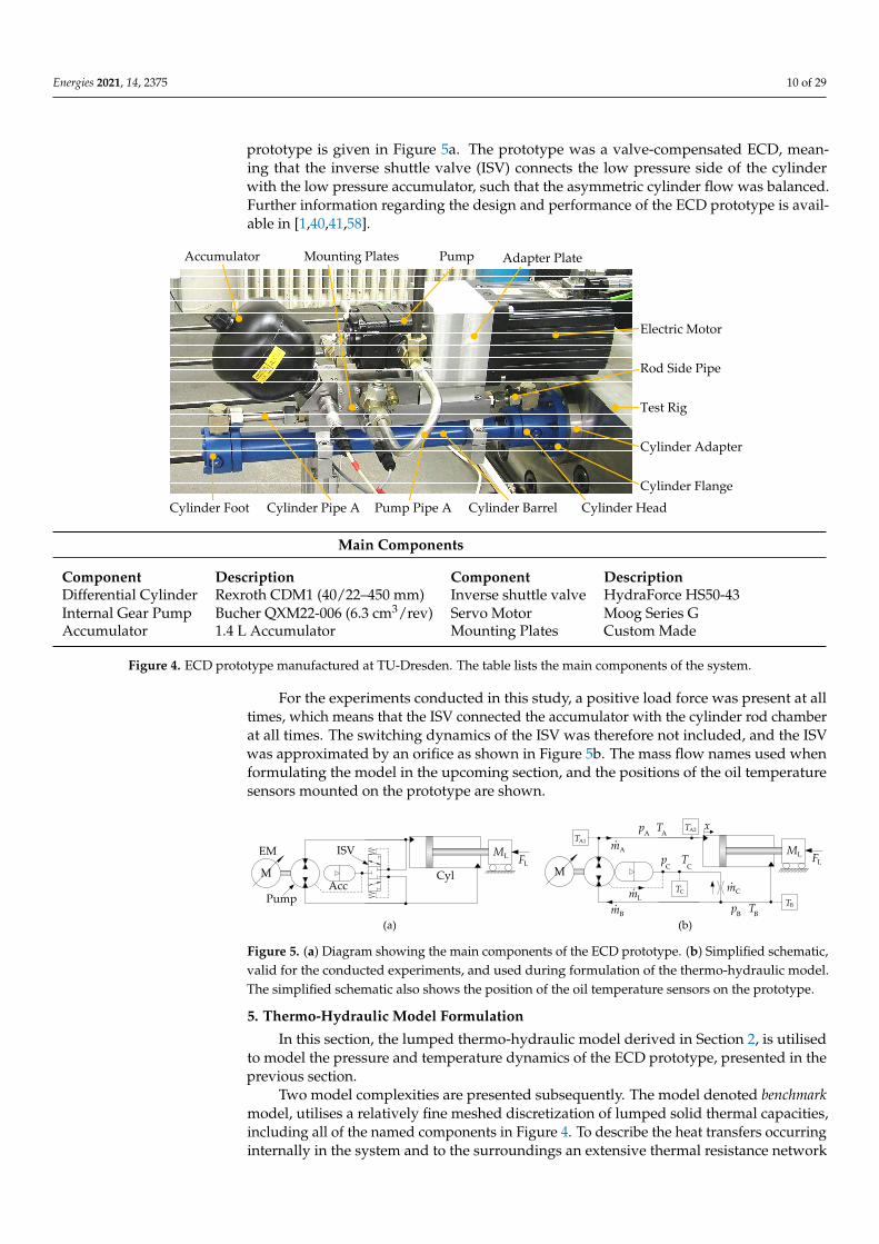
The ECD prototype shown in Figure 4 was manufactured and tested at the TechnicalUniversity of Dresden, Germany. The cylinder of the prototype was flanged on a generalpurpose test-rig, with the rod being connected to a load cylinder capable of loading theECD with varying load forces. The ECD was connected with the load cylinder via an inertiamass of 110 kg, which is not shown in Figure 4. On the cylinder, a manifold was mounted,which connects the cylinder chambers with the pump and a diaphragm accumulator usingan inverse shuttle valve for flow balancing. The pump was driven by a brushless DC motor.The pump and motor shafts were connected through the adapter plate. The adapter plateand accumulator were mounted on the manifold, such that the ECD forms a self-containedand compact drive system. The hydraulic diagram showing the main components of the

Energies 2021, 14, 2375 10 of 29

prototype is given in Figure 5a. The prototype was a valve-compensated ECD, mean-ing that the inverse shuttle valve (ISV) connects the low pressure side of the cylinderwith the low pressure accumulator, such that the asymmetric cylinder flow was balanced.Further information regarding the design and performance of the ECD prototype is avail-able in [1,40,41,58].

Cylinder Barrel Cylinder Head

Cylinder Flange

Rod Side Pipe

Cylinder Adapter

Cylinder Pipe ACylinder Foot

Accumulator

Electric Motor

Adapter Plate

Test Rig

Mounting Plates Pump

Pump Pipe A

Accumulator

Mounting Plate II

AdapterPlate

Mounting Plate III

Cylinder Barrel

Cylinder Foot(Barrel)

Cylinder Foot(End Cap)

Cylinder Head

Cylinder Flange

Pump Pipe A

Cylinder Pipe B

Cylinder Pipe A

PumpMounting Plate I

Electric Motor

Cylinder Barrel Manifold

Accumulator Pump Electric Motor

Main Components

Component Description Component DescriptionDifferential Cylinder Rexroth CDM1 (40/22–450 mm) Inverse shuttle valve HydraForce HS50-43Internal Gear Pump Bucher QXM22-006 (6.3 cm3/rev) Servo Motor Moog Series GAccumulator 1.4 L Accumulator Mounting Plates Custom Made

Figure 4. ECD prototype manufactured at TU-Dresden. The table lists the main components of the system.

For the experiments conducted in this study, a positive load force was present at alltimes, which means that the ISV connected the accumulator with the cylinder rod chamberat all times. The switching dynamics of the ISV was therefore not included, and the ISVwas approximated by an orifice as shown in Figure 5b. The mass flow names used whenformulating the model in the upcoming section, and the positions of the oil temperaturesensors mounted on the prototype are shown.

(a)

ML FLM

AccCyl

EM

Pump

ISV ML FLM

TA2TA1

TBm.B

m.A

m.L

x

p    T B B

p    T A A

m.C

p     T C C

(b)

TC

Figure 5. (a) Diagram showing the main components of the ECD prototype. (b) Simplified schematic,valid for the conducted experiments, and used during formulation of the thermo-hydraulic model.The simplified schematic also shows the position of the oil temperature sensors on the prototype.

5. Thermo-Hydraulic Model Formulation

In this section, the lumped thermo-hydraulic model derived in Section 2, is utilisedto model the pressure and temperature dynamics of the ECD prototype, presented in theprevious section.

Two model complexities are presented subsequently. The model denoted benchmarkmodel, utilises a relatively fine meshed discretization of lumped solid thermal capacities,including all of the named components in Figure 4. To describe the heat transfers occurringinternally in the system and to the surroundings an extensive thermal resistance network

Energies 2021, 14, 2375 11 of 29

is defined. This thermal network was developed in previous publications [40,41], and isused here as a benchmark for model validation and for comparison with a simpler modelcomplexity, i.e., the reduced model.

In the reduced model, a significantly coarser discretization is utilised. In [40,41],the forced convection resistances were found to be negligible, as the thermal behaviourwas governed by natural convection and radiation from the system to the surroundings.Therefore, the reduced model investigates, among other things, how model accuracy isaffected by neglecting forced convection resistances. Neglecting the forced convectionresistances may be done in several ways. If commercial simulation software is used,arbitrary small forced convection resistances may be defined to maintain the number oflumped temperatures. Alternatively, the temperature dynamics of multiple fluid and solidcontrol volumes may be lumped together, thus reducing the number of temperature statesin the model. The latter approach is featured here. As the temperature dynamics of multiplefluid volumes are lumped together, it is beneficial to neglect the coupling between thetemperature and pressure dynamics by utilising temperature independent fluid properties,as given in Section 3.1.

Table 1 compares the two model complexities.

Table 1. Comparison of the two model complexities.

Model Complexity

Benchmark Reduced

Fluid Properties Temperature Dependent Temperature Independent(Equations (31)–(33)) α = 0 and Equations (38) and (39)

Number of Thermal Capacities 3 Oil Capacities 1 Combined Oil/Solid Capacity18 Solid Capacities 1 Oil Capacity & 1 Solid Capacity

Number of Thermal Resistances18 Natural Convection & Radiation 5 Natural Convection & Radiation21 Conduction Resistances 1 Conduction Resistance23 Forced Convection Resistances 1 Forced Convection Resistance

The reason for dealing with two model complexities is to investigate how muchinformation and accuracy are lost when reducing the model complexity. As seen fromTable 1, the current study especially investigates the needed level of detail for the thermalsubmodels, including the number of thermal resistances used to model heat transfersin the system. The benchmark model demonstrated a good ability to provide accuratetemperature simulations for most of the thermal capacities in [41]. However, parametrisingthe 62 thermal resistances present in the benchmark model is both a time-consuming andtedious task. In addition, for instance, the forced convection resistances occurring inthe flow channels of a custom made manifold requires detailed knowledge about theconstruction of this to parametrise the resistances. Such detailed information may not beavailable during the design phase, where a design engineer desires to estimate the operatingtemperature for a given ECD under some loading conditions. To address the potentialchallenges of the benchmark model, a drastically reduced model, which requires limitedinformation for parametrisation, was investigated. This includes cylinder and accumulatordimensions as well as approximate dimensions of manifold, pump and electric motor.As such, the current investigation may be regarded as a natural next step toward a simplebut yet sufficiently accurate model level. The authors claim that if a thermo-hydraulicmodel should be useful for a design engineer, it should be relatively easy to parametriseeven though this may decrease the accuracy. By the end of the day, approximate estimationsor rough ideas are more useful than very accurate simulations that are never carried outdue to time-consuming model development or parameters unknown during the designphase. Estimating the operating temperature is important to determine to what extentcooling is required, i.e., to obtain a proper thermal design. This may include the additionof a fan, heat pipes mounted in the manifold, an oil cooler or a water cooled manifold.

Energies 2021, 14, 2375 12 of 29

The following sections show the derivation of the two model complexities, with anoffset in the system diagram in Figure 5b.

5.1. Benchmark Model

The pressure dynamics of the benchmark model are formulated as:

pA =βA βmech

βmech + βA

βmechβmech+pA−p0

(mA

ρA VA

− xAA

VAx

+ αA TA

),

VAx = VA0 + xAA

VA = VAx

(1 +

pA−p0βmech

) (40)

pB =βB βmech

βmech+βB

βmechβmech+pB−p0

(−mB−mC

ρB VB

+xAB

VBx

+αB TB

),

VBx = VB0+(Ls − x)AB

VB = VBx

(1 +

pB−p0βmech

) (41)

pC =pC βC

pC VC + βC Vgas

(mL + mC

ρC

+ αC VC TC +Vgas

Tgas

Tgas

),

VC = VAcc + VC0 −Vgas

Vgas =VAcc pacc0 Tgas

Tacc0 pC

(42)

The subscripts {A, B, C} in Equations (40)–(42) refer to the piston chamber, the rodside chamber and the accumulator, respectively, according to Figure 5b.

The gas temperature is modelled using Equation (14). The temperature dynamics ofthe oil control volumes are modelled from Equation (26) as:

TA =1

VA ρA cp,A

(QA + HA,pump + TA αA VA pA

)(43)

TB =1

VB ρB cp,B

(QB + HB,pump + H−

C+ TB αB VB pB

)(44)

TC =1

VC ρC cp,C

(QC + H+

C+ HL,pump + TC αC VC pC

)(45)

where QA , QB and QC are the sum of heat flows to the control volumes, HA,pump , HB,pump andHL,pump are the pump enthalpy flows to the control volumes. H+

Cand H−

Care the enthalpy

flow through the orifice. The enthalpy flows are modelled in Section 7.The benchmark model discretises the system into 18 solid thermal capacities each

associated with an individual temperature. The temperature dynamics of a solid capacityis modelled as:

Tj =∑i Qj,i

mj cp,j

Qi =∆Ti

Rth,i

(46)

where j is indexing the 18 solid capacities and i the heat transfer to the solid capacity.∑i Qj,i is the net sum of heat flow into capacity j, mj is the mass of the solid capacityand cp,j is the specific heat for the given solid material modelled as a function of thetemperature. Specific heats as a function of temperature are obtained from the library ofEES, and implemented as 1D lookup tables. The heat flow is described using the conceptof thermal resistances, Rth . Analogous to an electric circuit, the temperature (voltage) maybe described as the product of heat flow (current) and the thermal resistance [K/W]. ∑i Qj,i

is thus the sum of all heat flows through the thermal resistances connected to the capacity,and ∆Ti is the temperature difference across the thermal resistance. The heat flows to oiland solid capacities may be visualised by a thermal resistance network. The resistancenetwork for both the benchmark and the reduced model are presented in Section 6.

5.2. Reduced Model

The pressure dynamics of the reduced model are similar to the dynamics fromEquations (40)–(42), except that temperature independent fluid properties, p, β and α,are utilised. This entails that the temperature coupling term (αVT) vanishes.

Energies 2021, 14, 2375 13 of 29

Whereas the benchmark model includes 18 solid thermal capacities, the reduced modelonly includes five. These are the electric motor and adapter plate, the cylinder barrel,the manifold, the pump and the accumulator. In Figure 6a, these are illustrated as basicgeometries, which are used for heat transfer calculations. These include cubes (blue),horizontal cylinders (green) and spheres (yellow). For comparison, Figure 6b shows 15 ofthe 18 considered solid thermal capacities approximated as basic geometries used in thebenchmark model.

Cylinder Barrel Cylinder Head

Cylinder Flange

Rod Side Pipe

Cylinder Adapter

Cylinder Pipe ACylinder Foot

Accumulator

Electric Motor

Adapter Plate

Test Rig

Mounting Plates Pump

Pump Pipe A

Accumulator

Mounting Plate II

AdapterPlate

Mounting Plate III

Cylinder Barrel

Cylinder Foot(Barrel)

Cylinder Foot(End Cap)

Cylinder Head

Cylinder Flange

Pump Pipe A

Cylinder Pipe B

Cylinder Pipe A

PumpMounting Plate I

Electric Motor

Cylinder Barrel Manifold

Accumulator Pump Electric Motor

(b)(a)

Figure 6. (a) In the reduced model, natural convection and radiation to the surroundings are modelledto occur from five shapes. (b) In the benchmark model, natural convection and radiation are modelledto occur from 18 shapes (three not shown).

As noted in [40], the thermal behaviour of the system is governed by the naturalconvection and radiation resistances on the outer surfaces as these are considerably largerthan the forced convection resistances between the oil and the solid materials on the innersurfaces. Taking the cylinder barrel as an example, the combined natural convection andradiation resistance is more than nine times higher than the forced convection resistance.In the reduced model, this observation is exploited by neglecting all forced convectionresistances, except the forced convection between oil and accumulator, and thus reducingthe number of thermal resistances significantly.

This has the implication that all solids being in contact with oil (accumulator notincluded) are modelled to have the same temperature. This leads to a further simplificationcompared to the benchmark model, as contact and conduction resistances between solid ther-mal capacities are omitted. However, as a consequence, only three distinct temperaturesare modelled in the reduced model. These include the oil temperature in the accumu-lator TC , the accumulator shell temperature Tacc and the lumped system temperature,Tsys , combining the thermal capacity of the oil in the A and B chamber with the cylinderbarrel, pump, manifold, electric motor and adapter plate capacities. Even though theelectric motor and adapter plate are not in contact with the oil, these are included inthe lumped system temperature due to large contact areas with the pump and manifold,thus assuming the contact resistance to be small. All other thermal capacities, such aspipes, cylinder flanges, etc., are not included in the reduced model. This means that onlyapproximate dimensions of the main system components are needed to parametrise thethermal resistance network.

Energies 2021, 14, 2375 14 of 29

The temperature dynamics of the three control volumes of the reduced model aregiven as:

Tsys =Qlosses + HA,pump + HB,pump + H−

C− Qth

VA ρA cp,A + VB ρB cp,B + msteel cp,steel + malu cp,alu

, TC =HL,pump + H+

C− QVII

VA ρA cp,A + VC ρC

(47)

Tacc =QVII − QV

macc cp,acc

, Qlosses = QL,HM + QL,Cyl + QL,EM , Qth = QI + QII + QIII + QIV + QVI

QI to QVII are heat flows through the thermal resistances defined in the next section. msteel

and malu are the mass of steel and aluminium with temperature dependent specific heatscp,steel and cp,alu , respectively. QL,HM , QL,Cyl and QL,EM are hydro-mechanical pump losses,cylinder friction losses and losses of the electric machine, respectively. These are modelledin Section 7 along with the enthalpy flows H.

6. Thermal Resistance Networks

In this section, the heat flows to the control volumes and the solid capacities for bothmodel complexities are presented. As mentioned, the heat flows are calculated based onthe temperature differences across thermal resistances. This may beneficially be visualisedusing a thermal resistance network. The thermal resistance network for the benchmarkmodel was derived in [41] and is shown in Figure 7.

Hydraulic System

34

Mounting Plate I

Cylinder Adapter

Cylinder Flange

Adapter Plate

4140 46 47 43 4244 45

24

Rod

23

59 60

27

21

22 25

26

Cylinder  Pipe B

30

2932

38

1 19 20 18

28

31

35

58 55

56

57

Mounting Plate II

514948 50

53

52

Cylinder Pipe A

54

Pump

33

2

17

Accumula-tor

9

10

11 15 16

12Electric Motor

13

14

39

8Pump Pipe A

Cylinder Barrel

Piston

Cylinder Head

7

4 53

Cylinder Foot

6

37

T    & T rig        ∞ 

Natural Convection & Radiation

1‐18

Solid Thermal Capacity

Oil Thermal Capacity

Conduction

19‐39

Forced Convection

40‐60

Enthalpy Flow

Pump  pipe B

36

C

62

Mounting Plate III

61

B A

Figure 7. Thermal resistance network for the benchmark model. The thermal network was developedin [40,41]. Contact resistance is included in the conduction resistances.

The 62 thermal resistances in Figure 7 were computed in [40,41]. Examples of howto calculate thermal resistances for different geometries and flow conditions are given inSection 6, when calculating resistances for the reduced model.

In addition to heat exchanged through thermal resistances, heat is also ascribed as theconsequence of energy losses of the components. The power loss due to cylinder friction isentirely added to the cylinder barrel, 25% of the pump friction losses are added to each ofthe oil control volumes A and B and the remaining 50% are added to the pump housing.Finally, the electric motor power losses are added to the solid capacity of the electric motor.Leakage and valve throttling losses are ascribed inherently by the enthalpy flows.

The thermal resistance network for the reduced model is given in Figure 8. In additionto natural convection and radiation from the five basic shapes in Figure 6a, forced convec-

Energies 2021, 14, 2375 15 of 29

tion between oil and accumulator as well as heat conduction (contact resistance included)from the cylinder barrel through the cylinder head and flange to the test-rig are included.

The seven thermal resistances from Figure 8 are found as either conduction, convectionor radiation resistances given as [46]:

Rcond =L

kA, Rcont =

1hc A

, Rconv =1

hAs

, Rrad =1

As,Eff εσ(

T2s + T2

∞

)(Ts + T∞)

(48)

where Rcond is the conduction resistance (here for a plane wall example) modelling theheat transfer through a material. L is the length of which the heat transfer occurs, k is thethermal conductivity of the material and A is the cross-section area. Rcont is the contactresistance, with hc being the contact conductance. Rconv is forced or natural convectionresistance. Forced convection occurs between oil and solid elements, whereas naturalconvection takes place at the outer surfaces of the system, as no fan is incorporated in thesystem. h is the convective heat transfer coefficient. As is the surface area. Rrad is radiationresistance, with As,Eff being the effective radiation surface area. ε is the surface emissivityand σ is the Stefan–Boltzmann constant. Ts and T∞ are the surface temperature and theambient temperature, respectively.

CombinedOil & Solid 

Thermal Capacity

Solid Thermal Capacity

Enthalpy Flow

Natural Convection & Radiation

I ‐ V

Conduction

VI

Forced Convection

VII

Solid VolumesCylinder Barrel, Pump, 

Manifold, Electric Motor & Adapter Plate

I II

III IVV VI

VIIAccumulator

T    & T rig        ∞ 

Oil VolumesA + B

T  sys

Oil Thermal Capacity

C

Figure 8. Thermal resistance network for the reduced model. The natural convection and radiationresistance are found as a parallel connection of the convection and radiation resistances.

6.1. Heat Conduction

Only heat conduction from the cylinder barrel through the cylinder head and flangeto the test-rig is included in the reduced model. The test-rig is considered as a thermalreservoir, thus remaining at a constant temperature. The heat transfer is modelled as a serialconnection of two conduction and two contact resistances (Rcond and Rcont in Equation (48)).The apparent contact areas for calculation of the contact resistances are given in Figure 9aas A1 and (A1 + A2). The conduction resistances are modelled with areas (A1 + A2),(A1 + A2 + A3) and lengths L1 , L2 .

(a)

A1

Gas

Oil

R

r*

l

r*l/2

(b) (c) (d)

L 1 L2Tsys

TrigTsys

RVI  = RVI1  + RVI2  + RVI3  + RVI4

A2 A3

Figure 9. (a) The heat conduction from the cylinder barrel to the test-rig is modelled as a serial connection of two conductionand two contact resistances. (b) Bladder type gas-loaded accumulator. (c) The bladder accumulator is approximated as asphere when calculating the natural convection heat transfer from the outer surface. (d) Forced convection on the innersurface is approximated as internal pipe flow, with the length of the pipe being the oil height in the virtual sphere and thepipe radius being evaluated as the radius of the spherical cap at l/2.

Energies 2021, 14, 2375 16 of 29

6.2. Convection

The convective heat transfer coefficient, h in Equation (48), may be determined fromthe average Nusselt number (Nu). The Nusselt number is a function of the Reynolds(Re) and Prandtl (Pr) numbers for forced convection problems, and the Rayleigh (Ra) andPrandtl numbers for natural convection problems.

Nu(Re or Ra, Pr) =hLc

kRe =

VLc ρ

µPr =

µcp

kRa =

gαL3c ρ2cp

µk∆T (49)

where Lc is the geometry dependent characteristic length, V is the mean flow speed and g isthe gravitational acceleration. For natural convection problems, the fluid properties of theambient air are calculated at the reference temperature T = 0.5(Ts + T∞), i.e., at the meantemperature between surface and surroundings. Fluid properties for forced convectionproblems are evaluated at the lumped pressure and temperature of the oil control volumeusing the expressions derived in Section 3.

The Nusselt number depends on geometry, and the methodology utilised here is toidentify an appropriate approximation of the considered shape, such that well-knownmethodologies and formulas valid for basic shapes may be applied. This is done inFigure 6a, where the outer surfaces of the ECD prototype is approximated using the basicshapes of a cube (electric motor and adapter plate, pump and manifold), horizontal cylinder(cylinder barrel) and sphere (accumulator).

To illustrate this approach further, consider the accumulator, which is approximatedby a sphere for calculation of the natural convection resistance, as seen in Figure 9b,c.The forced convection between the oil and the accumulator shell is modelled by approxi-mating the flow as an internal pipe flow. The length and diameter of this pipe are updatedaccording to the oil level in the accumulator, which is illustrated in Figure 9c,d. The fluidheight present in the virtual sphere is calculated dependent on the oil volume in the accu-mulator, and is used as the pipe length when calculating the Nusselt number. The pipediameter is approximated as the diameter of the spherical cap containing the oil at half theoil height, as illustrated in Figure 9c.

Table 2 shows the expressions for calculation of the Nusselt numbers for the geometriesand flow conditions considered in the reduced model, obtained from [59,60]:

Table 2. Nusselt numbers for convective heat transfer problems in the reduced model. Aproj is the projected area of the cubeon a horizontal flat surface below the cube. di is internal diameter. The Nusselt number for internal pipe flow is valid forlaminar flows during hydrodynamic and thermal flow development.

Geometry Nusselt Number Prantdl Function Lc

Nat

ural

HorizontalNu =

(0.752 + 0.387(Ra f (Pr))1/6

)2f (Pr) =

(1 +

(0.559

Pr

)9/16)−16/9

Lc = 12 πd

Cylinder

Sphere Nu = 0.56((

Pr0.846+Pr

)Ra)1/4

+ 2 - Lc = d

Cube Nu = 5.748 + 0.752(

Raf (Pr)

)0.252f (Pr) =

(1 +

(0.492

Pr

)9/16)16/9 Lc = A

d

d =

√4

Aprojπ

Forc

ed

InternalPipe Flow Nu =

(49.37 + ( f1 − 0.7)3 + f 3

2

)1/3 f1 = 1.615(

RePr dil

)1/3

Lc = di

f2 =(

21+22Pr

)1/6(RePr di

l

)

The heat transfer coefficients for natural convection calculated based on the Nusseltnumbers given in Table 2 are valid for idealised conditions. In technical environmentssuch as workshops, factories, etc., the heat transfer coefficients can be assumed to be up

Energies 2021, 14, 2375 17 of 29

to 20% larger than the theoretical values, according to [61]. This is due to ambient airflow occurring from windows, doors, people walking around, etc. In [41], experimentsidentified that the ambient conditions caused the natural heat transfer coefficients to be16% larger than the theoretical values. For a fair comparison between the benchmark andreduced model, all natural convection heat transfer coefficients used in this paper have beenincreased by 16% compared to their theoretically obtained counterparts.

6.3. Radiation

All bodies above 0 K emit thermal radiation. However, for the current study, radiationheat transfer is assumed to only occur between the solid elements and the surroundings,and not internally between the solid elements. As seen in Equation (48) the effectiveradiation surface, As,Eff , is utilised instead of the actual surface area As , acknowledgingthat solid elements may be shadowing each other. This means that the effective radiationarea is smaller than the actual surface area. This effect is included in the benchmark model,however, the reduced model assumes As,Eff = As , as the shadowing effect is difficult todetermine without accurate knowledge of the relative placement of the solid components.

6.4. Thermal Resistances in the Reduced Model

In Table 3, the seven thermal resistances of the reduced model are exemplarily cal-culated. The resistances have been evaluated at oil and solid temperatures of 60 °C, anambient temperature of 20 °C, fluid velocities present for a piston speed of 150 mm/sand at the initial oil level in the accumulator. As mentioned, the heat transfer coefficientshave been increased by 16% compared to the idealised values to reflect the ambient flowconditions. Please note that the resistances are updated during the simulation, and thevalues given in Table 3 are only given as an example to illustrate the order of magnitude.

Table 3. Thermal resistances, according to Figure 8, evaluated at oil and solid temperatures of 60 °C, an ambient temperatureof 20 °C and for fluid velocities present for a piston speed of 150 mm/s.

Natural Convection & Radiation

ID Geometry As Aproj Lc ε hconv hrad hcomb Rth

I Horizontal980 cm2 - 79 mm 0.92 7.1 W

m2K 6.4 Wm2K 13.5 W

m2K 0.76 KWCylinder

II Cube1341 cm2 221 cm2 799 mm 0.26 5.0 W

m2K 1.8 Wm2K 6.8 W

m2K 1.1 KW(Manifold)

III Cube2268 cm2 469 cm2 928 mm 0.69 4.8 W

m2K 4.8 Wm2K 9.6 W

m2K 0.46 KW(Electric Motor)

IV Cube614 cm2 120 cm2 497 mm 0.92 5.7 W

m2K 6.4 Wm2K 12.1 W

m2K 1.34 KW(Pump)

V Sphere707 cm2 - 150 mm 0.92 5.9 W

m2K 6.4 Wm2K 12.4 W

m2K 1.14 KW(Accumulator)

Heat Conduction to Test-Rig

ID Geometry A1 A2 A3 L1 L2 k [46] hc [40] Rth

VI Plane Wall 20 cm2 28 cm2 75 cm2 73 mm 16 mm 63.9 WmK 6.5 kW

m2K0.37 K

W

Forced Convection (Oil to Accumulator)

ID Geometry As l di V Re hconv Rconv

VII Internal243 cm2 51.6 mm 113 mm 7.6 mm

s 28 51 Wm2K

0.80 KW

Pipe Flow

Energies 2021, 14, 2375 18 of 29

The simple thermal resistance network and the associated numerical values of theresistances given in Table 3 enable performing some rough estimations of the static thermalbehaviour of the system. From Figure 8, the equivalent thermal resistance to the surround-ings from the lumped system components, at Tsys , is 0.120 K/W (assuming TC = Tsys ). If theaverage losses of the ECD are 450 W, this yields a static system temperature of 54 °C abovethe ambient temperature. Note that this is a rough estimate as the thermal resistances inTable 2 are temperature dependent themselves.

In [41], one of the main conclusions was that the modelled temperature was sensi-tive towards estimation errors of the power losses. The equivalent thermal resistance of0.12 K/W may also be used to approximate the sensitivity towards estimation errors of theenergy losses of the system or the thermal resistances. Assume the average losses to beestimated within ± 20%. This would result in estimated static temperatures in the rangefrom 43 °C to 65 °C above ambient temperature, showing a relatively large sensitivitytowards power loss estimating errors.

Furthermore, Table 3 shows that the surface area weighted mean of the combined heattransfer coefficients for natural convection and radiation is 10.2 W

m2K . Note, if the theoreticalnatural heat transfer coefficients are used this number would equal 9.5 W

m2K . Assumingthis to be the only heat transfer occurring in the system, i.e., neglecting forced convectionand conduction, this may be used as an approximate number, in the early design phase ofan ECD to assess if special attention is required for the thermal design. As such it may bepossible for a design engineer to roughly estimate the static thermal behaviour of the ECD,if an estimate of the system losses and the outer surface area can be established.

7. Component Models

As the last step before the simulation results are presented, the component models ofthe cylinder, pump and orifice are presented. These are common for both the benchmarkand the reduced model and are needed to quantify the losses of the ECD and to define themass and enthalpy flows used in the dynamic equations. The hydraulic diagram includingthe components as well as mass and enthalpy flow names are repeated in Figure 10afor convenience.

FLML

M

TA2TA1

TB2

m.A

m.L

x

m.CTAcc

(b)

m.A H.A m

.B H

.B

m.L H.L

m.T

ω     τ

p T h  A    A    A

p T h  B     B     B

p T h  C     C     C

m.C

p T h  B     B     B

p T h  C     C     C

H.C

+H.C

‐

m.C

p    T    h   B        B        B

p    T    h   C        C        C

H.C

+H.C

‐

m.A H.A m

.B H

.B

m.L H.L

m.T

ω     τ 

p    T    h   A       A        A

p    T    h   B        B        B

p    T    h   C        C        C

(b)

(c)

FLML

M

TA2TA1

TBm.B

m.A

m.L

x

p    T B B

p    T A A

m.C

p     T C C

(a)

TCTC

Figure 10. (a) Simplified schematic valid for the conducted experiments. (b) Simple schematic showing the quantities usedfor modelling mass and enthalpy flow of the inverse shuttle valve/orifice. (c) The inputs to the static pump model are thefluid properties in the adjacent chambers, and the shaft speed ω. The shaft torque as well as mass and enthalpy flows aremodel outputs.

7.1. Cylinder and Orifice

Equation (50) expresses the motion dynamics and the friction losses of the cylinder.

Energies 2021, 14, 2375 19 of 29

x =1

ML

(pA AA − pB AB − (AA − AB)p0 − FL − FF) QL,Cyl = FF x (50)

FF =

(Fc + (Fs − Fc)e

−|x|xsw + Kp |pA − pB |

)tanh(γx) + BL x (51)

The term (AA − AB)p0 includes the force from the surroundings on the rod and isincluded because the modelled pressures are absolute. FL is the load force and FF is cylinderfriction modelled as a Stribeck characteristic curve including a pressure dependent frictionterm [62,63]. Fc is the Coulomb friction, Fs is the static friction, xsw is the Stribeck velocity,Kp is the pressure dependent friction coefficient and BL is the viscous friction coefficient.

The mass and enthalpy flows of the inverse shuttle valve/orifice are modelled accord-ing to Figure 10b as [52]:

mC = Ao Cd

√2ρ|pB − pC | sign(pB − pC) (52)

H+C=

{mC(hB − hC) , mC ≥ 0

0 , mC < 0H−

C=

{0 , mC ≥ 0

−mC(hC − hB) , mC < 0(53)

where A0 is the orifice area and Cd is the discharge coefficient.

7.2. Electric Motor

The dynamics of the electric motor is omitted in the model, i.e., the shaft speed equalsthe reference speed. Thus, only the loss behaviour of the motor is modelled. The losses ofthe electric motor are measured for varying motor speeds and torques and implemented asa 2D lookup table. The losses are assumed to be temperature independent and identical inboth generator and motor operation mode. For a visualisation of the loss behaviour of themotor, the measured efficiency map is shown in Figure 11a.

(a) (b)

0.75 0.8 0.83

0.75 0.8 0.83

0.8 0.83

0.88

0.9

0.85

0.8 0.75

0.5

Electric Motor Efficiency [‐] Total Pump Efficiency [‐]

Figure 11. (a) Measured efficiency map of the electric motor, as a function of torque and speed.Dotted lines are power levels. (b) Measured efficiency map of the pump as a function of pressuredifference, speed and temperature.

7.3. Pump

A pump model expressing the static relationship between the inputs (i.e., the pumpspeed, pressure difference across the pump and inlet temperature) and the outputs isneeded. The outputs include the mass and enthalpy flows as well as the shaft torque. Thisis visualised in Figure 10c. Here, it may also be seen that external leakage is modelled toonly occur from the high pressure chamber.

In addition to the mentioned model inputs, loss information or loss models arerequired, which may either be an analytical model or simply measured loss quantities,

Energies 2021, 14, 2375 20 of 29

implemented as look-up tables. The latter approach is used here. Figure 11b shows themeasured efficiency map of the pump. Losses are assumed to be equivalent in both motorand pump operation modes. The actual pumping process is modelled as an ideal process,with losses/irreversibilities added subsequently. E.g., leakage losses may be regardedas variable orifices surrounding the ideal pump process (as visualised in Figure 10c).From Figure 10c, it is important to note that the inlet pressure and temperature to the idealpump equal the states of the delivering chamber (rotation direction dependent), and theoutlet pressure equals the pressure in the receiving chamber. The output temperature,however, is calculated by assuming an isentropic compression process, as [47]:

S = f (T, p) ⇒ dS =

(∂S∂T

)p

dT +

(∂S∂p

)T

dp =cp

TdT − ανdp (54)

dS = 0−−−→ dT =αTρcp

dpApproximation−−−−−−−−→ Tout

∼= Tin +αTin

cp ρ(pout − pin) (55)

S is the entropy modelled as a function of temperature and pressure, pin and pout is eitherpA or pB depending on the direction of rotation. Likewise, the inlet temperature is eitherTA or TB . • denotes fluid properties evaluated at

pin+pout2 and Tin . The enthalpy change of

the fluid may be found by inserting the isentropic temperature change from Equation (55)in Equation (19):

dh = cp dT + ν(1− Tα)dp = cp

(αTρcp

dp

)+ ν(1− Tα)dp =

1ρ

dp (56)

Approximation−−−−−−−−→ ∆h ∼=1ρ(pout − pin) (57)

where ρ is the fluid density evaluated atpin+pout

2 andTin+Tout

2 . The ideal mass flow, mT , themass leakage flow, mL and the theoretical pump torque are modelled as:

mT = ωDp ρ mL =12

QL ρ τT ω = mT ∆h ⇒ τT = Dp(pout − pin) (58)

where DP is the geometric displacement of the pump and QL is the measured volumetricflow loss. Note that τT ends up being the familiar torque equation for incompressiblefluids. To include the compressibility of the fluid, somewhat more elaborate models areavailable, i.e., from [64], but are not considered here. The calculation of the mass andenthalpy flows, defined in Figure 10c, depend on the operating quadrant, i.e., the directionof pump rotation and the pressure difference across the pump. Likewise, the actual shafttorque τ must be calculated based on the operation quadrant by including the measuredtorque loss τL .

The relevant expressions for the four operating quadrants are given in Table 4:

Energies 2021, 14, 2375 21 of 29

Table 4. Pump torque, mass and enthalpy flows based on operation quadrant. ∆P = (pA − pB ).?

Only valid for mA > 0,†

Only valid for mB < 0.

Pump Model Outputs

Quadrant τ mA mB HA HB HL

I (ω ≥ 0)τT + τL mT − 2mL mT − mL mA (hB + ∆h− hA )

?mL ∆h

?mL (hB + ∆h− hC )

?

(∆P ≥ 0)

II (ω < 0) −τT − τL mT − 2mL mT − mL 0 mL (hA − hB )− mL (hA − hC )(∆P > 0) mT (hA + ∆h− hB )

III (ω < 0) −τT − τL mT + mL mT + 2mL mL ∆h† −mB (hA + ∆h− hB )

†mL (hA + ∆h− hC )

†

(∆P < 0)

IV (ω > 0)τT + τL mT + mL mT + 2mL

mL (hB − hA )− 0 mL (hB − hC )(∆P < 0) mT (hB + ∆h− hA )

8. Results

The ECD prototype presented in Section 4 was tested in the laboratory by controllingit to follow a sinusoidal position reference with a frequency of 0.4 Hz (tcycle = 2.5 s), reachingmaximum cylinder and motor speeds of ±300 mm/s and ±3600 RPM, respectively. Aconstant load force of 5 kN is requested by the load cylinder, but due to friction and loaddynamics, this is found to be varying between 3.9 kN and 5.7 kN. The test continued fora period of three hours until thermal equilibrium was reached. Oil temperatures weremeasured using four thermocouples (see position in Figure 10a) with an accuracy of±0.5 K.The surface temperatures of the prototype were monitored by a thermo-graphic camerahaving an accuracy of ± 1.5 K. The measured load force and the position reference wereused as the simulation inputs. The derived governing equations were simulated in MatLABSimulink using the ODE45-solver, with a maximum stepsize of 1/5000 s. Using a laptopwith an Intel i7-10610 1.8 GHz processor, a 10 min simulation of the benchmark model wascompleted within 20 min, whereas the simulation of the reduced model was completedwithin 13 min.

8.1. Loss Behaviour

As illustrated in the previous section, the modelled temperature is rather sensitivetowards inaccuracies between actual and modelled heat losses. Therefore, the simulatedand measured loss behaviour is compared in Figure 12.

Figure 12b,d,f show a good coherence between the measured and simulated pressure inall control volumes. For the pressure in the piston chamber (pA ), the oscillation frequency ismodelled fairly accurately while the measured damping is slightly larger than the modelleddamping. Interestingly, it is found that there are no noticeable differences between thepressures modelled in the benchmark and the reduced models, even though the dynamicpressure–temperature coupling is neglected in the reduced model.

No noticeable differences are found between the two model complexities for any ofthe quantities visualised in Figure 12, expect for the accumulator pressure. Here smalldeviations of approximately 0.05 bar can be seen.

Figure 12a shows a good coherence between the measured and simulated position.Combined with the accurately modelled chamber pressures, this leads to the cylinderpower being modelled accurately, as seen in Figure 12c.

Slight deviations exist between the modelled and estimated shaft torque and powerduring cylinder retraction, at ∼2 s and ∼4.5 s in Figure 12e. On average, it is found that theinput power to the hydraulic system and the output power are modelled with an acceptableaccuracy. This means that the losses are established with a sufficient degree of accuracyfor anticipating the thermal behaviour. In other words, deviations between modelled andsimulated temperatures are assessed to originate from inaccurate heat transfer modelsrather than loss model deviations.

Energies 2021, 14, 2375 22 of 29

Figure 12. (a) Measured and simulated piston position. (b) Measured and simulated pressure in the piston chamber pA .(c) Measured and simulated mechanical output power (W = xFcyl ). (d) Measured and simulated pressure in the rod chamberpB . (e) Measured and simulated shaft torque and shaft power (W = ωτ). (f) Measured and simulated accumulator pressure.

8.2. Static Temperatures

Even though the derived models are dynamic models, the transient temperaturedevelopment is not important in some applications. If a system is going to perform thesame task 24 h a day for 20 years, it is not important if static temperatures are reached after10 min or 10 h. In this situation, only the static temperatures are relevant to ensure that theoil temperature stays within limits.

Figure 13a compares the benchmark modelled oil and surface temperatures with themeasured values. Regarding the surface temperatures, the high number of simulatedthermal capacities in the benchmark model pays off in terms of the ability to fairly accuratelymodel the qualitative temperature distribution, e.g., the model predicts that the motor iswarmer than the pump and that the cylinder head is colder than the cylinder barrel. Thisinformation is lost in the reduced model due to the simplification of only including threethermal capacities. As seen in Figure 13b, only two different surface temperatures aremodelled, i.e., the surface temperature of the accumulator and the lumped temperature ofthe remaining system.

The benchmark model in Figure 13a models all surface temperatures within ±5.5 K.Furthermore the oil temperatures are estimated within approximately ±1.5 K, except forthe oil temperature in the rod side chamber, which is overestimated with approximately3 K. This is assessed to be satisfactorily accurate for analysis purposes, e.g., to analysethe effect of changing certain parameters such as areas and emissivities on the thermalbehaviour.

As mentioned, the reduced model in Figure 13b is not formulated such that it iscapable of predicting the individual temperature distribution of the system. This is becauseall system components, except the accumulator, are lumped in a single thermal capacity.This was chosen to avoid parametrising a high number of forced convection and conductionresistances. The modelled surface temperature of the system components are somewhatin-between the highest system temperature of the motor and the lowest system temperatureof the cylinder barrel. Given the reduced complexity of the model, this is the expectedresult, but it leads to deviations up to 6.4 K, considering the surface temperatures.

Energies 2021, 14, 2375 23 of 29

In terms of the modelled oil temperatures in the reduced model, these are overestimatedby 1.4 K to 6.8 K. However, all modelled oil temperatures are larger than the measured,meaning that the simulated temperatures are conservative estimates, which is desired interms of design tool applicability. For comparison, it can be noted that if the natural convec-tion resistances have not been corrected for the ambient flow conditions, i.e., the idealisedvalues are used, the modelled temperatures would be approximately 2 K larger, than theones given in Figure 13b.

A trade-off between modelling complexity and accuracy is identified in the compar-ison between the benchmark and the reduced model. Due to the simple thermal network,which may be parametrised relatively easy, this is much more applicable in the designphase, compared to the benchmark model. Furthermore, the reduced model produces rea-sonably accurate and conservative temperature estimates, which may be valuable to haveavailable in the design phase. In this manner, important choices related to the thermaldesign of the system can be made on a fairly informed basis.

71.1˚C75.1˚C 4.0˚C

70.8˚C75.1˚C 4.3˚C

76.9˚C75.1˚C ‐1.8˚C

59.1˚C54.1˚C ‐5.0˚C

75.9˚C75.1˚C ‐0.8˚C

78.1˚C75.1˚C  ‐3.0˚C

81.5˚C75.1˚C  ‐6.4˚C

MeasuredSimulatedDeviation

Oil Temperatures

73.7˚C75.1˚C 1.4˚C

TA1 TA2 TB TC71.6˚C75.0˚C 3.4˚C

68.3˚C75.1˚C 6.8˚C

73.6˚C75.1˚C 1.5˚C

59.1˚C57.0˚C ‐2.1˚C

75.9˚C74.8˚C ‐1.1˚C

78.1˚C76.9˚C ‐1.2˚C

81.5˚C82.5˚C 1.0˚C

69.6˚C68.3˚C ‐1.3˚C

71.1˚C66.3˚C ‐4.8˚C

70.8˚C68.9˚C ‐1.9˚C

54.3˚C52.5˚C ‐1.8˚C

35.4˚C30.5˚C ‐4.9˚C

76.9˚C71.5˚C ‐5.4˚C

Oil Temperatures

73.7˚C72.1˚C ‐1.6˚C

TA1 TA2 TB TC71.6˚C71.5˚C 0.1˚C

68.3˚C71.5˚C 3.2˚C

73.6˚C72.1˚C ‐1.5˚C

MeasuredSimulated Deviation

(b)(a)

Figure 13. (a) Simulated steady state temperatures of the benchmark model compared to the measuredstatic temperatures of the ECD prototype. (b) Simulated steady state temperatures of the reducedmodel compared to the measured static temperatures of the ECD prototype.

8.3. Transient Temperature

In applications where actuators are used on an on/off basis, i.e., the actuator isworking for a limited time with cooling breaks in between the operating cycles, transienttemperature behaviour may be relevant to optimise the thermal design. Figure 14 com-pares the simulated transient temperature responses of the two model complexities andthe measurements.

A general thing to observe from Figure 14 is that the benchmark model for most ofthe thermal capacities predicts the transient temperature more accurately than the reducedmodel. The reduced model heats up too slowly during the first 45 min, which can beexplained by all system components being lumped together. This means that the transienttemperature response is governed by the components with large heat capacities. In thiscase, this is the motor and the mounting plates (Figure 14d,f,g). A reasonably transient fitis seen for these components in the reduced model.

To illustrate how neglecting the dynamic pressure–temperature coupling in the reducedmodel influences the transient temperature, consider Figure 14a, where the oil temperaturein the piston chamber, TA , is shown. In the benchmark model, temperature oscillationsof ∼0.2 K are seen, and is due to pressure oscillations and the dynamic coupling by thethermal expansion coefficient α. In the reduced model, the same pressure oscillations arepresent, as shown in Figure 12b, but this does not result in any temperature oscillations,

Energies 2021, 14, 2375 24 of 29

as the dynamic coupling is neglected. The temperature oscillations of the benchmark modelare, however, insignificant with respect to the dominating dynamics; thus, it is found thatneglecting the dynamic coupling i.e., defining α = 0 is recommendable, as it enables adecoupled simulation of pressure and temperature dynamics.

Figure 14. (a) Measured and simulated oil temperature in the piston chamber TA . (b) Measured and simulated oiltemperature in the rod chamber TB . (c) Measured and simulated oil temperature and pressure in the accumulator TC and pC .(d) Measured and simulated surface temperatures of the motor and cylinder barrel. (e) Measured and simulated surfacetemperatures of the pump and accumulator shell. (f) Measured and simulated surface temperatures of mounting plate II.(g) Measured and simulated surface temperatures of mounting plate III. (h) Measured and simulated surface temperaturesof the cylinder head, flange and foot. This is only available for the benchmark model, as these components are not includedin the reduced model.

Another difference arising as a result of neglecting the pressure–temperature cou-pling is visible in Figure 14c, where the average accumulator pressure for one operatingcycle is plotted. As the thermal expansion of the oil is defined as zero in the reducedmodel, the accumulator pressure only increases due to thermal expansion of the gas inthe accumulator. For the benchmark model, the accumulator must contain a larger oilvolume as the oil temperatures increase, resulting in a higher pressure compared to thereduced model. However, both model complexities predicts the measured pressure within± 0.15 bar, which is fairly accurate.

To sum up the presentation of the modelling results, it is found that there is a trade-offin terms of accuracy and thermal modelling complexity. Both model complexities, however,predict the temperature with an accuracy found to be reasonable for design purposes. Notethat this is partly possible because the losses of the ECD prototype was modelled with ahigh degree of accuracy. For most applications, the relatively small differences in terms ofmodelled temperatures cannot justify the formulation of the elaborate thermal network ofthe benchmark model compared with the reduced model. Note that the number of resistances

Energies 2021, 14, 2375 25 of 29

are reduced from 62 in the benchmark model to 7 in the reduced model. More importantlythe seven resistances can be parametrised fully based on cylinder, motor, accumulatorand manifold dimensions. These are available with some accuracy in the design phaseof the system, thus making the reduced modelling framework a valuable tool for properthermal design. To fully utilise the framework as a design tool, the modelling accuracywhen including various heat transfer enhancing designs must be investigated. This maybe the effect of including a fan, an oil cooler, heat pipes in the manifold or even a watercooled manifold.

9. Conclusions

In this paper, a lumped thermo-hydraulic model for electro-hydraulic compact drives(ECDs) was derived and experimentally verified. To investigate the trade-off betweenaccuracy and modelling complexity, the paper presents two model complexities. It isfound that neglecting the dynamic pressure–temperature coupling does not affect themain pressure and temperature dynamics significantly. Therefore, it is recommended toneglect this coupling as it simplifies model development. Additionally, it is found that anelaborate thermal resistance network predicts the oil and surface temperatures of an ECDprototype slightly more accurately than a significantly simplified model structure. Formost applications, the small differences in terms of modelled temperatures cannot justifythe formulation of the elaborate thermal network compared to the simplified network. Thefindings in the paper may lead to the acceptance of simplified thermo-hydraulic modelstructures that are applicable in the early design phase where only limited informationabout the system is available. This may be an important contribution toward properthermal design of ECDs needed to expand the application range of the technology.

Author Contributions: Conceptualization: S.K., S.M. and L.S.; methodology: S.K., S.M. and L.S.;software: S.K.; experimental work: S.M.; data analysis: S.K. and S.M.; writing—original draftpreparation: S.K.; review: S.M., L.S. and M.K.E.; editing: S.K.; supervision; L.S., M.K.E., T.O.A. andJ.W.; project administration: M.K.E. and T.O.A.; funding acquisition: M.K.E. and T.O.A.. All authorshave read and agreed to the published version of the manuscript.

Funding: This research was funded by the Research Council of Norway, SFI Offshore Mechatronics,project number 237896/O30.

Institutional Review Board Statement: Not applicable.

Informed Consent Statement: Not applicable.

Data Availability Statement: Not applicable.

Conflicts of Interest: The authors declare no conflict of interest.

AbbreviationsThe following abbreviations are used in this manuscript:

CFD Computational Fluid DynamicsCV Control VolumeISV Inverse Shuttle ValveRPM Revolutions per MinuteCS Control SurfaceECD Electro-Hydraulic Compact DrivesMBW Moving Boundary Work

Energies 2021, 14, 2375 26 of 29

Appendix A. Nomenclature

Symbol Description Unit Symbol Description Unit

α Isobaric expansion coefficient K−1 H Enthalpy Flow W

β,βeff , βmech Isothermal, Effective and Mechanical Pa k Thermal Conductivity W/mK

Bulk Modulus Lc Characteristic Length m

ε Emissivity - m Mass Flowµ Dynamic Viscosity Ns/m2 n Normal Vector

ν Specific Volume m3/kg p Pressure Pa

ρ, ρA , ρF Mixture, Air, Oil density kg/m3 Q Heat Flow W

ω Shaft Speed rad/s Rth Thermal Resistance K/W

τ,τL ,τT Shaft Torque, Torque Losses, Nm S Entropy J/K

Theoretical Torque Ts ,T (Surface) Temperature K

• Property evaluated at averageconditions u Specific Internal Energy J/kg

• Temperature Indepedent Property U Internal Energy J

•A ,•B ,•C Quantify evaluated in CV A, B or C V,V Fluid Speed & Velocity Vector m/s

A, As Area & Surface Area m2 V, Vx Volume & Volume at p0 m3

cp , cv Isobaric & Isochoric Specific Heat J/kgK W Rate of Work W

d, di Diameter, Internal Diameter m x Piston Position m

FL , FF Load & Cylinder Friction Force N z Height in Gravitational Field m

h Convection Heat Transfer Coefficient W/m2Kh Specific Enthalpy J/kg

Appendix B. Modelling Parameters

Symbol Description Value Symbol Description Value

α0 Expansion Coefficient at p0 , T0

0.00067K−1 BL Cylinder Viscous Friction 285 Ns/m

β0 Bulk Modulus at p0 , T0 1.65 GPa Cd Orifice Discharge Coefficient 0.7βmech Mechanical Bulk Modulus 0.3 GPa cp0 Oil Specific Heat Parameter 657 J/kgKε Volumetric Air Ratio 0.01 Dp Pump Displacement 6.3 cm3/revκ Polytropic process coefficient 1.4 Fs Static Friction 90 NρF0 Oil Density at p0 , T0 873 kg/m3 Fc Coulomb Friction 15 Nσ Stefan-Boltzmann Constant g Gravitational Acceleration 9.82 m/s2

τ Thermal Time Constant 3.5 sAA Cylinder Piston Area 12 cm2 Kcp Oil Specific Heat Parameter 4.21 J/kgK2

AB Rod Chamber Area 8.8 cm2 KP Friction Parameter 0.9 N/barAo Orifice Area 14 mm2 ML Load Mass 112.5 kg

Energies 2021, 14, 2375 27 of 29

Symbol Description Value Symbol Description Value

ak1 Conductivity Parameter 0.17 W/mK p0 Atmospheric Pressure 1.01 barak2 Conductivity Parameter 97 µW/mK2 pacc0 Precharge Pressure 2.4 bar

aµ1 Viscosity Model Parameter 63 Ns/mm2

barR Air Gas Constant 287 J/kgK

aµ2 Viscosity Model Parameter 880 K T0 Reference Temperature 288.15 Kaµ3 Viscosity Model Parameter 178 K Tacc0 Precharge Temperature 288.15 Kaµ4 Viscosity Model Parameter 334 bar Trig ,Tinf Test-rig & Ambient Temp. 296.15 Kaµ5 Viscosity Model Parameter 3.26 bar/K Vacc Volume of Accumulator 1.4 L

References1. Michel, S.; Weber, J. Energy-efficient Electrohydraulic Compact Drives for Low Power Applications. In Proceedings of the

ASME/BATH Symposium on Fluid Power & Motion Control, Bath, UK, 12–14 September 2012.2. Wiens, T.; Deibert, B. A low-cost miniature electrohydrostatic actuator system. Actuators 2020, 9, 130. [CrossRef]3. Fassbender, D.; Minav, T. Finding the Perfect Match: Different Heavy-Duty Mobile Applications Call for Different Actuators. In

Proceedings of the 1st International Electronic Conference on Actuator Technology (IeCAT 2020), Online, 23–27 November 2020.4. Costa, G.K.; Sepehri, N. Four-Quadrant Analysis and System Design for Single-Rod Hydrostatic Actuators. J. Dyn. Syst. Meas.

Control 2018, 141. [CrossRef]5. Costa, G.K. A Critical Analysis of Valve-Compensated Hydrostatic Actuators: Qualitative Investigation. Actuators 2019, 8, 59.

[CrossRef]6. Gøytil, P.H.; Padovani, D.; Hansen, M.R. A novel solution for the elimination of mode switching in pump-controlled single-rod

cylinders. Actuators 2020, 9, 20. [CrossRef]7. Imam, A.; Rafiq, M.; Jalayeri, E.; Sepehri, N. A Pump-Controlled Circuit for Single-Rod Cylinders that Incorporates Limited

Throttling Compensating Valves. Actuators 2018, 7, 13. [CrossRef]8. Çalıskan, H.; Balkan, T.; Platin, B.E. A Complete Analysis and a Novel Solution for Instability in Pump Controlled Asymmetric

Actuators. J. Dyn. Syst. Meas. Control 2015, 137, 091008. [CrossRef]9. Minav, T.; Panu, S.; Matti, P. Direct-Driven Hydraulic Drive Without Conventional Oil Tank. In Proceedings of the ASME/BATH

Symposium on Fluid Power & Motion Control, Bath, UK, 10–12 September 2014; pp. 1–6. [CrossRef]10. Schmidt, L.; Roemer, D.B.; Pedersen, H.C.; Andersen, T.O. Speed-Variable Switched Differential Pump System for Direct

Operation of Hydraulic Cylinders. In Proceedings of the ASME/BATH Symposium on Fluid Power & Motion Control, Chicago,IL, USA, 12–14 October 2015.

11. Schmidt, L.; Groenkjaer, M.; Pedersen, H.C.; Andersen, T.O. Position Control of an Over-Actuated Direct Hydraulic CylinderDrive. Control Eng. Pract. 2017, 64, 1–14. [CrossRef]

12. Brahmer, B. Hybrid Drive using Servo Pump in Closed Loop. In Proceedings of the 8th International Fluid Power Conference,Dresden, Germany, 26–28 March 2012; pp. 93–102.

13. Cleasby, K.; Plummer, A.; Company, T. A novel high efficiency electrohydrostatic flight simulator motion system. In Proceedingsof the ASME/BATH Symposium on Fluid Power & Motion Control, Bath, UK, 10–12 September 2008; pp. 437–449.

14. Neubert, T. Elektro-hydraulische antriebssysteme mit drehzahlveränderbaren Pumpen. In Proceedings of the InternationalesFluidtechnisches Kolloquium, Aachen, Germany, 17–18 March 1998. (In German)

15. Gøytil, P.; Padovani, D.; Hansen, M.R. On the Energy Efficiency of Dual Prime Mover Pump-Controlled Hydraulic Cylinders. InProceedings of the ASME/BATH Symposium on Fluid Power & Motion Control, Longboat Key, FL, USA, 7–9 October 2019.

16. Ketelsen, S.; Padovani, D.; Andersen, T.O.; Ebbesen, M.K.; Schmidt, L. Classification and Review of Pump-Controlled DifferentialCylinder Drives. Energies 2019, 12, 1293. [CrossRef]

17. Grønkær, N.; Hansen, K.V.; Johansen, P.; Schmidt, L. Tribotronics in Electro-Hydraulic Actuator Technology: Improving Durabilityby Control. In Proceedings of the ASME/BATH Symposium on Fluid Power & Motion Control, Virtual, Online, 9–11 September2020.

18. Qu, S.; Fassbender, D.; Vacca, A.; Busquets, E. Formulation, Design and Experimental Verification of an Open Circuit Electro-Hydraulic Actuator. In Proceedings of the 2020 IEEE Global Fluid Power Society PhD Symposium (GFPS), Online, 19–21 October2020.

19. Qu, S.; Fassbender, D.; Vacca, A.; Busquets, E.; Neumann, U. A Closed Circuit Electro-Hydraulic Actuator with EnergyRecuperation Capacity. In Proceedings of the 12th International Fluid Power Conference, Dresden, Germany, 12–14 October 2020;pp. 89–98.

20. Zagar, P.; Kogler, H.; Scheidl, R.; Winkler, B. Hydraulic switching control supplementing speed variable hydraulic drives.Actuators 2020, 9, 129. [CrossRef]

21. Schmidt, L.; Ketelsen, S.; Brask, M.H.; Mortensen, K.A. A Class of Energy Efficient Self-Contained Electro-Hydraulic Drives withSelf-Locking Capability. Energies 2019, 12, 1866. [CrossRef]

Energies 2021, 14, 2375 28 of 29

22. Schmidt, L.; Ketelsen, S.; Padovani, D.; Mortensen, K.A. Improving the Efficiency and Dynamic Properties of a Flow Control Unitin a Self-Locking Compact Electro-Hydraulic Cylinder Drive. In Proceedings of the ASME/BATH Symposium on Fluid Power &Motion Control, Longboat Key, FL, USA, 7–9 October 2019.

23. Padovani, D.; Ketelsen, S.; Hagen, D.; Schmidt, L. A Self-Contained Electro-Hydraulic Cylinder with Passive Load-HoldingCapability. Energies 2019, 12, 292. [CrossRef]

24. Ketelsen, S.; Andersen, T.O.; Ebbesen, M.K.; Schmidt, L. A Self-Contained Cylinder Drive with Indirectly Controlled HydraulicLock. Model. Identif. Control. 2020, 41, 185–205. [CrossRef]

25. Hagen, D.; Padovani, D.; Choux, M. A Comparison Study of a Novel Self-Contained Electro-Hydraulic Cylinder versus aConventional Valve-Controlled Actuator—Part 1 : Motion Control. In Actuators; Multidisciplinary Digital Publishing Institute:Basel, Switzerland, 2019.

26. Ketelsen, S.; Kolks, G.; Andersen, T.O.; Schmidt, L.; Weber, J. Bootstrap Reservoir Concepts for Electro-hydraulic CompactCylinder Drives. In Proceedings of the 12th International Fluid Power Conference, Dresden, Germany, 12–14 October 2020.

27. Ketelsen, S.; Padovani, D.; Ebbesen, M.K.; Andersen, T.O.; Schmidt, L. A Gasless Reservoir Solution for Electro-HydraulicCompact Drives with Two Prime Movers. In Proceedings of the ASME/BATH Symposium on Fluid Power & Motion Control,Online, 9–11 September 2020.

28. Bucher Hydraulic. AX Series Piston Pumps and Motors; Bucher Hydraulic: Klettgau, Germany, 2019.29. Hagen, D.; Padovani, D.; Choux, M. A Comparison Study of a Novel Self-Contained Electro-Hydraulic Cylinder versus a

Conventional Valve-Controlled Actuator—Part 2: Energy Efficiency. In Actuators; Multidisciplinary Digital Publishing Institute:Basel, Switzerland, 2019.

30. Qu, S.; Fassbender, D.; Vacca, A.; Busquets, E. A High-Efficient Solution for Electro-Hydraulic Actuators with Energy RegenerationCapability. Energy 2021, 216, 119291. [CrossRef]

31. Minav, T.; Bonato, C.; Sainio, P.; Pietola, M. Position control of direct driven hydraulic drive. In Proceedings of the 9thInternational Fluid Power Conference, Aachen, Germany, 24–26 March 2014. [CrossRef]

32. Love, L.; Lanke, E.; Alles, P. Estimating the Impact (Energy, Emissions and Economics) of the US Fluid Power Industry;Technical Report December; Oak Ridge National Laboratory (ORNL): Oak Ridge, TN, USA, 2012. [CrossRef]

33. Ketelsen, S.; Schmidt, L.; Donkov, V.; Andersen, T. Energy saving potential in knuckle boom cranes using a novel pump controlledcylinder drive. Model. Identif. Control 2018, 39. [CrossRef]

34. Ketelsen, S.; Andersen, T.O.; Ebbesen, M.K.; Schmidt, L. Mass Estimation of Self-Contained Linear Electro-Hydraulic Actuatorsand Evaluation of the Influence on Payload Capacity of a Knuckle Boom Crane. In Proceedings of the ASME/BATH Symposiumon Fluid Power & Motion Control, Longboat Key, FL, USA, 7–9 October 2019.

35. Padovani, D.; Ketelsen, S.; Schmidt, L. Downsizing the Electric Motors of Energy Efficient Self-Contained Electro-hydraulicSystems by Hybrid Technologies. In Proceedings of the ASME/BATH Symposium on Fluid Power & Motion Control, Online,9–11 September 2020.

36. Minav, T.; Sainio, P.; Pietola, M. Efficiency of Direct Driven Hydraulic Setup in Arctic Conditions. In Proceedings of the FourteenthScandinavian International Conference on Fluid Power, Tampere, Finland, 20–22 May 2015.

37. Minav, T.; Papini, L.; Pietola, M. A Thermal Analysis of Direct Driven Hydraulics. In Proceedings of the 10th International FluidPower Conference, Dresden, Germany, 8–10 March 2016; pp. 235–247.

38. Minav, T.; Pietola, M. A study on thermal behavior of pump-controlled actuator. In Proceedings of the 15th ScandinavianInternational Conference on Fluid Power, Linköping, Sweden, 7–9 June 2017. [CrossRef]

39. Grønkær, N.; Nielsen, L.N.; Nielsen, F.Ø.; Ketelsen, S.; Schmidt, L. Multi-Objective Control of a Self-Contained CompactElectro-Hydraulic Cylinder Drive. In Proceedings of the 12th International Fluid Power Conference, Dresden, Germany,12–14 March 2020.

40. Michel, S.; Schulze, T.; Weber, J. Energy-efficiency and thermo energetic behaviour of electrohydraulic compact drives. In Pro-ceedings of the 9th International Fluid Power Conference, Aachen, Germany, 24–26 March 2014.

41. Michel, S.; Weber, J. Prediction of the thermo-energetic behaviour of an electrohydraulic compact drive. In Proceedings of the10th International Fluid Power Conference, Dresden, Germany, 8–10 March 2016; pp. 219–234.

42. Sidders, J.A.; Tilley, D.G.; Chappie, P.J. Thermal-Hydraulic Performance Prediction in Fluid Power Systems. Proc. Inst. Mech. Eng.Part I J. Syst. Control Eng. 1996, 210, 231–242. [CrossRef]

43. Munson, B.R.; Young, D.F.; Okiishi, T.H.; Huebsch, W.W. Fundamentals of Fluid Mechanics, 6th ed.; John Wiley & Sons:Hoboken, NJ, USA, 2010.

44. Cengel, Y.A.; Boles, M.A. Thermodynamics: An Engineering Approach, 5th ed.; McGraw-Hill: New York, NY, USA, 2006.45. Kneževic, D. Analysis of Changes of Bulk Modulus of Mineral Oil. In Proceedings of the 12th International Conference on

Tribology, Kragujevac, Serbia, 11–13 May 2011.46. Cengel, Y.A.; Cimbala, J.M.; Turner, R.H. Fundamentals of Thermal-Fluid Sciences, 4th ed.; McGraw-Hill: New York, NY, USA, 2012;

p. 1083.47. Smith, J.; Van Ness, H.; Abbott, M. Introduction to Chemical Engineering Thermodynamics, 6th ed.; McGraw-Hill: New York, NY,

USA, 2001.

Energies 2021, 14, 2375 29 of 29

48. Brun Hansen, H.; Windfeld Rasmussen, P. Modeling Hydraulic Accumulators for use in Wind Turbines. In Proceedings ofthe 13th Scandinavian International Conference on Fluid Power, Linköping, Sweden, 3–5 June 2013; Volume 92, pp. 327–334.[CrossRef]

49. Liniger, J. Design of Reliable Fluid Power Pitch Systems for Wind Turbines. Ph.D. Thesis, Aalborg University, Aalborg, Denmark, 2018.50. Liniger, J.; Sepehri, N.; Soltani, M.; Pedersen, H.C. Signal-based gas leakage detection for fluid power accumulators in wind

turbines. Energies 2017, 10, 331. [CrossRef]51. Busquets, E.; Ivantysynova, M. Temperature prediction of displacement controlled multi-actuator machines. Int. J. Fluid Power

2013, 14, 25–36. [CrossRef]52. Rituraj, R.; Vacca, A.; Morselli, M.A. Thermal modelling of external gear machines and experimental validation. Energies

2020, 13, 2920. [CrossRef]53. Pfeffer, A.; Glück, T.; Kemmetmüller, W.; Kugi, A. Mathematical modelling of a hydraulic accumulator for hydraulic hybrid

drives. Math. Comput. Model. Dyn. Syst. 2016, 22, 397–411. [CrossRef]54. Moran, M.; Shapiro, H. Fundamentals of Engineering Thermodynamics, 5th ed.; John Wiley & Sons: Hoboken, NJ, USA, 2006.55. Oppermann, M. A new approach for failure prediction in mobile hydraulic systems. Ph.D. Thesis, Hamburg University of

Technology, Hamburg, Germany, 2007.56. Chenggong, L.; Zongxia, J. Calculation Method for Thermal-Hydraulic System Simulation. J. Heat Transf. 2008, 130. [CrossRef]57. Kneževic, D.; Savic, V. Mathematical Modelling of Changing of Dynamic Viscosity, as a Function of Temperature and Pressure of

Mineral Oils for Hydraulic Systems. Mech. Eng. 2006, 4, 27–34.58. Michel, S.; Weber, J. Electrohydraulic Compact-drives for Low Power Applications considering Energy-efficiency and High

Inertial Loads. In Proceedings of the 7th FPNI PhD Symposium on Fluid Power, Reggio Emilia, Italy, 27–30 June 2012; pp. 1–18.59. Verein Deutscher Ingenieure. VDI Heat Atlas, 2nd ed.; VDI-Verlag GmbH: Dusseldorf, Germany, 2010. [CrossRef]60. Verein Deutscher Ingenieure. VDI-Wärmeatlas, 11th ed.; Springer: Berlin/Heidelberg, Germany, 2013.61. Jungnickel, G. Simulation des Thermischen Verhaltens von Werkzeugmaschinen; TU-Dresden: Dresden, Germany, 2010.62. Ruderman, M. Full- and Reduced-order Model of Hydraulic Cylinder for Motion Control. In Proceedings of the IECON 2017-43rd

Annual Conference of the IEEE Industrial Electronics Society, 29 October–1 November 2017.63. Ottestad, M; Hansen, N, Hansen, M.R. Reducing the Static Friction in Hydraulic Cylinders by Maintaining Relative Velocity

Between Piston and Cylinder. In Proceedings of the 12th International Conference on Control, Automation and Systems, JejuIsland, Korea, 17–21 October 2017.

64. Li, P.; Barkei, J.H. Hydraulic Effort and the Efficiencies of Pump and Motor with Compressible Fluid. In Proceedings of theASME/BATH Symposium on Fluid Power & Motion Control, Online, 9–11 September 2020.