Theoretically optimal forms for very long span bridges under ...

This is a repository copy of Theoretically optimal forms for very long span bridges under gravity loading.

White Rose Research Online URL for this paper:http://eprints.whiterose.ac.uk/136805/

Version: Published Version

Article:

Fairclough, H.E., Gilbert, M. orcid.org/0000-0003-4633-2839, Pichugin, A.V. et al. (2 more authors) (2018) Theoretically optimal forms for very long span bridges under gravity loading. Proceedings of the Royal Society A: Mathematical, Physical and Engineering Sciences, 474 (2217). ISSN 1364-5021

https://doi.org/10.1098/rspa.2017.0726

[email protected]://eprints.whiterose.ac.uk/

Reuse

This article is distributed under the terms of the Creative Commons Attribution (CC BY) licence. This licence allows you to distribute, remix, tweak, and build upon the work, even commercially, as long as you credit the authors for the original work. More information and the full terms of the licence here: https://creativecommons.org/licenses/

Takedown

If you consider content in White Rose Research Online to be in breach of UK law, please notify us by emailing [email protected] including the URL of the record and the reason for the withdrawal request.

mailto:[email protected]

https://eprints.whiterose.ac.uk/

rspa.royalsocietypublishing.org

Research

Cite this article: Fairclough HE, Gilbert M,

Pichugin AV, Tyas A, Firth I. 2018 Theoretically

optimal forms for very long-span bridges

under gravity loading. Proc. R. Soc. A 474:

20170726.

http://dx.doi.org/10.1098/rspa.2017.0726

Received: 13 October 2017

Accepted: 17 August 2018

Subject Areas:

structural engineering, civil engineering,

mathematical modelling

Keywords:

bridges, catenary of equal strength,

structural optimization, layout optimization

Author for correspondence:

Matthew Gilbert

e-mail: [email protected]

Electronic supplementary material is available

online at https://dx.doi.org/10.6084/m9.

igshare.c.4218686.

Theoretically optimal forms forvery long-span bridges undergravity loadingHelen E. Fairclough1, Matthew Gilbert1, Aleksey V.

Pichugin2, Andy Tyas1 and Ian Firth3

1Department of Civil and Structural Engineering, University of

Sheield, Mappin Street, Sheield S1 3JD, UK2Department of Mathematics, CEDPS, Brunel University London,

Uxbridge UB8 3PH, UK3COWI UK Ltd, Bevis Marks House, Bevis Marks, London EC3A 7JB, UK

MG, 0000-0003-4633-2839; AVP, 0000-0001-5194-4413

Long-span bridges have traditionally employed

suspension or cable-stayed forms, comprising vertical

pylons and networks of cables supporting a bridge

deck. However, the optimality of such forms over very

long spans appears never to have been rigorously

assessed, and the theoretically optimal form for a

given span carrying gravity loading has remained

unknown. To address this we here describe a new

numerical layout optimization procedure capable

of intrinsically modelling the self-weight of the

constituent structural elements, and use this to

identify the form requiring the minimum volume of

material for a given span. The bridge forms identified

are complex and differ markedly to traditional

suspension and cable-stayed bridge forms. Simplified

variants incorporating split pylons are also presented.

Although these would still be challenging to construct

in practice, a benefit is that they are capable of

spanning much greater distances for a given volume

of material than traditional suspension and cable-

stayed forms employing vertical pylons, particularly

when very long spans (e.g. over 2 km) are involved.

1. IntroductionSince construction of the 137 m span Union bridge

on the England–Scotland border in 1820, the world’s

longest bridge span has doubled approximately every

2018 The Authors. Published by the Royal Society under the terms of the

Creative Commons Attribution License http://creativecommons.org/licenses/

by/4.0/, which permits unrestricted use, provided the original author and

source are credited.

on October 10, 2018http://rspa.royalsocietypublishing.org/Downloaded from

http://crossmark.crossref.org/dialog/?doi=10.1098/rspa.2017.0726&domain=pdf&date_stamp=2018-09-19

mailto:[email protected]

https://dx.doi.org/10.6084/m9.figshare.c.4218686

https://dx.doi.org/10.6084/m9.figshare.c.4218686

http://orcid.org/0000-0003-4633-2839

http://orcid.org/0000-0001-5194-4413

http://creativecommons.org/licenses/by/4.0/

http://creativecommons.org/licenses/by/4.0/

http://rspa.royalsocietypublishing.org/

2

rspa.royalsocietypublishing.orgProc.R.Soc.A

474:20170726...................................................

50 years, and nine out of the 10 longest bridge spans in history have been constructed in the last 20

years. In recent years, plans have been developed for bridges in Italy, Norway and Indonesia with

spans of in excess of 3 km, while a more speculative, though still potentially feasible, proposal

has been mooted for a bridge with 5 km spans over the Strait of Gibraltar. While these specific

structures face challenges of a technical as well as economic and political nature, it is likely that

bridge spans will continue to increase in the twenty-first century.

Forms for long-span bridges have evolved over several centuries. The modern suspension

bridge form, pioneered by James Finlay in the USA, started to find favour at the turn of the

nineteenth century [1], and is still employed in the world’s longest span bridge structures, such

as the 1991 m span Akashi Kaikyo Bridge in Japan [2]. In the past few decades, the ease and

speed of construction of cable-stayed bridge forms has led to an increase in their popularity,

particularly for spans up to approximately 1200 m. This development has led to debate about

the relative merits of suspension versus cable-stayed bridges [3]. However, debate has often

centred on the importance of various practical considerations, for example, relating to ease of

construction or susceptibility to dynamic effects, rather than on a comparison of the theoretical

efficiency of these forms. Furthermore, and most significantly, it has seldom been questioned

whether these forms are appropriate when very long spans are involved, or whether more optimal

structural forms exist. This is important as a non-optimal form will consume more material than

is necessary, in some cases considerably more. Also, it is important to bear in mind that for any

given material the form will limit the overall span that can be attained. In the case of the Akashi

Kaikyo Bridge, consultant M. Ito stated that high-strength steel wire was developed to reduce

the dead weight because more than 90 percent of the cross section of the main cables is used to carry the

bridge’s own weight [4]. Similarly, K. H. Ostenfeld, Project Director for the Great Belt (East) Bridge

with the longest span in the world prior to Akashi Kaikyo at 1624 m, has stated that one of two

limiting factors for long-span bridges is the limits for known materials in carrying their own weight

[5], governed by the well-known square-cube law [6]. Also Lewis [7] indicates a practical limiting

span of less than 5 km for a suspension bridge when using steel, suggesting that materials with a

higher specific strength (the strength/weight ratio) might be necessary to achieve longer spans.

However, although lightweight composite materials [8,9], and even carbon nanotubes [10], have

been proposed for long-span bridges, metals such as steel have advantages, such as far greater

fracture toughness [11]. This coupled with plentiful supply and low cost means that steel is likely

to remain the dominant material for suspension cables for the foreseeable future. Thus, while

materials are unlikely to revolutionize longer span bridges in the near term, and recognizing

that constructability factors still dominate consideration of economical solutions, there is the

possibility for new, more materially efficient, structural forms to do so. This is the focus of the

present study.

Although there have been attempts to identify improved designs for very long-span bridges

by using engineering intuition [12,13], an alternative is to use layout optimization, the theoretical

basis of which was developed by Michell [14] in the early twentieth century, building on earlier

work by Clerk Maxwell [15]. This theory later stimulated the development of computer-based

numerical layout optimization methods [16,17]. Modern numerical layout optimization methods

have been found to be capable of identifying new forms and of obtaining very close estimates of

the volumes of the corresponding exact solutions. For example, layout optimization was used to

show that the minimum volume structure to carry a uniformly distributed load between pinned

supports was not the parabolic arch (or cable) form which had presumed to be optimal since

the time of Christiaan Huygens [18], but instead a more complex form comprising networks of

orthogonal tensile and compressive elements near the supports and a central parabolic section;

in this case the numerical volume obtained via extrapolation techniques was later shown to be

within 0.001% of the exact analytical solution subsequently derived [19]. Layout optimization has

also been used to investigate bridge-like forms, for example being used to show that changing

the ratio of the limiting compressive to tensile material strength gives rise to a family of optimal

structures which range from arch to cable-stayed forms [20], prompting follow on analytical

studies by practitioners [21].



3


474:20170726...................................................

However, long-span bridge structures are dominated by self-weight and standard layout

optimization techniques are not suitable in this case, since phenomena such as cable sag are not

modelled intrinsically as part of the formulation. Simplified models which assume self-weight

to be ‘lumped’ at end-nodes, and which implicitly assume that bending can be carried by the

element between nodes [22] are problematic in cases where self-weight effects are significant.

This is because in such a formulation the flexural effect of self-weight on the element itself

is ignored, and physically meaningful solutions may not be generated (e.g. a solution might

comprise long-spanning straight bars of constant cross section, which transmit a large proportion

of their self-weight directly to supports).

In fact, when self-weight is taken into account it has been known for almost two centuries that

each (non-vertical) element in an optimal structure must take the form of a catenary of equal strength

[23,24]. This is an element which is free of bending and has a cross section which varies along its

length, thus ensuring no excess material is present, a requirement in a rigorously optimal solution

(notwithstanding that uniform cross sections are normally preferred in practice, for practical

reasons). A key feature of such an element is that if the spatial positions of its end points are

known in advance then that element can take up one of only two possible shapes, depending

only on whether the force to be carried is compressive or tensile. This is significant as it means

that the standard layout optimization procedure [16,17] can be modified such that every potential

(non-vertical) member is an equal stress catenary element with an a priori defined shape. Thus

straight elements are replaced with suitably curved compression and/or tension elements. This

also means that applications where self-weight effects are significant can be tackled, such as very

long-span bridges, enabling new reference solutions for bridge structures subjected to gravity

loadings to be obtained.

In this paper, the formulation for elements of equal strength will first be outlined and then

used to provide a new layout optimization formulation. This will then be used to determine the

theoretically optimal form for a very long-span bridge of given span carrying gravity loading,

with the volume of material required compared with that required to construct traditional bridge

forms of the same span. Note that the influence of wind and other dynamic effects, while

significant in the design and construction of such spans, are beyond the scope of the present

study, although they can, in principle, be incorporated into structural optimization schemes.

2. Elements of equal strength

(a) Catenary elements

Gilbert [23] developed relations to describe the shape of the catenary of equal strength, a structural

form transferring its self-weight to two level end points. Its cross-sectional area A is proportional

to the axial force F, hence its weight per unit length is κF, where κ is a proportionality constant. In

an optimal skeletal structure the stresses at all points in an element must be purely axial, and equal

to the value of the limiting material stress. For a material with unit weight ρg then the weight per

unit length is Aρg. If the limiting stress in tension and compression is σT and σC, respectively,

then F = AσT and κ = ρg/σT for tensile elements, and F = −AσC and κ = −ρg/σC for compressive

elements. Unless otherwise stated, in this paper the limiting material stress will be taken to be the

same in tension and compression, such that σT = σC = σ0.

Routh [25, Art. 453] provides a concise derivation of the equation for this catenary in Cartesian

coordinates, which for our purposes can be reformulated as

κy = log(cos(C1 − κx)) + C2. (2.1)

If the origin is placed at the highest point of the curve C1 = C2 = 0. A plot of the curve is shown in

figure 1. The curve has vertical asymptotes at ±π/2|κ|. Therefore, elements with a span of π/|κ|are not possible, as they would have infinite length and volume. (For the steel material used in

this study, unless stated otherwise, the limiting material stress σ0 has been taken as 500 MPa and

the unit weight ρg as 80 kN m−3, so that the maximum span of an element is approx. 20 km.)



4


474:20170726...................................................

q

aA

aB

p

|k |

node A

node B

Figure 1. Approximate shape of an equally stressed element AB in compression.

We will need relations for elements connecting two arbitrary points on a plane, allowing these

to be incorporated in the layout optimization formulation that will be described in §3. It can be

shown, figure 1, that an equally stressed element connecting any two arbitrary points will consist

of a segment of the curve defined by equation (2.1) with non-zero C1 and C2. If the coordinates

of two nodes are denoted by (xA, yA) and (xB, yB), the expressions for the associated constants C1

and C2 can be established to be in the form

C1 = κxA − arctan

(

cos(κ(xB − xA)) − eκ(yB−yA)

sin(κ(xB − xA))

)

(2.2)

and

C2 = κyA − log

(

cos

(

arctan

(

cos(κ(xB − xA)) − eκ(yB−yA)

sin(κ(xB − xA))

)))

. (2.3)

The parameters that will be required in the layout optimization formulation are the reaction forces

exerted on the element end points, and the volume of the element. Note also that the horizontal

distance between the two connected points must be below π/|κ| in order for it to be possible to

connect them; thus elements with a span greater or equal to this limit will not be added to the

ground structure in the layout optimization formulation.

(i) Reaction forces

The angle of inclination of the centreline of the element at any point is given by

α = C1 − κx. (2.4)

In order to produce purely axial stresses the force must also be inclined:

qy = qx tan(α), (2.5)

where qy and qx are the vertical and horizontal components of the force q at the given point.

Component qx will be constant over the length of the element as only vertical self-weight forces

are applied between the end points. Given that an external force q is to be transmitted directly

between the end points, qx = q cos(θ ), where θ is as shown in figure 1. Combining this with

equation (2.5), gives

qy = q cos(θ ) tan(α), (2.6)

which, when used with values of αA and αB from equation (2.4), allows the vertical reaction forces

qy to be determined at the supports. Note that when self-weight effects become negligible, α will

tend to θ and hence qy in equation (2.6) will tend to q sin(θ ).



5


474:20170726...................................................

t

dsW

q

q + dq

Figure 2. Forces acting on an ininitesimal slice of a vertical, equally stressed element.

(ii) Volume

The volume V of an element AB with unit width is given by

VAB =∫B

AA ds, (2.7)

where A is the cross-sectional area of the element at a given position along the element. By noting

that the cross-sectional area at a point is proportional to the force at that point, it can be shown

that

VAB = − qx

ρg(tan(αB) − tan(αA)) = −q cos(θ )

ρg(tan(αB) − tan(αA)). (2.8)

Note that there will be two sets of values for αA and αB, one set for tensile elements and one set for

compressive elements (see equation (2.4), noting that the sign of κ changes depending on whether

tensile or compressive elements are involved).

(b) Vertical elements

The equations presented in the preceding section cannot be applied to perfectly vertical elements

as the curve never becomes completely vertical. Complementary equations for the thickness of an

optimal vertical element of varying cross section are therefore now derived.

If an infinitesimal slice of a vertical element is considered, as shown in figure 2, vertical

equilibrium and the requirement that the stress is always equal to the limiting stress gives

− 1

qdq = κ ds. (2.9)

Integrating both sides between the endpoints A and B gives:

qB = qA exp(κ(yA − yB)). (2.10)

(i) Reaction forces

Equation (2.10) relates the forces at each end of the element; however, unlike the catenary form,

there is no value q which relates this to the force to be transmitted. Therefore, the reaction forces

at the ends of vertical elements are defined in terms of qA. Trivially, the vertical reaction force at

point A is defined as 1 × qA and equation (2.10) provides the definition of the vertical reaction at

point B. Also, since the element is vertical, qAx = qBx = 0.



6


474:20170726...................................................

(ii) Volume

The volume of the vertical element is found by integrating the cross-sectional area of the element

over its length, which, due to (2.10), yields

VAB =∫B

AA ds = qA

ρg

(

exp(

κ(yA − yB))

− 1)

. (2.11)

3. Layout optimization

(a) Standard formulation

The standard (weightless) numerical layout optimization procedure involves discretizing

a design domain with n nodes, usually positioned on a uniform grid. These nodes are

interconnected with m potential truss elements, forming a ‘ground structure’, and optimization

is then used to find the minimum volume truss structure satisfying force equilibrium conditions,

explained diagramatically in figure 3a–c.

The classical ‘equilibrium’ plastic truss layout optimization formulation for a single load case

is defined in equation (3.1) as follows:

min V = cTq,

subject to:

Bq = f, (3.1)

q ≥ 0,

where V is the total volume of the structure. In the standard formulation not involving self-

weight qT = {q+1 , q−

1 , q+2 , q−

2 , . . . , q−m}, and q+

i , q−i are the tensile and compressive internal forces in

bar i (i = 1, . . . , m); cT = {l1/σT, l1/σC, l2/σT, l2/σC, . . . , lm/σC}, where li is the length of bar i and

σT and σC are, respectively, the limiting material stress in tension and compression. Note that

in the classical layout optimization formulation buckling instability is not modelled directly,

though the specified limiting material stress in compression can if necessary be reduced to

account for this. B is a suitable (2n × 2m) equilibrium matrix containing direction cosines and

fT = { f x1 , f

y1 , f x

2 , fy2 , . . . , f

yn }, where f x

j and fyj are the x and y components of the external load applied

to node j ( j = 1, . . . , n). The presence of supports at nodes can be accounted for by omitting the

relevant terms from f, together with the corresponding rows from B.

Consider now the contribution of a single element i to the volume of the structure and to the

global equilibrium matrix, which can be written as Vi = cTi qi and Biqi, where ci, Bi and qi are,

respectively, a vector containing terms that allow the volume to be derived from the element

force, the local equilibrium matrix, and the vector containing element force terms. The relevant

expressions can be written in expanded form as follows:

Vi =[

liσT

liσC

]

[

q+i

q−i

]

(3.2)

and

Biqi =

⎡

⎢

⎢

⎢

⎣

cos θi − cos θi

sin θi − sin θi

− cos θi cos θi

− sin θi sin θi

⎤

⎥

⎥

⎥

⎦

[

q+i

q−i

]

, (3.3)

where θi is the angle of inclination of the element.

This problem is in a form which can be solved using linear programming (LP), with the

member forces in q being the LP variables. Although posed as a plastic design problem, when

only a single load case is involved, as is the case here, the formulation furnishes solutions which

are identical to those obtained when using an elastic (minimum compliance) formulation [22].



7


474:20170726...................................................

L/2

W

(b) (c)

(d) (e)

( f )

(a)

Figure 3. Procedure employed to identify optimal (minimum volume) bridge structures. Steps (a–c) describe the standard

layout optimization formulation while steps (a,b) and (d) describe the new layout optimization formulation, used when

self-weight efects are signiicant. Steps (e,f ) show the result of subsequently applying geometry optimization. (a) Problem

deinition (simpliied multi-span bridge problem with multiple spans, with point load applied at the centre of each span;

the highlighted half span can be modelled due to symmetry). (b) Design domain discretized with nodes and assumed

boundary and load conditions. (c) Layout of straight (weightless) elements identiied via layout optimization. (Compressive

and tensile elements shown in red and blue, respectively.) (d) Layout of curved elements identiied via layout optimization.

(Curved elements may lie slightly outside the domain.) (e) Improved design, obtained by adjusting the positions of

active nodes using geometry optimization. (Detail shows an element with exaggerated self-weight, demonstrating the

curvature and non-uniform cross sections of these elements.) (f ) Resulting optimized design for the problem. (Online version

in colour.)

(b) Formulation with elements of equal strength

To take account of the effects of self-weight, the standard formulation can be modified to include

elements with equal strength along their length. Thus straight elements are replaced with suitably

curved compression and/or tension members, as indicated in figure 3d. By using the relations

given in §2, new terms for Vi and Biqi can be established which take account of self-weight effects

as follows.



8


474:20170726...................................................

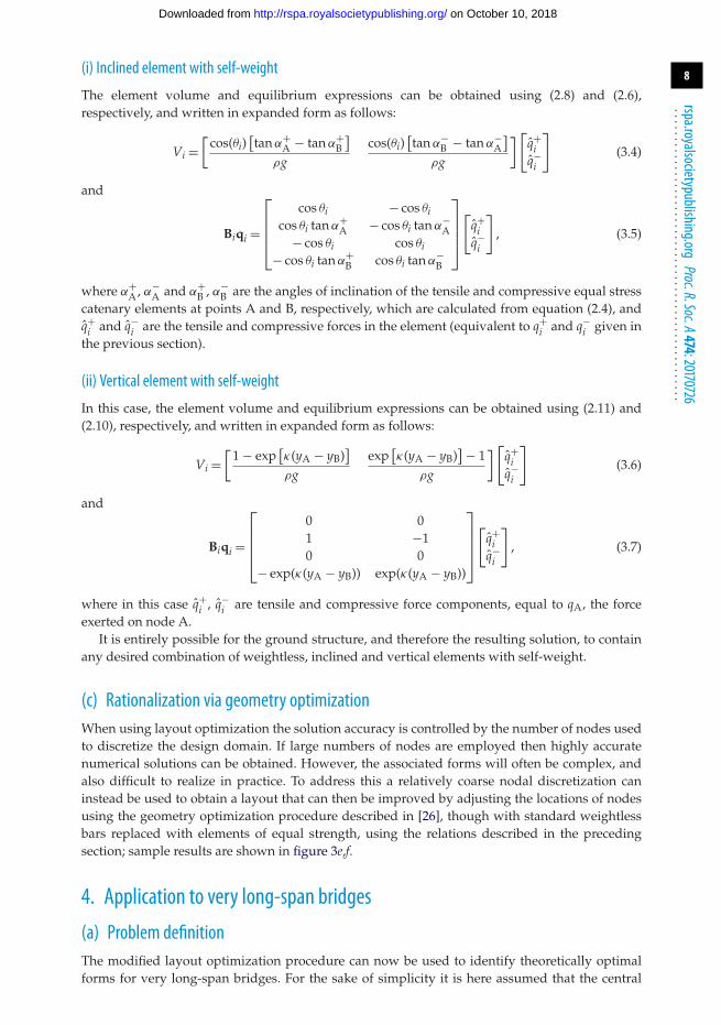
(i) Inclined element with self-weight

The element volume and equilibrium expressions can be obtained using (2.8) and (2.6),

respectively, and written in expanded form as follows:

Vi =[

cos(θi)[

tan α+A − tan α+

B

]

ρg

cos(θi)[

tan α−B − tan α−

A

]

ρg

]

[

q̂+i

q̂−i

]

(3.4)

and

Biqi =

⎡

⎢

⎢

⎢

⎣

cos θi − cos θi

cos θi tan α+A − cos θi tan α−

A− cos θi cos θi

− cos θi tan α+B cos θi tan α−

B

⎤

⎥

⎥

⎥

⎦

[

q̂+i

q̂−i

]

, (3.5)

where α+A , α−

A and α+B , α−

B are the angles of inclination of the tensile and compressive equal stress

catenary elements at points A and B, respectively, which are calculated from equation (2.4), and

q̂+i and q̂−

i are the tensile and compressive forces in the element (equivalent to q+i and q−

i given in

the previous section).

(ii) Vertical element with self-weight

In this case, the element volume and equilibrium expressions can be obtained using (2.11) and

(2.10), respectively, and written in expanded form as follows:

Vi =[

1 − exp[

κ(yA − yB)]

ρg

exp[

κ(yA − yB)]

− 1

ρg

]

[

q̂+i

q̂−i

]

(3.6)

and

Biqi =

⎡

⎢

⎢

⎢

⎣

0 0

1 −1

0 0

− exp(κ(yA − yB)) exp(κ(yA − yB))

⎤

⎥

⎥

⎥

⎦

[

q̂+i

q̂−i

]

, (3.7)

where in this case q̂+i , q̂−

i are tensile and compressive force components, equal to qA, the force

exerted on node A.

It is entirely possible for the ground structure, and therefore the resulting solution, to contain

any desired combination of weightless, inclined and vertical elements with self-weight.

(c) Rationalization via geometry optimization

When using layout optimization the solution accuracy is controlled by the number of nodes used

to discretize the design domain. If large numbers of nodes are employed then highly accurate

numerical solutions can be obtained. However, the associated forms will often be complex, and

also difficult to realize in practice. To address this a relatively coarse nodal discretization can

instead be used to obtain a layout that can then be improved by adjusting the locations of nodes

using the geometry optimization procedure described in [26], though with standard weightless

bars replaced with elements of equal strength, using the relations described in the preceding

section; sample results are shown in figure 3e,f.

4. Application to very long-span bridges

(a) Problem deinition

The modified layout optimization procedure can now be used to identify theoretically optimal

forms for very long-span bridges. For the sake of simplicity it is here assumed that the central



9


474:20170726...................................................

span of a notional multi-span bridge structure is being modelled, with the problem being as

described in figure 3, but with the point loads W replaced with a uniformly distributed load

w, applied at the same elevation. This configuration can also be used to approximately represent

a bridge with a central main span and shorter side-spans. (In fact, this representation will be

exact if the side-spans are equal to half the main span, and if reactions at the ends of the bridge

are purely horizontal, as is approximately the case, e.g. for the Akashi Kaikyo Bridge.) However,

other specific scenarios can readily be modelled using the general numerical procedure described.

The magnitude of w is assumed to include both traffic loading and the self-weight of deck

elements required to provide a continuous level traffic surface, though it does not include the

self-weight of material required in the deck to carry axial forces, if present, which is automatically

included in the model as part of the optimization process. Note also that in very long-span bridges

traffic loading becomes less significant than the self-weight of the deck and cables, which means

that the problem can justifiably be posed as a single load case layout optimization problem,

furnishing a structural form which consumes the minimum possible volume of material to carry

the distributed load w and the self-weight of the structural elements employed. (The inherent

bending resistance of the pylons and deck is not considered in the optimization directly, but will

be required to ensure that alternative load cases can be carried. Also, although wind and other

dynamic effects are very important in cable-supported bridges, particularly when spans are long,

various mitigation strategies can often be applied once the basic form has been established. For

example, to counter wind-induced vibration it has recently been suggested that the use of slotted

box girder decks will permit 5 km suspension bridge spans to be achieved [27], or alternatively

active control systems can potentially be employed [28]. These are therefore not considered

further here.)

In the interests of computational efficiency, a half span was modelled (taking advantage of

symmetry) and the adaptive solution strategy developed by Gilbert & Tyas [17] was employed

to enable problems with increasingly fine nodal resolutions to be solved. The load discretization

strategy used in [18] was also employed in order to reduce the discretization error associated with

the load. The largest model run contained 68 026 nodes and 2 313 734 325 potential connections,

including overlaps (i.e. over 2 billion potential connections).

(b) New reference volumes

Using the aforementioned assumptions, the layout optimization procedure has been used to

obtain new reference solutions for a range of bridge span lengths L, obtained by using increasingly

fine nodal resolutions; numerical results are shown in table 1. The spans quoted in the table

assume that high-strength steel is employed for all elements, with a limiting material strength

in tension and compression of 500 MPa and a unit weight of 80 kN m−3 - though other scenarios

can readily be modelled using the general numerical procedure described. Also shown are

extrapolated volumes computed using the power-law extrapolation scheme described in [18].

Models comprising nx = 200, 240, . . . , 600 divisions were used to provide source data, where nx is

the number of nodal divisions across the full span (the number of nodal divisions in the height of

the domain, ny was taken as nx × 3/8). A weighted nonlinear least-squares approach was used to

find best-fit coefficient values for use in the extrapolation, with the weighting factor taken as nx,

to increase the influence of fine resolution solutions.

For the 0 km span (weightless) case the extrapolated value was found to compare closely with

a recently published analytical value [20], showing that high-precision results can be obtained.

For the other spans considered the extrapolated values furnish new reference volumes, providing

benchmark values against which alternative bridge designs can be judged. (As suggested by Cox

[29], just as there is a limit on the thermal efficiency of a heat engine, set by the Carnot cycle, so

there is a lower limit on the volume of material necessary to form a structure. Even though this

will not normally be achievable in practice, it provides a useful basis on which to judge alternative

designs.)



10


474:20170726...................................................

Table 1. Numerical volumes (×wL2/σ0) for various bridge spans and nodal resolutions.

span

nx 0 km (weightless) 1 km (0.16(σ0/ρg)) 2.5 km (0.4(σ0/ρg)) 5 km (0.8(σ0/ρg))

numerical 200 0.726937 0.781744 0.875206 1.068504. . . . . . . . . . . . . . . . . . . . . . . . . . . . . . . . . . . . . . . . . . . . . . . . . . . . . . . . . . . . . . . . . . . . . . . . . . . . . . . . . . . . . . . . . . . . . . . . . . . . . . . . . . . . . . . . . . . . . . . . . . . . . . . . . . . . . . . . . . . . . . . . . . . . . . . . . . . . . . . . . . . . . . . . . . . . . . . . .

240 0.726759 0.781493 0.874886 1.067978. . . . . . . . . . . . . . . . . . . . . . . . . . . . . . . . . . . . . . . . . . . . . . . . . . . . . . . . . . . . . . . . . . . . . . . . . . . . . . . . . . . . . . . . . . . . . . . . . . . . . . . . . . . . . . . . . . . . . . . . . . . . . . . . . . . . . . . . . . . . . . . . . . . . . . . . . . . . . . . . . . . . . . . . . . . . . . . . .

280 0.726624 0.781327 0.874680 1.067679. . . . . . . . . . . . . . . . . . . . . . . . . . . . . . . . . . . . . . . . . . . . . . . . . . . . . . . . . . . . . . . . . . . . . . . . . . . . . . . . . . . . . . . . . . . . . . . . . . . . . . . . . . . . . . . . . . . . . . . . . . . . . . . . . . . . . . . . . . . . . . . . . . . . . . . . . . . . . . . . . . . . . . . . . . . . . . . . .

320 0.726535 0.781206 0.874535 1.067468. . . . . . . . . . . . . . . . . . . . . . . . . . . . . . . . . . . . . . . . . . . . . . . . . . . . . . . . . . . . . . . . . . . . . . . . . . . . . . . . . . . . . . . . . . . . . . . . . . . . . . . . . . . . . . . . . . . . . . . . . . . . . . . . . . . . . . . . . . . . . . . . . . . . . . . . . . . . . . . . . . . . . . . . . . . . . . . . .

360 0.726475 0.781120 0.874425 1.067293. . . . . . . . . . . . . . . . . . . . . . . . . . . . . . . . . . . . . . . . . . . . . . . . . . . . . . . . . . . . . . . . . . . . . . . . . . . . . . . . . . . . . . . . . . . . . . . . . . . . . . . . . . . . . . . . . . . . . . . . . . . . . . . . . . . . . . . . . . . . . . . . . . . . . . . . . . . . . . . . . . . . . . . . . . . . . . . . .

400 0.726425 0.781050 0.874337 1.067149. . . . . . . . . . . . . . . . . . . . . . . . . . . . . . . . . . . . . . . . . . . . . . . . . . . . . . . . . . . . . . . . . . . . . . . . . . . . . . . . . . . . . . . . . . . . . . . . . . . . . . . . . . . . . . . . . . . . . . . . . . . . . . . . . . . . . . . . . . . . . . . . . . . . . . . . . . . . . . . . . . . . . . . . . . . . . . . . .

440 0.726378 0.780995 0.874262 1.067038. . . . . . . . . . . . . . . . . . . . . . . . . . . . . . . . . . . . . . . . . . . . . . . . . . . . . . . . . . . . . . . . . . . . . . . . . . . . . . . . . . . . . . . . . . . . . . . . . . . . . . . . . . . . . . . . . . . . . . . . . . . . . . . . . . . . . . . . . . . . . . . . . . . . . . . . . . . . . . . . . . . . . . . . . . . . . . . . .

480 0.726342 0.780945 0.874201 1.066947. . . . . . . . . . . . . . . . . . . . . . . . . . . . . . . . . . . . . . . . . . . . . . . . . . . . . . . . . . . . . . . . . . . . . . . . . . . . . . . . . . . . . . . . . . . . . . . . . . . . . . . . . . . . . . . . . . . . . . . . . . . . . . . . . . . . . . . . . . . . . . . . . . . . . . . . . . . . . . . . . . . . . . . . . . . . . . . . .

520 0.726313 0.780903 0.874150 1.066866. . . . . . . . . . . . . . . . . . . . . . . . . . . . . . . . . . . . . . . . . . . . . . . . . . . . . . . . . . . . . . . . . . . . . . . . . . . . . . . . . . . . . . . . . . . . . . . . . . . . . . . . . . . . . . . . . . . . . . . . . . . . . . . . . . . . . . . . . . . . . . . . . . . . . . . . . . . . . . . . . . . . . . . . . . . . . . . . .

560 0.726286 0.780871 0.874109 1.066804. . . . . . . . . . . . . . . . . . . . . . . . . . . . . . . . . . . . . . . . . . . . . . . . . . . . . . . . . . . . . . . . . . . . . . . . . . . . . . . . . . . . . . . . . . . . . . . . . . . . . . . . . . . . . . . . . . . . . . . . . . . . . . . . . . . . . . . . . . . . . . . . . . . . . . . . . . . . . . . . . . . . . . . . . . . . . . . . .

600 0.726267 0.780844 0.874075 1.066753. . . . . . . . . . . . . . . . . . . . . . . . . . . . . . . . . . . . . . . . . . . . . . . . . . . . . . . . . . . . . . . . . . . . . . . . . . . . . . . . . . . . . . . . . . . . . . . . . . . . . . . . . . . . . . . . . . . . . . . . . . . . . . . . . . . . . . . . . . . . . . . . . . . . . . . . . . . . . . . . . . . . . . . . . . . . . . . . .

∞a 0.726031 0.780531 0.873674 1.066152. . . . . . . . . . . . . . . . . . . . . . . . . . . . . . . . . . . . . . . . . . . . . . . . . . . . . . . . . . . . . . . . . . . . . . . . . . . . . . . . . . . . . . . . . . . . . . . . . . . . . . . . . . . . . . . . . . . . . . . . . . . . . . . . . . . . . . . . . . . . . . . . . . . . . . . . . . . . . . . . . . . . . . . . . . . . . . . . . . . . . . . . . . . . . . . . . . . . . . . . . .

analytical — 0.7260325b — — —. . . . . . . . . . . . . . . . . . . . . . . . . . . . . . . . . . . . . . . . . . . . . . . . . . . . . . . . . . . . . . . . . . . . . . . . . . . . . . . . . . . . . . . . . . . . . . . . . . . . . . . . . . . . . . . . . . . . . . . . . . . . . . . . . . . . . . . . . . . . . . . . . . . . . . . . . . . . . . . . . . . . . . . . . . . . . . . . . . . . . . . . . . . . . . . . . . . . . . . . . .

dif. (%) — 0.0002 — — —. . . . . . . . . . . . . . . . . . . . . . . . . . . . . . . . . . . . . . . . . . . . . . . . . . . . . . . . . . . . . . . . . . . . . . . . . . . . . . . . . . . . . . . . . . . . . . . . . . . . . . . . . . . . . . . . . . . . . . . . . . . . . . . . . . . . . . . . . . . . . . . . . . . . . . . . . . . . . . . . . . . . . . . . . . . . . . . . . . . . . . . . . . . . . . . . . . . . . . . . . .

Notes: The new reference solutions are shown in italics typeface. (Quoted span lengths assume a limiting material stress σ0 = 500 MPa and

unit weightρg= 80 kN m−3.)aObtained by extrapolation, using a power-law extrapolation scheme as used in [18].bAnalytical solution obtained by Pichugin et al. [20].

(c) New structural forms

Structural forms corresponding to the new reference solutions for 1, 2.5 and 5 km span lengths

are shown in figure 4a. To provide visually clear solutions a layout optimization discretization

involving 30 nodal spacings across the full span was used prior to rationalizing the solutions

using geometry optimization; see appendix A for details.

The new reference forms shown in figure 4a quite closely resemble the weightless Michell

structure that was fully described analytically in [20], with tension and compressive elements

aligned (near)orthogonally. They also include a series of inclined compressive elements radiating

out from the supports, just as in [20]. The forms are also markedly different to traditional

cable-stayed or suspension bridge forms, and would clearly be extremely difficult to construct

in practice. However, to allow comparison with the former, the inclined compressive elements

can readily be removed by omitting candidate inclined compressive elements when setting up

the layout optimization problem. The resulting optimized cable-stayed bridge forms are shown

in figure 4d, and differ slightly from the standard ‘harp’ cable arrangement in that they have

non-uniform spacing of stays along the height of the pylon. However, most significantly, the

consumed material is up to 38% greater than that required for the corresponding (near) optimal

reference designs shown in figure 4a. Although the latter would be much more difficult to

fabricate than the more conventional cable-stayed forms shown in figure 4d, they can be used to

inspire a range of simplified forms. Thus figure 4b,c shows simplified split-pylon bridge structures

comprising, respectively, three and two pylons, consuming, respectively, approximately 6 and

12% more material than the corresponding reference designs in the 5 km span case; a computer-

generated render of a bridge comprising two 5 km spans designed to be potentially suitable for

the hypothetical Strait of Gibraltar crossing is also shown in figure 5.



11


474:20170726...................................................

span = 1 km span = 2.5 km span = 5 km

(e)

(d)

(c)

(b)

(a)

V = 1.40 V1 kmV = 1.50 V2.5 km V = 1.73 V5 km

V = 1.21 V1 kmV = 1.26 V2.5 km V = 1.38 V5 km

V = 1.07 V1 kmV = 1.09 V2.5 km V = 1.12 V5 km

V = 1.04 V1 km V = 1.05 V2.5 km V = 1.06 V5 km

V1 kmV2.5 km V5 km

Figure 4. Bridge forms for various spans and associated volumes, expressed in terms of the reference volume, where V1 km =0.7805wL2/σ0,V2.5 km = 0.8737wL2/σ0 andV5 km = 1.0662wL2/σ0 (wherew is the load applied at deck level, L is the span and

σ0 is the limiting strength of the material). The three-span lengths considered, 0.16(σ0/ρg), 0.4(σ0/ρg) and 0.8(σ0/ρg),

correspond to 1, 2.5 and 5 km, respectively, when σ0 is taken as 500 MPa and the unit weight ρg as 80 kN m−3. All solutions

shown were optimized via geometry optimization. (a) Reference design (simpliied layout shown for clarity). (b) Optimized

triple split-pylon design. (c) Optimized double split-pylon design. (d) Optimized cable-stayed design. (e) Optimized suspension

bridge design (all with variable cross-section cables). (Online version in colour.)

The optimized locations of all elements in the single, double and triple split-pylon cable-stayed

structures shown in figure 4b–d were found using geometry optimization techniques (appendix

A), indicating that a harp rather than fan style cable arrangement is most materially efficient.

Also, for comparative purposes, optimized suspension bridge configurations were obtained by

applying geometry optimization to the standard suspension bridge layout, as shown in figure 4e.

These bridges consume up to 73% more material than the corresponding reference designs shown

in figure 4a. (The bridge structures described here are actually somewhat lighter than those found

in constructed suspension bridges as the cable areas were here allowed to vary along the lengths

of the cables.)

Figure 6 presents results for all the cases described in normalized form, covering spans of

up to 10 km when using the same steel material as assumed before. Volumes for the fan style



12


474:20170726...................................................

Figure 5. Split-pylon concept bridge to cross Strait of Gibraltar, with two 5 km main spans (not showing additional measures

likely to be needed to counteract unbalanced live load efects, e.g. [30]). (Online version in colour.)

cable-stayed bridge form are also included for comparative purposes, along with those for

cable-stayed and suspension bridge forms constrained to use the larger span-to-dip (L/h) ratios

currently employed in the world’s current longest cable-stayed and suspension bridge spans,

respectively, found in the 1104 m span Russky Bridge, Russia (L/h = 4.4) and the 1991 m span

Akashi Kaikyo Bridge, Japan (L/h = 9). (Traditional suspension bridges have generally been built

with span-to-dip ratios of 8.5–13.5 and cable-stayed bridges with span-to-dip ratios of 3.4–4.9 [7].)

It is evident that traditional bridge forms with larger span-to-dip ratios become very inefficient as

spans increase, but that the simplified double and triple split-pylon forms remain comparatively

efficient even when the span is long.

(d) Inluence of span-to-dip ratio

The fact that a high span-to-dip ratio in a cable-supported bridge can lead to a high volume

of material being required has been known for many years (indeed this prompted the seminal

work of Davies Gilbert, who wanted to demonstrate to Thomas Telford that the initial shallow

suspension bridge design for the Menai Straits was structurally inefficient [24]). However, a low

span-to-dip ratio also requires the use of tall pylons, which can be problematic to construct. Also,

when non-uniform loadings are present it has been observed that midspan deflections increase

in suspension bridges when lower span-to-dip ratios are employed [30]. It is therefore of interest

to explore the influence of the limiting span-to-dip ratio on the volume of material required, and

to evaluate the performance of the new simplified forms when such limits are imposed. Figures 7

and 8 present volumes and corresponding forms when the span-to-dip ratios are limited to 4.4

and 9, respectively; key results from figures 6–8 are also tabulated in table 2, showing that the

span-to-dip ratios identified as being optimal in the present study are considerably lower than

those typically used in practice.

From figures 7 and 8 it is clear that even when a limit is placed on the span-to-dip ratio, the

corresponding reference form consumes considerably less material than traditional forms. The

simplified double split-pylon form is also much more materially efficient than traditional forms,

suggesting that this latter form could prove popular in practice. When the span-to-dip ratio is

increased to 9 the resulting double split-pylon form quite closely resembles the split-pylon design

tentatively proposed by Starossek [13] some years ago, though the latter uses a fan style cable



13


474:20170726...................................................

(a)

(a)

(b)

(b)

(c)

(c)

(d)

(d)

(e)

(e)

(h)(h)

( f )

( f )

(g)(g)

1 km 2.5 km 5 km 10 km

volu

me,

wL

2/s

0

0 0.2 0.4 0.6 0.8 1.0 1.2 1.4 1.6

span, s0/rg

0.5

1.0

1.5

2.0

2.5

3.0

3.5

4.0

Figure6. Volumeversus span for various bridge forms, using equal stress catenary elements andwithnodal positions identiied

via geometry optimization. (Span L= 0datapoints are taken from the literature; see table 2 for details. Indicated spandistances

of 1, 2.5, 5 and 10 km assume that σ0 is taken as 500 MPa and the unit weight ρg as 80 kN m−3) (a) Suspension bridge,

with span-to-dip ratio of 9, as in the Akashi Kaikyo Bridge, Japan. (b) Cable-stayed bridge with span-to-dip ratio of 4.4,

as in the Russky Bridge, Russia (harp cable arrangement assumed here). (c) Suspension bridge with optimal pylon height.

(d) Cable-stayed bridge with fan cable arrangement and optimal pylon height. (e) Cable-stayed bridge with optimal pylon

height. (f ) Optimized double split-pylon design. (g) Optimized triple split-pylon design. (h) Reference bridge design. (Online

version in colour.)

(a)

(a)

(b)

(b)

(c)

(c)

(d)

(d)

(e)

(e)

( f )( f )

(g)

(g)

1 km 2.5 km 5 km 10 km

volu

me,

wL

2/s

0 0.2 0.4 0.6 0.8 1.0 1.2 1.4 1.6

span, s/rg

0.5

1.0

1.5

2.0

2.5

3.0

Figure 7. Span-to-dip ratio of 4.4-volume versus span for diferent bridge designs: (a) harp style cable-stayed; (b) suspension;

(c) fan style cable-stayed; (d) optimized cable-stayed; (e) optimized double split-pylon; (f ) reference optimum form for the

given span-to-dip ratio; (g) reference with unrestricted span-to-dip ratio for comparative purposes. (Online version in colour.)



14


474:20170726...................................................

(a)

(a)

(b)

(b)

(c)

(c)

(d)

(d)

(e)

(e)

( f )

( f )

(g)(g)

0.5

1.0

1.5

2.0

2.5

3.0

3.5

4.0

0 0.2 0.4 0.6 0.8 1.0 1.2 1.4 1.6

1 km 2.5 km 5 km 10 km

volu

me,

wL

2/s

span, s/rg

Figure8. Span-to-dip ratio of 9-volume versus span for diferent bridge designs: (a) harp style cable-stayed; (b) suspension; (c)

fan style cable-stayed; (d) optimized cable-stayed; (e) optimized double split-pylon; (f ) reference optimum form for the given

span-to-dip ratio; (g) reference with unrestricted span-to-dip ratio for comparative purposes. (Online version in colour.)

arrangement rather than the hybrid cable arrangement observed to be optimal here. (A small

number of split-pylon cable-stayed bridges have been constructed in practice, though these have

generally spanned relatively short distances, and aesthetic or specific practical reasons for their

form have usually been cited by their designers. For example, the double split-pylon cable-stayed

bridge constructed near Düsseldorf Airport in Germany in 2002 was so designed to keep the

height of the structure low in order to avoid impeding air traffic [33]. Also, this bridge uses a fan

style cable arrangement, rather than the hybrid cable arrangement found to be most materially

efficient here.)

When the height available is unrestricted the optimal cable-stayed form resembles the harp

style form but has a non-uniform spacing of cables up the pylon (figure 6); this also leads to a

lower pylon height being required. As the height available is reduced the traditional harp style

form (with uniform spacing of cables up the pylon) becomes less efficient than both the fan style

form and also the suspension bridge form. Also, the optimal cable-stayed form begins to resemble

the fan style form, and has a similar volume.

(e) Inluence of reducing the limiting compressive stress

In this study, the limiting material stress has thus far been assumed to be the same in tension

and compression. However, it can be argued that a higher limiting stress should be adopted for

tension elements, to account for the likelihood that higher strength steel will be used for the

cables, and to account for a reduction in the stress sustainable by compression elements due to

buckling effects. On the other hand, in recent years very high strength hot-rolled steel has become

available which can potentially be used in the construction of pylon and deck elements carrying

compressive stresses, and appropriate detailing can be used to try to mitigate the detrimental

effects of buckling on the allowable stress. Nevertheless, it is of interest to explore cases when the

limiting tensile stress σT exceeds the limiting compressive stress σC. For example, figure 9 shows

optimized bridge forms when the limiting stress in compression is reduced to one-third and then

one-ninth of the limiting stress in tension (the latter case could e.g. represent a case where the

limiting tensile stress is 1800 MPa and the limiting compressive stress is 200 MPa). Firstly, it is

clear from the figure that the overall form of the optimal reference structure is largely unaffected,



15


474:20170726...................................................

Table 2. Comparison of volumes (×wL2/σ0) of traditional bridge forms with those of new reference solutions.

span

1 km (0.16 2.5 km (0.4 5 km (0.8

form L/ha igure 0 km (weightless) (σ0/ρg)) (σ0/ρg)) (σ0/ρg))

suspension 9 6a,8b 1.347222 [31,32] 1.648 2.508 18.985

optimal (4) 6c 1.000000 [31,32] 1.096 1.307 1.845. . . . . . . . . . . . . . . . . . . . . . . . . . . . . . . . . . . . . . . . . . . . . . . . . . . . . . . . . . . . . . . . . . . . . . . . . . . . . . . . . . . . . . . . . . . . . . . . . . . . . . . . . . . . . . . . . . . . . . . . . . . . . . . . . . . . . . . . . . . . . . . . . . . . . . . . . . . . . . . . . . . . . . . . . . . . . . . . . . . . . . . . . . . . . . . . . . . . . . . . . .

cable-stayed (fan) 4.4 7c 1.048 1.244 1.781. . . . . . . . . . . . . . . . . . . . . . . . . . . . . . . . . . . . . . . . . . . . . . . . . . . . . . . . . . . . . . . . . . . . . . . . . . . . . . . . . . . . . . . . . . . . . . . . . . . . . . . . . . . . . . . . . . . . . . . . . . . . . . . . . . . . . . . . . . . . . . . . . . . . . . . . . . . . . .

optimal 6d 1.041 1.224 1.672. . . . . . . . . . . . . . . . . . . . . . . . . . . . . . . . . . . . . . . . . . . . . . . . . . . . . . . . . . . . . . . . . . . . . . . . . . . . . . . . . . . . . . . . . . . . . . . . . . . . . . . . . . . . . . . . . . . . . . . . . . . . . . . . . . . . . . . . . . . . . . . . . . . . . . . . . . . . . . . . . . . . . . . . . . . . . . . . . . . . . . . . . . . . . . . . . . . . . . . . . .

cable-stayed (harp) 4.4 6b 1.052273 [31] 1.189 1.458 2.269. . . . . . . . . . . . . . . . . . . . . . . . . . . . . . . . . . . . . . . . . . . . . . . . . . . . . . . . . . . . . . . . . . . . . . . . . . . . . . . . . . . . . . . . . . . . . . . . . . . . . . . . . . . . . . . . . . . . . . . . . . . . . . . . . . . . . . . . . . . . . . . . . . . . . . . . . . . . . .

optimal (4/√3) — 0.866025 [31] 0.954 1.112 1.492

. . . . . . . . . . . . . . . . . . . . . . . . . . . . . . . . . . . . . . . . . . . . . . . . . . . . . . . . . . . . . . . . . . . . . . . . . . . . . . . . . . . . . . . . . . . . . . . . . . . . . . . . . . . . . . . . . . . . . . . . . . . . . . . . . . . . . . . . . . . . . . . . . . . . . . . . . . . . . . . . . . . . . . . . . . . . . . . . . . . . . . . . . . . . . . . . . . . . . . . . . .

cable-stayed (optimal) 4.4 7d 0.989 1.176 1.691. . . . . . . . . . . . . . . . . . . . . . . . . . . . . . . . . . . . . . . . . . . . . . . . . . . . . . . . . . . . . . . . . . . . . . . . . . . . . . . . . . . . . . . . . . . . . . . . . . . . . . . . . . . . . . . . . . . . . . . . . . . . . . . . . . . . . . . . . . . . . . . . . . . . . . . . . . . . . .

optimal 6e 0.946 1.102 1.476. . . . . . . . . . . . . . . . . . . . . . . . . . . . . . . . . . . . . . . . . . . . . . . . . . . . . . . . . . . . . . . . . . . . . . . . . . . . . . . . . . . . . . . . . . . . . . . . . . . . . . . . . . . . . . . . . . . . . . . . . . . . . . . . . . . . . . . . . . . . . . . . . . . . . . . . . . . . . . . . . . . . . . . . . . . . . . . . . . . . . . . . . . . . . . . . . . . . . . . . . .

split-pylon (double) 9 8e 1.197 1.483 2.275. . . . . . . . . . . . . . . . . . . . . . . . . . . . . . . . . . . . . . . . . . . . . . . . . . . . . . . . . . . . . . . . . . . . . . . . . . . . . . . . . . . . . . . . . . . . . . . . . . . . . . . . . . . . . . . . . . . . . . . . . . . . . . . . . . . . . . . . . . . . . . . . . . . . . . . . . . . . . .

4.4 7e 0.856 0.978 1.248. . . . . . . . . . . . . . . . . . . . . . . . . . . . . . . . . . . . . . . . . . . . . . . . . . . . . . . . . . . . . . . . . . . . . . . . . . . . . . . . . . . . . . . . . . . . . . . . . . . . . . . . . . . . . . . . . . . . . . . . . . . . . . . . . . . . . . . . . . . . . . . . . . . . . . . . . . . . . .

optimal 6f 0.838 0.951 1.197. . . . . . . . . . . . . . . . . . . . . . . . . . . . . . . . . . . . . . . . . . . . . . . . . . . . . . . . . . . . . . . . . . . . . . . . . . . . . . . . . . . . . . . . . . . . . . . . . . . . . . . . . . . . . . . . . . . . . . . . . . . . . . . . . . . . . . . . . . . . . . . . . . . . . . . . . . . . . . . . . . . . . . . . . . . . . . . . . . . . . . . . . . . . . . . . . . . . . . . . . .

split-pylon (triple) optimal 6g 0.811 0.914 1.134. . . . . . . . . . . . . . . . . . . . . . . . . . . . . . . . . . . . . . . . . . . . . . . . . . . . . . . . . . . . . . . . . . . . . . . . . . . . . . . . . . . . . . . . . . . . . . . . . . . . . . . . . . . . . . . . . . . . . . . . . . . . . . . . . . . . . . . . . . . . . . . . . . . . . . . . . . . . . . . . . . . . . . . . . . . . . . . . . . . . . . . . . . . . . . . . . . . . . . . . . .

reference 9 8f 1.130 1.320 1.711. . . . . . . . . . . . . . . . . . . . . . . . . . . . . . . . . . . . . . . . . . . . . . . . . . . . . . . . . . . . . . . . . . . . . . . . . . . . . . . . . . . . . . . . . . . . . . . . . . . . . . . . . . . . . . . . . . . . . . . . . . . . . . . . . . . . . . . . . . . . . . . . . . . . . . . . . . . . . .

4.4 7f 0.817 0.921 1.137. . . . . . . . . . . . . . . . . . . . . . . . . . . . . . . . . . . . . . . . . . . . . . . . . . . . . . . . . . . . . . . . . . . . . . . . . . . . . . . . . . . . . . . . . . . . . . . . . . . . . . . . . . . . . . . . . . . . . . . . . . . . . . . . . . . . . . . . . . . . . . . . . . . . . . . . . . . . . .

optimal (2√2) 6h, 7g, 8g 0.726031[21] 0.780531 0.873674 1.066152

. . . . . . . . . . . . . . . . . . . . . . . . . . . . . . . . . . . . . . . . . . . . . . . . . . . . . . . . . . . . . . . . . . . . . . . . . . . . . . . . . . . . . . . . . . . . . . . . . . . . . . . . . . . . . . . . . . . . . . . . . . . . . . . . . . . . . . . . . . . . . . . . . . . . . . . . . . . . . . . . . . . . . . . . . . . . . . . . . . . . . . . . . . . . . . . . . . . . . . . . . .

Notes: A discretization of 30 nodal spacings across the full span and geometry optimization was used except for the optimal reference forms.

Quoted span lengths assume a limiting material stress σ0 = 500 MPa and unit weight ρg= 80 kN m−3. The quoted volumes for the

weightless designs are computed using explicit analytical expressions given in [31,32] (for suspension bridges), [31] (for cable-stayed bridges)

and [20] (for optimal Michell structures).aOptimal span-to-dip (L/h) ratios for weightless designs indicated in parenthesis, where available in the cited sources. (The optimal

span-to-dip ratios for the longer span designs, which include self-weight, are similar, though not identical.)

though the horizontal extent of the fan region over a support reduces (as is also the case when self-

weight effects are neglected [20]). Also the optimal span-to-dip ratio increases for the reference

structure, and also for all the other bridge forms considered. The relative volumes of the cable-

stayed and suspension bridges fall, respectively, to 1.30 and 1.54 for the σT/σC = 3 case, and to 1.25

and 1.36, respectively, for the σT/σC = 9 case. This indicates that the advantage of the new forms

over traditional forms remains, though does reduce somewhat when the limiting compressive

stress is lower than the limiting tensile stress.

(f) Commentary

This study has focused on identifying theoretically optimal forms for carrying the predominant

load case for a hypothetical very long bridge span structure, i.e. self-weight loading, comprising

the weight of the cables, pylons and deck, together with uniformly distributed traffic

loading. It is sometimes argued that certain structural configurations become efficient when

asymmetric loadings due to traffic are involved (e.g. considering the fan-style cable-stayed bridge

configuration, the pylons are not subject to bending when asymmetric loadings due to traffic are

involved, which is advantageous if traffic loads are high). However, in the case of very long-span

bridges the magnitude of traffic loading in relation to self-weight becomes comparatively small,

reducing this effect. For example, in studies recently undertaken by a bridge design consultancy

for proposed suspension bridges incorporating spans ranging from 1.3 to 3.3 km, traffic loads



16


474:20170726...................................................

(d)

(c)

(b)

(a)

V = 1.73 V0sT/sC = 1 sT/sC = 3V = 1.54 V0

sT/sC = 9V = 1.36 V0

sT/sC = 9V = 1.25 V0

sT/sC = 9V = 1.04 V0

sT/sC = 3V = 1.30 V0

sT/sC = 3V = 1.04 V0

sT/sC = 1V = 1.38 V0

sT/sC = 1V = 1.06 V0

sT/sC = 9V0sT/sC = 3V0

sT/sC = 1V0

sT/sC = 9sT/sC = 3sT/sC = 1

Figure 9. Efect of reducing the limiting compressive stress on selected forms shown in igure 4, for the span = 0.8(σ0/ρg)

case (where the limiting tensile stress σT = σ0 and the limiting compressive stress is reduced as indicated). Volumes shown

are expressed in terms of the relevant reference volume. (a) Reference design (simpliied layout shown for clarity). (b)

Optimized triple split-pylon design. (c) Optimized cable-stayed design. (d) Optimized suspension bridge design. (All with

variable cross-section cables.) (Online version in colour.)

contributed only between 15 and 23% of the loads carried by the main cables [34] (all loads

unfactored). Thus although non-uniform traffic loading would need to be considered as part of

the detailed design phase it is unlikely to change the overall findings of the present study when

very long spans are involved. (By contrast when shorter spans are involved, of the sort likely to

be constructed in the immediate future, non-uniform traffic loading can be expected to have an

influence on form, with, in the case of multi-span bridges, alternate span traffic loading scenarios

being particularly important. This, for example, led to a ‘crossing stay’ cable arrangement being

chosen for the three-span Queensferry Crossing bridge across the Firth of Forth in Scotland,

completed in 2017 [35]. Also, cable size may need to be increased to reduce deflections if these

prove to be excessive.)

In this paper elements with non-uniform cross sections have been employed for all bridge

forms considered, both new and traditional. This means that material in all cross sections is

fully stressed, ensuring that the structures are as materially efficient as possible, thereby allowing

reference solutions to be obtained. However, it should be noted that while methods of realizing

non-uniform elements have been proposed (e.g. [36]), usually uniform cross sections are preferred

in practice, which will slightly increase the overall weight of all bridges forms considered.

Although the present study has focused on efficiency, the method proposed can potentially be

modified so as to minimize the likely cost of the overall bridge construction. For example, as the

cost of cables is likely to be higher than the cost of compression elements, this can be accounted



17


474:20170726...................................................

cC = cT cC = 19

cT

sC = 19

sT

sC = sT

C = 7.49 C0 C = 1.78 C0

C0 C = 0.55 C0

Figure 10. Efect of changing the relative cost of compressive and tensile members on the minimum cost C and corresponding

geometry of the triple split-pylon bridge form considered in igure 9, where C =∑

cTVT +∑

cCVC, and where cT, VTand cC,VC are the cost coeicients and volumes for tensile and compressive members, respectively. (Two limiting tensile to

compressive stress and cost ratios considered.) (Online version in colour.)

(a) (b) (c)

Figure 11. Appraising the relative eiciency of bridge forms by considering how deck loads are transmitted back to a support.

(a) Suspension bridge: the load path is comparatively long, so a large volume of material is required to transmit the forces

involved. (The same situation occurs in a fan cable-stayed bridge.) (b) Harp cable-stayed bridge: the load path is kept short, but

acute angles between the elements lead to high cable forces, and also to signiicant induced forces in the deck. (c) Split-pylon

cable-stayed bridge: the load path remains relatively short but the angles between the elements are less acute, ensuring cable

and induced deck forces are lower. (Online version in colour.)

for by including suitable cost coefficients in the optimization objective function. For example,

in figure 10 the minimum cost triple split-pylon design is sought, with the ratio of limiting

tensile and compressive stress varied together with the relative cost of tensile and compressive

members. Also, when modelling a bridge containing end spans, a cost could potentially be

ascribed to the resultant horizontal reaction forces, which would in practice need to be carried

by costly anchorages. These forces will generally be greatest in the case of suspension bridge

forms, adding to their relative cost, though the other cable-supported forms considered herein



18


474:20170726...................................................

would also require the use of external earth anchorages, due to the presence of tension at the

supports. Although ‘self-anchored’ cable-stayed bridge designs have become popular due to ease

of construction, a benefit of using earth anchorages for very long spans is that compression in

the deck can be controlled; this is discussed further by Gimseng [37]. Alternatively boundary

conditions in the optimization problem can easily be changed to, for example, prevent a solution

being generated which requires transmission of horizontal forces to supports.

Finally, an explanation for the comparative efficiency of the split-pylon form is given in

figure 11; this involves considering how directly deck loads are transmitted back to the supports.

Although constructing very long-span bridges based on these latter designs would no doubt be

challenging, the reward—significantly reduced material consumption—is clear.

5. ConclusionA means of obtaining the theoretically optimal bridge form to span a given distance under the

action of gravity loading has been described. This required the development of a new numerical

layout optimization procedure capable of intrinsically modelling the self-weight of the constituent

structural elements. To achieve this, equal strength catenary elements were employed, allowing

phenomena such as cable sag to be modelled in the optimization process in an entirely natural

manner. The procedure has been applied to the design of hypothetical very long-span bridges,

enabling the optimal reference form and associated required volume of material to be established

for a given span. The reference volume provides a benchmark against which traditional or

proposed new bridge designs can be objectively judged.

It has been found that the reference bridge forms differ markedly to traditional suspension

bridge and cable-stayed bridge forms involving vertical pylons, and also require much less

material to construct, especially when very long spans are involved. For example, a conventional

suspension bridge form spanning 5 km requires up to 73% more material than the corresponding

reference design when using steel. The reference designs have also been used as inspiration for

simple yet highly efficient bridge designs involving split pylons, which require comparatively

little more material than the reference designs.

Data accessibility. Geometrical data describing key reference and geometry optimized bridge forms are provided

in the electronic supplementary material.

Authors’ contributions. H.E.F. programmed the methods described and performed the numerical optimization

runs, on the suggestion of, and in consultation with, M.G. H.E.F., M.G., A.V.P. and A.T. wrote initial drafts

of the paper, which I.F. provided in-depth comments on, providing advice on practical bridge engineering

considerations and proposing additional modelling studies. All authors approved the final version of the

paper.

Competing interests. We have no competing interests.

Funding. H.E.F. acknowledges the financial support provided by the University of Sheffield, the UK

Engineering and Physical Sciences Research Council and Expedition Engineering Ltd, London, UK.

Acknowledgements. The authors are grateful to Linwei He of the University of Sheffield for making available

geometry optimization program code, which was extended in the present study to treat problems involving

self-weight.

Appendix AGeometry optimization has been used to generate many of solutions presented. For example,

figure 4a was obtained by starting with a layout optimized solution, obtained using a relatively

coarse nodal discretization, and then using geometry optimization to rationalize the solution; see

figure 12 for ‘before’ and ‘after’ layouts for this case. It is evident that the half-wheel-like section

over the supports appears smoother and more clearly defined after geometry optimization has

been performed.

Geometry optimization was also used to establish the most efficient joint positions for the

traditional and new simplified split pylon bridge forms considered. For example, figure 13 shows



19


474:20170726...................................................


(b)

(a)

Figure 12. Bridge forms rationalized using geometry optimization. (a) Layout optimized solutions, obtained using a coarse

nodal discretization. (b) Solutions obtained after using geometry optimization to rationalize (a). (Quoted span lengths assume

a limiting material stressσ0 = 500 MPa and unit weightρg= 80 kN m−3.) (Online version in colour.)


(b)

(a)

Figure 13. Sample bridge forms optimized using geometry optimization. (a) Harp style cable-stayed bridge, with cables

intersecting the pylon at equal vertical intervals. (b) Modiied form obtained after applying geometry optimization to the

structure in (a), showing resulting optimized pylon/cable intersection locations. (Quoted span lengths assume a limiting

material stressσ0 = 500 MPa and unit weightρg= 80 kN m−3.) (Online version in colour.)

‘before’ and ‘after’ layouts for a harp style cable-stayed bridge configuration, which indicates

that a lower volume solution is obtained if the cables are allowed to ‘bunch up’ near the top of the

pylon. In each case a discretization of 30 nodal spacings across the full span was used to ensure

visually clear solutions could be obtained (sensitivity studies indicate that this discretization gives

solutions which are slightly above, though within approximately 0.1%, of the solutions which can

be obtained using extremely fine numerical discretizations).

References1. Drewry CS. 1832 A memoir on suspension bridges, comprising the history of their origin and progress,

and of their application to civil and military purposes. London: Longman, Rees, Orme, Brown,Green & Longman.

2. Kitagawa M. 2004 Technology of the Akashi Kaikyo Bridge. Struct. Control Health Monit. 11,75–90. (doi:10.1002/stc.31)

3. Hansford M. 2012 Cable stay revolution hangs in the balance. New Civil Engineer, 5 July 2012,pp. 4–5.


http://dx.doi.org/doi:10.1002/stc.31


20


474:20170726...................................................

4. Ito M. 1996 Super long span cable-suspended bridges in Japan. In Proc. 15th Cong. IABSE,Copenhagen, Denmark, 16–20 June, pp. 1009–1018. Zurich, Switzerland: IABSE.

5. Ostenfeld KH. 1996 Comparison between different structural solutions. The Great Beltproject. In Proc. 15th Cong. IABSE, Copenhagen, Denmark, 16–20 June, pp. 1063–1078. Zurich,Switzerland: IABSE.

6. Galileo G. 1954 Dialogues concerning two new sciences. New York, NY: Dover Publications Inc.7. Lewis WJ. 2012 A mathematical model for assessment of material requirements for

cable supported bridges: implications for conceptual design. Eng. Struct. 42, 266–277.(doi:10.1016/j.engstruct.2012.04.018)

8. Meier U. 1987 Proposal for a carbon fibre reinforced composite bridge across the Straitof Gibraltar at its narrowest site. Proc. Inst. Mech. Eng. Part B: J. Eng. Manuf. 201, 73–78.(doi:10.1243/PIME_PROC_1987_201_048_02)

9. Xiong W, Cai C, Zhang Y, Xiao R. 2011 Study of super long span cable-stayed bridges withCFRP components. Eng. Struct. 33, 330–343. (doi:10.1016/j.engstruct.2010.10.013)

10. Damolini S. 2009 Carbon nanotubes and their application to very long span bridges. PhDthesis, Massachusetts Institute of Technology, Cambridge, MA.

11. Lu K. 2010 The future of metals. Science 328, 319–320. (doi:10.1126/science.1185866)12. Lin T, Chow P. 1991 Gibraltar Strait crossing – a challenge to bridge and structural engineers.

Struct. Eng. Int. 1, 53–58. (doi:10.2749/101686691780617779)13. Starossek U. 1996 Cable-stayed bridge concept for longer spans. J. Bridge Eng. 1, 99–103.

(doi:10.1061/(ASCE)1084-0702(1996)1:3(99))14. Michell AGM. 1904 The limits of economy of material in frame-structures. Phil. Mag. 8,

589–597. (doi:10.1080/14786440409463229)15. Maxwell JC. 1870 I. On reciprocal figures, frames, and diagrams of forces. Trans. R. Soc. Edinb.

26, 1–40. (doi:10.1017/S0080456800026351)16. Dorn WS, Gomory RE, Greenberg HJ. 1964 Automatic design of optimal structures. J. Mec. 3,

25–52.17. Gilbert M, Tyas A. 2003 Layout optimization of large-scale pin-jointed frames. Eng. Comput.

(Swansea) 20, 1044–1064. (doi:10.1108/02644400310503017)18. Darwich W, Gilbert M, Tyas A. 2010 Optimum structure to carry a uniform load between

pinned supports. Struct. Multidiscipl. Optim. 42, 33–42. (doi:10.1007/s00158-009-0467-0)19. Tyas A, Pichugin AV, Gilbert M. 2011 Optimum structure to carry a uniform load between

pinned supports: exact analytical solution. Proc. R. Soc. A 467, 1101–1120. (doi:10.1098/rspa.2010.0376)

20. Pichugin AV, Tyas A, Gilbert M, He L. 2015 Optimum structure for a uniform load overmultiple spans. Struct. Multidiscipl. Optim. 52, 1041–1050. (doi:10.1007/s00158-015-1278-0)

21. Beghini A, Baker WF. 2015 On the layout of a least weight multiple span structure withuniform load. Struct. Multidiscipl. Optim. 52, 447–457. (doi:10.1007/s00158-015-1248-6)

22. Bendsoe MP. 1995 Optimization of structural topology, shape, and material. Berlin, Germany:Springer Science & Business Media.

23. Gilbert D. 1826 On the mathematical theory of suspension bridges, with tables for facilitatingtheir construction. Phil. Trans. R. Soc. 116, 202–208. (doi:10.1098/rstl.1826.0019)

24. Calladine C. 2015 An amateur’s contribution to the design of Telford’s Menai suspensionbridge: a commentary on Gilbert (1826) ‘On the mathematical theory of suspension bridges’.Phil. Trans. R. Soc. A 373, 20140346. (doi:10.1098/rsta.2014.0346)

25. Routh EJ. 1896 A treatise on analytical statics: the parallelogram of forces. Forces acting at a point.Parallel forces. Forces in two dimensions. On friction. The principle of work. Forces in three dimensions.Graphical statics. Centre of gravity. On strings. The machines, vol. 1. Nancy: University Press.

26. He L, Gilbert M. 2015 Rationalization of trusses generated via layout optimization. Struct.Multidiscipl. Optim. 52, 677–694. (doi:10.1007/s00158-015-1260-x)

27. Ge Y-J. 2016 Aerodynamic challenge and limitation in long-span cable-supported bridges.In Proc. ACEM16 / Structures16 Conf. Jeju-do, Korea, 28 August–1 September.

28. Xu Y-L. 2013 Wind effects on cable-supported bridges. New York, NY: John Wiley & Sons.29. Cox HL. 2014 The design of structures of least weight. International Series of Monographs in

Aeronautics and Astronautics: Division 1: Solid and Structural Mechanics, vol. 8. Amsterdam,The Netherlands: Elsevier.

30. Gimsing NJ, Georgakis CT. 2011 Cable supported bridges: concept and design. New York, NY:John Wiley & Sons.


http://dx.doi.org/doi:10.1016/j.engstruct.2012.04.018

http://dx.doi.org/doi:10.1243/PIME_PROC_1987_201_048_02

http://dx.doi.org/doi:10.1016/j.engstruct.2010.10.013

http://dx.doi.org/doi:10.1126/science.1185866

http://dx.doi.org/doi:10.2749/101686691780617779

http://dx.doi.org/doi:10.1061/(ASCE)1084-0702(1996)1:3(99)


http://dx.doi.org/doi:10.1017/S0080456800026351


http://dx.doi.org/doi:10.1007/s00158-009-0467-0

http://dx.doi.org/doi:10.1098/rspa.2010.0376

http://dx.doi.org/doi:10.1098/rspa.2010.0376



http://dx.doi.org/doi:10.1098/rstl.1826.0019

http://dx.doi.org/doi:10.1098/rsta.2014.0346

http://dx.doi.org/doi:10.1007/s00158-015-1260-x


21


474:20170726...................................................

31. Croll JGA. 1997 Thoughts on the structural efficiency of cable-stayed and catenary suspensionbridges. Struct. Eng. 75, 173–175.

32. Dalton HC, French MJ, Croll JGA. 1997 Correspondence on “thoughts on the structuralefficiency of cable-stayed and catenary suspension bridges”. Struct. Eng. 75, 345–347.

33. Prehn W, Mertens M. 2002 Die Rheinquerung der a 44-Darstellung der Gesamtmaßnahme.Stahlbau 71, 386–392. (doi:10.1002/stab.200201350)

34. Jensen L, Bloomstine ML. 2009 Application of high strength steel in super long span modernsuspension bridge design. NSCC, pp. 494–501.

35. Carter M, Kite S, Hussain N, Minto B. 2010 Design of the Forth replacement crossing Scotland.Proc. Inst. Civil Eng. Bridge Eng. 163, 91–99. (doi:10.1680/bren.2010.163.2.91)

36. Gokyu I. 1970 Parallel cables. US Patent no. 3,500,625.37. Gimsing NJ. 1994 Suspended bridges with very long spans. In Proc. Int. Conf. IABSE-FIP, Cable-

stayed and Suspension Bridges, Deauville, 12–15 October, pp. 489–504.


http://dx.doi.org/doi:10.1002/stab.200201350

http://dx.doi.org/doi:10.1680/bren.2010.163.2.91


Theoretically optimal forms for very long span bridges under ...

Documents

Transcript of Theoretically optimal forms for very long span bridges under ...