1

Abstract The reliability of the structural performance of any given structure is affected by both in-service loading and material deterioration due to environmental attack. They must be evaluated at any given time in order to compute lifetime probability of failure. This paper presents an innovative methodology to derive the structure lifetime load effect due to existing traffic using a statistical tool known as Predictive Likelihood. Loss of resistance due to corrosion originated by chloride ingression is also taken into account. Finally the lifetime probability of failure is evaluated via the application of a time-discretization strategy. Keywords: bridge, structural reliability, safety, predictive likelihood, corrosion, traffic. 1 Introduction As the existing stock of bridges ages, there is an increasing need for the assessment and maintenance of existing structures. Ageing reinforced concrete structures are generally subject not only to in-service loading, but also to an aggressive environment which will eventually lead to material degradation. Consequently there is a reduction in the operational safety of such structures. Safety evaluation and damage assessment have been topics of intensive research in recent years (Li[1], Stewart et al [2])

Both the resistance and loading of a bridge structure are time-dependent variables and they must be considered in the service-life prediction of deteriorating structures. While much research has been carried out on the characterization of degradation mechanisms which lead to a reduction of resistance with time, Melchers [3] points out that load modelling is also a critical area demanding research as loads are typically the variables with the greatest uncertainty.

Paper 189 The Structural Reliability of Bridges subject to Time-Dependent Deterioration A. Bordallo-Ruiz1, C. McNally1, E.J. OBrien12 and C.C. Caprani3 1 School of Architecture, Landscape and Civil Engineering 2 UCD Urban Institute University College Dublin, Ireland 3 Department of Civil and Structural Engineering Dublin Institute of Technology, Ireland

©Civil-Comp Press, 2007 Proceedings of the Eleventh International Conference on Civil, Structural and Environmental Engineering Computing, B.H.V. Topping (Editor), Civil-Comp Press, Stirlingshire, Scotland

2

In recent years statistical models have been increasingly employed to assist the estimation of the lifetime traffic loading to which a bridge is subject. These models are focused on the development of statistical tools to obtain the characteristic load effect. However statistical methods, such as Predictive Likelihood (PL) (Butler [4], Davison [5]), can provide probability distribution functions of each characteristic value (predictand) as opposed to a single value. The characteristic value is defined as the value with an acceptably low probability of exceedance. For example, the Eurocode for bridge loading [6] defines the characteristic value as the level with a 10% probability of exceedance in 100 years, which is usually approximated as a 1000-year return period.

In the estimation of bridge traffic loading, Caprani [7] has shown that a complete 100 year lifetime extreme load effect distribution can be obtained from measured traffic characteristics. PL has proved to be an efficient computational tool to accurately define extreme load effect and will be used to determine the most likely distribution for the maximum lifetime loading effect, given both the data and a set of postulated predictands.

This approach opens the possibility of incorporating this methodology of prediction of lifetime extreme traffic loading into the general framework of structural reliability, in order to evaluate the lifetime probability of failure of any given structure.

This paper combines the load effect distribution with a model of material resistance. The example used for the latter is the deterioration of structural resistance of bridge beams due to loss of area of reinforcing steel through corrosion. Reinforcement corrosion has been established as the predominant causal factor for the premature deterioration of reinforced concrete (RC) structures leading to structural failure (Schiessl [8], Broomfield [9]). Loss of structural resistance due to spalling of concrete as well as the effect of other degradation mechanisms such as sulphate attack, carbonation, alkali-silica reaction and freeze-thaw cycle attack are not considered.

Finally the probability of failure for a given period of time is calculated.

Integration over the lifetime of the structure gives the probability of failure over a duration (0, tL], also called the cumulative time failure probability.

2 Time-variant resistance modelling 2.1 Bridge deterioration model In order to assess accurately the safety of any structure, the time-variant residual strength of the structural elements must be evaluated. This paper considers loss of strength due to environmental attack, expressed as reduction of reinforcement area originated by corrosion, as proposed by Enright and Frangopol [10]. For bridges,

3

corrosion initiation of reinforcement is normally due to chloride ion ingress. Assuming that it is a diffusion controlled process, chloride ingress can be modelled using Fick’s second Law of diffusion:

2

2

xCD

tC

C ∂∂

=∂∂ (1)

where C is the chloride ion concentration (% of the weight of cement) at distance

x cm from the concrete surface after t years of exposure to the chloride source. Dc is the chloride diffusion coefficient (cm2/year). 2.2 Corrosion initiation time It is taken that corrosion is initiated by the diffusion of chloride ions and that the concentration of chloride ions on the surface of the reinforcement is constant. Then the corrosion initiation time is given by (Thoft-Christensen et al [11], Lounis [12]):

21-

2erf

4

−

⎥⎥⎦

⎤

⎢⎢⎣

⎡⎟⎟⎠

⎞⎜⎜⎝

⎛ −=

o

cro

Ci C

CCDXT (2)

where Ti is the corrosion initiation time (years), X is the concrete cover (cm), Co

is the equilibrium chloride concentration at the concrete surface (% weight of concrete) and Ccr is the threshold chloride concentration at which corrosion begins (% weight of concrete). Therefore the corrosion initiation time is dependent on four random variables, which are considered in this paper to be lognormally distributed (the approach from different authors is not consistent – Hong [13], Schiessl [14], Stewart [15], Enright and Frangopol [10]).

2.3 Area loss of steel reinforcement It is assumed that the cross sectional loss of steel reinforcement due to corrosion propagation is the only cause of loss of resistance of a structural element. For a reinforced concrete element with equal diameter bars, subject to the same corrosion initiation times, the time-variant area of steel reinforcement can be expressed as:

⎪⎪⎪

⎩

⎪⎪⎪

⎨

⎧

+≥

+≤≤

≤

=

corr

ii

corr

iii

ii

rD

Tt

rD

TtTtDn

TtDn

tA

for0

for4

)(

for4

)(2

2

π

π

(3)

4

where n is the number of reinforcing bars, Di is the initial diameter of steel reinforcement, t is the elapsed time, rcorr is the corrosion rate (mm/year), and

)()( icorri TtrDtD −−= (4) is the diameter of a bar under corrosion.

When the corrosion rate is estimated based on a corrosion current density icorr, the latter can be transformed into the loss of metal by means of Faraday’s Law, which indicates that a corrosion density of icorr=1μA/cm2 corresponds to an uniform corrosion penetration of 11.6 μm/year (Val et al [16]). Consequently, the reduction of the diameter of a corroding bar, as stated in Equation (4) can be estimated as

∫=−T

T corrii

dttitDD )(0232.0)( (5)

If a constant annual corrosion rate is assumed, Equation (5) can be rewritten as

)(0232.0)( icorri TtitDD −=− (6) Consequently it is usual to define the corrosion rate as

corrcorr ir 0232.0= (7)

Alonso et al [17] have derived similar relationships.

2.4 Time-variant resistance Once the time-variant loss of steel reinforcement has been determined, the determination of the time-variant resistance is straightforward. It is sometimes convenient to express this time-variant resistance as a product of the initial resistance and a resistance degradation function:

)()( tgRtR o= (8)

where Ro is the initial resistance and g(t) is the resistance degradation function. The initial resistance Ro can be determined using equations for nominal resistance in relevant bridge design codes.

5

3 Bridge traffic load simulation 3.1 Data acquisition and simulation of bridge loading In order to determine the statistical distribution of bridge traffic loading, it is essential to have actual highway traffic data obtained from suitable installations. Weigh-In-Motion (WIM) technology is a tool that provides appropriate data for this purpose. Characteristics that are measured include gross vehicle weights, inter-axle spacing, vehicle headway, speed, flow rates and flow composition. In this paper, data from the A6 motorway near Auxerre, France, is used as the basis for simulating bridge traffic loading. This site has 4 lanes of traffic (2 in each direction) but only the traffic recorded in the slow lanes was used which is acknowledged to result in conservative loading effect for a 2-lane bridge. During the 5 days of measurement, 17 756 and 18 617 trucks were measured in the north and south slow lanes respectively; an average daily truck flow of 6744 trucks. This period is acknowledged to be short in duration. However the methodology proposed is general and only quantitative results may be affected by this short duration. In order to generalize the limited measured data, a Monte Carlo simulation process is used. Models for the simulation process are derived from the data measured on site. Monte Carlo simulations of 1000 1-day sample periods of truck traffic on a two-lane bidirectional bridge are generated. The load effects induced by heavy trucks and multiple truck presence events are recorded. Long term traffic growth is not considered in this model. For the purpose of prediction, the year is defined as consisting of 50 weeks of 5 weekdays each (allowing for 11 public holidays). 3.2 Analysis of extremes In this work an extreme value analysis is performed on the load effect data collected from the simulation process. Based on the method proposed by authors such as Castillo [18], Ang and Tang [19] and Coles [20], an algorithm is proposed in order to obtain the distribution of the lifetime maximum load effect considered. It is well known that when the extremes of interest are generated from a single statistical mechanism, the three Fisher and Tippet families can be expressed in a single form; the Generalized Extreme Value distribution (GEV) as described in Coles [20]:

⎪⎭

⎪⎬

⎫

⎪⎩

⎪⎨

⎧

⎥⎦

⎤⎢⎣

⎡⎟⎠⎞

⎜⎝⎛

σμ−

ξ−−=θξ

+

1

1exp);( xxG (9)

where [h]+ = max(h,0) and the parameter vector is θ=(μ,σ,ξ), i.e., the location,

6

scale and shape parameters of the distribution respectively. It is remarkable to note that considering traffic loading as a single statistical

generating mechanism will result in loss in accuracy. Caprani et al [21] have shown that the mechanisms of loading caused by different numbers of trucks simultaneously present on the bridge are statistically different; for example, the distribution of stress due to a single truck crossing is different to that of a 2-truck event. Caprani and OBrien [22] give a method known as Composite Distribution Statistics (CDS) which accounts for this, and they show that the exact distribution of load effect may be derived by considering the distribution associated with each mechanism as well as their relative frequency of occurrence.

Considering there to be nt event types and nd loading events per day, and using

the law of total probability, the exact distribution of daily maximum load effect, S is then given by

[ ]d

tnn

jjj fsFsSP ⎟⎟⎠

⎞⎜⎜⎝

⎛=≤ ∑

=1)( (10)

in which the cumulative distribution function and frequency of the jth type is Fj(·)

and fj respectively. In practice these quantities are difficult to derive but it is known (Gumbel [23]) that the exact distribution may be asymptotically approximated by

[ ] ∏=

==≤tn

jjC sGsGsSP

1)()( (11)

where Gj(·) is the GEV distribution of the jth event type and GC(·) represents the

CDS. Thus it is necessary to note each loading event according to its truck composition and to order the loading events separately, noting the maximum event of each type for each day of simulation.

3.3 Prediction by Predictive likelihood

There has been considerable work in recent years on the problem of predicting a characteristic value from a set of observed data (Nowak [24], O’Connor [25], Getachew [26]). Current methods of predicting characteristic load effects give greatly variable results, often being unduly influenced by a small number of extreme loading events. Predictive Likelihood (Bjørnstad [27]) addresses this problem by identifying the likelihood of a range of possible characteristic values. In the context of bridge traffic loading, PL is used to estimate the likelihood of lifetime maximum load effects. In addition to providing a more robust method of estimating the 10% fractile of the lifetime maximum, it provides a tool which can be applied in Reliability Theory.

7

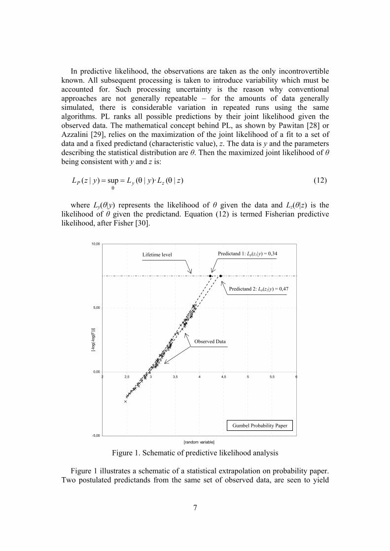
In predictive likelihood, the observations are taken as the only incontrovertible known. All subsequent processing is taken to introduce variability which must be accounted for. Such processing uncertainty is the reason why conventional approaches are not generally repeatable – for the amounts of data generally simulated, there is considerable variation in repeated runs using the same algorithms. PL ranks all possible predictions by their joint likelihood given the observed data. The mathematical concept behind PL, as shown by Pawitan [28] or Azzalini [29], relies on the maximization of the joint likelihood of a fit to a set of data and a fixed predictand (characteristic value), z. The data is y and the parameters describing the statistical distribution are θ. Then the maximized joint likelihood of θ being consistent with y and z is:

)|()·|(sup)|( zLyLyzL zyP θθ==θ

(12)

where Ly(θ|y) represents the likelihood of θ given the data and Lz(θ|z) is the

likelihood of θ given the predictand. Equation (12) is termed Fisherian predictive likelihood, after Fisher [30].

Figure 1. Schematic of predictive likelihood analysis

Figure 1 illustrates a schematic of a statistical extrapolation on probability paper.

Two postulated predictands from the same set of observed data, are seen to yield

-5,00

0,00

5,00

10,00

2 2,5 3 3,5 4 4,5 5 5,5 6

[random variable]

[-log

(-log

(F))]

Lifetime level Predictand 1: Lp(z1|y) = 0,34

Predictand 2: Lp(z2|y) = 0,47

Observed Data

Gumbel Probability Paper

8

different values of predictive likelihood. By considering a range of such predictands, the predictive likelihood function can be plotted to rank different possible lifetime maximum load effects. A detailed methodology regarding the theory behind the application of PL to bridge traffic loading plus all relevant computational aspects is presented by Caprani and OBrien [31]. The likelihood function is normalized and, for this paper, a GEV distribution fitted through the discrete points. A number of weighting functions are possible; the one adopted in this work is to use a weight of unity for all points below the mode of the distribution, and to use a weight equal to the reciprocal of the predictand for points above it. 4 Structural Reliability. Probability of failure In its most basic approximation, Structural Reliability (SR) aims to provide an estimate of the probability of failure (pf) of a given structural element. The probability is the sum of the failure probabilities for all the cases of resistance and load for which the load effect (S) exceeds the structural capacity to resist this effect (R), as expressed in Equation (13). In other words, any structural element is considered to have failed if its resistance R is less than the stress resultant S acting on it. The relative frequency of failure is then the number of failures divided by the total number of outcomes. Hence the probability of failure is (Melchers [32] or Stewart [15]):

)0()()()0( ≤==≤−= ∫ ∫∞

∞−

≥

∞−ZPdrdssfrfSRPp

rsSRf (13)

where fR(·) represents the probability density function (PDF) of the capacity and

fS(·) the PDF of the loading. Integrating once gives

)0()()()0( ≤==≤−= ∫∞

∞−ZPdssfsFSRPp SRf (14)

with FR(·) standing for the Cumulative Distribution Function of the capacity.

The solution to this integral can be found accurately using numerical techniques.

The inaccuracy of the obtained probability of failure derives only from the modelling of the stochastic variables, to which it is sensitive. To compute the lifetime probability of failure, the time-discretization strategy, as described by Petryna and Krätzig [33], is adopted. It represents an acceptable compromise between the time-integration approach that underestimates the actual reliability and the first-passage approach that involves highly demanding algorithms in terms of computation time. In the time-discretization, the entire lifetime is

9

subdivided into a number of time intervals at which the integration of the extreme value distributions for loading and resistance is evaluated.

Melchers [32] or COST 345 report [34] propose acceptable risks in society for different events. This approach enables the introduction of maintenance operations to return the probability of failure to acceptable values and facilitates maintenance planning for deteriorating concrete structures.

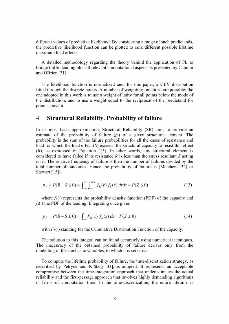
5 Example Let us consider a 20 m span, 13 m wide, two-lane, simply-supported bridge consisting of 5 reinforced concrete bridge beams as the one shown in Figure 2.

Figure 2. Example reinforced concrete bridge beam

For rectangular non-prestressed members for which the compression steel is neglected, the ultimate bending moment (flexure) is given by:

⎟⎠⎞

⎜⎝⎛ −=

2adfAM ysu

(15) where

bffA

ac

ys'85,0

= (16)

and As is the area of non-prestressed tension reinforcement, fy is the specified

yield strength of reinforcing bars, d is the distance from the extreme compression fiber to the centroid of non-prestressed tensile reinforcement and f’c is the specified compressive (cylinder) strength of concrete at 28 days and b is the width of the compression face of the member.

2600 mm

10T32

110 mm

500 mm

200 mm

50 mm 50 mm

10

The main descriptors, mean and coefficient of variation (COV), for all the stochastic variables in Equations (2), (15) and (16) are summarized in Table 1. As already stated all stochastic variables are taken to be lognormally distributed.

Mean COV

X [cm] 5,08 0,20 Dc [cm2/yr] 1,29 0,10 C0 [% cement] 0,10 0,10 Ccr [% cement] 0,04 0,10 Di [mm] 32 0,02 fy [N/mm2] 460 0,12 f’c [N/mm2] 25 0,18 d [cm] 110 0,10

Table 1. Probabilistic descriptors of main stochastic variables

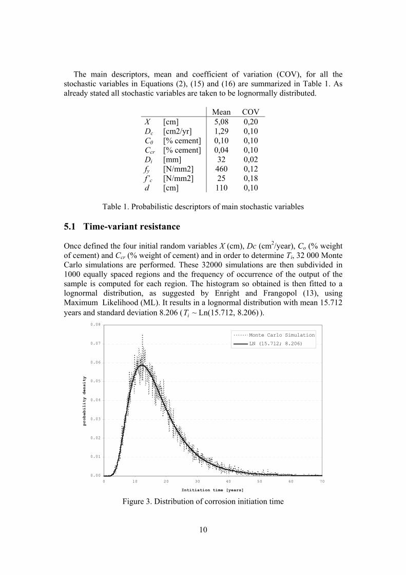
5.1 Time-variant resistance Once defined the four initial random variables X (cm), Dc (cm2/year), Co (% weight of cement) and Ccr (% weight of cement) and in order to determine Ti, 32 000 Monte Carlo simulations are performed. These 32000 simulations are then subdivided in 1000 equally spaced regions and the frequency of occurrence of the output of the sample is computed for each region. The histogram so obtained is then fitted to a lognormal distribution, as suggested by Enright and Frangopol (13), using Maximum Likelihood (ML). It results in a lognormal distribution with mean 15.712 years and standard deviation 8.206 ( 8.206) Ln(15.712,~iT ).

0.00

0.01

0.02

0.03

0.04

0.05

0.06

0.07

0.08

0 10 20 30 40 50 60 70

Intitiation time [years]

probability density

Monte Carlo Simulation

LN (15.712; 8.206)

Figure 3. Distribution of corrosion initiation time

11

Once corrosion initiation time has been obtained, the next step consists in determining the area of steel corroded at a given time. This is done by a Monte Carlo simulation of 32000 samples for which the residual area of tensile reinforcement after a given time is evaluated in accordance with Equation (3).

Finally, the residual capacity of the structure, Equation (15), is evaluated at a

given time. Again a histogram based on 1000 equally spaced regions and the frequency of occurrence of the output of the sample is fitted to a lognormal distribution using, again, ML, in a similar manner to the fit for corrosion initiation time shown in figure (3).

5.2 Traffic load effect

Based on the traffic described in paragraph 3.1, Caprani [7] has performed a

parametric study of the maximum load effect, 3 cases considered: bending moment at mid span for a simply supported bridge, left support shear in a simply-supported bridge and central support bending moment of a two-span continuous bridge, for a set of spans ranging from 20 to 50 m, for 100 years lifetime. At the same time a set of different distributions functions were fitted to the output of the different load effects considered, having ranked them according to their Maximum Likelihood values.

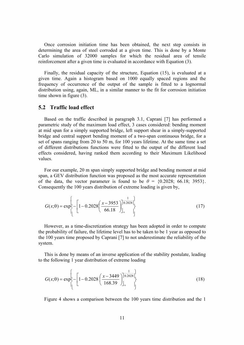
For our example, 20 m span simply supported bridge and bending moment at mid

span, a GEV distribution function was proposed as the most accurate representation of the data, the vector parameter is found to be θ = {0.2028; 66.18; 3953}. Consequently the 100 years distribution of extreme loading is given by,

⎪⎭

⎪⎬

⎫

⎪⎩

⎪⎨

⎧

⎥⎦

⎤⎢⎣

⎡⎟⎠⎞

⎜⎝⎛ −

−−=θ+

2028.01

18.6639532028.01exp);( xxG (17)

However, as a time-discretization strategy has been adopted in order to compute

the probability of failure, the lifetime level has to be taken to be 1 year as opposed to the 100 years time proposed by Caprani [7] to not underestimate the reliability of the system.

This is done by means of an inverse application of the stability postulate, leading

to the following 1 year distribution of extreme loading

⎪⎭

⎪⎬

⎫

⎪⎩

⎪⎨

⎧

⎥⎦

⎤⎢⎣

⎡⎟⎠⎞

⎜⎝⎛ −

−−=θ+

2028.01

39.16834492028.01exp);( xxG (18)

Figure 4 shows a comparison between the 100 years time distribution and the 1

12

year time one.

0

0.1

0.2

0.3

0.4

0.5

0.6

0.7

0.8

0.9

1

3000 3250 3500 3750 4000 4250kN·m

[cum

ulat

ive

prob

abili

ty]

0.0000

0.0006

0.0012

0.0018

0.0024

0.0030

0.0036

0.0042

0.0048

0.0054

0.0060[probability density]

CDF 100yr CDF 1yr

PDF 100yr PDF 1yr

Figure 4. PDF and CDF for 100-years and 1-year lifetime maximum bending

moment at midspan

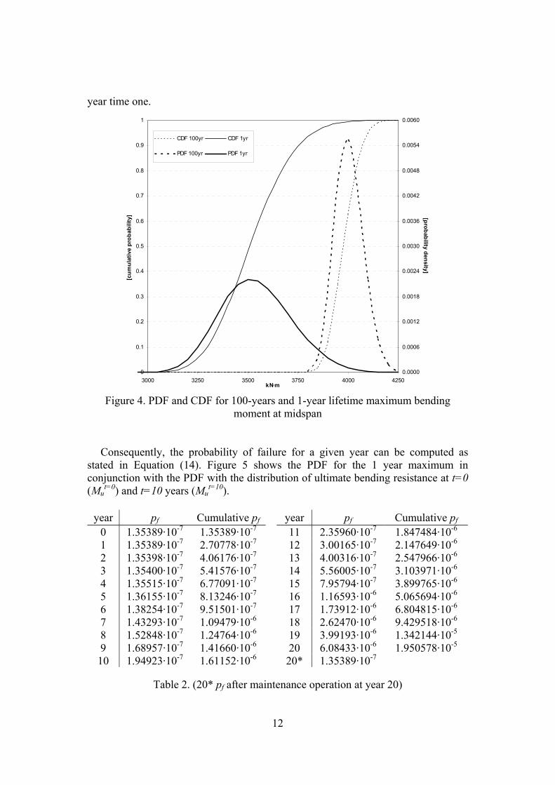
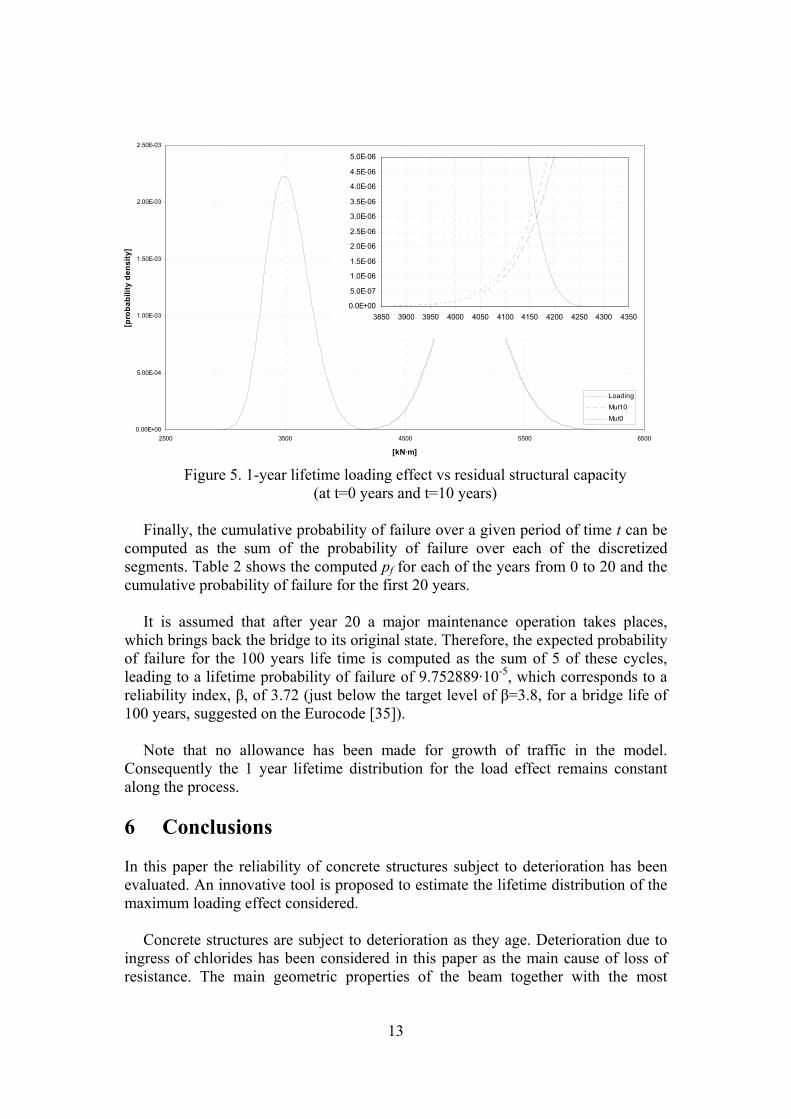
Consequently, the probability of failure for a given year can be computed as stated in Equation (14). Figure 5 shows the PDF for the 1 year maximum in conjunction with the PDF with the distribution of ultimate bending resistance at t=0 (Mu

t=0) and t=10 years (Mut=10).

year pf Cumulative pf year pf Cumulative pf

0 1.35389·10-7 1.35389·10-7 11 2.35960·10-7 1.847484·10-6 1 1.35389·10-7 2.70778·10-7 12 3.00165·10-7 2.147649·10-6 2 1.35398·10-7 4.06176·10-7 13 4.00316·10-7 2.547966·10-6 3 1.35400·10-7 5.41576·10-7 14 5.56005·10-7 3.103971·10-6 4 1.35515·10-7 6.77091·10-7 15 7.95794·10-7 3.899765·10-6 5 1.36155·10-7 8.13246·10-7 16 1.16593·10-6 5.065694·10-6 6 1.38254·10-7 9.51501·10-7 17 1.73912·10-6 6.804815·10-6 7 1.43293·10-7 1.09479·10-6 18 2.62470·10-6 9.429518·10-6 8 1.52848·10-7 1.24764·10-6 19 3.99193·10-6 1.342144·10-5 9 1.68957·10-7 1.41660·10-6 20 6.08433·10-6 1.950578·10-5 10 1.94923·10-7 1.61152·10-6 20* 1.35389·10-7

Table 2. (20* pf after maintenance operation at year 20)

13

0.00E+00

5.00E-04

1.00E-03

1.50E-03

2.00E-03

2.50E-03

2500 3500 4500 5500 6500

[kN·m]

[pro

babi

lity

dens

ity]

Loading

Mut10

Mut0

0.0E+00

5.0E-07

1.0E-06

1.5E-06

2.0E-06

2.5E-06

3.0E-06

3.5E-06

4.0E-06

4.5E-06

5.0E-06

3850 3900 3950 4000 4050 4100 4150 4200 4250 4300 4350

Figure 5. 1-year lifetime loading effect vs residual structural capacity (at t=0 years and t=10 years)

Finally, the cumulative probability of failure over a given period of time t can be

computed as the sum of the probability of failure over each of the discretized segments. Table 2 shows the computed pf for each of the years from 0 to 20 and the cumulative probability of failure for the first 20 years.

It is assumed that after year 20 a major maintenance operation takes places,

which brings back the bridge to its original state. Therefore, the expected probability of failure for the 100 years life time is computed as the sum of 5 of these cycles, leading to a lifetime probability of failure of 9.752889·10-5, which corresponds to a reliability index, β, of 3.72 (just below the target level of β=3.8, for a bridge life of 100 years, suggested on the Eurocode [35]).

Note that no allowance has been made for growth of traffic in the model.

Consequently the 1 year lifetime distribution for the load effect remains constant along the process.

6 Conclusions In this paper the reliability of concrete structures subject to deterioration has been evaluated. An innovative tool is proposed to estimate the lifetime distribution of the maximum loading effect considered.

Concrete structures are subject to deterioration as they age. Deterioration due to ingress of chlorides has been considered in this paper as the main cause of loss of resistance. The main geometric properties of the beam together with the most

14

representative environmental parameters are evaluated in order to obtain a distribution of residual strength at any given time t.

Regarding the loading, measured Weigh-In-Motion data is statistically modelled

to characterize the traffic at the site of measurement. Monte Carlo simulation is used to extend the amount of data available. This traffic is passed over a simply supported bridge of 20 m span and the influence line of the bending moment at midspan. The resulting output forms a population upon which a statistical analysis is carried out.

The method of predictive likelihood is applied to the bridge loading problem,

making use of an extension of it which accounts for composite distribution statistics problems. It results in a lifetime distribution of maximum loading effect, as opposed to a more conventional approach that would lead to a ‘characteristic value’. As many sources of variability are incorporated within the predictive likelihood distribution it is preferred to the conventional approach. On the other hand the output distribution of loading effect can be used to compute the reliability of the structure at any time.

Finally the probability of failure pf is computed from the distribution of residual

resistance and the distribution of loading effect. A time-discretization strategy is used to determine the lifetime probability of failure. 1-year intervals are considered. It is worth mention that no allowance has been made for the growth of traffic with time, remaining constant, consequently, the distribution of the 1 year lifetime maximum loading effect.

In summary, predictive likelihood has proved to be an efficient tool to compute

lifetime distributions for maximum loading effects. This, together with the fact that residual strength can be computed efficiently when it is mainly due to corrosion of reinforcement, lead to a very useful framework to efficiently compute probability of failure of existing structures, in which the real traffic loading can be measured using WIM technology.

It is expected that this approach will enable the introduction of maintenance

operations to return the probability of failure to acceptable values and will facilitate maintenance planning for deteriorating concrete structures. It is expected that these improved maintenance strategies will result in significant savings as unnecessary repair and rehabilitation of existing bridges may be avoided.

References [1] C.Q. Li, “Life cycle Modelling of corrosion affected concrete structures –

Initiation”, Journal of materials in civil engineering, 15(6), 594-601, 2003. [2] M.G. Stewart, D.V. Rosowsky, D.V. Val, “Reliability-based bridge

assessment using risk ranking decision analysis”, Structural Safety, 23, 397-405, 2001.

[3] R.E. Melchers, “Assesment of existing structures – Approaches and research needs”, Journal of Structural Engineering, 127(4), 406-411, 2001.

15

[4] R.W. Butler, “Approximate predictive pivots and densities”, Biometrika, 76, 489-501, 1989.

[5] A.C. Davison, “Approximate predictive likelihood”, Biometrika, 73, 323-332, 1986.

[6] EC 1, 1994, ‘Basis of design and actions on structures’, Part 2: ‘Traffic loads on bridges’, European Prestandard ENV 1991-3: European Committee for Standardisation, TC 250, Brussels.

[7] C.C. Caprani, “Probabilistic Analysis of Highway Bridge Traffic Loading”, Ph.D. Thesis, School of Architecture, Landscape, and Civil Engineering, University College Dublin, Ireland, 2005.

[8] P. Schiessel, “New approach to service life design of concrete structures”, Asian Journal of Civil Engineering (Building and Housing), 6(5), 393-407.

[9] J. Broomfield, “Corrosion of steel in concrete, understanding, investigating & repair”, E & FN Spon, London, 1997

[10] M.P. Enright, D.M. Frangopol “Probabilistic analysis of resistance degradation of reinforced concrete beams under corrosion”, Engineering Srtuctures, 20(11), 960-971, 1998.

[11] P. Thoft-Christensen, F.M. Jensen, C.R. Middleton and A. Blackmore, “Assesment of the reliability of concrete slab bridges”, in Reliability and Optimization of Structural Systems, ed. D.M. Frangopol, R.B. Corotis and R. Rackwitz, 321-328, Elsevier, London, 1997,

[12] Z. Lounis, “ Probabilistic modelling of chloride contamination and corrosion of concrete bridge structures”, Proceedings of the Fourth International Symposium on Uncertainty Modeling and Analysis (ISUMA ’03), Canadian Crown, 2003.

[13] H.P. Hong, “Assessment of aging reinforced concrete structures”, Journal of Structural Engineering, 126(12), 1458-1465, 2000.

[14] P. Schiessl, “Corrosion of steel in concrete”, Rep. RILEM No TC60-CSC RILEM, Chapman and Halll, London, 1988,

[15] M.G. Stewart, “Reliability-based assessment of ageing bridges using risk ranking and life cycle cost decision analysis”, Reliability Engineering and System Safety, 74, 263-273, 2001.

[16] D.V. Val, M.G. Stewart, R.E. Melchers, “Effect of reinforcement corrosion on reliability of highway bridges”, Engineering Structures, 20(11), 1010-1019, 1998.

[17] C. Alonso, C. Andrade, M. Castellote, P. Castro, “Chloride threshold values to depassivate reinforcing bars embedded in a standardized OPC mortar”, Cement and Concrete Research, 30, 1047-1055, 2000.

[18] E. Castillo, “Extreme Value Theory in Engineering”, New York, Academic Press, 1988.

[19] A.H.S. Ang and W.H. Tang, “Probability Concepts in Engineering Planning and Design, Vols. I and II”, Wiley and Sons, 1975.

[20] S.G. Coles, “An Introduction to Statistical Modeling of Extreme Values”, London, Springer-Verlag, 2001.

[21] C.C. Caprani, E.J. OBrien, G.J. McLachlan, “Characteristic traffic load effects from a mixture of loading events on short to medium span bridges”, Structural

16

Safety, in Press, 2007. [22] C.C. Caprani, E.J. OBrien, “Finding the distribution of bridge lifetime load

effect by Predictive Likelihood”, Proceedings of the 3rd International ASRAnet Colloquium, Glasgow, United Kingdom, 2006.

[23] E. J. Gumbel, “Statistics of Extremes”, Columbia University Press, 1958. [24] A.S. Nowak, “Live load model for highway bridges”, Structural Safety, 13,

53-66, 1994. [25] A.J. O’Connor, “Probabilistic traffic load modelling for highway bridges”,

Ph.D. Thesis, Department of Civil Engineering, Trinity College Dublin, 2001 [26] A. Getachew, “Traffic Load Effect on Bridges”, Ph.D. Thesis, Structural

Engineering, Royal Institute of Technology Stockholm, Sweden, 2003. [27] J.F. Bjørnstad, “Predictive likelihood: a review”, Statistical Science, 5(2), 242-

254, 1990. [28] Y. Pawitan, In all likelihood: statistical modelling and inference using

likelihood. Clarendon Press, Oxford, 2001. [29] A. Azzalini, “Statistical Inference: based on the likelihood”, Chapman & Hall,

London, 1996. [30] R.A. Fisher, ‘Statistical Methods and Scientific Inference’, Oliver and Boyd,

Edinburgh., 1956. [31] C.C. Caprani, E.J. OBrien, “Statistical Computation for Extreme Bridge

Traffic Load Effects”, Proceedings of the Eigth International Conference on Computational Structures Technology, ed. B.H.V. Topping, G. Montero and R. Montenegro, Civil-Comp Press, Stirlingshire, Scotland, 2006.

[32] R.E. Melchers, Structural reliability analysis and prediction 2nd ed. John Wiley, Chichester, 1999

[33] Y.S. Petryna, W.B. Krätzig, “Computational framework for long-term reliability analysis of RC structures”, Computational methods in applied mechanics and engineering, 194, 1619-1639, 2005.

[34] COST 345, “Procedures Required for Assessing Highway Structures”, Report of Working Group 1: “Report on the Current Stock of Highway Structures in European Countries, the Cost of their Replacement and the Annual Cost of Maintaining, Repairing and Renewing them”, available from http://cost345.zag.si/, 2004.

[35] EC 1, 1994, ‘Basis of design and actions on structures’, Part 1: ‘Basis of design’, European Prestandard ENV 1991-1: European Committee for Standardisation, TC 250, Brussels.