Bioindicator reliability

Bioindicator reliability:the example of Bel W3 tobacco (Nicotiana tabacum L.)

Xavier Vergea, Alain Chapuisb,*, Marcel Delpouxa

aUniversite Paul Sabatier, 39 allees Jules Guesde, 31 062-Toulouse Cedex, FrancebLaboratoire d’Aerologie UMR 5560 OMPT, 14 Avenue E. Belin, 31 400 Toulouse, France

Received 10 March 2001; accepted 8 October 2001

‘‘Capsule’’: Intrapopulation variation in ozone sensitiviy was found for a seed lot of Bel-W3 tobacco, a common sentinelbioindicator plant for ozone.

Abstract

The use of the Bel W3 tobacco variety revealed the existence of an intrapopulation variation of sensitivity to the ozone effectleading to the isolation of two categories of plants: sensitive and resistant. The use of sensitive plants revealed the existence of a

biological ozone efficiency threshold at a level close to 34.5 ppb. Under the threshold, the biological effects observed were weak orvery weak. They can be attributed to the occurrence of secondary phenomena (chemical, physiological, pathological, etc.), inducingor inhibiting necrosis, which become perceptible here. # 2002 Elsevier Science Ltd. All rights reserved.

Keywords: Bel W3; Bioindicator plants; Ozone; Atmospheric pollution; Ecotoxicology

1. Introduction

A major tropospheric pollutant in summer, ozone isvery carefully studied by the authorities responsible forsurveying air quality. However, measures to extend airmonitoring networks are limited by the high costinvolved. Additional networks of biological ozone indi-cators can be used to get around these difficultiesbecause they are easy to implement and less expensive.Their extension would not only allow an atmospheric

ozone surveillance program to be established, but alsothe detection of polluted zones inaccessible, for eco-nomic reasons, to chemical measurements.One of the bioindicators renowned to be the most sen-

sitive to this gas is the Bel W3 variety of tobacco (Nicoti-ana tabacum L.) developed at the end of the 1950s nearWashington (Heggestad andMenser, 1962;Menser et al.,1963; Manning and Feder, 1980; Heggestad, 1991). Thethreshold ozone levels, beyond which necrosis appears,are very low: 30 ppb for plants exposed for 8 h (Larsenand Heck, 1976). Since the beginning of the 1960s, thisBel W3 variety has often been used as an indicator ofthe biological effects of ozone, especially in the United

States (Craker et al., 1974; Walter and Barlow, 1974),the Netherlands (Posthumus, 1976), Israel (Goren andDonagi, 1979), United Kingdom (Ashmore et al., 1978,1980) and in France (Bonte, 1985; Van Haluwyn andGarrec, 1995; Garrec and Livertoux, 1997; Verge, 2000).Bioindicators are sensitive to numerous environ-

mental factors. Some, being able to interfere with ozoneeffects, must be recognized and taken into account inthe interpretation of results. Environmental factorsmodifying plant sensitivity have been identified: photo-periods and light intensities (Heck and Dunning, 1967),temperature and relative humidity (Dunning and Heck,1977), and a linear relation was obtained between ozonenecrosis by multiplying the hourly ozone concentrationby the corresponding hourly coefficient of evaporation(Macdowall et al., 1964).Besides, a synergistic effect of sulfur dioxide with

ozone (Menser and Heggestad, 1966) and sensitizationto later exposure by low levels of ozone (Steinbergerand Naveh, 1982) were observed. The injury observedon plants exposed for a week can be twice as extensiveas the total of damage observed on seven differentplants each exposed for one day over the same 7-dayperiod (Heagle and Heck, 1974).Finally, sensitivity to ozone is a genetically inherit-

able trait. Several genes of resistance for this gas were

0269-7491/02/$ - see front matter # 2002 Elsevier Science Ltd. All rights reserved.

PI I : S0269-7491(01 )00300-1

Environmental Pollution 118 (2002) 337–349

www.elsevier.com/locate/envpol

* Corresponding author. Fax: +335-61-33-27-90.

E-mail address: [email protected] (A. Chapuis).

identified on several tobacco varieties (Sand, 1960). ForBel W3, at least two genes are reported to control ozoneinjury (Taylor, 1968), and by selection more resistantstrains could be isolated (Aycock, 1972).In 1996, to set up an ozone surveillance biomonitor-

ing network, we used the Bel W3 tobacco variety. Dur-ing growth under glass, we observed characteristicozone necrosis on a few plants, showing that sensitivitybetween plants was different. This result called the useof this tobacco as a bioindicator into question, and wesubsequently analysed the difference of responsebetween the two categories of plants and the sensitivityof the most sensitive plants. These studies were made inthe open air to take into account environmental factorscapable of intervening on plant sensitivity. The resultsof this work experiments are presented here.

2. Materials and methods

2.1. Exposure station

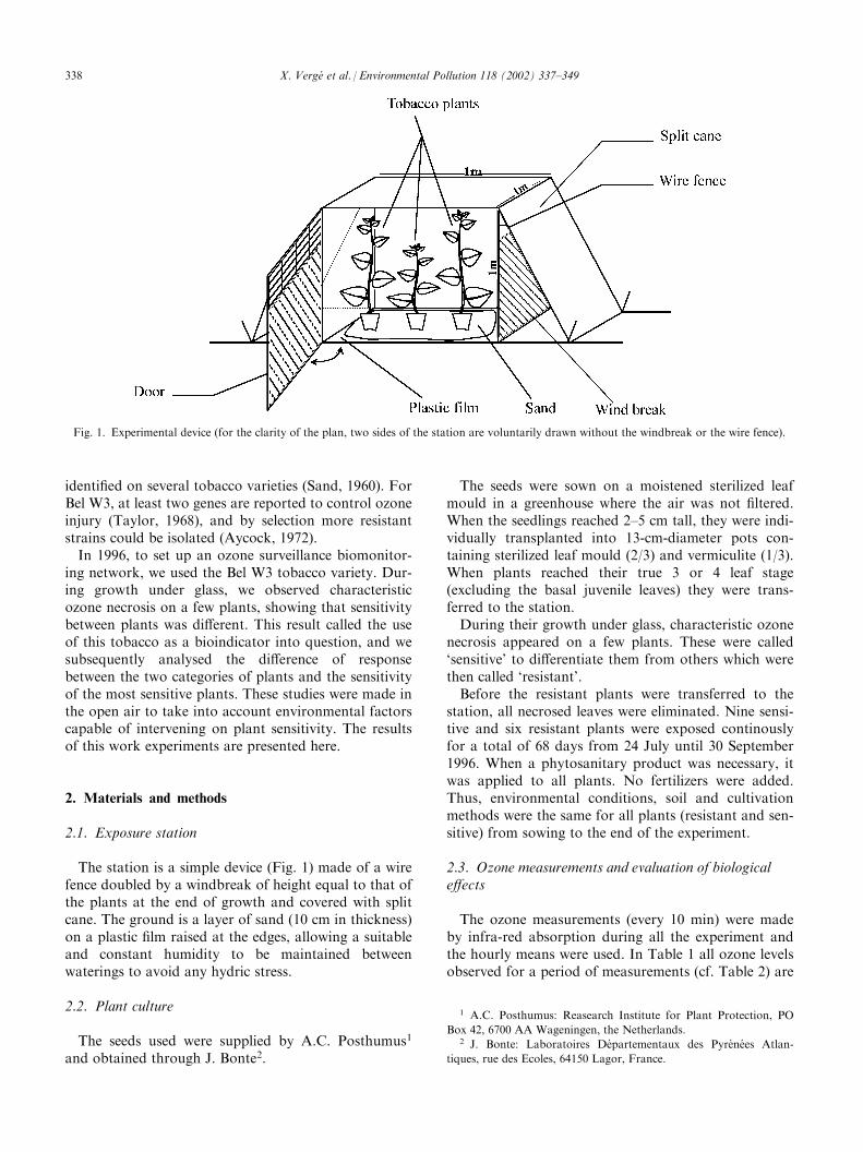
The station is a simple device (Fig. 1) made of a wirefence doubled by a windbreak of height equal to that ofthe plants at the end of growth and covered with splitcane. The ground is a layer of sand (10 cm in thickness)on a plastic film raised at the edges, allowing a suitableand constant humidity to be maintained betweenwaterings to avoid any hydric stress.

2.2. Plant culture

The seeds used were supplied by A.C. Posthumus1

and obtained through J. Bonte2.

The seeds were sown on a moistened sterilized leafmould in a greenhouse where the air was not filtered.When the seedlings reached 2–5 cm tall, they were indi-vidually transplanted into 13-cm-diameter pots con-taining sterilized leaf mould (2/3) and vermiculite (1/3).When plants reached their true 3 or 4 leaf stage(excluding the basal juvenile leaves) they were trans-ferred to the station.During their growth under glass, characteristic ozone

necrosis appeared on a few plants. These were called‘sensitive’ to differentiate them from others which werethen called ‘resistant’.Before the resistant plants were transferred to the

station, all necrosed leaves were eliminated. Nine sensi-tive and six resistant plants were exposed continouslyfor a total of 68 days from 24 July until 30 September1996. When a phytosanitary product was necessary, itwas applied to all plants. No fertilizers were added.Thus, environmental conditions, soil and cultivationmethods were the same for all plants (resistant and sen-sitive) from sowing to the end of the experiment.

2.3. Ozone measurements and evaluation of biologicaleffects

The ozone measurements (every 10 min) were madeby infra-red absorption during all the experiment andthe hourly means were used. In Table 1 all ozone levelsobserved for a period of measurements (cf. Table 2) are

1 A.C. Posthumus: Reasearch Institute for Plant Protection, PO

Box 42, 6700 AA Wageningen, the Netherlands.2 J. Bonte: Laboratoires Departementaux des Pyrenees Atlan-

tiques, rue des Ecoles, 64150 Lagor, France.

Fig. 1. Experimental device (for the clarity of the plan, two sides of the station are voluntarily drawn without the windbreak or the wire fence).

338 X. Verge et al. / Environmental Pollution 118 (2002) 337–349

Table 1

Graphic-table

IDFPa Pb O3 (ppb) Hours

R.Pl. S.Pl. 0-1h 1-2h 2-3h 3-4h 4-5h 5-6h 6-7h 7-8h 8-9h 9-10h 10-11h 11-12h 12-13h 13-14h 14-15h 15-16h 16-17h 17-18h 18-19h 19-20h 20-21h 21-22h 22-23h 23-24h

(a) Periods I–V

0.00 4.83 Ic

70-74

65-69 1 1

60-64 2 2 2 1 1 1

55-59 1 1 2 1 1 1 1 1

50-54 2 2 1 3 1 1 3 3

45-49 1 1 1 1 1 1 3 2 1 2 2 2 4 2 3 1

40-44 2 1 1 1 1 1 1 2 3 2 1 2 3 4

35-39 1 2 1 1 1 1 1 1 1 2 1 1 1 1 1 1 2

30-34 2 1 1 1 2 1 1 2 1 1 1 1 1

25-29 1 2 2 2 1 1 2 1 1 1 1

20-24 1 1 1 3 1 1 1 3 1 1 2 1

15-19 1 2 1 1 1 2 2 3 2 3 1

10-14 1 1 2 1 1 1

5-9 1 1 1 1 1 2 1

0-4 1 1 2 2 3 3 3 3

0.00 0.23 II 70-74

65-69

60-64

55-59 1 1 1

50-54 1 1 1 1 1 1 1 2

45-49 1 1 1 1 1 1 3 1

40-44 1 1 2 1 3 2 1 1 1

35-39 1 1 1 3 1 1 2 2 1 1 1 2 1

30-34 2 1 1 1 1 2

25-29 1 2 1 1 1 1 1 2 2 2 1 2 1 1 3

20-24 2 1 1 3 2 1 3 1 2 1

15-19 2 2 2 2 1 2 2 1 2 1 1 1

10-14 1 1 1 2 4 1 1 1 1 1

5-9 1 1 2 1 1 2 1

0-4 1 1

0.00 8.56 III 70-74

65-69

60-64

55-59 1

50-54 1 1 1 1 1 2 1 1

45-49 1 1 1 1 2 2 1 1

40-44 1 1 1 1 1 1 1 1 1 1 1

35-39 1 1 1 1 1 1 1 1

(Table continued on next page)

X.Vergeetal./Enviro

nmentalPollution118(2002)337–349

339

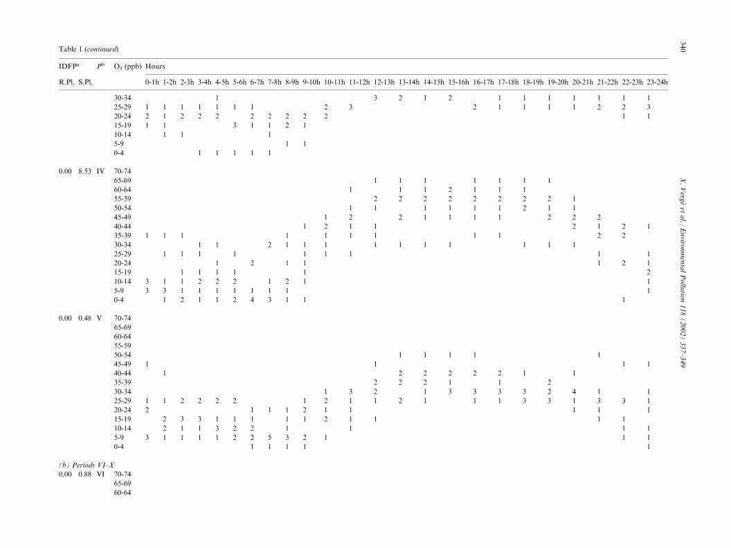
Table 1 (continued)



30-34 1 3 2 1 2 1 1 1 1 1 1 1

25-29 1 1 1 1 1 1 1 2 3 2 1 1 1 1 2 2 3

20-24 2 1 2 2 2 2 2 2 2 2 1 1

15-19 1 1 3 1 1 2 1

10-14 1 1 1

5-9 1 1

0-4 1 1 1 1 1

0.00 8.53 IV 70-74

65-69 1 1 1 1 1 1 1

60-64 1 1 1 2 1 1 1

55-59 2 2 2 2 2 2 2 2 1

50-54 1 1 1 1 1 1 2 1 1

45-49 1 2 2 1 1 1 1 2 2 2

40-44 1 2 1 1 2 1 2 1

35-39 1 1 1 1 1 1 1 1 1 2 2

30-34 1 1 2 1 1 1 1 1 1 1 1 1 1

25-29 1 1 1 1 1 1 1 1 1

20-24 1 2 1 1 1 2 1

15-19 1 1 1 1 1 2

10-14 3 1 1 2 2 2 1 2 1 1

5-9 3 3 1 1 1 1 1 1 1 1

0-4 1 2 1 1 2 4 3 1 1 1

0.00 0.48 V 70-74

65-69

60-64

55-59

50-54 1 1 1 1 1

45-49 1 1 1 1

40-44 1 2 2 2 2 2 1 1

35-39 2 2 2 1 1 2

30-34 1 3 2 1 3 3 3 3 2 4 1 1

25-29 1 1 2 2 2 2 1 2 1 1 2 1 1 1 3 3 1 3 3 1

20-24 2 1 1 1 2 1 1 1 1 1

15-19 2 3 3 1 1 1 1 1 2 1 1 1 1

10-14 2 1 1 3 2 2 1 1 1 1

5-9 3 1 1 1 1 2 2 5 3 2 1 1 1

0-4 1 1 1 1 1

(b) Periods VI–X

0.00 0.88 VI 70-74

65-69

60-64

340

X.Vergeetal./Enviro


Table 1 (continued)



55-59

50-54

45-49

40-44 1 1 1 1 1

35-39 1 2 3 3 3 3 3 3 1

30-34 1 1 1 3 4 3 2 1 1 1 1 3 2 1

25-29 1 1 3 1 1 3 1 2

20-24 1 5 1 1 1 1 1 1 1 1 1

15-19 2 2 2 1 1 2 1 1 1 1 1 1 1

10-14 2 1 2 3 3 2 2 4 1

5-9 1 2 2 2 1 1 1 1

0-4 1 1 2 4 5 3

0.01 0.40 VII 70-74

65-69 1 1

60-64 1 1 2 2 2

55-59 2 1 2 1 1 1 1

50-54 2 2 1 1 2 1 1

45-49 2 1 3 4 2 1 2

40-44 1 1 3 2 1 1 2 2 1 1

35-39 4 5 1 1 1 1 2 3

30-34 1 2 2 1 1 2

25-29 1 1 2 3 2 1

20-24 1 1 1 1 1 1 1

15-19 2 2 1 2 1 1 3 2 1

10-14 2 2 2 3 3 1 3 1 1 1 3

5-9 1 2 1 1 3 4 1 4 1 2 2 1

0-4 1 2 2 3 6 8 7

0.00 0.31 VIII 70-74

65-69

60-64

55-59 1 1 1

50-54 1 1 1 3 3 2

45-49 1 1 1 1 2 1 2 2 2 2 2 2 1

40-44 1 2 2 1 1 1 1 3 2 2 2 2 1 1 1

35-39 1 1 1 1 1 1 2 1 1 1 1 1

30-34 1 3 3 1 1 1 2 1

25-29 1 2 1 1 1 1 1 1

20-24 1 1 1 1 1 2 1 1 1

15-19 1 5 1 1 1 1

(Table continued on next page)

X.Vergeetal./Enviro


341

Table 1 (continued)



10-14 2 4 5 2 2 1 1 1 1 1 1 1 1 1

5-9 3 3 1 2 2 1 3 1 2 1

0-4 2 1 2 4 6 5 1 2 3 2 3

0.02 0.02 IX 70-74

65-69

60-64

55-59

50-54

45-49

40-44 1 1 1 1 1

35-39 1 1 2 2 3 3 2 2 1 1 1

30-34 1 1 1 2 2 1 1 1 1 1 2 1 2 3 1

25-29 2 2 3 1 1 2 2 1 2 2 2 4 3 2 1 2 1 2 1 1

20-24 1 1 2 3 2 1 1 1 2 1 1 1 1 1 1

15-19 1 1 1 1 3 1 1 1 1 1 1 1

10-14 1 1 1

5-9 1 1 1 3 1 2

0-4 1 1 1 1 2 2 3 1 1 1 1 1

0.16 0.85 X 70-74

65-69

60-64

55-59

50-54

45-49

40-44 1 2 2 1

35-39 1 1 1 2

30-34 2 1 2 2 1

25-29 1 1 1 2 3 2 2 1 1 2 2 2 1

20-24 1 1 1 2 1 1 1 1 1 1 2 1 1 1 1 1

15-19 1 2 1 2 1 1 4 1 1 1

10-14 1 1 1 1 1 1 1 1 3 2 2 1

5-9 1 1 2 3 1 1 1 1 1 1 1 1 1

0-4 3 3 3 4 3 2 2 2 4 1 1 2 3 3 3

a R.Pl., resistant plant; S.Pl., sensitive plant.b P, period.c During this period, no ozone measurement was made for 7 h (2 July, 04:00–11:00) due to a power cut.

342

X.Vergeetal./Enviro


collected and presented over 1 day. The originality ofthese tables is to assimilate the left column and theupper line to the ordinate and abscissa of a graph. Withthis presentation, the numeric values give a visual gra-phic impression. These graphic-tables are exhaustiveand synthetic and allow us to to make a detail compar-ison among periods very easily.Evaluation of the biological effects: the most char-

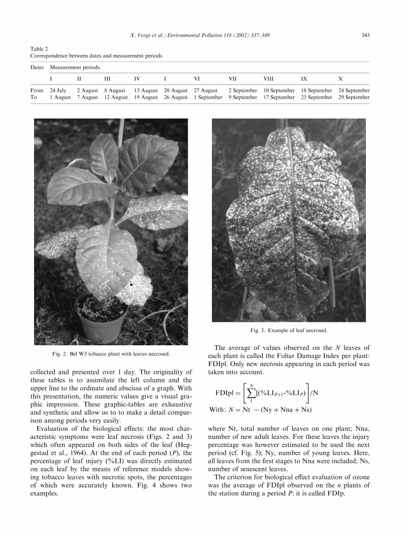
acteristic symptoms were leaf necrosis (Figs. 2 and 3)which often appeared on both sides of the leaf (Heg-gestad et al., 1964). At the end of each period (P), thepercentage of leaf injury (%LI) was directly estimatedon each leaf by the means of reference models show-ing tobacco leaves with necrotic spots, the percentagesof which were accurately known. Fig. 4 shows twoexamples.

The average of values observed on the N leaves ofeach plant is called the Foliar Damage Index per plant:FDIpl. Only new necrosis appearing in each period wastaken into account.

FDIpl ¼XN1

½ %LIPþ1-%LIPð Þ

" #=N

With: N ¼ Nt � Ny þNna þNsð Þ

where Nt, total number of leaves on one plant; Nna,number of new adult leaves. For these leaves the injurypercentage was however estimated to be used the nextperiod (cf. Fig. 5); Ny, number of young leaves. Here,all leaves from the first stages to Nna were included; Ns,number of senescent leaves.The criterion for biological effect evaluation of ozone

was the average of FDIpl observed on the n plants ofthe station during a period P: it is called FDIp.

Table 2

Correspondence between dates and measurement periods

Dates Measurement periods

I II III IV I VI VII VIII IX X

From 24 July 2 August 8 August 13 August 20 August 27 August 2 September 10 September 18 September 24 September

To 1 August 7 August 12 August 19 August 26 August 1 September 9 September 17 September 23 September 29 September

Fig. 2. Bel W3 tobacco plant with leaves necrosed.

Fig. 3. Example of leaf necrosed.

X. Verge et al. / Environmental Pollution 118 (2002) 337–349 343

FDIp ¼Xn1

FDIpl resistant or sensitiveð Þ

" #=n

Measurements and calculations are presented inFig. 5.The same plants being used throughout the experi-

mentation, the first leaves died and were shed before theend of the study. To be sure that the foliar injuryassessment was made on the same leaf as the oneobserved in the previous period, some leaves were

marked: a string was tied round the petiole of the fifth,tenth, etc., leaves.

3. Results

3.1. FDIp and plant sensitivity

The distribution of the periods is given in Table 2. InTable 3, biological measurements are presented andcompared with chemical values and with averages of

Fig. 4. Examples of reference models used to determine the leaf injury percentage (J. Bonte, personal communication).

Table 3

Comparison between FDIp, chemical (O3) and meteorological data

Periods (July to

September 1996)

Ozone (ppb)

hourly

mean

FDIp (%) Meteorological data

Resistant

plants

Sensitive

plants

Humidity

(%)

Precipitation Insolation

duration (min)

Temperature

(�C)

Wind speed

(m s�1)

Duration (min) Height (mm)

I 32.65 0.00 4.83 69.04 25 8.3 455.0 22.6 2.00

II 27.89 0.00 0.23 78.52 131 4.8 302.0 21.1 1.90

III 30.12 0.00 8.56 76.70 56 1.8 374.0 20.9 1.60

IV 31.96 0.00 8.53 67.18 0 0.0 673.0 21.0 1.90

V 25.18 0.00 0.48 79.73 157 6.5 269.0 18.8 1.70

VI 21.33 0.00 0.88 79.02 92 3.3 331.0 15.6 1.30

VII 12.57 0.01 0.40 65.66 0 0.0 645.0 16.5 2.20

VIII 24.57 0.00 0.31 67.25 91 4.0 532.0 15.2 1.50

IX 23.53 0.02 0.02 86.58 199 4.5 108.0 13.8 2.10

X 15.85 0.16 0.85 80.21 234 3.9 307.0 15.5 1.60


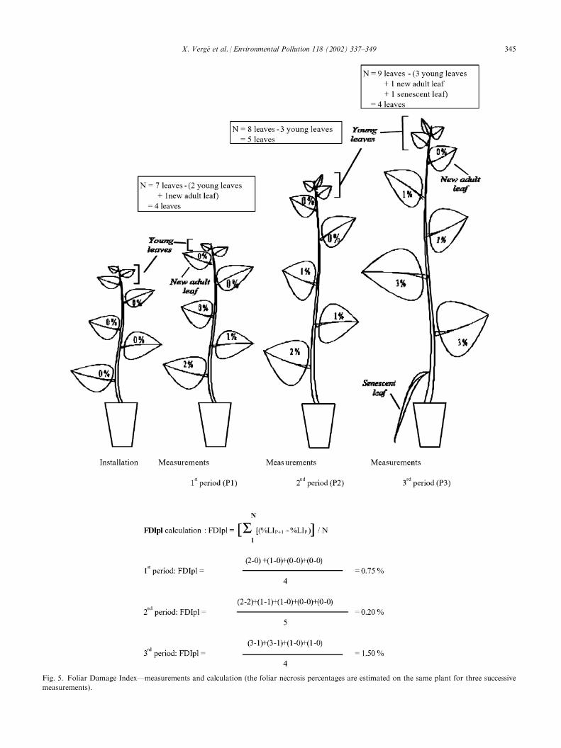
Fig. 5. Foliar Damage Index—measurements and calculation (the foliar necrosis percentages are estimated on the same plant for three successive

measurements).


meteorological observations. In this table, biologicalmeasurements are distributed in two categories accord-ing to the plants’ sensitivity: sensitive or resistant.Table 4 presents the extreme necrosis percentages onleaves (%LI), plants (FDIpl) and by period (FDIp)observed on the resistant and sensitive plants.For the resistant plants, periods when injury occured

(VII, IX and X) were very few (mean FDIp=0.02%—Table 3) and seem to have no link with ozone levelincrease. No necrosis was observed on three resistantplants. For the other three, leaf injuries only appearedon five leaves. The total percentage of each one waslower than 5%. The highest FDIpl and FDIp observedwere very low (respectively 0.56 and 0.16%—Table 4).Results obtained on sensitive plants, show higher

values (mean FDIp=2.51%—Table 3). All plantsdeveloped necrosis. The highest leaf injury was 75% fora few leaves. The highest FDIpl and FDIp reached 17.8and 8.56%, respectively (Table 4).So, using seeds coming from ozone sensitive plants,

the results revealed the existence of an intrapopulationvariation of sensitivity to the ozone effect leading tothe isolation of two categories of plants: sensitive andresistant.According to these results, it seems necessary to be

able to determine Bel W3 plant sensitivity before expo-sure to ambient ozone. So, before pursuing the use ofthis bioindicator, a precise and straightforward methodto estimate its sensitivity must be finalized. The sensi-tivity of the most sensitive plants is studied in the fol-lowing paragraph.

3.2. Comparative study: FDIp/ozone and meteorologicaldata

A principal component analysis (cf. Table 5 andFig. 6) was applied to the values presented in Table 3. Inthis figure most variables (except Rain2) are very closeto the correlation circle and thus are represented verywell. Table 5 shows that more than 80% of the totalvariance is explained by the axes 1 and 2. In Fig. 6‘ozon’ and ‘FDIp’ are very close. This result confirmsthe strong and positive correlation between ozone levelsand the appearance of leaf injuries and the interest ofthis bioindicator for studying this gas.

Table 4

Area necrosis percentages—comparison between sensitive and resis-

tant plants

Resistant plants Sensitive plants

Max. Min. Max. Min.

%LI 5 0 75 0

FDIpl (%) 0.56 0 17.8 0

FDIp (%) 0.16 0 8.56 0.02

Table 5

Principal component analysis—percentage of total variance explained

for each axis

Axis % Variance explained Cumulative

1 48.80 48.80

2 31.86 80.65

3 12.10 92.75

4 3.44 96.19

5 2.17 98.37

6 1.32 99.69

7 0.31 100.00

8 0.00 100.00

Fig. 6. Principal component analysis—graphic representation.

Table 6

Comparison between ozone levels and FDIp values (periods are clas-

sified with regard to the increase in diurnal ozone levels)

Periods Ozone (ppb) FDIp (%)

sensitive plants

Day (08:00–20:00) Night (20:00–08:00)

X 20.90 10.79 0.85

IX 26.11 20.96 0.02

VI 27.17 15.49 0.88

V 31.08 19.29 0.48

VIII 32.46 16.69 0.31

II 33.44 22.33 0.23

VII 34.77 12.38 0.40

III 35.97 24.27 8.56

I 38.15 27.15 4.83

IV 44.32 19.60 8.53


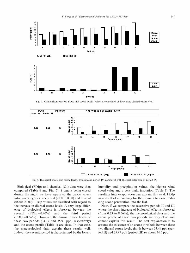
Biological (FDIp) and chemical (O3) data were thencompared (Table 6 and Fig. 7). Stomata being closedduring the night, we have separated the ozone valuesinto two categories: nocturnal (20:00–08:00) and diurnal(08:00–20:00). FDIp values are classified with regard tothe increase in diurnal ozone levels. A very large differ-ence of biological effects is observed between theseventh (FDIp=0.40%) and the third period(FDIp=8.56%). However, the diurnal ozone levels ofthese two periods (34.77 and 35.97 ppb, respectively)and the ozone profile (Table 1) are close. In that case,the meteorological data explain these results well.Indeed, the seventh period is characterized by the lowest

humidity and precipitation values, the highest windspeed value and a very hight insolation (Table 3). Theresulting high evaporation can explain this weak FDIpas a result of a tendancy for the stomata to close, redu-cing ozone penetration into the leaf.Now, if we compare the successive periods II and III

where the sharp increase of biological effect is observed(from 0.23 to 8.56%), the meteorological data and theozone profile of these two periods are very close andcannot explain this result. The best explanation is toassume the existence of an ozone threshold between thesetwo diurnal ozone levels, that is between 33.44 ppb (per-iod II) and 35.97 ppb (period III) so about 34.5 ppb.

Fig. 7. Comparison between FDIp and ozone levels. Values are classified by increasing diurnal ozone level.

Fig. 8. Biological effects and ozone levels. Typical case, period IV, compared with the particular case of period IX.


It should, however, be noted that:

1. Over the threshold, there is no proportionalitybetween ozone levels and FDIp. Indeed, for thefirst period, although the ozone level was raised,the FDIp was weakest. The meteorological datacan partly explain this result: dry atmosphere, highevaporation and so, stomata closed reducingozone penetration. But, in that case, the plantshaving just settled in situ, this result is alsoexplainable by a resistance reaction of the plantsconnected to the changes of environmental condi-tions. For the fourth period, the diurnal ozonelevels increased with regard to the period III butthe FDIp remained constant. The high evapora-tion can also explain this result.

2. Under the threshold, some biological effects areobserved even if they are weak or very weak. Incomparing the ozone profile and meteorologicaldata with the recorded FDIp values, no correla-tions were found. So, we can assume certain minorphenomena (chemical, physiological, pathological,etc.) inducing or inhibiting necrosis are masked bythe ozone effect at values over 34.5 ppb. Theybecome perceptible when the levels fall below thethreshold.

A particular case illustrating this hypothesis wasobserved. Indeed, during period IX, although the hourlymean ozone levels were not the lowest (23.53 ppb—Table 3), the FDIp value was the lowest (0.02%). Thepresence of high nocturnal ozone levels (Tables 1a and 6;Fig. 7) which exceeded diurnal values on three of the sixdays forming the period (Fig. 8) explains this result: alarge part of the ozone levels observed was present atnight while the stomata were closed.

4. Conclusion

Analysis of the results obtained from tobacco plantsrecognized as sensitive to ozone confirms the interest ofthe bioindicator Bel W3 to study the effect of this gas.Additional explanations based on more accurate fun-damental research are necessary to refine the conclu-sions but the utility of such a bioindicator should not becalled into question.The example of Bel W3 variety tobacco shows how

biological indicators must be used carefully: because oftheir biological nature the bioindicators characteristics’can evolve. Tests to estimate their sensitivity are thusnecessary and must be finalized. They are very impor-tant, particularly for bioindicators used in situ (sub-jected to varied environmental constituents) andespecially if the organism used is complex (integrationof numerous environmental factors). Every bioindicatorshould therefore have, besides its method of use, a test

allowing its sensitivity to be reassessed. The interest ofthe bioindicator and the value of the results depend onthese tests.

Acknowledgements

We thank in particular Alain SEVERAC, engineer atPaul Sabatier University of Toulouse, for his activeparticipation in the construction of the experimentalstations and in the maintenance and surveillance of thetobacco plants.

References

Ashmore, M.R., Bell, J.N.B., Reily, C.L., 1978. A survey of ozone

levels in the British Isles using indicator plants. Nature 276, 813–

815.

Ashmore, M.R., Bell, J.N.B., Reily, C.L., 1980. Distribution of phy-

totoxic ozone in the British Isles. Environmental Pollution (Series B)

1, 195–216.

Aycock, M.K., 1972. Combining ability estimates for weather fleck in

Nicotianna tabacum L. Crop Science 12, 672–674.

Bonte, M., 1985. Effets des polluant de l’air et des depots acides sur la

vegetation. In: Actes du seminaire de Rodez, 28–30 novembre

1985—Synthese des recherches en matiere de pollution atmo-

spherique. Ministere de l’environnement, France, pp. 177–193.

Craker, L.E., Berube, J.L., Frederikson, P.B., 1974. Community

monitoring of air pollution with plants. Atmospheric Environment

8, 845–853.

Dunning, J.A., Heck, W.W., 1977. Response of bean and tobacco to

ozone: effect of light intensity, temperature and relative humidity.

Journal of the Air Pollution Control Association 27, 882–886.

Garrec, J.P., Livertoux, M.E., 1997. Bioindication vegetale de l’ozone

dans l’agglomeration nanceienne durant l’ete 1996. Pollution atmo-

spherique 156, 8–87.

Goren, A., Donagi, A., 1979. Use of Bel W3 tobacco as an indicator

plant for atmospheric ozone during different seasons in the coastal

zone of Israel. International Journal of Biometeorology 23, 331–

335.

Heagle, A.S., Heck, W.W., 1974. Predisposition to tobacco to oxidant

air pollution injury by previous exposure to oxidants. Environment

and Pollution 7, 247–252.

Heck, W.W., Dunning, J.A., 1967. The effects of ozone on tobacco

and Pinto Bean as conditioned by several ecological factors. Journal

of the Air Pollution Control Association 17, 112–114.

Heggestad, H.E., 1991. Origin of Bel-W3, Bel-C and Bel-B tobacco

varieties and their use as indicator of ozone. Environmental Pollu-

tion 74, 264–291.

Heggestad, H.E., Menser, H.A., 1962. Leaf spot sensitive tobacco

strain Bel W3, a biologicalal indicator of air pollutant ozone. Phy-

topathology 52, 735.

Heggestad, H.E., Burleson, F.R., Middelton, J.T., Darley, E.F., 1964.

Leaf injury on tobacco varieties resulting from ozone, ozonated

hexene-1 and ambient air of metropolitan areas. International

Journal of Air and Water Pollution 8, 1–10.

Larsen, R.I., Heck, W.W., 1976. An air quality data analysis system

inter-relating effects, standards and needed source reduction. Part 3,

Vegetation injury. Journal of the Air Pollution Control Association

26, 325–333.

Macdowall, F.D.H., Mukammal, E.I., Cole, A.F.W., 1964. Direct

correlation of air-polluting ozone and tobacco weather fleck. Cana-

dian Journal of Plant Science 44, 410–417.


Manning, W.J., Feder, W.A., 1980. Biomonitoring Air Pollutants with

Plants. Applied Science Publishers, London.

Menser, H.A., Heggestad, H.E., 1966. Ozone and sulfur dioxide

synergism: injury to tobacco plants. Science 153, 424–425.

Menser, H.A., Heggestad, H.E., Street, O.E., 1963. Response of plants

to air pollutants. II. Effects of ozone concentration and leaf matur-

ity on injury to Nicotiana tabacum. Phytopathology 53, 1304–1308.

Posthumus, A.C., 1976. The use of higher plants as indicators for air

pollution in the Netherlands. In: Proceedings of the Kuopio Meet-

ing on plant Damages Caused by Air Pollution. L. Karenlampi,

Kuopio, pp. 115–120.

Sand, S.A., 1960. Weather fleck in shade tobacco as a problem of

interaction between genes and the environment. Tobacco Science 4,

137–146.

Steinberger, E.H., Naveh, Z., 1982. Effects of recurring exposures to

small ozone concentration on Bel-W3 tobacco plants. Agriculture

and Environment 7, 255–263.

Taylor, G.S., 1968. Ozone injury on Bel W3 tobacco controlled by at

least two genes. Phytopathology 58, 1069.

Van Haluwyn, C., Garrec, J.P., 1995. La region Boulogne-Calais-

Dunkerque: etude conjointe de vegetaux inferieurs et superieurs

pour la bioindication de la qualite de l’air. In: Bioindicateurs vege-

taux de la qualite de l’air. Rencontres et journees techniques.

Agence De l’Environnement et de la Maıtrise de l’Energie

(A.D.E.M.E.) et Institut National de Recherche Agronomique

(I.N.R.A.), Paris, pp. 91–97.

Verge, X., 2000. Variations spatio-temporelle de l’impact biologique et

genetique d’atmospheres diversement polluees dans les regions de

Toulouse et d’Albi (France). Thesis Paul Sabatier University, Tou-

louse. Atelier National de Reproduction des Theses, Universite

Pierre-Mendes-France, Grenoble.

Walker, J.T., Barlow, J.C., 1974. Response of indicator plants to

ozone levels in Georgia. Phytopathology 64, 1122–1127.


Bioindicator reliability

Documents

Transcript of Bioindicator reliability