IOP PUBLISHING INVERSE PROBLEMS

Inverse Problems 23 (2007) 785–798 doi:10.1088/0266-5611/23/2/018

The reconstruction of surface tangential componentsof the electromagnetic field from near-fieldmeasurements

N P Valdivia and E G Williams

Naval Research Laboratory, Acoustic Division, Code 7130, Washington, DC, USA

E-mail: valdivia@pa.nrl.navy.mil

Received 2 January 2007, in final form 2 February 2007Published 8 March 2007Online at stacks.iop.org/IP/23/785

AbstractWe consider the problem of reconstructing the surface tangential components ofthe electromagnetic field from electric (or magnetic) measurements on a nearbysurface. Mathematically, the electric (or magnetic) measurements satisfy theMaxwell system. We show that any solution to this equation admits a uniquerepresentation by a magnetic dipole, so that the problem is reduced to thesolution of a linear integral equation of the first kind. This integral equationis discretized using boundary element methods and conjugate gradients areutilized as a regularization method for the numerical solution. We studyuniqueness of the reconstruction and obtain stability estimates. In addition,we report numerical results applied to two cases: a sphere and a cylinder withflat end-caps.

1. Introduction

1.1. Overview

By virtue of the Straton–Chu [SC39] representation, the electromagnetic field around an objectwill be determined from its surface tangential components. For that reason, knowledge of thesurface tangential components of the electromagnetic field over a test object is of primordialimportance for the design of efficient radiators, source localization, mine detection, etc.Although measurement devices may be placed as close as desired to sample the tangentialcomponents on the object’s surface, such invasive interrogation can perturb the surface fieldsbeing sought. The best alternative is to estimate surface quantities by back-propagating fieldsmeasured on a more distant surface where the measurement devices’ interaction with the testobject is reduced. Several authors in the past have used this procedure for separable geometriesof the wave equation (like planar, cylindrical and spherical) with certain degree of success, butit was more recently that [GHW98, Mor03] utilize near-field measurements (as in near-fieldacoustic holography [WM80]) to increase the resolution of the reconstruction. By its physicalnature, the recovery of the surface tangential components from near-field measurements is

0266-5611/07/020785+14$30.00 © 2007 IOP Publishing Ltd Printed in the UK 785

786 N P Valdivia and E G Williams

an ill-posed problem, i.e., the presence of noise in the measurements will be amplified inthe solution and in most cases this solution will be useless. For that reason, the solution ofill-posed problems requires the use of regularization methods. In the separable geometriesmentioned before, the solution relies on the expansion of the electromagnetic field in termsof a complete set of eigenfunctions. The regularization method is applied by truncating thisexpansion in such a way that the effect of measurement noise is reduced in the final solution.

The previous procedures are numerically very efficient but they cannot be applied togeneral geometries. For general geometries, the boundary integral approach should be usedinstead. Although the best known integral representation for the electromagnetic field is givenby the Straton–Chu integral [SC39], this equation will be difficult to handle for this particularinverse problem. For that reason, in this work we use a representation based on the magneticdipole layer, which has a close similarity to the single layer representation [DIVW03] forthe solution of the inverse acoustic problem. We will prove that the integral representationthat we propose holds for the interior problem regardless of the wave number. Then, we willdemonstrate how this representation is used for the numerical solution of our inverse problem.

1.2. Mathematical models

Let be a bounded domain in R3 and denote as := ∂. We assume that R

3\ is connected.For a time-harmonic (e−iωt ) disturbance of frequency ω, the electrical field E = (E1, E2, E3)

T

and magnetic field H = (H1,H2,H3)T in an homogeneous as well as isotropic medium satisfy

Maxwell’s equationscurl E − ikH = 0,

curl H + ikE = 0,

div E = 0,

div H = 0,

x ∈ (or R3\) (1)

where the wave number k is given by k2 = (ε + iσ/ω)µω2. Here, σ 0 is the electricconductivity, ε > 0 is the electric permittivity and µ is the magnetic permeability. In thiswork σ, ε, µ are assumed to be constant. When E and H solve (1) in R

3\, then they alsosatisfy one of the Silver–Muller radiation conditions

limr→∞ r(H × x − E) = 0, r = |x|, x = x/r,

limr→∞ r(E × x − H) = 0.

(2)

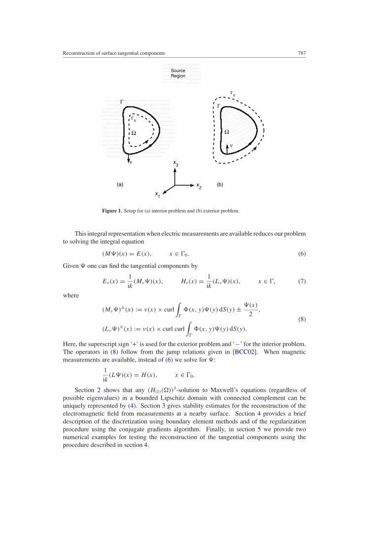
In our application for the interior (exterior) problem, measurements of the electric field Eor magnetic field H are taken on a surface 0 inside (outside) (see figure 1), then the inverseproblem is to recover the tangential components of the electromagnetic field on defined as

Eν = ν × E, Hν = ν × H, (3)

where ν is the unit normal with direction shown in figure 1.In this work, we will show that there is a unique representation of E,H by the surface

distribution of magnetic dipoles

E(x) = (M)(x) := curl∫

(x, y)(y) dS(y), x ∈ R3\,

H(x) = 1

ik(L)(x) := 1

ikcurl(M)(x),

(4)

where = (ϕ1, ϕ2, ϕ3) and

(x, y) = exp(ik|x − y|)4π |x − y| (5)

is the free space radiating fundamental solution to the Helmholtz equation.

Reconstruction of surface tangential components 787

Γ Γ

Γ0

Γ0

ν

ν

x1

x2

x3

(a) (b)

Ω Ω

Source Region

Figure 1. Setup for (a) interior problem and (b) exterior problem.

This integral representation when electric measurements are available reduces our problemto solving the integral equation

(M)(x) = E(x), x ∈ 0. (6)

Given one can find the tangential components by

Eν(x) = 1

ik(Mν)(x), Hν(x) = 1

ik(Lν)(x), x ∈ , (7)

where

(Mν)±(x) := ν(x) × curl∫

(x, y)(y) dS(y) ± (x)

2,

(Lν)±(x) := ν(x) × curl curl∫

(x, y)(y) dS(y).

(8)

Here, the superscript sign ‘+’ is used for the exterior problem and ‘−’ for the interior problem.The operators in (8) follow from the jump relations given in [BCC02]. When magneticmeasurements are available, instead of (6) we solve for :

1

ik(L)(x) = H(x), x ∈ 0.

Section 2 shows that any (H(1)())3-solution to Maxwell’s equations (regardless ofpossible eigenvalues) in a bounded Lipschitz domain with connected complement can beuniquely represented by (4). Section 3 gives stability estimates for the reconstruction of theelectromagnetic field from measurements at a nearby surface. Section 4 provides a briefdescription of the discretization using boundary element methods and of the regularizationprocedure using the conjugate gradients algorithm. Finally, in section 5 we provide twonumerical examples for testing the reconstruction of the tangential components using theprocedure described in section 4.

788 N P Valdivia and E G Williams

2. Representation by surface distribution of magnetic dipoles

We will characterize the electromagnetic field E,H in ⊂ R3 by the surface vector density

on . In other words, for a solution E,H to the Maxwell’s equations in (1) we would liketo find a vector function such that (4) holds.

We will assume that := ∂ is a Lipschitz boundary, which means that is locally thegraph of a Lipschitz function. Denote + := R

3\ and − := . We will consider only

with connected +. Recall that H(s)() denotes the Sobolev space of functions on whosepartial derivatives up to order s are square integrable and ‖ · ‖(s) denotes the standard norm inthis space. Similarly, H

(s)loc (+) denotes the function that is H(s)(B\) for every ball B that

contains . We let ‖ · ‖2 = ‖ · ‖(0) be the norm in the space L2().We denote as H

(s)() the vector functions that belong to (H (s)())3 and similarly forH

(s)loc(). The norm H

(s) of a vector function F = (F1, F2, F3) is defined as

‖F‖(s) =3∑

j=1

‖Fj‖(s).

We define as in [BCD02]

H(curl,G−) = U ∈ H(0)(−) : curl U ∈ H

(0)(−),H(curl,G+) =

U ∈ H(0)loc(+) : curl U ∈ H

(0)loc(+)

,

H(curl curl,G−) = U ∈ H(0)(−) : curl curl U ∈ H

(0)(−),H(curl curl,G+) =

U ∈ H(0)loc(+) : curl curl U ∈ H

(0)loc(+)

.

The spaces of complex-valued tangential vector fields are

Vπ = ν × H(1/2)() × ν,

endowed with the induced operator norm ‖ · ‖π , and let V ′π be its dual space. Let

H(−1/2)(div , ) := Y ∈ V ′

π : divY ∈ H(−1/2)().Finally, for U ∈ (C∞(±))3 we define the traces

γ ±d U := (ν × U)|, γ ±

n U := (ν × curl U)|.

The proof of the following lemmas can be found in [BCD02, BHvPC03].

Lemma 2.1. The trace operators γ ±d and γ ±

n can be extended to be linear and continuousoperators from H(curl,±) and H(curl curl,±), respectively, to H

(−1/2)(div, ).Moreover, they admit linear and continuous right inverses.

Lemma 2.2. The operators

M,L : H(−1/2)(div, ) → H(curl curl,±),

M,L : H(−1/2)(div, ) → H

(−1/2)(div, ),

are linear and continuous.

We have to note that if E,H ∈ H(curl,±) solves Maxwell’s equations (1) thenE,H ∈ H(curl curl,±).

Theorem 2.1. For any E,H ∈ H (curl,−) solution of Maxwell’s equations (1) there is aunique ∈ H

(−1/2)(div, ) such that (4) holds.

Proof. For the proof of this theorem we denote M− as (M) in − and similarly use M+

for (M) on +. Similar notation will be given to L− and L+. We first prove uniqueness of

Reconstruction of surface tangential components 789

the representation (4). By the jump relations of operators M,L for a vector field ∈ X (see[BCC02]) we get

curl M− − ikL− = 0, curl L− + ikM− = 0, in −,

curl M+ − ikL+ = 0, curl L+ + ikM+ = 0, in +,

(ν × L+) = (ν × L−), = (ν × M+) − (ν × M−), on ,

(9)

and the Silver–Muller radiation conditionslim

r→∞ r((L+ × x) − M+) = 0, r = |x|, x = x/r.

limr→∞ r((M+ × x) − L+) = 0.

(10)

Assume that M− = 0 in , then is trivial to observe from the relations given in (9) that L− = 0in −. The continuity of the trace operators γ −

d , γ −n allow us to get (ν × M−) = (ν × L−) = 0

on . The first jump relation in (9) yields that (ν × L+) = 0 on . M+, L+ ∈ H(curl,+)

satisfy the Maxwell system with the Silver–Muller radiation condition and the previousboundary condition, then the uniqueness of this exterior boundary-value problem (see [Mit95,BHvPC03]) implies that M+ = L+ = 0 in +. Finally, the continuity of the trace operator γ +

d

gives that (ν × M+) = 0, so the second jump relation in (9) is used to conclude that = 0.Now similarly we will prove the existence of . Using lemma 2.1 we get that for

E,H ∈ H (curl,−) there is X, Y− ∈ H(−1/2)(div, ) such that X = γ −

d H, Y− = γ −d E.

We set that Y+ = γ +d E∗, where E∗,H ∗ ∈ H (curl,+) is a solution to the exterior Maxwell

boundary-value problem with ν × H ∗ = X on . Let = Y+ − Y− on . We claim that (4)holds.

Let the functions U,V be defined as E,H in −, and in + as the solution E+,H + to theMaxwell exterior boundary problem with ν × H + = X on . Then ,L and U,V solvethe same transmission problem with Silver–Muller radiation condition in +. A solution tothis transmission problem is unique (see [BHvPC03, theorem 6.1]) then we can conclude thatU = M,V = L.

Theorem 2.2. Assume that Im k > 0. For any E,H ∈ H (curl,+) solution of Maxwell’sequations (1) that satisfies Silver–Muller radiation condition, there is ∈ H

(−1/2)(div, )

such that (4) holds.

Proof. The proof of existence is similar to the proof of existence in theorem 2.1. Note thatthe case of uniqueness follows from the uniqueness of the Maxwell interior boundary problemwhen Im k > 0 (see [Mit95]).

3. Stability estimates

In this section, we assume that is Lipschitz and that C are constants that just depend on thedomain and the Helmholtz equation operator. For F,G ∈ H

(1)() and f, g ∈ H(1)(), wewill use the inhomogeneous Maxwell’s equations in

curl E − ikH = F

curl H + ikE = G

div E = f

div H = g.

(11)

In addition to the notation of the previous section we will use for a function a and vectorfunction A = (A1, A2, A3)

‖a‖(s,τ )() :=∑|α|s

∫

|∂αa|2 e2τϕ, ‖A‖(s,τ )() :=∑|α|s

3∑j=1

∫

|∂αAj |2 e2τϕ.

790 N P Valdivia and E G Williams

Lemma 3.1. Let ϕ ∈ C2() and ∇ϕ = 0. Then we have the Carleman estimates forMaxwell’s equation (11),

τ(‖E‖2

(1,τ )() + ‖H‖2(1,τ )()

) C

‖F‖2(1,τ )() + ‖G‖2

(1,τ )()

+ ‖f ‖2(1,τ )() + ‖g‖2

(1,τ )(), (12)

for τ > C and all E,H ∈ H(2)() with support in .

Proof. Since curl curl E = −E + ∇div E, the equations in (10) can be transform into thediagonal operator systems

H + k2H = F − curl G + ∇g, E + k2E = −G − curl F + ∇f.

The conditions over ϕ guarantees that this function is strongly pseudo-convex for the Helmholtzoperator ( + k2). Since the Helmholtz operator is applied to each Cartesian component ofE,H , then we proceed as in [EINT02] to obtain (12).

Lemma 3.2. Let 0 be a bounded domain in R3 with ∂0 in C2. For any ball B that contains

0 we have that E,H ∈ H(2)(B\0), solution to Maxwell’s equations (1) that satisfy the

radiation condition (2), have the following estimates:

‖E‖(1)(B\0) + ‖H‖(1)(B\0) C

(1 +

1

|k|)

‖E‖(0)(∂0),

‖E‖(1)(B\0) + ‖H‖(1)(B\0) C

(1 +

1

|k|)

‖H‖(0)(∂0).

(13)

Proof. When the Maxwell’s equations are transformed in a similar manner to the previouslemma, we find that E satisfies the homogeneous Helmholtz equation Ej + k2Ej = 0 forj = 1, 2, 3 in B\0 and satisfies the radiation condition. The smoothness requirement over∂0 allows us to create an explicit Green’s function for the exterior Dirichlet problem for thehomogeneous Helmholtz equation for each Ej , so we conclude that∥∥∂α

l Ej

∥∥(0)

(B\0) C‖Ej‖(0)(∂0), l = 1, 2, 3

for any |α| 1. Since H = (curl E)/ik, we again use Green’s function representation foreach Ej to obtain∥∥∂α

l Hj

∥∥(0)

(B\0) C

|k| ‖Ej‖(0)(∂0), l = 1, 2, 3.

We join the two previous estimates to obtain the first estimate in (13).Since H also satisfies the homogeneous Helmholtz equation Hj + k2Hj = 0 for

j = 1, 2, 3 in B\0 and the radiation condition, we proceed as before to obtain the secondestimate in (13)

For the following stability theorem we assume that for any ball B

‖E‖(1)(B\) + ‖H‖(1)(B\) M. (14)

We just have to remind the reader that (14) is the physical assumption that the energy in R3\

for any solution to the exterior homogeneous Maxwell’s equation is finite.

Theorem 3.1. Let 0 be a bounded domain that contains . In addition ∂0 is C2. Then forany ball B that contains , the solutions E,H ∈ H

(2)(B\) to Maxwell’s equations (1) thatsatisfy the radiation condition (2), have the following stability estimate:

‖E‖(0)(B\) + ‖H‖(0)(B\) CM ln

(M

(1 + 1/|k|)‖E‖(0)(∂0)

)−1/4

. (15)

Reconstruction of surface tangential components 791

Proof. The estimate over B\ will be divided in two areas: B\0 and 0\. In the firstarea, the smoothness of ∂0 allows us to use the first estimate of lemma 3.2:

‖E‖2(1)(B\0) + ‖H‖2

(1)(B\0) C

(1 +

1

|k|)2

‖E‖2(0)(∂0). (16)

For the second area we will make use of the Carleman inequality in (12). But first weintroduce a function ϕ ∈ C2(B), such that ∇ϕ = 0, ϕ > 0 in B\ and ϕ = 0 on ∂. Itis not difficult to prove that such function exists for any open set . Then for d > 0 let(d) := B ∩ ϕ < d, and we use the estimate

‖E‖2(0)(0\) + ‖H‖2

(0)(0\) = ‖E‖2(0)(0\(d)) + ‖E‖2

(0)((d)\),

+ ‖H‖2(0)(0\(d)) + ‖H‖2

(0)((d)\). (17)

For the domain (d)\ we use Holder inequality for each j ,

‖Ej‖2(0)((d)\) =

∫(d)\

|Ej |2 (∫

(d)\1

)2/3 (∫(d)\

|Ej |6)1/3

.

Using the fact that Ej ∈ H(1)(0\), then the embedding theorems and simple integrationestimates yield for each j

‖Ej‖2(0)((d)\) Cd2/3‖Ej‖2

(1)(0\).

Note that a similar result can be obtained for each Hj . Then we have the estimate

‖E‖2(0)((d)\) + ‖H 2‖(0)((d)\) Cd2/3

‖E‖2(1)(0\) + ‖H‖2

(1)(0\). (18)

For the domain (d)\, we define a cut-off function χ ∈ C∞(R3) with supportin B\ that is 1 in 0\(d). In addition, we can find such a function with theproperty |∇jχ | Cdj . Let E,H be solutions to the Maxwell’s equations in B\,then let E0 = χE and H0 = χH so E0,H0 have support in B. In addition, we havecurl H0 + ikE0 = ∇χ × H, curl E0 − ikH0 = ∇χ × E, div E = ∇χ · E and div H = ∇χ · Hthen the estimate in (12) applied to E0,H0 gives

τ(‖E‖2

(1,τ )(0\(2d)) + ‖H‖2(1,τ )(0\(2d))

) C

‖∇χ × E‖2(1,τ )(B\) + ‖∇χ × H‖2

(1,τ )(B\)

+ ‖∇χ · E‖2(1,τ )(B\) + ‖∇χ · H‖2

(1,τ )(B\). (19)

We divide the estimates on the right-hand side of (19) into the domains where χ is neither 0nor 1, B\0 and (d)\. Set 0 = sup ϕ over B\0 and use the property that ϕ < d in(d)\ to bound the right-hand side of (19) by

Ce2τ0

(‖∇χ × E‖2(1)(B\0) + ‖∇χ × H‖2

(1)(B\0) + ‖∇χ · E‖2(1)(B\0)

+ ‖∇χ · H‖2(1)(B\0)

)+ e2τd

(‖∇χ × E‖2(1)((d)\)

+ ‖∇χ × H‖2(1)((d)\) + ‖∇χ · E‖2

(1)((d)\)

+ ‖∇χ · H‖2(1)((d)\)

).

Using the properties of the cut-off function χ used in the previous equation and the fact thatϕ 2d in 0\(d), we obtain the new estimate from (19):

τ e4τd(‖E‖2

(1)(0\(2d)) + ‖H‖2(1)(0\(2d))

) C

e2τ0

d4

(‖E‖2(1)(B\0) + ‖H‖2

(1)(B\0))

+e2τd

d4

(‖E‖2(1)(0\) + ‖H‖2

(1)(0\))

. (20)

792 N P Valdivia and E G Williams

We use the assumption ‖E‖(1)(B\) + ‖H‖(1)(B\) M , lemma 3.2, divide both sidesof (20) by e4τd and use the fact that τ > C to eliminate the left variable τ to obtain(‖E‖2

(1)(0\(2d)) + ‖H‖2(1)(0\(2d))

) C

e2τ(0−2d)

d4δ2 +

e−2τd

d4M2

, (21)

where δ = (1 + 1/|k|)‖E‖(0)(∂0). We minimize the right-hand side of (21) with respect toτ > 0 to obtain the minimum point at

2τ = 1

0 − dln

(dM2

(0 − 2d)δ2

),

where the minimized value will be bounded by Cd−4M2(1−θ)δ2θ ; here θ = d/(0 − d).We put together in (17) the previous estimate, the estimate in (18) and the estimate

2θ d/C to obtain

‖E‖2(0)(0\) + ‖H‖2

(0)(0\) C

d2/3M2 +

M2

d4

(δ

M

)d/C

. (22)

Letting d = [ln(M/δ)]−3/4 in (22), we obtain

‖E‖2(0)(0\) + ‖H‖2

(0)(0\) CM2L−2 + L12 e−L/C,where L = [ln(M/δ)]1/4. Using L12 e−L/C CL−2, we obtain the desired estimate (14).

Note that the stability estimate in (15) will hold if we exchange on the right-hand side‖E‖2

(0)(∂0) by ‖H‖2(0)(∂0). The proof is similar to the proof of the previous theorem and

just requires to use the second estimate in (13).

4. Numerical implementation

As exposed in the previous sections, our inverse problem is reduced to the solution of integralequations. The numerical solution of an integral equation is based on its discretization, whichis a reduction into a linear matrix system where numerical methods can be applied. Boundaryelement methods (BEM) will be our discretization method of choice since was proven tobe accurate in the area of acoustics (see [DIVW03, VW04, VW05]) for three-dimensionalsurfaces and can easily be extended to the area of electromagnetics.

4.1. Boundary elements methods discretization

We define (as in [CK92, DIVW03]) the single layer operator

(Sφ) (x) :=∫

(x, y)ϕ(y) dS(y).

The surface is decomposed into triangular elements with three nodes or quadrilateralelements with four nodes. In this paper (as recommended in [Val04]), iso-parametric linearfunctions are selected for interpolating the integral quantity ϕ. Denote as S ∈ C

m×n thediscretization of the S operator for x ∈ 0. Si , Sij ∈ C

m×n, i, j = 1, 2, 3, are respectivelythe first-order and second-order Cartesian partial derivatives of the operator S when x ∈ 0.The matrix Ss ∈ C

n×n is the boundary elements discretization of the operator S when x ∈ .Then Ss

i , Ssij ∈ C

n×n will denote the first- and second-order partial derivatives of the operatorS when x ∈ .

Equation (6) will be discretized as

MΨ = E, (23)

Reconstruction of surface tangential components 793

where

M = 0 −S3 S2

S3 0 −S1

−S2 S1 0

, Ψ =ϕ1

ϕ2

ϕ3

, E =E1

E2

E3

.

Here, the column vectors of m complex entries Ei , i = 1, 2, 3, represent the measurementsof the electric field Cartesian components Ei . Finally, the column vectors of n entriesϕi , i = 1, 2, 3, represent the Cartesian components of the vector field density ϕi . Theoperator L for x ∈ 0 in (4) is discretized as

L =S11 + k2S S12 S13

S12 S22 + k2S S23

S13 S23 S33 + k2S

.

The operator Mν in (7) for x ∈ is discretized as

Mν =−(

ν2Ss2 + ν3Ss

3

)ν2Ss

1 ν3Ss1

ν1Ss2 −(

ν1Ss1 + ν3Ss

3

)ν3Ss

2

ν1Ss3 ν2Ss

3 −(ν1Ss

1 + ν2Ss2

) +

1

2I,

where ν i , i = 1, 2, 3, is a diagonal matrix with entries given by the Cartesian coordinates νi

of the unit normal. Finally, the operator Lν in (7) for x ∈ is discretized as

Lν =

ν2Ss13 − ν3Ss

12 ν2Ss23 − ν3

(Ss

22 + k2Ss)

ν2(Ss

33 + k2Ss) − ν3Ss

23

ν3(Ss

11 + k2Ss) − ν1Ss

13 ν3Ss12 − ν1Ss

23 ν3Ss13 − ν1

(Ss

33 + k2Ss)

ν1Ss12 − ν2

(Ss

11 + k2Ss)

ν1(Ss

22 + k2Ss) − ν2Ss

12 ν1Ss23 − ν2Ss

13

.

As mentioned earlier, our inverse problem is reduced to the solution of (23). Once (23) issolved for Ψ then the magnetic field in 0 will be found using the matrix L:

H = 1

ikLΨ, H =

H1

H2

H3

. (24)

The tangential surface component of the electric field is found using the operator Mν :

Eν = MνΨ, Eν =Eν,1

Eν,2

Eν,3

, (25)

and the tangential surface component of the magnetic field is found using the operator Lν :

Hν = 1

ikLνΨ, Hν =

Hν,1

Hν,2

Hν,3

. (26)

4.2. Numerical regularization

In a realistic application, the measurements of the Cartesian components of the electric fieldwill contain errors. We will denote as Eδ the measured electric field and we assume that themeasurement errors e = Eδ − E are unbiased and uncorrelated with δ = ‖e‖2/‖E‖2 < 1/2.The later condition is imposed to avoid the case when the magnitude of the error is greaterthan 50% the magnitude of the measurements. Otherwise the reconstruction will be hopeless.

It is well known that the linear system in (23) ill-posed, i.e., the presence of errors in Eδ

will be amplified in the solution Ψ and in most of the cases the recovery will be useless. Then,it is necessary to use special regularization methods.

794 N P Valdivia and E G Williams

Table 1. Conjugate gradients for the normal equations algorithm.

Starting vector Ψ(0) = 0r(0) = Ed(0) = M∗r(0)

for l = 1, 2, . . .

α(l) = ∥∥M∗r(l−1)

∥∥22

/∥∥Md(l−1)

∥∥22 ,

Ψ(l) = Ψ(l−1) + α(l)d(l−1),

r(l) = r(l−1) − α(l)Md(l−1)

β(l) = ∥∥M∗r(l)

∥∥22

/∥∥M∗r(l−1)

∥∥22 ,

d(l) = M∗r(l) + β(l)d(l−1),

The best known way to apply regularization methods is by using the singular valuedecomposition (SVD), but this technique will involve the explicit creation of a decompositionthat is too time consuming or too memory demanding when the dimensions (3m × 3n) of Mare big. Instead we will rely on iterative regularization schemes like conjugate gradients forthe normal equations(CGNE) that access the matrix M only via matrix–vector multiplications.

In table 1, we show the algorithm for CGNE [HS52]. Like all iterative regularizationschemes for ill-posed problems, CGNE produce the phenomena of semi-convergence, i.e.,the vector Ψ(l) converges to the optimal regularization solution after a few iterations l,but if not stopped converges to a solution that is generally corrupted by the measurementerrors. That means that each iteration vector Ψ(l) can be considered as a regularized solution,with the iteration number l playing the role of the regularization parameter. The choice ofthe regularization parameter, or in this case the optimal iteration l, is crucial and we referthe reader to [Han98] for a review of several methods used to obtain this parameter. In thefollowing section, we will not use any of these methods for obtaining the optimal iteration,since our examples are based on numerical data and we can always obtain the optimal parameterby using the known solution.

5. Numerical examples

5.1. Example 1

We consider the interior problem where is the surface of a sphere with centre in the originand 0.25 m radius (see figure 2). The measurement surface 0 is a sphere with centre in theorigin and 0.2 m radius. The electromagnetic data are created using a point source (x, z)

with z = (−0.8, 0, 0) and A = (1, 1, 1)T so

E(x) = curlx (A(x, z)) , H(x) = 1

ikcurl curlx (A(x, z)) .

In this example, we assume that the electric conductivity σ = 0 and assume real valuesof k as shown in table 2. The surface is decomposed into n = 50 points and 48 quadrilateralelements of equally spaced area, as shown in figure 2. The number of points m, n = 194770 areobtained by symmetrically refining the quadrilateral elements over the midpoints (see [Atk97]for more details). This procedure reduces the size of the maximum side of the quadrilateralby half. Then we can compare the error of each refinement to check the order accuracy ofthe boundary element method. In this case, the relative error for the reconstruction of Hν

decreases by a factor 4 after each refinement, which is the expected behaviour with piecewiselinear elements [DIVW03]. Higher order elements give better results for noiseless examples,but these methods will not appear advantageous when noise is present as reported in [VW04].

Table 2 also lists the optimal relative errors of H, Eν, Hν using CGNE at three noise levelswith the respective optimal iteration number l. We can note in this table that an increase in

Reconstruction of surface tangential components 795

Figure 2. is a sphere with radius 0.25 m decomposed into 50 quadrilateral elements.

noise δ increases the error of the reconstruction and decreases the number of iterations l. Inparticular, this table shows the attractiveness of CGNE for ill-posed problems. We requireabout ten iterations when there is 1% measurement error and about five iterations for 5%measurement error. Specially for large problems this few number of iterations will speed thecalculation of the numerical solution.

5.2. Example 2

In this example, we consider the exterior problem (as shown in figure 3) where is a cylinderof radius 0.25 m, length 1 m and flat end-caps. 0 is a cylinder of radius 0.26 m and length1.8 m. Here we assume that the homogeneous medium is sea water, which is a conductivemedium. Here σ = 5, so ε = 7.0834 × 10−10 and µ = 1.2566 × 10−6. Theelectromagnetic data are created using two point sources with z1 = (−0.1,−0.25,−0.2), z2 =(0.1, 0.25,−0.1) and A = (1, 1, 1)T so

E(x) = curlx (A(x, z1)) + curlx (A(x, z2)) ,

H(x) = 1

ikcurl curlx (A(x, z1)) + curl curlx (A(x, z2)) .

This example is particular in the sense that the wave numbers are complex numbers. Thiscondition guarantees that the representation (4) holds for the exterior problem. The surface has 32 points around the radial coordinate and 21 points around the cylinder length. Thedistribution of the points in the end-caps can be observed in figure 3. The total number ofpoints in is n = 790. The surface 0 has 32 points around the radial coordinate and 19points around the cylinder length which makes m = 608.

796 N P Valdivia and E G Williams

Figure 3. Setup of numerical experiment 2.

Table 2. Optimal relative errors for example 1 achieved using l iterations for CGNE at noiselevels δ = 0.001, 0.01, 0.05. E1, E2, E3 are the relative error for the reconstruction of H, Eν , Hν ,respectively.

k δ = 0 m = n E1 E2 E3 l

1 0 50 0.0068 0.0019 0.0209 491 0 194 0.0004 0.0001 0.0054 1571 0 770 0.1552 × 10−4 0.4641 × 10−4 0.0017 9973 0 50 0.0036 0.0015 0.0110 473 0 194 0.0003 0.0001 0.0024 1673 0 770 0.9361 × 10−5 0.4369 × 10−4 0.0007 13856 0 50 0.0040 0.0024 0.0103 536 0 194 0.0002 0.0002 0.0014 1546 0 770 0.5624 × 10−5 0.6120 × 10−4 0.0004 17611 0.01 50 0.0474 0.0138 0.0789 111 0.01 194 0.0401 0.0105 0.0874 101 0.01 770 0.0295 0.0078 0.0844 103 0.01 50 0.0332 0.0129 0.0558 103 0.01 194 0.0253 0.0099 0.0589 93 0.01 770 0.0224 0.0083 0.0635 106 0.01 50 0.0212 0.0155 0.0375 126 0.01 194 0.0125 0.0087 0.0291 106 0.01 770 0.0101 0.0082 0.0302 111 0.05 50 0.2013 0.0557 0.2726 41 0.05 194 0.1330 0.0357 0.2025 41 0.05 770 0.0907 0.0222 0.1861 53 0.05 50 0.1136 0.0529 0.1541 53 0.05 194 0.0850 0.0343 0.1331 43 0.05 770 0.0516 0.0199 0.1118 56 0.05 50 0.0715 0.0486 0.0996 76 0.05 194 0.0441 0.0289 0.0722 66 0.05 770 0.0292 0.0188 0.0550 6

Reconstruction of surface tangential components 797

0 20 40 60 80 100 120 140 160 180 2000.2

0.3

0.4

0.5

0.6

0.7

0.8

0.9

iteration (l)

||(n

××

H) (l)

||2/||

n ×

H ||

2

0.1 MHz0.55 MHz1 MHz

Figure 4. Reconstruction error of Hν for CGNE iterations l for example 2.

0 .751.8

3.9

5.8

02

θLength

(a)

(b)

(c)

Figure 5. Reconstruction of Hν At f = 1 MHz.

In figure 4, we observe the phenomena of semi-convergence for three frequencies f =0.1 MHz, 0.55 MHz and 1 MHz (where ω = 2πf ). As shown in the previous example, CGNE

798 N P Valdivia and E G Williams

converges in a few iterations (about 20) to the optimal error. If the iteration is not stopped, theerror in the solution increases rapidly.

Finally, in figure 5 we show the reconstruction of Hν,1, Hν,2 and Hν,3 over the cylindricalsurface at 1 MHz. In (a) at the left is the exact Hν,1 compared with the reconstructed atthe right. Similarly in (b) and (c) we show the reconstructions of Hν,2 and Hν,3, respectively.Each Cartesian coordinate plot was multiplied by exp(iθm(xm)) and the real part is plotted.Here, θm(xm) is the angle of the maximum absolute value located at xm. This allow us to justlook at the general features of each coordinate regardless of the real and imaginary parts.

Acknowledgment

This work was supported by the Office of Naval Research.

References

[Atk97] Atkinson K E 1997 The Numerical Solution of Integral Equations of the Second Kind (New York:Cambridge University Press)

[BCC02] Buffa A, Costabel M and Schwab C 2002 Boundary element methods for Maxwell’s equations onnon-smooth domains Numer. Math. 92 679–710

[BCD02] Buffa A, Costabel M and Sheen D 2002 On traces for H(curl,ω) in Lipschitz domains J. Math. Anal.Appl. 276 845–67

[BHvPC03] Buffa A, Hiptmair R, von Petersdorff T and Schwab C 2003 Boundary element methods for Maxwell’stransmission problem in Lipschitz domains Numer. Math. 95 459–85

[CK92] Colton D and Kress R 1992 Inverse Acoustics and Electromagnetic Scattering Theory (New York:Springer)

[DIVW03] DeLillo T K, Isakov V, Valdivia N and Wang L 2003 The detection of surface vibrations from interioracoustical pressure Inverse Problems 19 507–24

[EINT02] Eller M, Isakov V, Nakamura G and Tataru D 2002 Uniqueness and stability in the Cauchy problem forMaxwell and elasticity systems Stud. Math. Appl. 31 329–49

[GHW98] Guo Y, Ko H W and White D M 1998 3-d localization of buried objects by nearfield electromagneticholography Geophysics 63 880–9

[Han98] Hansen P C 1998 Rank-Deficient and Discrete Ill-Posed Problems (Philadelphia, PA: SIAM)[HS52] Hestenes M R and Stiefel E L 1952 Method of conjugate gradients for solving linear systems J. Res.

Nat. Bur. Standards 49 409–36[Mit95] Mitrea M 1995 The method of layer potentials in electromagnetic scattering theory on nonsmooth

domains Duke Math. J. 77 111–33[Mor03] Morgan M A 2003 Electromagnetic holography on cylindrical surfaces using k-space transformations

PIER 42 303–37[SC39] Stratton J A and Chu L J 1939 Diffraction theory of electromagnetic waves Phys. Rev. 56 99–107[Val04] Valdivia N 2004 Uniqueness in inverse obstacle scattering with conductive boundary conditions Appl.

Anal. 83 825–51[VW04] Valdivia N and Williams E G 2004 Implicit methods of solution to integral formulations in boundary

element methods based near-field acoustic holography J. Acoust. Soc. Am. 116 1559–72[VW05] Valdivia N and Williams E G Krylov subspace iterative methods for boundary element method based

near-field acoustic holography J. Acoust. Soc. Am. 117 2005[WM80] Williams E G and Maynard J D 1980 Holographic imaging without the wavelength resolution limit

Phys. Rev. Lett. 45 554–7