General Formulation of the Electromagnetic Field Distribution in Machines and Devices Using Fourier...

IEEE TRANSACTIONS ON MAGNETICS, VOL. 46, NO. 1, JANUARY 2010 39

General Formulation of the Electromagnetic Field Distribution in Machinesand Devices Using Fourier Analysis

B. L. J. Gysen, K. J. Meessen, J. J. H. Paulides, and E. A. Lomonova

Electromechanics and Power Electronics Group, Department of Electrical Engineering, Eindhoven University of Technology,5600 MB, Eindhoven, The Netherlands

We present a general mesh-free description of the magnetic field distribution in various electromagnetic machines, actuators, anddevices. Our method is based on transfer relations and Fourier theory, which gives the magnetic field solution for a wide class of two-dimensional (2-D) boundary value problems. This technique can be applied to rotary, linear, and tubular permanent-magnet actuators,either with a slotless or slotted armature. In addition to permanent-magnet machines, this technique can be applied to any 2-D geometrywith the restriction that the geometry should consist of rectangular regions. The method obtains the electromagnetic field distributionby solving the Laplace and Poisson equations for every region, together with a set of boundary conditions. Here, we compare the methodwith finite-element analyses for various examples and show its applicability to a wide class of geometries.

Index Terms—Boundary value problem, Fourier analysis, permanent magnet.

LIST OF SYMBOLS

Magnetic vector potential m

Magnetic flux density vector

Remanent flux density

Unit vector -

Magnetic field strength vector m

Height

Current density vector

Region number -

Longitudinal direction

Magnetization vector m

Harmonic number

Harmonic number

Normal direction

Tangential direction

Spatial frequency or rad

Magnetic susceptibility

Offset in tangential direction

Permeability m

Permeability of vacuum m

Relative permeability

Angular direction

Width or rad

Bessel function of first kind of 0th order

Bessel function of first kind of 1th order

Bessel function of second kind of 0th order

Bessel function of second kind of 1th order

Manuscript received March 26, 2009; revised May 25, 2009. Current versionpublished December 23, 2009. Corresponding author: B. L. J. Gysen (e-mail:[email protected]).

Color versions of one or more of the figures in this paper are available onlineat http://ieeexplore.ieee.org.

Digital Object Identifier 10.1109/TMAG.2009.2027598

I. INTRODUCTION

E XTENSIVE modeling of the electromagnetic field distri-bution has become a crucial step in the design process

for developing electromagnetic devices, machines, and actua-tors which have improved position accuracy, acceleration, andforce density. During recent years, a lot of research and devel-opment has been conducted to be able to model or predict themagnetic field distribution in electromagnetic structures. Sev-eral analytical, semianalytical, and numerical techniques existin the literature:

• the magnetic equivalent circuit (MEC) [1], [2];• the charge model (CM) [3], [4];• transfer relations—Fourier analysis (TR-FA) [5]–[8];• Schwarz-Christoffel conformal mapping (SC) [9]–[12];• finite-element method (FEM) [13];• boundary-element method (BEM) [14].In general, each type of problem will have its own optimal

modeling technique, since high accuracy is not always pre-ferred and a low computational time could be more important.For almost every technique, these requirements are a tradeoff,although the increased computational capability of micropro-cessors enhanced the use of numerical methods. A large classof the mentioned methods (MEC, SC, FEM, FEM, amd BEM)require geometry discretization, mesh, prior to the calculationof the electromagnetic field distribution; hence, only solutionsat the predefined points are obtained. An increased mesh den-sity improves the accuracy, but also increases the computationaltime. Additionally, correct geometry discretization requiresprior knowledge to get a reliable solution. In ironless structures,without concentrated magnetic fields, or machines with a smallair gap and a large outer size, these methods become even moreproblematic due to the necessity of a high mesh density and/orsize.

For analytical or numerical calculation of secondary parame-ters, like force, electromotive force, or inductance, only the fieldsolution at a predetermined point or “line” is necessary. Numer-ical methods require the solution for the total meshed geom-etry in order to obtain these secondary parameters [15]–[17].

0018-9464/$26.00 © 2009 IEEE

Authorized licensed use limited to: Eindhoven University of Technology. Downloaded on January 8, 2010 at 07:47 from IEEE Xplore. Restrictions apply.

40 IEEE TRANSACTIONS ON MAGNETICS, VOL. 46, NO. 1, JANUARY 2010

Therefore, a mesh-free solution is preferred since the computa-tional time reduces and, in certain problems, it even allows foranalytical expressions which provide for direct means to illus-trate the dependencies of the geometric parameters and materialproperties.

This paper will discuss the analytical calculation of the elec-tromagnetic fields using transfer relations and Fourier analysis.The direct solution of the magnetostatic Maxwell equations isconsidered, which reduces to the Laplace equation in the airregion and the Poisson equation in a magnet or current car-rying region. This method originates from the book of Hague[5], which only considers the field solution for arbitrary posi-tioned current carrying wires between two parallel or concen-tric iron surfaces. Boules [7] applied this work for permanentmagnets by replacing them by an equivalent distribution of am-pere-conductors and using Hague’s field solution. The disad-vantage is that no irregular iron shapes can be considered andthat the magnet should have a simple geometric shape and mag-netization direction. The solutions of the Maxwell equations in-cluding permanent magnets described by harmonic series werepublished by Zhu et al. [8]. Recently, several publications ex-tended this method considering specific problems in differentcoordinate systems [18]–[24].

In this paper, the method is extensively described in a gener-alized manner, focusing on:

• model formulation;• methodology;• general field solutions in two-dimensional (2-D) coordi-

nate systems;• examples in 2-D coordinate systems (FEM comparison);• numerical limitations.

The model formulation can be applied for general 2-D prob-lems in the Cartesian, polar, and cylindrical coordinate system.The distinction between regions with periodical boundary con-ditions and Neumann boundary conditions in the tangential di-rection is made. Therefore, irregular rectangular iron shapes canbe considered; hence, a wide range of devices can be modeledusing this technique. Examples of the analytical solution for thethree coordinate systems are compared with 2-D finite-elementanalysis (Cedrat FLUX2D [25]). Furthermore, numerical prob-lems and drawbacks for certain conditions will be addressed.

II. MODEL FORMULATION

A. Model Assumptions

To obtain a semianalytical field solution, the following as-sumptions have to be made:

1) the problem can be described by a 2-D model;2) the materials are linear;3) the materials are homogeneous;4) the soft-magnetic material (iron) is infinite permeable;5) source terms are invariant in the normal direction within

one region.General electromagnetic devices have a 3-D geometry. Since

only 2-D problems can be considered, the geometry should beinvariant with one of the three dimensions, or its dependencyshould be negligible. In general, this is a valid assumption since

TABLE ICOORDINATE SYSTEMS

for example, in rotary actuators the 3-D effects due to the finiteaxial length are often negligible, and in tubular actuators, theaxisymmetry results inherently in a 2-D problem description.A large class of long-stroke actuators and machines exhibit acertain symmetry or periodicity. The use of Fourier theory al-lows one to use that periodicity to describe the magnetic fielddistribution. If the 2-D problem has no periodicity, it can be ob-tained by repeating the problem in the direction where the pe-riodicity should be obtained with the assumption that the elec-tromagnetic influence of the repetition on the 2-D problem isnegligible. Three different 2-D coordinate systems will be con-sidered: Cartesian , polar , and cylindrical . Thedirection of periodicity is arbitrary for the Cartesian coordinatesystem; either the or the -direction can be used, however, the

-direction is chosen in this paper. For the polar and cylindricalcoordinate system, the direction of periodicity is the and -di-rection, respectively, since physically no electromagnetic peri-odicity can be obtained in the -direction. For generality thenormal direction is referred as the -direction, the direction ofperiodicity or the tangential direction is referred as the -direc-tion, and the longitudinal (invariant) direction is referred as the-direction. A summary of the considered coordinate systems is

given in Table I.The analytical solution only applies to linear problems;

hence, the permeability of all materials is assumed to beisotropic and homogenous. The permanent magnets are mod-eled with a linear - magnetization curve in the secondquadrant with remanence and relative recoil permeability

.The relative permeability of the soft-magnetic material is as-

sumed to be infinite; hence, the magnetic field distribution isnot calculated inside the soft-magnetic material but the mag-netic field strength normal to the boundary of the soft-magneticmaterial is set to zero (Neumann boundary condition).

The source regions, magnets or current carrying coils, are in-variant in the normal direction. This implies that a source thatvaries in the normal direction should be described by multipleregions [23].

B. Examples

For every coordinate system, an example will be givenwhich indicates the applicability of the proposed method. Forthe Cartesian coordinate system a structure enclosed withsoft-magnetic material is considered which has an irregularrectangular shape, Fig. 1. This indicates that the model iseven applicable to structures enclosed by soft-magnetic mate-rial without periodicity. The example in the polar coordinatesystem is a three-phase rotary brushless permanent-magnetactuator with slotted stator, Fig. 2, indicating the ability of


GYSEN et al.: GENERAL FORMULATION OF THE ELECTROMAGNETIC FIELD DISTRIBUTION IN MACHINES AND DEVICES 41

Fig. 1. Boundary value problem in the Cartesian coordinate system.

Fig. 2. Boundary value problem in the polar coordinate system, a three-phaseslotted brushless PM actuator.

modeling slotted permanent-magnet actuators in a semianalyt-ical manner. For the cylindrical coordinate system, a slotlesstubular permanent-magnet actuator with axial magnetization ismodeled, Fig. 3. In that particular example, the field distributiondue to a finite stator length will be calculated which allows forcogging force calculation, as discussed in [21] for radial andHalbach magnetization.

C. Division in Regions

In order to solve the total field distribution in the electro-magnetic actuator or device, the 2-D geometry will be dividedinto several regions. Since the soft-magnetic materials are as-sumed to have infinite permeability, three different regions areconsidered:

• source-free regions (air, vacuum);• magnetized regions (permanent magnets);• current carrying regions (coils, wires).

Every region should be enclosed by four boundaries where eachboundary is in parallel with one of the two variant dimensionsunder consideration (normal or tangential). When a boundary is

Fig. 3. Boundary value problem in the cylindrical coordinate system, a slotlesstubular PM actuator.

not in parallel with one of the two dimensions, it can be approxi-mated by a finite number of rectangles with varying length [23].The division in and number of regions defines the form of the so-lution and the complexity of the problem. For the examples con-sidered, a number of 6, 7, and 12 regions is necessary to modelthe boundary value problem for the Cartesian (Fig. 1), polar(Fig. 2), and cylindrical (Fig. 3) coordinate system, respectively.

To simplify the magnetic field formulation, each region has alocal coordinate system. The main coordinate system is ,where the local coordinate system for every region isdefined as

(1)

where the offset is indicated in Figs. 4 and 5.

D. Motion

Since all regions have a parameter defining the offset inthe tangential direction, motion in this direction can easily beimplemented. Defining a set of fixed regions and a set of movingregions, an increment of the parameter for all regions withinthe moving set results in a positive displacement. Now it is pos-sible to calculate the field distribution for all positions of themoving part.

E. Boundary Value Problem

Dividing the geometry in regions results in a boundary valueproblem. This type of problem has three types of boundary con-ditions: periodic, Neumann, and continuous. The boundariesof a region parallel to the -direction should both be periodic(Fig. 4) or Neumann (Fig. 5). The boundaries parallel to the



Fig. 4. Definition of a region with periodic boundaries.

Fig. 5. Definition of a region with Neumann boundaries.

-direction can either be Neumann or continuous or a combi-nation of both. The division in regions is such that each regionhas constant permeability and the source term does not vary inthe normal direction.

The reason for applying Fourier theory to the solution of themagnetic field distribution is to satisfy the boundary conditionsin the tangential direction (constant ).

For a region with periodic boundary conditions, Fig. 4, andwidth , choosing the mean period of for the Fourierseries of the magnetic field inherently satisfies the periodicboundary conditions.

For a region with soft-magnetic boundaries, Fig. 5, the tan-gential magnetic field component at the boundary has to be zero.As a sine function has two zero crossings (at 0 and ), de-scribing the component of the magnetic field tangential to theboundary by means of a Fourier series with mean period ,where is the width of the region, inherently satisfies the Neu-mann boundary condition .

The boundary conditions in the normal direction (constant) will result in a set of equations which are used to solve the

unknown coefficients of the magnetic field description whichwill be discussed in Section IV.

III. SEMIANALYTICAL SOLUTION

A. Magnetostatic Maxwell Equations

In order to solve the magnetostatic field distribution, the mag-netic flux density can be written in terms of the magnetic vectorpotential as

(2)

since . For the remainder of this paper, the definitionof the magnetization vector as employed by Zhu [8] will beused wherein

(3)

(4)

with the magnetic susceptibility and the residual magne-tization. This definition of the magnetization vector gives theconstitutive relation in the form of

(5)

(6)

where is the relative permeability of the consideredregion . This reduces the magnetostatic Maxwell equations toa Poisson equation for every region , given by

(7)

with . Since only 2-D boundary value problems areconsidered, the magnetization vector only has componentsin the normal and tangential direction and the cur-rent density vector has only a component in the longitudinaldirection . Therefore, the magnetic vector potential has onlya component in the longitudinal direction which is onlydependent on the normal and tangential direction . ThePoisson equations in the different coordinate systems are there-fore given by

Cartesian :

(8)

Polar:

(9)Cylindrical:

(10)Note that when a particular region is considered, the local

coordinate systems need to be considered by replacing by .The magnetic flux density distribution can be obtained from thesolution of the magnetic vector potential by means of (2) and



the magnetic field strength is obtained from the flux densitydistribution by means of the constitutive relation (6).

B. Source Term Description

The description of the Fourier series for the source terms isdifferent for regions with periodical boundary conditions in thetangential direction than for region with Neumann boundaryconditions in the tangential direction, see Figs. 4 and 5. Thefunction which describes the source term, magnet or coil region,will be assigned as , which can be the normal or tangen-tial magnetization component , or the longitudinal currentdensity component

(11)

(12)

(13)

(14)

(15)

where the spatial frequencies for every region are definedas

(16)

For regions with periodical boundary conditions, the width ofthe region is defined as . Hence, using general Fourier theory,the source function as function of the tangential directionfor region can be written in terms of Fourier series as

(17)

(18)

(19)

(20)

For regions with Neumann boundary conditions, the width ofthe region is defined as , but the main period of the Fourierseries for the source term is still . The total source descrip-tion is therefore obtained by applying the imaging method [5],where the source is mirrored around its tangential boundariesas indicated in Fig. 6. A consequence of this imaging methodis that, for normal magnetized regions, the cosine terms willbe zero and, for the tangential magnetized regionsand longitudinal current density regions, the sine terms will bezero . After applying the imaging method,(17) to (20) can still be applied.

Fig. 6. Source description for regions with Neumann boundary conditions intangential direction. (a) Normal magnetized region. (b) Tangential magnetizedregion. (c) Longitudinal current source region.

C. Semianalytical Solution

Since the source terms are expressed by means of Fourieranalysis, the resulting solution for the magnetic vector potentialis also written in terms of Fourier components. The Poissonequation is solved with the use of separation of variables,hence the solution for the vector magnetic potential is givenby a product of two functions, one dependent on the normaldirection and one on the tangential direction . As men-tioned before, the functions for the tangential direction aresine and cosine functions since a Fourier description is used.The function for the normal direction is such that the Poissonequation is satisfied

(21)

(22)

Hence, the expressions for the magnetic flux density distributioncan generally be written as

(23)

(24)

(25)



where the functions and can be ob-tained by considering the transfer relations for every coordinatesystem [6], and are given by

1) Cartesian Coordinate System:

(26)

(27)

(28)

(29)

(30)

where and are defined as

(31)

(32)

2) Polar Coordinate System:

(33)

(34)

(35)

(36)

(37)


(38)

(39)

(40)

(41)

Cylindrical Coordinate System:

(42)

(43)

(44)

(45)

(46)


(47)

(48)

(49)

(50)

and and are defined as

(51)

(52)

For regions with Neumann boundary conditions in the tan-gential direction, Fig. 5, should be zero at the tangentialboundaries of the region; consequently, only contains sineterms . Since the normal and tangential componentof the magnetic flux density are linked via the magnetic vectorpotential, the sine terms of the tangential component will alsobe zero in that case .

The set of unknowns and or for everyregion are solved considering the boundary conditions in thenormal direction which will be discussed in the followingsection.

IV. BOUNDARY CONDITIONS

Due to the proper choice of the solution form for the magneticflux density distribution, the boundary conditions in the tangen-tial direction are inherently satisfied as discussed in Section II.To solve the unknown coefficients in the set of solutions forthe magnetic flux density distribution, the boundary conditionsin the normal direction have to be considered. Five types ofboundary conditions can be distinguished:

• Neumann boundary conditions;• continuous boundary conditions;• combination of Neumann and continuous boundary

conditions;• conservation of magnetic flux;• Ampère’s law.

Each of them will be considered in the following subsections.

A. Neumann Boundary Condition

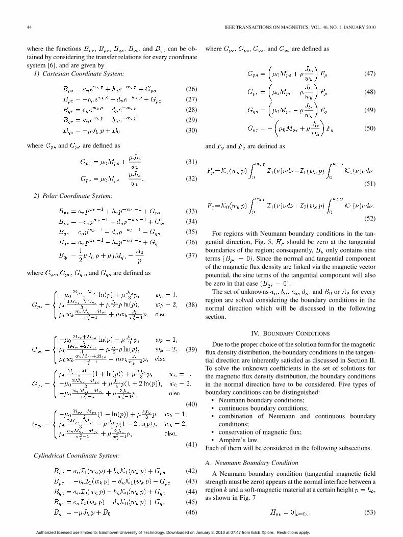
A Neumann boundary condition (tangential magnetic fieldstrength must be zero) appears at the normal interface between aregion and a soft-magnetic material at a certain height ,as shown in Fig. 7

(53)



Fig. 7. Neumann boundary condition for a region � with (a) periodic boundaryconditions and (b) Neumann boundary conditions in the tangential direction.

Using the constitutive relation (6), (53) can be written in termsof the magnetic flux density and magnetization as

(54)

Equation (54) implies that the sum of a Fourier series needsto be zero at height for all . This can be obtainedif every harmonic term of the Fourier series is zero includingthe dc term; hence, both the coefficients for the sine and cosineterms need to be zero as well as the dc term. Equation (54) cantherefore be rewritten in the following set of equations for everyharmonic :

(55)

(56)

(57)

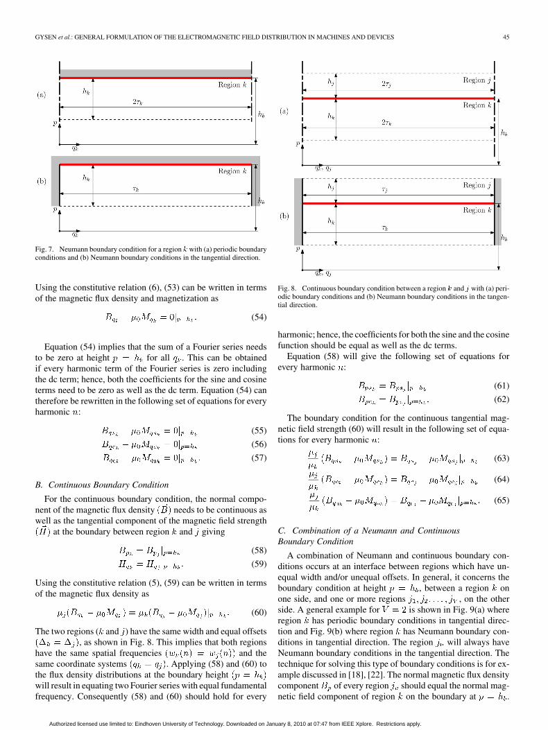
B. Continuous Boundary Condition

For the continuous boundary condition, the normal compo-nent of the magnetic flux density needs to be continuous aswell as the tangential component of the magnetic field strength

at the boundary between region and giving

(58)

(59)

Using the constitutive relation (5), (59) can be written in termsof the magnetic flux density as

(60)

The two regions ( and ) have the same width and equal offsets, as shown in Fig. 8. This implies that both regions

have the same spatial frequencies and thesame coordinate systems . Applying (58) and (60) tothe flux density distributions at the boundary heightwill result in equating two Fourier series with equal fundamentalfrequency. Consequently (58) and (60) should hold for every

Fig. 8. Continuous boundary condition between a region � and � with (a) peri-odic boundary conditions and (b) Neumann boundary conditions in the tangen-tial direction.

harmonic; hence, the coefficients for both the sine and the cosinefunction should be equal as well as the dc terms.

Equation (58) will give the following set of equations forevery harmonic :

(61)

(62)

The boundary condition for the continuous tangential mag-netic field strength (60) will result in the following set of equa-tions for every harmonic :

(63)

(64)

(65)

C. Combination of a Neumann and ContinuousBoundary Condition

A combination of Neumann and continuous boundary con-ditions occurs at an interface between regions which have un-equal width and/or unequal offsets. In general, it concerns theboundary condition at height , between a region onone side, and one or more regions , on the otherside. A general example for is shown in Fig. 9(a) whereregion has periodic boundary conditions in tangential direc-tion and Fig. 9(b) where region has Neumann boundary con-ditions in tangential direction. The region will always haveNeumann boundary conditions in the tangential direction. Thetechnique for solving this type of boundary conditions is for ex-ample discussed in [18], [22]. The normal magnetic flux densitycomponent of every region should equal the normal mag-netic field component of region on the boundary at .



Fig. 9. Boundary condition between regions � � � � and � with (a) periodicboundary conditions and (b) Neumann boundary conditions in the tangentialdirection.

Furthermore, the tangential magnetic field strength componentof region must equal the tangential magnetic field strength

component of every region on the respective boundary, andequal zero elsewhere. Therefore, the boundary conditions arerewritten in the form

(66)

(67)

Applying the constitutive relation (5) to (67) gives

(68)

Boundary condition (66) implies that two waveforms whichhave a different fundamental frequency should be equal for acertain interval. Boundary condition (68) implies that a wave-form should be equal to another waveform with different fun-damental frequency and zero elsewhere. Both boundary condi-tions are solved using the correlation technique which will bedescribed in the following subsections.

1) Normal Magnetic Flux Density: Substituting the generalfunctions for the magnetic flux density distribution in (66) givesthe following equations:

(69)

However, this equation has to be rewritten into an infinitenumber of equations in order to solve the infinite number of un-knowns. Therefore, the coefficients of region are written asa function of the coefficients of region . This can be obtainedby correlating (69) with and , respec-tively, over the interval where the boundary condition holds.Since the correlation on the left-hand side is only nonzero forthe harmonic that is considered for the sine or cosine term,respectively, the summation over disappears giving

(70)

(71)

which is a set of equations for every and region where thecorrelation functions and are given by

(72)

(73)

(74)

(75)

The solutions of these integrals are given in the Appendix.2) Tangential Magnetic Field Strength: Substituting the gen-

eral functions for the magnetic flux density distribution in (68)gives the following single equation:

(76)



However, this equation has to be rewritten into an infinitenumber of equations in order to solve the infinite number of un-knowns. Therefore, the coefficients of region are written asa function of the coefficients of region . This can be obtainedby correlating (76) with and , respectively,over the interval where the boundary condition holds (width ofregion ). The conditional (76) can be written into an uncondi-tional one by changing the bounds of the right-hand-side cor-relation integrals into the bounds where the boundary conditionholds. Since the correlation on the left-hand side is only nonzerofor the harmonic that is considered for the sine or cosine term,respectively, the summation over disappears giving

(77)

(78)

which is a set of equations for every where the correlationfunctions and are given by

(79)

(80)

(81)

(82)

(83)

(84)

The variable is equal to 1 when region has periodic boundaryconditions in tangential direction and equal to 2 when regionhas Neumann boundary conditions in tangential direction. Thesolutions of these integrals are given in the Appendix.

Fig. 10. Conservation of magnetic flux around soft-magnetic blocks sur-rounded by regions �� and �.

D. Conservation of Magnetic Flux

When the source term of a region inhibits a dc term for themagnetization in the tangential direction or currentdensity in the longitudinal direction , the magneticflux density in the tangential direction has an extra unknown( for Cartesian and cylindrical coordinate system or

for the polar coordinate system).When this region has a Neumann boundary condition in the

normal direction, this extra unknown is solved by the boundarycondition given in (57). In the case this region has a continuousboundary condition in the normal direction, this extra term issolved by (65). However, when this region is situated betweentwo other regions with different fundamental period, an extraboundary condition is necessary to solve the extra term. This sit-uation occurs for example with regions II of example 3 (Fig. 3)

, or with regions and of Fig. 10 . Inthese situations, soft-magnetic “blocks” appear in the structurewhich are surrounded by four different regions ( andin Fig. 10).

The extra boundary condition is given by setting the diver-gence of the magnetic field to zero (conservation of magneticflux) around the surface of the soft-magnetic block

(85)

Since only 2-D problems are considered, this surface integralchanges to a line integral over the boundary of the block; hence,the boundary condition for every coordinate system is given by

Cartesian:

(86)

Polar:

(87)



Fig. 11. Ampère’s law around soft-magnetic blocks surrounded by regions ��

� � � � and �.

Cylindrical:

(88)

For a problem concerning blocks on the same layer, thesame number of boundary conditions are obtained. However,only -1 conditions are independent when the model is peri-odic. The final independent equation is obtained by applyingAmpère’s law as explained in the following subsection.

E. Ampère’s Law

The final equation for solving the extra terms as explained inthe previous section is given by taking the contour integral ofthe magnetic field strength as shown in Fig. 11. Note that thiscontour integral could also be applied at the top of regions .The contour integral is given by

(89)

For every coordinate system, this equation reduces to

(90)

V. FINITE-ELEMENT COMPARISON

A. Example in the Cartesian Coordinate System

In this example, every region has Neumann boundary condi-tions in the tangential direction; hence, and of everyregion are zero or the coefficients and are set to zero. Thenormal magnetization of region II only has sine compo-nents and the longitudinal current den-sities of region IV and IV only have a dc component

. Neumann boundary conditions (56) and (57) are ap-plied at the bottom of region I and I and the top of region IVand IV . Furthermore, a continuous boundary condition is ap-plied between region II and III given by (61) and (64). Finally, acombination of Neumann and continuous boundary condition is

Fig. 12. Analytical solution of the magnetic flux density distribution for theexample in the Cartesian coordinate system.

applied at the bottom of region II and the top of region III givenby (70) and (78). Solving the set of equations for the parametersgiven in Table II gives the analytical solution shown in Fig. 12.Comparing this solution with the 2-D finite-element analysis inFig. 13 shows excellent agreement for every region. The onlynoticeable discrepancy is at the left and right boundary of themagnet in region II. Only a finite number of harmonics can betaken into account to describe the discontinuous magnetizationprofile.

B. Example in the Polar Coordinate System

This example considers a rotary actuator with slotted stator.The translator has a quasi-Halbach magnet array; hence, themagnetization profile of region II consists of a normaland tangential magnetization, only the dc components arezero . The magnetic field should be zero atthe center of the nonmagnetic shaft; hence, the coefficientsand of region I are set to zero. Regions IV have Neumannboundary conditions in the tangential direction; hence, coeffi-cients and of those regions are zero. The longitudinal cur-rent densities of regions IV have a dc term and cosine terms;hence, only the sine terms are zero . The amplitudesof the different currents are given by

(91)

(92)

(93)

where the commutation angle is set to radiansin this example. Neumann boundary conditions (56) and (57)are applied at the top of regions IV . Furthermore, continuousboundary conditions are applied between region I and II andbetween II and III given by (61), (62), (63), and (64). Finally,a combination of Neumann and continuous boundary conditionis applied at the top of region III given by (70), (71), (77), and(78). Solving the set of equations for the parameters given in



Fig. 13. Finite-element solution of the magnetic flux density distribution forthe example in the Cartesian coordinate system.

TABLE IIPARAMETERS OF THE MODEL IN THE CARTESIAN COORDINATE SYSTEM

Table III gives the analytical solution shown in Fig. 14. Again,very good agreement is obtained with the 2-D finite-elementanalysis shown in Fig. 15. It can be observed that only the mag-netic field distribution inside the quasi-Halbach array is difficultto obtain, since again, a high number of harmonics is requiredto obtain an accurate description of the discontinuous magneti-zation profile.

C. Example in the Cylindrical Coordinate System

The translator of the actuator under consideration consistsof an axial magnetized permanent-magnet array with soft-mag-netic pole pieces. Hence, regions II have a tangential magneti-zation with only a dc term . Furthermore,these regions as well as region IV have Neumann boundary con-ditions in the tangential direction; hence, coefficients andare zero. The magnetic flux density has to be zero at the centerof the axis, setting the coefficients and for region I to zero.Additionally, since region V has infinite height, coefficientsand are set to zero since the magnetic field is assumed tobe zero at . A combination of Neumann and continuousboundary conditions is applied at the top and bottom of regionsII and IV given by (70), (71), (77), and (78). Furthermore, thedivergence of the magnetic field is set to zero around 7 of the8 pole pieces given by (88), since the 8th equation would not

Fig. 14. Analytical solution of the magnetic flux density distribution for theexample in the polar coordinate system.

Fig. 15. Finite-element solution of the magnetic flux density distribution forthe example in the polar coordinate system.

TABLE IIIPARAMETERS OF THE MODEL IN THE POLAR COORDINATE SYSTEM

be an independent equation. The last independent equation isgiven by applying Ampère’s law at the bottom or top of regionsII given by (90). Solving the set of equations for the parametersgiven in Table IV gives the analytical solution shown in Fig. 16.



Fig. 16. Analytical solution of the magnetic flux density distribution for theexample in the cylindrical coordinate system.

Fig. 17. Finite-element solution of the magnetic flux density distribution forthe example in the cylindrical coordinate system.

Again, very good agreement is obtained with the 2-D finite-ele-ment analysis shown in Fig. 17. In this case excellent agreementis obtained for every region including the magnets since in thiscase, in order to describe the magnetization profile, only the dccomponent is necessary.

TABLE IVPARAMETERS OF THE MODEL IN THE CYLINDRICAL COORDINATE SYSTEM

VI. NUMERICAL LIMITATIONS

Modeling techniques which use a meshed geometry will havea limited accuracy related to the density of the mesh. The frame-work based on Fourier theory exhibits a similar problem in thefrequency domain. Therefore, the inaccuracies of the proposedmethod are all related to the limited amount of harmonics in-cluded in the solution. The two reasons for the possibility ofincluding a finite number of harmonics is a limiting computa-tional time and numerical accuracy. For an increased harmonicnumber, the value of the coefficients and are decreasingwhile and are increasing. Solving the sets of equations forthe boundary conditions results in a system of equations whichis ill-conditioned; hence, the solution becomes inaccurate.

This problem can be reduced by including proper scaling ofthe coefficients and for every region. This is pos-sible in the Cartesian and polar coordinate system since

Cartesian: (94)

Polar: (95)

for a given normal height . However, this scaling techniquecannot be applied for Bessel functions, making problems inthe cylindrical coordinate system difficult, if not impossible, toscale.

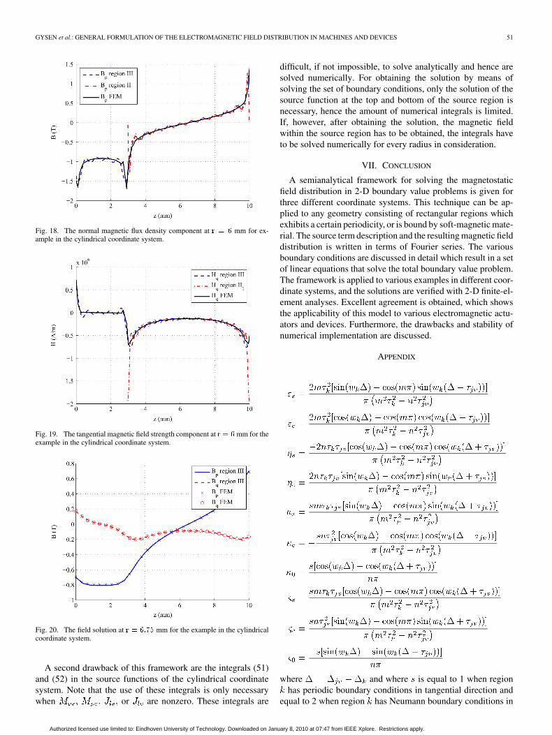
Limiting the number of harmonics will lead to inaccurate fieldsolutions at discontinuous points in the geometry, especially atthe corner points of magnets, current regions, or soft-magneticmaterial. The correlation technique which is used to satisfy theboundary conditions between regions with different spatial fre-quencies has drawbacks when only a finite number of harmonicscan be considered. In order to illustrate the effect, the analyticalfield solution is plotted at the boundary between region II andregion III of the example in the cylindrical coordinate system to-gether with the finite-element solution for the normal magneticflux density in Fig. 18 and the tangential magnetic field strengthin Fig. 19. However, this inaccuracy decays when the field solu-tion is not calculated at the boundaries but close to, for examplein the center of region III, as shown in Fig. 20, where very goodagreement is obtained. Additionally, the number of harmonicsfor each region should be chosen carefully, an extensive discus-sion on the effect of the number of harmonics taken into accountis given in [26].



Fig. 18. The normal magnetic flux density component at � � � mm for ex-ample in the cylindrical coordinate system.

Fig. 19. The tangential magnetic field strength component at � � � mm for theexample in the cylindrical coordinate system.

Fig. 20. The field solution at � � �� mm for the example in the cylindricalcoordinate system.

A second drawback of this framework are the integrals (51)and (52) in the source functions of the cylindrical coordinatesystem. Note that the use of these integrals is only necessarywhen or are nonzero. These integrals are

difficult, if not impossible, to solve analytically and hence aresolved numerically. For obtaining the solution by means ofsolving the set of boundary conditions, only the solution of thesource function at the top and bottom of the source region isnecessary, hence the amount of numerical integrals is limited.If, however, after obtaining the solution, the magnetic fieldwithin the source region has to be obtained, the integrals haveto be solved numerically for every radius in consideration.

VII. CONCLUSION

A semianalytical framework for solving the magnetostaticfield distribution in 2-D boundary value problems is given forthree different coordinate systems. This technique can be ap-plied to any geometry consisting of rectangular regions whichexhibits a certain periodicity, or is bound by soft-magnetic mate-rial. The source term description and the resulting magnetic fielddistribution is written in terms of Fourier series. The variousboundary conditions are discussed in detail which result in a setof linear equations that solve the total boundary value problem.The framework is applied to various examples in different coor-dinate systems, and the solutions are verified with 2-D finite-el-ement analyses. Excellent agreement is obtained, which showsthe applicability of this model to various electromagnetic actu-ators and devices. Furthermore, the drawbacks and stability ofnumerical implementation are discussed.

APPENDIX

where and where is equal to 1 when regionhas periodic boundary conditions in tangential direction and

equal to 2 when region has Neumann boundary conditions in



tangential direction. If , the correlation functionsare given by

REFERENCES

[1] V. Ostovic, Dynamics of Saturated Electric Machines. New York:Springer-Verlag, 1989.

[2] H. C. Roters, Electromagnetic Devices.. New York: Wiley, 1941.[3] G. Akoun and J.-P. Yonnet, “3d analytical calculation of the forces

exerted between two cuboidal magnets,” IEEE Trans. Magn., vol.MAG-20, no. 5, pp. 1962–1964, Sep. 1984.

[4] G. Xiong and S. Nasar, “Analysis of fields and forces in a permanentmagnet linear synchronous machine based on the concept of magneticcharge,” IEEE Trans. Magn., vol. 25, no. 3, pp. 2713–2719, May 1989.

[5] B. Hague, Electromagnetic Problems in Electrical Engineering.London, U.K.: Oxford Univ. Press, 1929.

[6] J. R. Melcher, Continuum Electromechanics. Cambridge, MA: MITPress, 1981.

[7] N. Boules, “Two-dimensional field analysis of cylindrical machineswith permanent magnet excitation,” IEEE Trans. Ind. Appl., vol. IA-20,no. 5, pp. 1267–1277, Sep. 1984.

[8] Z. Zhu, D. Howe, E. Bolte, and B. Ackermann, “Instantaneous mag-netic field distribution in brushless permanent magnet dc motors. PartI. Open-circuit field,” IEEE Trans. Magn., vol. 29, no. 1, pp. 124–135,Jan. 1993.

[9] K. J. Binns, P. J. Lawrenson, and C. W. Trowbridge, The Analytical andNumerical Solution of Electric and Magnetic Fields. London, U.K.:Wiley, 1992.

[10] T. A. Driscoll and L. N. Trefethen, Schwarz-Christoffel Mapping.Cambridge, U.K.: Cambridge Univ. Press, 2002.

[11] M. Markovic, M. Jufer, and Y. Perriard, “Analyzing an electromechan-ical actuator by Schwarz-Christoffel mapping,” IEEE Trans. Magn.,vol. 40, no. 4, pp. 1858–1863, Jul. 2004.

[12] D. Zarko, D. Ban, and T. Lipo, “Analytical calculation of magneticfield distribution in the slotted air gap of a surface permanent-magnetmotor using complex relative air-gap permeance,” IEEE Trans. Magn.,vol. 42, no. 7, pp. 1828–1837, Jul. 2006.

[13] J. M. Jin, The Finite Element Method in Electromagnetics, 2nd ed.New York: Wiley, 2002.

[14] L. C. Wrobel and M. H. Aliabadi, The Boundary Element Method.New York: Wiley, 2002.

[15] C. J. Carpenter, “Surface-integral methods of calculating forces onmagnetized iron parts,” Proc. IEE, vol. 107C, pp. 19–28, 1959.

[16] J. Coulomb, “A methodology for the determination of global electro-mechanical quantities from a finite element analysis and its applicationto the evaluation of magnetic forces, torques and stiffness,” IEEE Trans.Magn., vol. MAG-19, no. 6, pp. 2514–2519, Nov. 1983.

[17] J. Coulomb and G. Meunier, “Finite element implementation of virtualwork principle for magnetic or electric force and torque computation,”IEEE Trans. Magn., vol. MAG-20, no. 5, pp. 1894–1896, Sep. 1984.

[18] A. S. Khan and S. K. Mukerji, “Field between two unequal oppositeand displaced slots,” IEEE Trans. Energy Convers., vol. 7, no. 1, pp.154–160, Mar. 1992.

[19] D. Trumper, M. Williams, and T. Nguyen, “Magnet arrays for syn-chronous machines,” in Conf. Rec. 1993 Ind. Appl. Soc. Annu. Meeting,Oct. 1993, vol. 1, pp. 9–18.

[20] J. Wang, G. W. Jewell, and D. Howe, “A general framework for theanalysis and design of tubular linear permanent magnet machines,”IEEE Trans. Magn., vol. 35, no. 3, pp. 1986–2000, May 1999.

[21] J. Wang, D. Howe, and G. Jewell, “Fringing in tubular permanent-magnet machines: Part I. Magnetic field distribution, flux linkage, andthrust force,” IEEE Trans. Magn., vol. 39, no. 6, pp. 3507–3516, Nov.2003.

[22] Z. Liu and J. Li, “Analytical solution of air-gap field in permanent-magnet motors taking into account the effect of pole transition overslots,” IEEE Trans. Magn., vol. 43, no. 10, pp. 3872–3883, Oct. 2007.

[23] K. Meessen, B. Gysen, J. Paulides, and E. Lomonova, “Halbach perma-nent magnet shape selection for slotless tubular actuators,” IEEE Trans.Magn., vol. 44, no. 11, pp. 4305–4308, Nov. 2008.

[24] B. Gysen, K. Meessen, J. Paulides, and E. Lomonova, “Semi-analyt-ical calculation of the armature reaction in slotted tubular permanentmagnet actuators,” IEEE Trans. Magn., vol. 44, no. 11, pp. 3213–3216,Nov. 2008.

[25] “FLUX2D 10.2 User’s Guide,” Cedrat, Meylan, France, 2008.[26] S. W. Lee, W. Jones, and J. Campbell, “Convergence of numerical solu-

tions of iris-type discontinuity problems,” IEEE Trans. Microw. TheoryTech., vol. 19, no. 6, pp. 528–536, Jun. 1971.


General Formulation of the Electromagnetic Field Distribution in Machines and Devices Using Fourier...

Documents

Transcript of General Formulation of the Electromagnetic Field Distribution in Machines and Devices Using Fourier...