
System Reduction for Nanoscale IC Design
205
Mathematics in Industry 20 System Reduction for Nanoscale IC Design Peter Benner Editor
-
Upload
khangminh22 -
Category
Documents
-
view
1 -
download
0
Transcript of System Reduction for Nanoscale IC Design

Mathematics in Industry 20
System Reduction for NanoscaleIC Design
Peter Benner Editor

MATHEMATICS IN INDUSTRY 20
EditorsHans Georg BockFrank de HoogAvner FriedmanArvind GuptaAndré NachbinTohru OzawaWilliam R. PulleyblankTorgeir RustenFadil SantosaJin Keun SeoAnna-Karin Tornberg

More information about this series at http://www.springer.com/series/4650

Peter BennerEditor
System Reduction forNanoscale IC Design
123

EditorPeter BennerMax Planck Institute for Dynamics
of Complex Technical SystemsMagdeburg, Germany
ISSN 1612-3956 ISSN 2198-3283 (electronic)Mathematics in IndustryISBN 978-3-319-07235-7 ISBN 978-3-319-07236-4 (eBook)DOI 10.1007/978-3-319-07236-4
Library of Congress Control Number: 2017942739
Mathematics Subject Classification (2010): 94-02, 65L80, 94C05
© Springer International Publishing AG 2017This work is subject to copyright. All rights are reserved by the Publisher, whether the whole or part ofthe material is concerned, specifically the rights of translation, reprinting, reuse of illustrations, recitation,broadcasting, reproduction on microfilms or in any other physical way, and transmission or informationstorage and retrieval, electronic adaptation, computer software, or by similar or dissimilar methodologynow known or hereafter developed.The use of general descriptive names, registered names, trademarks, service marks, etc. in this publicationdoes not imply, even in the absence of a specific statement, that such names are exempt from the relevantprotective laws and regulations and therefore free for general use.The publisher, the authors and the editors are safe to assume that the advice and information in this bookare believed to be true and accurate at the date of publication. Neither the publisher nor the authors orthe editors give a warranty, express or implied, with respect to the material contained herein or for anyerrors or omissions that may have been made. The publisher remains neutral with regard to jurisdictionalclaims in published maps and institutional affiliations.
Printed on acid-free paper
This Springer imprint is published by Springer NatureThe registered company is Springer International Publishing AGThe registered company address is: Gewerbestrasse 11, 6330 Cham, Switzerland
Preface
The ongoing miniaturization of devices like transistors used in integrated circuits(ICs) has led to feature sizes on the nanoscale. The Intel Core 2 (Yorkfield), firstpresented in 2007, was produced using 45 nm technology. Recently, production hasreached 14 nm processes, e.g., in the Intel Broadwell, Skylake, and Kaby Lakemicroprocessors. Although the main principles in IC design and production arethose of microelectronics, nowadays, one therefore speaks of nanoelectronics.
With miniaturization now reaching double-digit nanometer length scales and thehuge number of semiconductor devices employed, which result in a correspondinglysignificant rise in integration density, the influence of the wiring and supplynetworks (interconnect and power grids) on the physical behavior of an IC canno longer be neglected and must be modeled with the help of dedicated networkequations in the case of computer simulations. Furthermore, critical semiconductordevices can often no longer be modeled by substitute schematics as done in thepast, using, e.g., the Partial Element Equivalent Circuit (PEEC) method. Instead,complex mathematical models are used, e.g., the drift-diffusion model. In additionto shortened production cycles, these developments in the design of new nano-electronic ICs now increasingly pose challenges in computer simulations regardingthe optimization and verification of layouts. Even in the development stage, it hasbecome indispensable to test all crucial circuit properties numerically. Thus, thefield of computational nanoelectronics has emerged.
The complexity of the mathematical models investigated in computationalnanoelectronics is enormous: small parts of an IC design alone may require millionsof linear and nonlinear differential-algebraic equations for accurate modeling,allowing the prediction of its behavior in practice. Thus, the full simulation of an ICdesign requires tremendous computational resources, which are often unavailable tomicroprocessor designers. In short, one could justifiably claim that the performanceof today’s computers is too low to simulate their successors!—a statement thathas been true for the last few decades and is debatably still valid today. Thus,the dimension reduction of the mathematical systems involved has become crucialover the past two decades and is one of the key technologies in computationalnanoelectronics.
v
vi Preface
The dimension or model reduction at the system level, or system reduction forshort, is mostly done by mathematical algorithms, which produce a much smaller(often by factors of 100 up to 10,000) model that reproduces the system’s responseto a signal up to a prescribed level of accuracy. The topic of system reductionin computational nanoelectronics is the focus of this book. The articles gatheredhere are based on the final reports for the network System Reduction in NanoscaleIC Design (SyreNe), supported by Germany’s Federal Ministry of Education andResearch (BMBF) as part of its Mathematics for Innovations in Industry andServices program. It was funded between July 1, 2007, and December 31, 2010(see syrene.org for a detailed description) and continued under the name ModelReduction for Fast Simulation of new Semiconductor Structures for Nanotechnologyand Microsystems Technology (MoreSim4Nano) within the same BMBF fundingscheme from October 1, 2010, until March 31, 2014 (see moresim4nano.org).
The goal of both research networks was to develop and compare methods forsystem reduction in the design of high-dimensional nanoelectronic ICs and to testthe resulting mathematical algorithms in the process chain of actual semiconduc-tor development at industrial partners. Generally speaking, two complementaryapproaches were pursued: the reduction of the nanoelectronic system as a whole(subcircuit model coupled to device equation) by means of a global method and thecreation of reduced order models for individual devices and large linear subcircuitswhich are linked to a single reduced system. New methods for nonlinear modelreduction and for the reduction of power grid models were developed to achievethis.
The book consists of five chapters, introducing novel concepts for the differentaspects of model reduction of circuit and device models. These include:
• Model reduction for device models coupled to circuit equations in Chap. 1 byHinze, Kunkel, Matthes, and Vierling
• Structure-exploiting model reduction for linear and nonlinear differential-algebraic equations arising in circuit simulation in Chap. 2 by Stykel andSteinbrecher
• The reduced representation of power grid models in Chap. 3 by Benner andSchneider
• Numeric-symbolic reduction methods for generating parameterized models ofnanoelectronic systems in Chap. 4 by Schmidt, Hauser, and Lang
• Dedicated solvers for the generalized Lyapunov equations arising in balancedtruncation based model reduction methods for circuit equations in Chap. 5 byBollhöfer and Eppler
The individual chapters describe the new algorithmic developments in the respec-tive research areas over the course of the project. They can be read independentlyof each other and provide a tutorial perspective on the respective aspects of SystemReduction in Nanoscale IC Design related to the sub-projects within SyreNe. Theaim is to comprehensively summarize the latest research results, mostly publishedin dedicated journal articles, and to present a number of new aspects never before

Preface vii
published. The chapters can serve as reference works, but should also inspire futureresearch in computational nanoelectronics.
I would like to take this opportunity to express my gratitude to the project part-ners Matthias Bollhöfer and Heike Faßbender (both from the TU Braunschweig),Michael Hinze (University of Hamburg), Patrick Lang (formerly the Fraunhofer-Institut für Techno- und Wirtschaftsmathematik (ITWM), Kaiserslautern), TatjanaStykel (at the TU Berlin during the project and now at the University of Augsburg),Carsten Neff (NEC Europe Ltd. back then), Carsten Hammer (formerly QimondaAG and then Infineon Technologies AG), and Peter Rotter (Infineon TechnologiesAG back then). Only their cooperation within SyreNe and their valued work in thevarious projects made this book possible.
Furthermore, I would like to particularly thank André Schneider, who helped incountless ways during the preparation of this book. This includes the LATEX setupas well as indexing and resolving many conflicts in the bibliographies. Without hishelp, I most likely never would have finished this project. My thanks also go toRuth Allewelt and Martin Peters of Springer-Verlag, who were very supportive andencouraging throughout this project. Their endless patience throughout the manydelays in the final phases of preparing the book is greatly appreciated!
Magdeburg, Germany Peter BennerDecember 2016
Contents
1 Model Order Reduction of Integrated Circuitsin Electrical Networks . . . . . . . . . . . . . . . . . . . . . . . . . . . . . . . . . . . . . . . . . . . . . . . . . . . . . . . 1Michael Hinze, Martin Kunkel, Ulrich Matthes,and Morten Vierling1.1 Introduction . . . . . . . . . . . . . . . . . . . . . . . . . . . . . . . . . . . . . . . . . . . . . . . . . . . . . . . . . . . . . 11.2 Basic Models . . . . . . . . . . . . . . . . . . . . . . . . . . . . . . . . . . . . . . . . . . . . . . . . . . . . . . . . . . . . 3
1.2.1 Coupling . . . . . . . . . . . . . . . . . . . . . . . . . . . . . . . . . . . . . . . . . . . . . . . . . . . . . . . . 41.3 Simulation of the Full System . . . . . . . . . . . . . . . . . . . . . . . . . . . . . . . . . . . . . . . . . . 7
1.3.1 Standard Galerkin Finite Element Approach .. . . . . . . . . . . . . . . . . 71.3.2 Mixed Finite Element Approach .. . . . . . . . . . . . . . . . . . . . . . . . . . . . . . 8
1.4 Model Order Reduction Using POD . . . . . . . . . . . . . . . . . . . . . . . . . . . . . . . . . . . 131.4.1 Numerical Investigation . . . . . . . . . . . . . . . . . . . . . . . . . . . . . . . . . . . . . . . . 161.4.2 Numerical Investigation, Position of the Semiconductor
in the Network . . . . . . . . . . . . . . . . . . . . . . . . . . . . . . . . . . . . . . . . . . . . . . . . . . 171.4.3 MOR for the Nonlinearity with DEIM . . . . . . . . . . . . . . . . . . . . . . . . 191.4.4 Numerical Implementation and Results with DEIM . . . . . . . . . . 20
1.5 Residual-Based Sampling . . . . . . . . . . . . . . . . . . . . . . . . . . . . . . . . . . . . . . . . . . . . . . 231.5.1 Numerical Investigation for Residual Based Sampling . . . . . . . 26
1.6 PABTEC Combined with POD MOR. . . . . . . . . . . . . . . . . . . . . . . . . . . . . . . . . . 271.6.1 Decoupling .. . . . . . . . . . . . . . . . . . . . . . . . . . . . . . . . . . . . . . . . . . . . . . . . . . . . . 281.6.2 Model Reduction Approach .. . . . . . . . . . . . . . . . . . . . . . . . . . . . . . . . . . . 301.6.3 Numerical Experiments . . . . . . . . . . . . . . . . . . . . . . . . . . . . . . . . . . . . . . . . 31
References . . . . . . . . . . . . . . . . . . . . . . . . . . . . . . . . . . . . . . . . . . . . . . . . . . . . . . . . . . . . . . . . . . . . . 34
2 Element-Based Model Reduction in Circuit Simulation . . . . . . . . . . . . . . . . . 39Andreas Steinbrecher and Tatjana Stykel2.1 Introduction . . . . . . . . . . . . . . . . . . . . . . . . . . . . . . . . . . . . . . . . . . . . . . . . . . . . . . . . . . . . . 392.2 Circuit Equations .. . . . . . . . . . . . . . . . . . . . . . . . . . . . . . . . . . . . . . . . . . . . . . . . . . . . . . . 40
2.2.1 Graph-Theoretic Concepts . . . . . . . . . . . . . . . . . . . . . . . . . . . . . . . . . . . . . 412.2.2 Modified Nodal Analysis and Modified Loop Analysis . . . . . . 412.2.3 Linear RLC Circuits . . . . . . . . . . . . . . . . . . . . . . . . . . . . . . . . . . . . . . . . . . . . 45
ix
x Contents
2.3 Model Reduction of Linear Circuits . . . . . . . . . . . . . . . . . . . . . . . . . . . . . . . . . . . 472.3.1 Balanced Truncation for RLC Circuits . . . . . . . . . . . . . . . . . . . . . . . . 482.3.2 Balanced Truncation for RC Circuits . . . . . . . . . . . . . . . . . . . . . . . . . . 522.3.3 Numerical Aspects . . . . . . . . . . . . . . . . . . . . . . . . . . . . . . . . . . . . . . . . . . . . . . 59
2.4 Model Reduction of Nonlinear Circuits. . . . . . . . . . . . . . . . . . . . . . . . . . . . . . . . 612.5 Solving Matrix Equations . . . . . . . . . . . . . . . . . . . . . . . . . . . . . . . . . . . . . . . . . . . . . . 66
2.5.1 ADI Method for Projected Lyapunov Equations . . . . . . . . . . . . . . 672.5.2 Newton’s Method for Projected Riccati Equations.. . . . . . . . . . . 68
2.6 MATLAB Toolbox PABTEC . . . . . . . . . . . . . . . . . . . . . . . . . . . . . . . . . . . . . . . . . . . 712.7 Numerical Examples . . . . . . . . . . . . . . . . . . . . . . . . . . . . . . . . . . . . . . . . . . . . . . . . . . . . 75References . . . . . . . . . . . . . . . . . . . . . . . . . . . . . . . . . . . . . . . . . . . . . . . . . . . . . . . . . . . . . . . . . . . . . 82
3 Reduced Representation of Power Grid Models. . . . . . . . . . . . . . . . . . . . . . . . . . 87Peter Benner and André Schneider3.1 Introduction . . . . . . . . . . . . . . . . . . . . . . . . . . . . . . . . . . . . . . . . . . . . . . . . . . . . . . . . . . . . . 873.2 System Description . . . . . . . . . . . . . . . . . . . . . . . . . . . . . . . . . . . . . . . . . . . . . . . . . . . . . 89
3.2.1 Basic Definitions . . . . . . . . . . . . . . . . . . . . . . . . . . . . . . . . . . . . . . . . . . . . . . . . 893.2.2 Benchmark Systems . . . . . . . . . . . . . . . . . . . . . . . . . . . . . . . . . . . . . . . . . . . . 94
3.3 Terminal Reduction Approaches . . . . . . . . . . . . . . . . . . . . . . . . . . . . . . . . . . . . . . . 963.3.1 (E)SVDMOR . . . . . . . . . . . . . . . . . . . . . . . . . . . . . . . . . . . . . . . . . . . . . . . . . . . 963.3.2 TermMerg . . . . . . . . . . . . . . . . . . . . . . . . . . . . . . . . . . . . . . . . . . . . . . . . . . . . . . . 1013.3.3 SparseRC . . . . . . . . . . . . . . . . . . . . . . . . . . . . . . . . . . . . . . . . . . . . . . . . . . . . . . . . 1033.3.4 MOR for Many Terminals via Interpolation .. . . . . . . . . . . . . . . . . . 106
3.4 ESVDMOR in Detail . . . . . . . . . . . . . . . . . . . . . . . . . . . . . . . . . . . . . . . . . . . . . . . . . . . 1083.4.1 Stability, Passivity, Reciprocity . . . . . . . . . . . . . . . . . . . . . . . . . . . . . . . . 1083.4.2 Error Analysis. . . . . . . . . . . . . . . . . . . . . . . . . . . . . . . . . . . . . . . . . . . . . . . . . . . 1143.4.3 Implementation Details . . . . . . . . . . . . . . . . . . . . . . . . . . . . . . . . . . . . . . . . . 120
3.5 Summary and Outlook .. . . . . . . . . . . . . . . . . . . . . . . . . . . . . . . . . . . . . . . . . . . . . . . . . 131References . . . . . . . . . . . . . . . . . . . . . . . . . . . . . . . . . . . . . . . . . . . . . . . . . . . . . . . . . . . . . . . . . . . . . 132
4 Coupling of Numeric/Symbolic Reduction Methodsfor Generating Parametrized Models of NanoelectronicSystems . . . . . . . . . . . . . . . . . . . . . . . . . . . . . . . . . . . . . . . . . . . . . . . . . . . . . . . . . . . . . . . . . . . . . . . . 135Oliver Schmidt, Matthias Hauser, and Patrick Lang4.1 Introduction . . . . . . . . . . . . . . . . . . . . . . . . . . . . . . . . . . . . . . . . . . . . . . . . . . . . . . . . . . . . . 135
4.1.1 Symbolic Modeling of Analog Circuits . . . . . . . . . . . . . . . . . . . . . . . 1374.2 Hierarchical Modelling and Model Reduction. . . . . . . . . . . . . . . . . . . . . . . . . 137
4.2.1 Workflow for Subsystem Reductions . . . . . . . . . . . . . . . . . . . . . . . . . . 1384.2.2 Subsystem Sensitivities . . . . . . . . . . . . . . . . . . . . . . . . . . . . . . . . . . . . . . . . . 1404.2.3 Subsystem Ranking .. . . . . . . . . . . . . . . . . . . . . . . . . . . . . . . . . . . . . . . . . . . . 1424.2.4 Algorithm for Hierarchical Model Reduction . . . . . . . . . . . . . . . . . 144
4.3 Implementations.. . . . . . . . . . . . . . . . . . . . . . . . . . . . . . . . . . . . . . . . . . . . . . . . . . . . . . . . 1444.4 Applications . . . . . . . . . . . . . . . . . . . . . . . . . . . . . . . . . . . . . . . . . . . . . . . . . . . . . . . . . . . . . 146
4.4.1 Differential Amplifier . . . . . . . . . . . . . . . . . . . . . . . . . . . . . . . . . . . . . . . . . . 1464.4.2 Reduction of the Transmission Line L1 by Using an
Adapted PABTEC Algorithm . . . . . . . . . . . . . . . . . . . . . . . . . . . . . . . . . . 149
Contents xi
4.4.3 Operational Amplifier . . . . . . . . . . . . . . . . . . . . . . . . . . . . . . . . . . . . . . . . . . 1504.5 Conclusions . . . . . . . . . . . . . . . . . . . . . . . . . . . . . . . . . . . . . . . . . . . . . . . . . . . . . . . . . . . . . 155References . . . . . . . . . . . . . . . . . . . . . . . . . . . . . . . . . . . . . . . . . . . . . . . . . . . . . . . . . . . . . . . . . . . . . 155
5 Low-Rank Cholesky Factor Krylov Subspace Methodsfor Generalized Projected Lyapunov Equations . . . . . . . . . . . . . . . . . . . . . . . . . . 157Matthias Bollhöfer and André K. Eppler5.1 Introduction . . . . . . . . . . . . . . . . . . . . . . . . . . . . . . . . . . . . . . . . . . . . . . . . . . . . . . . . . . . . . 1575.2 Balanced Truncation . . . . . . . . . . . . . . . . . . . . . . . . . . . . . . . . . . . . . . . . . . . . . . . . . . . . 158
5.2.1 Introduction to Balanced Truncation.. . . . . . . . . . . . . . . . . . . . . . . . . . 1585.2.2 Numerical Methods for Projected, Generalized
Lyapunov Equations . . . . . . . . . . . . . . . . . . . . . . . . . . . . . . . . . . . . . . . . . . . . 1605.3 Low-Rank Cholesky Factor Krylov Subspace Methods . . . . . . . . . . . . . . 161
5.3.1 Low-Rank Krylov Subspace Methods . . . . . . . . . . . . . . . . . . . . . . . . . 1625.3.2 Low-Rank Cholesky Factor Preconditioning .. . . . . . . . . . . . . . . . . 1635.3.3 Low-Rank Pseudo Arithmetic . . . . . . . . . . . . . . . . . . . . . . . . . . . . . . . . . . 1645.3.4 Approximate LRCF-ADI Preconditioning . . . . . . . . . . . . . . . . . . . . 1685.3.5 Selected Low-Rank Krylov Subspace Methods .. . . . . . . . . . . . . . 1695.3.6 Reduced Lyapunov Equation .. . . . . . . . . . . . . . . . . . . . . . . . . . . . . . . . . . 171
5.4 Numerical Results. . . . . . . . . . . . . . . . . . . . . . . . . . . . . . . . . . . . . . . . . . . . . . . . . . . . . . . 1735.4.1 Model Problems . . . . . . . . . . . . . . . . . . . . . . . . . . . . . . . . . . . . . . . . . . . . . . . . 1745.4.2 Different Krylov Subspace Methods and Their
Efficiency with Respect to the Selection of Shifts . . . . . . . . . . . . 1765.4.3 Truncated QR˘ Decomposition . . . . . . . . . . . . . . . . . . . . . . . . . . . . . . . 1795.4.4 Evolution of the Rank Representations
in the Low-Rank CG Method . . . . . . . . . . . . . . . . . . . . . . . . . . . . . . . . . . 1835.4.5 Numerical Solution Based on Reduced Lyapunov
Equations .. . . . . . . . . . . . . . . . . . . . . . . . . . . . . . . . . . . . . . . . . . . . . . . . . . . . . . . 1855.4.6 Incomplete LU Versus LU. . . . . . . . . . . . . . . . . . . . . . . . . . . . . . . . . . . . . . 1855.4.7 Parallel Approach .. . . . . . . . . . . . . . . . . . . . . . . . . . . . . . . . . . . . . . . . . . . . . . 188
5.5 Conclusions . . . . . . . . . . . . . . . . . . . . . . . . . . . . . . . . . . . . . . . . . . . . . . . . . . . . . . . . . . . . . 191References . . . . . . . . . . . . . . . . . . . . . . . . . . . . . . . . . . . . . . . . . . . . . . . . . . . . . . . . . . . . . . . . . . . . . 191
Index . . . . . . . . . . . . . . . . . . . . . . . . . . . . . . . . . . . . . . . . . . . . . . . . . . . . . . . . . . . . . . . . . . . . . . . . . . . . . . . 195
Chapter 1Model Order Reduction of Integrated Circuitsin Electrical Networks
Michael Hinze, Martin Kunkel, Ulrich Matthes, and Morten Vierling
Abstract We consider integrated circuits with semiconductors modeled by mod-ified nodal analysis and drift-diffusion equations. The drift-diffusion equationsare discretized in space using mixed finite element method. This discretizationyields a high-dimensional differential-algebraic equation. Balancing-related modelreduction is used to reduce the dimension of the decoupled linear network equa-tions, while the semidiscretized semiconductor models are reduced using properorthogonal decomposition. We among other things show that this approach deliversreduced-order models which depend on the location of the semiconductor in thenetwork. Since the computational complexity of the reduced-order models throughthe nonlinearity of the drift-diffusion equations still depend on the number ofvariables of the full model, we apply the discrete empirical interpolation methodto further reduce the computational complexity. We provide numerical comparisonswhich demonstrate the performance of the presented model reduction approach. Wecompare reduced and fine models and give numerical results for a basic networkwith one diode. Furthermore we discuss residual based sampling to construct PODmodels which are valid over certain parameter ranges.
1.1 Introduction
Computer simulations play a significant role in design and production of very largeintegrated circuits or chips that have nowadays hundreds of millions of semicon-ductor devices placed on several layers and interconnected by wires. Decreasing
M. Hinze (�) • U. Matthes • M. VierlingDepartment of Mathematics, University of Hamburg, Bundesstraße 55, 20146 Hamburg, Germanye-mail: [email protected]; [email protected];[email protected]
M. KunkelFakultät für Luft- und Raumfahrttechnik, Universität der Bundeswehr München,Werner-Heisenberg-Weg 39, 85577 Neubiberg, Germanye-mail: [email protected]
© Springer International Publishing AG 2017P. Benner (ed.), System Reduction for Nanoscale IC Design,Mathematics in Industry 20, DOI 10.1007/978-3-319-07236-4_1
1
2 M. Hinze et al.
physical size, increasing packing density, and increasing operating frequenciesnecessitate the development of new models reflecting the complex continuousprocesses in semiconductors and the high-frequency electromagnetic coupling inmore detail. Such models include complex coupled partial differential equation(PDE) systems where spatial discretization leads to high-dimensional ordinarydifferential equation (ODE) or differential-algebraic equation (DAE) systems whichrequire unacceptably high simulation times. In this context model order reduction(MOR) is of great importance. In the present work we as a first step towardsmodel order reduction of complex coupled systems consider electrical circuitswith semiconductors modeled by drift-diffusion (DD) equations as proposed ine.g. [46, 52]. Our general idea of model reduction of this system consists inapproximating this system by a much smaller model that captures the input-outputbehavior of the original system to a required accuracy and also preserves essentialphysical properties. For circuit equations, passivity is the most important propertyto be preserved in the reduced-order model.
For linear dynamical systems, many different model reduction approaches havebeen developed over the last 30 years, see [6, 42] for recent collection books on thistopic. Krylov subspace based methods such as PRIMA [32] and SPRIM [15, 16] arethe most used passivity-preserving model reduction techniques in circuit simulation.A drawback of these methods is the ad hoc choice of interpolation points thatstrongly influence the approximation quality. Recently, an optimal point selectionstrategy based on tangential interpolation has been proposed in [3, 20] that providesan optimal H2-approximation.
An alternative approach for model reduction of linear systems is balancedtruncation. In order to capture specific system properties, different balancingtechniques have been developed for standard and generalized state space systems,see, e.g., [19, 31, 35, 37, 49]. In particular, passivity-preserving balanced truncationmethods for electrical circuits (PABTEC) have been proposed in [38, 39, 51] thatheavily exploit the topological structure of circuit equations. These methods arebased on balancing the solution of projected Lyapunov or Riccati equations andprovide computable error bounds.
Model reduction of nonlinear equation systems may be performed by a trajectorypiece-wise linear approach [40] based on linearization, or proper orthogonaldecomposition (POD) (see, e.g., [45]), which relies on snapshot calculations andis successfully applied in many different engineering fields including computationalfluid dynamics and electronics [23, 29, 45, 48, 53]. A connection of POD to balancedtruncation was established in [41, 54].
A POD-based model reduction approach for the nonlinear drift-diffusion equa-tions has been presented in [25], and then extended in [23] to parameterizedelectrical networks using the greedy sampling proposed in [33]. An advantage ofthe POD approach is its high accuracy with only few model parameters. However,for its application to the drift-diffusion equations it was observed that the reductionof the problem dimension not necessarily implies the reduction of the simulationtime. Therefore, several adaption techniques such as missing point estimation [4]

1 MOR of Integrated Circuits in Electrical Networks 3
and discrete empirical interpolation method (DEIM) [10, 11] have been developedto reduce the simulation cost for the reduced-order model.
In this paper, we review results of [23–27] related to model order reductionof coupled circuit-device systems consisting of the differential-algebraic equationsmodeling an electrical circuit and the nonlinear drift-diffusion equations describ-ing the semiconductor devices. In a first step we show how proper orthogonaldecomposition (POD) can be used to reduce the dimension of the semiconductormodels. It among other things turns out, that the reduced model for a semiconductordepends on the position of the semiconductor in the network. We present numericalinvestigations from [25] for the reduction of a 4-diode rectifier network, whichclearly indicate this fact. Furthermore, we apply the Discrete Empirical InterpolationMethod (DEIM) of [10] for a further reduction of the nonlinearity, yielding afurther reduction of the overall computational complexity. Moreover, we adapt tothe present situation the Greedy sampling approach of [33] to construct POD modelswhich are valid over certain parameter ranges. In a next step we combine thepassivity-preserving balanced truncation method for electrical circuits (PABTEC)[38, 51] to reduce the dimension of the decoupled linear network equations withPOD MOR for the semiconductor model. Finally, we present several numericalexamples which demonstrate the performance of our approach.
1.2 Basic Models
In this section we combine mathematical models for electrical networks with math-ematical models for semiconductors. Electrical networks can be efficiently modeledby a differential-algebraic equation (DAE) which is obtained from modified nodalanalysis (MNA). Denoting by e the node potentials and by jL and jV the currents ofinductive and voltage source branches, the DAE reads (see [18, 28, 52])
ACd
dtqC.A
>C e; t/C ARg.A>R e; t/C ALjL C AVjV D �AIis.t/; (1.1)
d
dt�L. jL; t/ � A>L e D 0; (1.2)
A>V e D vs.t/: (1.3)
Here, the incidence matrix A D ŒAR;AC;AL;AV ;AI � D .aij/ represents the networktopology, e.g. at each non mass node i, aij D 1 if the branch j leaves nodei and aij D �1 if the branch j enters node i and aij D 0 elsewhere. Theindices R;C;L;V; I denote the capacitive, resistive, inductive, voltage source, andcurrent source branches, respectively. The functions qC, g and �L are continuouslydifferentiable defining the voltage-current relations of the network components. Thecontinuous functions vs and is are the voltage and current sources.
4 M. Hinze et al.
Under the assumption that the Jacobians
DC.e; t/ WD @qC
@e.e; t/; DG.e; t/ WD @g
@e.e; t/; DL. j; t/ WD @�L
@j. j; t/
are positive definite, analytical properties (e.g. the index) of DAE (1.1)–(1.3)are investigated in [14] and [13]. In linear networks, the matrices DC, DG andDL are positive definite diagonal matrices with capacitances, conductivities andinductances on the diagonal.
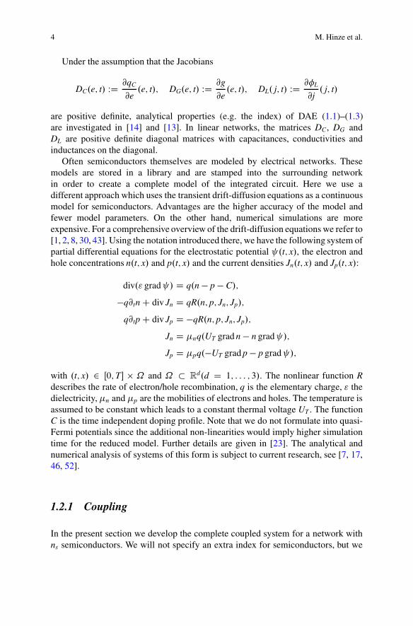
Often semiconductors themselves are modeled by electrical networks. Thesemodels are stored in a library and are stamped into the surrounding networkin order to create a complete model of the integrated circuit. Here we use adifferent approach which uses the transient drift-diffusion equations as a continuousmodel for semiconductors. Advantages are the higher accuracy of the model andfewer model parameters. On the other hand, numerical simulations are moreexpensive. For a comprehensive overview of the drift-diffusion equations we refer to[1, 2, 8, 30, 43]. Using the notation introduced there, we have the following system ofpartial differential equations for the electrostatic potential .t; x/, the electron andhole concentrations n.t; x/ and p.t; x/ and the current densities Jn.t; x/ and Jp.t; x/:
div." grad / D q.n � p � C/;
�q@tn C div Jn D qR.n; p; Jn; Jp/;
q@tp C div Jp D �qR.n; p; Jn; Jp/;
Jn D �nq.UT grad n � n grad /;
Jp D �pq.�UT grad p � p grad /;
with .t; x/ 2 Œ0;T� � ˝ and ˝ � Rd.d D 1; : : : ; 3/. The nonlinear function R
describes the rate of electron/hole recombination, q is the elementary charge, " thedielectricity, �n and �p are the mobilities of electrons and holes. The temperature isassumed to be constant which leads to a constant thermal voltage UT . The functionC is the time independent doping profile. Note that we do not formulate into quasi-Fermi potentials since the additional non-linearities would imply higher simulationtime for the reduced model. Further details are given in [23]. The analytical andnumerical analysis of systems of this form is subject to current research, see [7, 17,46, 52].
1.2.1 Coupling
In the present section we develop the complete coupled system for a network withns semiconductors. We will not specify an extra index for semiconductors, but we
1 MOR of Integrated Circuits in Electrical Networks 5
keep in mind that all semiconductor equations and coupling conditions need to beintroduced for each semiconductor.
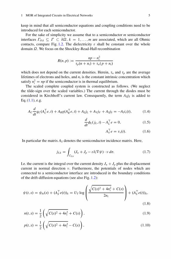
For the sake of simplicity we assume that to a semiconductor m semiconductorinterfaces �O;k � � � @˝ , k D 1; : : : ;m are associated, which are all Ohmiccontacts, compare Fig. 1.2. The dielectricity " shall be constant over the wholedomain˝ . We focus on the Shockley-Read-Hall recombination
R.n; p/ WD np � n2i�p.n C ni/C �n. p C ni/
which does not depend on the current densities. Herein, �n and �p are the averagelifetimes of electrons and holes, and ni is the constant intrinsic concentration whichsatisfy n2i D np if the semiconductor is in thermal equilibrium.
The scaled complete coupled system is constructed as follows. (We neglectthe tilde-sign over the scaled variables.) The current through the diodes must beconsidered in Kirchhoff’s current law. Consequently, the term ASjS is added toEq. (1.1), e.g.
ACd
dtqC.A
>C e; t/C ARg.A>R e; t/C ALjL C AVjV C ASjS D �AIis.t/; (1.4)
d
dt�L. jL; t/ � A>L e D 0; (1.5)
A>V e D vs.t/: (1.6)
In particular the matrix AS denotes the semiconductor incidence matrix. Here,
jS;k DZ�O;k
.Jn C Jp � "@tr / � � d�: (1.7)
I.e. the current is the integral over the current density Jn C Jp plus the displacementcurrent in normal direction �. Furthermore, the potentials of nodes which areconnected to a semiconductor interface are introduced in the boundary conditionsof the drift-diffusion equations (see also Fig. 1.2):
.t; x/ D bi.x/C .A>S e.t//k D UT log
0B@q
C.x/2 C 4n2i C C.x/
2ni
1CAC .A>S e.t//k;
(1.8)
n.t; x/ D 1
2
�qC.x/2 C 4n2i C C.x/
�; (1.9)
p.t; x/ D 1
2
�qC.x/2 C 4n2i � C.x/
�; (1.10)
6 M. Hinze et al.
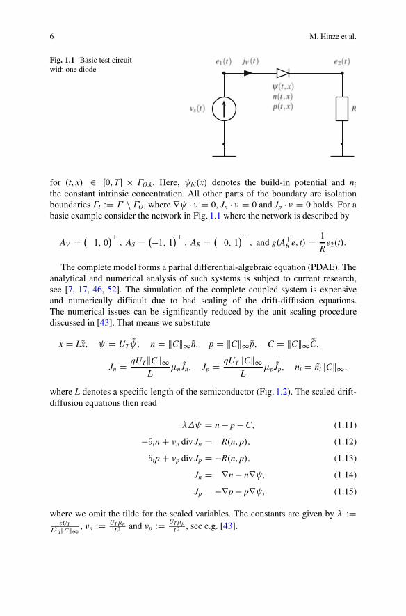
Fig. 1.1 Basic test circuitwith one diode
for .t; x/ 2 Œ0;T� � �O;k. Here, bi.x/ denotes the build-in potential and ni
the constant intrinsic concentration. All other parts of the boundary are isolationboundaries �I WD � n �O, where r � � D 0, Jn � � D 0 and Jp � � D 0 holds. For abasic example consider the network in Fig. 1.1 where the network is described by
AV D �1; 0
�>; AS D ��1; 1�> ; AR D �
0; 1�>; and g.A>R e; t/ D 1
Re2.t/:
The complete model forms a partial differential-algebraic equation (PDAE). Theanalytical and numerical analysis of such systems is subject to current research,see [7, 17, 46, 52]. The simulation of the complete coupled system is expensiveand numerically difficult due to bad scaling of the drift-diffusion equations.The numerical issues can be significantly reduced by the unit scaling procedurediscussed in [43]. That means we substitute
x D LQx; D UT Q ; n D kCk1 Qn; p D kCk1 Qp; C D kCk1 QC;
Jn D qUTkCk1L
�n QJn; Jp D qUTkCk1L
�p QJp; ni D QnikCk1;
where L denotes a specific length of the semiconductor (Fig. 1.2). The scaled drift-diffusion equations then read
D n � p � C; (1.11)
�@tn C �n div Jn D R.n; p/; (1.12)
@tp C �p div Jp D �R.n; p/; (1.13)
Jn D rn � nr ; (1.14)
Jp D �rp � pr ; (1.15)
where we omit the tilde for the scaled variables. The constants are given by WD"UT
L2qkCk1 , �n WD UT�n
L2and �p WD UT�p
L2, see e.g. [43].
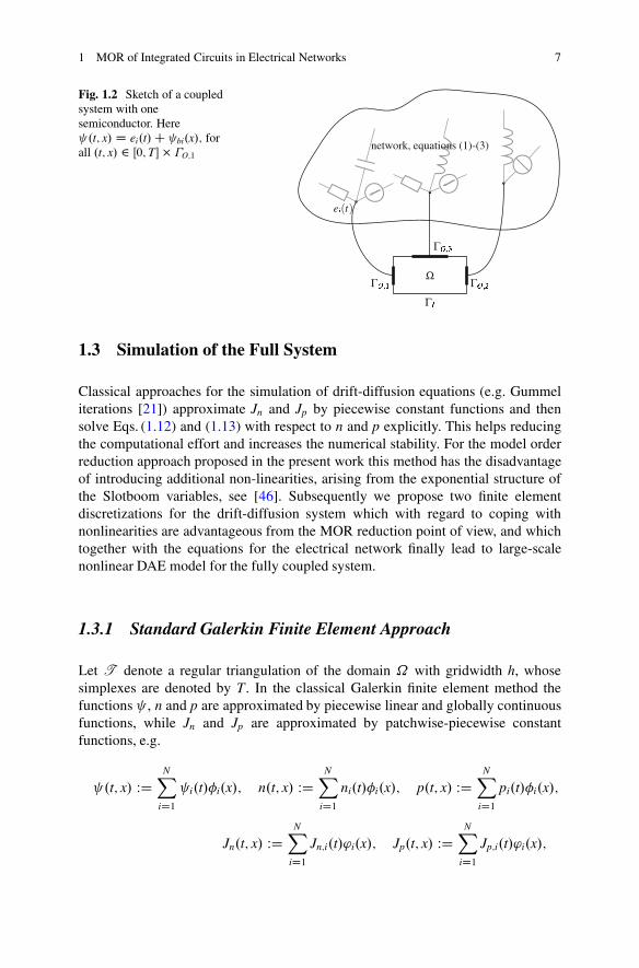
1 MOR of Integrated Circuits in Electrical Networks 7
Fig. 1.2 Sketch of a coupledsystem with onesemiconductor. Here .t; x/ D ei.t/C bi.x/; forall .t; x/ 2 Œ0; T� � �O;1
1.3 Simulation of the Full System
Classical approaches for the simulation of drift-diffusion equations (e.g. Gummeliterations [21]) approximate Jn and Jp by piecewise constant functions and thensolve Eqs. (1.12) and (1.13) with respect to n and p explicitly. This helps reducingthe computational effort and increases the numerical stability. For the model orderreduction approach proposed in the present work this method has the disadvantageof introducing additional non-linearities, arising from the exponential structure ofthe Slotboom variables, see [46]. Subsequently we propose two finite elementdiscretizations for the drift-diffusion system which with regard to coping withnonlinearities are advantageous from the MOR reduction point of view, and whichtogether with the equations for the electrical network finally lead to large-scalenonlinear DAE model for the fully coupled system.
1.3.1 Standard Galerkin Finite Element Approach
Let T denote a regular triangulation of the domain ˝ with gridwidth h, whosesimplexes are denoted by T. In the classical Galerkin finite element method thefunctions , n and p are approximated by piecewise linear and globally continuousfunctions, while Jn and Jp are approximated by patchwise-piecewise constantfunctions, e.g.
.t; x/ WDNX
iD1 i.t/�i.x/; n.t; x/ WD
NXiD1
ni.t/�i.x/; p.t; x/ WDNX
iD1pi.t/�i.x/;
Jn.t; x/ WDNX
iD1Jn;i.t/'i.x/; Jp.t; x/ WD
NXiD1
Jp;i.t/'i.x/;
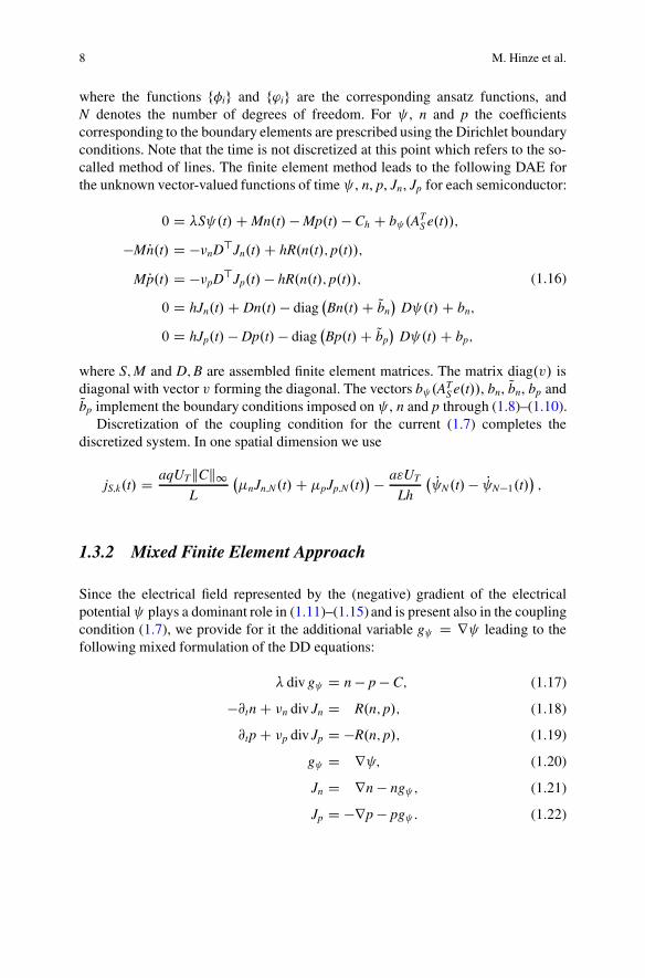
8 M. Hinze et al.
where the functions f�ig and f'ig are the corresponding ansatz functions, andN denotes the number of degrees of freedom. For , n and p the coefficientscorresponding to the boundary elements are prescribed using the Dirichlet boundaryconditions. Note that the time is not discretized at this point which refers to the so-called method of lines. The finite element method leads to the following DAE forthe unknown vector-valued functions of time , n, p, Jn, Jp for each semiconductor:
0 D S .t/C Mn.t/ � Mp.t/ � Ch C b .ATS e.t//;
�M Pn.t/ D ��nD>Jn.t/C hR.n.t/; p.t//;
M Pp.t/ D ��pD>Jp.t/ � hR.n.t/; p.t//;
0 D hJn.t/C Dn.t/� diag�Bn.t/C Qbn
�D .t/C bn;
0 D hJp.t/ � Dp.t/ � diag�Bp.t/C Qbp
�D .t/C bp;
(1.16)
where S;M and D;B are assembled finite element matrices. The matrix diag.v/ isdiagonal with vector v forming the diagonal. The vectors b .AT
S e.t//, bn, Qbn, bp andQbp implement the boundary conditions imposed on , n and p through (1.8)–(1.10).
Discretization of the coupling condition for the current (1.7) completes thediscretized system. In one spatial dimension we use
jS;k.t/ D aqUTkCk1L
��nJn;N.t/C �pJp;N.t/
� � a"UT
Lh
� P N.t/� P N�1.t/�;
1.3.2 Mixed Finite Element Approach
Since the electrical field represented by the (negative) gradient of the electricalpotential plays a dominant role in (1.11)–(1.15) and is present also in the couplingcondition (1.7), we provide for it the additional variable g D r leading to thefollowing mixed formulation of the DD equations:
div g D n � p � C; (1.17)
�@tn C �n div Jn D R.n; p/; (1.18)
@tp C �p div Jp D �R.n; p/; (1.19)
g D r ; (1.20)
Jn D rn � ng ; (1.21)
Jp D �rp � pg : (1.22)
1 MOR of Integrated Circuits in Electrical Networks 9
The weak formulation of (1.17)–(1.22) then reads: Find ; n; p 2 Œ0;T� � L2.˝/and g ; Jn; Jp 2 Œ0;T� � H0;N.div;˝/ such that
Z˝
div g ' DZ˝
.n � p/ ' �Z˝
C '; (1.23)
�Z˝
@tn ' C �n
Z˝
div Jn ' DZ˝
R.n; p/ '; (1.24)
Z˝
@tp ' C �p
Z˝
div Jp ' D �Z˝
R.n; p/ '; (1.25)
Z˝
g � � D �Z˝
div� CZ�
� � �; (1.26)
Z˝
Jn � � D �Z˝
n div� CZ�
n � � � �Z˝
n g � �;(1.27)Z
˝
Jp � � DZ˝
p div� �Z�
p � � � �Z˝
p g � �;(1.28)
are satisfied for all ' 2 L2.˝/ and � 2 H0;N.div;˝/ where the space H0;N.div;˝/is defined by
H.div;˝/ WD fy 2 L2.˝/d W div y 2 L2.˝/g;H0;N.div;˝/ WD fy 2 H.div;˝/ W y � � D 0 on �Ig :
Consequently, the boundary integrals on the right hand sides in Eqs. (1.26)–(1.28)reduce to integrals over the interfaces �O;k, where the values of , n and p aredetermined by the Dirichlet boundary conditions (1.8)–(1.10). We note that, incontrast to the standard weak form associated with (1.11)–(1.15), the Dirichletboundary values are naturally included in the weak formulation (1.23)–(1.28) andthe Neumann boundary conditions have to be included in the space definitions.This is advantageous in the context of POD model order reduction since thenon-homogeneous boundary conditions (1.8)–(1.10) are not present in the spacedefinitions.
Here, Eqs. (1.23)–(1.28) are discretized in space with Raviart-Thomas finiteelements of degree 0 (RT0), alternative discretization schemes for the mixed problemare presented in [8]. To describe the RT0-approach for d D 2 spatial dimensions, letT be a triangulation of˝ and let E be the set of all edges. Let EI WD fE 2 E W E �N�Ig be the set of edges at the isolation (Neumann) boundaries. The potential and the
concentrations are approximated in space by piecewise constant functions
h.t/; nh.t/; ph.t/ 2 Lh WD fy 2 L2.˝/ W yjT.x/ D cT ; 8T 2 T g;
10 M. Hinze et al.
with ansatz functions f'igiD1;:::;N and the discrete fluxes gh .t/, Jh
n.t/ and Jhp.t/ are
elements of the space
RT0 WD fy W ˝ ! Rd W yjT.x/ D aT C bTx; aT 2 R
d; bT 2 R; Œy�E � �E D 0;
for all inner edges Eg:
Here, Œy�E denotes the jump yjTC� yjT�
over a shared edge E of the elements TCand T�. The continuity assumption yields RT0 � H.div;˝/. We set
Hh;0;N.div;˝/ WD .RT0 \ H0;N.div;˝// � H0;N.div;˝/:
Then it can be shown, that Hh;0;N posses an edge-oriented basis f�jgjD1;:::;M . We usethe following finite element ansatz in (1.23)–(1.28)
h.t; x/ DNX
iD1 i.t/'i.x/; gh
.t; x/ DMX
jD1g ;j.t/�j.x/;
nh.t; x/ DNX
iD1ni.t/'i.x/; Jh
n.t; x/ DMX
jD1Jn;j.t/�j.x/;
ph.t; x/ DNX
iD1pi.t/'i.x/; Jh
p.t; x/ DMX
jD1Jp;j.t/�j.x/;
9>>>>>>>>>>>>=>>>>>>>>>>>>;
(1.29)
where N WD jT j, i.e. the number of elements of T , and M WD jE j � jEN j, i.e. thenumber of inner and Dirichlet boundary edges.
This in (1.23)–(1.28) yields
MXjD1
g ;j.t/Z˝
div�j 'k �NX
iD1.ni.t/ � pi.t//
Z˝
'i 'k D �Z˝
C 'k;
�NX
iD1Pni.t/
Z˝
'i 'k C �n
MXjD1
Jn;j.t/Z˝
div�j 'k �Z˝
R.nh; ph/ 'k D 0;
NXiD1
Ppi.t/Z˝
'i 'k C �p
MXjD1
Jp;j.t/Z˝
div�j 'k CZ˝
R.nh; ph/ 'k D 0;
MXjD1
g ;j.t/Z˝
�j � �l CNX
iD1 i.t/
Z˝
'i div�l DZ�
h �l � �;
1 MOR of Integrated Circuits in Electrical Networks 11
MXjD1
Jn;j.t/Z˝
�j � �l CNX
iD1ni.t/
Z˝
'i div�l CZ˝
nhgh � �l D
Z�
nh �l � �;
MXjD1
Jp;j.t/Z˝
�j � �l �NX
iD1pi.t/
Z˝
'i div�l CZ˝
phgh � �l D �
Z�
ph �l � �;
which represents a nonlinear, large and sparse DAE for the approximation of thefunctions , n, p, g , Jn, and Jp. In matrix notation it reads
0BBBBBBB@
0
�ML Pn.t/ML Pp.t/0
0
0
1CCCCCCCA
C
0BBBBBBB@
�ML ML D�nD
�pDD> MH
D> MH
�D> MH
1CCCCCCCA
„ ƒ‚ …AFEM
0BBBBBBB@
.t/n.t/p.t/
g .t/Jn.t/Jp.t/
1CCCCCCCA
CF .nh; ph; gh / D b.AT
S e.t//;
with
F .nh; ph; gh / WD
0BBBBBBB@
0
� R˝
R.nh; ph/ 'R˝
R.nh; ph/ '
0R˝
nhgh � �R
˝phgh
� �
1CCCCCCCA; b WD
0BBBBBBB@
� R˝
C '0
0R� h.AT
S e.t// � � �R� nh � � �
� R�
ph � � �
1CCCCCCCA;
(1.30)
and
Z˝
R.nh; ph/' WD
0B@R˝
R.nh; ph/'1:::R
˝R.nh; ph/'N
1CA :
All other integrals in F and b are defined analogously. The matrices ML 2 RN�N
and MH 2 RM�M are mass matrices in the spaces Lh and Hh;0;N , respectively, and
D 2 RN�M . The final DAE for the mixed finite element discretization now takes the
form
12 M. Hinze et al.
Problem 1.3.1 (Full Model)
ACd
dtqC.A
>C e.t/; t/C ARg.A>R e.t/; t/C ALjL.t/C AVjV.t/
CASjS.t/C AIis.t/ D 0; (1.31)
d
dt�L. jL.t/; t/ � A>L e.t/ D 0; (1.32)
A>V e.t/ � vs.t/ D 0; (1.33)
jS.t/ � C1Jn.t/ � C2Jp.t/ � C3 Pg .t/ D 0; (1.34)0BBBBBBB@
0
�ML Pn.t/ML Pp.t/0
0
0
1CCCCCCCA
C AFEM
0BBBBBBB@
.t/n.t/p.t/
g .t/Jn.t/Jp.t/
1CCCCCCCA
C F .nh; ph; gh /� b.AT
S e.t// D 0; (1.35)
where (1.34) represents the discretized linear coupling condition (1.7).
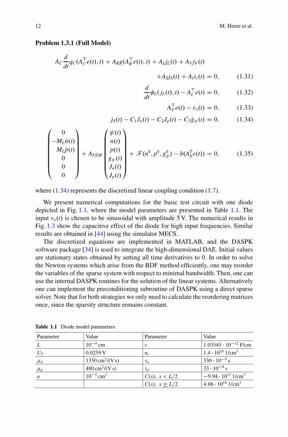
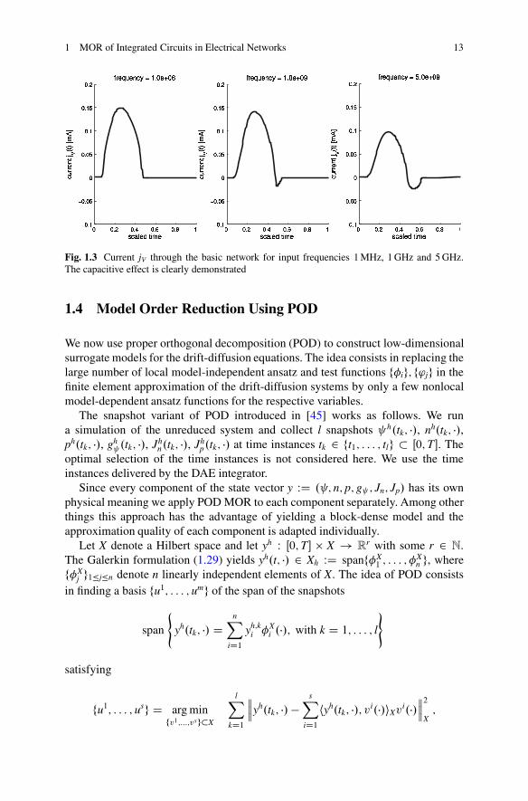
We present numerical computations for the basic test circuit with one diodedepicted in Fig. 1.1, where the model parameters are presented in Table 1.1. Theinput vs.t/ is chosen to be sinusoidal with amplitude 5 V. The numerical results inFig. 1.3 show the capacitive effect of the diode for high input frequencies. Similarresults are obtained in [44] using the simulator MECS.
The discretized equations are implemented in MATLAB, and the DASPKsoftware package [34] is used to integrate the high-dimensional DAE. Initial valuesare stationary states obtained by setting all time derivatives to 0. In order to solvethe Newton systems which arise from the BDF method efficiently, one may reorderthe variables of the sparse system with respect to minimal bandwidth. Then, one canuse the internal DASPK routines for the solution of the linear systems. Alternativelyone can implement the preconditioning subroutine of DASPK using a direct sparsesolver. Note that for both strategies we only need to calculate the reordering matricesonce, since the sparsity structure remains constant.
Table 1.1 Diode model parameters
Parameter Value Parameter Value
L 10�4 cm " 1:03545 � 10�12 F/cm
UT 0:0259V ni 1:4 � 1010 1/cm3
�n 1350 cm2/(V s) �n 330 � 10�9 s
�p 480 cm2/(V s) �p 33 � 10�9 s
a 10�5 cm2 C.x/; x < L=2 �9:94 � 1015 1/cm3
C.x/; x � L=2 4:06 � 1018 1/cm3
1 MOR of Integrated Circuits in Electrical Networks 13
Fig. 1.3 Current jV through the basic network for input frequencies 1 MHz, 1 GHz and 5 GHz.The capacitive effect is clearly demonstrated
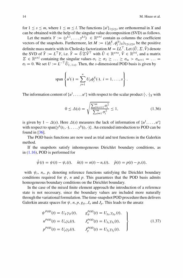
1.4 Model Order Reduction Using POD
We now use proper orthogonal decomposition (POD) to construct low-dimensionalsurrogate models for the drift-diffusion equations. The idea consists in replacing thelarge number of local model-independent ansatz and test functions f�ig; f'jg in thefinite element approximation of the drift-diffusion systems by only a few nonlocalmodel-dependent ansatz functions for the respective variables.
The snapshot variant of POD introduced in [45] works as follows. We runa simulation of the unreduced system and collect l snapshots h.tk; �/, nh.tk; �/,ph.tk; �/, gh
.tk; �/, Jhn.tk; �/, Jh
p.tk; �/ at time instances tk 2 ft1; : : : ; tlg � Œ0;T�. Theoptimal selection of the time instances is not considered here. We use the timeinstances delivered by the DAE integrator.
Since every component of the state vector y WD . ; n; p; g ; Jn; Jp/ has its ownphysical meaning we apply POD MOR to each component separately. Among otherthings this approach has the advantage of yielding a block-dense model and theapproximation quality of each component is adapted individually.
Let X denote a Hilbert space and let yh W Œ0;T� � X ! Rr with some r 2 N.
The Galerkin formulation (1.29) yields yh.t; �/ 2 Xh WD spanf�X1 ; : : : ; �
Xn g, where
f�Xj g1�j�n denote n linearly independent elements of X. The idea of POD consists
in finding a basis fu1; : : : ; umg of the span of the snapshots
span
(yh.tk; �/ D
nXiD1
yh;ki �
Xi .�/; with k D 1; : : : ; l
)
satisfying
fu1; : : : ; usg D arg minfv1;:::;vsg�X
lXkD1
���yh.tk; �/�sX
iD1hyh.tk; �/; vi.�/iXv
i.�/���2
X;
14 M. Hinze et al.
for 1 � s � m, where 1 � m � l. The functions fuig1�i�s are orthonormal in X andcan be obtained with the help of the singular value decomposition (SVD) as follows.
Let the matrix Y WD .yh;1; : : : ; yh;l/ 2 Rn�l contain as columns the coefficient
vectors of the snapshots. Furthermore, let M WD .h�Xi ; �
Xj iX/1�i;j�n be the positive
definite mass matrix with its Cholesky factorization M D LL>. Let . QU; ˙; QV/ denotethe SVD of QY WD L>Y, i.e. QY D QU˙ QV> with QU 2 R
n�n, QV 2 Rl�l, and a matrix
˙ 2 Rn�l containing the singular values �1 � �2 � : : : � �m > �mC1 D : : : D
�l D 0. We set U WD L�> QU.W; 1Ws/. Then, the s-dimensional POD basis is given by
span
8<:ui.�/ D
nXjD1
Uji�Xj .�/; i D 1; : : : ; s
9=; :
The information content of fu1; : : : ; usg with respect to the scalar product h�; �iX with
0 � .s/ DsPm
iDsC1 �2iPmiD1 �2i
� 1; (1.36)
is given by 1 � .s/. Here .s/ measures the lack of information of fu1; : : : ; usgwith respect to spanfyh.t1; �/; : : : ; yh.tl; �/g. An extended introduction to POD can befound in [36].
The POD basis functions are now used as trial and test functions in the Galerkinmethod.
If the snapshots satisfy inhomogeneous Dirichlet boundary conditions, asin (1.16), POD is performed for
Q .t/ D .t/ � r.t/; Qn.t/ D n.t/ � nr.t/; Qp.t/ D p.t/� pr.t/;
with r, nr, pr denoting reference functions satisfying the Dirichlet boundaryconditions required for , n and p. This guarantees that the POD basis admitshomogeneous boundary conditions on the Dirichlet boundary.
In the case of the mixed finite element approach the introduction of a referencestate is not necessary, since the boundary values are included more naturallythrough the variational formulation. The time-snapshot POD procedure then deliversGalerkin ansatz spaces for , n, p, g , Jn and Jp. This leads to the ansatz
POD.t/ D U � .t/; gPOD .t/ D Ug �g .t/;
nPOD.t/ D Un�n.t/; JPODn .t/ D UJn�Jn.t/;
pPOD.t/ D Up�p.t/; JPODp .t/ D UJp�Jp.t/:
9>>=>>;
(1.37)
1 MOR of Integrated Circuits in Electrical Networks 15
The injection matrices
U 2 RN�s ; Un 2 R
N�sn ; Up 2 RN�sp ;
Ug 2 RM�sg ; UJn 2 R
M�sJn ; UJp 2 RM�sJp ;
contain the (time independent) POD basis functions, the vectors �.�/ the correspond-ing time-variant coefficients. The numbers s.�/ are the respective number of PODbasis functions included. Assembling the POD system yields the DAE
0BBBBBBB@
0
� P�n.t/P�p.t/0
0
0
1CCCCCCCA
C APOD
0BBBBBBB@
� .t/�n.t/�p.t/�g .t/�Jn.t/�Jp.t/
1CCCCCCCA
C U>F .nPOD; pPOD; gPOD / D U>b.AT
S e.t//;
with
APOD D U>AFEMU
D
0BBBBBBB@
�U> MLUn U> MLUp U> DUg
�nU>n DUJn
�pU>p DUJp
U>g D>U I
U>JnD>Un I
�U>JpD>Up I
1CCCCCCCA
and U D diag.U ;Un;Up;Ug ;UJn ;UJp/. Note that we exploit the orthogonality ofthe POD basis functions, e.g. U>n MLUn D U>p MLUp D IN�N and U>g MHUg DU>Jn
MHUJn D U>JpMHUJp D IM�M . The arguments of the nonlinear functional have
to be interpreted as functions in space.All matrix-matrix multiplications are calculated in an offline phase. The nonlin-
ear functional F has to be evaluated online. The reduced model for the networknow reads
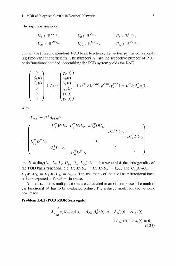
Problem 1.4.1 (POD MOR Surrogate)
ACd
dtqC.A
>C e.t/; t/C ARg.A>R e.t/; t/C ALjL.t/C AVjV.t/
CASjS.t/C AIis.t/ D 0;
(1.38)
16 M. Hinze et al.
d
dt�L. jL.t/; t/ � A>L e.t/ D 0;
(1.39)
A>V e.t/ � vs.t/ D 0;
(1.40)
jS.t/ � C1UJn�Jn.t/� C2UJp�Jp.t/ � C3Ug P�g .t/ D 0;
(1.41)0BBBBBBB@
0
� P�n.t/P�p.t/0
0
0
1CCCCCCCA
C APOD
0BBBBBBB@
� .t/�n.t/�p.t/�g .t/�Jn.t/�Jp.t/
1CCCCCCCA
C U>F .nPOD; pPOD; gPOD /� U>b.AT
S e.t// D 0:
(1.42)
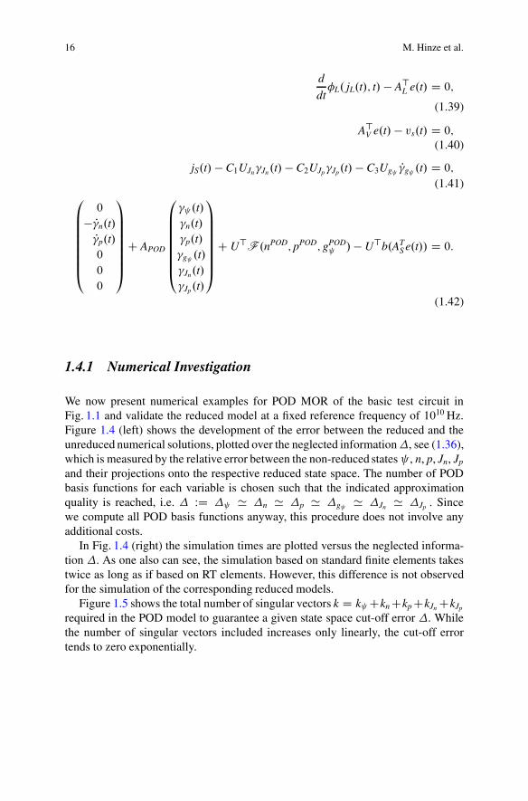
1.4.1 Numerical Investigation
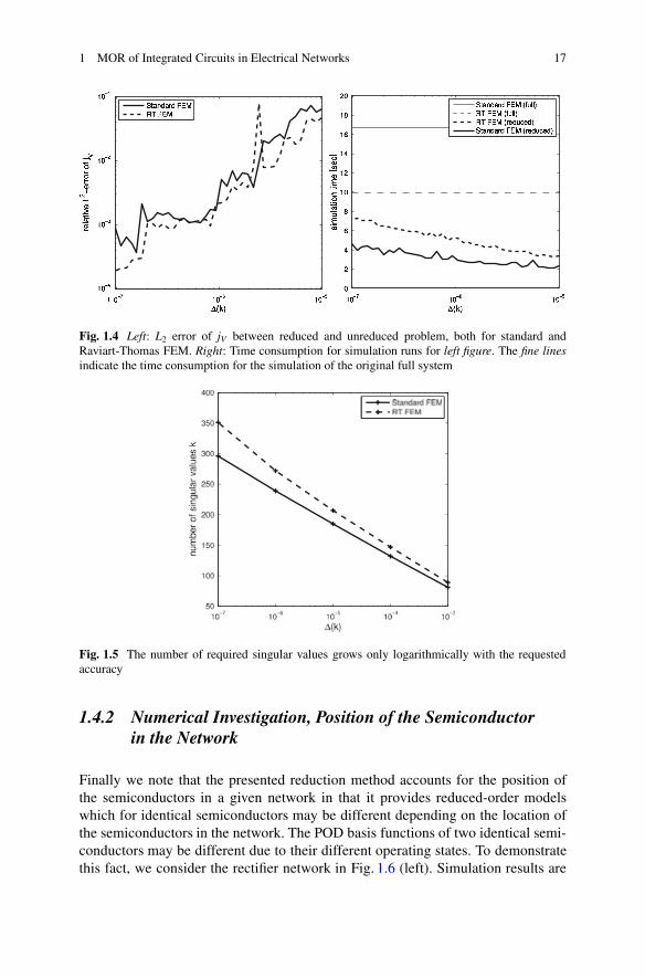
We now present numerical examples for POD MOR of the basic test circuit inFig. 1.1 and validate the reduced model at a fixed reference frequency of 1010 Hz.Figure 1.4 (left) shows the development of the error between the reduced and theunreduced numerical solutions, plotted over the neglected information, see (1.36),which is measured by the relative error between the non-reduced states , n, p, Jn, Jp
and their projections onto the respective reduced state space. The number of PODbasis functions for each variable is chosen such that the indicated approximationquality is reached, i.e. WD ' n ' p ' g ' Jn ' Jp : Sincewe compute all POD basis functions anyway, this procedure does not involve anyadditional costs.
In Fig. 1.4 (right) the simulation times are plotted versus the neglected informa-tion . As one also can see, the simulation based on standard finite elements takestwice as long as if based on RT elements. However, this difference is not observedfor the simulation of the corresponding reduced models.
Figure 1.5 shows the total number of singular vectors k D k Ckn Ckp CkJn CkJp
required in the POD model to guarantee a given state space cut-off error . Whilethe number of singular vectors included increases only linearly, the cut-off errortends to zero exponentially.
1 MOR of Integrated Circuits in Electrical Networks 17
Fig. 1.4 Left: L2 error of jV between reduced and unreduced problem, both for standard andRaviart-Thomas FEM. Right: Time consumption for simulation runs for left figure. The fine linesindicate the time consumption for the simulation of the original full system
Fig. 1.5 The number of required singular values grows only logarithmically with the requestedaccuracy
1.4.2 Numerical Investigation, Position of the Semiconductorin the Network
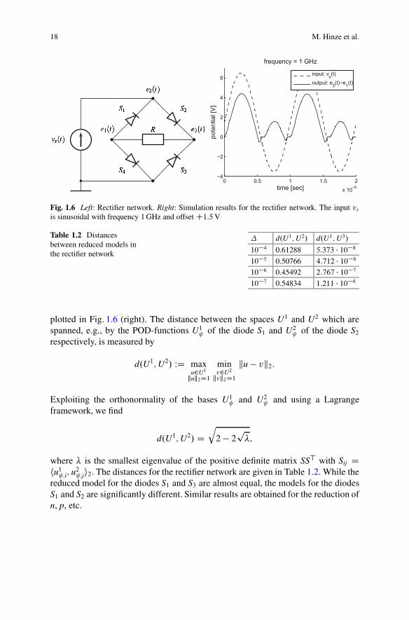
Finally we note that the presented reduction method accounts for the position ofthe semiconductors in a given network in that it provides reduced-order modelswhich for identical semiconductors may be different depending on the location ofthe semiconductors in the network. The POD basis functions of two identical semi-conductors may be different due to their different operating states. To demonstratethis fact, we consider the rectifier network in Fig. 1.6 (left). Simulation results are
18 M. Hinze et al.
0 0.5 1 1.5 2x 10⁻⁹
−4
−2
0
2
4
6
frequency = 1 GHz
time [sec]
pote
ntia
l [V]
input: vs(t)output: e3(t)−e1(t)
Fig. 1.6 Left: Rectifier network. Right: Simulation results for the rectifier network. The input vs
is sinusoidal with frequency 1 GHz and offsetC1:5V
Table 1.2 Distancesbetween reduced models inthe rectifier network
d.U1;U2/ d.U1;U3/
10�4 0.61288 5:373 � 10�8
10�5 0.50766 4:712 � 10�8
10�6 0.45492 2:767 � 10�7
10�7 0.54834 1:211 � 10�6
plotted in Fig. 1.6 (right). The distance between the spaces U1 and U2 which arespanned, e.g., by the POD-functions U1
of the diode S1 and U2 of the diode S2
respectively, is measured by
d.U1;U2/ WD maxu2U1
kuk2D1minv2U2
kvk2D1ku � vk2:
Exploiting the orthonormality of the bases U1 and U2
and using a Lagrangeframework, we find
d.U1;U2/ Dq2 � 2
p;
where is the smallest eigenvalue of the positive definite matrix SS> with Sij Dhu1 ;i; u
2 ;ji2. The distances for the rectifier network are given in Table 1.2. While the
reduced model for the diodes S1 and S3 are almost equal, the models for the diodesS1 and S2 are significantly different. Similar results are obtained for the reduction ofn, p, etc.
1 MOR of Integrated Circuits in Electrical Networks 19
1.4.3 MOR for the Nonlinearity with DEIM
The nonlinear function F in (1.42) has to be evaluated online which means that thecomputational complexity of the reduced-order model still depends on the numberof unknowns of the unreduced model. A reduction method for the nonlinearity isgiven by Discrete Empirical Interpolation (DEIM) [10]. This method is motivatedby the following observation. The nonlinearity in (1.42), see also (1.30), is given by
U>F .U�.t// D
0BBBBBBB@
0
U>n Fn.Un�n.t/;Up�p.t//U>p Fp.Un�n.t/;Up�p.t//
0
U>JnFJn.Un�n.t/;Ug �g .t//
U>JpFJp.Un�p.t/;Ug �g .t//
1CCCCCCCA;
see e.g. [23]. The subsequent considerations apply for each block component of F .For the sake of presentation we only consider the second block
U>n„ƒ‚…size sn�N
Fn„ƒ‚…N evaluations
. Un„ƒ‚…size N�sn
�n.t/; Up„ƒ‚…size N�sp
�p.t/ /; (1.43)
and its derivative with respect to �p,
U>n„ƒ‚…size sn�N
@Fn
@p.Un�n.t/;Up�p.t//
„ ƒ‚ …size N�N, sparse
Up„ƒ‚…size N�sp
:
Here, the matrices U.�/ are dense and the Jacobian of Fn is sparse. The evaluationof (1.43) is of computational complexity O.N/. Furthermore, we need to multiplylarge dense matrices in the evaluation of the Jacobian. Thus, the POD model orderreduction may become inefficient.
To overcome this problem, we apply Discrete Empirical Interpolation Method(DEIM) proposed in [10], which we now describe briefly. The snapshots h.tk; �/,nh.tk; �/, ph.tk; �/, gh
.tk; �/, Jhn.tk; �/, Jh
p.tk; �/ are collected at time instances tk 2ft1; : : : ; tlg � Œ0;T� as before. Additionally, we collect snapshots fFn.n.tk/; p.tk//gof the nonlinearity. DEIM approximates the projected function (1.43) such that
U>n Fn.Un�n.t/;Up�p.t// .U>n Vn.P>n Vn/
�1/P>n Fn.Un�n.t/;Up�p.t//;
where Vn 2 RN��n contains the first �n POD basis functions of the space spanned
by the snapshots fFn.n.tk/; p.tk//g associated with the largest singular values. Theselection matrix Pn D �
e�1 ; : : : ; e��n� 2 R
N��n selects the rows of Fn corresponding
20 M. Hinze et al.
to the so-called DEIM indices �1; : : : ; ��n which are chosen such that the growth ofa global error bound is limited and P>n Vn is regular, see [10] for details.
The matrix Wn WD .U>n Vn.P>n Vn/�1/ 2 R
sn��n as well as the whole interpolationmethod is calculated in an offline phase. In the simulation of the reduced-ordermodel we instead of (1.43) evaluate:
Wn„ƒ‚…size sn��n
P>n Fn„ƒ‚…�n evaluations
. Un„ƒ‚…size N�sn
�n.t/; Up„ƒ‚…size N�sp
�p.t/ /; (1.44)
with derivative
W>n„ƒ‚…size sn��n
@P>n Fn
@p.Un�n.t/;Up�p.t//
„ ƒ‚ …size �n�N, sparse
Up„ƒ‚…size N�sp
:
In the applied finite element method a single functional component of Fn onlydepends on a small constant number c 2 N components of Un�n.t/. Thus, thematrix-matrix multiplication in the derivative does not really depend on N sincethe number of entries per row in the Jacobian is at most c.
But there is still a dependence on N, namely the calculation of Un�n.t/. Toovercome this dependency we identify the required components of the vectorUn�n.t/ for the evaluation of P>n Fn. This is done by defining selection matricesQn;n 2 R
c�n�sn , Qn;p 2 Rc�p�sp such that
P>n Fn.Un�n.t/;Up�p.t// D OFn.Qn;nUn�n.t/;Qn;pUp�p.t//;
where OFn denotes the functional components of Fn selected by Pn restricted to thearguments selected by Qn;n and Qn;p.
Supposed that �n sn N we obtain a reduced-order model which does notdepend on N any more.
1.4.4 Numerical Implementation and Results with DEIM
We again use the basic test circuit with a single 1-dimensional diode depicted inFig. 1.1. The parameters of the diode are summarized in [23]. The input vs.t/ ischosen to be sinusoidal with amplitude 5 V. In the sequel the frequency of thevoltage source will be considered as a model parameter.
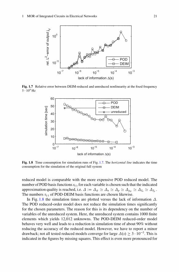
We first validate the reduced model at a fixed reference frequency of 5 � 109 Hz.Figure 1.7 shows the development of the relative error between the POD reduced,the POD-DEIM reduced and the unreduced numerical solutions, plotted over thelack of information of the POD basis functions with respect to the space spannedby the snapshots. The figure shows that the approximation quality of the POD-DEIM
1 MOR of Integrated Circuits in Electrical Networks 21
10−7 10−6 10−5 10−4 10−3
10−5
100
lack of information Δ(s)
rel.
L2 −erro
r of o
utpu
t jV
PODDEIM
Fig. 1.7 Relative error between DEIM-reduced and unreduced nonlinearity at the fixed frequency5 � 109 Hz
10−7 10−6 10−5 10−4 10−30
10
20
30
40
50
60
lack of information Δ(s)
sim
ulat
ion
time
[sec
]
PODDEIMunreduced
Fig. 1.8 Time consumption for simulation runs of Fig. 1.7. The horizontal line indicates the timeconsumption for the simulation of the original full system
reduced model is comparable with the more expensive POD reduced model. Thenumber of POD basis functions s.�/ for each variable is chosen such that the indicatedapproximation quality is reached, i.e. WD ' n ' p ' g ' Jn ' Jp :
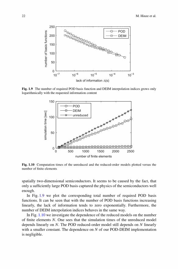
The numbers �.�/ of POD-DEIM basis functions are chosen likewise.In Fig. 1.8 the simulation times are plotted versus the lack of information .
The POD reduced-order model does not reduce the simulation times significantlyfor the chosen parameters. The reason for this is its dependency on the number ofvariables of the unreduced system. Here, the unreduced system contains 1000 finiteelements which yields 12,012 unknowns. The POD-DEIM reduced-order modelbehaves very well and leads to a reduction in simulation time of about 90% withoutreducing the accuracy of the reduced model. However, we have to report a minordrawback; not all tested reduced models converge for large.s/ � 3 � 10�5. This isindicated in the figures by missing squares. This effect is even more pronounced for
22 M. Hinze et al.
10−7 10−6 10−5 10−4 10−30
50
100
150
200
250
lack of information ∆(s)
num
ber o
f bas
is fu
nctio
ns PODDEIM
Fig. 1.9 The number of required POD basis function and DEIM interpolation indices grows onlylogarithmically with the requested information content
0 500 1000 1500 2000 25000
50
100
150
number of finite elements
sim
ulat
ion
time
[sec
]
PODDEIMunreduced
Fig. 1.10 Computation times of the unreduced and the reduced-order models plotted versus thenumber of finite elements
spatially two-dimensional semiconductors. It seems to be caused by the fact, thatonly a sufficiently large POD basis captured the physics of the semiconductors wellenough.
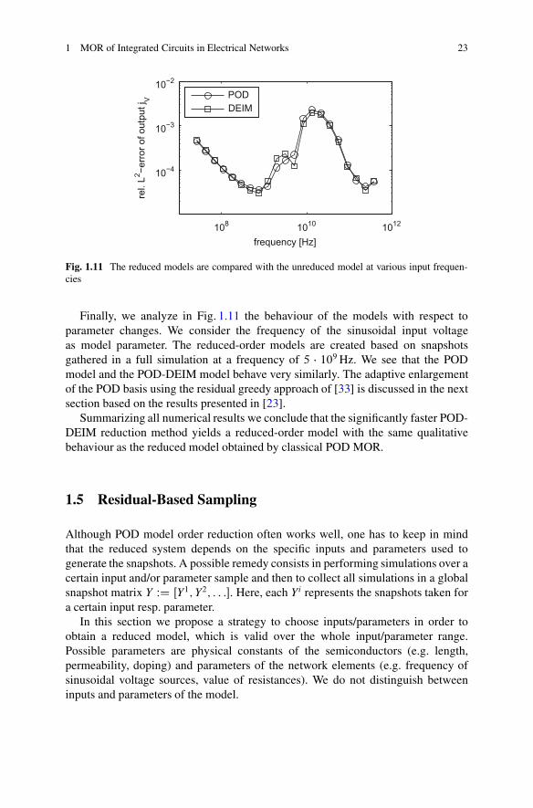
In Fig. 1.9 we plot the corresponding total number of required POD basisfunctions. It can be seen that with the number of POD basis functions increasinglinearly, the lack of information tends to zero exponentially. Furthermore, thenumber of DEIM interpolation indices behaves in the same way.
In Fig. 1.10 we investigate the dependence of the reduced models on the numberof finite elements N. One sees that the simulation times of the unreduced modeldepends linearly on N. The POD reduced-order model still depends on N linearlywith a smaller constant. The dependence on N of our POD-DEIM implementationis negligible.
1 MOR of Integrated Circuits in Electrical Networks 23
108 1010 1012
10−4
10−3
10−2
frequency [Hz]
rel.
L2 −erro
r of o
utpu
t jV POD
DEIM
Fig. 1.11 The reduced models are compared with the unreduced model at various input frequen-cies
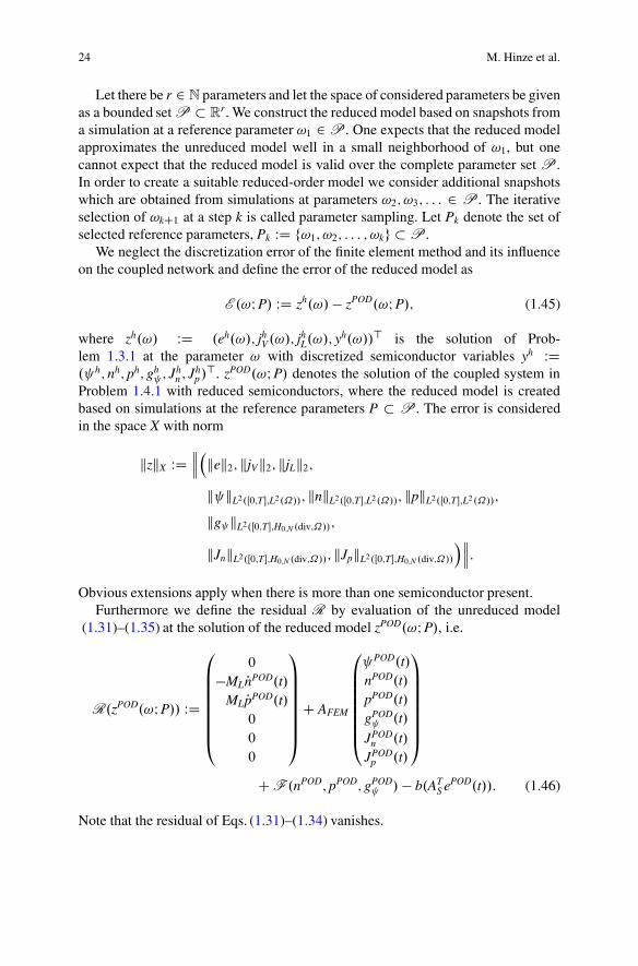
Finally, we analyze in Fig. 1.11 the behaviour of the models with respect toparameter changes. We consider the frequency of the sinusoidal input voltageas model parameter. The reduced-order models are created based on snapshotsgathered in a full simulation at a frequency of 5 � 109 Hz. We see that the PODmodel and the POD-DEIM model behave very similarly. The adaptive enlargementof the POD basis using the residual greedy approach of [33] is discussed in the nextsection based on the results presented in [23].
Summarizing all numerical results we conclude that the significantly faster POD-DEIM reduction method yields a reduced-order model with the same qualitativebehaviour as the reduced model obtained by classical POD MOR.
1.5 Residual-Based Sampling
Although POD model order reduction often works well, one has to keep in mindthat the reduced system depends on the specific inputs and parameters used togenerate the snapshots. A possible remedy consists in performing simulations over acertain input and/or parameter sample and then to collect all simulations in a globalsnapshot matrix Y WD ŒY1;Y2; : : :�. Here, each Yi represents the snapshots taken fora certain input resp. parameter.
In this section we propose a strategy to choose inputs/parameters in order toobtain a reduced model, which is valid over the whole input/parameter range.Possible parameters are physical constants of the semiconductors (e.g. length,permeability, doping) and parameters of the network elements (e.g. frequency ofsinusoidal voltage sources, value of resistances). We do not distinguish betweeninputs and parameters of the model.
24 M. Hinze et al.
Let there be r 2 N parameters and let the space of considered parameters be givenas a bounded set P � R
r. We construct the reduced model based on snapshots froma simulation at a reference parameter !1 2 P . One expects that the reduced modelapproximates the unreduced model well in a small neighborhood of !1, but onecannot expect that the reduced model is valid over the complete parameter set P .In order to create a suitable reduced-order model we consider additional snapshotswhich are obtained from simulations at parameters !2; !3; : : : 2 P . The iterativeselection of !kC1 at a step k is called parameter sampling. Let Pk denote the set ofselected reference parameters, Pk WD f!1; !2; : : : ; !kg � P .
We neglect the discretization error of the finite element method and its influenceon the coupled network and define the error of the reduced model as
E .!I P/ WD zh.!/� zPOD.!I P/; (1.45)
where zh.!/ WD .eh.!/; jhV.!/; jhL.!/; y
h.!//> is the solution of Prob-lem 1.3.1 at the parameter ! with discretized semiconductor variables yh WD. h; nh; ph; gh
; Jhn ; J
hp/>. zPOD.!I P/ denotes the solution of the coupled system in
Problem 1.4.1 with reduced semiconductors, where the reduced model is createdbased on simulations at the reference parameters P � P . The error is consideredin the space X with norm
kzkX WD����kek2; kjVk2; kjLk2;k kL2.Œ0;T�;L2 .˝//; knkL2.Œ0;T�;L2.˝//; kpkL2.Œ0;T�;L2 .˝//;
kg kL2.Œ0;T�;H0;N .div;˝//;
kJnkL2.Œ0;T�;H0;N .div;˝//; kJpkL2.Œ0;T�;H0;N .div;˝//
����:Obvious extensions apply when there is more than one semiconductor present.
Furthermore we define the residual R by evaluation of the unreduced model(1.31)–(1.35) at the solution of the reduced model zPOD.!I P/, i.e.
R.zPOD.!I P// WD
0BBBBBBB@
0
�ML PnPOD.t/ML PpPOD.t/
0
0
0
1CCCCCCCA
C AFEM
0BBBBBBB@
POD.t/nPOD.t/pPOD.t/gPOD .t/
JPODn .t/
JPODp .t/
1CCCCCCCA
C F .nPOD; pPOD; gPOD / � b.AT
S ePOD.t//: (1.46)
Note that the residual of Eqs. (1.31)–(1.34) vanishes.
1 MOR of Integrated Circuits in Electrical Networks 25
We note that the same definitions are used in [22] for linear descriptor systems.In [22] an error estimate is obtained by deriving a linear ODE for the error andexploiting explicit solution formulas. Here we have a nonlinear DAE and at thepresent state we are not able to provide an upper bound for the error kE .!I P/kX
which would yield a rigorous sampling method using for example the Greedyalgorithm of [33].
We propose to consider the residual as an estimate for the error. The evaluationof the residual is cheap since it only requires the solution of the reduced system andits evaluation in the unreduced DAE. It is therefore possible to evaluate the residualat a large set of test parameters Ptest � P . Similar to the Greedy algorithm of [33],we add to the set of reference parameters the parameter where the residual becomesmaximal.
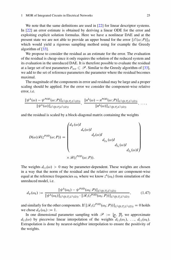
The magnitude of the components in error and residual may be large and a properscaling should be applied. For the error we consider the component-wise relativeerror, i.e.
k h.!/ � POD.!I P/kL2.Œ0;T�;L2 .˝//
k h.!/kL2.Œ0;T�;L2.˝//;
knh.!/ � nPOD.!I P/kL2.Œ0;T�;L2 .˝//
knh.!/kL2.Œ0;T�;L2.˝//; : : : ;
and the residual is scaled by a block-diagonal matrix containing the weights
D.!/R.zPOD.!I P// D
0BBBBBBB@
d .!/Idn.!/I
dp.!/Idg .!/I
dJn.!/IdJp.!/I
1CCCCCCCA
�R.zPOD.!I P//:
The weights d.�/.!/ > 0 may be parameter-dependent. These weights are chosenin a way that the norm of the residual and the relative error are component-wiseequal at the reference frequencies !k where we know zh.!k/ from simulation of theunreduced model, i.e.
d .!k/ WD k h.!k/� POD.!kI P/kL2.Œ0;T�;L2.˝//
k h.!k/kL2.Œ0;T�;L2.˝// � kR1.zPOD.!kI P//kL2.Œ0;T�;L2.˝//; (1.47)
and similarly for the other components. If kR1.zPOD.!kI P//kL2.Œ0;T�;L2 .˝// D 0 holdswe chose d .!k/ WD 1.
In one dimensional parameter sampling with P WD Œp; p�, we approximated.�/.!/ by piecewise linear interpolation of the weights d.�/.!1/, : : :, d.�/.!k/.Extrapolation is done by nearest-neighbor interpolation to ensure the positivity ofthe weights.
26 M. Hinze et al.
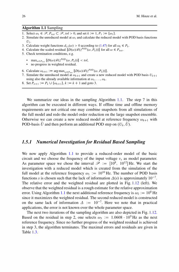
Algorithm 1.1 Sampling1. Select !1 2P , Ptest �P , tol > 0, and set k WD 1, P1 WD f!1g.2. Simulate the unreduced model at !1 and calculate the reduced model with POD basis functions
U1.3. Calculate weight functions d.�/.!/ > 0 according to (1.47) for all !k 2 Pk.4. Calculate the scaled residual kD.!/R.zPOD.!;Pk//k for all ! 2 Ptest.5. Check termination conditions, e.g.
• max!2Ptest kD.!/R.zPOD.!;Pk//k < tol,• no progress in weighted residual.
6. Calculate !kC1 WD arg max!2PtestkD.!/R.zPOD.!;Pk//k.
7. Simulate the unreduced model at !kC1 and create a new reduced model with POD basis UkC1
using also the already available information at !1, : : :, !k .8. Set PkC1 WD Pk [ f!kC1g, k WD kC 1 and goto 3.
We summarize our ideas in the sampling Algorithm 1.1. The step 7 in thisalgorithm can be executed in different ways. If offline time and offline memoryrequirements are not critical one may combine snapshots from all simulations ofthe full model and redo the model order reduction on the large snapshot ensemble.Otherwise we can create a new reduced model at reference frequency !kC1 withPOD-basis NU and then perform an additional POD step on .Uk; NU/.
1.5.1 Numerical Investigation for Residual Based Sampling
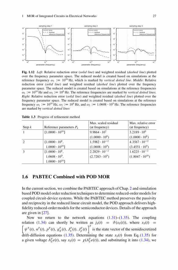
We now apply Algorithm 1.1 to provide a reduced-order model of the basiccircuit and we choose the frequency of the input voltage vs as model parameter.As parameter space we chose the interval P WD Œ108; 1012�Hz. We start theinvestigation with a reduced model which is created from the simulation of thefull model at the reference frequency !1 WD 1010 Hz. The number of POD basisfunctions s is chosen such that the lack of information.s/ is approximately 10�7.The relative error and the weighted residual are plotted in Fig. 1.12 (left). Weobserve that the weighted residual is a rough estimate for the relative approximationerror. Using Algorithm 1.1 the next additional reference frequency is !2 WD 108 Hzsince it maximizes the weighted residual. The second reduced model is constructedon the same lack of information WD 10�7. Here we note that in practicalapplications, the error is not known over the whole parameter space.
The next two iterations of the sampling algorithm are also depicted in Fig. 1.12.Based on the residual in step 2, one selects !3 WD 1:0608 � 109 Hz as the nextreference frequency. Since no further progress of the weighted residual is achievedin step 3, the algorithm terminates. The maximal errors and residuals are given inTable 1.3.
1 MOR of Integrated Circuits in Electrical Networks 27
108 1010 101210−4
10−3
10−2
10−1
100
101
102sampling step 1
parameter (frequency)
errorresidualreference frequencies
108 1010 101210−4
10−3
10−2
10−1
100
101
102sampling step 2
parameter (frequency)
errorresidualreference frequencies
108 1010 101210−4
10−3
10−2
10−1
100
101
102sampling step 3
parameter (frequency)
errorresidualreference frequencies
Fig. 1.12 Left: Relative reduction error (solid line) and weighted residual (dashed line) plottedover the frequency parameter space. The reduced model is created based on simulations at thereference frequency !1 WD 1010 Hz, which is marked by vertical dotted line. Middle: Relativereduction error (solid line) and weighted residual (dashed line) plotted over the frequencyparameter space. The reduced model is created based on simulations at the reference frequencies!1 WD 1010 Hz and !2 WD 108 Hz. The reference frequencies are marked by vertical dotted lines.Right: Relative reduction error (solid line) and weighted residual (dashed line) plotted over thefrequency parameter space. The reduced model is created based on simulations at the referencefrequency !1 WD 1010 Hz, !2 WD 108 Hz, and !3 WD 1:0608 � 109 Hz. The reference frequenciesare marked by vertical dotted lines
Table 1.3 Progress of refinement method
Max. scaled residual Max. relative errorStep k Reference parameters Pk (at frequency) (at frequency)
1 f1:0000 � 1010g 9:9864 � 102 3:2189 � 100.1:0000 � 108/ .1:0000 � 108/
2 f1:0000 � 108; 1:5982 � 10�2 4:3567 � 10�2
1:0000 � 1010g .1:0608 � 109/ .3:4551 � 109/3 f1:0000 � 108; 2:2829 � 10�2 1:6225 � 10�2
1:0608 � 109; .2:7283 � 109/ .1:8047 � 1010/1:0000 � 1010g
1.6 PABTEC Combined with POD MOR
In the current section, we combine the PABTEC approach of Chap. 2 and simulationbased POD model order reduction techniques to determine reduced-order models forcoupled circuit-device systems. While the PABTEC method preserves the passivityand reciprocity in the reduced linear circuit model, the POD approach delivers high-fidelity reduced-order models for the semiconductor devices. Details of the approachare given in [27].
Now we return to the network equations (1.31)–(1.35). The couplingrelation (1.34) can shortly be written as jS.t/ D #.xS.t//, where xS.t/ Dh T .t/; nT.t/; pT.t/; gT
.t/; JTn .t/; JT
p .t/iT
is the state vector of the semidiscretized
drift-diffusion equations (1.35). Determining the state xS.t/ from Eq. (1.35) fora given voltage AT
S e.t/, say xS.t/ D .ATS e.t//, and substituting it into (1.34), we
28 M. Hinze et al.
obtain the relationship
jS.t/ D g.ATS e.t//; (1.48)
where g.ATS e.t// WD #. .AT
S e.t/// describes the voltage-current relation for thesemidiscretized semiconductors. This relation can be considered as an input-to-output map, where the input is the voltage vector AT
S e.t/ at the contacts of thesemiconductors and the output is the approximate semiconductor current jS.t/.
Electrical networks usually contains very large linear subnetworks modelinginterconnects. In POD MOR we need to simulate the coupled DAE system (1.31)–(1.35) in order to determine the snapshots. To reduce the simulation time, we canfirst to separate the linear subsystem and approximate it by a reduced-order linearmodel of lower dimension using the PABTEC algorithm [38, 51], see also Chap. 2in this book. The decoupled device equations are then reduced using the PODmethod presented in Sect. 1.4. Combining these reduced-order linear and nonlinearmodels, we obtain a nonlinear reduced-order model that approximates the coupledsystem (1.31)–(1.35).
1.6.1 Decoupling
For the extraction of a linear subcircuit, we use a decoupling procedure from [47]that consists in the replacement of the nonlinear inductors and nonlinear capacitorsby controlled current sources and controlled voltage sources, respectively. Thenonlinear resistors and semiconductor devices are replaced by an equivalent circuitconsisting of two serial linear resistors and one controlled current source connectedparallel to one of the resistors. Such replacements introduce additional nodes andstate variables, but neither additional loops consisting of capacitors and voltagesources (CV-loops) nor cutsets consisting of inductors and current sources (LI-cutsets) occur in the decoupled linear subcircuit meaning that its index coincideswith the index of the original circuit, see [13] for the index analysis of the circuitequations. An advantage of the suggested replacement strategy is demonstrated inthe following example.
Example 1.6.1 Consider a circuit with a semiconductor diode as in Fig. 1.13. Wesuggest to replace the diode by an equivalent circuit shown in Fig. 1.14. If we wouldreplace the diode by a current source, then a decoupled linear circuit would haveI-cutset and, hence, lack well-posedness. Moreover, if we would replace the diodeby a voltage source, then the resulting linear circuit would have CV-loop, i.e., itwould be of index two, although the original circuit is of index one. Note that modelreduction of index two problems is more involved than of index one problems [50].
For simplicity, we assume that the circuit does not contain nonlinear devices otherthan semiconductors. Then after the replacements described above, the extracted
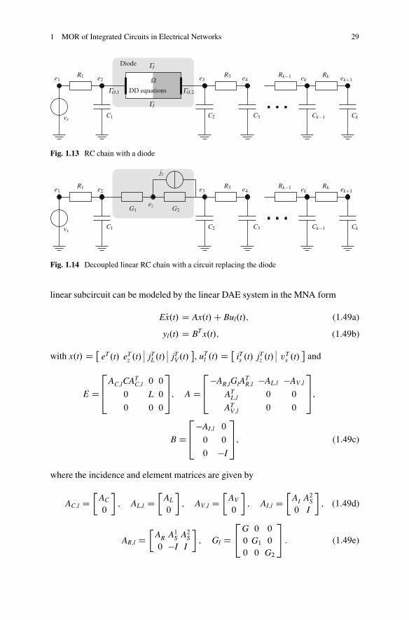
1 MOR of Integrated Circuits in Electrical Networks 29
Fig. 1.13 RC chain with a diode
Fig. 1.14 Decoupled linear RC chain with a circuit replacing the diode
linear subcircuit can be modeled by the linear DAE system in the MNA form
EPx.t/ D Ax.t/C Bul.t/; (1.49a)
yl.t/ D BTx.t/; (1.49b)
with x.t/ D eT.t/ eT
z .t/ jTL.t/ jTV.t/, uT
l .t/ D iTs .t/ jTz .t/ vT
s .t/
and
E D
264
AC;lCATC;l 0 0
0 L 0
0 0 0
375; A D
264
�AR;lGlATR;l �AL;l �AV;l
ATL;l 0 0
ATV;l 0 0
375;
B D
264
�AI;l 0
0 0
0 �I
375; (1.49c)
where the incidence and element matrices are given by
AC;l D�
AC
0
�; AL;l D
�AL
0
�; AV;l D
�AV
0
�; AI;l D
�AI A2S0 I
�; (1.49d)
AR;l D�
AR A1S A2S0 �I I
�; Gl D
24G 0 0
0 G1 0
0 0 G2
35 : (1.49e)
30 M. Hinze et al.
Here, C, L and G are the capacitance, inductance and conductance matrices, A1Sand A2S have entries in f0; 1g and f�1; 0g, respectively, and satisfy A1S C A2S D AS.Moreover, ez.t/ is the potential of the introduced nodes, and the new input variablejz.t/ is given by
jz.t/ D .G1 C G2/G�11 g.AT
S e.t// � G2ATS e.t/; (1.50)
where the matrices G1 and G2 are diagonal with conductances of the introducedlinear resistors in the replacement circuits on the diagonal. One can show that thelinear system (1.49) together with the decoupled nonlinear equations (1.35), (1.48)is state equivalent to the coupled system (1.31)–(1.35) together with the equation
ez.t/ D .G1 C G2/�1�G1.A1eR /Te.t/ � G2.A2eR /Te.t/ � jz.t/
�(1.51)
in the sense that these both systems have the same state vectors up to a permutation,see [47] for detail.
1.6.2 Model Reduction Approach
Applying the PABTEC method to the linear DAE system (1.49), we obtaina reduced-order model
OE d
dtOx.t/ D OAOx.t/C OB1 OB2 OB3
24 is.t/
jz.t/vs.t/
35 ;
264
Oyl;1.t/
Oyl;2.t/
Oyl;3.t/
375 D
24
OC1OC2OC3
35 Ox.t/;
(1.52)
where Oyl;j D OCj Ox.t/, j D 1; 2; 3, approximate the corresponding components of theoutput yl in (1.49b). Combining this reduced model with the semidiscretized drift-diffusion equations (1.35) via (1.48), we can determine the approximate snapshotswhich can then be used to compute the POD-reduced model as in (1.42). Thecoupling relation (1.41) can then be approximated by
OjS.t/ D C1UJn�Jn.t/C C2UJp�Jp.t/C C3Ug P�g .t/: (1.53)
As for the original system (1.34) and (1.35), we denote the relation between ATS e.t/
and OjS.t/ by
OjS.t/ D Og.ATS e.t//: (1.54)
Using (1.50) and (1.51), we have �.A2S/Te.t/ � ez.t/ D �ATS e.t/C G1g.AT
S e.t//.Then it follows from �.A2S/Te.t/ � ez.t/ OC2 Ox.t/ that the semiconductor voltage
1 MOR of Integrated Circuits in Electrical Networks 31
vector uS.t/ D ATS e.t/ can be approximated by OuS.t/ satisfying �G1
OC2 Ox.t/ �G1 OuS.t/ C Og.OuS.t// D 0. Thus, combining the reduced linear system (1.52) withthe reduced semiconductor model (1.42), we obtain a reduced-order coupled DAEsystem
OE d
dtOx.t/ � . OA C OB2.G1 C G2/ OC2/Ox.t/ � OB2G1 OuS.t/� OB1is.t/ � OB3vs.t/ D 0;
(1.55)
�G1OC2 Ox.t/ � G1 OuS.t/C Og.OuS.t// D 0;
(1.56)
OjS.t/ � C1UJn�Jn.t/ � C2UJp�Jp.t/ � C3Ug P�g .t/ D 0;
(1.57)0BBBBBBB@
0
� P�n.t/P�p.t/0
0
0
1CCCCCCCA
C APOD
0BBBBBBB@
� .t/�n.t/�p.t/�g .t/�Jn.t/�Jp.t/
1CCCCCCCA
C U>F .nPOD; pPOD; gPOD / � U>b.OuS.t// D 0:
(1.58)
Note that model reduction of the linear subsystem and the semiconductor model canbe executed independently.
1.6.3 Numerical Experiments
In this section, we present some results of numerical experiments to demonstrate theapplicability of the presented model reduction approaches for coupled circuit-devicesystems.
For model reduction of linear circuit equations, we use the MATLAB ToolboxPABTEC, see Chap. 2. The POD method is implemented in C++ based on theFEM library deal.II [5] for discretizing the drift-diffusion equations. The obtainedlarge and sparse nonlinear DAE system (1.31)–(1.35) as well as the small anddense reduced-order model (1.55)–(1.58) are integrated using the DASPK softwarepackage [9] based on a BDF method, where the nonlinear equations are solved usingNewton’s method. Furthermore, the direct sparse solver SuperLU [12] is employedfor solving linear systems.
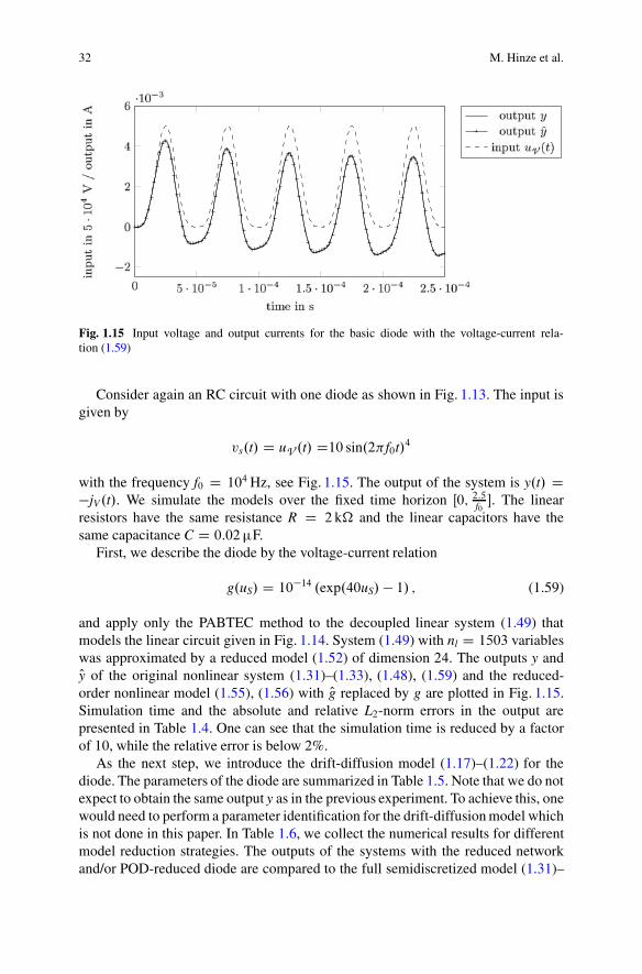
32 M. Hinze et al.
Fig. 1.15 Input voltage and output currents for the basic diode with the voltage-current rela-tion (1.59)
Consider again an RC circuit with one diode as shown in Fig. 1.13. The input isgiven by
vs.t/ D uV .t/ D10 sin.2�f0t/4
with the frequency f0 D 104 Hz, see Fig. 1.15. The output of the system is y.t/ D�jV.t/. We simulate the models over the fixed time horizon Œ0; 2:5f0
�. The linearresistors have the same resistance R D 2 k� and the linear capacitors have thesame capacitance C D 0:02 �F.
First, we describe the diode by the voltage-current relation
g.uS/ D 10�14 .exp.40uS/ � 1/ ; (1.59)
and apply only the PABTEC method to the decoupled linear system (1.49) thatmodels the linear circuit given in Fig. 1.14. System (1.49) with nl D 1503 variableswas approximated by a reduced model (1.52) of dimension 24. The outputs y andOy of the original nonlinear system (1.31)–(1.33), (1.48), (1.59) and the reduced-order nonlinear model (1.55), (1.56) with Og replaced by g are plotted in Fig. 1.15.Simulation time and the absolute and relative L2-norm errors in the output arepresented in Table 1.4. One can see that the simulation time is reduced by a factorof 10, while the relative error is below 2%.
As the next step, we introduce the drift-diffusion model (1.17)–(1.22) for thediode. The parameters of the diode are summarized in Table 1.5. Note that we do notexpect to obtain the same output y as in the previous experiment. To achieve this, onewould need to perform a parameter identification for the drift-diffusion model whichis not done in this paper. In Table 1.6, we collect the numerical results for differentmodel reduction strategies. The outputs of the systems with the reduced networkand/or POD-reduced diode are compared to the full semidiscretized model (1.31)–
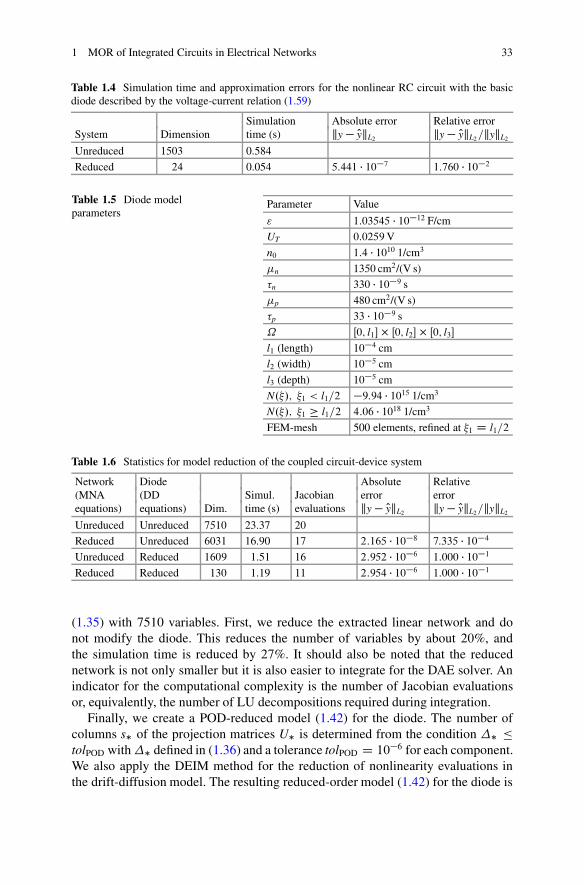
1 MOR of Integrated Circuits in Electrical Networks 33
Table 1.4 Simulation time and approximation errors for the nonlinear RC circuit with the basicdiode described by the voltage-current relation (1.59)
Simulation Absolute error Relative errorSystem Dimension time (s) ky� OykL2 ky� OykL2 =kykL2
Unreduced 1503 0.584
Reduced 24 0.054 5:441 � 10�7 1:760 � 10�2
Table 1.5 Diode modelparameters
Parameter Value
" 1:03545 � 10�12 F/cm
UT 0:0259V
n0 1:4 � 1010 1/cm3
�n 1350 cm2/(V s)
�n 330 � 10�9 s
�p 480 cm2/(V s)
�p 33 � 10�9 s
˝ Œ0; l1�� Œ0; l2� � Œ0; l3�l1 (length) 10�4 cm
l2 (width) 10�5 cm
l3 (depth) 10�5 cm
N.�/; �1 < l1=2 �9:94 � 1015 1/cm3
N.�/; �1 � l1=2 4:06 � 1018 1/cm3
FEM-mesh 500 elements, refined at �1 D l1=2
Table 1.6 Statistics for model reduction of the coupled circuit-device system
Network Diode Absolute Relative(MNA (DD Simul. Jacobian error errorequations) equations) Dim. time (s) evaluations ky� OykL2 ky� OykL2 =kykL2
Unreduced Unreduced 7510 23.37 20
Reduced Unreduced 6031 16.90 17 2:165 � 10�8 7:335 � 10�4
Unreduced Reduced 1609 1.51 16 2:952 � 10�6 1:000 � 10�1
Reduced Reduced 130 1.19 11 2:954 � 10�6 1:000 � 10�1
(1.35) with 7510 variables. First, we reduce the extracted linear network and donot modify the diode. This reduces the number of variables by about 20%, andthe simulation time is reduced by 27%. It should also be noted that the reducednetwork is not only smaller but it is also easier to integrate for the DAE solver. Anindicator for the computational complexity is the number of Jacobian evaluationsor, equivalently, the number of LU decompositions required during integration.
Finally, we create a POD-reduced model (1.42) for the diode. The number ofcolumns s� of the projection matrices U� is determined from the condition � �tolPOD with� defined in (1.36) and a tolerance tolPOD D 10�6 for each component.We also apply the DEIM method for the reduction of nonlinearity evaluations inthe drift-diffusion model. The resulting reduced-order model (1.42) for the diode is
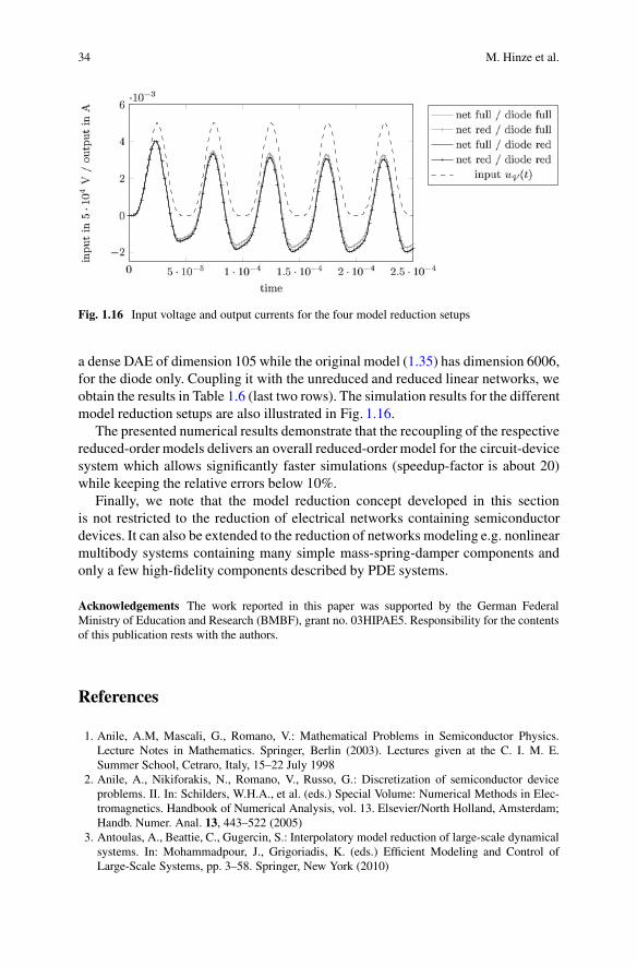
34 M. Hinze et al.
Fig. 1.16 Input voltage and output currents for the four model reduction setups
a dense DAE of dimension 105 while the original model (1.35) has dimension 6006,for the diode only. Coupling it with the unreduced and reduced linear networks, weobtain the results in Table 1.6 (last two rows). The simulation results for the differentmodel reduction setups are also illustrated in Fig. 1.16.
The presented numerical results demonstrate that the recoupling of the respectivereduced-order models delivers an overall reduced-order model for the circuit-devicesystem which allows significantly faster simulations (speedup-factor is about 20)while keeping the relative errors below 10%.
Finally, we note that the model reduction concept developed in this sectionis not restricted to the reduction of electrical networks containing semiconductordevices. It can also be extended to the reduction of networks modeling e.g. nonlinearmultibody systems containing many simple mass-spring-damper components andonly a few high-fidelity components described by PDE systems.
Acknowledgements The work reported in this paper was supported by the German FederalMinistry of Education and Research (BMBF), grant no. 03HIPAE5. Responsibility for the contentsof this publication rests with the authors.
References
1. Anile, A.M, Mascali, G., Romano, V.: Mathematical Problems in Semiconductor Physics.Lecture Notes in Mathematics. Springer, Berlin (2003). Lectures given at the C. I. M. E.Summer School, Cetraro, Italy, 15–22 July 1998
2. Anile, A., Nikiforakis, N., Romano, V., Russo, G.: Discretization of semiconductor deviceproblems. II. In: Schilders, W.H.A., et al. (eds.) Special Volume: Numerical Methods in Elec-tromagnetics. Handbook of Numerical Analysis, vol. 13. Elsevier/North Holland, Amsterdam;Handb. Numer. Anal. 13, 443–522 (2005)
3. Antoulas, A., Beattie, C., Gugercin, S.: Interpolatory model reduction of large-scale dynamicalsystems. In: Mohammadpour, J., Grigoriadis, K. (eds.) Efficient Modeling and Control ofLarge-Scale Systems, pp. 3–58. Springer, New York (2010)
1 MOR of Integrated Circuits in Electrical Networks 35
4. Astrid, P., Weiland, S., Willcox, K., Backx, T.: Missing point estimation in models describedby proper orthogonal decomposition. IEEE Trans. Autom. Control 53(10), 2237–2251 (2008)
5. Bangerth, W., Hartmann, R., Kanschat, G.: deal.II – a general-purpose object-oriented finiteelement library. ACM Trans. Math. Softw. 33(4), Article No. 24 (2007)
6. Benner, P., Hinze, M., ter Maten, E. (eds.): Model Reduction for Circuit Simulation. LectureNotes in Electrical Engineering, vol. 74. Springer, Berlin/Heidelberg (2011)
7. Bodestedt, M., Tischendorf, C.: PDAE models of integrated circuits and index analysis. Math.Comput. Model. Dyn. Syst. 13(1), 1–17 (2007)
8. Brezzi, F., Marini, L., Micheletti, S., Pietra, P., Sacco, R., Wang, S.: Discretization ofsemiconductor device problems. I. In: Schilders, W., ter Maten, E. (eds.) Special Volume:Numerical Methods in Electromagnetics. Handbook of Numerical Analysis, vol. 13, pp. 317–441. Elsevier, Amsterdam (2005)
9. Brown, P., Hindmarsh, A., Petzold, A.: A description of DASPK: a solver for large-scaledifferential-algebraic systems. Lawrence Livermore National Report, UCRL (1992)
10. Chaturantabut, S., Sorensen, D.C.: Discrete empirical interpolation for nonlinear modelreduction. Tech. Rep. 09-05, Department of Computational and Applied Mathematics, RiceUniversity (2009)
11. Chaturantabut, S., Sorensen, D.: Nonlinear model reduction via discrete empirical interpola-tion. SIAM J. Sci. Comput. 32(5), 2737–2764 (2010)
12. Demmel, J., Eisenstat, S., Gilbert, J., Li, X., Liu, J.: A supernodal approach to sparse partialpivoting. SIAM J. Matrix Anal. Appl. 20(3), 720–755 (1999)
13. Estévez, S.D., Tischendorf, C.: Structural analysis for electric circuits and consequences forMNA. Int. J. Circuit Theory Appl. 28, 131–162 (2000)
14. Estévez, S.D., Feldmann, U., März, R., Sturtzel, S., Tischendorf, C.: Finding beneficial DAEstructures in circuit simulation. In: Jäger, W., et al. (eds.) Mathematics - Key Technology forthe Future. Joint Projects Between Universities and Industry, pp. 413–428. Springer, Berlin(2003)
15. Freund, R.: SPRIM: structure-preserving reduced-order interconnect macromodeling. In: Tech-nical Digest of the 2004 IEEE/ACM International Conference on Computer-Aided Design,pp. 80–87. IEEE Computer Society, Los Alamos, CA (2004)
16. Freund, R.: Structure-preserving model order reduction of RCL circuit equations. In: Schilders,W., van der Vorst, H.A., Rommes, J. (eds.) Model Order Reduction: Theory, Research Aspectsand Applications. Mathematics in Industry, vol. 13, pp. 49–73. Springer, Berlin/Heidelberg(2008)
17. Günther, M.: Partielle differential-algebraische Systeme in der numerischen Zeitbereichs-analyse elektrischer Schaltungen. VDI Fortschritts-Berichte, Reihe 20, RechnerunterstützteVerfahren, Nr. 343 (2001)
18. Günther, M., Feldmann, U., ter Maten, J.: Modelling and discretization of circuit problems.In: Schilders, W.H.A., et al. (eds.) Handbook of Numerical Analysis, vol. 13. Elsevier/NorthHolland, Amsterdam; Handb. Numer. Anal. 13, 523–629 (2005)
19. Gugercin, S., Antoulas, A.: A survey of model reduction by balanced truncation and some newresults. Int. J. Control 77(8), 748–766 (2004)
20. Gugercin, S., Antoulas, A., Beattie, C.: H2 model reduction for large-scale linear dynamicalsystems. SIAM J. Matrix Anal. Appl. 30(2), 609–638 (2008)
21. Gummel, H.: A self-consistent iterative scheme for one-dimensional steady state transistorcalcula- tions. IEEE Trans. Electron Devices 11(10), 455–465 (1964)
22. Haasdonk, B., Ohlberger, M.: Efficient reduced models and a-posteriori error estimation forparametrized dynamical systems by offline/online decomposition. SimTech Preprint 2009-23(2009)
23. Hinze, M., Kunkel, M.: Residual based sampling in POD model order reduction of drift-diffusion equations in parametrized electrical networks. Z. Angew. Math. Mech. 92, 91–104(2012)
24. Hinze, M., Kunkel, M.: Discrete empirical interpolation in POD model order reduction of drift-diffusion equations in electrical networks. In: Scientific Computing in Electrical Engineering

36 M. Hinze et al.
SCEE 2010. Mathematics in Industry, vol. 16, Part 5, pp. 423–431. Springer, Berlin/Heidelberg(2012). doi:10.1007/978-3-642-22453-945
25. Hinze, M., Kunkel, M., Vierling, M.: POD model order reduction of drift-diffusion equationsin electrical networks. In: Benner, P., Hinze, M., ter Maten, E. (eds.) Model Reduction forCircuit Simulation. Lecture Notes in Electrical Engineering, vol. 74, pp. 171–186. Springer,Berlin/Heidelberg (2011)
26. Hinze, M., Kunkel, M., Matthes, U.: POD model order reduction of electrical networks withsemiconductors modeled by the transient drift–diffusion equations. In: Günther, M., Bartel, A.,Brunk, M., Schöps, S., Striebel, M. (eds.) Progress in Industrial Mathematics at ECMI 2010.Mathematics in Industry, vol. 17, pp. 163–169. Springer, Berlin/Heidelberg (2012)
27. Hinze, M., Kunkel, M., Steinbrecher, A., Stykel, T.: Model order reduction of coupled circuit-device systems. Int. J. Numer. Model. 25, 362–377 (2012)
28. Ho, C., Ruehli, A., Brennan, P.: The modified nodal approach to network analysis. IEEE Trans.Circuits Syst. 22, 504–509 (1975)
29. Holmes, P., Lumley, J., Berkooz, G.: Turbulence, Coherent Structures, Dynamical Systems andSymmetry. Cambridge Monographs on Mechanics. Cambridge University Press, Cambridge(1996)
30. Markowich, P.: The Stationary Semiconductor Device Equations. Computational Microelec-tronics. Springer, Wien/New York (1986)
31. Moore, B.: Principal component analysis in linear systems: controllability, observability, andmodel reduction. IEEE Trans. Autom. Control 26(1), 17–32 (1981)
32. Odabasioglu, A., Celik, M., Pileggi, L.: PRIMA: passive reduced-order interconnect macro-modeling algorithm. IEEE Trans. Comput. Aided Des. Integr. Circuits Syst. 17(8), 645–654(1998)
33. Patera, A., Rozza, G.: Reduced Basis Approximation and a Posteriori Error Estimationfor Parametrized Partial Differential Equations. MIT Pappalardo Graduate Monographs inMechanical Engineering. Massachusetts Institute of Technology, Cambridge (2007)
34. Petzold, L.R.: A description of DASSL: a differential/algebraic system solver. IMACS Trans.Sci. Comput. 1, 65–68 (1993)
35. Phillips, J., Daniel, L., Silveira, L.: Guaranteed passive balancing transformations for modelorder reduction. IEEE Trans. Comput. Aided Des. Integr. Circuits Syst. 22(8), 1027–1041(2003)
36. Pinnau, R.: Model reduction via proper orthogonal decomposition. In: Schilders, W.H.A., et al.(eds.) Model Order Reduction: Theory, Research Aspects and Applications. Selected PapersBased on the Presentations at the Workshop ‘Model Order Reduction, Coupled Problems andOptimization’, Leiden, The Netherlands, 19–23 September 2005. Mathematics in Industry,vol. 13, pp. 95–109. Springer, Berlin (2008)
37. Reis, T., Stykel, T.: Positive real and bounded real balancing for model reduction of descriptorsystems. Int. J. Control 83(1), 74–88 (2010)
38. Reis, T., Stykel, T.: PABTEC: passivity-preserving balanced truncation for electrical circuits.IEEE Trans. Comput. Aided Des. Integr. Circuits Syst. 29(9), 1354–1367 (2010)
39. Reis, T., Stykel, T.: Lyapunov balancing for passivity-preserving model reduction of RCcircuits. SIAM J. Appl. Dyn. Syst. 10(1), 1–34 (2011)
40. Rewienski, M.: A Trajectory Piecewise-Linear Approach to Model Order Reduction ofNonlinear Dynamical Systems. Ph.D. thesis, Massachusetts Institute of Technology (2003)
41. Rowley, C.: Model reduction for fluids, using balanced proper orthogonal decomposition. Int.J. Bifur. Chaos Appl. Sci. Eng. 15(3), 997–1013 (2005)
42. Schilders, W., van der Vorst, H., Rommes, J. (eds.): Model Order Reduction: Theory, ResearchAspects and Applications. Mathematics in Industry, vol. 13. Springer, Berlin/Heidelberg (2008)
43. Selberherr, S.: Analysis and Simulation of Semiconductor Devices. Springer, Wien/New York(1984)
44. Selva, S.M.: A coupled system for electrical circuits. Numerical simulations. PAMM 6(1), 51–54 (2006)

1 MOR of Integrated Circuits in Electrical Networks 37
45. Sirovich, L.: Turbulence and the dynamics of coherent structures. I: coherent structures. II:symmetries and transformations. III: dynamics and scaling. Q. Appl. Math. 45, 561–590 (1987)
46. Soto, M.S., Tischendorf, C.: Numerical analysis of DAEs from coupled circuit and semicon-ductor simulation. Appl. Numer. Math. 53(2–4), 471–88 (2005)
47. Steinbrecher, A., Stykel, T.: Model order reduction of nonlinear circuit equations. Int. J. CircuitTheory Appl. 41, 1226–1247 (2013). doi:10.1002/cta.1821
48. Striebel, M., Rommes, J.: Model order reduction of nonlinear systems in circuit simulation:status and applications. In: Benner, P., Hinze, M., ter Maten, E. (eds.) Model Reduction forCircuit Simulation. Lecture Notes in Electrical Engineering, vol. 74, pp. 279–292. Springer,Berlin/Heidelberg (2011)
49. Stykel, T.: Gramian-based model reduction for descriptor systems. Math. Control Signals Syst.16, 297–319 (2004)
50. Stykel, T.: Balancing-related model reduction of circuit equations using topological structure.In: Benner, P., Hinze, M., ter Maten, E. (eds.) Model Reduction for Circuit Simulation. LectureNotes in Electrical Engineering, vol. 74, pp. 53–80. Springer, Berlin/Heidelberg (2011)
51. Stykel, T., Reis, T.: The PABTEC algorithm for passivity-preserving model reduction of circuitequations. In: Proceedings of the 19th International Symposium on Mathematical Theory ofNetworks and Systems, MTNS 2010, Budapest, 5–9 July 2010, paper 363. ELTE, Budapest(2010)
52. Tischendorf, C.: Coupled Systems of Differential Algebraic and Partial Differential Equationsin Circuit and Device Simulation. Habilitation thesis, Humboldt-Universität Berlin (2004)
53. Verhoeven, A., ter Maten, E., Striebel, M., Mattheij, R.: Model order reduction for nonlinearIC models. In: Korytowski, A., Malanowski, K., Mitkowski, W., Szymkat, M. (eds.) SystemModeling and Optimization. IFIP Advances in Information and Communication Technology,vol. 312, pp. 476–491. Springer, Berlin/Heidelberg (2009)
54. Willcox, K., Peraire, J.: Balanced model reduction via the proper orthogonal decomposition.AIAA J. 40(11), 2323–2330 (2002)
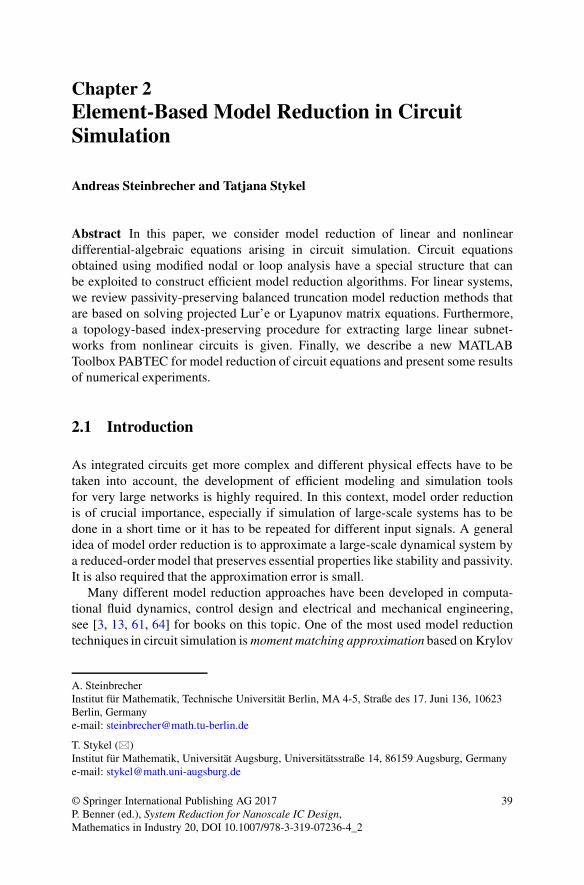
Chapter 2Element-Based Model Reduction in CircuitSimulation
Andreas Steinbrecher and Tatjana Stykel
Abstract In this paper, we consider model reduction of linear and nonlineardifferential-algebraic equations arising in circuit simulation. Circuit equationsobtained using modified nodal or loop analysis have a special structure that canbe exploited to construct efficient model reduction algorithms. For linear systems,we review passivity-preserving balanced truncation model reduction methods thatare based on solving projected Lur’e or Lyapunov matrix equations. Furthermore,a topology-based index-preserving procedure for extracting large linear subnet-works from nonlinear circuits is given. Finally, we describe a new MATLABToolbox PABTEC for model reduction of circuit equations and present some resultsof numerical experiments.
2.1 Introduction
As integrated circuits get more complex and different physical effects have to betaken into account, the development of efficient modeling and simulation toolsfor very large networks is highly required. In this context, model order reductionis of crucial importance, especially if simulation of large-scale systems has to bedone in a short time or it has to be repeated for different input signals. A generalidea of model order reduction is to approximate a large-scale dynamical system bya reduced-order model that preserves essential properties like stability and passivity.It is also required that the approximation error is small.
Many different model reduction approaches have been developed in computa-tional fluid dynamics, control design and electrical and mechanical engineering,see [3, 13, 61, 64] for books on this topic. One of the most used model reductiontechniques in circuit simulation is moment matching approximation based on Krylov
A. SteinbrecherInstitut für Mathematik, Technische Universität Berlin, MA 4-5, Straße des 17. Juni 136, 10623Berlin, Germanye-mail: [email protected]
T. Stykel (�)Institut für Mathematik, Universität Augsburg, Universitätsstraße 14, 86159 Augsburg, Germanye-mail: [email protected]
© Springer International Publishing AG 2017P. Benner (ed.), System Reduction for Nanoscale IC Design,Mathematics in Industry 20, DOI 10.1007/978-3-319-07236-4_2
39
40 A. Steinbrecher and T. Stykel
subspace methods, e.g., [6, 25, 30]. Although these methods are efficient forvery large sparse problems, the resulting reduced-order systems have only locallygood approximation properties, and stability and passivity are not necessarilypreserved. Furthermore, passivity-preserving model reduction methods based onKrylov subspaces have been developed for structured systems arising in circuitsimulation [26, 27, 42, 48] and also for general systems [4, 38, 66]. However, noneof these methods provides computable global error bounds. Another drawback ofKrylov subspace methods is the ad hoc choice of interpolation points that stronglyinfluence the approximation quality. An optimal point selection strategy based ontangential interpolation has been presented in [5, 32] that provides an optimal H2-approximation.
In this paper, we present a survey on passivity-preserving balanced truncationmodel reduction methods for linear circuit equations developed in [54, 56, 72]. Theyinvolve computing the spectral projectors onto the left and right deflating subspacescorresponding to the finite and infinite eigenvalues of an underlying pencil andsolving projected matrix equations. An important property of these methods is theexistence of computable error bounds that allow an adaptive choice of the order ofthe approximate model.
Furthermore, we consider model reduction of nonlinear circuits based on decou-pling linear and nonlinear subcircuits followed by reduction of the linear part [68].This model reduction approach can also be combined with the POD-based reductiontechnique for semiconductor devices, see Chap. 1, and further with hierarchicalreduction methods studied in Chap. 4. The developed model reduction algorithmsfor circuit equations were implemented as MATLAB toolbox PABTEC and testedon practical problems.
Notation Throughout the paper, Rn;m and C
n;m denote the spaces of n � mreal and complex matrices, respectively. The open left and right half-planes aredenoted by C� and CC, respectively, and i D p�1. The matrices AT and A�denote, respectively, the transpose and the conjugate transpose of A 2 C
n;m, andA�T D .A�1/T . An identity matrix of order n is denoted by In or simply by I. We userank.A/, im.A/ and ker.A/ for the rank, the range and the kernel of A, respectively.A matrix A 2 C
n;n is positive definite (semidefinite), if v�Av > 0 (v�Av � 0) forall non-zero v 2 C
n. Note that positive (semi)definiteness of A does not require A tobe Hermitian. For A;B 2 C
n;n, we write A > B (A � B) if A � B is positive definite(semidefinite). Furthermore, diag.A1; : : : ;As/ denotes a block diagonal matrix withblock entries Aj, j D 1; : : : ; s, on the diagonal.
2.2 Circuit Equations
In this section, we briefly describe the modeling of electrical circuits via differential-algebraic equations (DAEs) and discuss their properties. For more details on graphtheory and network analysis, we refer to [1, 20, 22, 40, 75].
2 Element-Based Model Reduction in Circuit Simulation 41
2.2.1 Graph-Theoretic Concepts
A general circuit can be modeled as a directed graph G whose vertices (nodes) nk
correspond to the nodes of the circuit and whose branches (edges) bk1;k2 D hnk1 ; nk2icorrespond to the circuit elements like capacitors, inductors and resistors. Forthe ordered pair bk1;k2 D hnk1 ; nk2i, we say that bk1;k2 leaves nk1 and enters nk2 .In this case, bk1;k2 is called incident with nk1 and nk2 . An alternating sequence.nk1 ; bk1;k2 ; nk2 ; : : : ; nks�1 ; bks�1;ks ; nks/ of vertices and branches in G is called a pathconnecting nk1 and nks if the branches bkj�1;kj are incident with the vertices nkj�1 andnkj for 2 � j � s. A path is closed if nk1 D nks . A closed path is called a loop ifnki ¤ nkj for 1 � i < j � s except for nk1 and nks . A graph G is called connectedif for every two vertices there exists a path connecting them. A cutset is a set ofbranches of a connected graph whose removal disconnects the graph, and this set isminimal with this property. A subgraph of the graph G is called a tree if it has allnodes of G, is connected and does not contain loops.
A directed graph G with nv vertices, nb branches and nl loops can be describedby an incidence matrix A0 D Œapq� 2 R
nv;nb with
apq D8<:
1 if branch q leaves vertex p;�1 if branch q enters vertex p;0 otherwise;
or by a loop matrix B0 D Œbpq� 2 Rnl;nb with
bpq D8<:
1 if branch q belongs to loop p and has the same orientation,�1 if branch q belongs to loop p and has the contrary orientation,0 otherwise:
For a connected graph, the matrices A0 and B0 satisfy the following relations
ker.B0/ D im.AT0 /; rank.A0/ D nv � 1; rank.B0/ D nb � nv C 1;
see [22, p. 213]. Removing linear dependent rows from A0 and B0, we obtain thefull rank matrices A 2 R
nv�1;nb and B 2 Rnb�nvC1;nb which are called the reduced
incidence matrix and the reduced loop matrix, respectively.
2.2.2 Modified Nodal Analysis and Modified Loop Analysis
We now consider a general nonlinear RLC circuit that contains nR resistors, nLinductors, nC capacitors, nV independent voltage sources and nI independent cur-rent sources. Such circuits are completely described by the graph-theoretic relationslike Kirchhoff’s current and voltage laws together with the branch constitutive
42 A. Steinbrecher and T. Stykel
relations that characterize the circuit elements. Kirchhoff’s current law states thatthe sum of the currents along all branches leaving and entering a circuit node iszero. Kirchhoff’s voltage law states that the sum of the voltages along the branchesof any loop is zero. Let
j D Œ jTR ; jTC ; jTL ; jTV ; jTI �T 2 R
nb ; v D ΠvTR ; v
TC ; v
TL ; v
TV ; v
TI �
T 2 Rnb
denote the vectors of branch currents and branch voltages, respectively, and let thereduced incidence and loop matrices
A D Œ AR ; AC ; AL ; AV ; AI �; B D Œ BR ; BC ; BL ; BV ; BI �
be partitioned accordingly, where the subscripts R ; C ; L; V and I stand for resistors,capacitors, inductors, voltage sources and current sources, respectively. ThenKirchhoff’s current and voltage laws can be expressed in the compact form as
A j D 0; B v D 0;
respectively, or, equivalently,
BT � D j; AT� D v;
where � 2 Rnb�nvC1 and � 2 R
nv�1 denote the vectors of loop currents and nodepotentials.
The branch constitutive relations for nonlinear capacitors, inductors and resistorsare given by
ddt�. jL/ D vL ; jC D d
dt qC .vC /; jR D g.vR /; (2.1)
where the functions � W RnL ! RnL , qC W RnC ! R
nC and g W RnR ! RnR describe
electromagnetic fluxes in the inductors, capacitor charges and resistor voltage-current characteristics, respectively. For current-controlled resistors, we have alsothe relation vR D %. jR /, where % W R
nR ! RnR is the resistor current-voltage
characteristic function. We assume that
(A1) the functions �, qC and g are continuously differentiable and their Jacobians
@�. jL /
@jLD L. jL/;
@qC .vC /
@vCD C .vC /;
@g.vR /
@vRD G.vR /;
are positive definite for all jL , vC and vR , respectively.
This assumption guarantees that inductors, capacitors and resistors are locallypassive, see [19] for details.
2 Element-Based Model Reduction in Circuit Simulation 43
Using Kirchhoff’s laws and the branch constitutive relations, the dynamicalbehaviour of a nonlinear circuit can be described using modified nodal analysis(MNA) [37] by the following system of DAEs
E .x/ ddt x D A x C f .x/C B u;
y D BT x;(2.2)
where
E .x/ D
264
ACC .ATC�/A
TC 0 0
0 L. jL / 0
0 0 0
375; A D
2640 �AL �AV
ATL 0 0
ATV 0 0
375 ;
f .x/ D
264
�AR g.ATR �/
0
0
375 ; B D
24�AI 0
0 0
0 �I
35 ; x D
24 �
jLjV
35 ;
(2.3)
and the input u and the output y have the form
u D�
jIvV
�; y D
� �vI�jV
�; (2.4)
respectively. Another approach for modeling electrical circuits is based on modifiedloop analysis (MLA), see [79]. In this case, the circuit equations take the form (2.2)with
E .x/ D
264
BLL.BTL �/B
TL 0 0
0 C .vC / 0
0 0 0
375 ; A D
2640 �BC �BI
BTC 0 0
BTI 0 0
375 ;
f .x/ D
264
�BR %.BTR �/
0
0
375 ; B D
264
0 �BV
0 0
�I 0
375 ; x D
24 �
vCvI
35 ;
(2.5)
and the input and the output are as in (2.4).We assume that the circuit is well-posed in the sense that
(A2) the circuit does not contain cutsets consisting of current sources (I-cutsets),(A3) the circuit does not contain loops consisting of voltage sources (V-loops).
These assumptions avoid open-circuit current sources and short-circuit voltagesources, respectively. Assumption (A2) is equivalent to
rank.ŒAC ; AL ; AR ; AV �/ D nv � 1;
44 A. Steinbrecher and T. Stykel
which is, on the other hand, equivalent to rank.BI/ D nI. In terms of rank conditions,(A3) means that rank.AV / D nV or, equivalently, rank.ŒBC ; BL ; BR ; BI �/ D nb �nv C 1.
The index concept plays an important role in the analysis of DAEs. To charac-terize different analytical and numerical properties of DAE systems, several indexnotations have been introduced in the literature, e.g., [17, 29, 33, 43]. For example,the differentiation index is roughly defined as the minimum of times that all or partof a DAE system must be differentiated with respect to t in order to determine thederivative of x as a continuous function of t and x. In the sequel, we will use theshorter term “index” instead of “differentiation index”. The following propositioncharacterizes the index of the MNA system (2.2), (2.3).
Proposition 2.2.1 ([24, 68]) Consider a circuit satisfying assumptions (A1)–(A3).
1. The index of the MNA system (2.2), (2.3) is at most two.2. The index of the MNA system (2.2), (2.3) is equal to zero if and only if
nV D 0 and rank.AC / D nv � 1: (2.6)
3. The index of the MNA system (2.2), (2.3) is equal to one if and only if
rank.ŒAC ; AV �/ D rank.AC /C nV and rank.ŒAC ; AR ; AV �/ D nv � 1:(2.7)
Similar, rank conditions can also be formulated for the MLA system (2.2), (2.5).Considering the topological structure of the circuit, the conditions (2.6) implythat the circuit does not contain voltage sources and the circuit graph containsa capacitive tree, respectively. Furthermore, the first condition in (2.7) implies thatthe circuit does not contain loops consisting of capacitors and/or voltage sources(CV-loops) except for loops consisting of capacitors only (C-loops), whereas thesecond condition in (2.7) means that the circuit does not contain cutsets consistingof inductors and/or current sources (LI-cutsets).
In the following, we will distinguish between nonlinear circuits, which containnonlinear elements, and linear circuits consisting exclusively of linear capacitors,inductors and resistors. A circuit element is called linear if the current-voltagerelation for this element is linear. Otherwise, the circuit element is called nonlinear.Without loss of generality we may assume that the circuit elements are ordered suchthat the incidence matrices are partitioned as
AC D A NC ; A QC
; AL D
A NL ; A QL; AR D
hA NR ; A QR
i; (2.8)
where the incidence matrices A NC , A NL and A NR correspond to the linear circuitcomponents, and A QC , A QL and A QR are the incidence matrices for the nonlineardevices. We also assume that the linear and nonlinear elements are not mutually

2 Element-Based Model Reduction in Circuit Simulation 45
connected, i.e.,
C .ATC�/ D
24NC 0
0 eC .ATQC�/
35 ; L. jL / D
24 NL 0
0 eL. j QL /
35 ; g.AT
R �/D24NGAT
NR �
eg.ATQR�/
35 ;
where NC 2 Rn NC ;n NC , NL 2 R
n NL ;n NL and NG 2 Rn NR ;n NR are the capacitance, inductance and
conductance matrices for the corresponding linear elements, whereas
eC W RnQC ! R
nQC ;n QC ; eL W Rn
QL ! Rn
QL ;n QL ; eg W RnQR ! R
nQR
describe the corresponding nonlinear components, and j QL is the current vectorthrough the nonlinear inductors.
2.2.3 Linear RLC Circuits
For simplification of notation, a linear RLC circuit containing nR linear resistors, nL
linear inductors, nC linear capacitors, nI current sources and nV voltage sources willbe described by the linear DAE system
E ddt x D Ax C Bu;
y D BTx;(2.9)
with the MNA matrices
E D
264
ACCATC 0 0
0 L 0
0 0 0
375 ; A D
264
�ARGATR �AL �AV
ATL 0 0
ATV 0 0
375 ; B D
264
�AI 0
0 0
0 �I
375 ;
(2.10)
or the MLA matrices
E D
264
BLLBTL 0 0
0 C 0
0 0 0
375 ; A D
264
�BRRBTR �BC �BI
BTC 0 0
BTI 0 0
375 ; B D
264
0 �BV
0 0
�I 0
375 :
(2.11)
Here, the subscripts R; C; L; V and I stand for linear resistors, linear capacitors,linear inductors, voltage sources and current sources, respectively, and L 2 R
nL;nL ,C 2 R
nC;nC , R 2 RnR;nR and G D R�1 are the inductance, capacitance, resistance
and conductance matrices, respectively. Linear circuits are often used to modelinterconnects, transmission lines and pin packages in VLSI networks. They arise
46 A. Steinbrecher and T. Stykel
also in the linearization of nonlinear circuit equations around DC operating points.According to (A1), we assume that
(A1 ) the matrices L, C and G are symmetric and positive definite.
This condition together with (A2) and (A3) guarantees that the pencil E � A isregular, i.e., det.E�A/¤ 0 for some 2 C, see [27]. In this case, we can definea transfer function
G.s/ D BT.sE � A/�1B
of the DAE system (2.9). Applying the Laplace transform to (2.9) with an initialcondition x.0/ D x0 satisfying Ex0 D 0, we obtain y.s/ D G.s/u.s/, whereu.s/ and y.s/ are the Laplace transformations of the input u.t/ and the output y.t/,respectively. Thus, the transfer function G.s/ describes the input-output relationof (2.9) in the frequency domain. Note that the MNA system (2.9), (2.10) and theMLA system (2.9), (2.11) have the same transfer function.
For any rational matrix-valued function G.s/, there exist matrices E, A, Bin andBout such that G.s/ D Bout.sE � A/�1Bin, see [21]. Then the DAE system
E ddt x D Ax C Binu;
y D Boutx;
is said to form a realization of G.s/. We will also denote a realization of G.s/ byG D .E; A; Bin; Bout/.
The transfer function G.s/ is called proper if lims!1G.s/ < 1, and improper,
otherwise. If G.s/ is proper and analytic in CC, then the H1-norm of G.s/ isdefined as
kGkH1D sup
s2CC
kG.s/k D lim� ! 0
� > 0
sup!2R
kG.� C i!/k;
where k � k denotes the spectral matrix norm.
2.2.3.1 Passivity
Passivity is the most important property of circuit equations. System (2.9) withx.0/ D 0 is passive if
Z t
0
u.�/Ty.�/ d� � 0 (2.12)
2 Element-Based Model Reduction in Circuit Simulation 47
for all t � 0 and all admissible u such that uTy is locally integrable. Passive elementscan store and dissipate energy, but they do not generate energy. Thus, capacitors,resistors and inductors are passive, while current and voltage sources are not.
It is well known in linear network theory [1] that the DAE system (2.9) is passiveif and only if its transfer function G.s/ D BT.sE � A/�1B is positive real, i.e., Gis analytic in CC and G.s/C G.s/� � 0 for all s 2 CC. Since the system matricesin (2.10) satisfy E D ET � 0 and A C AT � 0, the transfer function of (2.9), (2.10)is positive real, and, hence, this system is passive.
2.2.3.2 Stability
Stability is a qualitative property of dynamical systems which describes thebehaviour of their solutions under small perturbations in the initial data. For thelinear DAE system (2.9), stability can be characterized in terms of the finiteeigenvalues of the pencil E � A, e.g., [21]. System (2.9) is stable if all thefinite eigenvalues of E � A lie in the closed left half-plane and the eigenvalueson the imaginary axis are semi-simple, i.e., they have the same algebraic andgeometric multiplicity. System (2.9) is asymptotically stable if the pencil E � Ais c-stable, i.e., all its finite eigenvalues lie in the open left half-plane. Note thatpassivity of the MNA system (2.9), (2.10) implies that this system is stable [1,Theorem 2.7.2]. Topological conditions for the asymptotic stability of the MNAequations (2.9), (2.10) can be found in [58, 59].
2.2.3.3 Reciprocity
Another relevant property of circuit equations is reciprocity. We call a matrix S 2R
m;m a signature if S is diagonal and S2 D Im. System (2.9) is reciprocal withan external signature Sext 2 R
m;m if its transfer function satisfies
G.s/ D SextG.s/TSext
for all s 2 C. Obviously, the MNA system (2.9), (2.10) with symmetric L, C and Gis reciprocal with the external signature Sext D diag.InI ;�InV /.
2.3 Model Reduction of Linear Circuits
Consider the linear MNA system (2.9), (2.10) with E;A 2 Rn;n and B 2 R
n;m. Weaim to approximate this system by a reduced-order model
OE ddt Ox D OA Ox C OB u;
Oy D OC Ox; (2.13)
48 A. Steinbrecher and T. Stykel
where OE, OA 2 Rnr ;nr , OB 2 R
nr ;m, OC 2 Rm;nr and nr n. It is required that the
approximate system (2.13) has a small approximation error y � Oy and also preservespassivity and reciprocity. In the frequency domain, the error can be measured viaG � OG in an appropriate system norm, where OG.s/ D OC.s OE � OA/�1 OB is the transferfunction of system (2.13).
A classical approach for computing the reduced-order model (2.13) is based onthe projection of system (2.9) onto lower dimensional subspaces. In this case, thesystem matrices in (2.13) have the form
OE D WTE T; OA D WTA T; OB D WTB; OC D BT T; (2.14)
where the projection matrices W, T 2 Rn;nr determine the subspaces of interest.
In interpolation-based passivity-preserving model reduction methods like PRIMA[48], SPRIM [26, 27] and spectral zero interpolation [38, 66], the columns of thesematrices span certain (rational) Krylov subspaces associated with (2.9).
Balanced truncation also belongs to the projection-based model reduction tech-niques. This method consists in transforming the dynamical system into a balancedform whose appropriately chosen controllability and observability Gramians areboth equal to a diagonal matrix. Then a reduced-order model (2.13), (2.14) isobtained by projecting (2.9) onto the subspaces corresponding to the dominantdiagonal elements of the balanced Gramians. In order to capture specific systemproperties, different balancing techniques have been developed in the last 30 years[31, 46, 47, 52, 55, 69]. An important property of these techniques is the existence ofcomputable error bounds that allow us to approximate (2.9) to a prescribed accuracy.
In Sect. 2.3.1, we consider a passivity-preserving model reduction method forgeneral RLC circuits developed in [54, 72]. This method is based on balancingthe Gramians that satisfy the projected Lur’e matrix equations. For RC circuitsconsisting only of resistors, capacitors, current sources and/or voltage sources,this method can significantly be simplified. In Sect. 2.3.2, we present passivity-preserving model reduction methods for RC circuits developed in [56] that relyon balancing the solutions of the projected Lyapunov equations. Thereby, we willdistinguish three cases: RC circuits with current sources (RCI circuits), RC circuitswith voltage sources (RCV circuits) and RC circuits with both current and voltagesources (RCIV circuits). Finally, in Sect. 2.3.3, we discuss the numerical aspects ofthe presented balancing-related model reduction algorithms.
2.3.1 Balanced Truncation for RLC Circuits
First, we consider model reduction of general RLC circuits. Note that passivity ofthe MNA system (2.9), (2.10) can be characterized via the projected Lur’e equations
E X .A � BBT/T C .A � BBT/XET C 2PlBBTPTl D �2KcKT
c ;
EXB � PlBMT0 D �KcJT
c ; I � M0MT0 D JcJT
c ; X D PrXPTr � 0;
(2.15)
2 Element-Based Model Reduction in Circuit Simulation 49
and
ETY.A � BBT/C .A � BBT/TYE C 2PTrBBTPr D �2KT
o Ko;
�ETYB C PTrBM0 D �KT
o Jo; I � MT0M0 D JT
o Jo Y D PTl YPl � 0
(2.16)
with unknowns X 2 Rn;n, Kc 2 R
n;m, Jc 2 Rm;m and Y 2 R
n;n, Ko 2 Rm;n, Jo 2 R
m;m,respectively. Here, Pr and Pl are the spectral projectors onto the right and left defla-ting subspaces of the pencil E � .A � BBT/ corresponding to the finite eigenvaluesalong the right and left deflating subspaces corresponding to the eigenvalue at infi-nity, and
M0 D I � 2 lims!1BT.sE � A C BBT/�1B: (2.17)
In general, the solvability of the projected Lur’e equations (2.15) and (2.16) requiresthat system (2.9) is passive and R-minimal, i.e.,
rank.Œ E � A ; B �/ D rank.Œ ET � AT ; B �/ D n
for all 2 C. For the circuit equations (2.9), (2.10), however, the R-minimalitycondition can be removed.
Theorem 2.3.1 ([54]) Consider an MNA system (2.9), (2.10) satisfying (A1 ), (A2)and (A3). Then the projected Lur’e equations (2.15) and (2.16) are solvable.
Note that the solutions X and Y of (2.15) and (2.16) are not unique. However,there exist unique minimal solutions Xmin and Ymin that satisfy 0 � Xmin � X and0 � Ymin � Y for all symmetric solutions X and Y of (2.15) and (2.16), respectively.These minimal solutions Xmin and Ymin of (2.15) and (2.16), respectively, are calledthe controllability and observability Gramians of system (2.9). This system iscalled balanced if Xmin D Ymin D diag.�; 0/, where � D diag.�1; : : : ; �nf / with�1 � : : : � �nf � 0 and nf D rank.Pr/. The values �j are called the characteristicvalues of (2.9). Based on the energy interpretation of the Gramians Xmin andYmin, see [55], one can conclude that the truncation of the states of a balancedsystem corresponding to the small characteristic values does not change the systemproperties significantly. The characteristic values and balancing transformationmatrices can be determined from the singular value decomposition of the matrixQYTE QX, where QX and QY are the Cholesky factors of the Gramians Xmin D QX QXT andYmin D QY QYT . Taking into account the block structure of the MNA matrices in (2.10),we have ET D SintESint and AT D SintASint with
Sint D diag.Inv�1;�InL ;�InV /: (2.18)
This implies that Ymin D SintXminSint. Then instead of the more expensive singularvalue decomposition of QYT E QX, we can compute the eigenvalue decomposition of thesymmetric matrix QXTSintE QX. In this case, the numerical solution of only one Lur’eequation is required. If j are eigenvalues of QXTSintE QX, then �j D jjj. Thus, thereduced-order model (2.13), (2.14) can be determined by projecting (2.9) onto thesubspaces corresponding to the dominant eigenvalues of QXTSintE QX.
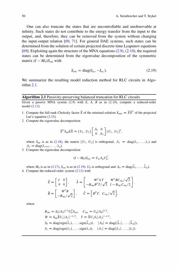
50 A. Steinbrecher and T. Stykel
One can also truncate the states that are uncontrollable and unobservable atinfinity. Such states do not contribute to the energy transfer from the input to theoutput, and, therefore, they can be removed from the system without changingthe input-output relation [69, 71]. For general DAE systems, such states can bedetermined from the solution of certain projected discrete-time Lyapunov equations[69]. Exploiting again the structure of the MNA equations (2.9), (2.10), the requiredstates can be determined from the eigenvalue decomposition of the symmetricmatrix .I � M0/Sext with
Sext D diag.InI ;�InV /: (2.19)
We summarize the resulting model reduction method for RLC circuits in Algo-rithm 2.1.
Algorithm 2.1 Passivity-preserving balanced truncation for RLC circuitsGiven a passive MNA system (2.9) with E, A, B as in (2.10), compute a reduced-ordermodel (2.13).
1. Compute the full-rank Cholesky factor QX of the minimal solution Xmin D QX QXT of the projectedLur’e equation (2.15).
2. Compute the eigenvalue decomposition
QXT SintE QX D ŒU1; U2 �
��1 0
0 �2
�ŒU1; U2 �
T ;
where Sint is as in (2.18), the matrix ŒU1; U2 � is orthogonal, �1 D diag.1; : : : ; r/ and�2 D diag.rC1; : : : ; q/.
3. Compute the eigenvalue decomposition
.I �M0/Sext D U0�0UT0 ;
where M0 is as in (2.17), Sext is as in (2.19), U0 is orthogonal and �0 D diag.O1; : : : ; Om/.4. Compute the reduced-order system (2.13) with
OE D�
I 0
0 0
�; OA D
"WT A T WT BC1=
p2
�B1BT T=p2 I � B1C1=2
#;
OBD�
WT B�B1=
p2
�; OC D
hBT T; C1=
p2i;
where
B1 D S0j�0j1=2UT0 Sext; C1 D U0j�0j1=2;
W D Sint QXU1j�1j�1=2; T D QXU1S1j�1j�1=2;
S0 D diag.sign.O1/; : : : ; sign.Om//; j�0j D diag.jO1j; : : : ; jOmj/;S1 D diag.sign.1/; : : : ; sign.r//; j�1j D diag.j1j; : : : ; jrj/:
2 Element-Based Model Reduction in Circuit Simulation 51
One can show that the reduced-order model computed by Algorithm 2.1 pre-serves not only passivity but also reciprocity. Moreover, we have the following errorbound
k OG � GkH1� kI C Gk2H1
.�rC1 C : : :C �q/
1 � kI C GkH1.�rC1 C : : :C �q/
;
provided kI C GkH1.�rC1 C : : : C �q/ < 1, see [54] for details. Note that this
error bound requires the computation of the H1-norm of G, which is expensive forlarge-scale systems. If r is chosen in Algorithm 2.1 such that
kI C OGkH1.�rC1 C : : :C �q/ < 1;
then we can estimate
k OG � GkH1� kI C OGk2H1
.�rC1 C : : :C �q/
1 � kI C OGkH1.�rC1 C : : :C �q/
; (2.20)
where only the evaluation of the H1-norm of the reduced-order system OG isrequired.
If the matrix I � M0MT0 is nonsingular, then the projected Lur’e equation (2.15)
can be written as the projected Riccati equation
EXFT C FXET C EXBTcBcXET C PlBoBT
oPTl D 0; X D PrXPT
r ; (2.21)
where
F D A � BBT � 2PlBMT0 .I � M0M
T0 /�1BTPr;
Bc D p2 J�1c BTPr; Bo D �p
2BJ�1o ;
JcJTc D I � M0M
T0 ; JT
o Jo D I � MT0 M0:
(2.22)
Note that the invertibility of I � M0MT0 depends on the topological structure of the
circuit.
Theorem 2.3.2 Consider an MNA system (2.9), (2.10). Let the matrix M0 be asin (2.17). Then I � M0M
T0 is nonsingular if and only if
rank.ZTCŒAI ; AV �/ D nI C nV ; ZT
RCŒAI ; AV � D 0; (2.23)
where ZC and ZRC are the basis matrices for ker.ATC/ and ker.ŒAR; AC �
T/, respec-tively.
Proof The result immediately follows from [54, Theorem 7].
The first condition in (2.23) is equivalent to the absence of loops of capacitors,voltage sources and current sources (CVI-loops) except for loops consisting ofcapacitive branches (C-loops). The second condition in (2.23) means that the circuit
52 A. Steinbrecher and T. Stykel
does not contain cutsets consisting of branches of inductors, voltage sources andcurrent sources (LVI-cutsets) except for cutsets consisting of inductive branches(L-cutsets).
2.3.2 Balanced Truncation for RC Circuits
We now present a Lyapunov-based balanced truncation model reduction approachfor RC circuits. In this approach, the Gramians of system (2.9) are defined asunique symmetric, positive semidefinite solutions of the projected continuous-timeLyapunov equations
EXAT C AXET D �PlBBTPTl ; X D PrXPT
r ;
ETYA C ATYE D �PTr BBTPr; Y D PT
l YPl:
The numerical solution of such equations is much less exhausting than of theprojected Lur’e or Riccati equations. For a balanced system, these Gramians areboth equal to a diagonal matrix
X D Y D diag.˙; 0/;
where ˙ D diag.�1; : : : ; �nf /. The values �j are called the proper Hankel singularvalues of system G D .E;A;B;BT/. They determine which states are important andwhich states can be removed from the system.
Note that Lyapunov-based balanced truncation does not, in general, guaranteethe preservation of passivity in the reduced-order model. However, the RC circuitequations either have a symmetric structure
E D ET � 0; A D AT � 0; (2.24)
or they can be transformed under preservation of passivity into a symmetric form.Then Lyapunov-based balanced truncation applied to symmetric systems is knownto be structure-preserving [45] and, hence, also passivity-preserving. All modelreduction algorithms presented in this section have been developed in [56].
2.3.2.1 RCI Circuits
First, we consider RCI circuits consisting of resistors, capacitors and current sourcesonly. The MNA matrices are then given by
E D ACCATC; A D �ARGAT
R; B D �AI: (2.25)
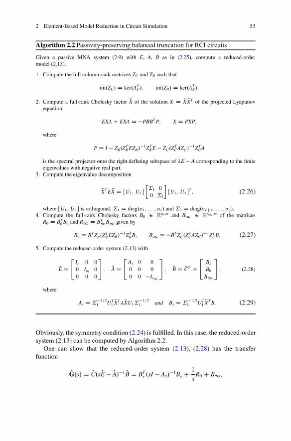
2 Element-Based Model Reduction in Circuit Simulation 53
Algorithm 2.2 Passivity-preserving balanced truncation for RCI circuits
Given a passive MNA system (2.9) with E, A, B as in (2.25), compute a reduced-ordermodel (2.13).
1. Compute the full column rank matrices ZC and ZR such that
im.ZC/ D ker.ATC/; im.ZR/ D ker.AT
R/:
2. Compute a full-rank Cholesky factor QX of the solution X D QX QXT of the projected Lyapunovequation
EXAC EXA D �PBBT P; X D PXP;
where
P D I � ZR.ZTR EZR/
�1ZTR E � ZC.Z
TCAZC/
�1ZTCA
is the spectral projector onto the right deflating subspace of E � A corresponding to the finiteeigenvalues with negative real part.
3. Compute the eigenvalue decomposition
QXT E QX D ŒU1; U2 �
�˙1 0
0 ˙2
�ŒU1; U2 �
T ; (2.26)
where ŒU1; U2 � is orthogonal, ˙1 D diag.�1; : : : ; �r/ and ˙2 D diag.�rC1; : : : ; �q/.4. Compute the full-rank Cholesky factors B0 2 R
r0;m and B1 2 Rr1 ;m of the matrices
R0 D BT0B0 and R1 D BT
1B
1given by
R0 D BT ZR.ZTR EZR/
�1ZTR B; R1 D �BT ZC.Z
TCAZC/
�1ZTCB: (2.27)
5. Compute the reduced-order system (2.13) with
OE D24 Ir 0 0
0 Ir0 0
0 0 0
35 ; OAD
24As 0 0
0 0 0
0 0 �Ir1
35 ; OBD OCT D
24 Bs
B0B1
35 ; (2.28)
where
As D ˙�1=21 UT
1QXT AQXU1˙
�1=21 and Bs D ˙
�1=21 UT
1QXT B: (2.29)
Obviously, the symmetry condition (2.24) is fulfilled. In this case, the reduced-ordersystem (2.13) can be computed by Algorithm 2.2.
One can show that the reduced-order system (2.13), (2.28) has the transferfunction
OG.s/ D OC.s OE � OA/�1 OB D BTs .sI � As/
�1Bs C 1
sR0 C R1;
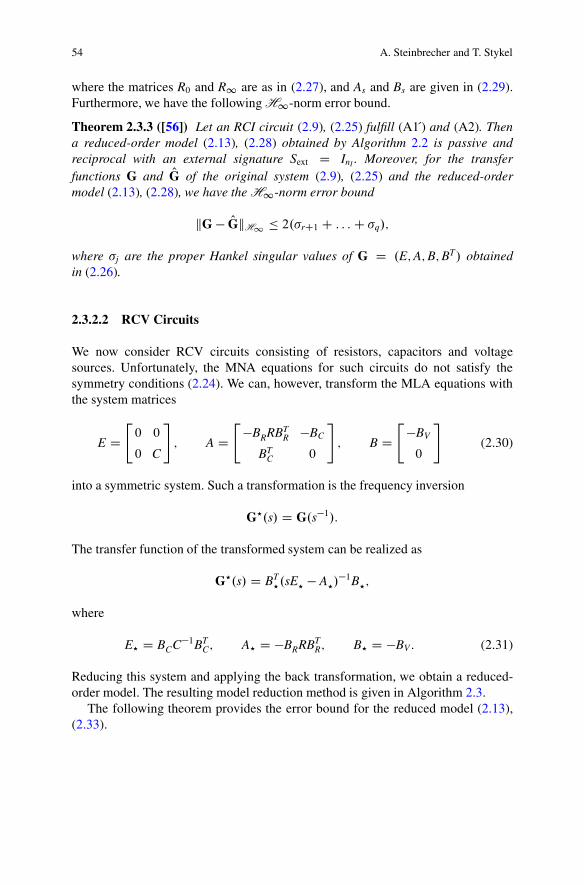
54 A. Steinbrecher and T. Stykel
where the matrices R0 and R1 are as in (2.27), and As and Bs are given in (2.29).Furthermore, we have the following H1-norm error bound.
Theorem 2.3.3 ([56]) Let an RCI circuit (2.9), (2.25) fulfill (A1 ) and (A2). Thena reduced-order model (2.13), (2.28) obtained by Algorithm 2.2 is passive andreciprocal with an external signature Sext D InI . Moreover, for the transferfunctions G and OG of the original system (2.9), (2.25) and the reduced-ordermodel (2.13), (2.28), we have the H1-norm error bound
kG � OGkH1� 2.�rC1 C : : :C �q/;
where �j are the proper Hankel singular values of G D .E;A;B;BT/ obtainedin (2.26).
2.3.2.2 RCV Circuits
We now consider RCV circuits consisting of resistors, capacitors and voltagesources. Unfortunately, the MNA equations for such circuits do not satisfy thesymmetry conditions (2.24). We can, however, transform the MLA equations withthe system matrices
E D"0 0
0 C
#; A D
"�BRRBT
R �BC
BTC 0
#; B D
"�BV
0
#(2.30)
into a symmetric system. Such a transformation is the frequency inversion
G?.s/ D G.s�1/:
The transfer function of the transformed system can be realized as
G?.s/ D BT?.sE? � A?/
�1B?;
where
E? D BCC�1BTC; A? D �BRRBT
R; B? D �BV : (2.31)
Reducing this system and applying the back transformation, we obtain a reduced-order model. The resulting model reduction method is given in Algorithm 2.3.
The following theorem provides the error bound for the reduced model (2.13),(2.33).
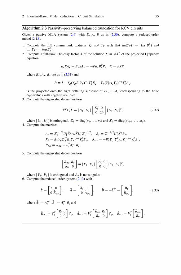
2 Element-Based Model Reduction in Circuit Simulation 55
Algorithm 2.3 Passivity-preserving balanced truncation for RCV circuits
Given a passive MLA system (2.9) with E, A, B as in (2.30), compute a reduced-ordermodel (2.13).
1. Compute the full column rank matrices YC and YR such that im.YC/ D ker.BTC/ and
im.YR/D ker.BTR/.
2. Compute a full-rank Cholesky factor QX of the solution X D QX QXT of the projected Lyapunovequation
E?XA? C E?XA? D �PB?BT?P; X D PXP;
where E?, A?, B? are as in (2.31) and
P D I � YR.YTR E?YR/
�1YTR E? � YC.Y
TC A?YC/
�1YTC A?:
is the projector onto the right deflating subspace of E? � A? corresponding to the finiteeigenvalues with negative real part.
3. Compute the eigenvalue decomposition
QXT E? QX D ŒU1; U2 �
�˙1 0
0 ˙2
�ŒU1; U2 �
T ; (2.32)
where ŒU1; U2 � is orthogonal, ˙1 D diag.�1; : : : ; �r/ and ˙2 D diag.�rC1; : : : ; �q/.4. Compute the matrices
As D ˙�1=21 UT
1QXT A? QXU1˙
�1=21 ; Bs D ˙
�1=21 UT
1QXT B?;
R0 D BT?YR.Y
TR E?YR/
�1YTR B?; R1 D �BT
?YC.YTC A?YC/
�1YTC B?;
QR1 D R1 � BTs A�1
s Bs:
5. Compute the eigenvalue decomposition
� QR1 R0R0 0
�D ŒV1; V2 �
��0 0
0 0
�ŒV1; V2 �
T ;
where ŒV1; V2 � is orthogonal and �0 is nonsingular.6. Compute the reduced-order system (2.13) with
OE D�
I 0
0 OE1
�; OAD
" OA1 0
0 OA1
#; OB D �OCT D
" OB1OB1
#; (2.33)
where OA1 D A�1s , OB1 D A�1
s Bs and
OE1 D VT1
�R0 00 0
�V1; OA1 D VT
1
� QR1 R0R0 0
�V1; OB1 D VT
1
� QR1
R0
�:
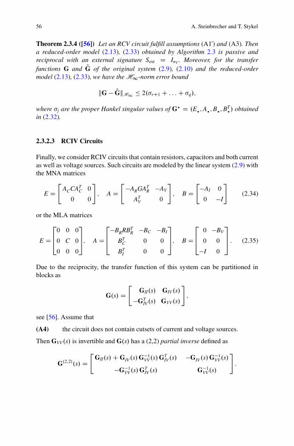
56 A. Steinbrecher and T. Stykel
Theorem 2.3.4 ([56]) Let an RCV circuit fulfill assumptions (A1 ) and (A3). Thena reduced-order model (2.13), (2.33) obtained by Algorithm 2.3 is passive andreciprocal with an external signature Sext D InV . Moreover, for the transferfunctions G and OG of the original system (2.9), (2.10) and the reduced-ordermodel (2.13), (2.33), we have the H1-norm error bound
kG � OGkH1� 2.�rC1 C : : :C �q/;
where �j are the proper Hankel singular values of G? D .E?;A?;B?;BT?/ obtained
in (2.32).
2.3.2.3 RCIV Circuits
Finally, we consider RCIV circuits that contain resistors, capacitors and both currentas well as voltage sources. Such circuits are modeled by the linear system (2.9) withthe MNA matrices
E D"
ACCATC 0
0 0
#; A D
"�ARGAT
R �AV
ATV 0
#; B D
"�AI 0
0 �I
#(2.34)
or the MLA matrices
E D
2640 0 0
0 C 0
0 0 0
375; A D
264
�BRRBTR �BC �BI
BTC 0 0
BTI 0 0
375; B D
2640 �BV
0 0
�I 0
375 : (2.35)
Due to the reciprocity, the transfer function of this system can be partitioned inblocks as
G.s/ D"
GII.s/ GIV.s/
�GTIV.s/ GVV.s/
#;
see [56]. Assume that
(A4) the circuit does not contain cutsets of current and voltage sources.
Then GVV.s/ is invertible and G.s/ has a (2,2) partial inverse defined as
G.2;2/.s/ D"
GII.s/C GIV.s/G�1VV.s/GTIV.s/ �GIV.s/G�1VV.s/
�G�1VV.s/GTIV .s/ G�1VV.s/
#:
2 Element-Based Model Reduction in Circuit Simulation 57
Algorithm 2.4 Passivity-preserving balanced truncation for RCIV circuits—IGiven a passive MNA system (2.9) with E, A, B as in (2.34), compute a reduced-ordermodel (2.13).
1. Compute a reduced-order model OG.2;2/ D . OE2;2; OA2;2; OB2;2; OC2;2/ by applying Algorithm 2.2 tothe system G.2;2/ D .E2;2;A2;2;B2;2;B
T2;2/ as in (2.36).
2. Compute the reduced-order system (2.13) with
OE D� OE2;2 0
0 0
�; OA D
" OA2;2 OB2�OBT
2 0
#; OB D OCT D
� OB1 0
0 �InV
�: (2.37)
where OB1 D OB2;2ŒInI ; 0�T and OB2 D OB2;2Œ0; InV �
T .
This rational function can be realized as G.2;2/.s/ D BT2;2.sE2;2 � A2;2/
�1B2;2 with
E2;2 D ACCATC; A2;2 D �ARGAT
R; B2;2 D Œ�AI ; �AV �: (2.36)
Note that the (2,2) partial inversion can interpreted as the replacements of all voltagesources by current sources. The system G.2;2/ D .E2;2;A2;2;B2;2;B
T2;2/ is symmetric
and passive. Then applying balanced truncation to this system and reversing thevoltage replacement, we obtain a required reduced-order model, see Algorithm 2.4.
The following theorem establishes the properties of the reduced-ordermodel (2.13), (2.37) and gives an error bound.
Theorem 2.3.5 ([56]) Consider an RCIV circuit fulfilling assumptions (A1 ),(A3) and (A4). Let ZR an ZC be the basis matrices for ker.AT
R/ andker.AT
C/, respectively, and let Z0R be the basis matrix for im.AR/. Assume thatAT
I ZR.ZTR ACCAT
CZR/�1ZT
R AV D 0 and ZTCAV has full column rank. Then the reduced-
order model (2.13), (2.37) obtained by Algorithm 2.4 is passive and reciprocalwith the external signature Sext D diag.InI ;�InV /. Moreover, for the transferfunctions G and OG of the original system (2.9), (2.34) and the reduced-ordermodel (2.13), (2.37), we have the error bound
kG � OGkH1� 2 .1C c21 C c21 c22/.�rC1 C : : :C �q/;
where �j are the proper Hankel singular values of the (2,2) partially inverted systemG.2;2/,
c1 D k.ATVZC.Z
TCARGAT
RZC/�1ZT
CAV/�1k;
c2 D kATVHAVk1=2kAT
I HAIk1=2
58 A. Steinbrecher and T. Stykel
with
H D QZ0R�.Z0R/TARGAT
RZ0R��1.Z0R/TQT and Q D I�ZR.Z
TR ACCAT
CZR/�1ZT
R ACCATC:
An alternative approach for model reduction of RCIV circuits is based onconsidering the frequency-inverted MLA system
G?.s/ D G.s�1/ D BT?.sE? � A?/
�1B?
with the matrices
E? D"
BC C�1BTC 0
0 0
#; A? D
"�BRRBT
R �BI
BTI 0
#; B? D
"0 �BV
�I 0
#:
Let G?.s/ be partitioned in blocks as
G?.s/ D"
G11.s/ G12.s/
�GT12.s/ G22.s/
#:
Assume that
(A5) the circuit does not contain loops of current and voltage sources.
Then G11.s/ is invertible and G?.s/ has an (1,1) partial inverse defined as
.G?/.1;1/.s/ D"
G�111 .s/ G�111 .s/G12.s/
GT12.s/G�111 .s/ G22.s/C GT
12.s/G�111 .s/G12.s/
#
D BT1;1.s E1;1 � A1;1/
�1B1;1;
where
E1;1 D BCC�1BTC; A1;1 D �BRRBT
R; B1;1 D Œ�BI; �BV �: (2.38)
Reducing this symmetric system and reversing the initial transformation, we obtaina required reduced-order model. This model reduction method is presented inAlgorithm 2.5.
The following theorem establishes the properties of the reduced-ordermodel (2.13), (2.39) and gives an error bound.
Theorem 2.3.6 ([56]) Consider an RCIV circuit fulfilling assumptions (A1 ),(A2) and (A5). Let YR and YC be the basis matrices for ker.BT
R/ andker.BT
C/, respectively, and let Y 0R be the basis matrix for im.BR/. Assume thatBT
VYR.YTR BCC�1BT
CYR/�1YT
R BI D 0 and YTC BI has full column rank. Then the
reduced-order model (2.13), (2.39) obtained by Algorithm 2.5 is passive and
2 Element-Based Model Reduction in Circuit Simulation 59
Algorithm 2.5 Passivity-preserving balanced truncation for RCIV circuits—II
Given a passive MLA system (2.9) with E, A, B as in (2.35), compute a reduced-ordermodel (2.13).
1. Compute a reduced-order model OG1 D . OE1; OA1; OB1; OC1/ using Algorithm 2.3, where E?, A?and B? are replaced, respectively, by E1;1, A1;1 and B1;1 as in (2.38).
2. Compute the reduced-order system (2.13) with
OE D� OE1 0
0 0
�; OA D
" OA1 OB11OC11 0
#; OBD
�0 OB12
InI 0
�; OC D
�0 �InIOC21 0
�; (2.39)
where OB11 D OB1ŒInI ; 0�T , OB12 D OB1Œ0; InV �
T , OC11 D ŒInI ; 0� OC1 and OC21 D Œ0; InV � OC1.
reciprocal with the external signature Sext D diag.InI ;�InV /. Moreover, for thetransfer functions G and OG of the original system (2.9), (2.35) and the reduced-order model (2.13), (2.39), we have the error bound
kG � OGkH1� 2.1C Qc21 C Qc21Qc22/.�rC1 C : : :C �q/;
where �j are the proper Hankel singular values of the system .G?/.1;1/,
Qc1 D k.BTI YC.Y
TCBRRBT
RYC/�1YT
CBI/�1k;
Qc2 D kBTV
QHBVk1=2kBTI
QHBIk1=2
with
QH D QQY 0R�.Y 0R/TBRRBT
RY 0R��1
.Y 0R/T QQT ; QQ D I�YR.YTR BCC�1BT
CYR/�1YT
R BCC�1BTC:
Remark 2.3.7 Model reduction methods for RC circuits can also be extended toRL circuits which contain resistors, inductors, voltage and/or current sources.Observing that the frequency-inverted MNA equations for RLI circuits as well as theMLA equations for RLV circuits yield symmetric systems, we can design balancedtruncation model reduction methods for RL circuits similar to Algorithms 2.2–2.5.
2.3.3 Numerical Aspects
The most expensive step in the presented model reduction algorithms is solvingmatrix equations. The numerical solution of the projected Lyapunov and Riccatiequations will be discussed in Sects. 2.5.1 and 2.5.2, respectively. Here, we considerthe computation of the matrix M0 and the projectors Pr and Pl required inAlgorithm 2.1 as well as the basis matrices required in Algorithms 2.2–2.5.
60 A. Steinbrecher and T. Stykel
Fortunately, using the MNA structure of the system matrices in (2.10), the matrixM0 and the projectors Pr and Pl can be computed in explicit form
M0 D"
I � 2ATI ZH�10 ZTAI 2AT
I ZH�10 ZTAV
�2ATVZH�10 ZTAI �IC2AT
VZH�10 ZTAV
#; (2.40)
Pr D24 H5.H4H2 � I/ H5H4ALH6 0
0 H6 0
�ATV.H4H2 � I/ �AT
V H4ALH6 0
35D SintP
Tl Sint; (2.41)
where Sint is given in (2.18), and
H0 D ZT .ARGATR C AIA
TI C AVAT
V/Z;
H1 D ZTCRIVALL�1AT
LZCRIV ;
H2 D ARGATR C AIA
TI C AVAT
V C ALL�1ATLZCRIVH�11 ZT
CRIVALL�1ATL ;
H3 D ZTCH2ZC;
H4 D ZCH�13 ZTC;
H5 D ZCRIVH�11 ZTCRIVALL�1AT
L � I;
H6 D I � L�1ATLZCRIVH�11 ZT
CRIVAL;
Z D ZCZ0RIV�C;
ZC is a basis matrix for ker.ATC/;
Z0RIV�C is a basis matrix for im.ZTCŒAR; AI; AV �/;
ZCRIV is a basis matrix for ker.ŒAC; AR; AI; AV �T /;
see [54, 72] for details. The basis matrices ZC and ZCRIV can be computed byanalyzing the corresponding subgraphs of the given network graph as described in[23]. For example, the matrix ZC can be constructed in the form
ZC D …C
26664
1k1: : :
1ks
0
37775
by searching the components of connectivity in the C-subgraph consisting of thecapacitive branches only. Here, 1ki D Œ1; : : : ; 1�T 2 R
ki , i D 1; : : : ; s, and …C isa permutation matrix. For this purpose, we can use graph search algorithms likebreadth-first-search [40]. As a consequence, the nonzero columns of
ARIV�C D ZTC ŒAR; AI ; AV �
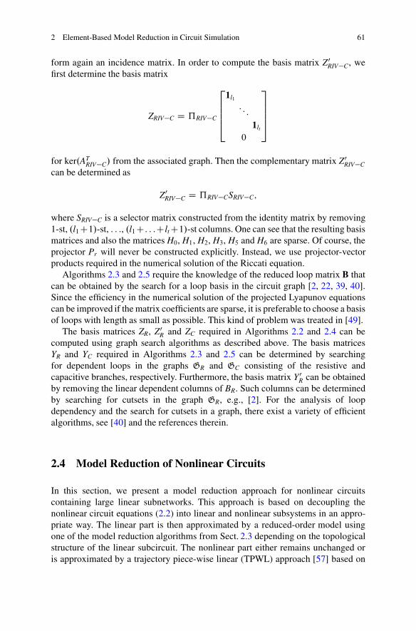
2 Element-Based Model Reduction in Circuit Simulation 61
form again an incidence matrix. In order to compute the basis matrix Z0RIV�C, wefirst determine the basis matrix
ZRIV�C D …RIV�C
26664
1l1: : :
1lt
0
37775
for ker.ATRIV�C/ from the associated graph. Then the complementary matrix Z0RIV�C
can be determined as
Z0RIV�C D …RIV�CSRIV�C;
where SRIV�C is a selector matrix constructed from the identity matrix by removing1-st, .l1C1/-st, : : :, .l1C: : :Clt C1/-st columns. One can see that the resulting basismatrices and also the matrices H0, H1, H2, H3, H5 and H6 are sparse. Of course, theprojector Pr will never be constructed explicitly. Instead, we use projector-vectorproducts required in the numerical solution of the Riccati equation.
Algorithms 2.3 and 2.5 require the knowledge of the reduced loop matrix B thatcan be obtained by the search for a loop basis in the circuit graph [2, 22, 39, 40].Since the efficiency in the numerical solution of the projected Lyapunov equationscan be improved if the matrix coefficients are sparse, it is preferable to choose a basisof loops with length as small as possible. This kind of problem was treated in [49].
The basis matrices ZR, Z0R and ZC required in Algorithms 2.2 and 2.4 can becomputed using graph search algorithms as described above. The basis matricesYR and YC required in Algorithms 2.3 and 2.5 can be determined by searchingfor dependent loops in the graphs GR and GC consisting of the resistive andcapacitive branches, respectively. Furthermore, the basis matrix Y 0R can be obtainedby removing the linear dependent columns of BR. Such columns can be determinedby searching for cutsets in the graph GR, e.g., [2]. For the analysis of loopdependency and the search for cutsets in a graph, there exist a variety of efficientalgorithms, see [40] and the references therein.
2.4 Model Reduction of Nonlinear Circuits
In this section, we present a model reduction approach for nonlinear circuitscontaining large linear subnetworks. This approach is based on decoupling thenonlinear circuit equations (2.2) into linear and nonlinear subsystems in an appro-priate way. The linear part is then approximated by a reduced-order model usingone of the model reduction algorithms from Sect. 2.3 depending on the topologicalstructure of the linear subcircuit. The nonlinear part either remains unchanged oris approximated by a trajectory piece-wise linear (TPWL) approach [57] based on
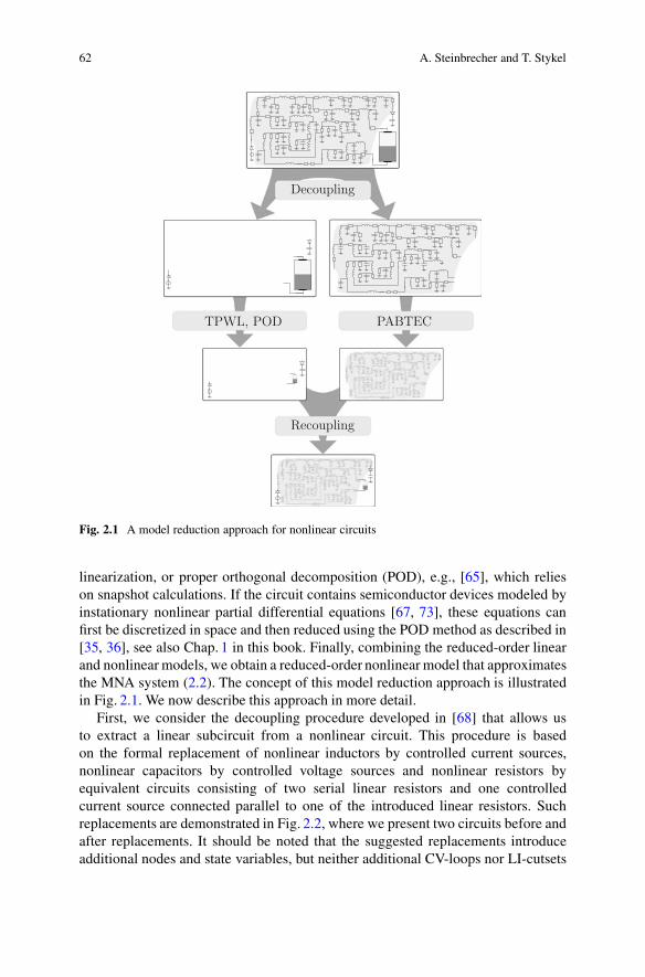
62 A. Steinbrecher and T. Stykel
Decoupling
TPWL, POD PABTEC
Recoupling
Fig. 2.1 A model reduction approach for nonlinear circuits
linearization, or proper orthogonal decomposition (POD), e.g., [65], which relieson snapshot calculations. If the circuit contains semiconductor devices modeled byinstationary nonlinear partial differential equations [67, 73], these equations canfirst be discretized in space and then reduced using the POD method as described in[35, 36], see also Chap. 1 in this book. Finally, combining the reduced-order linearand nonlinear models, we obtain a reduced-order nonlinear model that approximatesthe MNA system (2.2). The concept of this model reduction approach is illustratedin Fig. 2.1. We now describe this approach in more detail.
First, we consider the decoupling procedure developed in [68] that allows usto extract a linear subcircuit from a nonlinear circuit. This procedure is basedon the formal replacement of nonlinear inductors by controlled current sources,nonlinear capacitors by controlled voltage sources and nonlinear resistors byequivalent circuits consisting of two serial linear resistors and one controlledcurrent source connected parallel to one of the introduced linear resistors. Suchreplacements are demonstrated in Fig. 2.2, where we present two circuits before andafter replacements. It should be noted that the suggested replacements introduceadditional nodes and state variables, but neither additional CV-loops nor LI-cutsets
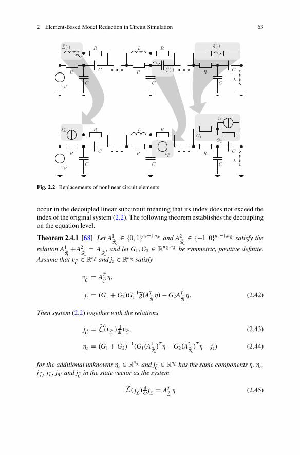
2 Element-Based Model Reduction in Circuit Simulation 63
Fig. 2.2 Replacements of nonlinear circuit elements
occur in the decoupled linear subcircuit meaning that its index does not exceed theindex of the original system (2.2). The following theorem establishes the decouplingon the equation level.
Theorem 2.4.1 [68] Let A1QR 2 f0; 1gnv�1;n QR and A2QR 2 f�1; 0gnv�1;n QR satisfy the
relation A1QR CA2QR D A QR , and let G1;G2 2 Rn
QR ;n QR be symmetric, positive definite.
Assume that v QC 2 Rn
QC and jz 2 Rn
QR satisfy
v QC D ATQC �;
jz D .G1 C G2/G�11 eg.AT
QR �/ � G2ATQR �: (2.42)
Then system (2.2) together with the relations
j QC D eC .v QC / ddtv QC ; (2.43)
�z D .G1 C G2/�1.G1.A
1QR /
T� � G2.A2QR /
T� � jz/ (2.44)
for the additional unknowns �z 2 Rn
QR and j QC 2 Rn
QC has the same components �, �z,j NL , j QL , jV and j QC in the state vector as the system
eL. j QL/ddt j QL D AT
QL � (2.45)
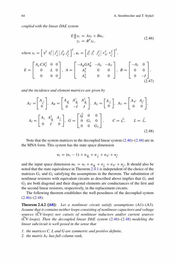
64 A. Steinbrecher and T. Stykel
coupled with the linear DAE system
E ddt x` D Ax` C Bu`;
y` D BTx`;(2.46)
where x` Dh�T �T
z jTNL jTV jTQCiT
, u` Dh
jTI jTz jTQL vTV vT
QCiT
,
E D
264
ACCATC 0 0
0 L 0
0 0 0
375 ; A D
264
�ARGATR �AL �AV
ATL 0 0
ATV 0 0
375 ; B D
264
�AI 0
0 0
0 �I
375 ;
(2.47)
and the incidence and element matrices are given by
AC D"
A NC0
#; AR D
"A NR A1QR A2QR0 �I I
#; AL D
�A NL0
�; AV D
"AV A QC0 0
#;
AI D"
AI A2QR A QL0 I 0
#; G D
24
NG 0 0
0 G1 0
0 0 G2
35 ; C D NC ; L D NL :
(2.48)
Note that the system matrices in the decoupled linear system (2.46)–(2.48) are inthe MNA form. This system has the state space dimension
n` D .nv � 1/C n QR C n NL C nV C n QC
and the input space dimension m` D nI C n QR C n QL C nV C n QC . It should also benoted that the state equivalence in Theorem 2.4.1 is independent of the choice of thematrices G1 and G2 satisfying the assumptions in the theorem. The substitution ofnonlinear resistors with equivalent circuits as described above implies that G1 andG2 are both diagonal and their diagonal elements are conductances of the first andthe second linear resistors, respectively, in the replacement circuits.
The following theorem establishes the well-posedness of the decoupled system(2.46)–(2.48).
Theorem 2.4.2 ([68]) Let a nonlinear circuit satisfy assumptions (A1)–(A3).Assume that it contains neither loops consisting of nonlinear capacitors and voltagesources (eCV-loops) nor cutsets of nonlinear inductors and/or current sources(eCV-loops). Then the decoupled linear DAE system (2.46)–(2.48) modeling thelinear subcircuit is well-posed in the sense that
1. the matrices C, L and G are symmetric and positive definite,2. the matrix AV has full column rank,
2 Element-Based Model Reduction in Circuit Simulation 65
3. the matrix ŒAC; AL; AR; AV � has full row rank.
Note that the presence of eCV-loops and eLI-cutsets in the original circuit wouldlead after the replacement of the nonlinear capacitors and nonlinear inductors byvoltage sources and current sources, respectively, to V-loops and I-cutsets in thedecoupled circuit that would violate its well-posedness.
The next theorem shows that slightly stronger conditions for the originalnonlinear circuit guarantee that the decoupled linear DAE system (2.46)–(2.48) iswell-posed and, in addition, has index at most one.
Theorem 2.4.3 ([68]) Let a nonlinear circuit satisfy assumptions (A1)–(A3). Ifthis circuit contains neither CV-loops except for NC-loops with linear capacitorsnor LI-cutsets, then the linear system (2.46)–(2.48) modeling the extracted linearsubcircuit is well-posed and is of index at most one.
The index one condition for system (2.46)–(2.48) implies that its transferfunction is proper. The approximation of such systems is much easier than that ofsystems with an improper transfer function [71].
Depending on the topology of the extracted linear subcircuit, we can nowapply one of the model reduction algorithms presented in Sect. 2.3 to the linearsystem (2.46)–(2.48). As a result, we obtain a reduced-order model (2.13) which canbe combined with the nonlinear subsystem in order to get a reduced-order nonlinearmodel.
According to the block structure of the input and output vectors of the extractedlinear DAE system (2.46)–(2.48), the reduced-order model (2.13) can be written inthe form
OE ddt Ox` D OAOx` C Œ OB1; OB2; OB3; OB4; OB5 �
2666664
jIjzj QLvVv QC
3777775;
2666664
Oy`1Oy`2Oy`3Oy`4Oy`5
3777775
D
2666664
OC1OC2OC3OC4OC5
3777775
Ox`;
(2.49)
where Oy`j D OCj Ox`, j D 1; : : : ; 5, approximate the corresponding components ofthe output of (2.46). Taking into account that �AT
QL � OC3 Ox` and �j QC OC5 Ox`,Eqs. (2.43) and (2.45) are approximated by
eC . Ov QC / ddt Ov QC D � OC5 Ox`; eL. Oj QL / d
dtOj QL D � OC3 Ox`; (2.50)
respectively, where Oj QL and Ov QC are approximations to j QL and v QC , respectively.Furthermore, for jz and �z defined in (2.42) and (2.44), respectively, we have
�.A2QR /T� � �z D �AT
QR �C G�11 eg.ATQR �/ D �v QR C G�11 eg.v QR /:
66 A. Steinbrecher and T. Stykel
Since �.A2QR /T�� �z OC2 Ox`, this equation is approximated by
0 D �G1OC2 Ox` � G1 Ov QR Ceg. Ov QR /; (2.51)
where Ov QR approximates v QR . Combining (2.45), (2.49), (2.50) and (2.51), we obtainthe reduced-order nonlinear model
OE .Ox/ ddt Ox D OA Ox C Of .Ox/C OB u;
Oy D OC Ox; (2.52)
where Ox Dh
OxT` ;
OjTL ; OvTC ; OvT
QRiT
, u Dh
jTI ; vTV
iTand
OE .Ox/ D
2664
OE 0 0 0
0 eL. Oj QL / 0 0
0 0 eC . Ov QC / 0
0 0 0 0
3775 ; Of .Ox/ D
26664
0
0
0
eg. Ov QR /
37775 ; OB D
2664
OB1 OB40 0
0 0
0 0
3775 ; (2.53)
OA D
2664
OA C OB2.G1 C G2/ OC2 OB3 OB5 OB2G1
� OC3 0 0 0
� OC5 0 0 0
�G1OC2 0 0 �G1
3775 ; OC D
� OC1 0 0 0OC4 0 0 0
�: (2.54)
This model can now be used for further investigations in steady-state analysis,transient analysis or sensitivity analysis of electrical circuits. Note that the errorbounds for the reduced-order linear subsystem (2.49) presented in Sect. 2.3 can beused to estimate the error in the output of the reduced-order nonlinear system (2.52)–(2.54), see [34] for such estimates for a special class of nonlinear circuits.
2.5 Solving Matrix Equations
In this section, we consider numerical algorithms for solving the projected Lya-punov and Riccati equations developed in [55, 70, 71]. In practice, the numericalrank of the solutions of these equations is often much smaller than the dimension ofthe problem. Then such solutions can be well approximated by low-rank matrices.Moreover, these low-rank approximations can be determined directly in factoredform. Replacing the Cholesky factors of the Gramians in Algorithms 2.1–2.5by their low-rank factors reduces significantly the computational complexity andstorage requirements in the balancing-related model reduction methods and makesthese methods very suitable for large-scale circuit equations.
2 Element-Based Model Reduction in Circuit Simulation 67
2.5.1 ADI Method for Projected Lyapunov Equations
We focus first on solving the projected Lyapunov equation
E X AT C A X ET D �PlBBTPTl ; X D PrX PT
r (2.55)
using the alternating direction implicit (ADI) method. Such an equation has to besolved in Algorithms 2.2–2.5. The ADI method has been first proposed for standardLyapunov equations [14, 44, 50, 76] and then extended in [70] to projected Lyapunovequations. The generalized ADI iteration for the projected Lyapunov equation (2.55)is given by
.E C �kA/Xk�1=2AT C AXk�1.E � �kA/T D �PlBBTPTl ;
.E C � kA/XTk AT C AXT
k�1=2.E � � kA/T D �PlBBTPTl
(2.56)
with an initial matrix X0 D 0 and shift parameters �1; : : : ; �k 2 C�. Here, � k
denotes the complex conjugate of �k. If the pencil E � A is c-stable, then Xk
converges towards the solution of the projected Lyapunov equation (2.55). The rateof convergence depends strongly on the choice of the shift parameters. The optimalshift parameters providing the superlinear convergence satisfy the generalized ADIminimax problem
f�1; : : : ; �qg D arg minf�1;:::;�qg2C�
maxt2Spf .E;A/
j.1 � �1t/ � : : : � .1� �q t/jj.1C �1t/ � : : : � .1C �q t/j ;
where Spf .E;A/ denotes the finite spectrum of the pencil E � A. If the matricesE and A satisfy the symmetry condition (2.24), then E � A has real non-positiveeigenvalues. In this case, the optimal real shift parameters can be determined by theselection procedure proposed in [78] once the spectral bounds
a D minfk W k 2 Sp�.E;A/ g; b D maxfk W k 2 Sp�.E;A/ g
are available. Here Sp�.E;A/ denotes the set of finite eigenvalues ofE � A with negative real part. In general case, the suboptimal ADI parameterscan be obtained from a set of largest and smallest in modulus approximate finiteeigenvalues of E � A computed by an Arnoldi procedure [50, 70]. Other parameterselection techniques developed for standard Lyapunov equations [15, 63, 77] canalso be used for the projected Lyapunov equation (2.55).
A low-rank approximation to the solution of the projected Lyapunov equa-tion (2.55) can be computed in factored form X ZkZT
k using a low-rank version ofthe ADI method (LR-ADI) as presented in Algorithm 2.6.
In order to guarantee for the factors Zk to be real in case of complex shift pa-rameters, we take these parameters in complex conjugate pairs f�k; �kC1 D � kg.
68 A. Steinbrecher and T. Stykel
Algorithm 2.6 The LR-ADI method for the projected Lyapunov equationGiven E, A 2 R
n;n, B 2 Rn;m, projector Pl and shift parameters �1; : : : ; �q 2 C�, compute a low-
rank approximation X ZkZTk to the solution of the projected Lyapunov equation (2.55).
1. Z.1/ D p�2Re.�1/ .EC �1A/�1PlB, Z1 D Z.1/;2. FOR k D 2; 3; : : :
Z.k/ Ds
Re.�k/
Re.�k�1/
�I � .� k�1 C �k/.EC �kA/�1A
�Z.k�1/;
Zk D Œ Zk�1; Z.k/ �IEND FOR
Then a novel approach for efficient handling of complex shift parameters in theLR-ADI method developed in [16] can also be extended to the projected Lyapunovequation (2.55). At each ADI iteration we have Zk D ŒZ.1/; : : : ;Z.k/ � 2 R
n;mk. Tokeep the low-rank structure in Zk for large mk, we can compress the columns of Zk
using the rank-revealing QR factorization [18] as described in [9].Finally, note that the matrices .E C �kA/�1 in Algorithm 2.6 do not have to be
computed explicitly. Instead, we solve linear systems of the form .E C �kA/x D Plbeither by computing (sparse) LU factorizations and forward/backward substitutionsor by using iterative Krylov subspace methods [62].
2.5.2 Newton’s Method for Projected Riccati Equations
We consider now the numerical solution of the projected Riccati equation
EXFT C FXET C EXBTcBcXET C PlBoBT
oPTl D 0; X D PrXPT
r (2.57)
with F, Bc and Bo as in (2.22). Such an equation has to be solved in Algorithm 2.1.The minimal solution Xmin of (2.57) is at least semi-stabilizing in the sense that allthe finite eigenvalues of E � F � EXminBT
c Bc are in the closed left half-plane.Consider the spaces
SPr D f X 2 Rn;n W X D XT ; X D PrXPT
r g;SPl D f X 2 R
n;n W X D XT ; X D PlXPTl g:
Since X D PrXPTr , EPr D PlE and FPr D PlF, the Riccati operator given by
R.X/ D EXFT C FXET C EXBTcBcXET C PlBoBT
oPTl
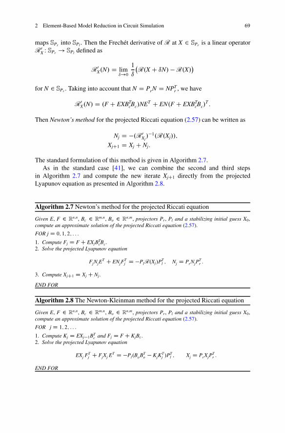
2 Element-Based Model Reduction in Circuit Simulation 69
maps SPr into SPl . Then the Frechét derivative of R at X 2 SPr is a linear operatorR 0X W SPr ! SPl defined as
R 0X.N/ D limı!0
1
ı
�R.X C ıN/ � R.X/
�
for N 2 SPr . Taking into account that N D PrN D NPTr , we have
R 0X.N/ D .F C EXBTcBc/NET C EN.F C EXBT
cBc/T :
Then Newton’s method for the projected Riccati equation (2.57) can be written as
Nj D �.R 0Xj/�1.R.Xj//;
XjC1 D Xj C Nj:
The standard formulation of this method is given in Algorithm 2.7.As in the standard case [41], we can combine the second and third steps
in Algorithm 2.7 and compute the new iterate XjC1 directly from the projectedLyapunov equation as presented in Algorithm 2.8.
Algorithm 2.7 Newton’s method for the projected Riccati equation
Given E, F 2 Rn;n, Bc 2 R
m;n, Bo 2 Rn;m, projectors Pr , Pl and a stabilizing initial guess X0,
compute an approximate solution of the projected Riccati equation (2.57).
FOR j D 0; 1; 2; : : :
1. Compute Fj D FC EXjBTcBc.
2. Solve the projected Lyapunov equation
FjNjET C ENjF
Tj D �PlR.Xj/P
Tl ; Nj D PrNjP
Tr :
3. Compute XjC1 D Xj C Nj.
END FOR
Algorithm 2.8 The Newton-Kleinman method for the projected Riccati equation
Given E, F 2 Rn;n, Bc 2 R
m;n, Bo 2 Rn;m, projectors Pr , Pl and a stabilizing initial guess X0,
compute an approximate solution of the projected Riccati equation (2.57).
FOR j D 1; 2; : : :
1. Compute Kj D EXj�1BTc and Fj D FC KjBc.
2. Solve the projected Lyapunov equation
EXj FTj C FjXj ET D �Pl.BoBT
o � KjKTj /P
Tl ; Xj D PrXjP
Tr :
END FOR
70 A. Steinbrecher and T. Stykel
Although Algorithms 2.7 and 2.8 are equivalent, they behave different in finiteprecision arithmetic and there are significant differences in their implementationespecially for large-scale problems.
Similarly to the standard state space case [8, 74], one can show that if E � F isc-stable, then for X0 D 0, all E � Fj are also c-stable and lim
j!1Xj D Xmin, see [10].
The convergence is quadratic if the pencil E � F � EXminBTc Bc is c-stable. Some
difficulties may occur if the pencil E � F has eigenvalues on the imaginary axis.For circuit equations, these eigenvalues are uncontrollable and unobservable [54].In that case, similarly to [12], one could choose a special stabilizing initial guessX0 that ensures the convergence of the Newton-Kleinman iteration. However, thecomputation of such a guess for large-scale problems remains an open problem.
A low-rank approximation to the minimal solution of the projected Riccatiequation (2.57) can be computed in factored form Xmin QR QRT with QR 2 R
n;k, k nusing the same approach as in [11]. Starting with K1 D EX0BT
c and F1 D F C K1Bc,we solve in each Newton-Kleinman iteration two projected Lyapunov equations
EX1;j FTj C FjX1;j ET D �PlBoBT
o PTl ; X1;j D PrX1;j PT
r ; (2.58)
EX2;j FTj C FjX2;j ET D �PlKjK
Tj PT
l ; X2;j D PrX2;j PTr ; (2.59)
for the low-rank approximations X1;j R1;jRT1;j and X2;j R2;jR
T2;j, respectively,
and then compute KjC1 D E.R1;jRT1;j � R2;jR
T2;j/B
Tc and FjC1 D F C KjC1Bc.
If the convergence is observed after jmax iterations, then an approximate solutionXmin QR QRT of the projected Riccati equation (2.57) can be computed in factoredform by solving the projected Lyapunov equation
EXFT C FXET D �PlQQTPTl ; X D PrXPT
r (2.60)
with Q D ŒBo; E.X1;jmax � X2;jmax/BTc � provided E � F is c-stable. For computing
low-rank factors of the solutions of the projected Lyapunov equations (2.58)–(2.60),we can use the generalized LR-ADI method presented in Sect. 2.5.1. Note that inthis method we need to compute the products .E C �Fj/
�1w, where w 2 Rn and
E C �Fj D E C �.A � BBT/ � � OKjBc with the low-rank matrices Bc 2 Rm;n and
OKj D p2PlBMT
0 J�Tc � Kj 2 R
n;m. One can use the Sherman-Morrison-Woodburyformula [28, Sect. 2.1.3] to compute these products as
.E C �Fj/�1w D w1 C M OKj
�.Im � BcM OKj
/�1Bcw1�;
where w1 D .E C �.A � BBT//�1w and M OKjD �.E C �.A � BBT//�1 OKj can be
determined by solving linear systems with the sparse matrix E C �.A � BBT/ eitherby computing sparse LU factorization or by using Krylov subspace methods [62].
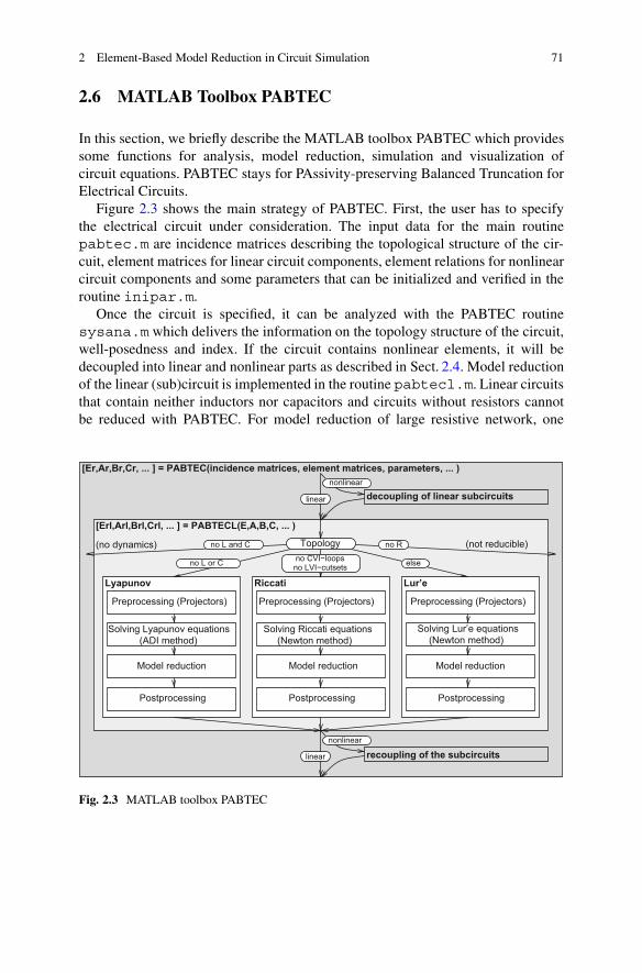
2 Element-Based Model Reduction in Circuit Simulation 71
2.6 MATLAB Toolbox PABTEC
In this section, we briefly describe the MATLAB toolbox PABTEC which providessome functions for analysis, model reduction, simulation and visualization ofcircuit equations. PABTEC stays for PAssivity-preserving Balanced Truncation forElectrical Circuits.
Figure 2.3 shows the main strategy of PABTEC. First, the user has to specifythe electrical circuit under consideration. The input data for the main routinepabtec.m are incidence matrices describing the topological structure of the cir-cuit, element matrices for linear circuit components, element relations for nonlinearcircuit components and some parameters that can be initialized and verified in theroutine inipar.m.
Once the circuit is specified, it can be analyzed with the PABTEC routinesysana.m which delivers the information on the topology structure of the circuit,well-posedness and index. If the circuit contains nonlinear elements, it will bedecoupled into linear and nonlinear parts as described in Sect. 2.4. Model reductionof the linear (sub)circuit is implemented in the routine pabtecl.m. Linear circuitsthat contain neither inductors nor capacitors and circuits without resistors cannotbe reduced with PABTEC. For model reduction of large resistive network, one
Topology
recoupling of the subcircuits
Postprocessing
(not reducible)
[Erl,Arl,Brl,Crl, ... ] = PABTECL(E,A,B,C, ... )
[Er,Ar,Br,Cr, ... ] = PABTEC(incidence matrices, element matrices, parameters, ... )
decoupling of linear subcircuits
(no dynamics)
Solving Lyapunov equations
Preprocessing (Projectors)
(ADI method)
Model reduction
Postprocessing
(Newton method)
Model reduction
Lur’e
Model reduction
Preprocessing (Projectors)
Solving Lur’e equations(Newton method)
Postprocessing
Solving Riccati equations
Preprocessing (Projectors)
itacciRvonupayL
linear
nonlinear
linear
nonlinear
no L and C no R
elseno CVI−loopsno LVI−cutsetsno L or C
Fig. 2.3 MATLAB toolbox PABTEC
72 A. Steinbrecher and T. Stykel
can use a graph-based algorithm presented in [60], which is not yet included inPABTEC. For other network structures, an appropriate model reduction method willbe chosen automatically. RC and RL circuits are reduced by the Lyapunov-basedbalanced truncation algorithms presented in Sect. 2.3.2, while for model reductionof general RLC circuit, Algorithm 2.1 is applied. If the circuit does not containCVI-loops and LIV-cutsets, then the Gramian in this algorithm is determined bysolving the projected Riccati equation (2.57). Otherwise, we have to solve theprojected Lur’e equation (2.15). Independent of the topological structure of thecircuit, the model reduction algorithms include the following steps: preprocessing,solving matrix equations, model reduction and postprocessing. In the preprocessingstep, the basis matrices required in the projector Pr or P are computed using graph-theoretical algorithms. If necessary, also the auxiliary matrices Hk and the matrixM0 are computed. The projected Lyapunov equations are solved by the LR-ADImethod described in Sect. 2.5.1, while the projected Riccati equation is solved bythe Newton or Newton-Kleinman method presented in Sect. 2.5.2. The numericalmethods for large-scale projected Lur’e equations proposed in [53] will be includedin a future release of PABTEC. Note that the matrix equation solvers in PABTECcan be seen as extension of the corresponding functions in the MATLAB toolboxLyaPACK1[51] and its successor MESS.2 Postprocessing involves the computationof error bounds and reduced-order initial vectors required for simulation.
The last step in PABTEC is combination of the reduced-order linear model withunchanged nonlinear part. PABTEC includes also the routines simorih.m andsimredh.m for simulation of the original and reduced-order models, respectively.
PABTEC provides the following routines:
• main routines listed in Table 2.1, which can be called by the user in the mainprogram;
• supplementary routines listed in Table 2.2, which are used in the main routines;• auxiliary routines listed in Table 2.3 which are used in the main and supplemen-
tary routines;• user supplied routines listed in Table 2.4, which provide the information on the
circuit.
The MATLAB toolbox PABTEC can be used by a line command or via a graphicaluser interface (GUI). PABTEC-GUI contains four tab panels shown in Figs. 2.4 and2.5 that enable the user to upload the circuit, set up all required parameters, performmodel reduction, simulate the original and reduced-order systems and save thesesystems and simulation data.
1http://www.netlib.org/lyapack/.2https://www.mpi-magdeburg.mpg.de/projects/mess
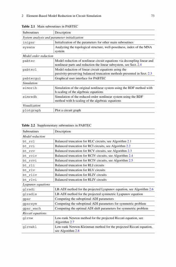
2 Element-Based Model Reduction in Circuit Simulation 73
Table 2.1 Main subroutines in PABTECg
Subroutines Description
System analysis and parameter initialization
inipar Initialization of the parameters for other main subroutines
sysana Analyzing the topological structure, well-posedness, index of the MNAsystem
Model order reduction
pabtec Model reduction of nonlinear circuit equations via decoupling linear andnonlinear parts and reduction the linear subsystem, see Sect. 2.4
pabtecl Model reduction of linear circuit equations using thepassivity-preserving balanced truncation methods presented in Sect. 2.3
pabtecgui Graphical user interface for PABTEC
Simulation
simorih Simulation of the original nonlinear system using the BDF method withh-scaling of the algebraic equations
simredh Simulation of the reduced-order nonlinear system using the BDFmethod with h-scaling of the algebraic equations
Visualization
plotgraph Plot a circuit graph
Table 2.2 Supplementary subroutines in PABTEC
Subroutines Description
Model reduction
bt_rcl Balanced truncation for RLC circuits, see Algorithm 2.1
bt_rci Balanced truncation for RCI circuits, see Algorithm 2.2
bt_rcv Balanced truncation for RCV circuits, see Algorithm 2.3
bt_rciv Balanced truncation for RCIV circuits, see Algorithm 2.4
bt_rcvi Balanced truncation for RCIV circuits, see Algorithm 2.5
bt_rli Balanced truncation for RLI circuits
bt_rlv Balanced truncation for RLV circuits
bt_rliv Balanced truncation for RLIV circuits
bt_rlvi Balanced truncation for RLIV circuits
Lyapunov equations
glradi LR-ADI method for the projected Lyapunov equation, see Algorithm 2.6
glradis LR-ADI method for the projected symmetric Lyapunov equation
gpar Computing the suboptimal ADI parameters
gparsym Computing the suboptimal ADI parameters for symmetric problem
gpar_wach Computing the optimal ADI shift parameters for symmetric problem
Riccati equations
glrnw Low-rank Newton method for the projected Riccati equation, seeAlgorithm 2.7
glrnwkl Low-rank Newton-Kleinman method for the projected Riccati equation,see Algorithm 2.8

74 A. Steinbrecher and T. Stykel
Table 2.3 Auxiliary subroutines in PABTEC
Subroutines Description
Graph-theoretical algorithms
fastlists Forming a node-branch-list from an incidence matrix
forest Computing a forest in the graph
inc_bas Computing the basis matrices for the left null and range spaces
of an incidence matrix
inc_rank Computing the rank of an incidence matrix
loopmatr Computing a reduced loop matrix from a reduced incidence matrix
Numerical linear algebra
garn Arnoldi method for computing the largest and smallest finiteeigenvalues of a pencil
garnsym Arnoldi method for computing the largest and smallest finiteeigenvalues of a symmetric pencil
nresl Computing the residual norms for the projected Lyapunov equationusing updated QR factorizations
nresr Computing the residual norm for the projected Riccati equation usingQR factorization
prodinvsym Computing the matrix-vector product E�v, where E� is a reflexiveinverse of symmetric E w.r.t. to a projector P
prodp Computing the matrix-vector product E�v, where E� is a reflexiveinverse of E w.r.t. to the projectors Pr and Pl
prodpsym Computing the projector-vector product Pv
prodpl Computing the projector-vector product Plv or PTl v
prodpr Computing the projector-vector product Prv or PTr v
Miscellaneous
hmatr Computing the matrices Hk required for the projectors Pr and Pl
incmat Determination of the incidence matrices
ininet Initialization of the network topology
matr2ascii Export the matrix in ASCII-format
m0m Computing the matrix M0 as in (2.40)
mnadae Construction of E;A;B from incidence and element matrices
Table 2.4 User supplied subroutines for PABTEC
Subroutines Description
netlist Incidence and element matrices for linear circuit components
PCN Matrix valued function for nonlinear capacitors
PLN Matrix valued function for nonlinear inductors
gN Nonlinear current-voltage relation for nonlinear resistors
uV Voltages of voltage sources
iI Currents of current sources
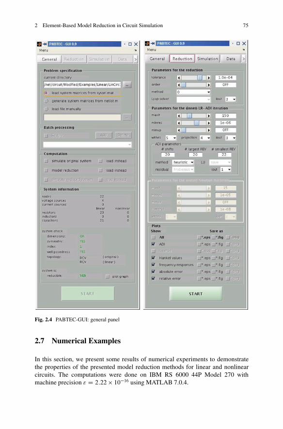
2 Element-Based Model Reduction in Circuit Simulation 75
Fig. 2.4 PABTEC-GUI: general panel
2.7 Numerical Examples
In this section, we present some results of numerical experiments to demonstratethe properties of the presented model reduction methods for linear and nonlinearcircuits. The computations were done on IBM RS 6000 44P Model 270 withmachine precision " D 2:22 � 10�16 using MATLAB 7.0.4.
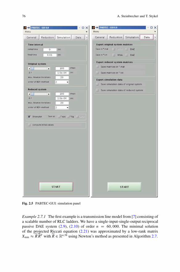
76 A. Steinbrecher and T. Stykel
Fig. 2.5 PABTEC-GUI: simulation panel
Example 2.7.1 The first example is a transmission line model from [7] consisting ofa scalable number of RLC ladders. We have a single-input-single-output reciprocalpassive DAE system (2.9), (2.10) of order n D 60; 000. The minimal solutionof the projected Riccati equation (2.21) was approximated by a low-rank matrixXmin eReRT witheR 2 R
n;58 using Newton’s method as presented in Algorithm 2.7.
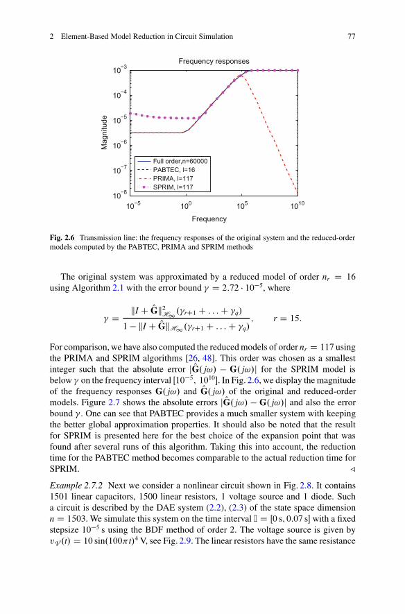
2 Element-Based Model Reduction in Circuit Simulation 77
10−5 100 105 101010−8
10−7
10−6
10−5
10−4
10−3
Mag
nitu
de
Frequency
Frequency responses
Full order,n=60000PABTEC, l=16PRIMA, l=117SPRIM, l=117
Fig. 2.6 Transmission line: the frequency responses of the original system and the reduced-ordermodels computed by the PABTEC, PRIMA and SPRIM methods
The original system was approximated by a reduced model of order nr D 16
using Algorithm 2.1 with the error bound � D 2:72 � 10�5, where
� D kI C OGk2H1
.�rC1 C : : :C �q/
1 � kI C OGkH1.�rC1 C : : :C �q/
; r D 15:
For comparison, we have also computed the reduced models of order nr D 117 usingthe PRIMA and SPRIM algorithms [26, 48]. This order was chosen as a smallestinteger such that the absolute error j OG. j!/ � G. j!/j for the SPRIM model isbelow � on the frequency interval Œ10�5; 1010�. In Fig. 2.6, we display the magnitudeof the frequency responses G. j!/ and OG. j!/ of the original and reduced-ordermodels. Figure 2.7 shows the absolute errors j OG. j!/ � G. j!/j and also the errorbound � . One can see that PABTEC provides a much smaller system with keepingthe better global approximation properties. It should also be noted that the resultfor SPRIM is presented here for the best choice of the expansion point that wasfound after several runs of this algorithm. Taking this into account, the reductiontime for the PABTEC method becomes comparable to the actual reduction time forSPRIM. GExample 2.7.2 Next we consider a nonlinear circuit shown in Fig. 2.8. It contains1501 linear capacitors, 1500 linear resistors, 1 voltage source and 1 diode. Sucha circuit is described by the DAE system (2.2), (2.3) of the state space dimensionn D 1503. We simulate this system on the time interval I D Œ0 s; 0:07 s� with a fixedstepsize 10�5 s using the BDF method of order 2. The voltage source is given byvV .t/ D 10 sin.100�t/4 V, see Fig. 2.9. The linear resistors have the same resistance
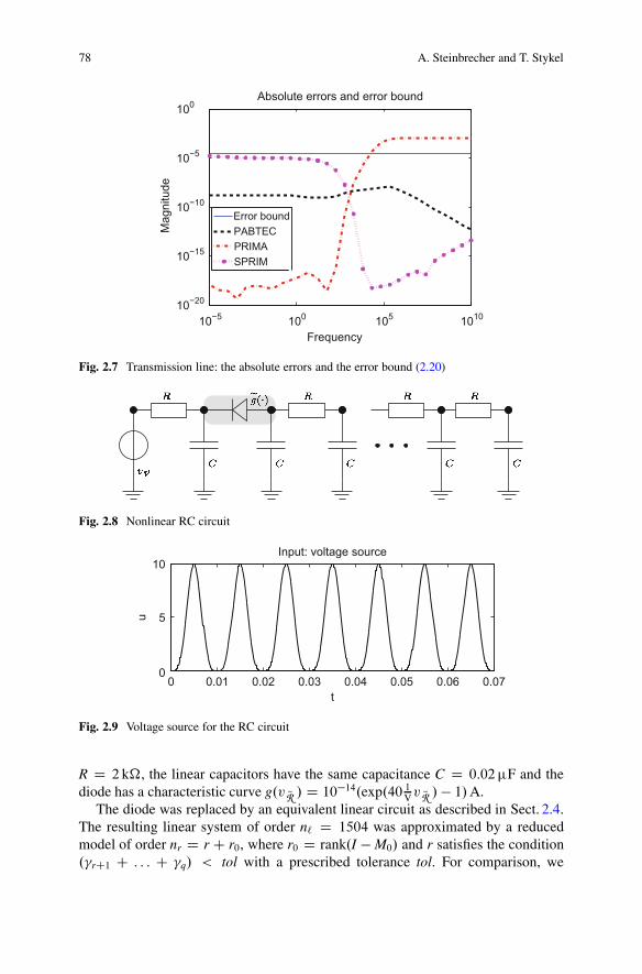
78 A. Steinbrecher and T. Stykel
10−5 100 105 101010−20
10−15
10−10
10−5
100
Frequency
Mag
nitu
de
Absolute errors and error bound
Error boundPABTECPRIMASPRIM
Fig. 2.7 Transmission line: the absolute errors and the error bound (2.20)
Fig. 2.8 Nonlinear RC circuit
0 0.01 0.02 0.03 0.04 0.05 0.06 0.070
5
10
t
u
Input: voltage source
Fig. 2.9 Voltage source for the RC circuit
R D 2 k�, the linear capacitors have the same capacitance C D 0:02 �F and thediode has a characteristic curve g.v QR / D 10�14.exp.40 1Vv QR /� 1/A.
The diode was replaced by an equivalent linear circuit as described in Sect. 2.4.The resulting linear system of order n` D 1504 was approximated by a reducedmodel of order nr D r C r0, where r0 D rank.I � M0/ and r satisfies the condition.�rC1 C : : : C �q/ < tol with a prescribed tolerance tol. For comparison, we
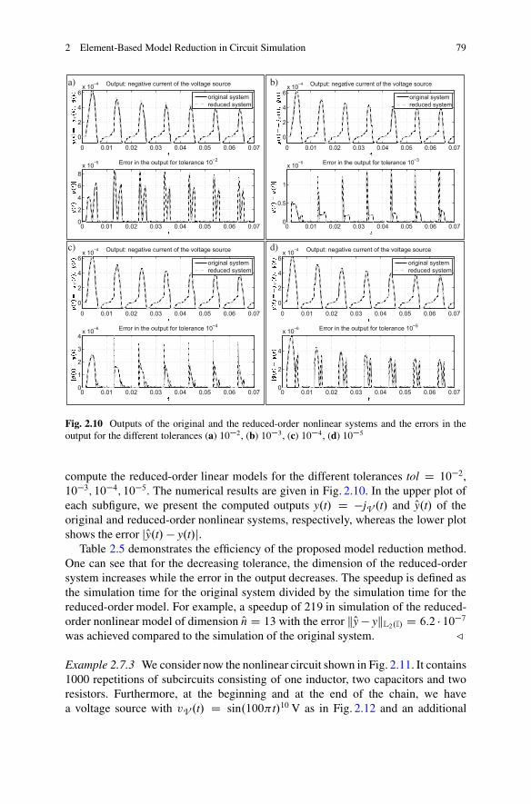
2 Element-Based Model Reduction in Circuit Simulation 79
0 0.01 0.02 0.03 0.04 0.05 0.06 0.07
0
2
4
6x 10⁻⁴ Output: negative current of the voltage source
original systemreduced system
0 0.01 0.02 0.03 0.04 0.05 0.06 0.070
2
4
6
8x 10⁻⁵ Error in the output for tolerance 10−2
V
0 0.01 0.02 0.03 0.04 0.05 0.06 0.07
0
2
4
6x 10⁻⁴ Output: negative current of the voltage source
original systemreduced system
0 0.01 0.02 0.03 0.04 0.05 0.06 0.070
0.5
1
x 10−5 Error in the output for tolerance 10−3
V
0 0.01 0.02 0.03 0.04 0.05 0.06 0.07
0
2
4
6x 10⁻⁴ Output: negative current of the voltage source
original systemreduced system
0 0.01 0.02 0.03 0.04 0.05 0.06 0.070
1
2
3
4x 10⁻⁶ Error in the output for tolerance 10−4
V
0 0.01 0.02 0.03 0.04 0.05 0.06 0.07
0
2
4
6x 10⁻⁴ Output: negative current of the voltage source
original systemreduced system
0 0.01 0.02 0.03 0.04 0.05 0.06 0.070
2
4
x 10−6 Error in the output for tolerance 10−5
V
a) b)
c) d)
Fig. 2.10 Outputs of the original and the reduced-order nonlinear systems and the errors in theoutput for the different tolerances (a) 10�2, (b) 10�3, (c) 10�4, (d) 10�5
compute the reduced-order linear models for the different tolerances tol D 10�2,10�3; 10�4; 10�5. The numerical results are given in Fig. 2.10. In the upper plot ofeach subfigure, we present the computed outputs y.t/ D �jV .t/ and Oy.t/ of theoriginal and reduced-order nonlinear systems, respectively, whereas the lower plotshows the error jOy.t/ � y.t/j.
Table 2.5 demonstrates the efficiency of the proposed model reduction method.One can see that for the decreasing tolerance, the dimension of the reduced-ordersystem increases while the error in the output decreases. The speedup is defined asthe simulation time for the original system divided by the simulation time for thereduced-order model. For example, a speedup of 219 in simulation of the reduced-order nonlinear model of dimension On D 13 with the error kOy � ykL2.I/ D 6:2 � 10�7was achieved compared to the simulation of the original system. G
Example 2.7.3 We consider now the nonlinear circuit shown in Fig. 2.11. It contains1000 repetitions of subcircuits consisting of one inductor, two capacitors and tworesistors. Furthermore, at the beginning and at the end of the chain, we havea voltage source with vV .t/ D sin.100�t/10 V as in Fig. 2.12 and an additional
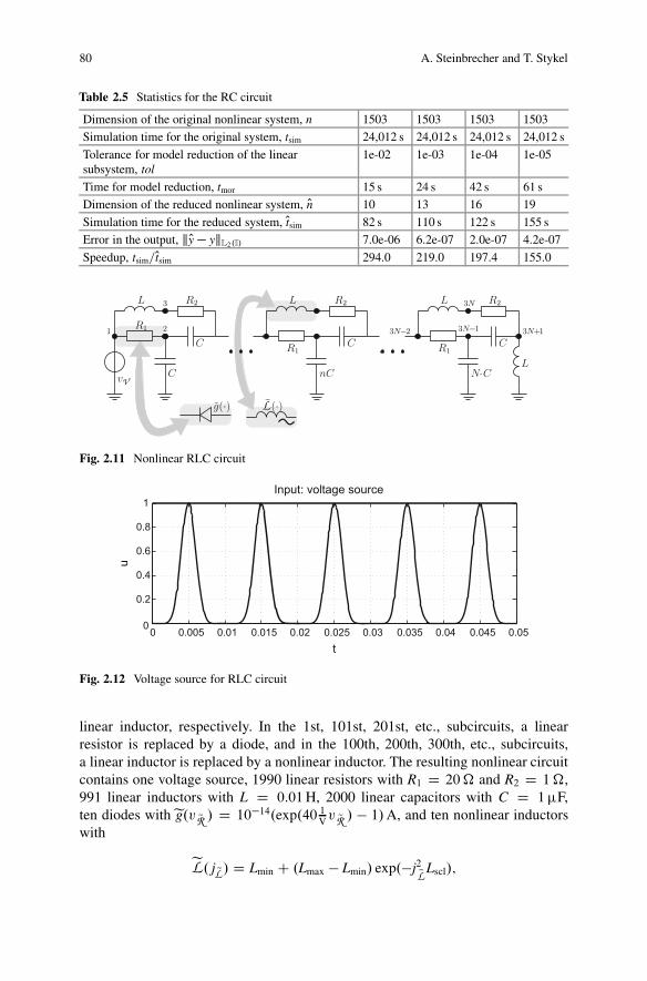
80 A. Steinbrecher and T. Stykel
Table 2.5 Statistics for the RC circuit
Dimension of the original nonlinear system, n 1503 1503 1503 1503
Simulation time for the original system, tsim 24,012 s 24,012 s 24,012 s 24,012 s
Tolerance for model reduction of the linearsubsystem, tol
1e-02 1e-03 1e-04 1e-05
Time for model reduction, tmor 15 s 24 s 42 s 61 s
Dimension of the reduced nonlinear system, On 10 13 16 19
Simulation time for the reduced system, Otsim 82 s 110 s 122 s 155 s
Error in the output, kOy� ykL2.I/ 7.0e-06 6.2e-07 2.0e-07 4.2e-07
Speedup, tsim=Otsim 294.0 219.0 197.4 155.0
Fig. 2.11 Nonlinear RLC circuit
0 0.005 0.01 0.015 0.02 0.025 0.03 0.035 0.04 0.045 0.050
0.2
0.4
0.6
0.8
1
t
u
Input: voltage source
Fig. 2.12 Voltage source for RLC circuit
linear inductor, respectively. In the 1st, 101st, 201st, etc., subcircuits, a linearresistor is replaced by a diode, and in the 100th, 200th, 300th, etc., subcircuits,a linear inductor is replaced by a nonlinear inductor. The resulting nonlinear circuitcontains one voltage source, 1990 linear resistors with R1 D 20� and R2 D 1�,991 linear inductors with L D 0:01H, 2000 linear capacitors with C D 1�F,ten diodes witheg.v QR / D 10�14.exp.40 1Vv QR / � 1/A, and ten nonlinear inductorswith
eL. j QL/ D Lmin C .Lmax � Lmin/ exp.�j2QLLscl/;
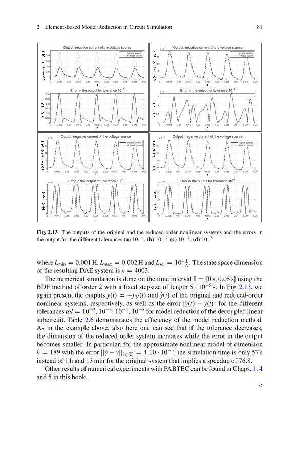
2 Element-Based Model Reduction in Circuit Simulation 81
0 0.005 0.01 0.015 0.02 0.025 0.03 0.035 0.04 0.045 0.05
0
0.01
0.02
0.03
0.04
Output: negative current of the voltage sourceoriginal systemreduced system
0 0.005 0.01 0.015 0.02 0.025 0.03 0.035 0.04 0.045 0.050
0.005
0.01
0.015
0.02
0.025
0.03Error in the output for tolerance 10−2
V
0 0.005 0.01 0.015 0.02 0.025 0.03 0.035 0.04 0.045 0.05
0
5
10
15
x 10−3 Output: negative current of the voltage sourceoriginal systemreduced system
0 0.005 0.01 0.015 0.02 0.025 0.03 0.035 0.04 0.045 0.050
0.5
1
1.5
x 10−3 Error in the output for tolerance 10−3
V
0 0.005 0.01 0.015 0.02 0.025 0.03 0.035 0.04 0.045 0.05
0
5
10
15
x 10−3 Output: negative current of the voltage sourceoriginal systemreduced system
0 0.005 0.01 0.015 0.02 0.025 0.03 0.035 0.04 0.045 0.050
1
2
3
x 10−4 Error in the output for tolerance 10−4
V
0 0.005 0.01 0.015 0.02 0.025 0.03 0.035 0.04 0.045 0.05
0
5
10
15
x 10−3 Output: negative current of the voltage sourceoriginal systemreduced system
0 0.005 0.01 0.015 0.02 0.025 0.03 0.035 0.04 0.045 0.050
1
2
3
4x 10⁻⁴ Error in the output for tolerance 10−5
V
Fig. 2.13 The outputs of the original and the reduced-order nonlinear systems and the errors inthe output for the different tolerances (a) 10�2, (b) 10�3 , (c) 10�4, (d) 10�5
where Lmin D 0:001H, Lmax D 0:002H and Lscl D 104 1A . The state space dimensionof the resulting DAE system is n D 4003.
The numerical simulation is done on the time interval I D Œ0 s; 0:05 s� using theBDF method of order 2 with a fixed stepsize of length 5 � 10�5 s. In Fig. 2.13, weagain present the outputs y.t/ D �jV .t/ and Oy.t/ of the original and reduced-ordernonlinear systems, respectively, as well as the error jOy.t/ � y.t/j for the differenttolerances tol D 10�2, 10�3, 10�4, 10�5 for model reduction of the decoupled linearsubcircuit. Table 2.6 demonstrates the efficiency of the model reduction method.As in the example above, also here one can see that if the tolerance decreases,the dimension of the reduced-order system increases while the error in the outputbecomes smaller. In particular, for the approximate nonlinear model of dimensionOn D 189 with the error jjOy � yjjL2.I/ D 4:10 � 10�5, the simulation time is only 57 sinstead of 1 h and 13 min for the original system that implies a speedup of 76.8.
Other results of numerical experiments with PABTEC can be found in Chaps. 1, 4and 5 in this book.
G
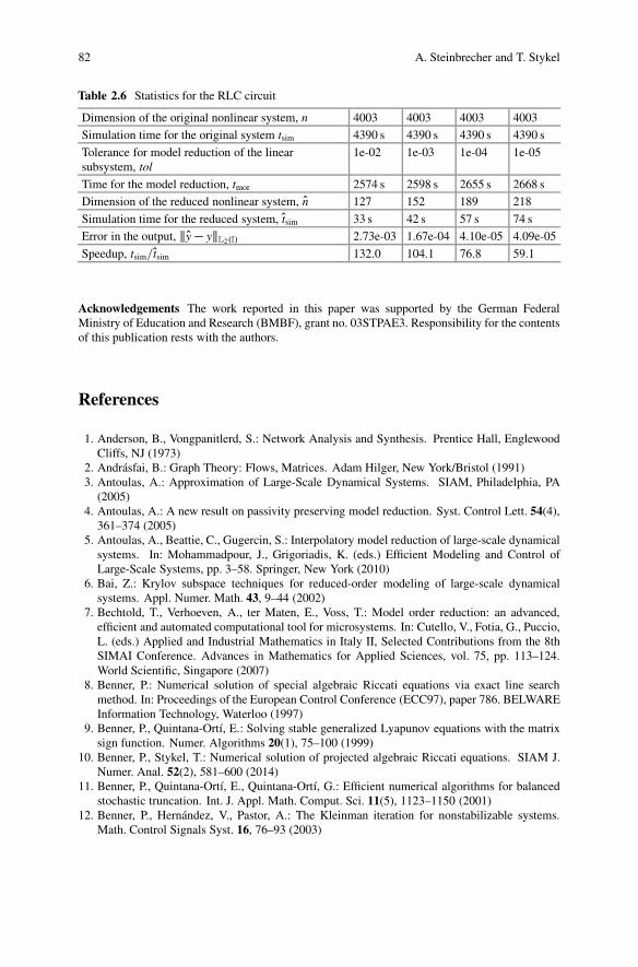
82 A. Steinbrecher and T. Stykel
Table 2.6 Statistics for the RLC circuit
Dimension of the original nonlinear system, n 4003 4003 4003 4003
Simulation time for the original system tsim 4390 s 4390 s 4390 s 4390 s
Tolerance for model reduction of the linearsubsystem, tol
1e-02 1e-03 1e-04 1e-05
Time for the model reduction, tmor 2574 s 2598 s 2655 s 2668 s
Dimension of the reduced nonlinear system, On 127 152 189 218
Simulation time for the reduced system, Otsim 33 s 42 s 57 s 74 s
Error in the output, kOy� ykL2.I/ 2.73e-03 1.67e-04 4.10e-05 4.09e-05
Speedup, tsim=Otsim 132.0 104.1 76.8 59.1
Acknowledgements The work reported in this paper was supported by the German FederalMinistry of Education and Research (BMBF), grant no. 03STPAE3. Responsibility for the contentsof this publication rests with the authors.
References
1. Anderson, B., Vongpanitlerd, S.: Network Analysis and Synthesis. Prentice Hall, EnglewoodCliffs, NJ (1973)
2. Andrásfai, B.: Graph Theory: Flows, Matrices. Adam Hilger, New York/Bristol (1991)3. Antoulas, A.: Approximation of Large-Scale Dynamical Systems. SIAM, Philadelphia, PA
(2005)4. Antoulas, A.: A new result on passivity preserving model reduction. Syst. Control Lett. 54(4),
361–374 (2005)5. Antoulas, A., Beattie, C., Gugercin, S.: Interpolatory model reduction of large-scale dynamical
systems. In: Mohammadpour, J., Grigoriadis, K. (eds.) Efficient Modeling and Control ofLarge-Scale Systems, pp. 3–58. Springer, New York (2010)
6. Bai, Z.: Krylov subspace techniques for reduced-order modeling of large-scale dynamicalsystems. Appl. Numer. Math. 43, 9–44 (2002)
7. Bechtold, T., Verhoeven, A., ter Maten, E., Voss, T.: Model order reduction: an advanced,efficient and automated computational tool for microsystems. In: Cutello, V., Fotia, G., Puccio,L. (eds.) Applied and Industrial Mathematics in Italy II, Selected Contributions from the 8thSIMAI Conference. Advances in Mathematics for Applied Sciences, vol. 75, pp. 113–124.World Scientific, Singapore (2007)
8. Benner, P.: Numerical solution of special algebraic Riccati equations via exact line searchmethod. In: Proceedings of the European Control Conference (ECC97), paper 786. BELWAREInformation Technology, Waterloo (1997)
9. Benner, P., Quintana-Ortí, E.: Solving stable generalized Lyapunov equations with the matrixsign function. Numer. Algorithms 20(1), 75–100 (1999)
10. Benner, P., Stykel, T.: Numerical solution of projected algebraic Riccati equations. SIAM J.Numer. Anal. 52(2), 581–600 (2014)
11. Benner, P., Quintana-Ortí, E., Quintana-Ortí, G.: Efficient numerical algorithms for balancedstochastic truncation. Int. J. Appl. Math. Comput. Sci. 11(5), 1123–1150 (2001)
12. Benner, P., Hernández, V., Pastor, A.: The Kleinman iteration for nonstabilizable systems.Math. Control Signals Syst. 16, 76–93 (2003)
2 Element-Based Model Reduction in Circuit Simulation 83
13. Benner, P., Mehrmann, V., Sorensen, D. (eds.): Dimension Reduction of Large-Scale Systems.Lecture Notes in Computational Science and Engineering, vol. 45. Springer, Berlin/Heidelberg(2005)
14. Benner, P., Li, J.R., Penzl, T.: Numerical solution of large Lyapunov equations, Riccatiequations, and linear-quadratic control problems. Numer. Linear Algebra Appl. 15, 755–777(2008)
15. Benner, P., Mena, H., Saak, J.: On the parameter selection problem in the Newton-ADI iterationfor large-scale Riccati equations. Electron. Trans. Numer. Anal. 29, 136–149 (2008)
16. Benner, P., Kürschner, P., Saak, J.: Efficient handling of complex shift parameters in the low-rank Cholesky factor ADI method. Numer. Algorithms 62(2), 225–251 (2013)
17. Brenan, K., Campbell, S., Petzold, L.: The Numerical Solution of Initial-Value Problemsin Differential-Algebraic Equations. Classics in Applied Mathematics, vol. 14. SIAM,Philadelphia, PA (1996)
18. Chan, T.: Rank revealing QR factorizations. Linear Algebra Appl. 88/89, 67–82 (1987)19. Chua, L.: Dynamic nonlinear networks: state-of-the-art. IEEE Trans. Circuits Syst. 27(11),
1059–1087 (1980)20. Chua, L., Desoer, C., Kuh, E.: Linear and Nonlinear Circuits. McGraw-Hill, New York (1987)21. Dai, L.: Singular Control Systems. Lecture Notes in Control and Information Sciences,
vol. 118. Springer, Berlin/Heidelberg (1989)22. Deo, N.: Graph Theory with Application to Engineering and Computer Science. Prentice-Hall,
Englewood Cliffs, NJ (1974)23. Estévez Schwarz, D.: A step-by-step approach to compute a consistent initialization for the
MNA. Int. J. Circuit Theory Appl. 30, 1–16 (2002)24. Estévez Schwarz, D., Tischendorf, C.: Structural analysis for electric circuits and consequences
for MNA. Int. J. Circuit Theory Appl. 28, 131–162 (2000)25. Freund, R.: Model reduction methods based on Krylov subspaces. Acta Numer. 12, 267–319
(2003)26. Freund, R.: SPRIM: structure-preserving reduced-order interconnect macromodeling. In:
Technical Digest of the 2004 IEEE/ACM International Conference on Computer-AidedDesign, pp. 80–87. IEEE Computer Society, Los Alamos, CA (2004)
27. Freund, R.: Structure-preserving model order reduction of RCL circuit equations. In: Schilders,W., van der Vorst, H., Rommes, J. (eds.) Model Order Reduction: Theory, Research Aspectsand Applications. Mathematics in Industry, vol. 13, pp. 49–73. Springer, Berlin/Heidelberg(2008)
28. Golub, G., Van Loan, C.: Matrix Computations, 3rd edn. The Johns Hopkins University Press,Baltimore/London (1996)
29. Griepentrog, E., März, R.: Differential-Algebraic Equations and Their Numerical Treatment.Teubner-Texte zur Mathematik, vol. 88. B.G. Teubner, Leipzig (1986)
30. Grimme, E.: Krylov projection methods for model reduction. Ph.D. thesis, University ofIllinois, Urbana-Champaign (1997)
31. Gugercin, S., Antoulas, A.: A survey of model reduction by balanced truncation and some newresults. Int. J. Control 77(8), 748–766 (2004)
32. Gugercin, S., Antoulas, A., Beattie, C.: H2 model reduction for large-scale linear dynamicalsystems. SIAM J. Matrix Anal. Appl. 30(2), 609–638 (2008)
33. Hairer, E., Wanner, G.: Solving Ordinary Differential Equations II - Stiff and Differential-Algebraic Problems, 2nd edn. Springer, Berlin (1996)
34. Heinkenschloss, M., Reis, T.: Model reduction for a class of nonlinear electrical circuits byreduction of linear subcircuits. Technical Report 702–2010, DFG Research Center MATHEON,Technische Universität Berlin (2010). http://http://www.math.tu-berlin.de/~reis/Publicat/pr_10_702.pdf
35. Hinze, M., Kunkel, M.: Residual based sampling in pod model order reduction of drift-diffusion equations in parametrized electrical networks. Z. Angew. Math. Mech. 92(2), 91–104(2012)

84 A. Steinbrecher and T. Stykel
36. Hinze, M., Kunkel, M., Steinbrecher, A., Stykel, T.: Model order reduction of coupled circuit-device systems. Int. J. Numer. Model. Electron. Networks Devices Fields 25, 362–377 (2012)
37. Ho, C.W., Ruehli, A., Brennan, P.: The modified nodal approach to network analysis. IEEETrans. Circuits Syst. 22(6), 504–509 (1975)
38. Ionutiu, R., Rommes, J., Antoulas, A.: Passivity-preserving model reduction using dominantspectral-zero interpolation. IEEE Trans. Comput. Aided Des. Integr. Circuits Syst. 27(12),2250–2263 (2008)
39. Ipach, H.: Graphentheoretische Anwendungen in der Analyse elektrischer Schaltkreise.Bachelorarbeit, Universität Hamburg (2013)
40. Jungnickel, D.: Graphs, Network and Algorithms. Springer, Berlin/Heidelberg (2005)41. Kleinman, D.: On an iterative technique for Riccati equation computations. IEEE Trans.
Autom. Control 13, 114–115 (1968)42. Knockaert, L., De Zutter, D.: Laguerre-SVD reduced-order modeling. IEEE Trans. Microwave
Theory Tech. 48(9), 1469–1475 (2000)43. Kunkel, P., Mehrmann, V.: Differential-Algebraic Equations. Analysis and Numerical Solution.
EMS Publishing House, Zürich (2006)44. Li, J.R., White, J.: Low rank solution of Lyapunov equations. SIAM J. Matrix Anal. Appl.
24(1), 260–280 (2002)45. Liu, W., Sreeram, V., Teo, K.: Model reduction for state-space symmetric systems. Syst.
Control Lett. 34(4), 209–215 (1998)46. Moore, B.: Principal component analysis in linear systems: controllability, observability, and
model reduction. IEEE Trans. Autom. Control 26(1), 17–32 (1981)47. Ober, R.: Balanced parametrization of classes of linear systems. SIAM J. Control Optim. 29(6),
1251–1287 (1991)48. Odabasioglu, A., Celik, M., Pileggi, L.: PRIMA: passive reduced-order interconnect macro-
modeling algorithm. IEEE Trans. Comput. Aided Des. Integr. Circuits Syst. 17(8), 645–654(1998)
49. Ovalekar, V., Narayanan, H.: Fast loop matrix generation for hybrid analysis and a comparisonof the sparsity of the loop impedance and MNA impedance submatrices. In: Proceedings ofthe IEEE International Symposium on Circuits and Systems, ISCAS ’92, vol. 4, pp. 1780–1783(1992)
50. Penzl, T.: A cyclic low-rank Smith method for large sparse Lyapunov equations. SIAM J. Sci.Comput. 21(4), 1401–1418 (1999/2000)
51. Penzl, T.: LYAPACK Users Guide. Preprint SFB393/00-33, Fakultät für Mathematik,Technische Universität Chemnitz, Chemnitz (2000). Available from http://www.tu-chemnitz.de/sfb393/sfb00pr.html
52. Phillips, J., Daniel, L., Silveira, L.: Guaranteed passive balancing transformations for modelorder reduction. IEEE Trans. Comput. Aided Des. Integr. Circuits Syst. 22(8), 1027–1041(2003)
53. Poloni, F., Reis, T.: A deflation approach for large-scale Lur’e equations. SIAM. J. MatrixAnal. Appl. 33(4), 1339–1368 (2012)
54. Reis, T., Stykel, T.: PABTEC: Passivity-preserving balanced truncation for electrical circuits.IEEE Trans. Compu. Aided Des. Integr. Circuits Syst. 29(9), 1354–1367 (2010)
55. Reis, T., Stykel, T.: Positive real and bounded real balancing for model reduction of descriptorsystems. Int. J. Control 83(1), 74–88 (2010)
56. Reis, T., Stykel, T.: Lyapunov balancing for passivity-preserving model reduction of RCcircuits. SIAM J. Appl. Dyn. Syst. 10(1), 1–34 (2011)
57. Rewienski, M.: A trajectory piecewise-linear approach to model order reduction of nonlineardynamical systems. Ph.D. thesis, Massachusetts Institute of Technology (2003)
58. Riaza, R., Tischendorf, C.: Qualitative features of matrix pencils and DAEs arising in circuitdynamics. Dyn. Syst. 22, 107–131 (2007)
59. Riaza, R., Tischendorf, C.: The hyperbolicity problem in electrical circuit theory. Math.Methods Appl. Sci. 33(17), 2037–2049 (2010)
2 Element-Based Model Reduction in Circuit Simulation 85
60. Rommes, J., Schilders, W.: Efficient methods for large resistor networks. IEEE Trans. Comput.Aided Des. Integr. Circuits Syst. 29(1), 28–39 (2010)
61. Roos, J., Costa, L. (eds.): Scientific Computing in Electrical Engineering SCEE 2008.Mathematics in Industry, vol. 14. Springer, Berlin/Heidelberg (2010)
62. Saad, Y.: Iterative Methods for Sparse Linear Systems. PWS Publishing Company, Boston,MA (1996)
63. Sabino, J.: Solution of large-scale Lyapunov equations via the block modified Smith method.Ph.D. thesis, Rice University, Houston (2006)
64. Schilders, W., van der Vorst, H., J., R. (eds.): Model Order Reduction: Theory, ResearchAspects and Applications. Mathematics in Industry, vol. 13. Springer, Berlin/Heidelberg(2008)
65. Sirovich, L.: Turbulence and the dynamics of coherent structures. I: coherent structures. II:symmetries and transformations. III: dynamics and scaling. Q. Appl. Math. 45, 561–590 (1987)
66. Sorensen, D.: Passivity preserving model reduction via interpolation of spectral zeros. Syst.Control Lett. 54(4), 347–360 (2005)
67. Soto, M.S., Tischendorf, C.: Numerical analysis of DAEs from coupled circuit and semicon-ductor simulation. Appl. Numer. Math. 53(2–4), 471–88 (2005)
68. Steinbrecher, A., Stykel, T.: Model order reduction of nonlinear circuit equations. Int. J.Circuits Theory Appl. 41, 1226–1247 (2013)
69. Stykel, T.: Gramian-based model reduction for descriptor systems. Math. Control Signals Syst.16, 297–319 (2004)
70. Stykel, T.: Low-rank iterative methods for projected generalized Lyapunov equations. Electron.Trans. Numer. Anal. 30, 187–202 (2008)
71. Stykel, T.: Balancing-related model reduction of circuit equations using topological structure.In: Benner, P., Hinze, M., ter Maten, E. (eds.) Model Reduction for Circuit Simulation. LectureNotes in Electrical Engineering, vol. 74, pp. 53–80. Springer, Berlin/Heidelberg (2011)
72. Stykel, T., Reis, T.: The PABTEC algorithm for passivity-preserving model reduction of circuitequations. In: Proceedings of the 19th International Symposium on Mathematical Theory ofNetworks and Systems, MTNS 2010, Budapest, 5–9 July 2010, paper 363. ELTE, Budapest(2010)
73. Tischendorf, C.: Coupled systems of differential algebraic and partial differential equations incircuit and device simulation. Habilitation thesis, Humboldt-Universität Berlin (2004)
74. Varga, A.: On computing high accuracy solutions of a class of Riccati equations. ControlTheory Adv. Technol. 10, 2005–2016 (1995)
75. Vlach, J., Singhal, K.: Computer Methods for Circuit Analysis and Design. Van NostrandReinhold, New York (1994)
76. Wachspress, E.: Iterative solution of the Lyapunov matrix equation. Appl. Math. Lett. 1, 87–90(1988)
77. Wachspress, E.: The ADI minimax problem for complex spectra. In: Kincaid, D., Hayes, L.(eds.) Iterative Methods for Large Linear Systems, pp. 251–271. Academic, San Diego (1990)
78. Wachspress, E.: The ADI Model Problem. Monograph, Windsor, CA (1995)79. Weinbreg, L., Ruehili, A.: Combined modified loop analysis, modified nodal analysis for large-
scale circuits. IBM Research Report RC 10407, IBM Research Devision (1984)
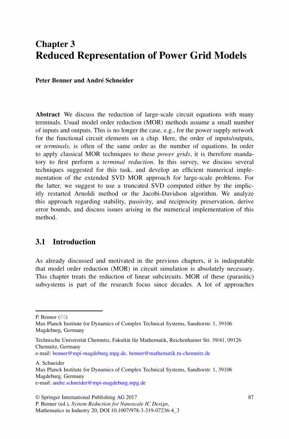
Chapter 3Reduced Representation of Power Grid Models
Peter Benner and André Schneider
Abstract We discuss the reduction of large-scale circuit equations with manyterminals. Usual model order reduction (MOR) methods assume a small numberof inputs and outputs. This is no longer the case, e.g., for the power supply networkfor the functional circuit elements on a chip. Here, the order of inputs/outputs,or terminals, is often of the same order as the number of equations. In orderto apply classical MOR techniques to these power grids, it is therefore manda-tory to first perform a terminal reduction. In this survey, we discuss severaltechniques suggested for this task, and develop an efficient numerical imple-mentation of the extended SVD MOR approach for large-scale problems. Forthe latter, we suggest to use a truncated SVD computed either by the implic-itly restarted Arnoldi method or the Jacobi-Davidson algorithm. We analyzethis approach regarding stability, passivity, and reciprocity preservation, deriveerror bounds, and discuss issues arising in the numerical implementation of thismethod.
3.1 Introduction
As already discussed and motivated in the previous chapters, it is indisputablethat model order reduction (MOR) in circuit simulation is absolutely necessary.This chapter treats the reduction of linear subcircuits. MOR of these (parasitic)subsystems is part of the research focus since decades. A lot of approaches
P. Benner (�)Max Planck Institute for Dynamics of Complex Technical Systems, Sandtorstr. 1, 39106Magdeburg, Germany
Technische Universität Chemnitz, Fakultät für Mathematik, Reichenhainer Str. 39/41, 09126Chemnitz, Germanye-mail: [email protected], [email protected]
A. SchneiderMax Planck Institute for Dynamics of Complex Technical Systems, Sandtorstr. 1, 39106Magdeburg, Germanye-mail: [email protected]
© Springer International Publishing AG 2017P. Benner (ed.), System Reduction for Nanoscale IC Design,Mathematics in Industry 20, DOI 10.1007/978-3-319-07236-4_3
87
88 P. Benner and A. Schneider
are available (see, e.g., Chap. 2 or [11, 47]), but recently a structural changehandicaps the explored algorithms, even makes them inapplicable in some cases.The established approaches assume a relatively small number of input and outputconnections of these parasitic systems, which is no longer true for some situationsnowadays. In these cases, a simulation of the full unreduced model might bemuch faster than the model reduction step itself such that MOR is not reasonableanymore.
It becomes increasingly important also to model the power supply of theelectronic devices such that a significant class of applications in circuit simula-tion, which violates the assumption above, are power grid networks. In modernmulti-layer integrated circuits (ICs) these power grids are own layers, which areresponsible for the power supply of functional circuit elements, e.g., transistors.As a consequence, there is a need for high connectivity, which leads to math-ematical models with a lot of inputs and outputs, i.e., one I/O-terminal (alsocalled pin) for each supplied element. The development of new MOR methodsbeing applicable to such challenging LTI systems is subject matter of this chap-ter.
Our goal is therefore to find a concept to compress the input/output matricesin such a way that we get a terminal reduced system with similar behavior. Thissystem realization enables then the use of classical MOR methods as described,e.g., in the previous chapter. Fundamentally, there are two popular types of MORmethods: either we use modal based methods and Krylov subspace (KROM)methods [2, 10, 11, 15, 19, 39] or Hankel norm approximations and balancedtruncation (BT) methods [2, 9–11, 38]. No matter which MOR method we use,with the help of the approach to first reduce the terminals and then to reduce theorder of the system, it is possible to apply the original I/O-data to a reduced-order model. The detailed procedure is described in this chapter. We illustratenumerical results obtained for the performance of this approach using exam-ples.
In Sect. 3.2 we lay the foundations for the approach. We introduce basic defini-tions and explain the mathematical systems appearing in this chapter. We highlightdifferent notations and special emphasis is given to the concept of the momentsof the transfer function of a system. Additionally, the numerical examples, whichplay a role throughout the whole chapter, are introduced. In Sect. 3.3 we attendto different approaches tackling MOR of linear systems with a lot of terminals.In [17], a modified conjugate gradient algorithm is suggested to analyze powergrids. Also [16, 27] propose rather theoretical ideas, especially in [16] a methodfor terminal compression is introduced, called SVDMOR, and is the starting pointof our work. In [33], an extended version, the ESVDMOR approach, is published,which we explain in detail. Additionally, we analyze the very similar algorithmTermMerg [32], which compresses the terminals by merging them together in aspecial manner. We also comment on two approaches based on very different ideas.The first approach, SparseRC [25, 26], is based on considering the network as agraph. This opens the door to graph theoretical ideas, such as partitioning and
3 Reduced Representation of Power Grid Models 89
node elimination, which leads to a MOR of the system. The second approach isbased on interpolation of measurements [3, 29]. With the help of the Loewnermatrix concept we show how to obtain the minimal realization of a reducedmodel.
As our focus is on ESVDMOR, Sect. 3.4 deals with the characteristics of thisapproach. Essential properties of the original system, such as stability, passivity, andreciprocity should not be destroyed during the reduction process. The preservationof these properties is an important task in circuit simulation. We introduce basicdefinitions and prove that the ESVDMOR approach is stability, passivity, andreciprocity preserving under certain conditions following [7]. Also, the analysis ofthe approximation error derived in [8] is reviewed. We also point out the numericalbottlenecks and explain how to avoid them. Here, the truncated singular valuedecomposition (SVD) plays an important role. We will basically introduce twoapproaches to perform a truncated SVD efficiently, building upon [6]. In Sect. 3.5,we conclude this chapter by assessing the theoretical results and the numericalexperiments. We give an outlook to problems of interest for future research in thearea of MOR for power grids.
3.2 System Description
3.2.1 Basic Definitions
Modeling in the area of circuit simulation, and also in areas such as mechanical,physical, biological and chemical applications, often leads to linear time-invariant(LTI) continuous-time systems of the form
EPx.t/ D Ax.t/C Bu.t/; Ex.0/ D Ex0;y.t/ D Cx.t/C Du.t/:
(3.1)
With reference to circuit simulation we have the following definitions:
• A 2 Rn�n is the resistance matrix,
• E 2 Rn�n is the conductance matrix,
• B 2 Rn�m is the input matrix,
• C 2 Rp�n is the output matrix, and
• D 2 Rp�m is the feed-through term, which in many practical applications is equal
to zero.
Furthermore,
• x.t/ 2 Rn contains internal state variables, e.g., currents or voltages,
• u.t/ 2 Rm is the vector of input variables, and
• y.t/ 2 Rp is the output vector.
90 P. Benner and A. Schneider
To ensure a unique solution we also need the initial value x0 2 Rn. The number
of state variables n is also called the order of the system. The number of inputs mand the number of outputs p are not necessarily equal. Unless otherwise noted, weassume the matrix pencil .E � A/ to be regular, i.e., det.E � A/ ¤ 0 for at leastone 2 C. The matrix E is allowed to be singular. In this case, the system (3.1)consists of a differential-algebraic equation (DAE) in semi-explicit form combinedwith an output term. Together, the equations in (3.1) form a descriptor system. Inthis chapter, we will use the notation explained above, but other notations are alsocommonly found in the literature, e.g.,
CPx.t/ D �Gx.t/C Bu.t/; Cx.0/ D Cx0;y.t/ D Lx.t/C Eu.t/:
(3.2)
Applying the Laplace transform to (3.1) leads to
.sEQx.s/ � Ex.0// D AQx.s/C BQu.s/;Qy.s/ D CQx.s/C DQu.s/:
After rearranging the DAE and using the initial condition Ex.0/ D Ex0, we get
.sE � A/Qx.s/ D Ex0 C BQu.s/; or
Qx.s/ D .sE � A/�1Ex0 C .sE � A/�1BQu.s/;
which we plug into the output term. Assuming Ex0 D 0, this term leads to a directlinear input-output mapping in frequency domain, Qy.s/ D �
C.sE � A/�1BCD� Qu.s/:
Definition 3.2.1 (The Transfer Function) The rational matrix-valued function
G.s/ D C.sE � A/�1B C D; (3.3)
with s 2 C is called the transfer function of the continuous-time descriptorsystem (3.1). If s D i!, then ! 2 R is called the (radial) frequency.
Note that, for simplicity, we denote Qy.s/ � y.s/ and Qx.s/ � x.s/. The distinctionbetween the variables x.t/ and x.s/ should be clear from the context and the differingarguments (t indicating time, s frequency domain). Using the notation (3.2), thetransfer function is sometimes described by
H.s/ D L.sC C G/�1B C E:
Modified nodal analysis (MNA) modeling of current driven (impedance form)RLC power grid circuits, i.e. the inputs are currents from current sources injectedinto the external nodes or terminals of the circuit, leads to systems with the following
3 Reduced Representation of Power Grid Models 91
block structure [20]:
�E1 00 E2
�Px D
�A1 A2
�AT2 0
�x C
�B10
�u;
y D BT1 0
x;
(3.4)
where A1, E1, E2 are symmetric, A1 is negative semidefinite, E1 is positivesemidefinite, E2 is positive definite, and B1 is an incidence matrix definingthe terminals. The impedance modeling of RC circuits (i.e., in the absence ofinductances) yields systems of DAE index 1 consisting of the upper left blocksof (3.4). If a system is voltage driven (admittance form), i.e., the inputs areterminal voltages provided by voltage sources and the outputs are terminal currents,it is possible to rewrite the system in impedance form [25]. Please note thatRLC circuits of the form above are always passive. More details about thischaracteristic, about the system structure of MNA modeled RLC circuits, and aboutprojection type reduction techniques for such current and voltage driven circuitsare available, e.g., in [22]. The corresponding transfer function of system (3.4) is
G.s/ D BT.sE � A/�1B: (3.5)
So far, MOR methods, i.e., the approximation of the system’s transferfunction (3.3), concentrate on reducing the order n of the system to asmaller order nr. Under the assumption that the dimensions of the input andoutput vectors are much smaller than the order of the system itself, i.e.,
m; p n; (3.6)
the important information is identified within the reduced model. Only the statescontaining this input-output information are preserved. A schematic overview ofthis conventional MOR approach is given in Fig. 3.1.
For the moment, we assume the reduced-order system OGr.s/ to have a fixed ordernr. The goal is to find OGr.s/ G.s/ such that kG. : / � OGr. : /k� in minimized insome appropriate norm k � k�. This will yield a small output error ky. : /� Oy. : /k� infrequency domain, and, ideally, after applying the inverse Laplace transform, alsoin time domain. The smaller nr, the larger is the error, such that it is an additionalchallenge to find the smallest possible nr for a given tolerance.
As already mentioned in Sect. 3.1, the assumption (3.6) is often violated due tonew tasks in applications. The circuit simulation of power grids as part of an IC isone of the most common examples for these kinds of systems. Before we presentdifferent methods to handle MOR including, at least transitional, terminal reduction,we need a few more basic definitions.
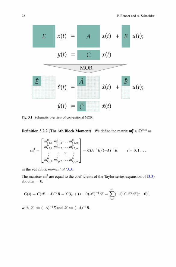
92 P. Benner and A. Schneider
Fig. 3.1 Schematic overview of conventional MOR
Definition 3.2.2 (The i-th Block Moment) We define the matrix m0i 2 C
p�m as
m0i D
266664
m0i 1;1 m0
i 1;2 : : : m0i 1;m
m0i 2;1 m0
i 2;2 : : : m0i 2;m
::::::
: : ::::
m0i p;1 m0
i p;2 : : : m0i p;m
377775 D C.A�1E/i.�A/�1B; i D 0; 1; : : :
as the i-th block moment of (3.3).
The matrices m0i are equal to the coefficients of the Taylor series expansion of (3.3)
about s0 D 0,
G.s/ D C.sE � A/�1B D C.In C .s � 0/K /�1L D1X
iD0.�1/iCK iL .s � 0/i;
with K WD .�A/�1E and L WD .�A/�1B.
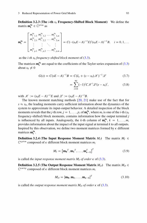
3 Reduced Representation of Power Grid Models 93
Definition 3.2.3 (The i-th s0 Frequency-Shifted Block Moment) We define thematrix ms0
i 2 Cp�m as
ms0i D
266664
ms0i 1;1 ms0
i 1;2 : : : ms0i 1;m
ms0i 2;1 ms0
i 2;2 : : : ms0i 2;m
::::::
: : ::::
ms0i p;1 ms0
i p;2 : : : ms0i p;m
377775 D C.�.s0E � A/�1E/i.s0E � A/�1B; i D 0; 1; : : :
as the i-th s0 frequency-shifted block moment of (3.3).
The matrices ms0i are equal to the coefficients of the Taylor series expansion of (3.3)
about s0 ¤ 0
G.s/ D C.sE � A/�1B D C.In C .s � s0/K /�1L (3.7)
D1X
iD0.�1/iCK iL .s � s0/
i; (3.8)
with K WD .s0E � A/�1E and L WD .s0E � A/�1B.The known moment matching methods [20, 21] make use of the fact that for
s s0, the leading moments carry sufficient information about the dynamics of thesystem to approximate its input-output behavior. A detailed inspection of the blockmoments reveals that the j-th row, j D 1; : : : ; p, of ms0
i , where mi is one of the i-th (s0frequency-shifted) block moments, contains information how the output terminal jis influenced by all inputs. Analogously, the k-th column of ms0
i , k D 1; : : : ;m,provides information about the impact of the input signal at terminal k to all outputs.Inspired by this observation, we define two moment matrices formed by � differentmatrices ms0
i .
Definition 3.2.4 (The Input Response Moment Matrix MI) The matrix MI 2C�p�m composed of � different block moment matrices mi
MI D m0
T ;m1T ; : : : ;mT
��1
T(3.9)
is called the input response moment matrix MI of order � of (3.3).
Definition 3.2.5 (The Output Response Moment Matrix MO) The matrix MO 2C�m�p composed of � different block moment matrices mi
MO D Œm0;m1; : : : ;m��1�T (3.10)
is called the output response moment matrix MO of order � of (3.3).
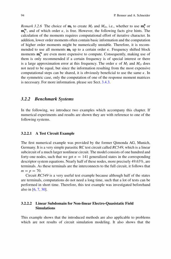
94 P. Benner and A. Schneider
Remark 3.2.6 The choice of mi to create MI and MO, i.e., whether to use m0i or
ms0i , and of which order �, is free. However, the following facts give hints. The
calculation of the moments requires computational effort of iterative character. Inaddition, lower order moments often contain basic information and the computationof higher order moments might be numerically unstable. Therefore, it is recom-mended to use all moments mi up to a certain order �. Frequency shifted blockmoments ms0
i are even more expensive to compute. Consequently, making use ofthem is only recommended if a certain frequency is of special interest or thereis a large approximation error at this frequency. The order � of MI and MO doesnot need to be equal, but since the information resulting from the most expensivecomputational steps can be shared, it is obviously beneficial to use the same �. Inthe symmetric case, only the computation of one of the response moment matricesis necessary. For more information. please see Sect. 3.4.3.
3.2.2 Benchmark Systems
In the following, we introduce two examples which accompany this chapter. Ifnumerical experiments and results are shown they are with reference to one of thefollowing systems.
3.2.2.1 A Test Circuit Example
The first numerical example was provided by the former Qimonda AG, Munich,Germany. It is a very simple parasitic RC test circuit called RC549, which is a linearsubcircuit of a much larger nonlinear circuit. The model consists of one hundred andforty-one nodes, such that we get n D 141 generalized states in the correspondingdescriptor system equations. Nearly half of these nodes, more precisely 49:65%, areterminals. As these terminals are the interconnects to the full circuit, it follows thatm D p D 70.
Circuit RC549 is a very useful test example because although half of the statesare terminals, computations do not need a long time, such that a lot of tests can beperformed in short time. Therefore, this test example was investigated beforehandalso in [6, 7, 30].
3.2.2.2 Linear Subdomain for Non-linear Electro-Quasistatic FieldSimulations
This example shows that the introduced methods are also applicable to problemswhich are not results of circuit simulation modeling. It also shows that the
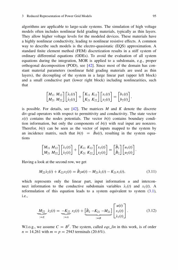
3 Reduced Representation of Power Grid Models 95
algorithms are applicable to large-scale systems. The simulation of high voltagemodels often includes nonlinear field grading materials, typically as thin layers.They allow higher voltage levels for the modeled devices. These materials havea highly nonlinear conductivity, leading to nonlinear resistive effects. A commonway to describe such models is the electro-quasistatic (EQS) approximation. Astandard finite element method (FEM) discretization results in a stiff system ofordinary differential equations (ODEs). To avoid the evaluation of all systemequations during the integration, MOR is applied to a subdomain, e.g., properorthogonal decomposition (POD), see [42]. Since most of the domain has con-stant material parameters (nonlinear field grading materials are used as thinlayers), the decoupling of the system in a large linear part (upper left block)and a small conductive part (lower right block) including nonlinearities, suchthat
�M11 M12
M21 M22
� �Px1.t/Px2.t/
�C�
K11 K12K21 K22
� �x1.t/x2.t/
�D�
b1.t/b2.t/
�;
is possible. For details, see [42]. The matrices M and K denote the discretediv-grad operators with respect to permittivity and conductivity. The state vectorx.t/ contains the nodes potentials. The vector b.t/ contains boundary condi-tion information, but only the components of b.t/ with real input are nonzero.Therefor, b.t/ can be seen as the vector of inputs mapped to the system byan incidence matrix, such that b.t/ D OBu.t/, resulting in the system equa-tions
�M11 M12
M21 M22
� �Px1.t/Px2.t/
�C�
K11 K12K21 K22
� �x1.t/x2.t/
�D� OB1
OB2� �
u1.t/u2.t/
�:
Having a look at the second row, we get
M22 Px2.t/C K22x2.t/ D OB2u.t/ � M21 Px1.t/ � K21x1.t/; (3.11)
which represents only the linear part, input information u and intercon-nect information to the conductive subdomain variables Px1.t/ and x1.t/. Areformulation of this equation leads to a system equivalent to system (3.1),i.e.,
M22„ƒ‚…WDE
Px2.t/ D �K22„ƒ‚…WDA
x2.t/C OB2 �K21 �M21
„ ƒ‚ …
WDB
24 u.t/
x1.t/Px1.t/
35 : (3.12)
W.l.o.g., we assume C D BT . The system, called eqs_lin in this work, is of ordern D 14;261 with m D p D 2943 terminals (20:6%).
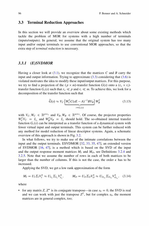
96 P. Benner and A. Schneider
3.3 Terminal Reduction Approaches
In this section we will provide an overview about some existing methods whichtackle the problem of MOR for systems with a high number of terminals(inputs/outputs). In general, we assume that the original system has too manyinput and/or output terminals to use conventional MOR approaches, so that theextra step of terminal reduction is necessary.
3.3.1 (E)SVDMOR
Having a closer look at (3.1), we recognize that the matrices C and B carry theinput and output information. Trying to approximate (3.3) considering that (3.6) isviolated motivates the idea to modify these input/output matrices. For this purpose,we try to find a projection of the . p � m/-transfer function G.s/ onto a .ro � ri/-transfer function Gr.s/ such that ro p and ri m. To achieve this, we look for adecomposition of the transfer function such that
bG.s/ VCWT
CC.sE � A/�1BVB
„ ƒ‚ …WDGr.s/
WTB (3.13)
with VC;WC 2 Rp�ro and VB;WB 2 R
m�ri . Of course, the projector propertiesWT
CVC D Iro and WTB VB D Iri should hold. The so-obtained internal transfer
function Gr.s/ can be interpreted as a transfer function of a dynamical system withfewer virtual input and output terminals. This system can be further reduced withany method for model reduction of linear descriptor systems. Again, a schematicoverview of this approach is shown in Fig. 3.2.
In what follows, we try to make use of the intimate correlations between theinput and the output terminals. ESVDMOR [32, 33, 35, 47], an extended versionof SVDMOR [16, 47], is a method which is based on the SVD of the inputand the output response moment matrices MI and MO, see Definitions 3.2.4 and3.2.5. Note that we assume the number of rows in each of both matrices to belarger than the number of columns. If this is not the case, the order � has to beincreased.
Applying the SVD, we get a low rank approximation of the form
MI D UI˙IV�I UIri
˙IriV�Iri; MO D UO˙OV�O UOro
˙OroV�Oro
; (3.14)
where
• for any matrix Z, Z� is its conjugate transpose—in case s0 D 0, the SVD is realand we can work with just the transpose ZT , but for complex s0, the momentmatrices are in general complex, too;
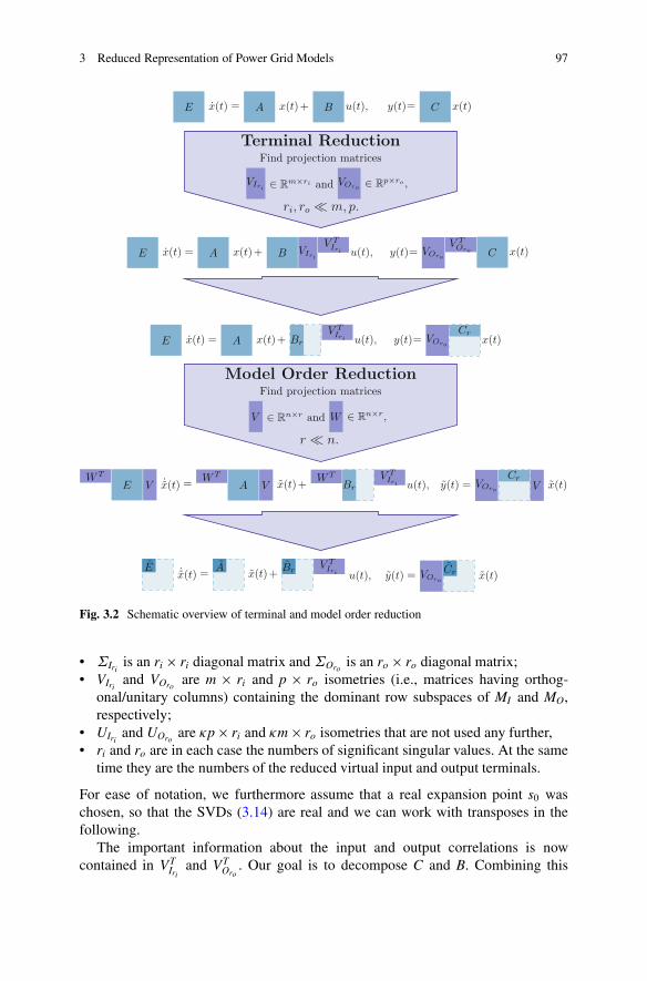
3 Reduced Representation of Power Grid Models 97
Fig. 3.2 Schematic overview of terminal and model order reduction
• ˙Iriis an ri � ri diagonal matrix and ˙Oro
is an ro � ro diagonal matrix;• VIri
and VOroare m � ri and p � ro isometries (i.e., matrices having orthog-
onal/unitary columns) containing the dominant row subspaces of MI and MO,respectively;
• UIriand UOro
are �p � ri and �m � ro isometries that are not used any further,• ri and ro are in each case the numbers of significant singular values. At the same
time they are the numbers of the reduced virtual input and output terminals.
For ease of notation, we furthermore assume that a real expansion point s0 waschosen, so that the SVDs (3.14) are real and we can work with transposes in thefollowing.
The important information about the input and output correlations is nowcontained in VT
Iriand VT
Oro. Our goal is to decompose C and B. Combining this
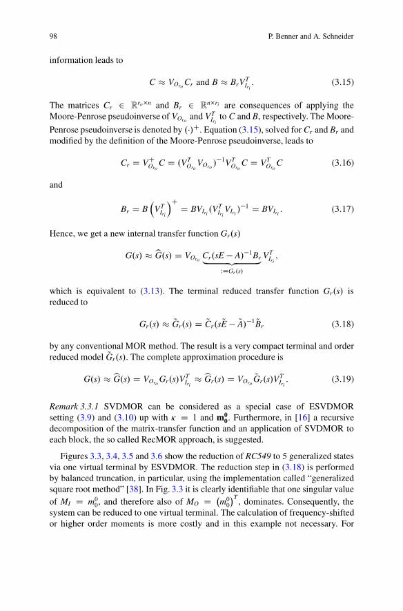
98 P. Benner and A. Schneider
information leads to
C VOroCr and B BrV
TIri: (3.15)
The matrices Cr 2 Rro�n and Br 2 R
n�ri are consequences of applying theMoore-Penrose pseudoinverse of VOro
and VTIri
to C and B, respectively. The Moore-
Penrose pseudoinverse is denoted by .�/C. Equation (3.15), solved for Cr and Br andmodified by the definition of the Moore-Penrose pseudoinverse, leads to
Cr D VCOroC D .VT
OroVOro
/�1VTOro
C D VTOro
C (3.16)
and
Br D B�
VTIri
�C D BVIri.VT
IriVIri/�1 D BVIri
: (3.17)
Hence, we get a new internal transfer function Gr.s/
G.s/ bG.s/ D VOroCr.sE � A/�1Br„ ƒ‚ …
WDGr.s/
VTIri;
which is equivalent to (3.13). The terminal reduced transfer function Gr.s/ isreduced to
Gr.s/ QGr.s/ D QCr.s QE � QA/�1 QBr (3.18)
by any conventional MOR method. The result is a very compact terminal and orderreduced model QGr.s/. The complete approximation procedure is
G.s/ bG.s/ D VOroGr.s/V
TIri
bGr.s/ D VOroQGr.s/V
TIri: (3.19)
Remark 3.3.1 SVDMOR can be considered as a special case of ESVDMORsetting (3.9) and (3.10) up with � D 1 and m0
0. Furthermore, in [16] a recursivedecomposition of the matrix-transfer function and an application of SVDMOR toeach block, the so called RecMOR approach, is suggested.
Figures 3.3, 3.4, 3.5 and 3.6 show the reduction of RC549 to 5 generalized statesvia one virtual terminal by ESVDMOR. The reduction step in (3.18) is performedby balanced truncation, in particular, using the implementation called “generalizedsquare root method” [38]. In Fig. 3.3 it is clearly identifiable that one singular valueof MI D m0
0, and therefore also of MO D �m00
�T, dominates. Consequently, the
system can be reduced to one virtual terminal. The calculation of frequency-shiftedor higher order moments is more costly and in this example not necessary. For
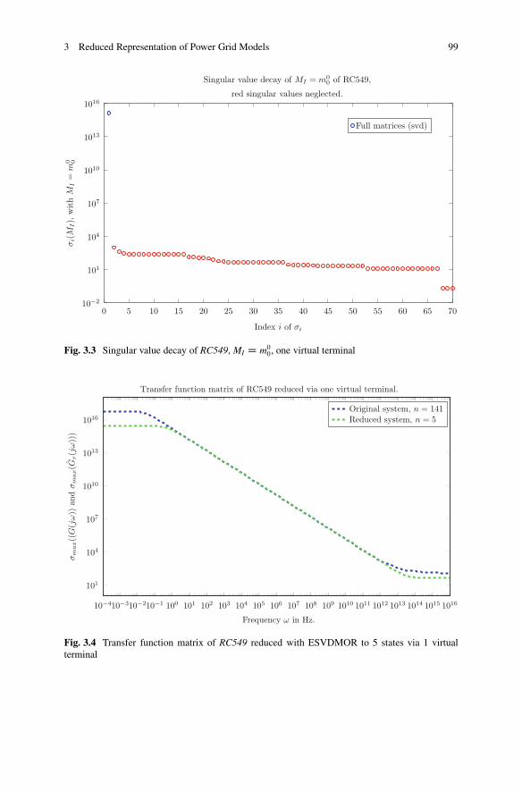
3 Reduced Representation of Power Grid Models 99
0 5 10 15 20 25 30 35 40 45 50 55 60 65 7010−2
101
104
107
1010
1013
1016
Index i of σi
σi(
MI),
with
MI
=m
0 0
Full matrices (svd)
Singular value decay of MI = m00 of RC549,
red singular values neglected.
Fig. 3.3 Singular value decay of RC549, MI D m00, one virtual terminal
10−410−310−210−1 100 101 102 103 104 105 106 107 108 109 1010 1011 1012 1013 1014 1015 1016
101
104
107
1010
1013
1016
Frequency ω in Hz.
σm
ax((
G(j
ω))
and
σm
ax(G
r(j
ω))
)
Original system, n = 141Reduced system, n = 5
Transfer function matrix of RC549 reduced via one virtual terminal.
Fig. 3.4 Transfer function matrix of RC549 reduced with ESVDMOR to 5 states via 1 virtualterminal
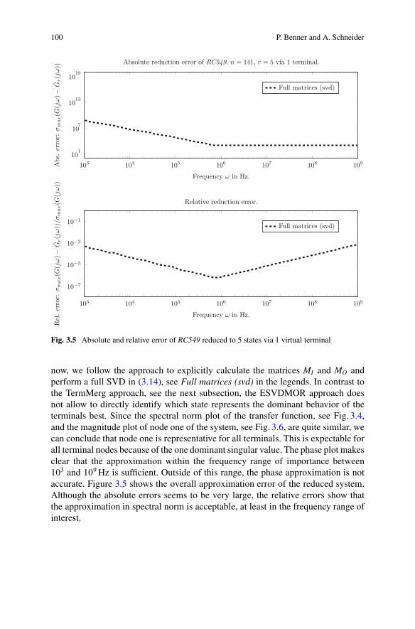
100 P. Benner and A. Schneider
103 104 105 106 107 108 10910
1
107
1013
1019
Frequency ω in Hz.
Abs.
erro
r:σm
ax(G
(jω)−
Gr(j
ω))
Absolute reduction error of RC549, n = 141, r = 5 via 1 terminal.
Full matrices (svd)
103 104 105 106 107 108 109
10−7
10−5
10−3
10−1
Frequency ω in Hz.
Rel
.er
ror:
σm
ax(G
(jω)−
Gr(j
ω))
/σm
ax(G
(jω))
Relative reduction error.
Full matrices (svd)
Fig. 3.5 Absolute and relative error of RC549 reduced to 5 states via 1 virtual terminal
now, we follow the approach to explicitly calculate the matrices MI and MO andperform a full SVD in (3.14), see Full matrices (svd) in the legends. In contrast tothe TermMerg approach, see the next subsection, the ESVDMOR approach doesnot allow to directly identify which state represents the dominant behavior of theterminals best. Since the spectral norm plot of the transfer function, see Fig. 3.4,and the magnitude plot of node one of the system, see Fig. 3.6, are quite similar, wecan conclude that node one is representative for all terminals. This is expectable forall terminal nodes because of the one dominant singular value. The phase plot makesclear that the approximation within the frequency range of importance between103 and 109 Hz is sufficient. Outside of this range, the phase approximation is notaccurate. Figure 3.5 shows the overall approximation error of the reduced system.Although the absolute errors seems to be very large, the relative errors show thatthe approximation in spectral norm is acceptable, at least in the frequency range ofinterest.
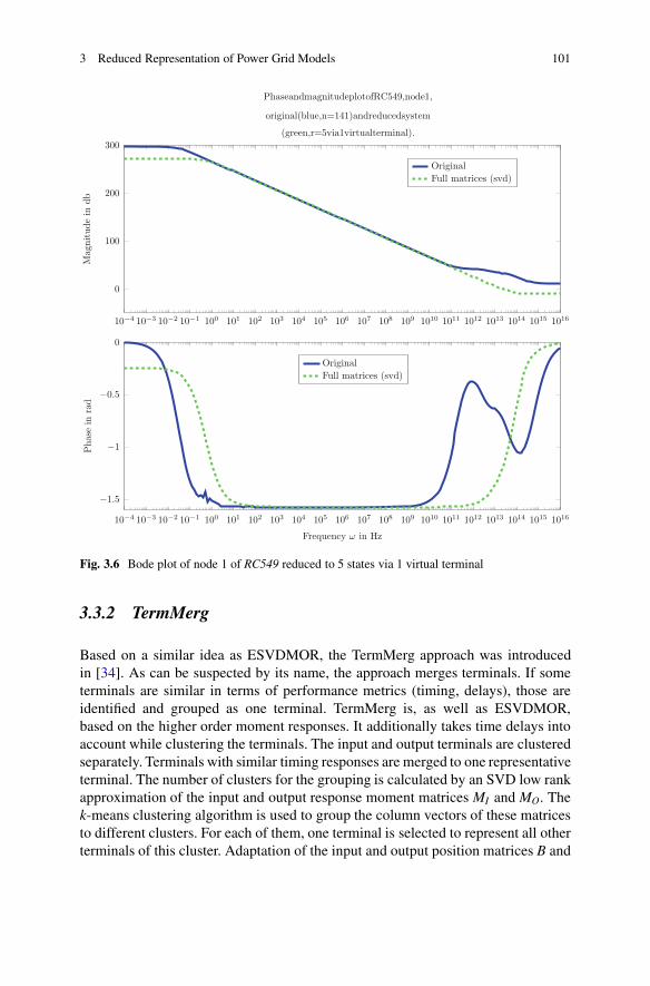
3 Reduced Representation of Power Grid Models 101
10−4 10−3 10−2 10−1 100 101 102 103 104 105 106 107 108 109 1010 1011 1012 1013 1014 1015 1016
−1.5
−1
−0.5
0
Frequency ω in Hz
Phas
ein
rad
Original
Full matrices (svd)
10−4 10−3 10−2 10−1 100 101 102 103 104 105 106 107 108 109 1010 1011 1012 1013 1014 1015 1016
0
100
200
300
Magnitude
indb
Original
Full matrices (svd)
PhaseandmagnitudeplotofRC549,node1,
original(blue,n=141)andreducedsystem
(green,r=5via1virtualterminal).
Fig. 3.6 Bode plot of node 1 of RC549 reduced to 5 states via 1 virtual terminal
3.3.2 TermMerg
Based on a similar idea as ESVDMOR, the TermMerg approach was introducedin [34]. As can be suspected by its name, the approach merges terminals. If someterminals are similar in terms of performance metrics (timing, delays), those areidentified and grouped as one terminal. TermMerg is, as well as ESVDMOR,based on the higher order moment responses. It additionally takes time delays intoaccount while clustering the terminals. The input and output terminals are clusteredseparately. Terminals with similar timing responses are merged to one representativeterminal. The number of clusters for the grouping is calculated by an SVD low rankapproximation of the input and output response moment matrices MI and MO. Thek-means clustering algorithm is used to group the column vectors of these matricesto different clusters. For each of them, one terminal is selected to represent all otherterminals of this cluster. Adaptation of the input and output position matrices B and
102 P. Benner and A. Schneider
C with respect to the representing vector of each cluster leads to a reduction in thenumber of terminals.
3.3.2.1 The k-Means Clustering Algorithm
The k-means clustering is a cluster analysis method to partition n observations into kclusters Cli, i D 1; 2; : : : ; k. Each observation belongs to the cluster with the nearestmean. We take a set of observations .x1; x2; : : : ; xn/, with xj 2 R
` for j D 1; : : : ; n,for granted. The k-means clustering aims to partition the n observations such as tominimize the within-cluster sum of squares
S DkX
iD1
Xxj2Cli
kxj � �ijj2: (3.20)
The vector�i represents the geometric centroids of the data in Cli. The final result isa set of k disjoint subsets Cli containing Ni data points each and n D Pk
iD1 Ni. Oneof the most commonly used k-means algorithms is the Lloyd algorithm [36] whichgives the global minimum of S in (3.20). The three main steps of the algorithmare:
• Initialization: Set k initial means �11; : : : ; �k1.
• Assignment: Each observation is assigned to the cluster with the closest mean,
Clit D .xj W jjxj � �i
tjj � jjxj � �i�tjj/;
for j D 1; : : : ; n, i� D 1; : : : ; k, and t denotes the iteration number, and• Update: The new center vectors of each cluster are calculated by,
�tC1i D 1
Nit
Xxj2Clit
xj:
The algorithm is repeated until there is no more change in the assignment step. Thestructure of this algorithm is responsible for the sensitivity to the initial choice of thenumber of clusters and their cluster centers. Fortunately, we calculate the numberof clusters beforehand by using the truncated SVD in (3.14). Note that the numberof reduced inputs ri and ro is equivalent to the number of input and output clusters,respectively.
Assume xj; j D 1; : : : ;m, to be a column vector of MI containing the momentsw.r.t. to one input node (node j) and all output nodes such that
MI D Œx1; x2; : : : ; xm�:
3 Reduced Representation of Power Grid Models 103
Following the Lloyd algorithm, we pick k different vectors out of the xj’s asinitial means, perform the steps described above, and save the resulting clustersCl1; : : : ;Clri as well as the corresponding centers�1; : : : ; �ri . Within TermMerg, weselect one representative terminal for each cluster. For each Cli we find the elementxj for which the distance from �i is the minimum among all elements in Cli.
Example 3.3.2 We consider a very simple matrix A defined as follows:
A D�1 3 5 7
2 4 6 8
�:
Suppose we group the four columns into two clusters Cl1 and Cl2. We choose theinitial centroids randomly as �11 D .3; 4/T and �21 D .5; 6/T . We compute adistance matrix containing the squared Euclidean distances of each element (columnindex) to each cluster (row index). For the first element a1 D .1; 2/T , the distancefrom the first centroid is given by .1�3/2C .2�4/2 D 8. We construct the distancematrix as
D D�8 0 8 32
32 8 0 8
�:
The first set of clusters is Cl11 D fa1; a2g and Cl21fa3; a4g. The new centroids are�1
2 D .2; 3/T and �22 D .6; 7/T . We repeat the process, and the second set ofclusters turns out to be the same as the first one. Consequently, the centroids staythe same. Since there is no further change in the centroids, the four columns can beclustered into Cl12 and Cl22.
3.3.2.2 The Reduction Step
Once we know the number of clusters for inputs and outputs, we perform k-meansto cluster the terminals. We find the representative terminal for each cluster andaccordingly replace columns of the input position matrix B and the rows of theoutput position matrix C. We include only the representative terminals.
3.3.3 SparseRC
In this subsection we comment on an approach based on a completely different ideafrom the one used in the approaches we introduced up to now. Indeed, SparseRC,which is introduced in [25, 26], also performs MOR although the number ofterminals may be very large. A specialty is that the approach is considerably moreuser-oriented. Its application is the reduction of parasitic RC circuits in simulation,
104 P. Benner and A. Schneider
e.g. power grids. In [26], the following five basic objectives for successful modelreduction are mentioned:
• the approximation error kG. : / � OG. : /k is small in an appropriate norm,• stability and passivity are preserved,• an efficient computation is possible,• for reconnection, the incidence input/output matrix B is preserved in some sense,
i.e., OB is a sub-matrix of B, and• the reduced system matrices OE and OA are sparse.
While the first three items can be nearly taken for granted in MOR, the last two itemsare user-oriented specifications which are hard to meet. Even if the last item may besatisfied by some approaches, the next-to-last item is in general not satisfied as inmost conventional MOR methods, the reduced model is not sparse. The SparseRCapproach promises to fulfill these five items. The basic idea is to apply extendedmoment matching projection (EMMP), see next section, to disjoint parts of theoriginal system.
3.3.3.1 MOR via Graph Partitioning and EMMP
Following [26], the EMMP (derived from an algorithm based on pole analysis viacongruence transformations called PACT [28] and from sparse implicit projection(SIP), see [48]) is a moment matching type reduction approach suitable for multi-terminal systems with only a few terminals. Within SparseRC, this projectionmethod is applied to subsystems connected via so called separator nodes. Eachsubsystem has just a few terminals and the connection of all reduced subsystemsleads to a reduced-order version of the original system.
Assume such a subsystem is given as an LTI system obtained from modeling anRC circuit. In this situation, system (3.4), re-arranged and in frequency domain, canbe written as
.sE � A/x.s/ D Bu.s/; (3.21)
when ignoring the output term. Now we do a simple block separation into selectednodes xs (terminals and separator nodes) and internal nodes xi. This leads to
�s
�Ei Ec
ETc Es
���
Ai Ac
ATc As
���xi
xs
�D�0
Bs
�u;
where Ai;Ei 2 R.n�s/�.n�s/, Bs 2 R
s�s with s � m being the number of selectednodes, i.e. the number of terminals m plus the separator nodes which are preservedbecause of the coupling within SparseRC. Applying a congruence transform with
3 Reduced Representation of Power Grid Models 105
W WD �A�1i Ac and
X D�
In�s W0 Is
�; Nx D XTx
such that .A;E;B/ are mapped to .XTAX;XTEX;XTB/, yields
�s
�Ei NEcNET
cNEs
���
Ai 0
0 NAs
���xi
Nxs
�D�0
Bs
�u; (3.22)
with
NEc D Ec C EiW;
NEs D Es C WTEiW C WT Ec C ETc W; (3.23)
NAs D As C ATc W: (3.24)
Solving the first row in (3.22) for xi and plugging the result into the equation of thesecond row of (3.22) leads to
.s NEs � NAs/Nxs � s2 NET.sEi � Ai/�1 NEc Nxs D Bsu:
Following [26] further on, the first two moments of system (3.21) at s D 0 are givenby NEs and NAs in (3.23) and (3.24). Consequently, a reduced-order model OA; OE 2 R
k�k,k � s, which preserves the first two admittance moments of (3.21) can be computed
via a moment matching projection V D WT Is
Tgiven by
OA D VTAV; OB D VTB;
OE D VTEV; and Ox D VTx D Nxs:
The question remains how to partition the original RC system with many terminalsin an appropriate way such that we can apply EMMP to the subsystems. Thereare two goals during this process, which depend on each other. One is to find apartitioning and the second is to avoid fill-in such that the reduced model is stillsparse. Usually, fill-in minimizing matrix reordering techniques similar to thoseused to compute an efficient Cholesky factorization can identify nodes causingfill-in. SparseRC avoids these techniques due to circuit size or topology. Instead,graph decomposition based on the non-zero pattern (nzp) of E � A is used due tothe analogy between circuit models and graphs. The fill-creating nodes, i.e., theseparation nodes, are identified and the circuit matrices are reordered in a so-called
106 P. Benner and A. Schneider
bordered block diagonal (BBD) form [49]. In this form, the individual blocksform the subsystems to be reduced and the border blocks contain the separatornodes, which are preserved during the EMMP. Both goals are achieved and thefive objectives for MOR above are fulfilled. For a detailed discussion, e.g., aboutthe matrix properties such as the singularity of Ai or implementation details, see[25, 26]. The approach is generalized to RLC networks in [25].
3.3.4 MOR for Many Terminals via Interpolation
This section deals with the modeling of RLC systems of the form (3.1) by meansof S-parameters (scattering parameters), i.e., measurements of frequency domainresponse data [29]. A typical application would be a black box problem. Givenis an electrical device, but the knowledge about the circuit inside the device isunidentified. With the help of, e.g., a Vector Network Analyzer (VNA), it ispossible to measure amplitude and phase properties. We get P samples at differentfrequencies fj, j D 1; : : : ;P, of the device with m inputs and p outputs as
S. j/ WD
2664
S. j/11 � � � S. j/
1m:::
::::::
S. j/p1 � � � S. j/
pm
3775 : (3.25)
The goal is to find the associated transfer function G.s/ such that its values at s D i!with ! D 2�fj are close to the scattering matrix. If kG.i 2�fj/ � S. j/k is small insome norm, the computed representation matrices belong to an accurate model. Theapproach uses tangential interpolation and the Loewner matrix concept to find amodel, even a reduced-order model, of this multiport device.
3.3.4.1 Tangential Interpolation and the Loewner Concept
Tangential interpolation is a form of the standard interpolation problem along atangential direction. Consider k different sampling points i 2 C, the tangentialdirections ri 2 C
m�1, and the tangential data wi 2 Cp�1, such that
� D f1; : : : ; kg � Ck;
R D Œr1; : : : ; rk� 2 Cm�k; and
W D Œw1; : : : ;wk� 2 Cp�k
3 Reduced Representation of Power Grid Models 107
is called the right interpolation data. Analogously, we define the left interpolationdata �j 2 C, lj 2 C
1�p and vj 2 C1�m at another h sampling points as
� D f�1; : : : ; �kg � Ch;
L D lT1 ; : : : ; l
Th
T 2 Ch�p; and
V D vT1 ; : : : ; v
Th
T 2 Ch�m:
The rational interpolation problem aims at finding a set of system matrices, suchthat the right and left interpolation constrains
G.i/ri D wi; i D 1; : : : ; k; (3.26)
and ljG.�j/ D vj; j D 1; : : : ; h; (3.27)
are fulfilled by the associated transfer function G.s/.
Definition 3.3.3 (The Loewner and the Shifted Loewner Matrix) Given are aset of P D kCh sampling points f1; : : : ; k; �1; : : : ; �hg and the values of a rationalmatrix function G.i/ and G.�j/ evaluated at these points. By defining tangentialdirections ri and lj we are able to compute the tangential data wi and vj. The matrix
L D
2664v1r1�l1w1�1�1 � � � v1rk�l1wk
�1�k:::
::::::
vhr1�lhw1�h�1 � � � vhrk�lhwk
�h�k
3775
is called the Loewner matrix. The shifted Loewner matrix is defined as
�L D
2664�1v1r1�1l1w1
�1�1 � � � �1v1rk�k l1wk�1�k
::::::
:::�hvhr1�1lhw1
�h�1 � � � �hvhrk�k lhwk�h�k
3775 :
By means of the matrices of Definition 3.3.3 and their properties, e.g., theysatisfy certain Sylvester equations and turn out to reveal some kind of tangentialcontrollability and observability Gramians, we can solve the modeling problem forthe given data.
Lemma 3.3.4 Assume k D h (half of P, if impossible ignore one sampling point)and det.zL � �L/ ¤ 0 for all z 2 fig [ f�jg. Then E D �L, A D ��L, B D V,
108 P. Benner and A. Schneider
C D W, and D D 0 is a minimal realization1 of the system whose transfer function
G.s/ D W.�L � sL/�1V
interpolates the given data such that (3.26) and (3.27) are satisfied.
Note that we assume exact data and the needed number of samples. For a proof andmore details we again point to [29]. There, it is also explained how to reveal theorder of the underlying system, how to handle different scenarios of measurements,and how to get reduced-order models. This kind of approach can be extended toparametric systems, see [3].
Another important information is how to get the tangential data from (3.25). Notethat, like in the scattering matrix, for real passive RC circuits the number of inputsis equal to the number of outputs m D p. In [29], it is proposed to define ri and lj asrows and columns of the identity matrix Im to be linearly independent. Consequently,for j D 1; : : : ; k, the right interpolation data can be constructed as
j D i!j; rj D eq; and wj D S. j/rj;
where eq 2 Rm�1 (an m-dimensional unit vector with entry 1 in its q-th position)
with j � q mod m. If q D 0 we set q D m, i.e., if the division of k and m is withoutresidual, we take the last row of Im as rj. Analogously, for j D 1; : : : ; h we get theleft interpolation data as
�j D �i!j; lj D rTj ; and vj D ljS. j/:
3.4 ESVDMOR in Detail
3.4.1 Stability, Passivity, Reciprocity
The preservation of properties is an important topic in MOR. Besides the essentialinformation encoded in the equations of the original system (3.1), e.g., resistancevalues or capacities, other information, e.g., structural characteristics (block struc-ture, sparsity) or physical qualities, can be of interest. The preservation of suchproperties is of prime importance in a lot of applications. Typically in circuitsimulation, three basic properties to preserve are stability, passivity, and reciprocity;see also Sect. 2.2.3. For this reason, in the following section we give some basicdefinitions and lemmas to establish facts on the preservation of these three propertiesin reduced-order models generated by ESVDMOR [7].
1Loosely speaking, a minimal realization of a descriptor system is a set of matrices .A;B;C;E/ ofminimal order yielding the transfer function G.s/ of the system.
3 Reduced Representation of Power Grid Models 109
3.4.1.1 Stability
In the analysis of dynamical systems it is important to study the dynamics if theconsidered time horizon goes to infinity. The reduced system is intended to showthe same behavior as the original one. The following basic definition and lemmacan be found, e.g., in [10, 14].
Definition 3.4.1 (Asymptotic Stability, c-Stability) The descriptor system (3.1)is asymptotically stable if all solutions x.t/ of EPx.t/� Ax.t/ D 0 converge to zero atinfinity, i.e.,
limt!1 x.t/ D 0:
The matrix pencil E � A, 2 C, is called c-stable if it is regular and thecorresponding system (3.1) is asymptotically stable.
Lemma 3.4.2 Consider a descriptor system (3.1) with a regular matrix pencilE � A. The following statements are equivalent:
1. System (3.1) is asymptotically stable.2. The finite eigenvalues of the pencil E � A, i 2 �.A;E/, lie in the open left
complex half-plane, i.e., i 2 C� D f 2 Cj Re./ < 0g.3. Consider the spectral projections Pr and Pl, respectively, onto the right and the
left deflating subspace of the pencil corresponding to the finite eigenvalues. Theprojected generalized continuous-time Lyapunov equation
ETXA C ATXE C PTr QPr D 0; X D PT
l XPl
has a unique Hermitian, positive semidefinite (psd) solution X for every Hermi-tian, psd right hand side matrix Q.
Remark 3.4.3 The infinite eigenvalues of the pencil do not affect the behavior of thehomogeneous system in Definition 3.4.1. Consequently they do not affect stability.A very useful observation of Lemma 3.4.2 is the connection between the stabilityof the system and the finite eigenvalues of the pencil. We use this fact to prove thefollowing theorem.
Theorem 3.4.4 Assume the descriptor system (3.1) with its transfer function (3.3)to be asymptotically stable. The ESVDMOR reduced-order system corresponding toOGr.s/ of (3.19) is asymptotically stable if the inner reduction to QGr.s/ of (3.18) isstability preserving.
Proof According to Lemma 3.4.2, we know that in the continuous-time casestability is preserved if the pencil of the reduced system is c-stable. Besidesregularity this means Re. Q/ < 0 for all Q 2 �. QA; QE/ (the spectrum of the matrixpencil QE � QA). Remembering that the original system G.s/ is asymptotically stable,i.e., .E � A/ is c-stable, the following implication is obvious:
110 P. Benner and A. Schneider
The inner reduction Gr.s/ QGr.s/ in (3.18) is stability preservingH) . QE � QA/ is c-stableH) the reduction G.s/ OGr.s/ in (3.19) is stability preserving.
Remark 3.4.5 Many established MOR methods for regular descriptor systems arestability preserving and can be applied along the lines of Theorem 3.4.4. Due to theircomputable error bounds we prefer the use of balanced truncation based approaches,see [5, 10], and in particular the specialized versions described in Chap. 2 dedicatedto circuit equations.
3.4.1.2 Passivity
One of the most common definitions of passivity of a circuit is the property thatits elements consume (or at least do not produce) energy. Thus, if the originalsystem is passive, also the reduced model should be passive in order to remainphysically meaningful. In other words, passivity preservation is important forstable, accurate, and interpretable simulation results, see also Chap. 2. A moremathematical definition of passivity is the following one, taken from [40].
Definition 3.4.6 (Passivity) A descriptor system (3.1) is called passive (or input-output-passive) if m D p and the system output y W R ! R
m satisfies
Z T
t0
u.t/Ty.t/dt � 0; (3.28)
for all possible inputs u W R ! Rm, where x.t0/ D 0, the functions u and y are
square integrable, and Œ0 � t0I T� � R is the time period of interest.
Since for linear systems a shifting of the time horizon is not a problem, we canassume t0 D 0. Passivity, such as in the previous definition, is hard to show.Therefore, we use another concept, discussed, e.g., in [20], for constructive passivitytesting.
Definition 3.4.7 (Positive Real Transfer Function) The transfer function (3.3) ispositive real iff the following three assumptions hold:
(i) G.s/ has no poles in CC D fs 2 Cj Re.s/ > 0g, and additionally there are nomultiple poles of G.s/ on the imaginary axis iR,
(ii) G.Ns/ D G.s/ for all s 2 C;
(iii) Re.x�G.s/x/ � 0 for all s 2 CC and x 2 Cm, i.e. G.s/� C G.s/ � 0 for all
s 2 CC.
To show some results about passivity preservation of ESVDMOR, we need to knowthe connection between passivity and positive realness.
3 Reduced Representation of Power Grid Models 111
Lemma 3.4.8 A descriptor system (3.1) is passive if, and only if, its transferfunction (3.3) is positive real.
Remark 3.4.9 The original proof can be found in [1]. In [1, 37, 41] another proofof this lemma shows the equivalence of passivity and the bounded realness of thescattering matrix function, which is nothing else than a Moebius transformationof G.s/. Subsequently, the equivalence of the bounded realness of this scatteringmatrix function and the positive realness of the transfer function is shown. Hencethe lemma is proven.
As already mentioned in Definition 3.4.6, for passive systems we assume that thenumber of inputs is equal to the number of outputs: m D p. We furthermoreassume (3.4) and (3.5). As before, the matrix pencil E�A is assumed to be regular.
Theorem 3.4.10 Consider a passive system of the form (3.4) with its transfer func-tion (3.5). The ESVDMOR reduced-order system corresponding to OGr.s/ of (3.19)is passive if the inner reduction to QGr.s/ of (3.18) is passivity preserving.
Proof Following Lemma 3.4.8, we show thatbGr.s/ in (3.19) is positive real. Hence,we show that the reduced system is passive. The i-th s0 frequency-shifted blockmoments of (3.5) are
ms0i D BT.�.s0E � A/�1E/i.s0E � A/�1B;
with det.s0E �A/ 6D 0. Following the technique used in [21], we define J D�
I 0
0 �I
�
with appropriate block structure. The properties of A1, E1, and E2 as well as the factthat J D JT and J2 D I lead to the following rules:
R1: J D J�1,R2: JE D EJ, hence JEJ D E,R3: .s0E � A/T D s0E � JAJ D s0JEJ � JAJ, hence .s0E � A/�T D .s0JEJ �JAJ/�1 D J�1.s0E � A/�1J�1 D J.s0E � A/�1J,R4: B D JB, andR5: for every matrix X, Y and i 2 N, .�X�1Y/i D X�1.Y.�X/�1/iX holds.
A straightforward calculation employing these rules shows that
ms0i
T D .BT .�.s0E � A/�1E/i.s0E � A/�1B/T
D BT .s0E � A/�T f.�.s0E � A/�1„ ƒ‚ …�X�1
E„ƒ‚…Y
/igTB
.R5/D BT .s0E � A/�T f.s0E � A/�1.E.�.s0E � A/�1//i.s0E � A/gT B
D BT .s0E � A/�T .s0E � A/Tf.E.�.s0E � A/�1//igT.s0E � A/�T B
D BT f.E.�.s0E � A/�1//igT.s0E � A/�T B
112 P. Benner and A. Schneider
.EDET /D BT ..�.s0E � A//�T E/i.s0E � A/�T B
.R3/D BT .�J.s0E � A/�1JE/i.J.s0E � A/�1J/B
.R5/D BT J.s0E � A/�1.JE.�J.s0E � A/�1//i.s0E � A/J.J.s0E � A/�1J/B
.R1;R2/D BT J.s0E � A/�1.E.�.s0E � A/�1//i.s0E � A/.s0E � A/�1JB
D BT J.s0E � A/�1.E.�.s0E � A/�1//iJB
.R4/D BT .s0E � A/�1.E.�.s0E � A/�1//iB
.R5 backwards/D BT .�.s0E � A/�1E/i.s0E � A/�1B
D ms0i :
By means of (3.14) it follows from (3.9) and (3.10) that MI D MO, such that VTIri
DVT
OroD VT
r . Hence
bG.s/ D VrBTr .sE � A/�1BrV
Tr ; (3.29)
with Br analogous to (3.17). If the MOR method used in (3.18) leads to a positivereal transfer function, passivity is preserved.
In Definition 3.4.7 and Lemma 3.4.8 it is shown that the system (3.4) is passiveif the Hermitian part of the transfer function along the imaginary axis is positivesemidefinite, i. e., GH D 1
2.G. j!/ C G. j!// � 0. As an illustration, in Fig. 3.7
we show the smallest nonzero eigenvalue of the Hermitian part of the originaltransfer function GH. j!/ and of the terminal, not yet order reduced transfer functionOGH. j!/. In every case the systems are positive semidefinite. Figure 3.8 shows therelative difference of these smallest eigenvalues to those of the original system. Aswe only add zero eigenvalues in (3.19) by multiplying VOro
D Vr and VTIri
D VTr
from the left and the right to the positive real transfer function QGr.s/, positivesemidefiniteness is preserved.
As inner reduction method, again the passivity-preserving balanced truncationapproaches described in Chap. 2 can be employed.
3.4.1.3 Reciprocity
Another important property of MOR methods is reciprocity preservation, which isa requirement for the synthesis of the reduced-order model as a circuit. We assumethe setting given in (3.4). An appropriate definition can be found, e.g., in [40].
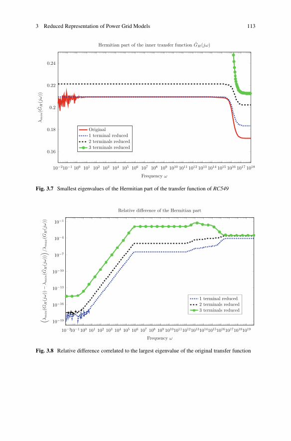
3 Reduced Representation of Power Grid Models 113
10−210−1 100 101 102 103 104 105 106 107 108 109 1010 1011 1012 1013 1014 1015 1016 1017 1018
0.16
0.18
0.2
0.22
0.24
Frequency ω
λm
in(G
H(j
ω))
Hermitian part of the inner transfer function GH(jω)
Original1 terminal reduced2 terminals reduced3 terminals reduced
Fig. 3.7 Smallest eigenvalues of the Hermitian part of the transfer function of RC549
10−210−1100 101 102 103 104 105 106 107 108 109 1010101110121013101410151016101710181019
10−19
10−16
10−13
10−10
10−7
10−4
10−1
Frequency ω
( λm
in(G
H(j
ω))−
λm
in(G
H(j
ω))
) /λm
ax(G
H(j
ω))
Relative difference of the Hermitian part
1 terminal reduced2 terminals reduced3 terminals reduced
Fig. 3.8 Relative difference correlated to the largest eigenvalue of the original transfer function
114 P. Benner and A. Schneider
Definition 3.4.11 A transfer function (3.3) is reciprocal if there exist m1;m2 2 N
with m1 C m2 D m, such that for ˙e D diag.Im1 ;�Im2/ and all s 2 C being not apole of G.s/, it holds
G.s/˙e D ˙eGT.s/:
The matrix ˙e is called external signature of the system. A descriptor system iscalled reciprocal if its transfer function is reciprocal.
As a consequence, a transfer function of a reciprocal system is a matrix of the form
G.s/ D�
G11.s/ G12.s/�GT
12.s/ G22.s/
�; (3.30)
where G11.s/ D GT11.s/ 2 R
m1;m1 and G22.s/ D GT22.s/ 2 R
m2;m2 . That is,
G.s/
�0 I
�I 0
�is a Hamiltonian matrix.
Theorem 3.4.12 Consider a reciprocal system of the form (3.4). The ESVDMORreduced-order system corresponding to OGr.s/ of (3.19) is reciprocal if the innerreduction to QGr.s/ of (3.18) is reciprocity preserving.
Proof Due to the reciprocity of the original system, the corresponding transferfunction (3.5) has the structure given in (3.30). Equation (3.29) shows that noneof the steps in ESVDMOR destroy this symmetric structure if (3.18) preservesreciprocity.
3.4.2 Error Analysis
Knowledge about the approximation error is motivated by the desire to meetthe (industrial) requirements placed on the reduced-order model and, at thesame time, to get a reduced model, which is as small as possible and as goodas necessary. Because approximation errors are, of course, caused at differentsteps of the algorithm, an analysis of these particular errors is an importantbasis to estimate the total approximation error. Most of the particular singleerrors are well studied. In the following section, we describe the results abouta priori error estimation of the ESVDMOR approximation in [8]. Based onthe known approximation errors, e.g. those of truncated SVD or balancedtruncation, we combine all errors, firstly with many assumptions and laterfor more general models, to derive a global error bound of the ESVDMORapproach.
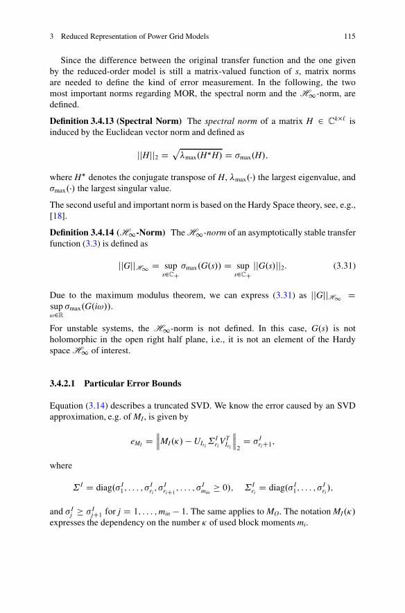
3 Reduced Representation of Power Grid Models 115
Since the difference between the original transfer function and the one givenby the reduced-order model is still a matrix-valued function of s, matrix normsare needed to define the kind of error measurement. In the following, the twomost important norms regarding MOR, the spectral norm and the H1-norm, aredefined.
Definition 3.4.13 (Spectral Norm) The spectral norm of a matrix H 2 Ck�` is
induced by the Euclidean vector norm and defined as
jjHjj2 Dpmax.H�H/ D �max.H/;
where H� denotes the conjugate transpose of H, max.�/ the largest eigenvalue, and�max.�/ the largest singular value.
The second useful and important norm is based on the Hardy Space theory, see, e.g.,[18].
Definition 3.4.14 (H1-Norm) The H1-norm of an asymptotically stable transferfunction (3.3) is defined as
jjGjjH1D sup
s2CC
�max.G.s// D sups2CC
jjG.s/jj2: (3.31)
Due to the maximum modulus theorem, we can express (3.31) as jjGjjH1D
sup!2R
�max.G.i!//.
For unstable systems, the H1-norm is not defined. In this case, G.s/ is notholomorphic in the open right half plane, i.e., it is not an element of the Hardyspace H1 of interest.
3.4.2.1 Particular Error Bounds
Equation (3.14) describes a truncated SVD. We know the error caused by an SVDapproximation, e.g. of MI , is given by
eMI D���MI.�/ � UIri
˙ Iri
VTIri
���2
D � IriC1;
where
˙ I D diag.� I1; : : : ; �
Iri; � I
riC1; : : : ; � I
min� 0/; ˙ I
riD diag.� I
1; : : : ; �Iri/;
and � Ij � � I
jC1 for j D 1; : : : ;min � 1. The same applies to MO. The notation MI.�/
expresses the dependency on the number � of used block moments mi.
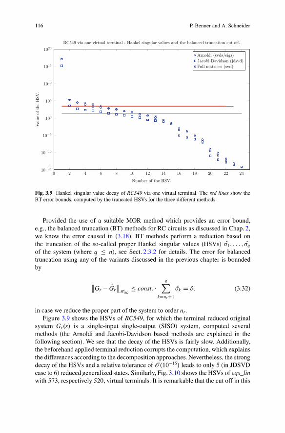
116 P. Benner and A. Schneider
0 2 4 6 8 10 12 14 16 18 20 22 2410−15
10−10
10−5
100
105
1010
1015
1020
Number of the HSV.
Val
ue
ofth
eH
SV
.
RC549 via one virtual terminal - Hankel singular values and the balanced truncation cut off.
Arnoldi (svds/eigs)
Jacobi Davidson (jdsvd)
Full matrices (svd)
Fig. 3.9 Hankel singular value decay of RC549 via one virtual terminal. The red lines show theBT error bounds, computed by the truncated HSVs for the three different methods
Provided the use of a suitable MOR method which provides an error bound,e.g., the balanced truncation (BT) methods for RC circuits as discussed in Chap. 2,we know the error caused in (3.18). BT methods perform a reduction based onthe truncation of the so-called proper Hankel singular values (HSVs) O�1; : : : ; O�q
of the system (where q � n), see Sect. 2.3.2 for details. The error for balancedtruncation using any of the variants discussed in the previous chapter is boundedby
��Gr � QGr
��H1
� const: �qX
kDnrC1O�k D ı; (3.32)
in case we reduce the proper part of the system to order nr.Figure 3.9 shows the HSVs of RC549, for which the terminal reduced original
system Gr.s/ is a single-input single-output (SISO) system, computed severalmethods (the Arnoldi and Jacobi-Davidson based methods are explained in thefollowing section). We see that the decay of the HSVs is fairly slow. Additionally,the beforehand applied terminal reduction corrupts the computation, which explainsthe differences according to the decomposition approaches. Nevertheless, the strongdecay of the HSVs and a relative tolerance of O.10�15/ leads to only 5 (in JDSVDcase to 6) reduced generalized states. Similarly, Fig. 3.10 shows the HSVs of eqs_linwith 573, respectively 520, virtual terminals. It is remarkable that the cut off in this
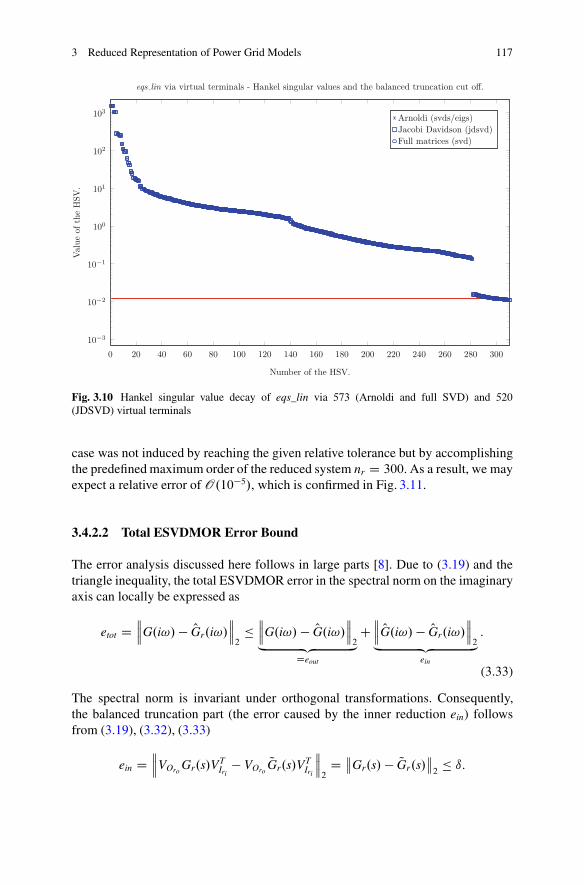
3 Reduced Representation of Power Grid Models 117
0 20 40 60 80 100 120 140 160 180 200 220 240 260 280 300
10−3
10−2
10−1
100
101
102
103
Number of the HSV.
Valu
eofth
eH
SV
.eqs lin via virtual terminals - Hankel singular values and the balanced truncation cut off.
Arnoldi (svds/eigs)
Jacobi Davidson (jdsvd)
Full matrices (svd)
Fig. 3.10 Hankel singular value decay of eqs_lin via 573 (Arnoldi and full SVD) and 520
(JDSVD) virtual terminals
case was not induced by reaching the given relative tolerance but by accomplishingthe predefined maximum order of the reduced system nr D 300. As a result, we mayexpect a relative error of O.10�5/, which is confirmed in Fig. 3.11.
3.4.2.2 Total ESVDMOR Error Bound
The error analysis discussed here follows in large parts [8]. Due to (3.19) and thetriangle inequality, the total ESVDMOR error in the spectral norm on the imaginaryaxis can locally be expressed as
etot D���G.i!/� OGr.i!/
���2
����G.i!/ � OG.i!/
���2„ ƒ‚ …
Deout
C��� OG.i!/� OGr.i!/
���2„ ƒ‚ …
ein
:
(3.33)
The spectral norm is invariant under orthogonal transformations. Consequently,the balanced truncation part (the error caused by the inner reduction ein) followsfrom (3.19), (3.32), (3.33)
ein D���VOro
Gr.s/VTIri
� VOroQGr.s/V
TIri
���2
D ��Gr.s/ � QGr.s/��2
� ı:
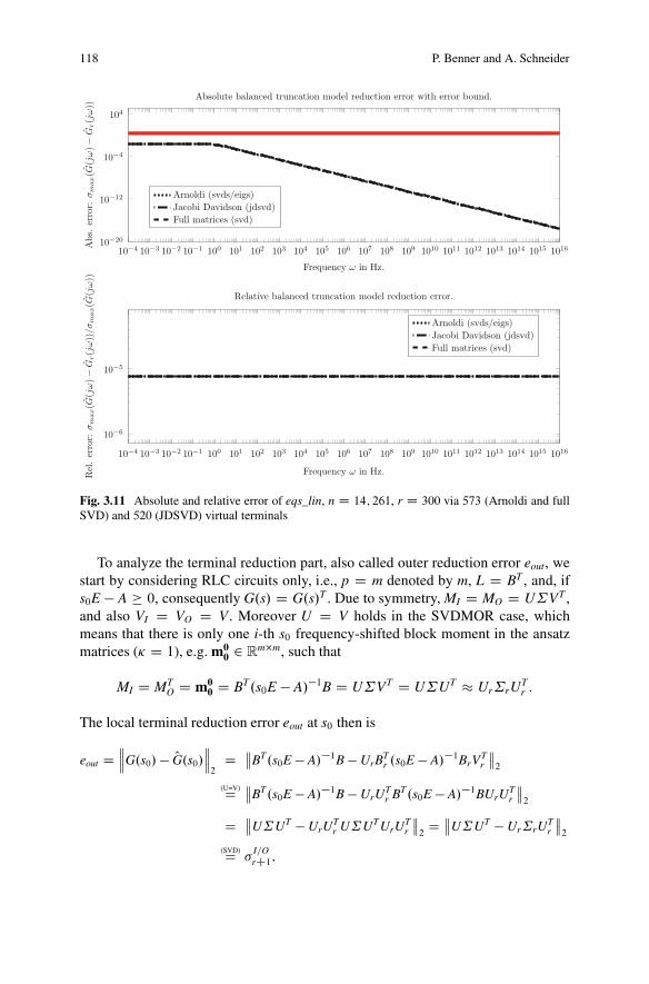
118 P. Benner and A. Schneider
10−4 10−3 10−2 10−1 100 101 102 103 104 105 106 107 108 109 1010 1011 1012 1013 1014 1015 101610−20
10−12
10−4
104
Frequency ω in Hz.
Abs.
erro
r:σm
ax(G
(jω)−
Gr(j
ω))
Absolute balanced truncation model reduction error with error bound.
Arnoldi (svds/eigs)
Jacobi Davidson (jdsvd)
Full matrices (svd)
10−4 10−3 10−2 10−1 100 101 102 103 104 105 106 107 108 109 1010 1011 1012 1013 1014 1015 1016
10−6
10−5
Frequency ω in Hz.Rel
.er
ror:
σm
ax(G
(jω)−
Gr(j
ω))
/σm
ax(G
(jω))
Relative balanced truncation model reduction error.
Arnoldi (svds/eigs)
Jacobi Davidson (jdsvd)
Full matrices (svd)
Fig. 3.11 Absolute and relative error of eqs_lin, n D 14; 261, r D 300 via 573 (Arnoldi and fullSVD) and 520 (JDSVD) virtual terminals
To analyze the terminal reduction part, also called outer reduction error eout, westart by considering RLC circuits only, i.e., p D m denoted by m, L D BT , and, ifs0E � A � 0, consequently G.s/ D G.s/T . Due to symmetry, MI D MO D U˙VT ,and also VI D VO D V . Moreover U D V holds in the SVDMOR case, whichmeans that there is only one i-th s0 frequency-shifted block moment in the ansatzmatrices (� D 1), e.g. m0
0 2 Rm�m, such that
MI D MTO D m0
0 D BT.s0E � A/�1B D U˙VT D U˙UT Ur˙rUTr :
The local terminal reduction error eout at s0 then is
eout D���G.s0/ � OG.s0/
���2
D ��BT.s0E � A/�1B � UrBTr .s0E � A/�1BrV
Tr
��2
(U=V)D ��BT.s0E � A/�1B � UrUTr BT.s0E � A/�1BUrU
Tr
��2
D ��U˙UT � UrUTr U˙UTUrU
Tr
��2
D ��U˙UT � Ur˙rUTr
��2
(SVD)D �I=OrC1;
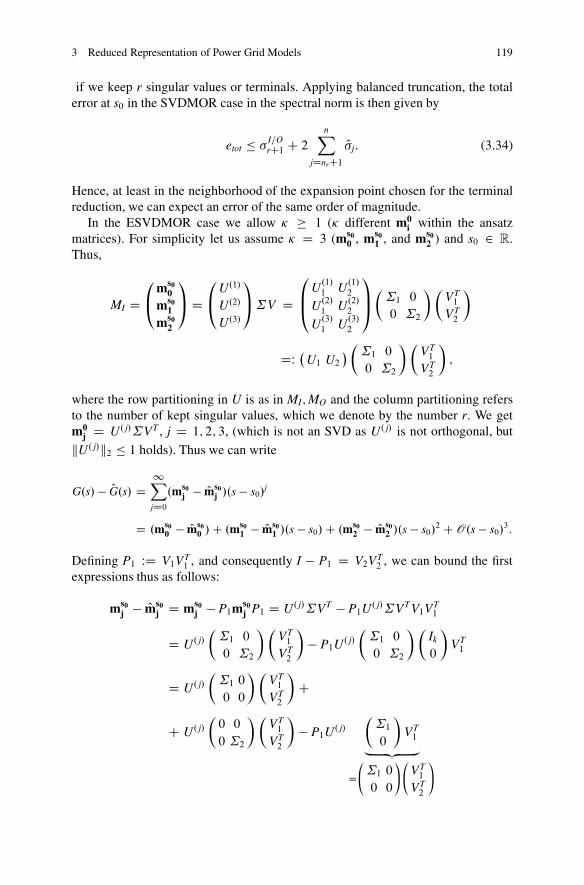
3 Reduced Representation of Power Grid Models 119
if we keep r singular values or terminals. Applying balanced truncation, the totalerror at s0 in the SVDMOR case in the spectral norm is then given by
etot � �I=OrC1 C 2
nXjDnrC1
O�j: (3.34)
Hence, at least in the neighborhood of the expansion point chosen for the terminalreduction, we can expect an error of the same order of magnitude.
In the ESVDMOR case we allow � � 1 (� different m0i within the ansatz
matrices). For simplicity let us assume � D 3 (ms00 , ms0
1 , and ms02 ) and s0 2 R.
Thus,
MI D0@ms0
0ms0
1
ms02
1A D
U.2/
U.3/
1A˙V D
0B@
U.1/1 U.1/
2
U.2/1 U.2/
2
U.3/1 U.3/
2
1CA�˙1 0
0 ˙2
��VT1
VT2
�
DW �U1 U2
� �˙1 0
0 ˙2
��VT1
VT2
�;
where the row partitioning in U is as in MI;MO and the column partitioning refersto the number of kept singular values, which we denote by the number r. We getm0
j D U. j/˙VT , j D 1; 2; 3, (which is not an SVD as U. j/ is not orthogonal, but
kU. j/k2 � 1 holds). Thus we can write
G.s/ � OG.s/ D1X
jD0
.ms0j � Oms0
j /.s � s0/j
D .ms00 � Oms0
0 /C .ms01 � Oms0
1 /.s � s0/C .ms02 � Oms0
2 /.s � s0/2 C O.s � s0/
3:
Defining P1 WD V1VT1 , and consequently I � P1 D V2VT
2 , we can bound the firstexpressions thus as follows:
ms0j � Oms0
j D ms0j � P1m
s0j P1 D U. j/˙VT � P1U
. j/˙VTV1VT1
D U. j/
�˙1 0
0 ˙2
��VT1
VT2
�� P1U
. j/
�˙1 0
0 ˙2
��Ik
0
�VT1
D U. j/
�˙1 0
0 0
��VT1
VT2
�C
C U. j/
�0 0
0 ˙2
��VT1
VT2
�� P1U
. j/
�˙1
0
�VT1
„ ƒ‚ …D0@˙1 0
0 0
1A0@VT
1
VT2
1A
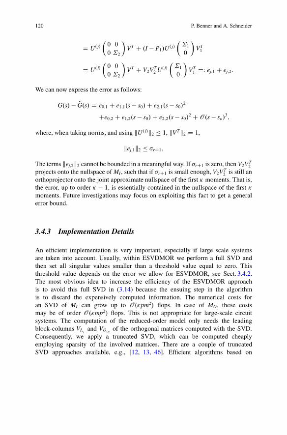
120 P. Benner and A. Schneider
D U. j/
�0 0
0 ˙2
�VT C .I � P1/U
. j/
�˙1
0
�VT1
D U. j/
�0 0
0 ˙2
�VT C V2V
T2 U. j/
�˙1
0
�VT1 DW ej;1 C ej;2:
We can now express the error as follows:
G.s/ � OG.s/ D e0;1 C e1;1.s � s0/C e2;1.s � s0/2
Ce0;2 C e1;2.s � s0/C e2;2.s � s0/2 C O.s � so/
3;
where, when taking norms, and using kU. j/k2 � 1, kVTk2 D 1,
kej;1k2 � �rC1:
The terms kej;2k2 cannot be bounded in a meaningful way. If �rC1 is zero, then V2VT2
projects onto the nullspace of MI , such that if �rC1 is small enough, V2VT2 is still an
orthoprojector onto the joint approximate nullspace of the first � moments. That is,the error, up to order � � 1, is essentially contained in the nullspace of the first �moments. Future investigations may focus on exploiting this fact to get a generalerror bound.
3.4.3 Implementation Details
An efficient implementation is very important, especially if large scale systemsare taken into account. Usually, within ESVDMOR we perform a full SVD andthen set all singular values smaller than a threshold value equal to zero. Thisthreshold value depends on the error we allow for ESVDMOR, see Sect. 3.4.2.The most obvious idea to increase the efficiency of the ESVDMOR approachis to avoid this full SVD in (3.14) because the ensuing step in the algorithmis to discard the expensively computed information. The numerical costs foran SVD of MI can grow up to O.�pm2/ flops. In case of MO, these costsmay be of order O.�mp2/ flops. This is not appropriate for large-scale circuitsystems. The computation of the reduced-order model only needs the leadingblock-columns VIri
and VOroof the orthogonal matrices computed with the SVD.
Consequently, we apply a truncated SVD, which can be computed cheaplyemploying sparsity of the involved matrices. There are a couple of truncatedSVD approaches available, e.g., [12, 13, 46]. Efficient algorithms based on
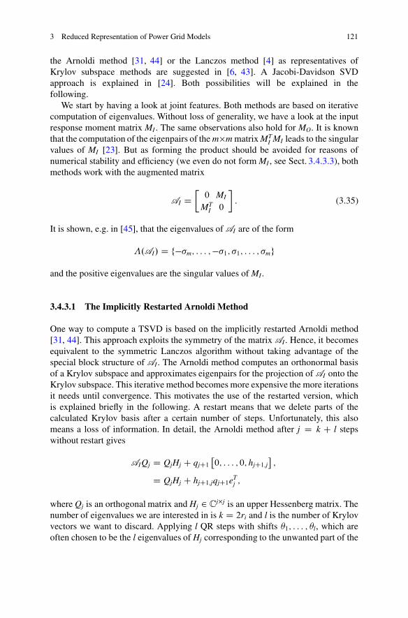
3 Reduced Representation of Power Grid Models 121
the Arnoldi method [31, 44] or the Lanczos method [4] as representatives ofKrylov subspace methods are suggested in [6, 43]. A Jacobi-Davidson SVDapproach is explained in [24]. Both possibilities will be explained in thefollowing.
We start by having a look at joint features. Both methods are based on iterativecomputation of eigenvalues. Without loss of generality, we have a look at the inputresponse moment matrix MI . The same observations also hold for MO. It is knownthat the computation of the eigenpairs of the m�m matrix MT
I MI leads to the singularvalues of MI [23]. But as forming the product should be avoided for reasons ofnumerical stability and efficiency (we even do not form MI , see Sect. 3.4.3.3), bothmethods work with the augmented matrix
AI D�0 MI
MTI 0
�: (3.35)
It is shown, e.g. in [45], that the eigenvalues of AI are of the form
�.AI/ D f��m; : : : ;��1; �1; : : : ; �mg
and the positive eigenvalues are the singular values of MI .
3.4.3.1 The Implicitly Restarted Arnoldi Method
One way to compute a TSVD is based on the implicitly restarted Arnoldi method[31, 44]. This approach exploits the symmetry of the matrix AI . Hence, it becomesequivalent to the symmetric Lanczos algorithm without taking advantage of thespecial block structure of AI . The Arnoldi method computes an orthonormal basisof a Krylov subspace and approximates eigenpairs for the projection of AI onto theKrylov subspace. This iterative method becomes more expensive the more iterationsit needs until convergence. This motivates the use of the restarted version, whichis explained briefly in the following. A restart means that we delete parts of thecalculated Krylov basis after a certain number of steps. Unfortunately, this alsomeans a loss of information. In detail, the Arnoldi method after j D k C l stepswithout restart gives
AIQj D QjHj C qjC10; : : : ; 0; hjC1;j
;
D QjHj C hjC1;jqjC1eTj ;
where Qj is an orthogonal matrix and Hj 2 Cj�j is an upper Hessenberg matrix. The
number of eigenvalues we are interested in is k D 2ri and l is the number of Krylovvectors we want to discard. Applying l QR steps with shifts �1; : : : ; �l, which areoften chosen to be the l eigenvalues of Hj corresponding to the unwanted part of the
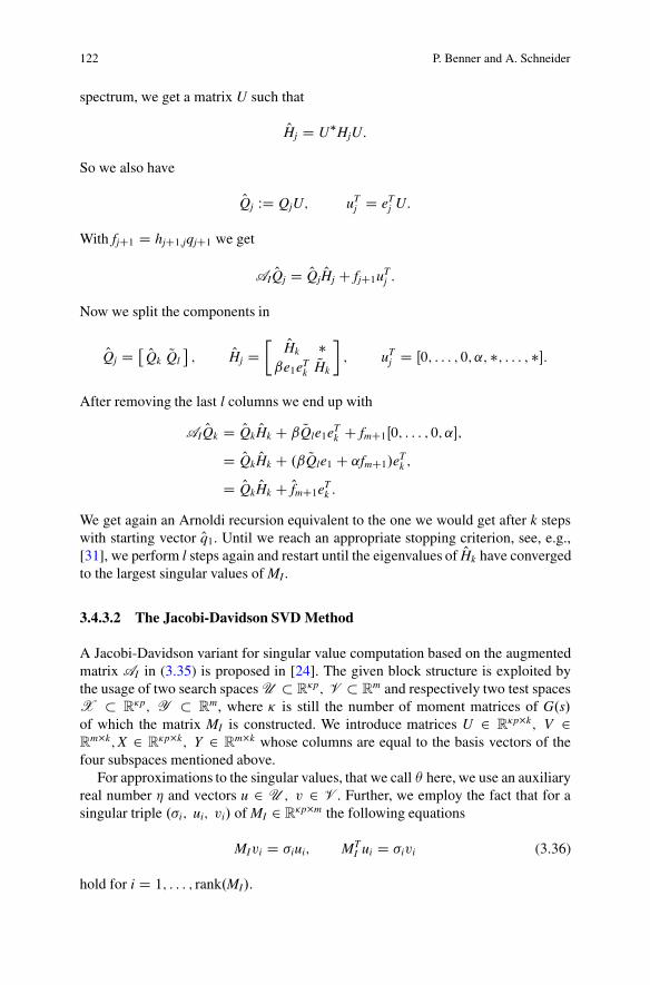
122 P. Benner and A. Schneider
spectrum, we get a matrix U such that
OHj D U�HjU:
So we also have
OQj WD QjU; uTj D eT
j U:
With fjC1 D hjC1;jqjC1 we get
AI OQj D OQj OHj C fjC1uTj :
Now we split the components in
OQj D OQk QQl
; OHj D
� OHk �ˇe1eT
kQHk
�; uT
j D Œ0; : : : ; 0; ˛;�; : : : ;��:
After removing the last l columns we end up with
AI OQk D OQk OHk C ˇ QQle1eTk C fmC1Œ0; : : : ; 0; ˛�;
D OQk OHk C .ˇ QQle1 C ˛fmC1/eTk ;
D OQk OHk C OfmC1eTk :
We get again an Arnoldi recursion equivalent to the one we would get after k stepswith starting vector Oq1. Until we reach an appropriate stopping criterion, see, e.g.,[31], we perform l steps again and restart until the eigenvalues of OHk have convergedto the largest singular values of MI .
3.4.3.2 The Jacobi-Davidson SVD Method
A Jacobi-Davidson variant for singular value computation based on the augmentedmatrix AI in (3.35) is proposed in [24]. The given block structure is exploited bythe usage of two search spaces U � R
�p; V � Rm and respectively two test spaces
X � R�p; Y � R
m, where � is still the number of moment matrices of G.s/of which the matrix MI is constructed. We introduce matrices U 2 R
�p�k; V 2R
m�k;X 2 R�p�k; Y 2 R
m�k whose columns are equal to the basis vectors of thefour subspaces mentioned above.
For approximations to the singular values, that we call � here, we use an auxiliaryreal number � and vectors u 2 U ; v 2 V . Further, we employ the fact that for asingular triple .�i; ui; vi/ of MI 2 R
�p�m the following equations
MIvi D �iui; MTI ui D �ivi (3.36)
hold for i D 1; : : : ; rank.MI/.
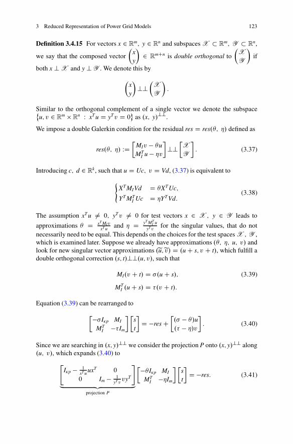
3 Reduced Representation of Power Grid Models 123
Definition 3.4.15 For vectors x 2 Rm; y 2 R
n and subspaces X � Rm; Y � R
n,
we say that the composed vector
�xy
�2 R
mCn is double orthogonal to
�X
Y
�if
both x ? X and y ? Y . We denote this by
�xy
�??
�X
Y
�:
Similar to the orthogonal complement of a single vector we denote the subspace˚u; v 2 R
m � Rn W xTu D yTv D 0
as .x; y/??.
We impose a double Galerkin condition for the residual res D res.�; �/ defined as
res.�; �/ WD�
MIv � �uMT
I u � �v
�??
�X
Y
�: (3.37)
Introducing c; d 2 Rk, such that u D Uc; v D Vd, (3.37) is equivalent to
(XTMIVd D �XTUc;
YT MTI Uc D �YT Vd:
(3.38)
The assumption xTu ¤ 0; yTv ¤ 0 for test vectors x 2 X ; y 2 Y leads to
approximations � D xT MIv
xT uand � D yT MT
I uyTv
for the singular values, that do notnecessarily need to be equal. This depends on the choices for the test spaces X ; Y ,which is examined later. Suppose we already have approximations .�; �; u; v/ andlook for new singular vector approximations .eu;ev/ D .u C s; v C t/, which fulfill adouble orthogonal correction .s; t/??.u; v/, such that
MI.v C t/ D �.u C s/; (3.39)
MTI .u C s/ D �.v C t/:
Equation (3.39) can be rearranged to
���I�p MI
MTI ��Im
� �st
�D �res C
�.� � �/u.� � �/v
�: (3.40)
Since we are searching in .x; y/?? we consider the projection P onto .x; y/?? along.u; v/, which expands (3.40) to
"I�p � 1
xT uuxT 0
0 Im � 1yTvvyT
#
„ ƒ‚ …projection P
���I�p MI
MTI ��Im
� �st
�D �res: (3.41)
124 P. Benner and A. Schneider
We also replace the unknown �; � by the known approximation �; � in (3.41). Since8ex 2 R
�p;8ey 2 Rm with uTex ¤ 0; vTey ¤ 0,
"I�p � 1
u TexexuT 0
0 Im � 1
v TeyeyvT
#�st
�D�
st
�
holds, we can expand (3.41) to the JDSVD correction equation.
"I�p� 1
xT uuxT 0
0 Im� 1yTvvyT
#���I�p MI
MTI ��Im
�"I�p� 1
u TexexuT 0
0 Im� 1
v TeyeyvT
#�st
�D �res;
(3.42)
with .s; t/??.u; v/. Ifex; ey are nonzero multiples of x; y, the operator in (3.42) issymmetric and maps .u; v/?? to .x; y/??.
At this point, the Galerkin choice of the test spaces needs to be explained. If wechoose X D U and Y D V , with dimU D dimV D k, we get
UTMIVd D �c; VT MTI Uc D �d
for (3.38). Again, we have approximations u D Uc and v D Vd. With test vectorsx D u; y D v, and with kuk D kvk D 1, we have singular value approximations� D � D uTAv which are equal. Furthermore, forex D u; ey D v the correctionequation (3.42) becomes
�I�p�uuT 0
0 Im�vvT
����I�p MI
MTI ��Im
��I�p�uuT 0
0 Im�vvT
��st
�D�res; (3.43)
in which the operator is symmetric and maps .u; v/?? to itself. We concludethe standard variant of the JDSVD in Algorithm 3.1. The orthonormalization isperformed by MGS and RMGS, which stands for the modified Gram- Schmidt- andthe repeated modified Gram- Schmidt- orthonormalization. Due to orthogonalitythis Galerkin choice is optimal for computing of the largest singular values whichis the problem we want to solve. Computing the singular values closest to atarget � is equivalent to computing the singular values of largest magnitude ofthe shifted and inverted matrix .A � �I/�1, which implies a different correctionequation.
A comparison of the influence of different decomposition methods appliedwithin the terminal reduction of RC549 to one terminal can be found in Fig. 3.12.The magnitude approximation is satisfying while the approximation of the phasebecomes even worse by means of Arnoldi or JDSVD. If we keep 66 terminals,
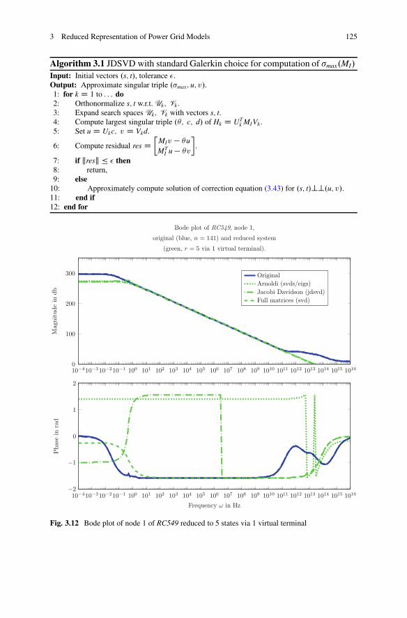
3 Reduced Representation of Power Grid Models 125
Algorithm 3.1 JDSVD with standard Galerkin choice for computation of �max.MI/
Input: Initial vectors .s; t/, tolerance �.Output: Approximate singular triple .�max; u; v/.1: for k D 1 to . . . do2: Orthonormalize s; t w.r.t. Uk; Vk.3: Expand search spaces Uk; Vk with vectors s; t.4: Compute largest singular triple .�; c; d/ of Hk D UT
k MIVk.5: Set u D Ukc; v D Vkd.
6: Compute residual res D�
MIv � �uMT
I u� �v�
.
7: if kresk � � then8: return,9: else
10: Approximately compute solution of correction equation (3.43) for .s; t/??.u; v/.11: end if12: end for
10−410−310−210−1 100 101 102 103 104 105 106 107 108 109 1010 1011 1012 1013 1014 1015 1016−2
−1
0
1
2
Frequency ω in Hz
Phas
ein
rad
10−410−310−210−1 100 101 102 103 104 105 106 107 108 109 1010 1011 1012 1013 1014 1015 10160
100
200
300
Mag
nitude
indb
Bode plot of RC549, node 1,
original (blue, n = 141) and reduced system
(green, r = 5 via 1 virtual terminal).
Original
Arnoldi (svds/eigs)
Jacobi Davidson (jdsvd)
Full matrices (svd)
Fig. 3.12 Bode plot of node 1 of RC549 reduced to 5 states via 1 virtual terminal
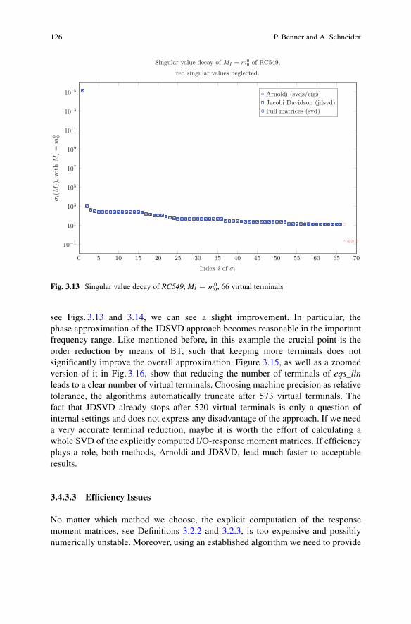
126 P. Benner and A. Schneider
0 5 10 15 20 25 30 35 40 45 50 55 60 65 70
10−1
101
103
105
107
109
1011
1013
1015
Index i of σi
σi(
MI),
with
MI
=m
0 0Singular value decay of MI = m0
0 of RC549,
red singular values neglected.
Arnoldi (svds/eigs)
Jacobi Davidson (jdsvd)
Full matrices (svd)
Fig. 3.13 Singular value decay of RC549, MI D m00, 66 virtual terminals
see Figs. 3.13 and 3.14, we can see a slight improvement. In particular, thephase approximation of the JDSVD approach becomes reasonable in the importantfrequency range. Like mentioned before, in this example the crucial point is theorder reduction by means of BT, such that keeping more terminals does notsignificantly improve the overall approximation. Figure 3.15, as well as a zoomedversion of it in Fig. 3.16, show that reducing the number of terminals of eqs_linleads to a clear number of virtual terminals. Choosing machine precision as relativetolerance, the algorithms automatically truncate after 573 virtual terminals. Thefact that JDSVD already stops after 520 virtual terminals is only a question ofinternal settings and does not express any disadvantage of the approach. If we needa very accurate terminal reduction, maybe it is worth the effort of calculating awhole SVD of the explicitly computed I/O-response moment matrices. If efficiencyplays a role, both methods, Arnoldi and JDSVD, lead much faster to acceptableresults.
3.4.3.3 Efficiency Issues
No matter which method we choose, the explicit computation of the responsemoment matrices, see Definitions 3.2.2 and 3.2.3, is too expensive and possiblynumerically unstable. Moreover, using an established algorithm we need to provide
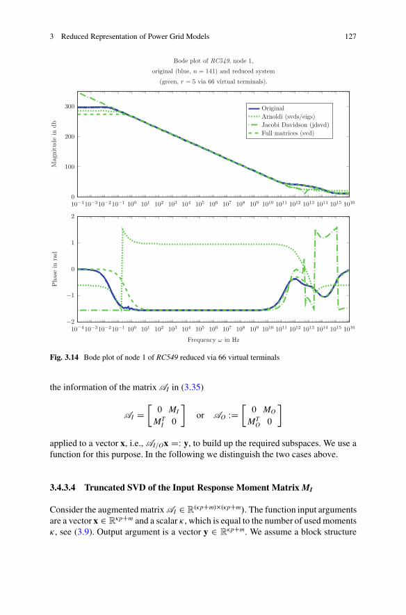
3 Reduced Representation of Power Grid Models 127
10−410−310−210−1 100 101 102 103 104 105 106 107 108 109 1010 1011 1012 1013 1014 1015 1016
−2
−1
0
1
2
Frequency ω in Hz
Phas
ein
rad
10−410−310−210−1 100 101 102 103 104 105 106 107 108 109 1010 1011 1012 1013 1014 1015 10160
100
200
300
Mag
nitude
indb
Bode plot of RC549, node 1,
original (blue, n = 141) and reduced system
(green, r = 5 via 66 virtual terminals).
Original
Arnoldi (svds/eigs)
Jacobi Davidson (jdsvd)
Full matrices (svd)
Fig. 3.14 Bode plot of node 1 of RC549 reduced via 66 virtual terminals
the information of the matrix AI in (3.35)
AI D�0 MI
MTI 0
�or AO WD
�0 MO
MTO 0
�
applied to a vector x, i.e., AI=Ox DW y, to build up the required subspaces. We use afunction for this purpose. In the following we distinguish the two cases above.
3.4.3.4 Truncated SVD of the Input Response Moment Matrix MI
Consider the augmented matrix AI 2 R.�pCm/�.�pCm/. The function input arguments
are a vector x 2 R�pCm and a scalar �, which is equal to the number of used moments
�, see (3.9). Output argument is a vector y 2 R�pCm. We assume a block structure
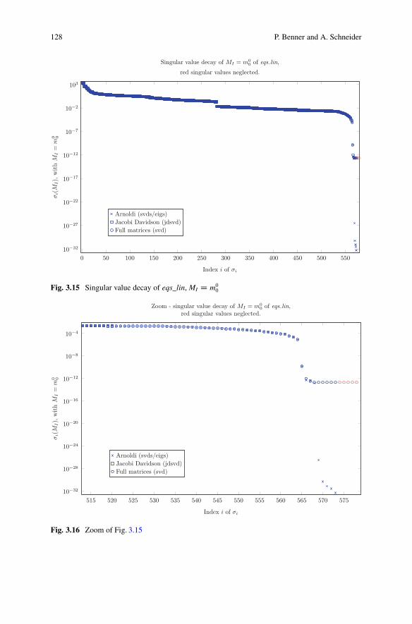
128 P. Benner and A. Schneider
0 50 100 150 200 250 300 350 400 450 500 550
10−32
10−27
10−22
10−17
10−12
10−7
10−2
103
Index i of σi
σi(
MI),
with
MI
=m
0 0Singular value decay of MI = m0
0 of eqs lin,
red singular values neglected.
Arnoldi (svds/eigs)
Jacobi Davidson (jdsvd)
Full matrices (svd)
Fig. 3.15 Singular value decay of eqs_lin, MI D m00
515 520 525 530 535 540 545 550 555 560 565 570 575
10−32
10−28
10−24
10−20
10−16
10−12
10−8
10−4
Index i of σi
σi(
MI),
with
MI
=m
0 0
Zoom - singular value decay of MI = m00 of eqs lin,
red singular values neglected.
Arnoldi (svds/eigs)
Jacobi Davidson (jdsvd)
Full matrices (svd)
Fig. 3.16 Zoom of Fig. 3.15
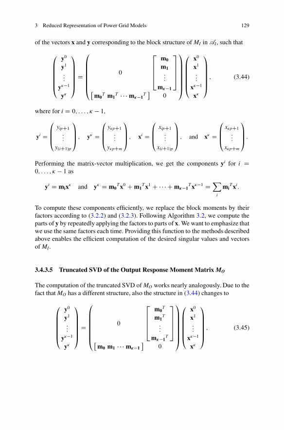
3 Reduced Representation of Power Grid Models 129
of the vectors x and y corresponding to the block structure of MI in AI , such that
0BBBBB@
y0
y1:::
y��1y�
1CCCCCA
D
0BBBBBB@
0
26664
m0
m1:::
m��1
37775
m0
T m1T � � � m��1
T
0
1CCCCCCA
0BBBBB@
x0
x1:::
x��1x�
1CCCCCA; (3.44)
where for i D 0; : : : ; � � 1,
yi D
0BB@
yipC1
:::
y.iC1/p
1CCA ; y� D
0BB@
y�pC1
:::
y�pCm
1CCA ; xi D
0BB@
xipC1
:::
x.iC1/p
1CCA ; and x� D
0BB@
x�pC1
:::
x�pCm
1CCA :
Performing the matrix-vector multiplication, we get the components yi for i D0; : : : ; � � 1 as
yi D mix� and y� D m0Tx0 C m1
Tx1 C � � � C m��1Tx��1 D
Xi
miTxi:
To compute these components efficiently, we replace the block moments by theirfactors according to (3.2.2) and (3.2.3). Following Algorithm 3.2, we compute theparts of y by repeatedly applying the factors to parts of x. We want to emphasize thatwe use the same factors each time. Providing this function to the methods describedabove enables the efficient computation of the desired singular values and vectorsof MI .
3.4.3.5 Truncated SVD of the Output Response Moment Matrix MO
The computation of the truncated SVD of MO works nearly analogously. Due to thefact that MO has a different structure, also the structure in (3.44) changes to
0BBBBB@
y0
y1:::
y��1y�
1CCCCCA
D
0BBBBBB@
0
26664
m0T
m1T
:::
m��1T
37775
m0 m1 � � � m��1
0
1CCCCCCA
0BBBBB@
x0
x1:::
x��1x�
1CCCCCA; (3.45)
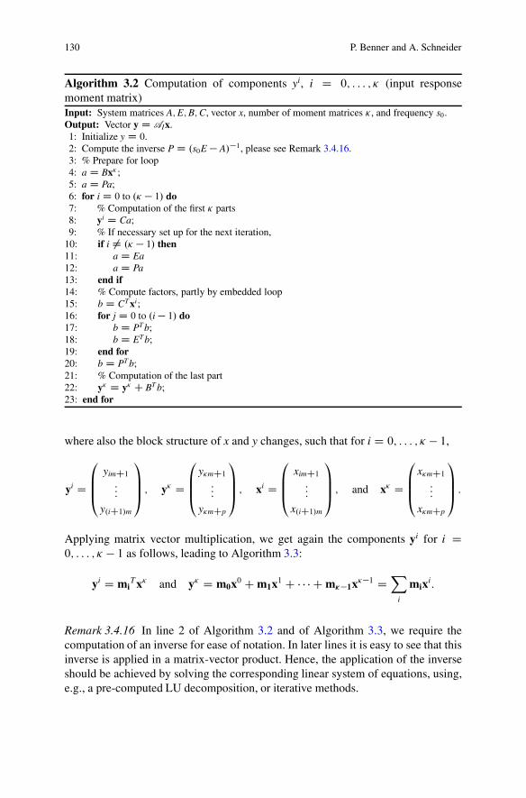
130 P. Benner and A. Schneider
Algorithm 3.2 Computation of components yi, i D 0; : : : ; � (input responsemoment matrix)Input: System matrices A;E;B;C, vector x, number of moment matrices �, and frequency s0.Output: Vector y D AIx.1: Initialize y D 0.2: Compute the inverse PD .s0E � A/�1, please see Remark 3.4.16.3: % Prepare for loop4: a D Bx� ;5: a D Pa;6: for i D 0 to .� � 1/ do7: % Computation of the first � parts8: yi D Ca;9: % If necessary set up for the next iteration,
10: if i ¤ .� � 1/ then11: a D Ea12: a D Pa13: end if14: % Compute factors, partly by embedded loop15: b D CT xi;16: for j D 0 to .i� 1/ do17: b D PT b;18: b D ET b;19: end for20: b D PT b;21: % Computation of the last part22: y� D y� C BT b;23: end for
where also the block structure of x and y changes, such that for i D 0; : : : ; � � 1,
yi D
0BB@
yimC1
:::
y.iC1/m
1CCA ; y� D
0BB@
y�mC1
:::
y�mCp
1CCA ; xi D
0BB@
ximC1
:::
x.iC1/m
1CCA ; and x� D
0BB@
x�mC1
:::
x�mCp
1CCA :
Applying matrix vector multiplication, we get again the components yi for i D0; : : : ; � � 1 as follows, leading to Algorithm 3.3:
yi D miTx� and y� D m0x0 C m1x1 C � � � C m��1x��1 D
Xi
mixi:
Remark 3.4.16 In line 2 of Algorithm 3.2 and of Algorithm 3.3, we require thecomputation of an inverse for ease of notation. In later lines it is easy to see that thisinverse is applied in a matrix-vector product. Hence, the application of the inverseshould be achieved by solving the corresponding linear system of equations, using,e.g., a pre-computed LU decomposition, or iterative methods.
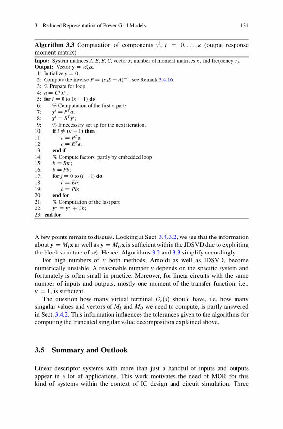
3 Reduced Representation of Power Grid Models 131
Algorithm 3.3 Computation of components yi, i D 0; : : : ; � (output responsemoment matrix)Input: System matrices A;E;B;C, vector x, number of moment matrices �, and frequency s0.Output: Vector y D AOx.1: Initialize y D 0.2: Compute the inverse PD .s0E � A/�1, see Remark 3.4.16.3: % Prepare for loop4: a D CT x� ;5: for i D 0 to .� � 1/ do6: % Computation of the first � parts7: yi D PT a;8: yi D BT yi;9: % If necessary set up for the next iteration,
10: if i ¤ .� � 1/ then11: a D PT a;12: a D ET a;13: end if14: % Compute factors, partly by embedded loop15: b D Bxi;16: b D Pb;17: for j D 0 to .i� 1/ do18: b D Eb;19: b D Pb;20: end for21: % Computation of the last part22: y� D y� C Cb;23: end for
A few points remain to discuss. Looking at Sect. 3.4.3.2, we see that the informationabout y D MIx as well as y D MOx is sufficient within the JDSVD due to exploitingthe block structure of AI . Hence, Algorithms 3.2 and 3.3 simplify accordingly.
For high numbers of � both methods, Arnoldi as well as JDSVD, becomenumerically unstable. A reasonable number � depends on the specific system andfortunately is often small in practice. Moreover, for linear circuits with the samenumber of inputs and outputs, mostly one moment of the transfer function, i.e.,� D 1, is sufficient.
The question how many virtual terminal Gr.s/ should have, i.e. how manysingular values and vectors of MI and MO we need to compute, is partly answeredin Sect. 3.4.2. This information influences the tolerances given to the algorithms forcomputing the truncated singular value decomposition explained above.
3.5 Summary and Outlook
Linear descriptor systems with more than just a handful of inputs and outputsappear in a lot of applications. This work motivates the need of MOR for thiskind of systems within the context of IC design and circuit simulation. Three
132 P. Benner and A. Schneider
basic, widely different approaches, are presented, i.e., reduction based on SVDsrevealing the I/O-behavior, a graph partitioning approach, and the interpolation-based construction of a reduced-order model from measurement data. Afterwards, aconcrete method of the first type, the so-called ESVDMOR, is explained in detail.The preservation of important properties is shown as well as the approximationerror is analyzed. Furthermore, special attention is given to an efficient truncatedSVD implementation in the framework of ESVDMOR. The performance of thethree proposed ESVDMOR implementations is illustrated using two test cases.In conclusion, one may say that in all three cases, the approximation of themagnitude of the frequency response can be achieved satisfactorily, while the phaseapproximation suffers from the additional truncation error in the truncated SVDapproaches. Hence, if preservation of the phase is of importance, one has to investmore computational resources and use the full SVD of the generalized momentmatrices.
Acknowledgements The authors want to thank Daniel Schmidthäusler, Sebastian Schöps andGeorg Denk for their support. The work reported in this chapter was supported by the GermanFederal Ministry of Education and Research (BMBF), grant no. 03BEPAE1. Responsibility for thecontents of this publication rests with the authors.
References
1. Anderson, B.D.O., Vongpanitlerd, S.: Network Analysis and Synthesis. Prentice Hall, Engle-wood Cliffs, NJ (1973)
2. Antoulas, A.C.: Approximation of Large-Scale Dynamical Systems. SIAM Publications,Philadelphia, PA (2005)
3. Antoulas, A.C., Ionita, A.C., Lefteriu, S.: On two-variable rational interpolation. LinearAlgebra Appl. 436(8), 2889–2915 (2012)
4. Baglama, J., Reichel, L.: Augmented implicitly restarted Lanczos bidiagonalization methods.SIAM J. Sci. Comput. 27(1), 19–42 (2005). doi:http://dx.doi.org/10.1137/04060593X
5. Benner, P.: Advances in balancing-related model reduction for circuit simulation. In: Roos, J.,Costa, L.R.J. (eds.) Scientific Computing in Electrical Engineering SCEE 2008. Mathematicsin Industry, vol. 14, pp. 469–482. Springer, Berlin/Heidelberg (2010)
6. Benner, P., Schneider, A.: Model order and terminal reduction approaches via matrix decom-position and low rank approximation. In: Roos, J., Costa, L.R.J. (eds.) Scientific Computing inElectrical Engineering SCEE 2008. Mathematics in Industry, vol. 14, pp. 523–530. Springer,Berlin/Heidelberg (2010)
7. Benner, P., Schneider, A.: On stability, passivity, and reciprocity preservation of ESVDMOR.In: Benner, P., Hinze, M., ter Maten, J. (eds.) Model Reduction for Circuit Simulation. LectureNotes in Electrical Engineering, vol. 74, pp. 277–288. Springer, Berlin/Heidelberg (2011)
8. Benner, P., Schneider, A.: Some remarks on a priori error estimation for ESVDMOR. In:Michielsen, B., Poirier, J.R. (eds.) Scientific Computing in Electrical Engineering SCEE 2010.Mathematics in Industry, vol. 16, pp. 15–24. Springer, Berlin/Heidelberg (2012)
9. Benner, P., Quintana-Ortí, E.S., Quintana-Ortí, G.: Parallel model reduction of large-scalelinear descriptor systems via balanced truncation. In: Proceedings of the 6th InternationalMeeting on High Performance Computing for Computational Science VECPAR’04, Valencia,28–30 June 2004, pp. 65–78 (2004)
3 Reduced Representation of Power Grid Models 133
10. Benner, P., Mehrmann, V., Sorensen, D.C. (eds.): Dimension Reduction of Large-ScaleSystems. Lecture Notes in Computational Science and Engineering, vol. 45. Springer,Berlin/Heidelberg (2005)
11. Benner, P., Hinze, M., ter Maten, E.J.W. (eds.): Model Reduction for Circuit Simulation.Lecture Notes in Electrical Engineering, vol. 74. Springer, Dordrecht (2011)
12. Berry, M.W., Pulatova, S.A., Stewart, G.W.: Algorithm 844: Computing sparse reduced-rank approximations to sparse matrices. ACM Trans. Math. Softw. 31(2), 252–269 (2005).doi:http://doi.acm.org/10.1145/1067967.1067972
13. Chan, T.F., Hansen, P.C.: Computing truncated singular value decomposition least squaressolutions by rank revealing QR-factorizations. SIAM J. Sci. Stat. Comput. 11(3), 519–530(1990)
14. Dai, L.: Singular Control Systems. Lecture Notes in Control and Information Sciences, vol.118. Springer, Berlin (1989)
15. Feldmann, P., Freund, R.W.: Efficient linear circuit analysis by Padé approximation via theLanczos process. In: Proceedings of EURO-DAC ’94 with EURO-VHDL ’94, Grenoble, pp.170–175. IEEE Computer Society Press, Los Alamitos (1994)
16. Feldmann, P., Liu, F.: Sparse and efficient reduced order modeling of linear subcircuits withlarge number of terminals. In: ICCAD ’04: Proceedings of the 2004 IEEE/ACM InternationalConference Computer-Aided Design, pp. 88–92. IEEE Computer Society, Washington, DC(2004)
17. Feldmann, P., Freund, R.W., Acar, E.: Power grid analysis using a flexible conjugate gradientalgorithm with sparsification. Tech. rep., Department of Mathematics, UC Davis (2006). http://www.math.ucdavis.edu/~freund/flexible_cg.pdf
18. Francis, B.A.: A Course in H1 Control Theory. Lecture Notes in Control and InformationSciences. Springer, Berlin/Heidelberg (1987)
19. Freund, R.W.: Model reduction methods based on Krylov subspaces. Acta Numer. 12, 267–319(2003)
20. Freund, R.W.: SPRIM: structure-preserving reduced-order interconnect macromodeling. In:Proceedings of the 2004 IEEE/ACM International Conference on Computer-Aided Design,ICCAD ’04, pp. 80–87. IEEE Computer Society, Washington, DC (2004)
21. Freund, R.W.: On Padé-type model order reduction of J-Hermitian linear dynamical systems.Linear Algebra Appl. 429(10), 2451–2464 (2008)
22. Freund, R.W.: The SPRIM algorithm for structure-preserving order reduction of general RCLcircuits. In: Benner, P., Hinze, M., ter Maten, J. (eds.) Model Reduction for Circuit Simulation.Lecture Notes in Electrical Engineering, vol. 74, pp. 25–52. Springer, Berlin/Heidelberg (2011)
23. Golub, G., Van Loan, C.: Matrix Computations, 3rd edn. Johns Hopkins University Press,Baltimore (1996)
24. Hochstenbach, M.E.: A Jacobi–Davidson type SVD method. SIAM J. Sci. Comput. 23(2),606–628 (2001)
25. Ionutiu, R.: Model order reduction for multi-terminal systems with applications to circuitsimulation. Ph.D. thesis, Jacobs University, Bremen and Technische Universiteit Eindhoven,Eindhoven (2011)
26. Ionutiu, R., Rommes, J., Schilders, W.H.A.: SparseRC: Sparsity preserving model reductionfor RC circuits with many terminals. IEEE Trans. Circuits Syst. 30(12), 1828–1841 (2011)
27. Jain, J., Koh, C.K., Balakrishnan, V.: Fast simulation of VLSI interconnects. In: IEEE/ACMInternational Conference on Computer Aided Design, ICCAD-2004, pp. 93–98 (2004)
28. Kerns, K., Yang, A.: Stable and efficient reduction of large, multiport RC networks by poleanalysis via congruence transformations. IEEE Trans. Circuits Syst. 16(7), 734–744 (1997)
29. Lefteriu, S., Antoulas, A.C.: A new approach to modeling multiport systems from frequency-domain data. IEEE Trans. Comput. Aided Des. Integr. Circuits Syst. 29(1), 14–27 (2010)
30. Lefteriu, S., Antoulas, A.C.: Topics in model order reduction with applications to circuitsimulation. In: Benner, P., Hinze, M., ter Maten, E.J.W. (eds.) Model Reduction for CircuitSimulation. Lecture Notes in Electrical Engineering, vol. 74, pp. 85–107. Springer, Dordrecht(2011)
134 P. Benner and A. Schneider
31. Lehoucq, R.B., Sorensen, D.C., Yang, C.: ARPACK Users’ Guide: Solution of Large ScaleEigenvalue Problems with Implicitly Restarted Arnoldi Methods. Software, Environments,Tools, vol. 6, 142 p. SIAM, Society for Industrial and Applied Mathematics, Philadelphia,PA (1998)
32. Liu, P., Tan, S.X.D., Li, H., Qi, Z., Kong, J., McGaughy, B., He, L.: An efficient methodfor terminal reduction of interconnect circuits considering delay variations. In: ICCAD ’05:Proceedings of the 2005 IEEE/ACM International Conference on Computer-Aided Design,pp. 821–826. IEEE Computer Society, Washington, DC (2005)
33. Liu, P., Tan, S.X.D., Yan, B., McGaughy, B.: An extended SVD-based terminal and modelorder reduction algorithm. In: Proceedings of the 2006 IEEE International Behavioral Model-ing and Simulation Workshop, pp. 44–49 (2006)
34. Liu, P., Tan, S.X.D., McGaughy, B., Wu, L., He, L.: TermMerg: an efficient terminal-reduction method for interconnect circuits. IEEE Trans. Circuits Syst. 26(8), 1382–1392(2007). doi:10.1109/TCAD.2007.893554
35. Liu, P., Tan, S.X.D., Yan, B., McGaughy, B.: An efficient terminal and model order reductionalgorithm. Integr. VLSI J. 41(2), 210–218 (2008)
36. Lloyd, S.P.: Least squares quantization in PCM. IEEE Trans. Inform. Theory 28, 129–137(1982)
37. Lozano, R., Maschke, B., Brogliato, B., Egeland, O.: Dissipative Systems Analysis andControl: Theory and Applications. Springer, New York, Inc., Secaucus, NJ (2000)
38. Mehrmann, V., Stykel, T.: Balanced truncation model reduction for large-scale systems indescriptor form. In: Benner, P., Mehrmann, V., Sorensen, D.C. (eds.) Dimension Reductionof Large-Scale Systems. Lecture Notes in Computational Science and Engineering, vol. 45,pp. 83–115. Springer, Berlin/Heidelberg (2005)
39. Odabasioglu, A., Celik, M., Pileggi, L.T.: PRIMA: passive reduced-order interconnect macro-modeling algorithm. IEEE Trans. Comput. Aided Des. Integr. Circuits Syst. 17(8), 645–654(1998)
40. Reis, T.: Circuit synthesis of passive descriptor systems – a modified nodal approach. Int. J.Circuit Theory Appl. 38(1), 44–68 (2010)
41. Reis, T., Stykel, T.: Positive real and bounded real balancing for model reduction of descriptorsystems. Int. J. Control 82(1), 74–88 (2010)
42. Schmidthausler, D., Schöps, S., Clemens, M.: Reduction of linear subdomains for non-linear electro-quasistatic field simulations. IEEE Trans. Magn. 49(5), 1669–1672 (2013).doi:10.1109/TMAG.2013.2238905
43. Schneider, A.: Matrix decomposition based approaches for model order reduction of linearsystems with a large number of terminals. Diplomarbeit, Chemnitz University of Technology,Faculty of Mathematics (2008)
44. Sorensen, D.C.: Implicit application of polynomial filters in a k-step Arnoldi method. SIAM J.Matrix Anal. Appl. 13(1), 357–385 (1992)
45. Stewart, G.W., Sun, J.G.: Matrix Perturbation Theory. Academic Press, inc., Boston, MA(1990)
46. Stoll, M.: A Krylov-Schur approach to the truncated SVD. Linear Algebra Appl. 436(8), 2795–2806 (2012)
47. Tan, S.X.D., He, L.: Advanced Model Order Reduction Techniques in VLSI Design. Cam-bridge University Press, New York (2007)
48. Ye, Z., Vasilyev, D., Zhu, Z., Phillips, J.R.: Sparse implicit projection (SIP) for reductionof general many-terminal networks. In: Proceedings of the 2008 IEEE/ACM InternationalConference on Computer-Aided Design, ICCAD ’08, pp. 736–743. IEEE Press, Piscataway,NJ (2008)
49. Zecevic, A.I., Siljak, D.D.: Balanced decompositions of sparse systems for multilevel parallelprocessing. IEEE Trans. Circuits Syst. I: Fundam. Theory Appl. 41(3), 220–233 (1994)
Chapter 4Coupling of Numeric/Symbolic ReductionMethods for Generating Parametrized Modelsof Nanoelectronic Systems
Oliver Schmidt, Matthias Hauser, and Patrick Lang
Abstract This chapter presents new strategies for the analysis and model orderreduction of systems of ever-growing size and complexity by exploiting thehierarchical structure of analog electronical circuits. Thereby, the entire circuit isconsidered as a system of interconnected subcircuits. Given a prescribed error-bound for the reduction process, a newly developed algorithm tries to achieve amaximal reduction degree for the overall system by choosing the reduction degreesof the subcircuits in a convenient way. The individual subsystem reductions withrespect to their prescribed error-bound are then performed using different reductiontechniques. Combining the reduced subsystems a reduced model of the overallsystem results. Finally, the usability of the new techniques is demonstrated on twocircuit examples typically used in industrial applications.
4.1 Introduction
In order to avoid immense time and financial effort for the production of deficientlydesigned prototypes of integrated circuits (ICs), industrial circuit design usesmathematical models and simulations for predicting and analysing the physicalbehavior of electronical systems. Hence, redesigns and modifications of the systemscan easily be carried out on a computer screen and tested by subsequent simulationruns. Thereby, analog circuits in general are modelled by systems of differential-algebraic equations (DAEs), which are composed of component characteristics andKirchhoff laws.
The development in fabrication technology of ICs during the last years led toan unprecedented increase of functionality of systems on a single chip. Nowadays,ICs have hundreds of millions of semiconductor devices arranged in several layers
O. Schmidt • M. Hauser • P. Lang (�)Fraunhofer Institute for Industrial Mathematics ITWM (Fraunhofer Institut für Techno-undWirtschaftsmathematik ITWM), Fraunhofer-Platz 1, 67663 Kaiserslautern, Germanyhttp://www.itwm.fraunhofer.de/abteilungen/systemanalyse-prognose-und-regelung/elektronik-mechanik-mechatronik/analog-insydes.html
© Springer International Publishing AG 2017P. Benner (ed.), System Reduction for Nanoscale IC Design,Mathematics in Industry 20, DOI 10.1007/978-3-319-07236-4_4
135
136 O. Schmidt et al.
and low-level physical effects such as thermal interactions or electromagneticradiation cannot be neglected anymore in order to guarantee a non-defectivesignal propagation. Mathematical models based on DAEs, however, have almostreached their limit and cannot model these effects accurately enough. Consequently,distributed elements for critical components such as semiconductor devices andtransmission lines are used which yield supplementary model descriptions basedon partial differential equations (PDEs), where also the spatial dependencies aretaken into account. The coupling with DAEs modelling the remaining parts of thecircuit then leads to systems of partial differential-algebraic equations (PDAEs).A spatial semidiscretization finally results in very high-dimensional systems ofDAEs, thus rendering analysis and simulation tasks unacceptably expensive andtime consuming.
Since design verification requires a large number of simulation runs withdifferent input excitations, for the reasons mentioned above, model order reduction(MOR) becomes inevitable. Dedicated techniques in various areas of research havebeen developed among which the most popular ones are numerical methods tayloredfor linear systems. Besides these, there also exist symbolic methods [8, 10, 15, 19,20], where symbolic means that besides the system’s variables also its parametersare given as symbols instead of numerical values (see Sect. 4.1.1). They indeed arecostly to compute, but allow deeper analytical insights into functional dependencesof the system’s linear and nonlinear behavior on its parameters by maintaining thedominant ones in their symbolic form. The basic idea behind these methods is astepwise reduction of the original system by comparing its reference solution to thesolution of the so far reduced system by using error functions which measure thedifference between the two solutions. Since the resulting reduced system containsits parameters and variables in symbolic form, these methods can be seen as a kindof parametric model order reduction (pMOR). Compared to the standard parametricmodel order reduction techniques [4, 12], the symbolic ones can be additionallyapplied to nonlinear systems.
In order to avoid infeasibility of analysis and reduction of systems of ever-growing size and complexity, new strategies exploiting their hierarchical structurehave been developed in the current research project. They further allow for acoupling of distinct reduction techniques for different parts of the entire circuits.
The corresponding algorithms have been implemented in Analog Insydes [1],the software tool for symbolic modeling and analysis of analog circuits, that isdeveloped and distributed by the Fraunhofer ITWMin Kaiserslautern, Germany. Itis based on the computer algebra system Mathematica [21].
The new approach has been successfully applied with significant savings incomputation time to both a differential and an operational amplifier typically used inindustry. The reduced models also proved to be very robust with regard to differentinputs such as highly non-smooth pulse excitations. Thus, the aptitude of the newhierarchical model reduction algorithm to circuits of industrial size has been shown.
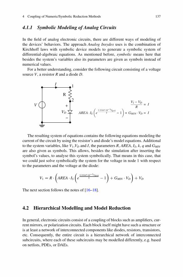
4 Coupling of Numeric/Symbolic Reduction Methods 137
4.1.1 Symbolic Modeling of Analog Circuits
In the field of analog electronic circuits, there are different ways of modeling ofthe devices’ behaviors. The approach Analog Insydes uses is the combination ofKirchhoff laws with symbolic device models to generate a symbolic system ofdifferential-algebraic equations. As mentioned before, symbolic means here thatbesides the system’s variables also its parameters are given as symbols instead ofnumerical values.
For a better understanding, consider the following circuit consisting of a voltagesource V , a resistor R and a diode D.
+
−VD
R
V
1
2
I
V1 −VDR
= I
AREA · IS
(e
3.33167·10−3VD·qk − 1
)+ GMIN ·VD = I
The resulting system of equations contains the following equations modeling thecurrent of the circuit by using the resistor’s and diode’s model equations. Additionalto the system variables, like V1,VD and I, the parameters R, AREA, IS, k, q and GMIN
are also given as symbols. This allows, besides the simulation after inserting thesymbol’s values, to analyse this system symbolically. That means in this case, thatwe could just solve symbolically the system for the voltage in node 1 with respectto the parameters and the voltage at the diode:
V1 D R ��
AREA � IS
�e3:33167�10�3VD �q
k � 1�
C GMIN � VD
�C VD
The next section follows the notes of [16–18].
4.2 Hierarchical Modelling and Model Reduction
In general, electronic circuits consist of a coupling of blocks such as amplifiers, cur-rent mirrors, or polarization circuits. Each block itself might have such a structure oris at least a network of interconnected components like diodes, resistors, transistors,etc. Consequently, the entire circuit is a hierarchical network of interconnectedsubcircuits, where each of these subcircuits may be modelled differently, e.g. basedon netlists, PDEs, or DAEs.
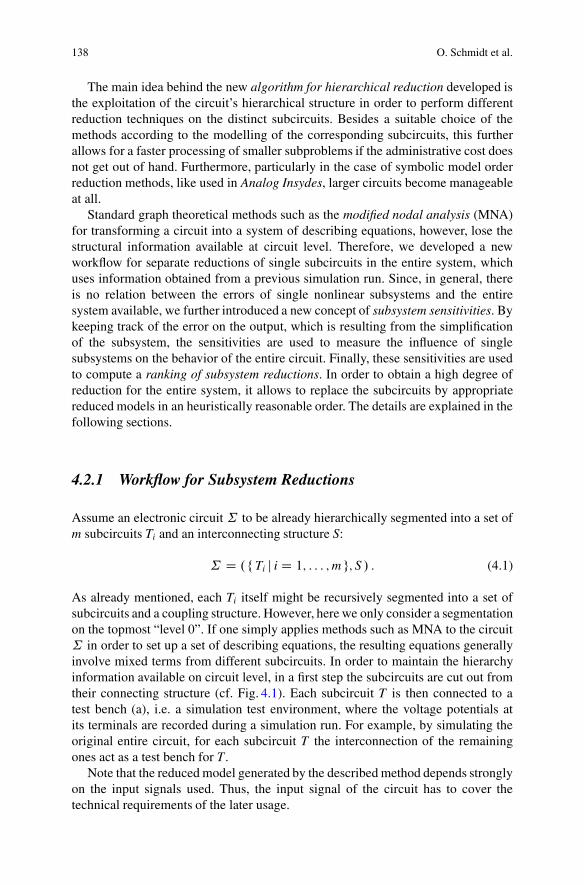
138 O. Schmidt et al.
The main idea behind the new algorithm for hierarchical reduction developed isthe exploitation of the circuit’s hierarchical structure in order to perform differentreduction techniques on the distinct subcircuits. Besides a suitable choice of themethods according to the modelling of the corresponding subcircuits, this furtherallows for a faster processing of smaller subproblems if the administrative cost doesnot get out of hand. Furthermore, particularly in the case of symbolic model orderreduction methods, like used in Analog Insydes, larger circuits become manageableat all.
Standard graph theoretical methods such as the modified nodal analysis (MNA)for transforming a circuit into a system of describing equations, however, lose thestructural information available at circuit level. Therefore, we developed a newworkflow for separate reductions of single subcircuits in the entire system, whichuses information obtained from a previous simulation run. Since, in general, thereis no relation between the errors of single nonlinear subsystems and the entiresystem available, we further introduced a new concept of subsystem sensitivities. Bykeeping track of the error on the output, which is resulting from the simplificationof the subsystem, the sensitivities are used to measure the influence of singlesubsystems on the behavior of the entire circuit. Finally, these sensitivities are usedto compute a ranking of subsystem reductions. In order to obtain a high degree ofreduction for the entire system, it allows to replace the subcircuits by appropriatereduced models in an heuristically reasonable order. The details are explained in thefollowing sections.
4.2.1 Workflow for Subsystem Reductions
Assume an electronic circuit ˙ to be already hierarchically segmented into a set ofm subcircuits Ti and an interconnecting structure S:
˙ D . f Ti j i D 1; : : : ;m g; S / : (4.1)
As already mentioned, each Ti itself might be recursively segmented into a set ofsubcircuits and a coupling structure. However, here we only consider a segmentationon the topmost “level 0”. If one simply applies methods such as MNA to the circuit˙ in order to set up a set of describing equations, the resulting equations generallyinvolve mixed terms from different subcircuits. In order to maintain the hierarchyinformation available on circuit level, in a first step the subcircuits are cut out fromtheir connecting structure (cf. Fig. 4.1). Each subcircuit T is then connected to atest bench (a), i.e. a simulation test environment, where the voltage potentials atits terminals are recorded during a simulation run. For example, by simulating theoriginal entire circuit, for each subcircuit T the interconnection of the remainingones act as a test bench for T.
Note that the reduced model generated by the described method depends stronglyon the input signals used. Thus, the input signal of the circuit has to cover thetechnical requirements of the later usage.
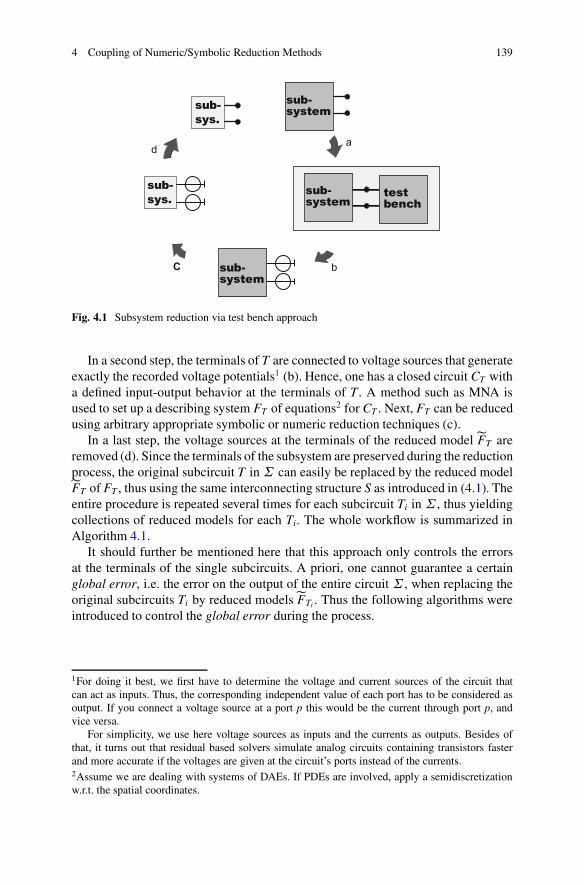
4 Coupling of Numeric/Symbolic Reduction Methods 139
Fig. 4.1 Subsystem reduction via test bench approach
In a second step, the terminals of T are connected to voltage sources that generateexactly the recorded voltage potentials1 (b). Hence, one has a closed circuit CT witha defined input-output behavior at the terminals of T. A method such as MNA isused to set up a describing system FT of equations2 for CT . Next, FT can be reducedusing arbitrary appropriate symbolic or numeric reduction techniques (c).
In a last step, the voltage sources at the terminals of the reduced model eFT areremoved (d). Since the terminals of the subsystem are preserved during the reductionprocess, the original subcircuit T in ˙ can easily be replaced by the reduced modeleFT of FT , thus using the same interconnecting structure S as introduced in (4.1). Theentire procedure is repeated several times for each subcircuit Ti in ˙ , thus yieldingcollections of reduced models for each Ti. The whole workflow is summarized inAlgorithm 4.1.
It should further be mentioned here that this approach only controls the errorsat the terminals of the single subcircuits. A priori, one cannot guarantee a certainglobal error, i.e. the error on the output of the entire circuit ˙ , when replacing theoriginal subcircuits Ti by reduced modelseFTi . Thus the following algorithms wereintroduced to control the global error during the process.
1For doing it best, we first have to determine the voltage and current sources of the circuit thatcan act as inputs. Thus, the corresponding independent value of each port has to be considered asoutput. If you connect a voltage source at a port p this would be the current through port p, andvice versa.
For simplicity, we use here voltage sources as inputs and the currents as outputs. Besides ofthat, it turns out that residual based solvers simulate analog circuits containing transistors fasterand more accurate if the voltages are given at the circuit’s ports instead of the currents.2Assume we are dealing with systems of DAEs. If PDEs are involved, apply a semidiscretizationw.r.t. the spatial coordinates.
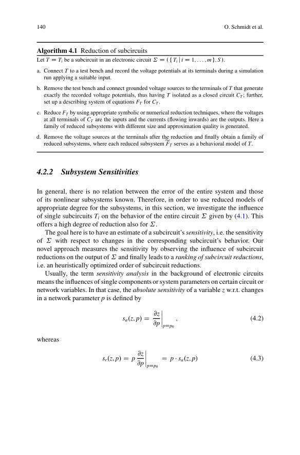
140 O. Schmidt et al.
Algorithm 4.1 Reduction of subcircuitsLet T D Ti be a subcircuit in an electronic circuit ˙ D . fTi j i D 1; : : : ;m g; S /.a. Connect T to a test bench and record the voltage potentials at its terminals during a simulation
run applying a suitable input.
b. Remove the test bench and connect grounded voltage sources to the terminals of T that generateexactly the recorded voltage potentials, thus having T isolated as a closed circuit CT ; further,set up a describing system of equations FT for CT .
c. Reduce FT by using appropriate symbolic or numerical reduction techniques, where the voltagesat all terminals of CT are the inputs and the currents (flowing inwards) are the outputs. Here afamily of reduced subsystems with different size and approximation quality is generated.
d. Remove the voltage sources at the terminals after the reduction and finally obtain a family ofreduced subsystems, where each reduced subsystemeFT serves as a behavioral model of T.
4.2.2 Subsystem Sensitivities
In general, there is no relation between the error of the entire system and thoseof its nonlinear subsystems known. Therefore, in order to use reduced models ofappropriate degree for the subsystems, in this section, we investigate the influenceof single subcircuits Ti on the behavior of the entire circuit ˙ given by (4.1). Thisoffers a high degree of reduction also for˙ .
The goal here is to have an estimate of a subcircuit’s sensitivity, i.e. the sensitivityof ˙ with respect to changes in the corresponding subcircuit’s behavior. Ournovel approach measures the sensitivity by observing the influence of subcircuitreductions on the output of˙ and finally leads to a ranking of subcircuit reductions,i.e. an heuristically optimized order of subcircuit reductions.
Usually, the term sensitivity analysis in the background of electronic circuitsmeans the influences of single components or system parameters on certain circuit ornetwork variables. In that case, the absolute sensitivity of a variable z w.r.t. changesin a network parameter p is defined by
sa.z; p/ D @z
@p
ˇˇpDp0
; (4.2)
whereas
sr.z; p/ D p@z
@p
ˇˇpDp0
D p � sa.z; p/ (4.3)
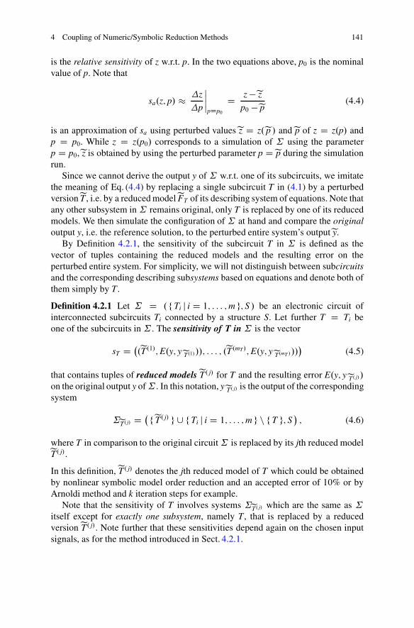
4 Coupling of Numeric/Symbolic Reduction Methods 141
is the relative sensitivity of z w.r.t. p. In the two equations above, p0 is the nominalvalue of p. Note that
sa.z; p/ z
p
ˇˇpDp0
D z �ezp0 �ep (4.4)
is an approximation of sa using perturbed valuesez D z.ep / andep of z D z.p/ andp D p0. While z D z.p0/ corresponds to a simulation of ˙ using the parameterp D p0,ez is obtained by using the perturbed parameter p Dep during the simulationrun.
Since we cannot derive the output y of ˙ w.r.t. one of its subcircuits, we imitatethe meaning of Eq. (4.4) by replacing a single subcircuit T in (4.1) by a perturbedversioneT , i.e. by a reduced modeleFT of its describing system of equations. Note thatany other subsystem in˙ remains original, only T is replaced by one of its reducedmodels. We then simulate the configuration of ˙ at hand and compare the originaloutput y, i.e. the reference solution, to the perturbed entire system’s outputey.
By Definition 4.2.1, the sensitivity of the subcircuit T in ˙ is defined as thevector of tuples containing the reduced models and the resulting error on theperturbed entire system. For simplicity, we will not distinguish between subcircuitsand the corresponding describing subsystems based on equations and denote both ofthem simply by T.
Definition 4.2.1 Let ˙ D . f Ti j i D 1; : : : ;m g; S / be an electronic circuit ofinterconnected subcircuits Ti connected by a structure S. Let further T D Ti beone of the subcircuits in ˙ . The sensitivity of T in ˙ is the vector
sT D �.eT .1/;E.y; yeT.1/ //; : : : ; .eT .mT /;E.y; yeT.mT / //
�(4.5)
that contains tuples of reduced modelseT. j/ for T and the resulting error E.y; yeT. j/ /
on the original output y of˙ . In this notation, yeT. j/ is the output of the correspondingsystem
eT. j/ D � feT. j/ g [ f Ti j i D 1; : : : ;m g n f T g; S � ; (4.6)
where T in comparison to the original circuit˙ is replaced by its jth reduced modeleT. j/.
In this definition,eT . j/ denotes the jth reduced model of T which could be obtainedby nonlinear symbolic model order reduction and an accepted error of 10% or byArnoldi method and k iteration steps for example.
Note that the sensitivity of T involves systems eT. j/ which are the same as ˙itself except for exactly one subsystem, namely T, that is replaced by a reducedversioneT. j/. Note further that these sensitivities depend again on the chosen inputsignals, as for the method introduced in Sect. 4.2.1.
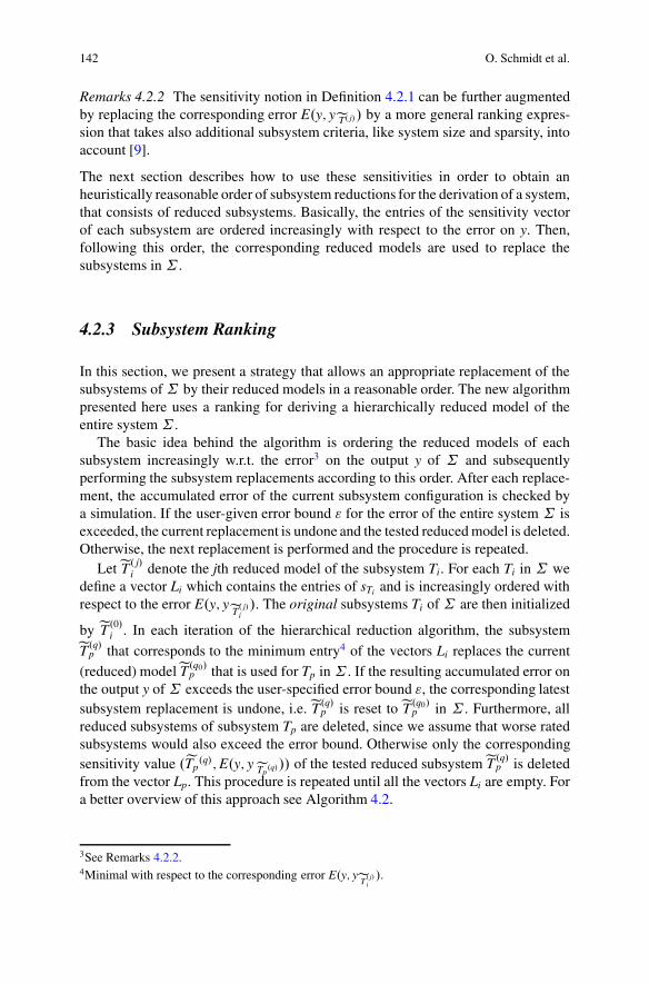
142 O. Schmidt et al.
Remarks 4.2.2 The sensitivity notion in Definition 4.2.1 can be further augmentedby replacing the corresponding error E.y; yeT. j/ / by a more general ranking expres-sion that takes also additional subsystem criteria, like system size and sparsity, intoaccount [9].
The next section describes how to use these sensitivities in order to obtain anheuristically reasonable order of subsystem reductions for the derivation of a system,that consists of reduced subsystems. Basically, the entries of the sensitivity vectorof each subsystem are ordered increasingly with respect to the error on y. Then,following this order, the corresponding reduced models are used to replace thesubsystems in ˙ .
4.2.3 Subsystem Ranking
In this section, we present a strategy that allows an appropriate replacement of thesubsystems of˙ by their reduced models in a reasonable order. The new algorithmpresented here uses a ranking for deriving a hierarchically reduced model of theentire system ˙ .
The basic idea behind the algorithm is ordering the reduced models of eachsubsystem increasingly w.r.t. the error3 on the output y of ˙ and subsequentlyperforming the subsystem replacements according to this order. After each replace-ment, the accumulated error of the current subsystem configuration is checked bya simulation. If the user-given error bound " for the error of the entire system ˙ isexceeded, the current replacement is undone and the tested reduced model is deleted.Otherwise, the next replacement is performed and the procedure is repeated.
Let eT. j/i denote the jth reduced model of the subsystem Ti. For each Ti in ˙ we
define a vector Li which contains the entries of sTi and is increasingly ordered withrespect to the error E.y; yeT. j/
i/. The original subsystems Ti of ˙ are then initialized
by eT .0/i . In each iteration of the hierarchical reduction algorithm, the subsystemeT.q/p that corresponds to the minimum entry4 of the vectors Li replaces the current(reduced) modeleT.q0/p that is used for Tp in ˙ . If the resulting accumulated error onthe output y of ˙ exceeds the user-specified error bound ", the corresponding latestsubsystem replacement is undone, i.e. eT.q/p is reset to eT .q0/p in ˙ . Furthermore, allreduced subsystems of subsystem Tp are deleted, since we assume that worse ratedsubsystems would also exceed the error bound. Otherwise only the correspondingsensitivity value .eTp
.q/;E.y; yeTp.q/ // of the tested reduced subsystemeT .q/p is deleted
from the vector Lp. This procedure is repeated until all the vectors Li are empty. Fora better overview of this approach see Algorithm 4.2.
3See Remarks 4.2.2.4Minimal with respect to the corresponding error E.y; yeT . j/
i/.
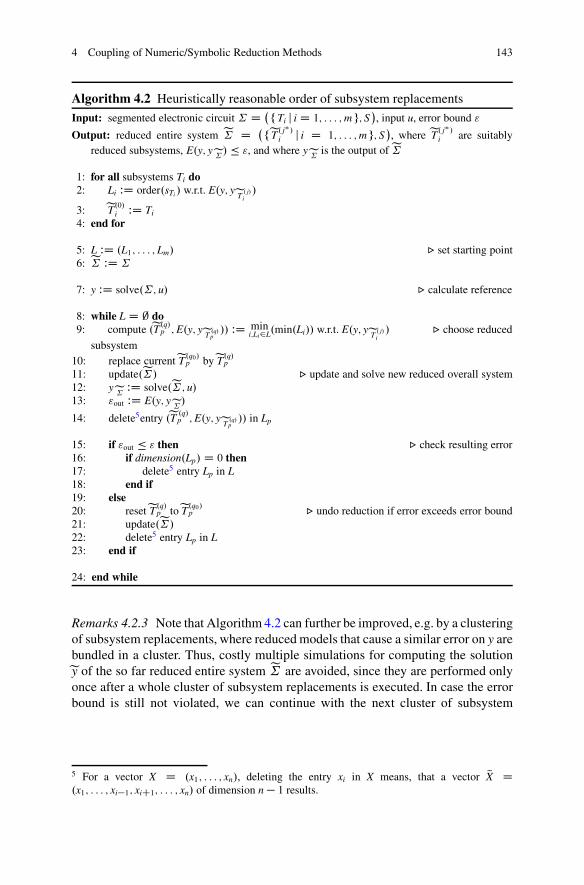
4 Coupling of Numeric/Symbolic Reduction Methods 143
Algorithm 4.2 Heuristically reasonable order of subsystem replacements
Input: segmented electronic circuit ˙ D � fTi j i D 1; : : : ;m g; S �, input u, error bound "
Output: reduced entire system e D � feT . j�/i j i D 1; : : : ;m g; S �, where eT. j�/
i are suitablyreduced subsystems, E.y; ye/ � ", and where ye is the output of e
1: for all subsystems Ti do2: Li WD order.sTi / w.r.t. E.y; yeT . j/
i/
3: eT.0/i WD Ti
4: end for
5: L WD .L1; : : : ; Lm/ F set starting point6: e WD ˙
7: y WD solve.˙; u/ F calculate reference
8: while L D ; do9: compute .eT .q/p ;E.y; yeT .q/
p// WD min
i;Li2L.min.Li// w.r.t. E.y; yeT . j/i/ F choose reduced
subsystem10: replace currenteT .q0/p byeT.q/p
11: update.e/ F update and solve new reduced overall system12: ye WD solve.e; u/13: "out WD E.y; ye/14: delete5entry .eT .q/
p ;E.y; yeT .q/p// in Lp
15: if "out � " then F check resulting error16: if dimension.Lp/ D 0 then17: delete5 entry Lp in L18: end if19: else20: reseteT .q/p toeT .q0/p F undo reduction if error exceeds error bound21: update.e/22: delete5 entry Lp in L23: end if
24: end while
Remarks 4.2.3 Note that Algorithm 4.2 can further be improved, e.g. by a clusteringof subsystem replacements, where reduced models that cause a similar error on y arebundled in a cluster. Thus, costly multiple simulations for computing the solutioney of the so far reduced entire system e are avoided, since they are performed onlyonce after a whole cluster of subsystem replacements is executed. In case the errorbound is still not violated, we can continue with the next cluster of subsystem
5 For a vector X D .x1; : : : ; xn/, deleting the entry xi in X means, that a vector QX D.x1; : : : ; xi�1; xiC1; : : : ; xn/ of dimension n� 1 results.
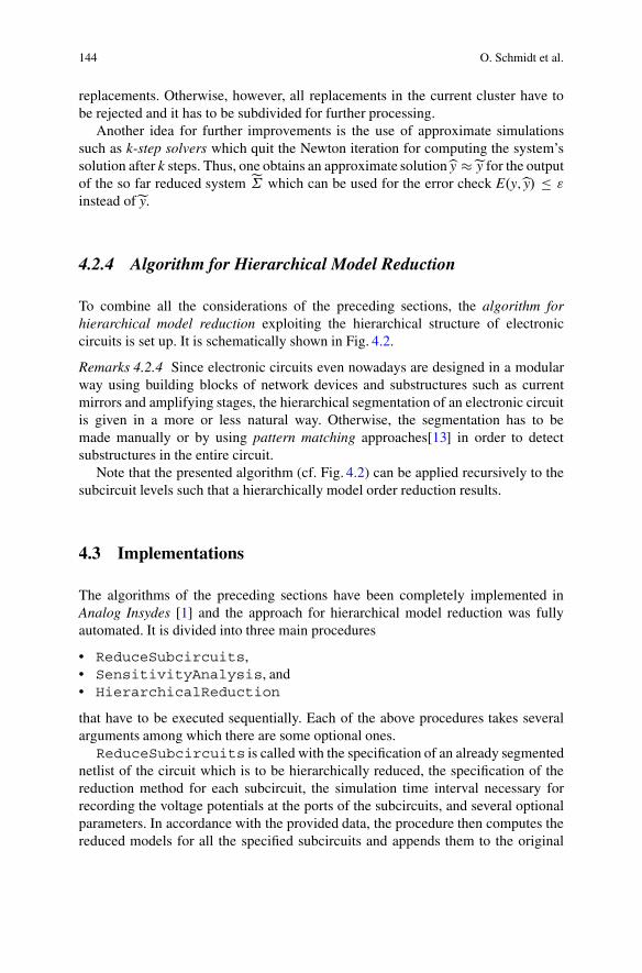
144 O. Schmidt et al.
replacements. Otherwise, however, all replacements in the current cluster have tobe rejected and it has to be subdivided for further processing.
Another idea for further improvements is the use of approximate simulationssuch as k-step solvers which quit the Newton iteration for computing the system’ssolution after k steps. Thus, one obtains an approximate solutionby ey for the outputof the so far reduced system e which can be used for the error check E.y;by/ � "
instead ofey.
4.2.4 Algorithm for Hierarchical Model Reduction
To combine all the considerations of the preceding sections, the algorithm forhierarchical model reduction exploiting the hierarchical structure of electroniccircuits is set up. It is schematically shown in Fig. 4.2.
Remarks 4.2.4 Since electronic circuits even nowadays are designed in a modularway using building blocks of network devices and substructures such as currentmirrors and amplifying stages, the hierarchical segmentation of an electronic circuitis given in a more or less natural way. Otherwise, the segmentation has to bemade manually or by using pattern matching approaches[13] in order to detectsubstructures in the entire circuit.
Note that the presented algorithm (cf. Fig. 4.2) can be applied recursively to thesubcircuit levels such that a hierarchically model order reduction results.
4.3 Implementations
The algorithms of the preceding sections have been completely implemented inAnalog Insydes [1] and the approach for hierarchical model reduction was fullyautomated. It is divided into three main procedures
• ReduceSubcircuits,• SensitivityAnalysis, and• HierarchicalReduction
that have to be executed sequentially. Each of the above procedures takes severalarguments among which there are some optional ones.
ReduceSubcircuits is called with the specification of an already segmentednetlist of the circuit which is to be hierarchically reduced, the specification of thereduction method for each subcircuit, the simulation time interval necessary forrecording the voltage potentials at the ports of the subcircuits, and several optionalparameters. In accordance with the provided data, the procedure then computes thereduced models for all the specified subcircuits and appends them to the original
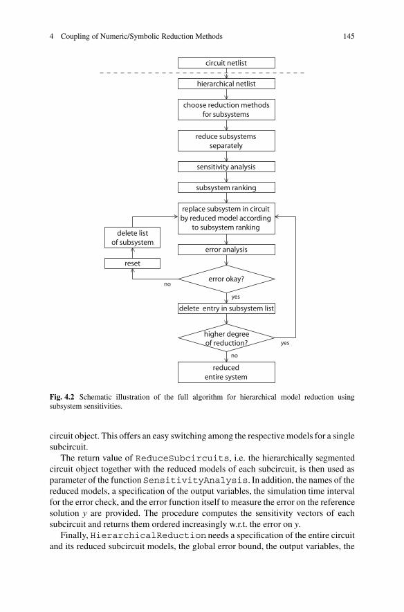
4 Coupling of Numeric/Symbolic Reduction Methods 145
circuit netlist
hierarchical netlist
choose reduction methodsfor subsystems
reduce subsystemsseparately
sensitivity analysis
subsystem ranking
replace subsystem in circuitby reduced model according
to subsystem ranking
error analysis
reducedentire system
delete entry in subsystem list
error okay?
higher degree of reduction?
delete listof subsystem
reset
no
yes
no
yes
Fig. 4.2 Schematic illustration of the full algorithm for hierarchical model reduction usingsubsystem sensitivities.
circuit object. This offers an easy switching among the respective models for a singlesubcircuit.
The return value of ReduceSubcircuits, i.e. the hierarchically segmentedcircuit object together with the reduced models of each subcircuit, is then used asparameter of the functionSensitivityAnalysis. In addition, the names of thereduced models, a specification of the output variables, the simulation time intervalfor the error check, and the error function itself to measure the error on the referencesolution y are provided. The procedure computes the sensitivity vectors of eachsubcircuit and returns them ordered increasingly w.r.t. the error on y.
Finally, HierarchicalReduction needs a specification of the entire circuitand its reduced subcircuit models, the global error bound, the output variables, the
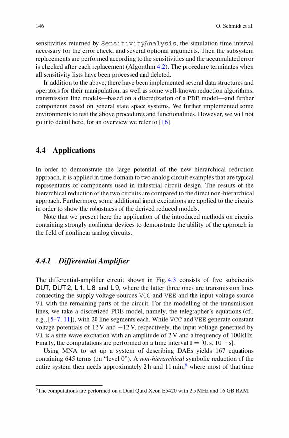
146 O. Schmidt et al.
sensitivities returned by SensitivityAnalysis, the simulation time intervalnecessary for the error check, and several optional arguments. Then the subsystemreplacements are performed according to the sensitivities and the accumulated erroris checked after each replacement (Algorithm 4.2). The procedure terminates whenall sensitivity lists have been processed and deleted.
In addition to the above, there have been implemented several data structures andoperators for their manipulation, as well as some well-known reduction algorithms,transmission line models—based on a discretization of a PDE model—and furthercomponents based on general state space systems. We further implemented someenvironments to test the above procedures and functionalities. However, we will notgo into detail here, for an overview we refer to [16].
4.4 Applications
In order to demonstrate the large potential of the new hierarchical reductionapproach, it is applied in time domain to two analog circuit examples that are typicalrepresentants of components used in industrial circuit design. The results of thehierarchical reduction of the two circuits are compared to the direct non-hierarchicalapproach. Furthermore, some additional input excitations are applied to the circuitsin order to show the robustness of the derived reduced models.
Note that we present here the application of the introduced methods on circuitscontaining strongly nonlinear devices to demonstrate the ability of the approach inthe field of nonlinear analog circuits.
4.4.1 Differential Amplifier
The differential-amplifier circuit shown in Fig. 4.3 consists of five subcircuitsDUT, DUT2, L1, L8, and L9, where the latter three ones are transmission linesconnecting the supply voltage sources VCC and VEE and the input voltage sourceV1 with the remaining parts of the circuit. For the modelling of the transmissionlines, we take a discretized PDE model, namely, the telegrapher’s equations (cf.,e.g., [5–7, 11]), with 20 line segments each. While VCC and VEE generate constantvoltage potentials of 12V and �12V, respectively, the input voltage generated byV1 is a sine wave excitation with an amplitude of 2V and a frequency of 100 kHz.Finally, the computations are performed on a time interval I D Œ0: s; 10�5 s�.
Using MNA to set up a system of describing DAEs yields 167 equationscontaining 645 terms (on “level 0”). A non-hierarchical symbolic reduction of theentire system then needs approximately 2 h and 11min,6 where most of that time
6The computations are performed on a Dual Quad Xeon E5420 with 2.5 MHz and 16 GB RAM.

4 Coupling of Numeric/Symbolic Reduction Methods 147
VCC
V1
VEE
1
2
RC1
Q1
Cload
RS2
3
Vout
RC2 RBIAS
RS1Q2
4Q3Q
4 5
6
7
9
8
DUT
DUT 2L 1
L 9
L 8
Fig. 4.3 Differential amplifier with its intuitive hierarchical segmentation into five subcircuitsDUT, DUT2, L1, L8, and L9.
(95%) is needed for the computation of the transient term ranking.7 Due to this,the computational costs are approximately the same for all choices of the errorbound ". The error function used first discretizes the time interval I to a uniform gridof 100 points and then takes the maximum absolute difference of the two solutionson this grid as a measure for the error.
With " equal to 3% the system is reduced to 124 equations and 416 terms, while apermitted error of 10% narrows these numbers down to 44 equations and 284 terms.The results are shown in Fig. 4.4. Note also that the error bound of 10% is fullyexploited.
In contrast to the immense time costs of the non-hierarchical approach, the newalgorithm for hierarchical reduction reduces the entire system in only 4min and50 s. The subcircuits DUT and DUT2 are reduced symbolically by using a sweepof error bounds
sw D f1%; 10%; 50%; 90%; 100%g; (4.7)
such that each subsystem yields 5 reduced subsystems. The three transmission linesL1, L8, and L9 are reduced numerically by applying Arnoldi’s algorithm [2, 3].
7A term ranking is a trade-off between accuracy and efficiency in computation time that estimatesthe influence of a term in a system of equations on its solution. Here, however, we use fullsimulations instead of low-accuracy estimates. For more details see [20].
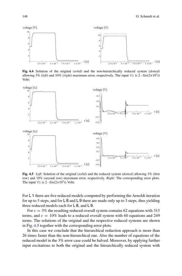
148 O. Schmidt et al.
2.5 10 6 5. 10 6 7.5 10 6 1. 10 5t s
2
4
6
8
10
voltage V
2.5 10 6 5. 10 6 7.5 10 6 1. 10 5t s
2
4
6
8
10
voltage V
Fig. 4.4 Solution of the original (solid) and the non-hierarchically reduced system (dotted)allowing 3% (left) and 10% (right) maximum error, respectively. The input V1 is 2 � Sin.2�105t/Volts
2.5 10 6 5. 10 6 7.5 10 6 1. 10 5t s
2
4
6
8
10
voltage V
2.5 10 6 5. 10 6 7.5 10 6 1. 10 5t s
0.2
0.1
0.1
0.2
0.3
voltage V
2.5 10 6 5. 10 6 7.5 10 6 1. 10 5t s
2
4
6
8
10
voltage V
2.5 10 6 5. 10 6 7.5 10 6 1. 10 5t s
0.4
0.2
0.2
0.4
0.6
0.8
voltage V
Fig. 4.5 Left: Solution of the original (solid) and the reduced system (dotted) allowing 3% (firstrow) and 10% (second row) maximum error, respectively. Right: The corresponding error plots.The input V1 is 2 � Sin.2�105t/ Volts
For L1 there are five reduced models computed by performing the Arnoldi iterationfor up to 5 steps, and for L8 and L9 there are made only up to 3 steps, thus yieldingthree reduced models each for L8, and L9.
For " D 3% the resulting reduced overall system contains 62 equations with 315terms, and " D 10% leads to a reduced overall system with 60 equations and 249terms. The solutions of the original and the respective reduced systems are shownin Fig. 4.5 together with the corresponding error plots.
In this case we conclude that the hierarchical reduction approach is more than26 times faster than the non-hierarchical one. Also the number of equations of thereduced model in the 3% error case could be halved. Moreover, by applying furtherinput excitations to both the original and the hierarchically reduced system with
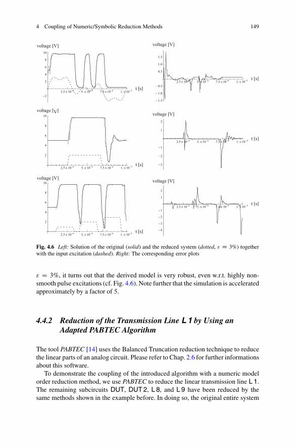
4 Coupling of Numeric/Symbolic Reduction Methods 149
2.5 10 6 5. 10 6 7.5 10 6 1. 10 5t s
2
2
4
6
8
10
voltage V
2.5 10 6 5. 10 6 7.5 10 6 1. 10 5t s
1.5
1.0
0.5
0.5
1.0
1.5
voltage V
2.5 10 6 5. 10 6 7.5 10 6 1. 10 5t s
2
4
6
8
10
voltage V
2.5 10 6 5. 10 6 7.5 10 6 1. 10 5t s
3
2
1
1
2
voltage V
2.5 10 6 5. 10 6 7.5 10 6 1. 10 5t s
2
4
6
8
10
voltage V
2.5 10 6 5. 10 6 7.5 10 6 1. 10 5t s
4
3
2
1
1
2
voltage V
Fig. 4.6 Left: Solution of the original (solid) and the reduced system (dotted, " D 3%) togetherwith the input excitation (dashed). Right: The corresponding error plots
" D 3%, it turns out that the derived model is very robust, even w.r.t. highly non-smooth pulse excitations (cf. Fig. 4.6). Note further that the simulation is acceleratedapproximately by a factor of 5.
4.4.2 Reduction of the Transmission Line L1 by Using anAdapted PABTEC Algorithm
The tool PABTEC [14] uses the Balanced Truncation reduction technique to reducethe linear parts of an analog circuit. Please refer to Chap. 2.6 for further informationsabout this software.
To demonstrate the coupling of the introduced algorithm with a numeric modelorder reduction method, we use PABTEC to reduce the linear transmission line L1.The remaining subcircuits DUT, DUT2, L8, and L9 have been reduced by thesame methods shown in the example before. In doing so, the original entire system
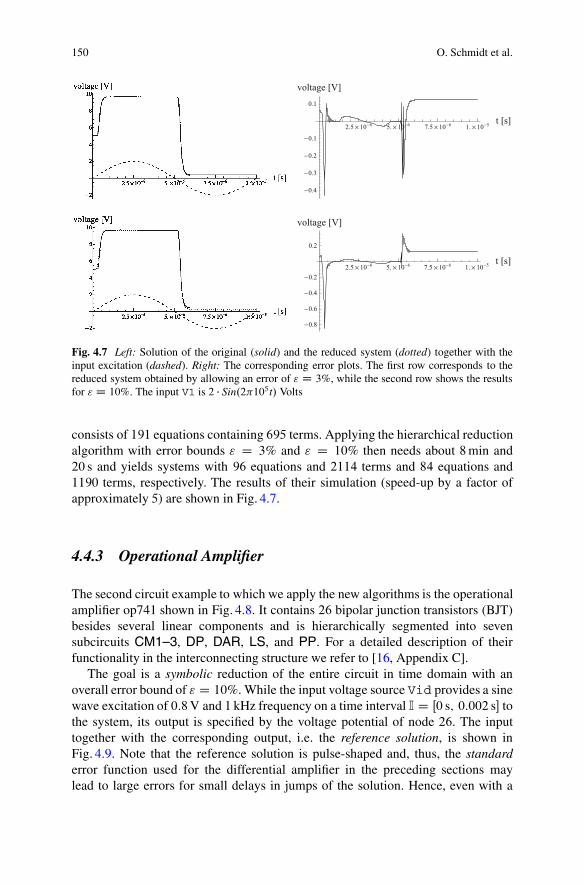
150 O. Schmidt et al.
2.5 10 6 5. 10 6 7.5 10 6 1. 10 5t s
0.4
0.3
0.2
0.1
0.1
voltage V
2.5 10 6 5. 10 6 7.5 10 6 1. 10 5t s
0.8
0.6
0.4
0.2
0.2
voltage V
Fig. 4.7 Left: Solution of the original (solid) and the reduced system (dotted) together with theinput excitation (dashed). Right: The corresponding error plots. The first row corresponds to thereduced system obtained by allowing an error of " D 3%, while the second row shows the resultsfor "D 10%. The input V1 is 2 � Sin.2�105t/ Volts
consists of 191 equations containing 695 terms. Applying the hierarchical reductionalgorithm with error bounds " D 3% and " D 10% then needs about 8min and20 s and yields systems with 96 equations and 2114 terms and 84 equations and1190 terms, respectively. The results of their simulation (speed-up by a factor ofapproximately 5) are shown in Fig. 4.7.
4.4.3 Operational Amplifier
The second circuit example to which we apply the new algorithms is the operationalamplifier op741 shown in Fig. 4.8. It contains 26 bipolar junction transistors (BJT)besides several linear components and is hierarchically segmented into sevensubcircuits CM1–3, DP, DAR, LS, and PP. For a detailed description of theirfunctionality in the interconnecting structure we refer to [16, Appendix C].
The goal is a symbolic reduction of the entire circuit in time domain with anoverall error bound of " D 10%. While the input voltage source Vid provides a sinewave excitation of 0:8V and 1 kHz frequency on a time interval I D Œ0 s; 0:002 s� tothe system, its output is specified by the voltage potential of node 26. The inputtogether with the corresponding output, i.e. the reference solution, is shown inFig. 4.9. Note that the reference solution is pulse-shaped and, thus, the standarderror function used for the differential amplifier in the preceding sections maylead to large errors for small delays in jumps of the solution. Hence, even with a
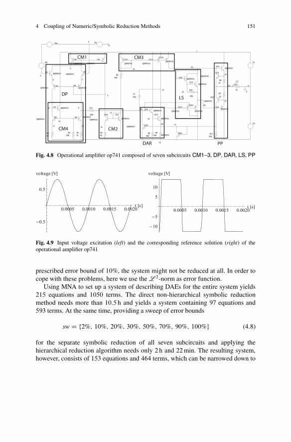
4 Coupling of Numeric/Symbolic Reduction Methods 151
Fig. 4.8 Operational amplifier op741 composed of seven subcircuits CM1–3, DP, DAR, LS, PP
Fig. 4.9 Input voltage excitation (left) and the corresponding reference solution (right) of theoperational amplifier op741
prescribed error bound of 10%, the system might not be reduced at all. In order tocope with these problems, here we use the L 2-norm as error function.
Using MNA to set up a system of describing DAEs for the entire system yields215 equations and 1050 terms. The direct non-hierarchical symbolic reductionmethod needs more than 10:5 h and yields a system containing 97 equations and593 terms. At the same time, providing a sweep of error bounds
sw D f2%; 10%; 20%; 30%; 50%; 70%; 90%; 100%g (4.8)
for the separate symbolic reduction of all seven subcircuits and applying thehierarchical reduction algorithm needs only 2 h and 22min. The resulting system,however, consists of 153 equations and 464 terms, which can be narrowed down to
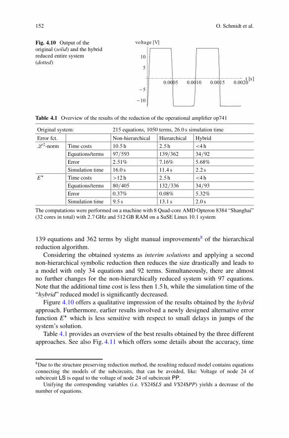
152 O. Schmidt et al.
Fig. 4.10 Output of theoriginal (solid) and the hybridreduced entire system(dotted)
Table 4.1 Overview of the results of the reduction of the operational amplifier op741
Original system: 215 equations, 1050 terms, 26:0 s simulation time
Error fct. Non-hierarchical Hierarchical Hybrid
L 2-norm Time costs 10:5 h 2:5 h <4 h
Equations/terms 97=593 139=362 34=92
Error 2:51% 7:16% 5:68%
Simulation time 16:0 s 11:4 s 2:2 s
E� Time costs >12 h 2:5 h <4 h
Equations/terms 80=405 132=336 34=93
Error 0:37% 0:08% 5:32%
Simulation time 9:5 s 13:1 s 2:0 s
The computations were performed on a machine with 8Quad-core AMD Opteron 8384 “Shanghai”(32 cores in total) with 2:7GHz and 512GB RAM on a SuSE Linux 10:1 system
139 equations and 362 terms by slight manual improvements8 of the hierarchicalreduction algorithm.
Considering the obtained systems as interim solutions and applying a secondnon-hierarchical symbolic reduction then reduces the size drastically and leads toa model with only 34 equations and 92 terms. Simultaneously, there are almostno further changes for the non-hierarchically reduced system with 97 equations.Note that the additional time cost is less then 1:5 h, while the simulation time of the“hybrid” reduced model is significantly decreased.
Figure 4.10 offers a qualitative impression of the results obtained by the hybridapproach. Furthermore, earlier results involved a newly designed alternative errorfunction E� which is less sensitive with respect to small delays in jumps of thesystem’s solution.
Table 4.1 provides an overview of the best results obtained by the three differentapproaches. See also Fig. 4.11 which offers some details about the accuracy, time
8Due to the structure preserving reduction method, the resulting reduced model contains equationsconnecting the models of the subcircuits, that can be avoided, like: Voltage of node 24 ofsubcircuit LS is equal to the voltage of node 24 of subcircuit PP.
Unifying the corresponding variables (i.e. V$24$LS and V$24$PP) yields a decrease of thenumber of equations.
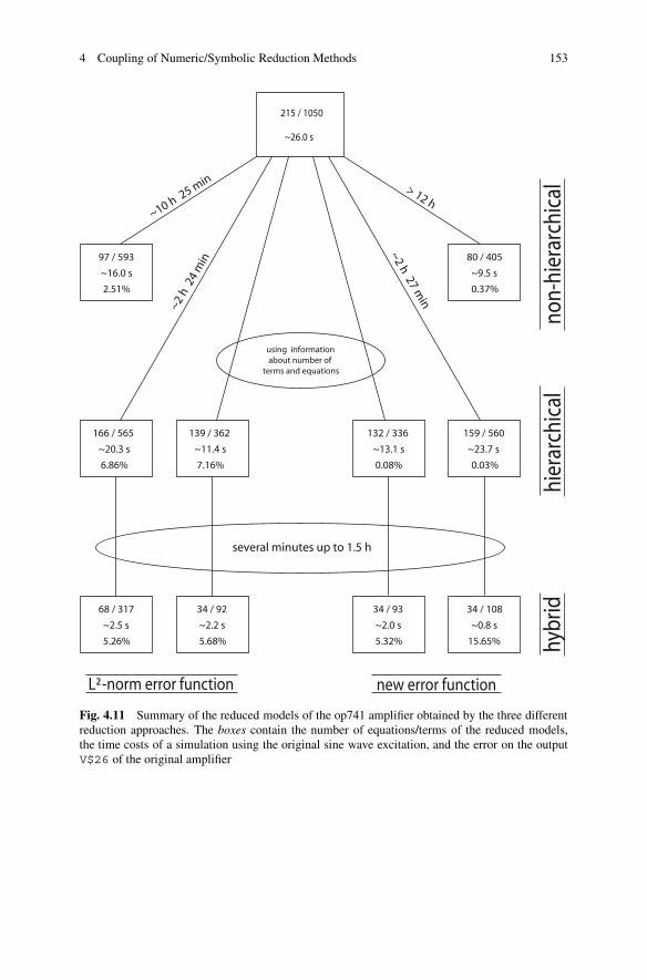
4 Coupling of Numeric/Symbolic Reduction Methods 153
215 / 1050
~26.0 s
97 / 593
~16.0 s
2.51%
80 / 405
~9.5 s
0.37%
lacihcrarei h- nonl aci hcr ar ei h
byhdir
L²-norm error function new error function
132 / 336
~13.1 s
0.08%
159 / 560
~23.7 s
0.03%
139 / 362
~11.4 s
7.16%
166 / 565
~20.3 s
6.86%
34 / 108
~0.8 s
15.65%
34 / 93
~2.0 s
5.32%
34 / 92
~2.2 s
5.68%
68 / 317
~2.5 s
5.26%
several minutes up to 1.5 h
using informationabout number of
terms and equations
~10 h 25 min > 12 h
~2 h 27 min
~2 h
24
min
Fig. 4.11 Summary of the reduced models of the op741 amplifier obtained by the three differentreduction approaches. The boxes contain the number of equations/terms of the reduced models,the time costs of a simulation using the original sine wave excitation, and the error on the outputV$26 of the original amplifier
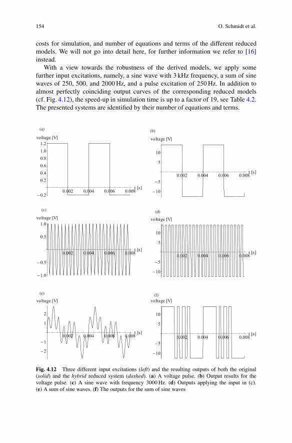
154 O. Schmidt et al.
costs for simulation, and number of equations and terms of the different reducedmodels. We will not go into detail here, for further information we refer to [16]instead.
With a view towards the robustness of the derived models, we apply somefurther input excitations, namely, a sine wave with 3 kHz frequency, a sum of sinewaves of 250, 500, and 2000Hz, and a pulse excitation of 250Hz. In addition toalmost perfectly coinciding output curves of the corresponding reduced models(cf. Fig. 4.12), the speed-up in simulation time is up to a factor of 19, see Table 4.2.The presented systems are identified by their number of equations and terms.
Fig. 4.12 Three different input excitations (left) and the resulting outputs of both the original(solid) and the hybrid reduced system (dashed). (a) A voltage pulse. (b) Output results for thevoltage pulse. (c) A sine wave with frequency 3000Hz. (d) Outputs applying the input in (c).(e) A sum of sine waves. (f) The outputs for the sum of sine waves
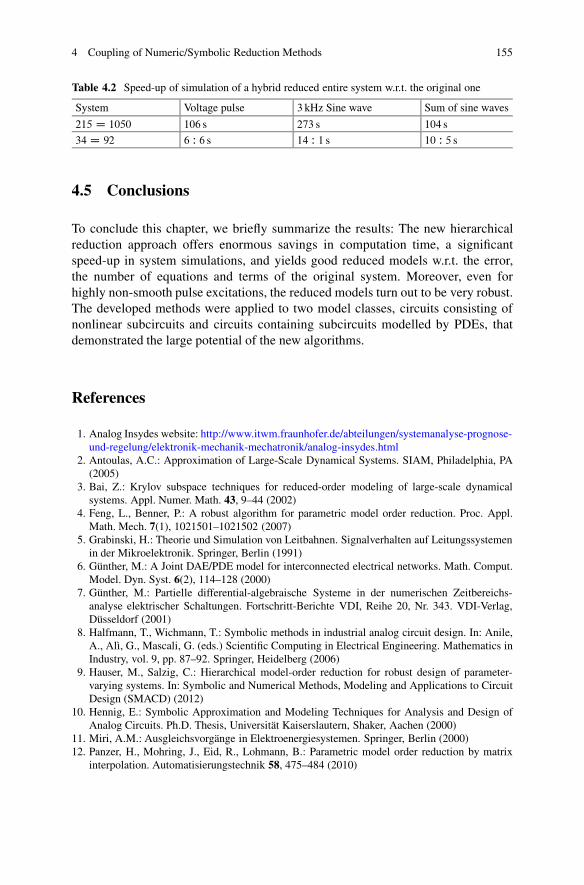
4 Coupling of Numeric/Symbolic Reduction Methods 155
Table 4.2 Speed-up of simulation of a hybrid reduced entire system w.r.t. the original one
System Voltage pulse 3 kHz Sine wave Sum of sine waves
215 D 1050 106 s 273 s 104 s
34 D 92 6 W 6 s 14 W 1 s 10 W 5 s
4.5 Conclusions
To conclude this chapter, we briefly summarize the results: The new hierarchicalreduction approach offers enormous savings in computation time, a significantspeed-up in system simulations, and yields good reduced models w.r.t. the error,the number of equations and terms of the original system. Moreover, even forhighly non-smooth pulse excitations, the reduced models turn out to be very robust.The developed methods were applied to two model classes, circuits consisting ofnonlinear subcircuits and circuits containing subcircuits modelled by PDEs, thatdemonstrated the large potential of the new algorithms.
References
1. Analog Insydes website: http://www.itwm.fraunhofer.de/abteilungen/systemanalyse-prognose-und-regelung/elektronik-mechanik-mechatronik/analog-insydes.html
2. Antoulas, A.C.: Approximation of Large-Scale Dynamical Systems. SIAM, Philadelphia, PA(2005)
3. Bai, Z.: Krylov subspace techniques for reduced-order modeling of large-scale dynamicalsystems. Appl. Numer. Math. 43, 9–44 (2002)
4. Feng, L., Benner, P.: A robust algorithm for parametric model order reduction. Proc. Appl.Math. Mech. 7(1), 1021501–1021502 (2007)
5. Grabinski, H.: Theorie und Simulation von Leitbahnen. Signalverhalten auf Leitungssystemenin der Mikroelektronik. Springer, Berlin (1991)
6. Günther, M.: A Joint DAE/PDE model for interconnected electrical networks. Math. Comput.Model. Dyn. Syst. 6(2), 114–128 (2000)
7. Günther, M.: Partielle differential-algebraische Systeme in der numerischen Zeitbereichs-analyse elektrischer Schaltungen. Fortschritt-Berichte VDI, Reihe 20, Nr. 343. VDI-Verlag,Düsseldorf (2001)
8. Halfmann, T., Wichmann, T.: Symbolic methods in industrial analog circuit design. In: Anile,A., Alì, G., Mascali, G. (eds.) Scientific Computing in Electrical Engineering. Mathematics inIndustry, vol. 9, pp. 87–92. Springer, Heidelberg (2006)
9. Hauser, M., Salzig, C.: Hierarchical model-order reduction for robust design of parameter-varying systems. In: Symbolic and Numerical Methods, Modeling and Applications to CircuitDesign (SMACD) (2012)
10. Hennig, E.: Symbolic Approximation and Modeling Techniques for Analysis and Design ofAnalog Circuits. Ph.D. Thesis, Universität Kaiserslautern, Shaker, Aachen (2000)
11. Miri, A.M.: Ausgleichsvorgänge in Elektroenergiesystemen. Springer, Berlin (2000)12. Panzer, H., Mohring, J., Eid, R., Lohmann, B.: Parametric model order reduction by matrix
interpolation. Automatisierungstechnik 58, 475–484 (2010)
156 O. Schmidt et al.
13. Pelz, G., Roettcher, U.: Pattern matching and refinement hybrid approach to circuit comparison.IEEE Trans. Comput.-Aided Des. Integr. Circuits Syst. 13, 264–276 (1994)
14. Reis, T., Stykel, T.: PABTEC: passivity-preserving balanced truncation for electrical circuits.IEEE Trans. Comput.-Aided Des. Integr. Circuits Syst. 29, 1354–1367 (2010)
15. Sommer, R., Hennig, E., Nitsche, G., Schwarz, P., Broz, J.: Automatic Nonlinear BehavioralModel Generation Using Symbolic Circuit Analysis. In: Fakhfakh, M., Tlelo-Cuautle, E.,Fernández, F.V. (eds.) Design of Analog Circuits through Symbolic Analysis, pp. 305–341.Bentham Science Publishers, Sharjah (2012). doi:10.2174/978160805095611201010305
16. Schmidt, O.: Structure-Exploiting Coupled Symbolic-Numerical Model Reduction for Electri-cal Networks. Dissertation, Technische Universität Kaiserslautern, Cuvillier, Göttingen (2010)
17. Schmidt, O.: Structure-exploiting symbolic-numerical model reduction of nonlinear electricalcircuits. In: Proceedings der 16th European Conference on Mathematics for Industry ECMI2010, Wuppertal. Mathematics in Industry, vol. 17, pp. 179–185. Springer, Berlin (2010)
18. Schmidt, O., Halfmann, T., Lang, P.: Coupling of numerical and symbolic techniques for modelorder reduction in circuit design. In: Benner, P., Hinze, M., ter Maten, E.J.W. (eds.) ModelReduction for Circuit Simulation. Lecture Notes in Electrical Engineering, vol. 74, pp. 261–275. Springer, Dordrecht (2011)
19. Sommer, R., Krauße, D., Schäfer, E., Hennig, E.: Application of symbolic circuitanalysis for failure detection and optimization of industrial integrated circuits. In:Fakhfakh, M., Tlelo-Cuautle, E., Fernández, F.V. (eds.) Design of Analog Circuitsthrough Symbolic Analysis, pp. 445–477. Bentham Science Publishers, Sharjah (2012).doi:10.2174/978160805095611201010305
20. Wichmann, T.: Symbolische Reduktionsverfahren für nichtlineare DAE-Systeme. Shaker,Aachen (2004)
21. Wolfram, S.: The Mathematica Book, 5th edn. Wolfram Media, Inc., Champaign (2003)
Chapter 5Low-Rank Cholesky Factor Krylov SubspaceMethods for Generalized Projected LyapunovEquations
Matthias Bollhöfer and André K. Eppler
Abstract Large-scale descriptor systems arising from circuit simulation oftenrequire model reduction techniques. Among many methods, Balanced Truncation isa popular method for constructing a reduced order model. In the heart of BalancedTruncation methods, a sequence of projected generalized Lyapunov equations has tobe solved. In this article we present a general framework for the numerical solutionof projected generalized Lyapunov equations using preconditioned Krylov subspacemethods based on iterates with a low-rank Cholesky factor representation. Thisapproach can be viewed as alternative to the LRCF-ADI method, a well establishedmethod for solving Lyapunov equations. We will show that many well-knownKrylov subspace methods such as (F)GMRES, QMR, BICGSTAB and CG can beeasily modified to reveal the underlying low-rank structures.
5.1 Introduction
The numerical simulation of large-scale integrated circuits nowadays approachessystem sizes of several hundred million equations. This ever-increasing size hasseveral sources; one of which is the accelerating scale of miniaturization, anotherreason is the increasing density of the integrated devices. The simulation ofthe complete system requires many simulation runs with different input signals.These simulation runs would be impossible to compute in acceptable time usingthe original system. Instead it is necessary to replace the original system by asignificantly smaller reduced model which inherits the essential structures andproperties of the original system as, e.g., passivity and stability. To deal with thisproblem model order reduction techniques (MOR) have turned out to be a keytechnology in order to generate reduced models. Among the most popular methods
M. Bollhöfer (�) • A.K. EpplerTU Braunschweig, Carl-Friedrich-Gauß-Fakultät, Institut Computational Mathematics,Universitätspl. 2, 38106 Braunschweig, Germanye-mail: [email protected]; [email protected]
© Springer International Publishing AG 2017P. Benner (ed.), System Reduction for Nanoscale IC Design,Mathematics in Industry 20, DOI 10.1007/978-3-319-07236-4_5
157
158 M. Bollhöfer and A.K. Eppler
for MOR are those based on Krylov subspace method or Balanced Truncation (BT)[3, 11, 30]. For problems arising from circuit simulation in particular passivity-preserving balanced truncation methods [33, 34, 45] are of particular interest, sincebeside reducing the circuit to a reduced order model, major important propertieslike stability and passivity have to be preserved to obtain a physically correct model(see also Chaps. 2 and 3). Another frequently used method mainly applied to partialdifferential-algebraic equations (PDAE) is the Proper Orthogonal Decomposition(POD) method, cf. [16, 26], Chap. 1.
This article is organized as follows. In Sect. 5.2 we will give a brief introductionto balanced truncation which is the motivation for our methods and requires tosolve several sequences of generalized projected Lyapunov equations. This includesexisting numerical methods for solving Lyapunov equations. In Sect. 5.3 we willpresent our novel approach for generalized projected Lyapunov equations basedon Krylov subspace methods. Finally we will use several examples from circuitsimulation, as well as other examples, to demonstrate our approach in Sect. 5.4.
5.2 Balanced Truncation
The basis for the numerical methods for generalized projected Lyapunov equationspresented in this paper are those using Balanced Truncation (BT). In particularpassivity-preserving Balanced Truncation methods will be of special interest formodel order reduction techniques applied to circuit simulation problems.
5.2.1 Introduction to Balanced Truncation
To start with the idea of Balanced Truncation we consider a linear time invariantdescriptor system
EPx D Ax C Buy D Cx C Du
where A;E 2 Rn;n;B 2 R
n;m;C 2 Rp;n;D 2 R
p;m
such that m; p n. Numerical methods for MOR replace E, A, B, C by smallermatrices QE, QA, QB, QC such that for all matrices the initial dimension n is replaced by asuitable l n, i.e., QA; QE 2 R
l;l, QB 2 Rl;m, QC 2 R
p;l.When using Balanced Truncation the reduction of the model is done by multi-
plying with matrices W 2 Rl;n, T 2 R
n;l in order to obtain the reduced descriptorsystem
.E;A;B;C;D/ ! . QE; QA; QB; QC;D/ D .WET;WAT;WB;CT;D/:
5 LRCF Krylov Subspace Methods for Lyapunov Equations 159
The transformation matrices W and T are constructed using the solutions ofgeneralized Lyapunov equations, the so-called proper controllability gramian Gpc
and the proper observability gramian Gpo. When E is singular one also has to takeinto account the improper controllability gramian and the improper observabilitygramian, for details we refer to [34]. For the computation of a reduced model wehave to compute X D Gpc and Y D Gpo by solving the projected generalizedLyapunov equations
EXAT C AXET C PlBBTPTl D 0; where X D PrXPT
r ;
ETYA C ATYE C PTr CTCPr D 0; where Y D PT
l YPl:(5.1)
Here Pl, Pr are obtained from the Weierstrass canonical form for .E;A/. To do sowe assume that det.A � E/ 6� 0. In this case there exist nonsingular V and Z suchthat
V�1EZ D�
I 00 N
�; V�1AZ D
�J 00 I
�: (5.2)
Here J;N denote matrices in Jordan canonical form where N nilpotent. The left andright projection of .E;A/ to
.PlEPr;PlAPr/ D�
V
�I 00 0
�Z�1; V
�J 00 0
�Z�1
�(5.3)
yields the projectors Pl and Pr of the matrix pencil E � A with respect to thesubspace of finite eigenvalues. By solving (5.1) we obtain symmetric, positivesemidefinite solutions X D RRT and Y D LLT , provided that the eigenvaluesof J from (5.2) are located in the open left half plane. In many applicationproblems for MOR in circuit simulation the matrices X, Y are numerically ofapproximate low rank. Using the singular value decomposition of LT ER and LTARthe balanced system is built. This way some general properties such as passivityare not necessarily preserved. To even preserve passivity it is necessary to solve theprojected Lur’e equations [33], see also Chap. 2. In some special cases these in turncan be traced back to algebraic Riccati equations of the form
EXAT CAXET C.EXCT �PlB/TR�1.EXCT �PlB/ D 0; where X D PrXPT
r (5.4)
and
ATYECETYAC.BTYE�CPr/TR�1.BTYE�CPr/ D 0; where Y D PT
l YPl: (5.5)
160 M. Bollhöfer and A.K. Eppler
For details we refer to [33, 34]. Solving Riccati equations using Newton’s methodor the Newton-Kleinman method [4, 44] (cf. also Sect. 2.5.2) requires solving asequence of projected, generalized Lyapunov equations of the form
EXkATk C AkXkET C PlBkBT
k PTl D 0; where Xk D PrXkPT
r ;
ETYkAk C ATk YkE C PT
r CTk CkPr D 0; where Yk D PT
l YkPl:(5.6)
Compared with the original pencil .E;A/, the matrix Ak in .E;Ak/ is obtained froma low-rank correction of A. For large-scale sparse systems arising from circuitsimulation this allows for the computation of sparse approximations (resp. sparsefactorizations) of .E;A/ and then to transfer these approximations to the pencil.E;Ak/ using the Sherman–Morrison–Woodbury formula [14] with respect to Ak.
5.2.2 Numerical Methods for Projected, Generalized LyapunovEquations
We will now describe in detail how projected, generalized Lyapunov equations oftype
EXAT C AXET C PlBBTPTl D 0; where X D PrXPT
r (5.7)
are solved numerically. For simplicity we restrict ourselves to solving a singleequation of this type which is at the heart of Balanced Truncation methods andin practice such equations have to be solved frequently, e.g. once per iteration inAlgorithm 2.7.
One of the most commonly used methods for solving (projected) generalizedLyapunov equations is the ADI method [28, 31, 44, 47]. The ADI method forsolving (5.7) consists of a sequence j D 1; 2; 3; : : : of steps, which is decomposedinto two half-steps
.E C �jA/Xj� 12 AT D �PlBBTPTl � AXj�1.E � �jA/
T ;
AXj.E C �jA/T D �PlBBTPT
l � .E � �jA/Xj� 12 AT :
From these two coupled equations we successively compute�Xj�
j. Here
�1; �2; �3; : : : refer to shift parameters that have to be chosen appropriately toachieve convergence, see [32, 47]. Starting with X0 D 0 and using that the righthand side PlBBTPT
l is symmetric and positive semidefinite one can easily verifythat all iterates Xj D RjRT
j are also symmetric and positive semidefinite. This can beused explicitly in the ADI method to represent the iterates by low rank Cholesky
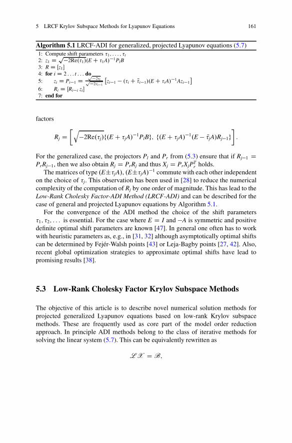
5 LRCF Krylov Subspace Methods for Lyapunov Equations 161
Algorithm 5.1 LRCF-ADI for generalized, projected Lyapunov equations (5.7)1: Compute shift parameters �1; : : : ; �t
2: z1 Dp�2Re.�1/.EC �1A/�1PlB3: R D Œz1�4: for i D 2 : : : t : : : do5: zi D Pi�1 D
p
�2�ip
�2�i�1
zi�1 � .�i C N�i�1/.EC �iA/�1Azi�1
6: Ri D ŒRi�i zi�
7: end for
factors
Rj D�q
�2Re.�j/f.E C �jA/�1PlBg; f.E C �jA/
�1.E � N�jA/Rj�1g�:
For the generalized case, the projectors Pl and Pr from (5.3) ensure that if Rj�1 DPrRj�1, then we also obtain Rj D PrRj and thus Xj D PrXjPT
r holds.The matrices of type .E˙�jA/, .E˙�jA/�1 commute with each other independent
on the choice of �j. This observation has been used in [28] to reduce the numericalcomplexity of the computation of Rj by one order of magnitude. This has lead to theLow-Rank Cholesky Factor-ADI Method (LRCF-ADI) and can be described for thecase of general and projected Lyapunov equations by Algorithm 5.1.
For the convergence of the ADI method the choice of the shift parameters�1; �2; : : : is essential. For the case where E D I and �A is symmetric and positivedefinite optimal shift parameters are known [47]. In general one often has to workwith heuristic parameters as, e.g., in [31, 32] although asymptotically optimal shiftscan be determined by Fejér-Walsh points [43] or Leja-Bagby points [27, 42]. Also,recent global optimization strategies to approximate optimal shifts have lead topromising results [38].
5.3 Low-Rank Cholesky Factor Krylov Subspace Methods
The objective of this article is to describe novel numerical solution methods forprojected generalized Lyapunov equations based on low-rank Krylov subspacemethods. These are frequently used as core part of the model order reductionapproach. In principle ADI methods belong to the class of iterative methods forsolving the linear system (5.7). This can be equivalently rewritten as
LX D B;
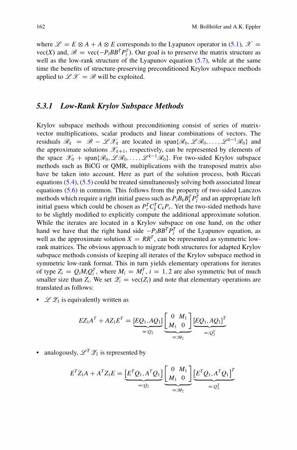
162 M. Bollhöfer and A.K. Eppler
where L D E ˝ A C A ˝ E corresponds to the Lyapunov operator in (5.1), X Dvec.X/ and, B D vec.�PlBBTPT
l /. Our goal is to preserve the matrix structure aswell as the low-rank structure of the Lyapunov equation (5.7), while at the sametime the benefits of structure-preserving preconditioned Krylov subspace methodsapplied to LX D B will be exploited.
5.3.1 Low-Rank Krylov Subspace Methods
Krylov subspace methods without preconditioning consist of series of matrix-vector multiplications, scalar products and linear combinations of vectors. Theresiduals Rk D B � LXk are located in spanfR0;LR0; : : : ;L
k�1R0g andthe approximate solutions XkC1, respectively, can be represented by elements ofthe space X0 C spanfR0;LR0; : : : ;L
k�1R0g. For two-sided Krylov subspacemethods such as BiCG or QMR, multiplications with the transposed matrix alsohave be taken into account. Here as part of the solution process, both Riccatiequations (5.4), (5.5) could be treated simultaneously solving both associated linearequations (5.6) in common. This follows from the property of two-sided Lanczosmethods which require a right initial guess such as PlBkBT
k PTl and an appropriate left
initial guess which could be chosen as PTr CT
k CkPr. Yet the two-sided methods haveto be slightly modified to explicitly compute the additional approximate solution.While the iterates are located in a Krylov subspace on one hand, on the otherhand we have that the right hand side �PlBBTPT
l of the Lyapunov equation, aswell as the approximate solution X D RRT , can be represented as symmetric low-rank matrices. The obvious approach to migrate both structures for adapted Krylovsubspace methods consists of keeping all iterates of the Krylov subspace method insymmetric low-rank format. This in turn yields elementary operations for iteratesof type Zi D QiMiQT
i , where Mi D MTi , i D 1; 2 are also symmetric but of much
smaller size than Zi. We set Zi D vec.Zi/ and note that elementary operations aretranslated as follows:
• LZ1 is equivalently written as
EZ1AT C AZ1E
T D ŒEQ1;AQ1�„ ƒ‚ …DWQ2
�0 M1
M1 0
�
„ ƒ‚ …DWM2
ŒEQ1;AQ1�T„ ƒ‚ …
DWQT2
• analogously, L TZ1 is represented by
ETZ1A C ATZ1E D ETQ1;A
TQ1
„ ƒ‚ …
DWQ2
�0 M1
M1 0
�
„ ƒ‚ …DWM2
ETQ1;A
TQ1
T
„ ƒ‚ …DWQT
2
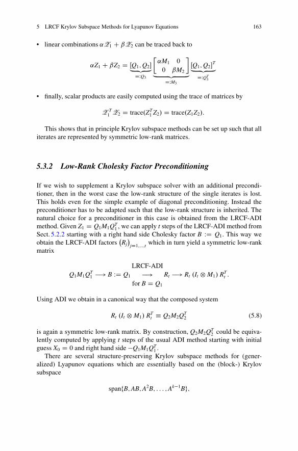
5 LRCF Krylov Subspace Methods for Lyapunov Equations 163
• linear combinations ˛Z1 C ˇZ2 can be traced back to
˛Z1 C ˇZ2 D ŒQ1;Q2�„ ƒ‚ …DWQ3
�˛M1 0
0 ˇM2
�
„ ƒ‚ …DWM3
ŒQ1;Q2�T„ ƒ‚ …
DWQT3
• finally, scalar products are easily computed using the trace of matrices by
Z T1 Z2 D trace.ZT
1 Z2/ D trace.Z1Z2/:
This shows that in principle Krylov subspace methods can be set up such that alliterates are represented by symmetric low-rank matrices.
5.3.2 Low-Rank Cholesky Factor Preconditioning
If we wish to supplement a Krylov subspace solver with an additional precondi-tioner, then in the worst case the low-rank structure of the single iterates is lost.This holds even for the simple example of diagonal preconditioning. Instead thepreconditioner has to be adapted such that the low-rank structure is inherited. Thenatural choice for a preconditioner in this case is obtained from the LRCF-ADImethod. Given Z1 D Q1M1QT
1 , we can apply t steps of the LRCF-ADI method fromSect. 5.2.2 starting with a right hand side Cholesky factor B WD Q1. This way weobtain the LRCF-ADI factors
�Rj�
jD1;:::;t which in turn yield a symmetric low-rankmatrix
Q1M1QT1 �! B WD Q1
LRCF-ADI�!
for B D Q1
Rt �! Rt .It ˝ M1/ RTt :
Using ADI we obtain in a canonical way that the composed system
Rt .It ˝ M1/ RTt � Q2M2Q
T2 (5.8)
is again a symmetric low-rank matrix. By construction, Q2M2QT2 could be equiva-
lently computed by applying t steps of the usual ADI method starting with initialguess X0 D 0 and right hand side �Q1M1QT
1 .There are several structure-preserving Krylov subspace methods for (gener-
alized) Lyapunov equations which are essentially based on the (block-) Krylovsubspace
spanfB;AB;A2B; : : : ;Ak�1Bg;
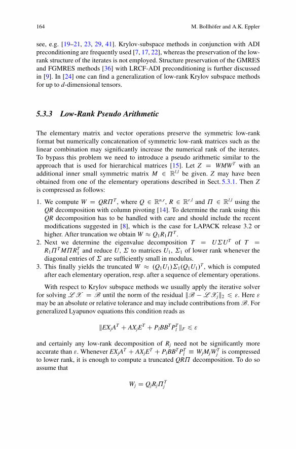
164 M. Bollhöfer and A.K. Eppler
see, e.g. [19–21, 23, 29, 41]. Krylov-subspace methods in conjunction with ADIpreconditioning are frequently used [7, 17, 22], whereas the preservation of the low-rank structure of the iterates is not employed. Structure preservation of the GMRESand FGMRES methods [36] with LRCF-ADI preconditioning is further discussedin [9]. In [24] one can find a generalization of low-rank Krylov subspace methodsfor up to d-dimensional tensors.
5.3.3 Low-Rank Pseudo Arithmetic
The elementary matrix and vector operations preserve the symmetric low-rankformat but numerically concatenation of symmetric low-rank matrices such as thelinear combination may significantly increase the numerical rank of the iterates.To bypass this problem we need to introduce a pseudo arithmetic similar to theapproach that is used for hierarchical matrices [15]. Let Z D WMWT with anadditional inner small symmetric matrix M 2 R
l;l be given. Z may have beenobtained from one of the elementary operations described in Sect. 5.3.1. Then Zis compressed as follows:
1. We compute W D QR˘T , where Q 2 Rn;r, R 2 R
r;l and ˘ 2 Rl;l using the
QR decomposition with column pivoting [14]. To determine the rank using thisQR decomposition has to be handled with care and should include the recentmodifications suggested in [8], which is the case for LAPACK release 3.2 orhigher. After truncation we obtain W Q1R1˘T .
2. Next we determine the eigenvalue decomposition T D U˙UT of T DR1˘T M˘RT
1 and reduce U, ˙ to matrices U1, ˙1 of lower rank whenever thediagonal entries of ˙ are sufficiently small in modulus.
3. This finally yields the truncated W .Q1U1/˙1.Q1U1/T , which is computed
after each elementary operation, resp. after a sequence of elementary operations.
With respect to Krylov subspace methods we usually apply the iterative solverfor solving LX D B until the norm of the residual kB � LXjk2 6 ". Here "may be an absolute or relative tolerance and may include contributions from B. Forgeneralized Lyapunov equations this condition reads as
kEXjAT C AXjE
T C PlBBTPTl kF 6 "
and certainly any low-rank decomposition of Rj need not be significantly moreaccurate than ". Whenever EXjAT C AXjET C PlBBTPT
l � WjMjWTj is compressed
to lower rank, it is enough to compute a truncated QR˘ decomposition. To do soassume that
Wj D QjRj˘Tj
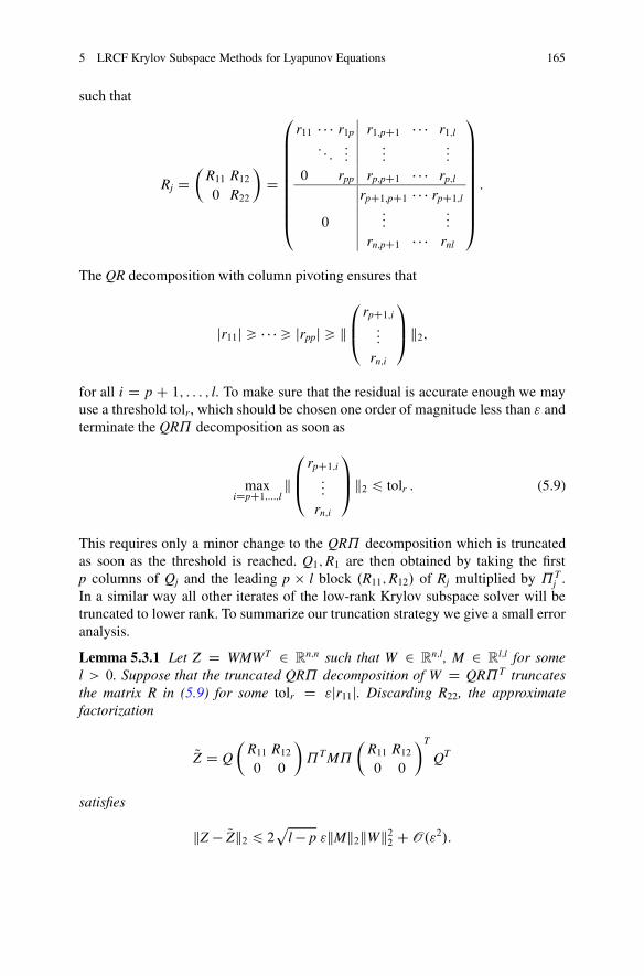
5 LRCF Krylov Subspace Methods for Lyapunov Equations 165
such that
Rj D�
R11 R120 R22
�D
0BBBBBBBBB@
r11 � � � r1p r1;pC1 � � � r1;l: : :
::::::
:::
0 rpp rp;pC1 � � � rp;l
rpC1;pC1 � � � rpC1;l0
::::::
rn;pC1 � � � rnl
1CCCCCCCCCA:
The QR decomposition with column pivoting ensures that
jr11j > � � � > jrppj > k
0B@
rpC1;i:::
rn;i
1CA k2;
for all i D p C 1; : : : ; l. To make sure that the residual is accurate enough we mayuse a threshold tolr, which should be chosen one order of magnitude less than " andterminate the QR˘ decomposition as soon as
maxiDpC1;:::;l k
0B@
rpC1;i:::
rn;i
1CA k2 6 tolr : (5.9)
This requires only a minor change to the QR˘ decomposition which is truncatedas soon as the threshold is reached. Q1;R1 are then obtained by taking the firstp columns of Qj and the leading p � l block .R11;R12/ of Rj multiplied by ˘T
j .In a similar way all other iterates of the low-rank Krylov subspace solver will betruncated to lower rank. To summarize our truncation strategy we give a small erroranalysis.
Lemma 5.3.1 Let Z D WMWT 2 Rn;n such that W 2 R
n;l, M 2 Rl;l for some
l > 0. Suppose that the truncated QR˘ decomposition of W D QR˘T truncatesthe matrix R in (5.9) for some tolr D "jr11j. Discarding R22, the approximatefactorization
QZ D Q
�R11 R120 0
�˘TM˘
�R11 R120 0
�T
QT
satisfies
kZ � QZk2 6 2p
l � p "kMk2kWk22 C O."2/:
166 M. Bollhöfer and A.K. Eppler
Moreover, suppose that
T WD �R11 R12
�˘TM˘
�R11 R12
�T
is decomposed as
T D U˙UT D .U1;U2/
�˙1 0
0 ˙2
�.U1;U2/
T
such that U 2 Rp;p is orthogonal,˙1 D diag.�1; : : : ; �r/,˙2 D diag.�rC1; : : : ; �p/,
j�1j > � � � > j�pj and j�ij 6 "j�1j for all i > r, then the approximate low rankfactorization
OZ D .Q
�Ip
0
�U1/ ˙1 .Q
�Ip
0
�U1/
T
satisfies
kZ � OZk2 6 .2p
l � p C 1/"kMk2kWk22 C O."2/:
Proof We first note that
jr11j D maxjD1;:::;l kRejj 6 max
kxk2D1kRxk2 D kRk2 D kWk2:
Conversely, using (5.9) we obtain
kR22k2 D maxkyk2D1
kR22yk2 D maxkyk2D1
kXi>p
R22eiyik2
6 maxkyk2D1
l�pXiD1
kR22eik2 jyij
6 maxkyk2D1
l�pXiD1
kR22eik22!1=2 l�pX
iD1jyij2
!1=2
6�.l � p/"2jr11j2
�1=2 6pl � p "kWk2:
It follows that
Z � QZ D Q
�0 0
0 R22
�˘TMWT C WM˘
�0 0
0 R22
�T
QT
CQ
�0 0
0 R22
�˘TM˘
�0 0
0 R22
�T
QT :
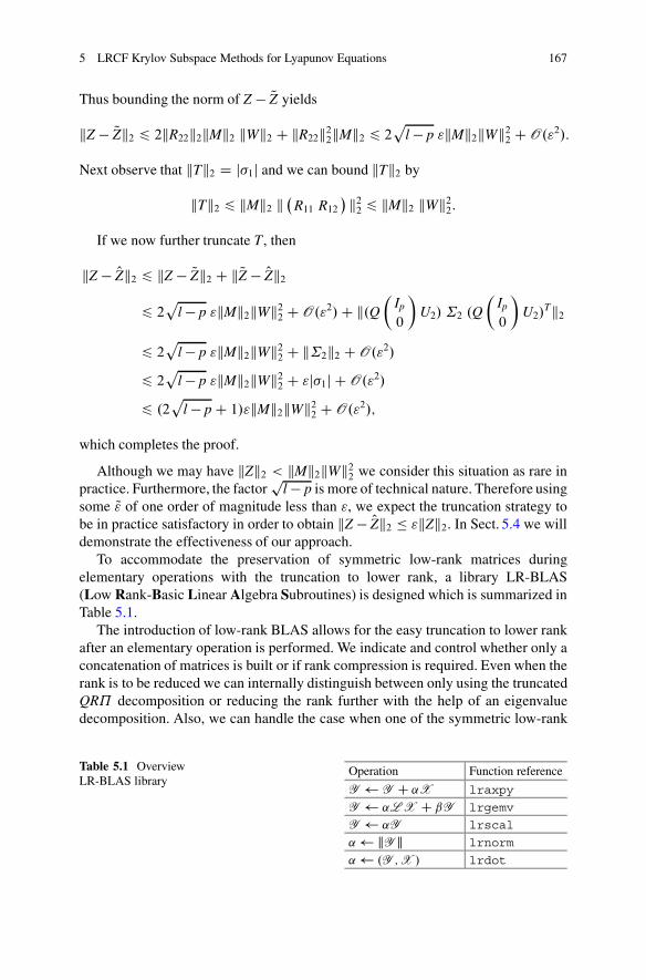
5 LRCF Krylov Subspace Methods for Lyapunov Equations 167
Thus bounding the norm of Z � QZ yields
kZ � QZk2 6 2kR22k2kMk2 kWk2 C kR22k22kMk2 6 2p
l � p "kMk2kWk22 C O."2/:
Next observe that kTk2 D j�1j and we can bound kTk2 by
kTk2 6 kMk2 k �R11 R12� k22 6 kMk2 kWk22:
If we now further truncate T, then
kZ � OZk2 6 kZ � QZk2 C kQZ � OZk2
6 2p
l � p "kMk2kWk22 C O."2/C k.Q�
Ip
0
�U2/ ˙2 .Q
�Ip
0
�U2/
Tk2
6 2p
l � p "kMk2kWk22 C k˙2k2 C O."2/
6 2p
l � p "kMk2kWk22 C "j�1j C O."2/
6 .2p
l � p C 1/"kMk2kWk22 C O."2/;
which completes the proof.
Although we may have kZk2 < kMk2kWk22 we consider this situation as rare inpractice. Furthermore, the factor
pl � p is more of technical nature. Therefore using
some Q" of one order of magnitude less than ", we expect the truncation strategy tobe in practice satisfactory in order to obtain kZ � OZk2 � "kZk2. In Sect. 5.4 we willdemonstrate the effectiveness of our approach.
To accommodate the preservation of symmetric low-rank matrices duringelementary operations with the truncation to lower rank, a library LR-BLAS(Low Rank-Basic Linear Algebra Subroutines) is designed which is summarized inTable 5.1.
The introduction of low-rank BLAS allows for the easy truncation to lower rankafter an elementary operation is performed. We indicate and control whether only aconcatenation of matrices is built or if rank compression is required. Even when therank is to be reduced we can internally distinguish between only using the truncatedQR˘ decomposition or reducing the rank further with the help of an eigenvaluedecomposition. Also, we can handle the case when one of the symmetric low-rank
Table 5.1 OverviewLR-BLAS library
Operation Function reference
Y Y C ˛X lraxpy
Y ˛LX C ˇY lrgemv
Y ˛Y lrscal
˛ kY k lrnorm
˛ .Y ;X / lrdot
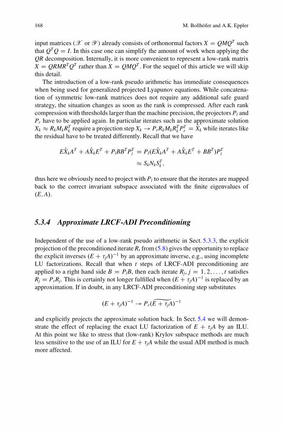
168 M. Bollhöfer and A.K. Eppler
input matrices (X or Y ) already consists of orthonormal factors X D QMQT suchthat QTQ D I. In this case one can simplify the amount of work when applying theQR decomposition. Internally, it is more convenient to represent a low-rank matrixX D QRMRTQT rather than X D QMQT . For the sequel of this article we will skipthis detail.
The introduction of a low-rank pseudo arithmetic has immediate consequenceswhen being used for generalized projected Lyapunov equations. While concatena-tion of symmetric low-rank matrices does not require any additional safe guardstrategy, the situation changes as soon as the rank is compressed. After each rankcompression with thresholds larger than the machine precision, the projectors Pl andPr have to be applied again. In particular iterates such as the approximate solutionXk RkMkRT
k require a projection step Xk ! PrRkMkRTk PT
r D OXk while iterates likethe residual have to be treated differently. Recall that we have
E OXkAT C A OXkET C PlBBTPTl D Pl.E OXkAT C A OXkET C BBT/PT
l
SkNkSTk ;
thus here we obviously need to project with Pl to ensure that the iterates are mappedback to the correct invariant subspace associated with the finite eigenvalues of.E;A/.
5.3.4 Approximate LRCF-ADI Preconditioning
Independent of the use of a low-rank pseudo arithmetic in Sect. 5.3.3, the explicitprojection of the preconditioned iterate Rt from (5.8) gives the opportunity to replacethe explicit inverses .E C �jA/�1 by an approximate inverse, e.g., using incompleteLU factorizations. Recall that when t steps of LRCF-ADI preconditioning areapplied to a right hand side B D PlB, then each iterate Rj, j D 1; 2; : : : ; t satisfiesRj D PrRj. This is certainly not longer fulfilled when .E C �jA/�1 is replaced by anapproximation. If in doubt, in any LRCF-ADI preconditioning step substitutes
.E C �jA/�1 ! Pr.BE C �jA/
�1
and explicitly projects the approximate solution back. In Sect. 5.4 we will demon-strate the effect of replacing the exact LU factorization of E C �jA by an ILU.At this point we like to stress that (low-rank) Krylov subspace methods are muchless sensitive to the use of an ILU for E C �jA while the usual ADI method is muchmore affected.
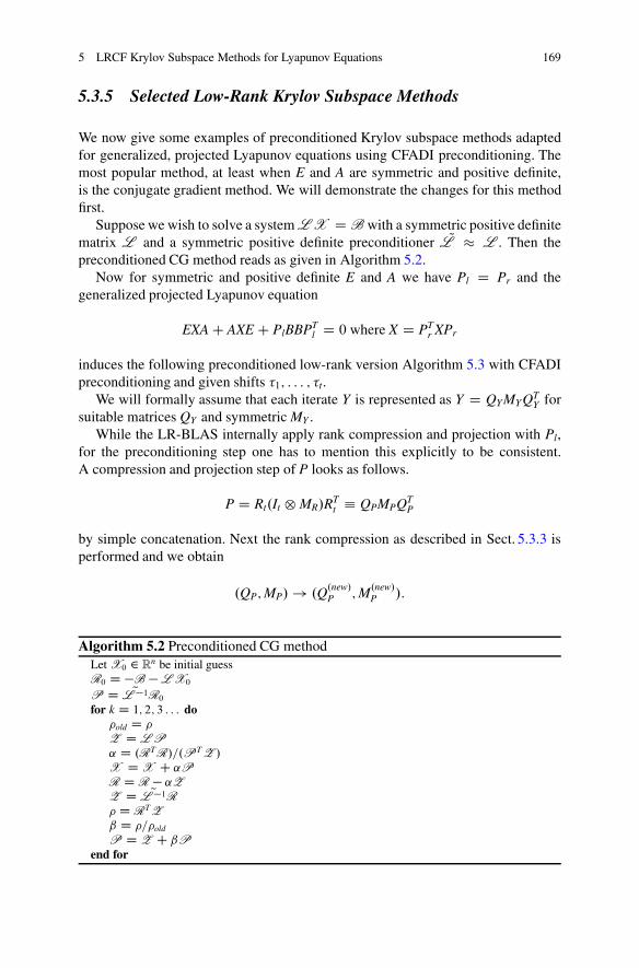
5 LRCF Krylov Subspace Methods for Lyapunov Equations 169
5.3.5 Selected Low-Rank Krylov Subspace Methods
We now give some examples of preconditioned Krylov subspace methods adaptedfor generalized, projected Lyapunov equations using CFADI preconditioning. Themost popular method, at least when E and A are symmetric and positive definite,is the conjugate gradient method. We will demonstrate the changes for this methodfirst.
Suppose we wish to solve a system LX D B with a symmetric positive definitematrix L and a symmetric positive definite preconditioner QL L . Then thepreconditioned CG method reads as given in Algorithm 5.2.
Now for symmetric and positive definite E and A we have Pl D Pr and thegeneralized projected Lyapunov equation
EXA C AXE C PlBBPTl D 0 where X D PT
r XPr
induces the following preconditioned low-rank version Algorithm 5.3 with CFADIpreconditioning and given shifts �1; : : : ; �t.
We will formally assume that each iterate Y is represented as Y D QYMYQTY for
suitable matrices QY and symmetric MY .While the LR-BLAS internally apply rank compression and projection with Pl,
for the preconditioning step one has to mention this explicitly to be consistent.A compression and projection step of P looks as follows.
P D Rt.It ˝ MR/RTt � QPMPQT
P
by simple concatenation. Next the rank compression as described in Sect. 5.3.3 isperformed and we obtain
.QP;MP/ ! .Q.new/P ;M.new/
P /:
Algorithm 5.2 Preconditioned CG methodLet X0 2 R
n be initial guessR0 D �B �LX0
P D QL �1R0
for k D 1; 2; 3 : : : do�old D �
Z D LP˛ D .RTR/=.PTZ /
X DX C ˛PR D R � ˛ZZ D QL �1R� D RTZˇ D �=�old
P D Z C ˇPend for
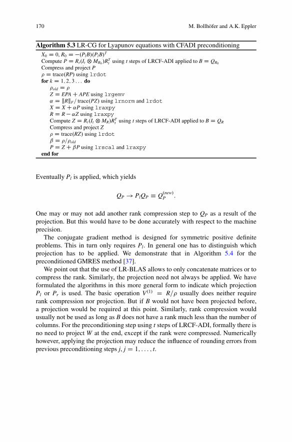
170 M. Bollhöfer and A.K. Eppler
Algorithm 5.3 LR-CG for Lyapunov equations with CFADI preconditioningX0 D 0, R0 D �.PlB/.PlB/T
Compute P D Rt.It ˝MR0 /RTt using t steps of LRCF-ADI applied to BD QR0
Compress and project P� D trace.RP/ using lrdotfor k D 1; 2; 3 : : : do
�old D �
Z D EPAC APE using lrgemv˛ D kRkF= trace.PZ/ using lrnorm and lrdotX D XC ˛P using lraxpyR D R� ˛Z using lraxpyCompute Z D Rt.It ˝MR/RT
t using t steps of LRCF-ADI applied to BD QR
Compress and project Z� D trace.RZ/ using lrdotˇ D �=�old
P D ZC ˇP using lrscal and lraxpyend for
Eventually Pl is applied, which yields
QP ! PlQP � Q.new/P :
One may or may not add another rank compression step to QP as a result of theprojection. But this would have to be done accurately with respect to the machineprecision.
The conjugate gradient method is designed for symmetric positive definiteproblems. This in turn only requires Pl. In general one has to distinguish whichprojection has to be applied. We demonstrate that in Algorithm 5.4 for thepreconditioned GMRES method [37].
We point out that the use of LR-BLAS allows to only concatenate matrices or tocompress the rank. Similarly, the projection need not always be applied. We haveformulated the algorithms in this more general form to indicate which projectionPl or Pr is used. The basic operation V.1/ D R=� usually does neither requirerank compression nor projection. But if B would not have been projected before,a projection would be required at this point. Similarly, rank compression wouldusually not be used as long as B does not have a rank much less than the number ofcolumns. For the preconditioning step using t steps of LRCF-ADI, formally there isno need to project W at the end, except if the rank were compressed. Numericallyhowever, applying the projection may reduce the influence of rounding errors fromprevious preconditioning steps j, j D 1; : : : ; t.
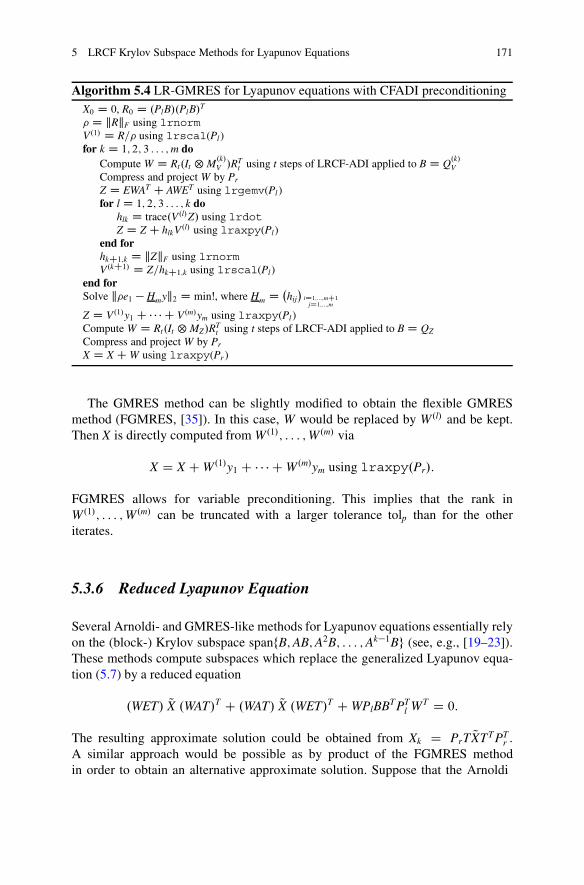
5 LRCF Krylov Subspace Methods for Lyapunov Equations 171
Algorithm 5.4 LR-GMRES for Lyapunov equations with CFADI preconditioningX0 D 0, R0 D .PlB/.PlB/T
� D kRkF using lrnormV.1/ D R=� using lrscal(Pl)for k D 1; 2; 3 : : : ;m do
Compute W D Rt.It ˝M.k/V /RT
t using t steps of LRCF-ADI applied to B D Q.k/V
Compress and project W by Pr
Z D EWAT C AWET using lrgemv(Pl )for l D 1; 2; 3 : : : ; k do
hlk D trace.V.l/Z/ using lrdotZ D Z C hlkV.l/ using lraxpy(Pl)
end forhkC1;k D kZkF using lrnormV.kC1/ D Z=hkC1;k using lrscal(Pl)
end forSolve k�e1 � Hmyk2 D minŠ, where Hm D
�hij
�iD1;:::;mC1
jD1;:::;m
Z D V.1/y1 C � � � C V.m/ym using lraxpy(Pl )Compute W D Rt.It ˝MZ/RT
t using t steps of LRCF-ADI applied to BD QZ
Compress and project W by Pr
X D XCW using lraxpy(Pr )
The GMRES method can be slightly modified to obtain the flexible GMRESmethod (FGMRES, [35]). In this case, W would be replaced by W.l/ and be kept.Then X is directly computed from W.1/; : : : ;W.m/ via
X D X C W.1/y1 C � � � C W.m/ym using lraxpy.Pr/:
FGMRES allows for variable preconditioning. This implies that the rank inW.1/; : : : ;W.m/ can be truncated with a larger tolerance tolp than for the otheriterates.
5.3.6 Reduced Lyapunov Equation
Several Arnoldi- and GMRES-like methods for Lyapunov equations essentially relyon the (block-) Krylov subspace spanfB;AB;A2B; : : : ;Ak�1Bg (see, e.g., [19–23]).These methods compute subspaces which replace the generalized Lyapunov equa-tion (5.7) by a reduced equation
.WET/ QX .WAT/T C .WAT/ QX .WET/T C WPlBBTPTl WT D 0:
The resulting approximate solution could be obtained from Xk D PrT QXTTPTr .
A similar approach would be possible as by product of the FGMRES methodin order to obtain an alternative approximate solution. Suppose that the Arnoldi
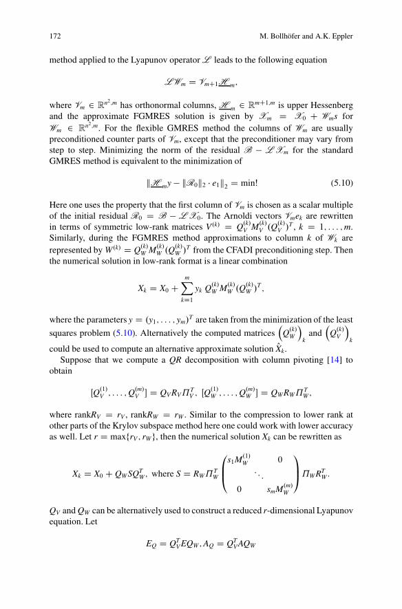
172 M. Bollhöfer and A.K. Eppler
method applied to the Lyapunov operator L leads to the following equation
LWm D VmC1H m;
where Vm 2 Rn2;m has orthonormal columns, H m 2 R
mC1;m is upper Hessenbergand the approximate FGMRES solution is given by Xm D X0 C Wms forWm 2 R
n2;m. For the flexible GMRES method the columns of Wm are usuallypreconditioned counter parts of Vm, except that the preconditioner may vary fromstep to step. Minimizing the norm of the residual B � LXm for the standardGMRES method is equivalent to the minimization of
kH my � kR0k2 � e1k2 D minŠ (5.10)
Here one uses the property that the first column of Vm is chosen as a scalar multipleof the initial residual R0 D B � LX0. The Arnoldi vectors Vmek are rewrittenin terms of symmetric low-rank matrices V.k/ D Q.k/
V M.k/V .Q.k/
V /T , k D 1; : : : ;m.
Similarly, during the FGMRES method approximations to column k of Wk arerepresented by W.k/ D Q.k/
W M.k/W .Q.k/
W /T from the CFADI preconditioning step. Then
the numerical solution in low-rank format is a linear combination
Xk D X0 CmX
kD1yk Q.k/
W M.k/W .Q.k/
W /T ;
where the parameters y D .y1; : : : ; ym/T are taken from the minimization of the least
squares problem (5.10). Alternatively the computed matrices�
Q.k/W
�k
and�
Q.k/V
�k
could be used to compute an alternative approximate solution OXk.Suppose that we compute a QR decomposition with column pivoting [14] to
obtain
ŒQ.1/V ; : : : ;Q.m/
V � D QVRV˘TV ; ŒQ
.1/W ; : : : ;Q.m/
W � D QWRW˘TW ;
where rankRV D rV , rankRW D rW . Similar to the compression to lower rank atother parts of the Krylov subspace method here one could work with lower accuracyas well. Let r D maxfrV ; rWg, then the numerical solution Xk can be rewritten as
Xk D X0 C QWSQTW ; where S D RW˘
TW
0B@
s1M.1/W 0: : :
0 smM.m/W
1CA˘WRT
W :
QV and QW can be alternatively used to construct a reduced r-dimensional Lyapunovequation. Let
EQ D QTVEQW ;AQ D QT
VAQW

5 LRCF Krylov Subspace Methods for Lyapunov Equations 173
and compute S as numerical solution of the reduced equation
EQ S ATQ C AQ S ET
Q C QTKR0QK D 0;
where R0 D EX0AT C AX0ET C BBT . For small r this could be computed withstandard methods [2]. We obtain
OXm D X0 C QWSQTW
as approximate solution of a reduced Lyapunov equation. In Sect. 5.4 we willdemonstrate the effectiveness of this approach.
In summary the low-rank Krylov subspace methods introduced in Sect. 5.3 allowfor structured iterative methods. If .PlEPr;PlAPr/ is already symmetric and PlEPr
positive semidefinite, one could use a low-rank version of the simplified QMR(SQMR) method [12] for symmetric indefinite problems. If even PlAPr is positivedefinite, then the low-rank CG method can be applied. Low-rank CG and low-rankSQMR can make use of the CFADI preconditioning approach while at the sametime low-rank structures and symmetry of the Lyapunov operator is preserved. In thegeneral case we could easily introduce low-rank Krylov subspace methods such aslow-rank BiCGStab, low-rank QMR and other methods (cf. [36]).
5.4 Numerical Results
In this section we will demonstrate the effectiveness of our approach. We willstart with the sensitivity of low-rank Krylov subspace methods with respect to theshifts used for the CFADI preconditioning step and compare them with the usualLRCF-ADI method. Next we will demonstrate different low-rank Krylov subspacemethods such as (F)GMRES, QMR and BICGSTAB for projected, generalizedLyapunov equations to evaluate their strengths and their weaknesses. We will furtherinvestigate replacing the direct solver for the single iterates .E C �jA/�1 by anapproximate factorization to compare the sensitivity of ADI and Krylov subspacemethods with respect to incomplete factorizations. Here we use as approximatefactorization the multilevel ILU factorization from the software package1 ILUPACKwhich is described in detail in [5]. Further numerical results will discuss the use ofthe reduced equation from Sect. 5.3.6 for the numerical solution. We will finallydemonstrate how parallel direct solvers can accelerate the process of solving large-scale projected Lyapunov equations.
1Matthias Bollhöfer and Yousef Saad. ILUPACK - preconditioning software package. Availableonline at http://ilupack.tu-bs.de/.ReleaseV2.4,June2011.
174 M. Bollhöfer and A.K. Eppler
Some of our experiments use the software package PABTEC, see [33] andSect. 2.6, which has been designed for the model order reduction of descriptorsystems arising from circuit simulation. Here we replaced the default LRCF-ADImethod by preconditioned low-rank Krylov subspace methods such as (F)GMRES,QMR and BICGSTAB and adapted the interfaces to allow for complete simulationruns based on Krylov subspace techniques.
5.4.1 Model Problems
In the following part we like to introduce three model problems which we willuse for demonstration. The first two are examples arise from descriptor systemsmodeling circuit-equations while the third one is a more academic parabolic partialdifferential equation. All these examples illustrate the applicability of low-rankKrylov subspace methods.
As our first two examples we discuss linear RLC networks of the following type,modeled using the modified nodal analysis (MNA). Let e be the vector of nodepotentials, vV , vI be the voltages of the voltage sources, respectively of the currentsources. Denote by iL; iV ; iI the currents through the inductors, voltage sources andcurrent sources. We define the state vector x, the vector of inputs u and the outputvector y via
x D0@ e
iLiV
1A ; u D
�iIvV
�; y D
�vI
iV
�:
Then the circuit equations can be written as
EPx D Ax C Bu
y D �BTx;
where E;A and B are given by
E D0@ACCAT
C 0 0
0 L 00 0 0
1A ; A D
0@�ARGAT
R �AL �AV
ATL 0 0
ATV 0 0
1A ; B D
0@�AI 0
0 0
0 �I
1A :
Here AC;AR;AL;AV ;AI refer to the incidence matrices with respect to thecapacitors, resistors, inductors, as well as with respect to the voltage sources andcurrent sources. C, L, G denote the capacitance matrix, the inductance matrix andthe conductivity matrix. The differential-algebraic equations which we discuss hereare of differentiation index 1 (cf. [6]).
5 LRCF Krylov Subspace Methods for Lyapunov Equations 175
Table 5.2 Large-scale RC circuits
Acronym Capacitors Resistors Voltage sources System size
RC1 2353 1393 109 974
RC2 3065 5892 21 3272
RC3 9999 9999 3 10; 002
RC4 12; 025 53; 285 78 29; 961
Example 5.4.1 As a first example we consider a RC high pass circuit provided byNEC Laboratories Europe. It consists of 2002 conductors, 2003 resistors and threevoltage sources. Using the MNA this leads to a system of dimension 2007with threeinputs and three outputs.
Example 5.4.2 We consider further test2 examples of several RC circuits. For somedetails we refer to [18]. Here we restrict ourselves to examples of following sizes,reported in Table 5.2.
The circuits in Table 5.2 are of differentiation index 2. Since we like todemonstrate the applicability of low-rank Krylov subspace methods for index-1systems we remove several voltage sources which are responsible for the higherindex. After removing these voltage sources we have for circuit RC1, six voltagesources and for each circuit RC2, RC3 and RC4, one voltage source. Furthermore,we artificially add resistors with average conductivity to ARGAT
R to make this matrixpositive definite. We are aware of changing the original shape of these circuits.However, our main goal is the demonstration of low-rank Krylov subspace methodsusing the PABTEC software as framework.
For both problem classes of RC circuits in Examples 5.4.1 and 5.4.2 we use thetechnology as provided by the software package PABTEC (see Sect. 2.6 and [33])to demonstrate solving an associated projected algebraic Riccati equation with thehelp of Newton’s method. Here in every Newton iteration step (cf. Algorithm 2.7 inChap. 2) a projected, generalized Lyapunov equation has to be solved.
Example 5.4.3 The final example we will use in our numerical experiments is theparabolic partial differential equation
vt D v C Bu � vxx C vyy C vzz C Bu;
where v D v.x; y; z; t/, .x; y; z/ 2 ˝ D Œ0; 1�3 and t � 0. We assume that we havesome initial value v.x; y; z; 0/ and homogeneous Dirichlet boundary conditions.To keep the discussion simple, we consider an academic control B such that afterdiscretization in space using a seven-point discretization stencil, the control reducesto the vector with all ones. Suppose that we have an equidistant mesh with meshsize h D 1
NC1 . This leads to a total system size of n D N3 unknowns. The
2http://sites.google.com/site/rionutiu2/research/software.
176 M. Bollhöfer and A.K. Eppler
semi-discretized ordinary differential equation is of type
Pw D �Aw C Bu;
where A is the discretized Laplacian operator in three spatial dimensions. Weapply model order reduction to these semi-discretized equations using balancedtruncation. For symmetry reasons we simply compute the associated Gramian asthe solution of the Lyapunov equation
XA C AX D BBT ;
meaning N6 unknowns for the referring Lyapunov operator. Since A is symmetricand positive definite, the Lyapunov equation X.�A/C .�A/X C BBT D 0 is stableand therefore balanced truncation can be applied. We know that the spectrum of Alies inside the interval .3�2; 12
h2/. This allows for a simple computation of the optimal
ADI shift-parameters introduced by Wachspress [47].We use this example in order to illustrate a low-rank version of the conjugate
gradient method. Furthermore, a parallel sparse direct solver for solving the shiftedsystems .A C �iI/x D b is used to examine the scalability. Finally, this exampledemonstrates the advantages of using multilevel incomplete factorizations ratherthan direct solvers within the CFADI method.
In the sequel all computations were conducted on a 64 GB Linux workstationwith four Intel Xeon E7440 Quadcore processors using Matlab Release R2008b.
5.4.2 Different Krylov Subspace Methods and Their Efficiencywith Respect to the Selection of Shifts
In the following experiments we will compare how flexible GMRES [35], GMRES[37], QMR [13] and BICGSTAB [46] can be used to solve projected generalizedLyapunov equations. We will describe how different choices of shifts affect theLRCF-ADI method and low-rank Krylov subspace methods. For this purpose weconsider Examples 5.4.1 and 5.4.2. Here it is necessary to use the heuristic approach(referred to as “Algorithm 1” in [32]) for calculating the shift parameters. As partof the passivity-preserving balanced truncation we will solve the projected Riccatiequations from (5.4), (5.5) up to a tolerance of 10�4. The same accuracy is usedfor truncating the Hankel singular values for Balanced Truncation. As a heuristicapproach we decided to solve each Lyapunov equation up a relative residual normof 10�6. One benefit of our class of Krylov subspace methods is that we can usethe norm provided by our Krylov-subspace method and do not need to explicitlyevaluate the residual-norm within the LRCF-ADI algorithm. We vary the numbert of calculated shift parameters from 4, 5, 10, 20 finally to 30. For the low-rankKrylov methods we use a tolerance of 10�8 for truncating the ranks which is two
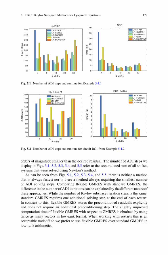
5 LRCF Krylov Subspace Methods for Lyapunov Equations 177
4 5 10 20 300
50
100
150
200
250
300
350
400
n=2007
# shifts
# A
DI s
teps
LRCF−ADILR−GMRESLR−FGRMESLR−QMRLR−BICGSTAB
4 5 10 20 300
5
10
15
20
25
30
35
40NEC
# shifts
time
in [s
]
LRCF−ADILR−GMRESLR−FGRMESLR−QMRLR−BICGSTAB
Fig. 5.1 Number of ADI steps and runtime for Example 5.4.1
5 10 20 300
20
40
60
80
100
120
140
160
180
200RC1, n=974
# shifts
# A
DI s
teps
LRCF−ADILR−FGRMESLR−QMRLR−BICGSTAB
5 10 20 300
2
4
6
8
10
12
14
16
18
20
RC1, n=974
# shifts
time
in [s
]
LRCF−ADILR−FGRMESLR−QMRLR−BICGSTAB
Fig. 5.2 Number of ADI steps and runtime for circuit RC1 from Example 5.4.2
orders of magnitude smaller than the desired residual. The number of ADI steps wedisplay in Figs. 5.1, 5.2, 5.3, 5.4 and 5.5 refer to the accumulated sum of all shiftedsystems that were solved using Newton’s method.
As can be seen from Figs. 5.1, 5.2, 5.3, 5.4, and 5.5, there is neither a methodthat is always fastest nor is there a method always requiring the smallest numberof ADI solving steps. Comparing flexible GMRES with standard GMRES, thedifference in the number of ADI iterations can be explained by the different nature ofthese approaches. While the number of Krylov subspace iteration steps is the same,standard GMRES requires one additional solving step at the end of each restart.In contrast to this, flexible GMRES stores the preconditioned residuals explicitlyand does not require an additional preconditioning step. The slightly improvedcomputation time of flexible GMRES with respect to GMRES is obtained by usingtwice as many vectors in low-rank format. When working with restarts this is anacceptable tradeoff so we prefer to use flexible GMRES over standard GMRES inlow-rank arithmetic.
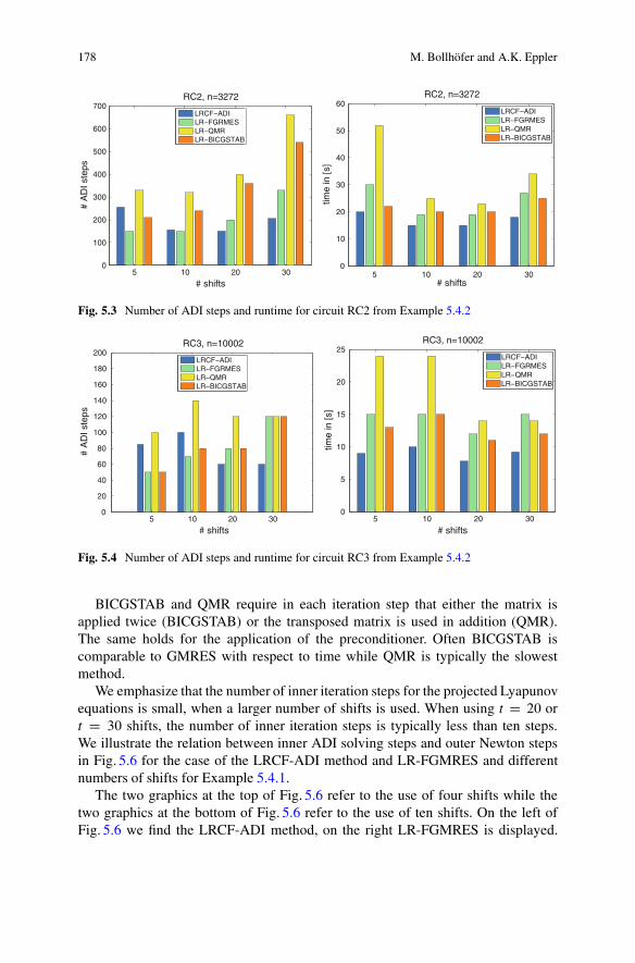
178 M. Bollhöfer and A.K. Eppler
5 10 20 300
100
200
300
400
500
600
700RC2, n=3272
# shifts
# A
DI s
teps
LRCF−ADILR−FGRMESLR−QMRLR−BICGSTAB
5 10 20 300
10
20
30
40
50
60RC2, n=3272
# shifts
time
in [s
]
LRCF−ADILR−FGRMESLR−QMRLR−BICGSTAB
Fig. 5.3 Number of ADI steps and runtime for circuit RC2 from Example 5.4.2
5 10 20 300
20
40
60
80
100
120
140
160
180
200RC3, n=10002
# shifts
# A
DI s
teps
LRCF−ADILR−FGRMESLR−QMRLR−BICGSTAB
5 10 20 300
5
10
15
20
25RC3, n=10002
# shifts
time
in [s
]
LRCF−ADILR−FGRMESLR−QMRLR−BICGSTAB
Fig. 5.4 Number of ADI steps and runtime for circuit RC3 from Example 5.4.2
BICGSTAB and QMR require in each iteration step that either the matrix isapplied twice (BICGSTAB) or the transposed matrix is used in addition (QMR).The same holds for the application of the preconditioner. Often BICGSTAB iscomparable to GMRES with respect to time while QMR is typically the slowestmethod.
We emphasize that the number of inner iteration steps for the projected Lyapunovequations is small, when a larger number of shifts is used. When using t D 20 ort D 30 shifts, the number of inner iteration steps is typically less than ten steps.We illustrate the relation between inner ADI solving steps and outer Newton stepsin Fig. 5.6 for the case of the LRCF-ADI method and LR-FGMRES and differentnumbers of shifts for Example 5.4.1.
The two graphics at the top of Fig. 5.6 refer to the use of four shifts while thetwo graphics at the bottom of Fig. 5.6 refer to the use of ten shifts. On the left ofFig. 5.6 we find the LRCF-ADI method, on the right LR-FGMRES is displayed.
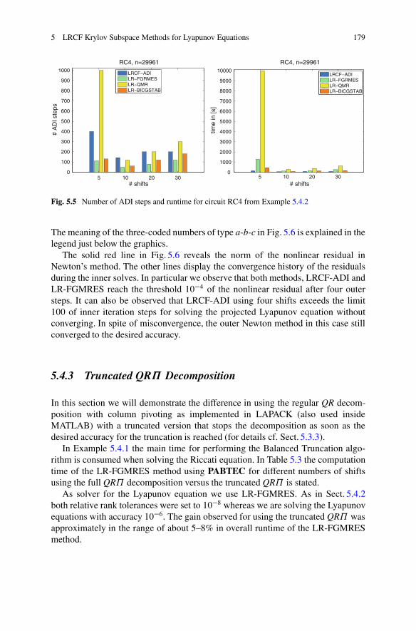
5 LRCF Krylov Subspace Methods for Lyapunov Equations 179
5 10 20 300
100
200
300
400
500
600
700
800
900
1000
RC4, n=29961
# shifts
# A
DI s
teps
LRCF−ADILR−FGRMESLR−QMRLR−BICGSTAB
5 10 20 300
1000
2000
3000
4000
5000
6000
7000
8000
9000
10000
RC4, n=29961
# shifts
time
in [s
]
LRCF−ADILR−FGRMESLR−QMRLR−BICGSTAB
Fig. 5.5 Number of ADI steps and runtime for circuit RC4 from Example 5.4.2
The meaning of the three-coded numbers of type a-b-c in Fig. 5.6 is explained in thelegend just below the graphics.
The solid red line in Fig. 5.6 reveals the norm of the nonlinear residual inNewton’s method. The other lines display the convergence history of the residualsduring the inner solves. In particular we observe that both methods, LRCF-ADI andLR-FGMRES reach the threshold 10�4 of the nonlinear residual after four outersteps. It can also be observed that LRCF-ADI using four shifts exceeds the limit100 of inner iteration steps for solving the projected Lyapunov equation withoutconverging. In spite of misconvergence, the outer Newton method in this case stillconverged to the desired accuracy.
5.4.3 Truncated QR˘ Decomposition
In this section we will demonstrate the difference in using the regular QR decom-position with column pivoting as implemented in LAPACK (also used insideMATLAB) with a truncated version that stops the decomposition as soon as thedesired accuracy for the truncation is reached (for details cf. Sect. 5.3.3).
In Example 5.4.1 the main time for performing the Balanced Truncation algo-rithm is consumed when solving the Riccati equation. In Table 5.3 the computationtime of the LR-FGMRES method using PABTEC for different numbers of shiftsusing the full QR˘ decomposition versus the truncated QR˘ is stated.
As solver for the Lyapunov equation we use LR-FGMRES. As in Sect. 5.4.2both relative rank tolerances were set to 10�8 whereas we are solving the Lyapunovequations with accuracy 10�6. The gain observed for using the truncated QR˘ wasapproximately in the range of about 5–8% in overall runtime of the LR-FGMRESmethod.

180 M. Bollhöfer and A.K. Eppler
0 20 40 60 80 10010
−6
10−4
10−2
Nor
mal
ized
res
idua
l nor
m
Iteration steps
LRCF−ADI iteration / Newton iteration
1-96-R
2-100-I
3-100-I
4-100-I
1 12
2
3
34 40 20 40 60
10−5
100
Nor
mal
ized
res
idua
l nor
m
Iteration steps
LR−FGMRES iteration / Newton iteration
1-60-15
2-52-13
3-44-11
4-28-7
0 10 20 30 40
10−6
10−4
10−2
Nor
mal
ized
res
idua
l nor
m
Iteration steps
LRCF−ADI iteration / Newton iteration
1-24-R
2-26-R
3-26-R
4-27-R
12
3
4
0 10 20 30 40
10−5
100
Nor
mal
ized
res
idua
l nor
m
Iteration steps
LR−FGMRES iteration / Newton iteration
1-30-3
2-30-3
3-20-2
4-20-2
12
3
4
legend for the symbols of type a-b-c
a number of outer Newton steps
b number of inner ADI solving steps
c if c is a number, then c denotes the number of FGMRES stepsif c = I, then the inner solver terminated after the number of iteration steps is exceededif c = R, then ADI converged with a sufficiently small residual
Fig. 5.6 Comparison of LRCF-ADI and LR-FGMRES using four (top line) and ten (bottom line)shifts
Table 5.3 Comparison ofstandard QR˘ and truncatedQR˘ within LR-FGMRES,Example 5.4.1
# Shifts Standard QR˘ (s) Truncated QR˘ (s)
4 19:25 18:43
5 7:33 6:90
10 4:03 3:90
20 3:95 3:79
30 4:24 4:20
5 LRCF Krylov Subspace Methods for Lyapunov Equations 181
The improvement using the truncated QR˘ decomposition can not only be usedin low-rank Krylov subspace methods, but it can also have a beneficial impact ofthe LRCF-ADI method. When solving the projected Riccati equations using LRCF-ADI, at each Newton step we have to concatenate the current approximate low-rank solution Z D QZQT
Z of the Riccati equation and the recent low-rank updateP D QPQT
P from solving the projected Lyapunov equation to obtain
Z C P D QZ QP
QZ QP
Trank�!
compressionQ.new/
Z .Q.new/Z /T :
Usually we would apply a slim QR decomposition
QZ QP
ŠD QR
such that Q has as many columns as
QZ QP
. After that we would apply a singular
value decomposition
RŠD Ur˙rV
Tr
to truncate the rank of R to some r and obtain
Q.new/Z D QUr˙r:
When we use the truncated QR˘ decomposition instead, we can alreadycompute approximately
QZ QP
ŠD QsRs˘T C E
such that kEk is small and Qs and RTs may already have significantly less columns s
than
QZ QP
. Next a singular value decomposition only needs to be applied to the
already reduced system
RsŠD Ur˙rV
Tr :
Thus, the truncated QR˘ decomposition may not only save time during the QR˘decomposition of
QZ QP
, but the singular value decomposition is also applied
to system of smaller size and may lead to additional improvements. To illustratethis effect we compare the LRCF-ADI method for Examples 5.4.1 and 5.4.2.Although the total computation time is not drastically improved, at least the timeof the rank compression is moderately improved. In Figs. 5.7 and 5.8 we illustratethe computation times of both rank compression techniques, accumulated over allNewton steps.
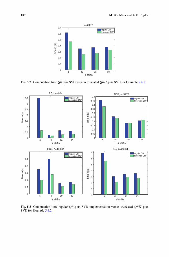
182 M. Bollhöfer and A.K. Eppler
5 10 20 300
0.1
0.2
0.3
0.4
0.5
0.6
0.7n=2007
# shifts
time
in [s
]
regular QRtruncated QRP
Fig. 5.7 Computation time QR plus SVD version truncated QR˘ plus SVD for Example 5.4.1
5 10 20 300
0.5
1
1.5
2
2.5
3
3.5
RC1, n=974
# shifts
time
in [s
]
regular QRtruncated QRP
5 10 20 300
0.05
0.1
0.15
0.2
0.25
0.3
0.35
0.4
0.45
0.5RC2, n=3272
# shifts
time
in [s
]
regular QRtruncated QRP
5 10 20 300
0.1
0.2
0.3
0.4
0.5
RC3, n=10002
# shifts
time
in [s
]
regular QRtruncated QRP
5 10 20 300
1
2
3
4
5
6
7
RC4, n=29961
# shifts
time
in [s
]
regular QRtruncated QRP
Fig. 5.8 Computation time regular QR plus SVD implementation versus truncated QR˘ plusSVD for Example 5.4.2
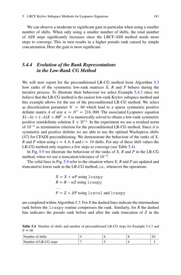
5 LRCF Krylov Subspace Methods for Lyapunov Equations 183
We can observe a moderate to significant gain in particular when using a smallernumber of shifts. When only using a smaller number of shifts, the total numberof ADI steps significantly increases since the LRCF-ADI method needs moresteps to converge. This in turn results in a higher pseudo rank caused by simpleconcatenation. Here the gain is most significant.
5.4.4 Evolution of the Rank Representationsin the Low-Rank CG Method
We will now report for the preconditioned LR-CG method from Algorithm 5.3how ranks of the symmetric low-rank matrices X, R and P behave during theiterative process. To illustrate their behaviour we select Example 5.4.3 since webelieve that the LR-CG method is the easiest low-rank Krylov subspace method andthis example allows for the use of the preconditioned LR-CG method. We selectas discretization parameter N D 60 which lead to a sparse symmetric positivedefinite matrix A of size n D N3 D 216; 000. The associated Lyapunov equationX.�A/C .�A/X C BBT D 0 is numerically solved to obtain a low-rank symmetricpositive semidefinite solution X 2 R
n;n. In the experiment we use a residual normof 10�6 as termination criterion for the preconditioned LR-CG method. Since A issymmetric and positive definite we are able to use the optimal Wachspress shifts[47] for CFADI preconditioning. We demonstrate the behaviour of the ranks of X,R and P when using t D 4; 6; 8 and t D 10 shifts. For any of these shift values theLR-CG method only requires a few steps to converge (see Table 5.4).
In Fig. 5.9 we illustrate the behaviour of the ranks of X, R and P in the LR-CGmethod, when we use a truncation tolerance of 10�8.
The solid lines in Fig. 5.9 refer to the situation where X, R and P are updated andtruncated to lower rank in the LR-CG method, i.e., whenever the operations
X D X C ˛P using lraxpyR D R � ˛Z using lraxpy: : :
P D Z C ˇP using lrscal and lraxpy
are completed within Algorithm 5.3. For X the dashed lines indicate the intermediaterank before the lraxpy routine compresses the rank. Similarly, for R the dashedline indicates the pseudo rank before and after the rank truncation of Z in the
Table 5.4 Number of shifts and number of preconditioned LR-CG steps for Example 5.4.3 andN D 60
Number of shifts 4 6 8 10
Number of LR-CG steps 7 5 4 3
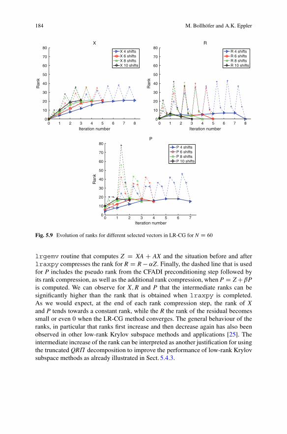
184 M. Bollhöfer and A.K. Eppler
0 1 2 3 4 5 6 7 80
10
20
30
40
50
60
70
80
Iteration number
Ran
kX
X 4 shiftsX 6 shiftsX 8 shiftsX 10 shifts
0 1 2 3 4 5 6 7 80
10
20
30
40
50
60
70
80
Iteration number
Ran
k
R
R 4 shiftsR 6 shiftsR 8 shiftsR 10 shifts
0 1 2 3 4 5 6 70
10
20
30
40
50
60
70
80
Iteration number
Ran
k
P
P 4 shiftsP 6 shiftsP 8 shiftsP 10 shifts
Fig. 5.9 Evolution of ranks for different selected vectors in LR-CG for N D 60
lrgemv routine that computes Z D XA C AX and the situation before and afterlraxpy compresses the rank for R D R � ˛Z. Finally, the dashed line that is usedfor P includes the pseudo rank from the CFADI preconditioning step followed byits rank compression, as well as the additional rank compression, when P D Z CˇPis computed. We can observe for X;R and P that the intermediate ranks can besignificantly higher than the rank that is obtained when lraxpy is completed.As we would expect, at the end of each rank compression step, the rank of Xand P tends towards a constant rank, while the R the rank of the residual becomessmall or even 0 when the LR-CG method converges. The general behaviour of theranks, in particular that ranks first increase and then decrease again has also beenobserved in other low-rank Krylov subspace methods and applications [25]. Theintermediate increase of the rank can be interpreted as another justification for usingthe truncated QR˘ decomposition to improve the performance of low-rank Krylovsubspace methods as already illustrated in Sect. 5.4.3.
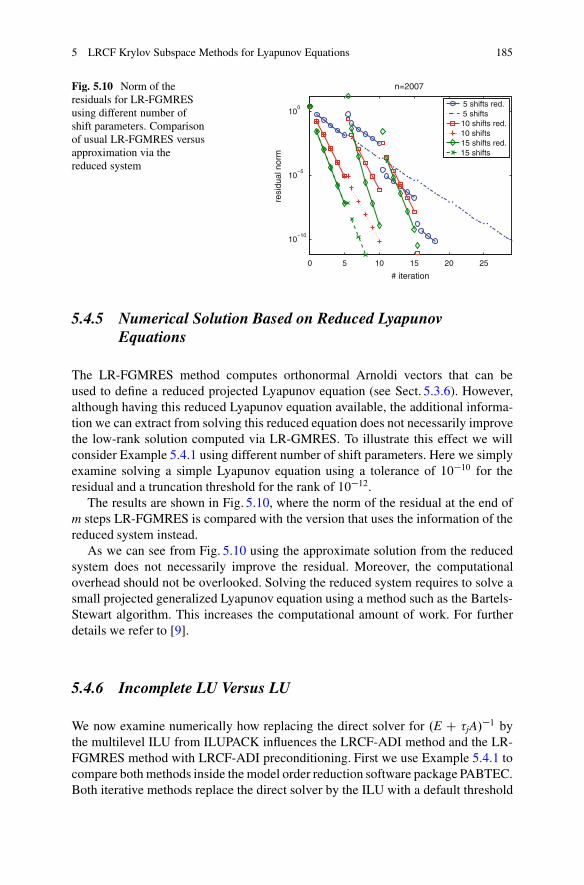
5 LRCF Krylov Subspace Methods for Lyapunov Equations 185
Fig. 5.10 Norm of theresiduals for LR-FGMRESusing different number ofshift parameters. Comparisonof usual LR-FGMRES versusapproximation via thereduced system
0 5 10 15 20 25
10−10
10−5
100
n=2007
resi
dual
nor
m# iteration
5 shifts red. 5 shifts10 shifts red.10 shifts15 shifts red.15 shifts
5.4.5 Numerical Solution Based on Reduced LyapunovEquations
The LR-FGMRES method computes orthonormal Arnoldi vectors that can beused to define a reduced projected Lyapunov equation (see Sect. 5.3.6). However,although having this reduced Lyapunov equation available, the additional informa-tion we can extract from solving this reduced equation does not necessarily improvethe low-rank solution computed via LR-GMRES. To illustrate this effect we willconsider Example 5.4.1 using different number of shift parameters. Here we simplyexamine solving a simple Lyapunov equation using a tolerance of 10�10 for theresidual and a truncation threshold for the rank of 10�12.
The results are shown in Fig. 5.10, where the norm of the residual at the end ofm steps LR-FGMRES is compared with the version that uses the information of thereduced system instead.
As we can see from Fig. 5.10 using the approximate solution from the reducedsystem does not necessarily improve the residual. Moreover, the computationaloverhead should not be overlooked. Solving the reduced system requires to solve asmall projected generalized Lyapunov equation using a method such as the Bartels-Stewart algorithm. This increases the computational amount of work. For furtherdetails we refer to [9].
5.4.6 Incomplete LU Versus LU
We now examine numerically how replacing the direct solver for .E C �jA/�1 bythe multilevel ILU from ILUPACK influences the LRCF-ADI method and the LR-FGMRES method with LRCF-ADI preconditioning. First we use Example 5.4.1 tocompare both methods inside the model order reduction software package PABTEC.Both iterative methods replace the direct solver by the ILU with a default threshold
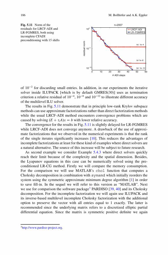
186 M. Bollhöfer and A.K. Eppler
Fig. 5.11 Norm of theresiduals for LRCF-ADI andLR-FGMRES, both usingincomplete CFADIpreconditioning with 15 shifts
0 10 20 30 40 50 60
10−10
10−5
100
n=2007
# ADI steps
resi
dual
nor
m
tol. 1e−4
tol 1e−8
tol. 1e−12
LRCF−ADILR−FGMRES
of 10�2 for discarding small entries. In addition, in our experiments the iterativesolver inside ILUPACK [which is by default GMRES(30)] uses as terminationcriterion a relative residual of 10�4, 10�8 and 10�12 to illustrate different accuracyof the multilevel ILU solver.
The results in Fig. 5.11 demonstrate that in principle low-rank Krylov subspacemethods can use approximate factorizations rather than direct factorization methodswhile the usual LRCF-ADI method encounters convergence problems which arecaused by solving .E C �iA/x D b with lower relative accuracy.
The convergence for the results in Fig. 5.11 is slightly delayed for LR-FGMRESwhile LRCF-ADI does not converge anymore. A drawback of the use of approxi-mate factorizations that we observed in the numerical experiments is that the rankof the single iterates significantly increases [10]. This reduces the advantages ofincomplete factorizations at least for these kind of examples where direct solvers area natural alternative. The source of this increase will be subject to future research.
As second example we consider Example 5.4.3 where direct solvers quicklyreach their limit because of the complexity and the spatial dimension. Besides,the Lyapunov equations in this case can be numerically solved using the pre-conditioned LR-CG method. Firstly we will compare the memory consumption.For the comparison we will use MATLAB’s chol function that computes aCholesky decomposition in combination with symamd which initially reorders thesystem using the symmetric approximate minimum degree algorithm [1] in orderto save fill-in. In the sequel we will refer to this version as “MATLAB”. Nextwe use for comparison the software package3 PARDISO [39, 40] and its Choleskydecomposition. For the incomplete factorization we will again use ILUPACK andits inverse-based multilevel incomplete Cholesky factorization with the additionaloption to preserve the vector with all entries equal to 1 exactly. The latter isrecommended since the underlying matrix refers to a discretized elliptic partialdifferential equation. Since the matrix is symmetric positive definite we again
3http://www.pardiso-project.org.
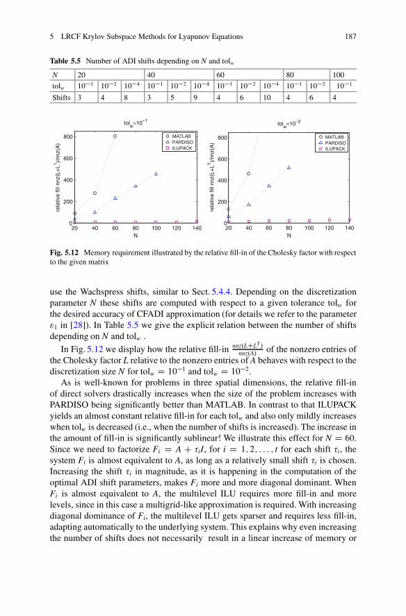
5 LRCF Krylov Subspace Methods for Lyapunov Equations 187
Table 5.5 Number of ADI shifts depending on N and tolw
N 20 40 60 80 100
tolw 10�1 10�2 10�4 10�1 10�2 10�4 10�1 10�2 10�4 10�1 10�2 10�1
Shifts 3 4 8 3 5 9 4 6 10 4 6 4
20 40 60 80 100 120 1400
200
400
600
800
tolw=10−1
N
rela
tive
fill n
nz(L
+LT
)/nn
z(A
)
MATLABPARDISOILUPACK
20 40 60 80 100 120 1400
200
400
600
800
tolw=10−2
N
rela
tive
fill n
nz(L
+LT
)/nn
z(A
)
MATLABPARDISOILUPACK
Fig. 5.12 Memory requirement illustrated by the relative fill-in of the Cholesky factor with respectto the given matrix
use the Wachspress shifts, similar to Sect. 5.4.4. Depending on the discretizationparameter N these shifts are computed with respect to a given tolerance tolw forthe desired accuracy of CFADI approximation (for details we refer to the parameter"1 in [28]). In Table 5.5 we give the explicit relation between the number of shiftsdepending on N and tolw .
In Fig. 5.12 we display how the relative fill-in nnz.LCLT /
nnz.A/ of the nonzero entries ofthe Cholesky factor L relative to the nonzero entries of A behaves with respect to thediscretization size N for tolw D 10�1 and tolw D 10�2.
As is well-known for problems in three spatial dimensions, the relative fill-inof direct solvers drastically increases when the size of the problem increases withPARDISO being significantly better than MATLAB. In contrast to that ILUPACKyields an almost constant relative fill-in for each tolw and also only mildly increaseswhen tolw is decreased (i.e., when the number of shifts is increased). The increase inthe amount of fill-in is significantly sublinear! We illustrate this effect for N D 60.Since we need to factorize Fi D A C �iI, for i D 1; 2; : : : ; t for each shift �i, thesystem Fi is almost equivalent to A, as long as a relatively small shift �i is chosen.Increasing the shift �i in magnitude, as it is happening in the computation of theoptimal ADI shift parameters, makes Fi more and more diagonal dominant. WhenFi is almost equivalent to A, the multilevel ILU requires more fill-in and morelevels, since in this case a multigrid-like approximation is required. With increasingdiagonal dominance of Fi, the multilevel ILU gets sparser and requires less fill-in,adapting automatically to the underlying system. This explains why even increasingthe number of shifts does not necessarily result in a linear increase of memory or
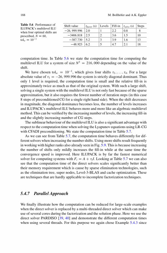
188 M. Bollhöfer and A.K. Eppler
Table 5.6 Performance ofILUPACK’s multilevel ILUwhen four optimal shifts areprescribed, N D 60,tolw D 10�1
Shift value tfactor (s) Levels Fill-in tsolve (s) Steps
�26; 999:996 2.0 1 2.2 0.8 8
�3406:818 2.5 2 3.6 1.5 10
�387:730 5.2 3 3.9 1.6 13
�48:923 6.2 5 4.7 2.1 18
computation time. In Table 5.6 we state the computation time for computing themultilevel ILU for a system of size N3 D 216; 000 depending on the value of theshift.
We have chosen tolw D 10�1, which gives four shifts �1; : : : ; �4. For a largeabsolute value of �1 D �26; 999:996 the system is strictly diagonal dominant. Thusonly 1 level is required, the computation time is small and the relative fill-in isapproximately twice as much as that of the original system. With such a large shift,solving a single system with the multilevel ILU is not only fast because of the sparseapproximation, but it also requires the fewest number of iteration steps (in this case8 steps of preconditioned CG for a single right hand side). When the shift decreasesin magnitude, the diagonal dominance becomes less, the number of levels increasesand ILUPACK’s multilevel ILU behaves more and more like an algebraic multilevelmethod. This can be verified by the increasing number of levels, the increasing fill-inand the slightly increasing number of CG steps.
The sublinear behaviour of the multilevel ILU is also a significant advantage withrespect to the computation time when solving the Lyapunov equations using LR-CGwith CFADI preconditioning. We state the computation time in Table 5.7.
As we can see from Table 5.7, the computation time behaves differently for dif-ferent solvers when increasing the number shifts. Using more shifts result frequentlyin working with higher ranks also already seen in Fig. 5.9. This is because increasingthe number of shifts only mildly increases the fill-in while at the same time theconvergence speed is improved. Here ILUPACK is by far the fastest numericalsolver for computing systems with Fi D A C �iI. Looking at Table 5.7 we can alsosee that the computation time of the direct solvers scales significantly better thantheir memory requirement which is cause by sparse elimination technologies, suchas the elimination tree, super nodes, Level-3-BLAS and cache optimization. Theseare techniques that are hardly applicable to incomplete factorization techniques.
5.4.7 Parallel Approach
We finally illustrate how the computation can be reduced for large-scale exampleswhen the direct solver is replaced by a multi-threaded direct solver which can makeuse of several cores during the factorization and the solution phase. Here we use thedirect solver PARDISO [39, 40] and demonstrate the different computation timeswhen using several threads. For this purpose we again chose Example 5.4.3 since
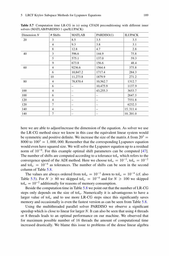
5 LRCF Krylov Subspace Methods for Lyapunov Equations 189
Table 5.7 Computation time LR-CG in (s) using CFADI preconditioning with different innersolvers (MATLAB/PARDISO 1 cpu/ILUPACK)
Dimension N # Shifts MATLAB PARDISO(1) ILUPACK
20 3 8.5 3.5 3:5
4 9.3 3.8 3:1
8 12.8 4.7 2:8
40 3 596.6 144.9 75:8
5 575.1 137.0 59:3
9 673.8 156.6 48:4
60 4 9236.6 1564.4 375:8
6 10,847.2 1717.4 284:3
10 11,273.8 1879.9 271:2
80 4 78,870.4 10,562.7 1312:7
6 – 10,475.9 1137:9
100 4 – 43,255.3 3653:7
100 6 – – 2647:5
120 4 – – 7551:8
120 7 – – 6232:5
140 4 – – 15; 311:4
140 7 – – 10; 201:0
here we are able to adjust/increase the dimension of the equation. As solver we usethe LR-CG method since we know in this case the equivalent linear system wouldbe symmetric and positive definite. We increase the size of the matrix A from 203 D8000 to 1003 D 1; 000; 000. Remember that the corresponding Lyapunov equationwould even have squared size. We will solve the Lyapunov equation up to a residualnorm of 10�6. For this example optimal shift parameters can be computed [47].The number of shifts are computed according to a tolerance tolw which refers to theconvergence speed of the ADI method. Here we choose tolw D 10�1, tolw D 10�2and tolw D 10�4 as tolerances. The number of shifts can be seen in the secondcolumn of Table 5.8.
The values are always ordered from tolw D 10�1 down to tolw D 10�4 (cf. alsoTable 5.5). For N > 80 we skipped tolw D 10�4 and for N > 100 we skippedtolw D 10�2 additionally for reasons of memory consumption.
Beside the computation time in Table 5.8 we point out that the number of LR-CGsteps only depends on the size of tolw. Numerically it is advantageous to have alarger value of tolw and to use more LR-CG steps since this significantly savesmemory and occasionally is even the fastest version as can be seen from Table 5.8.
Using the multithreaded parallel solver PARDISO we observe a significantspeedup which is close to linear for larger N. It can also be seen that using 4 threadsor 8 threads leads to an optimal performance on our machine. We observed thatfor maximum possible number of 16 threads the amount of computational timeincreased drastically. We blame this issue to problems of the dense linear algebra
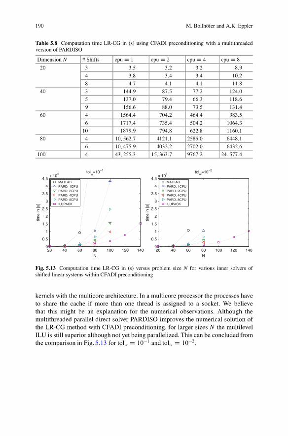
190 M. Bollhöfer and A.K. Eppler
Table 5.8 Computation time LR-CG in (s) using CFADI preconditioning with a multithreadedversion of PARDISO
Dimension N # Shifts cpuD 1 cpuD 2 cpuD 4 cpuD 8
20 3 3:5 3:2 3:2 8:9
4 3:8 3:4 3:4 10:2
8 4:7 4:1 4:1 11:8
40 3 144:9 87:5 77:2 124:0
5 137:0 79:4 66:3 118:6
9 156:6 88:0 73:5 131:4
60 4 1564:4 704:2 464:4 983:5
6 1717:4 735:4 504:2 1064:3
10 1879:9 794:8 622:8 1160:1
80 4 10; 562:7 4121:1 2585:0 6448:1
6 10; 475:9 4032:2 2702:0 6432:6
100 4 43; 255:3 15; 363:7 9767:2 24; 577:4
20 40 60 80 100 120 1400
0.5
1
1.5
2
2.5
3
3.5
4
4.5x 10
4 tolw
=10−1
N
time
in [s
]
MATLABPARD. 1CPUPARD. 2CPUPARD. 4CPUPARD. 8CPUILUPACK
20 40 60 80 100 120 1400
0.5
1
1.5
2
2.5
3
3.5
4
4.5x 10
4 tolw
=10−2
N
time
in [s
]
MATLABPARD. 1CPUPARD. 2CPUPARD. 4CPUPARD. 8CPUILUPACK
Fig. 5.13 Computation time LR-CG in (s) versus problem size N for various inner solvers ofshifted linear systems within CFADI preconditioning
kernels with the multicore architecture. In a multicore processor the processes haveto share the cache if more than one thread is assigned to a socket. We believethat this might be an explanation for the numerical observations. Although themultithreaded parallel direct solver PARDISO improves the numerical solution ofthe LR-CG method with CFADI preconditioning, for larger sizes N the multilevelILU is still superior although not yet being parallelized. This can be concluded fromthe comparison in Fig. 5.13 for tolw D 10�1 and tolw D 10�2.
5 LRCF Krylov Subspace Methods for Lyapunov Equations 191
5.5 Conclusions
In this article we have demonstrated the benefits of low-rank Krylov subspacemethods. When computing the approximate solution of generalized, projectedLyapunov equations, these novel low-rank Krylov subspace comprise the benefits ofKrylov subspace methods and the low-rank Cholesky factor representation similarto LRCF-ADI methods. While the superiority of low-rank Krylov subspace methodsis not always confirmed in the numerical experiments, their high potential has beenillustrated. We have also shown that techniques of early compressing the rankto the desired accuracy is beneficial for low-rank Krylov subspace methods. Theresults have demonstrated the applicability in model order reduction techniques,in particular for those problems arising from circuit simulation. We have furtheroutlined the wide range of their usage for other problems such as parabolic partialdifferential equations. We believe that this numerical case study helps understandingwhen and how low-rank Krylov subspace methods can be used as a technique formodel order reduction.
Acknowledgements The work reported in this paper was supported by the German FederalMinistry of Education and Research (BMBF), grant no. 03BOPAE4. Responsibility for the contentsof this publication rests with the authors.
References
1. Amestoy, P., Davis, T.A., Duff, I.S.: An approximate minimum degree ordering algorithm.SIAM J. Matrix Anal. Appl. 17(4), 886–905 (1996)
2. Bartels, R., Stewart, G.: Solution of the matrix equation AXCXBD C. Commun. ACM 15(9),820–826 (1972)
3. Benner, P.: Advances in balancing-related model reduction for circuit simulation. In: Roos, J.,Costa, L.R.J. (eds.) Scientific Computing in Electrical Engineering SCEE 2008. Mathematicsin Industry, vol. 14, pp. 469–482. Springer, Berlin/Heidelberg (2010)
4. Benner, P., Li, J.R., Penzl, T.: Numerical solution of large-scale Lyapunov equations, Riccatiequations, and linear-quadratic optimal control problems. Numer. Linear Algebra Appl. 15(9),755–777 (2008)
5. Bollhöfer, M., Saad, Y.: Multilevel preconditioners constructed from inverse–based ILUs.SIAM J. Sci. Comput. 27(5), 1627–1650 (2006)
6. Brenan, K.E., Campbell, S.L., Petzold, L.R.: The Numerical Solution of Initial-Value Problemsin Differential-Algebraic Equations. Classics in Applied Mathematics, vol. 14. SIAM,Philadelphia (1996)
7. Damm, T.: Direct methods and ADI preconditioned Krylov subspace methods for generalizedLyapunov equations. Numer. Linear Algebra Appl. 15(9), 853–871 (2008)
8. Drmac, Z., Bujanovic, Z.: On the failure of rank-revealing QR factorization software – a casestudy. ACM Trans. Math. Softw. 35(2), 12:1–12:28 (2008)
9. Eppler, A.K., Bollhöfer, M.: An alternative way of solving large Lyapunov equations. Proc.Appl. Math. Mech. 10(1), 547–548 (2010)
192 M. Bollhöfer and A.K. Eppler
10. Eppler, A.K., Bollhöfer, M.: Structure-preserving GMRES methods for solving large Lyapunovequations. In: Günther, M., Bartel, A., Brunk, M., Schoeps, S., Striebel, M. (eds.) Progressin Industrial Mathematics at ECMI 2010. Mathematics in Industry, vol. 17, pp. 131–136.Springer, Berlin (2012)
11. Freund, R.W.: SPRIM: structure-preserving reduced-order interconnect macromodeling.In: Proceedings of the International Conference on Computer Aided Design (ICCAD), pp. 80–87. IEEE Computer Society, San Jose (2004)
12. Freund, R., Jarre, F.: A QMR–based interior–point algorithm for solving linear programs.Math. Program. Ser. B 76(1), 183–210 (1997)
13. Freund, R., Nachtigal, N.: QMR: a quasi-minimal residual method for non-hermitian linearsystems. Numer. Math. 60, 315–339 (1991)
14. Golub, G.H., Van Loan, C.F.: Matrix Computations. Johns Hopkins Studies in MathematicalSciences, 3rd edn. The Johns Hopkins University Press, Baltimore (1996)
15. Hackbusch, W.: Hierarchische Matrizen. Springer, Berlin/Heidelberg (2009)16. Hinze, M., Volkwein, S.: Proper orthogonal decomposition surrogate models for nonlinear
dynamical systems: error estimates and suboptimal control. In: Dimension Reduction of Large-Scale Systems. Lecture Notes in Computational Sience and Engineering, vol. 45, Chap. 10,pp. 261–306. Springer, Berlin/Heidelberg (2005)
17. Hochbruck, M., Starke, G.: Preconditioned krylov subspace methods for lyapunov matrixequations. SIAM J. Matrix Anal. Appl. 16(1), 156–171 (1995)
18. Ionutiu, R., Rommes, J., Schilders, W.H.A.: SparseRC: sparsity preserving model reductionfor RC circuits with many terminals. IEEE Trans. Comput. Aided Des. Integr. Circuits Syst.30(12), 1828–1841 (2011)
19. Jaimoukha, I., Kasenally, E.: Krylov subspace methods for solving large Lyapunov equations.SIAM J. Numer. Anal. 31(1), 227–251 (1994)
20. Jbilou, K.: Block Krylov subspace methods for large continuous-time algebraic Riccatiequations. Numer. Algorithms 34, 339–353 (2003)
21. Jbilou, K.: An Arnoldi based algorithm for large algebraic Riccati equations. Appl. Math. Lett.19(5), 437–444 (2006)
22. Jbilou, K.: ADI preconditioned Krylov methods for large Lyapunov matrix equations. LinearAlgebra Appl. 432(10), 2473–2485 (2010)
23. Jbilou, K., Riquet, A.: Projection methods for large Lyapunov matrix equations. Linear AlgebraAppl. 415(2–3), 344–358 (2006)
24. Kressner, D., Tobler, C.: Krylov subspace methods for linear systems with tensor productstructure. SIAM J. Matrix Anal. Appl. 31(4), 1688–1714 (2010)
25. Kressner, D., Plešinger, M., Tobler, C.: A preconditioned low-rank CG method for parameter-dependent Lyapunov matrix equations. Technical report, EPFL (2012)
26. Kunisch, K., Volkwein, S.: Galerkin proper orthogonal decomposition methods for parabolicsystems. Numer. Math. 90, 117–148 (2001)
27. Levenberg, N., Reichel, L.: A generalized ADI iterative method. Numer. Math. 66, 215–233(1993)
28. Li, J.R., White, J.: Low rank solution of lyapunov equations. SIAM J. Matrix Anal. Appl.24(1), 260–280 (2002)
29. Mikkelsen, C.C.K.: Numerical methods for large lyapunov equations. Ph.D. thesis, PurdueUniversity (2009)
30. Odabasioglu, A., Celik, M., Pileggi, L.T.: PRIMA: passive reduced-order interconnect macro-modeling algorithm. IEEE Trans. Circuits Syst. 17(8), 645–654 (1998)
31. Penzl, T.: Lyapack — a MATLAB toolbox for large Lyapunov and Riccati equations,model reduction problems, and linear-quadratic optimal control problems (2000). Release 1.8available at http://www.tu-chemnitz.de/mathematik/industrie_technik/downloads/lyapack-1.8.tar.gz
32. Penzl, T.: A cyclic low-rank smith method for large sparse Lyapunov equations. SIAM J. Sci.Comput. 21(4), 1401–1418 (2000)
5 LRCF Krylov Subspace Methods for Lyapunov Equations 193
33. Reis, T., Stykel, T.: PABTEC: passivity-preserving balanced truncation for electrical circuits.IEEE Trans. Comput. Aided Des. Integr. Circuits Syst. 29(9), 1354–1367 (2010)
34. Reis, T., Stykel, T.: Positive real and bounded real balancing for model reduction of descriptorsystems. Int. J. Control 83(1), 74–88 (2010)
35. Saad, Y.: A flexible inner-outer preconditioned GMRES algorithm. SIAM J. Sci. Comput.14(2), 461–469 (1993)
36. Saad, Y.: Iterative Methods for Sparse Linear Systems, 2nd edn. SIAM, Philadelphia (2003)37. Saad, Y., Schultz, M.: GMRES: a generalized minimal residual algorithm for solving nonsym-
metric linear systems. SIAM J. Sci. Stat. Comput. 7(3), 856–869 (1986)38. Sabino, J.: Solution of large-scale Lyapunov equations via the block modified smith method.
Ph.D. thesis, Rice University, Houston, TX (2006)39. Schenk, O., Gärtner, K.: Solving unsymmetric sparse systems of linear equations with
PARDISO. J. Futur. Gener. Comput. Syst. 20(3), 475–487 (2004)40. Schenk, O., Gärtner, K.: On fast factorization pivoting methods for symmetric indefinite
systems. Electron. Trans. Numer. Anal. 23(1), 158–179 (2006)41. Simoncini, V.: A new iterative method for solving large-scale lyapunov matrix equations.
SIAM J. Sci. Comput. 29(3), 1268–1288 (2007)42. Starke, G.: Optimal alternating direction implicit parameters for nonsymmetric systems of
linear equations. SIAM J. Numer. Anal. 28(5), 1432–1445 (1991)43. Starke, G.: Fejér-Walsh points for rational functions and their use in the ADI iterative method.
J. Comput. Appl. Math. 46, 129–141 (1993)44. Stykel, T.: Low-rank iterative methods for projected generalized Lyapunov equations. Electron.
Trans. Numer. Anal. 30, 187–202 (2008)45. Stykel, T., Reis, T.: Passivity-preserving balanced truncation model reduction of circuit
equations. In: Roos, J., Costa, L. (eds.) Scientific Computing in Electrical Engineering SCEE2008. Mathematics in Industry, vol. 14, pp. 483–490. Springer, Berlin/Heidelberg (2010)
46. Van der Vorst, H.A.: Bi-CGSTAB: a fast and smoothly converging variant of Bi-CG for thesolution of nonsymmetric linear systems. SIAM J. Sci. Stat. Comput. 13(2), 631–644 (1992)
47. Wachspress, E.: Iterative solution of the Lyapunov matrix equation. Appl. Math. Lett. 107,87–90 (1988)
Index
H1-norm, 46
alternating direction implicit, 67alternating direction implicit method, 160Analog Insydes, 136, 137, 144asymptotically stable, 47augmented matrix, 121, 122
balanced, 49balanced truncation, 48, 116, 158
introduction, 158numerical results, 173
BBD. See bordered block diagonalblock moment, 92bordered block diagonal, 106boundary conditions, 5, 8, 9, 14branch constitutive relations, 42build-in potential, 6
characteristic values, 49circuit simulation, 87, 89conductance matrix, 89conductivity, 95contact, 5, 28controllability Gramian, 49correction equation, 124, 125coupled system, 24, 28coupling condition, 5, 8, 12current density, 4, 5current sources, 3, 28cutset, 41CV-loops, 44
DAE. See differential-algebraic equationDASPK, 12, 31DD equation. See drift-diffusion equationDEIM. See discrete empirical interpolation
methoddescriptor system. See system, descriptor
reciprocal, 114dielectricity, 4, 5differential-algebraic equation, 2, 3, 5, 8–12,
16, 24, 28–31, 90, 135, 137differentiation index, 44directed graph, 41discrete empirical interpolation method, 3,
19–23discretization, 2, 7–12doping profile, 4double orthogonal, 123drift-diffusion equation, 2, 4, 6, 8
(E)SVDMOR. See (extended) singular valuedecomposition MOR
(extended) singular value decompositionMOR, 88, 96–100, 108–120
electrical network, 2–7, 17–18, 28electro-quasistatic, 95electron and hole concentration, 4, 9electronic circuits
differential-amplifier circuit, 146operational amplifier circuit, 150transmission line, 146, 149
electrostatic potential, 4elementary charge, 4EMMP. See extended moment matching
projection
© Springer International Publishing AG 2017P. Benner (ed.), System Reduction for Nanoscale IC Design,Mathematics in Industry 20, DOI 10.1007/978-3-319-07236-4
195
196 Index
EQS. See electro-quasistaticerror
approximation, 114bound, 114, 138, 139, 141–143, 145function, 136, 147, 150, 152inner reduction, 117outer reduction, 118total ESVDMOR, 117, 119
extended moment matching projection, 104,105
external signature, 114
feed-through term, 89FEM. See finite element methodfinite element method, 95frequency, 90frequency-shifted block moment, 93, 111
Galerkin ansatz, 14Galerkin condition, 123Galerkin FEM, 7, 10, 13generalized projected Lyapunov equations, 160
low-rank CF-ADI method, 161low-rank Cholesky factor Krylov subspace
method, 161numerical methods, 160
Greedy algorithm, 3, 23, 25
H1-norm, 115Hamiltonian matrix, 114Hankel singular value, 116hierarchical structure, 137, 138, 144HSV. See Hankel singular value
IC. See integrated circuitILUPACK, 173, 185–188implicitly restarted Arnoldi method, 121improper, 46incidence matrix, 3, 5, 29, 41index, 4, 28input matrix, 89input response moment matrix, 93, 127integrated circuit, 88, 91, 135intrinsic concentration, 5, 6
Jacobi-Davidson SVD method, 122
k-means clustering algorithm, 101, 102Kirchhoff’s current law, 42
Kirchhoff’s laws, 5, 137Kirchhoff’s voltage law, 42
LI-cutsets, 44linear network, 3, 4, 33, 34linear subcircuit, 87Loewner matrix, 89, 107loop, 41loop matrix, 41low rank approximation, 96low-rank BLAS, 167low-rank Cholesky factor ADI method, 161low-rank Cholesky factor ADI preconditioning,
185low-rank Cholesky factor CG method, 169,
183low-rank Cholesky factor GMRES, 170low-rank Cholesky factor Krylov subspace
method, 161, 162numerical results, 173parallel approach, 188
low-rank Cholesky factor preconditioning,163, 168
low-rank pseudo arithmetic, 164LTI. See system, linear time invariantLyapunov equations
generalized projected, 160
mathematical models for semiconductors, 3matrix pencil, 90minimal realization, 108mixed FEM, 8–12, 14MNA, See modified nodal analysismobility, 4model order reduction, 2–3, 7, 9, 13–16, 19,
27, 31, 136, 141, 149hierarchical, 137–144parametric, 136
model parameter, 2, 4, 12, 20, 23, 26modified loop analysis, 43modified nodal analysis, 3, 29, 43, 90Moore-Penrose pseudoinverse, 98MOR. See model order reduction
Newton’s method, 69Newton-Kleinman method, 69nonlinear functional, 4, 7, 15, 19–20, 33
observability Gramian, 49offline phase, 15, 20, 26
Index 197
online phase, 15, 19output matrix, 89output response moment matrix, 93, 129
PABTEC, 3, 27–34, 71, 149, 174, 175, 179,185
parameter range, 3, 23, 24, 26PARDISO, 186–189partial differential equation, 136, 146partial differential-algebraic equation, 6passive, 46, 110passivity, 110
preservation, 2, 27PDAE. See partial differential-algebraic
equationPDE. See partial differential equationpermittivity, 95POD. See proper orthogonal decompositionpositive real, 47, 110power grid circuit, 88, 90, 91preconditioned CG method, 169projected Lur’e equations, 48projected Lyapunov equations, 52projected Riccati equation, 51proper, 46proper Hankel singular values, 52proper orthogonal decomposition, 2, 13–23
R-minimal, 49rational interpolation, 107Raviart-Thomas finite elements, 9, 17RC circuit, 91realization, 46reciprocal, 47, 112, 114reciprocity, 112
preservation, 112recombination, 4, 5reduced network, 33, 34reduced-order model, 2, 13, 15–17, 19, 21–24,
26–28, 30–34reference frequency, 16, 20, 25, 26reference parameter, 24, 25regular pencil, 46residual, 24–26residual-based sampling, 23, 26resistance matrix, 89RLC circuit, 45, 91, 104
S-parameters, 106scaled drift-diffusion equation, 6
scaling, 6, 25semiconductor, 2–7, 17, 24, 27, 28, 31separator nodes, 104simulation, 1–4, 6–13, 16, 17, 20, 23–27simulation time, 2, 4, 16, 21, 22, 28, 32, 34singular value decomposition, 14, 96singular values, 14, 17, 19singular vectors, 16snapshot, 2, 13–14, 19, 23, 24, 26, 28, 30SparseRC, 88, 103spectral norm, 115stable, 47
asymptotically, 109c-, 109
structure. See hierarchical structuresubsystem
ranking, 142reduction, 138sensitivities, 140
SVD. See singular value decompositionsymbolic equations, 136–137system
coupled, 30–32descriptor, 90, 158linear sub-, 87, 104linear time invariant, 89
tangential interpolation, 106Taylor series expansion, 93terminal reduction, 88, 91, 96, 97TermMerg, 88, 101test bench, 138, 140transfer function, 46, 90, 91, 96
positive real, 110, 112reciprocal, 114terminal reduced, 98
truncated QR˘ decomposition, 179truncated SVD, 115, 120, 127, 129
unreduced problem, 13, 16, 19, 21, 24–26
Vector Network Analyzer, 106voltage-current relation, 3, 28, 32
weak formulation, 9–10Weierstraß canonical form, 159weighted residual, 26weights, 25