State and Parameter Estimation for Time-varying Systems: a Takagi-Sugeno Approach
33
State and Parameter Estimation for Time-varying Systems: a Takagi-Sugeno Approach IFAC-Joint SSSC 24 janvier 2013 S. Bezzaoucha, B. Marx, D. Maquin, J. Ragot
-
Upload
inpl-nancy -
Category
Documents
-
view
0 -
download
0
Transcript of State and Parameter Estimation for Time-varying Systems: a Takagi-Sugeno Approach

State and Parameter Estimationfor Time-varying Systems: a
Takagi-Sugeno Approach
IFAC-Joint SSSC24 janvier 2013
S. Bezzaoucha, B. Marx, D. Maquin, J. Ragot

1. Context and motivation
ContextTo design an observer for time-varying linear systems
{
x(t) = A(t)x(t) + B(t)u(t)y(t) = Cx(t)
State and Parameter Estimation for Time-varying Systems 2 / 31 S. Bezzaoucha, B. Marx, D. Maquin, J. Ragot
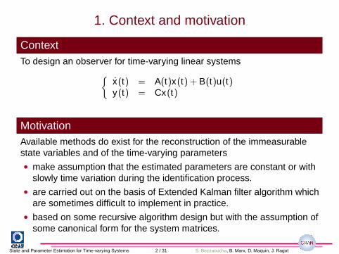
1. Context and motivation
ContextTo design an observer for time-varying linear systems
{
x(t) = A(t)x(t) + B(t)u(t)y(t) = Cx(t)
MotivationAvailable methods do exist for the reconstruction of the immeasurablestate variables and of the time-varying parameters• make assumption that the estimated parameters are constant or with
slowly time variation during the identification process.• are carried out on the basis of Extended Kalman filter algorithm which
are sometimes difficult to implement in practice.• based on some recursive algorithm design but with the assumption of
some canonical form for the system matrices.
State and Parameter Estimation for Time-varying Systems 2 / 31 S. Bezzaoucha, B. Marx, D. Maquin, J. Ragot

1. Context and motivation
Proposition
• Present a systematic procedure to deal with the simultaneous stateand parameter estimation for time-varying systems.
• Transform the original system into a polytopic linear model based onthe sector nonlinearity approach and the convex polytopictransformation.
• First contribution where the time-varying problem is treated in such away.
• Establish the convergence conditions of the state and parameterestimation errors, which will be expressed in linear matrix inequalities(LMIs) formulation using the Lyapunov method.
State and Parameter Estimation for Time-varying Systems 3 / 31 S. Bezzaoucha, B. Marx, D. Maquin, J. Ragot

Outline
Outline
1. Context and motivation
2. Problem statement
3. Observer design
4. Relaxed conditions
5. Noise measurement and filter synthesis
6. Illustrative example
7. Conclusions and perspectives
State and Parameter Estimation for Time-varying Systems 4 / 31 S. Bezzaoucha, B. Marx, D. Maquin, J. Ragot

2. Problem statement
Time-varying linear system
{
x(t) = A(t)x(t) + B(t)u(t)y(t) = Cx(t)
{
A(t) = A0 + θ(t)A, θ(t) ∈ [θ, θ]
B(t) = B0 + θ(t)B
θ(t) ∈ R is a time-varying parameter, non measurable but bounded.
Polytopic decomposition
θ(t) = µ1(θ(t))θ + µ2(θ(t))θ
µ1(θ(t)) =θ − θ(t)
θ − θ
µ2(θ(t)) =θ(t)− θ
θ − θ
2∑
i=1
µi(ξ(t)) = 1
0 ≤ µi(ξ(t)) ≤ 1, i = 1,2
State and Parameter Estimation for Time-varying Systems 5 / 31 S. Bezzaoucha, B. Marx, D. Maquin, J. Ragot

2. Problem statement
Time-varying linear system–> T-S (PLM) system
The initial linear system with the time-varying parameter θ(t) isexpressed as a PLM :
x(t) =2
∑
i=1
µi(θ(t))(Aix(t) + Biu(t))
{
A1 = A0 + θ A, B1 = B0 + θ BA2 = A0 + θ A, B2 = B0 + θ B
Case of n parameters
The proposed writting is applicable to the vector case with n parametersθj(t) affecting the matrices A(t) and B(t). Using the PLM representation,each parameter is written under the polytopic form and then a compactT-S form is deduced.
State and Parameter Estimation for Time-varying Systems 6 / 31 S. Bezzaoucha, B. Marx, D. Maquin, J. Ragot

3. Observer design
Simultaneous state and time-varying parameter observer
u(t)
θ(t)
x(t)
θ(t), x(t)
K ,L, α
y(t)
FIGURE: Système+Observateurs à EI
˙x(t) =2
∑
i=1
µi(θ(t))(Ai x(t) + Biu(t)) + Li(y(t)− y(t))
˙θ(t) =
2∑
i=1
µi(θ(t))(Ki(y(t)− y(t))− αi θ(t))
y(t) = Cx(t)
State and Parameter Estimation for Time-varying Systems 7 / 31 S. Bezzaoucha, B. Marx, D. Maquin, J. Ragot

3. Observer design
Classical design : L2 attenuation approach
Goal : Determine the observer gains Li , Ki and αi to minimize the effectof the time-varying parameter θ(t) on the state and parameter estimationerrors :• ex (t) = x(t)− x(t) the state estimation error• eθ(t) = θ(t)− θ(t) the time-varying parameter estimation error
Difficulty
The estimation problem is not trivial since the activation functions in thesystem depend on θ(t), while those of the observer depend on itsestimate θ(t), then its dynamics cannot be directly computed.
State and Parameter Estimation for Time-varying Systems 8 / 31 S. Bezzaoucha, B. Marx, D. Maquin, J. Ragot
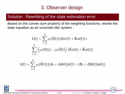
3. Observer design
Solution : Rewritting of the state estimation error
Based on the convex sum property of the weighting functions, rewrite thestate equation as an uncertain-like system :
x(t) =2
∑
i=1
µi(θ(t)) (Aix(t) + Biu(t))+
2∑
i=1
(
µi(θ(t))− µi(θ(t))
(
Aix(t) + Biu(t))
x(t) =2
∑
i=1
µi(θ(t)) ((Ai +∆A(t))x(t) + (Bi +∆B(t))u(t))
State and Parameter Estimation for Time-varying Systems 9 / 31 S. Bezzaoucha, B. Marx, D. Maquin, J. Ragot

Rewritting of the state estimation error
Problem
∆A(t) =
2∑
i=1
(µi(θ(t))− µi(θ(t)))Ai
= AΣA(t)EA
∆B(t) =
2∑
i=1
(µi(θ(t))− µi(θ(t)))Bi
= BΣB(t)EB
A =[
A1 A2]
, ΣA(t) =(
δ1(t)Inx 00 δ2(t)Inx
)
,
B =[
B1 B2]
, ΣB(t) =(
δ1(t)Inu 00 δ2(t)Inu
)
,
EA =[
Inx Inx
]T, EB =
[
Inu Inu
]T
ΣTA(t)ΣA(t) ≤ I, ΣT
B(t)ΣB(t) ≤ I
State and Parameter Estimation for Time-varying Systems 10 / 31 S. Bezzaoucha, B. Marx, D. Maquin, J. Ragot

3. Observer design
Estimation errors dynamic
x(t) =2
∑
i=1
µi(θ(t)) ((Ai +∆A(t))x(t) + (Bi +∆B(t))u(t))
˙x(t) =2
∑
i=1
µi(θ(t))(Ai x(t) + Biu(t)) + Li(y(t)− y(t))
˙θ(t) =
2∑
i=1
µi(θ(t))(Ki(y(t)− y(t))− αi θ(t))
ex(t) =
2∑
i=1
µi(θ(t)) ((Ai − LiC)ex (t) + ∆A(t)x(t) + ∆B(t)u(t))
eθ(t) =
2∑
i=1
µi(θ(t))(
θ(t)− KiCex (t) + αiθ(t)− αieθ(t))
State and Parameter Estimation for Time-varying Systems 11 / 31 S. Bezzaoucha, B. Marx, D. Maquin, J. Ragot

3. Observer design
Augmented system dynamic
Let us consider the augmented vectors ea(t) =(
eTx (t) eT
θ (t))T
and
ω(t) =(
xT (t) θT (t) θT (t) uT (t))T
.
ea(t) =2
∑
i=1
µi(θ(t)) (Φiea(t) + Ψi(t)ω(t))
Φi =
(
Ai − LiC 0−KiC −αi
)
Ψi(t) =
(
∆A(t) 0 0 ∆B(t)0 αi I 0
)
Our objective is to design the joint state and parameter observer with aminimal L2-gain of the transfer from the perturbation ω(t) to the errorea(t). The computation of the observer gains is detailed in the nexttheorem.
State and Parameter Estimation for Time-varying Systems 12 / 31 S. Bezzaoucha, B. Marx, D. Maquin, J. Ragot

3. Observer design : Theorem 1/2There exists a joint robust state and parameter observer for a lineartime-varying parameter system with an L2-gain from ω(t) to ea(t),bounded by β, if there exist matrices P0 = PT
0 > 0, Γ02 = (Γ0
2)T ,
Γ32 = (Γ3
2)T > 0, Fi and Ri and positive scalars P1, β, λ1, λ2, Γ1
2, Γ22, and
αi , solution of the optimization problem (1) under LMI constraints (2)(next slide), for i = 1,2 :
minP0,P1,Ri ,Fi ,αi ,λ1,λ2,Γ
02,Γ
12,Γ
22,Γ
32
β (1)
Γk2 < βI, for k = 0,1,2,3
The observer gains are given by
Li = P−10 Ri
Ki = P−11 Fi
αi = P−11 αi
State and Parameter Estimation for Time-varying Systems 13 / 31 S. Bezzaoucha, B. Marx, D. Maquin, J. Ragot
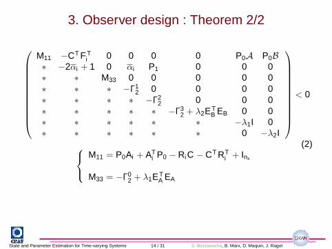
3. Observer design : Theorem 2/2
M11 −CT F Ti 0 0 0 0 P0A P0B
∗ −2αi + 1 0 αi P1 0 0 0∗ ∗ M33 0 0 0 0 0∗ ∗ ∗ −Γ1
2 0 0 0 0∗ ∗ ∗ ∗ −Γ2
2 0 0 0∗ ∗ ∗ ∗ ∗ −Γ3
2 + λ2ETB EB 0 0
∗ ∗ ∗ ∗ ∗ ∗ −λ1I 0∗ ∗ ∗ ∗ ∗ ∗ 0 −λ2I
< 0
(2)
M11 = P0Ai + ATi P0 − RiC − CT RT
i + Inx
M33 = −Γ02 + λ1ET
A EA
State and Parameter Estimation for Time-varying Systems 14 / 31 S. Bezzaoucha, B. Marx, D. Maquin, J. Ragot

3. Observer design : Proceeding
Augmented system dynamic
ea(t) =2
∑
i=1
µi(θ(t)) (Φiea(t) + Ψi(t)ω(t))
To guarantee the stability of the augmented system and theboundedness of the transfer from the input ω(t) to ea(t) (attenuate theeffect of ω(t) on the estimation), the bounded real lemma is applied andthe solution is expressed in terms of LMI. Considering the followingquadratic Lyapunov function and the L2 criterion
V (ea(t)) = eTa (t)Pea(t), P = PT > 0,P = diag(P0,P1)
V (t) + eTa (t)ea(t)− ωT (t)Γ2ω(t) < 0
Γ2 = diag(Γk2), Γ
k2 < βI, for k = 0,1,2,3
such that Γ2 allows to attenuate the transfer of some ω(t) components toea(t) components.
State and Parameter Estimation for Time-varying Systems 15 / 31 S. Bezzaoucha, B. Marx, D. Maquin, J. Ragot

3. Observer design : Proceeding
Augmented system dynamic
Applying the Lyapunov theory :
2∑
i=1
µji(θ(t))
(
ea(t)ω(t)
)T ((
ΦTi P + PΦi + I PΨi(t)Ψj
i(t)T (t)P −Γ2
))(
ea(t)ω(t)
)
< 0
The main difficulty for satisfying this condition is the presence oftime-varying terms Ψi(t). Then, the idea is to isolate and bound theseterms basing on the previous property ΣT
A(t)ΣA(t) ≤ I, ΣTB(t)ΣB(t) ≤ I.
Replacing each term by its definition and linearizing the obtained BMI(bilinear matrix inequalities), the theorem has been proved.
State and Parameter Estimation for Time-varying Systems 16 / 31 S. Bezzaoucha, B. Marx, D. Maquin, J. Ragot

4. Relaxed conditions
Relaxed conditionsIn order to bound the time-varying terms, the following property wasused :Consider two matrices X and Y with appropriate dimensions, atime-varying matrix ∆(t) and a positive scalar ε. The following propertyis verified (for ∆T (t)∆(t) ≤ I)
X T∆T (t)Y + Y T∆(t)X ≤ εX T X + ε−1Y T Y
Relaxed conditionsThe LMIs to solve may be relaxed using the convex sum property of theweighting functions µi(t)
µ2(t) = 1 − µ1(t)
x(t) =2
∑
i=1
µi(θ(t))(
(Ai +∆A(t))x(t) + (Bi +∆B(t))u(t))
∆A(t) = δ (t)(A − A )State and Parameter Estimation for Time-varying Systems 17 / 31 S. Bezzaoucha, B. Marx, D. Maquin, J. Ragot

4. Relaxed conditions
Relaxed conditions
∆A(t) = δ1(t)(A1 − A2) instead of ∆A(t) =2
∑
i=1
(µi(θ(t))− µi(θ(t)))Ai
∆B(t) = δ1(t)(B1 − B2) instead of ∆B(t) =2
∑
i=1
(µi(θ(t))− µi(θ(t)))Bi
δ1(t) = µ1(θ(t))− µ1(θ(t))
State and Parameter Estimation for Time-varying Systems 18 / 31 S. Bezzaoucha, B. Marx, D. Maquin, J. Ragot
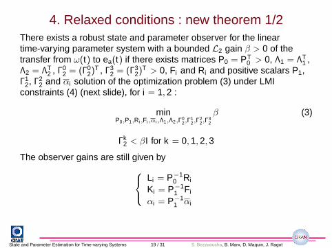
4. Relaxed conditions : new theorem 1/2There exists a robust state and parameter observer for the lineartime-varying parameter system with a bounded L2 gain β > 0 of thetransfer from ω(t) to ea(t) if there exists matrices P0 = PT
0 > 0, Λ1 = ΛT1 ,
Λ2 = ΛT2 , Γ0
2 = (Γ02)
T , Γ32 = (Γ3
2)T > 0, Fi and Ri and positive scalars P1,
Γ12, Γ2
2 and αi solution of the optimization problem (3) under LMIconstraints (4) (next slide), for i = 1,2 :
minP0,P1,Ri ,Fi ,αi ,Λ1,Λ2,Γ
02,Γ
12,Γ
22,Γ
32
β (3)
Γk2 < βI for k = 0,1,2,3
The observer gains are still given by
Li = P−10 Ri
Ki = P−11 Fi
αi = P−11 αi
State and Parameter Estimation for Time-varying Systems 19 / 31 S. Bezzaoucha, B. Marx, D. Maquin, J. Ragot

4. Relaxed conditions : new theorem 2/2
M11 −CT F Ti 0 0 0 0 P0 P0
∗ −2αi + 1 0 αi P1 0 0 0∗ ∗ −Γ0
2 + ΛA 0 0 0 0 0∗ ∗ ∗ −Γ1
2 0 0 0 0∗ ∗ ∗ ∗ −Γ2
2 0 0 0∗ ∗ ∗ ∗ ∗ −Γ3
2 + ΛB 0 0∗ ∗ ∗ ∗ ∗ ∗ −Λ1 0∗ ∗ ∗ ∗ ∗ ∗ 0 −Λ2
< 0
(4)where Λ1 and Λ2 are matrices (instead of scalars for the previousdevelopment) and where :
ΛA = (A1 − A2)TΛ1(A1 − A2)
ΛB = (B1 − B2)TΛ2(B1 − B2)
M11 = P0Ai + ATi P0 − RiC − CT RT
i + Inx
State and Parameter Estimation for Time-varying Systems 20 / 31 S. Bezzaoucha, B. Marx, D. Maquin, J. Ragot

5. Noise measurement and filter synthesis
Time-varying linear system with measurement noise
{
x(t) = A(t)x(t) + B(t)u(t)y(t) = Cx(t)+Gb(t)
where b(t) is the noise measurement and matrices A(t) and B(t) havebeen already defined previuosly.
Objective
Our objective is to attenuate the effect of the parametric variation andthe noise on the state and parameter estimations.
State and Parameter Estimation for Time-varying Systems 21 / 31 S. Bezzaoucha, B. Marx, D. Maquin, J. Ragot

5. Noise measurement and filter synthesis
Augmented system dynamic
ea(t) =2
∑
i=1
µi(θ(t)) (Φiea(t) + Ψi(t)ω(t))
ea(t) =(
eTx (t) eT
θ (t))T
, ω(t) =(
xT (t) θT (t) θT (t) uT (t) bT (t))
where ω(t) takes now into account the noise b(t).
Φi =
(
Ai − LiC 0−KiC −αi
)
Ψi(t) =
(
∆A(t) 0 0 ∆B(t) −LiG0 αi I 0 −KiG
)
Our objective is to design the joint state and parameter observer with aminimal L2-gain of the transfer from ω(t) to ea(t). The computation of theobserver gains is detailed in the next theorem.
State and Parameter Estimation for Time-varying Systems 22 / 31 S. Bezzaoucha, B. Marx, D. Maquin, J. Ragot
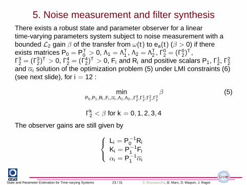
5. Noise measurement and filter synthesisThere exists a robust state and parameter observer for a lineartime-varying parameters system subject to noise measurement with abounded L2 gain β of the transfer from ω(t) to ea(t) (β > 0) if thereexists matrices P0 = PT
0 > 0, Λ1 = ΛT1 , Λ2 = ΛT
2 , Γ02 = (Γ0
2)T ,
Γ32 = (Γ3
2)T > 0, Γ4
2 = (Γ42)
T > 0, Fi and Ri and positive scalars P1, Γ12, Γ2
2and αi solution of the optimization problem (5) under LMI constraints (6)(see next slide), for i = 12 :
minP0,P1,Ri ,Fi ,αi ,Λ1,Λ2,,Γ
02,Γ
12,Γ
22,Γ
32
β (5)
Γk2 < β for k = 0,1,2,3,4
The observer gains are still given by
Li = P−10 Ri
Ki = P−11 Fi
αi = P−11 αi
State and Parameter Estimation for Time-varying Systems 23 / 31 S. Bezzaoucha, B. Marx, D. Maquin, J. Ragot

5. Noise measurement and filter synthesis
M11 −CT F Ti 0 0 0 0 −RiG P0 P0
∗ −2αi + 1 0 αi P1 0 −FiG 0 0∗ ∗ −Γ0
2 + ΛA 0 0 0 0 0 0∗ ∗ ∗ −Γ1
2 0 0 0 0 0∗ ∗ ∗ ∗ −Γ2
2 0 0 0 0∗ ∗ ∗ ∗ ∗ −Γ3
2 + ΛB 0 0 0∗ ∗ ∗ ∗ ∗ ∗ −Γ4
2 0 0∗ ∗ ∗ ∗ ∗ ∗ ∗ −Λ1 0∗ ∗ ∗ ∗ ∗ ∗ ∗ 0 −Λ2
< 0
(6)with :
ΛA = (A1 − A2)TΛ1(A1 − A2)
ΛB = (B1 − B2)TΛ2(B1 − B2)
M11 = P0Ai + ATi P0 − RiC − CT RT
i + Inx
State and Parameter Estimation for Time-varying Systems 24 / 31 S. Bezzaoucha, B. Marx, D. Maquin, J. Ragot
6. Illustrative example
Illustrative example
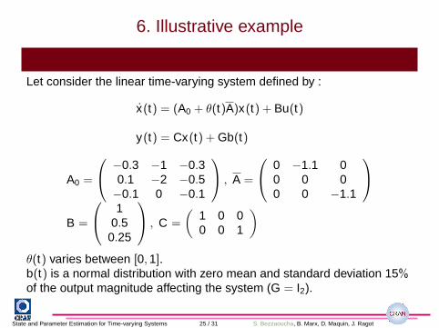
Let consider the linear time-varying system defined by :
x(t) = (A0 + θ(t)A)x(t) + Bu(t)
y(t) = Cx(t) + Gb(t)
A0 =
−0.3 −1 −0.30.1 −2 −0.5−0.1 0 −0.1
, A =
0 −1.1 00 0 00 0 −1.1
B =
10.5
0.25
, C =
(
1 0 00 0 1
)
θ(t) varies between [0,1].b(t) is a normal distribution with zero mean and standard deviation 15%of the output magnitude affecting the system (G = I2).
State and Parameter Estimation for Time-varying Systems 25 / 31 S. Bezzaoucha, B. Marx, D. Maquin, J. Ragot
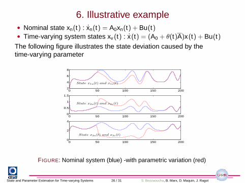
6. Illustrative example• Nominal state xn(t) : xn(t) = A0xn(t) + Bu(t)• Time-varying system states xv (t) : x(t) = (A0 + θ(t)A)x(t) + Bu(t)
The following figure illustrates the state deviation caused by thetime-varying parameter
0 50 100 150 2002
4
6
8
State x1n(t) and x1v(t)
0 50 100 150 2000
0.5
1
1.5
State x2n(t) and x2v(t)
0 50 100 150 2000
2
4
State x3n(t) and x3v(t)
FIGURE: Nominal system (blue) -with parametric variation (red)
State and Parameter Estimation for Time-varying Systems 26 / 31 S. Bezzaoucha, B. Marx, D. Maquin, J. Ragot

6. Illustrative example
Illustrative example
To illustrate the actual and estimated states : x0 =(
2 1 2)
,x0 =
(
0 0 0 0)
.
0 20 40 60 80 100 120 140 160 180 2000
2
4
6
8
10
State x1(t) and x1(t)
0 20 40 60 80 100 120 140 160 180 200−2
−1
0
1
2
State x2(t) and x2(t)
0 20 40 60 80 100 120 140 160 180 2000
1
2
3
4
5
State x3(t) and x3(t)
FIGURE: Actual and estimated statesState and Parameter Estimation for Time-varying Systems 27 / 31 S. Bezzaoucha, B. Marx, D. Maquin, J. Ragot

Actual and estimated time-varying parameter
0 20 40 60 80 100 120 140 160 180 200−0.5
0
0.5
1
Par. θ1(t) et θ1(t)
FIGURE: Time-varying parameter θ(t) and its estimate
State and Parameter Estimation for Time-varying Systems 28 / 31 S. Bezzaoucha, B. Marx, D. Maquin, J. Ragot
Conclusions and perspectives
Conclusions
• A new systematic procedure was presented to deal with the state andparameter estimation for time-varying systems.
• Based on a T-S representation (by the sector nonlinearity approachand the convex polytopic transformation).
• The estimation problem and observer synthesis are expressed interms of LMI optimization.
State and Parameter Estimation for Time-varying Systems 29 / 31 S. Bezzaoucha, B. Marx, D. Maquin, J. Ragot

Conclusions and perspectives
Conclusions
• A new systematic procedure was presented to deal with the state andparameter estimation for time-varying systems.
• Based on a T-S representation (by the sector nonlinearity approachand the convex polytopic transformation).
• The estimation problem and observer synthesis are expressed interms of LMI optimization.
Perspectives
• Application to nonlinear systems (biological wastewater treatmentplant).
• Use the results for Fault Tolerant Control (FTC).
State and Parameter Estimation for Time-varying Systems 29 / 31 S. Bezzaoucha, B. Marx, D. Maquin, J. Ragot

Thanks
Thanks
Thank you for your attention ! !
Get in touch : email [email protected] / [email protected] /[email protected] / [email protected]
State and Parameter Estimation for Time-varying Systems 30 / 31 S. Bezzaoucha, B. Marx, D. Maquin, J. Ragot

Technical details
The bounded real lemmaConsidering the system
x(t) = Ax(t) + Bu(t) (7)
System (7) is asymptotically stable if there exist a symmetric positiveP = PT > 0 and a positive scalar γ > 0 such that
(
AT P + PA PB∗ −γI
)
where I is the identity matrix and ∗ denotes the symmetric item in asymmetric matrix.
State and Parameter Estimation for Time-varying Systems 31 / 31 S. Bezzaoucha, B. Marx, D. Maquin, J. Ragot