Mobile Robot Simultaneous Localization and Mapping in Dynamic Environments
Upload
khangminh22Category
view
2download
0
Institut fur InformatikderTechnischenUniversitatMunchen
Robot Motion Planningin Time-varying Envir onments
Andr eaBaumann
VollstandigerAbdruck der von der Fakultat fur Informatik der TechnischenUniversitat
MunchenzurErlangungdesakademischenGradeseines
DoktorsderNaturwissenschaften
genehmigtenDissertation.
Vorsitzender: Univ.-Prof.Dr. Chr. Zenger
PruferderDissertation:
1. Univ.-Prof.Dr. H.-J.Siegert,em.
2. Univ.-Prof.Dr. Dr.h.c.W. Brauer
Die Dissertationwurdeam28. Juni2001beiderTechnischenUniversitatMunchen
eingereichtunddurchdie Fakultat fur Informatikam19. Oktober2001angenommen.


Abstract
Motion planningis oneof theprincipal tasksof autonomousrobotsystems.As a conse-quence,robotmotionplanningis oneof themostactive researchareasin roboticsandinthepastdecadesgreateffort hasbeenput into thedevelopmentof flexible motion plan-ningalgorithms.Theproblemsthatneededto betackledturnedout to bedemandingandmostof thesolutionsfoundsofararerestrictedin thesensethatthey eitherfind acollisionfree geometricpathignoring robot dynamicsor they computea time or energy optimaltrajectorybut they ignorecollisions. The obvious goal, however, is to find a planningapproachthat respectsbothobstaclesandrobot dynamics.By including the time in theplanningprocessit becomespossibleto handletrajectoriesthatarecollision freeandthatalsorespectthedynamiclimits of therobot. In addition,suchaplanningapproachwill becapableof dealingwith time-varyingobstacles.Thepositionof suchobstacleschangesover time (but is known in advancefor eachpoint in time). Examplescanbe found inindustrialmanufacturingprocesses.Considera robot in front of a productionline withmoving workpieces.
In this thesiswe presentsucha planningapproach.Our motion planningalgorithmconsidersrobot dynamics(i.e. force and torquelimits) and is able to deal with time-varying obstacles.Another characteristicof our approachis that the planningprocessandthe processof generatingtrajectoriesaredecoupled.This bearsthe advantagethatour plannercanhandledifferent typesof trajectorieswithout modification. For exam-ple, point-to-pointmotions,pathmotions,or even specialtypesof trajectoriesfor non-holonomicrobots. The planningprocessitself only handlesbasepoints,which defineallowedareasfor theactualtrajectory.
By modifying thepositionandthenumberof basepoints,theallowedtrajectoryareaand consequentlythe trajectory itself is modified. To guide the planningprocess,weintroduceseveral criteria uponwhich the evaluationof generatedtrajectoriesis based.Our main focus is on freedomfrom collision and robot dynamics,sincethesecriteriahaveprecedenceoverall othercriteria,suchastimeor energy consumption.
Oneof themainingredientsof motionplanningin time-varyingenvironmentsis a re-liable algorithmfor collision detection.We presentanextensionof anexistingalgorithm

ii ABSTRACT
for staticenvironmentsthatenablesusnotonly to detectcollisionswith moving obstaclesbut alsogivesusapreciseratingof thedepthof acollision.
To demonstratethe usefulnessof our approach,we have implementedour motionplanningalgorithmwithin thescopeof a robotsimulationsystemandwehavetestedit invariousscenarios.
Kurzfassung
Die PlanungvonBewegungenist einederwichtigstenAufgabeneinesautonomenRobot-ersystems.In derRobotik-Forschungist daherdie BewegungsplanungeinesderHaupt-themen,undeswurdenin denvergangenenJahrzehntengroßeAnstrengungenunternom-men,flexible Planungsverfahrenzuentwickeln. Die dabeizulosendenProblemeerwiesensich als anspruchsvoll, und die meistender existierendenAnsatzebeschranken sich en-twederaufdasFindenvonkollisionsfreiengeometrischenBahnenohneBerucksichtigungderRoboterdynamik,oderdie BerechnungeinerZeit- oderEnergie optimalenTrajekto-rie ohneBerucksichtigungvon Hindernissen.Der Vorteil einesBewegungsplaners,dersowohl die Hindernisseim Raumalsauchdie EinhaltungderdynamischenGrenzendesRobotersbeachtet,liegt aufderHand.DurchdenEinbezugderZeit wird esmoglich,Tra-jektorienzu berechnen,die sowohl kollisionsfreisind,alsauchdie DynamikdesRobot-ersberucksichtigen.Hinzukommt,dassesmit einemsolchenBewegungsplanermoglichwird, zeitvarianteHindernissein den Planungsvorgangmiteinzubeziehen.DieseHin-dernissehabendieEigenschaft,dassihr Aufenthaltsortsichmit derZeit andert(zu jedemZeitpunktaberbekanntist). Dies trif ft zum Beispielauf Szenarienzu, wie sie ausderAutomobilindustriebekanntsind. Man denke dabeianeinenRoboteramFließband,aufdemsichWerkstuckebewegen.
In der vorliegendenArbeit wird ein solchesVerfahrenzur Planungvon Roboterbe-wegungenvorgestellt.Der zugrundeliegendeBewegungsplanerbeziehtRoboterdynamikund zeitvarianteHindernissein den Planungsprozessmit ein. Eine weitereBesonder-heit desvorgestelltenVerfahrensist, dassdie Trajektorienerzeugungvom eigentlichenPlanungsvorgangentkoppeltist. DieshatdenVorteil, dassderPlanungsvorganguberver-schiedeneTrajektorientypenablaufenkann. SeiendasnunPunkt-zu-PunktBewegungenoderuberschliffeneBahnen,oderauchspezielleTrajektorienfur nichtholonomeRoboter.Die Planungselbstfindetnur uberStutzpunktestatt,die erlaubteBereichefur dieTrajek-toriedefinieren.
DurchdasModifizierenderPositionundderAnzahlderStutzpunktewird dererlaubteTrajektorienbereichunddamitauchdieTrajektorieselbstverandert.Um denFortgangderPlanungzu beurteilen,werdenverschiedeneKriterien eingefuhrt, nachdenendie gener-

iv KURZFASSUNG
ierteTrajektoriebewertetwird. BesonderenAugenmerklegenwir hierbeiaufKollisions-freiheit unddie dynamischenRandbedingungen,daeineEinhaltungdieserKriterien alsvorrangiganzusehenist.
Bei einer Bewegungsplanungmit zeitvariantenHindernissenist ein wichtiger Be-standteildie Erkennungvon KollisionendesRoboters.Wir erweiterndazuein bestehen-desVerfahrenumdieMoglichkeitderKollisionserkennungin zeitvariantenUmgebungen,undstelleneinenAlgorithmusvor, dernebendereigentlichenErkennungvonKollisionenauchnochunmittelbareineBewertungderKollisionstiefeerlaubt.
Um diePraxistauglichkeit unseresVerfahrensunterBeweiszustellen,wurdederPla-nungsalgorithmusim RahmeneinesRobotersimulationssystemsimplementiertund an-handverschiedenerSzenariengetestet.

Acknowledgments
Firstof all I would like to thankmy advisor, Hans-JurgenSiegert,for hisencouragement,advice,andresearchsupportthroughoutmy doctoralstudies.I amalsodeeplyindebtedto him for giving metheopportunityto lectureon robotmotionplanning.
I want to thankmy currentand former colleaguesBoris Baginski,AndreasKoller,Oliver Schmid,GerhardSchrott,andThomasWeiser. They provided a supportive andmostenjoyableworkingenvironment.I wantespeciallyto thankBoris for introducingmeto robotmotionplanningandfor proof-readingthis thesis.Sincerethanksgo to JenniferWeeksfor correctingmy un-Englishwordsandphrases.
This thesiswould not have beenpossiblewithout my parents’love andsupport,aswell asmy family andfriends’ encouragement.To all of you, thankyou.
Finally, specialthanksgo to Hans,for carefullyreadingthis thesis,but above all, forhispatience,love,andinspiration.


Contents
1 Intr oduction and Overview 11.1 Introduction . . . . . . . . . . . . . . . . . . . . . . . . . . . . . . . . . 11.2 Overview . . . . . . . . . . . . . . . . . . . . . . . . . . . . . . . . . . 3
2 RelatedWork 52.1 Classificationof Motion PlanningProblems . . . . . . . . . . . . . . . . 52.2 GeometricRepresentationandComputation. . . . . . . . . . . . . . . . 72.3 BasicPathPlanning. . . . . . . . . . . . . . . . . . . . . . . . . . . . . 8
2.3.1 TheoreticalResults . . . . . . . . . . . . . . . . . . . . . . . . . 92.3.2 CompleteAlgorithms . . . . . . . . . . . . . . . . . . . . . . . . 102.3.3 ResolutionCompleteAlgorithms . . . . . . . . . . . . . . . . . 112.3.4 ProbabilisticallyCompleteAlgorithms . . . . . . . . . . . . . . 132.3.5 HeuristicAlgorithms . . . . . . . . . . . . . . . . . . . . . . . . 14
2.4 TrajectoryPlanningAlgorithms . . . . . . . . . . . . . . . . . . . . . . 152.4.1 Optimal-timeControlPlanning . . . . . . . . . . . . . . . . . . 152.4.2 Minimal-timeTrajectoryPlanning . . . . . . . . . . . . . . . . . 162.4.3 Planningin Time-varyingEnvironments. . . . . . . . . . . . . . 17
3 An Approachto Planning in Time-varying Envir onments 193.1 Objectives . . . . . . . . . . . . . . . . . . . . . . . . . . . . . . . . . . 193.2 Outline . . . . . . . . . . . . . . . . . . . . . . . . . . . . . . . . . . . 203.3 Testingfor Collision . . . . . . . . . . . . . . . . . . . . . . . . . . . . 213.4 BasePointTrajectories . . . . . . . . . . . . . . . . . . . . . . . . . . . 233.5 TrajectoryRatings. . . . . . . . . . . . . . . . . . . . . . . . . . . . . . 243.6 Improving TrajectoryQuality . . . . . . . . . . . . . . . . . . . . . . . . 24
4 Modelling the World 274.1 Robots. . . . . . . . . . . . . . . . . . . . . . . . . . . . . . . . . . . . 27
4.1.1 Joints . . . . . . . . . . . . . . . . . . . . . . . . . . . . . . . . 30
viii CONTENTS
4.1.2 Links . . . . . . . . . . . . . . . . . . . . . . . . . . . . . . . . 354.2 Environment. . . . . . . . . . . . . . . . . . . . . . . . . . . . . . . . . 364.3 Collisions . . . . . . . . . . . . . . . . . . . . . . . . . . . . . . . . . . 384.4 Trajectories . . . . . . . . . . . . . . . . . . . . . . . . . . . . . . . . . 394.5 TheMotion PlanningProblem . . . . . . . . . . . . . . . . . . . . . . . 42
5 Generating Trajectories fr om BasePoints 455.1 Introduction . . . . . . . . . . . . . . . . . . . . . . . . . . . . . . . . . 455.2 BasePointTrajectories . . . . . . . . . . . . . . . . . . . . . . . . . . . 475.3 PolynomialTrajectories. . . . . . . . . . . . . . . . . . . . . . . . . . . 50
5.3.1 Point-to-PointMotion . . . . . . . . . . . . . . . . . . . . . . . 505.3.2 PathMotion . . . . . . . . . . . . . . . . . . . . . . . . . . . . . 525.3.3 InsertingandDeletingBasePoints. . . . . . . . . . . . . . . . . 58
5.4 ModifiedBang-BangTrajectories . . . . . . . . . . . . . . . . . . . . . 605.4.1 Point-to-PointMotion . . . . . . . . . . . . . . . . . . . . . . . 605.4.2 PathMotion . . . . . . . . . . . . . . . . . . . . . . . . . . . . . 625.4.3 InsertingandDeletingBasePoint . . . . . . . . . . . . . . . . . 63
5.5 SummaryandOutlook . . . . . . . . . . . . . . . . . . . . . . . . . . . 64
6 Forceand TorqueRating 696.1 Introduction . . . . . . . . . . . . . . . . . . . . . . . . . . . . . . . . . 696.2 ForceandTorqueCalculation. . . . . . . . . . . . . . . . . . . . . . . . 696.3 TrajectoryForceandTorqueRating . . . . . . . . . . . . . . . . . . . . 716.4 SummaryandOutlook . . . . . . . . . . . . . . . . . . . . . . . . . . . 74
7 Collision Rating 777.1 Introduction . . . . . . . . . . . . . . . . . . . . . . . . . . . . . . . . . 777.2 StaticCollision Test . . . . . . . . . . . . . . . . . . . . . . . . . . . . . 787.3 DynamicCollisionTest . . . . . . . . . . . . . . . . . . . . . . . . . . . 877.4 TrajectoryCollisionRating . . . . . . . . . . . . . . . . . . . . . . . . . 927.5 SummaryandOutlook . . . . . . . . . . . . . . . . . . . . . . . . . . . 94
8 Trajectory Planning 978.1 GlobalTrajectoryRating . . . . . . . . . . . . . . . . . . . . . . . . . . 978.2 FindingAlternativeTrajectories . . . . . . . . . . . . . . . . . . . . . . 102
8.2.1 Moving Sections . . . . . . . . . . . . . . . . . . . . . . . . . . 1038.2.2 AddingSections . . . . . . . . . . . . . . . . . . . . . . . . . . 1108.2.3 DeletingSections. . . . . . . . . . . . . . . . . . . . . . . . . . 1138.2.4 RandomisedSectionMovement . . . . . . . . . . . . . . . . . . 114
8.3 TrajectoryPlanningAlgorithm . . . . . . . . . . . . . . . . . . . . . . . 1168.4 SummaryandAnalysis . . . . . . . . . . . . . . . . . . . . . . . . . . . 118
9 Experimental Results 1239.1 TestEnvironmentandParameters . . . . . . . . . . . . . . . . . . . . . 123
9.1.1 RobS:a RobotSimulationSystem . . . . . . . . . . . . . . . . . 1239.1.2 Parameters . . . . . . . . . . . . . . . . . . . . . . . . . . . . . 124

CONTENTS ix
9.2 Experiments. . . . . . . . . . . . . . . . . . . . . . . . . . . . . . . . . 1269.2.1 Two Degreeof FreedomRobot. . . . . . . . . . . . . . . . . . . 1289.2.2 An IndustrialEnvironment . . . . . . . . . . . . . . . . . . . . . 1359.2.3 Benchmarksfor StaticEnvironments . . . . . . . . . . . . . . . 1389.2.4 RX90with aHeavy Hand . . . . . . . . . . . . . . . . . . . . . 1459.2.5 Sliding Door . . . . . . . . . . . . . . . . . . . . . . . . . . . . 1489.2.6 DLR Robotwith Handin AsteroidField . . . . . . . . . . . . . . 151
9.3 Summary . . . . . . . . . . . . . . . . . . . . . . . . . . . . . . . . . . 155
10 Conclusion 15710.1 Summary . . . . . . . . . . . . . . . . . . . . . . . . . . . . . . . . . . 15710.2 FutureResearch. . . . . . . . . . . . . . . . . . . . . . . . . . . . . . . 158
List of Figures 161
List of Tables 165
List of Algorithms 167
List of Symbols 171
Bibliography 175


CHAPTER 1
Intr oduction and Overview
A short introductioninto thesignificanceof robotmotionplanningis provided. We mo-tivateour work by giving evidencethat planningin time-varyingenvironmentsis usefuland important. At the endof this chapter, a preview on the remainingchapters of thisthesisis given.
1.1 Intr oduction
Thereis nodoubtthatrobotsareof greatbenefitto mankind.Robotsassistdoctorsduringmedicalsurgeries,they repeattediousmovementsin manufacturingplants,they trans-port heavy loads,or they observe andcontrol eventsin hazardousenvironments.Muchprogresshasbeenachieved in roboticsin thepastdecadesbut therearestill many openproblemsthat needto be solved in orderto reachthe ultimategoal of robotics: to cre-ateautonomousrobots. Traditionally, robotsareusedto performprogrammed,repeti-tious tasks,or taskswherea humanoperatorhasto constantlyspecifythemotions.Au-tonomousrobots,however, will acceptdescriptionsof taskson anabstractlevel andtheywill carryout thosetaskswithouthumaninterventionor explicit teaching.
Many differenttechnologiesneedto bedevelopedin orderto reachthatgoal.Amongthosearetechnologiesfor perception,automatedreasoning,planning,manipulationandlearning.Oneof themainplanningproblemsis motionplanning. Clearly, anautonomousrobotmustbeableto planits own motions,becauseby moving in therealworld therobotwill accomplishits tasks.Theclassicmotionplanningproblemcanbedescribedroughlyasfollows: givenaninitial configurationandafinal configurationof therobot,find apathconnectingboth configurationsthat avoids collisionswith obstacles.It is assumedthatgeometryandpositionof obstaclesis known in advanceandit is assumedthatobstaclesdonotmove.
In this thesiswe considermotion planningin an extendedsetting. First, we allowobstaclesto moveandsecond,wearenotonly interestedin findingageometriccollision-free path but we are interestedin finding a path that can be executedby a real-worldrobot, andto that endwe have to take into accountrobot dynamicssuchastorqueand

2 1. INTRODUCTION AND OVERVIEW
forcelimits.Considerthe following moving obstacleproblem.A heatingcell is giventhathasto
beloadedandunloadedby a robot. Thedoorto thecell is closedwhenheatingandopenotherwise.Therobotmustplan its motion for loadingandunloadingrespectingthe factthat thedoor is closedfrom time to time. It would beeasyfor therobot to wait until thedooris fully openedbut it might benecessaryto startmoving themanipulatorbeforethedoorhasevenstartedto openin orderto unloadandloadthecell in time beforethedoorclosesagain.
To seethenecessityfor takingrobotdynamicsinto account,consideranathleteliftingaheavy dumb-bell.Theathletedoesnotmovethedumb-bellonastraightline. Hehastorespectthelimits of hismusclesandhetriesto useaslittle energy aspossibleto fulfil thistask. He will utilise themassesof his forearmandupperarmto getdrive. Furthermore,hewill sparehis backby bendingtheknees.For a manipulatorthesamelaws of naturearevalid andshouldthereforebetakeninto accountduringmotionplanning.
The trajectoryof a manipulatorcan fulfil variousconstraints. Someof thosecon-straintsmustbefulfilled if wewantto planmotionsfor realworld, for example,theremustbeno collisionswith obstaclesandwe mustalwaysbewithin thejoint, torqueandforcelimits or wehaveto ensurethatamobilerobotdoesnotoverturn(mandatoryconstraints).Otherconstraintsareoptional, for example,keepingthemanipulatorsomedistanceawayfrom obstaclesfor safetyreasonsor keepingthe tool of the robot orientedin a certainway (e.g. to hold a cupfilled with liquid). Trajectoriescanalsobeevaluatedaccordingto certainoptimisationcriteria. Reasonableoptimisationsare, for example,to find thetime minimal trajectory, theenergy minimal trajectory, or a trajectorythatminimisesthemaximumtorqueandforce(in orderto sparetherobot’s mechanics).Our mainfocusinthis thesiswill beon techniquesfor computingtrajectoriesthat fulfil all mandatorycon-straints.In addition,wewill givehintsonhow thesetechniquescanbeextendedto handleoptionalconstraintsandoptimisationcriteria.
The above mentionedenvironmentscanbe describedas time-varyingsincethey arecharacterisedby thepresenceof bodiesthatmoveover time. Weassumethatthetrajecto-riesof all obstaclesis known in advance.Typical exampleswherethis assumptionholdsaremanufacturingtasksin which robotmanipulatorstrackandretrieve partsfrom mov-ing band-conveyorsor wheremanipulatorshave to movebetweenothermanipulators.Intheseenvironments,thepartson theconveyorsandthemachinepartsof existing robotshaveaknown trajectory. Othertime-varyingscenarioscanbefoundin aviationandspacetravel. Considertheproblemof navigatingaspaceshipthroughafield of asteroids.In thiscasethetrajectoriesof theasteroidsareknown in advance.Or think of anobjectpassingaspaceshuttlewheretheobjecthasto becaughtat aspecifiedtime.
The motion planningproblemfor robotsin a known time-varying environmentcanbedescribedasfollows: We aregivenan initial configurationof the robotandan initialpoint in timeaswell asafinal configurationof therobotandafinal point in time. Wearealsogiventhegeometriesandtrajectoriesof all obstacles.Thegoal is to find a trajectorythat movesthe robot from oneto the other timed configurationavoiding collision withobstaclesandrespectingall limits of therobot,includingtorqueandforcelimits.
Planningin time-varyingenvironmentsis substantiallyharderthanplanningin staticenvironments.In a staticenvironmentwhereall obstaclesarefixed, if a safepathfrom

1.2. OVERVIEW 3
initial to final configurationhasbeendetermined,thena suitablevelocity profile canal-waysbefoundfor therobotalongthatpath,providedthat theavailableforceandtorqueenablesthe robot to at leastcompensatefor gravity in all of its possiblepositions. In atime-varyingenvironment,however, pathplanningandvelocity planningcannotbeper-formedindependentlyof eachother, sincetheavoidanceof moving obstaclesdependsontherobot’sdynamics.
1.2 Overview
This thesisis structuredasfollows. We startin chaptertwo by reviewing relatedwork.A classificationof path and trajectoryplanningproblemsis given accompaniedby anoverview onknown resultson thesubject.Onefocusis onresultsregardingthecomputa-tionalcomplexity of motionplanningin differentsettings.
In chapterthree,we describeour approachto motion planningin time-varying en-vironments. We proposea plannerthat is able to searchin a high dimensionaltimedsearchspacebasedon flexible functionsfor ratingthequality of a giventrajectoryandasetof heuristicsfor improving trajectoryquality, includingrandomisationto escapelocalminima.
In the chapterthereafter, we give preliminariesnecessaryfor a formal treatmentofmotionplanningin a time-varyingenvironment. We introducemathematicaldefinitionsrelatedto robots,configurationof robots,trajectories,obstaclesandcollisions.
Oneof thenoveltiesin ourapproachto planningis thedistinctionbetweenbasepointtrajectoriesandexact trajectories. A basepoint trajectoryis definedby a finite setofpointsandit representsall exact trajectoriesthat run alongthosepointswithin a certaindistance.This distinctionenablesus to changefocusduring planning. Sometimesit isnecessaryto concentrateonoverallcharacteristicsof a trajectoryandto abstractfrom de-tails. For example,our heuristicsfor improving trajectoriesoperateon basepoint trajec-torieswhile theactualratingof quality is doneonexacttrajectoriesgeneratedfrom thosebasepoints. In chapterfive, the notion of basepoint trajectoriesis formalised. More-over, weanalysedifferentwayshow to generateexacttrajectoriesfrom agivenbasepointtrajectory, resultingin differentwell-known typesof exacttrajectoriesfor manipulators.
Thefollowing two chapters,chapterssix andseven,arededicatedto theratingof thequality of a giventrajectory. Beingableto ratethequality of a trajectoryin a consistentandreliableway is animportantprerequisitefor our motionplanner. We split ratingintotwo parts. In chaptersix, we considerthe rating of a trajectoryregardingthe dynamiclimits of therobot. A betterratingmeanslessviolation of thetorqueandforce limits oftherobot.Chaptersevencoverstheratingof a trajectoryregardingcollisionsof therobotwith staticobstacles,moving obstaclesandits own links. To this end,a novel collisionrating is appliedthat not only detectsthe absenceof collisionsbut alsoratescollisionsaccordingto their depth.Here,a betterratingmeanslessdeepcollisionsor no collisionsatall.
In chaptereight, we give a detaileddescriptionof our main algorithm for motionplanningin time-varyingenvironments.Besidesquality ratings,theimportantpartof ourmotionplanningapproachis to modify giventrajectoriesin orderto find trajectorieswith

4 1. INTRODUCTION AND OVERVIEW
improvedratings.In this chapter, heuristicsaregiventhatfind alternative trajectoriesbymoving, adding,anddeletingbasepointsof agiventrajectory.
To demonstratethe usefulnessof our approach,we have implementedour motionplanningalgorithmandwe have integratedit into a robotsimulationsystem.In chapternine, we show resultsof our algorithm in variousplanningsituations. We analysetheresultsregardingexecutiontime andtrajectoryquality for thedifferentparametersof thealgorithm. A shortdescriptionof therobotsimulationsystemwhich we have developedto testmotionplanningin time-varyingenvironmentscanbefoundthereaswell.
Weconcludein chaptertenby giving abrief summaryof this thesisandsomeremarkson futurework.

CHAPTER 2
RelatedWork
In this chapterwe presentvariousmotionplanningproblemsand the stateof researchfor algorithmssolvingtheseproblemsfor robots.We first classifymotionplanningusingthesurvey of [Hwang and Ahuja,1992]. We thenmove to techniquesfor modellingtheenvironmentand discussdifferent approachesto testingfor collisions. In the third partwe take a look at knownpath planningalgorithms,and finally, we focuson trajectoryplanningapproachesin staticandtime-varyingenvironments.
2.1 Classificationof Motion Planning Problems
Motion planningcomesin a varietyof forms andthe simplestversioncanbe describedasfollows. We aregivena robotsystem,which consistsof several rigid objects(links),attachedto eachotherthroughjoints or moving independently, anda threedimensionalenvironmentwith obstacles.The numberof real parametersthat determinethe robot’slinks placementarethedegreesof freedomof therobot. Eachplacementis calleda con-figurationof therobot. If thereis morethanonerobotpresent,thentheplanningproblemis calleda multi-movers problem.Often it is possibleto combinemultiple robotsto onerobot,asthis is equalto a singlerobot with a forked kinematicstructure.As for anex-ample,considertwo manipulatorsor a two fingergripper. Furthermore,motionplanningis eitherconstrainedor unconstrained. It is calledconstrainedif we have to copewithrestrictionsdueto reasonsotherthancollisionswith obstacles.Typical constraintmotionplanningproblemsareto keepa cupof teauprightwithout spilling any liquid duringtherobot’s movementor to staywithin thevelocity andaccelerationlimits of therobot. An-otherclassof constraintplanningproblemsis planningfor non-holonomicrobots,suchascar-like robots.Herethecurvatureof thepathof amobilerobotis restricteddueto theactualvelocityof therobotandthesteeringcapabilityimpliedby its wheels.
Dependingon thepropertiesof theobstaclesin theenvironment,we canclassifythemotion planningenvironmentasbeingeitherstatic, time-varying, or dynamic. In a dy-namic environment,only partial or no information on obstaclesis available at the be-ginningof theplanningprocess.For example,considera robot finding its way through

6 2. RELATED WORK
peoplewalking aroundin a building. In a staticenvironment,obstaclesdo not moveandthelocationof all obstaclesis known in advance.A staticenvironmentcanoftenbefoundin industrialmanufacturingwhereeachrobothasits own workspace.Wespeakof a time-varying motion planningproblemif the locationsor the configurationsof obstaclesarechangingover time but areknown beforetheplanningprocessbegins. Imaginealreadyplannedmovementsof anotherrobotor obstacleslayingonaconveyerbelt. If objectscanchangetheir shape,thenwe saythat it is a conformableplanningproblemotherwiseit iscallednonconformable. For example,considera robotthatneedsto moveflexible cablesin acarto reachsomeconfigurationbehindthecables.If robotscanmoveobjects,thenitis amovable-objectproblem,e.g.a robothasto openadooror it hasto moveboxesawayto reachthegoal.
In this work, we mainly considermanipulatorsin a time-varyingenvironmentwherethenumberof degreesof freedomis equalto thenumberof joints. Theplanningproblemsthatwe focuson areconstrained,sincewe want to staywithin thedynamiclimits of therobot.Furthermore,weassumethattheobstaclesarenonconformableandnotmovable.
It is advantageousin robotmotionplanningto distinguishbetweenphysicalspaceandconfiguration space. Thetermphysicalspace(or world or Cartesianspace)refersto thethreedimensionalspacein which robotsandobstaclesexist in, at a particularpoint intime. On the otherhand,a time configurationof the world and the robot is the setofindependentparameterscompletelyspecifyingthepositionsof every point of theobsta-clesandtherobot in thephysicalspaceat somepoint in time. Thespaceof all possibletime configurationsis calledconfigurationspace.If thereareno time-varyingobstacles,thena configurationis definedwithout the time, as the time is only usedto determinethe positionof the obstacles.Correspondingto theobstaclesin physicalspacewe haveC-obstacleregions in the configurationspaceindicating the configurationsresultingincollision (not reachablepositions)in thephysicalspace.Eachmotionplanningproblemmayhave its own configurationspaceandthenumberof dimensionsof theconfigurationspaceis usuallymuchhigherthanthree.
In kinodynamicmotionplanning(alsocalledtrajectoryplanning) we try to find robottrajectoriesthatsimultaneouslysatisfykinematicanddynamicconstraints.Examplesforkinematicconstraintsarestayingwithin given joint limits or avoiding obstacles.Exam-plesfor dynamicconstraintsarestayingwithin givenboundsfor velocityandacceleration,or forceandtorque.Thisapproachis differentto theclassicalarchitecture(cf. [Latombe,1996])whichbreakstheplanningprocessinto threeseparateparts(seeFigure2.1). First,a continuouscollision-freepath is generated.In a secondstep,calledtrajectorygener-ation, a velocity profile along the path is determined. In a final step,the trajectoryisexecuted. Here, the trajectoryis tracked by continuouslymeasuringthe robot’s actualmotionandby computingtheforcesthatneedto beexertedby theactuatorsat eachtimestepin orderto performthe desiredmotion. As observedby Latombe,this processcanresultin ratherinefficient trajectories.
Considerableeffort hasbeenput into researchon computingtrajectoriesfrom givencollision free and often shortestgeometricpaths. But apparently, minimal Euclideanlengthmaynotbethemostsuitablecriterionfor trajectories.A betterapproachmight beto take into accountthedynamicequationof therobot in conjunctionwith theactuators’saturationlimits during the planningprocess[Latombe,1996]. Moreover, if a problem

2.2. GEOMETRIC REPRESENTATION AND COMPUTATION 7
PathPlanner
TrajectoryGenerator
TrajectoryTracking Robot
Figure2.1: Classicalarchitectureof trajectoryplanning.
in a time-varyingenvironmentneedsto besolved,it is essentialto considerthedynamicequationsduring theplanningprocessandnot in a separatestepafterpathplanning(al-thoughthereexistsanapproachwherefirst a collision freepathin thestaticenvironmentis computedandthen,while trackingthe path,the velocity is adaptedto avoid movingobstacles.Wewill discussthelimitationsof this approachlaterin this chapter.)
2.2 GeometricRepresentationand Computation
Becausephysicalobjectsdefinespatialdistributionsin 3D-space,geometricrepresenta-tionsandcomputationsplayanimportantrolein robotics.Unlikeresearchersin computa-tionalgeometry, roboticsresearchersoftenpaylittle attentionto theunderlyingcombina-torial andcomplexity issues.On theotherhand,it is sometimesdifficult to applyresultsfrom computationalgeometryto robot motion planning,sincepracticalaspectsrelevantto roboticsareoftenignoredin computationalgeometry, e.g.only staticenvironmentsareconsideredusually. Sincetestingfor collisionsbetweentherobotandtheenvironmentisessentialto motionplanning,therepresentationof geometryis animportantissue.
Thereare four major representationschematafor modelling solids in the physicalspace[Hoffmann,1997]. In constructivesolid geometry(CSG) the objectsare repre-sentedby unions,intersections,or differencesof primitive solids. The boundaryrepre-sentation(BRep)definesobjectsby quilts of vertices,edges,andfaces.If the objectisdecomposedinto a setof nonintersectingprimitiveswe speakof spatialsubdivision. Fi-nally, themedialsurfacetransformationis aclosureof thelocusof thecentresof maximalinscribedspheres,anda functiongiving theminimaldistanceto thesolidboundary. MostsolidmodellingsystemsuseBRepandtherearemany methodsconvertingotherschematainto BRep[Hoffmann,1997].Researchhasfocusedonalgorithmsfor computingconvexhulls, intersectingconvex polygonsandpolyhedra,intersectinghalf-spaces,decomposingpolygons,andtheclosest-pointproblem.
Therearetwo differenttypesof collision testsin connectionwith robotmotionplan-ning: the static and the dynamiccollision test [Stifter, 1991]. The static collision testchecksif therobotcollidesataspecifiedconfigurationandpoint in timewith theenviron-ment.To makesurethatawholepathis collision free,adynamiccollision testis needed.

8 2. RELATED WORK
The dynamiccollision testdecidesfor a pathor a trajectoryif pathsectionsor a timeinterval is collision free.Thismeansfor agiventrajectoryin a time-varyingenvironmentthatonehasto determineif thereis any intersectionbetweentherobotandtheobstaclesduringa giventime interval in which therobotmovesalonga giventrajectorywhile theobstacleschangetheir positionover time.
Many algorithmsfor collisiondetectionarebasedontheuseof boundingvolumesandtechniquesfor hierarchicalspatialdecomposition.Thegoal is to divide theenvironmentin hierarchicalsub-groups.Hierarchicalspatialdatastructuresaredescribedin [Samet,1989]. Themaindifferencebetweenvariouscollision teststhatuseboundingvolumesistheshapeof theboundingvolumesaroundsub-groupsresultingin differentwaysof find-ing thesub-groups.Theshapeof theboundingvolumeshasto bechosensuchthattestingfor collision betweentwo boundingvolumescanbeperformedefficiently. Accordingtoa cost function given by [Weghorstet al., 1984] the choiceof the boundingvolumesisgovernedby two conflictingconstraints.First, theboundingvolumeshouldfit theorigi-nalmodelastightly aspossible,andsecond,testingtwo suchvolumesfor overlapshouldbeasfastaspossible[Gottschalket al., 1996].
Threedifferentmainshapesarecommonlyused.In [Beckmannetal.,1990]boxesareintroducedasboundingvolumeswith sidesparallelto thex-, y-, andz-plane. However,this kind of boxesis not suitedfor robotmotionplanningsincecollision testshave to bedonewith differentorientationsof thelinks of therobot.Recalculationof thehierarchicalrepresentationwouldbenecessaryeachtimetherobotor anobstaclechangesto adifferentorientationin the world. Another possibility is to usespheres[Hopcroft et al., 1983,Quinlan,1994,Martınez-Savador et al., 1998]. The third methodusesorientedboxesasboundingvolumes[Gottschalket al., 1996]. Here,eachbox canhave an individualorientationin order to make eachbox fit its enclosedmodelas tightly aspossible. In[Gottschalket al., 1996], spheresandorientedboxesarecomparedwith respectto thetightnessthe volumesboundgiven objectsand the numberof performedvolume testsduring many collision tests. The experimentalresultsindicate that one shouldpreferorientedboxesoverspheres.
In [Glavina,1991]adynamiccollisiontestis suggested,whichenlargesthesizeof theobstaclesby a safetydistanceandthenusesthestaticcollision testto checkthepathforfreedomfrom collisionatdiscretesteps.Theenlargementof theobstacleshasto belargerthanthemaximalpossiblemovementof the robot betweentwo consecutive tests.Laterin [Baginski,1997]this dynamiccollision testis improvedin threeaspects.First,not theobstaclesbut therobot is expanded.Second,thestepsizeandtheexpansionsizecanbemodified. This hastheadvantagethat in freeareasfewer testsarenecessary. Third, thesizesarechosendependingonthepositionof thelink in thekinematicchain,whichagainreducesthenumberof tests.
2.3 BasicPath Planning
In this section,we considerthe basicpathplanningproblem(alsoknown asthe pianomover’s problem[Schwartz and Sharir, 1983a]). The problemis to find a geometriccollision-freepathfor a robot in a known staticenvironment. The resultingpathis rep-

2.3. BASIC PATH PLANNING 9
resentedby curve segmentseachconnectinga pair of pointsin therobot’s configurationspace[Lozano-Perez,1983]. This curve mustnot intersecttheC-obstacleregion, whichis the imageof theobstaclesfrom physicalspaceprojectedinto theconfigurationspace.Therehasbeenconsiderableresearchon finding collision free shortestpaths. [HwangandAhuja, 1992,Halperin et al., 1997,Sharir,1989] give a good survey. In additionwewill mentionsomeresultsonkinodynamicplanningin time-varyingenvironmentsbutonly for thepurposeof comparison.For adetailedpresentationof resultsonkinodynamicplanning,we referto thenext section.
Somesolutionsto thebasicpathplanningproblemin staticenvironmentscanbeex-tendedto the problemwherewe are given a time-varying environmentandan uncon-strainedrobot. To this end,theconfigurationspacehasto be extendedby anadditionaldimensionrepresentingthetime[ErdmannandLozano-Perez,1987].Thenordinaryplan-nersfor thebasicpathplanningproblemcanbeusedto planin time-varyingenvironments,providedthatwecanmakesurethattheplannerneverdecreasesthetimedimensionalonga path(becausetherobot is not allowedto move backin time). However, this approachto planin time-varyingenvironmentsfailsassoonasdynamicconstraintsof a robothaveto be taken into accountbecauseit is likely that in theresultingpaths,at somepointsintime, theforceandtorquelimits of any realrobotareexceeded.
Let usnow returnto staticenvironments.We first focuson completealgorithmsandtheir complexity. A completealgorithmis guaranteedto find a collision-freepathif oneexists,otherwiseit returnsfailure. In [Gupta,1998]two moresubclassesareadded.First,the resolutioncompletealgorithms,which guaranteeto find a collision-freepathif oneexistsat a givenresolution.Second,theprobabilisticallycompletealgorithmsthatfind acollision-freepathif oneexistswith aprobabilityapproachingone.
Thehigh complexity of completepathplanningmethodsin high-dimensionalconfig-urationspacesmakesit necessaryto look for heuristicmethodsthatuseweaker notionsof completenessandthatcanbepartiallyadaptedto specificproblemdomainsin ordertoboostperformancein thosedomains.
2.3.1 Theoretical Results
Thefirst lower-boundresulton thecomplexity of thepianomover’s problemappearsin[Reif, 1979]. Reif shows that themover’s problemin a 3D-spaceis
�SPACE-hardeven
if themover’s problemis generalisedto a three-dimensionallinkagemadeof polyhedrallinks. (Theclass
�SPACE representstheproblemssolvableby analgorithmin polyno-
mial spacewith respectto theinputsize;aproblemis saidto be�
SPACE-hard,if all otherproblemsin
�SPACE canbereducedto thegivenproblemby apolynomialtimetransfor-
mation[Hopcroft andUllman, 1979].) It is reasonableto believe thatall�
SPACE-hardproblemsare intractable. The result remainstrue in morespecificcases,for example,when the robot is a planararm in which all joints are revolute [Halperin et al., 1997].However, it no longerholdsin somevery simplesettings,for instance,planningthepathof aplanararmwithin anemptycircle is in
�[Hopcroftetal., 1985]. (Theclass
�repre-
sentstheproblemssolvableby analgorithmin polynomialtime with respectto theinputsize.) In the paperof Reif, a polynomial-spacealgorithmis presented,proving that thegeneralisedmover’sproblemis
�SPACE-complete[Reif, 1979].

10 2. RELATED WORK
In 1983,SchwartzandSharirgaveanotherupperboundon pathplanningcomplexity[SchwartzandSharir,1983b]. They showedthatplanninga freepathin a configurationspacewith n dimensionsandafreespacedefinedby mpolynomialconstraintsof maximaldegreed hasatimecomplexity thatis exponentialin n andpolynomialin bothn andd. In[SchwartzandSharir,1983b]aplanningalgorithmbasedontheexactcell decompositionmethodwasgivenwith a doubleexponentialtime complexity. Later in [Canny, 1988]aplanningalgorithmbasedon a roadmapmethodwith exponentialtime complexity wasproposed.But, asLatombenoted,thereexist no implementationsof thesealgorithmsthatarefastenoughto constitutepracticalsolutions[Latombe,1996].
Thefirst resultonthecomputationalcomplexity of planningwith dynamicconstraintsin time-varyingenvironmentshasbeengivenby [Reif andSharir,1985]. Reif andShariranalysedthe problemwherethe dynamiclimitation of the robot is consideredand theobstaclesareallowedto movewith fixed,known velocity. They showedthatplanningthemovementof a singledisk (with velocity constraints)in threedimensionsis
�SPACE-
hard. For thespecialcaseof translationalobstaclemovement(known asasteroidavoid-anceproblem),Reif and Sharir gave an algorithm for the 2-dimensionalcase(with a3-dimensionalconfigurationspace)that is polynomialif thenumberof obstaclesis con-stant. Moreover, they gave an exponentialtime algorithmfor 3 dimensions(with a 4-dimensionalconfigurationspace).Thesealgorithmsrun in time O � n2 � k � 2� k � (2-D) and
O � 2nO � 1� � (3-D) respectively, wheren is thesizeof theinput (total numberof verticesandedgesof theobstacles)andk is thenumberof obstacles.
2.3.2 CompleteAlgorithms
Two kindsof completeplannershavebeendeveloped:generalonesfor anarbitrarynum-berof degreesof freedomandspecificoneswhich apply to restrictedfamiliesof robots,e.g.robotswith a fixed numberof degreesof freedomor planarrobots. All thoseplan-nershave in commonthat they try to divide the configurationspaceinto smallerpieces(allowedandforbiddenareas)or to reducethenumberof dimensionsof thesearchspace(roadmapmethods).
We first want to take a closerlook at the roadmapmethod.Herethegeneralideaisto representthe robot’s free spacein the form of a network of one-dimensionalcurves(roadmap)lying in the free configurationspace.To completethe planningprocessaf-ter the roadmapsare calculated,the start andgoal configurationsare connectedto theroadmapandthena simplegraphsearchin the roadmapis donethat finds a pathfromstartto goal.
The roadmapmethods,like the visibility graphof Nilsson [Nilsson, 1969], the re-tractionapproachof O’DunlaingandYap[O’DunlaingandYap,1982]basedon Voronoigraphs,the freeway methodsof Brooks[Brooks,1983],andthegeneralroadmapor sil-houettemethodof Canny [Canny, 1988] are landmarks. However, thesemethodsareeithernot applicableor very inefficient in higherdimensionalproblems,asthey all try tomapthehigherdimensionalsearchspaceto a oneor two dimensionalspace.
Thesimplevisibility graphmethod[Nilsson,1969]appliesto two-dimensionalcon-figurationspaceswith polygonalC-obstacles.Theroadmapwhich is calledthe“visibilitygraph” is built in the configurationspaceby connectingevery pair of the C-obstacles’
2.3. BASIC PATH PLANNING 11
verticesby a straightsegmentif the segmenthasno intersectionwith the interior of aC-obstacle.Themethodhasbeenmainlyusedfor pathplanningfor mobilerobots.
Themain ideaof the retractionapproach[O’DunlaingandYap,1982] is to defineacontinuousmappingfromtheconfigurationspaceontoaroadmap.In thetwo-dimensionalcasewith polygonalC-obstaclesthe simplestchoiceis to usethe Voronoi-diagram.Inprinciple,this methodis general,but at themomentmappingsexist only for low-dimen-sionalconfigurationspaces.Thefreewaymethod(notcomplete)in [Brooks,1983]resem-blestheretractionapproachandwasmainly developedfor mobile robots,asthemethodappliesto apolygonalrobottranslatingandrotatingamongpolygonalobstacles.Theideais to definea graph(similar to theVoronoidiagram)lying betweentheobstacles,but inadditiongiving possiblerotationangleson thegraphsections.
Finally, thesilhouettemethod[Canny, 1988]solvesthebasicmotionplanningprob-lemwith atimecomplexity thatis exponentialin thedimensionof theconfigurationspace.This methodpresumesthat the freeconfigurationspaceis a compactsemi-algebraicset.Theideais to recursively decreasethedimensionsof hyperplaneswhicharesweptacrosstheconfigurationspace.Now theroadmapis built by connectinglocally extremalpointsof the free configurationspacewith piecewise algebraiccurves. The recursionthen iscalled in the hyperplaneswherethe connectivity of the curveschangesandhencenewextremaappear.
Another extensively studiedapproachis to decomposethe searchor configurationspaceinto finite collectionsof exact cells (cf. [Schwartz andSharir,1983a,b,Lozano-Perez,1981,BrooksandLozano-Perez,1985]). For this exactcell decomposition,poly-gonsandtrapezoidswereusedin the 2-dimensionalcase.In the generalcaseof higherdimensions,thedecompositionis donein afinite collectionof semi-algebraiccells,wherethe freeconfigurationspaceagainhasto bedescribedasa semi-algebraicset. After thepartitionof thesearchspaceinto allowedandforbiddencells,asearchgraphis generatedrepresentingtheconnectivity betweenthefreecollectionof cells. This graphcanbeob-tainedby selectingan arbitrarypoint in eachcell andjoining it by a pathto the samplepointof everycell adjacentto this cell.
All thesemethodshavein common,thatthey needto calculatetheconfigurationspaceor the roadmapor the exact cell decompositionexplicitly, beforeany path planningispossible.Many of thesemethodsarelimited to configurationspacesof dimension2 or3 or requiretoo mucheffort for pre-calculation,which is oftennot suitablefor planningin changingenvironments. Nevertheless,someof thesemethodsmay be applicabletotime-varyingenvironmentsusingthetimeasanadditionaldimensionof theconfigurationspace.But thenthe problemis that the trajectoriesgivenvia the roadmapsmay not betraceableby the robot,becauseof its dynamiclimitations. The sameproblemoccursifonetakestheconnectivity graphrepresentingthefreecellsof theconfigurationspace.
2.3.3 ResolutionCompleteAlgorithms
The algorithmsof the last subsectionwork with a mathematicallyexact representationof configurationspaceand physicalspace. Sometimesthis is not feasibleor an exactrepresentationis notgivenat all. In contrastto this, resolutioncompletealgorithmsworkon adiscretisationof theconfigurationspaceor thephysicalspace.Resultson resolution

12 2. RELATED WORK
completeplannerscanbedividedinto thosethatsolvegeneralproblemswith anarbitrarynumberof degreesof freedomand specificoneswhich apply to restrictedfamilies ofrobots,e.g.,robotswith afixednumberof degreesof freedomor planarrobots.
Theroadmapplannersandtheexactcell decompositionmethodsfrom thelastsubsec-tion would alsofit here,becausethey usetheconfigurationspacefor their planningandnormallytheC-obstaclesarenot givenaspolygonalor assemi-algebraicsetsin thecon-figurationspace,but insteadhave to becalculatedfrom a givenscenein physicalspace.Oftenanexactcalculationis quitecomplicatedandhasto beapproximated.Hence,thecalculationof theC-obstaclesor thefreeconfigurationdependsontheresolutionusedfortheconfigurationspacecalculation.Consequently, theseplannersturnoutto beresolutioncompletealgorithmsin practice.
The approximatecell decompositiondiffers from theexact approachin the fact thatthecellsarenow requiredto have a simplepre-specifiedshape,e.g.a rectangularshape.Normally suchcellsonly allow a conservative approximationof thefreespace.Theap-proximatecell decompositionagainsplits theconfigurationspacein allowedandforbid-dencells. But now the allowed cells areequivalentto free configurationspaceandtheforbiddencellsmayrepresentfreeand/oroccupiedregions.Hereagainthesearchgraphis generatedrepresentingtheconnectivity betweenthefreecollectionof cells.
The approximatecell decompositionapproachwas first introducedin [Brooks andLozano-Perez,1985]. It wassubsequentlydevelopedby otherresearchers,e.g [LaugierandGermain,1985,Zhang,1995].Mostcell decompositionmethodsallow thesizeof thecells to be locally adaptedto the geometryof the C-obstacleregion. This is betterthankeepingthesizeof thecellsfixed,sinceif thefixedcell sizeis chosentoo largewe maynot find a pathandif thecell sizeis chosentoo small, computationmay take too muchtime.
However, thenumberof cellsto begeneratedis a polynomialfunctionof thenumberof semi-algebraicconstraintsusedto modeltherobotandtheobstaclesandof thedegreeof theseconstraints[Barraquandet al., 1990]. The numberof cells alsotendsto growexponentiallywith thenumberof degreesof freedom.In [Barraquandet al., 1990] it isproposednot to pre-computethewholeconnectivity of thefreespace,but to constructitincrementally, while it is searched.Thereexist threedifferentmethodsthat follow thisapproach.In thefirst two, the resolutionof thecell representationis changedhierarchi-cally during theplanningprocess[DuelenandWillnow, 1991,Zhu andLatombe,1991,ChenandHwang,1992,1996]. In the third method,the calculationof the allowedandforbiddencellsis doneduringthemovementfrom startto goalconfiguration[Wornetal.,1998].Let ustakeacloserlook at eachof thesemethods.
In [DuelenandWillnow, 1991,Zhu andLatombe,1991]a heuristicfor hierarchicalpathplanningis given.Hierarchicalpathplanningis donerecursively. Theexisting cellsare labelledasempty, full, or mixed. In eachrecursion,the actualcell decompositionsearchesfor afreepaththroughfreecells. If suchapathdoesnotexist,anotherpathgoingthroughfreeandmixedcellsis searched.Themixedcellsaredecomposedin smallercellsandthentheabove is repeated.Theheuristicgiven in [Zhu andLatombe,1991] tries tomaximisethevolumeof emptyandfull cellsduringthedecomposition.
Thesecondmethodthatconstructscellson thefly [ChenandHwang,1992,1996] iscalledSANDROS(Selective And Non-uniformlyDelayedRefinementOf Subgoals)and

2.3. BASIC PATH PLANNING 13
hasa globalandlocal component.Theglobalcomponentproducesa plausiblesequenceof subgoals(cells) to guidethe robot, anda local plannerthenteststhe reachabilityofeachsubgoalin thesequence.If thelocalplanneris not successfultheglobalplannerhasto generatea new sequenceof subgoals.For this processit couldbenecessaryto dividecells.Thisdivision is only donein onedimensionof theconfigurationspacestartingwiththe joint nearestto thebase.Now a new subgoalgraphis searched,preferringsubgoalswith largedistancesto theobstacles.Thelocalplanneris quitesimple,asit connectstwosubgoalsstepby steppreferringthosestepshaving a largerdistanceto theobstacles.
Finally, in [Worn et al., 1998,Henrichet al., 1998]a parallelonlineapproachwith aparallelisedA � -searchalgorithmis proposed.Theideais to mapthenodes(voxels) thathave to beconsideredin thenext stepof thesearchto theprocessors.Thecollision testitself is doneby distancecalculation.Theauthorsclaimthattheirapproachis suitablefortime-varyingenvironments,but they donotgiveadescriptionof thedynamicassumptionsandall experimentshavebeendonein staticenvironments.Wewill comparetheir resultswith ourown resultsin Section9.2.3(page138).
2.3.4 Probabilistically CompleteAlgorithms
Thehigh complexity of pathplanningfor robotswith many degreesof freedomhasmo-tivatedthedevelopmentof computationalschemesthatattemptto tradeoff completenessagainsttime. Onesuchscheme,probabilisticplanning[Barraquandet al., 1997],avoidscomputinganexplicit geometricrepresentationof thefreespace.
It samplestheconfigurationspaceby selectingalargenumberof configurationsatran-domandretainingonly thefreeconfigurationsasnodesfor a connectivity graph(globalplanner). For eachpair of nodesa connectionis madeif thereis a collision-freepathfrom onenodeto theotherin theconfigurationspace(local planner). Theseplannersareprobabilisticallycomplete,thatis, if apathexiststhey will find onewith highprobabilityif we let themrun longenough.
Variousstrategiescanbeappliedto sampletheconfigurationspace.The strategy in[Kavraki et al., 1996b,Kavraki andLatombe,1994a,b]proceedsassketchedabove. Anin-depthanalysiscanbefoundin [Kavraki etal.,1996a].In thefirst phase,aprobabilisticroadmapis generatedby samplingtheconfigurationspaceandconnectingthesamplesbya local planner. They testedvariouslocal planners,but finally preferredthe fastestandsimplestone,which only tries the connectionvia a straightline. Oncea roadmaphasbeenprecomputed,it is usedto processanarbitrarynumberof pathplanningqueries.Thenumberof samplesgeneratingthe roadmapincreasesthe precomputationtime. On theotherhand,fewer sampleswill solve lessproblems.In [EldracherandBaumann,1995,Eldracher,1996]aneuralnetmethodhasbeenproposedthatadaptsthegraphto changesin theenvironment.
TheZZ plannerof Glavina [Glavina, 1991]canbeseenasa probabilisticplanneraswell. Theideaof this planneris to moveon astraightline towardsthegoalconfigurationin theconfigurationspace(localplanner).Thisstraightline is testedstepby stepfor free-domfrom collision. Eachof thesestepscanbeseenasanew samplein theconfigurationspace.As soonassuchatestfails,thestrategyof thesamplegenerationchangesby takingsampleslocatedorthogonalto themoving direction.If thesesamplescanbesuccessfully

14 2. RELATED WORK
reached,the first strategy moving straighttowardsthe goal is usedagain. A third strat-egy (globalplanner)is taken if thesamplegenerationis no longersuccessful.This mayhappenif the sampleconfigurationreachedbeforeusingstrategy two is not the nearestconfigurationof all successfullyvisitedconfigurationsduring local planningso far. Thethird strategy generatesrandomsubgoalssomewherein theconfigurationspaceandagainthesesubgoalsareconnectedby usingthefirst two samplestrategies(local planner).Assoonasa connectionvia subgoalsis foundtheplannerstops.Theadvantageof this plan-ner is that thereis no precomputationnecessary, asthe”roadmap”is constructedon thefly duringtheplanningprocess.However, this roadmapis not storedfor futureplanningsteps.Sincethereis noexplorationof thefull configurationspace,thisplanneris suitablefor planningin high-dimensionalconfigurationspaces.
Thereexist approachesthat try to extendthe above probabilisticplannersto plan intime-varyingenvironments.Wediscusstheseapproachesin Section2.4.3on page17.
2.3.5 Heuristic Algorithms
Becauseof the high complexity of completeplanningseveral heuristictechniqueshavebeenproposedto speeduppathplanning.Heuristicalgorithmsoftensearcharegulargriddefinedovertheconfigurationspaceor they usediscretestepsizesandgenerateapathasasequenceof adjacentgrid pointsandstepsrespectively. Themostimpressiveresultswereobtainedusingpotentialfield methods,wheretheheuristicfunctionguidesthesearchforapath.Furthermore,thepotentialfield caneasilybeadaptedto thespecificproblemto besolved,in particulartheproblemof avoiding obstacles.
For example,BarraquandandLatombepresenta potential-guidedpathplannerwithrandomtechniquesto escapefrom local minima(RPP- RandomizedPathPlanner)[Bar-raquandandLatombe,1990,Barraquandetal.,1992].Thealgorithmstartswith theinitialconfigurationexecutingsteepestdescentmotionsin thepotentialfield. If alocalminimumis reachedit triesto escapewith randommotions.Eachof thesemotionsis immediatelyfollowedby a steepestdescentmotion. For thepotentialfield generationtheworkspaceis discretisedinto voxels.Thepotentialfield is thengeneratedby first computingthedis-tanceof all voxels to the obstaclesin the workspaceusinga wavefront algorithm. Therobot itself hascontrol points (normally a small numberin the orderof the numberoflinks) assignedto its links. For eachcontrolpoint of therobot,thedistanceof thevoxelsto thecontrolpointsin goalconfigurationsarecomputed.Now anarbitraryconfigurationof therobotcanberated,by usingtheactualpositionof thecontrolpointsin connectionwith the distanceto the obstaclesandtheir individual goal configurationdistance.Theresultingpathis normallyquitejerky, andfor this reasonit is transformedinto asmootherpathin anextrastepat theend.
TheBB-methodof Baginskicanalsobeseenasaheuristicplanner[Baginski,1996a,1999]. To our knowledge,it is currentlythefastestplannerfor high-dimensionalconfig-urationspaces.This plannerhasa local heuristicanda global probabilisticcomponent.The global planneris identicalto the global plannerof Glavina (describedabove). Thelocal plannerworks quite differently, as it doesnot constructa collision free pathstepby stepfrom startto goalconfiguration,ratherit modifiesa wholepathusinga heuristiccontrolledby thedepthof any occurringcollision. Thisdepthratingis doneby shrinking

2.4. TRAJECTORY PLANNING ALGORITHMS 15
the links of the robot. This is donesequentiallyuntil the shrunkrobot doesnot collideany more(if necessary, links get shrunkuntil they vanish). The amountof shrinkingisthentakenastheratingof theparticularconfigurationof the robot. By changinga pathlocally at thesectionwith theworstcollision (rating), the ratingor potentialof thepathis changed.Thenew pathis acceptedif theratinggetsbetter. Thepotentialitself is givenby theportionof the robotwhich collides. This principleof completepathmodificationin combinationwith a ratingof collision hasbeenusedbefore,e.g.in [Buckley, 1989].
The advantageof the BB-methodandthe previously mentionedZZ planneris, thatthey areapplicableto high dimensionalproblems,asthey do not try to explorethecom-pleteconfigurationspacebut rathertry to modify agivenpathin theconfigurationspace.The main disadvantageof many heuristicalplannersusingpotentialsis the presenceoflocal minimain thepotentialfield. Potentialfield functionsthatarefreeof local minimahave beenproposed,for examplein [Rimon andKoditschek,1992]. However, it is as-sumedthatthecomputationof thesefunctionsis at leastasexpensiveasdeterministicandcompletepathplanningitself.
2.4 Trajectory Planning Algorithms
In the next threesubsections,we take a closerlook at trajectoryplanningalgorithms,that is, algorithmsthatconsiderbothkinematicanddynamicconstraints.Therearetwomainfieldsof researchin theareaof kinodynamicmotionplanning.Oneapproachis tocomputeatrajectorystartingwith agivencollisionfreepathwhichis thenmodifiedto ad-ditionally fulfil dynamicconstraints.In this case,pathplanningis a kinematicproblem,involving the computationof a collision-freepath from start to goal, whereasvelocityplanningis inherentlya dynamicproblem,requiringtheconsiderationof robotdynamicand actuatorconstraints. The other approachis to computetrajectoriesdirectly fromscratchrespectingkinematicanddynamicconstraintssimultaneouslyfrom thebeginning.We focusour attentionon motionplannerswhich areableto find collision free trajecto-ries in environmentswith obstacles(in somework on motion planningan obstacle-freeenvironmentis assumed).
First, we want to take a look at two relatedproblems,wherethe time playsan im-portantrole during theplanningprocess.On theonehand,thereis optimal-timecontrolplanningwhich searchesfor a time parameterisationof a givenpath.On theotherhand,thereis minimaltimetrajectoryplanning, searchingfor thefastesttrajectoryfrom a startto a goalconfiguration.Originally neitherof theseplanningproblemsconsideredobsta-cles.
2.4.1 Optimal-time Control Planning
Theoptimal-timecontrol planningproblemis asfollows. The input is a geometriccol-lision-freecontinuouspathandthe output is supposedto be a velocity profile that letsthe robot executethe pathas fastaspossible. All obstaclesarefixed. In this problemit is assumedthat the basicpath planningproblemis alreadysolved. Let ψ � x� be thedescriptionof thegivenpathwith 0 x 1. x is thenormaliseddistancefrom thestartconfiguration( ψ � 0� ). At thegoalconfiguration( ψ � 1� ) this distanceis one.

16 2. RELATED WORK
The problemis to find the time parameterisation0 τ � t �� 1 of x τ � t � that min-imisesthe time to travel along ψ � x� , while satisfyingactuatorlimits. The equationofmotionof a manipulatorwith m degreesof freedomcanbewritten asM � c� c � V � c c���G � c�� Γ, wherec,c, andc respectively, denotethemanipulator’sconfiguration,velocity,andacceleration[Craig, 1986]. M is them � m inertiamatrix of themanipulator, V them-vector(quadraticin c) of thecentrifugalandCoriolis forces,andG them-vectorof thegravity forces.Γ is them-vectorof thetorquesappliedby thejoint actuators.
Researchontime-optimalcontrolof roboticmanipulatordatesbackto theearly1970s.Efficient methodsfor optimisingthe motion alongspecifiedpathshave beendevelopedfor a rigid manipulatormodel.Onetechniquedevelopedby [Luh andWalker,1977,LuhandLin, 1981]wasto minimisethetime requiredto movealongaspecifiedpathconsist-ing of straightlinesandcirculararcs. In this work, piecewiseconstantaccelerationandmaximumvelocity constraintswereassumed.Although theseassumptionsarecommonin manipulatorcontrol,themaximumachievableaccelerationandvelocitiescanactuallyvarysubstantiallywith manipulatorconfigurationandangularvelocities.
Minimum-timecontrolplanningbecomesa two-pointboundaryvalueproblem:Findτ � t � thatminimisest f , subjectto Γmin Γ Γmax, τ � 0�� 0, andτ � t f �� 1. Numericaltechniquessolve this problemby doinga discretisationof thepathψ � x� [Bobrow et al.,1985]. Their approachis using the actuators’torquesand forcesas the control input[Bobrow et al., 1985,ShinandMcKay, 1984]. It is assumedthat thepathof themanip-ulator’s tip is given eitherwith or without orientationandthe inversearm solutioncanbe determinedat eachpoint on thepath. The basicideaof their solutionis to selectanaccelerationprofile thatproducesthe largestvelocity profile suchthat, at eachpoint onthepath,thevelocity is no greaterthanthemaximumvelocityat which theactuatorscanhold themanipulatoron thepath. This is doneby usingso-calledswitchingcurvesandpoints. In [Ozaki andLin, 1996]not thetip of themanipulatorbut thejoint pathis takenandoptimisedby usingB-splinecurvesfor eachjoint.
It wasshown that thetime-optimalcontrolsaturatesat leastoneactuatorat all times,andthe actuatortorquemight be discontinuousat the switchingpoints. If the actuatorlimits representthe true actuatorcapabilities,the motionsthat arefasterthanthe time-optimal would obviously result in trackingerrors,or deviationsfrom the specifiedpath[Shiller et al., 1996].
This researchareais quite important for high productivity in industrial scenarios.Thereit is desirablethat the specifiedspeedsbe time-optimalso as to reducemotiontime andthusto minimisecycle times.In theclassicaloptimal-timecontrolplanning,noconstraintsotherthanthe dynamiconesareconsidered.In particular, obstaclesarenotallowedto move.
2.4.2 Minimal-time Trajectory Planning
Optimal-timecontrol planningfinds the fastesttrajectoryalonga givenpath. However,theremightexist pathsthatallow a shortertravel time.
In theminimal-timetrajectoryplanningproblem,thetrajectorywith theshortesttraveltime is soughtafter (againobstaclesareassumedto be fixed). Finding a minimal-timetrajectoryis � P-hardfor apoint robotunderNewtonianmechanicsin threedimensional
2.4. TRAJECTORY PLANNING ALGORITHMS 17
space[DonaldandXavier, 1995b].One approachto solve this problemapproximatelyis to find first a geometricfree
pathin the physicalspaceandthento iteratively deformthis pathto reducetravel time[Shiller andDubowsky, 1991].Eachiterationrequirescheckingthenew pathfor collisionandrecomputingtheoptimal-timecontrol.Thealgorithmstartsby selectingnear-optimalpathsfrom thework spacegrid usinga branchandboundsearch.To allow thesearchforpathsin thephysicalspace,obstacleshadowsaredefinedasregionsformedby grid pointsthatarenot accessible.Thesepathsarefurtheroptimisedwith local pathoptimisationtoobtaintheglobaloptimalsolution.
The approximationalgorithm in [Donald et al., 1993] and an improved versionin[Donald andXavier, 1995b,a],computea trajectoryε-closeto optimal in time polyno-mial in both � 1
ε � andthe geometrycomplexity avoiding staticobstacles.The dynamicboundsaregiven by the maximalvelocity andaccelerationin eachdimension.The al-gorithmitself plansin thestatespace.In additionto thedimensionsof theconfigurationspace,the statespacealsocontainsthe velocitiesin the joints. The searchis donein agraph(breadth-firstor A � ) discretisingthestatespace.Theverticesof thegraphsarethestates(configurationplus velocity vector)andthe edgescorrespondto a trajectorysec-tion (computedby thealgorithm)thateachtakesthesametime. The timestepis chosensuchthat thevelocity boundis a multiple of themaximalaccelerationmultiplied by thistimestep.In [Jacobset al., 1989,Heinzingeret al., 1990]a similaralgorithmis presentedwithoutconsiderationof obstacles.
Theresultin [Yamamotoet al., 1994]and[Mohri et al., 1995] is quitesimilar to thatonegiven by Shiller andDubowsky. The collision free minimum time trajectoriesaregeneratedin two levels.Firstacollision freepathis searchedusingexactcell decomposi-tions,geneticalgorithmsor potentialfields. Thesepathsarethensmoothedby B-splinesandfinally evolvedby a gradientmethod.Thepresentedexperimentswereonly doneintwo andthreedimensionalsearchspaceswith staticcircularobstacles.
2.4.3 Planning in Time-varying Envir onments
Only few resultsonplanningin time-varyingenvironmentswherethedynamicof a robotis consideredduringtheplanningprocesscanbefoundin theliteratureat thetime being.Thereexist someresultsfor non-holonomicmobilerobotmotionplanningin time-varyingenvironments,but thoseresultsare not applicableto higher-dimensionalconfigurationspaces.Resultsincludebasiccomplexity proofsandsolutionsfor restrictedcases.In [LeeandChien,1987],anoverview ontime-varyingobstacleavoidancefor robotmanipulatorscanbe found. They classify the approachesinto heuristicor analyticapproaches,andonlineor offline approaches.Furthermore,theconstraintswhich have to besatisfiedareintroduced,e.g.a time constraint(completethedesiredmotion in thespecifiedperiodoftime),collisionconstraints,andtorqueconstraints.
In [Kant andZucker,1986,1988],theplanningin time-varyingenvironmentsis splitinto two sub-problems:the pathplanningandthe velocity planningproblem. The pathproblemconsistsof computingapathavoidingall staticobstacles.Thevelocityplanningproblemdeterminesthe velocity along that pathsuchthat the robot avoids all movingobstacles.This laststepis carriedout on a space-timeplanein which theabscissais the

18 2. RELATED WORK
arc lengthof thepathandtheordinateis time. Undersomecircumstances,no trajectorywill befoundevenif oneexists.Furthermore,this approachis not suitablefor vehicles.
In [Reif andSharir,1994],Reif andSharirinvestigatethecomputationalcomplexityof planningthe motion of a body in 2-D and3-D space,so asto avoid collisionswithmoving obstaclesof known, easilycomputabletrajectories.They gave an algorithmfortheasteroidavoidanceproblemwhereneithertheobstacles(with velocitybound)nor therobot (no velocity bounds)may rotate. Their idea is to get from start to goal by twodifferenttypesof movements:adirectmovement,thatis, moving therobotwith constantvelocity until an obstacleis touched,or a contactmovement,that is, moving the robotalongtheboundaryof anobstacle.
An extensionof the ZZ plannerfor time-varying environmentshasbeensuggestedin [Baginski, 1996b]. The Z3 methodappliesthe ZZ methodin the time configurationspace.Theplannerhasto ensurenot to movebackin time duringsamplegeneration.Nodetailsaregivenontheusedcollision testandtheusedtrajectorytype,sinceit is assumedthat it can be decidedwhetherthe trajectoryplannedso far is executableby the robot(in the simplecaseof a robot without dynamicboundsthis is alwayspossible). If thetrajectoryis not traceable,thenit is suggestedto changethe time parameterisationsuchthat thedynamiclimits arefulfilled again,but now this ’new’ trajectoryhasto be testedfor collisions.Thepracticalresultsaregivenfor staticenvironments.
In [Fiorini, 1995,Fiorini andShiller,1998]anapproachis describedthatusesvelocityobstacleswhich defineateverypoint in time thesetof colliding velocitiesbetweenrobotandobstacles.Therobotandtheobstaclesarerepresentedascirclesandtheobstaclesaremoving translational.Thissetis computedusingtherelativevelocitiesbetweentherobotandeachobstacle.Fromthisset,thevelocitiesfor therobotavoiding theobstaclescanbecalculated.Within thissetthebestavoidancemanoeuvreis chosenheuristicallysuchthatthetrajectoryresultingfrom thesequenceof manoeuvresreachesthegoalandminimisesmotion time. A simple exampleis given (2 degreesof freedom),but no computationtimesarementioned.In [Shiller et al., 2001], this approachwasextendedto obstacleswith arbitrarytrajectories.
In [Kindel et al., 2000], a randomisedmotion plannerfor a kinodynamicasteroidavoidanceproblemis proposed.Here,the obstaclesaremoving translationalwith con-stantvelocity. The ideais basedon the probabilisticroadmapframework. A sampleoftheconfigurationspacerepresentstheconfigurationandthevelocity of the robotandinadditionthetime. A collision freetrajectoryis generatedby expandinga treeconsistingof reachablesubgoals.Thesubgoals(or milestones)aregeneratedrandomly, preferringregionswith few milestones.Thesemilestonesarethenconnectedvia trajectorysections.Thenew sampleis addedto theroadmapif it is admissible.Thegoalconfigurationitselfhasto berandomlychosenwithin someregion,thereforeit is necessary, thatthesamplingalgorithmattainsthegoal region with high probability. Their plannerwasmainly testedwith mobilerobots(non-holonomicandair-cushioned).
We would like to closethis chapterby remarkingthat at the time being,andto ourknowledge,no kinodynamicmotionplannersfor planningin time-varyingenvironmentsexist in literaturethatareableto planin higher-dimensionalsearchspaces.

CHAPTER 3
An Approachto Planning inTime-varying Envir onments
We givea roughoverview on our approach to motionplanning. We sketch our algorithmanddiscussits properties.
3.1 Objectives
Our goal is to develop an algorithm that is able to plan motionsof robotswith manydegreesof freedomandforked kinematicstructures.Usually the numberof degreesoffreedomequalthenumberof jointsof a robot.Specialcases,wherethisequalitydoesnothold, includemanipulatorswith grippersor fingersandcertaincasesof mobile robots.Althoughwe focusour attentionon thecasewheredegreesof freedomequalsnumberofjoints,our considerationsarealsovalid for thegeneralcase.
We attachgreatimportanceto the algorithm’s ability to handlerobotswith a largenumberof degreesof freedom.For example,a standardindustryrobot usedin carpro-ductionprocesseshasat leastsix degreesof freedom,andthis numbereasilyexceeds20in robotsspecialisedfor operatingin space[Hirzingeretal., 2000].Hence,ouralgorithmshouldbeableto searchin a high dimensionalsearchspacewithin a reasonableamountof time. Sinceexactsolutionsin high dimensionalsearchspacesarevery inefficient, weneedto find suitableheuristics.
The term forked kinematicstructure reflectsthe fact that the kinematicchain of arobot canhave branches,that is, the graphof robot link dependency is a tree. Exam-plesof forkedkinematicstructuresarerobotswith grippersandrobotsthatconsistof anarrangementof spatiallyseparatedsub-robots.
Our planningalgorithmhasto find a motion over time for eachdegreeof freedom(i.e. for eachdimensionin configurationspace)startingwith a givenconfigurationat agiven point in time andendingat a given configurationat anothergiven point in time.This motionmustnot collide with any obstacleandall dynamiclimits of therobotmustbekept.

20 3. AN APPROACH TO PLANNING IN TIME-VARYING ENVIRONMENTS
In the following, we first give a roughsketchof our planningalgorithm. Then,wetakeacloserlook at eachcomponent.
3.2 Outline
Thebasicoutlineof ouralgorithmis notnew. Ourwork hasbeeninspiredby recentworkon pathplanning,in particular, the ZZ plannerof Glavina andthe morepowerful BB-methodof Baginski [Glavina, 1991,Baginski,1999]. Both the ZZ andthe BB plannercanbeusedto planin highdimensionalsearchspaces.However, theseplannersareunableto handletimeandhence,they cannotbeusedto planin time-varyingenvironments.
Ouralgorithmfor planningmotionsin time-varyingenvironmentsproceedsasfollows(seeFigure3.1).Westartwith thetrivial basepoint trajectoryconsistingof theinitial timeconfigurationandthefinal time configuration.We generateanexact trajectoryfrom thisbasepoint trajectoryandcomputea ratingfor its quality. Thenthefollowing is repeateduntil a valid trajectoryis found(i.e. a collision-freetrajectorythatrespectsall kinematicanddynamicconstraintsof therobot):
Start
GenerateExactTrajectory
ModifyBasePoints
GenerateRandomTrajectory
GenerateExactTrajectory
RateExactTrajectory
local mini-mum?
RateExactTrajectory
improved? valid?
RejectModification
End
No
Yes
No
No
Yes
Yes
Figure3.1: High-levelflowchart of theplanningprocess.
We find and selecta pieceof the currenttrajectorywith the worst rating. This is

3.3. TESTING FOR COLLISION 21
possiblesincetheratingof thetrajectoryis donepiecewise.A pieceis apairof successivebasepoints. We thenmodify this piecelocally until we find a modificationthat lets usgeneratea trajectorywith a quality rating that is better than the last rating. Possiblemodificationsaremoving the basepoints,insertinga new basepoint or deletingoneofthetwo basepointsof theselectedpiece.If weareunableto improve therating(becausewearestuckin a localminimum),weuserandomisation.To thisend,werandomlymovethepiecein configurationspaceandadjustall neighbouringbasepointsin orderto reachabasepoint trajectorythatis likely to fulfil kinematicanddynamicconstraints.However,we do not insist any more that the new trajectoryhasa betterrating thanthe old one.Finally, westartall overby againselectingapieceof thecurrenttrajectorywith theworstratingandby repeatingtheabove.
A detaileddescriptionof this algorithmcanbe found in Chapter8. Let us discusssomeof its generalproperties.As we arenot ableto fully exploreconfigurationspace,we try to reachour goal by iteratively improving a given trajectory, that is, by doinga local search. With eachstep,we try to actually improve except for thoseoccasionswherewe apply randomisation.Whentrying to improve, we focuson a singlepieceofthecurrenttrajectoryandwe alwaysfocuson a piecewith theworst ratingsincesuchapieceis a goodcandidatefor a modificationthat likely yields a trajectorywith a betterrating. However, thecrucial ingredientsof this algorithmare,first, anefficient algorithmthatgeneratesexacttrajectoriesfrom basepoints,second,aconsistentandreliableratingfunction that reflectscollision depthandviolation of robotconstraints,andfinally, a setof fastheuristicsto modify a “badpiece”of thecurrentbasepoint trajectory.
Beforewetakeacloserlook at thosecomponentsin therestof thischapter, let usnotethatourplanneris notcomplete, sinceweallow arbitraryrealvaluedpositionsof thebasepoints.Hence,if theplannercannotfind asuitabletrajectory, thenthisdoesnot imply thatnoneexists. This shortcomingis inherentto many local planners,e.g. theRPPplanner[Barraquandet al., 1992], theZZ planner[Glavina, 1991],or theBB planner[Baginski,1999].
3.3 Testingfor Collision
To rate trajectories,we needa reliableway of testingwhethera given exact trajectorycollideswith the environment. The collision testshouldhave the following properties.First, if therearecollisions,we would like to know how “bad” thesecollisionsare. Thisqualitative ratingwill enableour plannerto betterjudgeits changes.If our collision testwouldonly return“yes,we havea collision” or “no, we arecollision-free”,thenin manycases,smallchangesto thetrajectorywouldnotchangeourrating.As aconsequence,ourplannerwouldbe“blind” mostof thetime. Second,thecollision testmustbefastsinceitwill beperformedmany timesfor eachplanningtask.
A commonapproachin pathplanningto obtaina fastcollision test, is to checkforcollision only at certainpointsof thepath.In our case,thatmeansthatwe checkfor col-lisionsat certainpointsin time, for example,we canusethebasepointsfrom which thegiventrajectoryis generated.To make surethat the robot doesnot collide betweentwosuccessive testedpoints,we needto calculateandrespectsafetydistances.Thesesafety
22 3. AN APPROACH TO PLANNING IN TIME-VARYING ENVIRONMENTS
distancesmustbe chosensuchthat it is guaranteedthat the trajectorydoesnot collidebetweentwo testedpointsin time. Thisprocedureis commonto pathplanningalgorithmsandvariantsthereofcanbefound,for example,in [Glavina,1991]and[Baginski,1999].Thecritical partof this procedureis that thesafetydistancesmustbechosenvery care-fully. If they aretoo large,theplannerwill havedifficultiesfinding its way throughareaswherethe free configurationspaceis narrow. If they aretoo small, we might overlookcollisions.
In researchon pathplanning,considerableeffort hasbeenmadeto find appropriatesafetydistancefunctions. In our caseof a time-varying environment, the situation iseven more intricate. Our safetydistancecomputationmustalsotake moving obstaclesinto account. Moreover, while two successive points of a path are always connectedby a straight line, two successive points of a trajectoryare connectedby an arbitrarycurvesincetrajectoriescontainavelocityprofile for therobot.Hence,oursafetydistancefunctionmustcopewith curvesinsteadof straightlines. In thefollowing, wegiveashortoverview on our collision testandthesafetydistancefunctionthatwe apply. Detailscanbefoundin Chapter7.
Let usfirst focuson thesafetydistance.As alreadymentioned,we testthetrajectoryfor collisionatdiscretetimesteps.For eachtimestep,asafetydistancebetweenrobotandenvironmentis determined.Thesafetydistancewill bechosensuchthat,if nocollision isdetectedatacertaintimestep,thenweknow thatneithertherobotreachesapointoutsidenor any moving obstaclereachesa point insidethis safetydistancebeforethenext pointof time is reached.As aconsequence,if nocollision is detectedat thediscretetimesteps,wecanbesurethatthewholetrajectoryis collision-free.
In orderto reducethesafetydistanceandto increaseprecision,weapplytwo methods.First,at thosetimestepswhereacollisionhasbeendetectedandwherethesafetydistancethatwehaveusedexceedsacertainlimit, weusebisectionto increaseprecision.Weinserta new point in time into theaffectedtime stepandrepeatthecollision test. Second,weusetwo differentkindsof safetydistancefunctions.Oneis mathematicallycorrectwhilethe other is approximateand is basedon heuristics. The approximatefunction yieldssmallersafetydistancesandis correctmostof thetime. We startplanningusingonly theapproximatesafetydistances.Whenwe have foundan“approximatelyvalid” trajectory,we do a collision testusing the correctsafetydistances.If this test fails, we continueplanningusing the correctsafetydistancesfrom thenon. However, in mostcases,thetrajectorythat our plannerfinds usingthe approximatesafetydistanceswill alreadybevalid. Thisapproachspeedsup theplanningprocessconsiderably.
Let usnow focuson thecollision testitself. A well-known ideato obtaina fastcolli-siontestis to pre-computeinformationon theshapeof therobotandtheobstaclesbeforetheplanningis started.This informationis thenreusedin every collision testthroughoutthe planningprocess.The robot andthe environmentis decomposedhierarchicallyandfor eachcomponenton eachlevel simpleboundingvolumesaredetermined.Thebound-ing volumesarelaterusedto quickly decidewhethercomponentscollide or not. A fastmethodfor detectingstaticcollisionof arbitrarygeometricobjectshasbeendevelopedbyGottschalk,Lin andManocha[Gottschalket al., 1996]. Their methodusesa hierarchicalstructurefor rapidinterferencedetectionwherethetrianglesdescribingtheworld andtherobot’s links areplacedin orientedboundingboxes.

3.4. BASE POINT TRAJECTORIES 23
Our collision testis basedon theideasfoundin [Gottschalket al., 1996]. In addition,we usea novel approachto accountfor safetydistancesandto ratea collision regardingits “depth”. This rating is performedasfollows. Let s be the sumof all extensionsoftherobot’s links. We testeachof therobot’s links in theorderthey appearin therobot’sshapestartingat therobot’s baseandendingat therobot’s tool(s). Our initial ratingis s,andfor eachlink thatis freewesubtractits extensionfrom our rating. If wefind a link incollision,wedeterminehow muchof thelink is in collision. If p percentof thelink is incollision,wesubtract1 � p� 100multipliedby its extensionfrom ourratingandweignoreall links thatfollow this link in therobot’s topology. As a consequence,theratingrangesfrom 0 to s, where0 indicatesa freerobotands indicatesa full collision. Webelievethatthis ratingalgorithmadequatelyreflectscollision depthevenin thecaseof a robotwith aforkedtopology.
3.4 BasePoint Trajectories
As alreadymentioned,we distinguishbetweenbasepoint trajectoriesandexact trajec-tories. This distinctionis oneof our keys to planningin time-varyingenvironments. Itallows usto switchour focusbetweenmodificationandevaluationof trajectories.Whenmodifying a trajectory, we operateon basepoints,that is, we move,add,anddeletebasepoints. To ratethe quality of a trajectory, however, the basepoint representationis notsufficient. We needto know the exact position,velocity, andaccelerationprofile of therobotbetweeneachpair of basepoints.
After eachmodificationof a trajectory, wegenerateanexacttrajectoryfrom thegivenbasepointsandwe do theratingon this generatedtrajectory. Generationof exacttrajec-toriescanbedonein variouswaysresultingin differentwell-known typesof trajectories.In fact, any kind of trajectorygenerationwill do as long as it is guaranteedthat whenincreasingthenumberof basepointsalongsomeimaginarypathof time configurations,thedeviation of the generatedtrajectoryfrom the imaginarypathapproacheszero. Theideato provethis for agiventrajectorytypeis to defineallowedareasin theconfigurationspacevia thebasepoints.Everypairof successivebasepointsdefinesintervalsof allowedvaluesfor eachdegreeof freedomandfor thetime. We have to prove thatany generatedtrajectorylies within theselimits. As thenumberof basepointsalongtheimaginarytra-jectoryincreases,theallowedintervalsgetmorepreciseandtheplannergetsmorecontrolover theshapeof theexacttrajectorythatis generatedfrom thebasepoints.
It is alsoimportantthatexacttrajectorygenerationis fast.In particular, wewouldpre-fer trajectorytypeswhereamodificationof onebasepoint requiresonly a localmodifica-tion of anexisting exact trajectory. Sucha behaviour would suit our planningapproach,sinceour plannerperformsa local searchmostof thetime.
Wehavelookedat four differenttypesof exacttrajectories.Polynomialpoint-to-pointmotion,polynomialpathmotion,amodifiedbang-bangpoint-to-pointmotion,andamod-ified bang-bangpathmotion. In thefirst two motion typeswe usecubicpolynomialstoconstructthecurvesbetweenbasepoints,thelasttwo motiontypesdoa linearmovementwith parabolicblendsat the basepoints. In the point-to-pointmotion typesthe robotcomesto a full stopat eachbasepoint,while in thepathmotiontypestherobotcanhave

24 3. AN APPROACH TO PLANNING IN TIME-VARYING ENVIRONMENTS
anarbitraryvelocityat thebasepoints.Eachtypeof motionhascertainadvantages.Pathmotionstendto needlesstorqueandforceandcertainlylook smoother. A point-to-pointmotioncanbeconstructedpiecewise for eachpair of basepointsseparately, while for apathmotion betweentwo basepoints the neighbouringbasepointsmustbe consideredtoo. In the modifiedbang-bangpathmotion fewer neighboursmustbe consideredthanin the polynomialpathmotion. The modifiedbang-bangpathmotion hasturnedout tobe a goodcompromisebetweenlocality andsmoothness.SeeChapter5 for a detailedtreatmentof this issue.
3.5 Trajectory Ratings
To guidetheplanningprocess,weneedawayto ratethecurrentexacttrajectory. Dif ferentcriteriacanbeusedto basethe ratingupon. Two of thosearemandatory:the trajectoryhasto be analysedwith regardto collisionsandthe dynamiclimits of the robot. Otheraspectsthat may alsobe consideredareoverall motion time andenergy. All the differ-ent ratingsareput togetherto form a singlerating for the trajectoryandheretheratingscanbecombinedandweightedin variouswaysto accountfor differencesin magnitude,importance,andcharacteristic.For example,it is reasonableto ignoretheratingof opti-misationconstraintsuntil theratingsfor mandatoryconstraintsindicatethatall mandatoryconstraintsarefulfilled. A discussionof this issuecanbefoundin Chapter8.
The rating itself is a vectorof realnumbers,whosedimensionis thenumberof sec-tions in the trajectory, that is, eachrealnumberin thevectorratesa singlesection.This“piecewise” ratingis necessarysinceourplannerneedsto know whichsectionsareworsethanothers.
To ratea trajectorysectionwith respectto collisions,we take themaximumcollisiondepththat we canfind for any collision alongthat section. To ratefor robot dynamics,wedetermineanapproximationfor themaximumtransgressionof torqueandforcelimitsalong the section,accumulatedover all joints. A detailedtreatmentof ratingscan befoundin Chapter6 andChapter7.
3.6 Impr oving Trajectory Quality
As alreadydescribedin anearliersectionof thischapter, afterrating,theplanningprocessselectsa sectionof the currenttrajectorywith the worst rating. We thentry to improvethe trajectoryby modifying the basepointsthat definethis section. If this modificationshouldfail to deliveranimprovedtrajectory, weswitchto thenext measure:weaddanewbasepoint to thesectionandtry to improvetheratingby modifying thetwo new sections.If thatfails too,we deleteoneof thetwo basepointsandagaintry to improve therating.If thatshouldfail, wedoa randommovementof theaffectedsection.
In the following, we focuson the strategy usedto modify the two basepointsof asectionin orderto getanimprovedrating.
A reasonablestrategy in staticenvironmentsfor modifying joints in somecollidingconfigurationis to move the colliding joint orthonormalto someaxis of the real worldor orthonormalto the directionof robot movement. Sucha movementlikely resultsin

3.6. IMPROVING TRAJECTORY QUALITY 25
a bettersituationsinceit directly changescollision depth(cf. [Baginski,1999]). In ourcase,whereobstaclesaremoving andcollisionsarenot theonly constraintthatneedstobe observed, thingsaremorecomplicated.As our rating considersdifferentproperties,we cannotassumethatanorthonormalmovementof thecolliding link in physicalspaceimprovestherating.
We proposea different,moregeneralmethodfor improving trajectories.Clearly, ourultimategoal is to find thebestpossiblemodificationin thedimensionsof theconfigura-tion space.Unfortunately, it is difficult to find anoptimalmodificationsincethenumberof dimensionscanbequitelarge. We thereforeuseheuristicsto find goodmodifications.Oneof the heuristicsthat we have testedworks asfollows. We try to modify the basepointsin therobot’s configurationspaceusinga certainorderon thejoints. Initially thisorderis eithertop-down or bottom-upalongtherobot’s topologytree.Duringprocessingthis orderwill bechanged,moving coordinatesof theconfigurationspacewhosemodifi-cationresultedin improvementsto thebeginningof theorder. Thisway, coordinatesthathaveprovento beusefultargetsfor modificationswill bethefirst to bemodifiedin subse-quentplanningsteps.For eachdegreeof freedomin thecurrentorder, welook for abetterpositioningof thetwo basepointsin theconfigurationspaceby moving orthonormallyinthedimensionsof the configurationspace.After eachmodification,the trajectoryis lo-cally adjustedandratedanew. Werepeatthisuntil thetwo basepointscannotbeimprovedfurther.
As our rating of the collision andthe dynamicsof the robot is very sensitive, evensmallchangesof a basepoint getreflectedin therating. This is oneof thekey propertiesthatenablesthe above strategy. Experimentalresultsshow that this strategy canhandlehigh dimensionalrobot configurationspacesvery well, even with complex movementsin theenvironmentanda narrow freeconfigurationspace.A detaileddescriptionof theplanningprocesscanbe found in Chapter8, while experimentalresultsarecoveredinChapter9.


CHAPTER 4
Modelling the World
In this chapter, we introducetermsthat weuseto describerobots,trajectories,environ-ments,and collisions. A completelisting of symbolscan be found on page 171. Forfurther readingon termsandnotionsusedin roboticswerefer to [Siegert andBocionek,1996] or [Latombe,1996]. First, we describethe topology of a robot usinga directedrootedtree. Thenext two subsectionspresentdefinitionsregarding therobot’s joints andlinks. Then,definitionsfor theenvironmentaregivenandfinally trajectoriesare formallyintroduced.
4.1 Robots
A robot � consistsof links ���� Ll � l 0 ������ n ! , joints "#$� Jj � j 1 ������ n ! , anda quadraticbooleanmatrix B describingthe topologyof the robot (bi j is true if f link jfollows link i). Onejoint connectstwo links. We saythat a link L j is connectedto theprevious link Lp � j � by the joint Jj . p � j � is a functionreturningthe index of thepreviouslink (see4.3). The numberof joints is greaterthanor equalto the degreesof freedomof the robot. The joints candependon eachotherandhave no spatialdistribution (seeSection4.1.1). Thespatialdistribution of a link canbezeroaswell, sowe candescribespecialjoints or mobilerobots(seeSection4.1.2).
Figure4.1shows anexampleof a robotwith six joints. Theyellow robotconsistsoftwo fingers,whichcanslidealonga rail. Eachfingerhastwo revolution joints (J2, J3 andJ5, J6 respectively) andthesliding movementof thefingeris via aprismaticjoint (J1 andJ4 respectively). In this case,therobothas6 degreesof freedom, or alternatively we saythatit is a6-dofrobot.
The topologyof a robot canbe describedby a rooteddirectedtreestructure,wherethenodesarelinks andtheedgesarejoints (Figure4.2).
Definition 4.1 RootedDir ectedTreeA rooteddirectedtreeis an acyclicgraph. Onenodeis markedastheroot. Each edge is

28 4. MODELLING THE WORLD
L0
L2
L3
L5
L6
J1
J2
J3
J4
J5
J6
Figure4.1: A robotconsistingof six jointsandsevenlinks (6-dofrobot).
directed.Each nodecanbereachedfromtherootnode. Thedepthof a nodei is equaltothenumberof edgeson thepathfromtherootnodeto nodei.
Theroot of the treeis thebaselink L0 of the robot. Thebaselink L0 is staticin theworld andhasnopreviousjoint or link. Eachedge(joint) connectstwo nodes(links). Thepositionof a link Li in the world dependson the previous joints, which areon the pathfrom thebaselink L0 to the link Li . Themovementof a joint Jj changesthepositionofall following jointsandlinks, whichhavea largerdepthandcanbereachedfrom thejointJj . Theedgesarelabelledwith acube,if theconnectionis via aprismaticjoint. Theedgeof a revolution joint is labelledwith acircle.
Thedirectedrootedtreecanalsoberepresentedasa Booleanmatrix B. Thedimen-sionsof thematrix areequalto thenumberof links. If thereis anedgefrom thenodeLi
to thenodeL j , thenthevaluebi j in the i-th row andthe j-th columnof thematrix B is 1(true)otherwiseit is 0 (false).Our exampleof thesix degreesof freedomrobotresultsinthefollowing BooleanmatrixB.
B %&&&&&&&&'
0 1 0 0 1 0 00 0 1 0 0 0 00 0 0 1 0 0 00 0 0 0 0 0 00 0 0 0 0 1 00 0 0 0 0 0 10 0 0 0 0 0 0
(*))))))))+ (4.1)
Now we want to look at the transitive closureof a Booleanmatrix. To this end,we

4.1. ROBOTS 29
L0
L1
L2
L3
L4
L5
L6
J1
J2
J3
J4
J5
J6
Depth
0
1
2
3
Figure4.2: Therooteddirectedtreeof thesixdegreeof freedomrobotin Figure4.1
needdefinitionsfor aBooleanproduct,aBooleanpower, andaBooleanunionfor Booleanmatrices.
Definition 4.2 Product of BooleanMatricesLetA andB beBooleanmatricesof dimensionn � n. ThentheBooleanproductC A , Bis definedas
ci j n-k. 1
aik , bkj
Hence,a connectionbetweeni and j via k exists(in C), if thereis a connectionfrom i tok (in A) andaconnectionfrom k to j (in B).
Definition 4.3 Power of a BooleanMatrixLetA bea Booleanmatrixof dimensionn � n. ThentheBooleanpowerAi is definedas
Ai i/k . 1
A A ,10�0�02, A3 4*5 6i times
Sincethe Booleanmatrix of a directedrobot tree representsthe reachabilityfromonelink via exactly one joint to anotherlink, the i-th power of a matrix representsthereachabilityfrom onelink via i joints to anotherlink.
Definition 4.4 Union of BooleanMatricesLet A andB beBooleanmatricesof dimensionn � n. ThentheBooleanunionC A 7 Bis definedas
ci j ai j 7 bi j
Thismeansthataconnectionbetweeni and j existsin C, if thereis aconnectionfromi to j in A or aconnectionfrom i to j in B.

30 4. MODELLING THE WORLD
Definition 4.5 TransitiveClosureof a BooleanMatrixLet I be the Booleann � n identity matrix and let A be a Booleanmatrix of dimensionn � n. ThenthetransitiveclosureA� of A is givenby
A� I 7 A1 7 A2 ����� An 8 1
Thetransitiveclosuregivesusthereachabilitybetweenlinks via anarbitrarynumberof joints.
In our six degreesof freedomrobotexample(seeFigure4.1) thetransitiveclosureofB is
B� %&&&&&&&&'
1 1 1 1 1 1 10 1 1 1 0 0 00 0 1 1 0 0 00 0 0 1 0 0 00 0 0 0 1 1 10 0 0 0 0 1 10 0 0 0 0 0 1
( ))))))))+ (4.2)
We will usethe transitive closurein thenext two subsectionsto definesetsfor previousandnext jointsandlinks.
4.1.1 Joints
A joint Jj is theconnectionof thelink Li to thelink L j , wherep � j �9 i. Thefunctionp � j �returnstheindex of thepreviousjoint of Jj . Let bi j betheelementsof theBooleanmatrixB, which representsthetopologyof agivenrobot.Then
p � j ��;: � 1 : if < i b j i 0i : if b j i 1
(4.3)
The spatialdistribution of eachjoint is zero. The connectionbetweentwo links iseithervia a revoluteor a prismaticjoint. In Figure4.3,a revolution joint (markedwith acircle)andaprismaticjoint (markedwith a box)aredepicted.
z z
Figure4.3: Exampleof a revolutionjoint (left) anda prismaticjoint (right).

4.1. ROBOTS 31
Eachjoint Jj hasits own coordinatesystem.The locationof this coordinatesystemis givenby a homogeneous4 � 4 matrix 0D j . This matrix givestheorientation0Rj andposition0p j of thejoint’sorigin relative to theworld’scoordinatesystem.
0D j %&&' 0Rj0p j
0 0 0 1
(*))+ =� jD0 � �>8 1� (4.4)
If a homogeneouspoint j p is given in the joint’s coordinatesystem,thenthepoint’spositionin the world is 0D j
j p. The movementof a joint is eitheraroundor alongthez-axisof thejoint’scoordinatesystem.Thereforethetransformationmatrices0D j changetheir valuesdependingon the joint’s values.To simplify our formulae,we introduceanindicatorλ j thatdeterminesthetypeof the j-th joint.
λ j ;: 1 : if the j-th joint is a revolutejoint0 : if the j-th joint is aprismaticjoint
(4.5)
Thecoordinatesystemof thejoint Jj in zeropositionis in arelativepositioniD j to thecoordinatesystemof thepreviousjoint Ji , wherei p � j � (seeFigure4.4). Furthermore,therelative positiondependson thepositionυ j of the joint Jj itself. Thevalueυ j of thejoint Jj givesthe rotationof a revolution joint aroundthe z-axis or the translationof aprismaticjoint alongthe z-axis of the joint’s coordinatesystem. υmin
j andυmaxj arethe
minimalandmaximalpossiblevaluesfor υ j , υminj υ j υmax
j .
World’sOrigin
z
Ji
zJj Jj
z
0Di
iD j
0D j
jE
0D jjE
Figure4.4: Relativepositionof two joints.
Thetransformationmatrix0D j from thecoordinatesystemof link L j in theworld canbecalculatedasfollows,providedthatthetransformationmatrix iD j of thepreviouslinkLi andtheactualposition0Di of thelink Li is known.
0D j 0DiiD j
jE � υ j �? 0Dp � j � p � j � D jjE � υ j �

32 4. MODELLING THE WORLD
The matrix iD j is equal to the Denavit-Hartenberg notation[Denavit and Hartenberg,1955,SiegertandBocionek,1996]of a joint in zeroposition,whichmeansthat iD j is thetransformationmatrix if υ j 0. Thevalueof thecurrentjoint υ j is not considereddur-ing calculationof the following joint positions(0Dl p � l �@ j), but in the transformationmatrix 0D j of joint Jj . This meansthatthecoordinatesystemsof joint Jj andlink L j areidentical.
For a revolution joint, jE � υi � is givenby a matrix describinga movementaroundthez-axis,
jE � υi �� %&&' cos� υi � � sin� υi � 0 0sin� υi � cos� υi � 0 0
0 0 1 00 0 0 1
( ))+andfor aprismaticjoint, jE � υi � describesa movementalongthez-axis.
jE � υi �� %&&' 1 0 0 00 1 0 00 0 1 υi
0 0 0 1
(*))+If all joints areindependent,thenthen independentυ j valuesgive theexactposition
andorientationof eachjoint andthereforea uniquepositionof the whole robot, whichis calledthen-dimensionalconfigurationof the robot. If therearedependentjoints (seeFigure4.5) like a gripper, a soft gripperjoint [Hirose,1993],or a helicoidaljoint [Hustyet al., 1997],thenthedimensionof theconfigurationis givenby thenumberof indepen-dentjoints. Thisnumberis equalto thedegreesof freedomof therobot.
J1 J2
J1
J2
J3
J1
J2 J3
Figure4.5: Examplesof dependentjoints: gripper (left), softgripper (middle),helicoidaljoint (right)
Thegripperon theleft sidemovesits shellssynchronouslyin theoppositedirectionsof thesamedistance.The joints of a soft gripperaremovedsynchronouslyat the sameangle.Thehelicoidaljoint is similar to abolt andnut. Screwing thebolt andnotscrewingthenut resultsin an up anddown movementof the nut. Thereforethis joint consistsoftwo rotationaljoints (J1 andJ2), which have the oppositeanglevalue. The translationvalue(J3) dependson theanglevalue.

4.1. ROBOTS 33
Definition 4.6 DependencyFunctionsof a RobotLet a robot � consistof n joints Jj andlet m bethenumberof dimensionsof therobot’sconfiguration space. Thefunctiond : ACBDA is called the index dependencyfunctionofthe robot if d mapsthe index of a joint to thedimensionof the configuration spacethatthejoint dependson. It holdsthat
d � j �� i for 1 j n and < i 1 i m : E j : d � j �F i
In addition, there are n valuedependencyfunctions f j : GHBIG , onefor each joint Jj ,that mapthe valueωd � j � of the configuration spacedimensiond � j � to the valueof thedependingjoint j:
f j � ωd � j � �F υ j for 1 j n
For a robot without dependingjoints the index dependency function and the valuedependency functionsare usually definedas d � j �J j and < j : f j � x�J x. But in thehelicoidal joint casein Figure4.5, the index dependency function is d � j �K 1 and thevaluedependency functionsarefor example f1 � x�� x f2 � x�L$� x, and f3 � x�L x. Theconfigurationof a robotclearlyindicatesthepositionof all joints in theworld.
Furthermorewe assumethat, for all joints Jj with the sameindex d � j � , the rangeof the dependingfunction that definesthe valid positionsfor the joint Jj is continuous.Moreover, for eachdimensioni of theconfigurationspace,thereexistsa lowerboundωl
iandanupperboundωu
i suchthat
υminj f j � ωd � j � �M υmax
j : if ωld � j � ωd � j � ωu
d � j �� f j � ωd � j � ��N υminj �O7P� f j � ωd � j � �MQ υmax
j � : if � ωd � j � N ωld � j � �R7P� ωd � j � Q ωu
d � j � �Definition 4.7 Configuration of a RobotLet robotR consistof n joints andlet d and f j bethedependencyfunctionsof therobot.Moreover, let theimageof d betheset � 1 ������2 m! . Thena configurationof therobotis anm-dimensionalvector Sω. Thesetof all valid configurationsform theconfigurationspaceTMU
of therobot.A configuration is valid if< j : υminj f j � ωd � j � �M υmax
j
Thevector Sυ V� f1 � ωd � 1� �W ������ fn � ωd � n� ��� is thejoint configurationof thereal robotin theworld.
Apart from thejoint limits υminj υmax
j , thedynamiclimits of the joints aregiven. Letθmax
j denotethemaximaltorqueof joint Jj if λ j 1 or themaximalforceif λ j 0.In the following, we give definitionsfor setsconcerninga joint. Thesetof previous
joints " pjj of a joint Jj consistsof all joints,whichcanmodify thepositionof Jj including
Jj . Theseareexactly theedgesonthepathfrom theroot to link L j . Hence,thecardinality
of " pjj is thesameasthedepthof nodeL j in therobot’s topologytree.

34 4. MODELLING THE WORLD
Definition 4.8 Setof PreviousJoints of a JointLet B betherootedtreematrixof a robot.Thenthesetof previousjoints " pj
j of a joint Jj
is " pjj $X Ji � � B� � i j 1 , i Y 0 Z
All positionsof the joints in the setof next joints " njj of Jj canbe modifiedby Jj
includingJj . In thetopologytreethesearetheedgesto all successorsof Jj .
Definition 4.9 Setof Next Joints of a JointLetB bethetopology treematrixof a robot.Thenthesetof next joints " nj
j of a joint Jj is" njj X Ji � � B� � j i 1 Z
Finally, we are interestedin all next links of a joint Ji . Theseareall links, whichchangetheir positionin theworld, if joint Ji is moved. Theseareall links belongingtothejoints in thenext joint set " nj
j .
Definition 4.10 Setof Next Links of a JointLetB betherootedtreematrixof a robot.Thenthesetof next links " nl
j of a joint Jj is" nlj X Li � � B� � j i 1 Z
After giving definitionsfor previousandnext joint sets,we have to look at the tran-sitive closureB� in connectionwith dependingjoints. If dependingjoints exist, thentheinterpretationsthata joint changesits positionif a previousjoint movesandthatall nextjoints changetheir positionsif the joint movesitself do not hold. For example,take thesoft gripperin Figure4.5andlet theindex dependency functionbe
d � j �� : 1 : if j 1 32 : if j 2
Thenthetransitiveclosurefor thesoft gripperis
B� %&&' 0 1 0 00 0 1 00 0 0 10 0 0 0
( ))+ � %&&' 1 1 1 10 1 1 10 0 1 10 0 0 1
( ))+\[Thismeansfor thedefinitionof thesetof previousjoints thatthejoint coordinatesystemof joint J2 moves, if J1 or J2 moves,but this is not correct,asJ2 movesaswell if J3
changesits position.We would like to modify the transitive closurein the sensethat it shouldnot only
representthe robot’s topologybut alsothe dependenciesof joint movement,that is, wewould like to know which joint movesif someotherjoint is changed.As all dependentjoints Ji of onejoint Jj changethe joint Jj itself, thedependentjoints Ji have to changeat leastthesamejoints asjoint Jj . We cangivea modifiedtransitiveclosuredefinitionasfollows.

4.1. ROBOTS 35
Definition 4.11 Modified TransitiveClosureLet B� be the transitiveclosure of the robot’s topology matrix B and let d be the indexdependencyfunction.Thenthemodifiedtransitiveclosure B� is� B� � i j l-
d � i �>. d � l � � B� � l j
Consideringagaintheprevioussoft gripperexample,themodifiedtransitive closureis
B� ˆ%&&' 0 1 0 00 0 1 00 0 0 10 0 0 0
(*))+ � %&&' 1 1 1 10 1 1 10 0 1 10 1 1 1
(*))+ [Let ˆ" pj
j , ˆ" njj , and ˆ" nl
j betherespectivesetsbelongingto themodifiedtransitiveclosure
B� . Using the modifiedtransitive closurewe cansay, the coordinatesystemof joint Jj
changesits positionin the world, if any joint Ji ] ˆ" pjj is moved. On the otherhand,all
elementsin ˆ" njj ^ ˆ" nl
j changetheir positionif joint Jj is modified.Thecompletedefinitionof a joint Jj is givenby a tupleconsistingof thetransforma-
tion matricesiD j , theminimalandmaximalpositionvaluesandthemaximaltorquevalue(υmin
j , υmaxj , θmax
j ), theindex of theconfigurationdimensiond � j � thatJj dependson,andthedependency functions f j � ωd � j � � .4.1.2 Links
A link Li is a rigid physicalbody modelledasa compactmanifold with boundary. Theboundaryof the links are given via facets. The facetsof the links are relative to thecoordinatesystemof joint Ji. The links Li 1 i n areconnectedvia the joints Ji toLp � i � andthereforethelink Li is moving with thejoint Ji . Eachrobothasonebaselink L0,which is the root of the robot tree. Thebaselink hasno previous joint andno previouslink and is static in the world. The positionof link Li dependson the positionsof theprevious joints. For L0 thesetof previous joints � pj
0 is empty. If the joints of the robotareindependent,thenthesetof previousjointscontainsall edgesof therootedtreeonthepathfrom the root to nodeLi andthe cardinalityof � pj
i is the sameasthe depthof thenodein thetree.
Definition 4.12 Setof PreviousJoints of a LinkThesetof previousjoints � pj
i of a link Li is� pji X Jj � � B� � j i 1 , j Y 0 Z
Thereforewe cansaythat thepositionof link Li in theworld dependson joints Jj ]� pji . Let ˆ� pj
i bethesetof previousjointsaccordingto themodifiedtransitiveclosureB� .Hence,thelink Li changesits positionif any joint Jj ] ˆ� pj
i is modified.

36 4. MODELLING THE WORLD
Themassmi of thelink is in thecentreof gravity of thelink. Thepositionof thecentreof gravity relative to thecoordinatesystemof Li andJi is gi . Ii is the3 � 3 inertia tensormatrix of link Li with respectto its centreof gravity. The inertia tensoris a symmetricmatrix,containingthemomentsandproductsof inertia.
Sinceit is possiblethata link hasno spatialdistribution,we canmodelspecialjointsandrobots. For example,in Figure4.5 thesecondlink L2 of thehelicoidaljoint hasnospatialdistribution. Anotherexampleis amobilerobot(seeFigure4.6).
J1
J2 J3
Figure4.6: A mobilerobotmodelledwith threejoints.
The possiblepositionof the mobile robot in x andy directionon a planecanbe re-alizedwith two prismaticjoints. Furthermore,a revolute joint canbeusedto definetheorientationof therobot. Sothehelicoidaljoint andthemobilerobothave thesamejointcombination,but thedifferenceis thatthejoints of themobilerobotareindependent.
Thecompletedefinitionof a link is givenby theboundary(a setof facets),themassmi , thecentreof gravity gi , andtheinertiatensorIi . For reasonsof simplicity, if a triangleor facett is elementof thelink Li thenwesayt ] Li .
4.2 Envir onment
Theenvironmentconsistsof obstacles_`a� Oi � i 0 ������2 o ! , whichcanmoveovertime.If anobstacledoesnotmove,thenwesaythatit is astaticobstacleotherwiseit is a time-varyingobstacle. Theboundariesof theobstaclesaremodelledwith facetsrelative to thecoordinatesystemof theobstacle.For theobstacleswewrite t ] Oi if a triangleor facettis elementof theobstacleOi.
For eachobstacleOi , thereis a function oi : GbBIG 6, returningthe orientationandpositionoi � t � of the obstacle’s coordinatesystemat time t. Let oi � t � be � oi c 1 � t �d oi c 2 � t �d oi c 3 � t �W oi c 4 � t �W oi c 5 � t �W oi c 6 � t ��� T in theworld at time t. Thefirst threevaluesof thevectorreturnthepositionin x, y andz directionandthe last threevaluesrepresentthe rotationamountaroundthex, y, andz axisof theworld (yaw-pitch-roll system[SiegertandBo-cionek,1996]). If theobstacleis static,thenthetranslationmatrixDOi � t � is constantovertime. OtherwisetheobstaclecoordinatesystemDOi � t � at time t is positionedasfollows

4.2. ENVIRONMENT 37
(for simplicity of writing wedroptheparametert).
DOi � t �e %&&' m11 m12 m13 oi c 1m21 m22 m23 oi c 2m31 m32 m33 oi c 30 0 0 1
( ))+ with
m11 cos� oi c 4 � cos� oi c 5 �m12 cos� oi c 4 � sin� oi c 5 � sin� oi c 6 �f� sin� oi c 4 � cos� oi c 6 �m13 cos� oi c 4 � sin� oi c 5 � cos� oi c 6 �R� sin� oi c 4 � sin� oi c 6 �m21 sin� oi c 4 � cos� oi c 5 �m22 sin� oi c 4 � sin� oi c 5 � sin� oi c 6 �R� cos� oi c 4 � cos� oi c 6 �m23 sin� oi c 4 � sin� oi c 5 � cos� oi c 6 �f� cos� oi c 4 � sin� oi c 6 �m21 � sin� oi c 5 �m22 cos� oi c 5 � sin� oi c 6 �m23 cos� oi c 5 � cos� oi c 6 �
In Figure4.7,a lilac time-varyingobstacleis moving over time. Theobstacle’s posi-tion is changingover timeaccordingto thefunction
oi � t �9g� 4t 30sin� 0 � 1t �d 0 0 0 0� T
Figure4.7: Movementof a time-varyingobstacleshownin intervalsof fiveseconds.
In additionto thefunctionoi � t � , themaximalspeedvaluesof eachobstaclearegiven.Thespeedvaluesof the time-varyingobstaclesareneeded,becausewe canonly look attheenvironmentat discretetime steps.Betweenthesetime stepswe have to estimatethepositionof theobstacle.This is againa six dimensionalvector SσOi g� σOi c 1 σOi c 2 σOi c 3 σOi c 4 σOi c 5 σOi c 6 � T . Thefirst threevaluesgivetheabsolutevalueof themaximalspeedin

38 4. MODELLING THE WORLD
thetranslationaldirectionsof theaxisandthelastthreein therotationaldirectionsaroundthe axis. The maximal speedvector SσOi specifiesthe maximal speedin the obstaclecoordinatesystemcentre,which is equalto SoOi .
In theexamplein Figure4.7,themaximalspeedvalue SσOi isSσOi =� 4 3 0 0 0 0� TSinceaconfigurationdeterminestheexactpositionof all jointsof a robot,weneedto
addthetime to aconfigurationto fix thepositionsof theobstaclesaswell.
Definition 4.13 Time Configuration of the WorldLet Sω bea valid configuration(seeDefinition4.7)of a robotRandlet t bea specificpointin time. Then Sϑ H��SωT t � T is calleda timeconfiguration. Theconfigurationspaceat timet containsall timeconfigurationsat timet andis denotedby
TMUt .
A time configurationdeterminesthepositionof links (andjoints) of therobotandofall staticandtime-varyingobstaclesat acertainpoint in time.
4.3 Collisions
In Section4.1.1we have introducedthe configurationandthe configurationspaceof arobot. In Section4.2 we have extendedthis to a time configuration.In this section,weintroducecollisionsanddefinecolliding andfreeconfigurations.
Definition 4.14 Colliding and FreeConfigurationA time configuration Sϑ is called a free configuration, if there is no intersectionof theboundaryof theobstacleswith thelinks’ facetsof therobotandif there is no intersectionof theboundaryof link Li with theboundaryof link L j , for i Y j . If a configuration is notfree, thenit is a colliding configuration.
Hence,eachtimeconfigurationis eithercolliding or free. In therestof this thesis,wealwaysmeana time configurationevenif we speakof a configuration.All freeconfigu-rationsconstitutethesetof freeconfigurations
TMUf andall colliding configurationsform
thesetof colliding configurationTMU
c.
Definition 4.15 Colliding and FreeConfiguration SpaceThesetof all freeconfigurationsis calledfreeconfigurationspace
TMUf andthesetof all
colliding configurationsis calledcolliding configurationspaceTMU
c. It holdsthatTMUf ^ TMU
c TMUtTMU
f h TMUc /0
In Figure4.8andFigure4.9,a cut throughtheconfigurationspaceof thesix degreesof freedomrobotexamplefrom Figure4.1canbeseen.
Figure4.8shows theconfigurationspacein themiddleandeightexampleconfigura-tionsaroundit. Thedependency functionsfor all joints ared � j �M j and f j � x�M x. The

4.4. TRAJECTORIES 39
ω5
ω6
Figure4.8: Two dimensionsof theconfiguration spaceof a 6-dofrobot. Here thedimen-sionsfor thejoint J5 andthejoint J6 areshown.
blackareain theconfigurationspaceindicatescolliding configurationsandthewhitearearepresentsfreeconfigurations.Thevaluesof thejointsJ1 J2 J3, andJ4 areconstant.Thevalueof joint J5 is placedon the horizontalaxis while the valueof J6 is placedon theverticalaxis. Thevaluesfor both joints rangebetween� 160and160degrees.Thetimeis kept constant,so the lilac obstacledoesnot move. The red arrows arepointing fromthetime configurationin therealworld towardstherespective point in theconfigurationspace.
Thenext Figure4.9showsa differentcut throughthesameconfigurationspace.Thistime, the valuesof the joints J1 J2 J3 J4, andJ5 arekept constantandJ1 J2 J3, andJ4
have thesamevaluesasbefore.Time is drawn alongthehorizontalaxisandthevalueofJ6 is placedon theverticalaxis.Thetimerangesbetween0 and50secondsandtherangeof joint J6 is againbetween� 160and160degrees.
4.4 Trajectories
In this section,we formally introducetrajectories.Trajectoriesareusedto describethemovementof a robot in theworld. Our trajectorydoesnot directly describea movement

40 4. MODELLING THE WORLD
t
ω6
Figure4.9: Two dimensionsof theconfiguration spaceof a 6-dofrobot. Here thedimen-sionsfor thetimeandjoint J6 areshown.
in thereal3-D world, but ratherin theconfigurationspace,aswe do our planningin theconfigurationspace.
Thetrajectoryis a functionof time thatreturnsavaluein thedimensionmof thecon-figurationspaceor thedegreesof freedomof therobot (without thetime). Thefunction(4.6) returnsa valid configurationSωt of therobotat a giventime t. Thefunction(4.7) isthetrajectoryfor a singledimensioni in theconfigurationspace.
T : GiBjG m (4.6)
T � t �k=Sωt
Ti : GiBjG (4.7)
Ti � t �k ωti
Ti � t � hasto becontinuouslydifferentiable(see[Kerneetal.,1988]for definitionof differ-entiable)for 1 i m (4.9),sincethederivationgivesthevelocity in theconfigurations.Thereforethefirst derivation(4.8) returnsa vector Sσt representingthespeedat time t for

4.4. TRAJECTORIES 41
all dimensionsof theconfigurationspace.
T : GiBeG m (4.8)
T � t �kml T1 � t �dt
������� Tn � t �dt n T bSσt
Ti : GiBeG (4.9)
Ti � t �k Ti � t �dt
σti
For arealrobot,it is importantthatthevelocity is continuousin eachjoint. Thevaluesωi 1 i m of theconfigurationspacearenot necessarilyequalto thereal joint valuesυi 1 i n of therobotsincethejoint valuesarecalculatedvia thedependency functionsf j � ωd � j � � (seeDefinition 4.6). Thereforethe dependency functions f j � ωd � j � � must becontinuouslydifferentiableaswell, if thevelocity in eachjoint needsto becontinuous.
T � t � itself hasto bederivablein eachdimensionaswell (4.10).ThesecondderivationTi � t � representstheaccelerationat time t for eachconfigurationdimensioni (4.11).
T : GoBpG m (4.10)
T � t �kql T1 � t �dt
������2 Tn � t �dt n T HSαt
Ti : GoBpG (4.11)
Ti � t �F Ti � t �dt
αti
It is sufficient to have differentiability sinceit is not necessaryto get a continuouspathfor theaccelerationof a joint.
Givenarobotanda trajectory, it is possibleto calculatetheposition,thevelocity, andtheaccelerationin eachmodelledjoint of therobotataspecifictime. Themodelledjointsarenot necessarilyequalto the real joints, aswe have demonstratedin theexamplesofthehelicoidaljoint (Figure4.5,page32) or themobilerobot(Figure4.6,page36).
Definition 4.16 Dynamic ConfigurationLet a robot, thedependencyfunctions(seeDefinition4.6), and a trajectoryT be given.Then Sυd, thedynamicconfiguration at timet (alsodenotedby TD � t � ), consistsof thepo-sitionvector Sυω Sυ, thespeedvector Sυσ, andtheaccelerationvector Sυα of themodelledjoints: Sυd � � Sυω � T r� Sυσ � T r� Sυα � T � T TD � t �
υω c j f j � Td � j � � t ���k f j � ωtd � j � �
υσ c j f j � Td � j � � t ��� Td � j � � t �υα c j f j � Td � j � � t ���s� Td � j � � t ��� 2 � f j � Td � j � � t ��� Td � j � � t �
If limitations for themodelledjoints in speedor accelerationaregivenaswell, thenit is possibleto determineif the trajectoryis traceable.The dynamicconfiguration Sυd

42 4. MODELLING THE WORLD
hasto satisfy the limitations of the joints at any time t. But as alreadymentionedinSection4.1.1,only themaximaltorqueof eachjoint is known.
The next stepis to take the dynamicconfiguration Sυd anda dynamicmodelof therobot to calculatethe torquesin the real joints. For a manipulatorconsistingof simplerevolution joints andprismaticjoints andall joints modelledseparatelywith exactly onejoint, a very simplemodelis givenby M � Sυω � Sυα � V � Sυσ Sυω ��� G � Sυω � (cf. Section2.4.1on page15). M is the n � n inertia matrix of the manipulator, V is the n-vectorof thecentrifugalandCoriolis forces,andG is the n-vectorof the gravity forces. We give anexactcalculationof theforcesandtorquesfor forkedmanipulatorsin Chapter6. We saythata trajectoryT is valid if thedynamiclimits arefulfilled at eachpoint in time.
It is moreinvolvedto gettheresultingtorquefor a helicoidaljoint or a mobilerobot.In thehelicoidaljoint case,thethreevaluesof the joints modellingthis specialjoint arecombinedto calculatethe resultingtorquein the joint’s drive. For a mobile robot it isdifferentas the valuesarenot connectedto a joint, but may leadto an overturnof themobile robot or cannotbe satisfiedat all. For example,a mobile robot cannotmoveagainstthe directionof its wheels. However a definition of the modelledjoint’s torquelimits hasto begiven.An appropriatemodelis needed,thatgivesustheresultingtorquesaccordingto therobot’s situation.Hence,we needa functionM : G 3n BtG n witch takesthedynamicconfigurationSυd at time t andreturnsthe forceor torquevaluesSτ for eachjoint.
4.5 The Motion Planning Problem
In this section,we usethe definitionsof the previous sectionsto formalisethe trajec-tory planningproblemin time-varyingenvironments,which is to find a valid trajectorybetweentwo timeconfigurationsthatis collision freeat any time t.
Thegivenproblemconsistsof onerobot � . Therobot � itself is composedof n � 1links Ll l 0 ������ n andn joints Jj j 1 ������� n. Theboundaryof the links is givenviafacets.Furthermorethemassml , thecentreof gravity gl , relativeto thecoordinatesystemof joint Jl , and the inertia tensormatrix Il are given for eachlink Ll . The joints aredefinedwith their relative position p � j � D j to thecoordinatesystemof theprevious joint,and the maximal joint values(υmin
j υmaxj ) and torquevalue (θmax
j ). The topology anddependenciesof therobotis givenbyamatrixBandthedependency functions(namelytheindex dependency functiond � j � andthevaluedependency functions f j � x� ). Furthermore,weneedadynamicmodelM : G 3n BeG n of therobot.
Theenvironmentis givenin theform of obstaclesOi i 0 ������� o. Theboundariesofobstaclesaredescribedusingfacets.For eachobstacle,thepositionDOi of theobstacleisgiven,dependingon time t. In addition,a maximalspeedvector SσOi is providedfor eachobstacle.
For a giventime configurationSϑs $��SωTs ts� T (start)anda secondtime configuration

4.5. THE MOTION PLANNING PROBLEM 43Sϑg g��SωTg tg � T (goal)a trajectoryT hasto befoundsuchthat
T � t �e SωTs for t ts
T � t �e SωTg for t u tg< t with ts t tg : � T � t �W t � is a freeconfigurationi.e. � T � t �W t � ] TMU
f< t with ts t tg : thedynamicconfigurationSυd TD � t � satisfiesthe
dynamiclimits i.e. < j 1 ������ n : � M � TD � t ��� j � θmaxj
Obvious conditionsare that the start time hasto be smallerthen the goal time ts tg.The first two equationsindicate,that the robot standsstill in the startconfigurationandcomesto a completestopin thegoalconfiguration.Moreover, we presumethat thestartconfigurationandthegoalconfigurationarecollision-free.


CHAPTER 5
GeneratingTrajectories fr om BasePoints
We first give requirementsfor describingexact trajectoriesusingbasepoints. We thenshowhow exact trajectoriescan be generatedusingtwo well knowtrajectorytypesforpoint-to-pointandpathmotions.Weprovethatthesetypesfulfil our requirements.Finally,wegivean outlookon othertrajectorytypes.
5.1 Intr oduction
A trajectoryis a functionof time in thedimensionsof theconfigurationsspace(seeSec-tion 4.4). As therearedifferenttypesof trajectories,like point-to-pointmotionsor pathmotions,we decidedto usetwo levelsof trajectorydescriptions.The upperlevel (basepoint trajectory)givesanapproximaterunof thetrajectoryvia basepointsandis thesub-ject of planning. The lower level (exact trajectory)givestheexact run of the trajectory.Dependingon the givenbasepointsandthekind of trajectory, the exact trajectoryovertimecanbegenerated(seeFigure5.1).Theadvantageof thisstrategy is thattheplanningcanbedonewith differentkindsof trajectorieswithout modifying theplanningprocess.As therearetwo levels, we needrequirementsfor the connectionbetweenthe two lev-els andpropertiesof the exact trajectorythat enableus to successfullyplan the robot’smotion.
The planningalgorithmitself needsoperationsthat enableit to changethe approxi-matetrajectoryandconsequentlytheexacttrajectory. Therearetwo basicoperations.v Addinga basepoint at time t. This operationfirst looks for a position i suchthat
the � i � 1� -th basepointhasasmallertimeandthe i-th basepointhasa largertime.Thenthe basepoint is insertedbetweenthesetwo basepoints. If the timesof allbasepointsarelargeror no basepoint exists,thenthenew basepoint is insertedasthefirst basepoint. On theotherhand,if all timesaresmaller, thenthebasepointis appendedat theend.

46 5. GENERATING TRAJECTORIES FROM BASE POINTS
BasePointTrajectory TrajectoryType
GenerateTrajectory
ExactTrajectory
Figure5.1: Chart of thetrajectorygenerationprocess.v Deleting the basepoint number i. When a basepoint is deleted,nothing elsechanges.
With thesetwo operations,basepointscanalsobe moved,sincethis is the sameasdeletingthe basepoint which hasto be moved and insertingit with a new time andadifferentposition.For bothbasicoperationstheexacttrajectoryhasto berecalculatedinthevicinity of thechange.Thesizeof thevicinity thatrequiresrecalculationdependsonthe typeof theexact trajectorythatwe areusing. We will discussthis issuein thenextsections,wherewe introduceexamplesof trajectorytypes.
To ensureprogressin the planningprocessand to get reasonableresults,we giverequirementswhichhaveto beconsideredfor thedefinitionof a trajectoryvia basepointsandthegenerationof anexacttrajectory.v TrajectoryGeneration - The trajectorygeneratedfrom the basepoints hasto be
derivabletwice in all dimensionsof theconfigurationspace(seeSection4.4,page39). Hence,the trajectoryitself is a continuousfunction over time in the config-urationspace.Furthermore,the derivationshave to be continuousaswell. Thisresultsin continuouspositionandspeedvaluesover time for eachdimensionin theconfigurationspace.Anotherimportantpoint for fastmotionplanningis the localstability of thegeneration.This meansthata small changeto a basepoint shouldnot resultin a largechangeof theexacttrajectory.v TrajectoryType- Theplanningalgorithmshouldhandledifferenttypesof trajecto-ries,likepoint-to-pointor pathmotions.Eventrajectoriesfor mobilerobotsshouldbepossible.Theplanningalgorithmusestheupperlevel of thetrajectorydescrip-tion (the basepoint description)and is thereforeindependentof the type of thetrajectory.v TrajectoryExactitude- As morebasepointsareusedto describethetrajectory, theexacttrajectoryhasto convergetowardstheimaginarytrajectorylying on thebasepoints.This meansthattheallowedareafor theexacttrajectoryhasto decreaseasmorebasepointsareinsertedon that imaginarytrajectory. In addition,the impactof moving abasepoint increaseswhenmorebasepointsareadded.

5.2. BASE POINT TRAJECTORIES 47v RobotLimits - The allowed areafor the exact trajectoryshouldrespectthe jointlimits of therobot.However, it doesnotneedto respecttherobot’sdynamiclimits,likespeedor acceleration.This is thetaskof thetrajectoryplanner.
In thenext section,we give a definition for basepoint trajectoriesthat fulfils the re-quirementsregardingtrajectoryexactitudeandrobotlimits. This is followedby examplesof well-known trajectorytypeswhereweshow thattherequirementsregardingtrajectorygenerationandtrajectorytypearefulfilled.
5.2 BasePoint Trajectories
In the following, we give a definition for describingthe trajectoryT � t � via basepoints,which ensurestrajectory exactitudeand robot limits of the above list. A trajectoryisdefinedvia m � 1 basepoints Sb0 ������2 Sbm. A basepoint is a time configurationin theconfigurationspaceSbi Sϑi a�wSωi ti �f T � ti � , wherethen dimensionsof Sωi arethedegreesof freedomof therobotrepresentingthepositionvalues(seeSubsection4.1.1,page30)Sωi g� ωi c 1 ������ ωi c n �R�
For a pair of basepoints Sbi Sbl it holdsthat ti N tl if i N l , for all i l 0 ������� m. ThetrajectorysectionSi 0 N i m is thetrajectoryT � t � betweenthebasepoints Sbi 8 1 and Sbi
coveringthetime x ti 8 1 ti x . ThesectionS0 consistsof thetrajectoryat time t0 (which is asinglepoint). Sincewe will usebasepointsto definean allowedareafor the trajectoryrun,weneedtwo distancevaluesfor eachtrajectorysection.
First, we allow that theexact trajectorymisseseachbasepoint by a certainamount.Assumethatfor eachbasepoint, thereexist 2n epsilonvaluesSεi zy εmin
i c 1 ������� εmini c n εmax
i c 1 ������ εmaxi c n { εmin
i c j εmaxi c j u 0
that give the maximal allowed distanceby which an exact trajectorymay miss thevaluesωi c j at time ti . A suitablechoicefor theseepsilonvalueswill begiven later. Foreachbasepoint Sbi with configurationSω at time ti andthetrajectoryTj � t � in dimensionjthefollowing holds
ωi c j � εmini c j Tj � ti �L ωi c j � εmax
i c j � (5.1)
To solve theplanningproblemandto reachthestartfrom thegoalconfiguration,it isnecessarythattheepsilonvaluesεmin
i c j εmaxi c j arezerofor thefirst basepoint (i 0) andthe
lastbasepoint (i m).Secondly, wedefineallowedareasbetweeneachpairof successivebasepointsthatan
exact trajectorymuststaywithin. A basepoint Sbi definesanallowedareafor the run ofa trajectoryin sectionSi . To this end,we assumethat for eachbasepoint thereexist 2ndeltavalues Sδi y δmin
i c 1 ������ δmini c n δmax
i c 1 ������� δmaxi c n { δmin
i c j δmaxi c j u 0

48 5. GENERATING TRAJECTORIES FROM BASE POINTS
thatgiveamaximalalloweddistancebetweenthevaluesof theexacttrajectorysectionSi 0 N i m andthe values Sω in the time interval x ti 8 1 ti | . For all configurationsT � t �betweentwo successivebasepoints Sbi 8 1 and Sbi thefollowing musthold
ωi c j � δmini c j Tj � t �M ωi c j � δmax
i c j ti 8 1 N t N ti � (5.2)
Clearly, thedeltavaluesδmin0 c j δmax
0 c j mustbezerofor thefirst basepoint (actuallytheyarenotusedatall, sincethetrajectorysectionbeforethefirst basepoint is notconsidered).To enablea successfultrajectorygeneration,it is necessarythat the epsilonand deltavaluesare chosensuchthat thereare no gapsbetweenallowed trajectoryareas. Thisimplies that therehasto beat leastoneconfigurationlying in thedeltaareaof Sbi, in theepsilonareaof Sbi , andin thedeltaareaof Sbi � 1.
We can include the epsilonand delta valuesinto the basepoints and we speakofextendedbasepoints Sb}i 0 i m thatdefineallowedareasfor anexacttrajectory:Sb}i zy~Sωi Sεi Sδi ti { T
, with i 0 ������ m�Let usnow turn to thechoiceof theepsilonanddeltavalues.If theepsilonanddelta
valuescanbe arbitrarythey would have to be consideredin the planningprocess.Thiswould increasethecomplexity of planning.To simplify planningandfurthermoreto fulfilthe requirementof trajectoryexactitude, we choosethe epsilonanddeltavaluesof thebasepoint Sbi accordingto its previousandnext section,sincethebasepoint Sbi describesthe sectionconnectingSi 8 1 andSi � 1. In the following, we definesuitableepsilonanddeltavalues.Let ωi c j ω0 c j if i N 0 andlet ωi c j ωmc j if i Q m.
δmini c j ωi c j � min � ωi 8 2 c j ωi 8 1 c j ωi c j ωi � 1 c j � (5.3)
δmaxi c j max � ωi 8 2 c j ωi 8 1 c j ωi c j ωi � 1 c j � � ωi c j
εmini c j � 0 : if i 0 m
ωi c j � max y ωi c j � δmini c j ωi � 1 c j � δmin
i � 1 c j { : if 0 N i N m
εmaxi c j � 0 : if i 0 m
min y ωi c j � δmaxi c j ωi � 1 c j � δmax
i � 1 c j { � ωi c j : if 0 N i N m
This choiceensuresthat the allowed areagetssmallerwhen more basepoints areaddedonanimaginarytrajectory. Ontheotherhand,wegetnogapsbetweenconsecutivesections.
In Figure 5.2 the basepoint trajectory is definedvia six basepoints Sb0 �� 2 2� T Sb1 V� 6 6� T Sb2 =� 10 11� T Sb3 =� 4 14� T Sb4 V� 12 18� T , and Sb5 =� 14 20� T. Thegreyareais theallowedareafor anexact trajectoryaccordingto thedeltaandepsilonvaluesthathavebeencomputedfrom thegivenbasepoints.
In theexample,thesix extendedbasepoints(consideringonly dimensionj) are Sb}0 � 2 0 0 0 2 2� T, Sb}1 �� 6 4 4 4 4 6� T, Sb}2 �� 10 6 0 8 0 11� T, Sb}3 �� 4 0 8 0 8 14� T,Sb}4 �� 12 8 2 8 2 18� T, and Sb}5 �� 14 0 0 10 0 20� T. Thenext figure(Figure5.3)addsfivebasepointsbetweentheexistingsix pointsof thepreviousfigure.

5.2. BASE POINT TRAJECTORIES 49
5 10 15 20
5
10
15
t
ω j
t0 t1 t2 t3 t4 t5
Sb0
Sb1
Sb2
Sb3
Sb4
Sb5
Figure5.2: Trajectorydefinedvia six basepoints.
5 10 15 20
5
10
15
t
ω j
t0 t1 t2 t3 t4 t5 t6 t7 t8 t9t10
Figure5.3: Trajectorydefinedvia elevenbasepoints.
Here,theallowedregion is smallerandthegeneratedtrajectoryis forcedcloserto thebasepoints. Note that the old trajectory(dottedline) is now outsidethe allowed area.Sincewe alwayscalculatethedeltaandepsilonvaluesfrom givenbasepoints,we dropthemin theextendedbasepointrepresentationandplanusingthebasepointsSbi a��Sωi ti � T
only.In thenext two sections,wepresentwell-known trajectorytypesthatfulfil theepsilon

50 5. GENERATING TRAJECTORIES FROM BASE POINTS
anddeltalimits. Firstly, we presentthepoint-to-pointandthepathmotion for a polyno-mial movementin eachjoint. Thereafter, we show the samefor a modifiedbang-bangtrajectory.
5.3 Polynomial Trajectories
In thissection,wefocusonthetrajectorygenerationwith apolynomialof degreethree.Inthis setting,themovementof eachdimensionin theconfigurationspaceis a polynomialmovement. Firstly, the casewherethe robot stopsat eachbasepoint is analysed,andafterwardswe look at thepathmotion,wheretherobotdoesnot stopat everybasepoint.Polynomialswith a higherdegreecould be usedaswell, but aswe only needto get acontinuousfunctionfor thevaluesandthevelocity, acubicpolynomialsuffices.
5.3.1 Point-to-Point Motion
Let a basepoint trajectorybegivenconsistingof m � 1 basepointsandlet thenumberofdegreesof freedomof therobotben. If thecubicpolynomial(seeFigure5.4) is chosen,thenthestartconfigurationSbi 8 1 andthegoalconfigurationSbi of asectionandthevelocitycanbe specified.For a point-to-pointmotion, the velocity in eachbasepoint andeachdimensionis zero.Thisholdsin particularfor thestartandendconfigurations.All of thefollowing calculationshaveto bedonefor eachdimensionin theconfigurationspace.Leti bethesectionnumber(i ] � 1 ������2 m! ) andlet j bethedimension( j ] � 1 ������� n ! ). Recallthatthefirst sectionS0 consistsonly of thebasepoint Sbo.
t
oi c j � t �
oi c j � 0�
oi c j � td �si c j � t �
ai c j � t � �t
Figure5.4: Theprofilesfor locationoi c j � t � , velocitysi c j � t � , andacceleration ai c j � t � of acubicpolynomial.
For acubicpolynomialthefunctionsof thelocationoi c j � t � , thevelocitysi c j � t � andthe
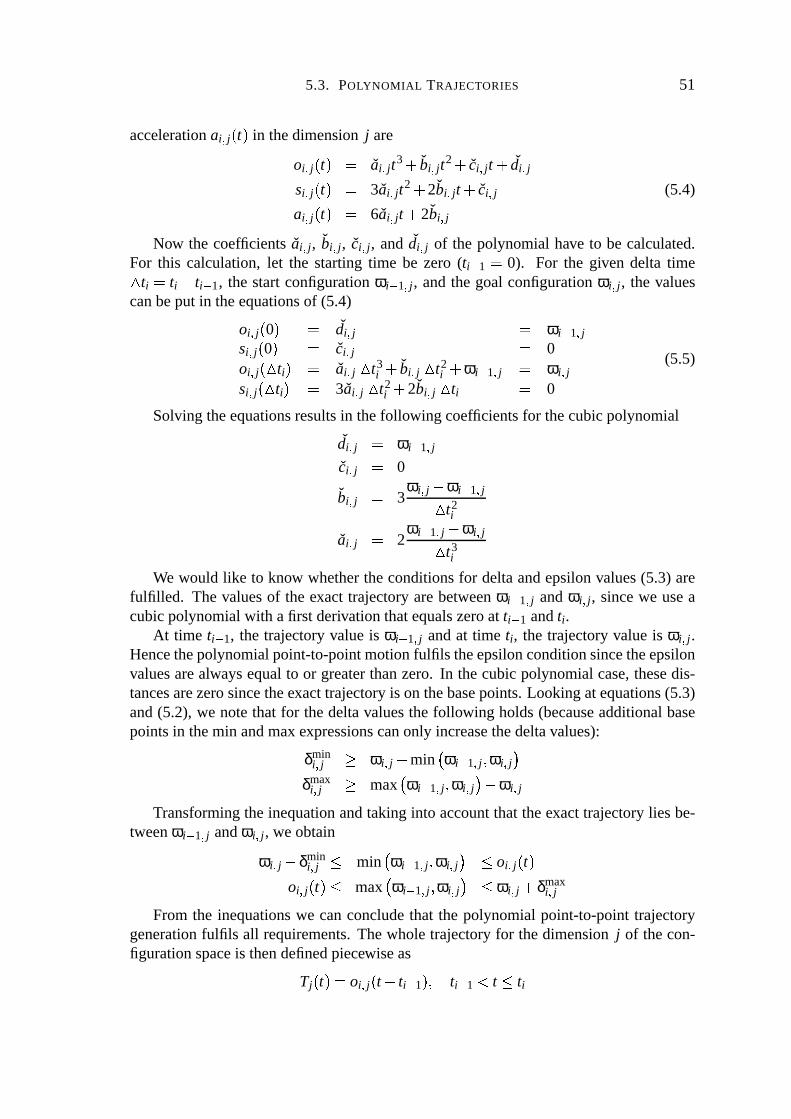
5.3. POLYNOMIAL TRAJECTORIES 51
accelerationai c j � t � in thedimensionj are
oi c j � t �e ai c j t3 � bi c j t2 � ci c j t � di c jsi c j � t �e 3ai c jt2 � 2bi c jt � ci c j (5.4)
ai c j � t �e 6ai c jt � 2bi c jNow the coefficients ai c j , bi c j , ci c j , and di c j of the polynomialhave to be calculated.
For this calculation,let the startingtime be zero (ti 8 1 0). For the given delta time
�ti ti � ti 8 1, the startconfigurationωi 8 1 c j , andthe goal configurationωi c j , the values
canbeput in theequationsof (5.4)
oi c j � 0� di c j ωi 8 1 c jsi c j � 0� ci c j 0oi c j � � ti � ai c j �
t3i � bi c j �
t2i � ωi 8 1 c j ωi c j
si c j � � ti � 3ai c j �t2i � 2bi c j �
ti 0
(5.5)
Solvingtheequationsresultsin thefollowing coefficientsfor thecubicpolynomial
di c j ωi 8 1 c jci c j 0
bi c j 3ωi c j � ωi 8 1 c j�
t2i
ai c j 2ωi 8 1 c j � ωi c j�
t3i
We would like to know whethertheconditionsfor deltaandepsilonvalues(5.3) arefulfilled. The valuesof the exact trajectoryarebetweenωi 8 1 c j andωi c j , sincewe useacubicpolynomialwith afirst derivationthatequalszeroat ti 8 1 andti.
At time ti 8 1, the trajectoryvalueis ωi 8 1 c j andat time ti, the trajectoryvalueis ωi c j .Hencethepolynomialpoint-to-pointmotionfulfils theepsilonconditionsincetheepsilonvaluesarealwaysequalto or greaterthanzero. In thecubicpolynomialcase,thesedis-tancesarezerosincetheexacttrajectoryis on thebasepoints.Lookingatequations(5.3)and(5.2), we notethat for thedeltavaluesthe following holds(becauseadditionalbasepointsin themin andmaxexpressionscanonly increasethedeltavalues):
δmini c j u ωi c j � min � ωi 8 1 c j ωi c j �
δmaxi c j u max � ωi 8 1 c j ωi c j � � ωi c j
Transformingtheinequationandtakinginto accountthat theexacttrajectorylies be-tweenωi 8 1 c j andωi c j , weobtain
ωi c j � δmini c j min � ωi 8 1 c j ωi c j � oi c j � t �
oi c j � t �M max � ωi 8 1 c j ωi c j � ωi c j � δmaxi c j
From the inequationswe canconcludethat the polynomialpoint-to-pointtrajectorygenerationfulfils all requirements.Thewhole trajectoryfor thedimensionj of thecon-figurationspaceis thendefinedpiecewiseas
Tj � t �F oi c j � t � ti 8 1 �W ti 8 1 N t ti
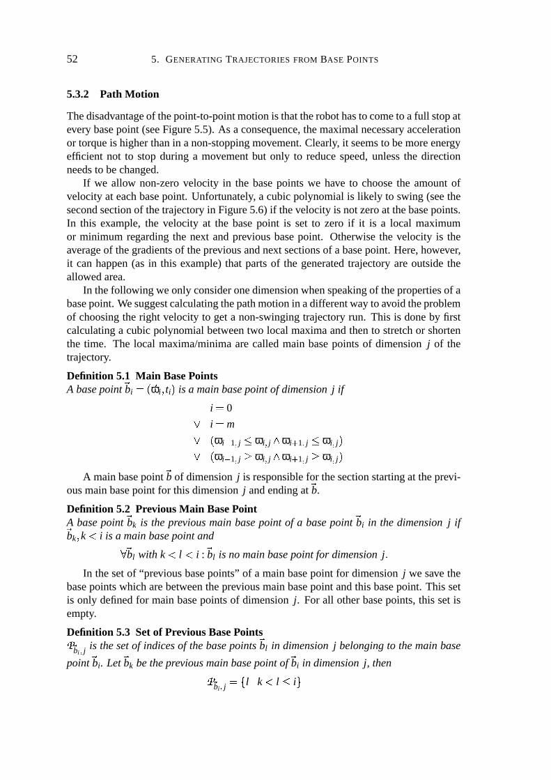
52 5. GENERATING TRAJECTORIES FROM BASE POINTS
5.3.2 Path Motion
Thedisadvantageof thepoint-to-pointmotionis thattherobothasto cometo afull stopateverybasepoint (seeFigure5.5). As aconsequence,themaximalnecessaryaccelerationor torqueis higherthanin anon-stoppingmovement.Clearly, it seemsto bemoreenergyefficient not to stopduring a movementbut only to reducespeed,unlessthe directionneedsto bechanged.
If we allow non-zerovelocity in the basepoints we have to choosethe amountofvelocity at eachbasepoint. Unfortunately, a cubicpolynomialis likely to swing(seethesecondsectionof thetrajectoryin Figure5.6)if thevelocity is notzeroat thebasepoints.In this example, the velocity at the basepoint is set to zero if it is a local maximumor minimum regardingthe next andprevious basepoint. Otherwisethe velocity is theaverageof thegradientsof thepreviousandnext sectionsof abasepoint. Here,however,it canhappen(as in this example)that partsof the generatedtrajectoryareoutsidetheallowedarea.
In thefollowing weonly consideronedimensionwhenspeakingof thepropertiesof abasepoint. Wesuggestcalculatingthepathmotionin adifferentwayto avoid theproblemof choosingtheright velocity to geta non-swingingtrajectoryrun. This is doneby firstcalculatinga cubicpolynomialbetweentwo local maximaandthento stretchor shortenthe time. The local maxima/minimaarecalledmain basepointsof dimension j of thetrajectory.
Definition 5.1 Main BasePointsA basepoint Sbi =��Sωi ti � is a mainbasepoint of dimensionj if
i 07 i m7 � ωi 8 1 c j ωi c j , ωi � 1 c j ωi c j �7 � ωi 8 1 c j u ωi c j , ωi � 1 c j u ωi c j �A mainbasepoint Sb of dimensionj is responsiblefor thesectionstartingat theprevi-
ousmainbasepoint for this dimensionj andendingat Sb.
Definition 5.2 PreviousMain BasePointA basepoint Sbk is the previousmain basepoint of a basepoint Sbi in the dimensionj ifSbk k N i is a mainbasepoint and< Sbl with k N l N i : Sbl is no mainbasepoint for dimensionj �
In thesetof “previousbasepoints” of a mainbasepoint for dimensionj we save thebasepointswhich arebetweenthepreviousmainbasepoint andthis basepoint. This setis only definedfor mainbasepointsof dimensionj. For all otherbasepoints,this setisempty.
Definition 5.3 Setof PreviousBasePoints���bi c j is thesetof indicesof thebasepoints Sbl in dimensionj belongingto themainbase
point Sbi. Let Sbk bethepreviousmainbasepoint of Sbi in dimensionj, then� �bi c j H� l � k N l i !
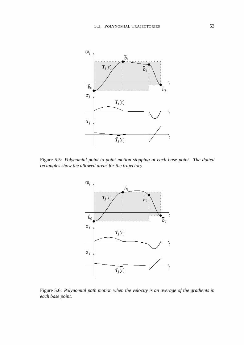
5.3. POLYNOMIAL TRAJECTORIES 53
t
ω j
Tj � t �Sb0
Sb1 Sb2 Sb3
t
σ j
Tj � t �t
α j
Tj � t �Figure5.5: Polynomialpoint-to-pointmotionstoppingat each basepoint. Thedottedrectanglesshowtheallowedareasfor thetrajectory
t
ω j
Tj � t �Sb0
Sb1 Sb2 Sb3
t
σ j
Tj � t �t
α j
Tj � t �Figure5.6: Polynomialpath motionwhenthe velocityis an average of the gradientsineach basepoint.

54 5. GENERATING TRAJECTORIES FROM BASE POINTS
For example,in Figure5.6, we have for thegivendimensionj themain basepointsSb0, Sb1, and Sb3. Thereis nopreviousmainbasepoint for Sb0. Thepreviousmainbasepointof Sb1 is Sb0 andthepreviousmainbasepoint of Sb3 is Sb1. Thesetof previousbasepointsisdefinedfor Sb1 and Sb3 as
���b1 c j H� 1 ! and
���b3 c j b� 2 3 ! respectively.
For themain basepointsof eachdimension j, we cancalculatethe functionsof thetime for thelocationof a joint oi c j � t � , thevelocity si c j � t � andtheaccelerationai c j � t � asinthecaseof a point-to-pointmotion (the hat-functionsonly exist for main basepointsineachdimensionandwill notbecalculatedfor otherbasepoints).
In Figure5.7, thetrajectoryis correct.Furthermore,themaximalvelocity andaccel-erationvaluesaresmalleror thesameasin thepoint-to-pointmotion.However it maybethatthetrajectoryis toofarawayfrom thebasepointsbetweentwo consecutivemainbasepointsanddoesnot lie insidetheallowedarea(seeFigure5.8). In theexample,two morebasepointsareaddedto thetrajectorydescription.Now thenew mainbasepointsof thisdimensionare Sb0, Sb2, and Sb5. Thesetsof thepreviousbasepointsarenow
� �b2 c j H� 1 2 !
and� �
b5 c j b� 3 4 5 ! (all othersetsareempty).Thefilled circlesarethebasepointsandthehollow circlesarethenearestpointsto the
basepointslying insidetheallowedareaat thesamepoint of time. In this invalid case,we have to stretchor shortenthetime to make thetrajectorybein theallowedareaagain(seeFigure5.9). Thisstretchingis doneby acubicpolynomial.
First, we look for a point ω }i c j for eachvalue ωi c j of the basepoint Sbi ���Sωi ti � attime ti that is insidethe allowed areaandthat is ascloseaspossibleto ol c j � ti �W i ] � �
bl c j(seehollow circlesin Figure5.8). Now the polynomial ol c j � t � is changedsuchthat thepolynomialtouchesthesepoints.Let ti bethetimewhenthevalueωi c j hasto bereached.The time ti c j is the time, whenthe original polynomial ol c j � t � reachesthe configurationω }i c j in dimensionj, thatis
ω }i c j ol c j � ti c j � with i ] � �bl c j
Thenext stepis to modify theoriginal time run, suchthat thetime point ti c j matcheswith ti. Sincethereare four boundaryconditions,a cubic polynomial is needed.Twoconditionsarethestarttimeandendtimeandtwo moreconditionshaveto ensurethatthederivationsequaloneat thebeginningandat theend.We alsohave to make surethatthepositionandvelocity functionarestill derivable. Hence,eachsectioni needsa functioncti c j for eachjoint j which changesthetime,suchthatthefollowing conditionsarevalid.Let Sbk bethepreviousmainbasepoint of Sbi in dimensionj.
cti c j � t �e ai c jt3 � bi c j t2 � ci c j t � di c jcti c j � ti 8 1 �t ti 8 1 c j � tkct i c j � ti 8 1 �t 1
cti � ti �t ti c j � tkct i c j � ti �t 1
Furthermorewe needa monotoneacceleratingfunction to ensurethat we do not gobackin time. In otherwords, ct i c j � x��u 0. Thereforethe changingtime function hasto

5.3. POLYNOMIAL TRAJECTORIES 55
t
ω j
Tj � t �Sb0
Sb1 Sb2 Sb3
t
σ j
Tj � t �t
α j
Tj � t �Figure5.7: Polynomialpathtrajectorywithoutconsideration of all basepoints,but onlythelocal maximaandminima.Thewholetrajectoryis insidetheallowedarea.
t
ω j
Tj � t �Sb0
Sb2 ω3 c jSb5
ω }3 c jt3t3 c j
t
σ j
Tj � t �t
α j
Tj � t �Figure5.8: Polynomialpathtrajectorywithoutconsideration of all basepoints,but onlythelocal maximaandminima.Parts of thetrajectoryareoutsidetheallowedarea.

56 5. GENERATING TRAJECTORIES FROM BASE POINTS
fulfil thefollowing condition
ti c j � ti 8 1 c j u 13
� ti � ti 8 1 � (5.6)
This can be seenwhen the coefficients a b c, and d are calculatedand the speedfunctionis analysed,by looking at thederivationandthemaximum.For simplicity, taketk 0, ti 8 1 0, and ti 8 1 c j 0. Then the first and secondderivation of cti c j � t � are asfollows
ct i c j � t �e 6ti � ti c j
t3i
t2 � 6ti � ti c j
t2i
t � 1
ct i c j � t �e 12ti � ti c j
t3i
t � 6ti � ti c j
t2i
Equatingthesecondderivationct i c j � t � with zeroandsolvingtheequationsfor t resultsin t 1
2ti. Sinceit holdsthat the quadraticpolynomial ct i c j equalsoneat the start timeandtheendtime, it is sufficient to examinethefirst derivationat t 1
2ti.
ct i c j � 12ti �Mu 0 � ti c jti
� 13
u 0
Hence,themaximalcompressionof thetime is onethird of theoriginal time. If anyof thesectionsSl doesnot fulfil condition(5.6) in dimensionj, then Sbl is takenasamainbasepoint of dimension j aswell andthe calculationfor theconfigurationdimension jstartsagain.If all sectionsfulfil thecondition,thenthenew functionsbetweentwo basepoints,with i ] � �
bl c j , are
oi c j � t �t ol c j � cti c j � t ���si c j � t �t sl c j � cti c j � t ��� cti c j � t �ai c j � t �t 2al c j � cti c j � t ��� cti c j � t �O� sl c j � cti c j � t ��� cti c j � t �
Figure5.9showsthemodifiedtrajectorywith stretchedtimesfor theexample.Thenext figure(Figure5.10)shows thepoint-to-pointmotionfor thesameexample.Note that in theexample,themaximalvelocity andaccelerationvaluesof themodi-
fied trajectorytendto besmallerthanthevaluesin a point-to-pointmotion for a sectionbetweentwo mainbasepoints.
Sincethe first derivationof cti c j at the intersectionsto theprevious andnext sectionequalsone,thespeedfunctionis still continuousin basepointsbelongingto thesamemainbasepointsi � 1 i ] �
bl c j . Let Sbk bethepreviousmainbasepointof Sbl in dimensionj.
si 8 1 c j � ti 8 1 �� sl c j � cti 8 1 c j � ti 8 1 ��� ct i 8 1 c j � ti 8 1 � sl c j � cti 8 1 c j � ti 8 1 ��� sl c j � ti 8 1 c j c n � tk � sl c j � cti c j � ti 8 1 ��� sl c j � cti c j � ti 8 1 ��� ct i c j � ti 8 1 �� si c j � ti 8 1 �

5.3. POLYNOMIAL TRAJECTORIES 57
t
ω j
Tj � t �Sb0
Sb2
Sb5
t
σ j
Tj � t �t
α j
Tj � t �Figure5.9: Polynomialpath trajectoryconsideringall points. Thewholetrajectoryliesinsidetheallowedarea.
t
ω j
Tj � t �Sb0
Sb2
Sb5
t
σ j
Tj � t �t
α j
Tj � t �Figure 5.10: Polynomial point-to-pointtrajectory consideringall points, for the samegivenbasepointsasin thelast figure.

58 5. GENERATING TRAJECTORIES FROM BASE POINTS
It is obviousthattheresultingtrajectorylies insidetheallowedareaandconsequentlyfulfils theepsilonanddeltalimits sincewehavechosenthepointsωi c j insidetheallowedarea.Second,we madesurethat the derivationof the stretchingfunction cti c j is greaterthenzero.
5.3.3 Inserting and DeletingBasePoints
Sincethe planningalgorithmneedsto insertanddeletebasepoints,we have to analysetheseoperationsregardingtheir impacton a polynomialmovement.In thefollowing weagainlook at a singledimensionif we speakof a basepoint Sbi . Hence,thefollowing hasto beappliedseparatelyto eachdimensionof thedegreesof freedomof therobot.
We first analysethe simplecaseof a polynomialpoint-to-pointtrajectory. If a newbasepoint Sbi is addedin a point-to-pointmotion,thentheold sectioni hasto bereplacedby two new sections.Thetwo new sectionsi andi � 1 haveto bemodified.If thei-th basepoint is deleted,thenonly thenew sectioni hasto berecalculated(seeFigure5.11).Twomainpointsconnectedvia a dottedline representa variablenumberof basepointsbut atleastone. Thesolid line connectstwo basepointswithout any otherbasepoint betweenthemandthedashedline representstherecalculationarea.
InsertBasePoint
Sb0
Sbi 8 1
Sbi Sbn
Sb0
Sbi 8 1 Sbi
Sbi � 1 Sbn� 1
DeleteBasePoint
Sb0
Sbi 8 1 Sbi
Sbi � 1 Sbn� 1
Sb0
Sbi 8 1
Sbi Sbn
Figure5.11: Insertionanddeletionof basepointsin a polynomialpoint-to-pointtrajec-tory.
If the trajectorymovementis a polynomialpathmotion, thenthingsaremorecom-plicatedandoften morethantwo sectionshave to be recalculated,sincetwo main base

5.3. POLYNOMIAL TRAJECTORIES 59
pointsspecifythe trajectoryrun. It is obvious that if theold sectioni of joint j belongsto
���bl c j , thenat leastall of thosesectionshave to be recalculatedfor joint j. But if the
new basepoint itself is a new mainbasepoint, thentwo or threeold mainsectionsmightchangetheir values.Wenow wantto takeacloserlook at thepossiblesituations.
InsertBasePoint
Sb0
Sbkbi 8 1 Sbi
Sbl Sbn
Case1
Sb0
Sbkbi 8 1
bi Sbi � 1
Sbl � 1 Sbn� 1
Case2
Sb0
Sbk Sbi 8 1Sbi Sbi � 1
Sbl � 1 Sbn� 1
Case3
Sb0
Sbkbi 8 1 Sbi Sbi � 1
Sbl � 1 Sbn� 1
Case4
Sb0
Sbkbi 8 1 Sbi
bi � 1
Sbl � 1 Sbn� 1
Figure5.12: Insertionanddeletionof a basepoint in a polynomialpathtrajectory.
In Figure5.12,wetakea look at thecase,whereSbi itself is amainbasepointand Sbi 8 1
is not a mainbasepoint (in dimensionj). Furthermore,let Sbk bethepreviousmainbasepointof Sbi andlet Sbi bethepreviousmainbasepoint of Sbl .
In thefirst case,thenew basepoint Sbi is not a mainbasepoint itself in dimensionj,so only the modifying functionsof the time for the previous andnext sectionhasto berecalculatedin this dimension.
If thenew basepoint Sbi is a mainbasepoint, thentherearethreedifferentcases.Thesecondandthird caseleavestheothermainbasepointsunchangedandthereforeonly the

60 5. GENERATING TRAJECTORIES FROM BASE POINTS
sectionsbetweenSbk and Sbi � 1 change.In thesecondcase,Sbi 8 1 and Sbi will becomeamainbasepointaswell. In thethird caseonly Sbi becomesamainbasepoint. Now notonly themodifying functionsof thetime have to berecalculatedbut thehat-functionsof thenewmainbasepointsand Sbi � 1 needrecalculationtoo.
ThefourthcasechangesSbi to anormalbasepointandthetrajectoryrunchangesfromSbk to Sbl � 1.If Sbi 8 1 is amainbasepointand Sbi is notamainbasepoint, thenwehave themirrored
cases.If neither Sbi 8 1 nor Sbi aremainbasepoints,thenonly caseone,casetwo, andthemirroredcasetwo would occur. If both Sbi 8 1 and Sbi aremain basepoints,thenit couldhappenthat threemain sectionschangetheir values,if you think of insertinga point insectioni � 1 in casethreethatis lower thanpoints Sbi and Sbi � 1.
If a basepoint getsdeletedwe againhave to distinguishwhethera basepoint or amainbasepoint is deleted.In thefirst case,a normalbasepoint leadsto a recalculationof modifying functionsof thetimeof thepreviousandnext section(revertingcaseoneofFigure5.12).In thesecondcase,thedeletionof amainbasepoint, it is morecomplicated.Justthink of revertingtheinsertionin Figure5.12.
To summarise,we can say that the path motion may lead to a trajectoryrun withlessvelocity and acceleration,but the addingand deleting is quite costly. Especiallyasthe numberof affectedsectionsis not constant(as in the point-to-pointmotion) andconsideringthe fact that the above operationshave to be performedfor eachdimensionseparately. Nevertheless,the methodpresentedhereensuresa non-swingingtrajectory,hencethemotionstaysin theallowedareadefinedby thegivenbasepoints.
5.4 Modified Bang-BangTrajectories
In a bang-bangtrajectory, the third derivation of the trajectoryof oneconfigurationdi-mensionis alwayszero.Thismeansthattheaccelerationis piecewiseconstantandjumpsfrom onevalueto another. In a traditionalbang-bangtrajectory, theaccelerationvalueiseitherzero,minimal,or maximal.In ourcase,theaccelerationcanbeof any value.In thenext two subsections,weanalysethepoint-to-pointmotionandthepathmotion.
5.4.1 Point-to-Point Motion
If the path motion stopsat every control point of the path (seeFig. 5.13), we have atrapezoidalvelocity profile. A point-to-pointmotion is split into an accelerationphase| ti 8 1 ti 8 1 � ta x , aconstantspeedphase| ti 8 1 � ta ti � ta x , andanegativeaccelerationphase| ti � ta ti x . We assumethat the accelerationdurationta is given. For example,ta couldbe chosenhalf the distancebetweentwo consecutive basepoints(ta �� ti 8 1 � ti ��� 2) orsmaller.
oi c j � t �k ���� ωi 8 1 c j � 12ai c j � t � ti 8 1 � 2 : if ti 8 1 t ti 8 1 � ta
oi c j � ti 8 1 � ta �R� si c j � t ��� ti 8 1 � ta ��� : if ti 8 1 � ta N t ti � taωi c j � 1
2ai c j � ti � t � 2 : if ti � ta t ti
(5.7)
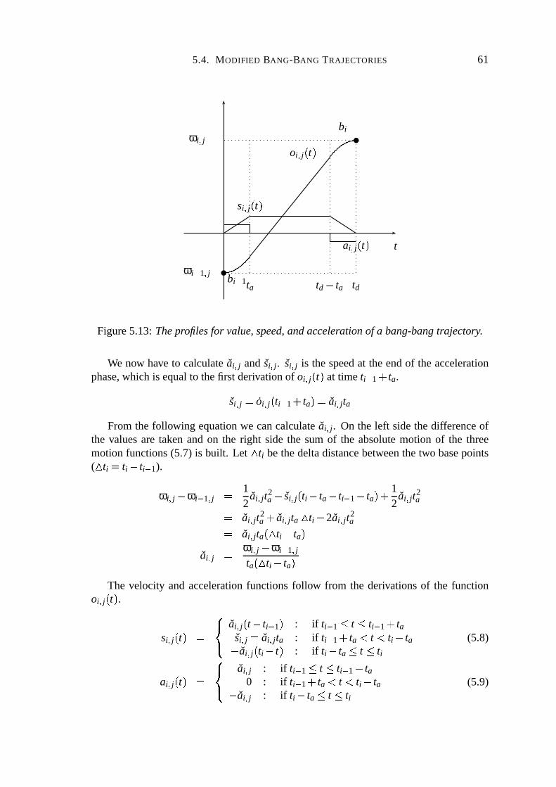
5.4. MODIFIED BANG-BANG TRAJECTORIES 61
t
bi 8 1
bi
ωi 8 1 c j
ωi c joi c j � t �
si c j � t �ai c j � t �
ta td � ta td
Figure5.13:Theprofilesfor value, speed,andacceleration of a bang-bangtrajectory.
We now have to calculateai c j andsi c j . si c j is thespeedat theendof theaccelerationphase,which is equalto thefirst derivationof oi c j � t � at time ti 8 1 � ta.
si c j oi c j � ti 8 1 � ta �F ai c jtaFromthe following equationwe cancalculateai c j . On the left sidethedifferenceof
the valuesare taken andon the right side the sumof the absolutemotion of the threemotionfunctions(5.7) is built. Let
�ti bethedeltadistancebetweenthetwo basepoints
(
�ti ti � ti 8 1).
ωi c j � ωi 8 1 c j 12
ai c j t2a � si c j � ti � ta � ti 8 1 � ta �R� 1
2ai c jt2
a ai c jt2a � ai c j ta �
ti � 2ai c j t2a ai c jta � � ti � ta �
ai c j ωi c j � ωi 8 1 c jta � � ti � ta �
The velocity andaccelerationfunctionsfollow from the derivationsof the functionoi c j � t � .
si c j � t �e ���� ai c j � t � ti 8 1 � : if ti 8 1 t ti 8 1 � tasi c j ai c j ta : if ti 8 1 � ta N t N ti � ta� ai c j � ti � t � : if ti � ta t ti
(5.8)
ai c j � t �e �� � ai c j : if ti 8 1 t ti 8 1 � ta0 : if ti 8 1 � ta N t N ti � ta� ai c j : if ti � ta t ti
(5.9)

62 5. GENERATING TRAJECTORIES FROM BASE POINTS
Sincethe trajectoryof a sectionlies betweenthe previous andthe next basepoint,we canusethesameargumentsasfor thepoint-to-pointmotionwith a polynomial(Sec-tion 5.3.1)to show thattherequirementsarefulfilled.
5.4.2 Path Motion
If thepathconsistsof only two basepoints,thenthetrajectoryrun is likeapoint-to-pointmotion,exceptthatwe take ta t1 8 t0
2 . Otherwisewe do not want to stopat every point.Therefore,wegetfrom oneto thenext sectionby acubicpolynomial(seeFigure5.14).
tSb0
Sb1 Sb2 Sb3
t
σ j
Tj � t �t
α j
Tj � t �Figure5.14: Thepathmotionwithout stoppingat each basepoint for a bang-bangtra-jectory.
We needat leasta cubicpolynomialsincewe have to satisfyfour conditions.Thesearetheconfigurationswhentheblendingstartsandendsandthevelocitiesat thesepoints.Let gi c j bethegradientof sectioni in dimensionj andlet ta c i bethemaximaldeltatimea joint mayleave thedirectconnection.Thismeansthattheblendingstartsat ti � ta c i andfinishesat ti � ta c i .
gi c j ���� ���0 : if i 0 m � 1
23
ωi � j 8 ωi � 1 � jti 8 ti � 1
: if i 1 mωi � j 8 ωi � 1 � j
ti 8 ti � 1: if 1 N i N m
(5.10)
ta c i ���� ���t1 8 t0
2 : if i 0tm 8 tm� 1
2 : if i m
min� ti 8 ti � 12 ti � 1 8 ti
2 ! : if 0 N i N m
(5.11)

5.4. MODIFIED BANG-BANG TRAJECTORIES 63
As thereis no sectionbeforethefirst andafter thelastsection,we have to treatthemseparately. We cannow calculatethecoefficientsof thecubicpolynomial fi c j � t � for thedurationfrom | ti � ta c i ti � ta c i x with thefollowing equations:
fi c j � t �e ai c jt3 � bi c j t2 � ci c j t � di c jfi c j � ti � ta c i �t ωi c j � gi c j ta c ifi c j � ti � ta c i �t ωi c j � gi � 1 c j ta c i (5.12)
fi c j � ti � ta c i �t gi c jfi c j � ti � ta c i �t gi � 1 c j
Solvingtheseequationsresultsin ai c j 0, sothepolynomialis quadratic.Therefore,the first derivation is a straight line for speedand the secondderivation is a constantvaluefor acceleration.This meansthat thetrajectoryis still a bang-bangtrajectory. Theblendingfunctionsaredefinedfor 0 N i N m. For the first and the last basepoint theblendingfunctionsaredifferentsincewedonothaveapreviousor next sectionandhencewe have to touchthesebasepoints.For i 0 andi m, thefollowing equationsneedtobesolved:
f0 c j � t0 �� ω0 c jf0 c j � t0 � ta c 0 �� 2ω0 c j � ω1 c j
3f0 c j � t0 �� 0
f0 c j � t0 � ta c 0 �� g1 c jfmc j � tm � ta c m�� 2ωmc j � ωm8 1 c j
3fmc j � tm�� ωmc j
fmc j � tm � ta c m�� gmc jfmc j � tm�� 0
Again, solvingtheequationsresultsin ai c j 0 andthereforea constantacceleration.Thesectionx ti 8 1 � ta c i 8 1 ti � ta c i | betweentheparabolicblendmovementis a linearmove-ment.
In Figure5.15andFigure5.14thedifferencebetweenstoppingat thebasepointsandnotstoppingcanbeseen.Theabsoluteaccelerationsaregettingsmallerfor apathmotion.Thattherequirementsarestill fulfilled is obvious,asthelinearconnectionsbetweentwobasepointsaretangentsto theblendfunctions.
5.4.3 Inserting and DeletingBasePoint
If the trajectorymovementis a point-to-pointmotion anda new basepoint is insertedin sectioni, thenonly this sectionhasto be replacedby two new sections.Deletingabasepoint i leadsto recalculationof onenew section.This is thesamesituationasin thepolynomialpoint-to-pointmotion(Figure5.11,page58).

64 5. GENERATING TRAJECTORIES FROM BASE POINTS
tSb0
Sb1 Sb2
Sb3
t
σ j
Tj � t �t
α j
Tj � t �Figure5.15:Thecorrespondingpoint-to-pointmotionstoppingat each basepoint.
On theotherhand,if it is a pathmotion,thenthesectioni hasto bereplacedby twonew sectionsandtheprevious i � 1 andnext sectionsi � 1 have to berecalculatedaswell(Figure5.16).As before,thedashedline indicatestheregionthatneedsto berecalculated.
This is becausetheblendingfunctionneedstwo consecutivesectionsto becalculated.Deletingabasepoint leadsto anew sectioni. Sothepreviousandnext sectionof thisnewsectionchangetherunof thetrajectoryaswell. This is muchbetterthanin thepolynomialpathmotion. In thepolynomialpathmotionupto four sectionsneedto bemodifiedwhenaddingabasepoint.
5.5 Summary and Outlook
In this chapter, the definition of a basepoint trajectoryhasbeenintroduced,which de-scribesallowed areasfor an exact trajectoryin the configurationspace.The advantageof this approachis thatour planningprocessis decoupledfrom theactualtrajectorytype.With eachnew basepoint theplanningprocessgetsmorecontrolon theactualrun of theexacttrajectory. Wehaveshown usingtwo well-known typesof trajectories,how anexacttrajectorycanbegeneratedsuchthatthetrajectoryrunis insidetheallowedarea.Wehaveanalysedtheoperationof deletionandinsertionof basepointsinto anexistingbasepointtrajectory. Hereour focuswason thelocality of thechangesthatarenecessaryto updatean existing exact trajectoryafter theseoperations.Our conclusionis that recalculationsafter changingbasepointsin thepolynomialpoint-to-pointmovementandin themodi-
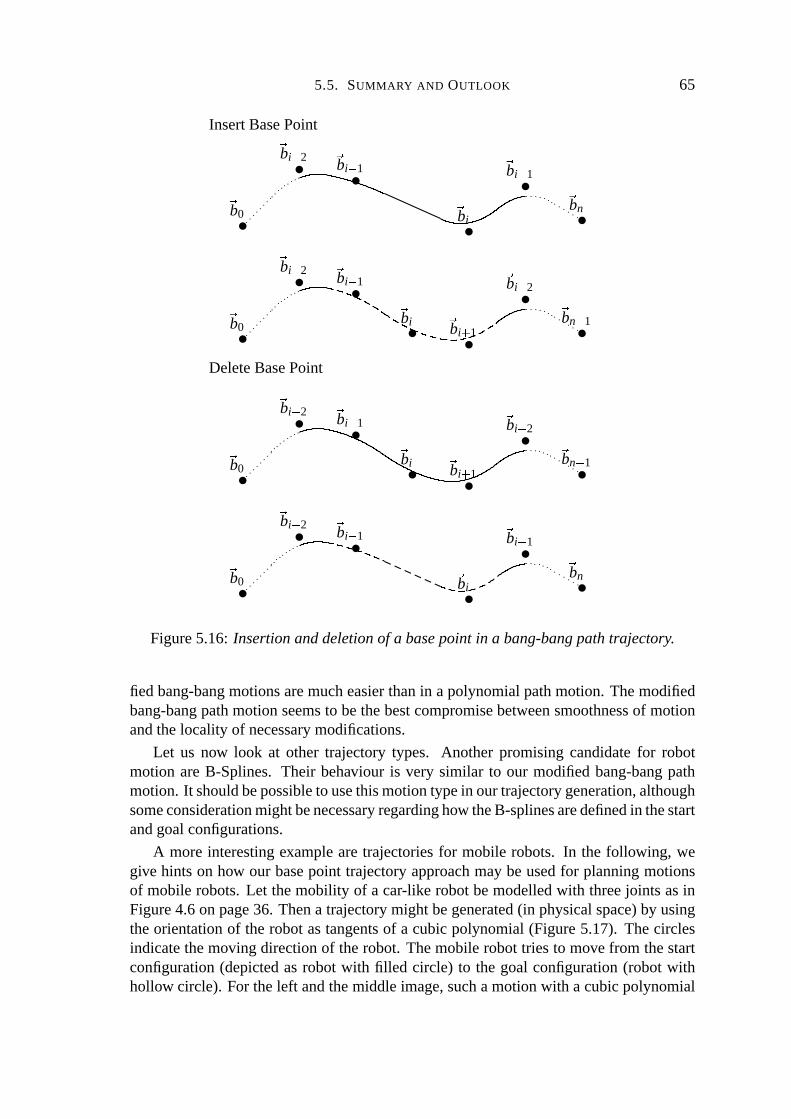
5.5. SUMMARY AND OUTLOOK 65
InsertBasePoint
Sb0
Sbi 8 2 Sbi 8 1 Sbi
Sbi � 1 Sbn
Sb0
Sbi 8 2 Sbi 8 1 Sbi Sbi � 1
Sbi � 2 Sbn� 1
DeleteBasePoint
Sb0
Sbi 8 2 Sbi 8 1 Sbi Sbi � 1
Sbi � 2 Sbn� 1
Sb0
Sbi 8 2 Sbi 8 1 Sbi
Sbi � 1 Sbn
Figure5.16: Insertionanddeletionof a basepoint in a bang-bangpathtrajectory.
fied bang-bangmotionsaremucheasierthanin a polynomialpathmotion. Themodifiedbang-bangpathmotionseemsto bethebestcompromisebetweensmoothnessof motionandthelocality of necessarymodifications.
Let us now look at other trajectorytypes. Another promisingcandidatefor robotmotion areB-Splines. Their behaviour is very similar to our modifiedbang-bangpathmotion.It shouldbepossibleto usethismotiontypein ourtrajectorygeneration,althoughsomeconsiderationmightbenecessaryregardinghow theB-splinesaredefinedin thestartandgoalconfigurations.
A moreinterestingexamplearetrajectoriesfor mobile robots. In the following, wegive hintson how our basepoint trajectoryapproachmaybeusedfor planningmotionsof mobile robots.Let themobility of a car-like robotbemodelledwith threejoints asinFigure4.6on page36. Thena trajectorymight begenerated(in physicalspace)by usingtheorientationof the robotastangentsof a cubicpolynomial(Figure5.17). Thecirclesindicatethemoving directionof therobot. Themobilerobottriesto move from thestartconfiguration(depictedasrobot with filled circle) to the goal configuration(robot withhollow circle). For theleft andthemiddleimage,suchamotionwith a cubicpolynomial

66 5. GENERATING TRAJECTORIES FROM BASE POINTS
canbegiven.
Figure5.17:Mobile robots’trajectories.
In [Buttelmannet al., 1999], trajectorygenerationfor non-holonomicautonomouscar-like robotswith straightlines,circles,andcubicpolynomialsis analysed.
Let us now considera basepoint trajectorythat definesallowed areasfor the exacttrajectory, as in Figure5.18. If a motion betweenbasepoints leaves the allowed area(middle)or cannotbegiven(right), thenwesuggestto take theedgesof theallowedareaastangentsto getanexacttrajectoryin theallowedarea.Hence,for therobotin thestartconfiguration(robotwith blackcircle)weconsiderthearrow in themoving directionandthetwo edgesof theallowedareathattherobottouches.If thearrow in themoving direc-tion pointsoutsidetheallowedarea,thenwe dropit, otherwisetheedgeis droppedwiththesmalleranglebetweentheedgeandthearrow. For thegoalconfiguration(robotwithhollow circle) thesameis done,but thearrow is oppositeto themoving direction. Nowtwo possibletrajectoriesfor eachsituationcanbegenerated(solidanddashedcurves),bytakingtheremaininglinesastangentsfor thecurves.
Figure5.18:Mobile robots’trajectoriesinsidetheallowedareas.
Theideais, thatalthoughthesetrajectoriesmaynot betraceable,we canusetheminour motion planner. We do not saythat thesetrajectoriescannotbe tracked becauseofkinematicconstraints,but becauseof dynamicconstraints.In otherwords,we pretend

5.5. SUMMARY AND OUTLOOK 67
thatamotionagainstthewheels’directionexceedstherobot’s forceor torquelimits, andwe let our ratingfunctiondiscardthosetrajectoriesthatcannotbetrackedby giving themabadrating.To useour technique,weneeda ratingfunctionthatratesthe“severity” of amovementagainstthewheels.We conjecturethatsucha ratingwould not bedifficult todesign.
In the above thoughts,we did not considerthe violation of the interval for the ori-entationangleof the mobile robot. This meanseither the robot hasto move clockwiseor in oppositedirectionviewed from the top. This canbe solvedby choosingthe rightcurve in theallowedareain Figure5.18. Thesolid linesareusedwhentheangleof thefollowing orientationis greaterthantheangleof thecurrentorientation(clockwise)andthedashedlines areusedif the angleof thenext orientationis smallerthanthe old one(counter-clockwise).
Thisis certainlynotthebestpossibleprocedurefor planningmotionsof mobilerobots,but it shows thegeneralityof our planningapproach.


CHAPTER 6
Forceand TorqueRating
In this section,we presenta trajectoryrating that reflectsviolation of robot dynamics.We assumethat gravity is presentandthat themaximalforcesandtorquesof therobot’sjointsareknown.Wefirstexplain theNewton-Euleralgorithmwhich is usedto determinethetorque. We thendiscussdifferentaspectsof a goodtrajectory.
6.1 Intr oduction
Thebasepoint trajectorydefinitionguaranteesthat in theexact trajectorytheconfigura-tion spacelimits (andhencethejoint limits) arekept. Whatremainsis to ratethequalityof thetrajectoryregardingthedynamiclimits of therobot.To thisend,weneedadynamicmodelof therobot.
An algorithmfor modellingrobotdynamicsthatis well-suitedfor forkedmanipulatorchainshasbeendevelopedby Murray andNeuman[Murray andNeumann,1986]. Wegiveashortreview of theirapproachin thefollowing section.Thenext stepis to definearatingthatreflectstheactualforceandtorqueandthegivendynamiclimits of therobot.Wegivesucha ratingfunctionin thesectionthereafter.
6.2 Forceand TorqueCalculation
For the different typesof trajectorieswe have to calculatethe torquein eachjoint oftherobot. TheNewton-Euleralgorithmof Murray andNeuman[Murray andNeumann,1986] cancalculatethe actualtorqueof eachjoint in linear time, doing a forward andbackwardcalculationalongtherobot’s topology. Specialjoints or mobile robotsarenotconsidered.
TheNewton-Euleralgorithmneedsthemassmi andthe inertia tensorIi of eachlinkLi with respectto its centreof gravity gi (givenin thecoordinatesystemof joint Ji andLi
respectively). In [Mirtich, 1996]analgorithmfor computingpolyhedralmasspropertiescanbe found. This algorithmcalculatesthe mass,the centreof gravity andthe inertia

70 6. FORCE AND TORQUE RATING
tensor, if thedensityof abodyis knownandtheshapeof thebodyis givenvia polyhedrals.This is mucheasierthanto giveaninertiatensor. Theresultingdynamicmodelis only anapproximationof thedynamicmodelof a realrobot,whichmayhaveaninhomogeneousmassdistribution. Nevertheless,theapproximationis sufficient for our purposes.
The forward recursionof the Newton-Euleralgorithm hasto calculatethe angularvelocity σ j , the angularaccelerationα j andlinear accelerationα j relative to the worldfor eachjoint Jj of therobot.Wewill giveashortoverview of thealgorithm,for adetaileddescriptionwereferto [Pu,1998].
Weassumethatthegravity g is in negativezdirectionof theworld coordinatesystem.The function p � j � returnsthe index of the previous joint of Jj . Let for eachjoint thecurrentpositionυ j υω c j , thecurrentspeedσ j υσ c j , andthecurrentaccelerationα j υα c j begiven.Thetypeof joint Jj is determinedby λ j , with λ j 1 if it is arevolutionjointandλ j 0 if it is a prismaticjoint. Rj � υ j � is therotation3 � 3 matrix convertingvectorsfrom thecoordinatesystemof theprevious joint in thecoordinatesystemof thecurrentjoint. Hence,this is theupperleft 3 � 3 matrix of � p � j � D j
jE � υ j ��� 8 1 (seeSection4.1.1,page30). The rotation matrix is constantfor prismatic joints. The translationvectorp j � υ j � is the vectordirectedfrom the coordinatesystemfrom Jp � j � to Jj . This is the
translationalpart of � p � j � D jjE � υ j ��� . This translationvector is constantfor revolute
joints.Theinitial valuesfor theforwardrecursiveequationsareSz � 0 0 1� TSσ0 � 0 0 0� TSα0 � 0 0 0� TSα0 � 0 0 �� g� T
This meansthat there is no angularvelocity or acceleration,but a linear accelerationbecauseof gravitation. Theforwardrecursiveequationsfor j 1 ������� n areSσ j Rj � υ j � Sσp � j � � λ j Szσ j (6.1)Sα j Rj � υ j � Sαp � j � � λ j yFy Rj � υ j � Sσp � j � { �\� Szσ j � � Szα j { (6.2)Sα j Rj � υ j �My Sαp � j � � Sα j � p j � υ j �R� Sσ j ��y Sσ j � p j � υ j � {k{�o� 1 � λ j � y Szα j � 2 y Rj � υ j � Sσp � j � { �\� Szσ j � { (6.3)
In Equation(6.1)theangularvelocityof joint Jj is derivedfromtheangularvelocityofthepreviousjoint andtheangularvelocityof thecurrentjoint if it is a revolutejoint. Theangularacceleration(6.2) combinestheangularaccelerationof thepreviousjoint and,ifthecurrentjoint is a revolution joint, theaccelerationof thejoint andtheaccelerationrateresultingfrom thecombinationof thepreviousspeedandthespeedof thecurrentaxis.
Thelinearvelocity (6.3) is derivedfrom thepreviouslinearaccelerationandthepartsfrom theangularvelocity andacceleration.If thecurrentjoint is a prismaticjoint, thenwehave to addthespeedandaccelerationpartsof thecurrentjoint.

6.3. TRAJECTORY FORCE AND TORQUE RATING 71
Thelocal equationsfor eachlink j 1 ������ n calculatethetranslationalforceFj andthe rotationaltorqueNj in the centreof gravity of eachlink, without consideringotherlinks.
Fj mj y Sα j � Sα j � g j � Sσ j � y Sσ j � g j {F{ (6.4)
Nj I j Sα j � Sσ j ��y I j Sσ j { (6.5)
Theforcecalculation(6.4)multipliesthemasswith theaccelerationamountin thecentreof gravity. Thetorque(6.5)needstheinertiatensorof thelink L j , andtheangularvelocityandacceleration.
Thebackwardrecursive equationsfor j n ������� 1 calculatethetranslationalforce f j
andtherotationaltorquen j in eachjoint. τ j storesthe forceandthe torquerespectivelyof eachjoint.
f j Fj � ∑�i:p � i ��. j
R8 1i � υi � fi (6.6)
n j Nj � g j � Fj � ∑�i:p � i ��. j
y R8 1i � υi � ni � pi � υi �@� y R8 1
i � υi � fi {k{ (6.7)
τ j λ jnTj Sz ��� 1 � λ j � f T
j Sz (6.8)
Theforce(6.6) in joint Jj needsto be thesumof all following forcesandits own force.This is almostthesamefor thetorque(6.7) in joint Jj , but considersthetorquesaswell.Finally, (6.8) givesthe forceandthe torquerespectively in joint Jj . This completesthetorqueandforcecalculationat discretetime steps,providedthatthepositions,velocitiesandaccelerationsin eachjoint aregiven.
6.3 Trajectory Forceand TorqueRating
Let M : G 3n B�G n bethefunctionwhich representsthedynamicmodelof therobotandlet Sυd be a dynamicconfiguration.ThenM � Sυd � returnsthe forcesandtorquesSτ in thejointsof therobot.
Sincewe areinterestedin the joints violating themaximalforceor torquelimit θmaxj
duringthetrajectoryrun,all thesejoints areconsideredin therating. Let δ : GoBeG beafunctionwhichclips thenegativevalues
δ � x��;: 0 : if x 0x : if x Q 0
Theratingof adynamicconfigurationSυd is thengivenby
rst n
∑j . 1
δ � � τ j � � θmaxj �
θmaxj
, with Sτ M � Sυd � (6.9)
This ratinghastwo importantproperties.First, theamountof capacityoverloadis setinrelationto themaximumcapacityof thejoint. Second,takingthesumgivesthepossibility
72 6. FORCE AND TORQUE RATING
of a subtlegraduationin the rating, becauseeven an improvementin a single joint isdetected.This hassomeadvantagescomparedto taking the maximumof all overloads,wheretheworst joint hasto improve thesituation.If theratingis zero,thenthedynamicconfigurationis valid andthereforetraceable.
Finally, we areinterestedin theratingof a wholetrajectoryT � t � betweena starttimets andagoaltime tg. Let TD � t � bethedynamicconfigurationSυd at time t of thetrajectoryT � t � ( Sυd TD � t � , seeChapter4.4). Theratingof a trajectorysectionTi is thengivenbythemaximumof all ratings
rt max � n
∑j . 1
δ � � M � TD � t ��� j � � θmaxj �
θmaxj
: with ti 8 1 t ti � (6.10)
Sincethe calculationis only possibleat a discretepoint in time, we have to choosethesepoints carefully. Testingat equaldistributed time points resultsin a inaccurateapproximationof therealvalueif thenumberof testsis small.This is becausefastmove-mentswouldbetestedatfewerpointsin timethanslow movements,sincetherobotmoveslarger distancesif it movesfast. Quite the oppositeshouldbe the case.We shouldtestmore often during fast movements,becausethe changesin the forcesand torquesarehigherduringa fastmovement,for example,think of the influenceof thegravity on theforcesin jointsduringmovement.
We suggesta test that dependsonly on the link movements. We test complianceof dynamic limits at time configurationssuchthat the maximal distanceof any pointin the robot’s joints doesnot exceeda distancep betweentwo consecutive testedtimeconfigurations.In this case,wesaythecalculationof theratingis donewith precisionp.
For eachlink Ll wechoosethreereferencepointsxl yl , andzl relative to theorigin ofJl , which approximatethesizeandthepositionof the link. In otherwords,the trianglegiven by the threepoints is a placeholderfor the link. Onepoint is in the origin xl � 0 0 0� T, thesecondgivestheexpansion
yl V� max� � vt c 1 � �W max� � vt c 2 � �W max� � vt c 3 � ��� Twith t ] Ll , andthethird is for keepingtheorientationzl ��2� yl c 1 �� yl c 2 yl c 3 � T (All valuesshouldbeunequalzeroif the link hasa distribution). The ideais to analysethemotionof thesepointsduring a time interval for eachlink in the real world. If we look at theconfigurationat ts andtg, noreferencepointof any link is allowedto movefurtherthenp,otherwisethetime interval is bisected.
Let doublegetMaxMovement (trajectoryT, doublets, doubletg) bethe functionthatreturnsthemaximaldistancebetweentwo consecutive referencepointsif the robot is inpositionT � ts� and T � tg � . If 0xs
l 0ysl , and 0zs
l , with l 1 ������2 n are the positionsof thereferencepointsrelative to theworld whentherobotis at time ts and0xg
l 0ygl , and0zg
l aretheir positionsat goaltime tg, thengetMaxMovement returns
max � � 0 xgl � 0 xs
l � � 0 ygl � 0 ys
l � � 0 zgl � 0 zs
l � : l 1 ������2 n� �We would like to note that the positionsof the referencepoints belongingto link Ll
dependon the set of previous joints � pjl of link Ll . Consequently, for eachcall of

6.3. TRAJECTORY FORCE AND TORQUE RATING 73
getMaxMovement the valuesof the exact trajectoryandfrom themthe positionsof thereferencepointshave to becalculatedat time ts andtg.
ThefunctiondoublerateTorqueAndForce (trajectoryT, doublets, doubletg) returnstheratingrt of thetrajectorysectionlying betweents andtg for aglobalgivenprecisionpaccordingto Equation6.10.Thecalculationis donerecursively by anembeddedfunction.
doublerateTorqueAndForce (trajectoryT, doublets, doubletg)pre-condition:ts N tg
/* calculateforceandtorqueat timets (Newton-Euleralgorithm)*/double[] τ M � TD � ts���/* calculateforceandtorquerating rs according to Equation6.9*/for (int i 1, i n, i ��� )
if ( � τi � Q θmaxi )
τi =� � τi � � θmaxi ��� θmax
ielse
τi 0
/* calculateforceandtorquebetweenx ts tg x */rateTorqueAndForceEmbedded(T,ts,tg,τ)
/* summaximumforcesandtorquesof all joints */doubler 0for (int i 1, i n, i ��� )
r �a τi
return r
TheabovefunctionrateTorqueAndForce first calculatestheforceandtorqueat timets andusesthe embeddedfunction void rateTorqueAndForceEmbedded (trajectoryT,doublets, doubletg, double[] τ) to calculatethe torqueandforce rating for the restoftrajectoryT recursively. τ storesthemaximalforcesandtorquesin eachjoint.
voidrateTorqueAndForceEmbedded (trajectoryT, doublets, doubletg, double[] τ)pre-condition:ts N tg

74 6. FORCE AND TORQUE RATING
/* check if themaximalmovementof each referencepoint is too large*/if (getMaxMovement(T,ts,tg) Q p) �
/* split theinterval */rateTorqueAndForceEmbedded(T,ts, � ts � tg ��� 2,τ)rateTorqueAndForceEmbedded(T, � ts � tg ��� 2,tg,τ)!
else �/* calculateforceandtorqueat timetg (Newton-Euleralgorithm)*/double[] τn M � TD � tg ���/* get thenew maximumforceandtorquefor each joint */for (int i 1, i n, i ��� )
if ( � τni � Q θmax
i ,�� � τni � � θmax
i ��� θmaxi Q τi)
τi =� � τni � � θmax
i ��� θmaxi!
The referencepoint techniquethat we have introducedherewill be usedagain inSection7.3 (DynamicCollision Test) on page87. The approximationworks quite wellif themovementof eachjoint insidethe interval is monotonein onedirection(which isthecasemostof thetime). We wantto remark,thatthecalculationof theabove functioncanonly terminateif the following conditionholds. Themaximaldistancesbetweenthereferencepointsmustapproachzeroif the time distanceapproacheszero. This is true ifthegeneratedtrajectoryis derivablein eachjoint.
6.4 Summary and Outlook
In this chapter, we have shown how the actualforce andtorqueviolation in eachjointgivesa rating for a trajectory. Later in Chapter8, we will calculatethe rating for eachtrajectorysection.Thentheforceandtorqueratingfor thewholetrajectoryis thesortedsequenceof the sectionratings. We call the rating rt that representsthe constraintthatforcesand torquesof the robotsare lower than the dynamiclimits of the robot torquelimit rating. In mostapplicationsthis is amandatoryconstraint.
Let usnow turn to otheraspectsof torqueandforce. For optimisationreasons,it canbeinterestingto considertheoverall energy usedin a trajectory. A rating re that reflectsthis is calledenergy rating. Here,thegoalis to useaslittle forceandtorquein eachjointaspossible.Theratingfor a singleconfigurationSυd canbegivenby
rse n
∑j . 1
� τ j �θmax
j, with Sτ M � Sυd �
As before,theratingof awholetrajectorysectionTi is themaximumratingappearingduring the respective time interval | ti 8 1 ti x . This rating normally never becomeszero,sinceeven if the robot doesnot move, the joints have to hold the links againstgravity.

6.4. SUMMARY AND OUTLOOK 75
For this reason,the planningalgorithm would never terminateif no other terminationcondition is given thanto reachzero in all ratingsof eachsection(seeSection8 for adetaileddiscussion).
Anotherdesiredoptimisationcouldbe to keeptorquesandforcesevenly distributedover time, that is, theusedforceandtorqueshouldbeidenticalin all trajectorysections.This meansthedeviation from themeanaverageshouldbezero.Let thenumberof basepointsbem. Thenthemeanaverage ratingcouldbegivenasfollows.
ra ����� r i � ∑mi . 1 r i
m����
with
r i max � n
∑j . 1
� τ j �θmax
j, with Sτ M � TD � t ���W ti 8 1 N t N ti �
This ratingconsidersall trajectorysectionsandtriesto decreasethedistanceto themeanaverageof all sections.
Another, quitedifferentratingis the timerating which triesto minimisethetime thatit takes the robot to move from start to goal. This usually fully exploits the dynamiclimits of at leastonejoint of therobot. However, a ratingmaximisingtheusedforceandtorqueis nothelpful,astherobotwould try to moveasmuchaspossiblebetweenthestartandgoal time point, but not straighttowardsthegoalconfiguration.A betterstrategy isto force the robot to useall the capacityit hasquite early, in orderto reachthe goal asquickly aspossible.In orderto forcetheexact trajectoryto reachthegoalconfigurationatanearlypoint in time,weneedatrajectoryof at leastfour basepointsandthelastthreebasepointsneedto havethesamepositionasthegoalconfiguration.This forcestheexacttrajectoryto reachthe goal configurationasearly asthe basepoint beforethe last basepoint andto standstill in the last trajectorysection.To this end,we suggesttwo ratingsfor thelastthreebasepoints Sbm8 2, Sbm8 1, and Sbm asfollows
rmc 1 n
∑j . 1
� ωmc j � ωm8 1 c j � � n
∑j . 1
� ωm8 1 c j � ωm8 2 c j �rmc 2 1
tm � tm8 1
Minimising theratingrmc 1 meansminimisingthedistanceof thebasepointsattimepointstm tg, tm8 1, andtm8 2. Therating rmc 2 is maximisingthe time elapsedbetweenthe lasttwo configurations.As a consequence,therobottriesto reachthelastbut onebasepointasearlyaspossible.Simultaneously, the robot’s configurationat this basepoint will bequitecloseto thegoalconfiguration.Thecombination(e.g. sum)of bothratingsshouldresultin thedesiredbehaviour. Notethatthis ratingis thesamefor all trajectorysections.
Finally, we would like to mentionthat besidescriteria relatedto torqueand force,many otherquality criteriaof trajectoriesexist, thatcanberatedandoptimised.For ex-ample,onemight be interestedin finding a short trajectory. The lengthof a trajectorymaybereducedin configurationspaceor in therealworld. A shortpathin theconfigu-rationspacedoesnot necessarilyimply a shorttrajectoryof the links in physicalspace.

76 6. FORCE AND TORQUE RATING
Theeasiestway is to approximatethemovementin theconfigurationspaceor themove-mentof a link’scoordinatesystemby linearmovements.Thentheoveralldistancecanbecalculatedandminimised.

CHAPTER 7
Collision Rating
A staticcollision testis giventhat not only detectscollisionsbut alsocomputesa ratingreflectingcollisiondepth.Thetestis extendedto a dynamiccollision testwhich is abletocheck for collisionsalonga giventimeinterval. We thenshowhowthedynamiccollisiontest can be usedto rate a completetrajectory. Finally, we summariseour resultsanddiscussextensions.
7.1 Intr oduction
Oneof themainingredientsfor ourmotionplanningalgorithmis areliableandconsistentfunction that ratesa given trajectorywith regard to collisions. Input to this functionis a trajectory, while the output is supposedto be a numberindicating its quality. Ahighernumberindicateslessquality, that is, deepercollisions,while zeromeansthatthetrajectoryis free. It is importantthat our rating function appropriatelyreflectscollisiondepthin orderto guideour planner. Ideally, thefunctionshouldreflecteventhesmallestimprovements.Efficiency is alsocrucial,sincemany intermediatetrajectorieswill needto berateduntil ourplanneris successful.
To speedup collision detection,we testfor collisionsonly at certainpointsin time.In eachcollision testa safetydistanceis incorporatedthat ensuresthat if two collisiontestsat successivepointsin time reportnocollision thenit is guaranteedthatno collisionwill occurin theinterval betweenthosetwo pointsin time. Thesafetydistancesandthetestpointsmustbechosencarefully. If thedistancesaretoo largeour plannerencountersproblemswhenfreespaceis narrow. If they aretoo smallwe have to performmany testsor we mightoverlookcollisions.
We solve this problemusing an adaptive algorithm. We start with only a few testpointsandconsequentlylargesafetydistances.At intervalswith no collision everythingis fine. At thosepointswherecollisionshavebeendetectedandwherethesafetydistancesexceedacertainlimit, wedoadditionaltestingat intermediatepointsin timewith smallersafetydistances.We continuebisectingaffectedintervals until the safetydistancesaresufficiently small.

78 7. COLLISION RATING
To further speedup computation,we usetwo differentsafetydistancefunctions,anapproximatefunction basedon heuristicsand a mathematicallycorrect function. Theapproximatefunction is usedin the beginning and it givesus safetydistancesthat areusuallysmallerthanthecorrectfunctionbut still appropriatein mostcases.After wehavefoundan“approximatelyfree” trajectoryusingtheapproximatesafetydistancefunction,we checkfor collisionsusingthe correctsafetydistances.If we find that therearestillcollisions,wecontinueoursearchusingonly theexactsafetydistancefunctionfrom thenon. However, our experimentalresultsshow thatin mostcasesthetrajectoryfoundusingtheapproximatesafetydistancefunctionis alreadyfree.
We have split our discussionof collision testingand rating into threesections. Inthe next sectiona static collision test is described. The static collision test evaluatesthe environmentat a given time t and configuration Sυ of the robot. We say that theconfigurationSυ of therobotat time t is freewith distanced if thereis no intersectionoftherobot’s triangleswith therobot’sor theobstacles’triangles.Furthermorethedistanceof all trianglesof one link have at leastdistanced to all obstacles’andrelevant links’triangles.If theconfigurationof therobotat thattime is not freewith distanced thenit iscolliding with a ratingc � Sυ t d � . If c � Sυ t d �k 0 thentheconfigurationis free.
In thesectionthereafter, we discussthedynamiccollision test. We usethedynamiccollisiontestto evaluatewhetherthereis any collisionduringatimeinterval | t1 t2 x� t1 t2.During this time the robot may move on a given trajectorysection. This is donebyperformingcollision testsat discretetime pointsover the section.Besidesthe collisioninformation,thedepthor ratingof thecollision is given,if theconfigurationor trajectorysectioncollides.
In Section7.4,we focuson theoverall collision ratingof a completetrajectoryusingthedynamiccollision test.
7.2 Static Collision Test
A well-known approachto collision testingis to pre-computegeometricalinformationontheparticipatingobjectsandto reusethat informationin orderto speedup eachcollisiontest.Geometricalinformationis gatheredby decomposingtheobjectshierarchicallyandby finding simpleboundingvolumesfor theobjects’componentson eachdecompositionlevel. The idea is to test for collision using the simple boundingvolumesfirst beforetestingthemorecomplex shapesof theobjects.Sincethedecompositionis hierarchic,thecollision testcanbeperformedin ahierarchicmanneraswell, startingwith theboundingvolume on the highestlevel and descendinginto deeperlevels if a collision hasbeendetected.
Our staticcollision testis basedon theorientedboundingbox methodof [Gottschalketal., 1996].For thiscollision testit is necessaryfor thesurfacesof theobstaclesandtherobotto bemodelledusingtriangles.For informationonconvertingsurfacesormodelrep-resentationsinto atrianglesurfacerepresentationof theenvironmentwereferto [Fortune,1992,Barequetet al., 1998].We giveadetaileddescriptionof themethodof [Gottschalket al., 1996] in the following. In addition,we describeour extensionsthat enableus totakesafetydistancesinto accountandto ratethequalityof acollision (thatis, its depth).

7.2. STATIC COLLISION TEST 79
Thefacetsof therobotandtheenvironmentarestoredin apre-computedhierarchicalrepresentationof theobjects’surfacesusingtight-fitting orientedboundingboxes.Thereis onehierarchicalrepresentation� Li for eachlink Li of the robot, one � S for the staticenvironment,andone � O j for eachtime-varyingobstacleO j . Thehierarchicalrepresenta-tion of theobject’ssurfaceis abinarytree,with eachnoderepresentingabox in thethreedimensionalphysicalspace.
In Figure 7.1, a two dimensionalexample for hierarchicalplacementof orientedboundingboxesaroundtrianglesis given.Fromleft to right andtop to bottom,thegroupof trianglesis dividedhierarchicallyandnew boxesarefound.Thechildren(e.g. � 00 and� 01) aretwo boxesdividing thetrianglesin thefather’sbox � 0 into two groups.
� 0
� 01
� 00
� 010
� 011
� 000
� 001
� 0100
� 0101
� 001� 0000 � 0001� 011
Figure7.1: Twodimensionalexamplefor hierarchical boxplacementwith six triangles.
In Figure7.2 thecorrespondingtreeis shown. The root containsall trianglesof theobject. A leaf containsonly onetriangle. The approachof the orientedboundingboxmethodis to find tight-fitting boundingboxesaroundgroupsof trianglesandto dividethetrianglesinto two groupssuchthat thevolumesof theboxesaregettingsmallerveryquickly [Gottschalket al., 1996].
The main part of the collision test is now to test two orientedboundingboxes (ofdifferenttrees)againsteachother, andto decidewhetherthey collide. A box � is givenby its centre So� , threeorthonormalunit vectorsSv� c i andthreeextensionse� c i , i 1 2 3.

80 7. COLLISION RATING
� 0� 00 � 01� 000 � 001 � 010 � 011� 0000 � 0001 � 0100 � 0101
Figure7.2: Hierarchical treeof the exampleabove. Each noderepresentsoneorientedboundingbox.
Theeightverticesof thebox � are So��� 3
∑i . 1 � e� c i Sv� c i
We adda safetydistanced by eitherenlarging eachextensionof onebox by d orenlargingtheextensionsof bothboxestakingpartin thecollisiontestby d
2. For simplicity,we look at an examplewherethe whole safetydistanceis addedto onebox. For thecollision test,thecentresandtheradii of theboxeshave to beprojectedontoa vector SL(seeFigure7.3). Thechoiceof SL will beexplainedlater.
So ¡So�
�d
r�L r
�L� � dSL ¢J� So� � So £�SL
Figure7.3: Projectionof orientedboundingboxontoa vector.

7.2. STATIC COLLISION TEST 81
In thethreedimensionalcasethelengthof theradii of a box � projectedon a vectorSL is calculatedasfollows.
r
�L� 3
∑i . 1
��� SL ¢¤� e� c i Sv� c i � ���If thereis a safetydistanced arounda box,asdemonstratedfor box � , thelengthof theradii of abox � is
r
�L� � d 3
∑i . 1
��� SL ¢¥�¦� d � e� c i � Sv� c i � ���Let
¡be an orientedboundingbox somewherein the hierarchicalrepresentationof
a robot’s link � Li andlet � be an orientedboundingbox somewherein the hierarchicalrepresentationof anobstacle� O j . Thetwo boxes
¡and � donotintersectandhavesafety
distanced (seeFigure7.3) if wefind aprojectionvector SL suchthatSL ¢J� So� � So £�MQ r
�L � r
�L� � d �
This meansthat if we find a projectiondirectionwherethecentreshave a farerdistancethanthe sumof the radii (and the safetydistance)of the boxes, then the boxesdo notintersectandhaveat leastthegivensafetydistance.
The vector SL is chosensuchthat all relative positionsof the two boxesarecovered.Thereforetheprojectiontesthasto bedonefifteentimeswith differentprojectionvectorsSL, trying to find onewhich satisfiestheabove condition. It hasto be repeatedsix timeswith the box axesandnine timeswith the crossproductof the box axes. The first sixprojections(threepossibilitiesper box) catchthe cases,wherethe boxesare lying ondifferentsidesof aplaneparallelto onesideof abox. In theothercasestheboxeshavetolie ondifferentsidesof aplanewhich is parallelto two edgesof theboxes.If thereis anyprojectionwhichsatisfiestheinequation,thentheboxesdonot intersectandhaveat leastsafetydistanced. Besidethe boxes,the trianglesinsidetheboxeshave thesamesafetydistance.If noprojectionis foundthatsatisfiestheinequation,thenthetwo boxescollideor do not have the safetydistanced. In this case,eachchild of the larger box is testedagainstthesmallerbox. If therearenochildrenleft in thelargerbox,thenthechildrenofthesmallerbox aretestedagainstthe largerbox. Both testshave to fulfil the inequationor thesplitting is repeated.
At the bottomof the hierarchyif thereareno children left in eitherbox, thenbothboxescontainasingletriangle.Let abeatrianglein aleafof � L j andletb beatrianglein aleafof � Oi . Furthermore,let Sva c 1 Sva c 2 Sva c 3 betheverticesof trianglea andlet Svb c 1 Svb c 2 Svb c 3betheverticesof triangleb. Thesetriangleshave to betestedagainsteachother.
Thetriangletestis donealmostthesamewayastheboxtest.Thereareseventeenpro-jectionsnecessaryto securefreedomfrom collision andsafetydistance.Theprojectionsaretwice on thenormalsof the triangles,ninetimeson thecrossproductof the trianglesides,andsix timeson the crossproductof the normaland the edgesof the triangles.Thefirst two testscover thecasewhereonetriangleliesoutsideaplanethroughtheothertriangle. The next nineprojectionstestwhetherthereis a planeparallelto the edgesof

82 7. COLLISION RATING
thetrianglesseparatingthem.Thelastsix testsareimportantfor thecaseof two trianglesin thesameplane.They checkwhethera planein oneedgeof thetriangleandverticaltothetriangleis separatingtheothertriangle.In Figure7.4,anexamplefor a projectiononthecrossproductof thenormalof trianglea andtheedge Sva c 1 � Sva c 3 is depicted(oneofthelastsix cases).
a
Sva c 3
Sva c 1 Sva c 2bSvb c 1
Svb c 2
Svb c 3
SLp
�L�va � 1 p
�L�va � 2p
�L�va � 3
p
�L�vb � 1 p
�L�vb � 2p
�L�vb � 3
Figure7.4: Projectionof two trianglesontoa vector.
Eachvertex of eachtriangleis projectedon theprojectionvector SL.
p
�L�vt � i SL ¢ Svt c i� SL � , with t a b andi 1 2 3
To securea distancelarger thand, the projectionvaluesp�L�vt c i have to be compared.
All projectionvaluesof onetrianglehave to bemorethand lessthevaluesof theothertriangle.
max y p
�L�vt1 � i � i 1 2 3{ � d min y p
�L�vt2 � i � i 1 2 3{
If theabove equationholdsfor eithert1 a t2 b or t1 b t2 a, thenthe trianglesaandb have at leastdistanced. It is obvious, that thegreatestdistanceof all projectionsgivea lowerboundfor therealdistancedr � a b� of thetrianglesa andb,
dr � a b�e max l min l p
�L j�vt2 � i � i 1 2 3n � max l p
�L j�vt1 � i � i 1 2 3n§n
with t1 t2 a b and SL j j 1 ������2 15
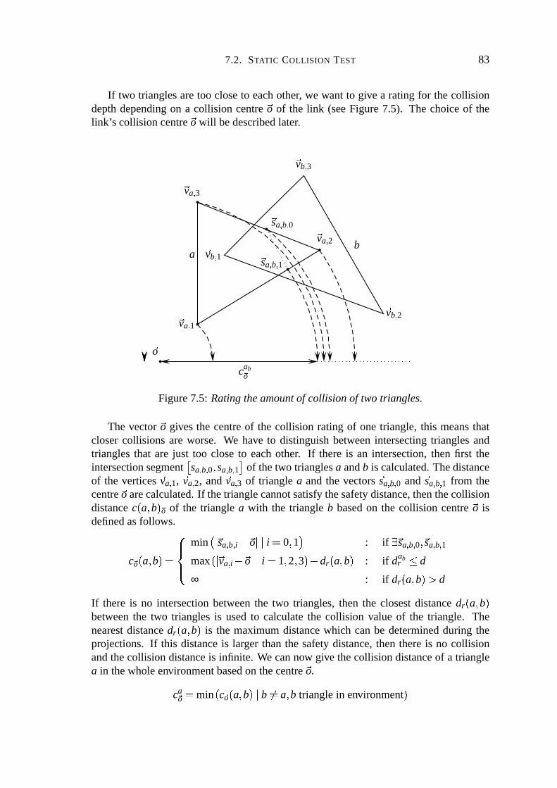
7.2. STATIC COLLISION TEST 83
If two trianglesaretoo closeto eachother, we want to give a rating for thecollisiondepthdependingon a collision centre So of the link (seeFigure7.5). The choiceof thelink’scollisioncentreSo will bedescribedlater.
a
Sva c 3
Sva c 1Sva c 2 bSvb c 1
Svb c 2
Svb c 3
So
Ssa c b c 0Ssa c b c 1cab�
o
Figure7.5: Ratingtheamountof collisionof two triangles.
The vector So givesthe centreof the collision rating of onetriangle,this meansthatclosercollisionsare worse. We have to distinguishbetweenintersectingtrianglesandtrianglesthat are just too closeto eachother. If thereis an intersection,thenfirst theintersectionsegment ¨ sa c b c 0 sa c b c 1 © of thetwo trianglesa andb is calculated.Thedistanceof the vertices Sva c 1, Sva c 2, and Sva c 3 of trianglea andthe vectors Ssa c b c 0 and Ssa c b c 1 from thecentreSo arecalculated.If thetrianglecannotsatisfythesafetydistance,thenthecollisiondistancec � a b� �o of the trianglea with the triangleb basedon the collision centre So isdefinedasfollows.
c�o � a b�F ��� �� min � � Ssa c b c i � So �ª� i 0 1� : if E Ssa c b c 0 Ssa c b c 1
max � � Sva c i � So �ª� i 1 2 3�«� dr � a b� : if dabr d
∞ : if dr � a b�@Q d
If thereis no intersectionbetweenthe two triangles,then the closestdistancedr � a b�betweenthe two trianglesis usedto calculatethe collision valueof the triangle. Thenearestdistancedr � a b� is the maximumdistancewhich canbe determinedduring theprojections. If this distanceis larger thanthe safetydistance,thenthereis no collisionandthecollision distanceis infinite. We cannow give thecollision distanceof a trianglea in thewholeenvironmentbasedon thecentreSo.
ca�o min � c �o � a b� � b Y a b trianglein environment�

84 7. COLLISION RATING
The next stepis to give a rating for eachlink Ll of the robot. For this we choosethecentre Sol basedon theconnectingjoint Jl andtheprevious link Lp � l � , soeachlink ofthe robot hasits own collision centre Sol . The centre So0 of the baselink canbe chosenarbitrarily, sincewe ignore the rating of the baselink becauseit cannotbe moved. Inadditionwe assumethat the baseis collision free for the whole planningprocess.Theposition of the collision centre Sol of the other links shouldbe close to the importanttrianglesandfar from thelessimportanttrianglesof thelink Ll . For a rotationaljoint thetrianglesnearestto rotationaxis aremoreimportant,sinceit takesmoreeffort to movea trianglenearerto the motion axis. If the connectionis via a translationaljoint, thenno triangleshave to bepreferredbecauseof the joint’s type. If we look at thekinematicstructureof the robotandthereforeat theprevious link of link Ll , we canmake anotherobservation. Thetriangleswhich arecloserto thepreviouslink aremoreimportant.Theproblemis that theprevious link Lp � l � changesits positionin relationto the link Ll . Forthiswetakethepointof contactwith thepreviousjoint in therealworld ascollisioncentre.Thispointhasto begivenwith thedescriptionof therobot.Similarconsiderationscanbefoundin [Baginski,1999]in connectionwith the“shrink centre”.
Theoverall ratingof a link Ll is basedon thecentreSol andreturnstheabsolutedepthof thecollision. Let a beatriangleof thelink Ll andlet b beatriangleof theenvironmentminusthelink itself andits following links. Moreover, let r l bethemaximalextensionofthelink r l max � � Sva c i � Sol �ª� a ] Ll i 1 2 3�
Cl ��� �� r l � d � min � c�ol� a b� � a ] Ll b ] ��¬9� nl
l ^ _ � : if E Ssa c b c 0 Ssa c b c 1d � min � � dr � a b� �� a ] Ll b ] ��¬9� nl
l ^ _ � : if E b : dr � a b�@ d
0 : if < b : dr � a b�@Q d
This meansthatif any trianglein thelink collideswith theconsideredenvironment,thenthecollision valueis the radialdistancebetweenthe intersectionwhich is closestto thecentreandthemaximalextensionof thelink plusthesafetydistance.If thesafetydistanceis not largeenough,thentheviolation partof thesafetydistanceis taken. Otherwisethecollisionvalueis zero.
During thecalculationof Cl it is importantto considerthetrianglesof theotherlinksapartfrom thetrianglesof Ll too, in orderto detecta self collision of therobot.All linksexcept the next links in � nl
l have to be considered.This representsthe stateof a link.A link nearerto thebaseis lessresponsiblefor a collision thanits children. In practice,onewould even excludethe neighbouringlinks from the calculation,firstly becauseofinaccuraciesintroducedduringmodellingandsecondlybecauseof thesafetydistanceweneedduringthedynamiccollision test.(It is usefulto addthedecisionwhethertwo linksshouldbetestedagainsteachotherto thegiveninformationof themodel.)
The ratingof a link Ll thatalsoconsidersthe topologyof the robot is definedrecur-sively asfollows.
Cl ���� ��� 0 : if l 0
Cl : if Cp � l � 0
r l � d : if Cp � l � Y 0

7.2. STATIC COLLISION TEST 85
Thismeansthata link collidescompletelyif apreviouslink collides.Thereforethewholeratingof therobotin position Sυ andall obstaclesat time t with safetydistanced is
C � Sυ t d �k ∑Ll ®°¯ Cl
Thisresultsin acollisionteststartingwith thelinks nearerto therobot’sbase,asthevalueCp � l � of the previous link hasto be known. As we cansave the minimal andmaximalcollision valueof all trianglesin eachboundingbox hierarchicallyfor the links of therobot, it is possibleto selectthe box with the worst possiblecollision valuefirst, so wecanmake surethatwe get themaximalcollision valuequitequickly. On theotherhand,the determinationof the collision valuecanbe stoppedif the trianglesin a box cannotworsentherating. Figure7.6shows thetime t (in milliseconds)necessaryfor a collisiontestwith rating(blackplot) andwithout rating(grey plot) usingdifferentsafetydistancesd (in millimetres)ontheleft side.Ontheright sidethepercentageof collisionsc is printedover thesafetydistanced. Clearly the curveswith ratingandwithout rating have to beequal.For safetydistanceslargerthanapproximately130all testsresultin collisions.Thetimesof thecollisiontestwithoutratingandsafetydistancezeroaresimilarto theoriginalones.The only differenceis that therearea few moreadditionsin thebox andtriangletest.
0 50 100 150 20001234567
0 50 100 150 20001234567
d
t
0 50 100 150 2000
0 � 20 � 40 � 60 � 81 � 0d
c
Figure7.6: Comparingcollision test: 500 testsper safetydistance, 6504obstacletri-angles,2494robot triangles,approximately30%of thetestsresultin collisionsif safetydistanceis zero.
We note that the timesdo not vary very muchfor smallersafetydistances,even ifthe rating is calculated.The other importantobservation is that the time for a collisiontest without a rating doesnot grow as quickly as the collision test with a rating. Wewill exploit this fact by computingthe rating only for small safetydistances.As longassafetydistancesare large, we do not rate. Furthermorethe time for a collision testwithout a ratingstopsgrowing whenthesafetydistanceis reached,whereall testsresultin collision.
The staticcollision testwith a rating detectson onehandif the robot hasa certaindistanced to theobstaclesat timet. Ontheotherhandaratingof thetimeconfigurationisgiven.Thetestcannotdetectif anobjectliestotally insidetherobot‘ssurfacesincewetestsurfacesagainsteachother. But sinceweassumethatthestartandthegoalconfigurationsarefreeandin particulararenotwithin anobstacle,it is obviousthatif a freetrajectoryisfound,nocrossingwith anobstacleis possible.

86 7. COLLISION RATING
ω6
t
ω6
ω5
ω6
ω5
ω6
t
Figure7.7: Four examplesof the ratedconfiguration spaceof a 6-dof robot. Theupperimagesshowtheconfigurationspacewithouta safetydistance, while in thelower imagesthere is a safetydistanceof 50. Theconfiguration spaceon theleft sideis thesameasinFigure4.8andthaton theright sideis thesameasin Figure4.9.
In Figure7.7theconfigurationspacefor thewell-known six degreesof freedomrobotis depicted(seeFigure4.1 on page28 for a descriptionof the robot). Only the joints J5andJ6 aremovedin theleft picturesandJ6 andthetime is changedin theright pictures.Thetwo configurationspacesarethesameasin Figure4.8onpage39andin Figure4.9onpage40,but now weratethecollisions.Thedarkeraregionis, theworsetheconfigurationof therobot is. Therating is donewithout any safetydistancein theupperconfigurationspacesandwith asafetydistanceof 50 in thelowerpictures.

7.3. DYNAMIC COLLISION TEST 87
7.3 Dynamic Collision Test
We aregivena time interval anda trajectory. Our goal is to detecta collision duringthetime interval by performingonly onestaticcollision test. During that interval, the robotis moving accordingto thegiventrajectoryandthetime-varyingobstaclesaremoving aswell. We have to determinea point in time within the interval andsafetydistancesthatare large enoughsuchthat whenour staticcollision testdetectsno collision, then it isguaranteedthatnocollision is presentalongthewholetime interval.
On the otherhand,we have to acceptthat it might be a falsealarmif a collision isdetectedby our statictest.This is simplybecauseour safetydistancesaresolarge.Afterall, theremustbeprovisionfor movementsof therobotandtheobstacleswithin thegiventime interval. In the casethat the static test reportsa collision and the currentsafetydistancesexceeda certainlimit (in otherwords,theprecisionof our collision testis toolow) wewill bisecttheinterval andrepeattheteston theresultingintervals.Wedeferthedescriptionof thisadaptionprocessto thenext section.In thissectionwewill concentrateon a singleinterval andwe will show how a suitablepoint in time andappropriatesafetydistancescanbefoundfor thestaticcollision test.
Work onsafetydistancecomputationin staticenvironmentscanbefoundin [Glavina,1991]and[Baginski,1999]. In [Glavina, 1991],a safetydistanceis appliedto thestaticobstacles,while no safetydistanceis appliedto the robot. In [Baginski, 1999], safetydistanceis achievedby blowing up therobot’s geometry. In time-varyingenvironments,however, it turnsout to beadvantageousto havedistinctsafetydistancesfor therobotandfor the time varying obstacles.This way the safetydistancescanbe kept lower thaninthecasewhereonly therobotor theobstacleshave a safetydistance.In particular, staticobstaclesdonothavesafetydistancesat all.
Thetime interval which hasto betestedstartsat ts andendsat tg. Firstly, we have tocalculatean interval | Sυb Sυt x which boundsthe positionsof the robot joints in the giventrajectorysection.Let υb c l andυt c l be the minimal andmaximallimits of joint Jl . Thisinformationcaneitherbeprovidedby thetrajectorygenerationalgorithmor theallowedareadescribedvia thebasepointscanbetaken. However, if we arestill at thebeginningof theplanningprocesswith only asmallnumberof basepointsandtheboundcannotbegivenby the trajectorygeneration,this is only a roughestimateandwill leadto a largesafetydistance.Consequently, it is likely thatthealgorithmreportscollisionsthatdo notactuallyexist. At theendof thissectionwedescribeanapproximationmethodthatavoidsthisproblem.
In addition,a speedvector SσOi �� σOi c 1 σOi c 2 σOi c 3 σOi c 4 σOi c 5 σOi c 6 � T for eachob-stacleOi is givenwhichspecifiestheminimalandmaximalpositionandorientationspeedfor thetime-varyingobjects(seeSection4.2). Let eOi bethemaximaldistanceany pointof theobstaclehasto theorigin oi � t � of theobstacle.
First,we calculatethesafetydistancefor thetime-varyingobjects.Themaximaldis-tanceapointof a time-varyingobjectcanreach(seeFigure7.8)dependson themaximaltranslationandrotationtheobjectcanperformduringa time interval.
Welook at thetime-varyingobjectat time ts � tg 8 ts2 ts� �
t. If theorigin oi � t � moveswith maximalor minimal speedin y-direction(seeFigure7.8), themaximaldistancethe

88 7. COLLISION RATING
Soi � ts� �t �
�x
�y
�p
eOi
�z
σOi c 6 �t
Figure7.8: Safetydistancefor a time-varyingobject.
point canmoveis
�y σOi c 2 �
t
The samedistancescanbe given for the x andz direction. The overall distancea pointcancover if thereis no rotationis
�pi ������
%'�
x
�y
�z
(+ ������ ������%' σOi c 1
σOi c 2σOi c 3 (+ ������
�t $± σ2
Oi c 1 � σ2Oi c 2 � σ2
Oi c 3�
t
Let usnext take a look at therotationalcase.In thefollowing, let cos� x� be � 1 if thevalueof x is greaterthanπ or smallerthan � π. For therotation(seeFigure7.8)we getamaximaldistance
�z if thereis a rotationaroundthez axis,of
�z ± sin� σOi c 6 �
t � 2 ��� 1 � cos� σOi c 6 �t ��� 2eOi ± 2 � 1 � cos� σOi c 6 �
t ��� eOi
whereeOi is thefurthestpoint of theobjectfrom theorigin. Theoverall distancea pointcancover if thereis no translationis
�oi ² 2 � 1 � cos�w± σ2
Oi c 4 � σ2Oi c 5 � σ2
Oi c 6�
t ��� eOi
So we can be surethat thereis no collision with a time-varying object betweentsandtg andthe robotdoesnot move if thecollision ratingC � Sυb ts� �
t max� � pi � �oi ���
with safetydistancemax� � pi � �oi � is zerowith thetime-varyingobstacleplacedat time� ts � tg ��� 2. Thismeansthatthefollowing inequationhasto hold for eachobstacleOi
d u �pi � �
oi
d u σpi
�t � ± 2 � 1 � cos� σoi
�t ��� eOi
with σpi �± σ2Oi c 1 � σ2
Oi c 2 � σ2Oi c 3 andσoi �± σ2
Oi c 4 � σ2Oi c 5 � σ2
Oi c 6

7.3. DYNAMIC COLLISION TEST 89
Thenext stepis to giveasafetydistancefor eachlink of therobot.Thesafetydistanceof the link hasto ensurethatno point on the link movesfurther thanthis distancefroma givenconfigurationwhile the joint valuesarein a deltainterval. We canusethesameobservationsasfor thetime-varyingobject.Therobotis in theobservationconfigurationSυb � �
υt 8 �υb
2 Sυb � � Sυ andthemaximaldeltatherobotjoints moveare
� Sυ. In Figure7.9therevolutioncasecanbeseenontheleft sideandtheprismaticcaseontherightside.Thedashedlinesindicatethemaximalpositionsthejoint mayhave. Thesymboldl representsthemaximaldistanceany point of the link hasfrom themiddle positionif the joint is arevolutionjoint anddl representsthisdistancefor aprismaticjoint. Let eLl bethemaximalextensionof thelink Ll . Sincewe assumethatall thelinks areconnected,this shouldbetheworstdistancetwo joints connectedto thesamelink canhave.
eLl
dl
dl
Figure7.9: Safetydistancefor a revolutejoint (left) anda prismaticjoint (right). Blackline indicatesmiddleposition,dashedlinesextremepositions.
If thelink Ll is connectedvia a prismaticjoint to thepreviouslink, thenthemaximaldistancea point canmove from thepositionυb c l � �
υl relative to thecoordinatesystemof this connectingjoint Jl is
dl � � υl � ���� υt c l � υb c l2
����Themaximaldistanceany point insidethelink canmovefor therevolutionconnection
is
dl �³ 2 � 1 � cos� � υl �2� eLl 2 l 1 � cos l υt c l � υb c l2 n¥n eLl
Both distancesarerelative to the coordinatesystemof the connectingjoint. Takingbothtogether, themaximaldistancedl a point insidethe link Ll canmove relative to theorigin of thejoint Jl is
dl λl dl ��� 1 � λl � dl
Now this distancerelative to theworld coordinatesystemis needed.To getthesafetydistancerelativeto theorigin of therobotall previousrevolutionandprismaticmovements

90 7. COLLISION RATING
have to beconsidered.Theeffect of rotationalmovementincreasesthe further the linksareaway from the rotationcentre. The overall safetydistancerelative to the origin ofthe whole robot can thenbe calculatedas follows, with the maximalpositiondistance
�υ j υt � j 8 υb � j
2 of a joint Jj andthemaximalextensioneLl of a link.
Dl ∑�i:Ji ®�´ pj
l
%' λi
%' ³ 2 � 1 � cos� � υi �2� ∑�j :Jj ®�´ pj
l µ ´ nji
eL j
(+ ��� 1 � λi � �υi
(+Thereis no safetydistancefor thebase.If thepreviouslink is thebase,thenonly the
connectingjoint to thebaseis considered.Otherwisethesumof eachrotationalparthasto beput togetherandmultiplied by theoverall distancefrom the joint to the link. Thisoverall distanceis thesumof theextensionsof all links from thecurrentlyobservedlinkandjoint respectively to the link for which thesafetydistanceis calculated.Finally thetranslationalsafetydistanceis added.
Let us take the examplein Figure 7.10. Let the link’s extensionbe 1 (eL1 � 2 1).For the left imagethe lower andupperpositionboundsof the joints (both revolute) are| � � 30 �� 30�W r� 30 30� x (dashedlines).Thesetof previousandnext jointsof a joint areforjoint J1, " pj
1 C� 1 ! and" nj1 C� 1 2 ! and" pj
2 C� 1 2 ! and" nj1 C� 2 ! for joint J2. Therefore
thesafetydistancesof link L1 andL2 are
D1 ³ 2 � 1 � cos� � υ1 ��� eL1 �³ 2 � 1 � cos� 30�2�D2 ³ 2 � 1 � cos� � υ1 ���*� eL1 � eL2 �R� ³ 2 � 1 � cos� � υ2 �2� eL2 ³ 2 � 1 � cos� 30�2� 2 �o³ 2 � 1 � cos� 30���
Thesolid lines indicatethetestpositionsof the link. We bisectedtheproblemtwiceat the secondlink andthe resultingsafetydistancesaredepictedin the middle andtheright pictureof Figure7.10. For this worstcase,wherethedistanceof the joint is equalto theextensionandtherobot’s top movesin analmostcircularmotionaroundthebase,this distanceis quitegood.
L1
L2
Figure7.10:Exactsafetydistancefor a robot(firstexample).
In general,the resultingsafetydistancesarea very poor upperlimit, especiallyforrobotswith lots of joints anddifferentorientedmotionaxis. In Figure7.11anotherstart

7.3. DYNAMIC COLLISION TEST 91
andgoalpositionis taken. Thereit canbeseenthattheresultingsafetydistanceis muchlargerthannecessary. Thisalsoresultsfrom thefactthattheactualpositionis notconsid-ered.
Figure7.11:Exactsafetydistancefor a robot(secondexample).
Nevertheless,usingtheseexact safetydistances,onefor eachtime-varyingobstacleandonefor eachlink of therobot,a trajectorycanbetestedfor collision anda collisionvaluecanbe calculatedfor a time interval andgiven joint intervals, by usingthe staticcollision testdescribedin Section7.2. Thealgorithmfor testinga trajectoryfor collisionwill bedescribedin thefollowing section.
As wehavealreadynoted,theexactsafetydistancescanbecomequitelargefor largerintervals. Hence,often a lot of time points in a given trajectoryhave to be testedtoensurefreedomfrom collision for a givensafetydistanced, sincethe time interval hasto bebisectedif themaximalsafetydistancefor any link is too large. For the trajectoryplanner, we suggesta two level collision test,onefor theroughplanningandonefor thefinal collision test.
We usethesameapproximationaswe did for thetorqueandforcerating(seeChap-ter6). Theretheapproximationwasdoneby choosingthreereferencepointsxl yl , andzl
relativeto theorigin of Jl for eachlink Ll , whichapproximatethesizeandthepositionofthelink. Onepoint is in theorigin al =� 0 0 0� T, thesecondgivestheexpansion
bl g� max� � vt c 1 � �d max� � vt c 2 � �W max� � vt c 3 � ��� Twith t ] Ll , and the third point cl ��2� bl c 1 �� bl c 2 bl c 3 � T is for keepingthe orientation.If we look at the configurationat ts and tg, no point is allowed to move further then2d, otherwisethe time interval is bisected(seeFigure 7.12). The movementitself isdeterminedusingthefunctiongetMaxMovement (seepage72). In theexampleweassumethat the robot moveswith constantvelocity from the dashedstartto goal configuration.Theboundsof theinterval arethengivenby theconfigurationof therobotatts andtg. Theadvantageof this methodis thattheactualpositionof therobotis takeninto accountandrevoking motionsareconsidered.Theapproximationworksquitewell if themovementof eachjoint insidethe interval is monotonein onedirection(which is thecasemostofthetime).

92 7. COLLISION RATING
Figure7.12:Approximatedsafetydistancefor therobotin thefirstexample.
In ourfirst example,thedifferencebetweentheapproximatedandtheexactdistanceisnot very large(compareFigure7.12with Figure7.10). In thesecondexample,however,thedifferenceis striking (compareFigure7.13with Figure7.11). Heretheadvantageofusingthecurrentpositionof the links of the robot canbe seen.Especiallythe approxi-matedsafetydistanceof thesecondlink, whichmovesin theoppositedirectionto thefirstlink, is muchbetterthantheexactsafetydistance.
Figure7.13: Approximatedsafetydistancefor therobotin thesecondexample.
7.4 Trajectory Collision Rating
In thissectionwedescribethecalculationof thecollisionvalueof a trajectoryT � t � basedonthedynamiccollisiontestof theprevioussection.Let T � t � returntherobot’sconfigura-tion in physicalspace.Thatis, if TD � t �9H� Sυω Sυσ Sυα � , thenT � t �9=� Sυω � . Eachtrajectorysectionbetweentwo consecutivebasepointsis ratedindependentlywith aprecisionvaluep representingthesafetydistance
rc max� C � Sυ t p� : Sυ T � t �d ti 8 1 t ti �Theoverall ratingof a trajectorysectionis thesortedsequenceof all sectionratings
(seeChapter8).Now we want to give an algorithmfor computingthe collision rating with a given
precision.To this end,let doublegetSafetyDist (trajectoryT, doublets, doubletg) bethe safetydistancewhich hasto be usedto securesafetydistancefor the time interval

7.4. TRAJECTORY COLLISION RATING 93| ts tg x . For theexactcase,this is themaximumof thesafetydistancesfor thetime-varyingobstacleplusthemaximumof thesafetydistancesof therobot’s links (dependingon thelowerandupperboundstherobot’s joint mayreach)
d max � � pi � �oi i 0 ������� o�O� max � Dl l 1 ������� n�O�
In the approximatedcasethe calculationof the safetydistanceis quite simple, asgetSafetyDist (T,ts,tg) = getMaxMovement (T,ts,tg) � 2. As describedon page72,dou-ble getMaxMovement (trajectoryT, doublets, doubletg) returnsthe maximaldistancebetweentwo consecutivereferencepointsif therobotis in positionT � ts� andT � tg � .
Furthermore,the testconfigurationof the robot hasto be calculatedto be usedforthe collision test. Let double[] getTestPosition (trajectoryT, doublets, doubletg)be the function which returnsthis robot configuration.For the approximation,this testconfigurationis simply themedianaveragebetweenthestartandthegoal configuration12 � T � ts�O� T � tg ��� .
As describedin theprevioussection,it is necessaryfor theexactcollision to becalcu-lated,firstly to gettheupperandlowerboundof therobot joint values.Thetestconfigu-rationis thenthemedianaveragebetweenthelowerandupperbound.Thesafetydistancecanbecalculatedaswehaveshown with thedynamiccollision test.
The algorithm doublerateCollision (trajectory T, doublets, doubletg) for cal-culating the trajectorycollision valuefor sectioni of a basepoint trajectoryT � t � withprecisionp (which is equalto themaximalsafetydistance)is asfollows.
doublerateCollision (trajectoryT, doublets, doubletg)pre-condition:ts N tg
/* calculatethesafetydistance*/doubled getSafetyDist (T,ts,tg)
/* if safetydistancesmallerthanprecision,thenreturntheratedcollisionvalue*/if (d p)
return C(getTestPosition (T,ts,tg),12 � ts � tg � ,p)
/* if there is nocollision, thenreturn*/if (C(getTestPosition (T,ts,tg),1
2 � ts � tg � ,d) � 0)return 0
/* calculatethecollisionvaluerecursively*/doublel,r = 0;l = rateCollision (T,ts,1
2 � ts � tg � )r = rateCollision (T,1
2 � ts � tg � ,tg)if (l u r)

94 7. COLLISION RATING
return lelse
return r
Theideaof thealgorithmis to testthewhole interval. If thereis no collision, then0is returned.Otherwisewe reducethe time interval, aslong asthe safetydistanceis toolarge. If theactualsafetydistanceis smallerthenthegivenprecisionp, thenthepositionis rated.
The above algorithmis simple,but therearea numberof optimisationsthat canbeemployed. First, the ratingof thecollision shouldonly be doneif thesafetydistanceisbelow the precision. As we have shown in Figure7.6, the collision testwith rating istime consuming,particularly for larger safetydistances.Second,it is not necessarytoconsiderall links in all collision tests.As assoonasa link is collision freein a collisiontest,the link doesnot have to be testedagainin the recursive calls. This happensquiteoftensincethesafetydistancefor links nearerto thebaseis smaller. This factalsoleadsto the third optimisation. The safetydistancescanbe different for eachlink andeachtime-varyingobstacle.Hence,in practicethegetSafetyDist functionshouldreturnonesafetydistancefor eachlink andonefor eachtimevaryingobstacle.
7.5 Summary and Outlook
Wehavedemonstratedhow theorientedboundingboxcollision testof [Gottschalket al.,1996] canbe modified in order to ratea configurationof the robot regardingcollisiondepth. We then extendedthe static collision test to a dynamiccollision test for time-varying environments. Therewe suggestedusingdifferentmethodsto computesafetydistances.An approximatemethodfor thecoarseplanningphaseandanexactmethodforthefinal validation.Finally, weshowedhow anoverall ratingof acompletetrajectorycanbecalculated.
Ourcollisionratingalgorithmhasmajoradvantagescomparedto existingapproaches.Firstof all, weareableto ratetheconfigurationof arobotindependentof theshapeof therobotandtheobstacles.For example,sincewedonotchangetheshapeor positionsof thetriangleswedonot requiretheparticipatingobjectsto beconvex (acommonprerequisitein existing approaches).Apart from this, thedistancecollision test(without rating)onlycostsslightly morethenthenormalcollision testwith theorientedboundingbox method[Gottschalket al., 1996]. This is quite important,aswe needthe distancecollision testfor our dynamiccollision test.
Let usdiscusssomeextensions.It maybeof interestto introduceweightedcollisionratingsums,with weightsdependentonthetypeof theobjectsparticipatingin acollision.For example,it is reasonableto assumethat a collision with a time-varying obstacleisnot as bad as a collision with a static obstacle. Let Cs � Sυ t p� be the collision valuewith the staticenvironmentandCt � Sυ t p� be the collision valuewith the time-varyingenvironment.To reflectthis, theratingcouldbegivenas
rs max� Cs � Sυ t p�R� cCt � Sυ t p� : Sυ T � t �W ti 8 1 t ti 0 N c N 1�

7.5. SUMMARY AND OUTLOOK 95
This collision typerating canbeusedinsteadof a simplecollision rating. As before,tohavea freetrajectorythis ratinghasto bezero.
Anotherideais to ratethecollisiondependingonthetimewhenthecollisionhappens(collision timerating). Herewe assumethatanearlysectionin collision is worsethenacollision thatoccurredlaterin time. A suitableratingwouldbe
rv 1ti
max� C � Sυ t p� : Sυ T � t �W ti 8 1 t ti �Sucha ratingwould beusefulif therobotmuststartto movebeforethewholetrajectoryis planned. However in addition, if the robot startsits movementbeforethe planningprocesshasfinished,thepartof thetrajectorythat is alreadyexecutedby therobotmustnotbefurtherchangedby theplanningprocess.


CHAPTER 8
Trajectory Planning
Wediscussdifferentaspectsof a goodtrajectory. Thereaftertherating of a wholetrajec-tory by combiningthesedifferentaspectsis given. In thesecondsection,wepresentandanalysetechniquesfor improving trajectoryquality by changingthe trajectory locally.There a threemain techniques,namelymoving, adding, anddeletingbasepoints. Thesetechniquesare thencombinedinto a planningalgorithmthat is able to plan trajectoriesin time-varyingenvironments.In the last section,weanalysethealgorithmanddiscussits properties.
8.1 Global Trajectory Rating
Let us first focus on somegeneralpropertiesof trajectories. First of all, we have todistinguishbetweenfreeandunfreetrajectories.
Definition 8.1 FreeTrajectory – UnfreeTrajectoryWe saya trajectoryis freeif there is no collision at any point of the trajectoryand allkino-dynamiclimits of the robotare fulfilled. If oneof thoseconditionsis violated,thenwespeakof an unfreetrajectory.
Basedon this notion,trajectoriescanbeevaluatedasfollows.v FreeTrajectory – If thetrajectoryis freethenit is interestingto know moreaboutthequalityof thetrajectory. For example,how fartheobjectsin theenvironmentareaway from thetrajectory. Furthermore,it is interestingto know how neartherobotgetsto thedynamiclimits of its joints. Anotherinterestingissueis thecomparisonof thetrajectoryto atimeor energy optimaltrajectory. Moreover, wemightwanttohaveanevenloadon therobot’s joints, to sparethehardwareof therobot.v UnfreeTrajectory – If a trajectoryis unfree,thenthedepthof thecollision withobstaclesis interesting.If thecollision valueis higher, thenthecollision is deeper

98 8. TRAJECTORY PLANNING
andnotasgoodasalowercollisionvalue.Furthermore,wewantto know if thecol-lision is with a staticor a time-varyingobstacle,becausea collision with a movingobjectdoesnot seemasbadasa collision with a staticobject.An earliercollisionis worsethana laterone,if we think of a real-timeplanner, wheretherobotcouldstartmoving assoonasearliersectionsof the trajectoryare free. Moreover, wemight wantto ratea trajectorywith regardto theamountof thetrajectorythatis incollision asit might take moretime to find a solutionwhenstartingwith a trajec-tory which is unfreeatmany pointsin time. Thesecondgrouparethekinodynamiclimits of the robot. It is importantto know how far the limits areviolated. If theviolation is small, it might bereasonableto presumethatthetrajectoryis nearertoa freetrajectory.
In Chapter6 (TorqueRating)andChapter7 (CollisionRating),wehavepresentedal-gorithmsthatcalculatetheratingsfor two of theaboveaspects.First,a ratingof collisiondepth(rc) andsecond,a ratingof theviolation of dynamiclimits of therobot(rt). Sinceour maingoalis to find a freetrajectoryfor a givenstartandgoaltime configuration,notall of the above aspectsareequally important. Our main concernis to get a trajectorywithout a collision andno violation of dynamiclimits. If both constraintsarefulfilled,thenthetrajectoryis a freetrajectory. Therefore,weconcentrateon thesetwo constraintsin the following, but all otherconstraintsor aspectscanbe addedto the plannerby ex-tendingtheoverall ratingfunction.
The simplestcombinationof ratings,without distinguishingbetweena free andanunfreetrajectory, is addingall ratingsr j poweredby ej andmultiplied by a weight f j .Both valueshave to be given asthey arepart of the rating. The weight is necessarytoput eachratingin theright proportionwith all otherratings.Thepowerej is for bringingdifferentgradientsof the ratingsin a usefulproportion. Theselectionof the two valuesf j andej couldbeup to thedesignerof theratingsaswell, but sometimesit is usefultochangethesevaluesaccordingto theproblem. For example,if a scenehasno obstaclesit couldbe usefulto lower the influenceof this rating,becauseonly self-collisiontakesplace.Alternatively considerarobotwithout limited dynamicsmoving in anenvironmentwithout time-varyingobstacles.In suchasetting,it couldbeusefulto lower theinfluenceof the torquerating. In the following, let r i c j be the rating r j of the trajectorysectionbetweenti 8 1 andti.
A rating function for somecriteria shouldhave the following properties.First, thevalueof theratinghasto representtheactualconditionof theconstraintin a trajectoryaswell aspossible.Theratingshouldhaveasfew localminimaaspossible.Weassumethattheconstraintthatwe rateis betterfulfilled if the rating for the trajectorydeliverslowervalues.Eachratinghasto beequalor greaterthanzero.
Definition 8.2 SimpleRatingLet T bea trajectorywith m � 1 basepoints.For all ratingsr j 0 j n let f j u 0 andej u 0. Thesimpleratingof sectioni is givenby
Ri n
∑j . 0
f j reji c j

8.1. GLOBAL TRAJECTORY RATING 99
Theoverall simpleratingRfor thewholetrajectoryis a sortedsequenceof all trajec-tory sectionratingsRi which are not zero (Ri Y 0). Let s� i � bea bijectivefunctionwith arangeandimageof 1 i m.
Rs =¶ Rs� 1� ������� Rs� l �¸· , with Rs� i � u Rs� j � if i N j
and < i l : Rs� i � Y 0 and < i Q l : Rs� i � 0
(If all ratingsRi 0, thenRs hasno elements(Rs =¶ · ) andl 0.)
The differentaspectsof a free andunfreetrajectoryleadto the partitioningof con-straintsinto mandatoryconstraintsandoptimisationconstraintsand thereforeto a twolevel rating.Thefirst is calledmandatoryratingandthesecondis calledoptimisationrat-ing. Normally themandatoryratingcontainsall aspectsnecessaryto geta freetrajectory,while theoptimisationratingratesa trajectoryaccordingto someoptimisationcriteria,assoonasthetrajectoryfulfils all mandatoryconstraints.In thisdistinctionwedonotexpectthat themandatoryconstraintsonly considergettinga freetrajectory. It is up to theuserto definewhich constraintsaremandatoryandwhicharenot.
The above definedrating is simple in the sensethat we do not distinguishbetweenmandatoryratingsandoptimisationratings. In practice,thesetwo typesof ratingsneedto behandleddifferently, namely, anoptimisationratingshouldonly beconsideredafterall mandatoryratingsarefulfilled. To this end,the ratingswill becombinedasfollows.As long asthereis at leastonesectionwith a mandatoryrating that is not fulfilled, therating consistsonly of mandatoryratingsandall optimisationratingsare ignored. Ontheotherhand,if all mandatoryratingsat all sectionsarefulfilled thenwe only consideroptimisationratings(with a negative sign). For this case,a lower boundco gives theminimal rating thatwe want to reach.After co hasbeenreached,our plannerstopsandreportssuccess.
We changethe propertiesof the rating function for somecriteriaasfollows. Again,thevalueof theratinghasto representtheactualconditionof theconstraintin atrajectoryaswell aspossibleandtheratingshouldhave asfew local minimaaspossible.But nowwe assumethat the constraintof a mandatoryrating is betterfulfilled if the rating forthe trajectorydelivers lower values,whereasan optimisationrating mustdeliver highervaluesfor theconstraintto bebetterfulfilled. Eachratinghasto beequalor greaterthanzero. For the mandatoryratingswe assumethat thevaluezerorepresentsthe conditionwhentheconstraintis fulfilled.
Theoverall ratingRi of a trajectorysectioni is acombinationof all mandatoryratingsr i c j 0 j l andoptimisationratingsr i c j l N j n for this trajectorysection.Usingthesimpleratingwe wouldnot distinguishbetweenmandatoryratingsandoptimisationrat-ingsapartfrom thesign.But aswehavementionedbefore,thesetwo typesof ratingshaveto behandleddifferently, thatis, anoptimisationratingshouldonly beconsideredafterallmandatoryratingsarefulfilled. For this we considerall mandatoryratingsr i c j 0 j lif for any sectionthemandatoryconstraintsarenot fulfilled. If all mandatoryratingsareequalto zero,thenonly theoptimisationratingsr i c j l N j m areconsidered.Further-more,a lowerboundco givestheminimal consideredrating.

100 8. TRAJECTORY PLANNING
Definition 8.3 ExtendedRatingLet T bea trajectorywith m � 1 basepoints.For all mandatoryratingsr j 0 j l andoptimisationratingsr j l N j n let f j u 0 andej u 0. Furthermore, let a boundco begiven.TheextendedratingRe
i of a sectioni is givenby
Rei ���� ��� ∑l
j . 0 f j reji c j : if E i: 0 N ∑l
j . 0 f j reji c j� ∑n
j . l � 1 f j reji c j : if < i: 0 ∑l
j . 0 f j reji c j
co : if Rei N co
Theoverall rating Re for thewholetrajectoryis thesortedsequenceof all trajectorysectionratingsRe
i Y co. Lets� i � bea bijectivefunctionwith a rangeandimageof 1 i m.
Re g¶ Res� 1� ������2 Re
s� l � · , with Res� i � u Re
s� j � if i N j
and < i l : Res� i � Y co and < i Q l : Re
s� i � co
(If all ratingsRei co, thenRe hasno elements(Re =¶ · ) andl 0.)
As a consequence,theoptimisationratingis only consideredif all mandatoryratingshavereachedzero.If co is chosento begreaterthanor equalto zero,thentheoptimisationratingswill notbeconsideredatall in theplanningprocesssincetheplannerstopsassoonasall mandatoryratingssignalfulfilment.
Let us next focuson how to comparetwo trajectorieswith their ratingsandhow todefinean order on trajectoryratings. Thereare two requirementsfor sucha relation.Firstly, we would preferit if onesectionof onetrajectoryT1 is worsethanall sectionsoftheothertrajectoryT2, thenT1 shouldbeconsideredworsethenT2 independentlyof theremainingsectionratingsof T1. In otherwords,if thereis aparticularlybadsectionin onetrajectorythenwe do not carehow goodor badtheothersectionsare. Second,in orderto measureimprovementwe would like to introducesomekind of ε valueby which thebadsectionsof thetwo trajectoriesin questionmustdiffer beforeweput themin relation.Thefollowing “epsilonsmaller”relationfulfils bothconditions.
Definition 8.4 Epsilon Smaller RelationLet T1 and T2 be two trajectories. The trajectoryT1 consistsof n} � 1 basepointsandhasthe extendedrating Re
1 ;¶ R1 c 1 ������ R1 c n · (n n} ), and the trajectoryT2 consistsofm} � 1 basepointsandhastheextendedratingRe
2 =¶ R2 c 1 ������� R2 c m· (m m} ). (Letn 0if Re
1 =¶ · andlet m 0 if Re2 =¶ · .)
Let k, with 1 k m,betheindex such that thefollowingconditionholds��< i 1 i k : R2 c 1 R2 c i �O,P�¹< i k N i m : R2 c 1 Q R2 c i �Let l , with 1 l min � n m� , betheindex such that thefollowingconditionholds�¹< i 1 i l : R1 c i R2 c i �O,P�¹< i l N i min � n m� : R1 c i Q R2 c i �
WesaytheratingRe1 is epsilonsmallerthantheratingRe
2 (Re1 N ε Re
2 or T1 N ε T2) if��< i 1 i min � k n� : R1 c i R2 c i �«,P� n N k 7ºE i 1 i k : R1 c i N R2 c i � (8.1)

8.1. GLOBAL TRAJECTORY RATING 101
and � n l , n N m�R7»�FE j 1 j l :j
∑i . 1
� R2 c i � R1 c i �MQ ε j � (8.2)
This relation ensuresthe following. First, one of the largest ratingsneedsto getsmaller(seeEquation8.1) andsecond,the sumof the other ratingsneedsto decreaseat leastby anepsilonvalue(seeEquation8.2). If epsilonis equalto zero,thenonly oneof thehighestratingshasto decrease.If epsilonis largerthanzero,thenit is not only upto onehighestratingto decreasebut it is alsonecessaryto reduceotherbadratingsby ep-silon with respectto their positionin thesortedsequence.Notethatthevalueby which asectionratinghasto improveis weightedby theindex of its ratingin theratingsequence.Hence,if theimprovementof theratingdoesnot take placeat theworstsection,thentheimprovementmustbehigher.
With this relationwe hopeto selecttrajectoriesthatimprove thesituationin a certainway. On theonehand,we would like to stayfocusedon a sectionwith theworst rating.Ontheotherhand,wewouldalsoliketo supportimprovementsthataffectbadsectionsinthevicinity of theselectedworstsection(which is thecaseif wedo only local changes).
We would like to mention,that in practice,the epsilonsmallerrelationneednot betestedonawholetrajectorybut only onselectedsetsof neighbouringsections.If weonlyselectoneworst sectionfor manipulation,it is sufficient to setthe focusfor theepsilonsmallerrelationon all neighbouringsectionsthatmight getchangedby a local changeoftheselectedworstsection.Thenumberof affectedsectionsdependsonthetrajectorytypebut is usuallymuchsmallerthantheoverall numberof sections.
After wehavedefineda relationon thesortedsequenceof sectionratings,weneedtodefineunderwhich conditionthesortedsequenceis “zero” dependingon a given lowerboundco.
Definition 8.5 Zero RelationLet T bea trajectoryconsistingof n} � 1 basepointswith extendedrating Re ;¶ R1 R������ Rn · (n n} ). We saytherating Re is zero for co (Re co 0 or T co 0) if Re is theemptysequence, that is, Re g¶ · (n 0).
For a given start rating Res, an epsilonvaluegreaterzero, anda finite sequenceof
ratingsRes Q ε Re
1 Q ε 0�0�0�Q ε Ren zerois eventuallyreachedif we assumethat a trajectory
canonly havea limited numberof basepoints.In thedescriptionof ouralgorithmweassumethatε andco areglobalparametersand
wedonotneedto addthemto theparameterlist of eachfunction.Theconditionfor valueε is thatit is greaterthan0.
Thefunctionratingrate (trajectoryT) returnstheextendedratingof thetrajectoryT(seeDefinition 8.3). We have giventwo exampleshow singleratingsmaybecalculated.First,thetorqueandforceratingonpage73(rateTorqueAndForce), secondthecollisionratingon page93 (rateCollision). Theoptimisationratingis consideredif thesumofthemandatoryratingsis equalto 0. Note that recalculationof a rating is only necessaryfor partsof thetrajectorywhich have changedin a planningstep.This certainlydepends

102 8. TRAJECTORY PLANNING
on thetrajectorytype. (In theworstcase,thewholetrajectorychanges,if onebasepointis changed.)
Furthermore,let bool zero (trajectoryT) determineif theratingof T is smallerthana lower boundco. Sinceanoptimisationratingcanbeunboundedit is necessaryto havea lowerbound,wherewecanstoptheplanningprocess.
The function bool smaller (trajectoryT1, trajectoryT2) comparestwo trajectoriesanddecides,if trajectoryT1 is epsilonsmallerthanT2 (seeDefinition 8.4). As we havementionedabove, we only want to apply the epsilonsmallerrelationto thosetrajectorysectionsthat changewhen the selectedworst sectionis modified by our planner. Forexample,if a basepoint changesits positionin a polynomialpoint-to-pointmotion,thenonly theprevioussectionandthenext sectionneedto beconsideredin theepsilonsmallerrelation. In a bang-bangpathmotion, the two previous sectionsandthe two followingsectionshave to betakeninto account.In thefollowing descriptionwe assumetheworstcase,thatis, all sectionsof thecurrenttrajectorychange.
boolsmaller (trajectoryT1, trajectoryT2)
/* calculateratings*/ratingR1 rate � T1 �ratingR2 rate � T2 �/* if ratingT2 is alreadyzero, thanT1 cannotbesmaller*/if (zero � T2 � )
return false
/* if ratingT1 is epsilonsmallerthanT2 or T1 is zero */if � R1 N ε R2 7 zero � T1 ���
return truereturn false
Theepsilonsmallerrelationis vital to ourplanningprocess.It letsourplannerdecidewhento acceptchangesto a trajectoryandwhento discardthem.Theepsilonvalueitselfis a tuningparameterto our algorithm. If ε is too largethenour plannerwill only acceptchangesthatare“big steps”. If ε is too small theneven theslightestimprovementmaydistractour plannerfrom moresuccessfuldirections.
8.2 Finding Alter nativeTrajectories
We want to analysedifferentoperationsfor manipulatinga giventrajectory. We changethe trajectoryby moving, adding,or deletingbasepointsandsectionsrespectively. The

8.2. FINDING ALTERNATIVE TRAJECTORIES 103
aim is to improve the rating for the resultingtrajectorysuchthat the new trajectorycanbeusedfor furthermodification. If noneof thesingleoperationsresult in a betterratedtrajectory, thenour plannerperformsa randommovement.
We usethedescriptionof a trajectoryfrom Chapter5 (TrajectoryGeneration),wherethetrajectoryis givenby its basepointsSb0 ������2 Sbm. ThesectionSi is thetrajectorybetweenti 8 1 andti. In the following, let Sbi be a time configurationof dimensionn consistingoftheconfigurationSωi andthetime ti, withoutconsiderationof theepsilonanddeltavalues.
8.2.1 Moving Sections
The sectionSi is moved by moving the basepoints Sbi 8 1 and Sbi . We move both basepoints sincethe rating is given via sections. If only one basepoint were moved thenit would not be possibleto determinewhetherthe previous or the following basepointshouldbe preferred.Apart from that,by moving bothbasepointstheplannerhasmorecontrolon therun of theresultingtrajectory. A basepoint canbemovedin all directionswithin the configurationspaceand also in time. The movementin the dimensionsoftheconfigurationspaceis usuallylimited by thejoint limits, but it couldbeunlimitedaswell. Themovementin thedimensionof time is limited by thetime of thepreviousandthe following basepoint. The problemof moving basepointsis, thatwith an increasednumberof dimensionsin theconfigurationspace,thenumberof directionsin which thebasepoint can be moved increasesexponentially. Therefore,it is necessaryto have areasonablestrategy for moving thebasepoints.
Note that thefirst andthe lastbasepoint cannotbemoved,neitherin positionnor intime sincethey representthestartandgoalconfigurations.Theposition Sωi andtime ti oftheotherbasepoints Sbi maybemovedby vectors Svi c j j 0 ������2 n � 1 in a positive or anegative direction. It is not necessaryto move bothbasepointsof theselectionsection.ThevectorsSvi c j aretheunit vectorsof theconfigurationspacedimensions.Themovementis only possibleif the resultingpositionis insidethe configurationspacelimits andthenew time of Sbi hasa deltadistanceδ Q 0 to the previous andthe following basepointti 8 1 � δ ti ti � 1 � δ.
Let us turn to the movementof the robot in the physicalworld. Whena dimensionof the configurationspaceis changed,thenthe resultingmovementof the real robot isdependenton the depthof the affectedjoints in the robot’s topology (seeFigure 4.2)andthe dependency functionsof the robot (seeDefinition 4.6). If, for example,a jointnearertowardsthe robot’s baseis moved, a lot more joints changetheir position thanduringa movementin a joint furtheraway from thebase.Apart from that, thedistancethetop joints travel normallyincreasesif a joint nearerto therobot’sbaseis moved.Thedependency functionof thejoint influencestheamountof changingaswell, for example,the real movementcould be a scaledversionof the configurationspacemovement. Ifthereare no dependency functions(i.e. thereis a one-to-onemappingbetweenrobotjointsandconfigurationspacedimensions)thenthespectrumof possiblemovementscanbequite large. Thesameamountof changein someconfigurationspacedimensionmayberesponsiblefor rotatingtheoutermostlink by 90degrees(afinger, for example)or mayberesponsiblefor rotatingthewholerobotby 90degrees.
A parameterthe usermay chooseis the orderin which the joints of the basepoints

104 8. TRAJECTORY PLANNING
aretested.Onereasonableorderwould be to test joints in the orderthey appearin therobot’s topologytree,eitherbottomup (“upwards”)or top down (“downwards”). (If wehavedependantjoints, thenthefirst joint of thedependantjoints givesthepositionin thebottom-upor top-down sequence.)
If a sectionSi is moved, thenin theworst casethereare � 3n � 2 � 1 O � 2nO� 1� � pos-sibilities to readjustthebasepoints Sbi 8 1 and Sbi , if we take all pairsof possiblechanges.Thefirst basepoint couldbechangedarbitrarily in all joints (3n), thesameholdsfor thesecondbasepoint (3n), andat leastsomethinghasto change( � 1). If only onedimensionis allowed to changefor eachbasepoint, thenthe numberof possibilitiesis reducedto� 2n2 ��� 4n O � n2 � . This numberresultsfrom the numberof possibilitiesto changeadimensionof the first basepoint (2n) combinedwith the possibilitiesof onedimensionof the secondbasepoint (2n), plus the number, if only the first or the last basepoint ischanged(2 � 2n� ). Thecomplexity canfurther be reducedif we alwayschangethe samedimensionin both basepointsof the currentsection. This resultsin � 32 � 1� n O � n�possibilitiespersectionmove. In our algorithmweusethelattermethod.
Let bool move (trajectoryTn, trajectoryTo, int i, int j, doubledp, doubledn) be afunction thatmovessectioni. Thedimensionof the time configurationthat is movedisj andthetrajectoryTo hasm basepoints. Theparametersdp anddn give theamountbywhich thepreviousbasepoint andthenext basepoint shouldbemoved. Here,previousandnext refer to thecurrentselectedsectioni, that is, thepreviousbasepoint of sectioni is Sbi 8 1 andthenext basepoint of sectioni is Sbi. Theminimal deltatime δ betweentwoconsecutive basepointsis a globalparameter. If thesectioncanbemoved,thentrue isreturned,otherwisefalse. Themodifiedtrajectoryis written to Tn.
boolmove (trajectoryTn, trajectoryTo, int i, int j, doubledp, doubledn)pre-condition:0 j N n 0 N i m δ Q 0
Tn To
/* check if thefirstor last basepoint is moved*/if ��� i � 1 � 0 7 dp Y 0�¼,�� i � m 7 dn Y 0���
return false
/* getandchange thebasepoints*/basepointbp To � ti 8 1 �basepointbn To � ti �bp c j bp c j � dp
bn c j bn c j � dn
/* distinguishbetweenjoint andtimeconfigurationandcheck limits */if � j N n � 1�£�
if ��� bp c j N ωminj 7 bp c j Q ωmax
j �½7�� bn c j N ωminj 7 bn c j Q ωmax
j ���return false

8.2. FINDING ALTERNATIVE TRAJECTORIES 105!else �
if � bp c j Q bn c j � δ �return false
if � dp Y 0 , bp c j N ti 8 2 � δ �return false
if � dn Y 0 , bn c j Q ti � 1 � δ �return false!
/* makenew trajectory*/Tn � ti 8 1 �� bp
Tn � ti �� bn
return true
In contrastto this, Glavina [Glavina, 1991] suggestsmovementsorthogonalto theactualmoving directionin configurationspaceto improve the situation. This resultsin2n � 2 possibilitiesif thedimensionof theconfigurationspaceis n. Usinganorthonor-malmovementconcerningthemovementdirectionin configurationspacewould resultincalculatingfirst thebasevectorof theorthonormalbaseSvi c 0 H� Sbi � 1 � Sbi 8 1 ��� � Sbi � 1 � Sbi 8 1 � .From this vector an orthonormalbaseusing Svi c 0 as first basevector can be generated.The disadvantageof this methodis, that for differentmoving directions,the amountofthe movementsof the real robot couldbe very different. Two differently generated,or-thonormalbasesfrom differentmoving directionsmay leadto a wide spectrumof realrobotmovementsin onecaseor, in theothercasethey maycontaina lot of very similarpositionsin physicalspace.
In Figure8.1,anexampleof a basepoint movementis depicted.In this example,noobstacleis moving andwe areonly interestedin the left finger of the robot, that is, weallow only joint J2 andJ3 to move. The two upperpicturesrepresentthe configurationspaceif only ω2 andω3 aremoved. On the left side,onecanseethe movementfor apolynomialpoint-to-pointmotion andon the right side the movementfor a bang-bangpathmotionis shown. Theredlinesrepresentthestartsituationconsistingof a trajectorywith threebasepoints. The yellow path demonstratesthe moving of the middle basepoint alongthedimensionsof theconfigurationspace.Every stepleadsto a betterexacttrajectory. Finally, thismovementresultsin thenew greentrajectory. In theright casethetrajectoryis alreadyfree. It canbeseen,that in thepathmotiontheexacttrajectorydoesnot touchthemiddlebasepoint.
Theexampleshows that thestepsizeλ of themovementsin theconfigurationspaceis an importantparameter. If the stepsizeλ is too short, thenthe changein the ratingmaynot besignificantenough,sincethenew ratinghasto beepsilonbetterthantheoldone. On the otherhand,stepsthataretoo big maynot follow thegradientof the ratingcorrectly. This parameterhasto be chosenby the user. In the upcomingchapterwithexperimentalresults,we will demonstratetheeffect of variousstepsizeson theplannedtrajectoriesandtheplanningtime. If a stepin onedirectionwassuccessful,thenthestep

106 8. TRAJECTORY PLANNING
ω2
ω3
ω2
ω3
Figure8.1:Movementof abasepoint. Lefthalf showsapolynomialpoint-to-pointmotion.Righthalf showsa modifiedbang-bangpathmotion
sizeis doubledandthesamedirectionis testedagain,until no moreimprovementcanbeachieved.
In contrastto this, Baginski [Baginski, 1999] movesa basepoint suchthat the col-liding joint of the robotdoesanorthogonalmovementin the3D objectspace.This is avery goodstrategy for gettinga robotout of anobstacle,but it hasits limitationsif otherconstraintsapartfrom collision needto beconsideredtoo. For example,if the trajectoryis unfreebecausethe dynamiclimit of onejoint is exceeded,thenit is quite difficult todecidewhich joint hasto bemoved.Sincewewantto giveanalgorithmfor arbitraryrat-ingswe cannotusesuchastrategy. Anotherreasonwhy weneeda moregeneralstrategyis thatourbasepointsmaynot bepointson theexacttrajectory.
Thenew ratingof thetrajectoryhasto bebetterthantheold one.More precisely, theratingRn of thenew trajectoryTn hasto beepsilonsmallerthantheratingRo of theoldtrajectoryTo, for someepsilonthat is given. Not all sectionsof thenew trajectoryhaveto be recalculated,only thesectionswhich changein the vicinity of sectionSi , andthatdependson thetypeof theexact trajectory. Theepsilonsmallerrelationis only checked

8.2. FINDING ALTERNATIVE TRAJECTORIES 107
for thechangedtrajectorysectionsaroundSi . We have discussedtheinfluenceof addingor deletingbasepointsonexacttrajectoriesin Chapter5.
Let bool moveSection (trajectoryTn, trajectoryTo, int i) be the function that triesto changethesectioni of trajectoryTo. Theglobalparameterλ determinesthedistancea basepoint is moved in onedimensionof the configurationspace.If a new trajectorycanbefoundthatis epsilonsmallerthantheold one,thenthetrajectoryTn is written andtrue is returned,otherwisefalse is returned.Wehave implementedtwo variantsof thisfunction. The first onealwaystakesthe first improving modificationthat canbe foundwhile thesecondonetakesthebestmodification.Theeffectof eachvariantwill beshownin thechapterwith experimentalresults.If theglobalparameterfirst is setto true thenthefirst modificationis taken,otherwisewe take thebestmodification.
For functionmoveSection weneedagloballist l thatholdsastuplesall possiblemov-ing directionsfor eachdimensionof theconfigurationspacein someorder. Eachelementof l is a tuple � j dp dn � , where j determinesthe dimensionof the configurationspace( j ] � 0 �>� n ! ), dp is themovementdirectionfor thepreviousbasepoint (dp ] �~� 1 0 1 ! ),anddn givesthemoving directionfor thenext basepoint (dn ] �~� 1 0 1 ! ). It holdsthateitherdp Y 0 or dn Y 0. This list will begeneratedbeforehandandcontains8 ( 3 0 3 � 1)tuplesfor eachdimensionandhence8n tuplesin total. During movements,the list willkeepits lengthbut theorderof theelementsin thelist will bechanged.Thelist definestheorderin whichwecheckthedimensionsof theconfigurationspace.Oneof ourheuristicsis to placethetuplesof adimensionthathasbeensuccessfullyusedto thefront of thelistsinceit is likely thatthesamedimensionwill besuccessfulin subsequentmovements.
The list operationlistElementlistFirst (list l ) returnsthefirst elementof the list.If the list is emptythennull is returned.OperationlistElementlistNext (listElemente) returnsthe elementafter e in a list. If thereis no elementfollowing e thennull isreturned. Operationlist listRemove (list l , int i) removesall elementsfor dimensioni from the list and returnsthe new list. list listInsert (list l , int i) addsall movingpossibilitiesof dimensioni to the front of list l . Hence,listRemove removes8 tuplesfrom thelist while listInsert inserts8 tuples.Thecontentof a list elementcanbereadwith int listReadTupel (listElemente, int i), wherei ] � 0 1 2 ! sinceeachtupleconsistsof threeelements.
boolmoveSection (trajectoryTn, trajectoryTo, int i)pre-condition:0 N i m, !zero (To)
listElemente nullboolmovedAny = false, movedOne = false, moved = falsetrajectoryTt To, Ts To, Ta To
Tn To
/* aslongastheratinggetsbettertry to movethesection*/movedOne = true

108 8. TRAJECTORY PLANNING
while (movedOne , !zero (Tn)) �e listFirst (l )movedOne = false
/* for all elementsin thelist */while (e Y null , !zero (Tn)) �
int j listReadTupel (e 0)doubledp λ ¾ listReadTupel � e 1�doubledn λ ¾ listReadTupel � e 2�/* if movementis possible, doubledistanceandtry again */moved = truewhile (moved , !zero (Ts)) �
moved = falseif � move (Tt Ta i j dp dn � ) �
if (smaller (Tt Ts) 7 zero (Tt)) �moved = movedOne = movedAny = trueTs Tt
dp 2 � 0 ¾ dp
dn 2 � 0 ¾ dn!!!/* takenext elementin list */e listNext (e)
/* if modeis “movefirst”, reorganiselist andstart fromthebeginning*/if � first , moved �£�
Tn Ta Ts
l listRemove (l j)l listInsert (l j)e null!
/* if modeis “movebest”, storebest*/if � !first �£�
if (smaller (Ts Tn))Tn Ts
if (e== null)Ta Tn!!
return movedAny

8.2. FINDING ALTERNATIVE TRAJECTORIES 109
If first is true, this algorithmtakesthe first successfulmodificationaccordingtotheorderof the list andthenmodifiesthe list. Hence,movementsin a dimensionwhichhave beensuccessfularemovedto theheadof the list. If first is false, thenthebestmodificationis taken. In the experimentalresultchapterwe discussthesetwo differentstrategiesin moredetail. We would expectthe first strategy to be fasterandthesecondstrategy to find moresolutionsbut probablyto takemoretime.
The function moveSection only modifiesonesectionof the list. For the planningprocessit is usefulto modify acompleteneighbourhoodof abadsectionafterthesectionhasbeenmoved. Functionbool moveInterval(trajectoryTn, trajectoryTo, int i, int j)tries to move the sectionsSi to Sj startingwith the worst sectionandthenmodifiestheneighbourhoodof the worst section. In this function, the list of possiblemovementsisgeneratedandkeptglobalfor eachsinglemovement.Hence,successfuldimensionsmoveto theheadof thelist duringmodificationof thewholeinterval (thisappliesonly if firstis true).
Aswehavementionedbefore,anotherchoicewehaveto makeis,whetherthepossiblemovementsstartwith the joints nearto the baseor with a joint at the otherendof therobot’s topology. To improve a collision it seemsto be a goodstrategy to startat thebottom of the robot, as upperjoints, which are in full collision, would not be able toimprove the rating. But if we considerother ratingsas well, this rationaleno longerapplies.In our experimentswe have testedbothvariants.Let theglobalparameterdowndeterminethesearchdirectionandthegenerationof theglobaldefinedlist l respectively.If down is true thesearchstartswith thetop joints,otherwiseif down is false thejointsnearerto thebasearetestedfirst. Furthermore,we alsohave tried to usea randomisationduring this list generation.If random is true we startat a randompositionin the jointhierarchy, but thenwe againmovebottom-upor top-down throughtherobot’s hierarchy.Let list generateList () be the function generatingthis list dependingon the globalparametersdown andrandom.
The function int maxRating (T) returnsthe sectionindex with the worst rating. Iftherearemoresectionswith thesamemaximalrating,thenthesmallerindex is returned.If all ratingsarezero,then � 1 is returned.
boolmoveInterval (trajectoryTn, trajectoryTo, int i, int j)pre-condition:0 N i j m, i j, !zero (To)
int s maxRating (To)boolmoved = trueboolmovedOne = trueboolmovedAny = false
/* generatetheglobal list l for themovementsdependingondown andrandom */list l = generateList()

110 8. TRAJECTORY PLANNING
/* moveaslongasthesectioncanbeimproved*/while (movedOne , s u i , s j) �
movedOne= false
/* movetheworst section*/moved = movedOne = moveSection(Tn,To,s)
/* movetheprevioussections*/for (s i � 1; s u i , moved;s ��� )
moved = moveSection(Tn,To,s)
/* movethenext sections*/moved = movedOnefor (s i � 1; s j , moved;s ��� )
moved = moveSection(Tn,To,s)
/* setmovedanyandget new maxrating*/if (movedOne)
movedAny = trues maxRating (Tn)!
return movedAny
Finally, we want to summarisethe parametersof the moving process.First of all,thereis theminimal timedistanceδ two consecutive basepointsmayhave, which couldinfluencethepossibilityof a move in thetime dimension.Thestepsizeλ determinestheamounta basepoint is moved while searchingfor betterratedtrajectories.Thenthereare four possibilitiesthe dimensionsof the configurationspaceareusedto modify thetrajectory. Bottom-up(down = false) indicatesthatsearchdirectionsis bottom-upin thehierarchyof therobot’s joints,otherwiseit is top-down. Thethird typeis to take thebestchoice(first = false), whichsearchesall dimensionsandtakesthebesttrajectory. Thelastparameterin thiscategory is, if thestartingdimensionin thebottom-upandtop-downsearchis chosenrandom(random = true). Finally, ε determinesthe epsilonsmallerrelationandco the zerorelation,which indicateif a trajectoryis betterthananotherorevenhas’zero rating’.
8.2.2 Adding Sections
A new basepoint is addedin asectionSi by choosinganew basepoint Sb j with ti 8 1 � δ t j ti � δ and insertingit into the old trajectory. If a sectionis too short (in termsoftime), thatis, thedeltadistancecannotbesatisfied,thenwecannotaddabasepoint to theselectedsection.(Recallthattheminimal timedistancedelta is aglobalparameterof ouralgorithm.) If thedeltaconditioncanbesatisfied,thenthetime of thenew basepoint is

8.2. FINDING ALTERNATIVE TRAJECTORIES 111
chosenin themiddleof theold sectionSi : t j ti 8 1 � ti 8 ti � 12 . Thevaluesof thenew base
point aretakenfrom thecurrenttrajectoryat time t j , aswe hopeto minimisethechangeto thetrajectoryrating.
t
ω3
ω2
ω3
Figure8.2: Addinga basepoint canworsena trajectory. Left half showsa polynomialpoint-to-pointmotion.Righthalf showsa modifiedbang-bangpathmotion
If the trajectoryconsistsonly of two basepoints(startandgoal configuration),thentwo basepointsareadded.This is reasonablebecauseafterthattheplanningprocesscanimmediatelycontinueby moving awholesection.
Sometimestheratingof thenew trajectorymaybeworsethantheold one,sincethetrajectorymaychangeits run simplydueto theexistenceof a new basepoint (evenif thenew basepoint is on theold trajectory).Clearly, this dependson thetrajectorytypethatweuse.Thiseffect is particularlyapparentfor point-to-pointmotiontypessincetherobotcomesto a full stopat thenew basepoint,but it alsohappenswith pathmotions.
In Figure8.2,two examplescanbeseenthatillustratethisbehaviour. Theleft exampleusesapolynomialpoint-to-pointmotion,while theright exampleshowsamodifiedbang-bangpathmotion. In both cases,the insertionof a new basepoint into an existing freetrajectoryleadsto anunfreetrajectory. On the left side,all joints otherthanJ3 arekept

112 8. TRAJECTORY PLANNING
still andthe time varyingobstacleis moving. The red line shows thepolynomialpoint-to-point trajectoryover the time whenthereareonly threebasepoints. The greenline,which is in collision, hasoneadditionalbasepoint. The geometricpath is identical inbothtrajectories(seeFigure8.2,lower left image)but sincetherobotcomesto afull stopat thenew basepoint, it collideswith themoving obstacleshortlyafterthenew stop(seeconfigurationspacein Figure8.2,upperleft image).On theright sidewe have thesamesituationasin theexamplefor moving a basepoint. Only joints J2 andJ3 canmove andthe time varyingobstacledoesnot changeits position. Insertinga basepoint on theredtrajectorychangesthe run from the red to the greentrajectory. The resultingtrajectorylies partly insidetheobstacleregion. In this example,a changein thegeometricpathisthereasonfor thecollision.
To compensatefor thisbehaviour, everytimeabasepoint is inserted,wesubsequentlymove thetwo new sectionsandthesurroundingsections(identicalto themoveoperationin theprevioussection)to find a trajectorythat is betterthantheold one. Dependingonthetypeof exacttrajectory, theneighbourshaveto beconsideredaswell, sincetherunofthetrajectorymaychangein thesesectionstoo (seeChapter5). For theadditionof anewbasepoint in combinationwith a subsequentmovementof thesurroundingsections,thesameconditionsapply asfor the movementof sectionsalone. The new trajectorymusthave an epsilonsmallerrating thanthe old one,otherwisethe insertionis rejectedandundone.For easeof presentation,weassumein thefollowing thatthewholetrajectoryisaffectedby aninsertion.
With the delta condition we make sure, that for a given start and end time of theplanningproblem,we get an upperboundon the numberof basepointscontainedin atrajectory. Let bool addSection (trajectoryTn, trajectoryTo, int i) be the function thattries to adda new basepoint in the trajectoryat sectioni. If the trajectoryconsistsoftwo elementsonly, thentwo basepointsareadded.If theadditionis successfulandthenew trajectoryis epsilonsmaller, then the trajectoryis modifiedandtrue is returned,otherwisethefunctionreturnsfalse.
Let booladdBasePoint (trajectoryTn, trajectoryTo, basePointb) beafunctionwhichinsertsthe basepoint b in To. The new trajectoryis written to Tn. If the basepoint hasbeeninserted,thentrue is returned.If thebasepoint cannotbe insertedbecauseof thetime limits, thenfalse is returned.Let noSection (trajectoryT) returnthenumberofsectionsin T (which is thenumberof basepointsminusone).
booladdSection (trajectoryTn, trajectoryTo, int i)pre-condition:0 N i m, !zero (To)
trajectoryTt To, Ts To
Tn To
/* generatenew basepoint dependingon theactualnumberof basepoints*/if (noSection (To) Q 1) �

8.2. FINDING ALTERNATIVE TRAJECTORIES 113
basePoint b To ��� ti � ti 8 1 ��� 2�if (!addBasePoint (Tt ,To,b))
return false!else �
basePoint b1 To ��� ti � 2ti 8 1 ��� 3�basePoint b2 To ��� 2ti � ti 8 1 ��� 3�if (!addBasePoint (Ts,To,b1))
return falseif (!addBasePoint (Tt ,Ts,b2))
return false!/* try to movechangedsurrounding*/moveInterval (Ts,Tt ,1,noSection(Tt))
/* check if thenew trajectoryis betterthantheold one*/if (smaller (Ts To � ) 7 zero (Ts)) �
Tn Ts
return true!return false
For this function,thesameparametersasfor themoving in theprevioussectionhaveto be consideredsincemoveInterval is part of the function. The only parameterthatwe would like to point out is theminimal time distanceδ betweentwo consecutive basepoints.Theaddingof abasepoint fails immediatelyif thereis not“enoughtime” to insertanew basepoint.
8.2.3 Deleting Sections
The sectionSi is deletedby droppingthe basepoint Sbi . It is obvious that the resultingtrajectorymaybeworsethantheold one.Hereagaintheoperationis followedby movingthenew sectionandthesurroundingsections,asthesesectionscouldchangedependingon thechosentrajectorytype. For easeof presentationwe againassume,that the worstcasehappensandthewholetrajectoryneedsto bechanged.
This operationcannotbeusedif thetrajectoryconsistsof only onesection.Let booldeleteSection (trajectoryTn, trajectoryTo, int i) bethefunction,which triesto deletethebasepoint Sbi in thebasepoint trajectory. If deletionis successfulandthenew trajec-tory is epsilonsmaller, thenthetrajectoryis modifiedandtrue is returned,otherwisethefunctionreturnsfalse. This functiononly fails if only thestartandgoalconfigurationsareleft.

114 8. TRAJECTORY PLANNING
Let bool deleteBasePoint (trajectoryTn, trajectoryTo, int i) bethefunctionwhichdeletesthe i-th basepoint in To. If i is thelastbasepoint, thenthelastbut onebasepointis deleted.The new trajectoryis written to Tn. If the basepoint hasbeendeleted,thentrue is returned.If thebasepoint cannotbedeletedbecauseit is thefirst or thelastbasepoint, thenfalse is returned.
booldeleteSection (trajectoryTn, trajectoryTo, int i)pre-condition:0 N i m, !zero (To)
/* deletebasepoint */trajectoryTt To, Ts To
Tn To
if (!deleteBasePoint (Tt ,To,i))if (!deleteBasePoint (Tt ,To,i � 1))
return false
/* try to movechangedsurrounding*/moveInterval (Ts,Tt ,1,noSection(Tt))
/* check if thenew trajectoryis betterthantheold one*/if (smaller (Ts To � ) 7 zero (Ts)) �
Tn Ts
return true!return false
No otherparametersarenecessaryapartfrom thosealreadypresentedin precedingsections.Deletingabasepointis,aslongasthereareenoughbasepoints,alwayspossible.Thecritical part is to reachanimprovedtrajectoryafterwardsby moving thebasepointsin thevicinity of thedeletedbasepoint.
8.2.4 RandomisedSectionMovement
All of theabove operationsareonly executedif the resultingtrajectoryis gettinganep-silon betterrating. However, it is possiblethat the trajectoryis in a local minimumandnoneof the above operationsachievesany improvement. We needa strategy to escapesuchlocalminima.
Onepossibility is to definesubgoalsandthen try to find a connectionbetweenthestartandgoal configurationsvia thesesubgoals[Glavina, 1991]. In sucha settingourplannerwould be usedasa local plannersearchingconnectionsvia subgoals,whereas

8.2. FINDING ALTERNATIVE TRAJECTORIES 115
the global plannergeneratesrandomsubgoalsandtries to find a connectionvia solvedsubgoalconnections.
The disadvantageof this methodis that the trajectoryplannedso far is lost after anew subgoalhasbeenchosen. We suggesta strategy that still usesrandomisationbutis moreconservative as far asthe alreadyplannedtrajectoryis concerned.We make alocal randommovementwith onesectionof the trajectoryandafter thatwe readjusttheneighbouringsections.
If thetrajectoryconsistsof only onesectionthenno randomisedmovementwould bepossible,sincewe cannotmove thestartandgoalconfigurations.In this casewe have toaddabasepointbeforemakingtherandommovement.Wesuggestmakingarandomisedmovementof a selectedworstsectionSi . This randomisedmovementworksasfollows.A randomconfigurationfor time � ti 8 1 � ti ��� 2 is generated(satisfyingjoint limits) andthen“applied” to eachbasepoint. All basepointsof thecurrenttrajectoryarereadjusteddependingon their time relative to the time � ti 8 1 � ti ��� 2 andthe start time andthe endtime respectively. As a consequence,we will not losethe relative time positionsof thebasepoints.
Let Sbr be the randomlygeneratedbasepoint. Thenthe dimensionsrepresentingthejoints in theconfigurationspacetakeavaluesomewherein thelimits of theconfigurationspace.For thedimensionrepresentingthetimewedonorandomisedmovementsincewedonotwantto changethedistributionof thebasepointsalongthetimeaxis.
In orderto adjustneighbouringbasepointswe needa functionthatchangesthebasepointsnearerto sectioni morethanthosewhich arefurther away. Let
�t j be the time
distancefrom time � ti 8 1 � ti ��� 2 to thetimeof basepoint Sb j .�
t j ����� ti 8 1 � ti2
� t j ����Thesimplestway is to readjustall basepointsof thetrajectorylinearly dependingon theamountof
�t j . Let Sω j betheconfigurationof Sb j without thetime. Thenew configurationSω j of thebasepoint Sb j is calculatedasfollows:Sω j �� �$¿ t j¿ t0
Sω j � y 1 � ¿ t j¿ t0 { Sωr : j N i¿ t j¿ tmSω j � y 1 � ¿ t j¿ tm { Sωr : j u i
A randomisedmovementnormallymakesthe ratingof the trajectoryworse,but de-liversa new startingpoint for the planningprocess. To eliminatethe risk of taking atrajectorythatis toobad,wesuggestgeneratingasetof randomtrajectoriesandselectingthe onewith the bestrating. Moreover, it is reasonableto generatenew trajectoriesaslongasthenew oneis betterthanthelastone.
In Figure8.3,fiverandomlygeneratedtrajectoriescanbeseen.Theredtrajectory(theoneon thefar left) is theoriginal trajectorywhile all othersaregeneratedrandomly. Thehighestratedsectionof theredtrajectoryis nearthestartingpositionof theleft fingeroftherobot.Foreachof thefivegeneratedtrajectories,thebestoutof tenrandomtrajectorieswastaken. Note that thebasepointsfurtheraway from thefirst sectionaremuchcloserto their originalpositionthantheearlierbasepoints.

116 8. TRAJECTORY PLANNING
Figure8.3: Setof fiverandomtrajectories.Theredtrajectoryonthefar left is theoriginalone. Each randomtrajectoryhasbeentakenoutof tenrandomlygeneratedtrajectories.
In the restof this chapter, let void randomSection (trajectoryTn, trajectoryTo, inti) be the function that createsa new trajectoryTn basedon the given To by randomlymodifying sectionSi . A global parameterof this function is the numberof maximalrandomtestsbeforechoosingthebestone.
8.3 Trajectory Planning Algorithm
After wehavedescribedsinglebasepointoperationsin thelastsectionwecannow presenttheoverall planningalgorithm. We first want to describethealgorithmandthenanalyseit with respectto termination.
All singlebasepoint operationsare alwaysappliedto the worst section,sincethisis the locationwherean improvementcanmost likely be achieved. Let max denotethemaximal numberof randomsectionmovementsthat we allow and let noSection (T)returnthenumberof sectionsin T.
boolplanTrajectory (T)
/* randomisedmovementcounter*/int r 0

8.3. TRAJECTORY PLANNING ALGORITHM 117
/* do until therating is zero, or nomore randomisedmovementsallowed*/while ��� r N�ÀfÁÂR�¼, !zero(T)) �
moved= false
/* movetheworst sectionaslongasit getsbetter*/if (moveInterval (Tt ,T,1,noSection (T)))
T Tt
/* if rating is not zero adda basepoint */if (!zero(T)) �
int s maxRating (T)if (!addSection (Tt ,T,s)) �
/* if no addwaspossibledeletea basepoint */if (!deleteSection (Tt ,T,s)) �
/* if no deletewaspossiblemoverandomised*/if (r ���VN\À�Á )
randomSection(Tt,T,s))!!T Tt!!
return zero(T)
We first try to improve the rating of the trajectoryby moving the whole trajectorywith moveInterval. The function alwaysmovesthe worst sectionfirst andthenthosesectionsimmediatelyto theleft andto theright of theworstsection,readjustingall of itsneighbours.Theindex of thesectionmaychangeduringthis process.If moveIntervalreturnsandtherating is not zerothena new basepoint is addedat theworstsectionandthe moving startsagain. If neithermoving nor addingis possiblethe worst sectionisdeleted.If this is alsonot successful,thena randomisedmove is executed,providedthatr is smallerthanmax.
An importantissuethatwehavenotpaidattentionyet is thechoiceof thestepsizeλ.Thecloserthecurrenttrajectoryis to theoptimalratingtheharderit getsfor theplannerto actuallyfind atrajectorywith theoptimalrating.Consideramultidimensionalfunctionthatwe wantto minimise.As long aswe arefar away from theminimumany movementtowardstheminimumis acceptable.Oncewearecloseto theminimumweneedto reducethesizeof our stepsin orderto make surethatwe do not overshoot.In our plannerwewould like to haveasimilarbehaviour. To thisend,weadjustthestepsizeλ accordingtothedistanceof thecurrentratingfrom theoptimum.If theratingis abovesomethreshold,theuserdefinedstepsizeis taken. Oncetheratingdropsbelow a threshold,thestepsizeis reduced.We suggesta logarithmicrelationshipbetweenratingandstepsizebelow the

118 8. TRAJECTORY PLANNING
threshold.In our experimentsweusethefollowing function.
λ } λ logλ � 1 � rmax � co � 1�whereλ } is the actualstepsizethat we usein the algorithm,λ is the userdefinedstepsize, rmax is the maximal rating of any section,andco is the optimisationbound. Theimportantpropertyof this functionis thatits valueis closeto theuserdefinedstepsizeforlarger ratingsandonly decreasessignificantlyfor ratingsvery closeto theoptimum. Inour experimentswe take theuserdefinedstepsizeasthethresholdvalue,that is, aslongastheratingis aboveλ wesetλ } λ.
Let usturn to a planningexample.In Figure8.4, the6 degreesof freedomrobotcanbeseen.Thescenecontainsstaticobstaclesandoneobstaclethatmovesin a curve fromright to left. Thefigureshowstheprogressof theplannerin four stateswhicharereachedduringtheplanning.For eachof thestates,thetrajectoryreachedat thatstateis indicatedby asequenceof images.
Eachcolumnshows oneplanningstate(onetrajectory)at differenttime steps.Fromtop to bottomthe time increasesby five secondswith eachimage.Fromleft to right therows depict the scenefor four differentplanningstatesat the samepoint in time. Thecolumnon the far left shows the initial trajectoryto which two basepointshave beenadded.Themoving obstaclecollideswith bothfingersof therobotandonefingercollideswith thestaticobstaclein thetop of thebox. In thesecondcolumn,thetwo basepointshave beenmoved in the configurationdimensionsresponsiblefor the right robot finger.In thethird column,morebasepoint dimensionshave beenmovedandthis time the leftfinger is alreadyfree while the right finger is still strugglingfor a suitablesidesteptoavoid themoving obstacle.Finally, thecolumnon thefar right shows thefreetrajectory.To solve this problem,our plannerhadto addtwo basepointsandto move themslightly.
8.4 Summary and Analysis
In this chapter, we have presentedour main algorithm for planningmotions in time-varyingenvironments.Thealgorithmis basedon varioussubroutinesfor ratingandtra-jectorygenerationthatwehavedescribedin thepreviouschapters.
In thefollowing,wewouldliketo giveanoverview ontheglobalparametersof theal-gorithm.Thereareparameterswhichinfluencethechoiceof thenext improvedtrajectory.Theseparametersdeterminethe strategy for testingthedimensionsof the configurationspace.Two parametersexist thatdeterminehow themoving is donefor a singledimen-sion. Two moreparametersdetermineif onetrajectoryis betterthananothertrajectory.In addition,thereareparametersfor summingthe ratings,influencingthe weightingofthedifferentratings,andoneparametergiving theexactitudeof theratings.Finally, twoparametersdeterminetheprocessof randommovements.Lastbut not least,thetrajectorytypeis animportantparameter.
In Figure8.5,thehigh-levelflow chartthatwehaveintroducedin Chapter3 is depictedagain. We have addedthe parametersof the algorithmto the relevant steps. The flowchartdoesnotgivetheexactrunof thealgorithm,but givesagoodoverview onwheretheparametersareimportantandwherethey influencethealgorithm. Theredpartsindicate

8.4. SUMMARY AND ANALYSIS 119
Figure8.4: A four stepplanningsequencefor the6 degreesof freedomrobot.
comments(dashedovals)or partsof thechartthathavechanged.Therearesomelocationswherethe flow chart is an abstractionfrom the real algorithm. First, modifying a basepoint doesnot only consistof a move,addor deleteoperation.Immediatelyafteranaddor deleteoperation,wemoveaffectedsectionsto improvethetrajectory. In theflow chart,thesemoveoperationsareimplicitly containedin the“modify basepoints” task.Second,whenwegeneratearandomtrajectorythenawholesetof trajectoriesis generated,beforewe selectthe bestone. We have addeda new decisionstepto the flow chartwherewe
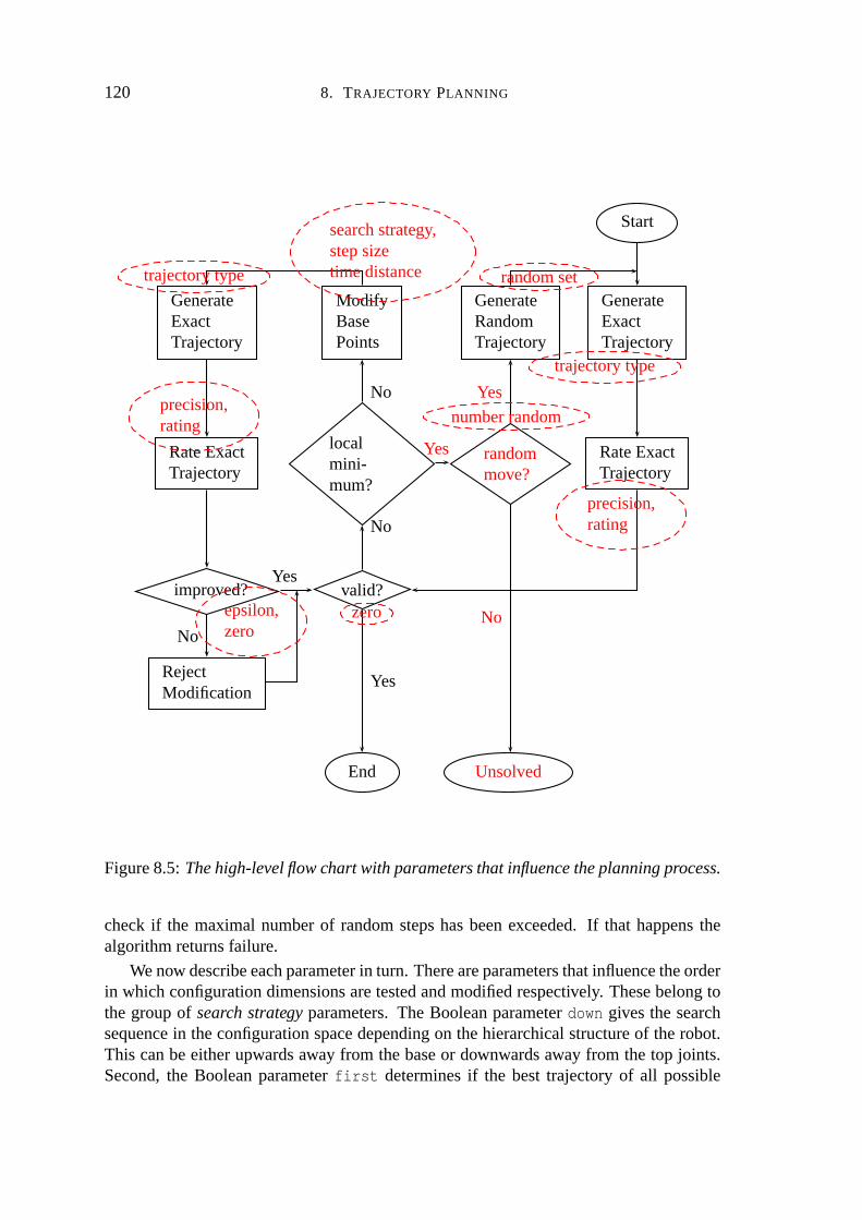
120 8. TRAJECTORY PLANNING
Start
GenerateExactTrajectory
ModifyBasePoints
GenerateRandomTrajectory
GenerateExactTrajectory
RateExactTrajectory
localmini-mum?
randommove?
RateExactTrajectory
improved? valid?
RejectModification
End Unsolved
No
Yes
No
No
Yes
Yes
Yes
No
searchstrategy,stepsizetimedistance
epsilon,zero
zero
numberrandom
trajectorytype
trajectorytype
precision,rating
precision,rating
randomset
Figure8.5: Thehigh-levelflowchart with parametersthat influencetheplanningprocess.
checkif the maximalnumberof randomstepshasbeenexceeded.If that happensthealgorithmreturnsfailure.
Wenow describeeachparameterin turn. Thereareparametersthatinfluencetheorderin which configurationdimensionsaretestedandmodifiedrespectively. Thesebelongtothe groupof search strategy parameters.The Booleanparameterdown givesthe searchsequencein theconfigurationspacedependingon thehierarchicalstructureof therobot.This canbeeitherupwardsaway from thebaseor downwardsaway from the top joints.Second,the Booleanparameterfirst determinesif the besttrajectoryof all possible
8.4. SUMMARY AND ANALYSIS 121
movesis takenor thefirst betterratedtrajectoryis takenasthenext trajectory. For thecasewherethefirst joint which improvesthetrajectoryis taken,the joint wherethesequencestartsto testfor animprovedratingis chosenrandomlyif theBooleanparameterrandomis setto true.
For themodificationof a singledimensionin theconfigurationspace,thestepsizeλgivesthe initial amountby which the basepointsaremoved in the configurationspacewhensearchingfor animprovedtrajectory. Thetimedistanceδ is importantfor themoveandaddoperations.This parameterdeterminesthe minimal time distancebetweentwobasepointsin a trajectory.
The next parametergroupinfluencesthe rating of the trajectory. The first andmostimportantparameteris the trajectorytype, sinceit influencesthegenerationof theexacttrajectoryandthereforetherating. We would like to mentionthat thealgorithmbehavesquite differently for eachtrajectorytype. For example,planningtasksexist that canbesolvedwith onetrajectorytypebut areunsolvablewith anothertype.Thenext parameteris theprecisionp, whichis importantaswell. Oftenratingsaredefinedvia afinite numberof configurationsalonga trajectory. The precisionvaluedetermineshow many discretetime stepson thetrajectoryaretakeninto accountfor this rating. This is doneby givinga limit for themaximaldistanceof any point on therobotbetweentwo consecutive timestepsand the maximal movementof a time-varying obstaclebetweentime steps. Theprecisionvalueis givenin theunit of themodelledscene.Someratingsmay ignorethisvalue,for example,aratingmaximisingthetimedistancebetweenthelasttwo basepointswill not needthis parameter. Otherparametersrelevant to rating arethe multiplicationcoefficients f j andexponentsej of theratings.
Theepsilonvalueε andtheoptimisationboundco definetheepsilonsmallerandthezero relationbetweentrajectoryratings. Theseparametersdetermineif a trajectoryhasimprovedor is alreadyvalid.
In thecase,whenthebasicoperationsof adding,moving,anddeletingbasepointsarenot successful,theparametermax givesthe total numberof randommovementsthatweallow during the planningprocess.The plannerstopsif morethanthis numberof ran-dommovementsis needed.Anotherparameter, calledrandomsetdetermineshow manytrajectoriesare randomlygeneratedbeforethe bestis taken. After that, more randomtrajectoriesaregeneratedaslongasthenew randomtrajectoryis betterthanthelastone.
In Table8.1,all parametersor groupsof parametersarecollectedandashortdescrip-tion is givenfor eachof them.
Let us now look at the terminationof the algorithm. The operationsmodifying atrajectoryareeithermoving,adding,or deletingbasepoints.All theseoperationsdecreasethe rating of the trajectoryby a given epsilonvalue. The only operationwhich hasnotto generatea bettertrajectoryis therandomisedmovement.But themaximalnumberofrandomisedmovementsis limited.
Thealgorithmstopsassoonasthe ratinghasdroppedbelow parameterco. Further-more, the delta valuegives the minimal distancebetweentwo basepoints in the timedimension.As aconsequence,thenumberof basepointspertrajectoryis limited. Hence,thealgorithmstopsaftera finite amountof time, eitherbecauseit hasfounda valid tra-jectoryor becauseno moreoperationsarepossibledueto thegivenlimits regardingthenumberof basepoints,themaximalnumberof randomisedmovements,andtherating.

122 8. TRAJECTORY PLANNING
Parameter Description
Trajectorytype Determinesthe typeof theexact trajectorygeneratedfrombasepoints.
Precision Givesthe exactitudep of the rating. A lower valuegivesmoreexactratings.
Rating Coefficientsandexponentsof theratings,aswell astherat-ing types.
Epsilon Usedin theepsilonsmallerrelation;determinesif a trajec-tory is betterthananother.
Zero Optimisationboundco that determineswhenoptimisationis sufficient.
Stepsize Givestheinitial distanceλ thatabasepoint is movedin theconfigurationspace.
Timedistance Two consecutive basepoints must have at least this timedistanceδ. Givesanimplicit boundon thenumberof basepointsin a trajectory.
Searchstrategy The order in which the dimensionsof the configurationspacearesearched,dependingon thetopologyof therobot.Thiscanbebottom-upor top-down. In additionthestartingdimensioncanbechosenrandomly. Alternatively, thebestdimensionis taken.
Numberrandom Maximal numberof randommovesbeforeplannersignalsfailure.
Randomset Numberof randomtrajectoriesfrom whichthenext randomtrajectoryis selected.
Table8.1: Parametersof thealgorithm.

CHAPTER 9
Experimental Results
In thischapter, wepresentvariousexperimentsthatwehaveconductedwith animplemen-tation of our planningalgorithm. We first givea short introductioninto theimplementa-tion andtheusedparameters. Thereafterwepresentresultsof thealgorithmobtainedindifferentplanningscenarios.
9.1 TestEnvir onmentand Parameters
To demonstratetheusefulnessof our planningapproach,we have implementedour plan-ning algorithm. The implementationis part of a robot simulationsystem(calledRobS)thathasbeenspecificallydesignedfor this purpose.Usingsoftware,weareableto simu-laterealworld robotscenarioswithout theneedfor expensiverobothardware.Our robotsimulationsystemcanhandlearbitraryrobotmodels,environmentswith staticandmov-ing obstacles,planningtasksand trajectories. It allows visualisationandanimationofmodels,configurationspacesandtrajectories(all imagesshown in this thesishave beencreatedusingRobS).
Themainimplementationof our algorithmhasbeendonein C++ while for visualisa-tion we have usedTcl/Tk andOpenGLMesa.All testswererun on a standardpersonalcomputerwith an Intel PentiumIII with 500MHz clock speedand128MByte of mainmemory. Theoperatingsystemis S.u.S.E.Linux with a2.2.13kernel.Theversionof theC++ compilerthatwehaveusedis egcs-1.1.2.
A shortoverview on therobotsimulationsystemis givenin thenext section.There-after, we focuson theparametersof our planningalgorithmandtheir possibleimpactonits performance.
9.1.1 RobS: a Robot Simulation System
Thearchitectureof RobSis basedon theModel-View-Control(MVC) paradigm[Busch-mannet al., 1996]. TheMVC architecturalpatterndividesaninteractiveapplicationintothreecomponents.The modelcontainsthe core functionality anddata. Views display
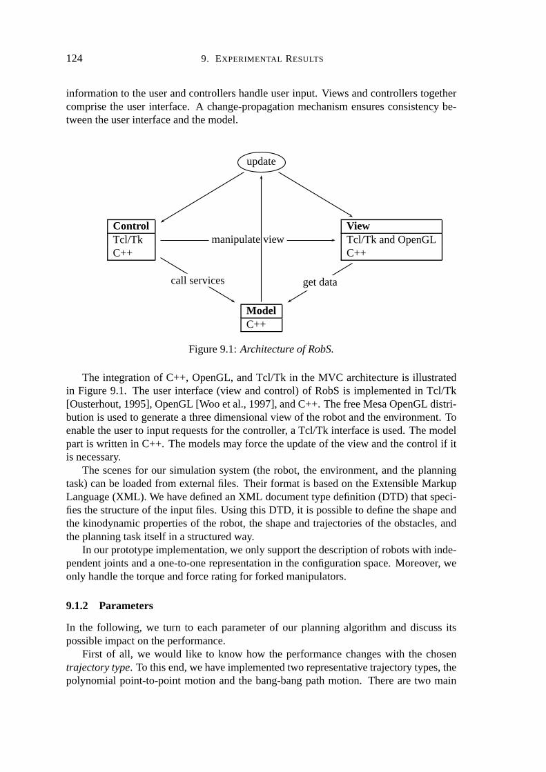
124 9. EXPERIMENTAL RESULTS
informationto theuserandcontrollershandleuserinput. Views andcontrollerstogethercomprisethe userinterface. A change-propagationmechanismensuresconsistency be-tweentheuserinterfaceandthemodel.
ControlTcl/TkC++
ViewTcl/Tk andOpenGLC++
ModelC++
update
call services getdata
manipulateview
Figure9.1: Architectureof RobS.
The integrationof C++, OpenGL,andTcl/Tk in the MVC architectureis illustratedin Figure9.1. The userinterface(view andcontrol) of RobSis implementedin Tcl/Tk[Ousterhout,1995],OpenGL[Wooetal.,1997],andC++. ThefreeMesaOpenGLdistri-bution is usedto generatea threedimensionalview of therobotandtheenvironment.Toenabletheuserto input requestsfor thecontroller, a Tcl/Tk interfaceis used.Themodelpart is written in C++. Themodelsmayforcetheupdateof theview andthecontrol if itis necessary.
The scenesfor our simulationsystem(the robot, the environment,andthe planningtask)canbe loadedfrom externalfiles. Their format is basedon theExtensibleMarkupLanguage(XML). We havedefinedanXML documenttypedefinition(DTD) thatspeci-fiesthestructureof theinput files. Usingthis DTD, it is possibleto definetheshapeandthekinodynamicpropertiesof the robot, theshapeandtrajectoriesof theobstacles,andtheplanningtaskitself in astructuredway.
In ourprototypeimplementation,weonly supportthedescriptionof robotswith inde-pendentjoints anda one-to-onerepresentationin theconfigurationspace.Moreover, weonly handlethetorqueandforceratingfor forkedmanipulators.
9.1.2 Parameters
In the following, we turn to eachparameterof our planningalgorithm and discussitspossibleimpacton theperformance.
First of all, we would like to know how the performancechangeswith the chosentrajectorytype. To thisend,wehaveimplementedtwo representativetrajectorytypes,thepolynomialpoint-to-pointmotion andthe bang-bangpathmotion. Therearetwo main

9.1. TEST ENVIRONMENT AND PARAMETERS 125
differencesthatweexpectfor thesetwo trajectorytypes.Oneconcernsthecalculationoftheexacttrajectoryandthetimenecessaryto calculatearating.Onepropertyof thepoly-nomialpoint-to-pointmovementis thatif a basepoint is changed,thenonly theprevioussectionandthefollowing sectionwill changeits rating(seeChapter5, Section5.3.3). Incontrastto this, in themodifiedbang-bangpathmotion,two sectionsbeforeandtwo sec-tionsafterthemodifiedbasepointmaychangetheir rating(seeChapter5, Section5.4.3).As aconsequence,we canexpecttheupdateof agivenexacttrajectoryandtheupdateofits ratingafterthemodificationof asectionto beperformedfasterfor apolynomialpoint-to-pointmotionthanfor abang-bangpathmotion.Ontheotherhand,weexpectthatwiththebang-bangpathmotionour plannershouldbeableto solve moreproblemsthanwiththe point-to-pointmotion. This holds in particularfor time critical problemssincethepathmotiondoesnotstopateachbasepoint. Weexpectthatthemodifiedbang-bangpathmotionenablesfastermovementsusinglesstorqueandforce.
Let usnow turn to theprecisionparameterp of theratings.Recallthat lower valuesfor p give higherratingprecision.We expecttheplanningtime to bereducedif a higherprecisionvalueis taken,but at thesametimesolutionsarefoundlessfrequently. Thepre-cisiongivestheminimal securitydistancefor which staticcollision testsaredoneduringplanning.Wehave to take into accountthatif thestartor goalconfigurationis closeto anobstaclethenthechosenprecisionvaluemustnot be too largesinceotherwisetheplan-ning processmayencounterdifficulties in leaving thestartconfigurationor approachingthegoalconfiguration.Theprecisionvalueis givenin theunit of thephysicalspace.Forexample,if the model is given in millimetre, thenthe unit for the precisionvalueis inmillimetrestoo.
Anotherparameteris the stepsizeλ. This parameterdetermineshow mucha basepoint is moved initially in onedimensionwhenwe look for a betterrating. We expectthatchangingthis valuewill result(dependingon therobotandtheenvironment)in verydifferentcomputationtimes. This is becausetoo small a stepsizemay result in manymovementsuntil the solutionis found,but too large a stepsizemay missthe situationswith thebestrating.Theunit of stepsizedependsontheunit representedby therespectiveconfigurationspacedimension.For example,in our implementationthedimensionrepre-sentingrotationaljoints is given in degreesandthedimensionrepresentingtranslationaljoints is givenin theunit of thescene(for ourexamples,millimetresor centimetres).Thetime dimensionis given in seconds.We do not useany strategy to normalisethemove-mentsof therobot’s joints,asis suggestedfor examplein [Qin andHenrich,1996].Heretheideais thatthejoints nearerto thebasearemovedlessthanthejoints furtheraway togetanequalamountof movementin thephysicalspacefor eachjoint. In ourconcept,weleave this to thespecificationof themodel.Thatis, weassumethatin themodeldescrip-tion, thedependency functionof eachjoint is specified,which is responsiblefor scalingaconfigurationspacemovementto anappropriatemovementin physicalspace.Theonlydimensionthatcannotbeinfluencedin this way is thetime dimension.In futureit wouldbe preferableto calculatethe units of the configurationspacedimensionsautomaticallyandto adjustthetimescaleto theplanningtask.
Anotherimportantparameteris theepsilonvaluewhich determinesif a rating is ep-silonsmallerthananotherrating.Smallerepsilonvaluestendto find solutionsevenif theratingdecreasesveryslowly, but canleadto averyslow decreasein ratingevenif another

126 9. EXPERIMENTAL RESULTS
dimensionin theconfigurationspacewould result in a larger changeof rating. In otherwords,theepsilonvalueshouldreflectthesteepnessof the rating function. If epsilonistoo small, our plannerwill make many small stepswherea few biggerstepswould beappropriate.If epsilonis too large, thentheplannermayoverlookpromisingsearchdi-rections.It wouldbeidealif wecouldadjusttheepsilonvalueon-the-flyduringplanning.For example,we could gatherlocal and/orglobal informationon the rating function insomeintelligentwayor wecouldanalysethehistoryof ratingsfor this purpose.
Let usnow turn to theparametersthatdeterminethesearchstrategy. Theinitial orderin which jointsaremovedcaneitherbefrom thebaseto thetop joints (bottom-up) or theotherwayround(top-down). Additionally, wehaveachoiceof eithertakingthefirst jointin thecurrentorderthat improvestheratingor we cantake the joint thatmakesthebestrating (best). If we have chosenthe latter strategy, the order in which joints aretestedis irrelevant. For thebottom-upandtop-down searchdirection,thestartingjoint maybechosenrandomly(randomjoint). It is quitedifficult to makeapredictionof thebehaviourof thesedifferentselectionmethods.However, thereshouldbe a significantdifferencebetweentakingthebestjoint or thefirst joint in thecurrentorder. Takingthebestratingresultsin longercomputationtimeswith a fasterdecreasingrating,sinceall configurationdimensionshave to betestedin eachmove. In contrastto this, taking thefirst joint thatimprovestheratingwill resultin lesscomputationtime for onemovementbut mayresultin smalleroverallchangesof therating. In ourexperiments,thebottom-upsearchstrategy(taking the first successfuljoint) turnedout to be a goodchoicein mostscenarios.Thereasonfor this maybethat it is helpful to try thosejoints first thathave a greaterimpacton the overall situation. Clearly, changingthe robot’s basejoint is likely to have moreimpactthanmoving a joint in therobot’s tool, e.g.a finger.
Anothergroupof parameterscontrol randomisedmovement.This groupconsistsofa parameterthat determinesthe maximumnumberof allowed randommoves(RandomNumber) andthe sizeof the setof randomtrajectoriesthat we generatebeforewe pickthe bestof themasthe next randomtrajectory(RandomSet). Most of our experimentshave beensolvedwithout randommoves. Our plannerhasusedrandommovesonly inthe “trap-task” benchmarkwith a staticenvironment. There,we have allowed up to 10randommovesandthesetsizewas25.
Finally, thereis thegroupof ratingparameters.In our experiments,we haveusedtheratingof thecollision andthetorqueandforceratingaswe havepresentedin Chapters7and 6. All factorsand exponentsfor the rating combinationhave beenset to 1 in allexperiments.
In Table9.1, an overview on parametersis given togetherwith valuesthat we haveusedin theexperiments.
9.2 Experiments
In thefollowing, wepresentvariousplanningscenariosandtestresultsthatshow theuse-fulnessof our planningapproach.We have divided our experimentsinto six parts. Inthefirst part,we presenta simplerobot in a not-so-simpletime-varyingenvironment.Inthesecondpart,we show a typical industrialtime-varyingenvironmentwith a robot that

9.2. EXPERIMENTS 127
Parameter Possiblevaluesandunits
Trajectorytype polynomialpoint-to-point,modifiedbang-bangtrajectory
Precision 1, 5, 10,20,50 (millimetre,centimetre)unit dependsonunit usedto modelthescene
Rating rc � rt (not changed)1 ¾ rateCollision 1 � 1 ¾ rateTorqueAndForce 1
Epsilon 108 8, 108 3, 1, 5, 10Zero 0 (notchanged)StepSize 1, 5, 10,20,50 (degree,millimetre,centimetre,seconds)
unit dependsonunit of theconfigurationspacedimensionsTimedistance 0.032sec(not changed)Searchstrategy bottom-up,top-down, best
random,fixed(only with bottom-upandtop-down)Numberrandom 0, 10Randomset 25 (notchanged)
Table9.1: Valuesusedfor parametersof thealgorithm.
needsto moveworkpiecesfrom a tableto a moving band-conveyor. Thenwe take a lookat benchmarksfor staticenvironmentswhich weredevelopedat the Universityof Karl-sruhe. (Unfortunately, no benchmarksexist for planningin time-varying environmentsyet.) Thenwe show an examplewith a focuson robot dynamics. In this examplewehave fitted a well-known typeof industrialrobot,anRX90, with a very heavy handthatit mustlift from theground. In thenext example,a long, slender6-dof robot in a smallroommustgraspinto asmallslidingdoor. Finally, we takea look at a spacerobotwith ahigh-dimensionalconfigurationspacethathasto copewith asteroids.
In Table9.2,we have collectedsomemeasurementcategoriesin which we areinter-ested.Our main interestduring the experimentsis whethera taskwassolved andhowlongit tookeitherto solveit or to signalfailure. In someexperiments,wehaveconducteda seriesof testsusingrandomstartandgoalconfigurations.In thesecases,aninterestingcharacteristicis thepercentageof solvedtasks.Anotherfocusis on thepercentageof therunningtime usedfor the collision test, the collision rating, andthe torquerating. Thenumberof basepointsin thefinal trajectoryis anotherreasonablemeasurementcategory.We will not analyseall parametersandresultsfor eachscenario,ratherwe selectthoseparametersthatarein somewaysignificantor representative for agivenscenario.
In therestof this chapter, we will usethefollowing abbreviations:m for metres,mmfor millimetres,cmfor centimetres,min for minutes,secfor seconds,kg for kilogrammes,g for grammes,N for Newton. In addition,weuseboldfacedandnormalprintednumbersin tables. If both kinds areusedin a table,thenthe bold numbersindicatenumbersforsolvedtaskswhile thenormalprintednumbersrepresentnumbersfor unsolvedtasks.Ifwe do not distinguish,thenthe tasksweresolved for all given parameters.Redvaluesindicatethebestvaluefor eachtrajectorytypein a testseries.

128 9. EXPERIMENTAL RESULTS
Result Unit
Runningtime secondsNumberof solvedtasks percentTorqueratingtime percentCollision ratingtime percentCollision testtime percentNumberof basepoints integer
Table9.2: Measurementcategories.
9.2.1 Two Degreeof FreedomRobot
Figure9.3 on page129 shows an environmentwith a simplerobot. The robot is a twodegreeof freedomrobot which hasto move in a rotating cube. The figure shows anexampleof aplanninginstancewith theinitial trivial pathfrom startto goalconfiguration.Fromleft to right andtop to bottom,thetime stepsfrom thestarttime 0 to thegoaltime25 secondslater canbe seen. The robot hasto move clockwisewhile the cubemovescounter-clockwise.
To getabetterimpressionof thescene,thedimensionsof thetaskaregivenin Figure9.2. The rotatingcubehaswalls with outsidelength1.5 m andinsidelength1.4 m. Itrotateswith a velocity of 0.1 radiansper secondsaroundthe centreof the cube. Therobotbaseandthecentreof thefirst joint respectively is 0.335m away from thecentre,asdepictedin theupperright imageof Figure9.2.
z z
y y0 � 575m
0 � 3m0 � 3mm2 1kg
m1 1kg
1 � 5m
1 � 4m
Figure9.2: Dimensionsof the2 degreesof freedomexample.
As for therobotdimensionswe alsoreferto Figure9.2. Thelengthof thefirst armisapproximately0.7m andof thesecondarm0.6m meters.Thecentreof gravity is located

9.2. EXPERIMENTS 129
Figure 9.3: Initial task for the two degreesof freedomrobot in a rotating cube. Thedurationof themovementis 25 seconds.

130 9. EXPERIMENTAL RESULTS
at g � 1 c 2� �� 0 � 3 0 0� T m from the joint coordinatesystem. The weight of eacharm ism� 1 c 2� 1 kg andtheinertiatensorlocatedat thecentreof gravity is Izz 30� 867108 3 kgm2 for eachlink. Thegravity is in thenegativez directionof thelinks. In theupperrightcornerthesceneattime0 andtherobotwith jointsin zeropositioncanbeseen.Thevaluesof the joints rangefrom υmin� 1 c 2� g� 160degreesto υmax� 1 c 2� 160degreesandthemaximaltorqueis θmax� 1 c 2� 0 � 1 Nm. Thestartvaluesfor theplanningtaskareυs g� 63� 61 133� 01�degreesandthegoalvaluesareυg g�2� 52� 05 �� 138� 80� degrees.
On pages131and132two solutionsareshown. Figure9.4showsa solutionwith thepolynomialpoint-to-pointmovementandFigure9.5 shows a solutionwith a bang-bangpath motion. The solutionsshow that the main problemfor the robot is changingtheorientationof its joints. This canonly be doneif the cornerof the cubehasthe rightposition.Thechallengefor theplanneris to find thetime window andthepositionof thecubewhereit cansafelyperformthis operation.
For this problem,wehaveanalysedtherunningtimeandwhetherasolutionhasbeenfounddependingonthechosenprecisionandstepsize.In thefollowing tables,thevaluesin boldfaceimplicateasolvedsolutionandthevalueitself is therunningtime in seconds.Numberswritten in normal font denotethe runningtime for an unsolved solution. Alltestshavebeenperformedwithout randommovements.
In Table9.3 resultsfor the modifiedbang-bangpathmotion are listed. The searchdirectionis bottom-upandthe first joint that improvesthe rating is taken. From left toright, wehaveincreasedthestepsizefor searchingabetterbasepoint in theconfigurationspace.Theprecisionis increasedfrom top to bottomresultingin lessexactratingsfor thetrajectory.
stepsize(mm)1 5 10 20 50
1 151� 05 51� 52 38� 24 17� 42 20� 645 38� 84 13� 38 11� 03 4 � 25 4 � 5510 18� 07 7 � 03 4 � 46 2 � 24 2 � 50
prec
isio
n
20 15� 00 5 � 81 4 � 80 1 � 67 2 � 0550 38� 22 13� 51 9 � 74 6 � 02 5 � 09
Table9.3: Time usedto solve the problemfor a modifiedbang-bangpathmotion withsearchdirectionbottom-up(epsilon= 108 8).
With the modifiedbang-bangpath motion, a solutioncould be found for all testedvalues. We note that as the planningtime increases,the precisiondecreases.This isbecausemoreratingshave to be calculated.For the stepsize, the time increasesif thestepsare too small or too large. This is becauseif the stepis too small, thena lot ofmoveshave to be donebeforethe goal is reached.On the otherhand,if stepsare toobig, thentrajectorieswith goodratingsmaybemissedout. Theoptimalstepsizein thisexampleis around20 mm. Thepercentageof therunningtime usedfor thetorqueratingis approximately4 percent,for thecollision ratingit is 13 percent,andfor thecollisiontestit is 73percent.Wewould liketo notethatit is difficult to split thetimenecessaryfor

9.2. EXPERIMENTS 131
Figure9.4: Solvedtaskfor thetwo degreesof freedomrobotwith a polynomialpoint-to-pointmovement.

132 9. EXPERIMENTAL RESULTS
Figure9.5: Solvedtaskfor thetwo degreesof freedomrobotwith a modifiedbang-bangpathmotion.

9.2. EXPERIMENTS 133
a collision testanda collision ratingsincecollision ratingdependson thecollision testsin orderto find thepointsin timewhereacollision ratingshouldtakeplace.
In anotherexperiment,we increasedthe maximal torqueof the joints to θmax� 1 c 2� 1 � 0 Nm. It is not surprisingthat the task is still solvable for all testedparameterval-ues.Theaveragerunningtime,however, dropsfrom 19� 49 secondsto 18� 46 seconds.Incontrastto this, if themaximaltorqueis decreasedto θmax� 1 c 2� 0 � 05Nm, thentheproblemis not solvableany morefor all testedvaluesof precisionandstepsize. It couldnot besolved for a precisionof 50 anda stepsizeof 50. Herethe averagecomputingtime is20� 21seconds.
Let usnow turn to thepolynomialpoint-to-pointmotion. In Table9.4, theresultsforthepolynomialpoint-to-pointmotionarelisted. We testedthesameparametervaluesasin thebang-bangpathmotion.Again, thesearchdirectionis bottom-upandthefirst jointthatimprovestheratingis taken.
stepsize(mm)1 5 10 20 50
1 163� 40 85� 62 35� 44 25� 44 17� 035 37� 98 17� 48 9 � 71 7 � 17 4 � 3410 27� 11 14� 4 6 � 84 4 � 54 2 � 69
prec
isio
n
20 13� 51 10� 04 4 � 67 5 � 48 2 � 4550 36� 23 14� 71 10� 89 5 � 34 6 � 23
Table9.4: Time usedto solve theproblemfor a polynomialpoint-to-pointmotion withsearchdirectionbottom-up(epsilon= 108 8).
Theresultsfor thepolynomialpoint-to-pointmovementarenot asgoodasthoseforthe bang-bangmotion. In particular, for somecombinationsof precisionandstepsize,no solutionhasbeenfound. It turnsout thatdynamiclimits of therobotaremorecriticalin point-to-pointmovementsthanin pathmotions. It is thereforemoredifficult to finda solution. If we increasethe maximal torqueto θmax� 1 c 2� 1 � 0 Nm andrepeatthe tests,thenwith all testedparametervaluessolutionscanbe found. Theaveragerunningtimefalls from 22� 76secondsto 17� 51seconds.If wedecreasethemaximaltorqueto θmax� 1 c 2� 0 � 05 Nm thenno solutionscanbefoundany moreandtheaveragerunningtime risesto26� 52seconds.
In thenext roundof experiments,weevaluatehow thesearchstrategy (bottom-up,top-down, or best)influencesthenumberof solutionsandtherunningtime. Wedothesetestsfor both trajectorytypesandwe have generated100 probleminstanceswith randomlychosenstartandgoalconfigurations.Therequirementsfor therandomlychosenexampleshave beenthat the startandgoal configurationare free andthat the start time is in theinterval | 0 20x andthe goal time is in the interval | 40 60x . The precisionvalueandthestepsizeare10 andtheepsilonvalueis again108 8.
In thefollowing tables,theinnertablesrepresentthefollowing values.Theexampleswhich needto besolvedarethoseproblems,wheretheinitial starttra-
jectoryis not free.Wewantto distinguishthesevalues,sincewhentestingwith randomly

134 9. EXPERIMENTAL RESULTS
valuefor all examples valuefor all exampleswhichneededto besolved
valuefor all solvedexamples valuefor all solvedexampleswhich neededto besolved
valuefor all unsolvedexamples
generatedinstances,thereis alwaysapercentageof trivial instanceswheretheinitial tra-jectoryis alreadyasolution(around10percent).
In Table9.5, thecolumnsrepresent:thenumberof randomlygeneratedproblemin-stances,the percentageof solved instances,the averageplanningtime and the averagenumberof basepointsin thesolution.
Pol
ynom
ial
Ban
g-B
ang
Bot
tom
-Up
Top-
Dow
n
Bes
t
Count Solved(%) Time(sec) BasePoints
x x100 6892 60
8
92 88100 100
0
3.57 5.232.54 3.87
15.42
3.89 4.783.68 4.58
6.25
x x100 6993 62
7
93 90100 100
0
4.07 5.882.50 3.72
24.96
3.86 4.703.65 4.47
6.71
x x100 6890 58
10
90 85100 100
0
4.21 6.172.94 4.53
15.71
3.83 4.693.64 4.55
5.50
x x100 6991 60
9
91 87100 100
0
4.74 6.872.85 4.33
23.78
3.97 4.863.69 4.56
6.78
x x100 6889 57
11
89 84100 100
0
6.70 9.865.00 7.80
20.53
3.55 4.283.40 4.19
4.72
x x100 6993 62
7
93 90100 100
0
7.46 10.804.54 6.81
46.16
3.60 4.323.45 4.18
5.57
Table9.5: Resultsfor the2-dof robotin a rotatingcube.
We note that planningwith the polynomial point-to-pointmotion is slightly fasterthan planningwith the bang-bangpath motion. This is becausethe calculationof theexact trajectoryis morecomplicatedin thepathmotion andthenumberof sectionsthatmaychangeif onesectionis movedis higher. However, with thebang-bangpathmotion

9.2. EXPERIMENTS 135
moreprobleminstancesgetsolved.This is dueto thedynamiclimitationsof thejointsoftherobot. Sincethepathmotiondoesnot stopat eachbasepoint themotionis smootherandhenceneedslesstorqueandforce.
If thesearchdirectionis changedfrom top-down to bottom-up,wenotethatthecom-putationtime decreasesandthatmoresolutionsarefound. Both effectscanbeexplainedby the fact thatat thebeginningof theplanningprocess,theextentof changeis greaterif a joint nearerto the baseis movedthanif oneat the top is moved. We alsonotethattakingthebestjoint in eachmovementdoesnot increasethenumberof solvedexamples.Again, the polynomialpoint-to-pointmotion solvesfewer instancesthanthe bang-bangpathmotion.Thecomputationtime is higherthanin thebottom-upor top-down strategy,sincea lot of alternativemovementshave to betestedbeforeamovecantakeplace.
Tosummarise,it is apparentthatthebottom-upsearchdirectionis thebestchoicehere.Themodifiedbang-bangpathmotionsolvesmoreinstances,but needsa longercomputa-tion time thanthepolynomialpoint-to-pointmotion.Sincethedifferencein computationtimeis only marginal,wecansaythatabottom-upsearchwith thebang-bangpathmotionis therecommendedcombinationfor this scenario.
9.2.2 An Industrial Envir onment
In this section,we want to take a look at a typical industrialenvironment. In Figure9.6andFigure9.7a robotmoving betweentwo tablesanda machinecanbeseen.Therobotis a six degreesof freedomrobot. On the machine,a plate moveson a conveyor beltfrom the workplacefor the machineandthe transportplacewherethe robot hasto putworkpieces.Thetwo figuresshow thefollowing scenario:therobotpicksupaworkpiecefrom tableoneandmovesit to thetransportplaceof themachine(shown in Figure9.6).Then(aftera little while), therobotpicksup a workpiecefrom thetransportplaceof themachineandmovesit to table two (shown in Figure9.7). This scenariois typical forautomatedmanufacturingwheremachinesareloadedandunloadedby robots.
To geta betterimpressionof thedimensions,we give a few sizesfor the robot. Thex, y, andz extensionsof the links given in centimetresrelative to their own coordinatesystemare from baseto top: L0 : � 20 20 30� , L1 : � 16 28 16� , L2 : � 32� 5 15 31� , L3 :� 12 34 12� , L4 : � 6 6 26� , L5 : � 6 3 6� , L6 : � 24 6 17� . For eachlink thedensityof thelink is 4 � 5g� cm2. The mass,locationof gravity, andthe inertia tensorwerecalculatedfrom themodel.Themaximaltorquein thejointsare:J1 : 0 � 5 Nm,J2 : 50Nm,J3 : 50Nm,J4 : 5 Nm, J5 : 5 Nm, J6 : 0 � 5 Nm.
Figure 9.6 shows a solution for the loading part with a bang-bangpath trajectoryconsistingof four basepoints. The startingpoint is at time 0 and the goal hasto bereached45secondslater. For aprecisionvalueof 5 andastepsizeof 10, thetrajectoryisfoundafter1.75secondsusingthebottom-upsearchdirection. In Figure9.7,a solutionfor thetransportfrom themachineto thesecondtablecanbeseen.Herethecomputationtimewas1.86seconds.
For therestof this experiment,we focuson therobot’smotionfor theloadingpartofthis scenario,that is, wheretherobotmovesa workpiecefrom tableoneto thetransportplaceof themachine(Figure9.6). In this exampleit is not possibleto take a large pre-cisionvaluebecausestartandgoalconfigurationsarequiteneartheobstacles.We have

136 9. EXPERIMENTAL RESULTS
1 2 3
4 5
Figure9.6: Loadingthemachine: a workpieceis movedfromtableoneto theconveyorbelt
run theexperimentwith aprecisionof 5 atdifferentstepsizes,differentsearchdirections,with andwithout randomjoint selection,andtwo differenttrajectorytypes(polynomialpoint-to-pointmotion and bang-bangpath motion). Table 9.6 shows the computationtimesin eachcase.
stepsize(mm)
Pol
ynom
ial
Ban
g-B
ang
Bot
tom
-Up
Top-
Dow
n
Ran
dom
1 5 10 20 50x x 1 � 98 2 � 12 1 � 56 1 � 41 1 � 71x x x 13� 10 8 � 72 18� 79 7 � 80 4 � 08x x 58� 29 27� 90 23� 42 29� 54 25� 86x x x 24� 37 10� 97 12� 41 14� 02 14� 68
x x 4 � 32 20� 97 1 � 75 1 � 33 1 � 59x x x 23� 73 17� 14 12� 52 10� 73 5 � 16x x 56� 83 50� 26 46� 05 21� 11 8 � 18x x x 63� 48 24� 22 15� 78 15� 20 5 � 97
Table9.6: Timeusedto solve themachineloadingtaskfor differentparameterchoices.
Theexampleswith therandomjoint strategy havebeendone50timesandtheaveragevaluesaretaken.Againwenotethatthebestjoint searchdirection,asfarascomputationtime is concerned,is bottom-upin thehierarchyof thejoints (thereis only oneexceptionfor thebang-bangmotionwith stepsize5). Moreover, wecanobservethatthebottom-upsearchdirectionis thebestchoicefor boththepolynomialpoint-to-pointandthemodifiedbang-bangpathtrajectoryfor this task.This is becausethereis a lot of freeconfigurationspaceandtherobotcaneasilyfind a free trajectoryby moving the joints nearertowards

9.2. EXPERIMENTS 137
thebase.On average,it doesnot decreasecomputingtime if we chosethestartingjointrandomly, but wewould like to mentionthatfor thepolynomial,bottom-up,randomcasethebesttime was0 � 51 andtheworst time was51� 12 seconds.If thesearchdirectionischangedto top-down, thenthe lower boundstaysthesame,but theupperboundrisesto81� 6 seconds.For the bang-bangtrajectorywe get a lower boundof 0 � 53 seconds,andanupperboundof 151� 15secondsfor thebottom-upstrategy and152� 19 secondsfor thetop-down strategy respectively.
1 2 3
4 5
Figure9.7: Unloadingthemachine: a workpieceis movedfromtheconveyor belt to thesecondtable
Anotherparameterthat we want to analyseis the epsilonvalue. For the bottom-upsearchdirectionandthepolynomialandbang-bangmotionwechangedtheepsilonvaluesandthestepsizes,leaving theprecisionunchangedat 5. In Table9.7 thevaluesfor thepolynomialpoint-to-pointmotionandin Table9.8theresultsfor themodifiedbang-bangtrajectoryarelisted.
stepsize1 5 10 20 50
108 8 1 � 97 2 � 11 1 � 56 1 � 41 1 � 70108 3 1 � 98 2 � 11 1 � 56 1 � 41 1 � 69
1 8 � 27 2 � 01 1 � 56 1 � 41 1 � 69
epsi
lon
5 8 � 29 2 � 00 1 � 55 1 � 41 1 � 7010 8 � 29 8 � 26 1 � 55 1 � 41 1 � 81
Table9.7: Time usedto solve the machineloadingexamplefor a polynomialpoint-to-pointmotionwith searchdirectionbottom-up.
Apparently, larger epsilonvaluesshouldonly beusedwith larger stepsizes.This isbecauseasmallerstepsizenormallyresultsin smallchangesin therating.Largerepsilonvaluestendto resultin shortercomputationtimes.

138 9. EXPERIMENTAL RESULTS
stepsize1 5 10 20 50
108 8 4 � 31 20� 82 1 � 74 1 � 32 1 � 60108 3 4 � 33 14� 95 1 � 72 1 � 31 1 � 61
1 13� 65 1 � 94 1 � 64 1 � 32 1 � 62ep
silo
n5 8 � 05 1 � 93 1 � 65 1 � 32 1 � 6010 8 � 05 7 � 66 1 � 64 1 � 31 1 � 95
Table9.8: Time usedto solve the machineloadingexamplefor a modifiedbang-bangpathmotionwith searchdirectionbottom-up.
9.2.3 Benchmarksfor Static Envir onments
In this section,we compareour algorithmwith existing planningalgorithms. Sincenoother implementationsfor plannersexist that areable to plan in time-varying environ-mentswe restrictour experimentsto thestaticcase.It is difficult to comparealgorithmssincethereexist no commonlyacceptedbenchmarksfor robot motion planning,espe-cially not for motionplanningin time-varyingenvironmentsor planningwith constraintson robotdynamics.Wepickedasetof staticbenchmarksandtwo existingplanningalgo-rithmsfor whichplanningtimesfor thebenchmarkshavebeenpublished.
At theInstitutefor ProcessControlandRobotics(IPR)of theUniversityof Karlsruhe,a parallelmotion planningalgorithmfor industrialrobot armswith six degreesof free-domin anon-line3D environmenthasbeendeveloped[Wornetal.,1998].ThemethodisbasedontheA � -searchalgorithmandworksin animplicitly discreteconfigurationspace.Theideais to mapeachconsideredconfigurationduringtheA � -searchexpansionprocessto oneprocessor. The collisionstestitself is doneby fast,hierarchicaldistancecompu-tations[Henrich andCheng,1992]. In principle, this approachshouldalsobe useful intime-varyingenvironments.However, the resultspublishedin [Worn et al., 1998] onlycover thestaticcase.
For theexperimentalresults,thebenchmarksfound in [Worn et al., 1998]aretaken.Thesebenchmarksarebasedonbenchmarksfor a two degreesof freedomplanningprob-lem originally presentedin [Hwang,1996]. Thebenchmarksconsistof five problemstosolve with a Puma260robotwhich is fixedto theceiling. ThePuma260robot itself hassix joints. Thereareno moving obstaclessincethebenchmarkshave beendevelopedforstaticenvironments.
Theotherplanningalgorithmthatwe would like to includein our comparisonis theBB-method[Baginski,1999],whichwasdevelopedat theInstitutefor Real-timeSystemsand Roboticsat the University of Munich. In [Baginski, 1999], resultsfor the abovementionedbenchmarkscanbe found aswell. Again, the BB-methodneitherconsidersdynamiclimits of therobotnor time-varyingobstacles.
In Figure9.8 four benchmarks,onein eachrow, aredepicted.Eachrow shows fourpositionsof theroboton theinitial trajectoryfrom startto goalconfiguration.
Thefirst exampleis a simpleproblemwheretherobothasto passonesmallobstacle(simple-task). In the secondexample,the robot movesfrom onebox to another(star-

9.2. EXPERIMENTS 139
Figure9.8: Benchmarktaskswith initial trajectories.Fromtop to bottom: simple-task,star-task,detour-task,bottleneck-task,andtrap-task.
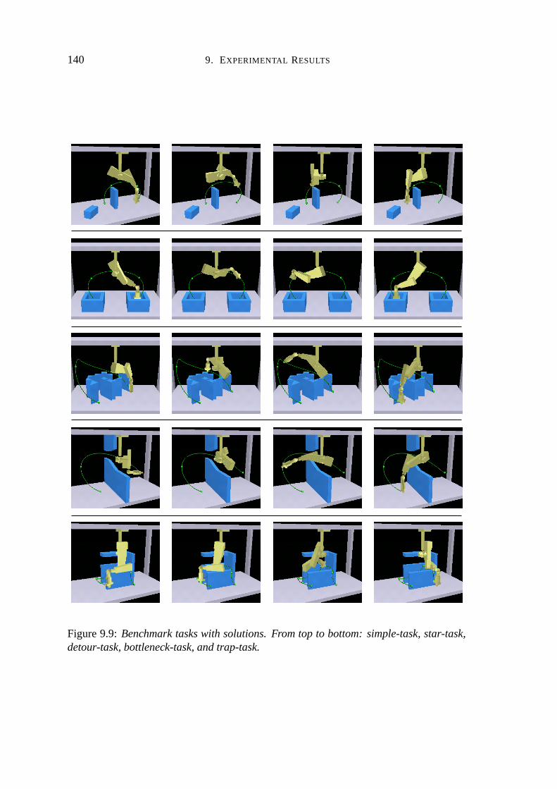
140 9. EXPERIMENTAL RESULTS
Figure9.9: Benchmarktaskswith solutions.Fromtop to bottom: simple-task,star-task,detour-task,bottleneck-task,andtrap-task.

9.2. EXPERIMENTS 141
task). In the third row, the robot hasto find its way over the obstaclesandnot throughtheobstacles(detour-task).In thefourthexample,therobothasto passasmallgapin thewall (bottleneck-task).Thefinal exampleis quitedifficult astherobotnearlygetstrappedin thehorseshoeshapedobstacle(trap-task).Thetravel time for eachtaskis 60 seconds.
Figure 9.9 shows possiblesolutionsto the problems. Again eachrow shows fourpositionsof therobotfor oneproblem.
For thetwo typesof trajectories,thepolynomialpoint-to-pointmotionandthemodi-fiedbang-bangpathmotion,weareinterestedin thecomputingtime. All of thefollowingtestshavebeendonefor bottomup andbestsearch(without randomstartjoint).
Let usnow turn to resultsfor thesimple-task.In Table9.9, the left columnlists theresultsfor thepolynomialtrajectorytypeandtheright showstheresultsfor thebang-bangmotion.
Polynomial Bang-Bang
Bot
tom
-Up stepsize
5 10 20 505 3 Ã 82 2 Ã 93 2 Ã 23 1 Ã 3810 1 Ã 74 2 Ã 14 1 Ã 63 1 Ã 0220 1 Ã 35 1 Ã 65 1 Ã 28 0 Ã 78
prec
isio
n
50 1 Ã 22 1 Ã 00 1 Ã 37 0 Ã 79
stepsize5 10 20 50
5 4 Ã 42 3 Ã 32 2 Ã 08 1 Ã 2910 3 Ã 11 2 Ã 38 1 Ã 55 0 Ã 8820 1 Ã 76 1 Ã 96 1 Ã 31 0 Ã 77
prec
isio
n
50 1 Ã 30 1 Ã 68 1 Ã 46 0 Ã 78
Bes
t
stepsize5 10 20 50
5 9 Ã 42 9 Ã 34 7 Ã 25 6 Ã 1210 7 Ã 43 6 Ã 53 5 Ã 11 4 Ã 6820 6 Ã 91 5 Ã 96 4 Ã 56 3 Ã 98
prec
isio
n
50 6 Ã 96 6 Ã 06 5 Ã 12 2 Ã 13
stepsize5 10 20 50
5 12Ã 10 10Ã 75 8 Ã 23 6 Ã 4310 7 Ã 76 7 Ã 23 5 Ã 34 4 Ã 0620 6 Ã 52 6 Ã 25 4 Ã 55 3 Ã 42
prec
isio
n
50 8 Ã 78 4 Ã 76 3 Ã 68 2 Ã 74
Table 9.9: Time usedto solve the simple-task benchmarkfor a polynomial point-to-point motion(left) andthemodifiedbang-bangpathmotion(right) with searchdirectionbottom-up(top)andbest(bottom).
The planningalgorithmsolved the problemfor all parameterswith an averagetimeof 1 � 80 for thebottomup searchand6 � 26 for takingthebestjoint. In comparisonto ourresults,theBB-methodneeded0 � 06seconds(Intel PentiumII, 266MHz)andtheparallelA � -searchrequiredapproximately2 secondson oneprocessor(Intel Pentium,133MHz,64MByte Main Memory).
The next exampleis the star-task wherethe robot hasto graspfrom one box intoanother. In Table9.10theleft tablesshowstheresultsfor thepolynomialmotion,whereastheright tablespresentthebang-bangtrajectoryresults.
The star-task hasbeensolved by our plannerfor all testedparametervalues. Theaverageplanningtime for thebottom-upsearchwas5 � 70 secondsandfor takingthebestjoint 11� 98. Thecomputationtime for theBB-methodwas0 � 59seconds,andtheparallelA � -searchalgorithm took approximately25 secondson one processorand lessthan 5secondsoneightPC’s.

142 9. EXPERIMENTAL RESULTS
Polynomial Bang-Bang
Bot
tom
-Up stepsize
5 10 20 505 2 Ã 35 2 Ã 40 3 Ã 52 2 Ã 1110 2 Ã 63 2 Ã 26 1 Ã 98 1 Ã 48
prec
isio
n
20 5 Ã 23 4 Ã 21 4 Ã 26 2 Ã 36
stepsize5 10 20 50
5 2 Ã 82 2 Ã 78 1 Ã 80 1 Ã 8410 1 Ã 36 3 Ã 47 2 Ã 11 2 Ã 62
prec
isio
n
20 4 Ã 49 9 Ã 33 53Ã 80 15Ã 23
Bes
t stepsize5 10 20 50
5 19Ã 44 11Ã 62 11Ã 16 8 Ã 7010 13Ã 18 9 Ã 16 7 Ã 82 7 Ã 06
prec
isio
n
20 12Ã 55 8 Ã 55 6 Ã 53 7 Ã 69
stepsize5 10 20 50
5 16Ã 34 8 Ã 18 8 Ã 20 9 Ã 5610 15Ã 41 12Ã 95 10Ã 13 7 Ã 81
prec
isio
n
20 31Ã 16 13Ã 10 24Ã 24 6 Ã 87
Table 9.10: Time usedto solve the star-task benchmarkfor a polynomial point-to-point motion(left) andthemodifiedbang-bangpathmotion(right) with searchdirectionbottom-up(top) andbest(bottom).
The third exampleis thedetour-task. Heretheproblemfor theplanneris to find thepathover theobstacles,insteadof moving right throughtheobstacles.Table9.11givesthecomputingtimesfor thetestedparameters.
Polynomial Bang-Bang
Bot
tom
-Up stepsize
5 10 20 505 33Ã 34 11Ã 44 29Ã 68 12Ã 7910 23Ã 64 23Ã 91 20Ã 65 12Ã 8420 18Ã 44 33Ã 00 68Ã 10 9 Ã 84
prec
isio
n
50 18Ã 83 36Ã 68 15Ã 23 2 Ã 16
stepsize5 10 20 50
5 5 Ã 87 5 Ã 54 44Ã 92 20Ã 9710 7 Ã 85 3 Ã 92 23Ã 27 4 Ã 5620 56Ã 91 64Ã 25 35Ã 12 14Ã 58
prec
isio
n
50 3 Ã 78 3 Ã 38 2 Ã 84 4 Ã 49
Bes
t
stepsize5 10 20 50
5 46Ã 24 40Ã 56 35Ã 87 30Ã 7810 34Ã 61 28Ã 67 33Ã 74 19Ã 7720 26Ã 30 37Ã 27 39Ã 73 17Ã 16
prec
isio
n
50 66Ã 93 102Ã 68 39Ã 85 10Ã 18
stepsize5 10 20 50
5 115Ã 13 34Ã 61 29Ã 93 29Ã 7510 60Ã 31 24Ã 88 21Ã 55 19Ã 8420 52Ã 25 20Ã 97 18Ã 01 14Ã 38
prec
isio
n
50 98Ã 61 14Ã 23 11Ã 62 11Ã 12
Table9.11: Time usedto solve the detour-task benchmarkfor a polynomial point-to-point motion(left) andthemodifiedbang-bangpathmotion(right) with searchdirectionbottom-up(top) andbest(bottom).
Unfortunatelynotall testedparametervaluesresultedin asolution.Therobotmaygetstuckin thelabyrinthif thestepsizeis toosmallor theprecisionvalueis toolarge.(Pleasenotethatif randommovesareallowedthenthesituationimprovesandmoresolutionsarefound.)TheBB-methodrequires0 � 70secondsandtheparallelA � -searchalgorithmtakesabout110secondsononeprocessorandstill 20 secondson eightprocessors.

9.2. EXPERIMENTS 143
Table9.12 shows the resultsfor the bottleneck-taskusing the polynomialpoint-to-point trajectoryon the left side. On theright side,thetimesfor themodifiedbang-bangpathmotioncanbeseen.
Polynomial Bang-Bang
Bot
tom
-Up stepsize
5 10 20 505 148Ã 84 147Ã 04 479Ã 04 140Ã 7210 427Ã 77 82Ã 84 219Ã 42 220Ã 74
prec
isio
n
20 82Ã 59 75Ã 64 97Ã 29 84Ã 57
stepsize5 10 20 50
5 59Ã 76 109Ã 88 35Ã 96 62Ã 6910 82Ã 04 52Ã 16 36Ã 37 102Ã 29
prec
isio
n
20 77Ã 65 388Ã 94 482Ã 07 83Ã 36
Bes
t stepsize5 10 20 50
5 78Ã 20 48Ã 45 40Ã 67 57Ã 5510 51Ã 78 32Ã 99 36Ã 98 46Ã 07
prec
isio
n
20 96Ã 33 105Ã 34 48Ã 29 29Ã 16
stepsize5 10 20 50
5 127Ã 47 62Ã 23 48Ã 13 36Ã 2510 84Ã 76 46Ã 10 36Ã 59 25Ã 67
prec
isio
n20 174Ã 81 84Ã 69 60Ã 45 34Ã 68
Table9.12:Timeusedto solvethebottleneck-taskbenchmarkfor apolynomialpoint-to-point motion(left) andthemodifiedbang-bangpathmotion(right) with searchdirectionbottom-up(top)andbest(bottom).
We observe that the problemdoesnot get solved if the precisionvalueis too large.This is becausetherobothasto find its way throughthesmallgapin thewall. Thesameobservationcanbemadefor thestepsize.If thestepsizeis large,therobotwill missthegapin thewall.
The calculationtime is relatively high comparedwith the resultof the BB-method.In [Baginski,1999], thecomputationtime for this problemis givenas0 � 65 seconds.Toexplain this discrepancy, we would like to mentionthat the BB-methodis, at the timebeing,presumablythebestplannerfor staticenvironments.However, it doesnot takeintoaccountdynamiclimitationsof therobotor moving obstacles.For thesameproblem,theparallelA � -searchin [Worn et al., 1998]needsabout23 secondson oneprocessor(IntelPentium,133MHz,64MByte Main Memory)andabout5 secondson eightPC’s.
To demonstratethe advantagesof our method,we try to comparethe dynamicbe-haviour of the solutionsfound with the BB-methodandwith our method. To this end,we distribute basepointsalongthe pathfound with the BB-method. The overall traveltime is thesameasin our solutions.In Figure9.10on the left sidethesolutionwith theBB-methodandon right sideoneof our solutionscanbeseen(precisionis 10, stepsizeis 20,searchdirectionis bottomup).
Thegreenline representsour solutionandtheredline theoptimisedpathfoundwiththeBB-method.Thepathlengthis optimisedin theconfigurationspace.It showsthatthegreenlines arecloserto the robot’s base.Thereforethe robot needslesstorqueto holdits upperandlower arm. In Figure9.11,thetorqueneededover thetime is depicted.Weonly show thevaluesfor thesecondandthethird joint countingfrom thebase.Thesearethejoints thatneedthemostforcein orderto hold therestof therobot.
Ontheleft side,thevaluesfor thedetour-taskcanbeseen.Theblackcurvesrepresent

144 9. EXPERIMENTAL RESULTS
L2
L3
Figure9.10: Comparisonof trajectoriesfoundwith theBB-methodandour method.Theredouterpathrepresentsthepathcomputedwith theBB-method,thegreeninner trajec-tory is generatedusingour algorithm.
0 10 20 30 40 500
0 � 51 � 01 � 52 � 02 � 5Nm
sec
J2
J3
0 10 20 30 40 500
0 � 51 � 01 � 52 � 02 � 5Nm
sec
J2
J3
Figure9.11: Torqueof the secondand third joint. The left sideshowsthe torquesforthe detour-taskand the right side the torquesof the bottleneck task. Theblack curvesrepresentthevaluesfor our solutionandthegrey curvesthesolutionof theBB-method.
the valuesfor our solution and the grey curves the solutionsof the BB-method. Theuppercurvesgive the valuesof joint two. This is the joint which hasto carry the mostweight. On theright side,thecurvesaregivenfor thebottleneck-task.It is obviousthatour solutionneedslesstorque.This is becauseour trajectoriesbring thecentreof gravityof thelinks nearerto therobot’sbase.
For the last benchmarkexample,computingtimesarenot given in either[Baginski,1999]or in [Worn et al., 1998]. We includeour resultsfor this benchmarkherefor the

9.2. EXPERIMENTS 145
sake of completeness.If we allow no randommovements,this problemis hardto solvefor our planner(its only solvable if the stepsize is large enoughsuchthat the robot isnot caughtin thetrap). For this lastexamplewe allow 10 randommovementsduringtheplanning.Thetimesfor thelastexamplearepresentedin Table9.13.Wehaveonly testedthebottom-upsearchdirection.
PolynomialB
otto
m-U
p stepsize5 10 20 50
5 1152Ã 31 2078Ã 64 479Ã 04 1054Ã 9520 229Ã 69 2145Ã 14 172Ã 47 29Ã 60
prec
isio
n
50 399Ã 67 5150Ã 69 181Ã 46 114Ã 12
Bang-Bang
Bot
tom
-Up stepsize
5 10 20 505 739Ã 02 1254Ã 81 72Ã 05 30Ã 9910 104Ã 48 640Ã 39 38Ã 57 8 Ã 58
prec
isio
n
20 535Ã 40 251Ã 43 104Ã 02 1495Ã 20
Table 9.13: Time usedto solve the trap -task benchmarkfor a polynomial point-to-point motion(left) andthemodifiedbang-bangpathmotion(right) with searchdirectionbottom-up.
Thesebenchmarkresultsreveal thatour plannerhasdifficulties to competewith thefastBB-methodasfar asrunningtime is concerned.But assoonasaspectsof realworldrobotsget important,namelytorqueand force, the solutionsfound by our plannerarebetter. And in situationswhereforce and torqueare critical, the solutionsfound by aplannerthatonly considerscollisionsmaynotevenbetraceable.
Comparedto theparallelA � -searchmethod,our planneris quitegood.Thecomputa-tion timesof ourplannerandthetimesgivenfor theA � -searchmethodaresimilar, takinginto accountthedifferencesin clockrateandnumberof concurrentprocessors.Moreover,theA � -searchplanningapproachis not applicableto higherdimensionalproblems,asitneedsto distributepossibleneighboursin theconfigurationspaceto theavailableproces-sors.In theexperimentsdescribedin [Wornetal.,1998],theconfigurationspacehasbeennormalisedsuchthat theactualnumberof dimensionsis in fact reducedby one. This ispossiblebecausein theabovebenchmarkstheimpactof theoutermostjoint is negligible.
9.2.4 RX90 with a Heavy Hand
In this section,we wantto show anexamplewhereit is not thecollision but thedynamiclimitation of the robot that plays the importantrole. To this end,we took a geometrymodelof theRX90robotof Staubli (seeFigure9.12)andwesetthemassesof therobot’slinks in a very specialway. We madethe handso heavy that thereexist unstablerobotconfigurations,thatis, configurationsthattherobotcannotmaintainbecauseit is notable

146 9. EXPERIMENTAL RESULTS
to compensatefor gravity. In otherwords,in someconfigurations,themaximalpossibletorquesin thesecondandthethird joint aretoosmallto carrytherestof therobot.
1 2 3
4 5
Figure9.12: Initial taskfor theRX90robotwith a heavytop.
Let us take a closerlook at Figure9.12. The robot hasto move its handfrom thebottomto the top. The initial trivial trajectoryis collision freeandwould bevalid if wewouldonly considercollisions.However, whentracingthis trivial trajectory, apositionisreachedwheretherobotholdsitsarmstretchedouthorizontally. Dueto thegivendynamicjoint limits andthe heavy hand,this positioncannotbe hold by the robot’s joints. As aconsequence,theinitial trajectoryis unfree.
Let us take a look at the next two figures. In Figure9.13, a solutioncomputedbyour planneris shown thatusesthemodifiedbang-bangpathmotion. Now therobotusesits own massto accelerateits handand it keepsthe tool closeto its centreof massinorderto reducethetorquesthatit needsto hold its own links. We would expecta similarmovementfrom anathletelifting aheavy dumb-bell.
The sameproblemsolved with the polynomialpoint-to-pointmotion is depictedinFigure9.14.Again theupperarmis keptnearto thecentreof massof therobot.
Wehaverun this taskfor differentstepsizes(1, 5, 10,20,50)andprecisionvalues(1,5, 10,20,50). With thebang-bangpathmotiontheaveragecomputationtimeis 3 secondsandwith the polynomialpoint-to-pointmotion this time is 2 Ä 16 seconds.The taskwassolvedfor all testedparametervalues.

9.2. EXPERIMENTS 147
1 2 3
4 5
Figure9.13:RX90tasksolvedwith a bang-bangpathmotion.
1 2 3
4 5
Figure9.14:RX90tasksolvedwith a polynomialpoint-to-pointmotion.

148 9. EXPERIMENTAL RESULTS
9.2.5 Sliding Door
Thefollowing examplewasintroducedin [Baginski,1999]asa staticexamplewith nar-row passagesandit wasusedfor comparisonswith the randomisedpathplanner(RPP)of ChallouandGini [Challouet al., 1998]. We have extendedthis exampleto a problemwith a time-varyingenvironment(seeFigure9.15)
Figure9.15:Movementof thetime-varyingobstaclesin theslidingdoorenvironment.
In theoriginalexample,theupperbaris fixedin themiddle,asin theupperleft picture.Thelowerbaris fixedquitenearto therobot’sbase,asin thesecondpicturefrom theleftin thetop row. Therobotitself is a six degreesof freedomrobot. In thefigure,theimagesequencefrom left to right andfrom top to bottomshows onecycle of movementof thetime-varyingobstacles.Thecycle repeatsevery80seconds.We let theupperbarbecomea sliding doorcreatinga gapto its left andright in analternatefashion,wheretherobotmayreachthrough.Thecycle of thesecondbar is twice asfastasthecycle of theupperbarandit movesvertically away from therobot’sbasetowardsthesliding doorandbackagain.
Before we presentour test results,we would like to give the exact dimensionsofthis example. We believe that this is a goodbenchmarkfor otherplannersbecausetheunderlyingproblemis not trivial andit is simpleto rebuild. Wewill notgivetheheightoftheobstaclessincetheir heightis not importantaslong they arehigh enoughin orderto

9.2. EXPERIMENTS 149
beanobstaclefor therobot. In Figure9.16thescenecanbeseenfrom above.
2000
1980
190
60
1100
600120
310350
-180 180
Figure9.16:Dimensionsof theslidingdoorenvironment.All valuesaregivenin millime-tresor degrees.
The sceneis mirroredvertically. The inner boundsof the box are1980mm x 1980mm. All robotslinks andjointsareidentical.Theoveralldimensionof onelink is 20mmx 350mmx 20mm. Thedensityis givenby 0.001g/mm2. This resultsin amassof 140gif we assumeanequaldistribution of themass.Thecentreof gravity is in themiddleofthelink, andtheinertiatensoris Izz Å 140Æ 12Ç 202 È 3502 É gmm2 Ê 1433833gmm2. Therobot in the figure is in zeroposition. The minimal andmaximalvaluesthe joints mayhaveare-180and180degrees.(As aconsequence,it is essentialto testfor self-collisionsof therobot.)Themaximaltorquein eachjoint is 0 Ä 07Nm.
Finally, we have to specify the movementsof the two time-varying obstacles.Thelargerbarchangesits positionfrom left to right with thefollowing functiondefinedovertime 250Ä 0sinÇ π Æ 40t É mm and the smallerbar changesits position up and down withË 200Ä 0sinÇ π Æ 20t É mm.
In Figure 9.17, the solution for a task can be seen,where the robot has to moveout of the left gap into the right gap. The start configurationfor the robot’s joints isÌυs Å Ç 13Í 73Í Ë 65Í 11Í Ë 30Í 30É (bottom-top)andthegoalconfigurationis mirrored
Ìυg ÅÇ Ë 13Í Ë 73Í 65Í Ë 11Í 30Í Ë 30É . The durationtime is 40 seconds.For this environment,
we only testedthe modifiedbang-bangtrajectoryandthe searchdirectionbottom-upintherobot’s joints, becausethis combinationturnedout to bethemostsuccessfulone.Tosolve this task,our plannerneededapproximately20 secondswith a precisionvalueof

150 9. EXPERIMENTAL RESULTS
Figure9.17:Solvedtaskwith modifiedbang-bangpathmotion.
10,a stepsizeequalto 50,andanepsilonof 10Î 8.First, the robotwaitsuntil the lower barhasmovedout of its way, beforegettingon
the right side. At theend,the robothasto hurry to reachits goalposition. This is onlypossibleif therobothasenoughtorqueto reachthegoalafterit haswaiteduntil thelowerbaris out of its way.
For thenext test,we kept theprecisionat 10 sincethis appearsto bea goodchoice.With larger valuesthe plannerwill not find its way thoughthe gapsandsmallervaluesresultin a longercomputingtime. If thestepsizeis decreased,thenthecomputingtimeis increased(a stepsizeof 20 resultsin acomputationtimeof 115seconds).
To reducethecapabilitiesof therobot,wechangedthemaximaltorqueto only 10percentof the original one(0.007Nm). Underthis circumstance,no result is found if thestepsizeis too large. For a stepsizeof 20, thecomputingtime is 235seconds.Now therobot’sstrategy changesa little sinceit cannotwait until thebaris outof its way. Instead,the robot tries to fold itself in sucha way that it is small enoughto passthe lower barbeforethebarhasstartedon its wayupwards.
Finally, wewantto analysethesceneusingrandomlychosenstartandgoalconfigura-tions.We let thetorquebetheoriginalvalueagain.For 1000randomlychosentaskswithastartingtimebetween0 and30secondsandagoaltimebetween50and80seconds,weobtainedthefollowing valuesfor astepsizeof 20and50 (seeTable9.14).

9.2. EXPERIMENTS 151
stepsize Count Solved(%) Time(sec) BasePoints
201000 984904 888
96
90 90100 100
0
44.40 45.1236.64 37.30
117.47
4.69 4.734.61 4.66
5.36
501000 984887 871
113
89 89100 100
0
31.71 32.2225.54 26.01
80.13
4.77 4.814.69 4.74
5.38
Table9.14:Resultsfor sliding doorenvironmentwith randomtasks.
We notethat a smallerstepsizesolvesmoretasks,but alsoneedsmorecomputingtime. Apparentlyit takesquite sometime to reachthe decisionthat the taskcannotbesolved. It would beinterestingto know how many of therandomtasksareactuallysolv-able.
9.2.6 DLR Robot with Hand in Asteroid Field
In this lastsectionwe want to show thatour planneris ableto plan in high-dimensionalsearchspaceswith a complex environmentconsistingof a largenumberof time-varyingobstacles.
Therobotis aspacerobotdevelopedfor spacetravel at theDLR (GermanAerospaceCenter)with a high-dimensionalconfigurationspace(Figure9.18). Thefirst threejointsof therobotareprismaticjoints suchthat therobotmaymove alongthex, y, andz-axis.Fromthereto thehandof therobot,sevenrotationaljoints follow to givetherobotlibertyof action. Thehanditself consistsof four fingers.Eachfingerhasfour rotationaljoints,wheretwo of themarelocatedat thebaseof thefinger. With this joint combination,thefingermaymovesidewaysor canbebent.Theothertwo jointsarefor bendingthefingersuchthatanitemcanbegraspedwith thehand.In total, therobothas26 joints.
In additionto therobot,thereareseventeensmallasteroidsin this scenewith varioustrajectories.The taskfor thespacerobot is to graspthewhite objectat a giventime. InFigure9.19,theinitial trajectoryof thetaskcanbeseen.
Therobothasto avoid all theobstacleswhile graspingthewhite ball. In Figure9.19,we have marked all collisions of the initial trajectorywith white arrows. Figure 9.20showsapossiblesolutionfor this task.
The taskwassolved in 30 minutesusinga precisionvalueof 10 anda stepsizeof20. Theepsilonvaluewassetto 0.001.Theplanningtime is quitelong,becausethefinalposition is very closeto the obstaclethat hasto be grasped.Moreover, many collisiontestsarenecessarysincethetime-varyingobstaclesarequitefast.Thepercentageof timeusedfor the torqueandforce rating is about6 percent,for thecollision testit is 39 percent,andfor thecollision rating41 percentwasused.
Thestartandgoalconfigurationsthatwe usedin theabove exampleareparticularlychallenging.To demonstratethis, we generated100randomtasksfor thesameenviron-ment(with identicalobstacletrajectories).In eachof thenew tasks,thestartingtimewassetto 0 andthegoaltime was60,while therestof thestartandgoalconfigurationswere

152 9. EXPERIMENTAL RESULTS
Figure9.18:Thespacerobotwith a high-dimensionalconfigurationspace.

9.2. EXPERIMENTS 153
1 2 3
4 5 6
7 8 9
10 11 12
Figure9.19: Initial trajectoryfor thehigh-dimensionalspacerobot.

154 9. EXPERIMENTAL RESULTS
1 2 3
4 5 6
7 8 9
10 11 12
Figure9.20:Solvedtaskfor thehigh-dimensionalspacerobot.

9.3. SUMMARY 155
chosenat random.Theaveragerunningtime of our planneron thesetaskswas5.3 min-utes(epsilon0.001,stepsizeandprecision20). Noneof therandomtaskshadaninitialfreetrajectory. Fromthese100tasks,63 percentweresolved.Notethatwedo not knowhow many of thetasksareactuallysolvable.If weconsidersolvedtasksonly, thentheav-eragecomputingtimewas4.98min with 5.25basepointson average.For eachunsolvedtask,theplannerneeded5.85min to signalfailureand5.19basepointswerecontainedinthefinal trajectoryonaverage.
9.3 Summary
We have shown in variousexperimentsthatour planningapproachis successfulin mostplanningscenarios.Ourplannerfindstrajectoriesfor robotswith high-dimensionalsearchspacesevenin complex environmentswith narrow freespaceandtime-varyingobstacles.Currently, to thebestof our knowledge,no otherplanningapproachexists,which is ca-pableof deliveringreasonableplanningresultsin suchsettings.A comparisonwith otherplannersis quitedifficult sincemostplannersdonot considertime-varyingenvironmentsor dynamicconstraintsof therobot.As farasbenchmarksin staticenvironmentsarecon-cerned,we have comparedour plannerwith the BB-methodandthe parallelA Ï -searchalgorithm. If the focusis on collisionsonly, thereis no way to improve uponthe BB-method. In comparisonto the A Ï -search,our planneris not too bad, if we take intoaccount,thatwedoour calculationsonly onasingleprocessor.


CHAPTER 10
Conclusion
In this chapterwesummariseour resultsandwetake a look at promisingdirectionsforfuture research on motionplanningin time-varyingenvironments.
10.1 Summary
In this thesis,we have presenteda motionplanningalgorithmfor robotsin time-varyingenvironments. The algorithm finds collision-freetrajectoriesthat respectthe dynamicconstraintsof the robot. Moreover, thealgorithmis ableto handleobstaclesthat move.To our knowledge,this algorithmis thefirst thatplansmotionsin suchageneralsetting.
The main concernof our researchwasto find a general,robust approachto motionplanningthat is capableof dealingwith a high dimensionalsearchspaceanda complexenvironment. The approachshouldbe robust enoughto be adaptableto specificneedsandextendableto handleadditionalconstraints.In our approach,threebasicalgorithmiccomponentsconstantlyinteractto improve aninitial trajectoryuntil a trajectoryis foundthat satisfiessomegiven criteria. The threecomponentsare: a rating componentthatevaluatesagivenexacttrajectoryaccordingto somegivenconstraints,asearchcomponentthatmodifiesa basepoint trajectory, andthirdly, a trajectorygenerationcomponentthatconstructsan exact trajectoryfrom a basepoint trajectory. Sincethe high dimensionalsearchspaceprohibits its full exploration,our plannerusesheuristicsfor a local searchincluding randomisationto escapelocal minima. In contrastto the classicapproachtomotion planning,wherepathplanningandtrajectorygenerationareseparatesuccessivetasks,our approachconsidersbothasa unit. At any time during theplanningprocess,ageometricpathtogetherwith a velocity profile for the robot’s joints is manipulatedandrated.
Eachof the threecomponentsin our approach(rating,search,trajectorygeneration)is adaptableandextendable.Sincethe searchcomponentdoesnot handleexact trajec-toriesdirectly but only basepoints,theplanningprocesscandealwith differenttypesoftrajectoriesby simply adaptingthe trajectorygenerationcomponent.It is evenpossibleto usea different trajectorytype for eachjoint of the robot. This might be necessary

158 10. CONCLUSION
in non-holonomicrobotsor robotswith specialtypesof joints. As trajectorytypes,wehave analysedpoint-to-pointmotionsandpathmotions. For eachtype we have testedpolynomialconnectionbetweenbasepointsanda modifiedbang-bangconnectionwith atrapezoidvelocityprofile. Two importantcriteriafor selectinga motiontypearesmooth-nessandthe locality of changesnecessaryif a singlebasepoint is moved. It turnedoutthatin generalthemodifiedbang-bangpathmotionis agoodcompromisein thatrespect.
Theratingcomponentis responsiblefor determiningthequality of a givenexact tra-jectory. The interfacebetweenrating and searchingis openenoughto handlevariouskindsof ratingcriteria.Our focusin this thesiswasonthemandatoryconstraints,namelyfreedomfrom collision andkeepingthedynamiclimits of therobot.
For collision ratingwe have adaptedandextendedanexisting collision test.Thecol-lision testitself is basedon thewell-known orientedboundingbox method.We have ex-tendedthismethodsuchthata trajectorycannotonly betestedfor freedomfrom collisionwith staticobstaclesbut alsowith time-varyingobstacles.Moreover, we have integrateda ratingof thecollision depthinto the collision test. Sucha rating is crucial in ordertoguidetheplanneroutof acollision. Thesecondratingfunctionconsiderstheviolationofdynamicconstraintsof the robot. Herethe quality of a trajectoryis determinedby howmuchtherobot’s forceandtorquelimits areexceeded.
Other typesof ratingsthat might be of interestreflectoptimisationcriteria suchastotal trajectorytime or energy. Wehave shown how ratingsof mandatoryconstraintsandratingsof optimisationcriteriacanbeintegrated,takinginto accountthattherequirementsof thetwo ratingtypesarequitedifferent.For example,it doesnotmakesenseto optimisea trajectoryfor energy aslongasit is still colliding.
To show theusefulnessof ourapproach,wehaveimplementedourplanningalgorithmwithin thescopeof a robotsimulationsystemandwehavetestedit in differentscenarios.Theresultsthatwe have obtainedarequitepromising.Our plannerbehaveswell in mostsituationsevenin quitecomplex set-upswherethefreeconfigurationspaceis particularlynarrow. A comparisonof our resultswith other algorithmsturnedout to be difficult,sinceat the time being no other implementationsfor motion planningin time-varyingenvironmentsfor arbitrarymanipulatorsexist (to ourknowledge).
10.2 Futur eResearch
We considerour work on motion planningin time-varyingenvironmentsasa first step.Therearestill many openproblemsandthereareseveralpromisingdirectionsfor futureresearchon this topic. Examplesare:planningfor mobilerobots,minimal timeplanning,andreal-timemotionplanning.
A reasonablenext stepwould be to addoptimisationratingsto theoverall trajectoryrating. Minimal time andminimal energy would be particularly interesting. We haveshown how theseratingscouldbe includedin our planningprocess.But theremight beotherwaysof handlingoptimisationcriteria. Onemight be temptedto find a minimaltime trajectoryby doing a bisectionof the goal time, startingwith a randomgoal time.However, this methodis likely to fail in time-varyingenvironmentssinceincreasingthegoal time doesnot necessarilymake it easierto find a trajectory. Thegoalconfiguration

10.2. FUTURE RESEARCH 159
mightnotevenbefreeat thedesiredtime.Anotherinterestingextensionwould beto integratemoremandatoryconstraints(be-
sidesfreedomfrom collisionanddynamiclimits). Considerarobotthatholdsacupfilledwith liquid. Heretheconstraintwouldbethattherobot’s tool is keptwithin acertainori-entationinterval relativeto theworld coordinatesystem.Or considerarobotthatneedstokeepits tool at anexactdistancefrom someobstacle,for example,to weld or paintsomeobject.
A quite interestingdirectionfor further researchis to developmoreinvolvedheuris-tics for moving a basepoint. Onecould switch betweendifferentstrategiesdependingon which of the constraintsis responsiblefor a badrating. This way we might be ableto decreaseplanningtime, sincewe canusemorespecialisedheuristics. For example,if a collision rating is badwe coulddo orthonormalmovementsof the links in thephys-ical world while if torqueand force rating is badwe move the basepoints in the timecoordinate.
At the endof Chapter5, we gave hints on how our approachcan be usedto plantrajectoriesfor mobile robots. It would be interestingto explore this further, andto findsuitabletrajectorytypes,ratings,anddynamicmodelsfor non-holonomicrobottypes.
Anotherextensionwould be to analyseothermorecomplex typesof joint combina-tions,e.g.gripper, soft gripper, or helicoidaljoints (aspresentedin Chapter4). For thesejoint combinationsappropriatedynamicmodelsneedto befoundbut we conjecturethatouralgorithmstill workssincetheplanningitself is donein theconfigurationspace.
Let usnow take a look at moreinvolvedproblemsettings.In our work we have dealtwith the basicmotion planningproblemwherea startanda goal configurationandtwopoints in time aregiven. This settingcould be variedin differentways. First, assumewe aregivena startconfigurationanda fixedstartingtime but the goal configurationistime-varying,that is, our plannercandecidewhenthegoal configurationis reachedbutdependingon the time, the goal configurationchanges.As for an example,consideraconveyor belt with moving workpieces.The robot’s taskis to graspthenext workpiecebut therobotcandecideby itself whento graspit.
Anothervariantwould beto have a goalconfigurationthat is only partially specifiedin theprobleminstance.For example,to graspa workpieceon a conveyer belt, it wouldsuffice to specifythat therobot’s tool musthave a certainpositionin thefinal configura-tion. Theplannercandecideitself how thefinal configurationlooksaslongasthetool isin theright position.
Anotherinterestingproblemextensionis to adda numberof intermediaterobotcon-figurationsto theprobleminstance.Therobotstill needsto reacha goalconfigurationata certaintime but it alsomustreacheachof thegivenintermediateconfigurationsin thegiven order. The interestingpart hereis that the plannercandecideat which points intime theintermediateconfigurationsarereached.
In this work, we have consideredmotion planningin known environments,that is,all obstaclesandtheir trajectoriesareknown in advance.Sometimes,however, only par-tial informationon theenvironmentis availablein thebeginningandinformationaboutobstaclesis gatheredby sensorswhile the robot is moving. It might be worthwhile toevaluatehow our algorithmcanbe adaptedto planningin dynamicenvironments.Onepossibleapproachwouldbeto startplanningwith theinitial information,thento startthe

160 10. CONCLUSION
robot movementandwhenever the environmentchangesin sucha way that the currenttrajectoryis jeopardised,a new trajectoryis plannedand thenexecuted. The above isiterateduntil thegoal is reached.It would benecessaryin eachroundto extrapolatethetrajectoriesof theobstaclesbasedon thesensorinformationgatheredsofar.
Finally, wewould like to pointout thatourapproachis well suitedfor parallelisation.First, sinceour rating is donepiecewise for eachpair of basepoints, the rating for thepiecesmaybedonein parallel. And second,if a trajectorytype is usedwherea modifi-cationof onebasepoint only resultsin local changesto theexact trajectory, thena localsearchto improvethetrajectorycanbeperformedat severalbasepointssimultaneously.

List of Figures
2.1 Classicalarchitectureof trajectoryplanning. . . . . . . . . . . . . . . . 7
3.1 High-levelflowchart of theplanningprocess. . . . . . . . . . . . . . . . 20
4.1 A robotconsistingof six joints andsevenlinks (6-dofrobot). . . . . . . . 284.2 Therooteddirectedtreeof thesix degreeof freedomrobotin Figure4.1 . 294.3 Exampleof a revolutionjoint (left) anda prismaticjoint (right). . . . . . 304.4 Relativepositionof two joints. . . . . . . . . . . . . . . . . . . . . . . . 314.5 Examplesof dependentjoints: gripper (left), softgripper (middle),heli-
coidal joint (right) . . . . . . . . . . . . . . . . . . . . . . . . . . . . . . 324.6 A mobilerobotmodelledwith threejoints. . . . . . . . . . . . . . . . . . 364.7 Movementof a time-varyingobstacleshownin intervalsof fiveseconds.. 374.8 Two dimensionsof the configuration spaceof a 6-dof robot. Here the
dimensionsfor thejoint J5 andthejoint J6 areshown.. . . . . . . . . . . 394.9 Two dimensionsof the configuration spaceof a 6-dof robot. Here the
dimensionsfor thetimeandjoint J6 areshown. . . . . . . . . . . . . . . 40
5.1 Chart of thetrajectorygenerationprocess.. . . . . . . . . . . . . . . . . 465.2 Trajectorydefinedvia six basepoints. . . . . . . . . . . . . . . . . . . . 495.3 Trajectorydefinedvia elevenbasepoints. . . . . . . . . . . . . . . . . . 495.4 Theprofilesfor locationoi Ð j Ç t É , velocitysi Ð j Ç t É , andaccelerationai Ð j Ç t É of
a cubicpolynomial. . . . . . . . . . . . . . . . . . . . . . . . . . . . . . 505.5 Polynomialpoint-to-pointmotionstoppingat each basepoint. Thedotted
rectanglesshowtheallowedareasfor thetrajectory . . . . . . . . . . . . 535.6 Polynomialpathmotionwhenthevelocityis an average of thegradients
in each basepoint. . . . . . . . . . . . . . . . . . . . . . . . . . . . . . 535.7 Polynomialpath trajectorywithout consideration of all basepoints,but
only the local maximaand minima. Thewhole trajectory is inside theallowedarea. . . . . . . . . . . . . . . . . . . . . . . . . . . . . . . . . 55

162 L IST OF FIGURES
5.8 Polynomialpath trajectorywithout consideration of all basepoints,butonly thelocal maximaandminima.Partsof thetrajectoryareoutsidetheallowedarea. . . . . . . . . . . . . . . . . . . . . . . . . . . . . . . . . 55
5.9 Polynomialpath trajectoryconsideringall points. Thewholetrajectorylies insidetheallowedarea. . . . . . . . . . . . . . . . . . . . . . . . . 57
5.10 Polynomialpoint-to-pointtrajectoryconsideringall points,for thesamegivenbasepointsasin thelast figure. . . . . . . . . . . . . . . . . . . . 57
5.11 Insertionanddeletionof basepointsin a polynomialpoint-to-pointtra-jectory. . . . . . . . . . . . . . . . . . . . . . . . . . . . . . . . . . . . 58
5.12 Insertionanddeletionof a basepoint in a polynomialpathtrajectory. . . 595.13 Theprofilesfor value, speed,andaccelerationof a bang-bangtrajectory. 615.14 The path motion without stoppingat each basepoint for a bang-bang
trajectory. . . . . . . . . . . . . . . . . . . . . . . . . . . . . . . . . . . 625.15 Thecorrespondingpoint-to-pointmotionstoppingat each basepoint. . . 645.16 Insertionanddeletionof a basepoint in a bang-bangpathtrajectory. . . 655.17 Mobile robots’trajectories.. . . . . . . . . . . . . . . . . . . . . . . . . 665.18 Mobile robots’trajectoriesinsidetheallowedareas. . . . . . . . . . . . 66
7.1 Twodimensionalexamplefor hierarchical boxplacementwith six triangles. 797.2 Hierarchical treeof the exampleabove. Each noderepresentsoneori-
entedboundingbox. . . . . . . . . . . . . . . . . . . . . . . . . . . . . . 807.3 Projectionof orientedboundingboxontoa vector. . . . . . . . . . . . . . 807.4 Projectionof two trianglesontoa vector. . . . . . . . . . . . . . . . . . . 827.5 Ratingtheamountof collisionof two triangles. . . . . . . . . . . . . . . 837.6 Comparingcollision test: 500 testsper safetydistance, 6504 obstacle
triangles,2494robot triangles,approximately30%of the testsresult incollisionsif safetydistanceis zero. . . . . . . . . . . . . . . . . . . . . . 85
7.7 Four examplesof theratedconfiguration spaceof a 6-dofrobot. Theup-per imagesshowtheconfigurationspacewithouta safetydistance, whilein the lower imagesthere is a safetydistanceof 50. Theconfigurationspaceon the left sideis the sameas in Figure 4.8 and that on the rightsideis thesameasin Figure4.9. . . . . . . . . . . . . . . . . . . . . . . 86
7.8 Safetydistancefor a time-varyingobject. . . . . . . . . . . . . . . . . . 887.9 Safetydistancefor a revolute joint (left) and a prismatic joint (right).
Black line indicatesmiddleposition,dashedlinesextremepositions. . . . 897.10 Exactsafetydistancefor a robot(firstexample).. . . . . . . . . . . . . . 907.11 Exactsafetydistancefor a robot(secondexample). . . . . . . . . . . . . 917.12 Approximatedsafetydistancefor therobotin thefirstexample. . . . . . . 927.13 Approximatedsafetydistancefor therobotin thesecondexample. . . . . 92
8.1 Movementof a basepoint. Left half showsa polynomialpoint-to-pointmotion.Righthalf showsa modifiedbang-bangpathmotion . . . . . . . 106
8.2 Addingabasepointcanworsena trajectory. Lefthalf showsapolynomialpoint-to-pointmotion.Righthalf showsa modifiedbang-bangpathmotion 111

L IST OF FIGURES 163
8.3 Setof five randomtrajectories. Thered trajectoryon the far left is theoriginal one. Each randomtrajectoryhasbeentakenoutof tenrandomlygeneratedtrajectories. . . . . . . . . . . . . . . . . . . . . . . . . . . . 116
8.4 A four stepplanningsequencefor the6 degreesof freedomrobot.. . . . . 1198.5 Thehigh-levelflowchart with parametersthat influencetheplanningpro-
cess. . . . . . . . . . . . . . . . . . . . . . . . . . . . . . . . . . . . . . 120
9.1 Architectureof RobS. . . . . . . . . . . . . . . . . . . . . . . . . . . . . 1249.2 Dimensionsof the2 degreesof freedomexample. . . . . . . . . . . . . . 1289.3 Initial taskfor the two degreesof freedomrobot in a rotatingcube. The
durationof themovementis 25 seconds.. . . . . . . . . . . . . . . . . . 1299.4 Solvedtaskfor thetwodegreesof freedomrobotwith a polynomialpoint-
to-pointmovement. . . . . . . . . . . . . . . . . . . . . . . . . . . . . . 1319.5 Solvedtaskfor the two degreesof freedomrobot with a modifiedbang-
bangpathmotion. . . . . . . . . . . . . . . . . . . . . . . . . . . . . . . 1329.6 Loadingthe machine: a workpieceis movedfrom table oneto the con-
veyor belt . . . . . . . . . . . . . . . . . . . . . . . . . . . . . . . . . . 1369.7 Unloadingthemachine: a workpieceis movedfromtheconveyor belt to
thesecondtable . . . . . . . . . . . . . . . . . . . . . . . . . . . . . . . 1379.8 Benchmark taskswith initial trajectories. From top to bottom: simple-
task,star-task,detour-task,bottleneck-task,andtrap-task. . . . . . . . . 1399.9 Benchmarktaskswith solutions.Fromtop to bottom: simple-task,star-
task,detour-task,bottleneck-task,andtrap-task.. . . . . . . . . . . . . . 1409.10 Comparisonof trajectoriesfoundwith the BB-methodand our method.
Theredouterpathrepresentsthepathcomputedwith theBB-method,thegreeninner trajectoryis generatedusingour algorithm. . . . . . . . . . . 144
9.11 Torqueof thesecondand third joint. Theleft sideshowsthe torquesforthedetour-taskandtheright sidethetorquesof thebottleneck task. Theblack curvesrepresentthevaluesfor our solutionandthegrey curvesthesolutionof theBB-method. . . . . . . . . . . . . . . . . . . . . . . . . . 144
9.12 Initial taskfor theRX90robotwith a heavytop. . . . . . . . . . . . . . . 1469.13 RX90tasksolvedwith a bang-bangpathmotion. . . . . . . . . . . . . . 1479.14 RX90tasksolvedwith a polynomialpoint-to-pointmotion. . . . . . . . . 1479.15 Movementof thetime-varyingobstaclesin theslidingdoorenvironment.. 1489.16 Dimensionsof thesliding door environment.All valuesare givenin mil-
limetresor degrees. . . . . . . . . . . . . . . . . . . . . . . . . . . . . . 1499.17 Solvedtaskwith modifiedbang-bangpathmotion. . . . . . . . . . . . . . 1509.18 Thespacerobotwith a high-dimensionalconfigurationspace. . . . . . . 1529.19 Initial trajectoryfor thehigh-dimensionalspacerobot. . . . . . . . . . . 1539.20 Solvedtaskfor thehigh-dimensionalspacerobot. . . . . . . . . . . . . . 154


List of Tables
8.1 Parametersof thealgorithm. . . . . . . . . . . . . . . . . . . . . . . . . 122
9.1 Valuesusedfor parametersof thealgorithm. . . . . . . . . . . . . . . . . 1279.2 Measurementcategories. . . . . . . . . . . . . . . . . . . . . . . . . . . 1289.3 Time usedto solve the problemfor a modifiedbang-bangpath motion
with searchdirectionbottom-up(epsilon= 10Î 8). . . . . . . . . . . . . . 1309.4 Time usedto solve the problemfor a polynomialpoint-to-pointmotion
with searchdirectionbottom-up(epsilon= 10Î 8). . . . . . . . . . . . . . 1339.5 Resultsfor the2-dof robotin a rotatingcube. . . . . . . . . . . . . . . . 1349.6 Timeusedto solvethemachineloadingtaskfor differentparameterchoices.1369.7 Time usedto solve themachineloadingexamplefor a polynomialpoint-
to-pointmotionwith searchdirectionbottom-up. . . . . . . . . . . . . . 1379.8 Time usedto solve the machineloadingexamplefor a modified bang-
bangpathmotionwith searchdirectionbottom-up. . . . . . . . . . . . . 1389.9 Timeusedto solve thesimple-taskbenchmarkfor apolynomialpoint-to-
point motion (left) andthemodifiedbang-bangpathmotion (right) withsearchdirectionbottom-up(top)andbest(bottom). . . . . . . . . . . . . 141
9.10 Time usedto solve the star-taskbenchmarkfor a polynomialpoint-to-point motion (left) andthemodifiedbang-bangpathmotion (right) withsearchdirectionbottom-up(top)andbest(bottom). . . . . . . . . . . . . 142
9.11 Timeusedto solvethedetour-taskbenchmarkfor apolynomialpoint-to-point motion (left) andthemodifiedbang-bangpathmotion (right) withsearchdirectionbottom-up(top)andbest(bottom). . . . . . . . . . . . . 142
9.12 Timeusedto solvethebottleneck-taskbenchmarkfor apolynomialpoint-to-point motion (left) and the modified bang-bangpath motion (right)with searchdirectionbottom-up(top)andbest(bottom). . . . . . . . . . 143
9.13 Time usedto solve the trap -taskbenchmarkfor a polynomialpoint-to-point motion (left) andthemodifiedbang-bangpathmotion (right) withsearchdirectionbottom-up.. . . . . . . . . . . . . . . . . . . . . . . . . 145
9.14 Resultsfor slidingdoorenvironmentwith randomtasks. . . . . . . . . . 151


List of Algorithms
In thefollowing we first give a listing of theglobalparametersusedin theplanningpro-cess.Thereafterthefunctionsof theplanningalgorithmaredescribed.Thepagenumberafter a function givesthe first appearanceof the function in the text. A moredetaileddescriptioncanbefoundthere.
Parameter Description
co theplanningprocessstopsaftertheratinghasreachedco.δ δ determinesthe minimal time distancebetweentwo consecutive
basepoints.down If down is true, thenthemodificationsof basepointsis performed
top-down alongthe robots’ link topology(startingat the top joint).Otherwisetheoppositeorderis used.
ε ε is greaterthan0 anddetermineswhethera trajectoryhasa betterratingthananothertrajectory.
first If first is true, thenthefirst modificationis chosenthatimprovesa rating.Otherwisethebestof all basepoint movementsis taken.
λ λ determinestheminimal stepsizethatabasepoint is movedin onedirection.
max max is thetotalnumberof randommovementsthatis allowedduringtheplanningprocess.
p p is theprecisionwhich is usedto calculatetheratingsof theexacttrajectory. Highervaluesresultin a lessexactrating.
random If random istrue, thenthebottom-upor top-downsearchin thebasepointdimensionsstartsat a randomlyselecteddimension.

168 L IST OF ALGORITHMS
Algorithm Description
addBasePoint ThefunctionbooladdBasePoint (trajectory Ñ n, trajectory Ñ o,basePoint b) insertsthebasepointb into thetrajectory Ñ o. Theresultingtrajectoryis written to Ñ n. (seepage112)
addSection The function bool addSection (trajectory Ñ n, trajectory Ñ o,int i) addsa new basepoint to Ñ o if the new trajectory Ñ n isbetterthantheoriginal oneaftermoving. (seepage112)
deleteBasePoint ThefunctionbooldeleteBasePoint (trajectory Ñ n, trajectoryÑ o, int i) deletesthe i-th basepoint. Theresultingtrajectoryiswritten to Ñ n. (seepage114)
deleteSection The function bool deleteSection (trajectory Ñ n, trajectoryÑ o, int i) deletesthe i-th basepoint in Ñ o if thenew trajectoryÑ n is betterthantheoriginaloneaftermoving. (seepage113)generateList The function list generateList () generatesa list depending
on the searchstrategy (bottom-up,top-down, random). Theelementsin thelist arethepossiblemovementsfor abasepoint.(seepage109)
getMaxMovement The function doublegetMaxMovement (trajectory Ñ , doublets, doubletg) returnsthemaximaldistancebetweenany refer-encepoint on the robot (threefor eachlink) at time ts andtg.(seepage72)
getSafetyDist ThefunctiondoublegetSafetyDist (trajectoryT, doublets,doubletg) returnsthemaximalsafetydistancesneededto en-surefreedomfrom collision in the time interval Ò ts Í tg Ó . (seepage92)
getTestPosition ThefunctiondoublegetTestPosition (trajectoryT, doublets, doubletg) returnsthe positionof the robot suitablefor thecollision test.(seepage93)
listFirst The function listElementlistFirst (list l ) returnsthe firstelementof thelist l . (seepage107)
listInsert Thefunction list listInsert (list l , int j) insertsthemovingpossibilitiesfor dimensionj atthefrontof list l . (seepage107)
listNext Thefunction listElementlistNext (listElemente) returnstheelementafterelemente. (seepage107)
listReadTupel The function int listReadTupel (listElemente, int i) readsthe i-th elementof tuplee. (seepage107)
listRemove The function list listRemove (list l , int j) removesall ele-mentsof dimension j from the list and returnsthe new list.(seepage107)
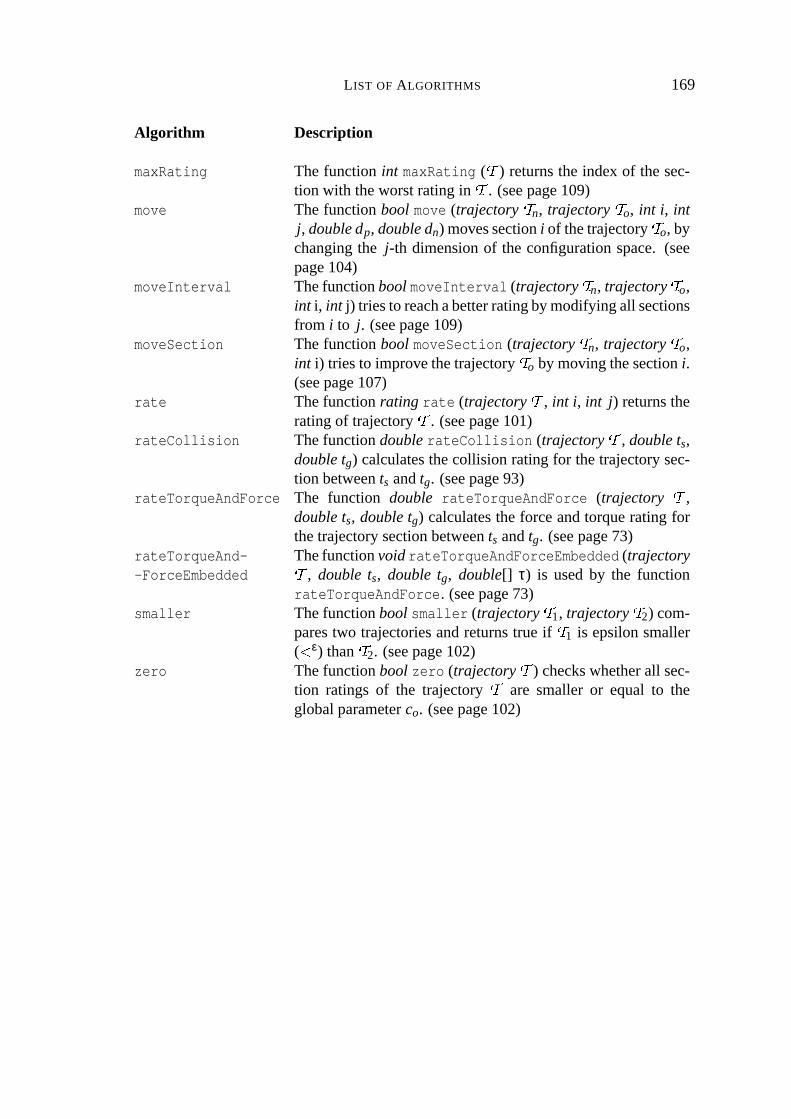
L IST OF ALGORITHMS 169
Algorithm Description
maxRating Thefunction int maxRating ( Ñ ) returnsthe index of thesec-tion with theworstratingin Ñ . (seepage109)
move Thefunctionbool move (trajectory Ñ n, trajectory Ñ o, int i, intj, doubledp, doubledn) movessectioni of thetrajectoryÑ o, bychangingthe j-th dimensionof the configurationspace.(seepage104)
moveInterval ThefunctionboolmoveInterval (trajectory Ñ n, trajectory Ñ o,int i, int j) triesto reachabetterratingbymodifyingall sectionsfrom i to j. (seepage109)
moveSection Thefunctionbool moveSection (trajectory Ñ n, trajectory Ñ o,int i) triesto improvethetrajectory Ñ o by moving thesectioni.(seepage107)
rate Thefunctionratingrate (trajectory Ñ , int i, int j) returnstheratingof trajectory Ñ . (seepage101)
rateCollision ThefunctiondoublerateCollision (trajectory Ñ , doublets,doubletg) calculatesthecollision ratingfor thetrajectorysec-tion betweents andtg. (seepage93)
rateTorqueAndForce The function double rateTorqueAndForce (trajectory Ñ ,doublets, doubletg) calculatestheforceandtorquerating forthetrajectorysectionbetweents andtg. (seepage73)
rateTorqueAnd--ForceEmbedded
ThefunctionvoidrateTorqueAndForceEmbedded (trajectoryÑ , doublets, doubletg, double[] τ) is usedby the functionrateTorqueAndForce. (seepage73)
smaller Thefunctionboolsmaller (trajectory Ñ 1, trajectory Ñ 2) com-parestwo trajectoriesandreturnstrue if Ñ 1 is epsilonsmaller( Ô ε) than Ñ 2. (seepage102)
zero Thefunctionboolzero (trajectory Ñ ) checkswhetherall sec-tion ratings of the trajectory Ñ are smaller or equal to theglobalparameterco. (seepage102)


List of Symbols
Whatfollows is a list of symbolstogetherwith shortdescriptions.If thereis a definitionor a detaileddescriptionfor the symbol in this work, thenthe pagenumberis given aswell. By convention,A, B, andC arebooleanmatrices.Vectorsaredenotedby Greekorsmallletterswith anarrow on top (
Ìω). The i-th valueof somevector
Ìω is denotedby ωi .
Symbol DescriptionÕ Thescalarproductbetweentwo vectorsisÌv Õ Ì
w Å�Ö Ìv Ö~Ö Ìw Ö cosφ, whereφis theanglebetweenthetwo vectors.Ö Ìv Ö Thelengthof avector
Ìv is thesquarerootof thesumoverall squaresof
thecomponentsÖ Ìv Ö�Å$× v21È v2
2È#Ø�Ø�Ø2È v2
n.
A Ù B The Booleanproductof the BooleanmatricesA and B. (seeDefini-tion 4.2onPage29)
Bi The Booleanpower of the Booleanmatrix B. (seeDefinition 4.3 onpage29)
A Ú B TheBooleanunionof theBooleanmatricesA andB. (seeDefinition4.4on page29)
BÏ The transitive closureof the Booleanmatrix B. (seeDefinition 4.5 onpage30)
BÏ The modified transitive closureof the Booleanmatrix B representingthe topologyof the robot andthe dependency functions. (seeDefini-tion 4.11onpage35)
λ j Thetypeof joint Jj is determinedby λ j . (seeEquation4.5onpage31)Ìυ Thejoint vectorof therobot,representingthejoint positions.(seeDef-
inition 4.7on page33)υ j Thevalueof the j-th joint of therobot. (seeDefinition4.7onpage33)υmin
j , υmaxj Theminimalor maximalvaluethe j-th joint of therobotmayhave. (see
Definition4.7onpage33)

172 L IST OF SYMBOLS
Symbol DescriptionÌυd The dynamicjoint configuration
Ìυd Å Ç Ìυω Í Ìυσ Í Ìυα
É of the robot. (seeDefinition4.16onpage41)Ì
υω Thepositionpartof therobot’sdynamicconfigurationÌυ; oftenwedrop
theω andwrite onlyÌυ. (seeDefinition4.16onpage41)Ì
υσ Thevelocity part of the robot’s dynamicconfigurationÌυ. (seeDefini-
tion 4.16onpage41)Ìυα Theaccelerationpartof therobot’sdynamicconfiguration
Ìυ. (seeDef-
inition 4.16on page41)Ìτ The currentforcesand torquesin the joints of the robot. (seeChap-
ter4.4on page39)Ìϑ Theconfigurationvectorof therobotextendedby thetime. (seeDefini-
tion 4.13onpage38)ÌσOi Themaximalspeedvectorof obstacleOi . (seeChapter4.2on page36)θmax
j Themaximaltorqueor forcethe j-th joint of therobothas.(seeChap-ter4.1.1onpage30)Ì
ω Theconfigurationvectorof therobot. (seeDefinition4.7on page33)ωi The valueof dimensioni of the configuration. (seeDefinition 4.7 on
page33)Ìωi The configurationvector of the i-th basepoint. (seeChapter5 on
page45)B The boolean Ç n È 1É£Û Ç n È 1É matrix describingthe topology of the
robot. (page27)Ìbi Thei-th basepoint
Ìbi Å Ç Ìωi Í ti É of abasepoint trajectory. (seeChapter5
onpage45)caÜ
o The collision valuefor the trianglea in the environmentbasedon theorientationvector
Ìo (page83).
Cl Thecollision valuefor thelink Ll in theenvironmentbasedon theori-entationvector
Ìol of thelink (page84).
C Ç Ìυ Í t Í d É Thecollision valuefor therobot in positionÌυ at time t with safetydis-
tanced. (page84).ÝMÞConfigurationspacecontainingall valid configurations. (seeDefini-tion 4.7on page33)ÝMÞ
c Configurationspacecontainingall colliding time configurations.(seeChapter4.3on page38)ÝMÞ
f Configurationspacecontainingall freetimeconfigurations.(seeChap-ter4.3on page38)ÝMÞ
t Configurationspacecontainingall valid configurationsextendedby thedimensionof thetime. (seeDefinition4.13onpage38)
d Ç j É Index dependency function returningthe dimensionof joint Jj in theconfigurationspace.(seeDefinition4.6onpage33)

L IST OF SYMBOLS 173
Symbol Description
0D j The homogeneoustransformationmatrix representingthe location ofjoint Jj in theworld. (seeChapter4.1.1on page30)
iD j Thehomogeneoustransformationmatrix from thecoordinatesystemofjoint Jj to joint Ji . (seeChapter4.1.1on page30)
DOi Thehomogeneoustransformationmatrix describingthelocationof thecoordinatesystemof obstacleOi . (seeChapter4.2onpage36)
jE Thehomogeneoustransformationmatrixof joint Jj from thejoint’sco-ordinatesystemin zeropositionto theactualposition.(page30)
f j Ç xÉ Valuedependency functionreturningthevalueof joint Jj if thevalueintheconfigurationspaced Ç j É is x. (seeDefinition4.6onpage33)
gi Positionof centreof gravity of link Li relative to thecoordinatesystemof joint Ji . (seeChapter4.1.2on page35)
Ii The3 Û 3 inertiatensormatrixof link Li relativeto thecentreof gravityof link Li . (seeChapter4.1.2on page35)ßSetof all joints J1 Í�Ä�Ä�Ä2Í Jn of therobot. (seeChapter4.1on page27 andChapter4.1.1on page30)ß pj
j Setof previousjoints of joint Jj . (seeDefinition4.8onpage34)ß njj Setof next jointsof joint Jj . (seeDefinition4.9onpage34)ß nlj Setof next links of joint Jj . (seeDefinition4.10on page34)
Ji The i-th joint in thejoint setß
. (seeChapter4.1on page27 andChap-ter4.1.1onpage30)àSetof all links L0 Í�Ä�Ä�Ä�Í Ln of therobot. (seeChapter4.1on page27 andChapter4.1.2on page35)à pj
j Setof previousjoints of link L j . (seeDefinition4.12on page35)Li The i-th link in the link set
à. (seeChapter4.1 on page27 andChap-
ter4.1.2onpage35)M M is a function á 3n â á n witch takesa dynamicconfiguration
Ìυd and
returnsthe forceor torquevaluesÌτ for eachjoint. (seeChapter4.4 on
page39)mi Themassof link Li . (seeChapter4.1.2on page35)ã
Setof all obstaclesO1 Í�Ä�Ä�Ä2Í Oo of theenvironment.(seeChapter4.2onpage36)
Oi The i-th obstaclein theenvironment.(seeChapter4.2onpage36)oi Ç t É Thetime-varyinglocationof obstaclei. (seeChapter4.2on page36)p Ç j É Functionreturningthe index of the previous link or the previous joint
of thelink L j or thejoint Jj respectively. (seeEquation4.3on page30)0p j The position of the coordinatesystemof joint Jj in the world. (see
Chapter4.1.1on page30)i p j Thepositionof thecoordinatesystemof joint Jj relativeto joint Ji . (see
Chapter4.1.1on page30)

174 L IST OF SYMBOLS
Symbol Description
0Rj The3 Û 3 rotationmatrixpartrepresentingtherotationof joint Jj in theworld. (seeChapter4.1.1on page30)
iRj The3 Û 3 rotationmatrix from thecoordinatesystemof joint Jj to jointJi . (seeChapter4.1.1on page30)äIs a tupleof threeelementsÇ ß Í à Í BÉ . Thefirst is thesetof joint
ß, the
secondis thesetof linksà
, andthethird is thebooleanÇ n È 1ÉMÛ Ç n È1É matrix B describingthe topologyof the robot. (seeChapter4.1 onpage27)
Si TrajectorysectionbetweenÌbi Î 1 and
Ìbi . (page45)Ñ O Thehierarchicalrepresentationof all trianglesof anobjectO in anori-
entedboundingbox tree(page79).)T Ç t É Functionof thetimedescribingthetrajectoryin theconfigurationspace
dimension.(seeChapter4.4on page39)TD Ç t É Functionof the time describingthe trajectoryin the real robot joints
returningtheposition,velocity, andaccelerationin thejoints. (seeDef-inition 4.16onpage41)
Ti Ç t É Functionof the time describingthe trajectoryin the i-th dimensionoftheconfigurationspacedimension.(seeChapter4.4on page39)
T Ç t É Functionof thetime describingthefirst derivationsof thetrajectoryintheconfigurationspacedimension.(seeChapter4.4on page39)
Ti Ç t É Functionof the time describingthe first derivationof the trajectoryinthe i-th dimensionof the configurationspacedimension. (seeChap-ter4.4onpage39)
T Ç t É Functionof thetime describingthesecondderivationsof thetrajectoryin theconfigurationspacedimension.(seeChapter4.4onpage39)
Ti Ç t É Functionof the time describingthesecondderivationof the trajectoryin the i-th dimensionof theconfigurationspacedimension.(seeChap-ter4.4onpage39)

Bibliography
Boris Baginski. Local motion planningfor manipulatorsbasedon shrinkingandgrow-ing geometrymodels. In Proceedingsof the1996IEEE InternationalConferenceonRoboticsandAutomation(ICRA’96), pages3303–3308,Minneapolis,Minnesota,April1996a.
BorisBaginski.TheZ3-methodfor fastpathplanningin dynamicenvironments.In M.H.Hamza,editor, Proceedingsof theIASTEDConferenceonApplicationsof Control andRobotics, pages47–52,Orlando,Florida, January1996b.IASTED Acta Press,Ana-heim,Calgary, Zurich.
Boris Baginski. Efficient dynamiccollision detectionusingexpandedgeometrymodels.In Proceedingsof theIEEE/RSJ/GIInternationalConferenceonIntelligentRobotsandSystems(IROS’97), pages1714–1719,Grenoble,France,September1997.
Boris Baginski. Motion Planning for Manipulators with Many Degreesof Freedom-TheBB-Method. Number195 in DISKI (Dissertationenzur KunstlichenIntelligenz).Infix-Verlag,SanktAugustin,1999.
Gill Barequet, Matthew Dickerson, and David Eppstein. On triangulating three-dimensionalpolygons. ComputationalGeometry:Theoryand Applications(CGTA),10(3):155–170,June1998.
JeromeBarraquand,LydiaKavraki, Jean-ClaudeLatombe,Tsai-YenLi, Rajeev Motwani,andPrabhavanRaghavan.A randomsamplingschemefor pathplanning.InternationalJournal of RoboticsResearch, 16(6):759–774,1997.
JeromeBarraquand,BrunoLanglois,andJean-ClaudeLatombe.Robotmotionplanningwith many degreesof freedomanddynamicconstraints.In H. Miura andS. Arimoto,editors,RoboticsResearch, volume5, pages435–444.MIT Press,1990.

176 BIBLIOGRAPHY
Jerome Barraquand,Bruno Langlois, and Jean-ClaudeLatombe. Numericalpotentialfield techniquesfor robot path planning. IEEE Transactionson Systems,Man andCybernetics, 22(2):224–241,March1992.
JeromeBarraquandandJean-ClaudeLatombe.A Monte-Carloalgorithmfor pathplan-ning with many degreesof freedom. In Proceedingsof the 1990IEEE InternationalConferenceon Roboticsand Automation(ICRA’90), pages1712–1717,Cincinnati,Ohio,May 1990.
NorbertBeckmann,Hans-PeterKriegel, Ralf Schneider, andBernhardSeeger. TheRÏ -tree: an efficient robust accessmethodfor pointsandrectangles.In HectorGarcia-Molina andH.V. Jagadish,editors,Proceedingsof the 1990ACM SIGMODInterna-tional Conferenceon Managementof Data, pages322–331,Atlantic City, NJ, May1990.
JamesE. Bobrow, Steven Dubowsky, andJ.S.Gibson. Time-optimalcontrol of roboticmanipulatorsalongspecifiedpaths. InternationalJournal of RoboticsResearch, 4(3):3–17,1985.
Rodney A. Brooks. Solvingthefind-pathproblemby goodrepresentationof freespace.IEEE Transactionson Systems,Man, and Cybernetics, SMC-13(3):190–197,March1983.
Rodney A. BrooksandTomasLozano-Perez. A subdivision algorithmin configurationspacefor findpathwith rotation.IEEETransactionsonSystems,Man,andCybernetics,15:224–233,1985.
CharlesE. Buckley. A foundationfor the“flexible–trajectory”approachto numericpathplanning. InternationalJournal of RoboticsResearch, MIT Press, 8(3):44–64,June1989.
FrankBuschmann,RegineMeunier, HansRohnert,PeterSommerlad,andMichaelStal.Pattern-OrientedSoftware Architecture: A Systemof Patterns. JohnWiley andSons,Chichester, New York, Brisbane,Toronto,Singapore,1996.
Maik Buttelmann,Martin Kieren, and Boris Lohmann. TrajektoriengenerierungundBahnregelungfur nichtholonome,autonomeFahrzeuge.In AutonomeMobile Systeme1999, volume 15 of Informatik aktuell, pages303–312.GuntherSchmidtand UweHanebeckandFranzFreyberger, November1999.
JohnF. Canny. The Complexity of RobotMotion Planning. MIT Press,Cambridge,Massachusetts,1988.
DanielChallou,DanielBoley, MariaGini, Vipin Kumar, andCurtisOlson.Parallelsearchalgorithmsfor robotmotionplanning. In KamalK. GuptaandAngel P. del Pobil, ed-itors, Practical Motion Planningin Robotics:CurrentApproachesandFuture Direc-tions, pages115–131.JohnWiley andSons,1998.

BIBLIOGRAPHY 177
PangC. ChenandYongK. Hwang.SANDROS:A motionplannerwith performancepro-portionalto taskdifficulty. In Proceedingsof the1992IEEE InternationalConferenceon RoboticsandAutomation(ICRA’92), pages2346–2353,Nice,France,May 1992.
PangC. ChenandYongK. Hwang. Performanceof theSANDROS planner. Technicalreport,SandiaNationalLaboratories,Albuquerque,New Mexico, April 1996.
JamesJ.Craig. Introductionto Robotics.MechanicsandControl. Addison-Wesley, 1986.
JacquesDenavit andRichardS.Hartenberg. A kinematicnotationfor lower-pair mecha-nismsbasedon matrices.ASMEJournal of AppliedMechanics, 22(77):215–221,June1955.
BruceR. Donald,PatrickXavier, JohnCanny, andJohnReif. Kinodynamicmotionplan-ning. Journalof theACM, 40(5):1048–1066,November1993.
BruceR. DonaldandPatrick G. Xavier. Provably goodapproximationalgorithmsforoptimal kinodynamicplanningfor cartesianrobotsandopenchainmanipulators.Al-gorithmica, 14(6):480–530,December1995a.
BruceR. DonaldandPatrickG. Xavier. Provablygoodapproximationalgorithmsfor op-timal kinodynamicplanning:Robotswith decoupleddynamicsbounds.Algorithmica,14(6):443–479,December1995b.
G. DuelenandC. Willnow. Path planningof transfermotionsfor industrial robotsbyheuristicallycontrolleddecompositionof the configurationspace. In ProceedingsoftheEuropeanRoboticsandIntelligentSystemConferenceEURISCON’91, pages217–224,Corfu,Greece,June1991.
Martin Eldracher. Planung kinematischer Trajektorien fur Manipulatoren mit Hilfevon Subzielenund neuronalenNetzen. Number 111 in DISKI (DissertationenzurKunstlichenIntelligenz).Infix-Verlag,Sankt-Augustin,1996.
Martin EldracherandPeterBaumann.Kinematicpathplanningfor manipulatorsin dy-namicenvironmentsusingadaptiveneuralmodelsandneuralsubgoalgeneration.Tech-nical report,TechnischeUniversitatMunchen,Munich,Germany, 1995.
MichaelErdmannandTomasLozano-Perez.On multiple moving objects.Algorithmica,2, 1987.
PaoloFiorini. RobotMotion PlanningAmongMoving Obstacles. PhDthesis,Universityof California,LosAngeles,CA, 1995.
PaoloFiorini andZvi Shiller. Motion planningin dynamicenvironmentsusingvelocityobstacles.TheInternationalJournal of RoboticsResearch, 17(7):760–772,July1998.
SteveFortune.Voronoidiagramsanddelaunaytriangulations.In D.-Z. Du andF. Hwang,editors,Computingin EuclideanGeometry, volume4 of LectureNotesSeriesonCom-puting, pages193–233.World ScientificPublishers,1992.

178 BIBLIOGRAPHY
BernhardGlavina. Planungkollisionsfreier Bewegungenfur Manipulatorendurch Kom-binationvonzielgerichteterSucheundzufallsgesteuerterZwischenzielerzeugung. PhDthesis,TechnischeUniversitatMunchen,February1991.
StefanGottschalk,Ming C.Lin, andDineshManocha.OBBTree:A hierarchicalstructurefor rapid interferencedetection. ComputerGraphics: ProceedingACM SIGGRAPH,pages171–180,1996.
Kamal K. Gupta. Overview andstateof the art. In Kamal K. GuptaandAngel P. delPobil,editors,PracticalMotionPlanningin Robotics:CurrentApproachesandFutureDirections, pages3–8.JohnWiley andSons,1998.
DanHalperin,LydiaKavraki, andJean-ClaudeLatombe.Robotics.In JacobE.GoodmanandJosephO’Rourke, editors,Handbookof Discreteand ComputationalGeometry,pages755–778.CRCPress,BocaRatonNew York, July1997.
Greg Heinzinger, Paul Jacobs,JohnCanny, andBred Paden. Time-optimaltrajectoriesfor a robot manipulator:A provably goodapproximationalgorithm. In Proceedingsof the 1990IEEE InternationalConferenceon Roboticsand Automation(ICRA’90),pages150–156,1990.
DomenikHenrich,ChristianWurll, andHeinz Worn. 6 dof pathplanningin dynamicenvironments- a parallelon-line approach. In Proceedingsof the 1998IEEE Inter-nationalConferenceon RoboticsandAutomation(ICRA’98), pages330–335,Leuven,Belgium,May 1998.
Dominik HenrichandXiaoqing Cheng. Fastdistancecomputationfor on-line collisiondetectionwith multi-armrobots. In Proceedingsof the1992IEEE InternationalCon-ferenceon RoboticsandAutomation(ICRA’92), pages2514–2519,Nice,France,May1992.
ShigeoHirose. Biologically inspiredrobots: Snake-like Locomotors andManipulators.OxfordSciencePublications,1993.
GerdHirzinger, Jorg Butterfass,MarkusGrebenstein,MatthiasHahnle,IngoSchafer, andNorbertSporer. Robonautsneedlight-weightarmsandarticulatedhands.In Proceed-ingsof the6thESAWorkshopon ASTRA, Noordwijk, Netherlands,2000.
ChristophM. Hoffmann. Solid modeling. In JacobE. GoodmanandJosephO’Rourke,editors,Handbookof Discrete and ComputationalGeometry, pages863–880.CRCPress,BocaRatonNew York, July1997.
JohnE. Hopcroft,DeborahA. Joseph,andSueH. Whitesides.On themovementof therobot armsin 2-dimensionalboundedregions. SIAM Journal on Computing, 14(2):315–333,1985.
JohnE. Hopcroft,JacobT. Schwartz,andMicha Sharir. Efficient detectionof intersec-tionsamongspheres.InternationalJournalof RoboticsResearch, 2(4):77–80,1983.

BIBLIOGRAPHY 179
JohnE. HopcroftandJeffrey D. Ullman. Introductionto automatatheory, languagesandcomputation. Addison-Wesley, 1979.
ManfredHusty, Adolf Karger, HansSachs,andWaldemarSteinhilper. KinematikundRobotik. Springer-VerlagBerlin Heidelberg New York, 1997.
YongK. Hwang.Completenessvs.efficiency in realapplicationsof motionplanning.InKamalGuptaandAngel P. del Pobil, editors,Practical Motion Planningin Robotics,WorkshopWT2 at the IEEE International Conferenceon Roboticsand Automation,Minneapolis,Minnesota,April 1996.
Yong K. HwangandN. Ahuja. Grossmotion planning– A survey. ACM ComputingSurveys, 24(3):219–291,September1992.
Paul Jacobs,Greg Heinzinger, JohnCanny, andBradPaden. Planningguaranteednear-time-optimaltrajectoriesfor a manipulatorin a clutteredworkspace. In ProceedingInternationalWorkshopon SensorialIntegration for Industrial Robots:ArchitecturesandApplications, pages162–167,November1989.
K. Kant andSteve W. Zucker. Towardsefficient trajectoryplanning: the path-velocitydecomposition.TheInternationalJournalof RoboticResearch, 5(3):72–89,1986.
K. Kant andSteve W. Zucker. Planningcollision free trajectoriesin time-varying en-vironments: a two level hierarchy. In Proceedingsof the 1988 IEEE InternationalConferenceon Roboticsand Automation(ICRA’88), pages1644–1649,Raleigh,NC,1988.
Lydia Kavraki, Mihail N. Kolountzakis,andJean-ClaudeLatombe. Analysis of prob-abilistic networks for pathplanning. In Proceedingsof the 1996IEEE InternationalConferenceonRoboticsandAutomation, pages3020–3025,Minneapolis,MN, 1996a.
Lydia Kavraki andJean-ClaudeLatombe. Randomizedpreprocessingin configurationspacefor fastpathplanning.In Proceedingsof the1994IEEEInternationalConferenceon RoboticsandAutomation(ICRA’94), pages2138–2145,1994a.
Lydia Kavraki and Jean-ClaudeLatombe. Randomizedpreprocessingin configura-tion spacefor fast path planning: Articulated robots. In Proceedingsof the 1994IEEE/RSJ/GIInternationalConferenceon IntelligentRobotsandSystems(IROS’94),pages1764–1771,Munich,Germany, 1994b.
Lydia Kavraki, PetrSvestka,Jean-ClaudeLatombe,andMark Overmars. Probabilisticroadmapsfor pathplanningin high-dimensionalconfigurationspaces.IEEE Transac-tionsonRoboticsandAutomation, 12(4):566–580,1996b.
Otto Kerne,JosephMaurer, JuttaSteffens,ThomasThode,andRudolf Voller. ViewegMathematikLexikon. FriedrichVieweg & Sohn,BraunschweigWiesbaden,1988.
RobertKindel, David Hsu,Jean-ClaudeLatombe,andStephenRock. Kinodynamicmo-tion planningamidstmoving obstacles.In Proceedingsof the2000IEEEInternationalConferenceonRoboticsandAutomation(ICRA’00), 2000.

180 BIBLIOGRAPHY
Jean-ClaudeLatombe.RobotMotionplanning. Kluwer AcademicPublishers,4thedition,1996.
C. LaugierandF. Germain.An adaptivecollision-freetrajectoryplanner. In Proceedingsof theInternationalConferenceonAdvancedRobotics, Tokyo, Japan,1985.
B.H. LeeandY.P. Chien. Time-varyingobstacleavoidancefor robotmanipulators:Ap-proachesanddifficulties. In Proceedingsof the IEEE 1987InternationalConferenceonRoboticsandAutomation(ICRA’87), 1987.
TomasLozano-Perez. Automatic planningof manipulatortransfermovements. IEEETransactionsSystems,Man andCybernetics, SMC-11:681–689,1981.
TomasLozano-Perez.Spatialplanning:A configurationspaceapproach.IEEE Transac-tionson Computers, 32:108–120,1983.
JohnsonY.S.LuhandChyuanS.Lin. Optimalpathplanningfor mechanicalmanipulators.ASMEJournalof DynamicSystems,MeasurementandControl, pages142–151,1981.
JohnsonY.S.LuhandMichaelW. Walker. Minimum-timealongthepathfor amechanicalarm. In Proceedings1977IEEE ConferenceDec. Contr, volume2, pages755–759,1977.
Begona Martınez-Savador, Angel P. del Pobil, and Miguel Perez-Francisco.Very fastcollision detectionfor practicalmotionplanningpart i: Thespatialrepresentation.InProceedingsof the1998IEEE InternationalConferenceon RoboticsandAutomation(ICRA’98), pages624–629,Leuven,Belgium,May 1998.
Brain Mirtich. Impulse-basedDynamicSimulationof Rigid BodySystems. PhD thesis,Universityof California,December1996.
Akira Mohri, Xiang D. Yang,andMotoji Yamamoto.Collision free trajectoryplanningfor manipulatorsusingpotentialfunction. In Proceedingsof the 1995IEEE Interna-tional ConferenceonRoboticsandAutomation(ICRA’95), pages3069–3074,1995.
J.J.MurrayandC.P. Neumann.Linearizationandsensitivity modelsof theNewton-Eulerdynamicrobotmodel.ASMEJournalof DynamicSystems,Measurement,andControl,108:272–276,September1986.
Nils J.Nilsson.A mobileautomaton:An applicationof artificial intelligencetechniques.In D.E. Walker andL.M. Norton, editors,Proceedingsof the 1st InternationalJointConferenceon Artificial Intelligence, pages509–520,Washington,D.C., May 1969.W. Kaufmann.
Colm O’DunlaingandCheeK. Yap. A retractionmethodfor planningthe motion of adisc. Journalof Algorithms, 6, 1982.
J.K. Ousterhout. Tcl und Tk: Entwicklung grafischer Benutzerschnittstellenfur dasXWindowsSystem. Addision-Wesley, Deutschland,1995.

BIBLIOGRAPHY 181
Hiroaki Ozaki and Chang-junLin. Optimal b-spline joint trajectory generationforcollision-freemovementsof a manipulatorunderdynamicconstraints.In Proceedingsof the 1996IEEE InternationalConferenceon Roboticsand Automation(ICRA’96),pages3592–3597,Minneapolis,Minnesota,April 1996.
HongjunPu. Novel algorithmstowards systematic,generalizedand compactrecursivegenerationandcomputationof thecompleterobotdynamicswith realisationaspectsinCAD-systems. Number687 in VereinDeutscherIngenieure:FortschrittberichteVDI.VDI-Verlag,Dusseldorf,1998.
CaigongQin andDominik Henrich. Pathplanningfor industrialrobotarms- a parallelrandomizedapproach.In Proceedingsof the InternationalSymposiumon IntelligentRoboticSystems(SIRS’96), pages65–72,July1996.
SeanQuinlan. Efficient distancecomputationbetweennon-convex objects. In Pro-ceedingsof the 1994 IEEE International Conferenceon Roboticsand Automation(ICRA’94), volume4, pages3324–3329,SanDiego,California,May 1994.
JohnReif andMicha Sharir. Motion planningin the presenceof moving obstacles.InProceedingsof the26thIEEE Symposiumon Foundationsof ComputerScience, pages144–154,Portland,OR,October1985.
JohnReif andMichaSharir. Motion planningin thepresenceof moving obstacles.Jour-nal of theACM, 41(4):764–790,July1994.
JohnH. Reif. Complexity of themover’sproblemandgeneralizations(extendedabstract).In 20thAnnualSymposiumon Foundationsof ComputerScience, pages421–427,SanJuan,PuertoRico,October1979.
Elon Rimon andDaniel E. Koditschek. Exactrobot navigation usingartifical potentialfunctions. IEEE Transactionson Roboticsand Automation, 8(5):501–518,October1992.
HananSamet. Hierarchicalspatialdatastructures. In Y.-F. Wang,editor, DesignandImplementationof LargeSpatialDatabases, volume409of LectureNotesin ComputerScience, pages193–212,SantaBarbara,California,July1989.Springer.
JacobT. SchwartzandMichaSharir. Onthe“pianomovers”problemI. thecaseof a two-dimensionalrigid polygonalbodymoving amidstpolygonalbarriers.Communicationon PureAppliedMathematics, 36:345–398,1983a.
JacobT. SchwartzandMichaSharir. OnthepianomoversproblemII. generaltechniquesfor computingtopologicalpropertiesof realalgebraicmanifolds.Advancesin appliedmathematics, 4:298–351,1983b.
MichaSharir. Algorithmic motionplanningin robotics.Computer, 22(3):9–20,1989.
Zvi Shiller, Hai Chang,andVincentWong.Thepracticalimplementationof time-optimalcontrol for roboticmanipulators.Robotics& Computer-IntegratedManufacturing, 12(1):29–39,1996.

182 BIBLIOGRAPHY
Zvi Shiller and Steven Dubowsky. On computingthe global time-optimalmotionsofroboticmanipulatorsin thepresenceof obstacles.IEEE Transactionson RoboticsandAutomation, 7(6):785–797,December1991.
Zvi Shiller, FredericLarge,andSepantaSekhavat. Motion planningin dynamicenviron-ments:Obstaclesmoving alongarbitrarytrajectories.In Proceedingsof the2001IEEEInternationalConferenceon Roboticsand Automation(ICRA’01), pages3716–3721,Seoul,Korea,May 2001.
K.G. Shin andN.D. McKay. Open-loopminimum-timecontrol of mechanicalmanipu-latorsandits application. In Proceedingsof the 1984AmericanControl Conference,pages1231–1236,1984.
Hans-Jurgen Siegert and Siegfried Bocionek. Robotik: ProgrammierungintelligenterRoboter. Springer-VerlagBerlin Heidelberg New York, 1996.
SabineStifter. MathematischeVerfahren fur Kollisionsproblemebei Robotern. InChatterji-Kulisch-Langwitz-Liedl-Purkert, editor, Jahrbuch Uberblicke Mathematik,pages61–76.Vieweg, 1991.
H. Weghorst,G. Hopper, andD. Greenberg. Improved computationalmethodsfor raytracing.ACM TransactionsonGraphics, pages52–69,1984.
MaisonWoo, JackieNeider, andTom Davis. OpenGLProgrammingGuide. Addision-Wesley, 1997.
Heinz Worn, Dominik Henrich,andChristianWurll. Motion planningin dynamicen-vironments- a parallelonlineapproach.In 3rd InternationalSymposiumon ArtificialLife andRobotics(AROB’98), Oita,Japan,January1998.
Motoji Yamamoto,Yukihiro Isshiki, and Akira Mohri. Collision free minimum timetrajectoryplanningfor manipulatorsusingglobalsearchandgradientmethod.In Pro-ceedingsof theIEEE/RSJInternationalConferenceon IntelligentRobotsandSystems(IROS’94), pages2184–2191,1994.
JianweiZhang. Ein integriertesVerfahren zur effizientenPlanungund AusfuhrungvonRoboterbewegungenin unscharfenUmgebungen. Number77in DISKI (DissertationenzurKunstlichenIntelligenz.Infix-Verlag,SanktAugustin,1995.
David Zhu andJean-ClaudeLatombe.New heuristicalgorithmsfor efficienthierarchicalpathplanning. IEEE Transactionson RoboticsandAutomation, 7(1):9–20,February1991.
Copyright © 2022 FDOKUMEN