A Branching Model for the Spread of

Infectious Animal Diseases in Varying

Environments

Pieter Trapman∗, Ronald Meester2, Hans Heesterbeek1

November 12, 2003

Abstract

This paper is concerned with a stochastic model, describing out-breaks of infectious diseases that have potentially great animal or hu-man health consequences, and which can result in such severe eco-nomic losses that immediate sets of measures need to be taken tocurb the spread. During an outbreak of such a disease, the environ-ment that the infectious agent experiences is therefore changing dueto the subsequent control measures taken. In our model, we introducea general branching process in a changing (but not random) environ-ment. With this branching process, we estimate the probability ofextinction and the expected number of infected individuals for differ-ent control measures. We also use this branching process to calculatethe generating function of the number of infected individuals at anygiven moment. The model and methods are designed using importantinfections of farmed animals, such as classical swine fever, foot-and-mouth disease and avian influenza as motivating examples, but havea wider application, for example to emerging human infections thatlead to strict quarantine of cases and suspected cases (e.g. SARS) andcontact and movement restrictions.

∗1: Faculty of Veterinary Medicine, Utrecht University, Yalelaan 7, 3584 CL Utrecht,The Netherlands; 2: Division of Mathematics, Vrije Universiteit Amsterdam, De Boelelaan1081a, 1081 HV Amsterdam, The Netherlands; *: Corresponding author. E-mail address:trapman@vet.uu.nl

1

1 Introduction

Recent outbreaks of infectious diseases of animals (e.g. classical swine fever(CSF), foot and mouth disease (FMD) and Avian Influenza (AI)) in West-ern Europe have had great impact on the economy, public life and animalhealth and welfare in the countries involved. During such an outbreak onewould like to be able to compare the effectiveness of proposed control mea-sures in, for example, their ability to reduce the expected final size and theexpected duration of the outbreak. Typical for the strategies aimed at stop-ping outbreaks of important diseases of farm animals, is that infected herdsare removed from the population by culling upon detection. For many in-fections preventive vaccination is not allowed in the European Union. Alsoemergency vaccination during outbreaks is not yet allowed. A second charac-teristic is that due to increasing quantity and quality of the imposed controlmeasures, the environment that the infectious agent experiences, is changing.By this we mean that consecutive measures can make, for example, contactopportunities between herds different in different phases of the outbreak, orcan make the infectious period, or rate with which infectivity is produced,differ for farms infected at different times.

In most cases, mathematical methods for computing outbreak character-istics such as expected final size and expected duration, assume a constantenvironment in that the control measures are not compounded in time anddo not lead to changes in the rates that govern epidemic spread (see e.g. [2]).In this paper we aim to develop stochastic methods, based on branchingprocesses, which allow us to compare the effectiveness of control strategiesduring such outbreaks in situations where the environment is varying becauseof changes in subsequent measures of control.

Much work has already been done to describe the spread of classical swinefever (see e.g. [10, 11, 1]) and foot and mouth disease (see e.g.[5, 6, 9, 8]). Inthis paper, we will model the spread of infections in a much more analytic waythan is done in earlier models [5, 6, 9, 1]. We use an iterative method thatcomputes properties of the spread, like the probability of a major outbreakof the infection and the final size of an epidemic (i.e. the total number ofinfected herds) very efficiently. Furthermore we can derive some propertiesof the duration of the epidemic. We allow for different types of herd.

In our model, it is essential that once the infection in a herd is detected,the whole herd will be culled. Therefore, our main interest is the numberof infected herds, but the number of infected animals in an infective herd is

2

important for determining the infectivity of a herd and the distribution ofthe detection times. We therefore model the spread of the infection on twolevels, namely the spread of the infections within a herd and the spread ofinfection between herds; both are described by a stochastic process.

We use a special branching process to describe the spread of the infec-tion among herds. The parameters of this branching process depend on thetime since the infection of the herd and on the environment, which is deter-mined by the real time. Using branching processes to describe epidemics isof course not new (see e.g. [4]), but no theory exists that gives short-termpredictions (as opposed to asymptotics) for general branching processes invarying environments, with an age-dependent birth rate.

For computations, it is necessary that after a certain moment the envi-ronment is constant. To achieve this we assume that after some time nonew measures will be taken and the effects of all measures taken in the pastwill either be constant or absent. In other words, although the values of theparameters may differ from those before certain measures were taken, thevalues are assumed to be constant after a given moment in time.

Our model can be used to predict the effects of various control measuresand strategies during an ongoing outbreak. Meester et al. gave a method toestimate the parameters from the data available during an outbreak, [10].We consider measures like single vaccination of all herds of a certain type,a total transport ban or killing of animals just after birth. Some of thesemeasures cause a varying environment. The fraction susceptible animals ina herd or the fraction susceptible herds of the total number of herds maybe varying and so the infection rate may vary in time as well. In fight-ing outbreaks, additional measures will be implemented as soon as presentmeasures turn out to be insufficient. A change in measure will change thevalues of the parameters. We assume that the changes in the environmentare deterministic.

We develop the theory using a classical swine fever outbreak in herds ofpigs as motivating example throughout. In our paper we use the same inputdata as Klinkenberg et al. [1].

3

2 Spread of the infection within a herd

2.1 The model

As mentioned in the introduction, we first need to model the spread of theinfection within one herd, since the infectivity of an infective herd, and alsothe time at which the infection is detected in a certain herd, depend on thenumber of infected animals in that herd. We use t for the time elapsed sincethe first measures were implemented. The variable τ is used for describingthe spread of the infection within the herds, it is the time since infection ofa particular herd and therefore relative. The τ -clock starts ticking at themoment the first animal in the herd becomes infected. From now on, we willcall τ the “infection-age” or “age” of the herd.

We use only four types of disease-related parameters:

µ: The recovery rate of individual animals in a herd.

λ: The infection rate of individual animals within a herd.

α: The per capita detection rate of infected animals within a herd.

β: The rate at which one infected animal infects susceptible herds.

We assume that as soon as an infection at a particular herd is detected, thewhole herd will be culled instantaneously. Further we assume that the rateof detection is proportional to the number of infected animals at infection-age τ , I(τ), i.e. the detection rate is αI(τ), where α does not depend onthe infection-age. We assume that the infection in a herd develops as anautonomous process until detection. The number of infected animals in aherd therefore depends only on the infection-age τ , and not on the absolutetime t.

We describe the number of infective animals by an ordinary birth anddeath process, writing pi(τ) for the probability of i infective animals in aherd at infection-age τ and δij for the Kronecker Delta function. We have,(see e.g. [3]):

pi(0) = δi1,

dp0(τ)

dτ= µp1(τ),

dp1(τ)

dτ= −(λ + µ)p1(τ) + 2µp2(τ),

4

dpi(τ)

dτ= −i(λ + µ)pi(τ) + (i − 1)λpi−1(τ) + (i + 1)µpi+1(τ) ∀ i ≥ 2.

Solving these differential equations leads to:

p0(τ) =erτ − 1

Rerτ − 1,

pi(τ) = (1 − p0(τ))(1 − Rp0(τ))(Rp0(τ))i−1 ∀ i ≥ 1,

where r = λ − µ and R = λµ

is the reproduction ratio. We assume λ > µ,otherwise the infection will typically only cause a minor outbreak within aherd, and will therefore typically not infect other herds.

Hence, conditioned on the event that the epidemic in a herd does notgo extinct before age τ , i.e. I(τ) > 0, I(τ) is geometrically distributed withparameter (1 − Rp0(τ)) = R−1

Rerτ−1, which is small for large τ .

A geometric random variable with small parameter can be approximatedby an exponential random variable with the same parameter. Therefore,for large τ , I(τ) can be approximated by H(τ), where H(τ) is an exponen-tial random variable with parameter R−1

Rerτ−1. Further, if X is exponentially

distributed with parameter x, than cX is exponentially distributed with pa-rameter x/c. Therefore, H(τ) is distributed as H(erτ − 1

R), where H is an

exponential random variable with parameter R−1R

. For large τ , the term 1R

isnegligible compared to erτ . So we use the approximation

I(τ) = Herτ , (1)

where the equality is in the distributional sense.We can interpret this approximation as follows. The random variable H

represents the random character of the start of the outbreak in a herd, whenonly a few animals are infective. If the disease does not go extinct, then afterthe initial phase, there are many infected animals in the herd, each of whichcauses an independent number of new infections per time unit. Accordingto the law of large numbers, this means that the growth rate is eventuallyalmost deterministic. We also use this approximation for small τ .

We use the word infective for animals or herds that are able to spread theinfection. We use the notation I(τ ; h) for the number of infective animals ina particular herd, with H = h given.

5

2.2 Discussion of the within-herd model

1. We assume that the infection and recovery rate of individual infectedanimals are independent of time and age.

2. It is possible to use alternatives for the birth and death process todescribe the spread within a herd, for example the contact process.The contact process is appropriate when we have a situation whereall animals are positioned in a row and do not change position. Eachanimal can only infect its two nearest neighbours. We assume thatrecovered animals with two infective neighbours are re-infected imme-diately. Therefore, we only consider the animals at the edge of a rowof infective animals. We still assume that the recovery rate is µ. Aninfective animal infects each of its susceptible neighbours with rate λ.We have that

pi(0) = δi1,

dp0(τ)

dτ= µp1(τ),

dp1(τ)

dτ= −(2λ + µ)p1(τ) + 2µp2(τ),

dpi(τ)

dτ= 2(−(λ + µ)pi(τ) + λpi−1(τ) + µpi+1(τ)) ∀ i ≥ 2.

We denote the number of infectives by I(τ). One can show thatE(I(τ)|I(τ) > 0) = 2rτ + o(τ). Furthermore, we can show thatVar(I(τ)|I(τ) > 0) = o(τ 2). This implies that for I(τ) > 0 we have

I(τ)E(I(τ)|I(τ)>0)

→ 1. So, in contrast to the birth and death model, we may

approximate the random variable I(τ) for large τ by a deterministicvariable 2rτ . This makes compuatations much easier in this case.

3. In the original model, the number of animals in one herd is assumed tobe very large compared to the number of infected animals. Therefore,we assume that the contact rate between infected and susceptible ani-mals is constant, and hence so is the birth rate. From data of outbreaksof CSF in the past, we can see that the number of infected animals untildetection of the infection within the herd, is small compared to the to-tal number of animals in the herd, so these assumptions seem justifiedin this case [11].

6

4. The within-herd infection and recovery parameters λ and µ can bemeasured experimentally or from data of past or on-going outbreaks.The parameter α depends on the development of symptoms of infectedanimals and how attentive the farmers are. Therefore, in reality thisα will change at the first detection of the infection in the country (orin neighbouring countries), due to higher awareness of farmers andveterinarians. It is very difficult to estimate α for the period beforethe time of the first detection. For the time after the first detection,we can estimate α from data of past outbreaks in the same area or tryto estimate this parameter during the ongoing epidemic. Using datafrom past outbreaks is dangerous, because the characteristics of thevirus and of the farming practice may have changed. Estimation ofthe parameters, during an on-going outbreak is done by Meester et al.[10]. This method has some problems, e.g. the time necessary to getenough data for a reliable estimate. Another problem is that in [10]the infectivity of a herd does not depend on the “age” of the herd.This independence of age is essential for the estimations made. For ourmodel it is not necessary that α is constant in time. It is possible toextend the model and use α(t) instead of α.

5. We assume that culling is the only measure which influences the within-herd spread of the infection. Vaccination is assumed to show no effecton the spread in the herd. For CSF this assumption is justified bythe fact that vaccination will lead to immunity only after two weeks.Therefore, during this first two weeks the spread of the infection isnot affected by this measure. For the time after these two weeks, weassume that we can use the same speed of propagation of the infection,for computational reasons. The approximation leads to results that areconservative, that is, too pessimistic.

6. We do not take characteristics of individual animals into account thatmight cause the individuals to differ in infectivity, susceptibility orcontact pattern. Often age and type of species can have a substantialinfluence. For CSF this implies we do not distinguish between the ageof animals in one herd. The detection rate and infectivity of herds withmany young animals does not significantly differ from the detection rateand infectivity of herds with especially older animals [11, 1].

7. We also use the approximation I(τ) = Herτ for small τ . This is not

7

correct, but due to the small number of infective animals at small τ ,the probability that the disease is detected at small τ is small too. Wewill see later that the number of infections in that period is as well, sothe overall influence of the events while the herd is ‘young’ is probablynot so large.

3 Spread of the disease between herds

3.1 The model for non-varying environments

In this section, we consider classical swine fever as a concrete example.We distinguish between two types of farms: multipliers (m) are,roughly

speaking, farms where young piglets are born, and finishers (f) are farms thatbuy piglets and fatten them. pm denotes the fraction multipliers of the totalnumber of herds and pf is the fraction finishers. We assume that within eitherof these types, a birth and death model (with the same parameters for bothtypes) describes the within-herd spread. The infectivity per non-transportcontact of both types of herds develops in the same way too. However,transport contacts are only allowed from multipliers to finishers. Therefore,we take a larger infectivity rate for contacts from multipliers to finishers.

We define Aξ(t, τ ; h) as the infectivity of a herd at time t, while the herdwas infected τ time units ago and with H = h, where ξ is a two-dimensionalvector, denoting the two types of herds involved in the contact, so that ξcan be ff , fm, mm or mf . When no measures are implemented, Aξ(t, τ ; h),with h a given realisation of H, is proportional to the number of infectedanimals in the herd.

Aξ(t, τ ; h) = βξI(τ ; h)

Here βξ is a constant depending only on ξ. Because the non-transport con-tacts all happen at the same rate we can define βm := βfm = βmm. Furtherwe write βf := βff and βmf is βf plus some additional term for infectionscaused by transport of piglets from multipliers to finishers. Because all non-transport infections happen at the same rate the ratio βm/βf is exactly theratio of the multipliers to the finishers. Note that the infectivity does notdepend on the absolute time t.

We define β by β := βm + βf , whence βm = pmβ and βf = pfβ. In orderto consider transport contacts we also define βmf = pfβ + βtr, where βtr

is the proportionality factor of the part of the infection rate that is due to

8

transport contacts. There is no term pf in front of βtr, because all transportcontacts are from multipliers to finishers. We assume that the total numberof herds is very large; in our computations, we assume it to be infinite.

We already know that the detection-rate is given by αI(τ ; h) = αherτ .From this we can deduce, for given h, the probability pnd(τ ; h) that an in-fected herd of age τ is not yet detected is

pnd(τ ; h) = e−∫ τ

0αhersds = e−

αr

h(erτ−1) (2)

In the case where no measures are implemented, the expected numberof infected multipliers by one infective multiplier up to age τ , for given h,µmm(τ ; h), is given by:

µmm(τ ; h) =βm

α(1 − e−

αhr

(erτ−1)). (3)

To see this, we first consider only one type of herd. We prove the followingproposition:

Proposition 1 Suppose that the infection and detection rate are propor-tional to the number of infective animals in a herd and that the environmentis non-varying. Then the distribution of the size of the progeny of an infectiveherd does not depend on the number of infective animals in that herd at thestart of the process.

Proof: The infection and the detection rate are proportional to the numberof infective animals in a herd. The ratio of infection rate and detection rateis given by β/α. We call the detection of the herd and the infections bythis herd events. The probability that an event is an infection is β

α+βand

a detection αα+β

. Therefore, the number of events, including detection, isdescribed by a geometric random variable with parameter α

α+β. Hence the

direct offspring distribution does not depend on the size at the start of theprocess. Moreover, the same holds for the offspring of this direct offspring.2

In the same way we can prove that the size of the future offspring of aninfective herd is independent of its age.

To prove (3), consider two types of herds. We note that 1 added tothe number of multipliers infected by one infective multiplier is given by ageometric random variable with parameter α

α+βm. (1 is added because the

9

final event will be the only detection, and the number of events is described bya geometric random variable.) So the expected number of future infections ofan infective multiplier is βm

α, at all times. The probability that an infective

herd is not yet detected at age τ is given by e−αr

h(erτ−1). From this andProposition 1 we deduce that the expected number of infections after age τis given by βm

αe−

αr

h(erτ−1). By subtracting the expected number of infectionsafter age τ from the expected total number of infections by one herd we getthe expected number of infections until age τ .

In the same way we can deduce µmf =βmf

α(1 − e−

αhr

(erτ−1)), µfm =βm

α(1 − e−

αhr

(erτ−1)) and µff =βf

α(1 − e−

αhr

(erτ−1)).

Now consider the probability pfkl that a finisher infects k multipliers and

l finishers. All events (infections of multipliers, infections of finishers anddetection of an infected herd) happen at a rate proportional to the numberof infective animals in the infective herd. Therefore, the rates are all propor-tional to each other. First, we only consider infections and detections, andwe do not yet consider the different types of herds infected. Detection occurswith rate αherτ and infection occurs with rate βmherτ + βfherτ = βherτ . Asin the proof of Proposition 1 we can describe the total number of events, Dsay, by an ordinary geometric random variable with parameter α

α+β. So the

probability that n + 1 events occur, i.e. n herds are infected by one finisher,is

P(D = n + 1) =( α

α + β

)( β

α + β

)n

If in total n herds are infected by one finisher, we know by the lack ofmemory property that the number of infected multipliers, Nfm, is binomiallydistributed with parameters n and βm

β. That is,

P(Nfm = k|D = n + 1) =

(

n

k

)

(βm

β

)k(βf

β

)n−k

.

Note that pfkl = P(Nfm = k, Nff = l) = P(Nfm = k|D = k + l + 1)P(D =

k + l + 1) =(

k+l

k

)

(βm

β)k(

βf

β)l( α

α+β)( β

α+β)k+l.

The generating function of gfkl is now given by

gf(s1, s2) =

∞∑

k=0

∞∑

l=0

pfkls

k1s

l2 =

α

α + β − βms1 − βfs2.

10

We can deduce

gm(s1, s2) =α

α + β + βtr − βms1 − (βf + βtr)s2

in the same way. Note that we did not need the distribution of the randomvariable H, we only needed the proportionality factors of the parameters.

In the special case where infection and detection rates are proportionaland these rates are known for the time before the first detection, we can alsogive the distribution function of the number of infective herds at the time ofthe first detection. This distribution function is the same as the distributionfunction of the number of direct infections by one herd, because it still holdsthat an event is a detection with probability α

α+βand the probabilities of

infections of finishers and multipliers are respectivelyβf

α+βand βm

α+β.

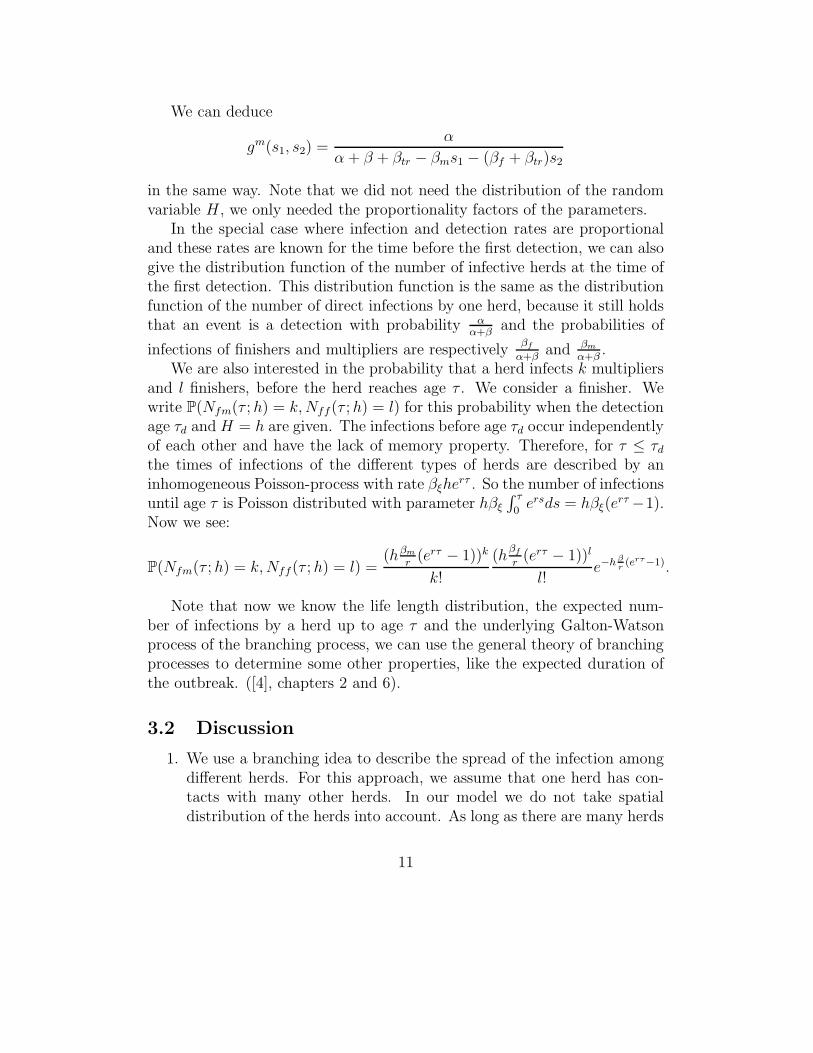
We are also interested in the probability that a herd infects k multipliersand l finishers, before the herd reaches age τ . We consider a finisher. Wewrite P(Nfm(τ ; h) = k, Nff(τ ; h) = l) for this probability when the detectionage τd and H = h are given. The infections before age τd occur independentlyof each other and have the lack of memory property. Therefore, for τ ≤ τd

the times of infections of the different types of herds are described by aninhomogeneous Poisson-process with rate βξherτ . So the number of infectionsuntil age τ is Poisson distributed with parameter hβξ

∫ τ

0ersds = hβξ(e

rτ −1).Now we see:

P(Nfm(τ ; h) = k, Nff(τ ; h) = l) =(hβm

r(erτ − 1))k

k!

(hβf

r(erτ − 1))l

l!e−h

β

r(erτ−1).

Note that now we know the life length distribution, the expected num-ber of infections by a herd up to age τ and the underlying Galton-Watsonprocess of the branching process, we can use the general theory of branchingprocesses to determine some other properties, like the expected duration ofthe outbreak. ([4], chapters 2 and 6).

3.2 Discussion

1. We use a branching idea to describe the spread of the infection amongdifferent herds. For this approach, we assume that one herd has con-tacts with many other herds. In our model we do not take spatialdistribution of the herds into account. As long as there are many herds

11

in an area, the local exhaustion of susceptible herds can be ignored.If the outbreak is in an advanced state, however, local depletion ofsusceptible herds (either by the epidemic progression or by so-calledpre-emptive culling) will certainly play a role. As long as there arerelatively few infected herds in a neighbourhood, (i.e. a group of herdsthat have contacts with each other) we assume that the infection ratedoes not directly depend on this number of infected herds. Measureslike ring-culling (culling of all herds within a certain distance of aninfected herd) and ring vaccination cannot be considered in our model.

2. We distinguish between two types of contacts, transport contacts andindirect contacts. We have assumed that the indirect contacts are thesame for all herds. Transport contacts are only from multipliers tofinishers. Indirect contacts include transport of the virus by wind, byvisits from an infective herd to a susceptible herd etc. Transport con-tacts are transports of infected animals from a multiplier to a finisher.

3. We simplify the model by assuming that the measures are implementedat the time of the introduction of the virus in the population (or, inother words, that the infection is detected immediately). It would bedesirable to implement the measures from the moment of first detection.It is difficult, however, to estimate parameters like α and β for the timebefore the first detection, when awareness is not yet heightened byannouncement of the outbreak, and when increased hygienic measureson farms are not yet taken. If we know the value of the parameters ofthe model for the period between introduction and first detection, weare able to estimate the probability of extinction and the expected finalsize of such a situation. However, these calculations still require thatwe use the information from our simplified model, where measures arestarted directly upon introduction.

4. The function µmm(τ ; h) is not required for our calculations of the finalsize and the probability of extinction. The reason why we include thisfunction in our paper is that this function is interesting in its own right.It gives the expected offspring τ time units after an infective herd isinfected itself. In practical applications, it is possible that by contacttracing some herd is suspected of being infected τ time-units ago. Thisµmm(τ ; h) is then the expected number of infected multipliers by the

12

suspected herd, if that suspected herd is a multiplier and if it is reallyinfected.

5. The proportionality of the infection rate to the detection rate is essen-tial in this section. Due to this property, we can find an underlyingordinary Galton-Watson process. Without this proportionality, we mayask whether it is possible to give a nice expression for the generatingfunction. We also lose the independence of h in the generating function,which gives some computational problems.

6. Knowing the generating function of the number of infected herds atthe first detection is important because if in some way it is possible toestimate parameters for the time before the first detection, we can usethe distribution function of the number of infective herds at the timemeasures are implemented. We do not have the ‘ages’ of the infectiveherds at the first detection, but we can find a worst-case-scenario, byfinding what age of a herd at t = 0 leads to the biggest offspring. If thedetection and infection rate does not depend in the same way on thenumber of infected animals, we cannot deduce the distribution functionat the time of the first detection in this way.

4 The model for varying environments

4.1 The approach

In the previous section, we considered the model for the spread of an infec-tious disease in non-varying environments. We heavily used the proportion-ality of the infection and detection rate of herds. This proportionality doesnot hold in a varying environment. Therefore, we need a different approach.

We consider only one type of herd; the multi-type model is a straightfor-ward generalisation of this. We assume that the spread within a herd is notinfluenced by the state of the environment. The detection rate only dependson the number of infected animals in a herd and is written as αI(τ ; h), whereI(τ ; h) is the number of infected animals as described in Section 2. In thissection, we assume that the within-herd spread is described by a birth-and-death process. So I(τ ; h) = herτ . We can easily deal with other descriptionsof the within-herd spread.

13

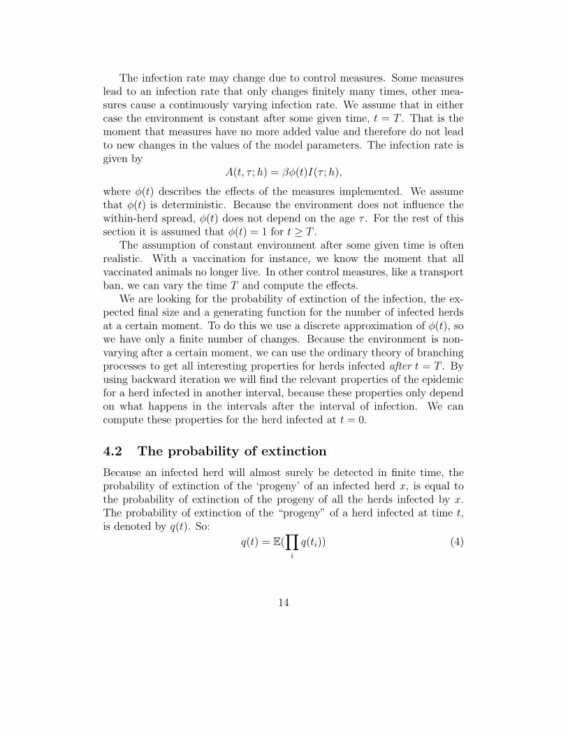
The infection rate may change due to control measures. Some measureslead to an infection rate that only changes finitely many times, other mea-sures cause a continuously varying infection rate. We assume that in eithercase the environment is constant after some given time, t = T . That is themoment that measures have no more added value and therefore do not leadto new changes in the values of the model parameters. The infection rate isgiven by

A(t, τ ; h) = βφ(t)I(τ ; h),

where φ(t) describes the effects of the measures implemented. We assumethat φ(t) is deterministic. Because the environment does not influence thewithin-herd spread, φ(t) does not depend on the age τ . For the rest of thissection it is assumed that φ(t) = 1 for t ≥ T .

The assumption of constant environment after some given time is oftenrealistic. With a vaccination for instance, we know the moment that allvaccinated animals no longer live. In other control measures, like a transportban, we can vary the time T and compute the effects.

We are looking for the probability of extinction of the infection, the ex-pected final size and a generating function for the number of infected herdsat a certain moment. To do this we use a discrete approximation of φ(t), sowe have only a finite number of changes. Because the environment is non-varying after a certain moment, we can use the ordinary theory of branchingprocesses to get all interesting properties for herds infected after t = T . Byusing backward iteration we will find the relevant properties of the epidemicfor a herd infected in another interval, because these properties only dependon what happens in the intervals after the interval of infection. We cancompute these properties for the herd infected at t = 0.

4.2 The probability of extinction

Because an infected herd will almost surely be detected in finite time, theprobability of extinction of the ‘progeny’ of an infected herd x, is equal tothe probability of extinction of the progeny of all the herds infected by x.The probability of extinction of the “progeny” of a herd infected at time t,is denoted by q(t). So:

q(t) = E(∏

i

q(ti)) (4)

14

Here, the times ti are the times that herds are infected by the herd infectedat time t; the expectation is over these random times of infection. The emptyproduct is defined as 1.

In order to make computations possible we use a discrete time approx-imation. We divide the positive real line into N + 1 intervals, labeled1, 2, . . . , N +1. The interval (0, T ] is divided into N intervals of equal length,where t is in interval i, if t ∈ ((i − 1) T

N, i T

N], 1 ≤ i ≤ N . The final interval

N + 1 is (T,∞); in this final interval all the model parameters are constant.The time t = 0, the moment of the first infection, is not included in one ofthe intervals, we treat this point in our notation as interval 0.

If the function φ(t) is discontinuous we may choose another discretisa-tion, so that the discontinuities are on the boundaries of intervals. It is notessential that all intervals have the same length.

For t in interval i, 1 ≤ i ≤ N , q(t) and φ(t) are approximately constant.In our “discrete time model” we will write q(i) and φ(i) for the value of qand φ in interval i. For instance, we can take φ(i) to be the value of φ(t)at the midpoint of interval i. Because we accept discontinuities in φ(t), thisfunction may differ significantly for neighbouring intervals.

Now, with n(i, j), the number of infections in interval j, due to one herdinfected in interval i, we can write (4) as:

q(i) = E

(

q(i)n(i,i)q(i + 1)n(i,i+1) · · · q(N + 1)n(i,N+1))

, (5)

where the expectation is over the numbers of infections in each interval.q(0) is the probability of extinction of the progeny of the herd infected attime t = 0. We assume that all infections and detections take place on themidpoint of the interval, except of course for the events in the final interval,because there we can compute everything explicitly.

Given that a herd is not yet detected and H = h, the probability ofinfection in a certain interval by that herd does not depend on the number ofinfections in previous intervals. Consider a herd infected in interval i, denoteby D(i; h) = k the event that this particular herd is detected in interval k,given H = h. After detection no further infections occur. Define n(i, l, k; h)as the number of infections in interval l due to a particular herd infected ininterval i, while H = h and the interval of detection k, are given. Now, byusing independence we have (writing PH for the distribution function of H)

q(i) =

∫ N+1∑

k=i

E(q(i)n(i,i,k;h)q(i + 1)n(i,i+1,k;h) · · ·

15

· · · q(k)n(i,k,k;h)|D(i; h) = k)P(D(i; h) = k)dPH

=

∫ N+1∑

k=i

E

(

k∏

l=i

(q(l)n(i,l,k;h)|D(i; h) = k)

)

P(D(i; h) = k)dPH

=

∫ N+1∑

k=i

k∏

l=i

E(q(l)n(i,l,k;h)|D(i; h) = k)P(D(i; h) = k)dPH .

Here the expectation inside the integral depends on h, contrary to the non-varying environment case. Note that the number of infections in a certaininterval is not independent of the interval of detection. It does not make anydifference for the number of infections whether a herd is detected shortly afterthe considered interval or very long after that, but it does make a differencewhether the detection is in the considered interval itself. So p(n; i, l, k; h) :=P(n(i, l, k; h) = n) depends on the detection interval k. For computationalreasons we suppose in this discrete model that for i ≤ N , p(0; i, i, k; h) = 1.We write pdet(i, k; h) for P(D(i; h) = k). We are interested in q := q(0). Wecan easily compute all these probabilities in our model.

Because we assume a birth-and-death process for the within-herd spread,we have to take the random character of H into account. Doing this leadsto the following formulae:

q(i) =N+1∑

k=i

∫ ∞

0

R − 1

Re−h R−1

R (E(q(i)n(i,i,k;h)) · · ·E(q(k)n(i,k,k;h))pdet(i, k, h)dh.

Here we have conditioned on the time of detection and on h. We can rewritethis formula as:

q(i) =

N+1∑

k=i

∫ ∞

0

R − 1

Re−h R−1

R (

k∏

l=i+1

(

∞∑

n=0

p(n; i, l, k; h)q(l)n))pdet(i, k; h)dh.

Here q(i) depends on q(l) for l > i. As mentioned before, we can computeq(N + 1) by the ordinary theory of branching processes. We use backwarditeration to compute q(0).

Note that we also know the probability of extinction for herds infectedafter time t = 0. If we estimate (for example by contact tracing) the mo-ment of infection of a certain herd, we can use this information to improvepredictions.

16

4.3 The expected final size of the epidemic

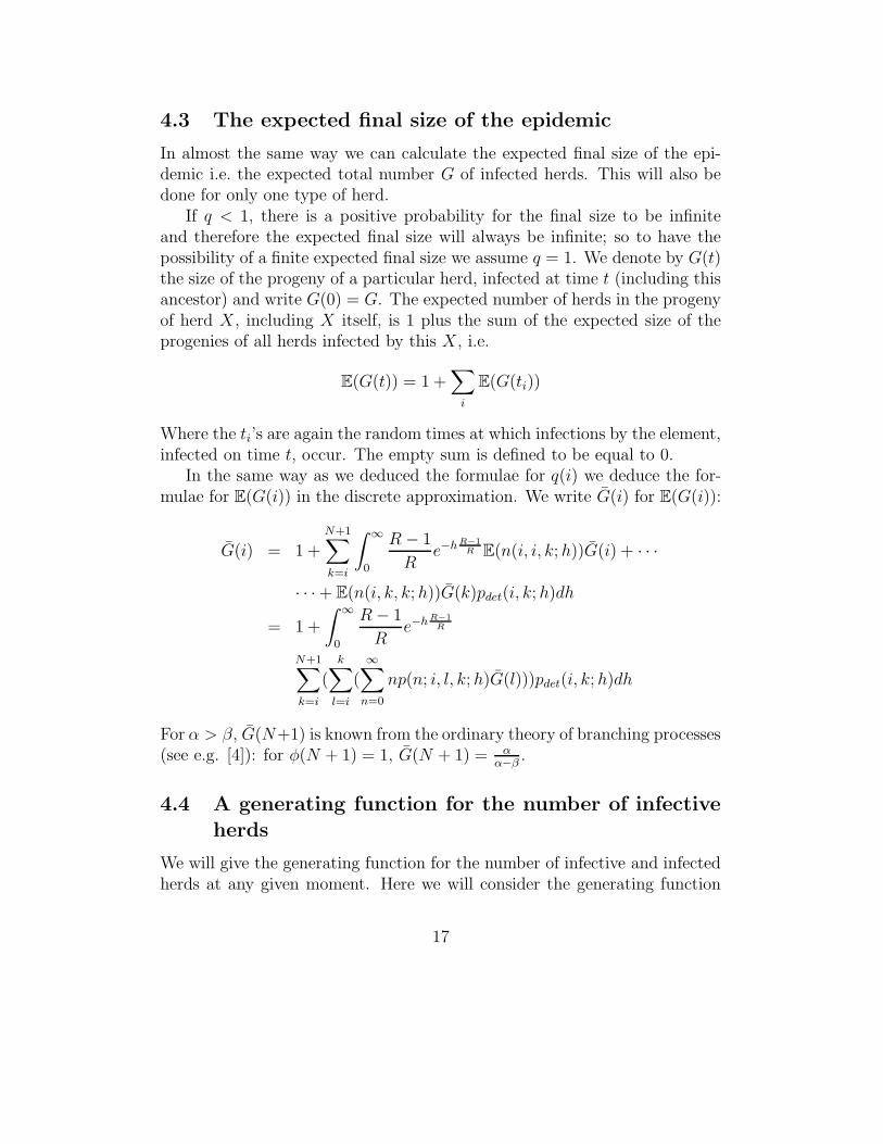
In almost the same way we can calculate the expected final size of the epi-demic i.e. the expected total number G of infected herds. This will also bedone for only one type of herd.

If q < 1, there is a positive probability for the final size to be infiniteand therefore the expected final size will always be infinite; so to have thepossibility of a finite expected final size we assume q = 1. We denote by G(t)the size of the progeny of a particular herd, infected at time t (including thisancestor) and write G(0) = G. The expected number of herds in the progenyof herd X, including X itself, is 1 plus the sum of the expected size of theprogenies of all herds infected by this X, i.e.

E(G(t)) = 1 +∑

i

E(G(ti))

Where the ti’s are again the random times at which infections by the element,infected on time t, occur. The empty sum is defined to be equal to 0.

In the same way as we deduced the formulae for q(i) we deduce the for-mulae for E(G(i)) in the discrete approximation. We write G(i) for E(G(i)):

G(i) = 1 +N+1∑

k=i

∫ ∞

0

R − 1

Re−h R−1

R E(n(i, i, k; h))G(i) + · · ·

· · ·+ E(n(i, k, k; h))G(k)pdet(i, k; h)dh

= 1 +

∫ ∞

0

R − 1

Re−h R−1

R

N+1∑

k=i

(k∑

l=i

(∞∑

n=0

np(n; i, l, k; h)G(l)))pdet(i, k; h)dh

For α > β, G(N+1) is known from the ordinary theory of branching processes(see e.g. [4]): for φ(N + 1) = 1, G(N + 1) = α

α−β.

4.4 A generating function for the number of infective

herds

We will give the generating function for the number of infective and infectedherds at any given moment. Here we will consider the generating function

17

for the infective and infected herds at time t = T , the time after which theparameter values are considered to be constant.

Remember that the age of an infective herd only influences the number ofinfective animals in that herd. From Proposition 1 in Section 3.1, we knowthat the expected direct offspring of a herd, born after t = T , is independentof the age of that herd, given that the herd is not yet detected at that time.Furthermore we know that the size of the offspring (infected after time t = T )of a herd, infective at that time, does not depend on the offspring of otherherds that are infective at time t = T . So for the distribution of the numberof infections after time t = T , only the distribution of the number of infectiveherds at that time is important.

By using Proposition 1 and the theory for ordinary branching processes,we can compute everything we want to know. We will determine the distri-bution of X, the number of infective herds at time t = T . Xi is the numberof infective herds at time T , from the progeny of one particular herd infectedin interval i. (Here the herd itself is a part of its own progeny.) We denoteX0 by X. We also use Yi for the number of infected herds in the progeny ofa particular herd infected in interval i, that is detected before time t = T .The generating function of the distribution of Xi and Yi is

gi(s1, s2) = E(sXi

1 sYi

2 ) =

∫ ∞

0

R − 1

Re−h R−1

R (E(sXi

1 sYi

2 |h))dh.

We write gi(s1, s2; h) = E(sXi

1 sYi

2 |h).We again assume that a herd does not infect other herds in the interval

wherein it becomes infected itself. So:

gi(s1, s2; h) = E(sXi

1 sYi

2 |h)

=N+1∑

k=i

pdet(i, k; h)E(sXi

1 sYi

2 |D(i, k; h), h)

= s2

N∑

k=i

pdet(i, k; h)E(

k∏

l=i

gl(s1, s2)n(i,l,k;h)) +

+s1pdet(i, N + 1; h)E(N∏

l=i

gl(s1, s2)n(i,l,N+1;h))

= s2

N∑

k=i

pdet(i, k; h)k∏

l=i

E(gl(s1, s2)n(i,l,k;h)) +

18

+s1pdet(i, N + 1; h)N∏

l=i

E(gl(s1, s2)n(i,l,N+1;h))

= s2

N∑

k=i

pdet(i, k; h)

k∏

l=i+1

∞∑

n=0

p(n; i, j, k; h)(gl(s1, s2))n +

+s1pdet(i, N + 1; h)

N∏

l=i+1

(

∞∑

n=0

p(n; i, l, N + 1; h)(gl(s1, s2))n).

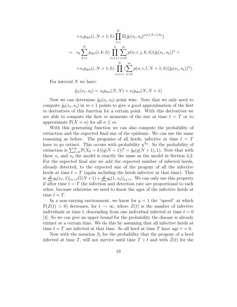
For interval N we have:

gN(s1, s2) = s2pdet(N, N) + s1pdet(N, N + 1)

Now we can determine g0(s1, s2) point wise. Note that we only need tocompute g0(s1, s2) in m + 1 points to give a good approximation of the firstm derivatives of this function for a certain point. With this derivatives weare able to compute the first m moments of the size at time t = T or toapproximate P(X = n) for all n ≤ m.

With this generating function we can also compute the probability ofextinction and the expected final size of the epidemic. We can use the samereasoning as before. The progenies of all herds, infective at time t = Thave to go extinct. This occurs with probability qX0 . So the probability ofextinction is

∑∞k=0 P(X0 = k)(q(N + 1))k = g0(q(N + 1), 1). Note that with

these s1 and s2 the model is exactly the same as the model in Section 4.2.For the expected final size we add the expected number of infected herds,already detected, to the expected size of the progeny of all the infectiveherds at time t = T (again including the herds infective at that time). Thisis d

ds1

g0(s1, 1)|s1=1G(N +1)+ dds2

g0(1, s2)|s2=1. We can only use this propertyif after time t = T the infection and detection rate are proportional to eachother, because otherwise we need to know the ages of the infective herds attime t = T .

In a non-varying environment, we know for q = 1 the “speed” at whichP(Z(t) > 0) decreases, for t → ∞, where Z(t) is the number of infectiveindividuals at time t, descending from one individual infected at time t = 0[4]. So we can give an upper bound for the probability the disease is alreadyextinct at a certain time. We do this by assuming that all infective herds attime t = T are infected at that time. So all herd at time T have age τ = 0.

Now with the notation St for the probability that the progeny of a herdinfected at time T , will not survive until time T + t and with Z(t) for the

19

number of infected herds at time t, we have that:

P(Z(T + t) = 0) =∞∑

k=0

P(Z(T ) = k)(St)k = g(St, 1).

4.5 Discussion

1. By using this iterative method, we can compute the expected final sizeof an outbreak very fast, but for computing any higher moments of thisfinal size, we need substantially more computational effort. By usingsimulations, it is possible to estimate these higher moments too. (see[1])

2. The lack of memory property is very important for our computations.We used it to write the formula of q(i) in a ‘convenient’ form, withexpectations in front of every q(l)n. The speed of computations alsoheavily depends on the lack of memory property of the infection rate.In each interval the number of infections by one herd is Poisson dis-tributed. We can easily integrate h out of the formula for q(i), forPoisson distributed numbers of infections. (With the given distribu-tion of H).

5 Results

In this section we use the Dutch classical swine fever epidemic of 1997 asexample. We use the same data as Klinkenberg et al. in [1]. However,Klinkenberg et al. used simulations and for every simulation the parameterswere (pseudo-)randomly chosen from the distributions of the parameters,while we used only estimations of parameters for our computations.

We consider the following set of control measures:

A Total transport prohibition,

B Killing of young piglets, in combination with a breeding ban,

C Vaccination of all piglets (not sows) at multiplier herds, followed byrecurrent vaccination of newborn piglets,

D Single vaccination of all pigs at finishing herds,

20

E Vaccination of piglets on arrival at finishing herds.

Choosing a (combination of) measure(s) is called a control strategy orscenario. The effects of different scenarios on the fraction of infective animalsin a multiplier, in a finisher and the possibility of transport-infections (φm(t),φf(t) and φtr(t) respectively) are given in Table 1 (This table is adaptedfrom [1]). For example, the 0 for φtr in strategy A means that infection isnot possible by transport contacts. As another example, φf(t) = t/100 fort ≤ 100 in strategy D means that at time t a fraction t/100 of the animalsin a finisher is infective. Note that the first 12 strategies are in a constantenvironment. Therefore, for those strategies we can compute properties ofthe spread of the disease directly. The probability of extinction is given inTable 2.

We also compute the expected final size of an epidemic; see Table 3. Weonly need to compute this for the strategies with almost sure extinction. Theexpected number of infected multipliers, while the initially infected herd wasa finisher is denoted by Gfm. In a similar way we define Gmm, Gmf , Gff . Thelast column of Table 3 is the expected number of infected herds, when initiallyfive multipliers and five finishers were infected. Note that we cannot comparethe expected final size with the results of Klinkenberg et al. (Table 6 in [1]),because they use the median of 1000 simulations, not the mean. The resultsof Klinkenberg et al. are given in Table 4. The 95% confidence intervals ofthe final size are also taken from [1] and were estimated by simulation.

We used the generating function for the number of infected and infectiveherds at time t = T , the point in time after which the parameter valuesare assumed to be constant, to estimate the size at time T (which varies fordifferent strategies). We estimate the first two moments of the size at timeT for the four pure strategies in a varying environment B, C, D, E. (Table5) Especially the results of B and C are of interest because they will give anidea of the variance of the final size of a herd.

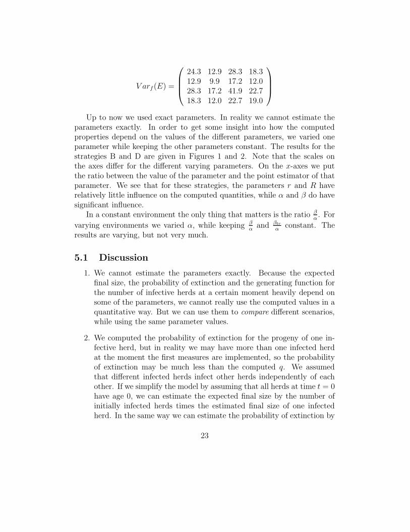
Next we give covariance matrices (for different strategies and differentinitially infected herds) of the number of infected multipliers not yet de-tected, the number of infected multipliers already detected, the number ofinfected finishers not yet detected and the number of finishers already de-tected, respectively. We denote by V ari(J) the covariance matrix for aninitially infected herd of type i, while the strategy is J . By comparing thevalues in these matrices to the results in Table 5, we know how much trustwe may put in the expected sizes.

21

V arm(B) =

0.85 2.19 0.52 8.432.19 16.97 2.63 56.600.52 2.63 1.06 10.218.43 56.60 10.21 237.42

V arf(B) =

0.38 0.98 0.23 3.430.98 8.02 1.17 23.840.23 1.17 0.48 4.133.43 23.84 4.13 90.10

V arm(C) =

0.92 0.66 0.20 0.680.66 1.68 0.25 1.000.20 0.25 0.21 0.260.68 1.00 0.26 1.87

V arf(C) =

0.92 0.67 0.20 0.670.67 1.67 0.25 1.000.20 0.25 0.21 0.260.67 1.00 0.26 1.87

V arm(D) =

56.4 27.5 97.8 48.727.5 18.4 53.2 24.297.8 53.2 197.9 90.648.7 24.2 90.6 54.5

V arf (D) =

23.0 11.4 39.5 17.611.4 8.1 22.2 10.539.5 22.2 80.9 32.517.6 10.5 32.5 18.0

V arm(E) =

55.0 29.0 65.3 46.829.0 21.0 38.9 29.765.3 38.9 95.5 59.446.8 29.7 59.4 53.0

22

V arf (E) =

24.3 12.9 28.3 18.312.9 9.9 17.2 12.028.3 17.2 41.9 22.718.3 12.0 22.7 19.0

Up to now we used exact parameters. In reality we cannot estimate theparameters exactly. In order to get some insight into how the computedproperties depend on the values of the different parameters, we varied oneparameter while keeping the other parameters constant. The results for thestrategies B and D are given in Figures 1 and 2. Note that the scales onthe axes differ for the different varying parameters. On the x-axes we putthe ratio between the value of the parameter and the point estimator of thatparameter. We see that for these strategies, the parameters r and R haverelatively little influence on the computed quantities, while α and β do havesignificant influence.

In a constant environment the only thing that matters is the ratio β

α. For

varying environments we varied α, while keeping β

αand βtr

αconstant. The

results are varying, but not very much.

5.1 Discussion

1. We cannot estimate the parameters exactly. Because the expectedfinal size, the probability of extinction and the generating function forthe number of infective herds at a certain moment heavily depend onsome of the parameters, we cannot really use the computed values in aquantitative way. But we can use them to compare different scenarios,while using the same parameter values.

2. We computed the probability of extinction for the progeny of one in-fective herd, but in reality we may have more than one infected herdat the moment the first measures are implemented, so the probabilityof extinction may be much less than the computed q. We assumedthat different infected herds infect other herds independently of eachother. If we simplify the model by assuming that all herds at time t = 0have age 0, we can estimate the expected final size by the number ofinitially infected herds times the estimated final size of one infectedherd. In the same way we can estimate the probability of extinction by

23

the computed probability for one herd, to the power of the number ofinitially infected herds. From previous outbreaks of FMD, CSF and AIin the Netherlands, one can see that as a rule several farms are alreadyinfected at the moment the first case is suspected or confirmed.

3. The results are very much the same as the results of Klinkenberg etal. but we do not need simulations to estimate the properties. Also,our method is much faster than using simulations. In Table 6 of [1]it is suggested that the expected final size, with initially five infectedmultipliers and five infected finishers, is estimated by simulations. Inreality the median of 1000 simulations is used in that paper. Thisexplains why our results differ on that point.

4. Note that strategy ABC gives an extremely high expected final size.Klinkenberg et al.[1] did not even give this final size. This is becausefor the given parameters the process is very near to a process with apositive probability of surviving i.e. a positive probability of an infinitefinal size.

5. Using the expected size at t = T and the variance of this size, we seethat the expected final size is not very informative in some scenarios.Large variance may imply that a large set of “numbers of infectedherds” have a not-ignorable probability, even if we know the exactparameters.

6. The computed covariance matrices do have values of different order inthem. Consider for instance strategy B. The variance of the numberof finishers and multipliers already detected is much higher than thevariance of the number of finishers and multipliers that are still alive attime t = T . This is because the infection rate decreases for this strategy.At the start of the process one infective herd may infect several otherherds with a relatively high probability, while after some time infectionsbecome rare. This is why the expected number of infective herds att = T is much less than the expected number of infected herds.

7. For constant environments we are interested in the variance of the finalsize. Note that in all of the strategies with almost sure extinction ina constant environment, only one type of herd can be infected, so weonly have to deal with one type of herd. We use the underlying Galton-Watson process to deduce the variance of the final size (see Section 2.11

24

of [4]). If we take m for the expected number of direct infections byone infective herd, the expected final size is 1

1−mand the variance is

m(1+m)(1−m)2

. Note that for a large expected final size, the variance will beof the square order of the final size. Due to this large variance, wecannot give exact quantitative predictions about the final size of anepidemic. This also indicates that there is a large intrinsic uncertaintyin the problem.

8. If the infection rates are increasing in time, the expected final sizewill decrease for increasing r, while for decreasing infection rates theexpected final size will increase for increasing r. This is because r canbe seen as a parameter describing the speed of the process in a constantenvironment. Large values of r correspond to short generation lengthscompared to small r. So, if the infection rate is increasing in time, then-th generation for small values of r will have a larger infection ratethan the n-th generation for large r.

The effect of decreasing R, the parameter describing the random effectsat the start of the within-herd spread, is less clear from formulae anddefinitions. From the figures we can only see that R has relative smalleffect on the expected final size and the probability of extinction.

9. Some parameters heavily influence the expected final size and the prob-ability of extinction. We have already seen that in a constant environ-ment r and R do not influence these quantities. For predictions theratios β : βtr : α are most important. So the estimation effort is bestdevoted towards estimating these ratios.

6 Conclusion and final remarks

By using a stochastic model, we could estimate the probability of extinctionand the expectation of the final size of an epidemic in a varying environment.We only need that the environment is not varying anymore after some giventime. We use a branching process in varying environments, depending on theage of the particles. In the constant environment the probability of extinctionand the final size are known. By using an iterative process, we computedthis probability and size for the time the environment is still varying.

25

By using generating functions, we can compute many important proper-ties, like the moments of the final size, and a lower bound for the probabilitythat the process has gone extinct after a given time. These generating func-tions are very useful especially if in a constant environment the expectednumber of infections after a certain age does not depend on that age. Thisonly holds if the infection and detection rate are in direct proportion, for thenon-varying environment.

It is difficult to estimate the parameters for the computations. Someof the properties computed in this model, like the probability of extinctionheavily depend on the parameters α and β, describing the infection anddetection rate. The model presented in this paper may be useful to comparethe effect of different measures, but it is very dangerous to use this modelfor absolute quantitative predictions.

We used the model to describe the spread of classical swine fever. It isworth investigating if the same model, with other parameters, may be usedto describe the spread of other animal diseases, with culling at detection,or even human diseases, which lead to strict quarantine of detected infectedindividuals (and suspected cases) and contact and movement restrictions.Emerging infections such as SARS are possible examples of this.

References

[1] Klinkenberg, D.; Everts-van der Wind, A.; Graat, E.A.M.

and De Jong, M.C.M.(2003), Quantification of the Effects of Con-trol Strategies on Classical Swine Fever Epidemics, Mathematical Bio-sciences 186 (2) 145-173.

[2] Diekmann, O. and Heesterbeek, J.A.P.(2000), Mathematical Epi-demiology of Infectious Diseases, Chichester: John Wiley & Son.

[3] Grimmett, G.R. and Stirzaker, D.R.(1992), Probability and Ran-dom Processes, New York: Oxford University Press Inc.

[4] Jagers, P.(1975), Branching Processes with Biological Applications,London: John Wiley & Son.

[5] Ferguson, N.M.; Donnelly C.A. and Anderson R.M.(2001),The Foot-and-Mouth Epidemic in Great Britain: Pattern of Spread andImpact of Interventions, Science 292 1155-1160.

26

[6] Ferguson, N.M.; Donnelly C.A. and Anderson R.M.(2001),Transmission Intensity and Impact of Control Policies on the Foot andMouth Epidemic in Great-Britain, Nature 413 542-547.

[7] Jagers, P. and Lu Z.W.(2002), Branching Processes with Deteri-orating Random Environments, Journal of Applied Probability 39 (2)395-401.

[8] Kao, R.R.(2002), The Role of Mathematical Modelling in the Controlof the 2001 FMD Epidemic in the UK, Trends in Microbiology 10 (6)279-286.

[9] Keeling, M.J.; Woolhouse, M.E.J.; Shaw, D.J.; Matthews,

L.; Chase-Topping, M.; Haydon, D.T.; Cornell, S.J.; Kappey,

J.; Wilesmith, J. and Grenfell B.T.(2001), Dynamics of the 2001UK Foot and Mouth Epidemic - Dispersal in a Heterogeneous Land-scape, Science 294 813-817.

[10] Meester, R.; de Koning, J.; de Jong, M.C.M. and Diekmann,

O.(2002), Modelling and Prediction of Classical Swine Fever Epidemics,Biometrics 41 178-184.

[11] Stegeman, A.; Elbers, A.R.W.; Smak, J. and de Jong,

M.C.M.(1999), Quantification of the Transmission of Classical SwineFever Virus between Herds during the 1997-1998 Epidemic in TheNetherlands, Preventive Veterinary Medicine 42 219-234.

27

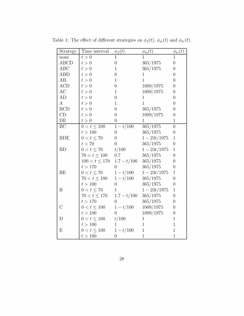
Table 1: The effect of different strategies on φf(t), φm(t) and φtr(t).

Strategy Time interval φf(t) φm(t) φtr(t)none t > 0 1 1 1ABCD t > 0 0 365/1975 0ABC t > 0 1 365/1975 0ABD t > 0 0 1 0AB t > 0 1 1 0ACD t > 0 0 1009/1975 0AC t > 0 1 1009/1975 0AD t > 0 0 1 0A t > 0 1 1 0BCD t > 0 0 365/1975 0CD t > 0 0 1009/1975 0DE t > 0 0 1 1BC 0 < t ≤ 100 1 − t/100 365/1975 0

t > 100 0 365/1975 0BDE 0 < t ≤ 70 0 1 − 23t/1975 1

t > 70 0 365/1975 0BD 0 < t ≤ 70 t/100 1 − 23t/1975 1

70 < t ≤ 100 0.7 365/1975 0100 < t ≤ 170 1.7 − t/100 365/1975 0t > 170 0 365/1975 0

BE 0 < t ≤ 70 1 − t/100 1 − 23t/1975 170 < t ≤ 100 1 − t/100 365/1975 0t > 100 0 365/1975 0

B 0 < t ≤ 70 1 1 − 23t/1975 170 < t ≤ 170 1.7 − t/100 365/1975 0t > 170 0 365/1975 0

C 0 < t ≤ 100 1 − t/100 1009/1975 0t > 100 0 1009/1975 0

D 0 < t ≤ 100 t/100 1 1t > 100 1 1 1

E 0 < t ≤ 100 1 − t/100 1 1t > 100 0 1 1

28

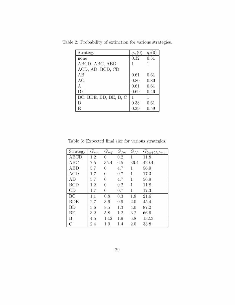
Table 2: Probability of extinction for various strategies.

Strategy qm(0) qf (0)none 0.32 0.51ABCD, ABC, ABD 1 1ACD, AD, BCD, CDAB 0.61 0.61AC 0.80 0.80A 0.61 0.61DE 0.69 0.46BC, BDE, BD, BE, B, C 1 1D 0.38 0.61E 0.39 0.59

Table 3: Expected final size for various strategies.

Strategy Gmm Gmf Gfm Gff G5m+5f ;f+m

ABCD 1.2 0 0.2 1 11.8ABC 7.5 35.4 6.5 36.4 429.4ABD 5.7 0 4.7 1 56.9ACD 1.7 0 0.7 1 17.3AD 5.7 0 4.7 1 56.9BCD 1.2 0 0.2 1 11.8CD 1.7 0 0.7 1 17.3BC 1.1 0.8 0.3 1.8 21.6BDE 2.7 3.6 0.9 2.0 45.4BD 3.6 8.5 1.3 4.0 87.2BE 3.2 5.8 1.2 3.2 66.6B 4.5 13.2 1.9 6.8 132.3C 2.4 1.0 1.4 2.0 33.8

29

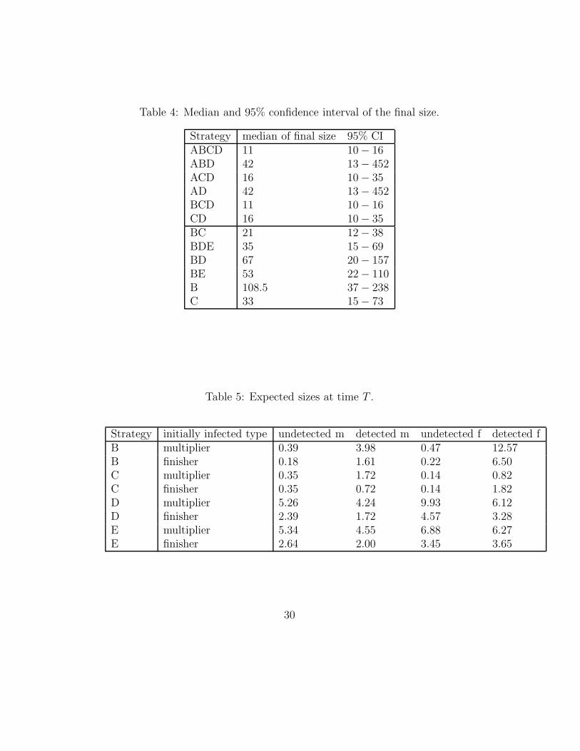
Table 4: Median and 95% confidence interval of the final size.

Strategy median of final size 95% CIABCD 11 10 − 16ABD 42 13 − 452ACD 16 10 − 35AD 42 13 − 452BCD 11 10 − 16CD 16 10 − 35BC 21 12 − 38BDE 35 15 − 69BD 67 20 − 157BE 53 22 − 110B 108.5 37 − 238C 33 15 − 73

Table 5: Expected sizes at time T .

Strategy initially infected type undetected m detected m undetected f detected fB multiplier 0.39 3.98 0.47 12.57B finisher 0.18 1.61 0.22 6.50C multiplier 0.35 1.72 0.14 0.82C finisher 0.35 0.72 0.14 1.82D multiplier 5.26 4.24 9.93 6.12D finisher 2.39 1.72 4.57 3.28E multiplier 5.34 4.55 6.88 6.27E finisher 2.64 2.00 3.45 3.65

30