Autonomous Robots 19, 53–65, 2005c© 2005 Springer Science + Business Media, Inc. Manufactured in The Netherlands.

Mobile Robot Simultaneous Localization and Mappingin Dynamic Environments∗

DENIS F. WOLF AND GAURAV S. SUKHATMERobotic Embedded Systems Laboratory, Center for Robotics and Embedded Systems, Department of Computer

Science, University of Southern California, Los Angeles, CA 90089, USAdenis@robotics.usc.edu

gaurav@robotics.usc.edu

Abstract. We propose an on-line algorithm for simultaneous localization and mapping of dynamic environments.Our algorithm is capable of differentiating static and dynamic parts of the environment and representing themappropriately on the map. Our approach is based on maintaining two occupancy grids. One grid models the staticparts of the environment, and the other models the dynamic parts of the environment. The union of the two grid mapsprovides a complete description of the environment over time. We also maintain a third map containing informationabout static landmarks detected in the environment. These landmarks provide the robot with localization. Results insimulation and real robots experiments show the efficiency of our approach and also show how the differentiationof dynamic and static entities in the environment and SLAM can be mutually beneficial.

Keywords: mapping, occupancy grids, dynamic environments, SLAM

1. Introduction

Simultaneous Localization and Mapping (SLAM) is afundamental problem in mobile robotics and has beenstudied extensively in the robotics literature (Thrunet al., 1998, 2000; Castellanos et al., 2001; Guivant andNebot, 2001, 2002; Tardos et al., 2004; Newman et al.,2002; Montemerlo et al., 2002; Nieto et al., 2002; Liuand Thrun, 2002; Fenwick et al., 2002; Haehnel et al.,2003). For the most part, research has concentrated onSLAM in static environments. In this article, whichis an extended version of Wolf and Sukhatme (2004),we explicitly consider the SLAM problem in dynamicenvironments. The presence of moving objects in theenvironment can lead SLAM algorithms to mistakesand result in incorrect maps. The explicit identificationof dynamic entities can certainly improve the accuracyof the localization and mapping processes.

∗Part of this work has been presented in the International Conferencein Robotics and Automation—ICRA 2004.

The approach presented in this paper is divided intotwo parts: mapping (and detection of) dynamic envi-ronments (i.e. maintaining separate representations forthe dynamic and static parts of the environment), androbot localization. These two tasks are interleaved, al-lowing the robot to perform simultaneous localizationand mapping.

Our mapping algorithm extends the occupancygrid technique introduced in Elfes (1986, 1989) andMoravec (1988) to dynamic environments. The result-ing algorithm is capable of detecting dynamic objectsin the environment and representing them on a map.Non-stationary objects are detected even when theymove out of the robot’s field of view, when the robot re-visits the already mapped area where the changes hap-pened. In order to do this, we maintain two occupancygrids maps. One map (S) is used to represent occu-pancy probabilities which correspond to the static partsof the environment and the other map (D) is used torepresent occupancy probabilities of the moving partsof the environment. A complete description of the en-vironment is obtained by the union of the information

54 Wolf and Sukhatme

present in the two maps (S ∪ D). In this case, the non-static entities will appear in the last position that theywere seen. This information is updated when the robotrevisits these already mapped areas.

Our localization algorithm is based on the well-known SLAM approach by Dissanayake et al. (2001).We use an Extended Kalman Filter (EKF) to incre-mentally estimate the correct position of the robot andlandmarks in the environment. Corners have been usedas landmarks.

Experimental tests have been performed using Ac-tiveMedia Pioneer Robots equipped with laser rangefinders in the California Science Center in Los Angeles.The results show that our algorithm is able to success-fully differentiate dynamic and static parts of the envi-ronment, and simultaneously localize the robot.

2. Related Work

Mapping of static environments has received consider-able attention recently, but in most cases, these algo-rithms cannot be directly applied to dynamic environ-ments. A good overview of mapping methods is givenin Thrun (2002). Examples of localization in dynamicenvironments can be seen in Aycard et al. (1998) andFox et al. (1999).

Usually, the presence of moving objects causeserrors and compromises the overall quality of themap. This is a considerable problem since many re-alistic robot applications are in non-static environ-ments. Mapping dynamic environments has been ad-dressed in recent years (Haehnel et al., 2002, 2003;Wang and Thorpe, 2002; Wang et al., 2003; Biswaset al., 2002; Wolf and Sukhatme, 2003; Andrade-Cetto and Sanfeliu, 2002; Avots et al., 2002), but stillhas many open questions. These include, how to dif-ferentiate static and dynamic parts of the environ-ment and, how to represent such information in themap.

Before discussing the details regarding related ap-proaches to this problem, we introduce a classificationof objects in a dynamic environment. There are twotypes of moving objects to be considered: objects thatare permanently in motion and objects that are station-ary part of the time (some times most of the time) andmove occasionally. The first category refers to objectsthat have changed location each time they are observedby the robot’s sensors. The second category refers toobjects that may or may not have moved since theywere observed previously. They are however known

to have moved at least once. In this work, when anobject moves at least once, it will be always con-sidered dynamic. The approach presented in this pa-per deals with both categories of moving objects. InHaehnel et al. (2002), a technique is presented to iden-tify moving objects in the environment based on thedifference of consecutive sensor readings. The objec-tive is filter out those sensor readings correspondingto dynamic objects in order to improve the quality ofthe map. Sample-based Joint Probabilistic Data Asso-ciation Filters have been used. In Wang and Thorpe(2002) a combination of SLAM and DTMO (Detec-tion and Tracking of Moving Objects)is proposed inwhich scan matching algorithms are used to SLAMand moving objects are detected and tracked. In Wanget al. (2003) a framework is given for solving the si-multaneous mapping, localization, detection and track-ing of moving objects. The idea is identify and keeptrack of moving objects in order to improve the qual-ity of the map. All the approaches cited above onlydeal with objects that move in the field of view ofthe robot. They do not address changes in the environ-ment when those changes occurred behind the robot’sback.

As far as we know, the only works that deal withthis case are (Biswas et al., 2002; Wolf and Sukhatme,2003; Haehnel et al., 2003). The work presented inBiswas et al. (2002) uses an off-line Bayesian ap-proach (based on the Expectation-Maximization al-gorithm) that can detect changes over time in an en-vironment. The basic idea of this approach rests ona map differencing technique. Maps of the same en-vironment are created at different points in time. Bycomparing those maps, the algorithm is able to iden-tify the parts of the environment that changed overtime.

The approach in Haehnel et al. (2003) uses the EMalgorithm to differentiate dynamic and static parts ofthe environment off-line. In the expectation step it esti-mates which measurements might correspond to staticparts of the environment. In the maximization step, theposition of the robot in the map is calculated. The al-gorithm iterates until no further improvement can beachieved. Both Biswas et al. (2002) and Haehnel et al.(2003) are off-line methods.

In prior work (Wolf and Sukhatme, 2003), we pre-sented an on-line mapping algorithm capable of differ-entiating static and dynamic parts of the environmenteven when the moving objects change position out ofthe field of the view of the robot. The algorithm could

Mobile Robot Simultaneous Localization and Mapping 55

also uniquely classify each moving object and keeptrack of its location on the map. On the other hand, thisapproach assumed ideal localization, which is a fairlynarrow assumption.

3. The Mapping Approach

In our mapping approach, two distinct occupancy gridmaps (S and D) are used. The static map S containsonly information about the static parts of the environ-ment such as the walls and other obstacles that havenever been observed to move. The dynamic map Dcontains information about the objects which have beenobserved to move at least once.

In the static map S, the occupancy probability of acell represents the probability of a static entity beingpresent at that cell. As dynamic entities are not repre-sented in this map, if that cell is occupied by an movingobject, the occupancy probability will indicate a freespace (i.e. not occupied by a static entity). In the samemanner, static parts of the environment are not repre-sented the dynamic map D. Thus when a cell in D hasa occupancy probability indicating free space, it meanssimply that no moving entity is currently occupyingthe cell. It does not exclude the possibility of the cellbeing occupied by a static part of the environment. Bythe use of these two maps, the algorithm presented hereis able to detect moving objects even if these objectsmove out of the view of the robot in an already mappedarea.

In our formulation both maps S and D are indepen-dently updated. The set of sensor readings is repre-sented by o. We use the discrete time index as super-script of the variables, for example ot means the sensorreadings at time t . Therefore, the problem is to estimatethe following:

p(St |o1 . . . ot ) (1)

p(Dt |o1 . . . ot ) (2)

The first step in order to correctly update both maps Sand D is to differentiate static and dynamic entities inthe environment. This can be performed if we includesome previous information about the static parts of theenvironment (St−1) in Eqs. (1) and (2). As the staticparts of the environment never change over time, theycan be used as a reference to determine which sensorreadings are generated by static and dynamic obstacles.Dynamic parts of the environment cannot be used for

this purpose. Thus Eqs. (1) and (2) become:

p(St | o1 . . . ot , St−1) (3)

p(Dt | o1 . . . ot , St−1) (4)

We are interested in estimating these quantities above,thus updating the static and dynamic maps.

3.1. Static Map Update

The update equation for the static map S (Eq. 3) isslightly different from the regular occupancy grid tech-nique, which assumes the environment does not changeover time. Since we explicitly deal with situations inwhich parts of the environment change their positionover time, we use some previous knowledge about theenvironment and compare with the current set of ob-servations in order to differentiate static and dynamicobstacles and keep only the static parts of the environ-ment in the map S.

Applying Bayes rule to Eq. (3) we obtain:

p(St | o1 . . . ot , St−1)

= p(ot |o1 . . . ot−1, St−1, St) · p(St |o1 . . . ot−1, St−1)

p(ot | o1 . . . ot−1, St−1)(5)

As we are mapping the static part of the environment,in the term p(ot | o1 . . . ot−1, St−1, St ) we assume thatall information from previous observations (o1 . . . ot−1)is incorporated in St−1 therefore the term o1 . . . ot−1

can be dropped. It is possible to rewrite that termas p(ot | St−1, St ) and applying this modification toEq. (5), we obtain:

p(St | o1 . . . ot , St−1)

= p(ot |St−1, St ) · p(St |o1 . . . ot−1, St−1)

p(ot | o1 . . . ot−1, St−1)(6)

Applying Bayes rule to the first term of Eq. (6), weobtain:

p(St |o1 . . . ot , St−1)

= p(St |ot , St−1) · p(ot |St−1) · p(St |o1 . . . ot−1, St−1)

p(St |St−1) · p(ot |o1 . . . ot−1, St−1)(7)

56 Wolf and Sukhatme

Following an analogous derivation, it is possible to cal-culate the non-occupancy of S, denoted by S̄.

p(S̄t |o1 . . . ot , St−1)

= p(S̄t |ot , St−1) · p(ot |St−1) · p(S̄t |o1 . . . ot−1, St−1)

p(S̄t |St−1) · p(ot |o1 . . . ot−1, St−1)(8)

Dividing Eq. (7) by Eq. (8), we can eliminate someterms, obtaining:

p(St |o1 . . . ot , St−1)

p(S̄t |o1 . . . ot , St−1)= p(St |ot , St−1)

p(S̄t |ot , St−1)· p(S̄t |St−1)

p(St |St−1)

· p(St |o1 . . . ot−1, St−1)

p(S̄t |o1 . . . ot−1, St−1)(9)

We can rewrite Eq. (9) substituting p(S̄) by 1 − p(S).

p(St |o1 . . . ot , St−1)

1 − p(St |o1 . . . ot , St−1)= p(St |ot , St−1)

1 − p(St |ot , St−1)(10)

·1 − p(St |St−1)

p(St |St−1)· p(St |o1 . . . ot−1, St−1)

1 − p(St |o1 . . . ot−1, St−1)

The term p(St |St−1) can be rewritten as p(S). Thisis a time-invariant term, which represents the priorknowledge about the occupancy of any cell in the map.The term p(St |o1 . . . ot−1, St−1) is the occupancy of St

given all observations up to the time step t −1 and pre-vious information about the map. It can be rewritten asp(St−1). Substituting the terms we obtain:

p(St |o1 . . . ot , St−1)

1 − p(St |o1 . . . ot , St−1)= p(St |ot , St−1)

1 − p(St |ot , St−1)

· 1 − p(S)

p(S)· p(St−1)

1 − p(St−1)(11)

Equation (11) can be converted to a log-odds form,which can be more efficiently computed.

logp(St |o1 . . . ot , St−1)

1 − p(St |o1 . . . ot , St−1)

= logp(St |ot , St−1)

1 − p(St |ot , St−1)+ log

1 − p(S)

p(S)

+ logp(St−1)

1 − p(St−1)(12)

Equation (12) gives a recursive formula for updatingthe static map S. The p(S) term is the prior for occu-pancy. If it is set to 0.5 (unbiased uncertainty), it canbe canceled. The occupancy for the static map p(St )is now calculated based on the previous informationabout this map p(St−1) and the inverse sensor modelp(St | ot , St−1).

Notice that the information about the previous oc-cupancy is also part of the inverse sensor model. Thatinformation allows us to determine if some previouslyfree space is now occupied, which means that some dy-namic entity has moved to that place. It is also possibleto detect if some entity that was previously consideredstatic has moved. Table 1 shows the possible inputs tothe inverse sensor model and the resulting values.

The first column in Table 1 represents the possibleoccupancy states of the cells in the previous static mapSt−1. The possible states are: Free, Unknown, and Oc-cupied. To be considered Free, the occupancy proba-bility of a grid cell must be below a pre-determinedlow threshold (we used 0.1 in our experiments). A verysmall occupancy probability means a high confidencethat the cell is not occupied by a static entity in theenvironment. If the occupancy probability has a valueabove a high threshold (0.9 in our experiments) that cellis considered Occupied. If the occupancy probability isin the middle of the low and high thresholds, it is con-sidered Unknown. The second column ot represents theinformation provided by the sensors. In this case, eachgrid cell can be Free or Occupied, according to the sen-sor readings at the current robot position. The valuesof the resulting inverse observation model are repre-sented, for simplicity, as: high value or low value. Highvalues are values above 0.5 (that will increase the occu-pancy probability of that cell) and low values are valuesbelow 0.5 (that will decrease the occupancy probabilityof that cell). The third column shows the six possiblecombinations. For the first three rows ot = Free. These

Table 1. Inverse observation model forthe static map.

St−1 ot p(St |St−1, ot )

Free Free Low

Unknown Free Low

Occupied Free Low

Free Occupied Low

Unknown Occupied High

Occupied Occupied High

Mobile Robot Simultaneous Localization and Mapping 57

are the trivial cases where no obstacles are detected,and, independent of the information about previous oc-cupancy, the inverse sensor model will result in a lowvalue, which will decrease the occupancy probability.The fourth row (St−1 = Free and ot = Occupied) isthis case where there is strong evidence that the spacewas previously free of static entities and is now occu-pied. In this case the observation is considered consis-tent with the presence of a dynamic object and the staticoccupancy probability will decrease. In the fifth row(St−1 = Unknown and ot = Occupied) there is uncer-tainty regarding the previous occupancy of that regionin the map and the obstacles detected will be initiallyconsidered static until they are detected to have moved.Therefore, the sensor model will result in a high value,which will increase the occupancy probability of staticentities in that region of the map. This situation occurswhen the robot is initialized once all the grid cells re-flect uncertainty about their occupation. The last rowof the table is also trivial and shows the case where thespace was previously occupied by a static obstacle andthe sensors still confirm that belief. In this case the sen-sor model will result in a high value, which will raisethe occupancy probability of a static obstacle on thatregion of the map.

3.2. Dynamic Map Update

By definition, the dynamic map D only contains infor-mation about the moving parts of the environment. Wedenote by p(Dt ) the occupancy probability of deter-mined region of the map being occupied by an movingobject at time t . Based on the sensor readings and in-formation about previous occupancy in the static map(St−1), it is possible to identify the moving parts of theenvironment and represent then in the dynamic map D.It is important to mention that the information about theprevious occupancy of the dynamic map (Dt−1) cannotbe used as a reference because it may change over time.

Similar to Eqs. (3) and (4) can be rewritten in thefollowing manner:

logp(Dt |o1 . . . ot , St−1)

1−p(Dt |o1 . . . ot , St−1)= log

p(Dt |ot , St−1)

1−p(Dt |ot , St−1)

+ log1 − p(D)

p(D)+ log

p(Dt−1)

1 − p(Dt−1)(13)

Equation (13) is similar to Eq. (12) in the sense that thenew estimation for the occupancy of p(Dt ) is basedon the previous occupancy of that map p(Dt−1) and

the sensor model p(Dt | ot , St−1). Usually, we makep(D) = 0.5, which means no a priori knowledge aboutthe occupancy in D and the entire term can be can-celed. In order to update the dynamic map D Eq. (13)also takes into account the information about previ-ous occupancy of the static map St−1 in its sensormodel.

It is important to state that we are not interested inkeeping all information about the occupancy of dy-namic objects over time. The objective of the dynamicmap is to maintain information about the dynamic ob-jects only at the present time. For example, if a partic-ular grid cell was occupied by an moving object in thepast and it is currently free, it it will be considered justfree. We do not keep any history about previous occu-pancy of the cells in D. The information in the mapjust needs to be set to represent the current occupancyof each cell. Of course, in order for the changes in theenvironment to be reflected on the map, those changesmust be sensed by the robot. If those changes occur inthe robot’s field of view, they will be reflected imme-diately in the map, otherwise the robot needs to revisitthe regions of the environment where the changes oc-curred, in order to detect them.

Table 2 shows the values of the inverse observationmodel used to update the dynamic map. The first andsecond columns are identical to the table used in thestatic map. However, for the dynamic map, the behaviorof the inverse observation model is slightly different.In the three first rows, as the observation ot indicates afree space, the occupancy probability will be triviallyupdated with a low value independent of the previousoccupancy on the static map. In the fourth row, theprevious occupancy in the static map states that thespace was free St−1 = Free but the sensor readingsshow some obstacle in that cell ot = Occupied. Thiscase characterizes the presence of a moving object andconsequently the dynamic map will be updated with a

Table 2. Inverse observation model fordynamic map.

St−1 ot p(Dt | ot , St−1)

Free Free Low

Unknown Free Low

Occupied Free Low

Free Occupied High

Unknown Occupied Low

Occupied Occupied Low

58 Wolf and Sukhatme

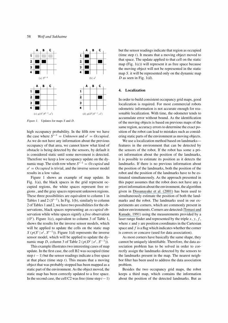
Figure 1. Updates for maps S and D.

high occupancy probability. In the fifth row we havethe case where St−1 = Unknown and ot = Occupied.As we do not have any information about the previousoccupancy of that area, we cannot know what kind ofobstacle is being detected by the sensors, by default itis considered static until some movement is detected.Therefore we keep a low occupancy update on the dy-namic map. The sixth row where St−1 = Occupied andot = Occupied is trivial, and the inverse sensor modelresults in a low value.

Figure 1 shows an example of map update. InFig. 1(a), the black spaces in the grid represent oc-cupied regions, the white spaces represent free re-gions , and the gray spaces represent unknown regions.These three possibilities are equivalent to column 1 inTables 1 and 2 (St−1). In Fig. 1(b), similarly to column2 of Tables 1 and 2, we have two possibilities for the ob-servations, black spaces representing an occupied ob-servation while white spaces signify a free observation(Ot ). Figure 1(c), equivalent to column 3 of Table 1,shows the results for the inverse sensor models, whichwill be applied to update the cells on the static mapS (p(St | ot , St−1)). Figure 1(d) represents the inversesensor model, which will be applied to update the dy-namic map D, column 3 of Table 2 (p(Dt | ot , St−1)).

This example illustrates two interesting cases of mapupdate. In the first case, the cell B2 was occupied (timestep t − 1) but the sensor readings indicate a free spaceat that place (time step t). This means that a movingobject that was probably stopped has been mapped as astatic part of the environment. As the object moved, thestatic map has been correctly updated to a free space.In the second case, the cell C2 was free (time step t −1)

but the sensor readings indicate that region as occupied(time step t). It means that a moving object moved tothat space. The update applied to that cell on the staticmap (Fig. 1(c)) will represent it as free space becausethe moving object will not be represented in the staticmap S. it will be represented only on the dynamic mapD as seen in Fig. 1(d).

4. Localization

In order to build consistent occupancy grid maps, goodlocalization is required. For most commercial robotsodometric information is not accurate enough for rea-sonable localization. With time, the odometer tends toaccumulate error without bound. As the identificationof the moving objects is based on previous maps of thesame region, accuracy errors to determine the exact po-sition of the robot can lead to mistakes such as consid-ering static parts of the environment as moving objects.

We use a localization method based on landmarks—features in the environment that can be detected bythe sensors of the robot. If the robot has some a pri-ori information about the position of the landmarks,it is possible to estimate its position as it detects thelandmarks. If there is no previous information aboutthe position of the landmarks, both the position of therobot and the position of the landmarks have to be es-timated simultaneously. As the approach presented inthis paper assumes that the robot does not have any apriori information about the environment, the algorithmgiven in Dissanayake et al. (2001) has been used tosimultaneously estimate the position of both the land-marks and the robot. The landmarks used in our ex-periments are corners, which are commonly present inindoor environments. Corners are detected (Tomasi andKanade, 1991) using the measurements provided by alaser range finder and represented by the triple x , y, f ,where x and y are position coordinates in the Cartesianspace and f is a flag which indicates whether the corneris convex or concave (used for data association).

As most corners have basically the same shape, theycannot be uniquely identifiable. Therefore, the data as-sociation problem has to be solved in order to cor-rectly assign the landmarks detected by the sensors tothe landmarks present in the map. The nearest neigh-bor filter has been used to address the data associationproblem.

Besides the two occupancy grid maps, the robotkeeps a third map, which contains the informationabout the position of the detected landmarks. But as

Mobile Robot Simultaneous Localization and Mapping 59

Table 3. Static and dynamic landmarkclassification.

Occupancy in S Type of landmark

Free Dynamic landmark

Unknown Dynamic landmark

Occupied Static landmark

we are dealing with dynamic environments, there is apossibility of moving objects being detected as land-marks. As moving objects change their position overtime, they may be used as references for localization.Using them as references can lead to errors in local-ization and (eventually) and mapping. Therefore, itis clearly necessary to differentiate static landmarks,which are suitable for localization.

The strategy used to differentiate static landmarksfrom dynamic landmarks (moving objects that can bedetected as landmarks) is based on the information pro-vided by the static map S. As shown in Table 3, a land-mark is considered static if, and only if the occupationprobability of the corresponding region in the staticmap is classified as occupied. If a landmark is foundin an empty area, it will be considered as a dynamicobject that moved to that position, so it will not be usedas a reference to localize the robot. If the occupationprobability is unknown, the landmark is also consid-ered dynamic and is not used for localization.

5. Experimental Results

In order to validate the ideas presented in this pa-per, extensive simulated and experimental tests havebeen performed. Experimental tests have been done us-ing ActiveMedia Pioneer Robots equipped with SICKlaser range finders and an Athlon XP 1600+ machine.Player1 has been used to perform the low level controlof the robots (Gerkey et al., 2001) and Player/Stagehave been used in the simulated experiments. Two ex-periment sets are reported here, both in Stage simulatorand real robots. Only mapping was performed in thefirst set of experiments, while SLAM was done in thesecond.

5.1. First Set of Experiments: Mapping

The purpose of the first set of experiments is to test themapping part of the proposed approach in an environ-ment with objects that are stationary most of the time,

Table 4. Mapping dynamic environment results.

Real Real Simulated Simulatedcorridors arena corridors arena

Total objects moved 20 20 20 20

Correct detected 19 19 20 20

Not detected 1 1 0 0

Detected static 3 0 0 0

moving occasionally. It is also important to mentionthat the Kalman Filter localization has not been usedduring these experiments. In order to have localization,beacons (reflexive pieces of paper) have been put in theenvironment. The robot had some a priori informationabout the position of those beacons. The experimentshave been performed on the corridors of the computerscience department at USC and in Player/Stage simula-tor. The robot built maps of two different environments,corridors and an open arena. Cylinders of paper rang-ing from 10 to 60 cm diameter were used as movingobjects. The basic difference between these two envi-ronments is that during the corridor experiments theobjects were not moved in front of the robot (they werehidden by the walls). Only after revisiting the regionwhere the objects were moved, the robot was able tonotice the changes in the environment and update themap. In the open arena, the objects were moved in frontof the robot.

The objects were moved 20 times in each experi-ment. As shown in Table 4, the algorithm was able tosuccessfully detect the moving objects. Some of theseobjects were not been detected in the experimental testsbecause of pathological cases where small objects arepositioned close to walls and other static obstacles inthe environment. As the grid size used in this experi-ment was 10 cm, the rounding of some laser readingsplus some small errors in localization erroneously con-sidered the moving object as part of the wall. The sameerrors in localization lead the robot to classify staticparts of the environment as dynamic as well.

5.2. Second Set of Experiments: SLAM

In the second set of experiments, objects that moveactively have been included in the test set. These ex-periments has also been performed in simulation andusing real robots. In the simulation experiments, a robotwas required to localize itself and build a map of itsenvironment (19 m × 11 m) while many other entities

60 Wolf and Sukhatme

(between 2 to 10) were moving independently in thevicinity. Besides those moving objects, some other ob-jects (square shaped boxes) were added to the environ-ment. The moving entities used in these experimentswere robots, which were the only autonomously con-trolled entities provided by the Stage simulator. Theseboxes were (manually) occasionally moved out of thefield of the view of the robot. In order to have a more re-alistic simulation, considerable error was added to theodometric information (which is accurate in the simu-lator). The effect of error can be seen in the Fig. 3(a),

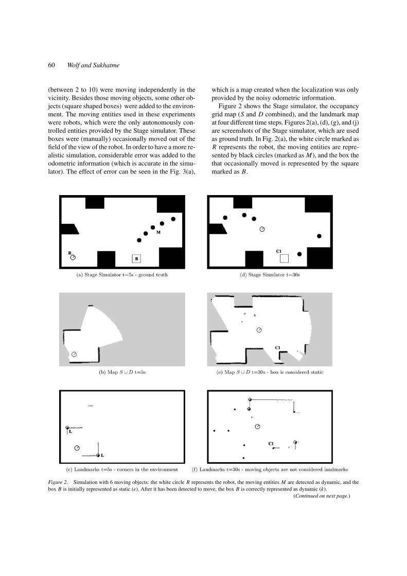
Figure 2. Simulation with 6 moving objects: the white circle R represents the robot, the moving entities M are detected as dynamic, and thebox B is initially represented as static (e). After it has been detected to move, the box B is correctly represented as dynamic (k).

(Continued on next page.)

which is a map created when the localization was onlyprovided by the noisy odometric information.

Figure 2 shows the Stage simulator, the occupancygrid map (S and D combined), and the landmark mapat four different time steps. Figures 2(a), (d), (g), and (j)are screenshots of the Stage simulator, which are usedas ground truth. In Fig. 2(a), the white circle marked asR represents the robot, the moving entities are repre-sented by black circles (marked as M), and the box thethat occasionally moved is represented by the squaremarked as B.

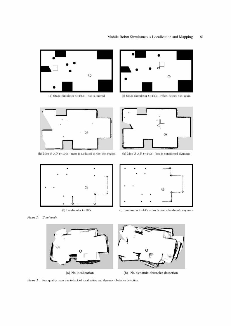
Mobile Robot Simultaneous Localization and Mapping 61

Figure 2. (Continued).

Figure 3. Poor quality maps due to lack of localization and dynamic obstacles detection.

62 Wolf and Sukhatme

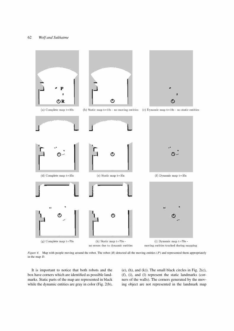
Figure 4. Map with people moving around the robot. The robot (R) detected all the moving entities (P) and represented them appropriatelyin the map D.

It is important to notice that both robots and thebox have corners which are identified as possible land-marks. Static parts of the map are represented in blackwhile the dynamic entities are gray in color (Fig. 2(b),

(e), (h), and (k)). The small black circles in Fig. 2(c),(f), (i), and (l) represent the static landmarks (cor-ners of the walls). The corners generated by the mov-ing object are not represented in the landmark map

Mobile Robot Simultaneous Localization and Mapping 63

because they cannot provide localization. The lines fol-lowing the walls in the landmark maps are the laserscans and the circles around determined landmarksidentify the landmarks that are being detected at thattime.

In Fig. 2(e), it is possible to see that the square boxhas been detected as static part of the environment. Therobot had not seen the box move at that time, there-fore it was considered static by default. The cornermarked as C1 has also been detected as a landmarkwhich could be used to provide localization. Duringthe experiment, the box was moved (out of the viewof the robot). As the robot revisited the part of themap, the region where was the box was updated as freespace (Fig. 2(h)). After a while, the box was detectedin a different position in the map and correctly clas-sified as dynamic part of the environment (marked asC2 on Fig. 2(k)), even after the robot has never seen itmoving. A short movie of the simulation is availableat: http://robotics.usc.edu/denis/videos/slam sim.avi.

As a result, the robot was able to differentiate thestatic and dynamic objects and show them appropri-ately on the map. All the moving objects in the en-vironment were correctly detected and only the staticlandmarks have been used for localization.

In order to show how detection of dynamic entitiesand SLAM can be mutually beneficial, we performedthe same experiment not using the EKF localization(Fig. 3(a)) and without differentiating dynamic entitiesin the environment (Fig. 3(b)). On both tests the robotfailed to create reasonable maps of the environment.Without the EKF the robot accumulated considerableerror in its localization estimate, which resulted in er-rors in detecting dynamic entities after revisiting analready mapped region of the environment. Withoutdifferentiating dynamic entities the robot consideredmoving objects as landmarks, which resulted in errorsin localization and consequently in mapping.

In order to test the robustness of the algorithms inreal situations, a set of experiments was conducted inthe California Science Center (CSC) in Los Angeles.During the experiments in the CSC, a large open space(14 m × 10 m) was mapped while three people activelywalked around the robot. The robot could correctlyidentify the static landmarks (corners) and successfullycreate maps of the environment differentiating staticand dynamic entities. Figure 4 shows the static and dy-namic maps, and their union. The robot his marked asR in Fig. 4(a). The three rows in Fig. 4 represent threedistinct time steps. Figures 4(b), (e), and (h) show the

occupancy grid of the static map (S). Figures 4(c), (f),and (i) show the occupancy grid of the dynamic map(D). The small black regions on the dynamic mapsrepresent the position of the moving objects (people)at that point in time (marked as P in the Fig. 4(a)).Figures 4(a), (d), and (g) show the complete map of theenvironment, where both static and dynamic entitiesare represented. The results presented in Fig. 4 showthe applicability of our approach in real world situa-tions. The robot was able to robustly create a map ofthe environment where static and dynamics entities arecorrectly identified and appropriately represented. Asground truth was not available during the experiments,the error in the robot’s pose could not be measured pre-cisely. We estimate that the uncertainty in the robot’sposition indicated by the EKF localization algorithm ison the order of few centimeters.

As identification of moving objects is based on thecomparison of the sensor measurements and the infor-mation contained in the map of the environment, smalllocalization/rounding errors lead to mistakes in differ-entiating static and dynamic parts of the environment.These mistakes are avoided if instead of comparingonly the occupancy of a determined cell we take intoaccount the occupancy of the neighborhood of that cell.

6. Conclusions and Future Work

We have proposed an approach to SLAM in dynamicenvironments which uses features that are likely to bestatic. We also demonstrated that detection of dynamicentities and SLAM are mutually beneficial. Experimen-tal and simulated tests show that our approach is ableto successfully create maps of dynamic environments,correctly differentiating static and dynamic parts of theenvironment and represent them in an occupancy grid.As the localization is based on corner detection, thealgorithm is also able to differentiate landmarks pro-vided by the static and dynamic entities, and use thestatic landmarks to do localization. The algorithm isrobust enough to detect dynamic entities both whenthey move in and out robot’s field of view.

As future work, we will investigate the use of differ-ent localization algorithms. They will be implementedin order to deal with non-structured environments. Al-ternative algorithms to detect moving entities may alsobe incorporated to our approach in order to improve theefficiency of the dynamic objects detection. We alsoplan to address the case where dynamic objects movevery slowly and close to static parts of the environment,

64 Wolf and Sukhatme

which created problems in the neighborhood compar-ison used in the present experiments. We also planto investigate how to use these techniques in outdoorenvironments, which introduce different challengesfor mapping, localization, and detection of dynamicentities.

7. Resources

The data-sets used in this article are available onthe Radish (Robotics Data Sets Repository) web-site(Howard and Roy, 2003).

Acknowledgments

The authors thank Boyoon Jung and Julia Vaughan fortheir valuable support during the tests in the CaliforniaScience Center. This work is supported in part by theDARPA MARS program under grants DABT63-99-1-0015 and 5-39509-A (via UPenn), ONR DURIP grantN00014-00-1-0638 and by the grant 1072/01-3 fromCAPES-BRAZIL.

Note

1. Player is a server and protocol that connects robots, sen-sors and control programs across the network. Stage simu-lates a population of Player devices, allowing off-line devel-opment of control algorithms. Player and Stage were devel-oped jointly at the USC Robotics Research Labs and HRL Labsand are freely available under the GNU Public License fromhttp://playerstage.sourceforge.net.

References

Andrade-Cetto, J. and Sanfeliu, A. 2002. Concurrent map build-ing and localization on indoor dynamic environments. Interna-tional Journal on Pattern Recognition and Artificial Intelligence,16:361–374.

Avots, D., Lim, E., Thibaux, R., and Thrun, S. 2002. A probabilistictechnique for simultaneous localization and door state estimationwith mobile robots in dynamic environments. In Proceedings ofthe International Conference on Intelligent Robots and Systems,pp. 521–526.

Aycard, O., Laroche, P., and Charpillet, F. 1998. Mobile robot lo-calization in dynamic environments using places recognition. InProceedings of the IEEE International Conference on Roboticsand Automation, pp. 3135–3139.

Biswas, R., Limketkai, B., Sanner S., and Thrun, S. 2002. To-wards object mapping in non-stationary environments with mobilerobots. In Proceedings of the International Conference on Intelli-gent Robots and Systems (IROS), pp. 1014–1019.

Castellanos, J., Neira, J., and Tards J. 2001. Multisensor fusionfor simultaneous localization and map building. IEEE Trans onRobotics and Automation, 17(6):908–914.

Dissanayake, M.W.M.G., Newman, P., Durrant-Whyte, H.F., Clark,S., and Csorba, M. 2001. A solution to the simultaneous localiza-tion and map building (SLAM) problem. IEEE Transactions onRobotic and Automation, 17(3):229–241.

Elfes, A. 1986. Sonar-based real-world mapping and navigation.IEEE Transactions on Robotics and Automation, 3(3):249–265.

Elfes, A. 1989. Using occupancy grids for mobile robot perceptionand navigation. Computer, 12(6):46–57.

Fenwick, J., Newman, P., and Leonard, J. 2002. Collaborative concur-rent mapping and localization. In Proc. of IEEE Conf on Roboticsand Automation, pp. 1810–1817.

Fox, D., Burgard, W., and Thrun, S. 1999. Markov localization formobile robots in dynamic environments. Journal of Artificial In-telligence Research, 2:391–327.

Gerkey, B.P., Vaughan, R.T., Stoy, K., Howard, A., Sukhatme, G.S.,and Mataric, M.J. 2001. Most valuable player: A robot deviceserver for distributed control. In Proceedings of the IEEE/RSJInternational Conference on Intelligent Robots and Systems,pp. 1226–1231.

Guivant, J.E. and Nebot, E. Optimization of the simultaneous local-ization and map-building algorithm for real-time implementation.IEEE Transactions on Robotics and Automation, 17(3):242–257.

Guivant, J. and Nebot, E. 2002. Improving computational and mem-ory requirements of simultaneous localization and map buildingalgorithms. IEEE International Conf on Robotics and AutomationICRA, pp. 2731–2736.

Haehnel, D., Schulz, D., and Burgard, W. 2002. Map buildingwith mobile robots in populated environments. In Proc. of theIEEE/RSJ International Conference on Intelligent Robots and Sys-tems (IROS), pp. 496–501.

Haehnel, D., Triebel, R., Burgard, W., and Thrun, S. 2003. Mapbuilding with mobile robots in dynamic environments. In Proc. ofthe IEEE International Conference on Robotics and Automation(ICRA), pp. 1557–1563.

Haehnel, D., Fox, D., Burgard, W., and Thrun, S. 2003. A highlyefficient FastSLAM algorithm for generating cyclic maps of large-scale environments from raw laser range measurements. In Proc. ofthe Conference on Intelligent Robots and Systems (IROS), pp. 206–211.

Howard, A. and Roy, N. 2003. Radish: The robotics data set reposi-tory http://radish.sourceforge.net.

Liu, Y. and Thrun, S. 2003. Results for outdoor-SLAM using sparseextended information filters. In Proc. of IEEE International Con-ference on Robotics and Automation, pp. 1227–1233,

Lu, F. and Milios, E. 1994. Globally consistent range scan alignmentfor environment mapping. Autonomous Robots 4:333–349.

Moravec, H. 1988. Sensor fusion in certainty grids for mobile robots.AI Magazine, 9(2):61–74.

Montemerlo, M., Thrun, S., Koller D., and Wegbreit, B. 2002. Fast-SLAM: A factored solution to the simultaneous localization andmapping problem. In Proceedings of the AAAI National Confer-ence on Artificial Intelligence, pp. 593–598.

Newman, P.M., Leonard, J.J., Neira, J., and Tardos, J. 2002. Ex-plore and return: Experimental validation of real time concurrentmapping and localization. In Proceedings of the 2002 IEEE In-ternational Conference on Robotics and Automation, pp. 1802–1809.

Mobile Robot Simultaneous Localization and Mapping 65

Nieto, J., Guivant, J., Nebot, E., and Thrun, S. 2003. Real time dataassociation for FastSLAM. In Proc. of IEEE International Con-ference on Robotics and Automation, pp. 512–518.

Tardos, J.D., Neira, J., Newman, P.M., and Leonard, J.J. 2002. Ro-bust mapping and localization in indoor environments using sonardata. International Journal of Robotics Research, 21(4):311–330.

Thrun, S. 2002. Robotic mapping: A survey. In Exploring ArtificialIntelligence in the New Millenium, G. Lakemeyer and B. Neberl(Eds.). Morgan Kaufmann.

Thrun, S., Burgard, W., and Fox, D. 1998. A probabilistic approach toconcurrent mapping and localization for mobile robots’. MachineLearning, 31:29–53.

Thrun, S., Burgard, W., and Fox, D. 2000. A real-time algorithmfor mobile robot mapping with applications to multi-robot and 3Dmapping. In Proceedings of the IEEE International Conferenceon Robotics and Automation, pp. 321–328.

Tomasi, C. and Kanade, T. 1991. Detection and tracking of pointfeatures, Carnegie Mellon University Technical Report CMU-CS-91-132.

Wang, C. and Thorpe, C. 2002. Simultaneous localization and map-ping with detection and tracking of moving objects. IEEE Interna-tional Conference on Robotics and Automation, pp. 2918–2924.

Wang, C.-C., Thorpe, C., and Thrun, S. 2003. Online simultaneouslocalization and mapping with detection and tracking of movingobjects: Theory and results from a ground vehicle in crowdedurban areas. In Proc. of the IEEE International Conference onRobotics and Automation (ICRA), pp. 842–849.

Wolf, D.F. and Sukhatme, G.S. 2003. Towards mapping dynamicenvironments. In In Proceedings of the International Conferenceon Advanced Robotics (ICAR), pp. 594–600.

Wolf, D. and Sukhatme, G. 2004. Online simultaneous localizationand mapping in dynamic environments. In Proc. of IEEE Inter-national Conference on Robotics and Automation, New Orleans,pp. 1301–1306.

Dennis F. Wolf is a Ph.D. student in the Computer Science depart-ment at University of Southern California (USC). His research in-

terests include localization and mapping in urban environments andmapping dynamic environments with mobile robots. Denis receivedhis B.Sc. in Computer Science from Federal University of Sao Carlos,Brazil in 1999 and his M.Sc. in Computer Science from Universityof Sao Paulo, Brazil in 2001.

Gaurav S. Sukhatme is an Assistant Professor in the ComputerScience Department at the University of Southern California (USC).He received his M.S. and Ph.D. in Computer Science from USC.He is the co-director of the USC Robotics Research Laboratory andthe director of the Robotic Embedded Systems Laboratory whichhe founded at USC in 2000. His research interests are in distributedmobile robotics and sensor/actuator networks. Prof. Sukhatme hasserved as PI on several NSF, DARPA and NASA grants. He is amember of AAAI, IEEE and the ACM and has served on severalconference program committees. He is on the editorial boards oftwo leading journals in robotics, IEEE Transactions on Robotics andAutomation, and Autonomous Robots and a leading magazine inubiquitous computing, IEEE Pervasive Computing. He has publishedover 100 technical papers and is a receipient of the NSF CAREERaward.