A Near-Tight Approximation Algorithm for the Robot Localization Problem

SIAM J. COMPUT. c© 20XX Society for Industrial and Applied MathematicsVol. 0, No. 0, pp. 000–000

A NEAR-TIGHT APPROXIMATION ALGORITHM FOR THEROBOT LOCALIZATION PROBLEM∗

SVEN KOENIG† , JOSEPH S. B. MITCHELL‡ , APURVA MUDGAL§ , AND CRAIG TOVEY§

Abstract. Localization is a fundamental problem in robotics. The “kidnapped robot” possessesa compass and map of its environment; it must determine its location at a minimum cost of traveldistance. The problem is NP-hard [G. Dudek, K. Romanik, and S. Whitesides, SIAM J. Comput.,27 (1998), pp. 583–604] even to minimize within factor c log n [C. Tovey and S. Koenig, Proceedingsof the National Conference on Artificial Intelligence, Austin, TX, 2000, pp. 819–824], where n isthe map size. No approximation algorithm has been known. We give an O(log3 n)-factor algorithm.The key idea is to plan travel in a “majority-rule” map, which eliminates uncertainty and permitsa link to the 1

2-Group Steiner (not Group Steiner) problem. The approximation factor is not far

from optimal: we prove a c log2−ε n lower bound, assuming NP �⊆ ZTIME(npolylog(n)), for the gridgraphs commonly used in practice. We also extend the algorithm to polygonal maps by discretizingthe problem using novel geometric techniques.

Key words. robotics, kidnapped robot, localization, approximation algorithm, hardness ofapproximation, computational geometry

AMS subject classifications. 68T37, 68T40, 68W25, 68U05

DOI. 10.1137/070682885

1. Introduction. Consider the following problem: a mobile robot is placed atan unknown position in an environment for which it has a map E . The robot con-structs a map E ′ of its local environment by going to different places and sensing theenvironment from there. It rules out positions whose local environment does not agreewith map E ′ until it infers the unique position where it was originally located. Theobjective is to complete this task by traveling the minimum possible distance. Thisis known as the kidnapped robot or localization problem [13, 32].

1.1. Motivation. In general, robots must localize when they are switched onbecause they may have been moved while switched off. Also, the control systems guid-ing a robot gradually accumulate error due to mechanical drift and sensor noise [15].Thus, it is necessary to localize from time to time to verify the actual position of therobot in the map, and then apply corrections. In this context, localization eliminatesthe need for complex and expensive position-guidance systems, such as radio beacons[7, 13], to be installed in buildings or streets with tall buildings, where three satellitesare not in view and so GPS is not effective. For situations in which such systemscannot be built, such as a Mars rover (see [30]), localization is the only possibility.

∗Received by the editors February 20, 2007; accepted for publication (in revised form) March 10,2009; published electronically DATE. This research was partially supported by the National ScienceFoundation (ACI-0328930, CCF-0431030, CCF-0528209, IIS-0098807, IIS-0412912, IIS-0099427, IIS-00907, and ITR/AP-01131), Metron Aviation, and NASA Ames. A preliminary version of this paperappeared as A near-tight approximation algorithm and lower bound for the kidnapped robot problemin Proceedings of the Seventeenth ACM-SIAM Symposium on Discrete Algorithms (SODA ’06),pages 133–142.

http://www.siam.org/journals/sicomp/x-x/68288.html†Computer Science Department, University of Southern California, Los Angeles, CA 90089

([email protected]).‡Applied Mathematics & Statistics, Stony Brook University, Stony Brook, NY 11794 (jsbm@ams.

sunysb.edu).§College of Computing, Georgia Tech, Atlanta, GA 30332 ([email protected], ctovey@cc.

gatech.edu).

1

2 S. KOENIG, J. MITCHELL, A. MUDGAL, AND C. TOVEY

observationobservation

��

��

�

�

Fig. 1.1. (a) A grid graph G with a robot at its center. The observation of the robot is shownon the right. (b) A simple polygon P with the visibility polygon V(p) for a robot placed at p.

1.2. Model. We study localization within two well-studied two-dimensionalmodels: models based on grid graphs and models based on polygons. A grid graphG is a finite rectangular region consisting of a union of unit square cells, as shown inFigure 1.1(a). Each cell can be either blocked or traversable. In the grid graph model,a robot is always in exactly one traversable cell. It starts in a traversable cell and canmove in a single step to any neighboring traversable cell, to its north, south, east, orwest. Tactile sensors allow the robot to determine the states (blocked/traversable) ofits four neighboring cells. In the polygonal model [48, 13], the environment is a poly-gon P and the robot occupies exactly one point p ∈ P . The robot is equipped with arange finder, a device that emanates a beam (laser or sonic) and determines distanceto the first point of contact with P ’s boundary in that direction. The robot sends outa series of beams spaced at regular angular intervals about its position, measuringthe distance to the boundary at each of these angles. The points of contact are thenjoined together to obtain a visibility polygon V (see Figure 1.1(b)). We use n to denotethe combinatorial size of the map: for grid graphs n is the number of cells in G, andfor a polygonal model n is the number of vertices in the map polygon P .

Following Dudek, Roamanik, and Whitesides [17], we view the localization prob-lem as having two phases: hypothesis generation and hypothesis elimination. Thefirst phase is to determine the set H of hypothetical locations, or hypotheses, thatare consistent with the sensing data obtained by the robot from its initial location(see Figure 1.2). The second phase is to determine which location h ∈ H is the truelocation of the robot. (The second phase is unnecessary if |H | = 1.) For the gridgraph model, H is simply the set of all traversable cells, and the localization problemfocuses on the second phase. For the polygonal model, Guibas, Motwani, and Ragha-van [23] provide an algorithm that generates the set of at most n hypotheses, usingthe visibility polygon observed by the robot in its initial location. Thus, we focushere on the hypothesis elimination problem.

By a strategy S we mean the hypothesis elimination routine employed in therobot’s computer. We measure the effectiveness of a strategy based on its worst-caseperformance. For strategy S, let W (h, S) be the distance traveled to localize if therobot is placed at hypothesis h ∈ H . Then the cost W (S) of strategy S is defined to bethe maximum distance, W (S) = maxh∈HW (h, S), traveled for any starting positionh. An optimal strategy S∗ has cost W (S∗) = minS∈S W (S), where S denotes theset of all possible localization strategies. OPT(G, H) denotes the cost of an optimalstrategy, where G is the map and H is the set of hypotheses. We say that a strategyis α-approximate if its cost is at most α · OPT(G, H).

ROBOT LOCALIZATION PROBLEM 3

��

��

��

� � ��

��

Fig. 1.2. Hypothesis generation. Based on the observed visibility polygon V, we generate theset H = {h1, h2, h3, h4} of hypotheses as the possible locations of the robot.

1.3. Previous work. Despite the considerable attention it has received in therobotics literature (e.g., [13, 32, 40, 45, 48]), localization has been the subject ofrelatively little theoretical work. Guibas, Motwani, and Raghavan [23] show how topreprocess the polygon P so that the set of hypotheses H consistent with a singleobservation V can be returned quickly. Their algorithm preprocesses P in O(n5) timeand space and generates hypotheses in O(m+log n+k) time, where m is the number ofvertices in the observed visibility polygon V , and k = |H | is the number of hypothesesgenerated. (Note that k ≤ n, and, in fact, k is at most the number of reflex verticesof P .)

Kleinberg [27] was the first to give interactive strategies for the hypothesis elimi-nation problem. He measures the performance of his strategies using the competitiveratio criterion, in contrast with our worst-case criterion. The competitive ratio com-pares the distance traveled by a robot following a strategy to that traveled by anomniscient verifier, i.e., a robot that has a priori knowledge of its position h ∈ H andprobes the environment just to verify this information. The distance traveled by anomniscient verifier at hypothesis h is exactly minS∈SW (h, S), and an α-competitivestrategy enables a robot initially located at hypothesis h to travel distance at mostα · minS∈SW (h, S) prior to completing localization.

In Kleinberg’s model the environment is a geometric tree, G(V, E), where V is a setof points in R

d and E is a set of line segments whose endpoints all lie in V . The edgesdo not intersect except at V and do not form cycles. The robot occupies a point onone of the edges and is capable of moving along an edge in either direction. Kleinbergfurther assumes that the only information available to the robot is the orientationof all edges incident at its current position p ∈ E. He gives an O(n2/3)-competitivealgorithm on geometric trees having bounded degree, and he gives an Ω(

√n) lower

bound. He also gives an O(n√

log nlog log n )-competitive algorithm for a geometric model

consisting of a packing of rectangles (obstacles) in the plane, with no two rectangles“stuck together” (i.e., two rectangles can nearly touch, but there remains a traversablegap between them) and each rectangle having at least unit width. In section 5.4, wegive an O(log3 n)-approximate strategy not just for geometric trees, but for geometricgraphs in any Euclidean space R

d.Dudek, Romanik, and Whitesides [17] consider the problem of designing com-

petitive strategies for the polygonal model; however, they assume that the robot cancompute only the visibility skeleton V∗(p), which is an approximation of visibilitypolygon V(p). The visibility skeleton V∗(p) (see [23]) is a contraction of V(p), con-sisting of only those vertices in V(p) that can be certified to be vertices of P . For thismodel, they give a greedy 2(k − 1)-competitive strategy minimum distance localiza-


tion (MDL) for hypothesis elimination, where k = |H | is the number of hypotheses.They also show that there are polygons P and sets of hypotheses H for which thebest strategy is 2(k − 1)-competitive. We believe that this line of work stands clos-est to ours in both geometric and algorithmic structure. We refer the reader to thebibliographic note at the end of section 3 for a discussion of the recent work on thisstrategy as well as a comparison with our results.

Dudek, Romanik, and Whitesides were also the first to study the localizationproblem from the worst-case perspective, which they describe as the height of a lo-calizing decision tree. They prove that computing an optimal localizing decision tree(i.e., an optimal worst-case strategy) is NP-hard by a reduction from the abstractdecision tree problem [25]. Tovey and Koenig [46] show that it is NP-hard even tofind a c · log n-approximate strategy, both for grid graphs and for polygons, using a re-duction from the set cover problem [28]. Schuierer [44] proposes a technique that usesgeometric overlay trees to reduce the running time of Dudek, Romanik, and White-sides greedy strategy. His technique, along with a careful choice of data structures,allows the robot to localize in computation time O(kn log n) and space O(kn).

Brown and Donald [5] describe algorithms for localization that allow for uncer-tainty in the measurements of range sensors. Fox, Burgard, and Thrun [21] use Markovlocalization to deduce the position of the robot from sensor data. In their work, globallocalization is achieved as a side effect of robot movement, and the length of the lo-calizing trajectory relative to the optimum is not considered. In Markov localizationand related approaches, localization and action are viewed in a compound setting;the effects of various actions are interpreted probabilistically and the robot is ableto predict the belief states ensuing from various actions. Long-range path planningusing these approaches remains problematic because of the large state space involved.

The motivation for competitive algorithms comes from theoretical work of a sim-ilar flavor in robot navigation in unknown environments. The objective of the robotis to navigate from a point s to a target t while avoiding obstacles/walls in the scene,which are not known to the robot a priori, but which the robot learns by encounteringthem. The goal is seek to minimize the competitive ratio of the distance traveled bythe robot to the length of the shortest obstacle-free path from s to t. Papadimitriouand Yannakakis [37] gave the first such results, achieving a competitive ratio of 1.5(which they show is the best possible) in the case that obstacles are unit squares.They, along with Eades, Lin, and Wormald [18] also give a lower bound of Ω(

√n) on

the competitive ratio in the case that t is an infinite wall and the obstacles are axis-aligned rectangles. Baeza-Yates, Culberson, and Rawlins [1] introduce the techniqueof spiral search, with which they obtain a (9+o(1))-competitive algorithm for findinga point on a line and a 13.81-competitive algorithm to search for a line at distance nfrom the origin. A restricted spiral search in a geometric tree forms the first part ofKleinberg’s localization algorithm. Blum, Raghavan, and Schieber [6] use a variant ofthe spiral search technique to give a strategy that matches the Ω(

√n) lower bound for

navigating between two points among axis-aligned rectangular obstacles. The naviga-tion problem has also been studied in the polygonal model, for which Klein [26] givesa lower bound of

√2 on the competitive ratio and gives a 5.72-competitive algorithm

for a subclass known as street polygons. Later, Kleinberg [29] improved the ratio to2√

2, and Datta and Icking [14] gave a 9.06-competitive algorithm for the broaderclass of generalized streets.

There are advantages to considering worst-case cost over the competitive ratiofor the localization problem. In online navigation problems, the map is not known,and hence the informational assumption of competitive analysis holds for the robot.


But in the localization problem the map is given a priori to the robot. Hence theinformation available to the robot is precisely what is needed for standard worst-caseanalysis. A competitive analysis assumes there is too little information available tothe robot, and too much to the omniscient verifier, than is realistic. From a practicalstandpoint, worst-case analysis better matches the roboticist’s concerns with guaran-teed rapid localization, rather than with comparisons against a nonexistent omniscientverifier. From a theoretical standpoint, it admits an O(log3 n)-approximation algo-rithm; in contrast, it is NP-hard to obtain a strategy with competitive ratio o(

√n) in

polygons [17].

1.4. Group Steiner problem. The Group Steiner problem is the following.(Rooted) Group Steiner problem. Given a weighted graph G = (V, E) with

k groups of vertices g1, g2, . . . , gk ⊂ V , find a minimum-weight tree that contains atleast one vertex from each group. There is a distinguished vertex r (the root vertex)that must be included in the tree.

The Group Steiner problem generalizes both minimum Steiner tree and set coverproblems. For purposes of our algorithm, we need a variant called the 1

2 -Group Steinerproblem [19], in which the goal is to find a minimum-weight tree that contains verticesfrom at least half of the groups.

An O(log2 n) algorithm for Group Steiner on trees is given by Garg, Konjevod,and Ravi [22]. They first solve a linear programming relaxation to get a fractionalsolution and then use an innovative randomized rounding scheme. A modificationof the algorithm, by Even, Kosarz, and Slany [19], yields an O(log n)-approximationfor the 1

2 -Group Steiner problem on trees. For general graphs, one can first proba-bilistically approximate the graph by a tree, using a result of Fakcharoenphol, Rao,and Talwar [20] (which is a recent improvement to Bartal [3]), losing an O(log n)factor in the process. Then the algorithm of Garg, Konjevod, and Ravi [22] is appliedto the resulting tree, giving an O(log3 n)-approximation for Group Steiner and anO(log2 n)-approximation for the 1

2 -Group Steiner problem.Theorem 1.1 (see [22, 19, 20]). There exists an O(log2 n)-approximation algo-

rithm A for the rooted 12 -Group Steiner problem that runs in randomized polynomial

time.The running time of this algorithm is high, and hence the computation time of

the robot will be large. As the approximation algorithm is used only as a black box,we will denote the running time by the (polynomial) P(n′) and instead concentrateon reducing the size n′ of the instance. However, if we are willing to trade off betweenrunning time and approximation factor, there are much faster algorithms available.Bateman et al. [4] give a

√k ln k-approximation algorithm that runs in O(nk2 log k)

time. Their algorithm is based on the fact that there exists a Group Steiner tree ofdepth 2 rooted at r with cost within

√k of optimal. By adapting their algorithm

to the 12 -Group Steiner problem, we get an O(

√n log2 n)-approximation strategy for

localization on grid graphs with computation time O(n3 log2 n) (the best previousfactor was Ω(n)). A more smooth trade-off can be obtained by using the algorithmof Charikar et al. [9] for the Directed Steiner tree problem (which includes the 1

2 -Group Steiner problem as a special case), yielding an i(i − 1)k(1/i)-approximationwith running time O(nik2i). For any ε > 0, the robot localizes by traveling distancewithin factor O(nε

ε2 ·logn) of the optimal and spending computation time O(n3ε log2 n).

We hope that future work on the 12 -Group Steiner problem will lead to algorithms

with better running times.


Chekuri and Pal [10] have recently described a O(log2 n)-factor quasi–polynomial-time algorithm for the Group Steiner problem. Since the algorithm involves set coverstyle arguments, this gives an O(log n) algorithm for the 1

2 -Group Steiner problemby stopping it when it covers half the groups. Thus our approximation algorithm isoptimal if we allow for quasi-polynomial time.

The problem they solve is the submodular orienteering problem (SOP). Here eachsubset X ⊆ V of a directed graph G(V, E) has a reward function f(X) which satisfiesthe submodular property. The objective is to construct a walk with maximum givenlength B such that the subset of vertices V ′ ⊆ V covered by the walk has maximumreward f(V ′). Their algorithm is reminiscent of Savitch’s algorithm: the algorithmguesses the middle node of the optimal walk and then recurses two times. However,here the second recursive call is dependent on the output of the first recursive call(i.e., the subset of vertices covered by it), unlike in Savitch’s algorithm where thetwo calls are independent. We add that the question of a polynomial-time O(log2 n)algorithm for Group Steiner is still open.

1.5. Our results. The main contribution of this paper is a polynomial-timestrategy, repeated half localization (RHL), which localizes the robot with travel dis-tance within a factor O(log3 n) of that of an optimal strategy; more precisely, theapproximation factor is O(log2 n log k), where k = |H | ≤ n is the number of hy-potheses. The key algorithmic idea is to plan travel in a “majority-rule” map, whicheliminates uncertainty and permits a link to the 1

2 -Group Steiner (not Group Steiner)problem. Section 2 describes the strategy for the commonly used grid graph model.Section 3 extends the algorithm to robots with line-of-sight (i.e., range finder) sensorsin polygons. In section 4, we give a log2−ε n approximation lower bound, assumingNP �⊆ ZTIME(npolylog(n)), for both grid graphs and the polygonal model. Sec-tion 5 sketches extensions of our strategy to a wide variety of models: robots withoutcompasses, limited-range sensors, polygons with holes, geometric trees, and three-dimensional environments. In section 6 we show that a variant of our strategy whichdoes not return to the origin after each half-localize step performs very poorly. Insection 7 we summarize and comment on some open problems.

The basic framework of the strategy is to break localization into a sequence ofhalf-localize steps.

HALF-LOCALIZE (G, H): Devise a strategy by which the robot can correctlyeliminate at least half of the hypotheses in H . The robot should travel a (worst-case)distance as small as possible to achieve this. HALF-OPT(G, H) denotes the cost ofthe optimal strategy.

Intuitively it might appear that an O(log2 n) algorithm for half-localization shouldbe a by-product of our O(log3 n) localization strategy and not vice versa. As anexample of this, consider the 1

2 -set cover problem, in which the objective is to coverhalf the elements at minimum cost. There is a constant factor approximation for this,and it is obtained by stopping the O(log n) greedy algorithm for set cover as soon as wecover half the elements. (Another example is the algorithm for 1

2 -Group Steiner [19],which is obtained by stopping the rounding scheme of [22] as soon as the tree covershalf the groups.)

However, half-localize seems to play a more fundamental role in our context. Webriefly discuss only the simpler grid graph case here. We construct a majority-rulemap, in which each cell is blocked or unblocked depending on what the majority ofthe current hypotheses in H assert. This majority-rule map permits three interrelatedsimplifications. If the robot tries to follow a route within the majority-rule map but


makes a minority observation (one inconsistent with at least half of the hypotheses),then the robot has half-localized. This permits a plan to be a path rather thana decision tree. Distances in the real environment are uncertain, but distances onthe majority-rule map are fixed. This permits us to model half-localization as aSteiner-type problem on a graph, although we are not able to model localization assuch. Finally, there is an essential equivalence between optimally half-localizing andhalving paths on the majority-rule map (see section 2.3).

2. Strategy for grid graphs.

2.1. Preliminaries. During half-localization the robot makes observations fromdifferent positions in its environment (grid graph G) to make a larger and larger localmap G′, until there is exactly one hypothesis in H that is consistent with G′. We saythat a hypothesis h ∈ H is active if the robot’s local map is consistent with it beinglocated at h. We denote the set of active hypotheses by H ′.

We distinguish between the absolute (global) position of the robot in the gridgraph G and its relative (local) position in G′ by using Greek letters for the latter(whenever possible). Let γ0 denote the initial position of the robot with respect tothe local map G′. We call γ0 the origin, and denote any other position in G′ by apair of coordinates. Coordinate γ = (x, y) denotes the cell in G′ lying x units to theeast and y units to the north of γ0. Negative values of x, y denote west and south,respectively. Thus a robot at coordinate γ ∈ G′ will be located at position p0 + γ ingrid graph G, where p0 ∈ G is its initial position. The robot can keep track of its localcoordinates by taking successive readings on the compass and odometer (we assumeerror-free motion and sensing during localization). At any point of time, the robot issure of its local coordinates but knows its global position only up to cells in H ′ + γ.

Suppose the robot makes an observation when at coordinate γ ∈ G′. The outcomedepends on its starting location h ∈ H . If the robot started from hypothesis h,the observation will be the same as that by a robot located at h + γ in G. Wedenote this observation by O(h, γ) and call it the opinion of h about γ. If h + γ isblocked, we set O(h, γ) = ∅. The hypothesis partition H(γ) is a partition of the setof hypotheses according to the following equivalence relation: h1 ∼ h2 if and only ifO(h1, γ) = O(h2, γ). Maj(γ) denotes the largest size class of H(γ). The “majorityopinion” at γ is the opinion common to the plurality of hypotheses h ∈ Maj(γ). Noteit may occur that |Maj(γ)| < 1

2 |H |. The lemmas that follow are valid in this casebecause the robot immediately half-localizes. Since there are two choices, blocked ortraversable, for each of the four neighboring cells of γ, an observation o can be writteno ∈ {b, t}4

⋃ {∅}, and we let G(γ, o) denote the class of H(γ) with opinion o at γ.

2.2. The majority-rule map. We now describe the majority-rule map Gmaj ,a data structure central to our half-localization algorithm.

Definition 2.1. The majority-rule map Gmaj is a local map in which each cell isblocked or traversable according to what the majority of hypotheses have to say aboutit (in case of a tie, we consider the cell to be traversable). The majority-rule map alsoincludes the hypothesis partitions for all local coordinates.

In other words, a cell γ ∈ Gmaj is blocked if and only if |Maj(γ)| > 12 |H | and

V(Maj(γ)) = ∅. If G is an l×m grid graph, the majority-rule map has size boundedby (2l − 1) × (2m − 1), since the absolute values of x- and y-coordinates for anyhypothesis are at most (l− 1) and (m− 1), respectively. Clearly, Gmaj requires space4nk (there are at most 4n cells, and we need to store the partition for each cell)and can be computed in time O(nk). Figure 2.1 shows the majority-rule map for


��

��

��

��

��

Fig. 2.1. (a) A half-localization problem with grid graph G and H = {h1, h2, h3, h4}. (b) Themajority-rule map for HALF-LOCALIZE(G, H) with two halving paths (γ0, γ1, γ2) and (γ0, γ3).

grid graph G and H = {h1, h2, h3, h4}. The black region is unreachable by the robotfor any starting hypothesis. The hypothesis partition is constant within each of theregions R0, R1, R2, R3, R4, R5, and R6. R5 and R6 lie outside the grid graph forthree different hypotheses and are blocked. Thus the only traversable regions areR0, R1, R2, R3, and R4, with Maj(R0) = {h1, h2, h3, h4}, Maj(R1) = {h2, h3, h4},Maj(R2) = {h1, h2, h3}, Maj(R3) = {h3, h4}, and Maj(R4) = {h1, h2}.

2.3. Halving paths. We now define the notion of a halving path in the majority-rule map.

Definition 2.2. A halving path is a (possibly self-intersecting) path C = (γ0, γ1,γ2, . . . , γm) in the majority-rule map satisfying |⋂m

i=0 Maj(γi)| ≤ 12 |H |.

The next two lemmas show an essential equivalence between half-localizationstrategies and halving paths.

Lemma 2.3. Let C be a halving path. There exists a strategy S(C) for half-localizing the robot with travel cost at most |C|.

Proof. Let C = (γ0, γ1, γ2, . . . , γm), where γi+1 is a neighbor of γi in Gmaj . Adescription of strategy S(C) is as follows (see Algorithm 1): the robot traces pathC from its initial position, taking observation oi at each new coordinate γi. If therobot finds that the next coordinate is blocked, it stops. We next show that this willhalf-localize the robot correctly.

After observation oi, the robot keeps only those hypotheses whose opinion at γi

is oi. Thus, it updates H ′ (the set of active hypotheses) correctly. We show that S(C)reduces the set of hypotheses by half. If the robot finds that the cell at coordinate γi

is blocked, it localizes to a set of size at most |G(γi, ∅)| ≤ 12 |H | (since γi ∈ Gmaj). If

observation oi is different from the majority opinion at γi, H ′ ⊆ G(γi, oi), which hassize at most 1

2 |H |. Thus the robot reaches γm if and only if for each γi, 0 ≤ i ≤ m−1,oi is the majority opinion at γi. Now there are two cases: if om is different fromthe majority opinion, the robot half-localizes; otherwise H ′ =

⋂mi=0 Maj(γi), which

is again at most 12 |H | (since C is a halving path).

In Figure 2.1, the halving path C1 = (γ0, γ1, γ2) satisfies |⋂2i=0 Maj(γi)| = |{h2, h3}|

≤ 12 |H |. The path (γ0, γ3) is an optimal halving path, with |Maj(γ0)

⋂Maj(γ3)| =

|{h1, h2}| ≤ 12 |H |. Note that we did not include intermediate cells in the description,


Data: Grid graph G, set of hypotheses H and a halving path (γ0, γ1, . . . , γm) ∈ Gmaj .Result: The robot half-localizes in at most m steps.Initialize H′ = Hfor i = 0 to m − 1 do

beginMake observation oi at coordinate γi

Update H′ = H′ ⋂G(pi, oi). Stop if |H′| ≤ 1

2|H|

Move to coordinate γi+1

end

endMake observation om at γm; Update H′ = H′ ⋂

G(γm, om). Stop.

Algorithm 1: Strategy S(C).

ssuming that the robot uses any shortest path in the majority-rule map to go from γi

to γi+1. The behavior of a robot following strategy S(C1) will be as follows. If it wasplaced at h1, it will hit a wall at γ1 and stop with H ′ = {h1}. If it was placed at h4,it will see a wall at γ2 and stop with H ′ = {h4}. If it was placed at either h2 or h3,it will make majority observations at both γ1, γ2 and half-localize to the set {h2, h3}of hypotheses.

The next lemma shows that any half-localization strategy S has an associatedhalving path with length at most W (S) (compare this with localization, for whichstrategies are decision trees [17] and hence hard to compute).

Lemma 2.4. Let S be a strategy for half-localization. There exists a halving pathC(S) of length at most W (S), the cost of the strategy S.

Proof. Consider a robot guided by S that stops as soon as it half-localizes. LetC(S) = (γ0, γ1, γ2, . . . , γm) be the maximum length path traced by the robot in its localmap G′ for any starting position in H . Let Hi denote the set of active hypotheses justafter the robot makes an observation at coordinate γi. For 0 ≤ i < m, |Hi| > 1

2 |H |,since otherwise the robot would have stopped at γi itself. Each coordinate γi isunblocked for at least |Hi| > 1

2 |H | hypotheses, and hence C(S) lies in the majority-rule map Gmaj .

We claim that I =⋂m

i=0 Maj(γi) is of size at most 12 |H |. Consider a robot

initially located at some h ∈ I. Guided by S, the robot will follow path C(S) andmake the majority observation oi at all coordinates γi (since I ⊂ Maj(γi)). But then|⋂m

i=0 Maj(γi)| = |Hm| ≤ 12 |H |, and hence C(S) is a halving path.

2.4. Computing halving paths. Let C∗H denote an optimal halving path for

the set of hypotheses H = {h1, h2, . . . , hk}. We approximate the problem of com-puting an optimal halving path by reducing it to an instance IG,H of the 1

2 -GroupSteiner problem.

The reduction is a restatement of the problem in terms of groups: we take V asthe set of traversable coordinates in the majority-rule map. The weight of edge (γ, γ′)is the length of the shortest path joining cells γ and γ′ in Gmaj . Origin γ0 is taken asthe root vertex. We make k groups, one for each hypothesis hi ∈ H . Group gi is theset of all coordinates γ ∈ V such that hi does not share the majority opinion at γ, i.e.,hi /∈ Maj(γ). Thus a tree T covers k′ groups if and only if

⋂x∈T Maj(x) has size k−k′.

In particular, T covers at least half the groups if and only if |⋂γ∈T Maj(γ)| ≤ 12 |H |.

In particular, every halving path is a 12 -Group Steiner tree.

Lemma 2.5. There exists an O(log2 n)-approximation algorithm for computingan optimal halving path.

Proof. Let T be the tree output by algorithm A (see Theorem 1.1) on instanceIG,H . Then, the weight of T is at most O(log2 n) · w(T ∗), where T ∗ is an optimal


12 -Group Steiner tree. Let C be the path of length at most 2 ·w(T ) traced by a depth-first search on T starting from the origin. C is a halving path since |⋂γ∈C Maj(x)| =|⋂γ∈T Maj(x)| ≤ 1

2 |H |. Since an optimal halving path C∗H covers half the groups,

w(T ∗) ≤ |C∗H |. Therefore, |C| ≤ O(log2 n) · |C∗

H |.2.5. Strategy RHL. The overall strategy is as follows (see Algorithm 2). In

each half-localize phase, the robot computes a near-optimal halving path C and thentraces C to reduce the set of (active) hypotheses by half. It retraces C to moveback to its initial position and proceeds with the next phase. We now bound theapproximation factor and computation time of strategy RHL.

Data: Grid graph G, the set of hypotheses HResult: The robot localizes to its initial position h ∈ Hwhile |H| > 1 do

beginCompute the majority-rule map Gmaj

Make instance IG,H of 12-Group Steiner problem

Solve IG,H to compute a halving path C (Lemma 2.5)Half-localize by strategy S(C) (Lemma 2.4)Move back to the starting location

end

endAlgorithm 2: Strategy RHL (repeated half localization).

Theorem 2.6. A robot guided by strategy RHL (Algorithm 2) correctly deter-mines its initial position h ∈ H by traveling at most O(log2 n log k) · OPT (G, H)distance, where k = |H | and n is the size of G. Further, the computation time of therobot is polynomial in n.

Proof. Since the number of active hypotheses reduces by at least half after eachphase, the robot localizes in m ≤ log |H |� = log k� phases. Let Hi denote the set ofactive hypotheses at the start of the ith phase. By Lemma 2.5, the distance traveledby the robot in the ith phase is at most O(log2 n) · |C∗

Hi|. By Lemma 2.4, |C∗

Hi| ≤

HALF-OPT(G, Hi) ≤ OPT(G, H), where the last inequality follows from the fact thatany localization plan also reduces the set of hypotheses by half. Therefore, the distancetraveled by the robot in each phase is at most O(log2 n) ·OPT(G, H). Since there areO(log k) phases, the total worst-case travel distance is O(log2 n log k) · OPT(G, H).Since instance IH can be constructed in O(nk) time, the computation time is at mostO(P(nk) · log n), where P() (a polynomial) is the time taken by the approximationalgorithm for 1

2 -Group Steiner (see section 1.4).The above theorem shows the performance ratio for a robot with very weak sen-

sors; the robot can only “see” four neighboring cells. We note that all of the theoremsof this section hold for robots on grid graphs with other kinds of sensors such asrange-finders or sonar. An interesting feature of our strategy is that it is well suitedto handling the problem of accumulation of errors caused by successive motion inthe estimates of orientation, distance, and velocity by the robot’s odometer. This isbecause after each half-localize phase the robot always returns to the origin, which itcan use to recalibrate its sensors [17].

3. Polygonal model. In this section, we extend our algorithm to polygons. Wefocus here on the case of simple polygons; in section 5 we discuss the extension to thecase of polygons with holes. The outline of the algorithm is the same: the robot worksin phases, in each phase reducing the set of hypotheses by half. However, since the


robot moves continuously, local coordinates γ lie in the Euclidean plane R2 (for grid

graphs, they were points on the integral lattice). As before, let opinion O(h, γ) denotethe observation, i.e., the visibility polygon observed by a robot at position h+ γ ∈ P .If the point h + γ lies outside P , we take O(h, γ) = ∅. For a coordinate γ ∈ R

2,the hypothesis partition H(γ) partitions hypotheses in H according to their opinionsO(h, γ). The majority-rule map denotes the subset of coordinates that lie inside Pfor the majority of hypotheses. In section 3.1, we will show that the majority-rulemap is a polygon with holes of size O(k2n2) and that this bound is tight in the worstcase. We let Pmaj denote the connected component of the majority-rule map thatcontains the origin γ0, and often we refer to Pmaj simply as the majority-rule map,since Pmaj is the component of interest to us.

In the polygonal model, a halving path C is a curve in the majority-rule map withone endpoint at the origin γ0 such that |⋂x∈C Maj(x)| ≤ 1

2 |H |. (Parameter x variesover the continuum of coordinates along the path C.) It is straightforward to extendLemmas 2.3 and 2.4 to the case of polygons with this new definition. A shortest pathPath(γ, γ′) between any two coordinates γ, γ′ ∈ Pmaj is piecewise linear with bendpoints at vertices (this includes the vertices of holes) of Pmaj . Hence, we can specifya halving path by a sequence (γ0, γ1, . . . , γm), where |⋂m

i=0 Maj(γi)| ≤ 12 |H |, and a

shortest path Path(γi, γi+1) is used to go from γi to γi+1.Since Pmaj consists of an infinite number of points, one cannot compute an ap-

proximation to the optimal halving path C∗H by reducing it to a 1

2 -Group Steiner prob-lem on a finite number of coordinates, as in section 2.4 for the case of grids. Instead,we discretize the problem to a finite, polynomial-size set of coordinates QH ⊂ Pmaj

such that there exists a halving path C = (γ0, γ1, . . . , γm) such that γi ∈ QH , and thelength of C is at most 2 times the length of an optimal halving path. To do so, wefirst calculate the boundaries of groups gi (i.e., coordinates γ such that hi /∈ Maj(γ)),which are polygons Ki ⊂ Pmaj with holes (see section 3.2). Hence the robot just needsto visit the boundary of at least half of the Ki’s. In section 3.4, we describe how toselect a special set of discrete points on the boundary of the Ki’s so that a halvingpath of length at most 2 times that of optimal passes through these points. Next, weconstruct the instance IP,H of the 1

2 -Group Steiner problem on the finite set of coordi-nate QH , as we did for the case of grid graphs in section 3.5. Finally, in section 3.6 wecombine all of the ingredients above to get an O(log2 n log k)-approximation algorithmfor the polygonal model.

3.1. Computing the majority-rule map. The boundary of the majority-rulemap can be constructed as follows. Let Pi denote a translation-congruent copy of themap polygon with hypothesis hi at the origin γ0. Clearly, coordinate γ is traversablefor hypothesis hi if and only if it lies inside polygon Pi. The overlay of all of thesepolygons, Overlay(P1, P2, . . . , Pk), partitions the plane into polygonal regions, knownas cells. Each cell C either lies completely inside copy Pi or lies completely outside it.The majority-rule map is formed by the union of all cells C that lie inside P for themajority of hypotheses (equivalently, for the majority of Pi’s). By this construction,the majority-rule map is a union of polygons (possibly with holes). The next lemmagives a tight bound on its worst-case complexity.

Lemma 3.1. Let A1, A2, . . . , Ak be k polygons (possibly with holes), each con-taining the origin and each with O(n) vertices. Then, the face, Amaj, containingthe origin in the majority-rule map they define has O(k2n2) vertices and can be con-structed in time O(k2n2). Furthermore, the upper bound of O(k2n2) on the numberof vertices is tight, even if the Ai’s are translates of the same simple polygon.


Proof. The upper bound is immediate, since the set of O(kn) line segments thatconstitute the edges of the k polygons define an arrangement having at most O(k2n2)vertices in total. The lower bound is illustrated in Figure 3.1. The time to constructAmaj follows from the fact that an arrangement of m segments in the plane canbe constructed in time O(m2), and, within this same time bound, the faces of themajority-rule map can be identified, after which the face containing the origin canbe constructed by breadth-first search in the dual graph of the arrangement. In fact,using the algorithm of Balaban [2], the arrangement can be constructed in output-sensitive time.

}

}

��

��

� ��

�

�

��

��

��

��

��

Fig. 3.1. An example with complexity Ω(k2n2) of the majority-rule map obtained by overlayingtranslates of copies of a simple polygon. The solid dots denote the set of hypotheses.

The above lemma also bounds the complexity of Pmaj and shows that it is tight,since it arises from the majority-rule map associated with translates of P .

3.2. Computing the group boundaries. Following the definition in section2.4, the group gi is defined to be the set of all coordinates γ ∈ Pmaj such that hi doesnot have the majority opinion at γ, i.e., hi /∈ Maj(γ). The complement gi of gi is theset of points gi = Pmaj\gi not in gi.

Consider a hypothesis hj (hj �= hi), and let Fij denote the face in Overlay(Pi, Pj)that contains the origin, γ0 (see Figure 3.2). First, we note the following.

Lemma 3.2. The face Fij has at most 2n edges.Proof. Consider an edge e of Fij . If e is a subsegment of both Pi and Pj , then


one of its endpoints must be a vertex v of Pi or Pj , and we can “charge” e to thatvertex. If e is a subsegment of Pi but not of Pj , then it forms a chord of Pj and canbe charged off to the vertex of Pj it occludes. Since each vertex is charged at mostonce, Fij has at most 2n edges.

Each of the O(n) edges e ⊂ ∂Fij is of one of three types: (i) e lies on the boundaryof Pi but not of Pj ; (ii) e lies on the boundary of Pj but not of Pi; or (iii) e lies onthe boundary of both Pi and Pj . A robot can distinguish between hi and hj if andonly if the robot sees an edge e of type (i) or (ii).

h1

h2

γ0

F12

Fig. 3.2. Top: A polygon P with two hypotheses h1 and h2. Bottom: The overlap of P1 andP2, with the face F12 containing γ0 highlighted.

If γ0 sees any edge of type (i) or type (ii), then the robot can distinguish betweenhi and hj without moving from the origin γ0. Thus, assume that all edges of Fij

that are visible from γ0 are of type (iii). Let e be an edge of Fij of type (i) or oftype (ii). The set V P (e) of points of Fij that are visible to some point of e is a simplepolygon (the visibility polygon of e) within Fij , which we know, by assumption, doesnot include point γ0. There is a chord of Fij , w(e), that lies on the boundary of V P (e),separating e from γ0. The line segment w(e) is often called a window (see 3.3).

Consider now the arrangement of the O(n) boundary edges of Fij together withthe set of all O(n) windows w(e) for edges e of type (i) or (ii). Let Gij denote the facein this arrangement that contains the origin γ0. Since Gij is a face in an arrangementof chords of a simple polygon, it is a simple polygon having linear (O(n)) complexity.(No chord can contribute more than once to the face.) Note too that Gij ⊂ Fij ⊂ Pi


w(e)

VP(e)

e

γ0 γ0

Fig. 3.3. Left: The visibility polygon, V P (e), is shown for an edge e of type (i), and thecorresponding chord (window) w(e) is shown highlighted. Right: The arrangement of all windowsw(e) for edges of type (i) or (ii) is shown, and the face, G12, containing γ0 is shaded.

and that the boundary of Gij is of two types: (a) a polygonal chain of type (iii)edges, which is on the common boundary, ∂Pi ∩ ∂Pj , of Pi and Pj , or (b) a window-chain consisting of a convex polygonal chain comprised of subsegments of windows. Awindow-chain of Gij separates γ0 from one or more edges of Fij of type (i) or type (ii).The next lemma follows from the definition of Gij .

Lemma 3.3. A robot can distinguish between hypothesis hi and hypothesis hj ifand only if it visits a window-chain on the boundary, ∂Gij, of Gij .

Proof. Each window w(e) cuts off the part of polygon V P (e) from which e of type(i) or (ii) is visible. In other words, as soon as the robot crosses w(e), it can use itssensors to check whether e exists or not, and hence will be able to distinguish hi fromhj . Since Gij is what remains after all visibility polygons V P (e) of edges of type (i)or (ii) have been chopped off, it satisfies the lemma (see Figure 3.3).

In other words, Gij is the connected component of coordinates including the originγ0 for which O(hi, γ) = O(hj , γ); i.e., the opinions of hi and hj are the same. Nextwe use the Gij ’s to construct the complement, gi, of group gi.

Let Ki be the face containing γ0 in the majority-rule map of the k − 1 polygonsGij for j �= i. Thus, the boundary of Ki consists of polygonal chains on the boundaryof Pi and polygonal chains comprised of segments and subsegments of the window-chains that appear on the boundaries of the polygons Gij . We refer to ∂K1 \ ∂Pi asthe window-boundary of Ki.

It is clear that Ki ⊆ Pmaj , since each point of Ki lies within a majority of thepolygons Gij , and therefore of the polygons Pj .

Lemma 3.4. Ki is a connected component of the set gi. A robot initially locatedat hypothesis hi will half-localize if and only if it travels to the window-boundary of Ki.

Proof. We first show that Ki ⊂ Pmaj . Let I denote the set of k − 1 indices[1 . . . n]\i. Consider any coordinate γ ∈ Ki. Let I ′ ⊂ I denote the set of indicesj such that γ ∈ Gij . Any coordinate inside Gij clearly belongs to both polygonsPi and Pj . Hence, γ is inside polygon P for at least |I ′| + 1 ≥ k−1

2 � + 1 ≥ k2 �

hypotheses. Thus, Ki ⊂ Pmaj . Further, the opinions O(hi, γ) = O(hj , γ) are thesame for any j ∈ I ′. Thus, the majority opinion at γ is the same as O(hi, γ) andhence hi ∈ Maj(γ).

For the second statement, note that if the robot crosses the boundary of Ki, itwill lie outside at least half of the k − 1 sets Gi1, Gi2, . . . , Gik and hence by making


an observation will be able to distinguish hi from at least k−12 � hypotheses. In the

worst case (if the robot is initially at hi), we will be left with at most k−k−12 � ≤ k

2 �hypotheses, and hence the robot will half-localize. (Note that the set of hypothe-ses remaining can be one more than that required for half-localization; however, thenumber of iterations remains O(log k), and hence the approximation factor is un-changed.)

Lemma 3.5. Ki has O(nk4/3α(n) log2/3 k) edges, where α(·) denotes the inverseAckermann function.

Proof. First note that the boundary of Ki that is not part of the window-boundaryhas complexity O(n), since it is a boundary shared with Pi. Thus, it suffices to boundthe complexity of the window-boundary of Ki.

Each of the O(nk) edges of the window-chains of the regions Gij can be mappedto a (finite length) curve in a “polar geodesic” coordinate system defined by the familyof all shortest (geodesic) paths within Pi from γ0 to points t ∈ ∂Pi on the boundary.Then, we appeal to the fact that the k-level in an arrangement of a set of m pseudo-segments has complexity O(mk1/3α(m/k) log2/3 k) [8]. Since we have m = O(nk),the total complexity of Ki is O(nk4/3α(n) log2/3 k).

(We expect that the complexity of Ki is O(nk4/3α(n)), which is the complexityof the k-level in an arrangement of (straight) line segments.)

Each region Ki = gi shares one or more polygonal chains on its window-boundarywith the boundary of set gi. In order to half-localize, the robot needs to visit at leasthalf of the groups gi. Thus, the robot needs to visit at least half of the window-boundaries of the Ki’s (i.e., at least half of the sets ∂Ki ∩∂gi), each of which consistsof O(nk4/3α(n) log2/3 k) edges that lie within the majority map Pmaj . Our goal is tofind a path within Pmaj that visits at least half of the sets ∂Ki ∩ ∂gi.

3.3. Comparison with visibility skeleton. In section 3.2 we construct cellsof the majority-rule map which distinguish between hypotheses according to theirvisibility polygons. On the other hand, the previous constructions of Guibas, Mot-wani, and Raghavan [23] and Dudek et al. [17] decompose the plane according to anapproximation called the visibility skeleton. We now show that an algorithm usingvisibility skeletons can perform much worse than one using visibility polygons.

Intuitively, a visibility skeleton is a contraction of the visibility polygon V so thatthe skeleton boundary consists of only those vertices that can be certified to be thevertices of V . The main loss in information is as follows: there may be a partialedge in the visibility polygon whose endpoints are blocked by two reflex vertices. Thevisibility skeleton remembers the “slope” of the line containing this edge but not itsvisible distance and length.

Figure 3.4 describes the advantage gained by describing decompositions with re-spect to visibility polygons. The north-south corridors N1 and N2 are very longcompared to the east-west corridors E1 and E2. Edges e1 and e2 have the sameslopes, but edge e1 is “nearer” than edge e2. The robot is located at one of the twohypotheses h1 and h2.

A robot using visibility polygons will localize as soon as it enters the north-southcorridor. This is because the distance and length of partial edge e1 for a robot locatedat the start of N1 will be smaller than that of partial edge e2 for a robot located atthe start of N2.

On the other hand, a robot using visibility skeletons will need to go up its northerncorridor until it finds a new vertex. The earliest such vertex is v2 for hypothesis h2.Therefore, the robot will go up the northern corridor until it reaches the window


��

��

��

��

��

��

Fig. 3.4.

formed by v2. If the robot sees v2, it concludes that it is at hypothesis h2, otherwiseit localizes to h1.

Thus our algorithm performs considerably better if we use visibility polygonsinstead of visibility skeletons.

3.4. The set of coordinates QH . In order to solve our half-localization prob-lem, we define a discrete set QH of points on the edges of ∂Ki ∩ ∂gi and then solvean instance of the 1

2 -Group Steiner problem on the corresponding point set.We first note that there does not exist a polynomial-size set of coordinates QH

such that every optimal path that half-localizes has bend points in QH . In particular,in Figure 3.5 we illustrate that there can be an exponential number of distinct points atwhich an optimal path visits a given subset, S, of a sequence of segments, “reflecting”off of each segment, according to the usual local optimality condition. In particular,there are 2k + 1 line segments, arranged in two parallel rows of k segments each. Letl0, l2, . . . , l2k−2 denote the line segments in the top row and l1, l2, . . . , l2k−1 the linesegments in the bottom row. The origin γ0 is located symmetrically to the left of l0and l1. The remaining line segment l2k is placed opposite the origin on the other sideof the rows. Let S ⊆ [0, 2k − 1] denote a subset of the line segments forming the tworows. Let CS denote the shortest length path visiting segments in S in increasingorder of index and ending at segment l2k. Then one can show that the 2Ω(k) spanningpaths contain an exponential number of distinct reflection points. Figure 3.5 showsthis for the case k = 2. We now describe the construction of the discrete set QH thatwe use for our approximation. Consider an optimal halving path C∗

H ⊂ Pmaj , whichvisits at least k

2 � of the sets ∂Ki ∩ ∂gi.Let r∗ be the (geodesic) radius of the smallest geodesic disk, centered on γ0, that

contains C∗H . Here, “geodesic” refers to shortest path distance within the majority-

rule map Pmaj (a geodesic will be a piecewise linear curve). Let rmin be the (geodesic)radius of the smallest geodesic disk, centered on γ0, that intersects at least k

2� of theboundaries ∂gi. Clearly, r∗ ≥ rmin. Further, we know that the length of C∗

H is at mostk · rmin, since one possible halving path stays within the geodesic disk, D0, of radiusrmin centered at γ0, and travels at most distance 2rmin between any two consecutivegroups visited by the path (just go via γ0, using geodesic paths to get to and from


��

��

��

��

��

��

Fig. 3.5. The construction showing the need for approximation with k = 2. Four shortest pathsfor the sequences of cells (l0, l1, l2, l3, l4), (l0, l2, l4), (l0, l3, l4), and (l0, l2, l4) are also shown.

γ0). Note too that it is easy to compute rmin by computing the shortest path mapwith respect to source γ0 within Pmaj ; see [33].

Consider the sequence of radii rmin, 2rmin, 4rmin, . . . , 2�log2 k�rmin. Note thatr∗ ∈ [2i′rmin, 2i′+1rmin] for some choice of i′ among the O(log k) possibilities in thesequence. For each choice of i′, we consider the axis-aligned square (this square isnot with respect to geodesic distance), centered at γ0, of side length 2 · 2i′rmin, anddecompose the square into a k-by-k grid of subsquares using k − 1 evenly spacedhorizontal/vertical lines. For each segment σ that is an edge of some ∂Ki ∩ ∂gi, wemark on σ the crossing points (if any) where σ crosses a grid line (i.e., where σ crossesbetween subsquares). This results in at most 2k − 2 marked points along σ, for eachchoice of i′, so O(k log k) marked points in total along σ.

We let QH be the union of the set of all marked points for all edges on theboundaries ∂Ki ∩ ∂gi, together with the endpoints of these edges. Since there are ksets ∂Ki∩∂gi, each with O(nk4/3α(n) log2/3 k) edges/vertices, and we place O(k log k)marked points per edge, this yields a total of O(nk10/3α(n) log5/3 k) points in QH .(Note that this bound is nearly linear in n, and one may expect that, in practice,k << n.)

Lemma 3.6. Suppose that an optimal halving path C∗H visits ∂g1, ∂g2, . . . , ∂gm,

with m = k/2�, and let edge ei ⊂ ∂gi be the first edge of gi visited along C∗H (after

leaving γ0). Then there exists a piecewise-linear halving path C = (γ0, γ1, . . . , γm) oflength at most 2 · |C∗

H | such that γi ∈ QH , and the shortest (geodesic) path in Pmaj isused to go from γi to γi+1.

Proof. Let pi ∈ ei be the first point where C∗H visits ∂gi. Let r∗ be the geodesic

radius of the smallest geodesic disk D0 (within Pmaj) centered at γ0 that containsC∗

H ; let i′ be such that r∗ ∈ [2i′rmin, 2i′+1rmin]. Then, we know that each segmentei intersects D0 and therefore also intersects the axis-aligned square of side length2 · 2i′+1rmin centered at γ0. Thus, within distance (1/k)2i′+1rmin of pi along theline segment containing ei there is a marked point γi of QH associated with thecorresponding grid partition into subsquares; in case the endpoint of ei is encounteredalong the segment before the marked point, we redefine γi to be this endpoint. Wecan modify the path to go through each γi (this is possible by sliding the endpointcontinuously along the edge to the coordinate in QH), adding distance (1/k)r∗) peri. In total, the cost of these detours is k · (1/k)r∗ = r∗, thus proving the claim.

3.5. Reduction to 12-Group Steiner. We formulate now the instance of the

12 -Group Steiner problem that we need to solve for half-localization.

INSTANCE IP,H . Take G as the complete graph on QH . Define the cost of anedge (γ, γ′) to be the length of a shortest path joining γ, γ′ in the majority-rule mapPmaj . Take the root as the origin γ0. Make k groups of points of QH correspondingto the sets g1, g2, . . . , gk.

As in section 2.4, a tree T covers k′ groups if and only if⋂

γ∈T Maj(γ) has size


k− k′. In particular, T covers at least half the groups if and only if |⋂γ∈T Maj(γ)| ≤12 |H |. Also every halving path gives a 1

2 -Group Steiner tree of the same cost. It iseasy to extend Lemma 2.5 to this case, given that a halving path of cost within twiceof optimal passes through points in QH (by Lemma 3.6).

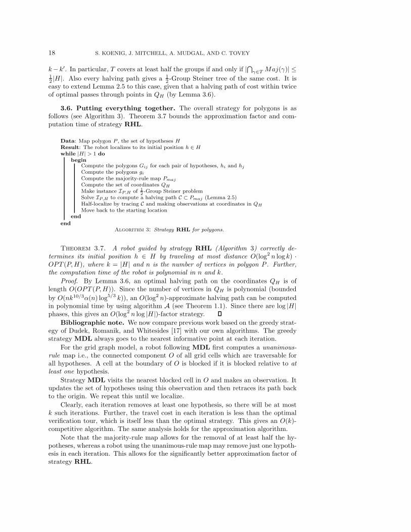
3.6. Putting everything together. The overall strategy for polygons is asfollows (see Algorithm 3). Theorem 3.7 bounds the approximation factor and com-putation time of strategy RHL.

Data: Map polygon P , the set of hypotheses HResult: The robot localizes to its initial position h ∈ Hwhile |H| > 1 do

beginCompute the polygons Gij for each pair of hypotheses, hi and hj

Compute the polygons gi

Compute the majority-rule map Pmaj

Compute the set of coordinates QH

Make instance IP,H of 12-Group Steiner problem

Solve IP,H to compute a halving path C ⊂ Pmaj (Lemma 2.5)Half-localize by tracing C and making observations at coordinates in QH

Move back to the starting locationend

endAlgorithm 3: Strategy RHL for polygons.

Theorem 3.7. A robot guided by strategy RHL (Algorithm 3) correctly de-termines its initial position h ∈ H by traveling at most distance O(log2 n log k) ·OPT (P, H), where k = |H | and n is the number of vertices in polygon P . Further,the computation time of the robot is polynomial in n and k.

Proof. By Lemma 3.6, an optimal halving path on the coordinates QH is oflength O(OPT (P, H)). Since the number of vertices in QH is polynomial (boundedby O(nk10/3α(n) log5/3 k)), an O(log2 n)-approximate halving path can be computedin polynomial time by using algorithm A (see Theorem 1.1). Since there are log |H |phases, this gives an O(log2 n log |H |)-factor strategy.

Bibliographic note. We now compare previous work based on the greedy strat-egy of Dudek, Romanik, and Whitesides [17] with our own algorithms. The greedystrategy MDL always goes to the nearest informative point at each iteration.

For the grid graph model, a robot following MDL first computes a unanimous-rule map i.e., the connected component O of all grid cells which are traversable forall hypotheses. A cell at the boundary of O is blocked if it is blocked relative to atleast one hypothesis.

Strategy MDL visits the nearest blocked cell in O and makes an observation. Itupdates the set of hypotheses using this observation and then retraces its path backto the origin. We repeat this until we localize.

Clearly, each iteration removes at least one hypothesis, so there will be at mostk such iterations. Further, the travel cost in each iteration is less than the optimalverification tour, which is itself less than the optimal strategy. This gives an O(k)-competitive algorithm. The same analysis holds for the approximation algorithm.

Note that the majority-rule map allows for the removal of at least half the hy-potheses, whereas a robot using the unanimous-rule map may remove just one hypoth-esis in each iteration. This allows for the significantly better approximation factor ofstrategy RHL.


To extend their algorithm to the polygonal model, Dudek, Romanik, and White-sides compute O by taking the intersection of shifted copies P1, P2, . . . , Pk of thepolygon with respect to different hypotheses. A robot has to check the boundaryof O to get new information. However, a robot may check whether an edge e ∈ Oexists by going to the boundary of its window w(e) inside O. Therefore, we takethe intersection of the regions formed by cutting off O at the various edge windowsw(e1), w(e2), . . . , w(em). We call this restricted region U . The robot then needs tovisit the nearest point on the boundary of U to get new information.

We refer the reader to the paper by Rao, Dudek, and Whitesides [38, 39] for theabove construction as well as randomized variants of MDL.

4. Inapproximability. We now show an Ω(log2−ε) lower bound for localizationby a reduction from the hardness of the Group Steiner problem.

4.1. Hardness of Group Steiner. A tree is said to be of arity d if each non-leaf vertex has exactly d children. A rooted tree has height H if all of its leaves areat distance H from the root. As usual, the level of a vertex is its distance from theroot; the root itself is at level 0, and there are H + 1 levels.

Definition 4.1 (see [3]). A hierarchically well-separated tree (HST) is definedto be a rooted, weighted tree in which (i) all leaves are at the same distance from theroot, and (ii) the weight of each edge is exactly 1

τ times the weight of its parent edge,where τ ≥ 1 is any desired constant.

To prove the lower bound, we use the recent result of Halperin and Krauthgamer[24] which establishes Ω(log2−ε n) hardness for the Group Steiner problem on HSTs.The next theorem, extracted from their proof, states their result in a detailed formsuited to our purpose.

Theorem 4.2 (see [24]). Let L be any NP-complete language. Then there exist aconstant c0 and an algorithm A that, given an instance I and a sufficiently large con-stant α, produces in expected running time O(|I|polylog(|I|)) an instance I ′ = (T, r,G)(r is also the root of T ) of the Group Steiner problem such that the following hold.

1. For some m ≤ |I|c0 , T is an HST with height H = (log m)α, arity d =mO(log m), and τ = mlog m. Further, each group g ∈ G is a subset of theleaves of T , and there are k = mO((log m)α+1) groups.

2. If I ∈ L, then there is a (rooted) tree T ′ ⊆ T of weight (log m)α covering allgroups.

3. If I /∈ L, then every tree T ′ ⊆ T covering all groups has weight Ω((log m)3α+2).

4.2. Reduction. The next theorem describes the reduction to an instance ofthe localization problem.

Theorem 4.3. Let L be any NP-complete language. Then there exist a constantc0 and an algorithm A′ that, given an instance I and a sufficiently large constant α,produces in expected running time O(|I|polylog(|I|)) an instance I ′′ = (G, H) of therobot localization problem on grid graphs such that the following hold.

1. For some m ≤ |I|c0 , G has N = mO((log m)α+1) cells and H has mO((log m)α+1)

hypotheses.2. For some β = mO((log m)α+1),

(a) if I ∈ L, then there exists a localization plan with worst-case costO(β · (log m)α), and

(b) if I /∈ L, every localization plan has cost Ω(β · (log m)3α+2).Proof. Let I ′ = (T (V, E), r,G) be the instance of Group Steiner on HSTs obtained

by running algorithm A on I (see Theorem 4.2 above). Let d, H , and τ denote the


arity, height, and weight factor of HST T , and let k denote the number of groups inG. G consists of k + 1 (disjoint) copies B0, B1, . . . , Bk of grid graph B, where B is an“embedding” of HST T respecting the weights on its edges.

The embedding B is best described inductively. Let B(v) denote the embeddingof the subtree rooted at vertex v ∈ T . Cell cv at the southwest corner of each B(v)corresponds to vertex v. For a leaf l, B(l) is a 3× (log k�+5) rectangle with a singletraversable cell cl at its southwest corner (Figure 4.1(b)). The reason for addingblocked space to cl will be clear later, when we use it to add “signatures” to leaf l.For a nonleaf vertex v, B(v) is formed by combining the embeddings of the subtreesrooted at its d children v1, v2, . . . , vd (see Figure 4.1(a)). B(v1), B(v2), . . . , B(vd) arepositioned along the top edge of B(v) separated by north-south walls of width 1.There is an east-west corridor ewv running along the bottom edge of B(v). Cell cvi isconnected to this corridor by a north-south corridor nsvi which corresponds to edgevvi ∈ T . We make the length of nsvi proportional to the weight of vvi: if v is at levelh, |nsvi | = β · 1

τh , where β is a scaling factor to be chosen later. Finally, B = B(r),where r is the root of T .

Let ah, bh be the length and breadth of the grid required to embed the subtreerooted at a level h vertex v ∈ T . To see that the tree “fits”, observe that B(v) fitsinto an ah × bh rectangle, where ah = d · ah+1 + (d − 1) and bh = bh+1 + β

τh . Hencebh = (log k�+5)+β ·∑H−1

α=h1

τα , and by induction one can show that ah = 4·dH−h−1.

��

��

��

��

�

��

(a) Block B(v)

��

�

�

�

�

�

�

��

��

��

(b) A leaf block with signature

Fig. 4.1.

Let wxy denote the weight of the path connecting x, y ∈ T . Let Puv be the uniquepath connecting cells cu and cv in B. We show that choosing β = 5dH · τH makesB an embedding of T in the following sense: for all vertices x, y ∈ T , β · wxy ≤|Pxy| ≤ 2β ·wxy. First observe that the length of any north-south corridor nsv is nowat least 5dH while any east-west corridor is less than 4dH . Therefore, |ewx| ≤ |nsv|for all u, v ∈ T . We charge the distances traveled along east-west corridors to thenorth-south corridors immediately preceding it. First assume that x is the parent ofy. Then Pxy consists of the north-south hallway nsy along with the portion of ewx

connecting cx to nsy. Clearly, β · wxy = |nsy| ≤ |Pxy| ≤ |nsy| + |ewx| ≤ 2β · wxy.Next consider the case when x, y are siblings with common parent z. Pxy consistsof north-south corridors nsx, nsy along with the portion of ewz connecting them.Hence, β · wxy = β · (wxz + wzy) = |nsx| + |nsy| ≤ |Pxy| ≤ |nsx| + |nsy| + |ewz| ≤2β · wxz + β · wzy ≤ 2β · wxy. For general x, y, let cz0=x, cz1 , . . . , czm=y be the cellscorresponding to vertices of T , in the order they occur along path Puv. By theconstruction of B, we know that for each i either (i) zi+1 is a parent of zi or vice-


versa, or (ii) zi, zi+1 are siblings. Therefore, β ·wzizi+1 ≤ |Pzizi+1 | ≤ 2β ·wzizi+1 . Since|Pxy| =

∑ |Pzizi+1 |, the length of Puv is within a factor of 2 of β ·∑wzizi+1 = β ·wxy.Let g1, g2, . . . , gk be the k groups in G. We make k + 1 copies B0, B1, . . . , Bk of

embedding B. Bi’s are the same except for distinguishing “signatures” at some leafblocks. B0 = B is the dummy copy and contains no signatures. For i > 0, Bi isformed by adding signature si (a binary encoding of i) to every leaf block B(l) of Bsuch that l ∈ gi (Figure 4.1(b)). To add si, first cell cl is extended to a north-southcorridor along the left edge of B(l). Then a set of log k eastern “alcoves” encoding iin binary are placed along the eastern edge: the jth alcove from the top is blockedif and only if the jth bit in the binary form is 0. A robot located at cl can read thevalue of i by going north and sensing the alcoves to its right for blockage.

��

��

��

��

��

��

��

� �

��

��

��

��

Fig. 4.2. Grid graph G.

Let x = 2 · a0 · b0. Grid graph G is an (x + a0) × ((k + 1) · b0 + k − 1) rectangleformed by connecting group blocks {Bi}i, as shown in Figure 4.2. B0, B1, B2, . . . , Bk

are placed along the right edge of G separated by east-west walls of width 1. Anorth-south corridor NS of width 1 runs alongside the left edge of G. The southwestcell of each block Bi is connected to this corridor by an east-west corridor EWi oflength x. The set of hypotheses H equals {h0, h1, . . . , hk}, where hi denotes the cellat the southwest corner of block Bi. Substituting values of k, H, d, τ as given byTheorem 4.2, we get β = 5dH · τH = mO((log m)α+1), |G| = O(a0b

20k) = mO((log m)α+1),

and |H | = k = mO((log m)α+1), where m ≤ |I|c0 . We complete the proof by showingthat the optimal localization plans for I′′ = (G, H) in the “yes” (I ∈ L) and “no”(I /∈ L) cases differ by a factor of Ω((log m)2α+2).

“Yes” case. Suppose I ∈ L. By Theorem 4.2, there exists a tree T ′ ⊆ T ofweight (log m)α, which covers all groups in G. As all groups g ∈ G consist of leavesof T , without loss of generality every root to leaf path in T ′ ends at a leaf of T .Let l0, l1, . . . , lt−1 be the leaves of T ′ in the order they are visited by a depth-firstsearch from the root. Consider the following plan: read the signatures at leaf blocksB(l0), B(l1), . . . , B(lt−1) in that order. As soon as a nonzero signature si0 , i0 > 0 isread, localize to hi0 . Otherwise, localize to h0.

To prove correctness, assume the robot was placed (without its knowledge) athypothesis hi0 . If i0 = 0, the robot will read zero signatures at all leaf blocks andcorrectly localize to h0. Suppose i0 > 0. Since T ′ covers all groups, group gi0 containsat least one leaf vertex from T ′. The robot will read signature si0 at the first such


vertex in the sequence l0, l1, . . . , lt−1 and localize to hi0 .The total travel cost of the robot is |Prl0 |+

∑t−2i=0 |Plili+1 | ≤ 2β·(wrl0+

∑t−2i=0 wlili+1)

≤ 2β · w(T ′) = O(β · (log m)α). We neglect the cost of reading signatures at li, as itis O(t · log k) = O(dH log k) ≤ β.

“No” case. Suppose I /∈ L. Assume that we have found a localization plan withcost o(C · (log m)3α+2). The number of movements for the plan is no larger thanthe length of an east-west hallway EWi. Now assume the robot starts at cell h0.Thus, it cannot visit a different east-west hallway and, as part of the localization,must determine that no leaf block in its group block has a nonzero signature. LetB(l0), B(l1), . . . , B(lt−1) be all the leaf blocks, in the order they are visited by therobot. The collection of groups that these leaves cover must equal G, for otherwisethe robot could not distinguish between hypotheses h0 and hi for the groups gi notcovered by them.

Let T ′ be the Group Steiner tree formed by taking the union of paths connecting rto l0 and li to li+1 for 0 ≤ i ≤ t−2. By Theorem 4.2, the weight of T is Ω((log m)3α+2).Therefore, the cost of the localization plan is at least |Prl0 |+

∑t−20 |Plili+1 | ≥ β ·(wrl0 +∑t−2

i=0 wlili+1) ≥ β · w(T ′) = Ω(β · (log m)3α+2).Corollary 4.4. For every fixed ε > 0, the robot localization problem can-

not be approximated within ratio log2−ε N on grid graphs of size N unless NP ⊆ZTIME(npolylog(n)).

Proof. Apply the algorithm in Theorem 4.3 with α = 2 · (1ε − 1). The logarithm

of the size of grid graph G is log N = O((log m)α+2), where m ≤ nc0 . The optimumlocalization plans in the “yes” and “no” cases differ by a factor of Ω((log m)2α+2) =Ω((log N)2−ε).

Corollary 4.5. For every fixed ε > 0, the robot localization problem cannotbe approximated within ratio log2−ε N on polygons with N vertices unless NP ⊆ZTIME(npolylog(n)).

Proof. The grid graph G in Theorem 4.3 above can be viewed as a polygon Pwith at most N vertices. Let h′

i denote the center of the cell hi in G. Consider thelocalization problem on P with hypotheses set H ′ = {h′

0, h′1, . . . , h

′k}. The optimal

localization plan in the “yes” case has cost O(β · (log m)α), as a robot with a rangefinder can only do better. However, when I /∈ L, a robot with a range finder may readthe signatures from a distance and localize at lesser cost. To rule this out, put small“twists” in polygon P just before every signature. Thus the robot cannot read thesignatures at a distance and therefore will travel at least Ω(β · (log m)3α+2) distance,as in Theorem 4.2 above. The “yes” and “no” cases differ by Ω((log m)α+2), and thebound follows by choosing α = 2 · (1 − 1

ε ).We note that a lower bound for Group Steiner can be extended to a similar lower

bound for localization on grid graphs. The main idea is the same as above: take ahard instance (G, r,G) of Group Steiner on grid graphs. Suppose G is an m × n gridgraph, and there are k = |G| groups. We make a map G′ that consists of k disjointcopies G1, G2, . . . , Gk of G. Each copy Gi is a scaled up (by a factor of β) version ofG. Thus, each cell of G corresponds to a β × β block in Gi. For each cell in groupgi ∈ G, we put a 3× log k� “signature” in the upper left corner of the correspondingblock of Gi. As before, we choose the scaling factor large enough so that the distancebetween signatures is much larger than their size. A good choice is β = k. Initially,the robot is placed at the center of block corresponding to r in one of the Gi’s.

In order to localize, the robot has to find the index of its component and, hence,must visit a set of blocks that covers all of the groups. This path can be translated


to a Group Steiner tree of proportional cost (divided by β) in G (since β is muchlarger than log k). Conversely, we can convert any Group Steiner tree in G into apath by doing depth-first search and then using that path in the scaled grid G′ asa localization plan. It is easy to see that this extends the same hardness factor tolocalization on grids.

Thus, it seems that further improvement (in either the lower bound or upperbound) in the approximation factor of our algorithm can come only after progress onthe Group Steiner problem on grid graphs.

5. Extensions to other models. Here we sketch some extensions of our algo-rithm.

5.1. Robot without compass. If the robot does not possess a compass buthas no actuator uncertainty with respect to changes in orientation, the lower boundremains valid. For the algorithm, redefine a hypothesis to be a (location, orientation)pair. For grid graphs, with four axis-parallel orientations per cell, the size of the setH of possible hypotheses remains O(n), and the algorithm extends naturally as therobot operates on the majority-rule map relative to (location, orientation) pairs in H .

For polygons there are at most n distinct embeddings, corresponding to rotations,of the visibility polygon V(hi) for each choice of hi. This follows since any one edge ofV(hi) that is not collinear with hi (as is the case for “shadow edges” or “windows” ofV(hi)) must fall on one of the n edges of P in any candidate pose. Thus, H consistsof at most n different poses, (hi, θj), each specified as a (location, orientation) pair.For each pose (hi, θj), we construct a copy Pi,j of the map polygon P . Pi,j is formedby first translating P so that hi coincides with the origin, and then rotating it abouthi so that direction θj points to the north. The majority-rule map and Algorithm 3are then directly applied to the polygons Pi,j , as in the translation-only case.

5.2. The limited-range version. Practical sensors have a limited range, D,beyond which the noise levels are too high to give reliable measurements [31]. Ouralgorithm for grids already assumes limited range of visibility, since we assume thatthe robot senses only the immediate neighboring grid cell; this can readily be extendedto allow the robot to sense all cells within grid graph distance D. Our algorithm forlocalization in polygons can also be extended to the limited-range case, as we nowdescribe.

In order to distinguish between hypothesis hi and hypothesis hj, the robot mustget within distance D of an edge of type (i) or type (ii) in the polygon Fij . If γ0 sees(within distance D) any point on an edge of type (i) or type (ii), then the robot candistinguish between hi and hj without moving from the origin γ0. Thus, assume thatall edges of Fij that are visible (within distance D) from γ0 are of type (iii). Let ebe an edge of Fij of type (i) or of type (ii). Assuming an unobstructed space, theset of points within distance D from some point of e is a region bounded by straightedges and circular arcs (of radius D). The portion of the boundary of V P (D)(e) thatseparates γ0 from e defines the window, w(e), of e; it consists now of O(1) curves(straight segments and radius-D arcs), instead of a single chord, as in the D = ∞case. We now define G

(D)ij to be the face containing the origin γ0 in the arrangement

of the O(n) boundary edges of Fij together with the set of all O(n) windows w(e) foredges e of type (i) or (ii). Again, as in Lemma 3.3, we have that a robot can distinguishbetween hypothesis hi and hypothesis hj if and only if it visits the boundary, ∂G

(D)ij .

This allows us to define the majority-rule map regions gi, the discrete point set QH ,and the half-localization algorithm as before. The only technical difference is the


presence of straight segments and (fixed radius) circular arcs in the arrangements;this does not affect the polynomiality or the correctness of the algorithm.

5.3. Polygons with holes. In the case that the map polygon P is a polygonaldomain with holes H1, H2, . . . , Hm, our method still applies, but the complexity of thestructures increases. Let n be the total number of vertices in the polygon (includingthe holes).

First, the polygons Fij are now polygons with holes of complexity O(n). Asingle edge can now have as many as O(n) windows (one for each hole). The Gij ’sare formed as before by taking the intersection of the regions chopped off by thesewindows; each has complexity O(n2) since each window-edge can occur only once.Finally, the majority-rule map’s Ki’s are also polygons with holes; each is formedfrom Gij , j �= i, and hence has complexity O(k2n4). The specification of the discretepoints QH applies to the case of multiply connected domains, and the argument ofLemma 3.6 applies as well. And hence the set of coordinates now has complexityO(k3n4). These bounds can be improved somewhat when the holes are convex.

From the above section, it is clear that the same framework works for a robotwith limited range sensors inside a polygonal map with holes.

5.4. Geometric trees. As described before, a geometric tree G = (V, E) is atree with V , a set of points in R

d, and E, a set of nonintersecting line segments whoseendpoints all lie in V [27]. An O(n

23 )-competitive localization strategy for bounded-

degree geometric trees was given by Kleinberg [27]. His strategy is Ω(n)-competitivefor trees with arbitrary degree.

Our approach gives an O(log2 n log k) algorithm for any geometric graph G =(V, E) in the plane, not just trees. First, we can assume that the robot begins atsome vertex of G, since the robot can initially perform a two-way spiral search toreach the closest vertex, while traveling at almost 9 times the cost of the optimalstrategy [1, 27]. The set of hypotheses is now of size k = O(n) and consists only ofvertices. We make k = |H | translation-congruent copies of G, with the ith copy Gi

having hi at the origin. To construct the majority-rule map, we overlay the copiesGi, 1 ≤ i ≤ k, and form the arrangement D(G, H) of line segments in

⋃i Gi. Each

edge in the arrangement has the same hypothesis partition, and hence the robot gainsnew information only by visiting new edges. Note that several edges may be collinear,since new points are added by translation. Next, we construct the majority-rule mapGmaj by finding the set of all half-traversable edges reachable from the origin γ0. Asthe robot can visit an edge only through one of its endpoints, an O(log2 n)-factorhalving path can be found by solving the 1

2 -Group Steiner problem on vertices ofGmaj . Since D(G, H) is formed by the intersection of k · |E| edges, it has complexityat most O(k2|E|2) and can be computed in O(k2|E|2) time by standard methods [2].Since at least one endpoint of every edge in the majority-rule map Gmaj is a vertexv ∈ ⋃

i Gi, Gmaj has O(n|E|) edges. Hence the computation time of the robot isP(n|E|) · log n, where P(·) is the running time for approximating the 1

2 -Group Steinerproblem. Since a grid graph is a geometric graph in R

2, Corollary 4.4 gives anΩ(log2−ε n) lower bound.

5.5. Three-dimensional grid graphs. Finally, we consider a three-dimen-sional grid graph G, which can be used to model buildings or offices with severalfloors. The majority-rule map Gmaj is a local map in which each cell is blocked orunblocked based on what the majority of hypotheses have to say about it. If G is anl1× l2× l3 cuboid, the majority-rule map has size (2l1−1)× (2l2−1)× (2l3−1), since


the absolute values the x-, y-, and z-coordinates for each hypothesis are l1 − 1, l2 − 1,and l3 − 1, respectively. Hence Gmaj requires space at most 8n and can be computedin O(nk) time. By making one vertex for each cell in Gmaj , we solve the 1

2 -GroupSteiner problem IG,H of size O(n). The performance ratio remains O(log2 n log k),and the running time is P(8n) log n.

6. Is returning to the origin necessary? In this section, we show that RHLperforms very poorly if we do not stipulate that the robot return to its startingposition after each half-localize step. In section 6.1, we construct a grid graph G anda set of hypotheses H such that a robot not returning to the origin travels distance(k − 1 − ε) · OPT (G, H), where k = |H | is the number of hypotheses and ε > 0is an arbitrarily small constant. In section 6.2, we show that our lower bound istight by proving that a robot not returning to the origin always localizes in at most(k − 1) · OPT (G, H) steps.

6.1. Lower bound. The grid graph G for the lower bound is reminiscent of theGroup Steiner tree construction. Let k be the number of hypotheses and x be aninteger greater than or equal to 3.

The building block B consists of two orthogonal corridors meeting at a cornerwhere the robot is located (see Figure 6.1(a)). The northern corridor has lengthx + 1 + log k, and the eastern corridor has length (k − 1) · x.

�

�

� �

�

�

��

��

��

� � � � ��

� �

��

��

��

Fig. 6.1. (a) Block By, where y = 10 . . . 0. (b) The northern corridor is bent at 3 units.

We make k copies B0, B1, . . . , Bk−1 of block B. By’s are the same except fordistinguishing “alcoves” along their northern and eastern corridors.

We now describe the construction of By. A set of log k alcoves encoding y inbinary are added along the western edge of the northern corridor (see Figure 6.1(a)).The jth alcove from the bottom is blocked if and only if the jth bit in the binaryencoding of y is 0.

In addition to this, we add log k alcoves encoding y in binary along the easterncorridor. The ith alcove is placed at distance (2i − 1)x and is blocked if and only ifthe ith bit in the binary encoding of y is 0.

Observe that By fits into an a × b rectangle, where a = 2 + x · (2log k − 1) =2 + x · (k − 1) and b = x + log k. One can further reduce the height of By by bendingthe northern corridor as shown in Figure 6.1(b). After this reduction, each block fitsinto a (2 + x · (k − 1)) × 5 rectangle.

Grid graph G is a (2 + x · k + log k) × (6k − 1) rectangle formed by connectingblocks {By}y as shown in Figure 6.2. B0, B1, . . . , Bk−1 are placed along the left edgeof G separated by east-west walls of width 1. A north-south corridor of width 1 runsalongside the right edge of G. The southwest cell of each block is connected to thiscorridor by an east-west corridor of length x+log k. This distance is chosen so that a


��

��

��

��

��

�

� � � � ��

��

��

��

Fig. 6.2. Grid graph G.

robot located inside a block By never goes outside it to half-localize. Finally, the set ofhypotheses H equals {h0, h1, . . . , hk−1}, where hy denotes the cell at the intersectionof the two orthogonal corridors in By.

Theorem 6.1. Let G be the (2+x ·k+log k)× (6k−1) grid graph as constructedabove and H = {h0, h1, . . . , hk−1}. Then a robot which computes the optimal half-localization strategy but does not return to the origin travels to the end of the easterncorridor of its block By before it localizes.

Proof. Consider a robot located at hy, where 0 ≤ y ≤ k − 1. To find its locationthe robot needs to find all bits in the binary representation of y. To half-localize, itsuffices to read one new bit in each phase.

The robot can read either the first alcove on the northern corridor or the firstalcove on the eastern corridor. Since the alcove on the eastern corridor is nearer byone grid cell, the robot moves x units east and “reads” the first alcove.

Suppose that the alcove is blocked, i.e., the first bit in the binary encoding of yis 0 (the case when it is 1 is similar). To read the next bit, either the robot can readthe second alcove on the eastern corridor at cost 2x, or it can go back to the originand then read the second alcove on the northern corridor at cost 2x + 2. Since theformer is optimal, the robot moves 2x units west to read the second alcove on theeastern corridor.

In general, at the start of the ith phase (i ≥ 2) the robot has read the first i − 1bits of the binary encoding of y and is located at alcove i− 1 on the eastern corridor.Either it can move 2i−1x steps to the west and check the ith alcove on the easterncorridor, or it can go back to read the ith alcove at the northern corridor at cost2i−1x + i. The optimal half-localization plan consists of going west to read the ithalcove on the eastern corridor.

Thus in each half-localize phase the robot goes west to read the next alcove onits eastern corridor. The robot will localize after it has gone until the end of theeastern corridor and checked the last alcove. The total distance traveled by the robotis (k − 1) · x.

Corollary 6.2. For every fixed ε > 0, there is a grid graph G and a set ofhypotheses H such that a robot following RHL without returning to the origin travelsat least (k − 1 − ε) · OPT (G, H) distance before determining its location h ∈ H.

Proof. Take the grid graph G and the set of hypotheses H constructed above. ByTheorem 6.1 a robot not returning to the origin travels distance (k−1) ·x to the endof the eastern corridor to determine its initial position hy ∈ H .

The optimal localization strategy consists of going x units up the northern corridor


and then reading the log k bit signature. It has cost OPT = x + log k.The approximation factor is (k−1)·x

x+log k . If we take x = (k−1) log kε , this is at least

k − 1 − ε.The next corollary shows that the lower bound in terms of the size of the grid

graph is Ω(√

nlog n ).

Corollary 6.3. There is a grid graph G and a set of hypotheses H such that arobot following RHL without returning to the origin travels distance Ω(

√n

log n ) ·OPT ,where n = |G| is the size of the grid graph.

Proof. Take x = 3 in Theorem 6.1. The grid graph now has size n = (2 + 3k +log k) × (6k − 1) = θ(k2). The optimal localization strategy has cost 3 + log k. Therobot travels distance 3(k−1). The approximation factor is 3(k−1)

3+log k . Since k = θ(√

n),

this is Ω(√

nlog n ).

6.2. Upper bound. We now show that a robot following strategy RHL withoutreturning to the origin localizes in at most (k − 1) · OPT steps.

Theorem 6.4. Consider a robot which computes the optimal half-localizationstrategy in each phase but does not return to the origin after each phase. Then ittravels distance at most (k − 1) · OPT before determining its initial position h ∈ H,where k = |H | is the number of hypotheses and OPT is the cost of the optimallocalization plan.

Proof. Let Pi−1 denote the path traced by the robot relative to the origin beforethe start of the ith half-localize phase. Let Qi denote the path traced by the robotduring the ith phase. Then we have that Pi = Pi−1 ◦Qi is the concatenation of Pi−1

followed by Qi.Since the robot always chooses the optimal half-localization strategy, the length of

Qi is less than or equal to any half-localization strategy for phase i. One such strategymakes the robot retrace the path Pi−1 back to the origin and then run the optimallocalization plan until the robot half-localizes. This has cost at most |Pi−1| + OPT ,and hence we have that |Qi| ≤ |Pi−1| + OPT .

Therefore, we get that |Pi| = |Pi−1◦Qi| = |Pi−1|+|Qi| ≤ |Pi−1|+(|Pi−1|+OPT ) =2 · |Pi−1| + OPT .

Since |P0| = 0, we see that |Pi| ≤ (2i−1) ·OPT . As the robot localizes in at mostm ≤ log k half-localize steps, the distance traveled by |Pm| is at most (2m−1)·OPT ≤(2log k − 1) · OPT = (k − 1) · OPT .

6.3. Discussion. This feature may become a problem in probabilistic environ-ments where the robot may incur noise by returning back to the origin, or if therobot gets trapped in a small corner from which it is hard to get out. However, westill feel that our algorithm makes sense, due to the large decrease in uncertaintybrought about by each half-localize step. If the robot motion is sufficiently correct,this decrease should more than offset the noise incurred by coming back to the origin.Further, the robot does not need to return to the origin “exactly.” Rather, it sufficesthat the robot be present within a small distance of the origin with high probability,as this will allow for near-optimal behavior in the next step. If continuous sensingand updating while returning back is allowed, the robot should perform reliably withsmall corrections.

The robot may get trapped in a corner, but in maps with “signatures” (suchas those we constructed above, as well as those in the NP-hardness construction ofDudek, Romanik, and Whitesides [17]), this may be the only way to localize efficiently.


In fact, it seems that only in such highly-replicated environments do such localizationstrategies make sense.

Further, the task of localization is just a prelude to the robot performing othertasks, such as going to a particular location. This new location may lie anywhere inthe map, so the robot will not lose by coming back to its starting place.

Finally, it seems that there is no way to bypass this return-to-origin constraint, asnot allowing the robot to return to the origin leads to exceptionally bad performance.In fact, we claim that no reasonable algorithm for localization can be found unless westipulate that the robot returns to the starting location after each half-localize step.

7. Conclusion and open problems. The main ideas of this paper are half-localization and the majority-rule map, which permit us to eliminate half the hy-potheses in each step. Earlier strategies for localization could eliminate only O(1)hypotheses in each step, thus leading to Ω(n)-approximations for general models.There is a log n factor gap between the upper and lower bounds; it appears that thisgap can be closed only by progress on the Group Steiner problem in grid graphs (andalso those given by Euclidean shortest path metrics inside a constrained region).

An appealing feature of our algorithm is its wide adaptability over a variety ofrobot models: the only issue is to devise algorithms for computing the majority-rulemap and the set of coordinates for the model at hand. We believe that the majority-rule map will play an important part in other robot navigation problems.

While our algorithms for localization in polygons have been restricted to twodimensions, we expect that the results can be extended to three-dimensional polyhe-dral domains P in which the robot moves inside P and sends out a series of beamsspaced at small solid angles over the sphere and joins them to compute the visibilitypolyhedron V (p). Modern three-dimensional range finders allow one to estimate thevisibility polyhedron from the robot [49].

In this paper, we do not address models with sensor noise, imperfections in therobot’s map, and odometer errors. While sensor noise can be easily accommodated [5],devising a good strategy for a model with odometer errors remains a major openproblem. This not only entails redefining what we mean by localization but alsorequires devising strategies that balance the need for resolving global position withthe need for removing local pose estimation errors.

Acknowledgment. We thank the anonymous referees for valuable commentsthat helped us improve the paper.

REFERENCES

[1] R. A. Baeza-Yates, J. C. Culberson, and G. J. E. Rawlins, Searching in the plane, Inform.and Comput., 2 (1993), pp. 234–252.

[2] I. J. Balaban, An optimal algorithm for finding segment intersections, in Proceedings of the11th ACM Symposium on Computational Geometry, ACM, New York, 1995, pp. 211–219.

[3] Y. Bartal, Probabilistic approximations of metric spaces and its algorithmic applications, inProceedings of the 37th IEEE Symposium on Foundations of Computer Science, IEEEComputer Society, Washington, DC, 1996, pp. 184–193.

[4] C. D. Bateman, C. S. Helvig, G. Robins, and A. Zelikovsky, Provably good routing treeconstruction with multi-port terminals, in Proceedings of the ACM/SIGDA InternationalSymposium on Physical Design, ACM, New York, 1997, pp. 96–102.

[5] R. G. Brown and B. R. Donald, Mobile robot self-localization without explicit landmarks,Algorithmica, 26 (2000), pp. 515–559.

[6] A. Blum, P. Raghavan, and B. Schieber, Navigating in unfamiliar geometric terrain, SIAMJ. Comput., 26 (1997), pp. 110–137.


[7] A. Chakraborty, H. Balakrishnan, and N. B. Priyantha, The cricket location-support sys-tem, in Proceedings of the 6th ACM/IEEE International Conference on Mobile Computingand Networking, ACM, New York, 2000, pp. 32–43.

[8] T. M. Chan, On levels in arrangements of curves, Discrete Comput. Geom., 29 (2003), pp.375–393.

[9] M. Charikar, C. Chekuri, T.-Y. Cheung, Z. Dai, A. Goel, S. Guha, and M. Li, Approxi-mation algorithms for directed Steiner problems, J. Algorithms, 33 (1999), pp. 73–91.

[10] C. Chekuri and M. Pal, A recursive greedy algorithm for walks in directed graphs, in Proceed-ings of the 46th IEEE Symposium on Foundations of Computer Science, IEEE ComputerSociety, Washington, DC, 2005, pp. 245–253.

[11] W.-P. Chin and S. Ntafos, Optimum watchman routes, Inform. Process. Lett., 28 (1) (1988),pp. 39–44.

[12] W.-P. Chin and S. Ntafos, The zoo-keeper route problem, Inform. Sci., 63 (1992), pp. 245–259.[13] I. J. Cox, Blanche—an experiment in guidance and navigation of an autonomous robot vehicle,

IEEE Trans. Robotics and Automation, 7 (1991), pp. 193–204.[14] A. Datta and C. Icking, Competitive searching in a generalized street, in Proceedings of the

10th ACM Symposium on Computational Geometry, ACM, New York, 1994, pp. 175–182.[15] E. Davis, Representing and Acquiring Geographic Knowledge, Pitman/Morgan Kaufmann, San

Francisco, 1986.[16] M. Dror, A. Efrat, A. Lubiw, and J. S. B. Mitchell, Touring a sequence of polygons,

in Proceedings of the 35th ACM Symposium on Theory of Computing, ACM, New York,2003, pp. 473–482.

[17] G. Dudek, K. Romanik, and S. Whitesides, Localizing a robot with minimum travel, SIAMJ. Comput., 27 (1998), pp. 583–604.

[18] P. Eades, X. Lin, and N. C. Wormald, Performance guarantees for motion planning withtemporal uncertainty, Australian Computing J., 25 (1993), pp. 21–28.

[19] G. Even, G. Kortsarz, and W. Slany, On network design: Fixed charge flows and thecovering Steiner problem, in Proceedings of the 8th Scandinavian Workshop on AlgorithmTheory, Turku, Finland, 2002, pp. 318–329.

[20] J. Fakcharoenphol, S. Rao, and K. Talwar, A tight bound on approximating arbitrary met-rics by tree metrics, in Proceedings of the 35th ACM Symposium on Theory of Computing,ACM, New York, 2003, pp. 448–455.

[21] D. Fox, W. Burgard, and S. Thrun, Active Markov localization for mobile robots, Roboticsand Automation Systems, 25 (1998), pp. 195–207.

[22] N. Garg, G. Konjevod, and R. Ravi, A polylogarithmic approximation algorithm for thegroup Steiner tree problem, J. Algorithms, 37 (2000), pp. 66–84.

[23] L. J. Guibas, R. Motwani, and P. Raghavan, The robot localization problem, SIAM J.Comput., 26 (1997), pp. 1120–1138.

[24] E. Halperin and R. Krauthgamer, Polylogarithmic inapproximability, in Proceedings of the35th ACM Symposium on Theory of Computing, ACM, New York, 2003, pp. 585–594.

[25] L. Hyafil and R. L. Rivest, Constructing optimal binary decision trees is NP-complete,Inform. Process. Lett., 5 (1) (1976), pp. 15–17.

[26] R. Klein, Walking an unknown street with bounded detour, Comput. Geom., 1 (1992), pp.325–351.

[27] J. M. Kleinberg, The localization problem for mobile robots, in Proceedings of the 35th IEEESymposium on Foundations of Computer Science, IEEE Computer Society, Washington,DC, 1994, pp. 521–531.

[28] C. Lund and M. Yannakakis, On the hardness of approximating minimization problems, J.ACM, 41 (5) (1994), pp. 960–981.

[29] J. M. Kleinberg, On-line search in a simple polygon, in Proceedings of the 5th ACM-SIAMSymposium on Discrete Algorithms, ACM, New York, SIAM, Philadelphia, 1994, pp. 8–15.

[30] D. P. Miller, D. J. Atkinson, B. H. Wilcox, and A. H. Mishkin, Autonomous navigationand control of a Mars rover, in Proceedings of the 11th IFAC Symposium on AutomaticControl in Aerospace, Tsukuba, Japan, 1989, pp. 127–130.

[31] G. Miller and E. Wagner, An optical rangefinder for autonomous robot cart navigation, inAutonomous Robot Vehicles, I. J. Cox and G. T. Wilfong, eds., Springer-Verlag, Berlin,1990, pp. 122–134.

[32] C. Ming Wang, Location estimation and uncertainty analysis for mobile robots, in AutonomousRobot Vehicles, I. J. Cox and G. T. Wilfong, eds., Springer-Verlag, Berlin, 1990, pp. 90–95.

[33] J. S. B. Mitchell, Geometric shortest paths and network optimization, in Handbook of Com-putational Geometry, J.-R. Sack and J. Urrutia, eds., North–Holland, Amsterdam, 2000,pp. 633–701.


[34] S. Ntafos, Watchman routes under limited visibility, Comput. Geom., 1 (1992), pp. 149–170.[35] J. O’Rourke, Visibility, in Handbook of Discrete and Computational Geometry, 2nd ed., J. E.

Goodman and J. O’Rourke, eds., Chapman & Hall/CRC, Boca Raton, FL, 2004, Chapter28.

[36] W. H. Plantinga and C. R. Dyer, Visibility, occlusion and the aspect graph, Internat. J.Computer Vision, 5 (1990), pp. 137–160.

[37] C. H. Papadimitriou and M. Yannakakis, Shortest paths without a map, Theoret. Comput.Sci., 84 (1991), pp. 127–150.

[38] M. Rao, G. Dudek, and S. Whitesides, Minimum distance localization for a robot withlimited visibility, in Proceedings of the IEEE International Conference on Robotics andAutomation, IEEE Robotics and Automation Society, Washington, DC, 2005, pp. 2438–2445.

[39] M. Rao, G. Dudek, and S. Whitesides, Randomized algorithms for minimum distance local-ization, Internat. J. Robotics Research, 26 (2007), pp. 917–934.

[40] W. D. Rencken, Concurrent localization and map building for mobile robots using ultrasonicsensors, in Proceedings of the IEEE/RSJ International Conference on Intelligent Robotsand Systems, IEEE, Washington, DC, 1993, pp. 2129–2197.

[41] R. D. Schiffenbauer, A Survey of Aspect Graphs, Technical report TR-CIS-2001-01, Dept.of Computer and Information Science, Polytechnic University, New York, NY, 2001.

[42] R. Simmons, R. Goodwin, K. Haigh, S. Koenig, and J. O’Sullivan, A layered architecturefor office delivery robots, in Proceedings of the 1st International Conference on AutonomousAgents, ACM, New York, 1997, pp. 245–252.

[43] D. Sleator and R. Tarjan, Amortized efficiency of list update and paging rules, Comm.ACM, 23 (1985), pp. 202–207.

[44] S. Schuierer, Intelligent Robots—Sensing, Modelling and Planning, World Scientific, Singa-pore, 1996, pp. 129–146.

[45] W. Thompson, H. Pick, B. Bennett, M. Heinrichs, S. Savitt, and K. Smith, Map-basedlocalization: The “drop-off” problem, in Proceedings of the DARPA Image UnderstandingWorkshop, San Diego, CA, 1990, pp. 706–719.

[46] C. Tovey and S. Koenig, Gridworlds as testbeds for planning with incomplete information,in Proceedings of the National Conference on Artificial Intelligence, Austin, TX, 2000, pp.819–824.

[47] J. Urrutia, Art gallery and illumination problems, in Handbook on Computational Geometry,J. Sack and J. Urrutia, eds., North–Holland, Amsterdam, 2000, pp. 973–1027.

[48] G. Weib, C. Wetzler, and E. Von Puttkamer, Keeping track of position and orientationof moving indoor systems by correlation of range-finder scans, in Proceedings of the Inter-national Conference on Intelligent Robots and Systems, IEEE Washington, DC, 1994, pp.595–601.

[49] O. Wulf and B. Wagner, Fast 3D-scanning methods for laser measurement systems, inthe 14th International Conference on Control Systems and Computer Science, Bucharest,Romania, 2003.

A Near-Tight Approximation Algorithm for the Robot Localization Problem

Documents

Transcript of A Near-Tight Approximation Algorithm for the Robot Localization Problem