Dual FastSLAM: Dual Factorization of the Particle Filter Based Solution of the Simultaneous...

J Intell Robot Syst (2009) 55:109–134DOI 10.1007/s10846-008-9296-4

Dual FastSLAM: Dual Factorization of the ParticleFilter Based Solution of the Simultaneous Localizationand Mapping Problem

D. Rodriguez-Losada · P. San Segundo ·F. Matia · L. Pedraza

Received: 16 April 2008 / Accepted: 12 November 2008 / Published online: 19 December 2008© Springer Science + Business Media B.V. 2008

Abstract The process of building a map with a mobile robot is known as theSimultaneous Localization and Mapping (SLAM) problem, and is considered essen-tial for achieving true autonomy. The best existing solutions to the SLAM problemare based on probabilistic techniques, mainly derived from the basic Bayes Filter.A recent approach is the use of Rao-Blackwellized particle filters. The FastSLAMsolution factorizes the Bayes SLAM posterior using a particle filter to estimate overthe possible paths of the robot and several independent Kalman Filters attached toeach particle to estimate the location of landmarks conditioned to the robot path.Although there are several successful implementations of this idea, there is a lackof applications to indoor environments where the most common feature is the linesegment corresponding to straight walls. This paper presents a novel factorization,which is the dual of the existing FastSLAM one, that decouples the SLAM into a mapestimation and a localization problem, using a particle filter to estimate over mapsand a Kalman Filter attached to each particle to estimate the robot pose conditionedto the given map. We have implemented and tested this approach, analyzing andcomparing our solution with the FastSLAM one, and successfully building featurebased maps of indoor environments.

Keywords SLAM · Particle filter · Indoor environments · Mobile robots

1 Introduction

The ability of a mobile robot to automatically build a map of its environment whilemoving and simultaneously localizing in such map is a challenging problem in mobilerobotics and has been the focus of many researchers in the last decades. Althoughsupplying an a priori man-made map is sometimes possible for some applications,

D. Rodriguez-Losada (B) · P. San Segundo · F. Matia · L. PedrazaUniversidad Politecnica de Madrid, C/Jose Gutierrez Abascal 2, 28006, Madrid, Spaine-mail: [email protected]

110 J Intell Robot Syst (2009) 55:109–134

being able to perform such Simultaneous Localization And Mapping (SLAM) taskis considered the key for true autonomy.

The probabilistic approach has dominated the solution to the SLAM problem.Many different approaches exist: occupancy grid mapping, Expectation Maximiza-tion, hybrid approaches and even topological SLAM. See [1] for a survey onprobabilistic robotic mapping. Since the seminal paper [2], the use of an ExtendedKalman Filter (EKF), has probably been the most extended approach to stochasticmapping. Some of the problems of SLAM-EKF as its O(n2) computational costhave been successfully worked around by different means, as the EKF inverseformulation (Information Filters) [3] or the division of the map into local maps [4–6].Nevertheless the EKF approaches can also suffer from other problems such as theinconsistency that appears due to linearizations [7–9] that can produce the divergenceof the estimation.

Rao-Blackwellized particle filters were applied to the SLAM problem [10] due toits interesting capabilities as the management of non linear models. This approachwas followed by several authors, firstly under a feature based approach [11] withthe name of FastSLAM (Factored Solution to SLAM) and later with grid mappingrepresentations [12, 13]. The main drawback of the particle filter approach is itscomputational complexity measured in the number of required particles to build amap. Montemerlo et al. [14] tries to reduce such number using an improved moreaccurate sampling distribution in an algorithm called FastSLAM 2.0, while [15] alsoproposes an improved sampling distribution for grid based particle filters.

Grid based particle filter can easily represent arbitrary object shapes, but typicallyrequires large amounts of memory. FastSLAM approaches allow a more compactmap representation, but rely on extraction of predefined features. Real validation ofthe original [11, 14] feature based FastSLAM algorithm was done with the outdoorsVictoria Park data set, using the tree as features (modelled as circles). The resultsprovided in [14] of successful mapping of that environment with just one particle letus think that an incremental maximum likelihood mapping is probably also able tosuccessfully build that map, with the desired topological correctness. Unfortunately,this is not the case for most indoor and outdoor environments containing largeloops. Apart from the original FastSLAM algorithms and some other approaches asstereo vision σ SLAM [16], grid based approaches have lately dominated in particlefilter based SLAM, because they can provide better accuracy than feature basedapproaches when features are sparse or difficult to extract and model. Such accuracyis very important, because as is has been shown by [17], FastSLAM presents theproblems of particle diversity depletion and inconsistency. Indoor environments,typically composed by straight walls and modelled with segments have in additionthe problem of observations partiality [18, 19] which can make those problems evenworse.

This paper presents a novel factorization of the feature based SLAM problem(which is basically the dual of the FastSLAM one) based on the intuition that ifthe main source of uncertainty is the odometry, then it could be more convenientto explicitly maintain the robot pose uncertainty associated to each particle andestimate with the particle filter over the possible maps, as the external sensor(laser rangefinder) has typically a very high accuracy. This factorization has beenimplemented, tested and successfully applied to real data, building for the first timewith particle filters (up to our knowledge) indoor feature based maps using segments.

J Intell Robot Syst (2009) 55:109–134 111

An overview of FastSLAM algorithms is presented in Section 2, while our novelfactorization is introduced in Section 3, as well as the algorithm resulting from suchfactorization. Some implementation details as the required environment model forindoor environments and the management of multiple observations is describedin Section 4. Simulations are presented in Section 5 to provide a performancecomparison between the different approaches, as well as experiments with realdata. A discussion about the behaviour of the algorithm in real environments isalso provided in this section. Our conclusions and current and future research aresummarized in Section 6.

2 FastSLAM

Let us suppose that a robot moves in the environment following a sequence of controlactions u1,. . . ,ut, being ut the control action at time step t. These control actions definethe movement of the robot according to its kinematics and dynamics. Although theseactions could theoretically be the rotational and translational speed, it is a commonpractice to use a simplified kinematic model and use the odometric measurements(typically extracted from optical encoders in the robot wheels) as control actions.The whole set of control actions up to time step t is denoted ut:

ut ≡ u1, u2, . . . , ut (1)

These control actions are proprioceptive measurements that accumulate errorover time. To perceive the environment a robot possesses exteroceptive sensors thatallow it to perform measurements, typically called observations. At each time step tthe robot is able to perform a measurement called zt. The whole set of measurementsup to time step t is denoted zt:

zt ≡ z1, z2, . . . , zt (2)

In a feature based mapping approach, the environment � is supposed to becomposed by ‘n’ distinguishable landmarks, and each landmark θ i is typically charac-terized by its location in space. Thus the environment is defined as a set of landmarks:

� ≡ θ1, . . . , θn (3)

The SLAM problem can be expressed in probabilistic terms as the posterior ofmap and robot pose (position and orientation) given the history of all measurements(both controls and observations):

p(

st,�t∣∣ zt, ut) (4)

where the robot pose at time step t will be denoted as st. The robot pose evolvesaccording to a probabilistic law, known as the motion model, which is a probabilisticfunction of the previous pose and the respective control h

(st−1,ut

)contaminated with

noise δt from the odometry sensors and model inaccuracies:

p(

st| st−1,ut) = h

(st−1,ut

) + δt (5)


The observation model is also a probabilistic law that relates the robot sensormeasurements with the map features, obviously taking into account the robot pose.The correspondence between the observation zt and a feature of the map is definedby the variable nt that represents the index of the corresponding feature. Theobservation model defines the probability of a measurement given the robot poseand the map p

(zt| st,�t

)as a function of the robot pose and the corresponding

feature g(st,θnt

)plus a noise εt that represents the sensors and the observation model

uncertainties:

p (zt|st,�t) = g (st, θn) + εt (6)

It is a common assumption that the noise involved in these equations is Gaussianwith zero mean (white noise) and covariance matrices Qt for the process model noiseand Rt for the measurement noise:

δt ∼ N (0, Qt)

εt ∼ N (0, Rt)(7)

FastSLAM [11] factorizes the posterior (4) as:

p(st,�t|zt, ut) = p

(st|zt, ut) p

(�t|st, zt, ut)

= p(st|zt, ut)

n∏

i=1

p(θi|st, zt, ut) (8)

where st is the robot path up to time step t, defined as:

st ≡ s1, s2, . . . , st (9)

This factorization formalizes the idea that if the robot path is known, then theproblem of estimating the n landmark positions becomes quite simple because thatestimation becomes independent for each landmark. Obviously, if the robot path isknown, the solution to the map estimation is straightforward. The FastSLAM coreidea can be summarized as:

If the robot path were known, the estimation problem would be reduced to asimple landmark estimation problem.

FastSLAM represents the first term of the equation p(

st∣∣ zt, ut

)with a particle

filter, with each particle st,[m] representing a hypothesis about a robot path. The setSt of m particles is represented by:

St = {st,[m]}

m ={

s[m]1 , s[m]

2 , . . . , s[m]t

}

m(10)

The conditioned second term of Eq. 8 p(θi| st, zt, ut

)is estimated with n indepen-

dent Kalman filters, one for each landmark, and each particle possesses its own setof n Kalman filters.

The particle filter set evolves in time when odometry measurements arrive througha sampling procedure that takes into account the odometry uncertainty. There aretwo versions of the FastSLAM algorithm, depending on the sample distribution.Version 1.0 uses the following sampling distribution:

s[m]t ∼ p

(st| ut, s[m]

t−1

)(11)


That is, each particle new pose is sampled from the motion model of the robot.Typical large odometry uncertainty and high sensor accuracy easily produce what isknown as the particle depletion problem. To alleviate this problem, the FastSLAM2.0 version of the algorithm [14] proposes an improved sampling distribution, whichis basically the same idea described in [13] for grid maps:

s[m]t ∼ p

(st| ut, zt, s[m]

t−1

)(12)

With this sampling distribution, the measurements zt are considered, drasticallyreducing the meaningful space of the sampled variable.

Once the robot path is sampled, the map attached to each particle is updated,following EKF-style equations [14] or with standard grid mapping techniques. Thisper particle map update can be typically done in constant time.

If the particle set St−1 is distributed according to p(

st−1∣∣ zt−1, ut−1

), which is an

asymptotically correct assumption, the resulting set of particles St will be distributedaccording to the product between this function and the respective sampling distribu-tion, which is known as the proposal distribution.

St ∼ proposal = p(

st−1∣∣ zt−1, ut−1

) (sampling

)(13)

There exist a mismatch between the proposal distribution and the target one.The importance weights take into account this difference. The importance weightof particle m is computed as:

w[m]t = target

proposal= p

(st∣∣ zt, ut

)

p(

st−1∣∣ zt−1, ut−1

) (sampling

) (14)

Because the particle set is finite, a resampling step is required in which particleswith a low importance weight are (randomly) replaced by samples with a high weight.

The computational cost of the algorithm is dominated by the particle copyingrequired in this resampling step, with a theoretical complexity of O(K*n), being Kthe number of particles. Nevertheless this complexity can be reduced to O(K∗log n)

by an adequate tree representation and management of the map features.One of the advantages of the FastSLAM approach is that its implementation is

quite straightforward. Nevertheless, it has been recently reported [17] the FastSLAMinconsistency and particle depletion problems. The origin of these problems lies inthe fact that each particle represents a hypothesis over the full robot path, despite thefact that the algorithm only has to maintain the robot pose for computations. Thus,each particle assumes that the robot path was exactly known for all preceding timesteps, being obvious that the probability of such event quickly becomes negligibleas the path length increases. Particle filters resampling step takes this into account,deleting particles with a low weight and duplicating particles with a high weight. Thisresampling approach provides a consistent estimation with a finite number of parti-cles if the system exhibits “exponential forgetting” of its past errors. Unfortunately,as explained above, this is not the case of FastSLAM, and every time a particle isdeleted, its estimation of path and map is lost forever, depleting the number of hy-pothesis about past poses and consequently degrading the filter statistics. As shownin [17] the percentage of distinct particles decay exponentially and irrespectively ofthe sample set size, and the filter estimation becomes inconsistent in only a few time


steps. Their conclusion is that FastSLAM is inherently inconsistent, but it can providean accurate local estimate that can be very valuable as a part of a larger framework.

Our initial implementation of FastSLAM showed high difficulty in closing evensmall loops. It was noted that the very low uncertainty of the observations, derivedfrom the feature extractor (i.e. a wall can be detected and extracted with a very highaccuracy) was causing particle depletion, requiring a prohibitive number of particles.The sampling step (Eq. 11) produced many particles with a very low weight at eachtime step. Also, sampling with Eq. 12 reduces the problem when the robot is movingin a known area. Unfortunately, in many situations the robot is not able to revisitor observe past features, for example when exploring new areas. In these situationsthe sampling distribution remains quite large, due to the typically large odometryuncertainty.

The improved proposal distributions of [13, 14] perform a kind of localization inthe given map, to sample afterwards from the resulting probability function. It has tobe taken into account that grid map based approaches do not retain any uncertaintyin the maps. The resulting behavior is like localizing the robot in a perfectly knownmap, and then sampling from the possible maps. The formalization of this idea iswhat motivates our formulation presented in the following section.

3 Dual FastSLAM

This section presents our novel formulation which is the dual of the FastSLAM [11]one, with an improved sampling distribution as in [14]. Dual FastSLAM is based onthe other possible factorization of the posterior (Eq. 4):

p(

st,�t∣∣ zt, ut) = p

(�t| zt, ut) p

(st| �t, zt, ut) (15)

The first term p(�t| zt, ut

)in the equation represents the probability of a map

given all the measurements (both control and observations), and the second termp

(st| �t, zt, ut

)represents the probability of a robot pose given a known map and all

the measurements. The core idea of Dual FastSLAM is the dual of FastSLAM:

If the map were known, the estimation problem would be reduced to a standardrobot continuous localization or pose tracking problem.

Dual FastSLAM uses a particle filter of k particles to estimate p(�t| zt, ut

). Each

particle �[m]t of the particle set �t contains a hypothesis of a possible map composed

by nm map features θ[m]t,i :

�t�= �

[1]t , . . . , �

[k]t

�[m]t

�= θ[m]t,1 , θ

[m]t,2 , . . . , θ

[m]t,nm

(16)

Given the map and the measurements, the robot pose estimation of the secondterm in Eq. 15 can be done with a Gaussian of mean s[m]

t and covariance matrix P[m]t :

p(

st| �[m]t , zt, ut

)∼ N

(s[m]

t , P[m]t

)(17)

It is important to highlight at this point that the map of each particle is treated asperfectly known and feature locations do not contain any uncertainty information, aslong as the different particles map hypothesis account for this uncertainty.


3.1 Sampling the Map

At each time step, the particle set �t has to be calculated incrementally from theprevious �t−1 taking into account the measurements zt, ut. The sampling distributionis defined as:

�[m]t ∼ p

(�t| �[m]

t−1, zt, ut)

(18)

This distribution takes into account the improvement proposed by FastSLAM 2.0in its sampling distribution (12), as it also uses the information of the last observation.

To obtain a closed form solution to the previous (Eq. 18) distribution, the first stepis to condition it to the robot pose st using the law of total probability:

�[m]t ∼

∫p

(�t| �[m]

t−1, zt, ut, st

)p

(st| �[m]

t−1, zt, ut)

dst (19)

Because the robot pose st is expressed as a condition, the first term in the integralcan be simplified using the Markov assumption, removing the irrelevant informationof ut and zt−1:

�[m]t ∼

∫p

(�t| �[m]

t−1, zt, st

)p

(st|�[m]

t−1, zt, ut)

dst (20)

Consider the second term of the integral. It is the common probability functionfor a standard pose tracking estimation problem in a known map. The measurementsare considered up to time step t, but the map used is the one built up to timestep t − 1. Let’s compute this function. From the previous time step we have

p(

st−1| �[m]t−1, zt−1, ut−1

)∼ N

(s[m]

t−1, P[m]t−1

). This is our estimation of robot pose per

particle. All the following computation is done for each particle [m]. We can integratethe odometry measurement ut through a standard motion update under the Gaussianassumption, where we use the typical EKF notation t|t − 1 that indicates that theodometry has been used but the correction of observations has not been performedyet:

p(

st| �[m]t−1, zt−1, ut

)= N

(s[m]

t|t−1, P[m]t|t−1

)

s[m]t|t−1 = h

(s[m]

t−1, ut

)

P[m]t|t−1 = Hs P[m]

t−1 HTs + Qt (21)

where Hs is the Jacobian of the motion model with respect to the robot pose:

Hs = ∂h(st−1,ut

)

∂st−1

∣∣∣∣∣st−1=s[m]

t−1

(22)

The integration of observation zt has to consider whether this observation matchesa feature existing in �

[m]t−1, or the observation correspond to a new feature not


represented in �[m]t−1. The first step is to compute the innovation v

[m]t,nt

and its covarianceV[m]

t,ntfrom the observation to every feature nt of the map:

v[m]t,nt

= zt − g(

s[m]t|t−1, θ

[m]t−1,nt

)

V[m]t,nt

= Gs P[m]t|t−1GT

s + R[m]t (23)

where Gs is the jacobian of the observation model with respect to the robot pose:

Hs = ∂g(st,θnt

)

∂st

∣∣∣∣∣st=s[m]

t|t−1

(24)

The Mahalanobis distance can be computed with the previous data, for everyfeature nt of the map:

d[m]t,nt

=(v

[m]t,nt

)T (V[m]

t,nt

)−1v

[m]t,nt

(25)

Under a nearest neighbor (NN) approach, the map feature with the lowestMahalanobis distance is chosen:

nt = arg minnt

d[m]t,nt

(26)

At this stage, we can decide between the two possibilities (old or new feature)with a confidence level α, using a Chi-squared distribution threshold. If the lowestdistance is above the threshold, then the observation does not correspond to a mapfeature, and the integration of measurement zt has no effect considering that the mapbeing used is �

[m]t−1, because it cannot be used to correct the robot pose:

if(

d[m]t,nt

> X 2dim(v

[m]t,nt

),α

)

p(

st| �[m]t−1, zt, ut

)= p

(st| �[m]

t−1, zt−1, ut)

= N(

s[m]t|t−1, P[m]

t|t−1

)

endif (27)

If the observation correspond to a feature contained in �[m]t−1, then it can be used

to correct the robot pose estimation, through the EKF update step:

if(

d[m]t,nt

≤ X 2

dim(v

[m]t,nt

),α

)

p(


)= N

(s[m]

t , P[m]t

)

K[m] = P[m]t|t−1GT

s

(V[m]

t,nt

)−1

s[m]t = s[m]

t|t−1 + Kv[m]t,nt

P[m]t = (

I − K[m]Gs)

P[m]t|t−1

endif (28)


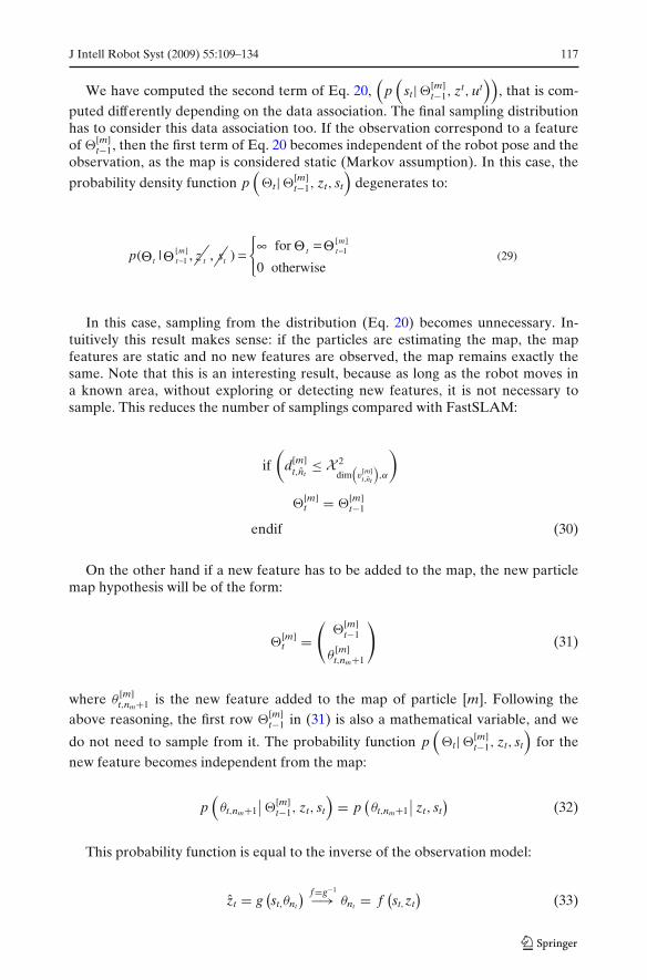
We have computed the second term of Eq. 20,(

p(


)), that is com-

puted differently depending on the data association. The final sampling distributionhas to consider this data association too. If the observation correspond to a featureof �

[m]t−1, then the first term of Eq. 20 becomes independent of the robot pose and the

observation, as the map is considered static (Markov assumption). In this case, the

probability density function p(

�t| �[m]t−1, zt, st

)degenerates to:

[ ]1( | ,m

t t tp z− , ts[ ]

1 for )

0 otherwise

mt t−⎧ =

= ⎨⎩

(29)Θ ΘΘ∞ Θ

In this case, sampling from the distribution (Eq. 20) becomes unnecessary. In-tuitively this result makes sense: if the particles are estimating the map, the mapfeatures are static and no new features are observed, the map remains exactly thesame. Note that this is an interesting result, because as long as the robot moves ina known area, without exploring or detecting new features, it is not necessary tosample. This reduces the number of samplings compared with FastSLAM:

if(

d[m]t,nt

≤ X 2

dim(v

[m]t,nt

),α

)

�[m]t = �

[m]t−1

endif (30)

On the other hand if a new feature has to be added to the map, the new particlemap hypothesis will be of the form:

�[m]t =

(�

[m]t−1

θ[m]t,nm+1

)

(31)

where θ[m]t,nm+1 is the new feature added to the map of particle [m]. Following the

above reasoning, the first row �[m]t−1 in (31) is also a mathematical variable, and we

do not need to sample from it. The probability function p(

�t| �[m]t−1, zt, st

)for the

new feature becomes independent from the map:

p(

θt,nm+1

∣∣ �[m]t−1, zt, st

)= p

(θt,nm+1

∣∣ zt, st)

(32)

This probability function is equal to the inverse of the observation model:

zt = g(st,θnt

) f=g−1

−→ θnt = f(st,zt

)(33)


Thus, the sampling of θ[m]t,nm+1 (and also �

[m]t ) can be done under the Gaussian

assumption as follows:

if(

d[m]t,nt

> X 2

dim(v

[m]t,nt

),α

)

sample θ[m]t,nm+1 ∼ N

(f(

s[m]t|t−1, zt , Fs P[m]

t|t−1 FTs + R[m]

t

)

�[m]t =

(�

[m]t−1

θ[m]t,nm+1

)

endif (34)

where Fs is the Jacobian of the inverse observation model with respect to the robotpose:

Fs = ∂ f(st,zt

)

∂st

∣∣∣∣∣st=s[m]

t|t−1,zt=zt

(35)

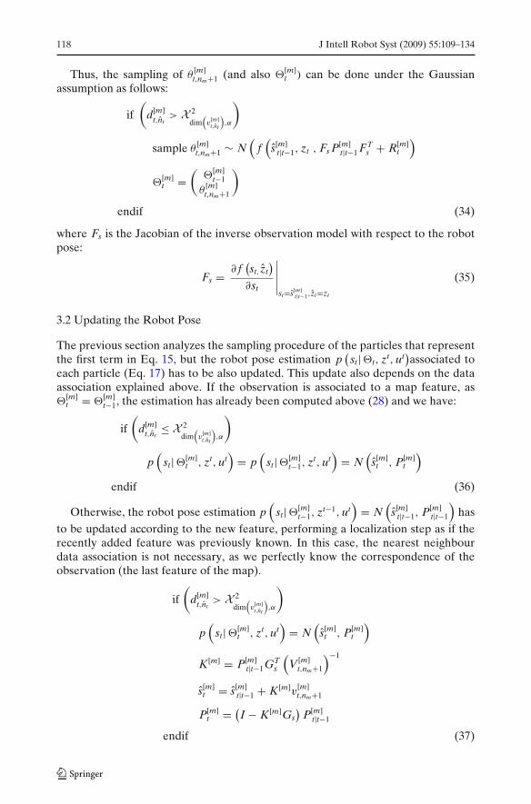
3.2 Updating the Robot Pose

The previous section analyzes the sampling procedure of the particles that representthe first term in Eq. 15, but the robot pose estimation p

(st| �t, zt, ut

)associated to

each particle (Eq. 17) has to be also updated. This update also depends on the dataassociation explained above. If the observation is associated to a map feature, as�

[m]t = �

[m]t−1, the estimation has already been computed above (28) and we have:

if(

d[m]t,nt

≤ X 2

dim(v

[m]t,nt

),α

)

p(


)= p

(st|�[m]

t−1, zt, ut)

= N(

s[m]t , P[m]

t

)

endif (36)

Otherwise, the robot pose estimation p(

st|�[m]t−1, zt−1, ut

)= N

(s[m]

t|t−1, P[m]t|t−1

)has

to be updated according to the new feature, performing a localization step as if therecently added feature was previously known. In this case, the nearest neighbourdata association is not necessary, as we perfectly know the correspondence of theobservation (the last feature of the map).

if(

d[m]t,nt

> X 2

dim(v

[m]t,nt

),α

)

p(


)= N

(s[m]

t , P[m]t

)

K[m] = P[m]t|t−1GT

s

(V[m]

t,nm+1

)−1

s[m]t = s[m]

t|t−1 + K[m]v[m]t,nm+1

P[m]t = (

I − K[m]Gs)

P[m]t|t−1

endif (37)


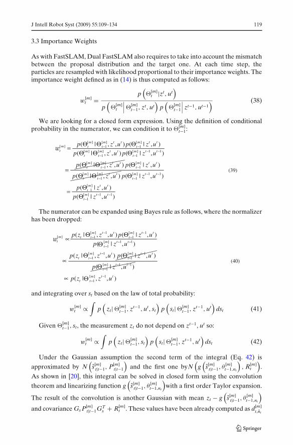
3.3 Importance Weights

As with FastSLAM, Dual FastSLAM also requires to take into account the mismatchbetween the proposal distribution and the target one. At each time step, theparticles are resampled with likelihood proportional to their importance weights. Theimportance weight defined as in (14) is thus computed as follows:

w[m]t =

p(�

[m]t |zt, ut

)

p(

�[m]t

∣∣∣ �[m]

t−1, zt, ut)

p(

�[m]t−1

∣∣∣ zt−1, ut−1

) (38)

We are looking for a closed form expression. Using the definition of conditionalprobability in the numerator, we can condition it to �

[m]t−1:

[ ] [ ] [ ][ ] 1 1

[ ] [ ] [ ] 1 11 1

[ ] [ ]1

( | , , ) ( | , )

( | , , ) ( | , )

( | , , )

m m t t m t tm t t t

t m m t t m t tt t t

m m t tt t

p z u p z u

p z u p z u

p z u

− −− −

− −

−

Θ Θ Θ=Θ Θ Θ

Θ Θ Θ=

[ ]1

[ ] [ ]1

( | , )

( | , , )

m t tt

m m t tt t

p z u

p z u

−

−Θ Θ Θ[ ] 1 11

[ ]1

[ ] 1 11

( | , )

( | , )

( | , )

m t tt

m t tt

m t tt

p z u

p z u

p z u

− −−

− −−

Θ=Θ

(39)

The numerator can be expanded using Bayes rule as follows, where the normalizerhas been dropped:

[ ] 1 [ ] 1[ ] 1 1

[ ] 1 11

[ ] 1 [ ] 11 1

( | , , ) ( | , )

( | , )

( | , , ) ( | , )

m t t m t tm t t t

t m t tt

m t t m t tt t t

p z z u p z u

p z u

p z z u p z u

− −− −

− −−

− −− −

Θ Θ

Θ Θ∝

[ ] 1 11( | , )m t t

tp z u− −−Θ

Θ

Θ [ ] 11( | , , )m t t

t tp z z u−−∝

(40)

∝

and integrating over st based on the law of total probability:

w[m]t ∝

∫p

(zt| �[m]

t−1, zt−1, ut, st

)p

(st|�[m]

t−1, zt−1, ut)

dst (41)

Given �[m]t−1, st, the measurement zt do not depend on zt−1, ut so:

w[m]t ∝

∫p

(zt| �[m]

t−1, st

)p

(st| �[m]

t−1, zt−1, ut)

dst (42)

Under the Gaussian assumption the second term of the integral (Eq. 42) is

approximated by N(

s[m]t|t−1, P[m]

t|t−1

)and the first one byN

(g

(s[m]

t|t−1, θ[m]t−1,nt

), R[m]

t

).

As shown in [20], this integral can be solved in closed form using the convolution

theorem and linearizing function g(

s[m]t|t−1, θ

[m]t−1,nt

)with a first order Taylor expansion.

The result of the convolution is another Gaussian with mean zt − g(

s[m]t|t−1, θ

[m]t−1,nt

)

and covariance Gs P[m]t|t−1GT

s + R[m]t . These values have been already computed as d[m]

t,nt


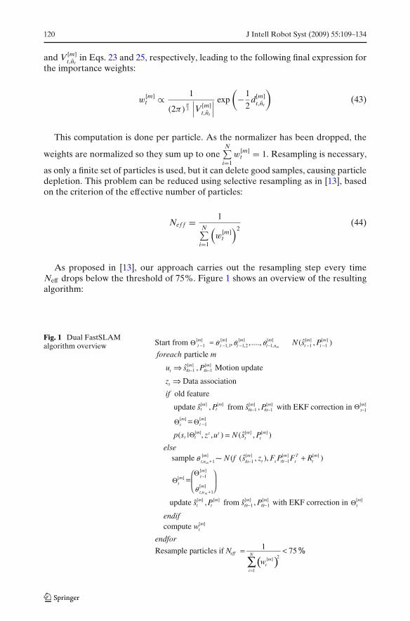
and V[m]t,nt

in Eqs. 23 and 25, respectively, leading to the following final expression forthe importance weights:

w[m]t ∝ 1

(2π)n2

∣∣∣V[m]

t,nt

∣∣∣

exp

(−1

2d[m]

t,nt

)(43)

This computation is done per particle. As the normalizer has been dropped, the

weights are normalized so they sum up to oneN∑

i=1w

[m]t = 1. Resampling is necessary,

as only a finite set of particles is used, but it can delete good samples, causing particledepletion. This problem can be reduced using selective resampling as in [13], basedon the criterion of the effective number of particles:

Nef f = 1N∑

i=1

(w

[m]t

)2(44)

As proposed in [13], our approach carries out the resampling step every timeNeff drops below the threshold of 75%. Figure 1 shows an overview of the resultingalgorithm:

Fig. 1 Dual FastSLAMalgorithm overview

[m] [m][m] [m] [m] [m],2 1,

[m] [m]t|t−1 t|t−1

t|t−1

t|t−1

t|t−1t|t−1

t|t−1

ˆStart from ,, ...., (s , )

particle

ˆ , Motion update

Data association

old feature

update

mt n t −1t −1t −1t −1,1t −1

t

t

N P

foreach m

u P

z

if

−

⇒

⇒

[m] [m] [m] [m] [m]1

[m] [m]

[m] [m] [m]

[m] [m] [m]| 1

ˆ, from , with EKF correction in

ˆ (s | , , ) ( , )

ˆ sample (f ( , ),

t t t

t

tttt t t

Tt s t t s

s s P

p z u N s P

elseN s z F P F

−

1mt,n + −

=

=

(

[m]

[m]

[m] [m] [m] [m] [m]

[m]

2[m]

1

)

ˆ ˆ update , from , with EKF correction in

compute

1Resample particles if

t

t

t t t

t

eff

ti

R

s s P

endifw

endfor

Nw

=

+

=

= 75N <∑

Θ

Θ

Θ

Θ

[m]1t−Θ

Θ

Θ

Θ

= θ θ θ

[m]1mt,n +θ

θ

s

ˆ P

t −1

⎞⎞ ⎞⎞

P

)


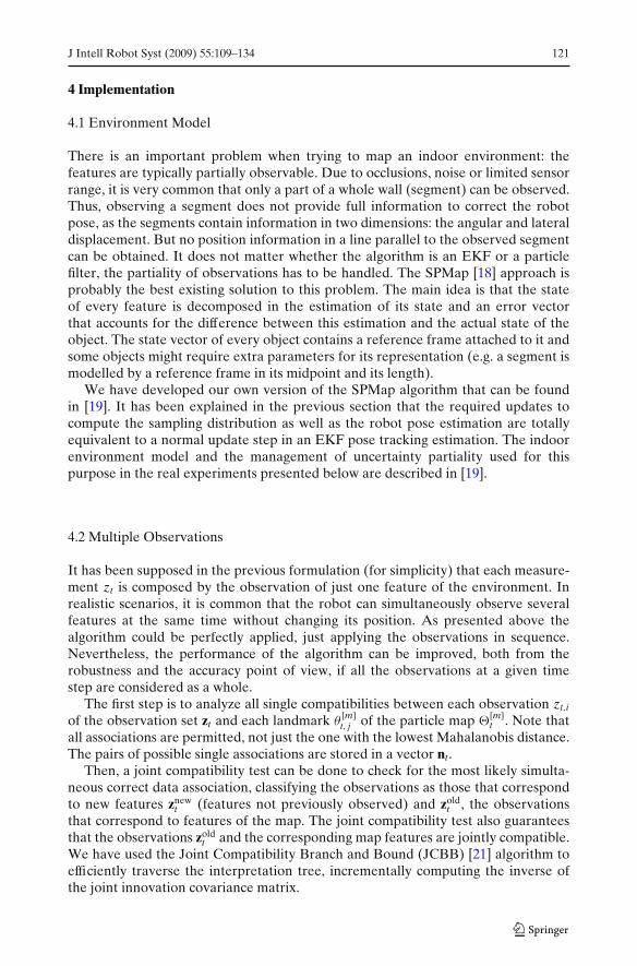
4 Implementation

4.1 Environment Model

There is an important problem when trying to map an indoor environment: thefeatures are typically partially observable. Due to occlusions, noise or limited sensorrange, it is very common that only a part of a whole wall (segment) can be observed.Thus, observing a segment does not provide full information to correct the robotpose, as the segments contain information in two dimensions: the angular and lateraldisplacement. But no position information in a line parallel to the observed segmentcan be obtained. It does not matter whether the algorithm is an EKF or a particlefilter, the partiality of observations has to be handled. The SPMap [18] approach isprobably the best existing solution to this problem. The main idea is that the stateof every feature is decomposed in the estimation of its state and an error vectorthat accounts for the difference between this estimation and the actual state of theobject. The state vector of every object contains a reference frame attached to it andsome objects might require extra parameters for its representation (e.g. a segment ismodelled by a reference frame in its midpoint and its length).

We have developed our own version of the SPMap algorithm that can be foundin [19]. It has been explained in the previous section that the required updates tocompute the sampling distribution as well as the robot pose estimation are totallyequivalent to a normal update step in an EKF pose tracking estimation. The indoorenvironment model and the management of uncertainty partiality used for thispurpose in the real experiments presented below are described in [19].

4.2 Multiple Observations

It has been supposed in the previous formulation (for simplicity) that each measure-ment zt is composed by the observation of just one feature of the environment. Inrealistic scenarios, it is common that the robot can simultaneously observe severalfeatures at the same time without changing its position. As presented above thealgorithm could be perfectly applied, just applying the observations in sequence.Nevertheless, the performance of the algorithm can be improved, both from therobustness and the accuracy point of view, if all the observations at a given timestep are considered as a whole.

The first step is to analyze all single compatibilities between each observation zt,i

of the observation set zt and each landmark θ[m]t, j of the particle map �

[m]t . Note that

all associations are permitted, not just the one with the lowest Mahalanobis distance.The pairs of possible single associations are stored in a vector nt.

Then, a joint compatibility test can be done to check for the most likely simulta-neous correct data association, classifying the observations as those that correspondto new features znew

t (features not previously observed) and zoldt , the observations

that correspond to features of the map. The joint compatibility test also guaranteesthat the observations zold

t and the corresponding map features are jointly compatible.We have used the Joint Compatibility Branch and Bound (JCBB) [21] algorithm toefficiently traverse the interpretation tree, incrementally computing the inverse ofthe joint innovation covariance matrix.


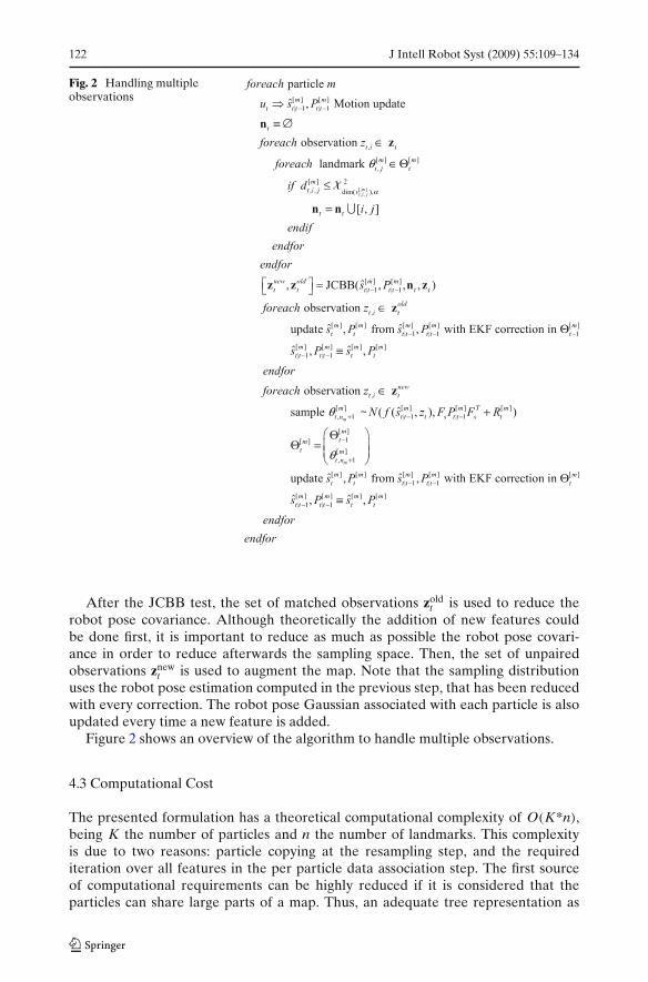
Fig. 2 Handling multipleobservations

~

After the JCBB test, the set of matched observations zoldt is used to reduce the

robot pose covariance. Although theoretically the addition of new features couldbe done first, it is important to reduce as much as possible the robot pose covari-ance in order to reduce afterwards the sampling space. Then, the set of unpairedobservations znew

t is used to augment the map. Note that the sampling distributionuses the robot pose estimation computed in the previous step, that has been reducedwith every correction. The robot pose Gaussian associated with each particle is alsoupdated every time a new feature is added.

Figure 2 shows an overview of the algorithm to handle multiple observations.

4.3 Computational Cost

The presented formulation has a theoretical computational complexity of O(K*n),being K the number of particles and n the number of landmarks. This complexityis due to two reasons: particle copying at the resampling step, and the requirediteration over all features in the per particle data association step. The first sourceof computational requirements can be highly reduced if it is considered that theparticles can share large parts of a map. Thus, an adequate tree representation as


in [14] of the map features can avoid the copy of the whole map every time a particleis copied.

The data association step requires linear time in the number of map features,because all of them are compared with the observation to check correspondence.If a lookup table (a grid that roughly divides the space) is built while adding newfeatures of the map, and the density of objects is finite, then this step could be done inconstant time. Because this work is focused on the formulation and the performanceof the dual factorization, these optimizations have not been implemented yet, beingsubject of further development.

5 Experiments

In this section, several experiments are presented. First, some results obtained fromsimulations are provided in order to provide a comparison of Dual FastSLAM withFastSLAM (1.0 and 2.0). Then, some experiments with real data are described,followed by a discussion explaining why the Dual FastSLAM approach could bebetter for use in indoor environments.

5.1 Simulation

To provide a fair comparison between FastSLAM and our algorithm, a simplesimulation is performed with Matlab. We have used the implementation of Baileyet al. [17] for FastSLAM and FastSLAM2.0. Neither algorithm has implementedany optimizations to avoid unnecessary complexity. The goal of this simulation is toanalyze the accuracy and the consistency of the estimation done by the algorithms,not the computational cost. Also, the algorithms are run with known data association.

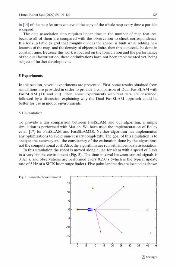
In this simulation the robot is moved along a line for 40 m with a speed of 3 m/sin a very simple environment (Fig. 3). The time interval between control signals is0.025 s, and observations are performed every 0.200 s (which is the typical updaterate of 5 Hz of a SICK laser range finder). Five point landmarks are located as shown

Fig. 3 Simulated environment


in the figure, and the laser field of view is 180◦ in front of the robot, with a range of30 m. The control noise deviation is 0.3 m/s and 3.0*�/180 rad/s for the forward androtational velocities.

The measurements z are bidimensional, providing both relative range and bearingto the observed point:

zt =(

rb

)=

⎛

⎝

√d2

x + d2y

tan−1(

dy

dx

)− ϕrobot

⎞

⎠

where

dx = xrobot − xlandmark

dy = yrobot − ylandmark (45)

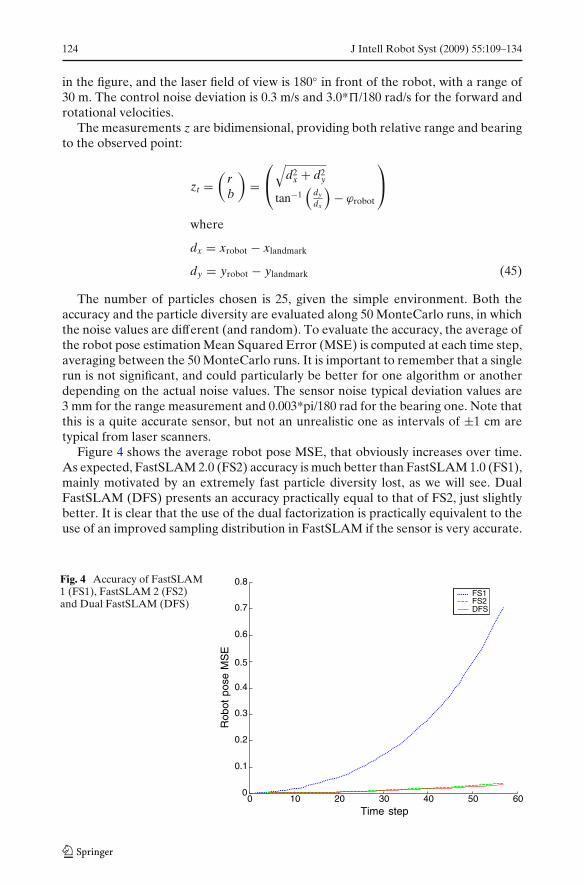
The number of particles chosen is 25, given the simple environment. Both theaccuracy and the particle diversity are evaluated along 50 MonteCarlo runs, in whichthe noise values are different (and random). To evaluate the accuracy, the average ofthe robot pose estimation Mean Squared Error (MSE) is computed at each time step,averaging between the 50 MonteCarlo runs. It is important to remember that a singlerun is not significant, and could particularly be better for one algorithm or anotherdepending on the actual noise values. The sensor noise typical deviation values are3 mm for the range measurement and 0.003*pi/180 rad for the bearing one. Note thatthis is a quite accurate sensor, but not an unrealistic one as intervals of ±1 cm aretypical from laser scanners.

Figure 4 shows the average robot pose MSE, that obviously increases over time.As expected, FastSLAM 2.0 (FS2) accuracy is much better than FastSLAM 1.0 (FS1),mainly motivated by an extremely fast particle diversity lost, as we will see. DualFastSLAM (DFS) presents an accuracy practically equal to that of FS2, just slightlybetter. It is clear that the use of the dual factorization is practically equivalent to theuse of an improved sampling distribution in FastSLAM if the sensor is very accurate.

Fig. 4 Accuracy of FastSLAM1 (FS1), FastSLAM 2 (FS2)and Dual FastSLAM (DFS)

0 10 20 30 40 50 600

0.1

0.2

0.3

0.4

0.5

0.6

0.7

0.8

Time step

Rob

ot p

ose

MS

E

FS1FS2DFS


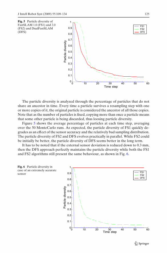
Fig. 5 Particle diversity ofFastSLAM 1.0 (FS1) and 2.0(FS2) and DualFastSLAM(DFS)

0 10 20 30 40 50 600

0.1

0.2

0.3

0.4

0.5

0.6

0.7

0.8

0.9

1

Time step

Part

icle

div

ers

ity

FS1

FS2

DFS

The particle diversity is analyzed through the percentage of particles that do notshare an ancestor in time. Every time a particle survives a resampling step with oneor more copies of it, the original particle is considered the ancestor of all those copies.Note that as the number of particles is fixed, copying more than once a particle meansthat some other particle is being discarded, thus loosing particle diversity.

Figure 5 shows the average percentage of particles at each time step, averagingover the 50 MonteCarlo runs. As expected, the particle diversity of FS1 quickly de-grades as an effect of the sensor accuracy and the relatively bad sampling distribution.The particle diversity of FS2 and DFS evolves practically in parallel. While FS2 couldbe initially be better, the particle diversity of DFS seems better in the long term.

It has to be noted that if the external sensor deviation is reduced down to 0.3 mm,then the DFS approach perfectly maintains the particle diversity while both the FS1and FS2 algorithms still present the same behaviour, as shown in Fig. 6.

Fig. 6 Particle diversity incase of an extremely accuratesensor

0 10 20 30 40 50 600

0.1

0.2

0.3

0.4

0.5

0.6

0.7

0.8

0.9

1

Time step

Par

ticle

div

ersi

ty

FS1FS2DFS


As described in Section 4.3, the computational complexity of the presentedapproach is the same as FastSLAM, but its underlying simplicity (we are using asingle EKF to estimate the robot pose given a map) can yield to the added advantageof lower computational requirements, compared with FastSLAM 2.

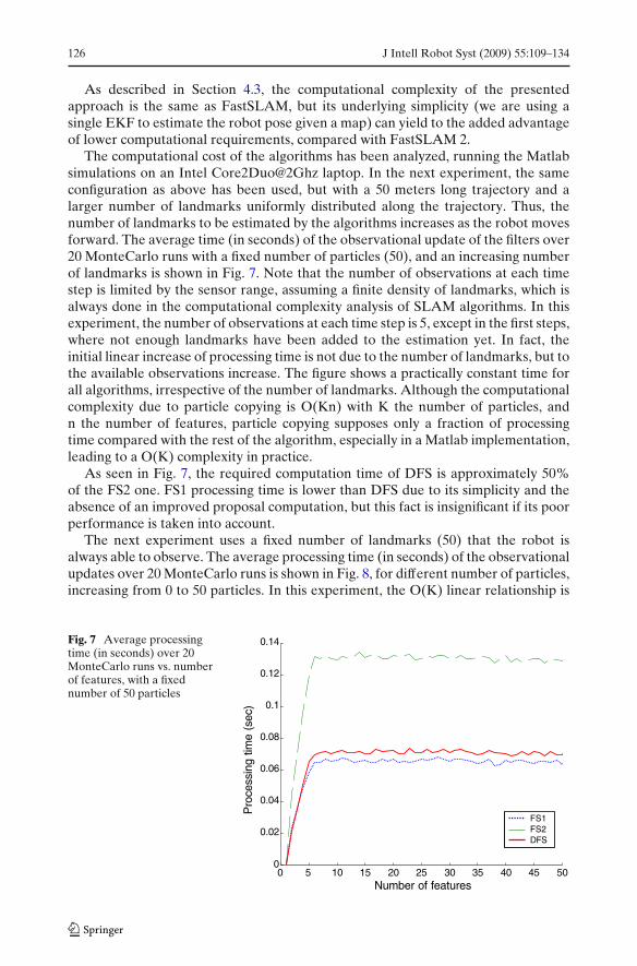
The computational cost of the algorithms has been analyzed, running the Matlabsimulations on an Intel Core2Duo@2Ghz laptop. In the next experiment, the sameconfiguration as above has been used, but with a 50 meters long trajectory and alarger number of landmarks uniformly distributed along the trajectory. Thus, thenumber of landmarks to be estimated by the algorithms increases as the robot movesforward. The average time (in seconds) of the observational update of the filters over20 MonteCarlo runs with a fixed number of particles (50), and an increasing numberof landmarks is shown in Fig. 7. Note that the number of observations at each timestep is limited by the sensor range, assuming a finite density of landmarks, which isalways done in the computational complexity analysis of SLAM algorithms. In thisexperiment, the number of observations at each time step is 5, except in the first steps,where not enough landmarks have been added to the estimation yet. In fact, theinitial linear increase of processing time is not due to the number of landmarks, but tothe available observations increase. The figure shows a practically constant time forall algorithms, irrespective of the number of landmarks. Although the computationalcomplexity due to particle copying is O(Kn) with K the number of particles, andn the number of features, particle copying supposes only a fraction of processingtime compared with the rest of the algorithm, especially in a Matlab implementation,leading to a O(K) complexity in practice.

As seen in Fig. 7, the required computation time of DFS is approximately 50%of the FS2 one. FS1 processing time is lower than DFS due to its simplicity and theabsence of an improved proposal computation, but this fact is insignificant if its poorperformance is taken into account.

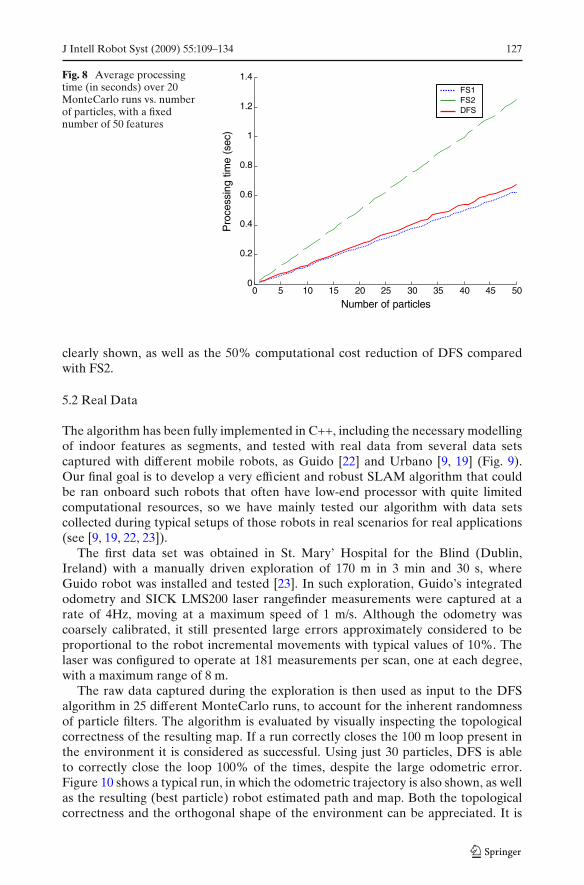
The next experiment uses a fixed number of landmarks (50) that the robot isalways able to observe. The average processing time (in seconds) of the observationalupdates over 20 MonteCarlo runs is shown in Fig. 8, for different number of particles,increasing from 0 to 50 particles. In this experiment, the O(K) linear relationship is

Fig. 7 Average processingtime (in seconds) over 20MonteCarlo runs vs. numberof features, with a fixednumber of 50 particles

0 5 10 15 20 25 30 35 40 45 500

0.02

0.04

0.06

0.08

0.1

0.12

0.14

Number of features

Pro

cess

ing

time

(sec

)

FS1FS2DFS


Fig. 8 Average processingtime (in seconds) over 20MonteCarlo runs vs. numberof particles, with a fixednumber of 50 features

0 5 10 15 20 25 30 35 40 45 500

0.2

0.4

0.6

0.8

1

1.2

1.4

Number of particles

Pro

cess

ing

time

(sec

)

FS1FS2DFS

clearly shown, as well as the 50% computational cost reduction of DFS comparedwith FS2.

5.2 Real Data

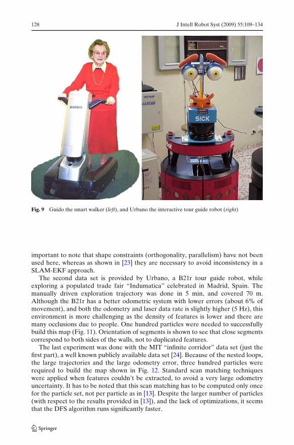
The algorithm has been fully implemented in C++, including the necessary modellingof indoor features as segments, and tested with real data from several data setscaptured with different mobile robots, as Guido [22] and Urbano [9, 19] (Fig. 9).Our final goal is to develop a very efficient and robust SLAM algorithm that couldbe ran onboard such robots that often have low-end processor with quite limitedcomputational resources, so we have mainly tested our algorithm with data setscollected during typical setups of those robots in real scenarios for real applications(see [9, 19, 22, 23]).

The first data set was obtained in St. Mary’ Hospital for the Blind (Dublin,Ireland) with a manually driven exploration of 170 m in 3 min and 30 s, whereGuido robot was installed and tested [23]. In such exploration, Guido’s integratedodometry and SICK LMS200 laser rangefinder measurements were captured at arate of 4Hz, moving at a maximum speed of 1 m/s. Although the odometry wascoarsely calibrated, it still presented large errors approximately considered to beproportional to the robot incremental movements with typical values of 10%. Thelaser was configured to operate at 181 measurements per scan, one at each degree,with a maximum range of 8 m.

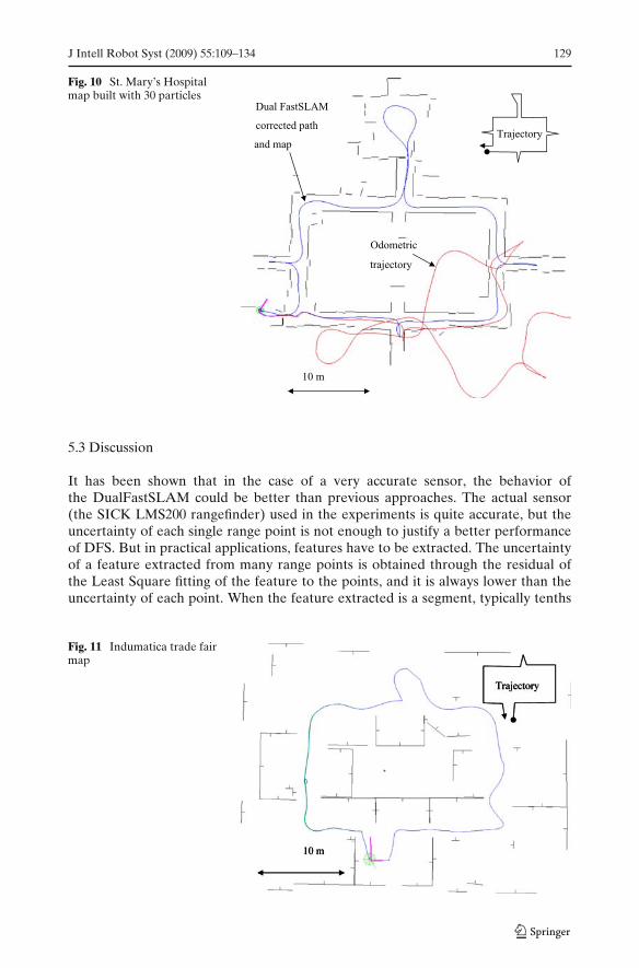
The raw data captured during the exploration is then used as input to the DFSalgorithm in 25 different MonteCarlo runs, to account for the inherent randomnessof particle filters. The algorithm is evaluated by visually inspecting the topologicalcorrectness of the resulting map. If a run correctly closes the 100 m loop present inthe environment it is considered as successful. Using just 30 particles, DFS is ableto correctly close the loop 100% of the times, despite the large odometric error.Figure 10 shows a typical run, in which the odometric trajectory is also shown, as wellas the resulting (best particle) robot estimated path and map. Both the topologicalcorrectness and the orthogonal shape of the environment can be appreciated. It is


Fig. 9 Guido the smart walker (left), and Urbano the interactive tour guide robot (right)

important to note that shape constraints (orthogonality, parallelism) have not beenused here, whereas as shown in [23] they are necessary to avoid inconsistency in aSLAM-EKF approach.

The second data set is provided by Urbano, a B21r tour guide robot, whileexploring a populated trade fair “Indumatica” celebrated in Madrid, Spain. Themanually driven exploration trajectory was done in 5 min, and covered 70 m.Although the B21r has a better odometric system with lower errors (about 6% ofmovement), and both the odometry and laser data rate is slightly higher (5 Hz), thisenvironment is more challenging as the density of features is lower and there aremany occlusions due to people. One hundred particles were needed to successfullybuild this map (Fig. 11). Orientation of segments is shown to see that close segmentscorrespond to both sides of the walls, not to duplicated features.

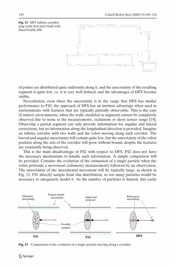
The last experiment was done with the MIT “infinite corridor” data set (just thefirst part), a well known publicly available data set [24]. Because of the nested loops,the large trajectories and the large odometry error, three hundred particles wererequired to build the map shown in Fig. 12. Standard scan matching techniqueswere applied when features couldn’t be extracted, to avoid a very large odometryuncertainty. It has to be noted that this scan matching has to be computed only oncefor the particle set, not per particle as in [13]. Despite the larger number of particles(with respect to the results provided in [13]), and the lack of optimizations, it seemsthat the DFS algorithm runs significantly faster.


Fig. 10 St. Mary’s Hospitalmap built with 30 particles

10 m

Trajectory

Dual FastSLAM

corrected path

and map

Odometric

trajectory

5.3 Discussion

It has been shown that in the case of a very accurate sensor, the behavior ofthe DualFastSLAM could be better than previous approaches. The actual sensor(the SICK LMS200 rangefinder) used in the experiments is quite accurate, but theuncertainty of each single range point is not enough to justify a better performanceof DFS. But in practical applications, features have to be extracted. The uncertaintyof a feature extracted from many range points is obtained through the residual ofthe Least Square fitting of the feature to the points, and it is always lower than theuncertainty of each point. When the feature extracted is a segment, typically tenths

Fig. 11 Indumatica trade fairmap

10 m

Trajectory


Fig. 12 MIT infinite corridormap (only first part) built withDual FastSLAM

of points are distributed quite uniformly along it, and the uncertainty of the resultingsegment is quite low, i.e. it is very well defined, and the advantages of DFS becomevisible.

Nevertheless, even when the uncertainty is in the range that DFS has similarperformance to FS2, the approach of DFS has an intrinsic advantage when used inenvironments with features that are typically partially observable. This is the caseof indoor environments, when the walls, modeled as segments cannot be completelyobserved due to noise in the measurements, occlusions or short sensor range [19].Observing a partial segment can only provide information for angular and lateralcorrections, but no information along the longitudinal direction is provided. Imaginean infinite corridor with two walls and the robot moving along such corridor. Thelateral and angular uncertainty will remain quite low, but the uncertainty of the robotposition along the axis of the corridor will grow without bound, despite the featuresare constantly being observed.

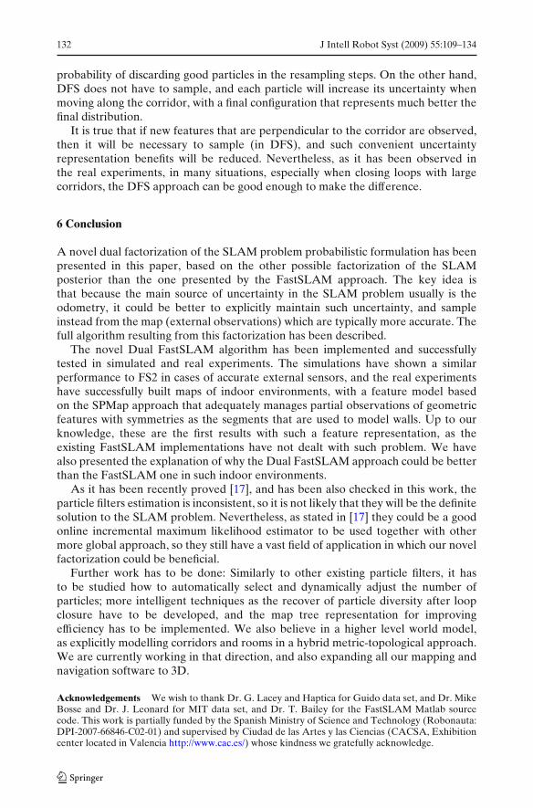
This is the main disadvantage of FS2 with respect to DFS. FS2 does not havethe necessary mechanisms to handle such information. A simple comparison willbe provided. Consider the evolution of the estimation of a single particle when therobot performs a movement (odometry measurement) followed by an observation.The uncertainty of the incremental movement will be typically large, as shown inFig. 13. FS1 directly sample from this distribution, so too many particles would benecessary to adequately model it. As the number of particles is limited, this easily

FS1 FS2

Odometry uncertainty

Feature model uncertainty Improved

proposal Robot pose uncertainty

Possible samples

DFS

Fig. 13 Comparison of the evolution of a single particle moving along a corridor


causes particle depletion. FS2 alleviates this problem by sampling from an improvedproposal that takes into account the external observation. Such proposal could havethe shape illustrated in the figure, reduced in the transversal direction to the corridorbut maintained along the corridor axis. Although the distribution is much smaller,FS2 has to sample from it, i.e. it has to sample without having reduced the uncertaintyin the longitudinal direction. It could be said that it suffers the same problem as FS1,but only in one dimension, the direction of the corridor. In both cases, they are able toexplicitly maintain uncertainty information for the features in the form of covariancematrices, but it has to be noted that in many cases such covariance will be extremelylow, almost negligible.

It is more intuitive to explicitly maintain the uncertainty of the robot pose, as itis the main source of uncertainty. Next figure shows that the feature model does notcontain uncertainty information, but each particle models the robot pose includingits covariance. When the robot moves along the corridor this covariance initiallyincreases according to pure odometry, but when the measurement is incorporated itis reduced again, but only in the corridor transversal direction, adequately modelingthe uncertainty along the corridor axis. The important difference is that DFS doesnot have to sample from this distribution, it maintains it. DFS has to sample onlywhen new features are detected.

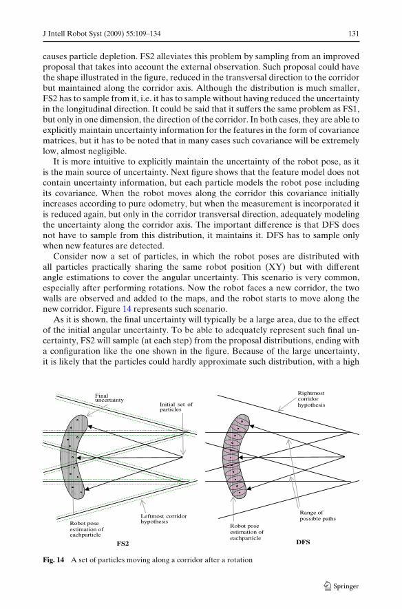
Consider now a set of particles, in which the robot poses are distributed withall particles practically sharing the same robot position (XY) but with differentangle estimations to cover the angular uncertainty. This scenario is very common,especially after performing rotations. Now the robot faces a new corridor, the twowalls are observed and added to the maps, and the robot starts to move along thenew corridor. Figure 14 represents such scenario.

As it is shown, the final uncertainty will typically be a large area, due to the effectof the initial angular uncertainty. To be able to adequately represent such final un-certainty, FS2 will sample (at each step) from the proposal distributions, ending witha configuration like the one shown in the figure. Because of the large uncertainty,it is likely that the particles could hardly approximate such distribution, with a high

FS2 DFS

Initial set of particles

Leftmost corridor hypothesis

Range of possible paths

Robot pose estimation of eachparticle

Robot pose estimation of eachparticle

Final uncertainty

Rightmost corridor hypothesis

Fig. 14 A set of particles moving along a corridor after a rotation


probability of discarding good particles in the resampling steps. On the other hand,DFS does not have to sample, and each particle will increase its uncertainty whenmoving along the corridor, with a final configuration that represents much better thefinal distribution.

It is true that if new features that are perpendicular to the corridor are observed,then it will be necessary to sample (in DFS), and such convenient uncertaintyrepresentation benefits will be reduced. Nevertheless, as it has been observed inthe real experiments, in many situations, especially when closing loops with largecorridors, the DFS approach can be good enough to make the difference.

6 Conclusion

A novel dual factorization of the SLAM problem probabilistic formulation has beenpresented in this paper, based on the other possible factorization of the SLAMposterior than the one presented by the FastSLAM approach. The key idea isthat because the main source of uncertainty in the SLAM problem usually is theodometry, it could be better to explicitly maintain such uncertainty, and sampleinstead from the map (external observations) which are typically more accurate. Thefull algorithm resulting from this factorization has been described.

The novel Dual FastSLAM algorithm has been implemented and successfullytested in simulated and real experiments. The simulations have shown a similarperformance to FS2 in cases of accurate external sensors, and the real experimentshave successfully built maps of indoor environments, with a feature model basedon the SPMap approach that adequately manages partial observations of geometricfeatures with symmetries as the segments that are used to model walls. Up to ourknowledge, these are the first results with such a feature representation, as theexisting FastSLAM implementations have not dealt with such problem. We havealso presented the explanation of why the Dual FastSLAM approach could be betterthan the FastSLAM one in such indoor environments.

As it has been recently proved [17], and has been also checked in this work, theparticle filters estimation is inconsistent, so it is not likely that they will be the definitesolution to the SLAM problem. Nevertheless, as stated in [17] they could be a goodonline incremental maximum likelihood estimator to be used together with othermore global approach, so they still have a vast field of application in which our novelfactorization could be beneficial.

Further work has to be done: Similarly to other existing particle filters, it hasto be studied how to automatically select and dynamically adjust the number ofparticles; more intelligent techniques as the recover of particle diversity after loopclosure have to be developed, and the map tree representation for improvingefficiency has to be implemented. We also believe in a higher level world model,as explicitly modelling corridors and rooms in a hybrid metric-topological approach.We are currently working in that direction, and also expanding all our mapping andnavigation software to 3D.

Acknowledgements We wish to thank Dr. G. Lacey and Haptica for Guido data set, and Dr. MikeBosse and Dr. J. Leonard for MIT data set, and Dr. T. Bailey for the FastSLAM Matlab sourcecode. This work is partially funded by the Spanish Ministry of Science and Technology (Robonauta:DPI-2007-66846-C02-01) and supervised by Ciudad de las Artes y las Ciencias (CACSA, Exhibitioncenter located in Valencia http://www.cac.es/) whose kindness we gratefully acknowledge.

http://www.cac.es/


References

1. Thrun, S.: Robotic mapping: A survey. In: Lakemeyer, G., Nebel, B. (eds.) Exploring ArtificialIntelligence in the New Millenium. Morgan Kaufmann, San Francisco (2002)

2. Smith, R., Self, M., Cheeseman, P.: Estimating uncertain spatial relationships in robotics. In:Lemmer, J.F., Kanal, L.N. (eds.) Uncertainty in Artificial Intelligence 2. Elsevier, New York(1988)

3. Liu, Y., Thrun, S.: Results for outdoor-SLAM using sparse extended information filters. IEEEInt. Conf. Robot. Autom. 1, 1227–1233 (2003)

4. Guivant, J., Nebot, E.: Optimization of the simultaneous localization and map-building al-gorithm for real-time implementation. IEEE Trans. Robot. Autom. 17(3), 242–257 (2001).doi:10.1109/70.938382

5. Williams, S., Dissanayake, G., Durrant-Whyte, H.F.: An efficient approach to the simultaneouslocalization and mapping problem. IEEE Int. Conf. Robot. Autom. 15(5), 406–411 (2002)

6. Tardos, J.D., Neira, J., Newman, P., Leonard, J.J.: Robust mapping and localization in indoorenvironment using sonar data. Int. J. Rob. Res. 21(4), 311–330 (2002)

7. Julier, S., Uhlmann, J.K.: A counter example to the theory of simultaneous localization and mapbuilding. IEEE ICRA’01. V.4. Seul, Corea., pp. 4238–4243 (2001)

8. Castellanos, J.A., Neira, J., Tardos, J.D.: Limits to the consistency of EKF-based SLAM.In: Fifth IFAC Symposium on Intelligent Autonomous Vehicles IAV’04. Lisbon, Portugal(2004)

9. Rodriguez-Losada, D., Matia, F., Pedraza, L., Jimenez, A., Galan, R.: Consistency of SLAM-EKF algorihtms for indoor environments. J. Intell. Robot. Syst. 50(4), 375–397 (2007). Springer.ISSN 0921-0296

10. Doucet, A., de Freitas, J.F.G., Murphy, K., Russel, S.: Raoblackwellized particle filter-ing for dynamic bayesian networks. Conf. on Uncertainty in Artifcial Intelligence (UAI)(2000)

11. Montemerlo, M., Thrun, S., Koller, D., Wegbreit, B.: FastSLAM: a factored solution to the simul-taneous localization and mapping problem. AAAI Nat. Conf. on Artif. Intelligence. Edmonton,Canada (2002)

12. Eliazar, A., Parr, R.: DP-SLAM: fast, robust simultaneous localization and mapping with-out predetermined landmarks. In: Proc. of the Int. Conf. on Artificial Intelligence (IJCAI)(2003)

13. Grisetti, G., Stachniss, C., Burgard, W.: Improving Grid-based SLAM with rao-blackwellizedparticle filters by adaptive proposals and selective resampling. IEEE ICRA’ 05, pp. 2443–2448,Barcelona, Spain (2005)

14. Montemerlo, M., Thrun, S., Koller, D., Wegbreit, B.: FastSLAM 2.0: an improved particlefiltering algorithm for simultaneous localization and mapping that provably converges. IJCAI,pp. 1151–1156 (2003)

15. Hahnel, D., Burgard, W., Fox, D., Thrun, S.: An efficient FastSLAM algorithm for generatingmaps of large-scale cyclic environments from raw laser range measurements. IEEE/RSJ IROS’03(2003)

16. Elinas, P., Sim, R., Little, J.J.: σSLAM: Stereo Vision SLAM using the rao-blackwellised particlefilter and a novel mixture proposal distribution. In: Proceedings of the IEEE InternationalConference on Robotics and Automation, pp. 1564–1570. Orlando, FL, (2006)

17. Bailey, T., Nieto, J., Nebot, E.: Consistency of the FastSLAM algorithm. In: IEEE InternationalConference on Robotics and Automation, 2006, pp. 424–429. Orlando, FL, USA, (2006)

18. Castellanos, J.A., Montiel, J.M., Neira, J., Tardos, J.D.: The SPmap: a probabilistic frameworkfor simultaneous localization and map building. IEEE Trans. Robot. Autom. 15(5), 948–953(1999)

19. Rodriguez-Losada, D., Matia, F., Galan, R.: Building geometric feature based maps for indoorservice robots. Robot. Auton. Syst. 54, 546–558 (2006). doi:10.1016/j.robot.2006.04.003

20. Montemerlo, M.: FastSLAM: a factored solution to the simultaneous localization and mappingproblem with unknown data association. PhD doctoral dissertation, CMU-RI-TR-03-28, Robot-ics Institute, Carnegie Mellon University, July (2003)

21. Neira, J., Tardos, J.D.: Data association in stochastic mapping using the joint compatibility test.IEEE Trans. Robot. Autom. 17(6), 890–897 (2001). doi:10.1109/70.976019

22. Lacey, G., Rodriguez-Losada, D.: The evolution of Guido: a smart walker for the blind. AcceptedIEEE Robot. Autom. Mag. 15(4), 75–83 (2008). doi:10.1109/MRA.2008.929924

http://dx.doi.org/10.1109/70.938382

http://dx.doi.org/10.1016/j.robot.2006.04.003

http://dx.doi.org/10.1109/70.976019

http://dx.doi.org/10.1109/MRA.2008.929924


23. Rodriguez-Losada, D., Matia, F., Jiménez, A., Galan, R., Lacey, G.: Implementing map basednavigation in Guido, the robotic SmartWalker. In: IEEE International Conference on Roboticsand Automation, pp. 3401–3406. Barcelona, Spain, (2005)

24. Bosse, M., Newman, P., Leonard, J., Teller, S.: Simultaneous localization and map building inlarge-scale cyclic environments using the atlas framework. Int. J. Robot. Res 23(12), 1113–1140(2004)

Dual FastSLAM: Dual Factorization of the Particle Filter Based Solution of the Simultaneous...

Documents

Transcript of Dual FastSLAM: Dual Factorization of the Particle Filter Based Solution of the Simultaneous...