On implicit regularization: Morse functions andapplications to matrix factorization

Mohamed Ali Belabbas

AbstractIn this paper, we revisit implicit regularization from the ground up using

notions from dynamical systems and invariant subspaces of Morse functions.The key contributions are a new criterion for implicit regularization—a leadingcontender to explain the generalization power of deep models such as neuralnetworks—and a general blueprint to study it. We apply these techniques tosettle the conjecture on implicit regularization in matrix factorization raisedin [4].

1 Introduction

Deep models, such as deep neural networks, have seen a tremendous growth in theirrange of applications, growth that far outpaced our theoretical understanding ofthem. One of the major outstanding questions is to understand their generalizingpower: why a deep model fitted with a relatively small amount of data providesgood performance for data points well outside its training set? On the one hand,fitting parameters uniquely to training data is very likely to not generalize well, onthe other hand, having an underdetermined model leaves open the question of howto select among the many candidate parameters that fit the data. The training stageof a model can be cast as an optimization procedure in which a cost function isminimized. This cost function measures a chosen notion of distortion between modelparameters and training data. For underdetermined models, the cost function has alarge number of minima; in fact, very often a continuum of them.

When optimizing a cost function with many minima, the optimization methodused dictates which minimum is selected. This is in stark contrast with, say, a typicalconvex optimization problem, where there is no uncertainty due to multiple minimaand the effect of the optimization method is confined to the speed of convergence.This non-uniqueness of solutions is in many applications seen as little more thanan inconvenience, and when one needs to obtain a unique solution, regularizationmethods, such as Tykhonov regularization, are nowadays well-understood. Theissue at hand here is that the methods yielding the best generalizing power fordeep models do not have explicit regularization terms, but are often simple gradientmethods, thus offering no understanding of what makes a good set of parameters for

1

arX

iv:2

001.

0426

4v2

[cs

.LG

] 3

1 Ja

n 20

20

the purpose of generalization. The theory of implicit regularization aims to uncoverthe rules of selection of parameters that are hidden in the training of deep models.It does so via the introduction of an auxiliary optimization problem, whose solutionshould be essentially unique and coincide with the local minimum selected [8–10].This auxiliary problem is thought of as regularizing the original problem implicitly.

The conjecture and our approach In order to better understand implicitregularization, the authors of [4] put forward a remarkable gradient flow: thefunction minimized is

J(X) =q∑i=1

(tr(AiX)− yi)2, (1)

where X and Ai’s are positive semi-definite matrices, and yi positive numbers1. Theauthors then conjecture that a gradient-like flow of J , when initialized near zeroand in the underdetermined regime (i.e., q � n2, where n is the dimension of X,we take here the definition to mean q ≤ n.), converges arbitrarily close to a globalminimizer of the problem

min ‖X‖∗ s.t. tr(AiX) = yi,

where ‖ · ‖∗ is the nuclear norm. The explicitly regularized problem is thus

min J(X) + λ‖X‖∗.

The best known results in the literature about the conjecture on implicit reg-ularization in matrix factorization are the ones in [4]: they showed it held for (i)the case q = 1 and (ii) the case of q ≥ 1 commuting matrices Ai, i.e., matrices sothat AiAj −AjAi = 0, with initial state X0 = I, I being the identity matrix. Theiranalysis was based on finding explicit forms of the solution of the gradient flowODE for X. The approach we take in this paper is entirely different. However, weshow in Example 4 below how their analysis of commuting matrices fits within ourframework, and as a consequence, we provide a rather unexpected characterizationof the convergence point in this case (see below Example 4).

Our analysis leads us to believe that the conjecture of [4] is “mostly true”. Wemean by this that while the conjecture is not true in its strictest form, a possibilityraised by the authors of the original paper in fact, and further substantiated in [1],there are regimes in which it is provably true (the tame spectrum regime, definedherein), and when moving away from this regime, the performance appears to degradeonly slowly. Using the results of our analysis, we can also manufacture settings inwhich the prediction of the conjecture does not hold even approximately; but for“typical” data, it appears to hold. Interestingly, we relate the performance to the

1The additional assumption that the Ai’s are positive semi-definite and yi > 0 allows us tosimplify the proof by making sure that all optimization problems are feasible. This assumption canbe relaxed at the expanse of additional cases to treat in the proofs, which we omit here.

2

spectral gap of ∑qi=1Ai and verify that for moderate to large spectral gaps, implicit

regularization occurs.In the proof, we make use of elementary notions from Morse theory and dynamical

systems, and we refer the reader to [2, 7] for thorough introductions, as we keep thereview of known material to a minimum in this paper. We summarize the proofof the conjecture below, after having introduced our general blueprint. We thenconclude and provide numerical evidence supporting our conclusion. The entirety ofthe proof of the conjecture is relegated to the Appendix.

2 Implicit Regularization: towards a general theory

Implicit regularization is in essence a notion of compatibility between two optimizationproblems. We propose here a way to quantify and understand this compatibility.

2.1 Primal and regularization problems

The first of the two problems is what we term the primal or training problem, itis given by

min J(µ;x), via x = f(µ, x), x(0) = x0(µ) (2)

where µ represent parameters or data, x is the variable we are optimizing over(the parameters of the model to be fitted), and x = f(µ;x) the method used tooptimize J , e.g. f(x) = −∂J

∂x . We assume that J(µ;x) is at least C2 in x. (Infact, J is real analytic for the case of implicit regularization in matrix factorization).A presentation of the primal problem should always include a description of theoptimization method used (here, f(µ;x)) and initial state x0(µ).

We denote by ϕt(x0) the solution at time t of the ODE in (2) with x(0) = x0, andby Crit J the set of critical points of J(µ, x), that is, the set of zeros of ∂J

∂x . Thisset of course depends on µ, but we often omit the explicit dependence to keep thenotation simple. We denote by Crit0 J the set of minima of J , and refer to the locallystable zeros of f as sinks. When using the gradient flow f(µ;x) = − grad J , thesinks are the local minima of J . The cases of interest are the ones where Crit0 Jhas large cardinality, and even contains connected components.2 Unless Crit0 J is asingleton, the local minima to which (2) will converge depends on the initial stateand the optimization method chosen.3

The second optimization problem, which we term the regularization problem,describes to which element of Crit0 J the primal problem converges. It is a problemof the form

R : minK(µ;x) s.t. r(µ;x) = 0, (3)2We note that if f is known, the function J is in fact not required. The set of critical points of

J can be replaced by the sets of zero of f , and minima by locally stable zeros of f , etc.3We consider below gradient with respect to a metric defined by the data µ. Hence grad J is not

necessarily equal to ∂J∂x

3

where K is a differentiable real-valued function and r an Rq-valued function. BothK and r can depend on µ. The feasible set of R, denoted by Feas(R), is the zeroset of r . It is required to be included in the set of minima of J :

Feas(R) := {x | r(x) = 0} ⊆ Crit0 J.

Said otherwise: feasible points of R are minima of J . Since the trajectories of agradient flow generically converge to a point in Crit0 J , this requirement simplyensures that the regularization problem selects one such point.

2.2 Pre-critical sets and compatible problems

We say that the primal problem is (exactly) implicitly regularized by the regu-larization problem if for all µ,

ϕ∞(µ;x0) ∈ arg minK(µ;x) s.t. r(µ;x) = 0.

If ϕ∞(µ;x0) is approximately a minimizer of K, we refer to the above as approxi-mately implicitly regularized.

It is important to note that in the regularization problem, the optimizationmethod is irrelevant, as we simply seek global minima. Many variations on thisdefinition are possible, such as requiring that it holds for all x0, or that we convergeto any minima of K(x), not necessarily a global one.

The following space, which we call the pre-critical set of R will play an essentialrole in implicit regularization:

Crit∗µ R := {x ∈ Rn | ∂K(µ;x)∂x

+ λ>∂r(µ;x)∂x

= 0 for some λ ∈ Rq}.

We can also define Crit∗µ R as the projection onto the x-coordinates of the setA := {(x, λ) ∈ Rn×q | ∂K(µ;x)

∂x + λ> ∂r(µ;x)∂x = 0}. This is a space of x ∈ Rn which

can be critical points of the Lagrangian L(µ;x, λ) = K(µ;x) + λ>r(µ;x) of problemR. More abstractly, we can think of it as the graph, over Rq, of the implicitlydefined function x(λ) given by ∂K

∂x + λ> ∂r∂x = 0. This space can be fairly complex:multi-valued, containing several connected components and non-smooth points, aswe will observe in the examples below. The terminology pre-critical set comesfrom the fact that points in Crit∗R which are in Feas(R) are critical points of R:Crit R = Feas(R) ∩ Crit∗R.

The space Crit∗R has a natural role in implicit regularization: if Crit∗R isan invariant subspace4 for the primal dynamics, then implicit regularization is ina sense more likely to occur: indeed, if we initialize the primal flow in this space,or if this space is an attractor for the primal flow, the primal flow converges to a

4Recall that S is an invariant subspace for the dynamics x = f(x) if for x0 ∈ S, the solutionx(t) ∈ S for all t.

4

critical point of the Lagrangian of R; said otherwise, it shows that the regularizationproblem is well-matched to the primal problem. Furthermore, since we are interestedin minimizers of R, it is sufficient to consider components of Crit∗R containing theminimizers of K, we call such a set of these components Crit∗µ,0 R or simply Crit∗0 R.Denote by M a set of data point µ. We have the following definition:

Definition 1 (Compatible primal and regularization problems). We say that theprimal problem (2) and the regularization problem R of Eq. (3) are compatibleover M if the space Crit∗µ,0 R is invariant for f(µ;x), for all µ ∈M .

We illustrate the definition on four examples. In particular, we revisit theapproach of [4] on implicit regularization on matrix factorization and show thatDefinition 1 yields new insights to it.

Example 1 (Trivial regularization problem). Starting from the primal problem, itis always possible to construct a regularization problem. Perhaps the simplest one,which we term the trivial regularization problem, is given by

K(µ;x) = ‖ϕ∞(µ, x0)− x‖2.

We call it trivial since the set Crit∗µ R for this regularization problem consists ofthe singleton {ϕ∞(µ;x0)}. The regularization problem and primal problem are thuscompatible in the sense of Def. 1, since ϕ∞(x0) is an equilibrium point of Eq. (2),and thus an invariant set for the dynamics.

Example 2. Let x, µi ∈ Rn, and yi ∈ R, for 1 ≤ i ≤ q. Set

J(µ;x) =q∑i=1

(µ>i x− yi)2.

Using the gradient for the Euclidean inner product as optimization method, andsetting x0(µ) = 0, we have

x = −q∑i=1

(µ>i x− yi)µi, x0 = 0. (4)

This problem is implicit regularized by the regularization problem

R : min 12‖x‖

2 s.t. µ>i x− yi = 0.

To see this, it suffices to solve the linear differential equation (4). We obtain in thiscase that

Crit∗R = {x ∈ Rn | x+q∑i=1

λiµi = 0 for some λ ∈ Rq},

equivalently, Crit∗R = span{µi}. This set is clearly invariant for the dynamics (4)and thus the problems are compatible in the sense of Definition 1, with M = Rn.

5

In the following example, the set Crit∗R has a richer structure than in theprevious two examples.

Example 3 (Matrix factorization with q = 1). Let A ∈ Rn×n be a positive definitematrix with distinct eigenvalues, U ∈ Rn×n and y be a positive number. Considerthe primal problem

J(U) = (tr(AUU>)− y)2,d

dtU = −(tr(AUU>)− y)AU,U(0) = U0,

and the regularization problem

min trUU> s.t. tr(AUU>) = y.

Writing X = UU>, it is easy to see that it is the problem of implicit regularizationin matrix factorization. A short calculation, which uses the fact that A is symmetric,yields

Crit∗R = {U ∈ Rn×n | (I − λA)U = 0 for some λ ∈ R}.The equation (I − λA)U admits non-trivial solutions only for λ ∈ spec(A), wherewe denote by spec(A) the set of eigenvalues of A, and in this case U = vw>, wherev is an eigenvector corresponding to λ, and w ∈ Rn is arbitrary. Hence

Crit∗R = ∪λi∈spec(A){viw> | w ∈ Rn, vi an eigenvector corresponding to λi},

this set is the union of n-dimensional subspaces of Rn×n. Now recalling thateigenvectors of A are orthogonal, it is easy to verify that each branch of Crit∗Ris invariant for the dynamics of U given above, thus showing compatibility of theprimal and selection problems.

The final example addresses the case studied in [4].

Example 4 (Matrix factorization with commuting matrices). Now assume we haveq positive definite matrices Ai, with primal problem

J(U) =q∑i=1

(tr(AiUU>)− yi)2,d

dtU = −

q∑i=1

(tr(AiUU>)− yi)AiU,U(0) = U0

and regularization problem

min trUU> s.t. tr(AiUU>) = yi, i = 1, . . . , q

The set pre-critical set is

Crit∗R = {U ∈ Rn×n | (I −q∑i=1

λiAi)U = 0 for some λ ∈ R}.

6

This set is in general difficult to study, as it requires to determine when the affinespace of matrices I + span{Ai} contains rank deficient matrices. If we assumethat the Ai commute, however, the situation is far simpler: commuting symmetricmatrices admit a common set of eigenvectors, hence there exists an orthogonalmatrix V such that Ai = V DiV

>, where Di is a diagonal matrix, with diagonalentries dij , i = 1, . . . , q, j = 1, . . . , n, and the columns of V are eigenvectors of theAi. We denote these columns by vi.

Now let I ⊆ {1, . . . , n} be a subset of cardinality q. We can, generically for thedi’s, find a unique solution λ = (λ1, . . . , λq) to the linear system

q∑i=1

λidi,k = 1, k ∈ I.

With these λi’s, a short calculation shows that the matrix (I − ∑qi=1 λiAi) =

V (I −∑qi=1 λiDi)V > has a kernel of dimension q, spanned by the vectors vi, i ∈ I.

There are(nq

)such subsets I, and to each of them corresponds a vector λ ∈ Rq and

thus a component of dimension q × n of Crit∗R:

{U ∈ Rn×n | U = vw>, w ∈ Rn, v ∈ span{vi | i ∈ I}}.

Similarly as in the previous example, this set is easily seen to be invariant for theprimal dynamics.

The analysis suggests that when the flow converges to a rank one matrix (whichwe show below is the case)

X = vv>,

then there exists q eigenvectors in the common set of eigenvectors of the Ai so that vis a linear combination of these q eigenvectors. Said otherwise, there exists a sparsevector x ∈ Rn, with ‖x‖0 ≤ q so that

v = V x.

This is a non-trivial statement when q < n, and we verified it in simulations. Notethat there are

(nq

)such linear subspaces, and when q is large, they can intersect

non-trivially.

2.3 A blueprint for implicit regularization

The criterion of Definition 1 by itself is clearly not sufficient for implicit regularizationto occur. For example, since the space Crit0 J contains points x not in Feas(R), onecan converge to a non-feasible point for R, even when initialized in Crit∗R. More,even if Feas(R) = Crit0 J , saddle points of the primal dynamics can become localsinks in an invariant space, allowing for the primal flow to converge to a non-feasiblepoint. This criterion, however, provides us with a general blueprint to study implicitregularization:

7

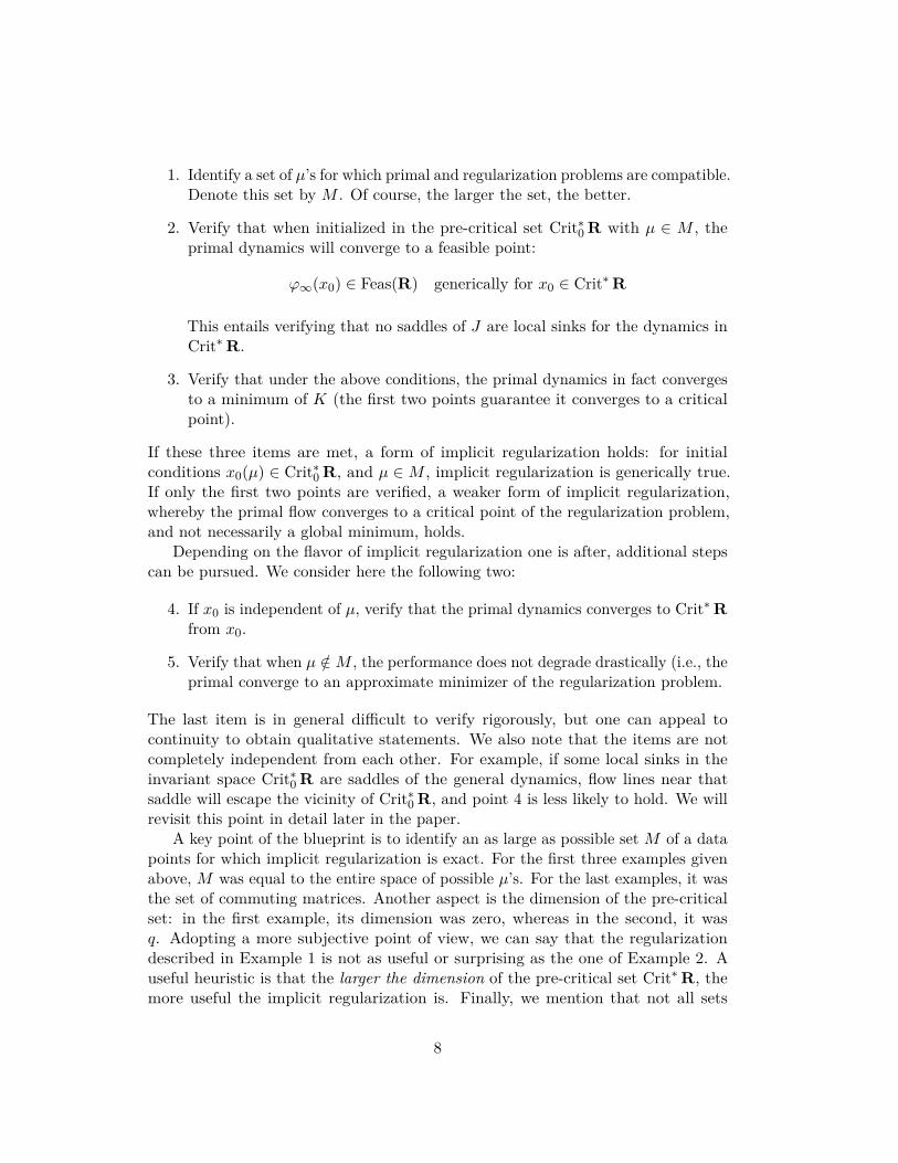
1. Identify a set of µ’s for which primal and regularization problems are compatible.Denote this set by M . Of course, the larger the set, the better.

2. Verify that when initialized in the pre-critical set Crit∗0 R with µ ∈ M , theprimal dynamics will converge to a feasible point:

ϕ∞(x0) ∈ Feas(R) generically for x0 ∈ Crit∗R

This entails verifying that no saddles of J are local sinks for the dynamics inCrit∗R.

3. Verify that under the above conditions, the primal dynamics in fact convergesto a minimum of K (the first two points guarantee it converges to a criticalpoint).

If these three items are met, a form of implicit regularization holds: for initialconditions x0(µ) ∈ Crit∗0 R, and µ ∈M , implicit regularization is generically true.If only the first two points are verified, a weaker form of implicit regularization,whereby the primal flow converges to a critical point of the regularization problem,and not necessarily a global minimum, holds.

Depending on the flavor of implicit regularization one is after, additional stepscan be pursued. We consider here the following two:

4. If x0 is independent of µ, verify that the primal dynamics converges to Crit∗Rfrom x0.

5. Verify that when µ /∈M , the performance does not degrade drastically (i.e., theprimal converge to an approximate minimizer of the regularization problem.

The last item is in general difficult to verify rigorously, but one can appeal tocontinuity to obtain qualitative statements. We also note that the items are notcompletely independent from each other. For example, if some local sinks in theinvariant space Crit∗0 R are saddles of the general dynamics, flow lines near thatsaddle will escape the vicinity of Crit∗0 R, and point 4 is less likely to hold. We willrevisit this point in detail later in the paper.

A key point of the blueprint is to identify an as large as possible set M of a datapoints for which implicit regularization is exact. For the first three examples givenabove, M was equal to the entire space of possible µ’s. For the last examples, it wasthe set of commuting matrices. Another aspect is the dimension of the pre-criticalset: in the first example, its dimension was zero, whereas in the second, it wasq. Adopting a more subjective point of view, we can say that the regularizationdescribed in Example 1 is not as useful or surprising as the one of Example 2. Auseful heuristic is that the larger the dimension of the pre-critical set Crit∗R, themore useful the implicit regularization is. Finally, we mention that not all sets

8

M are equivalent for implicit regularization insofar as item 5 is concerned. Forexample, the set exhibited in Example 4, which originated from the paper [4], doesnot lend itself well to generalization. This was in fact pointed out by the authors ofthe paper, though they arrived at this conclusion from a very different perspective,namely looking for explicit solutions of the primal problem. We reach this conclusionby noting that if we perturb one matrix Ai by a small amount, the trajectory ofthe primal system can stray very far from Crit∗R. Our proof below will exhibit adifferent set M , which we refer to as matrices with tame spectrum5 , that is bettersuited to study implicit regularization in matrix factorization.

2.4 How to determine the implicit regularizer?

A fundamental goal in the area is to determine the implicit regularizer R given aprimal flow. We provide here a brief overview of how our blueprint provides a pathto obtain such regularizer, but we postpone a thorough analysis to a forthcomingpublication.

We consider the training problem with cost J = ∑qi=1 l(µi, x), where l, the

loss function, depends on data points µi and parameters x. We assume that l ispositive semi-definite with minimum at zero, hence min J = 0. In Example 2 ,l(µ, x) = (c>x− y)2 (and µ = (c, y)), and in Example 4, l(µ, x) = tr(AX)− y, withµ = (A, y). The primal flow is taken to be the natural gradient of J :

x = −q∑i=1

∂l

∂x(µi, x) = f(µ, x). (5)

Following our Ansatz, we need to find a function K(x) so that the regularizationproblem R : minK(x) s.t. l(µi, x) = 0 is compatible with the above primal flow;said otherwise, so that Crit∗R is invariant for (5). We can show, but we omit thederivation here, that this requirement of invariance reduces to the system of partialdifferential equations (with unknowns K and λi)

∂2K

∂x2 f(µ, x) +q∑i=1

λi∂2l

∂x2 (µi, x)f(µ, x) = 0. (6)

This partial differential relation has a simple interpretation: the Hessian of K, actingon f , is a linear combination of the Hessians of l at the datapoints µi, acting on f .

As an example of how one can use this equation to determine potential implicitregularizers, consider the case of a loss function

l(µ, x) = σ(c>x− y), (7)5We say that positive semi-definite matrices Ai, i = 1, . . . , q have a tame spectrum if the

eigenvalues of∑q

i=1 Ai) are given by {α, β, · · · , β, 0, . . . , 0} for some α > β > 0. See Def. 3.

9

where σ is a twice differentiable real-valued (nonlinear) function with minimal valuezero, c ∈ Rn and y ∈ R. Its derivative and Hessian are given by

∂l

∂x= σ′(c>x− y)c and ∂2l

∂x2 = σ′′(c>x− y)cc>,

where σ′ and σ′′ are the first and second derivatives of σ, respectively. We usethe shorthand σi := σ(µi, x). One can then use Eq. (6) to produce candidateregularization problems. For the case described in Eq. (7), a short calculationeasily produces two such candidates. Using the specific form of f given in (5),we find that taking ∂2K/∂x2 to be a multiple of the identity matrix is a solutionof (6) for λi = d log(σ′i)(

∑j c>i cjσ

′j)−1 (here, d log f = d/dx(log(f))). Clearly, taking

K = ‖x‖2 fits the requirement and thus yields a regularization problem compatiblewith the primal problem. Another candidate is K = x>Qx with Q = ∑q

i=1 cic>i ,

and λi = (σ′′i )−1, but in this case the regularizer depends on the data. More can beextracted from Eq. (6), but this is outside the scope of this paper.

Implicit regularization in matrix factorization We now focus the abovediscussion to implicit regularization for matrix factorization, and describe the contentsof the remainder of the paper in more details. In a nutshell, we will illustrate howto apply items 1-5 of the above blueprint to the conjecture proposed in [4].

The primal problem is given by the differential equation

d

dtX = −

q∑i=1

(tr(AiX)− yi)(AiX +XAi), X(0) = X0δ (8)

where X0 ∈ Rn×n is a positive semi-definite matrix, δ is small constant (e.g. 107

times smaller than the yi’s, ‖Ai‖’s and ‖X0‖), the Ai ∈ Rn×n are positive semi-definite and yi > 0, for 1 ≤ i ≤ q. We will describe below the function J this flowminimizes. This type of matrix differential equation has a long history. Relatedflows were shown by Brockett in [3] to solve a variety of combinatorial problems,and the monograph [5] provides an in-depth look at many of their characteristics.For example, it is easy to see that the flow of (8) preserves the cone of positivesemi-definite matrices and moreover if rank(X0) = k, then rank(X(t)) ≤ k fort ∈ [0,∞] [5].

It was observed that when initialized near zero, i.e., when δ is small, the flowof (8) converged to (near) an X∗ with the property

R : X∗ ∈ arg minX‖X‖∗ s.t. tr(AiX) = yi, 1 ≤ i ≤ q, (9)

where ‖X‖∗ = trX is the nuclear or trace norm of X. With our terminology, itwas conjectured, roughly speaking, that the regularization problem R of Eq. (9)approximately regularizes the flow of Eq. (8) in the limit δ → 0. While convergenceof the flow to the set of matrices that meet the constraints tr(AiX) = yi may not

10

appear surprising given the form of (8), convergence to a global minimum of R wascertainly unexpected. As already mentioned, we believe that exact regularization asin Example 2 does not take place here, but yet via exhibiting a set of µ’s for whichit does, one can expect implicit regularization to be approximately true (as in step 5of the blueprint).

Remark 1. We consider below (see Eq. (13)) the family of problems

Rk : min ‖X‖∗ s.t. tr(AiX) = yi, rankX = k,

parametrized by the rank k of X, k = 1, . . . , n. We then, in essence, show that undercertain assumptions, the solution of the rank constrained problem with k = 1 and theproblem with k = n agree (see Theorem 26). Said otherwise, it says that under theseassumptions, the convex relaxation (problem with k = n) of the rank constrainedproblem (k = 1) is exact. It is in a sense remarkable that the conditions guaranteeingcompatibility of primal and regularization problem also yield exact relaxation.

We provide below a summary of the steps taken in the proof of the conjecture:

1. We show that the flow of (8) always goes near a rank 1 matrix, denote it byX1. (Theorem 4)

2. We introduce the so-called normal form for the system, and show that it existsgenerically in the underdetermined regime (termed rank spread condition). Thenormal form makes much of the proof more transparent. (Lem. 7 and Prop. 8)The construction of the normal form itself can be omitted at first reading, andone can immediately study the normal system described in Eq. (23), and thecorresponding regularization problem (26).

3. We show that the function J of Eq. (1) is a Morse-Bott function and the primalflow is a gradient of this function for a metric defined by the Ai’s. (Th. 9)

4. We show that the conjecture holds for commuting generalized projectionmatrices. This part is meant to illustrate the use of the items above by showinghow they immediately provide extensions on the extant result in the area, andcan be skipped at first reading. (Prop. 11 and Cor. 12)

5. We introduce the tame spectrum condition. It describes a set M of parametersfor which the pre-critical set Crit∗0 R is invariant for the dynamics → theproblems are compatible over tame matrices. (Def. 3, Th. 18)

6. We show that Crit∗0 R and Crit0 J intersect transversally and that no saddlesof J are sinks in Crit∗0 R→ when X0 ∈ Crit∗0 R, the flow converges to a feasiblepoint of R. (Th. 19).

7. We show that X1 of item 1 belongs to Crit∗0 R → when initialized near zero,the flow always goes near Crit∗0 R. (Prop. 20)

11

8. We show, relying on Lojasiewicz inequality, that when initialized near Crit∗0 R,the flow converges to a point near Crit∗0 R. (Prop. 22).

The above items roughly cover points 1, 2 and 4 of the blueprint. The analysis forpoint 3 is done in the last part:

9. Introduce intrinsic coordinates on Crit∗0 R. Write the dynamics and regu-larization problem in these coordinates (we call them reduced coordinates).(Lem. 23).

10. Show that in Crit∗0 R, J becomes a Morse function, that it has 3q critical points,of which 2q are minima, and only 2 of these correspond to global minima of R.(Th. 24).

11. Show that when initialized at the X1 of item 1, the flow converges to one ofthe two global minima of R (only sketch the last part) (Cor. 21).

12. Show that under the tame spectrum hypothesis, there always exists a globalminimum of R of rank 1. (Th. 26) → studying the problem in Crit∗0 R can bedone without loss of generality.

3 Background and notation

Problem set-up Let n, q be positive integers and let Ai ∈ Rn×n be real symmetricpositive semi-definite (psd) matrices of rank ri and yi be positive numbers, fori = 1, . . . , q. We denote by Sk,n the space of psd matrices in Rn×n of rank at most kand write Sn for Sn,n. The primal (training) problem is the Cauchy problem

X(t) = −q∑i=1

(tr(AiX(t))− yi) (AiX(t) +X(t)Ai) , X(0) = X0δ (10)

where X0 is a real symmetric matrix and δ > 0 a constant. We observe thatX = X>, i.e., symmetric matrices are an invariant set of system (10), and henceX(t) is symmetric for all t > 0 for which the solution exists.6 In fact, more is true:system (10) leaves the cone of positive semidefinite matrices invariant and does notincrease rank as mentioned earlier. Hence, if X0 is positive semidefinite of rank k,then X(t) is also psd and of rank at most k.

This motivates the introduction of the flow

U(t) = −q∑i=1

(tr(AiUU>)− yi

)AiU(t), U(0) = U0, (11)

where U ∈ Rn×k, whose trajectories can be mapped onto trajectories of (10) asfollows:

6We show below that a simple Lyapunov argument establishes existence of solutions for t > 0,and will thus omit this qualifier from now on.

12

Lemma 1. Let U(t) be the solution of (11) with U0 ∈ Rn×k, and let X(t) be thesolution of (10) with X0 = U0U>0 , then U(t) = X(t) when they exist.

To verify that the Lemma holds, it suffices to differentiate X(t) := U(t)U(t)>and observe that X and X then obey the same Cauchy problem. If X0 is of rank k,we note that there exists an O(k)-parametrized family of U0 so that X0 = U0U>0 ,where O(k) is the orthogonal group in dimension r.

From now on, we use the notation

ρi := tr(AiUU>)− yi,

or, depending on the context, ρi := tr(AiX)− yi.Consider the real-valued function

J(U) := 14

q∑i=1

(tr(AiUU>)− yi)2. (12)

A short calculation shows that the flow (11) is the gradient flow of (12) for theEuclidean inner product on Rn×n:

grad J(U) =q∑i=1

ρiAiU(t).

From Lemma 1, we conclude that the function

J(X) = 12

q∑i=1

(tr(AiX)− yi)2

is a Lyapunov function for the flow (10). We also say that (10) is gradient-like for J .(Note that we overload the notation for J as well; the context will dispel possibleconfusions). This fact can be used to show existence of solutions of Eq. (10).

We now introduce a slight generalization of the regularization problem forimplicit regularization, allowing for a rank 1 ≤ k ≤ n for X (and U)

Rk : minX∈Sn,k

trX s.t. tr(AiX) = yi, i = 1, . . . , q (13)

and its equivalent in the U coordinates

Rk : minU∈Rn×k

trUU> s.t. tr(AiUU>) = yi, i = 1, . . . , q. (14)

The cases k = 1 and k = n will be of most interest to us.

13

Notation and conventions We gather here some of the notation used throughoutthe paper. We let ei be the vector in Rn with all entries equal to 0, except for theith one, which is equal to 1. In general, the dimension of the matrices and vectorsintroduced in this section will depend on the context (e.g., ei could be a vector in Rmwith m < n as well). We generally use c > 0 to denote positive constant. The valueof c can change throughout the argument without further comments. We denoteby I the identity matrix. When we need to emphasize the dimension, we write Infor the identity matrix in Rn×n. We let O(n) be the orthogonal group: Θ ∈ O(n) ifΘΘ> = I.

Let X be a positive semi-definite (psd) matrix. We say that X is of ε-rank r ifthere exists a psd matrix Xr ∈ Sr,n so that

‖X −Xr‖/‖Xr‖ ≤ ε. (15)

We will also informally say that X is essentially of rank r. For example, if X isitself of rank r, then the previous inequality is trivially met. This type of bound isnecessary to quantify when a matrix is close to a subset of low rank matrices, sincethe zero matrix is in the closure of the sets of matrices of rank k for all k. Indeed,Iδ is arbitrarily close, in the Euclidean distance, to the set of rank 1 matrices but isof ε-rank 1 only for ε ≥ 1. A more geometric interpretation of (15) is that the anglebetween the lines spanned by X and Xr is small when ε is small. We say that x isε-close to y is ‖x− y‖ ≤ ε.

For a matrix B ∈ Rn×p, we denote by span{B} the vector subspace of Rnspanned by the columns of the B.

Given a collection N of disjoint subsets

N1, . . . , Nq ⊆ {1, . . . ,m},

we denote by DN the vector space of diagonal matrices with entries di satisfyingdi = dj if i, j ∈ Nk for some 1 ≤ k ≤ q. For example, if N1 = {1, 2} and N2 = {3}then matrices in DN are of the form diag([α, α, β]), α, β ∈ R. Throughout the paper,we also use

Ei :=∑j∈Ni

eje>j , (16)

the sets Ni will be clear from the context. The Ei’s are thus diagonal matrices with0 on the diagonal, except in the entries indexed by Ni, which are 1. Continuing theprevious example, we have

E1 = diag(1, 1, 0) and E2 = diag(0, 0, 1).

We let |Ni| be the cardinality of Ni. Given a vector x ∈ Rn, we denote by xi ∈ Rnits canonical projection onto the column span of Ei. For the sets Ni described above,we have

x1 =(x1 x2 0

)>and x2 =

(0 0 x3

)>.

14

Depending on the context, we may omit the zero entries and consider x1 ∈ R2

and x2 ∈ R or, more generally, xi ∈ R|Ni|. For a matrix U ∈ Rn×n, we denote by(u)1..m,1..n the submatrix of size m× n obtained by keeping the rows 1, . . . ,m andcolumns 1, . . . , n.

Given a vector subspace L ⊂ Rn, we denote by L⊥ its Euclidean orthogonal, i.e.x ∈ L⊥ if x>y = 0 for all y ∈ L. Recall that f(n) = Θ(g(n)) if there exists constantsc1 < c2 so that c1g(n) ≤ f(n) ≤ g(n) for all n large enough.

4 The rank 1 matrix bottleneck

The rank-1 bottlneck property of the flow refers to the fact that when initializednear zero, without any additional assumptions, the flow of Eq. (10) will be of ε-rank1 at some time t1, for an arbitrarily small ε provided that X0 is small enough.

The proof of the rank 1 bottleneck property contains two steps. In the first step,we exhibit a linear ODE and show that its solutions have the rank 1 bottleneckproperty. In the second step, we show that the system of Eq. (11) follows thetrajectory of this linear ODE closely for a positive time t1. The two steps togethereasily yield the proof for the general nonlinear system of Eq. (10).

Rank 1 bottleneck for linear systems The following result shows that thetrajectories of linear differential equation V = AV , A a positive semi-definitematrix, which start at a small, non-zero initial condition V (0) of arbitrary rank, willeventually be of ε-rank 1 generically for V (0). If V (0) is also of rank 1, then thestatement is trivially true.

Lemma 2. Let A ∈ Rn×n be a symmetric positive semi-definite matrix, V0 ∈ Rn×n.Define V (t, δ) := eAtV0δ. Then, generically for A and V0, there exists a matrix-valuedfunction V1(t, δ) of rank 1 such that for all ε > 0, there exists t∗ > 0, so that

‖V1(t, δ)− V (t, δ)‖‖V1(t, δ)‖ ≤ ε, for all t ≥ t∗, δ > 0

Furthermore, ‖V1(t, δ)‖ = Θ(δ) for all fixed t > 0.

Proof. Let P ∈ O(n) be so that PAP> = D where D is a diagonal matrix withdiagonal entries d1 ≥ d2 ≥ · · · ≥ dn ≥ 0 and let V (t) := PV (t)P>. Then V (t) =eDtV0, where V0 = PV0P>δ. Because eDt is diagonal, we have

V (t) =n∑i=1

editeiV0,iδ,

where V0,i is the ith row of V0. Define

V1(t, δ) := ed1te1V0,1δ. (17)

15

Then ‖V1(t, δ)‖ = ed1t‖V0,1‖δ and

‖V (t, δ)− V1(t, δ)‖ = ‖n∑i=2

editeiV0,iδ‖ ≤ c(n− 1)ed2tδ.

Normalizing by the norm of V1(t), we have

‖V (t, δ)− V1(t, δ)‖‖V1(t, δ)‖ ≤ (n− 1)ed2tcδ

ed1t‖V0,1‖δ≤ ce(d2−d1)t.

Generically for A, d2 − d1 < 0, and thus taking t∗ large enough yields the firststatement. The second statement is obvious from (17).

The error system The following result gives conditions under which the tra-jectories of (11) are well-approximated by trajectories of V = AV . Clearly, theapproximation will be valid only for a bounded set [0, T ], as the solutions V (t)generically diverge, whereas the solutions of (11), being trajectories of the gradientflow of J , are easily seen to be bounded.Lemma 3. Let Ai be positive semi-definite matrices and yi > 0, i = 1 . . . q, and set

A :=q∑i=1

yiAi.

Let U(t, δ) be the solution of (11) with initial condition U(0) = U0δ, for U0 ∈ Rn×nnonzero, and let V (t, δ) be the solution of V = AV , V (0) = U(0). Then, for all0 < ε < 1 and t∗ > 0, there is δ1 > 0 so that

‖U(t, δ)− V (t, δ)‖ ≤ εfor all 0 < δ < δ1, 0 ≤ t ≤ t∗. Furthermore, ‖U(t, δ) − V (t, δ)‖ = O(δ3) for0 < δ ≤ δ1, 0 ≤ t ≤ t∗.Proof. Using the matrix A introduced in the Lemma’s statement, we can rewrite (11)as

U = −q∑i=1

(tr(AiUU>)− yi)AiU = AU −q∑i=1

tr(AiUU>)AiU.

Consider the systemV = AV, V (0) = U0

where, without loss of generality, we assume that U0 is of unit norm. Set E(t) =V (t)− U(t). Then, differentiating E, we obtain

E = AE +q∑i=1

tr(AiUU>)AiU

= (A−q∑i=1

tr(AiUU>)Ai)E +q∑i=1

tr(AiUU>)AiV.

16

Replacing UU> by V V > − V >E − E>V + EE> in the previous equation, we get

E =[A−

q∑i=1

tr(Ai(V V > − V >E − E>V + EE>)

)Ai

]E

+q∑i=1

tr(Ai(V V > − V >E − E>V + EE>)

)AiV

Now set z := ‖E‖. Because yi > 0, then Ai ≤ cA for some constant c depending onthe yi’s; without loss of generality, we take c ≥ 1. We let λ be a largest eigenvalueof cA, which, generically for Ai, yi is unique. Then ‖V ‖ ≤ eλtδ and we obtain thebound (recall that d

dt‖e‖ ≤ ‖e‖)

z ≤ (λ+ q(e2λtδ2 + 2eλtδz + z2)λ2)z + qλ2(e2λtδ2 + 2eλtδz + z2)eλtδ.

Now let z1(t) be the solution of the differential equation

z1 = (λ+ qλ2(e2λtδ2 + 2eλtδ + 1))z1 + qλ2(e2λtδ2 + 2eλtδz1 + z1)eλtδ (18)= (λ+ qλ2(3e2λtδ2 + 2eλtδ + eλtδ + 1))z1 + qλ2e3λtδ3.

with z1(0) = 0. The above is a linear time-varying ODE with positive coefficient forz1 and a positive independent term qλ2e3λtδ3. Hence, its solution is positive and,when it exists, smooth. Let t1 > 0 be the first time for which z1(t1) = 1. For all0 ≤ t ≤ t1, z ≤ z1 and hence z(t) ≤ z1(t). The solution of equation (18) is givenexplicitly by

z1(t) = δ3λ2q exp(tλ (λq + 1) + 3δλqeλt + 3

2qδ2λe2λt)

)∫ t

0exp

(−λ2

(3qe2λsδ2 + 6qeλsδ − 4s+ 2λqs

))ds.

From the above equation, we see that for any t∗ > 0 and ε > 0 we can choose δ1small enough so that z1(t∗) < ε and thus, if moreover ε < 1, z(t∗) < ε. This provesthe first statement.

To obtain the second the statement, let t∗ > 0 and ε > 0 be fixed and δ1 chosenso that z1(t∗) ≤ ε. Let

k(δ) := exp(t∗λ (λp+ 1) + 3δλpeλt∗ + 3

2pδ2λe2λt∗)

)∫ t∗

0exp

(−λ2

(3qe2λsδ2 + 6qeλsδ − 4s+ 2λqs

))ds

Then it is easy to see that min0≤δ≤δ1 k(δ) := k∗ > 0. Then z1(t∗) ≤ k∗λ2qδ3 = O(δ3).

17

Rank 1 bottleneck for the flow We now put the results of the previous twoparagraphs together to show that when initialized near zero, the solutions of (10)will be essentially of rank 1 for some t1 ≥ 0.

Theorem 4 (Rank one bottleneck). Let U(t, δ) be the solution of (11) with initialstate U(0) = U0δ. Then, generically for U0, Ai and yi > 0, i = 1, . . . , q, for all0 < ε < 1, there exists t∗ > 0, δ > 0 and U1 ∈ Rn×n of rank 1 so that ‖U(t∗,δ)−U1‖

‖U1‖ ≤ ε.

Proof. Let A = ∑qi=1 yiAi, and V (t) be the solution of V = AV, V (0) = U0δ. Then,

using Lemma 2, we can find V1(t, δ), a rank one matrix-valued function and t∗ > 0so that

‖V1(t, δ)− V (t)‖‖V1(t, δ)‖ ≤ ε/2

for all δ > 0 and t ≥ t∗.Using Lemma 3, we can find for t∗ > 0, a δ1 > 0 so that ‖U(t∗, δ)− V (t∗, δ)‖ ≤

ε/2, for 0 < δ < δ1. Furthermore, since ‖V1(t∗, δ)‖ = Θ(δ) by Lemma 2, and‖U(t∗, δ)− V (t∗, δ)‖ = O(δ3) for 0 < δ < δ1, by Lemma 3, we can find δ > 0 so that‖U(t∗,δ)−V (t∗,δ)‖‖V1(t∗,δ)‖ ≤ ε/2. The result is now a consequence of the triangle inequality

(with U1 := V1(t∗, δ)).

Setting X(t) = UU>(t), we obtain as Corollary:

Corollary 5. Let X(t) be the solution of (10) with initial state X(0) = X0δ. Thenfor all 0 < ε < 1, there exists t∗ > 0, δ > 0 and X1 ∈ Rn×n, a symmetric positivesemidefinite matrix of rank 1, so that

‖X(t∗)−X1‖‖X1‖

≤ ε.

Remark 2. From the proof of Lemma 2, and in particular from Eq. (17), one cansee that the range space of V1(t∗, δ) is spanned the eigenvector corresponding to thelargest eigenvalue of A = ∑q

i=1 yiAi.

The following Corollary specializes the result to the case of U0 of rank 1. It willbe needed below.

Corollary 6. Under the assumptions of Th. 4 and generically for Ai, yi > 0,1 ≤ i ≤ q, and U0 ∈ Rn, for all 0 < ε < 1, there exists t∗ > 0, δ > 0 and U1 ∈ Rnso that ‖U(t∗,δ)−U1‖

‖U1‖ ≤ ε and U1 is an eigenvector of∑qi=1 yiAi associated with the

largest eigenvalue.

5 Compatibility of primal and regularization problems

In this second part of the analysis, we first describe conditions under which theimplicit regularization for matrix factorization is exactly true. The first condition

18

is called the rank-spread condition. Under this condition, we can exhibit a nor-mal form for the system (11) which renders its subsequent analysis particularlytransparent. As already mentioned, this condition is more restrictive than needed;we will comment on this aspect in Sec. 7. We then introduce the tame spectrumassumption, which we believe is more fundamental to exact implicit regularization.Under these two assumptions, we show that the pre-critical set Crit∗R is invariantfor the dynamics (11), and furthermore, Crit∗R contains all the minima of J(U).

5.1 Rank spreak condition and a normal form

We denote by ri the rank of the psd matrix Ai ∈ Rn×n, 1 ≤ i ≤ q. We assume that∑qi=1 ri ≤ n. To each matrix Ai, we assign an index set Ni ⊆ {1, . . . , n}, |Ni| = ri

such that for i 6= j, Ni ∩ Nj = ∅. We set N := ∪qi=1Ni. We can in fact choose,without loss of generality, the following assignment: define the cumulative sums

mi :=i∑

j=1ri, m0 := 0 and m :=

q∑j=1

ri, (19)

and letNi := {mi−1 + 1, . . . ,mi} and ri = |Ni|. (20)

Because the matrices Ai are positive semi-definite, there exists Bi ∈ Rn×ri sothat

Ai = BiB>i . (21)

Note that the Bi’s are not unique, but each is determined up to an O(ri) symmetry.We have the following definition:

Definition 2 (Rank spread condition). We say that the matrices Ai, i = 1, . . . , q,satisfy the rank spread condition if m := ∑q

i=1 ri ≤ n and

dim span{Bi, i = 1, . . . , q} = m,

where the Bi are as in Eq. (21).

This condition is met generically in the under-determined regime. It is easy tosee that the definition above is independent of the particular choice of Bi’s. Thefollowing result is key in establishing a normal form for the gradient flow (11). Recallthat ei is the vector in Rn with all entries equal to 0 except for the ith one, which isequal to 1.

Lemma 7. Let Ai be positive semi-definite matrices of rank ri satisfying the rankspread condition, i = 1 . . . q, and let Ni ⊆ {1, . . . , n} be given as in Eq. (20). Denoteby

Li := span{ej | j ∈ Ni},and let L := ⊕qi=1Li. Then there exist an invertible matrix P ∈ Rn×n with thefollowing properties, for 1 ≤ i ≤ q:

19

1. P>AiP is the identity on Li, and has L⊥i as kernel.

2. The matrices Mi := P−1AiP define injective maps Mi : Li → L and, inparticular, MiL

⊥i = 0.

3. The matrix P>P is block diagonal, with leading block of size m, and lowerblock equal to the (n−m)× (n−m) identity matrix. Furthermore, the leadingblock of P>P is the inverse of the leading block of

∑qi=1 P

−1AiP .

Proof. Because the Ai are positive semidefinite of rank ri, we can write Ai = BiB>i ,

for some Bi ∈ Rn×ri . The rank spread condition guarantees that m = ∑qi=1 ri ≤ n.

Hence, we can define the matrix B ∈ Rn×m with columns equal to the columns ofthe matrices Bi, with columns m0 + 1 to m1 taken from B1, m1 + 1 to m2 takenfrom B2, etc., where the mi’s were defined in Eq. (19). Set B⊥ ∈ Rn×(n−m) to be amatrix with orthonormal columns spanning the orthogonal subspace of the columnspan of B: namely, B⊥ satisfies

(B⊥)>B⊥ = I and B>B⊥ = 0.

We now define

P :=[B(B>B)−1 B⊥

]∈ Rn×n.

By construction, P is invertible and P> maps each column vector of the matricesBi to (necessarily distinct) vectors of the canonical basis of Rn. In particular,

span{P>Bi} = span{ej | j ∈ Ni}.

Writing Ai as BiB>i and using this fact, we obtain the first item.The second and third items follow directly from an evaluation of the matrix

products. For the second item, it is helpful to first verify that P−1 is equal to

P−1 =[B>

(B⊥)>

].

In coordinates, the first item states that P>AiP is a diagonal matrix with allentries equal to 0, save for the diagonal entries indexed in Ni, which are equal to 1.Recalling the definition given in Eq. (16), we have

P>AiP = Ei.

The second item states that P−1AiP is a matrix whose last n−m rows are equal to0, and whose columns are all 0 save for the columns indexed in Ni.

20

Normal form Relying on Lemma 7, we now construct a normal form for the flowof Eq. (11). We do so in the general case of X of rank k, corresponding to U ∈ Rn×k,since we often will use the case k = 1 below. Recall that ρi(U) = tr(AiUU>)− yiand the flow of interest is

U = −q∑i=1

ρiAiU.

We assume that the Ai, i = 1, . . . , q satisfy the rank spread condition of Def. 2. LetP ∈ Rn×n be as in Lemma 7 and introduce U ∈ Rn×k satisfying

PU = U,

then the above equation becomes

˙U = −q∑i=1

ρi(PU)P−1AiPU.

From item (1) in Lemma 7, we have that

ρi(PU) = tr(U>P>AiPU)− yi = tr(U>EiU)− yi =∑j∈Ni

k∑l=1

u2jl,

hence ρi(PU) depends only on the rows of U indexed by Ni. From item (2) inLemma 7, we have that P−1AiP has kernel L⊥i .

Putting the above two observations together, we have that ρi(PU)P−1AiPU onlydepends on the entries ujl of U with j ∈ Ni. Since Ej maps into Lj and E2

j = Ej ,we have the relation

P−1AiPEj = P−1AiPδij ,

where δij is the Kronecker delta (i.e., δij = 1 if and only if i = p, and is zerootherwise). We thus have the following relation:

q∑i=1

ρiP−1AiP =

q∑i=1

P−1AiPq∑j=1

ρjEj .

Observe that ∑pj=1 ρjEj maps L → L and can be expressed over this space as a

diagonal matrix D(U) with m non-zero entries, and with ρi on the diagonal entriesindexed by Ni. From item 3 in Lemma 7, we see that ∑p

i=1 P−1AiP maps L to itself,

and L⊥ to itself as well. Furthermore, when restricted to L, ∑pi=1 P

−1AiP can beexpressed as a matrix Q ∈ Sm (in fact, a direct calculation using the explicit formfor P given in the proof of Lemma 7 shows that Q = B>B.), and when restricted toL⊥, it is the zero map.

With the above observations in mind, set

x :=

u11 · · · u1k...

...um1 · · · umk

. (22)

21

The normal form comprises two sets of equations. The first is

d

dtx = −QDx, (23)

where Q = B>B as described above, and

D := D(x) =q∑i=1

(tr(x>Eix)− yi)Ei

where, with a slight abuse of notation, we set Ei = ∑j∈Ni

eje>j but with ej ∈ Rm

and ρi(x) = tr(x>Eix)− yi. The second set of equations deals with the variables inthe rows of U below the mth row (if there are any) and is given by

d

dtujl = 0 for j /∈ ∪iNi, l = 1, . . . , k. (24)

In summary, the normal form or normal system is given by Eqns. (23)and (24); it is obtained by changing variables, and observing that in the newvariables, the dynamics of a subset of the variables is given by Eq. (23), and thedynamics of the remaining variables is zero.

The regularization problem in normal coordinates We now write the opti-mization problem R in the normal coordinates. We again working in the case ofarbitrary rank k (see (14))

: Rk : minU∈Rn×k

‖U‖2 s.t. tr(AiUU>) = yi, i = 1, . . . , q. (25)

Let P be as in the statement of the Lemma 7 and let Ei = ∑j∈Ni

eje>j for the Ni

defined in (20).

Proposition 8. Consider the minimization problem over Rm×k

Rk : minx∈Rm×k

tr(x>Q−1x) s.t. tr(x>Eix) = yi, i = 1, . . . , q (26)

where Q−1 is the leading p × p block of P>P , P as is Lemma 7, and let x∗ be aminimizer. Then U∗ :=

((Px∗)> 0

)>∈ Rn×k is a minimizer of the problem of

Eq. (25).

We emphasize that the matrix Q appearing in the above lemma is the one of thenormal system of Eq. (23). With a slight abuse of notation, we refer to the problemabove as R as well, since it is related to the one of Eq. (14) by a change of variables.

22

Proof. Starting with the problem of Eq. (14), and setting PU = U , we get that it isequivalent to

minU∈Rn×k

tr(U>P>PU) s.t. tr(U>P>AiPU) = yi, 1 ≤ i ≤ q.

Using item 1 of Lemma 7, the constraints become tr(U>EiU) = yi. Observe thatthe variables ujl are not constrained if j > m, where we recall that m is definedin Eq. (19). Furthermore, from item 3 of Lemma 7, P>P is block diagonal with aleading block of size m, which we denoted by Q−1, and a lower principal block equalto the identity matrix. Hence

tr(U>P>PU) = tr((u)1..m,1..kQ

−1(u)>1..m,1..k)

+ tr((u)m+1..k,1..k(u)>m+1..k,1..k

)We conclude from the above equation that a constrained minimizer is so that

ujl = 0, for j = m+ 1, . . . , n, l = 1, . . . , k

Letting x ∈ Rm×k bex = (uil)i=1,...,m,l=1,...,k,

we recover the problem stated in Eq. (26).

A Morse-Bott function and a metric We now derive the function and theinner product for which the flow in normal variables is a gradient. We furthermoreshow that this function is a so-called Morse-Bott function, i.e., a C2 function whosecritical set is a closed manifold, and whose Hessian evaluated at any point of thecritical set has a kernel equal to the tangent space to the critical set at this point.Unless explicitly mentioned, we ignore the variables ujl with j > m when we referto the normal form. This can be done without loss of generality since the dynamicsof these variables is trivial.

Recall that the inner product induced by Q is defined as 〈x1, x2〉 := x>1 Qx2, forx1, x2 ∈ Rn and that the gradient of J for this inner product is

grad J = Q−1∂J

∂x.

Theorem 9. Let the sets Ni, i = 1, . . . , q be disjoint and so that ∪qi=1Ni = {1, . . . ,m}and k ∈ {1, . . . , n}. Consider the normal dynamics

x = −QD(x)x,

where Q ∈ Rm×m is a positive definite matrix, x ∈ Rm×k D(x) = ∑qi=1 ρiEi with

yi > 0, ρi(x) = tr(x>Eix)− yi, and Ei = ∑j∈Ni

eje>j . Define the function

Jk(x) = 14

q∑i=1

(tr(x>Eix)− yi)2.

Then

23

1. the normal dynamics is the gradient flow of Jk for the inner product inducedby Q−1.

2. The function Jk is a Morse-Bott function.

3. The set of local minima of Jk is given by x ∈ Rm×k such that ρi(x) = 0,i = 1, . . . , q.

We denoted the set of local minima of Jk by Crit0 Jk. The above Propositionthus says that

Crit0 Jk := {x ∈ Rm×k | ρi(x) = 0, i = 1 . . . , q}.

Proof. With this notation, it is easy to verify that for l = 1, . . . , k,

∂Jk∂xjl

= ρixjl if j ∈ Ni,

from which we obtain that ∂Jk∂x = ∑q

i=1 ρiEix = D(x)x. This proves the firststatement.

Since Q is non-degenerate, we obtain that gradJk = 0 if and only if

ρi(x)xjl = 0 for all l = 1, . . . , k, j ∈ Ni, i = 1 . . . , q. (27)

In order to verify that Jk is a Morse-Bott function, we need to verify that its zeroset is a closed submanifold of Rn×n, that the Hessian of Jk is non-degenerate atisolated critical points, and that the kernel of the Hessian spans the tangent spaceat the critical submanifolds.

From Eq. (27), we have that the critical set of Jk is given by the intersection of qsubsets given by either ρi(x) = 0, or xjl = 0, j ∈ Ni, l = 1, . . . , k, for i = 1, . . . , q. Wesee that the zero-set of ρi(x) = ∑

j∈Ni

∑kl=1 x

2jl − yi is a closed subset of Rm×nk—in

fact a sphere of radius √yi contained in Rri×k, where we recall that |Ni| = ri—andso is the linear subspace defined by xjl = 0, j ∈ Ni, l = 1, . . . , k. We conclude thatCrit Jk is the intersection of closed sets and thus is closed.

To evaluate the Jacobian of ∂Jk∂xjl

, it is easier to first write this matrix as a vector.We do so in a row first fashion. Hence we now represent x as a column vectorX ∈ Rmk with entries

X = (x11, x12, x1k, x21, . . . , xmk)>.

A short calculation shows that with this notation, we have

∂Jk∂X

= (D ⊗ In)X =: D1X, (28)

24

where ⊗ is the Kronecker product. Now recall the definition of the sets Ni, wedenote by Mi their counterparts after vectorization; more precisely, Mi contains theindices of the the Xj who were in a row with index in Ni:

j ∈Mi ⇔ Xj = xi′l for some i′ ∈ Ni, l = 1, . . . , k.

The set Mi has cardinality kri. As before, we let Ei ∈ Rmk×mk be the diagonalmatrix with zero entries except for the ones indexed by Mi, which are one, and weset Xi = EiX.

The matrix D1 is a diagonal matrix, with entries (D1)jj = ρi if j ∈Mi, or saidotherwise,

D1 =q∑i=1

ρiEi.

From Eq. (28), the critical set of Jk is easily seen to be defined by the intersectionof the zero sets ρi(X)Xj = 0, j ∈Mi.

Differentiating ρi(X), we obtain ∂ρi∂X = ∑

j∈Mi2Xjej . Hence, a short calculation

shows that

∂2J

∂X2 =q∑i=1

ρiEi +∑j∈Mi

2Xjej(EiX)> =

q∑i=1

ρiEi +∑j,l∈Mi

2XjXlejel

=

q∑i=1

[ρiEi + 2XiX

>i

]where we used the facts that Ei = ∑

l∈Miele>l and e>l X = Xl. The previous relation

shows that the matrix of second derivatives is block diagonal, with blocks of size|Mi|, and that, additionally, block i only depends on Xj with j ∈Mi. Therefore, itis sufficient to verify that the non-degeneracy condition holds for each block of ∂2J

∂X27.

Let X be a zero of grad J , and first assume that ρi(X) = 0. The correspondingzero-set is then a sphere of radius √yi in R|Mi|) and the ith block of ∂J2

k∂X2 is XiX

>i .

When evaluated on the set ρi(X) = ρi(Xi) = 0, the vector Xi is clearly non-zero,and is normal to the set ρi(X) = 0. Hence the kernel of XiX

>i is exactly the tangent

space of ρi(Xi) = 0.Now assume that Xj = 0 for all j ∈Mi. Then the zero-set is 0 dimensional in

R|Mi|. The ith block of ∂2Jk∂X2 is −yiEi, which has no kernel in R|Mi| as required. This

shows that Jk is a Morse-Bott function.To prove the last part, it suffices to observe that at any critical point X ∈ Rmk

such that ρi(X) = 0, the corresponding block of the Hessian is XiX>i , which is

7Alternatively, one could immediately argue that is is sufficient to verify that each term of J isMorse-Bott, since the terms do not share variables.

25

positive semi-definite. Hence the Hessian at the points belonging to the intersectionof the sets defined by ρi(X) = 0, i = 1, . . . , q is positive semi-definite, and thus thesepoints are minima. Reciprocally, for critical points such that Xi = 0 for any i, thecorresponding block of the Hessian is −yiEi, which is negative definite. Such pointscannot be minimizers.

The critical set of Jk can be visualized geometrically with ease. Consider thevectorized coordinates described in the proof of Theorem 9. We can write Rmk asthe product Rr1k ×Rr2k × · · · ×Rrqk. For each i = 1, . . . , q, choose either ρi(Xi) = 0,which is a sphere of radius √yi in Rrik, or Xi = 0, which is the origin of Rrni . Thecross product of these q elements is a component of the critical set. Alternatively,we can consider ρi(X) = 0 to be a subset of Rmk (i.e., a sphere cross-product theplane spanned by ej , j /∈Mi), and similarly for Xi = 0 (i.e., the plane spanned byej , j /∈ Mi). A component of the critical set is then the intersection of these setsin Rmk. The two points of view are equivalent. For example, take m = 3, k = 1and N1 = {1, 2}, N2 = {3}, and put coordinates (x, y, z) ∈ R3 on the state-space.The component of the critical set given by ρ1 = 0, ρ2 = 0 is then the union oftwo disjoint circles of radius √y1, centered around the z axis, and in the planesz = ±√y2. The component of the critical set given by ρ1 = 0 and X3 = 0 is a circleof radius √y1 centered at the origin and in the plane z = 0. Similarly, if m = 4, k = 1and N1 = {1, 2}, N2 = {3, 4}, the zero set determined by ρi = 0, i = 1, 2 is a torus(the product of two circles) in R4.

The previous Theorem shows the following important fact: the set of localminima of Jk is exactly the feasible set of R. Recalling that a gradient flowconverges generically for the initial condition to a local minimum, we have as aCorollary that the flow of the primal problem will converge generically to a feasiblepoint of R:Corollary 10. Consider the normal system of Eq. (23)

x = −QDx,with x ∈ Rm×k. Then Feas(Rk) = Crit0(Jk) and, in particular, generically for x(0),the solution converges to x∗ ∈ Feas(Rk).

5.2 The case of commuting generalized projection matrices.

As a direct consequence of the construction of the normal form, we can show thatvarious forms of implicit regularization take place in the particular case of commutinggeneralized projection matrices (defined below). This extends on the result of [4]insofar as we do not require the initial condition of the flow to be a multiple of theidentity. Recall that a symmetric matrix A is a projection matrix if A2 = A. Thisimplies, in particular, that the spectrum of A only contains 0 and 1. We say that Ais a generalized projection matrix if A2 = γA for some positive number γ. Inparticular, note that all rank 1 psd matrices are generalized projection matrices.

26

Proposition 11 (Commuting generalized projection matrices). Assume that Ai,i = 1, . . . , q are generalized projection matrices satisfying the rank spread condition,and that they pairwise commute. Then, generically for X0, for all ε > 0, there existsδ > 0 so that ϕ∞(X0δ) is ε-close to a minimizer of (13).

The above proposition says that the regularization problem R of Eq. (3) approx-imately regularizes the main system (10). It holds true for the rank k of X between1 and n.

Proof. We work in normal coordinates. Starting from the primal problem in Uvariables (11), we introduce PU = U , with P as in Lemma 7 and the normal variablesx ∈ Rm×k (see Eq. (22)), and ujl, j > m.

Now write Ai = BiB>i , i = 1, . . . , q for some Bi ∈ Rn×ri . Without loss

of generality, we can assume that the Bi have orthogonal columns and, as aconsequence of the generalized projection assumption, these columns have nec-essarily the same norm. The fact that the Ai’s pairwise commute tells us thatBiB

>i BjB

>j = BjB

>j BiB

>i , and the fact that they satisfy the rank spread condition

tells us that span{Bi} ∩ span{Bj} = {0}. From the above two facts, we obtain thatB>i Bj = 0 and thus conclude that Bi and Bj have orthogonal columns. Therefore,the corresponding matrix Q is diagonal, with the diagonal entries qjj = qj′j′ equalfor j, j′ ∈ Ni, and Q−1 has the same form.

From Proposition 8, we know that the minimizers in normal coordinates are sothat ujl = 0 for j > m and l = 1, . . . , k, and x is a minimizer of tr(x>Q−1x). Fromthe form Q−1 described above, we have

tr(x>Q−1x) =q∑i=1

q−1ii

∑j∈Ni,l=1,...,k

x2jl.

Recall that the constraints of the regularization problem R are ∑j∈Ni

∑kl=1 x

2jl =

yi. Hence, for any matrix x satisfying the constraints, the cost is tr(x>Q−1x) =∑qi=1 q

−1ii yi. Thus the minima of R are so that x is feasible for R, and ujl = 0,

j > m, l = 1, . . . , k.We now show that the primal problem converges to a point arbitrarily close to

global minimum of R. We have that x obeys the equation of the normal system (23)

x = −QD(x)x (29)

with D(x) = ∑mi=1(tr(x>Eix)− yi)Ei = ∑m

i=1 ρiEi and from Eq. (24)

ujl(t) = ujl(0), for m < j ≤ n.

From Corollary 10, we know that the system (29) converges generically to x∗ ∈ Rm×k

so that tr((x∗)>Eix∗

)= ∑

j∈Ni

∑nl=1 x

2jl = yi, i = 1, . . . , q, i.e., x∗ is feasible for

R. Choosing δ small enough, ujl, j > m is as small as needed.

27

The following corollary can be extracted from the proof of Prop. 11: for m = n,the convergence is global, and not only for small initial conditions:Corollary 12 (Commuting generalized projection matrices). Assume that Ai, i =1, . . . , q are generalized projection matrices of respective ranks ri, satisfying the rankspread condition, that they pairwise commute and that m = ∑q

i=1 ri = n Then,generically for X0, ϕ∞(X0δ) is ε-close to a minimizer of (13).

5.3 Tame spectrum assumption and compatibility of primal andregularization problems

We now present what we believe is the main mechanism at the heart of implicitregularization for matrix factorization. In the previous case, namely the case ofcommuting projection matrices Ai, once the flow converged to the constraint setFeas(R)—and we showed this happened generically for the initial condition sincethe flow was gradient and its set of minima was equal to the feasible set of theregularization problem—the fact that δ was small guaranteed that the systemconverged to near a minimizer of R. Said otherwise, in normal coordinates, the roleof the small initial condition was particularly transparent and, in particular, resultsof Sec. 4 were not needed.

Of course, this mechanism by itself does not explain the implicit regularizationphenomenon. We exhibit in this section a different, and more complex, dynamicalprocess taking place following the discussion of Section 2.

To this end, we will introduce the so-called tame spectrum assumption. Essentially,this assumption identifies a set M for which primal and regularization are compatible.Throughout this subsection, we assume that X is of rank 1, or equivalently thatk = 1 and U ∈ Rn. We now introduce the tame spectrum assumption.

The tame spectrum assumption We start with the following simple lemma:Lemma 13. Let Ai, i = 1, . . . , q be psd matrices satisfying the rank spread conditionand so that

∑qi=1Ai has spectrum {α′, β′, . . . , β′, 0, . . . , 0}. Then the matrix Q of the

normal system (23) has spectrum {α′, β′, . . . , β′}.Proof. Let Bi ∈ Rn×ri be such that Ai = BiB

>i . Let B ∈ Rn×m, m = ∑q

i=1 ri, bethe matrix whose columns are the columns of the Bi. On the one hand, from theproof of Lemma 7, we know that Q = B>B and from the rank spread condition, Qis of full rank. On the other hand, ∑q

i=1Ai = BB>, from which the result follows.

It is easy to see that when Q ∈ Rm×m is symmetric positive definite and hasa spectrum as {α′, β′, . . . , β′}, then there exists a vector v ∈ Rm and constantsα > β > 0 so that Q can be expressed as

Q := αvv> + βI.

28

We call v the leading eigenvector of Q. Note that in Lemma 13, we can replacethe assumption that the Ai satisfy the rank spread condition with the requirementthat ∑q

i=1Ai has rank m, where we recall that m = ∑qi=1 ri and ri = rankAi. The

parameter α is the spectral gap of Q.Definition 3 (Tame spectrum assumption). We say that the positive semidefinitematrices Ai, i = 1, . . . , q satisfy the tame spectrum assumption if

∑qi=1Ai is a psd

matrix of rank m with spectrum {α′, β′, · · · , β′, 0, · · · 0, }, with α′, β′ > 0, and thecorresponding leading eigenvector of Q is so that ‖vi‖2 := v>Eiv 6= 0, i = 1, . . . , q.

The condition that ‖vi‖ 6= 0 is generic for the Ai. The role of this assumption isto weed out particular cases, requiring lengthy computations, in the proofs below.

Recall the definition of the vector space DN in Sec. 3. The elements of DN canbe written as ∑q

i=1 νiEi, with νi ∈ R and Ei as in Eq. (16). The following vectorsubspace of Rm will play an important role: given a non-zero vector v ∈ Rm, wedefine

Λv := {x ∈ Rm | x = Λv for some Λ ∈ DN} .

Compatibility of primal and regularization problems We now show thatunder the tame spectrum assumption, the primal and regularization problems arecompatible. We do so in three steps:Lemma 14. Assume that the Ai, i = 1, . . . , q, satisfy the tame spectrum assumption,with leading eigenvector v ∈ Rm. The normal dynamics of Eq. (23), with x ∈ Rm,leaves Λv invariant, where v is the leading eigenvector of Q.

Proof. Let x ∈ Λv and Λ ∈ DN so that x = Λv. Since Λv is a vector space, TxΛv = Λvfor all x ∈ Λv. The dynamics of Eq. (23) is the sum of two terms, αvv>D(x)x andβD(x)x. The first term is clearly in TxΛv. Since D(x) ∈ DN , so is D(x)Λ and weconclude that the second term is in TxΛv as well, which proves the result.

The next result show that the set of minima of J1(x)—we denoted that set byCrit0 J1(x)—and Λv intersect transversally and that moreover the intersection isa finite set of points. This result will be key to study the dynamics of the primalproblem in Λv.Lemma 15. Assume that the tame spectrum assumption with leading eigenvector vholds. Then Λv intersects the set Crit0 J1 transversally, and this intersection is afinite set of points of cardinality 2q.Proof. Let x = Λv ∈ Λv. Then since Λ = ∑q

i=1 λiEi for some λi ∈ R, andsince ρi(x) = ρi(Eix) by definition of ρi, we have that points in the intersectionx ∈ Λv ∩ Crit0 J1(x) are solutions of ρi(xi) = ρ(λivi) = 0 or, equivalently,

λ2i ‖vi‖2 = yi, i = 1, . . . , q.

29

Hence, there are 2q points of intersection, characterized by λi = ±√yi/‖vi‖, andthese points are pairwise distinct.

To see that the intersection is transversal, recall that Crit0 J1 is a product ofq spheres S|Ni|−1 ⊂ R|Ni|, each of codimension one in R|Ni|. Similarly, Λv is theproduct of q lines λivi ⊂ R|Ni|. A line through the origin in Euclidean space alwaysintersects a sphere centered at the origin transversally, which proves the claim.

The importance of Λv stems from the following observation. Consider theoptimization problem in normal coordinates, described in Eq. (26). Its pre-criticalset is given by

Crit∗R1 = {x ∈ Rm | x = QΛx, for some Λ ∈ DN} (30)

Given a vector v ∈ Rm, we denote by v⊥ its orthogonal subspace in Rm. Namely,

v⊥ = {x ∈ Rm | v>x = 0}.

We can express Crit∗R1 explicitly as follows:

Lemma 16. Assume that the tame spectrum assumption holds with leading eigen-vector v ∈ Rm. Then

Crit∗R1 = Λv ∪ v⊥.

Note that Λv and v⊥ intersect generically at more than {0}, since v⊥ is ofdimension m− 1.

Proof. Let x ∈ Crit∗R1. Then x satisfies

(I − βΛ)x = αvv>Λx

for some Λ ∈ DN . Assume first that (x,Λ) is such that v>Λx = a 6= 0, i.e. Λx /∈ v⊥.Then x satisfies

(I − βΛ)x = av.

Since vi 6= 0 by the tame spectrum assumption, and since I −βΛ ∈ DN , we concludethat I − βΛ is invertible, with an inverse in DN , and x ∈ Λv.

Now assume that (x,Λ) is such that Λx ∈ v⊥. Then a = 0 and x satisfiesx = βΛx. Plugging this relation in v>Λx = 0, we obtain that v>x = 0 and thusx ∈ v⊥, which concludes the proof.

The following lemma says that the minimal values of R1 are obtained for x ∈ Λv,thus it will be sufficient to consider the component Λv of Crit∗R1.

Lemma 17. Assume that the tame spectrum assumption holds with leading eigen-vector v ∈ Rm. Consider the cost function K of optimization problem R1 and seta1 := minK s.t. x ∈ v⊥ ∩ Feas(R1) and a2 = minK s.t. Λv ∩ Feas(R1). Thena1 ≥ a2.

30

If either intersection in the Lemma statement is empty, the corresponding ai isset to +∞.

Proof. Under the assumptions of the Lemma, we have that Q = αvv> + βI. Usingthis expression for Q in Eq. (30), we obtain that R1 is

minx∈Rm

K(x) := x>(−α′vv> + βI)x s.t. x>Eix = yi, i = 1, . . . , q

where α′, β > 0. If x ∈ v⊥ ∩ Feas(R1), then the cost reduces to K(x) = β‖x‖2 =β∑qi=1√yi, for all x ∈ v⊥ satisfying the constraints. Hence a1 = β

∑qi=1√yi. Note

that β∑qi=1√yi is in fact an upper bound for K(x), x ∈ Feas(R1), since the term

x>vv>x is a square.From Lemma 15, we know that Crit0 J1 intersects Λv, and from Corollary 10,

we know that Crit0 J1 = Feas(R1). Hence Λv ∩ Feas(R1) is non-empty. The valueof the cost at these points is upper bounded by β∑q

i=1√yi, which is the value of

the cost of v⊥, which proves the claim.

We set, in view of the above Proposition,

Crit∗0 R1 = Λv.

As a consequence of Lemmas 14, 15, 16 and 17, we have shown the following:

Theorem 18. Under the tame spectrum assumption, the primal problem describedby J1, and the regularization problem R1 are compatible in the sense of Def. 1, withCrit∗0 R1 = Λv.

Convergence to critical points of the regularization problem Having es-tablished that the primal and regularization problems are compatible, we now showthat when initialized in Λv, the flow converges generically to a critical point of theregularization problem—recall that by critical point of the regularization problem,we mean a point x ∈ Crit∗R that meets the constraints ρi(x) = 0. We alreadyknow that all minima of the regularization problem are in Λv (Lemma 17), that Λvintersects Crit0 J1 transversally, and that Feas(R1) = Crit0 J1 (Theorem 9). This isnot sufficient to show convergence to Feas(R1) when in Λv however, as the dynamicsin Λv can have sinks that are saddles point for the general primal dynamics. Wethus show now that all the sinks of the flow restricted to Λv are also in Crit0 J1;said otherwise, no locally stable critical point of the flow restricted to the invariantsubspace Λv is a saddle or regular point for the dynamics in Rm.

Theorem 19. Assume that the tame spectrum assumption holds with leading eigen-vector v. Then the dynamics of the the normal system (23), with x ∈ Rm, is suchthat generically for x0 ∈ Λv, x(t) converges to a critical point of the regularizationproblem (26). In particular, all the sinks for the normal dynamics restricted to theinvariant subspace Λv are sinks for the normal dynamics in Rm.

31

Proof. Because J1 is a Morse-Bott function by Theorem 9, and the intersection of itscritical set with Λv is transversal and of dimension 0, the restriction of J1 : Λv → Ris a Morse function. Hence starting from x0, the flow converges to a critical point ofJ1 and, generically, to a minimum of J1. Furthermore x ∈ Λv ∩ Crit J1 is a sink forthe dynamics in Λv only if (1) x is a local minimum of Jn(x) or (2) a saddle pointof J1(x) and the Hessian of J1(x) is positive definite on Λv.

We thus need to show that there are no local sink of type (2) to prove theproposition. To this end, recall from the proof of Theorem 9 that the critical pointsof the gradient of J1(x) are characterized by ρi(xi)xi = 0, for some 1 ≤ i ≤ q, andthat the Hessian of J1(x) is block diagonal. To fix ideas, consider a saddle point sothat x1 = 0. The leading r1 × r1 block of the Hessian at such point is −yiEi. Theline

λ1

v10...0

,with λ1 ∈ R is clearly included in Λv, and the Hessian of J1(x) at this saddle point,restricted to this line, is negative definite. Hence saddles so that x1 = 0 are notlocal sinks in the dynamics restricted to Λv, but saddle points as well. The samereasoning applies to any i = 1, . . . , q, which concludes the proof.

Convergence to Crit∗0 R We now show that when initialized near 0, the primalflow goes arbitrarily close to the invariant space Λv, which we know contain allminimizers of the regularization problem.

Proposition 20. Assume that the tame spectrum assumption holds, with leadingeigenvector v ∈ Rm. Let W ∈ Rn be an eigenvector of

∑qi=1 yiAi associated to the

largest eigenvalue, and let w := (P−1W )1,...,m, where P is the matrix of Lemma 7.Then, generically for yi > 0, i = 1, . . . , q, we have w ∈ Λv.

Recall that from Corollary 6, we know that when initialized near zero, the primalflow goes arbitrarily close to such a W . The above Proposition thus says that theflow in normal coordinates goes arbitrarily close to a vector w ∈ Λv.

Proof. From Lemma 7, ∑qi=1 yiP

−1AiP ∈ Rn×n is a block diagonal matrix withleading block Q(∑q

i=1 yiEi) ∈ Rm×m, and other entries zero. Since W is an eigenvec-tor of ∑q

i=1 yiAi associated to the largest eigenvalue, w is an eigenvector associatedto the largest eigenvalue of Q(∑q

i=1 yiEi) ∈ Rm×m. Explicitly,

(αvv> + βI)(q∑i=1

yiEi)w = µw,

32

for some µ > 0. Set a1 := ∑qi=1 yiv

>Eiw and α1 := αa1; we get

α1v = (µI − βq∑i=1

yiEi)w. (31)

We now show that w ∈ Λv. The proof is similar to parts of the proof of Lemma 17.By construction, (µI − β∑q

i=1 yiEi) ∈ DN . If α1 6= 0, recalling that vi 6= 0 byassumption, we see that (µI − β∑q

i=1 yiEi) is invertible and the claim is proven. Ifα1 = 0, the previous relation implies that yiEi = β/µI or wi = 0, for i = 1, . . . , q. Ifall wi vanish, then w = 0, which is a contradiction. Thus, assume that wi 6= 0 forsome 1 ≤ i ≤ q, then yi = β/µ, which is not generic for y. Hence µI − β(∑ yiEi) isgenerically, for yi > 0, invertible, which concludes the proof

The following Corollary says that when writing w = Λv, the matrix Λ has eitherall positive or all negative entries. We will need this result in the next section.

Corollary 21. Let w be as in the statement of Prop. 20, and write w = Λv =∑qi=1 λiEiv. Then λi ≤ 0 for i = 1, . . . , q or λi ≥ 0 for i = 1, . . . , q.

Proof. Starting from Eq. (31), it is enough to show that µ−βyi ≥ 0, for i = 1, . . . , q,where µ is the largest eigenvalue of (αvv>+βI)(∑q

i=1 yiEi). Whether λi ≤ 0 or λi ≥ 0is then decided by the sign of α1, defined above Eq. (31). Set Dy = ∑q

i=1 yiEi anddenote by D1/2 its square root. Then a short calculation shows that (αvv> + βI)Dy

andR := D1/2

y (αvv> + βI)D1/2y

have the same eigenvalues and R is positive definite. Set v = D1/2y v and write

R = αvv> + βDy. Since µ is the largest eigenvalue of R,

µI − (αvv> + βDy) ≥ 0,

i.e. it is positive semi-definite. Thus µI − βDy ≥ αvv> ≥ 0. Since Dy is diagonal,with yi on the diagonal entries, the result is proven.

The following Proposition shows that if x0 is a point in Λv that converges, underthe primal gradient flow, to a critical point x∗, then starting close enough to x0guarantees that the flow will converge to a point close to x∗. Note that the factthat all sinks in Λv were also sinks in Rm plays a key role here: if x∗ were a sinkin Λv and a saddle for the general dynamics, with an unstable direction necessarilyoutside of Λv, the flow lines would escape the vicinity of Λv along this line. Thisfact is used implicitly below when appealing to the property that if x∗ is a sink inΛv, then J1(x∗) = 0.

Proposition 22. Assume that the tame spectrum assumption holds, with leadingeigenvector v ∈ Rm. Let x0 ∈ Λv be such that ϕ∞(x0) = x∗ ∈ Λv, where ϕt(x0)

33

is the solution of the normal dynamics x = −QDx at time t with initial state x0.Then generically for x0, for all ε > 0, there exists δ > 0, so that for all x1 with‖x1 − x0‖ < δ, ‖ϕ∞(x1)− x∗‖ < ε.

Note that the above statement is obvious in two cases: if x∗, in addition to beingan isolated sink in Λv, is also an isolated sink in Rm or if x1 ∈ Λv as well.

Proof. From Theorem 19, we know that generically for x0, x∗ ∈ Crit0 J1, the setof sinks for the normal dynamics in Rn. From the remark above, we can assumewithout loss of generality that x∗ belongs to a connected component of Crit0 J1 ofdimension larger than 0. From Theorem 9, we know that the sinks are such thatρi(x∗) = 0, i = 1, . . . , q, which implies that J1(x∗) = 0.

Recall the Lojasiewicz inequality [6, Prop. 1, p 67]: for an analytic function J1(x),there exists a δ1 > 0 so that for all x with ‖x − x∗‖ < δ1, there exists 1

2 ≤ θ < 1,and a constant c > 0 so that

|J1(x)|θ ≤ c‖ grad J1(x)‖.

Now consider the solution x(t) of the normal dynamics x = − grad J1(x) initial-ized at x2 near x∗. Denote by

a := minx∈(Crit J1−Crit0 J1)

J1(x).

That is, a is the lowest value of a critical point of J1 which is not a local minimum,for which we already know that J1 = 0. Assume, perhaps taking x2 closer to x∗,that J1(x2) < a. The following argument, showing that the length of the gradientflow line starting from x2 is bounded, is classical. Since J1(x(t)) > 0 away from thecritical set Crit J1, we can write

d

dtJ1(x(t))1−θ = (1− θ)(grad J1(x(t)))>x(t)J1(x(t))−θ

= −(1− θ)‖ grad J1(x(t))‖2J1(x(t))−θ

≥ −1− θc‖ grad J1(x(t))‖ ≥ −1− θ

c‖x‖.

where we used Lojasiewicz inequality to obtain the last line. We thus have that

Length(x(t)) =∫ ∞

0‖x(t)‖dt ≤ − c

1− θJ1(x(t))1−θ|∞0≤ kJ1(x2)1−θ

for some k > 0 and where we used the fact that J1(ϕ∞(x2)) = 0, which is an easyconsequence of the facts that J1(x2) < a and that a gradient flow converges to itscritical set. Hence, the length of trajectory of the normal system initialized at x2near x∗ has a length bounded by kJ1(x2)1−θ.

34

Since J1(x) is continuous, we can choose 0 < δ2 < min(δ1, ε/2) small enough sothat for all x2 with ‖x2−x∗‖ < δ2, the following two items hold: (1) kJ1(x2)1−θ < ε/2and (2) J1(x2) < a . The first item ensures that the length of the gradient flowline starting from x2 is upper-bounded by ε/2, and the second one ensures that thisgradient flow line converges to x∗2 such that J(x∗2) = 0, as discussed above.

Because limt→∞ ϕt(x0) = x∗, there exists T > 0 so that ‖ϕT (x0)− x∗‖ < δ2/2.Furthermore, since the flow ϕt(x) is continuous in both t and x, there exists δ > 0so that ‖ϕT (x)− ϕT (x0)‖ < δ2/2 for all x so that ‖x− x0‖ < δ.

It is now easy to see that for such x so that ‖x−x0‖ < δ, limt→∞ ϕt(x) is withinε of x∗. Indeed, by construction, for such x, ‖ϕT (x)− x∗‖ < δ2. Hence

‖ϕ∞(x)− x∗‖ ≤ ‖ϕ∞(x)− ϕT (x)‖+ ‖ϕT (x)− x∗‖,

and the first term is bounded by the length of the gradient flow line, which isbounded by ε/2, and the second term is upper bounded by ε/2 by construction.

6 Positivity and convergence to a global minimum

We have seen in the previous section that when initialized in Λv, the primal flowis the gradient of a Morse function whose minima all satisfied the constraints ofthe regularization problem, hence trajectories converged, generically for x0 ∈ Λv,to Feas(R1). From Lemma 15, we know that the intersection of Crit0 J1 and Λv

consists of 2q points. Hence, the primal flow converges a priori to any one of these.It is easy to verify that the 2q sinks of the flow in Λv yield different value of the costfunction of the regularization problem R1. What is perhaps the most surprisingaspect of implicit regularization for matrix factorization is that the flow will convergeto (near) a global minima of the regularization problem R1. This is due, as we willsee below, to the appearance of positive definite matrices with positive entries whenthe problem is considered in Λv. We add the assumption here that v has no zeroentries. This assumption holds generically for the Ai, and could be removed at theexpense of longer proofs.

In previous sections, we derived properties of the flow in Λv without derivingthe explicit form of the flow in that space. In this section, the proofs are moretransparent in coordinates suited to the dynamics Λv and thus we start by derivingthe explicit form of the normal dynamics in Λv. To this end, we introduce thereduced variables z ∈ Rq, defined by removing from x the repeated entries.Precisely, for x ∈ Λv then there exists a diagonal matrix Λ ∈ DN so that x = Λv.The matrix Λ can uniquely be written as

Λ =:q∑i=1

λiEi,

which defines the λi.

35

The reduced variables are rescaled λi, precisely

zi := λi‖vi‖. (32)

Note that by the tame spectrum assumption, ‖vi‖ 6= 0 and the above is well defined.Introduce the following vector

v =(‖v1‖ · · · ‖vq‖

)>∈ Rq

It is a vector with positive entries. We furthermore denote by Dv the diagonalmatrix

Dv := diag(v) ∈ Rq×q, Dv := diag(v) ∈ Rm×m

Note that Dv is invertible by the tame spectrum assumption. We now express thenormal dynamics in the reduced variables:

Lemma 23. Assume that the tame spectrum assumption holds, with leading eigenvec-tor v ∈ Rm. Consider the normal dynamics x = −QDx, x ∈ Rm. Define G ∈ Rq×qto be the positive semi-definite matrix with entries gij = ‖vi‖‖vj‖, i.e.

G = vv> ∈ Rq×q.

Then the dynamics in reduced variables is given by

z = − (αG+ βI)F (z)z, (33)

where F (z) is a diagonal matrix with entries fi(z) = z2i − yi

Proof. Starting from the normal dynamics, replacing x by Λv, we obtain Λv =−QDΛv. Now use the fact that since Λ is diagonal, Λv = Dv diag(Λ), (recall thatdiag applied to a vector yields a diagonal matrix and when applied to a diagonalmatrix, it yields a vector) and the fact that diagonal matrices commute to obtain

d

dtdiag(Λ) = −D−1

v QDvD diag(Λ) = −(αD−1v vv>Dv + βI)D diag(Λ),

where we used the fact that Q = αvv> + βI.Consider the matrix D−1

v vv>Dv. Clearly, it is of rank 1, and a short calculationshows that it is explicitly given by

D−1v vv>Dv =

v21 · · · v2

m... . . . ...v2

1 · · · v2m

;

note that it has identical rows. We obtain, using the explicit form of D−1v vv>Dv

just derived, shows that

λl = −αq∑i=1

∑j∈Ni

v2j ρi(x)λi − βρl(x)λl.

36

We simplify the above expression as follows: (i) ∑j∈Niv2j ρi(x)λi = ‖vi‖2ρi(x)λi and

(ii) ρi(x) = x>Eix− yi = v>ΛEiΛv − yi, and recalling that Λ = ∑qi=1 λiEi and that

EiEj = 0 if i 6= j, we obtain

ρi(x) = λ2i ‖vi‖2 − yi.

We conclude that

λl = −αq∑i=1‖vi‖2(‖vi‖2λ2

i − yl)λi − β(λ2l ‖vl‖2 − yi)λl.

Replace λi by zi/‖vi‖ in the last expression to get

zl = −αq∑i=1‖vi‖‖vl‖(z2

i − yi)zi − β(z2l − yl)zl,

as announced.

The matrix αG + βI is a positive definite matrix with positive entries. Thelatter fact will play a role in the next section. Thanks to the former, it definesan inner product on Rq and so does its inverse. We use this fact in the followingresult, characterizing the flow the normal dynamics in Λv more precisely than in theprevious section.

To this end, let Jr be a Morse function on Rq. The index of a critical point xof Jr is defined as the number of negative eigenvalues of the Hessian of Jr evaluatedat x. Note that local minima have index zero and local maxima have index q. Asbefore, we denote by Crit Jr the set of critical points of Jr. We decompose it as

Crit Jr = ∪qi=0 Criti Jr

where Criti Jr is the set of critical points of Jr of index i (this agrees with ourdefinition of Crit0 Jr as the set of local minima of Jr). We have the following result:

Theorem 24. The reduced dynamics of Eq. (33) is the gradient flow of the Morsefunction

Jr := 14

q∑i=1

(z2i − yi)2

for the inner product 〈x, y〉 := x> (αG+ βI)−1 y. The critical points of Jr haveentries in the set {−√yi, 0,√yi) and |Crit Jr| = 3q. Furthermore, the index of acritical point z is equal to the number of zero entries in z, consequently

|Criti Jr| = 2q−i(q

i

).

37

Proof. We first observe that ∂Jr∂zi

= (z2i − yi)zi = fi(z)zi, where fi(z) = (z2

i − yi) isas in the statement of Lemma 23. Thus

∂Jr∂z

= F (z)z, (34)

from which we see that the normal dynamics in reduced coordinates is the gradientflow of Jr for the inner product described in the statement of the Theorem.

The critical points of Jr are so that (z2i − yi)zi = 0 or, equivalently,

zi ∈ {−√yi, 0,

√yi}

and there are 3q of them as announced. To determine the index of the critical points,recall that the signature of the Hessian at a critical point is independent of the innerproduct [7]. Hence, it suffices to analyze the matrix of second derivatives of Jr. It iseasy to see from Eq. (34) that ∂2Jr

∂z2 is diagonal, with entries

∂2Jr∂z2

i

= 3z2i − yi.

From the above equation, we see that the index of a critical point z is precisely thenumber of entries of z that are zero, and that there are two choices for non-zeroentries. This yields the last statement of the Theorem.

As mentioned at the beginning of this section, we know that, generically forz0 ∈ Rq, the reduced dynamics will converge to a point in Crit0 Jr, and that thereare 2q such points and that they all correspond to x satisfying the constraints of (26).However, the corresponding value of the objective function is not the same for allelements of Crit0 Jr. To see this, first recall that from Lemma 17, we know that allminimizers of the regularization problem are in Λv. Hence, we can without loss ofgenerality study the regularization problem in reduced coordinates.

Denote by 1 the matrix of all one entries. The regularization problem in reducedcoordinates takes following form:

Proposition 25. Consider the constrained optimization problem

R1 : min x>Q−1x s.t. x>Eix = yi, i = 1, . . . , q, and x ∈ Λv

where Q = αvv> + βI. Let x∗ = Λ∗v be a critical point of this problem, withΛ∗ = ∑q

i=1 λ∗iEi. Then z∗ = λ∗i ‖vi‖ is a critical point of

Rr : min z>(−α′1 + βI)z, s. t. z2i = yi. (35)

Furthermore, the problem has 2 global minima, at zi = √yi, i = 1, . . . , q, andzi = −√yi, i = 1, . . . , q,.

38

Proof. Since x ∈ Λv, there exists Λ ∈ DN so that x = Λv. Plugging this last relationin the problem R1, it becomes

min v>ΛQ−1Λv s. t. ‖vi‖2λ2i = yi, i = 1, . . . , q.

Recall that Λv = Dv diag(Λ), and diag(Λ) = ∑qi=1

∑j∈Ni

λiej , and use the fact thatQ−1 = −α′vv> + β′I for some constants α′, β′ > 0, to rewrite the cost in the aboveproblem as

diag(Λ)>Dv(−α′vv> + β′I)Dv diag(Λ).

We have that Dvv =(v2

1 · · · v2m

)>, and thus

v>Dv diag(Λ)> =(v2

1 · · · v2m

)(q∑i=1

∑j∈Ni

λiej)

=q∑i=1

∑j∈Ni

v2jλi =

q∑i=1‖vi‖2λi

= v>λ.

For the second term of the cost, we have

diag(Λ)>DvDv diag(Λ) = v>Λ2v =q∑i=1

λ2i v>Eiv

=q∑i=1

λ2i ‖vi‖2.

Putting the two terms together, the cost is −α′λ>vv>λ+∑qi=1 λ

2i ‖vi‖2. Replacing

λi by zi/‖vi‖ or in matrix form λ = D−1v z, the regularization problem becomes

min z>D−1v vv>D−1

v z +∑qi=1 z

2i . Since D−1

v v is the vector of all ones, we get

min z>(−α′1 + βI)z s.t. z2i = yi, i = 1, . . . , q,

as announced.To prove that the global minima are such that the entries of the vector z have

the same sign, recall that the 2q feasible points for the problem Rr of Eq. (35) areso that zi = ±√yi. Writing 1 = ee>, where e is the vector of all ones, we see thatin order to minimize z>(−α′1 + β′I)z, we need to maximize |e>z|, from which thestatement follows.

The next Proposition shows that converging to a global minimum of Rr in Λv,which took place when the dynamics was constrained to the subspace of rank 1matrices, implies that the primal problem has converged to a global minimum of theoriginal regularization problem R.

39

Theorem 26. Assume that the tame spectrum assumption holds with leading eigen-vector v ∈ Rm. Then there are global minima of the regularization problem Rk,which are of rank 1.

Recall that in normal coordinates, the regularization problem takes the form

Rk : minx∈Rm×k

tr(x>Q−1x) s.t. tr(x>Eix) = yi, i = 1, . . . , q

and that from Proposition 8 we know that minimizers of R are of the form (Px, 0)>,where x is a minimizer of Rk with k = n.

Proof. Recall that if Q = αvv> + βI, with α, β > 0, then Q−1 = −α′vv> + β′I,with α′, β′ > 0. Furthermore, since the tame spectrum assumption implied the rankspread condition, we know that ∑q

i=1Ei = Im. Thusq∑i=1

tr(x>Eix) = tr(x>x) =q∑i=1

yi.

Plugging this relation into the cost, we get

x>Q−1x = −α′ tr(x>vv>x) + β′q∑i=1

yi.

We thus need to show that there is a global maximum of rank 1 for the problem

Tk : maxx∈Rm×k

tr(x>vv>x) s.t. tr(x>Eix) = yi, i = 1, . . . , q. (36)

Denote by xj , j = 1, . . . , k, the jth column of x. We will show that the aboveproblem admits a global maximum with xj = 0 for j ≥ 2. The proof goes byinduction on k.

We start with k = 2, and for ease of notation, we let x = x1 and z = x2. Theproblem (36) is

max(|v>x|2 + |v>z|2) s.t. x>Eix+ z>Eiz = yi, i = 1, . . . , q.

The terms of the cost function can be expressed as

|v>x|2 = |q∑i=1

v>i xi|2,

and similarly for |v>z|2, while the constraints are x>Eix+ z>Eiz = ‖xi‖2 + ‖zi‖2.We can thus rewrite (36) as

max(|q∑i=1

v>i xi|2 + |q∑i=1

v>i zi|2) s.t. ‖xi‖2 + ‖zi‖2 = yi, i = 1, . . . , q (37)

40

We claim that if a pair x, z is a global maximizer of (37), then the terms v>i xiare sign-consistent, for i = 1, . . . , q, and similarly for v>i zi. Indeed, if x (resp. z)satisfies the constraints, changing the sign of xi (resp. zi) yields an x (resp. z) thatalso does satisfy the constraints but changes the sign of v>i xi. For any x satisfyingthe constraints, arranging the signs of xi so that v>i xi are consistent clearly increases|∑q

i=1 v>i xi|, and similarly for z, which proves the claim. We assume without loss of

generality that all terms v>i xi and v>i zi are positive.We now furthermore claim that if x, z is a global maximizer of (37), then the

pairs xi and zi are both aligned with each other, and aligned with vi. Indeed, assumeit is not the case for xi, 1 ≤ i ≤ q, and without loss of generality, all v>i xi, v>i zi arepositive. Consider the map xi → Θxi, Θ ∈ SO(|Ni|): keeping all other entries ofx, z constant, it maps a feasible point to another feasible point since ‖Θxi‖2 = ‖xi‖2.This map is surjective onto the sphere of radius ‖xi‖ and thus contains a vectoraligned with vi in its image. Maximizing over Θ the quantity v>i Θxi, which is clearlydone when Θ is such that Θxi is aligned with vi, provides a feasible point with ahigher cost, which proves the claim. We can thus exhibit global maximizers x, z ofproblem (36) so that

xi = λivi and zi = µivi, i = 1, . . . , q,

for some µi, λi ≥ 0, i = 1, . . . , q. Plugging this into (37), we have that λi, µi aresolutions of

max(

(q∑i=1

λi‖vi‖2)2 + (q∑i=1

µi‖vi‖2)2)

s.t. λ2i + µ2

i = yi‖vi‖2

, i = 1, . . . , q. (38)

We now claim that if the pair λ, µ ∈ Rq is a global maximizer of (38), then oneof the following two alternatives hold:

1. there exists a constant c > 0 such that

λi = cµi, for i = 1, . . . , q,

2. λ > 0 and µ = 0 or λ = 0 and µ > 0, where the inequalities are to beunderstood entrywise.

To see this, introduce the Lagrange multipliers νi, i = 1, . . . , q and differentiate theLagrangian of problem (38) with respect to λi and µi. We obtain

∂

∂λi:

q∑i=1

λi‖vi‖2 − νiλi = 0

∂

∂µi:

q∑i=1

µi‖vi‖2 − νiµi = 0

41

Assume that λ1 = 0, then ∑qi=2 λi‖vi‖2 = 0. Since we know that λi ≥ 0, this implies

that λi = 0 for i = 1, . . . , q. Hence λ = 0. It is easy to see that having µ = 0additionally is not a maximizer. The same holds when switching the role of µ and λ.This shows the second alternative holds. We can now assume that λi 6= 0, µi 6= 0 forall 1 ≤ i ≤ q (otherwise, we are back to the case above). Solve the above equationfor νi, and we get that∑q

i=1 λi‖vi‖2λi

=∑qi=1 µi‖vi‖2

µi, i = 1, . . . , q.

Since the terms in the numerators are the same for all i, the ratios λi/µi are allthe same, which proves the first alternative. In either case, this implies the globalmaximizer of T2 is of rank 1.

When µ = 0 or λ = 0, the cost in (38) is easily seen to be (∑qi=1√yi‖vi‖)2, and

when λi = cµi for i = 1, . . . , q, the constraints yields λ2i = yi

(1+c2)‖vi‖2 . Plugging thisinto the cost in (38), we see that the cost is the same at such points. We concludethat there are global maximizers with µi = 0, i = 1, . . . , q, which proves the claimfor k = 2.

We are now done with the base case of the induction, and proceed with theinduction step. Assume that there is a global maximum x ∈ Rm×(k−1) for Tk−1 sothat x1 is the only non-zero column. We show that the statement holds true for Tk.To this end, let z ∈ Rm×k be a global maximum for Tk. We have that z obeys

max(k−1∑j=1|v>zj |2 + |v>zk|2) s.t.

k−1∑j=1

(zj)>Eizj + (zk)>Eizk = yi.

Let z ∈ Rm×(k−1) be a global maximizer of

maxk−1∑j=1|v>zj |2 s.t.

k−1∑j=1

(zj)>Eizj = yi − (zk)>Eizk.

We can assume using the induction hypothesis that only z1 is non-zero. Let w ∈ Rm×kbe the concatenation of z and zk. Then w ∈ Feas(Tk) by construction, and it is alsoa global maximizer. Since w only has two non-zero columns, it is also the solutionof the problem

max |v>w1|2 + |v>wk|2 s.t. (w1)>Eiw1 + (wk)>Eiwk = yi, i = 1, . . . , q

where wj = 0, j = 2, . . . , k − 1. We have shown above that this problem admits asolution so that wk = 0. Hence, there is a global optimizer x of Tk with only onenon-zero column, which concludes the proof of the Proposition.

42

Convergence to the global minima of Rn We now argue that the primaldynamics will converge to near a global minimum of the regularization problem R1.From Corollary 6, we know that for some t1 > 0, U(t1, δ) is arbitrarily close to amatrix U1 of rank 1. Without loss of generality (thanks to Lemma 1), we can assumethat U1 = u1e>1 , where u1 ∈ Rn is an eigenvector of ∑q

i=1 yiAi corresponding to thelargest eigenvalue (see Corollary 6). We know from Proposition 20 that u1 ∈ Λv,and if the dynamics is initialized close to Λv, it converges to a point close to Λv (byProposition 22). Assuming for a moment that X(0) is of rank 1, we thus want toshow that when initialized at u1, the normal dynamics (in Rn) converges to a globalminimum of the regularization problem R1 in Rn. From Theorem 26, we know thatit is also a global minimum of Rn.

The results of the previous section guaranteed that when initialized at u1, theflow will converge generically to a critical point of R1. We know that we can considerthe system in the reduced coordinates of Eq. (32), and the corresponding dynamicsis given in Eq. (33). We have shown in Theorem 24 that this dynamics was gradientfor a Morse function Jr had exactly 2q local minima, one local minima per orthant.

On the one hand, from Prop. 25, the global minima of the regularization problemR are in the positive orthant and negative orthant. On the other hand, fromCorollary 21, we know that if we write u1 = Λv, λi are either all negative or allpositive, i = 1, . . . , q, which implies that in normal coordinates, we can assume thatthe flow is initialized in either the positive or negative orthant. It thus suffices toshow that when initialized at a small value in the positive or negative orthant, theprimal dynamics will converge to the sink in that orthant.

We can do so by exhibiting positively invariant subspace for the dynamics. Weillustrate how this can be done in the case q = 2; a similar approach applies to q > 2.Recall that Q = α′G+ β′I with G = vv>, with v ∈ Rq a vector with strictly positiveentries. Assume without loss of generality that ‖v2‖ > ‖v1‖ = 1. We claim that thefollowing subset of R2 is positively invariant for the gradient flow:

z ∈ D if

z1 > 0z2 > 0z2 < γ1z1 +√y2

z2 > γ2z1 −√y1

for some γ1, γ2 > 0. We illustrate the set in Figure 1. Note that the points (0,√y1)and (√y2, 0) are saddle points of the dynamics. The global minimum (√y1,

√y2)

belongs to this set and is the only sink in this set. To verify that the set is invariant,one has to show that the vector field, when evaluated at the set’s boundary, pointstoward the inside of the set (which is well-defined, since the set is a closed, contractibleset of codimension 0). For the sides z1 = 0, 0 ≤ z2 ≤ √y2, and z2 = 0, 0 ≤ z1 ≤ √y1,this is clear from the expression of the dynamics (33): when z1 = 0 and 0 ≤ z2 ≤ √y2,we see that z2 > 0, and similarly z1 > 0 on the boundary z2 = 0, 0 ≤ z1 ≤ √y1.A normal vector to the side z2 = γ1z1 +√y2 is the vector ~n1 = [γ1,−1]>. It thus

43

z1

z2

(√y1,√

y2)

Figure 1: The area inside the red boundary is invariant for the dynamics and containsa unique sink at (√y1,

√y2).

suffices to verify that ~n>1 grad Jn|z1≥0,z2=x1+√y2≥0. Taking, for example, γ1 = ‖v2‖,we obtain

~n>1 grad Jn|z2=z1+√y2≥0

= (β‖v2‖(‖v2‖ − 1))z31 + (3β‖v2‖

√y2)z1 + (β‖v2‖(y1 + 2y2))z1.

When z1 > 0, since all the coefficients are positive, the previous expression is clearlypositive. A similar approach with γ2 = ‖v2‖ + β/α yields a similar result for theother boundary. In the case q ≥ 3, the complexity of writing down the boundary ofthe invariant subspace increases exponentially, and we omit this here.

The case of X of full rank When the primal flow is initialized exactly at amatrix X0 of rank 1, and the tame spectrum assumption holds, using the abovearguments, one can show that this dynamics will converge close to a global minimizerof the regularization problem of Rn.

We know from the first part of the paper that, whether or not the tame spectrumassumption holds, the primal system will go arbitrarily close to a rank 1 matrix, andthat the space of rank 1 matrices is invariant for the dynamics. However, even withthe tame spectrum assumption, a result such as Prop. 22 cannot be used to showthat the dynamics remains close (up to t = +∞) to the set of rank one matrices.The additional requirement here is that α� β. More precisely, if the tame spectrumassumption holds and α is much larger than β, then we will remain close to the setof rank one matrices. The intuition behind this fact is the following: consider thenormal dynamics

x = (αvv> + βI)QD(x)x,

with x ∈ Rm×n. Then clearly the term αvv>QD(x)x does not contribute to thecolumns of x becoming more linearly independent, since its contribution to xj isaligned with v for all columns xj . The term βID(x)x can increase the rank however.

44

Hence if α� 0, the dynamics, which we know starts arbitrarily close to a rank onematrix, will converge to its equilibrium before other modes in x, which can arisethanks to βID(x)x grow large. An asymptotic analysis (for large spectral gap, i.e.α large) is possible, but we omit it here). We confirm this analysis in simulations.

7 Conclusion and numerical validation

We have provided in the appendix an in-depth analysis of implicit regularization formatrix factorization following the blueprint provided in Section 2. Amongst the mainfindings was that under certain conditions, namely the tame spectrum condition,implicit the primal and regularization problem are compatible and approximateimplicit regularization provably holds. We now discuss briefly the assumption andprovide numerical evidence showing that when the tame spectrum assumption is ina sense squarely contradicted, the regularization problem and the points to whichthe primal flow converge seem to differ even in the limit δ → 0, where we recall thatδ is the magnitude of the initial condition.

What else can be proved about implicit regularization for matrix factor-ization? We focused in the appendix on providing a complete proof of the parts ofthe blueprint when the techniques involved could be applied to other settings besidesmatrix factorization. As such, we omitted some aspects of what would constitute acomplete proof of the conjecture of [4]. Most notably, we did not provide boundsguaranteeing that when the primal system starts near a rank 1 matrix with span inthe invariant subspace Λv, it converges to a point of rank 1 close to that subspace.We emphasize again that it is here important to verify that the limit point of thetrajectory of the flow, when initialized near the precritical space Crit∗0 Rn, does notleave the vicinity of that subspace. An important fact supporting this outcome is ofcourse that there are no saddle point of the general dynamics (i.e. the dynamicsnot restricted to Crit∗0 Rn) that reduce to sinks (i.e. locally stable equilibria) inCrit∗0 Rn.

Besides this, as we mentioned earlier, the hypotheses can be relaxed. For example,as a consequence of the rank spread condition, the intersection of the range spacesof the matrices Ai only contains {0}. This leaves out the trivial case of commuting,full rank (or generically any rank) matrices. One can extend the approach presentedhere to allow for matrices whose range spaces do not intersect trivially, but at theexpense of a much heavier notation and computations. In particular, relaxing therank spread assumption results in a version of the normal dynamics of the typeQDx where now D is a block diagonal matrix, instead of a diagonal matrix.

Finally, we mention that the relaxation mentioned in Remark 1 may be worthexploring on its own. The conditions under which it holds are constraining, but weshow in simulations (see Fig. 4) that the solution we obtain is close to optimal whenthe assumptions are violated.

45

Numerical validation We present here numerical evidence supporting the con-clusions made in the paper. We do not make a broad numerical study of implicitregularization for matrix factorization—we refer the reader to [1,4] for such studies—but focus on addressing a few points, namely: how robust are the results when thetame spectrum assumption is not exactly met, and does implicit regularization holdwhen we strongly break the hypothesis?

The tame spectrum assumption can be thought of as having two characteristics:the value of α, which is equal to the spectral gap of the matrix ∑q

i=1Ai, and thefact that n− 1 smallest eigenvalues of ∑q

i=1Ai are equal. We thus explore how theperformance depends on variations in these two aspects. To obtain the results below,we solved the ODE (10) and the regularization problem (12) numerically. We denoteby ϕ∞(x0) the point to which the ODE converged, and by min R the solution ofthe regularization problem obtained numerically.

In order to measure the performance of the regularization problem and identifyto which point the primal converges, one needs to carefully chose a metric reflectinghow well the problem has been regularized, and insure that this metric can beefficiently computed. The most appropriate metric, namely dist(ϕ∞(x0)), arg min R),is unfortunately not easy to compute in general. Indeed, while we showed whenthe tame spectrum assumption holds exactly, the set arg min R is essentially ofcardinality two, and the two values can be computed analytically, this may not holdwhen the assumption is not met exactly: the set can have high-cardinality, andnumerical methods can land on an element which is far away from ϕ∞(x0), yet acloser element in arg min R may exist. To avoid having to approximate the contentsof the arg min-set in the general case, we instead use the average ratio

RelativeError := K(ϕ∞(x0))−K(min R)K(max R)−K(min R) , (39)

where we denoted by max R the maximal value of K(x) under the constraintsρi(x) = 0.8 We normalized by the difference K(max R)−K(min R) for two reasons:first, it gives us a scale-free quantity and, perhaps more importantly, in manycases, a small difference K(ϕ∞(x0))−K(min R) misleadingly suggests that implicitregularization takes place, but in fact only reflects a set of parameters for whichK(ϕ∞(x0))−K(min R) is always small.

Another aspect we investigated is the dependence of the spectrum of ϕ∞(x0) onthe spectral gap. We mentioned at the end of the previous section, without givinga formal proof, that as α increases, ϕ∞(x0) is closer to being of rank one, and theoverall performance improves. In order to measure the distance of a rank one matrix,one could use the singular values (here, eigenvalues in fact) of ϕ∞(x0), but this

8Here, we assumed that m = n, i.e., the V variables of the normal dynamics (see Sec. 5.1) are ofthe same dimension as the original variables. Clearly, if this does not hold, then max R =∞.

46

measure is again unit dependent. We use here instead the ratio

SpectralRatio := λ1∑ni=1 λi

, (40)

where λ1 ≥ · · · ≥ λn are the eigenvalues of ϕ∞(x0). Hence if ϕ∞(x0) is of rank 1,the ratio above is one. In the worst case, all eigenvalues are equal and the ratio is 1

n .

Effect of spectral gap In a first set of simulations, we let n = 7, q = 3 andm = 7. We sampled N = 104 triplet of matrices A1 ∈ S3, A2 ∈ S2, A3 ∈ S2. Wetook δ = 10−10 and solved the ODE for T = 2500, after verifying that for a typicalrun, the ODE solver had converged in less than T = 50. The initial condition isX(0) = X0δ where X0 = U0U>0 , and U0 is sampled from a Gaussian ensemble withzero mean and unit norm. The yi where sampled from a uniform distribution withsupport (0, 5]. We show in Fig. 2 the average relative error and spectral ratio as afunction of the spectral gap α, where β = 1. We see that the relative error indeeddecreases rapidly as the spectral gap increases and, furthermore, performance ishighly correlated with the spectral ratio as predicted.

Effect of equality of smaller eigenvalues In a second set of simulations, weexplore the effect of violating the tame spectrum assumption. To this end, wesampled N = 104 pair of matrices A1, A2 ∈ S2, hence m = n = 4. The eigenvalues of∑4i=1Ai are so that λ1 = 1.5, and λ2, . . . , λ4 are sampled independently at random

from a uniform distribution with support [1, 1 + γ]. Hence for γ = 0, the tamespectrum assumption is met exactly, but as γ increases, the variance in the lowereigenvalues is increased. Since for increasing γ, the spectral gap decreases, we alsomeasured the performance for pairs Ai with spectrum of the associated Q being{1, 1, 1, 1.5} and {1.25, 1.25, 1.25, 1.5}. We see from this experiment, see Fig. 3, thatincreasing the variance in the lower eigenvalues affects performance minimally whencompared to the effect of the spectral gap.

Limit δ → 0 and tame spectrum assumption In a last set of experiments, weinvestigated whether one should expect that when the tame spectrum assumption isnot met, the limit as the size of x0 goes to zero still implies implicit regularization. Tothis end, we plot the relative error as a function of δ. For this case, we let n = m = 4and q = 2. We let the spectrum of ∑4

i=1Ai be {1, 1, 1, 2} and {1, 1, 2, 2}, where weunderstand the second case as strongly breaking the tame spectrum assumption. Wesee in Fig. 4 that in the former case, simulations seem to indicate that as δ → 0, therelative error indeed vanishes, whereas in the latter case, it reaches a minimum for acertain value of δ > 0, indicating that ϕ∞(x0) does not converge to the minimum ofR.

47

0 0.5 1 1.5 2 2.5 3

0

0.2

0.4

0.6

0.8

1

α

RelativeErrorSpectralRatio

Figure 2: The relative error of Eq. (39) and spectral ratio of Eq. (40) as a functionof the spectral gap α.

0 5 · 10−2 0.1 0.15 0.2 0.2510−2

10−1

γ

Rel

ativ

eErr

or

λ2...λ4 ∈ [1, 1 + γ]λ1...λ4 = 1, 1, 1, 1.5

λ1...λ4 = 1.25, 1.25, 1.25, 1.5

Figure 3: The relative error as a function of the dispersion of the eigenvaluesλ2, · · · , λ4. They are sampled uniformly at random from a uniform distribution withsupport [1, 1 + γ]. The eigenvalue λ1 = 3

2 . We compare with the relative error withspectrum {1, 1, 1, 3

2} and {54 ,

54 ,

54 ,

32 , }.

References

[1] Sanjeev Arora, Nadav Cohen, Wei Hu, and Yuping Luo. Implicit regularizationin deep matrix factorization. arXiv preprint arXiv:1905.13655, 2019.

48

3 4 5 6 7 8 9 10 11

10−2

10−1

x

Spectrum {1, 1, 2, 2}Spectrum {1, 1, 1, 2}

Figure 4: Relative error as a function of δ = 10−x, where the primal flow (10) isinitialized at δX0, and the spectrum of ∑q

i=1Ai is {1, 1, 1, 2} (i.e.,tame spectrumassumption met) or {1, 1, 2, 2}.

[2] Augustin Banyaga and David Hurtubise. Lectures on Morse homology, volume 29.Springer Science & Business Media, 2013.

[3] Roger W Brockett. Dynamical systems that sort lists, diagonalize matrices,and solve linear programming problems. Linear Algebra and its applications,146:79–91, 1991.

[4] Suriya Gunasekar, Blake E Woodworth, Srinadh Bhojanapalli, BehnamNeyshabur, and Nati Srebro. Implicit regularization in matrix factorization. InAdvances in Neural Information Processing Systems 30, pages 6151–6159, 2017.

[5] Uwe Helmke and John B Moore. Optimization and dynamical systems. SpringerScience & Business Media, 2012.

[6] S. Lojasiewicz. Ensembles semi-analytiques. IHES preprint, 1965.

[7] John Milnor. Morse theory.(AM-51), volume 51. Princeton university press,2016.

[8] Behnam Neyshabur, Ryota Tomioka, Ruslan Salakhutdinov, and Nathan Srebro.Geometry of optimization and implicit regularization in deep learning. arXivpreprint arXiv:1705.03071, 2017.

49

[9] Behnam Neyshabur, Ryota Tomioka, and Nathan Srebro. In search of thereal inductive bias: On the role of implicit regularization in deep learning.International Conference on Learning Representations, 2015, 2014.

[10] Daniel Soudry, Elad Hoffer, Mor Shpigel Nacson, Suriya Gunasekar, and NathanSrebro. The implicit bias of gradient descent on separable data. The Journalof Machine Learning Research, 19(1):2822–2878, 2018.

50