Data distribution for dense factorization on computers with memory heterogeneity

Available online at www.sciencedirect.com

Parallel Computing 33 (2007) 757–779

www.elsevier.com/locate/parco

Data distribution for dense factorization on computerswith memory heterogeneity

Alexey Lastovetsky *, Ravi Reddy

School of Computer Science and Informatics, UCD, Belfield, Dublin 4, Ireland

Received 22 November 2006; received in revised form 29 March 2007; accepted 1 June 2007Available online 14 June 2007

Abstract

In this paper, we study the problem of optimal matrix partitioning for parallel dense factorization on heterogeneousprocessors. First, we outline existing algorithms solving the problem that use a constant performance model of processors,when the relative speed of each processor is represented by a positive constant. We also propose a new efficient algorithm,called the Reverse algorithm, solving the problem with the constant performance model. We extend the presented algo-rithms to the functional performance model, representing the speed of a processor by a continuous function of the tasksize. The model, in particular, takes account of memory heterogeneity and paging effects resulting in significant variationsof relative speeds of the processors with the increase of the task size. We experimentally demonstrate that the functionalextension of the Reverse algorithm outperforms functional extensions of traditional algorithms.� 2007 Elsevier B.V. All rights reserved.

Keywords: Heterogeneous systems; Scheduling and task partitioning; Load balancing and task assignment; Data distribution; Parallelalgorithms; LU factorization

1. Introduction

The paper presents a static data distribution strategy for factorization of a large dense matrix on a cluster ofcomputers with memory heterogeneity that uses a functional performance model of the computers and analgorithm of set partitioning with this model. The functional model captures different aspects of heterogeneityof the computers including the heterogeneity of the memory structure and paging effects.

A number of distribution strategies for matrix factorization in heterogeneous environments have beendesigned and implemented. Arapov et al. [1] propose a distribution strategy for 1D parallel Cholesky factor-ization. They consider the Cholesky factorization to be an irregular problem and distribute data amongst theprocessors of the executing parallel machine in accordance with their relative speeds. The distribution strategydivides the matrix into a number of column panels such that the width of each column panel is proportionalto the speed of the processor. This strategy is developed into a more general 2D distribution strategy in [2].

0167-8191/$ - see front matter � 2007 Elsevier B.V. All rights reserved.

doi:10.1016/j.parco.2007.06.001

* Corresponding author. Tel.: +353 1 716 2916; fax: +353 1 269 7262.E-mail addresses: [email protected] (A. Lastovetsky), [email protected] (R. Reddy).

mailto:[email protected]

mailto:[email protected]

758 A. Lastovetsky, R. Reddy / Parallel Computing 33 (2007) 757–779

Beaumont et al. [3] and Boulet [4] employ a dynamic programming algorithm (DP) to partition the matrix inparallel 1D LU factorization. When processor speeds are accurately known and guaranteed not to change dur-ing program execution, the dynamic programming approach provides the best possible load balancing of theprocessors. A static group block distribution strategy [5,6] is used in parallel 1D LU factorization to partitionthe matrix into groups (or generalized blocks in terms of [2]), all of which have the same number of blocks. Thenumber of blocks per group (size of the group) and the distribution of the blocks in the group over the pro-cessors are fixed and are determined based on speeds of the processors, which are represented by a single con-stant number.

All these aforementioned distribution strategies are based on a performance model, which represents thespeed of each processor by a constant positive number and computations are distributed amongst the proces-sors such that their volume is proportional to this speed of the processor. The number characterizing the per-formance of the processor is typically its relative speed demonstrated during the execution of the code solvinglocally the core computational task of some given size. The single number model has proved to be accurateenough for heterogeneous distributed memory systems if partitioning of the problem results in a set of com-putational tasks each fitting into the main memory of the assigned processor.

But the model becomes less accurate in the following cases:

• The processors have significantly different sizes of main memory and the partitioning of the problem mayresult in some computational tasks not fitting into the main memory of the assigned processor. In this case,solution of the computational task of any fixed size does not guarantee accurate estimation of the relativespeed of the processors. The point is that beginning from some task size, the task of the same size will still fitinto the main memory of some processors and stop fitting into the main memory of others, causing the pag-ing and visible degradation of the speed of these processors. This means that their relative speed will startsignificantly changing in favor of non-paging processors as soon as the task size exceeds the critical value.

• Even if the processors of different architectures have almost the same size of main memory, they mayemploy different paging algorithms resulting in different levels of speed degradation for the task of the samesize, which again means the change of their relative speed as the task size exceeds the threshold causing thepaging.

Thus, taking account of memory heterogeneity and the effects of paging significantly complicates the designof algorithms that distribute computations in proportion with the relative speed of heterogeneous processors.One approach to this problem is to just avoid the paging as it is normally done in the case of parallel com-puting on homogeneous multi-processors. However avoiding paging in local and global heterogeneous net-works may not make sense because in such networks it is likely to have one processor running in thepresence of paging faster than other processors without paging. It is even more difficult to avoid paging inthe case of distributed computing on global networks. There may be no server available to solve the taskof the size you need without paging.

Therefore, to achieve acceptable accuracy of distribution of computations across heterogeneous processorstaking account of memory heterogeneity and effects of paging, a more realistic performance model of a set ofheterogeneous processors is needed. A few performance models have appeared recently that take into accountthe memory heterogeneity. Du et al. [7] present an analytical model for evaluating the performance impact ofmemory hierarchies and networks on cluster computing. The model quantitatively predicts the average execu-tion time per instruction based on the locality parameter values obtained by program memory access patternanalysis. Their study shows that the depth of the memory hierarchy is the most sensitive factor affecting theexecution time for many types of workloads. The model covers only homogeneous cluster platforms. Mane-gold et al. [8] identify a few basic memory access patterns and provide cost functions that estimate their accesscosts for each level of the memory hierarchy. Each level is characterized by a few parameters describing itssizes and timings. The cost functions are parameterized to accommodate various hardware characteristicsappropriately. Combining the basic patterns, they describe the memory access patterns of database opera-tions. Wang [9] studies the impact of memory access latency on load sharing problems on heterogeneous net-works of workstations. In addition to CPU speed and memory capacity, the method takes memory access timeinto consideration and shows that memory access latency is an important consideration in the design of load

A. Lastovetsky, R. Reddy / Parallel Computing 33 (2007) 757–779 759

sharing policies on heterogeneous networks of workstations. Rauber and Runger [10] propose a unifying com-putation model that models the memory access time of distributed shared-memory (DSM) systems by a mem-ory hierarchy comprising different memories with different capacities and access times. Drozdowski andWolniewicz [11] propose a model that considers both processor and memory heterogeneity. Their model char-acterizes the performance of the processor by the execution time of the task, represented by a piecewise linearfunction of its size, which is equivalent to representation of the speed of the processor by a unit step functionof the task size. The model is targeted mainly towards carefully designed scientific codes, efficiently using mem-ory hierarchy and running on dedicated multi-processor computer systems.

Applicability of the functional performance model of heterogeneous processors proposed in [12,13] is notlimited to carefully designed applications running on dedicated systems. It can accurately describe the perfor-mance of both carefully and casually designed applications on both dedicated systems and general-purposenetworks of heterogeneous computers. Under the functional model, the speed of each processor is representedby a continuous function of the task size. The speed is defined as the number of computation units performedby the processor per one time unit. The model is application centric in the sense that different applications willcharacterize the speed of the processor by different functions.

In this paper, an algorithm of optimal set partitioning with the functional model [13] is used as a buildingblock in the design of efficient algorithms of matrix partitioning for parallel LU factorization on a cluster ofheterogeneous processors. The data distribution algorithms, presented in this paper, use static data distribu-tion strategy and hence do not result in redistribution of data between steps of the execution of the LU fac-torization application.

The functional model does not take into account the cost of communications. This factor can be ignored ifthe contribution of communication operations in the total execution time of the application is negligible com-pared to that of computations. The LU application used in this paper falls into this category. Incorporation ofcommunication cost in the functional model and design of efficient data partitioning algorithms with such anextended model is a subject of our current research and out of scope of this paper.

The rest of the paper is organized as follows. In Section 2, we present a summary of the functional perfor-mance model and the set-partitioning algorithms with this model. In Section 3, the homogeneous LU factori-zation algorithm that is used for our heterogeneous modification is presented. In Section 4, two existingheterogeneous modifications of this algorithm using the constant model of heterogeneous processors are out-lined and our original modification also based on the constant performance model introduced. Section 5 pre-sents functional extensions of the three heterogeneous algorithms when distribution of columns of the matrixis based on the functional performance model of heterogeneous processors. Finally, experimental results on alocal network of heterogeneous computers are presented demonstrating the efficiency of the proposed strategy.

2. Partitioning algorithms using the functional performance model

Under the functional performance model, the speed of each processor is represented by a continuous func-tion of the task size.

The speed is defined as the number of computation units performed by the processor per one time unit. Themodel is application specific. In particular, this means that the computation unit can be defined differently fordifferent applications. The important requirement is that the computation unit does not vary during the exe-cution of the application. An arithmetical operation and the matrix update a = a + b · c, where a, b, and c arer · r matrices of the fixed size r, give us examples of computation units.

The task size is understood as a set of one, two or more parameters characterizing the amount and layout ofdata stored and processed during the execution of the computational task (compare with the notion of prob-lem size as the number of basic computations in the best sequential algorithm to solve the problem on a singleprocessor [14]). The number and semantics of the task size parameters are problem or even application spe-cific. It is assumed that the amount of stored data will increase with the increase of any of the task sizeparameters.

For example, the size of the task of multiplication of two dense rectangular n · k and k · m matrices can berepresented by three parameters, n, k, and m. The total number of matrix elements to store and processis (n · k + k · m + n · m). The total number of arithmetical operations needed to solve this task is


(2 · k � 1) · n · m. If k is large enough, the number can be approximated by 2 · k · n · m. Alternatively, acombined computation unit, which is made up of one addition and one multiplication, can be used to expressthis volume of computation. In this case, the total number of computation units will be approximately equal tok · n · m. Therefore, the speed of the processor demonstrated by the application when solving the task of size(n,k,m) can be calculated as k · n · m (or 2 · k · n · m) divided by the execution time of the application. Thisgives us a function, f : N3! R+, mapping task sizes to speeds of the processor. The functional performancemodel of the processor is obtained by continuous extension of function f : N3! R+ to function g:R3þ ! Rþ (f(n,k,m) = g(n,k,m) for any (n,k,m) from N3).Thus, under the proposed functional model, the speed of the processor is represented by a continuous func-

tion of the task size. Moreover, some further assumptions can be made about the shape of the function.Namely, it can be realistically assumed that along each of the task size variables, either the function is mono-tonically decreasing, or there exists point x such that

• On the interval [0, x], the function is�Monotonically increasing.� Concave, and� any straight line coming through the origin of the coordinate system intersects the graph of the function in

no more than one point.• On the interval [x,1), the function is monotonically decreasing.

The results of Kitchen et al. [15] justify these assumptions. They present the results of benchmark experi-ments carried out on Xeon, Opteron, Itanium2 and Power5-based clusters using the distributed memory ver-sion of the EuroBen benchmark suite [16]. The distributed-memory version of the EuroBen benchmark suitecontains 13 diverse programs. They compare and contrast the observed performance as a function of the tasksize.

Lastovetsky and Reddy [13] study the problem of optimal partitioning of an n-element set over p hetero-geneous processors with the functional model and design an algorithm of its solution of the complexityO(p · log2 n). The low complexity is mainly due to the assumption of bounded heterogeneity of the processors.The assumption will be inaccurate if the speed of some processors becomes too slow for large n effectivelyapproaching 0. One approach to this problem is to use a relaxed functional model where the speed of proces-sor is represented by a continuous function until some given size of the task and by zero for all sizes greaterthan this one. Data partitioning algorithms with that model are presented in [17]. The other approach is to usealgorithms not sensitive to the shape of performance functions such as the algorithm of complexityO(p2 · log2 n) presented in [12]. The special case of heterogeneous processors whose performance is character-ized by positive constants is studied in [3,4].

3. LU Factorization on homogeneous multi-processors

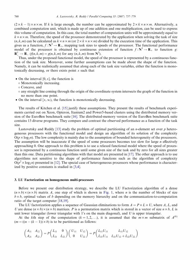
Before we present our distribution strategy, we describe the LU Factorization algorithm of a dense(n · b) · (n · b) matrix A, one step of which is shown in Fig. 1, where n is the number of blocks of sizeb · b, optimal values of b depending on the memory hierarchy and on the communication-to-computationratio of the target computer [18,19].

The LU factorization applies a sequence of Gaussian eliminations to form A = P · L · U, where A, L, andU are dense (n · b) · (n · b) matrices. P is a permutation matrix which is stored in a vector of size n · b, L isunit lower triangular (lower triangular with 1’s on the main diagonal), and U is upper triangular.

At the kth step of the computation (k = 1,2, . . .), it is assumed that the m · m submatrix of A(k)

(m = ((n � (k � 1)) · b) is to be partitioned as follows:

A11 A12

A21 A22

� �¼ P

L11 0

L21 L22

� �U 11 U 12

0 U 22

� �¼ P

L11U 11 L11U 12

L21U 11 L21U 12 þ L22U 22

� �

U0

L0

A22

A12

A21

A11

A

(n-(k-1))×b

bU0

L0~

22A

U12

L21

U11

L11

A

(n-(k-1))×b

b

Fig. 1. One step of the LU factorization algorithm of a dense matrix A of size (n · b) · (n · b).


where the block A11 is b · b, A12 is b · (m � b), A21 is (m � b) · b, and A22 is (m � b) · (m � b). L11 is unitlower triangular matrix, and U11 is an upper triangular matrix.

At first, a sequence of Gaussian eliminations is performed on the first m · b panel of A(k) (i.e., A11 and A21).Once this is completed, the matrices L11, L21, and U11 are known and we can rearrange the block equations

Fig.

U 12 ðL11Þ�1A12;eA22 A22L21U 12 ¼ L22U 22:

The LU factorization can be done by recursively applying the steps outlined above to the (m � b) · (m � b)matrix eA22. Fig. 1 shows how the column panel, L11 and L21, and the row panel, U11 and U12, are computedand how the trailing submatrix A22 is updated. In the figure, the regions L0, U0, L11, U11, L21, and U12 rep-resent data for which the corresponding computations are completed. Later row interchanges will be appliedto L0 and L21.

Now we present a parallel algorithm that computes the above steps on a one-dimensional arrangement of p

homogeneous processors. The algorithm can be summarized as follows:

1. A CYCLIC(b) distribution of columns is used to distribute the matrix A over a one-dimensional arrange-ment of p homogeneous processors as shown in Fig. 2. The cyclic distribution assigns columns of blockswith numbers 1,2, . . . ,n to processors 1,2, . . . ,p, 1,2, . . . ,p, 1,2, . . . , respectively, for a p-processor lineararray (n� p), until all n columns of blocks are assigned.

2. The algorithm consists of n steps. At each step (k = 1,2, . . .),

P1 P2 P3 P1 P2 P3

2. Column-oriented CYCLIC distribution of six column blocks on a one-dimensional array of three homogeneous processors.


• The processor owning the pivot column block of the size ((n � (k � 1)) · b) · b (i.e., A11 and A21) factors it;• All processors apply row interchanges to the left and the right of the current column block k:• The processor owning L11 broadcasts it to the rest of the processors, which convert the row panel A12 to

U12.• The processor owning the column panel L21 broadcasts it to the rest of the processors.• All the processors update their local portions of the matrix, A22, in parallel.The implementation of the algo-

rithm, which is used in the paper, is based on the ScaLAPACK [19] routine, PDGETRF, and consists of thefollowing steps:

1. PDGETF2: Apply the LU factorization to the pivot column panel of size ((n � (k � 1)) · b) · b (i.e.,A11

and A21). It should be noted here that only the routine PDSWAP employs all the processes involved inthe parallel execution. The rest of the routines are performed locally at the process owning the pivot columnpanel.• [Repeat b times (i = 1, . . . ,b)]� PDAMAX: find the (absolute) maximum element of the ith column and its location.� PDSWAP: interchange the ith row with the row that holds the maximum.� PDSCAL: scale the ith column of the matrix.� PDGER: update the trailing submatrix.

• The process owning the pivot column panel broadcasts the same pivot information to all the otherprocesses.

2. PDLASWP: All processes apply row interchanges to the left and the right of the current panel.3. PDTRSM: L11 is broadcast to the other processes, which convert the row panel A12 to U12.4. PDGEMM: The column panel L21 is broadcast to all the other processes. Then, all processes update their

local portions of the matrix, A22.

Because the largest fraction of the work takes place in the update of A22, therefore, to obtain maximumparallelism all processors should participate in its update. Since A22 reduces in size as the computation pro-gresses, a cyclic distribution is used to ensure that at any stage A22 is evenly distributed over all processors,thus obtaining their balanced load.

4. LU factorization on heterogeneous platforms with a constant performance model of processors

Heterogeneous parallel algorithms of LU factorization on heterogeneous platforms are obtained by mod-ification of the homogeneous algorithm presented in Section 3. The modification is in the distribution of col-umn panels of matrix A over the linear array of processors. As the processors are heterogeneous havingdifferent speeds, the optimal distribution that aims at balancing the updates at all steps of the parallel LU fac-torization will not be fully cyclic. So, the problem of LU factorization of a matrix on a heterogeneous platformis reduced to the problem of distribution of column panels of the matrix over heterogeneous processors of theplatform.

Traditionally, the distribution problem is formulated as follows: Given a dense (n · b) · (n · b) matrix A,how can we assign n columns of size n · b of the matrix A to p (n� p) heterogeneous processors P1,P2, . . . Pp

of relative speeds S = {s1, s2, . . . , sp},Pp

i¼1si ¼ 1, so that the workload at each step of the parallel LU factor-ization is best balanced? The relative speed si of processor Pi is obtained by normalization of its (absolute)speed ai, understood as the number of column panels updated by the processor per one time unit,si ¼ ai=

Ppi¼1ai. To explain what ‘‘the number of column panels updated by the processor Pi’’ means, let us

first consider the first step (k = 1) of the LU factorization. Remember that at step k (k = 1,2, . . .) of theLU factorization, column panels of size (n � (k � 1)) · b are updated. Assuming the partitioningPp

i¼1nð1Þi ¼ n for the first step, where nð1Þi denotes the number of column panels allocated to processor Pi,the number of column panels of size n · b updated by the processor Pi will be nð1Þi . Next, assuming the parti-tioning

Ppi¼1nð2Þi ¼ n� 1 for the second step (k = 2) of the LU factorization, where nð2Þi denotes the number of

column panels allocated to processor Pi, the number of column panels of size (n � 1) · b updated by the pro-cessor Pi is nð2Þi , and so on. While ai will increase with each next step of the LU factorization (because the


height of updated column panels will decrease as the LU factorization progresses, resulting in a larger numberof column panels updated by the processor per time unit), the relative speeds si are assumed to be constant.The optimal solution sought is the one that minimizes maxin

ðkÞi =si for each step of the LU factorization

ðPp

i¼1nðkÞi ¼ nðkÞÞ, where n(k) is the total number of column panels updated at the step k and nðkÞi denotes the

number of column panels allocated to processor Pi.

The motivation behind that formulation is the following. Strictly speaking, the optimal solution should

minimize the total execution time of the LU factorization, which is given byPn

k¼1maxpi¼1nðkÞi =aðkÞi , where aðkÞi

is the speed of processor Pi at step k of the LU factorization and nðkÞi is the number of column panels updated

by processor Pi at this step. However, if a solution minimizes maxpi¼1nðkÞi =aðkÞi for each k, it will also minimizePn

k¼1maxpi¼1nðkÞi =aðkÞi . Because maxp

i¼1nðkÞi =aðkÞi ¼ maxpi¼1nðkÞi =ðsi �

Ppi¼1aðkÞi Þ ¼ ð1=

Ppi¼1aðkÞi Þ �maxp

i¼1nðkÞi =si, then

for any given k the problem of minimization ofPn

k¼1maxpi¼1nðkÞi =aðkÞi will be equivalent to the problem of min-

imization of maxpi¼1nðkÞi =si. Therefore, if we are lucky and there exists an allocation that minimizes maxp

i¼1nðkÞi =si

for each step k of the LU factorization, then the allocation will be globally optimal, minimizingPnk¼1maxp

i¼1nðkÞi =aðkÞi . Fortunately, such an allocation does exist [3,4].

Now we briefly outline two existing approaches to solution of the above distribution problem, which are theGroup Block (GB) distribution algorithm [5] and the Dynamic Programming (DP) distribution algorithm[3,4].

The GB algorithm. This algorithm partitions the matrix into groups (or generalized blocks in terms of [2]),all of which have the same number of column panels. The number of column panels per group (the size of thegroup) and the distribution of the column panels within the group over the processors are fixed and deter-mined based on relative speeds of the processors. The relative speeds are obtained by running the DGEMMroutine that locally updates some particular dense rectangular matrix. The inputs to the algorithm are p, thenumber of heterogeneous processors in the one-dimensional arrangement, b, the block size, n, the size of thematrix in number of blocks of size b · b or the number of column panels, and S ¼ fs1; s2; . . . ; spg

Ppi¼1si ¼ 1

� �,

the relative speeds of the processors. The outputs are g, the size of the group, and d, an integer array of size p,the ith element of which contains the number of column panels in the group assigned to processor i. The algo-rithm can be summarized as follows:

(1) The size of the group g is calculated as b1/min(si)c (1 6 i 6 p). If g/p < 2, then g = b2/min(si)c. This con-dition is imposed to ensure there is sufficient number of blocks in the group.

(2) The group is partitioned so that the number of column panels di assigned to processor i in the group willminimize maxi

disi

(see [5] for a simple algorithm performing this partitioning).(3) In the group, processors are reordered to start from the slowest processors to the fastest processors for

load balance purposes.

The complexity of this algorithm is O(p · log2 p). At the same time, the algorithm does not guarantee that thereturned solution will be optimal.

The DP algorithm. Dynamic programming is used to distribute column panels of the matrix over the pro-cessors. The relative speeds of the processors are obtained by running the DGEMM routine that locallyupdates some particular dense rectangular matrix. The inputs to the algorithm are p, the number of hetero-geneous processors in the one-dimensional arrangement, b, the block size, n, the size of the matrix in numberof blocks of size b · b or the number of column panels, and S ¼ fs1; s2; . . . ; spg

Ppi¼1si ¼ 1

� �, the relative speeds

of the processors. The outputs are c, an integer array of size p, the ith element of which contains the number ofcolumn panels assigned to processor i, and d, an integer array of size n, the ith element of which contains theprocessor to which the column panel i is assigned. The algorithm can be summarized as follows:

(c1, . . . ,cp) = (0, . . . , 0);(d1, . . . ,dn) = (0, . . . , 0);


for(k = 1; k 6 n; k = k + 1) {Costmin =1;for(i = 1; i < = p; i = i + 1) {

Cost=(ci + 1)/si;if (Cost < Costmin) {Costmin = Cost; j = i;}

}dn�k+1 = j;cj = cj + 1;

}

The complexity of the DP algorithm is O(p · n). The algorithm returns the optimal allocation of the columnpanels to the heterogeneous processors [3,4]. The fact that the DP algorithm always returns the optimal solu-tion is not trivial. Indeed, at each iteration of the algorithm the column panel k is allocated to one of the pro-cessors, namely, to a processor, minimizing the cost of the allocation. At the same time, there may be severalprocessors with the same, minimal, cost of allocation. The algorithm randomly selects one of them. It is notobvious that allocation of the column panel to any of these processors will result in a globally optimal allo-cation. But, fortunately, for this particular distribution problem this is proved to be true.

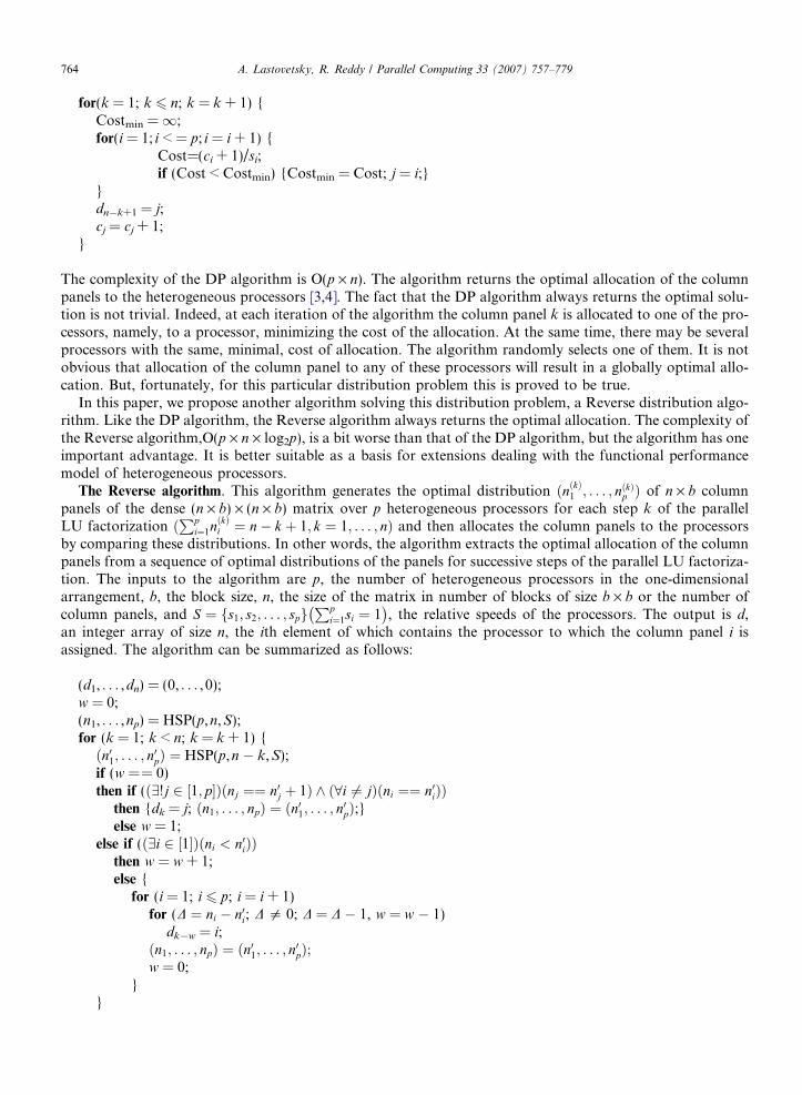
In this paper, we propose another algorithm solving this distribution problem, a Reverse distribution algo-rithm. Like the DP algorithm, the Reverse algorithm always returns the optimal allocation. The complexity ofthe Reverse algorithm,O(p · n · log2p), is a bit worse than that of the DP algorithm, but the algorithm has oneimportant advantage. It is better suitable as a basis for extensions dealing with the functional performancemodel of heterogeneous processors.

The Reverse algorithm. This algorithm generates the optimal distribution ðnðkÞ1 ; . . . ; nðkÞp Þ of n · b columnpanels of the dense (n · b) · (n · b) matrix over p heterogeneous processors for each step k of the parallelLU factorization ð

Ppi¼1nðkÞi ¼ n� k þ 1; k ¼ 1; . . . ; nÞ and then allocates the column panels to the processors

by comparing these distributions. In other words, the algorithm extracts the optimal allocation of the columnpanels from a sequence of optimal distributions of the panels for successive steps of the parallel LU factoriza-tion. The inputs to the algorithm are p, the number of heterogeneous processors in the one-dimensionalarrangement, b, the block size, n, the size of the matrix in number of blocks of size b · b or the number ofcolumn panels, and S ¼ fs1; s2; . . . ; spg

Ppi¼1si ¼ 1

� �, the relative speeds of the processors. The output is d,

an integer array of size n, the ith element of which contains the processor to which the column panel i isassigned. The algorithm can be summarized as follows:

(d1, . . . ,dn) = (0, . . . , 0);w = 0;(n1, . . . ,np) = HSP(p,n,S);for (k = 1; k < n; k = k + 1) {
ðn01; . . . ; n0pÞ ¼ HSP(p,n � k,S);if (w == 0)then if (ð9!j 2 ½1; p�Þðnj ¼¼ n0j þ 1Þ ^ ð8i 6¼ jÞðni ¼¼ n0iÞÞ
then {dk = j; ðn1; . . . ; npÞ ¼ ðn01; . . . ; n0pÞ;}else w = 1;

else if (ð9i 2 ½1�Þðni < n0iÞÞthen w = w + 1;else {

for (i = 1; i 6 p; i = i + 1)for (D ¼ ni � n0i; D 5 0; D = D � 1, w = w � 1)

dk�w = i;ðn1; . . . ; npÞ ¼ ðn01; . . . ; n0pÞ;w = 0;

}}


If (($i 2 [1,p])(ni = = 1))then dn = i;

Here, HSP(p,n,S) returns the optimal distribution of n column panels over p heterogeneous processors of therelative speeds S = {s1, s2, . . . , sp} by applying the algorithm for optimal distribution of independent chunks ofcomputations from [3,4] (HSP stands for Heterogeneous Set Partitioning). Thus, first we find the optimal dis-tributions of column panels for the first and second steps of the parallel LU factorization. If the distributionsdiffer only for one processor, then we assign the first column panel to this processor. The reason is that thisassignment guarantees a transfer from the best workload balance at the first step of the LU factorization to thebest workload balance at its second step. If the distributions differ for more than one processor, we postponeallocation of the first column panel and find the optimal distribution for the third step of the LU factorizationand compare it with the distribution for the first step. If the number of panel columns distributed to each pro-cessor for the third step does not exceed that for the first step, we allocate the first and second column panelsso that the distribution for each next step is obtained from the distribution for the immediate previous step byaddition of one more column panel to one of the processors. If not, we delay allocation of the first two columnpanels and find the optimal distribution for the fourth step and so on.

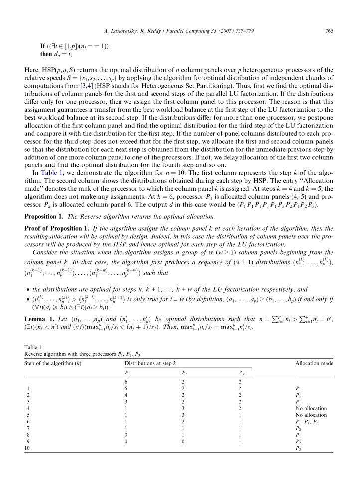
In Table 1, we demonstrate the algorithm for n = 10. The first column represents the step k of the algo-rithm. The second column shows the distributions obtained during each step by HSP. The entry ‘‘Allocationmade’’ denotes the rank of the processor to which the column panel k is assigned. At steps k = 4 and k = 5, thealgorithm does not make any assignments. At k = 6, processor P1 is allocated column panels (4, 5) and pro-cessor P2 is allocated column panel 6. The output d in this case would be (P1 P1 P1 P1 P1 P3 P2 P1P2 P3).

Proposition 1. The Reverse algorithm returns the optimal allocation.

Proof of Proposition 1. If the algorithm assigns the column panel k at each iteration of the algorithm, then the

resulting allocation will be optimal by design. Indeed, in this case the distribution of column panels over the pro-

cessors will be produced by the HSP and hence optimal for each step of the LU factorization.

Consider the situation when the algorithm assigns a group of w (w > 1) column panels beginning from the

column panel k. In that case, the algorithm first produces a sequence of (w + 1) distributions ðnðkÞ1 ; . . . ; nðkÞp Þ,ðnðkþ1Þ

1 ; . . . ; nðkþ1Þp Þ; . . . ; ðnðkþwÞ

1 ; . . . ; nðkþwÞp Þ such that

• the distributions are optimal for steps k, k + 1, . . . , k + w of the LU factorization respectively, and

• ðnðkÞ1 ; . . . ; nðkÞp Þ > ðnðkþiÞ1 ; . . . ; nðkþiÞ

p Þ is only true for i = w (by definition, (a1, . . . ,ap) > (b1, . . . , bp) if and only if

("i)(ai P bi) ^ ($i)(ai > bi)).

Lemma 1. Let (n1, . . . ,np) and ðn01; . . . ; n0pÞ be optimal distributions such that n ¼Pp

i¼1ni >Pp

i¼1n0i ¼ n0,ð9iÞðni < n0iÞ and ð8jÞðmaxp

i¼1ni=si 6 ðnj þ 1Þ=sjÞ. Then, maxpi¼1ni=si ¼ maxp

i¼1n0i=si.

Table 1Reverse algorithm with three processors P1, P2, P3

Step of the algorithm (k) Distributions at step k Allocation made

P1 P2 P3

6 2 21 5 2 2 P1

2 4 2 2 P1

3 3 2 2 P1

4 1 3 2 No allocation5 1 3 1 No allocation6 1 2 1 P1, P1, P3

7 1 1 1 P2

8 0 1 1 P1

9 0 0 1 P2

10 P3


Proof of Lemma 1. As n > n0

and (n1, . . . ,np) and ðn01; . . . ; n0pÞ are both optimal distributions, then

maxpi¼1ni=si P maxp

i¼1n0i=si. On the other hand, there exists j 2 [1,p] such that nj < n0j, which implies

nj þ 1 6 n0j. Therefore, maxpi¼1n0i=si P n0j=sj P ðnj þ 1Þ=sj. As we assumed that ð8jÞðmaxp

i¼1ni=si 6 ðnj þ 1Þ=sjÞ,then maxp

i¼1ni=si 6 ðnj þ 1Þ=sj 6 n0j=sj 6 maxpi¼1n0i=si. Thus, from maxp

i¼1ni=si P maxpi¼1n0i=si and

maxpi¼1ni=si 6 maxp

i¼1n0i=si we conclude that maxpi¼1ni=si ¼ maxp

i¼1n0i=si. h

We can apply Lemma 1 to the pair ðnðkÞ1 ; . . . ; nðkÞp Þ and ðnðkþlÞ1 ; . . . ; nðkþlÞ

p Þ for any l 2 [1,w � 1]. Indeed,Ppi¼1nðkÞi >

Ppi¼1nðkþlÞ

i and ð9iÞðnðkÞi < nðkþlÞi Þ. Finally, the HSP guarantees that ð8jÞðmaxp

i¼1nðkÞi =si 6

ðnðkÞj þ 1ÞsjÞ (see [3,4]). Therefore, maxpi¼1nðkÞi =si ¼ maxp

i¼1nðkþ1Þi =si ¼ . . . ¼ maxp

i¼1nðkþw�1Þi =si. In particular, this

means that for any (m1, . . . ,mp) such that minkþw�1j¼k nðjÞi 6 mi 6 maxkþw�1

j¼k nðjÞi (i = 1, . . . , p), we will have

maxpi¼1mi=si ¼ maxp

i¼1nðkÞi =si. The allocations made in the end by the Reverse algorithm for the column panelsk, k + 1, . . . ,k + w � 1 result in a new sequence of distributions for steps k, k + 1, . . . ,k + w � 1 of the LUfactorization such that each next distribution differs from the previous one for exactly one processor. Each

distribution (m1, . . . ,mp) in this new sequence satisfies the inequality minkþw�1j¼k nðjÞi 6 mi 6 maxkþw�1

j¼k nðjÞi

(i = 1, . . . ,p). Therefore, all they will have the same cost maxpi¼1nðkÞi =si, which is the cost of the optimal

distribution for these steps of the LU factorization found by the HSP. Hence, each distribution in thissequence will be optimal for the corresponding step of the LU factorization. h

Proposition 2. The complexity of the Reverse algorithm is O(p · n · log2 p).

Proof. At each iteration of this algorithm, we apply the HSP, which is of complexity O(p · log2p) [3,4]. Testingthe condition ð9!j 2 ½1�Þðnj ¼¼ n0j þ 1Þ ^ ð8i 6¼ jÞðni ¼¼ n0iÞ is of complexity O(p). Testing the conditionð9i 2 ½1; p�Þðni < n0iÞ is also of complexity O(p). Finally, the total number of iterations of the inner loop ofthe nest of loops.

for (i = 1; i 6 p; i = i + 1)
for (D ¼ ni � n0i; D 5 0; D = D � 1, w = w � 1)
dk�w = i;

during the execution of the algorithm cannot exceed the total number of allocations of column panels, n. Thus,the overall complexity of the algorithm is upper bounded by n · O(p · log2p) + n · O(p) + n · O(p) +p · n · O(1) = O(p · n · log2 p). h

5. LU Factorization on heterogeneous platforms with the functional performance model of processors

The problem of distribution of a dense square matrix over heterogeneous processors for the parallel LUfactorization, as it is formulated in Section 4, uses the constant performance model of processors that doesnot address the memory heterogeneity and paging effects. The functional performance model [12,13] addressesthe issues. Under this model, the speed of each computer is represented by a continuous and relatively smoothfunction of the task size. This model is application centric in the sense that, generally speaking, different appli-cations will characterize the speed of the processor by different functions.

In this section, we formulate the problem of optimal distribution of column panels of a dense square matrixfor its efficient LU factorization over a one-dimensional arrangement of heterogeneous processors with theirfunctional performance model. Then we describe how the distribution algorithms presented in Section 4 canbe modified for solution of the functional distribution problem.

5.1. Problem formulation

The problem of distributing a large dense square matrix A for its parallel LU factorization over a one-dimensional arrangement of heterogeneous processors using their functional performance model can be for-mulated as follows:


• Given� A dense n · n matrix A, and� p (n > p) heterogeneous processors P1, P2, . . . ,Pp of respective speeds S = {s1(x,y), s2(x,y), . . . , sp(x,y)},

where si(x,y) is the speed of the update of an x · y matrix by the processor i, measured in arithmeticaloperations per time unit and represented by a continuous function R+ · R+! R+,

• Assign the columns of the matrix A to the p processors so that the assignment minimizesPn

k¼1maxpi¼1

V ðn�k;nðkÞi Þsiðn�k;nðkÞi Þ

,

where V(x,y) is the number of operations needed to update a x · y matrix and nðkÞi is the number of columnsupdated by the processor Pi at step k of the parallel LU factorization.

This formulation is motivated by the n-step parallel LU factorization algorithm. One element of matrix A

may represent a single number with computations measured in arithmetical operations. Alternatively, it canrepresent a square matrix block of a given fixed size b · b. In this case, computations are measured in b · b

matrix operations. The formulation assumes that the computation cost is determined by the update of thetrailing matrix and fully ignores the communication cost. Therefore, the execution time of the kth step of

the LU factorization is estimated by maxpi¼1


, and the optimal solution has to minimize the overall exe-

cution time,Pn

k¼1maxpi¼1


.

Unlike the constant optimization problem considered in Section 4, the functional optimization problemcannot be reduced to the problem of minimization of the execution time of all n individual steps of the LUfactorization. Correspondingly, this functional matrix-partitioning problem cannot be reduced to a problemof partitioning a well-ordered set. The reason is that in the functional case there may be no globally optimalallocation of columns minimizing the execution time of all individual steps of the LU factorization. This com-plication is introduced by the use of the functional performance model of heterogeneous processors instead ofthe constant one. A simple example supporting this statement is designed as follows.

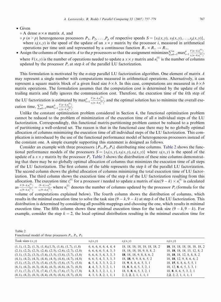
Consider an example with three processors {P1,P2,P3} distributing nine columns. Table 2 shows the func-tional performance models of the processors S = {s1(x,y), s2(x,y), s3(x,y)} where si(x,y) is the speed of theupdate of a x · y matrix by the processor Pi. Table 3 shows the distribution of these nine columns demonstrat-ing that there may be no globally optimal allocation of columns that minimizes the execution time of all stepsof the LU factorization. The first column of the table represents the step k of the parallel LU factorization.The second column shows the global allocation of columns minimizing the total execution time of LU factor-ization. The third column shows the execution time of the step k of the LU factorization resulting from thisallocation. The execution time tðkÞi for a processor i needed to update a matrix of sizeð9� kÞ � nðkÞi is calculated

asV ð9�k;nðkÞi Þsið9�k;nðkÞi Þ

¼ ð9�kÞ�nðkÞi

sið9�k;nðkÞi Þwhere nðkÞi denotes the number of columns updated by the processor Pi (formula for the

volume of computations explained below). The fourth column shows the distribution of columns, whichresults in the minimal execution time to solve the task size (9 � k, 9 � k) at step k of the LU factorization. Thisdistribution is determined by considering all possible mappings and choosing the one, which results in minimalexecution time. The fifth column shows these minimal execution times for the task size (9 � k, 9 � k). Forexample, consider the step k = 2, the local optimal distribution resulting in the minimal execution time for

Table 2Functional model of three processors P1, P2, P3

Task sizes (x,y) s1(x,y) s2(x,y) s3(x,y)

(1,1), (1,2), (1,3), (1,4),(1,5), (1,6), (1,7), (1,8) 6, 6, 6, 6, 6, 4, 4, 4 18, 18, 18, 18, 18, 18, 18, 2 18, 18, 18, 18, 18, 18, 18, 2(2,1), (2,2), (2,3), (2,4), (2,5), (2,6), (2,7), (2,8) 6, 6, 6, 6, 5, 4, 3, 3 18, 18, 18, 18, 9, 8, 8, 2 18, 18, 18, 18, 15, 12, 8, 2(3,1), (3,2), (3,3), (3,4), (3,5), (3,6), (3,7), (3,8) 6, 6, 6, 5, 4, 3, 3, 3 18, 18, 18, 9, 8, 8, 6, 2 18, 18, 18, 12, 8, 8, 8, 2(4,1), (4,2), (4,3), (4,4), (4,5), (4,6), (4,7), (4,8) 6, 6, 5, 4, 3, 3, 3, 3 18, 18, 9, 9, 8, 6, 5, 2 18, 18, 12, 9, 8, 6, 6, 2(5,1), (5,2), (5,3), (5,4), (5,5), (5,6), (5,7), (5,8) 6, 5, 4, 3, 3, 3, 2, 2 18, 9, 8, 8, 6, 5, 3, 1 18, 15, 8, 8, 6, 5, 5, 1(6,1), (6,2), (6,3), (6,4), (6,5), (6,6), (6,7), (6,8) 4, 4, 3, 3, 3, 2, 1, 1 18, 8, 8, 6, 5, 3, 2, 1 18, 12, 8, 6, 5, 3, 3, 1(7,1), (7,2), (7,3), (7,4), (7,5), (7,6), (7,7), (7,8) 4, 3, 3, 3, 2, 1, 1, 1 18, 8, 8, 6, 5, 3, 2, 1 18, 8, 8, 6, 5, 3, 2, 1(8,1), (8,2), (8,3), (8,4), (8,5), (8,6), (8,7), (8,8) 4, 3, 3, 3, 2, 1, 1, 1 2, 2, 2, 2, 1, 1, 1, 1 2,2, 2, 2, 1, 1, 1, 1

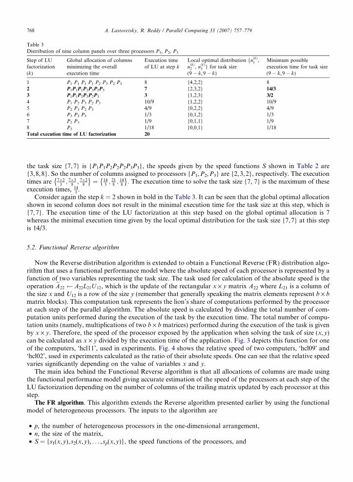
Table 3Distribution of nine column panels over three processors P1, P2, P3

Step of LUfactorization(k)

Global allocation of columnsminimizing the overallexecution time

Execution timeof LU at step k

Local optimal distribution fnðkÞ1 ,nðkÞ2 , nðkÞ3 } for task size(9 � k, 9 � k)

Minimum possibleexecution time for task size(9 � k, 9 � k)

1 P1 P1 P1 P1 P2 P3 P2 P3 8 {4,2,2} 82 P1P1P1P2P3P2P3 7 {2,3,2} 14/3

3 P1P1P2P3P2P3 3 {1,2,3} 3/2

4 P1 P2 P3 P2 P3 10/9 {1,2,2} 10/95 P2 P3 P2 P3 4/9 {0,2,2} 4/96 P3 P2 P3 1/3 {0,1,2} 1/37 P2 P3 1/9 {0,1,1} 1/98 P3 1/18 {0,0,1} 1/18Total execution time of LU factorization 20


the task size {7,7} is {P1P1P2P2P2P3P3}, the speeds given by the speed functions S shown in Table 2 are{3,8,8}. So the number of columns assigned to processors {P1,P2,P3} are {2,3,2}, respectively. The executiontimes are 7�2

3; 7�3

8; 7�2

8

� �¼ 14

3; 21

8; 14

8

� �: The execution time to solve the task size {7, 7} is the maximum of these

execution times, 143.

Consider again the step k = 2 shown in bold in the Table 3. It can be seen that the global optimal allocationshown in second column does not result in the minimal execution time for the task size at this step, which is{7,7}. The execution time of the LU factorization at this step based on the global optimal allocation is 7whereas the minimal execution time given by the local optimal distribution for the task size {7,7} at this stepis 14/3.

5.2. Functional Reverse algorithm

Now the Reverse distribution algorithm is extended to obtain a Functional Reverse (FR) distribution algo-rithm that uses a functional performance model where the absolute speed of each processor is represented by afunction of two variables representing the task size. The task used for calculation of the absolute speed is theoperation eA22 A22L21U 12, which is the update of the rectangular x · y matrix A22 where L21 is a column ofthe size x and U12 is a row of the size y (remember that generally speaking the matrix elements represent b · b

matrix blocks). This computation task represents the lion’s share of computations performed by the processorat each step of the parallel algorithm. The absolute speed is calculated by dividing the total number of com-putation units performed during the execution of the task by the execution time. The total number of compu-tation units (namely, multiplications of two b · b matrices) performed during the execution of the task is givenby x · y. Therefore, the speed of the processor exposed by the application when solving the task of size (x,y)can be calculated as x · y divided by the execution time of the application. Fig. 3 depicts this function for oneof the computers, ‘hcl11’, used in experiments. Fig. 4 shows the relative speed of two computers, ‘hcl09’ and‘hcl02’, used in experiments calculated as the ratio of their absolute speeds. One can see that the relative speedvaries significantly depending on the value of variables x and y.

The main idea behind the Functional Reverse algorithm is that all allocations of columns are made usingthe functional performance model giving accurate estimation of the speed of the processors at each step of theLU factorization depending on the number of columns of the trailing matrix updated by each processor at thisstep.

The FR algorithm. This algorithm extends the Reverse algorithm presented earlier by using the functionalmodel of heterogeneous processors. The inputs to the algorithm are

• p, the number of heterogeneous processors in the one-dimensional arrangement,• n, the size of the matrix,• S = {s1(x,y), s2(x,y), . . . , sp(x,y)}, the speed functions of the processors, and

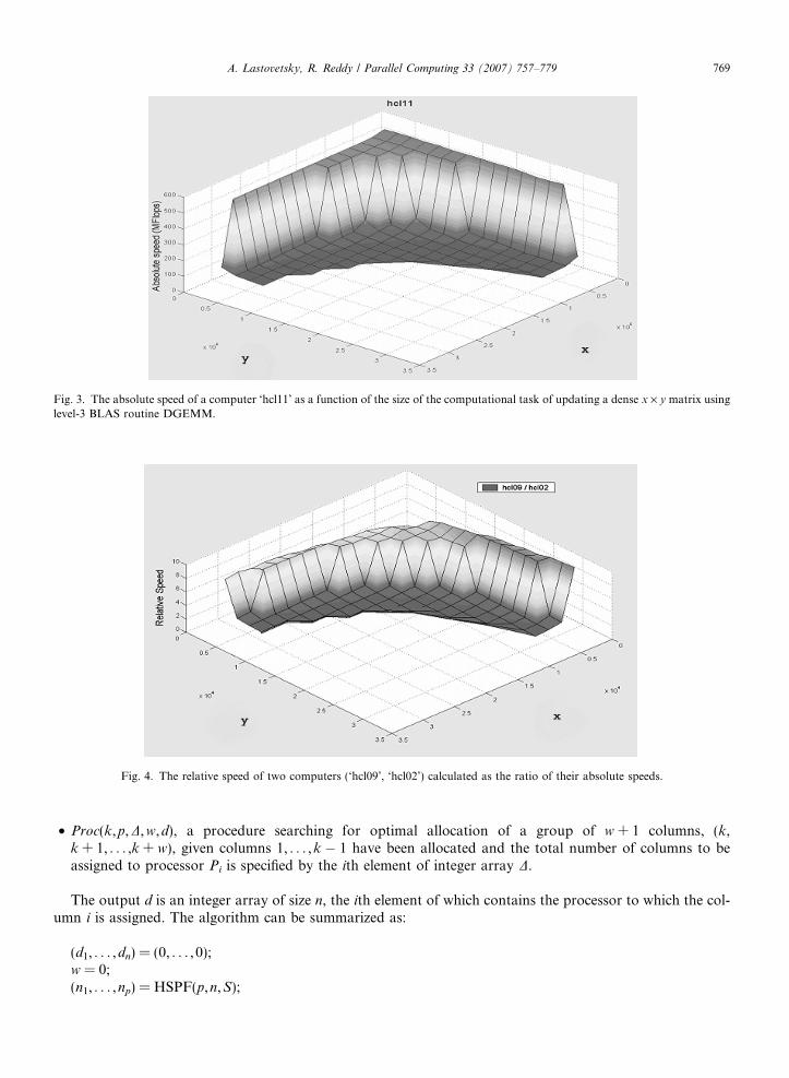
Fig. 3. The absolute speed of a computer ‘hcl11’ as a function of the size of the computational task of updating a dense x · y matrix usinglevel-3 BLAS routine DGEMM.

Fig. 4. The relative speed of two computers (‘hcl09’, ‘hcl02’) calculated as the ratio of their absolute speeds.


• Proc(k,p,D,w,d), a procedure searching for optimal allocation of a group of w + 1 columns, (k,k + 1, . . . ,k + w), given columns 1, . . . ,k � 1 have been allocated and the total number of columns to beassigned to processor Pi is specified by the ith element of integer array D.

The output d is an integer array of size n, the ith element of which contains the processor to which the col-umn i is assigned. The algorithm can be summarized as:

(d1, . . . ,dn) = (0, . . . , 0);w = 0;(n1, . . . ,np) = HSPF(p,n,S);


for (k = 1; k < n; k = k + 1) {ðn01; . . . ; n0pÞ ¼ HSPFðp; n� k; SÞ;if (w==0)then if (ð9!j 2 ½1; p�Þðnj ¼¼ n0j þ 1Þ ^ ð8i 6¼ jÞðni ¼¼ n0iÞÞ

then {dk = j; ðn1; . . . ; npÞ ¼ ðn01; . . . ; n0pÞ;}else w = 1;

else if (ð9i 2 ½1; p�Þðni < n0iÞÞthen w = w + 1;else {

for (i = 1; i 6 p; i = i + 1) fDi ¼ ni � n0i; gproc(k, p, D,w,d);ðn1; . . . ; npÞ ¼ ðn01; . . . ; n0pÞ;w = 0;

}}if (($i 2 [1,p])(ni = 1))then dn = i;

Here, HSPF(p,m,S) returns the optimal distribution of a set of m equal elements over p heterogeneous pro-cessors P1,P2, . . . ,Pp of respective speeds S = {s1(m,y), s2(m,y), . . . , sp(m,y)} using the set-partitioning algo-rithm [13]. (HSPF stands for Heterogeneous Set Partitioning using the Functional model of processors).The distributed elements represent column panels of the (m · b) · (m · b) trailing matrix at step (n � m) ofthe LU factorization. Function fi(y) = si(m,y) represents the speed of processor Pi depending on the numberof column panels of the trailing matrix, y, updated by the processor at the step (n � m) of the LU factoriza-tion. Fig. 5 gives geometrical interpretation of this step of the matrix-partitioning algorithm:

1. Surfaces zi = si(x,y) representing the absolute speeds of the processors are sectioned by the plane x = n � k

(as shown in Fig. 5(a) for three surfaces representing the absolute speeds of the processors ‘hcl02’, ‘hcl09’,‘hcl11’ used in the experiments). A set of p curves on this plane (as shown in Fig. 5(b)) will represent theabsolute speeds of the processors against variable y given parameter x is fixed.

2. The set-partitioning algorithm [13] is applied to this set of curves to obtain an optimal distribution of col-umns of the trailing matrix.

Proposition 3. If assignment of a column is performed at each step of the algorithm, the FR algorithm returns the

optimal allocation.

Proof. If a column is assigned at each iteration of the FR algorithm, then the resulting allocation will be opti-mal by design. Indeed, in this case the distribution of columns over the processors will be produced by theHSPF and hence be optimal for each step of the LU factorization. h

Proposition 4. If the speed of the processor is represented by a constant function of task size, the Functional

Reverse algorithm returns the optimal allocation.

Proof. If the speed of the processor is represented by a constant function of task size, the FR algorithm is func-tionally equivalent to the Reverse algorithm presented earlier. We have already proved that the Reverse algo-rithm returns the optimal allocation when constant performance model of heterogeneous processors is used. h

Proposition 5. If assignment of a column panel is performed at each iteration of the main loop of the FR algo-

rithm, its complexity will be bounded by O(p · n · log2 n).

Proof. At each iteration of this algorithm, we apply the HSPF. The first step of the HSPF, which involvesintersection of p surfaces by a plane to produce p curves is of complexity O(p). The second step of the HSPFis of complexity O(p · log2 n) [13]. Testing the condition ð9!j 2 ½1; p�Þðnj ¼¼ n0j þ 1Þ ^ ð8i 6¼ jÞðni ¼¼ n0iÞ is ofcomplexity O(p). Since there are n such steps, the overall complexity of the algorithm is upper bounded byn · O(p · log2 n) + n · O(p) + n · O(p) = O(p · n · log2 n). h

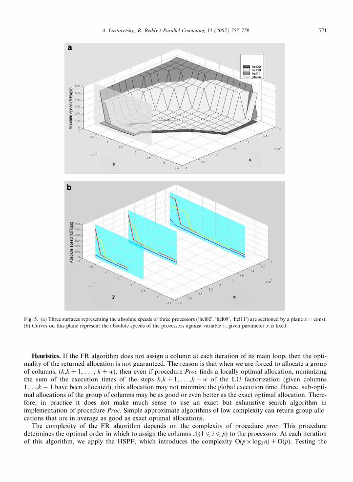
Fig. 5. (a) Three surfaces representing the absolute speeds of three processors (‘hcl02’, ‘hcl09’, ‘hcl11’) are sectioned by a plane x = const.(b) Curves on this plane represent the absolute speeds of the processors against variable y, given parameter x is fixed.


Heuristics. If the FR algorithm does not assign a column at each iteration of its main loop, then the opti-mality of the returned allocation is not guaranteed. The reason is that when we are forced to allocate a groupof columns, (k,k + 1, . . . , k + w), then even if procedure Proc finds a locally optimal allocation, minimizingthe sum of the execution times of the steps k,k + 1, . . . ,k + w of the LU factorization (given columns1,. . .,k � 1 have been allocated), this allocation may not minimize the global execution time. Hence, sub-opti-mal allocations of the group of columns may be as good or even better as the exact optimal allocation. There-fore, in practice it does not make much sense to use an exact but exhaustive search algorithm inimplementation of procedure Proc. Simple approximate algorithms of low complexity can return group allo-cations that are in average as good as exact optimal allocations.

The complexity of the FR algorithm depends on the complexity of procedure proc. This proceduredetermines the optimal order in which to assign the columns Di(1 6 i 6 p) to the processors. At each iterationof this algorithm, we apply the HSPF, which introduces the complexity O(p · log2 n) + O(p). Testing the


condition ð9!j 2 ½1; p�Þðnj ¼¼ n0j þ 1Þ ^ ð8i 6¼ jÞðni ¼¼ n0iÞ is of complexity O(p). Testing the conditionð9i 2 ½1; p�Þðni < n0iÞ is also of complexity O(p). Plus at one or more iterations of the algorithm, there is anapplication of the heuristic procedure proc. Since there are n steps of the algorithm, the overall complexityof the algorithm is upper bounded by n · O(p · log2 n) + n · O(p) + n · O(p) + n · O(p) + n · Ch = O(p ·n · log2 n) + n · Ch where Ch is the complexity introduced by the heuristic functional procedure at each step.

Therefore if we do not want to drastically affect the overall complexity of the algorithm, efficient polyno-mial heuristics should be employed. Some of these heuristics are:

• cycl: Allocate cyclically one by one the column until all the Di (1 6 i 6 p) have been assigned;• ftos: Allocate from the most loaded (maximum D) to the least loaded (minimum D). Sort Di(1 6 i 6 p) in

decreasing order. Assign Di (1 6 i 6 p) number of column to each processor Pi in that order;• stof: Allocate from the least loaded (minimum D) to the most loaded (maximum D). Sort Di in increasing

order. Assign Di (1 6 i 6 p) number of column to each processor Pi in that order;• dflt: Assign Di (1 6 i 6 p) number of column to each processor Pi in the default order of processors input to

this algorithm.

In Table 4, we demonstrate the heuristics for n = 10. The first column represents the step k of the algorithm.The second column shows the distributions obtained during step S2 by the set partitioning algorithm. Theentry ‘‘Allocation made’’ denotes the rank of the processor to which the column k is assigned. At stepsk = 4 and k = 5, the algorithm does not make any assignments. At k = 6, the different heuristics are appliedto assign (2,1) number of blocks to processors (P1,P3), respectively. Note here the heuristic dflt performs thesame assignment as heuristic ftos but it may not be the case always. For example using the heuristic cycl, thefinal output d would be (P1 P1 P1 P1 P3 P1 P2 P1 P2 P3).

Table 5 presents the complexities introduced by each of these heuristics. It can be seen that these heuristicsdo not affect the overall complexity of the algorithm, which is O(p · n · log2 n).

5.3. Functional GB algorithm

The GB algorithm presented earlier is extended to use the functional model of heterogeneous processors.The efficiency of the Functional Reverse algorithm over this algorithm is compared in the section on exper-imental results.

The Functional GB algorithm (FGB). This algorithm extends the Group Block algorithm presented earlierby using the functional model of heterogeneous processors. The main idea here is that at each step, the number

Table 4Functional Reverse algorithm using heuristics

Step of the algorithm (k) Distributions at step k Allocation made

P1 P2 P3

6 2 21 5 2 2 P1

2 4 2 2 P1

3 3 2 2 P1

4 1 3 2 No allocation5 1 3 1 No allocation

6 1 2 1 Heuristics

cycl ftos stof dflt

P1, P3, P1 P1, P1, P3 P3, P1, P1 P1, P1, P3

7 1 1 1 P2

8 0 1 1 P1

9 0 0 1 P2

10 P3

Table 5Heuristics and their complexities

Heuristic Complexity (Ch)

cycl O(p)ftos O(p · log2 p)stof O(p · log2 p)dflt O(p)


of column panels per group and the distribution of the column panels in the group over the processors arecalculated based on the absolute speeds of the processors given by the functional model, which are basedon the size of the problem solved at that step. That is the number of column panels per group and the distri-bution of column panels in a group amongst the processors are variable.

The inputs to the algorithm are p, the number of heterogeneous processors in the one-dimensional arrange-ment, b, the block size, n, the size of the matrix in number of blocks of size b · b or the number of columnpanels, and S = {s1(x,y), s2(x,y), . . . , sp(x,y)}, the speed functions of the processors. The outputs areG = {g1, . . . ,gm}, an integer array of size m, the ith element of which contains the size of the group and d,an integer array of size m · p logically representing an array of shape [m][p], the (i,j)th element of which con-tains the number of column panels in the group i assigned to processor j. The algorithm can be summarized asfollows:

(1) The size g1 of the first group of blocks is calculated as follows:(a) Apply HSPF(p,n,S) to return the optimal distribution (n1, . . . ,np) of n column panels wherePp

i¼1ni ¼ n. Calculate the load index li ¼ ni=Pp

k¼1nk (1 6 i 6 p).(b) The size of the group g1 is equal to b1/min(li)c (1 6 i 6 p). If g1/p < 2, then g1 = b2/min(li)c. This con-

dition is imposed to ensure there is sufficient number of blocks in the group.(c) This group is now partitioned such that the number of column panels dðiÞ1 assigned to processor i in

the group is proportional to the load indices li wherePp

i¼1dðiÞ1 ¼ g1 (1 6 i 6 p).(2) To calculate the size g2 of the second group, we repeat step 1 for the number of column panels equal to

n � g1 in matrix A. We recursively apply this procedure until we have fully vertically partitioned thematrix A.

(3) In each group, the processors are reordered to start from the slowest processors to the fastest processorsfor load balance purposes.

To calculate the complexity of the algorithm, consider the first step of the algorithm. The complexity ofHSPF is O(p · log2 n) [13]. The complexity of step 1.b is O(1). The complexity of step 1.c is O(p · log2p).So the total complexity for this step is O(p · log2 n) + O(p · log2 p) + O(1). In the worst case scenario, thereare n possible groups. So the complexity of the algorithm is upper bounded by n · (O(p · log2 n) +O(p · log2p) + O(1)) = O(p · n · log2 n).

5.4. Functional DP algorithm

The DP algorithm presented earlier is extended to use the functional model of heterogeneous processors.The efficiency of the Functional Reverse algorithm over this algorithm is compared in the section on exper-imental results.

The Functional DP algorithm (FDP). This algorithm extends the DP algorithm presented earlier by usingthe functional model of heterogeneous processors. The inputs to the algorithm are p, the number of hetero-geneous processors in the one-dimensional arrangement, b, the block size, n, the size of the matrix in numberof blocks of size b · b or the number of column panels, and S = {s1(x,y), s2(x,y), . . . , sp(x,y)}, the speed func-tions of the processors. The outputs are c, an integer array of size p, the ith element of which contains thenumber of column panels assigned to processor i, and d, an integer array of size n, the ith element of whichcontains the processor to which the column panel i is assigned. The algorithm can be summarized as follows:


(c1, . . . ,cp) = (0, . . . , 0);(d1, . . . ,dn) = (0, . . . , 0);for(k = 1; k 6 n; k = k + 1) {

Costmin =1;(n1, . . . ,np) = HSPF(p,k,S);for(i = 1; i < = p; i++) {

Cost = (ci + 1)/ni;if (Cost < Costmin) {Costmin = Cost; j = i;}

}dn�k+1 = j;cj = cj + 1;

}

To calculate the complexity of the algorithm, consider an iteration of the algorithm. The complexity ofHSPF is O(p · log2 n) [13]. The complexity of the for loop is O(p). Therefore, the total complexity will beO(p · log2 n) + O(p). Since there are n iterations, the complexity of the algorithm is upper bounded byn · (O(p · log2 n) + O(p)) = O(p · n · log2 n).

5.5. Concluding remarks

In the general case, the data distribution algorithms employing the functional model of heterogeneous pro-cessors do not provide optimal solutions to the optimization problem presented at the beginning of Section 5.1.At the same time, the FR and the FDP algorithms will always return optimal solutions in the following two cases:

(a) The speeds of the processors are constant functions of the task size. In this case, the FDP algorithm isidentical to the DP algorithm.

(b) The speeds of the processors allow the FR algorithm to assign a column at each step (see behind theFunctional Reverse distribution algorithm Proposition 3). In this case, both the FR and the FDP algo-rithms return the optimal solution.

The FGB algorithm may return non-optimal solutions even in these two cases.

6. Experimental results

A small heterogeneous local network of sixteen different Linux workstations shown in Table 6 is used in theexperiments. The network is based on 2 Gbit Ethernet with a switch enabling parallel communicationsbetween the computers. The experimental results are divided into two sections. The first section is devotedto building the functional representation of the speed of a processor. Then we present the experimental resultson the local network of heterogeneous computers shown in Table 6.

6.1. Implementation of the functional algorithms

In heterogeneous environments, most processors experience constant and unpredictable fluctuations in theworkload. Therefore, their performance is represented by speed bands rather than speed functions. This prop-erty of real-life environments can be used to minimize the cost of experimental building of the functional per-formance model of the processors. If we accept any appropriate function (continuous, etc.) fitting into thespeed band as a satisfactory approximation of the speed function, then the problem of efficient building thefunctional performance model can be formulated as follows:

• Find the optimal set of task sizes such that:�Running the application for this set is enough to build an approximation of the speed function fitting into

the speed band.� The total execution time to run the application for the set of task sizes is minimal.

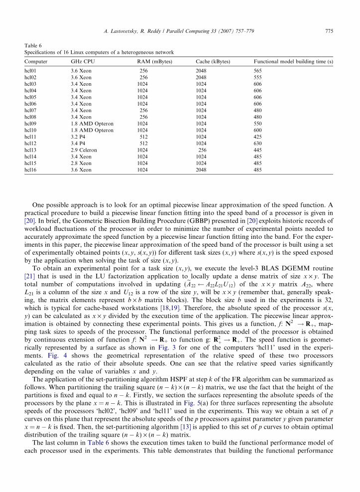
Table 6Specifications of 16 Linux computers of a heterogeneous network

Computer GHz CPU RAM (mBytes) Cache (kBytes) Functional model building time (s)

hcl01 3.6 Xeon 256 2048 565hcl02 3.6 Xeon 256 2048 555hcl03 3.4 Xeon 1024 1024 606hcl04 3.4 Xeon 1024 1024 606hcl05 3.4 Xeon 1024 1024 606hcl06 3.4 Xeon 1024 1024 606hcl07 3.4 Xeon 256 1024 480hcl08 3.4 Xeon 256 1024 480hcl09 1.8 AMD Opteron 1024 1024 550hcl10 1.8 AMD Opteron 1024 1024 600hcl11 3.2 P4 512 1024 425hcl12 3.4 P4 512 1024 630hcl13 2.9 Celeron 1024 256 445hcl14 3.4 Xeon 1024 1024 485hcl15 2.8 Xeon 1024 1024 485hcl16 3.6 Xeon 1024 2048 485


One possible approach is to look for an optimal piecewise linear approximation of the speed function. Apractical procedure to build a piecewise linear function fitting into the speed band of a processor is given in[20]. In brief, the Geometric Bisection Building Procedure (GBBP) presented in [20] exploits historic records ofworkload fluctuations of the processor in order to minimize the number of experimental points needed toaccurately approximate the speed function by a piecewise linear function fitting into the band. For the exper-iments in this paper, the piecewise linear approximation of the speed band of the processor is built using a setof experimentally obtained points (x,y, s(x,y)) for different task sizes (x,y) where s(x,y) is the speed exposedby the application when solving the task of size (x,y).

To obtain an experimental point for a task size (x,y), we execute the level-3 BLAS DGEMM routine
[21] that is used in the LU factorization application to locally update a dense matrix of size x · y. Thetotal number of computations involved in updating (eA22 A22L21U 12Þ of the x · y matrix A22, whereL21 is a column of the size x and U12 is a row of the size y, will be x · y (remember that, generally speak-ing, the matrix elements represent b · b matrix blocks). The block size b used in the experiments is 32,which is typical for cache-based workstations [18,19]. Therefore, the absolute speed of the processor s(x,y) can be calculated as x · y divided by the execution time of the application. The piecewise linear approx-imation is obtained by connecting these experimental points. This gives us a function, f: N2 ! R+, map-ping task sizes to speeds of the processor. The functional performance model of the processor is obtainedby continuous extension of function f: N2 ! R+ to function g: R2
þ ! Rþ. The speed function is geomet-rically represented by a surface as shown in Fig. 3 for one of the computers ‘hcl11’ used in the experi-ments. Fig. 4 shows the geometrical representation of the relative speed of these two processorscalculated as the ratio of their absolute speeds. One can see that the relative speed varies significantlydepending on the value of variables x and y.

The application of the set-partitioning algorithm HSPF at step k of the FR algorithm can be summarized asfollows. When partitioning the trailing square (n � k) · (n � k) matrix, we use the fact that the height of thepartitions is fixed and equal to n � k. Firstly, we section the surfaces representing the absolute speeds of theprocessors by the plane x = n � k. This is illustrated in Fig. 5(a) for three surfaces representing the absolutespeeds of the processors ‘hcl02’, ‘hcl09’ and ‘hcl11’ used in the experiments. This way we obtain a set of p

curves on this plane that represent the absolute speeds of the p processors against parameter y given parameterx = n � k is fixed. Then, the set-partitioning algorithm [13] is applied to this set of p curves to obtain optimaldistribution of the trailing square (n � k) · (n � k) matrix.

The last column in Table 6 shows the execution times taken to build the functional performance model ofeach processor used in the experiments. This table demonstrates that building the functional performance


model is inexpensive compared to the execution times of the parallel LU factorization, which range from min-utes to hours. It should be noted that the building of the functional performance model could be performed inparallel for each processor in the network shown in Table 6.

6.2. Numerical results

Fig. 6 shows the first set of experiments. For the range of task sizes (1024–11,264) used in these experiments,the speed of the processor is a constant function of the task size. These experiments demonstrate the optimalityof the FR and the DP algorithms over the GB algorithm when the speed of the processor is a constant func-tion of the task size. It should be noted that:

FDP algorithm is functionally equivalent to the DP algorithm when the speed of the processor is repre-sented by a constant function of task size. The figure shows the execution times of the LU factorization appli-cation using these algorithms. The single number speeds of the processors used for these experiments areobtained by running the DGEMM routine to update a dense non-square matrix of size 5120 · 320. The ratioof speeds of the most powerful computer hcl16 and the least powerful computer hcl01 is 609/226 � 2.7.

Table 7 shows the second set of experiments showing the execution times of the different data distributionalgorithms presented in this paper. We consider two cases for comparison in the range (1024, 25,600) of matrixsizes. The GB and DP algorithms uses single number speeds. For the first case the single number speeds areobtained by running the DGEMM routine to update a dense non-square matrix of size 16,384 · 1024. Thiscase covers the range of small sized matrices. For the second case the single number speeds are obtainedby running the DGEMM routine to update a dense non-square matrix of size 20,480 · 1440. This case coversthe range of large sized matrices. The ratios of speeds of the most powerful computer hcl16 and the least pow-erful computer hcl01 in these cases are (531/131 = 4.4) and (579/64 = 9), respectively. The cycl heuristic hasbeen used in the FR algorithm.

Table 8 shows the execution times of the LU factorization application employing different heuristics in theFR algorithm. The heuristics ftos and cycl outperform the heuristics stof and dflt. It is also shown that theseheuristics perform no worse than the heuristic employing an exhaustive search algorithm.

1024 3024 5024 7024 9024 11024

LU factorization (constant performance model)

0100200300400500600700800900

1000

Size of the matrix

Exe

cuti

on t

ime

(sec

)

GBDPReverse

Fig. 6. Execution times of the FR, DP, and GB distribution strategies for LU factorization of a dense square matrix.

Table 7Execution times (in seconds) of the LU factorization using different data distribution algorithms

Size of the matrix FR FDP FGB Reverse/DP GB

16,384 · 1024 20,480 · 1440 16,384 · 1024 20,480 · 1440

1024 15 17 18 16 18 20 185120 86 155 119 103 109 138 155

10,240 564 1228 690 668 711 919 92615,360 2244 3584 2918 2665 2863 2829 301820,480 7014 10,801 8908 9014 9054 9188 921325,360 14,279 22,418 19,505 27,204 26,784 27,508 26,983

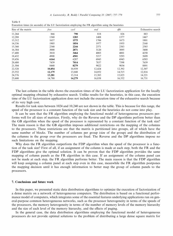
Table 8Execution times (in seconds) of the LU factorization employing the FR algorithm using the heuristics

Size of the matrix ftos cycl stof dflt Exhaustive search

11,264 866 790 818 826 88312,288 1360 1283 1408 1377 146713,312 1657 1575 1706 1673 180114,336 1905 1854 1977 1955 216815,360 2340 2244 2371 2383 258516,384 3000 2871 3120 3095 340017,408 3810 3464 4003 4001 425018,432 4908 4501 5217 5293 569919,456 6164 6287 6943 6943 650320,480 7439 7014 7837 7598 765921,504 8440 8279 9022 9034 889122,528 10,854 10,939 12,424 12,392 12,30723,552 12,175 13,048 14,052 14,515 12,81624,576 13,281 13,314 15,385 15,825 14,22125,600 14,780 14,279 16,838 16,552 16,731


The last column in the table shows the execution times of the LU factorization application for the locallyoptimal mapping obtained by exhaustive search. Unlike results for the heuristics, in this case, the executiontime of the LU factorization application does not include the execution time of the exhaustive search becauseof its very high cost.

Results for task sizes between 1024 and 10,240 are not shown in the table. This is because for this range, thespeed of the processor is a constant function of the task size and the heuristics do not come into play.

It can be seen that the FR algorithm employing the functional model of heterogeneous processors per-forms well for all sizes of matrices. Firstly, why do the Reverse and the DP algorithms perform better thanthe GB algorithm when the speed of the processor is represented by a constant function of the task size?The main reason is that the GB algorithm imposes additional restrictions on the mapping of the columnsto the processors. These restrictions are that the matrix is partitioned into groups, all of which have thesame number of blocks. The number of columns per group (size of the group) and the distribution ofthe columns in the group over the processors are fixed. The Reverse and the DP algorithms impose nosuch limitations on the mapping.

Why does the FR algorithm outperform the FDP algorithm when the speed of the processor is a func-tion of the task size? First of all, if an assignment of the column is made at each step, both the FR and theFDP algorithms give the optimal solution. It can be proven that the FDP algorithm provides the samemapping of column panels as the FR algorithm in this case. If an assignment of the column panel cannot be made at each step, the FR algorithm performs better. The main reason is that the FDP algorithmwill keep assigning a column panel at each step even in this case, meanwhile the FR algorithm postponesthe mapping decision until it has enough information to better map the group of column panels to theprocessors.

7. Conclusions and future work

In this paper, we presented static data distribution algorithms to optimize the execution of factorization ofa dense matrix on a network of heterogeneous computers. The distribution is based on a functional perfor-mance model of computers, which integrates some of the essential features underlying applications run on gen-eral-purpose common heterogeneous networks, such as the processor heterogeneity in terms of the speeds ofthe processors, the memory heterogeneity in terms of the number of memory levels of the memory hierarchyand the size of each level of the memory hierarchy, and the effects of paging.

In the general case, the data distribution algorithms employing the functional model of heterogeneousprocessors do not provide optimal solutions to the problem of distributing a large dense square matrix for


its parallel LU factorization over a one-dimensional arrangement of heterogeneous processors using theirfunctional performance model. It is shown that the FR algorithm employing the functional model of hetero-geneous processors performs well for all sizes of matrices. Of all the presented efficient polynomial heuristicsthat can be employed in the FR algorithm, the heuristics ftos and cycl perform the best. It is also shown thatthese heuristics perform no worse than the exhaustive search considering all the possible mappings.

Future work would involve extension of the distribution algorithms for two dimensional processor grids.For two-dimensional processor grids, the block cyclic distribution as used in ScaLAPACK is more naturaland scalable. However the problem of data partitioning employing the functional model of heterogeneous pro-cessors and the block cyclic distribution is very complex and is open for research. This can be deduced fromthe complexity of the problem of cyclic distribution of columns over a one-dimensional arrangement of het-erogeneous processors demonstrated in this paper. We can speculate that the FR algorithm can be appliedalong the row and the column dimensions of the matrix for data distribution on two-dimensional arrangementof heterogeneous processors. But a cursory study shows that this is not trivial.

References

[1] D. Arapov, A. Kalinov, A. Lastovetsky, I. Ledovskih, Experiments with mpC: efficient solving regular problems on heterogeneousnetworks of computers via irregularization, in: Proceedings of the 5th International Symposium on Solving Irregularly StructuredProblems in Parallel (IRREGULAR’98), Lecture Notes in Computer Science, vol. 1457, 1998, pp. 332–343.

[2] A. Kalinov, A. Lastovetsky, Heterogeneous distribution of computations while solving linear algebra problems on networks ofheterogeneous computers, in: Proceedings of the 7th International Conference on High Performance Computing and NetworkingEurope (HPCN Europe’99), Lecture Notes in Computer Science, vol. 1593, 1999, pp. 191–200.

[3] O. Beaumont, V. Boudet, A. Petitet, F. Rastello, Y. Robert, A proposal for a heterogeneous cluster ScaLAPACK (dense linearsolvers), IEEE Transactions on Computers 50 (10) (2001) 1052–1070, October.

[4] P. Boulet, J. Dongarra, F. Rastello, Y. Robert, F. Vivien, Algorithmic issues on heterogeneous computing platforms, ParallelProcessing Letters 9 (2) (1999) 197–213.

[5] J. Barbosa, J. Tavares, A.J. Padilha, Linear algebra algorithms in a heterogeneous cluster of personal computers, in: Proceedings ofthe 9th Heterogeneous Computing Workshop (HCW 2000), Cancun, Mexico, IEEE Computer Society Press, 2000, pp. 147–159, May.

[6] J. Barbosa, C.N. Morais, A.J. Padilha, Simulation of data distribution strategies for LU factorization on heterogeneous machines, in:Proceedings of the 17th International Parallel and Distributed Processing Symposium (IPDPS 2004), 26–30 April 2004, Santa Fe,New Mexico, USA, CD-ROM/Abstracts Proceedings, IEEE Computer Society, 2004.

[7] X. Du, X. Zhang, Z. Zhu, Memory hierarchy considerations for cost-effective cluster computing, IEEE Transactions on Computers 49(9) (2000) 915–933.

[8] S. Manegold, P. Boncz, M. Kersten, Generic database cost models for hierarchical memory systems, in: Proceedings of InternationalConference on Very Large Data Bases (VLDB), August 20–23, 2002, pp. 191–202.

[9] Yi-Min Wang, Memory latency consideration for load sharing on heterogeneous network of workstations, Journal of SystemsArchitecture 52 (1) (2006) 13–24.

[10] T. Rauber, G. Runger, A hierarchical computation model for distributed shared-memory machines, in: Proceedings of the 9thEuromicro Workshop on Parallel and Distributed Processing (PDP’01), IEEE Computer Society, 2001, pp. 57–64.

[11] M. Drozdowski, P. Wolniewicz, Out-of-core divisible load processing, IEEE Transactions on Parallel and Distributed Systems 14 (10)(2003) 1048–1056, October.

[12] A. Lastovetsky, R. Reddy, Data partitioning with a realistic performance model of networks of heterogeneous computers, in:Proceedings of the 17th International Parallel and Distributed Processing Symposium (IPDPS 2004), 26–30 April 2004, Santa Fe,New Mexico, USA, CD-ROM/Abstracts Proceedings, IEEE Computer Society, 2004.

[13] A. Lastovetsky, R. Reddy, Data partitioning with a functional performance model of heterogeneous processors, International Journalof High Performance Computing Applications 21 (1) (2007) 76–90.

[14] V. Kumar, A. Grama, A. Gupta, G. Karypis, Introduction to Parallel Computing: Design and Analysis of Algorithms, Benjamin-Cummings, Addison-Wesley, 1994, 597 p.

[15] C.A. Kitchen, M.F. Guest, M.J. Deegan, I. Kozin, R. Wain, The euroben benchmarks 2. Probing Parallel Performance on Xeon,Opteron, Itanium2 and Power5-based Clusters, March 2006. Available from: <http://www.cse.clrc.ac.uk/disco/DLAB_BENCH_WEB/Euroben2.0-dm/euroben2.0-dm.shtml>.

[16] A.J. van der Steen, The benchmark of the EuroBen group, Parallel Computing 17 (10–11) (1991) 1211–1221.[17] A. Lastovetsky, R. Reddy, Data partitioning for multiprocessors with memory heterogeneity and memory constraints, Scientific

Programming 13 (2) (2005) 93–112.[18] J. Choi, J. Dongarra, L.S. Ostrouchov, A.P. Petitet, D.W. Walker, R.C. Whaley, The design and implementation of the ScaLAPACK

LU, QR, and Cholesky factorization routines, Scientific Programming, 1058-9244 5 (3) (1996) 173–184.[19] L.S. Blackford, J. Choi, A. Cleary, E. D’Azevedo, J. Demmel, I. Dhillon, J. Dongarra, S. Hammarling, G. Henry, A. Petitet, K.

Stanley, D. Walker, R.C. Whaley, ScaLAPACK Users’ Guide, SIAM, 1997.

http://www.cse.clrc.ac.uk/disco/DLAB_BENCH_WEB/Euroben2.0-dm/euroben2.0-dm.shtml

http://www.cse.clrc.ac.uk/disco/DLAB_BENCH_WEB/Euroben2.0-dm/euroben2.0-dm.shtml


[20] A. Lastovetsky, R. Reddy, R. Higgins, Building the functional performance model of a processor, in: Proceedings of the 21st AnnualACM Symposium on Applied Computing (ACM SAC 2006), April 23–24, Dijon, France, 2006.

[21] J. Dongarra, J.D. Croz, I.S. Duff, S. Hammarling, A set of level-3 basic linear algebra subprograms, ACM Transactions onMathematical Software 16 (1) (1990) 1–17, March.

Data distribution for dense factorization on computers with memory heterogeneity

Documents

Transcript of Data distribution for dense factorization on computers with memory heterogeneity