Robust Resource Provisioning in Time-Varying Edge Networks

Ruozhou Yu, North Carolina State University

Guoliang Xue, Yinxin Wan, Arizona State University

Jian Tang, Syracuse University

Dejun Yang, Colorado School of Mines

Yusheng Ji, National Institute of Informatics, Japan

Outlines

2

Background and Motivation

System Modeling

Algorithm Design and Analysis

Performance Evaluation

Discussions, Future Work and Conclusions

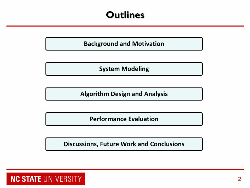
Geo-Distributed Services & Edge Computing

3

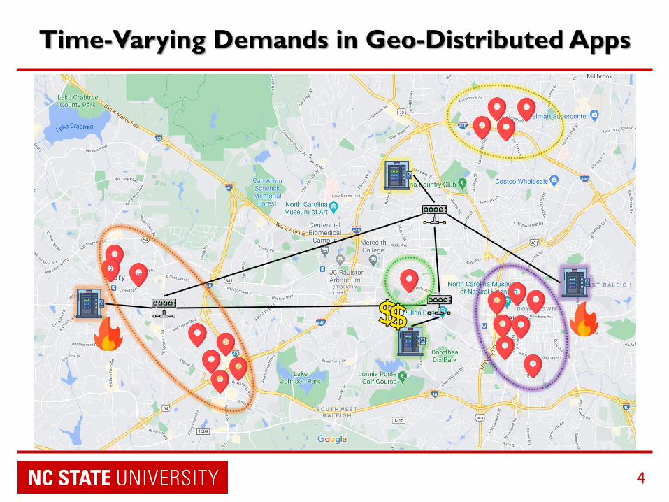
Time-Varying Demands in Geo-Distributed Apps

4

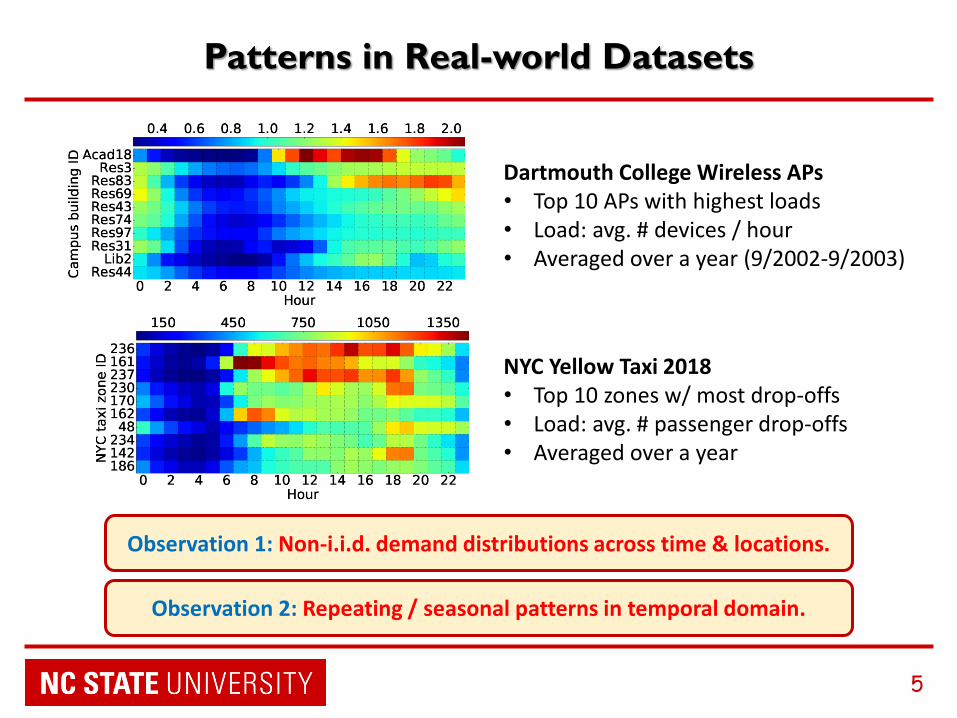
Patterns in Real-world Datasets

5

Dartmouth College Wireless APs• Top 10 APs with highest loads• Load: avg. # devices / hour• Averaged over a year (9/2002-9/2003)

NYC Yellow Taxi 2018• Top 10 zones w/ most drop-offs• Load: avg. # passenger drop-offs• Averaged over a year

Observation 1: Non-i.i.d. demand distributions across time & locations.

Observation 2: Repeating / seasonal patterns in temporal domain.

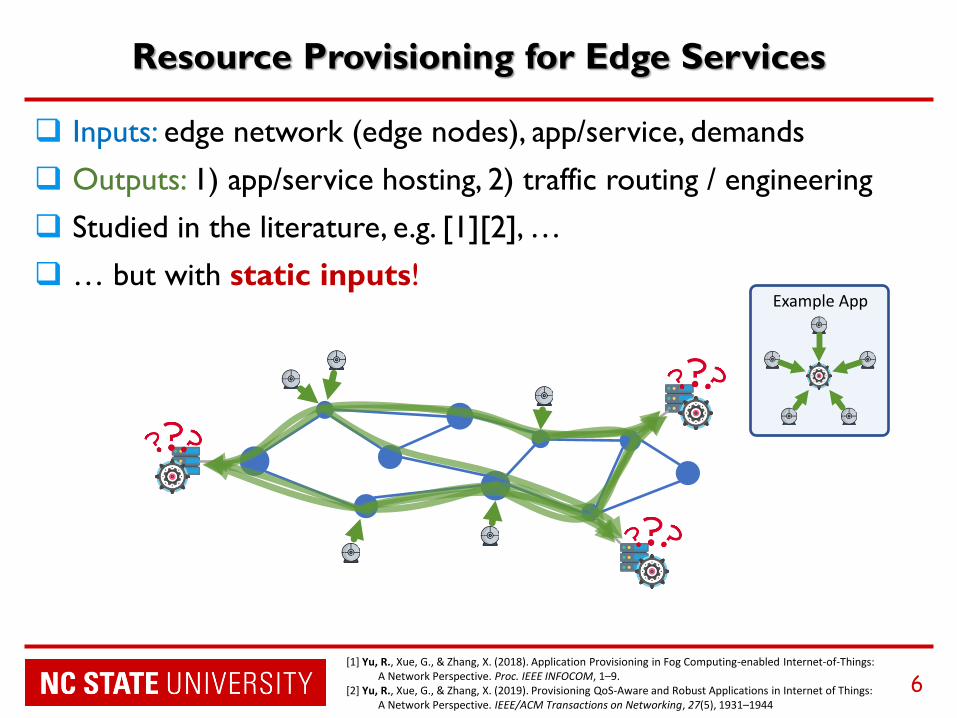
Resource Provisioning for Edge Services

6

Example App

❑ Inputs: edge network (edge nodes), app/service, demands

❑ Outputs: 1) app/service hosting, 2) traffic routing / engineering

❑ Studied in the literature, e.g. [1][2], …

❑ … but with static inputs!

[1] Yu, R., Xue, G., & Zhang, X. (2018). Application Provisioning in Fog Computing-enabled Internet-of-Things: A Network Perspective. Proc. IEEE INFOCOM, 1–9.

[2] Yu, R., Xue, G., & Zhang, X. (2019). Provisioning QoS-Aware and Robust Applications in Internet of Things: A Network Perspective. IEEE/ACM Transactions on Networking, 27(5), 1931–1944

Methodology Overview

7

App DemandsTime-varying, geo-distributed

Edge NetworkTopology, time-varying delays

Abstract System Model• Time-varying model• System risk model (CVaR)• Three-stage stochastic optimiz.

Optimization Framework• Nested Bender decomposition• Efficient subproblem solving

Service DeploymentGlobal fixed decisions

Inputs:

System-wide

Optimization:

Outputs:Net Provisioning

Per-time slot decisionsNet Estimation

Per-realization decisions

Outlines

8

Background and Motivation

System Modeling

Algorithm Design and Analysis

Performance Evaluation

Discussions, Future Work and Conclusions

System Model: Involved Parties

9

ESP

Edge Service Provider• Submits service requests

• Measures and predicts demands • Dynamically balances load

Example App

NM

Network Manager• Manages edge network

• Decides network policies• Provisions network resources (bw)

ECMEdge Computing Manager(s)

• Manages edge nodes & resources• Decides computing costs

Edge Network: A General Model

❑ Challenge: heterogeneous network environments

❑ Model: general directed graph G=(N, L), with edge nodes H and APs A

❖ Weights: link bandwidth, <link delay>, edge node cost, <AP demand>

10

Wireless RANs:

• Geo-distributed

• Limited capacity

• Interference

Backbones:

• Large-scale

• High latency

• ISP policies

Edge Network:

• Complex topo

• Distributed

• Dynamic load

Edge Demand Model

❑ Challenge: non-static, time-varying

❑ Observation: seasonal/repeating patterns❖ Example: the load in the same hour of workdays at an AP is similar

❑ Repeating time-slotted demand model

❖ Demand across slots in one period: non-i.i.d.

❖ Demand per slot across periods: i.i.d.

11

Period

… …Time

Slot

Edge Resource Provisioning /1

❑ Challenges: which decisions should be dynamic, which static?

❑ Formulation: a three-stage decision problem

❑ Stage 1: Service Deployment (SD)❖ Deploy edge service on host nodes by ECM

❖ Globally fixed: static across time slots & periods.

❑ Stage 2: Network Provisioning (NPR)❖ Network routing and bandwidth allocation by NM

❖ Per-slot: dynamic across time slots, but static for same slot across periods!

❑ Stage 3: Network Estimation (NE)❖ Instantaneous traffic allocation by ESP

❖ Dynamic: dynamic across both time slots and periods!

12

Objective and Overall Formulation

❑ Objective: minimize max traffic-averaged delay across time slots

❑ But {𝛿𝑡,𝑎} and {𝑑𝑡,𝑝} are both random…

13

𝑠. 𝑡.Stage 1: SD

Stage 2: NPR

Stage 3: NE

SO and CVaR

❑ Stochastic Optimization (SO): optimize a function inpresence of randomness (random objective and/or constraints)❖ Traditional approach: expectation optimization

❖ Issue: unbounded risk in rare but unfortunate scenarios

➢ E.g., abnormal demands due to public events, rare large-scale failures, …

❖ How to model these unfortunate scenarios?

❖ Value-at-Risk (VaR) and Conditional-Value-at-Risk (CVaR):

➢ Widely used in economics and finance

➢ VaR𝛼(R) = min { c ∈ ℝ | R does not exceed c with at least 𝛼 prob. }

➢ CVaR𝛼(R) = 𝔼[ R | R ≥ VaR𝛼(R) ]

❑ Expectation of R in the worst (1-𝛼) scenarios

❖ Our approach: optimize both expectation and CVaR

14

min𝒳∈ℱ max𝑡 𝔼[ 𝐷𝑡 ]

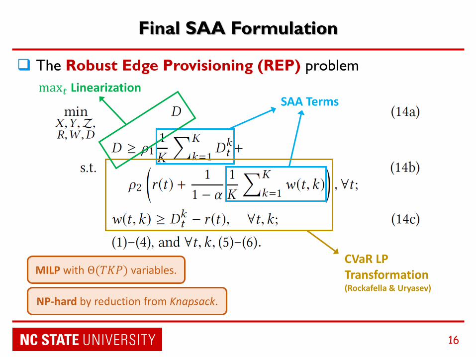
Final SAA Formulation

❑ The Robust Edge Provisioning (REP) problem

16

SAA Terms

CVaR LP Transformation(Rockafella & Uryasev)

max𝑡 Linearization

MILP with Θ(𝑇𝐾𝑃) variables.

NP-hard by reduction from Knapsack.

Outlines

17

Background and Motivation

System Modeling

Algorithm Design and Analysis

Performance Evaluation

Discussions, Future Work and Conclusions

Iterative Optimization Algorithm

❑ Benders’ decomposition: (Row Generation) In each iteration,add new constraints (cuts) to the problem that push the main problem towards the optimal:❖ INIT: feasible main solution; then proceed in iterations:

➢ Solve sub dual problem based on main solution (UB).

➢ If sub dual unbounded, add feasibility cut to main;if sub dual optimal, add optimality cut to main.

➢ Solve updated main (LB).

❖ Until UB – LB < 𝜖.

❑ Nested Benders’ decomposition❖ Apply two Benders’ decompositions for Phase-I and Phase-II respectively.

19

Convergence to optimality: proof by Benders.

Additional Techniques Applied

❑ Multiple Cuts (Birge & Louveaux)

❖ Dividing one optimality cut into one cut per sub-problem.

❖ Improves efficiency by pruning more sub-optimal region per-iteration.

❑ Fast Forward Fast Backward (FFFB)❖ Do not wait till Phase-II convergence to update Phase-I main problem

❖ Cuts based on non-optimal Phase-II solutions help prune more sub-optimal region per-iteration.

❑ Analytical Stage-3 Dual Solving❖ Linear time algorithm for solving the Stage-3 dual problems…

❖ … instead of cubic time for solving as an LP

21

Outlines

22

Background and Motivation

System Modeling

Algorithm Design and Analysis

Performance Evaluation

Discussions, Future Work and Conclusions

Simulation Settings

❑ Settings❖ Dataset: NYC Yellow Taxi 2018

➢ 12 months of Taxi drop-off data (~112 million taxi trips)

➢ Picked 5 or 20 most popular zones out of 262 (18% or 55% of all demands)

➢ 100-days for training: solving SAA formulation for SD and NPR

➢ 265-days for testing: evaluating solutions with NE

❖ Synthetic Data

➢ Random topologies: Watts-Strogatz with k = 4 and p = 0.3 (5 edge nodes)

➢ Deployment costs: 𝒩(1000, 2002); cost budget: 3300 (uniform)

➢ Pathbook: 3 min-hop paths for each AP-Edge node pair

➢ Network conditions:

❑ Normal scenario: 5 Gbps links with 𝒩(10, 42) ms delays

❑ Congested scenario: 2 Gbps links with half nodes experiencing 50× delays

❖ 𝜌1 = 𝜌2 = 0.5 (expectation vs. CVaR), 𝛼 = 0.95 (CVaR confidence), 𝜖 = 10−3 (convergence)

23

Experiment Results

24

Time-varying vs. Time-agnostic• Time-varying has increased advantage over time-agnostic with more slots.

=> Fixed provisioning without per-slot adjustment has poor performance.(For each slot, load is averaged over entire slot.)

T-Var: time-varying

T-Ago: time-agnostic

Setting: Small/Congested

Experiment Results

25

Optimal vs. Heuristics• Consistent performance advantage over heuristics

=> User satisfaction / revenue in the long-term

RAND: random edge node

AVG: optimiz. avg. delay

Setting: Medium/Normal

Outlines

28

Background and Motivation

System Modeling

Algorithm Design and Analysis

Performance Evaluation

Discussions, Future Work and Conclusions

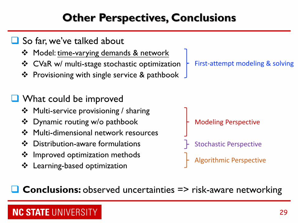
Other Perspectives, Conclusions

❑ So far, we’ve talked about❖ Model: time-varying demands & network

❖ CVaR w/ multi-stage stochastic optimization

❖ Provisioning with single service & pathbook

❑ What could be improved❖ Multi-service provisioning / sharing

❖ Dynamic routing w/o pathbook

❖ Multi-dimensional network resources

❖ Distribution-aware formulations

❖ Improved optimization methods

❖ Learning-based optimization

❑ Conclusions: observed uncertainties => risk-aware networking

29

First-attempt modeling & solving

Modeling Perspective

Stochastic Perspective

Algorithmic Perspective

Thank you very much!Q&A?

30