
Relaxed LMI conditions for control of nonlinear Takagi ...
200
UNIVERSIDAD POLIT ´ ECNICA DE VALENCIA DEPARTAMENTO DE INGENIER ´ IA DE SISTEMAS Y AUTOM ´ ATICA Tesis doctoral Condiciones LMI relajadas para control de modelos no-lineales Takagi-Sugeno Relaxed LMI conditions for control of nonlinear Takagi-Sugeno models Autor: Carlos V. Ari˜ no Latorre Director: Dr. Antonio Sala Piqueras Valencia, Diciembre 2007
-
Upload
khangminh22 -
Category
Documents
-
view
2 -
download
0
Transcript of Relaxed LMI conditions for control of nonlinear Takagi ...

UNIVERSIDAD POLITECNICA DE VALENCIA
DEPARTAMENTO DE INGENIERIA DE SISTEMAS YAUTOMATICA
Tesis doctoral
Condiciones LMI relajadas para control de modelosno-lineales Takagi-Sugeno
Relaxed LMI conditions for control of nonlinearTakagi-Sugeno models
Autor: Carlos V. Arino LatorreDirector: Dr. Antonio Sala Piqueras
Valencia, Diciembre 2007


RESUMEN
Los problemas de optimizacion de desigualdades matriciales lineales encontrol borroso se han convertido en la herramienta mas utilizada endicha area desde los anos 90. Muchos sistemas no lineales pueden sermodelados como sistemas borrosos de modo que el control borroso puedeconsiderarse como una tecnica de control no lineal. Aunque se hanobtenido muchos y buenos resultados, quedan algunas fuentes de conser-vadurismo cuando se comparan con otros enfoques de control no lineal.Esta tesis discute dichas cuestiones de conservadurismo y plantea nuevosenfoques para resolverlas.
La principal ventaja de la formulacion mediante desigualdades ma-triciales lineales es la posibilidad de asegurar estabilidad y prestacionesde un sistema no lineal modelado como un sistema borroso Takagi-Sugeno. Estos modelos estan formados por un conjunto de modeloslineales eligiendo el sistema a aplicar mediante el uso de unas reglasborrosas. Estas reglas se traducen en funciones de interpolacion o depertenecıa que nos indican el grado de validez de un modelo linealrespecto del resto. El mayor problema que presentan estas tecnicasbasadas en desigualdades matriciales lineales es que las funciones depertenencia no estan incluidas en las condiciones de estabilidad del sis-tema, lo que significa que se prueba la estabilidad y prestaciones paracualquier forma de interpolacion entre los diferentes modelos lineales.Esto genera una fuente de conservadurismo que serıa conveniente limi-tar.
En la tesis doctoral se presentan varias metodologıas capaces detrasladar la informacion de las funciones de pertenencia del sistema alproblema basado en desigualdades matriciales lineales de estabilidad yprestaciones. Las dos principales aportaciones propuestas se basan, res-pectivamente, en introducir una serie de matrices de relajacion que per-
iii

iv
mitan incorporar esta informacion y en aprovechar la descripcion de unaamplia clase de sistemas borrosos en productos tensoriales de modeloslineales, en los que cada funcion de pertenencia se obtiene del productocartesiano de varias funciones.
Por otro lado, el problema de estabilidad y prestaciones para sistemasborrosos Takagi-Sugeno esta basado en las condiciones de estabilidad deLyapunov y no resulta equivalente al problema en desigualdades ma-triciales lineales obtenido, siendo este ultimo conservativo respecto alprimero. Ası una de las mayores aportaciones de la tesis es la introduc-cion de nuevas condiciones de estabilidad y prestaciones que medianteun parametro de diseno permiten acercar esta equivalencia entre las ex-presiones, resultando equivalentes asintoticamente con el aumento delparametro. Como inconveniente, el aumento del parametro comportaun aumento en la complejidad del problema a resolver.

RESUM
Els problemes d’optimitzacio de desigualtats matricials lineals en controlborros s’han convertit en la ferramenta mes utilitzada a l’area des delsanys 90. Molts sistemes no lineals poden ser modelats com sistemesborrosos, de tal forma que el control borros es pot considerar com unatecnica de control no lineal. Malgrat que s’han obtingut molts i bonsresultats, queden algunes fonts de conservadorisme quan es comparenamb altres tecniques de control no lineal. Aquesta tesi discuteix lesquestions de conservadorisme i planteja noves tecniques per a resoldre-les.
El principal avantatge de la formulacio mitjancant desigualtats ma-tricials lineals es la possibilitat d’assegurar estabilitat i prestacions d’unsistema no lineal modelat com a un sistema borros Takagi-Sugeno. A-quests models estan formats per un conjunt de models lineals triant elsistema a aplicar mitjancant l’us d’unes regles borroses. Aquestes re-gles es tradueixen en funcions d’interpolacio o de pertenencia que ensindiquen el grau de validesa d’un model lineal respecte de la resta. El ma-jor problema que presenten aquestes tecniques basades en desigualtatsmatricials lineals es, que les funcions de pertenencia no estan inclosesen les condicions d’estabilitat del sistema, aixo significa que, es proval’estabilitat i prestacions per a qualsevol forma d’interpolacio entre elsdiferents models lineals. Aco genera una font de conservadorisme queseria convenient limitar.
En la tesis doctoral es presenten diverses metodologies que podentraslladar la informacio de les funcions de pertenencia del sistema alproblema basat en desigualtats matricials lineals d’estabilitat i presta-cions. Les dues principals aportacions proposades es basen, respecti-vament, en introduir una serie de matrius de relaxacio que permetenincorporar aquesta informacio, i en aprofitar la descripcio d’una amplia
v

vi
classe de sistemes borrosos en productes tensorials de models lineals,en els que cada funcio de pertenencia s’obte del producte cartesia dediverses funcions.
D’altra banda, el problema d’estabilitat i prestacions per a sistemesborrosos Takagi-Sugeno esta basat en les condicions d’estabilitat de Lya-punov i no es equivalent al problema en desigualtats matricials linealsobtingut, on aquest ultim resulta conservatiu respecte al primer. Aixıuna de les majors aportacions de la tesi es la introduccio de noves condi-cions d’estabilitat i prestacions que mitjancant un parametre de dissenypermeten aproximar aquesta equivalencia entre les expressions, resul-tant equivalents assimptoticament amb l’augment del parametre. Coma inconvenient l’augment del parametre comporta un augment de lacomplexitat del problema a resoldre.

ABSTRACT
Linear Matrix Inequalities (LMI) optimization problems became the toolof choice for fuzzy control in the 1990’s. Many nonlinear systems canbe modelled as fuzzy systems, so fuzzy control may be considered asa nonlinear control technique. Useful results have been obtained usingLMIs, however some sources of conservativeness remain when comparedto other nonlinear approaches. This thesis deals with such issues ofconservativeness and discusses some ideas on overcoming them.
The main advantage of Linear Matrix Inequalities formulations isthat they can ensure stability and performance of a nonlinear systemmodelled by a Takagi-Sugeno fuzzy system. The system is described byfuzzy IF-THEN rules which present “local” linear systems of the non-linear plant. These rules are numerically represented by a set of mem-bership functions. As a drawback, current linear matrix inequalitiesmethodologies do not include the shape of the membership functions.Therefore the stability is proved for any set of rules with any member-ship function that can be described by these linear models. This is asource of conservatism that can be reduced.
In this thesis some methodologies are presented which include themembership function information into the linear matrix inequalities sta-bility and performance problem. We propose two main contributionsin this area. The first method introduces a set of relaxation matricesthat incorporates the information on the membership functions. Theother uses the description of a wide class of Takagi-Sugeno fuzzy sys-tems, labelled as Tensor-Product Takagi-Sugeno fuzzy systems. In thesesystems, each membership function is the product of several membershipfunctions.
On the other hand, the problem of stability and performance forTakagi-Sugeno fuzzy systems is based on Lyapunov stability conditions
vii

viii
which are not equivalent to the linear matrix inequalities optimizationproblem, the second one is conservative compared to the first. That iswhy one of the main contributions of the thesis is a set of progressivelyless conservative sufficient conditions in order to hold stability or per-formance conditions for Takagi-Sugeno fuzzy systems. These conditionsare asymptotically equivalent. But the problem complexity increases asthe conditions are closer.

Acknowledgements
This document is the result of a lot of hard work. There are lots ofpeople I would like to thank for a huge variety of reasons. First of all,I would like to thank my Supervisor, Antonio Sala. I could not haveimagined having a better advisor for my PhD. His knowledge, common-sense and perspective have helped make my research both prolific andinteresting. Thank-you to Jose Luıs Navarro and Pedro Albertos forsupporting me at the beginning of my journey in research. I would alsolike to thank my colleagues in the Automatic and Control Group at theUniversity Jaume I of Castellon Roberto Sanchis, Nacho Penarrocha andJulio Romero for their patience and help with the academic tasks. Muchrespect to my old officemates, Emilio, Nacho, Jorn, Kiko and Javi fortheir helpful comments and suggestions.
Thanks to George Irwin for his help and attention during my stay atthe ISAC group of Queen’s University of Belfast and to Adrian for hissuggestions and grammatical corrections on the final document. I wouldalso like to express my gratitude to the Education and Science Ministryand the Department of Automatic Control at the Polytechnic Universityof Valencia for the scholarship which supported me during my researchand to the University Jaume I of Castellon for the economic support formy stay at the Queen’s University of Belfast.
Finally, I would also like to thank my parents, Agueda and Paco.They have always supported and encouraged me to do my best in allmatters of life. Most importantly I wish to thank my wife Mari forher understanding, patience, support, love, and all the other things thatmake it so wonderful to know her. To her I dedicate this thesis.
ix


Contents
1 Summary of the thesis 1
1.1 Introduction . . . . . . . . . . . . . . . . . . . . . . . . . . 1
1.2 Objectives . . . . . . . . . . . . . . . . . . . . . . . . . . . 2
1.2.1 Conservativeness of the positivity conditions forfuzzy summations . . . . . . . . . . . . . . . . . . 2
1.2.2 Local stability approach . . . . . . . . . . . . . . . 3
1.2.3 Tensor-product fuzzy systems . . . . . . . . . . . . 3
1.2.4 Memberships shape . . . . . . . . . . . . . . . . . 4
1.2.5 Uncertain memberships . . . . . . . . . . . . . . . 4
1.3 Structure of the thesis . . . . . . . . . . . . . . . . . . . . 4
I State of the art 7
2 Linear Matrix Inequalities stability analysis 9
2.1 Introduction . . . . . . . . . . . . . . . . . . . . . . . . . . 9
2.2 Stability concept . . . . . . . . . . . . . . . . . . . . . . . 10
2.2.1 Nonlinear systems . . . . . . . . . . . . . . . . . . 10
2.2.2 Lyapunov stability . . . . . . . . . . . . . . . . . . 11
2.2.3 Lyapunov stability theorem . . . . . . . . . . . . . 12
2.3 Linear matrix inequalities (LMI) . . . . . . . . . . . . . . 14
xi

xii CONTENTS
2.3.1 Properties of linear matrix inequalities . . . . . . . 14
2.3.2 Schur complement . . . . . . . . . . . . . . . . . . 15
2.3.3 S-procedure . . . . . . . . . . . . . . . . . . . . . . 16
2.3.4 Finsler Lemma . . . . . . . . . . . . . . . . . . . . 17
2.3.5 Linear matrix inequalities problems . . . . . . . . 17
2.3.6 Solving LMIs . . . . . . . . . . . . . . . . . . . . . 18
3 Takagi-Sugeno Models 19
3.1 Introduction . . . . . . . . . . . . . . . . . . . . . . . . . . 19
3.2 Definitions . . . . . . . . . . . . . . . . . . . . . . . . . . . 19
3.2.1 Takagi-Sugeno Fuzzy Models . . . . . . . . . . . . 20
3.2.2 PDC-controller . . . . . . . . . . . . . . . . . . . . 21
3.3 Sector nonlinearity . . . . . . . . . . . . . . . . . . . . . . 21
3.4 Stability of fuzzy models . . . . . . . . . . . . . . . . . . . 25
3.4.1 Stability of open-loop system . . . . . . . . . . . . 25
3.4.2 Stability of PDC closed-loop systems . . . . . . . . 26
3.5 Control Design for Takagi-Sugeno Fuzzy Systems . . . . . 28
3.5.1 Positiveness conditions . . . . . . . . . . . . . . . . 31
II Researched issues and contributions 35
4 Roadmap: Reducing the gap between the fuzzy and non-linear control 37
4.1 Introduction . . . . . . . . . . . . . . . . . . . . . . . . . . 37
4.2 Some Shadows . . . . . . . . . . . . . . . . . . . . . . . . 38
4.2.1 Conservatism of the Lyapunov approach . . . . . . 39
4.2.2 Conservativeness of the positivity conditions forfuzzy summations . . . . . . . . . . . . . . . . . . 39

CONTENTS xiii
4.2.3 Intrinsic conservativeness of the fuzzy approachversus a nonlinear one . . . . . . . . . . . . . . . . 40
4.2.4 Computational power . . . . . . . . . . . . . . . . 40
4.3 Some Lights . . . . . . . . . . . . . . . . . . . . . . . . . . 40
4.3.1 Arbitrarily complex Lyapunov functions . . . . . . 41
4.3.2 Asymptotically necessary and sufficient conditionsfor fuzzy summations. . . . . . . . . . . . . . . . . 41
4.3.3 Membership shape techniques . . . . . . . . . . . . 42
4.3.4 Local stability approach . . . . . . . . . . . . . . . 43
4.3.5 Uncertain memberships . . . . . . . . . . . . . . . 44
4.4 Conclusions . . . . . . . . . . . . . . . . . . . . . . . . . . 45
5 Relaxed LMI conditions, an asymptotically approach 47
5.1 Introduction . . . . . . . . . . . . . . . . . . . . . . . . . . 47
5.2 Problem statement . . . . . . . . . . . . . . . . . . . . . . 48
5.2.1 Multi-index notation. . . . . . . . . . . . . . . . . 50
5.3 Relaxed positivity conditions via dimensionality expansion 52
5.3.1 Relaxation by increasing the number of positivityconditions . . . . . . . . . . . . . . . . . . . . . . . 53
5.3.2 Relaxation via artificial decision variables . . . . . 56
5.3.3 Generalization to higher-dimensional fuzzy sum-mations . . . . . . . . . . . . . . . . . . . . . . . . 58
5.3.4 Recursive procedure . . . . . . . . . . . . . . . . . 59
5.3.5 Number of conditions and decision variables . . . . 61
5.3.6 Comparison to previous literature . . . . . . . . . 62
5.4 Examples . . . . . . . . . . . . . . . . . . . . . . . . . . . 64
5.5 Conclusions . . . . . . . . . . . . . . . . . . . . . . . . . . 76

xiv CONTENTS
6 Local stability results 79
6.1 Introduction . . . . . . . . . . . . . . . . . . . . . . . . . . 80
6.2 Local Fuzzy Models . . . . . . . . . . . . . . . . . . . . . 80
6.2.1 Stability analysis . . . . . . . . . . . . . . . . . . . 84
6.3 Stability analysis of Feedback Systems . . . . . . . . . . . 86
6.4 Algorithm . . . . . . . . . . . . . . . . . . . . . . . . . . . 88
6.5 Examples . . . . . . . . . . . . . . . . . . . . . . . . . . . 88
6.6 Conclusions . . . . . . . . . . . . . . . . . . . . . . . . . . 92
7 Relaxed LMI conditions: Overlap in membership func-tions 93
7.1 Introduction . . . . . . . . . . . . . . . . . . . . . . . . . . 93
7.2 Relaxed conditions with overlap information . . . . . . . . 94
7.2.1 Single sum relaxation . . . . . . . . . . . . . . . . 94
7.2.2 Double-sum relaxation . . . . . . . . . . . . . . . . 96
7.3 Shape-dependent positivity conditions for double fuzzysummations . . . . . . . . . . . . . . . . . . . . . . . . . . 99
7.3.1 Particular cases . . . . . . . . . . . . . . . . . . . . 102
7.3.2 Obtention of bounds in practice. . . . . . . . . . . 103
7.4 Generalization to higher dimensions . . . . . . . . . . . . 105
7.4.1 Multi-dimensional index notation . . . . . . . . . . 106
7.4.2 Relaxed conditions . . . . . . . . . . . . . . . . . . 107
7.5 Examples . . . . . . . . . . . . . . . . . . . . . . . . . . . 110
7.6 Conclusions . . . . . . . . . . . . . . . . . . . . . . . . . . 117
8 Stability Analysis with uncertain membership functions119
8.1 Introduction . . . . . . . . . . . . . . . . . . . . . . . . . . 119
8.2 Problem statement . . . . . . . . . . . . . . . . . . . . . . 120

CONTENTS xv
8.3 Main Result . . . . . . . . . . . . . . . . . . . . . . . . . . 122
8.4 Particular cases . . . . . . . . . . . . . . . . . . . . . . . . 125
8.5 Examples . . . . . . . . . . . . . . . . . . . . . . . . . . . 129
8.6 Conclusions . . . . . . . . . . . . . . . . . . . . . . . . . . 134
9 Tensor product TS systems 135
9.1 Introduction . . . . . . . . . . . . . . . . . . . . . . . . . . 135
9.2 Problem Statement . . . . . . . . . . . . . . . . . . . . . . 136
9.2.1 Sufficient Positivity Conditions . . . . . . . . . . . 140
9.2.2 Tensor-product fuzzy systems . . . . . . . . . . . . 141
9.2.3 Multi-dimensional tensor-product fuzzy systems . 142
9.3 Closed-loop tensor-product fuzzy systems . . . . . . . . . 149
9.4 Relaxed stability and performance conditions for TPTSfuzzy systems . . . . . . . . . . . . . . . . . . . . . . . . . 151
9.5 Robust stability of LTI multiaffine systems . . . . . . . . 153
9.5.1 Robust stability conditions . . . . . . . . . . . . . 154
9.6 Examples . . . . . . . . . . . . . . . . . . . . . . . . . . . 155
9.7 Conclusions . . . . . . . . . . . . . . . . . . . . . . . . . . 164
III Conclusions 165
10 Conclusions and future work 167
10.1 Future research lines . . . . . . . . . . . . . . . . . . . . . 170
11 Published Contributions 171
References 175


Chapter 1
Summary of the thesis
1.1 Introduction
In contrast to conventional control, fuzzy control was initially introducedas a model-free control design method based on a representation of theknowledge and the reasoning process of a human operator (Zadeh, 1973;Assilian & Mamdani, 1975). Fuzzy logic can capture the continuousnature of human decision making processes. Practical applications offuzzy control started to appear very quickly after the method had beenintroduced in publications. Moreover fuzzy modelling methodologieswere developed and most nonlinear process could be modelled as fuzzysystems. A drawback of knowledge-based, model-free fuzzy control isthat it does not allow for any kind of stability or robustness analysis,unless a model of the process is available.
In a parallel research line, new control methodologies appeared inthe field of robust control in the 1990’s. These technics were basedon Lyapunov stability and convex optimization where the optimizationproblem is subject to a set of Linear Matrix Inequalities (LMI). Thesemethodologies reached maturity after (Boyd, El Ghaoui, Feron, & Bal-akrishnan, 1994) and were applied to fuzzy control theory by (Tanaka& Wang, 2001), in particular to Takagi-Sugeno fuzzy models, becomingwidespread in the last 10 years. Results are available for control designof fuzzy systems with uncertainty, delay, descriptor forms.
LMIs have become a powerful tool in fuzzy control. They solved awide variety of stability and performance problems for Takagi-Sugenofuzzy models. The ability of fuzzy systems to approximate nonlinearmodels allowed control of large generic control problems.
1

2 Objectives
As a drawback there are several sources of conservatism on main-stream fuzzy control. The choice of the structure of the Lyapunov func-tion, conservativeness of the LMI conditions as they are not equivalentto the Lyapunov conditions, because they are independent of the mem-bership shape.
LMI fuzzy control theory is not able to find any solution in somecomplex scenarios, where other nonlinear control theory is successful,due to the membership functions are not included in the LMI conditions.The aim of the thesis is to introduce some new conditions in order toreduce this conservatism.
1.2 Objectives
The main objective of the thesis is to reduce the above discussed gapbetween fuzzy and nonlinear control. Four ways have been explored inorder to reduce this gap: Conservativeness of the positivity conditions for fuzzy summations. Local stability results for fuzzy systems. New stability conditions for Tensor product fuzzy systems. Membership-shape relaxation.
1.2.1 Conservativeness of the positivity conditions forfuzzy summations
Current literature (Tanaka & Wang, 2001; Liu & Zhang, 2003; Fang,Liu, Kau, Hong, & Lee, 2006) presents only sufficient conditions for en-suring stability or performance of Takagi-Sugeno Fuzzy models. Thereare many literature references in the area of stability and performanceconditions. So we explore the different ways to reduce this conservative-ness. These contributions have been published in (Sala & Arino, 2007b)and (Arino & Sala, 2007a).

Summary of the thesis 3
1.2.2 Local stability approach
Local quadratic stability results can be obtained, even in the case whereglobal quadratic-stability related LMIs are infeasible. Indeed, as com-mented in (Sugeno, 1992), it is an interesting question to determine forwhich initial conditions a fuzzy system is stable (or unstable) (Sugeno,1992). Example 6 in (Tanaka & Wang, 2001)(Chapter 2) shows that thebasin of attraction for fuzzy systems may be membership dependent. Inthis respect, the methodology presented here allows to determine thelargest sphere around the origin for which quadratic stability may beprovable in a given fuzzy system with known membership functions.These contributions have been published in (Arino & Sala, 2006a) and(Arino & Sala, 2006b).
1.2.3 Tensor-product fuzzy systems
Another example of conservativeness occurs when the membership func-tions can be expressed as the “tensor product” of simpler partitions,so that the fuzzy system can be written as a multi-dimensional fuzzysummation.
Removing part of the conservatism in current solutions for the tensor-product case above is indeed of interest; this product structure is oftenthe case in many engineering applications of fuzzy control: in the systematic “sector nonlinearity” fuzzy modelling techniques
reported in (Tanaka & Wang, 2001); in many man-made rulebases for multi-input fuzzy systems, wherethe rules are built via the conjunction of simpler concepts arisingfrom fuzzy partitions on each of the input domains. A typical ex-ample are rulebases formed with rules in the form“if z1 is large andz2 is small and . . . then . . . ”, “if z1 is medium and z2 is small and. . . then . . . ”, etc., with the antecedents covering all combinationsof fuzzy sets on z1, z2, etc.. in approximate interpolation and model reduction techniques basedin gridding and tensor-SVD algebra in (Baranyi, 2004).
These settings are a particular class of fuzzy models which will be de-noted as tensor-product fuzzy systems.

4 Structure of the thesis
In summary the objective is to define and analyzing the tensor-product fuzzy systems, by presenting fuzzy control design tools for themwhich explicitly use the tensor-product structure. The study of theproperties of this class of systems is very relevant as most of the fuzzysystems in nontrivial engineering applications of fuzzy control belong tothis class, as discussed above.
These contributions have been published in (Arino & Sala, 2007c)and(Arino & Sala, 2007b).
1.2.4 Memberships shape
When the expressions of the memberships as a function of some premisevariables are actually known, some zones of the possible membershipspace can be excluded. Reducing the size of the (multi-dimensional) setwhere the membership functions take values should obtain less conser-vative conditions than those expressed for any membership. However,LMI conditions in current literature do not take into account that fact.These contributions have been published in (Sala & Arino, 2007a).
1.2.5 Uncertain memberships
In most applications, we need to approximate the membership functionsand in these cases, it is difficult to take into account the knowledge ofthe membership functions shape. Therefore the ability to incorporatea wider class of constraints on the membership shape will improve thecurrent stability and performance results.
1.3 Structure of the thesis
The document is organized in three parts. Part I outlines with the stateof the art, and it is composed of two chapters. Chapter 2 introduces thereader to Lyapunov stability and linear matrix inequalities problems andChapter 3 presents the stability and performance problem in Takagi-Sugeno Fuzzy systems.
Part II presents the contributions and is organized in seven chapters:

Summary of the thesis 5 Chapter 4 exposes the problems with the LMI theory and dealswith the different points of view to tackle the problem. Chapter 5 presents asymptotical necessary and sufficient condi-tions for quadratic stability in Takagi-Sugeno fuzzy models. Chapter 6 presents local stability conditions to apply when globalstability can not be proved Chapter 7 deals with the introduction of the membership func-tions shape into the LMI stability conditions in order to relax thisexpressions and approach to nonlinear control specific results. Chapter 8 develops new stability and performance LMI condi-tions for TS fuzzy models with uncertain memberships functions. Chapter 9 deals with the Tensor Product Takagi-Sugeno modelsand presents a new stability results that take into account thespecial structure of these models.
Part III closes the thesis with a summary of contributions and openresearch lines.


Part I
State of the art
7


Chapter 2
Linear Matrix Inequalities stability analysis
2.1 Introduction
The most useful and general approach for studying the stability of non-linear control systems is the theory introduced in the late 19th cen-tury by the Russian mathematician Alexander Mikhailovich Lyapunov.Lyapunov’s work, The General Problem of Motion Stability, includestwo methods for stability analysis (the so-called linearization methodand the direct method) and was first published in 1892. The lineariza-tion method draws conclusions about a nonlinear system’s local stabilityaround an equilibrium point from the stability properties of its linear ap-proximation. The direct method is not restricted to local motion, anddetermines the stability properties of a nonlinear system by constructinga scalar “energy-like” function for the system and examining the func-tion’s time variation. However Lyapunov’s pioneering work on stabilityreceived little attention outside Russia, although it was translated intoFrench in 1908 (at the instigation of Poincare), and reprinted by Prince-ton University Press in 1947. The publication of the work by Lur’e anda book by La Salle and Lefschetz brought Lyapunov’s work to the at-tention of the larger control engineering community in the early 1960’s.Many refinements of Lyapunov’s methods have since been developed.Today, Lyapunov’s linearization method has come to represent the the-oretical justification of linear control, while Lyapunov’s direct methodhas become the most important tool for nonlinear system analysis anddesign. Together, the linearization method and the direct method con-stitute the so-called Lyapunov stability theory.
The objective of this chapter is to present Lyapunov stability theoryand illustrate its use in the analysis and the design of control systems.
9

10 Stability concept
2.2 Stability concept
The concept of stability and instability (Slotine & Li, 1991) are usefulin a wide field of knowledge: Finance, Medicine, Construction, Control,Chemistry, etc... So a clear definition of the concept of stability is neededin the control theory.
Qualitatively, a system is described as stable if starting the systemsomewhere near its desired operating point implies that it will stayaround the point ever after. And this point is called the equilibriumpoint. From this qualitative definition, we can classify three kinds ofequilibrium points (Slotine & Li, 1991; Boyd et al., 1994): Asymptotically stable: the system returns to the equilibrium point
after a small perturbation. Non-asymptotically stable: the system remains in the proximityof the equilibrium point after a small perturbation. Unstable equilibrium: the system keeps away from the equilibriumpoint after a small perturbation.
2.2.1 Nonlinear systems
Let us consider a class of nonlinear dynamic systems (Slotine & Li, 1991),which can be represented by a set of differential equations in the form
x = f (x, t) (2.1)
Where x is the (n× 1) state space vector, and f is a (n× 1) vectorfunction. The number of the states is also called the order of the system.And a solution x(t) of the equation is a trajectory.
If f is only a function of x, the system is said to be autonomous,otherwise the system is called non-autonomous.
A special class of nonlinear systems are linear systems (Antsaklis &Mitchel, 1997). The dynamics of linear systems have the form
x = A(t)x (2.2)
Linear Matrix Inequalities stability analysis 11
where A(t) is an (n× n) matrix. If A(t) is constant the system is calledLinear time-invariant (LTI) system, otherwise it is denoted as linear timevariant (LTV) system.
Equilibrium pointsIt is possible for a system trajectory to correspond to only a single point.Such a point is called an equilibrium point. As we shall see later, manystability problems are naturally formulated with respect to equilibriumpoints.
In autonomous systems state x′ is an equilibrium state (or equilib-rium point) of the system if once x(t) is equal to x, it remains equal to xfor all future time. Mathematically, this means that the constant vectorx′ satisfies
0 = f (x′)
In a linear time-invariant system 0 = Ax′. So x′ = 0 is the single equilib-rium point if A is not singular. On the other hand, nonlinear systemscan have several isolated equilibrium points.
2.2.2 Lyapunov stability
In the beginning of this chapter, an intuitive notion of stability was in-troduced, as a kind of behavior around an equilibrium point. However,since nonlinear systems may have much more complex and exotic be-havior than linear systems, the mere notion of stability is not enough todescribe the essential features of their motion. A number of more refinedstability concepts, such as asymptotic stability, exponential stability andglobal asymptotic stability, are needed. In this section, we define thesestability concepts formally, for autonomous systems, and explain theirpractical meanings.
Essentially, stability in the sense of Lyapunov means that the systemtrajectory can be kept arbitrarily close to the equilibrium point, startingsufficiently close to it. So let us define local stability as
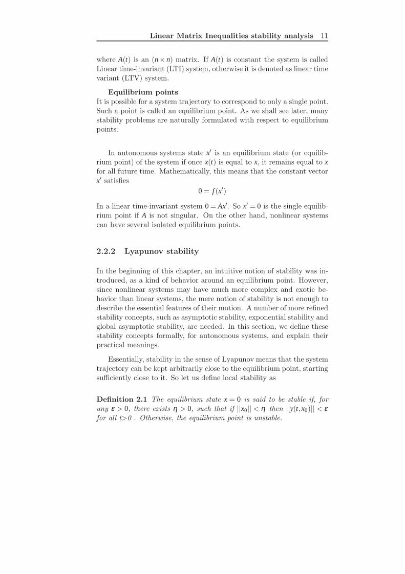
Definition 2.1 The equilibrium state x = 0 is said to be stable if, forany ε > 0, there exists η > 0, such that if ||x0|| < η then ||y(t,x0)|| < εfor all t>0 . Otherwise, the equilibrium point is unstable.

12 Stability concept
Also, Asymptotic stability in the sense of Lyapunov (Slotine & Li,1991) means that the equilibrium is stable and that, in addition, if thestates started close to the equilibrium point, they actually converge tothe equilibrium point.
Definition 2.2 An equilibrium point x = 0 is asymptotically stable if itis stable, and if in addition there exists some ε > 0 such that ||x(0)||< εimplies that x(t)→ 0 as t→ ∞.
2.2.3 Lyapunov stability theorem
Inside the ball B(ε), the equilibrium point x = 0 of the system (2.1) islocally stable, if there is a scalar function V (x) continuous and differen-tiable such that
V (x) ≥ 0 ∀x ∈ B(ε)
dVdt
≤ 0 t ≥ 0
V (0) = 0
where x is the state space vector of the system (2.1). And the func-tion V (x) is called Lyapunov function.
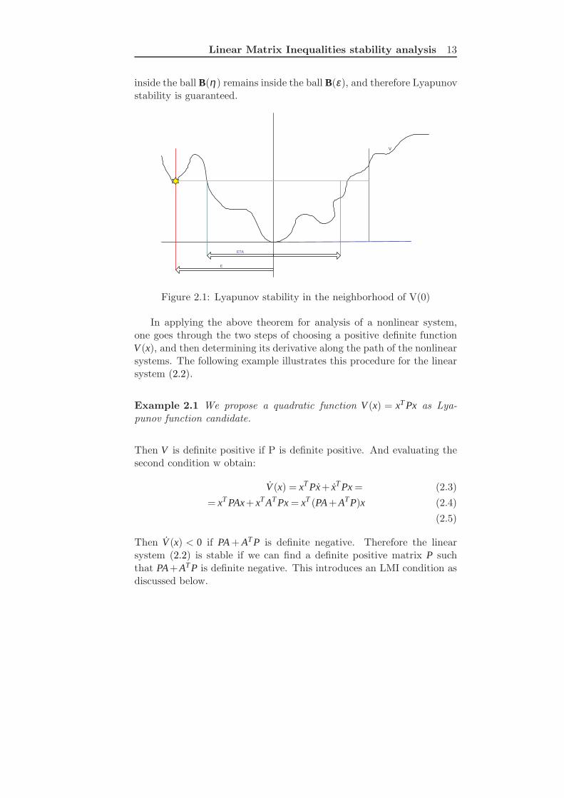
The result can be derived using the geometric interpretation of aLyapunov function, as illustrated in figure 2.1 in which is drawn theequipotentials of V on the state space of the system. In order to showstability, it must be shown that given any strictly positive number ε > 0,there exists a smaller positive number η such that any trajectory startinginside the ball B(η) remains inside the ball B(ε) for all future time. Letm be the minimum of V on the ball B(ε). Since V is continuous andpositive definite, m exists and is strictly positive. Furthermore, sinceV (0) = 0, there exists a ball B(η) around the origin such that V (x) < mfor any x inside the ball. Consider now a trajectory whose initial pointis in the ball B(η) . Since V is non-increasing along system trajectories,V remains strictly smaller than m, and therefore the trajectory cannotpossibly cross the outside sphere B(ε) . Thus, any trajectory starting
Linear Matrix Inequalities stability analysis 13
inside the ball B(η) remains inside the ball B(ε), and therefore Lyapunovstability is guaranteed.
ETA
E
V
Figure 2.1: Lyapunov stability in the neighborhood of V(0)
In applying the above theorem for analysis of a nonlinear system,one goes through the two steps of choosing a positive definite functionV (x), and then determining its derivative along the path of the nonlinearsystems. The following example illustrates this procedure for the linearsystem (2.2).
Example 2.1 We propose a quadratic function V (x) = xT Px as Lya-punov function candidate.
Then V is definite positive if P is definite positive. And evaluating thesecond condition w obtain:
V (x) = xT Px+ xT Px = (2.3)
= xT PAx+ xT AT Px = xT (PA + AT P)x (2.4)
(2.5)
Then V (x) < 0 if PA + AT P is definite negative. Therefore the linearsystem (2.2) is stable if we can find a definite positive matrix P suchthat PA+AT P is definite negative. This introduces an LMI condition asdiscussed below.

14 Linear matrix inequalities (LMI)
2.3 Linear matrix inequalities (LMI)
A linear matrix inequality (Gahinet & Apkarian, 1994; Boyd et al., 1994;Anderson, Kraus, Mansour, & Dasgupta, 1995; Scherer, Gahinet, &Chilali, 1997) is an expression of the form:
A(x) = A0 + x1A1+ ...+ xNAN < 0 (2.6)
where x = (x1, ...,xN) is a vector of N real numbers called the decisionvariables. A0, ...,AN are real symmetric matrices. the inequality < 0 in (2.6) means definite negative. That is equiv-alent to saying that all eigenvalues λ (A(x)) are negative, or equiv-alently, the maximum eigenvalue is negative.
2.3.1 Properties of linear matrix inequalities
Convex set. The linear matrix inequality (2.6) defines a convex con-straint on x. That is, the set
Φ = x|A(x) < 0 (2.7)
of solutions of the LMI A(x) < 0 is convex. In fact, if x1 and x2 are in Φthen αx1 +(1−α)x2 is in Φ, where 0≤ α ≤ 1.
A(αx1 +(1−α)x2) = αA(x1)+ (1−α)A(x2) < 0
where we used that A(x) is affine and where the inequality follows fromthe fact that 0≤ α ≤ 1.
A set of linear matrix inequalities (LMIs) is a finite set oflinear matrix inequalities:
A1(x) < 0, . . . ,Ak(x) < 0 (2.8)

Linear Matrix Inequalities stability analysis 15
Any set of linear matrix inequalities can be expressed as a linear matrixinequality in the form
A(x) =
A1(x) 0 . . . 00 A2(x) . . . 0...
.... . .
...0 0 . . . Ak(x)
< 0 (2.9)
The last inequality indeed makes sense as A(x) is symmetric for anyx. Further, since the set of eigenvalues of A(x) is simply the union of theeigenvalues of A1(x), . . . ,Ak(x), any x that satisfies A(x) also satisfies theset of LMIs (2.8).
Affine constrains. A third important property amounts to incorpo-rating affine constraints in linear matrix inequalities. By this, we meanthat combined constraints (in the unknown x) of the form x = Au+b forsome u. The LMI constrain A(x) < subject to x = Au+b can be rewrittenas an LMI of u as A(u) < 0.
Congruence transformation. If M is a square matrix and T isnon-singular, then the product T T MT is called a congruence transfor-mation of M. For symmetric matrices M this transformation does notchange the number of positive and negative eigenvalues of M. Indeed, ifan LMI A(x) < 0 holds for some x then uT A(x)u < 0 holds for any nonzerou and x in Φ, (2.7). In particular if u = T v, vT T T A(x)T v < 0, thereforeT T A(x)T < 0 for any x in Φ, (2.7).
2.3.2 Schur complement
Let A(x) be an affine function which is partitioned according to
A(x) =
(
A11(x) A12(x)A12(x)T A22(x)
)
(2.10)
then A(x) < 0 is equivalent to:
A11(x) < 0A22(x)−A12(x)T A22(x)−1A12(x) < 0
(2.11)
and
A22(x) < 0A11(x)−A12(x)A11(x)−1A12(x)T < 0
(2.12)

16 Linear matrix inequalities (LMI)
The second inequalities in (2.11) and (2.12) are nonlinear in x. Using thatresult follows that nonlinear matrix inequalities in the form (2.11) canbe converted into linear matrix inequalities. The proof can be obtainedwith the congruence transformation
T =
(
I −A−122 AT
120 I
)
2.3.3 S-procedure
Sometimes a quadratic function should be negative whenever some otherquadratic functions are all negative. This constraint can be expressedas an LMI defining the quadratic functions. Sometimes this LMI isconservative, but often a useful approximation of the constraint.
The S-procedure for quadratic functions and non-strict in-equalities: Let F0, . . . ,Fp the quadratic function of the variable u ∈Rn:
Fi(u) = uT Tiu+2biu+ vi i = 0, . . . , p (2.13)
where Ti is a symmetric matrix. We consider the following condition onF0, . . . ,Fp:
F0(u) > 0 ∀u | Fi(u)≥ 0, i = 0, . . . , p (2.14)
Obviously if there exist τ1≥ 0, . . . ,τp ≥ 0 such that for all u,
F0(u)−p
∑i=1
τiFi(u)≥ 0 (2.15)
then (2.14) holds.
If p=1, the converse holds, provided that there is some u0 such thatF1(u0) > 0, See (Wolkowicz & Stern, 1995; Nocedal & Wright, 1999; Boyd& Vandenberghe, 2004)
The inequality (2.15) can be rewritten as an LMI as
(
T0 b0
bT0 v0
)
−p
∑i=1
τi
(
Ti bi
bTi vi
)
≥ 0 (2.16)
Farkas Lemma is a particular case of the s-procedure, where thefunctions Fi are affine. In that case (2.14) and (2.15) are equivalent. See(Boyd & Vandenberghe, 2004)

Linear Matrix Inequalities stability analysis 17
The S-procedure for quadratic forms and strict inequalities:
Another variation of the s-procedure involves quadratic forms andstrict inequalities. Let T0, . . . ,Tp ∈ Rn×n be symmetric matrices. Weconsider the following conditions on T0, . . . ,Tp
uT T0u > 0 ∀u 6= 0 | uT Tiu≥ 0, i = 0, . . . , p (2.17)
it is obvious that if there exist τ1≥ 0, . . . ,τp ≥ 0 such that
T0−p
∑i=1
τiTi > 0 (2.18)
then (2.17) holds.
2.3.4 Finsler Lemma
Let x ∈ Rn, Q = QT ∈ Rn×n and R ∈ Rm×n. The following statements areequivalent (Boyd et al., 1994):
1. xT Qx < 0 for all x 6= 0 such that Rx = 0
2. RT⊥QR⊥ < 0 where RR⊥ = 0
3. Q−σRT R < 0 for some scalar σ ∈ R
4. Q + XR + RTXT < 0 for some matrix X ∈ Rn×m
2.3.5 Linear matrix inequalities problems
There are two generic problems related to the study of linear matrixinequalities:
1. The LMI optimization problem. Let an objetctive functionf : Φ→ R where Φ = x|A(x) < 0. The problem to determineminx f (x) is called an optimization problem with an LMI constraint.If the function f is linear f = c1xn + · · ·+ cnxn, the optimizationproblem is a generalization of linear programming to a cone ofpositive semidefinite matrices. It is also called semidefinite pro-gramming.

18 Linear matrix inequalities (LMI)
2. The LMI feasibility problem. Test whether exist x ∈ Rn suchthat A(x) < 0. That is, A(x) < 0 is feasible if and only ifminx λmax(A(x)) < 0. Therefore involves minimizing the functionf : x→ λmax(A(x)). That is possible because this function is convexas it has been shown above.
2.3.6 Solving LMIs
A solution method for an LMI optimization problems is an algorithmthat computes a solution of the problem (to some given accuracy), givena particular problem from the class, i.e., an instance of the problem.Since the late 1940s, a large effort has gone into developing algorithms forsolving various classes of optimization problems, analyzing their proper-ties, and developing good software implementations. The effectivenessof these algorithms varies considerably, and depends on factors such asthe particular forms of the objective and constraint functions, how manyvariables and constraints there are, and special structure, such as spar-sity. (A problem is sparse if each constraint function depends on only asmall number of the variables).
High quality implementations of LMI optimization problems are a-vailable in (Gahinet, Nemirovski, Laub, & Chilali, 1995; Sturm, 1999)software.
Chapter 3
Takagi-Sugeno Models
3.1 Introduction
This Chapter outlines model-based fuzzy control systems. The centralsubject is a systematic framework for the stability and design of non-linear fuzzy control systems. Building on the so-called Takagi-Sugenofuzzy model, a number of the most important issues in fuzzy control sys-tems are addressed. These include stability analysis, systematic designprocedures, incorporation of performance specifications, robustness andobserver design.
3.2 Definitions
This section shows the definition of the Takagi-Sugeno fuzzy model (TSfuzzy model). followed by construction procedures of such models. Thena model-based fuzzy controller design utilizing the concept of “paralleldistributed compensation” is described. The main idea of the controllerdesign is to derive each control rule so as to compensate each rule of afuzzy system. The design procedure is conceptually simple and natural.Moreover, it is shown in this chapter that the stability analysis andcontrol design problems can be reduced to linear matrix inequality (LMI)problems.
First we present the Takagi-Sugeno Fuzzy model as an approxima-tion of a given nonlinear plant, described by fuzzy IF-THEN rules whichpresent “local” linear systems of the nonlinear plant (Babuska, 1998;Babuska, Fantuzzi, & Verbruggen, 1996). So each rule expresses a sig-
19

20 Definitions
nificant feature of the plant, expressed as a linear system. Then thewhole plant is described by the interpolation among these linear sys-tems. This feature is very useful in order to reduce the control probleminto linear matrix inequalities conditions.
3.2.1 Takagi-Sugeno Fuzzy Models
Takagi-Sugeno (Takagi & Sugeno, 1985) (TS) fuzzy model is definedby IF-THEN rules that represent local linear dynamics of a nonlinearsystem. The rules of the TS fuzzy models are usually expressed as:
IF z is Mi THEN
δxi = Aixi + Biuyi = Cixi
The local models represented by Aixi + Biu are used to compute thefinal output as follows:
δx =r
∑i=1
µi(z)(Ai · x+ Bi ·u) (3.1)
y =r
∑i=1
µi(z)Cix (3.2)
r
∑i=1
µi(z) = 1, µi(z) > 0 ∀z i = 1. . . r (3.3)
In continuous models, δ represents the derivative operator and indiscrete case, it represents the advance operator. x(t) ∈ R
n is the statespace vector, u(t) ∈ R
m is the input vector of the model and y(t) ∈ Rp
is the output vector. Matrices Ai ∈ Rn×n, Bi ∈ R
n×m and Ci ∈ Rp×n for
i = 1. . . r represents a set of linear models. z(t) is the premise variablesand µi(z) represents the membership functions of fuzzy set Mi that hold(3.3)

Takagi-Sugeno Models 21
3.2.2 PDC-controller
The parallel distributed compensation (PDC) controller began with amodel-based design prodedure proposed by (Sugeno & Kang, 1986) with-out stability analysis. The LMI stability analysis was done in (Tanaka& Sugeno, 1992) and it was named PDC in (Wang, Tanaka, & Griffin,1995).
In the PDC controller design, each control rule is designed for thecorresponding rule of a TS fuzzy model. Therefore the designed fuzzycontroller shares the fuzzy sets with the fuzzy model, that are the mem-bership functions in the inference procedure. For the TS fuzzy modelsthe PDC-controller is defined as:
IF z is Mi THEN
ui(t) =−Fixi(t)
So Each rule represents a linear controller (state feedback law). Othercontrollers such as output feedback controllers and dynamic output feed-back controllers can also be used. As is shown in Chapter 5 they can beused in our approaches. The fuzzy controller is expressed by the follow-ing control input vector:
u(t) =−r
∑i=1
µiFix(t) (3.4)
The above expression is usually denoted as a parallel distributed com-pensation controller, PDC-controller.
3.3 Sector nonlinearity
In order to design a fuzzy controller, we need a Takagi-Sugeno fuzzymodel for a nonlinear system. Therefore the construction of a fuzzymodel represents an important and basic procedure in this approach. Inthis section we discuss the issue of how to construct such a fuzzy model.In general there are two approaches for constructing fuzzy models: Experimental identification using input and output data.

22 Sector nonlinearity Mathematical approximation from nonlinear equations.
There has been an extensive literature on fuzzy modelling using input-output data following Takagi’s, Sugeno’s, and Kang’s excellent work(Takagi & Sugeno, 1985; Sugeno & Nishida, 1985; Sugeno & Kang, 1986,1988). The procedure mainly consists of two parts: structure identifica-tion and parameter identification. The identification approach to fuzzymodelling is suitable for plants that are unable or too difficult to berepresented by analytical physical models. On the other hand, non-linear dynamic models for mechanical systems can be readily obtainedby, for example, the Lagrange method and the Newton-Euler method.In such cases, the second approach, which derives a fuzzy model fromgiven nonlinear dynamical models, is more appropriate. This section fo-cuses on this second approach. This approach utilizes the idea of sectornonlinearity.
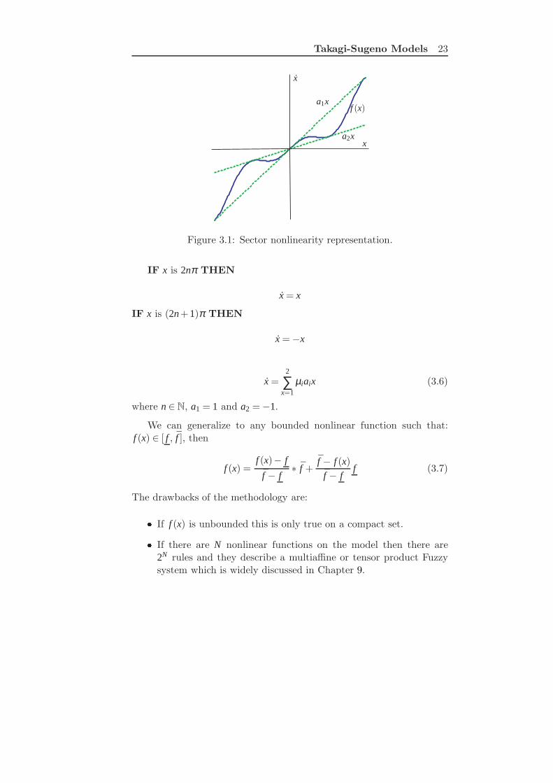
The idea of using sector nonlinearity in fuzzy model constructionfirst appeared in (Kawamoto, Tada, Ishigame, & Taniguchi, 1992) andexpanded in (Tanaka & Wang, 2001). Sector nonlinearity is based onthe following idea. Consider a nonlinear system x = f (x), x ∈R . Theaim is to find a global sector such that a1x ≤ f (x) ≤ a2x. Figure 3.1illustrates the sector nonlinearity approach. This approach guaranteesan exact fuzzy model construction. However, it is sometimes difficultto find global sectors for general nonlinear systems. In this case, wecan consider local sector nonlinearity. This is reasonable as variables ofphysical systems are always bounded.
Example 3.1 Let us considerer the nonlinear model
x = cos(x)x (3.5)
then as cos(x) ∈ [−1,1]
cos(x) =cos(x)+1
2∗1+
1−cos(x)2
(−1)
defining the membership functions µ1 = 1+cos(x)2 and µ2 = 1−cos(x)
2 clearlyµ1 and µ2 fulfill (3.3). Then a TS fuzzy representation of the system is:
Takagi-Sugeno Models 23
a1x
a2xx
x
f (x)
Figure 3.1: Sector nonlinearity representation.
IF x is 2nπ THEN
x = x
IF x is (2n+1)π THEN
x =−x
x =2
∑x=1
µiaix (3.6)
where n ∈ N, a1 = 1 and a2 =−1.
We can generalize to any bounded nonlinear function such that:f (x) ∈ [ f , f ], then
f (x) =f (x)− f
f − f∗ f +
f − f (x)
f − ff (3.7)
The drawbacks of the methodology are: If f (x) is unbounded this is only true on a compact set. If there are N nonlinear functions on the model then there are2N rules and they describe a multiaffine or tensor product Fuzzysystem which is widely discussed in Chapter 9.

24 Sector nonlinearity
M
m
u
lx
Figure 3.2: Inverted pendulum system.
Example 3.2 Inverted pendulum TS model
The equations of motion for the inverted pendulum (Cannon, 2003)are
x1 = x2 (3.8)
x2 =gsin(x1)−amlx2
2sin(2x1)/2−acos(x1)u4l/3−aml cos2(x1)
(3.9)
where x1 denotes the angle in radians of the pendulum from the verticaland x2 is the angular velocity; g is the acceleration due to gravity, mis the mass of the pendulum, M is the mass of the cart, l is the lengthof the pendulum, and u is the force applied to the cart; a = 1/(m +M). following the reasoning in (Tanaka & Wang, 2001) we choose thenonlinear functions
f1 =1
4l/3−aml cos2(x1)
f2 = sin(x1)/x1
f3 = x2 sin(2x1)
f4 = cos(x1)
where x1∈ (−π/2,π/2) and x2 ∈ [−α ,α ]. Defining the membership func-tions µim as in (3.7), where the subindex i corresponds to the nonlinearlinear function fi and m is the membership function number for fi, that

Takagi-Sugeno Models 25
is 1 or 2. We obtain the TS model
(
x1
x2
)
=2
∑i=1
2
∑j=1
2
∑k=1
2
∑l=1
µ1iµ2 jµ3kµ4l
[
Ai jkl
(
x1
x2
)
+ Bi jklu
]
(3.10)
where Ai jkl and Bi jkl are defined from the bounds of f1, f2, f3, f4.
There are several contributions on nonlinear systems are modelledas TS models (Sugeno & Nishida, 1985; Sugeno & Kang, 1986; Babuska,1998; Hori, Tanaka, & Wang, 2002; Baranyi, 2004; Feng, 2006) etc...There are also interesting results (Fantuzzi & Rovatti, 1996; Ying, 1998;Wang, Li, Niemann, & Tanaka, 2000; Tanaka & Wang, 2001) that showTS models are universal approximators.
3.4 Stability of fuzzy models
Lyapunov stability theory proves that such a system is stable if thereexist positive α , β and a function V (x) such that:
β‖x‖ ≥V (x)≥ α‖x‖, dVdx
< 0, V (0) = 0, ∀ x
The most popular Lyapunov Functions proposed in literature are quad-ratic forms:
V (x) = xT Px (3.11)
with matrix P being symmetric and definite positive. So we review thebasic results on quadratic stability of the Takagi-Sugeno fuzzy model(3.1).
3.4.1 Stability of open-loop system
Let us first consider the stability of continuous system without inputs(u), that is:
x =r
∑i=1
µi(x)Ai · x (3.12)
In this case, we take the quadratic form shown above V (x) = xT Pxas our Lyapunov function. Due to P being definite positive the first

26 Stability of fuzzy models
condition holds. So we only need to prove that V < 0. First we obtainthe value of V , using (3.12), that is:
V = xT [r
∑i=1
µi(ATi P+ PAi)]x
as the membership functions are greater than 0 a sufficient condition forstability is:
ATi P+ PAi < 0, i : 1..r (3.13)
where < means definite negative. As it can be seen these conditions areindependent for any membership function. That makes these conditionsconservative. This thesis contributes new conditions in order to reducethe conservatism of the conditions.
The above equations are LMIs, hence widely available LMI optimiza-tion software either finds a P or determines that the LMI is infeasible.
Remark: Note that the membership functions µ do not appear inthe LMI conditions. Hence, the same P defines a quadratic Lyapunovfunction for multiple nonlinear systems with the same “vertex models”as the original one. Such generality is good in case a feasible P is foundbut, on the contrary,it is too restrictive a condition as in some cases asolution can not be reached despite the underlying system being stable.
3.4.2 Stability of PDC closed-loop systems
The objective here is to illustrate the basic ideas of stability analysisand stable fuzzy control via LMIs.
First we define the nonlinear control law by a PDC controller (3.4).The substituting (3.4) into (3.1), The closed-loop system can be rewrit-ten as:
x =r
∑i=1
r
∑j=1
µiµ j(Ai−BiFj)x (3.14)
Note that we have used the equality ∑ri=1 µi = 1 to obtain the above
expression.
Denote:
Gi j = Ai−BiFj (3.15)

Takagi-Sugeno Models 27
As ∑i ∑ j µiµ j = 1, it may be considered as an open-loop one andstability addressed by (3.13), i.e., looking for a common P such that:
GTi jP+ PGi j < 0 ∀ i, j
However, there are much less conservative conditions. Stability analysisin such a case has been discussed in (Tanaka & Wang, 2001) and (Kim &Lee, 2000), among others. The main results in those works to be appliedin this contribution are the following.
Theorem 3.1 (Tanaka & Wang, 2001) The equilibrium of the systemdescribed by (3.1) is globally asymptotically stable if there exists a com-mon positive definite matrix P such that:
GTii P+ PGii < 0 (3.16)
(
Gi j + G ji
2
)T
P+ P
(
Gi j + G ji
2
)
≤ 0 (3.17)
where (3.17) must hold only if µiµ j 6= 0.
Proof: note that system (3.14) can be rewritten as:
x =r
∑i=1
µ2i (Ai−BiFi)x+
r
∑i=1
∑j>i
µiµ j(Ai−BiFj + A j−B jFi)x (3.18)
then we take the quadratic Lyapunov function defined in (3.11).
V =r
∑i=1
µ2i (GT
ii P+PGii)x+r
∑i=1
∑j>i
µiµ j[(Gi j +G ji)T P+P(Gi j +G ji)]x (3.19)
so V is definite positive if (3.16) and (3.17) hold.
Theorem 3.2 (Kim & Lee, 2000) The equilibrium of the fuzzy controlsystem (3.1) is globally quadratically stable if there exist symmetric pos-itive matrix P and symmetric matrices Xi j such that
ΛTii P + PΛii + Xii < 0, i : 1, ...,n (3.20)
ΛTi jP+ PΛi j + Xi j < 0, i < j ≤ r (3.21)
X11 . . . X1n...
. . ....
Xn1 . . . Xnn
> 0 (3.22)

28 Control Design for Takagi-Sugeno Fuzzy Systems
whereΛii = Gii
Λi j =Gi j + G ji
2
3.5 Control Design for Takagi-Sugeno FuzzySystems
In many situations, Lyapunov-based conditions for stability or perfor-mance of a fuzzy control system may be expressed in the form
Ξ(t) =r
∑i=1
r
∑j=1
µi(z(t))µ j(z(t))x(t)T Qi jx(t) > 0 ∀ x 6= 0 (3.23)
where z(t) are denoted as premise variables (usually measurable) and rdenotes the number of fuzzy “rules” or “local models”. Symmetry (Qi j =QT
ji), and a fuzzy partition condition (3.3) are assumed to hold. Notationµi will be used as shorthand for µi(z(t)). Also, in most cases, “positive”in the text below should be understood as shorthand for “positive forx 6= 0”. Note that, the fuzzy partition condition (3.3) also implies:
r
∑i=1
r
∑j=1
µiµ j = 1 (3.24)
A typical example of the use of condition (3.23) is proving quadraticstability of the fuzzy system (3.1) with a fuzzy PDC state-feedback con-troller (3.4)
V =r
∑i=1
r
∑j=1
µi(z(t))µ j(z(t))x(t)T ((Ai−BiFj)
T P+ P(Ai−BiFj))x(t) (3.25)
Introducing the notation Gi j = Ai−BiFj, Λi j = 12(Gi j +G ji), matrices Qi j
in (3.23) are (Kim & Lee, 2000):
Qii = −GTii P−PGii (3.26)
Qi j = −ΛTi jP−PΛi j (3.27)

Takagi-Sugeno Models 29
Where P > 0 is a symmetric matrix, which defines a Lyapunov functionV (x) = xT Px, to be obtained via LMI algorithms (Boyd et al., 1994;Tanaka & Wang, 2001; Boyd & Vandenberghe, 2004).
Stabilization design
If Fj in (3.4) is also to be designed, applying the change of variableξ = P−1x, (3.25) can be rewritten as
r
∑i=1
r
∑j=1
µi(z(t))µ j(z(t))ξ (t)T (X(Ai−BiFj)T +(Ai−BiFj)X)ξ (t) (3.28)
r
∑i=1
r
∑j=1
µi(z(t))µ j(z(t))ξ (t)T (XATi −XFT
j BTi + AiX −BiFjX)ξ (t) (3.29)
where X = P−1 and defining Mi as Mi = FiX , Qi j may be se to
Qi j =−(AiX + XAiT −BiM j−MT
j BTi ) (3.30)
Decay-rate performance requirement
The speed of response is related to the decay rate, that is, the largestLyapunov exponent α (Boyd et al., 1994) such that
limt→∞
eαt‖x(t)‖ = 0 (3.31)
A sufficient condition for (3.31) with Lyapunov candidate V = xT Px is
V <−2αV (3.32)
for any initial point. Then if V (t) < V (x0)e−2αt and P > 0 then (3.31)holds.
In Fuzzy control it can be applied introducing by Qi j such that
Qi j =−(AiX + XAiT −BiM j−MT
j BTi +2αX) (3.33)
where X > 0 and Mi = FiX are LMI decision variables (for details, see(Tanaka & Wang, 2001; Kim & Lee, 2000)).

30 Control Design for Takagi-Sugeno Fuzzy Systems
Controller and observer design
In many applications, the state is not readily available. Then a statespace observer is needed to apply the fuzzy controller. A fuzzy observeris defined in (Tanaka & Wang, 1997; Tanaka, Ikeda, & Wang, 1998) as
˙x =r
∑i=1
µi(z)(Aix + Biu+ Ki(y− y)) (3.34)
y =r
∑i=1
Cix (3.35)
Therefore, the PDC controller is computed using the state space esti-mation x as
u =r
∑i=1
µiFix
In (Tanaka et al., 1998), the augmented close-loop plant (3.36) is pro-posed
(
x˙x
)
=
(
Ai−BiFj BiFj
0 Ai−K jCi
)[
xx
]
(3.36)
where x = x− x. Then with the Lyapunov function candidate
V = (xT xT )
(
P1 00 γP2
)(
xx
)
(3.37)
where γ is a positive constant. The systems (3.36) can be stabilized if(3.23) holds, with Qi j defined as
Qi j = AiX + XAiT −BiM j−MT
j BTi (3.38)
where X = P−11 , M j = FjX and if (3.23) holds, with Qi j defined as
Qi j = ATi P2+ P2Ai−N jCi−CT
i NTj (3.39)
where N j = P2K j. This result is similar to the separation principle forlinear systems. It has also been proved for TS fuzzy systems in (Ma, Sun,& He, 1998). Note that, in the presented results the system model do notinclude stability conditions of output stabilization for uncertain fuzzymodels. This has been reported in (Guerra, Kruszewski, Vermeiren, &Tirmant, 2006).

Takagi-Sugeno Models 31
Disturbance rejection
Considerer the following TS fuzzy system with a disturbance w, in (Tuan,Apkarian, Narikiyo, & Yamamoto, 2001)
x =r
∑i=1
µi(z)(Aix+ B1iw + B2iu) (3.40)
y =r
∑i=1
µi(z)(Cix+ D11iw + D12iu) (3.41)
The disturbance rejection can be realized by minimizing γ such that
sup‖w‖2 6=0
‖y‖2‖w‖2
≤ γ (3.42)
The related performance condition in (Tuan et al., 2001) uses as Qi j thematrix:
PATi + RT
j BT2i + AiP+ B2iR j B1i PCT
i + RTj DT
12i
BT1i −γI DT
11iCiP+ D12iR j D11i −γI
(3.43)
Then the H∞ disturbance rejection is lower than γ
Other performance settings
The reader is referred to (Tanaka & Wang, 2001; Fang et al., 2006;Sala, Guerra, & Babuska, 2005) and references therein for details onthe possibilities of different Qi j. Also the reader can consult (Chen,Chang, Su, Chung, & Lee, 2005; Hsiao, Hwang, Chen, & Tsai, 2005) forfuzzy delay systems , (Guerra & Vermeiren, 2004; Choi & Park, 2003)for uncertain ones, non-quadratic Lyapunov functions, (Chen, Tseng, &Uang, 2000) for output feedback control, etc.
3.5.1 Positiveness conditions
Of course, requiring Qi j > 0 is a trivial sufficient condition for positive-ness of (3.23), but much less conservative conditions appear in literature.One of the first was proposed in

32 Control Design for Takagi-Sugeno Fuzzy Systems
Theorem 3.3 (Tanaka & Sano, 1994). Expression (3.23) underfuzzy partition condition holds if
Qii > 0 i = 1. . . r (3.44)
Qi j + Q ji > 0 i = 1. . . r i < j (3.45)
In (Tuan et al., 2001) more relaxed conditions for (3.23) are presented
Theorem 3.4 (Tuan et al., 2001). Expression (3.23) under fuzzypartition condition holds if
Qii > 0 i = 1. . . r (3.46)
2r−1
Qii + Qi j + Q ji > 0 i = 1. . . r i 6= j (3.47)
Another popular one is Theorem 2 in (Liu & Zhang, 2003), which ismainly based on the scheme in (Kim & Lee, 2000). The conditions in(Liu & Zhang, 2003) may be proved by means of reordering (3.23) as
Ξ =r
∑i=1
µ2i xT Qiix+
r
∑i=1
∑i< j≤r
µiµ jxT (Qi j + Q ji)x > 0 (3.48)
Hence, if Xii ≤ Qii and Xi j + X ji ≤ Qi j + Q ji for i 6= j, as µiµ j is alwaysgreater or equal than 0,
Ξ≥r
∑i=1
µ2i xT Xiix+
r
∑i=1
∑i< j≤r
µiµ jxT (Xi j + X ji)x > 0 (3.49)
which may be expressed in matrix form as in Theorem 7 in (Kim & Lee,2000), yielding:
Theorem 3.5 (Liu & Zhang, 2003, Theorem 2). Expression (3.23)under fuzzy partition condition holds if there exist matrices Xi j = XT
ji suchthat:
Xii ≤ Qii (3.50)
Xi j + X ji ≤ Qi j + Q ji i 6= j (3.51)
X =
X11 . . . X1r...
. . ....
Xr1 . . . Xrr
> 0 (3.52)

Takagi-Sugeno Models 33
Note: In (Kim & Lee, 2000), Xi j are forced to be symmetric (moreconservative than (Liu & Zhang, 2003)). Also, it is well-known thatconditions (3.51) need to be enforced only when µiµ j 6= 0, i.e., refer-ring to overlapping fuzzy sets. The reader is also referred to (Teixeira,Assuncao, & Avellar, 2003) for related conditions.


Part II
Researched issues andcontributions
35


Chapter 4
Roadmap: Reducing the gap between the fuzzy
and nonlinear control
As have been shown in the introduction, LMI formulations for fuzzycontrol became the tool of choice in the 1990s. Many nonlinear sys-tems can be modelled as fuzzy systems (sector-nonlinearity), so fuzzycontrol may be considered as a technique for nonlinear control. In spiteof the obtained results some sources of conservativeness remain whencompared to other nonlinear approaches. This chapter, inspired by thework exposed in (Sala, 2007), can be understood as a brief compilationof the main contributions of this thesis.
4.1 Introduction
Fuzzy control started as a heuristic methodology in the 1970’s, codingcontrol rules by hand, trying to embed heuristic and reasoning into thecontrol block. However, most of the widespread heuristic rules haveno fundamental differences with standard PID regulators (the fuzzy-PD, fuzzy-PI and alike) and many other heuristic designs, which fuzzifyoperation rules for a complex plant, are one-of-a-kind tailored develop-ments which therefore have little interest for a broad audience. Due tothese reasons, the emphasis on heuristics and logic reasoning in fuzzycontrol has almost disappeared, in favor of rigorous mathematical tools,in order to guarantee control specifications expressed in terms of sta-bility, performance, robustness to modelling errors, etc. for a class ofnonlinear systems, for which a systematic modelling methodology (sec-tor nonlinearity (Tanaka & Wang, 2001)) is available to transform them
37
38 Some Shadows
into Takagi-Sugeno form (3.1):
x =r
∑i=1
µi fi, xk+1 =r
∑i=1
µi fi
with fi linear. In this way, nonlinear systems may be “embedded” intoa linear time-varying (LTV) dynamics and LTV design tools appliedreadily.
The advantages of the fuzzy approach are that efficient semidefinite-programing tools (LMI (Boyd et al., 1994; Boyd & Vandenberghe, 2004),sum-of-squares (Prajna, Papachristodoulou, & Parrilo, 2002)), widelyused in linear systems, can be almost directly applied to nonlinear con-trol problems. Unfortunately, there is a price to pay: the objective ofthis Chapter is discussing the specific disadvantages of the fuzzy ap-proach versus “direct nonlinear” alternatives. The reader is referred to(Sala et al., 2005) for other considerations, trends and open issues infuzzy modelling, identification and control.
Nowadays, Linear Matrix Inequality (LMI) techniques have becomethe tool of choice in order to design fuzzy controllers when a fuzzy modelof the process is available in the Takagi-Sugeno form: LMIs were intro-duced by (Tanaka & Sugeno, 1992) in the fuzzy control community, be-coming widespread in the last 10 years. Results are available for systemswith uncertainty, delay, descriptor forms, etc.
As it has been shown in Chapter 3, the most frequently consideredsetting is the so called parallel-distributed-compensation (PDC) in whicha fuzzy TS controller shares the membership functions with the plant tobe controlled (3.4). Conditions for decrescence of a Lyapunov functionsin such settings end up requiring to prove positiveness of a so-calleddouble fuzzy summation1 (Tanaka & Wang, 2001; Liu & Zhang, 2003),in expressions such as (3.23).
4.2 Some Shadows
Basically, there are several sources of conservatism on mainstream fuzzycontrol results. The following will be chosen for discussion below:
1Other settings (fuzzy observers, descriptor systems, fuzzy Lyapunov functions,etc.) may require a higher summation dimension.

Roadmap: Reducing the gap between the fuzzy andnonlinear control 39
1. choice of the Lyapunov function family,
2. conservativeness on the most used theorems on “positivity of fuzzysummations”,
3. results are independent of the membership shape,
4. computational power
and some recent ideas to overcome them will be discussed in Section 4.3.
Other issues, such as uncertainty structures, adaptive approaches,observers, etc. are also important, deserving further attention, but theyhave not been elaborated here. The reader is referred to (Labiod &Guerra, 2007; ?, ?) for recent relevant contributions in some of thosetopics.
Let us discuss the above-selected issues in some detail:
4.2.1 Conservatism of the Lyapunov approach
In fuzzy control, the search of Lyapunov functions is only made on aparticular family of candidate functions, hence a stable system may nothave a Lyapunov function in the particular class being sought. Thisproblem is common to nonlinear control theory: the Lyapunov approachis not constructive.
The approach using the quadratic Lyapunov function xT Px has beendeeply explored. Improvements are available: a piecewise quadraticfunction (Feng, 2003; Johansson, 1999), and fuzzy Lyapunov functionsfor continuous (Tanaka, Hori, & Wang, 2003) or discrete (Guerra &Vermeiren, 2004) systems.
4.2.2 Conservativeness of the positivity conditions forfuzzy summations
Current literature (Tanaka & Wang, 2001; Liu & Zhang, 2003; Fanget al., 2006) presents only sufficient conditions for (3.23) to hold. Hencea Lyapunov function fulfilling (3.23) may exist but the conditions abovemay fail to find it. There is a long-term quest in the fuzzy communityto find necessary and sufficient conditions for positivity of (3.23).

40 Some Lights
4.2.3 Intrinsic conservativeness of the fuzzy approach ver-sus a nonlinear one
The last open issue regards the knowledge of the membership functionshape. Indeed, in order to implement a fuzzy PDC controller, the valuesof µi should be a known function of some measurable variables. How-ever, the LMI conditions in the above works do not depend on the shapeof the membership functions. This is good, because the results applyto a set of nonlinear time-varying systems (as long as they share thesame ”vertices”), but it is, evidently, conservative for a particular sys-tem. On the contrary, Lyapunov-based nonlinear control usually takesinto account the exact shape of the nonlinearity in order to derive re-sults, being less conservative than the fuzzy approach when used for aparticular system.
As a trivial example, consider x = µ1(z) · x + (1− µ1(z)) · (−x). Itcannot be proved stable for an arbitrary µ1, 0≤ µ1(z)≤ 1 (it is unstablefor µ1(z) = 1). However, it is stable for, say, µ1 = 0.2+ 0.2sin(x) asx = (−1+2µ1)x is, trivially, an exponentially stable first-order nonlinearsystem when µ1≤ b < 0.5, b ∈R. The example is a clear case indicatingthat this situation may happen even in first-order systems: by usingnonlinear control ideas, once the explicit formula of the membershipfunctions has been included in the TS model, Lyapunov functions maybe obtained where fuzzy methodologies fail.
4.2.4 Computational power
The number of decision variables in some of the latest LMI results ishuge. Even if LMI solvers use polynomial-time algorithms, the exponentof the system order is large and many results can only be implementedfor simple systems.
4.3 Some Lights
There are some ideas reducing conservativeness on the first three casesabove, but heavily increasing the fourth problem (computational power)so there is a tradeoff. The results, however, diminish the gap betweenfuzzy and nonlinear control, at least in theory.

Roadmap: Reducing the gap between the fuzzy andnonlinear control 41
4.3.1 Arbitrarily complex Lyapunov functions
It is interesting to mention three possibilities of getting arbitrarily com-plex Lyapunov functions:
(1) higher-degree homogeneous Lyapunov functions (Chesi, Garulli,Tesi, & Vicino, 2003)
(2) exacerbate the piecewise idea (the point-wise approach in (Jo-hansen, 2000));
(3) use“resampling”, checking for V (t +k)−V (t)≤ 0, k > 1 (Kruszewski& Guerra, 2005) (indeed, if a system is stable, there will exist a kso that even V (x) = xT x will do; complexity lies in the predictorsneeded in the approach and in an underlying non-delayed Lya-punov function expression).
4.3.2 Asymptotically necessary and sufficient conditionsfor fuzzy summations. Chapter 5
Consider a multi-dimensional index variable i∈ 1, . . . ,rn where r is thenumber of rules and n is an arbitrary complexity parameter. Denotethe permutations of i by P(i). Then, results in (Liu & Zhang, 2003;Fang et al., 2006) are particular cases of finding a multi-dimensionalarrangement of matrices (tensor) fulfilling, for all i:
∑j∈P(i)
Q j1 j2 > ∑j∈P(i)
12(Xj + XT
j ) (4.1)
and the inequality (with complexity n−2):
∑k∈Bn−2
µkξ T
X(k,1,1) . . . X(k,1,r)...
. . ....
X(k,r,1) . . . X(k,r,r)
ξ > 0 (4.2)
In a suitable recursive framework, it can be proved that the above con-ditions become necessary and sufficient with n→∞, and establish some“tolerance” parameter for finite n as it is shown in Chapter 5
The main issue with these conditions is, however, that they are nec-essary only asymptotically; hence, unfeasibility does not imply that the

42 Some Lights
original fuzzy control problem is not solvable as they are only sufficient.In (Kruszewski, Sala, Guerra, & Arino, 2007) a complementary approach(necessary and asymptotically sufficient condition) is presented.
4.3.3 Membership shape techniques
Incorporating membership-shape information may relax conservative-ness. There are two types of such information: restrictions on the memberships themselves (which would apply to
LTV systems and, hence, to nonlinear systems embedded as LTV,i.e., Takagi-Sugeno models), say µ1µ2 < 0.1 Nonlinearity-related restrictions (restrictions on the membershipshape in particular regions of the state space), such as x1 ≥ 0⇒µ2 < 0.4 i.e., in a certain zone of the state space, a particularmodel is not totally active so the Lyapunov function may take itinto account.
Each of those two classes will be discussed in more detail in Chapters7 and 9. Another promising possibility is designing the membershipsof the fuzzy controller (not necessarily the same and the same numberthan those of the plant) to achieve some performance objectives. A firstapproach in that direction appears in (Lam & Leung, 2007).
Membership-only restrictions (LTV)
(a) Overlap bounds. Chapter 7. As the membership functions forfuzzy controllers are known, the following set of bounds can be easilycomputed:
0≤ µi(z)µ j(z)≤ βi j ∀ z (4.3)
The bounds βi j may be used to set up some relaxed LMIs. From (Sala& Arino, 2007a), expression (3.23) holds if there exist matrices Xi j = XT
ji
Roadmap: Reducing the gap between the fuzzy andnonlinear control 43
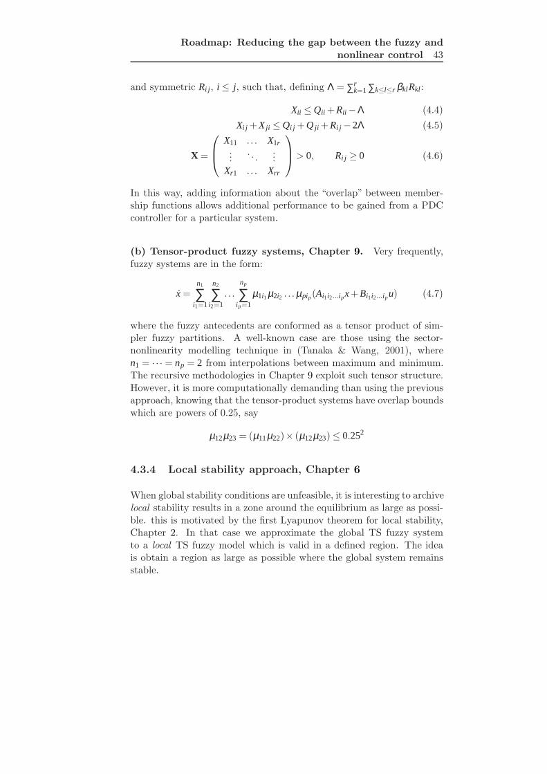
and symmetric Ri j, i≤ j, such that, defining Λ = ∑rk=1∑k≤l≤r βklRkl:
Xii ≤Qii + Rii−Λ (4.4)
Xi j + X ji ≤Qi j + Q ji + Ri j−2Λ (4.5)
X =
X11 . . . X1r...
. . ....
Xr1 . . . Xrr
> 0, Ri j ≥ 0 (4.6)
In this way, adding information about the “overlap” between member-ship functions allows additional performance to be gained from a PDCcontroller for a particular system.
(b) Tensor-product fuzzy systems, Chapter 9. Very frequently,fuzzy systems are in the form:
x =n1
∑i1=1
n2
∑i2=1
. . .np
∑ip=1
µ1i1µ2i2 . . .µpip(Ai1i2...ipx+ Bi1i2...ipu) (4.7)
where the fuzzy antecedents are conformed as a tensor product of sim-pler fuzzy partitions. A well-known case are those using the sector-nonlinearity modelling technique in (Tanaka & Wang, 2001), wheren1 = · · · = np = 2 from interpolations between maximum and minimum.The recursive methodologies in Chapter 9 exploit such tensor structure.However, it is more computationally demanding than using the previousapproach, knowing that the tensor-product systems have overlap boundswhich are powers of 0.25, say
µ12µ23 = (µ11µ22)× (µ12µ23)≤ 0.252
4.3.4 Local stability approach, Chapter 6
When global stability conditions are unfeasible, it is interesting to archivelocal stability results in a zone around the equilibrium as large as possi-ble. this is motivated by the first Lyapunov theorem for local stability,Chapter 2. In that case we approximate the global TS fuzzy systemto a local TS fuzzy model which is valid in a defined region. The ideais obtain a region as large as possible where the global system remainsstable.

44 Some Lights
If the membership functions µ(x) of the fuzzy system (3.14) in aregion Ω can be expressed as
µ(x) =nv
∑p=1
βp(x)vp, ∀ x ∈Ω (4.8)
then the system can be equivalently expressed as:
x =n
∑i=1
n
∑j=1
βiβ j(A∗i −B∗i F∗j )x (4.9)
where
A∗p =n
∑i=1
vpiAi (4.10)
B∗p =n
∑i=1
vpiBi (4.11)
F∗p =n
∑i=1
vpiFi (4.12)
nv
∑p=1
βp(x) = 1 βp(x) > 0 ∀x ∈Ω p = 1. . .nv
This model is valid only in the region Ω. If the region is close tox = 0 then the TS model tends to the linearised model of the system atthe equilibrium point. Therefore if the linearised system is stable withthis local modelling we will find an ellipsoidal region Ω∗ ⊂Ω where thesystem is stable.
4.3.5 Uncertain memberships, Chapter 8
The majority of works on fuzzy control for TS models assume that themembership functions are known. But, in most cases, the applied mem-berships functions are only an approximation. As the memberships areneeded to compute the PDC controller that stabilize the plant, the con-ditions in Section 3.5 cannot be applied to prove stability. New shape-dependent LMI conditions have been developed and the allowed uncer-tainty description is more general than that in (Lam & Leung, 2005),which did consider only multiplicative uncertainty.
Roadmap: Reducing the gap between the fuzzy andnonlinear control 45
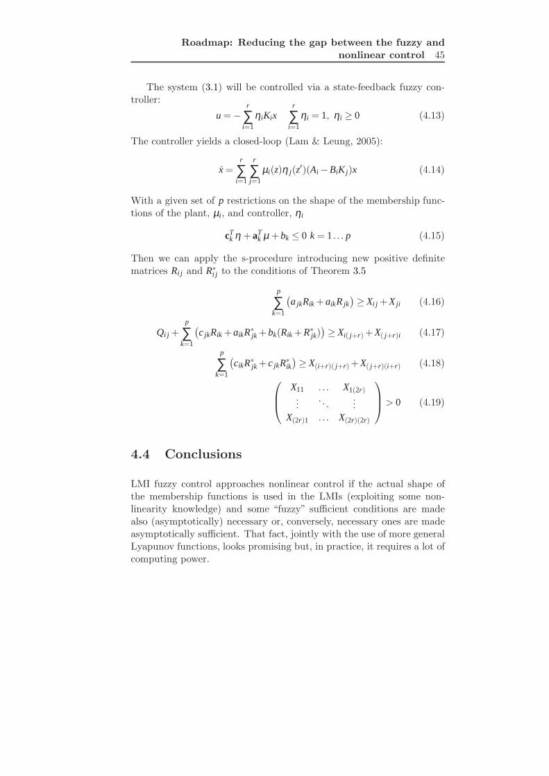
The system (3.1) will be controlled via a state-feedback fuzzy con-troller:
u =−r
∑i=1
ηiKixr
∑i=1
ηi = 1, ηi ≥ 0 (4.13)
The controller yields a closed-loop (Lam & Leung, 2005):
x =r
∑i=1
r
∑j=1
µi(z)η j(z′)(Ai−BiK j)x (4.14)
With a given set of p restrictions on the shape of the membership func-tions of the plant, µi, and controller, ηi
cTk η + aT
k µ + bk ≤ 0 k = 1. . . p (4.15)
Then we can apply the s-procedure introducing new positive definitematrices Ri j and R∗i j to the conditions of Theorem 3.5
p
∑k=1
(
a jkRik + aikR jk)
≥ Xi j + X ji (4.16)
Qi j +p
∑k=1
(
c jkRik + aikR∗jk + bk(Rik + R∗jk))
≥ Xi( j+r) + X( j+r)i (4.17)
p
∑k=1
(
cikR∗jk + c jkR∗ik)
≥ X(i+r)( j+r) + X( j+r)(i+r) (4.18)
X11 . . . X1(2r)...
. . ....
X(2r)1 . . . X(2r)(2r)
> 0 (4.19)
4.4 Conclusions
LMI fuzzy control approaches nonlinear control if the actual shape ofthe membership functions is used in the LMIs (exploiting some non-linearity knowledge) and some “fuzzy” sufficient conditions are madealso (asymptotically) necessary or, conversely, necessary ones are madeasymptotically sufficient. That fact, jointly with the use of more generalLyapunov functions, looks promising but, in practice, it requires a lot ofcomputing power.


Chapter 5
Relaxed LMI conditions, an asymptotically
approach
5.1 Introduction
The aim of this chapter is to provide a set of progressively less conserva-tive sufficient conditions in order to prove stability or performance con-ditions for Takagi-Sugeno Fuzzy systems. These conditions are asymp-totically necessary. This is not a new area in Fuzzy control, there aremany literature references in the area of stability and performance con-ditions of Takagi-Sugeno (TS) (Takagi & Sugeno, 1985) fuzzy controlsystems. Currently, most of the significant results use a linear matrixinequality (LMI) approach (Boyd et al., 1994), which reached maturityin the fuzzy area with (Tanaka & Wang, 2001).
Basically, the most frequently considered setting is parallel-distrib-uted-compensation (PDC), in which a fuzzy TS controller shares themembership functions with the plant to be controlled. In many cases,PDC fuzzy control design involves checking positivity of “double” fuzzysummations in the form (3.23).
The first nontrivial sufficient conditions for such positivity were re-ported in the 1990’s (Tanaka & Wang, 2001). Later research has focusedin conceiving less conservative LMI conditions, such as the ones in (Kim& Lee, 2000; Teixeira et al., 2003; Liu & Zhang, 2003). Recently, (Fanget al., 2006) provided sufficient conditions which are less conservativethan those in (Kim & Lee, 2000; Teixeira et al., 2003; Liu & Zhang,2003). However, the problem of finding necessary and sufficient posi-tivity conditions (i.e., the “least conservative sufficient conditions”) forfuzzy summations remains open. Note that, even if necessary and suf-
47

48 Problem statement
ficient conditions for fuzzy summations were found, conservatism wouldremain in many cases due to the limited choices of Lyapunov functions(for instance, quadratic stability is more conservative than other possi-bilities, such as the ones in (Guerra & Vermeiren, 2004)).
This chapter provides an infinite family of sufficient conditions forpositivity of fuzzy summations which improve over the ones in (Kim &Lee, 2000; Teixeira et al., 2003; Liu & Zhang, 2003; Fang et al., 2006)(actually, the cited conditions are particular cases). A theorem is pre-sented which introduces a parameter, n, related to the complexity of theresulting LMI conditions. As n increases, the conditions are asymptoti-cally exact, i.e., they become necessary for a large enough n. The resultsin this work are based on Polya’s theorems on positivity of homogeneousforms in the standard simplex which date back to the 1920’s (Polya &Szego, 1928), refined in (Powers & Reznick, 2001; Loera & Santos, 1996;Scherer, 2005).
The presented results close an open theoretical problem, in an asymp-totic sense. In practice, however, there are two shortcomings: first,bounds on n to achieve necessity and sufficiency can be stated for fixedQi j in (3.23), but that is not the case if Qi j contain LMI decision vari-ables (then, a sort of “tolerance” parameter needs to be introduced);second, the reachable value of n is limited by numerical precision ofsolver software and the available computing power.
5.2 Problem statement
Widely-used conditions (Tanaka & Wang, 2001; Sala et al., 2005; Guerra& Vermeiren, 2004; Fang et al., 2006) for stability or performance of aclosed-loop fuzzy control system may be expressed, for some matricesQi j (assumed symmetric, without loss of generality), in the form (3.23)
Ξ(t) =r
∑i=1
r
∑j=1
µi(z)µ j(z)xT Qi jx > 0 ∀x 6= 0
where z and x are system variables which change with time and µi(z)denotes the membership functions of a fuzzy partition
µ1(z),µ2(z), . . . ,µr(z)
being z a set of known variables, and r the number of “rules”.

Relaxed LMI conditions, an asymptotically approach 49
A well-known example (Tanaka & Wang, 2001) of conditions forquadratic stabilizability of a continuous-time Takagi-Sugeno (TS) fuzzysystem
x =r
∑i=1
µi(z)(Aix+ Biu)
with a parallel-distributed compensator (3.4) u =−∑ri=1 µi(z)Kix may be
written, for some symmetric matrix T > 0, in the form (3.23) as it isshown in Chapter 3. Where the most important stability and perfor-mance conditions are expressed in this way.
Importantly, if Qi j are linear in some matrix decision variables, linearmatrix inequality (LMI) techniques (Boyd et al., 1994; Tanaka & Wang,2001) may be used to find feasible values for the unknown matrices, ifsufficient LMI conditions for (3.23) to hold are stated; the objective ofthis chapter is studying such sufficient conditions. Historically, condi-tions in (Tanaka & Wang, 2001):
Qii > 0, Qi j + Q ji > 0 ∀ i, j = 1, . . . ,r i≤ j (5.1)
were the first proposed ones, which have been generalised in literature(Kim & Lee, 2000; Liu & Zhang, 2003; Teixeira et al., 2003). Recently,(Fang et al., 2006) provided some sufficient conditions which improvedover the previously cited ones. Section 5.3 will further improve suchconditions.
As a generalization of (3.23), other fuzzy control results require pos-itiveness of a p-dimensional fuzzy summation, i.e., checking
Ξ(t) =r
∑i1=1
r
∑i2=1
. . .r
∑ip=1
µi1(z)µi2(z) . . . µip(z)xT Qi1i2...ipx > 0 ∀x 6= 0 (5.2)
The case p = 2 reduces to (3.23). Conditions requiring p = 3 are, for in-stance, the fuzzy dynamic controllers in (Li, Niemann, Wang, & Tanaka,1999; Tanaka & Wang, 2001), using Qi jk = Ei jk + ET
i jk, with
Ei jk =
(
AiQ11+ BiC jk Ai + BiD jCk
Ai jk AiP11+Bi jCk
)
< 0 (5.3)
or the output-feedback ones in (Fang et al., 2006; Chen et al., 2005).For convenience, shorthand µi denoting µi(z) will be used in the fromnow on.

50 Problem statement
5.2.1 Multi-index notation.
In order to streamline notation in multi-dimensional summations (5.2),the following notation will be used:
Ip = i = (i1, i2, . . . , ip) ∈ Np | 1≤ i j ≤ r ∀ j = 1,2, . . . , p (5.4)
∑i∈Ip
γi =r
∑i1=1
r
∑i2=1
. . .r
∑ip=1
γi1i2...ip (5.5)
For some suitably defined multi-dimensional γi = γi1i2...ip (γi1i2...ip will beeither a number or a matrix), i.e., boldface symbol i will denote a multi-index in a p-dimensional index set Ip (Ip has rp elements). For instance,triple-summations in a four-rule fuzzy system will be spanned by a multi-index i ∈ I3, where I3 has 43 elements:
1,1,1,1,1,2, . . . ,1,1,4,1,2,1, . . . ,4,4,4
By convention, the juxtaposition of several multi-indices, resultingin a higher-dimensional one, will be symbolized by parentheses:
i ∈ Ip, j ∈ Iq, . . . ,m ∈ It ⇒ k = (i, j, . . . ,m) ∈ Ip+q+···+t (5.6)
When the context is clear, by mere concatenation k = ij . . .m. One-dimensional indices, say j ∈ I1 are ordinary integer index variables: theywill be typed in italic typeface (say, j, 1≤ j ≤ r) when its one-dimen-sionality should be emphasized.
Multi-dimensional fuzzy summations. The purpose of multi-indexnotation is to compactly represent multi-dimensional fuzzy summations,as follows.
First, let us define the following notation, specific for membershipfunctions as a shorthand for a product:
µi =p
∏l=1
µil = µi1µi2 . . .µip i ∈ Ip (5.7)
For instance µ(3,5,1,1) = µ3µ5µ21 will be the membership associated to the
term Q(3,5,1,1) in a 4-dimensional fuzzy summation with 5 or more rules.Note that if t = (i,k)
µt = µiµk (5.8)
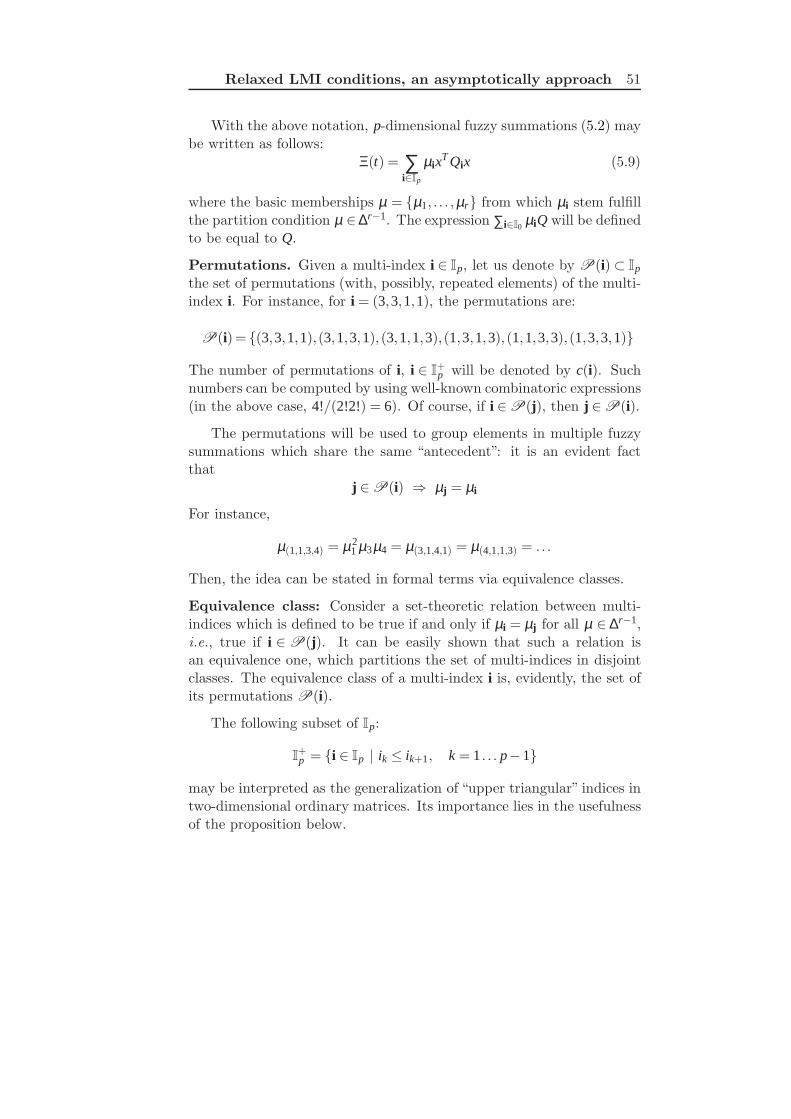
Relaxed LMI conditions, an asymptotically approach 51
With the above notation, p-dimensional fuzzy summations (5.2) maybe written as follows:
Ξ(t) = ∑i∈Ip
µixT Qix (5.9)
where the basic memberships µ = µ1, . . . ,µr from which µi stem fulfillthe partition condition µ ∈∆r−1. The expression ∑i∈I0
µiQ will be definedto be equal to Q.
Permutations. Given a multi-index i ∈ Ip, let us denote by P(i) ⊂ Ip
the set of permutations (with, possibly, repeated elements) of the multi-index i. For instance, for i = (3,3,1,1), the permutations are:
P(i)= (3,3,1,1),(3,1,3,1), (3,1,1,3),(1,3,1,3), (1,1,3,3),(1,3,3,1)
The number of permutations of i, i ∈ I+p will be denoted by c(i). Such
numbers can be computed by using well-known combinatoric expressions(in the above case, 4!/(2!2!) = 6). Of course, if i ∈P(j), then j ∈P(i).
The permutations will be used to group elements in multiple fuzzysummations which share the same “antecedent”: it is an evident factthat
j ∈P(i) ⇒ µj = µi
For instance,
µ(1,1,3,4) = µ21µ3µ4 = µ(3,1,4,1) = µ(4,1,1,3) = . . .
Then, the idea can be stated in formal terms via equivalence classes.
Equivalence class: Consider a set-theoretic relation between multi-indices which is defined to be true if and only if µi = µj for all µ ∈ ∆r−1,i.e., true if i ∈P(j). It can be easily shown that such a relation isan equivalence one, which partitions the set of multi-indices in disjointclasses. The equivalence class of a multi-index i is, evidently, the set ofits permutations P(i).
The following subset of Ip:
I+p = i ∈ Ip | ik ≤ ik+1, k = 1. . . p−1
may be interpreted as the generalization of “upper triangular” indices intwo-dimensional ordinary matrices. Its importance lies in the usefulnessof the proposition below.

52 Relaxed positivity conditions via dimensionalityexpansion
Proposition 5.1 Given any index j ∈ Ip, there exists a unique permu-tation of it, say i, which belongs to I
+p ( i.e, P(j) ∩ I
+p has only one
element). Hence, given any Qj, j ∈ Ip:
∑j∈Ip
µjQj = ∑i∈I
+p
∑j∈P(i)
µjQj = ∑i∈I
+p
µi ∑j∈P(i)
Qj =
= ∑i∈I
+p
µiQi =r
∑i1=1
r
∑i2=i1
. . .r
∑ip=ip−1
µi1µi2 . . .µip Qi (5.10)
where Qi = ∑j∈P(i) Qj.
Proof is evident by arranging the elements of j in increasing order,giving a unique permutation i in I
+p which belongs to the equivalence
class of j. The number of elements in I+p is the number of equivalence
classes. Then, Qi is just the sum of all Qj for all j in the equivalenceclass of i.
Remark: Expression (5.10) is a compact way of writing a multiplefuzzy summation as an homogeneous polynomial in µ , with coefficientsxT Qix. For instance, for p = 3 and r = 2 and some Qj:
∑j∈I3
µjxT Qjx = xT (µ3
1Q111+ µ21µ2Q112+ µ1µ2
2Q122+ µ32Q222
)
x
is an homogeneous polynomial1 of degree 3 in µ , where
Q111 = Q111, Q112 = Q112+ Q121+ Q211
Q122 = Q122+ Q212+ Q221, Q222 = Q222
5.3 Relaxed positivity conditions via dimen-
sionality expansion
As previously discussed, the most trivial sufficient check of (3.23) ischecking positive-definiteness of Qi j, which often fails. This section dis-cusses two possible paths in order to obtain less conservative conditions;
1evidently, it is also an homogeneous polynomial of degree 2 in x, i.e., a quadraticform.

Relaxed LMI conditions, an asymptotically approach 53
the first option will resort to splitting the number of positivity condi-tions, the second option will discuss the addition of artificial decisionvariables.
The results below will be based on the evident fact that
1 =r
∑i=1
µi =
(
r
∑i=1
µi
)p
= ∑i∈Ip
µi (5.11)
for any positive integer p.
5.3.1 Relaxation by increasing the number of positivityconditions
Now, consider the 2-dimensional fuzzy summation (3.23). Based on(5.11), proving (3.23) is equivalent to proving, for n≥ 2:
[Ξ]n(t) =
(
r
∑i=1
µi
)n−2
· Ξ(t) = ∑i∈In
µixT Qi1i2x > 0 (5.12)
i.e., a 2-dimensional fuzzy summation may be expanded to any desiredlevel of nested sums. Of course, [Ξ]n = Ξ, i.e., notation [Ξ]n will denotethe equivalent expression of Ξ as an homogeneous polynomial of degree nappearing in (5.12) above. [Ξ]n will be referred to as the dimensionalityexpansion of degree n.
The parameter n may be considered as a sort of complexity param-eter. The results in this section will show that the larger n is, the lessconservative the proposed conditions are, but the more computationallydemanding the procedure is.
Note that, by using Proposition 5.1:
[Ξ]n = ∑i∈In
µixT Qi1i2x = ∑
i∈I+n
µi ∑j∈P(i)
xT Q j1 j2x = ∑i∈I
+n
µixT Qix (5.13)
whereQi = ∑
j∈P(i)
Q j1 j2 (5.14)
For instance, given i = 1,1,1,3, which has four permutations
1,1,1,3, 1,1,3,1, 1,3,1,1, 3,1,1,1

54 Relaxed positivity conditions via dimensionalityexpansion
results in Qi = Q11+ Q11+ Q13+ Q31 = 2Q11+ Q13+ Q31.
Let us now consider conditions for proving positivity of Ξ in (3.23).
Proposition 5.2 For a fixed n, the positive-definiteness conditions
Qi = ∑j∈P(i)
Q j1 j2 > 0 ∀ i ∈ I+n (5.15)
are sufficient for positivity of Ξ in (3.23).
Proof: it is almost evident as, Ξ = [Ξ]n = ∑i∈I+p
µixT Qix. Hence, Ξ isexpressed as a sum of positive terms if (5.15) holds (as µi ≥ 0).
Theorem 5.1 (Matrix Polya Theorem) For each collection of ma-trices Qi j fulfilling (3.23), i.e., Ξ > 0 for any fuzzy partition µ and anyx 6= 0, there exists a finite n such that condition (5.15) holds, i.e., (5.15)become necessary and sufficient for some finite value of n.
Proof: The proof follows the lines of a similar result in (Scherer,2005) in a different context. Consider ‖x‖ to be the Euclidean norm ofvector x in (3.23). Denote as
κ = min‖x‖=1,µ∈∆r−1
Ξ (5.16)
which, by assumption exists and is positive (existence is proved by con-tinuity of polynomials and compactness of the finite-dimensional unitballs and the simplex ∆r−1). Denote as
L = maxi≤ j
1c(i j)
max(λmax(Qi j),−λmin(Qi j)) (5.17)
where Qii = Qii, Qi j = Qi j + Q ji, for i 6= j, arise from the permutationequivalence classes of 2-dimensional indices, and the cardinals are c(ii) =1, and for j 6= i, c(i j) = 2. For any i ≤ j, as λmax(Qi j) < c(i j)L andλmin(Qi j)‖x‖ ≤ xT Qi jx ≤ λmax(Qi j)‖x‖, the constant L is positive (other-wise Ξ would be non-positive for all x, contradicting the assumptions)and |xT Qi jx| ≤ c(i j)L‖x‖ holds for any vector x.
For a fixed x, expression (3.23) is an homogeneous polynomial in µof degree 2, whose coefficients are xT Qiix = xT Qiix (those multiplying µ2
i )

Relaxed LMI conditions, an asymptotically approach 55
and xT Qi jx = xT (Qi j +Q ji)x (those multiplying µiµ j for i≤ j). Hence, forany x with unit norm, (3.23) is an homogeneous polynomial in µ whoselower value is greater than κ (by definition) in the standard simplex,and whose coefficients (divided by the cardinal of the correspondingpermutation) are upper bounded by L in absolute value. Then, from(Powers & Reznick, 2001) (use notation λ = κ , d = 2, aα = xT Qi jx, N =n−2 in (Powers & Reznick, 2001)), for any value of n such that:
n >Lκ
, n≥ 2
all coefficients of the corresponding dimensionality expansion of degreen (i.e., xT Qix, i ∈ I
+n ) will be positive. As x is an arbitrary unit norm
vector, xT Qix > 0 entails Qi being a positive definite matrix, denoted asQi > 0 in (5.15).
The reader is referred to Example 5.1 in the following section, whichillustrates conditions (5.15) for different settings.
Remark: it is easily shown that if (5.15) holds for some n0, it doesfor any n≥ n0 (indeed, the coefficients of [Ξ]n are a positive linear com-bination of those of [Ξ]m if n≥m). Hence, the conditions in Proposition5.2 are less and less conservative as n increases, becoming asymptot-ically exact: if (3.23) holds, a large enough dimensionality expansionn will hold. Hence, when n→ ∞, (5.15) and (3.23) become equivalentconditions.
Using the bound2 for n provided in the proof of Theorem 5.1, aversion of it can be rewritten as stated below, where f loor(a) denotesthe largest integer s such that s≤ a.
Theorem 5.2 The first of the following statements implies the secondone:
1. For any fuzzy partition µ ∈ ∆r−1, for any vector x 6= 0, given anytolerance level κ > 0
r
∑i=1
r
∑j=1
µiµ jxT Qi jx≥ κxT x
2 The upper bound for finding the required n is not tight. Providing tighter boundsthan L/κ in the second condition is a matter of current research. In (Loera & Santos,2001) other bounds and conjectures are put forward.

56 Relaxed positivity conditions via dimensionalityexpansion
2. There exists n ∈ N, 2≤ n ≤ f loor( Lκ + 1) (L as defined in (5.17)),
such that
∑j∈P(i)
Q j1 j2 > 0 ∀ i ∈ I+n
The “gap” between Theorem 5.2 and the necessary and sufficientconditions sought after in the fuzzy control community is now expressedvia the tolerance level κ , which may be chosen to be as small as desired.
Note that, in the case Qi j includes some decision variables (for sub-sequent LMI optimizations), the constraint −L · I ≤ Qi j/c(i j) ≤ L · I fora predefined L should be enforced3 (in addition to the tolerance κ) toensure that (5.17) holds, in order to compute the bound for n.
5.3.2 Relaxation via artificial decision variables
This subsection discusses a closely related path to obtaining sufficientconditions for positivity of fuzzy summations, based on the introductionof artificial decision variables. These will allow using a much lower valuefor n, compared to the one required in the previous theorems.
Theorem 5.3 A sufficient condition for positivity of Ξ in (3.23) is thepositivity condition below, for n≥ 2:
∑k∈In−2
µkξ T
X(k,1,1) . . . X(k,1,r)...
. . ....
X(k,r,1) . . . X(k,r,r)
ξ > 0 (5.18)
if there exist matrices Xj, j ∈ In so that
∑j∈P(i)
Q j1 j2 ≥ ∑j∈P(i)
12(Xj + XT
j ) ∀ i ∈ I+n (5.19)
Proof: Starting from (5.12):
Ξ = [Ξ]n = ∑i∈In
µixT Qi1i2x = ∑
i∈I+n
µi ∑j∈P(i)
xT Q j1 j2x (5.20)
3Usually, in Lyapunov-function-based fuzzy control setups, such constraint can beenforced with no loss of generality as Lyapunov functions can be arbitrarily scaled.

Relaxed LMI conditions, an asymptotically approach 57
Hence, if (5.19) holds, as µi ≥ 0,
∑i∈I
+n
µi ∑j∈P(i)
xT Q j1 j2x≥ ∑i∈I
+n
µi ∑j∈P(i)
xT 12(Xj + XT
j )x =
= ∑i∈I
+n
µi ∑j∈P(i)
xT Xjx = ∑i∈In
µixT Xix =
= ∑k∈In−2
r
∑i=1
r
∑j=1
µkµiµ jxT X(k,i, j)x =
= ∑k∈In−2
µkξ T
X(k,1,1) . . . X(k,1,r)...
. . ....
X(k,r,1) . . . X(k,r,r)
ξ (5.21)
where ξ = (µ1xT µ2xT . . . µrxT )T . Hence, if (5.18) holds, (3.23) also does.For n = 2, the leftmost summation over In−2 in the last two expressionsmust be deleted (this case is a well-known result in (Liu & Zhang, 2003)).
Note that, without loss of generality, the equality restrictions X(k,i,i) =XT
(k,i,i) and X(k,i, j) = XT(k, j,i) can be enforced, as the sign of (5.18) only de-
pends on the symmetric component. In this way, the number of decisionvariables is reduced.
Corollary 5.1 Given some Qi j fulfilling (3.23), if conditions (5.15) holdfor some n, then there exist feasible Xi in Theorem 5.3 for a lower orequal value of n.
Proof: As (5.15) holds by assumption, there exists n0 such that theleft-hand side of (5.19) is positive-definite for all i ∈ In for any n ≥ n0.Then, consider the same value of n0 for Theorem 5.3, and denote by Ithe identity matrix. Take X(k,i,i) = εI > 0, and X(k,i, j) = 0 when i 6= j.It’s easy to check that condition (5.19) holds for a sufficiently smallε . Furthermore, all matrices being added in (5.18) are positive definite(they are εI). In this way, a feasible set of decision variables for Theorem(5.3) has been found.
The examples in the following section will show that the actuallyneeded value of n is much lower for Theorem 5.3 than Theorem 5.1, dueto the new decision variables introduced.

58 Relaxed positivity conditions via dimensionalityexpansion
Theorem 5.3 is still not useful, because it replaces a positivity con-dition (3.23) with another similar one (5.18) with a possibly higher di-mension. Hence, some extra developments (useful for their own sake,anyway) are needed in order to turn Theorem 5.3 into a practically ap-plicable solution.
5.3.3 Generalization to higher-dimensional fuzzy summa-tions
Polya’s theorem applies to homogeneous forms (Loera & Santos, 1996,2001; Powers & Reznick, 2001) of any dimension (5.2), and not only toquadratic forms (3.23). Hence, the results can be generalised to otherfuzzy control setups involving p-dimensional fuzzy summations for anyp, as proposed below.
Theorem 5.4 Consider proving positivity of a p-dimensional fuzzy sum-mation (p≥ 2) for some fuzzy partition ∑i∈Ip
µi = 1, given by (5.2). Con-sider now its dimensionality expansion [Ξ]n = (∑r
i=1 µi)n−pΞ, with n≥ p.
Then, a sufficient condition for Ξ > 0 when x 6= 0 is
∑k∈In−2
µkξ T
X(k,1,1) . . . X(k,1,r)...
. . ....
X(k,r,1) . . . X(k,r,r)
ξ > 0 for ξ 6= 0 (5.22)
if there exist matrices Xi, i ∈ In, so that:
∑j∈P(i)
Q j1 j2... jp > ∑j∈P(i)
12(Xj + XT
j ) ∀ i ∈ I+n (5.23)
Furthermore, the condition is asymptotically exact with a large enoughn so a statement analogous to Theorem 5.2 can be made.
Proof: The proof of the above theorem follows identical lines to thatof Theorem 5.3, just by changing j1 j2 in (5.20) and (5.21) to j1 j2 . . . jp.
In order to prove the asymptotic exactness, matrix Polya theoremcan be also set up for p greater than 2, resulting in a bound n > p(p−1)L
2κ(Powers & Reznick, 2001) for which positivity of all Qi holds. Hence, itis easy to show that, given some Qi, i ∈ Ip, if (5.2) holds, then Theorem

Relaxed LMI conditions, an asymptotically approach 59
5.4 will hold for a large enough n, i.e., it is asymptotically exact, and nwill be lower or equal than p(p−1)L
2κ +1. Details are omitted for brevity,as they are a replica of those discussed for p = 2.
Theorem 5.4 reduces to Theorem 5.3 for p = 2. The case p = 3would directly apply to the cubic parametrization dynamic controllersin (Li et al., 1999; Tanaka & Wang, 2001) or the output feedback fuzzycontrollers in (Chen et al., 2005; Fang et al., 2006).
Remark: note that n can be equal to p in Theorem 5.4. The suffi-cient conditions arising from this choice will be denoted as non-expandedconditions: such conditions state positivity of a p-dimensional summa-tion if a particular (p−2)-dimensional positivity condition holds.
5.3.4 Recursive procedure
The previous remark provides the missing link in order to express aversion of Theorems 5.3 and 5.4 computable in practice. This sectiondiscusses a methodology to set up a collection of LMI constraints via arecursive procedure. Note that the LMIs cannot be solved until all theconstraints, for all the recursion steps, have been set up.
Given a value of the complexity parameter n ≥ 2, a super-index insquare brackets will be used to indicate recursion steps, denoted byh = 0,1, . . . ,hmax = f loor((n−1)/2).
Theorem 5.5 Computable sufficient conditions for proving positivenessof a p-dimensional fuzzy summation may be obtained as follows, for anydesired value of the complexity parameter n:
1. ( initialisation) Obtain the dimensionality expansion of degree n of
the fuzzy summation, n ≥ p, setting Q[0]i = Qi1i2...ip, i ∈ In. The
dimension of the multi-indices in iteration step h will be denotedby dh, starting with d0 = n.
2. ( recursive procedure) Consider now iteration step h≥ 0, trying to
set up sufficient conditions for ∑i∈IdhxT Q[h]
i x > 0, with dh > 2. Apply
Theorem 5.4 by setting a constraint (5.23) and then considering a

60 Relaxed positivity conditions via dimensionalityexpansion
new (dh−2)-dimensional summation (5.22), i.e.:
∑j∈P(i)
Q[h]j > ∑
j∈P(i)
12(X [h]
j +(X [h]j )T ) ∀ i ∈ I
+dh
(5.24)
∑k∈Idh−2
µkξ T
X [h](k,1,1) . . . X [h]
(k,1,r)...
. . ....
X [h](k,r,1) . . . X [h]
(k,r,r)
ξ > 0 for ξ 6= 0 (5.25)
Note that any sufficient condition for (5.25) implies positivity ofthe original summation. Then, considering dh+1 = dh−2, and
Q[h+1]k =
X [h](k,1,1) . . . X [h]
(k,1,r)...
. . ....
X [h](k,r,1) . . . X [h]
(k,r,r)
k ∈ Idh+1 (5.26)
expression (5.25) may be written as
∑i∈Idh+1
µiξ T Q[h+1]i ξ > 0 (5.27)
i.e., sufficient conditions for (5.25) may be stated applying non-expanded conditions (5.24) and (5.25) recursively, until h = hmax
is reached, and dhmax = 1 or dhmax = 2, depending on whether thestarting complexity parameter n is odd or even, respectively.
3. ( termination) Use either the well-known sufficient conditions in(Tanaka & Wang, 2001) for 1-dimensional sums when dhmax = 1, orthose in (Liu & Zhang, 2003) for 2-dimensional ones when dhmax =2.
The result of the above procedure is a set of conditions which are suffi-cient for the positivity of Ξ in (3.23). LMI conditions are obtained if theoriginal Qi are affine in some matrix decision variables.
Proof: Proof is evident and almost outlined in the theorem state-ment, which describes an algorithm. Indeed, given a p-dimensional sum-mation Ξ, for a chosen n, the recursion above sets up a “ladder” of suf-ficient conditions with dimension n− 2, n− 4, . . . , so that each one is

Relaxed LMI conditions, an asymptotically approach 61
a sufficient condition for the preceding one, i.e., the following chain ofimplications can be built:
[p-dimensional sum]: Ξ > 0 ⇔ [n-dimensional sum]: [Ξ]n > 0
⇑(5.25)[n−2-dimensional sum] and (5.24), d0 = n
⇑(5.25)[n−4-dimensional sum] and(5.24), d1 = n−2
⇑. . .
Hence, proving the final conditions , i.e., ∑i∈Idhmaxµiξ T Q[hmax]
i ξ > 0 entails
proving the initial p-dimensional condition and, as those conditions havedimensionality one or two, standard literature results can be used (mostof which, in fact, are particular cases of Proposition 5.2 and Theorem5.3, see Section 5.3.6). Once all conditions have been set up, an LMIsolver can be used.
5.3.5 Number of conditions and decision variables
The number of conditions needed in Proposition 5.2 is the number ofelements in I
+n , i.e., the combinatorial number:
NC1 =
(
r + n−1n
)
Proving positivity of fuzzy summations via the sufficient conditions inProposition 5.2 does not need any new decision variable apart from thosein Qi j. NC1 grows approximately as O(nr−1) when n grows.
The above expression also gives the number of conditions (5.24) ina particular iteration (replacing n by dh). Hence, the total number ofconditions (5.24) is:
NC =hmax
∑h=0
(
r + n−2h−1n−2h
)
and, after applying the termination conditions:
NC2 = NC + r(r +1)/2+1, NC2 = NC + r

62 Relaxed positivity conditions via dimensionalityexpansion
if n was even or odd, respectively. NC2 grows at the rate O(nr) when ngrows.
With r rules, if Qi were t×t, the matrices Q[h]i are of size (t ·rh)×(t ·rh).
Hence, after symmetry considerations, a number of trh(trh−1)/2 decisionvariables is introduced for each h, i.e., the recursive procedure needs NVdecision variables with NV given by
NV =hmax
∑h=1
trh(trh−1)/2 (5.28)
If dhmax = 2, then (Liu & Zhang, 2003) needs additional decision vari-ables: the total number is obtained by replacing hmax by hmax + 1 in(5.28). The rate of growth with n is O(rn).
In summary, the number of conditions is polynomial-complexity in n,but the number of decision variables in the recursive procedure is expo-nential in n. To avoid such explosion of decision variables, some simplifi-cations can be made, such as choosing a lower-dimensional arrangementfor X variables, i.e., Xi = Xi1...iq with i ∈ Ip, q ≤ p (see Example 5.1 inSection 5.4).
5.3.6 Comparison to previous literature
The presented approach includes previous literature results on relaxedLMI conditions for fuzzy control as a particular case.
Corollary 5.2 Proposition 5.2 with n = 2 are the conditions stated inTheorem 7 in (Tanaka & Wang, 2001);
Proof: Indeed, restating Proposition 5.2 for the particular case inconsideration, it says that ∑r
i=1∑ri=1 µiµ jxT Qi jx > 0 if Qii > 0 (for the
only permutation of the multi index i, i) and Qi j +Q ji > 0 (when i < j,corresponding to the two permutations of i, j ∈ I
+2 ) .
Corollary 5.3 if Theorem 5.3 were adapted to n = 2, conditions in (Liu& Zhang, 2003) would have been obtained.

Relaxed LMI conditions, an asymptotically approach 63
Proof: It’s evident just considering, as done above, the unique per-mutation if i, i, yielding Qii > 1
2(Xii + XTii ) in (5.19) and the permuta-
tions i, j and j, i when i < j, yielding
Qi j + Q ji <12
(
(Xi j + XTi j )+ (X ji + XT
ji))
Now consider a symmetric matrices Xi j j and Xi j = XTji , the sufficient
condition is expressed by Qii ≤ Xii and Qi j + Q ji ≤ Xi j + X ji, jointly withthe positive-definiteness of the matrix whose blocks are Xi j.
Corollary 5.4 Theorem 5.5 with p = 2, n = 3 sets up the conditions in(Fang et al., 2006).
Proof: Denote Sym(X) = 12(X + XT ). Consider a double summation
(p = 2), after a dimensionality increase (n = 3). The results in this workassert that positivity of the double summation holds when conditions(5.23) are applied, i.e., Qii ≤ Sym(Xiii) (for permutations i, i, i), Qii +Qi j +Q ji ≤ Sym(Xii j +Xi ji +X jii) (for permutations of i, i, j, i 6=
j) Qi j +Q ji +Qik +Qki +Q jk +Qk j ≤ Sym(Xi jk +X jik +Xik j +Xki j +X jki +Xk ji) (for permutations of i, j,k,l i 6= j, i 6= k, j 6= k)
and, subsequently, positivity of a one-dimensional summation ∑ri=1 µiQi
is proved, where the new Qi is formed from the decision variables Xi jk asin (5.26).
Considering now Xi j j symmetric and Xi jk = XTik j the conditions result
in: Qii ≤ Xiii, Qii + Qi j + Q ji ≤ Xii j + XTii j + X jii, Qi j +Q ji +Qik +Qki +Q jk +Qk j ≤ Xi jk +X jik +Xki j +XT
i jk +XTjik +XT
ki j

64 Examples
and the positivity of the remaining one-dimensional fuzzy summationis proved if each Qi is positive definite. The resulting conditions areanalogous (we use a more general notation) to the ones in Theorem 5 in(Fang et al., 2006).
5.4 Examples
In this section, three examples are presented. The first one illustrateshow the various Qi previously discussed are computed via combinatoricpermutation formulae. The second one applies the conditions in section5.3 to a numerical example. And the third applies these conditions toa specific Qi formed of a Quadratic Parallel Distributed Compensation(QPDC) controller. This example illustrates that the additional degreesof freedom in QPDC controllers allow to achieve a more stringent per-formance requirements than of a PDC controller.
Example 5.1 Consider proving ∑3i=1 ∑3
j=1 µiµ jxT Qi jx > 0, i.e., n = 2, r =3 with Proposition 5.2. For i = (1,1), i = (1,2), i = (1,3), i = (2,2),i = (2,3), and i = (3,3) (which are the six elements of I
+2 ), the conditions
(5.15) are, respectively,
Q11 > 0, Q12+ Q21 > 0, Q13+ Q31 > 0, (5.29)
Q22 > 0, Q23+ Q32 > 0, Q33 > 0 (5.30)
which are well-known conditions stated in (Tanaka et al., 1998; Tanaka& Wang, 2001).
Consider now a dimensionality expansion to n = 3. In order to prove
3
∑i=1
3
∑j=1
µiµ jxT Qi jx =
3
∑k=1
3
∑i=1
3
∑j=1
µkµiµ jxT Qi jx > 0
the permutations of
I+3 = (1,1,1),(1,1,2),(1,1,3),(1,2,2), (1,2,3),
(1,3,3),(2,2,2),(2,2,3),(2,3,3),(3,3,3) (5.31)

Relaxed LMI conditions, an asymptotically approach 65
must be considered. The result are the conditions
Q111 = Q11 > 0, Q112 = Q11+ Q12+ Q21 > 0,
Q113 = Q11+ Q13+ Q31 > 0, Q122 = Q12+ Q21+ Q22 > 0,
Q123 = Q12+ Q21+ Q13+ Q31+ Q23+ Q32 > 0,
Q133 = Q13+ Q31+ Q33 > 0, Q222 = Q22 > 0,
Q223 = Q22+ Q23+ Q32 > 0,
Q233 = Q23+ Q32+ Q33 > 0, Q333 = Q33 > 0 (5.32)
Observe that the obtained conditions are sums with positive coefficientsof those for n = 2 (cf. remark in page 55).
Considering now n = 8, the condition associated to the equivalenceclass of, for instance, i = (1,1,1,2,2,2,3,3) ∈ I
+8 is:
Q11122233=6!
1!3!2!Q11+
6!2!2!2!
(Q12+ Q21)+6!
3!1!2!Q22+
+6!
2!3!1!(Q13+ Q31)+
6!3!2!1!
(Q23+ Q32)+6!
3!3!0!Q33 =
60Q11+90(Q12+Q21)+60(Q13+Q31)+60(Q23+Q32)+60Q22+20Q33> 0
That of i = (1,1,1,1,1,2,3,3) is:
Q11111233=6!
3!1!2!Q11+
6!4!0!2!
(Q12+ Q21)+6!
4!1!1!(Q13+ Q31)+
+6!
5!0!1!(Q23+ Q32)+
6!5!1!0!
Q33 =
60Q11+15(Q12+ Q21)+30(Q13+ Q31)+6(Q23+ Q32)+6Q33 > 0
and so on. Of course, for large values of n, generation of the vast numberof resulting conditions must be carried out automatically by means ofa suitable computer program. For instance, the number of positivityconditions required in Proposition 5.2 for n = 50 is 1326.
As discussed in Section 5.3.5, Theorem 5.5 involves a high numberof decision variables in Xi which, however, may be reduced by stickingto a lower-dimensional X . For instance, conditions for n = 4 for a 2-rule

66 Examples
fuzzy system may be stated, taking X12 = XT21, X11 = XT
11, X22 = XT22, as:
1111 : Q11≥ X11
1112 : 2Q11+ Q12+ Q21≥ 2X11+ X12+ X21
1122 : Q11+ Q22+2Q12+2Q21≥ X11+ X22+2X12+2X21
1222 : 2Q22+ Q12+ Q21≥ 2X22+ X12+ X21
2222 : Q22≥ X22(
X11 X12
X21 X22
)
> 0
where a 2-dimensional decision variable X has been chosen instead ofthe 4-dimensional one which arises from direct application of Theorem5.5 (see next example).
Example 5.2 Consider a continuos fuzzy system, taken from Example1 in (Fang et al., 2006), defined by:
x =3
∑i=1
µi(Aix+ Biu)
where A1 =
(
1.59 −7.290.01 0
)
, B1 =
(
10
)
,
A2 =
(
0.02 −4.640.35 0.21
)
, B2 =
(
80
)
,
A3 =
(
−a −4.330 0.05
)
, B3 =
(
−b+6−1
)
.
Analogously to (Fang et al., 2006), existence of a stabilising controlleris cast as a quadratic Lyapunov condition ∑3
i=1∑3j=1 µiµ jxT Qi jx > 0 where
Qi j are defined by (3.1).
Feasibility of the sufficient conditions arising from Proposition 5.2are evaluated for different values of a, b. The obtained feasible pointsfor n = 5,10,20,35,50 are depicted in Figure 5.1. The LMI solver wasMatlab LMI Toolbox (Gahinet et al., 1995).
Similarly, results with Theorem 5.5 (n ranging from 2 to 4) for thesame grid of values for a and b are depicted in Figure 5.2. Indeed, resultsfor n = 2 and n = 3 coincide with those reported in (Fang et al., 2006).

Relaxed LMI conditions, an asymptotically approach 67
a
b
0
4
4
1
5
5
2
2
6
6
3
3
7
7
8
8
9
9 10
Legend: ×→ n = 5 , → n = 10, ⋆ → n = 20, + → n = 35, • → n = 50
Figure 5.1: Stabilization region based on Proposition 5.2 with differentvalues of n
a
b
0
4
4
1
5
5
2
2
6
6
3
3
7
7
8
8
9
9 10
Legend: × → n = 2, → n = 3, • → n = 4
Figure 5.2: Stabilization region based on Theorem 5.5 with differentvalues of n

68 Examples
As expected, n = 4 improves over those results.
Let us detail the procedure used to set up the conditions for n = 4(the notation Sym(N) = 1
2(N + NT ) will be used).
First, Theorem 5.3 with n = 4 is applied. As a result, if the followingconditions hold:
Q1111= Q11 > Sym(X1111) (5.33)
Q1112= 2Q11+1(Q12+ Q21) >
Sym(X1112+ X1121+ X1211+ X2111) (5.34)
...
Q1122= Q11+2(Q12+ Q21)+ Q22 >
Sym(X1122+ X1212+ X1221+ X2112+ X2121+ X2211) (5.35)
...
Q1223= 2(Q12+ Q21)+ (Q13+ Q31)+
2(Q23+ Q32)+2Q22 >
Sym(X1223+ X1232+ X1322+ X2123+ X2132+ X2231+
+X2213+ X2312+ X2321+ X3122+ X3212+ X3221) (5.36)
...
Q3333= Q33 > Sym(X3333) (5.37)
(the total number of elements of I+4 for r = 3 is 15, but only 5 inequalities
have been shown, for brevity) then positivity of
3
∑k=1
3
∑l=1
µklξ T Hklξ > 0 (5.38)
where
Hkl =
Xkl11 Xkl12 Xkl13
Xkl21 Xkl22 Xkl23
Xkl31 Xkl32 Xkl33
ensures that the original quadratic stabilisation conditions do also hold.
Finally, in order to test the positivity of (5.38) the conditions of (Liu& Zhang, 2003) are added, introducing decision variables Yi j fulfilling

Relaxed LMI conditions, an asymptotically approach 69
Yi j = Y Tji and
Sym(H11) > Y11 (5.39)
Sym(H22) > Y22, Sym(H33) > Y33, (5.40)
Sym(H12+ H21) > Y12+Y21 (5.41)
Sym(H13+ H31) > Y13+Y31 (5.42)
Sym(H23+ H32) > Y23+Y32 (5.43)
and
Y11 Y12 Y13
Y21 Y22 Y23
Y31 Y23 Y33
> 0 (5.44)
As a result, the problem is cast as a set of LMIs with decision variablesT and M j in Qi j, from (3.1). Also Xik jl (81 matrices of size 3×3) andthe Ymn (9 matrices of size 9×9), i.e., a total of 23 LMI’s (adding T > 0)with 504 scalar decision variables.
Note that the recursive procedure in Theorem 5.5 with n = 4 achievedbetter results than the original Polya conditions (Proposition 5.2) withn = 50. Larger values of n in the above computations resulted in nu-merical problems (slow progress) with the LMI solver, due to the largenumber of LMI constraints (in Proposition 5.2) or decision variables (inTheorem 5.5). This did not allow additional feasiblility points to befound. The average computation times in seconds per test point (304tests were needed to plot the whole figure) were, for Figure 1 0.11, 0.45,2.49, 11.5 and 33.7 s, for n = 5, 10, 20, 35 and 50, respectively (increasingthe LMI solver iteration limit to 650). Regarding Figure 2 (with defaultoptions), with n = 3 the average time per test point was 0.13 s, whereasthat for n = 4 was 11.7 s (i.e., it took about 1 hour to compute the fullfigure). The computer was a dual Pentium 4, 3.0 GHz, Matlab 7.1, 1GB RAM.
Example 5.3 (Quadratic-Parametrisation Controllers.)
Once a criterion for positivity of (5.2) is described, it will be appliedto the design of quadratic-parametrisation controllers, to be denoted asQPDC controllers:
u =−r
∑i=1
r
∑j=1
µiµ jFi jx (5.45)

70 Examples
which are a generalisation of the PDC ones, inspired on some proposalsin (Tanaka & Wang, 2001). Clearly, the PDC control law is a particularcase of the QPDC law (setting Fi j = Fi).
A Takagi-Sugeno system (3.1) under QPDC control yields a closedloop given by:
x =r
∑i=1
r
∑j=1
r
∑k=1
µiµ jµk(Ai−BiFjk)x (5.46)
Therefore, following the same reasoning than in Section 3.5, The equilib-rium of the continuous TS fuzzy system (3.1) is quadratically stabilizablevia a QPDC control law (5.45) if there exist matrices M jk such that:
∑i jk
µi jkξ T Qi jkξ > 0
where
Qi jk =−(AiX −BiM jk + XATi −MT
jkBTi )
Clearly, Theorem 5.5 can be applied to solve previous positivity con-ditions.
The system to be controlled will be taken from (Kim & Lee, 2000),and it will be given by:
x1 = x2 +sinx3−0.1x4 +(x21 +1)u
x2 = x1 +2x2 (5.47)
x3 = x21x2 + x1 (5.48)
x4 = sinx3 (5.49)

Relaxed LMI conditions, an asymptotically approach 71
Under the assumption that x1 ∈ [−a,a] and x3 ∈ [−b,b], the abovenonlinear system is exactly represented by the TS model:
A1 =
0 1 1 −0.11 2 0 01 a2 0 00 0 1 0
A2 =
0 1 sinb/b −0.11 2 0 01 a2 0 00 0 sinb/b 0
A3 =
0 1 1 −0.11 2 0 01 0 0 00 0 1 0
A4 =
0 1 sinb/b −0.11 2 0 01 0 0 00 0 sinb/b 0
B1 = B2 =(
(1+ a2) 0 0 0)T
B3 = B4 =(
1 0 0 0)T
with membership functions:
M1(x) =x2
1
a2
M3(x) =
bsinx3−x3 sinbx3(b−sinb) x3 6= 0
1 x3 = 0
µ1(x) = M1(x)M3(x)
µ2(x) = M1(x)(1−M3(x))
µ3(x) = (1−M1(x))M3(x)
µ4(x) = (1−M1(x))(1−M3(x))
In order to compare the achieved QPDC controllers with those in(Kim & Lee, 2000), the same constraints on the control input as in

72 Examples
(Kim & Lee, 2000) will be enforced. The results applying Theorem 2 in(Liu & Zhang, 2003), which relaxes some symmetry conditions in (Kim& Lee, 2000), will also be compared. The constrain ‖u‖2 ≤ δ can beexpressed in terms of QPDC controllers as
(
1 x(0)T
x(0) X
)
≥ 0 (5.50)
(
X MTii
Mii δ 2I
)
≥ Zii, i = 1...r (5.51)
(
X MTi j
Mi j δ 2I
)
+
(
X MTji
M ji δ 2I
)
≥ Zi j + ZTi j,
i = 1...r, i < j ≤ r (5.52)
Z11 . . . Z1r...
. . ....
Zr1 . . . Zrr
> 0 (5.53)
where X = P−1, Mi j = FiX , Zi j = ZTji and Zii symmetric.
Where the initial states in this example are x(0)=(
−1.2 0.5 0.7 −0.6)T
,a = 1.4 and b = 0.7.
Results: Using PDC control and (Kim & Lee, 2000), the lower boundof δ for which the resulting LMIs were feasible was 5.116. With (Liu& Zhang, 2003), the limit of δ was 4.65. For a QPDC controller, thefeasibility bound obtained with Theorem 5.2 with n = 3 is δ ≥ 4.484.Theorem 5.5 obtains a new QPDC controller with δ ≥ 4.272, significantlyimproving over previous results.
In order to show the additional flexibility of the QPDC controller,figures 5.3 (PDC) and 5.4 (QPDC) compare the first element of the 1×4state-feedback matrix F below:
u =−F(x)x =−(
F1(x) F2(x) F3(x) F4(x))
x
as a function of M1 and M3 above, used to define the membership func-tions. Indeed, the peak “gain” is reduced in the QPDC case.
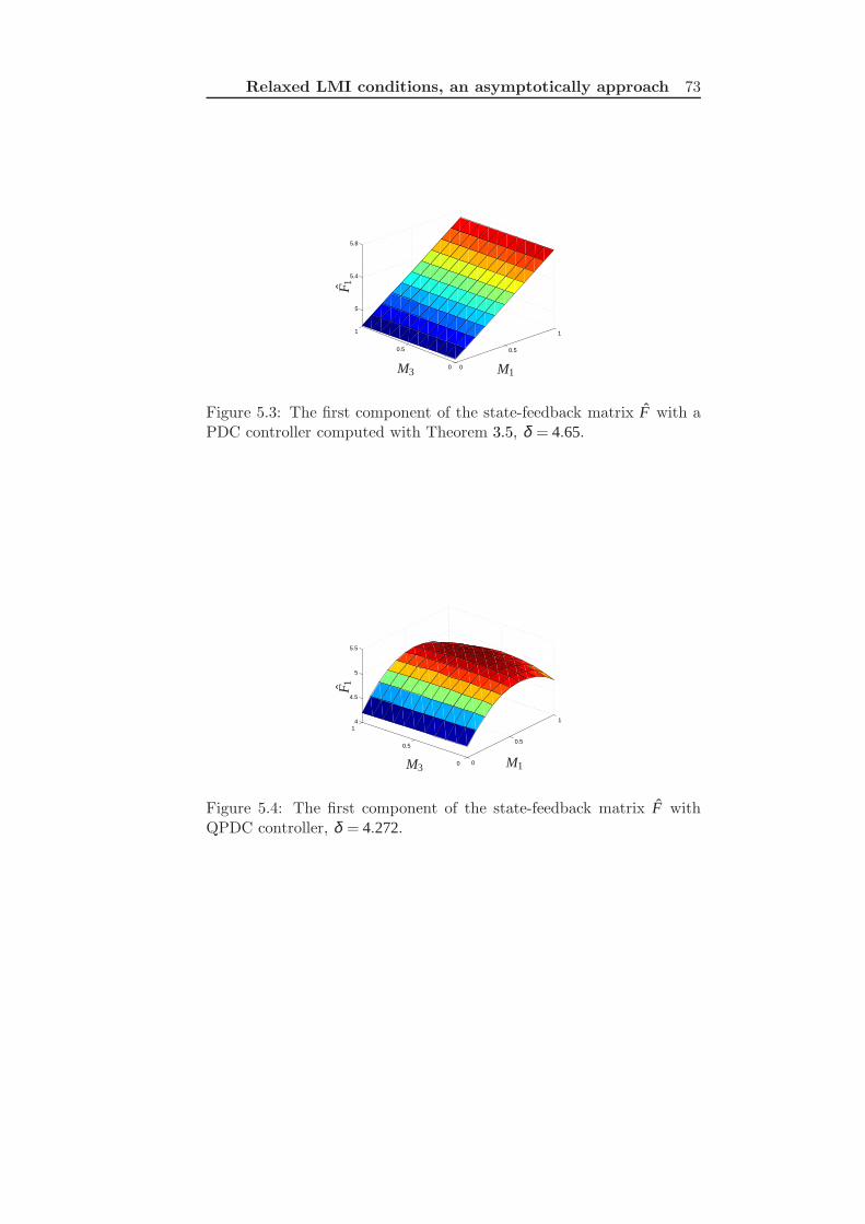
Relaxed LMI conditions, an asymptotically approach 73
0
0.5
1
0
0.5
1
5
5.4
5.8
M1M3
F 1
Figure 5.3: The first component of the state-feedback matrix F with aPDC controller computed with Theorem 3.5, δ = 4.65.
0
0.5
1
0
0.5
1 4
4.5
5
5.5
M1M3
F 1
Figure 5.4: The first component of the state-feedback matrix F withQPDC controller, δ = 4.272.

74 Examples
M
mθ
Figure 5.5: TORA model.
Example 5.4 Consider the system shown in Figure 5.5, which repre-sents a translational oscillator with an eccentric rotational proof massactuator (TORA) (Jankovic, Fontaine, & Kokotovic, 1996; Tanaka &Wang, 2001).
It consists of a platform that can oscillate without damping in the hor-izontal plane (no gravity effect). On the platform a rotating eccentricmass is actuated by a dc motor. Its motion applies a force to the plat-form which can be used to damp the translational oscillations. Assumingthat the motor torque is the control variable, the task is to find a controllaw to asymptotically stabilize the system at a desired equilibrium, withrestrictions on the control action. Let x1 and x2 denote the translationalposition and velocity of the cart with x2 = x1. Let x3 = θ and x4 = x3
denote the angular position and velocity of the rotational proof mass.Then the system dynamics can be described by the equation
x = f (x)+ g(x)u (5.54)

Relaxed LMI conditions, an asymptotically approach 75
where u is the torque applied to the eccentric mass and
f (x) =
x2−x+εx2
4 sinx3
1−ε2 cos2 x3
x4ε cosx3(x1−εx2
4 sinx3)1−ε2 cos2 x3
(5.55)
g(x) =
0−ε cosx3
1−ε2 cos2 x3
01
1−ε2 cos2 x3
(5.56)
with ε = 0.1.
As in (Jankovic et al., 1996; Tanaka & Wang, 2001), introduce newstate variables z1 = x1 + sinx3, z2 = x2+ εx4cosx3, y1 = x3, y2 = x4, andemploy the feedback transformation
v =1
1− ε2cos2y1[ε cosy1(z1− (1+ y2
2)ε siny1)+ u] (5.57)
the system can be described in the following form
z1 = z2 (5.58)
z2 =−z1 + ε siny1 (5.59)
y1 = y2 (5.60)
y2 = v (5.61)
The T-S model of the TORA system can be constructed as in (Tanaka& Wang, 2001) from (5.58)-(5.61) by using the sector nonlinearity fuzzymodel construction described in Chapter 3.
x =4
∑i=1
µi(Aix+ Biu) (5.62)

76 Conclusions
where
A1 =
0 1 0 0−1 0 ε απ
απ 00 0 0 1−ε
1−ε2 0 0 0
, B1 =
0001
1−ε2
(5.63)
A2 =
0 1 0 0−1 0 ε 2
π 00 0 0 10 0 0 0
, B2 =
0001
(5.64)
A3 =
0 1 0 0−1 0 ε 00 0 0 1ε
1−ε2 0 −ε2
1−ε2 0
, B3 =
0001
1−ε2
(5.65)
A4 =
0 1 0 0−1 0 ε 00 0 0 1ε
1−ε2 0 −ε2(1+a2)1−ε2 0
, B4 =
0001
1−ε2
(5.66)
(5.67)
In this simulation, as in (Tanaka & Wang, 2001), x4 ∈ [−a,a], with a = 4and 0 < α < 1 we take for instance al pha = 0.99.
As in the previous example, in order to compare the achieved PDCcontroller computed with the multidimensional summation conditions ofTheorem 5.3, with those in (Liu & Zhang, 2003), we impose a constrainon the control input. δ = 500 and x0 = [0101]T . The archived resultswith Theorem 3.5 are the maximum decay rate α = 0.008 and for thepresented theorem 5.3 and the parameter n = 3 the maximum obtaineddecay rate is α = 0.0147. As is shown, in mechanical systems the pre-sented procedure shows a great improvement with previous technics.
5.5 Conclusions
This chapter has shown how to improve some results in previous litera-ture, achieving less conservative sufficient conditions on positive definite-ness of fuzzy summations (related to stability and performance criteriain fuzzy control). Based on Polya’s theorem, it can be shown that the

Relaxed LMI conditions, an asymptotically approach 77
conditions are progressively less conservative as a complexity parametern increases, becoming asymptotically exact. Bounds for n can be com-puted if a tolerance parameter is introduced. The number of conditionsis polynomial in n; if decision variables are introduced, the number ofthem may be exponential in n.
The achievable value of n in a particular fuzzy control problem de-pends on solver accuracy and available computing resources. Previouslyreported conditions in literature correspond to n = 2 and n = 3 in thepresented approach.


Chapter 6
Local stability results
In most literature contributions, LMI stability conditions are devisedin order to prove stability and performance of Takagi-Sugeno (Takagi& Sugeno, 1985) fuzzy systems as has been shown in The Chapter 1.However, such laws are usually independent of the values of member-ship functions, and valid for any arbitrary shapes of them. Knowledgeof the shape of the membership functions may allow to lift some conser-vativeness.
The LMI conditions in the above works do not dependent on theshape of the membership functions. The values of the membership areneeded when implementing a fuzzy controller, but LMI conditions incontroller design are usually stated as valid for any underlying fuzzypartition. The conditions may be conservative: a particular nonlinearsystem (modelled as a fuzzy TS one (Tanaka & Wang, 2001)) may bestable, but the LMI conditions may fail to pinpoint the fact.
In summary, there is still some conservativeness to be lifted if knowl-edge of the shape of the membership functions for a articular TS modelis introduced in the LMI framework.
As a conclusion from the above, “pure nonlinear” control strate-gies (feedback linearisation, backstepping, Lyapunov synthesis (Khalil,1996)) on an original nonlinear model may find better solutions than“fuzzy control” ones on an “equivalent” fuzzy TS model. This is due tofuzzy control conditions usually been set in order to hold for a “convexfamily” of nonlinear systems, making them conservative if a “particularone” in such family is the only target for control design.
79

80 Introduction
6.1 Introduction
When LMI stability conditions (3.13) are unfeasible, other alternativeconditions must be sought. Fuzzy or piecewise Lyapunov functions arediscussed in (Johansson, 1999), Fuzzy Lyapunov functions are discussedin (Oliveira, Bernussou, & Geromel, 1999), non-PDC regulator are dis-cussed in (Guerra & Vermeiren, 2004) and some ellipsoidal bounds arediscussed in (Calayore & El Ghaoui, 2004).
A different alternative, not commonly explored in current literature,is trying to achieve local stability results in a zone around the equi-librium as large as possible. Such a result is motivated on the firstLyapunov theorem for local stability: if the linearised system in x = 0 isexponentially stable, then so it is the nonlinear one, for initial conditionsin a sufficiently small neighborhood of x = 0. Ellipsoidal characterisa-tions of subsets of those basins of attraction may be expressed via LMIconditions, as discussed in the following section.
6.2 Local Fuzzy Models
In order to analyze the local stability of a TS fuzzy model (3.1) withina region, the original model is modified using the information of themembership functions.
Lemma 6.1 if the membership functions µ(x) of a fuzzy system de-scribed in (3.12) in a region of Ω can be themselves expressed as a convexsum of some vectors vp:
µ(x) =nv
∑p=1
βp(x)vp, ∀ x ∈Ω (6.1)
where:
µ(x) = [µ1(x),µ2(x), . . . ,µn(x)]
nv
∑p=1
βp(x) = 1 βp(x) > 0 ∀x ∈Ω p = 1. . .nv

Local stability results 81
Then the system can be transformed to:
x =nv
∑p=1
βp(x)A∗p · x (6.2)
where
A∗p =n
∑i
vpiAi (6.3)
Proof: The expression (6.1) can be substituted in the system equa-tion (3.12):
µ(x) =nv
∑p=1
βp(x)vp (6.4)
vp = [vp1,vp2, . . . ,vpn] (6.5)
µi(x) =nv
∑p=1
βp(x)vpi (6.6)
x =n
∑i=1
nv
∑p=1
βp(x)vpiAi · x (6.7)
x =nv
∑p=1
βp(x)n
∑i
vpiAi · x (6.8)
so the local representation of the system in Ω
x =nv
∑p=1
βp(x)A∗p · x ∀x ∈Ω
where:nv
∑p=1
βp(x) = 1 βp(x) > 0 ∀x ∈Ω p : 1. . .nv
Lemma 6.2 If the membership functions µ(x) of the fuzzy system (3.14)in a region Ω can be expressed as (6.1), then the system can be equiva-lently expressed as:
x =n
∑i=1
n
∑j=1
βiβ j(A∗i −B∗i F∗j )x (6.9)

82 Local Fuzzy Models
where
A∗p =n
∑i=1
vpiAi (6.10)
B∗p =n
∑i=1
vpiBi (6.11)
F∗p =n
∑i=1
vpiFi (6.12)
The proof uses the same procedure as Lemma 6.1 above.
The convex-combination conditions for the membership functionsrequired in the above lemmas are easy to meet. Indeed µi are assumedto be known in fuzzy systems. Then, the result below may be appliedto obtain a (possibly conservative) vertex set.
Note 6.1 Let us consider a region Ω. If bounds µMi and µm
i on theextremum values of the membership functions in Ω can be computed, insuch a way that:
µMi ≥max
x∈Ωµi(x) µm
i ≤minx∈Ω
µi(x) (6.13)
then there exist a set of βp(x), p = 1, . . . ,nv so that the vector of mem-bership functions
µ(x) = [µ1(x),µ2(x), . . . ,µn(x)]
may be expressed in Ω as:
µ(x) =nv
∑p=1
βp(x)vp, x ∈Ω (6.14)
where:nv
∑p=1
βp(x) = 1 βp(x) > 0 ∀x ∈Ω p : 1. . .nv
Indeed, the linear restrictions µMi ≥ µi ≥ µm
i , ∑i µi = 1 describe a boundedpolytope with a finite number of vertices (Luenberger, 2003).

Local stability results 83
Well-known linear-programming-related methods to obtain the mem-bership vector vertices may be used (related to the obtention of the basicfeasible solutions in an LP problem (Luenberger, 2003)). A related al-ternative is described below.
Lemma 6.3 Consider the set Σi of at most 2n−1 vectors defined by:
Σi = [µ1, ..., µi−1,X , µi+1, ..., µn],
X = 1− ∑1≤ j ≤ n
j 6= i
µ j
such that µ j ∈ µMj ,µm
j j 6= i, µmi ≤ X ≤ µM
i (6.15)
Then, the vectors belonging to the set
Σ =n⋃
i=1
Σi (6.16)
satisfy (6.14) for some βp.
Indeed, as there is only one equality restriction in memberships, allexcept one of them are“free”to attain an extremum value; the remainingone must fulfill the add-1 restriction and be inside its required bounds.The above lema produces the union of all the “all minus one” combina-tions, and the sought vertices will belong to such set.
Example. For instance, if three memberships have minimum andmaximum values given by 0.15,0.3,0.35 and 0.6,0.5,0.4, the set Σ1 isoriginated by the four combinations:
(X1,0.3,0.35),(X2,0.5,0.35),
(X3,0.3,0.4),(X4,0.5,0.4)
with X1 = 1−0.65= 0.35, X2 = 0.15, X3 = 0.3, X4 = 0.1. As X4 is out ofthe required range, the candidate vertices kept are:
Σ1 = (0.35,0.3,0.35),(0.15,0.5,0.35),
(0.3,0.3,0.4)

84 Local Fuzzy Models
The set Σ2 is generated by:
(0.15,X1,0.35),(0.6,X2,0.35),
(0.15,X3,0.4),(0.6,X4,0.4)
with X1 = 0.5, X2 = 0.05, X3 = 0.45 and X4 = 0. Hence,
Σ2 = (0.15,0.5,0.35),(0.15,0.45,0.4)
Regarding the third membership,
(0.15,0.3,X1),(0.6,0.3,X2),
(0.15,0.5,X3),(0.6,0.5,X4)
results inΣ3 = (0.15,0.5,0.35)
hence the resulting set of vertices to compute the local models is:
Σ = (0.35,0.3,0.35),(0.15,0.5,0.35),
(0.3,0.3,0.4),(0.15,0.45,0.4)
6.2.1 Stability analysis
By using the transformed models discussed in the above section, localstability results may be obtained.
Lemma 6.4 The ellipsoidal region Ω∗ ⊂Ω
Ω∗ = x |xT Px≤VM , P > 0 (6.17)
is a basin of attraction of the equilibrium point x = 0 of the system (3.1),i.e., all trajectories with initial state in Ω∗ converge assymptotically tox = 0, if
(6.18)
VM ≤ minxT Px |x ∈ ∂Ω (6.19)
where ∂Ω denotes the boundary of Ω and P verifies:
A∗pT P + PA∗p < 0 p : 1, . . . ,nv (6.20)

Local stability results 85
Proof: As, by Lemma 6.1, the system can be expressed in Ω as:
x =nv
∑p=1
βp(x)A∗p · x
if the LMI (6.20) is feasible for a positive definite matrix P, V (x) = xT Pxis a decreasing function with time, so a Lyapunov function has beenobtained ensuring that Ω∗ is an invariant set. La Salle’s theorem (Khalil,1996) ensures that every solution starting in Ω∗ will approach x = 0.
As the expression of the local system (6.2) is not valid outside Ω, thenthe local stability can only be proved in the largest ellipsoid Ω∗ containedin Ω, which will be defined by a value of Vm equal to the minimum valueof V (x) in the boundary of Ω (∂Ω).
The following lemma is useful in order to set up an LMI characteri-sation of the largest ellipsoid in Ω which is a Lyapunov equipotential1.
Suppose Ω defined as a symmetric polytope that contains x = 0:
Ω = x | |aTi x| ≤ 1i : 1, ...,np (6.21)
Lemma 6.5 Θ = x | xT Q−1x≤ 1, Q = QT > 0 is an ellipsoid containedin Ω which itself contains the maximum volume sphere centered at x = 0if the LMI problem
minimize λsubject to λ I > Q−1 > 0Q > 0, aT
1 Qai ≤ 1, i = 1, ...np
is feasible. Then, no other ellipsoid in Ω contains a larger centeredsphere.
The proof appears in (Boyd et al., 1994) chapter 3.
1Largest is here understood as containing the largest spherical ball around x = 0,i..e, guaranteeing stability for the largest initial distance from the origin.

86 Stability analysis of Feedback Systems
Theorem 6.1 Consider the system (3.12). The largest spherical basinof attraction of x = 0 provable by a quadratic Lyapunov function in asymmetric polytopic region Ω has a radius λ− 1
2 given by the solution ofthe following LMI problem:
minimize λ subject to
λ I > P > 0 (6.22)
P > 0 (6.23)(
P a j
aTj 1
)
> 0, j : 1...np (6.24)
A∗pT P+ PA∗P < 0, p : 1...nv (6.25)
and Ω is defined as (6.21). The ellipsoid Θ = x | xT Px≤ 1 is, of course,also contained in the basin of attraction of x = 0.Proof: Conditions (6.25) imply that trajectories inside any equipotentialregion defined by P converge to the point x = 0, as shown in Lemma 6.4.Applying the Schur complement, the conditions (6.24) are equivalent to
aTp P−1ap < 1, i : 1..np
Then, conditions (6.24) keep Θ inside Ω and the condition (6.22) alongwith the LMI objective, maximize the radius of the quadratically invari-ant sphere contained in Θ, from Lemma 6.5.
6.3 Stability analysis of Feedback Systems
Some interesting results for local stability of feedback systems may befound by using the theorems in Chapter 3 and adding the conditions ofLemma 6.5.
The theorem below adapts Theorem 3.1 to the local model frameworkpreviously presented.
Theorem 6.2 Consider the feedback fuzzy system (3.14).The largestspherical basin of attraction of x = 0 provable by a quadratic Lyapunovfunction in a symmetric polytopic region Ω has a radius λ− 1
2 given bythe solution of the following LMI problem:

Local stability results 87
minimize λ subject to
G∗iiT P+ PG∗ii < 0 (6.26)
(
G∗i j + G∗ji2
)T
P+ P
(
G∗i j + G∗ji2
)
≤ 0 (6.27)
P > 0 (6.28)(
P a j
aTj 1
)
> 0 (6.29)
λ I > P (6.30)
where:G∗i j = A∗i −B∗i F∗j
The theorem below is based on Theorem 3.5 for local models.
Theorem 6.3 The feedback fuzzy system (3.14).The largest sphericalbasin of attraction of x = 0 provable by a quadratic Lyapunov function ina symmetric polytopic region Ω has a radius λ− 1
2 given by the solutionof the following LMI problem:
minimize λ subject to
G∗iiT P+ PG∗ii + Xii < 0 (6.31)
(
G∗i j + G∗ji2
)T
P+ P
(
G∗i j + G∗ji2
)
+ Xi j + X ji ≤ 0 (6.32)
X11 . . . X1n...
. . ....
Xn1 . . . Xnn
> 0 (6.33)
P > 0 (6.34)(
P a j
aTj 1
)
> 0 (6.35)
λ I > P (6.36)

88 Algorithm
where: P is a definite positive matrix and matrices Xi j = XTji .
6.4 Algorithm
These results may be combined in order to obtain an algorithm to com-pute the largest ball around x = 0 for which attraction is ensured.
Basically, the procedure will first check the extreme cases: (1) check-ing for feasibility of LMI problems as stated in Section 3.5 (2) checkingfor stability of the linearised model around x = 0.
If the first one is unfeasible but the second one is feasible, selectinga polytopic region on the state space and a scaling factor ρ allows to setup a bisection procedure in order to determine the largest feasible ρ .
6.5 Examples
Example 6.1 Let us have a fuzzy system given by:
x =2
∑i=1
µi(x)Aix (6.37)
A1 =
(
−0.5 −1−1 −0.5
)
(6.38)
A2 =
(
−0.5 11 −0.5
)
(6.39)
Figure 6.1 shows the membership functions µ1 and µ2 which, for sim-plicity, depend only on x2. The value of a = 1 will be assumed.
Define Ωk as a rectangle bounded in x2, unbounded in x1:
Ωk = x | |(0 1/ρk)x| ≤ 1

Local stability results 89
µ1 µ2
x2
1
a−a0 0
Figure 6.1: membership functions µ1(x2), µ2(x2)
where k is the iteration number.Note that the maximum and minimum values of µi in Ω are easily ob-tained, and the Lemma 6.5 can be applied.
In the proposed procedure, the LMIs for ρ = 1 are unfeasible. How-ever, the linearised model is:
x = (0.5A1 +0.5A2)x =
(
−0.5 00 −0.5
)
(6.40)
which is stable. Hence, there exists a zone around x = 0 (possibly small)where local stability holds. The procedures in this chapter allow to deter-mine the largest sphere around x = 0 for which local quadratic stabilityholds.
Let us consider for the fist iteration ρ1 = 0.1. The maximum andminimum values of µ are, in that case: µM
1 = 0.55, µm1 = 0.45, µM
2 = 0.55,µm
2 = 0.45Then the vertices obtained in the region Ω1 are:
v1 =(
0.45 0.55)
v2 =(
0.55 0.45)
The local fuzzy model from Lemma 6.1 is described by:
A∗1 =
(
−0.5 0.10.1 −0.5
)
A∗2 =
(
−0.5 −0.1−0.1 −0.5
)

90 Examples
And, solving the LMIs:
A∗1T P + PA∗1 < 0
A∗2T P + PA∗2 < 0
X > 0
local stability in a certain ellipsoidal region inside Ω1 is proved.
When the same procedure is applied to ρ = 0.5 the LMIs are un-feasible. The LMIs are, however, feasible for any ρ < 0.5. for instance,ρn = 0.499 results in the following LMI conditions:
A∗1T P+ PA∗1 < 0
A∗2T P+ PA∗2 < 0
P0
1/ρn
0 1/ρn 1
> 0
P > 0
λ I > P
which are feasible for the above value of ρn and, the matrix P obtainedfor the minimum λ defines an ellipsoid:
Θ = x | xT Px≤ 1
P =
(
3.8274 00 4.016
)
which conforms the guaranteed basin of attraction.
Trajectories with starting points inside the ellipsoid Θ are guaranteedto converge to the origin. Points outside the ellipsoid may lead to eitherconvergent or non-convergent trajectories.
Example 6.2 Let us have a fuzzy system given by:
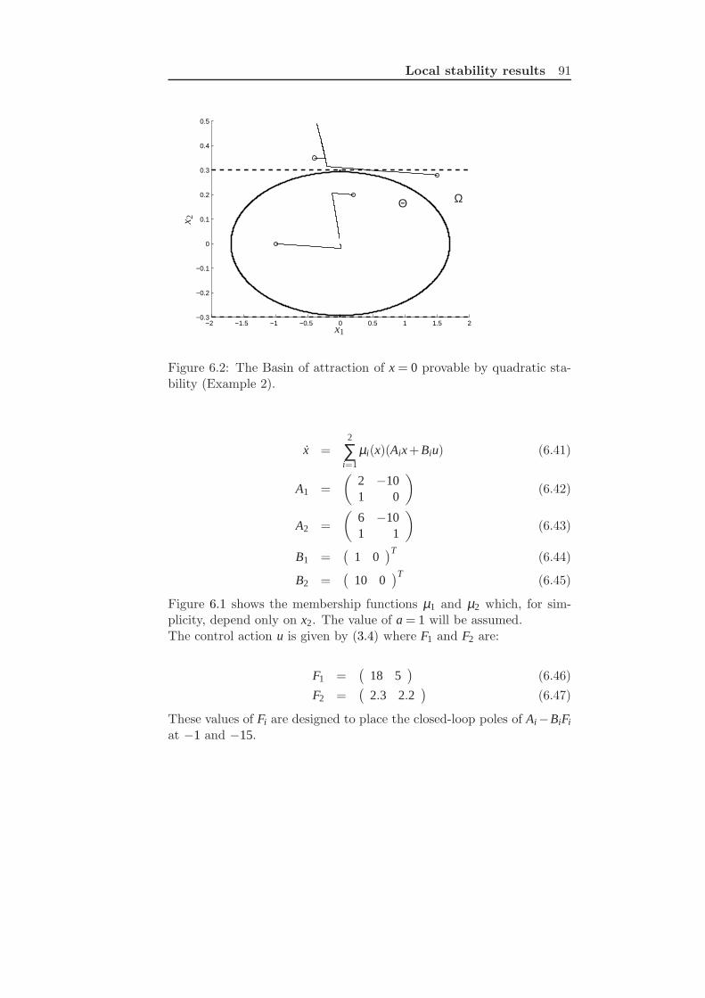
Local stability results 91
−2 −1.5 −1 −0.5 0 0.5 1 1.5 2−0.3
−0.2
−0.1
0
0.1
0.2
0.3
0.4
0.5
x1
x 2Θ Ω
Figure 6.2: The Basin of attraction of x = 0 provable by quadratic sta-bility (Example 2).
x =2
∑i=1
µi(x)(Aix+ Biu) (6.41)
A1 =
(
2 −101 0
)
(6.42)
A2 =
(
6 −101 1
)
(6.43)
B1 =(
1 0)T
(6.44)
B2 =(
10 0)T
(6.45)
Figure 6.1 shows the membership functions µ1 and µ2 which, for sim-plicity, depend only on x2. The value of a = 1 will be assumed.The control action u is given by (3.4) where F1 and F2 are:
F1 =(
18 5)
(6.46)
F2 =(
2.3 2.2)
(6.47)
These values of Fi are designed to place the closed-loop poles of Ai−BiFi
at −1 and −15.

92 Conclusions
Conveniently, we take the same region shape Ω as in Example 1.Then the maximum ρ obtained is 0.3 and the maximum ellipsoid θ thatensures stability for its points is illustrated in Figure 6.2, with some ex-amples of initial points.
6.6 Conclusions
This chapter shows how local stability results (the largest sphere aroundx = 0 for which a quadratic Lyapunov function can be proven via LMI)may be obtained in fuzzy systems via the knowledge of the membershipfunctions, even when no feasible quadratic Lyapunov function can befound to prove global stability. The discovered sphere is part of a largerellipsoidal guaranteed basin of attraction.
The methodology used is based on transformation of the membershipfunctions by expressing them as a convex combination of some points inthe membership space. These points are obtained from the knowledgeof the maximum and minimum values of the memberships in the zoneunder study.

Chapter 7
Relaxed LMI conditions: Overlap in
membership functions
7.1 Introduction
The objective of this chapter is to reduce, the gap between fuzzy andnonlinear control discussed in Chapter 4 by looking at the membershipfunctions shape. Indeed, for a particular application, when the expres-sions of the memberships as a function of some premise variables areactually known, some zones of the possible membership space can beexcluded (only for that particular case, of course). Reducing the size ofthe (multi-dimensional) set where the membership functions take val-ues “should” obtain less conservative conditions than those expressed for“any” membership. However, LMI conditions in current literature donot take into account that fact.
This contribution presents results generalizing ones presented inChapter 5 in order to incorporate any multivariate polynomial constrainton the membership shapes, such as µ2
1 − µ32 µ3− 4µ2µ4− 0.1≥ 0. The
most interesting particular cases are: (a) asserting that the member-ship vector is always inside (or outside) a particular ellipse (or set ofthem); (b) asserting that the overlap (measured as a product) of somememberships is below a particular value, say µ1µ4µ2≤ 0.03.
In summary, this work provides membership-shape dependent condi-tions for fuzzy closed-loop analysis and controller design problems, whichare less conservative than other approaches in literature. The results al-low specialization of the designs to a particular nonlinear plant, and giveroom to greater flexibility of the designs (such as multiple performanceobjectives in different operation regions).
93

94 Relaxed conditions with overlap information
The structure of the chapter is as follows: next section relaxes theconditions in theorem 3.5 using bounds on the products of the member-ship functions (measuring the degree of overlap) and introducing addi-tional artificial LMI variables. The approach is directly applicable withminor modifications to other settings where stability or performance(decay rate, H∞, etc.) requires positivity of a double fuzzy summa-tion ∑i ∑ j µiµ jxT Qi jx > 0, for instance (Tuan et al., 2001). The requiredbounds on the membership functions are easily obtained in practice, asexamples will illustrate. As an additional result, relaxed LMI condi-tions for single fuzzy summations ∑i µixT Qix > 0 are also proposed frombounds on the maximum value of the memberships. An alternative ap-proach, based on changes of variable, as is reported in Chapter 6, butthat approach does not apply to the product bounds. The next sectionwill generalize these results to any shape that can be expressed as aquadratic form of the membership functions. And finally an approachfor relaxing the conditions for any polynomial constrain of the member-ship functions’ constraints using the stability and performance resultsfrom Chapter 5 will be shown. Numerical examples are provided insection 7.5.
7.2 Relaxed conditions with overlap informa-
tion
This section presents relaxations of the above results, which apply whennontrivial bounds on the maximum firing strength of each membershipfunction (or their products) are known.
7.2.1 Single sum relaxation
If a bound for µ j is known, so that
µ j(z)≤ β j ∀ z
the following theorem allows to set up stability and performance condi-tions which are less conservative that those in Chapter 3.
Theorem 7.1 Expression Ξ(t) = ∑ri=1 µi(z(t))x(t)T Qix(t) is positive if
there exist symmetric positive definite matrices N1, . . . , Nr such that,
Relaxed LMI conditions: Overlap in membership functions95
for all i:
Qi + Ni−r
∑j=1
β jN j > 0 (7.1)
If Qi > 0 is a linear matrix inequality (LMI (Boyd et al., 1994; Tanaka& Wang, 2001)), the above expressions are LMIs, too.
Proof: Consider an arbitrary positive definite N j. Then, by using thepartition condition (3.3) and the fact that xT N jx≥ 0 for any x:
µ j ≤ β j
r
∑i=1
µi (7.2)
µ jxT N jx ≤ β jx
T N jxr
∑i=1
µi =r
∑i=1
µiβ jxT N jx (7.3)
Hence, the term
H j = µ jxT N jx−
r
∑i=1
µiβ jxT N jx (7.4)
is negative semi-definite, i.e., H j ≤ 0. As a result, it may be added to Ξand positiveness of Ξ will be proved if positiveness of Ξ + H j is shown,i.e.,
Ξ≥ Ξ + H j =r
∑i=1
µixT Qix+ µ jx
T N jx−r
∑i=1
µiβ jxT N jx =
= xT
(
µ j(Q j +(1−β j)N j)+ ∑i6= j
µi(Qi−β jN j)
)
x (7.5)
Such positivity occurs if
Qi−β jN j > 0 ∀i 6= j (7.6)
and, for the case i = j
Q j +(1−β j)N j > 0 (7.7)

96 Relaxed conditions with overlap information
In order to complete the proof, if a bound β j is known for all j, theconditions may be stated similarly, i.e.:
Ξ≥ Ξ +r
∑j=1
H j =r
∑i=1
µixT Qix+
r
∑j=1
(
µ jxT N jx−
r
∑i=1
µiβ jxT N jx
)
=
= xT
(
r
∑i=1
µi(Qi + Ni−r
∑j=1
β jN j)
)
x (7.8)
from which conditions (7.1) are readily obtained.
The theorem indicates that a negative definite Q j may be “compen-sated”by addition of a positive matrix to it, in expression (7.7), if it firesonly up to a limited strength β j and the rest of fuzzy models (which willfire with strengths adding at least 1−β j) are positive enough, fulfilling(7.6).
Note that the trivial bound β j = 1 is useless. Bounds lower than 1arise with the use of non-normal fuzzy sets. Note also that, by fixingN j = 0, Theorem 7.1 reduces to the standard conditions in literature.
The ideas arising from Theorem7.1 can be extended to a more inter-esting and useful result involving double sums, as discussed below.
7.2.2 Double-sum relaxation
Assume that knowledge of the specific shape of the membership functionsallows to set up a bound:
0≤ µi(z)µ j(z)≤ βi j ∀ z (7.9)
The bounds βi j may be used to set up some relaxations of Theorem1, similarly to the previously considered single-sum case. The trivialbounds in this case are obtained with: µiµ j ≤ µi(1−µi)≤ 0.25 and, fori = j, βii = 1 if the involved fuzzy sets are normal.
Theorem 7.2 Consider an antecedent fuzzy partition fulfilling the over-lap bounds (7.9). Expression (3.23) holds if there exist matrices Xi j = XT
ji
Relaxed LMI conditions: Overlap in membership functions97
and symmetric Ri j, i≤ j, such that:
Xii ≤ Qii + Rii−Λ (7.10)
Xi j + X ji ≤Qi j + Q ji + Ri j−2Λ (7.11)
X =
X11 . . . X1r...
. . ....
Xr1 . . . Xrr
> 0, Ri j ≥ 0 (7.12)
where
Λ =r
∑k=1
∑k≤l≤r
βklRkl
Proof. Consider an arbitrary symmetric positive definite Rkl. Usingcondition (3.24),
µkµl ≤ βkl
r
∑i=1
r
∑j=1
µiµ j (7.13)
µkµlxT Rklx≤ βklx
T Rklxr
∑i=1
r
∑j=1
µiµ j =r
∑i=1
r
∑j=1
µiµ jxT βklRklx (7.14)
Then, the term:
Hkl = µkµlxT Rklx−
r
∑i=1
r
∑j=1
µiµ jxT βklRklx
is negative-semidefinite, i.e., Hkl ≤ 0, so it may be added to Ξ in (3.23),i.e.:
Ξ≥ Ξ + Hkl = µkµlxT Rklx+
r
∑i=1
r
∑j=1
µiµ jxT (Qi j−βklRkl)x (7.15)
and, if the resulting Ξ+Hkl were proved to be positive, Ξ would evidentlybe positive. Reordering the above expression as in (3.48) results in
Ξ≥ µkµlxT Rklx+
r
∑i=1
µ2i xT (Qii−βklRkl)x+
+r
∑i=1
∑i< j≤r
µiµ jxT (Qi j + Q ji−2βklRkl)x (7.16)

98 Relaxed conditions with overlap information
Considering all the different pairs of membership functions, yielding dif-ferent βkl (for k : 1. . . r, k ≤ l ≤ r), an expression of Ξ + ∑r
k=1∑k≤l≤r Hkl
can be easily obtained:
Ξ≥ Ξ +r
∑k=1
∑k≤l≤r
Hkl =r
∑i=1
∑i≤ j≤r
µiµ jxT Ri jx+
r
∑i=1
µ2i xT (Qii−
r
∑k=1
∑k≤l≤r
βklRkl)x+
r
∑i=1
∑i< j≤r
µiµ jxT (Qi j + Q ji−2
r
∑k=1
∑k≤l≤r
βklRkl)x (7.17)
By straightforward manipulations of the expression (7.17), if conditions(7.10) and (7.11) hold, then
Ξ≥r
∑i=1
µ2i xT (Qii + Rii−
r
∑k=1
∑k≤l≤r
βklRkl)x+
r
∑i=1
∑i< j≤r
µiµ jxT (Qi j + Q ji + Ri j−2
r
∑k=1
∑k≤l≤r
βklRkl)x≥r
∑i=1
µ2i xT Xiix+
r
∑i=1
∑i< j≤r
µiµ jxT (Xi j + X ji)x(7.18)
Finally, using an argumentation analogous to that in (3.49), a sufficientcondition for Ξ > 0 is stated in the theorem.
Proposition 7.1 For the trivial off-diagonal bound βkl = 0.25, Theorem7.2 does not provide better results than Theorem 3.5, i.e., Theorem 7.2with normal partitions is only useful in fuzzy models with 3 or morerules.
Proof. Indeed, assume that feasible Xi j, Rkl , k < l have been obtainedwith Theorem 7.2, so that
Xii ≤ Qii−0.25Rkl (7.19)
Xi j + X ji ≤ Qi j + Q ji−0.5Rkl (i, j) 6= (k, l) (7.20)
Xkl + Xlk ≤Qkl + Qlk +0.5Rkl (7.21)
Take X ′i j = Xi j for all pairs (i, j) except (k,k), (l, l), (k, l), (l,k), andtake X ′kk = Xkk +0.25Rkl , X ′ll = Xll +0.25Rkl , X ′kl = Xkl−0.25Rkl , X ′lk = Xlk−

Relaxed LMI conditions: Overlap in membership functions99
0.25Rkl . Then, conditions (3.50)–(3.51) are fulfilled for X ′i j. Consider
now an arbitrary vector ξ = (ξ T1 . . .ξ T
k . . .ξ Tl . . .ξ T
r )T where ξi is itself avector compatible with the dimensions of Xii. Then,
ξ T X′ξ = ξ T Xξ +(
ξ Tk ξ T
l
)
(
0.25Rkl −0.25Rkl
−0.25Rkl 0.25Rkl
)(
ξk
ξl
)
=
= ξ T Xξ +0.25(ξk−ξl)T Rkl(ξk−ξl) (7.22)
proves that X′ ≥ X, as (ξk− ξl)T Rkl(ξk− ξl) ≥ 0. Hence, the matrix X′
in (3.52) formed with the X ′i j is positive definite, i.e., the procedure hasobtained a feasible solution for Theorem 3.5.
The numerical examples in Section 7.5 will show that Theorem 3improves over Theorem 3.5 when βi j < 0.25.
Remark: if βkl = 0 (i.e., fuzzy sets µk and µl are disjoint and non-overlapping), Rkl dissapears from Λ. Hence, the LMI (7.10) or (7.11) inwhich Rkl appears may be eliminated as Rkl can be as large as needed.In this way, the usual conditions regarding completely non-overlappingmemberships in literature (Kim & Lee, 2000) are recovered as a partic-ular case.
7.3 Shape-dependent positivity conditions fordouble fuzzy summations
Denote by µ(z) the column vector of membership functionsµ(z) = (µ1(z),µ2(z), . . . ,µr(z))T in (3.23). On the sequel, the shorthandnotation µ will be used instead of µ(z), as previously introduced for theindividual membership components.
Assume that knowledge of: the specific shape of the membership functions, the set of values Ω taken by premise variables z,
allows to set up a bound, for some known S, t and v, in the form:
µT Sµ + tµ + v≤ 0 ∀ z ∈Ω (7.23)

100 Shape-dependent positivity conditions for double fuzzysummations
where parameters S, t and v are, respectively, a matrix (of dimensionsr×r), a row vector (1×r) and a scalar. The elements of S will be denotedby si j, and βi j will denote:
βi j = (si j + ti + v)
The left-hand side term in (7.23) is a second-order polynomial in themembership functions. Particular examples are, for instance, knowledgeon degrees of membership function overlap (say, µ1µ2 < 0.15, µ1µ3 = 0,(µ1 + µ2)∗µ4 ≤ 0.4), ellipsoidal sets (such as (µ1−0.9)2 +2(µ2−0.1)2 ≤0.052) or drilling ellipsoidal “holes” (such as (µ1−0.9)2 +2(µ2−0.1)2 ≥0.052); see section 7.3.1 for further discussion.
Proposition 7.2 If the membership functions conform a fuzzy parti-tion, then the matrix B whose elements are βi j fulfills:
µTBµ ≤ 0 (7.24)
Proof: Indeed, using condition (3.3),
0≥ µT Sµ + tµ + v =r
∑i=1
r
∑j=1
µiµ jsi j +r
∑i=1
tiµi + v =
=r
∑i=1
r
∑j=1
µiµ jsi j +r
∑i=1
r
∑j=1
µiµ jti +r
∑i=1
r
∑j=1
µiµ jv =
=r
∑i=1
r
∑j=1
µiµ j(si j + ti + v) =r
∑i=1
r
∑j=1
µiµ jβi j (7.25)
Hence, any second-order polynomial restriction on the membershipshape can be expressed as an homogeneous quadratic form.
Theorem 7.3 Assume knowledge about the particular membership func-tion shape is available via a constraint matrix B, with elements βi j,fulfilling (7.24). Then, expression (3.23) is proved if there exists a sym-metric matrix R≥ 0 so that the condition:
Ξ′(t) =r
∑i=1
r
∑j=1
µiµ jxT Q′i jx > 0 ∀ x 6= 0 (7.26)

Relaxed LMI conditions: Overlap in membership functions101
holds, where
Q′i j = Qi j + βi jR
i.e. Qi j is replaced in (3.23) by Q′i j involving an additional matrix vari-able.
Proof: consider an arbitrary symmetric positive semi-definite R.Then, the term
H = xT Rxr
∑i=1
r
∑j=1
µiµ jβi j =r
∑i=1
r
∑j=1
µiµ jxT βi jRx (7.27)
verifies H ≤ 0, so it may be added to Ξ in (3.23) and, if the resultingsum is positive, Ξ will evidently be positive, i.e.,
Ξ≥ Ξ + H =r
∑i=1
r
∑j=1
µiµ jxT (Qi j + βi jR)x = Ξ′ (7.28)
Multiple restrictions can be incorporated by repeated application ofTheorem 7.3, i.e.:
Corollary 7.1 Assume that knowledge about the particular membershipfunction shape is available via a set of matrices B[k], k = 1, . . . , t, with
elements β [k]i j . Expression (3.23) is proved if there exist positive semi-
definite matrices Rk, k = 1, . . . , t, so that the condition (7.26) holds, where
Q′i j = Qi j +t
∑k=1
β [k]i j Rk
In order to check condition (7.26), well-known expressions can beused, such as the ones in (Tuan et al., 2001), or (Liu & Zhang, 2003).For instance, straightforward application of (Liu & Zhang, 2003) yieldsthe following theorem:
Theorem 7.4 Consider an antecedent fuzzy partition fulfilling thebounds (7.23). Expression (3.23), under shape constraints B[k], k =

102 Shape-dependent positivity conditions for double fuzzysummations
1, . . . , t, holds if there exist matrices Xi j = XTji and symmetric Rk ≥ 0 such
that:
Xii ≤Qii +t
∑k=1
β [k]ii Rk (7.29)
Xi j + X ji ≤ Qi j + Q ji +t
∑k=1
(β [k]i j + β [k]
ji )Rk (7.30)
X =
X11 . . . X1r...
. . ....
Xr1 . . . Xrr
> 0 (7.31)
7.3.1 Particular cases
Membership function overlap. Assume that a bound on the overlapbetween fuzzy sets defined by µk and µl, for k 6= l, is expressed as:
µkµl ≤ γkl (7.32)
It is a particular case of (7.23) with ti = 0 and
skl = slk =12, v =−γkl (7.33)
si j = 0 ∀ (i, j) 6= (k, l) (7.34)
resulting in βkl = βlk = 12− γkl, the rest of βi j =−γkl .
The conditions of Theorem 7.4 result in:
Xii ≤ Qii− γklR (7.35)
Xi j + X ji ≤ Qi j + Q ji−2γklR (i, j) 6= (k, l) (7.36)
Xkl + Xlk ≤ Qi j + Q ji +(1−2γkl)R (7.37)
X =
X11 . . . X1r...
. . ....
Xr1 . . . Xrr
> 0, R≥ 0 (7.38)
As it can be seen, the results are equivalent to ones obtained in theprevious section.
Ellipsoidal hole. The interior (or exterior) of any ellipse, parabolaor hiperbola can be considered via a suitable B. As a simple example,

Relaxed LMI conditions: Overlap in membership functions103
Let us assume that the condition
r
∑i=1
(µi− ci)2≥ δ 2 (7.39)
is known to hold, i.e., the membership functions are known to lie outsideof a particular hyper-sphere.
Then,
r
∑i=1
(µ2i + c2
i −2ciµi)≥ δ 2 (7.40)
r
∑i=1
µ2i +
r
∑i=1
r
∑j=1
µiµ j(r
∑k=1
c2k)−2
r
∑i=1
r
∑j=1
µiµ jci ≥ δr
∑i=1
r
∑j=1
µiµ j (7.41)
so we have, denoting by φ =−δ 2 + ∑rk=1 c2
k ,
r
∑i=1
µ2i (1−2ci)+ φ +
r
∑i=1
r
∑j=i+1
µiµ j(2φ −2ci−2c j)≥ 0 (7.42)
so the previous results apply with
βii =−(1−2ci)−φ (7.43)
βi j =−φ +2ci i 6= j (7.44)
In general, one may specify that the membership functions are out-side of an arbitrary ellipsoidal quadratic form, in the form:
µT Sµ− v≤ 0 (7.45)
where S is a positive definite matrix. A set of such ellipsoids may beused to exclude any zones which are known to be out of the range of themembership function vector (Figure 7.1). Using a negative definite S isequivalent to stating that the membership vector lies inside a particularellipsoid.
7.3.2 Obtention of bounds in practice.
As the shape of the membership functions is known in fuzzy control1, ob-taining the bounds for any second-order polynomial in the form (7.23)
1See (Lam & Leung, 2005) for conditions with uncertain memberships.

104 Shape-dependent positivity conditions for double fuzzysummations
Figure 7.1: Ellipsoidal holes on the add-1 simplex in R3.
0 2 4 6 8 100
0.1
0.2
0.3
0.4
0.5
0.6
0.7
0.8
0.9
1
µ1 µ2µ3
z(t)
Mem
ber
ship
Figure 7.2: Fuzzy partition with limited overlap.
is, in principle, easy, as the problem can be approached as an opti-mization one. Indeed, choosing arbitrary S and t, maximising J(z) =µ(z)T Sµ(z)+ tµ(z) over the expected range of values of the premise vari-ables z, previously denoted as Ω, yields a value Jmax = maxz∈Ω J(z). OnceJmax is available2, an expression in the form (7.23) can be obtained fromJ(z)− Jmax ≤ 0, i.e., the polynomial µT Sµ + tµ− Jmax≤ 0.
As an example, consider the fuzzy partition in Figure 7.2. In thiscase, the bounds µ2− 0.86≤ 0 and µ1µ3− 0.0045≤ 0 may be easilycomputed by line-search on the one-dimensional set where the premisevariable takes values.
In other common cases, membership functions are the cartesian prod-uct of simpler ones, describing either fuzzy partitions on individual vari-
2The optimization on Ω can be carried out by using any optimization technique;even a brute-force approach evaluating the memberships on a dense-enough grid on zmay suffice.

Relaxed LMI conditions: Overlap in membership functions105
ables or basic nonlinearities in the system equations, following the mod-elling methodology in (Tanaka & Wang, 2001). In that case, if themembership functions are the cartesian product of w fuzzy partitions, itcan be shown that certain products of memberships can be bounded bya power of 0.25 (because µ(1−µ)≤ 0.25). For instance, consider “high”and “low” to be contrary concepts defined on pressure and temperatureuniverses. If a membership µ1 is “temperature is low and pressure islow”, and other membership µ2 is “temperature is high and pressure ishigh”, then µ1µ4≤ 0.252. Details and examples of these situations appearin (Sala & Arino, 2007a).
The reader may browse at this moment, if so wished, Example 7.1in Section 7.5, which shows some numeric results.
7.4 Generalization to higher dimensions
As a generalization of (3.23), other fuzzy control results require posi-tiveness of a p-dimensional fuzzy summation, i.e., checking
Ξ(t) =r
∑i1=1
r
∑i2=1
. . .r
∑ip=1
µi1(z)µi2(z) . . .µip(z)xT Qi1i2...ip x≥ 0 (7.46)
The case p = 2 reduces to (3.23). Conditions requiring p = 3 are, forinstance, the fuzzy dynamic controllers in (Li et al., 1999; Tanaka &Wang, 2001), using Qi jk = Ei jk + ET
i jk, with
Ei jk =
(
AiQ11+ BiC jk Ai + BiD jCk
Ai jk AiP11+Bi jCk
)
< 0 (7.47)
for suitably defined A ,B,C ,D . Triple fuzzy summations are needed alsoin the output-feedback settings in (Fang et al., 2006; Chen et al., 2005).
Consider also the possibility that a restriction on the shape of themembership functions is given by a multivariate polynomial of degree p,for instance
µ41−2µ3 + µ1µ2−0.3 < 0 (7.48)
with p = 4, where monomials of degree four, one, two and zero appear.
Now, choose any arbitrary integer n, n ≥ p. By multiplying each ofthe atomic monomials of degree q (0≤ q ≤ p) by (∑r
i=1 µi)n−q (which is

106 Generalization to higher dimensions
identically equal to one), any polynomial of degree p can be converted toan homogeneous polynomial of degree n. For instance, the above (7.48)gets converted in
µ41−2µ3(∑
i
µi)3 + µ1µ2(∑
i
µi)2−0.3(∑
i
µi)4 < 0 (7.49)
So, let us restate a generalised version of the theorem, introducingsome notation from (Sala & Arino, 2007b).
7.4.1 Multi-dimensional index notation
In order to streamline notation in multi-dimensional summations (7.46),we will follow the multi-index notation in Section 5.2.1 to handle p-dimensional vectors of natural numbers (denoted by boldfaced vari-ables), and its associated p nested summations:
Ip = (i1, i2, . . . , ip) | 1≤ i j ≤ r, j = 1,2, . . . , p
∑i∈Ip
γi =r
∑i1=1
r
∑i2=1
. . .r
∑ip=1
γi1i2...ip (7.50)
By convention, the cartesian product of several multi-indices, result-ing in a higher-dimensional one, will be symbolized by parentheses:
i ∈ Ip, j ∈ Iq, . . . ,m ∈ It ⇒ k = (i, j, . . . ,m) ∈ Ip+q+···+t (7.51)
and sometimes by mere juxtaposition, such as in γi1...ip in (7.50) One-dimensional indices, say j ∈ I1 are ordinary integer index variables: theywill be typed in italic typeface as j, 1≤ j≤ r when its one-dimensionalityshould be emphasised.
Multi-dimensional fuzzy summations. The purpose of multi-indexnotation is to compactly represent multi-dimensional fuzzy summations,as follows.
First, let us define the following notation, specific for membershipfunctions as a shorthand for a product:
µi =p
∏l=1
µil = µi1µi2 . . .µip i ∈ Ip (7.52)

Relaxed LMI conditions: Overlap in membership functions107
With the above notation, p-dimensional fuzzy summations (7.46) maybe written as follows:
Ξ(t) = ∑i∈Ip
µixT Qix (7.53)
where the basic memberships µ = µ1, . . . ,µr from which µi stem fulfillthe add-1 partition condition.
Permutations. Given a multi-index i ∈ Ip, let us denote by P(i) ⊂ Ip
the set of permutations (with, possibly, repeated elements) of the multi-index i. The permutations will be used to group elements in multiplefuzzy summations which share the same “antecedent”: it’s an evidentfact that j ∈P(i) ⇒ µj = µi.
The following subset of Ip will be used in later developments:
I+p = i ∈ Ip | ik ≤ ik+1, k = 1. . . p−1 (7.54)
7.4.2 Relaxed conditions
This section discusses how to obtain relaxed conditions for positivity offuzzy summations under information on membership shape given by adegree-q constraint:
∑i∈Iq
µiβi ≤ 0 (7.55)
The coefficients βi may be considered elements of a multi-dimensionalarray (tensor (Temple, 2004)) B, generalising the matrix appearing in(7.24).
Note that any polynomial of degree lower or equal to q may be ex-pressed as an homogeneous q-dimensional summation (7.55), by follow-ing the methodology used to obtain (7.49).
Theorem 7.5 Consider a p-dimensional fuzzy summation condition(7.46), jointly with shape-dependent knowledge expressed as constraintsof degree q (7.55). Choose any arbitrary integer n so that n≥max(p,q).The positivity condition (7.46) (in the region determined by the con-straints (7.55)) is fulfilled if there exists a positive definite matrix R sothat the condition ∑i∈In
µixT Q′ix≥ 0, i = (i1, i2, . . . , in), holds with:
Q′i = Qi1i2...ip + βi1i2...iq R (7.56)

108 Generalization to higher dimensions
Proof: As ∑rk=1 µk = 1, it’s straightforward that:
∑i∈Ip
µixT Qix≥ ∑
i∈Ip
µixT Qix+ xT Rx ∑
i∈Iq
µiβi =
= (r
∑k=1
µk)n−p ∑
i∈Ip
µixT Qix+(
r
∑k=1
µk)n−q ∑
i∈Iq
µixT βiRx =
= ∑i∈In
µixT Q′ix (7.57)
so positivity of the last term implies positivity of the first one.
Note that an extension to multiple restrictions (say, t restrictions) isstraightforward, by using:
Q′i = Qi1i2...ip +t
∑k=1
β [k]i1i2...iq Rk (7.58)
for some positive-definite Rk associated to each constraint tensor B[k].
Once the new Q′i are defined as above, any sufficient condition toprove positivity of an n-dimensional fuzzy summation may be used. Forinstance, n = 3 may be handled by adapting the conditions in (Fanget al., 2006, Theorem 5).
Theorem 7.6 Given a set of t degree-3 polynomial restrictions, ex-pressed as t homogeneous forms (7.55), and any Qi jk expressing somefuzzy control requirements, the 3-dimensional summation
r
∑i=1
r
∑j=1
r
∑k=1
µiµ jµkxT Qi jkx
is positive (in the region determined by the constraints) if there exist
Xi jk, Rl so that, being Q′i jk = Qi jk + ∑tl=1 β [l]
i jkRl:
R≥ 0 Xi jk = XTik j (7.59)
Q′iii ≤ Xiii (7.60)
Q′ii j + Q′i ji + Q′jii ≤ Xii j + Xi ji + X jii i < j (7.61)
Q′i jk + Q′ik j + Q′jik + Q′jki + Q′ki j + Q′k ji ≤Xi jk + Xik j + X jik + X jki + Xki j + Xk ji i < j < k (7.62)
Xi11. . .Xi1r.... . .
...Xir1 . . .Xirr
> 0 ∀i (7.63)

Relaxed LMI conditions: Overlap in membership functions109
In fact, any n ≥ 2 may be handled by using Theorems 4 and 5 in(Sala & Arino, 2007b). Substituting Q′ from (7.58) in the theorems of(Sala & Arino, 2007b), the result is:
Theorem 7.7 A sufficient condition for positivity of Ξ in (7.46), underas set of t constraints in the form (7.55), is the positivity condition below,for n≥max(p,q):
∑k∈In−2
µkξ T
X(k,1,1) . . . X(k,1,r)...
. . ....
X(k,r,1) . . . X(k,r,r)
ξ > 0 (7.64)
if there exist matrices Xj, j ∈ In, and positive-definite Rl, l = 1, . . . , t, sothat, for all i ∈ I
+n
∑j∈P(i)
(Q j1 j2... jp +t
∑l=1
β [l]j1 j2... jqRl)≥ ∑
j∈P(i)
12(Xj + XT
j ) (7.65)
The proof is a trivial adaptation of those in (Sala & Arino, 2007b)(changing Q by Q′) and, hence, omitted. The number of decision vari-ables can be reduced by assuming X(k,i, j) = XT
(k, j,i) with no loss of gener-ality.
The above theorem must be applied recursively as, given a start-ing value of n, it provides sufficient conditions for the positivity of then-dimensional sum expressed as an (n−2)-dimensional one. Hence, re-peated application of the theorem is needed until: (a) 2-dimensionalfuzzy summations are obtained (using Theorem 2 in (Liu & Zhang,2003) as a last step) when starting from an even n; (b) in the odd-ncase, one-dimensional fuzzy summations are obtained, stating then thecondition that each of the elements in the sum must be positive. Thereader is referred to (Sala & Arino, 2007b) for details.
Remark: Theorem 5 in (Fang et al., 2006) is the particular case
of Theorem 7.7 for n = 3 and β [l]i = 0; Theorem 2 in (Liu & Zhang,
2003) is Theorem 7.7 for n = 2. Note, for the first case, that (7.60),(7.61) and (7.62) correspond to the 1, 3 and 6 permutations of indexesiii, i j j and i jk, respectively, which appear in (7.65); then, (7.63) is thecondition to prove positivity of the remaining 1-dimensional sum (7.64).The particularisation to (Liu & Zhang, 2003) is also straightforward(there are only 2 permutation of the index i j).
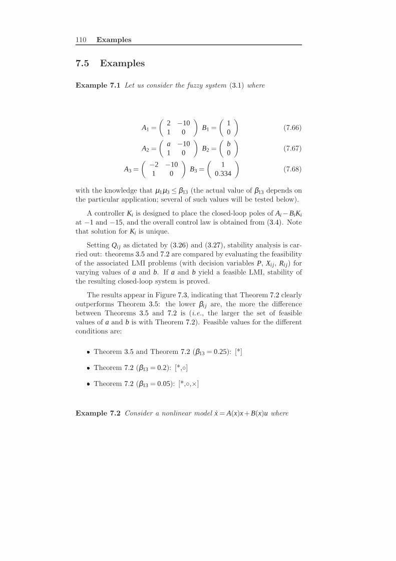
110 Examples
7.5 Examples
Example 7.1 Let us consider the fuzzy system (3.1) where
A1 =
(
2 −101 0
)
B1 =
(
10
)
(7.66)
A2 =
(
a −101 0
)
B2 =
(
b0
)
(7.67)
A3 =
(
−2 −101 0
)
B3 =
(
10.334
)
(7.68)
with the knowledge that µ1µ3≤ β13 (the actual value of β13 depends onthe particular application; several of such values will be tested below).
A controller Ki is designed to place the closed-loop poles of Ai−BiKi
at −1 and −15, and the overall control law is obtained from (3.4). Notethat solution for Ki is unique.
Setting Qi j as dictated by (3.26) and (3.27), stability analysis is car-ried out: theorems 3.5 and 7.2 are compared by evaluating the feasibilityof the associated LMI problems (with decision variables P, Xi j, Ri j) forvarying values of a and b. If a and b yield a feasible LMI, stability ofthe resulting closed-loop system is proved.
The results appear in Figure 7.3, indicating that Theorem 7.2 clearlyoutperforms Theorem 3.5: the lower βi j are, the more the differencebetween Theorems 3.5 and 7.2 is (i.e., the larger the set of feasiblevalues of a and b is with Theorem 7.2). Feasible values for the differentconditions are: Theorem 3.5 and Theorem 7.2 (β13 = 0.25): [*] Theorem 7.2 (β13 = 0.2): [*,] Theorem 7.2 (β13 = 0.05): [*,,×]
Example 7.2 Consider a nonlinear model x = A(x)x+ B(x)u where

Relaxed LMI conditions: Overlap in membership functions111
2 3 4 5 6 7 81
2
3
4
5
6
7
8
9
10
a
b
Figure 7.3: LMI feasibility as a function of a and b: – ∗: Feasible withTheorem 3.5 and Theorem 7.2 with β13 = 0.25, – : additional feasiblepoints obtained with Theorem 7.2 and β13 = 0.20, – ×: further feasiblepoints obtained with Theorem 7.2 and β13 = 0.05, – unfeasible grid pointshave been left blank.

112 Examples
A(x) = 0.75x−2.25sin(x)+ sin(x)x−2.5 (7.69)
B(x) = 0.42x+1.25sin(x)−0.42sin(x)x−0.25 (7.70)
for which PDC fuzzy controllers are to be designed when x ∈ [−π,π].In this case, x may be written as x = ∑2
i=1νi pi, and sin(x) as sin(x) =
∑2i=1ηiqi, with:
x = ν1(x) ·π + ν2(x) · (−π), sin(x) = η1(x) ·1+ η2(x) · (−1)
where membership functions are ν1 = 12π (x + π), ν2 = 1 − µ1,
η1 = 12(sin(x)+1), η2 = 1−η1, resulting in
A(x) = 0.752
∑i=1
νi pi−2.252
∑i=1
ηiqi +(2
∑i=1
ηiqi)(2
∑i=1
νi pi)−2.5
A(x) =2
∑i=1
2
∑j=1
νiη j(0.75pi−2.25q j + piq j−2.5) =2
∑i=1
2
∑j=1
νiη jai j
where
a11 = 0.748,a12 =−1.035,a21 =−10.247,a22 = 0.536
and similarly
B(x) =2
∑i=1
2
∑j=1
νiη j(0.42pi +1.25q j−0.42piq j−0.25) =2
∑i=1
2
∑j=1
νiη jbi j
where:b11 = 1,b12 = 1.139,b21 = 1,b22 =−4.139
Then, if µ1 = ν1η1, µ2 = ν1η2, µ3 = ν2η1 and µ4 = ν2η2 were defined, afuzzy TS with four models:
x =4
∑i=1
µi(aix+ biu) (7.71)
a1 = 0.748,a2 =−1.035,a3 =−10.247,a4 = 0.536 (7.72)
b1 = 1,b2 = 1,139,b3 = 1,b4 =−4.139 (7.73)
will exactly describe the nonlinear system under analysis for x ∈ [−π,π].The reader is referred to Chapter 9 and (Tanaka & Wang, 2001) for moreexamples of this cartesian-product nonlinear modelling methodology.

Relaxed LMI conditions: Overlap in membership functions113
If Theorem 3.5 is applied with the obtained set of four models andQi j given by (3.33), no feasible stabilizing PDC state-feedback controlleru =−∑4
i=1 µiKix can be found by the LMIs.
However, note that:
µ1µ4 = µ3µ2 = ν1ν2η1η2≤ 0.252
as ν1ν2 ≤ 0.25 and η1η2 ≤ 0.25. Hence, Theorem 3 may be used withβ14 = β23 = 0.0625. In this case, Theorem 3 shows that there exists afeasible stabilizing PDC controller for the nonlinear system expressed asa cartesian TS one which achieves a decay rate performance of 0.1369.
Regarding H∞ performance, the model x = A(x)x + B(x)u + w, y = xhas been tested with conditions (3.43), searching for the minimum γ .Without the relaxations considered in Theorem 3 the problem was, ev-idently, unfeasible from the considerations above. With the relaxationsarising from β14 and β23, a value of γmin = 7.3002 was obtained as theLMI-guaranteed H∞ bound.
Example 7.3 Consider the system (3.1), with r = 3 and
A1 =
−0.74 0.61 0.870.39 −0.26 0.560.99 0.05 −0.16
B1 =
0.99 0.650.2 0.870.76 0.12
A2 =
0.69 0.07 0.350.48 0.86 0.370.1 0.31 0.3
B2 =
0.96 0.360.76 0.170.04 0.20
A3 =
0.28 0.39 0.580.32 0.13 0.200.68 0.34 0.19
B3 =
0.32 0.020.72 0.150.29 0.06
The fastest decay rate3 with a state feedback PDC law provable byTheorem 2 in (Liu & Zhang, 2003), using the Qi j in (3.33), is α = 0.51.
Now, the procedures in this chapter will be applied to achieve im-proved decay rates when some knowledge about the membership func-tion shape is available (Figure 7.4).
3Note that the chosen performance measure has been decay rate, for simplicity, butother features such as robustness margins or H∞ bounds may be tested by selectinga different Qi j, as discussed in Section 3.5.

114 Examples
µ1µ1
µ2µ2 µ3µ3
Figure 7.4: Example 1: (left) case 1, (right) case 2. Shaded area denotespossible values of membership functions inside the triangle µ1+µ2+µ3 =1, µi ≥ 0. Isometric projection.
Case 1. Assume that, for a particular system, the membership vectordoes not lie inside a sphere centered at the origin (ci = 0 in (7.39)) withradius δ (Figure 7.4-left), and that fact is known to the designer to takeadvantage of it.
Then, conditions (7.43) and (7.44) in Theorem 7.4 result in:
Xii ≤ Qii +(δ 2−1)R (7.74)
Xi j + X ji ≤ Qi j + Q ji +2δ 2R i < j (7.75)
Note that, for 0≤ δ ≤ 1, the conditions are less conservative as δ in-creases, because there is a larger addition to the off-diagonal terms(proportional to δ ) and a smaller subtraction to the diagonal ones (pro-portional to 1−δ ). In fact, the extreme case δ = 1 indicates that onlythe canonical vertices (µ1,µ2,µ3) ∈ (1,0,0),(0,1,0),(0,0,1) are possi-ble values of memberships (corresponding, for instance, to a switchinglinear system). In that extreme case, conditions (7.74) and (7.75) resultin:
Xii ≤ Qii (7.76)
Xi j + X ji ≤ Qi j + Q ji +2R i < j (7.77)
Hence, with a large enough R, Xi j = 0 for i 6= j can be made to be asolution of (7.77), so (3.23) holds if Qii > 0, which is a well known resultin “crisp” switching linear systems.
Let us check different cases for δ with the above system. In partic-ular, values of δ > 1/
√2 produce faster decay rates than the case with
arbitrary memberships: for δ = 0.72 the decay rate is α = 0.96; for δ = 1it is α = 3.4.

Relaxed LMI conditions: Overlap in membership functions115
Case 2. Using expressions (7.43)-(7.44) as before, the knowledge thatthe membership vector lies outside of a sphere with center (0, 0.5, 0.5)and radius 0.4 is cast into the LMIs. The result is a decay α = 0.62. If asphere with center (0,0,1) and radius 0.49 is used, the achievable decayis α = 0.56. With both circles and two relaxation variables R1, R2, theachievable decay rate is α = 0.66.
Case 3: Multi-objective design (dual specifications). Consider theproblem of achieving different levels of specifications in different regionsof the working space4. For instance, only stability may suffice for certaininfrequent cases whereas a faster decay may be desired near a particularoperation point. The operation point will be assumed to be given bya particular condition on the membership functions (stating that themembership vector µ is inside or outside a region with a polynomialboundary).
Under these assumptions, the LMI conditions for mere stability,stated for any unrestricted membership shape, may be adjoined withthe decay rate ones incorporating membership shape information.
For instance, α = 1.11 is the fastest decay when the distance of themembership vector to the point (1,0,0) is smaller than 0.75 (i.e., con-ditions on the membership vector being inside a sphere are setup), si-multaneously ensuring overall stability via a shared Lyapunov function:conditions in Theorem 7.4 with Qi j in (3.33) are stated with α = 1.11and suitable βi j (obtained from (7.43) and (7.44)); additionally, condi-tions in (Liu & Zhang, 2003, Theorem 2) using α = 0 are also stated,with different decision variables Xi j. The LMI solver is able to find a fea-sible solution for both sets of constraints simultaneously; when α > 1.11on the first set of (shape-dependent) restrictions, the problem renders
4The above multi-objective design is different, and complementary, to the usualapproach in literature of achieving different sorts of performance bounds on all thestate space (mixed H2/H∞, H∞ plus decay rate, etc. (Gahinet et al., 1995; Li et al.,1999)): the same performance type but with different level in different regions issuggested here. Note also that some definitions are needed in order to rigorouslydefine the meaning of “local” decay rate in terms of basins of attraction and Lyapunovlevel sets. The definition of, say, a “local” H∞ norm would also be cumbersome.These issues are, however, omitted for brevity as they are not the main objectiveof the chapter. In the example in consideration, in a set of premise variables Ω, a“local” decay rate α will be said to have been proved when a Lyapunov function isfound fulfilling V (x)≤−2αV (x) for all z ∈Ω (indeed, z may include some or all of thecomponents of x, as usual in TS modelling (Tanaka & Wang, 2001)).

116 Examples
−0.5 0 0.5 1 1.5 2 2.5 3 3.55
5.5
6
6.5
7
7.5
Figure 7.5: Feasible points (example 2) under different restrictions withTheorem 7.7, n = 3. ‘⊗’: βi jk = 0; ‘*’: µ1µ2µ3≤ 0.0004; ‘+’ µ1µ2µ3 = 0.Horizontal axis denotes parameter a, vertical axis denotes parameter b.
unfeasible.
Example 7.4 Consider the system:
A1 =
(
1.59 −7.290.01 0
)
B1 =
(
10
)
A2 =
(
0.02 −4.640.35 0.21
)
B2 =
(
80
)
A3 =
(
−a −4.330 0.05
)
B3 =
(
−b+6−1
)
A stabilising PDC controller is to be designed. The ranges of valuesof parameters a and b yielding a feasible LMI solution are comparedfollowing several methods, for a ∈ [−0.5,3.25], b ∈ [5.25,7.25].
The procedure in (Liu & Zhang, 2003, Theorem 2) does not yieldany feasible value in this parameter range.
Even with no restriction (βi = 0), Theorem 7.6 (i.e., (Fang et al.,2006)), produces feasible stabilising regulators for the values of a and bindicated by the “cart wheel” symbol in Figure 7.5.
When the restriction µ1µ2µ3≤ 0.0004is enforced, a few more feasiblepoints appear (indicated by a star) using Theorem 7.6. The restriction

Relaxed LMI conditions: Overlap in membership functions117
µ1µ2µ3 = 0 produces a larger set of feasible points; the + sign on thefigure pinpoints those combinations of parameter values yielding feasiblecontrollers only under the last restriction.
In all cases, the LMI solver was Matlab LMI Toolbox with defaultoptions.
7.6 Conclusions
This chapter shows how to relax stability and performance conditions forfuzzy control models with knowledge of membership function overlap;two theorems relaxing some LMI stability and performance conditionsin (Tanaka & Wang, 2001; Kim & Lee, 2000; Liu & Zhang, 2003) havebeen presented. The conditions consider a set of known bounds in µi
and µiµ j, which generalize the relaxations when µiµ j = 0 previously re-ported in literature for non-overlapping fuzzy sets. As a result, morefreedom in guaranteeing control requirements is available. A numericalexample shows how the feasibility regions for typical fuzzy control prob-lems become larger as the overlap bounds become smaller, showing theimprovements over previous work.
The proposed technique may prove useful in fuzzy control applica-tions. In fuzzy PDC control techniques, membership functions are as-sumed to be known so the required bounds may be easily obtained. Im-portantly this technique is particularly well suited to widespread cartesian-product Takagi-Sugeno modelling of nonlinear systems.


Chapter 8
Stability Analysis with uncertain membership
functions
8.1 Introduction
Fuzzy control has reached maturity and acceptance nowadays via a for-malisation of the performance requirements and controller design tech-niques. In particular, there is a vast amount of literature on controldesign for Takagi-Sugeno (TS) (Takagi & Sugeno, 1985) fuzzy systemsvia linear matrix inequalities (LMI) (Boyd et al., 1994; Tanaka & Wang,2001; Liu & Zhang, 2003). There may be other (possibilistic) interpre-tations of fuzziness in a control context (Bondia, Sala, Pico, & Sainz,2006). The reader is referred to (Sala et al., 2005; Feng, 2006) for areview of the current trends and open issues in fuzzy modelling, identi-fication and control.
The majority of works on fuzzy control for TS models assume theparallel distributed compensation (PDC) paradigm (Tanaka & Wang,2001), i.e., the membership functions of the controller, say ηi, are thesame as the ones from the process, say µi. Furthermore, the proposedstability and performance conditions are shape-independent, i.e., validfor any non-negative membership function setup.
Recent contributions in the non-PDC case are (Lam & Leung, 2005,2007; Guerra & Vermeiren, 2004). In particular, in (Lam & Leung,2005), LMI stability conditions were given for non-PDC fuzzy systemswith uncertain degrees of membership expressed as a multiplicative un-certainty inequality ρm
i µi ≤ ηi ≤ ρMi µi. Lam and Leung’s conditions are
shape-dependent, in the sense that they achieve a reduction of conser-vativeness by setting up conditions which are only valid for membership
119

120 Problem statement
functions having a constrained shape. In the same spirit, (Sala & Arino,2007a) presents some shape-dependent conditions for the PDC case.
The main objective of this chapter is presenting new shape-dependentLMI conditions to design controllers for Takagi-Sugeno fuzzy systemswith uncertain memberships. The allowed uncertainty description ismore general than that in (Lam & Leung, 2005), which did consideronly multiplicative uncertainty.
The structure of the chapter is as follows. The next section willdescribe the fuzzy systems and closed-loop equations to be discussed.Section 8.3 presents the main result which extends the uncertainty de-scriptions in literature. Section 8.4 applies it to particular cases of ad-ditive and multiplicative uncertainty. Section 8.5 will show numericalexamples illustrating the possibilities of the approach. A conclusion sec-tion closes the chapter.
8.2 Problem statement
Consider a Takagi-Sugeno fuzzy system (3.1) of order n with r rules:
x =r
∑i=1
µi(z)(Aix+ Biu)r
∑i=1
µi(z) = 1, µi(z)≥ 0 (8.1)
The above system will be controlled via a state-feedback fuzzy controller:
u =−r
∑i=1
ηi(z′)Kix
r
∑i=1
ηi(z′) = 1, ηi(z
′)≥ 0 (8.2)
where z′ denotes measurable scheduling variables. The controller yieldsa closed-loop (Lam & Leung, 2005):
x =r
∑i=1
r
∑j=1
µi(z)η j(z′)(Ai−BiK j)x (8.3)
On the following µi, ηi will be used as shorthand for µi(z), ηi(z′), respec-tively.
Conditions for stability and performance of the above closed-loopsystem may be cast as positivity of fuzzy summations, similar that ones

Stability Analysis with uncertain membership functions 121
in (3.23), in the form:
ψT Θψ = ψT
(
r
∑i=1
r
∑j=1
µiη jQi j
)
ψ ≥ 0 ∀ψ 6= 0 (8.4)
where Qi j are symmetric Rn×n matrices, possibly including unknown
decision variables to be found via optimization algorithms (usually LMI(Boyd et al., 1994; Tanaka & Wang, 2001)). For instance, stability isproved if (8.4) holds with ψ = x and (Lam & Leung, 2005):
Qi j =−(
(Ai−BiK j)P+ P(Ai−BiK j)T ) (8.5)
Apart from mere stability, if performance is sought, there are also LMIconditions (Tanaka & Wang, 2001; Tuan et al., 2001) resulting in dif-ferent expressions1 for Qi j above. In the same way, different expressionsfor Qi j may be proposed to deal with discrete systems (Tanaka & Wang,2001; Guerra & Vermeiren, 2004). The reader is referred to the cited ref-erences and the review articles (Feng, 2006; Sala et al., 2005) for detailson the different options for Qi j.
In this context, there are two extreme situations: Parallel Distributed Compensation (PDC). If the membership func-tions µi are perfectly known and z is measurable, a usual approachis setting ηi = µi; this approach is the widely-known parallel dis-tributed compensation (3.4), for which the LMI framework, intro-duced by (Tanaka & Wang, 2001), is nowadays well developed.Widely-used positivity conditions for (8.4) in the PDC case arethe adaptation of (Liu & Zhang, 2003, Theorem 2). Shape-independent conditions. If µi and η j may be arbitrary, theonly possibility for (8.4) to hold is enforcing the naive conditions
Qi j > 0 ∀ i, j (8.7)
1Note that most of the cited literature considers Qi j for cases where ηi = µi, i.e.,applied to
ψT Θψ = ψT
(
r
∑i=1
r
∑j=1
µiµ jQi j
)
ψ ≥ 0 ∀ψ 6= 0 (8.6)
However, such Qi j also apply to (8.4) without modification.The difference between the PDC and non-PDC cases are in the LMIs needed to
prove (8.4), which are different to those needed for (8.6). Of course, all LMI’s proving(8.4) –such as the ones in this chapter– prove as well (8.6), but they may be very
conservative for the PDC case (8.6).

122 Main Result
as, for instance, say µ3 = η5 = 1 (the rest being zero) involvesΘ = Q35 in (8.4) and the numbers 3, 5 may be arbitrarily replacedby any i or j.
However, there are intermediate cases where the membership func-tions µi are not perfectly known, hence ηi 6= µi, yielding non-PDC setupsbut, on the other hand, some knowledge on them is available which mightbe used for stating conditions which are less conservative than (8.7).In particular, (Lam & Leung, 2005) states conditions which guaranteeclosed-loop stability2 of (8.3) when:
ρmi ≤
µi
ηi≤ ρM
i (8.8)
given known values of the bounds ρmi and ρM
i .
Lemma 8.1 (Lam & Leung, 2005) Expression (8.4) holds if thereexists P > 0 and matrices Xi j = X ji = XT
i j such that:
ρMi Qii−Xii > 0, ρm
i Qii−Xii > 0 (8.9)
ρMj Qi j + ρM
i Q ji−2Xi j > 0, ρmj Qi j + ρm
i Q ji−2Xi j > 0 (8.10)
ρmj Qi j + ρM
i Q ji−2Xi j > 0, ρMj Qi j + ρm
i Q ji−2Xi j > 0 (8.11)
X11 . . . X1r...
. . ....
Xr1 . . . Xrr
> 0 (8.12)
The developments in next section will present less conservative con-ditions for the above case, as numerical examples in Section 8.5 willlater show. The case will be denoted as multiplicative uncertainty, be-ing a particularization of a more general uncertainty description to bediscussed in next section.
8.3 Main Result
Consider a set of p restrictions on the shape of the membership functionsof the plant, µi, and controller, ηi, given by:
cTk η + aT
k µ + bk ≤ 0 k = 1. . . p (8.13)
2The cited work discussed only the particular case of Qi j in (8.5) but it is, trivially,generalisable to any other performance-related expression of Qi j.
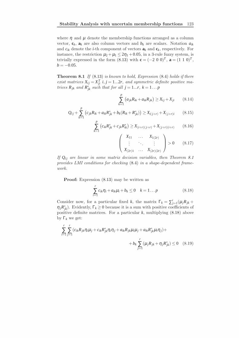
Stability Analysis with uncertain membership functions 123
where η and µ denote the membership functions arranged as a columnvector, ck, ak are also column vectors and bk are scalars. Notation aik
and cik denote the i-th component of vectors ak and ck, respectively. Forinstance, the restriction µ2+ µ1≤ 2η1+0.05, in a 3-rule fuzzy system, istrivially expressed in the form (8.13) with c = (−2 0 0)T , a = (1 1 0)T ,b =−0.05.
Theorem 8.1 If (8.13) is known to hold, Expression (8.4) holds if thereexist matrices Xi j = XT
ji i, j = 1...2r, and symmetric definite positive ma-trices R jk and R∗jk such that for all j = 1...r, k = 1. . . p
p
∑k=1
(
a jkRik + aikR jk)
≥ Xi j + X ji (8.14)
Qi j +p
∑k=1
(
c jkRik + aikR∗jk + bk(Rik + R∗jk))
≥ Xi( j+r) + X( j+r)i (8.15)
p
∑k=1
(
cikR∗jk + c jkR∗ik)
≥ X(i+r)( j+r) + X( j+r)(i+r) (8.16)
X11 . . . X1(2r)...
. . ....
X(2r)1 . . . X(2r)(2r)
> 0 (8.17)
If Qi j are linear in some matrix decision variables, then Theorem 8.1provides LMI conditions for checking (8.4) in a shape-dependent frame-work.
Proof: Expression (8.13) may be written as
r
∑i=1
cikηi + aikµi + bk ≤ 0 k = 1. . . p (8.18)
Consider now, for a particular fixed k, the matrix Γk = ∑rj=1(µ jR jk +
η jR∗jk). Evidently, Γk ≥ 0 because it is a sum with positive coefficients ofpositive definite matrices. For a particular k, multiplying (8.18) aboveby Γk we get:
r
∑i=1
r
∑j=1
(cikR jkηiµ j + cikR∗jkηiη j + aikR jkµiµ j + aikR∗jkµiη j)+
+ bk
r
∑j=1
(µ jR jk + η jR∗jk)≤ 0 (8.19)

124 Main Result
Subsequently, by using the equalities ∑ri=1 µi = 1 and ∑r
i=1ηi = 1 in
bkΓk = bk
r
∑j=1
(r
∑i=1
ηiµ jR jk +r
∑i=1
µiη jR∗jk)
we get a negative-semi-definite matrix to be denoted as Hk given by:
Hk =r
∑i=1
r
∑j=1
(cikR jkηiµ j + cikR∗jkηiη j + aikR jkµiµ j+
+ aikR∗jkµiη j + bk(ηiµ jR jk + µiη jR∗jk))≤ 0 (8.20)
As (8.20) holds for each k, denoting by H = ∑pk=1Hk, evidently H ≤ 0,
i.e.:
H =p
∑k=1
r
∑i=1
r
∑j=1
(cikR jkηiµ j + cikR∗jkηiη j + aikR jkµiµ j+
+ aikR∗jkµiη j + bk(ηiµ jR jk + µiη jR∗jk))≤ 0 (8.21)
Taking H above and Θ from (8.4), it is evident that if Θ+H > 0 can beproved, then Θ > 0. Then, conveniently grouping terms:
Θ+ H =r
∑i=1
r
∑j=1
(
µiµ j
p
∑k=1
aikR jk + ηiη j
p
∑k=1
cikR∗jk+
+ µiη j
(
Qi j +p
∑k=1
c jkRik + aikR∗jk + bk(Rik + R∗jk)
))
=
=r
∑i=1
(
µ2i
p
∑k=1
aikRik + η2i
p
∑k=1
cikR∗ik
)
+ ∑i< j≤r
(
µiµ j
p
∑k=1
aikR jk + a jkRik+
+ηiη j
p
∑k=1
cikR∗jk + c jkR∗ik
)
+r
∑i=1
r
∑j=1
µiη j(Qi j+
+r
∑k=1
c jkRik + aikR∗jk + bk(Rik + R∗jk)) (8.22)
Consider now the variables Xi j = XTji i, j = 1. . . r, which fulfill (8.14)-
(8.16). By suitably grouping terms, and associating (8.14) to the termswhere µiµ j appears, (8.15) to those with µiη j and (8.16) to those with

Stability Analysis with uncertain membership functions 125
ηiη j, we have3:
Θ+ H ≥r
∑i=1
(
µ2i Xii + η2
i Xii)
+r
∑i=1
∑i< j≤r
(µiµ j(Xi j + X ji)+
+ ηiη j(X(i+r)( j+r) + X( j+r)(i+r)))+r
∑i=1
r
∑j=1
(
µiη j(Xi( j+r) + X( j+r)i))
(8.23)
By taking the same ψ as in (8.4), and definingξ = [µ1ψT . . . µrψT η1ψT . . . ηrψT ]T , the terms in the right-hand sideof (8.23) may be expressed as follows:
ψT (Θ+ H)ψ ≥ ξ T
X11 . . . X1(2r)...
. . ....
X(2r)1 . . . X(2r)(2r)
ξ (8.24)
Hence, given (8.24), if (8.17) holds, ψT (Θ + H)ψ > 0 for ψ 6= 0 and,hence, (8.4) holds.
8.4 Particular cases
Let us now consider some particular cases of Theorem 8.1.
Multiplicative uncertainty Consider now the multiplicative uncer-tainty case, also discussed in (Lam & Leung, 2005):
ρmi ≤
ηi
µi≤ ρM
i (8.25)
Corollary 8.1 If (8.25) is known to hold, Expression (8.4) holds ifthere exist matrices Xi j = XT
ji i, j = 1...2r, and symmetric definite positive
3Note that (8.14) implies ∑pk=1 aikRik ≥ Xii, and an analogous consideration may be
made with (8.16): the diagonal terms µ2i , η2
i need not be explicitly written in thetheorem statement.

126 Particular cases
matrices Ri j, N ji, R∗i j and N∗ji such that for all i, j = 1...r:
Ri jρmj −Ni jρM
j + R jiρmi −N jiρM
i ≥ Xi j + X ji (8.26)
Qi j− (Ri j−Ni j)− (R∗i j−N∗i j)≥ Xi( j+r) + X( j+r)i (8.27)
R∗i j
ρMi−
N∗i j
ρmi
+R∗jiρM
j−
N∗jiρm
j≥ X(i+r)( j+r) + X( j+r)(i+r) (8.28)
X11 . . . X1(2r)...
. . ....
X(2r)1 . . . X(2r)(2r)
> 0 (8.29)
Proof: The uncertainty description can be expressed as:
ηk−ρMk µk ≤ 0 −ηk + ρm
k µk ≤ 0 (8.30)
Hence, the theorem will be proved by using Theorem 8.1 with 2r con-straints, divided in two groups (both with bk = 0): One with akk = −ρM
k , aik = 0 for i 6= k and ckk = +1, cik = 0 fori 6= k; Theorem 8.1 will be applied using Mik and M∗ik as relaxationvariables, Another group (consider a′k = ak+r, c′k = ck+r) with a′kk = ρm
k , a′ik = 0for i 6= k and c′kk =−1, c′ik = 0 for i 6= k; Theorem 8.1 will be appliedusing Tik and T ∗ik as relaxation variables.
Note that (8.14)–(8.16) in this case reduce to
a j jMi j + aiiM ji + a′j jTi j + a′iiTji ≥ Xi j + X ji (8.31)
Qi j +(
c j jMi j + aiiM∗ji + c′j jTi j + a′iiT
∗ji
)
≥ Xi( j+r) + X( j+r)i (8.32)
ciiM∗ji + c j jM
∗i j + c′iiT
∗ji + c′j jT
∗i j ≥ X(i+r)( j+r) + X( j+r)(i+r) (8.33)
because most of the aik, cik, a′ik, c′ik are zero.
The conditions for the theorem being proved arise immediately oncethe values of aik, cik, a′ik, c′ik are substituted above and the followingchanges of variable are made:
Mi j = Ni j Ti j = Ri j ρMi M∗i j = R∗i j ρm
i T ∗i j = N∗i j

Stability Analysis with uncertain membership functions 127
Additive uncertainty Consider a set of known additive bounds onthe membership functions, δk, so that, given (8.4), it is known that:
|µk−ηk|< δk k = 1. . . r (8.34)
Corollary 8.2 If the membership functions satisfy (8.34), expression(8.4) holds if there exist matrices Ri j, Ni j, Xi j = XT
ji and Xi( j+r) = XT( j+r)i
i, j = 1...r, such that:
Mi j = Ri j−Ni j, M+i j = Ri j + Ni j (8.35)
Mi j + M ji ≥ Xi j + X ji (8.36)
Qi j−2Mi j−r
∑k=1
δk(M+ik + M+
k j)≥ Xi( j+r) + X( j+r)i (8.37)
for all i = 1. . . ,r, j = 1. . . ,r and
Y11 =
X11 . . . X1r...
. . ....
Xr1 . . . Xrr
Y12 =
X1(r+1) . . . X1(2r)...
. . ....
Xr(r+1) . . . Xr(2r)
(8.38)
(
Y11 Y12
Y T12 Y11
)
> 0 (8.39)
Proof: The uncertainty description can be expressed as:
ηk−µk−δk ≤ 0 −ηk + µk−δk ≤ 0 (8.40)
Hence, the theorem will be proved by using Theorem 8.1 with 2r con-straints, divided in two groups: One with akk = 1, aik = 0 for i 6= k and ckk = −1, cik = 0 for i 6=
k; Theorem 8.1 will be applied using Rik and R∗ik as relaxationvariables, Another one with akk =−1, aik = 0 for i 6= k and ckk = +1, cik = 0 fori 6= k; Theorem 8.1 will be applied using Nik and N∗ik as relaxationvariables.
The conditions for the theorem being proved arise almost immediatelyonce those for Theorem 8.1 are written as (8.31)–(8.33) and the following

128 Particular cases
equalities are enforced: R∗i j = N ji, N∗i j = R ji. Details are omitted forbrevity.
The following two lemmas show that: (a) the PDC case is recoveredfrom the above corollaries under no uncertainty and, (b) as expected,the conditions proposed with the additive or multiplicative uncertaintybounds are less conservative than the trivial ones Qi j > 0.
Lemma 8.2 When the membership error bounds δi is equal to zero, orthe multiplicative bounds are equal to one (i.e., µi = ηi), a feasible set ofvariables for corollaries 8.1 and 8.2 may be obtained if (Liu & Zhang,2003, Theorem 2) (which applies to the PDC case) is feasible.
Proof: Note that, when δ = 0 and ρmi = ρM
i = 1, enforcing R∗i j = Ri j,N∗i j = Ni j, X(i+r)( j+r) = Xi j in corollary 8.1 leaves conditions (8.26)–(8.29)identical to (8.36)–(8.39) in corollary 8.2 so a unified analysis is possible,considering only corollary 8.2 in the sequel.
If δi = 0 for all i, then (8.37) can be rewritten as
Qi j−2Mi j ≥ Xi( j+r) + X( j+r)i (8.41)
Taking Mi j = Qi j/2 and Xi( j+r) = 0, which fulfill (8.41), the inequality(8.36) gets converted into:
Qi j/2+ Q ji/2≥ Xi j + X ji (8.42)
and the matrix Y12 is equal to 0. Finally (8.39) is
(
Y11 00 Y11
)
> 0 (8.43)
equivalent to Y11 > 0.This condition and (8.42) are the ones in (Liu &Zhang, 2003, Theorem 2): if the latter is feasible, corollaries 8.1 and 8.2without uncertainty will be feasible as well.
Lemma 8.3 If Qi j > 0 for all i, j = 1. . . r, then corollaries 8.1 and 8.2are satisfied.

Stability Analysis with uncertain membership functions 129
Proof: Regarding corollary 8.2, take all Ni j = 0, and all X(i+r) j = Xi( j+r) =0. Then, take Ri j = 0 for i 6= j and Rii = εiI for i = 1. . . r, choosing a smallenough εi > 0 so that Qii≫ 2εiI (I denotes the identity matrix). ThenXi j = 0, i 6= j, fulfills (8.36) and (8.37), and for i = j Xii = εiI fulfills (8.36).Finally all Xi j form a diagonal positive matrix that satisfies (8.39) if ε issmall enough.
Corollary 8.1 is also satisfied with the same choice of Ni j and Ri j plusN∗i j = Ni j, R∗i j = Ri j. Details are analogous to those above for Corollary8.2.
8.5 Examples
Example 8.1 Let us consider the system:
x =3
∑i=1
µi(x)(Aix+ Biu) (8.44)
A1 =
0.39 0.85 0.480.81 0.010 0.340.51 0.28 0.078
, B1 =
0.1 0.580.016 0.320.80 0.58
A2 =
0.0089 0.35 0.960.76 0.54 0.380.14 0.85 0.25
, B2 =
0.031 0.0360.87 0.530.75 0.78
A3 =
0.84 0.094 0.80.19 0.2 0.130.82 0.58 0.33
, B3 =
0.054 0.160.21 0.840.47 0.64
A state-feedback fuzzy controller with the structure
u =−2
∑j=1
η j(x)Fjx
is proposed, where functions η j(x) are an approximation of µ j(x) fulfilling(8.34), for a shared δk = δ . Several values of the uncertainty δ will betested, ranging from δ = 0 (which is the well-known PDC case ηi = µi)to δ = 1 (indicating absolute ignorance on the shape of µi).

130 Examples
Table 8.1: Decay rate α achievable as a function of the uncertainty δδ 0 0.05 0.1 0.15 0.2 0.25 0.3 . . . 1
α 0.36 0.35 0.33 0.31 0.30 0.29 0.28 . . . 0.28
The control objective will be finding the Fj maximizing the achievablequadratic decay rate α (roughly, analogous to the dominant pole of alinear system), by checking (8.4) with conditions from (Tanaka & Wang,2001)
Qi j =−AiY −YATi + BiM j + MT
j Bi−2αY (8.45)
where Y is a positive-definite matrix related to a Lyapunov function andM j = FjY . The sufficient conditions provided in corollary 8.2 will be used,searching for the maximum value of α for which a feasible LMI solutionexists (which is a generalized eigenvalue problem). The maximum αachieved for different values of δ appears in Table 8.1.
The results in the referred table show that the more precise theknowledge of µ is (lower δ ), the faster decay rates can be achieved. Theresults for δ = 0 are coincident with those (Liu & Zhang, 2003, Theorem2) for the PDC case, as discussed in Lemma 8.2. Furthermore, theresults for δ = 1 are coincident with the ones obtained by using a non-fuzzy linear regulator u = −Kx robustly stabilising a polytopic system(Boyd et al., 1994) via the LMI conditions:
Qi =−AiY −YATi + BiM + MT Bi−2αY > 0
Such conditions are, in fact, equivalent to the shape-independent onesQi j > 0 (indeed, conditions for M1 in (8.45) are the same as those for M2,etc. so there is no loss of generality by assuming M1 = M2 = · · ·= M).
In summary, with the methodology in this chapter, a smooth tran-sition between a full-PDC fuzzy controller and a robust linear one isachieved: as uncertainty increases the feasible performance decreases. Ifthe uncertainty is greater than 0.3, the performance of fuzzy and non-fuzzy controllers is the same.
Example 8.2 Let us consider an example of DC motor controlling aninverted pendulum on a gear train (Kuschewski, Hui, & Zak, 1993):

Stability Analysis with uncertain membership functions 131
Figure 8.1: Inverted pendulum controlled by a DC motor
The state equations describing the plant are
x1x2x3
=
x2gl sinx1 + NKm
ml2 x3
−KbNLa
x2− RaLa
x3
+
001
La
u (8.46)
where the state variables are: x1 = θp, x2 = θp, x3 the dc motor currentand the input u is the Voltage of the dc motor supposed less than 100V.Km is the motor torque constant, Kb is the back emf constant, and N isthe gear ratio. Reasonable parameters for the plant are g = 9.8 m./s.2,l = 1 m., m = 1 Kg., N = 10, Km = 0.1 Nm/A, Kb = 0.1 V s/rad, Ra = 1 Ωand La = 100 mH. this parameters lead to
x1
x2
x3
=
x2
9.8sinx1 + x3
−10x2−10x3
+
0010
u (8.47)
Fuzzy modelling for the nonlinear system was done in (Tanaka &Sano, 1994; Kawamoto, 1996), following sector nonlinearity proceduredescribed in Section 3.3. The fuzzy model is as follows
x = µ1(A1x+ B1u)+ µ2(A2x+ B2u) (8.48)

132 Examples
Here,
x = (x1 x2 x3)T (8.49)
A1 =
0 1 09.8 0 10 −10 −10
, B1 =
0010
(8.50)
A1 =
0 1 00 0 10 −10 −10
, B2 =
0010
(8.51)
(8.52)
the membership functions are defined as
µ1(x) =
sinx1x1
, x1 6= 01 x1 = 0
(8.53)
µ2 = 1−µ1 (8.54)
This fuzzy model exactly represents the dynamics of the nonlinear me-chanical system under −π ≤ x1≤ π.We design a disturbance rejection fuzzy controller. We can rewrite thesystem as:
x =2
∑i=1
µi(Aix+ Biu)+ Bww (8.55)
y = x1 (8.56)
where Bw = (1 1 0)T is the direction of the disturbance w. Then positivityconditions of the closed loop system controlled by a PDC controller (8.2)can be formulated as
2
∑i=1
2
∑j=1
µ1η jxT Qi jx (8.57)
where Qi j are the conditions for disturbance rejection obtained in Section3.5. For a proper comparison, considerer the system without knowl-edge of the membership functions. Then the best controller is a Lin-ear controller. In this case the best disturbance rejection coefficient isγM = 0.31102. On the other hand let us considerer µi = ηi then the per-formance conditions yield to Theorem 3.5 and the obtained coefficient isγm = 0.28434. So our system with some information on the ηi boundariesmust be between γM and γm.

Stability Analysis with uncertain membership functions 133
Considering the relative uncertainty (8.25)
ρm ≤ ηi
µi≤ ρM (8.58)
with ρm = 1/1.5 and ρM = 1.5 Then the best disturbance rejectioncoefficient obtained for Lemma 8.1 is γ = 0.291 and for Corollary 8.1 isγ = 0.289. So the result of Corollary 8.1 improves the result of CorollaryLemma 8.1.
Example 8.3 Let us now discuss the same example as in (Lam & Le-ung, 2005) regarding multiplicative uncertainty. Consider a TS fuzzysystem with 2 rules, with matrices
A1 =
(
2 −101 0
)
, A2 =
(
a −101 1
)
B1 =
(
10
)
, B2 =
(
b0
)
Analogously to (Lam & Leung, 2005), a two-rule state-feedback fuzzycontroller is built by designing the Fi, i = 1,2, by pole-placement so thatthe closed-loop poles of Ai−BiFi are at −1 and −15 (unique solution).Then, stability of the overall closed-loop system (8.3) is tested for dif-ferent values of a and b, and different values of ρM
i and ρmi in (8.25).
Figure 8.2 shows the values of a and b for which the closed loop canbe proved stable, for different uncertainty levels: the left plot presentsthe results with Corollary 8.1, whereas the right one presents the resultswith Lemma 8.1; the tested uncertainty values were ρM
i = ε , ρmi = 1/ε for
ε taking values in 2,1.5,1.2,1.1,1. All points feasible for a particularvalue of ε were as well feasible for lower values of it.
Clearly, Corollary 8.1 in this work achieves better results than (Lam& Leung, 2005) in all tested uncertain cases, i.e., it finds a larger setof values for a and b yielding a stable closed loop. As expected, for nouncertainty in memberships (ρM
i = ρmi = 1) the PDC case is recovered
in both cases (denoted with • in the figure), with results coincident tothose from Theorem 3.5.

134 Conclusions
1 2 3 4 5 62
3
4
5
6
7
8
9
10
1 2 3 4 5 62
3
4
5
6
7
8
9
10Corollary 8.1 Lemma 8.1
aa
bb
Figure 8.2: Feasible values of parameters a and b for Example 2: –(left): Corollary 8.1, – (right) Lemma 8.1. Legend: [ 2 symbol]: ρM
i = 2,ρm
i = 1/2; [ © symbol]: ρMi = 1.5, ρm
i = 1/1.5; [ × symbol]: ρMi = 1.2,
ρmi = 1/1.2; [ + symbol]: ρM
i = 1.1, ρmi = 1/1.1; [ • symbol]: ρM
i = ρmi = 1,
i.e., PDC controller
8.6 Conclusions
This chapter presents an extension of the methodology in (Lam & Leung,2005) to consider arbitrary linear constraints in the shape of uncertainmembership functions in a non-PDC fuzzy control setup. The proposedextensions apply to various stability and performance requirements incontinuous and discrete systems, by making different choices for Qi j.
The main contribution of the chapter is, thus, the ability to incorpo-rate a wider class of constraints on the membership shape than (Lam &Leung, 2005). Interestingly, with the same type of restrictions, numer-ical examples illustrate that improvements over (Lam & Leung, 2005)may also be achieved, at least in the particular cases of the examples.
The examples in the chapter also illustrate the gradual loss of per-formance from a “full-PDC” fuzzy controller to a “robust linear” one asuncertainty in the memberships increases.

Chapter 9
Tensor product TS systems
In many fuzzy models, membership functions with multiple argumentsare defined as the product of simpler ones, where all possible combina-tions of such products conform a fuzzy partition. In particular, suchsituations arise with widely-used fuzzy modelling techniques for nonlin-ear systems (Tanaka & Wang, 2001; Babuska et al., 1996). These type offuzzy models will be denoted as tensor-product fuzzy systems, becausetheir expressions can be understood as operations on multi-dimensionalarrays.
This chapter discusses the generalization to tensor-product fuzzy sys-tems of the results on stability and performance of Takagi-Sugeno fuzzysystems with LMIs. They were shown in Chapter 3.
9.1 Introduction
In many situations in fuzzy systems the membership functions can beexpressed as the “tensor product” of simpler partitions, so that the fuzzysystem can be written as a multi-dimensional fuzzy summation, for in-stance x = ∑r
i=1∑rj=1∑r
k=1 µiµ jµk(Ai jkx + Bi jku). The tensor notation tobe used in this chapter is motivated by the use of multidimensional ar-rays to describe this class of fuzzy systems (see (Baranyi, Tikk, Yam, &Patton, 2003)).
Removing part of the conservatism in current solutions for the tensor-product case above is indeed of interest; this product structure is oftenthe case in many engineering applications of fuzzy control: in the systematic “sector nonlinearity” fuzzy modelling techniques
135
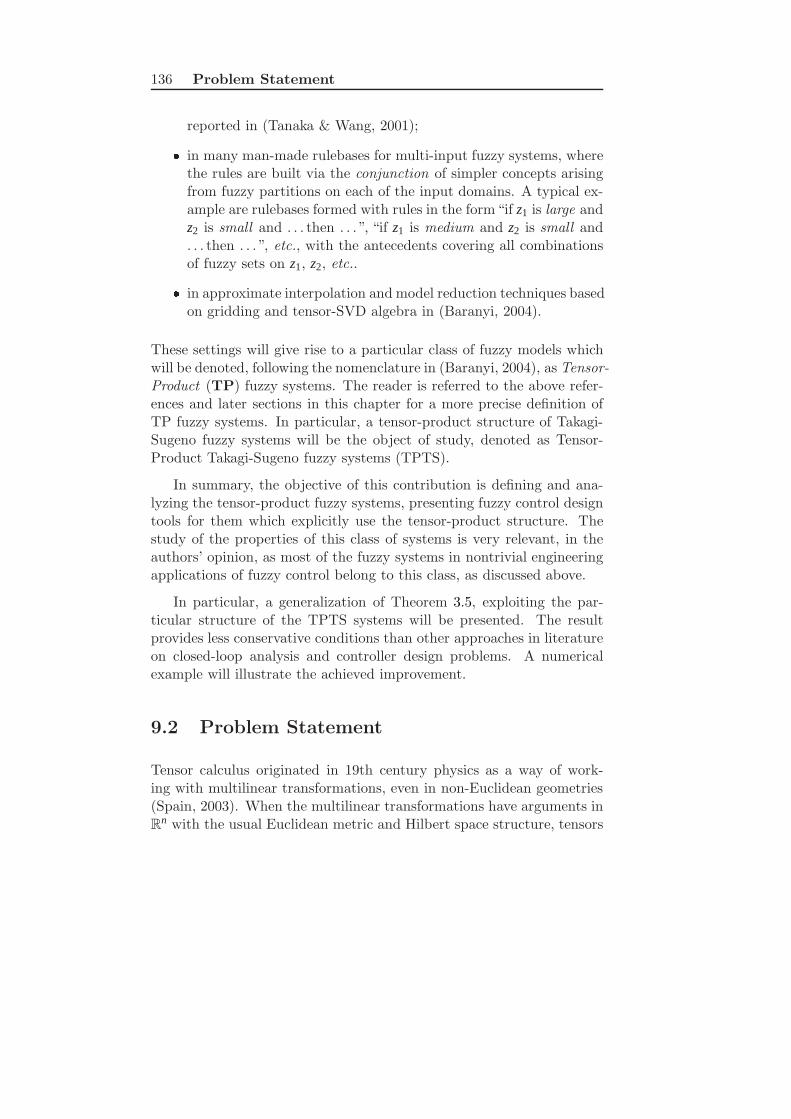
136 Problem Statement
reported in (Tanaka & Wang, 2001); in many man-made rulebases for multi-input fuzzy systems, wherethe rules are built via the conjunction of simpler concepts arisingfrom fuzzy partitions on each of the input domains. A typical ex-ample are rulebases formed with rules in the form“if z1 is large andz2 is small and . . . then . . . ”, “if z1 is medium and z2 is small and. . . then . . . ”, etc., with the antecedents covering all combinationsof fuzzy sets on z1, z2, etc.. in approximate interpolation and model reduction techniques basedon gridding and tensor-SVD algebra in (Baranyi, 2004).
These settings will give rise to a particular class of fuzzy models whichwill be denoted, following the nomenclature in (Baranyi, 2004), as Tensor-Product (TP) fuzzy systems. The reader is referred to the above refer-ences and later sections in this chapter for a more precise definition ofTP fuzzy systems. In particular, a tensor-product structure of Takagi-Sugeno fuzzy systems will be the object of study, denoted as Tensor-Product Takagi-Sugeno fuzzy systems (TPTS).
In summary, the objective of this contribution is defining and ana-lyzing the tensor-product fuzzy systems, presenting fuzzy control designtools for them which explicitly use the tensor-product structure. Thestudy of the properties of this class of systems is very relevant, in theauthors’ opinion, as most of the fuzzy systems in nontrivial engineeringapplications of fuzzy control belong to this class, as discussed above.
In particular, a generalization of Theorem 3.5, exploiting the par-ticular structure of the TPTS systems will be presented. The resultprovides less conservative conditions than other approaches in literatureon closed-loop analysis and controller design problems. A numericalexample will illustrate the achieved improvement.
9.2 Problem Statement
Tensor calculus originated in 19th century physics as a way of work-ing with multilinear transformations, even in non-Euclidean geometries(Spain, 2003). When the multilinear transformations have arguments inR
n with the usual Euclidean metric and Hilbert space structure, tensors
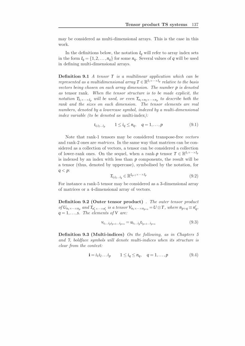
Tensor product TS systems 137
may be considered as multi-dimensional arrays. This is the case in thiswork.
In the definitions below, the notation Iq will refer to array index setsin the form Iq = 1,2, . . . ,nq for some nq. Several values of q will be usedin defining multi-dimensional arrays.
Definition 9.1 A tensor T is a multilinear application which can berepresented as a multidimensional array T ∈R
I1×···×Ip relative to the basisvectors being chosen on each array dimension. The number p is denotedas tensor rank. When the tensor structure is to be made explicit, thenotation TI1×···×Ip will be used, or even Tn1×n2×···×np to describe both therank and the sizes on each dimension. The tensor elements are realnumbers, denoted by a lowercase symbol, indexed by a multi-dimensionalindex variable (to be denoted as multi-index):
ti1i2...ip 1≤ iq ≤ nq, q = 1, . . . , p (9.1)
Note that rank-1 tensors may be considered transpose-free vectorsand rank-2 ones are matrices. In the same way that matrices can be con-sidered as a collection of vectors, a tensor can be considered a collectionof lower-rank ones. On the sequel, when a rank-p tensor T ∈ R
I1×···×Ip
is indexed by an index with less than p components, the result will bea tensor (thus, denoted by uppercase), symbolised by the notation, forq < p:
Ti1i2...iq ∈RIq+1×···×Ip (9.2)
For instance a rank-5 tensor may be considered as a 3-dimensional arrayof matrices or a 4-dimensional array of vectors.
Definition 9.2 (Outer tensor product) . The outer tensor productof Un1×···×np and Tn′1×···×n′s is a tensor Vn1×···×np+s =U⊗T , where np+q≡ n′q,q = 1, . . . ,s. The elements of V are:
vi1...ipip+1...ip+s = ui1...iptip+1...ip+s (9.3)
Definition 9.3 (Multi-indices) On the following, as in Chapters 5and 7, boldface symbols will denote multi-indices when its structure isclear from the context:
i = i1i2 . . . ip 1≤ iq ≤ nq, q = 1, . . . , p (9.4)

138 Problem Statement
and, similarly, the cartesian product of index sets will be referred to bythe notation:
Ip = I1×·· ·× Ip (9.5)
For instance, if either the dimensions have been suitably defined be-forehand or they are not relevant to a particular discussion, the elementsreferred to in (9.1) will be denoted as ti, i∈ Ip for convenience. The multi-index will be said to have rank p, as the tensor it indexes. Note that,the multi-indices sets Ip are formed of the cartesian product of differentindex sets. On the other hand, the multi-indices sets defined in Chapters5 and 7 were formed of the cartesian product of the same index set.
Multi-indices of higher rank will also be represented by the juxta-position of indices of smaller rank. For instance, the elements of thetensor resulting from the outer product in (9.3) will be denoted, whenconvenient, by vij = uitj, for suitably defined i ∈ Ip, j ∈ I
′s.
The following definition extends the usual matrix product along pshared dimensions1.
Definition 9.4 (product) The ordinary product of two tensors U ∈R
I′′
s×Ip and V ∈ RIp×I
′q, which share the dimensions Ip, is a tensor T ∈
RI′′
s×I′q which will be denoted as T = U ·p V whose elements are:
ti′′i′ = ti′′1...i′′si′1...i′q =n1
∑i1=1
n2
∑i2=1
. . .np
∑ip=1
ui′1...i′′si1i2...ip vi1i2...ipi′1...i′q= ∑
i∈Ip
ui′′ivii′
The notation U ·V (or UV ) will be used to represent the product withshared index of rank 1, i.e., UV = U ·V = U ·1V (if U and V are rank-2tensors, UV is the usual matrix product).
As an example of the use of the product notation, a quadratic form(xT Qx in matrix notation) may be expressed as (x⊗ x) ·2 Q.
1There are other alternative definitions and notations for (inner) tensor products(De Lathauwer, De Moor, & Vandewalle, 2000; Baranyi, 2004), as the number andposition of the shared dimensions may vary. The one presented here has been adoptedfor convenience.

Tensor product TS systems 139
Proposition 9.1 Given rank-p tensors A1, A2, a rank-q tensor B and arank-(p+q) tensor C, the ordinary product and the outer product verify:
A1 ·p A2 = A2 ·p A1 (9.6)
(A⊗B) ·p+qC = A ·p (C ·q B) (9.7)
Note that A1 ·p A2 is a real number, which is the generalization of the vec-tor scalar product. For a rank-2 tensor (matrix)
√A ·2 A is the Frobenius
norm.
Definition 9.5 (unfolding) The unfolding operation (“flattening”),denoted as f lr←qV reduces the rank of a tensor V ∈ RI1×···×Ir×···×Iq×···×Ip byone, converting it to a new tensor U ∈ RI1×···×I′r×···×Iq−1×Iq+1×···×Ip whoseelements are given by:
ui1...ir ...ip = vi1...ir−1 jr ir+1...iq−1 jqiq+1...ip (9.8)
where (ir−1) = ( jr−1)∗nq +( jq−1),i.e., jr−1 is the integer part of thequotient (ir−1)/nq, and ( jq−1) is the remainder.
As unfolding can be nested, successive applications of the operatorcan rearrange the tensor as a matrix or even as a vector. The notation
f lp←q←r←···←t←s = f lp←q f lq←r . . . f lt←s p < q < r < .. . t < s
will be later used.
Example 9.1 Consider the tensor of rank 3, with n1 = 2, n2 = 3, n3 = 2given by: ti1i2i3 = 2i1−13i2−15i3−1. Then,
f l2←3T =
(
1 5 3 15 9 452 10 6 30 18 90
)
and
f l1←2←3T = f l1←2 f l2←3T = (1 5 3 15 9 45 2 10 6 30 18 90)
Example 9.2 Unfolding a rank-3 tensor T may produce 6 different ma-trices: f l1←2T , f l1←3T , f l2←1T , f l2←3T , f l3←1T and f l3←2T . The n-mode matrix of a rank-p tensor T (Definition 4 in (Baranyi, 2004))is, for n > 2, the transpose of the matrix resulting from the unfoldingf l2←1←3←4←···←n−1←n+1←pT .

140 Problem Statement
As unfolding is just a reordering of the tensor elements, it’s easy toprove the following proposition (details omitted for brevity).
Proposition 9.2 The inner product of tensors remains invariant underunfolding on any of the shared dimensions, i.e.,
( f lr←qU) ·p−1 ( f lr←qV ) = U ·p V
In particular, the above proposition generalises the transformationfrom (9.14) to (9.15), which used the fact that
(µ⊗µ⊗ x⊗ x) ·4 X = f l1←3 f l2←4(µ⊗µ⊗ x⊗ x) ·2 f l1←3 f l2←4X
There are many other definitions in tensor algebra (n-mode tensor-matrix products (De Lathauwer et al., 2000; Baranyi, 2004), etc.) whichare out of the scope of this work. The reader is referred to the just citedworks and textbooks (Spain, 2003; Temple, 2004) for further informationabout tensor algebra.
9.2.1 Sufficient Positivity Conditions
Sufficient conditions for positivity of Ξ in (3.23) are discussed in Chapter3. For convenience, some of them are reviewed below.
Lemma 9.1 If there exist matrices Xi j = XTji such that:
Xii ≤ Qii (9.9)
Xi j + X ji ≤ Qi j + Q ji i < j (9.10)
defining
Θ(t) =r
∑i=1
r
∑j=1
µi(z(t))µ j(z(t))x(t)T Xi jx(t) (9.11)
then Ξ(t) in (3.23) fulfills
Ξ(t)≥Θ(t) (9.12)

Tensor product TS systems 141
Proof: The proof is evident after reordering (3.23) and (9.11) as
Ξ(t) =r
∑i=1
µ2i xT Qiix+
r
∑i=1
r
∑j=i+1
µiµ jxT (Qi j + Q ji)x (9.13)
Θ(t) =r
∑i=1
µ2i xT Xiix+
r
∑i=1
r
∑j=i+1
µiµ jxT (Xi j + X ji)x (9.14)
respectively. In this way, (9.9) and (9.10) indicate that each term in thesummations in Ξ in (9.13) is larger than the corresponding one in thereordered Θ in (9.14).
Note that, in addition to an expression in the form (9.14), anotherexpression for Θ is:
Θ(t) = (µ1xT µ2xT . . .µnxT )
X11 . . . X1r...
. . ....
Xr1 . . . Xrr
µ1xµ2x...
µnx
(9.15)
which yields the well-known theorem 3.5.
9.2.2 Tensor-product fuzzy systems
This section will first present the fuzzy systems and fuzzy summationsin Chapter 3 with tensor notation, and then generalize the expressionsvia a new definition, which will encompass widely used classes of fuzzysystems. Basically, a so-called rank-p tensor will denote a p-dimensionalarray of real numbers. The reader is referred to section 9.2 for tensordefinitions, notation and operations with them.
Tensor expression for fuzzy systems
Note that the Takagi-Sugeno system (3.1) may be considered, byjuxtaposing Ai and Bi as a matrix with size n× (n+ w), as:
x =r
∑i=1
µi(Ai Bi)
(
xu
)
(9.16)
Consider now the one-dimensional array of matrices (Ai Bi) to be thecomponents of a suitably defined rank-3 tensor S so that the element si jk

142 Problem Statement
is the element ( j,k) of the matrix (Ai Bi), for j = 1, . . . ,n, k = 1, . . . ,(n+w).Consider also the membership functions to be arranged as a vector (rank-1 tensor). Then, (9.16) may be written as a tensor product
x = (µ ·1 S)
(
xu
)
(9.17)
because the tensor product µ ·1 S produces the so-called system matrix(rank-2 tensor):
µ ·1 S =r
∑i=1
µi(Ai Bi) (9.18)
As the memberships are a rank-1 tensor, the above fuzzy systems will bealso denoted as rank-1 fuzzy systems. The case of higher dimensionality(higher tensor rank) will be discussed later in this section.
It’s also straightforward to check that the double fuzzy summationsin (3.23) may also be expressed as:
Ξ = (µ⊗µ⊗ x⊗ x) ·4 Q (9.19)
where Q is a rank-4 tensor (a “matrix” of matrices Qi j), i.e., element qi jkl
is equal to the element at position (k, l) of the matrix Qi j. Note that Ξis a scalar.
9.2.3 Multi-dimensional tensor-product fuzzy systems
In many applications, membership functions in a multi-input fuzzy modelare chosen to be the product of simpler memberships with a linguisticinterpretation, and all the possible products of such simpler member-ships appear as rule antecedents2. Let us discuss a couple of simplemotivating examples.
Example 9.3 Consider a so-called fuzzy-PD regulator built by settingup a fuzzy partition on an“error (e)” variable (say, a partition with 5 setsgiven by negative large, negative, zero, positive, positive large), and another(different) partition in the “error derivative (de)” (say, a partition with3 sets negative, zero, positive ).
2Such simpler functions usually refer to a reduced number of input variables (butthe definitions later in this section allow for any set of variables in any membership).

Tensor product TS systems 143
For convenience, the membership functions on the error partition willbe denoted by (µ11(e), . . . ,µ15(e)), respectively, and those on the errorderivative, by (µ21(de),µ22(de),µ23(de)). The partitions are assumed toverify ∑5
i=1 µ1i = 1, ∑3i=1 µ2i = 1.
Once such partitions have been defined, rules are stated in a formsuch as:
IF e is negative large and de is positive THEN u = u13
IF e is negative and de is zero THEN u = u22...
In this example, the total number of rules is 5×3= 15. If the conjunctionis interpreted as the algebraic product, the output of the controller maybe expressed as:
u =5
∑i1=1
3
∑i2=1
µ1i1(e)µ2i2(de)ui1i2 (9.20)
Now, consider the tensor outer product of the vectors (i.e., rank-1 tensors) µ1 = (µ11(e), . . . ,µ15(e)) and µ2 = (µ21(de),µ22(de),µ23(de)).Then, considering the following “membership tensor”,
µ1(e)⊗µ2(de) =
µ11(e)µ21(de) µ11(e)µ22(de) µ11(e)µ23(de)µ12(e)µ21(de) µ12(e)µ22(de) µ12(e)µ23(de)µ13(e)µ21(de) µ13(e)µ22(de) µ13(e)µ23(de)µ14(e)µ21(de) µ14(e)µ22(de) µ14(e)µ23(de)µ15(e)µ21(de) µ15(e)µ22(de) µ15(e)µ23(de)
it’s easy to see that (9.20) may be expressed as an inner product of twotensors:
u = (µ1⊗µ2) ·2U (9.21)
for a suitably crafted matrix (rank-2 tensor) U of size 5× 3 whose el-ements are the corresponding rule consequents ui j for i = 1, . . . ,5, j =1,2,3.
Example 9.4 Consider a nonlinear model x = A(x)x+ B(x)u where

144 Problem Statement
A(x) = 0.75x−2.25sin(x)+ sin(x)x−2.5 (9.22)
B(x) = 0.42x+1.25sin(x)−0.42sin(x)x−0.25 (9.23)
for which a fuzzy model is to be set up for x ∈ [−π,π]. In this case, xmay be written as x = ∑2
i=1 νi pi, and sin(x) as sin(x) = ∑2i=1 ηiqi, with:
x = ν1(x) ·π + ν2(x) · (−π), sin(x) = η1(x) ·1+ η2(x) · (−1)
where membership functions are ν1 = 12π (x + π), ν2 = 1 − µ1,
η1 = 12(sin(x)+1), η2 = 1−η1, resulting in
A(x) = 0.752
∑i=1
νi pi−2.252
∑i=1
ηiqi +(2
∑i=1
ηiqi)(2
∑i=1
νi pi)−2.5
A(x) =2
∑i=1
2
∑j=1
νiη j(0.75pi−2.25q j + piq j−2.5) =2
∑i=1
2
∑j=1
νiη jai j
where
a11 = 0.748,a12 =−1.035,a21 =−10.247,a22 = 0.536
and similarly
B(x) =2
∑i=1
2
∑j=1
νiη j(0.42pi +1.25q j−0.42piq j−0.25) =2
∑i=1
2
∑j=1
νiη jbi j
where:b11 = 1,b12 = 1.139,b21 = 1,b22 =−4.139
Hence, the fuzzy system can be expressed as:
x =2
∑i=1
2
∑j=1
νiη j(ai jx+ bi ju) = ∑i∈I2
µi(aix+ biu) (9.24)
where i is a two-dimensional index variable (i1, i2) taking values in the setI2 = 1,2×1,2, and µi = νi1ηi2, using the multiindex notation in theAppendix9.2. In an analogous way to (9.20) in the previous example, atensor notation can be thought of (see below).
Motivated by the above examples, let us consider now a definitionfor a general tensor-product fuzzy model in the Takagi-Sugeno (TS)

Tensor product TS systems 145
framework (TS fuzzy systems are the most frequently used process modelfor fuzzy control in current literature), in order give a compact notationto fuzzy systems whose expression is a multi-dimensional sum, as in theabove examples.
Definition 9.6 Tensor-product Takagi-Sugeno fuzzy systems.Consider a vector of measurable variables, z, in an universe of discourseZ. Consider also p fuzzy partitions defined on Z, each of them with n1,. . . np fuzzy sets, respectively.
The fuzzy sets will be assumed to have linguistic labels denoted byM1i1, i1 = 1, . . . ,n1 for the first partition, M2i2, i2 = 1, . . . ,n2 for the secondpartition, etc. and membership functions arranged in rank-1 tensors:
µ1 = (µ11(z) µ12(z) . . . µ1n1(z))
µ2 = (µ21(z) µ22(z) . . . µ1n2(z))... (9.25)
µp = (µp1(z) µp2(z) . . . µpnp(z))
fulfillingnl
∑k=1
µlk = 1 0≤ µlk ≤ 1 l = 1, . . . , p
Then, a rank-p continuous-time tensor-product Takagi-Sugeno fuzzysystem (TPTS) built on the above fuzzy sets will be defined as the onedescribed by the rules3:
IF z is (M1i1 and M2i2 and Mpip) THEN x = Ai1i2...ip x +Bi1i2...ip u
being its output evaluated with:
x = ∑i∈Ip
µi(Aix+ Biu) (9.26)
3In many applications, such as the one in Example 9.3, the rules have the form:
IF z1 is M1i1 and z2 is M2i2 and ... and zp is Mpip THEN x = Ai1i2...ip x+Bi1i2...ip u
i.e., fuzzy partitions are defined over universes of discurse of smaller dimension, sothat Z = Z1×Z2× . . .Zp. However, that’s not necessary, in principle, for the results inthis chapter to apply. For instance if Z is R
2, we could have p = 3, with three fuzzypartitions defined on, say, z1 + z2, z1−
√z2 and (sin(z1)+1)/(cos(z2)+1). Hence, the
rules above in this footnote are a particular case of the ones in Definition 9.6.

146 Problem Statement
where x and u are the TPTS state and input variables, respectively, i =i1i2 . . . ip, and
µi =p
∏k=1
µkik (9.27)
Remark: Analogous definitions may be cast for discrete-time TPTSsystems and also for systems incorporating output equations, but theyare omitted for brevity.
Using tensor notation, the following definition for TPTS systems isequivalent to the previous one (proof is omitted as it is just an issue ofnotation).
Definition 9.7 Consider a state vector x with dimension d, and aninput vector u with dimension w, and form a vector of dimension n+ wby juxtaposing x and u. Consider a set of p fuzzy partitions defined ona universe Z, each of them arranged as a rank-1 tensor µi, i = 1, . . . , p,i.e., as in (9.25) above. Then, a TPTS fuzzy system is described by:
x = (µ ·p S)
(
xu
)
(9.28)
where S is a tensor with rank p + 2 and dimensions n1, n2, . . . , np,np+1 = d, np+2 = d + w and
µ = µ1⊗µ2⊗·· ·⊗µp
is a tensor with dimensions n1, n2, . . . , np (whose elements are, evi-dently, given by (9.27)), denoted as membership tensor. S will be de-noted as consequent tensor4.
An example of a membership tensor element is, for instance µ3,4,1,1 =µ13µ24µ31µ41, which will denote a particular rule in a rank-4 TPTS fuzzysystem.
Note that µ ·p S is a rank-2 tensor (i.e., a matrix which multipliesthe state-input vector with the ordinary matrix-vector multiplication).
4Notation in (9.28) is somehow different from that in (Baranyi, 2004), but equiva-lent. We wanted to emphasise the concept of “membership tensor” (generated via anouter product) whereas Baranyi used n-mode products (De Lathauwer et al., 2000)for subsequent singular-value-related computations.
Tensor product TS systems 147
Obviously, the notations (9.26) and (9.28) are equivalent to an ex-pression such as:
x =n1
∑i1=1
n2
∑i2=1
. . .np
∑ip=1
µ1i1µ2i2 . . .µpip(Ai1i2...ipx+ Bi1i2...ipu) (9.29)
For instance, the fuzzy system (9.24) may be considered a rank-2TPTS one.
Remarks on TPTS modelling: Many fuzzy systems in practicehave the tensor-product structure: Example 9.3 shows how they naturally arise from man-made rules. Another paradigmatic example is the “sector nonlinearity” mod-
elling methodology in (Tanaka & Wang, 2001); Example 9.4 inthis work is one of the simplest cases of the referred modellingtechnique. The reader is also referred to Example 3, in section2.2.1 of the referred book, which results in a 16-rule model TPTSdescribed by a membership tensor of dimensions 2×2×2×2 (ofcourse, the authors there do not use the notation introduced here),i.e., a rank-4 TPTS system. Last, (Baranyi, 2004) proposes a tensor-product based method-ology to approximate functions of multiple variables via Takagi-Sugeno fuzzy systems. The procedure, instead of being based onthe previously-discussed sector-nonlinearity approach, is based onmulti-dimensional gridding, lookup and interpolation. A subse-quent step of complexity reduction based on higher-order singularvalue decomposition (De Lathauwer et al., 2000) is needed in orderto get a reduced number of rules.
In fact, fuzzy system without a TSTP structure are seldom present inapplications, except in the simplest cases (even some first-order single-input TS systems can be better modelled as TSTP, by using the sector-nonlinearity methodology above cited, as demonstrated in Example 9.4in this work).
Proposition 9.3 Standard TS fuzzy systems are rank-1 TPTS fuzzysystems. Conversely, TPTS systems are a subclass of standard TS fuzzysystems.

148 Problem Statement
Proof: The first affirmation is evident from the definitions, and ithas already been discussed in Section 9.2.2. Regarding the second one,consider the well-known identity
n1
∑i1=1
n2
∑i2=1
. . .np
∑ip=1
µ1i1 . . .µpip = 1 (9.30)
It shows that the tensor product conforms a fuzzy partition composedof q = n1×n2×·· ·×np fuzzy sets. Such partition is given by the rank-1membership functions obtained by unfolding (flattening) the tensor µonto a vector. The idea can be formalised by using proposition 9.2, as:
x = (µ ·p S)
(
xu
)
= ( f l1←···←pµ ·1 f l1←···←pS)
(
xu
)
(9.31)
Hence, the original TPTS fuzzy system is expressed as a standard TSone because the membership tensor has been unfolded onto a vector, andthe consequent tensor S has been suitably rearranged by the f l operatoras a rank 3 tensor. Such rank-3 tensor f l1←···←pS produces an ordinarymatrix when subject to the product with the unfolded f l1←···←pµ (rank1).
Example 9.5 Consider a TP fuzzy system with p = 2, n1 = 2, n2 = 3.It may be equivalently considered as an “unfolded” fuzzy system with 6membership functions, denoted as βk(z) given by:
k = 1 β1(z) = µ11(z)µ21(z)
k = 2 β2(z) = µ11(z)µ22(z)
k = 3 β3(z) = µ11(z)µ23(z)
k = 4 β4(z) = µ12(z)µ21(z)
k = 5 β5(z) = µ12(z)µ22(z)
k = 6 β6(z) = µ12(z)µ23(z)
As another example, consider the fuzzy model of Example 9.4. In thesame way as above, if µ1 = ν1η1, µ2 = ν1η2, µ3 = ν2η1 and µ4 = ν2η2
were defined, a fuzzy TS with four models:
x =4
∑i=1
µi(aix+ biu) (9.32)
a1 = 0.748,a2 =−1.035,a3 =−10.247,a4 = 0.536 (9.33)
b1 = 1,b2 = 1,139,b3 = 1,b4 =−4.139 (9.34)

Tensor product TS systems 149
will exactly describe the nonlinear system under analysis for x ∈ [−π,π].
The reader is referred to (Tanaka & Wang, 2001) for more exam-ples of this tensor-product nonlinear modelling methodology (althoughtensor notation is not used and the final model is always unfolded).
Remark: Proposition (9.3) seems to make ill-fated any attemptto approach fuzzy control design for TPTS systems because TPTS areTS systems and vice-versa. However, a crucial fact is overlooked inthis argumentation: most results for stability and performance of TSfuzzy systems are independent of the membership shapes – particularlythose in (Tanaka & Wang, 2001; Kim & Lee, 2000; Liu & Zhang, 2003).However, an unfolded TPTS system does not sweep over all possiblemembership values5. Hence, such membership-independent stability andperformance conditions are conservative in the case of TPTS systems.This is the key issue motivating the work in Section 9.4.
9.3 Closed-loop tensor-product fuzzy systems
Definition 9.8 (tensor-product controller) Given a rank-p TPTSsystem (9.26), a controller in the form:
u =−∑j∈Ip
µj(z)Fjx =−(µ ·p F)x (9.35)
will be denoted as rank-p tensor product PDC controller (F is a rank-(p+2) tensor formed by suitably arranging matrices Fj).
By analogy with (3.14), it is straightforward to prove that, when arank-p tensor-product PDC controller is used to control a rank-p system(9.26), the closed loop equations are given by:
x = ∑i∈Ip
∑j∈Ip
µiµjGij = ((µ ⊗ µ) ·2p G)x (9.36)
where Gij = Ai−BiFj defines a tensor G with rank 2p+2 (note that, forfixed i and j, Bi and Fj are rank-2 tensors, following notation (9.2), sothe product is well defined, being the usual matrix product).
5for instance, it’s impossible to have β1 = 0.1 and β2 or β3 larger than 0.1 inExample 9.5.

150 Closed-loop tensor-product fuzzy systems
In general, analogously to (3.23), many stability and performancecriteria for tensor-product closed-loop fuzzy systems can be expressedas requiring, for any x 6= 0:
Θ = ∑i∈Ip
∑j∈Ip
µiµjxT Qijx > 0 (9.37)
For instance, it’s almost evident to check that a condition for quadraticstability of a TPTS fuzzy system is (9.37) with Qij given by (3.1) butreplacing the i and j with its boldfaced counterparts.
In tensor notation, stability and performance conditions (9.37) looklike
Θ = (µ⊗ µ⊗ x⊗ x) ·2p+2 Q > 0 (9.38)
for a suitably defined tensor Q with rank 2p+2. Indeed,
Θ = ∑i∈Ip
∑j∈Ip
n
∑k=1
n
∑l=1
µiµjxkxlQijkl
Unfolding to a TS system. A possibility to work with TPTSsystems is considering them as ordinary TS systems (Proposition 9.3)and design fuzzy controllers for them. Indeed, this is the commonlyconsidered option in literature which this chapter seeks to improve.
The above argumentation may be equivalently stated by using Propo-sition 9.2 on (9.38), which results in stating:
Θ = ( f l1←···←pµ⊗ f l1←···←pµ⊗ x⊗ x) ·4 f l1←···←p f l(p+1)←···←2pQ (9.39)
where f l1←···←pµ is a rank-1 tensor (i.e., the memberships of an ordinaryTS system arranged as a vector, suitably ordered) so (9.39) may bewritten as (9.19), i.e., (3.23). Hence, LMIs for such conditions can beapplied, such as Theorem 3.5 (details are omitted for brevity).
The next section discusses an explicit use of the tensor-product formof the memberships in order to produce conditions less conservative thanthe “unfolding + Theorem 3.5” procedure used in literature.

Tensor product TS systems 151
9.4 Relaxed stability and performance condi-
tions for TPTS fuzzy systems
Theorem 9.1 Expression (9.37) (equiv. (9.38)) holds if there exists arank-(2p + 2) tensor X such that the conditions stated below hold. Forease of notation, note that Xikjs i, j ∈ Ip−1, k,s ∈ Ip is a rank-2 tensor(matrix), and the same applies to Qikjs. The conditions are:
Xikjs = XTisjk (9.40)
Xikjk ≤ Qikjk (9.41)
Xikjs + Xisjk ≤ Qikjs + Qisjk (9.42)
Y = f lp←2p+1 f l2p←2p+2X , i.e.,
Yij =
Xi1j1 . . . Xi1jnp
.... . .
...Xinpj1 . . . Xinpjnp
(9.43)
∑i∈Ip−1
∑j∈Ip−1
µiµjξ (t)TYijξ (t) > 0 (9.44)
where Y is a rank-(2p) tensor (hence Yij is a matrix).
If (9.44) can be proved by a set of LMI sufficient conditions, thensuch conditions jointly with (9.41)–(9.43) are still an LMI problem stat-ing sufficient conditions for (9.37).
Proof. Note that, for i∈ Ip−1, k ∈ Ip, for any tensor T of rank greaterthan p:
∑h∈Ip
µhTh = ∑i∈Ip−1
np
∑k=1
µikTik = ∑i∈Ip−1
µi
np
∑k=1
µpkQik
Similarly, (9.37) may be written as:
Θ = ∑i∈Ip−1
∑j∈Ip−1
µiµj
np
∑k=1
np
∑s=1
µpkµpsxT Qikjsx (9.45)
Then, Lemma 9.1 can be applied to
δij =np
∑k=1
np
∑s=1
µpkµpsxT Qikjsx (9.46)

152 Relaxed stability and performance conditions for TPTSfuzzy systems
considering i and j as fixed, so that, if (9.41), (9.42) hold, then (consid-ering the analogous formulas to (9.13) and (9.14)):
δij ≥ pij =np
∑k=1
np
∑s=1
µpkµpsxT Xikjsx (9.47)
and, hence, building the matrix Yij in (9.43),
pij = ξ TYijξ (9.48)
where ξ = f l1←2(µp⊗ x) = (µp1x1 . . . µp1xn µp2x1 . . . µpnp xn) expressedas a column vector. As the elements of the membership tensors are allpositive, we have
Θ≥ ∑i∈Ip−1
∑j∈Ip−1
µiµj pij (9.49)
and the proof is complete. 2
The above theorem is a generalization of Theorem 3.5. It providesa sufficient condition which transforms computation of positivity condi-tions for a “double p-dimensional sum” (9.37) into computations with a“double (p−1)-dimensional sum” and larger matrices (the size of Yij is(np ·n)× (np ·n), where n is the size of the square matrices Qij).
From a computational point of view, recursive application of theabove theorem allows to reach p = 1, and directly applying Theorem 3.5as a last step. Then, Theorem 2 allows to assert that (9.37) holds if acertain nq×nq matrix is positive definite.
Note that the size of the final matrix is the same as the one obtainedby unfolding (9.37) and applying Theorem 3.5: the number of elementsof tensors X , Y and Q are the same, but arranged differently. However,the larger number of relaxation variables X in Theorem 9.1, with varioussizes, allows to produce less conservative results as the example in nextsection shows.
Recursive application of Theorem 9.1 for a rank-p TP fuzzy systemneeds p−1 tensors of decision variables (of rank 2p+2, 2p, . . . , 4). Allof these tensors have the same number of elements as the original Q.

Tensor product TS systems 153
9.5 Robust stability of LTI multiaffine systems
An application of this Tensor-Product Description and relaxation mayalso be done to prove robust stability on linear time-invariant (LTI)multiaffine or Tensor-Product systems (Arino & Sala, 2007b; Andersonet al., 1995). Robust control, understood as the study of the propertiesof open-and closed-loop systems with uncertain parameters. Robustcontrol techniques for a class of dynamics systems in state-space form,for which some “sector bounds” can be computed, are well known forat least 20 years. The sector bounds may arise either from uncertainparameters (even time-varying) (Gahinet, Apkarian, & Chilali, 1996;Amato, Mattei, & Pironti, 1998; Bliman, 2004) in linear systems, orfrom sector bounded nonlinearities from first-principle equations (suchas those used in gain scheduling or fuzzy control developments) (Rugh& Shamma, 2000; Apkarian & Adams, 1998; Tanaka, Ikeda, & Wang,1996; Ebihara & Hagiwara, 2005; Dettori & Scherer, 2000)
Definition 9.9 Let us define a multiaffine system as the one describedby
,Boyd : 1994x =n1
∑i1=1
n2
∑i2=1
. . .np
∑ip=1
α1i1α2i2 . . .αpip Ai1i2...ip x (9.50)
where α j ∈Ωn j , where Ωn j is the n j-dimensional simplex given by:
Ωn j =
α j ∈Rn j |
n j
∑i=1
α ji = 1, α ji ≥ 0, i = 1. . .n j
and j ranges from 1 to p.
Note that, in fact, this system looks like the Tensor-Product Tanaka-Sugeno Fuzzy System proposed in section 9.2.2. Definition 9.9 may berecast as follows.
Definition 9.10 A multiaffine linear system can be described using themultiindex notation by
x = ∑i∈Ip
αiAix (9.51)
where i = i1, . . . , ip ∈ Ip, and αi is obtained from (9.27) for some pre-defined αlk, k = 1, . . . ,nl , l = 1, . . . , p.

154 Robust stability of LTI multiaffine systems
Evidently, the definition with p = 1 refers to usual polytopic systems.
9.5.1 Robust stability conditions
Let us now generalise some well-known results on robust stability of poly-topic dynamic systems (via parameter-dependent quadratic-in-the-stateLyapunov functions) to the previously defined multiaffine (multipoly-topic) case.
Consider a uncertain multiaffine LTI system
x = ∑i∈Ip
αiAix (9.52)
where the additional assumption of αi being time-invariant is made.
Proposition 9.4 The multiaffine LTI system (9.52) is robustly stable ifthere exists a collection of positive-definite matrices Pj, j ∈ Ip such that:
Θ = ∑i∈Ip
∑j∈Ip
αiαjxT Qijx > 0 (9.53)
for all x 6= 0, and for any value of the parameters αi, where
Qij =−(ATi Pj + PjAi) (9.54)
Proof: Considerer as a candidate Lyapunov function
V = ∑j∈Ip
αjxT Pjx (9.55)
then the system is stable if the conditions below hold for any value ofthe parameters αi:
Pj > 0 j ∈ Ip (9.56)
V = ∑i∈Ip
∑j∈Ip
αiαjxT (AT
i Pj + PjAi)x < 0 (9.57)
2
Note that Qi j is a symmetric matrix.
Of course, when the conditions are stated for p = 1, the well-knownconditions for robust stability of polytopic systems (via affinely param-eter dependent Lyapunov functions) are recovered.
The expression (9.53) is equivalent positivity condition that one in(9.37) and then theorem 9.1 can be applied in order to proof stability.

Tensor product TS systems 155
9.6 Examples
The following examples illustrates the effectivenes of the new stabilityconditions (Theorem 9.1) compared to the usual approach in literature.The first one applies this new conditions to a Takagi-Sugeno Fuzzy Modeland the second applies it to a multiaffine Linear Time invariant system.
Example 9.6 Consider a continuous fuzzy plant composed of the fol-lowing four rules:
R11: IF x1 is M11 and x2 is M21 THEN x = A11x+ B11uR12: IF x1 is M11 and x2 is M22 THEN x = A12x+ B12uR21: IF x1 is M12 and x2 is M21 THEN x = A21x+ B21uR22: IF x1 is M12 and x2 is M22 THEN x = A22x+ B22u
where
A11 =
(
0.5 −0.050 −5
)
,B11 =
(
a0.1
)
A12 =
(
−10 00 −10
)
,B12 =
(
10.2
)
A21 =
(
−1 0.10 −2
)
,B21 =
(
10.4
)
A22 =
(
b −0.010 −3
)
,B22 =
(
10.05
)
represented by the equations:
x = ∑i∈I2
µi(Aix+ Biu) =2
∑i1=1
2
∑i2=1
µ1i1µ2i2(Ai1i2x+ Bi1i2u) (9.58)
where I2 = 1,2×1,2. Membership functions µ11,µ12 and µ21,µ22are supposed to be fuzzy partitions on the domain of x1 and x2 respec-tively. Hence, the system conforms to the definition of a rank-2 TPTSone. The shape of each of the four membership functions is arbitrary aslong as µ11 = 1−µ12 and µ21 = 1−µ22.

156 Examples
A stabilising PDC controller with 4 rules is to be designed,
u =−∑i∈I2
µiFix
The stabilization conditions expressed in the form (9.37) are obtainedfrom (3.33) with α = 0, resulting in:
Qij =−ZAi−ATi Z + BiNj + NT
j BjiT (9.59)
where i, j ∈ I2, and Z, Nj are LMI decision variables. Z should be asymmetric positive-definite matrix, and the PDC controller is providedby Fj = NjZ−1.
The parameters a in B11, and b in A22, will take values in a prescribedgrid, in order to check the feasibility of the associated fuzzy controlsynthesis problem under two different approaches.
Usual approach. A first possibility in order to design the aboveregulator would be considering the fuzzy system to be a four-rule stan-dard one (unfolding), with A1 = A11, A2 = A12, A3 = A21 and A4 = A22,using a similar notation for B, generating Qi j, i, j = 1, . . . ,4.
This well-known approach has been compared to the one proposedin this work. Note that 16 Lyapunov matrices (9.59) are defined in bothapproaches, the only difference is how they are indexed (via two integerindices from 1 to 4, in the usual approach; via two rank-2 indices of size1,2×1,2 in this work).
Proposed approach. Applying Theorem 9.1, expression (9.37)holds if there exist a rank-6 tensor X from which matrices Xikjs can beextracted so that Xikjs = XT
isjk for each i, j ∈ I1, k,s ∈ I1 (I1 = I1 = 1,2),and
Xi1j1≤ Qi1j1, Xi2j2≤ Qi2j2 (9.60)
Xi1j2 + Xi2j1≤ Qi1j2 + Qi2j1 (9.61)
Yij =
(
Xi1j1 Xi1j2
Xi2j1 Xi2j2
)
(9.62)
∑i∈I1
∑j∈I1
µiµjξ TYijξ > 0 (9.63)
Then, regarding the positivity of ∑i∈I1 ∑j∈I1µiµjξ TYijξ Theorem 3.5 is
directly applied, because i and j are now one-dimensional indices: Theo-rem 3.5 requires the existence of matrices Wi j = W T
i j for each i, j ∈ 1,2,

Tensor product TS systems 157
such that
W11≤Y11,W22≤ Y22 (9.64)
W12+W21≤ Y12+Y21 (9.65)(
W11 W12
W21 W22
)
≥ 0 (9.66)
Note that the set of conditions (9.59) jointly with (9.60)–(9.62),(9.64)–(9.66) are LMIs.
Results. Figure 9.1 shows the values of a and b where a stabilisingcontroller is found, based on either Theorem 3.5 (after unfolding) orTheorem 9.1, using a suitable LMI solver.
−11 −10 −9 −8 −7 −6 −5 −4 −3 −2 −1−2
−1
0
1
2
3
4
5
6
7
8
b
a
Figure 9.1: Parameter values for which feasible stabilising regulators arefound: unfolding + Theorem 3.5 (); Theorem 9.1(, ×).
In this figure, the mark indicates the existence of feasible stabilisingregulators proved by Theorem 3.5 (and, of course, also by Theorem 9.1);the × mark indicates parameter values for which stabilizability is proved

158 Examples
from Theorem 9.1, but not from Theorem 3.5. Hence, substantiallybetter results are obtaining by exploiting the tensor-product structureof the four involved TS rules.
Similar results are obtained when the methodology is applied to thenonlinear system in Example 9.4 expressed as a rank-2 TPTS fuzzysystem: the usual approach does not find a stabilising controller, whereasthe one proposed in this work does.
Example 9.7 Consider the system (9.67) below, with two uncertaintime-invariant parameters m and n which are assumed to belong to aknown interval, i.e., m ∈ [m1, m2] and n ∈ [n1, n2] respectively.
x = A x =
(
−18(1+3m n) 0.3 (n−m)
0.3 (m−n) −1
)
x (9.67)
This system can be represented exactly taking the maximum and mini-mum posible values of m and n by the multiaffine expression
x =2
∑i=1
2
∑j=1
α1iα2 jAi jx (9.68)
for some α11, α12, α21, α22 fulfilling α11+α12 = 1, α21+α22 = 1, 0≤ αi j ≤1 and
Ai j =
(
ai j bi j
−bi j −1
)
where the values of matrix elements ai j, bi j are:
ai j =−18(1+3mi n j), bi j = 0.3 (n j−mi)
Indeed, the representation (9.68) is obtained by just replacing
m = α11m1 + α12m2 n = α21n1 + α22n2
in (9.67) and carrying out straightforward algebraic manipulations. Forinstance, with m and n taking values in the interval [−1, 1], the resulting

Tensor product TS systems 159
vertex matrices are:
A11 =
(
−0.5000 00 −1
)
A12 =
(
0.2500 −0.60.6 −1
)
A21 =
(
0.2500 0.6−0.6 −1
)
A22 =
(
−0.500 00 −1
)
The above multiaffine model is not equivalent to the polytopic onein the form:
x =4
∑i=1
αiAix (9.69)
for any arbitrary set of αi > 0, such that ∑4i=1αi = 1, which describes the
convex hull of
A1 = A11,A2 = A12,A3 = A21,A4 = A22
Instead, the multiaffine model is strictly included inside the mentionedconvex hull.
Indeed, the matrix
Au =
(
0.25 00 −1
)
(9.70)
with an unstable pole, is not described by any m, n ∈ [−1, 1] in (9.67),but it belongs the polytopic form (9.69), as
Au = 0.5A2 +0.5A3
even if A2 and A3 are themselves stable.
To further illustrate this, Figure 9.2 shows the posibles values of theelements 11 and 12 of the matrix A, denoted as a11 and a12. In thisfigure, It is shown that the multiaffine model 9.9 is not convex in thespace of values of the matrix A.

160 Examples
a 12
a11
0
0 0.2−0.2−0.4
0.6
0.6
A11
A12
A21
A22
Figure 9.2: The multiaffine set of matrix coefficients in (9.67) lies insidethe arrow-like shape.
The poles of the matrix A can be computed symbolically. Obtainedby using Mathematica 5.0 software, they are given by:
−45−15mn−∆80
−45−15mn+ ∆80
where
∆ =√
1225−576m2 +102mn−576n2 +225m2 n2
Then, with any n,m ∈ [−1,1], the system is stable (stability has beenassessed by plotting the poles achieved in a dense enough grid coveringthe mentioned intervals; in fact, the range of values of m and n whichstabilize the system appears in Figure 9.3).

Tensor product TS systems 161
−5 0 5−5
−4
−3
−2
−1
0
1
2
3
4
5
m
n
Figure 9.3: Values of n and m yielding a stable system (white).
However, the existence of unstable matrices (such as (9.70) above)in the polytopic convex hull makes any polytopic-based approach futileand, of course, a set of Lyapunov functions valid for all the convex hullis impossible to be found, no matter which technique were to be used(Gahinet et al., 1996; Feron, Apkarian, & Gahinet, 1996; Chesi, Garulli,Tesi, & Vicino, 2005; Oliveira & Peres, 2006).
Now, Theorem 9.1 is applied to the multiaffine parametric descrip-tion in example 9.2 in order to look for a parameter-dependent Lyapunovfunction (9.55).
From the theorem, considering suitable Qi j in the form (9.54) for theexpressions below, the system is robustly stable if there exist symmetric

162 Examples
matrices Xik, jk and matrices Xik, js = XTis, jk such that, from (9.41),
AT11P11+ P11A11+ X11,11≤ 0 (9.71)
AT12P12+ P12A12+ X12,12≤ 0 (9.72)
AT21P21+ P21A21+ X21,21≤ 0 (9.73)
AT22P22+ P22A22+ X22,22≤ 0 (9.74)
AT11P21+ P21A11+ X11,21≤ 0 (9.75)
AT12P22+ P22A12+ X12,22≤ 0 (9.76)
AT21P11+ P11A21+ X21,11≤ 0 (9.77)
AT22P12+ P12A22+ X22,12≤ 0 (9.78)
from (9.42)
AT11P12+ P12A11+ AT
12P11+ P11A12+
+X11,12+ X12,11≤ 0 (9.79)
AT21P22+ P22A21+ AT
22P21+ P21A22+
+X21,22+ X22,21≤ 0 (9.80)
AT11P22+ P11A22+ AT
12P21+ P11A12+
+X11,22+ X12,21≤ 0 (9.81)
AT21P12+ P12A21+ AT
22P11+ P11A22+
+X21,12+ X22,11≤ 0 (9.82)
and from (9.43), forming the following augmented symmetric matrices
Y11 =
(
X11,11 X11,12
X12,12 X12,12
)
(9.83)
Y12 =
(
X11,21 X11,22
X12,22 X12,22
)
(9.84)
Y21 =
(
X21,11 X21,12
X22,12 X22,12
)
(9.85)
Y22 =
(
X21,21 X21,22
X22,22 X22,22
)
(9.86)
robust stability is proved if the following reduced condition holds:
2
∑i=1
2
∑j=1
α1iα1 jξ TYi, jξ T > 0 (9.87)

Tensor product TS systems 163
−5 0 5−5
−4
−3
−2
−1
0
1
2
3
4
5
m
n
Figure 9.4: Different boxes for which robust stability of the multiaffinesystem can be proved.
This is a condition in which the indices in the summations are one-dimensional, compared to the original one with two-dimensional sum-mations.
Thus, applying again the theorem 9.1 to (9.87) (i.e., one iteration ofthe recursive procedure suggested in the previous section), the obtainedconditions, introducing new auxiliary variables, are:
H11≤ Y11 H22≤ Y22 (9.88)
H12+ H21≤ Y12+Y21 (9.89)(
H11 H12
H21 H22
)
> 0 (9.90)
where H12 = HT21, and H11, H22 are symmetric decision matrices.
Then the inequalities (9.71)-(9.86), (9.88)-(9.90) form a set of LMIsufficient conditions than can be tested with the Matlab LMI Toolbox(Gahinet et al., 1995) obtaining a valid parameter-dependent Lyapunovfunction for this case. The decision variables are the matrices Xi j, Pi j,Hi j (i, j ∈ 1,2), where Xi j and Pi j are matrices of size 2×2 and Hi j arematrices of size 4×4.
164 Conclusions
Expanding the range of m and n to the interval [−q,q] for both cases,the system has stable poles up to q =
√3 (from the symbolic formula and
Figure 9.3). The multiaffine parametric stability conditions being testedalso keep feasible until that value of q so, in this particular example,they provide a tight result.
Of course, the multi-affine approach can only prove robust stabilityfor boxes (or, with some modifications, for convex polytopes) in theparameter space. Other boxes of parameter values have also been testedwith positive robust stability results (see Figure 9.4), so results seem tobe non-conservative in this case (understanding, of course, that the non-convex robust stability zone in the above figure cannot be directly foundby the algorithm). No such claim is made for other cases, of course.
9.7 Conclusions
This chapter has provided a generalization of double-fuzzy summationresults in literature to multiple summations with a tensor-product struc-ture. Such structure is indeed common in many fuzzy models allowingfor less conservative results in fuzzy controller designs for such systems,as demonstrated in the numerical example. Although, for simplicity, thechosen example only considers stabilisation, the presented procedure ap-plies to other more sophisticated performance/robustness requirements,by considering well-known different choices for Qij.
This chapter has also presented robust stability results for multiaffine(multipolytopic) uncertain LTI systems by means of the use of a mul-tiaffine parametric Lyapunov function. The results provide conditionswhich are less conservative than those that arise from only consider-ing the polytopic convex hull, as such a hull comprises a larger set ofsystems, some of which could be unstable.
LMI conditions for computations are obtained via a recursive proce-dure involving the addition of artificial decision variables.

Part III
Conclusions
165


Chapter 10
Conclusions and future work
This thesis has dealt with the analysis of nonlinear systems via Takagi-Sugeno fuzzy models: new LMI conditions for stability and performanceof a Takagi-Sugeno fuzzy model have been discussed. These conditionsare presented in order to use the available membership function informa-tion in the linear matrix inequalities arising from well-known stabilityand performance problems. The proposed conditions improve over cur-rent literature, where Linear matrix inequalities methodologies do notinclude any information about the shape of the membership functions:stability is proved for any set of rules, with any membership functionshape, as long as the linear vertex models are maintained. This is asource of conservatism that has been reduced in this work.
In this sense, this thesis has taken some steps towards improving theLyapunov-based theory for nonlinear control via Takagi-Sugeno fuzzysystems. In these concluding remarks, we summarize the contributionsand give some suggestions for future research.
Sufficient and asymptotical necessary results.Extension of Polya’s Theorem
In Chapter 5, some results in previous literature have been improved,achieving less conservative sufficient conditions on positive-definitenessof fuzzy summations (related to stability and performance criteria infuzzy control), with a extension of the Polya’s theorem (Polya & Szego,1928). We have shown the conditions are progressively less conservativeas a complexity parameter n increases, becoming asymptotically exact.Bounds for n can be computed if a tolerance parameter is introduced.The number of conditions is polynomial in n; if decision variables are
167

168
introduced, the number of them may be exponential in n. The achiev-able value of n in a particular fuzzy control problem depends on solveraccuracy and available computing resources.
Local Stability
As discussed in Chapter 6, Some local stability results for TS modelsmay be obtained in fuzzy systems via the knowledge of the membershipfunctions, even when no feasible quadratic Lyapunov function can befound to prove global stability1. The stability is achieved in the largestsphere around x = 0 for which a quadratic Lyapunov function can beproven via LMIs), therefore the found sphere is part of a larger ellipsoidalguaranteed basin of attraction.
The methodology used is based on transformation of the membershipfunctions by expressing them as a convex combination of some points inthe membership space. These points are obtained from the knowledgeof the maximum and minimum values of the memberships in the zoneunder study.
Overlap relaxed results
In order to relax stability and performance conditions for fuzzy controlmodels with knowledge of membership function overlap, two theoremsrelaxing some LMI stability and performance conditions in (Tanaka &Wang, 2001; Kim & Lee, 2000; Liu & Zhang, 2003) have been presentedin Chapter 7. The conditions consider a set of known bounds in themembership functions, which generalize the relaxations previously re-ported in literature for non-overlapping fuzzy sets. As a result, morefreedom in guaranteeing control requirements is available.
The proposed technique may prove useful in fuzzy control applica-tions: in fuzzy PDC control techniques, membership functions are as-sumed to be known so the required bounds may be easily obtained, andthe conditions are computationally simple.
1The concept of global understood as for any membership function shape; some-times, TS models are themselves a local model (sector nonlinearity approach), henceit will not be possible to prove anything outside the domain of definition of the originalTS model.

Conclusions and future work 169
Stability Analysis with uncertain membership functions
In most applications, we need to approximate the membership functionsand in these cases, it is difficult to take into account the knowledge of themembership functions’ shape. Chapter 8 considers arbitrary linear con-straints in the shape of uncertain membership functions in a non-PDCfuzzy control setup. The proposed methodology applies to various sta-bility and performance requirements in continuous and discrete systems.The gradual loss of performance from a “full-PDC” fuzzy controller to a“robust linear” one as uncertainty in the memberships increases is alsoshown.
Conditions for Tensor-product TS models
Tensor-product structures are common in many fuzzy models and theresults in Chapter 9 allow for less conservative conditions in fuzzy con-troller designs for such systems. We also presented, as a corollary,robuststability results for multiaffine (multipolytopic) uncertain LTI systemsby means of the use of a multiaffine parametric Lyapunov function. Theresults provide conditions which are less conservative than those thatarise from only considering the polytopic convex hull, as such hull com-prises a larger set of systems some of which could be unstable.
LMI conditions for computations are obtained via a recursive proce-dure involving the addition of artificial decision variables.
Applications of the results
The thesis has provided several methodologies in order to control non-linear dynamical systems. The results are generic and have direct ap-plications to basically any nonlinear system modelled via the sector-nonlinearity Takagi-Sugeno methodology discussed in Section 3.3. Theresults are specially useful when several nonlinearities yield a multi-dimensional tensor product system, where the methodology in Chapter9 is able to relax the conditions significantly.

170 Future research lines
10.1 Future research lines
In this thesis, we have shown how LMI optimization can be used toanalyze the stability of nonlinear dynamical systems. The results havedirect applications, and can be extended in many promising ways. Inthis section, we point out some open problems and give ideas for futureresearch. The thesis has presented many ways to reduce the conservationism
of LMI stability and performance conditions. Most of them arenot mutually exclusive, but the intensive use of all of them willincrease the computational cost. Therefore further developmentswill compare the computational cost of the different methodologiesand choose the best trade-off for different scenarios. Fuzzy systems can be embedded into the polynomial system class,for which sum of squares sufficient stability conditions can bestated and solved with recent tools, such as SOSTOOLS (Prajnaet al., 2002), which translate some sum-of-squares (SOS) polyno-mial problems to linear matrix inequalities. So it would be inter-esting to apply the presented results to a more general class ofpolynomial fuzzy systems. There are several contributions where the complexity of the Lya-punov function is increased in order to relax the stability and per-formance conditions. In the thesis, the complexity of the LMIconditions is increased and most of the results are not mutuallyexclusive with other contributions in the literature, but there isnot a criterium to choose the relative complexity of the Lyapunovfunction and the LMI conditions. It would be very useful to beable to compare between “more complex Lyapunov functions withsimple conditions” and “simpler Lyapunov functions with complexconditions”.

Chapter 11
Published Contributions
Journal papers Sala, A. and Arino, C. (2007). Assymptotically necessary andsufficient conditions for stability and performance in fuzzy control.Fuzzy Sets and Systems, 158, 2671-2686. Sala, A. and C. Arino (2007). Relaxed stability and performanceconditions for Takagi-Sugeno fuzzy systems with knowledge onmembership function overlap. Systems, Man and Cybernetics,Part B, IEEE Transactions on 37(3), 727–732. Arino, C. and Sala, A. (2007). Relaxed LMI conditions for closedloop fuzzy systems with tensor product structure. Eng. Appl.Artif. Intell., 20, 1036-1046. Arino, C.; Sala, A. and Navarro, J.L. Diseno de controladoresen varios puntos de funcionamiento para una clase de modelosborrosos Takagi-Sugeno afines. Revista Iberoamericana de Au-tomatica e Informatica Industrial,2007, 4, 98-105. Arino, C. and Sala, A. Extensions to “Stability Analysis of FuzzyControl Systems Subject to Uncertain Grades of Membership”Man and Cybernetics, Part B, IEEE Transactions on (in press) Sala, A. and Arino. Relaxed stability and performance LMI condi-tions for Takagi-Sugeno fuzzy systems with polynomial constraintson membership function shapes. Fuzzy Systems, IEEE Transac-tions (submitted)
171

172 Antonio Sala, Carlos Arino. Reduciendo distancias entre el controlborroso y el control no lineal: luces y sombras. Revista Iberoamer-icana de Automatica e Informatica Industrial (submitted)
Conference papers Arino, C. and Sala, A. Design of Multiple-Parameterisation PDCControllers via Relaxed Conditions for Multi-Dimensional FuzzySummations Proc. FUZZ-IEEE 2007 IEEE International Confer-ence on Fuzzy Systems, London, 2007. Arino, C. and Sala, A. Quadratic parameter-dependent stability ofmultiaffine systems Proc. ECC ’07 European Control Conference,2007. Arino, C. and Sala, A. Tracking Control design for a class of affineMIMO Takagi-Sugeno models Proc. ICINCO 2007 - 4th Inter-national Conference on Informatics in Control, Automation andRobotics, 2007. Kruszewski, A., Sala, A., Guerra, T. and Arino, C. Sufficient andasymptotic necessary conditions for the stabilization of Takagi-Sugeno model Adv. Fuzzy Neural Control, 2007, Proceedings ofthe 3rd IFAC Conference on, 2007. Arino, C. and Sala, A. Local Stability of Open- and Closed-Loopfuzzy systems Proceedings’ IEEE International CCA / CACSD /ISIC, 2006. Arino, C. and Sala, A. Determining Ellipsoidal Basins of Attrac-tion of Fuzzy Systems. Proceedings’ ICINCO 2006 - Third Inter-national Conference on Informatics in Control, Automation andRobotics, 2006. Sala, A.; Esparza, A.; Arino, C. and Roig, J. V. Encoding Fuzzy di-agnosis rules as optimisation problems Proceedings’ ICINCO 2006- Third International Conference on Informatics in Control, Au-tomation and Robotics, 2006.

Published Contributions 173 Navarro, J.; Arino, C. ; Sala, A. and Diez, J.L. A Saturation BasedInterpolation Method for Fuzzy Systems Proc. 16th IFAC WorldCongress, 2005. Arino, C.; Sala, A. and Navarro, J. Calibracion en linea de unsensor de biomasa. Proc. 26º Jornadas de Automatica, 2005. Arino, C.; Sala, A. and Navarro, J. Controladores LMIs para sis-temas Borrosos afines Proc. 26º Jornadas de Automatica, 2005. Arino, C. and Sala, A. An Alternative aggregation algorithm forfuzzy local models Proc. IFAC’04 Workshop on advanced Fuzzy /Neural Control, 2004.


References
Amato, F., Mattei, M., & Pironti, A. (1998). A note on quadratic stabil-ity of uncertain linear discrete-time systems. Automatic Control,IEEE Transactions on, 43 (2), 227–229.
Anderson, B. D. O., Kraus, F., Mansour, M., & Dasgupta, S. (1995).Easily testable sufficient conditions for the robust stability of sys-tems with multilinear parameter dependence. Automatica, 31 (1),25–40.
Antsaklis, P., & Mitchel, A. (1997). Linear systems. NY: McGraw-Hill.
Apkarian, P., & Adams, R. (1998). Advanced gain-scheduling techniquesfor uncertain systems. IEEE Trans. Control Syst. Techn., 6, 21–32.
Arino, C., & Sala, A. (2006a). Determining ellipsoidal basins of at-traction of fuzzy systems. In Proceedings’ ICINCO 2006 - ThirdInternational Conference on Informatics in Control, Automationand Robotics.
Arino, C., & Sala, A. (2006b). Local stability of open- andclosed-loop fuzzy systems. In Proceedings’ IEEE InternationalCCA/CACSD/ISIC.
Arino, C., & Sala, A. (2007a). Design of multiple-parameterisation PDCcontrollers via relaxed conditions for multi-dimensional fuzzy sum-mations. In Fuzzy Systems Conference, 2007. FUZZ-IEEE 2007.IEEE International (pp. 1–6).
Arino, C., & Sala, A. (2007b). Quadratic parameter-dependent sta-bility of multiaffine systems. In Proc. ECC ’07 European ControlConference 2007.
175

176 REFERENCES
Arino, C., & Sala, A. (2007c). Relaxed LMI conditions for closed-loop fuzzy systems with tensor-product structure. EngineeringApplications of Artificial Intelligence, 20 (8), 1036–1046.
Assilian, S., & Mamdani, E. (1975). An experiment in Linguistic Syn-thesis with a Fuzzy Logic Controller. Internat. J. Man-MachineStud, 7, 1–13.
Babuska, R. (1998). Fuzzy Modeling for Control. Kluwer AcademicPublishers Norwell, MA, USA.
Babuska, R., Fantuzzi, C., & Verbruggen, H. B. (1996). Improvedinference for takagi-sugeno models. In Proc. IEEE Conf. on FuzzySystems (Vol. New Orleans, pp. 653–664).
Baranyi, P. (2004). TP model transformation as a way to LMI-basedcontroller design. Industrial Electronics, IEEE Transactions on,51 (2), 387–400.
Baranyi, P., Tikk, D., Yam, Y., & Patton, R. J. (2003). From differentialequations to PDC controller design via numerical transformation.Computers in Industry, 51 (3), 281–297.
Bliman, P. (2004). A convex approach to robust stability for linear sys-tems with uncertain scalar parameters. SIAM Journal on Controland Optimization, 42 (6), 2016–2042.
Bondia, J., Sala, A., Pico, J., & Sainz, M. A. (2006). Controller designunder fuzzy pole-placement specifications: An interval arithmeticapproach. Fuzzy Systems, IEEE Transactions on, 14 (6), 822–836.
Boyd, S., El Ghaoui, L., Feron, E., & Balakrishnan, V. (1994). Linearmatrix inequalities in system and control theory. Philadelphia,USA: Ed. SIAM.
Boyd, S., & Vandenberghe, L. (2004). Convex Optimization. CambridgeUniversity Press.
Calayore, G., & El Ghaoui, L. (2004). Ellipsoidal bounds for uncertainlinear equations and dynamical systems. Automatica, 40, 773-787.
Cannon, R. (2003). Dynamics of Physical Systems. Courier DoverPublications.

REFERENCES 177
Chen, B., Tseng, C., & Uang, H. (2000). Mixed H 2/∞ fuzzy outputfeedback control design for nonlinear dynamic systems: an LMIapproach. Fuzzy Systems, IEEE Transactions on, 8 (3), 249-265.
Chen, S.-S., Chang, Y.-C., Su, S.-F., Chung, S.-L., & Lee, T.-T. (2005).Robust static output-feedback stabilization for nonlinear discrete-time systems with time delay via fuzzy control approach. FuzzySystems, IEEE Transactions on, 13 (2), 263–272.
Chesi, G., Garulli, A., Tesi, A., & Vicino, A. (2003). HomogeneousLyapunov functions for systems with structured uncertainties. Au-tomatica, 39 (6), 1027–1035.
Chesi, G., Garulli, A., Tesi, A., & Vicino, A. (2005). Polynomiallyparameter-dependent Lyapunov functions for robust stability ofpolytopic systems: an LMI approach. Automatic Control, IEEETransactions on, 50 (3), 365–370.
Choi, D., & Park, P. (2003). H∞ state-feedback controller design fordiscrete-time fuzzy systems using fuzzy weighting-dependent Lya-punov functions. Fuzzy Systems, IEEE Transactions on, 11 (2),271-278.
De Lathauwer, L., De Moor, B., & Vandewalle, J. (2000). A MultilinearSingular Value Decomposition. SIAM Journal on Matrix Analysisand Applications, 21, 1253.
Dettori, M., & Scherer, C. (2000). New robust stability and performanceconditions based on parameter dependent multipliers. In Decisionand Control, 2000. Proceedings of the 39th IEEE Conference on(Vol. 5, pp. 4187–4192 vol.5).
Ebihara, Y., & Hagiwara, T. (2005). A dilated LMI approach to robustperformance analysis of linear time-invariant uncertain systems.Automatica, 41 (11), 1933–1941.
Fang, C.-H., Liu, Y.-S., Kau, S.-W., Hong, L., & Lee, C.-H. (2006). ANew LMI-Based Approach to Relaxed Quadratic Stabilization ofT-S Fuzzy Control Systems. IEEE Trans. Fuzzy Syst., 14, 286-397.
Fantuzzi, C., & Rovatti, R. (1996). On the approximation capabilitiesof the homogeneous Takagi-Sugeno. In Fuzzy Systems, 1996., Pro-ceedings of the Fifth IEEE International Conference on (Vol. 2,pp. 1067–1072 vol.2).

178 REFERENCES
Feng, G. (2003). Controller synthesis of fuzzy dynamic systems basedon piecewise Lyapunov functions and bilinear matrix inequalities.Fuzzy Systems, 2003. FUZZ’03. The 12th IEEE International Con-ference on, 2.
Feng, G. (2006). A Survey on Analysis and Design of Model-BasedFuzzy Control Systems. IEEE TRANSACTIONS ON FUZZYSYSTEMS, 14 (5), 676.
Feron, E., Apkarian, P., & Gahinet, P. (1996). Analysis and synthe-sis of robust control systems via parameter-dependent Lyapunovfunctions. Automatic Control, IEEE Transactions on, 41 (7), 1041–1046.
Gahinet, P., & Apkarian, P. (1994). A linear matrix inequality approachto H∞ control. International Journal of Robust and Nonlinear Con-trol, 4 (4), 421–448.
Gahinet, P., Apkarian, P., & Chilali, M. (1996). Affine parameter-dependent Lyapunov functions and real parametric uncertainty.Automatic Control, IEEE Transactions on, 41 (3), 436–442.
Gahinet, P., Nemirovski, A., Laub, A., & Chilali, M. (1995). LMIControl Toolbox. Math Works.
Guerra, T., Kruszewski, A., Vermeiren, L., & Tirmant, H. (2006). Con-ditions of output stabilization for nonlinear models in the Takagi-Sugeno’s form. Fuzzy Sets and Systems, 157 (9), 1248–1259.
Guerra, T., & Vermeiren, L. (2004). LMI-based relaxed non-quadratic stabilization conditions for nonlinear systems in theTakagi-Sugeno’s form. Automatica, 10, 823 - 829.
Hori, T., Tanaka, K., & Wang, H. (2002). A piecewise Takagi-Sugenofuzzy model construction and relaxation of stability conditions. InDecision and Control, 2002, Proceedings of the 41st IEEE Confer-ence on (Vol. 2, pp. 2149–2150 vol.2).
Hsiao, F.-H., Hwang, J.-D., Chen, C.-W., & Tsai, Z.-R. (2005). Robuststabilization of nonlinear multiple time-delay large-scale systemsvia decentralized fuzzy control. Fuzzy Systems, IEEE Transactionson, 13 (1), 152–163.

REFERENCES 179
Jankovic, M., Fontaine, D., & Kokotovic, P. (1996). TORA exam-ple: cascade- and passivity-based control designs. Control SystemsTechnology, IEEE Transactions on, 4 (3), 292–297.
Johansen, T. (2000). Computation of Lyapunov functions for smoothnonlinear systems using convex optimization. Automatica, 36 (11),1617–1626.
Johansson, M. (1999). Piecewise quadratic stability of fuzzy systems.IEEE Trans. Fuzzy Syst., 7, 713-722.
Kawamoto, S. (1996). Nonlinear control and rigorous stability analysisbased on fuzzy system for inverted pendulum. In Fuzzy Systems,1996., Proceedings of the Fifth IEEE International Conference on(Vol. 2, pp. 1427–1432 vol.2).
Kawamoto, S., Tada, K., Ishigame, A., & Taniguchi, T. (1992). Anapproach to stability analysis of second order fuzzy systems. InFuzzy Systems, 1992., IEEE International Conference on (pp.1427–1434).
Khalil, H. (1996). Nonlinear systems (2nd. ed.). Upper Saddle River,New Jersey, USA: Ed. Prentice-Hall.
Kim, E., & Lee, H. (2000). New approaches to relaxed quadratic stabilitycondition of fuzzy control systems. IEEE Transactions on FuzzySystems, 2, 1571-1582.
Kruszewski, A., & Guerra, T. (2005). New Approaches for the Sta-bilization of Discrete Takagi-Sugeno Fuzzy Models. In Decisionand Control, 2005 and 2005 European Control Conference. CDC-ECC’05. 44th IEEE Conference on (pp. 3255–3260).
Kruszewski, A., Sala, A., Guerra, T., & Arino, C. (2007). Sufficient andasymptotic necessary conditions for the stabilization of Takagi-Sugeno model. In Adv. Fuzzy Neural Control, 2007, Proceedingsof the 3rd IFAC Conference on.
Kuschewski, J., Hui, S., & Zak, S. (1993). Application of feedforwardneural networks to dynamical system identification and control.Control Systems Technology, IEEE Transactions on, 1 (1), 37–49.
180 REFERENCES
Labiod, S., & Guerra, T. (2007). Adaptive fuzzy control of a classof SISO nonaffine nonlinear systems. Fuzzy Sets and Systems,158 (10), 1126–1137.
Lam, H., & Leung, F. (2005). Stability analysis of fuzzy control systemssubject to uncertain grades of membership. Systems, Man andCybernetics, Part B, IEEE Transactions on, 35 (6), 1322–1325.
Lam, H., & Leung, F. (2007). Fuzzy controller with stability and per-formance rules for nonlinear systems. Fuzzy Sets and Systems,158 (2), 147–163.
Li, J., Niemann, D., Wang, H., & Tanaka, K. (1999). Parallel distributedcompensation for Takagi-Sugeno fuzzy models: multiobjective con-troller design. In American Control Conference, 1999. Proceedingsof the 1999 (Vol. 3, pp. 1832–1836 vol.3).
Liu, X., & Zhang, Q. (2003). New approaches to H∞ controller designsbased on fuzzy observers for T-S fuzzy systems via LMI. Automat-ica, 39 (9), 1571–1582.
Loera, J. A. de, & Santos, F. (1996). An effective version of Polya’stheorem on positive definite forms. Journal of Pure and AppliedAlgebra, 108 (3), 231–240.
Loera, J. A. de, & Santos, F. (2001). Erratum to: ”An effective version ofPolya’s theorem on positive definite forms” [J. Pure Appl. Algebra108 (1996) 231-240]. Journal of Pure and Applied Algebra, 155 (2-3), 309–310.
Luenberger, D. (2003). Linear and nonlinear programming (2nd ed.).Springer.
Ma, X.-J., Sun, Z.-Q., & He, Y.-Y. (1998). Analysis and design of fuzzycontroller and fuzzy observer. Fuzzy Systems, IEEE Transactionson, 6 (1), 41–51.
Nocedal, J., & Wright, S. (1999). Numerical Optimization.
Oliveira, M. d., Bernussou, J., & Geromel, J. (1999). A new discrete-timerobust stability condition. System & Control Letters, 37, 261-265.

REFERENCES 181
Oliveira, R. C., & Peres, P. L. (2006). Lmi conditions for robust stabil-ity analysis based on polynomially parameter-dependent lyapunovfunctions. Systems & Control Letters, 55 (1), 52–61.
Polya, G., & Szego, G. (1928). Aufgaben und Lehrsatze aus der Analysis.Bull. Amer. Math. Soc. 34 (1928), 233-234.
Powers, V., & Reznick, B. (2001). A new bound for Polya’s Theoremwith applications to polynomials positive on polyhedra. Journalof Pure and Applied Algebra, 164 (1-2), 221–229.
Prajna, S., Papachristodoulou, A., & Parrilo, P. (2002). Sostools: Sumof squares optimization toolbox for matlab – user’s guide.
Rugh, W. J., & Shamma, J. S. (2000). Research on gain scheduling.Automatica, 36 (10), 1401–1425.
Sala, A. (2007). Reducing the gap between fuzzy and nonlinear control.In Adv. Fuzzy Neural Control, 2007, Proceedings of the 3rd IFACConference on.
Sala, A., & Arino, C. (2007a). Relaxed stability and performance con-ditions for Takagi-Sugeno fuzzy systems with knowledge on mem-bership function overlap. Systems, Man and Cybernetics, Part B,IEEE Transactions on, 37 (3), 727–732.
Sala, A., & Arino, C. (2007b). Asymptotically necessary and sufficientconditions for stability and performance in fuzzy control: Applica-tions of Polya’s theorem. Fuzzy Sets and Systems, 158 (24), 2671–2686.
Sala, A., Guerra, T. M., & Babuska, R. (2005). Perspectives of fuzzysystems and control. Fuzzy Sets Syst., 156, 432-444.
Scherer, C. (2005). Relaxations for robust linear matrix inequalityproblems with verifications for exactness. SIAM Journal on MatrixAnalysis and Applications, 27 (2), 365–395.
Scherer, C., Gahinet, P., & Chilali, M. (1997). Multiobjective output-feedback control via LMI optimization. Automatic Control, IEEETransactions on, 42 (7), 896–911.
Slotine, J.-J. E., & Li, W. (1991). Applied nonlinear control. EnglewoodCliffs,New Jersey: Ed. Prentice Hall.

182 REFERENCES
Spain, B. (2003). Tensor Calculus: A Concise Course. Dover Publica-tions.
Sturm, J. (1999). Using SeDuMi 1.02, a MATLAB toolbox for opti-mization over symmetric cones (Updated for Version 1.05). Opti-mization Methods and Software, 625–653.
Sugeno, M. (1992). Fuzzy control: Principles, practice, and perspectives.Fuzzy Systems, 1992., IEEE International Conference on, 109-.
Sugeno, M., & Kang, G. (1988). Structure identification of fuzzy model.Fuzzy Sets and Systems, 28 (1), 15–33.
Sugeno, M., & Kang, G. T. (1986). Fuzzy modeling and control ofmultilayer incinerator. Fuzzy Sets Syst., 18 (3), 329–345.
Sugeno, M., & Nishida, M. (1985). Fuzzy control of model car. FuzzySets and Systems, 16 (2), 103–113.
Takagi, T., & Sugeno, M. (1985). Fuzzy identification of systems and itsapplications to modelling and control. IEEE Trans. on Systems,Man and Cybernetics, 15(1), 116–132.
Tanaka, K., Hori, T., & Wang, H. (2003). A multiple lyapunov functionapproach to stabilization of fuzzy control systems. IEEE Transac-tions on Fuzzy Systems, 6, 250-265.
Tanaka, K., Ikeda, T., & Wang, H. (1996). Robust stabilization of aclass of uncertain nonlinear systems via fuzzy control: quadraticstabilizability, H∞ control theory, and linear matrix inequalities.Fuzzy Systems, IEEE Transactions on, 4 (1), 1–13.
Tanaka, K., Ikeda, T., & Wang, H. (1998). Fuzzy regulators and fuzzyobservers: Relaxed stability conditions and LMI-based designs.IEEE Transactions on Fuzzy Systems, 6, 250-265.
Tanaka, K., & Sano, M. (1994). A robust stabilization problem offuzzy control systems and its application to backing up controlof a truck-trailer. Fuzzy Systems, IEEE Transactions on, 2 (2),119–134.
Tanaka, K., & Sugeno, M. (1992). Stability analysis and design of fuzzycontrol systems. Fuzzy Sets Syst., 45 (2), 135–156.

REFERENCES 183
Tanaka, K., & Wang, H. (1997). Fuzzy regulators and fuzzy observers: alinear matrix inequality approach. In Decision and Control, 1997.,Proceedings of the 36th IEEE Conference on (Vol. 2, pp. 1315–1320vol.2).
Tanaka, K., & Wang, H. O. (2001). Fuzzy control systems design andanalysis. New York, USA: Ed. John Wiley & Sons.
Teixeira, M., Assuncao, E., & Avellar, R. (2003). On relaxed LMI-baseddesigns for fuzzy regulators and fuzzy observers. Fuzzy Systems,IEEE Transactions on, 11 (5), 613-623.
Temple, G. (2004). Cartesian Tensors: An Introduction. Dover Publi-cations.
Tuan, H., Apkarian, P., Narikiyo, T., & Yamamoto, Y. (2001). Parame-terized linear matrix inequality techniques in fuzzy control systemdesign. Fuzzy Systems, IEEE Transactions on, 9 (2), 324–332.
Wang, H., Li, J., Niemann, D., & Tanaka, K. (2000). T-S fuzzymodel with linear rule consequence and PDC controller: a uni-versal framework for nonlinear control systems. In Fuzzy Systems,2000. FUZZ IEEE 2000. The Ninth IEEE International Confer-ence on (Vol. 2, pp. 549–554 vol.2).
Wang, H., Tanaka, K., & Griffin, M. (1995). Parallel distributed com-pensation of nonlinear systems by Takagi-Sugeno fuzzy model. InFuzzy Systems, 1995. International Joint Conference of the FourthIEEE International Conference on Fuzzy Systems and The SecondInternational Fuzzy Engineering Symposium., Proceedings of 1995IEEE International Conference on (Vol. 2, pp. 531–538 vol.2).
Wolkowicz, H., & Stern, R. (1995). Indefinite trust region subproblemsand nonsymmetric eigenvalue perturbations. SIAM Journal onOptimization, 5 (2), 286–313.
Ying, H. (1998). Sufficient conditions on uniform approximation of mul-tivariate functions by general Takagi-Sugeno fuzzy systems withlinear rule consequent. Systems, Man and Cybernetics, Part A,IEEE Transactions on, 28 (4), 515–520.
Zadeh, L. (1973). Outline of a new approach to the analysis of complexsystems and decision processes. IEEE Transactions on Systems,Man, and Cybernetics, 3, 28–44.