Self evolving Takagi‑Sugeno‑Kang fuzzy neural network.
180
This document is downloaded from DR‑NTU (https://dr.ntu.edu.sg) Nanyang Technological University, Singapore. Self evolving Takagi‑Sugeno‑Kang fuzzy neural network. Nguyen Ngoc Nam 2012 Nguyen, N. N. (2012). Self evolving Takagi‑Sugeno‑Kang fuzzy neural network. Doctoral thesis, Nanyang Technological University, Singapore. https://hdl.handle.net/10356/50807 https://doi.org/10.32657/10356/50807 Downloaded on 15 Jan 2022 12:48:52 SGT
-
Upload
khangminh22 -
Category
Documents
-
view
2 -
download
0
Transcript of Self evolving Takagi‑Sugeno‑Kang fuzzy neural network.

This document is downloaded from DR‑NTU (https://dr.ntu.edu.sg)Nanyang Technological University, Singapore.
Self evolving Takagi‑Sugeno‑Kang fuzzy neuralnetwork.
Nguyen Ngoc Nam
2012
Nguyen, N. N. (2012). Self evolving Takagi‑Sugeno‑Kang fuzzy neural network. Doctoralthesis, Nanyang Technological University, Singapore.
https://hdl.handle.net/10356/50807
https://doi.org/10.32657/10356/50807
Downloaded on 15 Jan 2022 12:48:52 SGT
SELF-EVOLVING TAKAGI-
SUGENO-KANG FUZZY NEURAL
NETWORK
Nguyen Ngoc Nam
Department of Computer Engineering
Nanyang Technological University
A thesis submitted to the Nanyang Technological University in
fulfillment of the requirement for the degree of
Doctor of Philosophy
2012
Self Evolving Takagi-Sugeno-Kang Fuzzy Neural Network
NTU-School of Computer Engineering (SCE) I
Self-Evolving Takagi-Sugeno-Kang
Fuzzy Neural Network
by
Nguyen Ngoc Nam
A thesis submitted to the Nanyang Technological University in fulfillment of the
requirement for the degree of Doctor of Philosophy
January 2012
Summary
Fuzzy neural networks is a popular combination in soft computing that unites the human-like
reasoning style of fuzzy systems with the connectionist structure and learning ability of neural
networks. There are two types of fuzzy neural networks, namely the Mamdani model, which is
focused on interpretability, and the Takagi-Sugeno-Kang (TSK) model, which is focused on
accuracy. The main advantage of the TSK-model over the Mamdani-model is its ability to
achieve superior system modeling accuracy. TSK fuzzy neural networks are widely preferred
over their Mamdani counterparts in dynamic and complex real-life problems that require high
precision.
This Thesis is mainly focused on addressing the existing problems of TSK fuzzy neural networks.
Existing TSK models proposed in the literature can be broadly classified into three classes. Class
I TSK models are essentially fuzzy systems that are unable to learn in an incremental manner.
Class II TSK networks, on the other hand, are able to learn in incremental manner, but are
generally constrained to time-invariant environments. In practice, many real-life problems are
time-variant, in which the characteristics of the underlying data-generating processes might
change over time. Class III TSK networks are referred to as evolving fuzzy systems. They adopt
incremental learning approaches and attempt to solve time-variant problems. However, many

Self Evolving Takagi-Sugeno-Kang Fuzzy Neural Network
NTU-School of Computer Engineering (SCE) II
evolving systems still encounter three critical issues; namely: 1) Their fuzzy rule base can only
grow, 2) They do not consider the interpretability of the knowledge bases and 3) They cannot
give accurate solutions when solving complex time-variant data sets that exhibit drift and shift
behaviors.
In this Thesis, a generic self-evolving Takagi–Sugeno–Kang fuzzy framework (GSETSK) is
proposed to overcome the above-listed deficiencies of existing TSK networks with the following
contributions:
A novel fuzzy clustering algorithm known as Multidimensional-Scaling Growing Clustering
(MSGC) is proposed to empower GSETSK with the incremental learning ability. MSGC also
employs a novel merging approach to ensure a compact and interpretable knowledge base in the
GSETSK framework. MSGC is inspired by human cognitive process models and it can work in
fast-changing time-variant environments.
To keep an up-to-date fuzzy rule base when dealing with time-variant problems, a novel
„gradual‟-forgetting-based rule pruning approach is proposed to unlearn outdated data by deleting
obsolete rules. It adopts the Hebbian learning mechanism behind the long-term potentiation
phenomenon in the brain. It can detect the drift and shift behaviors in time-variant problems and
give accurate solutions for such problems.
A recurrent version of GSETSK, the RSETSK (Recurrent Self-Evolving TSK Fuzzy Neural
Network) is also presented. This extension aims to improve the ability of GSETSK in dealing
with dynamic and temporal problems by implementing a recurrent rule layer in its architecture.
The proposed fuzzy neural networks have been successfully applied in three real life applications;
namely: 1) Stock Market Trading System, 2) Option Trading and Hedging and 3) Traffic
Prediction. The encouraging results suggest that the proposed networks can be used in more
challenging real-life applications in the areas of medical or financial data analysis, signal
processing and biometrics.

Self Evolving Takagi-Sugeno-Kang Fuzzy Neural Network
NTU-School of Computer Engineering (SCE) III
Acknowledgements
I would like to acknowledge the guidance, the support and the motivation from my supervisor,
Assoc. Prof. Quek Hiok Chai. His profound knowledge in Computational Intelligence has
inspired and has shaped my directions into this promising field of research.
I would like to thank the Center for Computational Intelligence (C2I) and the lab technicians, Tan
Swee Huat and Lau Boon Chee, for providing the support and the necessary facilities. I would
also like to thank my friends and colleagues in C2I for the fruitful research and academic
discussions; namely, Tan Wi-Meng Javan, Cheu Eng Yow, Ting Chan Wai, Tung Whye Loon,
Tung Sau Wai and Richard Jayadi Oentaryo.
I would also like to express my gratitude to my parents for their continued support in my
education.
Finally, I would like to express my appreciation to the School of Computer Engineering, Nanyang
Technological University for funding my scholarship.
Self Evolving Takagi-Sugeno-Kang Fuzzy Neural Network
NTU-School of Computer Engineering (SCE) IV
Table of Contents
Abstract ......................................................................................................................................... I
Acknowledgements ....................................................................................................................III
Table of Contents ...................................................................................................................... IV
List of Figures ......................................................................................................................... VIII
List of Tables.............................................................................................................................. XI
Chapter 1 Introduction ....................................................................................................... 1
1.1 Background .................................................................................................. 1
1.2 Takagi-Sugeno-Kang Fuzzy Neural Networks ............................................. 2
1.3 Problem Statement ........................................................................................ 3
1.4 Contribution .................................................................................................. 6
1.5 Organization of the Thesis ............................................................................ 7
Chapter 2 Literature Review .............................................................................................. 8
2.1 Introduction ................................................................................................... 8
2.2 Neural Networks ........................................................................................... 8
2.2.1 Characteristics of Neural Networks ..................................................... 8
2.2.2 Basic Concepts of Neural Networks .................................................... 9
2.2.3.1 Processing Elements ............................................................... 9
2.2.3.2 Connections........................................................................... 10
2.2.3.3 Learning Rules ...................................................................... 11
2.2.3 Advantages and Issues of Neural Networks ...................................... 12
2.3 Fuzzy Systems ............................................................................................. 13
2.3.1 Advantages and Issues of Fuzzy Systems .......................................... 14
2.3.2 Interpretability – Accuracy Trade Off ............................................... 15
2.4 Fuzzy Neural Networks ............................................................................... 17
2.4.1 Generating Membership Functions .................................................... 17
2.4.1.1 Clustering: Fuzzy C-Means (FCM) Algorithm ..................... 22
2.4.1.2 Clustering: Learning Vector Quantization(LVQ) Algorithm 24

Self Evolving Takagi-Sugeno-Kang Fuzzy Neural Network
NTU-School of Computer Engineering (SCE) V
2.4.1.3 Comparison of Popular Clustering Techniques .................... 25
2.4.2 Identifying Fuzzy Rules ..................................................................... 26
2.4.3 Specifying Reasoning Methods ......................................................... 28
2.4.4 Parameter Learning ............................................................................ 28
2.5 Self-Evolving TSK Fuzzy Neural Networks ............................................... 29
2.5.1 Introduction ....................................................................................... 29
2.5.2 Self-Evolving Learning Approach .................................................... 30
2.6 Unlearning Motivations for Evolving TSK Fuzzy Neural Networks .......... 32
2.6.1 Concept Drifting ............................................................................... 33
2.6.2 Concept Shifting ............................................................................... 35
2.7 Summary ..................................................................................................... 36
2.7.1 Online Incremental Learning in Time-Variant Environments ........... 36
2.7.2 Unlearning Strategy to Address Time-Variant Problems .................. 37
2.7.3 Compact and Interpretable Knowledge Base ..................................... 39
2.7.4 Research Challenges .......................................................................... 40
Chapter 3 Generic Self Evolving TSK Fuzzy Neural Network (GSETSK) ................ 41
3.1 Introduction ................................................................................................. 41
3.2 Architecture & Neural Computations.......................................................... 43
3.2.1 Forward Reasoning ............................................................................ 45
3.2.2 Backward Computations of GSETSK ............................................... 48
3.2.2.1 Computing Output Error of Each Fuzzy Rule ...................... 48
3.2.2.2 Determining Backward Firing Strength of Each Fuzzy Rule 49
3.2.3 Fuzzy Rule Potentials ........................................................................ 51
3.3 Structure Learning of GSETSK .................................................................. 53
3.3.1 Multidimensional-Scaling Growing Clustering ................................. 53
3.3.1.1 Merging of Fuzzy Membership Functions......................... 56
3.3.1.2 Comparison Among Existing Clustering Techniques ....... 60
3.3.2 Rule Pruning Algorithm .................................................................... 61
3.4 Parameter Learning of GSETSK ................................................................. 65
3.5 Simulation Results & Analysis ................................................................... 67
3.5.1 Online Identification of a Nonlinear Dynamic System With Nonvarying
Characteristics .................................................................................. 67

Self Evolving Takagi-Sugeno-Kang Fuzzy Neural Network
NTU-School of Computer Engineering (SCE) VI
3.5.2 Analysis Using a Nonlinear Dynamic System With Time-Varying
Characteristics ................................................................................... 71
3.5.3 Benchmark on Mackey-Glass Time Series ........................................ 74
3.6 Summary ..................................................................................................... 77
Chapter 4 Recurrent Self Evolving TSK Fuzzy Neural Network (RSETSK) ............. 79
4.1 Introduction ................................................................................................. 79
4.2 Architecture & Neural Computations.......................................................... 81
4.2.1 Recurrent Properties in RSETSK ...................................................... 82
4.2.2 Fuzzy Rule Potentials in RSETSK .................................................... 83
4.3 Learning Algorithms of RSETSK ............................................................... 84
4.4 Simulation Results & Analysis ................................................................... 87
4.4.1 Online Identification of a Nonlinear Dynamic System ...................... 87
4.4.2 Analysis Using a Nonlinear Dynamic System With Regime-shifting
Properties ......................................................................................... 91
4.4.3 Analysis Using Dow Jones Index Time Series .................................. 94
4.5 Summary ..................................................................................................... 98
Chapter 5 Stock Market Trading System – A Financial Case Study ........................... 99
5.1 Introduction ................................................................................................. 99
5.2 Stock Trading System Using RSETSK ..................................................... 101
5.3 Experiments On Real-world Financial Data ............................................. 106
5.3.1 Experimental Setup .......................................................................... 106
5.3.2 Experimental Results and Analysis ................................................. 108
5.3.2.1 Analysis using IBM Stock .................................................. 108
5.3.2.2 Analysis Using Singapore Exchange Limited Stock .......... 113
5.4 Summary ................................................................................................... 117
Chapter 6 Option Trading & Hedging System – A Real World Application ............ 119
6.1 Introduction ............................................................................................... 119
6.2 Option Trading System Using GSETSK ................................................... 121
6.3 Experiments On Real-world Financial Data ............................................. 123
6.3.1 Experimental Setup .......................................................................... 123
6.3.2 Experimental Results and Analysis ................................................. 125
6.3.2.1 Analysis using GBPUSD Currency Futures ....................... 125
6.3.2.2 Analysis using Gold Futures and Options ........................... 129

Self Evolving Takagi-Sugeno-Kang Fuzzy Neural Network
NTU-School of Computer Engineering (SCE) VII
6.4 Summary ................................................................................................... 131
Chapter 7 Traffic Prediction – A Real-life Case Study ................................................ 133
7.1 Introduction ............................................................................................... 133
7.2 Experiments on Real-world Traffic Data .................................................. 134
7.2.1 Experimental Setup .......................................................................... 134
7.2.2 Experimental Results and Analysis ................................................. 136
7.3 Summary ................................................................................................... 145
Chapter 8 Conclusions & Future Work ........................................................................ 146
8.1 Conclusion ................................................................................................. 146
8.1.1 Theoretical Contributions ................................................................ 147
8.1.2 Practical Contributions .................................................................... 148
8.1.2.1 Self-Evolving Takagi–Sugeno–Kang Fuzzy Framework 148
8.1.2.2 Recurrent Self-Evolving Takagi-Sugeno-Kang Fuzzy
Neural Network .............................................................. 149
8.2 Limitations ................................................................................................ 151
8.3 Future Research Directions ....................................................................... 153
8.3.1 Extensions to the Proposed Networks ............................................. 153
8.3.1.1 Online Feature Selection .................................................. 153
8.3.1.2 Consequent Terms Selection ........................................... 154
8.3.1.3 Type-2 Implementation ................................................... 156
8.3.2 Application Domains for the Proposed Networks ........................... 157
Bibliography ............................................................................................................................. 159
Author’s Publications .............................................................................................................. 167

Self Evolving Takagi-Sugeno-Kang Fuzzy Neural Network
NTU-School of Computer Engineering (SCE) VIII
List of Figures
Figure 1-1: Motivations & Research objectives ............................................................................5
Figure 2-1: A typical single-layered feed-forward network ........................................................10
Figure 2-2: A typical multi-layered feed-forward network .........................................................11
Figure 2-3: A typical single-layered recurrent network ..............................................................11
Figure 2-4: A typical fuzzy system .............................................................................................14
Figure 2-5: Trapezoidal membership function and Gaussian membership function ...................18
Figure 2-6: Fuzzy membership functions representing linguistic terms “slow”, “moderate”,
“fast” ........................................................................................................................21
Figure 2-7: An evolving cluster drifts to a new region ...............................................................34
Figure 2-8: Concept drift in time-space domain..........................................................................34
Figure 2-9: Apple stock prices in period 2001-2011 ...................................................................35
Figure 2-10: Concept shift in time-space domain .......................................................................35
Figure 2-11: Two types of knowledge base: (a) Deteriorated with highly overlapping and
indistinguishable fuzzy sets; (b) Interpretable with highly distinguishable
fuzzy sets ...............................................................................................................40
Figure 3-1: Structure of the GSETSK network ...........................................................................44
Figure 3-2: The Gaussian membership function (0 , ( ))tback
.................................................50
Figure 3-3: Three possible actions in the CheckKnowledgeBase procedure ...............................58
Figure 3-4: The willingness parameter WP decreases after each expansion ...............................59
Figure 3-5: A typical example of how the potential of a fuzzy rule can change over time .........62
Figure 3-6: The flowchart of GSETSK learning process ............................................................64
Figure 3-7: GSETSK‟s modeling performance and the fuzzy sets derived by GSETSK,
SAFIS and SONFIN, respectively, for comparison ................................................70
Figure 3-8: GSETSK‟s modeling performance during time [9 0 0 , 2 1 0 0 ]t ............................73
Figure 3-9: The evolution of GSETSK‟s fuzzy rule base and online learning error of
GSETSK during the simulation .............................................................................73
Figure 3-10: The evolution of the fuzzy rules for SAFIS, eTS, Simpl_eTS and GSETSK ........76
Figure 3-11: Semantic interpretation of the fuzzy sets in GSETSK for the Mackey-Glass
data set ..................................................................................................................77
Figure 4-1: Structure of the RSETSK network ...........................................................................81

Self Evolving Takagi-Sugeno-Kang Fuzzy Neural Network
NTU-School of Computer Engineering (SCE) IX
Figure 4-2: Nonlinear Dynamic System (a) Outputs of the plant and the performance of
RSETSK (b) Fuzzy sets derived by RSESK ..........................................................89
Figure 4-3: RSETSK‟s modeling performance during time [1, 3 0 0 0 ]t ..................................93
Figure 4-4: RSETSK‟s self-evolving process (a) The evolution of RSETSK‟s fuzzy rule base
(b) Online learning error of RSETSK ....................................................................94
Figure 4-5: Dow Jones time series forecasting results ................................................................96
Figure 4-6: The evolution of the fuzzy rules in RSETSK ...........................................................97
Figure 4-7: Highly interpretable knowledge base derived by RSETSK .....................................97
Figure 5-1: Trading system without a predictive model ...........................................................104
Figure 5-2: Trading system with RSETSK predictive model ...................................................104
Figure 5-3: Price and trading signals on IBM ...........................................................................110
Figure 5-4. Portfolio values on IBM achieved by the trading systems with different
predictive models. ................................................................................................111
Figure 5-5. Enlarged part of Figure 5-3 from time t=900 to t=1000 .........................................112
Figure 5-6. Semantic interpretation of the fuzzy sets derived in RSETSK ...............................113
Figure 5-7: Price and trading signals on SGX ...........................................................................115
Figure 5-8. Portfolio values on SGX achieved by the trading systems .....................................115
Figure 5-9: SGX time series forecasting results ........................................................................116
Figure 5-10: The evolution of the fuzzy rules in RSETSK .......................................................117
Figure 6-1. Trading system with GSETSK predictive model ...................................................122
Figure 6-2: Price prediction on GBPUSD futures using GSETSK ...........................................126
Figure 6-3: Price prediction on GBPUSD futures using RSPOP ..............................................126
Figure 6-4: Semantic interpretation of the fuzzy sets derived in GSETSK...............................128
Figure 6-5: Price prediction for the gold data set using GSETSK ............................................130
Figure 6-6: Trend prediction accuracy for the gold data set .....................................................131
Figure 7-1: Location of site 29 along PIE (Singapore) and (b) actual site at exit 15 ................135
Figure 7-2: Traffic densities of three lanes along Pan Island Expressway ................................135
Figure 7-3: Traffic modeling and prediction results of GSETSK for lane L1 at time t+5
across three-cross validation groups ....................................................................138
Figure 7-4: Traffic modeling and prediction results of RSETSK for lane L1 at time t+5
across three-cross validation groups ....................................................................139
Figure 7-5: Traffic flow forecast results for GSETSK, RSETSK and the various
benchmarked NFSs ..............................................................................................141

Self Evolving Takagi-Sugeno-Kang Fuzzy Neural Network
NTU-School of Computer Engineering (SCE) X
Figure 7-6: The fuzzy sets derived by GSETSK during the training set of CV1 for lane
L1 traffic prediction at time t+5 ...........................................................................144
Figure 8-1: Type-2 fuzzy set with uncertainty mean .................................................................156

Self Evolving Takagi-Sugeno-Kang Fuzzy Neural Network
NTU-School of Computer Engineering (SCE) XI
List of Tables
Table 2-1: Comparison among existing clustering techniques .................................................... 25
Table 2-2: Taxonomy of TSK fuzzy neural networks proposed in the literature ........................ 31
Table 2-3: Comparison among self-evolving TSK fuzzy neural networks ................................. 39
Table 3-1: Comparison among existing clustering techniques .................................................... 60
Table 3-2: Comparison of GSETSK with other evolving models ............................................... 68
Table 3-3: Comparison of GSETSK with other benchmarked models ....................................... 74
Table 4-1: Comparison of RSETSK against other recurrent models .......................................... 90
Table 4-2: Forecasting 50 years of Dow Jones Index ................................................................. 95
Table 5-1: Comparison of different prediction systems on IBM stock ..................................... 109
Table 5-2: Comparison of different trading systems on IBM stock .......................................... 112
Table 5-3: Comparison of different trading systems on SGX stock.......................................... 115
Table 5-4: Fuzzy rules extracted from RSETSK ....................................................................... 118
Table 6-1: Comparison of different predictive models on GBPUSD futures dataset................ 127
Table 6-2: Profits generated on different option strike prices using the proposed option
trading system ........................................................................................................ 129
Table 6-3: Comparison of different trading systems on gold futures ........................................ 130
Table 7-1: Benchmarking of results of the highway traffic flow prediction experiment .......... 143
Table 7-2: Semantic interpretation of fuzzy rules in GSETSK ................................................. 144
Self Evolving Takagi-Sugeno-Kang Fuzzy Neural Network Chapter 1
NTU-School of Computer Engineering (SCE) 1
Chapter 1: Introduction
1.1 Background
The concept of soft computing, which was introduced by Zadeh [1], serves to highlight the
emergence of computing methodologies in which the focus is on exploiting the tolerance for
imprecision and uncertainty to achieve tractability, robustness and low solution cost. In effect, the
role model for soft computing is the human mind. Many studies on the human cognitive process
have been done to explore the way human being reasons and works out solution to a complex
problem. The results of these studies led to a new breed of intelligent systems and machines with
human-like performances. The principal components of Soft Computing are Fuzzy Logic,
Neural Network, Evolutionary Computation, Machine Learning and Probabilistic
Reasoning. In fact, many real life problems can be solved most effectively by using these
components of Soft Computing in combination rather than using each component exclusively. A
prominent example of a particularly effective combination of these components is known as
‘neuro fuzzy computing’.
NEURO fuzzy computing is a popular framework for solving problems in soft computing due to
its capability to combine the human-like reasoning style of fuzzy systems with the connectionist
structure and learning ability of neural networks [2]. Neuro-fuzzy hybridization is also widely
known as fuzzy neural networks (FNN) or neuro-fuzzy systems (NFS). The main strength of the
neuro-fuzzy approach is that it can provide insights to the user about the symbolic knowledge
embedded within the network [3]. Neuro fuzzy computing is widely applied in commercial and
An investment in knowledge pays the best interest. Benjamin Franklin (1706-1790)

Self Evolving Takagi-Sugeno-Kang Fuzzy Neural Network Chapter 1
NTU-School of Computer Engineering (SCE) 2
industrial applications. It also attracts the growing interest of researchers, scientists, engineers and
students in various scientific and engineering areas.
1.2 Takagi-Sugeno-Kang Fuzzy Neural Networks
Fuzzy neural networks combine the advantages of fuzzy logic and neural network for modeling
data. Neural networks are low-level computational structures and algorithms that offer good
performance when dealing with data, while fuzzy logic techniques offer the ability of dealing
with issues such as reasoning on a higher level. However, fuzzy systems do not have much
learning ability, while neural networks work like black boxes which do not allow users to extract
knowledge from the systems or incorporate symbolic knowledge into the systems. The hybrid
fuzzy neural networks address the demerits of both fuzzy systems and neural networks. More
specially, fuzzy neural networks can generalize from data, generate fuzzy rules to create a
linguistic model of the problem domain and learn/tune the system parameters. This is in contrast
against traditional fuzzy systems in which the knowledge base must be inserted by experts and
the system parameters must be tuned manually to achieve the desired results.
Fuzzy neural networks can be broadly classified into two types. The first type is the linguistic
fuzzy neural networks that are focused on interpretability, mainly using the Mamdani model [4].
The second type, on the other hand, is the precise fuzzy neural networks that are focused on
accuracy, mainly using the Takagi-Sugeno-Kang (TSK) model [5]. The main advantage of the
TSK-model over the Mamdani-model is its ability to achieve higher level of system modeling
accuracy while using a lesser number of rules. This Thesis is mainly focused on addressing the
existing problems of TSK fuzzy neural networks.

Self Evolving Takagi-Sugeno-Kang Fuzzy Neural Network Chapter 1
NTU-School of Computer Engineering (SCE) 3
1.3 Problem Statement
Existing TSK models proposed in the literature can be broadly classified into three classes. Class
I TSK models are essentially fuzzy systems that are unable to learn in an incremental manner. To
be considered as an incremental sequential learning approach, a learning system must satisfy the
following criteria [6].
1) All the training observations are sequentially presented to the learning system.
2) At any time, only one training observation is seen and learnt.
3) A training observation is discarded as soon as the learning procedure for that particular
observation is completed.
4) The learning system has no prior knowledge as to how many total training observations
will be presented.
Popular systems such as ANFIS [7], SOFNN [8], and DFNN [9] belong to class I. There is a
continuing trend of using TSK neural networks for solving function approximation and
regression-centric problems. In practice, these problems are online, meaning that the data is not
all available prior to training but is sequentially presented to the learning system. Thus,
incremental learning is preferred over offline learning in TSK networks.
Class II TSK networks, on the other hand, are able to learn in an incremental manner, but are
generally limited to time-invariant environments. In real life, time-variant problems, which most
often occurred in many areas of engineering, usually possess non-stationary, temporal data
streams which are modified continuously by the ever-changing underlying data-generating
processes. Dynamic approaches such as FITSK [10] and DENFIS [11] are candidates for class II.
Online incremental learning in these approaches is only appropriate for time-invariant problems

Self Evolving Takagi-Sugeno-Kang Fuzzy Neural Network Chapter 1
NTU-School of Computer Engineering (SCE) 4
in which the underlying data-generating processes do not change with time. These systems cannot
handle more complex time-variant data sets. DENFIS implicitly assumes prior knowledge of the
upper and lower bounds of the data set to normalize data before learning [12]. The approaches in
FITSK [10] and [13] require the number of clusters or rules to be specified prior to training,
which is an impossible task in time-variant problems.
Lastly, Class III TSK networks are fuzzy systems that adopt incremental learning approaches and
attempt to solve time-variant problems. However, many Class III systems still encounter three
critical issues; namely: 1) Their fuzzy rule base can only grow, 2) They do not consider the
interpretability of the knowledge bases and 3) They cannot give accurate solutions when solving
complex time-variant data sets that exhibit drift and shift behaviors (or regime shifting
properties). Most of the systems [14], [15], [16], [17]-[18] do not possess an unlearning
algorithm, which may lead to the collection of obsolete knowledge over time and thus degrade the
level of human interpretability of the resultant knowledge base. Unlearning, which stemmed from
neurobiology, was introduced by Hopfield et al in 1983 [19] to implement an idea of Crick and
Mitchinson [20] about the function of dream sleep. In [21], it was demonstrated that unlearning
greatly improves network performance by means such as enhancing network storage capacity. In
addition, unlearning is an efficient way to address the concept drifts and shifts which are the
‗concept changes‘ of the underlying distribution of online data streams as it separates past data
from new data by decaying the effects of past data on the final outputs. To deal with fast-
changing time-variant problems, an efficient unlearning algorithm is needed. Besides, most of the
existing TSK systems do not consider the semantic meaning of their derived knowledge bases.
Systems such as SONFIN [15], RSONFIN [22], TRFN [23] use gradient descent algorithms to
heuristically tune their membership functions, thus results in indistinguishable fuzzy sets. It is
difficult to derive any human interpretable knowledge from the structure of such systems. Figure
1-1 summarizes the motivations and research objectives of this Thesis.

Self Evolving Takagi-Sugeno-Kang Fuzzy Neural Network Chapter 1
NTU-School of Computer Engineering (SCE) 5
To
Ad
dre
ss t
he E
xis
tin
g P
rob
lem
s o
f T
SK
fu
zzy
neu
ral
net
wo
rks
Cla
ss I
I N
etw
ork
s C
lass
I N
etw
ork
s
Off
lin
e o
r
pse
udoin
crem
enta
l
lear
nin
g
Ab
le t
o w
ork
in
tim
e-
var
iant
env
iron
men
ts
Lo
w-l
evel
inte
rpre
tabil
ity
of
kno
wle
dg
e bas
e
Mono
ton
ical
ly
gro
win
g r
ule
bas
e E
xis
tin
g
Pro
ble
ms
Cla
ss I
II N
etw
ork
s
Inac
cura
te w
hen
solv
ing
tim
e-v
aria
nt
pro
ble
ms
RS
ET
SK
On
line
incr
emen
tal
lear
nin
g
Co
mp
act&
in
terp
reta
ble
kno
wle
dg
e bas
e
Heb
bia
n-b
ased
un
lear
nin
g
to g
ive
accu
rate
solu
tio
ns
for
tim
e-v
aria
nt
pro
ble
ms
Rec
urr
ent
stru
ctu
re f
or
bet
ter
abil
ity i
n s
olv
ing
tem
po
ral
pro
ble
ms
Un
able
to
wo
rk i
n
tim
e-v
aria
nt
env
iro
nm
ents
GS
ET
SK
Pro
po
sed
Arch
itec
ture
& A
pp
roach
es
Tra
ffic
Pre
dic
tio
n
Op
tio
n T
rad
ing
& H
ed
gin
g
Sto
ck
Tra
din
g
Fig
ure
1-1
: M
oti
vat
ions
& R
esea
rch O
bje
ctiv
es
Ob
jecti
ves
MS
GC
Exis
tin
g T
SK
Netw
ork
s
Ap
pli
cati
on
s

Self Evolving Takagi-Sugeno-Kang Fuzzy Neural Network Chapter 1
NTU-School of Computer Engineering (SCE) 6
1.4 Contribution
This thesis focuses on the development of a generic Takagi-Sugeno-Kang framework that can
overcome the deficiencies of existing TSK networks mentioned above. It has the following
characteristics:
1) Able to learn in an incremental manner with high accuracy.
2) Able to work in fast-changing time-variant environments.
3) Able to derive a compact and interpretable rule base with highly distinguishable fuzzy
sets.
4) Able to unlearn obsolete data to keep a current rule base and address the drift and shift
behaviors of time-variant problems.
The framework is termed the generic self-evolving Takagi–Sugeno–Kang fuzzy framework
(GSETSK). A novel fuzzy clustering algorithm known as Multidimensional-Scaling Growing
Clustering (MSGC) is proposed to empower GSETSK with an incremental learning ability.
MSGC also employs a novel merging approach to ensure a compact and interpretable knowledge
base in the GSETSK framework. MSGC is inspired by human cognitive process models and it
can work in fast-changing time-variant environments. To keep an up-to-date fuzzy rule base when
dealing with time-variant problems, a novel ‗gradual‘-forgetting-based rule pruning approach is
proposed to unlearn outdated data by deleting obsolete rules. It adopts the Hebbian learning
mechanism behind the long-term potentiation phenomenon in the brain. It can detect the drift and
shift behaviors in time-variant problems and give accurate solutions for such problems. A
recurrent version of GSETSK, the RSETSK (Recurrent Self-Evolving TSK Fuzzy Neural
Network) is also presented. This extension aims to improve the ability of GSETSK in dealing
with dynamic and temporal problems. The proposed fuzzy neural networks have been

Self Evolving Takagi-Sugeno-Kang Fuzzy Neural Network Chapter 1
NTU-School of Computer Engineering (SCE) 7
successfully applied to three real life applications, namely: 1) Stock Market Trading System, 2)
Option Trading and Hedging and 3) Traffic Prediction.
1.5 Organization of the thesis
This thesis is organized as follows:
Chapter 2 presents a literature review about the fields that are related to this research
work. A brief introduction on related systems and existing techniques is given.
Chapter 3 presents the architecture and the learning algorithm of the proposed Generic
Self-Evolving Takagi-Sugeno-Kang Fuzzy Neural Network (GSETSK). The performance
of the network is evaluated through applications on three benchmarking case-studies: 1)
Nonlinear dynamic system with nonvarying characteristics; 2) Nonlinear dynamic system
with time-varying characteristics; and 3) Mackey-Glass time series.
Chapter 4 presents an extension of GSETSK, the RSETSK (Recurrent Self-Evolving
TSK Fuzzy Neural Network). This extension aims to improve the ability of GSETSK in
dealing with dynamic and temporal problems by implementing a recurrent rule layer in
its architecture.
Chapter 5 to Chapter 7 present successful applications of the proposed networks on three
real-world problems; namely: 1) Stock Market Trading System, 2) Option Trading and
Hedging and 3) Traffic Prediction.
Chapter 8 concludes this research and suggests directions for future work.

Self Evolving Takagi-Sugeno-Kang Fuzzy Neural Network Chapter 2
NTU-School of Computer Engineering (SCE) 8
Chapter 2: Literature Review
2.1 Introduction
This section presents a brief literature review of the components in soft computing that are
relevant to this research, specifically, neural networks, fuzzy systems and the hybrid fuzzy neural
networks. The advantages and drawbacks of modeling data using neural networks and fuzzy
systems are discussed, then how existing fuzzy neural networks overcome the drawbacks are
mentioned. Lastly, the deficiencies of existing Takagi-Sugeno-Kang fuzzy neural networks are
briefly reviewed.
2.2 Neural Networks
An artificial neural network, usually called "neural network", is a mathematical model or
computational model that tries to simulate the structure and/or functional aspects of biological
neural networks of the human brain. Neural networks are a promising new generation of
information processing systems. They possess the ability to learn, recall and generalize from
training patterns or data. Artificial neural networks are good at various tasks such as pattern
identification, function approximation, optimization, and data clustering.
2.2.1 Characteristics of Neural Networks
In summary, an artificial neural network is a parallel information processing structure with the
following characteristics [4]:
It is a neural inspired mathematical model.
Most of the fundamental ideas of science are essentially simple, and may,
as a rule, be expressed in a language comprehensible to everyone.
Albert Einstein (1879-1955)

Self Evolving Takagi-Sugeno-Kang Fuzzy Neural Network Chapter 2
NTU-School of Computer Engineering (SCE) 9
It consists of a large number of highly interconnected processing elements called neurons
or nodes.
Its connections (weights) hold the knowledge of the system.
A processing element can dynamically respond to its input stimulus, and the response
completely depends on its local information; that is, the state of the node. The input
signals arrive at the node via neuron connections and connection weights.
It has the ability to learn, recall, and generalize from training data by assigning or
adjusting the connection weights. If input signals are new to the network, neural network
can sensibly detect that and automatically adjust its connection weights and even the
network structure to optimize its performance.
Its collective behavior demonstrates the computational power, and no single neuron
carries specific information (distributed representation property). Therefore, the
performance of a neural network is severely affected under faulty conditions such as
damaged neurons or broken connections.
2.2.2 Basic Concepts of Neural Networks
2.2.2.1 Processing Elements
Neural networks consist of a large number of processing elements called neurons or nodes. The
information processing of a neuron consists of two parts: input and output. Associated with the
input of a neuron is an aggregation function f which serves to combine information from external
sources or other neurons into a net input to the neuron. The links between neurons are associated
with weights. Each neuron has an internal state called its activation or activity level that is a
function of the inputs it has received.

Self Evolving Takagi-Sugeno-Kang Fuzzy Neural Network Chapter 2
NTU-School of Computer Engineering (SCE) 10
2.2.2.2 Connections
A neural network consists of a set of highly interconnected neurons such that each neuron output
is connected through weights to other neurons or back to itself. The structure that organizes the
neurons and the connection geometry among them define the functionality of a neural network. It
is important to point out where the connection originates and terminates besides specifying the
function of each neuron.
A common artificial neural network consists of three layers of neurons: a layer of input neurons
is connected to a layer of hidden neurons, which is connected to a layer of output neurons.
Neural networks are often classified as single layer or multi-layer. In single-layer networks, all
neurons are connected to one another. They are of more potential computational power than
hierarchically structured multi-layer networks. Multi-layer networks can be feed-forward
networks in which signal flows from the input to output or recurrent networks in which there are
closed-loop signal paths. The feedback of signals can be from a neuron back to itself, to its
neighboring neurons in the same layer or to neurons in the preceding layers.
Figure 2-1 shows a single-layered feed-forward network.
Figure 2-1: A typical single-layered feed-forward network.
Figure 2-2 shows a multi-layered feed-forward network.
Self Evolving Takagi-Sugeno-Kang Fuzzy Neural Network Chapter 2
NTU-School of Computer Engineering (SCE) 11
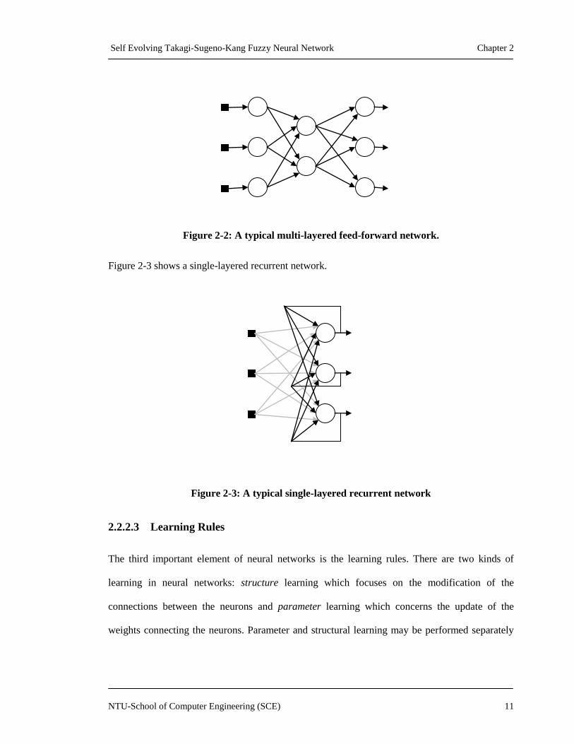
Figure 2-2: A typical multi-layered feed-forward network.
Figure 2-3 shows a single-layered recurrent network.
Figure 2-3: A typical single-layered recurrent network
2.2.2.3 Learning Rules
The third important element of neural networks is the learning rules. There are two kinds of
learning in neural networks: structure learning which focuses on the modification of the
connections between the neurons and parameter learning which concerns the update of the
weights connecting the neurons. Parameter and structural learning may be performed separately

Self Evolving Takagi-Sugeno-Kang Fuzzy Neural Network Chapter 2
NTU-School of Computer Engineering (SCE) 12
or simultaneously. In parameter learning, there are three types of training available - supervised,
reinforcement and unsupervised training.
2.2.3 Advantages and Issues of Neural Networks
Neural networks are used to solve real life problems by modeling the data. The first advantage of
modeling data using neural networks is that they are able to learn from numerical data without
explicit requirement of the functional or distributional form of the underlying model [24].
Second, they are universal function approximators that can approximate any function with good
accuracy [25]. They are also nonlinear models that can flexibly model complex real world data.
Neural networks also have good fault-tolerance characteristics because of their distributed
knowledge representational attribute. Last but not least, they are able to model given problem
domains and derive reasonable outputs in response to the inputs. However, neural networks also
have many issues listed as follow:
1. Neural networks are black box models [26]. More specifically, there is no way to
extract the embedded knowledge from the weight matrix of a trained neural network in
relation to the dynamics of the problem domain that it has modeled. There is also no way
to explain how a particular decision is arrived at in a human interpretable way.
2. Neural networks cannot make use of a priori knowledge. Since neural networks are
black box models, one cannot incorporate a priori knowledge. Thus, neural networks
have to acquire knowledge from scratch.
3. Neural network cannot solve the stability and plasticity dilemma. Once trained, a
neural network cannot incorporate new data or information.
4. It is hard to derive the optimization of network structure of neural networks since there
is no guideline in constructing neural networks. Their users have to deal with a large

Self Evolving Takagi-Sugeno-Kang Fuzzy Neural Network Chapter 2
NTU-School of Computer Engineering (SCE) 13
number of variables [26] such as choice of neural network model, choice of number of
neurons and number of hidden layers.
2.3 Fuzzy Systems
Fuzzy systems are based on the concepts of fuzzy set theory, if-then fuzzy rules and fuzzy
reasoning. Due to their multidisciplinary nature, fuzzy systems are also known by other names
such fuzzy inference systems [27], fuzzy expert systems [28], fuzzy rule-based system [29], fuzzy
models [5], fuzzy logic controllers [30].
The concept of fuzzy sets was introduced by Professor Zadeh A. Lotfi in 1965. The theory of
fuzzy sets or fuzzy logic provides a mathematical framework to represent vagueness in linguistic,
to capture the uncertainties associated with the human cognitive processes, such as thinking and
reasoning. The fuzzy systems, which are empowered by the fuzzy logic concepts, are used as
control or expert systems. Figure 2-4 shows a typical fuzzy system, with the following main
components:
Input fuzzifier - transforms crisp measured data (e.g., Tom is 1.8m in height) into suitable
linguistic values (i.e., fuzzy sets, for example ―average‖, or ―tall‖).
Fuzzy rule base – stores the linguistic fuzzy rules in the form of ―if-then‖ associated with
the system. It controls the actions in response to the input fuzzified by the input fuzzifier.
Fuzzy rules, together with fuzzy sets, form the fuzzy knowledge base.
Inference engine – performs the inference procedure to derive appropriate outputs from
the given inputs using the fuzzy rules and an inference/reasoning scheme.
Output defuzzifier – transforms the fuzzified outputs derived by the inference engine to
crisp values.

Self Evolving Takagi-Sugeno-Kang Fuzzy Neural Network Chapter 2
NTU-School of Computer Engineering (SCE) 14
Figure 2-4: A typical fuzzy system
2.3.1 Advantages and Issues of Fuzzy Systems
Fuzzy systems utilize high-level IF-THEN fuzzy rules to model the problem domain in solving
problems. Because the fuzzy rules are intuitive to the understanding of the human user,
knowledge can be easily extracted from the systems. A priori knowledge from human experts can
be incorporated into the model that comprises of linguistic expressions formulated in the form of
if-then fuzzy rules [31]. Fuzzy systems offer the ability of dealing with issues such as reasoning
on a higher level using the human-like reasoning style.
However, fuzzy systems also have severe drawbacks. They are unable to formulate the fuzzy
knowledge base including the membership functions and the if-then fuzzy rules from available
numerical data [4]. The fuzzy rules are inserted into the systems by experts so they may be
inaccurate and biased as opinions may differ with different experts. The experts also have to deal
with the optimization of the membership functions and the if-then fuzzy rules in the knowledge
base from numerical data [4]. This may be impossible for a complex system with many variables.

Self Evolving Takagi-Sugeno-Kang Fuzzy Neural Network Chapter 2
NTU-School of Computer Engineering (SCE) 15
The above drawbacks of fuzzy systems can be addressed by integrating with neural networks to
create the hybrid fuzzy neural networks which will be discussed later.
2.3.2 Interpretability – Accuracy Trade Off
Fuzzy logic was motivated by two objectives. First, it aims to ease difficulties in developing and
analyzing complex systems with high accuracy. Second, it is motivated by observing that human
reasoning can make use of concepts and knowledge that are vague, imprecise and incomplete.
Therefore, modeling problem domains using fuzzy systems is also mainly characterized by two
characteristics: interpretability and accuracy. Interpretability concerns the capability of the fuzzy
model to express the behavior of the modeled system in a human understandable way. Accuracy
concerns the capability of the fuzzy model in representing the modeled system that can
approximate the desired outputs in response to the input data. Interpretability of a fuzzy system
depends on several factors such as the model structure, the number of input variables, the number
of if-then fuzzy rules and the number of linguistic terms. Accuracy of a fuzzy system depends on
how close the approximation of the fuzzy model is to the response of the real system that is being
modeled.
In reality, there is a trade-off between interpretability and accuracy. In other words, in fuzzy
systems, to achieve high degree of interpretability and accuracy is a contradictory task. Normally
only one of the two properties dominates (the other). Professor Lotfi Zadeh (1973) also stated in
the Principle of Incompatibility that ―as the complexity of a system increases, our ability to make
precise and yet significant statements about its behavior diminishes until a threshold is reached
beyond which precision and significance (or relevance) become almost mutually exclusive” [32].
Self Evolving Takagi-Sugeno-Kang Fuzzy Neural Network Chapter 2
NTU-School of Computer Engineering (SCE) 16
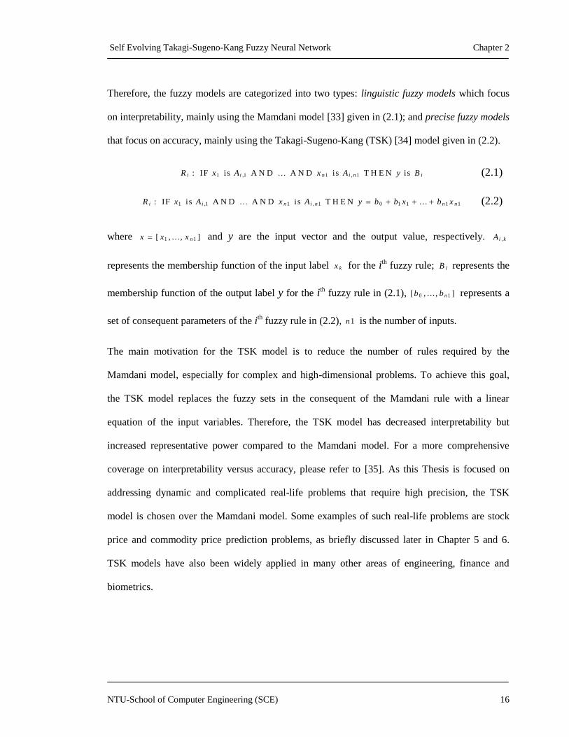
Therefore, the fuzzy models are categorized into two types: linguistic fuzzy models which focus
on interpretability, mainly using the Mamdani model [33] given in (2.1); and precise fuzzy models
that focus on accuracy, mainly using the Takagi-Sugeno-Kang (TSK) [34] model given in (2.2).
1 ,1 1 , 1: IF is A N D A N D is T H E N isi i n i n iR x A x A y B (2.1)
1 ,1 1 , 1 0 1 1 1 1: IF is A N D A N D is T H E N ...i i n i n n nR x A x A y b b x b x (2.2)
where 1 1[ , . . . , ]nx x x and y are the input vector and the output value, respectively. ,i kA
represents the membership function of the input label kx for the ith fuzzy rule; iB represents the
membership function of the output label y for the ith fuzzy rule in (2.1), 0 1[ , . . . , ]nb b represents a
set of consequent parameters of the ith fuzzy rule in (2.2), 1n is the number of inputs.
The main motivation for the TSK model is to reduce the number of rules required by the
Mamdani model, especially for complex and high-dimensional problems. To achieve this goal,
the TSK model replaces the fuzzy sets in the consequent of the Mamdani rule with a linear
equation of the input variables. Therefore, the TSK model has decreased interpretability but
increased representative power compared to the Mamdani model. For a more comprehensive
coverage on interpretability versus accuracy, please refer to [35]. As this Thesis is focused on
addressing dynamic and complicated real-life problems that require high precision, the TSK
model is chosen over the Mamdani model. Some examples of such real-life problems are stock
price and commodity price prediction problems, as briefly discussed later in Chapter 5 and 6.
TSK models have also been widely applied in many other areas of engineering, finance and
biometrics.

Self Evolving Takagi-Sugeno-Kang Fuzzy Neural Network Chapter 2
NTU-School of Computer Engineering (SCE) 17
2.4 Fuzzy Neural Networks
Neural network and fuzzy system both are popular approaches and are widely used in different
fields and applications. However, both have their own advantages and drawbacks. The integration
of neural network and fuzzy system creates a hybrid model that can address the issues of both
approaches. The hybrid model fuzzy neural network can learn new knowledge or use a prior
knowledge to shorten its training cycle. Meanwhile it exhibits the understandable human-like
style of reasoning through its linguistic model that comprises of if-then fuzzy rules and linguistic
terms described by the membership functions. The terms fuzzy neural network and neuro-fuzzy
system can be used interchangeably. The following lists the characteristics of the network
structure of a fuzzy neural network.
It represents a set of IF-THEN fuzzy rules with each fuzzy rule may use more than one
linguistic variable in its antecedent and consequent section;
Each input/output linguistic variable is described by an input/output linguistic term; and
Each input/output term is represented by exactly one fuzzy set only.
There are three important aspects that should be considered in constructing a fuzzy neural
network [36], including: generating membership functions for input/output linguistic terms,
identifying the if-then fuzzy rules for the rule base, and specifying the reasoning method for the
reasoning mechanism. These important aspects will be discussed briefly in the following sections.
2.4.1 Generating Membership Functions
Generating membership functions is an important aspect in designing a fuzzy neural network.
Determining appropriate membership functions can help to enhance the accuracy performance of
the system and to reduce the number of redundant rules. The most commonly used membership

Self Evolving Takagi-Sugeno-Kang Fuzzy Neural Network Chapter 2
NTU-School of Computer Engineering (SCE) 18
functions are triangular, trapezoidal, Gaussian and bell-shaped. Equation (2.3) and (2.4)
mathematically describe the trapezoidal and Gaussian membership functions. Triangular and bell-
shaped membership functions can be described by equation (2.3) using parameters such that
and by equation (2.4) using parameters such that and , respectively.
0
( ; , , , )1
T
x o r x
xx
xx
xx
(2.3)
2
2
2
2
( )
2
( )
2
( ; , , , ) 1
x
G
x
e x
x x
e x
(2.4)
Figure 2-5: (a) Trapezoidal membership function μT(x; 3,4,6,8) (b) Gaussian membership
function μG(x; 0.5,4,1,6)

Self Evolving Takagi-Sugeno-Kang Fuzzy Neural Network Chapter 2
NTU-School of Computer Engineering (SCE) 19
There are several approaches to the generation of fuzzy membership functions:
Heuristics – uses predefined shapes for membership functions and has been used
successfully in rule-based pattern recognition applications. Unfortunately, the shapes of
the heuristic membership functions are inflexible to model all kinds of data. Moreover,
the parameters associated with the membership functions must be provided by experts
[37].
Histograms – provides information regarding the distribution of input values, which can
be modeled by parameterized functions such as Gaussian, thus directly yielding
membership functions. This approach is easy to implement and the membership functions
can be used for classifying data [37], but the histograms of different classes frequently
overlap, therefore the applicability for finding linguistic terms is limited.
Nearest neighbors – employs the technique that assigns class memberships to a sample
instead of a particular class, where the class memberships depend on the sample‘s
distance from its nearest neighbors. The primary use of the nearest neighbor techniques
involves situations where the a priori probabilities and class conditional densities are
unknown. The algorithm is simple however it does not generate smooth membership
curves in overlapping regions.
Neural networks – generates membership functions from labeled training data. In order to
generate class membership values, a multilayer network is trained using a suitable
training algorithm such as the back-propagation algorithm. This approach is capable of
generating complex membership functions for classifying data. However the membership
values are not necessarily indicative of the similarity of a feature to a class and the shapes
of the membership functions are unpredictable in regions where there is no training data
[37].
Self Evolving Takagi-Sugeno-Kang Fuzzy Neural Network Chapter 2
NTU-School of Computer Engineering (SCE) 20
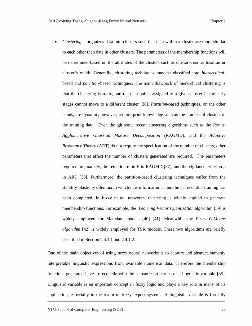
Clustering – organizes data into clusters such that data within a cluster are more similar
to each other than data in other clusters. The parameters of the membership functions will
be determined based on the attributes of the clusters such as cluster‘s center location or
cluster‘s width. Generally, clustering techniques may be classified into hierarchical-
based and partition-based techniques. The main drawback of hierarchical clustering is
that the clustering is static, and the data points assigned to a given cluster in the early
stages cannot move to a different cluster [38]. Partition-based techniques, on the other
hands, are dynamic, however, require prior knowledge such as the number of clusters in
the training data. Even though some recent clustering algorithms such as the Robust
Agglomerative Gaussian Mixture Decomposition (RAGMD), and the Adaptive
Resonance Theory (ART) do not require the specification of the number of clusters, other
parameters that affect the number of clusters generated are required. The parameters
required are, namely, the retention ratio P in RAGMD [37], and the vigilance criterion ρ
in ART [38]. Furthermore, the partition-based clustering techniques suffer from the
stability-plasticity dilemma in which new information cannot be learned after training has
been completed. In fuzzy neural networks, clustering is widely applied to generate
membership functions. For example, the Learning Vector Quantization algorithm [39] is
widely employed for Mamdani models [40] [41]. Meanwhile the Fuzzy C-Means
algorithm [42] is widely employed for TSK models. These two algorithms are briefly
described in Section 2.4.1.1 and 2.4.1.2.
One of the main objectives of using fuzzy neural networks is to capture and abstract humanly
interpretable linguistic expressions from available numerical data. Therefore the membership
functions generated have to reconcile with the semantic properties of a linguistic variable [35].
Linguistic variable is an important concept in fuzzy logic and plays a key role in many of its
application, especially in the realm of fuzzy expert systems. A linguistic variable is formally

Self Evolving Takagi-Sugeno-Kang Fuzzy Neural Network Chapter 2
NTU-School of Computer Engineering (SCE) 21
defined by Zadeh (1975) [32,43-44] with a quintuple (x, T(x), U, G, M) where x is the name of the
variable; T(x) is the linguistic term set of x; U is a universe of discourse; G is a syntactic rule for
generating the names of values of x; and M is a semantic rule that associates each value of x with
its meaning. Each linguistic term is characterized by a fuzzy set that is described mathematically
using a membership function.
In Figure 2-6, an example of a linguistic variable x named x=―speed‖ with U = [0, 100] is given.
It is characterized by three linguistic terms T(x)={―slow‖, ―moderate‖, ―fast”} where each of
these linguistic terms is assigned one of the three triangular or trapezoidal membership functions
by a semantic rule M. These membership functions cover the entire universe of discourse U=[0,
100] of the linguistic variable x. The common characteristics of all the fuzzy sets described by the
membership functions in Figure 2-6 that characterize the linguistic terms of T(x) are normalized
and convex. Plus, the linguistic terms also followed a partial ordering, e.g., ―slow‖
―moderate‖ ―fast‖.
Figure 2-6: Fuzzy membership functions representing linguistic terms “slow”,
“moderate”, “fast”
There are still many controversial discussions about the definition of interpretability and its
criteria for linguistic variables. However, the formal definitions on the semantic properties of
interpretable linguistic variables were proposed as follow [45] :
40 60 80
slow moderate fast
0
0.5
1

Self Evolving Takagi-Sugeno-Kang Fuzzy Neural Network Chapter 2
NTU-School of Computer Engineering (SCE) 22
Coverage – membership functions ( )iX x where ( )iX T x can cover the entire
universe of discourse. More specifically, x U , ( )iX T x such that ( ) 0iX x .
Normalized – membership function ( )iX x where ( )iX T x is normalized if
( )iX T x such that ( ) 1iX x .
Convex – membership function ( )iX x where ( )iX T x is convex if , , ix y z X :
( ) m in ( ( ) , ( ) )i i iX X Xx y z y x z .
Ordered – membership function ( )iX x where , , , ,1 2( ) ,i i nX T x X X X X is
ordered if 1 2 i nX X X X .
where the symbol denotes a partial ordering such that 1 2X X denotes 1X precedes 2X .
In practice, a fuzzy knowledge base is considered interpretable if it contains highly
distinguishable fuzzy sets which have the above semantic properties.
2.4.1.1 Clustering: Fuzzy C-Means (FCM) Algorithm
Fuzzy C-Means algorithm is widely employed to generate membership functions in TSK models.
Step 1: Given data set 1 2{ , , . . . , , . . . , }k nX X X XX , define c as the number of clusters, m
as the exponent weight and a small positive number as the terminating criterion.
Step 2: Initialize iteration 0T and randomly initialize fuzzy pseudo-partition ( 0 )
P . A
fuzzy pseudo-partition of P is a family of fuzzy subsets 1 2 c, ,P P P P which
satisfies (2.5) and (2.6),
Self Evolving Takagi-Sugeno-Kang Fuzzy Neural Network Chapter 2
NTU-School of Computer Engineering (SCE) 23
1
( ) 1 {1, 2 , ..., } ,
c
i k
i
X k n
(2.5)
1
0 ( ) {1, 2 , ..., } ,
n
i k
k
X n i c
(2.6)
where ( )i kX denotes the membership of kX in fuzzy subset iP .
Step 3: Compute the cluster centers ( ) ( ) ( ) ( )
1 2, , ..., , ...,T T T T
j cV V V V for ( )T
P using (2.7),
( ) 1
1
( ( ))
fo r 1 ...
( ( ))
n
m
j k k
T kj
n
m
j k
k
X X
V j c
X
(2.7)
Step 4: Update ( 1 )T
P with (2.8),
11
2 1( )
( 1)
2( )
1
( ) fo r 1 ... , 1 ...
mTc
k iT
kiT
j k j
X V
X i c k n
X V
(2.8)
If 2
( )0
T
k jX V then
( 1) ( 1)( ) 1 an d ( ) 0 fo r 1 .. ,
T T
k ki jX X j c j i
Step 5: Compare ( 1 )T
P with ( )T
P using (2.9),
( 1) ( ) ( 1) ( )
1 1
P P ( ) ( )
c n
T T T T
k kj j
j k
E X X
(2.9)
If E then 1T T and go to step 3. If E then stop.

Self Evolving Takagi-Sugeno-Kang Fuzzy Neural Network Chapter 2
NTU-School of Computer Engineering (SCE) 24
2.4.1.2 Clustering: Learning Vector Quantization (LVQ) Algorithm
Learning Vector Quantization algorithm is widely employed to generate membership functions in
Mamdani models.
Step 1: Given data set 1 2{ , , . . . , , . . . , }k nX X X XX define c as the number of clusters,
as the learning constant where 0 1 , a small positive ε as the terminating
criterion and Tmax as the maximum number of iterations.
Step 2: Initialize iteration 0T , weights ( 0 ) ( 0 ) ( 0 ) ( 0 )
1 2, , ..., , ...,j cV V V V V and initial
learning constant 0
.
Step 3: For T = 0...Tmax:
For k = 1…n:
a. Find winner w using (2.10),
( ) ( )m in ( ) fo r 1 ...
T T
k w k jj
X V X V j c (2.10)
b. Update the weights of the winner with (2.11),
( 1) ( ) ( ) ( )( )
T T T T
w w k wV V X V
(2.11)
End for k
c. Compute E(T+1)
using (2.12),
( 1 ) ( )
22( 1) ( 1) ( )
1
T Tc
T T T
j j
j
E V V V V
(2.12)

Self Evolving Takagi-Sugeno-Kang Fuzzy Neural Network Chapter 2
NTU-School of Computer Engineering (SCE) 25
d. If E(T+1)
≤ ε stop, else adjust learning rate α(T+1)
to satisfy (2.13) and
(2.14),
( )
0
T
T
(2.13)
( ) 2
0
( )T
T
(2.14)
End for T
Both FCM and LVQ are offline clustering techniques. They are batch-learning approaches,
meaning they require the training data to be available before training. In addition, they require the
number of clusters to be specified in advance. Hence, they are not applicable for online
applications.
2.4.1.3 Comparison of Popular Clustering Techniques
This Section benchmarks some of the existing clustering techniques proposed in the literature,
namely FCM [42], LVQ [39], FLVQ [46], FKP [47], PFKP [47], and ECM [11]. They are widely
used in fuzzy neural networks. Table 2-1 illustrates the comparisons of the various techniques.
Table 2-1: Comparison among existing clustering techniques
Features Clustering techniques
FCM FKP PFKP LVQ FLVQ ECM
Type of learning Offline Offline Offline Online Online Online
A prior knowledge
of number of cluster Y Y Y Y Y N
A prior knowledge
of upper/lower
bounds of dataset
N N N N N Y
Y=Yes, N=No
Self Evolving Takagi-Sugeno-Kang Fuzzy Neural Network Chapter 2
NTU-School of Computer Engineering (SCE) 26
From Table 2-1, FCM [42], FKP [47], PFKP [47] perform clustering in the offline mode. All the
clustering techniques in Table 2-1, with the exception of ECM, require the number of clusters to
be defined prior to training. ECM is an incremental clustering technique, however it cannot
handle complex time-variant data sets because it implicitly assumes prior knowledge of the upper
and lower bounds of the data sets before learning.
2.4.2 Identifying Fuzzy Rules
Identifying interpretable if-then fuzzy rules is the most important aspect in designing a fuzzy
neural network as the main objective of using fuzzy neural networks is to abstract humanly
interpretable fuzzy rule base from numerical data. A fuzzy rule base is a linguistic model of a
problem domain. It is characterized by a collection of high-level IF-THEN fuzzy rules. The IF-
THEN fuzzy rules contribute in modeling the dynamics of the problem domain and the associated
response action/behavior of a human expert in handling the problem. In short, the fuzzy rules help
to model the problem domain from a human perspective (linguistic model) rather than the
physical perspective (mathematical models). The form of the if-then fuzzy rules used in linguistic
fuzzy neural networks based on the Mamdani model is given in (2.1). Another form used in
precise fuzzy neural networks based on the TSK model is given in (2.2), in which the antecedents
are linguistic terms but the consequent is a function of the inputs. Below is an example of a fuzzy
rule base which is formed by if-then fuzzy rules.
Rule 1: If traffic condition is heavy and road condition is slippery, then speed is very
slow
Rule 2: If traffic condition is light and road condition is slippery, then speed is slow
Rule 3: If traffic condition is heavy and road condition is dry, then speed is slow
Rule 4: If traffic condition is light and road condition is dry, then speed is fast

Self Evolving Takagi-Sugeno-Kang Fuzzy Neural Network Chapter 2
NTU-School of Computer Engineering (SCE) 27
This fuzzy rule base constituting of four fuzzy rules describes how a driver decides on his driving
speed depending on the condition of the road and traffic. In the four fuzzy rules, traffic condition
and road condition are the input linguistic variables; speed is the output linguistic variable; the
vague terms very slow, slow, fast, heavy, light, slippery and dry are the linguistic terms. These
linguistic terms are associated with fuzzy sets mathematically described by membership functions
on the universe of discourse of traffic condition, road condition and speed values.
There are a number of approaches to identify if-then fuzzy rules from numerical data [38,48-52].
They can be categorized as follows:
Expert knowledge – capitalizes on the information that human experts provide including
fuzzy linguistic terms and if-then fuzzy rules. In the next step, neural network learning
techniques are then employed to perform optimization on the fuzzy linguistic terms and
if-then fuzzy rules. Even though the advantage of this approach is fast learning
convergence, it might be biased or incorrect due to the biased and imprecise information
from different experts [50].
Supervised learning – employs supervised learning that uses back-propagation to identify
the if-then fuzzy rules. Even though the advantage of this approach is the capability of
modeling nonlinear data accurately [53], it works like black box which does not reveal
any semantic interpretability from the results [50].
Hybrid learning – comprises of two different stages. The first stage is unsupervised
learning in which self-organized learning or clustering is used to generate the
membership functions, and competitive learning is used to identify the if-then fuzzy
rules. The second stage is supervised learning in which back-propagation is used to
optimize the parameters of the input and output membership functions [50]. The
advantage of this approach is that it can increase the accuracy of the abstracted model

Self Evolving Takagi-Sugeno-Kang Fuzzy Neural Network Chapter 2
NTU-School of Computer Engineering (SCE) 28
through the unconstrained optimization in the second stage. However, at the end, the
membership functions are deviated from human-interpretable linguistic terms [54]. Back-
propagation algorithms normally result in highly overlapping fuzzy sets which
deteriorates human interpretability.
2.4.3 Specifying Reasoning Methods
Specifying reasoning methods is another important aspect in designing a fuzzy neural network. A
reasoning method, or equivalently, an approximate reasoning method, is an inference process by
which a possibly imprecise conclusion is deduced from a collection of imprecise premises [55].
The inference process in fuzzy neural networks mimics human reasoning in the sense that a
human being has to make decisions based on incomplete, vague and fuzzy information. In fuzzy
neural networks, the reasoning method defines the mathematical operations that are used to
perform inference on the collection of if-then fuzzy rules and given facts to derive outputs for
solving problems. In practice, an online reasoning method, which interleaves with (rule) learning
process, is preferred over an offline reasoning method.
2.4.4 Parameter Learning
The learning process of a fuzzy neural network normally consists of two phases: structural
learning and parameter learning. Structural learning comprises of the above mentioned steps such
as generating membership functions and identifying rules. Parameter learning concerns about
tuning the parameters of each derived rule such as connection weights and membership functions
in order to achieve higher accuracy learning performance. Currently, there are many parameter
learning methods, each with pros and cons. For instance, in the popular ANFIS [7] fuzzy neural
network, two learning phases have been employed: forward and backward learning. In the
forward learning phase, all the antecedent parameters of ANFIS are fixed, and all the consequent

Self Evolving Takagi-Sugeno-Kang Fuzzy Neural Network Chapter 2
NTU-School of Computer Engineering (SCE) 29
parameters are tuned using the Kalman filter algorithm [4]. For backward learning, all the
consequent parameters are fixed, and the antecedent parameters are adjusted by the back
propagation delta learning method [56]. Gradient descent [4] and recursive-least-square
algorithms [4] are widely used for tuning parameters in TSK fuzzy neural networks.
2.5 Self-evolving TSK Fuzzy Neural Networks
2.5.1 Introduction
The main focus of this Thesis is the Takagi-Sugeno-Kang fuzzy neural networks. Existing TSK
networks proposed in the literature can be broadly classified into three classes as briefly discussed
in Section 1.3. Table 2-2 illustrates the taxonomy of TSK fuzzy neural networks.
Recently, TSK fuzzy neural networks are widely applied for solving function approximation and
regression-centric problems. In practice, most of these problems are online [17], meaning that the
data in these problems is not all available at the beginning but is sequentially presented. New data
keeps coming at every instant of time. A typical example of such problems is the stock price
prediction problem. In the stock market, a stock price can change at every tick, and it can hit a
new high or low that was not reached before, at any time. Static (or non-constructive) fuzzy
neural networks which employ offline batch learning algorithms are not sufficient to address such
a problem, as it might be impossible to acquire all the training data before learning. Furthermore,
static systems cannot incorporate new data after training, which renders them useless when
dealing with online problems. A popular example of static systems is ANFIS [7], which possesses
a fixed structure. Some self-organizing (or constructive [57]) networks such as DFNN [9] and
SOFNN [8] are also not suitable to address online problems as they are unable to learn in an
incremental manner. They basically employ pseudo-incremental learning approaches [58], in
which a copy of the training data is usually kept for the tuning phase or for performing rule

Self Evolving Takagi-Sugeno-Kang Fuzzy Neural Network Chapter 2
NTU-School of Computer Engineering (SCE) 30
pruning later. Considering the growing scale in volume of stock trading information, a complete
revisit of past data would be extremely costly. ANFIS, DFNN and SOFNN belong to Class I TSK
networks.
Many self-organizing learning systems in Class II TSK networks [10-11,13] have been developed
to solve online problems. These self-organizing approaches are able to learn incrementally,
however they are generally limited to time-invariant environments. In real life, many online
problems are time-variant. In such problems, the characteristics of the underlying data-generating
processes might change with time, and no prior knowledge about the number of clusters/rules or
the upper/lower bound of the dataset is provided. Thus, self-organizing learning algorithms which
require some prior knowledge about the dataset are generally unable to address time-variant
problems.
2.5.2 Self-evolving Learning Approach
To address online time-variant problems which have nonstationary characteristics, a class of self-
evolving [17] TSK fuzzy neural networks (Class III) has been developed. These evolving systems
generally employ incremental sequential learning [6], or simply incremental learning approach.
In practical online applications, incremental learning is preferred over batch learning as it greatly
improves the efficiency of online systems. More specifically, incremental learning does not
require data to be stored, thus it uses much less memory. In addition, it can help the learning
system to quickly incorporate new data since it only involves incremental updates. This
advantage is illustrated in stock market trading activities, in which huge and growing trading data
sets need to be processed daily. To be considered as an incremental sequential learning approach,
a learning system must satisfy four criteria as defined in [6]. The criteria are listed below.

Self Evolving Takagi-Sugeno-Kang Fuzzy Neural Network Chapter 2
NTU-School of Computer Engineering (SCE) 31
1) All the training observations are sequentially (one-by-one) presented to the learning
system.
2) At any time, only one training observation is seen and learnt.
3) A training observation is discarded as soon as the learning procedure for that particular
observation is completed.
4) The learning system has no prior knowledge as to how many total training observations
will be presented.
Self-evolving systems in Class III TSK networks such as [14-18] adopt incremental learning
approaches and attempt to solve time-variant problems. However, many evolving systems do not
possess an unlearning algorithm, which may lead to the collection of obsolete knowledge over
time and thus degrade the level of human interpretability of the resultant knowledge base. In these
systems, older and newer information are treated equally. Hence, even though these systems can
work in time-variant environments by evolving with the data stream, or self-constructing the
knowledge base without prior knowledge of the data sets, they might not give the most accurate
solutions for time-variant problems, as briefly discussed in the next Section.
Table 2-2: Taxonomy of TSK fuzzy neural networks proposed in the literature
TSK Networks Class III Class II Class I
Type Self-evolving Self-organizing Static/Self-organizing
Data stream Time-variant Time-invariant Time-invariant
Learning
schema
Incremental without any prior
assumptions of data
Incremental with
assumptions of data
Batch-learning or pseudo-
incremental
Examples SONFIN [15], eTS [17], FLEXFIS
[16], TSK-FCMAC [18],
RSONFIN [22], TRFN [23],
RSEFNN [59], SEIT2FNN [60]
DENFIS [11],
FITSK [10], [13]
ANFIS [7], DFNN [9],
SOFNN [8], GA-TSKfnn
[61], MSTSK [62]

Self Evolving Takagi-Sugeno-Kang Fuzzy Neural Network Chapter 2
NTU-School of Computer Engineering (SCE) 32
2.6 Unlearning Motivations for Evolving TSK Fuzzy Neural
Networks
Unlearning, which stemmed from neurobiology, was introduced by Hopfield et al in 1983 [19] to
implement an idea of Crick and Mitchinson [20] about the function of dream sleep. In [21], it was
demonstrated that unlearning greatly improves network performance such as the enhancement of
network storage capacity. Although many self-evolving systems attempt to address time-variant
problems by employing incremental learning, they still lack an efficient unlearning algorithm.
Thus, they encounter two critical issues, namely: 1) their fuzzy rule base can only grow, and 2)
they cannot give the most accurate solution when solving complex time-variant data sets that
exhibit regime-shifting properties. These two issues are presented below.
First, evolving systems which employ incremental learning generally learn new data by creating
more rules. In such evolving systems, the number of fuzzy sets and fuzzy rules will grow
monotonically. Their fuzzy rule bases retain many obsolete rules, which can no longer describe
the current data characteristics, especially when dealing with time-variant problems. This leads to
confusing fuzzy rule bases with many redundant rules, and thus deteriorates human
interpretability.
Second, when working in time-variant environments, evolving systems without unlearning
capabilities are unable to provide the most accurate solutions. Data streams in time-variant
problems evolve over time, where past data are generally less important than current data.
Besides having temporal characteristics (meaning explicitly dependent on time), time-variant
problems also exhibit regime shifting properties. To clearly understand the term ‗regime shifting‘,
one must understand the definition of ‗concept drift‘ and ‗concept shift‘ as described below.

Self Evolving Takagi-Sugeno-Kang Fuzzy Neural Network Chapter 2
NTU-School of Computer Engineering (SCE) 33
2.6.1 Concept drifting
In machine learning literature, concept drifting and concept shifting [63] are two different types
of ‗concept change‘ of the underlying distribution of online data streams [64]. To clarify, concept,
which is normally interpreted as a cognitive unit of meaning, here refers to the set of cognitive
patterns that define the underlying statistical properties of the data streams. Concept drift refers to
a gradual evolution of the concept over time. Concept drift is said to appear in a data stream when
that data stream‘s underlying data-generating processes change and the data distribution slides
through the data space from one region to another. It concerns the time-space representation of
the data streams. While the concept of (data) density is represented in the data space domain, drift
and shift are concepts in the joint data time-space domain [64]. A typical real-life example of
concept drift is weather prediction rules that may vary radically with the season [63]. Other
obvious examples are music trends, fashion trends, or investment trends that may change with
time. It can be easily observed that all processes that occur in human activities, such as financial,
biological processes are likely to experience concept drifts.
To illustrate concept drift, one may consider a data cluster moving from one region to another.
Consider in 2-D spatial data space, the original data points marked by diamond samples, which
changes over time into a data distribution marked by circular samples, as illustrated in Figure 2-7.
If a conventional clustering process would be applied that weights all new incoming samples
equally, the cluster center would end up exactly in the middle of the combined data cloud,
averaging old and new data, which is wrong (marked by the star shape). An efficient learning
technique should be able to detect such a drift in data distribution and treat old data and new data
differently, and the cluster center would end up correctly in the middle of the new data cloud
(new concept).
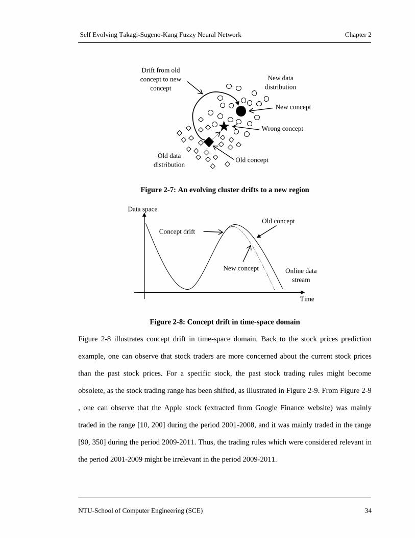
Self Evolving Takagi-Sugeno-Kang Fuzzy Neural Network Chapter 2
NTU-School of Computer Engineering (SCE) 34
Figure 2-7: An evolving cluster drifts to a new region
Figure 2-8: Concept drift in time-space domain
Figure 2-8 illustrates concept drift in time-space domain. Back to the stock prices prediction
example, one can observe that stock traders are more concerned about the current stock prices
than the past stock prices. For a specific stock, the past stock trading rules might become
obsolete, as the stock trading range has been shifted, as illustrated in Figure 2-9. From Figure 2-9
, one can observe that the Apple stock (extracted from Google Finance website) was mainly
traded in the range [10, 200] during the period 2001-2008, and it was mainly traded in the range
[90, 350] during the period 2009-2011. Thus, the trading rules which were considered relevant in
the period 2001-2009 might be irrelevant in the period 2009-2011.
Wrong concept
concept
Drift from old
concept to new
concept
Old data
distribution
New concept
Old concept
New data
distribution
Old concept
New concept
Concept drift
Online data
stream
Time
Data space

Self Evolving Takagi-Sugeno-Kang Fuzzy Neural Network Chapter 2
NTU-School of Computer Engineering (SCE) 35
Figure 2-9: Apple stock prices in period 2001-2011
2.6.2 Concept shifting
Concept shifting is an extreme form of concept drifting. It refers to the abrupt change in the
underlying concept, or simply means the displacement of the old data distribution with a new data
distribution within a short time. Instantaneous changes in data distribution would cause the
learning model to produce inaccurate results if it continues to use the old concept. Concept
shifting is also termed as ‗regime shifting‘ in this Thesis. Figure 2-10 illustrates concept shift in
time-space domain. Without correcting for this concept shift, the learning model would derive
inaccurate outputs which lie between the old and new conceptual boundaries.
Figure 2-10: Concept shift in time-space domain
Old concept
New concept
Concept drift
Online data
stream
Time
Data space
Wrong concept

Self Evolving Takagi-Sugeno-Kang Fuzzy Neural Network Chapter 2
NTU-School of Computer Engineering (SCE) 36
Many real life problems are likely to experience concept drifts and shifts, in which newer data is
considered more important (and relevant) than older data. Drift and shift handling was already
applied in other machine learning techniques such as support vector machines [65-66], ensemble
classifiers [67], and instance-based (lazy) learning approaches [68-69]. However, currently very
few fuzzy neural networks have attempted to address this issue. Many existing evolving fuzzy
systems which treat older information and newer information equally are unable to detect concept
drifts and shifts [64]. Thus, they are unable to give the most accurate results when dealing with
the data sets that exhibit regime shifting properties. Drifts and shifts indicate the necessity of
(gradual) unlearning previously learned relationships (in terms of structure and parameters)
during the incremental learning process as they are no longer valid and should hence be removed
from the model (for instance, consider completely new trading rules when the stock market
conditions change) [64]. Unlearning is an efficient way to address the concept drift and shift in
online data streams. It separates past data from new data by decaying the effects of past data on
the final outputs. Thus, to deal with fast-changing time-variant problems, learning systems should
also adopt unlearning algorithms.
2.7 Research Challenges
This section surmises issues and weakness of existing TSK fuzzy neural networks that this Thesis
attempts to address. They are briefly discussed as follows.
2.7.1 Online Incremental Learning in Time-Variant Environments.
Online incremental learning is necessary in real-life applications. As analyzed in Section 2.5.1,
Class I TSK networks such ANFIS [7], DFNN [9], and SOFNN [8] violate the criteria to be
considered as an incremental learning approach. Class II TSK networks such as DENFIS [11],

Self Evolving Takagi-Sugeno-Kang Fuzzy Neural Network Chapter 2
NTU-School of Computer Engineering (SCE) 37
FITSK [10] improve from Class I by employing incremental learning, however they still cannot
address time-variant problems.
To address this problem, the Thesis relies on a novel clustering technique known as
Multidimensional Growing Clustering (MSGC). MSGC can learn incrementally without any
assumptions about the dataset. MSGC is inspired by human cognitive process models [70], as
explained in Chapter 3.
2.7.2 Unlearning Strategy to Address Time-Variant Problems
As many existing evolving TSK systems do not possess unlearning capabilities, they are unable
to provide the most accurate and up-to-date solutions when solving complex time-variant data
sets that show drift and shift behaviors. A comparison among evolving TSK systems in the
literature is shown in Table 2-3. From 1998-2010, Juang et al. proposed a class of feed-forward
and recurrent self-evolving networks such as SONFIN [15], RSONFIN [22], TRFN [23] and
RSEFNN [59] to address online problems. However, these networks do not take unlearning into
consideration. Based on Juang‘s works, many other improved networks were developed such as
HO-RNFS [71], T-SORNFN [72]. Juang et al. also proposed type-2 TSK fuzzy neural networks
such as SEIT2FNN [60] and IT2FNN-SVR [73] to handle problems with uncertainties such as
noisy data. Other popular evolving systems such as eTS [17], FLEXFIS [16], and [14] were
proposed during 2004-2008. In 2009, Ting and Quek [18] proposed a simple network termed as
TSK0-FCMAC to regulate the blood glucose levels in diabetes patients. Since all of these
networks do not possess unlearning algorithms, their number of membership functions and fuzzy
rules grow monotonically, resulting in confusing knowledge bases with many obsolete rules. In
addition, these networks cannot detect and address concept drifts and shifts in complex time-
variant problems. Simpl_eTS [74] is among a few TSK networks ([64,74-76] )that possess an
unlearning algorithm. It is a modification of eTS with a rule-pruning algorithm which monitors

Self Evolving Takagi-Sugeno-Kang Fuzzy Neural Network Chapter 2
NTU-School of Computer Engineering (SCE) 38
the population of each rule. If a rule amounts to less than 1% of the total data samples at that
current moment, it is considered as obsolete, and it will be pruned. This approach considers the
contribution of old data and new data equally in determining the obsolete rules, thus it cannot
detect drifts and shifts in online data streams [64]. In systems such as eTS+ [76] and xTS [75],
the age of a cluster is used to determine if a rule (cluster) is obsolete. However, the age of the
cluster in [75-76] is determined by a self-driven formula which does not incorporate the
membership degrees of the samples forming that cluster. In 2010, Lughofer and Angelov [64] are
the first to apply drift and shift handling in fuzzy systems. They proposed a method for
autonomous detection of drifts and shifts in data streams based on the age of the fuzzy rule. This
method computes the age of the fuzzy rule based on a self-driven mathematical formula, which is
not biologically plausible. In addition, the method detects the drift and shift by observing the
gradient of the age, which is a complicated process.
For unlearning, this Thesis proposed a novel ‗brain-inspired‘ rule pruning algorithm which
applies a ‗gradual‘ forgetting approach and adopts the Hebbian learning mechanism behind the
long-term potentiation phenomenon [77] in the brain. This approach is is simple, computationally
efficient and biologically plausible.

Self Evolving Takagi-Sugeno-Kang Fuzzy Neural Network Chapter 2
NTU-School of Computer Engineering (SCE) 39
Table 2-3: Comparison among self-evolving TSK fuzzy neural networks
TSK Networks
[Author, year of publication]
[references]
Network
Structure
Fuzzy
Logic
Type
Un-
learning
Antecedent Parameters
Tuning method
SONFIN
[Juang and Lin, 1998] [15]
Feed-forward Type-1 No Gradient descent
RSONFIN
[Juang and Lin, 1999] [22]
Recurrent Type-1 No Gradient descent
TRFN
[Juang, 2000][23]
Recurrent Type-1 No Gradient descent
eTS
[Angelov and Filev, 2004] [17]
Feed-forward Type-1 No Recursive update of
potential
Simpl_eTS
[Angelov and Filev, 2005] [74]
Feed-forward Type-1 Yes Recursive update of scatter
xTS
[Angelov and Zhou, 2006] [75]
Feed-forward Type-1 Yes NM
HO-RNFS
[Theocharis, 2006] [71]
Recurrent Type-1 No Gradient descent
FLEXFIS
[Lughofer, 2008] [16]
Feed-forward Type-1 No Winner-take-all like
algorithm
SEIT2FNN
[Juang and Tso, 2008] [60]
Feed-forward Type-2 No Gradient descent
TSK-FCMAC
[Ting and Quek ,2009] [18]
Feed-forward Type-1 No NM
RSEFNN
[Juang et al., 2010] [59]
Recurrent Type-1 No Gradient descent
eTS+
[Angelov, 2010] [76]
Feed-forward Type-1 Yes NM
T-SORNFN
[Chen, 2010] [72]
Recurrent Type-1 No Gradient descent
IT2FNN-SVR
[Juang et al., 2010] [73]
Feed-forward Type-2 No NM
ds-eTS
[Lughofer and Angelov,2011][64]
Feed-forward Type-1 Yes Gradient descent
NM = Not Mentioned.
2.7.3 Compact and Interpretable Knowledge Base
Many existing TSK networks [15,22-23,59] do not take in consideration of the interpretability of
the knowledge base. They generally employ back-propagation or gradient descent algorithms to
heuristically tune the widths of their antecedent membership functions, which can results in
highly overlapping and indistinguishable fuzzy sets. Thus, the semantic meaning of the derived
knowledge base is deteriorated. SONFIN [15] and its recurrent version, RSONFIN [22], set the

Self Evolving Takagi-Sugeno-Kang Fuzzy Neural Network Chapter 2
NTU-School of Computer Engineering (SCE) 40
widths of fuzzy sets in all input dimensions to be the same during learning. New fuzzy sets are
created whenever a new rule is identified, which is redundant.
Figure 2-11: Two types of knowledge base: (a) Deteriorated with highly overlapping and
indistinguishable fuzzy sets; (b) Interpretable with highly distinguishable fuzzy sets.
To overcome this issue, a novel merging approach is employed in the proposed MSGC technique.
This approach can prevent the derived fuzzy sets from expanding too many times to protect their
semantic meanings. Together with the proposed rule pruning strategy, MSGC helps to maintain a
compact and understandable knowledge base, which can be illustrated in the experiments
throughout this Thesis.
2.7.4 Summary
This Thesis proposes novel learning/unlearning algorithms to address the above-listed
deficiencies of existing TSK networks. Most of real-life problems require solutions with
incremental learning ability, high accuracy and fast speed. In addition, the interpretability of the
knowledge bases derived is another important aspect to consider when designing solutions for
such complex problems. This Thesis takes all such issues into consideration. The next Chapter 3
provides a detailed mathematics and insights to the generic TSK framework that is developed to
pursue the motivations of this Thesis.

Self Evolving Takagi-Sugeno-Kang Fuzzy Neural Network Chapter 3
NTU-School of Computer Engineering (SCE) 41
Chapter 3: Generic Self Evolving TSK Fuzzy Neural
Network (GSETSK)
3.1 Introduction
This chapter presents the architecture and the learning algorithm of the proposed Generic Self-
Evolving Takagi-Sugeno-Kang Fuzzy Neural Network (GSETSK). GSETSK attempts to address
the existing problems of TSK fuzzy neural networks as identified in Section 2.7. Another goal in
designing GSETSK is achieving a fast and efficient framework that can be applied in real-life
applications which require high precision. GSETSK can learn in an incremental manner and can
work in time-variant environments. GSETSK‘s initial empty rule base is empty. New rules are
sequentially added to the rule base by a novel fuzzy clustering algorithm termed as MSGC.
MSGC is completely data-driven and does not require prior knowledge of the numbers of clusters
or rules present in the training data set. In addition, MSGC does not assume the upper or lower
bounds of the data set. Highly overlapping membership functions are merged and obsolete rules
are constantly pruned to derive a compact fuzzy rule base while maintaining a high level of
modeling accuracy. A detailed comparison between the proposed MSGC and other clustering/rule
generating algorithms is briefly presented in Section 3.3.1. In order to implement the unlearning
motivation, a novel rule pruning algorithm which applies a ‗gradual‘ forgetting approach and
adopts the Hebbian learning mechanism behind the long-term potentiation phenomenon [77] in
the brain, is proposed. For parameter tuning, GSETSK employs a localized version of the
You cannot teach a man anything; you can only help him discover it in
himself.
Galileo Galilei (1564-1642)

Self Evolving Takagi-Sugeno-Kang Fuzzy Neural Network Chapter 3
NTU-School of Computer Engineering (SCE) 42
recursive least-square algorithm [78] for high-accuracy online learning performance. The
parameter tuning phase is used only for tuning the consequent parameters of the fuzzy rules. The
dynamic learning/unlearning mechanisms in GSETSK help to ensure an efficient and fast
framework that can be applied for real-life applications.
This chapter is organized as follows. Section 3.2 briefly discusses the general structure of the
GSETSK and its neural computations. Section 3.3 presents the structural learning phase and its
rule pruning algorithm. Section 3.4 discusses its parameter learning phase. Section 3.5 briefly
evaluates the performance of the GSETSK models using three different simulations. These
simulations have the following goals:
1. Demonstrate the online incremental learning ability of GSETSK in complex
environments such as the nonlinear dynamic system with nonvarying characteristics (in
Section 3.5.1). The derived knowledge base of GSETSK is also illustrated, to show that
the proposed MSGC algorithm can generate a compact rule base with highly
distinguishable fuzzy sets.
2. Demonstrate the ability of GSETSK to work in time-variant environments such as the
nonlinear dynamic system with time-varying characteristics (in Section 3.5.2). The
evolving rule base of GSETSK is also illustrated, to show how GSETSK can keep a
current and relevant rule base in time-variant problems.
3. Demonstrate the superior performance of GSETSK when benchmarked against other
evolving models using the Mackey-Glass time series prediction simulation (in Section
3.5.3).

Self Evolving Takagi-Sugeno-Kang Fuzzy Neural Network Chapter 3
NTU-School of Computer Engineering (SCE) 43
3.2 Architecture & Neural Computations
The GSETSK model is basically an FNN [4] that consists of six layers of computing nodes as
shown in Figure 3-1. They are: Layer I (the input layer), Layer II (the input linguistic layer),
Layer III (the rule layer), Layer IV (the normalization layer), Layer V (the consequent layer) and
Layer VI (the output layer). From Figure 3-1, the structure of the proposed GSETSK model
defines a set of TSK-type IF-THEN fuzzy rules. The fuzzy rules are incrementally constructed by
presenting the training observations { ( ( ) , ( )) }X t d t sequentially (one-by-one), where ( )X t
and ( )d t denote the vectors containing the inputs and the corresponding desired outputs,
respectively, at any time t. Each fuzzy rule kR in GSETSK has the form shown in (3.1).
11 1, , ,
11
: IF ( is ) A N D ( is ) . . .A N D ( is )
T H E N ... . . .
k k kni
k i nj i j n j
k o k k ik i n k n
R x IL x IL x IL
y b b x b x b x
(3.1)
where 1[ , ... , , . . . , ]T
i nX x x x represents the numeric inputs of GSETSK;
,( 1, ..., ( ), 1, ..., ( ))k
ii ii j
IL j J t k K t denotes the ij th linguistic label of the input xi
that is part of the antecedent of rule kR ; ( )iJ t is the number of fuzzy sets of xi ; ( )K t is
the number of fuzzy rules at time t;
ky is the crisp output of rule kR ;
n is the number of inputs;
[ , . . . , ]o k n kb b represents a set of consequent parameters of rule kR .
For simplicity, the proposed GSETSK network is modeled as a multiple-input–single-output
(MISO) network. A multiple-input–multiple-output (MIMO) network can be viewed as an

Self Evolving Takagi-Sugeno-Kang Fuzzy Neural Network Chapter 3
NTU-School of Computer Engineering (SCE) 44
aggregation of MISOs. For clarity of subsequent discussion, the output of a node in Figure 3-1 is
denoted by Z with the superscripts denoting its layer and the subscripts denoting its origin. For
example, I
iZ is the output of the ith node in layer I. All the outputs of a layer are propagated to
the inputs of the connecting nodes at the next layer.
Figure 3-1: Structure of the GSETSK network
Each input node iI may connect to a different number of input linguistic nodes ( )iJ t . Hence the
total number of nodes in layer II at each time t is= 1
( )n
ii
J t . Also, at each time t, layer III
consists of ( )K t rule nodes kR . It should be noted that ( )K t and ( )iJ t change over time,
increasing to accommodate new data or decreasing to keep a compact fuzzy rule base. Each rule
I1
R1 N1 IL1,1
ILn,Jn(t)
C1
Ii
In
x1
xi
xn
ILi,1
ILi,ji
ILi,Ji(t)
IL1,J1(t)
ILn,1
Rk
RK(t)
Nk
NK(t
) CK(t)
Ck O
X
y
Lay
er I
(Inp
ut)
Lay
er II
(Inp
ut
Lin
gu
istic)
Lay
er III
(Ru
le)
Lay
er IV
(No
rmalizatio
n)
Lay
er V
(Co
nseq
uen
t)
Lay
er VI
(Su
mm
ation
)
d
Structural
Learning
Forward
Operation
Self Evolving Takagi-Sugeno-Kang Fuzzy Neural Network Chapter 3
NTU-School of Computer Engineering (SCE) 45
node kR is directly connected to a normalization node kN in layer IV. Subsequently, each
normalization node kN is directly connected to a consequent node kC in layer V. Hence, the
numbers of nodes in layer III, layer IV and layer V are the same. For clarity of subsequent
discussion, the variables i and j are used to refer to arbitrary nodes in layers I, II, and the variable
k for layer III, IV, V respectively. The output node at layer VI is a summation node which
connects to all nodes in layer V.
Detailed mathematic functions of each layer of GSETSK are presented below.
3.2.1 Forward Reasoning
Layer I: Input Layer
, 1, ...,I
i iZ x i n (3.2)
Layer I nodes are called linguistic nodes. They represent linguistic variables such as ‗speed‘,
‗price‘ etc. Each node receives only one element of the vectored data input, and outputs to several
nodes of the next layer.
Layer II: Input Linguistic Layer
, ,,( ) ( ) , 1, ..., , 1, ..., ( )i ii
II I
i j i i j i i ii jZ Z x i n j J t (3.3)
where , ii j is a fuzzy membership function of the fuzzy linguistic node , ii jIL .
Layer II nodes are called input-label nodes. They represent labels such as ‗fast‘, ‗slow‘ etc. They
constitute the antecedent of the fuzzy rules in GSETSK. The label , ii jIL denotes the jth linguistic
label of the ith linguistic variable input. The input linguistic layer measures the matching degree
of each input with its corresponding linguistic nodes. Each linguistic node in this layer has a
Gaussian membership function with its center and width dynamically computed during the

Self Evolving Takagi-Sugeno-Kang Fuzzy Neural Network Chapter 3
NTU-School of Computer Engineering (SCE) 46
structural learning phase. With the use of Gaussian membership function, (3.3) can be expressed
as in (3.4),
2,
2
,
( )
,,( ) , 1, ..., , 1, ..., ( )
i i ji
i ji
ii
x m
II
i j i i ii jZ x e i n j J t
(3.4)
where , ii jm and , ii j are, respectively, the center and the width of the Gaussian membership
function of the jth linguistic label of the ith linguistic variable input xi.
Layer III: Rule Layer
Each node in rule-base layer represents a single Sugeno-type fuzzy rule and is called a rule node.
The net output or the firing strength of a rule node kR is computed based on the activation of its
antecedents as in (3.5),
1
1, , ,m in ( , .. . , , . . . ) , 1, . . . , ( )
k k kni
III II II II
k kj i j n j
r Z Z Z Z k K t (3.5)
where ,
k
i
II
i jZ is the output of the jth linguistic label of the ith linguistic variable input xi that
connects to the kth rule; kr is the forward firing strength of kR .
Layer IV: Normalization layer
Each node in this layer computes the normalized firing strength of a fuzzy rule as in (3.6),
( )
1
, 1, . . . , ( )
III
kIV
k kK t III
kk
ZZ k K t
Z
(3.6)
where k is the normalized firing strength.
Layer V: Consequence Layer

Self Evolving Takagi-Sugeno-Kang Fuzzy Neural Network Chapter 3
NTU-School of Computer Engineering (SCE) 47
Each node in this layer represents a TSK rule. The outputs of this layer are weighted with their
incoming normalized firing strengths as in (3.7),
( ) , 1, ..., ( )V IV
k k kZ Z f X k K t (3.7)
where ( )kf X is a linear function of consequent node Ck.
Layer VI: Summation Layer
The output node in this layer corresponds to the output of the GSETSK model. It combines the
activations of all its consequent nodes in layer V as in (3.8),
( )
1
K t
V I V
k
k
Z Z
(3.8)
where V
kZ is the output of consequent node Ck in layer V. The output node in this layer
corresponds to the output of the GSETSK model.
Although the GSETSK appears structurally similar to other evolving networks such as
SONFIN[15], FLEXFIS [16] and eTS [17], there are distinct differences between them. SONFIN
uses back-propagation to tune its membership functions, which can result in highly overlapping
and indistinguishable membership functions. The number of membership functions and fuzzy
rules in FLEXFIS and eTS will grow monotonically, especially when solving time-variant
problems. Ouyang et al. [14] proposed a merge-based fuzzy clustering algorithm to merge highly
similar clusters. However, this algorithm does not prune irrelevant rules, which results in a
continuously growing fuzzy rule base over time. In contrast, the GSETSK employs a Hebbian-
based rule pruning algorithm which takes into consideration the backward connections from layer
VI to layer III via layer V as presented in Section 3.2.2 and Section 3.2.3. This novel rule pruning
algorithm ensures a compact and up-to-date fuzzy rule base in the GSETSK network.

Self Evolving Takagi-Sugeno-Kang Fuzzy Neural Network Chapter 3
NTU-School of Computer Engineering (SCE) 48
3.2.2 Backward Computations of GSETSK
The backward connections from layer VI to layer III via layer V in the GSETSK solely serve the
purpose of computing the potentials of the fuzzy rules in GSETSK. These fuzzy rule potentials
will subsequently be used to determine if the rules will be pruned or kept. Inspired by the learning
algorithm in POPFNN [79], the GSETSK adopts the Hebbian learning mechanism to compute its
fuzzy rule potentials. However, POPFNN [79] and its family of networks [47,80-81] are of
Mamdani-type fuzzy neural networks in which the output of each fuzzy rule is a set of fuzzy
linguistic labels. The Hebbian learning algorithm employed in POPFNN is based on the firing
strengths of the rules nodes (forward firing) and the membership values derived at the output-
label nodes (backward firing).
In contrast, the GSETSK model adopts the TSK‘s fuzzy model and the output of each rule in
GSETSK has the form of a linear function of the input vector. Hence, a novel approach to
compute the fuzzy rule potentials based on the observed training data pair ( ( ) , ( ))X t d t is
proposed in GSETSK. At each rule node kR , the forward firing strength kr has been described in
(3.5); and the backward firing strength b a ck
kr is computed in two steps as follows.
3.2.2.1 Computing Output Error of Each Fuzzy Rule
Layer V (Backward Operation): At time t, the desired output ( )d t is directly transmitted to each
consequent node Ck in layer V. The output of the linear function of the consequent node Ck in
response to the input ( )X t is a crisp value ( )ky t given by (3.9),
1 1( ) ( ) ( ) ( ) . . . ( ) ( ) . . . ( ) ( ) , 1, . . . , ( )k o k k ik i n k ny t b t b t x t b t x t b t x t k K t (3.9)

Self Evolving Takagi-Sugeno-Kang Fuzzy Neural Network Chapter 3
NTU-School of Computer Engineering (SCE) 49
where 0[ ( ) , . . . , ( ) ]k n kb t b t represents a set of consequent parameters of rule kR at time t. Note that
ky is the output of the fuzzy rule kR . It is different from V
kZ , which is the output of the
consequent node Ck. For each rule kR , the difference between the computed output ( )ky t and
the desired output ( )d t is given by
( ) ( ) ( ) , 1, . . . , ( )k ke t d t y t k K t (3.10)
where ( )ke t is the output error of rule kR at time t.
3.2.2.2 Determining Backward Firing Strength of Each Fuzzy Rule
Layer V (Backward Operation): The values 1 ( ){ ( ) , , ( ) , , ( )}k K te t e t e t will then be used to
form a Gaussian membership function with the mean of zero and the width (or variance) at time t
formulated in (3.11),
( )
1
( )
( )
( )
K t
k
kb a c k
e t
t
K t
(3.11)
This membership function measures how closely the computed output ( )ky t can approximate the
desired output ( )d t . Denote ( 0 , ( ) )b a c k t as the Gaussian membership function with center 0
and width ( )b a c k t . Figure 3-2 shows such a Gaussian membership function, which can be
approximated by an isosceles triangle with unity height and the length of its bottom edge equal to
2 ( )b a ck t [82].

Self Evolving Takagi-Sugeno-Kang Fuzzy Neural Network Chapter 3
NTU-School of Computer Engineering (SCE) 50
Figure 3-2: The Gaussian membership function (0 , ( ))tb a ck
.
The backward firing strength of b a ck
kr of rule kR at time t is then determined by (3.12),
2 2( ) (0 , ( ) , ( )) ex p ( ( ) / ( ) )
b a ck
k b a ck k k b a ckr t t e t e t t (3.12)
In Mamdani-type models such as POPFNN, the backward firing strength of a fuzzy rule is
defined by how close the desired output is to the centers of the membership functions in the rule‘s
output-label nodes. The idea in GSETSK is similar. At layer V, the Gaussian function
( 0 , ( ) )b a c k t is formulated to measure the degree of closeness between the desired output ( )d t
and the computed output ( )ky t . When ( 0 , ( ) , ( ) ) 1k kt e t , ( ) 0ke t , and ( ) ( )ky t d t . The
smaller the value of ( )ke t , the greater the value of ( 0 , ( ) , ( ) )k kt e t . That also means the closer
the computed output ( )ky t is to the desired output ( )d t , the greater the backward firing strength
of rule kR . It can be observed from (3.11) that the width ( )b a c k t is constructed using the
average of the errors of all rules at time t. This approach is built on the idea that the existing fuzzy
rules in GSETSK at time t should be compared against each other in terms of how well they can
approximate the desired output. However, it should be noted that the backward firing strength
only forms a part of the formula to calculate the fuzzy rule potentials as presented in Section
3.2.3.

Self Evolving Takagi-Sugeno-Kang Fuzzy Neural Network Chapter 3
NTU-School of Computer Engineering (SCE) 51
3.2.3 Fuzzy Rule Potentials
GSETSK is an online model which functions by interleaving reasoning (testing) and learning
(training) activities. At any time t, GSETSK carries out the activities as follows.
1. It performs structural learning to formulate the fuzzy rules and to learn the membership
functions using the input ( )X t as presented in Section 3.3.
2. It performs forward reasoning to approximately infer the output ( )y t based on the input
( )X t and its knowledge at time ( 1)t as presented in Section 3.2.
3. It performs tuning of the network parameters using the recursive least square algorithm as
presented in Section 3.4.
4. It performs backward computing to update its fuzzy rule potentials to keep an up-to-date
knowledge base by pruning outdated rules.
GSETSK relies on fuzzy rule potentials in its rule-pruning algorithm to delete obsolete fuzzy
rules that can no longer describe the current observed data characteristics. The potential kP of a
fuzzy rule kR in GSETSK indicates its importance or influence in the entire rule base of the
system. At any time t, the potential kP of a fuzzy rule kR can be recursively computed based on
the current training data ( ( ) , ( ))X t d t as shown in (3.13),
( ) ( 1) ( ( )) ( ( )) 1, ( )b a ck
k k k kP t P t r X t r d t k K t (3.13)
where ( 1)kP t is the potential of rule kR at time ( 1)t ; ( ( ) )kr X t is the forward firing strength
of rule kR as given in (3.5); and ( ( ))b a ck
kr d t is the backward firing strength of rule kR as given
in (3.12).
Self Evolving Takagi-Sugeno-Kang Fuzzy Neural Network Chapter 3
NTU-School of Computer Engineering (SCE) 52
Equation (3.13) indicates that the importance of a fuzzy rule kR in GSETSK is reinforced if its
input antecedents and computed output can closely mimic the information expressed in the
training pair ( ( ) , ( ))X t d t . This totally complies with the Hebbian learning mechanism behind
the long-term potentiation phenomenon [77] in the brain. The mechanism is based on the Hebb
theory which states that the synaptic connections of the associative memories formed in the brain
are strengthened when coincident pre-synaptic and post-synaptic activities occur.
To account for complex time-variant data sets, GSETSK needs to separate its new learning from
its old learning to avoid catastrophic forgetting [83]. More specifically, GSETSK needs to decay
the effects of its old learning as new data pairs become available. This is achieved by a forgetting
mechanism that gradually removes the outdated rules from GSETSK. This helps to maintain a set
of up-to-date fuzzy rules that best describes the current characteristics of the incoming data.
Furthermore, the rule base will be more compact and can be better interpreted by human experts.
This is done by adding a forgetting factor to the original formulation described in (3.13) and is
now given in (3.14),
( ) ( 1) ( ( )) ( ( )) (0 ,1] 1, ( )b a ck
k k k kP t P t r X t r d t k K t (3.14)
where is the forgetting factor. The smaller is, the faster the effects of old learning decay.
The rule kR will be pruned if ( )kP t falls below the predefined parameter th r e s P . The details of
the rule pruning algorithm in GSETSK will be presented in Section 3.3.2.

Self Evolving Takagi-Sugeno-Kang Fuzzy Neural Network Chapter 3
NTU-School of Computer Engineering (SCE) 53
3.3 Structure Learning of GSETSK
At each arrival of data observations ( ( ) , ( ))X t d t , GSETSK performs its learning process which
consists of two phases; namely structural and parameter learning. This section describes the
structural learning phase of GSETSK.
GSETSK employs a novel clustering technique known as Multidimensional-Scaling Growing
Clustering (MSGC) to partition the input space from the training data to formulate its fuzzy rules.
Initially there is no rule in the rule base of the GSETSK network. New rules are sequentially
added to the rule base if the existing rules are not sufficient to describe the new data. Highly
overlapping membership functions will be merged and obsolete rules will be constantly pruned
based on their fuzzy potentials.
3.3.1 Multidimensional-Scaling Growing Clustering
The MSGC has the following advantages:
1) It does not require the number of cluster/fuzzy rules to be specified prior to training.
2) It does not require prior knowledge about the upper/lower bounds of the datasets.
3) It can quickly learn in an incremental manner.
4) It can ensure a compact and interpretable knowledge base.
In MSGC, each fuzzy rule is a cluster which is identified in the multidimensional input space.
After a cluster is identified, the corresponding 1-D membership function for each input dimension
is derived by decomposing the multidimensional cluster. The multidimensional scaling approach
in the MSGC technique is inspired by human cognitive process models [70]. Multidimensional
scaling is normally used to provide a visual representation of the pattern of proximities among a
Self Evolving Takagi-Sugeno-Kang Fuzzy Neural Network Chapter 3
NTU-School of Computer Engineering (SCE) 54
set of objects. A simple example of multidimensional scaling is that in order to distinguish two
bottles of whisky (objects), the experts must compare the shapes of the bottles or the taste of tots
of whisky (stimuli). Multidimensional scaling representations have been employed as the
underpinnings of a number of successful cognitive process models [84]. In these models, the
spatial stimulus representations generated by multidimensional scaling are manipulated by
processes that model cognitive phenomena [70]. In MSGC, the clusters are manipulated by the
corresponding 1-D membership functions.
The clustering process is described as follows. Assume the arrival of a new training data pair
( ( ) , ( ))X t d t , where 1( ) [ ( ) , ... , ( ) , ... , ( )]T
i nX t x t x t x t . Initially, there is no cluster identified, i.e
( ) 0K t . If ( ( ) , ( ))X t d t is the first incoming training observation (i.e 1t ), MSGC
immediately creates a new cluster and projects the newly created cluster to the 1-D inputs to form
the Gaussian membership functions as described by (3.15) and (3.16),
, ( 1 ) ( )ii J t im x t (3.15)
, ( 1 )ii J t i (3.16)
where , ( 1 )ii J tm and , ( 1 )ii J t are the center and width of the input label , ( 1 ) , ( 1) 1ii J t iIL J t ,
respectively; and i is a predefined constant which can be set to some arbitrary values or based
on a user‘s prior observations. A new cluster corresponds to a new rule node in layer III.
For the next training observations, MSGC will determine whether a new rule should be created to
cover the new data or not, based on the rule firing strengths as computed using (3.5) (page 46). At
time t, MSGC performs a partial activation of the GSETSK network via the forward connections
of layers I-III to derive the firing strengths ( ( ) ) , 1, . . . . , ( )kr X t k K t .

Self Evolving Takagi-Sugeno-Kang Fuzzy Neural Network Chapter 3
NTU-School of Computer Engineering (SCE) 55
The maximum firing strength is then determined using (3.17),
1 ( )
arg m ax ( ( ))k
k K t
r X t
(3.17)
where indicates that the th rule achieves the maximum firing strength among all existing
fuzzy rules in the rule base.
A new rule is created if ( ( ) )r X t , where (0 ,1) is a predefined threshold. controls the
number of rules created. The higher the value of , the more rules are created. In order to
achieve a balance between having highly distinguishable clusters (rules) and using a sufficient
number of rules, is normally predefined at 0.4. After a rule (cluster) is created, the
corresponding 1-D Gaussian membership function for each input dimension is formulated. The
center of the new membership function in the ith dimension is set using (3.15). However, to
determine the width of the new membership function in the ith dimension, , ( 1 )ii J t , an extra step
is taken as follows. Denote as the th input label in the ith dimension that has the largest
matching degree with ( )ix t . can be found using (3.18),
2,
2
,
( ( ) )
1 ( )
a rg m a x
i i j
i j
x t m
j J i t
e
(3.18)
The width of the new membership function in the ith dimension, , ( 1 )ii J t can be determined by
(3.19),
, ( 1 ) ,( )ii J t i ix t m (3.19)
where ,im is the center of the membership function that is nearest to ( )ix t ; and 0 is a
predefined constant that determines the degree of overlap between two arbitrary membership

Self Evolving Takagi-Sugeno-Kang Fuzzy Neural Network Chapter 3
NTU-School of Computer Engineering (SCE) 56
functions. It can be observed that the width , ( 1 )ii J t is directly proportional to the distance
between ( )ix t and the center of the nearest fuzzy set. The greater , the bigger the width of a
newly created fuzzy set. is set at 0.5 in all experiments in this paper. The widths of the 1-D
membership functions will not be tuned during the parameter learning phase of the GSETSK,
therefore they are carefully set using (3.19) to make sure the membership functions are sufficient
to cover the entire input space. Any highly overlapping fuzzy sets will be merged as presented in
Section 3.3.1.1. It should be noted that the min operation in (3.5) can ensure that, for any rule kR ,
when the matching degree ,
k
i
II
i jZ in any arbitrary ith input dimension is small, the firing strength
kr will be small. This subsequently leads to the weakening of the fuzzy rule kR ‘s potential, which
is computed using (3.14). As a result, kR can potentially be pruned and replaced by a new fuzzy
rule which has new membership functions that represent the current data better. This dynamic
mechanism ensures highly distinguishable fuzzy sets that can well-represent data with time-
varying characteristics in GSETSK.
3.3.1.1 Merging of Fuzzy Membership Functions
The MSGC technique employed in GSETSK is sufficient to maintain a consistent and compact
rule base by performing the procedure CheckKnowledgeBase which consists of two steps, namely
CheckSimilarity and MergeMembership. Denote ,, ( 1 ) , ( 1 )( )i ii J t i J tm as the new membership
function in the ith dimension. After ,, ( 1 ) , ( 1 )( )i ii J t i J tm is created using (3.15) and (3.19), the
step CheckSimilarity is carried out to measure the similarity between ,, ( 1 ) , ( 1 )( )i ii J t i J tm and
its nearest membership function , ,( , )i im .

Self Evolving Takagi-Sugeno-Kang Fuzzy Neural Network Chapter 3
NTU-School of Computer Engineering (SCE) 57
To determine the similarity measure of two Gaussian fuzzy sets, a fuzzy subset-hood measure
[85] is computed. The fuzzy subset-hood measure which defines the degree that fuzzy set A is a
subset of fuzzy set B can be approximated by (3.20) [10].
m ax (m in ( ( ), ( ))) m ax (m in ( ( ), ( )))
( , )m ax ( ( )) 1
x U A B x U A B
x U A
x x x xS A B
x
(3.20)
At time t, the procedure CheckKnowledgeBase is performed as follows:
Procedure CheckKnowledgeBase
Begin
Perform CheckSimilarity to determine ,, ( 1 ) , ( 1 ) , ,( ( ) , ( , ) )i ii J t i J t i iS m m , which is
the similarity between the newly created fuzzy set and its nearest membership function
, ,( , )i im .
IF ,, ( 1 ) , ( 1 ) , ,( ( ) , ( , ) ) > i ii J t i J t i iS m m th r e s A
Replace the newly created fuzzy set with the th one; set ( 1) = ( )i iJ t J t
ELSE IF ,, ( 1 ) , ( 1 ) , ,( ( ) , ( , ) ) > i ii J t i J t i iS m m th r e s B
MergeMembership; set ( 1) = ( )i iJ t J t
ELSE Accept the newly created fuzzy set; set ( 1) = ( ) + 1i iJ t J t }
End

Self Evolving Takagi-Sugeno-Kang Fuzzy Neural Network Chapter 3
NTU-School of Computer Engineering (SCE) 58
In the above procedure, thresA and thresB (thresA > thresB) are two predefined similarity
thresholds used to determine three actions as illustrated in Figure 3-3. The three actions that can
be performed in the CheckKnowledgeBase procedure are:
1. The newly created fuzzy set is merged with its nearest membership function to create a
larger fuzzy set, as shown in Figure 3-3(a).
2. The newly created fuzzy set is replaced by its nearest membership function, as shown in
Figure 3-3(b).
3. The newly created fuzzy set is accepted, as shown in Figure 3-3(c).
These two thresholds determine the number of fuzzy sets created. The higher the value of thresA
and thresB, the more fuzzy sets are created. However, thresA is normally preset at 0.8, which
has the semantic meaning that if the matching degree between the new membership function and
the th membership function is over 80% then the new membership function should be replaced
by the th one. Similarly, thresB is preset at 0.7. The semantic meaning is that if the matching
degree between the new membership function and the th membership function is over 70% but
below 80%, these two membership functions should be merged. The thresholds of 70% and 80%
are considered reasonable for similarity measures [86].
Figure 3-3: Three possible actions in the CheckKnowledgeBase procedure
1.0 1.0 1.0
(a) (b) (c)

Self Evolving Takagi-Sugeno-Kang Fuzzy Neural Network Chapter 3
NTU-School of Computer Engineering (SCE) 59
The MergeMembership step in the CheckKnowledgeBase procedure attempts to merge two highly
overlapping membership functions into a Gaussian function with a larger width. However, to
maintain the meaning of a membership function and to prevent a membership function from
expanding too many times, a Willingness Parameter (WP) is employed. WP indicates the
willingness of a membership function to expand/merge with another membership function. WP
decreases each time the membership function performs an expansion. At time t, a membership
function will not be allowed to merge if its ( ) 0W P t . The parameter WP maintains the
semantic meaning of a fuzzy set by preventing its width from growing overly large. For the th
fuzzy set, its WP at time t is determined by (3.21),
,, ( 1 ) , ( 1 ) , ,
1 0
( ) ( ) (1 .5 ( )) (1 ( ( ) , ( , ) ) ) ,
(0 ) 0 .5
i iu u i J t i J t i i
a lw a y s a lw a y s
W P t W P t W P t S m m
W P
(3.21)
where ut indicates the last time when the th fuzzy set expands.
The initial value of WP is set at 0.5 to make sure WP always decreases. The smaller the
similarity measure between ,, ( 1 ) , ( 1 )( )i ii J t i J tm and , ,( , )i im in (3.21) (meaning the
harder it is for the two membership functions to merge), the faster the WP of the th fuzzy set
decreases. Figure 3-4 illustrates how WP behaves. Note that the th fuzzy set only expands
when ,, ( 1 ) , ( 1 ) , ,( ( ) , ( , ) ) ( , ]i ii J t i J t i iS m m th r e s B th r e s A .
Figure 3-4: The willingness parameter WP decreases after each expansion.
Number of
expansion E E=1 E=2 E=3 E=4 0.0
0.5
WP

Self Evolving Takagi-Sugeno-Kang Fuzzy Neural Network Chapter 3
NTU-School of Computer Engineering (SCE) 60
Consider that a Gaussian membership function can be approximated by an isosceles triangle with
unity height and the length of its bottom edge equal to 2 [82]; the width and center of the
new membership function after merging two arbitrary membership functions 1 1,m and
2 2,m , 1 2m m are determined by (3.22) and (3.23),
1 2 1 2( )
2n ew
m m
(3.22)
1 2 1 2[ ( ) ] / 2n ewm m m (3.23)
Merging two membership functions will create a new one with a larger width which can cover a
larger region. This leads to fewer fuzzy sets in each dimension. In addition, the fuzzy sets are
highly distinguishable. The MSGC clustering technique ensures a consistent and compact
knowledge base in the GSETSK network.
3.3.1.2 Comparison Among Existing Clustering Techniques
This section benchmarks MSGC against some of the existing clustering techniques discussed in
Section 2.4.1.3, namely FCM [42], LVQ [39], FLVQ [46], FKP [47], PFKP [47], and ECM [11].
Table 3-1: Comparison among existing clustering techniques
Features Clustering techniques
FCM FKP PFKP LVQ FLVQ ECM MSGC
Type of learning Offline Offline Offline Online Online Online Online
A prior knowledge
of number of cluster Y Y Y Y Y N N
A prior knowledge
of upper/lower
bounds of dataset
N N N N N Y N
Parameter tuning
required Y Y Y Y Y Y N
Merging functional N N N N N N Y
Y=Yes, N=No

Self Evolving Takagi-Sugeno-Kang Fuzzy Neural Network Chapter 3
NTU-School of Computer Engineering (SCE) 61
As can be observed from Table 3-1, MSGC possesses many preferred features, when
benchmarked against other popular clustering techniques. In GSETSK, the membership functions
need not to be tuned, thus improves the network training speed. Besides, Gaussian membership
functions are used to ensure high accuracy as GSETSK attempts to work in real-life fast-changing
time-variant environments which require high precision.
3.3.2 Rule Pruning Algorithm
The rule-pruning process in the GSETSK is to remove obsolete fuzzy rules that no longer can
model the current data characteristics, and to maintain a compact and current rule base. This can
improve the level of human interpretability of the resultant fuzzy rule base. The computed fuzzy
rules potentials , 1, . . . , ( )kP k K t as described in (3.14) are employed to determine which rules
will be pruned. At time t, the rule kR will be pruned if ( )kP t th r e s P , where th r e s P is a
predefined parameter. The greater th r e s P is, the more obsolete rules in GSETSK will be pruned.
th r e s P is normally preset to 0.5. It should be noted that the potential of a newly created rule is
defined as unity. The semantic meaning of setting th r e s P at 0.5 is that if a rule loses half of its
initial potential, it should be pruned. Parameters such as thresA, thresB, and th r e s P can be set
to the constants specified above in any experiment, as they only serve to provide the semantic
meanings for these constants. After a set of obsolete rules are pruned, the number of rules
( 1)K t will be updated accordingly. The rule pruning process may result in obsolete fuzzy
label(s) which are not connected to any rule node(s). Therefore, GSETSK will scan through each
ith input dimension to accordingly remove any obsolete label and update ( ) iJ t .
Simpl_eTS [74] is among a few TSK fuzzy networks that employs a rule pruning algorithm. Its
algorithm monitors the population of each rule. If a rule amounts to less than 1% of the total data
samples at that current moment, it will be pruned. This approach considers the contribution of old

Self Evolving Takagi-Sugeno-Kang Fuzzy Neural Network Chapter 3
NTU-School of Computer Engineering (SCE) 62
data and new data equally in determining the obsolete rules, thus it cannot detect drifts and shifts
in online data streams [64].
Together with the novel clustering technique MSGC, the proposed rule pruning algorithm helps
GSETSK to address the drift and shift (or regime shifting) behaviors of time-variant data sets.
The fuzzy rule potentials in GSETSK work as indicators to detect any drift and shift in the data
distribution. Figure 3-5 shows an example of how a rule potential can change over time.
Figure 3-5: A typical example of how the potential of a fuzzy rule can change over time
It should be noted that the proposed rule pruning algorithm cannot work perfectly without the
MSGC algorithm. The min operation in (3.5) can ensure that, for any rule kR , when the matching
degree ,
k
i
II
i jZ in any arbitrary ith input dimension is small, the firing strength kr will be small.
That means that if there is any shift/drift in the data distribution of the input space, the firing
strength kr will be affected. Then, the fuzzy rule kR ‘s potential will be weakening, and
subsequently, the rule kR can potentially be pruned and replaced by a new fuzzy rule which has
new membership functions that is better representation of the new data distribution.
1.0
0.5
Reach pruning
threshold. The rule is
deleted. A new rule is
created for new data
distribution.
Time
Fuzzy rule
potential
Go up significantly
as the rule is
repeatedly fired.
Still go up but with
decreased rate, as the
rule is fired with
smaller strengths.
Detect a shift in data
distribution. The rule
becomes less relevant.
Detect a drift in data
distribution. The rule
potential significantly
decreases.

Self Evolving Takagi-Sugeno-Kang Fuzzy Neural Network Chapter 3
NTU-School of Computer Engineering (SCE) 63
The proposed rule pruning algorithm in GSETSK is simple, biologically plausible, and fast as it
only requires a recursive computation. As analyzed in Section 2.6, most of existing evolving TSK
systems cannot give the most accurate solutions for time-variant problems which exhibit regime
shifting properties. This can later be demonstrated by the experimental results in Section 3.5. It is
obvious that all processes that occur in human activities, such as financial, biological processes
are likely to experience concept drifts. In many real life problems, newer data is considered more
important (and relevant) than older data. Thus, addressing drifts and shifts is an essential matter
that TSK fuzzy neural networks should take into consideration. In the next section, the second
phase of learning in GSETSK which is the parameter tuning phase is presented. Figure 3-6 shows
the flowchart of the GSETSK learning process.

Self Evolving Takagi-Sugeno-Kang Fuzzy Neural Network Chapter 3
NTU-School of Computer Engineering (SCE) 64
Initialize thresholds and
parameters of the GSETSK
Get new input training tuple
(X(t),d(t))
Is the rule base
empty?
Create new input fuzzy
labels using equations (3.15)
and (3.16)
Create new fuzzy rule
( 1), ( 1) 1
K tR K t
Insert the new rule into the
rule base.
Use X(t) to fire forward to
find rule with highest firing
strength using equation
(3.17)
( ( )) ?r X t
Create new fuzzy rule
Create new input fuzzy
labels using equation (3.15)
and (3.19)
Perform CheckKnowledgeBase
procedure including 2 steps: 1)
CheckSimilarity and 2)
MergeMembership
Has the new
rule existed?
Discard the new rule and do
not add it to the fuzzy rule
base
Perform rule pruning to delete
obsolete rules from the rule
base
(see Section 3.3.2)
Perform parameter learning
(see Section 3.4)
( 1)K tR
YES
NO
YES
Initial rule
formation
YES
Insert the new rule
into the rule base.
( 1) ( ) 1K t K t
NO
Continue learning
with new data
Incremental rule creation&membership merger
NO
Figure 3-6: The flowchart of GSETSK learning process.

Self Evolving Takagi-Sugeno-Kang Fuzzy Neural Network Chapter 3
NTU-School of Computer Engineering (SCE) 65
3.4 Parameter Learning of GSETSK
In this phase, only the consequent parameters in the consequent nodes at layer V will be
tuned. In GSETSK, the output node at layer VI, based on the observed data pair ( , )X D ,
is shown in (3.24),
( )
1
( ) ( )
1 1
1 1
( ) [ .. . . . . ]
K t
V
k
k
K t K t
k k k o k k ik i n k n
k k
y Z
f X b b x b x b x
(3.24)
where 0[ , ... , , . . . , ]T
k k ik n kB b b b is the parameter vector of the consequent node Ck; k is the
normalized firing strength at the normalization node Nk.
Assuming that the GSETSK network models a system with T number of training samples
( 1 , (1)) , , ( , ( ) ) , , ( , ( ) )X d X t d t X T d T . GSETSK adapts a localized version of the
recursive linear-least-squares (RLS) algorithm [78] as presented in [10] to reduce the space
complexity and the computational cost as well as to enhance the training speed. Assuming that a
rule Rk stays in the fuzzy rule base after T number of training samples, and assuming that the
GSETSK has only two inputs 1x and 2x , a local approximation that can represent the input-
output relationships at the consequent node Ck is shown in (3.25),
1 2
0
11 2
2
1 2
(1) (1) (1) (1) (1) (1) (1)
( ) ( ) ( ) ( ) ( ) ( ) ( )
( ) ( ) ( ) ( ) ( ) ( ) ( )
k k k k
k
kk k k k
k
k k k k
x x d
b
bt t x t t x t t d t
b
T T x T T x T T d T
(3.25)

Self Evolving Takagi-Sugeno-Kang Fuzzy Neural Network Chapter 3
NTU-School of Computer Engineering (SCE) 66
Equation (3.25) can be represented in the form of
A B = D (3.26).
Denote pa as the pth row of the matrix A. Using RLS, B can be iteratively estimated as
( 1)1 1 1 1
1 11
1 1
( )
1
T pp p p pp p
Tp pp p
p pT
pp p
B B C a d a B
C a a CC C
a C a
(3.27)
where (0 ,1] is the forgetting factor, with an initial condition 0C = I where is a large
positive number and I is the identity matrix of dimension , where is the number of
consequent parameters of one rule. The localized version of RLS algorithm empowers the
GSETSK with fast training ability [10]. The computational cost for this algorithm is only
2(( 1) ( ))n K t where n is the number of inputs and ( )K t is the number of fuzzy rules at
time t. For each newly created rule RK(t+1), its parameters are determined by the weighted average
of the parameters of the other rules [17]. The weights are the normalized firing strengths of the
existing rules. More specifically, the parameters for the rule RK(t+1) are initialized as in (3.28),
( )
, ( 1) ,
1
1, ...,
K t
i K t k i k
k
b b i n
(3.28)
where 0[ , ..., , ..., ]T
k ik n kb b b is the parameter vector of the rule kR and k is the normalized
firing strength of the rule kR . Extensive experiments were conducted to evaluate the performance
of the proposed GSETSK against other established neural fuzzy systems. The results are
presented in the next section.

Self Evolving Takagi-Sugeno-Kang Fuzzy Neural Network Chapter 3
NTU-School of Computer Engineering (SCE) 67
3.5 Simulation Results & Analysis
Three different simulations were performed to evaluate the performance of GSETSK, they are,
namely: 1) Nonlinear Dynamic System With Nonvarying Characteristics; 2) Nonlinear Dynamic
System With Time-Varying Characteristics; and 3) Mackey-Glass Time Series. The background
information of the data sets and the objectives of the simulations are given in the respective
subsections. In these experiments, an important parameter that needs to be predefined is , the
forgetting factor which is used in (3.14) to determine the fuzzy rule potentials. The smaller is,
the faster GSETSK can ‗forget‘. In many research works [58], is normally set to be in the range
[0.97, 0.99]. is set at 0.99 in the following experiments.
3.5.1 Online Identification of a Nonlinear Dynamic System With
Nonvarying Characteristics
This benchmark investigates the online learning ability of GSETSK to approximate a nonlinear
dynamic plant with non time-varying characteristics as described in [12] and [15]. The plant to be
learnt is defined by the difference equation (3.29):
3
2
( )( 1) ( )
1 ( )
y ty t u t
y t
(3.29)
where ( ) s in ( 2 / 1 0 0 )u t t is the current input signal and ( )y t is the current output signal of
the system.
The initial conditions ( ( ) , ( ))u t y t are given as 0 , 0 , ( ) [ 1 .0 ,1 .0 ]u t and ( ) [ 1 .5 ,1 .5 ]y t .
The output of the plant behaves nonlinearly depending on both its past value and input. The
purpose is to predict ( 1)y t when given ( ( ) , ( ))u t y t . 50,000 and 200 observation data points

Self Evolving Takagi-Sugeno-Kang Fuzzy Neural Network Chapter 3
NTU-School of Computer Engineering (SCE) 68
are, respectively, generated for the purpose of training and evaluating the performance of the
proposed GSETSK.
Figure 3-7 shows the highly distinguishable membership functions derived by the GSETSK
model and its approximation performance on the test set with 200 data points. One can observe
that GSETSK is able to approximate the actual outputs well. In this simulation, the models to be
evaluated are MRAN [87], RANEKF [88], SAFIS [12], SONFIN [15], eTS [17], and Simpl_eTS
[74]. These models employ incremental learning. Among them, eTS, Simpl_eTS and SONFIN
are TSK fuzzy systems. MRAN and RANEKF are radial basis function neural networks. SAFIS
is not a TSK model but it is based on the functional equivalence of a radial basis function neural
network and a fuzzy system. Table 3-2 benchmarks the performances of the models in this
simulation.
Table 3-2: Comparison of GSETSK with other evolving models
Network Type Testing RMSE No of Rules
MRAN Neural Net 0.0129 10 rule nodes
RANEKF Neural Net 0.0184 11 rule nodes
SAFIS Hybrid 0.0116 8 fuzzy rules
SONFIN T-S 0.0130 10 fuzzy rules
eTS T-S 0.0082 19 fuzzy rules
Simpl_eTS T-S 0.0122 18 fuzzy rules
GSETSK T-S 0.0012 8 fuzzy rules
Table 3-2 shows that GSETSK outperforms the MRAN and RANEKF networks, delivering
higher accuracy with fewer rules. It should be noted that MRAN and RANEKF are radial basis
function neural networks, therefore they behave like black-box models. Thus, there is no way to
explain the derived rules in a human interpretable way. GSETSK can also achieve significantly
better results than other TSK systems such as eTS, Simpl_eTS and SONFIN in terms of the
number of rules identified and the prediction accuracies for the unseen data in the test set. Only
SAFIS can generalize the training data set with the same number of rules as GSETSK. However

Self Evolving Takagi-Sugeno-Kang Fuzzy Neural Network Chapter 3
NTU-School of Computer Engineering (SCE) 69
SAFIS provides significantly lower prediction accuracy (RMSE = 0.0116). Furthermore, the
fuzzy membership functions generated by SAFIS‘s structural learning process are highly
overlapping, which makes it difficult to derive any human interpretable knowledge from the
structure of SAFIS. This can be shown in Figure 3-7(d).
For comparison, Figure 3-7 shows the fuzzy membership functions for two inputs [i.e
( ( ) , ( ))u t y t ] and an output ( 1)y t that GSETSK, SAFIS and SONFIN created to model the
nonlinear dynamic plant using the training set described earlier. One can observe that the fuzzy
membership functions derived using GSETSK are highly distinguishable, unlike the highly
overlapping fuzzy sets derived in SAFIS. There are only 8 fuzzy sets in total generated in
GSETSK for both input dimensions, compared against 12 fuzzy sets generated in SONFIN. It
should be noted that SONFIN needs to perform fuzzy measure on its membership functions after
tuning with back-propogation to achieve results shown in Figure 3-7. This demonstrates that
GSETSK derives a more compact and more meaningful interpretable fuzzy rule base than SAFIS
or SONFIN and at the same time still achieving favorable accuracy. The average training time
reported by GSETSK for 50,000 observations is only 1 9 .0 1 0 .1 2 s . The total network size is 35
nodes (2 input nodes, 1 output node, 8 nodes for each layer from layer II to layer V) after training
50,000 observations.

Self Evolving Takagi-Sugeno-Kang Fuzzy Neural Network Chapter 3
NTU-School of Computer Engineering (SCE) 70
(a)
(b)
(c)
(d)
(e)
(f)
(g)
Figure 3-7: GSETSK’s modeling performance and the fuzzy sets derived by GSETSK,
SAFIS and SONFIN, respectively, for comparison.

Self Evolving Takagi-Sugeno-Kang Fuzzy Neural Network Chapter 3
NTU-School of Computer Engineering (SCE) 71
3.5.2 Analysis Using a Nonlinear Dynamic System With Time-
Varying Characteristics
This benchmark investigates the online learning ability of GSETSK to provide an approximate of
the nonlinear dynamic plant with time-varying characteristics. The properties of the nonlinear
dynamic plant described in Section 3.5.1 are modified as shown in (3.30),
3
2
( )( 1) ( ) ( )
1 ( )
y ty t u t n t
y t
(3.30)
where ( )n t is a disturbance to be introduced into the system as shown in (3.31),
0 1 1 0 0 0 a n d 2 0 0 1
( ) 0 .5 1 0 0 1 1 5 0 0
1 1 5 0 1 2 0 0 0
t t
n t t
t
(3.31)
In this benchmark, the GSETSK model is employed to perform online learning of the
characteristics of the modified nonlinear dynamic plant for a duration of [1, 3 0 0 0 ]t . It should
be noted that the time-variant data generated by this nonlinear dynamic plant exhibits regime
shifting properties. More specifically, the data ranges in this simulation vary with time.
Figure 3-8 shows the online modeling performances of the proposed GSETSK. It can easily be
observed that GSETSK is able to accurately capture and model the underlying dynamics of the
nonlinear dynamic plant described in (3.30). GSETSK continuously changes its structure and
parameters to track the new system characteristics in three different scenarios 1) the disturbance
is introduced at time 1 0 0 0t ; 2) the disturbance is modified at time 1 5 0 0t ; and 3) the
disturbance is removed at time 2 0 0 0t . More specially, GSETSK creates new rules to learn the
underlying characteristics of the new data, then performs parameter tuning to adjust its
parameters, and lastly deletes obsolete rules that no longer can describe the new system

Self Evolving Takagi-Sugeno-Kang Fuzzy Neural Network Chapter 3
NTU-School of Computer Engineering (SCE) 72
characteristics. This results in a dynamic and compact fuzzy rule base in GSETSK. As shown in
Figure 3-9, the rule base in GSETSK evolves during the simulation. During time [1, 2 0 0 ]t , the
number of rules gradually moves upward as the network attempts to learn and model the new
data. From time [ 2 0 1,1 0 0 0 ]t , the GSETSK stops adding new rules and the number of rules
remains at 10 as these rules are sufficient to describe the current data. There is a significant spike
in the GSETSK learning error at time 1 0 0 0t as can be observed in Figure 3-9. Also, the
number of rules in the GSETSK starts climbing up when the disturbance is introduced to the
system at time 1 0 0 0t . This is due to the GSETSK beginning to evolve in respond to the
changes in the underlying characteristics of the nonlinear plant. During time [1 0 0 1,1 5 0 0 ]t , the
number of rules stabilizes at 14 and then gradually decreases to 11 as the obsolete rules that were
learnt during time [1,1 0 0 0 ]t are gradually pruned from the fuzzy rule base of the GSETSK.
This whole process repeats again when the disturbance is modified at time 1 5 0 0t and finally,
when the disturbance is removed at time 2 0 0 0t . It should be noted that during time
[1 5 0 1, 2 0 0 0 ]t , the number of rules reaches 10 again, but these 10 rules are different from the
10 rules that the GSETSK learns during the period [1,1 0 0 0 ]t . This explains why the dynamic
GSETSK continues to create new rules to learn the original data again after the disturbance is
completely removed at time 2 0 0 0t .
As mentioned in Section 3.3.3, while Simpl_eTS totally relies on new data in its rule pruning
algorithm, GSETSK employs a ‗gradual‘ forgetting approach which is based on the fuzzy rule
potentials. This explains why the number of rules in the GSETSK stays at 11 long after the
disturbance is completely removed at time 2 0 0 0t , while 10 rules are enough to describe the
original data during time [1,1 0 0 0 ]t . This is because there is one ‗obsolete‘ rule that still has its
incrementally computed fuzzy rule potential remaining above the pruning threshold. This rule has

Self Evolving Takagi-Sugeno-Kang Fuzzy Neural Network Chapter 3
NTU-School of Computer Engineering (SCE) 73
been repeatedly activated during the period [1 0 0 1, 2 0 0 0 ]t . It might be redundant in the period
[ 2 0 0 1, 3 0 0 0 ]t but it can enable GSETSK to respond more efficiently if more similar
disturbances are introduced to the system from time 3 0 0 0t onwards. The average training
time reported by GSETSK for 3000 observations is only 2 .1 7 2 0 .0 8 s . This demonstrates
GSETSK‘s fast learning ability in incremental time-variant environments.
Figure 3-8: GSETSK’s modeling performance during time [9 0 0 , 2 1 0 0 ]t
Figure 3-9: The evolution of GSETSK’s fuzzy rule base and online learning error of
GSETSK during the simulation.

Self Evolving Takagi-Sugeno-Kang Fuzzy Neural Network Chapter 3
NTU-School of Computer Engineering (SCE) 74
3.5.3 Benchmark on Mackey-Glass Time Series
The dynamics of the Mackey–Glass differential delay equation are defined in (3.32). This time
series is a popular benchmark problem considered by many researchers. The time series is
computed as suggested in Jang‘s thesis [89].
1 0
0 .2 ( )( ) 0 .1 ( )
1 ( )
y ty t y t
y t
(3.32)
The fourth-order Runge-Kutta method was applied to compute 6000 observations with time step
of 0.1, initial condition: (0 ) 1 .2y , 1 7 and ( ) 0y t for t 0 . The goal of the task was to
use known values of the time series of past 18, 12, 6, and current time
[ ( 1 8 ), ( 1 2 ), ( 6 ), ( )]y t y t y t y t to predict the values ( 8 5 )y t (same as in [11]). From the
computed series, 3000 input-output data pairs from 2 0 1 3 0 0 0t were extracted and used as
training data; 500 data pairs from 5 0 0 1 5 5 0 0t were used as testing data.
Table 3-3 tabulates the performances of the models in this benchmark study. The nondimensional
error index (NDEI [90]) which is defined as the root mean-square error (RMSE) divided by the
standard deviation of the target series is used to compare the model performance. The evolving
models evaluated are RAN [91], eTS [17], Simpl_eTS [74], SAFIS [12] and GSETSK. In this
simulation, 0 .5 and two values of forgetting factor 0 .9 9 and 0 .9 7 are chosen.
Table 3-3: Comparison of GSETSK with other benchmarked models
Network NDEI Rules (nodes, units)
SAFIS 0.380 21 rules
eTS 0.356 99 fuzzy rules
Simpl_eTS 0.376 21 fuzzy rules
RAN 0.373 113 units
GSETSK ( 0 .99 ) 0.330 37 fuzzy rules
GSETSK ( 0 .9 7 ) 0.410 20 fuzzy rules
Self Evolving Takagi-Sugeno-Kang Fuzzy Neural Network Chapter 3
NTU-School of Computer Engineering (SCE) 75
It can be seen from Table 3-3 that all the models achieve comparable prediction accuracies. When
using the forgetting rate 0 .9 9 , GSETSK achieves the smallest NDEI, at the cost of using
more rules than SAFIS and Simpl_eTS. However, as mentioned in the first benchmark study (see
Section 3.5.1), SAFIS produces membership functions that are highly overlapping, which leads to
difficulty in deriving human interpretable knowledge. When using the forgetting rate 0 .9 7 ,
GSETSK tends to forget the learnt rules faster, resulting in smallest number of rules among all
the models, but at the cost of having the highest NDEI. It should be noted that the data set in this
simulation is non time-varying, and the testing data is used with the recalling procedure. Thus, if
the rules learnt in GSETSK are forgotten quickly during the learning (training) procedure, then
the accuracy achieved by GSETSK will drop during the testing (recalling) procedure. This
happens when some rules which are learnt during the training procedure and are relevant to the
data during the testing procedure might already be pruned before testing is performed. This is a
trade-off between achieving high prediction accuracy and having a compact and up-to-date fuzzy
rule base that GSETSK encounters in recall. However, it should be noted that GSETSK is
designed to perform swift learning in time-varying environments by achieving a dynamic and
current rule base. Compared to the rule pruning algorithm employed in Simpl_eTS, the approach
in GSETSK can respond more efficiently if repeated disturbances occur in the time-varying
environment, as has been analyzed earlier in the second benchmark (see Section 3.5.2). Figure 3-
10 shows the evolution of the fuzzy rules for SAFIS, eTS, Simpl_eTS and GSETSK. Figure 3-11
shows the membership functions that GSETSK creates in the benchmark using the forgetting rate
0 .9 7 . It can be observed that the membership functions in GSETSK are highly
distinguishable.

Self Evolving Takagi-Sugeno-Kang Fuzzy Neural Network Chapter 3
NTU-School of Computer Engineering (SCE) 76
(a)
(b)
Figure 3-10: The evolution of the fuzzy rules for (a) SAFIS, eTS, Simpl_eTS and (b)
GSETSK

Self Evolving Takagi-Sugeno-Kang Fuzzy Neural Network Chapter 3
NTU-School of Computer Engineering (SCE) 77
Figure 3-11: Semantic interpretation of the fuzzy sets in GSETSK for the Mackey-Glass
data set.
3.6 Summary
This chapter presents a novel self-evolving Takagi–Sugeno–Kang fuzzy framework named
GSETSK. It adopts an online data-driven incremental-learning-based-approach using the
perspective of strict online learning as defined in [6]. GSETSK can account for time-varying
characteristics for time-variant environments. GSETSK also attempts to address the issue of
achieving compact and up-to-date fuzzy rule bases in TSK models by using a simple and
biologically plausible rule pruning approach. This algorithm enables GSETSK to model complex
and time-variant problems which exhibit regime shifting properties. It also improves the
interpretability of derived knowledge bases by using a novel fuzzy set merging approach.
The GSETSK network employs a novel clustering technique known as MSGC to compute the
bell-shaped (Gaussian) fuzzy sets during its structure learning. MSGC does not require prior

Self Evolving Takagi-Sugeno-Kang Fuzzy Neural Network Chapter 3
NTU-School of Computer Engineering (SCE) 78
knowledge of the number of cluster/fuzzy rules in the data set. Using a dynamic approach as
stated in Section 3.2.1, MSGC attempts to generate a compact fuzzy rule base with highly
distinguishable fuzzy sets which do not require parameter-tuning. In addition, GSETSK also
employs a ‗gradual‘-forgetting-based rule pruning approach which is based on the fuzzy rule
potentials to delete obsolete rules in its fuzzy rule base over time. This is the main difference
between GSETSK and other evolving TSK fuzzy systems. It enables GSETSK to possess an up-
to-date and better interpretable fuzzy rule base while maintaining a high level of modeling
accuracy when operating in time-varying conditions. It also helps GSETSK to efficiently and
accurately address time-variant problems which exhibit regime-shifting properties. The fuzzy rule
potentials in GSETSK are reinforced or weakened depending on the relevance between the fuzzy
rules and the current data using brain-like learning mechanisms. This provides GSETSK with a
‗smooth‘ learning ability in time-variant environments in which disturbances might occur
repeatedly. To tune the consequent parameters, GSETSK adopts a localized version of the
recursive linear-least-squares (RLS) algorithm for high accuracy with fast speed.
The performance of the GSETSK network was evaluated using three simulations. The results of
the GSETSK network are encouraging when benchmarked against other evolving neural
networks and TSK fuzzy systems. GSETSK can be used in more challenging real-life
applications in the areas of medical or financial data analysis, signal processing and biometrics.
The work in [92] demonstrates the effectiveness of using the GSETSK network in the modeling
and forecasting of real-life stock prices. It is a preliminary work on building an effective stock
trading decision model that can be applied on real-life stock dataset. Such a stock trading system
is presented in Chapter 5 in full details. The next chapter presents an enhanced recurrent version
of GSETSK which is focused on dealing with temporal problems.

Self Evolving Takagi-Sugeno-Kang Fuzzy Neural Network Chapter 4
NTU-School of Computer Engineering (SCE) 79
Chapter 4: Recurrent Self Evolving TSK Fuzzy Neural
Network (RSETSK)
4.1 Introduction
Extensive experimentation has shown that the class of feedforward fuzzy neural networks is
capable of obtaining successful results in complex real life applications, including modeling and
control of highly complex systems. However, their counterparts, recurrent fuzzy neural networks,
have been shown to work better for applications involving temporal relationships, which most
often occurred in many areas of engineering. In such applications, the output is often a nonlinear
function of past output or past input or both. To solve such type of problems, a feedforward
network such as GSETSK generally requires the knowledge of number of delayed input and
output in advance. However, in practice, the exact order of the temporal problem is usually
unknown. Furthermore, using feedforward network in temporal problems will increase the input
dimension and results in a large network size [23]. Hence, there is a continuing trend of using
recurrent fuzzy neural networks for dealing with temporal and dynamic problems. The main
reason is recurrent networks are capable of implementing memories which give them the
possibility of retaining information to be used later. By their inherent characteristic of
memorizing past information, recurrent networks are good candidates to process patterns with
spatio-temporal dependencies, such as nonlinear prediction of time series [93]. Thus, this chapter
proposes a novel recurrent fuzzy neural network called RSETSK (recurrent self-evolving Takagi-
Anyone who stops learning is old, whether at twenty or eighty. Anyone
who keeps learning stays young. The greatest thing in life is to keep your
mind young.
Henry Ford (1863-1947)

Self Evolving Takagi-Sugeno-Kang Fuzzy Neural Network Chapter 4
NTU-School of Computer Engineering (SCE) 80
Sugeno-Kang fuzzy neural network). RSETSK is an enhanced version of GSETSK to address
temporal problems. Similar to GSETSK, RSETSK is able to address the time-variant data sets
that exhibit drift and shift behaviors.
This chapter is organized as follows. Section 4.2 briefly discusses the general structure of
RSETSK and the differences between RSETSK and GSETSK. Section 4.3 presents its learning
algorithms. Section 4.4 briefly evaluates the performance of the RSETSK models using three
different simulations. These simulations have the following goals:
1. Demonstrate the online incremental learning ability of RSETSK in complex
environments such as the nonlinear dynamic temporal system with nonvarying
characteristics (in Section 4.4.1). The number of rules derived in RSETSK also
demonstrates that RSETSK can result in smaller network size compared to its non-
recurrent version GSETSK.
2. Demonstrate the ability of RSETSK to work in time-variant environments such as the
nonlinear dynamic temporal system with time-varying characteristics (in Section 4.4.2).
The evolving rule base of RSETSK is also illustrated, to show how RSETSK can keep a
current and relevant rule base in temporal problems.
3. Demonstrate the superior performance of RSETSK when benchmarked against other
evolving models using the Dow Jones Index Time Series prediction problem (in Section
4.4.3)

Self Evolving Takagi-Sugeno-Kang Fuzzy Neural Network Chapter 4
NTU-School of Computer Engineering (SCE) 81
4.2 Architecture & Neural Computations
Figure 4-1 shows the six-layer structure of the proposed RSETSK model, which is almost similar
to the GSETSK model. The detailed mathematical functions of each layer of RSETSK are also
similar to its non-recurrent version, GSETSK. However there are two main differences between
RSETSK and GSETSK. They are: 1) Layer III in RSETSK is a recurrent layer 2) RSETSK has
backward connections from layer VI to layer IV via layer V. These differences are briefly
presented below.
Figure 4-1: Structure of the RSETSK network
IV1
R1 N1 IL1,1
ILn,Jn (t)
F1
IVi
IVn
x1
xi
xn
ILi,1
ILi,ji
ILi,Ji(t)
IL1,J1(t)
ILn,1
Rk
RK(t)
Nk
NK(t
) FK(t)
Fk y
X
L
ayer I
(Inp
ut)
Lay
er II
(Inp
ut
Lin
gu
istic
Lab
el)
Lay
er III
(Recu
rrent
Ru
le)
Lay
er IV
(No
rmalizatio
n)
Lay
er V
(Co
nseq
uen
t)
Lay
er VI
(Su
mm
ation
)
d
Forward
Operation
Structural
Learning

Self Evolving Takagi-Sugeno-Kang Fuzzy Neural Network Chapter 4
NTU-School of Computer Engineering (SCE) 82
4.2.1 Recurrent Properties in RSETSK
Layer III in RSETSK is a recurrent rule layer. Each node in this rule-base layer represents a
single Sugeno-type fuzzy rule and is termed a rule node. The spatial firing strength of a rule node
kR is computed based on the activation of its antecedents as in (4.1),
,
1,...,
( ) m in ( ( )), 1, ..., ( )i
kk ii j
i n
r X x k K t
(4.1)
where ,
( )i
k
ii jx is the membership value of the jth linguistic label of the ith input xi that connects
to the kth rule, as illustrated in Figure 4-1; and kr is the forward spatial firing strength of kR . The
spatial firing strength kr is only a part of the output of a rule node. Note that each node in this
layer has an internal feedback loop. At time t, the output of a recurrent rule node kR is a temporal
firing strength ( ( ) )k X t , which is a combination of the current spatial firing strength ( ( ) )kr X t
and the previous temporal firing strength ( ( 1))k X t as in (4.2),
1( ( ) ) (1 ( )) ( ( ) ) ( ) ( ( 1))k k k k kX t t r X t t X t (4.2)
where ( ) [ 0 ,1]k t is a feedback weight that determines how the previous temporal firing
strength affects the current one. The feedback weights are initialized randomly and will be
subsequently tuned in the parameter learning phase.
Although the RSETSK appears structurally similar to other recurrent self-evolving networks such
as RSONFIN [22], TRFN [23], HO-RNFS [71], and RSEFNN [59], there are distinct differences
between them. In the recurrent systems mentioned above, the membership functions are highly
overlapping and indistinguishable due to the use of back-propagation or gradient descent
algorithms to heuristically tune the membership functions. In addition, the number of membership
functions and fuzzy rules in these systems will grow monotonically, especially when working in

Self Evolving Takagi-Sugeno-Kang Fuzzy Neural Network Chapter 4
NTU-School of Computer Engineering (SCE) 83
time-variant environments where new data keeps coming in continuously. In contrast, the
RSETSK employs a Hebbian-based rule pruning algorithm which takes into consideration the
backward connections from layer VI to layer IV via layer V.
4.2.2 Fuzzy Rule Potentials in RSETSK
RSETSK uses the backward connections from layer VI to layer IV via layer V to compute its
fuzzy rule potentials, which is quite different from the GSETSK model. In GSETSK, the
backward connections are from layer VI to layer III via layer V. The reason is the forward firing
strengths of the rule nodes at layer III in GSETSK are already in the range (0, 1], thus they can be
used directly in (3.13) to compute the fuzzy rule potentials, together with their backward
counterparts. In contrast, the temporal firing strengths of the recurrent rule nodes at layer III in
RSETSK (computed as in (4.2)) are not normalized, thus the normalized firing strengths at layer
IV are used instead to compute the fuzzy rule potentials. The rule pruning algorithm in RSETSK
is similar its non-recurrent version‘s pruning algorithm. The RSETSK also adopts the Hebbian
learning mechanism to compute its fuzzy rule potentials. For each rule kR , the forward
normalized temporal firing strength k has been described in (4.2), and the backward firing
strength b a ck
k is similarly computed in two steps as in GSETSK.
Currently, there are very few recurrent networks that possess a rule pruning algorithm. Although
recurrent networks can memorize the patterns with spatio-temporal dependencies, these well-
memorized patterns can be obsolete in many cases, especially in datasets that exhibit regime
shifting properties, in which the data ranges may vary over time. RSETSK implements a rule-
pruning algorithm which relies on fuzzy rule potentials to delete obsolete fuzzy rules that can no
longer describe the current observed data characteristics. The potential kP of a rule kR in
RSETSK indicates its importance or influence in the entire rule base of the system. So the idea of

Self Evolving Takagi-Sugeno-Kang Fuzzy Neural Network Chapter 4
NTU-School of Computer Engineering (SCE) 84
pruning a rule is simple: If a rule is no longer important, it should be deleted. At any time t, the
potential kP of a fuzzy rule kR can be recursively computed based on the current training data
( ( ) , ( ))X t d t as shown in (4.3),
( ) ( 1) ( ( )) ( ( )) (0 ,1] 1, ( )b a ck
k k k kP t P t X t d t k K t (4.3)
where ( 1)kP t is the potential of rule kR at time ( 1)t ; ( ( ) )k X t is the forward firing
strength of rule kR as given in (4.2); and ( ( ))b a ck
k d t is the backward firing strength of rule kR ,
is the forgetting factor. The smaller is, the faster the effects of old learning decay. The rule
kR will be pruned if ( )kP t falls below the predefined parameter th r e s P . This helps to maintain
a set of up-to-date fuzzy rules that best describes the current characteristics of the incoming data.
Furthermore, the rule base will be more compact and can be better interpreted by human experts.
4.3 Learning Algorithms of RSETSK
At each arrival of data observations ( ( ) , ( ))X t d t , RSETSK performs its learning process which
consists of two phases; namely structural and parameter learning. Its structural learning phase
which is similar to GSETSK is not described here. This section only discusses the parameter
learning phase of RSETSK. The primary objective of this phase is to minimize the difference
[denoted as error E t ] between the computed network output y t and the desired output
d t as formulated in (4.4),
21m in im iz e ( ) [ ( ) ( )]
2E t y t d t (4.4)

Self Evolving Takagi-Sugeno-Kang Fuzzy Neural Network Chapter 4
NTU-School of Computer Engineering (SCE) 85
Similar to GSETSK, RSETSK also use the recursive least square algorithm (RLS) [78] to tune its
consequent parameters. The output at layer VI based on the observed data pair ,X D is shown
in (4.5),
( )
1
( ) ( )
1 1
1 1
( ) [ .. . . . . ]
K t
k
k
K t K t
k k k o k k ik i n k n
k k
y o
f X b b x b x b x
(4.5)
where 0[ , ... , , . . . , ]T
k k ik n kB b b b is the parameter vector of the consequent node Fk; k is the
normalized firing strength at the normalization node Nk. Assume that the RSETSK network
models a system with T training samples ( 1 , (1)) , , ( , ( ) ) , , ( , ( ) )X d X t d t X T d T .
Also assume that a rule kR stays in the fuzzy rule base after T training samples, and the RSETSK
has only two inputs 1x and 2x . A local approximation that can represent the input-output
relationships at the consequent node kF is shown in (4.6),
1 2
0
11 2
2
1 2
(1) (1) (1) (1) (1) (1) (1)
( ) ( ) ( ) ( ) ( ) ( ) ( )
( ) ( ) ( ) ( ) ( ) ( ) ( )
k k k k
k
kk k k k
k
k k k k
x x d
b
bt t x t t x t t d t
b
T T x T T x T T d T
(4.6)
Or matrix form:
A B = D (4.7)
Denote pa as the pth row of the matrix A. Using RLS, B can be iteratively estimated as in (4.8).

Self Evolving Takagi-Sugeno-Kang Fuzzy Neural Network Chapter 4
NTU-School of Computer Engineering (SCE) 86
( 1)1 1 1 1
1 11
1 1
( )
1
T pp p p pp p
Tp pp p
p pT
pp p
B B C a d a B
C a a CC C
a C a
(4.8)
where (0 ,1] is a forgetting factor, with initial condition 0C = I where is a large
positive number and I is the identity matrix of dimension , where is the number of
consequent parameters of one rule.
In order to further improve the speed of the parameter learning phase, a new approach can be
considered, in which not all the rules in RSETSK need to perform parameter tuning. Only the
consequent parameters of the most important rules are tuned. Assume the current rule base of
RSETSK is 1,. . . , ( ){ }k k K tR . The fuzzy rule potentials determined in (4.3) can be used to rank the
fuzzy rules in the descending order of importance. The parameter tuning process can be
performed as follows.
Repeat
1) Find the most important rule 'kR in 1,. . . , ( ){ }k k K tR which has not been tuned:
1 ( )
' a rg m ax ( )k
k K t
k P t
(4.9)
2) Tune the parameters of rule 'kR using (4.8). Activate the network to get the new
output 'k n e wo . Get the new network output ynew as in (4.10),
' 'n e w o ld k o ld k n e wy y o o (4.10)
3) Get the new network error ( )n e wE t using (4.4).
4) Mark the rule 'kR as having been tuned.
Self Evolving Takagi-Sugeno-Kang Fuzzy Neural Network Chapter 4
NTU-School of Computer Engineering (SCE) 87
Until ( )n e wE t th r e s E or all rules have been tuned.
The feedback weight ( )k t is tuned by gradient descent algorithm as in (4.11)
( )
( ) ( )( )
k k
k
E tt t
t
(4.11)
where is a learning constant and
( )
1
2
( ) ( ) ( ) ( ). .
( ) ( ) ( ) ( )
( ) ( )( ( ) ( )) . ( ( )) . .( ( 1) ( ))
( )
k
k k k
K t
k kk
k k k
k
E t E t y t t
t y t t t
t ty t d t f X t t r t
t
(4.12)
4.4 Simulation Results & Analysis
Three different simulations were performed to evaluate the performance of RSETSK. They are,
namely: 1) Nonlinear Dynamic System; 2) Nonlinear Dynamic System With Regime-shifting
Properties; and 3) Dow Jones Index Time Series. Similarly to GSTSK, in all experiments, two
important predefined parameters need to be noted. They are, namely: 1) - the forgetting factor,
and 2) - the overlapping degree.
4.4.1 Online Identification of a Nonlinear Dynamic System
This experiment investigates the online learning ability of RSETSK to approximate a nonlinear
dynamic plant as described in [22] and [23]. The plant to be learnt is defined by (4.13):
( 1) ( ( ) , ( 1) , ( 2 ) , ( ) , ( 1))p p p py t f y t y t y t u t u t (4.13)
where

Self Evolving Takagi-Sugeno-Kang Fuzzy Neural Network Chapter 4
NTU-School of Computer Engineering (SCE) 88
1 2 3 4 5 3 4
, , , ,1 2 3 4 52 2
3 2
( 1)( )
1
x x x x x x xf x x x x x
x x
(4.14)
As seen from (4.13), the output of the plant depends on three previous outputs and two previous
inputs. Normally, a feedforward network needs five input nodes to feed the appropriate past
values of output py and input u . However, due to the recurrent property of RSETSK, only the
current values ( )py t and ( )u t needed to be used as inputs in the network. The feedback
structure of the RSETSK is able to capture the dependence of the system‘s output on past output
and input values. To compare with previous studies on the problem, the training is done with 10
epochs of 900 time steps each. The input ( )u t is an independent and identically distributed
uniform sequence over the interval [-2, 2] for half of the 900 time steps, and a sinusoidal
1 .0 5 s in ( / 4 5 )k for the remaining time period. Note that there is no repetition of the training
data in any of the 10 epochs. In this experiment, 0 .9 9 and 0 .5 are chosen. The models
to be evaluated are memory neural network [94], RFNN [95], RSONFIN [22], TRFN [23], HO-
RNFS [71], and RSEFNN [59]. These models are all recurrent networks. A similar experiment
has been done in [22] to verify the superior performance of the recurrent networks over
feedforward networks. For the testing experiments, the following input signal is used:
s in ( / 2 5 ) 2 5 0
1 .0 2 5 0 5 0 0( )
1 .0 5 0 0 7 5 0
0 .3 s in ( / 2 5 ) 0 .1 s in ( / 3 2 ) 0 .6 s in ( / 1 0 ) 7 5 0 1 0 0 0
t t
tu t
t
t t t t
(4.15)
Table 4-1 benchmarks the performances of the models in this experiment. Figure 4-2 shows the
highly distinguishable membership functions derived by the RSETSK model and the performance
of RSETSK. One can observe that RSETSK can closely mimic the actual outputs.
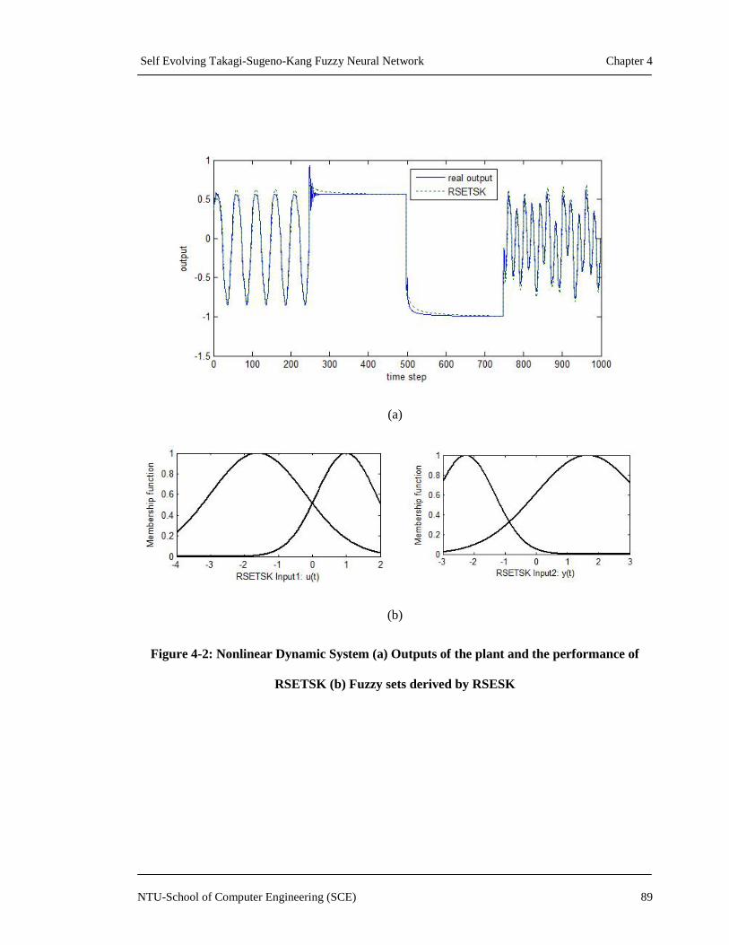
Self Evolving Takagi-Sugeno-Kang Fuzzy Neural Network Chapter 4
NTU-School of Computer Engineering (SCE) 89
(a)
(b)
Figure 4-2: Nonlinear Dynamic System (a) Outputs of the plant and the performance of
RSETSK (b) Fuzzy sets derived by RSESK

Self Evolving Takagi-Sugeno-Kang Fuzzy Neural Network Chapter 4
NTU-School of Computer Engineering (SCE) 90
Table 4-1: Comparison of RSETSK against other recurrent models
Network Training
time steps
Training
RMSE
Testing
RMSE
No of Rules
Memory neural network 90000 0.1521 0.2742 NA
TRFN-S 9000 0.0084 0.0346 3
RSONFIN 9000 0.0248 0.0780 4
HO-RNFS 9000 0.0542 0.0815 3
RSEFNN-LF 9000 0.0199 0.0397 4
RFNN 10000 0.0114 0.0575 16
GSETSK 9000 0.0201 0.0062 5
RSETSK 9000 0.0198 0.0057 4
Table 4-1 shows that RSETSK outperforms the other networks in terms of testing RSME, while
using a comparable number of rules. It should be noted that memory neural network [94] behaves
like black-box models, in which there is no way to derive any human interpretable rules.
RSETSK can also achieve significantly better results than other recurrent systems in training
RSME, except TRFN-S and RFNN. However, RFNN is a network with a fixed structure, which
requires the number of rules to be specified prior to training. All recurrent models such as TRFN-
S [23], RSONFIN [22], HO-RNFS [71], and RSEFNN [59] employ gradient descent or back-
propagation algorithms to tune the centers and widths of their fuzzy sets in their parameter
training phase, which eventually leads to highly overlapping fuzzy sets. Hence, it is difficult to
derive human interpretable knowledge from the structure of these recurrent models.
In RSONFIN [22] and RSEFNN [59], there are 9 and 8 fuzzy sets, respectively, generated in the
two input variables ( )py t and ( )u t . In RSETSK, only 4 fuzzy sets are generated in the two input
variables. Figure 4-2 shows the fuzzy membership functions for two inputs that RSETSK created
to model the nonlinear dynamic plant using the training set described earlier. One can observe

Self Evolving Takagi-Sugeno-Kang Fuzzy Neural Network Chapter 4
NTU-School of Computer Engineering (SCE) 91
that the fuzzy membership functions derived using RSETSK are highly distinguishable. The
merging approach in RSETSK helps the network to derive a compact and meaningful
interpretable fuzzy rule base while still achieving favorable accuracy.
4.4.2 Analysis Using a Nonlinear Dynamic System With Regime-
shifting Properties
This experiment investigates the online learning ability of RSETSK to provide an approximate of
the nonlinear dynamic plant with regime shifting properties. The properties of the nonlinear
dynamic plant described in Section 4.4.2 are modified as shown in (4.16),
( 1) ( ( ) , ( 1) , ( 2 ) , ( ) , ( 1)) ( )p p p py t f y t y t y t u t u t n t (4.16)
where ( )n t is a disturbance to be introduced into the system given by
0 1 1 0 0 0 an d 2 0 0 1
( )2 1 0 0 1 2 0 0 0
t tn t
t
(4.17)
In this experiment, the RSETSK model is employed to perform online learning of the
characteristics of the modified nonlinear dynamic plant for a duration of [1, 3 0 0 0 ]t . It should
be noted that the time-variant data generated by this nonlinear dynamic plant exhibits regime
shifting properties. More specifically, the data ranges in this experiment vary with time. For the
entire simulation [1, 3 0 0 0 ]t , the control inputs ( )u t are generated as follows.
s in ( / 2 5 ) ( m o d 1 0 0 0 ) 2 5 0
1 .0 2 5 0 ( m o d 1 0 0 0 ) 5 0 0( )
1 .0 5 0 0 ( m o d 1 0 0 0 ) 7 5 0
0 .3 s in ( / 2 5 ) 0 .1 s in ( / 3 2 ) 0 .6 s in ( / 1 0 ) 7 5 0 ( m o d 1 0 0 0 ) 1 0 0 0
t t
tu t
t
t t t t
(4.18)

Self Evolving Takagi-Sugeno-Kang Fuzzy Neural Network Chapter 4
NTU-School of Computer Engineering (SCE) 92
Figure 4-3 shows the online modeling performances of the proposed RSETSK. It can easily be
observed that RSETSK is able to accurately capture and model the underlying dynamics of the
nonlinear dynamic plant described in (4.16). The RSETSK continuously changes its structure and
parameters to track the new system characteristics in two different scenarios 1) the disturbance is
introduced at time 1 0 0 0t ; 2) the disturbance is removed at time 2 0 0 0t . More specifically,
RSETSK creates new rules to learn the underlying characteristics of the new data, then performs
parameter tuning to adjust its parameters, and lastly deletes obsolete rules that no longer can
describe the new system characteristics. This results in a dynamic and compact fuzzy rule base in
RSETSK. As shown in Figure 4-4, the rule base in RSETSK evolves during the simulation.
During time [1, 2 5 0 ]t , the number of rules gradually moves upward as the network attempts to
learn and model the new data. From time [ 2 5 0 ,1 0 0 0 ]t , the RSETSK stops adding new rules
and the number of rules remains at 4 as these rules are sufficient to describe the current data. At
time 1 0 0 0t , there is a significant shift in input data range as can be observed in Figure 4-3.
Also, the number of rules in the RSETSK starts climbing up when the disturbance is introduced
to the system at time 1 0 0 0t . This is due to the RSETSK beginning to evolve in response to the
changes in the underlying characteristics of the nonlinear plant. During time [1 0 0 1,1 5 0 0 ]t , the
number of rules goes up to 7 and then gradually decreases to 5 as the obsolete rules that were
learnt during time [1,1 0 0 0 ]t are gradually pruned from the fuzzy rule base of the RSETSK. It
should be noted that during time [1 7 5 0 , 2 0 0 0 ]t , the number of rules stabilizes at 6. Among
these 6 rules, 4 of them are new rules that are learnt during time [1 0 0 0 , 2 0 0 0 ]t , the remaining
two are obsolete rules that are learnt during time [1,1 0 0 0 ]t . Not all the obsolete rules are
pruned during time [1 0 0 0 , 2 0 0 0 ]t , because RSETSK employs a ‗gradual‘ forgetting approach
which is based on the fuzzy rule potentials. Since the potentials of some obsolete rules are still
above the pruning threshold, the rules are not pruned yet. They will be pruned, if in the next time

Self Evolving Takagi-Sugeno-Kang Fuzzy Neural Network Chapter 4
NTU-School of Computer Engineering (SCE) 93
steps they are still not activated. This whole process repeats again when the disturbance is
removed at time 2 0 0 0t . RSETSK continues to create new rules to relearn the original data
after the disturbance is completely removed at time 2 0 0 0t . The number of rules finally
stabilizes at 4 again after the rules learnt during time [1 0 0 0 , 2 0 0 0 ]t are pruned.
It can be observed that, in this experiment, if RSETSK does not possess a rule pruning algorithm,
it might finish the learning process with 8 rules, with many of which being obsolete. Existing
recurrent networks such as RSONFIN [22], TRFN [23], HO-RNFS [71], and RSEFNN [59] do
not consider this issue, resulting in obsolete rule bases with many redundant rules when they deal
with time-variant datasets with regime shifting properties as in this experiment. G-FNN recurrent
networks [96] basically employ the outputs of their feedforward version to feed back to their
fuzzy rules. No internal memory structure is implemented in G-FNN, so their recurrent models do
not have much advantage over their feedforward models [96]. Although a rule pruning algorithm
is mentioned in G-FNN, the approach‘s computational cost is high. Also, since GFNN does not
differentiate between new data and past data, well-learnt information in GFNN can be easily
forgotten. The ‗gradual‘ forgetting approach in RSETSK allows ‗smooth‘ learning in time-variant
environments in which disturbances might occur repeatedly. The average training time reported
by RSETSK for 3000 observations is only 1 .8 5 5 0 .0 8 s . This demonstrates RSETSK‘s fast
learning ability in incremental time-variant environments.
Figure 4-3: RSETSK’s modeling performance during time [1, 3 0 0 0 ]t

Self Evolving Takagi-Sugeno-Kang Fuzzy Neural Network Chapter 4
NTU-School of Computer Engineering (SCE) 94
(a)
(b)
Figure 4-4: RSETSK’s self-evolving process (a) The evolution of RSETSK’s fuzzy rule base
(b) Online learning error of RSETSK
4.4.3 Analysis Using Dow Jones Index Time Series
This experiment investigates the online learning ability of RSETSK using a real-world financial
time-series based on the Dow Jones Industrial Average (DJIA) market index. About 50 years of
daily index values were collected from the Yahoo! Finance website on the ticker symbol ―^DJI‖
for the period from January 4, 1960 to December 31, 2010, which provided 12,838 data points for
the experiment. Figure 4-5 shows the time-variant behavior of the time series with a nonuniform
distribution in the range 5 3 5.7 6 , 1 4 1 6 5.0 0 . It can be observed that after a long quiet time in
the period 1960-1980, there are significant shifts in data ranges after the 1980s. The daily
movements also become sharper with many noteworthy peaks and troughs. It should be noted that
RSETSK is an online structure which does not require any prior knowledge of the complete set of

Self Evolving Takagi-Sugeno-Kang Fuzzy Neural Network Chapter 4
NTU-School of Computer Engineering (SCE) 95
data points at any point in time. In this experiment, RSETSK attempts to perform an online
simulation of the daily forecast of the Dow Jones index using the following input and output
vectors
in p u t vec to r [ ( 3), ( 2 ), ( 1), ( )]y t y t y t y t
o u tp u t v ec to r [ ( 1)]y t
where y t is the absolute value from the Dow Jones index time series.
Previous studies [97] have shown that evidence of nonlinear predictability in the stock market can
be found using past data values. In this experiment, the system output does not depend only on
the 4 past states 3y t , 2y t , 1y t and y t but also on other further past states. A
feedforward network with these 4 states normally does not include past states beyond 3y t .
In contrast, the recurrent structure in RSETSK can memorize the past states prior to 3y t for
output prediction. Based on availability constraints, the experiment was benchmarked against
DENFIS [11] and GSETSK as a reference model. DENFIS is a feedforward self-evolving
network but it is not fully online as it implicitly assumes prior knowledge of the upper and lower
bounds of the data set to normalize data before learning.
Table 4-2: Forecasting 50 years of Dow Jones Index
Network R NDEI No of Rules
DENFIS 0.998 0.019 6
GSETSK 0.998 0.022 8
RSETSK 0.998 0.020 6
Figure 4-5 shows that RSETSK can quickly mimic the movements of the time series. All the
peaks and troughs are well predicted. It can be seen from Table 4-2 that RSETSK has almost
similar results as DENFIS although RSETSK performs the estimation completely online without

Self Evolving Takagi-Sugeno-Kang Fuzzy Neural Network Chapter 4
NTU-School of Computer Engineering (SCE) 96
prior knowledge of the complete data set. Also, from Figure 4-6, one can observe that the rule
base in RSETSK evolves over time. More specifically, new rules are added to describe new data
and obsolete rules are pruned to maintain a compact and up-to-date rule base at all time. During
the simulation, there are at least 7 major reorganizations in the rule base. RSETSK outperforms
its feedforward version GSETSK in this experiment. The average simulation time reported by
RSETSK for 12,838 data points is only 8 .3 7 5 0 .0 5 s . This demonstrates RSETSK‘s fast
learning ability in real-life problems.
Figure 4-5: Dow Jones time series forecasting results.

Self Evolving Takagi-Sugeno-Kang Fuzzy Neural Network Chapter 4
NTU-School of Computer Engineering (SCE) 97
Figure 4-6: The evolution of the fuzzy rules in RSETSK
Figure 4-7: Highly interpretable knowledge base derived by RSETSK.
Self Evolving Takagi-Sugeno-Kang Fuzzy Neural Network Chapter 4
NTU-School of Computer Engineering (SCE) 98
4.5 Summary
This chapter presents a novel recurrent self-evolving Takagi–Sugeno–Kang fuzzy framework
named RSETSK. Similar to its non-recurrent version GSETSK, it employs MSGC for its
structural learning phase and adopts an online data-driven incremental-learning-based-approach.
The main difference between RSETSK and GSETSK is that Layer III in RSETSK is a recurrent
layer. This recurrent structure allows RSETSK to address temporal problems better than
GSETSK, resulting in a smaller network size. It also does not require the knowledge of number of
delayed input and output in advance. The performance of the RSETSK network was evaluated
using three simulations. The results of the RSETSK network are encouraging when benchmarked
against other recurrent systems. The third experiment, a stock index prediction simulation,
demonstrates the applicability of RSETSK in real world problems.

Self Evolving Takagi-Sugeno-Kang Fuzzy Neural Network Chapter 5
NTU-School of Computer Engineering (SCE) 99
Chapter 5: Stock Market Trading System – A Financial
Case Study
5.1 Introduction
The prediction of stock market movements has become a thriving research topic and, if
successful, may result in substantial financial rewards. In practice, there are two major
approaches to the analysis of stock market movement prediction; namely: Fundamental and
technical analysis. Fundamental analysis is based on economic, financial and other qualitative and
quantitative factors to estimate the intrinsic values of the securities [98]. Technical analysis is
based on the foundation that history will repeat itself and that the correlation between price and
volume reveals market behaviors [99]. More specifically, this approach studies past market data
to predict future movements. A well known hypothesis amongst academics, the Efficient Market
Hypothesis (EMH) [100], suggests that the prediction of stock market prices is futile and implies
that the technical analysis approach to forecasting is invalid. However, the hypothesis is highly
controversial. Many recent works [101-103] from statistical and behavioral finance perspectives
have challenged the EMH and have exemplified the evidence on the predictability of stock
market using technical analysis. In the real world, technical analysis is becoming more popular
and is widely used among traders and financial professionals.
Recently, computational intelligence techniques such as neural networks [104] are widely used
for stock market prices or stock market trend prediction [105]. Neural networks are extensively
People who are high-level investors are not concerned about the market going up or going down because their knowledge will allow them to make money either way.
Robert Kiyosaki (1947- )

Self Evolving Takagi-Sugeno-Kang Fuzzy Neural Network Chapter 5
NTU-School of Computer Engineering (SCE) 100
employed for technical financial forecasting because of their ability to learn non-linear complex
patterns in data and self-adaptation for various statistical distributions. More specifically, they are
universal function approximators, meaning that they can capture and model any input-output
relationship given the right data and configuration. In [106], the authors reported that neural
networks outperformed other non-neural approaches in most of forecasting studies. In [97], a
single layer feedforward neural network was used to predict security returns from past real-world
returns. The results indicate strong evidence of nonlinear predictability in stock market returns. In
[107], a neural network was employed to predict the proper time to move money into and out of
the stock market. The results significantly outperformed the buy-and-hold strategy. However,
despite yielding promising results in stock market prediction, neural networks are mainly
considered as black-box models because their knowledge is represented by links and weights.
There is no way to derive any human interpretable information from the networks.
Subsequently, there is a continuing trend in using fuzzy neural networks (FNNs) [4] to predict the
stock market. Some works that applied FNNs in forecasting stocks are [99], [108-112] . In [108],
an Adaptive Neural Fuzzy Inference System (ANFIS) [7] is used to predict future trends. In [99],
ANFIS is used to control the stock market process model. The disadvantage of ANFIS is that it is
unable to learn in an incremental manner [6] due to its fixed structure. In [109], a rough-set based
neuro-fuzzy system named RSPOP was used as a stock predictive model which employs the time-
delayed price difference forecast approach. The approach is claimed to perform better than the
price forecast approach because it avoids the deterministic shifts in range of values of out-of-
sample forecasts. However, RSPOP employs a batch learning approach and is computationally
expensive because of its post-training process based on rough-set theory for information and
optimization [58]. In [112], a hybrid system integrating a wavelet and TSK fuzzy rules is
proposed. The method employs offline learning algorithm and requires preprocessing of data. In

Self Evolving Takagi-Sugeno-Kang Fuzzy Neural Network Chapter 5
NTU-School of Computer Engineering (SCE) 101
[110], a FNN called GLC is proposed for predicting stock prices. The advantage of GLC is that it
can address the time-variant datasets. In [111], a trading system using a hierarchical
coevolutionary fuzzy system to predict a series of percentage price oscillator (PPO) is proposed.
Both GLC [110] and HiCEFS [111] employ genetic algorithms, which are generally slow and
computationally costly.
In this chapter, we propose a stock trading decision model with a novel price prediction model
empowered by RSETSK, a recurrent self-evolving Takagi-Sugeno-Kang fuzzy neural network.
RSETSK possesses dynamic structure with online learning/unlearning abilities and can learn
incrementally in time-variant environments. It is fast, interpretable, biologically plausible, and
potentially, of superior performance. Unlike existing price prediction models, RSETSK employs
a novel rule pruning algorithm to keep a compact and current rule base at all times. Besides, by
inheriting the advantages of recurrent networks, RSETSK is able to outperform other prediction
models in the literature in terms of accuracy.
5.2 Stock Trading System Using RSETSK
The main approach in stock trading is to identify early trends and maintain an investment position
(long, short, or hold) until evidence indicates that the trend has reversed. It is obvious that trends
in stock prices can be very volatile, almost chaotic at times. Investors generally rely on two types
of market analysis to identify the trends: fundamental and technical. Fundamental analysis
focuses on the reasons of price movement, and this process is very complicated since there are so
many factors that may affect the price change such as political, psychotically events [113].
Technical analysis [101] is the study of market action, based on the foundation that the market
action discounts everything. It assumes that anything that can possibly affect the market is
already reflected in the prices, and all the new information will be immediately reflected in those
prices. Compared with fundamental analysis, technical analysis can be easily performed for any

Self Evolving Takagi-Sugeno-Kang Fuzzy Neural Network Chapter 5
NTU-School of Computer Engineering (SCE) 102
stock because it only analyzes the historical quantitative data that are easy to obtain, such as the
price and volume. Thus, stock trading systems usually employ the results of the technical analysis
to generate trading signals accordingly.
In this section, a stock trading system with the RSETSK predictive model is presented. In order to
assess the trading performance of the proposed approach, a stock trading system without a
predictive model is also introduced. Profits and losses generated by all systems will be compared.
Assume the price value of a security is represented as a time series ( )u T , where ( )u t represents
a value at time instant t. In all systems, the trading action at time t is denoted as ( )F t where
( ) { 1,1}F t with -1 and 1 representing the buy and sell actions, respectively. The trading
system return is subsequently modeled by the final portfolio value using a multiplicative return
( )R t [114] given in (5.1),
( ) ( 1){1 ( ) ( 1)} {1 | ( ) ( 1) |}R t R t r t F t F t F t (5.1)
where ( ) { ( ) / ( 1)} 1r t u t u t ; is the transaction cost rate, which is assumed to be a fraction
of the transacted price value.
There are numerous ways to generate buy and sell signals using technical analysis techniques.
One of the simplest and most popular approaches for deciding when to buy and sell is using
moving averages [97,115]. Moving averages (MAs) smooth the price data to define the current
trend direction and filter the noise. There are many variants of MAs used in technical analysis.
Among them, MACD [103] (moving average convergence/divergence) oscillator originally
developed by Gerald Appel is widely used due to its simplicity and efficiency. MACD is a
computation of the difference between two exponential moving averages (EMAs) [103] of
closing prices. Exponential moving averages highlight recent changes in a stock's price. The

Self Evolving Takagi-Sugeno-Kang Fuzzy Neural Network Chapter 5
NTU-School of Computer Engineering (SCE) 103
EMA of a price series is given as in (5.4). By comparing EMAs of different lengths, the MACD
can gauge changes in the trend of a security. MACD consists of Fast signal given in (5.2) and
Slow signal given in (5.3). The Fast signal computes the difference between the lo n g EMA and
the s h o r t EMA of time series u(T) where lo n g sh o r t . The Slow signal computes the
s lo w EMA of the Fast signal.
fa s t ( ) E M A ( ) E M A ( )u u
sh o r t lo n gt t t (5.2)
s lo w ( ) E M A ( )fa s t
s lo wt t
(5.3)
E M A ( ) ( ) (1 ) E M A ( 1)u u
t u t t (5.4)
where 2 / ( 1) , is the number of time instants of the moving average; and E M A ( )u
t is
the EMA of time instant t. In practice, the Slow signal of MACD can be used to generate the
buy/sell signal, as illustrated in (5.5),
( ) (s lo w ( ))F t s ig n t (5.5)
where ( )F t is the trading action at time t.
Equation (5.5) has the meaning that at time t, if the MACD Slow signal of a security is below 0, a
sell action should be triggered, and vice versa for the buy action. However, in order to reduce the
number of false trading actions by eliminating the ―whiplash‖ signals which happen when the
Slow signal slightly fluctuates around zero, a whipsaw signal filter is introduced as in (5.6),
1, w h e n s lo w ( )
( ) 1, w h e n s lo w ( )
( 1) , o th e rw is e
t
F t t
F t
(5.6)

Self Evolving Takagi-Sugeno-Kang Fuzzy Neural Network Chapter 5
NTU-School of Computer Engineering (SCE) 104
where is the width of the whipsaw signal filter. The stock trading system without a predictive
model using MACD to generate trading decisions is shown Figure 5-1. The work in [109] has
further demonstrated that trading systems using moving average trading rules are able to achieve
high returns as compared against other trading strategies as shown in [115].
Trading SystemProfits/Losses
R(t)
Price
Series
Transaction
cost δ
trade
F(t)
Figure 5-1: Trading system without a predictive model.
Trading SystemProfits/Losses
R(t)
Price
Series
Transaction
cost δ
trade
F(t)
RSETSK
predictive model
u(t)
u(t-1)
...
u(t-n+1)
Supervised
learning
u(t+1)
forecast
u’(t+1)
Figure 5-2: Trading system with RSETSK predictive model.
However, using MACD to generate trading decisions does not always work perfectly. That is
because MACD is a trend following indicator which can identify the current trend but is unable to
forecast the trend in the future. Since the MACD is based on moving averages, it is inherently a
lagging indicator. Thus, the stock trading system without a predictive model always generates
buy or sell decisions late after the actual trend reversal. In order to take prompt trading action, a
predictive model should be adopted. Figure 5-2 shows the proposed stock trading system with
RSETSK as a predictive model. The historical price series is represented in n–tuples

Self Evolving Takagi-Sugeno-Kang Fuzzy Neural Network Chapter 5
NTU-School of Computer Engineering (SCE) 105
[ ( 1), ..., ( 1) , ( )]u t n u t u t , where n is the embedding dimension. The n-tuples are used as
inputs to the RSETSK predictive model to predict the future price, '( 1)u t . In this system, the
RSETSK predictive model is trained using supervised learning, using one training instant at a
time. This is the main difference between the proposed RSETSK predictive model and other
existing predictive models. Other models such as [99,109,111] employ a batch learning approach
in which a set of data needs to be available before training. RSETSK follows a strict online
learning approach which satisfies the following criteria.
1) All the training observations are sequentially (one-by-one) presented to the learning
system.
2) At any time, only one training observation is seen and learnt.
3) A training observation is discarded as soon as the learning procedure for that particular
observation is completed.
4) The learning system has no prior knowledge as to how many total training observations
will be presented.
These criteria are defined in [6] to be considered incremental sequential learning approaches.
They are much desired in fast changing environments such as stock price predictions, because in
real life, a full training data set may not be available at the beginning. RSETSK functions by
interleaving reasoning (testing) and learning (training) activities. It is different from other systems
[99,109,111] that need to be trained first before testing. It should be noted that a stock price series
is chaotic, evolving and time-variant. Thus, a well-trained static predictive model might not work
for new incoming data. RSETSK can continuously learn new data because it is essentially a self-
evolving system which takes in consideration of time-variant problems. The predicted
price, '( 1)u t , is then used for the computation of the moving averages as given in (5.7)-(5.9).
The trading signal F t is decided by the forecast value '( 1)u t as in (5.10),
Self Evolving Takagi-Sugeno-Kang Fuzzy Neural Network Chapter 5
NTU-School of Computer Engineering (SCE) 106
' 'fa s t ( 1) E M A ( 1) E M A ( 1)
u u
sh o r t lo n gt t t (5.7)
s lo w ( 1) E M A ( 1)fa s t
s lo wt t
(5.8)
' 'E M A ( ) '( 1) (1 ) E M A ( )
u ut u t t (5.9)
1, w h e n s lo w ( 1)
( ) 1, w h e n s lo w ( 1)
( 1) , o th e rw is e
t
F t t
F t
(5.10)
where 2 / ( 1) , is the number of time instants of the moving average, and '( 1)u t is
the forecast price value for time instant ( 1)t . Extensive experiments were conducted to
evaluate the performance of the proposed RSETSK stock trading model. The results are presented
in the next section.
5.3 Experiments On Real-world Financial Data
5.3.1 Experimental Setup
In this section, the proposed stock trading system with the RSETSK predictive model is used to
trade the actual stocks in the real-world stock market. The forecasting performances of the
RSETSK predictive model are benchmarked against other well-known FNNs, such as dynamic
evolving neural-fuzzy inference system (DENFIS) [11], and rough set-based pseudo outer-
product fuzzy neural network (RSPOP) [116]. The trading performances of all trading systems
including the proposed trading system using RSETSK, the simple buy-and-hold strategy, the
trading system without prediction, the trading system with perfect prediction and the trading
systems with other predictive models (DENFIS, RSPOP) are evaluated using the historical data of
International Business Machines Corporation (IBM) and Singapore Exchange Limited (SGX)
Self Evolving Takagi-Sugeno-Kang Fuzzy Neural Network Chapter 5
NTU-School of Computer Engineering (SCE) 107
stock. All the predictive models are constructed as five-input one-output systems and configured
with default parameters. In these experiments, the trading signals for trading system without
predictive model is computed using (5.2)–(5.5). The trading signals for trading system with
RSETSK, DENFIS and RSPOP predictive models are computed using (5.7)–(5.10). The trading
signals for trading system with perfect prediction are also computed using (5.7)–(5.10), but the
predicted '( 1)u t is replaced with the actual future price ( 1)u t . The portfolio end value
( )R T is computed using (5.1), where the initial portfolio value (0 ) 1 .0R and the transaction
cost rate is 0 .2 . The final multiplicative return ( )R T is an important factor to evaluate all
the trading systems in this experiment. The width of the whipsaw signal filter 0 .1 % is used
in (5.10).
In the first experiment, all the predictive models are trained in a batch learning mode, meaning
that the full training data set is available before training. The predictive models are then trained to
predict the other out-of-sample data set (testing set). The training and testing sets are partitioned
from the historical price series and do not overlap. Then, the simple buy-and- hold strategy, the
trading system without prediction, the trading system with perfect prediction, and the trading
systems with different predictive model are evaluated with the out-of-sample data set using the
final portfolio value ( )R T .
In the second experiment, the predictive models are trained in an incremental online mode. There
is no full training set available at the beginning. All the training observations are sequentially
(one-by-one) presented to the predictive models. As RSPOP employs a batch learning approach,
it is not applicable in this experiment. Only DENFIS and RSETSK are applied in this experiment.
Both DENFIS and RSETSK are evolving systems that can continuously learn new data. They
function by interleaving reasoning (testing) and learning (training) activities, meaning that they

Self Evolving Takagi-Sugeno-Kang Fuzzy Neural Network Chapter 5
NTU-School of Computer Engineering (SCE) 108
are able to learn from the current training instant and use the learnt knowledge to predict the
output of the next training instant. In the real world, this online learning approach is more
desirable than the batch learning approach, as real-world data is always complicated, time-
varying and evolving.
5.3.2 Experimental Results and Analysis
5.3.2.1 Analysis using IBM Stock
The predictive models are trained with five previous values of the price series as inputs. The
experimental price series consists of 4852 price values obtained from the Yahoo Finance website
on the counter NYSE:IBM from the period of January 2nd, 1992 to April 1st, 2011. The in-
sample training data set is constructed using the first 2296 data points and the out-of-sample test
data set is constructed using the more recent 2556 data points. Trading signals are generated using
heuristically chosen moving average parameters 12, 8, and 5 ( , ,lo n g sh o r t s lo w ) and the
portfolio end values are computed with a transaction cost of 0.2%.
Table 5-1 shows the benchmarking results of different prediction systems, including the mean
square error and the prediction accuracy indicated by the Pearson correlation [117] between the
actual, and predicted '( 1)u t series. More specifically, RSETSK is benchmarked against other
fuzzy neural networks such as DENFIS [11] and RSPOP [109] and non-fuzzy neural networks
such as such as radial basis function networks (RBFN [118]) and feed-forward neural network
trained using back-propagation (FFNN-BP [119]).
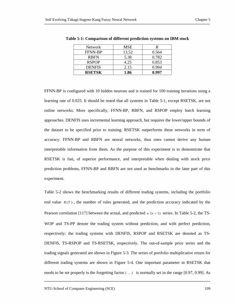
Self Evolving Takagi-Sugeno-Kang Fuzzy Neural Network Chapter 5
NTU-School of Computer Engineering (SCE) 109
Table 5-1: Comparison of different prediction systems on IBM stock
Network MSE R
FFNN-BP 13.52 0.564
RBFN 5.38 0.782
RSPOP 4.25 0.853
DENFIS 2.15 0.994
RSETSK 1.86 0.997
FFNN-BP is configured with 10 hidden neurons and is trained for 100 training iterations using a
learning rate of 0.025. It should be noted that all systems in Table 5-1, except RSETSK, are not
online networks. More specifically, FFNN-BP, RBFN, and RSPOP employ batch learning
approaches. DENFIS uses incremental learning approach, but requires the lower/upper bounds of
the dataset to be specified prior to training. RSETSK outperforms these networks in term of
accuracy. FFNN-BP and RBFN are neural networks, thus ones cannot derive any human
interpretable information from them. As the purpose of this experiment is to demonstrate that
RSETSK is fast, of superior performance, and interpretable when dealing with stock price
prediction problems, FFNN-BP and RBFN are not used as benchmarks in the later part of this
experiment.
Table 5-2 shows the benchmarking results of different trading systems, including the portfolio
end value ( )R T , the number of rules generated, and the prediction accuracy indicated by the
Pearson correlation [117] between the actual, and predicted '( 1)u t series. In Table 5-2, the TS-
WOP and TS-PP denote the trading system without prediction, and with perfect prediction,
respectively; the trading systems with DENFIS, RSPOP and RSETSK are denoted as TS-
DENFIS, TS-RSPOP and TS-RSETSK, respectively. The out-of-sample price series and the
trading signals generated are shown in Figure 5-3. The series of portfolio multiplicative return for
different trading systems are shown in Figure 5-4. One important parameter in RSETSK that
needs to be set properly is the forgetting factor . is normally set in the range [0.97, 0.99]. As

Self Evolving Takagi-Sugeno-Kang Fuzzy Neural Network Chapter 5
NTU-School of Computer Engineering (SCE) 110
this is a recall experiment, is set to be 0.99. Previous studies [97] have shown the evidence of
nonlinear predictability in the stock market using past data values. In this experiment, the system
output '( 1)u t does not depend only on the five past states 4 , 3 , ( 2 ) , ( 1)u t u t u t u t ,
and ( )u t but also on other further past states. A feedforward network (like DENFIS or RSPOP)
with these five states normally does not include past states beyond 4u t . In contrast, the
recurrent structure in RSETSK can memorize the past states prior to 4u t for output
prediction [22].
Figure 5-3: Price and trading signals on IBM.

Self Evolving Takagi-Sugeno-Kang Fuzzy Neural Network Chapter 5
NTU-School of Computer Engineering (SCE) 111
Figure 5-4: Portfolio values on IBM achieved by the trading systems with different
predictive models.
It can be observed that RSETSK outperforms the other predictive models (DENFIS and RSPOP)
in term of accuracy and number of fuzzy rules. RSETSK can achieve the highest accuracy of
0.997 using only 9 rules. The stock trading system using RSETSK achieves the highest final
return ( ) 5 .3 2R T , among the trading systems with predictive model. Compared with the
trading systems using DENFIS and RSPOP, the trading system with RSETSK achieved an
increase of 2.87 and 3.17 in final portfolio value ( )R T , respectively.
One can observe from Table 5-2 that the simple buy-and-hold strategy only achieved a final
portfolio value of ( ) 1 .6 3R T . The trading system without a predictive model yielded a slightly
higher portfolio end value of ( ) 1 .7 2R T . As shown in Table 5-2, the trading systems with
predictive models yielded higher returns than the trading system without predictive model and
yielded lower returns than the trading system with perfect prediction. More specifically, the

Self Evolving Takagi-Sugeno-Kang Fuzzy Neural Network Chapter 5
NTU-School of Computer Engineering (SCE) 112
proposed trading system with RSETSK predictive model yielded an increase of 3.60 in ( )R T
when compared against the trading system without predictive model.
Table 5-2: Comparison of different trading systems on IBM stock
Network R No of Fuzzy Rules R(T)
Buy&Hold N.A N.A 1.63
TS-WOP N.A N.A 1.72
TS-WPP N.A N.A 7.54
TS-RSPOP 0.853 15 2.15
TS-DENFIS 0.994 12 2.45
TS-RSETSK 0.997 9 5.32
Figure 5-5 is the enlarged part of Figure 5-3 from time t = 900 to 1000. As shown in Figure 5-5,
the trading system with RSETSK predictive model generated the buy and sell signals earlier
through the use of the predictive value '( 1)u t . Based on this advantage, the proposed stock
trading systems with RSPOP, DENFIS, and RSETSK predictive model yielded a higher return
than the trading system without a predictive model. However, the trading systems with predictive
models are unable to forecast with exact accuracy, unlike the trading system with perfect
prediction, which uses the actual future price value '( 1) ( 1)u t u t . Therefore the trading
systems with predictive models yielded a lower portfolio end value than the trading system with
perfect prediction. The average training time reported by RSETSK is only 1 .9 3 0 .0 5 s .
Figure 5-5: Enlarged part of Figure 5-3 from time t=900 to t=1000

Self Evolving Takagi-Sugeno-Kang Fuzzy Neural Network Chapter 5
NTU-School of Computer Engineering (SCE) 113
Figure 5-6 shows the membership functions generated in the knowledge base of RSETSK after
training. It can be easily observed that all the membership functions are highly distinguishable.
There are in total only 15 membership functions generated in five input dimensions. One can
easily assign semantic meanings for the derived fuzzy sets, as shown in Figure 5-6.
Figure 5-6: Semantic interpretation of the fuzzy sets derived in RSETSK
5.3.2.2 Analysis Using Singapore Exchange Limited (SGX) Stock
This experiment investigates the online learning ability of RSETSK using a real-world financial
time-series based on the SGX stock times series. About 6 years of daily index values were

Self Evolving Takagi-Sugeno-Kang Fuzzy Neural Network Chapter 5
NTU-School of Computer Engineering (SCE) 114
collected from the Yahoo! Finance website on the ticker symbol S68.SI for the period from Jan 3,
2005 to April 1, 2011, which provided 1,592 data points for the experiment. Figure 5-7 shows the
time-variant behavior of the time series with a nonuniform distribution in the range [1.78, 16.40].
Only DENFIS and RSETSK are applied as predictive models in this experiment as they are
evolving systems that adopt incremental learning approach [6]. Both systems attempt to perform
an online simulation of the daily forecast of the SGX stock prices using five previous values of
the price series as inputs. Reasoning (testing) and learning (training) activities are performed
simultaneously. Trading signals are generated using heuristically chosen moving average
parameters 12, 8, 5 and the portfolio end values are computed with a transaction cost of 0.2%. In
this online simulation, the forgetting factor in RSETSK is set to be 0.97 so that RSETSK can
unlearn fast to keep a compact and current rule base.
As shown in Table 5-3, RSETSK outperforms DENFIS in term of accuracy and number of rules.
RSETSK achieved the accuracy of 0.9979 using only 4 rules, while DENFIS yielded the accuracy
of 0.9965 using 6 rules. It should be noted that DENFIS is not fully online. In contrast, RSETSK
is fully online and it does not require any prior knowledge of the complete set of data points at
any point in time. As a result, the stock trading system using RSETSK achieves the higher final
return of ( ) 1 1 .4 0R T . Compared with the trading system using DENFIS, the trading system
with RSETSK achieved an increase of 1.11 in final portfolio value ( )R T . The simple buy-and-
hold achieved a final portfolio value ( ) 4 .4 1R T . The trading system without a predictive
model yielded a slightly higher portfolio end value of ( ) 5 .8 5R T . The results again show that
the trading systems with predictive models yielded higher returns than the trading system without
forecast model and yielded lower returns than the trading system with perfect prediction. Figure
5-7 shows the price series and the trading signals generated. Figure 5-8 shows the series of
portfolio multiplicative return for different trading systems.

Self Evolving Takagi-Sugeno-Kang Fuzzy Neural Network Chapter 5
NTU-School of Computer Engineering (SCE) 115
Table 5-3: Comparison of different trading systems on SGX stock
Network Buy&Hold TS-
WOP
TS-WPP TS-
DENFIS
TS-
RSETSK
R(T) 4.41 5.85 15.44 10.31 11.40
No. of Rules N.A N.A N.A 6 4
R N.A N.A N.A 0.9965 0.9979
Figure 5-7: Price and trading signals on SGX.
Figure 5-8. Portfolio values on SGX achieved by the trading systems.

Self Evolving Takagi-Sugeno-Kang Fuzzy Neural Network Chapter 5
NTU-School of Computer Engineering (SCE) 116
Figure 5-9 shows that RSETSK can quickly mimic the movements of the time series throughout
the online simulation. All the peaks and troughs are well predicted. Also, from Figure 5-10, one
can observe that the rule base in RSETSK evolves over time. More specifically, new rules are
added to describe new data and obsolete rules are pruned to maintain a compact and up-to-date
rule base at all times. This is an important feature of RSETSK. During the simulation, there are
at least 4 major reorganizations in the RSETSK rule base, as marked in Figure 5-10. The
reorganizations correspond to the trajectory shifts in the SGX price series, as shown in Figure 5-
9. The number of rules in other self-evolving systems such as DENFIS will only grow with time,
in which many rules will become obsolete. In contrast, RSETSK always attempts to improve the
currency of the rule base by slowly unlearning the old data. This characteristic is desired in fast
and evolving problems such as time series prediction, as it improves the level of human expert
interpretability of the derived fuzzy rule base. This is also applied in real life trading, as stock
traders pay more attention to what are working now, not in the past. Table 5-4 lists the fuzzy rules
derived by RSETSK. The average simulation time reported by RSETSK for 1,592 data points is
only 0 .8 2 0 .0 5 s . This demonstrates RSETSK‘s fast learning ability in real-life problems.
Figure 5-9: SGX time series forecasting results.

Self Evolving Takagi-Sugeno-Kang Fuzzy Neural Network Chapter 5
NTU-School of Computer Engineering (SCE) 117
Figure 5-10: The evolution of the fuzzy rules in RSETSK
Table 5-4: Fuzzy rules extracted from RSETSK
Rule y(t-4) y(t-3) y(t-2) y(t-1) y(t)
R1 low low low - low
R2 low low low - high
R3 low high high - high
R4 high high high - high
5.4 Summary
A trading system with a novel predictive model empowered by the recurrent self-evolving
Takagi–Sugeno–Kang fuzzy network is presented. The RSETSK predictive model adopts an
online incremental-learning-based-approach to forecast the future security prices in order to
generate profitable trading decisions. RSETSK possesses many features which are desired in
evolving problems such as time series prediction. First, it is an online structure which does not
require prior knowledge of the number of cluster/fuzzy rules in the data set. Second, for using a
novel rule pruning algorithm, RSETSK‘s fuzzy rule base is kept compact and up-to-date at all
times, with highly distinguishable fuzzy sets. The recurrent structure in RSETSK results in a high
level of modeling accuracy when working with time-variant datasets. Two types of experiments
were carried out to evaluate the performance of RSTSK. The first one is a recall experiment. The
second experiment is an online simulation. Results in both experiments show that the RSETSK
provides accurate prediction of stock trend and that the trading system with RSETSK is able to
yield higher profit than the simple buy-and-hold strategy, the trading system without prediction,

Self Evolving Takagi-Sugeno-Kang Fuzzy Neural Network Chapter 5
NTU-School of Computer Engineering (SCE) 118
and the trading systems with other predictive models. The second experiment shows that
RSETSK is able to achieve a dynamic, compact and current resultant rule base. However, it
should be noted that the settings of the parameters of the moving averages can heavily affect the
profitability of the trading systems. And the trading results may vary for different stocks. A
generic guideline or an automated approach to selecting the optimal parameters for different
stocks can be considered as possible future works.

Self Evolving Takagi-Sugeno-Kang Fuzzy Neural Network Chapter 6
NTU-School of Computer Engineering (SCE) 119
Chapter 6: Option Trading & Hedging System – A Real
World Application
6.1 Introduction
Financial organizations nowadays are increasingly trading in options and other derivative
securities to reduce their exposure to the erratic price fluctuations of the economic markets.
Research has thus flourished that aims at supplementing traders‘ expertise and traditional
financial tools with the power of non-parametric, numerical computing techniques such as neural
networks and neural fuzzy systems [120]. These non-parametric pricing models attempt to
address the limitations of traditional models whose parameters are calibrated to match only
certain conditions, by pricing and risk-managing financial derivatives in a model-free approach.
Their goal is to eliminate model risk by assuming as little as possible and, in particular, no pre-
specified model.
Neural networks are extensively employed for financial models because of their ability to learn
complex non-linear patterns in data and self-adaptation for various statistical distributions.
However, despite yielding promising results in financial applications, neural networks are mainly
considered as black-box models because their knowledge is represented by links and weights.
There is no way to derive any human interpretable information from the networks. Besides, they
are generally applicable and reliable only when a huge amount of representative data is available.
In 1988, White [121] was the first to use neural networks for market forecasting. Since then, there
It's not whether you're right or wrong that's important, but how much
money you make when you're right and how much you lose when you're
wrong.
George Soros (1930 - )

Self Evolving Takagi-Sugeno-Kang Fuzzy Neural Network Chapter 6
NTU-School of Computer Engineering (SCE) 120
have been many studies using neural networks to predict the financial markets [97,107,122].
However, the amount of research work dedicated to the commodities market is still insignificant.
Recently, there is a continuing trend in using neural fuzzy systems (NFSs) [4] for developing
financial models. NFSs combine the human-like reasoning style of fuzzy systems with the
connectionist structure and learning ability of neural networks [2]. The advantage of neuro-fuzzy
approach is that it can provide insights to the user about the symbolic knowledge embedded
within the network. More specifically, NFSs can generalize from training data, learn/tune system
parameters, and generate the fuzzy rules to create a linguistic model of the problem domain.
Although many neural fuzzy based trading models have been developed for stock trading or
currency trading, only a few current works [123-124] are focused on enhancing and protecting
trading results using options. Options, as a derivative security, provide a means to manage
financial risks. They are powerful tools for hedging and speculation, without which the means of
creating portfolios and trading strategies would be very limited. The buyer of an option enters
into a contract with the right, but not the obligation, to purchase or sell an underlying asset at a
later date at a price agreed upon today.
In [123], Tung and Quek proposed a self-organizing network, GenSoFNN, which emulates the
information handling and knowledge acquisition of the hippocampal memory [125]. In [124],
Teddy et al. proposed a localized learning network, PSECMAC, which is inspired by the
neurophysiological aspects of the human cerebellum. Both of these approaches are focused on
finding mis-priced arbitrage opportunities to take up trading positions. These systems can learn
incrementally from online data streams. However, they face some major challenges. First, they do
not possess an unlearning algorithm, which may lead to the collection of obsolete knowledge over
time and thus degrade the level of human interpretability of the resultant knowledge base.
Second, in these systems, older and newer information are treated equally. Hence, they might not

Self Evolving Takagi-Sugeno-Kang Fuzzy Neural Network Chapter 6
NTU-School of Computer Engineering (SCE) 121
give accurate solutions for online problems which exhibit regime shifting properties, e.g option
pricing problem.
This chapter investigates an option trading decision model with a price prediction model
empowered by a generic self-evolving Takagi-Sugeno-Kang [4] fuzzy neural network
(GSETSK). The proposed prediction system is employed in practice within a hedging system to
ensure that the user is not left exposed to unnecessary risks. Extensive experiments are conducted
using real-world datasets such as Gold and British pound-Dollar futures and options. This chapter
is organized as follows. Section 6.2 presents the structure of the option trading system and the
trading strategy. Section 6.3 evaluates the performance of the novel GSETSK-based trading
system using real-world data.
6.2 Option Trading System Using GSETSK
Similar to the approach used in the stock trading case study in Chapter 5, in this chapter, technical
analysis is used to generate trading decisions. The main approach is still to identify early trends of
the underlying assets and maintain an investment position (long, short, or hold) until evidence
indicates that the trend has reversed.
In this section, an option trading system with the GSETSK predictive model is presented. Figure
6-1 shows the proposed option trading system with GSETSK as a predictive model. In this option
trading system, again, MACD [103] is used due to its simplicity and efficiency. More
specifically, MACD is used to predict the security‘s trend. In practice, a natural strategy for
aggressive traders is to use the predicted trend to take a position in the security. However, a more
conservative strategy is preferable for other traders [120]. They perform the trading in options
only to minimize the risk. By doing so, they reduce the rate of return on investment, but they also

Self Evolving Takagi-Sugeno-Kang Fuzzy Neural Network Chapter 6
NTU-School of Computer Engineering (SCE) 122
can reduce the exposure to price fluctuations. Thus, they can minimize losses in unforeseen
circumstances, which cannot be done in direct trading strategies.
Trading SystemProfits/Losses
R(t)
Price
Series
trade
F(t)
GSETSK
predictive model
u(t)
u(t-1)
...
u(t-n+1)
Supervised
learning
u(t+L)
forecast
u’(t+L)
Figure 6-1: Trading system with GSETSK predictive model.
Arbitrage is a popular trading strategy in option trading. An arbitrage opportunity arises when the
Law of One Piece [126] is violated [123]. Arbitrage can help investors to construct a zero
investment portfolio with a sure profit. In practice, arbitrage happens when there is a price
difference between two or more markets. A trader can strike a combination of matching deals that
take advantage of the imbalance, and thus make profit on the difference between the market
prices.
In our proposed option trading system, an interesting arbitrage trade strategy is employed. It is
called Delta Hedging Trading Strategy [126]. This strategy is basically the construction of
positions that do not react to small changes in the price of the underlying security. A trader can
perform delta hedging by establishing a short (or long) position in the asset that the option can be
converted into. This strategy has been shown to deliver better average returns than those
explained by common measures of risk [120]. Assume a trader decides to short a security. In
order to perform a delta hedge, he would buy a number of call options to cover the risk of taking
a naked short on the security. When the security‘s price goes down, the trader‘s portfolio will
result a profit because the short position becomes more profitable than the cost of buying the

Self Evolving Takagi-Sugeno-Kang Fuzzy Neural Network Chapter 6
NTU-School of Computer Engineering (SCE) 123
options. On another hand, an increase in price also leads to a profit, because the rise in the price
of the call options is greater than the loss from the short position. If the asset does not move in the
expected direction, the trader only loses the investment made in buying the option contracts
(which is substantially less than investing in the asset itself). This example illustrates how we can
design a hedge to offset any excesses in the underlying security or asset, here in this paper the
currency or gold price.
In order to perform a delta hedge on a portfolio, a trader needs to determine the number of
contracts to be written to hedge the portfolio. Assuming for instance a portfolio value of $10,000
and an option contract value of 100 times the current option value, the number of contracts can be
calculated as in (6.1)-(6.2) below [120].
P o rtfo lio v a lu e
N o . o f c o n tra c t=O p tio n d e lta × O p tio n c o n tra c t v a lu e
(6.1)
1O p tio n d e lta ( )N d (6.2)
where
2
0
1
ln ( / ) ( / 2 )S X Td
T
.
The option delta that appears in (6.1) is defined in (6.2), where S0 is the current asset price, X is
the exercise price, σ is the volatility, T is the time to maturity (in years), and N is the cumulative
distribution function of the standard normal distribution.
In our proposed trading system, the GSETSK predictive model is used to predict the future prices
of the underlying asset for the next L days. It also predicts the future trends using MACD. Then
the trading system will make trading decisions based on the circumstances, such as whether the
option is trading in-the-money or out-of-money or whether the future trend is up or down. For
instance, if future trend is down, the trader shorts the asset, buys call options today and exercises
Self Evolving Takagi-Sugeno-Kang Fuzzy Neural Network Chapter 6
NTU-School of Computer Engineering (SCE) 124
them when the price reaches the expected lowest level. It should be noticed that the options are
assumed to be American style options which allow the trader to exercise them whenever desired.
In order to determine whether the future price trend is up or down, a GSETSK predictive model
computes the MACD slow signal for L days later, it would predict an uptrend if all the latest
predicted / 2L predicted slow’ is greater than the filter width (which can be mathematically
described by (6.3).
u p if / 2 1, .. . , : '( )F u tu re tre n d =
d o w n if / 2 1, .. . , : '( )
l L L L s lo w t l
l L L L s lo w t l
(6.3)
where is the width of the whipsaw signal filter to reduce the number of false trading actions by
eliminating the ―whiplash‖ signals. This trading system uses options instead of directly trading in
the underlying asset itself. This helps to minimize risks arising from unpredictable price
movements. Extensive experiments were conducted to evaluate the performance of the proposed
GSETSK trading model. The results are presented in the next section.
6.3 Experiments On Real-world Financial Data
6.3.1 Experimental Setup
In this section, the proposed option trading system with the GSETSK predictive model is used to
trade the actual future and options in the real-world market. The forecasting performances of the
GSETSK predictive model are benchmarked against other well-known NFSs, such as the
dynamic evolving neural-fuzzy inference system (DENFIS) [11], and the rough set-based pseudo
outer-product fuzzy neural network (RSPOP) [116]. The data used for training and testing the
networks is the Gold and British Pound-Dollar futures and options. Figures 6-2 and 6-5 show the
complex and time-variant behaviors of the data sets. Daily samples of this data were obtained

Self Evolving Takagi-Sugeno-Kang Fuzzy Neural Network Chapter 6
NTU-School of Computer Engineering (SCE) 125
from the Bloomberg and Data Stream databases. To simplify the experiment setup, transaction
costs are ignored here. In the first experiment, all the predictive models (DENFIS, RSPOP,
GSETSK) are trained in a batch learning mode, meaning that the full training data set is available
before training. The predictive models are then trained to predict the other out-of-sample data set
(testing set). The training set and testing set which are partitioned from the historical price series
do not overlap. Then, the trading systems with different predictive model (DENFIS, RSPOP and
GSETSK) are evaluated by observing their arbitrage performances using real-life GBP vs. USD
currency future option with various strike prices.
In the second experiment, the predictive models are trained in an incremental online mode. There
is no full training set available at the beginning. All the training observations are sequentially
(one-by-one) presented to the predictive models. As RSPOP employs a batch learning approach,
it is not applicable in this experiment. Only DENFIS and GSETSK are used in this experiment.
All the predictive models (DENFIS, RSPOP and GSETSK) are configured with default
parameters. Two prediction values have been considered to compare the performances of these
predictive models. The first is the future trend (buy/sell signal) of the market (the likely direction
of the price i.e., to rise or fall, in the next L days). L is set to be 5 in all experiments, which mean
the predictive models would predict the trend for the next 5 days. The second prediction value is
the actual price of the asset.
6.3.2 Experimental Results and Analysis
6.3.2.1 Analysis using GBPUSD Currency Futures
In this experiment, the British pound vs. US dollar data was obtained from CME 2000–2002. The
data consists of the daily closing quotes of the GBP versus USD currency futures and the daily
closing bid/ask prices of American style call options on such futures during the period of October

Self Evolving Takagi-Sugeno-Kang Fuzzy Neural Network Chapter 6
NTU-School of Computer Engineering (SCE) 126
2002 to June 2003. In total, 792 data samples are available in the futures option data set, which
contains the historic real-world pricing data for the call options with five different strike prices.
The various option strike prices are $158, $160, $162, $166 and $168, with 159, 158, 173, 137
and 165 data samples respectively. The strike prices reflect the path of the index during the time-
to-maturity period.
Figure 6-2: Price prediction on GBPUSD futures using GSETSK.
Figure 6-3: Price prediction on GBPUSD futures using RSPOP.

Self Evolving Takagi-Sugeno-Kang Fuzzy Neural Network Chapter 6
NTU-School of Computer Engineering (SCE) 127
Figure 6-2 shows the out-of-sample price series predicted by GSETSK for the period February
4th, 2002 to September 10
th, 2002. It can be easily observed that GSETSK can closely mimic the
movement of the real price data. Table 6-1 shows the benchmarking results of different predictive
models, the number of rules generated, and the prediction accuracy indicated by the Pearson
correlation [117] between the actual, and predicted price, and the nondimensional error index
(NDEI) which is defined as the root mean squared error divided by the standard deviation of the
true output values [31]. It can be observed that GSETSK outperforms the other predictive models
(DENFIS and RSPOP) in term of accuracy and number of rules. GSETSK can achieve the highest
accuracy of 0.988 using only 5 rules. It should be noted that RSPOP employs batch learning
approach, while GSETSK still employs incremental learning in this recall experiment. Figure 6-3
shows the out-of-sample price series predicted by RSPOP. This algorithm‘s performance depends
significantly on the availability of a huge amount of training data. Thus it performs poorly in this
experiment, where small training data set is provided.
Table 6-1: Comparison of different predictive models on GBPUSD futures dataset
Network R NDEI No of Rules
RSPOP 0.909 0.431 9
DENFIS 0.983 0.203 6
GSETSK 0.988 0.177 5
Figure 6-4 shows the membership functions generated in the knowledge base of GSETSK after
training. It can be easily observed that all the membership functions are highly distinguishable.
There are only 15 membership functions generated in five input dimensions in total. One can
easily assign semantic meanings for the derived fuzzy sets, as shown in Figure 6-4.

Self Evolving Takagi-Sugeno-Kang Fuzzy Neural Network Chapter 6
NTU-School of Computer Engineering (SCE) 128
Figure 6-4: Semantic interpretation of the fuzzy sets derived in GSETSK
The trading results have been computed based on the Strike price, exercise price, etc. using delta
hedging, the number of options to be bought or sold is calculated, and the trades executed. Table
6-2 shows the profits obtained using this option trading system with GSETSK predictive models
for call options with various exercise prices. The average return on investment is a promising
5.97%.

Self Evolving Takagi-Sugeno-Kang Fuzzy Neural Network Chapter 6
NTU-School of Computer Engineering (SCE) 129
Table 6-2: Profits generated on different option strike prices
using the proposed option trading system
Strike Price Profit Obtained
$155 4.28
$156 7.12
$158 -4.35
$160 -3.27
$162 18.72
$164 13.29
6.3.2.2 Analysis using Gold Futures and Options
This experiment investigates the online learning ability of GSETSK using a real-world gold data,
which was collected from COMEX for 2000–2002. In total, 741 data samples are available in the
gold futures data set. Figure 6-5 shows the time-variant behavior of the time series with a
nonuniform distribution in the range [268.6, 360.6]. Only DENFIS and GSETSK are used as
predictive models in this experiment as they are evolving systems that adopt incremental learning
approach [6]. Both systems attempt to perform an online simulation of the forecast of the gold
futures using five previous values of the price series as inputs. Reasoning (testing) and learning
(training) activities are performed simultaneously. Trading signals are generated using
heuristically chosen moving average parameters 12, 8, 5.
As shown in Table 6-3, GSETSK outperforms DENFIS in term of accuracy and number of rules.
GSETSK achieved the accuracy of 0.981 using only 8 rules, while DENFIS yielded an accuracy
of 0.972 using 8 rules. It should be noted that DENFIS is not fully online, while GSETSK is a
self-evolving system that does not require any prior knowledge of the complete set of data points
at any point in time. From Figure 6-5, one can observe that GSETSK can quickly mimic the
movements of the time series throughout the online simulation. All the peaks and troughs are well

Self Evolving Takagi-Sugeno-Kang Fuzzy Neural Network Chapter 6
NTU-School of Computer Engineering (SCE) 130
predicted. Figure 6-6 shows the trend prediction accuracy with the desired and predicted trend
results for gold data. One can easily observe that the predicted trend values by GSETSK are quite
accurately and follow closely the desired trend values. On the whole, the GSETSK predictive
model is able to follow the market trend with good accuracy. The average simulation time
reported by GSETSK for 742 data points is only 0 .8 2 0 .0 5 s . This demonstrates GSETSK‘s
fast learning ability in real-life problems.
Table 6-3: Comparison of different trading systems on gold futures
Network R NDEI No. of Rules
DENFIS 0.972 0.228 10
GSETSK 0.981 0.201 8
Figure 6-5: Price prediction for the gold data set using GSETSK

Self Evolving Takagi-Sugeno-Kang Fuzzy Neural Network Chapter 6
NTU-School of Computer Engineering (SCE) 131
Figure 6-6: Trend prediction accuracy for the gold data set
6.4 Summary
In this chapter, an option trading decision model with a price prediction model empowered by a
generic self-evolving Takagi-Sugeno-Kang fuzzy neural network (GSETSK) is briefly discussed.
The proposed prediction system is employed in practice within a hedging system to ensure that
the user is not left exposed to unnecessary risks. Existing predictive models cannot provide
insights to the user about the semantic meanings of the derived knowledge. Besides, they treat
older and newer information equally, and thus cannot give accurate solutions for online problems
which exhibit shifting properties such as time series prediction problems. GSETSK attempts to
address these problems. Despite not having a recurrent structure, GSETSK still achieves
encouraging results in experiments using real-world datasets including Gold and British pound-
Dollar futures and options. Results in these experiments show that the GSETSK provides
accurate prediction of price trend and that the trading system with GSETSK is able to yield higher
profit than the trading systems with other established predictive models. Using these predictions a
portfolio can be designed allowing the user to use the benefit of forecasting values provided to

Self Evolving Takagi-Sugeno-Kang Fuzzy Neural Network Chapter 6
NTU-School of Computer Engineering (SCE) 132
take profitable and safe positions in the market. In the next chapter, both GSETSK and its
recurrent version RSETSK would be benchmarked in another real-life case study which is the
traffic prediction problem.

Self Evolving Takagi-Sugeno-Kang Fuzzy Neural Network Chapter 7
NTU-School of Computer Engineering (SCE) 133
Chapter 7: Traffic Prediction – A Real-life Case Study
7.1 Introduction
Transportation is one of the major concerns for any fast growing city. The prediction of traffic
flow has the potential to improve traffic conditions and trim down travel delays. It is becoming an
interesting research topic that many local transport authorities around the world strive to address.
With more vehicles on the road, there is a strong need for a traffic prediction system that can
facilitate better utilization of available road capacity. The needed system can be used to analyze
real-time traffic data to estimate traffic conditions so that local transport authorities can develop
effective traffic control strategies based on the traffic estimations. The traffic prediction system
can also be used by travelers to make timely and informed travel decisions. This chapter presents
such a traffic prediction system, which is implemented using the proposed networks, GSETSK
and RSETSK.
Traffic engineers have resorted to alternative methods such as neural networks, but despite some
promising results, the difficulties in their design and implementation remain unresolved. In
addition, the opaqueness of trained networks prevents the understanding of the underlying
models. Subsequently, fuzzy neural networks which combine the human-like reasoning style of
fuzzy systems with the connectionist structure and learning ability of neural networks have been
being used for traffic prediction. In [127], a fuzzy neural network based on the Hebbian–
Everything is theoretically impossible, until it is done. One could write a
history of science in reverse by assembling the solemn pronouncements of
highest authority about what could not be done and could never happen.
Robert Heinlein (1907-1988)

Self Evolving Takagi-Sugeno-Kang Fuzzy Neural Network Chapter 7
NTU-School of Computer Engineering (SCE) 134
Mamdani rule reduction architecture is employed to predict the traffic flow in an expressway in
Singapore. In [38], an generic self-organizing fuzzy neural network (GenSoFNN) which adopts a
pseudo-incrementally learning approach is proposed to address the same problem. However, both
of these methods are not able to adapt to new information as they generally use offline learning
methods. In real life, traffic prediction is an online problem with new data coming at every instant
of time. A dynamic prediction model that can continuously adapt to new information is preferred
over a static prediction model. GSETSK and RSETSK are self-evolving systems which can
incrementally learn with high accuracy without any prior assumption about the data sets. In
addition, they can derive a compact and interpretable rule base with highly distinguishable fuzzy
sets. Finally, they are able to unlearn obsolete data to keep a current rule base and address the
drift and shift behaviors of traffic data. This chapter is organized as follows. Section 7.2 evaluates
the performance of the proposed networks (GSETSK and RSETSK) on real-world traffic data.
Section 7.3 concludes the chapter.
7.2 Experiments on Real-world Traffic Data
7.2.1 Experimental Setup
This experiment is conducted to evaluate the effectiveness of the proposed networks in data
modeling and prediction using a set of highway traffic flow data. The raw traffic flow data for the
simulation was obtained from [128]. The data were collected using loop detectors embedded
beneath the road surface of the Pan Island Expressway (PIE) in Singapore (see Figure 7-1). The
traffic data set has four input attributes: normalized time and the traffic densities of the three
highway lanes [38].

Self Evolving Takagi-Sugeno-Kang Fuzzy Neural Network Chapter 7
NTU-School of Computer Engineering (SCE) 135
Figure 7-1: Location of site 29 along PIE (Singapore) and (b) actual site at exit 15
Figure 7-2: Traffic densities of three lanes along Pan Island Expressway
The data are normalized in the following manner. The lane traffic density is computed by the
number of vehicles per kilometer per lane. The final lane density is normalized by the average
density of the respective lane.
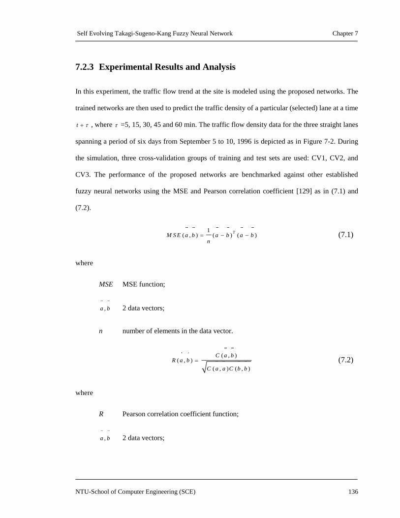
Self Evolving Takagi-Sugeno-Kang Fuzzy Neural Network Chapter 7
NTU-School of Computer Engineering (SCE) 136
7.2.3 Experimental Results and Analysis
In this experiment, the traffic flow trend at the site is modeled using the proposed networks. The
trained networks are then used to predict the traffic density of a particular (selected) lane at a time
t , where =5, 15, 30, 45 and 60 min. The traffic flow density data for the three straight lanes
spanning a period of six days from September 5 to 10, 1996 is depicted as in Figure 7-2. During
the simulation, three cross-validation groups of training and test sets are used: CV1, CV2, and
CV3. The performance of the proposed networks are benchmarked against other established
fuzzy neural networks using the MSE and Pearson correlation coefficient [129] as in (7.1) and
(7.2).
1
( , ) ( ) ( )T
M S E a b a b a bn
(7.1)
where
MSE MSE function;
,a b 2 data vectors;
n number of elements in the data vector.
( , )
( , )
( , ) ( , )
C a bR a b
C a a C b b
(7.2)
where
R Pearson correlation coefficient function;
,a b 2 data vectors;

Self Evolving Takagi-Sugeno-Kang Fuzzy Neural Network Chapter 7
NTU-School of Computer Engineering (SCE) 137
C(.,.) covariance between two data vectors.
Figures 7-3 shows the respective modeling (recall) and predicting (generalization) performances
of the GSETSK on lane 1 traffic density using training and test sets of CV1, CV2, and CV3 at
=5. Figures 7-4 shows the respective modeling (recall) and predicting (generalization)
performances of the RSETSK on lane 1 traffic density using training and test sets of CV1, CV2,
and CV3 at =5.
From Figure 7-3, it can be observed that the GSETSK network is able to accurately capture and
model the underlying dynamics governing the flow of traffic of lane L1. It also accurately
predicts the traffic trends of lane L1 for a prediction horizon of 5 min (i.e t+5). Figure 7-4 shows
that RSETSK performs better than its feed-forward counterpart in many cases. Figure 7-5 shows
the average Pearson values and the average MSEs derived from the three cross-validation groups
of each time interval with respect to the three different lanes L1, L2 and L3 using the various
benchmarked NFSs. In all scenarios, the proposed GSETSK and RSETSK networks are proven to
perform better than other benchmarked NFSs by achieving higher accuracy (Pearson values) and
lower prediction errors. The results also show that the proposed networks are able to provide
reasonable forecasts of the unseen future traffic conditions.

Self Evolving Takagi-Sugeno-Kang Fuzzy Neural Network Chapter 7
NTU-School of Computer Engineering (SCE) 138
Figure 7-3: Traffic modeling and prediction results of GSETSK for lane L1 at time t+5
across three-cross validation groups.
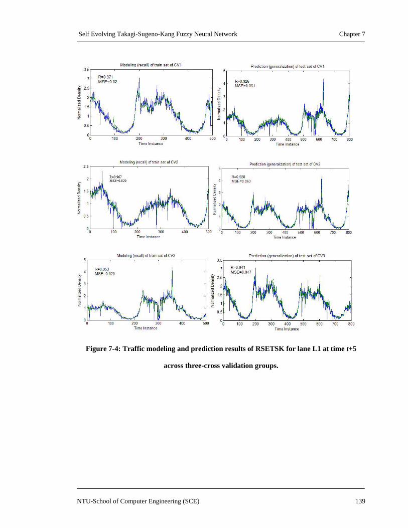
Self Evolving Takagi-Sugeno-Kang Fuzzy Neural Network Chapter 7
NTU-School of Computer Engineering (SCE) 139
Figure 7-4: Traffic modeling and prediction results of RSETSK for lane L1 at time t+5
across three-cross validation groups.

Self Evolving Takagi-Sugeno-Kang Fuzzy Neural Network Chapter 7
NTU-School of Computer Engineering (SCE) 140
(a)

Self Evolving Takagi-Sugeno-Kang Fuzzy Neural Network Chapter 7
NTU-School of Computer Engineering (SCE) 141
(b)
Figure 7-5: Traffic flow forecast results for GSETSK, RSETSK and the various
benchmarked NFSs (a) Prediction accuracy across 3 lanes (b) Prediction error across 3
lanes

Self Evolving Takagi-Sugeno-Kang Fuzzy Neural Network Chapter 7
NTU-School of Computer Engineering (SCE) 142
Table 7-1 benchmarks the proposed networks against other established architectures. They are,
namely: the Hebbian-rule-reduction-based Mamdani network (Hebb-R-R) [127], rough-set-based
POPFNN-CRI (RSPOP) [116] , POPFNN-CRI [47], GenSoFNN [38], EFuNN [130], and
DENFIS [11]. The Hebb-R-R, RSPOP-CRI, and POPFNN-CRI networks are batch-learning
models while GenSoFNN is a self-organizing network that uses pseudoincremental learning
approach. EFuNN and DENFIS are evolving fuzzy rule-based systems. Among the benchmarked
models, DENFIS is the only TSK network. Table 7-1 benchmarks the average R, the average
MSE, and their standard deviations as well as the average number of rules derived for the various
prediction horizons using the proposed models (GSETSK and RSETSK) and the other models for
predicting of the traffic densities across the three lanes. It can be observed that the proposed
models outperform other models in terms of the number of rules identified and the prediction
accuracies for the unseen data in the test set. In addition, the proposed models employ
incremental learning approach, meaning that they can continuously adapt to new information.
Thus, they can be considered as suitable candidates for addressing online traffic prediction
problems.
The specifications for the system to conduct this experiment are listed as follows:
Intel Core Duo CPU, Q9400 @ 2.66GHz
4.00 GB of RAM
Window 7 Enterprise version
Microsoft Visual Studio 2008
The real-time performance of the proposed GSETSK network is shown by the average training
time for all the 45 traffic simulations (based on the three straight lanes with five prediction
horizons and three cross-validation groups for each prediction horizon). The average simulation

Self Evolving Takagi-Sugeno-Kang Fuzzy Neural Network Chapter 7
NTU-School of Computer Engineering (SCE) 143
time reported by GSETSK is only 0 .8 5 0 .0 5 s . This demonstrates GSETSK‘s fast learning
ability in real-life traffic prediction problems.
Table 7-1: Benchmarking of results of the highway traffic flow prediction experiment
Network Rule-learning Average R
(Stdev)
Average MSE
(Stdev)
Average #
rules
Hebb-R-R Batch 0.864 (±0.046) 0.114 (±0.042) 8.1
RSPOP-CRI Batch 0.834 (± 0.041) 0.146 (±0.038) 14.4
POPFNN-CRI Batch 0.814 (±0.042) 0.173 (±0.053) 40.0
GenSoFNN Pseudo-Inc 0.813 (±0.028) 0.164 (±0.037) 50.0
EFuNN Evolving 0.798 (±0.050) 0.189 (±0.041) 234.5
eFSM Evolving 0.840 (±0.043) 0.154 (±0.040) 20.3
DENFIS Evolving 0.831 (±0.051) 0.153 (±0.054) 9.7
GSETSK Evolving 0.875 (±0.042) 0.132 (±0.040) 8.9
RSETSK Evolving 0.893 (±0.043) 0.131 (±0.040) 8.5
Figure 7-6 shows the highly distinguishable membership functions derived by the GSETSK
model using the training set of cross validation group CV1 for the predicting of lane L1 traffic
trends at time t+5. A total of 8 rules are identified by GSETSK based on the given training data.
There are only 9 fuzzy sets in total generated in GSETSK for all input dimensions. To illustrate
the intuitiveness of the fuzzy rules identified, a mapping of semantic labels to each fuzzy
membership function is performed. As formulated in [32,43-44], a linguistic variable is
characterized by a quintuple (L, T(L),U,G,M), where L is the name of the variable; T(L) is the
linguistic term set of L; U is a universe of discourse; G is a syntactic rule that generates T(L); and
M is a semantic rule that associates each T(L) with its meaning. Here, the names L of the input
linguistic variables
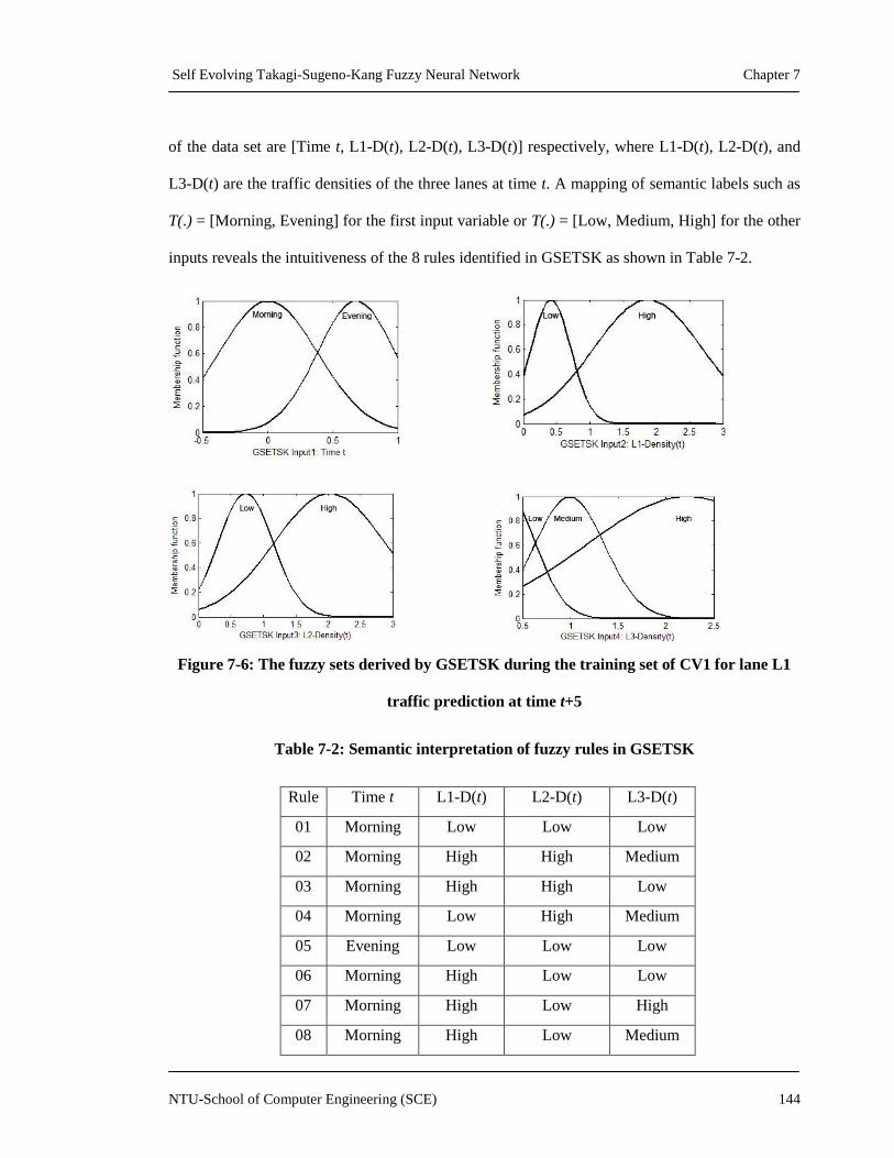
Self Evolving Takagi-Sugeno-Kang Fuzzy Neural Network Chapter 7
NTU-School of Computer Engineering (SCE) 144
of the data set are [Time t, L1-D(t), L2-D(t), L3-D(t)] respectively, where L1-D(t), L2-D(t), and
L3-D(t) are the traffic densities of the three lanes at time t. A mapping of semantic labels such as
T(.) = [Morning, Evening] for the first input variable or T(.) = [Low, Medium, High] for the other
inputs reveals the intuitiveness of the 8 rules identified in GSETSK as shown in Table 7-2.
Figure 7-6: The fuzzy sets derived by GSETSK during the training set of CV1 for lane L1
traffic prediction at time t+5
Table 7-2: Semantic interpretation of fuzzy rules in GSETSK
Rule Time t L1-D(t) L2-D(t) L3-D(t)
01 Morning Low Low Low
02 Morning High High Medium
03 Morning High High Low
04 Morning Low High Medium
05 Evening Low Low Low
06 Morning High Low Low
07 Morning High Low High
08 Morning High Low Medium

Self Evolving Takagi-Sugeno-Kang Fuzzy Neural Network Chapter 7
NTU-School of Computer Engineering (SCE) 145
Using the same training set of cross validation group CV1 for the predicting of lane L1 traffic
trends at time t+5, the RSETSK model identifies only 8 fuzzy sets in total. The average training
time is also around 0 .8 1 0 .0 7 s . The fuzzy sets derived are highly distinguishable. The results
show that the proposed networks can be promising candidates for real-life traffic prediction
systems.
7.3 Summary
This chapter investigates the application of the proposed networks (GSETSK and RSETSK) on
the prediction of traffic trends. Traffic prediction is becoming a popular topic of research and it
has the potential to improve traffic conditions and trim down travel delays. The performances of
the proposed networks are evaluated by comparing the results with other established methods.
The results show that GSETSK and RSETSK outperform other methods in terms of the number
of rules identified and the prediction accuracies. Besides, the proposed networks derive an
interpretable rule base with highly distinguishable fuzzy sets which can be easily comprehended.
It should be noted that GSETSK and RSETSK can learn incrementally with high accuracy
without any prior assumption about the data sets. Their fast learning ability makes them viable
candidates for the online traffic prediction applications.

Self Evolving Takagi-Sugeno-Kang Fuzzy Neural Network Chapter 8
NTU-School of Computer Engineering (SCE) 146
Chapter 8: Conclusions & Future Work
8.1 Conclusion
The advantages of combining fuzzy systems and neural networks have led to the active research
interest in the field of fuzzy neural systems. This Thesis is mainly focused on addressing the
existing problems of Takagi-Sugeno-Kang fuzzy neural networks which are mainly used for
solving dynamic and complex real-life problems that require high precision. Existing TSK
models proposed in the literature can be broadly classified into three classes. Class I TSK models
are essentially fuzzy systems that are unable to learn in an incremental manner. Class II TSK
networks, on the other hand, are able to learn in incremental manner, but are generally limited to
time-invariant environments. Class III TSK networks are fuzzy systems that adopt incremental
learning approaches and attempt to solve time-variant problems. However, many Class III
systems still encounter three critical issues; namely: 1) Their fuzzy rule base can only grow, 2)
They do not consider the interpretability of the knowledge bases and 3) They cannot give
accurate solutions when solving complex time-variant data sets that exhibit drift and shift
behaviors (or regime shifting properties).
This Thesis focuses on the development of a novel online biologically plausible fuzzy neural
network that can address the mentioned deficiencies of TSK networks. This final chapter
summarizes the contributions achieved by the research in this Thesis, the constraints of the
proposed computational models, and the possible directions for future research efforts.
The learning and knowledge that we have, is, at the most, but little
compared with that of which we are ignorant.
Plato (423 BC-347 BC)

Self Evolving Takagi-Sugeno-Kang Fuzzy Neural Network Chapter 8
NTU-School of Computer Engineering (SCE) 147
8.1.1 Theoretical Contributions
The theoretical works of this Thesis are summarized as follows:
This thesis proposes the basis for a self-evolving TSK framework which is fast and
efficient and can be applied in real-life applications that require high precision. The
framework adopts an incremental online learning approach and has the ability to work in
time-variant environments. The motivations for developing self-evolving online learning
computational models for solving real-life problems are highlighted in Section 2.5.
This thesis highlights that unlearning, which is stemmed from neurobiology, is necessary
in self-evolving systems that attempt to address time-variant problems. In Section 2.6, the
thesis describes that unlearning is an efficient way to address the concept drift and shift in
online data streams. This thesis proposes a novel ‗gradual‘ unlearning approach that
adopts the Hebbian learning mechanism behind the long-term potentiation phenomenon
in the brain (see Section 3.2).
This thesis describes that overlapping and indistinguishable fuzzy sets in the knowledge
base of a fuzzy neural network can deteriorate its interpretability. In Section 3.3, the
thesis proposes a novel merging approach to derive a compact and understandable
knowledge base in a fuzzy neural network.
This thesis highlights that recurrent fuzzy neural networks are better candidates than
feedforward networks for solving problems involving temporal relationships. This thesis
proposes a recurrent self-evolving framework in Section 4.2 to address dynamic and
temporal problems more efficiently.

Self Evolving Takagi-Sugeno-Kang Fuzzy Neural Network Chapter 8
NTU-School of Computer Engineering (SCE) 148
8.1.2 Practical Contributions
The practical contributions of this thesis are summarized as follows:
8.1.2.1 Self-Evolving Takagi–Sugeno–Kang Fuzzy Framework
Generic self-evolving Takagi–Sugeno–Kang fuzzy framework (GSETSK) is an economic and
fast framework that can be applied in modeling many real-world applications with good
semantics, high precision and ease. The ‗backbone‘ of the framework is a novel fuzzy clustering
algorithm known as Multidimensional-Scaling Growing Clustering (MSGC) which empowers
GSETSK with an incremental learning ability. MSGC is completely data-driven and does not
require prior knowledge of the numbers of clusters or rules present in the training data set. In
addition, MSGC does not assume the upper or lower bounds of the data set. MSGC is inspired by
human cognitive process models and it can work in fast-changing time-variant environments.
MSGC also employs a novel merging approach to ensure a compact and interpretable knowledge
base in the GSETSK framework as described in Chapter 3. Highly overlapping membership
functions are merged and obsolete rules are constantly pruned to derive a compact fuzzy rule base
while maintaining a high level of modeling accuracy.
To keep an up-to-date fuzzy rule base when dealing with time-variant problems, a novel
‗gradual‘-forgetting-based rule pruning approach is proposed to unlearn outdated data by deleting
obsolete rules. This approach is simple, biologically plausible and efficient. It adopts the Hebbian
learning mechanism behind the long-term potentiation phenomenon in the brain. It can detect the
drift and shift behaviors in time-variant problems and give accurate solutions for such problems.
The performance of GSETSK has been demonstrated in three benchmarking case studies. In
Section 3.5.1, GSETSK has shown its online learning ability in complex environments, more
specifically, a nonlinear dynamic system with non-varying characteristics. The derived

Self Evolving Takagi-Sugeno-Kang Fuzzy Neural Network Chapter 8
NTU-School of Computer Engineering (SCE) 149
knowledge base of GSETSK, which is compact with highly distinguishable fuzzy sets, is
illustrated. Section 3.5.2 proves the ability of GSETSK to work in time-variant problems. The
section also features the evolving rule base of GSETSK to illustrate the learning/unlearning
mechanisms in GSETSK. Section 3.5.3 shows the superior performance of GSETSK in solving a
well-known regression problem; which is the Mackey-glass time series predictions. In general,
GSETSK has shown that it is a viable candidate for solving complex and time-variant problems
which require high accuracy.
In Chapter 6, an option trading and hedging system using GSETSK as a predictive model is
presented. The proposed prediction system is employed in practice within a hedging system to
ensure that the trader is not left exposed to unnecessary risks. The GSETSK predictive model is
more advantageous than existing predictive models because it provides insights to the trader
about the semantic meanings of the derived knowledge and it addresses the shifting properties of
the time series. Results in the experiments on real-life data show that GSETSK provides accurate
prediction of price trends and that the trading system with GSETSK is able to yield higher profit
than the trading systems with other established predictive models. Using these predictions a
portfolio can be designed allowing the user to use the benefit of forecasting values provided to
take profitable and safe positions in the market.
8.1.2.2 Recurrent Self-Evolving Takagi-Sugeno-Kang Fuzzy Neural Network
A recurrent version of GSETSK, the RSETSK (Recurrent Self-Evolving TSK Fuzzy Neural
Network) is presented in Chapter 4. This extension aims to improve the ability of GSETSK in
dealing with dynamic and temporal problems.
Unlike GSETSK, RSETSK does not require the knowledge of the number of delayed input and
output in advance when solving temporal problems. The main difference between RSETSK and

Self Evolving Takagi-Sugeno-Kang Fuzzy Neural Network Chapter 8
NTU-School of Computer Engineering (SCE) 150
its non-recurrent version is its inherent recurrent structure which empowers it with the ability to
process patterns with spatio-temporal dependencies better.
Extensive experiments were conducted to evaluate the performance of RSETSK. Section 4.4.1
shows its superior online learning ability in complex environments such as the nonlinear temporal
problem with nonvarying characteristics. In this simulation, RSETSK outperforms other recurrent
networks in the literature in terms of accuracy and the number of rules. The derived knowledge
base of RSETSK is compact and meaningful. In Section 4.4.2, the rule evolution process of
RSETSK is shown to explain why unlearning is needed in recurrent fuzzy neural. In Section
4.4.3, RSETSK is benchmarked against its non recurrent version GSETSK using the Dow Jones
Index Time Series dataset. The case study in Section 4.4.3 shows that RSETSK is an excellent
alternative over its non-recurrent version in solving problems that exhibit temporal behaviors.
In Chapter 5, a stock market trading system using a novel price prediction model empowered by
RSETSK is proposed. The RSETSK predictive model is able to forecast the future security prices
in order to generate profitable trading decisions using technical analysis, more specially, using the
simple and efficient MACD oscillator. Compared to existing predictive models, RSETSK
possesses many features which are desired in evolving problems such as time series prediction.
The recurrent structure in RSETSK results in a high level of modeling accuracy when working
with time-variant stock datasets. Extensive experiments show that the RSETSK provides accurate
prediction of stock trend and that the trading system with RSETSK is able to yield higher profit
than the simple buy-and-hold strategy, the trading system without prediction, and the trading
systems with other predictive models.
In Chapter 7, a traffic prediction system to forecast traffic trends using RSETSK is presented. The
experimental results showed that RSETSK performs better than its feedforward counterpart,
GSETSK.

Self Evolving Takagi-Sugeno-Kang Fuzzy Neural Network Chapter 8
NTU-School of Computer Engineering (SCE) 151
To conclude, the research achievements in this thesis concur with the research objectives
highlighted in Figure 1-1.
8.2 Limitations
This work presents the development of a Takagi-Sugeno-Kang fuzzy neural framework to address
the existing problems of TSK systems. Even though the proposed architectures have shown
promising results, some further issues can still be investigated:
Currently, the input and output features have all been empirically selected. No feature
selection step to remove redundant attributes is employed in the proposed networks.
Feature subset selection is a preprocessing step in computational learning tasks. It
generates significant computational advantages by reducing the input dimensionality and
alleviates the ―curse of dimensionality‖ when dealing with large dimensional problem. It
also helps to achieve improvement in the interpretability of the learning system by
reducing the number of rules. As the proposed networks are online system, an online
feature selection that is workable in time-variant environments is required.
The main advantage of the TSK-model over the Mamdani-model is its ability to achieve
higher level of system modeling accuracy. More specifically, TSK model can represent a
complex system in term of fewer TSK-type rules. Furthermore, the TSK-model can give
better accuracy with the same number of rules when compared to the Mamdani-model.
Normally, a typical TSK fuzzy rule has the form shown in (8.1) which is a linear equation
involving the input terms and their consequent parameters.
1 ,1 1 , 1 0 1 1 1 1: IF is A N D A N D is T H E N ...i i n i n n nR x A x A y b b x b x (8.1)

Self Evolving Takagi-Sugeno-Kang Fuzzy Neural Network Chapter 8
NTU-School of Computer Engineering (SCE) 152
where 1 1[ , . . . , ]nx x x and y are the input vector and the output value, respectively. ,i kA
represents the membership function of the input label xk for the ith fuzzy rule; 0 1[ , . . . , ]nb b
represents a set of consequent parameters of the ith fuzzy rule, n1 is the number of inputs.
If the dimension of the input or output space is high, the number of terms used in the
linear equation can be large even though some terms are, in fact, of little significance.
The interpretability of the TSK network can be improved if the number of terms can be
reduced. Insignificant terms should be removed from the network. Hence, instead of
using the linear combination of all the input variables as the consequent part, only the
most significant input variables should be used as the consequent terms. This will further
improve the interpretability of fuzzy rules in the proposed networks. Thus, an online term
reduction approach should be devised to achieve this goal.
The proposed networks are type-1 fuzzy logic systems (FLSs). Type-2 FLSs [131] appear
to be a more promising method than their type-1 counterparts in handling problems with
uncertainties such as noisy data and different word meanings. That is, type-2 fuzzy sets
allow researchers to model and minimize the effects of uncertainties in rule-based
systems. Some examples of uncertainties are: (1) the words that are used in antecedents
and consequents of rules can mean different things to different people; (2) consequents
obtained by polling a group of experts will often be different for the same rule, because
the experts will not necessarily be in agreement [132]. Type-1 FLSs are certain, therefore
they are unable to directly handle these uncertainties. In contrast, type-2 FLSs are proven
to be useful in handling these uncertainties. Extending the current proposed networks to
type-2 can help to improve their abilities in dealing with uncertainties and noisy data. It
also helps to further improve their accuracy in dealing with complex uncertain real-life
problems.
Self Evolving Takagi-Sugeno-Kang Fuzzy Neural Network Chapter 8
NTU-School of Computer Engineering (SCE) 153
8.3 Future Research Directions
This section presents two possible directions for future research; namely 1) the extensions to the
proposed networks, and 2) the application domains for the proposed networks.
8.3.1 Extensions to the Proposed Networks
8.3.1.1 Online Feature Selection
Feature selection is important in many practical problems as it can help learning systems to
achieve both generalization performance and fast learning ability. There are mainly two feature
selection approaches: filter approach where the features are selected independently from the
modeling system and wrapper approach where features are selected using the modeling system.
The filter approach employs statistics computed from the empirical data distribution [133] or
semantics-preserving information contained within the empirical dataset [3]. The wrapper
approach can yield better performance at the expense of increased computational effort [134].
Feature selection approaches are often offline algorithms, such as principal component analysis
(PCA) [135], linear discriminant analysis (LDA) [136], sensitivity analysis [137], or decision tree
[138]. However, most of real-life problems are online, meaning that the data is not all available at
the beginning but is sequential presented. Thus, an online incremental feature selection approach
is required to deal with such online problems.
Many incremental feature selection methods have been proposed, such as incremental principal
component analysis (IPCA) [139], incremental linear discriminant analysis (ILDA) [140]. In
[139], Hall et al. proposed a method to incremental update the eigenvectors and eigenvalues to
determine the most important features. In [141], Pang et al. proposed an ILDA algorithm to
incrementally update a between-class scatter matrix and within-class scatter matrix. In [142], an
ILDA algorithm based on the singular decomposition technique is proposed. In [143], an

Self Evolving Takagi-Sugeno-Kang Fuzzy Neural Network Chapter 8
NTU-School of Computer Engineering (SCE) 154
extended version of IPCA which uses the accumulation ratio as the IPCA feature selection is
proposed. The accumulation ratio will change every instant of time when a new sample comes. In
[144], a new method which employ a resource allocation network with long-term memory (RAN-
LTM) is proposed. This approach seems promising to be used in fuzzy neural networks.
In conclusion, an in-depth study is needed to explore the possibility of using an online future
selection approach in the proposed networks (GSETSK and RSETSK). Furthermore, a
deselection approach should also be considered to remove insignificant features in online data
streams with nonstationary characteristics.
8.3.1.2 Consequent Terms Selection
TSK network generally can model complex systems with higher accuracy while using fewer
number of rules than Mamdani network. However, if the dimension of the input space is high, the
number of terms used in the linear equation of each TSK fuzzy rule is also large. Thus,
insignificant consequent terms should be removed from the TSK fuzzy rules to ensure a more
compact and better interpretable TSK network. Only the most significant input variables should
be used as the consequent terms.
Several algorithms have been developed in order to identify the significant consequent terms such
as the Sensitivity Calculation Method [145]; the Competitive Learning method [48]; the Weight
Decay Method [145]. In [145], a network pruning method based on the estimation of the
sensitivity of the global cost function is proposed. In [48], competitive learning is used to identify
the terms with larger weights and delete those with smaller one. However these methods cannot
detect the correlation between candidate terms. This leads to the inaccuracy in computing the
significance degree of each term, eventually the inaccuracy in finding the significant terms.
Another pruning method which uses backpropagation learning to decay the weights of the
insignificant terms to zero is proposed in [145]. However, this approach is slow and cannot
Self Evolving Takagi-Sugeno-Kang Fuzzy Neural Network Chapter 8
NTU-School of Computer Engineering (SCE) 155
guarantee that the most significant terms can be determined. Besides, all the above methods are
not applicable for online learning systems. In [15], the significant terms are chosen and
incrementally added to the network whenever the parameter learning cannot further improve the
network output accuracy during the on-line learning process. This method is efficient; however it
uses many heuristic parameters.
A better algorithm should be devised in order to achieve the significant terms for each fuzzy rule.
The algorithm should be applicable in online learning systems such as GSETSK and RSETSK.
Rough-set approach [146] is gaining more popularity recently and it can be considered as a
potential solution. Rough set theory was introduced by Pawlak to deal with imprecise or vague
concepts. A rough set is a formal approximation of a crisp set by a pair of sets which gives the
lower and the upper approximation of the original set. The lower approximation describes the
domain objects that are known with certainty to belong to the subset of interest, whereas the
upper approximation describes the objects that possibly belong to the subset. There are two
fundamental but important concepts of rough set knowledge reduction: a reduct and the core. A
reduct of knowledge is its critical part, which is sufficient enough to define all basic concepts in
the considered knowledge, whereas the core is the most important part of the knowledge. The
knowledge of decision rules is represented by the value attribute pair in the rough set knowledge
reduction [146]. With the representation of decision rules as such, rough set theory then provides
the logical methods employing attribute dispensability and decision rule consistency for
knowledge reduction and analysis.
Attribute dispensability is defined as follows: an attribute RR is dispensable if it satisfies
( R ) ( R { } )IN D IN D R (8.2)
in which ( R )IN D is the indiscernibility relation over R, which is the intersection of all
equivalence relations belonging to R.
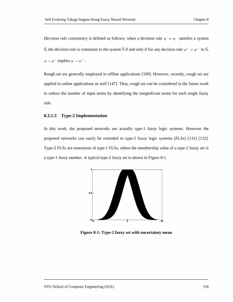
Self Evolving Takagi-Sugeno-Kang Fuzzy Neural Network Chapter 8
NTU-School of Computer Engineering (SCE) 156
Decision rule consistency is defined as follows: when a decision rule satisfies a system
S, the decision rule is consistent in the system S if and only if for any decision rule in S,
implies .
Rough set are generally employed in offline applications [109]. However, recently, rough set are
applied in online applications as well [147]. Thus, rough set can be considered in the future work
to reduce the number of input terms by identifying the insignificant terms for each single fuzzy
rule.
8.3.1.3 Type-2 Implementation
In this work, the proposed networks are actually type-1 fuzzy logic systems. However the
proposed networks can easily be extended to type-2 fuzzy logic systems (FLSs) [131] [132].
Type-2 FLSs are extensions of type-1 FLSs, where the membership value of a type-2 fuzzy set is
a type-1 fuzzy number. A typical type-2 fuzzy set is shown in Figure 8-1.
Figure 8-1: Type-2 fuzzy set with uncertainty mean
Self Evolving Takagi-Sugeno-Kang Fuzzy Neural Network Chapter 8
NTU-School of Computer Engineering (SCE) 157
Consider extending the proposed GSETSK network to an interval type-2 fuzzy system. Each rule
of type-2 GSETSK (GSETSK-II) will have the following form:
~ ~ ~ ~ ~
1 ,1 1 , 1 0 1 1 1 1: IF is A N D A N D is T H E N ...i i n i n n nR u le x A x A y b b x b x (8.3)
where ~
,i jA are interval type-2 fuzzy sets, and ~
ib are interval sets, with
~
[ , ]i i i i ib c s c s
where ic determines the center of the interval and is determines the interval range.
Extending the current proposed networks to type-2 can help to improve their abilities in dealing
with uncertainties and noisy data. It also helps to further improve their accuracy in dealing with
complex uncertain real-life problems. Thus, an in-depth study on how to extend the proposed
networks to type-2 should be carefully investigated.
8.3.2 Application Domains for the Proposed Networks
The proposed fuzzy neural networks have been successfully applied in three real life applications;
namely: 1) Stock Market Trading System, 2) Option Trading and Hedging and 3) Traffic
Prediction. The encouraging results suggest that the proposed networks can be used in more
challenging real-life applications in the areas of medical or financial data analysis, signal
processing and biometrics. The proposed stock trading system in Chapter 5 and the proposed
option trading system in Chapter 6 were designed to be able to adapt to many technical analysis
approaches. In fact, it is possible to use a combination of multiple technical indicators to devise
trading systems with better accuracy based on the proposed systems.
The fuzzy rules identified by the proposed networks based on the real-life data can help experts to
better understand how the networks achieve the final results. This can empower the experts the

Self Evolving Takagi-Sugeno-Kang Fuzzy Neural Network Chapter 8
NTU-School of Computer Engineering (SCE) 158
ability to evaluate or monitor the performance of the networks in the fields that require high
accuracy performance such as blood glucose regulation for diabetes mellitus patients.

Self Evolving Takagi-Sugeno-Kang Fuzzy Neural Network
NTU-School of Computer Engineering (SCE) 159
Bibliography
[1] L. A. Zadeh, "Fuzzy logic, neural networks, and soft computing," Commun. ACM, vol.
37, pp. 77-84, 1994.
[2] S. Mitra and Y. Hayashi, "Neuro-fuzzy rule generation: survey in soft computing
framework," IEEE Trans. Neural Netw., vol. 11, pp. 748-768, 2000.
[3] Q. Shen and R. Jensen, "Semantics-preserving dimensionality reduction: rough and
fuzzy-rough-based approaches," IEEE Trans. Knowl. Data Eng., vol. 16, pp. 1457-1471,
2004.
[4] C. T. Lin and C. S. G. Lee, Neural Fuzzy Systems: A Neuro-Fuzzy Synergism to
Intelligent Systems. New Jersey: Prentice Hall PTR, 1996.
[5] T. Takagi and M. Sugeno, "Fuzzy Identification of Systems and its Applications to
Modeling and Control," IEEE Trans. Systs., Man, Cybern., vol. 15, pp. 116-132, 1985.
[6] G.-B. Huang, P. Saratchandran, and N. Sundararajan, "A generalized growing and
pruning RBF (GGAP-RBF) neural network for function approximation," IEEE Trans.
Neural Netw., vol. 16, pp. 57-67, Jan. 2005.
[7] R. Jang, "ANFIS: adaptive-network-based fuzzy inference system," IEEE Trans. Systs.,
Man, Cybern. B, vol. 23, pp. 665-685, 1993.
[8] G. Leng, G. Prasad, and T. M. McGinnity, "An on-line algorithm for creating self-
organizing fuzzy neural networks," Neural Netw., vol. 17, pp. 1477–1493, 2004.
[9] S.Wu and M. J. Er, "Dynamic fuzzy neural networks:A novel approach to function
approximation," IEEE Trans. Syst. Man Cybern. B, Cybern., vol. 30, pp. 358–364, Apr.
2000.
[10] K. H. Quah and C. Quek, "FITSK: online local learning with generic fuzzy input Takagi-
Sugeno-Kang fuzzy framework for nonlinear system estimation," IEEE Trans. Systs.,
Man, Cybern. B, vol. 36, pp. 166-178, 2006.
[11] N. K. Kasabov and Q. Song, "DENFIS: Dynamic evolving neural-fuzzy inference system
and its application for time-series prediction," IEEE Trans. Systs., Man, Cybern. B, vol.
10, pp. 144-154, 2002.
[12] H. J. Rong, N. Sundararajan, G. B. Huang, and P. Saratchandran, "Sequential adaptive
fuzzy inference system (SAFIS) for nonlinear system identification and prediction,"
Fuzzy Sets Syst., vol. 157, pp. 1260–1275, 2006.
[13] D. Kukolj and E. Levi, "Identification of complex systems based on neural and Takagi-
Sugeno fuzzy model," IEEE Trans. Systs., Man, Cybern. B, vol. 34, pp. 272-282, 2004.
[14] C. S. Ouyang, W. J. Lee, and S. J. Lee, "A TSK-type neuro fuzzy network approach to
system modeling problems," IEEE Trans. Systs., Man, Cybern. B, vol. 35, pp. 751-767,
2005.
[15] C. F. Juang and C. T. Lin, "An online self-constructing neural fuzzy inference network
and its applications," IEEE Trans. Fuzzy Syst., vol. 6, pp. 12-32, 1998.
[16] E. D. Lughofer, "FLEXFIS: A robust incremental learning approach for evolving Takagi-
Sugeno fuzzy models," IEEE Trans. Fuzzy Syst., vol. 16, pp. 1393-1410, Dec. 2008.
[17] P. P. Angelov and D. P. Filev, "An approach to online identification of Takagi-Sugeno
fuzzy models," IEEE Trans. Systs., Man, Cybern. B, vol. 34, pp. 484-498, 2004.
[18] C. W. Ting and C. Quek, "A Novel Blood Glucose Regulation Using TSK0-FCMAC: A
Fuzzy CMAC Based on the Zero-Ordered TSK Fuzzy Inference Scheme," IEEE Trans.
Neural Netw., vol. 20, pp. 856 - 871 2009.
[19] M. Adya and F. Collopy, "How effective are neural networks at forecasting and
prediction? A review and evaluation," Int. J. Forecasting, vol. 17, pp. 481-495, 1998.

Self Evolving Takagi-Sugeno-Kang Fuzzy Neural Network
NTU-School of Computer Engineering (SCE) 160
[20] F. Crick and G. Mitchinson, "The function of dream sleep," Nature, vol. 304, pp. 111-
114, 1983.
[21] S. Wimbauer and J. L. v. Hemmen, "Hebbian Unlearning," in Proc. Analysis of
Dynamical Cognitive System, Advance Course, 1995, pp. 121-136.
[22] C. F. Juang and C. T. Lin, "A recurrent self-organizing neural fuzzy inference system,"
IEEE Trans. Neural Netw., vol. 10, pp. 828-845, 1999.
[23] C. F. Juang, "A TSK-type recurrent fuzzy network for dynamic systems processing by
neural network and genetic algorithms," IEEE Trans. Fuzzy Syst., vol. 10, pp. 155-1170,
2002.
[24] S. S. Haykin, Neural Networks: A Comprehensive Foundation. New Jersey: Prentice
Hall, 1999.
[25] K. Hornik, "Approximation capabilities of multilayer feedforward networks," Neural
Netw., vol. 4, pp. 251-257, 1991.
[26] J. Sjoberg, Q. Zhang, L. Ljung, A. Benveniste, B. Deylon, and P.-Y. e. al., "Nonlinear
Black-Box Modeling in System Identification: a Unified Overview: Trends in System
Identification," Automatica, vol. 31, pp. 1691-1724, 1995.
[27] J.-S.R.Jang and C.-T. Sun, Neuro-fuzzy and soft computing: a computational approach to
learning and machine intelligence: Upper Saddle River, NJ: Prentice Hall, 1995.
[28] A. Kandel, Fuzzy expert systems. Boca Raton, FL: CRC Press, 1992.
[29] A. Lotfi, H. C. Andersen, and A. C. Tsoi, "Matrix formulation of fuzzy rule-based
systems " IEEE Trans. Syst. Man Cybern. B, Cybern., vol. 26, pp. 332-340, 1996.
[30] C. C. Lee, "Fuzzy logic in control systems: fuzzy logic controller," IEEE Trans. Syst.
Man Cybern. B, Cybern., vol. 20, pp. 404-418, 1990.
[31] J.-S.R.Jang, C.-T. Sun, and M. Eiji, Neuro-fuzzy and soft computing: a computational
approach to learning and machine intelligence. New Jersey: Prentice Hall, 1997.
[32] L. A. Zadeh, "The concept of a linguistic variable and its application to approximate
reasoning-III," Information Sciences, vol. 9, pp. 43–80, 1975c.
[33] E. H. Mamdani, "Application of fuzzy logic to approximate reasoning using linguistic
systems," IEEE Trans. Comput., pp. 1182-1191, 1977.
[34] T. Takagi and M. Sugeno, "Fuzzy identification of systems and its application to
modeling and control," IEEE Trans. Syst., Man, Cybern. B, vol. 15, pp. 116–132, Feb.
1985.
[35] J. Casillas, O. Cordón, F. Herrera, and L. Magdalena, Interpretability Issues in Fuzzy
Modeling (Studies in fuzziness and soft computing, No. 128). Berlin: Springer-Verlag,
2003.
[36] J.-S. R. Jang and C.-T. Sun, "Neuro-fuzzy modeling and control," in Proc. of the IEEE,
1995, pp. 378-406.
[37] S. Medasani, J. Kim, and R. Krishnapuram, "An overview of membership function
generation techniques for pattern recognition," International Journal of Approximate
Reasoning, vol. 19, pp. 391-417, 1998.
[38] W. L. Tung and C. Quek, "GenSoFNN: a generic self-organizing fuzzy neural network,"
IEEE Trans. Neural Netw., vol. 13, pp. 1075-1086, 2002.
[39] T. Kohonen, Self-Organization and Associative Memory. Berlin, New York: Springer-
Verlag, 1989.
[40] R. W. Zhou and C. Quek, "POPFNN: A Pseudo Outer-product Based Fuzzy Neural
Network," Neural Networks, vol. 9, pp. 1569-1581.
[41] C. T. Lin, "A neural fuzzy control system with structure and parameter learning," Fuzzy
Sets and Systems, vol. 70, pp. 183-212, 1995.

Self Evolving Takagi-Sugeno-Kang Fuzzy Neural Network
NTU-School of Computer Engineering (SCE) 161
[42] J. C. Bezdek, Pattern Recognition with Fuzzy Objective Function Algorithms. New York:
Plenum Press, 1981.
[43] L. A. Zadeh, "The concept of a linguistic variable and its application to approximate
reasoning-I," Information Sciences, vol. 8, pp. 199–249, 1975a.
[44] L. A. Zadeh, "The concept of a linguistic variable and its application to approximate
reasoning-II," Information Sciences, vol. 8, pp. 301–357, 1975b.
[45] R. Mikut, J. Jakel, and L. Groll, "Interpretability issues in data-based learning of fuzzy
systems," Fuzzy Sets and Systems, vol. 150, pp. 179-197, 2005.
[46] F. L. Chung and T. Lee, "Fuzzy Learning Vector Quantization," in Int. Joint Conf.
Neural Networks, 1993, pp. 2739-2742.
[47] K. K. Ang, C. Quek, and M. Pasquier, "POPFNN-CRI(S): pseudo outer product based
fuzzy neural network using the compositional rule of inference and singleton fuzzifier,"
IEEE Trans. Systs., Man, Cybern. B, vol. 33, 2003.
[48] C. T. Lin and C. S. G. Lee, "Neural-network-based fuzzy logic control and decision
system," IEEE Trans. Comput., vol. 40, pp. 1320-1336, 1991.
[49] R. R. Yager, "Modeling and formulating fuzzy knowledge bases using neural networks,"
Neural Netw., vol. 7, pp. 1273-1283, 1994.
[50] C. Quek and R. W. Zhou, "The POP learning algorithms: reducing work in identifying
fuzzy rules," Neural Netw., vol. 14, pp. 1431-1445, 2001.
[51] I. Hayashi, H. Nomura, H. Yamasaki, and H. Wakami, "Construction of fuzzy inference
rules by NDF and NDFL," Int. J Approx. Reason., vol. 6, pp. 241-266, 1992.
[52] H. Ishibuchi and H. Tanaka, "Interpolation of fuzzy if-then rules by neural networks," Int.
J Approx. Reason., vol. 10, pp. 3-27, 1994.
[53] C. Quek and W. L. Tung, "A novel approach to the derivation of fuzzy membership
functions using the Falcon-MART architecture," Pattern Recognit. Lett., vol. 22, pp. 941-
958, 2001.
[54] J. V. d. Oliveira, "Towards neuro-linguistic modeling: Constraints for optimization of
membership functions," Fuzzy Sets and Systems, vol. 106, pp. 357-380, 1999.
[55] L. A. Zadeh, "Calculus of fuzzy restrictions," in Fuzzy sets, fuzzy logic, and fuzzy
systems: selected papers by Lotfi A. Zadeh, ed: World Scientific Publishing Co., Inc.,
1996, pp. 210-237.
[56] S. Horikawa, T. Furuhashi, and Y. Uchikawa, "On fuzzy modeling using fuzzy neural
networks with the backpropagation algorithm," IEEE Trans. Neural Netw., vol. 3, pp.
801–806, 1992.
[57] L. Franco, D. A. Elizondo, and J. e. M. Jerez, Constructive Neural Networks (Studies in
Computational Intelligence): Berlin Heidelbergm Germany: Springer-Verlag, 2010.
[58] W. L. Tung and C. Quek, "eFSM--a novel online neural-fuzzy semantic memory model,"
IEEE Trans. Neural Netw., vol. 21, pp. 136-157, 2010.
[59] C. F. Juang, Y. Y. Lin, and C. C. Tu, "A recurrent self-evolving fuzzy neural network
with local feedbacks and its application to dynamic system processing," Fuzzy Set Syst.,
vol. 161, pp. 2552-2568, 2010.
[60] C. F. Juang and Y.-W. Tsao, "A Self-Evolving Interval Type-2 Fuzzy Neural Network
With Online Structure and Parameter Learning," IEEE Trans. Fuzzy Syst., vol. 16, pp.
1411 - 1424, 2008.
[61] A. M. Tang, C. Quek, and G. S. Ng, "GA-TSKfnn: Parameters tuning of fuzzy neural
network using genetic algorithms," Expert Syst. Appl., vol. 29, pp. 769-781, 2005.
[62] D. Wang, C. Quek, and G. S. Ng, "Novel Self-Organizing Takagi Sugeno Kang Fuzzy
Neural Networks Based on ART-like Clustering," Neural Processing Letters, vol. 20, pp.
39 - 51, 2004.

Self Evolving Takagi-Sugeno-Kang Fuzzy Neural Network
NTU-School of Computer Engineering (SCE) 162
[63] A. Tsymbal, "The problem of concept drift: definitions and related work, Technical
Report TCD-CS-2004-15," Department of Computer Science, Trinity College Dublin,
Ireland, 2004.
[64] E. Lughofer and P. Angelov, "Handling drifts and shifts in on-line data streams with
evolving fuzzy systems," Appl. Soft Comput., vol. 11, pp. 1568-4946, 2011.
[65] T. J. R. Klinkenberg, "Detection concept drift with support vector machines," in Proc.
Seventh Int. Conf. Mach. Learning (ICML), Morgan Kaufmann, 2000, pp. 487–494.
[66] R. Klinkenberg, "Learning drifting concepts: example selection vs. example weighting,"
Intelligent Data Analysis, vol. 8, pp. 281–300, 2004.
[67] S. Ramamurthy and R. Bhatnagar, "Tracking recurrent concept drift in streaming data
using ensemble classifiers," in Proceedings of the Sixth International Conference on
Machine Learning and Applications (ICMLA), 2007, pp. 404–409.
[68] J. Beringer and E. Hüllermeier, "Efficient instance-based learning on data streams,"
Intelligent Data Analysis, vol. 11, pp. 627–650, 2007.
[69] S. J. Delany, P. Cunningham, A. Tsymbal, and L. Coyle, "A case-based technique for
tracking concept drift in spam filtering," Knowledge-Based Systems, vol. 18, pp. 187–
195, 2005.
[70] D. L. Michael, "Determining the dimensionality of multidimensional scaling
representations for cognitive modeling," J Math Psychol, vol. 45, pp. 149 - 166, 2001.
[71] J. B. Theocharis, "A high-order recurrent neuro-fuzzy system with internal dynamics:
Application to the adaptive noise cancellation," Fuzzy Set Syst., vol. 157, pp. 471–500,
2006.
[72] C.-S. Chen, "TSK-Type Self-Organizing Recurrent-Neural-Fuzzy Control of Linear
Microstepping Motor Drives," IEEE Trans. Power Electron., vol. 25, pp. 2253 - 2265
2010.
[73] C. F. Juang, R.-B. Huang, and W.-Y. Cheng, "An Interval Type-2 Fuzzy-Neural Network
With Support-Vector Regression for Noisy Regression Problems," IEEE Trans. Fuzzy
Syst., vol. 18, pp. 686-699, 2010.
[74] P. P. Angelov and D. P. Filev, "Simpl_eTS: A simplified method for learning evolving
Takagi-Sugeno fuzzy models," presented at the Proc. 14th IEEE Int. Conf. Fuzzy Syst.,
Reno, NV, 2005.
[75] P. Angelov and X. Zhou, "Evolving fuzzy systems from data streams in real-time,"
presented at the International Symposium on Evolving Fuzzy Systems, Ambleside, UK,
2006.
[76] P. Angelov, "Evolving Takagi-Sugeno Fuzzy Systems From Streaming Data (eTS+)," in
Evolving Intelligent Systems: Methodology and Applications, ed: John Wiley & Sons,
2010.
[77] J. R. Whitlock, A. J. Heynen, M. G. Shuler, and M. F. Bear, "Learning induces long-term
potentiation in the hippocampus," Science, vol. 313, pp. 1093–1097, 2006.
[78] M. H. Hayes, Recursive Least Squares: Statistical Digital Signal Processing and
Modeling. Wiley, 1996.
[79] R. W. Zhou and C. Quek, "POPFNN: A Pseudo Outer-product Based Fuzzy Neural
Network," Neural Netw., vol. 9, pp. 1569-1581, 1996.
[80] C. Quek and R. Zhou, "POPFNN-AARS(S): A pseudo outer-product based fuzzy neural
network," IEEE Trans. Syst. Man Cybern. B, Cybern., vol. 29, pp. 859–870, Dec. 1999.
[81] C. Quek and R. Zhou, "Structure and learning algorithms of a nonsingleton input fuzzy
neural network based on the approximate analogical reasoning schema," Fuzzy Sets Syst.,
vol. 157, pp. 1814–1831, 2006.

Self Evolving Takagi-Sugeno-Kang Fuzzy Neural Network
NTU-School of Computer Engineering (SCE) 163
[82] C. T. Lin and C. S. G. Lee, "Real-time supervised structure/parameter learning for fuzzy
neural network," IEEE Int. Conf. Fuzzy Syst., vol. 1283-1291, 1992.
[83] R. M. French, "Catastrophic forgetting in connectionist networks," presented at the
Encyclopedia of Cognitive Science, L. Nadel, Ed. London, U.K, 2003.
[84] R. M. Nosofsky, "Similarity scaling and cognitive process models," Annual Review of
Psychology, vol. 43, pp. 25-53, 1992.
[85] J. Yen and R. Langari, Fuzzy Logic: Intelligence, Control and Information. Englewood
Cliffs, NJ: Prentice Hall, 1999.
[86] I. B. Turksen and Z. Zhong, "An approximate analogical reasoning approach based on
similarity measure and interval valued fuzzy sets," Fuzzy Sets Syst.,, vol. 34, pp. 323-346,
1990.
[87] Y. W. Lu, N. Sundararajan, and P. Saratchandran, "A sequential learning scheme for
function approximation using minimal radial basis function (RBF) neural networks,"
Neural Comput., vol. 9, pp. 461–478, 1997.
[88] V. Kadirkamanathan and M. Niranjan, "A function estimation approach to sequential
learning with neural networks," Neural Comput., vol. 5, pp. 954–975, 1993.
[89] J. S. Jang, "Neuro-Fuzzy Modeling: Architecture, Analyzes and Applications," Ph.D
dissertation, Dept. Elect. Eng. Comput. Sci., Univ. California, Berkeley, 1992.
[90] R. S. C. III, "Predicting the Mackey-glass timeseries with cascade-Correlation learning,"
Proc. 1990 Connectionist Models Summer School, pp. 117–123, 1990.
[91] J. Platt, "A resource allocation network for function interpolation," Neural Computat.,
vol. 3, pp. 213–225, 1991.
[92] N. N. Nguyen and C. Quek, "Stock Price Prediction using Generic Self-Evolving Takagi-
Sugeno-Kang (GSETSK) Fuzzy Neural Network," presented at the Proc. IJCNN‘2010
Neural Networks, 2010.
[93] E. P. Santos and F. J. V. Zuben, "Efficient second-order learning algorithm for discrete-
time recurrent neural networks," in Recurrent Neural Networks: Design and
Applications, L. R. Medsker and L. C. Jain, Eds., ed Fla, USA: CRC Press, 2000, pp. 47-
75.
[94] P. S. Sastry, G. Santharam, and K. P. Unnikrishnan, "Memory neural networks for
identification and control of dynamic systems," IEEE Trans. Neural Netw., vol. 5, pp.
306–319, 1994.
[95] C.H.Lee and C.C.Teng, "Identification and control of dynamic systems using recurrent
fuzzy neural networks," IEEE Trans. Fuzzy Syst., vol. 8, pp. 349–366, 2000.
[96] Y. Gao and M. J. Er., "NARMAX time series model prediction: feed-forward and
recurrent fuzzy neural network approaches," Fuzzy Sets Syst., vol. 150, pp. 331–350,
2005.
[97] R. Gencay, "The predictability of security returns with simple technical trading rules," J.
Empir. Finance, vol. 5, pp. 347-359, 1998.
[98] B. Graham and D. Dodd, Security Analysis: Principles and Techniques. New York:
McGraw-Hill, 1940.
[99] G. S. Atsalakis and K. P. Valavanis, "Forecasting stock market short-term trends using a
neuro-fuzzy based methodology," Expert Syst. Appl., vol. 36, pp. 10696-10707, 2009.
[100] E. F. Fama, "Efficient capital markets: II," J. Finance, vol. 46, pp. 1575–1617, Dec.
1991.
[101] A. W. Lo, H. Mamaysky, and J.Wang, "Foundations of technical analysis: Computational
algorithms, statistical inference, and empirical implementation," J. Finance, vol. 55, pp.
1705–1765, 2000.
Self Evolving Takagi-Sugeno-Kang Fuzzy Neural Network
NTU-School of Computer Engineering (SCE) 164
[102] A. Shleifer, Inefficient Markets: An Introduction to Behavioral Finance. New York:
Oxford Univ. Press, 2000.
[103] T. Plummer and A. Ridley, Forecasting Financial Markets: The Psychological Dynamics
of Successful Investing, 4th ed. London, U.K.: Kogan Page, 2003.
[104] S. Haykin, Neural Networks: A Comprehensive Foundation, 2nd ed. Englewood Cliffs,
NJ: Prentice-Hall, 1998.
[105] E. M. Azoff, Neural Network Time Series Forecasting of Financial Markets. New York:
Wiley, 1994.
[106] M. Adya and F. Collopy, "How effective are neural networks at forecasting and
prediction? A review and evaluation," Int. J. Forecasting, vol. 17, pp. 481–495, 1998.
[107] M. Austin and C. Looney, "Security market timing using neural network models," New
Rev. Appl. Expert Syst., vol. 3, pp. 3-14, 1997.
[108] P. Cheng, C. Quek, and M. L. Mah, "Predicting the impact of anticipatory action on US
stock market—An event study using ANFIS (a neural fuzzy model)," Comput. Intell.,
vol. 23, pp. 117–141, 2007.
[109] K. K. Ang and C. Quek, "Stock Trading Using RSPOP: A Novel Rough Set-Based
Neuro-Fuzzy Approach," IEEE Trans. Neural Netw., vol. 17, pp. 1301-1315, 2006.
[110] T. Z. Tan, C. Quek, and G. S. Ng, "Biological brain-inspired genetic complementary
learning for stock market and bank failure prediction," Comput. Intell., vol. 23, pp. 236–
261, 2007.
[111] H. Huang, M. Pasquier, and C. Quek, "Financial Market Trading System With a
Hierarchical Coevolutionary Fuzzy Predictive Model," IEEE Trans. Evol. Comput., vol.
13, pp. 56-70, 2009.
[112] P. C. Chang and C. Y. Fan, "A Hybrid System Integrating a Wavelet and TSK Fuzzy
Rules for Stock Price Forecasting," IEEE Trans. Systs., Man, Cybern. B, vol. 38, pp. 802
- 815, 2008
[113] J. S. Abarbanell and B. J. Bushee, "Fundamental analysis, future earnings, and stock
prices," J. Account. Res., vol. 35, pp. 1-24, 1997.
[114] J. Moody, L. Wu, Y. Liao, and M. Saffell, "Performance functions and reinforcement
learning for trading systems and portfolios," Journal of Forecasting, vol. 17, pp. 441-
470, 1998.
[115] W. Brock, J. Lakonishok, and B. LeBaron, "Simple technical trading rules and the
stochastic properties of stock returns," J. Finance, vol. 47, pp. 1731–1764, 1992.
[116] K. K. Ang and C. Quek, "RSPOP: Rough Set-Based Pseudo Outer-Product Fuzzy Rule
Identification Algorithm," Neural Comput., vol. 17, pp. 205-243, 2005.
[117] R. N. Goldman and J. S. Weinberg, Statistics: An Introduction. NJ: Prentice-Hall, 1985.
[118] S. Chen, C. F. N. Cowan, and P. M. Grant, "Orthogonal least squares learning algorithm
for radial basis," IEEE Trans. Neural Netw., vol. 2, pp. 302–309, 1991.
[119] D. E. Rumelhart, G. E. Hinton, R. J. Williams, D. E. Rumelhart, and J. L. McClelland,
"Learning internal representations by error propagation," in Parallel Distributed
Processing: Explorations in the Microstructure of Cognition. vol. 1, ed: Cambridge,
MA:MIT Press, 1986.
[120] C. Quek, M. Pasquier, and N. Kumar, "A novel recurrent neural network-based
prediction system for option trading and hedging," Appl. Intell., vol. 29, pp. 138-151,
2008.
[121] H. White, "Economic prediction using neural networks: the case of IBM daily stock
returns," in Proceedings of the 2nd Annual IEEE conference on neural networks, 1988,
pp. 451–458.
Self Evolving Takagi-Sugeno-Kang Fuzzy Neural Network
NTU-School of Computer Engineering (SCE) 165
[122] W. Chiang, T. Urban, and G. Baldridge, "A neural network approach to mutual fund net
asset value forecasting," Omega Int J Manag Sci, vol. 24, pp. 205–215, 1996.
[123] W. L. Tung and C. Quek, "GenSo-OPATS: A brain-inspired dynamically evolving option
pricing model and arbitrage trading system," in Proc. IEEE CEC, Edinburgh, Scotland,
2005, pp. 2429–2436.
[124] S. D. Teddy, E. M.-K. Lai, and C. Quek, "A cerebellar associative memory approach to
option pricing and arbitrage trading," Neurocomputing, vol. 71, 2008.
[125] M. A. Gluck and C. E. Myers, Gateway to memory: an introduction to neural network
modeling of the hippocampus and learning. Cambridge: Mass., MIT Press, 2001.
[126] D. M. Chance, An Introduction to Derivatives & Risk Management, 6 ed.: Thomson
(South-Western), 2004.
[127] F. Liu, C. Quek, and G. Ng, "A novel generic hebbian ordering-based fuzzy rule base
reduction approach to mamdani neuro-fuzzy system," Neural Comput., vol. 19, pp. 1656-
1680, 2007.
[128] G. K. Tan, "Feasibility of predicting congestion states with neural networks," Final Year
Project, School of Civil Structural Engineering, Nanyang Technological Univ.,
Singapore, 1997.
[129] R. N. Goldman and J. S. Weinberg, Statistics: An Introduction. NJ: Prentice-Hall, 1985.
[130] N. K. Kasabov, "Evolving fuzzy neural networks for supervised/unsupervised online
knowledge-based learning," IEEE Trans. Systs., Man, Cybern., B, vol. 31, pp. 902-918,
2001.
[131] N. N. Karnik, J. M. Mendel, and Q. Liang, "Type-2 fuzzy logic systems," IEEE Trans.
Fuzzy Syst., vol. 7, pp. 643–658, 1999.
[132] J. M. Mendel and R. I. John, "Type-2 fuzzy sets made simple," IEEE Trans. Fuzzy Syst.,
vol. 10, pp. 117–127, 2002.
[133] T. W. S. Chow and D. Huang, "Estimating optimal feature subsets using efficient
estimation of high-dimensional mutual information," IEEE Trans. Neural Netw., vol. 16,
pp. 213-224, 2005.
[134] R. Kohavi and G. H. John, "Wrappers for feature subset selection," Artificial Intelligence,
vol. 97, pp. 273-324, 1997.
[135] R. W. Preisendorfer, Principle Component Analysis in Meteorology and Oceanography:
Elsevier Science Publishing Company, 1988.
[136] A. M. Martinez and A. C. Kak, "PCA versus LDA," IEEE Trans. Pattern Anal. Mach.
Intell., vol. 23, pp. 228-233, 2001.
[137] T. Hastie, R. Tibshirani, and J. Friedman, The elements of statistical learning: Data
Mining, Inference, and Prediction, 2 ed.: Springer, 2009.
[138] J. Abonyi, J. A. Roubos, and F. Szeifert, "Data-Driven Generation of Compact, Accurate,
and Linguistically-Sound Fuzzy Classifiers Based on a Decision-Tree Initialization," Int.
J Approx. Reason., vol. 32, pp. 1-21, 2002.
[139] P. M. Hall, D. Marshall, and R. R. Martin, "Incremental Eigenanalysis for
Classification," in British Machine Vision Conference, 1998, pp. 286-295.
[140] J. Weng, Y. Zhang, and W. S. Hwang, "Candid covariance-free incremental principal
component analysis," IEEE Trans. Pattern Anal. Mach. Intell., vol. 25, pp. 1034-1040,
2003.
[141] S. Pang, S. Ozawa, and N. Kasabov, "Incremental linear discriminant analysis for
classification of data streams," IEEE Trans. Syst. Man Cybern. B, Cybern., vol. 35, pp.
905-914, 2005.
[142] H. Zhao and P. C. Yuen, "Incremental linear discriminant analysis for face recognition,"
IEEE Trans. Syst. Man Cybern. B, Cybern., vol. 38, pp. 210-221, 2008.

Self Evolving Takagi-Sugeno-Kang Fuzzy Neural Network
NTU-School of Computer Engineering (SCE) 166
[143] S. Ozawa, S. Pang, and N. Kasabov, "A modified incremental principal component
analysis for on-line learning of feature space and classifier," in PRICAI 2004: Trends in
Artificial Intelligence, 2004, pp. 231-240.
[144] S. Ozawa, S. L. Toh, S. Abe, S. Pang, and N. Kasabov, "Incremental learning of feature
space and classifier for face recognition," Neural Netw., vol. 18, pp. 575-584, 2005.
[145] R. Reed, "Pruning algorithms—A survey," IEEE Trans. Neural Netw., vol. 4, pp. 740–
747, 1993.
[146] Z. Pawlak, Rough Sets: Theoretical Aspects of Reasoning about Data: Kluwer Academic
Publishers, 1992.
[147] M.-B. Pang and G.-G. He, "Chaos Rapid Recognition of Traffic Flow by Using Rough
Set Neural Network," in International Symposiums on Information Processing 2008, pp.
168 - 172.
Self Evolving Takagi-Sugeno-Kang Fuzzy Neural Network
NTU-School of Computer Engineering (SCE) 167
Author’s Publication
N. N. Nguyen and C. Quek, "RSFCMAC: A novel rough set–based rule reduction approach for
fuzzy CMAC architecture with yager-inference-scheme " presented at the IEEE Int. Conf. on
Fuzzy Syst., 2009.
N. N. Nguyen and C. Quek, "Stock Price Prediction using Generic Self-Evolving Takagi-Sugeno-
Kang (GSETSK) Fuzzy Neural Network," presented at the Proc. IJCNN’2010 Neural Networks,
2010.
N. N. Nguyen and C. Quek, "GSETSK - A Generic Self Evolving TSK Fuzzy Neural Network,"
Appl. Soft Comput., undergoing review.
N. N. Nguyen and C. Quek, "Stock Market Trading System With a Recurrent Self-Evolving TSK
Predictive Model," Int. J. Forecasting, undergoing 2nd
revision.
N. N. Nguyen and C. Quek, "A Recurrent Self-Evolving TSK Fuzzy Neural Network for Option
Trading and Hedging," Int. J. Forecasting, paper under preparation.
N. N. Nguyen and C. Quek, "Traffic Prediction using a Generic Self-Evolving Takagi-Sugeno-
Kang (GSETSK) Fuzzy Neural Network," presented at the Proc. IJCNN’2012 Neural Networks,
submitted for publication.


![[0.93]General Type-2 Fuzzy Sugeno Integral for Edge Detection](https://static.fdokumen.com/doc/165x107/631b12ae19373759090eb1cd/093general-type-2-fuzzy-sugeno-integral-for-edge-detection.jpg)