Chandra High-Energy Transmission Grating Spectrum of AE Aquarii
arX
iv:a
stro
-ph/
0610
134v
4 1
1 Ju
l 200
7Submitted to the Astrophysical JournalPreprint typeset using LATEX style emulateapj v. 10/09/06
PROBING THE DARK MATTER AND GAS FRACTION IN RELAXED GALAXY GROUPS WITH X-RAYOBSERVATIONS FROM Chandra AND XMM
Fabio Gastaldello1, David A. Buote1, Philip J. Humphrey1, Luca Zappacosta1, James S. Bullock1, FabrizioBrighenti2,3, & William G. Mathews2
Submitted to the Astrophysical Journal
ABSTRACT
We present radial mass profiles within ∼ 0.3 rvir for 16 relaxed galaxy groups-poor clusters (kTrange 1-3 keV) selected for optimal mass constraints from the Chandra and XMM data archives.After accounting for the mass of hot gas, the resulting mass profiles are described well by a two-component model consisting of dark matter (DM), represented by an NFW model, and stars from thecentral galaxy. The stellar component is required only for 8 systems, for which reasonable stellar mass-to-light ratios (M/LK) are obtained, assuming a Kroupa IMF. Modifying the NFW dark matter haloby adiabatic contraction does not improve the fit and yields systematically lower M/LK. In contrast toprevious results for massive clusters, we find that the NFW concentration parameter (cvir) for groupsdecreases with increasing Mvir and is inconsistent with no variation at the 3σ level. The normalizationand slope of the cvir-Mvir relation are consistent with the standard ΛCDM cosmological model withσ8 = 0.9 (considering a 10% bias for early forming systems). The small intrinsic scatter measuredabout the cvir-Mvir relation implies the groups represent preferentially relaxed, early forming systems.The mean gas fraction (f = 0.05 ± 0.01) of the groups measured within an over-density ∆ = 2500is lower than for hot, massive clusters, but the fractional scatter (σf/f = 0.2) for groups is larger,implying a greater impact of feedback processes on groups, as expected.Subject headings: Cosmology: observations— dark matter— galaxies: halos— X-rays: galaxies:
clusters—methods: data analysis
1. INTRODUCTION
The properties of dark matter (DM) halos are a pow-erful discriminator between different cosmological scena-rios of structure formation. Dissipationless simulationsof Cold Dark Matter (CDM) models find that the radialdensity profiles of DM halos are fairly well described be-tween approximately 0.01-1 rvir (where rvir is the virialradius) by the 2-parameter NFW model suggested byNavarro et al. (1997). Of particular importance is thedistribution of halo concentration (cvir, the ratio betweenrvir and the characteristic radius of the density profile,rs) and Mvir, the virial mass. Low mass halos are moreconcentrated because they collapse earlier than halos oflarger mass, thus producing a predicted correlation be-tween cvir and Mvir. A significant scatter at fixed virialmass is expected and thought to be related to the distri-bution of halo formation epoch (e.g., Bullock et al. 2001;Wechsler et al. 2002). The cvir-Mvir relation and its scat-ter is a source of deviation from the self-similar scalingrelation expected if the observable properties of halosare driven by simple gravitational collapse of the domi-nant dark matter component (e.g., Thomas et al. 2001).For the currently favored ΛCDM model the median cvir
varies slowly over a factor of 100 in Mvir, whereas thescatter remains very nearly constant (e.g., Bullock et al.2001; Dolag et al. 2004; Kuhlen et al. 2005). The pre-cise relation between cvir and Mvir is expected to varysignificantly as a function of the cosmological parame-
1 Department of Physics and Astronomy, University of Califor-nia at Irvine, 4129 Frederick Reines Hall, Irvine, CA 92697-4575
2 UCO/Lick Observatory, University of California at Santa Cruz,1156 High Street, Santa Cruz, CA 95064
3 Dipartimento di Astronomia, Universita di Bologna, via Ran-zani 1, Bologna 40127, Italy
ters, including σ8 and w, the dark energy equation ofstate (Dolag et al. 2004; Kuhlen et al. 2005), making anobservational test of this relation a very powerful tool forcosmology.
High quality X-ray data from Chandra and XMMobservations indicate that the NFW model is a re-markably good description of the mass profiles of mas-sive galaxy clusters out to large portions of theirvirial radii (e.g., Pratt & Arnaud 2002; Lewis et al.2003; Pointecouteau et al. 2005; Vikhlinin et al. 2006;Zappacosta et al. 2006). Typical values and scat-ter of concentrations determined from the samples ofclusters analyzed in Pointecouteau et al. (2005) andVikhlinin et al. (2006) are in general agreement with thesimulation results. The cvir-Mvir relation measured byPointecouteau et al. (2005), when fitted with a powerlaw, has a slope of α = −0.04 ± 0.03. This slope isquite consistent with a constant value and is marginallyconsistent (≈ 2σ) with ΛCDM (Dolag et al. 2004). Theoptical study by Lokas et al. (2006) using galaxy kine-matics for six nearby relaxed Abell clusters obtained re-sults consistent with the above X-ray studies but withlarger uncertainty (e.g., α = −0.6 ± 1.3).
Observational tests of ΛCDM have proven controver-sial at the galaxy scale (see discussion in Humphrey et al.2006). Recently, using high quality X-ray Chandra data,in Humphrey et al. (2006) we obtained accurate massprofiles for 7 elliptical galaxies, well described by a two-component model comprising an NFW DM halo anda stellar mass component. Omitting the latter com-ponent, which dominates the mass budget in the in-ner regions, leads to unphysically large concentrations(see also Mamon & Lokas 2005) and may explain somelarge values found in the literature for elliptical galaxies
2 Gastaldello et al.
(Sato et al. 2000; Khosroshahi et al. 2004). The mea-sured cvir-Mvir relation of the 7 galaxies generally agreeswith ΛCDM, provided the galaxies represent preferen-tially relaxed, earlier forming systems.
Very few constraints exist on the group scale, wherethe simulations of DM halos are more reliable, com-pared to massive clusters, because a large number of ob-jects can be simulated at once (e.g., Bullock et al. 2001).Sato et al. (2000) investigated the c-M relation in X-raysusing ASCA for a sample of objects ranging from 1012
to 1015 M⊙, including objects in the mass range dis-cussed in this paper. (However, neither the names ofthe objects in their sample, nor the description of thedata reduction and analysis, has appeared in the litera-ture.) The slope obtained for the c-M relation was steep,−0.44±0.13. The limited spatial resolution of ASCA andenergy dependence of its PSF made problematic the de-termination of reliable density and temperature profiles,and the authors neglected any stellar mass component intheir fits. Optical studies of groups using galaxy-galaxylensing (Mandelbaum et al. 2006) and caustics in redshiftspace Rines & Diaferio (2006) obtain cvir-Mvir relationsthat are consistent with CDM simulations and with novariation in c with M , but with large errors.
The scale of galaxy groups is also particularly intere-sting for the investigation of the influence of baryons onthe DM profile. While the stellar mass component isclearly distinguished from the NFW DM component inthe gravitating mass profiles obtained from Chandra ob-servations of elliptical galaxies (Humphrey et al. 2006),X-ray studies of relaxed clusters do not report signifi-cant deviations from a single NFW profile fitted to thegravitating mass (Lewis et al. 2003; Pointecouteau et al.2005; Vikhlinin et al. 2006; Zappacosta et al. 2006), ex-cept for a few group-scale objects (Vikhlinin et al. 2006).The group scale seems to represent a transition in thecharacter of the mass profiles (and temperature profiles,Humphrey et al. 2006) and needs to be systematicallyexplored.
X-ray studies of mass profiles in galaxy systems havethe advantage that the pressure tensor of the hot gasis isotropic and the gas in hydrostatic equilibrium (HE)traces the entire 3D cluster potential well. If one is care-ful to choose relaxed objects (i.e., with smooth, regularX-ray images) then hydrostatic equilibrium is a good ap-proximation and the resulting gravitating mass is reli-able, accurate to at least ∼ 15% even in the presence ofturbulence (e.g., Evrard et al. 1996; Faltenbacher et al.2005; Nagai et al. 2007). Because of limitations of previ-ous X-ray telescopes like ROSAT and ASCA, some sim-plifying assumptions like isothermality had to be madefor the determination of group masses (see Mulchaey2000, and references therein). Chandra and XMM haveprovided for the first time high quality, spatially re-solved spectra of the diffuse hot gas of X-ray groups (e.g.,Buote et al. 2003; Sun et al. 2003; O’Sullivan et al. 2003;Buote et al. 2004; Pratt & Arnaud 2005).
An investigation of the detailed mass profiles of galaxygroups (M = 1013-1014 M⊙) with higher quality Chan-dra and XMM data is, therefore, timely. In this paperwe present measurements of the mass profiles of a sam-ple of 16 groups chosen to provide the best mass de-terminations with current X-ray data. We selected theobjects both to be the most relaxed systems (i.e., very
regular X-ray image morphology), to insure hydrostaticequilibrium is a good approximation, and to have thehighest quality Chandra and XMM data, which allowfor the most precise measurements of the gas densityand temperature profiles. This paper is part of a series(see also Humphrey et al. 2006; Zappacosta et al. 2006;Buote et al. 2006) using high-quality Chandra and XMMdata to investigate the mass profiles of galaxies, groupsand clusters, placing constraints upon the cvir-Mvir rela-tion over ≈ 2.5 orders of magnitude in Mvir. It is alsothe first in a series investigating the X-ray properties ofgroups and poor clusters: in future papers we will inves-tigate the entropy and heavy element abundance profiles.This paper is organized as follows. In § 2 we discuss thetarget selection and in § 3 the data-reduction. We dis-cuss the spectral analysis in § 5, the mass analysis in § 6and present the results in § 7. We discuss the resultsfor individual objects in the sample in § 8, comparingwith previous work in the literature. The systematic un-certainties in our analysis are discussed in § 9, and wepresent a discussion of our results in § 10 with our con-clusions in § 11. All distance-dependent quantities havebeen computed assuming H0= 70 km s−1 Mpc−1, Ωm=0.3 and ΩΛ= 0.7. Our assumed virial radius is defined asthe radius of a sphere of mass Mvir, the mean density ofwhich (for redshift 0) is 101 times the critical density ofthe universe (appropriate for the assumed cosmologicalmodel) and estimated at the redshift of the object. Wewill quote values for concentrations and masses at differ-ent over-densities to ease comparison with previous workin Appendix A. Our analysis procedure is described ingreater detail in Appendix B. All the errors quoted areat the 68% confidence limit.
2. TARGET SELECTION
For this study we choose, whenever possible, to focuson X-ray bright objects observed by both Chandra andXMM to exploit the complementary characteristics of thetwo satellites. The unprecedented spatial resolution ofChandra allows the temperature and density profiles tobe resolved in the core, allowing us to disentangle thestellar and dark matter components. The unprecedentedsensitivity of XMM ensures good S/N even in the faintouter regions, which is crucial because good constraintson the virial mass of the halo require density and temper-ature constraints over as large a radial range as possible.We looked for bright objects in the temperature range1-3 keV with sufficiently long exposures in the Chandraand XMM archives, together with our proprietary data.The potential targets were processed (§ 3) and the im-ages in the 0.5-10 keV band examined (§ 4) for evidenceof disturbances: we choose objects which have a very reg-ular X-ray morphology, showing no or only weak signs ofdynamical activity, with the peak of the emission coinci-dent with a luminous elliptical galaxy which is the mostluminous group member. The only exception is RGH80which has two elliptical galaxies of comparable sizes inthe core and probably a submerging group in the south(Mahdavi et al. 2005). We include this object becauseit is part of a complete, X-ray flux–limited sample of15 groups that is scheduled to be observed by Chandra.It also allows an interesting comparison of derived massproperties with those obtained for the obviously relaxedsystems in the sample.
Dark Matter and Gas Fraction in Galaxy Groups. 3
TABLE 1The group sample and journal of observations
Group z Dist ACIS Chandra exp EPIC pn XMM exp routc ∆d
Mpc Aim point (ks) filter mode (ks) kpc
NGC 5044 0.0090 38.8 S 20.2 Thin FF 19.5/19.3/8.9 + 38.4/38.4/32.0b 326 101.9NGC 1550 0.0124 53.6 I 9.8 + 9.6a Medium FF 21.4/22.6/17.8 213 102.2NGC 2563 0.0149 64.5 Medium FF 20.4/20.8/16.5 219 102.4A 262 0.0163 70.7 S 28.7 Thin EFF 23.5/23.4/15.0 254 102.5NGC 533 0.0185 80.3 S 36.7 Thin FF 38.1/37.4/30.1 271 102.7MKW 4 0.0200 87.0 S 29.8 Medium EFF 14.0/13.9/9.4 336 103.1IC 1860 0.0223 97.1 Thin FF 34.1/34.8/28.0 323 103.1NGC 5129 0.0230 100.2 Medium FF 10.9/12.0/10.7 241 103.1NGC 4325 0.0257 112.2 S 30.0 Thin FF 20.8/20.8/14.7 238 103.3ESO 5520200 0.0314 137.7 Thin EFF 32.2/32.2/26.7 418 103.8AWM 4 0.0317 139.0 Medium EFF 17.5/17.2/12.5 455 103.9ESO 3060170 0.0358 157.5 I 13.8 + 13.9a 245 104.2RGH 80 0.0379 167.0 S 38.5 Thin EFF 32.8/32.6/26.3 533 104.4MS 0116.3-0115 0.0452 200.2 S 39.0 350 105.0A 2717 0.049 217.7 Thin FF 49.2/49.6/42.9 730 105.3RXJ 1159.8+5531 0.081 368.0 S 75.0 625 108.0
Note. — Listed above are the groups in our sample. Redshifts were obtained from NED and the distance is the inferred luminosity distancefor a cosmological model with H0= 70 km s−1 Mpc−1,Ωm= 0.3 and ΩΛ= 0.7. The ACIS aim-point refers to S if the aim-point is located onthe S3 chip or to I if the aim-point is located on one of the ACIS-I chips. The ACIS mode of all the observations was the Very Faint mode.The pn mode refers to FF if it is Full Frame or to EFF if it is Extended Full Frame; the MOS detectors were always in FF mode. The exposuretimes are net exposure times, after flare cleaning as described in the text, and for XMM they refer to MOS1/MOS2/pn.a observed twice with ACIS-I, with the core centered on ACIS-I0 in one occasion and on ACIS-I1 in the other.b the first set of exposures refers to the central pointing and the second set to the offset pointing.c the outer radius used in our analysis.d the assumed over-density, calculated at the redshift of the object.
The details of the observations are given in Table 1.We do not consider for analysis the available XMM ob-servations of ESO 3060170, MS 0116.3-0115 and RXJ1159.8+5531, because they are heavily contaminated byflares. We also do not consider the Chandra observa-tion of ESO 5520200 because of insufficient S/N for ourpurposes. In order to use as large a radial range aspossible for objects observed in the ACIS-S configura-tion but lacking XMM data (MS 0116.3-0115 and RXJ1159.8+5531), we follow Vikhlinin et al. (2006) and alsouse the ACIS-S2 CCD in the analysis.
The present sample has been selected preferentially forX-ray brightest and most relaxed groups to obtain thebest constraints on the mass profiles in individual ob-jects with current data. Although the sample is biasedand is not statically complete, our analysis of these sys-tems represents an essential step in the investigation ofDM in galaxy groups with X-rays. In future work wewill compare these results to those obtained using thecomplete, X-ray flux-limited sample of 15 groups notedabove.
3. DATA REDUCTION
3.1. Chandra
For data reduction we used the CIAO 3.2 and Hea-soft 5.3 software suites, in conjunction with the Chan-dra Caldb calibration database 3.0.0. In order to en-sure the most up-to-date calibration, all data were re-processed from the “level 1” events files, following thestandard Chandra data-reduction threads4. We appliedcorrections to take account of a time-dependent drift inthe detector gain and, for ACIS-I observations, the ef-fects of “charge transfer inefficiency”, as implemented inthe standard CIAO tools. From regions of least sourcecontamination of the CCDs we extracted a light-curve
4 http://cxc.harvard.edu/ciao/threads/index.html
(5.0-10.0 keV) to identify periods of high background.Point source detection was performed using the CIAOtool wavdetect (Freeman et al. 2002). The source listscreated in different energy bands (so as to identify un-usual soft or hard sources) were combined, and dupli-cated sources removed. The final list was checked by vi-sual inspection of the images. The resolved point sourceswere finally removed so as not to contaminate the diffuseemission. Further details about the Chandra data reduc-tion can be found in Humphrey & Buote (2006).
3.2. XMM
We generated calibrated event files with SAS v6.0.0using the tasks emchain and epchain. We consideredonly event patterns 0-12 for MOS and 0 for pn. Brightpixels and hot columns were removed by applying theexpression (FLAG == 0) to the extraction of spectraand images. We correct statistically for the pn out-of-time (OoT) events. Following the standard procedure,we generate an OoT event list, processed in the same wayas the observation, and then subtract it from the imagesand spectra, after being multiplied by the mode depen-dent ratio of integration and read-out time (6.3% for FullFrame and 2.3% for Extended Full Frame). The energyscale of the pn over the whole spectral bandpass has beenfurther improved using the task epreject. We clean thedata for soft proton flares using a threshold cut methodby means of a Gaussian fit to the peak of the histogramof the 100s time bins of the light curve (see Appendix Aof Pratt & Arnaud 2002; De Luca & Molendi 2004) andexcluding periods where the count rate lies more than3σ away from the mean. The lightcurves were extractedfrom regions of least source contamination (excising thebright group core in the central 5′ and the point sourcelist from the SOC pipeline, after visual inspection) intwo different energy bands: a hard band, 10-12 keV forMOS and 10-13 keV for pn, and a wider band, 0.5-10
4 Gastaldello et al.
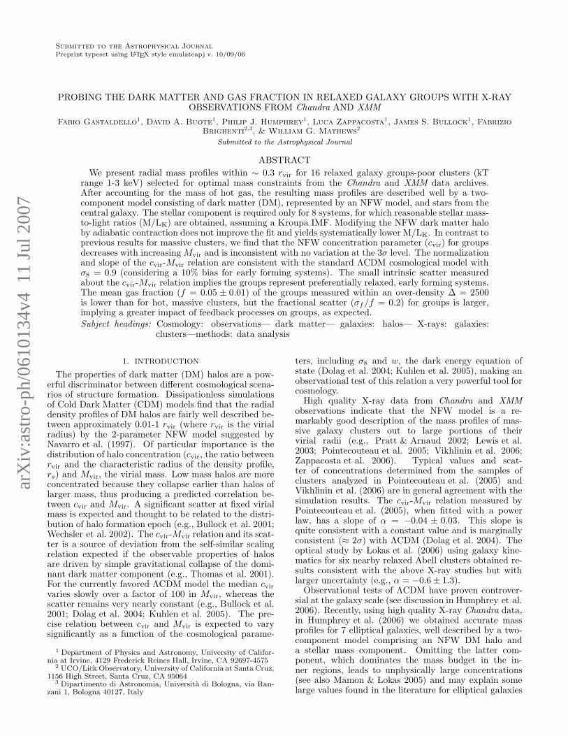
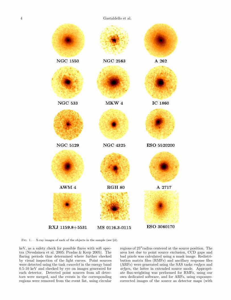
Fig. 1.— X-ray images of each of the objects in the sample (see §4).
keV, as a safety check for possible flares with soft spec-tra (Nevalainen et al. 2005; Pradas & Kerp 2005). Theflaring periods thus determined where further checkedby visual inspection of the light curves. Point sourceswere detected using the task ewavelet in the energy band0.5-10 keV and checked by eye on images generated foreach detector. Detected point sources from all detec-tors were merged, and the events in the correspondingregions were removed from the event list, using circular
regions of 25′′radius centered at the source position. Thearea lost due to point source exclusion, CCD gaps andbad pixels was calculated using a mask image. Redistri-bution matrix files (RMFs) and ancillary response files(ARFs) were generated using the SAS tasks rmfgen andarfgen, the latter in extended source mode. Appropri-ate flux-weighting was performed for RMFs, using ourown dedicated software, and for ARFs, using exposure-corrected images of the source as detector maps (with
Dark Matter and Gas Fraction in Galaxy Groups. 5
pixel size of 1′, the minimum scale modeled by arfgen)to sample the variation in emission, following the pre-scription of Saxton & Siddiqui (2002). Spectral resultsobtained using ARFs are completely consistent with theother frequently employed method (e.g. Arnaud et al.2001) of correcting directly the spectra for vignetting(Gastaldello et al. 2003; Morris & Fabian 2005).
3.3. Background subtraction
Insuring proper background subtraction is one of thekey challenges associated with the spectral fitting of lowsurface brightness, diffuse, X-ray emission. The back-ground experienced by both Chandra and XMM consistsof (1) an extreme time variable component due to soft (E∼ tens of keV) protons channeled by the telescopes mir-rors, (2) a slowly changing (with variability time scalemuch longer than the length of a typical observation)quiescent component due to high energy particles (E >a few MeV), and (3) the sky X-ray background, decom-posed into the extragalactic Cosmic X-ray background byAGN and the Galactic X-ray emission (e.g Lumb et al.2002; Markevitch et al. 2003).
The “blank fields” distributed by the observatories arenot a perfect representation of the background in any oneobservation. Firstly, there are significant long term vari-ations in the quiescent particle background. Secondly,the soft Galactic background component varies stronglyfrom field to field. Finally, there may be some residualmild flaring.
Two approaches have been investigated to obtainmore accurate background estimates than provided bythe “blank field” background templates: the doublesubtraction technique (see details in Appendix A ofArnaud et al. 2002) and a complete modeling of thevarious background components (e.g. Lumb et al. 2002;Markevitch et al. 2003). Double subtraction is, in prin-ciple, very effective, but particular care has to be takento locate a region in the field of view of the observa-tion completely free of source emission; this is difficultfor nearby objects. The complete modeling of the vari-ous background components can rely on a large numberof observations performed to characterize the quiescentparticle background component (stowed or Dark Moonfor Chandra, closed for XMM), and on the large numberof observations which constitute the “blank field” datasets to characterize the sky background components. Thedrawback is that the resulting model, which also includesa source component, is complicated, and parameter de-generacies can arise. However, the method is particu-larly effective for studying groups and poor clusters be-cause the source component (mainly characterized by the∼ 1 keV Fe-L shell blend) is clearly spectrally separatedfrom all the other background components. For the useof this approach to the Chandra data we refer the readerto Humphrey & Buote (2006). Here we will describethe procedure used for XMM data which elaborates andupdates the procedure described in Buote et al. (2004).The algorithm implemented has the following main steps:
– Characterization of the quiescent particle back-ground. We co-add individual spectra taken fromclosed observations. The spectra in the 0.4-12 keVband for MOS and 0.4-13 keV band for pn can beadequately described by a broken power law con-
tinuum and several Gaussians for the instrumen-tal lines. Typical values for the model parametersare: 0.7-0.8 for the slope at low energies, 1.0-1.2keV for the break energies, 0.2 for the high energyslope for MOS, 0.4-0.5 for the high energy slope forpn. While the low-energy slope exhibits significantvariation between the observations in our study, thehigh-energy slope is very stable. These results areconsistent with previous studies (Lumb et al. 2002;De Luca & Molendi 2004; Nevalainen et al. 2005).The spectral shape of the continuum broken powerlaw does not change significantly across the detec-tor, nor does it vary in time (as in the MOS studyby De Luca & Molendi 2004) at high energies.
– The model derived from the closed data is fittedto the spectra of the Out of Field of View (OFV)events of each observation. Portions of the MOSand pn detectors are not exposed to the sky, andtherefore neither cosmic X-ray photons nor low en-ergy particle–induced events (like from soft pro-tons) are collected. Indeed, while this is almost ex-actly true for the MOS (the fraction of OoT eventsis 0.35% in FF mode), for the pn a higher frac-tion of in FOV events events are assigned to theOFV region as OoT (6.3% in FF mode and 2.3%in EFF). In the case of strong flaring, this OoTcontribution can seriously affect the pn OFV spec-trum. We therefore chose to extract OFV eventsfor the pn after the flare cleaning. The model de-rived from the OFV data is taken as the initial rep-resentation of the quiescent particle background forthe particular observation.
– To the broken power-law plus Gaussian lines de-scribing the quiescent instrumental background(not vignetted and implemented as a backgroundmodel in Xspec), we add the components describingthe sky X-ray background, following Lumb et al.(2002): a power law with slope Γ = 1.41 andnormalization as reported in De Luca & Molendi(2004), free to vary within the cosmic variance asΩ−1/2 (Barcons et al. 2000) where Ω is the solid an-gle covered by the observation; two thermal compo-nents with temperatures 0.07 and 0.20 keV respec-tively, and abundances fixed at solar. When model-ing sources projected toward the North Polar Spur(NGC 5129) we found it necessary to add a thirdthermal component at ∼ 0.4 keV, in agreementwith Markevitch et al. (2003) and Vikhlinin et al.(2005).
– This model, plus a source component described bya thermal plasma with temperature and abundancefree to vary, was fitted jointly to the outermostannuli used in the spectral extraction (see below).The parameters of the source component were freeto vary in each annulus. The normalizations ofthe cosmic components and of the broken powerlaw component were scaled according to the ratioof the annuli area, while the normalizations of theinstrumental lines were free to vary, given the factthat these components are highly spatially variable(e.g. De Luca & Molendi 2004; Lumb et al. 2002).An inter-calibration constant free to vary between
6 Gastaldello et al.
0.9 and 1.1 was added to the model to take into ac-count any cross-calibration differences between thethree EPIC instruments. Given the best fit modelfor these annuli, we generate a pulse height ampli-tude (PHA) correction file used in Xspec.
– For the annuli not involved in the background fit-ting, we scale the resulting model to the area ofthe annular region of interest in the spectral ex-traction and generate a PHA file. To take intoaccount the variable instrumental lines, we renor-malized the instrumental line components in themodel using the corresponding regions extractedfrom the background templates.
We mention that possible slight variations in the par-ticle continuum across the detector plane (see AppendixA of De Luca & Molendi 2004), or residual mild flaring,has been modeled by slightly changing the high energyslope of the broken power law. This does not have anytangible effect on the spectral parameters derived for softX-ray sources like the objects considered in this paper.
4. X-RAY IMAGES
The X-ray image of each group was examined to iden-tify any significant surface brightness disturbances in-dicating departures from hydrostatic equilibrium. Lowlevel X-ray disturbances like the weak signs of AGN ac-tivity in the center of Abell 262 (Blanton et al. 2004), orthe presence of a submerging group in the south of RGH80 (Mahdavi et al. 2005), do not seriously impact X-ray mass determinations, provided care is taken to avoidhighly disturbed emission (Buote & Tsai 1995; Schindler1996). The images for 15 objects in the sample are shownin Fig.1: for objects which have XMM data we showthe combined MOS1 and MOS2 image in the 0.5-2.0 keVband. For those objects with only Chandra data (3 out of16) we did the following: For RXJ 1159.8+5531 and MS0116.3-0115 we display the 0.5-10 keV ACIS-S3 image,while for ESO 3060170 we show the 0.5-10 keV ACIS-I image. The images were processed to remove pointsources using the CIAO tool dmfilth, which replaces pho-tons in the vicinity of each point source with a locally es-timated background. The images where then flat-fieldedwith a 1.7 keV exposure map for Chandra images anda 1.25 keV exposure map for XMM. Then we smoothedthe images with a 5′′ Gaussian for Chandra and a 16′′
Gaussian for XMM to make large-scale structure moreapparent. For both the Chandra and XMM images ofNGC 5044 we refer the reader to Buote et al. (2003).
None of the objects show obvious large scale distur-bance in their X-ray emission. The only notable sub-structure is the infalling subgroup in the southern regionof RGH 80, evident as a tail of enhanced emission. Somedisturbance is also present in the core of RGH 80 as re-vealed by our Chandra image. We masked in our analysisthe region of enhanced X-ray emission associated withthe subgroup. For other systems some low-amplitude,small-scale disturbances are present, such as a surfacebrightness discontinuity, reminiscent of a cold front, inthe NW of IC 1860; the cavities in the central 10 kpc ofAbell 262, as revealed by the Chandra image presented inBlanton et al. (2004); and the filamentary structures andpossible cavities in NGC 5044 (Buote et al. 2003). The
“cooling wake” discussed in the XMM image of NGC5044 by Finoguenov et al. (2006), is simply the brightSE arm of the finger-like structure caused by the cavi-ties. Hint of cavities have been detected in NGC 4325(Russell et al. 2007) and there are signs of sloshing in thecore of MKW 4. We asses the impact of these featuresin § 9.6.
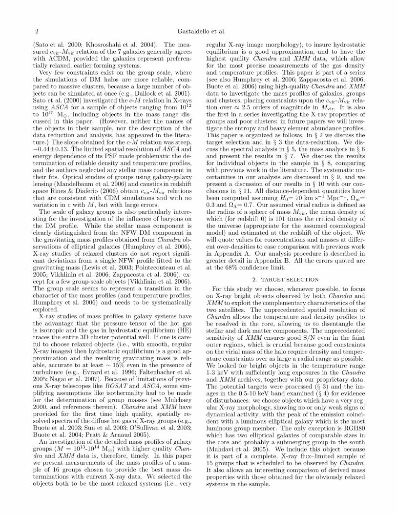
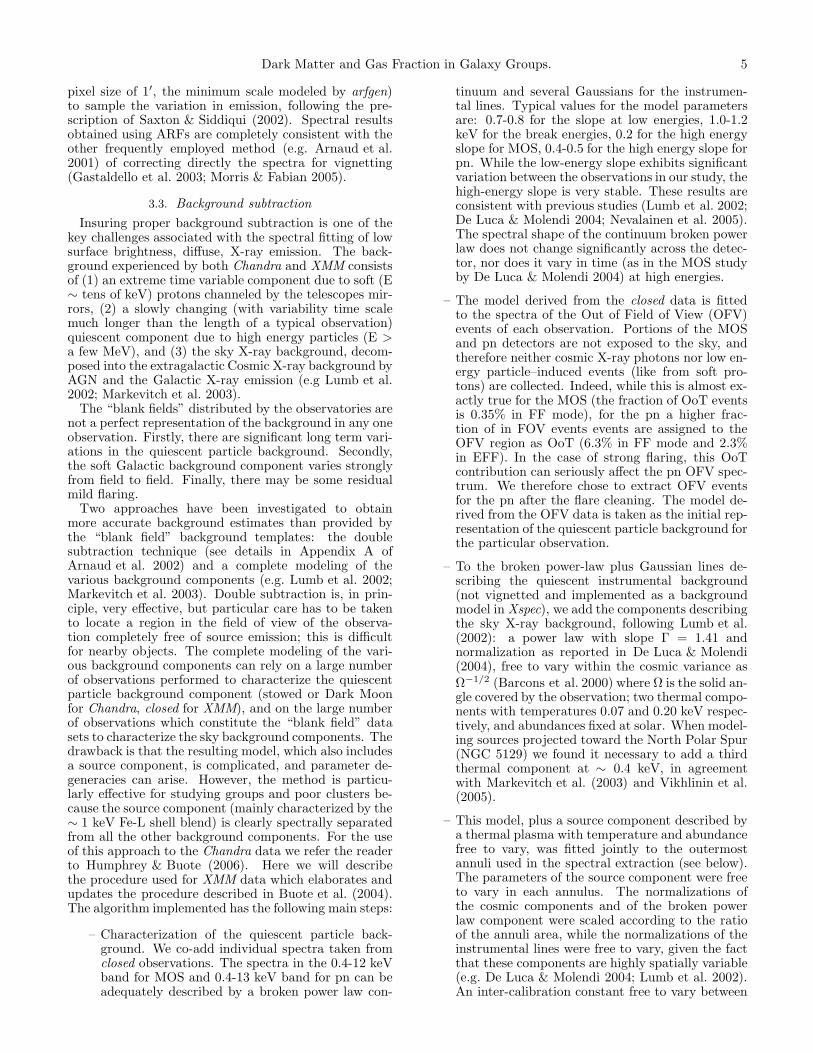
Fig. 2.— Temperature profile for the NGC 533 group derivedfrom XMM data (black) and from Chandra data (red). The innertwo XMM bins have not been considered in the derivation of themass profile.
5. SPECTRAL ANALYSIS
We extracted spectra in concentric circular annuli lo-cated at the X-ray centroid computed within a radiusof 30′′, with the initial center on the peak of the X-rayemission. The widths of the annuli were chosen to haveapproximately equal background-subtracted counts andto have a minimum width of 60′′ for XMM to avoid under-sampling of the PSF. For Chandra, given the better PSF,the widths of the annuli, in practice, were only limitedby count statistics. The spectra were re-binned to ensurea signal-to-noise ratio of at least 3 and a minimum 20counts per bin (necessary for the validity of the χ2 mini-mization method). We fitted the background-subtractedspectrum with an APEC thermal plasma modified byGalactic absorption (Dickey & Lockman 1990) to eachannulus. The free parameters are temperature, nor-malization (proportional to emission measure), and theabundances Fe, O and, when possible, Si and S. The im-pact of unresolved point sources, in particular LMXB inthe central galaxy, was taken into account by adding a7.3 keV bremsstrahlung component for all annuli withinthe twenty-fifth magnitude isophote (D25) of the cen-tral galaxy, taken from LEDA. (This model gives a goodfit to the composite spectrum of the detected sourcesin nearby galaxies, Irwin et al. 2003.) This is particu-larly relevant for the inner XMM annuli, where in generalpoint sources are not detected. The spectral fitting wasperformed with Xspec (ver 11.3.1, Arnaud 1996). We es-timated the statistical errors on the fitted parameters bysimulating spectra for each annulus using the best fitting
Dark Matter and Gas Fraction in Galaxy Groups. 7
TABLE 2Optical properties of the group central galaxy
Name Group re (B) re (K) LB LK
kpc (arcsec) kpc (arcsec) 1010 L⊙ 1011 L⊙
NGC 5044 NGC 5044 . . . . . . . . . . . . 4.53 (24.5) 6.98 2.87
NGC 1550 NGC 1550 6.45 (25.5) 3.05 (12.1) 4.33 2.09
NGC 2563 NGC 2563 5.89 (19.3) 3.73 (12.2) 3.84 2.66
NGC 708 A 262 25.60 (77.1) 10.16 (30.6) 3.84 4.12
NGC 533 NGC 533 16.92 (45.4) 9.22 (25.2) 12.4 6.14
NGC 4073 MKW 4 19.24 (47.5) 10.25 (25.3) 13.7 7.18
IC 1860 IC 1860 8.34 (18.5) 8.03 (17.8) 6.08 4.38
NGC 5129 NGC 5129 13.34 (28.7) 6.60 (14.2) 12.0 4.99
NGC 4325 NGC 4325 . . . . . . . . . . . . 5.22 (10.1) 4.61 2.33
ESO 552-020 ESO5520200 . . . . . . . . . . . . 15.7 (25.0) 15.6 8.19
NGC 6051 AWM 4 10.21 (16.1) 10.33 (16.3) 9.91 7.50
ESO 306-017 ESO3060170 . . . . . . . . . . . . 18.51 (26.0) 18.5 6.95
MCG 6-29-77 RGH80 . . . . . . . . . . . . 5.11 (6.8) . . . . . . . . 2.93
MCG 6-29-78 RGH80 . . . . . . . . . . . . 6.23 (8.3) 4.21 2.39
UGC 842 MS 0116.3-0115 . . . . . . . . . . . . 9.69 (10.9) 9.29 5.77
ESO 349-22 A 2717 . . . . . . . . . . . . 15.53 (16.2) 9.20 5.42
2MASSX J11595215 RXJ 1159.8+5531 . . . . . . . . . . . . 9.77 (6.4) 23.6 10.3
Note. — The optical properties of the central galaxy of each group. LB was obtained from LEDA,re in the B band from RC3 (de Vaucouleurs et al. 1991), LK (using the luminosity distance of Table 1)and re in the K band from 2MASS.
models and then fitted the simulated spectra in exactlythe same manner as done for the actual data. From 20Monte Carlo simulations we compute the standard devi-ation for each free parameter, which we quote as the “1σ” error (these error estimates generally agree very wellwith those obtained using the standard ∆χ2 approach inXspec, e.g., Humphrey & Buote 2006).
If an object has been observed by both Chandra andXMM we selected for our final analysis only the Chandradata in the inner core region were the temperature risesoutward from the center. The XMM spectra extracted inwide annuli are not as well fitted by a single temperatureemission model as are the Chandra spectra in narrowerannuli, suggesting that departures from single temper-ature emission in the projected spectra stem primarilyfrom the steep radial temperature gradient present inthe core, as shown in Fig.2 for NGC 533. The betterChandra PSF also allows us to exclude point sources un-detected with XMM, in particular LMXB in the centralgalaxy. Unresolved LMXB still affect the Chandra data,but to a much lesser extent than XMM data. This com-ponent is evident as an excess at energies greater than∼ 3 keV and can contribute, if neglected, to the multi-phase appearance of XMM spectra.
6. MASS MODELING
To calculate the gravitating mass distribution we solvethe equation of hydrostatic equilibrium assuming spher-ical symmetry. By requiring spherical symmetry we ob-tain spherically averaged mass profiles which allows us totest the spherically averaged DM profiles obtained fromcosmological simulations and to facilitate comparison toprevious observational studies.
Following the approach adopted in Humphrey et al.(2006), we assume parametrizations for the temperatureand mass profiles to calculate the gas density assuming
hydrostatic equilibrium,
ρg(r) = ρg0T0
T (r)exp
(−µmAG
kB
∫ r
r0
M dr
r2T
)
, (1)
where r is the radius from the center of the gravitationalpotential, ρg is the gas density, ρg0 and T0 are densityand temperature at some “reference” radius r0, kB isBoltzmann’s constant, G is the universal gravitationalconstant, mA is the atomic mass unit and µ (taken to be0.62) is the mean atomic weight of the gas. The ρg(r)and T (r) profiles are fitted simultaneously to the data toconstrain the parameters of the temperature and massmodels. Since the gravitating mass also contains the gasmass, eq. (1) is solved iteratively for ρg.
This “parametric mass method” is the principal ap-proach employed in this study. We assess systematicerrors in this adopted method in §9.5 by comparing toresults obtained using other solutions to the hydrostaticequilibrium equation. Firstly, rather than solving for thegas density, we can solve for the temperature,
T (r) = T0ρg0
ρg(r)− µmAG
kBρg(r)
∫ r
r0
ρgM dr
r2, (2)
which provides an alternative implementation of the“parametric mass method”. Note that in both cases theparameters of the mass model are obtained from fittingthe gas density and temperature data. The goodness-of-fit for any mass model (e.g., NFW) can be assesseddirectly from the residuals of the fit. Secondly, we usethe more traditional formulation of the hydrostatic equi-librium equation (Mathews 1978),
M(< r) = rkBT (r)
GµmA
(
−d ln ρg
d ln r− d ln T
d ln r
)
(3)
which involves parametrizing independently ρg and Tusing simple functional forms in order to evaluate the
8 Gastaldello et al.
derivatives in Eq. (3). Since, however, the mass pro-file itself is not parametrized, we denote this traditionalapproach a “non-parametric mass method”. Since themass profile itself is produced by this method, if onewants to evaluate the success of a particular mass model(e.g., NFW) then additional fitting is required. Con-sequently, following previous studies (e.g., Lewis et al.2003) for each annulus we assign a three dimensional ra-
dius value r ≡ [(R3/2out + R
3/2in )/2]2/3, where Rin and Rout
are respectively the inner and outer radii of the (two-dimensional) annulus. At each radius r we calculate thetotal enclosed gravitating mass M(< r) according to theequation of hydrostatic equilibrium. The errors on theresulting mass “data points” were estimated from theMonte Carlo simulations used to estimate the errors fordensity and temperatures (§5), giving a set of mass val-ues at each radius. From those we calculate the stan-dard deviation which we quote as the “1σ” error for thismethod. To analyze the shape of the mass profiles, wefitted parametrized models to the mass values.
There are several reasons why we adopt equation [1]instead of equation [3] for our analysis. Firstly, as notedabove, the “parametric mass method” allows a partic-ular mass model to be constrained immediately by thegas density and temperature data and the goodness-of-fit of the mass model can be assessed in a straightfor-ward manner. Secondly, despite the high-quality X-raydata provided by Chandra and XMM, it is still not pos-sible to compute accurate derivatives of the tempera-ture and density profiles at each radius. Consequently,smooth models must be fitted to the entire radial profiles,which may not produce physical solutions to equation [3];e.g., jagged, non-monotonically increasing mass profiles.Thirdly, we analyze the projected temperatures and den-sities which requires the models for the gas density (den-sity squared, see below) and temperature to be projectedalong the line-of-sight. This requires evaluating the mod-els at least out to the virial radius, well outside the outerradius of most of the groups in our sample. By usingthe “parametric mass method” any extrapolation of thegas density (equation [1]) or temperature (equation [2])is performed consistently within the context of the as-sumed mass profile. It is for this last reason we havea slight preference for using equation [1] over equation[2] for this study. Nevertheless, despite these differences,we find that the different approaches to the mass mod-eling represented by the three equations give consistentresults, within the errors, for the global halo properties(see also §9.5).
For our default analysis we projected parametrizedmodels of the three-dimensional quantities, ρ2
g and T ,and fitted these projected models to the results obtainedfrom our analysis of the data projected on the sky (see§5). The models have been integrated over each radialbin (rather than only evaluating at a single point withinthe bin) to provide a consistent comparison. They alsohave been projected along the line of sight including theradial variation in the plasma emissivity Λ(T, ZFe), usinga model fitted to the observed ZFe profile. We provide areview of the projection of spherical coronal gas modelsfor comparison to X-ray spectral data in Appendix B.
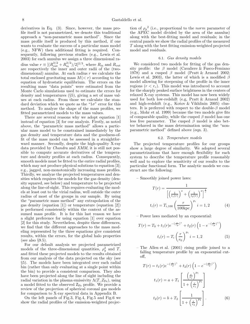
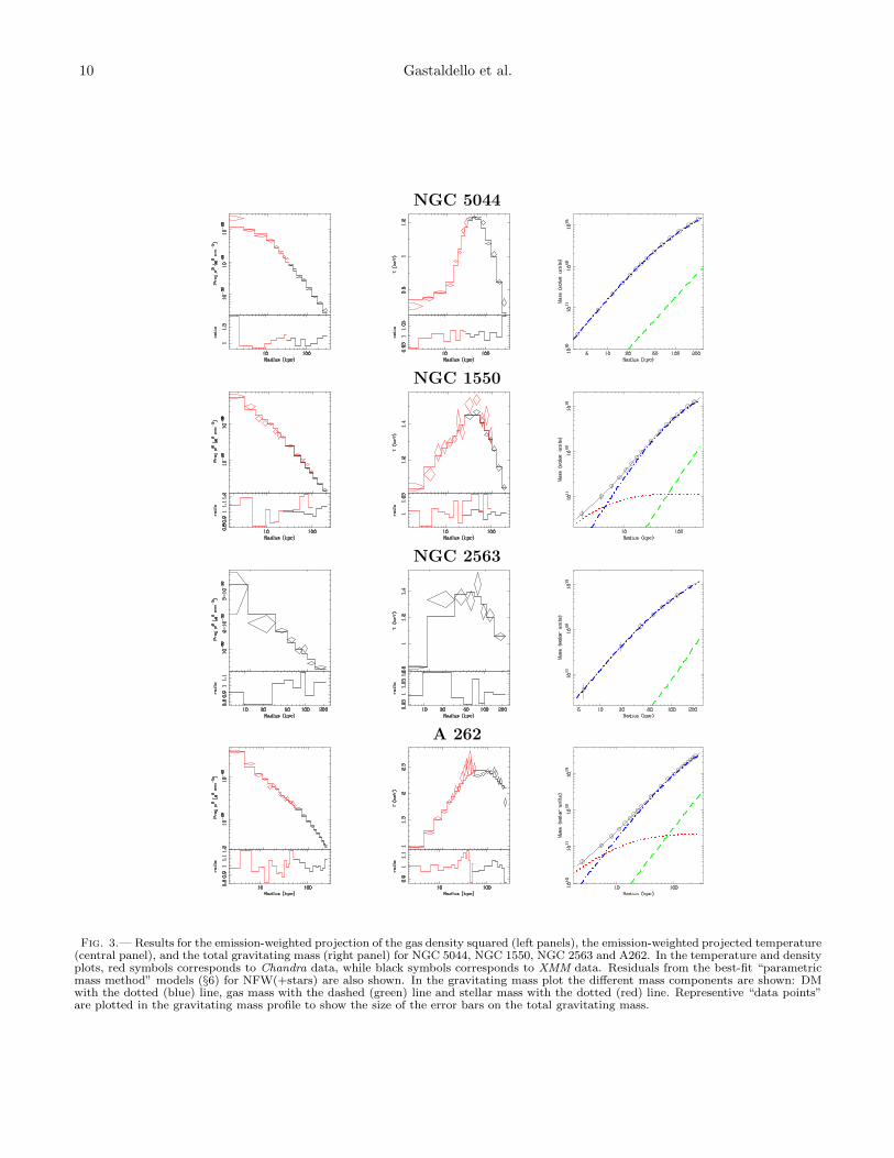
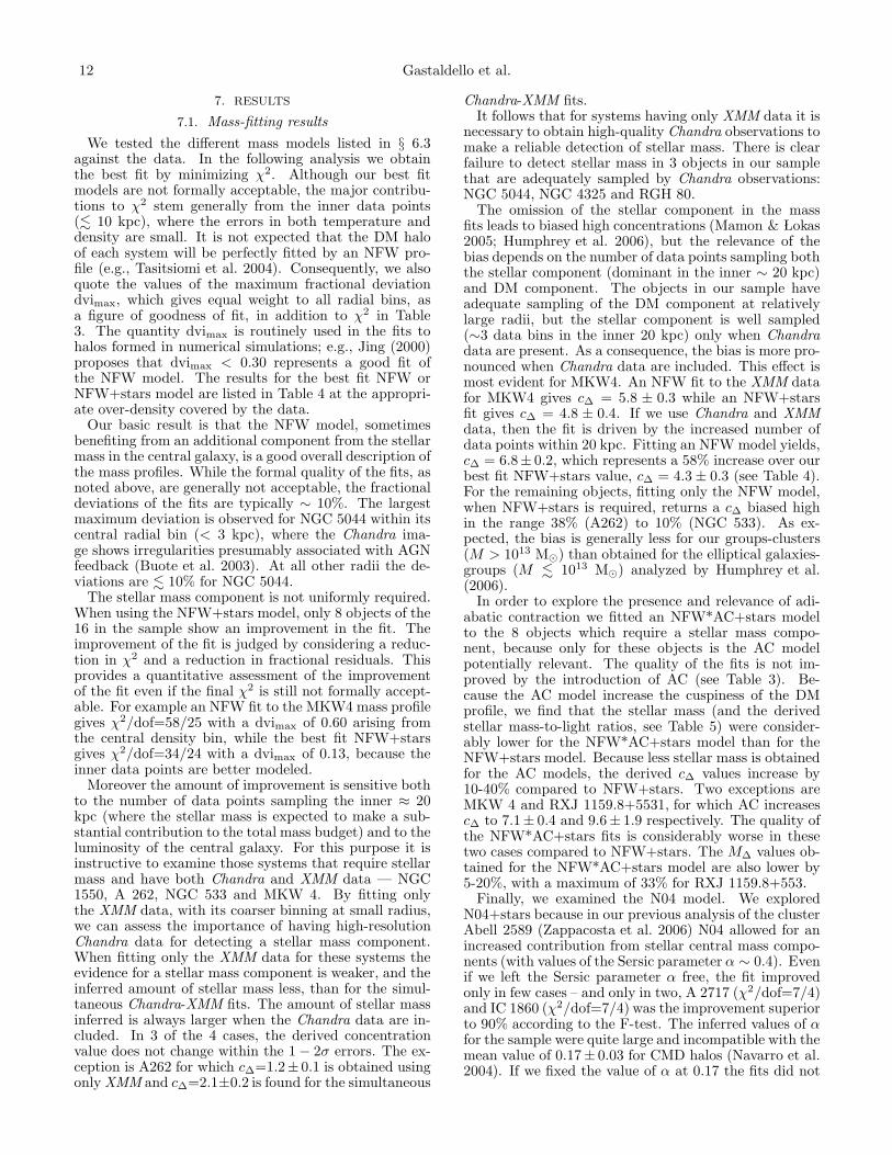
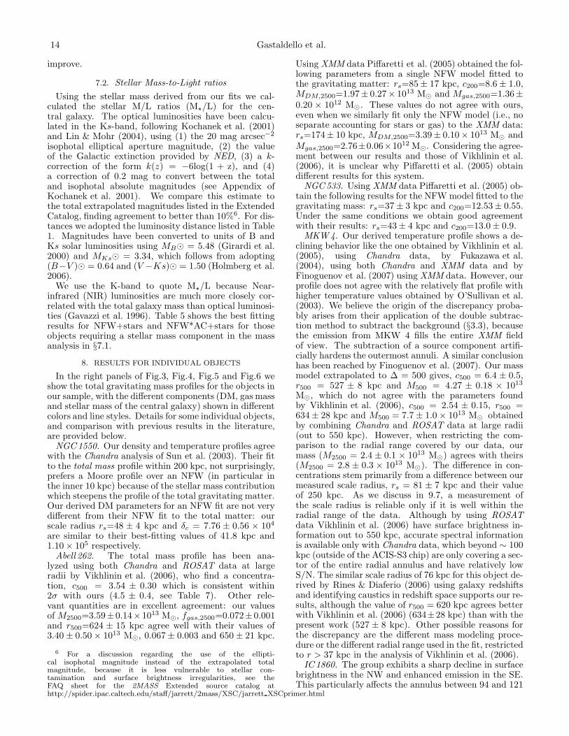
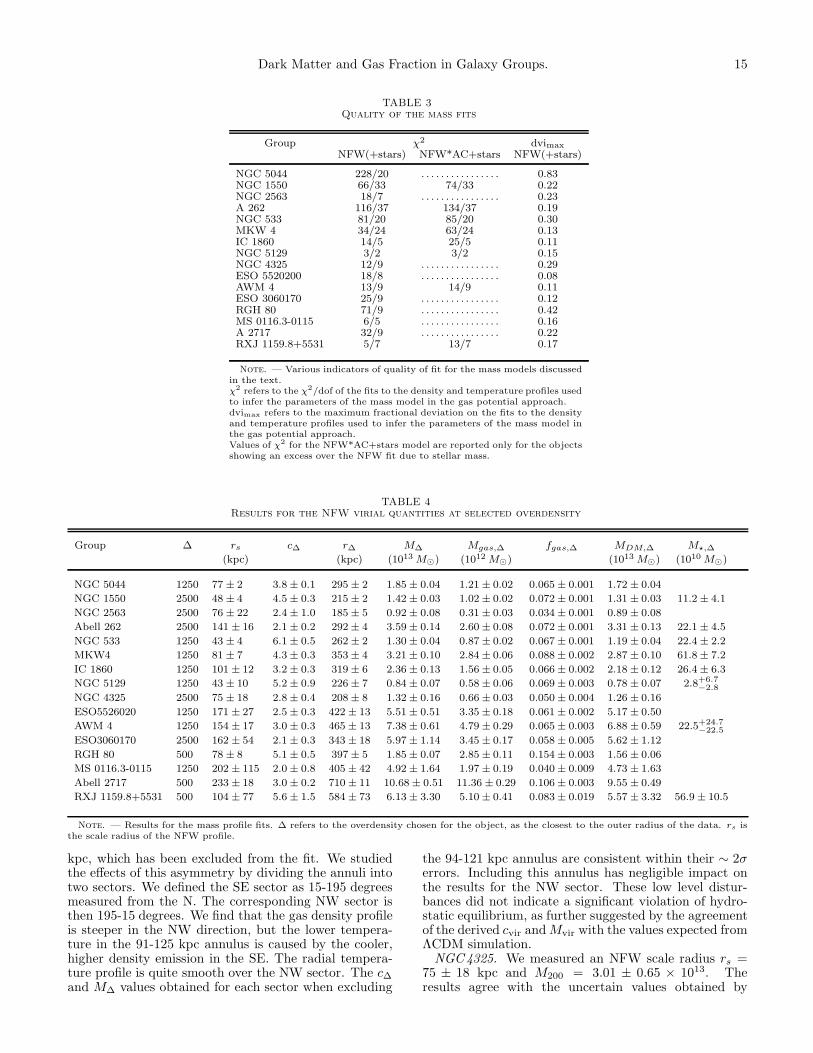
On the left panels of Fig.3, Fig.4, Fig.5 and Fig.6 weshow the radial profiles of the emission-weighted projec-
tion of ρg2 (i.e., proportional to the norm parameter of
the APEC model divided by the area of the annulus)along with the best-fitting model and residuals; in thecentral panels we show the radial profiles of the measuredT along with the best fitting emission-weighted projectedmodel and residuals.
6.1. Gas density models
We considered two models for fitting of the gas den-sity profile: the β model (Cavaliere & Fusco-Femiano1978) and a cusped β model (Pratt & Arnaud 2002;Lewis et al. 2003), the latter of which is a modified βmodel allowing for steepening of the profile in the innerregions (r < rc). This model was introduced to accountfor the sharply peaked surface brightness in the centers ofrelaxed X-ray systems. This model has now been widelyused for both low-redshift (e.g, Pratt & Arnaud 2002)and high-redshift (e.g., Kotov & Vikhlinin 2005) clus-ters. It is preferred with respect to the double-β model(e.g., Mohr et al. 1999) because the two models give fitsof comparable quality, while the cusped β model has oneless free parameter. The cusped β model is also bet-ter behaved in the mass determination using the “non-parametric method” defined above (eqn. 3).
6.2. Temperature models
The projected temperature profiles for our groupsshow a large degree of similarity. We adopted severalparametrizations that have enough flexibility for eachsystem to describe the temperature profile reasonablywell and to explore the sensitivity of our results to theparticular functional form. The analytic models we con-struct are the following:
– Smoothly joined power laws:
T (r) =1
[(
1t1(r)
)s
+(
1t2(r)
)s] 1
s
ti(r) = Ti,100
(
r
100kpc
)pi
i = 1, 2 (4)
– Power laws mediated by an exponential:
T (r) = T0 + t1(r)e−( r
rp)γ
+ t2(r)(
1 − e−( r
rp)γ
)
ti(r) = Ti
(
r
r0
)pi
i = 1, 2 (5)
– The Allen et al. (2001) rising profile joined to afalling temperature profile by an exponential cut-off,
T (r) = t1(r)e−( r
rp)γ
+ t2(r)(
1 − e−( r
rp)γ
)
t1(r) = a + T1
(
rr1
)p1
1 +(
rr1
)p1
t2(r) = b + T2
1
1 +(
rr2
)p2
. (6)
Dark Matter and Gas Fraction in Galaxy Groups. 9
The third (“RiseFall”) model has been adopted in par-ticular for temperature profiles showing an inner coreflattening like NGC 533, NGC 4325 and NGC 5044, whilethe first two models provide comparable fits to the gen-eral profile. We will assess how different choices of tem-perature profile, together with density profiles, affect ourmass measurements in §9.5.
6.3. Mass models
We compute the total gravitating mass as the sum ofDM, stars, and hot gas: MDM +Mstars +Mgas. For thisstudy we only consider the contribution of the centralgalaxy to the stellar mass. The X-ray data provide adirect measurement of the hot gas density and thereforeof Mgas. We tested the following mass models againstthe data:
– MDM = NFW, Mstars= 0: A single NFWmodel to investigate scenarios like the ones ofLoeb & Peebles (2003) and El-Zant et al. (2004)and the effect of the omission of the stellar mass, ifpresent, on the derived concentration parameter.
– MDM = NFW, Mstars= deV. A NFW model plusa model for a stellar component. We adopted ade Vaucolueurs stellar mass potential using theanalytical approximation to the deprojected Sersicmodel of Prugniel & Simien (1997) with n = 4.The de Vaucolueurs profile is a good description ofthe stellar light distribution even for objects whichfollow the more general Sersic profile with Sersic in-dex n 6= 4 (see appendix A of Padmanabhan et al.2004). The de Vaucolueurs effective radius re ismeasured in the K-band by the Two Micron AllSky Survey (2MASS ) as listed in the ExtendedSource Catalog (Jarrett et al. 2000, see Tab.2). Werefer to this model as NFW+stars.
– MDM = NFW*AC, Mstars= deV. A NFW compo-nent modified by the adiabatic contraction modelof Gnedin et al. (2004)5 plus a de Vaucolueurs com-ponent for the stellar mass, to explore the impor-tance of baryon condensation in the central galaxyfor the DM halo profile. We refer to this model asNFW*AC+stars.
– Finally we also examined the recently suggestedSersic-like profile (Navarro et al. 2004, hereafterN04) which should be a better parametrization ofthe innermost regions of CDM halos.
To obtain the true virial radius and virial mass (andconcentration) we initially take r∆ and M∆ obtained forthe DM component, where ∆ corresponds to the over-density level (2500, 1250, 500) closest to the radial rangecovered by the data and listed in Table 4. Then we addedMgas and Mstars to MDM to give a new M∆. A new r∆
is then computed, and the process repeated, until r∆
changes by < 0.001%. (We note that in our previousstudies by Humphrey et al. 2006 and Zappacosta et al.2006 we also computed the virial radius appropriate for
5 The adiabatic contraction code we usedwas made publicly available by Oleg Gnedin at:http://www.astronomy.ohio-state.edu/∼ognedin/contra/
all of the mass components.) The values thus obtainedhave then been converted to various over-densities (inparticular the virial over-density, listed for each objectin Table 1) in Table 7 by using the formula providedby Hu & Kravtsov (2003) appropriate for an NFW halo.We prefer this procedure for extrapolating the mass andconcentration to ∆ ≈ 101 (for comparison with theoret-ical models) because it does not involve also extrapolat-ing Mgas. We find that the extrapolated values for thegas mass are sensitive to the radial range over which thedensity profile is fitted (see §9.7).
10 Gastaldello et al.
NGC 5044
NGC 1550
NGC 2563
A 262
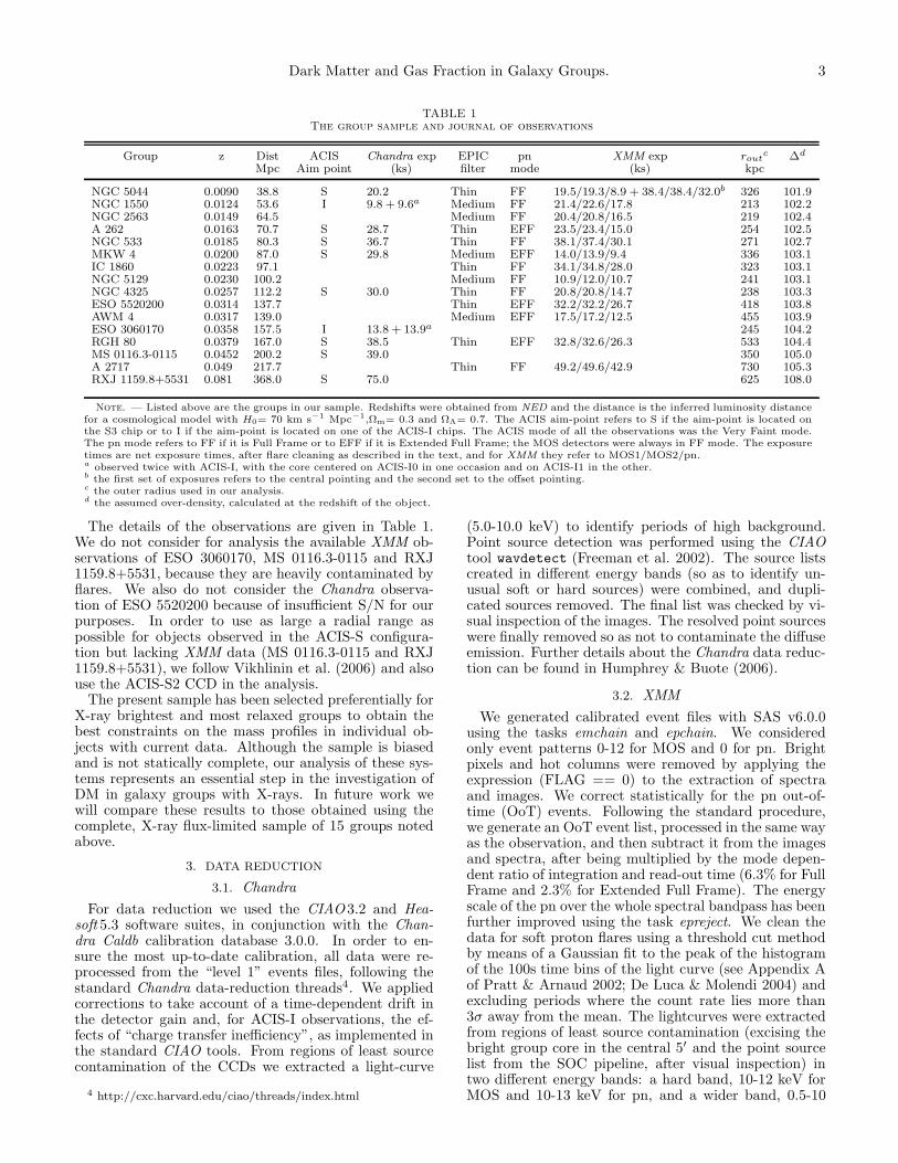
Fig. 3.— Results for the emission-weighted projection of the gas density squared (left panels), the emission-weighted projected temperature(central panel), and the total gravitating mass (right panel) for NGC 5044, NGC 1550, NGC 2563 and A262. In the temperature and densityplots, red symbols corresponds to Chandra data, while black symbols corresponds to XMM data. Residuals from the best-fit “parametricmass method” models (§6) for NFW(+stars) are also shown. In the gravitating mass plot the different mass components are shown: DMwith the dotted (blue) line, gas mass with the dashed (green) line and stellar mass with the dotted (red) line. Representive “data points”are plotted in the gravitating mass profile to show the size of the error bars on the total gravitating mass.
Dark Matter and Gas Fraction in Galaxy Groups. 11
NGC 533
MKW 4
IC 1860
NGC 5129
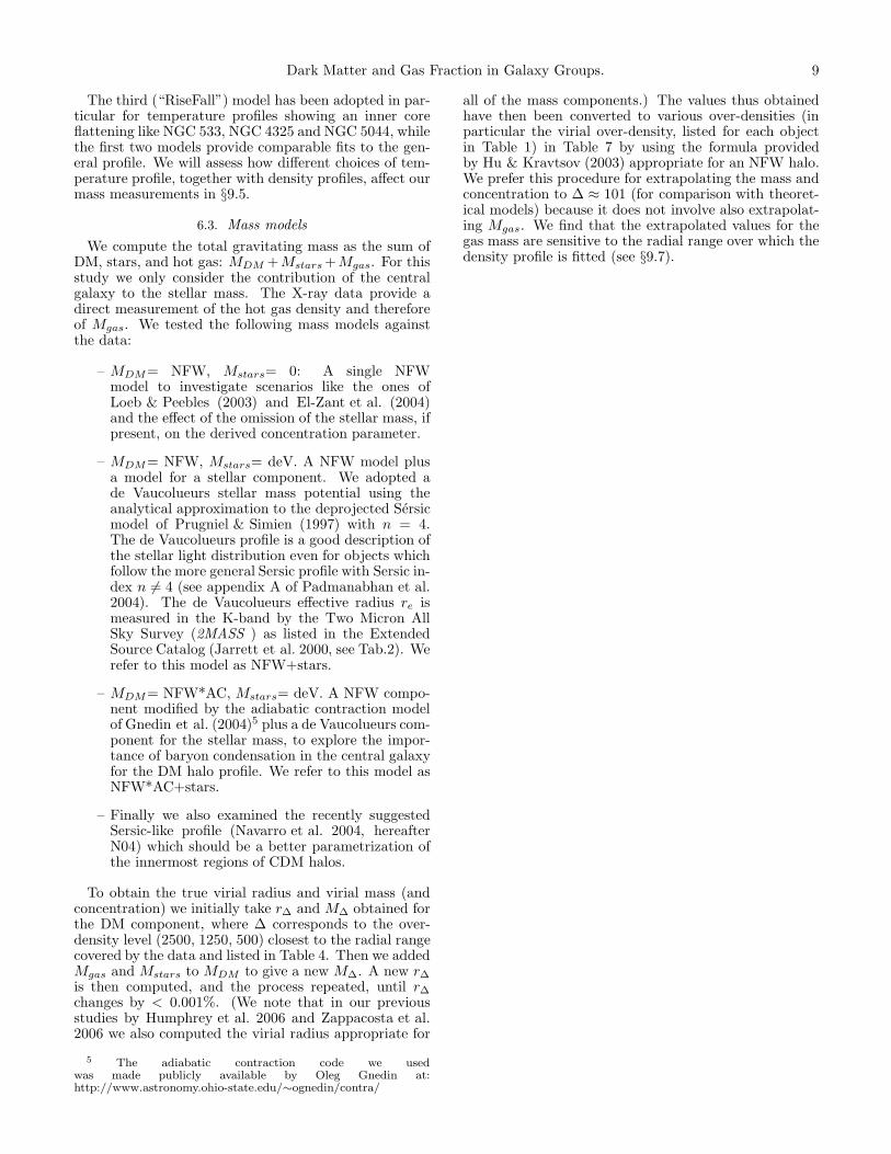
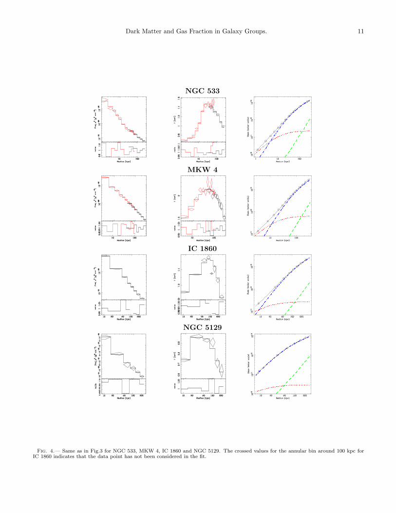
Fig. 4.— Same as in Fig.3 for NGC 533, MKW 4, IC 1860 and NGC 5129. The crossed values for the annular bin around 100 kpc forIC 1860 indicates that the data point has not been considered in the fit.
12 Gastaldello et al.
7. RESULTS
7.1. Mass-fitting results
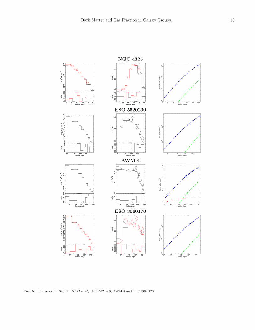
We tested the different mass models listed in § 6.3against the data. In the following analysis we obtainthe best fit by minimizing χ2. Although our best fitmodels are not formally acceptable, the major contribu-tions to χ2 stem generally from the inner data points(. 10 kpc), where the errors in both temperature anddensity are small. It is not expected that the DM haloof each system will be perfectly fitted by an NFW pro-file (e.g., Tasitsiomi et al. 2004). Consequently, we alsoquote the values of the maximum fractional deviationdvimax, which gives equal weight to all radial bins, asa figure of goodness of fit, in addition to χ2 in Table3. The quantity dvimax is routinely used in the fits tohalos formed in numerical simulations; e.g., Jing (2000)proposes that dvimax < 0.30 represents a good fit ofthe NFW model. The results for the best fit NFW orNFW+stars model are listed in Table 4 at the appropri-ate over-density covered by the data.
Our basic result is that the NFW model, sometimesbenefiting from an additional component from the stellarmass in the central galaxy, is a good overall description ofthe mass profiles. While the formal quality of the fits, asnoted above, are generally not acceptable, the fractionaldeviations of the fits are typically ∼ 10%. The largestmaximum deviation is observed for NGC 5044 within itscentral radial bin (< 3 kpc), where the Chandra ima-ge shows irregularities presumably associated with AGNfeedback (Buote et al. 2003). At all other radii the de-viations are . 10% for NGC 5044.
The stellar mass component is not uniformly required.When using the NFW+stars model, only 8 objects of the16 in the sample show an improvement in the fit. Theimprovement of the fit is judged by considering a reduc-tion in χ2 and a reduction in fractional residuals. Thisprovides a quantitative assessment of the improvementof the fit even if the final χ2 is still not formally accept-able. For example an NFW fit to the MKW4 mass profilegives χ2/dof=58/25 with a dvimax of 0.60 arising fromthe central density bin, while the best fit NFW+starsgives χ2/dof=34/24 with a dvimax of 0.13, because theinner data points are better modeled.
Moreover the amount of improvement is sensitive bothto the number of data points sampling the inner ≈ 20kpc (where the stellar mass is expected to make a sub-stantial contribution to the total mass budget) and to theluminosity of the central galaxy. For this purpose it isinstructive to examine those systems that require stellarmass and have both Chandra and XMM data — NGC1550, A 262, NGC 533 and MKW 4. By fitting onlythe XMM data, with its coarser binning at small radius,we can assess the importance of having high-resolutionChandra data for detecting a stellar mass component.When fitting only the XMM data for these systems theevidence for a stellar mass component is weaker, and theinferred amount of stellar mass less, than for the simul-taneous Chandra-XMM fits. The amount of stellar massinferred is always larger when the Chandra data are in-cluded. In 3 of the 4 cases, the derived concentrationvalue does not change within the 1 − 2σ errors. The ex-ception is A262 for which c∆=1.2± 0.1 is obtained usingonly XMM and c∆=2.1±0.2 is found for the simultaneous
Chandra-XMM fits.It follows that for systems having only XMM data it is
necessary to obtain high-quality Chandra observations tomake a reliable detection of stellar mass. There is clearfailure to detect stellar mass in 3 objects in our samplethat are adequately sampled by Chandra observations:NGC 5044, NGC 4325 and RGH 80.
The omission of the stellar component in the massfits leads to biased high concentrations (Mamon & Lokas2005; Humphrey et al. 2006), but the relevance of thebias depends on the number of data points sampling boththe stellar component (dominant in the inner ∼ 20 kpc)and DM component. The objects in our sample haveadequate sampling of the DM component at relativelylarge radii, but the stellar component is well sampled(∼3 data bins in the inner 20 kpc) only when Chandradata are present. As a consequence, the bias is more pro-nounced when Chandra data are included. This effect ismost evident for MKW4. An NFW fit to the XMM datafor MKW4 gives c∆ = 5.8 ± 0.3 while an NFW+starsfit gives c∆ = 4.8 ± 0.4. If we use Chandra and XMMdata, then the fit is driven by the increased number ofdata points within 20 kpc. Fitting an NFW model yields,c∆ = 6.8± 0.2, which represents a 58% increase over ourbest fit NFW+stars value, c∆ = 4.3 ± 0.3 (see Table 4).For the remaining objects, fitting only the NFW model,when NFW+stars is required, returns a c∆ biased highin the range 38% (A262) to 10% (NGC 533). As ex-pected, the bias is generally less for our groups-clusters(M > 1013 M⊙) than obtained for the elliptical galaxies-groups (M . 1013 M⊙) analyzed by Humphrey et al.(2006).
In order to explore the presence and relevance of adi-abatic contraction we fitted an NFW*AC+stars modelto the 8 objects which require a stellar mass compo-nent, because only for these objects is the AC modelpotentially relevant. The quality of the fits is not im-proved by the introduction of AC (see Table 3). Be-cause the AC model increase the cuspiness of the DMprofile, we find that the stellar mass (and the derivedstellar mass-to-light ratios, see Table 5) were consider-ably lower for the NFW*AC+stars model than for theNFW+stars model. Because less stellar mass is obtainedfor the AC models, the derived c∆ values increase by10-40% compared to NFW+stars. Two exceptions areMKW 4 and RXJ 1159.8+5531, for which AC increasesc∆ to 7.1± 0.4 and 9.6± 1.9 respectively. The quality ofthe NFW*AC+stars fits is considerably worse in thesetwo cases compared to NFW+stars. The M∆ values ob-tained for the NFW*AC+stars model are also lower by5-20%, with a maximum of 33% for RXJ 1159.8+553.
Finally, we examined the N04 model. We exploredN04+stars because in our previous analysis of the clusterAbell 2589 (Zappacosta et al. 2006) N04 allowed for anincreased contribution from stellar central mass compo-nents (with values of the Sersic parameter α ∼ 0.4). Evenif we left the Sersic parameter α free, the fit improvedonly in few cases – and only in two, A 2717 (χ2/dof=7/4)and IC 1860 (χ2/dof=7/4) was the improvement superiorto 90% according to the F-test. The inferred values of αfor the sample were quite large and incompatible with themean value of 0.17± 0.03 for CMD halos (Navarro et al.2004). If we fixed the value of α at 0.17 the fits did not
Dark Matter and Gas Fraction in Galaxy Groups. 13
NGC 4325
ESO 5520200
AWM 4
ESO 3060170
Fig. 5.— Same as in Fig.3 for NGC 4325, ESO 5520200, AWM 4 and ESO 3060170.
14 Gastaldello et al.
improve.
7.2. Stellar Mass-to-Light ratios
Using the stellar mass derived from our fits we cal-culated the stellar M/L ratios (M⋆/L) for the cen-tral galaxy. The optical luminosities have been calcu-lated in the Ks-band, following Kochanek et al. (2001)and Lin & Mohr (2004), using (1) the 20 mag arcsec−2
isophotal elliptical aperture magnitude, (2) the valueof the Galactic extinction provided by NED, (3) a k-correction of the form k(z) = −6log(1 + z), and (4)a correction of 0.2 mag to convert between the totaland isophotal absolute magnitudes (see Appendix ofKochanek et al. 2001). We compare this estimate tothe total extrapolated magnitudes listed in the ExtendedCatalog, finding agreement to better than 10%6. For dis-tances we adopted the luminosity distance listed in Table1. Magnitudes have been converted to units of B andKs solar luminosities using MB⊙ = 5.48 (Girardi et al.2000) and MKs⊙ = 3.34, which follows from adopting(B−V )⊙ = 0.64 and (V −Ks)⊙ = 1.50 (Holmberg et al.2006).
We use the K-band to quote M⋆/L because Near-infrared (NIR) luminosities are much more closely cor-related with the total galaxy mass than optical luminosi-ties (Gavazzi et al. 1996). Table 5 shows the best fittingresults for NFW+stars and NFW*AC+stars for thoseobjects requiring a stellar mass component in the massanalysis in §7.1.
8. RESULTS FOR INDIVIDUAL OBJECTS
In the right panels of Fig.3, Fig.4, Fig.5 and Fig.6 weshow the total gravitating mass profiles for the objects inour sample, with the different components (DM, gas massand stellar mass of the central galaxy) shown in differentcolors and line styles. Details for some individual objects,and comparison with previous results in the literature,are provided below.
NGC1550. Our density and temperature profiles agreewith the Chandra analysis of Sun et al. (2003). Their fitto the total mass profile within 200 kpc, not surprisingly,prefers a Moore profile over an NFW (in particular inthe inner 10 kpc) because of the stellar mass contributionwhich steepens the profile of the total gravitating matter.Our derived DM parameters for an NFW fit are not verydifferent from their NFW fit to the total matter: ourscale radius rs=48 ± 4 kpc and δc = 7.76 ± 0.56 × 10⁴
are similar to their best-fitting values of 41.8 kpc and1.10 × 105 respectively.
Abell 262. The total mass profile has been ana-lyzed using both Chandra and ROSAT data at largeradii by Vikhlinin et al. (2006), who find a concentra-tion, c500 = 3.54 ± 0.30 which is consistent within2σ with ours (4.5 ± 0.4, see Table 7). Other rele-vant quantities are in excellent agreement: our valuesof M2500=3.59±0.14×10¹³ M⊙, fgas,2500=0.072±0.001and r500=624 ± 15 kpc agree well with their values of3.40 ± 0.50 × 10¹³ M⊙, 0.067 ± 0.003 and 650 ± 21 kpc.
6 For a discussion regarding the use of the ellipti-cal isophotal magnitude instead of the extrapolated totalmagnitude, because it is less vulnerable to stellar con-tamination and surface brightness irregularities, see theFAQ sheet for the 2MASS Extended source catalog athttp://spider.ipac.caltech.edu/staff/jarrett/2mass/XSC/jarrett XSCprimer.html
Using XMM data Piffaretti et al. (2005) obtained the fol-lowing parameters from a single NFW model fitted tothe gravitating matter: rs=85 ± 17 kpc, c200=8.6 ± 1.0,MDM,2500=1.97± 0.27× 10¹³ M⊙ and Mgas,2500=1.36±0.20 × 10¹² M⊙. These values do not agree with ours,even when we similarly fit only the NFW model (i.e., noseparate accounting for stars or gas) to the XMM data:rs=174± 10 kpc, MDM,2500=3.39± 0.10 × 10¹³ M⊙ andMgas,2500=2.76±0.06×10¹² M⊙. Considering the agree-ment between our results and those of Vikhlinin et al.(2006), it is unclear why Piffaretti et al. (2005) obtaindifferent results for this system.
NGC533. Using XMM data Piffaretti et al. (2005) ob-tain the following results for the NFW model fitted to thegravitating mass: rs=37 ± 3 kpc and c200=12.53 ± 0.55.Under the same conditions we obtain good agreementwith their results: rs=43 ± 4 kpc and c200=13.0 ± 0.9.
MKW4. Our derived temperature profile shows a de-clining behavior like the one obtained by Vikhlinin et al.(2005), using Chandra data, by Fukazawa et al.(2004), using both Chandra and XMM data and byFinoguenov et al. (2007) using XMM data. However, ourprofile does not agree with the relatively flat profile withhigher temperature values obtained by O’Sullivan et al.(2003). We believe the origin of the discrepancy proba-bly arises from their application of the double subtrac-tion method to subtract the background (§3.3), becausethe emission from MKW 4 fills the entire XMM fieldof view. The subtraction of a source component artifi-cially hardens the outermost annuli. A similar conclusionhas been reached by Finoguenov et al. (2007). Our massmodel extrapolated to ∆ = 500 gives, c500 = 6.4 ± 0.5,r500 = 527 ± 8 kpc and M500 = 4.27 ± 0.18 × 10¹³
M⊙, which do not agree with the parameters foundby Vikhlinin et al. (2006), c500 = 2.54 ± 0.15, r500 =634 ± 28 kpc and M500 = 7.7 ± 1.0 × 10¹³ M⊙ obtainedby combining Chandra and ROSAT data at large radii(out to 550 kpc). However, when restricting the com-parison to the radial range covered by our data, ourmass (M2500 = 2.4 ± 0.1 × 10¹³ M⊙) agrees with theirs(M2500 = 2.8 ± 0.3 × 10¹³ M⊙). The difference in con-centrations stem primarily from a difference between ourmeasured scale radius, rs = 81 ± 7 kpc and their valueof 250 kpc. As we discuss in 9.7, a measurement ofthe scale radius is reliable only if it is well within theradial range of the data. Although by using ROSATdata Vikhlinin et al. (2006) have surface brightness in-formation out to 550 kpc, accurate spectral informationis available only with Chandra data, which beyond ∼ 100kpc (outside of the ACIS-S3 chip) are only covering a sec-tor of the entire radial annulus and have relatively lowS/N. The similar scale radius of 76 kpc for this object de-rived by Rines & Diaferio (2006) using galaxy redshiftsand identifying caustics in redshift space supports our re-sults, although the value of r500 = 620 kpc agrees betterwith Vikhlinin et al. (2006) (634±28 kpc) than with thepresent work (527 ± 8 kpc). Other possible reasons forthe discrepancy are the different mass modeling proce-dure or the different radial range used in the fit, restrictedto r > 37 kpc in the analysis of Vikhlinin et al. (2006).
IC 1860. The group exhibits a sharp decline in surfacebrightness in the NW and enhanced emission in the SE.This particularly affects the annulus between 94 and 121
Dark Matter and Gas Fraction in Galaxy Groups. 15
TABLE 3Quality of the mass fits
Group χ2 dvimax
NFW(+stars) NFW*AC+stars NFW(+stars)
NGC 5044 228/20 . . . . . . . . . . . . . . . . 0.83NGC 1550 66/33 74/33 0.22NGC 2563 18/7 . . . . . . . . . . . . . . . . 0.23A 262 116/37 134/37 0.19NGC 533 81/20 85/20 0.30MKW 4 34/24 63/24 0.13IC 1860 14/5 25/5 0.11NGC 5129 3/2 3/2 0.15NGC 4325 12/9 . . . . . . . . . . . . . . . . 0.29ESO 5520200 18/8 . . . . . . . . . . . . . . . . 0.08AWM 4 13/9 14/9 0.11ESO 3060170 25/9 . . . . . . . . . . . . . . . . 0.12RGH 80 71/9 . . . . . . . . . . . . . . . . 0.42MS 0116.3-0115 6/5 . . . . . . . . . . . . . . . . 0.16A 2717 32/9 . . . . . . . . . . . . . . . . 0.22RXJ 1159.8+5531 5/7 13/7 0.17
Note. — Various indicators of quality of fit for the mass models discussedin the text.χ2 refers to the χ2/dof of the fits to the density and temperature profiles usedto infer the parameters of the mass model in the gas potential approach.dvimax refers to the maximum fractional deviation on the fits to the densityand temperature profiles used to infer the parameters of the mass model inthe gas potential approach.Values of χ2 for the NFW*AC+stars model are reported only for the objectsshowing an excess over the NFW fit due to stellar mass.
TABLE 4Results for the NFW virial quantities at selected overdensity
Group ∆ rs c∆ r∆ M∆ Mgas,∆ fgas,∆ MDM,∆ M⋆,∆
(kpc) (kpc) (1013 M⊙) (1012 M⊙) (1013 M⊙) (1010 M⊙)
NGC 5044 1250 77 ± 2 3.8 ± 0.1 295 ± 2 1.85 ± 0.04 1.21 ± 0.02 0.065 ± 0.001 1.72 ± 0.04
NGC 1550 2500 48 ± 4 4.5 ± 0.3 215 ± 2 1.42 ± 0.03 1.02 ± 0.02 0.072 ± 0.001 1.31 ± 0.03 11.2 ± 4.1
NGC 2563 2500 76 ± 22 2.4 ± 1.0 185 ± 5 0.92 ± 0.08 0.31 ± 0.03 0.034 ± 0.001 0.89 ± 0.08
Abell 262 2500 141 ± 16 2.1 ± 0.2 292 ± 4 3.59 ± 0.14 2.60 ± 0.08 0.072 ± 0.001 3.31 ± 0.13 22.1 ± 4.5
NGC 533 1250 43 ± 4 6.1 ± 0.5 262 ± 2 1.30 ± 0.04 0.87 ± 0.02 0.067 ± 0.001 1.19 ± 0.04 22.4 ± 2.2
MKW4 1250 81 ± 7 4.3 ± 0.3 353 ± 4 3.21 ± 0.10 2.84 ± 0.06 0.088 ± 0.002 2.87 ± 0.10 61.8 ± 7.2
IC 1860 1250 101 ± 12 3.2 ± 0.3 319 ± 6 2.36 ± 0.13 1.56 ± 0.05 0.066 ± 0.002 2.18 ± 0.12 26.4 ± 6.3
NGC 5129 1250 43 ± 10 5.2 ± 0.9 226 ± 7 0.84 ± 0.07 0.58 ± 0.06 0.069 ± 0.003 0.78 ± 0.07 2.8+6.7−2.8
NGC 4325 2500 75 ± 18 2.8 ± 0.4 208 ± 8 1.32 ± 0.16 0.66 ± 0.03 0.050 ± 0.004 1.26 ± 0.16
ESO5526020 1250 171 ± 27 2.5 ± 0.3 422 ± 13 5.51 ± 0.51 3.35 ± 0.18 0.061 ± 0.002 5.17 ± 0.50
AWM 4 1250 154 ± 17 3.0 ± 0.3 465 ± 13 7.38 ± 0.61 4.79 ± 0.29 0.065 ± 0.003 6.88 ± 0.59 22.5+24.7−22.5
ESO3060170 2500 162 ± 54 2.1 ± 0.3 343 ± 18 5.97 ± 1.14 3.45 ± 0.17 0.058 ± 0.005 5.62 ± 1.12
RGH 80 500 78 ± 8 5.1 ± 0.5 397 ± 5 1.85 ± 0.07 2.85 ± 0.11 0.154 ± 0.003 1.56 ± 0.06
MS 0116.3-0115 1250 202 ± 115 2.0 ± 0.8 405 ± 42 4.92 ± 1.64 1.97 ± 0.19 0.040 ± 0.009 4.73 ± 1.63
Abell 2717 500 233 ± 18 3.0 ± 0.2 710 ± 11 10.68 ± 0.51 11.36 ± 0.29 0.106 ± 0.003 9.55 ± 0.49
RXJ 1159.8+5531 500 104 ± 77 5.6 ± 1.5 584 ± 73 6.13 ± 3.30 5.10 ± 0.41 0.083 ± 0.019 5.57 ± 3.32 56.9 ± 10.5
Note. — Results for the mass profile fits. ∆ refers to the overdensity chosen for the object, as the closest to the outer radius of the data. rs isthe scale radius of the NFW profile.
kpc, which has been excluded from the fit. We studiedthe effects of this asymmetry by dividing the annuli intotwo sectors. We defined the SE sector as 15-195 degreesmeasured from the N. The corresponding NW sector isthen 195-15 degrees. We find that the gas density profileis steeper in the NW direction, but the lower tempera-ture in the 91-125 kpc annulus is caused by the cooler,higher density emission in the SE. The radial tempera-ture profile is quite smooth over the NW sector. The c∆
and M∆ values obtained for each sector when excluding
the 94-121 kpc annulus are consistent within their ∼ 2σerrors. Including this annulus has negligible impact onthe results for the NW sector. These low level distur-bances did not indicate a significant violation of hydro-static equilibrium, as further suggested by the agreementof the derived cvir and Mvir with the values expected fromΛCDM simulation.
NGC4325. We measured an NFW scale radius rs =75 ± 18 kpc and M200 = 3.01 ± 0.65 × 10¹³. Theresults agree with the uncertain values obtained by
16 Gastaldello et al.
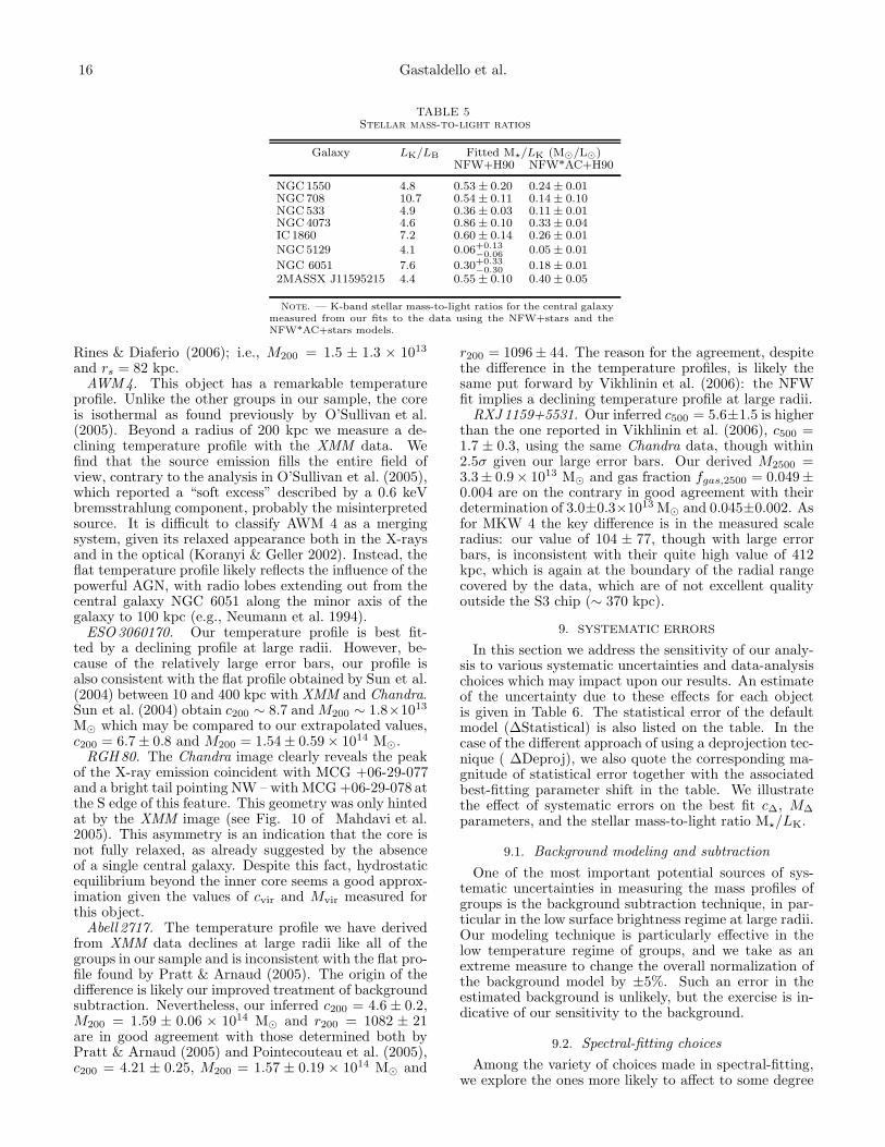
TABLE 5Stellar mass-to-light ratios
Galaxy LK/LB Fitted M⋆/LK (M⊙/L⊙)NFW+H90 NFW*AC+H90
NGC 1550 4.8 0.53 ± 0.20 0.24 ± 0.01NGC 708 10.7 0.54 ± 0.11 0.14 ± 0.10NGC 533 4.9 0.36 ± 0.03 0.11 ± 0.01NGC 4073 4.6 0.86 ± 0.10 0.33 ± 0.04IC 1860 7.2 0.60 ± 0.14 0.26 ± 0.01NGC 5129 4.1 0.06+0.13
−0.06 0.05 ± 0.01
NGC 6051 7.6 0.30+0.33−0.30 0.18 ± 0.01
2MASSX J11595215 4.4 0.55 ± 0.10 0.40 ± 0.05
Note. — K-band stellar mass-to-light ratios for the central galaxymeasured from our fits to the data using the NFW+stars and theNFW*AC+stars models.
Rines & Diaferio (2006); i.e., M200 = 1.5 ± 1.3 × 10¹³
and rs = 82 kpc.AWM4. This object has a remarkable temperature
profile. Unlike the other groups in our sample, the coreis isothermal as found previously by O’Sullivan et al.(2005). Beyond a radius of 200 kpc we measure a de-clining temperature profile with the XMM data. Wefind that the source emission fills the entire field ofview, contrary to the analysis in O’Sullivan et al. (2005),which reported a “soft excess” described by a 0.6 keVbremsstrahlung component, probably the misinterpretedsource. It is difficult to classify AWM 4 as a mergingsystem, given its relaxed appearance both in the X-raysand in the optical (Koranyi & Geller 2002). Instead, theflat temperature profile likely reflects the influence of thepowerful AGN, with radio lobes extending out from thecentral galaxy NGC 6051 along the minor axis of thegalaxy to 100 kpc (e.g., Neumann et al. 1994).
ESO3060170. Our temperature profile is best fit-ted by a declining profile at large radii. However, be-cause of the relatively large error bars, our profile isalso consistent with the flat profile obtained by Sun et al.(2004) between 10 and 400 kpc with XMM and Chandra.Sun et al. (2004) obtain c200 ∼ 8.7 and M200 ∼ 1.8×10¹³
M⊙ which may be compared to our extrapolated values,c200 = 6.7 ± 0.8 and M200 = 1.54 ± 0.59 × 10¹⁴ M⊙.
RGH80. The Chandra image clearly reveals the peakof the X-ray emission coincident with MCG +06-29-077and a bright tail pointing NW – with MCG +06-29-078 atthe S edge of this feature. This geometry was only hintedat by the XMM image (see Fig. 10 of Mahdavi et al.2005). This asymmetry is an indication that the core isnot fully relaxed, as already suggested by the absenceof a single central galaxy. Despite this fact, hydrostaticequilibrium beyond the inner core seems a good approx-imation given the values of cvir and Mvir measured forthis object.
Abell 2717. The temperature profile we have derivedfrom XMM data declines at large radii like all of thegroups in our sample and is inconsistent with the flat pro-file found by Pratt & Arnaud (2005). The origin of thedifference is likely our improved treatment of backgroundsubtraction. Nevertheless, our inferred c200 = 4.6 ± 0.2,M200 = 1.59 ± 0.06 × 10¹⁴ M⊙ and r200 = 1082 ± 21are in good agreement with those determined both byPratt & Arnaud (2005) and Pointecouteau et al. (2005),c200 = 4.21 ± 0.25, M200 = 1.57 ± 0.19 × 10¹⁴ M⊙ and
r200 = 1096 ± 44. The reason for the agreement, despitethe difference in the temperature profiles, is likely thesame put forward by Vikhlinin et al. (2006): the NFWfit implies a declining temperature profile at large radii.
RXJ1159+5531. Our inferred c500 = 5.6±1.5 is higherthan the one reported in Vikhlinin et al. (2006), c500 =1.7 ± 0.3, using the same Chandra data, though within2.5σ given our large error bars. Our derived M2500 =3.3± 0.9× 10¹³ M⊙ and gas fraction fgas,2500 = 0.049±0.004 are on the contrary in good agreement with theirdetermination of 3.0±0.3×10¹³ M⊙ and 0.045±0.002. Asfor MKW 4 the key difference is in the measured scaleradius: our value of 104 ± 77, though with large errorbars, is inconsistent with their quite high value of 412kpc, which is again at the boundary of the radial rangecovered by the data, which are of not excellent qualityoutside the S3 chip (∼ 370 kpc).
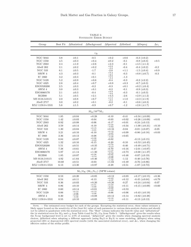
9. SYSTEMATIC ERRORS
In this section we address the sensitivity of our analy-sis to various systematic uncertainties and data-analysischoices which may impact upon our results. An estimateof the uncertainty due to these effects for each objectis given in Table 6. The statistical error of the defaultmodel (∆Statistical) is also listed on the table. In thecase of the different approach of using a deprojection tec-nique ( ∆Deproj), we also quote the corresponding ma-gnitude of statistical error together with the associatedbest-fitting parameter shift in the table. We illustratethe effect of systematic errors on the best fit c∆, M∆
parameters, and the stellar mass-to-light ratio M⋆/LK.
9.1. Background modeling and subtraction
One of the most important potential sources of sys-tematic uncertainties in measuring the mass profiles ofgroups is the background subtraction technique, in par-ticular in the low surface brightness regime at large radii.Our modeling technique is particularly effective in thelow temperature regime of groups, and we take as anextreme measure to change the overall normalization ofthe background model by ±5%. Such an error in theestimated background is unlikely, but the exercise is in-dicative of our sensitivity to the background.
9.2. Spectral-fitting choices
Among the variety of choices made in spectral-fitting,we explore the ones more likely to affect to some degree
Dark Matter and Gas Fraction in Galaxy Groups. 17
TABLE 6Systematic Error Budget
Group Best Fit ∆Statistical ∆Background ∆Spectral ∆Method ∆Deproj ∆re
c∆
NGC 5044 3.8 ±0.1 -0.5 +0.2 +0.6 -0.3 (±0.2)NGC 1550 4.5 ±0.3 +0.4 ±0.2 -0.1 -0.8 (±0.3) +0.5NGC 2563 2.4 ±1.0 +2.6 +2.3 -0.1 +4.5 (±1.4)
Abell 262 2.1 ±0.2 +0.2 +0.8−0.6 -0.4 -0.4 (±0.2) -0.2
NGC 533 6.1 ±0.5 -1.7 -2.0 +1.1 -1.5 (±0.4) +0.9
MKW 4 4.3 ±0.3 -0.1 +0.3−0.7 -0.3 +0.8 (±0.7) -0.3
IC 1860 3.2 ±0.3 +0.1 +0.9−0.4 -1.3
NGC 5129 5.2 ±0.9 +0.6 -0.4 -0.3 -0.2 (±2.2)NGC 4325 2.8 ±0.4 +0.7 +0.9 +0.3 -0.7 (±0.3)
ESO5520200 2.5 ±0.3 -0.2 -0.3 +0.1 +0.2 (±0.4)AWM 4 3.0 ±0.3 +0.1 -0.2 -0.1 -0.9 (±0.3)
ESO3060170 2.1 ±0.3 -0.4 +0.8−0.6 -0.3 -0.1 (±0.3)
RGH80 5.1 ±0.5 +2.1 +4.5 -2.6 +2.9 (±1.2)
MS 0116.3-0115 2.0 ±0.8 +0.7 +1.5−0.5 +1.0 +2.3 (±1.9)
Abell 2717 3.0 ±0.2 +0.1 -0.2 -0.1 +0.6 (±0.3)RXJ 1159.8+5531 5.6 ±1.5 -0.9 +0.7 -1.2 +2.6 (±1.7)
M∆/1013M⊙
NGC 5044 1.85 ±0.04 +0.28 -0.10 -0.41 +0.34 (±0.09)NGC 1550 1.42 ±0.03 -0.04 -0.03 +0.02 +0.26 (±0.09) +0.01NGC 2563 0.92 ±0.08 -0.06 -0.17 +0.01 -0.24 (±0.13)
Abell 262 3.59 ±0.14 -0.19 +0.24−0.62 +0.34 +1.00 (±0.31) +0.10
NGC 533 1.30 ±0.04 +0.15−0.01 +0.16 -0.04 -0.01 (±0.07) -0.05
MKW 4 3.21 ±0.10 -0.10 +0.12−0.07 +0.09 -0.86 (±0.18) +0.03
IC 1860 2.36 ±0.13 -0.08 +0.12−0.20 +0.65
NGC 5129 0.84 ±0.07 +0.08−0.03 -0.02 -0.13 (±0.15)
NGC 4325 1.32 ±0.16 -0.15 -0.20 -0.10 +0.53 (±0.45)
ESO5520200 5.51 ±0.51 +0.35 +0.70−0.13 -0.40 +0.49 (±0.71)
AWM 4 7.38 ±0.61 -0.27 -0.70 +0.16 +2.01 (±0.87)
ESO3060170 5.97 ±1.14 +1.30 +2.07−0.74 +0.73 +0.68 (±1.37)
RGH80 1.85 ±0.07 +0.26−0.14
+0.05−0.40 +0.48 -0.07 (±0.19)
MS 0116.3-0115 4.92 ±1.64 +0.46 +0.68−1.42 -1.12 -0.40 (±3.76)
Abell 2717 10.68 ±0.51 -0.03 +1.02 +0.49 -0.76 (±0.86)RXJ 1159.8+5531 6.13 ±3.30 +0.97 -0.29 +0.51 -1.87 (±0.72)
M⋆/LK (M⊙/L⊙) (NFW+stars)
NGC 1550 0.53 ±0.20 +0.05 +0.12 +0.03 +0.17 (±0.15) +0.36
Abell 262 0.54 ±0.11 -0.13 +0.23−0.37 +0.12 -0.45 (±0.04) +0.79
NGC 533 0.36 ±0.03 +0.20 +0.26 -0.27 +0.24 (±0.04) -0.07
MKW 4 0.86 ±0.10 +0.51−0.66
+0.59−0.54 +0.11 +0.15 (±0.09) +0.60
IC 1860 0.60 ±0.14 +0.01 +0.02−0.23 +0.53
NGC 5129 0.06 +0.13−0.06
+0.13−0.06 -0.06 +0.06 +0.43 (±0.19)
AWM 4 0.30 +0.33−0.30 +0.08 ±0.12 +0.14 +0.82 (±0.38)
RXJ 1159.8+5531 0.55 ±0.10 +0.05 +0.10−0.13 +0.11 -0.13 (±0.13)
Note. — The estimated error budget for each of the groups. Excepting the statistical error, these values estimate alikely upper bound on the sensitivity of the (best fit) value of each parameter to various data-analysis choices and shouldnot be added in quadrature with the statistical error. The “Best” column indicates the best-fit value and “∆Statistical”the 1σ statistical error for M∆ and c∆ from Table 4 and for M⋆/LK from Table 5. “∆Background” gives the results whenthe X-ray background level is set to ±5% of nominal, “∆Spectral” gives the results when changing spectral analysischoices, ∆Method when adopting a different approach (using Eq.2 or Eq.3) to mass modeling, ∆Deproj when usingprojected (2D) or deprojected (3D) spectral results (with the associated statistical error), and ∆re when changing theeffective radius of the stellar profile.
18 Gastaldello et al.
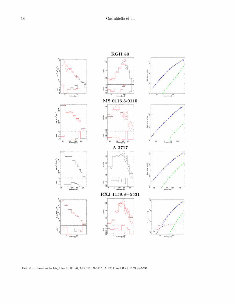
RGH 80
MS 0116.3-0115
A 2717
RXJ 1159.8+5531
Fig. 6.— Same as in Fig.3 for RGH 80, MS 0116.3-0115, A 2717 and RXJ 1159.8+5531.
Dark Matter and Gas Fraction in Galaxy Groups. 19
the inferred gas density and temperature in each radialbin.
The plasma code. Different plasma codes choose froma large, overlapping, but incomplete set of atomic data,leading to differences in the inferred abundances and,therefore, density and, to a lesser extent, temperature.We experimented with replacing the APEC model withthe MEKAL plasma model.
Bandwidth. To estimate the impact of the bandwidthon our fits, we experimented with fitting the data withdifferent lower limits for the energy band. In addition toour preferred choice of 0.5 keV, we use 0.4 keV and 0.7keV.
Hydrogen column-density. We take into ac-count possible deviations for NH from the value ofDickey & Lockman (1990) allowing the parameter tovary by ±25%.
9.3. Deprojection method
We analyzed the possible systematics involved withthe projection of 3D models using instead the “onion-peeling” technique (e.g., Fabian et al. 1981; Kriss et al.1983; Buote 2000b). Only for the object IC 1860 wedid not perform this exercise because of the exclusion ofan inner bin (see §8). The results were consistent withthe ones obtained by the 2D analysis (see Table 6) butwith larger error bars given the quality of the currentdata. This is the main reason for having adopted the 2Danalysis as our default. In Fig.7 we plot as a functionof the fraction of the virial radius the quantities ∆ρ/ρ3D
(where ∆ρ = ρ2D−ρ3D with ρ2D the value of the best fitmodel of the 2D analysis) and the corresponding quan-tity ∆T /T3D. The plotted errors are the fractional errorson the derived 3D quantities. There is more scatter inthe density as a consequence of larger uncertainties inthe derived 3D iron abundances, while the temperaturesdetermined with the two methods are generally consis-tent. This fact reinforces the notion that, for the range oftemperatures spanned by the objects considered in thispaper, the spectroscopic temperatures are not biased sig-nificantly (see discussion in §9.4, §10.5).
9.4. Response weighting
Since the effective area of the detector response ofACIS on Chandra and EPIC on XMM are a decreas-ing function of energy, fitting a 1T model to a spec-trum having a range of temperature components above∼ 3 keV will tend to yield a temperature that is biasedlow (Mazzotta et al. 2004; Vikhlinin 2006). This effectis negligible for average temperatures around 1 keV (seeAppendix B and Buote 2000c) as it is the case for the ob-jects in our sample. As a further systematic check we ap-plied a straightforward averaging of the plasma emissiv-ity over the detector response in our method as explainedin Appendix B. The results obtained using the responseweighting are very consistent with the ones obtained byour default projection analysis. For example, for NGC1550 we obtain c∆ = 4.5 ± 0.3, M∆ = 1.45 ± 0.03 × 10¹³
M⊙ and M⋆,∆ = 11.1 ± 4.0 × 10¹¹ M⊙; for MKW 4 weobtain c∆ = 5.1 ± 0.4, M∆ = 2.91 ± 0.10 × 10¹³ M⊙
and M⋆,∆ = 60.7 ± 7.3 × 10¹¹ M⊙; for NGC 533 we ob-tain c∆ = 5.3 ± 0.4, M∆ = 1.41 ± 0.06 × 10¹³ M⊙ andM⋆,∆ = 31.6 ± 2.1 × 10¹¹ M⊙.
9.5. Mass derivation method
For each system we tried all the three methods de-scribed in §6. By using all the approaches we have anestimate of the robustness of the inferred mass and virialquantities. We also include in this estimate the fact thatdifferent temperature and density profiles may be ableto fit the same data adequately but give rise to differentglobal halo parameters. To test this, we cycled througheach of our adopted gas density and temperature profiles.
9.6. X-ray asymmetries and disturbances
There are systems displaying low level asymmetries (IC1860), substructure (RGH 80), and AGN cavities (A 262)or possible AGN-induced disturbances (NGC 5044). Forthe objects which have a mild degree of disturbance inthe core we found that the results obtained excludingthe disturbed regions agreed with those obtained overthe entire radial range within the 1-2σ errors. For A262we excluded the inner 20 kpc to avoid (1) the cavitieswhich affect the central 10 kpc, and (2) the stellar masscomponent of the central galaxy. In this case fitting anNFW profile gives, c∆ = 2.4 ± 0.3 and M∆ = 3.44 ±0.15 × 10¹³ M⊙. For NGC 5044 we obtain c∆ = 3.9 ±0.1 and M∆ = 1.83 ± 0.04 × 10¹³ M⊙ after excludingthe central 5 kpc where there is evidence of a disturbedmorphology. We exclude the inner 30 kpc of RGH 80and find c∆ = 6.5 ± 1.0 and M∆ = 1.78 ± 0.08 × 10¹³
M⊙. Finally, for IC 1860 we perform a sector analysis,extracting spectra and re-deriving our mass profiles fromsuitably oriented semi-annuli, as detailed in §8. We foundconsistent results within their ∼ 2σ errors. Therefore, weinfer no systematic error associated with including thecentral, mildly disturbed, regions in these systems.
9.7. Radial Range & Extrapolation
It is customary to extrapolate mass profiles out tothe virial radius defined within an over-density ∆ ∼100 − 500. This facilitates a consistent comparison totheoretical studies which usually quote results in this ra-dial range, corresponding to the entire virialized portionof the halo. X-ray studies of global scaling relations be-tween mass, temperature, and luminosity also prefer touse such large virial radii to seek the tightest relationsbetween these global quantities.
However, extrapolating the mass profiles can lead tosystematic errors in cvir, Mvir, and the gas mass/fraction.Vikhlinin et al. (2006) argue that biased extrapolation ofthe gas density profiles is the main reason for the under-estimate of gravitational masses and low normalizationsof the M − T relations found with earlier X-ray tele-scopes (e.g., Nevalainen et al. 2000), using a β model fitfor the gas density and a polytropic approximation forthe temperature profile. Rasia et al. (2006) suggest thatthe same systematic error affects cvir, in the sense thata restricted radial range tends to return a higher cvir, inthe context of the NFW profile, than the value derivedusing data extending out to the virial radius.
Our procedure for mitigating extrapolation bias as-suming the halo follows an NFW profile is as follows. Weobtain the mass profile within an appropriate r∆ corre-sponding to the outer radius of the X-ray data for eachgroup. The values of c∆ and M∆ are extrapolated to∆ ≈ 101 assuming the NFW profile applies, using the
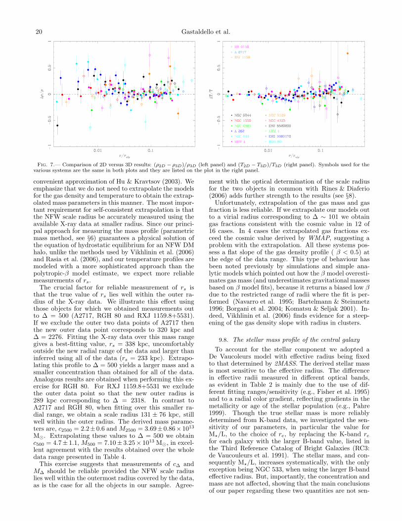
20 Gastaldello et al.
Fig. 7.— Comparison of 2D versus 3D results: (ρ2D − ρ3D)/ρ3D (left panel) and (T2D − T3D)/T3D (right panel). Symbols used for thevarious systems are the same in both plots and they are listed on the plot in the right panel.
convenient approximation of Hu & Kravtsov (2003). Weemphasize that we do not need to extrapolate the modelsfor the gas density and temperature to obtain the extrap-olated mass parameters in this manner. The most impor-tant requirement for self-consistent extrapolation is thatthe NFW scale radius be accurately measured using theavailable X-ray data at smaller radius. Since our princi-pal approach for measuring the mass profile (parametricmass method, see §6) guarantees a physical solution ofthe equation of hydrostatic equilibrium for an NFW DMhalo, unlike the methods used by Vikhlinin et al. (2006)and Rasia et al. (2006), and our temperature profiles aremodeled with a more sophisticated approach than thepolytropic-β model estimate, we expect more reliablemeasurements of rs.
The crucial factor for reliable measurement of rs isthat the true value of rs lies well within the outer ra-dius of the X-ray data. We illustrate this effect usingthose objects for which we obtained measurements outto ∆ = 500 (A2717, RGH 80 and RXJ 1159.8+5531).If we exclude the outer two data points of A2717 thenthe new outer data point corresponds to 320 kpc and∆ = 2276. Fitting the X-ray data over this mass rangegives a best-fitting value, rs = 338 kpc, uncomfortablyoutside the new radial range of the data and larger thaninferred using all of the data (rs = 233 kpc). Extrapo-lating this profile to ∆ = 500 yields a larger mass and asmaller concentration than obtained for all of the data.Analogous results are obtained when performing this ex-ercise for RGH 80. For RXJ 1159.8+5531 we excludethe outer data point so that the new outer radius is289 kpc corresponding to ∆ = 2318. In contrast toA2717 and RGH 80, when fitting over this smaller ra-dial range, we obtain a scale radius 131 ± 76 kpc, stillwell within the outer radius. The derived mass parame-ters are, c2500 = 2.2±0.6 and M2500 = 3.69±0.86×10¹³
M⊙. Extrapolating these values to ∆ = 500 we obtainc500 = 4.7± 1.1, M500 = 7.10± 3.25× 10¹³ M⊙, in excel-lent agreement with the results obtained over the wholedata range presented in Table 4.
This exercise suggests that measurements of c∆ andM∆ should be reliable provided the NFW scale radiuslies well within the outermost radius covered by the data,as is the case for all the objects in our sample. Agree-
ment with the optical determination of the scale radiusfor the two objects in common with Rines & Diaferio(2006) adds further strength to the results (see §8).
Unfortunately, extrapolation of the gas mass and gasfraction is less reliable. If we extrapolate our models outto a virial radius corresponding to ∆ ∼ 101 we obtaingas fractions consistent with the cosmic value in 12 of16 cases. In 4 cases the extrapolated gas fractions ex-ceed the cosmic value derived by WMAP, suggesting aproblem with the extrapolation. All these systems pos-sess a flat slope of the gas density profile ( β < 0.5) atthe edge of the data range. This type of behaviour hasbeen noted previously by simulations and simple ana-lytic models which pointed out how the β model overesti-mates gas mass (and underestimates gravitational massesbased on β model fits), because it returns a biased low βdue to the restricted range of radii where the fit is per-formed (Navarro et al. 1995; Bartelmann & Steinmetz1996; Borgani et al. 2004; Komatsu & Seljak 2001). In-deed, Vikhlinin et al. (2006) finds evidence for a steep-ening of the gas density slope with radius in clusters.
9.8. The stellar mass profile of the central galaxy
To account for the stellar component we adopted aDe Vaucoleurs model with effective radius being fixedto that determined by 2MASS. The derived stellar massis most sensitive to the effective radius. The differencein effective radii measured in different optical bands,as evident in Table 2 is mainly due to the use of dif-ferent fitting ranges/sensitivity (e.g., Fisher et al. 1995)and to a radial color gradient, reflecting gradients in themetallicity or age of the stellar population (e.g., Pahre1999). Though the true stellar mass is more reliablydetermined from K-band data, we investigated the sen-sitivity of our parameters, in particular the value forM⋆/L, to the choice of re, by replacing the K-band re
for each galaxy with the larger B-band value, listed inthe Third Reference Catalog of Bright Galaxies (RC3:de Vaucouleurs et al. 1991). The stellar mass, and con-sequently M⋆/L, increases systematically, with the onlyexception being NGC 533, when using the larger B-bandeffective radius. But, importantly, the concentration andmass are not affected, showing that the main conclusionsof our paper regarding these two quantities are not sen-
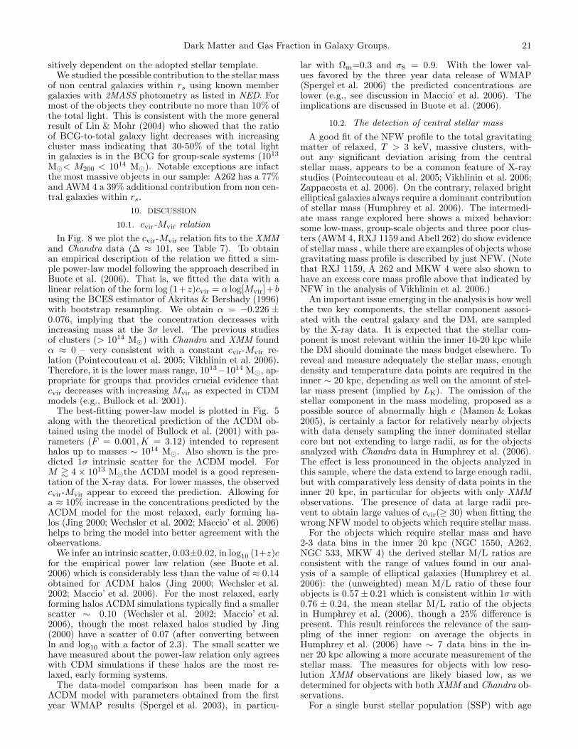
Dark Matter and Gas Fraction in Galaxy Groups. 21
sitively dependent on the adopted stellar template.We studied the possible contribution to the stellar mass
of non central galaxies within rs using known membergalaxies with 2MASS photometry as listed in NED. Formost of the objects they contribute no more than 10% ofthe total light. This is consistent with the more generalresult of Lin & Mohr (2004) who showed that the ratioof BCG-to-total galaxy light decreases with increasingcluster mass indicating that 30-50% of the total lightin galaxies is in the BCG for group-scale systems (1013
M⊙< M200 < 1014 M⊙). Notable exceptions are infactthe most massive objects in our sample: A262 has a 77%and AWM 4 a 39% additional contribution from non cen-tral galaxies within rs.
10. DISCUSSION
10.1. cvir-Mvir relation
In Fig. 8 we plot the cvir-Mvir relation fits to the XMMand Chandra data (∆ ≈ 101, see Table 7). To obtainan empirical description of the relation we fitted a sim-ple power-law model following the approach described inBuote et al. (2006). That is, we fitted the data with alinear relation of the form log (1+z)cvir = α log[Mvir]+busing the BCES estimator of Akritas & Bershady (1996)with bootstrap resampling. We obtain α = −0.226 ±0.076, implying that the concentration decreases withincreasing mass at the 3σ level. The previous studiesof clusters (> 1014 M⊙) with Chandra and XMM foundα ≈ 0 – very consistent with a constant cvir-Mvir re-lation (Pointecouteau et al. 2005; Vikhlinin et al. 2006).Therefore, it is the lower mass range, 1013−1014 M⊙, ap-propriate for groups that provides crucial evidence thatcvir decreases with increasing Mvir as expected in CDMmodels (e.g., Bullock et al. 2001).
The best-fitting power-law model is plotted in Fig. 5along with the theoretical prediction of the ΛCDM ob-tained using the model of Bullock et al. (2001) with pa-rameters (F = 0.001, K = 3.12) intended to representhalos up to masses ∼ 1014 M⊙. Also shown is the pre-dicted 1σ intrinsic scatter for the ΛCDM model. ForM & 4 × 10¹³ M⊙the ΛCDM model is a good represen-tation of the X-ray data. For lower masses, the observedcvir-Mvir appear to exceed the prediction. Allowing fora ≈ 10% increase in the concentrations predicted by theΛCDM model for the most relaxed, early forming ha-los (Jing 2000; Wechsler et al. 2002; Maccio’ et al. 2006)helps to bring the model into better agreement with theobservations.
We infer an intrinsic scatter, 0.03±0.02, in log10 (1+z)cfor the empirical power law relation (see Buote et al.2006) which is considerably less than the value of ≈ 0.14obtained for ΛCDM halos (Jing 2000; Wechsler et al.2002; Maccio’ et al. 2006). For the most relaxed, earlyforming halos ΛCDM simulations typically find a smallerscatter ∼ 0.10 (Wechsler et al. 2002; Maccio’ et al.2006), though the most relaxed halos studied by Jing(2000) have a scatter of 0.07 (after converting betweenln and log10 with a factor of 2.3). The small scatter wehave measured about the power-law relation only agreeswith CDM simulations if these halos are the most re-laxed, early forming systems.
The data-model comparison has been made for aΛCDM model with parameters obtained from the firstyear WMAP results (Spergel et al. 2003), in particu-
lar with Ωm=0.3 and σ8 = 0.9. With the lower val-ues favored by the three year data release of WMAP(Spergel et al. 2006) the predicted concentrations arelower (e.g., see discussion in Maccio’ et al. 2006). Theimplications are discussed in Buote et al. (2006).
10.2. The detection of central stellar mass
A good fit of the NFW profile to the total gravitatingmatter of relaxed, T > 3 keV, massive clusters, with-out any significant deviation arising from the centralstellar mass, appears to be a common feature of X-raystudies (Pointecouteau et al. 2005; Vikhlinin et al. 2006;Zappacosta et al. 2006). On the contrary, relaxed brightelliptical galaxies always require a dominant contributionof stellar mass (Humphrey et al. 2006). The intermedi-ate mass range explored here shows a mixed behavior:some low-mass, group-scale objects and three poor clus-ters (AWM 4, RXJ 1159 and Abell 262) do show evidenceof stellar mass , while there are examples of objects whosegravitating mass profile is described by just NFW. (Notethat RXJ 1159, A 262 and MKW 4 were also shown tohave an excess core mass profile above that indicated byNFW in the analysis of Vikhlinin et al. 2006.)
An important issue emerging in the analysis is how wellthe two key components, the stellar component associ-ated with the central galaxy and the DM, are sampledby the X-ray data. It is expected that the stellar com-ponent is most relevant within the inner 10-20 kpc whilethe DM should dominate the mass budget elsewhere. Toreveal and measure adequately the stellar mass, enoughdensity and temperature data points are required in theinner ∼ 20 kpc, depending as well on the amount of stel-lar mass present (implied by LK). The omission of thestellar component in the mass modeling, proposed as apossible source of abnormally high c (Mamon & Lokas2005), is certainly a factor for relatively nearby objectswith data densely sampling the inner dominated stellarcore but not extending to large radii, as for the objectsanalyzed with Chandra data in Humphrey et al. (2006).The effect is less pronounced in the objects analyzed inthis sample, where the data extend to large enough radii,but with comparatively less density of data points in theinner 20 kpc, in particular for objects with only XMMobservations. The presence of data at large radii pre-vent to obtain large values of cvir(≥ 30) when fitting thewrong NFW model to objects which require stellar mass.
For the objects which require stellar mass and have2-3 data bins in the inner 20 kpc (NGC 1550, A262,NGC 533, MKW 4) the derived stellar M/L ratios areconsistent with the range of values found in our anal-ysis of a sample of elliptical galaxies (Humphrey et al.2006): the (unweighted) mean M/L ratio of these fourobjects is 0.57 ± 0.21 which is consistent within 1σ with0.76 ± 0.24, the mean stellar M/L ratio of the objectsin Humphrey et al. (2006), though a 25% difference ispresent. This result reinforces the relevance of the sam-pling of the inner region: on average the objects inHumphrey et al. (2006) have ∼ 7 data bins in the in-ner 20 kpc allowing a more accurate measurement of thestellar mass. The measures for objects with low reso-lution XMM observations are likely biased low, as wedetermined for objects with both XMM and Chandra ob-servations.
For a single burst stellar population (SSP) with age
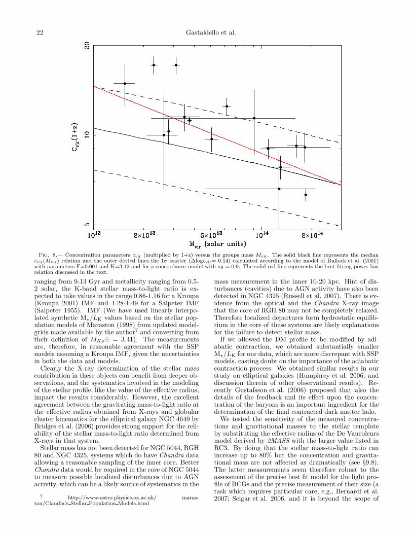
22 Gastaldello et al.
Fig. 8.— Concentration parameters cvir (multiplied by 1+z) versus the groups mass Mvir. The solid black line represents the mediancvir(Mvir) relation and the outer dotted lines the 1σ scatter (∆logcvir= 0.14) calculated according to the model of Bullock et al. (2001)with parameters F=0.001 and K=3.12 and for a concordance model with σ8 = 0.9. The solid red line represents the best fitting power lawrelation discussed in the text.
ranging from 9-13 Gyr and metallicity ranging from 0.5-2 solar, the K-band stellar mass-to-light ratio is ex-pected to take values in the range 0.86-1.16 for a Kroupa(Kroupa 2001) IMF and 1.28-1.49 for a Salpeter IMF(Salpeter 1955). IMF (We have used linearly interpo-lated synthetic M⋆/LK values based on the stellar pop-ulation models of Maraston (1998) from updated model-grids made available by the author7 and converting fromtheir definition of MKs⊙ = 3.41). The measurementsare, therefore, in reasonable agreement with the SSPmodels assuming a Kroupa IMF, given the uncertaintiesin both the data and models.
Clearly the X-ray determination of the stellar masscontribution in these objects can benefit from deeper ob-servations, and the systematics involved in the modelingof the stellar profile, like the value of the effective radius,impact the results considerably. However, the excellentagreement between the gravitating mass-to-light ratio atthe effective radius obtained from X-rays and globularcluster kinematics for the elliptical galaxy NGC 4649 byBridges et al. (2006) provides strong support for the reli-ability of the stellar mass-to-light ratio determined fromX-rays in that system.
Stellar mass has not been detected for NGC 5044, RGH80 and NGC 4325, systems which do have Chandra dataallowing a reasonable sampling of the inner core. BetterChandra data would be required in the core of NGC 5044to measure possible localized disturbances due to AGNactivity, which can be a likely source of systematics in the
7 http://www-astro.physics.ox.ac.uk/ maras-ton/Claudia’s Stellar Population Models.html
mass measurement in the inner 10-20 kpc. Hint of dis-turbances (cavities) due to AGN activity have also beendetected in NGC 4325 (Russell et al. 2007). There is ev-idence from the optical and the Chandra X-ray imagethat the core of RGH 80 may not be completely relaxed.Therefore localized departures form hydrostatic equilib-rium in the core of these systems are likely explanationsfor the failure to detect stellar mass.
If we allowed the DM profile to be modified by adi-abatic contraction, we obtained substantially smallerM⋆/LK for our data, which are more discrepant with SSPmodels, casting doubt on the importance of the adiabaticcontraction process. We obtained similar results in ourstudy on elliptical galaxies (Humphrey et al. 2006, anddiscussion therein of other observational results). Re-cently Gustafsson et al. (2006) proposed that also thedetails of the feedback and its effect upon the concen-tration of the baryons is an important ingredient for thedetermination of the final contracted dark matter halo.
We tested the sensitivity of the measured concentra-tions and gravitational masses to the stellar templateby substituting the effective radius of the De Vaucoleursmodel derived by 2MASS with the larger value listed inRC3. By doing that the stellar mass-to-light ratio canincrease up to 80% but the concentration and gravita-tional mass are not affected as dramatically (see §9.8).The latter measurements seem therefore robust to theassessment of the precise best fit model for the light pro-file of BCGs and the precise measurement of their size (atask which requires particular care, e.g., Bernardi et al.2007; Seigar et al. 2006, and it is beyond the scope of
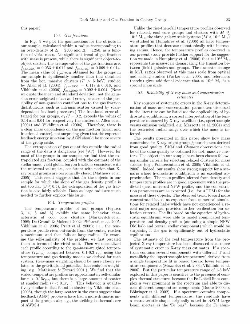
Dark Matter and Gas Fraction in Galaxy Groups. 23
this paper).
10.3. Gas fractions
In Fig. 9 we plot the gas fractions for the objects inour sample, calculated within a radius corresponding toan over-density of ∆ = 2500 and ∆ = 1250, as a func-tion of virial mass. No significant trend of gas fractionwith mass is present, while there is significant object-to-object scatter: the average value of the gas fractions are,fgas,2500 = 0.053 ± 0.012 and fgas,1250 = 0.069 ± 0.014.The mean value of fgas,2500 obtained for the groups inour sample is significantly smaller than that obtainedfrom the hot, massive clusters (T > 5 keV) studiedby Allen et al. (2004), fgas,2500 = 0.118 ± 0.016, andVikhlinin et al. (2006), fgas,2500 = 0.092 ± 0.004. (Notewe quote the mean and standard deviation, not the gaus-sian error-weighted mean and error, because of the pos-sibility of non-gaussian contributions to the gas fractiondistributions, such as intrinsic scatter caused by scale-dependent feedback processes.) The fractional error ob-tained for our groups, σf/f = 0.2, exceeds the values of0.14 and 0.04 for, respectively the clusters of Allen et al.(2004) and Vikhlinin et al. (2006). Therefore, there isa clear mass dependence on the gas fraction (mean andfractional scatter), not surprising given that the expectedfeedback energy injection by AGN should be more severeat the group scale.
The extrapolation of gas quantities outside the radialrange of the data is dangerous (see §9.7). However, formost of the groups in our sample, we find that the ex-trapolated gas fraction, coupled with the estimate of thestellar mass, yield global baryon fractions consistent withthe universal value; i.e., consistent with notion that X-ray bright groups are baryonically closed (Mathews et al.2005). This result suggests that for the objects in oursample for which the slope of the gas density profile isnot too flat (β & 0.5), the extrapolation of the gas frac-tion is also fairly reliable. Data at large radii are muchneeded to further explore this issue.
10.4. Temperature profiles
The temperature profiles of our groups (Figures3, 4, 5 and 6) exhibit the same behavior char-acteristic of cool core clusters (Markevitch et al.1998; De Grandi & Molendi 2002; Piffaretti et al. 2005;Vikhlinin et al. 2005; Pratt et al. 2006); i.e., the tem-perature profile rises outwards from the center, reachesa maximum, and then falls at large radius. To exam-ine the self-similarity of the profiles, we first rescaledthem in terms of the virial radii. Then we normalizedeach profile according to the gas-mass-weighted temper-ature (Tgmw) computed between 0.1-0.3 rvir using thetemperature and gas density models we derived for eachsystem. (Gas-mass weighting should be more closely re-lated to the gravitational potential than emission weight-ing, e.g., Mathiesen & Evrard 2001.) We find that thescaled temperature profiles are approximately self-similarfor r > 0.15rvir, but there is a large amount of scatterat smaller radii (r < 0.1rvir). This behavior is qualita-tively similar to that found in clusters by Vikhlinin et al.(2006), though the large scatter in the cores suggest thatfeedback (AGN) processes have had a more dramatic im-pact at the group scale; e.g., the striking isothermal coreof AWM 4.
Unlike the rise-then-fall temperature profiles observedfor relaxed, cool core groups and clusters with M &1013 M⊙, the three galaxy scale systems (M < 1013 M⊙)we studied in Humphrey et al. (2006) all have temper-ature profiles that decrease monotonically with increas-ing radius. Hence, the temperature profiles observed inour present study provide further support for the sugges-tion we made in Humphrey et al. (2006) that ≈ 1013 M⊙
represents the mass-scale demarcating the transition be-tween (field) galaxies and groups. The dramatic changein M/L ratios observed at this mass scale from opticaland lensing studies (Parker et al. 2005, and referencestherein) gives additional evidence that ≈ 1013 M⊙ is aspecial mass scale.
10.5. Reliability of X-ray mass and concentrationestimates
Key sources of systematic errors in the X-ray determi-nation of mass and concentration parameters discussedin the literature can be listed as: the applicability of hy-drostatic equilibrium, a correct interpretation of the tem-perature measured by X-ray satellites (i.e., spectroscopicversus emission weighted, e.g. Mazzotta et al. 2004) andthe restricted radial range over which the mass is in-ferred.
The results presented in this paper show how massconstraints for X-ray bright groups/poor clusters derivedfrom good quality XMM and Chandra observations canbe of the same quality as obtained for hot, massive clus-ters. The objects in our sample have been chosen follow-ing similar criteria for selecting relaxed clusters for massstudies (e.g., Pointecouteau et al. 2005; Vikhlinin et al.2006). Indeed, our results show strong support for a sce-nario where hydrostatic equilibrium is an excellent ap-proximation. The mass profiles inferred from density andtemperature profiles are in good agreement with the pre-dicted quasi-universal NFW profile, and the concentra-tion parameters are as expected (i.e., for ΛCDM) for themasses of these objects. The observed trend toward moreconcentrated halos, as expected from numerical simula-tions for relaxed halos which have not experienced a re-cent major merger, provides further verification our se-lection criteria. The fits based on the equation of hydro-static equilibrium were able to model complicated tem-perature and density profiles (assuming a simple NFWDM halo and central stellar component) which would besurprising if the gas is significantly out of hydrostaticequilibrium.
The estimate of the real temperature from the pro-jected X-ray temperature has been discussed as a sourceof systematic error in X-ray mass estimates. If a spec-trum contains several components with different T andmetallicity the “spectroscopic temperature” derived froma single temperature fit is biased toward lower temper-ature components (Mazzotta et al. 2004; Vikhlinin et al.2006). But the particular temperature range of 1-3 keVexplored in this paper is sensitive to the presence of com-plex thermal structure, because the Fe-L shell lines com-plex is very prominent in the spectrum and able to dis-cern different temperature components (Buote 2000c,b;Bohringer et al. 2002). If a spectrum contains compo-nents with different temperatures, the residuals havea characteristic shape, originally noted in ASCA largebeam spectra as the ‘Fe bias”, because the Fe abun-
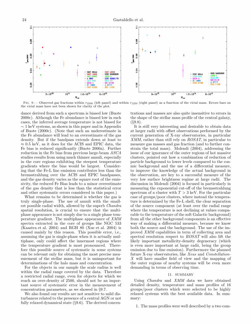
24 Gastaldello et al.
Fig. 9.— Observed gas fractions within r2500 (left panel) and within r1250 (right panel) as a function of the virial mass. Errors bars onthe virial mass have not been shown for clarity of the plot.
dance derived from such a spectrum is biased low (Buote2000c). Although the Fe abundance is biased low in suchcases, the inferred average temperature is not biased for∼ 1 keV systems, as shown in this paper and in Appendixof Buote (2000c). (Note that such an underestimate inthe Fe abundance will lead to an overestimate of the gasdensity. But if the bandpass extends down at least to≈ 0.5 keV, as it does for the ACIS and EPIC data, theFe bias is reduced significantly (Buote 2000a). Furtherreduction in the Fe bias from previous large-beam ASCAstudies results from using much thinner annuli, especiallyin the core regions exhibiting the steepest temperaturegradients where the bias would be largest. Consider-ing that the Fe-L line emission contributes less than thebremsstrahlung over the ACIS and EPIC bandpasses,and the gas density varies as the square root of the emis-sivity, the reduced Fe Bias leads to a minor overestimateof the gas density that is less than the statistical errorand other systematic errors considered in this paper.)
What remains to be determined is whether the gas istruly single-phase. The use of annuli with the small-est possible radial width, allowed by the superb Chandraspatial resolution, is crucial to ensure that the multi-phase appearance is not simply due to a single phase tem-perature gradient. The multiphase appearance of XMMspectra extracted in the core of groups like NGC 533(Kaastra et al. 2004) and RGH 80 (Xue et al. 2004) iscaused mainly by this reason. This possible error, i.e.,assuming the gas is single-phase when it is actually mul-tiphase, only could affect the innermost regions wherethe temperature gradient is most pronounced. There-fore this possible source of systematic in some systemscan be relevant only for obtaining the most precise mea-surement of the stellar mass, but it is unimportant fordeterminations of the halo mass and concentration.
For the objects in our sample the scale radius is wellwithin the radial range covered by the data. Thereforea restricted radial range, even for objects for which wereach an over-density of 2500, should not be an impor-tant source of systematic error in the measurement ofconcentration parameters, as we showed in §9.7.
We also found our results are not sensitive to mild dis-turbances related to the presence of a central AGN or notfully relaxed dynamical state (§9.6). The derived concen-
trations and masses are also quite insensitive to errors inthe shape of the stellar mass profile of the central galaxy,(§9.8).
It is still very interesting and desirable to obtain dataat larger radii with offset observations performed by thecurrent generation of X-ray observatories, in particularXMM, rather than still rely on ROSAT, in particular tomeasure gas masses and gas fraction (and to further con-strain the total mass). Molendi (2004), addressing theissue of our ignorance of the outer regions of hot massiveclusters, pointed out how a combination of reduction ofparticle background to lower levels compared to the cos-mic background and the use of a differential measure,to improve the knowledge of the actual background inthe observation, are key to a successful measure of thevery low surface brightness regime at large radii. Thediscussion in Molendi (2004) is focused in particularly inmeasuring the exponential cut-off of the bremsstrahlungspectrum of a cluster with T > 3 keV. For the particularcase of groups/poor clusters, where instead the tempera-ture is determined by the Fe-L shell, the clear separationof the source component (at least over the radial rangewhere the temperature is not declining at values compa-rable to the temperature of the soft Galactic background)from all the other background components is an effectiveway of making a differential measure, because we knowboth the source and the background. The use of the im-proved XMM capabilities in term of collecting area andspectral resolution respect to ROSAT will also lift thelikely important metallicity-density degeneracy (whichis even more important at large radii, being the groupemission due to line emission). Furthermore the plannedfuture X-ray observatories, like Xeus and Constellation-X will have smaller field of view and the mapping ofthe outer regions of nearby systems will be even moredemanding in terms of observing time.
11. SUMMARY
Using Chandra and XMM data we have obtaineddetailed density, temperature and mass profiles of 16groups/poor clusters which were selected to be highlyrelaxed systems with the best available data. In sum-mary:
1. The mass profiles were well described by a two com-
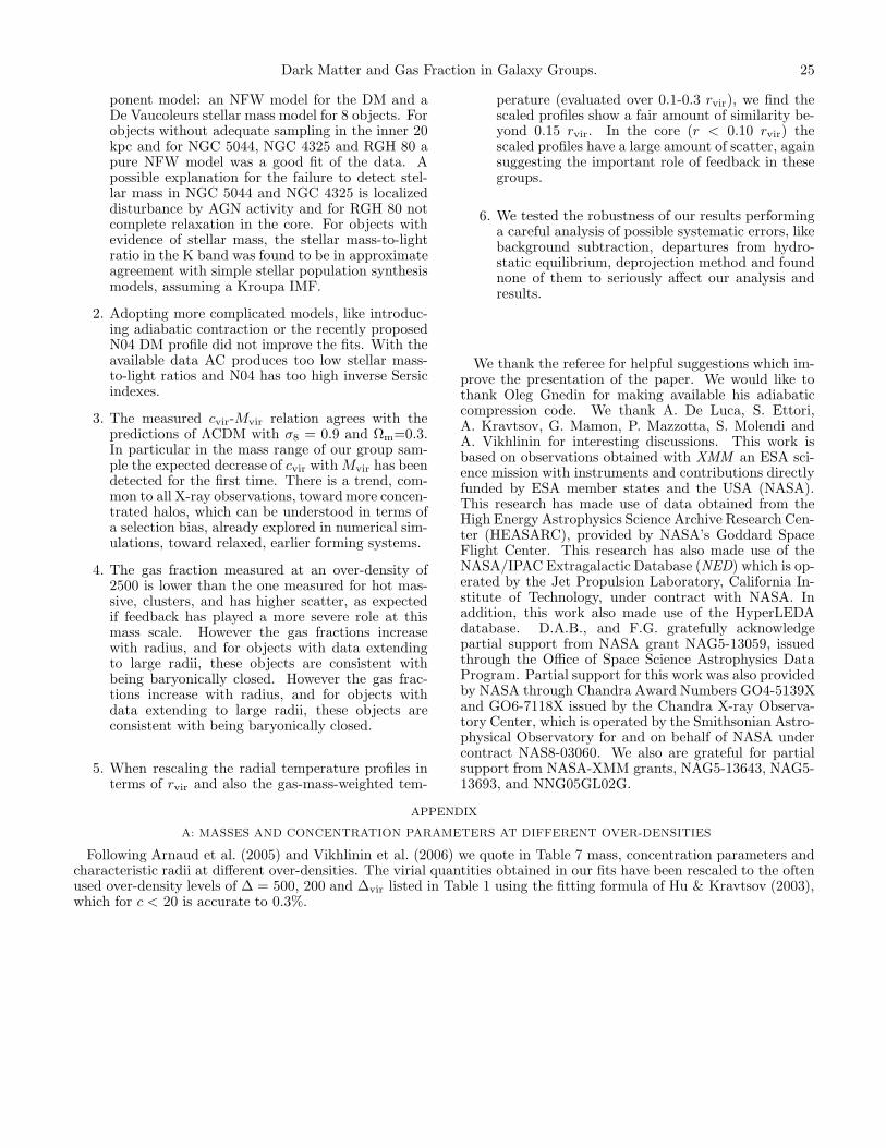
Dark Matter and Gas Fraction in Galaxy Groups. 25
ponent model: an NFW model for the DM and aDe Vaucoleurs stellar mass model for 8 objects. Forobjects without adequate sampling in the inner 20kpc and for NGC 5044, NGC 4325 and RGH 80 apure NFW model was a good fit of the data. Apossible explanation for the failure to detect stel-lar mass in NGC 5044 and NGC 4325 is localizeddisturbance by AGN activity and for RGH 80 notcomplete relaxation in the core. For objects withevidence of stellar mass, the stellar mass-to-lightratio in the K band was found to be in approximateagreement with simple stellar population synthesismodels, assuming a Kroupa IMF.
2. Adopting more complicated models, like introduc-ing adiabatic contraction or the recently proposedN04 DM profile did not improve the fits. With theavailable data AC produces too low stellar mass-to-light ratios and N04 has too high inverse Sersicindexes.
3. The measured cvir-Mvir relation agrees with thepredictions of ΛCDM with σ8 = 0.9 and Ωm=0.3.In particular in the mass range of our group sam-ple the expected decrease of cvir with Mvir has beendetected for the first time. There is a trend, com-mon to all X-ray observations, toward more concen-trated halos, which can be understood in terms ofa selection bias, already explored in numerical sim-ulations, toward relaxed, earlier forming systems.
4. The gas fraction measured at an over-density of2500 is lower than the one measured for hot mas-sive, clusters, and has higher scatter, as expectedif feedback has played a more severe role at thismass scale. However the gas fractions increasewith radius, and for objects with data extendingto large radii, these objects are consistent withbeing baryonically closed. However the gas frac-tions increase with radius, and for objects withdata extending to large radii, these objects areconsistent with being baryonically closed.
5. When rescaling the radial temperature profiles interms of rvir and also the gas-mass-weighted tem-
perature (evaluated over 0.1-0.3 rvir), we find thescaled profiles show a fair amount of similarity be-yond 0.15 rvir. In the core (r < 0.10 rvir) thescaled profiles have a large amount of scatter, againsuggesting the important role of feedback in thesegroups.
6. We tested the robustness of our results performinga careful analysis of possible systematic errors, likebackground subtraction, departures from hydro-static equilibrium, deprojection method and foundnone of them to seriously affect our analysis andresults.
We thank the referee for helpful suggestions which im-prove the presentation of the paper. We would like tothank Oleg Gnedin for making available his adiabaticcompression code. We thank A. De Luca, S. Ettori,A. Kravtsov, G. Mamon, P. Mazzotta, S. Molendi andA. Vikhlinin for interesting discussions. This work isbased on observations obtained with XMM an ESA sci-ence mission with instruments and contributions directlyfunded by ESA member states and the USA (NASA).This research has made use of data obtained from theHigh Energy Astrophysics Science Archive Research Cen-ter (HEASARC), provided by NASA’s Goddard SpaceFlight Center. This research has also made use of theNASA/IPAC Extragalactic Database (NED) which is op-erated by the Jet Propulsion Laboratory, California In-stitute of Technology, under contract with NASA. Inaddition, this work also made use of the HyperLEDAdatabase. D.A.B., and F.G. gratefully acknowledgepartial support from NASA grant NAG5-13059, issuedthrough the Office of Space Science Astrophysics DataProgram. Partial support for this work was also providedby NASA through Chandra Award Numbers GO4-5139Xand GO6-7118X issued by the Chandra X-ray Observa-tory Center, which is operated by the Smithsonian Astro-physical Observatory for and on behalf of NASA undercontract NAS8-03060. We also are grateful for partialsupport from NASA-XMM grants, NAG5-13643, NAG5-13693, and NNG05GL02G.
APPENDIX
A: MASSES AND CONCENTRATION PARAMETERS AT DIFFERENT OVER-DENSITIES
Following Arnaud et al. (2005) and Vikhlinin et al. (2006) we quote in Table 7 mass, concentration parameters andcharacteristic radii at different over-densities. The virial quantities obtained in our fits have been rescaled to the oftenused over-density levels of ∆ = 500, 200 and ∆vir listed in Table 1 using the fitting formula of Hu & Kravtsov (2003),which for c < 20 is accurate to 0.3%.
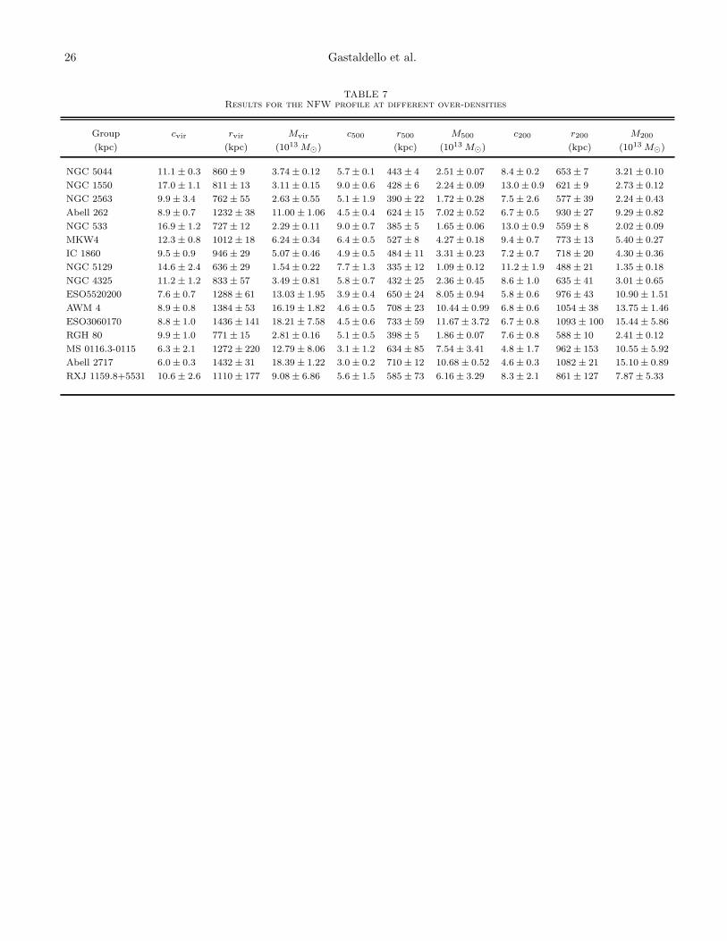
26 Gastaldello et al.
TABLE 7Results for the NFW profile at different over-densities
Group cvir rvir Mvir c500 r500 M500 c200 r200 M200
(kpc) (kpc) (1013 M⊙) (kpc) (1013 M⊙) (kpc) (1013 M⊙)
NGC 5044 11.1 ± 0.3 860 ± 9 3.74 ± 0.12 5.7 ± 0.1 443 ± 4 2.51 ± 0.07 8.4 ± 0.2 653 ± 7 3.21 ± 0.10
NGC 1550 17.0 ± 1.1 811 ± 13 3.11 ± 0.15 9.0 ± 0.6 428 ± 6 2.24 ± 0.09 13.0 ± 0.9 621 ± 9 2.73 ± 0.12
NGC 2563 9.9 ± 3.4 762 ± 55 2.63 ± 0.55 5.1 ± 1.9 390 ± 22 1.72 ± 0.28 7.5 ± 2.6 577 ± 39 2.24 ± 0.43
Abell 262 8.9 ± 0.7 1232 ± 38 11.00 ± 1.06 4.5 ± 0.4 624 ± 15 7.02 ± 0.52 6.7 ± 0.5 930 ± 27 9.29 ± 0.82
NGC 533 16.9 ± 1.2 727 ± 12 2.29 ± 0.11 9.0 ± 0.7 385 ± 5 1.65 ± 0.06 13.0 ± 0.9 559 ± 8 2.02 ± 0.09
MKW4 12.3 ± 0.8 1012 ± 18 6.24 ± 0.34 6.4 ± 0.5 527 ± 8 4.27 ± 0.18 9.4 ± 0.7 773 ± 13 5.40 ± 0.27
IC 1860 9.5 ± 0.9 946 ± 29 5.07 ± 0.46 4.9 ± 0.5 484 ± 11 3.31 ± 0.23 7.2 ± 0.7 718 ± 20 4.30 ± 0.36
NGC 5129 14.6 ± 2.4 636 ± 29 1.54 ± 0.22 7.7 ± 1.3 335 ± 12 1.09 ± 0.12 11.2 ± 1.9 488 ± 21 1.35 ± 0.18
NGC 4325 11.2 ± 1.2 833 ± 57 3.49 ± 0.81 5.8 ± 0.7 432 ± 25 2.36 ± 0.45 8.6 ± 1.0 635 ± 41 3.01 ± 0.65
ESO5520200 7.6 ± 0.7 1288 ± 61 13.03 ± 1.95 3.9 ± 0.4 650 ± 24 8.05 ± 0.94 5.8 ± 0.6 976 ± 43 10.90 ± 1.51
AWM 4 8.9 ± 0.8 1384 ± 53 16.19 ± 1.82 4.6 ± 0.5 708 ± 23 10.44 ± 0.99 6.8 ± 0.6 1054 ± 38 13.75 ± 1.46
ESO3060170 8.8 ± 1.0 1436 ± 141 18.21 ± 7.58 4.5 ± 0.6 733 ± 59 11.67 ± 3.72 6.7 ± 0.8 1093 ± 100 15.44 ± 5.86
RGH 80 9.9 ± 1.0 771 ± 15 2.81 ± 0.16 5.1 ± 0.5 398 ± 5 1.86 ± 0.07 7.6 ± 0.8 588 ± 10 2.41 ± 0.12
MS 0116.3-0115 6.3 ± 2.1 1272 ± 220 12.79 ± 8.06 3.1 ± 1.2 634 ± 85 7.54 ± 3.41 4.8 ± 1.7 962 ± 153 10.55 ± 5.92
Abell 2717 6.0 ± 0.3 1432 ± 31 18.39 ± 1.22 3.0 ± 0.2 710 ± 12 10.68 ± 0.52 4.6 ± 0.3 1082 ± 21 15.10 ± 0.89
RXJ 1159.8+5531 10.6 ± 2.6 1110 ± 177 9.08 ± 6.86 5.6 ± 1.5 585 ± 73 6.16 ± 3.29 8.3 ± 2.1 861 ± 127 7.87 ± 5.33
Dark Matter and Gas Fraction in Galaxy Groups. 27
B: RELATING X-RAY OBSERVATIONS TO SPHERICAL MODELS OF CORONAL GAS WITH VARIABLE PLASMAEMISSIVITY
We relate the spherical models of density (ρg) and temperature (T ) of the hot gas in elliptical galaxies, galaxy groups,and clusters (§6) to the parameters obtained from conventional spectral fitting of X-ray data, such as from Chandraand XMM. Since much of the relevant material is scattered throughout the literature spanning over at least 30 years,this appendix provides an opportunity to give a self-contained, up-to-date presentation. Our treatment fully accountsfor radial variations of the plasma emissivity which are often neglected, especially when inferring the gas density. Wefollow the standard procedure where emission from coronal plasma characterized by a single temperature (1T) is fittedto the X-ray spectrum extracted from a circular annulus (2D) or, if the data have been deprojected, a spherical shell(3D). The density and temperature (and abundance) parameters obtained from such a 1T fit are compared to theemission-weighted (and projected if 2D) spherical models of ρg and T (and abundances). It is assumed the annuliare chosen to be sufficiently wide so that the detector point spread function may be neglected. We discuss additionalweighting by detector responses at the end of this section.
For any spectral quantity, such as luminosity (erg s−1), that results from integrating between photon energy E1 toenergy E2, we use the notation,
L(∆E) ≡∫ E2
E1
dL
dEdE, (B1)
to represent the bandpass integration. For a coronal plasma emitting within a volume Vi at a temperature Ti withchemical abundances ZFe,i, ZO,i, ZSi,i, etc. the luminosity is given in xspec by,
L(∆E)i = 4π [DA (1 + z)]2
normiΛxs(Ti, Zi; ∆E), (B2)
where we have used the symbol Zi to represent all the abundances, z is the redshift, DA is the angular diameterdistance (cm), and Λxs is the plasma emissivity (erg s−1 cm3) corresponding to the xspec implementation of therelevant coronal plasma code (e.g., apec, mekal). To give a precise definition8 of normi that accounts for spatialvariations of the temperature and abundances within Vi, we refer to the volume emissivity (erg s−1 cm−3 ) of a coronalplasma,
ǫ(~x; ∆E) = ne(~x)nH(~x)Λ(T (~x), Z(~x); ∆E), (B3)
where, e.g., T (~x) ≡ T (x, y, z), and the plasma emissivity in xspec is related to the conventional definition9 by,Λxs ≡ 1014Λ. It is convenient to work in terms of the volume mass density of the gas, ρg(~x), rather than the volumenumber densities, ne(~x) and nH(~x), separately. To a very good approximation, for this calculation one may assume afully ionized gas of pure H and He in which case,
ne =2 + µ
5µ
ρg
mu, nH =
4 − 3µ
5µ
ρg
mu, (B4)
where µ is the mean atomic weight of the gas and mu is the atomic mass unit. (Note that using µ = 0.62 correspondingto the solar He abundance leads to ne = 1.22nH.) By setting equation [B2] equal to the luminosity obtained byintegrating equation [B3] over the volume Vi and solving for normi one finds,
normi =
[
10−14
4π[DA(1 + z)]2(2 + µ)(4 − 3µ)
(5µ)2m2u
]
1
Λxs(Ti, Zi; ∆E)
∫
Vi
ρ2g(~x)Λxs(T (~x), Z(~x); ∆E)d3x, (B5)
where normi ∝∫
ρ2gd3x if Λxs is constant over the volume Vi. If Λxs varies over the volume, then the parameters Ti
and Zi obtained from fitting a 1T coronal plasma model to the spectrum with multiple temperatures and abundanceswill reflect average quantities weighted by the emission profile within the volume and the detector response. We defertreatment of the detector response to the end of this section and focus now on the deprojection and projection ofemission-weighted spherical quantities.
Deprojection Analysis: If the spectra are deprojected so that the normi values refer to spherical shells, then equation[B5] can be immediately recast in terms of the weighted square of the gas density,
〈ρ2g〉i ≡
[
4π[DA(1 + z)]2
10−14
(5µ)2m2u
(2 + µ)(4 − 3µ)
]
normi
Vi(B6)
=1
Λxs(Ti, Zi; ∆E)
3
(r3i − r3
i−1)
∫ ri
ri−1
ρ2g(r)Λxs(T (r), Z(r); ∆E)r2dr, (B7)
where Vi = 4π3 (r3
i − r3i−1) is the volume of the spherical shell. Note, however, that many deprojection programs like
projct in xspec and others based on the widely used “onion peeling” deprojection method (Fabian et al. 1981) givenormi with respect to the volume, 4π
3 (r2i − r2
i−1)3/2, representing the intersection of the 3D shell with the cylinder of
8 In the xspec Users’ Manual, normi is called K. But the term “norm” is actually displayed for this parameter for the coronal plasmamodels like apec.
9 This expression is not given in the xspec Users’ Manual, but it follows from the definition of normi (i.e., K) in that manual.
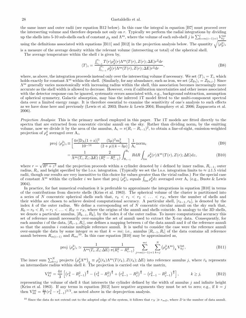
28 Gastaldello et al.
the same inner and outer radii (see equation B12 below). In this case the integral in equation [B7] must proceed overthe intersecting volume and therefore depends not only on r. Typically we perform the radial integrations by dividing
up the shells into 5-10 sub-shells each of constant ρg and Λxs, where the volume of each sub-shell j is∑j
k=m(i−1)+1 V intkj
using the definitions associated with equations [B11] and [B12] in the projection analysis below. The quantity√
〈ρ2g〉i
is a measure of the average density within the relevant volume (intersecting or total) of the spherical shell.The average temperature within the shell i is given by,
〈T 〉i =
∫ ri
ri−1T (r)ρ2
g(r)Λxs(T (r), Z(r); ∆E)r2dr∫ ri
ri−1ρ2
g(r)Λxs(T (r), Z(r); ∆E)r2dr, (B8)
where, as above, the integration proceeds instead only over the intersecting volume if necessary. We set 〈T 〉i = Ti, whichholds exactly for constant Λxs within the shell. (Similarly, for any abundance, such as iron, we set 〈ZFe〉i = ZFe,i.) SinceΛxs generally varies monotonically with increasing radius within the shell, this association becomes increasingly moreaccurate as the shell width is allowed to decrease. However, even if calibration uncertainties and other issues associatedwith the detector response can be ignored, systematic errors associated with, e.g., background subtraction, assumptionof spherical symmetry, Galactic absorption, may bias the inferred 1T model fitted to the multi-component spectraldata over a limited energy range. It is therefore essential to examine the sensitivity of one’s analysis to such effectsas we have done here and previously (Lewis et al. 2003; Buote & Lewis 2004; Humphrey et al. 2006; Zappacosta et al.2006).
Projection Analysis: This is the primary method employed in this paper. The 1T models are fitted directly to thespectra that are extracted from concentric circular annuli on the sky. Rather than dividing normi by the emittingvolume, now we divide it by the area of the annulus, Ai = π(Ri − Ri−1)2, to obtain a line-of-sight, emission-weightedprojection of ρ2
g averaged over Ai,
proj 〈ρ2g〉i ≡
[
4π[DA(1 + z)]2
10−14
(5µ)2m2u
(2 + µ)(4 − 3µ)
]
1
Ainormi (B9)
=1
Λxs(Ti, Zi; ∆E)
2
(R2i − R2
i−1)
∫ Ri
Ri−1
RdR
∫
los
ρ2g(r)Λxs(T (r), Z(r); ∆E)dz, (B10)
where r =√
R2 + z2 and the projection proceeds within a cylinder denoted by i defined by inner radius, Ri−1, outerradius, Ri, and height specified by the l.o.s. integration. (Typically we set the l.o.s. integration limits to ≈ ±1.5 virialradii, though our results are very insensitive to this choice for values greater than the virial radius.) For the special caseof constant Λxs within the cylinder i we have that proj 〈ρ2
g〉i equals∫
losρ2
gdz averaged over Ai (e.g., Buote & Lewis2004).
In practice, for fast numerical evaluation it is preferable to approximate the integrations in equation [B10] in termsof the contributions from discrete shells (Kriss et al. 1983). The spherical volume of the cluster is partitioned intoa series of N concentric spherical shells such that, r0 < r1 < r2 < . . . < rN , where the number of shells andtheir widths are chosen to achieve desired computational accuracy. A particular shell, [rk−1, rk], is denoted by theindex k of the outer radius. We define a corresponding set of N concentric circular annuli on the sky such that,R0 = r0 < R1 = r1 < . . . < RN = rN , where the origins of the annuli and shells coincide. In analogy to the 3D shells,we denote a particular annulus, [Rk−1, Rk], by the index k of the outer radius. To insure computational accuracy thisset of reference annuli necessarily over-samples the set of annuli used to extract the X-ray data. Consequently, foreach annulus i of the data, [Ri−1, Ri], one defines a mapping between i of the data annuli and k of the reference annuliso that the annulus i contains multiple reference annuli. It is useful to consider the case were the reference annuliover-sample the data by some integer m so that k = mi; i.e., annulus [Ri−1, Ri] of the data contains all referenceannuli between Rm(i−1) and Rmi
10. In this case equation [B10] may be approximated as,
proj 〈ρ2g〉i ≃
1
Λxs(Ti, Zi; ∆E)
1
π(R2i − R2
i−1)
mi∑
j=m(i−1)+1
N∑
k=j
(
ρ2gΛxs
)
kVint
kj , (B11)
The inner sum∑N
k=j projects(
ρ2gΛxs
)
k≡ ρ2
g(rk)Λxs(T (rk), Z(rk); ∆E) into reference annulus j, where rk representsan intermediate radius within shell k. The projection is carried out via the matrix,
Vintkj =
4π
3
[
(
r2k − R2
j−1
)3
2 −(
r2k − R2
j
)3
2 +(
r2k−1 − R2
j
)3
2 −(
r2k−1 − R2
j−1
)3
2
]
, k ≥ j, (B12)
representing the volume of shell k that intersects the cylinder defined by the width of annulus j and infinite height(Kriss et al. 1983). If any terms in equation [B12] have negative arguments they must be set to zero; e.g., if k = jthen Vint
kk = 4π3 (r2
k − r2k−1)3/2, as noted above in the deprojection analysis.
10 Since the data do not extend out to the adopted edge of the system, it follows that rN ≫ rmD , where D is the number of data annuli.
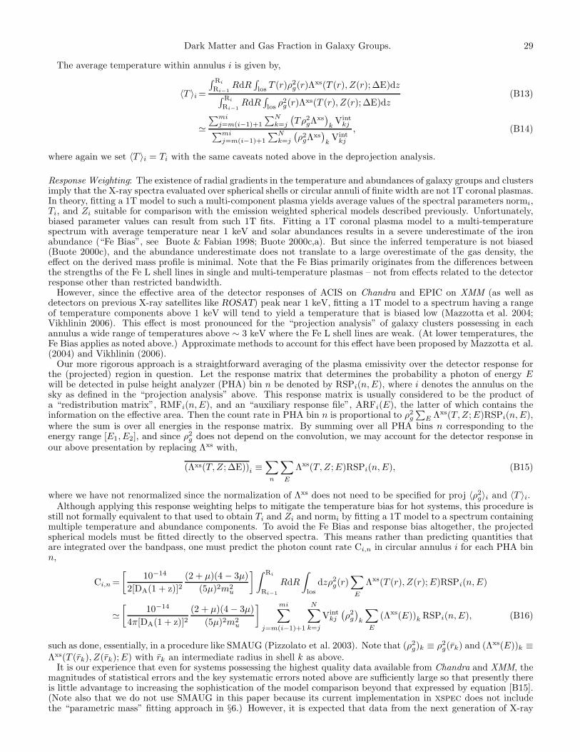
Dark Matter and Gas Fraction in Galaxy Groups. 29
The average temperature within annulus i is given by,
〈T 〉i =
∫ Ri
Ri−1RdR
∫
los T (r)ρ2g(r)Λxs(T (r), Z(r); ∆E)dz
∫ Ri
Ri−1RdR
∫
losρ2
g(r)Λxs(T (r), Z(r); ∆E)dz(B13)
≃∑mi
j=m(i−1)+1
∑Nk=j
(
Tρ2gΛxs
)
kVint
kj∑mi
j=m(i−1)+1
∑Nk=j
(
ρ2gΛxs
)
kVint
kj
, (B14)
where again we set 〈T 〉i = Ti with the same caveats noted above in the deprojection analysis.
Response Weighting: The existence of radial gradients in the temperature and abundances of galaxy groups and clustersimply that the X-ray spectra evaluated over spherical shells or circular annuli of finite width are not 1T coronal plasmas.In theory, fitting a 1T model to such a multi-component plasma yields average values of the spectral parameters normi,Ti, and Zi suitable for comparison with the emission weighted spherical models described previously. Unfortunately,biased parameter values can result from such 1T fits. Fitting a 1T coronal plasma model to a multi-temperaturespectrum with average temperature near 1 keV and solar abundances results in a severe underestimate of the ironabundance (“Fe Bias”, see Buote & Fabian 1998; Buote 2000c,a). But since the inferred temperature is not biased(Buote 2000c), and the abundance underestimate does not translate to a large overestimate of the gas density, theeffect on the derived mass profile is minimal. Note that the Fe Bias primarily originates from the differences betweenthe strengths of the Fe L shell lines in single and multi-temperature plasmas – not from effects related to the detectorresponse other than restricted bandwidth.
However, since the effective area of the detector responses of ACIS on Chandra and EPIC on XMM (as well asdetectors on previous X-ray satellites like ROSAT) peak near 1 keV, fitting a 1T model to a spectrum having a rangeof temperature components above 1 keV will tend to yield a temperature that is biased low (Mazzotta et al. 2004;Vikhlinin 2006). This effect is most pronounced for the “projection analysis” of galaxy clusters possessing in eachannulus a wide range of temperatures above ∼ 3 keV where the Fe L shell lines are weak. (At lower temperatures, theFe Bias applies as noted above.) Approximate methods to account for this effect have been proposed by Mazzotta et al.(2004) and Vikhlinin (2006).
Our more rigorous approach is a straightforward averaging of the plasma emissivity over the detector response forthe (projected) region in question. Let the response matrix that determines the probability a photon of energy Ewill be detected in pulse height analyzer (PHA) bin n be denoted by RSPi(n, E), where i denotes the annulus on thesky as defined in the “projection analysis” above. This response matrix is usually considered to be the product ofa “redistribution matrix”, RMFi(n, E), and an “auxiliary response file”, ARFi(E), the latter of which contains theinformation on the effective area. Then the count rate in PHA bin n is proportional to ρ2
g
∑
E Λxs(T, Z; E)RSPi(n, E),where the sum is over all energies in the response matrix. By summing over all PHA bins n corresponding to theenergy range [E1, E2], and since ρ2
g does not depend on the convolution, we may account for the detector response inour above presentation by replacing Λxs with,
(Λxs(T, Z; ∆E))i ≡∑
n
∑
E
Λxs(T, Z; E)RSPi(n, E), (B15)
where we have not renormalized since the normalization of Λxs does not need to be specified for proj 〈ρ2g〉i and 〈T 〉i.
Although applying this response weighting helps to mitigate the temperature bias for hot systems, this procedure isstill not formally equivalent to that used to obtain Ti and Zi and normi by fitting a 1T model to a spectrum containingmultiple temperature and abundance components. To avoid the Fe Bias and response bias altogether, the projectedspherical models must be fitted directly to the observed spectra. This means rather than predicting quantities thatare integrated over the bandpass, one must predict the photon count rate Ci,n in circular annulus i for each PHA binn,
Ci,n =
[
10−14
2[DA(1 + z)]2(2 + µ)(4 − 3µ)
(5µ)2m2u
]∫ Ri
Ri−1
RdR
∫
los
dzρ2g(r)
∑
E
Λxs(T (r), Z(r); E)RSPi(n, E)
≃[
10−14
4π[DA(1 + z)]2(2 + µ)(4 − 3µ)
(5µ)2m2u
] mi∑
j=m(i−1)+1
N∑
k=j
Vintkj
(
ρ2g
)
k
∑
E
(Λxs(E))k RSPi(n, E), (B16)
such as done, essentially, in a procedure like SMAUG (Pizzolato et al. 2003). Note that (ρ2g)k ≡ ρ2
g(rk) and (Λxs(E))k ≡Λxs(T (rk), Z(rk); E) with rk an intermediate radius in shell k as above.
It is our experience that even for systems possessing the highest quality data available from Chandra and XMM, themagnitudes of statistical errors and the key systematic errors noted above are sufficiently large so that presently thereis little advantage to increasing the sophistication of the model comparison beyond that expressed by equation [B15].(Note also that we do not use SMAUG in this paper because its current implementation in xspec does not includethe “parametric mass” fitting approach in §6.) However, it is expected that data from the next generation of X-ray
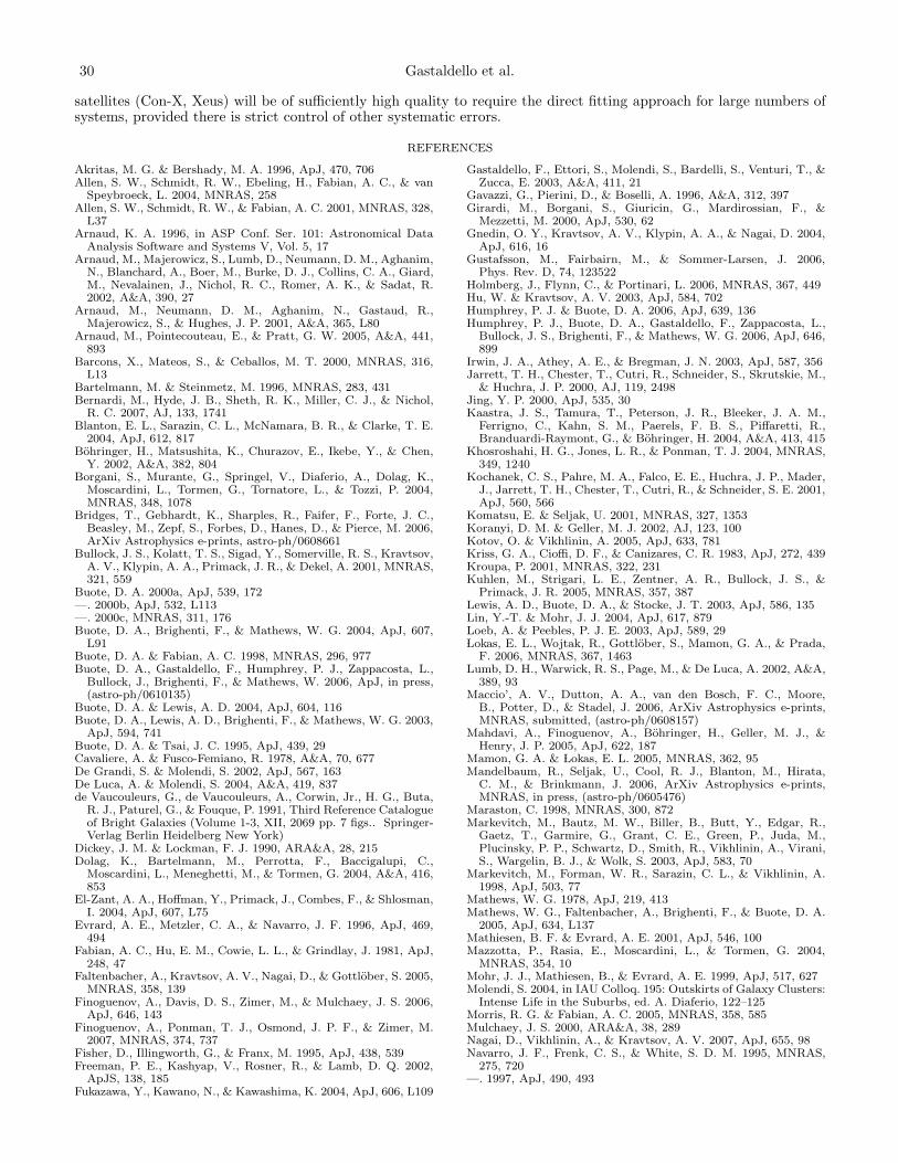
30 Gastaldello et al.
satellites (Con-X, Xeus) will be of sufficiently high quality to require the direct fitting approach for large numbers ofsystems, provided there is strict control of other systematic errors.
REFERENCES
Akritas, M. G. & Bershady, M. A. 1996, ApJ, 470, 706Allen, S. W., Schmidt, R. W., Ebeling, H., Fabian, A. C., & van
Speybroeck, L. 2004, MNRAS, 258Allen, S. W., Schmidt, R. W., & Fabian, A. C. 2001, MNRAS, 328,
L37Arnaud, K. A. 1996, in ASP Conf. Ser. 101: Astronomical Data
Analysis Software and Systems V, Vol. 5, 17Arnaud, M., Majerowicz, S., Lumb, D., Neumann, D. M., Aghanim,
N., Blanchard, A., Boer, M., Burke, D. J., Collins, C. A., Giard,M., Nevalainen, J., Nichol, R. C., Romer, A. K., & Sadat, R.2002, A&A, 390, 27
Arnaud, M., Neumann, D. M., Aghanim, N., Gastaud, R.,Majerowicz, S., & Hughes, J. P. 2001, A&A, 365, L80
Arnaud, M., Pointecouteau, E., & Pratt, G. W. 2005, A&A, 441,893
Barcons, X., Mateos, S., & Ceballos, M. T. 2000, MNRAS, 316,L13
Bartelmann, M. & Steinmetz, M. 1996, MNRAS, 283, 431Bernardi, M., Hyde, J. B., Sheth, R. K., Miller, C. J., & Nichol,
R. C. 2007, AJ, 133, 1741Blanton, E. L., Sarazin, C. L., McNamara, B. R., & Clarke, T. E.
2004, ApJ, 612, 817Bohringer, H., Matsushita, K., Churazov, E., Ikebe, Y., & Chen,
Y. 2002, A&A, 382, 804Borgani, S., Murante, G., Springel, V., Diaferio, A., Dolag, K.,
Moscardini, L., Tormen, G., Tornatore, L., & Tozzi, P. 2004,MNRAS, 348, 1078
Bridges, T., Gebhardt, K., Sharples, R., Faifer, F., Forte, J. C.,Beasley, M., Zepf, S., Forbes, D., Hanes, D., & Pierce, M. 2006,ArXiv Astrophysics e-prints, astro-ph/0608661
Bullock, J. S., Kolatt, T. S., Sigad, Y., Somerville, R. S., Kravtsov,A. V., Klypin, A. A., Primack, J. R., & Dekel, A. 2001, MNRAS,321, 559
Buote, D. A. 2000a, ApJ, 539, 172—. 2000b, ApJ, 532, L113—. 2000c, MNRAS, 311, 176Buote, D. A., Brighenti, F., & Mathews, W. G. 2004, ApJ, 607,
L91Buote, D. A. & Fabian, A. C. 1998, MNRAS, 296, 977Buote, D. A., Gastaldello, F., Humphrey, P. J., Zappacosta, L.,
Bullock, J., Brighenti, F., & Mathews, W. 2006, ApJ, in press,(astro-ph/0610135)
Buote, D. A. & Lewis, A. D. 2004, ApJ, 604, 116Buote, D. A., Lewis, A. D., Brighenti, F., & Mathews, W. G. 2003,
ApJ, 594, 741Buote, D. A. & Tsai, J. C. 1995, ApJ, 439, 29Cavaliere, A. & Fusco-Femiano, R. 1978, A&A, 70, 677De Grandi, S. & Molendi, S. 2002, ApJ, 567, 163De Luca, A. & Molendi, S. 2004, A&A, 419, 837de Vaucouleurs, G., de Vaucouleurs, A., Corwin, Jr., H. G., Buta,
R. J., Paturel, G., & Fouque, P. 1991, Third Reference Catalogueof Bright Galaxies (Volume 1-3, XII, 2069 pp. 7 figs.. Springer-Verlag Berlin Heidelberg New York)
Dickey, J. M. & Lockman, F. J. 1990, ARA&A, 28, 215Dolag, K., Bartelmann, M., Perrotta, F., Baccigalupi, C.,
Moscardini, L., Meneghetti, M., & Tormen, G. 2004, A&A, 416,853
El-Zant, A. A., Hoffman, Y., Primack, J., Combes, F., & Shlosman,I. 2004, ApJ, 607, L75
Evrard, A. E., Metzler, C. A., & Navarro, J. F. 1996, ApJ, 469,494
Fabian, A. C., Hu, E. M., Cowie, L. L., & Grindlay, J. 1981, ApJ,248, 47
Faltenbacher, A., Kravtsov, A. V., Nagai, D., & Gottlober, S. 2005,MNRAS, 358, 139
Finoguenov, A., Davis, D. S., Zimer, M., & Mulchaey, J. S. 2006,ApJ, 646, 143
Finoguenov, A., Ponman, T. J., Osmond, J. P. F., & Zimer, M.2007, MNRAS, 374, 737
Fisher, D., Illingworth, G., & Franx, M. 1995, ApJ, 438, 539Freeman, P. E., Kashyap, V., Rosner, R., & Lamb, D. Q. 2002,
ApJS, 138, 185Fukazawa, Y., Kawano, N., & Kawashima, K. 2004, ApJ, 606, L109
Gastaldello, F., Ettori, S., Molendi, S., Bardelli, S., Venturi, T., &Zucca, E. 2003, A&A, 411, 21
Gavazzi, G., Pierini, D., & Boselli, A. 1996, A&A, 312, 397Girardi, M., Borgani, S., Giuricin, G., Mardirossian, F., &
Mezzetti, M. 2000, ApJ, 530, 62Gnedin, O. Y., Kravtsov, A. V., Klypin, A. A., & Nagai, D. 2004,
ApJ, 616, 16Gustafsson, M., Fairbairn, M., & Sommer-Larsen, J. 2006,
Phys. Rev. D, 74, 123522Holmberg, J., Flynn, C., & Portinari, L. 2006, MNRAS, 367, 449Hu, W. & Kravtsov, A. V. 2003, ApJ, 584, 702Humphrey, P. J. & Buote, D. A. 2006, ApJ, 639, 136Humphrey, P. J., Buote, D. A., Gastaldello, F., Zappacosta, L.,
Bullock, J. S., Brighenti, F., & Mathews, W. G. 2006, ApJ, 646,899
Irwin, J. A., Athey, A. E., & Bregman, J. N. 2003, ApJ, 587, 356Jarrett, T. H., Chester, T., Cutri, R., Schneider, S., Skrutskie, M.,
& Huchra, J. P. 2000, AJ, 119, 2498Jing, Y. P. 2000, ApJ, 535, 30Kaastra, J. S., Tamura, T., Peterson, J. R., Bleeker, J. A. M.,
Ferrigno, C., Kahn, S. M., Paerels, F. B. S., Piffaretti, R.,Branduardi-Raymont, G., & Bohringer, H. 2004, A&A, 413, 415
Khosroshahi, H. G., Jones, L. R., & Ponman, T. J. 2004, MNRAS,349, 1240
Kochanek, C. S., Pahre, M. A., Falco, E. E., Huchra, J. P., Mader,J., Jarrett, T. H., Chester, T., Cutri, R., & Schneider, S. E. 2001,ApJ, 560, 566
Komatsu, E. & Seljak, U. 2001, MNRAS, 327, 1353Koranyi, D. M. & Geller, M. J. 2002, AJ, 123, 100Kotov, O. & Vikhlinin, A. 2005, ApJ, 633, 781Kriss, G. A., Cioffi, D. F., & Canizares, C. R. 1983, ApJ, 272, 439Kroupa, P. 2001, MNRAS, 322, 231Kuhlen, M., Strigari, L. E., Zentner, A. R., Bullock, J. S., &
Primack, J. R. 2005, MNRAS, 357, 387Lewis, A. D., Buote, D. A., & Stocke, J. T. 2003, ApJ, 586, 135Lin, Y.-T. & Mohr, J. J. 2004, ApJ, 617, 879Loeb, A. & Peebles, P. J. E. 2003, ApJ, 589, 29 Lokas, E. L., Wojtak, R., Gottlober, S., Mamon, G. A., & Prada,
F. 2006, MNRAS, 367, 1463Lumb, D. H., Warwick, R. S., Page, M., & De Luca, A. 2002, A&A,
389, 93Maccio’, A. V., Dutton, A. A., van den Bosch, F. C., Moore,
B., Potter, D., & Stadel, J. 2006, ArXiv Astrophysics e-prints,MNRAS, submitted, (astro-ph/0608157)
Mahdavi, A., Finoguenov, A., Bohringer, H., Geller, M. J., &Henry, J. P. 2005, ApJ, 622, 187
Mamon, G. A. & Lokas, E. L. 2005, MNRAS, 362, 95Mandelbaum, R., Seljak, U., Cool, R. J., Blanton, M., Hirata,
C. M., & Brinkmann, J. 2006, ArXiv Astrophysics e-prints,MNRAS, in press, (astro-ph/0605476)
Maraston, C. 1998, MNRAS, 300, 872Markevitch, M., Bautz, M. W., Biller, B., Butt, Y., Edgar, R.,
Gaetz, T., Garmire, G., Grant, C. E., Green, P., Juda, M.,Plucinsky, P. P., Schwartz, D., Smith, R., Vikhlinin, A., Virani,S., Wargelin, B. J., & Wolk, S. 2003, ApJ, 583, 70
Markevitch, M., Forman, W. R., Sarazin, C. L., & Vikhlinin, A.1998, ApJ, 503, 77
Mathews, W. G. 1978, ApJ, 219, 413Mathews, W. G., Faltenbacher, A., Brighenti, F., & Buote, D. A.
2005, ApJ, 634, L137Mathiesen, B. F. & Evrard, A. E. 2001, ApJ, 546, 100Mazzotta, P., Rasia, E., Moscardini, L., & Tormen, G. 2004,
MNRAS, 354, 10Mohr, J. J., Mathiesen, B., & Evrard, A. E. 1999, ApJ, 517, 627Molendi, S. 2004, in IAU Colloq. 195: Outskirts of Galaxy Clusters:
Intense Life in the Suburbs, ed. A. Diaferio, 122–125Morris, R. G. & Fabian, A. C. 2005, MNRAS, 358, 585Mulchaey, J. S. 2000, ARA&A, 38, 289Nagai, D., Vikhlinin, A., & Kravtsov, A. V. 2007, ApJ, 655, 98Navarro, J. F., Frenk, C. S., & White, S. D. M. 1995, MNRAS,
275, 720—. 1997, ApJ, 490, 493
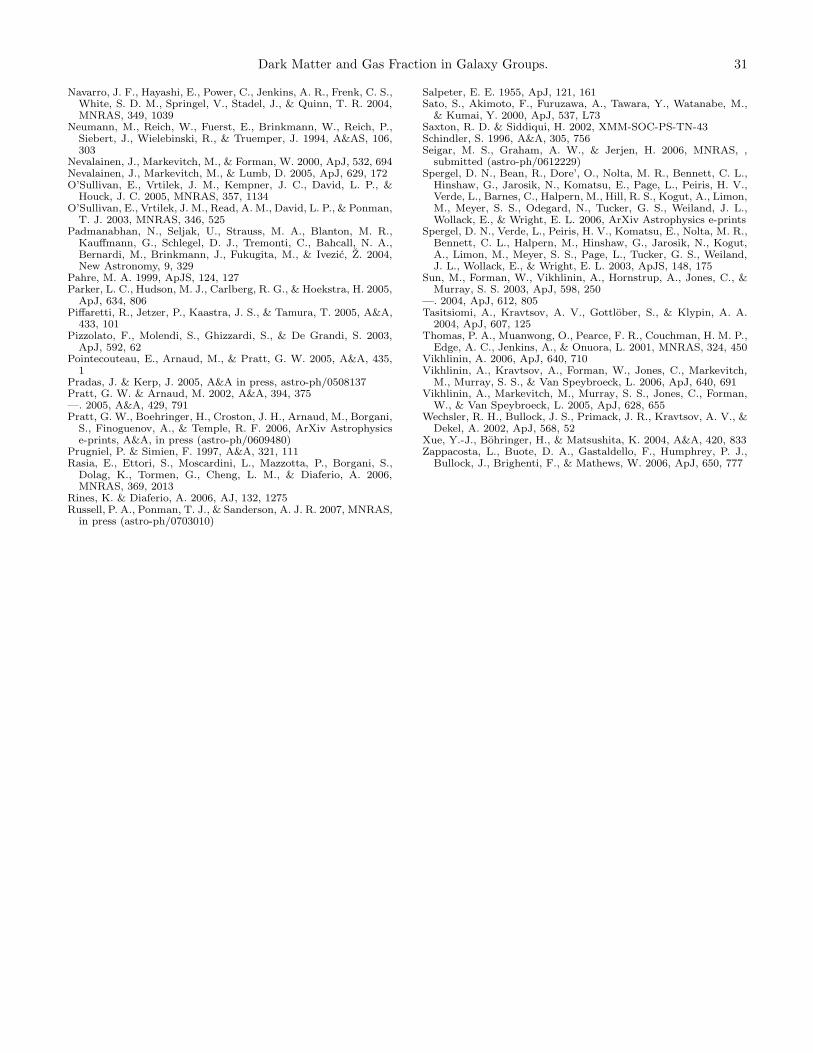
Dark Matter and Gas Fraction in Galaxy Groups. 31
Navarro, J. F., Hayashi, E., Power, C., Jenkins, A. R., Frenk, C. S.,White, S. D. M., Springel, V., Stadel, J., & Quinn, T. R. 2004,MNRAS, 349, 1039
Neumann, M., Reich, W., Fuerst, E., Brinkmann, W., Reich, P.,Siebert, J., Wielebinski, R., & Truemper, J. 1994, A&AS, 106,303
Nevalainen, J., Markevitch, M., & Forman, W. 2000, ApJ, 532, 694Nevalainen, J., Markevitch, M., & Lumb, D. 2005, ApJ, 629, 172O’Sullivan, E., Vrtilek, J. M., Kempner, J. C., David, L. P., &
Houck, J. C. 2005, MNRAS, 357, 1134O’Sullivan, E., Vrtilek, J. M., Read, A. M., David, L. P., & Ponman,
T. J. 2003, MNRAS, 346, 525Padmanabhan, N., Seljak, U., Strauss, M. A., Blanton, M. R.,
Kauffmann, G., Schlegel, D. J., Tremonti, C., Bahcall, N. A.,Bernardi, M., Brinkmann, J., Fukugita, M., & Ivezic, Z. 2004,New Astronomy, 9, 329
Pahre, M. A. 1999, ApJS, 124, 127Parker, L. C., Hudson, M. J., Carlberg, R. G., & Hoekstra, H. 2005,
ApJ, 634, 806Piffaretti, R., Jetzer, P., Kaastra, J. S., & Tamura, T. 2005, A&A,
433, 101Pizzolato, F., Molendi, S., Ghizzardi, S., & De Grandi, S. 2003,
ApJ, 592, 62Pointecouteau, E., Arnaud, M., & Pratt, G. W. 2005, A&A, 435,
1Pradas, J. & Kerp, J. 2005, A&A in press, astro-ph/0508137Pratt, G. W. & Arnaud, M. 2002, A&A, 394, 375—. 2005, A&A, 429, 791Pratt, G. W., Boehringer, H., Croston, J. H., Arnaud, M., Borgani,
S., Finoguenov, A., & Temple, R. F. 2006, ArXiv Astrophysicse-prints, A&A, in press (astro-ph/0609480)
Prugniel, P. & Simien, F. 1997, A&A, 321, 111Rasia, E., Ettori, S., Moscardini, L., Mazzotta, P., Borgani, S.,
Dolag, K., Tormen, G., Cheng, L. M., & Diaferio, A. 2006,MNRAS, 369, 2013
Rines, K. & Diaferio, A. 2006, AJ, 132, 1275Russell, P. A., Ponman, T. J., & Sanderson, A. J. R. 2007, MNRAS,
in press (astro-ph/0703010)
Salpeter, E. E. 1955, ApJ, 121, 161Sato, S., Akimoto, F., Furuzawa, A., Tawara, Y., Watanabe, M.,
& Kumai, Y. 2000, ApJ, 537, L73Saxton, R. D. & Siddiqui, H. 2002, XMM-SOC-PS-TN-43Schindler, S. 1996, A&A, 305, 756Seigar, M. S., Graham, A. W., & Jerjen, H. 2006, MNRAS, ,
submitted (astro-ph/0612229)Spergel, D. N., Bean, R., Dore’, O., Nolta, M. R., Bennett, C. L.,
Hinshaw, G., Jarosik, N., Komatsu, E., Page, L., Peiris, H. V.,Verde, L., Barnes, C., Halpern, M., Hill, R. S., Kogut, A., Limon,M., Meyer, S. S., Odegard, N., Tucker, G. S., Weiland, J. L.,Wollack, E., & Wright, E. L. 2006, ArXiv Astrophysics e-prints
Spergel, D. N., Verde, L., Peiris, H. V., Komatsu, E., Nolta, M. R.,Bennett, C. L., Halpern, M., Hinshaw, G., Jarosik, N., Kogut,A., Limon, M., Meyer, S. S., Page, L., Tucker, G. S., Weiland,J. L., Wollack, E., & Wright, E. L. 2003, ApJS, 148, 175
Sun, M., Forman, W., Vikhlinin, A., Hornstrup, A., Jones, C., &Murray, S. S. 2003, ApJ, 598, 250
—. 2004, ApJ, 612, 805Tasitsiomi, A., Kravtsov, A. V., Gottlober, S., & Klypin, A. A.
2004, ApJ, 607, 125Thomas, P. A., Muanwong, O., Pearce, F. R., Couchman, H. M. P.,
Edge, A. C., Jenkins, A., & Onuora, L. 2001, MNRAS, 324, 450Vikhlinin, A. 2006, ApJ, 640, 710Vikhlinin, A., Kravtsov, A., Forman, W., Jones, C., Markevitch,
M., Murray, S. S., & Van Speybroeck, L. 2006, ApJ, 640, 691Vikhlinin, A., Markevitch, M., Murray, S. S., Jones, C., Forman,
W., & Van Speybroeck, L. 2005, ApJ, 628, 655Wechsler, R. H., Bullock, J. S., Primack, J. R., Kravtsov, A. V., &
Dekel, A. 2002, ApJ, 568, 52Xue, Y.-J., Bohringer, H., & Matsushita, K. 2004, A&A, 420, 833Zappacosta, L., Buote, D. A., Gastaldello, F., Humphrey, P. J.,
Bullock, J., Brighenti, F., & Mathews, W. 2006, ApJ, 650, 777
Copyright © 2022 FDOKUMEN