State feedback control of switched linear systems: An LMI approach

Journal of Computational and Applied Mathematics 194 (2006) 192–206www.elsevier.com/locate/cam

State feedback control of switched linear systems:An LMI approach

V.F. Montagnera, V.J.S. Leiteb, R.C.L.F. Oliveiraa, P.L.D. Peresa,∗aDT/FEEC/UNICAMP, CP 6101, 13081-970, Campinas, SP, Brazil

bUnED Divinópolis, CEFET-MG, R. Monte Santo, 319, 35502-036, Divinópolis, MG, Brazil

Received 16 July 2004; received in revised form 24 June 2005

Abstract

This paper addresses the problem of state feedback control of continuous-time switched linear systems witharbitrary switching rules. A quadratic Lyapunov function with a common matrix is used to derive a stabilizingswitching control strategy that guarantees: (i) the assignment of all the eigenvalues of each linear subsystem insidea chosen circle in the left-hand half of the complex plane; (ii) a minimum disturbance attenuation level for theclosed-loop switched system. The proposed design conditions are given in terms of linear matrix inequalities thatencompass previous results based on quadratic stability conditions with fixed control gains. Although the quadraticstability based on a fixed Lyapunov matrix has been widely used in robust control design, the use of this condition toprovide a convex design method for switching feedback gains has not been fully investigated. Numerical examplesshow that the switching control strategy can cope with more stringent design specifications than the fixed gainstrategy, being useful to improve the performance of this class of systems.© 2005 Elsevier B.V. All rights reserved.

Keywords: Switched linear systems; Switched control; Quadratic Lyapunov function; Linear matrix inequalities; Pole location;H∞ control; Continuous-time systems

∗ Corresponding author. Tel.: +55 19 3788 3759; fax: +55 19 3289 1395.E-mail addresses: [email protected] (V.F. Montagner), [email protected] (V.J.S. Leite),

[email protected] (R.C.L.F. Oliveira), [email protected] (P.L.D. Peres).

0377-0427/$ - see front matter © 2005 Elsevier B.V. All rights reserved.doi:10.1016/j.cam.2005.07.005

http://www.elsevier.com/locate/cam

mailto:[email protected]




V.F. Montagner et al. / Journal of Computational and Applied Mathematics 194 (2006) 192–206 193

1. Introduction

Switched systems are a class of hybrid systems consisting of several subsystems (modes of operation)and a switching rule indicating the active subsystem at each instant of time [5,17]. Among the dynamicalsystems that exhibit switching behavior, it is possible to cite the electrical circuits with electronic switchesthat define the important family of power converters [13], biochemical processes [7] and all the systemssubject to switching control laws [15,21–23]. It is worth mentioning that switching control strategiesare important to improve the performance of some systems, to guarantee their robustness and also toimplement some adaptive control schemes [9]. Note also that switched systems can be used to modellinear systems subject to actuator failures, that is, systems that can abruptly change the number of controlinputs [24]. In the context of switched systems with linear continuous-time subsystems, the issues ofstability analysis and control have been studied in the last few years [10,19,20] and, as stated in [16],the basic problems are: (a) to find the conditions that guarantee the system stability (or find a controllaw that guarantees the system stabilizability or even the achievement of some performance index) underany switching rule; (b) to find the switching strategy that guarantees the system stability (or the systemstabilizability or even the achievement of some performance index). These and other issues such as thecontrollability and the reachability problems [25,27] have been under investigation and much attentionhas been paid on the switched linear systems [24,29]. Undoubtedly, a systematic way to study the stabilityand control problems for this class of systems is provided by the use of Lyapunov functions.

Several important results on robust stability and filtering for linear systems have been obtained in thelast decades from the use of a common quadratic Lyapunov function [1]. This approach is appealingbecause of its numerical simplicity and also by the possibility to express the tests in terms of linear matrixinequalities (LMIs), solved in polynomial time by interior point based algorithms [6]. Another interestingfeature is that the fixed Lyapunov function can cope with arbitrarily fast time-varying systems, thusencompassing the switched systems. Concerning the stability of autonomous switched linear systems,[18] shows that a common quadratic Lyapunov function exists if all the matrices are asymptotically stableand commute pairwise. The quadratic stabilizability problem for continuous-time systems in polytopicdomains has been solved in [2], where an LMI condition is used to determine a fixed state feedback gain,allowing to deal with time-varying uncertain parameters and thus being useful for switched systems aswell. Extensions of this condition have provided several results in robust control and filter design (see[3] and references therein), including performance indexes such as the H∞ norm, which are entirelyapplicable to the robust stabilizability of switched linear systems with arbitrary switching rules by meansof fixed gains.

The main drawback of the quadratic stabilization by means of fixed gains is that the results can beconservative, that is, the switched system may be stabilizable through switching strategies but does notadmit a fixed constant stabilizing feedback for all subsystems. Some recent results explore the use ofswitching control strategies based on quadratic Lyapunov functions, as in [28], by means of a state de-pendent switching strategy and in [11], where parameterized LMIs need to be solved to obtain a set ofgains that stabilize the closed-loop system for a given switching function. Many results based on quadraticstability to design switched stabilizing control gains for switched linear systems take into account priorinformation on the switching function or on the state space partitions, which in fact, when available, canbe useful for control synthesis. However, there are systems for which this previous information is notavailable and thus the control design must be carried out for arbitrary switching functions. It is also worthto mention that results based on quadratic Lyapunov functions for stability analysis and control design

194 V.F. Montagner et al. / Journal of Computational and Applied Mathematics 194 (2006) 192–206

for Takagi–Sugeno fuzzy systems [26] could be applied to switched linear systems. Takagi–Sugeno fuzzysystems can be viewed as a family of linear subsystems combined through the use of membership func-tions, which includes all the intermediate models. In the case of switched linear systems, the transitionsfrom one subsystem to another are instantaneous (there exists no intermediate models). Then, althoughin principle results on stabilizability of Takagi–Sugeno fuzzy systems could be applied to switched linearsystems, the conditions would need to take into account information on intermediate models, introducingunnecessary additional computation. Other classes of Lyapunov functions can be used to address thecontrol of switched linear systems, such as piecewise [12] or multiple [4] Lyapunov functions but, ingeneral, the numerical solution requires a high computational effort.

The aim of this paper is to address problem (a) described above, that is, to determine a stabilizingswitched state feedback control law that guarantees, for any arbitrary switching rule: (i) the locationof the poles of each closed-loop linear subsystems of a continuous-time switched linear system insidea circle of given center and radius located in the open left-half of the complex plane; (ii) an upperbound (as small as possible) for the H∞ attenuation level of the closed-loop switched system. The firstfeature is important since it allows to improve the dynamical response assigning bounds for overshoot,settling time and frequency of oscillation [8], and the second one assures the robustness of the switchedsystem facing disturbances that are energy signals. The switching rule and the state vector are assumedto be unknown a priori but available (measured or estimated) in real time for feedback. Differently fromprevious results in the context of continuous-time switched linear systems, this paper provides sufficientLMI design conditions based on quadratic Lyapunov functions with a common matrix which, with a verylow numerical complexity, allow to determine switched state feedback gains that stabilize the closed-loop system including pole location and H∞ performance specification, being suitable for switchedsystems subject to arbitrary switching functions not known a priori but available on line. The proposedconditions contain the quadratic stabilizability with fixed gains as a particular case, but the use of extramatrix variables in the design conditions provided in the paper allows to highly improve the systemperformance, as illustrated through numerical examples including a study of a model of an activatedsludge process [7].

2. Problem formulation

Consider the continuous-time switched system

x(t) = Aj(t)x(t) + B1j (t)w(t) + B2j (t)u(t), (1)

z(t) = Cj(t)x(t) + D1j (t)w(t) + D2j (t)u(t). (2)

The switching rule j (t), defined as

j (t) : R+ → J, J = {1, 2, . . . , N} (3)

arbitrarily selects which linear mode (A, B1, B2, C, D1, D2)j , j =1, . . . , N , is active. The vector of statevariables is x(t) ∈ Rn, w(t) ∈ Rr is an exogenous input, u(t) ∈ Rmj is the control input of subsystemj, z(t) ∈ Rp is the controlled output and Aj(t) ∈ Rn×n, B1j (t) ∈ Rn×r , B2j (t) ∈ Rn×mj , Cj(t) ∈ Rp×n,D1j (t) ∈ Rp×r and D2j (t) ∈ Rp×mj are the subsystem matrices, j =1, . . . , N . It is assumed that the statevector is available for feedback and that the switching rule j (t) is not known a priori but it is available inreal time.


rj

dj

-(rj+dj)

Imag

Real

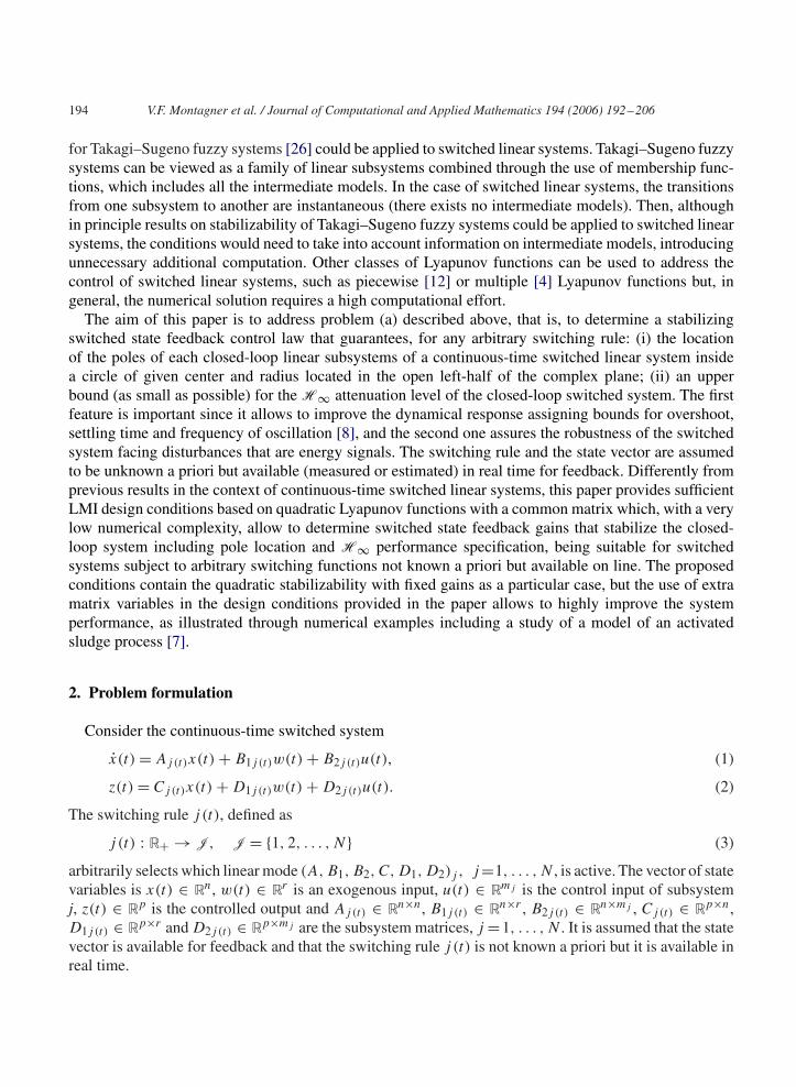
Fig. 1. Circular region C(dj , rj ) for pole location.

The aim here is to determine a stabilizing switching state feedback control law

u(t) = Kj(t)x(t) (4)

such that:

(i) the poles of each linear subsystem j, j = 1, . . . , N of the closed-loop switched system, that is, theeigenvalues of Aj defined as

Aj�(Aj + B2jKj ) (5)

are located inside the circle in the complex plane with center at (−(rj +dj ), 0), radius rj and distancedj from the imaginary axis, depicted in Fig. 1 and denoted C(dj , rj ).

(ii) for any input w(t) ∈ L2 it is possible to determine a bound � ∈ R+ such that z(t) ∈ L2 verifies

‖z(t)‖2 < �‖w(t)‖2. (6)

Any value of � satisfying (6) is called an H∞ guaranteed cost of the closed-loop switched systemand it is of great interest to determine the switched control gains Kj that provide the smallest �attenuation level.

Concerning (i), a necessary and sufficient condition assuring that all the eigenvalues of matrix Aj givenby (5) lie inside C(dj , rj ) is provided by the existence of a symmetric positive definite matrix W ∈ Rn×n

such that [8]

(Aj + dj I)W + W(Aj + dj I)′ + 1

rj(Aj + dj I)W(Aj + dj I)′ < 0. (7)

As discussed in [14], the subsystem modes damp asymptotically at desired rates if the circle centerand radius are adequately chosen. Note also that the closed-loop behavior of each subsystem j can bedesigned independently, by an appropriate choice of dj , rj , j = 1, . . . , N . Actually, the choice of dj andrj can be used to impose bounds on the transient responses for each linear subsystem. For instance, from


Fig. 1, it can be noticed that, based on the value of dj , it is possible to determine an upper bound for thesettling time of the transient response when the system operates at subsystem j, given by 3�j or 5�j , with�j = 1/dj . The value rj gives the upper bound on the natural frequency of oscillation for the transientresponse. Notice also that a lower bound on the dumping factor �j , which determines the overshoot, canbe computed through

�j =√

(rj + dj )2 − r2

j

rj + dj

. (8)

Whenever the time interval between two consecutive switchings (called dwell time) is long enough toallow the accommodation of the eigenvalues of Aj +B2jKj , the transient responses will obey the boundsof settling time, natural frequency and dumping factor imposed by dj and rj . Otherwise, in the case ofarbitrarily fast switchings, the existence of a quadratic Lyapunov function with a fixed matrix W alwaysassure the closed-loop global stability.

In order to cope with specification (ii), by applying the switched control law (4) to (1)–(2) one gets

x(t) = Aj (t)x(t) + B1j (t)w(t), (9)

z(t) = Cj (t)x(t) + D1j (t)w(t) (10)

with switching rule j (t) as in (3), Aj is given by (5) and Cj�Cj + D2jKj . Then, the continuous-timeclosed-loop system (9)–(10) is such that (6) holds if there exists a symmetric positive definite matrixW ∈ Rn×n such that [3]⎡

⎣ AjW + WA′j B1j WC′

j

B ′1j −I D′

1j

CjW D1j −�2I

⎤⎦ < 0, j = 1, . . . , N . (11)

Note that conditions (7) and (11) can easily be extended to deal with robust pole location as well as H∞guaranteed cost computation for uncertain systems in polytopic domains by means of fixed state feedbackgains. Based on the convex characteristics of quadratic stability [3], it suffices to test the conditions atthe vertices of the polytope to assure the desired properties for the overall uncertainty domain.

In the sequel, these results will be extended to cope with requirements (i) and (ii) in the context ofswitched systems by means of the switched control law (4). The desired closed-loop characteristics, inboth cases, will be assured by the existence of a common quadratic Lyapunov function.

3. Main results

Consider system (1)–(2) without exogenous disturbances, that is, w(t)= 0, and the problem of findinga switching control law as (4) such that the closed-loop switched system x(t) = (Aj + B2jKj )x(t), withj (t) given by (3), is asymptotically stable. A sufficient condition is provided by the following result.

Lemma 1. If there exist a symmetric positive definite matrix W ∈ Rn×n and matrices Zj ∈ Rmj×n, j =1, . . . , N , such that

AjW + WA′j + B2jZj + Z′

jB′2j < 0, j = 1, . . . , N (12)


then the switched control law (4) with

Kj = ZjW−1, j = 1, . . . , N (13)

assures the closed-loop stability of the switched system.

Proof. Straightforward, by noting that (12) can be rewritten as

(Aj + B2jKj )W + W(Aj + B2jKj )′ < 0, j = 1, . . . , N (14)

with Kj given by (13). The closed-loop stability is then assured by the common Lyapunov functionv(x) = x′Px, P = W−1. �

If one is interested on imposing not only the closed-loop stability but also a pole location C(dj , rj ) foreach mode j of the switched system, that is, to assure requirement (i), condition (7) must hold for all j,j =1, . . . , N . Lemma 2 gives sufficient conditions to determine the gains Kj such that the eigenvalues ofeach linear mode of the closed-loop system (Aj + B2jKj ), j = 1, . . . , N lie inside the region C(dj , rj )

depicted in Fig. 1.

Lemma 2. If there exist a symmetric positive definite matrix W ∈ Rn×n and matrices Zj ∈ Rmj×n, j =1, . . . , N , such that[


jB′2j + 2djW AjW + B2jZj + djW

WA′j + Z′

jB′2j + djW −rjW

]<0, j=1, . . ., N (15)

then the switched control law (4) with Kj given by (13) assures to each linear closed-loop subsystemAj , j = 1, . . . , N the pole location C(dj , rj ) specified in Fig. 1.

Proof. Using Schur complement, Eq. (15) with Kj given by (13) yields

(Aj + B2jKj + dj I)W + W(Aj + B2jKj + dj I)′

+ 1

rj(Aj + B2jKj + dj I)W(Aj + B2jKj + dj I)′ < 0, j = 1, . . . , N (16)

which assures the desired pole location for each linear mode of operation of the switched system. �

Lemma 2 deserves some important remarks. First, note that the closed-loop stability of the switchedsystem for arbitrary switching sequences is also guaranteed by Lemma 2, since for dj > 0 and rj > 0(16) implies

(Aj + B2jKj )W + W(Aj + B2jKj )′

< − 2djW − 1

rj(Aj + B2jKj + dj I)W(Aj + B2jKj + dj I)′ < 0, j = 1, . . . , N . (17)

Although the concept of eigenvalue cannot be applied for switched systems, Lemma 2 guarantees theassignment of the eigenvalues of each linear mode of operation (i.e., subsystem) of the switched system


inside the circle C(dj , rj ) of Fig. 1. In this sense, the transient response due to a transition from mode(Aj +B2jKj ) to mode (Ak +B2kKk), j, k ∈ J, j �= k, will respect the dynamical constraints representedby C(dk, rk), whenever the time interval between the two consecutive switching instants is long enough toallow the accommodation of each mode [16]. The slowest dynamical behavior of all the linear subsystemscan be computed as being associated to a pole with real part equal to −d, where d = min dj , yielding (atthe worst case) the time constant � = 1/d and dwell time between 3� and 5�. As a final remark, a simpleprocedure to choose the parameters dj and rj is the following: (i) select dj = d based on the maximumallowable settling time; (ii) solve Lemma 2 using line searches for rj = r until find the minimum valueof r, in order to minimize the oscillations in the transient responses.

Consider now system (1)–(2) with w(t) ∈ L2. The following lemma assures (ii), that is, provides aswitched state feedback control law as (4) such that the closed-loop switched system has a prespecified� disturbance attenuation level.

Lemma 3. If there exists a symmetric positive definite matrix W ∈ Rn×n and matrices Zj ∈ Rmj×n, j =1, . . . , N , such that

⎡⎣AjW + WA′

j + B2jZj + Z′jB

′2j B1j WC′

j + Z′jD

′2j

B ′1j −I D′

1j

CjW + D2jZj D1j −�2I

⎤⎦ < 0, j = 1, . . . , N (18)

then the state feedback control law (4) with Kj given by (13) assures that (6) holds for the closed-loopswitched system.

Proof. Using Kj given by (13), (18) can be rewritten as

⎡⎣ (Aj + B2jKj )W + W(Aj + B2jKj )

′ B1j W(Cj + D2jKj )′

B ′1j −I D′

1j

(Cj + D2jKj )W D1j −�2I

⎤⎦ < 0, j = 1, . . . , N (19)

which assures that (6) holds. �

It is important to stress that a feasible solution to (18) provides one gain Kj for each linear mode j,j = 1, . . . , N , of the closed-loop system assuring that the closed-loop switched system is stable withan H∞ guaranteed cost � for any arbitrary switching rule j (t). By defining � = �2 and minimizing �under (18), the lowest level of disturbances attenuation for the switched system such that (19) holds isobtained. Individual H∞ costs could also be computed for each subsystem, by simply defining �j = �2

j ,j = 1, . . . , N . The common Lyapunov matrix W assures the overall stability, and the guaranteed cost�gc of the controlled switched system is equal to the worst case individual cost. Note that condition (18)contains (14), which can be recovered from the block (1, 1) of the LMI.

With the results of Lemmas 1–3, one is able to determine a stabilizing switching control law asin (4) with Kj given by (13), which can include pole location constraints C(dj , rj ) for each linearmode (thus improving the transient responses) or impose a (global or individual) prescribed level � ofdisturbance attenuation, improving the robustness properties of the switched system against disturbances.Both requirements can be combined in a unique set of N LMIs, as proposed in next lemma.


Lemma 4. If there exist a symmetric positive definite matrix W ∈ Rn×n and matrices Zj ∈ Rmj×n, j =1, . . . , N , such that

⎡⎢⎢⎣


jB′2j + 2djW AjW + B2jZj + djW B1j WC′

j + Z′jD

′2j

WA′j + Z′

jB′2j + djW −rjW 0 0

B ′1j 0 −I D′

1j

CjW + D2jZj 0 D1j −�2I

⎤⎥⎥⎦

< 0 j = 1, . . . , N (20)

then the state feedback control law (4) with Kj given by (13) assures the stability of the closed-loopswitched system with � disturbance attenuation level and the pole location of each linear subsysteminside the circle C(dj , rj ) depicted in Fig. 1.

Proof. If (20) holds, then with Kj given by (13) and by using Schur complement one has

⎡⎢⎢⎢⎣

(Aj + B2jKj + dj I)W + W(Aj + B2jKj + dj I)′

+ 1

rj(Aj + B2jKj + dj I)W(Aj + B2jKj + dj I)′ B1j W(Cj + D2jKj )

′

B ′1j −I D′

1j

(Cj + D2jKj )W D1j −�2I

⎤⎥⎥⎥⎦ < 0

j = 1, . . . , N (21)

which assures that both (16) (block (1, 1) of the LMI negative definite) and (19) hold. �

It is important to remark that, with mj = m and the choice Zj = Z, j = 1, . . . , N , it is possible torecover quadratically stability based results for robust control of switched systems (i.e., stabilization bymeans of a common fixed gain), for all the four lemmas presented here. Observe that the control matricesB2j , D2j in (1)–(2) may have a different number of columns depending on the subsystem, which issuitable, for instance, to address the problem of failure of actuators. As it will be illustrated by means ofexamples, the switching strategy can provide improvements in the closed-loop dynamics of the switchedsystem. Moreover, in some cases a switched control can provide closed-loop stability for systems whichdo not admit a fixed quadratic stabilizing feedback gain. The complexity of the LMIs can be estimatedas being proportional to S3R where S is the number of scalar variables and R is the number of LMIrows [6]. Lemmas 1 and 2 and, for a given �, Lemmas 3 and 4 have S = n(n + 1)/2 + n

∑Nj=1 mj and

RL1 = n(N + 1), RL2 = 2nN , RL3 = n(3N + 1) and RL4 = 4nN (note that the constraint W > 0 doesnot need to be imposed separately in Lemmas 2 and 4, since −rjW < 0 already appears in the block(2, 2) of the LMIs (15) and (20)) implying that the problems to be solved are more complex than thecorresponding quadratic stabilizability conditions by fixed gain, which yield SQS = n(n + 1)/2 + nm

and the same number of LMI rows, but Lemmas 1–4 can still be solved in polynomial time by meansof specialized algorithms such as interior point methods [3,6]. Finally, note that additional constraintssuch as decentralization could be incorporated following the lines depicted in [14], by simply imposinga block diagonal structure to matrices Zj , j = 1, . . . , N and W in Lemmas 1–4.


4. Examples

The first example illustrates how a switching controller that stabilizes independently each one of thesubsystems of a switched system sometimes cannot guarantee the overall stability of the closed-loopsystem. Consider the switched system, borrowed from [15], with two linear continuous-time modes ofoperation given by matrices

A1 =[

0 1−3 −0.2

], B21 =

[01

], A2 =

[−0.2 −31 0

], B22 =

[10

]. (22)

It is worth mentioning that this simple system does not admit a fixed quadratically stabilizing feedbackgain. As it can be verified, the control gains

K1s = [1 0 ] , K2s = [0 1 ] (23)

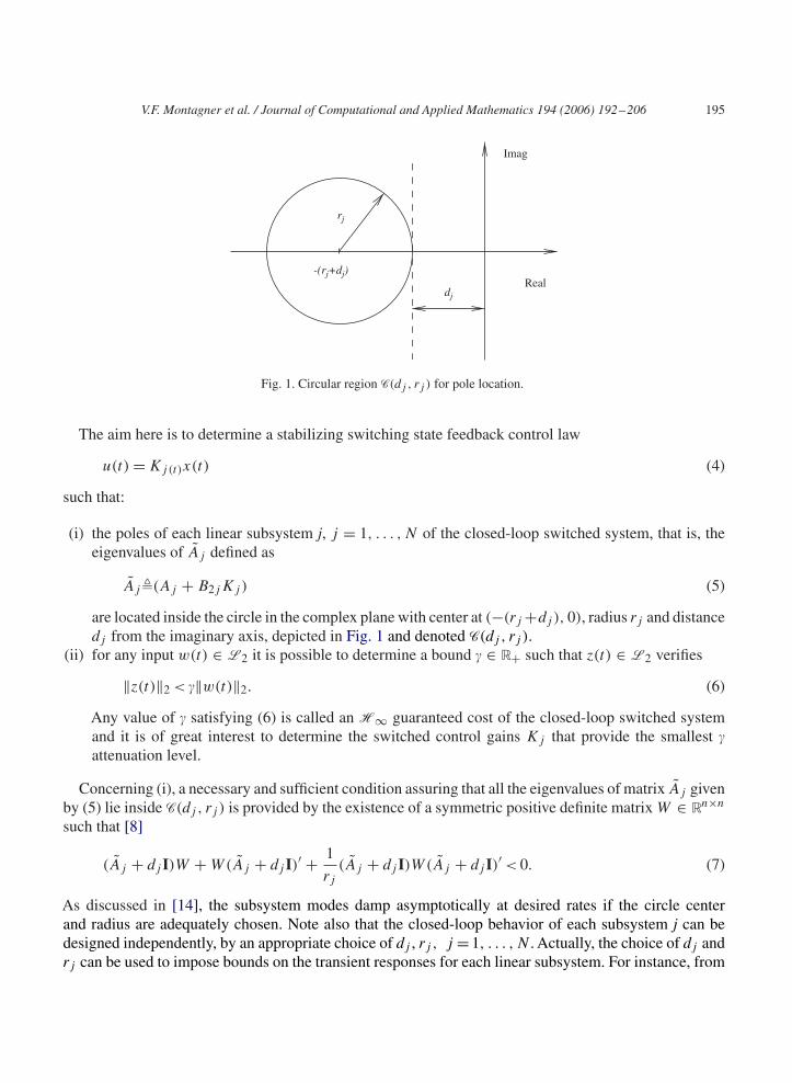
are such that both closed-loop subsystems are individually stable with eigenvalues −0.10 ± 1.41i. How-ever, the closed-loop switched system becomes unstable when initialized at subsystem j (0) = 1, withx(0) = [1 0]′, switching regularly at every 0.5 s from one mode of operation to another, as illustrated inthe phase diagram shown in Fig. 2 (dashed line). On the other hand, the results of Lemmas 1–4 can beapplied to the problem, yielding switching control laws that quadratically stabilize the switched system.For instance, using Lemma 2, one can assure the overall stability under any arbitrary switching rule,providing pole location in the region C(0, 1) for each one of the subsystems, by means of the switchedgains

K1 = [2.102 −1.369] , K2 = [−1.369 2.102 ] (24)

which allocate the closed-loop poles of both subsystems at −0.78 ± 0.53i. The phase diagram of theswitched system with the switched gains (24) is also shown in Fig. 2 (solid line) for the same initial

0 0.5 1 1.5 2 2.5

-2

-1.5

-1

-0.5

0

0.5

x1

x 2

Fig. 2. Phase diagram for the switched system described by matrices (22) with the switched gains given by (23) (dashed line)and with the switched gains computed through Lemma 2 (24) (solid line) for x(0) = [1 0]′, j (0) = 1 switching at every 0.5 s.


0 0.5 1 1.5 2 2.5 3 -0.8

-0.6

-0.4

-0.2

0

0.2

0.4

0.6

0.8

1

t

x1pl

x1est

x2pl

x2est

Fig. 3. Trajectory of the state variables for the closed-loop switched system described by matrices (22) with the switchedstabilizing gains (25) given by Lemma 1 (dashed lines) and with the switched gains (26) also assuring a prescribed pole locationcomputed through Lemma 2 (solid line), starting at x(0) = [1 0]′, j (0) = 1 and switching at every 0.5 s.

condition and switching rule. Undoubtedly, the switched control of Lemma 2 provides a remarkably betterdynamical behavior.

Consider now a comparison between the transient responses of system (22) with the switched statefeedback gains calculated through Lemma 1 (stabilizability), given by

K1est = [1.571 −0.871] , K2est = [−0.871 1.571] (25)

which locate the poles of both subsystems at −0.54±1.07i and the switched state feedback gains obtainedthrough Lemma 2 (stabilization with pole location), for the pole location specifications dj = 0.9, rj = 1,j = 1, 2, given by

K1pl = [1.104 −2.713] , K2pl = [−2.713 1.104] (26)

which locate the poles of both subsystems at −0.98, −1.93. Using the previous initial condition andswitching rule, one has the transient response shown in Fig. 3, where the solid lines represent the trajectoryof the state variables for the closed-loop system with gains (26) from Lemma 2, which assures stabilitywith pole location, and the dashed lines represent the closed-loop trajectories with gains (25) from Lemma1 (only assuring stability). Notice the high improvement in the transient behavior obtained through thegains of Lemma 2, allowing smoother and faster transient responses at each switching instant, thanks tothe pole location constraints.

The second example shows how the use of switched gains can improve the closed-loop dynamics ofthe subsystems of a switched system. Consider the following switched system with two subsystems:

A1 =[

1 −33 −2

], B21 =

[10

], A2 =

[1 −32 −2

], B22 =

[10

]. (27)


-1.5 -1 -0.5 0 0.5

-0.6

-0.4

-0.2

0

0.2

0.4

0.6

Real

Imag

Fig. 4. Pole locations for the closed-loop subsystems of the switched system (27) with fixed gain (◦, dashed line, rf = 0.47) andswitched gains (∗, solid line, rs = 0.26).

The design objective is to allocate the poles of both linear subsystems in the region C(0.5, r), with aminimum radius r. Lemma 2 can be used to address this problem, providing both fixed and switched statefeedback controls. The minimum value obtained with the fixed control gain

Kf = [−0.957 2.582 ] , Wf =[

334.591 818.346818.346 2402.676

](28)

has been rf = 0.47 while the switched law given by (4) with

K1 = [−0.224 2.361] , K2 = [−0.716 2.360 ] , Ws =[

2.006 4.0454.045 8.183

](29)

yields rs = 0.26, guaranteeing better closed-loop behavior (less oscillatory, smaller overshoot) than thefixed gain. Fig. 4 shows both pole locations.

The third example illustrates how a switched control can improve the level of disturbances attenuationof a switched system. The system is described as in (1)–(2) with matrices

A1 =[−1 −1 1

0 −1 32 2 −2

], B21 =

[−1−1−1

], A2 =

[−4 −1 21 −7 22 0 −1

], B22 =

[ 1−11

]

C1 = C2 =[

0 1 00 0 1

], D21 = D22 =

[01

], B11 = B12 = I3×3, D11 = D12 = 02×3.

Using the results of Lemma 3, the lowest attenuation level obtained by means of the fixed state feedbackgain

Kf = [0.151 1.292 −0.440 ]


has been �f = 22.790, while the switched control law as in (4) with

K1 = [1.748 2.741 2.656 ], K2 = [−0.660 1.092 −4.095]

yields �s = 1.016, which represents a huge improvement.The fourth example is concerned with the control of an activated sludge process with three distinct

phases, borrowed from [7]. The four state variables represent the concentrations of: x1—readily biodegrad-able substrate, x2—nitrate, x3—ammonia and x4—dissolved oxygen in the sludge. The subsystem 1represents the aerobic phase, 2 is an intermediate phase from 1 to 3, which is the anoxic phase. In theaerobic phase, the control of the process is performed by two manipulated variables: the inlet flow rateof carbon concentration and the inlet flow rate of air. In phases 2 and 3, only the inlet flow rate of carbonis available for control. The switching from one phase to another is made by an operator in function ofthe total removal of the main substrate, in a sequence not known a priori but continuously available. Fordetails about the model the reader is referred to [7]. The system matrices are given by

A1 =⎡⎢⎣

−100.863 0 0 00 −1.160 5.430 0

−5.488 0 −6.590 0−35.893 0 −24.815 −115.160

⎤⎥⎦ ,

A2 =⎡⎢⎣

−100.863 0 0 00 −1.160 5.430 0

−5.488 0 −6.590 0−35.893 0 −24.815 −1.160

⎤⎥⎦ ,

A3 =⎡⎢⎣

−74.597 −39.034 0 0−9.244 −8.050 0 0−4.042 −3.013 −1.160 0

0 0 0 −20.160

⎤⎥⎦ ,

B21 =⎡⎢⎣

1.143 00 00 00 9.500

⎤⎥⎦ , B22 =

⎡⎢⎣

1.143000

⎤⎥⎦ , B23 =

⎡⎢⎣

1.143000

⎤⎥⎦ ,

B11 = B12 = B13 =⎡⎢⎣

0.083 00 00 0.3330 0

⎤⎥⎦ ,

C1 =[

10 0 0 00 0 0 100

], C2 = C3 =

[10 0 0 00 0 0 0

]

D21 =[

1 00 1

], D22 = D23 =

[10

], D11 = D12 = D13 = 02×2.

The pole locations chosen for each subsystem areC(7, 10) (j=1), C(0, 15) (j=2) andC(0, 30) (j=3),which represents more stringent dynamic behavior for subsystem 1 when compared to the situation of a


-70 -60 -50 -40 -30 -20 -10 0 10

-30

-20

-10

0

10

20

30

Real

Imag

Fig. 5. Pole locations for each one of the subsystems of example 4. C(7, 10) (j = 1, ◦, solid), C(0, 15) (j = 2, �, dashed) andC(0, 30) (j = 3, ×, dashed-dotted).

single control input (subsystems 2 and 3). The switched gains obtained through the conditions of Lemma4 are given by

K1 =[

59.022 50.511 44.388 −0.0293.834 −0.442 2.207 10.300

], K2 = [62.494 38.833 37.626 0.476] ,

K3 = [−0.798 131.451 93.047 1.054]

with the Lyapunov matrix

W =⎡⎢⎣

0.362 −0.021 0.146 0.608−0.021 0.100 −0.129 −0.2480.146 −0.129 0.217 0.4780.608 −0.248 0.478 8.814

⎤⎥⎦

assuring to the closed-loop switched system stability with a guaranteed H∞ attenuation level of � =104.157. Fig. 5 shows the pole locations for the three subsystems.

5. Conclusion

The problem of synthesis of state feedback controllers for switched systems with linear modes ofoperation (subsystems) and no prior knowledge of the switching function has been addressed throughLMI tests, which can be solved by polynomial time algorithms. The conditions allow the determinationof a switched control law by state feedback gains that guarantee the assignment of the poles of eachlinear subsystem of the switched system inside an arbitrary circle in the open left-half complex plane andthe overall stability with a prescribed H∞ attenuation level for the closed-loop switched system. Theconditions can also be used to verify the existence of a fixed (robust) state feedback gain, but examples


show that the switching control strategy can cope with more stringent design specifications, extending theresults based on quadratic Lyapunov functions with a common matrix to improve the dynamical responseof this class of systems. The LMI formulation allows to readily incorporate structural constraints whichcan make the conditions suitable to address decentralized or output feedback control problems.

Acknowledgements

The authors would like to thank the reviewers for their valuable remarks and suggestions. The authorsare also grateful to the Brazilian agencies CAPES, CNPq, FAPESP and FAPEMIG for the financialsupport. V.J.S. Leite thanks the LAAS/CNRS and V.F. Montagner thanks the EECS/UCB for receivingthem as visiting scholars.

References

[1] B.R. Barmish, Necessary and sufficient conditions for quadratic stabilizability of an uncertain system, J. Optim. TheoryAppl. 46 (4) (1985) 399–408.

[2] J. Bernussou, P.L.D. Peres, J.C. Geromel, A linear programming oriented procedure for quadratic stabilization of uncertainsystems, Systems Control Lett. 13 (1) (1989) 65–72.

[3] S. Boyd, L. El Ghaoui, E. Feron, V. Balakrishnan, Linear Matrix Inequalities in System and Control Theory, SIAM Studiesin Applied Mathematics, Philadelphia, PA, 1994.

[4] M.S. Branicky, Multiple Lyapunov functions and other analysis tools for switched and hybrid systems, IEEE Trans.Automat. Control 43 (4) (1998) 475–482.

[5] R.A. DeCarlo, M.S. Branicky, S. Pettersson, B. Lennartson, Perspectives and results on the stability and stabilizability ofhybrid systems, Proc. IEEE 88 (7) (2000) 1069–1082.

[6] P. Gahinet, A. Nemirovskii, A.J. Laub, M. Chilali, LMI Control Toolbox User’s Guide, The Math Works Inc., Natick, MA,1995.

[7] C.-S. Gómez Quintero, I. Queinnec, M. Spérandio, A reduced linear model of an activated sludge process, in: Ninth IFACInternational Symposium on Computer Applications in Biotechnology, Nancy, France, March 2004, in CD-rom.

[8] W.M. Haddad, D.S. Bernstein, Controller design with regional pole constraints, IEEE Trans. Automat. Control 37 (1)(1992) 54–69.

[9] J.P. Hespanha, D. Liberzon,A.S. Morse, Overcoming the limitations of adaptive control by means of logic-based switching,Systems Control Lett. 49 (1) (2003) 49–65.

[10] B. Hu, X. Xu, A.N. Michel, P.J. Antsaklis, Robust stabilizing control laws for a class of second-order switched systems,in: Proceedings of the 1999 American Control Conference, vol. 4, San Diego, CA, June 1999, pp. 2960–2964.

[11] Z. Ji, L. Wang, G. Xie, F. Hao, Linear matrix inequality approach to quadratic stabilisation of switched systems, IEE Proc.Control Theory Appl. 151 (3) (2004) 289–294.

[12] M. Johansson, Piecewise Linear Control Systems—A computational Approach, Lecture Notes in Control and InformationScience, vol. 284, Springer, Heidelberg, Germany, 2003.

[13] J.G. Kassakian, M.F. Schlecht, G.C. Verghese, Principles of Power Electronics, Addison-Wesley, Boston, MA, 1991.[14] V.J.S. Leite, V.F. Montagner, P.L.D. Peres, Robust pole location by parameter dependent state feedback control, in:

Proceedings of the 41st IEEE Conference on Decision and Control, Las Vegas, December 2002, pp. 1864–1869.[15] D.J. Leith, R.N. Shorten, W.E. Leithead, O. Mason, P. Curran, Issues in the design of switched linear control systems: a

benchmark study, Internat. J. Adapt. Control Signal Process. 17 (2) (2003) 103–118.[16] D. Liberzon, A.S. Morse, Basic problems in stability and design of switched systems, IEEE Control Systems Mag. 19 (5)

(1999) 59–70.[17] O. Maler, A. Pnueli (Eds.), Hybrid Systems: Computation and Control, Lecture Notes in Computer Science, vol. 2623,

Springer, Berlin, 2003.


[18] K.S. Narendra, J. Balakrishnan, A common Lyapunov function for stable LTI systems with commuting A-matrices, IEEETrans. Automat. Control 39 (12) (1994) 2469–2471.

[19] P. Peleties, R.A. DeCarlo, Asymptotic stability of m-switched systems using Lyapunov-like functions, in: Proceedings ofthe 1991 American Control Conference, vol. 2, Boston, MA, June 1991, pp. 1679–1684.

[20] S. Pettersson, B. Lennartson, Stability and robustness for hybrid systems, in: Proceedings of the 35th IEEE Conference onDecision and Control, vol. 2, Kobe, Japan, December 1996, pp. 1202–1207.

[21] A.V. Savkin, R.J. Evans, Hybrid Dynamical Systems, Controller and Sensor Switching Problems, Birkhäuser, Boston, MA,2002.

[22] A.V. Savkin, E. Skafidas, R.J. Evans, Robust output feedback stabilizability via controller switching, Automatica 35 (1)(1999) 69–74.

[23] E. Skafidas, R.J. Evans, A.V. Savkin, I. Petersen, Stability results for switched controller systems, Automatica 35 (4) (1999)553–564.

[24] Z.D. Sun, S.S. Ge, Dynamic output feedback stabilization of a class of switched linear systems, IEEE Trans. CircuitsSystems Part I: Fund. Theory Appl. 50 (8) (2003) 1111–1115.

[25] Z.D. Sun, S.S. Ge, T.H. Lee, Controllability and reachability criteria for switched linear systems, Automatica 38 (5) (2002)775–786.

[26] K. Tanaka, H. Wang, Fuzzy Control Systems Design and Analysis: A Linear Matrix Inequality Approach, Wiley, NewYork, 2001.

[27] G. Xie, L. Wang, Controllability and stabilizability of switched linear-systems, Systems & Control Lett. 48 (2) (2003)135–155.

[28] G.S. Zhai, H. Lin, P.J. Antsaklis, Quadratic stabilizability of switched linear systems with polytopic uncertainties, Internat.J. Control 76 (7) (2003) 747–753.

[29] X.L. Zhang, J. Zhao, An algorithm of uniform ultimate boundedness for a class of switched linear systems, Internat. J.Control 75 (16–17) (2002) 1399–1405.

State feedback control of switched linear systems: An LMI approach

Documents

Transcript of State feedback control of switched linear systems: An LMI approach