Stability of Metabolic Correlations under Changing Environmental Conditions in Escherichia coli –...

Stability of Metabolic Correlations under ChangingEnvironmental Conditions in Escherichia coli – A SystemsApproachJedrzej Szymanski1., Szymon Jozefczuk1., Zoran Nikoloski2, Joachim Selbig1,2, Victoria Nikiforova1,3,

Gareth Catchpole1, Lothar Willmitzer1*

1 Max-Planck Institute for Molecular Plant Physiology, Potsdam, Germany, 2 Institute of Biochemistry and Biology, University of Potsdam, Potsdam, Germany, 3 Timiryazev

Institute of Plant Physiology, Russian Academy of Sciences, Moscow, Russia

Abstract

Background: Biological systems adapt to changing environments by reorganizing their cellular and physiological programwith metabolites representing one important response level. Different stresses lead to both conserved and specificresponses on the metabolite level which should be reflected in the underlying metabolic network.

Methodology/Principal Findings: Starting from experimental data obtained by a GC-MS based high-throughput metabolicprofiling technology we here develop an approach that: (1) extracts network representations from metabolic condition-dependent data by using pairwise correlations, (2) determines the sets of stable and condition-dependent correlationsbased on a combination of statistical significance and homogeneity tests, and (3) can identify metabolites related to thestress response, which goes beyond simple observations about the changes of metabolic concentrations. The approach wastested with Escherichia coli as a model organism observed under four different environmental stress conditions (cold stress,heat stress, oxidative stress, lactose diauxie) and control unperturbed conditions. By constructing the stable networkcomponent, which displays a scale free topology and small-world characteristics, we demonstrated that: (1) metabolite hubsin this reconstructed correlation networks are significantly enriched for those contained in biochemical networks such asEcoCyc, (2) particular components of the stable network are enriched for functionally related biochemical pathways, and (3)independently of the response scale, based on their importance in the reorganization of the correlation network a set ofmetabolites can be identified which represent hypothetical candidates for adjusting to a stress-specific response.

Conclusions/Significance: Network-based tools allowed the identification of stress-dependent and general metaboliccorrelation networks. This correlation-network-based approach does not rely on major changes in concentration to identifymetabolites important for stress adaptation, but rather on the changes in network properties with respect to metabolites.This should represent a useful complementary technique in addition to more classical approaches.

Citation: Szymanski J, Jozefczuk S, Nikoloski Z, Selbig J, Nikiforova V, et al. (2009) Stability of Metabolic Correlations under Changing Environmental Conditions inEscherichia coli – A Systems Approach. PLoS ONE 4(10): e7441. doi:10.1371/journal.pone.0007441

Editor: Paul Cobine, Auburn University, United States of America

Received May 25, 2009; Accepted September 15, 2009; Published October 15, 2009

Copyright: � 2009 Szymanski et al. This is an open-access article distributed under the terms of the Creative Commons Attribution License, which permitsunrestricted use, distribution, and reproduction in any medium, provided the original author and source are credited.

Funding: The work was funded by Max Planck Society. J. S. and Z. N. are supported by GoFORSYS project funded by the Federal Ministry of Education andResearch, Grant no. 0313924. The funders had no role in study design, data collection and analysis, decision to publish, or preparation of the manuscript.

Competing Interests: The authors have declared that no competing interests exist.

* E-mail: [email protected]

. These authors contributed equally to this work.

Introduction

Biological systems exposed to new environmental cues react by

adapting their cellular and physiological program in order to

optimize the likelihood of survival under the new condition. Due

to the crucial role of adaptation, there have been numerous studies

investigating the response of biological systems to environmental

challenges [1,2,3]. The relative biological (physiological) simplicity

of unicellular organisms (e.g., Saccharomyces cerevisiae, E. coli) and

availability of their respective annotated genomes have prompted

the employment of integrated, systems-oriented approaches, often

relying on transcriptome data, to study the response towards

changing environment [3,4]. Examples comprise oxidative stress

[5,6,7], temperature shifts [8,9,10,11,12,13], or changes in carbon

sources, such as the classical lactose diauxie [14,15].

In contrast to the abundance of systems-oriented approaches

describing changes on the transcriptome or interactome level,

relatively few studies have employed the metabolome [16,17].

Metabolite concentrations represent a vital readout of the cellular

machinery which may even be considered to be closer to the

complex phenotype than transcripts or proteins [18,19,20].

Based on an established high-throughput metabolic profiling

technology [21,22], we conducted a comprehensive study focusing

on the dynamic response of E. coli to four different environmental

perturbations: cold, heat, oxidative stress, and a lactose diauxic shift,

on the metabolite level. The resulting data are explored via the

reconstruction and interpretation of networks, based on metabolite-

metabolite pair wise correlation [17,23]. The reconstruction of such

a network, which presents a binary simplification of the underlying

covariance matrix for a certain significance threshold, renders it

PLoS ONE | www.plosone.org 1 October 2009 | Volume 4 | Issue 10 | e7441

possible to apply network analysis tools, thereby bringing a new

context of data analysis and introducing a system-wide level of

reasoning. Network-based analysis of metabolite correlations should

be regarded as an abstraction bridging the gap between purely

topological approaches [24] and flux-balance-constrained methods

(e.g., Flux Balance Analysis (FBA) [25] and Metabolic Control

Analysis (MCA) (for a review see, [26]).

A direct relationship between metabolic pathways, biological

function, and metabolite correlations is not yet well-established

[27]. Recent approaches have demonstrated that the covariance

matrix in its classical form does not provide enough information to

reverse engineer an underlying enzymatic system [28]. Neverthe-

less, it has been concurrently shown not only that the covariance

matrix can represent a characteristic fingerprint for a physiological

state of an investigated system, but also that it changes with steady-

state concentrations of metabolites in mutant organisms [29] and

reflects such complex processes such as an increase in anaerobic

respiration in hepatic tumor [30]. Thus it is reasonable to assume

that both differences and commonalities between any measured

systems could be reflected in the underlying features of such a

reconstructed network.

As outlined above we analyzed the metabolic response of E. coli

towards four different stresses and control growth conditions. One

of the goals was to identify candidate metabolites which are

important for the organism to adjust to the new environmental

challenge. Classically these metabolites are identified by either

mutant screens or looking for metabolites which display a major

change in concentration. (e.g. Brauer et al. 2006 [31]). As we show

in following sections, the analysis of the metabolite-metabolite

covariance matrix is a new approach to detect such metabolites. In

addition it provides a platform to interpret the observed changes

on the systemic level.

In the following sections we will address the following questions:

(1) the stability of the correlations for different environmental

conditions; (2) the relationship between metabolite-metabolite

correlations with respect to existing knowledge represented in

pathway databases (e.g., EcoCyc); (3); the extent to which the

properties of the reconstructed networks reflect the biological

differences resulting from the studied environmental cues and,

finally, (4) the role of particular metabolite in the conditional

correlation network rewiring.

Results and Discussion

Early and Mid-Log Phase During Control Growth Displaythe Smallest Number of Metabolic Changes

As outlined in the Introduction we are interested to analyze the

response of E. coli when exposed to four new environmental

conditions. A prerequisite for such an analysis is the identification

of a growth phase where metabolite changes are minimal thus

allowing to assign changes in metabolites to the applied stress

condition and not to changes in the general growth condition. To

identify this time window we in a first pilot experiment followed

the metabolic changes E. coli displays during a normal batch-type

growth curve in an unperturbed state ( cf. fig. 1a) (cf. Materials and

Methods for the exact conditions). The results of this analysis are

shown in Figure 1b in the form of a k-means clustering using an

arbitrary k-value of 10. It shows that the metabolic complement (at

least as assayable via our analysis) remains relatively constant

during early and mid logarithmic growth phase ( time points 1–6

in Figure 1b) which is not surprising and in agreement with

transcriptomic data [32]. In striking contrast massive changes in

metabolites occur at later growth phases specifically upon entry

into stationary phase (cf. Figure 1a, b; time 8–11). Based on this

observation we decided to apply the various stresses at the early

logarithmic growth phase, equivalent to time point o minutes in

Figure 1a and to follow the response of the cells over a total

number of five time points during the adjustment phase (defined

by the duration of the respective lag phase, cf. supplementary

Figure S1 for an example). All experiments were performed in

three independent biological replicates; moreover, for each time

point and each biological replicate, three samples were taken,

resulting in nine samples (for each time point). Obtained data were

normalized to internal standards and optical density of the culture

Figure 1. Metabolic changes during E. coli culture growth. (A) Growth curve (optical density) of unperturbed E. coli culture. Numbers ofrespective sampling time points are marked in the curve. Time point 0 minutes marks the application of the respective stress condition. (B) Relativechanges of metabolites pools normalized to culture OD and time point 1. Fold change is presented on log10 scale. To reveal main trends of metabolicchanges 10 K means clusters are color coded.doi:10.1371/journal.pone.0007441.g001

Metabolic Correlations


at the moment of sampling (see Materials and Methods). The sampling

procedure, including 5 seconds of filtering on a 0.45 mm filter was

chosen as being extensively used in microorganisms studies [33]

and as shown to be superior in comparison with deep temperature

quenching [34]. As it is crucial for covariance analysis, that

measured metabolites are quantified precisely and in all samples,

from a total pool of 247 metabolites identified in the analyzed

samples 170 most reliable peaks were selected along the criteria of

quality of chromatographic separation, confirmed biological

source, detection in all analyzed chromatograms and a reasonable

signal to noise ratio (see Materials and Methods for more details).

Analysis of the data obtained for the different stress treatments by

k-means clustering are shown in supplementary Figure S2 together

with a quantification of the similarity between the different clusters

using Mantel statistics.

Metabolite Covariance Allows for Identification ofSignificant Correlations: Development of theHomogeneity Test

While the initial question is that of identifying whether or not

the covariance displayed by the relative metabolite concentrations

is sufficient to identify significant correlations, of additional interest

is the issue of how these correlations are conserved among the

applied conditions (treatments). Figure 2 shows an example matrix

of metabolite-metabolite correlations for a small subset of

metabolites and the different patterns exhibited following each

treatment. As illustrated, the observed pair-wise correlations fall

into one of three categories: those which correlate under all

applied conditions (e.g., proline-threonine), only under one or more

(but not all) conditions (e.g., fumarate-malate), and those which

display no significant correlation under any of the conditions

tested (e.g., fumarate-cysteine).

It is expected that any such classification is greatly influenced by

the applied significance threshold. Thus, for the cysteine-proline

pair, following both cold and lactose stress, correlations are

nevertheless apparent, despite falling below the significance

threshold. A similar observation can be made for the malate-

fumarate pair: although this correlation was found to exceed the

highest significance threshold only in the case of heat, a correlation

can also be identified by visual inspection in the case of lactose shift

and under control conditions.

We are interested in both, stable (observed under all

experimental conditions) and environment-specific correlations.

A classical method of correlation network reconstruction applies

an arbitrary significance threshold to the correlation coefficients

[35]. When comparing several networks, on the same nodes

(metabolites) but differing in their wiring, the simplest method to

find a stable component is to determine their intersection.

However, this may lead to a considerable loss of information,

particularly when correlation coefficients in any of the treatments

Figure 2. Example subset of metabolites showing different patterns of correlations across the treatments. Significant correlations aremarked by red stars pinpointing values significant with p-value respectively: *** ,1025, ** ,1024, ** ,1023, ‘,1022.doi:10.1371/journal.pone.0007441.g002



fall marginally short of the significance threshold (as exemplified in

Fig. 2). A technique with lower information loss, used here, relies

on the homogeneity test which can be employed to assess the

correlations (and thus the resulting network) that can and should

be regarded as stable or specific in addition to the significance

threshold tests. To this end, we use a two step approach (detailed

in Materials and Methods): (1) a union network is reconstructed where

there is a link between nodes (metabolites) if and only if this

particular pair of metabolites correlates significantly with a

Bonferroni corrected p-value of ,0.01 under at least one

environmental cue (2) a homogeneity test is performed on the Z-

scores of correlation coefficients from different treatments for each

edge of the union network with a test p-value threshold of 0.01.

This ‘‘soft intersection’’ method renders it possible to avoid a sharp

correlation coefficient cutoff and makes the robustness of a

particular correlation dependent on all compared conditions and

not on each one, separately. A decision to qualify a given

correlation as stable or stress-specific must thereby be supported

by both the correlation significance test and the homogeneity test

of the correlation coefficient’s distribution in all experimental

conditions.

Reconstructed Networks Differ in the Number of Edgesand Network Density

As a first step in our analysis we reconstructed a correlation

matrix for each of the five conditions representing bootstrapped

Pearson correlation coefficients between pairs of metabolites. (Cf.

Supplementary Table S2 for all correlation values for all pairs of

metabolites). Correlation networks were obtained by discretizing

of these matrices along significance threshold criteria (see Materials

and Methods for details); note that in this step the significance

threshold is the only criterion applied (Table 1). Considering two

related parameters, network density and edge number, reveals that

the control and heat networks display the highest density and

largest number of edges, and in doing so, along with the cold stress

network, they also possess the smallest number of isolated nodes.

Furthermore, the data suggest an (inverse) relationship between

network density and average variance of the metabolite time

courses. Thus heat stress and control conditions display the lowest

average variance (being an average value from values of variances

exhibited by all metabolites in response to particular stress) over all

metabolites measured (0.226 in the case of control and 0.352 for

heat stress) but the greatest network densities.

Despite the considerable difference in network density, a

substantial degree of network overlap (as determined by the

number of significant edges common to the two conditions

compared) is observed. This degree ranges from 6% common

edges between the two most disparate stresses (oxidative and heat

stress) to the 22% conserved edges observed when comparing cold

and heat stresses (cf. Table 2). Even though not so striking in terms

of percentage, this overlap is statistically highly significant as

displayed by a comparison with an exemplary random network (p-

values exceed 1e-100 when applying the Fisher exact test). Only 9

metabolite pairs reach the absolute significance threshold in all

conditions, which may be regarded as unexpected in the case of a

system constrained by the same underlying metabolic pathways.

However, as we discuss later, this result is an underestimation

caused by the strict ‘‘yes or no’’ discretization criterion, testing the

correlation homogeneity between different conditions allows

detection of much denser stable network components.

The overlap between the individual networks and the stable

component ranges from 26% to 53% (Table 2). This comparison

may however, not be straightforwardly interpreted, since the stable

component in defined experimental conditions permits correla-

tions below the absolute significance threshold. We note that this is

a direct consequence of the criterion used for including an edge in

the stable component (which may not appear in the networks for

separate conditions and would have been filtered out by the simple

intersection method), which ultimately renders the method more

powerful. Despite this apparent difference, the proportion of the

stable component to the entire network is only varying by a factor

of two (from 26% to 53%) indicating largely constant ratio

between stress-specific network rewiring and the homeostasis of

the system represented by its stably wired backbone. A difference

in shortest path length between two metabolites in different

networks is also, in most cases, significantly smaller than those

obtained for random network rewiring (see Materials and Methods).

Analysis of the Stable Network Component: ModularStructure and Scale-Free Topology

For construction of the stable component network, the

correlation significance and homogeneity tests were applied to the

complete data set, yielding 169 stable links (correlations) organized

in 16 connected components, the largest of which containing 55

nodes (metabolites) and 15 smaller ones containing between two

and six (Figure 3a, cf. also Table 3). From the total pool of

metabolites, 63 remained isolated; however, only nine of these

showed no significant correlation in any of the treatments. The

number of isolated metabolites is stable and largely independent of

the correlation significance criterion. Thus when the correlation

significance criterion was used without correcting for multiple

comparisons (p-value threshold fixed on 0.01), the number of

isolated metabolites only slightly decreases down to 55. These

findings validate the robustness of the method against varying

threshold values. Therefore this observation indicates that connec-

tivity of the metabolites in the stable network component is indeed

related to their fluctuations as a result of prevailing environmental

condition and not to statistical significance threshold.

Analysis of the stable component topology was performed by

applying a goodness-of-fit test for normal, power-law, and

exponential distributions. Using a non-linear least squares method

and based on the p-values obtained (,0.0001 in both cases) the

latter two were deemed most probable. Subsequent calculation of

the Akaike information criterion score [36,37] indicated that the

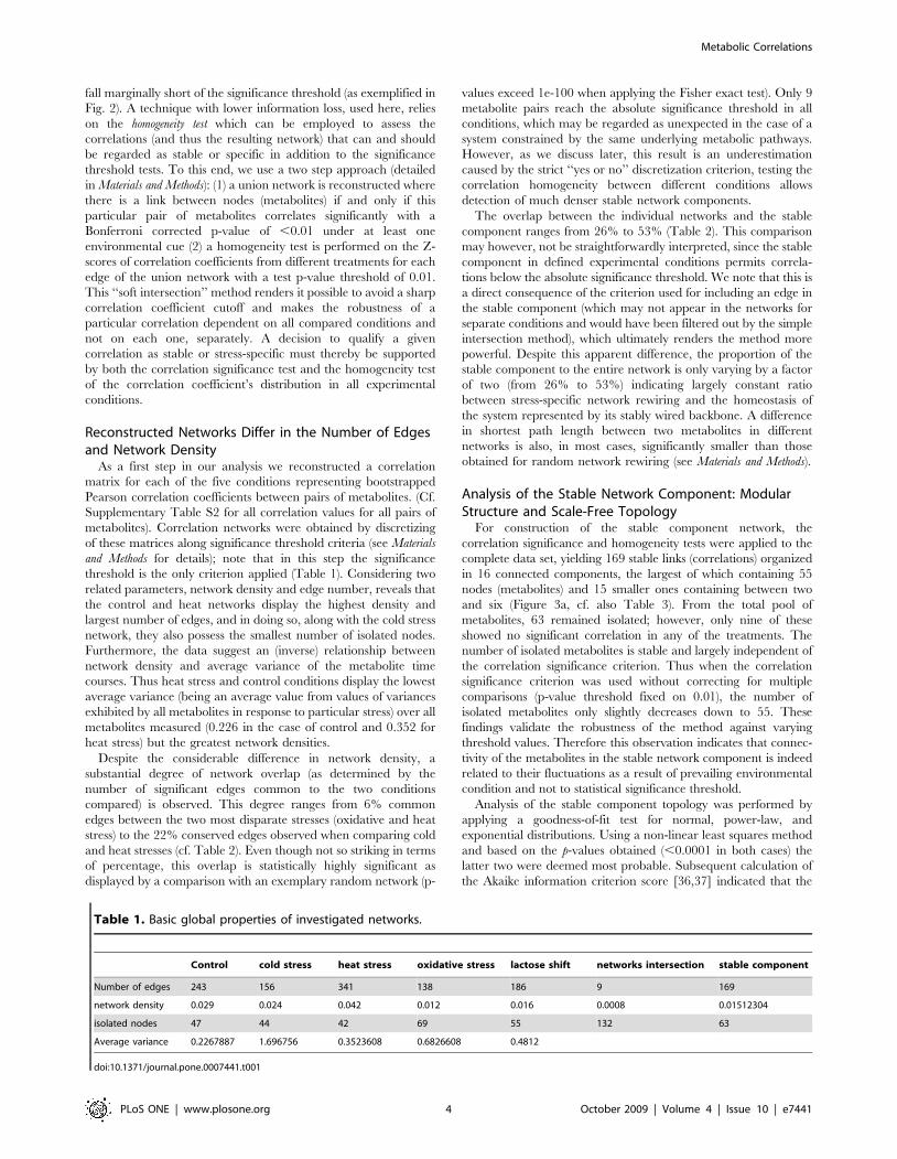
Table 1. Basic global properties of investigated networks.

Control cold stress heat stress oxidative stress lactose shift networks intersection stable component

Number of edges 243 156 341 138 186 9 169

network density 0.029 0.024 0.042 0.012 0.016 0.0008 0.01512304

isolated nodes 47 44 42 69 55 132 63

Average variance 0.2267887 1.696756 0.3523608 0.6826608 0.4812

doi:10.1371/journal.pone.0007441.t001



power-law is more accurate in the case of the stable component

network (for k = 20.7588). The power-law degree distribution is

widely referred as a salient property of hierarchical scale-free

networks and has been reported to be characteristic not only for

biological, but also for other self-organizing systems [38,39,40].

Moreover, these networks exhibit short average path length and

hierarchical organization, marked by locally-dense globally-sparse

architecture directly reflected in the large number of poorly

connected nodes and a relatively low number of highly connected

nodes, called hubs [41,42]. This finding thus suggests the

hierarchical organization of the stable component, where a

relatively small fraction of the metabolites, the network hubs, is

responsible for most of the observed network connectivity.

Analysis of the Stable Network Component: LocalNetwork Properties Are Related to Underlying MetabolicPathways

Networks constructed as described in the preceding paragraph

are based on experimental data in the form of metabolite

measurements. In order to see whether or not they reflect existing

knowledge we compared the connectivity of the hub metabolites in

the stable network described above with their connectivity in the

metabolic pathways as defined in the EcoCyc database [http://

www.ecocyc.org] [43,44],. To this end we reconstructed the E. coli

metabolic network which was subsequently reduced for so called

currency metabolites (e.g., H2O, CO2, ATP and cofactors, see

Materials and Methods for a complete list); these appear as major

connectors in original networks, but as being only donors,

acceptors or carriers for particular chemical group transfers they

play rather a role of reaction parameters and do not constitute a

defined step in metabolic pathway (discussed more deeply and

applied in Fell and Wagner 2000 [45], Ma and Zeng 2003 [46]

and Albert 2005 [47]). Among 150 measured metabolites, 68 were

annotated with a name matching an entry in the EcoCyc database,

of which 49 could be mapped directly to the major connected

component of the metabolic pathways and thus used for

subsequent analysis. A general shift of the connectivity value for

this subset of metabolites was estimated by a nonparametric

location shift test and a significant bias of all measurable

metabolites in the direction of more connected ones in the

metabolic pathways was detected (p-value of 5.408e-06 for

alternative hypothesis).

In a second test we compared the pathway connectivity of hubs in

the stable component network with that of metabolites having no

hub property in the stable component network. This test clearly

showed that a high connectivity in the experimental network is

significantly related to the high connectivity in the metabolic

pathways (location shift p-value ,0.05). As the measured metabo-

lites are scattered across the investigated pathways, local network

properties (e.g., connectivity) may have a negligible discriminatory

power. Therefore, we also investigated local-global properties of the

pathway network, specifically, the betweenness of measured

metabolites, recently related to robustness of complex networks

Table 2. Networks comparison.

Control Cold stress Heat stress Lactose shiftOxidativestress

Randomizednetwork

Stablecomponent

Control overlap percentage - 12.3*** 20.6*** 13.6*** 10.3*** 1.6 29.6***

intersecting edges - 30 50 33 25 4 72

path difference - 1.11*** 1.73*** 1.19** 1.11*** 1.26 0.80*

Cold stress overlap percentage 19.2*** - 22.4*** 14.7*** 11.5*** 1.3 29.5***

intersecting edges 30 - 35 23 18 2 46

path difference 1.11*** - 1.78** 1.36*** 0.96*** 1.49 0.92***

Heat stress overlap percentage 14.7*** 10.3*** - 9.4*** 6.5*** 1.8 26.7***

intersecting edges 50 35 - 32 22 6 91

path difference 1.73*** 1.78** - 1.50*** 1.69*** 1.99 1.16***

Lactose shift overlap percentage 17.7*** 12.4*** 17.2*** - 8.1*** 1.1 34.9***

intersecting edges 33 23 32 - 15 2 65

path difference 1.19** 1.36*** 1.50*** - 0.98*** 1.51 0.82***

Oxidative stress overlap percentage 18.1*** 13*** 15.9*** 10.9*** - 0 31.9***

intersecting edges 25 18 22 15 - 0 44

path difference 1.11*** 0.96*** 1.69*** 0.98*** - 1.82 0.66**

random overlap percentage 2.4 1.2 3.6 1.2 0 - 0.6

intersecting edges 4 2 6 2 0 - 1

path difference 1.26 1.49 1.99 1.51 1.82 - 1.25

Stable component overlap percentage 42.6*** 27.2*** 53.8*** 38.5*** 26*** 0.6 -

intersecting edges 72 46 91 65 44 1 -

path difference 0.80* 0.92*** 1.16*** 0.82*** 0.66** 1.25 -

Percentage of the edge overlap, number of intersecting edges and difference in average path length between individual stress networks, stable component andrandomized network. Difference in average path length describes how the shortest path between two corresponding metabolites differs in two different networks (seeMaterials and Methods for more details). Significant results are marked with stars (*,0.1,**,0.001,***,0.0001) highlighted with bold font (p-value ,0.001). Numbersmean what percent of the row network is shared with a column network. A random network is only an example – the significance tests were done for 1000randomization permutations.doi:10.1371/journal.pone.0007441.t002



[48]. Also in this case, metabolites characterized by high

betweenness in metabolic pathways are mostly those of high

connectivity in the correlation network reconstructed from exper-

iments (supplementary Table S1). As measured metabolites are

rarely connected by a single reaction, shortest paths analysis, such as

applied in betweenness, is a good candidate to bridge metabolite-

metabolite correlations with metabolic pathways, especially since

independence of local network connectivity was proven to be an

intrinsic property of metabolic networks defining their robustness

[49]. Thus in conclusion all three measures support the notion that

the networks reconstructed based on the metabolic profiling data do

reflect existing knowledge about biochemical pathways.

An exemplary comparison between a subnetwork of metabolic

pathways and related system of stable correlations is shown on Fig. 4.

It is important to note, that correlation between amino acids might

be a result not only of their common biosynthetic pathways but also

of their coordinated outflow for protein synthesis or conversely, a

result of amino acids release as a result of protein degradation.

Nevertheless we observe a significant and stable correlation between

amino acids being or sharing common substrates, e.g. threonine/

aspartate/lysine, proline/glutamate and proline/arginine, alanine/

valine or glycine/serine. On the other hand correlations of the

central metabolites such as pyruvate, succinate, malate or a-

ketoglutarate might be more dependent on the biochemical

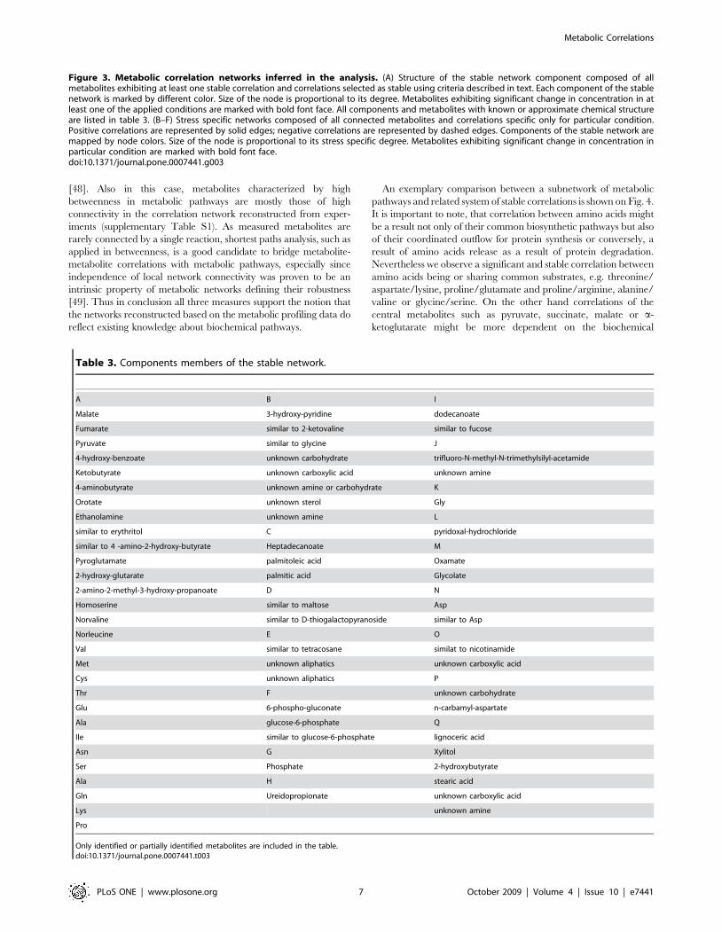
Table 3. Components members of the stable network.

A B I

Malate 3-hydroxy-pyridine dodecanoate

Fumarate similar to 2-ketovaline similar to fucose

Pyruvate similar to glycine J

4-hydroxy-benzoate unknown carbohydrate trifluoro-N-methyl-N-trimethylsilyl-acetamide

Ketobutyrate unknown carboxylic acid unknown amine

4-aminobutyrate unknown amine or carbohydrate K

Orotate unknown sterol Gly

Ethanolamine unknown amine L

similar to erythritol C pyridoxal-hydrochloride

similar to 4 -amino-2-hydroxy-butyrate Heptadecanoate M

Pyroglutamate palmitoleic acid Oxamate

2-hydroxy-glutarate palmitic acid Glycolate

2-amino-2-methyl-3-hydroxy-propanoate D N

Homoserine similar to maltose Asp

Norvaline similar to D-thiogalactopyranoside similar to Asp

Norleucine E O

Val similar to tetracosane similat to nicotinamide

Met unknown aliphatics unknown carboxylic acid

Cys unknown aliphatics P

Thr F unknown carbohydrate

Glu 6-phospho-gluconate n-carbamyl-aspartate

Ala glucose-6-phosphate Q

Ile similar to glucose-6-phosphate lignoceric acid

Asn G Xylitol

Ser Phosphate 2-hydroxybutyrate

Ala H stearic acid

Gln Ureidopropionate unknown carboxylic acid

Lys unknown amine

Pro

Only identified or partially identified metabolites are included in the table.doi:10.1371/journal.pone.0007441.t003

Figure 3. Metabolic correlation networks inferred in the analysis. (A) Structure of the stable network component composed of allmetabolites exhibiting at least one stable correlation and correlations selected as stable using criteria described in text. Each component of the stablenetwork is marked by different color. Size of the node is proportional to its degree. Metabolites exhibiting significant change in concentration in atleast one of the applied conditions are marked with bold font face. All components and metabolites with known or approximate chemical structureare listed in table 3. (B–F) Stress specific networks composed of all connected metabolites and correlations specific only for particular condition.Positive correlations are represented by solid edges; negative correlations are represented by dashed edges. Components of the stable network aremapped by node colors. Size of the node is proportional to its stress specific degree. Metabolites exhibiting significant change in concentration inparticular condition are marked with bold font face.doi:10.1371/journal.pone.0007441.g003



pathways structure, but also of more unpredictable behavior

because of their pleiotropic character. Even though, identification

of correlations being stable across all studied conditions helps to

detect close metabolic relationships, such as e.g. pyruvate/malate,

pyruvate/a-ketoglutarate or pyruvate/valine.

Analysis of the Stable Component Network: Identificationof Functionally-Related Modules

Modularity of the stable component is directly represented by

the presence of 16 disconnected components. No other hierarchi-

cal decomposition of the components gave a satisfactory result,

suggesting that each of the disconnected components is relatively

uniformly connected and may be treated as a structural network

unit (Fig. 3a).

The major component A of the stable component network

covers most primary metabolism and amino acids, representing a

significant part of the homeostatic system. Component B consists

mainly of unknown metabolites and as a result, functional

characterization is unfortunately not possible. On the other hand,

component C contains palmitic, palmitoleic and heptadecanoate

acid and is therefore likely to be related to lipid metabolism.

Cluster D contains maltose, and other sugars of unknown exact

chemical configuration. Glucose-6-phosphate correlates tightly

with gluconic acid-6-phosphate and some G-6-P related structure

within component F. The isolated nodes are denoted as cluster Q

(not shown in this figure but contained in the supplementary Table

S1). These examples suggest that emerging correlations between

metabolites, which are expected to be closely related by function,

tend to also be stable.

To directly assess the relationship between correlation network

structure and metabolic pathways, average shortest paths in the

metabolic pathways were computed for the members of each

network component and for each module. Use of shortest paths

instead of the direct common links is advantageous because

measured and annotated metabolites are rarely directly connected

in metabolic pathways. The shortest path length, as minimal

number of steps needed to reach one metabolite from another,

allows working on a small subset of identified metabolites keeping

in the same the information of the whole network structure.

Additionally in order to correct for a potential bias introduced by

the limited subset of metabolites annotated from our experimental

system, the average EcoCyc shortest path distance for 1000

random sets of 49 metabolites was calculated. This resulted in an

average value of 8.59, while performing the same analysis on the

subset of 49 measured and annotated metabolites resulted in an

average distance of 6.66. Thus we observe a significant location

shift for the whole network (p-value ,2.2e-16), indicating that the

measured and annotated metabolites are in closer proximity on

the metabolic pathways as compared to a subset of the same size

chosen at random. Because of the low number of EcoCyc-mapped

metabolites, only cluster A could be compared against isolated

nodes, since all other clusters contain no or too few annotated

metabolites. The result of this analysis leads to an average distance

of 8.54 for unconnected metabolites as compared to 5.64 for

metabolites of module A, thus significantly separating the two

groups and arguing for structural constraints of the stable

correlation network topology. Upon omission of the two most

distant metabolites, orotate and 4-hydroxybenzoate, from module

A, an even lower value of 4.7 is obtained. Thus, we suggest that

metabolic pathways are extensively reflected in conserved

metabolic correlations, although not exclusively in a trivial path

length-dependent fashion. The noticeable occurrence of conserved

correlations between metabolites, displaying a large distance in the

metabolic pathways, strongly suggests more complex interactions,

hinting at allosteric regulatory mechanisms. We point out that

similar analysis of condition-specific networks, treated separately,

does not show comparable results.

With regard to these findings, the reliance of our approach on

time-course data offers a more powerful way for understanding the

dependencies in a biological system arising as a result of

biochemical reactions. While similar results can be obtained from

Figure 4. Overlap between correlation networks and metabolic pathways. (A) A selected subset of metabolic pathways network, includingTCA cycle, glycolysis and synthesis of several amino acids. Metabolites measured in our experiments are marked black. (B) Union of correlationnetworks obtained in 5 investigated conditions. Edges are shaded according to the number of treatments in which they were found significant. (C)Stable network component identified by testing homogeneity of the correlations obtained in different conditions.doi:10.1371/journal.pone.0007441.g004



studies reliant on biological variability, they are more difficult to

interpret [50]. Finally, our results suggest that only a limited

number of these correlations, remaining stable across the different

conditions, may carry additional information about underlying

biochemical reactions, yet to be assessed

Stress-Specific Networks: Hypothesis Creation forIdentification of Candidate Metabolites Important forCondition-Specific Response

Having considered the stable network, next we focus the

analysis on stress-specific network components (Fig. 3b–f).

To select the stress-dependent correlations, the previously

described stable network component was used. This is, of course,

reliant on the tenet that a stress-dependent network may be

defined by interactions which appear significant following a

particular stress, but are not present in the stable component.

Hence, a desired network can be obtained by simply subtracting

one from the other (Table 2). From these networks, we concluded

that heat and cold stresses share the highest percentage of stress-

related connections, which makes this pairing suitable for

determining common responses.

The other remaining question concerns those correlations

which appear upon each of the applied stresses, but which are

not present in control conditions. In order to extract them using

we obtained a ‘‘soft intersection’’ of 4 stress networks and

discarded those correlations which are either significant or close

to significance in control conditions. The result is the identification

of three classes of stress-specific correlations: firstly, those which

are specific for all stresses and can therefore distinguish stress

conditions from control; secondly, those which are specific for both

cold and heat stress; and thirdly, correlations specific for only one

particular treatment (Table 4). The number of correlations which

are significant for only a single condition is surprisingly large; in all

cases except cold stress about 50% of all correlations are stress-

specific (compared to Table 1).

From the available pool of links, only 63 links (correlations) form

a network present in the four stress conditions but not in the

control. This network is composed of four major disconnected

components in which malate, Val, Ala, Pro, homoserine, 2-

aminobutyrate and 3 unknown metabolites accumulate most of

the network connectivity. 11 correlations were identified as specific

to both heat and cold, with ethanolamine, Thr, Phe, Pro, 2-

aminobutyrate, 2-amino-2-methyl-3-hydroxypropanoate, uracil,

and 2 unknowns as the only connected metabolites (data available

in supplementary Table S1, networks not shown).

To determine compounds whose abundance significantly changes in

response to an applied condition, the time courses of individual

metabolites were first studied to reveal those which significantly either

accumulate or dwindle. A list of the most ‘‘responsive’’ metabolites was

then generated for each treatment in turn (supplementary Table S1,

mapped by bold font face on Fig. 3). The number of common and

stress-specific connections in correlation networks was then compared

between ‘‘responsive’’ and ‘‘non-responsive’’ metabolites and this then

expressed as a ratio (table 5).

The first notable observation concerns the extent to which large

changes in a single metabolite results in a change of the network

structure, expressed by the appearance of new correlations. We

determined that most stress-responsive metabolites are significant-

ly enriched for connections in the stable component, having on

average, 2.46 times higher connectivity than non-responsive

Table 4. Global properties of the condition-specific networks.

Control specificcold stressspecific

heat stressspecific

oxidative stressspecific

lactose shiftspecific

heat and coldstressintersection

Stablecomponent ofstress conditions

number of edges 130 86 221 64 85 11 63

Network density 0.011 0.0076 0.019 0.0057 0.0076 0.0009 0.0056

number of orphans 77 83 61 112 94 140 102

Edge number, density and number of isolates in condition-specific networks.doi:10.1371/journal.pone.0007441.t004

Table 5. Comparison of condition-specific and stable connectivity of the metabolites.

Metabolite degree for single stress and combinednetworks

Metabolite degree when common connections aresubtracted (only stress specific connections)

Condition Ratio Test significance Ratio Test significance

Control 0.93 0.673 1.73 0.005

Cold stress 0.99 0.659 1.91 0.011

Heat stress 0.84 0.440 1.90 0.041

Lactose shift 1.73 0.163 4.19 2.85e-07

Oxdidative stress 1.71 0.071 4.67 8.92e-06

Temperature stress 1.73 0.131 1.87 0.125

Stable component 2.46 0.036 - -

Degree of the most stress responsive metabolites is compared to the degree of non responsive ones and displayed as ratio. This comparison was done for singlestresses including control and combined networks and for the same networks but subtracted for presence of the common correlations. The significance of thedifference (i.e. degree of responsive vs non-responsive metabolites) is checked by Wilcoxon rank sum test.doi:10.1371/journal.pone.0007441.t005



metabolites. This implies that the metabolites exhibiting the

highest number of stable correlations are also those which also

most radically respond to changes of environmental conditions.

Alternatively, the first column of Table 5 suggests that the total

connectivity of metabolites in any individual network is much less

related to their response. This relationship becomes more

significant only when stress-specific connections are isolated

through the removal of those which are shared with the stable

component. As a result, a large change in the concentration of a

given metabolite does not necessarily induce a complete change of

its environment in the network, although it appears to be tightly

connected with the gain of new correlative neighbors. We believe

this to be an important observation as it gives a strong rationale for

the search of the new stress-related biomarkers via network

analysis. Moreover, it also points out that the hub property could

be indicative for the involvement of the metabolite in stress

adaptation.

It is important to mention, that most of observed correlations are

positive and only these seem to be conserved across different

conditions. Significant negative correlations are only observed in

case of three conditions, control, oxidative stress and the lactose

shift. In each case however they contribute less than 15% of all

significant correlations found. This disproportion between the

number of negative and positive correlations is a common feature of

correlation networks and has also been observed e.g. in case of

transcriptome data and other highly clustered datasets [51,52]. The

reason for the overrepresentation of positive correlations must

remain speculative, however it is self-explanatory that clusters of

commonly co-regulated genes or metabolites will enrich the pool of

positive correlations independently of general increase or decrease.

Negative correlation between metabolites on the other hand is

sometimes referred to direct or indirect substrate/product relation-

ships respectively competing pathway branching [30]. This feature

is met with a higher likelihood under conditions of limited nutrient

resources, where pathways are competing for intermediates and the

production of one metabolite requests a decreased pool of another

one. In this respect it is interesting to note that the diauxic shift

experiment where cells are experiencing a shortage in glucose

supply displays the highest proportion of negative correlations (25

out of 186 significant correlations) which is in vast excess of the

control condition ( 7/243 negative versus total correlations) but

similar to the oxidative stress experiment ( 19/138).

Network-Based Analysis Leads to the Identification ofNumerous Metabolites of Hypothetical Importance forStress Adaptation

As shown in Fig. 3a–f, all stress-based networks exhibit a high

number of specific correlations localized in component A (denoted

by green color of the nodes), covering primary metabolism and

most amino acid synthesis pathways. Nevertheless, even in this

tightly connected subnetwork, heat hubs, representing the peak of

heat stress connectivity, may be discriminated from control and

lactose shift hubs. Lactose shift and control conditions on the other

hand seem to overlap to some extent in range of component A.

The control conditions contains relatively few new connections

in comparison to the stable component network, highlighting

mainly primary metabolites of component A as network hubs.

Importantly under control conditions metabolites of component B

form a clear separate community.

The lactose shift derived network on the other hand contains a

number of metabolites as network hubs which are represented as

isolated nodes without any connections in the stable component

network, such as PEP, leucine, asparagine or glycerol-3-phos-

phate. In this regard the lactose shift network seems to be very

distinct from all the other conditional networks, which indicates

highly specific change in the metabolic system.

Oxidative stress hubs are localized mainly in component A,

however among these we also observe several metabolites

belonging to other components. Uracil, which represents an

isolated node in the stable component network, exhibits several

oxidative stress specific negative correlations with metabolites of

component A. This feature is shared by cold and oxidative stress

networks and is in contrast to heat stress and control conditions,

where uracil displays a positive correlation.

The most sparse pattern of correlations is exhibited by the cold

stress network. Similarly to lactose shift, cold stress engages numerous

metabolites without connectivity in the stable network, such as leucine,

oxalate, trehalose, phenylalanine or uracil. The first two are network

hubs, next to methionine, ethanolamine, 2-hydrohyglutarate and

several not precisely annotated compounds. In the cold stress specific

network metabolites of component B form a partially separated

community, which makes it similar to control and lactose shift. In

addition to being present in part of the connectivity within component

A and B, a significant number of the cold stress-dependent correlations

are localized peripherally to the other stresses, indicating a significantly

different way of stress adaptation.

Heat stress finally exhibits a compact connectivity enrichment

mostly due to a significant increase in connectivity between

members of component A e.g. alanine, threonine or fumarate.

Phenylalanine, trehalose, uracil and arginine, which are isolated

nodes in the stable network component become heat specific hubs.

The analysis of the networks resulting from the various

treatments thus clearly shows a high degree of specificity. As

outlined in the Introduction one of our goals was to assess the

possibility to use a network based analysis for the identification of

metabolites which might be crucial for one or several stress

conditions. Hubs which manifest under one or more stress

conditions might represent metabolites important for adjusting

the cellular machinery towards the new environmental condition

and thus could represent candidates for metabolic adjustment

and/or signaling during this phase. We will next discuss four

examples in an exemplary fashion in some detail in order to

introduce the concept before a more comprehensive analysis.

With respect to using the conditional hub property as an

identified for an interesting metabolite three situations can be

distinguished: Metabolites which present a hub only for one

specific condition, for more than one or for all stress conditions.

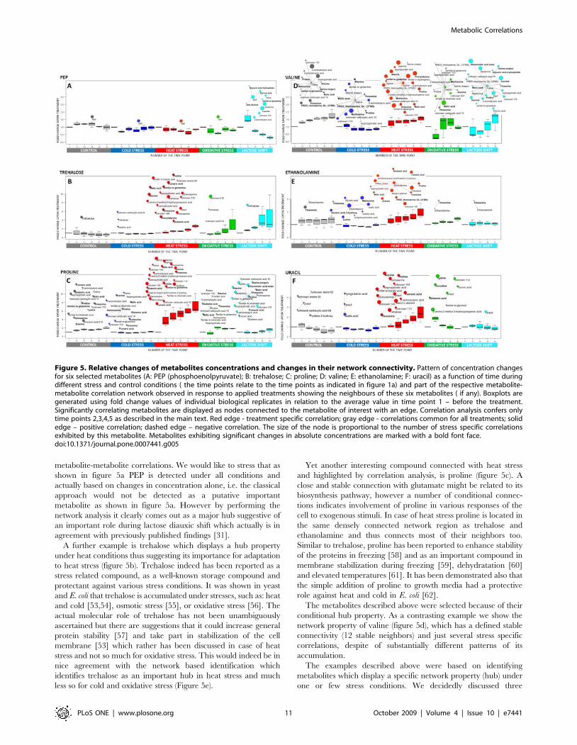
An example for the first group is PEP. It is an isolated node in

all treatments, except the lactose shift, where it becomes one of the

main network connectors (Figure 5a.). In glucose starvation,

induced by lactose diauxie, rapidly increasing phosphoenolopyr-

uvate (PEP) shows especially high number of negative correlations

with several transiently decreasing amino acids, such as valine

(Figure 5c.), glutamine, leucine or homoserine. PEP is a phosphate

donor for phosphotransferase system (PTS) responsible for glucose

import and its accumulation has been recently proposed to be a

direct effect of low glucose import from glucose deficient medium

[31]. This interpretation is supported by observation that PEP

level decrease to the initial level after adaptation phase (40 min,

data not shown). Interestingly, beside several amino acids PEP

correlates negatively with pyruvate and malate. This indicates that

probably accumulation of PEP is a result of the shift of metabolic

resources coming from other parts of central metabolism. This

might also result in decreased pools of some amino acids,

especially if an increased protein synthesis occurs. Such interpre-

tation, although speculative and not directly supported by

measuring of metabolic fluxes, might be taken as an example of

hypothesis creation based on analysis of condition specific



metabolite-metabolite correlations. We would like to stress that as

shown in figure 5a PEP is detected under all conditions and

actually based on changes in concentration alone, i.e. the classical

approach would not be detected as a putative important

metabolite as shown in figure 5a. However by performing the

network analysis it clearly comes out as a major hub suggestive of

an important role during lactose diauxic shift which actually is in

agreement with previously published findings [31].

A further example is trehalose which displays a hub property

under heat conditions thus suggesting its importance for adaptation

to heat stress (figure 5b). Trehalose indeed has been reported as a

stress related compound, as a well-known storage compound and

protectant against various stress conditions. It was shown in yeast

and E. coli that trehalose is accumulated under stresses, such as: heat

and cold [53,54], osmotic stress [55], or oxidative stress [56]. The

actual molecular role of trehalose has not been unambiguously

ascertained but there are suggestions that it could increase general

protein stability [57] and take part in stabilization of the cell

membrane [53] which rather has been discussed in case of heat

stress and not so much for oxidative stress. This would indeed be in

nice agreement with the network based identification which

identifies trehalose as an important hub in heat stress and much

less so for cold and oxidative stress (Figure 5e).

Yet another interesting compound connected with heat stress

and highlighted by correlation analysis, is proline (figure 5c). A

close and stable connection with glutamate might be related to its

biosynthesis pathway, however a number of conditional connec-

tions indicates involvement of proline in various responses of the

cell to exogenous stimuli. In case of heat stress proline is located in

the same densely connected network region as trehalose and

ethanolamine and thus connects most of their neighbors too.

Similar to trehalose, proline has been reported to enhance stability

of the proteins in freezing [58] and as an important compound in

membrane stabilization during freezing [59], dehydratation [60]

and elevated temperatures [61]. It has been demonstrated also that

the simple addition of proline to growth media had a protective

role against heat and cold in E. coli [62].

The metabolites described above were selected because of their

conditional hub property. As a contrasting example we show the

network property of valine (figure 5d), which has a defined stable

connectivity (12 stable neighbors) and just several stress specific

correlations, despite of substantially different patterns of its

accumulation.

The examples described above were based on identifying

metabolites which display a specific network property (hub) under

one or few stress conditions. We decidedly discussed three

Figure 5. Relative changes of metabolites concentrations and changes in their network connectivity. Pattern of concentration changesfor six selected metabolites (A: PEP (phosphoenolpyruvate); B: trehalose; C: proline; D: valine; E: ethanolamine; F: uracil) as a function of time duringdifferent stress and control conditions ( the time points relate to the time points as indicated in figure 1a) and part of the respective metabolite-metabolite correlation network observed in response to applied treatments showing the neighbours of these six metabolites ( if any). Boxplots aregenerated using fold change values of individual biological replicates in relation to the average value in time point 1 – before the treatment.Significantly correlating metabolites are displayed as nodes connected to the metabolite of interest with an edge. Correlation analysis confers onlytime points 2,3,4,5 as described in the main text. Red edge - treatment specific correlation; gray edge - correlations common for all treatments; solidedge – positive correlation; dashed edge – negative correlation. The size of the node is proportional to the number of stress specific correlationsexhibited by this metabolite. Metabolites exhibiting significant changes in absolute concentrations are marked with a bold font face.doi:10.1371/journal.pone.0007441.g005



examples (PEP, trehalose and proline) where there is substantial

evidence in the scientific literature for their importance for stress

adjustment thus strengthening our concept. Figure 5 f and g show

two more examples where metabolites based on a conditional hub

property are identified, i.e. ethanolamine and uracil. Specifically

the case of ethanolamine is interesting and shall thus be discussed

again in some more detail. It displays a stable correlation with

threonine across all the conditions however more important shows

a substantial increase in connectivity under cold and heat stress.

Again it is important to note that changes in ethanolamine

concentration alone would not result in its immediate identifica-

tion again demonstrating the potential of correlation analysis for

identification of important metabolites. Ethanolamine is the

second most abundant head group for phospholipids in biological

membranes; however, the biophysical properties of phospholipids

are mainly defined by the fatty acid component [62]. The specific

detection of ethanolamine under both cold and heat stress may

suggest a link between lipid metabolism and temperature stress.

This is supported by observation that correlations in frame of

module C, conferring such lipid related compounds as heptade-

canoate, palmitoleate and palmitic acid are highest in case of cold

stress. It was shown in various biological models that a decrease in

temperature causes changes in membrane lipid composition

[63,64,65]. Finally during longer periods of unfavoured temper-

atures the membrane lipid composition of E. coli can change

toward an increase of more saturated fatty acids under heat [64]

and unsaturated fatty acids under low temperature [66] again

lending support to the identification of ethanolamine as an

important metabolite involved in the adjustment of the system

towards the two temperature stresses.

Table 6 finally gives an overview of all metabolites being a

conditional hub under one or more stress conditions. Furthermore

the reverse may also be interesting, i.e. a metabolite losing its hub

property under one specific stress conditions. These might be

traced in supplementary Table S1.

ConclusionWe here describe results obtained by following the response of

E. coli towards four different stress conditions and control

conditions over time on the metabolite level. We construct

metabolic networks based on metabolite –metabolite correlations

and identify various network topology parameters. We show that

the network differs considerably between the five different

conditions. A stable component of the network containing those

correlations found under all conditions is shown to reflect

biochemical pathways as described e.g. in EcoCyc. We demon-

strate that network properties displayed by metabolites under only

one or several stress conditions can be used as a novel filter to

identify metabolites which very likely play an important role

during the adjustment phase of E. coli to the specific prevailing

condition. As this novel approach does not rely on major changes

in concentration to identify metabolites important for stress

adaptation, but rather on the changes in network properties with

respect to metabolites, we believe this to be a useful complemen-

tary technique in addition to more classical approaches.

Materials and Methods

Bacterial strains and Growth ConditionsWe used wild type Escherichia coli K12 MG1655 strain, obtained

from the American Type Culture Collection (ATCCH 700926).

Bacteria were grown from the single colony aerobically in 1000 ml

flasks containing MOPS minimal medium [67] (obtained from

Teknova CA, product number M2006) in 37uC. All cultures were

grown aerobically in a thermostatically controlled 37uC culture

room, with aeration provided by magnetic stirrer. The tempera-

ture and pH were carefully monitored during growth. Starting

cultures were inoculated from a single colony and grown

overnight. Each experimental culture was then inoculated from

such an overnight culture at a dilution of 1:20 into 150 ml fresh

MOPS minimal medium in a 1000 ml flask. Growth of cultures

was monitored by measuring optical density (OD) at 600 nm using

an Eppendorf Biophotometer. All cultures were grown until early-

mid log phase (OD 0.6), at which point each of the perturbations

was applied.

Oxidative stress: 200 mg/ml of 30% pre-warmed hydrogen

peroxide (Fluka) was added to constantly stirring cultures. The

amount of hydrogen peroxide used for the stress was calculated to

cause a non-lethal ,40 minute lag phase. This was monitored by

plating on solid LB medium and calculating viable cell number.

Cold stress: Cultures were transferred from 37uC into an ice

cold water bath in order to lower the temperature, while stirring,

to 16uC in less than 2 minutes. When 16uC had been attained,

flasks were transferred to a 16uC water bath while constantly

stirring.

Heat stress: Cultures were transferred from 37uC to a 50uCwater bath. While stirring, the temperature of each culture was

raised to 45uC in under two minutes. The constantly stirring

cultures were then transferred to a 45uC water bath to maintain

this temperature. In both temperature treatments the temperature

was constantly monitored ensuring that the cold treatment culture

Table 6. Stress specific hubs.

Control Heat stress Cold stress Lactose shift Oxdidative stress Cold/Heat stress Common stress response

Pyruvate Trehalose Ethanolamine ethanimidic acid Lys Ethanolamine malate

Norvaline Ala Met Leu Pyroglutamate Thr Val

isopropyl-malate Uracil oxalate glycerol-3-phosphate Norvaline Phe Ala

4-hydroxy-benzoate Phe N-carbamyl-Asn PEP Cys 2-aminobutyrate Pro

Norleucine Arg Glu Malate homoserine

Gln Pro 2-ketobutyrate Asn 2-aminobutyrate

Thr Ethanolamine Succinate Glu

Putrescine

Stress specific hubs and chosen metabolites being hubs in cold/heat stress and in common stress response. Only identified metabolites are mentioned, the full tableavailable in supplementary materials.doi:10.1371/journal.pone.0007441.t006



never exceeded 16uC and the heat treatment culture never

dropped below 45uCGlucose–lactose shift: Carbon source concentrations of 0.15%

lactose and 0.05% glucose were used. This meant that the

adaptation phase was observed at OD,0.6.

SamplingThe first two time points were taken before stress at OD 0.5 and

0.6. Following stress application the subsequent sampling time

points were at 10 minute intervals for up to 40 minutes (lactose

shift and oxidative stress) or 50 minutes (cold, heat and control).

Rapid filtering as described by Bolten et al using 2.5 cm diameter,

0.45 mm pore size DuraporeH filter disks (Millipore Corporation,

MA) and a vacuum manifold and pump was used. Metabolite

(1 ml) and transcript (4 ml) samples were taken simultaneously.

Filters with adhering bacteria were rapidly transferred into 2 ml

centrifuge tubes and flash frozen in liquid nitrogen. The whole

process took less than five seconds (metabolites) or 10 seconds

(transcripts) per sample from sampling to flash freezing in liquid

nitrogen.

For GC-MS metabolite analysis, each of the filter discs with

adhered bacteria was extracted in 500 ml cold Methanol (Merck)

as this has previously been shown to be superior to hot methanol,

hot ethanol, cold perchloric acid, hot alkaline and cold methanol/

chloroform extraction protocols [68]. The extraction solution

contained 0.1 mg/ml cholesterol as an analytical internal standard.

Tubes were subsequently shaken at 4uC for 10 min at 1000 rpm

and again frozen in liquid nitrogen. This freeze-thaw cycle was

repeated to ensure cell membrane rupture. Finally filters were

removed, samples centrifuged for 3 min at 14,000 rpm at 4uC(Eppendorf 5417R) and 450 ml of the supernatant transferred into

new 2 ml centrifuge tubes. These samples were then dried to

complete dryness in a rotary vacuum centrifuge device. Dried

samples were subsequently stored at 220uC for a maximum of two

weeks before analysis.

Extraction and Measurement of MetabolitesDerivatization of the samples was done following the modified

version of protocol described in [69] including methoximation,

through a 90 min 30uC reaction with 5 ml of 40 mg/ml

methoxyamine hydrochloride (Sigma-Aldrich) in pyridine (Merck),

followed by derivatization of acidic protons via a 30 min 37uCreaction with the addition of 45 ml MSTFA (N-methyl-N-

trimethylsilyltrifluoroacetamide) (Machery-Nagel). 1 ml of the

derivatized sample was injected onto the column and analysis

was commenced in non-split mode.

GC-MS hardware comprised an Agilent 6890 series GC system

fitted with a 7683 series autosampler injector (Agilent Technol-

ogies GmbH, Waldbronn, Germany) coupled to a Leco Pegasus 2

time-of-flight mass spectrometer (LECO, St. Joseph, MI, USA).

Identical chromatogram acquisition parameters were used as those

previously described (Weckwerth et al, 2004). Chromatograms

were processed using Leco ChromaTOF software (version 3.25)

and analytical peaks determined using the method of Lisec et al.

2006 [22] with a modified peak picking algorithm which searches

for local apex intensity from all mass traces in raw chromatograms.

All chromatograms were next manually checked. The identifica-

tion of metabolites was confirmed by comparing spectrum and

retention index of given peak with chemical library standards. Also

to exclude possible export errors from Leco ChromaTOF software

to cdf file format the height of given peak was compared with row

chromatographic data. Peaks were also curated according to their

quality; co-eluting, overloaded and too small (height,100) peaks

were excluded from the analysis. All data were normalized to cell

number and the chromatographic internal standard.

Metabolic Data AnalysisEach experimental condition was independently repeated three

times and in each of these repetitions, three technical replicas were

made. The row data was normalized to optical density of the

sample (number of cells) and peak intensity of internal standard

(cholesterol).

Correlation AnalysisData used for correlation analysis cover time points from stress

application to the beginning of stationary phase and include 3

biological replicas per time point. Each biological replica comes

from 3 technical ones. Because of different dynamics of growth

upon stress the data includes different number of time points for

different stresses: 5 time points for control, heat and cold

treatments and 4 time points for oxidative stress and lactose shift.

For this data we used non-parametric Spearman’s rank-order

correlation to obtain correlation matrix for each of the investigated

datasets. To reconstruct individual networks the correlation

coefficient matrices were transformed into binary adjacency

matrices according to a,0.01 [99%] p-value threshold corrected

for a multiple comparisons using Bonferroni correction. To

diminish the influence of single or few measurements on the

observed correlation coefficient, all the significant correlations

were recalculated using non-parametric bootstrap analysis using

1000 bootstrap samples.

Stable ComponentTo find the significant correlations, which are also conserved in

all of the networks we use a simple two step approach.

(1) In the first step a ‘‘union’’ network is reconstructed. This is

equivalent to superimposing the networks from specific

conditions one on the other. Thus an edge in the resulting

network exists if the underlying metabolite-metabolite corre-

lation is found significant at least in one of the treatments.

Edges of the union network gains a weight from 1 to 5, in

respect to the number of conditions in which they were found,

however in our study all the edges of union network were

treated equally.

(2) In the second step a correlation homogeneity test is performed

for all edges of the union network. For each edge of the union

network 5 correlations coefficients coming from 5 individual

stress networks are taken. After transformation into their Z-

scores, they are tested for homogeneity of the distribution. In

result only those edges, which pass a Chi square test with p-

value cutoff ,1E-4 are taken as stable. For a proper

homogeneity test performance all the correlations, which pass

the absolute significance threshold, are treated equally.

Each edge of the resulting ‘‘stable network’’ (‘‘stable compo-

nent’’ as referred in the text) passes two criteria – it is significant at

least in one of the individual networks and the distribution of

correlation coefficients exhibit a homogeneous distribution for all

of the individual networks. Accordingly we refer to the edges of a

stable component as to ‘‘stable edges’’ or ‘‘stable connections’’ and

to the rest as to ‘‘conditional’’ or ‘‘condition/stress specific’’.

Network Topology AnalysisModularity analysis was performed using Newman’s bottom-up

centrality, random walk and leading eigenvector algorithms.

Topology analysis was performed using cumulative degree



distribution and non-linear least squares for distribution function

parameters estimation. Akaike Information Criteria (AIC) for

goodness-of-fit determination was used to estimate the optimal fit

[36,37]. Shortest path analysis used for network comparison was

performed to compare the differences in distance for each pair of

metabolites, when different conditions are applied to the system.

For this purpose, geodesic matrices were obtained for each

network and normalized to a network diameter. Subsequently for

each network-to-network comparison path length difference

matrix was computed. The obtained result was compared to

1000 random network rewirings preserving the original degree

distribution. An average path length distribution for random

networks was used to estimate comparison significance.

EcoCyc Network ReconstructionDatabase of the metabolic reactions was downloaded from

EcoCyc [http://www.ecocyc.org]. Initially 2-mode network was

reconstructed, containing metabolites and reactions as nodes and

edges representing contribution of metabolites in particular

reactions. Subsequently the currency metabolites as main

connectors, represented by ions, cofactors and small inorganic

molecules were removed from the network. The choice of them

was reasoned by a number of nonspecific network shortcuts they

introduce into the metabolic network structure. Among removed

metabolites were: H2O, ATP, ADP, Pi, PPi, NAD, NADH, CO2,

H+, NH4+, NADP, NADPH, CO-A, AMP, O2, CMP, GTP,

GDP, UDP, CTP, UMP, HCO3, SO3, UTP, TMP, H2O2. The

list was composed basing on previous published studies [45,46,47].

Many non-defined molecules were also removed, including such as

‘‘polypeptide’’ or ‘‘disaccharide’’. Resulting network was trans-

formed into classical 1-mode view, where nodes representing

metabolites are linked by edges representing reactions. A main

connected component of the network consists of 613 metabolites

connected by 568 reactions.

SoftwareNetwork properties analysis and all operations were performed

using R 2.7.1 software [70] and Pajek 1.22 [71]. Base set of R

packages was used for statistical analysis of the metabolic data,

igraph 0.5.2 R package [72] was used for graph analysis and

operations on the networks. Visualization and feature mapping

was done using Cytoscape 2.5.1 software [73].

Supporting Information

Figure S1 E. coli growth curves. Growth curve ( optical density)

of unperturbed ( left) and perturbed ( right; oxidative stress

experiment is shown as an example) E. coli cultures. The x-axis

displays the growth time in minutes. The numbers next to the

curve refer to the numbering used in Figure 1b and supplementary

Figure 1.

Found at: doi:10.1371/journal.pone.0007441.s001 (0.08 MB TIF)

Figure S2 Comparison of metabolic time courses observed in

different conditions. K means clustering of metabolite behavior in

control and stressed cultures. Changes observed in metabolites

during early and mid logarithmic growth phase (time points 1 to 6)

and stationary phase (time point 8 to 10) for control culture. Time

points 1 to 10 represents unequal time spans after application of a

stress factor. These are respectively: 0, 10 min, 20 min, 30 min,

40 min, 90 min, 150 min, 210 min, 235 min, 260 min. The

growth curve corresponding to the time points indicated is shown

in Figure 1a. 10 clusters for each condition were identified. Time

courses of all metabolites for particular conditions are located in

rows. Colors representing clusters identified for particular

conditions are located in columns. Value denoted on the plot

represents Mantel statistics score, comparing euclidean distance

matrices obtained for the corresponding treatments. For each pair

significance of the test statistics was approaching 0.

Found at: doi:10.1371/journal.pone.0007441.s002 (0.09 MB TIF)

Table S1 Basic information about metabolites analyzed in this

study. It concerns: metabolites quantification, their variance of its

concentration in different conditions, reference to significant

accumulation or degradation, basic network properties and

KEGG identifiers.

Found at: doi:10.1371/journal.pone.0007441.s003 (0.10 MB

XLS)

Table S2 Pearson correlation coefficient matrices used for the

analysis.

Found at: doi:10.1371/journal.pone.0007441.s004 (1.90 MB

XLS)

Acknowledgments

We thank to Alvaro Cuadros Inostroza for assistance in programming and

data management and to Diego Sanchez and Bjorn Usadel for inspiring

discussions and critical review of the manuscript.

Author Contributions

Conceived and designed the experiments: LW. Performed the experiments:

SJ. Analyzed the data: JJS SJ GC. Contributed reagents/materials/analysis

tools: JJS SJ. Wrote the paper: JJS. Supervision: LW. Supervised the data

analysis: ZN JS VN.

References

1. Bijlsma R, Loeschcke V (1997) Environmental Stress, Adaptation, and

Evolution: Birkhauser.

2. Hirt H, Shinozaki K (2004) Plant Responses to Abiotic Stress: Springer.

3. Storz G, Hengge-Aronis R (2000) Bacterial Stress Responses: ASM Press.

4. Stefan H, Willem HM (2003) Yeast Stress Responses: Springer.

5. Pomposiello PJ, Bennik MHJ, Demple B (2001) Genome-Wide TranscriptionalProfiling of the Escherichia coli Responses to Superoxide Stress and Sodium

Salicylate. Journal of Bacteriology 183: 3890–3902.

6. Chang D-E, Smalley DJ, Conway T (2002) Gene expression profiling of

Escherichia coli growth transitions: an expanded stringent response model.Molecular Microbiology 45: 289–306.

7. Koerkamp MG, Rep M, Bussemaker HJ, Hardy GPMA, Mul A, et al. (2002)Dissection of Transient Oxidative Stress Response in Saccharomyces cerevisiae

by Using DNA Microarrays. MBC 13: 2783–2794.

8. Gadgil M, Kapur V, Hu W-S (2005) Transcriptional Response of Escherichia

coli to Temperature Shift Biotechnol Prog 21: 689–699.

9. Phadtare S, Inouye M (2004) Genome-Wide Transcriptional Analysis of the

Cold Shock Response in Wild-Type and Cold-Sensitive, Quadruple-csp-

Deletion Strains of Escherichia coli. Journal of Bacteriology 186: 7007–7014.

10. Becerra M, Lombardıa L, Gonzalez-Siso MI, Rodrıguez-Belmonte E,

Hauser NC, et al. (2003) Genome-wide analysis of the yeast transcriptome

upon heat and cold shock. Comp Funct Genom 4: 366–375.

11. Sahara, Goda T, Ohgiya S (2002) Comprehensive Expression Analysis of Time-

dependent Genetic Responses in Yeast Cells to Low Temperature The Journal

Of Biological Chemistry 277: 50015–50021.

12. Schade B, Whiteway GJM, Entian KD, Thomas DY (2004) Cold Adaptation in

Budding Yeast. Molecular Biology of the Cell 15: 5492–5502.

13. Tai SL, Lapujade PD, Walsh MC, Pronk JT, Daran JM (2007) Acclimation of

Saccharomyces cerevisiae to Low Temperature: A Chemostat-based Transcrip-

tome Analysis. Molecular Biology of the Cell 18: 5100–5112.

14. Chang DE, Smalley DJ, Conway T (2002) Gene expression profiling of

Escherichia coli growth transitions: an expanded stringent response model.

Microbiology 45 (2): 289–306.

15. Traxler MF, Chang DE, Conway T (2006) Guanosine 3-5-bispyrophosphate

coordinates global gene expression during glucose-lactose diauxie in Escherichia

coli. Proc Natl Acad Sci U S A 103: 2374–2379.

16. Schauer N, Fernie AR (2006) Plant metabolomics: towards biological function

and mechanism. Trends in Plant Science 11: 508–516.



17. Weckwerth W, Fiehn O (2002) Can we discover novel pathways using

metabolomic analysis? Current Opinion in Biotechnology 13: 156–160.

18. Winder CL, Dunn WB, Schuler S, Broadhurst D, Jarvis R, et al. (2008) Global

Metabolic Profiling of Escherichia coli Cultures: an Evaluation of Methods for

Quenching and Extraction of Intracellular Metabolites. Anal Chem 80:2939–2948.

19. Ohashi Y, Hirayama A, Ishikawa T, Nakamura S, Shimizu K, et al. (2008)Depiction of metabolome changes in histidine-starved Escherichia coli by CE-

TOFMS. Molecular BioSystems 4: 135–147.

20. Wittmann C, Weber J, Betiku E, Kromer J, Bohm D, et al. (2007) Response offluxome and metabolome to temperature-induced recombinant protein synthesis

in Escherichia coli. Journal of Biotechnology 132: 375–384.

21. Kopka J (2006) Current challenges and developments in GC-MS based

metabolite profiling technology. Journal of Biotechnology 124: 312–322.

22. Lisec J, Schauer N, Kopka J, Willmitzer L, Fernie AR (2006) Gaschromatography mass spectrometry-based metabolite profiling in plants. Nature

Protocols 1: 387–396.

23. Kose F, Weckwerth W, Linke T, Fiehn O (2001) Visualizing plant metabolomic

correlation networks using clique-metabolite matrices. Bioinformatics 17:1198–1208.

24. Jeong H, Tombor B, Albert R, Oltvai ZN, Barabasi AL (2000) The large-scale

organization of metabolic networks. Nature 407: 651–654.

25. Schuster S (2001) Flux determination by isotopomer balancing - a successful

application of theory to experiment. Trends in Biotechnology 19: 85–85.

26. Fell D (1992) Metabolic control analysis: a survey of its theoretical and

experimental development. Biochem J Sep 1: 313–330.

27. Marcotte EM (2001) The path not taken. Nature Biotechnology. pp 626–627.

28. Steuer R, Kurths J, Fiehn O, Weckwerth W (2003) Observing and interpreting

correlations in metabolomic networks. Bioinformatics 19: 1019–1026.

29. Kusano M, Fukushima A, Arita M, Jonsson P, Moritz T, et al. (2007) Unbiased

characterization of genotype-dependent metabolic regulations by metabolomic

approach in Arabidopsis thaliana. BMC Systems Biology 1: 53.

30. Southam AD, Easton JM, Stentiford GD, Ludwig C, Arvanitis TN, et al. (2008)

Metabolic changes in flatfish hepatic tumours revealed by NMR-basedmetabolomics and metabolic correlation networks. J Proteome Res 7:

5277–5285.

31. Brauer MJ, Yuan J, Bennett BD, Lu W, Kimball E, et al. (2006) Conservation ofthe metabolomic response to starvation across two divergent microbes. Proc Natl

Acad Sci U S A 103: 19302–19307.

32. Chang DE, Smalley DJ, Conway T (2002) Gene expression profiling of

Escherichia coli growth transitions: an expanded stringent response model. Mol

Microbiol 45: 289–306.

33. Bolten CJ, Kiefer P, Letisse F, Portais JC, Wittmann C (2007) Sampling for

metabolome analysis of microorganisms. Anal Chem 79: 3843–3849.

34. Taymaz-Nikerel H, de Mey M, Ras C, ten Pierick A, Seifar RM, et al. (2009)

Development and application of a differential method for reliable metabolomeanalysis in Escherichia coli. Anal Biochem 386: 9–19.

35. Steuer R, Nesi AN, Fernie AR, Gross T, Blasius B, et al. (2007) From structure

to dynamics of metabolic pathways: application to the plant mitochondrial TCAcycle. Bioinformatics 23: 1378–1385.

36. Akaike H (1983) Information measures and model selection. Proceedings of the44th Session of the International Statistical Institute. pp 277–291.

37. Sakamoto T, Ishiguro M, Kitagawa G (1986) Akaike Information Criterion

Statistics. Holland: D. Reidel.

38. Arita M (2005) Scale-Freeness and Biological Networks. J Biochem (Tokyo) 138:

1–4.

39. Barabasi AL, Albert R (2000) Topology Of Evolving Networks: Local Events

and Universality. Physical Review Letters 85: 5234–5237.

40. Watts DJ, Strogatz SH (1998) Collective dynamics of ‘small-world’ networks.Nature 393: 440–442.

41. Amaral LA, Scala A, Barthelemy M, Stanley HE (2000) Classes of small-worldnetworks. Proc Natl Acad Sci U S A 97: 11149–11152.

42. Strogatz SH (2001) Exploring complex networks. Nature 410: 268–276.

43. Karp PD, Riley M, Saier M, Paulsen IT, Collado-Vides J, et al. (2002) TheEcoCyc Database. Nucleic Acids Res 30: 56–58.

44. Keseler IM, Collado-Vides J, Gama-Castro S, Ingraham J, Paley S, et al. (2005)EcoCyc: a comprehensive database resource for Escherichia coli. Nucl Acids Res

33: D334–337.

45. Fell DA, Wagner A (2000) The small world of metabolism. Nat Biotech 18:1121–1122.

46. Ma H-W, Zeng A-P (2003) The connectivity structure, giant strong component

and centrality of metabolic networks 10.1093/bioinformatics/btg177. Bioinfor-matics 19: 1423–1430.

47. Albert R (2005) Scale-free networks in cell biology. J Cell Sci 118: 4947–4957.

48. Newman MEJ (2006a) Modularity and community structure in networks. PNAS103: 8577–8582.

49. Smart AG, Amaral LAN, Ottino JM (2008) Cascading failure and robustness inmetabolic networks. Proc Natl Acad Sci U S A 105: 13223–13228.

50. Muller-Linow M, Weckwerth W, Hutt M-T (2007) Consistency analysis of

metabolic correlation networks. BMC Systems Biology 1: 44.51. Nikiforova VJ, Daub CO, Hesse H, Willmitzer L, Hoefgen R (2005) Integrative

gene-metabolite network with implemented causality deciphers informationalfluxes of sulphur stress response. J Exp Bot 56: 1887–1896.

52. Szymanski J, Bielecka M, Carrari F, Fernie AR, Hoefgen R, et al. (2007) On theprocessing of metabolic information through metabolite-gene communication

networks: An approach for modelling causality. Phytochemistry 68: 2163–2175.

53. Kandror O, DeLeon A, Goldberg AL (2002) Trehalose synthesis is inducedupon exposure of Escherichia coli to cold and is essential for viability at low

temperatures. Proc Natl Acad Sci U S A 99: 9727–9732.54. Attfield PV (1987) Trehalose accumulates in Saccharomyces cerevisiae during

exposure to agents that induce heat shock response. FEBS Letters 225: 259–263.

55. Hounsa CG, Brandt EV, Thevelein J, Hohmann S, Prior BA (1998) Role oftrehalose in survival of Saccharomyces cerevisiae under osmotic stress.

Microbiology 144: 671–680.56. Benaroudj N, Lee DH, Goldberg AL (2001) Trehalose Accumulation during

Cellular Stress Protects Cells and Cellular Proteins from Damage by OxygenRadicals. J Biol Chem 276: 24261–24267.

57. Virgilio C, Hottiger T, Dominguez J, Boller T, Wiemken A (1994) The role of

trehalose synthesis for the acquisition of thermotolerance in yeast. EuropeanJournal of Biochemistry 219: 179–186.

58. Rudolph AS, Crowe JH (1985) Membrane stabilization during freezing: the roleof two natural cryoprotectants, trehalose and proline. Cryobiology 22: 367–377.

59. Csonka LN, Hanson AD (1991) Prokaryotic osmoregulation: genetics and

physiology. Annu Rev Microbiol 45: 569–606.60. Carpenter JF, Crowe JH (1988) Modes of stabilization of a protein by organic

solutes during desiccation. Cryobiology 25: 459–470.61. Hottiger T, De Virgilio C, Hall MN, Boller T, Wiemken A (1994) The role of

trehalose synthesis for the acquisition of thermotolerance in yeast. II.Physiological concentrations of trehalose increase the thermal stability of

proteins in vitro. Eur J Biochem 219: 187–193.

62. Shahjee HM, Banerjee K, Ahmad F (2002) Comparative analysis of naturallyoccurring L-amino acid osmolytes and their D-isomers on protection of

Escherichia coli against environmental stresses. J Biosci 27: 515–520.63. Evans RI, McClure PJ, Gould GW, Russell NJ (1998) The effect of growth

temperature on the phospholipid and fatty acyl compositions of non-proteolytic

Clostridium botulinum. International Journal of Food Microbiology 40:159–167.

64. Rottem S, Markowitz O, Razin S (1978) Thermal Regulation of the Fatty AcidComposition of Lipopolysaccharides and Phospholipids of Proteus mirabilis.

European Journal of Biochemistry 85: 445–450.65. Zhang Y-M, Rock CO (2008) Membrane lipid homeostasis in bacteria. Nature

Reviews Microbiology 6: 222–233.

66. Marr AG, Ingraham JL (1962) Effect of temperature on the composition of fattyacids in Escherichia coli. J Bacteriol 84: 1260–1267.

67. Neidhardt FC, Bloch PL, Smith DF (1974) Culture Medium for Enterobacteria.Journal of Bacteriology 119: 736–747.

68. Prasad Maharjan R, Ferenci T (2003) Global metabolite analysis: the influence

of extraction methodology on metabolome profiles of Escherichia coli. AnalyticalBiochemistry 313: 145–154.

69. Roessner U, Luedemann A, Brust D, Fiehn O, Linke T, et al. (2001) MetabolicProfiling Allows Comprehensive Phenotyping of Genetically or Environmentally

Modified Plant Systems. Plant Cell 13: 11–29.

70. Gentleman RIaR (1996) R: A language for data analysis and graphics. Journal ofComputational and Graphical Statistics 5: 299–314.

71. Batagelj V, Mrvar A (1998) Pajek - Program for Large Network Analysis.Connections 21: 47–57.

72. Csardi G, Nepusz T (Copyright 2003-2009) igraph library. MTA RMKI,Konkoly-Thege Miklos st. 29-33., Budapest 1121, Hungary.

73. Shannon P, Markiel A, Ozier O, Baliga NS, Wang JT, et al. (2003) Cytoscape: A

Software Environment for Integrated Models of Biomolecular InteractionNetworks. Genome Res 13: 2498–2504.



Stability of Metabolic Correlations under Changing Environmental Conditions in Escherichia coli –...

Documents

Transcript of Stability of Metabolic Correlations under Changing Environmental Conditions in Escherichia coli –...