applied sciences

Article

Sparse Envelope Spectra for Feature Extraction ofBearing Faults Based on NMF

Lin Liang 1,2, Lei Shan 1, Fei Liu 1,*, Ben Niu 1 and Guanghua Xu 1,3

1 School of Mechanical Engineering, Xi’an Jiaotong University, Xi’an 710049, China; lianglin@xjtu.edu.cn (L.L.);shan3lei@stu.xjtu.edu.cn (L.S.); niuben1996@stu.xjtu.edu.cn (B.N.); aii@xjtu.edu.cn (G.X.)

2 Key Laboratory of Education Ministry for Modern Design and Rotor-Bearing System, Xi’an JiaotongUniversity, Xi’an 710049, China

3 State Key Laboratory for Manufacturing Systems Engineering, Xi’an Jiaotong University, Xi’an 710054, China* Correspondence: fayelau@xjtu.edu.cn; Tel.: +86-029-8266-3707

Received: 26 December 2018; Accepted: 17 February 2019; Published: 21 February 2019�����������������

Featured Application: Except for rolling bearings, this method is also used for analysis of theimpact modulation cause by gear localized faults.

Abstract: Periodic impulses and the oscillation response signal are the vital feature indicators ofrolling bearing faults. However, finding the suitable feature frequency band is usually difficultdue to the interferences of other components and multiple resonance regions. According to thecharacteristics of non-negative matrix factorization (NMF) on a spectrogram, the feature extractionmethod from a sparse envelope spectrum for rolling bearing faults is proposed in this paper. On thebasis of the time–frequency distribution (TFD) of the periodic transient oscillations, the basic matrixcan be interpreted as the spectral bases, and the time weight matrix corresponding to spectral basescan be extracted by NMF. Because the bases and the weights have a one-to-one correspondence,the frequency band filtering with the basic component and the time domain envelope of the weightvector are calculated respectively. Then, the sparse envelope spectrum can be derived by the innerproduct of the above results. The effectiveness of the proposed method is verified by simulations andexperiments. Compared with band-pass filtering and spectral kurtosis methods, and considering thetime weights and corresponding the spectral bases for the periodic transient oscillations, the weakfault-rated feature can be enhanced in the sparse spectrum, while other components and noiseare weakened. Therefore, the proposed method can reduce the requirement of selecting frequencyband filtering.

Keywords: feature extraction; time–frequency distribution; non-negative matrix factorization; rollingbearing fault

1. Introduction

As an important component in rotating machinery, the rolling bearing is a frequent area inmachinery failure which can bring about economic losses and casualties [1]. Therefore, the conditionmonitoring and fault diagnosis of the rolling bearings are important means of health assessment,and the feature extraction based on vibration signals [2,3] is of significant interest to researchers.

Theoretically, once the rolling bearing has a localized fault (such as pitting, spalling, etc.), whichcreates the periodic impulses during the rotation of rotor, the periodic resonance of structures canbe excited in the vibration signal. Thus, the frequency of the transient oscillation is decided by thenatural frequency of the mechanical system, and the repetition frequency of the transient oscillationcorresponds to the fault-related impulses [4]. The periodic vibration response signal is clearly

Appl. Sci. 2019, 9, 755; doi:10.3390/app9040755 www.mdpi.com/journal/applsci

Appl. Sci. 2019, 9, 755 2 of 22

non-stationary because the magnitude of oscillations decreases exponentially, and the signal having adiscretized spectrum and wide frequency band of the high rotational speed of bearing is shown inFigure 1a,b. The discrete interval of frequency is the repetition period of the impact excitation. However,in incipient stages, due to the lower amplitude of the transient oscillation, the large noise and othercomponents often interfere with the identification of discrete frequencies [5], as shown in Figure 1c.Therefore, the feature extraction of periodic impulses is proposed with various detection methods,such as spectrum analysis, cepstral analysis [6], envelope analysis, and time–frequency analysis.

Appl. Sci. 2019, 9, x FOR PEER REVIEW 2 of 23

natural frequency of the mechanical system, and the repetition frequency of the transient oscillation corresponds to the fault-related impulses [4]. The periodic vibration response signal is clearly non-stationary because the magnitude of oscillations decreases exponentially, and the signal having a discretized spectrum and wide frequency band of the high rotational speed of bearing is shown in Figure 1a,b. The discrete interval of frequency is the repetition period of the impact excitation. However, in incipient stages, due to the lower amplitude of the transient oscillation, the large noise and other components often interfere with the identification of discrete frequencies [5], as shown in Figure 1c. Therefore, the feature extraction of periodic impulses is proposed with various detection methods, such as spectrum analysis, cepstral analysis [6], envelope analysis, and time–frequency analysis.

(a) (b)

(c)

Figure 1. Simulation signal of bearing fault. The carrier frequency is 2200 Hz and the fault feature frequency (fh) is 80 Hz: (a) Simulation signal waveform; (b) Discretized frequency spectrum of simulation signal; (c) Spectrum of simulation signal with added noise.

According to the frequency representation of the vibration response caused by the fault-related impulses, the envelope demodulation can be used to extract the repetitive frequency of the transient oscillations with band-pass filtering and envelope transformation [7]. However, when the impact excitation has low energy, the magnitude of the exponential decay signal is also small and leads to difficulty in the selection of a resonance region. Moreover, it often interacts with the frequency band of other components and the excitation response of random impulses. It is obvious that the optimal filtering frequency band cannot be obtained easily. Thus, to capture the signature of repetitive transients, the spectral kurtosis (SK) is proposed [8,9]. SK selects the best band-pass filter based on spectral kurtosis variation. However, the kurtosis index is susceptible to various outliers that are independent of the fault [10], so the selected frequency band could be unable to extract valid fault information.

Unlike the response of random impact excitation, the periodic transient oscillation corresponds to the discrete components of the resonance frequency band. However, due to the influence of noise

Am

plitu

de

Am

plitu

de

Figure 1. Simulation signal of bearing fault. The carrier frequency is 2200 Hz and the fault featurefrequency (fh) is 80 Hz: (a) Simulation signal waveform; (b) Discretized frequency spectrum ofsimulation signal; (c) Spectrum of simulation signal with added noise.

According to the frequency representation of the vibration response caused by the fault-relatedimpulses, the envelope demodulation can be used to extract the repetitive frequency of the transientoscillations with band-pass filtering and envelope transformation [7]. However, when the impactexcitation has low energy, the magnitude of the exponential decay signal is also small and leadsto difficulty in the selection of a resonance region. Moreover, it often interacts with the frequencyband of other components and the excitation response of random impulses. It is obvious that theoptimal filtering frequency band cannot be obtained easily. Thus, to capture the signature of repetitivetransients, the spectral kurtosis (SK) is proposed [8,9]. SK selects the best band-pass filter basedon spectral kurtosis variation. However, the kurtosis index is susceptible to various outliers thatare independent of the fault [10], so the selected frequency band could be unable to extract validfault information.

Unlike the response of random impact excitation, the periodic transient oscillation corresponds tothe discrete components of the resonance frequency band. However, due to the influence of noise andother components, it is difficult to observe the discretization spectra. In this case, the time–frequency

Appl. Sci. 2019, 9, 755 3 of 22

analysis provides a localized feature representation for the repetitive transients, and the time–frequencydistribution (TFD) of the signal has been adopted to identify the response of the system, such as thenatural frequency and damping ratio [11–14]. Moreover, due to splitting the signal into differentfrequency bands and central frequencies, the wavelet transform is also used for frequency bandoptimization. In related research, Qiu [5] constructed a suitable filter for envelope analysis byselecting the optimal parameters of the wavelet filter, and Su [15] proposed the optimal Morletwavelet filter. Yiakopoulos [16] also adopted the wavelet transform of the original signal to envelopethe low-frequency feature. The results denote that the performances are very dependent on the waveletbasis and the practical applicability is limited.

In addition, the short time Fourier transform (STFT) has also been adopted to represent thenon-stationary information of the vibration signal [17–19]. In view of the non-negative property of theTFD, the non-negative matrix factorization (NMF) is suitable for the analysis of vibration signals due tothe ability of the parts-based representation. Delong [19] proposed the constrained NMF of the spectralmatrix and used the decomposed basis matrix to extract features. After utilizing the semi-binaryNMF of the spectrum, Wodecki [18] selected the appropriate decomposition frequency band forslicing analysis based on the principle of maximum kurtosis. Meanwhile, Wodecki [17] also adoptedstandard NMF on spectrograms and utilized the basis vector to filter frequency bands. In addition tovibration signals, the speech signal has also been analyzed while performing NMF [20–22]. Unliketraditional band-pass filtering, the NMF-based methods can decompose frequency bands accordingto time–frequency distribution adaptively, and the interference component in the bands cannotbe eliminated.

By applying NMF to the TFD, the frequency distribution of the vibration response can bedecomposed into the base matrix, which can be interpreted as the spectral bases and the weightmatrix which is the time envelope corresponding to the spectral bases. For the periodic transientoscillations, the spectral bases can reflect the natural frequency band, while the magnitude change ofthe periodic transient oscillations is also represented by the weight matrix. Due to the influence ofnoise and the decomposed frequency band, neither the band-pass filtering based on the frequency basematrix nor the envelope of the time weight matrix can clearly extract the impact features. However,since the bases and the weights have a one-to-one correspondence, it means that the same featurecomponent with different amplitudes can exist in the band-pass filtering and the envelope of timeweights. Thus, the inner product of the above results can be used to obtain a sparse envelope spectrum,which can enhance the components of fault features and weaken interference components.

The rest of this paper is organized as follows. Section 2 gives a brief description of NMF andprovides the characteristics of NMF of time–frequency distribution, and then introduces the principlesand processes of the proposed method. Section 3 verifies the proposed method with simulated signalsand fault bearing data. Conclusions are drawn in Section 4.

2. Materials and Methods

2.1. NMF

With the non-negative constraints, NMF is also widely used in image recognition, data miningetc. [23–25]. Given a non-negative matrix V =

[v1 v2 · · · vn

]∈ Rm×n, where m and n are

the numbers of samples and features respectively, NMF is designed to decompose the matrix Vinto the product of two non-negative matrices W =

[w1 w2 · · · wr

]∈ Rm×r and H =[

h1 h2 · · · hr

]T∈ Rr×n, such that Equation (1) holds:

Vn×m ≈Wn×rHr×m

s.t. W ≥ 0, H ≥ 0(1)

Appl. Sci. 2019, 9, 755 4 of 22

where W and H are the basis matrix and the weight matrix, respectively, and r is the low rank of theembedding space. Normally, the choice of r is to satisfy (m + n) < mn. W can be regarded as a set ofbases that linearly approximate the observed array V , and H is the non-negative projection weight ofthe observed array V on the basis W.

Due to the purely additive expression, NMF provides a good explanation of the localcharacteristics of data. In addition, from the perspective of clustering, the decomposition result of NMFis clustering for the non-negative data [26]. Ding [27] proved the consistency among NMF, K-meansand spectral clustering methods. We can interpret the columns of W as the posterior probabilities forrow clustering and the rows of H as the posterior probabilities for column clustering.

For the solution of Equation (1), the objective function based on Euclidean distance is written as:

min : fNMF(V||WH) = 12 ||V−WH||2F = 1

2 ∑ij

(Vij − (WH)ij

)2

s.t. W ≥ 0, H ≥ 0, (2)

where ||•||2F denotes the Frobenius norm. Using the gradient descent method for this optimizationproblem, the classical multiplicative iterative rules are given by:

H← HWTV

WTWH, (3)

W←WVHT

WHHT . (4)

The multiplicative iterative algorithm is simple and easy to use, but the poor performance andconvergence are also pointed out in paper [28,29]. Therefore, improved algorithms are proposed, suchas the alternating least squares algorithm [30], the projected quasi-Newton algorithm [31], the projectedgradient algorithm [28], and the block principal pivoting algorithm [32]. The block principal pivotingalgorithm is developed with the non-negative least squares (NNLS) framework. min

W≥0‖HTWT − VT‖2

F, by fixing H

minH≥0‖WH− V‖2

F, by fixing W(5)

To obtain good convergence, the main iterative rules are as follows:

H←(

WTW)−1

WTV, (6)

W← VHT(

HHT)−1

. (7)

Meanwhile, block principal rotation [33] is used to improve the convergence of the algorithm.Hence, the block principal pivoting algorithm is chosen for analyzing complex vibration signals inthis paper.

2.2. Time Frequency Separation of Time–Frequency Matrix

For the original signal x(t), its STFT coefficient is defined as:

STFT(t, f ) =N−1

∑k=0

x(t)w(t− k)e−j2π f k/N , (8)

where w(t− k) is a window function, tk is the time corresponding to each slip window and N is theoverall number of the computed frames. Considering the frequency band selection and the strong

Appl. Sci. 2019, 9, 755 5 of 22

noise in vibration signals, the window function with low side-lobes is applied, such as the hanningwindow, hamming window, etc.

From the coefficient STFT(t, f ), the TFD is set to V = |STFT(t, f )|, and then the NMF algorithmis adopted to decompose V . According to the clustering, the sub-matrix W =

[w1 w2 · · · wr

]will be interpreted as spectral bases; that is, the cluster of the frequency domain. Each wi includessome frequency regions. Meanwhile, the magnitude envelope of signals belonging to the frequencyregion is represented by weight vector hi. This correspondence can be explained by the bilinear NMFmodel [34]. In this model, the non-negative data matrix is approximately represented by a sum of thelinear combination of rank-one non-negative matrices:

V = w1h1 + w2h2 + · · ·+ wrhr + E, (9)

where E represents error or noise.Note that the frequency base vector wi and the time weight vector hi have a one-to-one

correspondence. It can be considered that the feature extraction of signals is realized either by spectralbasis or by the time weight matrix.

Figure 2 depicts the correspondence between wi and hi. The original signal shown in Figure 2 ismixed with the two non-continuous sinusoidal components of f 1 = 1000 Hz and f 2 = 2300 Hz, wherethe component of f 1 contains three non-zero segments and the component of f 2 contains four segments.Applying NMF with r = 2, two spectral bases and two time weight vectors are obtained from the TFDof the original signal. It can be clearly seen that w1 and h1 are the descriptions of the sinusoidal signalof frequency f 1 in the frequency domain and the time envelope respectively. Likewise, the sinusoidalsignal of the frequency f 2 is described in both the time domain and the frequency domain by the basisw2 and the weight vector h2. Therefore, NMF on a spectrogram is a powerful method to describe eachtransient oscillation and its position in time with a set of spectral bases and weights.

Appl. Sci. 2019, 9, x FOR PEER REVIEW 5 of 23

is represented by weight vector hi. This correspondence can be explained by the bilinear NMF model [34]. In this model, the non-negative data matrix is approximately represented by a sum of the linear combination of rank-one non-negative matrices:

= + + + +1 1 2 2 r rV w h w h w h E , (9)

where E represents error or noise. Note that the frequency base vector wi and the time weight vector hi have a one-to-one

correspondence. It can be considered that the feature extraction of signals is realized either by spectral basis or by the time weight matrix.

Figure 2 depicts the correspondence between wi and hi. The original signal shown in Figure 2 is mixed with the two non-continuous sinusoidal components of f1 = 1000 Hz and f2 = 2300 Hz, where the component of f1 contains three non-zero segments and the component of f2 contains four segments. Applying NMF with r = 2, two spectral bases and two time weight vectors are obtained from the TFD of the original signal. It can be clearly seen that w1 and h1 are the descriptions of the sinusoidal signal of frequency f1 in the frequency domain and the time envelope respectively. Likewise, the sinusoidal signal of the frequency f2 is described in both the time domain and the frequency domain by the basis w2 and the weight vector h2. Therefore, NMF on a spectrogram is a powerful method to describe each transient oscillation and its position in time with a set of spectral bases and weights.

Figure 2. Non-negative matrix factorization (NMF) on time–frequency distribution (TFD). The lower left part is the basis matrix W, and the upper right part is the weight matrix H.

2.3. Feature Extraction Based on Sparse Envelope Spectrum

As a spectral basis, each column vector of W represents different frequency regions. Thus, the original signal x(t) can be filtered with the base wi containing the fault characteristic information, and the filtered spectrum is given by:

=( ) ( )fX f X f iw (10)

This can be followed by performing the inverse Fourier transform (IFT) on the filtered spectrum; the filtered waveform is calculated as follows:

( ) ( ( ))f fx t X f= IFT (11)

Figure 2. Non-negative matrix factorization (NMF) on time–frequency distribution (TFD). The lowerleft part is the basis matrix W, and the upper right part is the weight matrix H.

Appl. Sci. 2019, 9, 755 6 of 22

2.3. Feature Extraction Based on Sparse Envelope Spectrum

As a spectral basis, each column vector of W represents different frequency regions. Thus,the original signal x(t) can be filtered with the base wi containing the fault characteristic information,and the filtered spectrum is given by:

X f ( f ) = X( f )wi (10)

This can be followed by performing the inverse Fourier transform (IFT) on the filtered spectrum;the filtered waveform is calculated as follows:

x f (t) = IFT(X f ( f )) (11)

Next, the envelope signal is obtained from the filtered signal x f (t), which is defined as:

xe(t) =√

x2f (t) + x′2f (t) (12)

where x′ f (t) is the Hilbert transform of the signal x f (t), and x′ f (t) = 1π

∫ +∞−∞

x(t)t−τ dτ. Finally,

removing the zero-frequency component, the spectrum of the envelope signal is computed by Fouriertransform (FT):

HW( f ) = FT(xe(t)). (13)

After computing the envelope spectrum, the feature information of the fault frequency can beobserved. However, the acquired vibration signal includes not only the impact excitation caused bybearing defects, but also the external impacts. The envelope spectrum usually contains a lot of noiseand other interference components. Therefore, to improve performance, it is necessary to furtheranalyze the selected filter band.

Generally speaking, each spectral basis wi describes the frequency region of the transientoscillation, while the weight vector hi indicates its time envelope. Thus, performing Fourier transformon hi can display the frequency components of the time envelope:

HH( f ) = FT(hi). (14)

Obviously, the band-pass filtering is realized by the spectral base wi for the transform of thewhole signal. The weight vector hi is obtained from the TFD directly, where the frequency componentof each slip moment is calculated by the local signal. This difference leads to the different amplitudedistributions of the two envelope spectra. However, the periodic impact component, as the maincharacteristic, has a larger amplitude in both envelope spectra. Therefore, to enhance the fault-relatedfrequency, the product of the two squared spectra is defined as:

H( f ) = H2W( f )•H2

H( f ). (15)

The squares of the components represent the energy of the frequency component, which canhighlight a larger component than that of the amplitude spectrum [3]. The inner product, denotedby “•”, can strengthen the common frequency of the envelope spectra and reduce other frequencies.As a result, the envelope spectrum becomes sparse, and the feature frequency of bearing faults can beclearly observed naturally. The algorithm of the sparse envelope spectrum extracted by combining Wand H is described as follows.

Step 1: Calculating the STFT coefficients of the vibration signal with a low side-lobes windowfunction and obtaining its TFD matrix. To better extract the impact response waveform, it isrecommended to use a smaller window length;

Step 2: Applying NMF on the TFD matrix with low rank r. Considering that the frequencyspectrum often contains multiple frequency regions, r is set to k ≤ r ≤ k + 3, where k is the estimated

Appl. Sci. 2019, 9, 755 7 of 22

number of resonance regions. By properly increasing the value of r, the similar frequency distributionin the decomposition results can be avoided;

Step 3: Removing spectral basis with the low frequency region in W;Step 4: Computing the filtered spectrum according to Equation (9) by the remaining spectral basis;Step 5: Calculating the filtered signal and its envelope spectrum HW( f );Step 6: Obtaining the envelop spectrum HH( f ) of each weight vector’s corresponding

frequency basis;Step 7: Getting the sparse envelope spectra with Equation (12);Step 8: Selecting the sparse spectrum with the maximum amplitude at the fault frequency in

H( f ) as the final result.

3. Results

3.1. Numerical Experiment

To evaluate the performance of the proposed method, according to the proposed vibration modelof a rolling bearing [35,36], the synthetic signal x(t) is generated by:

x(t) = ∑k

Ake−Bkt sin(2π fkt− kT + ϕk) + ∑m

Pm sin(m2π fot) + n(t) (16)

The exponentially decaying component usually indicates a localized fault in rolling bearings orexternal excitation, such as electromagnetic interference. Ak is the amplitude of impulse. T is theperiod of impulse, fh = 1/T is the fault feature frequency, fk is the natural frequency and Bk and ϕk arethe damping ratio and phase respectively. It is obvious that the vibration response excited by a bearingfault is periodic. The second item of Equation (16) corresponds to the rotor fault, which is representedby the frequency harmonic component fo. Pm is the amplitude of the harmonic, and the last item n(t) isGaussian white noise.

Considering the low frequency position for the rotor harmonic fault, the impact excitations areonly computed in an experiment. The outer ring fault-related frequency fh is set to 80 Hz, and theexcited natural frequency is set to 2200 Hz. Meanwhile, three non-periodic transient oscillations areadded, where the carrier frequencies are 1000 Hz, 2600 Hz and 3000 Hz, and the fractional bandwidthsare set to 0.1, 0.3 and 0.1. The phases are all zero. Finally, the Gaussian white noise with signal-to-noiseratio (SNR) = 0 is added, and the vibration response signal is sampled at 10,240 Hz. The components ofthe simulated signal are described in Figure 3, and its waveform and spectrum are shown in Figure 4,where the red line denotes the envelope of the valid fault component. In Figure 4, because of the strongbackground noise and the random transient interference, it is difficult to directly observe the impactresponse caused by the local fault and its frequency component.

The Hanning window with 33 samples and 97% overlap rate is used for the STFT of the signals.Then, NMF is performed on the TFD of the simulated signal, where the low rank dimension r = 5.Figure 5 illustrates the decomposed spectral basis and the time weight vectors. For the distributionof spectral basis W, the basis w5 has a wide frequency band of about 2000 Hz, which can contain theperiodic transient oscillations of 2200 Hz and the transient impact excitation component of 2600 Hz.The frequency basis w2 focuses on the frequency band around 3000 Hz and corresponds to thetransient oscillation components of natural frequency 3000 Hz. The frequency basis w3 is concentratedin the frequency band of 1000 Hz, which is the frequency feature of the other transient impactexcitation components. In addition, the bases w1 and w4 correspond to the noise components. Asfor the distribution of the time weight matrix H, the two peaks h2 at approximately 0.14 s and 0.22 scorrespond to the two impulses whose natural frequency is 3000 Hz; the peak h3 at approximately 0.35s corresponds to the impulse whose natural frequency is 1000 Hz. Useful feature components of othertime weight vectors are difficult to observe.

Appl. Sci. 2019, 9, 755 8 of 22

Appl. Sci. 2019, 9, x FOR PEER REVIEW 7 of 23

3. Results

3.1. Numerical Experiment

To evaluate the performance of the proposed method, according to the proposed vibration model of a rolling bearing [35,36], the synthetic signal x(t) is generated by:

( ) sin(2 ) sin( 2 ) ( )kB tk k k m o

k mx t A e f t kT P m f t n tπ ϕ π−= − + + + (16)

The exponentially decaying component usually indicates a localized fault in rolling bearings or external excitation, such as electromagnetic interference. Ak is the amplitude of impulse. T is the period of impulse, fh = 1/T is the fault feature frequency, fk is the natural frequency and Bk and φk are the damping ratio and phase respectively. It is obvious that the vibration response excited by a bearing fault is periodic. The second item of Equation (16) corresponds to the rotor fault, which is represented by the frequency harmonic component fo. Pm is the amplitude of the harmonic, and the last item n(t) is Gaussian white noise.

Considering the low frequency position for the rotor harmonic fault, the impact excitations are only computed in an experiment. The outer ring fault-related frequency fh is set to 80 Hz, and the excited natural frequency is set to 2200 Hz. Meanwhile, three non-periodic transient oscillations are added, where the carrier frequencies are 1000 Hz, 2600 Hz and 3000 Hz, and the fractional bandwidths are set to 0.1, 0.3 and 0.1. The phases are all zero. Finally, the Gaussian white noise with signal-to-noise ratio (SNR) = 0 is added, and the vibration response signal is sampled at 10,240 Hz. The components of the simulated signal are described in Figure 3, and its waveform and spectrum are shown in Figure 4, where the red line denotes the envelope of the valid fault component. In Figure 4, because of the strong background noise and the random transient interference, it is difficult to directly observe the impact response caused by the local fault and its frequency component.

Figure 3. The model of simulated signal.

Cyclic impulses

Noncyclic impulses

Gaussian noise

Impulse response

Simulated signal

Figure 3. The model of simulated signal.Appl. Sci. 2019, 9, x FOR PEER REVIEW 8 of 23

(a)

(b)

Figure 4. (a) Waveform of the simulated signal; (b) Spectrum of the simulated signal.

The Hanning window with 33 samples and 97% overlap rate is used for the STFT of the signals. Then, NMF is performed on the TFD of the simulated signal, where the low rank dimension r = 5. Figure 5 illustrates the decomposed spectral basis and the time weight vectors. For the distribution of spectral basis W, the basis w5 has a wide frequency band of about 2000 Hz, which can contain the periodic transient oscillations of 2200 Hz and the transient impact excitation component of 2600 Hz. The frequency basis w2 focuses on the frequency band around 3000 Hz and corresponds to the transient oscillation components of natural frequency 3000 Hz. The frequency basis w3 is concentrated in the frequency band of 1000 Hz, which is the frequency feature of the other transient impact excitation components. In addition, the bases w1 and w4 correspond to the noise components. As for the distribution of the time weight matrix H, the two peaks h2 at approximately 0.14 s and 0.22 s correspond to the two impulses whose natural frequency is 3000 Hz; the peak h3 at approximately 0.35 s corresponds to the impulse whose natural frequency is 1000 Hz. Useful feature components of other time weight vectors are difficult to observe.

Figure 5. NMF on the TFD of the simulated signal.

The spectral bases w2, w3, and w5, which contain the impact excitations, are selected to extract impulse responses. The sparse envelope spectra constructed with three frequency bases and weight

0 0.1 0.2 0.3Time [s]

-5

0

5

0 1000 2000 3000 4000 5000Frequency [Hz]

0

0.02

0.04

0.06

0.08

0.1

Figure 4. (a) Waveform of the simulated signal; (b) Spectrum of the simulated signal.

Appl. Sci. 2019, 9, x FOR PEER REVIEW 8 of 23

(a)

(b)

Figure 4. (a) Waveform of the simulated signal; (b) Spectrum of the simulated signal.

The Hanning window with 33 samples and 97% overlap rate is used for the STFT of the signals. Then, NMF is performed on the TFD of the simulated signal, where the low rank dimension r = 5. Figure 5 illustrates the decomposed spectral basis and the time weight vectors. For the distribution of spectral basis W, the basis w5 has a wide frequency band of about 2000 Hz, which can contain the periodic transient oscillations of 2200 Hz and the transient impact excitation component of 2600 Hz. The frequency basis w2 focuses on the frequency band around 3000 Hz and corresponds to the transient oscillation components of natural frequency 3000 Hz. The frequency basis w3 is concentrated in the frequency band of 1000 Hz, which is the frequency feature of the other transient impact excitation components. In addition, the bases w1 and w4 correspond to the noise components. As for the distribution of the time weight matrix H, the two peaks h2 at approximately 0.14 s and 0.22 s correspond to the two impulses whose natural frequency is 3000 Hz; the peak h3 at approximately 0.35 s corresponds to the impulse whose natural frequency is 1000 Hz. Useful feature components of other time weight vectors are difficult to observe.

Figure 5. NMF on the TFD of the simulated signal.

The spectral bases w2, w3, and w5, which contain the impact excitations, are selected to extract impulse responses. The sparse envelope spectra constructed with three frequency bases and weight

0 0.1 0.2 0.3Time [s]

-5

0

5

0 1000 2000 3000 4000 5000Frequency [Hz]

0

0.02

0.04

0.06

0.08

0.1

Figure 5. NMF on the TFD of the simulated signal.

Appl. Sci. 2019, 9, 755 9 of 22

The spectral bases w2, w3, and w5, which contain the impact excitations, are selected to extractimpulse responses. The sparse envelope spectra constructed with three frequency bases and weightvectors are given in Figure 6, in which most of the feature components are significantly enhanced andnoise is almost eliminated. In the spectrum of Figure 6c, the frequency component of 80 Hz (denoted bythe arrow) is effectively extracted in the sparse envelope spectrum constructed with the bases w5 andh5. The envelope spectra extracted by other bases such as w2 and w3 do not have the certain featurecomponents because both point to aperiodic impact. It is noted that the impulsive features are extracted,which confirms that the sparse envelope spectrum offers huge advantages for the representation offeature information. To compare the effects of the proposed method, the results of the envelopedemodulation with band-pass filtering [17] are also presented in Figure 7. The feature componentof 80 Hz can be observed by the frequency band filtering with basis w5 in Figure. Compared withFigure 6c, it can be seen that no clear fault features can be observed due to the influence of in-band noisealthough the frequency basis w5 corresponds to the frequency band of 2200 Hz. This illustrates that theposition and bandwidth of band-pass filtering can seriously affect the envelope effect. Considering thetime domain envelope of the impulse series, as shown in Figure 8, the proposed method can obtain asparse envelope spectrum. Therefore, the frequency feature of band-pass filtering is greatly enhanced,and is eliminated for in-band noise.

Appl. Sci. 2019, 9, x FOR PEER REVIEW 9 of 23

vectors are given in Figure 6, in which most of the feature components are significantly enhanced and noise is almost eliminated. In the spectrum of Figure 6c, the frequency component of 80 Hz (denoted by the arrow) is effectively extracted in the sparse envelope spectrum constructed with the bases w5 and h5. The envelope spectra extracted by other bases such as w2 and w3 do not have the certain feature components because both point to aperiodic impact. It is noted that the impulsive features are extracted, which confirms that the sparse envelope spectrum offers huge advantages for the representation of feature information. To compare the effects of the proposed method, the results of the envelope demodulation with band-pass filtering [17] are also presented in Figure 7. The feature component of 80 Hz can be observed by the frequency band filtering with basis w5 in Figure. Compared with Figure 6c, it can be seen that no clear fault features can be observed due to the influence of in-band noise although the frequency basis w5 corresponds to the frequency band of 2200 Hz. This illustrates that the position and bandwidth of band-pass filtering can seriously affect the envelope effect. Considering the time domain envelope of the impulse series, as shown in Figure 8, the proposed method can obtain a sparse envelope spectrum. Therefore, the frequency feature of band-pass filtering is greatly enhanced, and is eliminated for in-band noise.

For comparison, Figure 9a presents the kurtogram [9] of the same signal, from which the optimal demodulation band is 960–1280 Hz and the waveform and spectrum of the filtered signal are presented in Figure 9b,c. The extracted result indicates that the filtered signal with maximum kurtosis still has noise interference and the transient feature of the waveform is not very clear. When envelope analysis is applied to this signal, little fault frequency can be obtained, as shown in Figure 9d. In fact, we know that kurtosis is a measure of the peakedness, so it easily tends to highlight the outliers of the signal caused by noise.

(a) (b)

(c)

Figure 6. Sparse envelop spectrums is obtained with decomposed sub-matrices: (a) Basis w2 and

weight vector h2 ; (b) Basis w3 and weight vector h3 ; (c) Basis w5 and weight vector h5 .

0 100 200 300 400 500 600Frequency [Hz]

0

0.02

0.04

0.06

0.08

0.1

0 100 200 300 400 500 600Frequency [Hz]

0

0.1

0.2

0.3

0 100 200 300 400 500 600Frequency [Hz]

0

0.01

0.02

0.03

0.04fh

Figure 6. Sparse envelop spectrums is obtained with decomposed sub-matrices: (a) Basis w2 andweight vector h2; (b) Basis w3 and weight vector h3; (c) Basis w5 and weight vector h5.

For comparison, Figure 9a presents the kurtogram [9] of the same signal, from which the optimaldemodulation band is 960–1280 Hz and the waveform and spectrum of the filtered signal are presentedin Figure 9b,c. The extracted result indicates that the filtered signal with maximum kurtosis still hasnoise interference and the transient feature of the waveform is not very clear. When envelope analysis

Appl. Sci. 2019, 9, 755 10 of 22

is applied to this signal, little fault frequency can be obtained, as shown in Figure 9d. In fact, we knowthat kurtosis is a measure of the peakedness, so it easily tends to highlight the outliers of the signalcaused by noise.

Appl. Sci. 2019, 9, x FOR PEER REVIEW 10 of 23

(a) (b)

(c)

Figure 7. Envelope spectrum by band-pass filtering: (a) Frequency basis w2 ; (b) Frequency basis w3

; (c) Frequency basis w5 .

(a) (b)

0 100 200 300 400 500 600Frequency [Hz]

0

0.02

0.04

0.06

0.08

0 100 200 300 400 500 600Frequency [Hz]

0

0.05

0.1

0 100 200 300 400 500 600Frequency [Hz]

0

0.02

0.04

0.06fh

0 100 200 300 400 500 600Frequency [Hz]

0

1

2

3

0 100 200 300 400 500 600Frequency [Hz]

0

1

2

3

4

Figure 7. Envelope spectrum by band-pass filtering: (a) Frequency basis w2; (b) Frequency basis w3;(c) Frequency basis w5.

Appl. Sci. 2019, 9, x FOR PEER REVIEW 10 of 23

(a) (b)

(c)

Figure 7. Envelope spectrum by band-pass filtering: (a) Frequency basis w2 ; (b) Frequency basis w3

; (c) Frequency basis w5 .

(a) (b)

0 100 200 300 400 500 600Frequency [Hz]

0

0.02

0.04

0.06

0.08

0 100 200 300 400 500 600Frequency [Hz]

0

0.05

0.1

0 100 200 300 400 500 600Frequency [Hz]

0

0.02

0.04

0.06fh

0 100 200 300 400 500 600Frequency [Hz]

0

1

2

3

0 100 200 300 400 500 600Frequency [Hz]

0

1

2

3

4

Figure 8. Cont.

Appl. Sci. 2019, 9, 755 11 of 22Appl. Sci. 2019, 9, x FOR PEER REVIEW 11 of 23

(c)

Figure 8. Envelope spectrum from weight vector: (a) h2 ; (b) h3 ; (c) h5 .

(a)

(b)

(c)

(d)

Figure 9. Fault characteristics extracted by the fast spectral kurtosis method: (a) Kurtogram of the simulated signal, the global maximum is achieved for = 960cf Hz and Level = 6; (b) Waveform of

the filtered signal; (c) Spectrum of the filtered signal; (d) Envelope spectrum of the filtered signal.

3.2. Experimental Verification

3.2.1. Case 1

To further explore the effectiveness of the proposed method, the data from the Case Western Reserve University Bearing Data Center [37] is used for the verification. The test stand consists of a two-horsepower motor with a torque transducer and a dynamometer to apply different loads. Vibration data was collected using accelerometers, which were attached to the housing with magnetic

0 100 200 300 400 500 600Frequency [Hz]

0

1

2

3

fh

0 0.1 0.2 0.3 0.4Time [s]

-2

-1

0

1

2

0 1000 2000 3000 4000 5000Frequency [Hz]

0

0.01

0.02

0.03

0.04

0 100 200 300Frequency [Hz]

0

0.005

0.01

0.015

Figure 8. Envelope spectrum from weight vector: (a) h2; (b) h3; (c) h5.

Appl. Sci. 2019, 9, x FOR PEER REVIEW 11 of 23

(c)

Figure 8. Envelope spectrum from weight vector: (a) h2 ; (b) h3 ; (c) h5 .

(a)

(b)

(c)

(d)

Figure 9. Fault characteristics extracted by the fast spectral kurtosis method: (a) Kurtogram of the simulated signal, the global maximum is achieved for = 960cf Hz and Level = 6; (b) Waveform of

the filtered signal; (c) Spectrum of the filtered signal; (d) Envelope spectrum of the filtered signal.

3.2. Experimental Verification

3.2.1. Case 1

To further explore the effectiveness of the proposed method, the data from the Case Western Reserve University Bearing Data Center [37] is used for the verification. The test stand consists of a two-horsepower motor with a torque transducer and a dynamometer to apply different loads. Vibration data was collected using accelerometers, which were attached to the housing with magnetic

0 100 200 300 400 500 600Frequency [Hz]

0

1

2

3

fh

0 0.1 0.2 0.3 0.4Time [s]

-2

-1

0

1

2

0 1000 2000 3000 4000 5000Frequency [Hz]

0

0.01

0.02

0.03

0.04

0 100 200 300Frequency [Hz]

0

0.005

0.01

0.015

Figure 9. Fault characteristics extracted by the fast spectral kurtosis method: (a) Kurtogram of thesimulated signal, the global maximum is achieved for fc = 960 Hz and Level = 6; (b) Waveform of thefiltered signal; (c) Spectrum of the filtered signal; (d) Envelope spectrum of the filtered signal.

3.2. Experimental Verification

3.2.1. Case 1

To further explore the effectiveness of the proposed method, the data from the Case WesternReserve University Bearing Data Center [37] is used for the verification. The test stand consistsof a two-horsepower motor with a torque transducer and a dynamometer to apply different loads.Vibration data was collected using accelerometers, which were attached to the housing with magnetic

Appl. Sci. 2019, 9, 755 12 of 22

bases. Smith [38] conducted a comprehensive analysis of each type of fault in the data set andsummarized all the data into three types of faults, namely, obvious (Y), weak (P), and cannot bediagnosed (N). Faults marked as “P” or “N” are recommended for the performance analysis of thenewly proposed algorithm.

The fault of the inner ring bearing numbered 277DE, marked as “P”, is adopted for identification.The sensor for 277DE data is located at the motor driving end, and far from the fan end of the faultbearing, which means the test signal is coupled with a large amount of interference components.The analyzed data set consists of 4096 sampling data with a sampling frequency of 12 kHz, and itswaveform and frequency spectrum are shown in Figure 10. According to the structural parameters ofthe bearing and the rotation speed, the characteristic frequency of the fault bearing is f i = 142.9 Hz.In the frequency spectrum of Figure 10b, distinct frequency bands can be observed except for theharmonic frequency of the rotation speed, and the high frequency region is located in the range of1900–4000 Hz.

Appl. Sci. 2019, 9, x FOR PEER REVIEW 12 of 23

bases. Smith [38] conducted a comprehensive analysis of each type of fault in the data set and summarized all the data into three types of faults, namely, obvious (Y), weak (P), and cannot be diagnosed (N). Faults marked as “P” or “N” are recommended for the performance analysis of the newly proposed algorithm.

The fault of the inner ring bearing numbered 277DE, marked as “P”, is adopted for identification. The sensor for 277DE data is located at the motor driving end, and far from the fan end of the fault bearing, which means the test signal is coupled with a large amount of interference components. The analyzed data set consists of 4096 sampling data with a sampling frequency of 12 kHz, and its waveform and frequency spectrum are shown in Figure 10. According to the structural parameters of the bearing and the rotation speed, the characteristic frequency of the fault bearing is fi = 142.9 Hz. In the frequency spectrum of Figure 10b, distinct frequency bands can be observed except for the harmonic frequency of the rotation speed, and the high frequency region is located in the range of 1900–4000 Hz.

(a)

(b)

Figure 10. Inner ring fault bearing: (a) Waveform of the fault signal; (b) Frequency spectrum of the fault signal.

After STFT is computed with the same parameters in the simulation experiment, the TFD matrix is decomposed by NMF with low rank r = 5; the basis and weight vectors are shown in Figure 11. Because the high frequency bands usually have small noise interference, for the five decomposed frequency regions in Figure 11, the spectral bases w3, w4, w5 are located at the frequency band of 1900–4000 Hz and selected to extract the impulse response. The three selected frequency regions and the sub-matrix of corresponding weight are adopted to calculate the inner product of the squared envelope, and the sparse envelope spectra are displayed in Figure 12.

Am

plitu

de

Am

plitu

de

Figure 10. Inner ring fault bearing: (a) Waveform of the fault signal; (b) Frequency spectrum of thefault signal.

After STFT is computed with the same parameters in the simulation experiment, the TFD matrixis decomposed by NMF with low rank r = 5; the basis and weight vectors are shown in Figure 11.Because the high frequency bands usually have small noise interference, for the five decomposedfrequency regions in Figure 11, the spectral bases w3, w4, w5 are located at the frequency band of1900–4000 Hz and selected to extract the impulse response. The three selected frequency regions andthe sub-matrix of corresponding weight are adopted to calculate the inner product of the squaredenvelope, and the sparse envelope spectra are displayed in Figure 12.

In Figure 12a, constructed by frequency basis w3 and weight vector h3, the fault characteristicfrequency fi can be observed clearly. The sparse envelope spectrum constructed by the spectral basesw4 and w5 are shown in Figure 12b,c. Thereinto, an obvious rotational frequency of 29.2 Hz and doubleharmonic components are found, while the frequency of the inner ring fault is smaller. Although thefrequency band regions of the three frequency bases are all located in the 1900–4000 Hz region, the threesparse envelope spectra are different. It can be supposed that w3 corresponds to the vibration responseexcited by fault, while w5 can be generated by other components, such as motor vibration excitation orbearing friction. Due to the overlapping of multi-frequency bands, the bases w3 and w5 are very close,as shown in Figure 13. Therefore, except for w3, the sparse envelope spectrum constructed by the basisw5 and the weight h5 also contains part of the features of the periodic impact response.

Appl. Sci. 2019, 9, 755 13 of 22Appl. Sci. 2019, 9, x FOR PEER REVIEW 13 of 23

Figure 11. NMF on the TFD of the inner ring fault bearing.

(a)

(b)

(c)

Figure 12. Spare envelope spectra are obtained with decomposed sub-matrices: (a) Basis 3w and

weight vector 3h ; (b) Basis 4w and weight vector 4h ; (c) Basis 5w and weight vector 5h . fi =

fault characteristic frequency.

In Figure 12a, constructed by frequency basis w3 and weight vector h3, the fault characteristic frequency fi can be observed clearly. The sparse envelope spectrum constructed by the spectral bases

Figure 11. NMF on the TFD of the inner ring fault bearing.

Appl. Sci. 2019, 9, x FOR PEER REVIEW 13 of 23

Figure 11. NMF on the TFD of the inner ring fault bearing.

(a)

(b)

(c)

Figure 12. Spare envelope spectra are obtained with decomposed sub-matrices: (a) Basis 3w and

weight vector 3h ; (b) Basis 4w and weight vector 4h ; (c) Basis 5w and weight vector 5h . fi =

fault characteristic frequency.

In Figure 12a, constructed by frequency basis w3 and weight vector h3, the fault characteristic frequency fi can be observed clearly. The sparse envelope spectrum constructed by the spectral bases

Figure 12. Spare envelope spectra are obtained with decomposed sub-matrices: (a) Basis w3 andweight vector h3; (b) Basis w4 and weight vector h4; (c) Basis w5 and weight vector h5. f i = faultcharacteristic frequency.

Appl. Sci. 2019, 9, 755 14 of 22

Appl. Sci. 2019, 9, x FOR PEER REVIEW 14 of 23

w4 and w5 are shown in Figure 12b,c. Thereinto, an obvious rotational frequency of 29.2 Hz and double harmonic components are found, while the frequency of the inner ring fault is smaller. Although the frequency band regions of the three frequency bases are all located in the 1900–4000 Hz region, the three sparse envelope spectra are different. It can be supposed that w3 corresponds to the vibration response excited by fault, while w5 can be generated by other components, such as motor vibration excitation or bearing friction. Due to the overlapping of multi-frequency bands, the bases w3 and w5 are very close, as shown in Figure 13. Therefore, except for w3, the sparse envelope spectrum constructed by the basis w5 and the weight h5 also contains part of the features of the periodic impact response.

Figure 13. Position of three frequency band filtering.

To compare the effects, band-pass filtering is also applied. Figure 14 shows the envelope demodulation results with the three frequency bands. Because of the large in-band noise, the fault characteristic frequency is influenced by other frequency components. Compared with the result of Figure 12, due to the combination of the time domain envelope of the impulse response shown in Figure 15, the proposed method can obtain the sparse envelope spectrum constructed with the frequency basis w3 and the weight h3, thereby effectively extracting the fault characteristic frequency.

(a)

(b)

0 2000 4000 6000Frequency [Hz]

0

0.01

0.02

0.03

0.04

Am

plitu

de w5 w4

w3

Figure 13. Position of three frequency band filtering.

To compare the effects, band-pass filtering is also applied. Figure 14 shows the envelopedemodulation results with the three frequency bands. Because of the large in-band noise, the faultcharacteristic frequency is influenced by other frequency components. Compared with the resultof Figure 12, due to the combination of the time domain envelope of the impulse response shownin Figure 15, the proposed method can obtain the sparse envelope spectrum constructed with thefrequency basis w3 and the weight h3, thereby effectively extracting the fault characteristic frequency.

Appl. Sci. 2019, 9, x FOR PEER REVIEW 14 of 23

w4 and w5 are shown in Figure 12b,c. Thereinto, an obvious rotational frequency of 29.2 Hz and double harmonic components are found, while the frequency of the inner ring fault is smaller. Although the frequency band regions of the three frequency bases are all located in the 1900–4000 Hz region, the three sparse envelope spectra are different. It can be supposed that w3 corresponds to the vibration response excited by fault, while w5 can be generated by other components, such as motor vibration excitation or bearing friction. Due to the overlapping of multi-frequency bands, the bases w3 and w5 are very close, as shown in Figure 13. Therefore, except for w3, the sparse envelope spectrum constructed by the basis w5 and the weight h5 also contains part of the features of the periodic impact response.

Figure 13. Position of three frequency band filtering.

To compare the effects, band-pass filtering is also applied. Figure 14 shows the envelope demodulation results with the three frequency bands. Because of the large in-band noise, the fault characteristic frequency is influenced by other frequency components. Compared with the result of Figure 12, due to the combination of the time domain envelope of the impulse response shown in Figure 15, the proposed method can obtain the sparse envelope spectrum constructed with the frequency basis w3 and the weight h3, thereby effectively extracting the fault characteristic frequency.

(a)

(b)

0 2000 4000 6000Frequency [Hz]

0

0.01

0.02

0.03

0.04

Am

plitu

de w5 w4

w3

Appl. Sci. 2019, 9, x FOR PEER REVIEW 15 of 23

(c)

Figure 14. Envelope spectrum with band-pass filtering: (a) Filtered with 3w ; (b) Filtered with 4w ; (c) Filtered with 5w .

(a)

(b)

(c)

Figure 15. Envelope spectrum from H matrix: (a) 3h ; (b) 4h ; (c) 5h .

Additionally, the fast spectral kurtosis method is also used to analyze the signal. The results are shown in Figure 16. The optimal demodulation band is located in the 2625–3125 Hz region, and the waveform and spectrum of the filtered signal are presented in Figure 16b,c. Compared with the proposed method, although the envelope spectrum obtained by the fast spectral kurtosis method contains fault characteristic frequencies, it also contains many interference components, which increases the difficulty of identification and is not as simple and intuitive as the sparse spectrum.

Figure 14. Envelope spectrum with band-pass filtering: (a) Filtered with w3; (b) Filtered with w4;(c) Filtered with w5.

Appl. Sci. 2019, 9, 755 15 of 22

Appl. Sci. 2019, 9, x FOR PEER REVIEW 15 of 23

(c)

Figure 14. Envelope spectrum with band-pass filtering: (a) Filtered with 3w ; (b) Filtered with 4w ; (c) Filtered with 5w .

(a)

(b)

(c)

Figure 15. Envelope spectrum from H matrix: (a) 3h ; (b) 4h ; (c) 5h .

Additionally, the fast spectral kurtosis method is also used to analyze the signal. The results are shown in Figure 16. The optimal demodulation band is located in the 2625–3125 Hz region, and the waveform and spectrum of the filtered signal are presented in Figure 16b,c. Compared with the proposed method, although the envelope spectrum obtained by the fast spectral kurtosis method contains fault characteristic frequencies, it also contains many interference components, which increases the difficulty of identification and is not as simple and intuitive as the sparse spectrum.

Figure 15. Envelope spectrum from H matrix: (a) h3; (b) h4; (c) h5.

Additionally, the fast spectral kurtosis method is also used to analyze the signal. The resultsare shown in Figure 16. The optimal demodulation band is located in the 2625–3125 Hz region,and the waveform and spectrum of the filtered signal are presented in Figure 16b,c. Comparedwith the proposed method, although the envelope spectrum obtained by the fast spectral kurtosismethod contains fault characteristic frequencies, it also contains many interference components, whichincreases the difficulty of identification and is not as simple and intuitive as the sparse spectrum.

3.2.2. Case 2

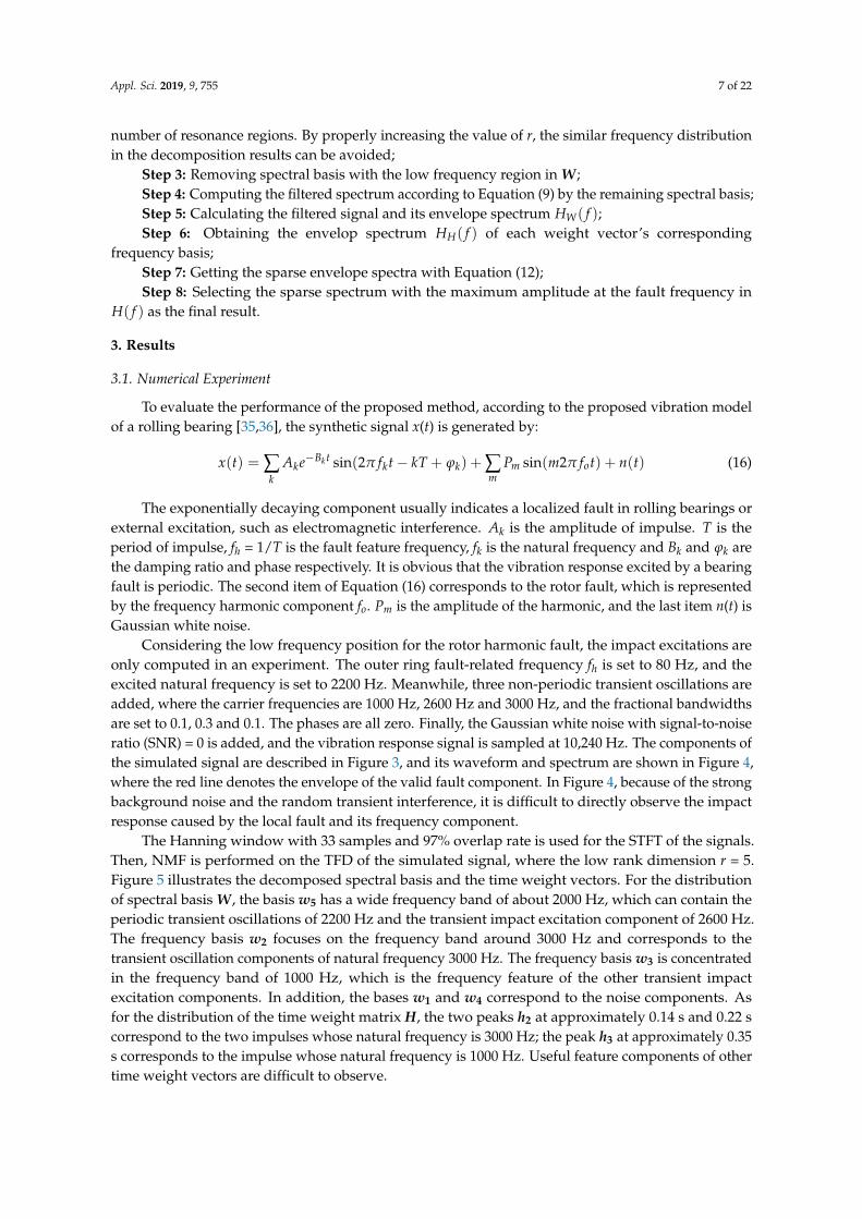
Another experiment is carried out on the test bench of mechanical equipment failure simulation,and its structure is shown in Figure 17. The rotating shaft is driven by an alternating current (AC)motor, and fault simulation can be conducted by replacing the fault motors. The motor bearing is6203. The inner ring peeling fault is simulated on the inner ring of the motor drive end bearing. Whenthe rotation frequency fr is 20 Hz, the fault characteristic frequency fi is 99.5 Hz. The accelerometeris installed at the vertical direction of the motor end bearing. The vibration signal is acquired withthe sampling frequency of 20,480 Hz and the sample size of 4096. Figure 18 shows the waveformand frequency spectrum of the acquired signal. In Figure 18a, weak impulse features are buried ininterference and noise, while it is shown that from the spectrum shown in Figure 18b, there are multipleresonance frequency bands, and the rotating characteristic frequencies are submerged.

Appl. Sci. 2019, 9, 755 16 of 22Appl. Sci. 2019, 9, x FOR PEER REVIEW 16 of 23

(a)

(b)

(c)

(d)

Figure 16. Fault characteristics extracted by the fast spectral kurtosis method: (a) Kurtogram of the simulated signal, the global maximum is achieved for = 2625cf Hz and Level = 4.6; (b) Waveform

of the filtered signal; (c) Spectrum of the filtered signal; (d) Envelope spectrum of the filtered signal.

3.2.2. Case 2

Another experiment is carried out on the test bench of mechanical equipment failure simulation, and its structure is shown in Figure 17. The rotating shaft is driven by an alternating current (AC) motor, and fault simulation can be conducted by replacing the fault motors. The motor bearing is 6203. The inner ring peeling fault is simulated on the inner ring of the motor drive end bearing. When the rotation frequency fr is 20 Hz, the fault characteristic frequency fi is 99.5 Hz. The accelerometer is installed at the vertical direction of the motor end bearing. The vibration signal is acquired with the sampling frequency of 20,480 Hz and the sample size of 4096. Figure 18 shows the waveform and frequency spectrum of the acquired signal. In Figure 18a, weak impulse features are buried in interference and noise, while it is shown that from the spectrum shown in Figure 18b, there are multiple resonance frequency bands, and the rotating characteristic frequencies are submerged.

Figure 16. Fault characteristics extracted by the fast spectral kurtosis method: (a) Kurtogram of thesimulated signal, the global maximum is achieved for fc = 2625 Hz and Level = 4.6; (b) Waveform ofthe filtered signal; (c) Spectrum of the filtered signal; (d) Envelope spectrum of the filtered signal.Appl. Sci. 2019, 9, x FOR PEER REVIEW 17 of 23

(a)

(b)

Figure 17. (a) Mechanical equipment failure simulation (MFS) test bench; (b) Fault motor.

(a)

(b)

Figure 18. Outer ring fault bearing: (a) Waveform; (b) Frequency spectrum of the fault signal.

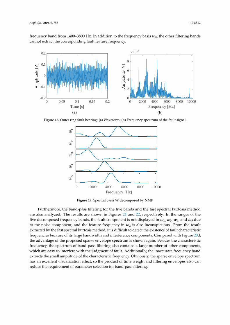
First, the proposed method is applied to the sampled signal. After computing STFT with the same parameters, the TFD matrix from the STFT coefficients is decomposed by NMF with low rank r = 5, and the decomposed bases are shown in Figure 19. The five spectral bases correspond to different frequency bands of 895–7400 Hz. Afterwards, the corresponding five band-pass filtering with frequency bases from w1 to w5 and the time envelope based on the weight matrix H are computed. The resulting sparse envelope spectra are shown in Figure 20. In Figure 20b, the fault characteristic frequency fi is effectively extracted, in which the frequency basis w2 corresponds to the resonance frequency band from 1400–3800 Hz. In addition to the frequency basis w3, the other filtering bands cannot extract the corresponding fault feature frequency.

0 0.05 0.1 0.15 0.2Time [s]

-0.2

-0.1

0

0.1

0.2

0 2000 4000 6000 8000 10000Frequency [Hz]

0

2

4

6

8

10-3

Figure 17. (a) Mechanical equipment failure simulation (MFS) test bench; (b) Fault motor.

First, the proposed method is applied to the sampled signal. After computing STFT with thesame parameters, the TFD matrix from the STFT coefficients is decomposed by NMF with low rankr = 5, and the decomposed bases are shown in Figure 19. The five spectral bases correspond todifferent frequency bands of 895–7400 Hz. Afterwards, the corresponding five band-pass filtering withfrequency bases from w1 to w5 and the time envelope based on the weight matrix H are computed.The resulting sparse envelope spectra are shown in Figure 20. In Figure 20b, the fault characteristicfrequency fi is effectively extracted, in which the frequency basis w2 corresponds to the resonance

Appl. Sci. 2019, 9, 755 17 of 22

frequency band from 1400–3800 Hz. In addition to the frequency basis w3, the other filtering bandscannot extract the corresponding fault feature frequency.

Appl. Sci. 2019, 9, x FOR PEER REVIEW 17 of 23

(a)

(b)

Figure 17. (a) Mechanical equipment failure simulation (MFS) test bench; (b) Fault motor.

(a)

(b)

Figure 18. Outer ring fault bearing: (a) Waveform; (b) Frequency spectrum of the fault signal.

First, the proposed method is applied to the sampled signal. After computing STFT with the same parameters, the TFD matrix from the STFT coefficients is decomposed by NMF with low rank r = 5, and the decomposed bases are shown in Figure 19. The five spectral bases correspond to different frequency bands of 895–7400 Hz. Afterwards, the corresponding five band-pass filtering with frequency bases from w1 to w5 and the time envelope based on the weight matrix H are computed. The resulting sparse envelope spectra are shown in Figure 20. In Figure 20b, the fault characteristic frequency fi is effectively extracted, in which the frequency basis w2 corresponds to the resonance frequency band from 1400–3800 Hz. In addition to the frequency basis w3, the other filtering bands cannot extract the corresponding fault feature frequency.

0 0.05 0.1 0.15 0.2Time [s]

-0.2

-0.1

0

0.1

0.2

0 2000 4000 6000 8000 10000Frequency [Hz]

0

2

4

6

8

10-3

Figure 18. Outer ring fault bearing: (a) Waveform; (b) Frequency spectrum of the fault signal.Appl. Sci. 2019, 9, x FOR PEER REVIEW 18 of 23

Figure 19. Spectral basis W decomposed by NMF.

(a)

(b)

(c)

(d)

(e)

w1

w2

w3

w4

0 2000 4000 6000 8000 10000Frequency [Hz]

w5

0 100 200 300 400 500 600Frequency [Hz]

0

2

4

10-8

0 100 200 300 400 500 600Frequency [Hz]

0

0.5

1

10-6

fi

0 100 200 300 400 500 600Frequency [Hz]

0

0.5

1

1.5

10-8

fi

0 100 200 300 400 500 600Frequency [Hz]

0

0.5

110-7

0 100 200 300 400 500 600Frequency [Hz]

0

1

2

10-7

Figure 19. Spectral basis W decomposed by NMF.

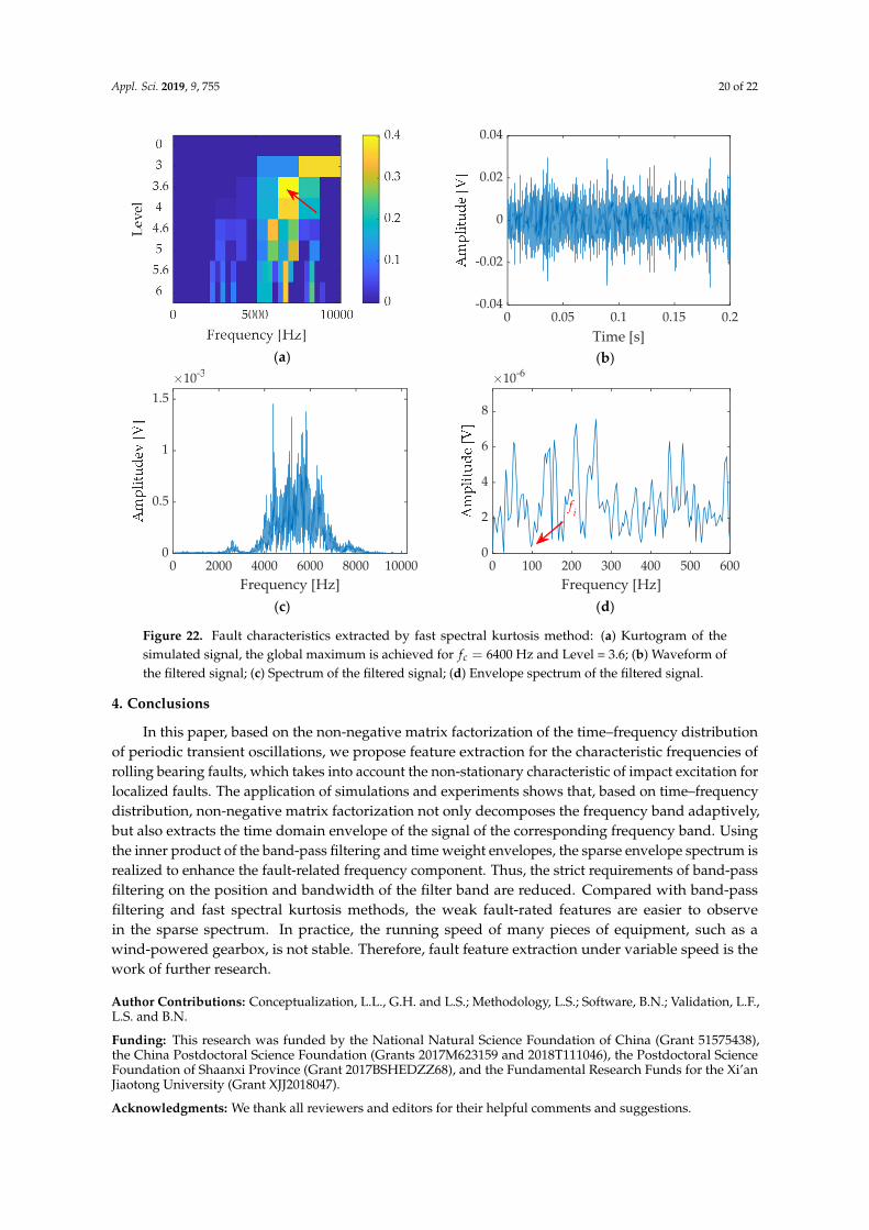
Furthermore, the band-pass filtering for the five bands and the fast spectral kurtosis methodare also analyzed. The results are shown in Figures 21 and 22, respectively. In the ranges of thefive decomposed frequency bands, the fault component is not displayed in w1, w3, w4, and w5 dueto the noise component, and the feature frequency in w2 is also inconspicuous. From the resultextracted by the fast spectral kurtosis method, it is difficult to detect the existence of fault characteristicfrequencies because of its large bandwidth and interference components. Compared with Figure 20d,the advantage of the proposed sparse envelope spectrum is shown again. Besides the characteristicfrequency, the spectrum of band-pass filtering also contains a large number of other components,which are easy to interfere with the judgment of fault. Additionally, the inaccurate frequency bandextracts the small amplitude of the characteristic frequency. Obviously, the sparse envelope spectrumhas an excellent visualization effect, so the product of time weight and filtering envelopes also canreduce the requirement of parameter selection for band-pass filtering.

Appl. Sci. 2019, 9, 755 18 of 22

Appl. Sci. 2019, 9, x FOR PEER REVIEW 18 of 23

Figure 19. Spectral basis W decomposed by NMF.

(a)

(b)

(c)

(d)

(e)

w1

w2

w3

w4

0 2000 4000 6000 8000 10000Frequency [Hz]

w5

0 100 200 300 400 500 600Frequency [Hz]

0

2

4

10-8

0 100 200 300 400 500 600Frequency [Hz]

0

0.5

1

10-6

fi

0 100 200 300 400 500 600Frequency [Hz]

0

0.5

1

1.5

10-8

fi

0 100 200 300 400 500 600Frequency [Hz]

0

0.5

110-7

0 100 200 300 400 500 600Frequency [Hz]

0

1

2

10-7

Figure 20. Obtained sparse spectrum with decomposed sub-matrix: (a) Basis w1 and weight vector h1;(b) Basis w2 and weight vector h2; (c) Basis w3 and weight vector h3; (d) Basis w4 and weight vector h4;(e) Basis w5 and weight vector h5.

Appl. Sci. 2019, 9, 755 19 of 22

Appl. Sci. 2019, 9, x FOR PEER REVIEW 19 of 23

Figure 20. Obtained sparse spectrum with decomposed sub-matrix: (a) Basis 1w and weight vector

1h ; (b) Basis 2w and weight vector 2h ; (c) Basis 3w and weight vector 3h ; (d) Basis 4w and

weight vector 4h ; (e) Basis 5w and weight vector 5h .

Furthermore, the band-pass filtering for the five bands and the fast spectral kurtosis method are also analyzed. The results are shown in Figures 21 and 22, respectively. In the ranges of the five decomposed frequency bands, the fault component is not displayed in w1, w3, w4, and w5 due to the noise component, and the feature frequency in w2 is also inconspicuous. From the result extracted by the fast spectral kurtosis method, it is difficult to detect the existence of fault characteristic frequencies because of its large bandwidth and interference components. Compared with Figure 20d, the advantage of the proposed sparse envelope spectrum is shown again. Besides the characteristic frequency, the spectrum of band-pass filtering also contains a large number of other components, which are easy to interfere with the judgment of fault. Additionally, the inaccurate frequency band extracts the small amplitude of the characteristic frequency. Obviously, the sparse envelope spectrum has an excellent visualization effect, so the product of time weight and filtering envelopes also can reduce the requirement of parameter selection for band-pass filtering.

(a)

(b)

(c)

(d)

0 100 200 300 400 500 600Frequency [Hz]

0

1

2

10-3

fi

0 100 200 300 400 500 600Frequency [Hz]

0

2

4

6

10-3

fi

0 100 200 300 400 500 600Frequency [Hz]

0

0.5

1

1.5

2

10-3

fi

0 100 200 300 400 500 600Frequency [Hz]

0

1

2

310-3

Appl. Sci. 2019, 9, x FOR PEER REVIEW 20 of 23

(e)

Figure 21. Envelope spectrum with band-pass filtering: (a) Filtered with 1w ; (b) Filtered with 2w ; (c) Filter with 3w ; (d) Filtered with 4w ; (e) Filtered with 5w .

(a)

(b)

(c)

(d)

Figure 22. Fault characteristics extracted by fast spectral kurtosis method: (a) Kurtogram of the simulated signal, the global maximum is achieved for = 6400cf Hz and Level = 3.6; (b) Waveform

of the filtered signal; (c) Spectrum of the filtered signal; (d) Envelope spectrum of the filtered signal.

4. Conclusions

In this paper, based on the non-negative matrix factorization of the time–frequency distribution of periodic transient oscillations, we propose feature extraction for the characteristic frequencies of rolling bearing faults, which takes into account the non-stationary characteristic of impact excitation for localized faults. The application of simulations and experiments shows that, based on time–frequency distribution, non-negative matrix factorization not only decomposes the frequency band

0 100 200 300 400 500 600Frequency [Hz]

0

1

2

3

4

10-3

0 0.05 0.1 0.15 0.2Time [s]

-0.04

-0.02

0

0.02

0.04

0 2000 4000 6000 8000 10000Frequency [Hz]

0

0.5

1

1.510-3

0 100 200 300 400 500 600Frequency [Hz]

0

2

4

6

8

10-6

fi

Figure 21. Envelope spectrum with band-pass filtering: (a) Filtered with w1; (b) Filtered with w2; (c)Filter with w3; (d) Filtered with w4; (e) Filtered with w5.

Appl. Sci. 2019, 9, 755 20 of 22

Appl. Sci. 2019, 9, x FOR PEER REVIEW 20 of 23

(e)

Figure 21. Envelope spectrum with band-pass filtering: (a) Filtered with 1w ; (b) Filtered with 2w ; (c) Filter with 3w ; (d) Filtered with 4w ; (e) Filtered with 5w .

(a)

(b)

(c)

(d)

Figure 22. Fault characteristics extracted by fast spectral kurtosis method: (a) Kurtogram of the simulated signal, the global maximum is achieved for = 6400cf Hz and Level = 3.6; (b) Waveform

of the filtered signal; (c) Spectrum of the filtered signal; (d) Envelope spectrum of the filtered signal.

4. Conclusions

In this paper, based on the non-negative matrix factorization of the time–frequency distribution of periodic transient oscillations, we propose feature extraction for the characteristic frequencies of rolling bearing faults, which takes into account the non-stationary characteristic of impact excitation for localized faults. The application of simulations and experiments shows that, based on time–frequency distribution, non-negative matrix factorization not only decomposes the frequency band

0 100 200 300 400 500 600Frequency [Hz]

0

1

2

3

4

10-3

0 0.05 0.1 0.15 0.2Time [s]

-0.04

-0.02

0

0.02

0.04

0 2000 4000 6000 8000 10000Frequency [Hz]

0

0.5

1

1.510-3

0 100 200 300 400 500 600Frequency [Hz]

0

2

4

6

8

10-6

fi

Figure 22. Fault characteristics extracted by fast spectral kurtosis method: (a) Kurtogram of thesimulated signal, the global maximum is achieved for fc = 6400 Hz and Level = 3.6; (b) Waveform ofthe filtered signal; (c) Spectrum of the filtered signal; (d) Envelope spectrum of the filtered signal.

4. Conclusions

In this paper, based on the non-negative matrix factorization of the time–frequency distributionof periodic transient oscillations, we propose feature extraction for the characteristic frequencies ofrolling bearing faults, which takes into account the non-stationary characteristic of impact excitation forlocalized faults. The application of simulations and experiments shows that, based on time–frequencydistribution, non-negative matrix factorization not only decomposes the frequency band adaptively,but also extracts the time domain envelope of the signal of the corresponding frequency band. Usingthe inner product of the band-pass filtering and time weight envelopes, the sparse envelope spectrum isrealized to enhance the fault-related frequency component. Thus, the strict requirements of band-passfiltering on the position and bandwidth of the filter band are reduced. Compared with band-passfiltering and fast spectral kurtosis methods, the weak fault-rated features are easier to observein the sparse spectrum. In practice, the running speed of many pieces of equipment, such as awind-powered gearbox, is not stable. Therefore, fault feature extraction under variable speed is thework of further research.

Author Contributions: Conceptualization, L.L., G.H. and L.S.; Methodology, L.S.; Software, B.N.; Validation, L.F.,L.S. and B.N.

Funding: This research was funded by the National Natural Science Foundation of China (Grant 51575438),the China Postdoctoral Science Foundation (Grants 2017M623159 and 2018T111046), the Postdoctoral ScienceFoundation of Shaanxi Province (Grant 2017BSHEDZZ68), and the Fundamental Research Funds for the Xi’anJiaotong University (Grant XJJ2018047).

Acknowledgments: We thank all reviewers and editors for their helpful comments and suggestions.

Appl. Sci. 2019, 9, 755 21 of 22

Conflicts of Interest: The authors declare no conflict of interest.

References

1. Ericsson, S.; Grip, N.; Johansson, E.; Persson, L.E.; Sjoberg, R.; Stromberg, J.O. Towards automatic detectionof local bearing defects in rotating machines. Mech. Syst. Signal Process. 2005, 19, 509–535. [CrossRef]

2. Tandon, N.; Nakra, B. Detection of defects in rolling element bearings by vibration monitoring. Indian J.Mech. Eng. Div. 1993, 73, 271–282.

3. Reif, Z.; Lai, M. Detection of Developing Bearing Failures by Means of Vibration; The American Society ofMechanical Engineers: New York, NY, USA, 1989; pp. 231–236.

4. Nikolaou, N.G.; Antoniadis, I.A. Rolling element bearing fault diagnosis using wavelet packets. NDT & EInt. 2002, 35, 197–205.

5. Qiu, H.; Lee, J.; Lin, J.; Yu, G. Wavelet filter-based weak signature detection method and its application onrolling element bearing prognostics. J. Sound Vib. 2006, 289, 1066–1090. [CrossRef]

6. Park, C.S.; Choi, Y.C.; Kim, Y.H. Early fault detection in automotive ball bearings using the minimumvariance cepstrum. Mech. Syst. Signal Process. 2013, 38, 534–548. [CrossRef]

7. McFadden, P.; Smith, J. Vibration monitoring of rolling element bearings by the high-frequency resonancetechnique—A review. Tribol. Int. 1984, 17, 3–10. [CrossRef]

8. Antoni, J. The spectral kurtosis: A useful tool for characterising non-stationary signals. Mech. Syst. SignalProcess. 2006, 20, 282–307. [CrossRef]

9. Antoni, J.; Randall, R.B. The spectral kurtosis: Application to the vibratory surveillance and diagnostics ofrotating machines. Mech. Syst. Signal Process. 2006, 20, 308–331. [CrossRef]

10. Barszcz, T.; Jablonski, A. A novel method for the optimal band selection for vibration signal demodulationand comparison with the kurtogram. Mech. Syst. Signal Process. 2011, 25, 431–451. [CrossRef]

11. Yu, K.P.; Yang, K.; Bai, Y.H. Estimation of modal parameters using the sparse component analysis basedunderdetermined blind source separation. Mech. Syst. Signal Process. 2014, 45, 302–316. [CrossRef]

12. Zhang, Z.Y.; Hua, H.X.; Xu, X.Z.; Huang, Z. Modal parameter identification through gabor expansion ofresponse signals. J. Sound Vib. 2003, 266, 943–955. [CrossRef]

13. Li, Z.; Crocker, M.J. A study of joint time-frequency analysis-based modal analysis. IEEE Trans. Instrum. Meas.2006, 55, 2335–2342. [CrossRef]

14. Le, T.-P.; Paultre, P. Modal identification based on the time–frequency domain decomposition ofunknown-input dynamic tests. Int. J. Mech. Sci. 2013, 71, 41–50. [CrossRef]

15. Su, W.S.; Wang, F.T.; Zhu, H.; Zhang, Z.X.; Guo, Z.G. Rolling element bearing faults diagnosis basedon optimal morlet wavelet filter and autocorrelation enhancement. Mech. Syst. Signal Process. 2010, 24,1458–1472. [CrossRef]

16. Yiakopoulos, C.T.; Antoniadis, I.A. Wavelet based demodulation of vibration signals generated by defects inrolling element bearings. Shock Vib. 2002, 9, 293–306. [CrossRef]

17. Wodecki, J.; Kruczek, P.; Wyłomanska, A.; Bartkowiak, A.; Zimroz, R. Novel method of informative frequencyband selection for vibration signal using nonnegative matrix factorization of short-time fourier transform.In Proceedings of the 2017 IEEE 11th International Symposium on Diagnostics for Electrical Machines, PowerElectronics and Drives (SDEMPED), Tinos, Greece, 29 August–1 September 2017; pp. 129–133.

18. Wodecki, J.; Zdunek, R.; Wyłomanska, A.; Zimroz, R. Local fault detection of rolling element bearingcomponents by spectrogram clustering with semi-binary NMF. Diagnostyka 2017, 18, 3–8.

19. Cui, D.; Zhang, Q.; Xiao, M.; Wang, L. Feature spectrum extraction algorithm for rolling bearings based onspectrogram and constrained nmf. Bearing 2014, 5, 48–52. [CrossRef]

20. Grais, E.M.; Erdogan, H. Single channel speech music separation using nonnegative matrix factorization andspectral masks. In Proceedings of the 2011 17th International Conference on Digital Signal Processing (DSP),Corfu, Greece, 6–8 July 2011; pp. 1–6.

21. King, B.; Févotte, C.; Smaragdis, P. Optimal cost function and magnitude power for nmf-based speechseparation and music interpolation. In Proceedings of the 2012 IEEE International Workshop on MachineLearning for Signal Processing (MLSP), Santander, Spain, 23–26 September 2012; pp. 1–6.

Appl. Sci. 2019, 9, 755 22 of 22

22. Sun, M.; Li, Y.; Gemmeke, J.F.; Zhang, X. Speech enhancement under low snr conditions via noise estimationusing sparse and low-rank nmf with kullback–leibler divergence. IEEE Trans. Audio Speech Lang. Process.2015, 23, 1233–1242. [CrossRef]

23. Xiao, Y.; Zhu, Z.; Zhao, Y.; Wei, Y.; Wei, S.; Li, X. Topographic nmf for data representation. IEEE Trans. Cybern.2014, 44, 1762–1771. [CrossRef]

24. Raj, B.; Singh, R.; Virtanen, T. Phoneme-dependent nmf for speech enhancement in monaural mixtures.In Proceedings of the Twelfth Annual Conference of the International Speech Communication Association,Florence, Italy, 27–31 August 2011.

25. Kalayeh, M.M.; Idrees, H.; Shah, M. Nmf-knn: Image annotation using weighted multi-view non-negativematrix factorization. In Proceedings of the IEEE Conference on Computer Vision and Pattern Recognition,Columbus, OH, USA, 23–28 June 2014; pp. 184–191.

26. Kim, J.; Park, H. Fast nonnegative matrix factorization: An active-set-like method and comparisons. SIAM J.Sci. Comput. 2011, 33, 3261–3281. [CrossRef]

27. Ding, C.; He, X.; Simon, H.; Jin, R. On the equivalence of nonnegative matrix factorization andk-means-spectral clustering. In Proceedings of the 2005 SIAM International Conference on Data Mining; SIAM:Philadelphia, PA, USA, 2005.

28. Lin, C.J. Projected Gradient Methods for Nonnegative Matrix Factorization; MIT Press: Cambridge, MA, USA,2007; pp. 2756–2779.

29. Grippo, L.; Sciandrone, M. On the convergence of the block nonlinear gauss–seidel method under convexconstraints. Oper. Res. Lett. 2000, 26, 127–136. [CrossRef]

30. Berry, M.W.; Browne, M.; Langville, A.N.; Pauca, V.P.; Plemmons, R.J. Algorithms and applications forapproximate nonnegative matrix factorization. Comput. Stat. Data Anal. 2007, 52, 155–173. [CrossRef]

31. Kim, D.; Sra, S.; Dhillon, I.S. Fast newton-type methods for the least squares nonnegative matrixapproximation problem. In Proceedings of the 2007 SIAM International Conference on Data Mining; SIAM:Philadelphia, PA, USA, 2007; pp. 343–354.

32. Kim, J.; Park, H. Toward faster nonnegative matrix factorization: A new algorithm and comparisons.In Proceedings of the Eighth IEEE International Conference on Data Mining, ICDM ‘08, Pisa, Italy,15–19 December 2008; pp. 353–362.

33. Van Benthem, M.H.; Keenan, M.R. Fast algorithm for the solution of large-scale non-negativity-constrainedleast squares problems. J. Chemom. A J. Chemom. Soc. 2004, 18, 441–450. [CrossRef]

34. Cichocki, A.; Zdunek, R.; Phan, A.H.; Amari, S.-I. Nonnegative Matrix and Tensor Factorizations: Applications toExploratory Multi-Way Data Analysis and Blind Source Separation; John Wiley & Sons: Hoboken, NJ, USA, 2009.

35. Miao, Y.H.; Zhao, M.; Lin, J.; Lei, Y.G. Application of an improved maximum correlated kurtosisdeconvolution method for fault diagnosis of rolling element bearings. Mech. Syst. Signal Process. 2017, 92,173–195. [CrossRef]

36. Chen, X.F.; Du, Z.H.; Li, J.M.; Li, X.; Zhang, H. Compressed sensing based on dictionary learning forextracting impulse components. Signal Process. 2014, 96, 94–109. [CrossRef]

37. Case Western Reserve University. Bearing Data Center Website. Available online: https://csegroups.case.edu/bearingdatacenter/pages/welcome-case-western-reserve-university-bearing-data-center-website(accessed on 15 January 2019).

38. Smith, W.A.; Randall, R.B. Rolling element bearing diagnostics using the case western reserve universitydata: A benchmark study. Mech. Syst. Signal Process. 2015, 64–65, 100–131. [CrossRef]

© 2019 by the authors. Licensee MDPI, Basel, Switzerland. This article is an open accessarticle distributed under the terms and conditions of the Creative Commons Attribution(CC BY) license (http://creativecommons.org/licenses/by/4.0/).