
SOME RESULTS RELATED TO DISTRIBUTION FUNCTIONS OF CHI-SQUARE TYPE RANDOM VARIABLES WITH RANDOM...
15
Bull. Korean Math. Soc. 45 (2008), No. 3, pp. 509–522 SOME RESULTS RELATED TO DISTRIBUTION FUNCTIONS OF CHI-SQUARE TYPE RANDOM VARIABLES WITH RANDOM DEGREES OF FREEDOM Tran Loc Hung, Tran Thien Thanh, and Bui Quang Vu Reprinted from the Bulletin of the Korean Mathematical Society Vol. 45, No. 3, August 2008 c ⃝2008 The Korean Mathematical Society
-
Upload
independent -
Category
Documents
-
view
1 -
download
0
Transcript of SOME RESULTS RELATED TO DISTRIBUTION FUNCTIONS OF CHI-SQUARE TYPE RANDOM VARIABLES WITH RANDOM...
Bull. Korean Math. Soc. 45 (2008), No. 3, pp. 509–522
SOME RESULTS RELATED TO DISTRIBUTION FUNCTIONSOF CHI-SQUARE TYPE RANDOM VARIABLES WITH
RANDOM DEGREES OF FREEDOM
Tran Loc Hung, Tran Thien Thanh, and Bui Quang Vu
Reprinted from theBulletin of the Korean Mathematical Society
Vol. 45, No. 3, August 2008
c⃝2008 The Korean Mathematical Society
Bull. Korean Math. Soc. 45 (2008), No. 3, pp. 509–522
SOME RESULTS RELATED TO DISTRIBUTION FUNCTIONSOF CHI-SQUARE TYPE RANDOM VARIABLES WITH
RANDOM DEGREES OF FREEDOM
Tran Loc Hung, Tran Thien Thanh, and Bui Quang Vu
Abstract. The main aim of this paper is to present some results relatedto asymptotic behavior of distribution functions of random variables of
chi-square type χ2N =
PNi=1 X2
i with degrees of freedom N , where Nis a positive integer-valued random variable independent on all standardnormally distributed random variables Xi. Two ways for computing thedistribution functions of chi-square type random variables with random
degrees of freedom are considered. Moreover, some tables concerningconsidered distribution functions are demonstrated in Appendix.
1. Introduction
Let X1, X2, . . . , Xn be n independent identically distributed (i.i.d.) randomvariables of standard normal law N (0, 1). The sum X2
1 + X22 + · · ·+ X2
n is saidto be a chi-square random variable of n degrees of freedom, denoted by χ2
n.The density function of random variable χ2
n is defined by (we refer the readerto [2] and [3].)
fn(x) =
0 if x ≤ 0,x
n2 −1
2n2 Γ( n
2 )e−
x2 if x > 0,
(1)
where Γ(s) =∫ ∞0
e−xxs−1dx denotes the Gamma function.It has long been known that in probability theory and statistics, the chi-
square distribution of random variable χ2n (also chi-squared or χ2-distribution)
is one of the most widely used theoretical probability distributions in inferentialstatistics, for instance in chi-square tests and in estimating variances. This dis-tribution enters the problem of estimating the mean of a normally distributedpopulation and the problem of estimating the slope of a regression line via its
Received October 22, 2007.2000 Mathematics Subject Classification. 60F05, 60E10, 60G50, 62E20.
Key words and phrases. random sum, chi-square random variable with degrees of freedom.This work is partially supported by the National Basic Research Program 2006-2008
(MOST, Vietnam) code 101806 and Asia Research Center (VNU, Vietnam) Grant 2007-2008.
c⃝2008 The Korean Mathematical Society
509
510 TRAN LOC HUNG, TRAN THIEN THANH, AND BUI QUANG VU
role in Student’s t-distribution. Moreover, it also enters all analysis of varianceproblems via its role in the F -distribution, which is the distribution of the ra-tio of two independent chi-square random variables divided by their respectivedegrees of freedom (see [2] and [3] for more details).
During the last several decades the random-index approach has risen to be-come one of the most important tools available for investigating some problemsof Applied Statistics (for a deeper discussion of this we refer the reader to [4]and [8]).
The question arises as to what happens if the degrees of freedom n of achi-square random variable χ2
n shall be replayed by a positive integer-valuedrandom variable N. The answer of above question is main aim of this paper.The applications of probability distributions of the random variable of chi-square type χ2
N with random degrees of freedom N in some applied problemsof statistics will be taken up in the next research results.
This paper is divided into five main sections. The second section dealswith the asymptotic behaviors of distributions of chi-square random variableχ2
n (Theorem 2.1) and of chi-square type χ2N with random degrees of freedom
N (Theorems 2.2-2.8). The third section gives the proofs of all results insecond section. The fourth section describes two approaches to computationof the distribution functions of the random variable of chi-square type χ2
N
with random degrees of freedom N. The Appendix (last section) devotes tosome tables concerning the distribution functions of chi-square type χ2
N withrandom degrees of freedom N in some concrete cases.
2. Main results
Throughout this paper, we denote by Z a random variable degenerated atpoint 1, and by φZ(t) = eit its characteristic function.
From now on, the notation d−→ will mean the convergence in distribution andP−→ will denote the convergence in probability.
Theorem 2.1. Let χ2n be a chi-square random variable of n degrees of freedom
(n is positive integer number). Then
χ2n
n
d−→ Z,
as n → ∞.
Theorem 2.2. Let X1, X2, . . . be a sequence of i.i.d. random variables withchi-square distribution function χ2
n. Suppose that N is a positive integer-valuedrandom variable independent of all Xi. Furthermore, let us consider the randomsum SN :=
∑Ni=1 Xi. Then
SN
n
d−→ N,
as n → ∞.
DISTRIBUTION FUNCTIONS OF CHI-SQUARE TYPE 511
We now return to some interesting results concerning to random variableχ2
Nn:= X2
1 + · · ·+ X2Nn
, if for the random variable χ2n with degrees of freedom
n, the fixed number n will be replaced by the positive integer-valued randomvariables Nn, n ≥ 1, independent of all Xi ∼ N (0, 1), i = 1, 2, . . . , Nn. Thefollowing theorems will be main results of this paper.
Theorem 2.3. Let Nn ∼ Binomial(n, p), p ∈ (0, 1). Then
χ2Nn
np
d−→ Z,
as n → ∞.
Theorem 2.4. Let Nn ∼ Poisson(λn), λn > 0, n = 1, 2, . . . and λn → ∞ asn → ∞. Then
χ2Nn
λn
d−→ Z,
as n → ∞.
Theorem 2.5. Let {Nn, n ≥ 1} be a sequence of positive integer-valued randomvariables, independent from all Xi ∼ N (0, 1), i = 1, 2, . . . . Furthermore, assumethat the following conditions are satisfied
(2) E(Nn) → ∞;E|Nn − E(Nn)|
E(Nn)→ 0 as n → ∞.
Then, as n → ∞ we get
(3)χ2
Nn
E(Nn)d−→ Z.
Remark 1. (a) Theorem 2.5 is generalization of Theorems 2.1, 2.3, and 2.4.(b) It is easily seen that E(χ2(1)) = 1. Thus, as a fundamental result from
random sum, it follows E(χ2Nn
) = E(χ2(1))E(Nn). Then, (3) in Theorem 2.5can be formulated as follows
(4)χ2
Nn
E(χ2Nn
)d−→ Z, as n → ∞.
Theorem 2.6. Let Nn ∼ Uniform(n). Then, as n → ∞, we have
χ2Nn
n
d−→ U ∼ Uniform[0, 1].
Theorem 2.7. Let Nn ∼ Geometric(pn) and suppose that pn → 0 as n → ∞.Then
pnχ2Nn
d−→ Y ∼ Exp(1),as n → ∞.
Remark 2. According to Theorems 2.6 and 2.7 we can see the conditionE(Nn) → ∞ in (2) (as n → ∞) is not sufficient to confirm conclusion as inRemark 1.b.
512 TRAN LOC HUNG, TRAN THIEN THANH, AND BUI QUANG VU
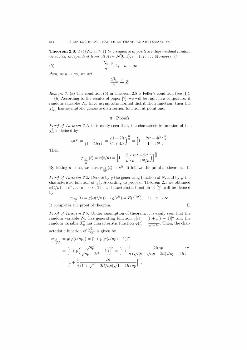
Theorem 2.8. Let {Nn, n ≥ 1} be a sequence of positive integer-valued randomvariables, independent from all Xi ∼ N (0, 1), i = 1, 2, . . . . Moreover, if
(5)Nn
n
P−→ 1, n → ∞
then, as n → ∞, we getχ2
Nn
n
d−→ Z.
Remark 3. (a) The condition (5) in Theorem 2.8 is Feller’s condition (see [1]).(b) According to the results of paper [7], we will be right in a conjecture: if
random variables Nn have asymptotic normal distribution function, then theχ2
Nnhas asymptotic generate distribution function at point one.
3. Proofs
Proof of Theorem 2.1. It is easily seen that, the characteristic function of theχ2
n is defined by
φ(t) =1
(1 − 2it)n2
=( 1 + 2it
1 + 4t2
)n2 =
[1 +
2it − 4t2
1 + 4t2
]n2.
Then
φχ2n
n
(t) = φ(t/n) =[1 +
2n
( int − 2t2
n + 4t2/n
)]n2.
By letting n → ∞, we have φχ2n
n
(t) → eit. It follows the proof of theorem. ¤
Proof of Theorem 2.2. Denote by g the generating function of N, and by φ thecharacteristic function of χ2
n. According to proof of Theorem 2.1 we obtainedφ(t/n) → eit, as n → ∞. Then, characteristic function of SN
n will be definedby
φSNn
(t) = g(φ(t/n)) → g(eit) = E(eitN ), as n → ∞.
It completes the proof of theorem. ¤
Proof of Theorem 2.3. Under assumption of theorem, it is easily seen that therandom variable Nn has generating function g(t) = [1 + p(t − 1)]n and therandom variable X2
k has characteristic function φ(t) = 1√1−2it
. Then, the char-
acteristic function ofχ2
Nn
np is given by
φχ2Nnnp
= g(φ(t/np)) = [1 + p(φ(t/np) − 1)]n
=[1 + p
( √np
√np − 2it
− 1)]n
=[1 +
1n
2itnp
(√
np +√
np − 2it)√
np − 2it
]n
=[1 +
1n
2it
(1 +√
1 − 2it/np)√
1 − 2it/np
]n
.
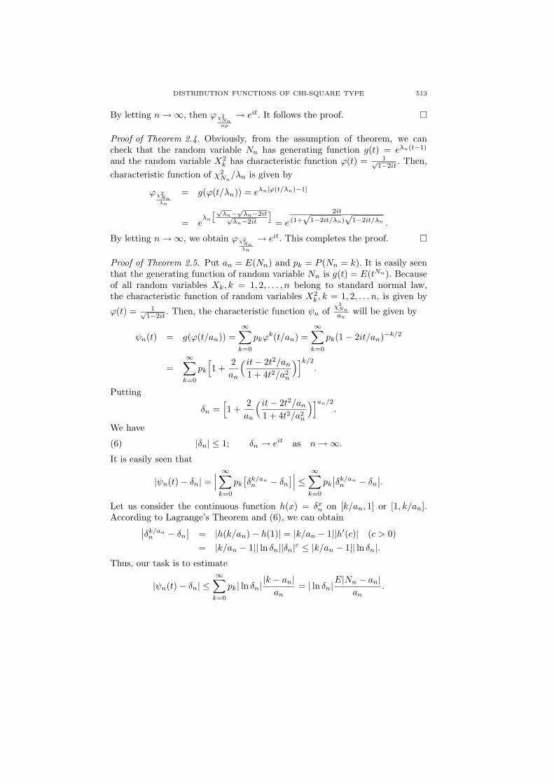
DISTRIBUTION FUNCTIONS OF CHI-SQUARE TYPE 513
By letting n → ∞, then φχ2Nnnp
→ eit. It follows the proof. ¤
Proof of Theorem 2.4. Obviously, from the assumption of theorem, we cancheck that the random variable Nn has generating function g(t) = eλn(t−1)
and the random variable X2k has characteristic function φ(t) = 1√
1−2it. Then,
characteristic function of χ2Nn
/λn is given by
φχ2Nnλn
= g(φ(t/λn)) = eλn[φ(t/λn)−1]
= eλn
[√λn−
√λn−2it√
λn−2it
]= e
2it
(1+√
1−2it/λn)√
1−2it/λn .
By letting n → ∞, we obtain φχ2Nnλn
→ eit. This completes the proof. ¤
Proof of Theorem 2.5. Put an = E(Nn) and pk = P (Nn = k). It is easily seenthat the generating function of random variable Nn is g(t) = E(tNn). Becauseof all random variables Xk, k = 1, 2, . . . , n belong to standard normal law,the characteristic function of random variables X2
k , k = 1, 2, . . . n, is given by
φ(t) = 1√1−2it
. Then, the characteristic function ψn ofχ2
Nn
anwill be given by
ψn(t) = g(φ(t/an)) =∞∑
k=0
pkφk(t/an) =∞∑
k=0
pk(1 − 2it/an)−k/2
=∞∑
k=0
pk
[1 +
2an
( it − 2t2/an
1 + 4t2/a2n
)]k/2
.
Putting
δn =[1 +
2an
( it − 2t2/an
1 + 4t2/a2n
)]an/2
.
We have
|δn| ≤ 1; δn → eit as n → ∞.(6)
It is easily seen that
|ψn(t) − δn| =∣∣∣ ∞∑
k=0
pk
[δk/ann − δn
]∣∣∣ ≤ ∞∑k=0
pk
∣∣δk/ann − δn
∣∣.Let us consider the continuous function h(x) = δx
n on [k/an, 1] or [1, k/an].According to Lagrange’s Theorem and (6), we can obtain∣∣δk/an
n − δn
∣∣ = |h(k/an) − h(1)| = |k/an − 1||h′(c)| (c > 0)= |k/an − 1|| ln δn||δn|c ≤ |k/an − 1|| ln δn|.
Thus, our task is to estimate
|ψn(t) − δn| ≤∞∑
k=0
pk| ln δn||k − an|
an= | ln δn|
E|Nn − an|an
.
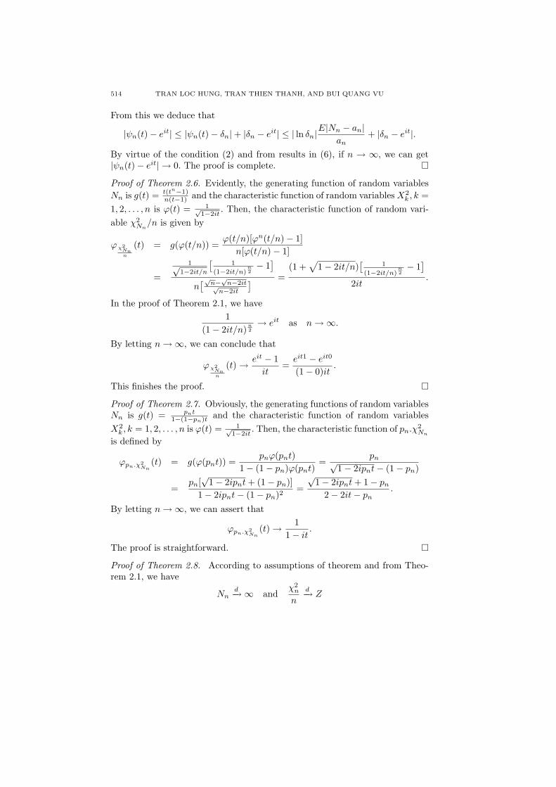
514 TRAN LOC HUNG, TRAN THIEN THANH, AND BUI QUANG VU
From this we deduce that
|ψn(t) − eit| ≤ |ψn(t) − δn| + |δn − eit| ≤ | ln δn|E|Nn − an|
an+ |δn − eit|.
By virtue of the condition (2) and from results in (6), if n → ∞, we can get|ψn(t) − eit| → 0. The proof is complete. ¤
Proof of Theorem 2.6. Evidently, the generating function of random variablesNn is g(t) = t(tn−1)
n(t−1) and the characteristic function of random variables X2k , k =
1, 2, . . . , n is φ(t) = 1√1−2it
. Then, the characteristic function of random vari-able χ2
Nn/n is given by
φχ2Nnn
(t) = g(φ(t/n)) =φ(t/n)[φn(t/n) − 1]
n[φ(t/n) − 1]
=
1√1−2it/n
[1
(1−2it/n)n2− 1
]n[√
n−√
n−2it√n−2it
] =(1 +
√1 − 2it/n)
[1
(1−2it/n)n2− 1
]2it
.
In the proof of Theorem 2.1, we have1
(1 − 2it/n)n2→ eit as n → ∞.
By letting n → ∞, we can conclude that
φχ2Nnn
(t) → eit − 1it
=eit1 − eit0
(1 − 0)it.
This finishes the proof. ¤
Proof of Theorem 2.7. Obviously, the generating functions of random variablesNn is g(t) = pnt
1−(1−pn)t and the characteristic function of random variablesX2
k , k = 1, 2, . . . , n is φ(t) = 1√1−2it
. Then, the characteristic function of pn.χ2Nn
is defined by
φpn.χ2Nn
(t) = g(φ(pnt)) =pnφ(pnt)
1 − (1 − pn)φ(pnt)=
pn√1 − 2ipnt − (1 − pn)
=pn[
√1 − 2ipnt + (1 − pn)]
1 − 2ipnt − (1 − pn)2=
√1 − 2ipnt + 1 − pn
2 − 2it − pn.
By letting n → ∞, we can assert that
φpn.χ2Nn
(t) → 11 − it
.
The proof is straightforward. ¤
Proof of Theorem 2.8. According to assumptions of theorem and from Theo-rem 2.1, we have
Nnd−→ ∞ and
χ2n
n
d−→ Z
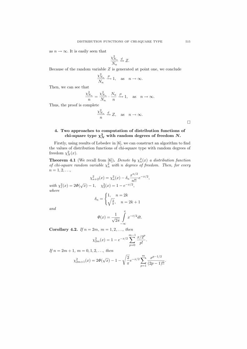
DISTRIBUTION FUNCTIONS OF CHI-SQUARE TYPE 515
as n → ∞. It is easily seen that
χ2Nn
Nn
d−→ Z.
Because of the random variable Z is generated at point one, we conclude
χ2Nn
Nn
P−→ 1, as n → ∞.
Then, we can see that
χ2Nn
n=
χ2Nn
Nn· Nn
n
P−→ 1, as n → ∞.
Thus, the proof is complete
χ2Nn
n
d−→ Z, as n → ∞.
¤
4. Two approaches to computation of distribution functions ofchi-square type χ2
N with random degrees of freedom N.
Firstly, using results of Lebedev in [6], we can construct an algorithm to findthe values of distribution functions of chi-square type with random degrees offreedom χ2
N (x).
Theorem 4.1 (We recall from [6]). Denote by χ2n(x) a distribution function
of chi-square random variable χ2n with n degrees of freedom. Then, for every
n = 1, 2, . . .,
χ2n+2(x) = χ2
n(x) − δnxn/2
n!!e−x/2,
with χ21(x) = 2Φ(
√x) − 1, χ2
2(x) = 1 − e−x/2,where
δn =
{1, n = 2k√
2π , n = 2k + 1
and
Φ(x) =1√2π
x∫−∞
x−t/2dt.
Corollary 4.2. If n = 2m, m = 1, 2, . . ., then
χ22m(x) = 1 − e−x/2
m−1∑p=0
x/2p
p!.
If n = 2m + 1, m = 0, 1, 2, . . ., then
χ22m+1(x) = 2Φ(
√x) − 1 −
√2π
e−x/2m∑
p=1
xp−1/2
(2p − 1)!!.
516 TRAN LOC HUNG, TRAN THIEN THANH, AND BUI QUANG VU
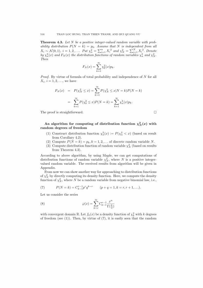
Theorem 4.3. Let N be a positive integer-valued random variable with prob-ability distribution P (N = k) = pk. Assume that N is independent from allXi ∼ N (0, 1), i = 1, 2, . . .. Put χ2
n =∑n
i=1 Xi2 and χ2
N =∑N
i=1 Xi2. Denote
by χ2n(x) and FN (x) the distribution functions of random variables χ2
n and χ2N .
Then
FN (x) =∞∑
k=1
χ2k(x)pk.
Proof. By virtue of formula of total probability and independence of N for allXi, i = 1, 2, . . ., we have
FN (x) = P (χ2N ≤ x) =
∞∑k=1
P (χ2N ≤ x|N = k)P (N = k)
=∞∑
k=1
P (χ2k ≤ x)P (N = k) =
∞∑k=1
χ2n(x)pk.
The proof is straightforward. ¤
An algorithm for computing of distribution function χ2N(x) with
random degrees of freedom
(1) Construct distribution function χ2n(x) := P (χ2
n < x) (based on resultfrom Corollary 4.2).
(2) Compute P (N = k) = pk, k = 1, 2, . . . of discrete random variable N .(3) Compute distribution function of random variable χ2
N (based on resultsfrom Theorem 4.3).
According to above algorithm, by using Maple, we can get computations ofdistribution functions of random variable χ2
N , where N is a positive integer-valued random variable. The received results from algorithm will be given inAppendix.
From now we can show another way for approaching to distribution functionsof χ2
N by directly computing its density function. Here, we compute the densityfunction of χ2
N , where N be a random variable from negative binomial law, i.e.,
(7) P (N = k) = Cr−1k−1p
rqk−r (p + q = 1, k = r, r + 1, . . .).
Let us consider the series
(8) φ(x) =∞∑
k=r
Cr−1k−1
xn
Γ(k2 )
with convergent domain R. Let fk(x) be a density function of χ2k with k degrees
of freedom (see (1)). Then, by virtue of (7), it is easily seen that the random
DISTRIBUTION FUNCTIONS OF CHI-SQUARE TYPE 517
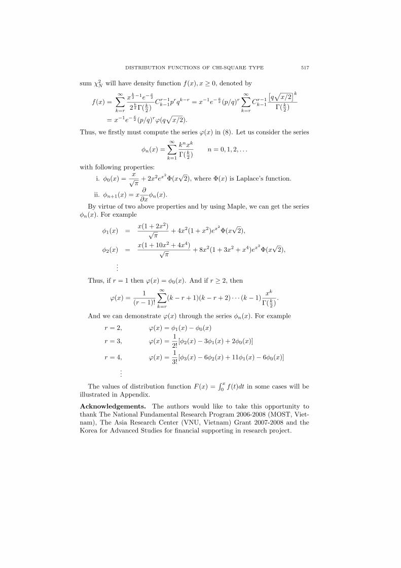
sum χ2N will have density function f(x), x ≥ 0, denoted by
f(x) =∞∑
k=r
xk2−1e−
x2
2k2 Γ(k
2 )Cr−1
k−1prqk−r = x−1e−
x2 (p/q)r
∞∑k=r
Cr−1k−1
[q√
x/2]k
Γ(k2 )
= x−1e−x2 (p/q)rφ(q
√x/2).
Thus, we firstly must compute the series φ(x) in (8). Let us consider the series
ϕn(x) =∞∑
k=1
knxk
Γ(k2 )
n = 0, 1, 2, . . .
with following properties:
i. ϕ0(x) =x√π
+ 2x2ex2Φ(x
√2), where Φ(x) is Laplace’s function.
ii. ϕn+1(x) = x∂
∂xϕn(x).
By virtue of two above properties and by using Maple, we can get the seriesϕn(x). For example
ϕ1(x) =x(1 + 2x2)√
π+ 4x2(1 + x2)ex2
Φ(x√
2),
ϕ2(x) =x(1 + 10x2 + 4x4)√
π+ 8x2(1 + 3x2 + x4)ex2
Φ(x√
2),
...
Thus, if r = 1 then φ(x) = ϕ0(x). And if r ≥ 2, then
φ(x) =1
(r − 1)!
∞∑k=r
(k − r + 1)(k − r + 2) · · · (k − 1)xk
Γ(k2 )
.
And we can demonstrate φ(x) through the series ϕn(x). For example
r = 2, φ(x) = ϕ1(x) − ϕ0(x)
r = 3, φ(x) =12!
[ϕ2(x) − 3ϕ1(x) + 2ϕ0(x)]
r = 4, φ(x) =13!
[ϕ3(x) − 6ϕ2(x) + 11ϕ1(x) − 6ϕ0(x)]
...
The values of distribution function F (x) =∫ x
0f(t)dt in some cases will be
illustrated in Appendix.
Acknowledgements. The authors would like to take this opportunity tothank The National Fundamental Research Program 2006-2008 (MOST, Viet-nam), The Asia Research Center (VNU, Vietnam) Grant 2007-2008 and theKorea for Advanced Studies for financial supporting in research project.
518 TRAN LOC HUNG, TRAN THIEN THANH, AND BUI QUANG VU
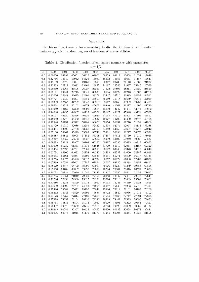
Appendix
In this section, three tables concerning the distribution functions of randomvariable χ2
N with random degrees of freedom N are established.
Table 1. Distribution function of chi square-geometry with parameterp = 1/2.
x 0.00 0.01 0.02 0.03 0.04 0.05 0.06 0.07 0.08 0.09
0.0 0.00000 03999 05651 06925 08006 08959 09818 10608 11354 12049
0.1 0.12716 13349 13952 14525 15089 15632 16157 16663 17157 176430.2 0.18109 18572 19021 19460 19890 20317 20733 21140 21538 219370.3 0.22323 22712 23081 23461 23827 24187 24543 24897 25245 255900.4 0.25930 26267 26596 26927 27251 27572 27895 28211 28520 28829
0.5 0.29141 29441 29745 30041 30338 30635 30922 31213 31503 317860.6 0.32066 32348 32625 32901 33178 33447 33716 33985 34253 345120.7 0.34777 35039 35297 35552 35809 36060 36318 36569 36815 37059
0.8 0.37309 37555 37797 38042 38283 38517 38753 38992 39232 394590.9 0.39694 39922 40152 40378 40609 40840 41061 41287 41506 41730
1.0 0.41949 42167 42390 42600 42814 43032 43247 43461 43671 438821.1 0.44088 44295 44507 44715 44922 45127 45327 45528 45728 459351.2 0.46127 46329 46526 46726 46925 47115 47312 47508 47705 47892
1.3 0.48082 48278 48462 48648 48837 49027 49209 49400 49577 497681.4 0.49948 50131 50312 50488 50673 50856 51031 51210 51391 515601.5 0.51729 51910 52086 52259 52432 52605 52775 52947 53113 532881.6 0.53451 53623 53788 53958 54119 54282 54450 54607 54778 54942
1.7 0.55100 55267 55429 55582 55742 55901 56058 56217 56373 565381.8 0.56685 56845 56995 57152 57308 57457 57611 57760 57910 580661.9 0.58217 58357 58503 58657 58802 58952 59102 59242 59385 59537
2.0 0.59683 59821 59967 60104 60253 60397 60533 60675 60817 60955
2.1 0.61090 61232 61373 61511 61648 61779 61919 62047 62187 623222.2 0.62454 62595 62721 62859 62990 63122 63243 63378 63513 636422.3 0.63774 63900 64031 64158 64282 64413 64537 64660 64787 649162.4 0.65035 65161 65287 65405 65533 65651 65771 65899 66017 66135
2.5 0.66255 66375 66498 66617 66734 66857 66972 67088 67202 673202.6 0.67439 67554 67662 67787 67894 68007 68125 68238 68352 684612.7 0.68579 68678 68792 68905 69019 69126 69239 69339 69453 69558
2.8 0.69668 69782 69887 69992 70099 70206 70307 70415 70521 706232.9 0.70732 70834 70940 71040 71143 71247 71350 71451 71553 71652
3.0 0.71755 71851 71949 72052 72151 72248 72342 72451 72547 726413.1 0.72736 72833 72930 73027 73123 73216 73310 73409 73501 736023.2 0.73686 73783 73869 73973 74067 74153 74243 74339 74428 74516
3.3 0.74609 74699 74787 74873 74968 75057 75149 75233 75318 754113.4 0.75496 75582 75672 75757 75848 75926 76012 76101 76187 762663.5 0.76352 76443 76520 76605 76684 76772 76849 76936 77015 771023.6 0.77176 77257 77344 77426 77503 77584 77665 77747 77824 77898
3.7 0.77978 78057 78134 78210 78286 78365 78442 78523 78595 786733.8 0.78751 78834 78894 78974 79050 79129 79193 79272 79353 794173.9 0.79497 79573 79639 79715 79784 79863 79929 80002 80069 80137
4.0 0.80215 80284 80357 80423 80492 80570 80632 80698 80772 80841
4.1 0.80906 80978 81045 81110 81173 81244 81308 81384 81438 81508
DISTRIBUTION FUNCTIONS OF CHI-SQUARE TYPE 519
4.2 0.81579 81642 81704 81774 81838 81900 81961 82038 82100 821614.3 0.82220 82287 82344 82417 82476 82540 82601 82663 82718 827854.4 0.82851 82905 82968 83032 83090 83155 83213 83276 83331 833924.5 0.83449 83515 83569 83629 83683 83750 83809 83856 83917 83978
4.7 0.84030 84095 84148 84198 84260 84318 84376 84425 84490 845424.8 0.84597 84647 84709 84762 84819 84867 84923 84971 85028 850824.9 0.85134 85194 85249 85303 85353 85406 85454 85513 85561 85613
5.0 0.85666 85719 85763 85811 85866 85917 85974 86020 86065 86116
5.1 0.86164 86210 86262 86311 86369 86410 86458 86509 86561 866095.2 0.86651 86700 86756 86798 86841 86892 86937 86987 87034 870745.3 0.87118 87178 87212 87266 87307 87351 87398 87445 87493 875315.4 0.87584 87623 87671 87707 87760 87800 87845 87890 87935 87971
5.5 0.88016 88061 88106 88149 88185 88234 88273 88324 88361 883955.6 0.88447 88482 88532 88567 88609 88650 88694 88728 88770 888115.7 0.88850 88893 88935 88976 89013 89052 89092 89131 89166 892035.8 0.89252 89292 89327 89363 89396 89435 89483 89513 89552 89590
5.9 0.89620 89660 89706 89745 89777 89816 89851 89888 89922 89956
6.0 0.89992 90030 90080 90112 90141 90178 90214 90248 90278 903146.1 0.90347 90386 90421 90456 90494 90524 90555 90591 90631 906606.2 0.90694 90729 90764 90798 90832 90858 90894 90927 90960 90992
6.3 0.91020 91059 91086 91126 91155 91179 91210 91249 91283 913146.4 0.91346 91378 91414 91434 91466 91499 91532 91562 91593 916166.5 0.91651 91685 91710 91739 91772 91802 91832 91861 91886 919136.6 0.91947 91981 92004 92033 92063 92095 92112 92150 92180 92209
6.7 0.92230 92259 92288 92316 92347 92377 92402 92429 92459 924866.8 0.92506 92541 92562 92589 92616 92644 92673 92699 92726 927526.9 0.92774 92806 92826 92859 92880 92912 92932 92958 92984 930177 0.93284 93525 93757 93982 94188 94405 94602 94791 94983 95158
8 0.95340 95505 95662 95812 95965 96119 96247 96382 96510 966339 0.96758 96875 96990 97091 97197 97305 97399 97492 97584 97664
10 0.97766 97839 97920 97988 98057 98130 98199 98265 98323 9838911 0.98448 98496 98555 98605 98654 98707 98754 98796 98844 98883
12 0.98932 98963 99001 99030 99074 99107 99132 99171 99200 9923013 0.99254 99279 99311 99336 99355 99380 99401 99419 99451 9946714 0.99488 99500 99520 99536 99553 99570 99586 99606 99616 9963615 0.99645 99655 99669 99678 99690 99704 99714 99722 99732 99743
16 0.99756 99760 99768 99777 99785 99800 99807 99816 99818 9983017 0.99831 99840 99842 99845 99851 99860 99863 99867 99871 9987518 0.99881 99884 99888 99893 99896 99902 99903 99906 99912 99912
19 0.99917 99918 99924 99924 99927 99932 99933 99934 99935 9993720 0.99948 99942 99944 99946 99957 99950 99951 99953 99955 99956
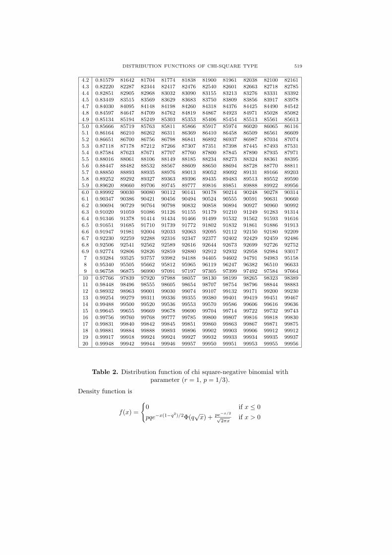
Table 2. Distribution function of chi square-negative binomial withparameter (r = 1, p = 1/3).
Density function is
f(x) =
{0 if x ≤ 0
pqe−x(1−q2)/2Φ(q√
x) + pe−x/2√
2πxif x > 0
520 TRAN LOC HUNG, TRAN THIEN THANH, AND BUI QUANG VU
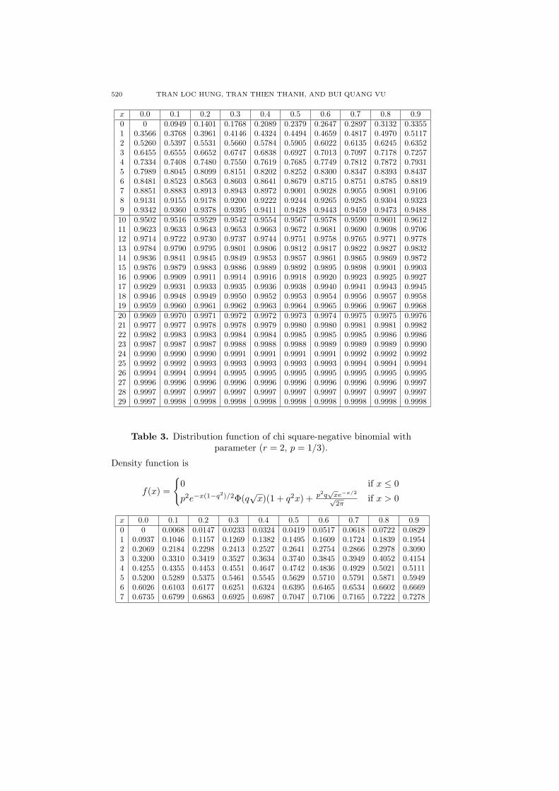
x 0.0 0.1 0.2 0.3 0.4 0.5 0.6 0.7 0.8 0.90 0 0.0949 0.1401 0.1768 0.2089 0.2379 0.2647 0.2897 0.3132 0.33551 0.3566 0.3768 0.3961 0.4146 0.4324 0.4494 0.4659 0.4817 0.4970 0.51172 0.5260 0.5397 0.5531 0.5660 0.5784 0.5905 0.6022 0.6135 0.6245 0.63523 0.6455 0.6555 0.6652 0.6747 0.6838 0.6927 0.7013 0.7097 0.7178 0.72574 0.7334 0.7408 0.7480 0.7550 0.7619 0.7685 0.7749 0.7812 0.7872 0.79315 0.7989 0.8045 0.8099 0.8151 0.8202 0.8252 0.8300 0.8347 0.8393 0.84376 0.8481 0.8523 0.8563 0.8603 0.8641 0.8679 0.8715 0.8751 0.8785 0.88197 0.8851 0.8883 0.8913 0.8943 0.8972 0.9001 0.9028 0.9055 0.9081 0.91068 0.9131 0.9155 0.9178 0.9200 0.9222 0.9244 0.9265 0.9285 0.9304 0.93239 0.9342 0.9360 0.9378 0.9395 0.9411 0.9428 0.9443 0.9459 0.9473 0.948810 0.9502 0.9516 0.9529 0.9542 0.9554 0.9567 0.9578 0.9590 0.9601 0.961211 0.9623 0.9633 0.9643 0.9653 0.9663 0.9672 0.9681 0.9690 0.9698 0.970612 0.9714 0.9722 0.9730 0.9737 0.9744 0.9751 0.9758 0.9765 0.9771 0.977813 0.9784 0.9790 0.9795 0.9801 0.9806 0.9812 0.9817 0.9822 0.9827 0.983214 0.9836 0.9841 0.9845 0.9849 0.9853 0.9857 0.9861 0.9865 0.9869 0.987215 0.9876 0.9879 0.9883 0.9886 0.9889 0.9892 0.9895 0.9898 0.9901 0.990316 0.9906 0.9909 0.9911 0.9914 0.9916 0.9918 0.9920 0.9923 0.9925 0.992717 0.9929 0.9931 0.9933 0.9935 0.9936 0.9938 0.9940 0.9941 0.9943 0.994518 0.9946 0.9948 0.9949 0.9950 0.9952 0.9953 0.9954 0.9956 0.9957 0.995819 0.9959 0.9960 0.9961 0.9962 0.9963 0.9964 0.9965 0.9966 0.9967 0.996820 0.9969 0.9970 0.9971 0.9972 0.9972 0.9973 0.9974 0.9975 0.9975 0.997621 0.9977 0.9977 0.9978 0.9978 0.9979 0.9980 0.9980 0.9981 0.9981 0.998222 0.9982 0.9983 0.9983 0.9984 0.9984 0.9985 0.9985 0.9985 0.9986 0.998623 0.9987 0.9987 0.9987 0.9988 0.9988 0.9988 0.9989 0.9989 0.9989 0.999024 0.9990 0.9990 0.9990 0.9991 0.9991 0.9991 0.9991 0.9992 0.9992 0.999225 0.9992 0.9992 0.9993 0.9993 0.9993 0.9993 0.9993 0.9994 0.9994 0.999426 0.9994 0.9994 0.9994 0.9995 0.9995 0.9995 0.9995 0.9995 0.9995 0.999527 0.9996 0.9996 0.9996 0.9996 0.9996 0.9996 0.9996 0.9996 0.9996 0.999728 0.9997 0.9997 0.9997 0.9997 0.9997 0.9997 0.9997 0.9997 0.9997 0.999729 0.9997 0.9998 0.9998 0.9998 0.9998 0.9998 0.9998 0.9998 0.9998 0.9998
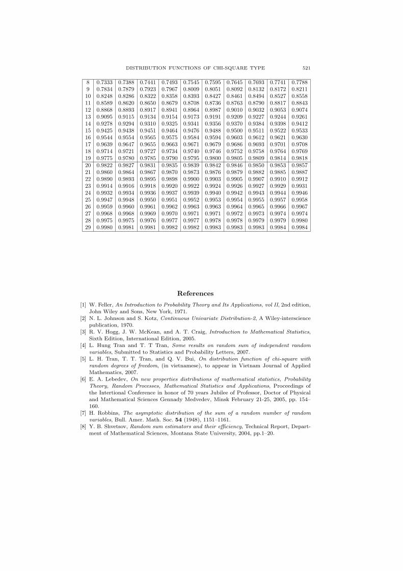
Table 3. Distribution function of chi square-negative binomial withparameter (r = 2, p = 1/3).
Density function is
f(x) =
{0 if x ≤ 0
p2e−x(1−q2)/2Φ(q√
x)(1 + q2x) + p2q√
xe−x/2√
2πif x > 0
x 0.0 0.1 0.2 0.3 0.4 0.5 0.6 0.7 0.8 0.90 0 0.0068 0.0147 0.0233 0.0324 0.0419 0.0517 0.0618 0.0722 0.08291 0.0937 0.1046 0.1157 0.1269 0.1382 0.1495 0.1609 0.1724 0.1839 0.19542 0.2069 0.2184 0.2298 0.2413 0.2527 0.2641 0.2754 0.2866 0.2978 0.30903 0.3200 0.3310 0.3419 0.3527 0.3634 0.3740 0.3845 0.3949 0.4052 0.41544 0.4255 0.4355 0.4453 0.4551 0.4647 0.4742 0.4836 0.4929 0.5021 0.51115 0.5200 0.5289 0.5375 0.5461 0.5545 0.5629 0.5710 0.5791 0.5871 0.59496 0.6026 0.6103 0.6177 0.6251 0.6324 0.6395 0.6465 0.6534 0.6602 0.66697 0.6735 0.6799 0.6863 0.6925 0.6987 0.7047 0.7106 0.7165 0.7222 0.7278
DISTRIBUTION FUNCTIONS OF CHI-SQUARE TYPE 521
8 0.7333 0.7388 0.7441 0.7493 0.7545 0.7595 0.7645 0.7693 0.7741 0.77889 0.7834 0.7879 0.7923 0.7967 0.8009 0.8051 0.8092 0.8132 0.8172 0.821110 0.8248 0.8286 0.8322 0.8358 0.8393 0.8427 0.8461 0.8494 0.8527 0.855811 0.8589 0.8620 0.8650 0.8679 0.8708 0.8736 0.8763 0.8790 0.8817 0.884312 0.8868 0.8893 0.8917 0.8941 0.8964 0.8987 0.9010 0.9032 0.9053 0.907413 0.9095 0.9115 0.9134 0.9154 0.9173 0.9191 0.9209 0.9227 0.9244 0.926114 0.9278 0.9294 0.9310 0.9325 0.9341 0.9356 0.9370 0.9384 0.9398 0.941215 0.9425 0.9438 0.9451 0.9464 0.9476 0.9488 0.9500 0.9511 0.9522 0.953316 0.9544 0.9554 0.9565 0.9575 0.9584 0.9594 0.9603 0.9612 0.9621 0.963017 0.9639 0.9647 0.9655 0.9663 0.9671 0.9679 0.9686 0.9693 0.9701 0.970818 0.9714 0.9721 0.9727 0.9734 0.9740 0.9746 0.9752 0.9758 0.9764 0.976919 0.9775 0.9780 0.9785 0.9790 0.9795 0.9800 0.9805 0.9809 0.9814 0.981820 0.9822 0.9827 0.9831 0.9835 0.9839 0.9842 0.9846 0.9850 0.9853 0.985721 0.9860 0.9864 0.9867 0.9870 0.9873 0.9876 0.9879 0.9882 0.9885 0.988722 0.9890 0.9893 0.9895 0.9898 0.9900 0.9903 0.9905 0.9907 0.9910 0.991223 0.9914 0.9916 0.9918 0.9920 0.9922 0.9924 0.9926 0.9927 0.9929 0.993124 0.9932 0.9934 0.9936 0.9937 0.9939 0.9940 0.9942 0.9943 0.9944 0.994625 0.9947 0.9948 0.9950 0.9951 0.9952 0.9953 0.9954 0.9955 0.9957 0.995826 0.9959 0.9960 0.9961 0.9962 0.9963 0.9963 0.9964 0.9965 0.9966 0.996727 0.9968 0.9968 0.9969 0.9970 0.9971 0.9971 0.9972 0.9973 0.9974 0.997428 0.9975 0.9975 0.9976 0.9977 0.9977 0.9978 0.9978 0.9979 0.9979 0.998029 0.9980 0.9981 0.9981 0.9982 0.9982 0.9983 0.9983 0.9983 0.9984 0.9984
References
[1] W. Feller, An Introduction to Probability Theory and Its Applications, vol II, 2nd edition,
John Wiley and Sons, New York, 1971.[2] N. L. Johnson and S. Kotz, Continuous Univariate Distribution-2, A Wiley-interscience
publication, 1970.[3] R. V. Hogg, J. W. McKean, and A. T. Craig, Introduction to Mathematical Statistics,
Sixth Edition, International Edition, 2005.[4] L. Hung Tran and T. T Tran, Some results on random sum of independent random
variables, Submitted to Statistics and Probability Letters, 2007.[5] L. H. Tran, T. T. Tran, and Q. V. Bui, On distribution function of chi-square with
random degrees of freedom, (in vietnamese), to appear in Vietnam Journal of AppliedMathematics, 2007.
[6] E. A. Lebedev, On new properties distributions of mathematical statistics, Probability
Theory, Random Processes, Mathematical Statistics and Applications, Proceedings ofthe Intertional Conference in honor of 70 years Jubilee of Professor, Doctor of Physicaland Mathematical Sciences Gennady Medvedev, Minsk February 21-25, 2005, pp. 154–160.
[7] H. Robbins, The asymptotic distribution of the sum of a random number of randomvariables, Bull. Amer. Math. Soc. 54 (1948), 1151–1161.
[8] Y. B. Shvetsov, Random sum estimators and their efficiency, Technical Report, Depart-ment of Mathematical Sciences, Montana State University, 2004, pp.1–20.

522 TRAN LOC HUNG, TRAN THIEN THANH, AND BUI QUANG VU
Tran Loc HungDepartment of MathematicsHue UniversityVietnam
E-mail address: [email protected]
Tran Thien Thanh
Department of MathematicsHue UniversityVietnam
Bui Quang VuDepartment of MathematicsHue University
Vietnam