The Great Lakes Geographer, Vol.7, No.1, 2000

Short Term Fluctuations of Lake Erie Water

Levels and the El Niño/Southern Oscillation

P.D. LaValle, V.C. Lakhan, and A.S. TrenhaileDepartment of Earth Sciences, Memorial Hall, University of Windsor, Windsor, Ontario, Canada N9B 3P4

This study assesses the relationship between short term fluctuations of Lake Erie water levels and the El Niño/Southern Oscillation

(ENSO) using data collected from May 1978 to May 1997. After standardizing the collected data, graphical and Box-Jenkins time

series techniques are utilized to assess the temporal interrelationship of the Southern Oscillation Index and Lake Erie water level

variables. The statistical results demonstrate that a first-order auto regressive m odel AR (1) provides the best fit for the data se ts

of the analyzed variables. Both the graphical and statistical results suggest that short term Lake Erie water levels are fluctuating

in response to the two ENS O phases, El N iño and La Niñ a. Negative values of the Southern Oscillation Inde x are related to higher

lake levels while positive values are associated with lower lake levels.

Keyw ords: El N iño, La Niñ a, ENSO , Southern Oscillation, la ke levels

Since 1978, a research team from the University of

Windsor has been engaged in a program to monitor

shoreline change and lake levels along th e northern

shore of Lake Erie. An analysis of the time series of

shoreline and lake level d ata dem onstrates a dynam ic

linkage between lake levels and shoreline behaviour.

With lake level fluctuations associated with either an

aggradation or retreat of th e shorelin e, it was decided to

advance an explanation for the lake level fluctuations

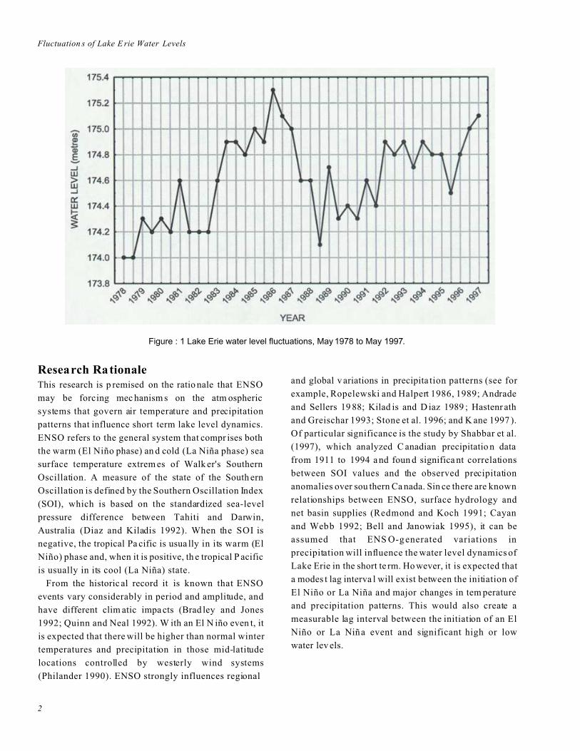
demonstrated in Figure 1. The graph clearly shows that

lake levels rose from 174.0 metres in November 1978

to a high of 175.3 metres in May 1986, and had

declined to 174.1 metres by November 1988. Between

May 1989 and November 1991, they fluctuated around

a mean value of 174.6 metres. Lake levels have

remained above 174.5 metres since 1992, and by 1997

they attain ed a heig ht of 175 .1 metres.

A numb er of exp lanations have be en prop osed to

account for fluctuations of Lake Erie water levels,

including the effects of precipitation, evaporation,

water inflows and outflows, and consumptive use of

water (Quinn 1978; Quinn and Guerra 1986). The

primary objective of this paper is to determine whether

lake levels in the short term are also fluc tuating in

response to the El Niño/Sou thern Oscillation (EN SO).

The research utilized a time series (1978-1997) of data

on Lake Erie w ater levels (LEW L) and the S outhern

Oscillation Index (SOI). Although LEWL and SO I data

have been obtained for the period of 1918 to the

present, this paper analyzed only the data from May

1978 to May 1997, b ecause th is is the perio d durin g

which the Univ ersity of W indsor in vestigated the

impacts of fluctuating lake levels on the beaches and

shoreline of northern Lake Erie. It is worthwhile to

concen trate on the LEWL and SOI data from the past

twenty years because, as Trenberth and Hoar (1996)

reported, the low frequency variability and the negative

trend in the SOI in recent decade s have b een quite

unusu al. The clim atic and h ydrolo gic impa cts of ENSO

events in the past twenty years have been relatively

severe because "the tendency for more frequent El Niño

events and fewer La Niña events since the late 70s has

been linked to decadal changes in climate throughout

the Pacific ba sin" (Tren berth and Hoar 1 996, 57).

These authors reported that the recent warm trend

related to El Niñ o in the tro pical Pacific from 1990 to

June 1995 has been the longest on record since 1882.

Obtaining greater insights on the short term relationsh ip

between lake levels and ENSO events will enhance

decision making not only in the implementation of

better shore pro tection strategies, but also in the

managemen t of water supplies and wetland habitats.

Fluctuation s of Lake E rie Water Levels

2

Figure : 1 Lake Erie water level fluctuations, May 1978 to May 1997.

Research RationaleThis research is p remised on the ratio nale that ENSO

may be forcing mec hanism s on the atm ospheric

systems that govern air temperature and precipitation

patterns that influence short term lake level dynamics.

ENSO refers to the general system that compr ises both

the warm (El Niño phase) an d cold (La Niña phase) sea

surface temperature extrem es of Walk er's Southern

Oscillation. A measure of the state of the South ern

Oscillation is defined by the Southern Oscillation Index

(SOI), which is based on the standardized sea-level

pressure difference between Tahiti and Darwin,

Australia (Diaz and Kiladis 1992). When the SOI is

negative, the tropical Pa cific is usua lly in its warm (El

Niño) phase and, when it is positive, th e tropical P acific

is usually in its cool (La Niña) state.

From the historic al record it is known that ENSO

events vary considerably in period and amplitude, and

have different clim atic impa cts (Brad ley and Jones

1992; Quinn and Neal 1992). W ith an El N iño even t, it

is expected that there will be higher than normal winter

temperatures and precipitation in those mid-latitude

locations controlled by westerly wind systems

(Philander 1990). ENSO strongly influences regional

and global v ariations in precipita tion patterns (see for

example, Ropelewski and Halpert 1986, 1989; Andrade

and Sellers 19 88; Kilad is and D iaz 1989 ; Hastenr ath

and Greischar 1993; Stone et al. 1996; and K ane 1997 ).

Of particular significance is the study by Shabbar et al.

(1997), which analyzed C anadian precipitatio n data

from 1911 to 1994 a nd foun d significa nt correlations

between SOI values and the observed precipitation

anomalies over sou thern Ca nada. Sin ce there are known

relationships between ENSO, surface hydrology and

net basin supplies (Redmond and Koch 1991; Cayan

and Webb 1992; Bell and Janowiak 1995), it can be

assumed that ENS O-g enerated variations in

precipitation will influence the water level dynamics of

Lake Erie in the short te rm. Ho wever, it is expected that

a modes t lag interva l will exist between the initiation of

El Niño or La Niña and major changes in tem perature

and precipitation patterns. This would also create a

measurable lag interval between the initiation of an El

Niño or La Niña event and significant high or low

water lev els.

LaValle, L akhan, an d Trenha ile

3

MethodsData AcquisitionThe May 1978 to May 1997 semi-annual (May and

November of each year) LEWL data used in this paper

were collected by the Canadian Hydro graphic Service

from the Kingsville Gaging Station, located on the

northern shore of L ake Erie , Canada (Environment

Canada 1997). A time series (1978-1997) of the SOI

was obtained from the Climatic Research Unit at the

University of East Anglia. The form of the Index used

in this study is defined as the sea-level air pressure

difference between Tahiti, and Darwin, Australia,

divided by the standard deviation of these differences

and multiplied by 10 (Troup 1965). An eve nt is

considered to be related to El Niñ o whe n this Index is

significan tly less than zero for a period of several

months, and to La Niña when the SOI is significantly

greater than zero for several months. Although there is

not a perfect one-to-one correlation between observed

El Niño events and the SOI, the relationship has been

found to be very strong (G lantz 199 6).

Data AnalysisTo compare the serial dynamics of LEWL with the

SOI, the data were standardized to remove the effects of

the different units of measurement present in the

variable set, and to convert each variable into a

dimensionless parame ter. The d ata were c onverte d to

standard scores (z) using th e formu la:

z = (X - :) / F

where X is a variate score, : is the data mean, and F is

the standard deviation. In this paper the standardized

Lake Erie wa ter level data will be referred to as

SLEWL, and the values of the standardized SOI will be

referred to as SSO I.

After graphing the standard values of SSOI and

SLEWL, Box-Jenkins time series techniqu es were used

to analyze the tem poral behaviour of the variables

SLEWL and SSOI, and their temporal interrelation ships

with each oth er. Box-Jenkins ARIMA (au toregressive

integrated movin g averag e) mod els assume that a time

series is stationary. According to Richards (1979) and

Chatf ield (1985) a stationary time series has the

following properties: a) a constant mean, implying that

there is no significant secular trend; b) homogeneity of

variance, which can be evaluated by using a test for

homo geneity of variance; c) n o signif icant determin istic

periodic movements or seasonal effects, and; d) an

autocorrelation function (depicted on correlograms)

dependent on lag interval and not on the starting

position in the time series.

Since the SLEWL and SS OI data were tested and

found to be stationary, this paper utilized the time series

procedures which have been discussed by Chatfield

(1985). They inv olve: 1) construc ting correlograms

depicting serial autoc orrelation coefficien ts on one axis

and their corresponding lag intervals on another for the

variables SLEWL and SSOI; 2) producing partial

correlograms depicting the partial autocorrelation

coefficien ts for each of the variables (SLEWL and

SSOI) at each lag interval; 3) examining the observed

configurations in the correlograms and partial

correlograms in order to fit the data to either an

autoregressive model or a moving-average model. It

should be noted that the data may not conform to the

requirem ents of any m odel; 4) testi ng the resid uals

from the fitted models fo r serial autocorrelation on

correlograms. This is do ne to asses s the goo dness-o f-fit

of the applied models; 5) treating tho se sets of resid uals

that are found to be unautocorrelated as random

variables, and cross-correlating them with each other at

a number of lag intervals in order to portray any

tempo ral relationsh ips that m ay exist b etween them.

To facilitate interpretation of obtained time series

results, it should be noted that, in ARIMA modelling,

the most basic tool is the correlogram depicting lag

intervals on one axis and the corresponding

autocorrelation coefficients on the other. Basically, the

autocorrelation coefficient is like a common correlation

coefficient, except that it measu res the strength of the

relationsh ip between values of a time series separated

by a set time interval called a lag. The line connecting

the autocorrelation values for each lag describes the

autocorrelation function (ACF). On a correlogram

there are two das hed lines running parallel to th e axis

containing all of the points where the autocorrelation

coefficient is zero. These are called the five percent

(5%) confidence bands, and any autocorrelation

coefficient falling outside of these bands is considered

Fluctuation s of Lake E rie Water Levels

4

to be significantly greater or less than zero at the 0.05

level.

Once the appropriate model is fit to the time series

data, the goodness-of-fit can be ascertained using the

Box-Ljung Q statistics (see StatSoft Inc. 199 7).

Basically, it is necessary to extract the residuals from

each of the models fitted to the analyzed data, and then

construct correlograms of the autocorrelations found in

the residuals. The probability values associated with the

Q statistics are printed on the correlog rams pre sented in

this paper. When working at the 0.05 significan ce level,

if any Q statistic is less than 0.05, the null hypothesis

that absolute values of the autocorr elation co efficients

are not signif icantly dif ferent from zero has to be

rejected. If a mod el is to be considered to be adequate,

then the probabilities associated with the Box-Ljung Q

values m ust be gre ater than 0 .05.

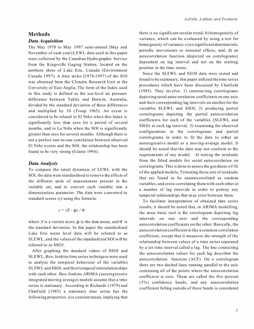
Results and DiscussionThe graph of the values of the standardized Sou thern

Oscillation Index (SSO I) and the standardized Lake

Erie water levels (SLEWL) (Figure 2) reveals four

distinctive SSOI troughs, each having negative values

of less than -1.4. There are also two peaks with SSOI

values greater than 1.4. Based on several studies (for

example, Nicholls 1993; Bell and Janowiak 1995) that

plotted SOI va lues, it is reasonable to claim that

positive values of SSO I are related to La Niñ a events

and negative values to El Niño events. Therefore,

negative SSOI values less than -1.4 are consid ered to

reflect El Niño events, and SS OI valu es greater th an 1.4

La Niña ev ents (Figure 2). Here it must be emphasized

that the four El Niño events shown in Figure 2

substan tiate Suplee's (1999) observations that four of

the strongest El Niño events of this century have

occurred since 1980.

.

Figure 2: Standardized Southern Oscillation Index and standardized lake levels

LaValle, L akhan, an d Trenha ile

5

The observed inverse rela tionship shown in Figure 2

is significant because the negative values of the SSOI

are related to higher lake levels, while the positive

values are associated with lower lake levels. Each of

the higher water level peaks can be attributed to El

Niño events which tend to promote higher than normal

mean basin water su pplies. Th e La Niñ a events, w ith

drier conditions, seem to produce lower lake levels.

The statistical nature of the relationships between the

variables SSOI and SLEWL were determined using the

Box-Jenkins procedures described above. The results,

obtained by usin g the SSOI and SLEWL data in the

time series modules of the Statistica software (StatS oft

Inc. 1997), clearly highlight the appropriateness of

Box-Jenkins ARIMA m odelling procedures that place

emph asis on the recent past rather than the distant pas t.

Without providing a detailed description of all the

Box-Jenkins time series re sults, it is, nevertheless,

worthwhile to emph asize that a firs t-order

autoregressive model AR(1) provides the best fit for the

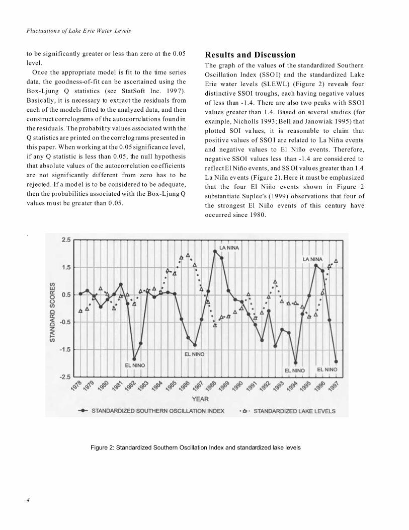
SLEWL data set. The correlogram depicting the

autocorrelation function of the SLEWL data (Figure 3)

demonstrates that the ACF declined from significant

autocorrelations at lag one, to insignificant

autocorrelations at lags greater than one. When the

residuals from the A R(1) m odel w ere subjec ted to

autocorrelation analysis, and a correlogram (Figure 4)

of the error terms or residuals was constructed, no

significant autocorrelations were observed. The

probabilities associated with the Box-Ljung Q statistics

were all quite high, indicating no significant

autocorrelation in the set of residuals. These results

emphasize that the AR (1) mod el is the best c hoice to

describe the serial behaviour of Lake Erie water levels.

Evidently, the standardized Lake Erie water level

move ments seem to be asso ciated w ith a long mem ory

stochastic process.

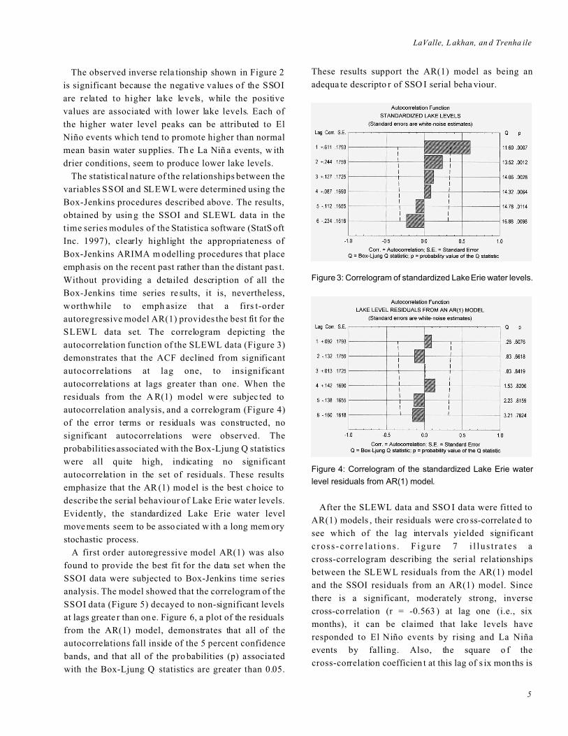
A first order autoregressive model AR(1) was also

found to provide the best fit for the data set when the

SSOI data were subjected to Box-Jenkins time se ries

analysis. The model showed that the correlogram of the

SSOI data (Figure 5) decayed to non-significant levels

at lags greate r than on e. Figure 6, a plot of the residuals

from the AR(1) model, demonstrates that all of the

autocorrelations fall inside of the 5 percent confidence

bands, and that all of the pro babilities (p) associa ted

with the Box-Ljung Q statistics are greater than 0.05.

These results support the AR(1) model as being an

adequa te descripto r of SSO I serial beha viour.

Figure 3: Correlogram of standardized Lake Erie water levels.

Figure 4: Correlogram of the standardized Lake Erie water

level residuals from AR(1) model.

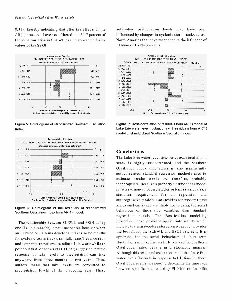
After the SLEWL data and SSO I data were fitted to

AR(1) models , their residuals were cro ss-correlate d to

see which of the lag intervals yielded significant

c ross -cor re la t ions . F i g u re 7 i l l u s t r a t e s a

cross-correlogram describing the seri al relationships

between the SLEWL residuals from the AR(1) model

and the SSOI residuals from an AR(1) model. Since

there is a significant, moderately strong, inverse

cross-co rrelation (r = -0.563 ) at lag one (i.e., six

months), it can be claimed that lake levels have

responded to El Niño events by rising and La Niña

events by falling. Also, the square o f the

cross-correlation coefficien t at this lag of s ix mon ths is

Fluctuation s of Lake E rie Water Levels

6

0.317, thereby indicatin g that after the effects of the

AR(1) processe s have b een filtered out, 31.7 percent of

the serial variation in SLEWL can be accounted for by

values of the SS OI.

Figure 5: Correlogram of standardized Southern Oscillation

Index.

Figure 6: Correlogram of the residuals of standardized

Southern Oscillation Index from AR(1) model.

The relationship between SLEWL and SSOI at lag

one (i.e., six mon ths) is not u nexpec ted because when

an El Niño or La Niña develops it takes some months

for cyclonic storm tracks, rainfall, runoff, evaporation

and temperatu re patterns to adjust. It is w orthwh ile to

point out that Meadows et al. (1997) suggested that the

response of lake levels to precipitation can take

anywhere from three months to two years. These

authors found that lake lev els are correlated to

precipitation levels of the preceding year. These

antecedent precipitation levels may have been

influenced by changes in cyclonic storm tracks across

North America that have responded to the influence of

El Niño or La Niña ev ents.

Figure 7: Cross-correlation of residuals from AR(1) model of

Lake Erie water level fluctuations with residuals from AR(1)

model of standardized Southern Oscillation Index.

ConclusionsThe Lake Erie water level time series examin ed in this

study is highly autocorrelated, and the Southern

Oscillation Index time series is also signific antly

autocorrelated; standard regression method s used to

estimate secular trends are, therefo re, proba bly

inappropriate. Becaus e a prope rly fit time series model

must have non-autocorrelated error term s (residuals ), a

statistical requirement fo r all regression and

autoregressive models, Box-Jenkins (or modern) time

series analysis is more suitable for tracking the serial

behaviour of these tw o variables than standard

regression models. The Box-Jenkins modelling

procedures have provided appropriate results which

indicate that a first-order autoregressive model provides

the best fit for the SLEW L and S SOI da ta sets. It is

apparent that the serial behavio ur of short term

fluctuations in Lake Erie water levels an d the South ern

Oscillation Index behave in a stochastic man ner.

Although this research has dem onstrated that Lak e Erie

water levels fluctuate in response to E l Niño/Sou thern

Oscillation events, we nee d to determine the time lags

between specific an d recurrin g El N iño or La Niña

LaValle, L akhan, an d Trenha ile

7

events and chang es in water levels. A more elaborate

study is currently investiga ting the controls on the lag

effects, and the processes which are link ed to ENS O. In

addition, a longer time series (1918 to present) of SOI

and LEWL data are being analyzed to determine

whether there are also distinct relationships over the

long term between ENSO events and Lake Erie water

levels.

Since many problems associated with shoreline

management are related to rising or falling water levels,

more reliable estimates of the temporal behaviour of

water levels are needed. A knowledge of the history of

lake level fluctuations cou pled with So uthern

Oscillation Index observations can provide a relevant

means of making short term predictions about water

level behavio ur that cou ld affect sho rt term shoreline

planning decisions. The resu lts obtaine d from th is

research will be helpful for the construction of models

to simulate w ater level scenarios relative to shoreline

manag ement. The models can then be useful for dealing

with associated water level problems. Ongoing research

provide evidence that shows that high lak e levels

during El Niño events, an d fairly low water lev els

during La Niña events, create problems for shoreline

residents. For instance, during the 1995 La Niña ev ent,

shoreline dwellers along Lake Erie, Ontario,

complained that they c ould not gain access to the Lake

from their boat slips. Also during this La N iña even t,

farmers a long L ake Erie, O ntario, suffe red a dro ught.

Further study of the relationship between water levels

and the El Niño-La Niña/Southern Oscillation

phenomena may lead to a more effective means of

coping with the dynamics of water level change in the

Great Lakes.

ReferencesAndrade, E.R., and Sellers, W .D. 1988. ‘El Niño and

its effect on precipitation in Arizona and w estern

New M exico,’ Journa l of Clima te, 8: 403-410.

Bell, G.D., an d Janow iak, J.E. 19 95. ‘Atm ospheric

circulation associated with the Midwest floods of

1993’, Bulletin of the American Meteorological

Society , 76(5): 681-695.

Bradley, R.S., and Jones, P.D . (eds.) 1992. Clima te

since A.D. 1500. London and New York: Routledge.

Cayan, D.R., and Webb , R.H. 1992 . ‘El Niño/So uthern

Oscillation and streamflow in the western United

States’. In El Niño. Historical and paleoclima tic

aspects of the Southern Oscillation, eds. H.F. Diaz

and V. Markgraf, pp. 29-68. Cambridge, UK:

Cambridge U niversity Press.

Chatfield, C. 198 5. The analysis of time series: An

introduction. London and New York: Chapman and

Hall.

Diaz, H.F., and Kiladis, G .N. 199 2. ‘Atm ospheric

teleconnections associated with the extreme phase of

the Southern O scillation’. In El Niño. Historical and

paleoclim atic aspects of the Southern Oscillation,

eds. H.F. Diaz and V. Markgraf, pp. 7-28.

Cambridge, UK : Cambridge University Press.

Environment Canada 1997. Great Lakes month ly mean

water level data. Ottawa, ON: Canadian

Hydrographic Service, Environment Canada.

Glantz, M.H. 1 996. Curren ts of chan ge: El N iño's

impact on climate and soc iety. Cambridge, UK:

Cambridge U niversity Press.

Hastenrath, S., and Greischar, L. 1993. ‘Circulation

mechanisms related to northeast B razil rainfall

anom alies,’ Journal of Geophysical Re search, 98:

5093-5102.

Kane, R.P. 1997 . ‘Relationship of E l Niño-Sou thern

Oscillation and Pac ific Sea Surface T emperature with

Rainfall in Various Regions of the G lobe,’ Mon thly

Weather Review, 125: 1792-1800.

Kiladis, G.N., an d Diaz, H .F. 1989 . ‘Globa l climate

anomalies associated with extreme s in the Southe rn

Oscillation ’, Journa l of Clima te, 2: 1069-1090.

Meadow s, G.A., M eadow s, L.A., W ood, W .L.,

Hubertz, J.M., and Perlin, M. 1997. ‘The rela tionship

between Great Lakes water levels, wave energies and

shoreline damag e’, Bulletin of the American

Meteo rologica l Society , 78 (4): 675-683.

Nicholls, N. 199 3. ‘ENS O, drou ght and flooding rain

in South-East Asia’. In South-E ast Asia's

environmental future: Th e search for sustain ability ,

eds. H. Brookfield and Y. Byron, pp. 154-175.

Tokyo, Japan: United Nations University Press and

Oxford University Press.

Philander, S.G. 19 90. El Niño, La Niña, and the

Southern Oscillation. San Diego, CA: Aca demic

Press, Inc.

Fluctuation s of Lake E rie Water Levels

8

Quinn, F. 1978. ‘Hydrologic response model of the

North American Great L akes’, Journal of Hydrology,

37: 295-307.

Quinn, F., and Guerra, B. 1986. ‘Current perspectives

on the Lake E rie water b alance’, Journal of Great

Lakes Research, 12: 109-116.

Quinn, F., and Neal, V.T. 1992. ‘The historical record

of El Niño Events’. In Climate since A.D. 1500, eds.

R.S. Bradley and P.D. Jones, pp. 623-648. London

and New York: Routledge.

Redmond, K., and Koch, R. 1991. ‘ENSO vs. surface

climate variability in the western United States’,

Water Resources Research, 27: 2381-2399.

Richards, K.S. 19 79. Stochastic Proce sses in

One-Dimensional Series: An Introduction. East

Anglia: Conce pts and T echniqu es in Modern

Geography #23.

Ropele wski, C.F., and Halpert, M.S. 1 986. ‘N orth

American precipitation and temperature patterns

associated with the El Niño/Southern Oscillation

(ENSO)’, Monthly Weather Review, 114: 2352-2362.

Ropele wski, C.F., and Ha lpert, M.S . 1989.

‘Precipitation patterns associated with the high index

phase of the Southern Oscillation’, Journal of

Clima te, 2: 268-289.

Shabbar, A., Bon sal, B., and Khan dekar, M . 1997.

‘Canadian precipitation patterns associated with the

Southern Oscillation ’, Journal of Clima te, 10

(December): 3016-3027.

StatSoft, Inc. 1997. STATISTICA for Windows

[Computer program manua l], Tulsa, O K: StatS oft,

Inc.

Stone, R.C., Hammer, G.L., and Marcussen, T. 1996.

‘Prediction of globa l rainfall pro babilit ies using

phases of the Southern Oscillation Ind ex’, Nature ,

384: 252-255.

Suplee, C. 199 9. ‘El Niñ o/La N iña’, National

Geog raphic , 195 (3): 72-95.

Trenberth, K.E., and Hoar, T.J. 1996. ‘The 1990-1995

El Niño-S outhern Oscillation event’, Geophysical

Research Letters, 23 (1): 57-60.

Troup, A.J. 1965. ‘The Southern Oscillation’,

Quarte rly Journal of the Royal Meteorological

Society , 91: 490-506.