Reproductive ecology and life history of human males - UCL ...
184
1 Reproductive Ecology And Life History Of Human Males: A Migrant Study Of Bangladeshi Men Kesson Shane Magid Thesis submitted for the degree of Doctor of Philosophy to Department of Anthropology University College London 2011
-
Upload
khangminh22 -
Category
Documents
-
view
5 -
download
0
Transcript of Reproductive ecology and life history of human males - UCL ...
1
Reproductive Ecology And Life History Of Human Males:
A Migrant Study Of Bangladeshi Men
Kesson Shane Magid
Thesis submitted for the degree of
Doctor of Philosophy
to
Department of Anthropology
University College London
2011

2Kesson S. Magid - UCL
Declaration
I, Kesson Shane Magid declare confirm that the work presented in this thesis is my own. Where information has been derived from other sources, I confirm that this has been indicated in the thesis.
Singed: .......................................................... Date: .............................
3Kesson S. Magid - UCL
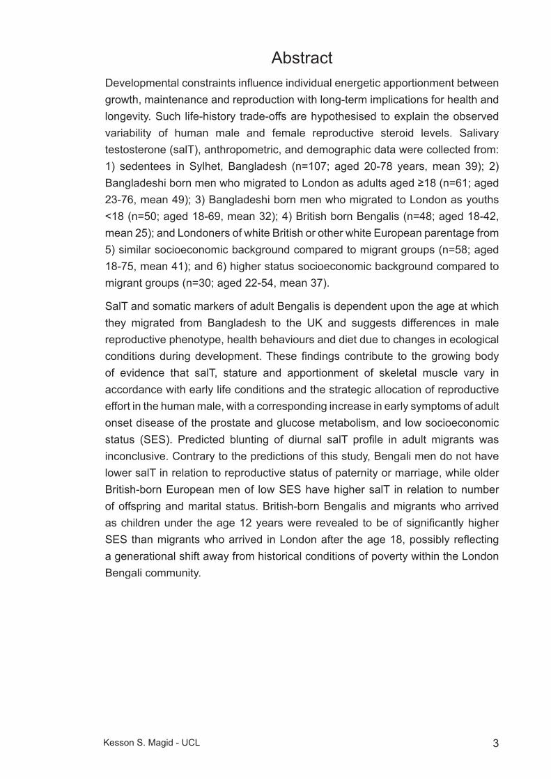
AbstractDevelopmental constraints influence individual energetic apportionment between growth, maintenance and reproduction with long-term implications for health and longevity. Such life-history trade-offs are hypothesised to explain the observed variability of human male and female reproductive steroid levels. Salivary testosterone (salT), anthropometric, and demographic data were collected from: 1) sedentees in Sylhet, Bangladesh (n=107; aged 20-78 years, mean 39); 2) Bangladeshi born men who migrated to London as adults aged ≥18 (n=61; aged 23-76, mean 49); 3) Bangladeshi born men who migrated to London as youths <18 (n=50; aged 18-69, mean 32); 4) British born Bengalis (n=48; aged 18-42, mean 25); and Londoners of white British or other white European parentage from 5) similar socioeconomic background compared to migrant groups (n=58; aged 18-75, mean 41); and 6) higher status socioeconomic background compared to migrant groups (n=30; aged 22-54, mean 37).
SalT and somatic markers of adult Bengalis is dependent upon the age at which they migrated from Bangladesh to the UK and suggests differences in male reproductive phenotype, health behaviours and diet due to changes in ecological conditions during development. These findings contribute to the growing body of evidence that salT, stature and apportionment of skeletal muscle vary in accordance with early life conditions and the strategic allocation of reproductive effort in the human male, with a corresponding increase in early symptoms of adult onset disease of the prostate and glucose metabolism, and low socioeconomic status (SES). Predicted blunting of diurnal salT profile in adult migrants was inconclusive. Contrary to the predictions of this study, Bengali men do not have lower salT in relation to reproductive status of paternity or marriage, while older British-born European men of low SES have higher salT in relation to number of offspring and marital status. British-born Bengalis and migrants who arrived as children under the age 12 years were revealed to be of significantly higher SES than migrants who arrived in London after the age 18, possibly reflecting a generational shift away from historical conditions of poverty within the London Bengali community.
4Kesson S. Magid - UCL
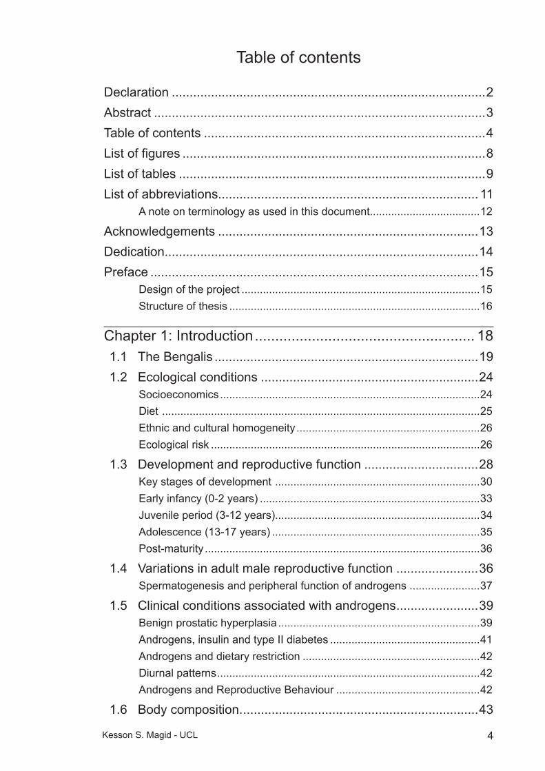
Table of contents
Declaration ........................................................................................2Abstract .............................................................................................3Table of contents ...............................................................................4List of figures .....................................................................................8List of tables ......................................................................................9List of abbreviations......................................................................... 11
A note on terminology as used in this document....................................12
Acknowledgements .........................................................................13Dedication........................................................................................14Preface ............................................................................................15
Design of the project ..............................................................................15Structure of thesis ..................................................................................16
Chapter 1: Introduction ...................................................... 181.1 The Bengalis ..........................................................................191.2 Ecological conditions .............................................................24
Socioeconomics .....................................................................................24Diet ........................................................................................................25Ethnic and cultural homogeneity ............................................................26Ecological risk ........................................................................................26
1.3 Development and reproductive function ................................28Key stages of development ...................................................................30Early infancy (0-2 years) ........................................................................33Juvenile period (3-12 years)...................................................................34Adolescence (13-17 years) ....................................................................35Post-maturity ..........................................................................................36
1.4 Variations in adult male reproductive function .......................36Spermatogenesis and peripheral function of androgens .......................37
1.5 Clinical conditions associated with androgens .......................39Benign prostatic hyperplasia ..................................................................39Androgens, insulin and type II diabetes .................................................41Androgens and dietary restriction ..........................................................42Diurnal patterns ......................................................................................42Androgens and Reproductive Behaviour ...............................................42
1.6 Body composition. ..................................................................43

5Kesson S. Magid - UCL
Muscle tissue .........................................................................................43Adipose tissue ........................................................................................43Immune system ......................................................................................45
1.7 Human male life history theory ..............................................45General model of life history ..................................................................46Life history theory and growth ................................................................47Life history theory and human reproductive ecology..............................49Aging ......................................................................................................50Predictions of this study .........................................................................50
Chapter 2: Methods and validation studies ...................... 572.1 Recruitment and interviews ....................................................57
Bangladeshi Sedentees (SED) ..............................................................57London ...................................................................................................58Adult Migrants (ADM) .............................................................................59Young Migrants (YOM) ...........................................................................59British-born Bengalis (2NG) ...................................................................59British-born European, low SES (ELO) ..................................................59British-born European, high SES (EHI) ..................................................59
2.2 Anthropometry: ......................................................................59Height .....................................................................................................59Weight and Body Mass Index ................................................................60
2.3 Arm anthropometric measures ...............................................60Arm Length.............................................................................................60Arm Circumference ................................................................................61Skinfolds.................................................................................................61Triceps skinfold (TSF) ............................................................................62Biceps skinfold (BSF) .............................................................................62Estimates of Mid-Upper Arm tissue apportionment ................................62
2.4 Questionnaires .......................................................................63Prostate symptoms ................................................................................64Relationship status .................................................................................64Socioeconomic status ............................................................................64
2.5 Fasting blood glucose and dried blood spots .........................652.6 Salivary sampling ..................................................................652.7 Salivary Testosterone and Cortisol ........................................65
Salivary assay protocol ..........................................................................66
2.8 Salivary validation studies ......................................................66
6Kesson S. Magid - UCL
Betel nut study .......................................................................................66Betel nut results .....................................................................................67Matched saliva/serum samples ..............................................................68
2.9 Statistical analysis ..................................................................69Missing values analysis..........................................................................69Residential variation in salivary T ...........................................................69Validation study results ..........................................................................70Serum to salivary T comparisons ...........................................................71Inter-daily variation: ................................................................................72Intra-daily variation .................................................................................73
2.10 Conclusions ...........................................................................73
Chapter 3: Testing developmental hypotheses .................. 753.1 Introduction ............................................................................75
Hypotheses ............................................................................................76
3.2 Methods .................................................................................77Recruitment ............................................................................................77Statistical analysis: .................................................................................78
3.3 Results ...................................................................................80Descriptives ............................................................................................80Age at migration and salivary T ..............................................................88Diurnal salT ratio and residence group ..................................................88
3.4 Age of maturity ......................................................................983.5 Conclusions .........................................................................101
Overall conclusions: .............................................................................103
Chapter 4: Diet and health............................................... 1044.1 Diet .......................................................................................105
Food frequencies .................................................................................105Dietary patterns ....................................................................................107
4.2 Health behaviours ................................................................ 110Alcohol .................................................................................................110Smoking ...............................................................................................110Betel Nut .............................................................................................. 111Activity: sport and exercise per week ...................................................112
4.3 Prostate symptoms .............................................................. 113Hormonal and physical measures ........................................................114
4.4 Fasting blood glucose .......................................................... 115

7Kesson S. Magid - UCL
4.5 Dietary or health behaviours and salT ................................ 1164.6 Conclusions ......................................................................... 116
Fasting blood glucose: .........................................................................117Dietary patterns: ..................................................................................117Prostate symptoms ..............................................................................118
Chapter 5: Social factors and reproductive function ........ 120Methods ...............................................................................................121Results .................................................................................................122Socioeconomic measures ....................................................................122
5.1 Reproductive strategies .......................................................125Methods ...............................................................................................126
Results: ................................................................................................126
5.2 Conclusions .........................................................................128
Chapter 6: Conclusions ................................................... 130Limitations and future directions ..........................................................137
Appendix 1: Demographic questionnaire ......................................139Appendix 2: Food habits questionnaire .........................................146Appendix 3: Salivary testosterone assays: methods and results from Magid 2005 ................................................................152Appendix 4: Laboratory assay validation ......................................156References ...................................................................................162

8Kesson S. Magid - UCL
List of figuresFigure 1: Map of Bangladesh ...........................................................................19
Figure 2: Estimated UK Bengali population ......................................................22
Figure 3: Areas of London with large Bengali populations ...............................23
Figure 4: Diagram of the hypothalamic-pituitary-testicular axis ........................30
Figure 5: Male life history allocations ...............................................................47
Figure 6: Project design....................................................................................51
Figure 7: Model of the male reproductive life course........................................52
Figure 8: Salivary T and recent betel nut use ...................................................68
Figure 9: Matched Salivary T to SerumT .........................................................71
Figure 10: Sequence of hypothesis statements ...............................................79
Figure 11: Regression of anthropometric variables by participant age .............85
Figure 12: General anthropometric measures ..................................................86
Figure 13: Mid-upper arm anthropometric measures .......................................86
Figure 14: Mean diurnal salT by residence ......................................................89
Figure 15: Composite age of maturity ...........................................................100
Figure 16: Average reported food frequencies ...............................................108
Figure 17: Reported physical activity.............................................................. 112
Figure 18: Mean prostate symptoms ............................................................. 113
Figure 19: Fasting blood glucose ................................................................... 115
Figure 20: UK SES by residence group..........................................................123
Figure 21: House crowding.............................................................................123
Figure 22: Salivary T by marital status ..........................................................127
9Kesson S. Magid - UCL
List of tablesTable 1: Estimated UK Bengali population .......................................................22
Table 2: Recruitment data.................................................................................58
Table 3: Anthropometric technical errors of measurement (TEM) ....................63
Table 4: Betel Nut Repeated Measures ANOVA ...............................................67
Table 5: Missing values analysis : Little's MCAR test .......................................69
Table 6: Serum T assay QCs ............................................................................71
Table 7: Paired t-test of inter-daily sample waking (WAKE), 30 Minutes Post-Waking (W+30) and Bedtime (BED) salivary T (pg/mL) ...........72
Table 8: Paired t-test of intra-daily sample Waking (WAKE), 30 Minutes Post-Waking (W+30) and Bedtime (BED) salivary T (pg/mL) ...........73
Table 9: Descriptive measures by residence group, all ages, mean (std dev) ............................................................................................82
Table 10: Descriptive measures by residence group, split at age ≤39, mean (std dev) ..................................................................................83
Table 11: Descriptive measures by residence group, split at age ≥40, mean (std dev) ..................................................................................84
Table 12: Body anthropometrics (height & weight): MLR contrast coefficients ........................................................................................90
Table 13: Body anthropometrics (BMI): MLR contrast coefficient.....................91
Table 14: Arm anthropometrics (LogAL & MUAC) : MLR contrast coefficients ........................................................................................92
Table 15: Arm anthropometrics (MUA & LogMUA): MLR contrast coefficients ........................................................................................93
Table 16: Untransformed (waking) salivary T MLR contrast coefficients ..........94
Table 17: Untransformed (wake +30) salivary T MLR contrast coefficients ........................................................................................95
Table 18: Untransformed (bed) salivary T MLR contrast coefficients ...............96
Table 19: Untransformed (day mean) salivary T MLR contrast coefficients ........................................................................................97
Table 20: Estimated marginal means, composite age at maturity (years) ..............................................................................................99

10Kesson S. Magid - UCL
Table 21: Dietary food frequencies .................................................................109
Table 22: SES variables, by residence group split age 40 .............................124
Table 23: Regression coefficients: total number of offspring ..........................127
Table 24: MLR Regression coefficients for men <40, resident in London ......128

11Kesson S. Magid - UCL
List of abbreviations
2NG: Second-Generation migrant, British-born BengaliADM: Adult Migrant, Bangladesh-born and migrated to the UK aged 18
years or olderAL: Arm lengthANCOVA: Analysis of Covariance General Linear ModelAR: Androgen ReceptorBD: BangladeshBDT Bangladeshi TakaBED: Evening salivary sample BPH: Benign Prostatic HyperplasiaBSF: Biceps Skin FoldDAYM: Averaged daily salivary sampleDHT: DihydrotestosteroneDIR: Diurnal ratioE2: OestradiolEHI: British-born European of high socioeconomic statusELO: British-born European of low socioeconomic statusFSH: Follicular Stimulating HormoneGBP: Pound Sterling GH: Growth HormoneGnRH: Gonadotropin Releasing HormoneHPT: Hypothalamic Pituitary Testicular axisIPSS(+QoL): International Prostate Symptom Score (+ Quality of Life score)LH: Luteinising HormoneLUTS: Lower Urinary Tract SymptomsMeanAM: Averaged morning salivary samplesMLR: Multiple Linear Regression MUA: Mid-Upper ArmMUAC: Mid-Upper Arm CircumferenceONS: Office of National StatisticssalT: Salivary testosterone SES: Socioeconomic statusT: TestosteroneTSF: Triceps Skin FoldW+30: Thirty minutes post-waking salivary sample WAKE: Waking salivary sample YOM: Youth migrant, Bangladesh-born and migrated to the UK before
age 18.

12Kesson S. Magid - UCL
A note on terminology as used in this document
Bengali refers to the ethno-linguistic group native to the regions of historic Bengal, encompassing the modern state Bangladesh as well as surrounding regions of the Indian subcontinent.
Bangla refers to the language (and sometimes culture) of the Bengali people.
Bangladeshi refers to the citizens and culture of the state of Bangladesh, though Sylheti refers to both a dialect of Bangla and to the residents of the Sylhet district of Northeast Bangladesh.
Londoni is the term Sylheti sedentees apply to Bengalis living in the UK (usually without regard to whether they actually live in London).
While in practice these terms are commonly used interchangeably by Bengalis living in the UK1 within this thesis London-born children of Bangladeshi-born migrants will be referred to as “Bengali” or “British-born Bengalis” to distinguish the ethnic and political terminology.
1 In an informal poll conducted on the British Bengali social networking website www.networkbangla.co.uk in November 2007, I received the following responses to the question, “How would you rank the following in terms of importance how you'd describe your own identity, i.e. no.1 being the most important and 7 being least im-portant? For the poll, just pick the most important then post your full ranking!”
None of the 58 respondents numbered their responses, so if they specified multiple identities, each identity was given a weight of one.
Preferred Self Identity N % Asian 1 1.3Bangladeshi 6 7.9Bengali 10 13.2British 11 14.5British-Bangladeshi 5 6.6British-Bengali 13 17.1Muslim 17 22.4Other 13 17.1Total 76 100
Though “Muslim” was preferred more than any other identity, there was not a single significantly preferred name for cultural identity, and the number of individuals select-ing an identity versus those not choosing it was not significant, X2(12,6), p=.07.

13Kesson S. Magid - UCL
AcknowledgementsEvery thesis project is a team effort and this one is no exception, though I am sure there will be inadvertent exceptions from this list. I would like to thank all the research assistants who helped collect the data, in particular David Lawson, Farid Ahamed, Zhaved Selehin, and Raskin Ahmed as well as the rest of the team from SUST. I am grateful to Robert Chatterton and for opening his lab to me, and Shanthi Muttukrishna for her assistance in interpreting assay results. I thank Osul Chaudhury, Lynnette Leidy Sievert, Lauren Houghton, Taniya Sharmeen, Khurshida Begum and Ale Núñez de la Mora, for their support in Sylhet and London. I thank Ben Wright and my UCL colleagues in Reproduction Lunch for stimulating discussion.
I am grateful for the funding of this project by the ESRC, ProstateUK, and the Bogue Foundation. I thank all of the participants and recruitment places for their generosity of time and trust.
I thank Ruth Mace for her supervision and advice at UCL. I’m exceptionally grateful for all the years of support, intellectual supervision, and discussion from my supervisor Gillian Bentley. Lastly, I am grateful beyond measure to my partner, planner, and graphic designer Elliot Kemp.

14Kesson S. Magid - UCL
Dedication
Dedicated to the memory of my father Dr. Ken Magid.
15Kesson S. Magid - UCL
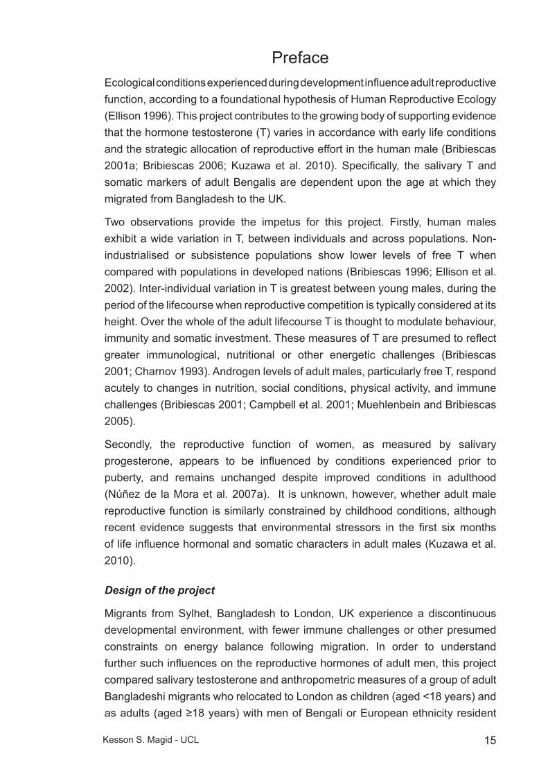
PrefaceEcological conditions experienced during development influence adult reproductive function, according to a foundational hypothesis of Human Reproductive Ecology (Ellison 1996). This project contributes to the growing body of supporting evidence that the hormone testosterone (T) varies in accordance with early life conditions and the strategic allocation of reproductive effort in the human male (Bribiescas 2001a; Bribiescas 2006; Kuzawa et al. 2010). Specifically, the salivary T and somatic markers of adult Bengalis are dependent upon the age at which they migrated from Bangladesh to the UK.
Two observations provide the impetus for this project. Firstly, human males exhibit a wide variation in T, between individuals and across populations. Non-industrialised or subsistence populations show lower levels of free T when compared with populations in developed nations (Bribiescas 1996; Ellison et al. 2002). Inter-individual variation in T is greatest between young males, during the period of the lifecourse when reproductive competition is typically considered at its height. Over the whole of the adult lifecourse T is thought to modulate behaviour, immunity and somatic investment. These measures of T are presumed to reflect greater immunological, nutritional or other energetic challenges (Bribiescas 2001; Charnov 1993). Androgen levels of adult males, particularly free T, respond acutely to changes in nutrition, social conditions, physical activity, and immune challenges (Bribiescas 2001; Campbell et al. 2001; Muehlenbein and Bribiescas 2005).
Secondly, the reproductive function of women, as measured by salivary progesterone, appears to be influenced by conditions experienced prior to puberty, and remains unchanged despite improved conditions in adulthood (Núñez de la Mora et al. 2007a). It is unknown, however, whether adult male reproductive function is similarly constrained by childhood conditions, although recent evidence suggests that environmental stressors in the first six months of life influence hormonal and somatic characters in adult males (Kuzawa et al. 2010).
Design of the project
Migrants from Sylhet, Bangladesh to London, UK experience a discontinuous developmental environment, with fewer immune challenges or other presumed constraints on energy balance following migration. In order to understand further such influences on the reproductive hormones of adult men, this project compared salivary testosterone and anthropometric measures of a group of adult Bangladeshi migrants who relocated to London as children (aged <18 years) and as adults (aged ≥18 years) with men of Bengali or European ethnicity resident

16Kesson S. Magid - UCL
all their lives in London, or with Sylheti sedentees. Age at migration acts as an experimental variable in this study in order to observe whether adult patterns of salT variation are influenced by ecological conditions experienced during development.
Structure of thesis
Chapter one introduces the project in three parts. I begin by describing the ecological conditions and background of the Bengalis living in the UK and Bangladesh. Next, I place the project in context with other research and the current state of our understanding of male reproductive development, adult function and behaviour. Finally, I present the theoretical basis for the project and propose hypotheses to test interactions of biological signals measured by hormones with developmental markers, health and behavioural change, and cultural conditions.
Chapter two describes the methods of the project, and presents results validating these methods for this project.
Chapters three through five present the results of the project. They fall into three general, overlapping categories of development, dietary and health behaviours, and social ecology. These three categories frame the hypotheses tested within the three results chapters presented in this thesis.
Chapter three tests developmental hypotheses: If developmental conditions influence investment in persistent structures and response thresholds of hormonal axes and somatic tissue, then the timing of a change in ecological conditions at a point in the lifecourse will measurably influence reproductive function in adult men as well as physical growth and developmental tempo and during childhood. The specific predictions are that Bengali men who spent all or part of their childhood in London will show higher salT, taller stature and will recall reaching sexual maturity at an earlier age than Bengalis who spent their childhood in Sylhet.
Chapter four tests hypotheses related to diet and health. Regarding dietary and health behaviours, if men live in Sylhet all their lives, do they report nutritional stress? Do men who migrated to London as adults consume similar diets as sedentees? Does childhood acculturation to life in London influence Bengali dietary and health behaviours? The predictions are that men from Sylhet are not nutritionally stressed, that the Bengali diet in London is similar to that of sedentee counterparts, with less consumption of fish and more consumption of other meat. Bengalis who spent all or part of their childhood in London will show greater similarity in their patterns of dietary and health behaviours to SES-matched British European men compared with Bengalis who did not migrate to London as children.

17Kesson S. Magid - UCL
Regarding ecological conditions and health, if adult onset diseases are related to a mismatch between early life developmental conditions and adult ecology, does migration after key stages of development mean migrants are more prone to symptoms of prostatic disease and dysregulation of glucose metabolism? Proximately, if men have high salT, are they more likely to report more LUTS than men who have low salT? The prediction tested is that Bengalis who migrated London after childhood will report more lower urinary tract symptoms (LUTS) than British-born Bengalis, and Bengalis who migrated as children. Finally, do dietary and health behaviours adequately explain Bengali inter-population variation in measures of salT tested in chapter three?
Chapter five tests hypotheses based on social ecology and male reproduction. Regarding socioeconomic positioning, if a male is of high SES relative to current surrounding ecological conditions, does he divert more effort toward reproductive function than men of low SES, relative to current ecological conditions? Is current relative SES more influential on reproductive effort of men in the latter half of their reproductive stage of life, compared to men in the first half of this stage of life? The specific predictions are that high SES males have higher salT, and that relative SES is more highly associated with salT in men aged 40 years or older. Finally, do SES, dietary and health behaviours adequately explain Bengali inter-population variation in measures of salT tested in chapter three?
Regarding relationship and reproductive status, if different ecologies during childhood development determine coordination of male endocrine function and the social relationships of pair-bonds and offspring, do men who are exposed to Western influences of acculturation during childhood development exhibit greater reduction in reproductive function if they are married or married with children as compared to men who were less exposed to such influences? The specific prediction is that Bengalis who spent all or part of their childhood in London and British European men will show lower salT if they are married or have young children than Bengalis who spent all of their childhood in Sylhet.
Chapter six draws conclusions from the findings of the project as a whole at two levels of inquiry. Proximately, how does the functioning of reproductive organs and hormonal axes interact with developmental history and current surroundings? Ultimately, how do these results reflect the balancing of the competing biological functions of survivorship and reproductive effort has been shaped by natural selection? These principles extend to the field of evolutionary medicine, where trade-offs of investment between competing physiological requirements explain senescence and disease.
18Kesson S. Magid - UCL Chapter one
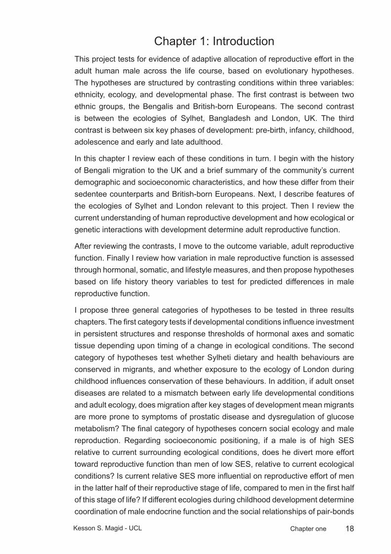
IntroductionChapter 1: This project tests for evidence of adaptive allocation of reproductive effort in the adult human male across the life course, based on evolutionary hypotheses. The hypotheses are structured by contrasting conditions within three variables: ethnicity, ecology, and developmental phase. The first contrast is between two ethnic groups, the Bengalis and British-born Europeans. The second contrast is between the ecologies of Sylhet, Bangladesh and London, UK. The third contrast is between six key phases of development: pre-birth, infancy, childhood, adolescence and early and late adulthood.
In this chapter I review each of these conditions in turn. I begin with the history of Bengali migration to the UK and a brief summary of the community’s current demographic and socioeconomic characteristics, and how these differ from their sedentee counterparts and British-born Europeans. Next, I describe features of the ecologies of Sylhet and London relevant to this project. Then I review the current understanding of human reproductive development and how ecological or genetic interactions with development determine adult reproductive function.
After reviewing the contrasts, I move to the outcome variable, adult reproductive function. Finally I review how variation in male reproductive function is assessed through hormonal, somatic, and lifestyle measures, and then propose hypotheses based on life history theory variables to test for predicted differences in male reproductive function.
I propose three general categories of hypotheses to be tested in three results chapters. The first category tests if developmental conditions influence investment in persistent structures and response thresholds of hormonal axes and somatic tissue depending upon timing of a change in ecological conditions. The second category of hypotheses test whether Sylheti dietary and health behaviours are conserved in migrants, and whether exposure to the ecology of London during childhood influences conservation of these behaviours. In addition, if adult onset diseases are related to a mismatch between early life developmental conditions and adult ecology, does migration after key stages of development mean migrants are more prone to symptoms of prostatic disease and dysregulation of glucose metabolism? The final category of hypotheses concern social ecology and male reproduction. Regarding socioeconomic positioning, if a male is of high SES relative to current surrounding ecological conditions, does he divert more effort toward reproductive function than men of low SES, relative to current ecological conditions? Is current relative SES more influential on reproductive effort of men in the latter half of their reproductive stage of life, compared to men in the first half of this stage of life? If different ecologies during childhood development determine coordination of male endocrine function and the social relationships of pair-bonds

19Kesson S. Magid - UCL Chapter one
and offspring, do men who are exposed to Western influences of acculturation during childhood development exhibit greater reduction in reproductive function if they are married or married with children as compared to men who were less exposed to such influences?
The Bengalis1.1
The Bengali community provides the ethnographic basis of this research due to their unique multi-generational history of migration to the UK, which allows for recruitment of participants across age categories and country of birth. Bengalis in the UK form a geographically-concentrated and culturally cohesive migrant community originating from a single, homogenous population, >95% of whom are descended from the land-holding middle-class of Sylhet, a distinct region of modern-day Northeast Bangladesh (See fig 1) (Eade et al. 1996; Siddiqui 2004).
Map of BangladeshFigure 1:
Adapted from Bangladesh Demographic and Health Survey (NIPORT 2009)

20Kesson S. Magid - UCL Chapter one
On average, Bengalis in Britain are significantly younger and more ethnically segregated than other South Asian minorities or the British population as a whole (DCLG 2009), and together with Pakistanis are the poorest major ethnic minority in Britain (ONS 2002).
In this section I will review the history of Bengali migration to the UK, how this history contributed to their current demographic and socioeconomic characteristics. These characteristics form the basis of contrasts and assumed consistencies between the migrant and sedentee populations, and between migrants and their ethnically-European London neighbours.
The UK Bengali community has a long history of immigration to East London, with the earliest settlers arriving in the late 1940s and are now entering the third generation of regular migration (Eade et al. 1996). The UK Bengali community originates from the Sylheti middle class for a number of historical reasons.
Unlike the rest of present-day Bangladesh, Sylhet was included within the Assam province of British India, which allowed Sylheti landholders to acquire wealth by consolidating cultivation into lucrative export crops like tea, unlike the tenant farming of neighbouring Bengal province (Banglapedia 2010). This led to the formation of a socioeconomically distinct landholding class in Sylhet (Gardner and Shukur 1994). The male offspring of these families were not required to work the land and had the economic means to migrate and connections to the shipping industry, so many joined the steamship trade in Calcutta (Alexander et al. 2010; Gardner 2002).
The first Bengalis to arrive in significant numbers in London were “lascars”, teams of men employed on steamships serving the British Empire up to the 1960s (Al-mahmood 2008). Many of the contracts were one-way, so those who stayed behind remained in the docklands of East London, where they maintained close links to Sylhet and uncertain futures in London (Alexander et al. 2010; www.portcities.org 2010). Those that found work or started businesses in East London did so from relatively unskilled capacities as textile labourers in the “rag trade”, small shops or the first Indian restaurants, the latter remains an important source of income and employment within the Bengali community to this day (Carey 2004).
The 1962 passage of the first UK Commonwealth Immigrants Act restricted migration of unskilled labour from East Pakistan, which included Sylhet following the 1947 partition of India (a period of great social and political upheaval in the region, see ecology section below). Bengali migrants required vouchers, which were set to decrease in number each year following the Act. Despite these limitations, this was the period when the bulk of first generation male migrants arrived through networks of Sylheti relatives and friends based in the UK to work in the developing restaurant business or factories. The UK Bengali population
21Kesson S. Magid - UCL Chapter one
is estimated to have increased ten-fold in the period between 1960 and 1970s (see figure 2), and the vast majority of these arrivals were men (DCLG 2009). Many of these arrivals continued to support families in Sylhet, splitting their time between the two countries (Gardner 2002). Shifting economic cycles and the violent Bangladeshi War of Independence of 1971 prompted many of the Bengalis living in the UK to bring their female family members and children, and further restrictions of migration laws in the 1980s meant only family members could migrate to the UK (Alexander et al. 2010; Dench et al. 2006; Gardner and Shukur 1994).
This led to a period of “chain” migration when most of the migrants were wives and children of the original “voucher” migrants. The average age of a Bengali wife is about 10 years younger than her husband (Mitra et al. 1997). The age profile of the UK Bengali population shifted downward as a demographic consequence of these “chain” migrants. By 2001 there was a balanced sex ratio between the ages of 15-29, but 50% more men in the 30-44 age range (UK Census data, cited in Alexander, 2010). Almost 1/3 of Bengali migrants had arrived in the UK after 1985, and most of them were women and adult children of first generation migrants (Ahmed 2005).
The timing of this “chain” migration shapes the present day contrast in socioeconomic profile of Bengalis living in London and Sylhet.
Bengali migration peaked between 1980-1985, ten years later than peak migration flows from present-day India and Pakistan (1975-1984). As this Bengali migration was for family reunification purposes, it did not coincide with a period of economic prosperity, which had allowed for rapid economic integration and a higher level of employment for other South Asian migrants. This may explain the legacies of underemployment and high level of “blue collar” employment (Ansari 2004; Peach 1999).
Lack of opportunity and cultural resistance to women working outside the home means that Bengali families have the lowest participation rates for females in the labour force (22%), highest male unemployment rate (32%), highest average family size (4.7 persons) of any British ethnic minority (Dunnell 2008; UK Office for National Statistics 2005b). The young age structure, tendency to have only one wage-earner, high unemployment and large average family size has led to a dependence upon social housing. In the 1980s the largest concentration of housing was in blocks of flats in Tower Hamlets, where the dockland industry of the borough had been recently removed and economic activity had collapsed. This legacy of deprivation helps explain the present socioeconomic conditions of the UK Bengali community (Eade et al. 1996), which will be described in further detail in the Ecology section of this chapter.
22Kesson S. Magid - UCL Chapter one
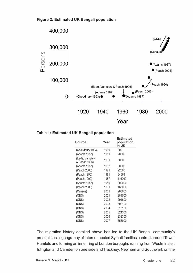
Estimated UK Bengali populationFigure 2: Estimated UK Bengali Population
1920 1940 1960 1980 2000
0
100,000
200,000
300,000
400,000
(Choudhury 1993)(Adams 1987)
(Adams 1987)
(Eade, Vamplew & Peach 1996)(Peach 2005)
(Adams 1987)
(Peach 1990)
(Census)
(Peach 2005)
(ONS)
Year
Per
sons
Estimated UK Bengali populationTable 1:
Source YearEstimated population in UK
(Choudhury 1993) 1939 200(Adams 1987) 1951 2000(Eade, Vamplew & Peach 1996) 1961 6000
(Adams 1987) 1962 5000(Peach 2005) 1971 22000(Peach 1990) 1981 64561(Peach 1990) 1987 116000(Adams 1987) 1989 200000(Peach 2005) 1991 163000(Census) 2001 283063(ONS) 2001 281500(ONS) 2002 291600(ONS) 2003 302100(ONS) 2004 313100(ONS) 2005 324300(ONS) 2006 338300(ONS) 2007 353900
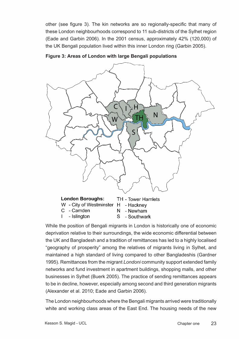
The migration history detailed above has led to the UK Bengali community’s present social geography of interconnected Sylheti families centred around Tower Hamlets and forming an inner ring of London boroughs running from Westminster, Islington and Camden on one side and Hackney, Newham and Southwark on the
23Kesson S. Magid - UCL Chapter one
other (see figure 3). The kin networks are so regionally-specific that many of these London neighbourhoods correspond to 11 sub-districts of the Sylhet region (Eade and Garbin 2006). In the 2001 census, approximately 42% (120,000) of the UK Bengali population lived within this inner London ring (Garbin 2005).
Areas of London with large Bengali populationsFigure 3:
While the position of Bengali migrants in London is historically one of economic deprivation relative to their surroundings, the wide economic differential between the UK and Bangladesh and a tradition of remittances has led to a highly localised “geography of prosperity” among the relatives of migrants living in Sylhet, and maintained a high standard of living compared to other Bangladeshis (Gardner 1995). Remittances from the migrant Londoni community support extended family networks and fund investment in apartment buildings, shopping malls, and other businesses in Sylhet (Buerk 2005). The practice of sending remittances appears to be in decline, however, especially among second and third generation migrants (Alexander et al. 2010; Eade and Garbin 2006).
The London neighbourhoods where the Bengali migrants arrived were traditionally white and working class areas of the East End. The housing needs of the new
24Kesson S. Magid - UCL Chapter one
immigrants created competition for housing and other resources, likely contributing to the rise of racial conflict in Tower Hamlets in the 1980s (Alexander et al. 2010; Dench et al. 2006). While much of the white population moved further east to suburban Essex or other regions of London, the white working-classes of East London remain well-matched as a control group of non-ethnic Bengalis living under similar ecological conditions.
The migration history of the London Bengalis supports an assumption of ethnic homogeneity and comparable genetic admixture when comparing the migrant and sedentee populations, key to building hypotheses for this project. This history has essentially maintained two intact branches of the Sylheti family tree, living within the contrasting ecologies of London and Sylhet. I now turn to the ecological differences and consistencies of these respective locations.
Ecological conditions1.2
Human migration and settlement gives insight into how individual hormonal profiles respond to profound external changes in culture and environment, here referred to as “ecologies”. Migration between two ecologies will have a different effect depending on the point in the lifecourse when an individual relocates (Warnes 1992). In this section I describe salient features of both ecologies, the contrasting SES and consistencies of dietary and cultural conditions of Bengalis living in London and Sylhet, and the ecological risk factors facing males born and raised in either location.
Socioeconomics
Bengalis are the most recent, youngest, poorest, most underemployed and, by measures of education housing and health, the most disadvantaged Asian immigrant group in London (Eade et al. 1996; Garbin 2005; ONS 2002).
Households are traditionally married couple families with all relationships contained within the ethnic group (Peach 1999). Families are large, sometimes extended, and living conditions are cramped, with the highest levels of overcrowded housing (1.5 or more persons per room), of any ethnic group according to the UK ONS (2005) (Kempson 2000).
The Bengali community is highly dependant upon social housing, a rate 3 times that of the total population, and owner-occupation is 38%, (less than half the London average) and the majority of households live in social sector rented accommodation (Peach 2005).
As an ethnic group, Bengalis have the highest unemployment rates in Britain (20%); four times that of White British men. Bengali males have the lowest rates of
25Kesson S. Magid - UCL Chapter one
economic activity (61.7 %), and for two fifths of these men, it is due to being long-term sick or disabled (UK Office for National Statistics 2005a). More Bengalis fall into the category “never worked or long-term unemployed” than any other ethnic group (17.1% compared to 2.7% of all people) (Peach 2005).
Bengalis who are employed work mostly (65%) in the hotels and catering industry, representing the particular reliance upon the Indian restaurant trade (Carey 2004). Of Indian restaurants in the UK, an estimated 85% are owned by Bengalis (Carey 2004).
There is not a tradition of educational attainment in the community Forty percent of Bengali men do not possess any qualifications, the highest rate of any UK ethnic group are the most likely ethnic group to be unqualified (UK Office for National Statistics 2002; UK Office for National Statistics 2005a).
While the reliance upon low-skilled employment and limited educational attainment have historically contributed to poverty in the community, there are signs of generational shifts toward an improved educational and professional achievement in third generation Bengalis (Economist 2007; Sunder and Uddin 2007).
In contrast, the sedentee community is of a traditionally landholding class of high socioeconomic position relative to the surrounding population (Gardner and Shukur 1994; Siddiqui 2004).
Diet
There is no indication that Sylheti sedentees of the middle classes from which the migrants originate are currently nutritionally stressed. It is important to distinguish this population from the well-documented poor and nutritionally-stressed populations of Bangladesh (Brown et al. 1982; Koenig et al. 1990; NIPORT 2009).
Diet is highly conserved within the migrant community. Most meals are prepared and consumed in the home, with imported foods from Bangladesh widely available from specialist shops throughout East London, and the observation of halal dietary restrictions has buffered the adoption of new dietary practices in the UK (Núñez-de la Mora et al. 2004).
While previous work suggests there may be increased consumption of meat proteins in the migrant population, and reduced fish consumption among young migrants and British-born Bengalis, migrants report shopping at markets specialising in Bangladeshi produce and purchasing imported foods regularly. They report frequent consumption of Asian main meals and consuming ‘western’ foods only rarely or occasionally (Núñez-de la Mora et al. 2004). Western-style
26Kesson S. Magid - UCL Chapter one
fast food is also increasingly available in Sylhet and consumption patterns of fried foods and sweet snacks among younger sedentees and migrants may be contributing to increased diabetes and obesity risk in developing nations like Bangladesh (Yach et al. 2006).
Ethnic and cultural homogeneity
Islam and village tradition, combined with a compact social geography, extensive family networks and marginal economic integration keep Bengalis culturally distinct and socially closed off from other ethnic groups in London (Lieberson 1963). Peach (1999) parallels the “encapsulation” of the London Bengalis to the Hasidic community of Williamsburg, Brooklyn. The households are traditionally married couple families with all relationships contained within the ethnic group. Levels of intermarriage are extremely low, at 3%, they are lower than for any other ethnic group in Britain (Dunnell 2008).
In Britain, the ethnic and cultural homogeneity of the Bengalis appears to be continuing to be maintained trans-generationally (Eade 1994). In fact, disengagement of the community may be increasing among British born Bengalis as they embrace a more fundamentalist Islamic identity than their parents (DCLG 2009; Hussain 2007).
These observations are supported by Indices of Dissimilarity, as calculated from Local Base Statistics (ESRC 1991 census holding, University of Manchester Computer Centre). According to this measure, Bengalis are the most segregated ethnic group in Britain (Eade et al. 1996). Bengalis are segregated from fellow South Asian or other migrant ethnic groups, and are more segregated from Indians than they are from Whites, they are equally as segregated from Pakistanis as they are from Whites.
Ecological risk
Compared with migrants in London, sedentees are subject to greater ecological risk factors from infectious disease and environmental instability (i.e. political unrest, periodic flooding, poor public health and sanitation), Adult and childhood life expectancy is much lower in Bangladesh for all socioeconomic groups, with under age five mortality for those in the top quintile of income in Bangladesh still 12 times that of the UK average. For males born in Bangladesh, under-five mortality is 81 per 1000 live births and for those in the highest wealth quintiles, this figure was 72 (both sexes) (Kabir and Islam 2001). In the UK the male under-five mortality has national rate of six per 1000 (WHO 2006a).
For males resident in Bangladesh, immune factors place a considerable constraint upon growth and development. Disease burden, sanitation and public health

27Kesson S. Magid - UCL Chapter one
are areas of considerable contrast between the two ecologies of Sylhet and London (Howard and Bartram 2003; NIPORT 2009; Heitzman et al. 1989). These ecological factors are influential across social and economic boundaries.
Unsafe disposal of solid waste and poor municipal sanitation mean there is a very high exposure to water-borne pathogens in Sylhet (Alam et al. 2006a). A 2003 study of water quality in Sylhet detected unsafe levels of coliform bacteria in the two main sources of drinking water for residents, the Surma River and tube wells, as well as in 100% of the drinking water served in restaurants, indicating high risk of bacterial gastroenteritis (Alam et al. 2006b; Iqbal et al. 2006).
Drinking water in the Sylhet district also contains high levels of arsenic: where more than 50% of the tube wells exceed WHO safety guideline of 0.01 mg/litre, and 29.3% exceeded the 0.1 mg/litre level (Howard and Bartram 2003; WHO 2007).
Infectious diseases at high prevalence in Bangladesh include bacterial diarrhoea, hepatitis A and E, typhoid fever and leptospirosis.
In the case of diarrhoeal infection, susceptibility appears to cut across demographic categories in both children and adults (Mitra et al. 1997; Stanton and Clemens 1987).
By international standards both child and adult mortality risk from infectious disease in this region is high. Early life exposure to these ecological stresses leads to a high rate of infant mortality (WHO 2006; Ezzati et al. 2002).
Infectious diseases are the largest cause of childhood death in Bangladesh, with diarrhoeal diseases causing 20% of non-neonatal death in children under-5 years in Bangladesh, followed by pneumonia (18%)(Ahmed et al. 2009; WHO 2006).
While the national figures are likely skewed by children born into poverty, a study of infant mortality in Bangladesh found maternal education and other measures of economic status reduced infant mortality, but were still much higher than observed values for women living in inner-city London (Kabir and Islam 2001).
The mean years of life expectancy at birth for ethnic Bengali males living in England is 74.4, for white British males, it is 76.2. In comparison, the life expectancy at birth for men living in Bangladesh is 62. Adult mortality is 2.46 times higher for Bangladeshi men than for men in the UK (251 to 102 per 1000, respectively) (WHO 2006a; WHO 2006b).
Over the lifetimes of the men studied, those living in Bangladesh experienced acutely stressful events in ways that would not have been experienced by migrants living in the UK. Bangladesh has been the site of political and natural disasters over the last half century. Social upheaval following partition of India in 1947, a
28Kesson S. Magid - UCL Chapter one
period of conflict with West Pakistan leading to the War of Independence in 1971, numerous floods and cyclones have led to periodic food shortages, devastation, and hardship for the population. Even during periods of relative political stability, living in Bangladesh carries greater risks and is less predictable than in the UK, with the limited state infrastructure or access to health care, unreliable power supply, and high rates of accidental death by drowning and injury (Giashuddin et al. 2009; Linnan and Centre 2008; Rahman 2005). For instance, reported road traffic deaths and injuries in Bangladesh are, respectively, 30 and 50 times those in the UK and the figure is estimated to be vastly under-reported in Bangladesh (Rahman 2005; WHO 2009).
Men within the UK Bengali community are at high risk of adult onset diseases of non-insulin-dependent diabetes mellitus (NIDDM) and heart disease, and associations between lower SES and poor health likely contribute to the level of risk in this community (Balarajan and Raleigh 1997; Bhopal et al. 1999; Marmot 2006).
Development and reproductive function1.3
Having introduced the characteristics of the ethnic Bengalis, and the ecological conditions where they live, the remaining variable of relevance to this life history analysis of their reproductive function is developmental timing. The project split the male life span into six key phases of development: pre-birth, infancy, childhood, adolescence and early and late adulthood.
The points in the life course at which ecological conditions modulate male reproductive function are unclear, in part due to the difficulties in determining whether adult steroid levels are a product of current or developmental conditions. Sex steroids are crucial to organisation as well as regulation of adult reproductive processes (Forest 1983). The former are relatively irreversible (e.g. sexual differentiation or pubertal timing), while the latter may fluctuate in response to current environment throughout life (e.g. spermatogenesis, fat deposition).
“Programming” refers to finite periods of development when the long-term organisation of a physiological system is sensitive to environmental stimuli (Lucas 1994). Sensitive periods of organisation preceding sexual maturity shape the adult reproductive phenotype of humans and other mammals (Davies and Norman 2002).
Migration between two contrasting ecologies, with age at migration as an experimental variable, allows for the testing of predictions of how ecological conditions experienced during key developmental stages lead to variations in adult physiological characteristics (Greulich 1958; Lasker 1995). In this project,

29Kesson S. Magid - UCL Chapter one
the physiological variable of interest is the organisation and regulation of the hypothalamic-pituitary-testicular (HPT) axis.
I begin with an outline of the components of the HPT axis, before moving on to discuss its role in the development of the human male at the key points of importance to the design of this project.
The HPT axis regulates male reproductive neuroendocrine activity, and consequently, adult patterns of androgen variation. All the components of the axis interact through agonistic and antagonistic feedback loops, in order to modulate sex steroid and gonadotropin production and spermatogenesis. Beyond the hormones directly regulating male reproductive physiology, the HPT axis is sensitive to other hormones such as cortisol, leptin, and thyroid hormone. As androgens, in particular T, influence somatic systems, this sensitivity to other hormonal factors is important for coordinating male reproductive and somatic functioning.
The HPT axis primarily communicates through 6 major hormones: the sex steroid testosterone, two gonadotropins, luteinising hormone (LH) and follicular stimulating hormone (FSH), two cytokines, inhibin and activin, and the small neurosecretory peptide gonadotropin releasing hormone (GnRH).
LH and FSH are manufactured by and released from the pituitary gland to stimulate the two major testicular functions: androgen production and spermatogenesis. These two functions are anatomically compartmentalised within the testes into intratubular and extratubular regions. These regions contain two specialised and separated cell-types, Leydig and Sertoli. LH stimulates Leydig cells to produce and secrete T (steroidogenesis). The extratubular Leydig cells produce the majority of the body’s T (in males, 95% of circulating testosterone is of testicular origin) (van Houten and Gooren 2000). Because lipid-soluble steroids can easily pass through cellular boundaries, the T produced by the Leydig cells passes through the barrier between the extratubular and intratubular regions to bind with androgen receptors within Sertoli cells, where spermatogenesis occurs. FSH acts upon Sertoli cells to initiate spermatogenesis and to secrete inhibin or activin. These cytokines have a broad range of effects, influencing Leydig cell T production, and pituitary FSH secretion. Both FSH and LH are regulated by pulsatile (meaning secreted rhythmically) release from the hypothalamus of GnRH. In turn, circulating T exerts negative feedback upon GnRH and the pituitary gonadotrophins. Due to its wide number of targets and differential effects within the HPA axis, T functions as a primary messenger between the testes and the brain.

30Kesson S. Magid - UCL Chapter one
Diagram of the hypothalamic-pituitary-testicular axisFigure 4:
Hypothalamus
Pituitary
GNRH (+)
Inhibin (-)
Activin (+)
T (-)LH (+)
FSH (+)
Testis
Leydigcells Leydig
cells
Leydigcells
T (+)
Sertoli cells(Seminiferous Tubule)
Sperm
Figure 4: Diagram of the hypothalamic-pituitary-testicular axis illustrating sites of secretion of steroids and gonadotropins, the negative (-) and positive (+) feedback loops regulating other components of the axis and spermatogenesis. (Adapted from Griffin, 1996)
Key stages of development
This project divides the male life history into six developmental stages importance to the alignment of adult somatic and reproductive function. These stages are 1. Pre-birth 2. Early infancy (from birth to age 2 years) 3. Mid-childhood (age 3-12) 4. Adolescence/puberty (age 13-18) 5. Early adulthood (age 19-39) 6. Later adulthood (age 40 years and older). The periods of organisation critical to adult reproductive function within each of these stages will be described below.
Maternal investment and pre-birth factors: Prior to conception, maternal condition dictates the environment of foetal development (Ounsted et al. 2008). A developing male will be subject to environmental constraints or stressors as filtered by maternal intra-uterine conditions, and phenotype will be responsive to early genetic and developmental organisation (Grjibovski et al. 2004). Intra-
31Kesson S. Magid - UCL Chapter one
uterine investment will in turn reflect maternal ecological and biogenetic history, for example the persistence of lower birth weight of British-born South Asian mothers (Leon and Moser 2010). Maternal age, as well as the spacing and number of any previous births may also influence maternal investment (Fessler et al. 2005; Jasienska 2009).
In recent years, mounting data indicate paternal genomic imprinting or other as yet unknown mechanisms of transgenerational transmission may influence male development. Fathers subjected to environmental stress during critical windows in their development appear to influence the phenotype of their offspring (Pembrey 2010; Pembrey et al. 2005).
Hormonal adjustments in response to intra-uterine conditions are thought to condition the foetal hypothalamic pituitary gonadal (HPG) axis in ways that endure into later life. Inter-uterine adjustments of the human HPG axis explain correlations between low birthweight and the timing or duration of pubertal development (Delemarre-van de Waal et al. 2002; Hernández and Mericq 2008) or variations in levels of salivary oestradiol in adult women (Jasienska et al. 2006) and serum LH and T in adult men (Cicognani et al. 2002; but see also Meas et al. 2010). Experimental evidence from other mammals links restricted foetal nutrition and endocrine disruptions to enduring alterations of HPG functioning (Rhind et al. 2001).
While there is supportive evidence that foetal conditioning influences female fecundity in animals and humans, the lifelong alterations of androgen profiles due to foetal conditioning do not appear to affect male fecundability, that is, male gonads produce adequate numbers of spermatocytes for reproduction in spite of wide variations in androgens (Davies and Norman 2002). While adult reproductive functioning of the male gonads does not appear significantly affected by inter-uterine conditions, early developmental energetic conditions have been hypothesised to relate to T-dependent somatic apportionment in adult life (Bribiescas 2001a; Ellison 2003).
Beyond the development of foetal reproductive organs, another androgen-sensitive tissue, skeletal muscle plays an important role in developmental energetic allocation strategies. The ratio of muscle tissue to fat is acutely reflective of foetal metabolic constraints. Under conditions of adequate maternal nutrition, the developing foetus absorbs and sequesters glucose through foetal insulin. The glucose required for growth is deposited in the liver and muscle tissues in the form of glycogen, all additional glucose is diverted by foetal insulin to into fat stores (Johnson and Everitt, 2000). This trade–off holds lifelong implications for metabolic function and somatic investment (Bribiescas 2001a).

32Kesson S. Magid - UCL Chapter one
Under conditions of maternal nutritional stress, glucose is diverted preferentially toward growth at the expense of adipose storage. Muscle tissue both consumes and stores glycogen. The energetically expensive developing brain lacks glycogen stores, thus it is wholly reliant upon circulating glucose levels (Johnson and Everitt 2000). Considerable evidence suggests muscle tissue under such conditions develops insulin resistance in order to shunt glucose and sustain the growth of the brain (Campbell and Cajigal 2001; Ozanne and Hales 1999; Reaven 1998). Such conditions would arise more commonly in humans than in other species, as the human brain requires an extraordinary amount of developmental resources. This muscle insulin resistance may lead to systemic decreased insulin sensitivity in later life, with health consequences (Gluckman et al. 2005).
Androgens play a crucial organisational role in foetal masculinisation. The sex-determining region of the Y-chromosome prompts differentiation of the embryonic Sertoli and Leydig cells, forming the essential endocrinological and physical structure of the testis by the 8th gestational week (GW) (O'Shaughnessy and Fowler 2011). Leydig cells in the human testis actively secrete androgens from at least 8-10 GW onwards. In most mammals, including humans, this initial testicular organisation and functioning is independent of the HPG axis, which does not develop until approximately 26 GW (Beck-Peccoz et al. 1991). This pituitary-independent phase of Leydig cellular function coincides with the most critical period of foetal masculinisation (O'Shaughnessy and Fowler 2011). During the “masculinisation programming window” of 8 to 12 GW in the human (Welsh et al. 2008, Scott et al. 2009), testicular hormones actively divert anatomical development of the embryo from female to male line, without which the precursors to male reproductive organs atrophy and spontaneously regress (Johnson and Everitt 2000).
These HPG axis-independent foetal Leydig cells form a distinct population from those of the mature male testis (“biphasic”), and possibly those of the neonatal testis (“triphasic”) (Prince 2001), both of which are reliant upon pituitary gonadotropins to function. This means the cellular source of the foetal peak in testosterone is distinct from the two later neonatal and pubertal peaks. There is limited evidence as to the sensitivity of the foetal Leydig cells to ecological stressors or inter-uterine conditions during this masculinisation window. But it represents a critical period when the early formation, density and number of foetal Leydig cells potentially alter lifetime reproductive functional capacities and regulation through priming the developing components of the HPT axis and migration of stromal cells of the prostate (Bierhoff et al. 1997).The influences of pre-birth conditions (as measured by birth weight) upon adult male metabolism are well-documented, and appear linked to reproductive function (Hales and Barker 2001; Kuzawa 2007). Debate surrounds whether these phenotypic adjustments to intrauterine conditions result

33Kesson S. Magid - UCL Chapter one
from evolved predictive cues to match foetal phenotype to future environment, constraints from the mother to maximise maternal fitness, or are merely making the “best of a bad start” (Gluckman et al. 2005; Jones 2005; Kuzawa 2005; Wells 2010a).
Genetic developmental effects will include those factors that define limitations of plasticity or adaptations to environment shaped over evolutionary time, presumably including adaptations to famine (Neel 1962). Though the actual identity of “thrifty genes” remains somewhat elusive (Prentice et al. 2005), conditions of frequent famine in the Indian subcontinent (Maharatna 1996; Sen 1977) have been proposed as selective for the so-called “thin-fat baby” phenotype (Yajnik et al. 2002). This describes similarities among South Asian infants of low birth weight, greater central adiposity, and metabolic efficiency during rapid postnatal growth (Yajnik 2004).
While assuming Bangladeshi migrants to London and those living in Sylhet share a common biogenetic history, early interactions between genes, maternal cues and ecological variables may be especially finely tuned in these populations, with rapid responsiveness to changes in environment that may have lifelong repercussions for adult reproductive health.
Early infancy (0-2 years)
The extreme dependency of the human infant means the early post-natal environment remains highly buffered by maternal investment. This investment may be modulated by stresses upon the mother, disease load, number and demands of siblings, and cultural influences upon care or duration of breastfeeding (Mace and Sear 1997; Núñez-de la Mora et al. 2005). Contrasts in the biocultural environments of Sylhet and London will influence some, if not all of the above conditions (Núñez de la Mora 2005).
As the pre-weaning period carries the greatest risk of mortality over the human life-course (Jones 2009), there has been enormous selection pressure on the modulation of neonatal growth to maximise survival and accurately interpret signals of maternal condition and environmental risk (Kuzawa 2005; Wells 2006).
This period of dependency coincides with rapid growth of the infant brain and deposition of fat reserves. In addition, earlier investment in foetal growth (or lack thereof) means this is the period of rapid “catch up” growth in low birth weight babies, which has been associated with “thrifty” adaptations with pleiotropic or predictive effects, and health consequences in later life (Eriksson et al. 1999; Forsén et al. 2000; Gluckman et al. 2007).

34Kesson S. Magid - UCL Chapter one
Postnatal T peak (0-6mos): Within the first 6 months following birth, humans and some primates experience a characteristic second peak in Leydig cell activity and circulating T. At this stage of development the Leydig cells are no longer functionally independent of pituitary control via LH (Chen et al. 2009). A LH surge prompts Leydig cells to produce T until plasma concentrations approach the low end of normal adult levels (2-3 ng/mL) by around 2 months postpartum, after which the concentrations decline to .5 ng/mL. Following this peak, the neonatal population of Leydig cells regress or appear dormant, and testicular testosterone remains low until puberty (Bergadá et al. 2006).
While the function of this peak is not entirely clear, it is proposed as a critical window of male reproductive development when the feedback between components of the HPT axis are coordinated to thresholds of activity (Mann, 1996). In the brain, masculinisation and adult patterns of social and sexual behaviour are sensitive to disruption during this period in primate and other animal models.
In the testis this surge coincides with a second phase of Leydig and Sertoli cellular differentiation and apoptosis (Berensztein et al. 2002). The number of Sertoli cells differentiated at this period appears to be especially important for adult sperm count and testicular descent according to rat and primate models (Mann and Fraser 1996; Sharpe et al. 2003).
Recently, developmental stresses as estimated by neonatal growth rates have been associated with adult levels of LH, T, and somatic factors such as muscle mass and grip strength (Gettler et al. 2010; Kuzawa et al. 2010).
Juvenile period (3-12 years)
This post-weaning period of development has been described as a “phenotypic limbo” in which offspring are nutritionally independent from direct nourishment from the mother, but are not yet reproductively functional (Bogin 1999; Pagel and Harvey 1993).
The juvenile stage is referred to as reproductively quiescent as measures of sex hormones and activity of the reproductive glands are extremely low. While a period of quiescence is observed in every major taxonomic group, it is comparatively prolonged in most mammals, and among mammals, human juvenile periods are particularly long (Pereira and Fairbanks 1993). This suggests the juvenile stage has been prolonged due to selective pressure (Bogin 2009).
Growth velocities slow down during this stage, as compared to the rapid rate of neonatal growth (Tanner 1978). This coincides with a period of socialisation, acquaintance with cultural practices and sources of nutrition, and a period of frequent immune challenge.

35Kesson S. Magid - UCL Chapter one
Observations relate environmental stresses upon male children during this period to the phenotype of their male offspring (Bygren et al. 2001; Pembrey et al. 2005). Though the mechanism of this effect is not yet known, it has led to speculation that this period is a critical window for the organisation of trans-generational epigenetic information, which is particularly relevant to males (Pembrey 2010).
Adrenarche occurs at the end of the juvenile period (at approximately 7 years old in males), with a rise of adrenally-derived androgens (Worthman 1999). There is a subsequent reduction in hypothalamic sensitivity to androgens, with potential to adjust the HPT axis. This stage of development is postulated as important to the coordination of the male reproductive axis function and maturation with stress, risk taking and socialisation signals relayed by the adrenal corticosteroid, cortisol (Campbell 2003).
Adolescence (13-17 years)
Puberty begins with GnRH pulses that precipitate adult-like HPT function. In response to these pulses the pituitary gland begins producing peptide gonadotrophins FSH and luteinising hormone LH. Clinical and animal studies suggest developmental canalisation of male reproductive function. Hormonal activity during this period is thought to “set” many of the thresholds of activation and function for the remainder of a male’s lifetime. Pubertal hormone–level variation precipitate long-term changes in pituitary and gonadal hormone receptor sensitivity, which may influence HPT irreversibly throughout the lifetime of the individual. This pubertal establishment of adult reproductive hormone function is an important step in characterising the evolution of male reproductive strategies (Bribiescas 2000).
Prior to maturity, children’s body composition is relatively similar. But dimorphism appears at puberty with consequent changes in fat or muscle deposition and strength (Bribiescas 2006). Male growth rates suddenly accelerate to double or more those of childhood. This period of growth appears more highly heritable than childhood growth, and less subject to ecological influences (Tanner 1962). Despite this, there is likely an ecological component, particularly to the timing of the start of puberty and the duration and rate of the growth spurt. This is a critical period in which androgens play a determinative role in growth. Bone growth coincides with the increase of androgens, and they are thought to counter-balance the effects of oestrogens, which precipitates the ossification of the epiphysial plates of the long bones, thereby ending their further growth (Knussmann and Sperwien 1988). The interaction between somatic development and T may be revealed by the positive correlation between morning salivary T and stature in Nepalese men, but only during seasons of energetic stress (Ellison and Panter-Brick 1996).

36Kesson S. Magid - UCL Chapter one
Post-maturity
Inter-population differences in salivary testosterone are most pronounced in early reproductive years, with a trend toward convergence in later years.
Androgen levels of Western males decline with age, and many symptoms characteristic of hypogonadism in younger males are similar to normal age-related changes in older males, with losses in skeletal muscle mass and increased fat deposition (Campbell and Cajigal 2001; Ellison et al. 2002; Morley et al. 2005).
Unlike females, males lack a distinct cessation of their reproductive stage of life but there is increasing evidence of a pronounced shift in male reproductive function and fertility in mid-life, around the ages 35-45. In longitudinal studies of American populations, there is a clear age-related decline in male T of 1% per year after the age of 40 (Gray et al. 1991; Harman et al. 2001), while in Japanese populations T flattens and remains stable after age 40(Bribiescas 2006; Uchida et al. 2006). Cross-cultural analysis shows an age-related decrease in the mean difference in T between populations living in developed and developing nations, where the greatest differences are between young males and they are non significant after age 45(Ellison et al. 2002).
While the mechanisms of this decline are still unclear, early developmental events like the LH-dependent differentiation of Leydig cell number and senescence into adulthood may relate to exposure to oxidative stress (Chen et al. 2009). The mechanisms regulating “normal” reproductive function in the adult male will be covered in the next section.
Variations in adult male reproductive function1.4
As a largely medical science, endocrinology focuses primarily on mechanistic explanations of androgens and how they proximately influence biological processes like reproduction, digestion, growth and development and the diseases they cause when these processes are disrupted. But much of what defines normal variation in male metabolism, morphology and behaviour is due to the actions of androgens. Understanding the interaction between androgens and human ecological variation gives insight into how evolution has shaped the human male to optimise the balance between survivorship and reproductive success. The balance of somatic expenses and energetic resources is regulated in part by androgens, as are aspects of male behaviour, and the androgen of most widespread influence is T. The interactions between androgens, the environment, and the body are important in explaining the proximate mechanisms by which evolved life history strategies are coordinated.
37Kesson S. Magid - UCL Chapter one
Application of life history theory allows for the interpretation of inter-individual variation in T, and associated clinical conditions from an evolutionary medical perspective. For men living under conditions of high nutritional intake and low physical exertion that characterise life in “developed” nations like the UK, energetic resources are unconstrained and stable, relative to Bangladesh. For men living under conditions of high pathogenic stress and ecological disruption that characterise life in “developing” nations like Bangladesh, energetic resources are constrained and less predictable, relative to the UK. If reproductive effort requires costly or risky somatic, metabolic and behavioural investment, then men under relatively affluent and stable conditions are expected to invest more into reproductive effort than men living in less affluent and unstable conditions. This difference in ecologies is predicted to lead to higher levels of T in men living in the UK than men living in Bangladesh. Over the course of a lifetime, the investment into the costly tissues, metabolic processes and behaviours linked with reproductive effort may have pleiotropic effects (Bribiescas and Ellison 2007), in which case men living in the UK will have higher incidence of disease associated with reproductive function.
For males, the primary constraints upon net lifetime reproductive opportunities are competitive interactions with other males for access to females and female choice. T corresponds to competitive and mate-seeking behaviour, as has been widely observed in birds (Ketterson et al. 1992; Wingfield et al. 1990) and in mammals including primates (reviewed in Fairbanks 2009)).
In social species, both of the above constraints are expected to limit reproductive opportunities for males of lower rank more than those of higher rank. Therefore, if T influences reproductive effort, it is expected to be higher in males of high rank compared to subordinates. This pattern has been observed in group living primates (Muller and Wrangham 2004; Rose et al. 1971), though the association is not always consistent and appears strongest at times of social instability (Sapolsky 1991). Data also support an association between social status and T in humans (Book et al. 2001; Dabbs and Morris 1990; Mazur and Booth 1998).
Spermatogenesis and peripheral function of androgens
Despite inter-individual or inter-population T variation, there is little indication of a high sensitivity of the primary reproductive process regulated by androgens, spermatogenesis. Testosterone shows 10-fold inter-individual variability between males, but only under extreme pathological conditions does testosterone production drop below levels presumed necessary to support adequate spermatogenesis for male fertility (Bribiescas 2001a; Ellison and Panter-Brick 1996; Lamb and Bennett 1994). The overall energetic investment in spermatogenesis by mammals is fairly negligible—especially in contrast to the energetic investment in reproduction by
38Kesson S. Magid - UCL Chapter one
females. In contrast to female physiology, direct metabolic investment from males in conception and development of offspring is relatively limited (Trivers 1972). Perhaps for this reason, ecological constraints and fluctuations rarely impinge upon male fecundability and basal reproductive function appears fairly robust to hormonal variation in males.
Although initiation of the spermatogenesis process requires a certain amount of stimulation by FSH, LH and T, the continuation of optimal spermatogenesis relies mainly upon the ongoing presence of FSH. Though T and LH are seen as playing a “permissive” role in spermatogenesis, they do not modulate the process (Johnson and Everitt 2000). But spermatogenesis appears to be such a robust metabolic process that human males with FSH transcription/receptor mutations and mice in which FSH production is absent still exhibit enough spermatogenesis to allow limited fecundity (Kumar et al. 1997; Tapanainen et al. 1997). Thus, spermatogenesis is an extremely resilient process which functions under even severely compromised hormonal conditions. In contrast, human female and mouse oogenesis and fecundability are highly sensitive to perturbations of reproductive axis hormones (Kumar et al. 1997; Layman et al. 1997).
There is significant variation in human sperm count (from 1-120million/ml), with a degree of controversy over the absolute threshold that defines full-fecundity (a general consensus of 20million/ml). Non-Western populations seem to show a tendency toward lower sperm counts compared to American males, but this does not seem to lead to subfecundity.
Efe and Lese men show reduced salivary T compared to males born and raised in Boston, USA. (Bentley et al. 1993; Ellison et al. 1989). African populations such as !Kung and Namibian men presented significantly lower T levels than American males. Turkana men (Campbell and Leslie 1995) showed lowered gonadotrophin levels (FSH and LH) compared to Western controls, perhaps reflective of reduced GnRH levels or pulsatility., decreased pituitary sensitivity to GnRH stimulation or greater inhibin suppression of GSH production.
Male reproductive capability also relies upon a suite of accessory glands of the urogenital tract to support and protect the spermatozoa on their journey between generations. Androgens also regulate these accessory glands including the prostate (which supplies nutrients, optimal pH, ionic milieu, etc.) for the travelling spermatozoa.
While the HPT axis forms the central hormonal network regulating male reproductive function, the components of the axis are also sensitive to other hormonal messengers such as cortisol, leptin, and thyroid hormone. Just as the HPT can be affected by these “non-reproductive” hormones, androgens, (particularly testosterone and its metabolites) exert influence peripherally, beyond
39Kesson S. Magid - UCL Chapter one
the glands of the HPT axis. This sensitivity to outside hormonal factors is important, as it hints to wider roles of androgens in somatic and energetic regulation.
As the primary adrenocorticoid, cortisol influences acute stress responses as well as patterns of activity and awakening (Tsigos and Chrousos 2002). Leptin, “the voice of the adipose tissue” (Blum 1997) regulates fat deposition. Balancing the proportion of somatic adipose and anabolic tissue has important consequences for development and lifelong metabolic adaptation to energetic conditions, as both tissues are potential sources and consumers of glucose (Campbell and Cajigal 2001; Reaven 1998). These adaptations of basal metabolic rates and balancing energetic costs are further regulated by insulin, which controls the concentration of circulating blood glucose.
Beyond the HPT axis, androgen receptors (AR) are found on the accessory glands of the male urogenital system such as the prostate and the pilosebaceous glands of hair follicles (Johnson and Everitt 2000). The prostate is the major site of non-testicular DHT (Hsing et al. 2002). These receptors are activated by the approximately 4% of unbound circulating T and thus able to enter prostatic cells through diffusion. However 95% of T entering the cell is converted to 5α-dihydrotestosterone (DHT) by the enzyme 5α-reductase (van Houten and Gooren 2000). Unlike T, DHT seems to be more effective upon organ receptors and has less regulatory effect upon LH. DHT is considered the major effector hormone in certain androgen dependant tissues, particularly in promoting hair growth, secretion of sebum and prompting the smooth muscle cells of the prostate to divide.
The division of muscle cells within the prostate continues throughout life, and as they become more numerous, the amount of 5α-reductase also increases. The prostate also responds to circulating E2, which reduces factors that inhibit smooth muscle cell division. The process becomes a “vicious circle” although T decreases with age, the amount of T being converted to DHT accelerates in an age-dependant manner (perhaps due to E2 levels) promoting further growth (Wick et al. 2003). Eventually, the prostate enlarges to sizes with pathological implications, these pathologies will be discussed in further detail below.
Clinical conditions associated with androgens1.5
Benign prostatic hyperplasia
As discussed above, AR within the prostate are responsive to the androgens T and DHT, which leads to proliferative growth over the lifetime of a human male. Growth of the prostate leads to one of the most common diseases of male ageing, benign prostatic hyperplasia (BPH) and the associated lower urinary tract
40Kesson S. Magid - UCL Chapter one
symptoms (LUTS). The development of BPH requires testicular androgens, as evidenced by the reduction of prostate cellular growth by androgen inhibition. Men with reduced exposure of the prostate to androgens through physical (i.e. castration), pharmacological, or genetic means do not develop BPH (Bartsch et al. 2000; Bribiescas 2010). Below, I will discuss how populations vary widely in prostate disease rates, which has led to the hypothesis that these variations are due to influence of androgens during early development (vom Saal et al. 1997) or over the adult lifespan (Kehinde et al. 2006; Slater and Oliver 2000). The reproductive hormone hypothesis of prostate disease mirrors one proposed to explain the associations between mean salivary progesterone and the incidence of breast cancer within populations (Bribiescas and Ellison 2007; Jasienska and Thune 2001).
The incidence and severity of LUTS increases with age and is affected by diet, ethnicity and health behaviours (Hsing et al. 2002; Platz and De Marzo 2004). LUTS are also described as “prostatism” in men, and correlate with BPH. The causal link between LUTS and BPH is ambiguous, but appears to be a consequence of the enlargement of internal smooth muscle, duct epithelium, and connective tissue within the prostate gland. As the urethra passes through this gland, the enlarged prostate restricts the flow of urine and causes pain or an inability to completely empty the bladder. Impaired, painful or irregular urination ranks as a significant negative factor in quality of life indices (Morley et al. 2005). In North America and Western Europe these conditions are highly prevalent in older males, estimated to be 50% of all men over 50 and to increase by 10% of the population for every decade. However, a limited number of studies suggest a greater variability in BPH prevalence in non-Western indigenous and migratory populations (Campbell et al. 2005). Investigations of prostate cell neoplasia have focused on a genetic/environmental role for activity of 5α-reductase (Hsing et al. 2002).
African-American males have highest rate of BPH in world, while Japanese and Chinese have the lowest, by factor of 30-50 fold in risk (Jin et al. 1999; van Houten and Gooren 2000).
When Southeast Asians migrate to a Western country, prevalence of prostatic neoplasm increases but still remains low, even in second and third generations (Cook et al. 1999). Environmental factors such as diet and health behaviours affect rates of neoplasm, but there is also a likely genetic component. Asian males exhibit a lower incidence of CAG repeat length of androgen receptors and variation in this repeat length is associated with risk of prostate neoplasm. There also may be differences in peripheral androgen metabolism due to variations in the transcription of prostatic 5α-reductase. Lower levels of 5α found in Asian men
41Kesson S. Magid - UCL Chapter one
theoretically slow progression from neoplasm to clinical cancer (Ross et al. 1992; van Houten and Gooren 2000).
In comparative populations from a similar ethnic background, African-American males residing in Washington D.C. showed much greater levels of T than indigenous Nigerians (Ahluwalia et al. 1981). Certainly, it suggests higher T levels in American populations may be an example of physiologic release due to greater energetic availability rather than suppression among non-Western populations. Environmental factors such as diet and activity patterns play a more central role in disease aetiology (Meikle et al. 1997).
Sex steroids, particularly E2 and DHT are implicated in prostate enlargement and are also suggested to foster cancerous growth. But a direct link between androgen-derived prostatic neoplasm and cancer risk is still far from agreed (Hsing et al. 2002). Steroid sensitive disease incidence varies across populations greatly (Jin et al. 1999).
In the past, the prevailing aetiologic significance has been couched in terms of ethnicity, and looked primarily at genetic differences in these populations. A limited number of studies on non-industrialised people suggest symptoms of prostate hyperplasia among subsistence–living peoples are particularly high (Campbell et al. 2005).
From this perspective, clinical research on Western populations should be viewed as representative of the extreme range of human variability and not the most common or healthiest representation of human populations (Ellison 1994).
Androgens, insulin and type II diabetes
Insulin plays an important role as a hormonal signal of the fed state in response to elevated blood glucose levels and amino acids. An inability to produce sufficient insulin or failure of insulin receptors leads to impaired carbohydrate, fat and protein metabolism. This condition is called diabetes mellitus. When diabetes occurs gradually with few signs of acute metabolic disturbance it is referred to as Non Insulin Dependant (or Type II) Diabetes Mellitus (NIDDM).
While there is a heritable component, the disease is associated with “miscalibrated” energy balance and is linked to obesity. A diet low in fat and high in fibre, combined with daily exercise has been suggested to reduce insulin levels and grant some epidemiological protection against irregular insulin levels leading to NIDDM. In addition, decreased insulin level might reduce proliferation of SMC within the prostate (Hales and Barker 2001). Measures of visceral body fat, insulin, E2 and T all correlate in men with so-called “metabolic syndrome”.
42Kesson S. Magid - UCL Chapter one
Androgens and dietary restriction
In comparison to females, dietary factors are less significant in altering male hormonal profiles. Modest negative energy balances fail to effect significant changes in important sex steroid levels. More severe fasting or famine conditions appear to downregulate GnRH availability, subsequently reducing LH and T, but not FSH. Based on studies of animals and humans, increases in peripheral hormones under periods of caloric restriction such as leptin and cortisol are a possible route of action upon the HPT axis (Bribiescas 2000).
Diurnal patterns
The pulsatility of GnRH release is reflected by rhythmic fluctuations in circulating gonadotrophin and T concentrations, peaking at 1 to 3 hour intervals. Circulating testosterone generally exhibits a diurnal pattern, with peak levels early in the morning and a gradual decline throughout the day (Johnson and Everitt 2000). The generally observed pattern of male testosterone is diurnal, with a peak in the morning. These observations are based upon clinical and epidemiological samplings from populations resident in high-income, developed nations. There is less clear evidence of such an AM peak in populations of men residing in low-income nations or living under subsistence farming or foraging conditions. The limited evidence from these populations suggests less consistent pattern of an AM peak. (Bribiescas and Hill 2010; Vitzthum et al. 2009).
Birth seasonality in females appears associated with fluctuations in ovarian function (Ellison et al. 1993; Rojansky et al. 1992), evidence for seasonal fluctuations in T is inconsistent for human males.
T and the gonadotropins exhibit pulsatile secretion patterns, and these patterns are less ordered in older men than in young men (Keenan et al. 2006; Veldhuis et al. 2009). According to the “ensemble” model of the HPT axis, the degree to which these pulses are ordered reflects the degree of integration of functional thresholds of each component of the axis (Veldhuis et al. 2009). Conversely, irregularity of pulses suggests a less well-integrated HPT axis, and young men return to regular pulsatile functioning after experimental disruption more quickly than older men (Liu et al. 2006).
Androgens and Reproductive Behaviour
Humans form long-term pair bonds with mates, a reproductive strategy uncommon in ~95% of mammals. Across species, socially monogamous behaviour is influenced by magnitude of paternal care, mode of resource access, and mate choice (Reichard and Boesch 2003).
43Kesson S. Magid - UCL Chapter one
In monogamous birds, T increases in situations of high reproductive competition, and declines when males are required to care for offspring. This association between male reproductive challenges and T has been observed in a variety of other vertebrates, including primates. These observations led to the hypothesis that T modulates male-male competition, affiliative bonding, and direct paternal care amongst pair-bonded species (Archer 2006; Wingfield et al. 1990).
The length and types of human pair bonds vary significantly across cultures based on socioecological conditions. The degree of paternal investment in offspring and mate-seeking competition between human males is also widely variable reflecting the compromise between reproductive interests and offspring investment strategies (Ellison 2009).
A growing body of data suggests an association between pair bonding and/or parenthood and salivary testosterone in human males (Burnham et al. 2003; Gray et al. 2006). While cross-cultural research in this area is expanding (Gray et al. 2007), the bulk of these studies investigated North American men, with limited cultural variation in mate choice, extramarital sex and direct paternal investment in offspring.
Body composition.1.6
Beyond the reproductive axis, T levels regulate somatic tissues, particularly anabolic muscle. Modulation of skeletal muscle mass may represent a mechanism by which T regulates the balance of male energetic expenditure upon reproductive effort.
Muscle tissue
T is a key hormone in the regulation of muscle anabolism and metabolism. T administration to humans stimulates fat catabolism and adipose redistribution while stimulating muscular protein synthesis and glucose uptake (Johnson and Everitt 2000). T even increases the metabolic rates of isolated muscle cells in vitro (Tsai and Sapolsky 1996). The importance of mediating muscle mass to human male reproductive ecology will be investigated in further detail in a developmental and comparative context in the corresponding sections.
Adipose tissue
Within the HPT axis, T is thought to inhibit the frequency of GnRH pulsatility and thereby suppress LH production (Crowley et al. 1991). However, the T metabolite E2 also inhibits the release of hypothalamic GnRH production and decreases pituitary sensitivity to GnRH.

44Kesson S. Magid - UCL Chapter one
In a process called aromatisation, the enzyme aromatase converts T within adipocytes (fat cells) to E2. This process has been suggested as explanation of lower T and hypogonadism in obese men (Kley et al. 1981). Aromatisation might function as a mechanism of androgenic modulation of somatic composition between adipose and muscle. T converted to E2 by adipose tissue has the similar inhibitory effects as if it were still in circulation, but without the ameliorating effects upon muscle tissue. Men investing in greater adiposity may exhibit greater aromatisation of circulating T and also exhibit hypothalamic and pituitary inhibition as a result of higher E2 levels.
The fact that both of these hormones elicit similar responses from the hypothalamus might reflect the process by which the brain monitors bodily states of tissue distribution through differential sensitivity to the two sex steroids. Studies of caloric restriction in rats show dramatic reductions in FSH and LH, followed by reduced T production and release (Bergendahl et al. 1998). Administration of GnRH eliminated this effect, and suggests hypothalamic receptors are monitoring energetic status, and modulate pituitary GnRH receptors. The mechanism of this monitoring is unknown, but most likely to be through direct signalling molecules of energetic status: particularly insulin, cortisol, and leptin.
Leptin, a protein hormone synthesised primarily by adipose tissue serves as a circulating signal of nutritional status and reflects fat stores and body weight. While leptin was once thought as the direct link between adipocytes and metabolism, immune function and reproduction, this association now appears more complex. The linkage between leptin and adiposity appears more relevant in populations with high caloric intake and low energetic demands (Chan et al. 2006), and may not reflect energetic status or body mass in foraging or subsistance-living people (Lindeberg et al. 2001). In populations where energy intake and output are equal, leptin reflects the amount of stored triglycerides in adipose tissue (Barb 1999). Studies of chimpanzees and humans show sexual dimorphism in leptin levels is a commonality, with females showing higher levels than males after sexual maturity (Barb 1999; Bribiescas and Anestis 2010). During adolescence, leptin levels in males fall or remain flat as T levels increase during puberty, while females show a pronounced rise (Rutters et al. 2009). It was once thought that a prepubertal pulse in leptin might represent a “permissive factor” by signalling the brain that the body is metabolically ready to go through puberty (Kiess et al. 1998). Now, however, the degree to which maturity is reliant on such a signal is not as clear in humans as it is in other species, and is more applicable to females than males (Chan et al. 2006; Rutters et al. 2009).

45Kesson S. Magid - UCL Chapter one
Immune system
Recently, the role of T in the regulation of energetic resources has been postulated as a modulating factor in balancing costs of immune system challenges and maintenance (Campbell et al. 2001; McDade 2005; Muehlenbein and Bribiescas 2005). T appears to regulate energy allocation by altering anabolically sensitive tissue, including skeletal muscle mass. However, the regulation of energetic resources also extends to the immune system, and immune activity appears suppressed by T (Muehlenbein and Bribiescas 2005). The maintenance of immunocompetence is energetically expensive and potentially crucial to the advertisement of genetic fitness to mates (Hamilton and Zuk 1982). Energetic investment into high reproductive effort and costly anabolic muscle competes with investment into immunocompetence, and males under significant immune stress would be expected to be unable to invest as heavily into reproductive effort, as measured by T (Folstad and Karter 1992). Assessing changes in testosterone and immune factors during infection may yield insight into male physiological ecology (Muehlenbein and Bribiescas 2005). These ideas have received some support from observations of greater numbers of chest infections among Turkana males of Kenya exhibiting higher testosterone, though the direction of causation is still unclear (Campbell et al. 2001).
Human male life history theory1.7
Life history theory applies Darwinian principles to the study of human demography and epidemiology (Hill and Hurtado 1996). Namely, these principles assume biological evolution occurs through the mechanism of natural selection and adaptation is the result (Ellison 2001b). Adaptations are not abstract, they are specific to ecological conditions. Biological evolution is a cumulative response to the selective forces of previous environments. Therefore, inquiry into the nature of adaptation must include functional aspects of an organism’s contemporary environment, but also the evolutionary history and selective forces that have shaped it over time.
J.T. Bonner said “the ultimate description of an organism is not just a description of its adult phase, but that of its whole life cycle.” ((1965), quoted in Hill and Hurtado, 1996 p.19). Extending this logic, perhaps the ultimate description of a species is not just the description of a typical life-cycle, but all the collective life-cycles preceding the present. As most of the morphological evolution of our species presumably took place in a band-level foraging context, most of the collective life-cycles occurred under these conditions and much of life history theory is premised upon the demography of foraging populations.
46Kesson S. Magid - UCL Chapter one
Humans have evolved fertility and mortality patterns that lead to the highest contribution to the future gene pool, constrained within general human morphological, physiological, and social limitations, and the environments in which our species lives. This contribution can be direct in the form of reproduction or through helping kin likely to share the same genes (Hamilton 1964; Hill 1993).
General model of life history
Life history theory predicts that selection will favour physiological mechanisms that efficiently regulate the allocation of energy and time between four general competing functions: reproduction, maintenance, storage and growth (Hill 1993; Kaplan et al. 2000).
An organism’s physiology can be thought of in economic terms, with energy a currency that must be divided and portioned. Energy can be spent only once and its rate of accumulation is dependent upon ecological conditions, so investments must weigh costs, risks, benefits, and future expectations. All of the consumers of metabolic energy produce measurable, somatic characteristics. Figure 5 illustrates a schematic of these competing interests as they apply to the life history of the human male. Broadly, investment in preadult growth is reflected by skeletal measures of stature, male investment in reproduction by somatic muscle, investment in maintenance by immunocompetence, and investment in storage by adipose tissue.

47Kesson S. Magid - UCL Chapter one
Male life history allocationsFigure 5:
MetabolicEnergy
Ecological Constraints
+ Androgen -Output: Skeletal Stature M
uscle Mass Immune Resistance Adipose Tissue
Process: J
uvenile Growth Reproduction Maintenance Storage
“Purpose”: “C
onstruction” Advertisement & “Housekeeping” “Savings”
Competition
Food Diet
Pathogens
Maternal Investment
Figure 5: Simplified schematic of male life history variables: At any given time, available energy must be allocated between competing costs. Life history theory predicts such distri-bution will be based on optimal reproductive benefit as shaped by natural selection.
Life history theory and growth
Life history theory’s foundations lie in investigations of growth rates by population ecologist Eric Charnov, who proposed measures of analysis of characters that are invariant across species or populations over time (Charnov 1993). This search for biological “laws” governing growth, maintenance or timing was premised on the idea that natural selection favours individuals that maximise their reproductive success by optimising trade-offs between growth and maintenance. This requires a view of the collective instances over the entirety of a lifespan, as potential rewards are balanced by risk and investment at any given moment.
When there are invariants within and across species, they are presumed to be constrained by universal, unchanging and predictable principles such as molecular limitations on cellular size (West 2006). Invariance in growth patterns is described as “canalisation”. The continued diversion of energetic resources
48Kesson S. Magid - UCL Chapter one
to canalised growth despite fluctuations in ecological conditions is known as homeorhesis (Ellison 2001a).
When patterns of growth are variable they are predicted as optimal solutions to changeable conditions (Charnov 1993). Physiological adaptation must deal with degrees of certainty and variability in environmental conditions. Over evolutionary history the range of environmental variation, its pattern, and its predictability have selected for physiological mechanisms to track that variation and continuously adjust to it through phenotypic plasticity. For this reason, flexible adaptive phenotypic responses to predictably uncertain components of the environment are likely to be very advantageous and should be observable in humans. Such flexible adaptive phenotypic responses in individuals are known as reaction norms (Stearns 2000).
Much of human growth is highly canalised, indicating homeorhesis (Ellison 2001a). The basic pattern of human growth appears universal, and for the most part do not require population-specific standards (Ellison 2001a). Overall growth trajectories parallel standard growth centile lines across populations. Children of developing nations who are in the highest socioeconomic classes develop at same median rates as those in developed countries (Eveleth and Tanner 1990; Haas and Campirano 2006).
While migrants from poor to affluent conditions show a convergence from lower toward higher growth trajectories (Eveleth and Tanner 1990; Stinson 2000), ethnic patterns of growth remain distinct among migrants into the second and third generation (Chinn et al. 1996; Rona and Chinn 1986). Compared to the host population, trans-generational persistence of lower birthweight, patterns of “catch up” growth and adult obesity in migrants (Leon and Moser 2010; Wells) may be in part due to maternal constraints, somatic limitations and historical trends as discussed in the developmental section above ((Pollard et al. 2011; Wells 2010b)
The degree to which genetic, trans-generational and ecological factors contribute to observed ethnic variations in patterns of growth remains unclear, but a review of worldwide variations in growth by Haas and Campirano (2006) suggested that, across populations, the experience of favourable growing environments leads to comparable average linear growth prior to puberty.
Human skeletal growth is more tightly canalised than growth in weight. Soft tissues serve as reservoirs for carbohydrates, lipids and amino acids. This dynamic allocation strategy ensures the availability of important metabolic substrates is buffered from variation in intake and utilisation. Based on these observations, homeorhesis and the robust nature of human growth trajectories means slower

49Kesson S. Magid - UCL Chapter one
growth is adaptive for those who grow up under conditions of chronically low energy (Eveleth and Tanner 1990; Stinson 2000).
Bone age, the point at which epiphysial plates are fused is more accurately predictive of stage of reproductive maturity as compared to chronological age (Eveleth and Tanner 1990). This is thought to occur because skeletal maturation is influenced by the production of gonadal steroids (Tanner 1962). Androgens have a stimulatory effect on cellular proliferation and growth that are responsible for the elongation of long bones. In contrast, oestrogens stimulate the process of mineral deposition that results in ossification and eventual fusion of the epiphyses to the shaft of the bone (Johnson and Everitt 2000). In addition, androgen levels correspond to prolonged absolute period of skeletal growth prior to sexual maturity (Tanner 1962).
Beyond the age of 17.5 years, growth in male stature virtually ceases among British men (Tanner 1962). It should be noted that cessation of growth is subject to inter-population variation. A longitudinal study of boys living in rural Hyderabad, India under conditions of nutritional stress showed a comparatively prolonged pubertal growth period, with a mean age of completed growth of 19.2 years, though boys in the same region receiving adequate nutrition did not significantly differ (17.8 years) from British populations (Satyanarayana et al. 1989). When sampling from men who were not nutritionally stressed during childhood, one would expect the effects of ecological change post-maturity will not be expressed in measures of skeletal stature.
Life history theory and human reproductive ecology
Reproductive ecology focuses on the interaction between physiology of human reproduction and adaptation to environmental conditions. As natural selection operates through differential reproductive success due to heritable biological variation over evolutionary time, reproductive ecology plays a critical role in the shaping of human adaptations. The essential question of reproductive ecology is how an organism balances between the often-competing interests of reproductive effort and survivorship. The question is answered by estimating the overall allocation of resources to reproduction rather than to other competing biological functions such as growth or maintenance. In evolutionary studies, reproductive effort is a variable subject to strategic alterations in response to current constraints of individual constitutional and ecological circumstances. This is in contrast to the prevalent medical perspective, which often assumes that there is one optimum of reproductive function which is disrupted by pathological influences. Thus the primary assumption of human reproductive ecology is that the strategically variable allocation of reproductive effort has been shaped by natural selection (Ellison 2001b).

50Kesson S. Magid - UCL Chapter one
Aging
Human males lack the relatively clearly marked start and cessation of reproductive stage that occurs with female menarche and menopause. This makes a life-history analysis of male reproduction less conveniently demarcated and any division of the male reproductive stage is somewhat arbitrary, but these are not reasons to expect a change in reproductive strategies for aging human males. Along with the shift in male hormonal activity described in the development section, male fertility also appears to peak in the fourth decade of life in populations living in modern Germany and in hunter-gatherer populations (Hill and Hurtado 1996; Plas et al. 2000).
There is increasing evidence of a pronounced shift in male reproductive function and fertility in mid-life, around the ages 35-45. In longitudinal studies of American populations, there is a clear age-related decline in male T of 1% per year after the age of 40 (Gray et al. 1991; Harman et al. 2001), while in Japanese populations T flattens and remains stable after age 40(Bribiescas 2006; Uchida et al. 2006). Cross-cultural analysis shows an age-related decrease in the mean difference in T between populations living in developed and developing nations, where the greatest differences are between young males, and they are non significant after age 45 (Ellison et al. 2002).
Together, the above observations suggest a shift in reproductive life history of the human male around the age of 40 (Bribiescas 2006; Bribiescas 2010). While males appear to retain fecundability late into life, the likelihood of further reproduction declines for most men, excepting those with higher status or wealth (Cronk 1991; Kaplan et al. 2000; Marlowe 2000).
Predictions of this study
As reviewed above, ecological cues and constraints on metabolic energy mediate levels of androgens, which coordinate early development and adult reproductive function. The relevant ecological conditions of life experienced during key developmental stages in London and Sylhet are hypothesised to influence salT levels of adult Bengali men.
This project applies life history theory to predict male reproductive function across three key variables 1. Ethnicity 2. Ecology 3. Development. The design of the project is illustrated in figure 6, where the timing of an ecological change on the developmental “clock” separates Bengalis by time of migration, between men who migrated before or during maturity “young migrants” and men who migrated after maturity “adult migrants”. Young migrants are subdivided by whether they migrated as infants (before age 2 years), juveniles (age 2 to 12) and adolescents (age 13 to 18). Sedentees and British-born Bengalis serve to reference a constant

51Kesson S. Magid - UCL Chapter one
ecology throughout development and adulthood. The British-born Europeans serve as an ethnic outgroup, living under similar ecological conditions as the Bengalis in London. All men are subdivided by whether they are in the first or second part of their reproductive stage of life, at age 40.
Project designFigure 6:
This project design allows for the following assumptions:1. Ethnic variation: While subject to gene-environment interactions, influences upon reproductive function due to genetic variations in the migrant Bengalis is assumed to remain a constant, when compared to sedentees as a consequence of the migration history and geography of what is effectively two branches of one Sylheti family. 2. Ecology: The ecological influences of living in London upon the Bengalis op-erate on several levels:Influence of low relative SES upon reproductive function should be similar in British-born Bengalis to those of SES matched British-born Europeans. Accul-turation should also mean the health behaviours and dietary patterns of men who were born in London should be more similar than those of men born in Bangladesh. However, the high levels of segregation and preserved cultural practices of the London Bengalis are expected to limit the differences in diet and health behaviours between this population and Sylheti sedentees.

52Kesson S. Magid - UCL Chapter one
Model of the male reproductive life courseFigure 7:
0 1 2 3 4 5 6 7 8 9 10 11 12 14 16 18
{ {{
25 30 40 50 60 70 80 Time (years)
Birt
h
Adr
enar
che
Pub
erty
Infancy Juvenile Adolescence
Con
cept
ion
Pre-birth
A B C
Young Adulthood
OlderAdulthood
Sen
esce
nce
= Potential net reproductive opportuties
Predicted Adult ConditionGroup Ecological condition salT Anthropometric
Measures Health measures
Poor
Afflu
ent
Phen
otypic
ma
tching
g
Daily
mea
n
Diur
nal
varia
tion
Ontol
ogica
l va
riatio
n
Pater
nity/
Marita
l Stat
us
SES
Statu
re
(Heig
ht, A
L)Sk
eletal
Mu
scle
Axial
Bod
y Fa
t
Pros
tate
symp
toms
FBG
(AM/PM)
(Old/Young Adult)
SEDA, B, C
N/A matched low low low no effect short low low low low
ADMA, B, C
C mismatch chronically raised low low no effect short high high high high
YOM (9-
18yr)
A, ~B ~B, C partial
matchdynamic,
raisedlow/
mediumlow/
mediumpartial effect taller* high high lower* lower*
YOM (3-8yr)
A, ~B ~B, C partial
match+dynamic,
raised higher higher partial effect taller* high high lower* lower*
YOM (0-2yr)
A, ~B ~B, C partial
match++dynamic,
raised highest highest reduced taller* high high higher* lower*
2NG ~A ~A, B, C ~matched dynamic,
raised high high reduced >all MG <EHI tall high high low low?
ELO N/A A, B, C matched dynamic,
raised high high reduced >all MG <EHI tall high high low low
EHI N/A A, B, C matched dynamic,
raised high high reduced highest tall high high low low
* = compared to ADU + = indicates higher level of matchingMG = migrant groups
Figure 7: model of the male reproductive life course: key stages of development are of importance to adult condition, and are split into three broad categories, A: Pre-birth; B: Childhood and adolescence, which is subdivided between infancy (birth to aged two years), juvenile (aged two through 12 years) and adolescent stages (aged 12 through 18); C: Adulthood, which is subdivided between young and older adulthood at aged 40 years. Ecological cues and constraints during stages A and B are hypothesised to influence repro-

53Kesson S. Magid - UCL Chapter one
ductive function of men during stage C. If energetic conditions in Sylhet are interpreted by a developing male as “poor” and conditions in London are classified as “affluent”, then males are predicted to respond to a change from poor to affluent conditions by maximising poten-tial net lifetime reproductive opportunities. If this change occurs in early childhood, age of adrenarche and puberty will be earlier, and stature will be taller than for men who experi-ence the same change in conditions later in life. The later this change occurs in life, there will be a greater mismatch between adult ecological conditions and hormonal thresholds of reproductive activity, as measured by salT and prostate symptoms, and males will discount maximal investment in reproductive function in early life with earlier senescence in later life.
Life in Sylhet is more constrained by immune challenges and environmental instability, as compared to London. While stress due to pathogens and instability is not directly measured in this project, the assumption that childhood growth and development includes exposure to these stresses is based on epidemiological and historical evidence presented above. Hypothesis: Men who reached maturity in Sylhet will be phenotypically “matched” to this ecology in measurable ways in adulthood. Predictions: Bengalis who migrated prior to puberty will be taller than those migrating after puberty, and the age in childhood when a male migrates will predict adult salT, height, skeletal muscle and age at maturity.
3. Development: The model of the male lifecourse applied to this project is illustrated in figure 7. During the first developmental phase (A) pre-birth and trans-generational factors such maternal condition and inter-uterine development are important for establishing metabolic requirements in early life. The prereproductive phase (B) contains three subdivisions: the first two years of life are important for structural organisation of the HPT axis, the peripheral organs of the male reproductive system and possibly thresholds of function during the postnatal peak in T. The reproductively quiescent juvenile period is devoted to socialisation, growth and timing of maturity. Adolescence is important to the establishment of adult reproductive function and the cessation of growth. Males entering the reproductive phase (C) may employ different strategies, depending on whether they are maximising early reproductive opportunities at the expense of accumulation of resources, status or skills over the long term. While individual profiles of reproductive opportunities may actually be more curved in their distribution, potential opportunities for males may be highly “stacked” in a short period of their reproductive phase, or they may be distributed in a more “spaced” distribution. This phase contains two subdivisions: Early adulthood is important to the maximisation of reproductive opportunities based on balancing physical competition for immediate gain and the accumulation of skills, status and other capital over the long term, and this is expected to be the time when male physical competitive interactions are at their highest levels. Late adulthood is a period of shifting from highly physical competition of young males to the investment of paternal resources into offspring and the maintenance of survivorship, which would be expected to coincide with reduction in androgens, as illustrated in
54Kesson S. Magid - UCL Chapter one
figure 5. Alternatively, late adulthood allows for continued seeking of further reproductive opportunities for males able to capitalise on accumulated resources (see section on aging, above), which would be expected to coincide with retention of higher androgens from young adulthood. The timing and degree of this shift in reproductive effort will be subject to the likelihood of future reproductive opportunities. In evolutionary history, older males were unlikely to succeed in direct physical competition with younger males for reproductive opportunities, but older males will have had the opportunity to acquire status in early adulthood. The diversion of metabolic energy toward reproductive effort is more likely to be maintained in older males of high status than in men of the same age of lower status.
In summary, the migrants in this study transition from one set of ecological conditions to another during one of the developmental phases outlined above. Men are expected to match their reproductive phenotypes to ecological conditions experienced during development in ways that balance survivorship and competition that have been shaped by selective pressures over evolutionary time.
This project builds upon earlier findings, summarised in Appendix 3 that adult Bengali migrants had higher salT than sedentees (Cronk 1991) and that salT differences were reflected in apportionment of muscle mass and height in migrants who spent all or part of their childhood in London (Magid 2005; Magid et al. 2007). Hypotheses based upon the life-history model illustrated in figure 7 will be tested according to methodology detailed in chapter two, and presented in three results chapters, framed around developmental history, dietary and health behaviours, and social ecology. I begin by testing in chapter three whether developmental conditions influence investment in persistent structures and response thresholds of hormonal axes and somatic tissue depending upon timing of a change in ecological conditions. These will be measured by salT, anthropometric measures, and recalled age of maturity. The specific predictions are that Bengali men who spent all or part of their childhood in London will show higher salT, taller stature, and will recall reaching sexual maturity at an earlier age than Bengalis who spent their childhood in Sylhet.
In chapter four I test hypotheses related to dietary and health behaviours. I begin by testing the assumption that Bengali populations in both Sylhet and London are not nutritionally stressed, and that Sylheti dietary and health behaviours are conserved in migrants. I will also test whether exposure to the ecology of London during childhood influences conservation of these behaviours. The predictions are that men from Sylhet are not nutritionally stressed, that the Bengali diet in London is similar to that of sedentee counterparts, with less consumption of fish and more consumption of other meat. Bengalis who spent all or part of their
55Kesson S. Magid - UCL Chapter one
childhood in London will show greater similarity in their patterns of dietary and health behaviours to SES-matched British European men compared with Bengalis who did not migrate to London as children.
The second part of chapter four moves to the testing of evolutionary medical hypotheses of health. If adult onset diseases are related to a mismatch between early life developmental conditions and adult ecology, does migration after key stages of development mean migrants are more prone to symptoms of prostatic disease and dysregulation of glucose metabolism? Proximately, if men have high salT, and T stimulates proliferative growth of the prostate over the male life-span, are they more likely to report more LUTS than men who have low salT? The prediction tested is that Bengalis who migrated London after childhood will report more LUTS than British-born Bengalis, and Bengalis who migrated as children. Finally, do dietary and health behaviours adequately explain Bengali inter-population variation in measures of salT tested in chapter three?
Chapter five tests hypotheses of social ecology and male reproduction. Regarding socioeconomic positioning, if a male is of high SES relative to current surrounding ecological conditions, does he divert more effort toward reproductive function than men of low SES, relative to current ecological conditions? Is current relative SES more influential on reproductive effort of men in the latter half of their reproductive stage of life, compared to men in the first half of this stage of life? The specific predictions are that high SES males have higher salT, and that relative SES is more highly associated with salT in men aged 40 years or older. Finally, do SES, dietary and health behaviours adequately explain Bengali inter-population variation in measures of salT tested in chapter three?
The second part of chapter five tests hypotheses concerning relationship and reproductive status: If different ecologies during childhood development determine coordination of male endocrine function and the social relationships of pair-bonds and offspring, do men who are exposed to Western influences of acculturation during childhood development exhibit greater reduction in reproductive function if they are married or married with children as compared to men who were less exposed to such influences? The specific prediction is that Bengalis who spent all or part of their childhood in London and British European men will show lower salT if they are married or have young children than Bengalis who spent all of their childhood in Sylhet.
Chapter six draws conclusions from the findings of the project as a whole at two levels of inquiry. Proximately, how does the functioning of reproductive organs and hormonal axes interact with developmental history and current surroundings? Ultimately, how do these results reflect the balancing of the competing biological functions of survivorship and reproductive effort that has been shaped by natural

56Kesson S. Magid - UCL Chapter one
selection? These principles extend to the field of evolutionary medicine, where trade-offs of investment between competing physiological requirements explain senescence and disease.
57Kesson S. Magid - UCL Chapter two
Methods and validation studies Chapter 2: In this chapter I describe participant recruitment, methods of data collection, sample storage and laboratory analysis. In the second half of this chapter I describe the results of experiments to validate salT measures of individual inter- and intra-daily variation and the influence of chewing betel nut.
Recruitment and interviews2.1
The study recruited healthy males over 18 years of age. All were screened for non-insulin dependent diabetes (NIDDM) and thyroid disorders. Other exclusion criteria were first-order relatedness to another participant (e.g. brothers, fathers). Ethical approval and Data Protection approval were granted by the UCL Research Ethics Committee (ID: 0144/002), and Osmani Medical College in Sylhet. Participants were given an honorarium (£10 in UK, Tk500 in BD) upon completion of the study.
Initial target sample size comprising 70 per group was determined using an a priori power analysis for ANOVA (using G*Power) with a specified significance value (α = 0.05), power (1-ß =0.95), and a conventional “medium” effect size (Cohen’s “f” = 0.25) (Magid 2006).
Bangladeshi Sedentees (SED)
Data were collected on two separate field visits to Sylhet. Participants recruited in 2007 were asked to list any third-order (e.g. first cousins) or more closely related migrants living in the UK/Europe, Australia/New Zealand, or USA/Canada. Of 32 recruits, 2 (6%) did not list any relatives in these countries.
2005
Fifty-five men aged 20-78 (mean 39) born and resident in Sylhet, NE Bangladesh all their lives were recruited within the boundaries of Sylhet City Corporation. All measures were collected by a field team led by Dr. Farid Ahamed, University of Chittagong, Department of Anthropology. Dr. Ahamed assisted with pilot studies in London and trained in anthropometric techniques.
2007
A further 32 males aged 25-78 (mean 54) were recruited in the same region, in order to match the age range of adult migrants in the UK. All physical measures were collected by the author. Four postgraduate research assistants from Shah Jilal University of Science and Technology (Sylhet),
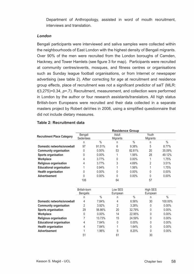
58Kesson S. Magid - UCL Chapter two
Department of Anthropology, assisted in word of mouth recruitment, interviews and translation.
London
Bengali participants were interviewed and saliva samples were collected within the neighbourhoods of East London with the highest density of Bengali migrants. Over 90% of the men were recruited from the London boroughs of Camden, Hackney, and Tower Hamlets (see figure 3 for map). Participants were recruited at community centres/events, mosques, and fitness centres or organisations such as Sunday league football organisations, or from Internet or newspaper advertising (see table 2). After correcting for age at recruitment and residence group effects, place of recruitment was not a significant predictor of salT (MLR: t(3,275)=0.34, p=.7). Recruitment, measurement, and collection were performed in London by the author or four research assistants/translators. All high status British-born Europeans were recruited and their data collected in a separate masters project by Robert deVries in 2008, using a simplified questionnaire that did not include dietary measures.
Recruitment dataTable 2:
Residence Group
Recruitment Place Category Bengali Sedentees
Adult Migrants
Youth Migrants
n % n % n %Domestic networks/snowball 97 91.51% 6 9.38% 5 8.77%Community organisation 0 0.00% 53 82.81% 20 35.09%Sports organisation 0 0.00% 1 1.56% 28 49.12%Workplace 4 3.77% 0 0.00% 1 1.75%Religious organisation 4 3.77% 3 4.69% 2 3.51%Educational organisation 1 0.94% 1 1.56% 1 1.75%Health organisation 0 0.00% 0 0.00% 0 0.00%Advertisement 0 0.00% 0 0.00% 0 0.00%
106 64 57
British-born Bengalis
Low SES European
High SES European
n % n % n %Domestic networks/snowball 4 7.84% 4 6.56% 30 100.00%Community organisation 2 3.92% 2 3.28% 0 0.00%Sports organisation 29 56.86% 20 32.79% 0 0.00%Workplace 0 0.00% 14 22.95% 0 0.00%Religious organisation 7 13.73% 15 24.59% 0 0.00%Educational organisation 4 7.84% 0 0.00% 0 0.00%Health organisation 4 7.84% 1 1.64% 0 0.00%Advertisement 1 1.96% 5 8.20% 0 0.00%
51 61 30

59Kesson S. Magid - UCL Chapter two
Adult Migrants (ADM)
Sixty-one men aged 23-76 (mean 49) who were born in Bangladesh and migrated to the UK to settle permanently after an assumed age of sexual maturity (≥ age 18)
Young Migrants (YOM)
Fifty men aged 18-69 years (mean 32) born in the District of Sylhet, Bangladesh and who migrated to the UK to settle permanently at an age prior to sexual maturity (< age 18, mean age at migration 8 years)
British-born Bengalis (2NG)
Forty-eight men aged 18-42 years (mean 25) born in the UK with both parents born in Bangladesh.
British-born European, low SES (ELO)
Fifty-eight men aged 18-75 (mean 41) born in the UK or Ireland, with both parents of European descent, all resident in London and of similar neighbourhoods and socioeconomic background, as measured by education, income and employment as the migrant groups.
British-born European, high SES (EHI)
Thirty men aged 22-54 (mean 37) born in the UK or Ireland, with both parents of European descent, resident in London and of high socioeconomic background, as measured by education, income and employment.
Anthropometry:2.2
All measurements were taken according to standardized methods (Lohman et al. 1988). Standing height, weight, arm length and mid-upper arm circumference, triceps, and biceps skinfold measures were collected by KSM or one of four other trained research assistants. Inter- and intra-measurer errors were within recommended technical errors of measurement (Ulijaszek and Kerr 1999)See table 2.2. Estimated mid-upper arm muscle and bone (MUAMus+Bone) was calculated according to the method proposed by Muller and Martorell (1988). Estimated axial fat and skin (MUAFat+Skin) was calculated by subtracting MUAMus+Bone from the total cross sectional area of the mid-upper arm.
Height
Height was assessed using a Seca 214 stadiometer (Seca Corp. Colombia, MD. USA) according to the following method (Gordon et al. 1988). Participants were

60Kesson S. Magid - UCL Chapter two
either barefoot or in thin socks and asked to stand with feet positioned with heels against the back of the footplate and medial borders of the feet at an angle of about 60°. The vertical plane was positioned along the line of the spine with heels, buttocks, scapulae and base of the cranium in contact with the vertical measure. All head coverings were requested to be removed and the head was positioned in the Frankfort Horizontal Plane where the lower orbital socket was placed in horizontal plane with the external auditory meatus (Henderson and Gregory 2002). Arms were held freely at the sides with palms facing the trunk of the body. Participants were asked to stand as fully erect as possible and take a deep breath. The movable headboard was positioned on the uppermost point of the head with sufficient pressure to compress the hair. Measurement was recorded to the nearest 0.1 cm as indicated on the scale. Intermeasurer differences were found to be within 0.1 cm.
Weight and Body Mass Index
Weight was assessed using a Tanita HD180 digital electronic scale (Tanita Corporation, Arlington Heights IL. USA). Participants asked to remove shoes, all heavy clothing, and any objects from pockets before stepping on the scale.
Anthropometric indices of body mass index (BMI) were categorised into US Dept of Health and Human Services divisions where BMI <18.5:Underweight, 18.5-24.9: Normal, 25-29.9: Overweight, >30: Obese (www.cdc.gov/nccdphp/dnpa/bmi/faq.htm).
Arm anthropometric measures2.3
Arm length (AL) and arm circumference (AC) were determined using a flexible measuring tape provided by Chasmor Ltd, (London UK.) according to the following method (Callaway et al. 1988). All arm measures were taken from the right arm with the arm muscles in a relaxed state and with the participant standing. Arm circumference and skinfolds were taken with the participant’s arm hanging loosely at the side of the trunk. All arm measurements were taken to the nearest 0.1 cm and repeated three times to reduce inter-measurement error (all CV<1.5%).
Arm Length
Participants were asked to remove any clothing obstructing access to the shoulder area and the elbow bent at 90° in order to palpate anatomical landmarks. The measurement was taken from the lateral projection of the acromion process of the scapula to the inferior margin of the olecranon process of the ulna.
61Kesson S. Magid - UCL Chapter two
Arm Circumference
Upon determining AL, the mean of three measures was divided by two and the mid-point of the upper arm was measured from the lateral projection of the acromion process. A small mark was made with a pen at this point. Using the mark, the zero mark of the tape was positioned just below the mid-point using the left hand, and the remaining part of the tape was aligned along the top of the tape using the right hand. Measurements were taken to the nearest 0.1 cm and repeated three times. All intra- and intermeasurer variations were within recommended limits of 0.2 cm (Callaway et al. 1988) (See table 3).
Skinfolds
Skinfold, or sometimes “fatfold” measurements gauge the thickness of a double layer of skin and subcutaneous adipose tissue at specific sites. A standardized pressure is applied at specific points on the body using calibrated spring-loaded callipers. These measures are useful as 40-60% of total body fat is deposited subcutaneously (Wang et al. 1997). Alone, skinfolds provide a simple and noninvasive method of estimating general fatness (Harrison et al. 1988). During adulthood, circumferences of the limbs, when combined with skinfold measures of subcutaneous adipose tissue at the corresponding level can provide cross-sectional areas of adipose tissue or the underlying area of muscle plus bone. When computed from appropriate formulae, such measures can provide a rough index of the relative somatic apportionment of adipose and muscle tissue (Callaway et al. 1988).
Anthropometric muscle + bone area estimations are limited by several assumptions: 1) the mid-arm circumference is circular 2) skinfold measures are twice the average adipose tissue diameter and this subcutaneous adipose tissue mantle is uniform in thickness 3) the muscle and bone compartments of the mid arm are also assumed to be circular 4) inter- and intra-muscle adipose tissue is absent. 5) the neurovascular bundle of the medial aspect of the arm is not accounted separately, and is included in muscle + bone estimation (Forbes 1987; Martine et al. 1997). These assumptions generally lead to an overestimation of total muscle + bone as the circumference of the arm is actually an ellipse, there is variability in the thickness of subcutaneous deposits of adipose tissue, muscle tissue has an irregular cross-sectional outline which contains minute amounts of inter- and intramuscular adipose tissue, and the medial neurovascular bundle contributes approximately 2-3 cm2 area to muscle + bone estimations (Forbes 1987; Heymsfield et al. 1982; Martine et al. 1997).
Skinfolds were measured according to the methods outlined by Harrison, et al. (1988) using a Holtain/Whitehouse Skinfold Calliper (Holtain Ltd., Pembrokeshire

62Kesson S. Magid - UCL Chapter two
UK). Approximately 1 cm above the midpoint mark of AL, the measurer’s thumb and forefinger of the left hand was used to elevate a double fold of skin and subcutaneous adipose tissue. Upon elevating the skinfold, callipers were held with the measurer’s right hand at the same horizontal plane and level with the midpoint mark. The pressure was released from the callipers gently. Upon full release of calliper pressure, the measurer counted 3 seconds and took the reading in 0.1 cm. The 3-second count was standardised to reduce error effects of fluids being forced from skinfold tissues. The callipers were then removed, and the entire procedure repeated two more times to obtain three independent measures. Mean values were reported, those with CVs over 5% for length and circumference, or 15% for skinfolds were remeasured for a fourth reading or discarded. Triceps skinfold measurements were discarded from one participant due to high CV. Technical error of measurement (see table 3) was calculated using the following formulae (Muller and Martorell 1988; Ulijaszek and Kerr 1999).
TEM = √(∑N((∑KM2)−((∑KM)2 ⁄ K))) ⁄ N(K−1) (1)
Total TEM = √((TEM(intra1)
2 +TEM (intra2)2) +TEM (inter)2) ⁄ 2 (2)
Where M, measurement; K number of times measured (In this study K=3 for all arm anthropometric measures); N number of subjects
Triceps skinfold (TSF)
The skinfold was elevated by placing the thumb and forefinger approximately 8 cm apart along a line perpendicular to the long axis of the arm along the posterior ridge of the arm over the triceps muscle.
Biceps skinfold (BSF)
The skinfold was elevated from the anterior aspect of the arm, over the belly of the biceps muscle at the same horizontal plane as the triceps skinfold.
Estimates of Mid-Upper Arm tissue apportionment
Prediction of the mid-upper arm cross-sectional area and muscle + bone area from anthropometric data was calculated using the following formulae (de Koning et al. 1986; Forbes 1987):
Total cross sectional area:
Cross Sectional Area = (AC)2⁄4π (3)
Where AC = Arm Circumference
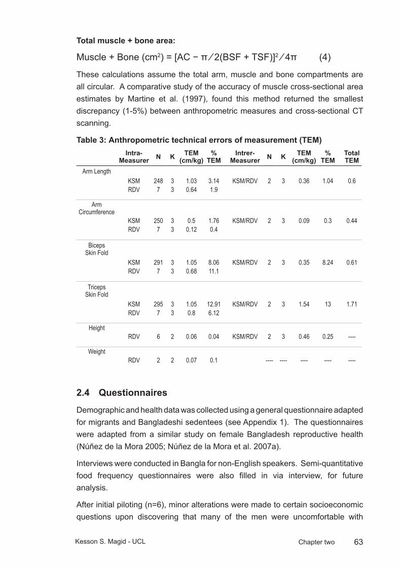
63Kesson S. Magid - UCL Chapter two
Total muscle + bone area:
Muscle + Bone (cm2) = [AC − π ⁄ 2(BSF + TSF)]2 ⁄ 4π (4)
These calculations assume the total arm, muscle and bone compartments are all circular. A comparative study of the accuracy of muscle cross-sectional area estimates by Martine et al. (1997), found this method returned the smallest discrepancy (1-5%) between anthropometric measures and cross-sectional CT scanning.
Anthropometric technical errors of measurement (TEM)Table 3: Intra-
Measurer N K TEM (cm/kg)
% TEM
Intrer-Measurer N K TEM
(cm/kg)%
TEMTotal TEM
Arm LengthKSM 248 3 1.03 3.14 KSM/RDV 2 3 0.36 1.04 0.6RDV 7 3 0.64 1.9
Arm Circumference
KSM 250 3 0.5 1.76 KSM/RDV 2 3 0.09 0.3 0.44RDV 7 3 0.12 0.4
Biceps Skin Fold
KSM 291 3 1.05 8.06 KSM/RDV 2 3 0.35 8.24 0.61RDV 7 3 0.68 11.1
Triceps Skin Fold
KSM 295 3 1.05 12.91 KSM/RDV 2 3 1.54 13 1.71RDV 7 3 0.8 6.12
HeightRDV 6 2 0.06 0.04 KSM/RDV 2 3 0.46 0.25 ----
WeightRDV 2 2 0.07 0.1 ---- ---- ---- ---- ----
Questionnaires2.4
Demographic and health data was collected using a general questionnaire adapted for migrants and Bangladeshi sedentees (see Appendix 1). The questionnaires were adapted from a similar study on female Bangladesh reproductive health (Núñez de la Mora 2005; Núñez de la Mora et al. 2007a).
Interviews were conducted in Bangla for non-English speakers. Semi-quantitative food frequency questionnaires were also filled in via interview, for future analysis.
After initial piloting (n=6), minor alterations were made to certain socioeconomic questions upon discovering that many of the men were uncomfortable with

64Kesson S. Magid - UCL Chapter two
socioeconomic questions regarding number and relation of people living in their home (question III.4, appendix 1). The question was altered and “rather not say” was included as an option. The only socioeconomic indicator used for analysis in this study was total household income. Additional questions were added regarding number and age of siblings and household members during the participant’s childhood (see questions 1.15-1.17, appendix 1).
Native English speakers were given the option of completing the questionnaire online using the UCL Opinio web-based survey portal (http://www.ucl.ac.uk/isd/students/e-learning/tools/opinio). To encourage completion of the questionnaire, a number of questions were dropped from the web-based version. These questions were: from the Demographic and Health Questionnaire: IV.1-2, which distinguished paid work from home; VIII.8-IX.2, which asked whether practiced contraception, details of birthweight, and open-ended questions regarding leisure activities and social networks. From the Dietary Questionnaire: I.6-14 regarding places eaten outside the home and children’s eating habits; III.1-10 regarding frozen, preserved and ready-made meals; and III.24, 33, 37, 41-44 which ask frequency of consumption of squash, seafood, nuts, fizzy drinks, and alternatives to cow’s milk (see appendices 1 & 2 for complete printouts of questionnaires).
Prostate symptoms
The occurrence and severity of LUTS were assessed using the International Prostate Symptom Score (IPSS) (Barry et al. 1992). The IPSS combines reported symptoms of frequency, bother, and interference of daily urinary activities. The self-assessed symptoms were combined with perceived quality of life using 6-point Likert scales, summed to score 1-35.
IPSS scores are a World Health Organisation adopted international measure of prostate health used successfully in industrialized countries with a variety of cultures (Barry et al. 1992). Scores were broken into three categories of severity: 0-7 asymptomatic to mild, 8-19 moderate, and 20-23 severe.
Relationship status
Questions on marital status (Questions I.12-I.14, Appendix A) and number of offspring (question VIII, appendix 1) were asked to obtain relationship and fatherhood measures.
Socioeconomic status
To estimate wealth, an index was created of 11 household possessions in the UK, and 8 in Bangladesh (see appendix 1, question III.5). This method of estimating SES is frequently used in cross-cultural contexts as an indicator of the level

65Kesson S. Magid - UCL Chapter two
of wealth that is consistent with expenditure and income measures (Gwatkin et al. 2007; Montgomery et al. 2000). Television ownership was added to the Bangladeshi questionnaire and assumed nearly ubiquitous in the UK households, while “washing machine”, “tumble dryer”, “dishwasher” and “central heating” were omitted, as these are not common household possessions in Bangladesh where servants usually perform domestic chores.
Fasting blood glucose and dried blood spots2.5
Fasting blood glucose (FBG) levels were measured from finger-prick blood samples using a disposable lancet and Bayer Asencia blood glucose monitor and detection strips (Bayer Diagnostics, Berkshire UK). Participants were asked not to eat any food or drink aside from water or tea without milk or sugar for 6 hours prior to testing, in practice this meant most (>90%) of the FBG sampling occurred in the morning, before breakfast
Salivary sampling 2.6
A total of six salivary samples were collected from each participant, one upon waking (WAKE), one approximately 30 minutes following waking (W+30), and one right before bed (BED). Participants were asked to record exact times of waking, sampling and going to sleep. The samples were collected over two nonconsecutive days at all three time points. For diurnal ratio (DIR), the two morning samples from both days were averaged (MeanAM) and divided by the mean of BED. Daily mean (DAYM) is an average of MeanAM and BED.
Salivary Testosterone and Cortisol2.7
Cortisol and Testosterone were assayed from saliva samples to measure the potential influence of a changed environment upon daily variation in hormone levels in migrants. Steroid salivary assays are noninvasive, stable at room temperature, and an accurate measure of bioavailable free T (Dabbs 1990). All participants were asked to not brush their teeth, consume food or chew betel nut for at least 1 hour prior to providing a sample. Sticks of Carefree sugarless chewing gum provided as a stimulant for saliva flow, as this has been validated as not interfering with the assay (Dabbs 1990).
Measurements of salivary hormones should involve multiple samples in order to account for pulsatile and diurnal variation (Dabbs 1990), so samples were collected over two nonconsecutive days. Tubes contained either sodium azide or methionine as preservative and were stored at room temperature for 3-6 months, then refrigerated at 5°c until analysis.
66Kesson S. Magid - UCL Chapter two
Salivary assay protocol
Salivary testosterone assays were measured by radioimmunoassay without extraction. Antiserum was prepared in the laboratory of Dr. Robert Chatterton at Northwestern University, Chicago USA, where all analyses were performed. The interassay CVs were all within 15% for high (100pg/ml), low (50pg/ml), and internal (pooled saliva sample) quality controls. The sensitivity was 0.028 nmol/L.
Samples of salivary T were analysed according to the following criteria:
Outlying points with readings over 500pg/ml were excluded as they fell outside the standard curve (highest standard=480pg/ml) and estimates beyond this concentration could not be accurately estimated. Readings were made in duplicate and all with a CV greater than 15% were re-analysed or excluded. Of 2018 samples, a total of 39 (1.9%) were excluded for high CV. In addition, outlying readings were identified with absolute salT values showing Z-scores greater than 2.58 (40 samples, 2%) and 3.29 (17 samples, 0.8%). Of these outlying readings, a further 3 samples were dropped from further analysis, 10 were recoded as the daily mean concentration of salT for that participant, 7 were recoded as a singulate reading due to spillage or other laboratory error for the duplicate reading, and 9 were analysed without applying a correction factor.
Salivary validation studies2.8
As salT was analysed over different years, a number of samples and QCs were measured repeatedly. These repeat measures were used to adjust readings between years of analysis. A total of 191 samples first collected and analysed in 2005, 66 samples first collected and analysed in 2006, and 17 samples first collected and analysed in 2008 were measured a second time in 2010. From these repeat measures, a correction factor of 3.06 was applied to all other readings from 2005, and 0.84 was applied to all other readings from 2006. Repeat measures from 2008 assays did not require a correction factor to match 2010 readings.
Betel nut study
As the chewing of betel nut (paan) is endemic practice among Bangladeshi males, (especially the older generation), a sub-study on potential interaction effects of betel nut chewing upon the salivary hormone assay was run on a sample of 20 male participants according to the following method: men were instructed not to chew paan for at least 12 hours prior to the study, and they were asked not to consume any food or drink aside from water for at least 30 minutes prior to the study. One saliva sample was taken as a baseline, following which the participant prepared and chewed their paan in their usual manner, typically a combination of betel nut, calcium oxide, and tobacco wrapped in a betel leaf to form a “quid”
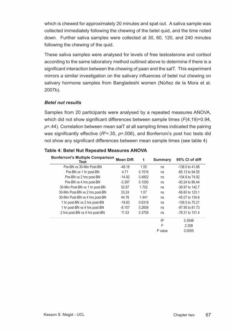
67Kesson S. Magid - UCL Chapter two
which is chewed for approximately 20 minutes and spat out. A saliva sample was collected immediately following the chewing of the betel quid, and the time noted down. Further saliva samples were collected at 30, 60, 120, and 240 minutes following the chewing of the quid.
These saliva samples were analysed for levels of free testosterone and cortisol according to the same laboratory method outlined above to determine if there is a significant interaction between the chewing of paan and the salT. This experiment mirrors a similar investigation on the salivary influences of betel nut chewing on salivary hormone samples from Bangladeshi women (Núñez de la Mora et al. 2007b).
Betel nut results
Samples from 20 participants were analysed by a repeated measures ANOVA, which did not show significant differences between sample times (F(4,19)=0.94, p=.44). Correlation between mean salT at all sampling times indicated the pairing was significantly effective (R2=.35, p=.006), and Bonferroni’s post hoc tests did not show any significant differences between mean sample times (see table 4)
Betel Nut Repeated Measures ANOVATable 4: Bonferroni's Multiple Comparison
Test Mean Diff. t Summary 95% CI of diff
Pre-BN vs 30-Min Post-BN -48.16 1.55 ns -138.0 to 41.68Pre-BN vs 1 hr post-BN 4.71 0.1516 ns -85.13 to 94.55Pre-BN vs 2 hrs post-BN -14.92 0.4802 ns -104.8 to 74.92Pre-BN vs 4 hrs post-BN -3.397 0.1093 ns -93.24 to 86.44
30-Min Post-BN vs 1 hr post-BN 52.87 1.702 ns -36.97 to 142.730-Min Post-BN vs 2 hrs post-BN 33.24 1.07 ns -56.60 to 123.130-Min Post-BN vs 4 hrs post-BN 44.76 1.441 ns -45.07 to 134.6
1 hr post-BN vs 2 hrs post-BN -19.63 0.6318 ns -109.5 to 70.211 hr post-BN vs 4 hrs post-BN -8.107 0.2609 ns -97.95 to 81.732 hrs post-BN vs 4 hrs post-BN 11.53 0.3709 ns -78.31 to 101.4
R2 0.3548F 2.308
P value 0.0055

68Kesson S. Magid - UCL Chapter two
Salivary T and recent betel nut useFigure 8: Salivary T and recent betel nut use
0 60 120 180 240 300150
200
250
300
Minutes after chewing betel nut quid
Saliv
ary
T pg
/ml
Pre-betel nut
Error bars ± SEM.
Matched saliva/serum samples
A smaller subgroup of 20 individuals provided a time-matched blood sample and saliva sample to validate the reliability of the salivary assay in determining serum concentrations of testosterone in this study population. The blood samples were collected at Sylhet Osmani Medical College by Dr. Kurshida Begum according to the methodology described above.
Salivary T assays were measured by radioimmunoassay without extraction see appendix 4 for laboratory protocol. Antiserum was prepared in the laboratory of Dr. Robert Chatterton at Northwestern University, Chicago USA, where all analyses were performed. The interassay CVs were all within 15% for high (100pg/ml), low (50pg/ml), and internal (pooled saliva sample) quality controls. The sensitivity was 0.028 nmol/L.
Samples of salT were analysed according to the following criteria:
The overall degree of diurnal change in salivary T was expressed as a mean value at each time point over two nonconsecutive days, with the evening sample value subtracted from the morning value and expressed as a percentage. The morning sample was considered the peak level of T, as has been observed in numerous other studies (Campbell et al. 2005; Ellison et al. 2002) and can be considered a “top” baseline for the day.
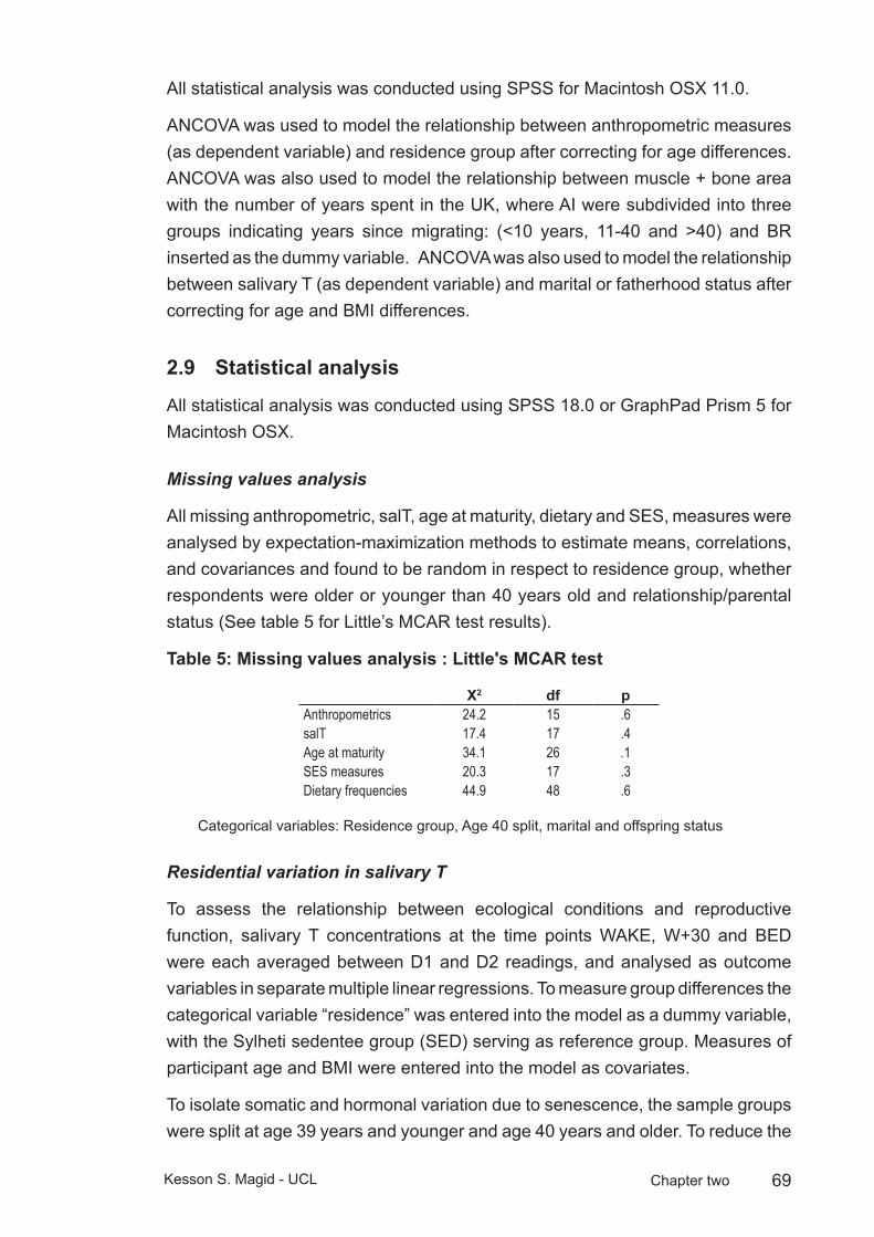
69Kesson S. Magid - UCL Chapter two
All statistical analysis was conducted using SPSS for Macintosh OSX 11.0.
ANCOVA was used to model the relationship between anthropometric measures (as dependent variable) and residence group after correcting for age differences. ANCOVA was also used to model the relationship between muscle + bone area with the number of years spent in the UK, where AI were subdivided into three groups indicating years since migrating: (<10 years, 11-40 and >40) and BR inserted as the dummy variable. ANCOVA was also used to model the relationship between salivary T (as dependent variable) and marital or fatherhood status after correcting for age and BMI differences.
Statistical analysis2.9
All statistical analysis was conducted using SPSS 18.0 or GraphPad Prism 5 for Macintosh OSX.
Missing values analysis
All missing anthropometric, salT, age at maturity, dietary and SES, measures were analysed by expectation-maximization methods to estimate means, correlations, and covariances and found to be random in respect to residence group, whether respondents were older or younger than 40 years old and relationship/parental status (See table 5 for Little’s MCAR test results).
Missing values analysis : Little'sTable 5: MCAR test
X2 df pAnthropometrics 24.2 15 .6salT 17.4 17 .4Age at maturity 34.1 26 .1SES measures 20.3 17 .3Dietary frequencies 44.9 48 .6
Categorical variables: Residence group, Age 40 split, marital and offspring status
Residential variation in salivary T
To assess the relationship between ecological conditions and reproductive function, salivary T concentrations at the time points WAKE, W+30 and BED were each averaged between D1 and D2 readings, and analysed as outcome variables in separate multiple linear regressions. To measure group differences the categorical variable “residence” was entered into the model as a dummy variable, with the Sylheti sedentee group (SED) serving as reference group. Measures of participant age and BMI were entered into the model as covariates.
To isolate somatic and hormonal variation due to senescence, the sample groups were split at age 39 years and younger and age 40 years and older. To reduce the

70Kesson S. Magid - UCL Chapter two
influence of acute variations in salT in order to assess the relationship between ecological conditions and reproductive function, salT concentrations at the time points WAKE, W+30 and BED were each averaged between D1 and D2 readings, and analysed as outcome variables in separate multiple linear regressions.
Analyses of salT or anthropometric variables by residence group were performed with two separate multiple linear regressions (MLR), to test two hypotheses, after correcting for age and/or BMI where appropriate.
The first model, MLRI measured group differences from SED. The categorical variable “residence” was entered into the model as a dummy variable, with SED serving as reference group. Measures of participant age and BMI were entered into the model as covariates where appropriate.
The second model, MLRII applied planned orthogonal contrasts to test for differences between groups with contrasting developmental histories. Contrast 1 compared the men with shared childhood under Bangladeshi conditions (SED, ADM) to men with shared (all or part) childhood in the UK (YOM, 2NG, ELO, EHI). Contrast 2 subdivided the men who lived in the UK as children according to ethnicity (YOM, 2NG) versus (ELO, EHI). Contrast 3 compared Bengalis with differing childhood conditions: YOM versus 2NG. Contrast 4 compared European males with differing socioeconomic status, EHI versus ELO. The final planned contrast compared Bengali men experiencing different conditions in adulthood: SED versus ADM. Post hoc Sidak comparisons were run of all remaining group differences.
For age at migration analysis, MLRI, the groups YOM and ADU were split into developmental period of migration. YOM were split into three periods; infancy: aged <2 years (n=6); childhood: aged 2-12 (n=12); adolescence: aged 12-18 (n=15). ADU were split between early adulthood: age 18-30 (n=36) and late adulthood (n=12). A second model, MLRII included 2NG (n=26) as a reference group, and MLRIII combined 2NG with infant YOM into a single pre-birth to age 2 group (n=32) with late adult ADM serving as reference group.
Validation study results
Repeated measures and correction factors:
As salT was analysed over several years, a number of samples and QCs were measured repeatedly. These repeat measures were used to adjust readings between years of analysis. A total of 191 samples collected and analysed in 2005, 66 samples collected and analysed in 2006, and 17 samples collected and analysed in 2008 were measured again in 2010. From these repeat measures, a correction factor of 3.06 was applied to all other readings from 2005, and 0.84

71Kesson S. Magid - UCL Chapter two
was applied to all other readings from 2006. Repeat measures from 2008 assays did not require a correction factor to match 2010 readings.
Serum to salivary T comparisons
Method: a total of 22 participants were asked to provide a saliva sample according to the same collection procedure detailed for all samples collected in the field. Immediately following the provision of a saliva sample, a serum sample was collected. Two sample tubes were mislabelled and were therefore dropped from the final analysis.
Serum concentrations of total T were determined using a commercially available radioimmunoassay (Diagnostic System Laboratories, Webster, Texas USA) at the Chatterton laboratory at Northwestern University. High and low concentration QCs were within recommended limits (see table 6)
Serum T assay QCsTable 6: QC Expected Read
I 0.65 ± 0.2 0.62II 5.7 ± 1.7 5.02
Result: A linear regression of salT by serum T concentrations was significant (F(1,18)=4.9, p=.04) indicating the correlation between matched salT and serum T samples, with Pearson’s R2=.21 (see figure 9).
Matched Salivary T to SerumT Figure 9: Matched Salivary T to Serum T
2000 3000 4000 5000 60000
50
100
150
200
250
Serum T (pg/ml)
Saliv
ary
T (p
g/m
l)
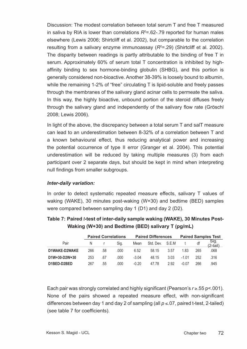
72Kesson S. Magid - UCL Chapter two
Discussion: The modest correlation between total serum T and free T measured in saliva by RIA is lower than correlations R2=.62-.79 reported for human males elsewhere (Lewis 2006; Shirtcliff et al. 2002), but comparable to the correlation resulting from a salivary enzyme immunoassay (R2=.29) (Shirtcliff et al. 2002). The disparity between readings is partly attributable to the binding of free T in serum. Approximately 60% of serum total T concentration is inhibited by high-affinity binding to sex hormone-binding globulin (SHBG), and this portion is generally considered non-bioactive. Another 38-39% is loosely bound to albumin, while the remaining 1-2% of “free” circulating T is lipid-soluble and freely passes through the membranes of the salivary gland acinar cells to permeate the saliva. In this way, the highly bioactive, unbound portion of the steroid diffuses freely through the salivary gland and independently of the salivary flow rate (Gröschl 2008; Lewis 2006).
In light of the above, the discrepancy between a total serum T and salT measure can lead to an underestimation between 8-32% of a correlation between T and a known behavioural effect, thus reducing analytical power and increasing the potential occurrence of type II error (Granger et al. 2004). This potential underestimation will be reduced by taking multiple measures (3) from each participant over 2 separate days, but should be kept in mind when interpreting null findings from smaller subgroups.
Inter-daily variation:
In order to detect systematic repeated measure effects, salivary T values of waking (WAKE), 30 minutes post-waking (W+30) and bedtime (BED) samples were compared between sampling day 1 (D1) and day 2 (D2).
Paired Table 7: t-test of inter-daily sample waking (WAKE), 30 Minutes Post-Waking (W+30) and Bedtime (BED) salivary T (pg/mL)
Paired Correlations Paired Differences Paired Samples TestPair N r Sig. Mean Std. Dev. S.E.M t df Sig.
(2-tail)D1WAKE-D2WAKE 266 .58 .000 6.52 58.15 3.57 1.83 265 .068D1W+30-D2W+30 253 .67 .000 -3.04 48.15 3.03 -1.01 252 .316D1BED-D2BED 267 .55 .000 -0.20 47.78 2.92 -0.07 266 .945
Each pair was strongly correlated and highly significant (Pearson’s r ≥.55 p<.001). None of the pairs showed a repeated measure effect, with non-significant differences between day 1 and day 2 of sampling (all p ≤.07, paired t-test, 2-tailed) (see table 7 for coefficients).
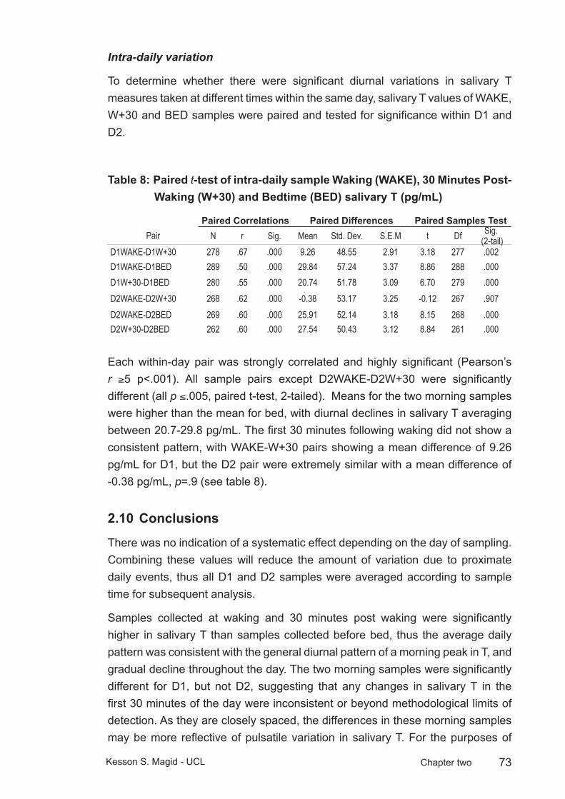
73Kesson S. Magid - UCL Chapter two
Intra-daily variation
To determine whether there were significant diurnal variations in salivary T measures taken at different times within the same day, salivary T values of WAKE, W+30 and BED samples were paired and tested for significance within D1 and D2.
Paired Table 8: t-test of intra-daily sample Waking (WAKE), 30 Minutes Post-Waking (W+30) and Bedtime (BED) salivary T (pg/mL)
Paired Correlations Paired Differences Paired Samples TestPair N r Sig. Mean Std. Dev. S.E.M t Df Sig.
(2-tail)D1WAKE-D1W+30 278 .67 .000 9.26 48.55 2.91 3.18 277 .002D1WAKE-D1BED 289 .50 .000 29.84 57.24 3.37 8.86 288 .000D1W+30-D1BED 280 .55 .000 20.74 51.78 3.09 6.70 279 .000D2WAKE-D2W+30 268 .62 .000 -0.38 53.17 3.25 -0.12 267 .907D2WAKE-D2BED 269 .60 .000 25.91 52.14 3.18 8.15 268 .000D2W+30-D2BED 262 .60 .000 27.54 50.43 3.12 8.84 261 .000
Each within-day pair was strongly correlated and highly significant (Pearson’s r ≥5 p<.001). All sample pairs except D2WAKE-D2W+30 were significantly different (all p ≤.005, paired t-test, 2-tailed). Means for the two morning samples were higher than the mean for bed, with diurnal declines in salivary T averaging between 20.7-29.8 pg/mL. The first 30 minutes following waking did not show a consistent pattern, with WAKE-W+30 pairs showing a mean difference of 9.26 pg/mL for D1, but the D2 pair were extremely similar with a mean difference of -0.38 pg/mL, p=.9 (see table 8).
Conclusions2.10
There was no indication of a systematic effect depending on the day of sampling. Combining these values will reduce the amount of variation due to proximate daily events, thus all D1 and D2 samples were averaged according to sample time for subsequent analysis.
Samples collected at waking and 30 minutes post waking were significantly higher in salivary T than samples collected before bed, thus the average daily pattern was consistent with the general diurnal pattern of a morning peak in T, and gradual decline throughout the day. The two morning samples were significantly different for D1, but not D2, suggesting that any changes in salivary T in the first 30 minutes of the day were inconsistent or beyond methodological limits of detection. As they are closely spaced, the differences in these morning samples may be more reflective of pulsatile variation in salivary T. For the purposes of

74Kesson S. Magid - UCL Chapter two
measuring diurnal decline, WAKE and W+30 samples may be averaged to obtain a value for the morning peak, from which the averaged BED samples may be subtracted to obtain a value for diurnal decline.
75Kesson S. Magid - UCL Chapter three
Testing developmental hypothesesChapter 3:
Introduction3.1
In this chapter I test the hypothesis that improvements in developmental conditions increase reproductive investment in migrant males as measured by adult somatic and hormonal characteristics. Age at migration serves as a predictive variable for daily patterns of salivary testosterone, two measures of stature (standing height and humeral length), estimates of skeletal muscle and axial body fat.
In applying a life history analysis to anthropometric and hormonal measures, this chapter makes the following two assumptions. Firstly, the shift in environment from Sylhet, Bangladesh to London, UK, during childhood will influence patterns of growth and reproductive strategies in ways that will be detectable in adult males. Secondly, phenotypic matching to ecological conditions will be based on cues received during growth and, when the environment improves or becomes less stochastic, plastic characteristics will correspond to adult environment with a more matched phenotype. Phenotypic characters that are more canalised or have undergone irreversible development will be mismatched to adult environment (Kuzawa 2007; Stearns 2000; West-Eberhard 1989).
Life-history trade-offs are evident in observed variability in human male and female reproductive steroid hormone levels. Non-industrialised or subsistence populations show lower levels of free testosterone when compared with populations in developed nations (Bribiescas 1996; Ellison et al. 2002). Measures of testosterone (T) are presumed to reflect greater immunological, nutritional or other energetic challenges (Bribiescas 2001a; Charnov 1993). Androgen levels of adult males, particularly free T, respond acutely to changes in nutrition, social conditions, physical activity, and immune challenges (Muehlenbein and Bribiescas 2005) (Campbell et al. 2001) (Bribiescas 2001a).
For women, adult progesterone levels appear to be influenced by conditions experienced prior to puberty, and remain unchanged despite improved conditions in adulthood (Núñez de la Mora et al. 2007a). It is unknown, however, whether adult male reproductive function is similarly constrained by childhood conditions, although recent evidence suggests that environmental stressors in the first six months of life influence hormonal and somatic characters in adult males (Kuzawa et al. 2010).
Migrants from Sylhet, Bangladesh to London, UK experience a discontinuous developmental environment, with fewer immune challenges or other presumed constraints on energy balance following migration. In order to understand further such influences on the reproductive hormones of adult men, this project
76Kesson S. Magid - UCL Chapter three
compared salivary testosterone and anthropometric measures of a group of adult Bangladeshi migrants who relocated to London as children (aged <18 years) and as adults (aged >18 years) with men of Bengali or European ethnicity resident all their lives in London, or with Sylheti sedentees. Age at migration acts as an experimental variable in this study in order to observe whether adult patterns of salT variation are influenced by ecological conditions experienced during development.
Hypotheses
This chapter tests three main hypotheses:
The experience of more limited or stressful conditions during development prior to maturity constrains investment in reproductive effort, and primes males to respond to improvement in conditions during early adulthood with an immediate increase in reproductive function. This is a discounting future survivorship by increasing investment into reproductive competition, as measured by salT when young adults, if childhood conditions were poor and they have improved. In contrast, men divert more resources toward reproductive competition at older ages if they have attained high status, irrespective of preadult developmental conditions. In men aged under 40, investment in reproductive effort will be influenced more by immediate conditions than by those experienced prior to maturity, if the immediate conditions are an improvement from childhood conditions.
1. Men in a less constrained environment are free to invest greater resources into reproductive effort. If men migrate to the UK before the age of maturity, they will show greater investment in reproductive effort than sedentees and adult migrants as measured by salT and into growth, as measured by skeletal stature, muscle and body fat.
Predictions:
a. All migrant and British-born Bengalis will show higher salT, as well as greater BMI and skeletal muscle compared to sedentees.
b. Stature of young migrants will be greater than sedentees and adult migrants.
c. Young migrants and British-born Bengalis will have sexually matured at a younger age than adult migrants or sedentees.
2. If developmental environments of energetic affluence permit the adoption of a more diverse set of strategies in male reproductive effort, (in effect a wider bandwidth of potential reproductive strategies), this will be reflected in wider daily variation in reproductive hormones. Therefore, young men who

77Kesson S. Magid - UCL Chapter three
experienced an environment of fewer constraints will have greater inter- and intra-individual variability in salT.
Predictions:
British-born Bengalis will show greater diurnal variation in salT compared to young migrants, and both young migrants and British Bengalis will show greater diurnal variation compared to adult migrants and sedentees. European males will show similar diurnal variation to young migrants and British-born Bengalis, and greater measures of salT than sedentees and adult migrants.
3. In evolutionary history, older males were unlikely to succeed in direct physical competition with younger males for reproductive opportunities, but older males will have had the opportunity to acquire status in early adulthood. The diversion of metabolic energy toward reproductive effort is more likely to be maintained in older males of high status than in men of the same age of lower status. If older males are of high social status, relative to surroundings, they will invest more in reproductive effort. If they are lower, they will invest less into reproductive effort.
Predictions:
Adult migrants over the age of 40 will have greater salivary T than sedentees, high status European males will have greater salivary T than low status Europeans.
Methods3.2
Recruitment
Salivary testosterone, anthropometric, and demographic data were collected from the following populations according to methods described in chapter two.
1. ADM: Bengali migrants who arrived in London at <18 years old (pre/peri-puberty) (N=61)
2. YOM: Bangladeshi migrants who arrived in London at >18 years old (post-puberty) (N=50)
3. 2NG: Second generation ethnic Bengalis born in the UK (N=48)
4. SED: Native Bengalis resident in Bangladesh (N=107)
5. ELO: Native Londoners of white British or other white European parentage, of similar socioeconomic background compared to migrant groups (N=58)

78Kesson S. Magid - UCL Chapter three
6. EHI: Native Londoners of white British or other white European parentage, of higher status socioeconomic background compared to migrant groups (N=30)
Statistical analysis:
To isolate somatic and hormonal variation due to senescence, the sample groups were split at age 39 years and younger (<40) and age 40 years and older (≥40). In order to assess the relationship between ecological conditions and reproductive function and to reduce the influence of acute variations in salT, concentrations at the time points WAKE, W+30 and BED were each averaged between D1 and D2 readings, and analysed as outcome variables in separate multiple linear regressions.
Analyses of salT or anthropometric variables by residence group were performed with four separate multiple linear regressions (MLR), after correcting for age and/or BMI where appropriate. The addition of height as a separate covariate did not significantly improve the model, so was not included.
The first regression (MLR-I) tested for differences from the sedentee reference group. The categorical variable “residence” was entered into the model as a dummy variable. Measures of participant age and BMI were entered into the model as covariates where appropriate. The second model tested for differences between groups depending on age of migration or ethnic differences.
The second regression (MLR-II) applied planned orthogonal contrasts to test for differences between groups with contrasting developmental histories, with the hypothesis that men who spent more of their childhood in the UK would have greater reproductive investment, expressed as higher salT (see figure 10).
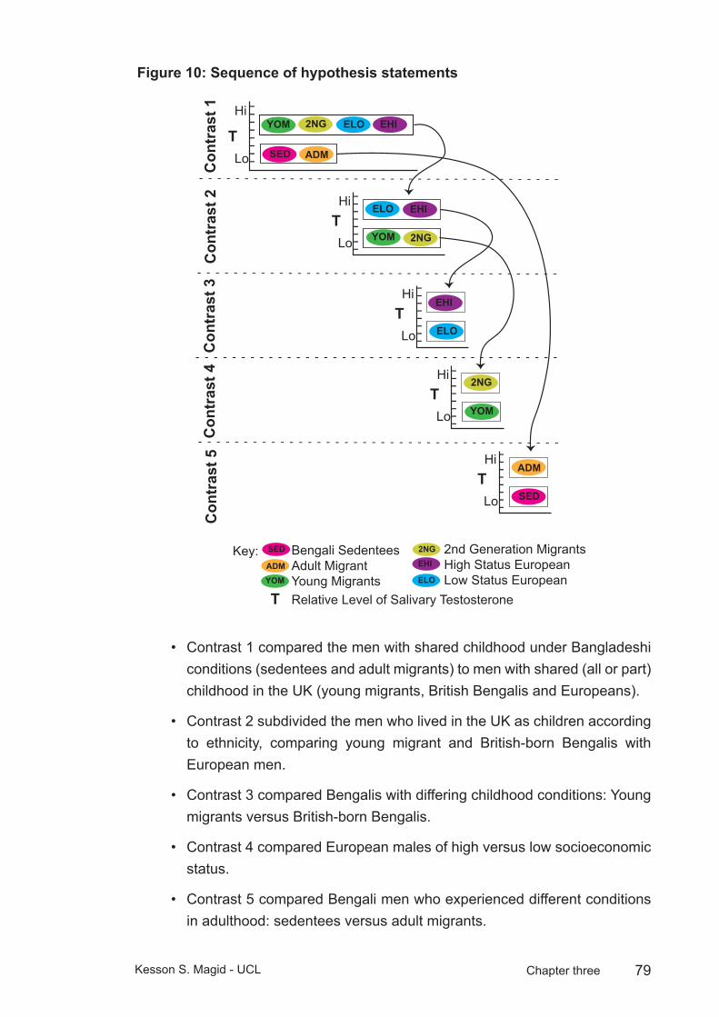
79Kesson S. Magid - UCL Chapter three
Sequence of hypothesis statementsFigure 10:
SED
YOM
ADM
2NG ELO EHIT
Hi
Lo
YOM 2NG
ELO EHITHi
Lo
ELO
EHITHi
Lo
THi
Lo
Con
tras
t 1C
ontr
ast 2
Con
tras
t 3C
ontr
ast 4
Con
tras
t 5
THi
Lo
YOM
2NG
SED
ADM
Bengali SedenteesAdult MigrantYoung Migrants
2nd Generation MigrantsHigh Status EuropeanLow Status European
SED
YOM
ADM
2NG
ELO
EHI
T Relative Level of Salivary Testosterone
Key:
Contrast 1 compared the men with shared childhood under Bangladeshi • conditions (sedentees and adult migrants) to men with shared (all or part) childhood in the UK (young migrants, British Bengalis and Europeans).
Contrast 2 subdivided the men who lived in the UK as children according • to ethnicity, comparing young migrant and British-born Bengalis with European men.
Contrast 3 compared Bengalis with differing childhood conditions: Young • migrants versus British-born Bengalis.
Contrast 4 compared European males of high versus low socioeconomic • status.
Contrast 5 compared Bengali men who experienced different conditions • in adulthood: sedentees versus adult migrants.
80Kesson S. Magid - UCL Chapter three
Post hoc Sidak comparisons were run of all remaining group • differences.
For age at migration analysis, (MLRIII), migrants were split according to stages of development when relocated. Young migrants were split into three periods; infancy: aged ≤2 years (n=6); childhood: aged 3-12 (n=12); adolescence: aged 13-18 (n=15); early adulthood: age 19-30 (n=36) and late adulthood ≥30 years (n=12).
A final analysis of age at migration (MLR-IV) included 2NG (n=26) as a reference group, and combined British-born with infant migrants into a single pre-birth to age 2 group (n=32) with adult migrants who arrived ≥30 serving as reference group.
Results3.3
Descriptives
The adult migrants were significantly older than all other groups with an average of 48.8 years (15.8 SD), and the British-born Bengalis were the youngest group, averaging 24.5 years (5.7 SD), the average of all populations was 37.9 (15 SD). This cohort effect reflects the demography of the UK Bengali community, with most adult male migration having occurred in the 1970s, which was followed by wives and children in the 1980s (see chapter 1).
All migrant groups under the age of 40 have more upper arm muscle, and more axial body fat, compared to sedentees. All migrants over the age of 40 have more muscle, but not more axial fat than sedentees. Youth migrants and British Bengalis are both taller than adult migrants and sedentees, and British Bengalis were taller than youth migrants. Upper arm length was consistent within ethnic groups, with no difference between residence categories, and both measures of stature were higher in the European groups than the Bengali groups.
Residence groups were significantly different from one another in all anthropometric variables, except between a) youth migrants and British-born Bengalis for weight, AL and both MUA tissue estimates; b) sedentees and adult migrants for both MUA tissue estimates; c) sedentees and all three migrant groups for arm length; and d) high and low status European men for MUAFat+Skin (tables 9,10 and 11).
Regressions of anthropometric variables by age were significantly different (all p≤.05) in the SED group for weight (slope=.15), AC (slope=.06), and both MUA estimates (M+B slope=.46; F+S slope=-.20) and was significant in the YOM group for height (slope=-.28). Analyses of these measures were therefore corrected for age effects.
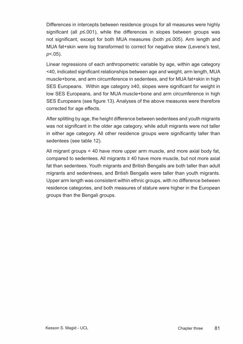
81Kesson S. Magid - UCL Chapter three
Differences in intercepts between residence groups for all measures were highly significant (all p≤.001), while the differences in slopes between groups was not significant, except for both MUA measures (both p≤.005). Arm length and MUA fat+skin were log transformed to correct for negative skew (Levene’s test, p<.05).
Linear regressions of each anthropometric variable by age, within age category <40, indicated significant relationships between age and weight, arm length, MUA muscle+bone, and arm circumference in sedentees, and for MUA fat+skin in high SES Europeans. Within age category ≥40, slopes were significant for weight in low SES Europeans, and for MUA muscle+bone and arm circumference in high SES Europeans (see figure 13). Analyses of the above measures were therefore corrected for age effects.
After splitting by age, the height difference between sedentees and youth migrants was not significant in the older age category, while adult migrants were not taller in either age category. All other residence groups were significantly taller than sedentees (see table 12).
All migrant groups < 40 have more upper arm muscle, and more axial body fat, compared to sedentees. All migrants ≥ 40 have more muscle, but not more axial fat than sedentees. Youth migrants and British Bengalis are both taller than adult migrants and sedentnees, and British Bengalis were taller than youth migrants. Upper arm length was consistent within ethnic groups, with no difference between residence categories, and both measures of stature were higher in the European groups than the Bengali groups.
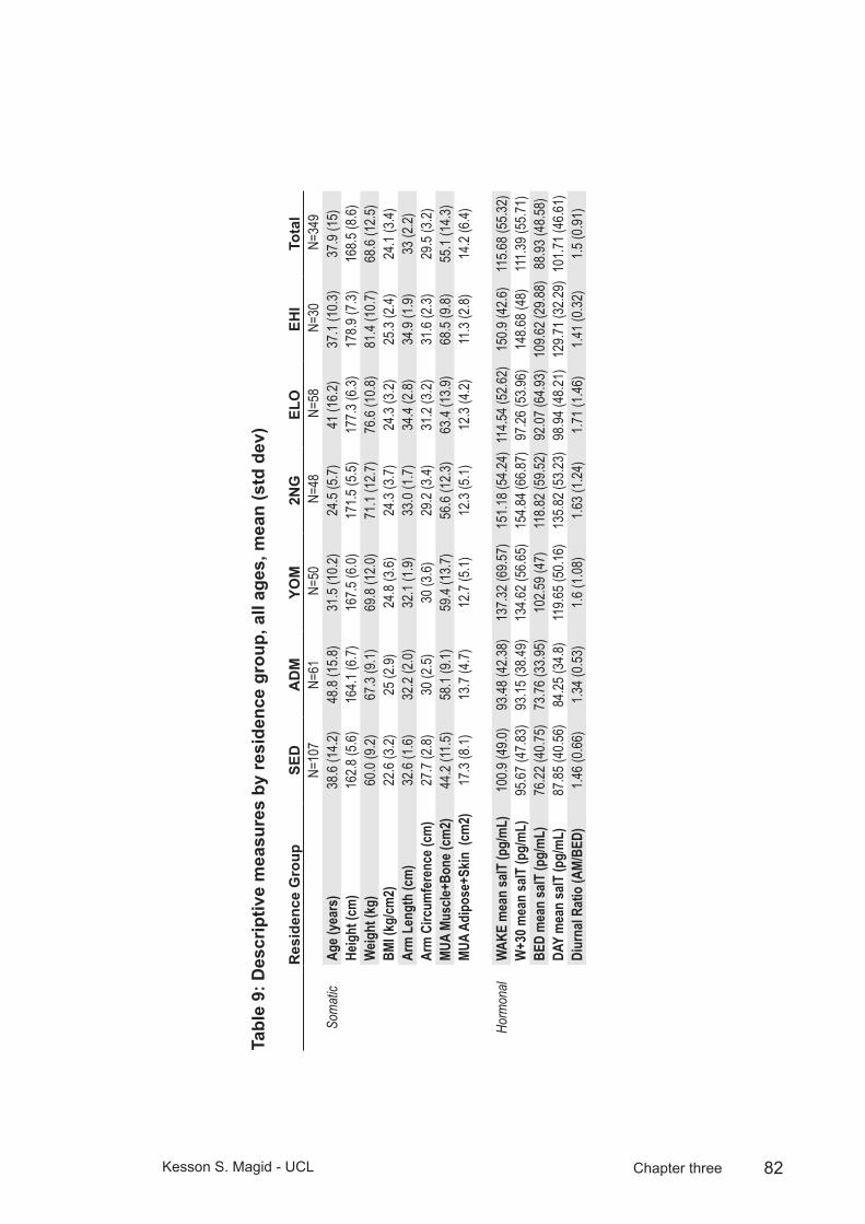
82Kesson S. Magid - UCL Chapter three
Des
crip
tive
mea
sure
s by
resi
denc
e gr
oup,
all
ages
, mea
n (s
td d
ev)
Tabl
e 9:
Res
iden
ce G
roup
SED
AD
MYO
M2N
GEL
OEH
ITo
tal
N=10
7N=
61 N
=50
N=4
8 N
=58
N=3
0 N
=349
Som
atic
Age (
year
s)38
.6 (1
4.2)
48.8
(15.8
)31
.5 (1
0.2)
24.5
(5.7)
41 (1
6.2)
37.1
(10.3
)37
.9 (1
5)He
ight
(cm
)16
2.8 (5
.6)16
4.1 (6
.7)16
7.5 (6
.0)17
1.5 (5
.5)17
7.3 (6
.3)17
8.9 (7
.3)16
8.5 (8
.6)W
eight
(kg)
60.0
(9.2)
67.3
(9.1)
69.8
(12.0
)71
.1 (1
2.7)
76.6
(10.8
)81
.4 (1
0.7)
68.6
(12.5
)BM
I (kg
/cm2)
22.6
(3.2)
25 (2
.9)24
.8 (3
.6)24
.3 (3
.7)24
.3 (3
.2)25
.3 (2
.4)24
.1 (3
.4)Ar
m L
engt
h (c
m)
32.6
(1.6)
32.2
(2.0)
32.1
(1.9)
33.0
(1.7)
34.4
(2.8)
34.9
(1.9)
33 (2
.2)Ar
m C
ircum
fere
nce (
cm)
27.7
(2.8)
30 (2
.5)30
(3.6)
29.2
(3.4)
31.2
(3.2)
31.6
(2.3)
29.5
(3.2)
MUA
Musc
le+Bo
ne (c
m2)
44.2
(11.5)
58.1
(9.1)
59.4
(13.7
)56
.6 (1
2.3)
63.4
(13.9
)68
.5 (9
.8)55
.1 (1
4.3)
MUA
Adip
ose+
Skin
(cm
2)17
.3 (8
.1)13
.7 (4
.7)12
.7 (5
.1)12
.3 (5
.1)12
.3 (4
.2)11
.3 (2
.8)14
.2 (6
.4)
Horm
onal
WAK
E m
ean
salT
(pg/
mL)
100.9
(49.0
)93
.48 (4
2.38)
137.3
2 (69
.57)
151.1
8 (54
.24)
114.5
4 (52
.62)
150.9
(42.6
)11
5.68 (
55.32
)W
+30 m
ean
salT
(pg/
mL)
95.67
(47.8
3)93
.15 (3
8.49)
134.6
2 (56
.65)
154.8
4 (66
.87)
97.26
(53.9
6)14
8.68 (
48)
111.3
9 (55
.71)
BED
mea
n sa
lT (p
g/m
L)76
.22 (4
0.75)
73.76
(33.9
5)10
2.59 (
47)
118.8
2 (59
.52)
92.07
(64.9
3)10
9.62 (
29.88
)88
.93 (4
8.58)
DAY
mea
n sa
lT (p
g/m
L)87
.85 (4
0.56)
84.25
(34.8
)11
9.65 (
50.16
)13
5.82 (
53.23
)98
.94 (4
8.21)
129.7
1 (32
.29)
101.7
1 (46
.61)
Diur
nal R
atio
(AM/
BED)
1.46 (
0.66)
1.34 (
0.53)
1.6 (1
.08)
1.63 (
1.24)
1.71 (
1.46)
1.41 (
0.32)
1.5 (0
.91)
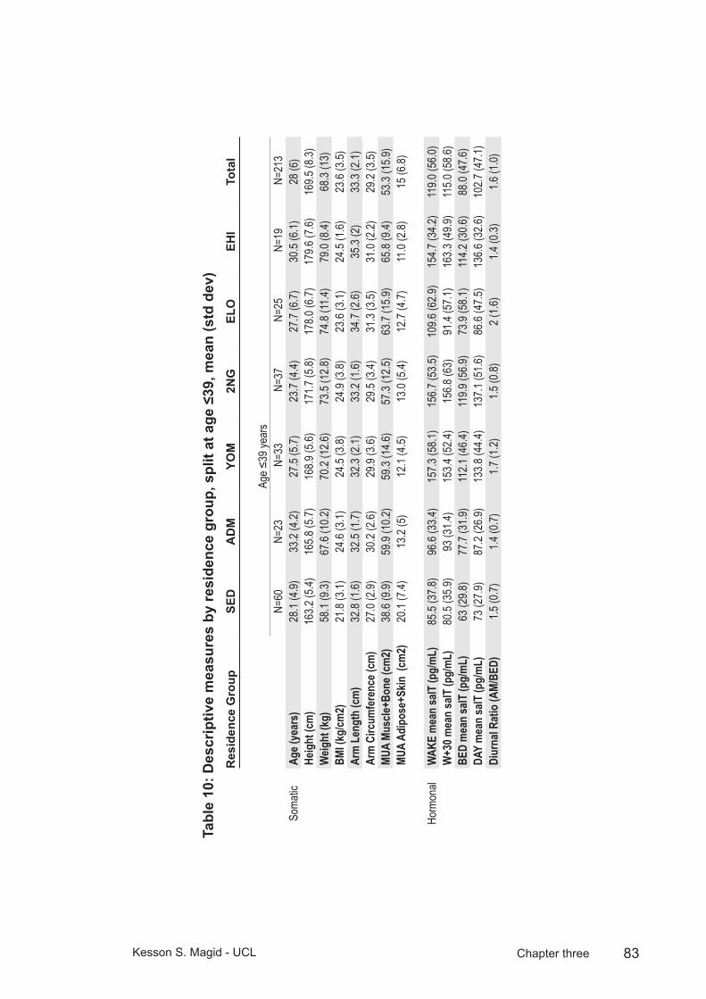
83Kesson S. Magid - UCL Chapter three
Des
crip
tive
mea
sure
s by
resi
denc
e gr
oup,
spl
it at
age
≤39
, mea
n (s
td d
ev)
Tabl
e 10
: R
esid
ence
Gro
upSE
DA
DM
YOM
2NG
ELO
EHI
Tota
l
Age ≤
39 ye
ars
N=60
N=23
N=3
3 N
=37
N=2
5 N
=19
N=2
13So
matic
Age (
year
s)28
.1 (4
.9)33
.2 (4
.2)27
.5 (5
.7)23
.7 (4
.4)27
.7 (6
.7)30
.5 (6
.1)28
(6)
Heig
ht (c
m)
163.2
(5.4)
165.8
(5.7)
168.9
(5.6)
171.7
(5.8)
178.0
(6.7)
179.6
(7.6)
169.5
(8.3)
Weig
ht (k
g)58
.1 (9
.3)67
.6 (1
0.2)
70.2
(12.6
)73
.5 (1
2.8)
74.8
(11.4)
79.0
(8.4)
68.3
(13)
BMI (
kg/cm
2)21
.8 (3
.1)24
.6 (3
.1)24
.5 (3
.8)24
.9 (3
.8)23
.6 (3
.1)24
.5 (1
.6)23
.6 (3
.5)Ar
m L
engt
h (c
m)
32.8
(1.6)
32.5
(1.7)
32.3
(2.1)
33.2
(1.6)
34.7
(2.6)
35.3
(2)
33.3
(2.1)
Arm
Circ
umfe
renc
e (cm
)27
.0 (2
.9)30
.2 (2
.6)29
.9 (3
.6)29
.5 (3
.4)31
.3 (3
.5)31
.0 (2
.2)29
.2 (3
.5)MU
A Mu
scle+
Bone
(cm
2)38
.6 (9
.9)59
.9 (1
0.2)
59.3
(14.6
)57
.3 (1
2.5)
63.7
(15.9
)65
.8 (9
.4)53
.3 (1
5.9)
MUA
Adip
ose+
Skin
(cm
2)20
.1 (7
.4)13
.2 (5
)12
.1 (4
.5)13
.0 (5
.4)12
.7 (4
.7)11
.0 (2
.8)15
(6.8)
Horm
onal
WAK
E m
ean
salT
(pg/
mL)
85.5
(37.8
)96
.6 (3
3.4)
157.3
(58.1
)15
6.7 (5
3.5)
109.6
(62.9
)15
4.7 (3
4.2)
119.0
(56.0
)W
+30 m
ean
salT
(pg/
mL)
80.5
(35.9
)93
(31.4
)15
3.4 (5
2.4)
156.8
(63)
91.4
(57.1
)16
3.3 (4
9.9)
115.0
(58.6
)BE
D m
ean
salT
(pg/
mL)
63 (2
9.8)
77.7
(31.9
)11
2.1 (4
6.4)
119.9
(56.9
)73
.9 (5
8.1)
114.2
(30.6
)88
.0 (4
7.6)
DAY
mea
n sa
lT (p
g/m
L)73
(27.9
)87
.2 (2
6.9)
133.8
(44.4
)13
7.1 (5
1.6)
86.6
(47.5
)13
6.6 (3
2.6)
102.7
(47.1
)Di
urna
l Rat
io (A
M/BE
D)1.5
(0.7)
1.4 (0
.7)1.7
(1.2)
1.5 (0
.8)2 (
1.6)
1.4 (0
.3)1.6
(1.0)

84Kesson S. Magid - UCL Chapter three
Des
crip
tive
mea
sure
s by
resi
denc
e gr
oup,
spl
it at
age
≥40
, mea
n (s
td d
ev)
Tabl
e 11
:
Res
iden
ce G
roup
SED
AD
MYO
M2N
GEL
OEH
ITo
tal
Age ≥
40 ye
ars
N=45
N=34
N=7
N=2
N=2
7 N
=11
N=1
33So
matic
Age (
year
s)52
.6 (9
.6)59
.6 (11
.1)47
.4 (8
.5)41
(1.4)
54.3
(11)
48.5
(3.6)
54 (1
0.6)
Heig
ht (c
m)
161.9
(5.8)
163.6
(6.8)
161 (
5.2)
171.8
(6.5)
176.1
(5.9)
177.7
(7.2)
166.9
(8.9)
Weig
ht (k
g)62
.1 (8
.6)67
(9.3)
64.9
(10.5
)68
.4 (4
.8)78
.4 (1
0.5)
85.6
(13.1
)69
.2 (1
2.4)
BMI (
kg/cm
2)23
.6 (3
.1)25
(2.8)
24.9
(2.9)
23.2
(0.1)
25.2
(3.2)
26.7
(3)
24.7
(3.1)
Arm
Len
gth
(cm
)32
.2 (1
.6)32
.1 (1
.9)31
.6 (1
)32
.8 (0
.4)34
.1 (3
)34
.4 (1
.6)32
.8 (2
.2)Ar
m C
ircum
fere
nce (
cm)
28.6
(2.5)
29.6
(2.4)
30.2
(3.2)
29.3
(0.7)
31.2
(3)
32.6
(2.2)
29.8
(2.9)
MUA
Musc
le+Bo
ne (c
m2)
52 (8
.9)56
.7 (8
.7)59
.4 (11
.1)54
(1.2)
63.7
(12)
73.2
(9.2)
57.8
(11.4)
MUA
Adip
ose+
Skin
(cm
2)13
.3 (7
.3)13
.4 (4
.2)13
.8 (5
.2)14
.3 (4
.2)12
.2 (3
.6)11
.8 (2
.9)13
(5.5)
Horm
onal
WAK
E m
ean
salT
(pg/
mL)
121.1
(54.9
)84
.1 (4
1)73
.7 (5
2.1)
151.4
(12.5
)11
2.2 (4
4.4)
144.4
(55.5
)10
9.0 (5
2.4)
W+3
0 mea
n sa
lT (p
g/m
L)11
5.8 (5
4.1)
85.5
(40.1
)89
.8 (4
4.4)
106.9
(45.6
)10
0.1 (5
3.1)
123.5
(33.1
)10
4.3 (4
9.5)
BED
mea
n sa
lT (p
g/m
L)93
.8 (4
6.4)
65.6
(33.3
)70
.9 (4
5.1)
76.1
(40.3
)10
4.5 (6
8.4)
101.8
(28.3
)87
.5 (4
9.1)
DAY
mea
n sa
lT (p
g/m
L)10
7.3 (4
6)76
.5 (3
6.9)
74.3
(35.6
)10
2.6 (3
4.7)
104.9
(48.9
)11
7.9 (2
9.4)
97.2
(44.4
)Di
urna
l Rat
io (A
M/BE
D)1.4
(0.6)
1.3 (0
.4)1.5
(0.6)
1.9 (0
.6)1.5
(1.4)
1.4 (0
.4)1.4
(0.8)
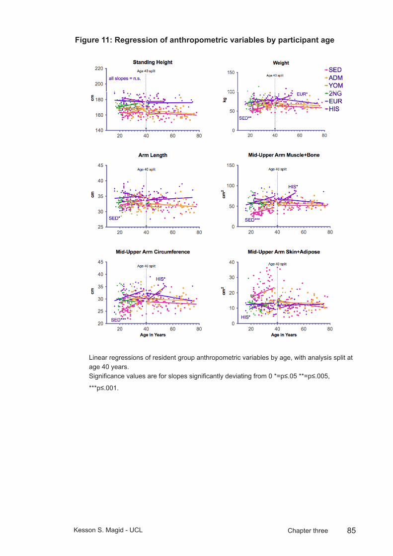
85Kesson S. Magid - UCL Chapter three
Regression of anthropometric variables by participant ageFigure 11:
Fig 1:
Figure 1: Linear regressions of resident group anthropometric variables by age, with analysis split at age 40 years.
Significance values are for slopes significantly deviating from 0 *=p≤.05 **=p≤.005, ***p≤.001.
Linear regressions of resident group anthropometric variables by age, with analysis split at age 40 years.Significance values are for slopes significantly deviating from 0 *=p≤.05 **=p≤.005,
***p≤.001.

86Kesson S. Magid - UCL Chapter three
General anthropometric measuresFigure 12:
Standing Height
SED ADM YOM 2NG EUR HIS100
120
140
160
180
200cm
Arm Length
SED ADM YOM 2NG ELO EHI30
32
34
36
38
40
cm
Weight
SED ADM YOM 2NG ELO EHI0
20
40
60
80
100
kg
BMI
SED ADM YOM 2NG ELO EHI0
10
20
30
40
kg
/m2
Age ≥40Age <40
Mid-upper arm anthropometric measuresFigure 13:
Fig. 3: Mid-upper arm anthropometric measures
Figure 3: Resident group anthropometric variables by age, with analysis split at age 40 years.
Figure 12 and 13: Resident group anthropometric variables by age, with analysis split at age 40 years. Error: ± 95% CI.

87Kesson S. Magid - UCL Chapter three
The covariate, participant age, was significantly related to resident group, F(1,257) = 4.08, p < .005, partial η2 = .07, so an interaction effect was included in the model. After correcting for variance due to age and BMI, residence was a significant predictor of salT at all three sample times WAKE: F(6,257) = 10.80, p < .005, partial η2 = .17; W+30: F(6,263) = 11.67, p < .005, partial η2 = .18; BED: F(6,269) = 6.22, p < .005, partial η2 = .10.
Planned contrasts (MLR-II) revealed that levels of salT in youth migrants (127.7 ±8.1 pg/mL) and British-born Bengalis (136.6 ±8.9 pg/mL), but not adult migrants (78.2 ±6.0 pg/mL) were significantly higher than sedentees (90.7 ±4.3 pg/mL). Among the European males, salT of low SES men (95.4 ±6.5 pg/mL) was not significantly different from either sedentees or adult migrants, while high SES men (127.5 ±7.7 pg/mL) had significantly greater salT concentrations than low status men, sedentees, or adult migrants, but were not different from youth migrants or British-born Bengalis (table 16, 17, 18 and 19).
Residence group differences in salT were greater in younger men than in older men. After splitting the older from younger group, the interaction effect between residence group and age was no longer significant.
Salivary T levels were not different between adult migrants and sedentees <40. In contrast, sedentee morning and evening salT is greater than that of adult migrants ≤40 (see fig. 14). Youth migrants and British-born Bengalis under 40 show no significant difference in salT, and have greater salT at all time points than sedentees, and greater morning, but not evening salT compared to adult migrants. Under 40 year olds in all Bengali groups resident in London have greater salT compared to low SES Europeans, but youth migrants and British-born Bengalis show no difference from high SES Europeans. High SES European salT is greater than sedentees, low SES Europeans, and morning samples from adult migrants.
Differences in salT were largest between morning samples from the younger men in all groups (tables 16 and 17). Youth migrants, British-born Bengalis and high status Europeans had significantly greater salT than sedentees at all three sample times (p < .001). High SES European salT was higher than low SES Europeans (p < .001). Post hoc Sidak comparisons within age <40 indicated significant differences between adult migrants and youth migrants, British-born Bengalis and high SES Europeans for both AM samples (p < .005), and between low SES Europeans and both youth migrants and British-born Bengalis for all three daily samples (AM samples p < .005; BED: p < .05) (see tables16,17 and 18).

88Kesson S. Magid - UCL Chapter three
Age at migration and salivary T
In MLR-I, age at migration significantly predicted salT, F(4,74)=3.2 p=.017, partial η2 = .14. Planned contrasts showed the difference between childhood migrants (aged 3-12) and adult migrants was significant (p=.049), while the contrasts between all other stages of migration and older adult migrants were not significant. Inclusion of British-born Bengalis (MLR-III) or combining them with infant migrants into one group (MLR-IV) failed to improve the model, MLR-III: F(5,99)=2.37 p=.045, MLR-IV: F(4,100)=2.99. None of the planned contrasts in MLR-II or III were significant.
Thus, child migrants who arrived aged 3-12 years have significantly greater levels of salT than adult migrants who arrived at ages 18-30, but infants (aged 2 or under) and adolescent migrants (aged 13-17) were not measurably different from the adult migrant group. However, the small sample size of infant migrants (n=6) limits the likelihood of detecting a difference in this group.
Diurnal salT ratio and residence group
Residence group showed no significant relationship with diurnal ratio of AM/PM salT, within either age group <40: F(5,153)=0.35 p=.88 or age group ≥40: F(5,106)=.45 p=.82. MLR of residential differences in AM variance showed the variance in sedentees to be greater than adult migrants <40 years (p=.035) and ≥40 to be greater than adult migrants (p<.001), and both low and high SES European groups (p=.011 and .031, respectively).
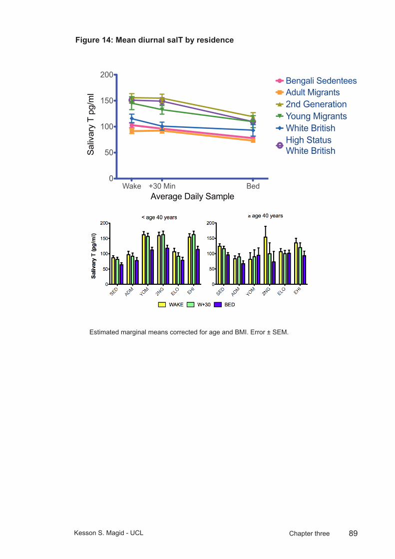
89Kesson S. Magid - UCL Chapter three
Mean diurnal salT by residenceFigure 14:
Wake +30 Min Bed0
50
100
150
200Bengali SedenteesAdult Migrants2nd GenerationYoung MigrantsWhite BritishHigh Status White British
Average Daily Sample
Sal
ivar
y T
pg/m
l
Estimated marginal means corrected for age and BMI. Error ± SEM.
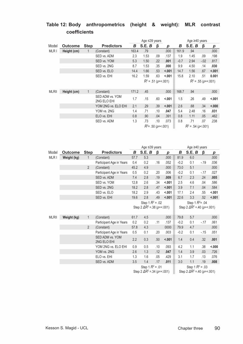
90Kesson S. Magid - UCL Chapter three
Body anthropometrics (height & weight): MLR contrast Table 12: coefficients
Age ≤39 years Age ≥40 yearsModel Outcome Step Predictors B S.E. B β p B S.E. B β pMLR I Height (cm) 1 (Constant) 163.4 .79 .000 161.9 .94 .000
SED vs. ADM 2.3 1.53 .09 .137 1.9 1.45 .09 .198SED vs. YOM 5.3 1.50 .22 .001 -0.7 2.94 -.02 .817SED vs. 2NG 8.7 1.53 .35 .000 9.9 4.50 .14 .030SED vs. ELO 14.4 1.66 .53 <.001 14.7 1.56 .67 <.001SED vs. EHI 16.2 1.59 .63 <.001 15.8 2.10 .51 0.001
R2 = .51 (p=<.001) R2 = .55 (p=<.001)
MLRII Height (cm) 1 (Constant) 171.2 .45 .000 168.7 .94 .000SED ADM vs. YOM 2NG ELO EHI 1.7 .15 .60 <.001 1.5 .26 .49 <.001
YOM 2NG vs. ELO EHI 2.1 .29 .39 <.001 2.6 .68 .34 <.000YOM vs. 2NG 1.4 .71 .10 .047 5.4 2.48 .16 .031ELO vs. EHI 0.8 .90 .04 .391 0.8 1.11 .05 .462SED vs. ADM 1.3 .73 .10 .073 0.8 .71 .07 .238
R2= .50 (p=<.001) R2 = .54 (p<.001)
Age ≤39 years Age ≥40 yearsModel Outcome Step Predictors B S.E. B β p B S.E. B β pMLR I Weight (kg) 1 (Constant) 57.7 5.3 .000 81.9 6.0 .000
Participant Age in Years 0.4 0.2 .16 .052 -0.2 0.1 -.19 .0362 (Constant) 45.2 4.9 .000 73.0 5.1 .000
Participant Age in Years 0.5 0.2 .20 .006 -0.2 0.1 -.17 .027SED vs. ADM 7.4 2.8 .19 .009 6.7 2.3 .24 .005SED vs. YOM 12.8 2.6 .34 <.001 2.5 4.6 .04 .586SED vs. 2NG 18.2 2.8 .47 <.001 3.9 7.1 .04 .584SED vs. ELO 18.2 2.9 .43 <.001 17.1 2.4 .55 <.001SED vs. EHI 19.6 2.8 .49 <.001 22.6 3.3 .52 <.001
Step 1 R2 = .02 Step 2 ΔR2 =.38 (p=<.001)
Step 1 R2= .04 Step 2 ΔR2 =.40 (p=<.001)
MLRII Weight (kg) 1 (Constant) 61.7 4.5 .000 79.8 5.7 .000Participant Age in Years 0.2 0.2 .11 .137 -0.2 0.1 -.17 .061
2 (Constant) 57.8 4.3 0000 79.9 4.7 .000Participant Age in Years 0.5 0.1 .20 .003 -0.2 0.1 -.15 .051SED ADM vs. YOM 2NG ELO EHI 2.2 0.3 .50 <.001 1.4 0.4 .32 .001
YOM 2NG vs. ELO EHI 0.9 0.5 .10 .093 4.2 1.1 .38 <.000YOM vs. 2NG 2.6 1.3 .12 .047 1.4 3.9 .03 .726ELO vs. EHI 1.3 1.6 .05 .429 3.1 1.7 .13 .076SED vs. ADM 3.5 1.4 .17 .011 3.0 1.1 .19 .008
Step 1 R2 = .01 Step 2 ΔR2 =.34 (p=<.001)
Step 1 R2 = .03 Step 2 ΔR2 =.40 (p=<.001)
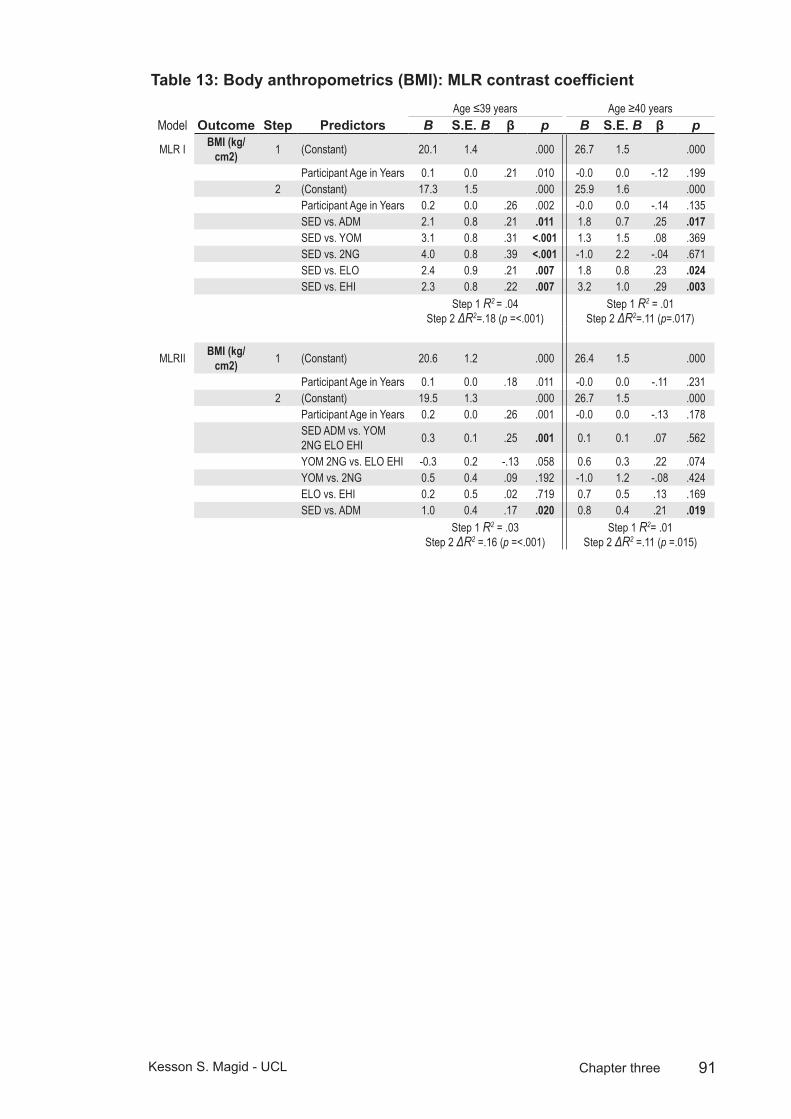
91Kesson S. Magid - UCL Chapter three
Body anthropometrics (BMI): MLR contrast coefficientTable 13: Age ≤39 years Age ≥40 years
Model Outcome Step Predictors B S.E. B β p B S.E. B β p
MLR I BMI (kg/cm2) 1 (Constant) 20.1 1.4 .000 26.7 1.5 .000
Participant Age in Years 0.1 0.0 .21 .010 -0.0 0.0 -.12 .1992 (Constant) 17.3 1.5 .000 25.9 1.6 .000
Participant Age in Years 0.2 0.0 .26 .002 -0.0 0.0 -.14 .135SED vs. ADM 2.1 0.8 .21 .011 1.8 0.7 .25 .017SED vs. YOM 3.1 0.8 .31 <.001 1.3 1.5 .08 .369SED vs. 2NG 4.0 0.8 .39 <.001 -1.0 2.2 -.04 .671SED vs. ELO 2.4 0.9 .21 .007 1.8 0.8 .23 .024SED vs. EHI 2.3 0.8 .22 .007 3.2 1.0 .29 .003
Step 1 R2 = .04 Step 2 ΔR2=.18 (p =<.001)
Step 1 R2 = .01 Step 2 ΔR2=.11 (p=.017)
MLRII BMI (kg/cm2) 1 (Constant) 20.6 1.2 .000 26.4 1.5 .000
Participant Age in Years 0.1 0.0 .18 .011 -0.0 0.0 -.11 .2312 (Constant) 19.5 1.3 .000 26.7 1.5 .000
Participant Age in Years 0.2 0.0 .26 .001 -0.0 0.0 -.13 .178SED ADM vs. YOM 2NG ELO EHI 0.3 0.1 .25 .001 0.1 0.1 .07 .562
YOM 2NG vs. ELO EHI -0.3 0.2 -.13 .058 0.6 0.3 .22 .074YOM vs. 2NG 0.5 0.4 .09 .192 -1.0 1.2 -.08 .424ELO vs. EHI 0.2 0.5 .02 .719 0.7 0.5 .13 .169SED vs. ADM 1.0 0.4 .17 .020 0.8 0.4 .21 .019
Step 1 R2 = .03 Step 2 ΔR2 =.16 (p =<.001)
Step 1 R2= .01 Step 2 ΔR2 =.11 (p =.015)
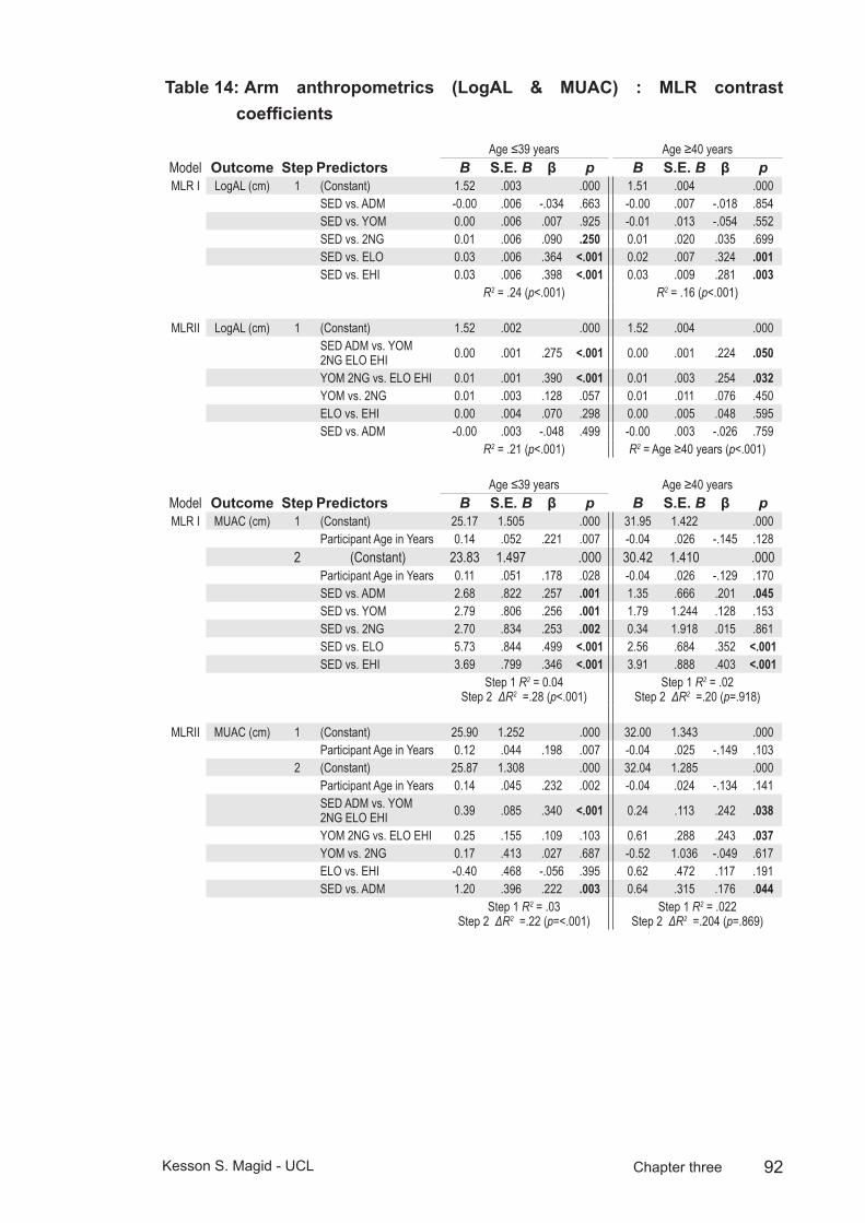
92Kesson S. Magid - UCL Chapter three
Arm anthropometrics (LogAL & MUAC) : MLR contrast Table 14: coefficients
Age ≤39 years Age ≥40 yearsModel Outcome Step Predictors B S.E. B β p B S.E. B β pMLR I LogAL (cm) 1 (Constant) 1.52 .003 .000 1.51 .004 .000
SED vs. ADM -0.00 .006 -.034 .663 -0.00 .007 -.018 .854SED vs. YOM 0.00 .006 .007 .925 -0.01 .013 -.054 .552SED vs. 2NG 0.01 .006 .090 .250 0.01 .020 .035 .699SED vs. ELO 0.03 .006 .364 <.001 0.02 .007 .324 .001SED vs. EHI 0.03 .006 .398 <.001 0.03 .009 .281 .003
R2 = .24 (p<.001) R2 = .16 (p<.001)
MLRII LogAL (cm) 1 (Constant) 1.52 .002 .000 1.52 .004 .000SED ADM vs. YOM 2NG ELO EHI 0.00 .001 .275 <.001 0.00 .001 .224 .050
YOM 2NG vs. ELO EHI 0.01 .001 .390 <.001 0.01 .003 .254 .032YOM vs. 2NG 0.01 .003 .128 .057 0.01 .011 .076 .450ELO vs. EHI 0.00 .004 .070 .298 0.00 .005 .048 .595SED vs. ADM -0.00 .003 -.048 .499 -0.00 .003 -.026 .759
R2 = .21 (p<.001) R2 = Age ≥40 years (p<.001)
Age ≤39 years Age ≥40 yearsModel Outcome Step Predictors B S.E. B β p B S.E. B β pMLR I MUAC (cm) 1 (Constant) 25.17 1.505 .000 31.95 1.422 .000
Participant Age in Years 0.14 .052 .221 .007 -0.04 .026 -.145 .1282 (Constant) 23.83 1.497 .000 30.42 1.410 .000
Participant Age in Years 0.11 .051 .178 .028 -0.04 .026 -.129 .170SED vs. ADM 2.68 .822 .257 .001 1.35 .666 .201 .045SED vs. YOM 2.79 .806 .256 .001 1.79 1.244 .128 .153SED vs. 2NG 2.70 .834 .253 .002 0.34 1.918 .015 .861SED vs. ELO 5.73 .844 .499 <.001 2.56 .684 .352 <.001SED vs. EHI 3.69 .799 .346 <.001 3.91 .888 .403 <.001
Step 1 R2 = 0.04 Step 2 ΔR2 =.28 (p<.001)
Step 1 R2 = .02 Step 2 ΔR2 =.20 (p=.918)
MLRII MUAC (cm) 1 (Constant) 25.90 1.252 .000 32.00 1.343 .000Participant Age in Years 0.12 .044 .198 .007 -0.04 .025 -.149 .103
2 (Constant) 25.87 1.308 .000 32.04 1.285 .000Participant Age in Years 0.14 .045 .232 .002 -0.04 .024 -.134 .141SED ADM vs. YOM 2NG ELO EHI 0.39 .085 .340 <.001 0.24 .113 .242 .038
YOM 2NG vs. ELO EHI 0.25 .155 .109 .103 0.61 .288 .243 .037YOM vs. 2NG 0.17 .413 .027 .687 -0.52 1.036 -.049 .617ELO vs. EHI -0.40 .468 -.056 .395 0.62 .472 .117 .191SED vs. ADM 1.20 .396 .222 .003 0.64 .315 .176 .044
Step 1 R2 = .03 Step 2 ΔR2 =.22 (p=<.001)
Step 1 R2 = .022 Step 2 ΔR2 =.204 (p=.869)
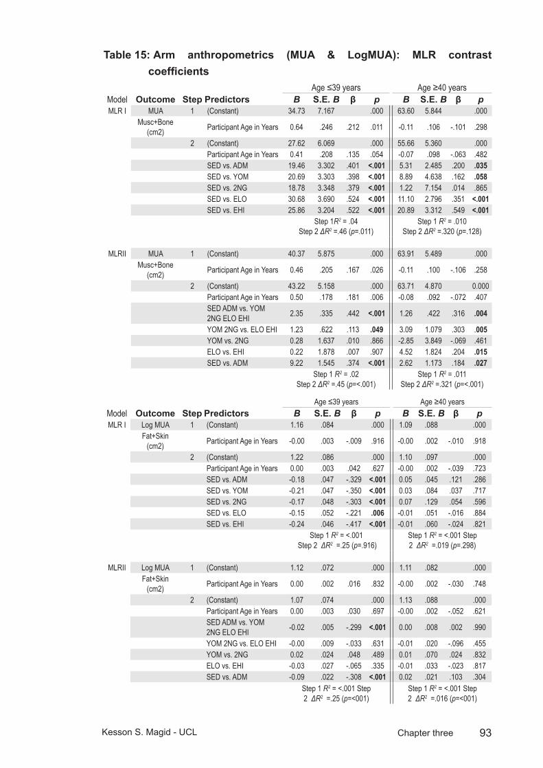
93Kesson S. Magid - UCL Chapter three
Arm anthropometrics (MUA & LogMUA): MLR contrast Table 15: coefficients
Age ≤39 years Age ≥40 yearsModel Outcome Step Predictors B S.E. B β p B S.E. B β pMLR I MUA 1 (Constant) 34.73 7.167 .000 63.60 5.844 .000
Musc+Bone (cm2) Participant Age in Years 0.64 .246 .212 .011 -0.11 .106 -.101 .298
2 (Constant) 27.62 6.069 .000 55.66 5.360 .000Participant Age in Years 0.41 .208 .135 .054 -0.07 .098 -.063 .482SED vs. ADM 19.46 3.302 .401 <.001 5.31 2.485 .200 .035SED vs. YOM 20.69 3.303 .398 <.001 8.89 4.638 .162 .058SED vs. 2NG 18.78 3.348 .379 <.001 1.22 7.154 .014 .865SED vs. ELO 30.68 3.690 .524 <.001 11.10 2.796 .351 <.001SED vs. EHI 25.86 3.204 .522 <.001 20.89 3.312 .549 <.001
Step 1R2 = .04 Step 2 ΔR2 =.46 (p=.011)
Step 1 R2 = .010 Step 2 ΔR2 =.320 (p=.128)
MLRII MUA 1 (Constant) 40.37 5.875 .000 63.91 5.489 .000Musc+Bone
(cm2) Participant Age in Years 0.46 .205 .167 .026 -0.11 .100 -.106 .258
2 (Constant) 43.22 5.158 .000 63.71 4.870 0.000Participant Age in Years 0.50 .178 .181 .006 -0.08 .092 -.072 .407SED ADM vs. YOM 2NG ELO EHI 2.35 .335 .442 <.001 1.26 .422 .316 .004
YOM 2NG vs. ELO EHI 1.23 .622 .113 .049 3.09 1.079 .303 .005YOM vs. 2NG 0.28 1.637 .010 .866 -2.85 3.849 -.069 .461ELO vs. EHI 0.22 1.878 .007 .907 4.52 1.824 .204 .015SED vs. ADM 9.22 1.545 .374 <.001 2.62 1.173 .184 .027
Step 1 R2 = .02 Step 2 ΔR2 =.45 (p=<.001)
Step 1 R2 = .011 Step 2 ΔR2 =.321 (p=<.001)
Age ≤39 years Age ≥40 yearsModel Outcome Step Predictors B S.E. B β p B S.E. B β pMLR I Log MUA 1 (Constant) 1.16 .084 .000 1.09 .088 .000
Fat+Skin (cm2) Participant Age in Years -0.00 .003 -.009 .916 -0.00 .002 -.010 .918
2 (Constant) 1.22 .086 .000 1.10 .097 .000Participant Age in Years 0.00 .003 .042 .627 -0.00 .002 -.039 .723SED vs. ADM -0.18 .047 -.329 <.001 0.05 .045 .121 .286SED vs. YOM -0.21 .047 -.350 <.001 0.03 .084 .037 .717SED vs. 2NG -0.17 .048 -.303 <.001 0.07 .129 .054 .596SED vs. ELO -0.15 .052 -.221 .006 -0.01 .051 -.016 .884SED vs. EHI -0.24 .046 -.417 <.001 -0.01 .060 -.024 .821
Step 1 R2 = <.001 Step 2 ΔR2 =.25 (p=.916)
Step 1 R2 = <.001 Step 2 ΔR2 =.019 (p=.298)
MLRII Log MUA 1 (Constant) 1.12 .072 .000 1.11 .082 .000Fat+Skin
(cm2) Participant Age in Years 0.00 .002 .016 .832 -0.00 .002 -.030 .748
2 (Constant) 1.07 .074 .000 1.13 .088 .000Participant Age in Years 0.00 .003 .030 .697 -0.00 .002 -.052 .621SED ADM vs. YOM 2NG ELO EHI -0.02 .005 -.299 <.001 0.00 .008 .002 .990
YOM 2NG vs. ELO EHI -0.00 .009 -.033 .631 -0.01 .020 -.096 .455YOM vs. 2NG 0.02 .024 .048 .489 0.01 .070 .024 .832ELO vs. EHI -0.03 .027 -.065 .335 -0.01 .033 -.023 .817SED vs. ADM -0.09 .022 -.308 <.001 0.02 .021 .103 .304
Step 1 R2 = <.001 Step 2 ΔR2 =.25 (p=<001)
Step 1 R2 = <.001 Step 2 ΔR2 =.016 (p=<001)
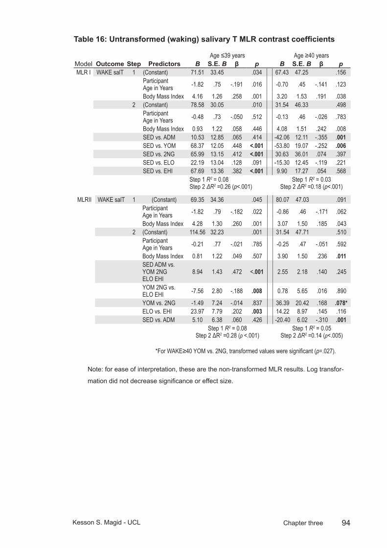
94Kesson S. Magid - UCL Chapter three
Untransformed (waking) salivary T MLR contrast coefficientsTable 16:
Age ≤39 years Age ≥40 yearsModel Outcome Step Predictors B S.E. B β p B S.E. B β pMLR I WAKE salT 1 (Constant) 71.51 33.45 .034 67.43 47.25 .156
Participant Age in Years -1.82 .75 -.191 .016 -0.70 .45 -.141 .123
Body Mass Index 4.16 1.26 .258 .001 3.20 1.53 .191 .0382 (Constant) 78.58 30.05 .010 31.54 46.33 .498
Participant Age in Years -0.48 .73 -.050 .512 -0.13 .46 -.026 .783
Body Mass Index 0.93 1.22 .058 .446 4.08 1.51 .242 .008SED vs. ADM 10.53 12.85 .065 .414 -42.06 12.11 -.355 .001SED vs. YOM 68.37 12.05 .448 <.001 -53.80 19.07 -.252 .006SED vs. 2NG 65.99 13.15 .412 <.001 30.63 36.01 .074 .397SED vs. ELO 22.19 13.04 .128 .091 -15.30 12.45 -.119 .221SED vs. EHI 67.69 13.36 .382 <.001 9.90 17.27 .054 .568
Step 1 R2 = 0.08 Step 2 ΔR2 =0.26 (p<.001)
Step 1 R2 = 0.03 Step 2 ΔR2 =0.18 (p<.001)
MLRII WAKE salT 1 (Constant) 69.35 34.36 .045 80.07 47.03 .091Participant Age in Years -1.82 .79 -.182 .022 -0.86 .46 -.171 .062
Body Mass Index 4.28 1.30 .260 .001 3.07 1.50 .185 .0432 (Constant) 114.56 32.23 .001 31.54 47.71 .510
Participant Age in Years -0.21 .77 -.021 .785 -0.25 .47 -.051 .592
Body Mass Index 0.81 1.22 .049 .507 3.90 1.50 .236 .011SED ADM vs. YOM 2NG ELO EHI
8.94 1.43 .472 <.001 2.55 2.18 .140 .245
YOM 2NG vs. ELO EHI -7.56 2.80 -.188 .008 0.78 5.65 .016 .890
YOM vs. 2NG -1.49 7.24 -.014 .837 36.39 20.42 .168 .078*ELO vs. EHI 23.97 7.79 .202 .003 14.22 8.97 .145 .116SED vs. ADM 5.10 6.38 .060 .426 -20.40 6.02 -.310 .001
Step 1 R2 = 0.08 Step 2 ΔR2 =0.28 (p <.001)
Step 1 R2 = 0.05 Step 2 ΔR2 =0.14 (p<.005)
*For WAKE≥40 YOM vs. 2NG, transformed values were significant (p=.027).
Note: for ease of interpretation, these are the non-transformed MLR results. Log transfor-
mation did not decrease significance or effect size.
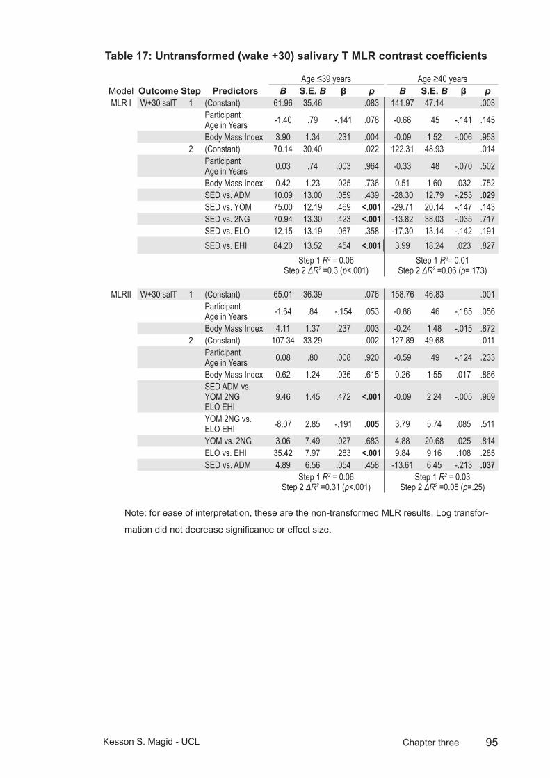
95Kesson S. Magid - UCL Chapter three
Untransformed (wake +30) salivary T MLR contrast coefficientsTable 17:
Age ≤39 years Age ≥40 yearsModel Outcome Step Predictors B S.E. B β p B S.E. B β pMLR I W+30 salT 1 (Constant) 61.96 35.46 .083 141.97 47.14 .003
Participant Age in Years -1.40 .79 -.141 .078 -0.66 .45 -.141 .145
Body Mass Index 3.90 1.34 .231 .004 -0.09 1.52 -.006 .9532 (Constant) 70.14 30.40 .022 122.31 48.93 .014
Participant Age in Years 0.03 .74 .003 .964 -0.33 .48 -.070 .502
Body Mass Index 0.42 1.23 .025 .736 0.51 1.60 .032 .752SED vs. ADM 10.09 13.00 .059 .439 -28.30 12.79 -.253 .029SED vs. YOM 75.00 12.19 .469 <.001 -29.71 20.14 -.147 .143SED vs. 2NG 70.94 13.30 .423 <.001 -13.82 38.03 -.035 .717SED vs. ELO 12.15 13.19 .067 .358 -17.30 13.14 -.142 .191SED vs. EHI 84.20 13.52 .454 <.001 3.99 18.24 .023 .827
Step 1 R2 = 0.06 Step 2 ΔR2 =0.3 (p<.001)
Step 1 R2= 0.01 Step 2 ΔR2 =0.06 (p=.173)
MLRII W+30 salT 1 (Constant) 65.01 36.39 .076 158.76 46.83 .001Participant Age in Years -1.64 .84 -.154 .053 -0.88 .46 -.185 .056
Body Mass Index 4.11 1.37 .237 .003 -0.24 1.48 -.015 .8722 (Constant) 107.34 33.29 .002 127.89 49.68 .011
Participant Age in Years 0.08 .80 .008 .920 -0.59 .49 -.124 .233
Body Mass Index 0.62 1.24 .036 .615 0.26 1.55 .017 .866SED ADM vs. YOM 2NG ELO EHI
9.46 1.45 .472 <.001 -0.09 2.24 -.005 .969
YOM 2NG vs. ELO EHI -8.07 2.85 -.191 .005 3.79 5.74 .085 .511
YOM vs. 2NG 3.06 7.49 .027 .683 4.88 20.68 .025 .814ELO vs. EHI 35.42 7.97 .283 <.001 9.84 9.16 .108 .285SED vs. ADM 4.89 6.56 .054 .458 -13.61 6.45 -.213 .037
Step 1 R2 = 0.06 Step 2 ΔR2 =0.31 (p<.001)
Step 1 R2 = 0.03 Step 2 ΔR2 =0.05 (p=.25)
Note: for ease of interpretation, these are the non-transformed MLR results. Log transfor-
mation did not decrease significance or effect size.
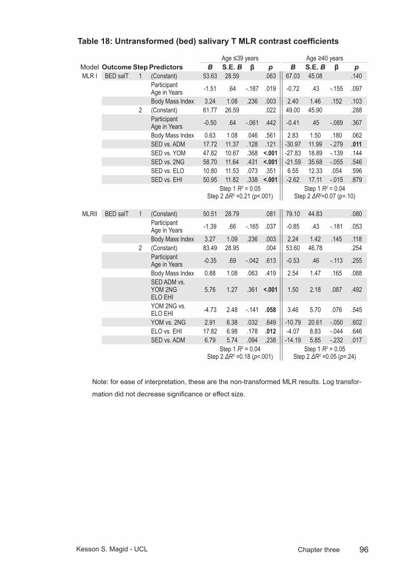
96Kesson S. Magid - UCL Chapter three
Untransformed (bed) salivary T MLR contrast coefficientsTable 18:
Age ≤39 years Age ≥40 yearsModel Outcome Step Predictors B S.E. B β p B S.E. B β pMLR I BED salT 1 (Constant) 53.63 28.59 .063 67.03 45.08 .140
Participant Age in Years -1.51 .64 -.187 .019 -0.72 .43 -.155 .097
Body Mass Index 3.24 1.08 .236 .003 2.40 1.46 .152 .1032 (Constant) 61.77 26.59 .022 49.00 45.90 .288
Participant Age in Years -0.50 .64 -.061 .442 -0.41 .45 -.089 .367
Body Mass Index 0.63 1.08 .046 .561 2.83 1.50 .180 .062SED vs. ADM 17.72 11.37 .128 .121 -30.97 11.99 -.279 .011SED vs. YOM 47.82 10.67 .368 <.001 -27.83 18.89 -.139 .144SED vs. 2NG 58.70 11.64 .431 <.001 -21.59 35.68 -.055 .546SED vs. ELO 10.80 11.53 .073 .351 6.55 12.33 .054 .596SED vs. EHI 50.95 11.82 .338 <.001 -2.62 17.11 -.015 .879
Step 1 R2 = 0.05 Step 2 ΔR2 =0.21 (p<.001)
Step 1 R2 = 0.04 Step 2 ΔR2=0.07 (p=.10)
MLRII BED salT 1 (Constant) 50.51 28.79 .081 79.10 44.83 .080Participant Age in Years -1.39 .66 -.165 .037 -0.85 .43 -.181 .053
Body Mass Index 3.27 1.09 .236 .003 2.24 1.42 .145 .1182 (Constant) 83.49 28.95 .004 53.60 46.78 .254
Participant Age in Years -0.35 .69 -.042 .613 -0.53 .46 -.113 .255
Body Mass Index 0.88 1.08 .063 .419 2.54 1.47 .165 .088SED ADM vs. YOM 2NG ELO EHI
5.76 1.27 .361 <.001 1.50 2.18 .087 .492
YOM 2NG vs. ELO EHI -4.73 2.48 -.141 .058 3.46 5.70 .076 .545
YOM vs. 2NG 2.91 6.38 .032 .649 -10.79 20.61 -.050 .602ELO vs. EHI 17.82 6.98 .178 .012 -4.07 8.83 -.044 .646SED vs. ADM 6.79 5.74 .094 .238 -14.19 5.85 -.232 .017
Step 1 R2 = 0.04 Step 2 ΔR2 =0.18 (p<.001)
Step 1 R2 = 0.05 Step 2 ΔR2 =0.05 (p=.24)
Note: for ease of interpretation, these are the non-transformed MLR results. Log transfor-
mation did not decrease significance or effect size.

97Kesson S. Magid - UCL Chapter three
Untransformed (day mean) salivary T MLR contrast coefficientsTable 19:
Age ≤39 years Age ≥40 yearsModel Outcome Step Predictors B S.E. B β p B S.E. B β p
MLR I DAYM salT 1 (Constant) 62.85 28.04 .026 85.24 40.22 .036
Participant Age in Years -1.61 .62 -.201 .011 -0.70 .38 -.168 .068
Body Mass Index 3.58 1.06 .264 .001 2.02 1.30 .142 .1232 (Constant) 71.11 24.22 .004 62.60 40.49 .125
Participant Age in Years -0.42 .59 -.053 .475 -0.34 .40 -.081 .401
Body Mass Index 0.60 .98 .044 .544 2.65 1.32 .186 .047SED vs. ADM 14.69 10.35 .107 .158 -33.24 10.58 -.331 .002SED vs. YOM 60.11 9.71 .468 <.001 -37.97 16.67 -.210 .025SED vs. 2NG 63.21 10.60 .469 <.001 -7.45 31.47 -.021 .813SED vs. ELO 14.00 10.50 .096 .185 -6.10 10.88 -.056 .576SED vs. EHI 63.27 10.77 .425 <.001 0.75 15.09 .005 .961
Step 1 R2 = 0.07 Step 2 ΔR2 =0.29 (p<.001)
Step 1R2 = 0.04 Step 2 ΔR2 =0.12 (p=.007)
MLRII DAYM salT 1 (Constant) 61.24 28.57 .034 97.47 39.88 .016
Participant Age in Years -1.62 .66 -.192 .014 -0.86 .38 -.203 .027
Body Mass Index 3.71 1.08 .266 .001 1.91 1.27 .136 .1352 (Constant) 98.55 26.46 .000 62.65 41.39 .133
Participant Age in Years -0.30 .63 -.036 .632 -0.50 .41 -.118 .221
Body Mass Index 0.85 .99 .061 .395 2.50 1.31 .177 .059SED ADM vs. YOM 2NG ELO EHI
7.31 1.16 .457 <.001 0.84 1.89 .054 .660
YOM 2NG vs. ELO EHI -6.08 2.27 -.181 .008 3.53 4.93 .087 .476
YOM vs. 2NG 0.99 5.83 .011 .866 8.09 17.82 .044 .651ELO vs. EHI 24.13 6.38 .240 <.001 4.08 7.82 .049 .603SED vs. ADM 6.26 5.24 .087 .235 -15.67 5.18 -.282 .003
Step 1 R2 = 0.07 Step 2 ΔR2 =0.26 (p<.001)
Step 1 R2 = 0.06 Step 2 ΔR2 =0.09 (p=.039)
Note: for ease of interpretation, these are the non-transformed MLR results. Log transfor-
mation did not decrease significance or effect size.

98Kesson S. Magid - UCL Chapter three
Age of maturity3.4
Age of puberty onset was estimated by asking participants to recall and estimate their age at four developmental milestones: 1) when their voice first broke; 2) the first appearance of pubic hair; 3) the first appearance of facial hair or start of shaving; 4) and first nocturnal emission (See appendix 1 section VIII, questions 2-5). Combined recall questions of this type have been shown as reliable estimates of relative maturational rates with low test-retest variation (Gilger et al. 1991; Kaiser and Gruzelier 1999). Recalled age of each milestone was analysed by ANCOVA predicted by residence group membership, after correcting for age at recruitment in order to reduce potential recall bias.
A composite age of maturity for each participant was calculated by averaging all valid responses. Recalled age of voice breaking and of composite age of maturity were log-transformed prior to regression to correct for heterogeneity of variance (Levene’s test: 4.46(4,122) p=.002 and 3.19(4,232), p=.01, respectively).
Missing data was high for all age of maturity variables, as might be expected with retrospective data, and with questions of a personal and sensitive nature (and in the case of nocturnal emissions, a non-universal milestone of puberty). Within residence groups, participants responding “do not remember” ranged from 21-34%, while “rather not say” ranged from 0.5-12%. Patterns of missing data were analysed by expectation-maximization methods to estimate means, correlations, and covariances and found to be random in respect to residence group and whether respondents were older or younger than 40 years old (Little’s MCAR test: X2=34.05, df=26, p=.13).
Men who spent the entirety of their childhood in Bangladesh reported the latest average age of maturity for all measures; adult migrants had the latest composite age of maturity, at 16.6±0.2 years and reported the latest average age of maturity for all measures except for appearance of facial hair/shaving, for which sedentees, with a composite age of 16.2±0.2 years were later (see table 20 for detailed descriptives). Men who spent the entirety of their childhood in the UK reported the earliest average age of maturity; British-born Bengalis and Europeans both had a composite age of maturity of 14.2±0.2 years, with British-born Bengalis reporting the earliest age of maturity for all measures except for appearance of pubic hair, for which Europeans were earlier. Youth migrants fell between the two extremes, with a composite age of maturity of 15.5±0.5 years.
Composite age of maturity was significantly predicted by residence group, F(1,235)=15.32, p<.001, after correcting for participant age at recruitment. Planned contrasts revealed that British-born Bengalis and Europeans matured earlier than sedentees (t(235)=-3.93 and -6.42, both p<.001), while age of maturity was not

99Kesson S. Magid - UCL Chapter three
significantly different between youth or adult migrants and sedentees (t(235)=-1.45 and 0.21, both p>.1). Residence group was a significant predictor of each individual measure of age of maturity, after correcting for age at recruitment.
Among youth migrants, age at migration significantly predicted composite age of maturity, and planned contrasts of developmental stages showed that migrants arriving in the UK before age 2 matured significantly earlier than those arriving after age 2 (Estimated marginal means correcting for age at recruitment: 13.5±1.0 years, n=6 versus 16.3±0.5, n=15, F(1,18)=5.48, p=.03).
Estimated marginal means, composite age at maturity (years)Table 20:
Bengali Sedentees
Adult Migrants
Youth migrants
Second Generation Migrants
European
N 107 74 60 56 62Mean(SD) Mean(SD) Mean(SD) Mean(SD) Mean(SD)
Voice Broke Age Recall 15 (2) 16 (3) 15 (3) 13 (1) 14 (1)Shave/Beard Age Recall 17 (3) 17 (2) 16 (2) 15 (2) 15 (2)Pubic Hair Age Recall 16 (2) 16 (3) 15 (2) 13 (1) 13 (2)Nocturnal Emiss Age Recall 16 (2) 17 (2) 16 (4) 13 (1) 14 (1)Composite age of puberty recall 16.3 (2) 16.3 (1.8) 15.7 (2.5) 14.5 (1.4) 14.2 (1.4)
a. Covariates appearing in the model are evaluated at the following values: Age Participant Recruited = 39.4631.
After correcting for participant age at recruitment, an earlier composite age of maturity significantly correlated to increased morning and evening salT. Age of shaving and pubic hair both correlated with morning salT, and nocturnal emission correlated with all three daily samples, after correcting for age at recruitment. After also correcting for variation due to residence group, these correlations were no longer significant, except in the case of nocturnal emission, which remained significantly correlated to all daily samples. Within residence groups, composite age of maturity of British-born Bengalis aged <40 years significantly correlated to WAKE+30 and BED salT, after correcting for age at recruitment (r=-.68, -.61; df=12, 13; both p<.02). A negative correlation between age of maturity and WAKE salT of sedentees and WAKE+30 of adult migrants approached significance (r=-.17, -.28 respectively, both p=.08), but when split by age 40, the relationship was no longer significant. For all other residence groups, composite age of maturity was not significantly correlated to either morning or evening salT, after correcting for age at recruitment.
Partial correlations between composite age of maturity and anthropometric variables of standing height, weight, and MUA muscle+bone (but not axial fat) were all significant after correcting for age at recruitment (all r=-.28 or -.29, df=220-223, p<.01) but were no longer significant after also correcting for residence group.

100Kesson S. Magid - UCL Chapter three
Composite age of maturity Figure 15:
Voice breaking
SEDADM
YOM2NG
EUR12
14
16
18
20
Age
in Y
ears
Pubic hair
SEDADM
YOM2NG
EUR10
12
14
16
18
20
Residence Group
Age
in Y
ears
Facial hair/shaving
SEDADM
YOM2NG
EUR12
14
16
18
20
First nocturnal emission
SEDADM
YOM2NG
EUR10
12
14
16
18
20
22
Residence Group
Composite age of maturity
SED ADM YOM 2NG EUR12
14
16
18
20
Residence Group
Age
in Y
ears
Mean age of recalled maturity by residence group. Error: ± 95% CI.

101Kesson S. Magid - UCL Chapter three
Conclusions3.5
The above data support hypothesis 1: The experience of more constrained or stressful conditions during development constrains investment in reproductive effort, while priming males to respond to improvement in conditions during young adulthood with an immediate increase in reproductive functioning.
Predictions: If men migrate to the UK before the age of maturity, they will show greater investment into
a. reproductive effort than sedentees and adult migrants, as measured by higher concentrations of salT and an earlier age at maturity
b. growth, as measured by skeletal stature, muscle and body fat.
Findings: All migrant and British-born Bengalis show greater salT, greater BMI and skeletal muscle compared to sedentees. The stature of young migrants is taller, and age of maturity earlier than sedentees and adult migrants. Compared to non-nutritionally stressed sedentee counterparts, migration to the UK prior to sexual maturity promotes greater investment into reproductive effort as measured by somatic and hormonal characteristics of migrant men in early adulthood.
There are no measured salT differences between younger (< age 40) migrants and sedentees if migration occurs after the age of maturity. However, older (≥ age 40) sedentees appear to invest more into reproductive function as measured by salT than adult migrant counterparts.
The influences of these environmental stresses upon salT and age at maturity are both subject to critical periods of development: younger men under age 40 set their adult reproductive function according to their childhood environment, particularly during the juvenile period, which includes the “slow growth” between ages 9-12 years. But adult reproductive tempo appears to be set at an earlier age, as migration after age 2 years did not predict an earlier age of maturity than men who migrate after maturity, while men who were born in the UK, regardless of their ethnicity, mature at an earlier age than those who spent all or the latter part of their childhood in Bangladesh.
The juvenile period is generally considered a quiescent stage of male reproductive development, yet men who migrated between ages 2 and 12 have higher salT than sedentees, while men migrating earlier or later than this do not. However, the limited sample size of infant migrants in particular (≤ age 2 years, n=6) does not allow a rejection of the hypothesis that migration during infancy relates to adult salT.
The juvenile period of apparent dormancy of the testis and low levels of circulating sex hormones falls between the postnatal peak of activity in the first year of life and
102Kesson S. Magid - UCL Chapter three
the surge of activity accompanying puberty (see chapter 1). Recently, however an intriguing line of research suggests this is a sensitive period for male responses to environmental cues with implications for adult reproduction (Pembrey 2010; Pembrey et al. 2005), though admittedly, these are trans-generational effects.
The influence of present or early adult experience appears more important to reproductive functioning in older men, with higher socioeconomic status relative to current surroundings associated with greater testosterone.
The height of youth and second-generation migrants supports the hypothesis that conditions in the UK are more conducive to childhood growth than Bangladesh. Migrating prior to age of maturity leads to taller adult standing height, but this plasticity is not great enough to allow the young migrants to grow as tall as Bengalis born in the UK. While actual measurement of leg length is lacking from these data, the lack of differences in arm length indicates this is a more canalised trait, suggesting femoral length or other long bones of the legs are more responsive to improvements in childhood environment.
Hypothesis 2 was only partly supported: Young men who experienced an environment of fewer constraints will have greater inter- and intra-individual variability in salT.
Predictions: British-born Bengalis will show greater diurnal variation in salT compared to young migrants, and both young migrants and British Bengalis will show greater diurnal variation compared to adult migrants and sedentees. European males will show similar diurnal variation to young migrants and British-born Bengalis, and greater measures of salT than sedentees and adult migrants.
Findings: The difference between groups was greatest for the morning salT of young men, which fits with the expectation that these conditions produce the greatest variance in samples. But there was not a consistent pattern of the overall degree of daily decline. The lack of a consistent pattern between diurnal change in salT and residence group fits with findings which suggest the morning peak and the daily decline frequently observed in clinical studies e.g. (Diver et al. 2003), is less predictable or regular in non-Western populations (Bribiescas and Hill 2010; Vitzthum et al. 2009).
There has been speculation that morning testosterone peaks are more reflective of physiological “set points” while evening levels are more reflective of daily social and ecological interactions. However, the residence groups with the highest morning salT also had the highest evening levels, so are either subject to daily environmental influences which promote high salT, or the rate of decline is not more flexible in men with higher salT.
103Kesson S. Magid - UCL Chapter three
Hypothesis 3 was supported: If older males are of high social status, relative to surroundings, they will invest more in reproductive effort. If they are lower, they will invest less into reproductive effort.
Findings: Older males base their reproductive effort upon current more than upon early life conditions.
The lower salT of adult migrants compared to sedentees over the age of 40 hints at the importance of relative social positioning for men in the latter half of their reproductive career. The influence of social position on testosterone will be explored in further detail in chapter 5.
Overall conclusions:
Early life developmental conditions appear to influence both the developmental tempo and adult reproductive function of the human male. Men moving to an ecology presumed of less energetic stress than that of their early to mid childhood grow more skeletal muscle and higher salT than sedentee counterparts in the first half of the male reproductive stage of life, but this difference is reversed in the second half of adulthood. If they are still children when ecological conditions change, they also mature earlier, grow taller and maintain a higher daily salT profile than their sedentee counterparts. Taken together this suggests a flexibility in male reproductive strategy that switches at some point in the latter portion of a male’s life, possibly from one dependent upon early life conditions, to one more reliant on current social status.

104Kesson S. Magid - UCL Chapter four
Diet and healthChapter 4: In this chapter I test dietary and health behavioural hypotheses, focussing on developmental influences of a change in ecology upon these behaviours, and health outcomes as measured by prostate symptoms and fasting blood glucose. I then test whether dietary and health behaviours adequately explain Bengali inter-population variation in measures of salT observed in chapter three.
The specific dietary hypotheses are that current conditions of the Bangladeshi sedentee population means they are not nutritionally stressed, and that acculturation to life in the UK (as measured by age at migration or place of birth for Bengalis) leads to the adoption of more Western diet, in terms of food frequencies and eating patterns, as measured by number of meals and snacks per day. Previous work in this community, using the same measures of diet, leads to the prediction is that migrants will consume more meat and less fish than sedentees (Núñez-de la Mora et al. 2004). If dietary patterns shift with acculturation, there should be a significant relationship between the age at migration and the frequency of consumption of foods typical of the sedentee diet. This diet includes reduction in the amount of rice and fish consumed per week, but an increase in the amount of meat.
I then test whether period of residence in the UK, and presumed acculturation, influences health behaviours of smoking, betel nut use, alcohol consumption, and activity patterns. Finally, I moves to the testing of evolutionary medical hypotheses of health. If adult onset diseases relate to a mismatch between early life developmental conditions and adult ecology, does migration after key stages of development mean migrants are more prone to symptoms of prostatic disease and dysregulation of glucose metabolism? Proximately, if men have high salT, and T stimulates proliferative growth of the prostate over the male life-span, are they more likely to report more LUTS than men who have low salT? If this is the case one would predict youth migrants, British-born Bengalis, and European men should have higher incidence of LUTS than adult migrants or sedentees, after correcting for age at recruitment. Alternatively, men whose childhood development is “mismatched” to their adult ecology should show greater symptoms of disease than those who have remained in the same conditions all their lives. In this case, adult migrants and youth migrants should show a greater incidence of LUTS and dysregulation of glucose metabolism than British born Bengalis or European men. Finally, adult dietary or health behavioural differences will be applied as explanatory variables for the apparent differences in salT between migrant groups.
105Kesson S. Magid - UCL Chapter four
Diet4.1
Food frequencies
Participants were asked to estimate their regular weekly consumption of 22-24 food items from a closed number of 5 optional frequencies ranging from “Rarely or never” to “Daily” (see Appendix 2 for full questionnaire). Staple foods like rice or vegetables were given additional options of “Once daily”, “Twice daily”, or “With every meal”. The number of items included on the list was adapted to resident/ethnic group (i.e. pork was omitted from Bengali questionnaires). For responses to individual foods, chi-square tests were run on categorical responses, and two-tailed t-tests were run on combined weekly averages and estimates of weekly consumption of foods.
Average weekly consumption of foods was estimated by converting the responses “Rarely or never” to 0, “< 1 time weekly” to 0.5, “1-2 times weekly” to 1.5, “3-4 times weekly” to 3.5, “Daily” or “Once daily” to 7, “Twice daily” to 14, and “With every meal” was 7 multiplied by the number meals per day reported by the participant, or if not reported, 7 times the average meals per day for their residence group.
The semi-quantitative food frequency questionnaire was adapted from a previous study of females from the same ethnic and geographic populations (Núñez-de la Mora, 2004). The intention of this dietary analysis is to establish consumption patterns and proportional variations in diet between residence groups, not to establish a precise nutritional profile.
Of all groups, sedentees reported the highest average weekly consumption of rice (15.8±0.5), of total fruit and vegetables (19.5±1.1), and together with adult migrants, fish (sedentees: 2.5±0.1, adult migrants: 2.6±0.2, t(166)= -0.31, p=.7). With the exception of the non-significant difference from adult migrants in fish consumption, sedentees ate more of these foods than all other residence groups (ANOVA: rice: F(4,281)=126.16, p<.001; fruit & vegetable: F(4,280)=20.65, p<.001; fish: F(4,270)=32.78, p<.001; see table 21 for descriptives).
Rice and fish consumption show a pronounced inverse relationship with age at migration to the UK (see fig. 16). In the case of rice, only 10% of British-born Bengalis (n=3) consume rice at least once daily, while 95% of adult migrants (n=59) and 93% of sedentees (n=100) said they eat rice at least once a day. Youth migrants fall between these two extremes, with 54% (n=19) eating rice on a daily basis. Sedentees were 124 times more likely than British-born Bengalis, and 12 times more likely than youth migrants to say they consume rice on at least a daily basis (X2=85.76 and 29.81 respectively, both df=1 and p<.001). Half of all sedentees (n=54) said they consume rice with every meal, while only 6% of adult
106Kesson S. Magid - UCL Chapter four
migrants (n=4) reported eating rice this frequently. Instead, 82% of adult migrants (n=51) said they eat rice twice daily, compared with 39% of sedentees (n=42).
Not one British-born Bengali reported consuming fish 3-4 times a week (which was the highest category for this variable), compared with 63% of both sedentees (n=67) and adult migrants (n=39), and 46% of youth migrants (n=16). Differences in proportion of sedentees or adult migrants and youth migrants eating fish 3-4 times a week was not quite significant (X2=3.33, df=1, p=.07), but on average youth migrants consume significantly less fish than their Bangladeshi-born counterparts (1.9±0.3 versus 2.6±0.1 times/week; t(201)=2.56, p=.01), and significantly more than British-born Bengalis (5.0±0.1; t(61)=4.78, p<.001).
While fish and rice consumption is roughly similar between sedentees and adult migrants, these two groups show the largest difference in average total fruit and vegetable consumption per week (19.5±1.1 versus 6.0±1.0 times/week; t(165)=8.20, p<.001). This is mainly due to reported frequency of eating vegetables in curry: 82% of sedentees (n=87) said they eat vegetables in curry at least daily, compared to 22% of adult migrants (n=13) and 26% of youth migrants (n=9; X2=43.31 and 86.75 respectively, both df=6 and p<.001). Only 2, or 7% of British-born Bengalis said they eat vegetable curry on a daily basis, but average weekly fruit and vegetable consumption was slightly higher than migrant Bengalis (9.1±2.2 versus 7.0±0.8 for migrants), though this difference was not significant (t(124)=-1.11, p=.3).
Excluding fish, British-born Bengalis and youth migrants report the highest meat consumption of all groups, averaging 2.9±0.4 and 2.7±0.4 times per week (t(61)=-0.362, p=.7), significantly more than adult migrants (1.6±0.2), sedentees (0.7±0.1) and Europeans (1.1±0.2). Sedentees report eating eggs more frequently than both migrant groups X2=12.54, df=3, p=.006 and British-born Bengalis X2=15.85, df=3, p=.001. All Bengalis living in London eat meat more frequently than sedentees, and this difference remains significant if including fish consumption, but the difference is no longer significant if egg consumption is also included.
Dairy consumption was lowest among adult migrants, where all but 3 (95%, n=59) said they rarely or never consume dairy products, a significantly greater proportion (odds ratio range: 4.4-17.1) than all other Bengali groups (X2=12.24, df=3, p=.007). Average weekly dairy consumption was not significantly different between any of the other Bengali groups, but all consume dairy less frequently than Europeans (X2=32.80, df=3, p<.001).
British-born Bengalis and youth migrants consume fried food, sweet snacks and chips more frequently than adult migrants but not more than Europeans. British-born Bengalis consume fried foods and sweet snacks more frequently than sedentees (X2=12.24 and 23.84 respectively, both df=3, p≤.001), Adult migrants

107Kesson S. Magid - UCL Chapter four
did not report eating fried foods or sweet snacks more frequently than sedentees, but youth migrants eat sweets more frequently than sedentees (X2=9.04, df=3, p<.03). Age at migration has a significant positive relationship with weekly consumption of fried food, sweet snacks and chips (see fig. 16).
Dietary patterns
There is no difference in the average of 2.2±0.1 meals per day reported by sedentees and migrants (t(235)= 0.35, p=.73). Migrants consume 1.7±0.1 nasta or snacks per day, which is more than the 1.4±0.1 reported by sedentees (t(235)= -2.34, p=.02). British-born Bengalis eat 2.7±0.2 meals a day, significantly more than Bangladeshi-born Bengalis (t(235)= -2.93, p=.004), but report the same number of nasta per day as migrants.
European men average 2.9±0.1 meals and 2.0±0.2 snacks daily, significantly more than migrant Bengalis (meals: t(259)=-5.40, p<.001, snacks: t(259)=-2.99, p=.003), but the eating patterns of British-born Bengalis and European men, as measured in number of meals and snacks, are not significantly different.
Of Bengalis resident in London, 93% reported always eating Halal. Five youth migrants, 3 British-born Bengalis, and 1 adult migrant said they do not always eat Halal (or 4.4%, 2.8%, 1.2% of each group, respectively). Sedentees were not asked to avoid offence, and on the assumption of ubiquity of the Halal diet in the 92.6% majority Muslim region of Sylhet (Bangladesh Bureau of Statistics, 2001).
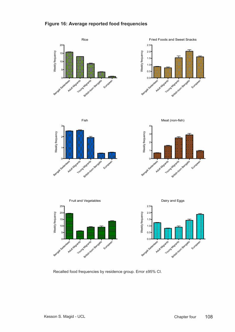
108Kesson S. Magid - UCL Chapter four
Average reported food frequenciesFigure 16:
Rice
Benga
li Sed
entee
s
Adult M
igran
ts
Young
Migr
ants
British
-born
Benga
lis
Europe
an0
5
10
15
20
Wee
kly fr
eque
ncy
Fish
Benga
li Sed
entee
s
Adult M
igran
ts
Young
Migr
ants
British
-born
Benga
lis
Europe
an0
1
2
3
Wee
kly fr
eque
ncy
Fruit and Vegetables
Benga
li Sed
entee
s
Adult M
igran
ts
Young
Migr
ants
British
-born
Benga
lis
Europe
an0
5
10
15
20
25
Wee
kly fr
eque
ncy
Meat (non-fish)
Benga
li Sed
entee
s
Adult M
igran
ts
Young
Migr
ants
British
-born
Benga
lis
Europe
an0
1
2
3
4
Wee
kly fr
eque
ncy
Dairy and Eggs
Benga
li Sed
entee
s
Adult M
igran
ts
Young
Migr
ants
British
-born
Benga
lis
Europe
an0.0
0.5
1.0
1.5
2.0
2.5
Wee
kly fr
eque
ncy
Fried Foods and Sweet Snacks
Benga
li Sed
entee
s
Adult M
igran
ts
Young
Migr
ants
British
-born
Benga
lis
Europe
an0.0
0.5
1.0
1.5
2.0
2.5
Wee
kly fr
eque
ncy
Average Reported Food Frequencies
Recalled food frequencies by residence group. Error ±95% CI.

109Kesson S. Magid - UCL Chapter four
Die
tary
food
freq
uenc
ies
Tabl
e 21
: Sede
ntees
Adult
Migr
ants
Youth
migr
ants
Britis
h-bo
rn B
enga
lisBr
itish-
born
Eur
opea
ns
Food
Typ
eM
ode
(%)
Avg
times
/w
k (S
D)
Mod
e (%
)Av
g tim
es/w
k (S
D)
Mod
e (%
)Av
g tim
es/w
k (S
D)
Mod
e (%
)Av
g tim
es/w
k (S
D)
Mod
e (%
)Av
g tim
es/w
k (S
D)
Rice
Ever
y mea
l (50.4
%)
15.8
(5.4)
Twice
daily
(82.2
%)
13 (2
.8)Tw
ice da
ily (4
2.8%
)5.5
(1.7)
3-4 t
imes
wee
kly (6
8.9%
)3.6
(2.5)
Rare
ly/ne
ver (
62.2%
)1.0
(3.1)
Pasta
Rare
ly/ne
ver (
77.5%
)0.3
(0.7)
Rare
ly/ne
ver (
93.4%
)0.1
(0.3)
Rare
ly/ne
ver (
82.3%
)0.3
(0.4)
<1 tim
e wee
kly (5
1.7%
)0.4
(0.6)
Rare
ly/ne
ver (
81.1%
)0.3
(0.8)
Potat
o (no
t ch
ips)
1-2 t
imes
wee
kly (3
9.2%
)1.5
(2)
Rare
ly/ne
ver (
80.6%
)0.4
(0.9)
Rare
ly/ne
ver (
54.2%
)0.9
(1.0)
1-2 t
imes
wee
kly (3
7%)
1.1 (1
)Ra
rely/
neve
r (54
%)
0.7 (1
.1)
Lenti
ls/dh
al<1
time w
eekly
(36.7
%)
4.4 (6
.1)<1
time w
eekly
(66.1
%)
0.5 (0
.9)Ra
rely/
neve
r (48
.5%)
2.6 (1
.5)Ra
rely/
neve
r (48
.2%)
0.5 (0
.7)Ra
rely/
neve
r (97
.8%)
0.01 (
0.1)
Chick
peas
Rare
ly/ne
ver (
67.6%
)0.3
(0.6)
Rare
ly/ne
ver (
100%
)0
Rare
ly/ne
ver (
97.1%
)0.3
(0.3)
Rare
ly/ne
ver (
62%
)0.2
(0.2)
Rare
ly/ne
ver (
60.8%
)0.6
(1)
Fruit
Rare
ly/ne
ver (
45.7%
)1.0
(1.6)
<1 tim
e wee
kly (4
2.3%
)2.5
(4)
<1 tim
e wee
kly (3
0.3%
)3.6
(1.9)
3-4 t
imes
wee
kly (4
1.3%
)3.2
(4.3)
Twice
daily
(26.4
%)
7.9 (7
.3)Fr
uit ju
iceRa
rely/
neve
r (78
.3%)
0.3 (0
.6)Ra
rely/
neve
r (80
%)
0.5 (1
.2)Ra
rely/
neve
r (62
.8%)
1.3 (1
.2)3-
4 tim
es w
eekly
(32.1
%)
1.6 (1
.4)Ra
rely/
neve
r (62
.2%)
1.0 (1
.5)Sa
ladRa
rely/
neve
r (43
.8%)
1.8 (3
.6)Ra
rely/
neve
r (46
.6%)
0.6 (1
.3)Ra
rely/
neve
r (42
.8%)
1.5 (1
.2)Ra
rely/
neve
r (55
.1%)
1.7 (4
.1)<1
time w
eekly
(39.1
%)
1.6 (2
.8)Ve
getab
les
(in cu
rry)
Ever
y mea
l (53.7
%)
13.6
(7.3)
Rare
ly/ne
ver (
46.6%
)2.5
(4.5)
Rare
ly/ne
ver (
23.5%
)5.4
(2.2)
1-2 t
imes
wee
kly (3
5.7%
)2.5
(4)
n/an/a
Vege
tables
(st
eame
d/bo
iled)
Rare
ly/ne
ver (
66.9%
)2.9
(6.1)
Rare
ly/ne
ver (
90.7%
)0.1
(0.2)
Rare
ly/ne
ver (
78.7%
)1.8
(1.4)
Rare
ly/ne
ver (
64.2%
)0.3
(0.5)
<1 tim
e wee
kly (3
2.6%
)3.2
(4.7)
Eggs
Rare
ly/ne
ver (
47.6%
)1.0
(1.3)
Rare
ly/ne
ver (
67.7%
)0.7
(1.1)
Rare
ly/ne
ver (
65.7%
)0.9
(0.9)
<1 tim
e wee
kly (4
2.8%
)0.6
(0.8)
Rare
ly/ne
ver (
74.5%
)0.4
(0.9)
Chee
seRa
rely/
neve
r (97
.1%)
0.03 (
0.1)
Rare
ly/ne
ver (
95.1%
)0.1
(0.5)
Rare
ly/ne
ver (
81.8%
)0.7
(0.6)
Rare
ly/ne
ver (
53.5%
)0.4
(0.8)
Rare
ly/ne
ver (
73.5%
)0.4
(0.9)
Othe
r dair
yRa
rely/
neve
r (73
.5%)
0.2 (0
.5)Ra
rely/
neve
r (95
.1%)
0.04 (
0.2)
Rare
ly/ne
ver (
82.8%
)0.5
(0.7)
Rare
ly/ne
ver (
64.2%
)0.4
(0.6)
Rare
ly/ne
ver (
61.5%
)0.9
(1.4)
Fish
3-4 t
imes
wee
kly (6
3.2%
)2.5
(1.4)
3-4 t
imes
wee
kly (6
2.9%
)2.6
(1.3)
3-4 t
imes
wee
kly
(45.7
%)
1.5 (1
.2)<1
time w
eekly
(57.1
%)
0.5 (0
.5)Ra
rely/
neve
r (63
.6%)
0.6 (1
)
Chick
enRa
rely/
neve
r (67
.9%)
0.4 (0
.7)Ra
rely/
neve
r (56
.4%)
0.9 (1
.3)1-
2 tim
es w
eekly
(4
8.5%
)1.2
(1.0)
1-2 t
imes
wee
kly (4
6.4%
)1.5
(1.2)
Rare
ly/ne
ver (
60%
)0.5
(0.9)
Beef
Rare
ly/ne
ver (
72.3%
)0.3
(0.6)
Rare
ly/ne
ver (
96.7%
)0.0
5 (0.3
)Ra
rely/
neve
r (79
.4%)
0.7 (0
.7)Ra
rely/
neve
r (75
%)
0.3 (0
.7)Ra
rely/
neve
r (75
%)
0.2 (0
.4)La
mb/M
utton
/Go
atRa
rely/
neve
r (93
.3%)
0.04 (
0.2)
Rare
ly/ne
ver (
69.3%
)0.6
(1)
Rare
ly/ne
ver (
47%
)1.3
(1.1)
1-2 t
imes
wee
kly (3
7%)
1.1 (1
.1)Ra
rely/
neve
r (90
.9%)
0.1 (0
.3)
Pork
n/an/a
n/an/a
n/an/a
n/an/a
Rare
ly/ne
ver (
82.5%
)0.2
(0.6)
Turke
yn/a
n/an/a
n/an/a
n/an/a
n/aRa
rely/
neve
r (93
.9%)
0.2 (0
.7)Ch
ipsRa
rely/
neve
r (88
.8%)
n/aRa
rely/
neve
r (90
.1%)
0.1 (0
.4)Ra
rely/
neve
r (74
.2%)
0.8 (0
.8)<1
time w
eekly
(51.7
%)
0.6 (0
.7)Ra
rely/
neve
r (91
.3%)
0.1 (0
.2)Ot
her f
ried
foods
Rare
ly/ne
ver (
65.7%
)0.5
(0.9)
Rare
ly/ne
ver (
86%
)0.3
(0.9)
Rare
ly/ne
ver (
58.8%
)1.1
(1.0)
<1 tim
e wee
kly (4
4.4%
)0.8
(0.9)
Rare
ly/ne
ver (
78.8%
)0.4
(0.8)
Swee
t sna
cks/
dess
erts
Rare
ly/ne
ver (
75.2%
)0.4
(0.9)
Rare
ly/ne
ver (
80.6%
)0.5
(1.1)
Rare
ly/ne
ver (
55.8%
)1.4
(1.2)
1-2 t
imes
wee
kly (3
7%)
1.3 (1
.2)Ra
rely/
neve
r (46
.1%)
1.2 (1
.4)

110Kesson S. Magid - UCL Chapter four
Health behaviours4.2
Analyses were split by participants aged above and below 40 years, to reduce cohort differences in smoking and betel nut chewing, and to reference other comparisons between younger male health behaviours and reproductive functioning.
Alcohol
Sedentees were not asked whether they consumed alcohol. As a majority Muslim nation, alcohol is not widely available, its consumption is prohibited under the Bangladeshi Narcotics Control Act (1990), and drinking carries a severe social and religious stigma.
Total units consumed per week were estimated based on reported frequency and number of beers, wine and spirits, and were multiplied by 0.5 for “On rare occasions”, 1 for “Once a week or less”, and 2 for “More than once a week”.
Most (95%) of migrant and British-born Bengalis said they never consumed alcohol. Bengalis who consume alcohol (n=6) were relatively evenly distributed between British-born (n=2, 6.9%), adult (n=3, 3.5%) and youth migrants (n=2, 6.1%).
Most (94%) of European men said they consume alcohol. Average units of alcohol consumed per week were not different between low and high status Europeans (9.0±1.2 and 10.1±2 units, respectively; t(71)=-.452, p=.65). While number of units consumed per week negatively correlated with age, it was not quite significant (r=-.20, p=.07), and older men >40 did not drink less than those <40 (8.0±1.3 and 9.8±1.8 units, respectively; t(78)=.768, p=.45).
Smoking
A 3-way loglinear analysis of residence group x age 40 split x current smoking produced a final model that retained all effects. The likelihood ratio of this model was X2=170.16, df=23, p<.001, indicating the highest-order interaction was significant, but the partial association suggested that the interaction between residence and smoking was not significant (X2=9.03, df=5, p=.11). To break down this effect, separate chi-square tests were performed on smoking rates within each residential group.
Overall rates of current smoking were not significantly different between sedentees, adult, or youth migrants (38.7%, 41.0%, 38.2% respectively; X2=0.11, df=2, p=.95). Within these three Bangladeshi-born groups, older men >40 were 2.6 times more likely to currently smoke than those <40 (X2=10.11, df=1, p=.001).
111Kesson S. Magid - UCL Chapter four
British-born Bengalis were much less likely to currently smoke (13.80%, odds ratio: 0.25) than the Bangladesh-born groups (X2=10.11, df=1, p=.007), and were not significantly different from British-born Europeans (X2=1.36, df=1, p=.24).
Rates of smoking within low and high status Europeans were not different from one another (24.5% and 23.3%, respectively; X2=0.02, df=1, p=.90), and older European men >40 were no more likely to currently smoke than those <40 (19.4% and 28.3% respectively; X2=.85, df=1, p=.36).
Betel Nut
European males were not asked about betel nut habits, as within the UK the practice is almost exclusive to Asian communities. Only 2 of 29 British-born Bengalis (7%) were betel nut users, and both said they only used it on special occasions, so were not included in further analysis.
Of Bangladeshi-born men, a 3-way loglinear analysis of residence group x age 40 split x current betel nut usage produced a final model that retained all effects. The likelihood ratio of this model was X2=111.58, df=11, p<.001, indicating the highest-order interaction was significant, and the partial association suggested that the interaction between the age 40 split and betel nut usage was not significant (X2=.19, df=1, p=.7). To break down this effect, separate chi-square tests were performed on smoking rates within each Bangladeshi-born residential group.
Sedentees had the highest prevalence of current betel nut usage at 84.1%, and were 4.6 times more likely to use betel nut than adult migrants (53.2%; X2=18.90, df=1, p<.001), and 8.9 times more than youth migrants (37.1%; X2=29.21, df=1, p<.001). The difference between adult and youth migrants was not significant (X2=2.32, df=1, p<.13). Betel nut usage was not different between men aged >40 (69.3%) and men <40 (65.5%; X2=.33, df=1, p<.57).
While migrants were generally less likely to chew betel nut than sedentees, neither age nor overall number of years spent in the UK, nor an interaction between the two predicted betel nut usage (Logistic Regression: X2=0.299, df=1, p=.58).
Frequency of betel nut usage differed between sedentees and migrants (Logistic Regression: X2=9.33, df=4, p=.05), with 51% of sedentees using it more than 3 times a day, compared with 30% of migrants. Migrants were significantly more likely to say they used betel nut only on special occasions compared to sedentees (21% and 10%, respectively; odds ratio: 3.8, p=.007). Frequency was not different between men split at age 40 (X2=5.47, df=4, p=.24).

112Kesson S. Magid - UCL Chapter four
Activity: sport and exercise per week
High SES European males were not asked if they regularly walked for at least 20 minutes every day as they were interviewed using a truncated version of the questionnaire.
Sedentees (91.5%) were the most likely residence group to say they walk for at least 20 minutes every day and were 3.7-8.7 times more likely to walk regularly than all other residence groups (all p≤.005), aside from young migrants (p=.35). Sedentees were also the least likely group to say they regularly practiced sport or exercise (46.7%).
In contrast, British-born Bengalis were least likely to say they walked regularly (55.2%), but 100% of the 29 respondents said they regularly exercised or practiced sport. Young migrants were the residence group with the second highest rates of regular exercise and walking (86.1% for both). Walking rates were not significantly different between British-born Bengalis and European men (59.3%) or adult migrants (74.6%), though in the latter case this difference was nearly significant (X2=3.37, df=1, p=.07).
Frequency of exercise per week negatively correlated with age (r=-.16, p=.04), but on average, younger men <40 did not report exercising significantly more than those >40 (2.7±0.2 and 2.4±0.3 times/week, respectively; t(157)=.745, p=.46). After correcting for age effects, residence groups did not differ in exercise frequency (MLR: F(6,157)=1.52, p=.18).
Reported physical activityFigure 17: Reported Physical Activity
Seden
tees
Adult M
igran
ts
Young
Migr
ants
British
-born
Benga
lis
Europe
an
Seden
tees
Adult M
igran
ts
Young
Migr
ants
British
-born
Benga
lis
Europe
an0
50
100
150
Regularly Exercise/Sport
Walk 20 Min Daily
%
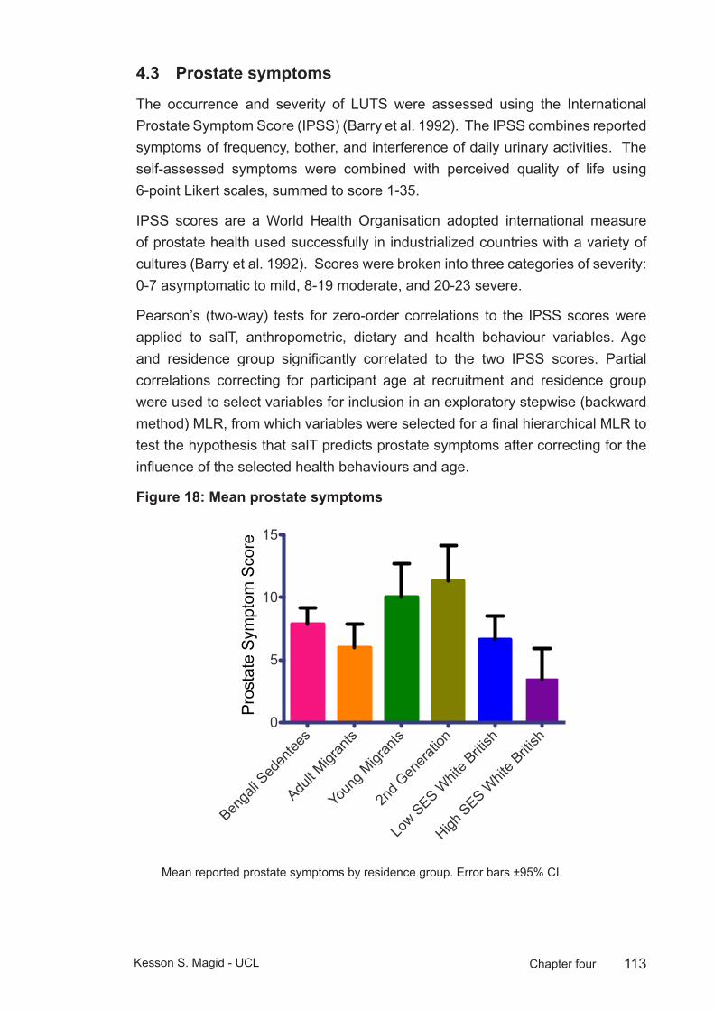
113Kesson S. Magid - UCL Chapter four
Prostate symptoms4.3
The occurrence and severity of LUTS were assessed using the International Prostate Symptom Score (IPSS) (Barry et al. 1992). The IPSS combines reported symptoms of frequency, bother, and interference of daily urinary activities. The self-assessed symptoms were combined with perceived quality of life using 6-point Likert scales, summed to score 1-35.
IPSS scores are a World Health Organisation adopted international measure of prostate health used successfully in industrialized countries with a variety of cultures (Barry et al. 1992). Scores were broken into three categories of severity: 0-7 asymptomatic to mild, 8-19 moderate, and 20-23 severe.
Pearson’s (two-way) tests for zero-order correlations to the IPSS scores were applied to salT, anthropometric, dietary and health behaviour variables. Age and residence group significantly correlated to the two IPSS scores. Partial correlations correcting for participant age at recruitment and residence group were used to select variables for inclusion in an exploratory stepwise (backward method) MLR, from which variables were selected for a final hierarchical MLR to test the hypothesis that salT predicts prostate symptoms after correcting for the influence of the selected health behaviours and age.
Mean prostate symptoms Figure 18: Mean Prostate Symptomology
Benga
li Sed
entee
s
Adult M
igran
ts
Youn
g Migr
ants
2nd G
enera
tion
Low S
ES Whit
e Briti
sh
High S
ES Whit
e Briti
sh0
5
10
15
Pros
tate
Sym
ptom
Sco
re
Mean reported prostate symptoms by residence group. Error bars ±95% CI.
114Kesson S. Magid - UCL Chapter four
Hormonal and physical measures
Both IPSS measures significantly correlated to participant age at recruitment, height and residence group, but not to other anthropometric variables or salT in zero-order Pearson’s correlations. MUA muscle+bone (but not axial fat) and weight both negatively correlated to IPSS measures after correcting for age at recruitment, but not after also correcting for residence group, so this association between axial muscle and prostate symptoms is explained by residence group. After correcting for age at recruitment and residence, salT was significantly correlated to both IPSS measures, though the effect was greater without the QoL measure. In exploratory MLR, mean evening salT, but not morning salT was a significant predictor variable for IPSSTotal (without QoL).
In exploratory MLR, weekly consumption of rice, fruit and vegetables, and fish all significantly and negatively correlate to both IPSS scores. Weekly consumption of meat (excluding fish) and of fried foods and sweet snacks correlate positively to both IPSS scores.
Health behaviours: Correcting for age at recruitment and residence group, IPSS scores do not correlate with whether men said they drink alcohol, use betel nut, exercise regularly or walk 20 minutes a day. But the exercise frequency and number of alcoholic drinks per week negatively correlate to IPSS score, while smoking positively correlates to IPSS scores. Reported frequency of betel nut use significantly positively correlates to IPSS scores.
To test whether residence group predicts prostate symptoms independent of dietary or health behaviours, a hierarchical entry-method MLR was run on IPSS and IPSS+QoL scores with the following three steps:
1) Age at recruitment and BMI
2) Smoking frequency, Betel nut frequency, Weekly units of alcohol consumed, Weekly exercise frequency, Number of daily meals and Estimated weekly consumption of the following foods: Rice, Meat (non-fish), Fish, Fruit and Vegetables, Fried foods and snacks
3) Residence groups (dummy variable: Sedentees), mean of MeanAM salT and BED salT.
Results: The physical measures and health behaviours (Step 2) of the model significantly predicted both IPSS scores (IPSS: F(13,108)=3.18, IPSS+QoL: =3.26, both p<.001). Inclusion of residence group and salT variables (step 3) slightly improved the overall fit of the model r2 from .28 to .31, but this change was not significant (change statistics for IPSS: F(6,102)=0.77). The strongest
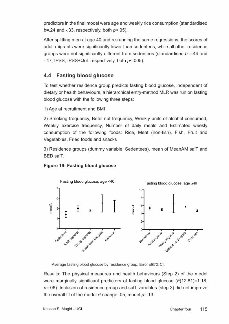
115Kesson S. Magid - UCL Chapter four
predictors in the final model were age and weekly rice consumption (standardised b=.24 and -.33, respectively, both p<.05).
After splitting men at age 40 and re-running the same regressions, the scores of adult migrants were significantly lower than sedentees, while all other residence groups were not significantly different from sedentees (standardised b=-.44 and -.47, IPSS, IPSS+QoL respectively, both p<.005).
Fasting blood glucose4.4
To test whether residence group predicts fasting blood glucose, independent of dietary or health behaviours, a hierarchical entry-method MLR was run on fasting blood glucose with the following three steps:
1) Age at recruitment and BMI
2) Smoking frequency, Betel nut frequency, Weekly units of alcohol consumed, Weekly exercise frequency, Number of daily meals and Estimated weekly consumption of the following foods: Rice, Meat (non-fish), Fish, Fruit and Vegetables, Fried foods and snacks
3) Residence groups (dummy variable: Sedentees), mean of MeanAM salT and BED salT.
Fasting blood glucoseFigure 19:
Fasting blood glucose, age <40
Seden
tees
Adult m
igran
ts
Young
migr
ants
British
-born
Benga
lis
Europe
an3
4
5
6
7
mm
ol/L
Fasting blood glucose, age ≥40
Seden
tees
Adult m
igran
ts
Young
migr
ants
British
-born
Benga
lis
Europe
an0
2
4
6
8
10
mm
ol/L
Average fasting blood glucose by residence group. Error ±95% CI.
Results: The physical measures and health behaviours (Step 2) of the model were marginally significant predictors of fasting blood glucose (F(12,81)=1.18, p=.06). Inclusion of residence group and salT variables (step 3) did not improve the overall fit of the model r2 change .05, model p=.13.

116Kesson S. Magid - UCL Chapter four
However, after splitting men at age 40 and re-running the same regressions the final model was highly significant and a strong predictor of fasting blood glucose for men <40, and the differences between sedentees and all residence groups were significant contributors to the model. The standardized b for residence groups ranged from .67 for adult migrants to 2.27 for British-born Bengalis (all p<.001, final model r2=.71, F(18,35)=4.74, p=<.001). Other positive predictors of fasting blood glucose in the final model were; age; betel nut and alcohol use; fish, rice, fried foods and snack consumption; and times exercised per week, the only significant negative predictor was meat consumption (largest significant standardized b=1.85 was for alcohol consumption, smallest was and 0.27 for fried foods and snacks, all p<.05).
For men >40, the model was not significant at any step, (all p=.5-.9). Salivary T did not predict fasting blood glucose in any of the models.
Dietary or health behaviours and salT 4.5
To test whether adult dietary or health behaviours explain differences in salT between Bengalis resident in London, a GLM was run to predict daily mean salT including in the model: age at recruitment, BMI, SES, smoking, betel nut chewing, regular exercise or walking 20 minutes daily, number of daily meals, and consumption of rice, fruit and vegetables, meat, fried foods, and fish. This model was significant (F(13,40)=2.98, p=.004), after which neither residence group, nor age at migration significantly improved the model (t(14,39)=1.22, p=.2 and t(14,38)=0.06, p=.9, respectively).
To test whether adult dietary or health behaviours explain differences in salT between migrants and sedentees a GLM was run to predict daily mean salT as outcome and residence group (selecting ethnic Bengalis only) as predictor with all dietary, smoking, betel nut usage, exercise, age and BMI, as covariates. In the final model, sedentee salT was significantly higher than adult migrants (respective estimated marginal means: 96±5 versus 79±7 pg/mL, p=.05) while there is no significant difference between sedentees and young migrants or British-born Bengalis (respective estimated marginal means: 110±9 versus 104±12 pg/mL).
Conclusions4.6
Adult migrants share many of the dietary characteristics of sedentees, notably in consumption of rice and fish. While fish and rice consumption don’t appear to decline after migration, adult migrants partly follow the documented pattern of more frequent consumption of meat, a “special menu” Bengali food, but they don’t report consuming more sweet snacks or fried foods as found elsewhere (Chowdhury et al. 2000). However the adult migrants do report eating more
117Kesson S. Magid - UCL Chapter four
snacks than the sedentees, and the customary nasta in both sedentee and migrant Bengali households is sweetened tea and biscuits, so these two results appear somewhat contradictory.
The sedentees appear to make up for a lower consumption of protein from meats other than fish by consuming more eggs, and the lack of a difference between sedentees and migrants when frequency of meat and egg consumption are combined indicates that the sedentees aren’t necessarily consuming substantially less protein overall. Sedentees stand apart from all other groups in their reported consumption of fruit and vegetables, which indicates a maintenance of the traditional Bengali diet in Sylhet. In comparison, all Bengalis living in London eat fruit and vegetables much less frequently. This may be due to the expense of purchasing traditional Bengali vegetables, a concern expressed in focus groups of British Bengalis (Lawrence et al. 2007). The other striking feature of food frequencies was the clear acculturation trend away from rice and toward meat and fried foods among young migrants and British-born Bengalis.
Fasting blood glucose:
While the food frequencies indicate an increased adoption of a diabetogenic diet, the results of the fasting blood glucose regressions indicated that even after correcting for dietary differences, younger London Bengalis, and British-born Bengalis in particular were likely to have high fasting blood glucose compared to sedentees. The fact that these differences were not seen between older men >40 may be due to the relatively small number of young migrants and British-born Bengalis in this age range (n=4 and 1, respectively). But the fact that the model was not significant when comparing only the adult migrants and sedentees >40 suggests that residence group or health behaviours are not explanatory of fasting blood glucose levels. When looking at the data of the older men, it is critical to remember that diagnosed diabetes was an exclusion criterion for recruitment in this project, and it is likely that this selective sub-clinical group represents a different cohort than those <40 who currently have high fasting blood glucose and may develop the disease at a later date. The lack of an explanatory effect of salT in any of the models is not necessarily surprising, as previous associations between insulin and T were strongest when measured as a ratio to E2 or longitudinally (Laaksonen et al. 2004; Phillips et al. 2002).
Dietary patterns:
The lack of a significant difference between sedentees and migrants in number of meals per day supports the assumption that the sedentee population is not currently under nutritional stress. Of course a lack of a difference does not confirm a hypothesis, and the lack of portion or meal size means there may be a lower
118Kesson S. Magid - UCL Chapter four
number of calories consumed per meal, though in light of the lack of significant differences in BMI, one can conclude that the sedentee population is not subjected to high dietary restriction. Migrants eat more snacks than sedentees though, suggesting a change in consumption to more of a modern British “grazing” pattern throughout the day and fewer family meals eaten together (Pollard et al. 2002). The nearly universal observation of Halal indicates that the migrant community maintains dietary patterns with cultural and religious considerations in mind, this fits with other studies of the British Bengali population (Chowdhury et al. 2000).
Prostate symptoms
The proximate hypothesis that prostate symptoms relate directly to salT, after correcting for dietary and health behaviours, was not supported except in the case of adult migrants aged ≥40 years. If lifetime exposure of the prostate to high T were responsible for LUTS, men with the highest T would have the highest incidence of symptoms. Instead, only Bengalis, but not Europeans who spent all or part of their childhood in London show high rates of symptoms. This does not fully support the hypothesis that men whose childhood development occurred under more constrained energetic conditions than those of their adulthood will exhibit a greater number of prostate symptoms. If this were the case, after correcting for age, both adult migrants and youth migrants would exhibit the highest incidence of LUTS. Instead, it would appear that men who spent all of their childhood in Bangladesh have the lowest rates of LUTS. This may be due to the poorer diet amongst Bengalis who migrated as children or were born in Britain. Keeping in mind small sample size for British-born Bengalis and youth migrants over age 40, incidence of prostate symptoms increase at a roughly linear rate.
Overall, these results suggest that youth migrants and British-born Bengalis adopt a poorer diet than other Bengali groups or Europeans. These health behaviours do not fully explain the difference in fasting blood glucose between the young men of these groups and their sedentee counterparts, and combined with the well-documented risk factors of South Asian ethnicity and low SES for NIDDM (Bhopal et al. 1999; McKeigue et al. 1991) these results suggest younger men of the migrant community are at a very high risk of adult-onset diseases in the future.
After correcting for adult dietary and health behaviours, differences in salT between Bengalis resident in London due to differences in developmental timing of migration were no longer evident. Bengalis who migrated at ages before maturity or were British-born adopt a diet that includes less rice, less fish, and more fried foods and meat compared with adult migrants. These behaviours, possibly combined with improvements in SES for Bengalis who spent all or part of their childhood in London, contribute to greater investment in reproductive function than Bengalis

119Kesson S. Magid - UCL Chapter four
who spent all of their childhood in Sylhet, as measured by salT. This change in behaviours, investment in reproductive function and growth is also reflected in increased stature, skeletal muscle mass, fasting glucose and prostate symptoms, compared to sedentees, adult and adolescent migrants.
The lack of a significant difference between sedentees and Bengalis who spent all or part of their childhood in London, once current dietary and health behaviours are taken into account, suggests the ecological differences experienced during childhood in London or Sylhet are not as influential upon adult salT as present surroundings and behaviours, or that current conditions are masking the influence of earlier developmental conditions. In addition, the unexpected finding of significantly higher salT among sedentees as compared to adult migrants, once current dietary and health behaviours are taken into account suggests that current conditions for sedentees in Sylhet, including presumed exposure to parasites or other ecological stressors are either not affecting salT at all, or other factors are counteracting such stressors to lead to higher salT levels in the sedentees when compared to men who shared the same childhood but are no longer subject to the stressors in adulthood. A potential distinguishing factor to the observed differences in salT between sedentees and adult migrants may be perceived status, and their SES relative to their surroundings. This will be explored further in the next chapter.
120Kesson S. Magid - UCL Chapter five
Social factors and reproductive functionChapter 5: In this chapter I test hypotheses relating two measures of current social ecology: male status and reproductive relationships, to investment in reproductive effort as measured by salT of Bengali and European men. The first part of the chapter concerns socioeconomic hypotheses: if men are of low SES, relative to surroundings, then they will invest less into reproductive effort, as measured by salT than men who are of high SES, relative to surroundings. The influence of relative SES on male reproductive effort is hypothesised to be greater following a shift in male reproductive function and fertility in mid-life, at age 40 years. All males appear to retain fecundability late into life, but the likelihood of further reproduction declines for most men after age 40, excepting those with higher status or wealth (Cronk 1991; Kaplan et al. 2000; Marlowe 2000).
The second half of the chapter concerns two variables of male reproductive status, current marriage and number of offspring. The length and types of human pair bonds vary significantly across cultures based on socioecological conditions. The degree of paternal investment in offspring and mate-seeking competition between human males is also widely variable reflecting the compromise between reproductive interests and offspring investment strategies (Ellison 2009).
Socioeconomics
Dominance and rank are critically important to reproductive investment in males (Archer 2006; Dabbs and Dabbs 2000), and SES is arguably the closest approximation to social rank in humans (Sapolsky 2004). Psychosocial stress, as mediated by glucocorticoids, appears to suppress male gonadal function (Hardy et al. 2005). Health biomarkers of stress and SES correlate to relative positioning in a society more than absolute measures of wealth, in such a way that low-status individuals in wealthy countries with high inequality have poorer health outcomes than those resident in countries with low inequality (Marmot 2006; Wilkinson and Pickett 2009). In the context of this project, low-status men in the UK are expected to experience greater SES-related stress than high-status men living in Bangladesh, despite the great disparity in absolute measures of wealth between the two countries.
A fundamental transition for the male life history is the allocation of reproductive effort to the competing requirements between competition for mating opportunities and investment in maintaining current pair-bonds and paternal care. Younger males are more likely to compete physically for mating opportunities, regardless of SES as they will not have offspring in which to invest paternal care, and low status may mean all of a male’s reproductive opportunities will occur in early adulthood. If men survive to older adulthood, they are unlikely to succeed in direct
121Kesson S. Magid - UCL Chapter five
physical competition with younger males, but they are likely to have further mating opportunities if they are of high status.
The contrasting ecologies of the UK and Bangladesh allow for the testing of two hypotheses:
1. If a male is of high SES relative to current surrounding ecological conditions, he is expected to divert more effort toward reproductive function than men of low SES, relative to current ecological surroundings.
Prediction: High SES males, relative to current surroundings will have higher salT than low SES males.
2. If salT modulates male allocation of reproductive effort between competition for mating opportunities and investment in maintaining current pair-bonds and paternal care, this allocation will be of greater importance in the later portion of adulthood. Current relative SES is hypothesised to be more influential on reproductive effort of men in the latter half of their reproductive stage of life, compared to men in the first half of this stage of life. Prediction: High SES males have higher salT, and that relative SES is more highly associated with salT in men aged 40 years or older.
Methods
To estimate wealth, an index was created of 11 household possessions in the UK, and 8 in Bangladesh (see Appendix 1: III.5). This method of estimating SES is frequently used in cross-cultural contexts as an indicator of the level of wealth that is consistent with expenditure and income measures (Gwatkin et al. 2007; Montgomery et al. 2000). Television ownership was added to the Bangladeshi questionnaire and assumed nearly ubiquitous in the UK households, while “washing machine”, “tumble dryer”, “dishwasher” and “central heating” were omitted as these are not common household possessions in Bangladesh where servants usually perform domestic chores.
The wealth index for Bengalis living in Sylhet is relative. As described in chapter 1, this population falls within a middle to high SES population by the standards of urban Bangladesh (Islam 2005). As this group is from the middle class, 89% of sedentees reported monthly household income at or above the national average for urban populations of Tk 9878 Bangladeshi taka (or approximately £82 GBP).
Housing type was categorised in the UK as “bedsit/hostel”, “flat/maisonette”, or “house” and in Bangladesh as “katcha”: corrugated iron or mud brick construction, “semi-pakka”: concrete walls with corrugated iron roofing or “pakka”: a permanent structure with concrete walls and roof (UN-HABITAT 1996). Number of rooms and total persons (adults and children) permanently resident were divided by number
122Kesson S. Magid - UCL Chapter five
of rooms to create an index of household crowding. All participants were asked if they owned or rented their accommodation and if renting, whether they were private or local authority tenants.
Participants were also asked to select a band estimating their total monthly income after tax.
Results
A principal component analysis (PCA) was conducted on 16 items for UK residents, and separately on 12 items for sedentees (see table 22 for descriptives). As income was frequently omitted, PCA excluded this variable pairwise and a factor weight was assigned to each participant. All variables were significantly correlated to income, aside from central heating and owning a freezer (both p>.2).
The London Bengali community was not socioeconomically homogenous. Residence group significantly predicts SES (ANOVA F(4,277)=67.0, r^2=.49 p<.0001; see figure 20). Age at recruitment is not a significant covariate for SES, except for migrants who arrived in London before adulthood. Within youth migrants, older males are significantly more likely to have a lower SES, as do those who migrated as an adolescent between the ages 12-18 years versus those who migrated as an infant or child, after correcting for age at recruitment. Youth migrant and British-born Bengalis are of significantly higher SES (0.06±0.5 SD) than adult migrants (adult migrants: −0.74±0.7; youth migrants: −0.07±0.5). Youth migrants were of significantly lower SES than low SES Europeans (0.24±0.8), while for British-born Bengalis this difference was not significant. High SES Europeans were significantly higher than all other groups (1.4±0.8).
Socioeconomic measures
Within the UK, SES quintile with participant age at recruitment as a covariate does not significantly predict daily salT, but the model becomes significant if including residence group (ANCOVA F(5,201)=10.31, p<.001). Both SES and residence significantly contribute to the model (F(4,184)=2.47 and 3.82, both p≤.05), with a nearly significant interaction effect as well (F(13,184)=1.67, p=.07). Parameter estimates indicate the interaction between residence group and SES is significant for all three Bengali groups in the UK, but not for Europeans.

123Kesson S. Magid - UCL Chapter five
UK SES by residence groupFigure 20:
Adult M
igran
ts
Youn
g Migr
ants
British
-born
Benga
lis
Low S
ES Euro
pean
High S
ES Euro
pean
-1
0
1
2
SES
Inde
x
Reported housing crowding by residence group. Error ±95% CI.
House crowdingFigure 21: Housing crowding
Benga
li Sed
entee
s
Adult M
igran
ts
Youn
g Migr
ants
British
-born
Benga
lis
Low SES Euro
pean
High SES Euro
pean
0.0
0.5
1.0
1.5
2.0
Pers
ons/
room
Composite SES index by residence group. Error ±95% CI. .
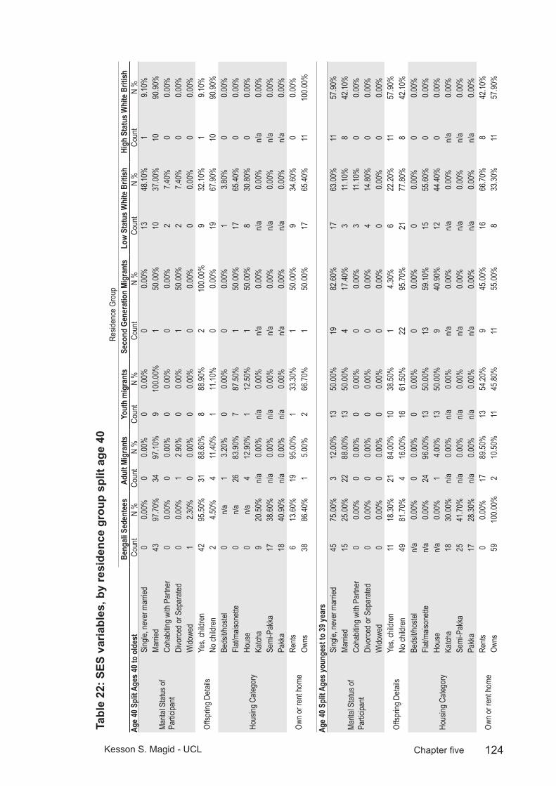
124Kesson S. Magid - UCL Chapter five
SES
varia
bles
, by
resi
denc
e gr
oup
split
age
40
Tabl
e 22
: Re
siden
ce G
roup
Beng
ali S
eden
tees
Adul
t Mig
rant
sYo
uth
mig
rant
sSe
cond
Gen
erat
ion
Migr
ants
Low
Stat
us W
hite
Brit
ishHi
gh S
tatu
s Whi
te B
ritish
Age 4
0 Spl
it Age
s 40 t
o ol
dest
Coun
tN
%Co
unt
N %
Coun
tN
%Co
unt
N %
Coun
tN
%Co
unt
N %
Marita
l Stat
us of
Pa
rticipa
nt
Sing
le, ne
ver m
arrie
d0
0.00%
00.0
0%0
0.00%
00.0
0%13
48.10
%1
9.10%
Marri
ed43
97.70
%34
97.10
%9
100.0
0%1
50.00
%10
37.00
%10
90.90
%Co
habit
ing w
ith P
artne
r0
0.00%
00.0
0%0
0.00%
00.0
0%2
7.40%
00.0
0%Di
vorce
d or S
epar
ated
00.0
0%1
2.90%
00.0
0%1
50.00
%2
7.40%
00.0
0%W
idowe
d1
2.30%
00.0
0%0
0.00%
00.0
0%0
0.00%
00.0
0%
Offsp
ring D
etails
Yes,
child
ren
4295
.50%
3188
.60%
888
.90%
210
0.00%
932
.10%
19.1
0%No
child
ren
24.5
0%4
11.40
%1
11.10
%0
0.00%
1967
.90%
1090
.90%
Hous
ing C
atego
ry
Beds
it/hos
tel0
n/a1
3.20%
00.0
0%0
0.00%
13.8
0%0
0.00%
Flat/m
aison
ette
0n/a
2683
.90%
787
.50%
150
.00%
1765
.40%
00.0
0%Ho
use
0n/a
412
.90%
112
.50%
150
.00%
830
.80%
00.0
0%Ka
tcha
920
.50%
n/a0.0
0%n/a
0.00%
n/a0.0
0%n/a
0.00%
n/a0.0
0%Se
mi-P
akka
1738
.60%
n/a0.0
0%n/a
0.00%
n/a0.0
0%n/a
0.00%
n/a0.0
0%Pa
kka
1840
.90%
n/a0.0
0%n/a
0.00%
n/a0.0
0%n/a
0.00%
n/a0.0
0%
Own o
r ren
t hom
eRe
nts6
13.60
%19
95.00
%1
33.30
%1
50.00
%9
34.60
%0
0.00%
Owns
3886
.40%
15.0
0%2
66.70
%1
50.00
%17
65.40
%11
100.0
0%
Age 4
0 Spl
it Age
s you
nges
t to
39 ye
ars
Marita
l Stat
us of
Pa
rticipa
nt
Sing
le, ne
ver m
arrie
d45
75.00
%3
12.00
%13
50.00
%19
82.60
%17
63.00
%11
57.90
%Ma
rried
1525
.00%
2288
.00%
1350
.00%
417
.40%
311
.10%
842
.10%
Coha
biting
with
Par
tner
00.0
0%0
0.00%
00.0
0%0
0.00%
311
.10%
00.0
0%Di
vorce
d or S
epar
ated
00.0
0%0
0.00%
00.0
0%0
0.00%
414
.80%
00.0
0%W
idowe
d0
0.00%
00.0
0%0
0.00%
00.0
0%0
0.00%
00.0
0%
Offsp
ring D
etails
Yes,
child
ren
1118
.30%
2184
.00%
1038
.50%
14.3
0%6
22.20
%11
57.90
%No
child
ren
4981
.70%
416
.00%
1661
.50%
2295
.70%
2177
.80%
842
.10%
Hous
ing C
atego
ry
Beds
it/hos
teln/a
0.00%
00.0
0%0
0.00%
00.0
0%0
0.00%
00.0
0%Fla
t/mais
onett
en/a
0.00%
2496
.00%
1350
.00%
1359
.10%
1555
.60%
00.0
0%Ho
use
n/a0.0
0%1
4.00%
1350
.00%
940
.90%
1244
.40%
00.0
0%Ka
tcha
1830
.00%
n/a0.0
0%n/a
0.00%
n/a0.0
0%n/a
0.00%
n/a0.0
0%Se
mi-P
akka
2541
.70%
n/a0.0
0%n/a
0.00%
n/a0.0
0%n/a
0.00%
n/a0.0
0%Pa
kka
1728
.30%
n/a0.0
0%n/a
0.00%
n/a0.0
0%n/a
0.00%
n/a0.0
0%
Own o
r ren
t hom
eRe
nts0
0.00%
1789
.50%
1354
.20%
945
.00%
1666
.70%
842
.10%
Owns
5910
0.00%
210
.50%
1145
.80%
1155
.00%
833
.30%
1157
.90%
125Kesson S. Magid - UCL Chapter five
Average housing overcrowding was greatest for adult migrants, at 1.4±.09 persons/per room (see figure 21). In independent 2-tailed t test this was not significantly different from overcrowding rates for sedentees 1.3±.07 (: t(126)=-1.0, p=.3. All other groups living in London are less crowded than adult migrants, (ANOVA: F(5,230)=22.3, p<.001), while rates of crowding between youth migrants and British-born Bengalis do not differ from one another (0.98±.1 and 1.14±.2, respectively; t(34)=.47, p=.5), but were significantly more crowded than either European group (0.4±.05 for low SES, 0.5±.03 for high SES; difference from combined British-born and youth migrant Bengalis t(64)=4.2 p<.001).
For sedentees, the score on the Bangladeshi SES index does not predict salT, after correcting for age and BMI (F(4,63)=1.97, p=.11). After splitting at age 40, SES still had no predictive effect upon salT within the sedentee population.
To determine whether SES explained salT differences between Bengalis resident in London, a GLM was run predicting daily mean salT after selecting out migrants and British-born Bengalis, correcting for age, BMI and SES quintiles. The interaction effect between age at recruitment and SES significantly predicted salT (F(5,63)=2.79, p=.03), as did residence group alone (F(1,63)=6.21, p=.02), no other variables or interactions were significant. To check for a cohort effect, year of migration was added as a covariate, but did not significantly improve the model after correcting for age at recruitment (t(5,75)=0.07, p=.9).
Reproductive strategies5.1
A growing body of data suggests an association between pairbonding and/or parenthood and testosterone of human males (Burnham et al. 2003; Gray et al. 2006). This association is thought to reflect the trade off between paternal investment in current offspring and effort directed toward obtaining further reproductive opportunities. While cross-cultural research in this area is expanding (Gray et al. 2007; Kuzawa et al. 2009), the bulk of these studies investigated North American men, with limited cultural variation in mate choice, extramarital sex and direct paternal investment in offspring. Previous analysis of a subsection of the Bengali sedentee population suggests the influence of marital or paternity status are not reflected by measures of salT (Magid et al. 2006).
Pair bonds in Bangladesh are traditionally arranged by guardians, usually older male relatives through a marriage broker, with a dowry paid to the groom at marriage (Aziz and Research 1979). The contrasts between Western and non-Western populations in the degree to which pairbonded men or fathers show lower reproductive investment than non-pairbonded or childless men are hypothetically due, at least in part, to differences in the social ecology of male relationships in the contrasting cultures. If the influence of different ecologies during childhood
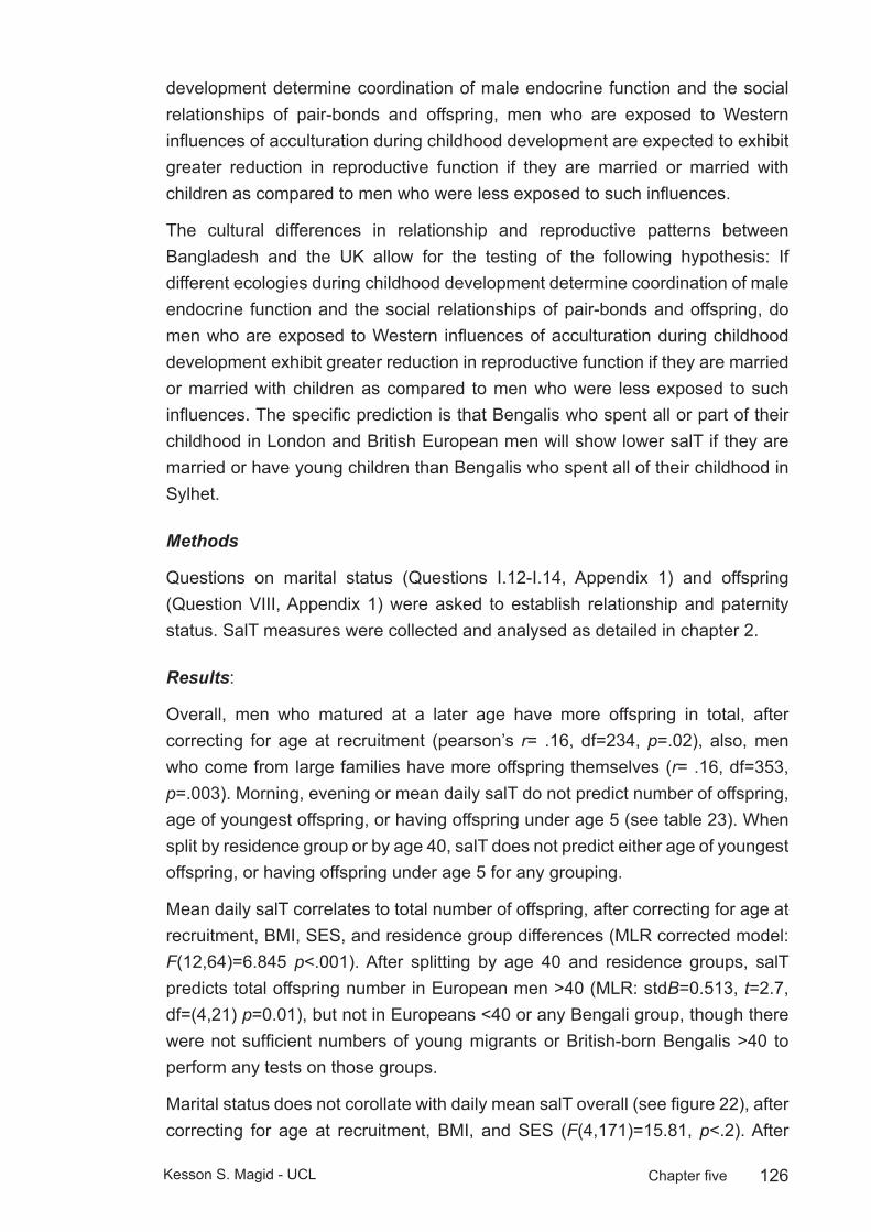
126Kesson S. Magid - UCL Chapter five
development determine coordination of male endocrine function and the social relationships of pair-bonds and offspring, men who are exposed to Western influences of acculturation during childhood development are expected to exhibit greater reduction in reproductive function if they are married or married with children as compared to men who were less exposed to such influences.
The cultural differences in relationship and reproductive patterns between Bangladesh and the UK allow for the testing of the following hypothesis: If different ecologies during childhood development determine coordination of male endocrine function and the social relationships of pair-bonds and offspring, do men who are exposed to Western influences of acculturation during childhood development exhibit greater reduction in reproductive function if they are married or married with children as compared to men who were less exposed to such influences. The specific prediction is that Bengalis who spent all or part of their childhood in London and British European men will show lower salT if they are married or have young children than Bengalis who spent all of their childhood in Sylhet.
Methods
Questions on marital status (Questions I.12-I.14, Appendix 1) and offspring (Question VIII, Appendix 1) were asked to establish relationship and paternity status. SalT measures were collected and analysed as detailed in chapter 2.
Results:
Overall, men who matured at a later age have more offspring in total, after correcting for age at recruitment (pearson’s r= .16, df=234, p=.02), also, men who come from large families have more offspring themselves (r= .16, df=353, p=.003). Morning, evening or mean daily salT do not predict number of offspring, age of youngest offspring, or having offspring under age 5 (see table 23). When split by residence group or by age 40, salT does not predict either age of youngest offspring, or having offspring under age 5 for any grouping.
Mean daily salT correlates to total number of offspring, after correcting for age at recruitment, BMI, SES, and residence group differences (MLR corrected model: F(12,64)=6.845 p<.001). After splitting by age 40 and residence groups, salT predicts total offspring number in European men >40 (MLR: stdB=0.513, t=2.7, df=(4,21) p=0.01), but not in Europeans <40 or any Bengali group, though there were not sufficient numbers of young migrants or British-born Bengalis >40 to perform any tests on those groups.
Marital status does not corollate with daily mean salT overall (see figure 22), after correcting for age at recruitment, BMI, and SES (F(4,171)=15.81, p<.2). After
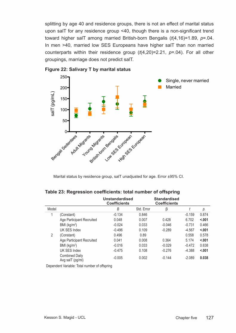
127Kesson S. Magid - UCL Chapter five
splitting by age 40 and residence groups, there is not an effect of marital status upon salT for any residence group <40, though there is a non-significant trend toward higher salT among married British-born Bengalis (t(4,16)=1.89, p=.04. In men >40, married low SES Europeans have higher salT than non married counterparts within their residence group (t(4,20)=2.21, p=.04). For all other groupings, marriage does not predict salT.
Salivary T by marital status Figure 22:
Salivary T by marital status
Benga
li Sed
entee
s
Adult M
igran
ts
Young
Migr
ants
British
-born
Benga
lis
Low SES Euro
pean
High SES Euro
pean
0
50
100
150
200
250Single, never marriedMarried
salT
(pg/
mL)
Marital status by residence group, salT unadjusted for age. Error ±95% CI.
Regression coefficients: total number of offspringTable 23: Unstandardised
CoefficientsStandardised Coefficients
Model B Std. Error β t p.1 (Constant) -0.134 0.846 -0.159 0.874
Age Participant Recruited 0.048 0.007 0.428 6.702 <.001BMI (kg/m2) -0.024 0.033 -0.046 -0.731 0.466UK SES Index -0.496 0.109 -0.289 -4.567 <.001
2 (Constant) 0.496 0.89 0.558 0.578Age Participant Recruited 0.041 0.008 0.364 5.174 <.001BMI (kg/m2) -0.016 0.033 -0.029 -0.472 0.638UK SES Index -0.475 0.108 -0.276 -4.388 <.001Combined Daily Avg salT (pg/ml) -0.005 0.002 -0.144 -2.089 0.038
Dependent Variable: Total number of offspring
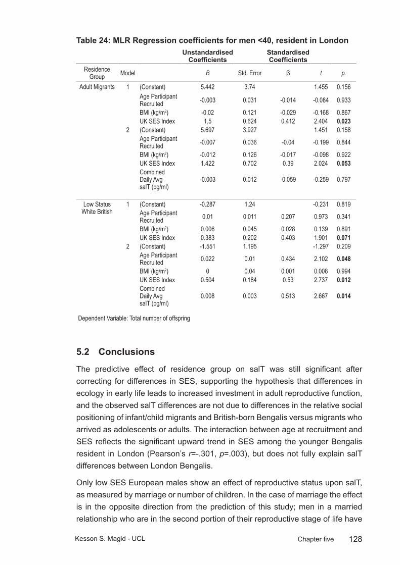
128Kesson S. Magid - UCL Chapter five
MLR Regression coefficients for men <40, resident in LondonTable 24: Unstandardised
CoefficientsStandardised Coefficients
Residence Group Model B Std. Error β t p.
Adult Migrants 1 (Constant) 5.442 3.74 1.455 0.156Age Participant Recruited -0.003 0.031 -0.014 -0.084 0.933
BMI (kg/m2) -0.02 0.121 -0.029 -0.168 0.867UK SES Index 1.5 0.624 0.412 2.404 0.023
2 (Constant) 5.697 3.927 1.451 0.158Age Participant Recruited -0.007 0.036 -0.04 -0.199 0.844
BMI (kg/m2) -0.012 0.126 -0.017 -0.098 0.922UK SES Index 1.422 0.702 0.39 2.024 0.053Combined Daily Avg salT (pg/ml)
-0.003 0.012 -0.059 -0.259 0.797
Low Status White British
1 (Constant) -0.287 1.24 -0.231 0.819Age Participant Recruited 0.01 0.011 0.207 0.973 0.341
BMI (kg/m2) 0.006 0.045 0.028 0.139 0.891UK SES Index 0.383 0.202 0.403 1.901 0.071
2 (Constant) -1.551 1.195 -1.297 0.209Age Participant Recruited 0.022 0.01 0.434 2.102 0.048
BMI (kg/m2) 0 0.04 0.001 0.008 0.994UK SES Index 0.504 0.184 0.53 2.737 0.012Combined Daily Avg salT (pg/ml)
0.008 0.003 0.513 2.667 0.014
Dependent Variable: Total number of offspring
Conclusions5.2
The predictive effect of residence group on salT was still significant after correcting for differences in SES, supporting the hypothesis that differences in ecology in early life leads to increased investment in adult reproductive function, and the observed salT differences are not due to differences in the relative social positioning of infant/child migrants and British-born Bengalis versus migrants who arrived as adolescents or adults. The interaction between age at recruitment and SES reflects the significant upward trend in SES among the younger Bengalis resident in London (Pearson’s r=-.301, p=.003), but does not fully explain salT differences between London Bengalis.
Only low SES European males show an effect of reproductive status upon salT, as measured by marriage or number of children. In the case of marriage the effect is in the opposite direction from the prediction of this study; men in a married relationship who are in the second portion of their reproductive stage of life have
129Kesson S. Magid - UCL Chapter five
higher levels of salT than non-married men. For total number of offspring, the prediction that men would have lower salT if they had young children, or that age of youngest child would have a significant negative relationship with salT, is not supported. European men of low SES with more children overall have higher levels of salT. High SES Europeans do not show a systematic relationship between salT and offspring number or age, so the different patterns in paternity or relationship appear related to SES. The difference between older European men and any of the Bengali groups, with regard to reproductive status suggests a different reproductive strategy for men who grew to maturity in Bangladesh.
Unfortunately, a comparison that cannot be drawn from these results whether paternity or relationship status will have an effect upon older Bengali men who were born in Britain or came here as children because of the lack of men over 40 in these groups. The total number of offspring is much lower in the European group, as compared to either adult migrants or sedentees in the same latter portion of their reproductive stage of life. It may be that the effects of paternity upon reproductive function in older men is subject to a threshold dependent on the difference between having one child or two.
Overall, the lack of a paternity or relationship status effect upon salT in the Bengali population suggests the pattern of reduced salT among fathers or married men observed in Western populations may reflect aspects of paternal investment or mate-seeking that do not apply within Bengali culture.

130Kesson S. Magid - UCL Chapter six
ConclusionsChapter 6: This project applies life history theory to predict male reproductive function across the three variables of ethnicity, ecology, and development. The preceding three results chapters present variations in Bengali and European male reproductive phenotype, health behaviours and diet due to changes in ecological conditions during development. These findings contribute to the growing body evidence that salT, stature and apportionment of skeletal muscle vary in accordance with early life conditions and the strategic allocation of reproductive effort in the human male (chapter three), with a corresponding increase in early symptoms of adult onset disease of the prostate and glucose metabolism (chapter four), and in accordance with perceived status and relative SES (chapter five). Predicted blunting of diurnal salT profile in adult migrants (chapter three) were inconclusive. Contrary to the predictions of this study, sedentees do not show lower levels of salT than adult migrant counterparts, despite greater exposure to presumed ecological stressors such as exposure to pathogens and environmental risks (chapter three). The presumption that the London Bengali community is socioeconomically homogeneous was not supported (chapter five). Bengali men do not have lower salT in relation to reproductive status of paternity or marriage, regardless of any acculturation due to developmental exposure to life in London, while older British-born European men of low SES have higher salT in relation to number of offspring and marital status (chapter five).
The measures used in this study were subject to differential environmental sensitivity, depending on the point in development when conditions improved. Five key points in the life history were considered: 1. Pre-birth 2. Infancy (0-2 yo) 3. Mid-childhood (3-8 yo) 4. Late-childhood/adolescence (9-18 yo) 4. Adulthood (18 years+). Each period contains critical developmental phases that influence adult male reproductive effort, as measured by salivary testosterone and somatic indices. This chapter draws conclusions from these findings at two levels of inquiry. At the proximate level, how does the functioning of reproductive organs and hormonal axes interact with developmental history and current surroundings? At the ultimate level, how do these results reflect the balancing of the competing biological functions of survivorship and reproductive effort has been shaped by natural selection? These principles extend to the field of evolutionary medicine, where trade-offs of investment between competing physiological requirements explain senescence and disease.
Proximately, exposure to the ecological conditions in London, if experienced during childhood lead to males growing taller, more muscular, maturing earlier and with higher testosterone compared to ethnically matched sedentees.
131Kesson S. Magid - UCL Chapter six
The influences of these contrasting environments are subject to critical periods of development: younger men set their reproductive effort according to their childhood environment, particularly during the juvenile period of “slow growth” between ages 3-12, while older migrants show decreased reproductive effort due to either current or previous adult experience, with higher SES relative to current surroundings associated with greater salT in sedentee counterparts. If migrating after the age of maturity, there are no measured differences in salT between migrants and sedentees in early adulthood before age 40, while older sedentees appear to invest more into reproductive function as measured by salT than their adult migrant counterparts. This contrasts with the somatic data from men under age 40, which show greater amounts of both skeletal muscle and axial fat in all migrant groups compared to sedentees, regardless of age of migration. The high levels of T in the older sedentees in the absence of corresponding raised skeletal muscle may indicate another modulating influence on muscular growth or apportionment, or reduced sensitivity of muscle cells to testosterone in older men living under the environmental stresses of life in Bangladesh.
The juvenile period is commonly considered a quiescent stage of male reproductive development, but in this study it appears sensitive to ecological conditions. This period of apparent dormancy of the testes and low levels of circulating sex hormones falls between the postnatal peak of activity in the first year of life and the surge of activity accompanying puberty. This leaves open the possibility that sensitivity during adrenarche is important in the coordination of the early initiation of puberty (Campbell 2003). The limited sample size of youth migrants who experienced a change in ecological conditions before and after adrenarche (approximately aged 7 years in males) was not large enough to definitively establish whether adult salT levels were “set” during this developmental period. The potential role of adrenarche may be pursued in future work applying a similar research design with a larger sample size.
Demographic observations relate environmental stresses upon male children during this period to the phenotype of their male offspring (Bygren et al. 2001; Pembrey et al. 2005). Though the mechanism of this effect is not yet known, it has led to speculation that this period is a critical window for the organisation of trans-generational epigenetic information, which is particularly relevant to males (Pembrey 2010).
The finding of an earlier timing of puberty for infant migrants and British-born Bengalis also supports the hypothesis that childhood development in the UK is less constrained than in Bangladesh. As age of migration only predicted earlier maturity for migrants who arrived before age 2, a change in environment during these years could conceivably alter both the tempo and hormonal parameters of
132Kesson S. Magid - UCL Chapter six
sexual maturity. This early stage of infancy may be important to the establishment of HPT axis thresholds of activity, after which the tempo of maturity is no longer sensitive to conditions conducive to growth.
Of course, behavioural differences between men living in London and Sylhet may prompt greater acquisition of muscle at younger ages and retention into late adulthood. Any potential behavioural difference is not accompanied by an increase in salT implies the opposite conclusion: that environmental conditions in the UK somehow increase the sensitivity of muscle cells to testosterone. In either case, the strength of the link between axial muscle and testosterone appears to be subject to the environment in which an older male lives.
Measures of current dietary and health behaviours appear to explain much of this variation, as salT differences between sedentees and youth migrants or British-born Bengalis are no longer significant, once these factors are taken into account. This does not necessarily mean the current diet and health behaviours of these groups is the cause of variation in reproductive function in these men, as presumably these adult behavioural patterns reflect developmental experience. The change in diet between migrants and sedentees reflects developmental experiences, with a departure from consumption of vegetables among all Bengalis resident in London. One of the most significant explanatory dietary variables for salT was consumption of rice. Vegetarians and Asian men have higher plasma levels of SHBG and slightly lower levels of free T than men on Western diet (Key et al. 1990; van Houten and Gooren 2000; Zitzmann and Nieschlag 2001). The adoption of a Western diet high in fat and protein, compared to Asian diet higher in vegetables may influence reproductive physiology as plant compounds are reduced by gut microflora to phytoestrogens, chemicals resembling steroidal oestrogens in structure or function and able to bind to estrogen receptors (van Houten and Gooren 2000).
Dietary effects upon free T are typically very small though, and a direct causal link between rice consumption and salT seems unlikely to explain all the variance attributed to early life conditions. Rice consumption as a variable more plausibly represents correlated acculturation or ecological exposure over the lifespan in that it mirrors developmental age at migration for youth migrants and was much lower in British-born Bengalis, while rice consumption was only slightly lower for adult migrants compared to sedentees.
The measures above were analysed before taking SES into full consideration in chapter five. The creation of an SES index revealed youth migrant and British-born Bengalis to be of significantly higher SES than adult migrants, though they were matched to low SES British-born Europeans. From these findings, the SES of the men sampled in the London Bengali community were not homogeneous. A

133Kesson S. Magid - UCL Chapter six
re-examination of the developmental hypotheses tested in chapter three with the composite SES index included in the analysis suggests that ecological conditions aside from SES also determine adult reproductive function in the London Bengali population.
The differences in SES between British-born and migrant Bengalis who arrived before the age of 12 and all migrants arriving after age 12 may reflect a cohort effect of the previously documented changing SES of London Bengalis (Sunder and Uddin 2007).
The height of youth migrants and British-born Bengalis supports the general assumption of this study: that conditions in the UK are more conducive to childhood growth than Bangladesh. Migrating prior to age of maturity leads to taller adult standing height, but the limits of this plasticity is shown by the failure of youth migrants to grow as tall as Bengalis born in the UK. While actual measurement of leg length was not collected in this project, the lack of differences in arm length indicates this is a more canalised trait, suggesting femoral length or other long bones of the legs are more responsive to improvements in childhood environment than humeral length. Whatever the conditions conducive to growth in childhood, they do not appear to allow for increased reproductive function in males if they are experienced after maturity. Presumed conditions of ecological stress from pathogens or other environmental risks do not appear to constrain adult sedentee reproductive function when comparing measures of salT or (in men over 40) skeletal muscle to adult migrants.
The difference between the older males hints at the importance of relative social positioning for men in the latter half of their adult lives. While much has been made of the potential links between relative status and health outcomes at older ages (Marmot 2006) (Wilkinson and Pickett 2009), this is the first study to my knowledge to contrast testosterone levels of men of living at high SES in a poor nation with men of the same heritage living at a low SES in a wealthy nation. The link between T and dominance is well-established in primate and other mammalian research, (Muller and Wrangham 2004; Rose et al. 1971), but is less clear in human hierarchies (Book et al. 2001; Dabbs and Morris 1990; Mazur and Booth 1998).
One major confounding feature of the research on human hierarchies is the difficulty in determining which social positioning is of greatest importance (Sapolsky 2004). In the case of migrants moving to the UK from Sylhet, the Londoni are considered wealthy and they form a powerful economic class. Money from London has led to a proliferation of shopping malls, hotels and apartment buildings in Sylhet. The Sylheti middle classes from which this sedentee population was recruited is broadly reliant upon money from London either directly in the form of remittances,
134Kesson S. Magid - UCL Chapter six
or indirectly through the management and rental income of properties owned by their Londoni relations. The findings of this study suggest the influence of SES upon adult male reproduction may correspond to relative positioning in a society, much like other measures of health outcomes. It would appear that the influence of status at older ages is not reliant upon the gauge of success or affluence in early life, or by one’s extended kin group, but is reflected by immediate relative social positioning.
Low SES relative to surroundings appears related to low salT in older males over the age of 40, while the salT and muscle mass measures of older men of high relative SES are not lower in the second half of the reproductive phase. This has some resemblance to the well documented “victory effect” in humans (Booth et al. 1989; Mazur and Booth 1998), where after a competitive interaction, the victor retains a high level of testosterone, while that of the loser declines. While there was not a direct link between being in the high or low SES group among the Sylheti sedentees, this was a within-population variable, and by not by indices of wealth in Bangladesh. The sedentees are an affluent group in a very poor nation, and this may influence perceptions of status. In contrast, migrant neighbourhoods abut the financial district of London and the Bengalis historically have lived in conditions of poverty within one of the wealthiest cities in Europe. The SES indices of the migrants included those of their rich London neighbours, and thus give a more accurate measure of their positioning relative to the surrounding population. This means the comparisons between the salT of low SES adult migrants >40 with sedentees is likely to accurately reflect the influence of SES.
The lack of a paternity or marital effect among Bengalis in London or Sylhet suggests the mechanisms of reduction in reproductive function observed in relation to paternity or marital status do not apply to Bengalis. This is in contrast to the significant difference observed in European males, though the direction of the effect was the opposite of predictions. This may indicate the success of older males with high salT within a low SES group to attract and retain partners, as opposed to younger males with high salT. The tradition of marital arrangement in the Bengali community may not allow for such variations in salT to correlate to partnership status and mate-seeking competition to the same degree as observed in Western populations.
While the differences in morning salT were greatest in young men, there was not a consistent pattern of the overall degree of daily decline. The lack of a consistent pattern between diurnal change in salT and residence group does fit with findings which suggest the morning peak and daily decline frequently observed in clinical studies (Diver et al. 2003) is less predictable or regular in non-Western populations (Vitzthum et al. 2009) (Bribiescas and Hill 2010).

135Kesson S. Magid - UCL Chapter six
There has been speculation that morning testosterone peaks are more reflective of physiological “set points” and evening levels more reflective of daily social and ecological interactions, but the residence groups with the greatest morning salT also had the greatest evening levels, so are either subject to daily environmental influences which promote high salT, or the rate of decline is not more flexible in men with higher salT.
Ultimately, the adjustments to human male reproductive function presented in this thesis are developmental responses to environmental perturbations, and are ultimately the product of evolutionary processes. The males in this study respond to contrasting ecological conditions in order to balance the competing biological functions of survivorship and reproductive effort. Natural selection will have favoured phenotypic matching to ecological conditions based on cues received during growth (within maternal constraints), and when the environment improves or becomes less stochastic, phenotypic characters with plasticity will correspond with a more matched phenotype.
From the perspective of life history theory, a developing male relies upon: a) inherited information on historical conditions to: b) interpret indicators of current ecological conditions in order to: c) adopt a fitness-maximising reproductive strategy between stability and responsiveness to changes in ecology. In a sense, the HPT axis (and measures of reproductive function) could be thought of like a thermostat, a reaction norm (Stearns 2000) where the range of calibrations on the dial are set by conditions during development.
Without wishing to caricature human prehistory (Lee 1968), the Hobbesian description of a life “nasty, brutish and short” (Hobbes 1651) neatly cleaves how a developing male assesses current conditions, based on evolutionary history to optimally interact with future conditions. A male must make life-history allocations based on estimating whether ecological conditions are likely to be nasty or nice, i.e. will the future ecology be limited in resources and high in pathogens or will resources be relatively abundant and stable? A male must estimate whether life will be brutish or hospitable, based on the levels of male-male cooperation or competition and an individual’s position in social hierarchies. Finally, a male must make allocations based on forecasting whether his life will be short or long, as male lifetime reproductive opportunities may be spaced over the entirety of a long adulthood or only immediately following maturity (see figure 7).
Ecological cues and constraints experienced prior to birth and during infancy and childhood development were hypothesised to influence reproductive function of men during adulthood. If males have a limited period of time when the basic construction of a body must be completed, they will be subject to the constraints of this construction. Thus a male who is born under circumstances of environmental
136Kesson S. Magid - UCL Chapter six
depletion will not be able to modulate his physiology to the same degree as male who was born in environmental affluence, if both men are in an environment of affluence, post maturity. Organisational effects of foetal sexual differentiation, such as formation, density and number of Leydig cells, or migration of stromal cells of the prostate (Bierhoff et al. 1997) will also determine lifetime reproductive functional capacities and regulation.
Within genetically homogeneous populations living in two ecologies, energetic conditions in Sylhet are interpreted by a developing male as “poor” and conditions in London are classified as “affluent”, thus males were predicted to respond to a change from poor to affluent conditions by maximising potential net lifetime reproductive opportunities.
The findings support this assumption that migrants respond to an improvement in conditions with increased growth, earlier maturity, and increased investment into adult reproductive function. The degree to which men respond to such changes is limited by developmental timing. The later this change occurs in life, there greater the mismatch between adult ecological conditions and hormonal thresholds of reproductive activity, as measured by salT and prostate symptoms. Males will discount maximal investment in reproductive function in early life with earlier senescence during late adulthood. A male who is under circumstances of plenty, relative to childhood condition, will show more persistently raised levels of T throughout the day, though the evidence for males who migrate at later ages showing signs of a maximised reproductive effort with a blunted diurnal salT profile was not found.
The early signs of poor prostate health and glucose metabolism among the youth migrant and British-born Bengalis may represent a negative outcome of the shift to more affluent conditions as compared to men who reached adulthood in Bangladesh, and the adoption of a lifestyle of maximal competition.
In the allocating of reproductive effort toward competition versus investment in current pair-bonds or offspring there will be a point where the risk of death, injury or loss of status associated with failed competitive encounters will outweigh the value of investing into current offspring (Kaplan and Lancaster 2003; Low 2001; Trivers 1972). While there was not clear evidence of such a trade-off in Bengali men, the nature of pair-bonds and paternal investment in a culture where older male relatives arrange marriages may mean the trade-off does not occur at marriage or with small children. Potential future research might investigate whether the trade-off is actually one generation removed, with the hypothesis that Bengali men modulate T in relation to whether their offspring have married or not, as competition for a desirable marital arrangement for offspring may be of
137Kesson S. Magid - UCL Chapter six
greater importance to male reproductive fitness in a society where men have little influence over their own marriage.
The relationship between SES and older males fits with a pattern where relative positioning is of greatest importance in later life. Older males of high SES have advantages, particularly if there have been high rates of male mortality, then it is about timing of male reproduction. Males must make a forecast of the best strategy of timing any challenging until they have amassed the appropriate amount of resources.
Limitations and future directions
The interpretation of these findings should be considered in light of potential limitations due to a cross-sectional design which cannot fully correct for cohort or demographic factors. The first generation of migrants from Bangladesh may originate from men selectively more or less likely to invest in reproductive effort and growth. Longitudinal studies suggest that migrants have alternatively been identified as more or less healthy than sedentees, as measured by height, weight, blood pressure and immune function, though Polish migrants from a high SES home community are less likely to show selective bias than those from low SES groups (Zielińska 1991). All sedentees and migrants were of a relatively homogenous, and high SES group within Bangladesh. Potential selection bias due to genetic factors was reduced by recruiting from men with immediate relations who had migrated to Western nations (UK, Europe, USA, Canada, Australia or New Zealand). However, within-family variation in motivations or traits that lead to migration cannot be ruled out completely when interpreting the results of this study.
If there were a selection bias in the migration from Bangladesh to the UK, one would hypothesise that men with higher T or men who had more investment in childhood growth (as measured by taller stature) would be more motivated toward risk-taking behaviour like migration than their other family members. However, there was no difference in salT between adult migrants and sedentees <40 years of age, and for men ≥40 years, the difference was in the opposite direction of the prediction, with sedentees showing higher salT than their migrant counterparts. Also, taller men did not migrate, as the adult migrants were not significantly taller than sedentees.
Youth migrants who arrived in the UK since 1980s usually arrived for the purpose of family reunification, which reduces the degree of potential selection bias. Of course, parents may have chosen only to bring the healthiest or most outgoing boys (presumably those with higher T) with them, but any selection within this group did not lead to different measures of salT from the British-born Bengalis.

138Kesson S. Magid - UCL Chapter six
In a comparative population, an analysis of South Asians living in Glasgow did not find evidence of a positive selection bias for height among migrant children (Shams and Williams 1997).
Height differences between migrant groups might be due to a secular trend in increasing stature, in such a way where recent migrants might be taller than those who migrated 20 or more years ago. However, any recent trends in height would be expected to have a negative relationship with age within residential groups, and there was not a significant trend between height and age within any of the groups aside from youth migrants (figure 11). In the case of youth migrants, there was not a significant relationship between height and age when separating the older men (≥40 years) from the younger men, so differences within these cohorts would not appear to be subject to a secular trend. Men would have arrived before 1983 if they were under 18 at the time of migration and be over 40 at the time of recruitment (2005 or later). Potentially, conditions for children who migrated prior to the early 1980s were significantly less conducive to growth in stature, but this trend is not observed in Bengalis born in the UK, and growing up during a similar historical period and ecological conditions.
The skinfold calculations are not without limitations, in comparison to more objective clinical measures such as CT scanning, there is a 1-5% error in tissue estimates (Martine et al. 1997). As comparison, bioelectrical impedance estimated error of total fat free muscle in individuals with normal electrolyte balance is 3.5-6% (Kyle et al. 2004). Also, the estimates of muscularity were only based upon one region of axial apportionment, and could be subject to variation due to active training or exertion.
Sample size limits the analysis and conclusions based upon age at migration in youth migrants, particularly those who arrived before age 2 (N=6). The lack of a correlation between infant migration and adult salT or other reproductive parameters is inconclusive with a sample at this size. A post hoc calculation for ANCOVA with a specified significance value (α = 0.05), and a conventional “medium” effect size (Cohen’s “f” = 0.25) specifying N=33, 3 groups (infant, child, adolescent) and two covariates (age, BMI) returns a power of 1-ß =0.10, indicating the limits of any conclusions to be drawn from null results within this residence group (Faul et al. 2007). An obvious expansion of this project or further research would be to collect more data from men who arrived in the UK as infants and children, in order to increase the power of any analysis and potentially further discriminate between developmental milestones by dividing childhood age at migration into smaller subgroups.
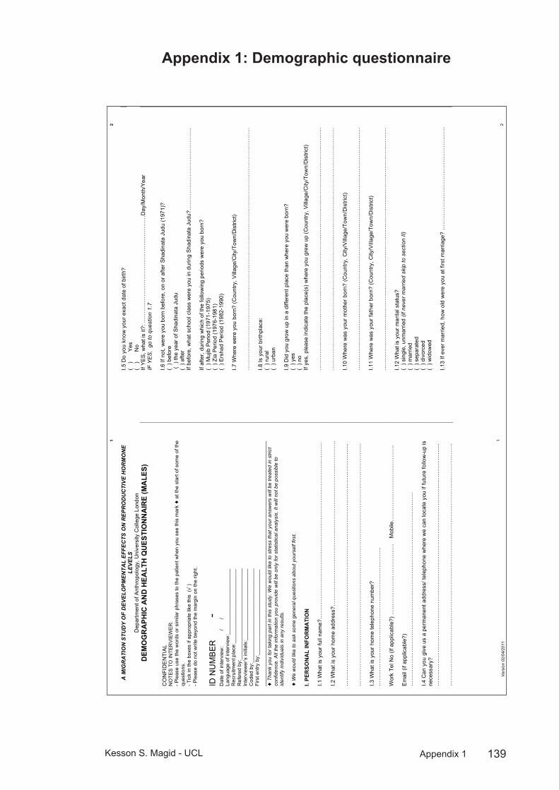
139Kesson S. Magid - UCL Appendix 1
Demographic questionnaireAppendix 1:
Ver
sion
02/
04/2
011
1 1
A M
IGR
ATI
ON
STU
DY
OF
DEV
ELO
PM
EN
TAL
EFF
EC
TS O
N R
EP
RO
DU
CTI
VE
HO
RM
ON
E LE
VE
LS
Dep
artm
ent o
f Ant
hrop
olog
y, U
nive
rsity
Col
lege
Lon
don
DEM
OG
RA
PHIC
AN
D H
EALT
H Q
UES
TIO
NN
AIR
E (M
ALE
S)
CO
NFI
DE
NTI
AL
NO
TES
TO IN
TER
VIE
WER
: - P
leas
e us
e th
e w
ords
or s
imila
r phr
ases
to th
e pa
tient
whe
n yo
u se
e th
is m
ark !
at t
he s
tart
of s
ome
of th
e qu
estio
ns.
- Tic
k in
the
boxe
s if
appr
opria
te li
ke th
is ("
) - P
leas
e do
not
writ
e be
yond
the
mar
gin
on th
e rig
ht.
ID N
UM
BE
R
-
Dat
e of
inte
rvie
w:
/
/
Lang
uage
of i
nter
view
:___
____
____
____
____
____
R
ecru
itmen
t pla
ce:_
____
____
____
____
____
____
_ R
efer
ed b
y:__
____
____
____
____
____
____
____
__
Inte
rvie
wer
’s in
itial
s:__
____
____
____
____
____
___
Cod
ed b
y:__
____
____
____
____
____
____
____
___
Firs
t ent
ry b
y:__
____
____
____
____
____
____
____
__
____
____
____
____
____
____
____
____
____
____
____
____
____
____
____
____
____
____
____
!
Tha
nk y
ou fo
r ta
king
par
t in
this
stu
dy. W
e w
ould
like
to s
tress
that
you
r ans
wer
s w
ill b
e tre
ated
in s
trict
co
nfid
ence
. All
the
info
rmat
ion
you
prov
ide
will
be
only
for s
tatis
tical
ana
lysi
s. It
will
not
be
poss
ible
to
iden
tify
indi
vidu
als
in a
ny re
sults
. !
We
wou
ld li
ke to
ask
som
e ge
nera
l que
stio
ns a
bout
you
rsel
f firs
t. I.
PER
SON
AL
INFO
RM
ATI
ON
I.1
Wha
t is
your
full
nam
e?…
……
……
……
……
……
……
……
……
……
……
……
……
……
……
……
. I.2
Wha
t is
your
hom
e ad
dres
s?…
……
……
……
……
……
……
……
……
……
……
……
……
……
……
. …
……
……
……
……
……
……
……
……
……
……
……
……
……
……
……
……
……
……
……
……
……
…
……
……
……
……
……
……
……
……
……
……
……
……
……
……
……
……
……
……
……
……
……
I.3
Wha
t is
your
hom
e te
leph
one
num
ber?
…
……
……
……
……
……
……
……
……
……
……
……
…..
Wor
k Te
l No
(if a
pplic
able
?) …
……
……
……
……
……
…..
Mob
ile…
……
……
……
……
……
……
.. E
mai
l (if
appl
icab
le?)
…
……
……
……
……
……
……
……
……
……
……
……
……
……
……
……
……
….
I.4 C
an y
ou g
ive
us a
per
man
ent a
ddre
ss/ t
elep
hone
whe
re w
e ca
n lo
cate
you
if fu
ture
follo
w-u
p is
ne
cess
ary?
…
……
……
……
……
……
……
……
……
……
……
……
……
……
……
……
……
……
……
……
……
……
…
……
……
……
……
……
……
……
……
……
……
……
……
……
……
……
……
……
……
……
……
……
2 2
I.5 D
o yo
u kn
ow y
our e
xact
dat
e of
birt
h?
( )
Yes
(
) N
o If
YE
S, w
hat i
s it?
: ……
……
……
……
……
……
……
……
……
…D
ay/M
onth
/Yea
r IF
YE
S,
go to
que
stio
n 1.
7 I.6
If n
ot, w
ere
you
born
bef
ore,
on
or a
fter S
hadi
nata
Jud
u (1
971)
? (
) bef
ore
( )
the
year
of S
hadi
nata
Jud
u (
) afte
r If
befo
re, w
hat s
choo
l cla
ss w
ere
you
in d
urin
g S
hadi
nata
Jud
u?…
……
……
……
……
……
……
…..
If af
ter,
durin
g w
hich
of t
he fo
llow
ing
perio
ds w
ere
you
born
? (
) Muj
ib P
erio
d (1
971-
1975
) (
) Zia
Per
iod
(197
6-19
81)
( ) E
rsha
d P
erio
d (1
982-
1990
) I.7
Whe
re w
ere
you
born
? (C
ount
ry, V
illag
e/C
ity/T
own/
Dis
trict
) …
……
……
……
……
……
……
……
……
……
……
……
……
……
……
……
……
……
……
……
……
……
I.8
Is y
our b
irthp
lace
: (
) rur
al
( ) u
rban
I.9
Did
you
gro
w u
p in
a d
iffer
ent p
lace
than
whe
re y
ou w
ere
born
? (
) yes
(
) no
If ye
s, p
leas
e in
dica
te th
e pl
ace(
s) w
here
you
gre
w u
p (C
ount
ry, V
illag
e/C
ity/T
own/
Dis
trict
) …
……
……
……
……
……
……
……
……
……
……
……
……
……
……
……
……
……
……
……
……
……
…
……
……
……
……
……
……
……
……
……
……
……
……
……
……
……
……
……
……
……
……
……
I.1
0 W
here
was
you
r mot
her b
orn?
(Cou
ntry
, City
/Vill
age/
Tow
n/D
istri
ct)
……
……
……
……
……
……
……
……
……
……
……
……
……
……
……
……
……
……
……
……
……
…
I.11
Whe
re w
as y
our f
athe
r bor
n? (C
ount
ry, C
ity/V
illag
e/To
wn/
Dis
trict
) …
……
……
……
……
……
……
……
……
……
……
……
……
……
……
……
……
……
……
……
……
……
I.1
2 W
hat i
s yo
ur m
arita
l sta
tus?
(
) sin
gle,
unm
arrie
d (if
nev
er m
arrie
d sk
ip to
sec
tion
II)
( ) m
arrie
d (
) sep
arat
ed
( ) d
ivor
ced
( ) w
idow
ed
I.13
If ev
er m
arrie
d, h
ow o
ld w
ere
you
at fi
rst m
arria
ge?
……
……
……
……
……
……
……
……
……
.

140Kesson S. Magid - UCL Appendix 1
Ver
sion
02/
04/2
011
3 3
Ple
ase
list t
he d
ates
and
you
r age
at a
ll pr
evio
us m
arria
ges,
if a
pplic
able
. I.1
4 D
ate
of m
arria
ge: …
……
……
……
…dd
/m/y
Age
at m
arria
ge:…
……
……
……
……
……
……
b.
D
ate
of m
arria
ge: …
……
……
……
…dd
/m/y
Age
at m
arria
ge:…
……
……
……
……
……
……
c.
D
ate
of m
arria
ge: …
……
……
……
…dd
/m/y
Age
at m
arria
ge:…
……
……
……
……
……
……
d.
D
ate
of m
arria
ge: …
……
……
……
…dd
/m/y
Age
at m
arria
ge:…
……
……
……
……
……
……
1.
15 C
ould
you
ple
ase
tell
us w
ho w
as re
gula
rly li
ving
in y
our h
ouse
hold
dur
ing
the
first
5 y
ears
of
your
chi
ldho
od?
Ple
ase
spec
ify w
ho (I
f nec
essa
ry, t
ick
mor
e th
an o
ne)
( ) n
ot s
ure
( ) f
athe
r
(
) mot
her
( ) b
roth
er
( ) s
iste
r (
) gra
ndm
othe
r
( ) g
rand
fath
er
( ) a
unt
( ) u
ncle
(
) oth
er fa
mily
mem
bers
……
……
……
……
……
……
……
……
……
…...
......
......
......
......
...
......
......
......
......
......
......
......
......
......
......
......
......
......
......
......
......
......
......
......
......
......
......
......
1.
16 C
ould
you
ple
ase
tell
us w
ho w
as re
gula
rly li
ving
in y
our h
ouse
hold
whe
n yo
u w
ere
6-13
ye
ars
of a
ge?
Ple
ase
spec
ify w
ho (I
f nec
essa
ry, t
ick
mor
e th
an o
ne)
( ) f
athe
r
(
) mot
her
( ) b
roth
er
( ) s
iste
r (
) gra
ndm
othe
r
( ) g
rand
fath
er
( ) a
unt
( ) u
ncle
(
) oth
er fa
mily
mem
bers
……
……
……
……
……
……
……
……
……
…...
......
......
......
......
...
......
......
......
......
......
......
......
......
......
......
......
......
......
......
......
......
......
......
......
......
......
......
......
1.
17 D
o yo
u ha
ve a
ny s
iblin
gs (b
roth
ers
or s
iste
rs)?
(
) Yes
(
) No
If ye
s, p
leas
e gi
ve th
eir s
ex, a
nd y
ear t
hey
wer
e bo
rn. (
If yo
u ar
e no
t sur
e w
hat y
ear t
hey
wer
e bo
rn, p
leas
e lis
t how
man
y ye
ars
they
are
old
er o
r yo
unge
r tha
n yo
u)
Sex
Year
bor
n 1.
(
) Bro
ther
( )
Sis
ter
2.
(
) Bro
ther
( )
Sis
ter
3.
(
) Bro
ther
( )
Sis
ter
4.
(
) Bro
ther
( )
Sis
ter
5.
(
) Bro
ther
( )
Sis
ter
6.
(
) Bro
ther
( )
Sis
ter
7.
(
) Bro
ther
( )
Sis
ter
8.
(
) Bro
ther
( )
Sis
ter
9.
(
) Bro
ther
( )
Sis
ter
10
(
) Bro
ther
( )
Sis
ter
__
____
____
____
____
____
____
____
____
____
____
____
____
____
____
____
____
____
____
____
4 4
II. M
IGR
ATI
ON
!
The
que
stio
ns in
the
follo
win
g se
ctio
n co
ncer
n th
e hi
stor
y of
mig
ratio
n of
you
r fa
mily
and
you
rsel
f. Th
is w
ill
give
us
an id
ea o
f the
type
of e
nviro
nmen
t you
live
d in
at d
iffer
ent s
tage
s of
you
r lif
e. If
you
wer
e bo
rn in
the
UK
, ski
p to
que
stio
n II.
11
II.1
If yo
u w
ere
not b
orn
in th
e U
K, i
n w
hat y
ear d
id y
ou a
rrive
in th
e U
K?…
……
……
……
……
……
. II.
2 H
ow o
ld w
ere
you
whe
n yo
u ar
rived
in th
e U
K?
……
……
……
……
……
……
……
……
……
……
.. II.
3 W
here
did
you
live
bef
ore
com
ing
to th
e U
K?
(Cou
ntry
, City
/Villa
ge/T
own/
Dis
trict
) …
……
……
……
……
……
……
……
……
……
……
……
……
……
……
……
……
……
……
……
……
……
II.
4 Is
that
pla
ce:
( ) u
rban
(
) rur
al
II.5
Wha
t was
you
r hou
seho
ld’s
hea
d’s
occu
patio
n be
fore
you
cam
e to
the
UK
? …
……
……
……
……
……
……
……
……
……
……
……
……
……
……
……
……
……
……
……
……
……
II.
6 W
ho m
oved
toge
ther
with
you
at t
he ti
me
of m
igra
tion?
(ple
ase
tick
all t
hat a
pply
) (
) wife
(
) fat
her i
n la
w
( ) f
athe
r
(
) mot
her i
n la
w
( ) m
othe
r
(
) sis
ter i
n la
w
( ) s
iste
r
(
) bro
ther
in la
w
(
) bro
ther
(
) son
in la
w
( ) s
on
( ) d
augh
ter i
n la
w
( ) d
augh
ter
( ) o
ther
fam
ily m
embe
rs…
……
……
……
……
……
……
……
……
……
……
……
……
……
……
……
….
( ) m
igra
ted
with
out a
ny fa
mily
mem
bers
II.
7 W
hat w
as th
e pu
rpos
e of
you
r mig
ratio
n fro
m B
angl
ades
h? (p
leas
e tic
k al
l tha
t app
ly)
( ) e
cono
mic
(
) edu
catio
n (
) acc
ompa
ny fa
mily
(
) mar
riage
(
) oth
er s
peci
fy …
……
……
……
……
……
……
……
……
……
……
II.
8 Is
/are
ther
e an
y ot
her m
embe
r(s) o
f you
r fam
ily li
ving
in B
angl
ades
h?
( ) y
es
( ) n
o If
yes,
ple
ase
spec
ify w
ho (I
f nec
essa
ry, t
ick
mor
e th
an o
ne)
( ) w
ife
( ) f
athe
r in
law
(
) fat
her
( ) m
othe
r in
law
(
) mot
her
( ) s
iste
r in
law
(
) sis
ter
( ) b
roth
er in
law
( ) b
roth
er
( ) s
on in
law
(
) son
(
) dau
ghte
r in
law
(
) dau
ghte
r (
) oth
er fa
mily
mem
bers
……
……
……
……
……
……
……
……
……
……
……
……
……
……
……
……
. W
here
in B
angl
ades
h do
they
live
? (to
wn/
villa
ge/to
wn/
dist
rict)
……
……
……
……
……
……
……
……
……
……
……
……
……
……
……
……
……
……
……
……
……
….

141Kesson S. Magid - UCL Appendix 1
Ver
sion
02/
04/2
011
5 5
II.9
Whe
re d
id y
ou li
ve w
hen
first
arr
ivin
g in
the
UK
? (c
ity/to
wn)
……
……
……
……
……
……
……
….
II.10
Wha
t was
you
r hou
seho
ld’s
hea
d’s
occu
patio
n w
hen
first
arr
ivin
g in
the
UK
? …
……
……
……
……
……
……
……
……
……
……
……
……
……
……
……
……
……
……
……
……
……
. II.
11 If
you
wer
e bo
rn in
the
UK
to B
angl
ades
hi p
aren
ts, i
n w
hich
yea
r did
they
arr
ive
in th
e U
K?
Fath
er …
……
……
……
….
( ) D
on’t
know
M
othe
r ……
……
……
……
. (
) Don
’t kn
ow
( ) N
ot A
pplic
able
__
____
____
____
____
____
____
____
____
____
____
____
____
____
____
____
____
____
____
___
III. S
OC
IOEC
ON
OM
IC IN
FOR
MA
TIO
N
! T
he fo
llow
ing
sect
ion
asks
que
stio
ns a
bout
you
rsel
f and
you
r fa
mily
. W
e on
ly u
se th
is in
form
atio
n to
ca
tego
rise
heal
th c
ondi
tions
. You
will
not
be
iden
tifie
d pe
rson
ally
, and
onl
y m
embe
rs o
f the
rese
arch
team
w
ill h
ave
acce
ss to
thes
e pa
pers
. If y
ou p
refe
r no
t to
answ
er a
que
stio
n, p
leas
e tic
k th
e bo
x “I’
d ra
ther
not
sa
y” a
nd s
kip
that
que
stio
n.
III.1
Wha
t typ
e of
acc
omm
odat
ion
does
you
r hou
seho
ld o
ccup
y?
( ) h
ouse
(
) fla
t (
) oth
er, s
peci
fy…
……
……
……
……
……
……
……
……
……
……
III
.2 D
oes
your
hou
seho
ld o
wn
or re
nt a
ccom
mod
atio
n?
(
) ow
ns
( ) r
ents
If
you
rent
, who
is y
our l
andl
ord?
( )
I’d ra
ther
not
say
(
) Cou
ncil
/ Loc
al a
utho
rity
( ) P
rivat
e la
ndlo
rd o
r let
ting
agen
cy
III.3
How
man
y ro
oms
do y
ou h
ave
for u
se b
y yo
ur h
ouse
hold
? D
o no
t cou
nt b
athr
oom
s, to
ilets
, hal
ls o
r lan
ding
s, o
r roo
ms
that
can
onl
y be
use
d fo
r sto
rage
suc
h as
cup
boar
ds.
Do
coun
t all
othe
r roo
ms,
for e
xam
ple
kitc
hens
, liv
ing
room
s, b
edro
oms,
util
ity ro
oms
and
stud
ies.
If
two
room
s ha
ve b
een
conv
erte
d in
to o
ne, c
ount
them
as
one
room
. N
umbe
r of r
oom
s……
……
……
……
……
……
……
……
……
……
……
.. (
) I’d
rath
er n
ot s
ay
III.4
How
man
y m
embe
rs a
re th
ere
perm
anen
tly li
ving
in y
our h
ouse
hold
? P
leas
e in
dica
te th
eir r
elat
ions
hip
to y
ou a
nd th
eir a
ges:
(
) I’d
rath
er n
ot s
ay
Rel
atio
nshi
p to
you
A
ge
6 6
III.5
In y
our h
ouse
hold
, do
you
have
a:
Y
es
No
a. C
ar
b. C
D p
laye
r
c.
Was
hing
mac
hine
d.
Fre
ezer
e.
Tum
ble
drye
r
f.
Cen
tral h
eatin
g
g.
Vid
eo/D
VD
pla
yer
h. D
ishw
ashe
r
i.
Hom
e co
mpu
ter
j. M
icro
wav
e
k.
Sat
ellit
e/ca
ble
tele
visi
on
III.6
Ple
ase
tick
your
tota
l hou
seho
ld in
com
e in
a m
onth
afte
r tax
? (P
leas
e in
clud
e th
e m
onie
s ea
rned
by
all
the
mem
bers
of y
our
hous
ehol
d, p
leas
e in
clud
e m
onie
s fro
m b
enef
its, s
alar
ies
and
pens
ions
) (
) I’
d ra
ther
not
say
(
) le
ss th
an £
500
( )
£1,5
00 –
2,0
00
(
) £3
,000
– 3
,500
(
) £
500-
£1,0
00
( )
£2,0
00 –
2,5
00
(
) £3
,500
– 4
,000
(
) £
1,00
0 –
1,50
0
(
) £2
,500
– 3
000
( )
£4,0
00 o
r mor
e III
.8 C
ould
you
ple
ase
spec
ify th
e so
urce
s of
you
r hou
seho
ld in
com
e? (P
leas
e tic
k al
l tha
t app
ly)
( )I’
d ra
ther
not
say
(
) Ear
ning
s fro
m e
mpl
oym
ent o
r sel
f-em
ploy
men
t (
) Sta
te re
tirem
ent p
ensi
on
( ) P
ensi
on fr
om fo
rmer
em
ploy
er
( ) C
hild
ben
efit
( ) J
ob-s
eeke
rs a
llow
ance
(
) Inc
ome
supp
ort
( ) F
amily
cre
dit
( ) H
ousi
ng b
enef
it (
) Oth
er s
tate
ben
efits
(
) Int
eres
t fro
m s
avin
gs a
nd in
vest
men
ts (e
g. s
tock
s an
d sh
ares
) (
) Oth
er k
inds
of r
egul
ar a
llow
ance
from
out
side
you
r hou
seho
ld (e
g. m
aint
enan
ce, s
tude
nt
gran
ts, r
ent)
____
____
____
____
____
____
____
____
____
____
____
____
____
____
____
____
____
____
____
__
IV. E
MPL
OYM
ENT
INFO
RM
ATI
ON
!
We
ask
this
info
rmat
ion
beca
use
ther
e ar
e of
ten
rela
tions
hips
bet
wee
n he
alth
issu
es a
nd w
heth
er p
eopl
e ar
e em
ploy
ed in
or
outs
ide
of th
e ho
me.
IV
.1 H
ave
you
ever
wor
ked
outs
ide
the
hom
e?
( ) y
es
( ) n
o IV
.2 H
ave
you
ever
wor
ked
from
hom
e (e
.g. c
ompu
ting,
boo
k-ke
epin
g, e
tc.)?
(
) yes
, ple
ase
spec
ify …
……
……
……
……
……
……
……
……
……
……
……
……
……
……
……
……
(
) no
IV.3
Wha
t is
your
cur
rent
occ
upat
ion?
Incl
ude
self-
empl
oym
ent,
volu
ntee
r w
ork,
retir
ed)
……
……
……
……
……
……
……
……
……
……
……
……
……
……
……
……
……
……
……
……
……
…
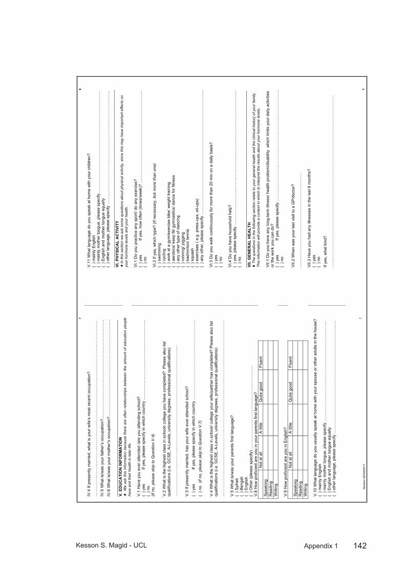
142Kesson S. Magid - UCL Appendix 1
Ver
sion
02/
04/2
011
7 7
IV.4
If p
rese
ntly
mar
ried,
wha
t is
your
wife
’s m
ost r
ecen
t occ
upat
ion?
…
……
……
……
……
……
……
……
……
……
……
……
……
……
……
……
……
……
……
……
……
……
IV
.5 W
hat i
s/w
as y
our f
athe
r’s o
ccup
atio
n?…
……
……
……
……
……
……
……
……
……
……
……
….
IV.6
Wha
t is/
was
you
r mot
her’s
occ
upat
ion?
……
……
……
……
……
……
……
……
……
……
……
…...
____
____
____
____
____
____
____
____
____
____
____
____
____
____
____
____
____
___
V. E
DU
CA
TIO
N IN
FOR
MA
TIO
N
!
We
ask
this
info
rmat
ion
beca
use
ther
e ar
e of
ten
rela
tions
hips
bet
wee
n th
e am
ount
of
educ
atio
n pe
ople
ha
ve a
nd th
eir
heal
th in
late
r lif
e.
V.1
Hav
e yo
u ev
er a
ttend
ed /a
re y
ou a
ttend
ing
scho
ol?
(
) yes
If
yes,
ple
ase
spec
ify in
whi
ch c
ount
ry …
……
……
……
……
……
……
……
……
……
.. (
) no
(if
no,
ple
ase
skip
to Q
uest
ion
V.4
) V
.2 W
hat i
s th
e hi
ghes
t cla
ss in
sch
ool/
colle
ge y
ou h
ave
com
plet
ed?
Ple
ase
also
list
qu
alifi
catio
ns (i
.e. G
CS
E, A
-Lev
els,
uni
vers
ity d
egre
es, p
rofe
ssio
nal q
ualif
icat
ions
) …
……
……
……
……
……
……
……
……
……
……
……
……
……
……
……
……
……
……
V
.3 If
pre
sent
ly m
arrie
d, h
as y
our w
ife e
ver a
ttend
ed s
choo
l?
( ) y
es
If ye
s, p
leas
e sp
ecify
in w
hich
cou
ntry
……
……
……
……
……
……
……
……
……
…..
( ) n
o (
if no
, ple
ase
skip
to Q
uest
ion
V.7
) V
.4 W
hat i
s th
e hi
ghes
t cla
ss in
sch
ool/
colle
ge y
our w
ife/p
artn
er h
as c
ompl
eted
? P
leas
e al
so li
st
qual
ifica
tions
(i.e
. GC
SE
, A-L
evel
s, u
nive
rsity
deg
rees
, pro
fess
iona
l qua
lific
atio
ns)
……
……
……
……
……
……
……
……
……
……
……
……
……
……
……
……
……
……
……
……
……
…
V.5
Wha
t is/
was
you
r par
ents
firs
t lan
guag
e?
( ) S
ylhe
ti (
) Ben
gali
( ) E
nglis
h (
) Oth
er (p
leas
e sp
ecify
) ……
……
……
……
……
……
……
……
……
……
. V
.8 H
ow p
rofic
ient
are
you
in y
our p
aren
ts fi
rst l
angu
age?
Not
at a
ll A
littl
e Q
uite
goo
d Fl
uent
S
peak
ing
Rea
ding
W
ritin
g
V
.9 H
ow p
rofic
ient
are
you
in E
nglis
h?
N
ot a
t all
A li
ttle
Qui
te g
ood
Flue
nt
Spe
akin
g
R
eadi
ng
Writ
ing
V.1
0 W
hat l
angu
age
do y
ou u
sual
ly s
peak
at h
ome
with
you
r spo
use
or o
ther
adu
lts in
the
hous
e?
( ) m
ainl
y E
nglis
h (
) mai
nly
mot
her t
ongu
e, p
leas
e sp
ecify
……
……
……
……
……
……
……
……
……
……
……
……
.. (
) Eng
lish
and
mot
her t
ongu
e eq
ually
(
) oth
er la
ngua
ge, p
leas
e sp
ecify
……
……
……
……
……
……
……
……
……
……
……
……
……
…..
8 8
V.1
1 W
hat l
angu
age
do y
ou s
peak
at h
ome
with
you
r chi
ldre
n?
( ) m
ainl
y E
nglis
h (
) mai
nly
mot
her t
ongu
e, p
leas
e sp
ecify
……
……
……
……
……
……
……
……
……
……
……
……
…
( ) E
nglis
h an
d m
othe
r ton
gue
equa
lly
( ) o
ther
lang
uage
, ple
ase
spec
ify …
……
……
……
……
……
……
……
……
……
……
……
……
…...
...
____
____
____
____
____
____
____
____
____
____
____
____
____
____
____
____
____
____
____
__
VI. P
HYS
ICA
L A
CTI
VITY
!
In th
is s
ectio
n w
e as
k so
me
ques
tions
abo
ut p
hysi
cal a
ctiv
ity, s
ince
this
may
hav
e im
port
ant e
ffect
s on
yo
ur h
orm
one
leve
ls a
nd y
our
heal
th.
VI.1
Do
you
prac
tice
any
spor
t/ do
any
exe
rcis
e?
( ) y
es
If ye
s, h
ow o
ften
(tim
es/w
eek)
? …
……
……
……
……
……
……
……
……
……
……
…..
( ) n
o V
I.2 If
yes
, whi
ch ty
pe?
(If n
eces
sary
, tic
k m
ore
than
one
) (
) sw
imm
ing
( ) c
yclin
g (
) wor
k at
a g
ym/e
xerc
ise
bike
/ wei
ght t
rain
ing
( ) a
erob
ics/
kee
p fit
/ gym
nast
ics/
dan
ce fo
r fitn
ess
( ) a
ny o
ther
type
of d
anci
ng
( ) r
unni
ng/ j
oggi
ng
( ) b
adm
into
n/ te
nnis
(
) squ
ash
( ) e
xerc
ises
( e.
g. p
ress
-ups
, sit-
ups)
(
) any
oth
er, p
leas
e sp
ecify
……
……
……
……
……
……
……
……
……
……
……
……
……
……
……
.. V
I.3 D
o yo
u w
alk
cont
inuo
usly
for m
ore
than
20
min
on
a da
ily b
asis
? (
) yes
(
) no
VI.4
Do
you
have
hou
seho
ld h
elp?
(
) yes
, ple
ase
spec
ify …
……
……
……
……
……
……
……
……
……
……
……
……
……
……
……
……
(
) no
__
____
____
____
____
____
____
____
____
____
____
____
____
____
____
____
____
____
_ VI
I. G
ENER
AL
HEA
LTH
!
The
que
stio
ns in
the
follo
win
g se
ctio
n re
late
to y
our
gene
ral h
ealth
and
the
clin
ical
his
tory
of y
our
fam
ily.
This
info
rmat
ion
will
pro
vide
a c
onte
xt in
whi
ch to
inte
rpre
t the
resu
lts a
bout
you
r ho
rmon
e le
vels
. V
II.1
Do
you
have
any
long
-term
illn
ess/
hea
lth p
robl
em/d
isab
ility
whi
ch li
mits
you
r dai
ly a
ctiv
ities
or
the
wor
k yo
u ca
n do
? (
) yes
If
yes,
ple
ase
spec
ify …
……
……
……
……
……
……
……
……
……
……
……
……
……
. (
) no
VII.
2 W
hen
was
you
r las
t vis
it to
a G
P/d
octo
r?
……
……
……
……
……
……
……
……
……
……
……
…
VII.
3 H
ave
you
had
any
illne
sses
in th
e la
st 6
mon
ths?
(
) yes
(
) no
If ye
s, w
hat k
ind?
…
……
……
……
……
……
……
……
……
……
……
……
……
……
……
……
……
……
……
……
……
…

143Kesson S. Magid - UCL Appendix 1
Ver
sion
02/
04/2
011
9 9
II.4
Hav
e yo
u be
en d
iagn
osed
with
any
inte
stin
al p
aras
itic
infe
ctio
n in
the
past
6 m
onth
s (e
.g.,
amoe
bas,
gia
rdia
, sch
isos
omia
sis/
bilh
arzi
as)?
(
) yes
(
) no
If ye
s, w
hat k
ind?
……
……
……
……
……
……
……
……
……
……
……
……
……
……
……
……
……
…..
VII.
5 D
o yo
u su
ffer f
rom
any
of t
hese
dis
ease
s?
Dia
bete
s
(
) yes
( )
no (
) do
n’t k
now
H
eart
dise
ase
( ) y
es (
) no
( )
don’
t kno
w
Hyp
erlip
idem
ias
(Hig
h ch
oles
tero
l)
( ) y
es (
) no
( )
don’
t kno
w
Hyp
erte
nsio
n (H
igh
bloo
d pr
essu
re)
(
) yes
( )
no (
) do
n’t k
now
A
naem
ias
( ) y
es (
) no
( )
don’
t kno
w
Arth
ritis
or r
heum
atis
m
( ) y
es (
) no
( )
don’
t kno
w
Oth
er (p
leas
e sp
ecify
)
…
……
……
……
……
……
……
……
……
……
……
……
……
……
……
……
……
……
……
……
……
……
. V
II.6
Is th
ere
any
hist
ory
of d
iabe
tes
in y
our f
amily
? (
) yes
, if y
es p
leas
e sp
ecify
who
……
……
……
……
……
……
……
……
……
……
……
……
……
……
(
) no
( ) d
on’t
know
V
II.7
Is th
ere
any
hist
ory
of h
yper
tens
ion
(hig
h bl
ood
pres
sure
) in
your
fam
ily?
( ) y
es, i
f yes
ple
ase
spec
ify w
ho …
……
……
……
……
……
……
……
……
……
……
……
……
……
…
( ) n
o (
) don
’t kn
ow
VII.
8 Is
ther
e an
y hi
stor
y of
car
diov
ascu
lar d
isea
se (e
.g.,
hear
t atta
ck, s
troke
) in
your
fam
ily?
( ) y
es, i
f yes
ple
ase
spec
ify w
ho …
……
……
……
……
……
……
……
……
……
……
……
……
……
…
( ) n
o (
) don
’t kn
ow
VII.
9 Is
ther
e an
y hi
stor
y of
thyr
oid
dise
ases
in y
our f
amily
? (
) yes
(
) no
( ) d
on’t
know
If
yes,
ple
ase
spec
ify w
hich
mem
ber o
f you
r clo
se fa
mily
has
bee
n af
fect
ed a
nd b
y w
hich
kin
d …
……
……
……
……
……
……
……
……
……
……
……
……
……
……
……
……
……
……
……
……
……
. V
II.10
Is th
ere
any
hist
ory
of c
ance
r in
your
fam
ily?
( ) y
es
( ) n
o (
) don
’t kn
ow
If ye
s, p
leas
e sp
ecify
whi
ch m
embe
r of y
our c
lose
fam
ily h
as b
een
affe
cted
and
by
whi
ch k
ind
…
……
……
……
……
……
……
……
……
……
……
……
……
……
……
……
……
……
……
……
……
……
. V
II.11
Hav
e yo
u ha
d an
y op
erat
ions
? (
) yes
, ple
ase
spec
ify …
……
……
……
……
……
……
……
……
……
……
……
……
……
……
……
……
(
) no
VII.
12 A
re y
ou a
veg
etar
ian?
(
) yes
(
) no
If ye
s, p
leas
e sp
ecify
wha
t typ
e:
( ) v
egan
(no
anim
al p
rodu
cts)
(
) lac
to-o
vo v
eget
aria
n (n
o m
eat,
fish,
ch
icke
n, e
tc. b
ut d
o ea
t dai
ry a
nd e
ggs)
(
) oth
er, p
leas
e sp
ecify
......
......
......
......
......
.
10
10
VII.
13 H
ave
you
been
on
a sp
ecia
l die
t in
the
last
3 m
onth
s?
( ) n
o (
) yes
If
yes,
wha
t wer
e th
e re
ason
s?
( ) t
o lo
se w
eigh
t (
) to
gain
wei
ght
( ) l
ow fa
t (
) hig
h fib
re
( ) o
ther
, ple
ase
spec
ify th
e ki
nd o
f die
t and
the
reas
on…
……
……
……
……
……
……
……
…...
......
......
......
......
......
......
......
......
......
......
......
.....
VII.
14 H
ave
you
lost
or g
aine
d w
eigh
t in
the
past
3 m
onth
s?
( ) y
es, p
leas
e sp
ecify
am
ount
……
……
……
……
……
……
……
……
……
……
……
……
……
……
(
) no
VII.
15 D
o yo
u re
gula
rly ta
ke a
ny n
utrit
iona
l sup
plem
ents
, vita
min
s or
min
eral
s?
( ) y
es,
(
) no
If ye
s, p
leas
e sp
ecify
wha
t kin
d …
……
……
……
……
……
……
……
……
……
……
……
……
…
VII.
16 H
ave
you
take
n an
y m
edic
atio
ns d
urin
g th
e pa
st m
onth
? (
) yes
(
) no
If ye
s, h
ow m
any
kind
s (in
clud
ing
hom
eopa
thy/
kabi
raji)
N
ame
of m
edic
ine
Hav
e yo
u ta
ken
this
med
icin
e in
the
last
2 w
eeks
? (Y
es/N
o)
1
2
3
4
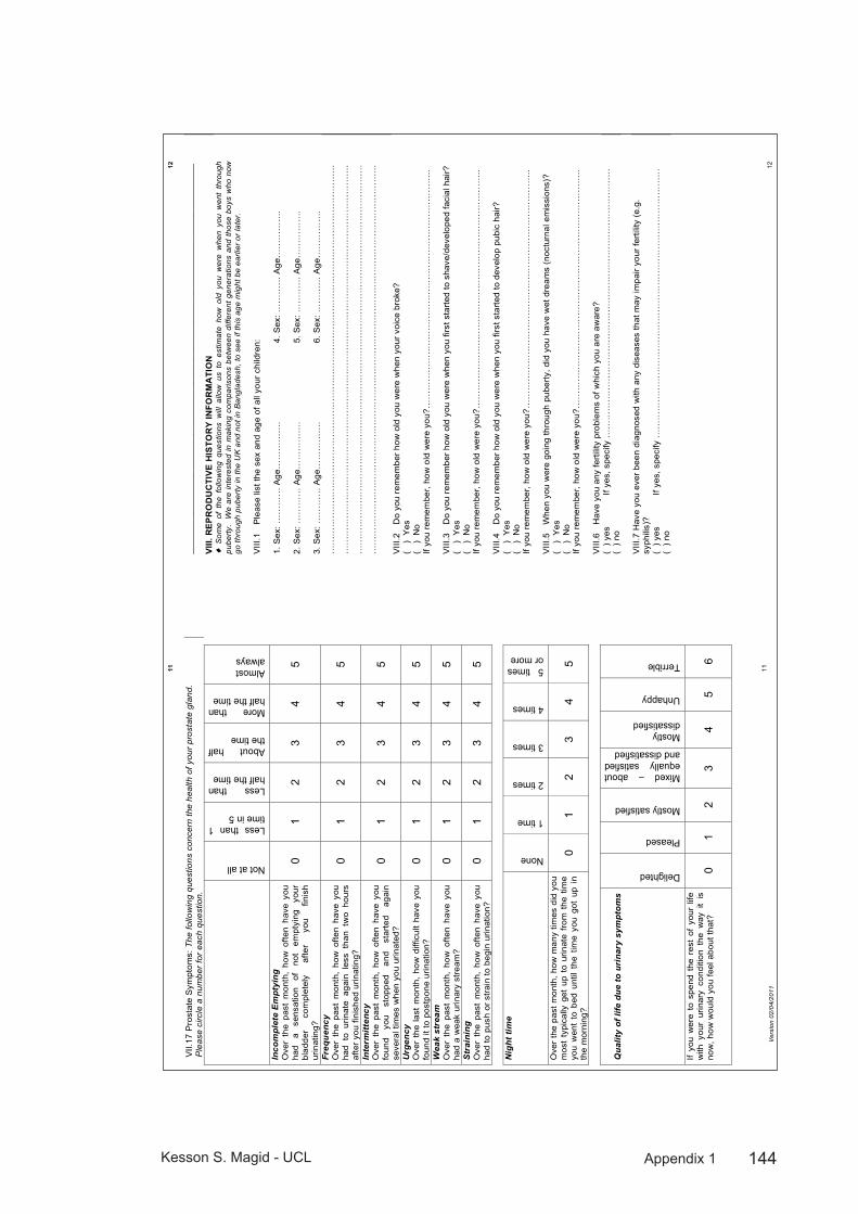
144Kesson S. Magid - UCL Appendix 1
Ver
sion
02/
04/2
011
11
11
VII.
17 P
rost
ate
Sym
ptom
s: T
he fo
llow
ing
ques
tions
con
cern
the
heal
th o
f you
r pr
osta
te g
land
. P
leas
e ci
rcle
a n
umbe
r fo
r ea
ch q
uest
ion.
Not at all
Less than 1 time in 5
Less than half the time
About half the time
More than half the time
Almost always
Inco
mpl
ete
Em
ptyi
ng
Ove
r th
e pa
st m
onth
, ho
w o
ften
have
you
ha
d a
sens
atio
n of
no
t em
ptyi
ng
your
bl
adde
r co
mpl
etel
y af
ter
you
finis
h ur
inat
ing?
0 1
2 3
4 5
Freq
uenc
y O
ver
the
past
mon
th,
how
ofte
n ha
ve y
ou
had
to u
rinat
e ag
ain
less
tha
n tw
o ho
urs
afte
r you
fini
shed
urin
atin
g?
0 1
2 3
4 5
Inte
rmitt
ency
O
ver
the
past
mon
th,
how
ofte
n ha
ve y
ou
foun
d yo
u st
oppe
d an
d st
arte
d ag
ain
seve
ral t
imes
whe
n yo
u ur
inat
ed?
0 1
2 3
4 5
Urg
ency
O
ver
the
last
mon
th,
how
diff
icul
t ha
ve y
ou
foun
d it
to p
ostp
one
urin
atio
n?
0 1
2 3
4 5
Wea
k st
ream
O
ver
the
past
mon
th,
how
ofte
n ha
ve y
ou
had
a w
eak
urin
ary
stre
am?
0 1
2 3
4 5
Str
aini
ng
Ove
r th
e pa
st m
onth
, ho
w o
ften
have
you
ha
d to
pus
h or
stra
in to
beg
in u
rinat
ion?
0
1 2
3 4
5
Nig
ht ti
me
None
1 time
2 times
3 times
4 times
5 times or more
Ove
r th
e pa
st m
onth
, how
man
y tim
es d
id y
ou
mos
t ty
pica
lly g
et u
p to
urin
ate
from
the
tim
e yo
u w
ent
to b
ed u
ntil
the
time
you
got
up i
n th
e m
orni
ng?
0 1
2 3
4 5
Qua
lity
of li
fe d
ue to
uri
nary
sym
ptom
s
Delighted
Pleased
Mostly satisfied
Mixed – about equally satisfied and dissatisfied
Mostly dissatisfied
Unhappy
Terrible
If yo
u w
ere
to s
pend
the
res
t of
you
r lif
e w
ith y
our
urin
ary
cond
ition
the
way
it
is
now
, how
wou
ld y
ou fe
el a
bout
that
? 0
1 2
3 4
5 6
12
12
____
____
____
____
____
____
____
____
____
____
____
____
____
____
____
____
____
____
____
__
VIII.
REP
RO
DU
CTI
VE H
ISTO
RY
INFO
RM
ATI
ON
!
Som
e of
the
fol
low
ing
ques
tions
will
allo
w u
s to
est
imat
e ho
w o
ld y
ou w
ere
whe
n yo
u w
ent
thro
ugh
pube
rty.
W
e ar
e in
tere
sted
in m
akin
g co
mpa
rison
s be
twee
n di
ffere
nt g
ener
atio
ns a
nd t
hose
boy
s w
ho n
ow
go th
roug
h pu
bert
y in
the
UK
and
not
in B
angl
ades
h, to
see
if th
is a
ge m
ight
be
earli
er o
r la
ter.
V
III.1
P
leas
e lis
t the
sex
and
age
of a
ll yo
ur c
hild
ren:
1.
Sex
: ……
……
Age
……
……
….
2. S
ex: …
……
… A
ge…
……
……
. 3.
Sex
: ……
……
Age
……
……
….
4. S
ex: …
……
… A
ge…
……
……
. 5.
Sex
: ……
……
Age
……
……
….
6. S
ex: …
……
… A
ge…
……
……
. …
……
……
……
……
……
……
……
……
……
……
……
……
……
……
……
……
……
……
……
……
……
. …
……
……
……
……
……
……
……
……
……
……
……
……
……
……
……
……
……
……
……
……
……
. …
……
……
……
……
……
……
……
……
……
……
……
……
……
……
……
……
……
……
……
……
……
. …
……
……
……
……
……
……
……
……
……
……
……
……
……
……
……
……
……
……
……
……
……
. V
III.2
D
o yo
u re
mem
ber h
ow o
ld y
ou w
ere
whe
n yo
ur v
oice
bro
ke?
( )
Yes
(
) N
o If
you
rem
embe
r, ho
w o
ld w
ere
you?
……
……
……
……
……
……
……
……
……
……
……
……
……
.. V
III.3
D
o yo
u re
mem
ber h
ow o
ld y
ou w
ere
whe
n yo
u fir
st s
tarte
d to
sha
ve/d
evel
oped
faci
al h
air?
(
) Y
es
( )
No
If yo
u re
mem
ber,
how
old
wer
e yo
u?…
……
……
……
……
……
……
……
……
……
……
……
……
…..
VIII
.4
Do
you
rem
embe
r how
old
you
wer
e w
hen
you
first
sta
rted
to d
evel
op p
ubic
hai
r?
( )
Yes
(
) N
o If
you
rem
embe
r, ho
w o
ld w
ere
you?
……
……
……
……
……
……
……
……
……
……
……
……
……
.. V
III.5
W
hen
you
wer
e go
ing
thro
ugh
pube
rty, d
id y
ou h
ave
wet
dre
ams
(noc
turn
al e
mis
sion
s)?
( )
Yes
(
) N
o If
you
rem
embe
r, ho
w o
ld w
ere
you?
……
……
……
……
……
……
……
……
……
……
……
……
……
.. V
III.6
H
ave
you
any
ferti
lity
prob
lem
s of
whi
ch y
ou a
re a
war
e?
( ) y
es
If ye
s, s
peci
fy …
……
……
……
……
……
……
……
……
……
……
……
……
……
……
…
( ) n
o V
III.7
Hav
e yo
u ev
er b
een
diag
nose
d w
ith a
ny d
isea
ses
that
may
impa
ir yo
ur fe
rtilit
y (e
.g.
syph
ilis)
? (
) yes
If
yes,
spe
cify
……
……
……
……
……
……
……
……
……
……
……
……
……
……
……
(
) no
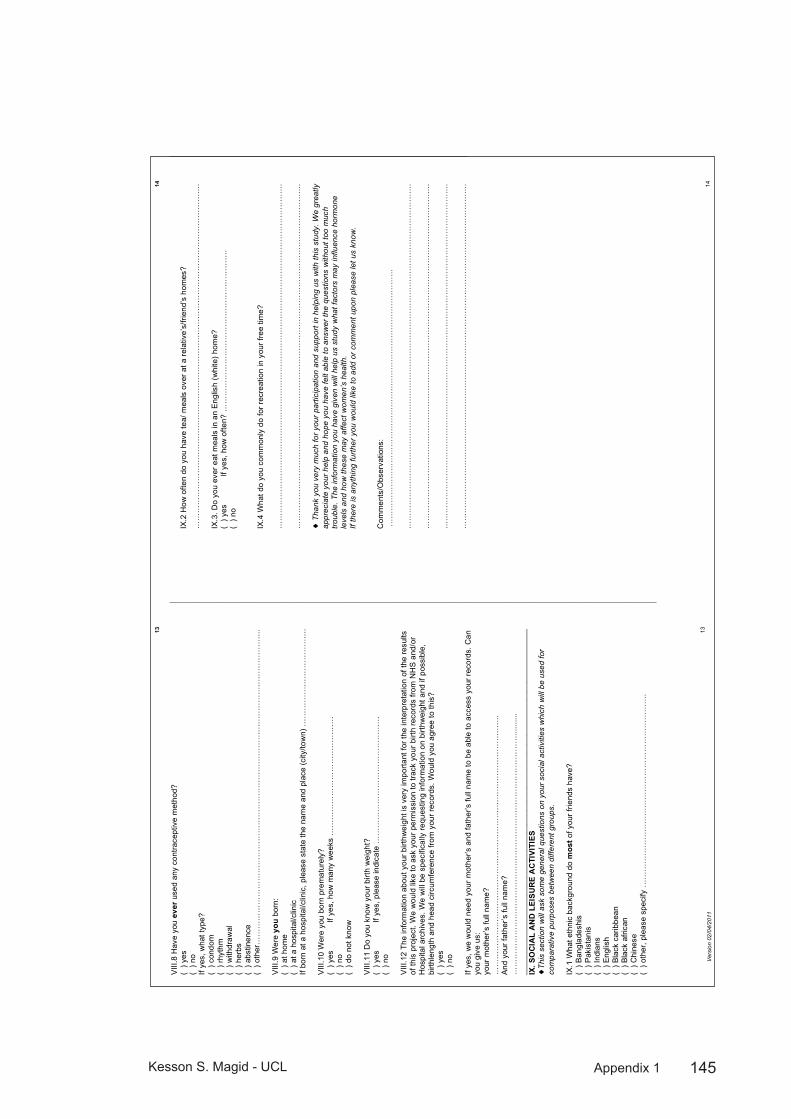
145Kesson S. Magid - UCL Appendix 1
Ver
sion
02/
04/2
011
13
13
VIII
.8 H
ave
you
ever
use
d an
y co
ntra
cept
ive
met
hod?
(
) yes
(
) no
If ye
s, w
hat t
ype?
(
) con
dom
(
) rhy
thm
(
) with
draw
al
( ) h
erbs
(
) abs
tinen
ce
( ) o
ther
……
……
……
……
……
……
……
……
……
……
……
……
……
……
……
……
……
……
……
…..
VIII
.9 W
ere
you
born
: (
) at h
ome
( ) a
t a h
ospi
tal/c
linic
If
born
at a
hos
pita
l/clin
ic, p
leas
e st
ate
the
nam
e an
d pl
ace
(city
/tow
n) …
……
……
……
……
……
….
VIII
.10
Wer
e yo
u bo
rn p
rem
atur
ely?
(
) yes
If
yes,
how
man
y w
eeks
……
……
……
……
……
……
……
…
( ) n
o (
) do
not k
now
V
III.1
1 D
o yo
u kn
ow y
our b
irth
wei
ght?
(
) yes
If
yes,
ple
ase
indi
cate
……
……
……
……
……
……
……
……
(
) no
VIII
.12
The
info
rmat
ion
abou
t you
r birt
hwei
ght i
s ve
ry im
porta
nt fo
r the
inte
rpre
tatio
n of
the
resu
lts
of th
is p
roje
ct. W
e w
ould
like
to a
sk y
our p
erm
issi
on to
trac
k yo
ur b
irth
reco
rds
from
NH
S a
nd/o
r H
ospi
tal a
rchi
ves.
We
will
be
spec
ifica
lly re
ques
ting
info
rmat
ion
on b
irthw
eigh
t and
if p
ossi
ble,
bi
rthle
ngth
and
hea
d ci
rcum
fere
nce
from
you
r rec
ords
. Wou
ld y
ou a
gree
to th
is?
(
) yes
(
) no
If ye
s, w
e w
ould
nee
d yo
ur m
othe
r’s a
nd fa
ther
’s fu
ll na
me
to b
e ab
le to
acc
ess
your
reco
rds.
Can
yo
u gi
ve u
s:
your
mot
her’s
full
nam
e?
……
……
……
……
……
……
……
……
……
……
……
……
……
……
……
……
.. A
nd y
our f
athe
r’s fu
ll na
me?
…
……
……
……
……
……
……
……
……
……
……
……
……
……
……
…...
......
. __
____
____
____
____
____
____
____
____
____
____
____
____
____
____
____
____
____
____
____
IX
. SO
CIA
L A
ND
LEI
SUR
E A
CTI
VITI
ES
!Th
is s
ectio
n w
ill a
sk s
ome
gene
ral q
uest
ions
on
your
soc
ial a
ctiv
ities
whi
ch w
ill b
e us
ed fo
r co
mpa
rativ
e pu
rpos
es b
etw
een
diffe
rent
gro
ups.
IX
.1 W
hat e
thni
c ba
ckgr
ound
do
mos
t of y
our f
riend
s ha
ve?
( ) B
angl
ades
his
( ) P
akis
tani
s (
) Ind
ians
(
) Eng
lish
( ) B
lack
car
ibbe
an
( ) B
lack
afri
can
( ) C
hine
se
( ) o
ther
, ple
ase
spec
ify …
……
……
……
……
……
……
……
……
……
……
……
….
14
14
IX.2
How
ofte
n do
you
hav
e te
a/ m
eals
ove
r at a
rela
tive’
s/fri
end’
s ho
mes
?
……
……
……
……
……
……
……
……
……
……
……
……
……
……
……
……
……
……
……
……
……
….
IX.3
. Do
you
ever
eat
mea
ls in
an
Eng
lish
(whi
te) h
ome?
(
) yes
If
yes,
how
ofte
n? …
……
……
……
……
……
……
……
……
……
….
( ) n
o IX
.4 W
hat d
o yo
u co
mm
only
do
for r
ecre
atio
n in
you
r fre
e tim
e?
……
……
……
……
……
……
……
……
……
……
……
……
……
……
……
……
……
……
……
……
……
….
……
……
……
……
……
……
……
……
……
……
……
……
……
……
……
……
……
……
……
……
……
….
! T
hank
you
ver
y m
uch
for y
our
parti
cipa
tion
and
supp
ort i
n he
lpin
g us
with
this
stu
dy. W
e gr
eatly
ap
prec
iate
you
r hel
p an
d ho
pe y
ou h
ave
felt
able
to a
nsw
er th
e qu
estio
ns w
ithou
t too
muc
h tro
uble
. The
info
rmat
ion
you
have
giv
en w
ill h
elp
us s
tudy
wha
t fac
tors
may
influ
ence
hor
mon
e le
vels
and
how
thes
e m
ay a
ffect
wom
en’s
hea
lth.
If th
ere
is a
nyth
ing
furth
er y
ou w
ould
like
to a
dd o
r co
mm
ent u
pon
plea
se le
t us
know
. C
omm
ents
/Obs
erva
tions
: …
……
……
……
……
……
……
……
……
……
……
……
……
……
……
……
….
……
……
……
……
……
……
……
……
……
……
……
……
……
……
……
……
……
……
……
……
……
….
……
……
……
……
……
……
……
……
……
……
……
……
……
……
……
……
……
……
……
……
……
….
……
……
……
……
……
……
……
……
……
……
……
……
……
……
……
……
……
……
……
……
……
….
……
……
……
……
……
……
……
……
……
……
……
……
……
……
……
……
……
……
……
……
……
….

146Kesson S. Magid - UCL Appendix 2
Food habits questionnaireAppendix 2:
Ve
rsio
n 02
/04/
2011
1 1
A M
IGR
ATI
ON
STU
DY
OF
DE
VE
LOP
ME
NTA
L E
FFE
CTS
ON
RE
PR
OD
UC
TIV
E H
OR
MO
NE
LE
VE
LS
Dep
artm
ent o
f Ant
hrop
olog
y, U
nive
rsity
Col
lege
Lon
don
FOO
D H
AB
ITS
QU
ESTI
ON
NA
IRE
(MA
LE M
IG)
C
ON
FID
EN
TIA
L N
OTE
S T
O IN
TER
VIE
WE
R:
- Ple
ase
use
the
wor
ds o
r sim
ilar p
hras
es to
the
patie
nt w
hen
you
see
this
mar
k !
at t
he s
tart
of s
ome
of th
e qu
estio
ns.
- Tic
k in
the
boxe
s if
appr
opria
te li
ke th
is ("
) If t
he q
uest
ion
is n
ot a
pplic
able
, ple
ase
cros
s th
e nu
mbe
r off.
ID
NU
MB
ER
.
D
ate
of in
terv
iew
:
/
/
La
ngua
ge o
f int
ervi
ew:_
____
____
____
____
____
__
Rec
ruitm
ent p
lace
:___
____
____
____
____
____
___
Ref
ered
by:
____
____
____
____
____
____
____
____
In
terv
iew
er’s
initi
als:
____
____
____
____
____
____
_ C
oded
by:
____
____
____
____
____
____
____
____
_ Fi
rst e
ntry
by:
____
____
____
____
____
____
____
__
____
____
____
____
____
____
____
____
____
____
____
____
____
____
____
____
____
____
____
____
____
____
!
Tha
nk y
ou fo
r ag
reei
ng to
take
par
t in
this
sur
vey.
The
follo
win
g qu
estio
ns r
elat
e to
you
r usu
al e
atin
g ha
bits
. P
leas
e an
swer
all
the
ques
tions
as
fully
as
you
can.
The
info
rmat
ion
will
be
held
in s
trict
con
fiden
ce.
I. FO
OD
WA
YS
I.1 H
ow m
any
mea
ls d
o yo
u no
rmal
ly e
at a
day
……
……
……
……
……
……
……
……
……
……
……
……
……
…...
I.2
How
man
y na
sta/
snac
k br
eaks
do
you
norm
ally
hav
e a
day…
……
……
……
……
……
……
……
……
……
……
I.3
Do
you
alw
ays
eat H
alal
? (
) yes
(
) no
I.4 W
hich
type
of h
ome-
cook
ed fo
od d
o yo
u ea
t at h
ome?
Fo
od ty
pe
Dai
ly
Mon
thly
O
nly
on s
peci
al
occa
sion
s N
ever
AS
IAN
Mai
n m
eals
E
NG
LIS
H m
ain
mea
ls
I.5
Wha
t typ
e of
Eng
lish
(i.e.
non
-Ban
glad
eshi
, “W
este
rn”)
food
s do
you
eat
the
mos
t?
……
……
……
……
……
……
……
……
……
……
……
……
……
……
……
……
……
……
……
……
……
……
……
……
...
……
……
……
……
……
……
……
……
……
……
……
……
……
……
……
……
……
……
……
……
……
……
……
……
...
I.6 D
o yo
ur c
hild
ren
(or c
hild
ren
in y
our h
ouse
hold
) eat
diff
eren
t mea
ls o
r foo
d fro
m y
ours
? (
) yes
(
) no
If ye
s, w
hat t
ype
of fo
od d
o th
ey e
at?
……
……
……
……
……
……
……
……
……
……
……
……
……
……
……
……
……
……
……
……
……
……
……
……
...
……
……
……
……
……
……
……
……
……
……
……
……
……
……
……
……
……
……
……
……
……
……
……
……
.
Ve
rsio
n 02
/04/
2011
2 2
I.7 D
o yo
u ev
er e
at o
utsi
de th
e ho
me?
If s
o, w
here
, wha
t typ
e of
food
, and
how
ofte
n?
H
ow F
requ
ently
? Ty
pe o
f pla
ce
Type
of f
ood
Whi
ch m
eal?
(L
unch
, Din
ner,
etc.
) D
aily
W
eekl
y/
Fortn
ight
ly
Mon
thly
Le
ss th
an
once
a
mon
th
Nev
er
I.8
Who
doe
s th
e sh
oppi
ng fo
r foo
d at
hom
e? …
……
……
……
……
……
……
……
……
……
……
……
……
I.9
W
here
is th
e sh
oppi
ng is
nor
mal
ly d
one?
……
……
……
……
……
……
……
……
……
……
……
……
……
. I.1
0 H
ow fa
r do
you
norm
ally
trav
el w
hen
shop
ping
for f
ood?
…
……
……
……
……
……
……
……
……
……
……
……
……
……
……
……
……
……
……
……
……
……
……
……
…...
I.1
3 D
o yo
u bu
y fo
od in
bul
k?
( ) y
es
( ) n
o If
yes,
wha
t typ
e an
d ho
w o
ften?
Ty
pe o
f foo
d W
eekl
y Fo
rtnig
htly
M
onth
ly
Less
than
onc
e a
mon
th
I.1
4 W
hat i
s th
e m
ost e
xpen
sive
food
item
on
your
sho
ppin
g lis
t tha
t you
buy
regu
larly
? …
……
……
……
……
……
……
……
……
……
……
……
……
……
……
……
……
……
……
……
……
……
……
……
…...
I.1
5 D
o yo
u bu
y an
y im
porte
d fo
ods
from
Ban
glad
esh?
(
) yes
(
) no
If ye
s, w
hat t
ypes
? …
……
……
……
……
……
……
……
……
……
……
……
……
……
……
……
……
……
……
……
……
……
……
……
…...
…
……
……
……
……
……
……
……
……
……
……
……
……
……
……
……
……
……
……
……
……
……
……
……
…...
…
……
……
……
……
……
……
……
……
……
……
……
……
……
……
……
……
……
……
……
……
……
……
……
…...

147Kesson S. Magid - UCL Appendix 2
Ve
rsio
n 02
/04/
2011
3 3
If yo
u m
igra
ted
from
Ban
glad
esh:
(
) not
app
licab
le (i
f bor
n in
the
UK
, ple
ase
skip
to s
ectio
n II)
III
.1 W
hich
food
s do
you
eat
mor
e of
in E
ngla
nd
than
whe
n yo
u liv
ed in
Ban
glad
esh?
…
……
……
……
……
……
……
……
……
……
……
……
……
……
……
……
……
……
……
……
……
……
……
……
……
……
……
……
……
……
……
……
……
……
……
……
……
……
……
……
……
……
……
……
……
……
……
……
……
……
……
……
……
……
……
…
III.2
W
hich
food
s do
you
eat
less
of i
n E
ngla
nd
than
whe
n yo
u liv
ed in
Ban
glad
esh?
…
……
……
……
……
……
……
……
……
……
……
……
……
……
……
……
……
……
……
……
……
……
……
……
…...
……
……
......
......
......
......
......
......
......
......
.....
......
......
......
......
......
......
......
......
......
......
......
......
......
....
......
......
......
......
......
......
......
......
......
......
......
......
......
II
. N
ON
-FO
OD
HA
BITS
II.
1 D
o yo
u currently
che
w b
etel
nut
(paa
n)?
( ) y
es
( ) n
o (if
no,
ple
ase
skip
to q
uest
ion
II.5)
If
yes,
how
ofte
n do
you
che
w?
Mor
e th
an 3
tim
es/d
ay
3 tim
es/d
ay
(afte
r eac
h m
eal)
Less
than
3
times
/day
O
n w
eeke
nds
On
spec
ial
occa
sion
s (e
.g.,
wed
ding
s)
II.2
How
old
wer
e yo
u w
hen
you
star
ted
chew
ing
bete
l nut
?....
......
......
......
......
......
……
……
……
……
……
…...
II.
3 W
hy d
id y
ou s
tart
chew
ing
bete
l nut
? …
……
……
……
……
……
……
……
……
……
……
……
……
……
……
……
……
……
……
……
……
……
……
……
…...
…
……
……
……
……
……
……
……
……
……
……
……
……
……
……
……
……
……
……
……
……
……
……
……
….
II.4
Wha
t ing
redi
ents
do
you
put i
nto
your
bet
el q
uid
(e.g
., lim
e, s
pice
s, e
tc)?
…
……
……
……
……
……
……
……
……
……
……
……
……
……
……
……
……
……
……
……
……
……
……
……
…...
…
……
……
……
……
……
……
……
……
……
……
……
……
……
……
……
……
……
……
……
……
……
……
……
…...
II.
5 H
ave
you
ever
che
wed
bet
el n
ut (p
aan)
, and
now
giv
en u
p?
( ) y
es
( ) n
o (if
no,
ple
ase
skip
to q
uest
ion
II.11
) If
yes,
how
ofte
n di
d yo
u ch
ew?
Mor
e th
an 3
tim
es/d
ay
3 tim
es/d
ay
(afte
r eac
h m
eal)
Less
than
3
times
/day
O
n w
eeke
nds
On
spec
ial
occa
sion
s (e
.g.,
wed
ding
s)
II.6
How
old
wer
e yo
u w
hen
you
star
ted
chew
ing
bete
l nut
?……
……
……
……
……
……
……
……
……
……
. II.
7 H
ow o
ld w
ere
you
whe
n yo
u st
oppe
d?...
....…
……
……
……
……
……
……
……
……
……
……
……
……
...
Ve
rsio
n 02
/04/
2011
4 4
II.8
Why
did
you
sta
rt ch
ewin
g be
tel n
ut?
……
……
……
……
……
……
……
……
……
……
……
……
……
……
……
……
……
……
……
……
……
……
……
……
…
……
……
……
……
……
……
……
……
……
……
……
……
.....…
……
……
……
……
……
……
……
……
……
……
…
II.9
If yo
u no
long
er c
hew
bet
el n
ut, w
hy d
id y
ou s
top?
…
……
……
……
……
……
……
……
……
……
……
……
……
……
……
……
……
……
……
……
……
……
……
……
…...
II.
10
Wha
t ing
redi
ents
did
you
put
into
you
r bet
el q
uid?
…
……
……
……
……
……
……
……
……
……
……
……
……
……
……
……
……
……
……
……
……
……
……
……
…...
…
……
……
……
……
……
……
……
……
……
……
……
……
……
……
……
……
……
……
……
……
……
……
……
…...
**
****
****
****
****
****
****
****
****
****
****
****
****
****
****
****
****
****
****
****
****
****
****
****
****
****
****
****
****
****
****
**
II.11
D
o yo
u currently
sm
oke
ciga
rette
s?
( ) y
es
( ) n
o (if
no,
ple
ase
skip
to q
uest
ion
II.15
) If
yes,
how
ofte
n do
you
sm
oke?
M
ore
than
3
times
/day
3
times
/day
(afte
r ea
ch m
eal)
Less
than
3
times
/day
O
n w
eeke
nds
On
spec
ial
occa
sion
s (e
.g.,
wed
ding
s)
II.12
H
ow m
any
pack
ets
of c
igar
ette
s pe
r wee
k (2
0 in
pac
k)?
……
……
……
……
……
……
……
….…
II.
13
How
old
wer
e yo
u w
hen
you
star
ted
smok
ing?
……
……
……
……
……
……
……
……
……
……
.. II.
14
Why
did
you
sta
rt sm
okin
g?
……
……
……
……
……
……
……
……
……
……
……
……
……
……
……
……
……
……
……
……
……
……
……
……
...
……
……
……
……
……
……
……
……
……
……
……
……
……
……
……
……
……
……
……
……
……
……
……
……
…
II.15
H
ave
you
ever
sm
oked
cig
aret
tes,
and
now
giv
en u
p?
( ) y
es
( ) n
o (if
no,
ple
ase
skip
to q
uest
ion
II.21
) If
yes,
how
ofte
n di
d yo
u sm
oke?
M
ore
than
3
times
/day
3
times
/day
(a
fter e
ach
mea
l)
Less
than
3
times
/day
O
n w
eeke
nds
On
spec
ial
occa
sion
s (e
.g.,
wed
ding
s)
II.
16
How
man
y pa
cket
s of
cig
aret
tes
did
you
smok
e pe
r wee
k (2
0 in
pac
k)?
……
……
……
……
……
……
…
II.17
H
ow o
ld w
ere
you
whe
n yo
u st
arte
d sm
okin
g?
……
……
……
……
……
……
……
……
.. II.
18
Why
did
you
sta
rt sm
okin
g?
……
……
……
……
……
……
……
……
……
……
……
……
……
……
……
……
……
……
……
……
……
……
……
……
...
……
……
……
……
……
……
……
……
……
……
……
……
……
……
……
……
……
……
……
……
……
……
……
……
...
II.19
H
ow o
ld w
ere
you
whe
n yo
u st
oppe
d?…
...…
……
……
……
……
……
……
……
……
……
……
…...
......
......
. II.
20
Why
did
you
sto
p sm
okin
g?
……
……
……
……
……
……
……
……
……
……
……
……
……
……
……
……
……
……
……
……
……
……
……
……
...
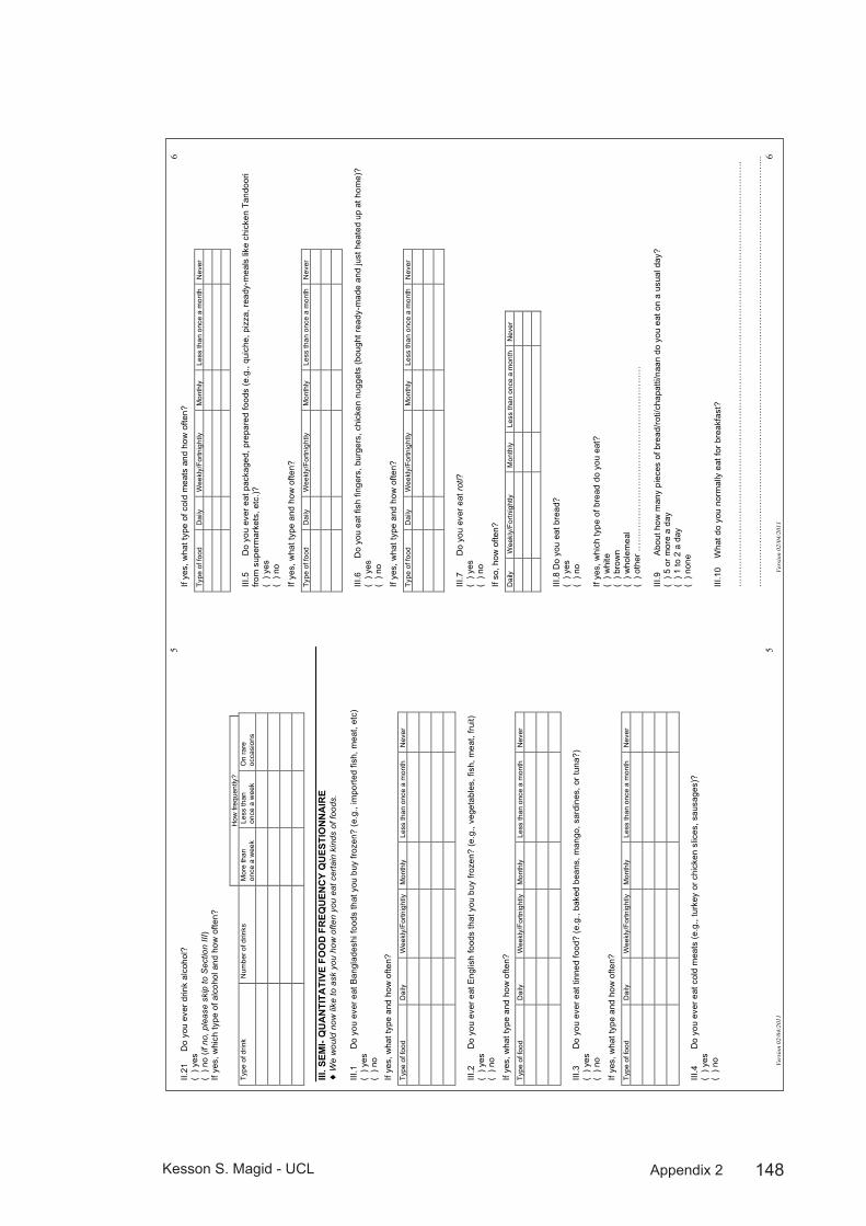
148Kesson S. Magid - UCL Appendix 2
Ve
rsio
n 02
/04/
2011
5 5
II.21
D
o yo
u ev
er d
rink
alco
hol?
(
) yes
(
) no
(if n
o, p
leas
e sk
ip to
Sec
tion
III)
If ye
s, w
hich
type
of a
lcoh
ol a
nd h
ow o
ften?
H
ow fr
eque
ntly
? Ty
pe o
f drin
k N
umbe
r of d
rinks
M
ore
than
on
ce a
wee
k Le
ss th
an
once
a w
eek
On
rare
oc
casi
ons
III. S
EMI-
QU
AN
TITA
TIVE
FO
OD
FR
EQU
ENC
Y Q
UES
TIO
NN
AIR
E !
We
wou
ld n
ow li
ke to
ask
you
how
ofte
n yo
u ea
t cer
tain
kin
ds o
f foo
ds.
III.1
D
o yo
u ev
er e
at B
angl
ades
hi fo
ods
that
you
buy
froz
en?
(e.g
., im
porte
d fis
h, m
eat,
etc)
(
) yes
(
) no
If ye
s, w
hat t
ype
and
how
ofte
n?
Type
of f
ood
Dai
ly
Wee
kly/
Fortn
ight
ly
Mon
thly
Le
ss th
an o
nce
a m
onth
N
ever
III.2
D
o yo
u ev
er e
at E
nglis
h fo
ods
that
you
buy
froz
en?
(e.g
., ve
geta
bles
, fis
h, m
eat,
fruit)
(
) yes
(
) no
If ye
s, w
hat t
ype
and
how
ofte
n?
Type
of f
ood
Dai
ly
Wee
kly/
Fortn
ight
ly
Mon
thly
Le
ss th
an o
nce
a m
onth
N
ever
III.3
D
o yo
u ev
er e
at ti
nned
food
? (e
.g.,
bake
d be
ans,
man
go, s
ardi
nes,
or t
una?
) (
) yes
(
) no
If ye
s, w
hat t
ype
and
how
ofte
n?
Type
of f
ood
Dai
ly
Wee
kly/
Fortn
ight
ly
Mon
thly
Le
ss th
an o
nce
a m
onth
N
ever
III.4
D
o yo
u ev
er e
at c
old
mea
ts (e
.g.,
turk
ey o
r chi
cken
slic
es, s
ausa
ges)
? (
) yes
(
) no
Ve
rsio
n 02
/04/
2011
6 6
If ye
s, w
hat t
ype
of c
old
mea
ts a
nd h
ow o
ften?
Type
of f
ood
Dai
ly
Wee
kly/
Fortn
ight
ly
Mon
thly
Le
ss th
an o
nce
a m
onth
N
ever
III
.5
Do
you
ever
eat
pac
kage
d, p
repa
red
food
s (e
.g.,
quic
he, p
izza
, rea
dy-m
eals
like
chi
cken
Tan
door
i fro
m s
uper
mar
kets
, etc
.)?
( ) y
es
( ) n
o
If ye
s, w
hat t
ype
and
how
ofte
n?
Type
of f
ood
Dai
ly
Wee
kly/
Fortn
ight
ly
Mon
thly
Le
ss th
an o
nce
a m
onth
N
ever
III
.6
Do
you
eat f
ish
finge
rs, b
urge
rs, c
hick
en n
ugge
ts (b
ough
t rea
dy-m
ade
and
just
hea
ted
up a
t hom
e)?
( ) y
es
( ) n
o
If ye
s, w
hat t
ype
and
how
ofte
n?
Type
of f
ood
Dai
ly
Wee
kly/
Fortn
ight
ly
Mon
thly
Le
ss th
an o
nce
a m
onth
N
ever
III
.7
Do
you
ever
eat
roti?
(
) yes
(
) no
If so
, how
ofte
n?
Dai
ly
Wee
kly/
Fortn
ight
ly
Mon
thly
Le
ss th
an o
nce
a m
onth
N
ever
III.8
Do
you
eat b
read
? (
) yes
(
) no
If ye
s, w
hich
type
of b
read
do
you
eat?
(
) whi
te
( ) b
row
n (
) who
lem
eal
( ) o
ther
……
……
……
……
……
……
……
……
……
……
…
III.9
A
bout
how
man
y pi
eces
of b
read
/roti/
chap
atti/
naan
do
you
eat o
n a
usua
l day
? (
) 5 o
r mor
e a
day
( ) 1
to 2
a d
ay
( ) n
one
III.1
0 W
hat d
o yo
u no
rmal
ly e
at fo
r bre
akfa
st?
……
……
……
……
……
……
……
……
……
……
……
……
……
……
……
……
……
……
……
……
……
……
……
……
. …
……
……
……
……
……
……
……
……
……
……
……
……
……
……
……
……
……
……
……
……
……
……
……
…...
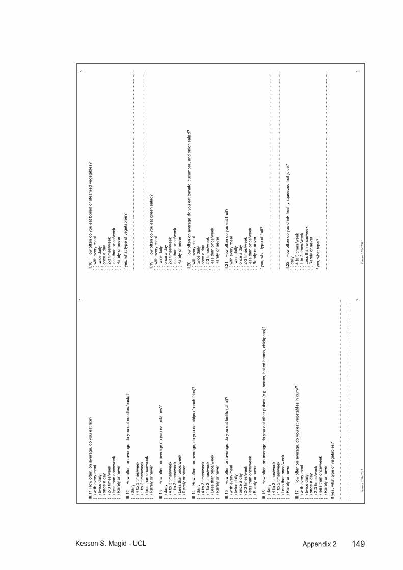
149Kesson S. Magid - UCL Appendix 2
Ve
rsio
n 02
/04/
2011
7 7
III.1
1 H
ow o
ften,
on
aver
age,
do
you
eat r
ice?
(
) with
eve
ry m
eal
( ) t
wic
e da
ily
( ) o
nce
a da
y (
) 2-3
tim
es/w
eek
( ) l
ess
than
onc
e/w
eek
( ) R
arel
y or
nev
er
III.1
2 H
ow o
ften,
on
aver
age,
do
you
eat n
oodl
es/p
asta
? (
) dai
ly
( ) 4
to 3
tim
es/w
eek
( ) 1
to 2
tim
es/w
eek
( ) l
ess
than
onc
e/w
eek
( ) R
arel
y or
nev
er
III.1
3 H
ow o
ften
on a
vera
ge d
o yo
u ea
t pot
atoe
s?
( ) d
aily
(
) 4 to
3 ti
mes
/wee
k (
) 1 to
2 ti
mes
/wee
k (
) Les
s th
an o
nce/
wee
k (
) Rar
ely
or n
ever
III
.14
H
ow o
ften,
on
aver
age,
do
you
eat c
hips
(fre
nch
fries
)?
( ) d
aily
(
) 4 to
3 ti
mes
/wee
k (
) 1 to
2 ti
mes
/wee
k (
) Les
s th
an o
nce/
wee
k (
) Rar
ely
or n
ever
III
.15
How
ofte
n, o
n av
erag
e, d
o yo
u ea
t len
tils
(dha
l)?
( ) w
ith e
very
mea
l (
) tw
ice
daily
(
) onc
e a
day
( ) 2
-3 ti
mes
/wee
k (
) les
s th
an o
nce/
wee
k (
) Rar
ely
or n
ever
III
.16
How
ofte
n, o
n av
erag
e, d
o yo
u ea
t oth
er p
ulse
s (e
.g.,
bean
s, b
aked
bea
ns, c
hick
peas
)?
( ) d
aily
(
) 4 to
3 ti
mes
/wee
k (
) 1 to
2 ti
mes
/wee
k (
) Les
s th
an o
nce/
wee
k (
) Rar
ely
or n
ever
III
.17
How
ofte
n on
ave
rage
, do
you
eat v
eget
able
s in
cur
ry?
(
) with
eve
ry m
eal
( ) t
wic
e da
ily
( ) o
nce
a da
y (
) 2-3
tim
es/w
eek
( ) l
ess
than
onc
e/w
eek
( ) R
arel
y or
nev
er
If ye
s, w
hat t
ype
of v
eget
able
s?
……
……
……
……
……
……
……
……
……
……
……
……
……
……
……
……
……
……
……
……
……
……
……
……
...
……
……
……
……
……
……
……
……
……
……
……
……
……
……
……
……
……
……
……
……
……
……
……
……
...
Ve
rsio
n 02
/04/
2011
8 8
III.1
8 H
ow o
ften
do y
ou e
at b
oile
d or
ste
amed
veg
etab
les?
(
) with
eve
ry m
eal
( ) t
wic
e da
ily
( ) o
nce
a da
y (
) 2-3
tim
es/w
eek
( ) l
ess
than
onc
e/w
eek
( ) R
arel
y or
nev
er
If ye
s, w
hat t
ype
of v
eget
able
s?
……
……
……
……
……
……
……
……
……
……
……
……
……
……
……
……
……
……
……
……
……
……
……
……
...
……
……
……
……
……
……
……
……
……
……
……
……
……
……
……
……
……
……
……
……
……
……
……
……
...
III.1
9 H
ow o
ften
do y
ou e
at g
reen
sal
ad?
( ) w
ith e
very
mea
l (
) tw
ice
daily
(
) onc
e a
day
( ) 2
-3 ti
mes
/wee
k (
) les
s th
an o
nce/
wee
k (
) Rar
ely
or n
ever
III
.20
How
ofte
n on
ave
rage
do
you
eat t
omat
o, c
ucum
ber,
and
onio
n sa
lad?
(
) with
eve
ry m
eal
( ) t
wic
e da
ily
( ) o
nce
a da
y (
) 2-3
tim
es/w
eek
( ) l
ess
than
onc
e/w
eek
( ) R
arel
y or
nev
er
III.2
1 H
ow o
ften
do y
ou e
at fr
uit?
(
) with
eve
ry m
eal
( ) t
wic
e da
ily
( ) o
nce
a da
y (
) 2-3
tim
es/w
eek
( ) l
ess
than
onc
e/w
eek
( ) R
arel
y or
nev
er
If ye
s, w
hat t
ype
of fr
uit?
……
……
……
……
……
……
……
……
……
……
……
……
……
……
……
……
……
……
……
……
……
……
……
……
...
……
……
……
……
……
……
……
……
……
……
……
……
……
……
……
……
……
……
……
……
……
……
……
……
...
III.2
2
How
ofte
n do
you
drin
k fre
shly
squ
eeze
d fru
it ju
ice?
(
) dai
ly
( ) 4
to 3
tim
es/w
eek
( ) 1
to 2
tim
es/w
eek
( ) L
ess
than
onc
e/w
eek
( ) R
arel
y or
nev
er
If ye
s, w
hat t
ype?
……
……
……
……
……
……
……
……
……
……
……
……
……
……
……
……
……
……
……
……
……
……
……
……
...

150Kesson S. Magid - UCL Appendix 2
Ve
rsio
n 02
/04/
2011
9 9
III.2
3 H
ow o
ften
do y
ou d
rink
pack
aged
frui
t jui
ce (c
once
ntra
ted)
? (
) dai
ly
( ) 4
to 3
tim
es/w
eek
( ) 1
to 2
tim
es/w
eek
( ) L
ess
than
onc
e/w
eek
( ) R
arel
y or
nev
er
If ye
s, w
hat t
ype?
……
……
……
……
……
……
……
……
……
……
……
……
……
……
……
……
……
……
……
……
……
……
……
……
...
III.2
4 D
o yo
u dr
ink
squa
sh (e
.g.,
Rib
ena
or s
imila
r)?
( )
yes
( )
no
If ye
s, w
hat t
ype?
……
……
……
……
……
……
……
……
……
……
……
……
……
……
……
……
……
……
……
……
……
……
……
……
...
III.2
5 H
ow o
ften,
on
aver
age,
do
you
eat c
hees
e (
) dai
ly
( ) 4
to 3
tim
es/w
eek
( ) 1
to 2
tim
es/w
eek
( ) L
ess
than
onc
e/w
eek
( ) R
arel
y or
nev
er
If ye
s, w
hat t
ype(
s)?
……
……
……
……
……
……
……
……
……
……
……
……
……
……
……
……
……
……
……
……
……
……
……
……
...
……
……
……
……
……
……
……
……
……
……
……
……
……
……
……
……
……
……
……
……
……
……
……
……
...
III.2
6 H
ow o
ften
do y
ou e
at y
oghu
rt/la
ssi?
(
) dai
ly
( ) 4
to 3
tim
es/w
eek
( ) 1
to 2
tim
es/w
eek
( ) L
ess
than
onc
e/w
eek
( ) R
arel
y or
nev
er
III.2
7 D
o yo
u ev
er e
at c
ream
or o
ther
dai
ry p
rodu
cts
(e.g
., cr
eam
che
ese,
crè
me
fraic
he, f
rom
age
frais
, etc
)?
( ) d
aily
(
) 4 to
3 ti
mes
/wee
k (
) 1 to
2 ti
mes
/wee
k (
) Les
s th
an o
nce/
wee
k (
) Rar
ely
or n
ever
If ye
s, w
hat t
ype(
s)?
……
……
……
……
……
……
……
……
……
……
……
……
……
……
……
……
……
……
……
……
……
……
……
……
...
……
……
……
……
……
……
……
……
……
……
……
……
……
……
……
……
……
……
……
……
……
……
……
……
...
III.2
8 H
ow o
ften
do y
ou e
at c
hick
en
( )
daily
(
) 4 to
3 ti
mes
/wee
k (
) 1 to
2 ti
mes
/wee
k (
) Les
s th
an o
nce/
wee
k (
) Rar
ely
or n
ever
Ve
rsio
n 02
/04/
2011
10
10
III.2
9 H
ow o
ften
do y
ou e
at tu
rkey
? (
) dai
ly
( ) 4
to 3
tim
es/w
eek
( ) 1
to 2
tim
es/w
eek
( ) L
ess
than
onc
e/w
eek
( ) R
arel
y or
nev
er
III.3
0 H
ow o
ften
do y
ou e
at b
eef?
(
) dai
ly
( ) 4
to 3
tim
es/w
eek
( ) 1
to 2
tim
es/w
eek
( ) L
ess
than
onc
e/w
eek
( ) R
arel
y or
nev
er
III.3
1 H
ow o
ften
do y
ou e
at la
mb?
(
) dai
ly
( ) 4
to 3
tim
es/w
eek
( ) 1
to 2
tim
es/w
eek
( ) L
ess
than
onc
e/w
eek
( ) R
arel
y or
nev
er
III.3
2 H
ow o
ften
do y
ou e
at fi
sh?
( ) d
aily
(
) 4 to
3 ti
mes
/wee
k (
) 1 to
2 ti
mes
/wee
k (
) Les
s th
an o
nce/
wee
k (
) Rar
ely
or n
ever
If ye
s, w
hat t
ype?
…
……
……
……
……
……
……
……
……
……
……
……
……
……
……
……
……
……
……
……
……
……
……
……
…...
…
……
……
……
……
……
……
……
……
……
……
……
……
……
……
……
……
……
……
……
……
……
……
……
…...
III
.33
How
ofte
n do
you
eat
sea
food
? (
) dai
ly
( ) 4
to 3
tim
es/w
eek
( ) 1
to 2
tim
es/w
eek
( ) L
ess
than
onc
e/w
eek
( ) R
arel
y or
nev
er
III.3
4 H
ow o
ften
do y
ou e
at e
ggs?
(
) dai
ly
( ) 4
to 3
tim
es/w
eek
( ) 1
to 2
tim
es/w
eek
( ) L
ess
than
onc
e/w
eek
( ) R
arel
y or
nev
er
III.3
5 H
ow o
ften
do y
ou e
at fr
ied
food
?
( ) d
aily
(
) 4 to
3 ti
mes
/wee
k (
) 1 to
2 ti
mes
/wee
k (
) Les
s th
an o
nce/
wee
k (
) Rar
ely
or n
ever
If ye
s, w
hat t
ype
(e.g
., fri
ed fi
sh, c
hick
en, b
hajis
, pur
is e
tc)?
……
……
……
……
……
……
……
……
……
……
……
……
……
……
……
……
……
……
……
……
……
……
……
……
...
……
……
……
……
……
……
……
……
……
……
……
……
……
……
……
……
……
……
……
……
……
……
……
…..
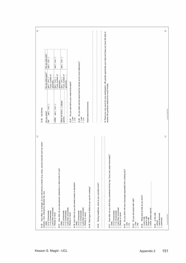
151Kesson S. Magid - UCL Appendix 2
Ve
rsio
n 02
/04/
2011
11
11
III.3
6 H
ow o
ften,
on
aver
age,
do
you
eat s
avou
ry s
nack
s (e
.g.,c
risps
, sav
oury
bis
cuits
suc
h as
cre
am
crac
kers
, mur
i, ch
anac
hur,
Bom
bai m
ix, e
tc).
( ) d
aily
(
) 4 to
3 ti
mes
/wee
k (
) 1 to
2 ti
mes
/wee
k (
) Les
s th
an o
nce/
wee
k (
) Rar
ely
or n
ever
III
.37
How
ofte
n do
you
eat
pea
nuts
, pis
tach
ios
or o
ther
kin
ds o
f nut
s?
( ) d
aily
(
) 4 to
3 ti
mes
/wee
k (
) 1 to
2 ti
mes
/wee
k (
) Les
s th
an o
nce/
wee
k (
) Rar
ely
or n
ever
III
.38
How
ofte
n do
you
eat
sw
eet s
nack
s or
des
serts
?
( ) d
aily
(
) 4 to
3 ti
mes
/wee
k (
) 1 to
2 ti
mes
/wee
k (
) Les
s th
an o
nce/
wee
k (
) Rar
ely
or n
ever
III
.39
Wha
t typ
e of
oil/
fat d
o yo
u us
e fo
r coo
king
? …
……
……
……
……
……
……
……
……
……
……
……
……
……
……
……
……
……
……
……
……
……
……
……
…...
III
.40
Dur
ing
mea
ltim
es, w
hat d
o yo
u no
rmal
ly d
rink?
…
……
……
……
……
……
……
……
……
……
……
……
……
……
……
……
……
……
……
……
……
……
……
……
…...
…
……
……
……
……
……
……
……
……
……
……
……
……
……
……
……
……
……
……
……
……
……
……
……
…...
III
.41
How
ofte
n do
you
drin
k fiz
zy s
wee
tene
d dr
inks
(eg.
Coc
a co
la, p
epsi
lem
onad
e)?
( ) d
aily
(
) 4 to
3 ti
mes
/wee
k (
) 1 to
2 ti
mes
/wee
k (
) Les
s th
an o
nce/
wee
k (
) Rar
ely
or n
ever
III
.42
Do
you
drin
k m
ilk (a
s a
beve
rage
sep
arat
ely
from
coo
king
etc
)?
( ) y
es
( ) n
o III
.43
Do
you
eat c
erea
l with
milk
? (
) Yes
(
) No
III.4
4 W
hat k
ind
of m
ilk d
o yo
u dr
ink?
(
) cow
’s m
ilk
( ) g
oat’s
milk
(
) soy
a m
ilk
( ) o
ther
, ple
ase
spec
ify…
……
……
……
……
……
……
…
III.4
5 Is
the
milk
: (
) who
le
( ) s
emi-s
kim
med
(
) ski
mm
ed
Ve
rsio
n 02
/04/
2011
12
12
III.4
6
Hot
Drin
ks
Do
you
drin
k?
Do
you
add
suga
r?
Do
you
add
milk
? te
a
y
es (
) no
( )
ye
s (
) no
( )
if ye
s, n
umbe
r of
spoo
nful
s……
….
yes
( ) n
o (
)
coffe
e
yes
( ) n
o (
) ye
s (
) no
( )
if ye
s, n
umbe
r of
spoo
nful
s……
….
yes
( ) n
o (
)
Oth
er h
ot d
rink
( ),
plea
se
spec
ify…
……
……
……
……
……
……
…
yes
( ) n
o (
) if
yes,
num
ber o
f sp
oonf
uls…
……
.
yes
( ) n
o (
)
III.4
7 D
o yo
u ad
d sa
lt to
you
r mea
l at t
he ta
ble?
(
) yes
(
) no
III.4
8 D
o yo
u of
ten
eat t
he s
ame
food
for d
inne
r as
for l
unch
(lef
tove
rs)?
(
) yes
(
) no
Obs
erva
tions
/Com
men
ts:
……
……
……
……
……
……
……
……
……
……
……
……
……
……
……
……
……
……
……
……
……
……
……
……
...
……
……
……
……
……
……
……
……
……
……
……
……
……
……
……
……
……
……
……
……
……
……
……
……
...
……
……
……
……
……
……
……
……
……
……
……
……
……
……
……
……
……
……
……
……
……
……
……
……
...
! T
hank
you
ver
y m
uch
for y
our
parti
cipa
tion.
We
grea
tly a
ppre
ciat
e yo
ur h
elp
and
hope
you
hav
e fe
lt ab
le to
an
swer
the
ques
tions
with
out t
oo m
uch
trou
ble.
152Kesson S. Magid - UCL Appendix 3
Salivary testosterone assays: methods and Appendix 3:
results from Magid 2005Methods
Salivary T assays were measured by radioimmunoassay without extraction. Antiserum was prepared in the Ob/Gyn Laboratory of Dr. Robert Chatterton at the Feinberg School of Medicine, Northwestern University, Chicago USA, where all analysis was performed. The interassay CVs were all within 15% for high (100pg/ml), low (50pg/ml), and internal (pooled saliva sample) quality controls. The sensitivity was 0.028 nmol/L. Salivary cortisol will be analysed using a similar radioimmunoassay technique, validated and used in the Chatterton lab.
Samples of salivary T measured so far have been analysed according to the following criteria:
Outlying points with readings over 500pg/ml were excluded as they fell outside the standard curve (highest standard=480pg/ml) and estimates beyond this concentration could not be accurately estimated. Readings were made in duplicate and all with a CV greater than 15% were re-analysed or excluded. Of 676 samples, a total of 36 of were excluded.
The overall degree of diurnal change in salivary T was expressed as a mean value at each time point over two nonconsecutive days, with the evening sample value subtracted from the morning value and expressed as a percentage. The morning sample was considered the peak level of T, as has been observed in numerous other studies (Campbell et al., 2005;Ellison et al., 2002) and can be considered a “top” baseline for the day.
All statistical analysis was conducted using SPSS for Macintosh OSX 11.0.
ANCOVA was used to model the relationship between anthropometric measures (as dependent variable) and residence group after correcting for age differences. ANCOVA was also used to model the relationship between muscle + bone area with of the number of years spent in the UK, where AI were subdivided into three groups indicating years since migrating: (<10 years, 11-40 and >40) and BR inserted as the dummy variable.
Results
Mean ages of the adult immigrants and Bangladeshi residents were significantly different. Controlling for age, salivary testosterone levels of adult immigrants

153Kesson S. Magid - UCL Appendix 3
(AI) to the UK were significantly greater than those of Bangladeshi residents (BR) for morning (BR=201, AI=245 pg/ml) and evening (BR=154, AI=210 pg/ml) samples.
Figure 1: Mean Diurnal Salivary Testosterone Diurnal salivary T profiles for both residence groups showing significant difference between group mean waking (BR: 201.5 ±9.1, AI: 245.2 ±13.1 pg/ml) 30 minutes post-waking (BR: 181.5 ±8.8, AI: 244.3 ±13.1) and evening (BR: 154.1 ±8.9, AI: 210.2 ±12.6) samples and significant differences between morning and evening samples for both groups.
The immigrant group, but not the sedentee group showed a significant negative linear correlation between age and testosterone. The two groups did not significantly differ in BMI, but an ANCOVA correcting for both age and BMI effects still showed a significant difference.
Paired t-tests between residence groups revealed a diurnal rhythm in both AI and BR, with significant differences between group mean waking (BR: 201.5 ±9.1, AI: 245.2 ±13.1) 30 minutes post-waking (BR: 181.5 ±8.8, AI: 244.3 ±13.1) and evening (BR: 154.1 ±8.9, AI: 210.2 ±12.6) samples and significant differences between morning and evening samples for both groups (all p<0.05). BR, but not AI showed significant variation between waking and 30-minutes post-waking samples, suggesting a steeper decline in salivary T levels. The

154Kesson S. Magid - UCL Appendix 3
degree of diurnal change in salivary T was not significantly different between the two resident groups, indicating a similar pattern of declining salivary T throughout the day, but from different baseline concentrations (see figure. 3).
In order to further assess the influence of age, participants were broken down into age brackets by decade. Immigrants at younger, but not older ages showed significantly higher levels of salivary testosterone when compared to sedentees (fig. 2). The diurnal profiles, when broken down by age categories showed a similar degree of daily decline across age groups, but from different baseline levels in the youngest category (20-29 years) (fig 2).
Figure 2: Age-related differences in salivary T between residence groups are significant in younger (ages 20-29: BR=184.1 ± 11.1 AI=295.6 ± 37.8; ages 30-39: BR=168.1 ± 15.3 AI=247.5 ± 73.2) but not older men (ages 40-49: BR=147.1 ± 55.4 AI=266.5 ± 37.5; ages 50-59: BR=184.8 ± 17.0 AI=242.4 ± 54.0).
An ANCOVA controlling for age showed a significant positive relationship between years since immigrating and pooled T in the AI group with years in the UK categorised as three subgroups (<10years, 11-40years, >40years, n=24, 19, 16 respectively) (F(3, 59)=4.7. p<0.01) the BR group was included as a dummy variable (indicating 0 years in UK). In a separate ANCOVA also controlling for age, years in the UK was predictive of total salivary T concentrations F(5,109)=7.68, p<0.001. A similar regression model with a selection of age subgroup of 20-49 year olds showed an even stronger association between

155Kesson S. Magid - UCL Appendix 3
years spent in the UK and salivary T F(1,75)=15.02, p<0.001. The same modelling based on older men (age 50+) was not significant.
Figure 3: Diurnal Salivary Testosterone by Age Group: Comparison of daily testosterone profiles between residence groups, subdivided into 10-year age categories. (All comparisons independent t-test between AI and BR age subgroups). Both residence groups showed significant diurnal change in paired t-tests of mean waking (BR= 201.5 ± 9.1, AI=244.5 ± 13.0) and evening (BR= 154.1 ± 8.9, AI=210.2 ± 10.6) samples.

156Kesson S. Magid - UCL Appendix 4
Laboratory assay validation Appendix 4:
Assay Method:A competitive equilibrium for specific antibody sites is established at room temperature with either a testosterone standard or sample and 3H-T tracer. All standards and samples are run in duplicate, marked “a” and “b”. The unbound steroid is removed from solution by addition of dextran coated charcoal and centrifugation at 4C. Bound radioactivity in the supernatant is measured by liquid scintillation. The amount of radioactivity is inversely related to the amount of T in the standard sample. A logit-log plot of percent bound radioactivity versus concentration of standards will give a linear dose response curve. Saliva concentrations are then calculated from the curve. If the duplicate samples have a CV over 15%, they must be re-assayed or not reported.Quality Controls: Pooled saliva samples, immediately aliquoted, stored unpreserved at -20C. A variation of 15% from the running mean of the previous ten assays is allowed. If any two QC parameters are outside of the acceptable limits, the assay will be re-run.
Codes for QCs used throughout: Count values for the following QC references:NSB: Non Specific Binding (raw count)B0: Percent Binding
Dose values for the following QC references:QC1: Stripped saliva, dosed to 100pg/ml TQC2: Stripped saliva, dosed to 50pg/ml TIQC: Internal QC made from a pool aliquot from numerous participant saliva samplesXQC: External QC made from a pool of male lab workers at Chatterton LabKQC 0: Saliva samples from male researcher (KSM) pooled over several days and frozen as aliquotsKQC Hi: Spiked KQC, diluted ½ with 480pg/ml T (Std7)KQC Lo: Spiked KQC, diluted ½ with 7.5pg/ml T (Std1)QC “A” were prepared and run at the beginning of the assay, immediately following stdsQC “B” were prepared and run at end of assay, last sample
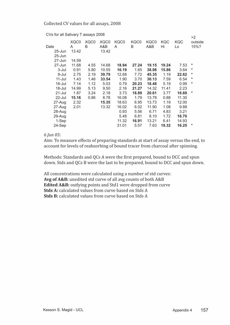
157Kesson S. Magid - UCL Appendix 4
Collected CV values for all assays, 2008
CVs for all Salivary T assays 2008
DateXQC0 A
XQC0 B
XQC0 A&B
KQC0 A
KQC0 B
KQC0 A&B
KQC Hi
KQC Lo
>2 outside 15%?
25-Jun 13.42 13.4225-Jun27-Jun 14.5927-Jun 11.68 4.55 14.68 18.94 27.24 19.15 19.24 7.53 *
3-Jul 0.91 5.80 10.55 16.19 1.65 38.98 15.86 3.64 *9-Jul 2.75 2.19 39.79 12.68 7.72 45.35 1.19 22.62 *
11-Jul 1.43 1.46 33.54 1.90 3.70 30.13 7.59 6.54 *16-Jul 7.14 1.12 5.03 0.79 20.23 18.48 5.19 0.99 *18-Jul 14.99 5.13 9.50 2.16 21.27 14.32 11.41 2.2321-Jul 1.87 3.24 2.18 3.73 18.89 20.61 3.77 16.69 *22-Jul 15.16 0.86 8.78 16.08 1.79 13.78 0.88 11.30
27-Aug 2.32 15.35 18.63 6.95 13.73 1.19 12.0027-Aug 2.01 13.32 16.02 6.02 11.90 1.08 9.8828-Aug 0.93 5.56 6.71 4.83 3.2129-Aug 5.48 6.81 8.10 1.72 16.701-Sep 11.32 16.91 13.21 6.41 14.93
24-Sep 31.01 5.57 7.63 19.32 16.25 *
6 Jun 05: Aim: To measure effects of preparing standards at start of assay versus the end, to account for levels of reabsorbing of bound tracer from charcoal after spinning.
Methods: Standards and QCs A were the first prepared, bound to DCC and spun down. Stds and QCs B were the last to be prepared, bound to DCC and spun down.
All concentrations were calculated using a number of std curves:Avg of A&B: unedited std curve of all avg counts of both A&BEdited A&B: outlying points and Std1 were dropped from curveStds A: calculated values from curve based on Stds AStds B: calculated values from curve based on Stds A

158Kesson S. Magid - UCL Appendix 4
Assay 4 Std Curves
Dose Avg of A&B Stds A Stds B
Edited A&B
NSB 353.0 353.0 353.0 353.0B0 2043.0 2043.0 2043.0 2077.5T 3782.5 3782.5 3782.5 3782.5
7.50 1916.0 1878.5 1897.3 dropped15.00 1905.7 1795.0 1850.4 2016.530.00 1885.7 1877.5 1881.6 1885.760.00 1788.0 1693.5 1740.8 1788.0
120.00 1645.8 1622.0 1633.9 1645.8240.00 1365.0 1335.0 1350.0 1365.0480.00 1017.8 994.5 1006.1 1017.8
Values returnedQC1a 23.25 13.81 42.05 45.92QC1b 14.16 7.36 29.95 34.23QC2a 22.55 13.30 41.15 45.08QC2b 4.97 1.60 16.10 19.73IQC A 97.16 74.91 124.86 115.50IQC B 69.49 50.94 95.69 92.37
QC1 QC1 A QC1 Bintra assay
intra assay
read a read b avg A cv A read a read b avg B cv Bavg A&B
CV A&B
Avg of A&B 30.84 16.61 23.72 42.40 14.74 13.60 14.17 5.71 18.95 42.35Stds A 19.51 9.04 14.28 51.86 7.75 6.97 7.36 7.47 10.82 54.15Stds B 51.55 33.31 42.43 30.40 30.75 29.15 29.95 3.76 36.19 28.69Edited A&B 54.68 37.55 46.11 26.27 35.03 33.44 34.23 3.28 40.17 24.44
QC2 QC2 A QC2 Bintra assay
intra assay
reading a
reading b avg A cv A
reading a
reading b avg B cv B
avg A&B
CV A&B
Avg of A&B 25.19 20.05 22.62 16.07 8.83 1.93 5.38 90.71 14.00 75.38Stds A 15.25 11.48 13.36 19.92 3.87 0.19 2.03 128.09 7.70 89.48Stds B 44.51 37.89 41.20 11.37 22.24 10.54 16.39 50.46 28.80 53.28Edited A&B 48.23 41.98 45.10 9.79 26.35 13.33 19.84 46.42 32.47 48.45
IQC IQC A IQC Bintra assay
intra assay
reading a
reading b avg A cv A
reading a
reading b avg B cv B
avg A&B
CV A&B
Avg of A&B 86.91 108.16 97.54 15.41 68.11 70.88 69.50 2.82 83.52 22.03Stds A 65.92 84.68 75.30 17.61 49.77 52.12 50.95 3.26 63.12 25.41Stds B 114.22 136.10 125.16 12.36 94.20 97.20 95.70 2.21 110.43 17.43Edited A&B 107.18 124.15 115.66 10.37 91.15 93.59 92.37 1.86 104.02 14.57
Results:All intra-assay CVs were outside acceptable limits for QC1 and QC2 for all curvesValues returned for all curves were considerably below expected spiked values for QC1 and QC2IQC was within acceptable limits for combined edited curve.
26-31 Oct 06Aim: To establish working std curve from 2005 stock and newly prepared 2006 stock.
Methods: A small internal QC drawn from 15 samples was measured (SA06 QC

159Kesson S. Magid - UCL Appendix 4
0), as well as a spiked QC (50% Std7). Concentrations were calculated from both curves.
Results:
SA06 QC SA06 QC Hi (50% Std7)SA06 QC Lo (50% Std3)
Std assay 26Oct06 186.4817037 273.1397269Std assay 31Oct06 162.6423677 309.69 121.23
9-11 Nov 06Aim: The first assay run with a new set of T standards on 8Nov06 seemed to show lower than expected QC values. This could be due to decay of T-As, so an old standard dosed at 60pg/ml was run and calculated according to the new curve. In addition, the old IQC used in 2005 was calculated using the new standards.
11 Nov 06: Three of the old standards (S1, S4, S7) were run at the end of the assay. In addition, the old IQC was run again.
Results: IQC was within acceptable CV from running avg for 2005 assays on both days
9 Nov: Old Std 4 had good recovery using the new standard curve: 63.12 pg/ml11 Nov: Old Std 1 fell below limit of detection of assayOld Std 4 had considerably lower recovery (approximately. 50% of expected value)Old Std 7 recovery was within acceptable limits
Results:
9-Nov-06 reading a reading b avg cv
running avg, 2005
cv from running avg
IQC 97.10 86.50 91.80 8.16 112.51 13.02Old Std 4 (60pg/ml) 56.83 69.41 63.12 14.0911-Nov-06IQC 137.53 113.93 125.73 13.27 112.51 8.31Old Std 1 (7.5pg/ml)
Below low std
Below low std
Old Std 4 (60pg/ml) 26.15 33.32 29.73 17.06 60.00 35.67Old Std 7 (480pg/ml) 411.33 438.37 424.85 4.50 480.00 8.13
23 Jun 08: Old Standards from November 2006 were run alongside newly made-up ones.
Results:Both IQC & XQC were not significantly different when calculated using old or new standards:
23/6 new stds 23/6 old stds avg cvIQC 150.78 152.93 151.86 1.0XQC 176.90 190.94 183.93 5.4
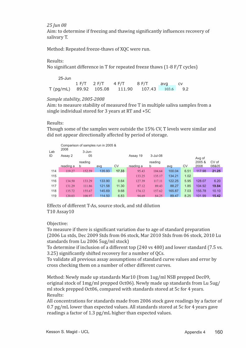
160Kesson S. Magid - UCL Appendix 4
25 Jun 08Aim: to determine if freezing and thawing significantly influences recovery of salivary T.
Method: Repeated freeze-thaws of XQC were run.
Results:No significant difference in T for repeated freeze thaws (1-8 F/T cycles)
25-Jun1 F/T 2 F/T 4 F/T 8 F/T avg cv
T (pg/mL) 89.92 105.08 111.90 107.43 103.6 9.2
Sample stability, 2005-2008Aim: to measure stability of measured free T in multiple saliva samples from a single individual stored for 3 years at RT and +5C
Results:Though some of the samples were outside the 15% CV, T levels were similar and did not appear directionally affected by period of storage.
Comparison of samples run in 2005 & 2008
Lab ID Assay 2
3-Jun-05 Assay 19 3-Jul-08
reading areading b avg CV reading a
reading b avg CV
Avg of 2005 & 2008
CV of 08&05
114 119.27 152.59 135.93 17.33 95.43 104.64 100.04 6.51 117.98 21.25115 133.25 135.17 134.21 1.02116 134.50 133.29 133.90 0.64 127.39 117.11 122.25 5.95 128.07 6.20117 131.29 111.86 121.58 11.30 87.12 89.43 88.27 1.85 104.92 19.84118 135.72 155.67 145.69 9.68 174.12 157.62 165.87 7.03 155.78 10.10119 120.03 108.97 114.50 6.83 94.69 84.25 89.47 8.25 101.99 15.42
Effects of different T-As, source stock, and std dilutionT10 Assay10
Objective: To measure if there is significant variation due to age of standard preparation (2006 Lu stds, Dec 2009 Stds from 06 stock, Mar 2010 Stds from 06 stock, 2010 Lu standards from Lu 2006 5ug/ml stock)To determine if inclusion of a different top (240 vs 480) and lower standard (7.5 vs. 3.25) significantly shifted recovery for a number of QCs.To validate all previous assay assumptions of standard curve values and error by cross checking them on a number of other different curves.
Method: Newly made up standards Mar10 (from 1ug/ml NSB prepped Dec09, original stock of 1mg/ml prepped Oct06). Newly made up standards from Lu 5ug/ml stock prepped Oct06, compared with standards stored at 5c for 4 years.Results: All concentrations for standards made from 2006 stock gave readings by a factor of 0.7 pg/mL lower than expected values. All standards stored at 5c for 4 years gave readings a factor of 1.3 pg/mL higher than expected values.

161Kesson S. Magid - UCL Appendix 4
Repeated measures and correction factors:As salT was analysed over different years, a number of samples and QCs were measured repeatedly. These repeat measures were used to adjust readings between years of analysis. A total of 191 samples collected and analysed in 2005, 66 samples collected and analysed in 2006, and 17 samples collected and analysed in 2008 were measured again in 2010. From these repeat measures, a correction factor of 3.06 was applied to all other readings from 2005, and 0.84 was applied to all other readings from 2006. Repeat measures from 2008 assays did not require a correction factor to match 2010 readings.
Serum to salivary T comparisonsMethod: a total of 22 participants were asked to provide a saliva sample according to the same collection procedure detailed for all samples collected in the field. Immediately following the provision of a saliva sample, a serum sample was collected. Two sample tubes were mislabelled and were therefore dropped from the final analysis.Serum T was analysed by RIA using a kit from Serum T assay QCs
QC Expected ReadI 0.65 ± 0.2 0.62II 5.7 ± 1.7 5.02
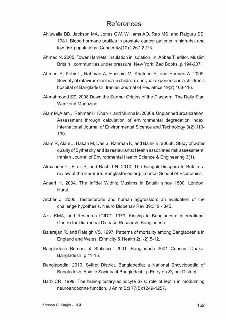
162Kesson S. Magid - UCL
References Ahluwalia BB, Jackson MA, Jones GW, Williams AO, Rao MS, and Rajguru SS.
1981. Blood hormone profiles in prostate cancer patients in high-risk and low-risk populations. Cancer 48(10):2267-2273.
Ahmed N. 2005. Tower Hamlets: insulation in isolation. In: Abbas T, editor. Muslim Britain : communities under pressure. New York: Zed Books. p 194-207.
Ahmed S, Kabir L, Rahman A, Hussain M, Khatoon S, and Hannan A. 2009. Severity of rotavirus diarrhea in children: one year experience in a children's hospital of Bangladesh. Iranian Journal of Pediatrics 19(2):108-116.
Al-mahmood SZ. 2008 Down the Surma: Origins of the Diaspora. The Daily Star, Weekend Magazine.
Alam M, Alam J, Rahman H, Khan K, and Munna M. 2006a. Unplanned urbanization: Assessment through calculation of environmental degradation index. International Journal of Environmental Sicence and Technology 3(2):119-130.
Alam R, Alam J, Hasan M, Das S, Rahman K, and Banik B. 2006b. Study of water quality of Sylhet city and its restaurants: Health associated risk assessment. Iranian Journal of Environmental Health Science & Engineering 3(1).
Alexander C, Firoz S, and Rashid N. 2010. The Bengali Diaspora In Britain: a review of the literature. Banglastories.org: London School of Economics.
Ansari H. 2004. The Infidel Within: Muslims in Britain since 1800. London: Hurst.
Archer J. 2006. Testosterone and human aggression: an evaluation of the challenge hypothesis. Neuro Biobehav Rev 39:319 - 345.
Aziz KMA, and Research ICfDD. 1979. Kinship in Bangladesh: International Centre for Diarrhoeal Disease Research, Bangladesh.
Balarajan R, and Raleigh VS. 1997. Patterns of mortality among Bangladeshis in England and Wales. Ethnicity & Health 2(1-2):5-12.
Bangladesh Bureau of Statistics. 2001. Bangladesh 2001 Census. Dhaka, Bangladesh. p 11-15.
Banglapedia. 2010. Sylhet District. Banglapedia; a National Encyclopedia of Bangladesh: Asiatic Society of Bangladesh. p Entry on Sylhet District.
Barb CR. 1999. The brain-pituitary-adipocyte axis: role of leptin in modulating neuroendocrine function. J Anim Sci 77(5):1249-1257.

163Kesson S. Magid - UCL
Barry MJ, Fowler FJ, Leary MPO, Bruskewitz RC, Holtgrewe HL, Mebust WK, and Cockett AT. 1992. The American Urological Association symptom index for benign prostatic hyperplasia. The Measurement Committee of the American Urological Association. J Urol 148(5):1549-1557; discussion 1564.
Bartsch G, Rittmaster RS, and Klocker H. 2000. Dihydrotestosterone and the concept of 5-α reductase inhibition in human benign prostatic hyperplasia. European Urology 37(4):367-380.
Beck-Peccoz P, Padmanabhan V, Baggiani AM, Cortelazzi D, Buscaglia M, Medri G, Marconi AM, Pardi G, and Beitins IZ. 1991. Maturation of hypothalamic-pituitary-gonadal function in normal human fetuses: Circulating levels of gonadotropins, their common a-subunit and free testosterone, and discrepancy between immunological and biological activities of circulating follicle-stimulating hormone. J Clin Endocrinol Metab 73(3):525-532.
Bentham G. 1988. Migration and morbidity: Implications for geographical studies of disease. Social Science & Medicine 26(1):49-54.
Bentley GR, Harrigan AM, Campbell B, and Ellison PT. 1993. Seasonal effects on salivary testosterone levels among lese males of the Ituri Forest, Zaire. American Journal of Human Biology 5(6):711-717.
Berensztein EB, Sciara MI, Rivarola MA, and Belgorosky A. 2002. Apoptosis and proliferation of human testicular somatic and germ cells during prepuberty: High rate of testicular growth in newborns mediated by decreased apoptosis. J Clin Endocrinol Metab 87(11):5113-5118.
Bergadá I, Milani C, Bedecarrás P, Andreone L, Ropelato MG, Gottlieb S, Bergadá C, Campo S, and Rey RA. 2006. Time course of the serum gonadotropin surge, inhibins, and anti-mullerian hormone in normal newborn males during the first month of life. J Clin Endocrinol Metab 91(10):4092-4098.
Bergendahl M, Aloi JA, Iranmanesh A, Mulligan TM, and Veldhuis JD. 1998. Fasting suppresses pulsatile luteinizing hormone (LH) secretion and enhances orderliness of LH release in young but not older men. Journal of Clinical Endocrinology Metabolism 83(6):1967-1975.
Bhopal R, Unwin N, White M, Yallop J, Walker L, Alberti KGMM, Harland J, Patel S, Ahmad N, Turner C and others. 1999. Heterogeneity of coronary heart disease risk factors in Indian, Pakistani, Bangladeshi, and European origin populations: cross sectional study. BMJ 319(7204):215-220.

164Kesson S. Magid - UCL
Bierhoff E, Walljasper U, Hofmann D, Vogel J, Wernert N, and Pfeifer U. 1997. Morphological analogies of fetal prostate stroma and stromal nodules in BPH. The Prostate 31(4):234-240.
Blum WF. 1997. Leptin: the voice of the adipose tissue. HormRes 48 Suppl 4:2-8.
Bogin B. 1999. Evolutionary perspective on human growth. Annual Review of Anthropology 28(1):109-153.
Bogin B. 2009. Childhood, adolescence, and longevity: A multilevel model of the evolution of reserve capacity in human life history. American Journal of Human Biology 21(4):567-577.
Book AS, Starzyk KB, and Quinsey VL. 2001. The relationship between testosterone and aggression: A meta-analysis. Aggression and Violent Behavior 6(6):579-599.
Booth A, Shelley G, Mazur A, Tharp G, and Kittok R. 1989. Testosterone, and winning and losing in human competition. Hormones and behavior 23(4):556-571.
Bribiescas R. 1996. Testosterone levels among Aché hunter-gatherer men. Human Nature 7(2):163-188.
Bribiescas RG. 2000. Male reproductive ecology: Development and life history. American Journal of Physical Anthropology:111-111.
Bribiescas RG. 2001a. Reproductive ecology and life history of the human male. American Journal of Physical Anthropology 116(S33):148-176.
Bribiescas RG. 2001b. Reproductive physiology of the human male: An evolutionary and life history perspective. In: Ellison PT, editor. Reproductive ecology and human evolution. New York: Aldine de Gruyter. p 107-133.
Bribiescas RG. 2006. Men : Evolutionary and Life History. Cambridge, Mass. ; London: Harvard University Press. 306 p. p.
Bribiescas RG. 2010. An evolutionary and life history perspective on human male reproductive senescence. Annals of the New York Academy of Sciences 1204(1):54-64.
Bribiescas RG, and Anestis SF. 2010. Leptin associations with age, weight, and sex among chimpanzees (Pan troglodytes). Journal of Medical Primatology 39(5):347-355.

165Kesson S. Magid - UCL
Bribiescas RG, and Ellison PT. 2007. How hormones mediate trade-offs in human health and disease. In: Stearns SC, and Koella JC, editors. Evolution in Health and Disease. Oxford: Oxford University Press. p 77–93.
Bribiescas RG, and Hill KR. 2010. Circadian variation in salivary testosterone across age classes in Ache Amerindian males of Paraguay. American Journal of Human Biology 22(2):216-220.
Brown K, Black R, and Becker S. 1982. Seasonal changes in nutritional status and the prevalence of malnutrition in a longitudinal study of young children in rural Bangladesh. The American Journal of Clinical Nutrition 36(2):303-313.
Buerk R. 2005. Expat cash flows back to Bangladesh. BBC News.
Burnham TC, Chapman JF, Gray PB, McIntyre MH, Lipson SF, and Ellison PT. 2003. Men in committed, romantic relationships have lower testosterone. Hormones and Behavior 44(2):119-122.
Bygren L, Kaati G, and Edvinsson S. 2001. Longevity determined by paternal ancestors' nutrition during their slow growth period. Acta Biotheoretica 49(1):53-59.
Callaway CW, Chumlea WC, Bouchard C, Himes JH, Lohman TG, Martin AD, Mitchell CD, Mueller WH, Roche AF, and Seefelt VD. 1988. Circumferences. In: Lohman TG, Roche AF, and Martorell R, editors. Anthropometric Standardization Reference Manual. Champaign, Ill.: Human Kinetics. p 39-54.
Campbell BC. 2003. Pubertal maturation, adrenarche, and the onset of reproduction in human males. In: Wachter KW, and Bulatao RA, editors. Offspring : human fertility behavior in biodemographic perspective. Washington, D.C.: National Academies Press.
Campbell BC, and Cajigal A. 2001. Diabetes: energetics, development and human evolution. Med Hypotheses 57(1):64-67.
Campbell BC, and Leslie PW. 1995. Reproductive ecology of human males. American Journal of Physical Anthropology 38(s21):1.
Campbell BC, Leslie PW, Little MA, and Campbell KL. 2005. Pubertal timing, hormones, and body composition among adolescent Turkana males. American Journal of Physical Anthropology 128(4):896-905.
Campbell BC, Lukas WD, and Campbell KL. 2001. Reproductive ecology of male immune function and gonadal function. In: Ellison PT, editor. Reproductive Ecology and Human Evolution. New York: Aldine de Gruyter. p 159-178.

166Kesson S. Magid - UCL
Carey S. 2004. Curry Capital: The Restaurant Sector in London’s Brick Lane, London. Institute of Community Studies Working Papers. London: Institute of Community Studies.
Chan JL, Matarese G, Shetty GK, Raciti P, Kelesidis I, Aufiero D, De Rosa V, Perna F, Fontana S, and Mantzoros CS. 2006. Differential regulation of metabolic, neuroendocrine, and immune function by leptin in humans. Proceedings of the National Academy of Sciences 103(22):8481-8486.
Charnov EL. 1993. Life History Invariants: Some Explorations of Symmetry in Evolutionary Ecology. May RM, and Harvey PH, editors. Oxford ; New York: Oxford University Press.
Chen H, Ge R-S, and Zirkin BR. 2009. Leydig cells: From stem cells to aging. Molecular and Cellular Endocrinology 306(1-2):9-16.
Chinn S, Cole T, Preece M, and Rona R. 1996. Growth charts for ethnic populations in UK. The Lancet 347(9004):839-840.
Chowdhury AMM, Helman C, and Greenhalgh T. 2000. Food beliefs and practices among British Bangladeshis with diabetes: Implications for health education. Anthropology & Medicine 7(2):209 - 226.
Cicognani A, Alessandroni R, Pasini A, Pirazzoli P, Cassio A, Barbieri E, and Cacciari E. 2002. Low birth weight for gestational age and subsequent male gonadal function. The Journal of Pediatrics 141(3):376-379.
Cook LS, Goldoft M, Schwartz SM, and Weiss NS. 1999. Incidence of adenocarcinoma of the prostate in Asian immigrants to the United States and their descendants. The Journal of Urology 161(1):152-155.
Cronk L. 1991. Wealth, Status, and Reproductive Success among the Mukogodo of Kenya. American Anthropologist 93(2):345-360.
Crowley WF, Jr., Whitcomb RW, Jameson JL, Weiss J, Finkelstein JS, and O'Dea LS. 1991. Neuroendocrine control of human reproduction in the male. Recent ProgHormRes 47:27-62.
Dabbs JM. 1990. Salivary testosterone measurements: reliability across hours, days, and weeks. Physiology & behavior 48(1):83-86.
Dabbs JM, and Dabbs MG. 2000. Heroes, Rogues, and Lovers : Testosterone and Behavior. New York: McGraw-Hill.
Dabbs JM, and Morris R. 1990. Testosterone, social class, and antisocial behavior in a sample of 4,462 men. Psychological Science 1(3):209-211.
167Kesson S. Magid - UCL
Davies MJ, and Norman RJ. 2002. Programming and reproductive functioning. Trends in Endocrinology and Metabolism 13(9):386-392.
DCLG. 2009. The Bangladeshi Muslim Community in England: Understanding Muslim Ethnic Communities. In: Department of Communities LGaS, editor. London: HMSO.
de Koning FFL, Binkhorst RRA, Kauer JJM, and Thijssen HHO. 1986. Accuracy of an anthropometric estimate of the muscle and bone area in a transversal cross-section of the arm. International Journal of Sports Medicine 7(5):246-249.
Delemarre-van de Waal HA, van Coeverden SCCM, and Engelbregt MTJ. 2002. factors affecting onset of puberty. Hormone Research in Paediatrics 57(Suppl. 2):15-18.
Dench G, Gavron K, and Young M. 2006. The New East End: Kinship, Race and Conflict. London: Profile Books.
Diver MJ, Imtiaz KE, Ahmad AM, Vora JP, and Fraser WD. 2003. Diurnal rhythms of serum total, free and bioavailable testosterone and of SHBG in middle-aged men compared with those in young men. Clinical Endocrinology 58(6):710-717.
Dunnell K. 2008. Diversity and Different Experiences in the UK: National Statistician's Annual Article on Society. In: Statistics OfN, editor. London: Office for National Statistics.
Eade J. 1994. Identity, nation and religion: Educated young Bangladeshi Muslims in London's 'East End'. International Sociology 9(3):377-394.
Eade J, and Garbin D. 2006. Competing visions of identity and space: Bangladeshi Muslims in Britain. Contemporary South Asia 14(2):181-193.
Eade J, Vamplew T, and Peach C. 1996. Bangladeshis: the encapsulated community. In: Peach C, editor. The Ethnic Minority Populations of Britain, Ethnicity in the 1991 Census. London: Office for National Statistics. p 150-156.
Economist. 2007 Bangladeshis in Britain: from Brick Lane to the fast lane. The Economist.
Ellison PT. 1994. Advances in human reproductive ecology. Annual Review of Anthropology 23(1):255-275.
Ellison PT. 1996. Developmental influences on adult ovarian hormonal function. American Journal of Human Biology 8(6):725-734.
168Kesson S. Magid - UCL
Ellison PT. 2001a. On Fertile Ground. Cambridge, Mass. ; London: Harvard University Press. 358 p. p.
Ellison PT. 2001b. Reproductive Ecology and Human Evolution. New York: Aldine de Gruyter.
Ellison PT. 2003. Energetics and reproductive effort. American Journal of Human Biology 15(3):342-351.
Ellison PT. 2009. Social relationships and reproductive ecology. In: Gray PB, and Ellison PT, editors. Endocrinology of Social Relationships. Cambridge, MA: Harvard University Press. p 54-73.
Ellison PT, Bribiescas RG, Bentley GR, Campbell BC, Lipson SF, Panter-Brick C, and Hill K. 2002. Population variation in age-related decline in male salivary testosterone. Human Reproduction 17(12):3251-3253.
Ellison PT, Lipson SF, and Meredith MD. 1989. Salivary testosterone levels in males from the Ituri Forest of Zaïre. American Journal of Human Biology 1(1):21-24.
Ellison PT, and Panter-Brick C. 1996. Salivary testosterone levels among Tamang and Kami males of central Nepal. Hum Biol 68(6):955-965.
Ellison PT, Panter-Brick C, Lipson SF, and O'Rourke MT. 1993. The ecological context of human ovarian function. Human Reproduction 8(12):2248-2258.
Eriksson JG, Forsén T, Tuomilehto J, Winter PD, Osmond C, and Barker DJP. 1999. Catch-up growth in childhood and death from coronary heart disease: longitudinal study. BMJ 318(7181):427-431.
Eveleth PB, and Tanner JM. 1990. Worldwide Variation in Human Growth: Cambridge University Press. xii,397p. p.
Ezzati M, Lopez AD, Rodgers A, Vander Hoorn S, and Murray CJL. 2002. Selected major risk factors and global and regional burden of disease. The Lancet 360(9343):1347-1360.
Fairbanks LA. 2009. Influences on aggression in group-living monkeys. In: Gray PB, and Ellison PT, editors. Endocrinology of Social Relationships. Cambridge, MA: Harvard University Press. p 159-195.
Faul F, Erdfelder E, Lang A-G, and Buchner A. 2007. G*Power 3: A flexible statistical power analysis program for the social, behavioral, and biomedical sciences. Behavior Research Methods 39(2):175-191.

169Kesson S. Magid - UCL
Fessler DMT, Navarrete CD, Hopkins W, and Izard MK. 2005. Examining the terminal investment hypothesis in humans and chimpanzees: Associations among maternal age, parity, and birth weight. American Journal of Physical Anthropology 127(1):95-104.
Folstad I, and Karter AJ. 1992. Parasites, bright males, and the immunocompetence handicap. The American Naturalist 139(3):603-622.
Forbes GB. 1987. Human Body Composition: Growth, Aging, Nutrition, and Activity. New York: Springer-Verlag.
Forest MG. 1983. Role of androgens in fetal and pubertal development. Hormone Research in Paediatrics 18(1-3):69-83.
Forsén T, Eriksson J, Tuomilehto J, Reunanen A, Osmond C, and Barker D. 2000. The fetal and childhood growth of persons who develop type 2 diabetes. Annals of Internal Medicine 133(3):176-182.
Garbin D. 2005. Bangladeshi diaspora: socio-cultural dynamics, religious trends and transnational politics. In: Menski W, and Chanda B, editors. Proceedings of the European Human Rights Conference on Bangladesh Extremism, Intolerance and Violence . London: CEMS-SOAS. p 1-10.
Gardner K. 1995. Global Migrants, Local Lives: Migration and Transformation in Rural Bangladesh. Oxford: Oxford University Press. 316 p.
Gardner K. 2002. Age, Narrative and Migration : the Life Course and Life Histories of Bengali Elders in London. Oxford: Berg. vii, 254p. p.
Gardner K, and Shukur A. 1994. "I'm Bengali, I'm Asian, and I'm living here': The changing identitiy of British Bengalis. In: Ballard R, and Banks M, editors. Desh Pardesh : The South Asian presence in Britain. London: Hurst.
Gettler LT, Agustin SS, and Kuzawa CW. 2010. Testosterone, physical activity, and somatic outcomes among Filipino males. American Journal of Physical Anthropology 142(4):590-599.
Giashuddin S, Rahman A, Rahman F, Mashreky S, Chowdhury S, Linnan M, and Shafinaz S. 2009. Socioeconomic inequality in child injury in Bangladesh - implication for developing countries. International Journal for Equity in Health 8(1):7.
Gilger JW, Geary DC, and Eisele LM. 1991. Reliability and validity of retrospective self-reports of the age of pubertal onset using twin, sibling, and college student data. Adolescence.
170Kesson S. Magid - UCL
Gluckman PD, Hanson MA, and Beedle AS. 2007. Early life events and their consequences for later disease: A life history and evolutionary perspective. American Journal of Human Biology 19(1):1-19.
Gluckman PD, Hanson MA, and Spencer HG. 2005. Predictive adaptive responses and human evolution. Trends in Ecology & Evolution 20(10):527-533.
Granger DA, Shirtcliff EA, Booth A, Kivlighan KT, and Schwartz EB. 2004. The "trouble" with salivary testosterone. Psychoneuroendocrinology 29(10):1229-1240.
Gray A, Feldman HA, McKinlay JB, and Longcope C. 1991. Age, disease, and changing sex hormone levels in middle-aged men: Results of the Massachusetts Male Aging Study. J Clin Endocrinol Metab 73(5):1016-1025.
Gray P, Ellison P, and Campbell B. 2007. Testosterone and marriage among Ariaal men of northern Kenya. Current Anthropology 48(5):750-755.
Gray PB, Yang CJ, and Pope HGJ. 2006. Fathers have lower salivary testosterone levels than unmarried men and married non-fathers in Beijing, China. Proceedings of the Royal Society of London B: Biological Sciences 273:333-339.
Greulich WW. 1958. Growth of children of the same race under different environmental conditions. Science 127(3297):515-516.
Grjibovski A, Bygren LO, Svartbo B, and Magnus P. 2004. Housing conditions, perceived stress, smoking, and alcohol: determinants of fetal growth in Northwest Russia. Acta Obstetricia et Gynecologica Scandinavica 83(12):1159-1166.
Gröschl M. 2008. Current status of salivary hormone analysis. Clin Chem 54(11):1759-1769.
Gwatkin DR, Rutstein S, Johnson K, Suliman E, Wagstaff A, and Amouzou A. 2007. Socio-economic differences in health, nutrition, and population within developing countries. Washington, D.C.: The World Bank.
Haas JD, and Campirano F. 2006. Interpopulation variation in height among children 7 to 18 years of age. Food Nutr Bull 27(4 Suppl Growth Standard):S212-223.
Hales CN, and Barker DJP. 2001. The thrifty phenotype hypothesis: Type 2 diabetes. British Medical Bulletin 60(1):5-20.
Hamilton W, and Zuk M. 1982. Heritable true fitness and bright birds: a role for parasites? Science 218(4570):384-387.
171Kesson S. Magid - UCL
Hamilton WD. 1964. The genetical evolution of social behaviour. I. Journal of Theoretical Biology 7(1):1-16.
Hardy M, Gao H-B, Dong Q, Ge R, Wang Q, Chai W, Feng X, and Sottas C. 2005. Stress hormone and male reproductive function. Cell and Tissue Research 322(1):147-153.
Harman SM, Metter EJ, Tobin JD, Pearson J, and Blackman MR. 2001. Longitudinal effects of aging on serum total and free testosterone levels in healthy men. J Clin Endocrinol Metab 86(2):724-731.
Harrison GG, Buskirk ER, Lindsay Carter JE, Johnston FE, Lohman TG, Pollock ML, Roche AF, and Wilmore J. 1988. Skinfold thicknesses and measurement technique. In: Lohman TG, Roche AF, and Martorell R, editors. Anthropometric Standardization Reference Manual. Champaign, Ill.: Human Kinetics. p 55-68.
Heitzman J, Worden RL, and Library of Congress. Federal Research Division. 1989. Bangladesh : a country study. Washington, D.C.: The Division : For sale by the Supt. of Docs., U.S. G.P.O. xxxvi, 306 p. p.
Henderson L, and Gregory J, editors. 2002. The National Diet & Nutrition Survey : Adults Aged 19 to 64 Years. London: HMSO.
Hernández M, and Mericq V. 2008. Pubertal development in girls born small for gestational age. Journal of Pediatric Endocrinology & Metabolism 21(3):201-208.
Heymsfield SB, McManus C, Smith J, Stevens V, and Nixon DW. 1982. Anthropometric measurement of muscle mass: revised equations for calculating bone-free arm muscle area. Am J Clin Nutr 36(4):680-690.
Hill K. 1993. Life history theory and evolutionary anthropology. Evolutionary Anthropology: Issues, News, and Reviews 2(3):78-88.
Hill K, and Hurtado AM. 1996. Ache Life History. New York: Aldine de Gruyter. xix, 561p. p.
Hobbes T. 1651. Leviathan. Peterborough, Ont.: Broadview Press.
Howard G, and Bartram J. 2003. Domestic Water Quantity, Service Level, and Health: World Health Organization.
Hsing AW, Reichardt JKV, and Stanczyk FZ. 2002. Hormones and prostate cancer: Current perspectives and future directions. The Prostate 52(3):213-235.

172Kesson S. Magid - UCL
Hussain D. 2007. Globalization,God and Galloway: The Islamisization of Bangladeshi communities in London. Journal of Creative Communications 2(1):189-218.
Iqbal S, Haque À, Iqbal M, and Chowdhury M. 2006. Water Quality Assessment of Surma River in Sylhet City. Journal of Chemical Engineering, Official publication of the Institution of Engineers, Bangladesh 24.
Islam N. 2005. Dhaka Now: Contemporary Urban Development. Dhaka: Bangladesh Geographic Society.
Jasienska G. 2009. Reproduction and lifespan: Trade-offs, overall energy budgets, intergenerational costs, and costs neglected by research. American Journal of Human Biology 21(4):524-532.
Jasienska G, and Thune I. 2001. Lifestyle, hormones, and risk of breast cancer. BMJ 322(7286):586-587.
Jasienska G, Ziomkiewicz A, Lipson SF, Thune I, and Ellison PT. 2006. High ponderal index at birth predicts high estradiol levels in adult women. American Journal of Human Biology 18(1):133-140.
Jin B, Turner L, Zhou Z, Zhou EL, and Handelsman DJ. 1999. Ethnicity and migration as determinants of human prostate size. The Journal of clinical endocrinology & metabolism 84(10):3613-3619.
Johnson MH, and Everitt BJ. 2000. Essential Reproduction. Oxford: Blackwell Science. xvi, 285 p. p.
Jones JH. 2005. Fetal programming: Adaptive life-history tactics or making the best of a bad start? American Journal of Human Biology 17(1):22-33.
Jones JH. 2009. The force of selection on the human life cycle. Evolution and Human Behavior 30(5):305-314.
Kabir A, and Islam M. 2001. Factors influencing infant and child mortality in Bangladesh. The Sciences 1(5):292-295.
Kaiser J, and Gruzelier JH. 1999. The Adolescence Scale (AS-ICSM). Acta Pædiatrica 88:64-68.
Kaplan H, Hill K, Lancaster JA, and Hurtado M. 2000. A theory of human life history evolution: Diet, intelligence, and longevity. Evolutionary Anthropology: Issues, News, and Reviews 9(4):156-185.
Kaplan HS, and Lancaster JB. 2003. An evolutionary and ecological analysis of human fertility, mating patterns, and parental investment. In: Wachter KW, and Bulatao RA, editors. Offspring: Human fertility behavior in
173Kesson S. Magid - UCL
biodemographic perspective. Washington DC: National Acadamies Press. p 170-223.
Keenan DM, Takahashi PY, Liu PY, Roebuck PD, Nehra AX, Iranmanesh A, and Veldhuis JD. 2006. An ensemble model of the male gonadal axis: Illustrative Application in Aging Men. Endocrinology 147(6):2817-2828.
Kehinde E, Akanji A, Memon A, Bashir A, Daar A, Al-Awadi K, and Fatinikun T. 2006. Prostate cancer risk: The significance of differences in age related changes in serum conjugated and unconjugated steroid hormone concentrations between Arab and Caucasian men. International Urology and Nephrology 38(1):33-44.
Kempson E. 2000. Overcrowding among Bangladeshi Households in Tower Hamlets: Policy Studies Institute.
Ketterson ED, Nolan V, Wolf L, and Ziegenfus C. 1992. Testosterone and avian life histories - Effects of experimentally elevated testosterone on behavior and correlates of fitness in the Dark-Eyed Junco (Junco-Hyemalis). American Naturalist 140(6):980-999.
Key TJA, Roe L, Thorogood M, Moore JW, Clark GMG, and Wang DY. 1990. Testosterone, sex hormone-binding globulin, calculated free testosterone, and oestradiol in male vegans and omnivores. British Journal Of Nutrition 64(01):111-119.
Kiess W, Blum WF, and Aubert ML. 1998. Leptin, puberty and reproductive function: lessons from animal studies and observations in humans. EurJEndocrinol 138(1):26-29.
Kley HK, Deselaers T, and Peerenboom H. 1981. Evidence for Hypogonadism in Massively Obese Males Due to Decreased Free Testosterone. Horm Metab Res 13(11):639,641.
Knussmann R, and Sperwien A. 1988. Relations between anthropometric characteristics and androgen hormone levels in healthy young men. Annals of Human Biology 15(2):131-142.
Koenig MA, Phillips JF, Campbell OM, and D'Souza S. 1990. Birth intervals and childhood mortality in rural Bangladesh. Demography 27(2):251-265.
Kumar TR, Wang Y, Lu N, and Matzuk MM. 1997. Follicle stimulating hormone is required for ovarian follicle maturation but not male fertility. NatGenet 15(2):201-204.

174Kesson S. Magid - UCL
Kuzawa CW. 2005. Fetal origins of developmental plasticity: Are fetal cues reliable predictors of future nutritional environments? American Journal of Human Biology 17(1):5-21.
Kuzawa CW. 2007. Developmental origins of life history: Growth, productivity, and reproduction. American Journal of Human Biology 19(5):654-661.
Kuzawa CW, Gettler LT, Muller MN, McDade TW, and Feranil AB. 2009. Fatherhood, pairbonding and testosterone in the Philippines. Hormones and Behavior 56(4):429-435.
Kuzawa CW, McDade TW, Adair LS, and Lee N. 2010. Rapid weight gain after birth predicts life history and reproductive strategy in Filipino males. Proceedings of the National Academy of Sciences 107(39):16800-16805.
Kyle UG, Bosaeus I, De Lorenzo AD, Deurenberg P, Elia M, Gomez JM, Heitmann BL, Kent-Smith L, Melchior JC, Pirlich M and others. 2004. Bioelectrical impedance analysis--part I: review of principles and methods. Clin Nutr 23(5):1226-1243.
Laaksonen DE, Niskanen L, Punnonen K, Laaksonen DE, Nyyssönen K, Tuomainen T-P, Valkonen V-P, Salonen R, and Salonen JT. 2004. Testosterone and sex hormone‚ α-binding globulin predict the metabolic syndrome and diabetes in middle-aged men. Diabetes Care 27(5):1036-1041.
Lamb EJ, and Bennett S. 1994. Epidemiologic studies of male factors in infertility. Ann N Y Acad Sci 709:165-178.
Lasker GW. 1995. The study of migrants as a strategy for understanding human biological plasticity. In: Mascie-Taylor CGN, and Bogin B, editors. Human Variability and Plasticity. Cambridge: Cambridge University Press. p 110–114.
Lawrence JM, Devlin E, Macaskill S, Kelly M, Chinouya M, Raats MM, Barton KL, Wrieden WL, and Shepherd R. 2007. Factors that affect the food choices made by girls and young women, from minority ethnic groups, living in the UK. Journal of Human Nutrition and Dietetics 20(4):311-319.
Layman LC, Lee EJ, Peak DB, Namnoum AB, Vu KV, van Lingen BL, Gray MR, McDonough PG, Reindollar RH, and Jameson JL. 1997. Delayed puberty and hypogonadism caused by mutations in the follicle-stimulating hormone ·-Subunit Gene. The New England Journal of Medicine 337(9):607-611.
Lee RB. 1968. What hunters do for a living, or how to make out on scarce resources. In: Lee RB, and DeVore I, editors. Man the hunter : the first
175Kesson S. Magid - UCL
intensive survey of a single, crucial stage of human development, man's once universal hunting way of life. New York: Aldine de Gruyter. p 30-48.
Leon DA, and Moser KA. 2010. Low birth weight persists in South Asian babies born in England and Wales regardless of maternal country of birth. Slow pace of acculturation, physiological constraint or both? Analysis of routine data. Journal of Epidemiology and Community Health.
Lewis JG. 2006. Steroid analysis in saliva: an overview. Clinical Biochemist Reviews 27(3):139-146.
Lewis SJ. 2003. Migration and health impact assessment. Public Health 117(5):305-311.
Lieberson S. 1963. Ethnic Patterns in American Cities. New York: The Free Press of Glencoe.
Lindeberg S, Söderberg S, Ahrén B, and Olsson T. 2001. Large differences in serum leptin levels between nonwesternized and westernized populations: the Kitava study. Journal of Internal Medicine 249(6):553-558.
Linnan M, and Centre UIR. 2008. Child Mortality and Injury in Asia : an Overview. Florence, Italy: UNICEF Innocenti Research Centre.
Liu PY, Pincus SM, Takahashi PY, Roebuck PD, Iranmanesh A, Keenan DM, and Veldhuis JD. 2006. Aging attenuates both the regularity and joint synchrony of LH and testosterone secretion in normal men: analyses via a model of graded GnRH receptor blockade. American Journal of Physiology - Endocrinology And Metabolism 290(1):E34-E41.
Lohman TG, Roche AF, and Martorell R, editors. 1988. Anthropometric Standardization Reference Manual. Champaign, Ill.: Human Kinetics. 177p. p.
Low BS. 2001. Why Sex Matters : a Darwinian Look at Human Behavior. Princeton, N.J. [u.a.] ;Princeton University Press.
Lucas A. 1994. Role of nutritional programming in determining adult morbidity. Archives of Disease in Childhood 71(4):288-290.
Mace R, and Sear R. 1997. Birth interval and the sex of children in a traditional African population: An evolutionary analysis. Journal of Biosocial Science 29(4):499-507.
Magid KS. 2005. Reproductive endocrinology in males in relation to Bangladeshi migration [MSc.]. London: University College London. 89 p.
176Kesson S. Magid - UCL
Magid KS. 2006. Life course effects of migration in Bangladeshi men [MRes.]. London: University College London. 89 p.
Magid KS, Ahamed FU, and Bentley GR. 2007. Changes in mid upper arm somatic muscle allocation among Bangladeshi male migrants to the UK. Abstracts of the 32nd annual meeting of the human biology association Philadelphia, Pennsylvania march 28-29, 2007. American Journal of Human Biology 19(2):246-290.
Magid KS, Chatterton RT, Ahamed FU, and Bentley GR. 2006. No effect of marriage or fatherhood on salivary testosterone levels in Bangladeshi men. Human Behavior and Evolution Society meeting. Philadelphia, PA.
Maharatna A. 1996. Infant and Child Mortality during Famines in Late 19th and Early 20th Century India. Economic and Political Weekly 31(27):1774-1783.
Mann DR, and Fraser HM. 1996. The neonatal period: a critical interval in male primate development. J Endocrinol 149(2):191-197.
Marlowe F. 2000. The patriarch hypothesis. Human Nature 11(1):27-42.
Marmot MG. 2006. Status Syndrome. JAMA: The Journal of the American Medical Association 295(11):1304-1307.
Martine T, Claessens AL, Vlietinck R, Marchal G, and Beunen G. 1997. Accuracy of anthropometric estimation of muscle cross-sectional area of the arm in males. American Journal of Human Biology 9(1):73-86.
Mazur A, and Booth A. 1998. Testosterone and dominance in men. Behav Brain Sci 21(3):353-363; discussion 363-397.
McDade TW. 2005. Life history, maintenance, and the early origins of immune function. American Journal of Human Biology 17(1):81-94.
McKeigue PM, Shah B, and Marmot MG. 1991. Relation of central obesity and insulin resistance with high diabetes prevalence and cardiovascular risk in South Asians. The Lancet 337(8738):382-386.
Meas T, Deghmoun S, Lévy-Marchal C, and Bouyer J. 2010. Fertility is not altered in young adults born small for gestational age. Human Reproduction 25(9):2354-2359.
Meikle AW, Stephenson RA, Lewis CM, Wiebke GA, and Middleton RG. 1997. Age, genetic, and nongenetic factors influencing variation in serum sex steroids and zonal volumes of the prostate and benign prostatic hyperplasia in twins. The Prostate 33(2):105-111.
177Kesson S. Magid - UCL
Mitra SN, National Institute of Population Research and Training (Bangladesh), and Mitra and Associates (Firm). 1997. Bangladesh demographic and health survey, 1996-1997. Dhaka, Bangladesh: National Institute of Population Research and Training : Mitra and Associates. xxii, 252 p. p.
Montgomery MR, Gragnolati M, Burke KA, and Paredes E. 2000. Measuring living standards with proxy variables. Demography 37(2):155-174.
Morley JE, Haren MT, Kim MJ, Kevorkian RR, and Perry HM. 2005. Testosterone, aging and quality of life. Journal of Endocrinological Investigation 28(3 Suppl):76-80.
Muehlenbein M, and Bribiescas R. 2005. Testosterone-mediated immune functions and male life histories. Am J Hum Biol 17:527 - 558.
Muller MN, and Wrangham RW. 2004. Dominance, aggression and testosterone in wild chimpanzees: a test of the 'challenge hypothesis'. Animal Behaviour 67(1):113-123.
Muller WH, and Martorell R. 1988. Reliability and accuracy of measurement. In: Lohman TG, Roche AF, and Martorell R, editors. Anthropometric Standardization Reference Manual. Champaign, Ill.: Human Kinetics. p 83-86.
NIPORT. 2009. Bangladesh Demographic and Health Survey 2007. Dhaka, Bangladesh and Calverton, Maryland, USA: National Institute of Population Research and Training, Mitra and Associates, and Macro International.
Neel JV. 1962. Diabetes mellitus: a "thrifty" genotype rendered detrimental by "progress"? Am J Hum Genet 14:353-362.
Núñez de la Mora A. 2005. Developmental effects on reproductive hormone levels: A migrant study. London: University College London, University of London. 209 p.
Núñez de la Mora A, Chatterton RT, Choudhury OA, Napolitano DA, and Bentley GR. 2007a. Childhood conditions influence adult progesterone levels. PLOS Medicine 4(5):e167.
Núñez de la Mora A, Chatterton RT, Mateo ET, Jesmin F, and Bentley GR. 2007b. Effect of chewing betel nut on measurements of salivary progesterone and estradiol. American Journal of Physical Anthropology 132(2):311-315.
Núñez-de la Mora A, Chatterton R, Choudhury O, Napolitano D, Hochman J, and Bentley G. 2004. Fresh or frozen?: Changing food habits among Bangladeshi migrant women in London. Am J Hum Biol 16:216.
178Kesson S. Magid - UCL
Núñez-de la Mora A, Napolitano DA, Choudhury OA, and Bentley GR. Changes in breastfeeeding practices among Bangladeshi women in London; 2005; Milwakee, Wisconsin. Am J Phys Anthropol. p 159.
O'Shaughnessy PJ, and Fowler PA. 2011. Endocrinology of the mammalian fetal testis. Reproduction 141(1):37-46.
ONS. 2002. Minority Ethnic Groups in the UK. London: Office for National Statistics.
Ounsted M, Scott A, and Ounsted C. 2008. Transmission through the female line of a mechanism constraining human fetal growth. International Journal of Epidemiology 37(2):245-250.
Ozanne SE, and Hales CN. 1999. The long-term consequences of intra-uterine protein malnutrition for glucose metabolism. Proceedings of the Nutrition Society 58(03):615-619.
Pagel MD, and Harvey PH. 1993. Evolution of the juvenile period in mammals. In: Pereira ME, and Fairbanks LA, editors. Juvenile primates : Life History, Development, and Behavior. New York ; Oxford: Oxford University Press. p 28-37.
Peach C. 1999. London and New York: contrasts in British and American models of segregation with a comment by Nathan Glazer. International Journal of Population Geography 5(5):319-347.
Peach C. 2005. Muslims in Britain. In: Abbas T, editor. Muslim Britain: Communities Under Pressure.
Pembrey ME. 2010. Male-line transgenerational responses in humans. Human Fertility 13(4):268-271.
Pembrey ME, Bygren LO, Kaati G, Edvinsson S, Northstone K, Sjostrom M, and Golding J. 2005. Sex-specific, male-line transgenerational responses in humans. Eur J Hum Genet 14(2):159-166.
Pereira ME, and Fairbanks LA. 1993. Juvenile Primates : Life History, Development, And Behavior. New York ; Oxford: Oxford University Press. xvi,428p. p.
Phillips GB, Jing T, and Heymsfield SB. 2002. Relationships in Men of Sex Hormones, Insulin, Adiposity, and Risk Factors for Myocardial Infarction. Metabolism 52(6):784-790.
Plas E, Berger P, Hermann M, and Pfl¸ger H. 2000. Effects of aging on male fertility? Experimental Gerontology 35(5):543-551.
179Kesson S. Magid - UCL
Platz EA, and De Marzo AM. 2004. Epidemiology of Inflammation and Prostate Cancer. The Journal of Urology 171(2, Supplement 1):S36-S40.
Pollard J, Kirk SFL, and Cade JE. 2002. Factors affecting food choice in relation to fruit and vegetable intake: a review. Nutrition Research Reviews 15:373-387.
Pollard TM, Rousham EK, and Colls R. 2011. Intergenerational and familial approaches to obesity and related conditions. Annals of Human Biology 38(4):385-389.
Prentice AM, Rayco-Solon P, and Moore SE. 2005. Insights from the developing world: thrifty genotypes and thrifty phenotypes. Proceedings of the Nutrition Society 64(02):153-161.
Prince F. 2001. The triphasic nature of Leydig cell development in humans, and comments on nomenclature. J Endocrinol 168(2):213-216.
Rahman A. 2005. Bangladesh Health and Injury Survey : Report on Children. Dhaka: Directorate General of Health Services, Ministry of Health and Family Welfare, Govt. of the People's Republic of Bangladesh.
Reaven GM. 1998. Hypothesis: muscle insulin resistance is the ("not-so") thrifty genotype. Diabetologia 41(4):482-484.
Reichard UH, and Boesch C. 2003. Monogamy : mating strategies and partnerships in birds, humans, and other mammals. Cambridge, United Kingdom: Cambridge University Press.
Rhind S, Rae M, and Brooks A. 2001. Effects of nutrition and environmental factors on the fetal programming of the reproductive axis. Reproduction 122(2):205-214.
Rojansky N, Brzezinski A, and Schenker JG. 1992. Seasonality in human reproduction: an update. Human Reproduction 7(6):735-745.
Rona RJ, and Chinn S. 1986. National Study of Health and Growth: social and biological factors associated with height of children from ethnic groups living in England. Annals of Human Biology 13(5):453-471.
Rose RM, Holaday JW, and Bernstein IS. 1971. Plasma Testosterone, Dominance Rank and Aggressive Behaviour in Male Rhesus Monkeys. Nature 231(5302):366-368.
Ross RK, Bernstein L, Pike MC, Henderson BE, Lobo RA, Stanczyk FZ, and Shimizu H. 1992. 5-alpha-reductase activity and risk of prostate cancer among Japanese and US white and black males. The Lancet 339(8798):887-889.
180Kesson S. Magid - UCL
Rutters F, Nieuwenhuizen AG, Verhoef SPM, Lemmens SGT, Vogels N, and Westerterp-Plantenga MS. 2009. The relationship between leptin, gonadotropic hormones, and body composition during puberty in a Dutch children cohort. European Journal of Endocrinology 160(6):973-978.
Sapolsky R. 2004. Social status and health in humans and other animals. Annu Rev Anthropol 33:393 - 418.
Sapolsky RM. 1991. Testicular function, social rank and personality among wild baboons. Psychoneuroendocrinology 16(4):281-293.
Satyanarayana K, Radhaiah G, Mohan KR, Thimmayamma BVS, Rao N, Rao BS, and Akella S. 1989. The adolescent growth spurt of height among rural Indian boys in relation to childhood nutritional background: An 18 year longitudinal study. Annals of Human Biology 16(4):289-300.
Sen A. 1977. Starvation and exchange entitlements: a general approach and its application to the Great Bengal Famine. Cambridge Journal of Economics 1(1):33.
Shams M, and Williams R. 1997. Generational changes in height and body mass differences between British Asians and the general population in Glasgow. Journal of biosocial science 29(01):101-109.
Sharpe RM, Fraser HM, Brougham MFH, McKinnell C, Morris KD, Kelnar CJH, Wallace WHB, and Walker M. 2003. Role of the neonatal period of pituitary-testicular activity in germ cell proliferation and differentiation in the primate testis. Human Reproduction 18(10):2110-2117.
Shirtcliff EA, Granger DA, and Likos A. 2002. Gender differences in the validity of testosterone measured in saliva by immunoassay. Hormones and Behavior 42(1):62-69.
Siddiqui T. 2004. Institutionalising Diaspora Linkage: the Emigrant Bangladeshis in UK and USA. Dhaka: International Orginisation for Migration. 107 p.
Slater S, and Oliver RTD. 2000. Testosterone: Its role in development of prostate cancer and potential risk from use as hormone replacement therapy. Drugs & Aging 17(6):431-439.
Stanton BF, and Clemens JD. 1987. Socioeconomic variables and rates of diarrhoeal disease in urban Bangladesh. Transactions of the Royal Society of Tropical Medicine and Hygiene 81(2):278-282.
Stearns SC. 2000. Life history evolution: successes, limitations, and prospects. Naturwissenschaften 87(11):476-486.

181Kesson S. Magid - UCL
Stinson S. 2000. Growth variation: biological and cultural factors. In: Stinson S, Bogin B, Huss-Ashmore R, and O'Rourke D, editors. Human Biology : an Evolutionary and Biocultural Approach. New York ; Chichester: Wiley. p 640p.
Sunder D, and Uddin L. 2007. A comparative analysis of Bangladeshi and Pakistani educational attainment in London secondary schools. InterActions: UCLA Journal of Education and Information Studies 3(2).
Szklarska A, Lipowicz A, Lopuszanska M, Bielicki T, and Koziel S. 2008. Biological condition of adult migrants and nonmigrants in Wrocław, Poland. American Journal of Human Biology 20(2):139-145.
Tanner JM. 1962. Growth at Adolescence. Oxford: Blackwell Scientific Publications. 325 p.
Tanner JM. 1978. Foetus Into Man. London: Open Books. 250 p.
Tapanainen JS, Aittomaki K, Min J, Vaskivuo T, and Huhtaniemi IT. 1997. Men homozygous for an inactivating mutation of the follicle-stimulating hormone (FSH) receptor gene present variable suppression of spermatogenesis and fertility. Nat Genet 15(2):205-206.
Trivers RL. 1972. Parental investment and sexual selection. In: Campbell B, editor. Sexual Selection and the Descent of Man, 1871-1971. London Heinemann p136-179.
Tsai LW, and Sapolsky RM. 1996. Rapid stimulatory effects of testosterone upon myotubule metabolism and sugar transport, as assessed by silicon microphysiometry. Aggressive Behavior 22(5):357-364.
Tsigos C, and Chrousos GP. 2002. Hypothalamic-pituitary-adrenal axis, neuroendocrine factors and stress. Journal of Psychosomatic Research 53(4):865-871.
Uchida A, Bribiescas RG, Ellison PT, Kanamori M, Ando J, Hirose N, and Ono Y. 2006. Age related variation of salivary testosterone values in healthy Japanese males. The Aging Male 9(4):207-213.
UK Office for National Statistics. 2002. Minority Ethnic Groups in the UK. In: Statistics OoN, editor. London: HMSO.
UK Office for National Statistics. 2005a. Annual Local Area Labour Force Survey 2001/2002. In: Statistics OfN, editor. London: Her Majesty's Stationery Office.
UK Office for National Statistics. 2005b. Focus on Ethinicity and Identity. In: Statistics OfN, editor. London: Her Majesty's Stationery Office.
182Kesson S. Magid - UCL
Ulijaszek SJ, and Kerr DA. 1999. Anthropometric measurement error and the assessment of nutritional status. British Journal Of Nutrition 82:165-177.
UN-HABITAT. 1996. An urbanizing world: global report on human settlements, 1996. New York: United Nations Centre for Human Settlements. Report nr 0198233469. 215 p.
van Houten ME, and Gooren LJ. 2000. Differences in reproductive endocrinology between Asian men and Caucasian men--a literature review. Asian JAndrol 2(1):13-20.
vom Saal FS, Timms BG, Montano MM, Palanza P, Thayer KA, Nagel SC, Dhar MD, Ganjam VK, Parmigiani S, and Welshons WV. 1997. Prostate enlargement in mice due to fetal exposure to low doses of estradiol or diethylstilbestrol and opposite effects at high doses. Proceedings of the National Academy of Sciences 94(5):2056-2061
Veldhuis JD, Keenan DM, Liu PY, Iranmanesh A, Takahashi PY, and Nehra AX. 2009. The aging male hypothalamic-pituitary-gonadal axis: Pulsatility and feedback. Molecular and Cellular Endocrinology 299(1):14-22.
Vitzthum VJ, Worthman CM, Beall CM, Thornburg J, Vargas E, Villena M, Soria R, Caceres E, and Spielvogel H. 2009. Seasonal and circadian variation in salivary testosterone in rural Bolivian men. American Journal of Human Biology 21(6):762-768.
Wang ZM, Deurenberg P, Wang W, and Heymsfield SB. 1997. Proportion of adipose tissue-free body mass as skeletal muscle: Magnitude and constancy in men. American Journal of Human Biology 9(4):487-492.
Warnes T. 1992. Migration and the life course. Migration processes and patterns 1:175-187.
Wells JCK. 2006. Is early development in humans a predictive adaptive response anticipating the adult environment? Trends Ecol Evol 21(8):424-425; author reply 425-426.
Wells JCK. 2010a. The thrifty phenotype: An adaptation in growth or metabolism? American Journal of Human Biology 23(1):65-75.
Wells JCK. 2010b. Maternal capital and the metabolic ghetto: An evolutionary perspective on the transgenerational basis of health inequalities. American Journal of Human Biology 22(1):1-17.
Wells JCK. 2011. An evolutionary perspective on the trans-generational basis of obesity. Annals of Human Biology 38(4):400-409.
West G. 2006. Laws of Biology. National History Museum, London UK.

183Kesson S. Magid - UCL
West-Eberhard MJ. 1989. Phenotypic plasticity and the origins of diversity. Annual Review of Ecology and Systematics 20:249-278.
WHO. 2006a. World Health Organisation Mortality Country Factsheet: Bangladesh. World Health Organisation.
WHO. 2006b. World Health Organisation Mortality Country Factsheet: United Kingdom. World Health Organisation.
WHO. 2007. Guidelines for drinking-water quality. Geneva: World Health Organisation.
WHO. 2009. Regional report on status of road safety : the South-East Asia region : a call for policy direction. New Delhi, India: World Health Organization, Regional Office for South-East Asia.
Wick G, Berger P, Jansen-Durr P, and Grubeck-Loebenstein B. 2003. A Darwinian-evolutionary concept of age-related diseases. Experimental Gerontology 38(1-2):13-25.
Wilkinson R, and Pickett K. 2009. The Spirit Level: Why equality is better for everyone: Penguin.
Wingfield JC, Hegner RE, Dufty AM, Jr., and Ball GF. 1990. The "Challenge Hypothesis": Theoretical implications for patterns of testosterone secretion, mating systems, and breeding strategies. The American Naturalist 136(6):829-846.
Worthman CM. 1999. Epidemiology of human development. In: Panter-Brick C, and Worthman CM, editors. Hormones, Health, and Behavior : a socio-ecological and lifespan perspective. Cambridge: Cambridge University Press. p 47-104.
www.portcities.org. 2010. Bengali-speaking community in the Port of London. London: New Opportunities Fund, UK.
Yach D, Stuckler D, and Brownell KD. 2006. Epidemiologic and economic consequences of the global epidemics of obesity and diabetes. Nat Med 12(1):62-66.
Yajnik CS. 2004. Early Life Origins of Insulin Resistance and Type 2 Diabetes in India and Other Asian Countries. The Journal of Nutrition 134(1):205-210.
Yajnik CS, Fall CHD, Coyaji KJ, Hirve SS, Rao S, Barker DJP, Joglekar C, and Kellingray S. 2002. Neonatal anthropometry: the thin-fat Indian baby. The Pune Maternal Nutrition Study. Int J Obes Relat Metab Disord 27(2):173-180.
184Kesson S. Magid - UCL
Zielińska D. 1991. Is there a selective rural–urban migration in respect to height and weight? American Journal of Human Biology 3(4):363-368.
Zitzmann M, and Nieschlag E. 2001. Testosterone levels in healthy men and the relation to behavioural and physical characteristics: facts and constructs. European Journal of Endocrinology 144(3):183-197.