Remote sensing of glaciers

Trim size: 189mm x 246mm Tedesco c07.tex V3 - 10/01/2014 2:16 P.M. 23

7 Remote sensingof glaciersBruce H. Raup1, Liss M. Andreassen2, Tobias Bolch3 andSuzanne Bevan41NSIDC, University of Colorado, Boulder, USA2Norwegian Water Resources and Energy Directorate, Oslo, Norway3University of Zurich, Zurich, Switzerland4Swansea University, UK

Summary

Many elements of the cryosphere respond to changes in climate, but mountain glaciers areparticularly good indicators of climate change, because they respond more quickly thanmost other ice bodies on Earth. Changes in glaciers are easily noticed by specialists andnon-specialists alike, in ways that other climate indicators, such as ocean temperature orstatistics of atmospheric circulation indices, are not. Remote sensing methods are capableof measuring many parameters of mountain glaciers and the changes they exhibit, leadingto greater insight into processes affecting changes in glaciers and, hence, climate.Field-based measurements are indispensable, as they yield high-precision data and give

key insights into processes. However, due to expense and difficult logistics, such measure-ments are limited to a small number of sites. Remote sensing can cover large numbers ofglaciers per image, and some long-term data collections (e.g., Landsat) are available forfree. Algorithms and computational resources are now capable of producingmaps of glacierboundaries at useful accuracy over large regions in a short time. New sensors will be comingonline soon that will continue and extend this capability.Mass balance is an important parameter indicating the health of a glacier. Mass balance

can be estimated from satellite data by the “geodeticmethod” ofmeasuring volume changes,where the change in volume is estimated by subtracting two digital terrain models of theglacier surface. A more recent approach to detect mass changes in land ice is through mea-surement of the gravitational field using the Gravity Recovery and Climate Experiment(GRACE) satellite system, which measures changes in mass below the orbit track.Advances have been made recently in remote sensing of glaciers on a number of fronts,

including more complete and more accurate glacier inventories, improved glacier mappingtechniques, and new insights from gravimetric satellites.Through international cooperativeefforts such as the Global Land Ice Measurements from Space (GLIMS) initiative and theGlobal Terrestrial Network for Glaciers (GTN-G), satellite remote sensing of glaciers has ledto the ability to produce glacier outlines quickly over large regions, leading to the production

Remote Sensing of the Cryosphere, First Edition. Edited by M. Tedesco.© 2015 John Wiley & Sons, Ltd. Published 2015 by John Wiley & Sons, Ltd.Companion Website: www.wiley.com/go/tedesco/cryosphere

Trim size: 189mm x 246mm Tedesco c07.tex V3 - 10/01/2014 2:16 P.M. Page 124

124 Bruce H. Raup et al.

of nearly complete global glacier inventories.These remote sensing products are being usedto better understand climate, hydrological systems, andwater resources, as our environmentcontinues to change.

7.1 Introduction

Many elements of the cryosphere respond to changes in climate, but mountainglaciers are particularly good indicators of climate change because they respondmore quickly than most other ice bodies on earth (Lemke et al., 2007; Kääb et al.,2007). Changes in glaciers are easily noticed by specialists and non-specialists alikein ways that other climate indicators, such as ocean temperature or statistics ofatmospheric circulation indices, are not.The most important parameter indicating the health of a glacier is its mass

balance – the difference between accumulation, in the form of snow, avalanchesand wind-blown snow, and ablation, which occurs principally through melt forland-terminating glaciers and melt plus iceberg calving for glaciers terminating inlakes or the ocean.The elevation atwhich accumulation and ablation occur in equalamounts over the course of a year is known as the equilibrium line altitude, or ELA.End-of-season mass balance can be measured at a point on a glacier, and this

quantity is generally positive (mass gain) in the accumulation area above the ELA,and negative (mass loss) in the ablation area below the ELA. Integrating such pointmeasurements over the entire surface of the glacier yields the mass balance for thewhole glacier for that year. The quantity is usually expressed as a water-equivalentchange in thickness, in meters. Changes in volume or mass, measured with remotesensing methods, can be related directly to in situmeasurements of mass balance.There are long records of field-based measurements of mass balance (e.g., Zemp

et al., 2009), and these are valuable due to their detail and record length. However,field measurements on glaciers are laborious and expensive, and thus remote sens-ing techniques are necessary to extend our understanding to larger spatial scalesand more glacier systems.Glacier volume or mass, and their changes, can be investigated through remote

sensing observations of glacier area or length, changes in elevation inferred fromdigital elevation models of the glacier surface estimated at two different times, orthe end-of-summer snow line, which approximates the ELA (Braithwaite, 1984;Rabatel et al., 2005). The connection between glacier geometry, as seen in 2-Dimagery and mass balance, is complex, so some sort of modeling must be doneto relate the two. Simple glacier flow models, together with long records of glacierlength, have been used to estimate changes in regional climate (Oerlemans, 2005).To estimate total glacier volume over large areas from satellite imagery, scaling

relationships between glacier length or area and thickness or volume have beenused (Bahr et al., 1997; Raper and Braitwaite, 2005; Radic and Hock, 2010).However, scaling approaches have large uncertainty and are suitable for largesamples of glaciers only; themethod can estimate the average volume, for example,

https://www.researchgate.net/publication/7988494_Extracting_a_Climate_Signal_from_169_Glacier_Records?el=1_x_8&enrichId=rgreq-489250a7-e82f-4dc4-8363-8c6a2c049e74&enrichSource=Y292ZXJQYWdlOzI3NzcwNjcxNDtBUzoyMzg4MjU3NjcxNzQxNDZAMTQzMzk1MTkwODIzNA==


Remote sensing of glaciers 125

for a system of glaciers, but not an individual one. The uncertainties of the scalingapproaches can be reduced by taking into account empirical relationships betweenthe glacier shear stress and the topography. Recent modeling advances, based onthese parameters, allow the calculation of an approximate glacier bed topographyand, hence, the glacier thickness and volume (Farinotti et al., 2009; Paul andLinsbauer, 2012).Glacier monitoring has been an internationally coordinated activity since 1894

(Haeberli, 1998), yet only recently are we beginning to have a nearly complete andaccuratemap of glaciers on Earth. Following decades of field-basedmeasurements,many national programs are using remote sensing techniques to map glaciers intheir respective countries (Paul et al., 2002; Casassa et al., 2002; Bajracharya andShrestha, 2011; Lambrecht and Kuhn, 2007; Andreassen et al., 2008; Bolch et al.,2010a). International initiatives such as Global Land Ice Measurements fromSpace (GLIMS; Raup et al., 2007) are bringing these results together into a singledatabase (http://glims.org) and are driving more analysis in order to completethe data set. Remote sensing data are now used to measure many parameters ofglaciers, including location, areal extent and changes in area, mass and volumechanges, ice velocity, distribution of supraglacial features such as rock debris,ponds, and lakes, steepness, distribution of glacier area over elevation, and others.The following sections give a brief overview of how satellite data can be used toderive many of these measurements from space.

7.2 Fundamentals

Optical satellite imagers (instruments that produce imagery) are much like mod-ern digital cameras, in that they sense and record the intensity of electromagneticradiation (radiance) in several different parts of the spectrum (called bands orchannels), which can be combined or analyzed in many different ways to deriveinformation about thematerials on the ground (see also Chapter 2).Materials haveunique reflectance spectra which depend on their molecular make-up. Figure 7.1shows high resolution spectra of several materials typically found in images ofglacierized terrain.For example, the local maximum in the green part of the visible spectrum for

deciduous vegetation is due to the chlorophyll content of the leaves.The reflectanceis higher still in the near-infrared part of the spectrum. By contrast, fresh snow hashigh reflectance across the visible parts of the spectrum, then drops to much lowervalues in the infrared.The shape of the reflectance curve of a material is known as its spectral signa-

ture. Automatic methods for discriminating materials on the basis of their differ-ent spectral signatures, specifically adapted to the task of mapping glaciers, relyon differences in spectral signature. For clean glacier ice, automatic methods canbe used to discriminate glaciers from surrounding materials. Many glaciers haverock and morainal debris covering their surfaces, making it nearly impossible to



1.6

1.8

2.0

2.2

2.4

2.6

2.8

3.0

3.2

Gla

cier

ice

Dec

iduo

us v

eget

atio

n

Coa

rse-

grai

n sn

ow

Reflectance (%)

Instr

um

en

t p

ass b

an

ds a

nd

sp

ectr

al re

flecta

nces

Wavele

ng

th (

µm)

00.

40.

60.8

1.0

1.2

1.4

20406080100

Fin

e-gr

ain

snow

1

12

34

4’5’

54 5 626

519

1617

76

54

BG G P

an

12

34

R RN

IR

Bas

alt

SW

IR

57

7

77

76

58

9A

ST

ER

EO

-1, A

LI

EO

-1, H

YP

ER

ION

ET

M+

ET

M, P

AN

MO

DIS

MS

S

QU

ICK

BIR

D, M

ULT

I

SP

OT, P

AN

TM

SP

OT

IR

1514

1311

8

43

21

1289

310

23

Figu

re7.1

Refle

ctan

cespectraof

severaltyp

icalmaterialsen

coun

teredin

satellite

imageryof

glacierizedterrain,

andpa

ssband

sofseveral

sensorsinthevisib

lean

dne

ar-in

frared

(VNIR

),an

dshort-waveinfrared

(SW

IR)p

artsof

thespectrum

.



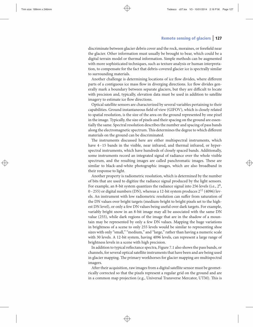
discriminate between glacier debris cover and the rock, moraines, or forefield nearthe glacier. Other information must usually be brought to bear, which could be adigital terrain model or thermal information. Simple methods can be augmentedwith more sophisticated techniques, such as texture analysis or human interpreta-tion, to compensate for the fact that debris-covered glacier ice is spectrally similarto surrounding materials.Another challenge is determining locations of ice flow divides, where different

parts of a contiguous ice mass flow in diverging directions. Ice flow divides gen-erally mark a boundary between separate glaciers, but they are difficult to locatewith precision and, typically, elevation data must be used in addition to satelliteimagery to estimate ice flow directions.Optical satellite sensors are characterized by several variables pertaining to their

capabilities. Ground instantaneous field of view (GIFOV), which is closely relatedto spatial resolution, is the size of the area on the ground represented by one pixelin the image. Typically, the size of pixels and their spacing on the ground are essen-tially the same. Spectral resolution describes the number and spacing of pass bandsalong the electromagnetic spectrum.This determines the degree to which differentmaterials on the ground can be discriminated.The instruments discussed here are either multispectral instruments, which

have 4–15 bands in the visible, near infrared, and thermal infrared, or hyper-spectral instruments, which have hundreds of closely spaced bands. Additionally,some instruments record an integrated signal of radiance over the whole visiblespectrum, and the resulting images are called panchromatic images. These aresimilar to black-and-white photographic images, which are also broadband intheir response to light.Another property is radiometric resolution, which is determined by the number

of bits that are used to digitize the radiance signal produced by the light sensors.For example, an 8-bit system quantizes the radiance signal into 256 levels (i.e., 28,0–255) or digital numbers (DN), whereas a 12-bit system produces 212 (4096) lev-els. An instrument with low radiometric resolution can suffer from saturation ofthe DN values over bright targets (medium-bright to bright pixels set to the high-est DN level), or only a few DN values being useful over dark targets. For example,variably bright snow in an 8-bit image may all be associated with the same DNvalue (255), while dark regions of the image that are in the shadow of a moun-tain may be represented by only a few DN values. Mapping the huge variationsin brightness of a scene to only 255 levels would be similar to representing shoesizes with only “small,” “medium,” and “large,” rather than having a numeric scalewith 30 levels. A 12-bit system, having 4096 levels, can represent a large range ofbrightness levels in a scene with high precision.In addition to typical reflectance spectra, Figure 7.1 also shows the pass bands, or

channels, for several optical satellite instruments that have been and are being usedin glacier mapping.The primary workhorses for glacier mapping are multispectralimagers.After their acquisition, raw images from a digital satellite sensormust be geomet-

rically corrected so that the pixels represent a regular grid on the ground and arein a common map projection (e.g., Universal Transverse Mercator, UTM). This is



generally done by the data provider. An additional step, important for most glaciermapping efforts, is to orthorectify the imagery. In simple terms, orthorectificationadjusts the locations of image pixels to correct for distortions caused by terrain.For example, the peak of a tall mountain on the left side of an image will appearcloser to the left edge of the image than it should, due to parallax. Orthorectifica-tion corrects for this effect, and produces an image where it appears that the vieweris looking straight down (vertically) on all parts of the image (Schowengerdt, 2007).

7.3 Satellite instruments for glacier research

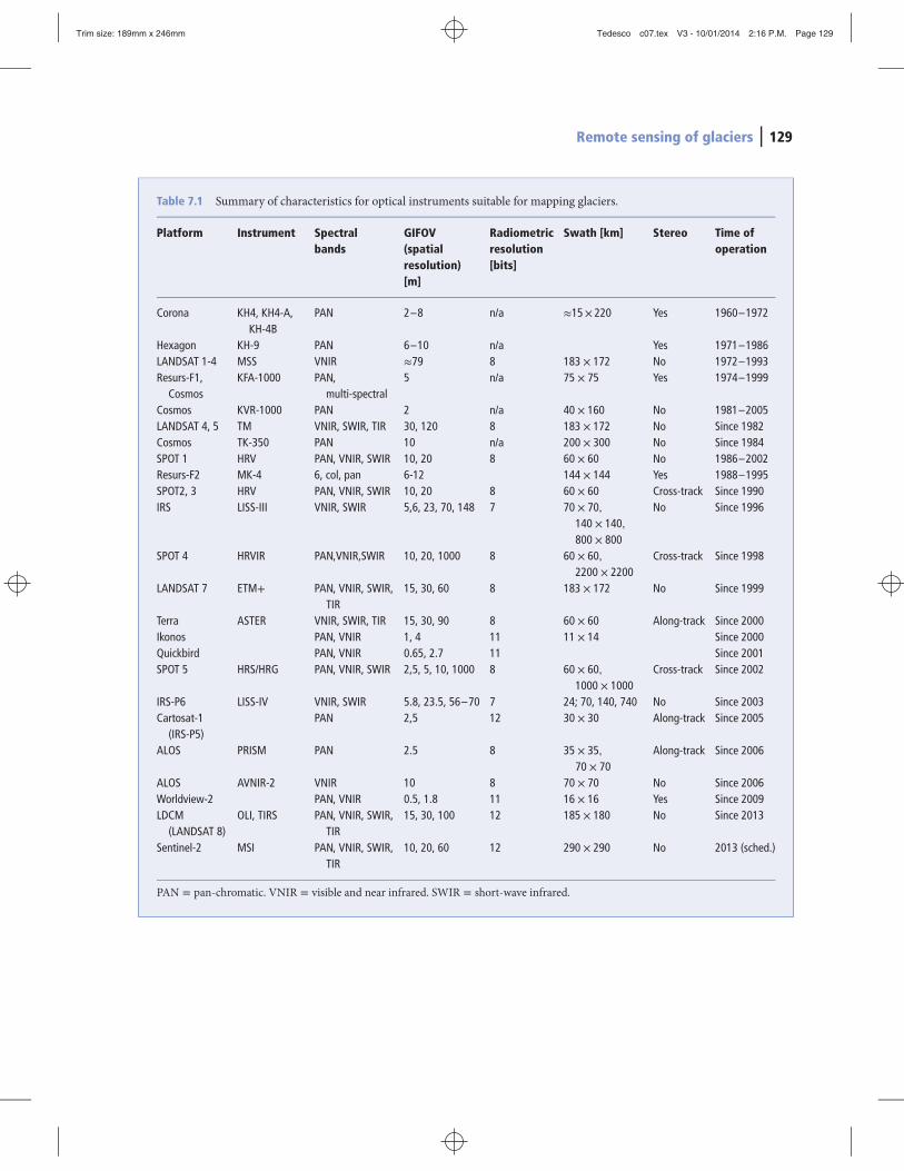
A variety of satellite data sources can be used for studying glaciers, from declas-sified Corona photographs (panchromatic images) through LANDSAT, AdvancedSpaceborneThermal Emission and Reflection Radiometer (ASTER), Satellite Pourl’Observation de la Terre (SPOT), to instruments recently or nearly online, such asthe high spatial resolution Quickbird or Worldview satellites (Table 7.1).The first spaceborne sensors to acquire imagery systematically were flying on

the US Corona program strategic reconnaissance satellites, in operation between1960 and 1972.Themost useful characteristics of the Corona panchromatic imagesare their stereo capability and a spatial resolution of approximately 2–8 meters(Dashora et al., 2007). Corona or other reconnaissance images such as Hexagon(see Table 7.1) have recently been used to map earlier extents of glaciers with highprecision (Bhambri et al., 2011; Narama et al., 2010; Bolch et al., 2010b), extendingthe observational record by a decade into the past.A comprehensive and continuous survey of the Earth’s surface began with the

launch of the first LANDSAT satellite (originally called Earth Resources Technol-ogy Satellite, or ERTS-1) in 1972. The satellite carried the multispectral scanner(MSS), recording in four wavelength bands in the visible and near infrared spec-trum with a GIFOV of about 80 m × 80 m. The first sensor to acquire data in theshort wave infrared, which makes it suitable for automated glacier mapping, wastheThematic Mapper (TM) aboard the LANDSAT 4 satellite, launched in 1982.The LANDSAT instruments, from the MSS through the TM instruments on

LANDSAT 4 and 5, to the Enhanced Thematic Mapper Plus (ETM+) instrumenton LANDSAT 7, have been particularly useful because they collectively cover along time span and have a wide swath (185 km), allowing the coverage of largeareas in one image. In addition, LANDSAT images are now available at no cost asorthorectified products (http://landsat.gsfc.nasa.gov/).The LANDSAT bands wereselected to be able to measure radiance in parts of the spectrum with absorptionfeatures associated with a number of common natural materials, including bandsin the visible and near-infrared (useful for distinguishing vegetation from rocksand from water), and bands in the thermal infrared (useful for measuring thermalinertia, temperature and temperature ranges). Othermultispectral imagers, such asthe French SPOT satellites, the Indian IRS (Indian Remote Sensing) satellites andthe Japanese instrument ASTER on board the Terra satellite, have similar capabil-ities (e.g., Figure 7.2). Recent developments include ultra high resolution imagery

https://www.researchgate.net/publication/216703554_Glacier_changes_in_the_Garwhal_Himalaya_India_1968-2006_based_on_remote_sensing?el=1_x_8&enrichId=rgreq-489250a7-e82f-4dc4-8363-8c6a2c049e74&enrichSource=Y292ZXJQYWdlOzI3NzcwNjcxNDtBUzoyMzg4MjU3NjcxNzQxNDZAMTQzMzk1MTkwODIzNA==

https://www.researchgate.net/publication/236771433_Remote_Sensing_Models_and_Methods_for_Image_Processing_93?el=1_x_8&enrichId=rgreq-489250a7-e82f-4dc4-8363-8c6a2c049e74&enrichSource=Y292ZXJQYWdlOzI3NzcwNjcxNDtBUzoyMzg4MjU3NjcxNzQxNDZAMTQzMzk1MTkwODIzNA==

https://www.researchgate.net/publication/228656758_A_repository_of_earth_resource_information_CORONA_satellite_programme?el=1_x_8&enrichId=rgreq-489250a7-e82f-4dc4-8363-8c6a2c049e74&enrichSource=Y292ZXJQYWdlOzI3NzcwNjcxNDtBUzoyMzg4MjU3NjcxNzQxNDZAMTQzMzk1MTkwODIzNA==



Table 7.1 Summary of characteristics for optical instruments suitable for mapping glaciers.

Platform Instrument Spectralbands

GIFOV(spatialresolution)[m]

Radiometricresolution[bits]

Swath [km] Stereo Time ofoperation

Corona KH4, KH4-A,KH-4B

PAN 2–8 n/a ≈15× 220 Yes 1960–1972

Hexagon KH-9 PAN 6–10 n/a Yes 1971–1986LANDSAT 1-4 MSS VNIR ≈79 8 183 × 172 No 1972–1993Resurs-F1,

CosmosKFA-1000 PAN,

multi-spectral5 n/a 75 × 75 Yes 1974–1999

Cosmos KVR-1000 PAN 2 n/a 40 × 160 No 1981–2005LANDSAT 4, 5 TM VNIR, SWIR, TIR 30, 120 8 183 × 172 No Since 1982Cosmos TK-350 PAN 10 n/a 200 × 300 No Since 1984SPOT 1 HRV PAN, VNIR, SWIR 10, 20 8 60 × 60 No 1986–2002Resurs-F2 MK-4 6, col, pan 6-12 144 × 144 Yes 1988–1995SPOT2, 3 HRV PAN, VNIR, SWIR 10, 20 8 60 × 60 Cross-track Since 1990IRS LISS-III VNIR, SWIR 5,6, 23, 70, 148 7 70 × 70,

140 × 140,800 × 800

No Since 1996

SPOT 4 HRVIR PAN,VNIR,SWIR 10, 20, 1000 8 60 × 60,2200 × 2200

Cross-track Since 1998

LANDSAT 7 ETM+ PAN, VNIR, SWIR,TIR

15, 30, 60 8 183 × 172 No Since 1999

Terra ASTER VNIR, SWIR, TIR 15, 30, 90 8 60 × 60 Along-track Since 2000Ikonos PAN, VNIR 1, 4 11 11 × 14 Since 2000Quickbird PAN, VNIR 0.65, 2.7 11 Since 2001SPOT 5 HRS/HRG PAN, VNIR, SWIR 2,5, 5, 10, 1000 8 60 × 60,

1000 × 1000Cross-track Since 2002

IRS-P6 LISS-IV VNIR, SWIR 5.8, 23.5, 56–70 7 24; 70, 140, 740 No Since 2003Cartosat-1

(IRS-P5)PAN 2,5 12 30 × 30 Along-track Since 2005

ALOS PRISM PAN 2.5 8 35 × 35,70 × 70

Along-track Since 2006

ALOS AVNIR-2 VNIR 10 8 70 × 70 No Since 2006Worldview-2 PAN, VNIR 0.5, 1.8 11 16 × 16 Yes Since 2009LDCM

(LANDSAT 8)OLI, TIRS PAN, VNIR, SWIR,

TIR15, 30, 100 12 185 × 180 No Since 2013

Sentinel-2 MSI PAN, VNIR, SWIR,TIR

10, 20, 60 12 290 × 290 No 2013 (sched.)

PAN = pan-chromatic. VNIR = visible and near infrared. SWIR = short-wave infrared.



Figure 7.2 (a) Example of anASTER image, acquired09-16-2010, of glaciers in theChugach Range of southernAlaska. Bands 3N, 2, and 1are displayed as red, green,and blue. (b) Oblique aerialphotograph, taken in 1977, ofFive Stripe Glacier, visible inthe ASTER image at arrow.The snow line is clearly visiblein (b) as the transitionbetween bare glacier ice(gray) and snow (white), butthe snow line in the ASTERimage is almost above thehighest elevation of FiveStripe Glacier.



with a resolution of one meter and below (e.g., Ikonos, Quickbird) and fast repeatcycles (e.g., Rapid-Eye).The instruments described above are passive, in that they sense solar radia-

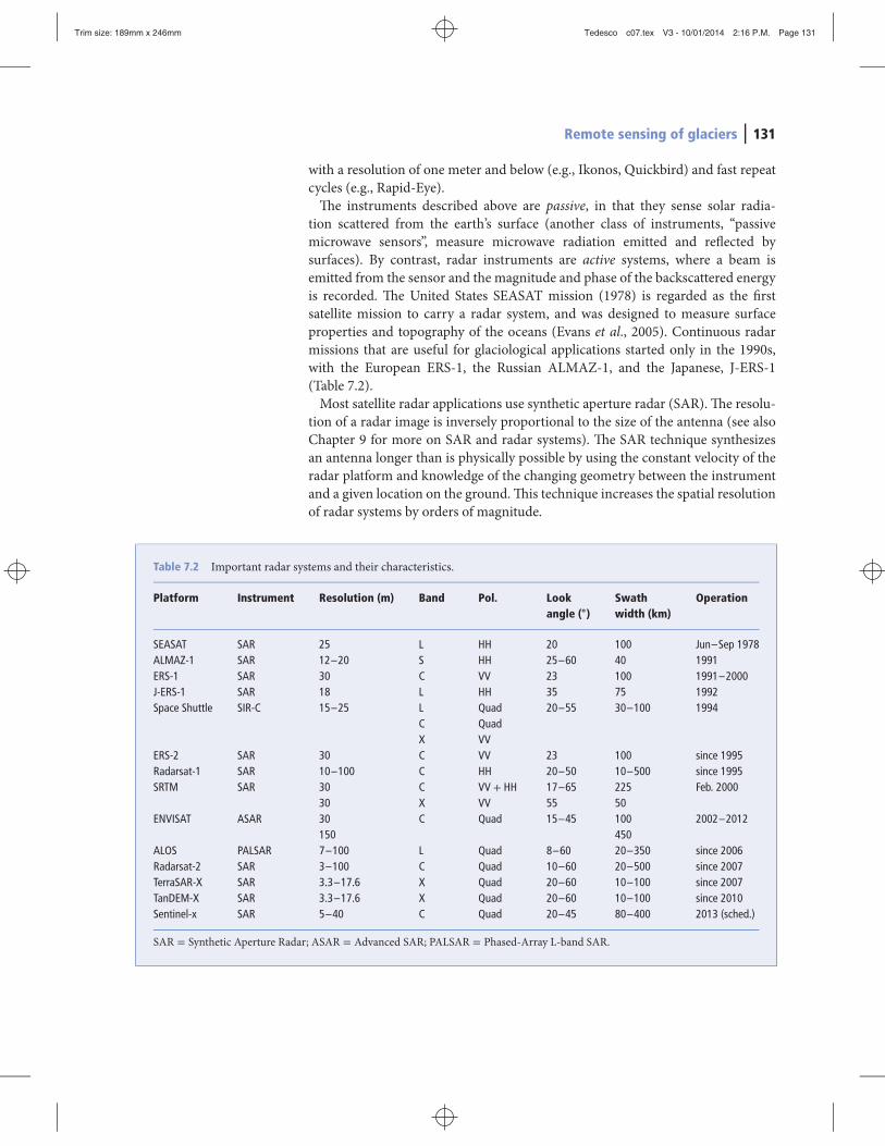
tion scattered from the earth’s surface (another class of instruments, “passivemicrowave sensors”, measure microwave radiation emitted and reflected bysurfaces). By contrast, radar instruments are active systems, where a beam isemitted from the sensor and the magnitude and phase of the backscattered energyis recorded. The United States SEASAT mission (1978) is regarded as the firstsatellite mission to carry a radar system, and was designed to measure surfaceproperties and topography of the oceans (Evans et al., 2005). Continuous radarmissions that are useful for glaciological applications started only in the 1990s,with the European ERS-1, the Russian ALMAZ-1, and the Japanese, J-ERS-1(Table 7.2).Most satellite radar applications use synthetic aperture radar (SAR). The resolu-

tion of a radar image is inversely proportional to the size of the antenna (see alsoChapter 9 for more on SAR and radar systems). The SAR technique synthesizesan antenna longer than is physically possible by using the constant velocity of theradar platform and knowledge of the changing geometry between the instrumentand a given location on the ground.This technique increases the spatial resolutionof radar systems by orders of magnitude.

Table 7.2 Important radar systems and their characteristics.

Platform Instrument Resolution (m) Band Pol. Lookangle (∘)

Swathwidth (km)

Operation

SEASAT SAR 25 L HH 20 100 Jun–Sep 1978ALMAZ-1 SAR 12–20 S HH 25–60 40 1991ERS-1 SAR 30 C VV 23 100 1991–2000J-ERS-1 SAR 18 L HH 35 75 1992Space Shuttle SIR-C 15–25 L

CX

QuadQuadVV

20–55 30–100 1994

ERS-2 SAR 30 C VV 23 100 since 1995Radarsat-1 SAR 10–100 C HH 20–50 10–500 since 1995SRTM SAR 30

30CX

VV + HHVV

17–6555

22550

Feb. 2000

ENVISAT ASAR 30150

C Quad 15–45 100450

2002–2012

ALOS PALSAR 7–100 L Quad 8–60 20–350 since 2006Radarsat-2 SAR 3–100 C Quad 10–60 20–500 since 2007TerraSAR-X SAR 3.3–17.6 X Quad 20–60 10–100 since 2007TanDEM-X SAR 3.3–17.6 X Quad 20–60 10–100 since 2010Sentinel-x SAR 5–40 C Quad 20–45 80–400 2013 (sched.)

SAR = Synthetic Aperture Radar; ASAR = Advanced SAR; PALSAR = Phased-Array L-band SAR.



Other systems to measure surface elevation are laser and radar altimeters. Laseraltimetry systems such as Geoscience Laser Altimetry System (GLAS), aboard theNASA Ice, Cloud, and land Elevation Satellite (ICESat), or radar altimetry sys-tems such as the ENVISAT RA2 or CryoSat-2, transmit a pulse (laser light orradar beam) to the surface, and measure the time to receive the reflected response,thereby determining the elevation of the surface. ICESat GLAS was designed tostudy primarily the Greenland and Antarctic ice sheets, but has also been used tostudy mountain glacier elevation changes from space (Kääb, 2008; Moholdt et al.,2010). The footprint of the transmitted spot for GLAS is approximately 70m but,as the spacing of laser pulses on the ground is large compared to the size of mostglaciers, this instrument can only be used to study a limited number of largermountain glaciers or ice caps.New satellites suited to studyingmountain glaciers are planned to be launched in

the near future. Particularly promising is the European Sentinel-2 satellite, sched-uled to be launched in 2014, with a higher temporal and spatial resolution thanthe LANDSAT TM and ETM+ sensors. The LANDSAT Data Continuity Mission(LCDM) is valuable as well (Table 7.1).

7.4 Methods

7.4.1 Image classification for glacier mapping

Image classification is the process of assigning material classes (vegetation, rock,snow, water, etc.) to each pixel in an image. This first step is essential before cre-ating a map of features (e.g., glaciers, lakes) in the imagery, although mappingfeatures (e.g., glaciers) from a classified image (a map of materials) is not trivial,as many features involve a mixture of materials. For example, a glacier is domi-nantly ice, but it will often contain medial moraines or rock debris cover at theterminus, and the debris cover may even support vegetation. The “glacier” willtherefore contain ice, rock, and vegetation classes in the classified image.Many dif-ferent image classification and feature identification methods have been evaluatedfor glaciermapping, includingmanual digitization, supervised classification (max-imum likelihood, minimum distance, spectral angle mapper, etc.), unsupervisedclassification, fuzzy classification techniques, and band arithmetic and thresholdtechniques (Sidjak and Wheate, 1999; Paul et al., 2002; Albert, 2002; Racoviteanuet al., 2009; Gjermundsen et al., 2011).Supervised classification begins with the operator selecting representative sets of

pixels that are representative of identifiable materials in the image, such as vegeta-tion, snow, glacier ice, and so on. The differences between the spectral signaturesof these “training sets” (or end-members) are then used to assign the rest of thepixels in the image to one of those categories. Linear unmixing, a fuzzy classifica-tion technique, begins the same way but assigns fractional end-member contentto each pixel. Unsupervised techniques such as ISODATA operate similarly, but



attempt to identify the end-members automatically by employing cluster detectionalgorithms. Details on image classification methods can be found in several books(e.g., Schowengerdt, 2007; Richards, 1986).There is a trade-off between the time required to create glacier outlines from a

method and the accuracy of the resulting outlines (Albert, 2002). Manual digiti-zation, done by a glaciologist experienced in studying glaciers in remote sensingimagery, can achieve the highest accuracy in most types of terrain. Errors of inter-pretation can occur in some situations involving complicated patterns of debriscover on the glacier or seasonal snow attached to the glacier, but humans tend todo better in such situations than current computer algorithms. Mapping glaciersby hand, however, is the most time-consuming, and hence costly, of the availablemethods, and is therefore impractical for any but small regional studies.Several studies (Albert, 2002; Paul et al., 2002; Racoviteanu et al., 2009) have con-

cluded that the best trade-off between processing time and accuracy is obtained byband arithmetic techniques, such as computing band ratios or using normalizeddifferences, such as the normalized difference snow index (NDSI; see also Chapter3). In the band ratio technique, the ratio of bands in the near-infrared (NIR) or redparts of the spectrum and the short-wave infrared (SWIR) is computed, resultingin a “ratio image” that has high values over snow and ice, and low values over rockand vegetation. A threshold is applied to produce a binary raster mask indicat-ing regions of snow/ice and non-snow/ice. Glacier outlines are then derived byconverting the raster mask to a vector representation.Both band ratios NIR/SWIR and red/SWIR have been shown to be well suited

for glacier mapping, as they both take advantage of the large difference in spectralsignature between snow and other materials in those spectral bands (Figure 7.1).Some studies have shown preference for Red/SWIR, as this discriminates betterbetween ice and snow in shadow cast by adjacent terrain (Paul and Kääb, 2005).Andreassen et al. (2008) used the spectral characteristics of snow and ice in LAND-SAT bands TM3 (Red) and TM5 (SWIR) for automatic classification of glaciers inJotunheimen in southern Norway (Figure 7.3).The subset of the full scene used intheir analysis contains neither clouds nor stark shadow, and there is no significantdebris on the ice. The image is therefore well suited to the band ratio method.The normalized difference snow index (NDSI; see also Chapter 3), another

band arithmetic technique that is defined as (VIS-NIR)∕(VIS +NIR), can beused similarly to map glacier outlines (e.g., Sidjak andWheate, 1999; Racoviteanuet al., 2008b). For LANDSAT TM, for example, NDSI is obtained from the ratio(TM2-TM5)∕(TM2 + TM5). It was developed to map snow (Hall et al., 1995;Salomonson and Appel, 2004; see Chapter 3), but since glacier ice is composedof densified snow, the spectral characteristics are similar (Figure 7.1). While theNDSI is useful for glacier mapping, the good performance and simplicity of theband ratio method for clean ice has resulted in the community predominantlyusing it to do classification (Racoviteanu et al., 2009). The band ratio methodis easily automated but, as it relies on differences in spectral signatures of thematerials in the image, it erroneously excludes parts of the glacier that arecovered with rock debris. While newer techniques, discussed below, address these



(a) (b) (c)

(d)0 5 10

Km(e) (f)

Figure 7.3 Automatic classification of snow and ice for asubset of glaciers in Jotunheimen, southern Norway, using aLANDSAT TM scene from 9 August 2003. (a) Red-green-blue (RGB) composite of TM bands 5, 4 and 3.(b) LANDSAT band TM3 (0.63–0.69 μm). (c) LANDSAT

band TM5 (1.55–1.75 μm). (d) Ratio image of TM3/TM5.(e) Thresholded image of TM3/TM5 >2.0 and median filter(3 ∗ 3 kernel). (f) Same as (a), with outlines (in white)derived from raster to vector conversion of (e).

shortcomings, manual editing is generally needed to include debris-covered parts,to exclude seasonal snow and sometimes adjacent lakes, or to include parts of theglacier in heavy shadow.

7.4.2 Mapping debris-covered glaciers

More sophisticated methods than the ones presented above have been developedfor automatically classifying debris-covered ice as part of the glacier. Somemethods use thermal data, while others use topographic texture, curvature (geo-morphometrics; Bishop et al., 2001; Brenning, 2009), velocity, image differencing,or coherence images of SAR data (see next page) for detection of ice motion andto delineate the glacier boundary.

Trim size: 189mm x 246mm Tedesco c07.tex V3 - 10/01/2014 2:16 P.M. 5


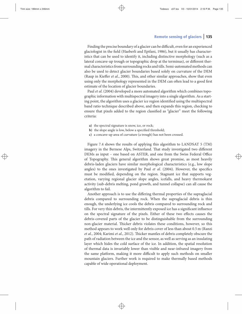
Finding the precise boundary of a glacier can be difficult, even for an experiencedglaciologist in the field (Haeberli and Epifani, 1986), but it usually has character-istics that can be used to identify it, including distinctive morphology (such as alateral concave-up trough or topographic drop at the terminus), or different ther-mal characteristics from surrounding rocks and tills. Semi-automatedmethods canalso be used to detect glacier boundaries based solely on curvature of the DEM(Raup in Kieffer et al., 2000). This, and other similar approaches, show that evenusing only the morphology represented in the DEM can often lead to a good firstestimate of the location of glacier boundaries.Paul et al. (2004) developed a more automated algorithm which combines topo-

graphic information withmultispectral imagery into a single algorithm. As a start-ing point, the algorithm uses a glacier ice region identified using the multispectralband ratio technique described above, and then expands this region, checking toensure that pixels added to the region classified as “glacier” meet the followingcriteria:

a) the spectral signature is snow, ice, or rock;b) the slope angle is low, below a specified threshold;c) a concave-up area of curvature (a trough) has not been crossed.

Figure 7.4 shows the results of applying this algorithm to LANDSAT 5 (TM)imagery in the Bernese Alps, Switzerland. That study investigated two differentDEMs as input – one based on ASTER, and one from the Swiss Federal Officeof Topography. This general algorithm shows great promise, as most heavilydebris-laden glaciers have similar morphological characteristics (e.g., low slopeangles) to the ones investigated by Paul et al. (2004). However, the specificsmust be modified, depending on the region. Stagnant ice that supports veg-etation, varying regional glacier slope angles, icefalls, and heavy thermokarstactivity (sub-debris melting, pond growth, and tunnel collapse) can all cause thealgorithm to fail.Another approach is to use the differing thermal properties of the supraglacial

debris compared to surrounding rock. When the supraglacial debris is thinenough, the underlying ice cools the debris compared to surrounding rock andtills. For very thin debris, the intermittently exposed ice has a significant influenceon the spectral signature of the pixels. Either of these two effects causes thedebris-covered parts of the glacier to be distinguishable from the surroundingnon-glacier material. Thicker debris violates these conditions, however, so thismethod appears to work well only for debris cover of less than about 0.5m (Ranziet al., 2004; Karimi et al., 2012). Thicker mantles of debris completely obscure thepath of radiation between the ice and the sensor, as well as serving as an insulatinglayer which hides the cold surface of the ice. In addition, the spatial resolutionof thermal data is invariably lower than visible and near-infrared imagery fromthe same platform, making it more difficult to apply such methods on smallermountain glaciers. Further work is required to make thermally based methodscapable of wide operational deployment.



Grosser aletsch glacier

Oberaletsch glacier

3 km

= both DEM= only ASTER= only DEM25

Figure 7.4 Results of applying a debris-covered glacier mapping algorithm to LANDSAT 5 imagery of the Bernese Alps,Switzerland, and two digital elevation models (adapted from Paul et al., 2004).

7.4.3 Glacier mapping with SAR data

One main advantage of active radar systems is that they can operate in almost anyweather as well as at night, because the beam and the backscattered radiation inthe microwave region penetrate through clouds and do not depend on sunlight.In general, SAR data are capable of distinguishing snow and ice from surroundingareas, due to the different backscattering signal from different materials.A limitation is that spaceborne satellite SAR systems are usually limited to one

frequency of the emitted beam, which hampers the correct classification of glaciers(Rott, 1994). This is especially true if glaciers have variable surface roughness, forexample due to crevasses, different snow and ice facies (snow, firn, glacier ice,refrozen melt water), and debris cover. The variable nature of the returned signalmakes finding the glacier boundary difficult. Hence, SAR data has so far playedonly a minor role for glacier mapping.An application where SAR performs better than optical methods in glacier stud-

ies is the discrimination of different snow facies. SAR data are often used to maptemporal changes of snow and ice areas due to the temporal change of the surface’sbackscatter characteristics, best observable in the C band (4 to 8GHz) and X band(8 to 12GHz) (Nagler and Rott, 2000). The backscattering ratio of a summer and



winter image is used to discriminate between ice and snow in summer, while awinter image is best for obtaining the longer term ELA, because the SAR signalintegrates over several meters depth in the snow pack and the boundary betweenice and firn is therefore averaged over a few years (Floricioiu and Rott, 2001).Recent efforts have focused on using SAR data for the detection of glaciers in

areas with frequent cloud cover, and for debris-covered glaciers where the opticaldata are limited. One promising approach is the use of SAR coherence images(Atwood et al., 2010), where areas with changing surfaces (e.g., due to glaciermotion or down-wasting) decorrelate (the phase of the returned beam changesover time), in contrast to coherent stable areas. In addition, by taking advantageof the phase coherence of the transmitted radar beam, data from multiple passescan be analyzed for differences in the phase of the returned beam, which can beused for mapping topography, detecting subtle changes in the surface (includingdebris-covered areas), and mapping ice flow velocity. This technique is known asinterferometric SAR, or InSAR (see Chapter 9 also for more InSAR applications).Once glacier outlines are obtained by anymethod, basic glacier parameters, such

as slope, aspect, elevation range, minimum,median, andmaximum elevations, etc.can be obtained by examining DEM values within the outline or on the bound-ary (Paul et al., 2009). Such parameters are generally stored as key parts of glacierinventories, such as theWorld Glacier Inventory and the GLIMSGlacier Database.

7.4.4 Assessing glacier changes

Time series of satellite imagery, or imagery combined with other data sources, canbe used to detect and map changes in glacier extent, thickness, and surface char-acteristics.When studying a series of images, the first step is to co-register them using

ground control points (GCPs) or tie points. GCPs register the images to knownlocations on the ground, while tie points are features identifiable in both (or all)images, but may not be precisely located on the ground. This co-registrationstep is crucial, as many artifacts (false changes) can appear if there are offsetsbetween the images. For change detection involving multi-temporal DEMs,proper co-registration is even more important, since improper co-registrationleads to biases in the elevation differences everywhere in the domain, not just atthe boundaries of different regions within the domain, as might be the case withclassified imagery (Nuth and Kääb, 2011).Changes in glacier area and length are easy to obtain directly from satellite

observations, because they are directly related to changes in the observedtwo-dimensional (planimetric) information in the imagery. Changes in glaciervolume or mass are more important scientifically (due to the connection toclimate, and consequences such as sea level change or changes to hydrologicalresources), but they are more difficult to observe from satellite data.



7.4.5 Area and length changes

A simple yet effective way to detect change is the method of image differencing,where an earlier image is subtracted from a later one taken with identical or sim-ilar solar geometry (nearly the same time of day and day of year) (e.g., Sabins,2007). The subtraction is usually done separately on each band, and results ina grid of numbers that are near zero in areas of no or little change, and whichcan be positive or negative for changed regions in the image. The grid is typi-cally rescaled to positive numbers for display so that, for a single band, areas ofno change appear gray, areas that have become more reflective (e.g., an area newlysnow-covered) appear bright, and less reflective parts of the image (e.g., wheresnow or ice has been removed) look dark. Each difference band can be viewed onits own, or the rescaled difference bands can be displayed as red-green-blue, andthe colors then yield information about changes in materials on the ground, sincethey indicate changes in spectral signature (e.g., by the appearance of vegetationon a moraine).Mapping changes in glacier area based on repeat glacier extent mapping is

straightforward in theory: create maps of glacier ice from two (or more) differentimages, and compare the computed areas. This can be done either from theraster map or from vector outlines that have been derived from a classified image.Another choice that the analystmustmake is whether to comparemaps of contigu-ous glacier ice as a whole, or to compare computed areas on a glacier-by-glacierbasis. If the aim is to compute glacier area change for each separate glacier, greatcare must be taken to ensure that the ice divides (the boundaries between glaciersat their upper reaches) match exactly. If the ice divides do not match, then onecan easily obtain the erroneous result that the glacier or glaciers on one side of adivide have grown, while those on the other side have shrunk, even if the total icearea did not change. This kind of investigation is therefore most safely performedover a whole system or mountain range (e.g., Racoviteanu et al., 2008a).Satellite imagery can also be used to derive length changes. High-resolution

satellite imagery has been used to reconstruct glacier front variations over aperiod of four decades for the well-known Gangotri Glacier of northern India(Bhambri et al., 2012). A study from Jostedalsbreen, Norway, showed that thehigh spatial variability measured from field data could be observed by LANDSAT(within one pixel, 30m resolution) for glacier tongues not in cast shadow(Paul et al., 2011).As satellite imagery only goes back a few decades, it is common to assess

glacier changes by comparing with other sources such as aerial photographs,topographic maps or inventory data (Casassa et al., 2002). Glacier outlines derivedfrom topographic maps are a valuable source, but they are usually mapped bynon-glaciologists and might contain inaccuracies due to the existence of seasonalsnow or misinterpretation of debris cover (Andreassen et al., 2008; Bhambriand Bolch, 2009). Satellite imagery has also been used in several regions to map



glacier changes since the Little Ice Age maximum bymapping the glacier forefield,which is spectrally different from the terrain beyond the Little Ice Age maximummoraines (Paul and Kääb, 2005; Baumann et al., 2009).

7.4.6 Volumetric glacier changes

DEMs can be used to measure volume changes of glaciers by subtracting pairs ofDEMs. DEMs can be generated by different methods, such as space- and airborneoptical stereo data, interferometric SAR (InSAR) data, space and airborne radarand laser altimetry, and topographic maps. There are three nearly global eleva-tion products available today with high enough spatial resolution to study glacierchanges:

1 The Shuttle Radar Topography Mission (SRTM) flown in February 2000.2 ASTER Global DEM, version 2 (GDEM2) based upon stereo scenes acquired from 2000

to the present.3 The ICESat mission from 2003 to 2009 using spaceborne laser altimetry, or Light Detec-

tion and Ranging (LiDAR).

These data sets all have different strengths and limitations. The SRTM DEM hasrelatively high resolution and covers the globe between 59∘S and 60∘N latitude, butit includes data voids in mountainous regions of high relief. Radar penetration ofsnow in the upper reaches of glaciers can lead to elevation biases there (Gardelleet al., 2012). The ICESat elevation estimates are the most accurate (e.g., Nuth andKääb, 2011), but the spatial coverage is much poorer, with 170m spacing betweenpoints along-track and hundreds or thousands of meters between tracks, depend-ing on latitude. Nevertheless, these data are valuable for obtaining region-wideinformation (Kääb et al., 2012; Bolch et al., 2013; Gardner et al., 2013).While the SRTM and standard ASTER DEMs have been proved to be useful as

a baseline data set, more accurate DEMs are generally needed for precise volumechange determination (e.g., Berthier et al., 2010). Such DEMs can be created fromindividual image pairs from suitable optical stereo satellite instruments, such asASTER, SPOT5, ALOS, and Cartosat-1 (e.g., Kääb et al., 2012; Berthier et al.,2007). LiDAR DEMs acquired using airborne systems are generally the mostprecise, but are limited to smaller areas. One of the largest ice bodies mappednearly completely with LiDAR to date is Vatnajökull, the largest ice cap of Iceland(Johannesson et al., 2012).Elevation change of glaciers can be calculated by DEM differencing or repeat

altimetry measurements (Figure 7.5). DEM differencing is a popular techniquethat has been used for decades to assess glacier changes (e.g., Finsterwalder, 1954;Abermann et al., 2009). Changes in the volume of the glacier are converted tomasschanges using estimates of density. This method is called the geodetic method



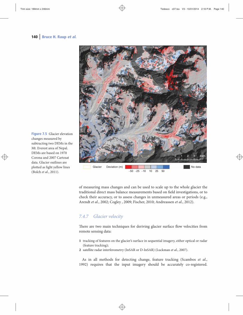
Figure 7.5 Glacier elevationchanges measured bysubtracting two DEMs in theMt. Everest area of Nepal.DEMs are based on 1970Corona and 2007 Cartosatdata. Glacier outlines areplotted as light yellow lines(Bolch et al., 2011).

Glacier Deviation (m)

0 1 2 3 4km

–50 –25 –10 10 25 50

No data

of measuring mass changes and can be used to scale up to the whole glacier thetraditional direct mass balance measurements based on field investigations, or tocheck their accuracy, or to assess changes in unmeasured areas or periods (e.g.,Arendt et al., 2002; Cogley , 2009; Fischer, 2010; Andreassen et al., 2012).

7.4.7 Glacier velocity

There are two main techniques for deriving glacier surface flow velocities fromremote sensing data:

1 tracking of features on the glacier’s surface in sequential imagery, either optical or radar(feature tracking);

2 satellite radar interferometry (InSAR or D-InSAR) (Luckman et al., 2007).

As in all methods for detecting change, feature tracking (Scambos et al.,1992) requires that the input imagery should be accurately co-registered.



Feature tracking software, such as IMCORR or Cosi-corr (see Heid and Kääb(2012) for a comparison of algorithms), automatically finds matching featuresfrom both images and outputs a displacement vector for each location on a grid.For glaciers, these individual features could be ice pinnacles, crevasses, boulders,or a distinctive pattern of debris and ice, which can be identified on both images.Compared to field methods, where a day’s work might produce a handful ofvelocity measurements for a glacier, feature tracking in satellite imagery is muchmore effective, yielding tens of thousands of vectors.When feature tracking is applied to radar data, matching is generally done using

the intensity images, which are images of the strength of the returned beam, eitherby tracking large-scale features thatmovewith the ice and are visible in the imagery,or by tracking the small-scale pattern of light and dark in the intensity image thatis due to phase coherence from one image to the next over stable surfaces. Thislatter technique is known as “speckle tracking,” and it allows smaller patch sizes tobe used compared to feature-tracking (Strozzi et al., 2002; Joughin, 2002). Studiesthat use feature tracking for velocitymeasurement includeKääb (2005), Bolch et al.(2008), Scherler et al. (2008), and Quincey et al. (2009).Interferometric synthetic aperture radar (InSAR) is used for the observation of

geometric displacements of the ground or glacier surface. Displacements on theorder of centimeters or even millimeters can be measured, depending on the timedifference between acquisitions. InSAR is based on the fact that the phase of theradar beam returned to the instrument from a spot on the ground does not changefrom overflight to overflight, provided the instrument is in the same position,unless the surface is changing. With two overflights, the phase part of the radarimages can be subtracted to create an interferogram, which is a depiction of howthe phase has changed from one overflight to the next. A single interferogramcontains information about changes on the ground (deformation of the surface, orchanged dielectric properties), as well as effects from differing satellite positionsbetween overflights (orbital contributions) and topography. If the instrument is inslightly different positions for the two overflights, the effect on the interferogramcan be modeled and removed.Tomeasure surface velocity with this technique, the effect of topographymust be

removed. This can be done using a DEM from an external source, such as SRTMor GDEM2, in which case only two satellite overflights are required (two-passmethod). Alternatively, in the three-pass method, the first two images are used togenerate a DEM. The time separation should be short between these two in orderto minimize effects of surface deformation and, thus, decorrelation of the signal.The image of the third overflight is then used, together with the first or secondimage, to retrieve another interferogram. The second interferogram contains notonly information about topography, but also the displacement, and by combiningthe two interferograms, the component of the ice velocity in the direction towardor away from the satellite sensor can be isolated.The three-pass method is generally known as differential interferometric syn-

thetic aperture radar, or D-InSAR. D-InSARmakes it possible to detect sub-meterchanges in images that have a nominal ground resolution of several meters.



Problems with this technique for glacier velocity mapping include difficultyachieving the stability of the phase (phase coherence) necessary to make themethod work, data availability, and layover (radar beam shadowing) in regions ofhigh relief.An example study using this technique is described in Yasuda and Furuya (2013),

who studied short-term glacier velocity fluctuations in the Kunlun Shan range.More information about this technique can be found in Eldhuset et al. (2003) andLuckman et al. (2007).

7.5 Glaciers of the Greenland ice sheet

7.5.1 Surface elevation

The earliest satellite observations of surface elevation change over the Greenlandice sheet were based on radar altimeter data from the ERS-1 (1992–95) and ERS-2(1995–2003) satellites (Johannessen et al., 2005; Zwally et al., 2005). The resultsindicated that the ice sheet was growing above the ELA and thinning at lower ele-vations,with an overall gain in volume.However, both studies indicatedmore rapidelevation increases at high elevations and less thinning over the margins than didresults from repeat aircraft laser altimeter surveys within the same period (Krabillet al., 2000). The differences at lower altitudes, where slopes are steeper, are prob-ably due to the much larger footprint of the radar altimeter (≈20 km) comparedwith the 1–3m airborne LiDAR footprint. At higher elevations, the differencemaybe due to changes in the radar penetration depth being superimposed on surfaceelevation changes (Thomas et al., 2008).Since 2002, the ICESat instrument GLAS, a laser altimeter, has been able to

sample the faster-flowing outlet glaciers more precisely than the satellite radaraltimeter systems, although the crossover points required to detect change aregeographically sparse. Data from this instrument have shown that dynamicthinning is far more significant on the fast-flowing marine-terminating outletglaciers than on the slower flowing parts of the ice sheet, and now reaches alllatitudes in Greenland (Figure 7.6; Pritchard et al., 2009). Chapter 8 contains moredetails on Accumulation and Surface Elevation techniques over Greenland.

7.5.2 Glacier extent

Observations of surface elevation change have focused attention on the frontalbehavior, dynamics, and flow rates of the tidewater outlet glaciers in Greenland,where the greatest changes appeared to be concentrated.The long archive of images from the LANDSAT series of satellites has proved to

be particularly useful for monitoring the ice-front positions of these outlet glaciersall around the ice sheet.Manual identification of ice fronts in LANDSAT images, atmulti-year intervals from 1972 to 2010, showed that marine-terminating glaciers



Figure 7.6 Rate of change ofsurface elevation forGreenland based on IceSATGLAS data collected after2002 (Pritchard et al., 2009).Major outlet glaciers arelabeled: H – Helheim Glacier;K – Kangerdlussuaq Glacier;J – Jacobshavn Glacier;S – Sortebrae; P – PetermannGlacier, R – Ryder Glacier.

P R

SK

H

500 km

J

<–1.5 –0.5 –0.2 0

meter per year

0.2 0.5

in the south-east and west were generally stable between 1972 and 1985, but begana gradual retreat in 1992, which accelerated between 2000 and 2010 (Howat andEddy, 2011). A higher temporal resolution time series based on LANDSAT imagesidentified a synchronous re-advance in 2006 in the southeast (Murray et al., 2010).The transition from stability to general retreat, which began in the early 1990s, wascoincident with warming trends in land and sea surface temperatures (Howat andEddy, 2011; Bevan et al., 2012).Automating the identification of ice-fronts using edge-detection techniques on

over 100 000 Moderate Resolution Imaging Spectroradiometer (MODIS) imagesallowed a ten-year daily time series of ice front positions to be produced for 32 eastGreenland glaciers (Seale et al., 2011). In spite of the trade-off between revisit fre-quency (daily compared to 16 days in the case of LANDSAT) and spatial resolution(250m, compared to 15 or 30m for LANDSAT), a seasonal advance and retreatcycle of magnitude proportional to glacier width was identified. Ice fronts can beidentified all year using SAR imagery, including during the polar night and whenclouds obscure the ice fronts in optical imagery. This capability allows mosaics ofthe entire ice sheet to be generated for the same time of year at annual intervals,with the earliest coverage available in 1992. Moon and Joughin (2008) used SARmosaics compiled for 1992, 2000, 2006 and 2007 to compare ice-front retreat ratesbetween epochs and between land and tidewater terminating glaciers.Occasionally, large individual calving events fromGreenland outlet glaciers with

floating tongues are observed in near real time in satellite imagery. For example, inAugust 2010, the PetermannGlacier in northernGreenland calved back by an esti-mated 28 km (Johannessen et al., 2011). The now multi-decadal archive of opticaland SAR imagery allows these events to be placed in a longer term perspective.



7.5.3 Glacier dynamics

The retreat of outlet glacier ice fronts around the ice sheet often accompanies, orresults in, an acceleration in ice flow via mechanisms which have yet to be fullyunderstood (Joughin et al., 2010). The application of feature-tracking and InSARtechniques has resulted in surface velocity measurements over large numbers ofglaciers at multi-year intervals, in addition to high-resolution time series of mea-surements on individual glaciers.Undoubtedly, the most dramatic stories for Greenland to be revealed, using

remote sensing to measure ice velocities, concerned the rapid doubling or moreof flow speeds by three major outlet glaciers. First, in the west, JakobshavnIsbrae began speeding up in 1998 (Joughin et al., 2004; Luckman and Murray,2005) and then, in the southeast, Helheim began to accelerate around 2002, andKangerlussuaq around 2004 (Howat et al., 2005; Luckman et al., 2006). The lattertwo have since decelerated, but both are still flowing faster than before (Howatet al., 2007; Murray et al., 2010).In parallel with results for these individual glaciers, themapping of surface veloc-

ities around the whole of Greenland showed a widespread acceleration south of66∘N between 1996 and 2000, which rapidly extended to 70∘N by 2000 (Rignotand Kanagaratnam, 2006; Joughin et al., 2010). Mirroring the pattern of ice-frontretreat, feature tracking of early LANDSAT 5 images from 1985 has demonstratedthat flow speeds were also stable around the ice sheet until temperatures beganincreasing in themid-1990s (Bevan et al., 2012).Moon et al. (2012) used data froma number of satellites to investigate changes in glacier speed for many of the ≈200of Greenland’s major outlet glaciers, and document complex patterns of velocitychange that depend on glacier type (terminating in the ocean versus ice shelvesversus land). These results indicate that the changes currently being experiencedbyGreenland’s glaciers aremore complex than previously thought. Underlying thiscomplexity, however, appears to be an oceanic driver that is causingmajor changesin Greenland’s outlet glaciers (Walsh et al., 2012).Comparing annual ice discharge flux for a glacier, based on remotely sensed flow

speeds, with surface mass balance, allows an estimate of net mass balance for thecatchment to bemade. For example, in 1995/96, glaciers in the southeastern part ofthe ice sheet were shown to be flowing faster thanwas required tomaintain balance(Rignot et al., 2004).This flux-balancemethod also showed that, between 2000 and2010, Jakobshavn Isbrae and Kangerdlugssuaq must have been losing mass, whileHelheim was apparently gaining mass (Howat et al., 2011).Feature tracking and InSAR have also been used to investigate short-term vari-

ability in ice flow speeds. Examples include the surge of Sortebrae (Pritchard et al.,2005), the mini-surge of Ryder Glacier and seasonal cycles of acceleration anddeceleration on outlet glaciers (Luckman andMurray, 2005) and land-terminatingsectors of the ice-sheet (Joughin et al., 2008; Palmer et al., 2011). Such short-termaccelerations are thought to be driven by seasonal surface melt, percolating to thebed and increasing the basal water pressure, thereby enhancing basal lubrication



(Zwally et al., 2002). Once an efficient subglacial drainage system is re-established,the flow speeds decrease again (e.g., Sundal et al., 2011).InSAR can be used not only to measure surface velocities, but also to identify

parts of a glacier that are moving differently from other parts in a qualitativesense. InSAR analysis has been used, for example, to locate the boundaries of rockglaciers, which typically are spectrally indistinguishable from their surroundings,based on finding areas that are exhibiting creep. As another example, InSARcan be used to identify the location of grounding lines on glaciers with floatingtongues. The grounding lines are indicated by the limit of tidal flexure revealed bydifferencing two velocity-only interferograms. This technique was used in north-ern Greenland to reveal the inland migration of grounding lines between 1992and 1996, indicating glacier thinning with a dynamic origin (Rignot et al., 2001).

7.6 Summary

Advances have been made recently in remote sensing of glaciers on a numberof fronts, including more complete and accurate glacier inventories, improvedglacier mapping techniques, and new insights from gravimetric satellites.Throughinternational cooperative efforts such as the Global Land Ice Measurements fromSpace (GLIMS) initiative (Raup et al., 2007) and the Global Terrestrial Networkfor Glaciers (GTN-G; Haeberli et al., 2007), satellite remote sensing of glaciers hasled to the ability to produce glacier outlines quickly over large regions, leading tothe production of nearly complete global glacier inventories.Another recent project, spurred by sea level modeling needs and deadlines of

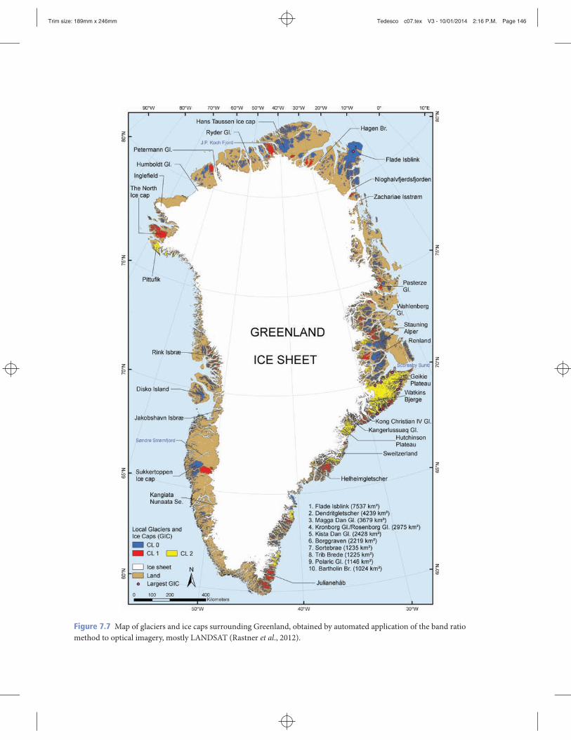
the Fifth Assessment Report of the Intergovernmental Panel on Climate Change(IPCC), has led to the production of a nearly globally complete set of glacier out-lines, known as the Randolph Glacier Inventory (RGI). This data set lacks thethorough attributes and documentation of data sources of GLIMS data, but it hasproved crucial to the IPCCwork. For example, the glaciers and ice caps on and nearGreenland have been completely mapped for the first time for the RGI (Figure 7.7;Rastner et al., 2012). Both RGI and GLIMS outlines can be downloaded from theGLIMS website (http://glims.org). Glaciers from both GLIMS and the RGI in cen-tral Asia and the greater Himalayan region are being used for various ongoingprojects (Figure 7.8). As discussed above, simple band ratio techniques can mapglacier ice quickly, but debris cover remains a difficulty. More sophisticated tech-niques, such as texture analysis or the “fuzzy C-means” method (Schowengerdt,2007), have yielded promising results for awide range of glacier types (Racoviteanuet al., 2009; Furfaro et al., submitted).Recent results from a completely different type of measurement, satellite

gravimetry, have yielded direct estimates of mass changes in glacier ice. TheGravity Recovery and Climate Experiment (GRACE) system is a pair of satellites,orbiting in tandem, that use laser interferometry to measure the distance between


Figure 7.7 Map of glaciers and ice caps surrounding Greenland, obtained by automated application of the band ratiomethod to optical imagery, mostly LANDSAT (Rastner et al., 2012).



70°

40°

Legend

Vertical Scale

30°

80° 80° 100°

GLIMS AND RGI glacier outlines in Asia

Glacier from GLIMSand RGI

0 2000 4000 6000

0 200

Horizontal Scale400 600

km

m

Figure 7.8 Glacier map for Central Asia, produced from GLIMS and RGI data sources using the GMT (Generic MappingTools) software.

the two satellites, producing information on changes in the gravitational field(Tapley et al., 2004). One study applied GRACE data to measure glacier icechanges in all major glacierized regions on Earth (Jacob et al., 2012). The spatialresolution of this technique is coarse (some 100 km) and the uncertainties arelarge compared to the signal in some regions (e.g., Himalaya), as the gravitysignal depends on many other factors, including groundwater depletion andfluvial erosion. However, this method produces estimates of mass change thatare independent of any other technique. It is probable that future systems willhave better spatial resolution, and so will have better signal-to-noise performance(Silvestrin et al., 2012).In summary, remote sensingmethods are capable ofmeasuringmany parameters

of glaciers and glacier change, leading to greater insight into processes affectingchanges in glaciers and hence climate. Field-based measurements are indispens-able, as they yield high-precision data and give key insight into processes.However,due to expense and difficult logistics, such measurements are limited to a smallnumber of sites. Remote sensing can cover large numbers of glaciers per image,and some long-term data collections (LANDSAT) are available for free. Algo-rithms and computational resources are now capable of producing maps of glacierboundaries at useful accuracy over large regions in a matter of days or hours. Newsensors will be coming online soon that will continue and extend this capability.Gravitation-sensing satellites can directly measure changes in mass along theirorbit tracks, though still at low resolution compared to individual glaciers.



References

Abermann, J., Lambrecht, A., Fischer, A. & Kuhn, M. (2009). Quantifyingchanges and trends in glacier area and volume in the Austrian Ötztal Alps(1969–1997–2006).The Cryosphere 3, 205–215.

Albert, T.H. (2002). Evaluation of Remote Sensing Techniques for Ice-Area Clas-sification Applied to the Tropical Quelccaya Ice Cap, Peru. Polar Geography 26,210–226.

Andreassen, L.M., Paul, F., Kääb, A. & Hausberg, J.E. (2008). LANDSAT-derivedglacier inventory for Jotunheimen,Norway, and deduced glacier since the 1930s.The Cryosphere 2, 131–145.

Andreassen, L.M., Kjøllmoen, B., Rasmussen, A., Melvold, K. & Nordli, Ø. (2012).Langfjordjøkelen, a rapidly shrinking glacier in northern Norway. Journal ofGlaciology. Accepted.

Arendt, A.A., Echelmeyer, K.A., Harrison, W.D., Lingle, C.S. & Valentine, V.B.(2002). Rapid wastage of Alaska glaciers and their contribution to rising sealevel. Science 297(5580), 382– 386.

Atwood, D.K., Meyer, F. & Arendt, A.A. (2010). Using L-band SAR coherence todelineate glacier extent. Canadian Journal of Remote Sensing 36(S1), S186.

Bahr, D.B., Meier, M.F. & Peckham, S.D. (1997). The Physical Basis of GlacierVolume-Area Scaling. Journal of Geophysical Research 102, 20355–20362.

Bajracharya, S.R. & Shrestha, B.R. (Eds.) (2011).The status of glaciers in the HinduKush-Himalayan Region. ICIMOD, Kathmandu, Nepal.

Baumann, S., Winkler, S. & Andreassen, L.M. (2009). Mapping glaciers in Jotun-heimen, South-Norway, during the “Little Ice Age” maximum. The Cryosphere3, 231–243.

Berthier, E., Arnaud, Y., Vincent, C. & Rémy, F. (2006). Biases of SRTM inhigh-mountain areas: Implications for the monitoring of glacier volumechanges. Geophysical Research Letters 33, L08502, doi:10.1029/2006GL025862.

Berthier, E., Arnaud, Y., Kumar, R., Ahmad, S., Wagnon, P. & Chevallier P. (2007).Remote Sensing Estimates of Glacier Mass Balances in the Himachal Pradesh(Western Himalaya, India). Remote Sensing of Environment 108, 327–338.

Berthier, E., Schiefer, E., Clarke, G.K.C., Menounos, B. & Rèmy F. (2010). Contri-bution of Alaskan glaciers to sea-level rise derived from satellite imagery.NatureGeoscience 3, 92–95, doi:10.1038/NGEO737.

Bevan, S.L., Luckman, A.J. & Murray, T. (2012). Glacier dynamics over the lastquarter of a century atHelheim,Kangerdlugssuaq and 14 othermajorGreenlandoutlet Glaciers.The Cryosphere Discussions 6, 1637–1672.

Bhambri, R. & Bolch, T. (2009). Glacier Mapping: A Review with special referenceto the Indian Himalayas. Progress in Physical Geography 33(5), 672–704.

Bhambri, R., Bolch, T., Chaujar, R.K. & Kulshreshtha S.C. (2011). Glacier changesin the Garhwal Himalaya, India, from 1968 to 2006 based on remote sensing.Journal of Glaciology 57(203), 543–556.



Bhambri, R., Bolch, T. & Chaujar, R.K. (2012). Frontal recession of GangotriGlacier, Garhwal Himalayas, from 1965–2006, measured through highresolution remote sensing data. Current Science 102(3), 489–494.

Bishop, M., Bonk, R., Kamp, U. & Shroder, J. (2001). Terrain Analysis and DataModeling for Alpine Glacier Mapping. Polar Geography 25, 182–201.

Bolch, T., Buchroithner,M.F., Peters, J., Baessler,M.&Bajracharya, S. (2008). Iden-tification of glacier motion and potentially dangerous glacial lakes in the Mt.Everest region/Nepal using spaceborne imagery.NaturalHazards and Earth Sys-tem Science 8, 1329–1340.

Bolch, T., Menounos, B. & Wheate, R. (2010a). LANDSAT-based Inventory ofGlaciers in Western Canada, 1985–2005. Remote Sensing of Environment 114,127–137.

Bolch, T., Yao, T., Kang, S., Buchroithner, M.F., Scherer, D., Maussion, F., Huint-jes, E. & Schneider, C. (2010b). A glacier inventory for the western Nyainqen-tanglha Range and Nam Co Basin, Tibet, and glacier changes 1976–2009. TheCryosphere 4, 419–433.

Bolch, T., Pieczonka, T. & Benn, D.I. (2011). Multi-decadal mass loss of glaciers inthe Everest area (Nepal Himalaya) derived from stereo imagery.The Cryosphere5, 349–358.

Bolch, T., Sandberg Sørensen, L., Simonssen, S.B.,Mölg,N.,Machguth,H., Rastner,P. & Paul, F. (2013). Mass loss of Greenland’s glaciers and ice caps 2003–2008revealed from ICESat laser altimetry data. Geophysical Research Letters 40, doi:10.1029/2012GL054710.

Braithwaite, R.J. (1984). Can the Mass Balance of a Glacier Be Estimated from ItsEquilibrium-Line Altitude? Journal of Glaciology 30(106), 364–368.

Brenning, A. (2009). Benchmarking classifiers to optimally integrate terrain analy-sis andmultispectral remote sensing in automatic rock glacier detection.RemoteSensing of Environment 113(1), 239–247.

Casassa, G., Smith, K., Rivera, A., Araos, J., Schnirch, M, & Schneider, C. (2002).Inventory of glaciers in Isla Riesco, Patagonia, Chile, based on aerial photogra-phy and satellite imagery. Annals of Glaciology 34, 373–378.

Casey, K.A., Kääb, A. & Benn, D.I. (2012). Geochemical characterization ofsupraglacial debris via in situ and optical remote sensing methods: a case studyin Khumbu Himalaya, Nepal.The Cryosphere 6, 85–100.

Cogley, J.G. (2009). Geodetic and direct mass-balancemeasurements: comparisonand joint analysis. Annals of Glaciology 50(50), 96–100.

Dashora, A., Lohani, B. & Malik, J.N. (2007). A repository of earth resource infor-mation --- Corona satellite programme. Current Science 92(7), 926–932.

Eldhuset, K., Andersen, P.H., Hauge, S., Isaksson, E. & Weydahl, D.J. (2003). ERSTandem InSAR Processing for DEM Generation, Glacier Motion Estimationand Coherence Analysis on Svalbard. International Journal of Remote Sensing24, 1415–1437.

Evans, D.L., Alpers, W., Cazenave, A., Elachi, C., Farr, T., Glackin, D., Holt, B.,Jones, L., Liu, W.T., McCandless, W., Menard, Y., Moore, R. & Njoku, E. (2005).



Seasat – A 25-year legacy of success. Remote Sensing of Environment 94(3),384–404. ISSN 0034–4257, 10.1016/j.rse.2004.09.011.

Farinotti, D., Huss, M., Bauder, A. & Funk, M. (2009). An estimate of the glacierice volume in the Swiss Alps. Global and Planetary Change 68(3), 225–231.

Finsterwalder, R. (1954). Photogrammetry and glacier research with special refer-ence to glacier retreat in the eastern Alps. Journal of Glaciology 2(15), 306–315.

Fischer, A. (2010). Glaciers and climate change: Interpretation of 50 years of directmass balance of Hintereisferner. Global and Planetary Change 71(1–2), 13–26.

Floricioiu, D. & Rott, H. (2001). Seasonal and short-term variability of multifre-quency, polarimetric radar backscatter of Alpine terrain from SIR-C/X-SARand AIRSAR data. IEEE Transactions on Geoscience and Remote Sensing 39(12),2634–2648.

Furfaro, R., Kargel, J. & Leonard, G. (submitted). Fuzzy C Mean Applications toand Validation of ASTER-Based Landcover Mapping of Root Glacier (Alaska).The Cryosphere.

Gardner, A.S., Moholdt, G., Cogley, J.G., Wouters, B., Arendt, A.A., Wahr, J.,Berthier, E., Pfeffer, T.W., Kaser, G., Hock, R., Ligtenberg, S.R.M., Bolch, T.,Sharp, M.J., Hagen, J.O., van den Broeke, M.R. & Paul, F. (2013). Narrowing thegap: A consensus estimate of glacier mass wastage. Science.

Gjermundsen, E., Mathieu, R., Kääb, A., Chinn, T., Fitzharris, B., & Hagen, J.O.(2011). Assessment of multispectral glacier mapping methods and derivation ofglacier area changes, 1978–2002, in the central Southern Alps, New Zealand,from ASTER satellite data, field survey and existing inventory data. Journal ofGlaciology 57(204), 667–683.

Haeberli, W. (1998). Historical evolution and operational aspects of worldwideglacier monitoring. In: Haeberli, W., Hoelzle, M. & Suter, S. (eds). Into thesecond century of worldwide glacier monitoring: prospects and strategies, 35–51.UNESCO Studies and Reports in Hydrology.

Haeberli, W. & Epifani, F. (1986). Mapping the Distribution of Buried GlacierIce – an Example from Lago Delle Locce, Monte Rosa, Italian Alps. Annals ofGlaciology 8, 78–81.

Haeberli, W., Hoelzle, M., Paul, F. & Zemp, M, (2007). Integrated monitoring ofmountainGlaciers as key indicators of global climate change: the EuropeanAlps.Annals of Glaciology 46, 150–160.

Hall, D.K., Riggs, G.A. & Salomonson, V.V. (1995). Development of Methods forMapping Global Snow Cover Using Moderate Resolution Imaging Spectrora-diometer Data. Remote Sensing of Environment 54(2), 127–140.

Heid, T. & Kääb, A. (2012). Evaluation of existing image matching methods forderiving glacier surface displacements globally from optical satellite imagery.Remote Sensing of Environment 118, 339–355.

Howat, I.M. & Eddy, A. (2011). Multi-decadal retreat of Greenland’s marine-terminating glaciers. Journal of Glaciology 57(203), 389–396.

Howat, I.M., Joughin, I., Tulaczyk, S. & Gogineni, S. (2005). Rapid retreat andacceleration of Helheim glacier, east Greenland.Geophysical Research Letters 32,L22502.



Howat, I.M., Joughin, I. & Scambos, T.A. (2007). Rapid changes in ice dischargefrom Greenland outlet glaciers. Science 315(5818), 1559–1561.

Howat, I.M., Ahn, Y., Joughin, I., van den Broeke, M.R., Lenaerts, J.T.M. & Smith,B. (2011). Mass balance of Greenland’s three largest outlet glaciers, 2000–2010.Geophysical Research Letters 38, L12501.

Jacob, T., Wahr, J., Pfeffer, T.W. & Swenson, S. (2012). Recent contributions ofglaciers and ice caps to sea level rise. Nature 482, 514–518.

Johannessen, O.M., Khvorostovsky, K., Miles, M.W. & Bobylev, L.P. (2005). Recentice-sheet growth in the interior of Greenland. Science 310, 1013–1016.

Johannessen, O.M., Babiker, M. & Miles, M.W. (2011). Petermann Glacier, NorthGreenland: massive calving in 2010 and the past half century. The CryosphereDiscussions 5(1), 169–181.

Johannesson, T., Björnsson, H., Magnusson, E., Gudmundsson, S., Palsson, F.,Sigurdsson, O., Thorsteinsson, T. & Berthier, E. (2012). Ice-volume changes,bias-estimation of mass-balance measurements and changes in subglacial lakesderived by LiDAR-mapping of the surface of Icelandic glaciers. Annals ofGlaciology 54(63).

Joughin, I. (2002). Ice-sheet Velocity Mapping: a Combined Interferometric andSpeckle-tracking Approach. Annals of Glaciology 34, 195–201.

Joughin, I., Abdalati, W. & Fahnestock, M. (2004). Large fluctuations in speed onGreenland’s Jakobshavn Isbrae glacier. Nature 432, 608–610.

Joughin, I., Howat, I., Alley, R.B., Ekstrom, G., Fahnestock, M., Moon, T., Nettles,M., Truffer, M., and Tsai, V.C. (2008). Ice-front variation and tidewater behavioron Helheim and Kangerdlugssuaq glaciers, Greenland. Journal of GeophysicalResearch 113, F01004.

Joughin, I., Smith, B.E., Howat, I.M., Scambos, T. & Moon, T. (2010). Greenlandflow variability from ice-sheet-wide velocity mapping. Journal of Glaciology56(197), 415–430.

Krabill, W., Abdalati, W., Frederick, E., Manizade, S., Martin, C., Sonntag, J.,Swift, R., Thomas, R., Wright, W. & Yungel, J. (2000). Greenland ice sheet:High-elevation balance and peripheral thinning. Science 289, 428–430.

Kääb, A. (2005). Combination of SRTM3 and Repeat ASTER Data for DerivingAlpine Glacier Flow Velocities in the Bhutan Himalaya. Remote Sensing of Envi-ronment 94, 463–474.

Kääb, A., Chiarle, M., Raup, B. & Schneider, C. (2007). Climate Change Impactson Mountain Glaciers and Permafrost. Global and Planetary Change 56, vii–ix.

Kääb, A. (2008). Glacier Volume Changes Using ASTER Satellite Stereo and ICE-Sat GLAS Laser Altimetry. A Test Study on Edgeøya, Eastern Svalbard. IEEETransactions on Geoscience and Remote Sensing 46, 2823–2830.

Kääb, A. (2010). The role of remote sensing in worldwide glacier monitoring.In:Pellika, P. (ed). Remote Sensing of Glaciers, 285–296. CRC Press.

Kääb, A., Berthier E., Nuth, C., Gardelle, J. & Arnaud, Y. (2012). Contrasting pat-terns of early twenty-first-century glacier mass change in the Himalayas.Nature488(7412), 495–498.



Karimi, N., Farokhnia, A., Karimi, L., Eftekhari, M. &Ghalkhani, H. (2012). Com-bining optical and thermal remote sensing data for mapping debris-coveredglaciers (Alamkouh Glaciers, Iran). Cold Regions Science and Technology 71,73–83.

Kieffer,H., Kargel, J.S., Barry, R. et al. (2000).NewEyes in the SkyMeasureGlaciersand Ice Sheets. Eos Transactions, American Geophysical Union 81(24), 265–271.

Lambrecht & Kuhn (2007). Glacier Changes in the Austrian Alps During the LastThree Decades, Derived from the New Austrian Glacier Inventory. Annals ofGlaciology 46, 177–184.

Lemke, P., Ren, J., Alley, R.B., Allison, I., Carrasco, J., Flato, G., Fujii, Y., Kaser,G., Mote, P., Thomas, R.H. & Zhang, T. (2007). Observations: Changes in Snow,Ice and Frozen Ground. In: Solomon, S., Qin, D., Manning, M., Chen, Z., Mar-quis,M., Averyt, K.B., Tignor,M. &Miller, H.L. (eds).Climate Change 2007:ThePhysical Science Basis. Contribution of Working Group I to the Fourth Assess-ment Report of the Intergovernmental Panel on Climate Change. Cambridge,UK and New York, NY, USA: Cambridge University Press.

Luckman, A., &Murray, T. (2005). Seasonal variations in velocity before retreat ofJakobshavn Isbrae, Greenland. Geophysical Research Letters 32, L08501.

Luckman, A.,Murray, T., de Lange, R., &Hanna, E. (2006). Rapid and synchronousice-dynamic changes in eastGreenland.Geophysical Research Letters 33, L03503.

Luckman, A., Quincey, D. & Bevan, S. (2007).The potential of satellite radar inter-ferometry and feature tracking for monitoring flow rates of Himalayan glaciers.Remote Sensing of Environment 111(2–3), 171–181.

Moholdt, G., Nuth, C., Hagen, J.O. & Kohler, J. (2010). Recent elevation changes ofSvalbard glaciers derived from ICESat laser altimetry. Remote Sensing of Envi-ronment 114, 2756–2767.

Mool, P., Bajracharya S.R., Joshi S.P., Sakya K. & Baidya A. (2002). Inventory ofglaciers, glacial lakes and glacial lake outburst floods monitoring and early warn-ing systems in the Hindu-KushHimalayan region, Nepal. International Center forIntegrated Mountain Development (ICIMOD) tech. pub., 227 pp. Kathmandu,Nepal. ISBN 92 9115 345 1.

Moon, T. & Joughin, I. (2008). Changes in ice front position on Greenland’s outletglaciers from 1992 to 2007. Journal of Geophysical Research 113, F02022.

Moon, T., Joughin I., Smith, B. & Howat, I. (2012). 21st-Century evolution ofGreenland outlet glacier velocities. Science 336(6081), 576–578.

Murray, T., Scharrer, K., James, T.D., Dye, S.R., Hanna, E., Booth, A.D., Selmes, N.,Luckman, A., Hughes, A.L.C., Cook, S. & Huybrechts, P. (2010). Ocean regula-tion hypothesis for glacier dynamics in southeast Greenland and implicationsfor ice sheet mass changes. Journal of Geophysical Research 115, F03026.

Nagler, T. & Rott, H. (2000). Retrieval of wet snow by means of multitemporalSAR data. IEEE Transactions on Geoscience and Remote Sensing 38(2), 754–765,doi:10.1109/36.842004

Narama, C., KääbA., Duishonakunov,M.&AbdrakhmatovK. (2010). Spatial vari-ability of recent glacier area changes in the Tien Shan Mountains, Central Asia,



using Corona (≈1970), LANDSAT (≈2000), and ALOS (≈2007) satellite data.Global and Planetary Change 71(1–2), 42–54.

Nuth, C. & Kääb A. (2011). Co-registration and bias corrections of satelliteelevation data sets for quantifying glacier thickness change. The Cryosphere 5,271–290.

Oerlemans, J. (2005). Extracting a Climate Signal from 169 Glacier Records. Sci-ence 308, 675–677.

Palmer, S., Shepherd, A., Nienow, P. & Joughin, I. (2011). Seasonal speedup of theGreenland ice sheet linked to routing of surface water. Earth and Planetary Sci-ence Letters doi.org/10.1016/j.epsl.2010.12.037.

Paul, F. & Kääb, A. (2005). Perspectives on the production of a glacier inventoryfrom multispectral satellite data in Arctic Canada: Cumberland Peninsula, Baf-fin Island. Annals of Glaciology 42, 59–66.

Paul, F. & Linsbauer, A. (2012). Modeling of glacier bed topography from glacieroutlines, central branch lines, and a DEM. International Journal of GeographicalInformation Science 1, 1–18.

Paul, F., Kääb, A., Maisch, M., Kellenberger, T. & Haeberli, W. (2002). The newremote-sensing derived Swiss glacier inventory: I.Methods. Annals of Glaciology34, 355–361.

Paul, F., Huggel, C. & Kääb, A. (2004). Combining Satellite Multispectral ImageData and a Digital Elevation Model for Mapping Debris-covered Glaciers.Remote Sensing of Environment 89, 510–518.

Paul, F., Barry, R.G., Cogley, J.G., Frey, H., Haeberli, W., Ohmura, A., Ommanney,C.S.L., Raup, B., Rivera, A., &Zemp,M. (2009). Recommendations for theCom-pilation of Glacier InventoryData fromDigital Sources.Annals of Glaciology 50,119–126.

Paul, F., Andreassen, L.M.&Winsvold, S.H. (2011). A new glacier inventory for theJostedalsbreen region, Norway, fromLANDSATTMscenes of 2006 and changessince 1966. Annals of Glaciology 52(59), 153–162.

Pritchard, H., Murray, T., Luckman, A., Strozzi, T. & Barr, S. (2005). Glacier surgedynamics of Sortebræ, east Greenland, from synthetic aperture radar featuretracking. Journal of Geophysical Research 110, F03005.

Pritchard, H.D., Arthern, R.J., Vaughan, D.G. & Edwards, L.A. (2009). Extensivedynamic thinning on the margins of the Greenland and Antarctic ice sheets.Nature 461(7266), 971–975.

Quincey, D.J., Luckman, A. & Benn, D. (2009). Quantification of Everest regionglacier velocities between 1992 and 2002, using satellite radar interferometryand feature tracking. Journal of Glaciology 55(192), 596–606.

Rabatel, A., Dedieu, J.P. & Vincent, C. (2005). Using remote-sensing data to deter-mine equilibrium-line altitude andmass-balance time series: validation on threeFrench glaciers, 1994–2002. Journal of Glaciology 51(175), 539–546.

Racoviteanu, A.E., Arnaud, Y., Williams, M.W. & Ordonez, J. (2008a). DecadalChanges in Glacier Parameters in the Cordillera Blanca, Peru, Derived fromRemote Sensing. Journal of Glaciology 54, 499–510.



Racoviteanu, A., Williams, M.W. & Barry, R. (2008b). Optical remote sensing ofglaciermass balance: a reviewwith focus on theHimalaya. Sensors, Special issue:Remote sensing of the environment, 3355–3383.

Racoviteanu, A.E., Paul, F., Raup, B., Singh Khalsa, S.J. & Armstrong, R. (2009).Challenges and recommendations inmapping of glacier parameters from space:results of the 2008 Global Land and Ice Measurements from Space (GLIMS)workshop, Boulder, Colorado, USA. Annals of Glaciology 53, 53–69.

Radic, V. & Hock, R. (2010). Regional and global volumes of glaciers derived fromstatistical upscaling of glacier inventory data. Journal of Geophysical Research,Earth Surface 115, doi:10.1029/2009JF001373.

Ranzi, R., Grossi G., Iacovelli, L. & Taschner, S. (2004). Use of multispectralASTER images for mapping debris-covered glaciers within the GLIMS Project.Proceedings of the International Geoscience and Remote Sensing Symposium2004, 1144–1147.

Raper, S.C.B. & Braithwaite, R.J. (2005).The Potential for Sea Level Rise: New Esti-mates from Glacier and Ice Cap Area and Volume Distributions. GeophysicalResearch Letters 32, doi: 10.1029/2004GL021981.

Raup, B., Kääb, A., Kargel, J.S., Bishop, M.P., Hamilton, G., Lee, E., Paul, F., Rau,F., Soltesz, D., Singh Khalsa, S.J., Beedle, M. & Helm, C. (2007). Remote SensingandGIS Technology in the Global Land IceMeasurements from Space (GLIMS)Project. Computers and Geosciences 33, 104–125.

Rastner, P., Bolch, T., Mölg, N., Machguth, H., Le Bris, R. & Paul, F. (2012).The first complete inventory of the local glaciers and ice caps on Green-land. The Cryosphere 6, 1483–1495, www.the-cryosphere.net/6/1483/2012/,doi:10.5194/tc-6-1483-2012.

Richards, J.A. (1986). Remote Sensing Digital Image Analysis. Springer-Verlag Inc.Rignot, E. & Kanagaratnam, P. (2006). Changes in the velocity structure of the

Greenland ice sheet. Science 311(5763), 986–990.Rignot, E., Gogineni, S., Joughin, I. & Krabill, W. (2001). Contribution to the

glaciology of northern Greenland from satellite radar interferometry. Journal ofGeophysical Research 106(D24), 34007–30019.

Rignot, E., Braaten, D., Gogineni, S.P., Krabill, W.B. & McConnell, J.R. (2004).Rapid ice discharge from southeast Greenland glaciers. Geophysical ResearchLetters 31, L10401.

Rott, H. (1994). Thematic studies in Alpine areas by means of polarimetric SARand optical imagery. Advances in Space Research 14(3), 217–226.

Sabins, F.F., Jr. (2007). Remote Sensing: Principles and Applications, 3rd Edition.Long Grove, Illinois, USA. Waveland Press, Inc.

Salomonson, V.V. & Appel, I. (2004). Estimating fractional snow cover fromMODIS using the normalized difference snow index. Remote Sensing ofEnvironment 89, 351–360.

Scambos, T.A., Dutkiewicz, M.J., Wilson, J.C. & Bindschadler, R.A. (1992). Appli-cation of ImageCross-Correlation to theMeasurement ofGlacierVelocityUsingSatellite Image Data. Remote Sensing of Environment 42, 177–186.



Scherler, D., Leprince, S. & Strecker, M.R. (2008). Glacier-surface velocities inalpine terrain from optical satellite imagery – accuracy improvement and qual-ity assessment. Remote Sensing of Environment 112(10), 3806–3819.

Schowengerdt, R.A. (2007). Remote Sensing: Models and Methods for Image Pro-cessing, 3rd Edition. San Diego, CA, Academic Press.

Seale, A., Christoffersen, P., Mugford, R.I. & O’Leary, M. (2011). Ocean forcingof the Greenland ice sheet: Calving fronts and patterns of retreat identified byautomatic satellite monitoring of eastern outlet glaciers. Journal of GeophysicalResearch 116, F03013.

Sidjak, R.W. & Wheate, R.D. (1999). Glacier Mapping of the Illecillewaet Icefield,British Columbia, Canada, Using LANDSAT TM and Digital Elevation Data.International Journal of Remote Sensing 20, 273–284.

Silvestrin, P., Aguirre, M., Massotti, L., Leone, B., Cesare, S., Kern, M. & Haag-mans, R. (2012).TheFuture of the SatelliteGravimetryAfter theGOCEMission.In: Kenyon S. et al. (eds) Geodesy for Planet Earth, International Association ofGeodesy Symposia 136(2), 223–230, doi: 10.1007/978-3-642-20338-1_27.

Strozzi, T., Luckman, A., Murray, T.,Wegmuller, U. &Werner, C.L. (2002). GlacierMotion Estimation Using SAR Offset-Tracking Procedures. IEEE Transactionson Geoscience and Remote Sensing 40, 2384–2391.

Sundal, A.V., Shepherd, A., Nienow, P., Hanna, E., Palmer, S. & Huybrechts, P.(2011). Melt-induced speed-up of Greenland ice sheet offset by efficient sub-glacial drainage. Nature 469(7331), 521–524.

Tapley, B.D., Bettadpur, S., Ries, J.C., Thompson, P.F. & Watkins, M.M. (2004).GRACE measurements of mass variability in the Earth system. Science305(5683), 503–505.

Thomas, R., Davis, C., Frederick, E., Krabill, W., Li, Y., Manizade, S. & Martin,C. (2008). A comparison of Greenland ice-sheet volume changes derived fromaltimetry measurements. Journal of Glaciology 54(185), 203–212.

Walsh, K.M., Howat, I.M., Ahn, Y. & Enderlin, E.M. (2012). Changes in themarine-terminating glaciers of central east Greenland, 2000–2010. TheCryosphere 6, 211–220.

Yasuda, T. & Furuya, M. (2013). Short-term glacier velocity changes at West Kun-lun Shan, Northwest Tibet, detected by Synthetic Aperture Radar data. RemoteSensing of Environment, 128, 87–106.

Zemp, M., Hoelzle, M. & Haeberli, W. (2009). Six decades of glacier mass-balanceobservations: a review of the worldwide monitoring network.Annals of Glaciol-ogy 50, 101–111.

Zwally, H.J., Abdalati, W., Herring, T., Larson, K., Saba, J. & Steffen, K. (2002).Surface melt-induced acceleration of Greenland ice-sheet flow. Science 51,218–222.

Zwally, H.J., Giovinetto, M.B., Li, J., Cornejo, H.G., Beckley, M.A., Brenner, A.C.,Sabba, J.L. & Li, D. (2005). Mass changes of the Greenland and Antarctic icesheets and shelves and contributions to sea-level rise: 1992–2002. Journal ofGlaciology 51, 509–527.



Acronyms

ASTER Advanced SpaceborneThermal Emission and ReflectionRadiometer

DN Digital NumbersELA Equilibrium Line AltitudeERTS 1 Earth Resources Technology SatelliteETM+ EnhancedThematic Mapper PlusGCP ground control pointsGIFOV Ground instantaneous field of viewGLAS Geoscience Laser Altimetry SystemGLIMS Global Land Ice Measurements from SpaceGRACE The Gravity Recovery and Climate ExperimentGTN-G Global Terrestrial Network for GlaciersICESat Ice, Cloud, and land Elevation SatelliteIPCC Intergovernmental Panel on Climate ChangeIRS Indian Remote SensingLDCM LANDSAT Data Continuity MissionLIDAR Light Detection and RangingMSS Multispectral scannerNDSI normalized difference snow indexNIR Near InfraredRGI Randolph Glacier InventorySPOT Satellite Pour l’Observation de la TerreSRTM Shuttle Radar Topography MissionSWIR short-wave infraredTM Thematic MapperUTM Universal Transverse Mercator

Websites cited

http://glims.orghttp://landsat.gsfc.nasa.gov/

Remote sensing of glaciers

Documents

Transcript of Remote sensing of glaciers