of remote sensing - Moodle@Units

❙1 CONCEPTS AND FOUNDATIONS

OF REMOTE SENSING

1.1 INTRODUCTION

Remote sensing is the science and art of obtaining information about an object,area, or phenomenon through the analysis of data acquired by a device that is notin contact with the object, area, or phenomenon under investigation. As you readthese words, you are employing remote sensing. Your eyes are acting as sensorsthat respond to the light reflected from this page. The “data” your eyes acquire areimpulses corresponding to the amount of light reflected from the dark and lightareas on the page. These data are analyzed, or interpreted, in your mental compu-ter to enable you to explain the dark areas on the page as a collection of lettersforming words. Beyond this, you recognize that the words form sentences, andyou interpret the information that the sentences convey.

In many respects, remote sensing can be thought of as a reading process.Using various sensors, we remotely collect data that may be analyzed to obtaininformation about the objects, areas, or phenomena being investigated. The remo-tely collected data can be of many forms, including variations in force distribu-tions, acoustic wave distributions, or electromagnetic energy distributions. Forexample, a gravity meter acquires data on variations in the distribution of the

1

COPYRIG

HTED M

ATERIAL

force of gravity. Sonar, like a bat’s navigation system, obtains data on variationsin acoustic wave distributions. Our eyes acquire data on variations in electro-magnetic energy distributions.

Overview of the Electromagnetic Remote Sensing Process

This book is about electromagnetic energy sensors that are operated from airborneand spaceborne platforms to assist in inventorying, mapping, and monitoringearth resources. These sensors acquire data on the way various earth surfacefeatures emit and reflect electromagnetic energy, and these data are analyzed toprovide information about the resources under investigation.

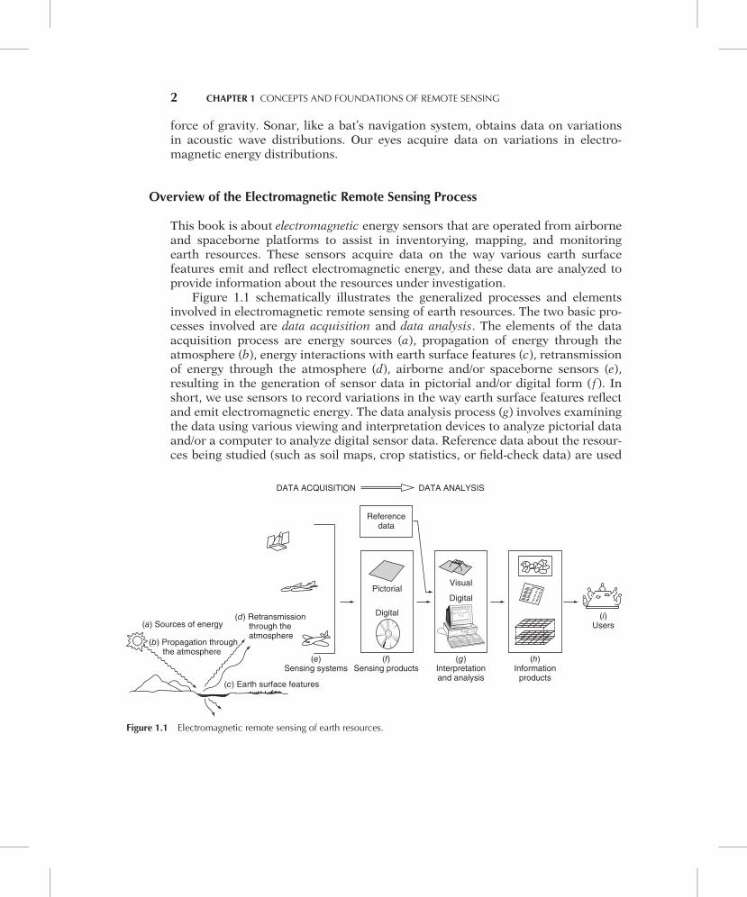
Figure 1.1 schematically illustrates the generalized processes and elementsinvolved in electromagnetic remote sensing of earth resources. The two basic pro-cesses involved are data acquisition and data analysis. The elements of the dataacquisition process are energy sources (a), propagation of energy through theatmosphere (b), energy interactions with earth surface features (c), retransmissionof energy through the atmosphere (d), airborne and/or spaceborne sensors (e),resulting in the generation of sensor data in pictorial and/or digital form ( f). Inshort, we use sensors to record variations in the way earth surface features reflectand emit electromagnetic energy. The data analysis process (g) involves examiningthe data using various viewing and interpretation devices to analyze pictorial dataand/or a computer to analyze digital sensor data. Reference data about the resour-ces being studied (such as soil maps, crop statistics, or field-check data) are used

(a) Sources of energy

(c) Earth surface features

(e)Sensing systems

(f)Sensing products

(g)Interpretationand analysis

(h)Information

products

(i)Users

(b) Propagation through the atmosphere

(d) Retransmission through the atmosphere

DATA ACQUISITION DATA ANALYSIS

Referencedata

Digital

PictorialVisual

Digital

Figure 1.1 Electromagnetic remote sensing of earth resources.

2 CHAPTER 1 CONCEPTS AND FOUNDATIONS OF REMOTE SENSING

when and where available to assist in the data analysis. With the aid of the refer-ence data, the analyst extracts information about the type, extent, location, andcondition of the various resources over which the sensor data were collected. Thisinformation is then compiled (h), generally in the form of maps, tables, or digitalspatial data that can be merged with other “layers” of information in a geographicinformation system (GIS). Finally, the information is presented to users (i), whoapply it to their decision-making process.

Organization of the Book

In the remainder of this chapter, we discuss the basic principles underlying theremote sensing process. We begin with the fundamentals of electromagneticenergy and then consider how the energy interacts with the atmosphere and withearth surface features. Next, we summarize the process of acquiring remotelysensed data and introduce the concepts underlying digital imagery formats. Wealso discuss the role that reference data play in the data analysis procedure anddescribe how the spatial location of reference data observed in the field is oftendetermined using Global Positioning System (GPS) methods. These basics willpermit us to conceptualize the strengths and limitations of “real” remote sensingsystems and to examine the ways in which they depart from an “ideal” remotesensing system. We then discuss briefly the rudiments of GIS technology and thespatial frameworks (coordinate systems and datums) used to represent the posi-tions of geographic features in space. Because visual examination of imagery willplay an important role in every subsequent chapter of this book, this first chapterconcludes with an overview of the concepts and processes involved in visual inter-pretation of remotely sensed images. By the end of this chapter, the reader shouldhave a grasp of the foundations of remote sensing and an appreciation for theclose relationship among remote sensing, GPS methods, and GIS operations.

Chapters 2 and 3 deal primarily with photographic remote sensing. Chapter 2describes the basic tools used in acquiring aerial photographs, including bothanalog and digital camera systems. Digital videography is also treated in Chapter 2.Chapter 3 describes the photogrammetric procedures by which precise spatialmeasurements, maps, digital elevation models (DEMs), orthophotos, and otherderived products are made from airphotos.

Discussion of nonphotographic systems begins in Chapter 4, which describesthe acquisition of airborne multispectral, thermal, and hyperspectral data. InChapter 5 we discuss the characteristics of spaceborne remote sensing systemsand examine the principal satellite systems used to collect imagery from reflectedand emitted radiance on a global basis. These satellite systems range from theLandsat and SPOT series of moderate-resolution instruments, to the latest gen-eration of high-resolution commercially operated systems, to various meteor-ological and global monitoring systems.

1.1 INTRODUCTION 3

Chapter 6 is concerned with the collection and analysis of radar and lidardata. Both airborne and spaceborne systems are discussed. Included in this lattercategory are such systems as the ALOS, Envisat, ERS, JERS, Radarsat, andICESat satellite systems.

In essence, from Chapter 2 through Chapter 6, this book progresses from thesimplest sensing systems to the more complex. There is also a progression fromshort to long wavelengths along the electromagnetic spectrum (see Section 1.2).That is, discussion centers on photography in the ultraviolet, visible, and near-infrared regions, multispectral sensing (including thermal sensing using emittedlong-wavelength infrared radiation), and radar sensing in the microwave region.

The final two chapters of the book deal with the manipulation, interpretation,and analysis of images. Chapter 7 treats the subject of digital image processing anddescribes the most commonly employed procedures through which computer-assisted image interpretation is accomplished. Chapter 8 presents a broad range ofapplications of remote sensing, including both visual interpretation and computer-aided analysis of image data.

Throughout this book, the International System of Units (SI) is used. Tablesare included to assist the reader in converting between SI and units of other mea-surement systems.

Finally, a Works Cited section provides a list of references cited in the text. Itis not intended to be a compendium of general sources of additional information.Three appendices provided on the publisher’s website (http://www.wiley.com/college/lillesand) offer further information about particular topics at a level ofdetail beyond what could be included in the text itself. Appendix A summarizesthe various concepts, terms, and units commonly used in radiation measurementin remote sensing. Appendix B includes sample coordinate transformation andresampling procedures used in digital image processing. Appendix C discussessome of the concepts, terminology, and units used to describe radar signals.

1.2 ENERGY SOURCES AND RADIATION PRINCIPLES

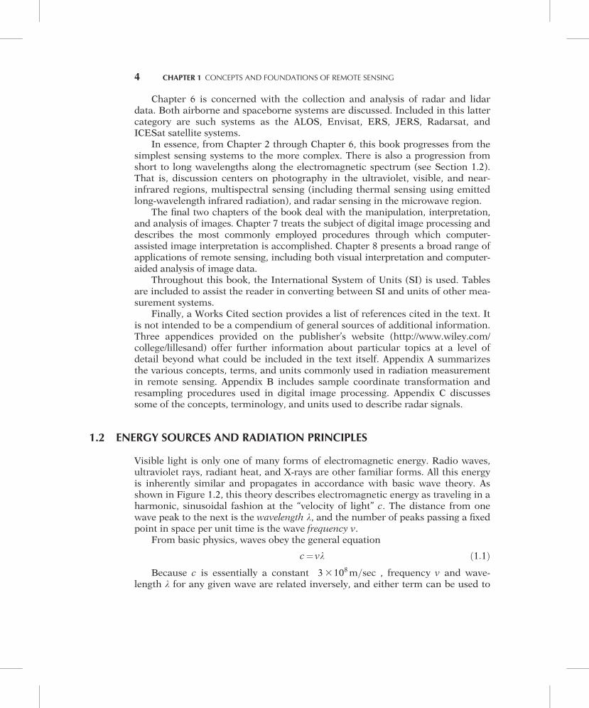
Visible light is only one of many forms of electromagnetic energy. Radio waves,ultraviolet rays, radiant heat, and X-rays are other familiar forms. All this energyis inherently similar and propagates in accordance with basic wave theory. Asshown in Figure 1.2, this theory describes electromagnetic energy as traveling in aharmonic, sinusoidal fashion at the “velocity of light” c. The distance from onewave peak to the next is the wavelength l, and the number of peaks passing a fixedpoint in space per unit time is the wave frequency v.

From basic physics, waves obey the general equation

c¼ vl ð1:1ÞBecause c is essentially a constant 33108m=sec

� �, frequency v and wave-

length l for any given wave are related inversely, and either term can be used to


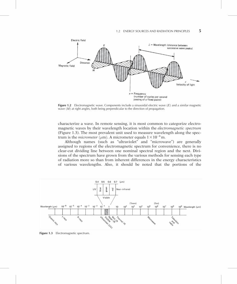
characterize a wave. In remote sensing, it is most common to categorize electro-magnetic waves by their wavelength location within the electromagnetic spectrum(Figure 1.3). The most prevalent unit used to measure wavelength along the spec-trum is the micrometer �mð Þ. A micrometer equals 1310�6m.

Although names (such as “ultraviolet” and “microwave”) are generallyassigned to regions of the electromagnetic spectrum for convenience, there is noclear-cut dividing line between one nominal spectral region and the next. Divi-sions of the spectrum have grown from the various methods for sensing each typeof radiation more so than from inherent differences in the energy characteristicsof various wavelengths. Also, it should be noted that the portions of the

Figure 1.2 Electromagnetic wave. Components include a sinusoidal electric wave Eð Þ and a similar magneticwave Mð Þ at right angles, both being perpendicular to the direction of propagation.

Figure 1.3 Electromagnetic spectrum.

1.2 ENERGY SOURCES AND RADIATION PRINCIPLES 5

electromagnetic spectrum used in remote sensing lie along a continuum char-acterized by magnitude changes of many powers of 10. Hence, the use of logarith-mic plots to depict the electromagnetic spectrum is quite common. The “visible”portion of such a plot is an extremely small one, because the spectral sensitivityof the human eye extends only from about 0:4 �m to approximately 0:7 �m. Thecolor “blue” is ascribed to the approximate range of 0.4 to 0:5 �m, “green” to 0.5to 0:6 �m, and “red” to 0.6 to 0:7 �m. Ultraviolet (UV) energy adjoins the blue endof the visible portion of the spectrum. Beyond the red end of the visible region arethree different categories of infrared (IR) waves: near IR (from 0.7 to 1:3 �m), midIR (from 1.3 to 3 �m; also referred to as shortwave IR or SWIR), and thermal IR(beyond 3 to 14 �m, sometimes referred to as longwave IR). At much longer wave-lengths (1 mm to 1 m) is the microwave portion of the spectrum.

Most common sensing systems operate in one or several of the visible, IR, ormicrowave portions of the spectrum. Within the IR portion of the spectrum, itshould be noted that only thermal-IR energy is directly related to the sensation ofheat; near- and mid-IR energy are not.

Although many characteristics of electromagnetic radiation are most easilydescribed by wave theory, another theory offers useful insights into how electro-magnetic energy interacts with matter. This theory—the particle theory—suggeststhat electromagnetic radiation is composed of many discrete units called photonsor quanta. The energy of a quantum is given as

Q ¼ hv ð1:2Þwhere

Q ¼ energy of a quantum; joules Jð Þh ¼ Planck’s constant, 6:626310�34 J secv ¼ frequency

We can relate the wave and quantum models of electromagnetic radiationbehavior by solving Eq. 1.1 for v and substituting into Eq. 1.2 to obtain

Q¼hcl

ð1:3Þ

Thus, we see that the energy of a quantum is inversely proportional to itswavelength. The longer the wavelength involved, the lower its energy content. Thishas important implications in remote sensing from the standpoint that naturallyemitted long wavelength radiation, such as microwave emission from terrain fea-tures, is more difficult to sense than radiation of shorter wavelengths, such asemitted thermal IR energy. The low energy content of long wavelength radiationmeans that, in general, systems operating at long wavelengths must “view” largeareas of the earth at any given time in order to obtain a detectable energy signal.

The sun is the most obvious source of electromagnetic radiation for remotesensing. However, all matter at temperatures above absolute zero (0 K, or �273�C)continuously emits electromagnetic radiation. Thus, terrestrial objects are also


sources of radiation, although it is of considerably different magnitude and spectralcomposition than that of the sun. How much energy any object radiates is, amongother things, a function of the surface temperature of the object. This property isexpressed by the Stefan–Boltzmann law, which states that

M¼ sT4 ð1:4Þwhere

M ¼ total radiant exitance from the surface of amaterial; watts Wð Þm�2

s ¼ Stefan–Boltzmann constant, 5:6697310�8 Wm�2 K�4

T ¼ absolute temperature Kð Þ of the emittingmaterial

The particular units and the value of the constant are not critical for the stu-dent to remember, yet it is important to note that the total energy emitted from anobject varies as T4 and therefore increases very rapidly with increases in tempera-ture. Also, it should be noted that this law is expressed for an energy source thatbehaves as a blackbody. A blackbody is a hypothetical, ideal radiator that totallyabsorbs and reemits all energy incident upon it. Actual objects only approach thisideal. We further explore the implications of this fact in Chapter 4; suffice it to sayfor now that the energy emitted from an object is primarily a function of its tem-perature, as given by Eq. 1.4.

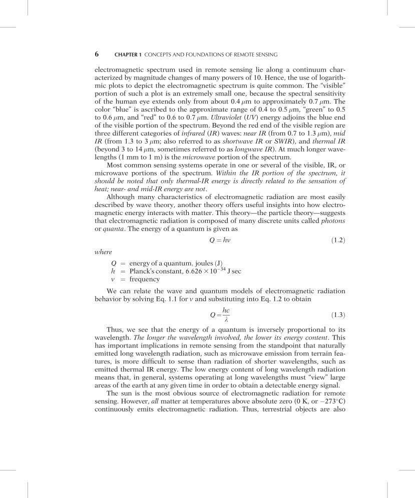
Just as the total energy emitted by an object varies with temperature, thespectral distribution of the emitted energy also varies. Figure 1.4 shows energydistribution curves for blackbodies at temperatures ranging from 200 to 6000 K.The units on the ordinate scale Wm�2�m�1

� �express the radiant power coming

from a blackbody per 1-�m spectral interval. Hence, the area under these curvesequals the total radiant exitance, M, and the curves illustrate graphically what theStefan–Boltzmann law expresses mathematically: The higher the temperature ofthe radiator, the greater the total amount of radiation it emits. The curves alsoshow that there is a shift toward shorter wavelengths in the peak of a blackbodyradiation distribution as temperature increases. The dominant wavelength, orwavelength at which a blackbody radiation curve reaches a maximum, is relatedto its temperature by Wien’s displacement law,

lm ¼AT

ð1:5Þ

where

lm ¼ wavelength of maximum spectral radiant exitance, �mA ¼ 2898 mmKT ¼ temperature, K

Thus, for a blackbody, the wavelength at which the maximum spectral radiantexitance occurs varies inversely with the blackbody’s absolute temperature.We observe this phenomenon when a metal body such as a piece of iron isheated. As the object becomes progressively hotter, it begins to glow and its color

1.2 ENERGY SOURCES AND RADIATION PRINCIPLES 7

changes successively to shorter wavelengths—from dull red to orange to yellowand eventually to white.

The sun emits radiation in the same manner as a blackbody radiator whosetemperature is about 6000 K (Figure 1.4). Many incandescent lamps emit radia-tion typified by a 3000 K blackbody radiation curve. Consequently, incandescentlamps have a relatively low output of blue energy, and they do not have the samespectral constituency as sunlight.

The earth’s ambient temperature (i.e., the temperature of surface materialssuch as soil, water, and vegetation) is about 300 K (27°C). From Wien’s displace-ment law, this means the maximum spectral radiant exitance from earth featuresoccurs at a wavelength of about 9:7 �m. Because this radiation correlates withterrestrial heat, it is termed “thermal infrared” energy. This energy can neither beseen nor photographed, but it can be sensed with such thermal devices as radio-meters and scanners (described in Chapter 4). By comparison, the sun has amuch higher energy peak that occurs at about 0:5 �m, as indicated in Figure 1.4.

1

101

102

103

104

105

106

107

108

109Visible radiant energy band

Blackbody radiation curveat the sun’s temperature

Blackbody radiation curveat the earth’s temperature

Blackbody radiation curveat incandescent lamp temperature

0.1 0.2 0.5 1 2 5 10 20 50 100

Wavelength (μm)

Spe

ctra

l rad

iant

exi

tanc

e, M

λ (W

m–

2 μm

–

1 )

1000 K

500 K

300 K

200 K

6000 K

4000 K

3000 K

2000 K

Figure 1.4 Spectral distribution of energy radiated from blackbodies of various temperatures.(Note that spectral radiant exitance Ml is the energy emitted per unit wavelength interval.Total radiant exitance M is given by the area under the spectral radiant exitance curves.)


Our eyes—and photographic sensors—are sensitive to energy of this magnitudeand wavelength. Thus, when the sun is present, we can observe earth features byvirtue of reflected solar energy. Once again, the longer wavelength energy emittedby ambient earth features can be observed only with a nonphotographic sensingsystem. The general dividing line between reflected and emitted IR wavelengths isapproximately 3 �m. Below this wavelength, reflected energy predominates; aboveit, emitted energy prevails.

Certain sensors, such as radar systems, supply their own source of energy toilluminate features of interest. These systems are termed “active” systems, in con-trast to “passive” systems that sense naturally available energy. A very commonexample of an active system is a camera utilizing a flash. The same camera usedin sunlight becomes a passive sensor.

1.3 ENERGY INTERACTIONS IN THE ATMOSPHERE

Irrespective of its source, all radiation detected by remote sensors passes throughsome distance, or path length, of atmosphere. The path length involved can varywidely. For example, space photography results from sunlight that passes throughthe full thickness of the earth’s atmosphere twice on its journey from source tosensor. On the other hand, an airborne thermal sensor detects energy emitteddirectly from objects on the earth, so a single, relatively short atmospheric pathlength is involved. The net effect of the atmosphere varies with these differencesin path length and also varies with the magnitude of the energy signal beingsensed, the atmospheric conditions present, and the wavelengths involved.

Because of the varied nature of atmospheric effects, we treat this subject on asensor-by-sensor basis in other chapters. Here, we merely wish to introduce thenotion that the atmosphere can have a profound effect on, among other things,the intensity and spectral composition of radiation available to any sensing sys-tem. These effects are caused principally through the mechanisms of atmosphericscattering and absorption.

Scattering

Atmospheric scattering is the unpredictable diffusion of radiation by particles inthe atmosphere. Rayleigh scatter is common when radiation interacts with atmo-spheric molecules and other tiny particles that are much smaller in diameter thanthe wavelength of the interacting radiation. The effect of Rayleigh scatter is inver-sely proportional to the fourth power of wavelength. Hence, there is a muchstronger tendency for short wavelengths to be scattered by this mechanism thanlong wavelengths.

A “blue” sky is a manifestation of Rayleigh scatter. In the absence of scatter,the sky would appear black. But, as sunlight interacts with the earth’s atmosphere,

1.3 ENERGY INTERACTIONS IN THE ATMOSPHERE 9

it scatters the shorter (blue) wavelengths more dominantly than the other visiblewavelengths. Consequently, we see a blue sky. At sunrise and sunset, however, thesun’s rays travel through a longer atmospheric path length than during midday.With the longer path, the scatter (and absorption) of short wavelengths is so com-plete that we see only the less scattered, longer wavelengths of orange and red.

Rayleigh scatter is one of the primary causes of “haze” in imagery. Visually,haze diminishes the “crispness,” or “contrast,” of an image. In color photography,it results in a bluish-gray cast to an image, particularly when taken from high alti-tude. As we see in Chapter 2, haze can often be eliminated or at least minimizedby introducing, in front of the camera lens, a filter that does not transmit shortwavelengths.

Another type of scatter is Mie scatter, which exists when atmospheric particlediameters essentially equal the wavelengths of the energy being sensed. Watervapor and dust are major causes of Mie scatter. This type of scatter tends to influ-ence longer wavelengths compared to Rayleigh scatter. Although Rayleigh scattertends to dominate under most atmospheric conditions, Mie scatter is significantin slightly overcast ones.

A more bothersome phenomenon is nonselective scatter, which comes aboutwhen the diameters of the particles causing scatter are much larger than thewavelengths of the energy being sensed. Water droplets, for example, cause suchscatter. They commonly have a diameter in the range 5 to 100 �m and scatterall visible and near- to mid-IR wavelengths about equally. Consequently, this scat-tering is “nonselective” with respect to wavelength. In the visible wavelengths,equal quantities of blue, green, and red light are scattered; hence fog and cloudsappear white.

Absorption

In contrast to scatter, atmospheric absorption results in the effective loss ofenergy to atmospheric constituents. This normally involves absorption of energyat a given wavelength. The most efficient absorbers of solar radiation in thisregard are water vapor, carbon dioxide, and ozone. Because these gases tend toabsorb electromagnetic energy in specific wavelength bands, they strongly influ-ence the design of any remote sensing system. The wavelength ranges in whichthe atmosphere is particularly transmissive of energy are referred to as atmo-spheric windows.

Figure 1.5 shows the interrelationship between energy sources and atmo-spheric absorption characteristics. Figure 1.5a shows the spectral distribution ofthe energy emitted by the sun and by earth features. These two curves representthe most common sources of energy used in remote sensing. In Figure 1.5b, spec-tral regions in which the atmosphere blocks energy are shaded. Remote sensingdata acquisition is limited to the nonblocked spectral regions, the atmosphericwindows. Note in Figure 1.5c that the spectral sensitivity range of the eye (the


“visible” range) coincides with both an atmospheric window and the peak level ofenergy from the sun. Emitted “heat” energy from the earth, shown by the smallcurve in (a), is sensed through the windows at 3 to 5 �m and 8 to 14 �m usingsuch devices as thermal sensors. Multispectral sensors observe simultaneouslythrough multiple, narrow wavelength ranges that can be located at various pointsin the visible through the thermal spectral region. Radar and passive microwavesystems operate through a window in the region 1 mm to 1 m.

The important point to note from Figure 1.5 is the interaction and the inter-dependence between the primary sources of electromagnetic energy, the atmosphericwindows through which source energy may be transmitted to and from earth surfacefeatures, and the spectral sensitivity of the sensors available to detect and record theenergy. One cannot select the sensor to be used in any given remote sensing taskarbitrarily; one must instead consider (1) the spectral sensitivity of the sensorsavailable, (2) the presence or absence of atmospheric windows in the spectralrange(s) in which one wishes to sense, and (3) the source, magnitude, and

(a)

(b)

(c)

Figure 1.5 Spectral characteristics of (a) energy sources, (b) atmospheric transmittance, and(c) common remote sensing systems. (Note that wavelength scale is logarithmic.)

1.3 ENERGY INTERACTIONS IN THE ATMOSPHERE 11

spectral composition of the energy available in these ranges. Ultimately, however,the choice of spectral range of the sensor must be based on the manner in whichthe energy interacts with the features under investigation. It is to this last, veryimportant, element that we now turn our attention.

1.4 ENERGY INTERACTIONS WITH EARTH SURFACE FEATURES

When electromagnetic energy is incident on any given earth surface feature, threefundamental energy interactions with the feature are possible. These are illu-strated in Figure 1.6 for an element of the volume of a water body. Various frac-tions of the energy incident on the element are reflected, absorbed, and/ortransmitted. Applying the principle of conservation of energy, we can state theinterrelationship among these three energy interactions as

EI lð Þ¼ER lð ÞþEA lð ÞþET lð Þ ð1:6Þwhere

EI ¼ incident energyER ¼ reflected energyEA ¼ absorbed energyET ¼ transmitted energy

with all energy components being a function of wavelength l.

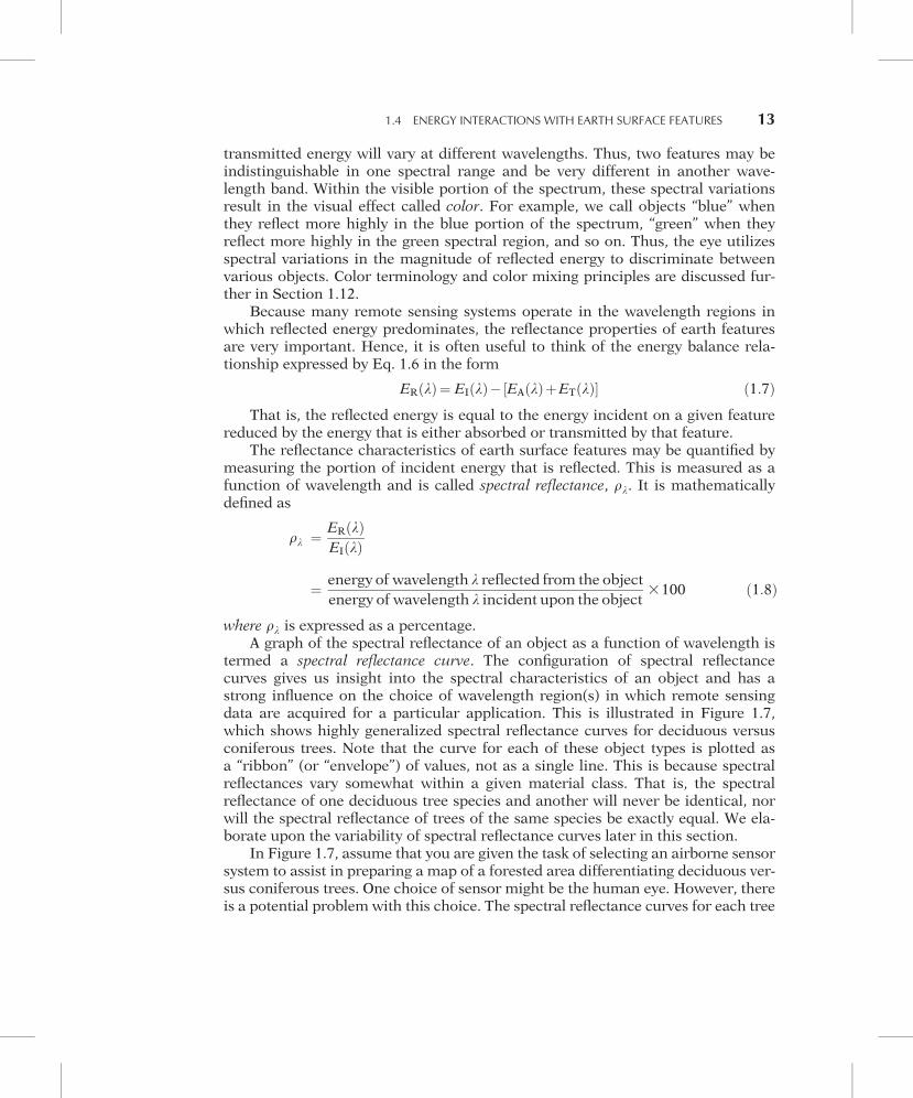
Equation 1.6 is an energy balance equation expressing the interrelationshipamong the mechanisms of reflection, absorption, and transmission. Two pointsconcerning this relationship should be noted. First, the proportions of energyreflected, absorbed, and transmitted will vary for different earth features, depend-ing on their material type and condition. These differences permit us to distin-guish different features on an image. Second, the wavelength dependency meansthat, even within a given feature type, the proportion of reflected, absorbed, and

EI(λ) = Incident energy

ER(λ) = Reflected energy

EA(λ) = Absorbed energy ET(λ) = Transmitted energy

EI(λ) = ER(λ) + EA(λ) + ET(λ)

Figure 1.6 Basic interactions between electromagnetic energy and an earth surfacefeature.


transmitted energy will vary at different wavelengths. Thus, two features may beindistinguishable in one spectral range and be very different in another wave-length band. Within the visible portion of the spectrum, these spectral variationsresult in the visual effect called color. For example, we call objects “blue” whenthey reflect more highly in the blue portion of the spectrum, “green” when theyreflect more highly in the green spectral region, and so on. Thus, the eye utilizesspectral variations in the magnitude of reflected energy to discriminate betweenvarious objects. Color terminology and color mixing principles are discussed fur-ther in Section 1.12.

Because many remote sensing systems operate in the wavelength regions inwhich reflected energy predominates, the reflectance properties of earth featuresare very important. Hence, it is often useful to think of the energy balance rela-tionship expressed by Eq. 1.6 in the form

ER lð Þ¼ EI lð Þ� EA lð ÞþET lð Þ½ � ð1:7ÞThat is, the reflected energy is equal to the energy incident on a given feature

reduced by the energy that is either absorbed or transmitted by that feature.The reflectance characteristics of earth surface features may be quantified by

measuring the portion of incident energy that is reflected. This is measured as afunction of wavelength and is called spectral reflectance, rl. It is mathematicallydefined as

rl ¼ ER lð ÞEI lð Þ

¼ energy of wavelength l reflected from the objectenergy of wavelength l incident upon the object

3100 ð1:8Þ

where rl is expressed as a percentage.A graph of the spectral reflectance of an object as a function of wavelength is

termed a spectral reflectance curve. The configuration of spectral reflectancecurves gives us insight into the spectral characteristics of an object and has astrong influence on the choice of wavelength region(s) in which remote sensingdata are acquired for a particular application. This is illustrated in Figure 1.7,which shows highly generalized spectral reflectance curves for deciduous versusconiferous trees. Note that the curve for each of these object types is plotted asa “ribbon” (or “envelope”) of values, not as a single line. This is because spectralreflectances vary somewhat within a given material class. That is, the spectralreflectance of one deciduous tree species and another will never be identical, norwill the spectral reflectance of trees of the same species be exactly equal. We ela-borate upon the variability of spectral reflectance curves later in this section.

In Figure 1.7, assume that you are given the task of selecting an airborne sensorsystem to assist in preparing a map of a forested area differentiating deciduous ver-sus coniferous trees. One choice of sensor might be the human eye. However, thereis a potential problem with this choice. The spectral reflectance curves for each tree

1.4 ENERGY INTERACTIONS WITH EARTH SURFACE FEATURES 13

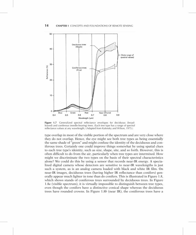
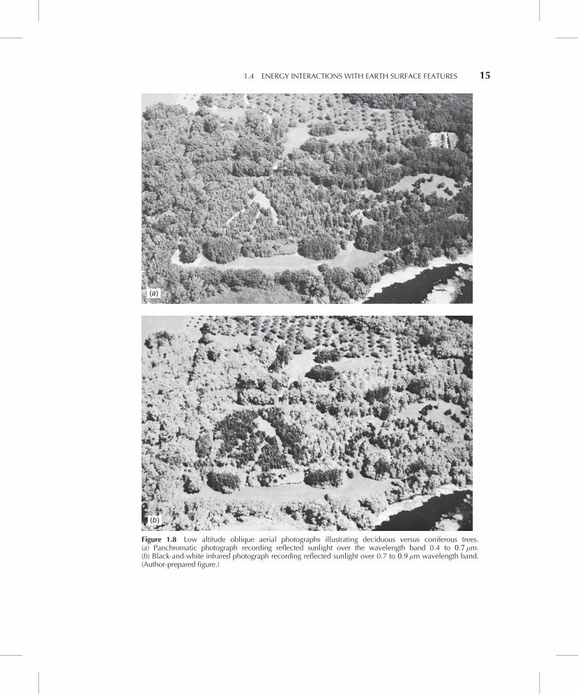
type overlap in most of the visible portion of the spectrum and are very close wherethey do not overlap. Hence, the eye might see both tree types as being essentiallythe same shade of “green” and might confuse the identity of the deciduous and con-iferous trees. Certainly one could improve things somewhat by using spatial cluesto each tree type’s identity, such as size, shape, site, and so forth. However, this isoften difficult to do from the air, particularly when tree types are intermixed. Howmight we discriminate the two types on the basis of their spectral characteristicsalone? We could do this by using a sensor that records near-IR energy. A specia-lized digital camera whose detectors are sensitive to near-IR wavelengths is justsuch a system, as is an analog camera loaded with black and white IR film. Onnear-IR images, deciduous trees (having higher IR reflectance than conifers) gen-erally appear much lighter in tone than do conifers. This is illustrated in Figure 1.8,which shows stands of coniferous trees surrounded by deciduous trees. In Figure1.8a (visible spectrum), it is virtually impossible to distinguish between tree types,even though the conifers have a distinctive conical shape whereas the deciduoustrees have rounded crowns. In Figure 1.8b (near IR), the coniferous trees have a

Figure 1.7 Generalized spectral reflectance envelopes for deciduous (broad-leaved) and coniferous (needle-bearing) trees. (Each tree type has a range of spectralreflectance values at any wavelength.) (Adapted from Kalensky and Wilson, 1975.)


(a)

(b)

Figure 1.8 Low altitude oblique aerial photographs illustrating deciduous versus coniferous trees.(a) Panchromatic photograph recording reflected sunlight over the wavelength band 0.4 to 0:7 �m.(b) Black-and-white infrared photograph recording reflected sunlight over 0.7 to 0:9 �m wavelength band.(Author-prepared figure.)


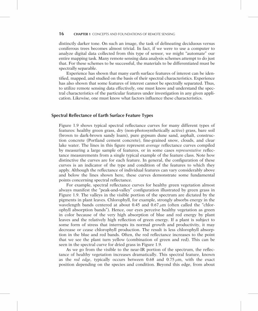
distinctly darker tone. On such an image, the task of delineating deciduous versusconiferous trees becomes almost trivial. In fact, if we were to use a computer toanalyze digital data collected from this type of sensor, we might “automate” ourentire mapping task. Many remote sensing data analysis schemes attempt to do justthat. For these schemes to be successful, the materials to be differentiated must bespectrally separable.

Experience has shown that many earth surface features of interest can be iden-tified, mapped, and studied on the basis of their spectral characteristics. Experiencehas also shown that some features of interest cannot be spectrally separated. Thus,to utilize remote sensing data effectively, one must know and understand the spec-tral characteristics of the particular features under investigation in any given appli-cation. Likewise, one must know what factors influence these characteristics.

Spectral Reflectance of Earth Surface Feature Types

Figure 1.9 shows typical spectral reflectance curves for many different types offeatures: healthy green grass, dry (non-photosynthetically active) grass, bare soil(brown to dark-brown sandy loam), pure gypsum dune sand, asphalt, construc-tion concrete (Portland cement concrete), fine-grained snow, clouds, and clearlake water. The lines in this figure represent average reflectance curves compiledby measuring a large sample of features, or in some cases representative reflec-tance measurements from a single typical example of the feature class. Note howdistinctive the curves are for each feature. In general, the configuration of thesecurves is an indicator of the type and condition of the features to which theyapply. Although the reflectance of individual features can vary considerably aboveand below the lines shown here, these curves demonstrate some fundamentalpoints concerning spectral reflectance.

For example, spectral reflectance curves for healthy green vegetation almostalways manifest the “peak-and-valley” configuration illustrated by green grass inFigure 1.9. The valleys in the visible portion of the spectrum are dictated by thepigments in plant leaves. Chlorophyll, for example, strongly absorbs energy in thewavelength bands centered at about 0.45 and 0:67 �m (often called the “chlor-ophyll absorption bands”). Hence, our eyes perceive healthy vegetation as greenin color because of the very high absorption of blue and red energy by plantleaves and the relatively high reflection of green energy. If a plant is subject tosome form of stress that interrupts its normal growth and productivity, it maydecrease or cease chlorophyll production. The result is less chlorophyll absorp-tion in the blue and red bands. Often, the red reflectance increases to the pointthat we see the plant turn yellow (combination of green and red). This can beseen in the spectral curve for dried grass in Figure 1.9.

As we go from the visible to the near-IR portion of the spectrum, the reflec-tance of healthy vegetation increases dramatically. This spectral feature, knownas the red edge, typically occurs between 0.68 and 0:75 �m, with the exactposition depending on the species and condition. Beyond this edge, from about


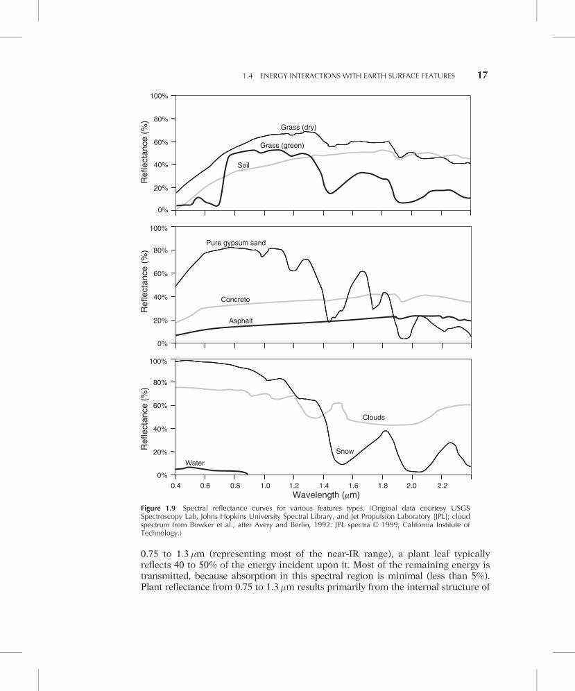
Figure 1.9 Spectral reflectance curves for various features types. (Original data courtesy USGSSpectroscopy Lab, Johns Hopkins University Spectral Library, and Jet Propulsion Laboratory [JPL]; cloudspectrum from Bowker et al., after Avery and Berlin, 1992. JPL spectra © 1999, California Institute ofTechnology.)

0.75 to 1:3 �m (representing most of the near-IR range), a plant leaf typicallyreflects 40 to 50% of the energy incident upon it. Most of the remaining energy istransmitted, because absorption in this spectral region is minimal (less than 5%).Plant reflectance from 0.75 to 1:3 �m results primarily from the internal structure of


plant leaves. Because the position of the red edge and the magnitude of the near-IRreflectance beyond the red edge are highly variable among plant species, reflectancemeasurements in these ranges often permit us to discriminate between species,even if they look the same in visible wavelengths. Likewise, many plant stressesalter the reflectance in the red edge and the near-IR region, and sensors operatingin these ranges are often used for vegetation stress detection. Also, multiple layers ofleaves in a plant canopy provide the opportunity for multiple transmissions andreflections. Hence, the near-IR reflectance increases with the number of layers ofleaves in a canopy, with the maximum reflectance achieved at about eight leaflayers (Bauer et al., 1986).

Beyond 1:3 �m, energy incident upon vegetation is essentially absorbed orreflected, with little to no transmittance of energy. Dips in reflectance occur at1.4, 1.9, and 2:7 �m because water in the leaf absorbs strongly at these wave-lengths. Accordingly, wavelengths in these spectral regions are referred to aswater absorption bands. Reflectance peaks occur at about 1.6 and 2:2 �m,between the absorption bands. Throughout the range beyond 1:3 �m, leafreflectance is approximately inversely related to the total water present in aleaf. This total is a function of both the moisture content and the thickness ofa leaf.

The soil curve in Figure 1.9 shows considerably less peak-and-valley variationin reflectance. That is, the factors that influence soil reflectance act over less spe-cific spectral bands. Some of the factors affecting soil reflectance are moisturecontent, organic matter content, soil texture (proportion of sand, silt, and clay),surface roughness, and presence of iron oxide. These factors are complex, vari-able, and interrelated. For example, the presence of moisture in soil will decreaseits reflectance. As with vegetation, this effect is greatest in the water absorptionbands at about 1.4, 1.9, and 2:7 �m (clay soils also have hydroxyl absorptionbands at about 1.4 and 2:2 �m). Soil moisture content is strongly related to thesoil texture: Coarse, sandy soils are usually well drained, resulting in low moisturecontent and relatively high reflectance; poorly drained fine-textured soils willgenerally have lower reflectance. Thus, the reflectance properties of a soil are con-sistent only within particular ranges of conditions. Two other factors that reducesoil reflectance are surface roughness and content of organic matter. The pre-sence of iron oxide in a soil will also significantly decrease reflectance, at least inthe visible wavelengths. In any case, it is essential that the analyst be familiarwith the conditions at hand. Finally, because soils are essentially opaque to visi-ble and infrared radiation, it should be noted that soil reflectance comes from theuppermost layer of the soil and may not be indicative of the properties of the bulkof the soil.

Sand can have wide variation in its spectral reflectance pattern. The curveshown in Figure 1.9 is from a dune in New Mexico and consists of roughly 99%gypsum with trace amounts of quartz (Jet Propulsion Laboratory, 1999). Itsabsorption and reflectance features are essentially identical to those of its parent


material, gypsum. Sand derived from other sources, with differing mineral com-positions, would have a spectral reflectance curve indicative of its parent mate-rial. Other factors affecting the spectral response from sand include the presenceor absence of water and of organic matter. Sandy soil is subject to the same con-siderations listed in the discussion of soil reflectance.

As shown in Figure 1.9, the spectral reflectance curves for asphalt and Port-land cement concrete are much flatter than those of the materials discussed thusfar. Overall, Portland cement concrete tends to be relatively brighter thanasphalt, both in the visible spectrum and at longer wavelengths. It is important tonote that the reflectance of these materials may be modified by the presence ofpaint, soot, water, or other substances. Also, as materials age, their spectralreflectance patterns may change. For example, the reflectance of many types ofasphaltic concrete may increase, particularly in the visible spectrum, as their sur-face ages.

In general, snow reflects strongly in the visible and near infrared, and absorbsmore energy at mid-infrared wavelengths. However, the reflectance of snow isaffected by its grain size, liquid water content, and presence or absence of othermaterials in or on the snow surface (Dozier and Painter, 2004). Larger grains ofsnow absorb more energy, particularly at wavelengths longer than 0:8 �m. At tem-peratures near 0°C, liquid water within the snowpack can cause grains to sticktogether in clusters, thus increasing the effective grain size and decreasing thereflectance at near-infrared and longer wavelengths. When particles of con-taminants such as dust or soot are deposited on snow, they can significantly reducethe surface’s reflectance in the visible spectrum.

The aforementioned absorption of mid-infrared wavelengths by snow can per-mit the differentiation between snow and clouds. While both feature types appearbright in the visible and near infrared, clouds have significantly higher reflectancethan snow at wavelengths longer than 1:4 �m. Meteorologists can also use bothspectral and bidirectional reflectance patterns (discussed later in this section) toidentify a variety of cloud properties, including ice/water composition andparticle size.

Considering the spectral reflectance of water, probably the most distinctivecharacteristic is the energy absorption at near-IR wavelengths and beyond.In short, water absorbs energy in these wavelengths whether we are talkingabout water features per se (such as lakes and streams) or water contained invegetation or soil. Locating and delineating water bodies with remote sensingdata are done most easily in near-IR wavelengths because of this absorptionproperty. However, various conditions of water bodies manifest themselves pri-marily in visible wavelengths. The energy–matter interactions at these wave-lengths are very complex and depend on a number of interrelated factors. Forexample, the reflectance from a water body can stem from an interaction withthe water’s surface (specular reflection), with material suspended in the water,or with the bottom of the depression containing the water body. Even with


deep water where bottom effects are negligible, the reflectance properties of awater body are a function of not only the water per se but also the material inthe water.

Clear water absorbs relatively little energy having wavelengths less thanabout 0:6 �m. High transmittance typifies these wavelengths with a maximum inthe blue-green portion of the spectrum. However, as the turbidity of water chan-ges (because of the presence of organic or inorganic materials), transmittance—and therefore reflectance—changes dramatically. For example, waters containinglarge quantities of suspended sediments resulting from soil erosion normallyhave much higher visible reflectance than other “clear” waters in the same geo-graphic area. Likewise, the reflectance of water changes with the chlorophyllconcentration involved. Increases in chlorophyll concentration tend to decreasewater reflectance in blue wavelengths and increase it in green wavelengths.These changes have been used to monitor the presence and estimate the con-centration of algae via remote sensing data. Reflectance data have also been usedto determine the presence or absence of tannin dyes from bog vegetation inlowland areas and to detect a number of pollutants, such as oil and certainindustrial wastes.

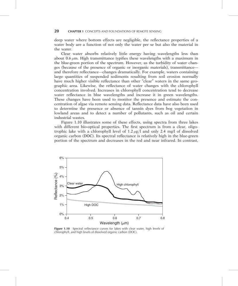
Figure 1.10 illustrates some of these effects, using spectra from three lakeswith different bio-optical properties. The first spectrum is from a clear, oligo-trophic lake with a chlorophyll level of 1:2 �g=l and only 2.4 mg/l of dissolvedorganic carbon (DOC). Its spectral reflectance is relatively high in the blue-greenportion of the spectrum and decreases in the red and near infrared. In contrast,

Figure 1.10 Spectral reflectance curves for lakes with clear water, high levels ofchlorophyll, and high levels of dissolved organic carbon (DOC).


the spectrum from a lake experiencing an algae bloom, with much higher chlor-ophyll concentration 12:3 �g=lð Þ, shows a reflectance peak in the green spectrumand absorption in the blue and red regions. These reflectance and absorption fea-tures are associated with several pigments present in algae. Finally, the thirdspectrum in Figure 1.10 was acquired on an ombrotrophic bog lake, with veryhigh levels of DOC (20.7 mg/l). These naturally occurring tannins and other com-plex organic molecules give the lake a very dark appearance, with its reflectancecurve nearly flat across the visible spectrum.

Many important water characteristics, such as dissolved oxygen concentra-tion, pH, and salt concentration, cannot be observed directly through changesin water reflectance. However, such parameters sometimes correlate withobserved reflectance. In short, there are many complex interrelationshipsbetween the spectral reflectance of water and particular characteristics. Onemust use appropriate reference data to correctly interpret reflectance measure-ments made over water.

Our discussion of the spectral characteristics of vegetation, soil, and waterhas been very general. The student interested in pursuing details on this subject,as well as factors influencing these characteristics, is encouraged to consult thevarious references contained in the Works Cited section located at the end ofthis book.

Spectral Response Patterns

Having looked at the spectral reflectance characteristics of vegetation, soil, sand,concrete, asphalt, snow, clouds, and water, we should recognize that these broadfeature types are often spectrally separable. However, the degree of separationbetween types varies among and within spectral regions. For example, water andvegetation might reflect nearly equally in visible wavelengths, yet these featuresare almost always separable in near-IR wavelengths.

Because spectral responses measured by remote sensors over various featuresoften permit an assessment of the type and/or condition of the features, theseresponses have often been referred to as spectral signatures. Spectral reflectanceand spectral emittance curves (for wavelengths greater than 3:0 �m) are oftenreferred to in this manner. The physical radiation measurements acquired overspecific terrain features at various wavelengths are also referred to as the spectralsignatures for those features.

Although it is true that many earth surface features manifest very distinctivespectral reflectance and/or emittance characteristics, these characteristics resultin spectral “response patterns” rather than in spectral “signatures.” The reason forthis is that the term signature tends to imply a pattern that is absolute and unique.This is not the case with the spectral patterns observed in the natural world. Aswe have seen, spectral response patterns measured by remote sensors may be


quantitative, but they are not absolute. They may be distinctive, but they are notnecessarily unique.

We have already looked at some characteristics of objects that influence theirspectral response patterns. Temporal effects and spatial effects can also enter intoany given analysis. Temporal effects are any factors that change the spectral char-acteristics of a feature over time. For example, the spectral characteristics ofmany species of vegetation are in a nearly continual state of change throughout agrowing season. These changes often influence when we might collect sensor datafor a particular application.

Spatial effects refer to factors that cause the same types of features (e.g., cornplants) at a given point in time to have different characteristics at different geo-graphic locations. In small-area analysis the geographic locations may be metersapart and spatial effects may be negligible. When analyzing satellite data, thelocations may be hundreds of kilometers apart where entirely different soils, cli-mates, and cultivation practices might exist.

Temporal and spatial effects influence virtually all remote sensing operations.These effects normally complicate the issue of analyzing spectral reflectanceproperties of earth resources. Again, however, temporal and spatial effects mightbe the keys to gleaning the information sought in an analysis. For example, theprocess of change detection is premised on the ability to measure temporal effects.An example of this process is detecting the change in suburban development neara metropolitan area by using data obtained on two different dates.

An example of a useful spatial effect is the change in the leaf morphology oftrees when they are subjected to some form of stress. For example, when a treebecomes infected with Dutch elm disease, its leaves might begin to cup and curl,changing the reflectance of the tree relative to healthy trees that surround it. So,even though a spatial effect might cause differences in the spectral reflectances ofthe same type of feature, this effect may be just what is important in a particularapplication.

Finally, it should be noted that the apparent spectral response from surfacefeatures can be influenced by shadows. While an object’s spectral reflectance(a ratio of reflected to incident energy, see Eq. 1.8) is not affected by changes inillumination, the absolute amount of energy reflected does depend on illumina-tion conditions. Within a shadow, the total reflected energy is reduced, and thespectral response is shifted toward shorter wavelengths. This occurs because theincident energy within a shadow comes primarily from Rayleigh atmosphericscattering, and as discussed in Section 1.3, such scattering primarily affects shortwavelengths. Thus, in visible-wavelength imagery, objects inside shadows willtend to appear both darker and bluer than if they were fully illuminated. Thiseffect can cause problems for automated image classification algorithms; forexample, dark shadows of trees on pavement may be misclassified as water. Theeffects of illumination geometry on reflectance are discussed in more detail laterin this section, while the impacts of shadows on the image interpretation processare discussed in Section 1.12.


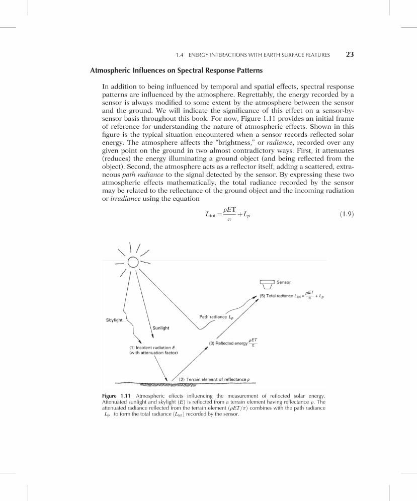
Atmospheric Influences on Spectral Response Patterns

In addition to being influenced by temporal and spatial effects, spectral responsepatterns are influenced by the atmosphere. Regrettably, the energy recorded by asensor is always modified to some extent by the atmosphere between the sensorand the ground. We will indicate the significance of this effect on a sensor-by-sensor basis throughout this book. For now, Figure 1.11 provides an initial frameof reference for understanding the nature of atmospheric effects. Shown in thisfigure is the typical situation encountered when a sensor records reflected solarenergy. The atmosphere affects the “brightness,” or radiance, recorded over anygiven point on the ground in two almost contradictory ways. First, it attenuates(reduces) the energy illuminating a ground object (and being reflected from theobject). Second, the atmosphere acts as a reflector itself, adding a scattered, extra-neous path radiance to the signal detected by the sensor. By expressing these twoatmospheric effects mathematically, the total radiance recorded by the sensormay be related to the reflectance of the ground object and the incoming radiationor irradiance using the equation

Ltot ¼ rET�

þLp ð1:9Þ

Figure 1.11 Atmospheric effects influencing the measurement of reflected solar energy.Attenuated sunlight and skylight Eð Þ is reflected from a terrain element having reflectance r. Theattenuated radiance reflected from the terrain element rET=�ð Þ combines with the path radianceLp� �

to form the total radiance Ltotð Þ recorded by the sensor.


where

Ltot ¼ total spectral radiancemeasured by sensorr ¼ reflectance of objectE ¼ irradiance on object; incoming energyT ¼ transmission of atmosphereLp ¼ path radiance; from the atmosphere and not from the object

It should be noted that all of the above factors depend on wavelength. Also, asshown in Figure 1.11, the irradiance Eð Þ stems from two sources: (1) directly reflec-ted “sunlight” and (2) diffuse “skylight,” which is sunlight that has been previouslyscattered by the atmosphere. The relative dominance of sunlight versus skylight inany given image is strongly dependent on weather conditions (e.g., sunny vs. hazyvs. cloudy). Likewise, irradiance varies with the seasonal changes in solar elevationangle (Figure 7.4) and the changing distance between the earth and sun.

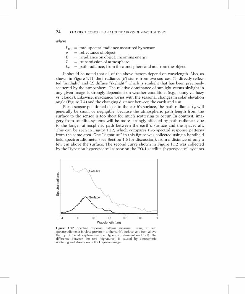
For a sensor positioned close to the earth’s surface, the path radiance Lp willgenerally be small or negligible, because the atmospheric path length from thesurface to the sensor is too short for much scattering to occur. In contrast, ima-gery from satellite systems will be more strongly affected by path radiance, dueto the longer atmospheric path between the earth’s surface and the spacecraft.This can be seen in Figure 1.12, which compares two spectral response patternsfrom the same area. One “signature” in this figure was collected using a handheldfield spectroradiometer (see Section 1.6 for discussion), from a distance of only afew cm above the surface. The second curve shown in Figure 1.12 was collectedby the Hyperion hyperspectral sensor on the EO-1 satellite (hyperspectral systems

0.4 0.5 0.6 0.7 0.8 0.9 1

Satellite

Surface

Spectr

al ra

dia

nce

Wavelength (μm)

Figure 1.12 Spectral response patterns measured using a fieldspectroradiometer in close proximity to the earth’s surface, and from abovethe top of the atmosphere (via the Hyperion instrument on EO-1). Thedifference between the two “signatures” is caused by atmosphericscattering and absorption in the Hyperion image.


are discussed in Chapter 4, and the Hyperion instrument is covered in Chapter 5).Due to the thickness of the atmosphere between the earth’s surface and the satel-lite’s position above the atmosphere, this second spectral response pattern showsan elevated signal at short wavelengths, due to the extraneous path radiance.

In its raw form, this near-surface measurement from the field spectro-radiometer could not be directly compared to the measurement from the satellite,because one is observing surface reflectance while the other is observing the so-called top of atmosphere (TOA) reflectance. Before such a comparison could beperformed, the satellite image would need to go through a process of atmosphericcorrection, in which the raw spectral data are modified to compensate for theexpected effects of atmospheric scattering and absorption. This process, discussedin Chapter 7, generally does not produce a perfect representation of the spectralresponse curve that would actually be observed at the surface itself, but it can pro-duce a sufficiently close approximation to be suitable for many types of analysis.

Readers who might be interested in obtaining additional details about theconcepts, terminology, and units used in radiation measurement may wish toconsult Appendix A.

Geometric Influences on Spectral Response Patterns

The geometric manner in which an object reflects energy is an important con-sideration. This factor is primarily a function of the surface roughness of theobject. Specular reflectors are flat surfaces that manifest mirror-like reflections,where the angle of reflection equals the angle of incidence. Diffuse (or Lamber-tian) reflectors are rough surfaces that reflect uniformly in all directions. Mostearth surfaces are neither perfectly specular nor perfectly diffuse reflectors. Theircharacteristics are somewhat between the two extremes.

Figure 1.13 illustrates the geometric character of specular, near-specular,near-diffuse, and diffuse reflectors. The category that describes any given surfaceis dictated by the surface’s roughness in comparison to the wavelength of theenergy being sensed. For example, in the relatively long wavelength radio range, asandy beach can appear smooth to incident energy, whereas in the visible portionof the spectrum, it appears rough. In short, when the wavelength of incidentenergy is much smaller than the surface height variations or the particle sizes thatmake up a surface, the reflection from the surface is diffuse.

Diffuse reflections contain spectral information on the “color” of the reflectingsurface, whereas specular reflections generally do not. Hence, in remote sensing,we are most often interested in measuring the diffuse reflectance properties of terrainfeatures.

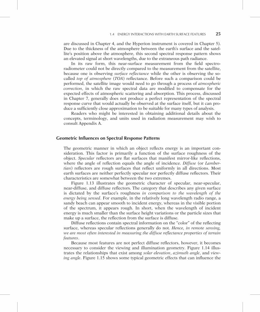
Because most features are not perfect diffuse reflectors, however, it becomesnecessary to consider the viewing and illumination geometry. Figure 1.14 illus-trates the relationships that exist among solar elevation, azimuth angle, and view-ing angle. Figure 1.15 shows some typical geometric effects that can influence the


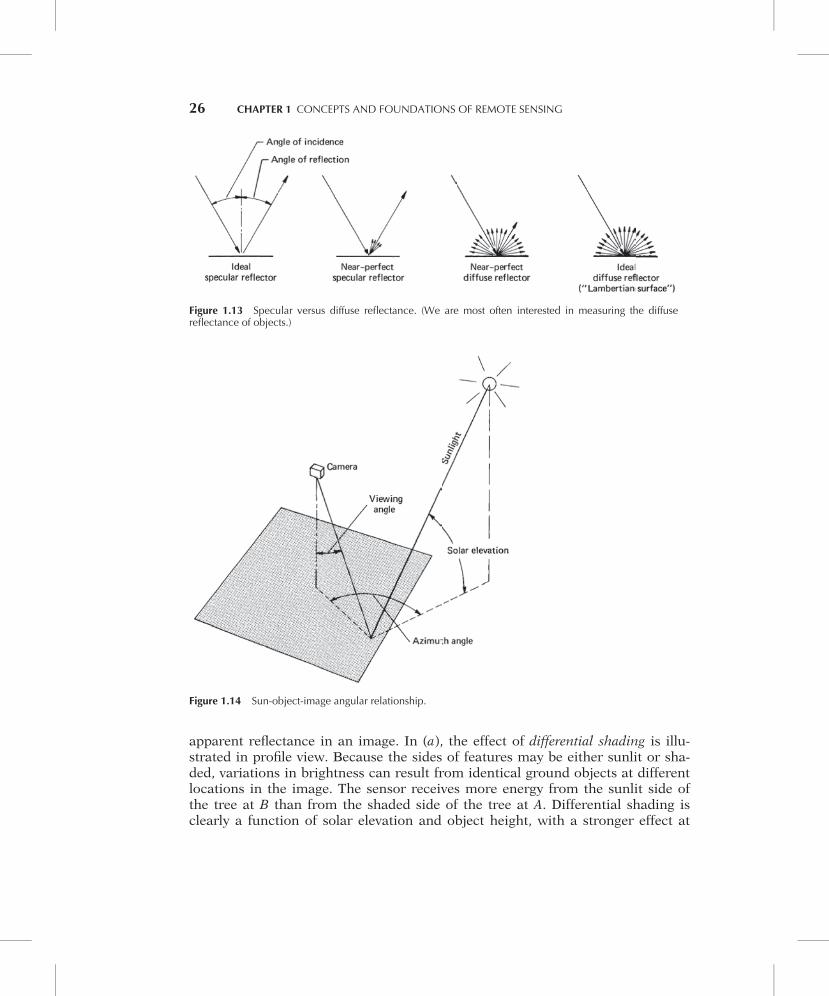
apparent reflectance in an image. In (a), the effect of differential shading is illu-strated in profile view. Because the sides of features may be either sunlit or sha-ded, variations in brightness can result from identical ground objects at differentlocations in the image. The sensor receives more energy from the sunlit side ofthe tree at B than from the shaded side of the tree at A. Differential shading isclearly a function of solar elevation and object height, with a stronger effect at

Figure 1.13 Specular versus diffuse reflectance. (We are most often interested in measuring the diffusereflectance of objects.)

Figure 1.14 Sun-object-image angular relationship.


low solar angles. The effect is also compounded by differences in slope and aspect(slope orientation) over terrain of varied relief.

Figure 1.15b illustrates the effect of differential atmospheric scattering. As dis-cussed earlier, backscatter from atmospheric molecules and particles adds light(path radiance) to that reflected from ground features. The sensor records moreatmospheric backscatter from area D than from area C due to this geometriceffect. In some analyses, the variation in this path radiance component is smalland can be ignored, particularly at long wavelengths. However, under hazy condi-tions, differential quantities of path radiance often result in varied illuminationacross an image.

As mentioned earlier, specular reflections represent the extreme in directionalreflectance. When such reflections appear, they can hinder analysis of the ima-gery. This can often be seen in imagery taken over water bodies. Figure 1.15cillustrates the geometric nature of this problem. Immediately surrounding point Eon the image, a considerable increase in brightness would result from specularreflection. A photographic example of this is shown in Figure 1.16, whichincludes areas of specular reflection from the right half of the large lake in thecenter of the image. These mirrorlike reflections normally contribute little infor-mation about the true character of the objects involved. For example, the smallwater bodies just below the larger lake have a tone similar to that of some of thefields in the area. Because of the low information content of specular reflections,they are avoided in most analyses.

The most complete representation of an object’s geometric reflectance proper-ties is the bidirectional reflectance distribution function (BRDF). This is a mathe-matical description of how reflectance varies for all combinations of illuminationand viewing angles at a given wavelength (Schott, 2007). The BRDF for any givenfeature can approximate that of a Lambertian surface at some angles and be non-Lambertian at other angles. Similarly, the BRDF can vary considerably withwavelength. A variety of mathematical models (including a provision for wave-length dependence) have been proposed to represent the BRDF (Jupp andStrahler, 1991).

(a) (b) (c)

Figure 1.15 Geometric effects that cause variations in focal plane irradiance: (a) differential shading,(b) differential scattering, and (c) specular reflection.


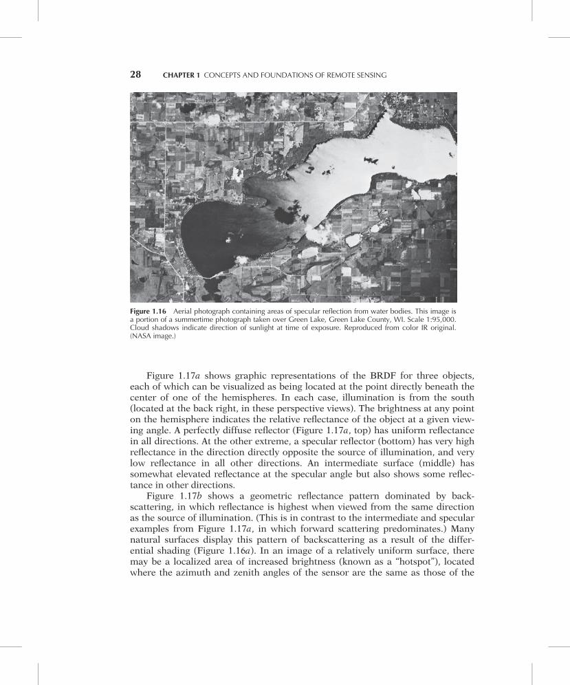
Figure 1.17a shows graphic representations of the BRDF for three objects,each of which can be visualized as being located at the point directly beneath thecenter of one of the hemispheres. In each case, illumination is from the south(located at the back right, in these perspective views). The brightness at any pointon the hemisphere indicates the relative reflectance of the object at a given view-ing angle. A perfectly diffuse reflector (Figure 1.17a, top) has uniform reflectancein all directions. At the other extreme, a specular reflector (bottom) has very highreflectance in the direction directly opposite the source of illumination, and verylow reflectance in all other directions. An intermediate surface (middle) hassomewhat elevated reflectance at the specular angle but also shows some reflec-tance in other directions.

Figure 1.17b shows a geometric reflectance pattern dominated by back-scattering, in which reflectance is highest when viewed from the same directionas the source of illumination. (This is in contrast to the intermediate and specularexamples from Figure 1.17a, in which forward scattering predominates.) Manynatural surfaces display this pattern of backscattering as a result of the differ-ential shading (Figure 1.16a). In an image of a relatively uniform surface, theremay be a localized area of increased brightness (known as a “hotspot”), locatedwhere the azimuth and zenith angles of the sensor are the same as those of the

Figure 1.16 Aerial photograph containing areas of specular reflection from water bodies. This image isa portion of a summertime photograph taken over Green Lake, Green Lake County, WI. Scale 1:95,000.Cloud shadows indicate direction of sunlight at time of exposure. Reproduced from color IR original.(NASA image.)


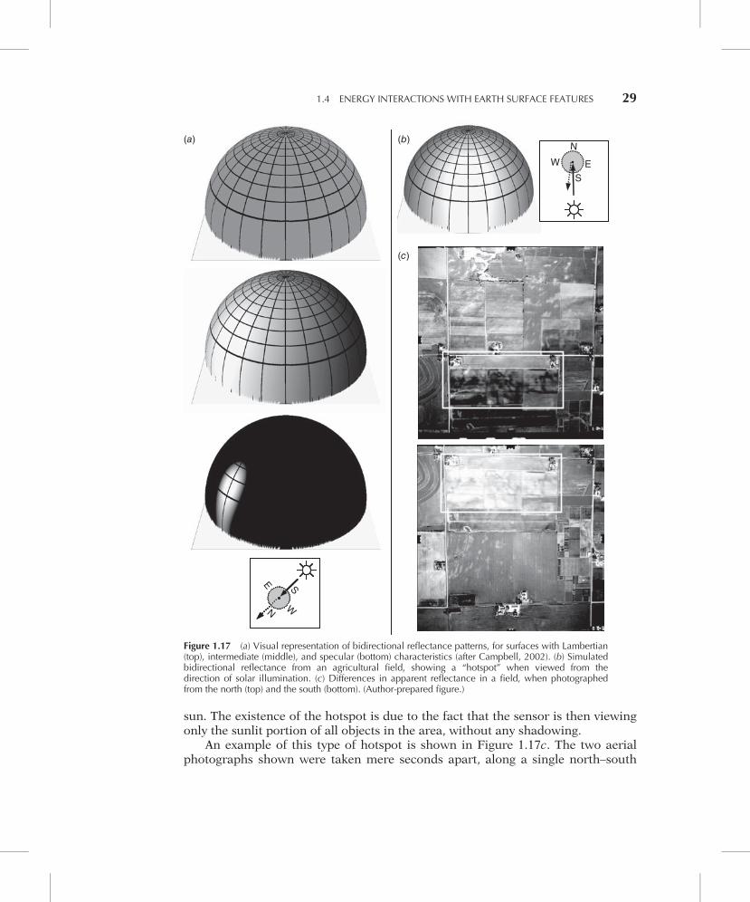
sun. The existence of the hotspot is due to the fact that the sensor is then viewingonly the sunlit portion of all objects in the area, without any shadowing.

An example of this type of hotspot is shown in Figure 1.17c. The two aerialphotographs shown were taken mere seconds apart, along a single north–south

(a) (b)

(c)

S

WN

E

E

S

W

N

E

S

W

N

E

S

W

N

Figure 1.17 (a) Visual representation of bidirectional reflectance patterns, for surfaces with Lambertian(top), intermediate (middle), and specular (bottom) characteristics (after Campbell, 2002). (b) Simulatedbidirectional reflectance from an agricultural field, showing a “hotspot” when viewed from thedirection of solar illumination. (c) Differences in apparent reflectance in a field, when photographedfrom the north (top) and the south (bottom). (Author-prepared figure.)


flight line. The field delineated by the white box has a great difference in itsapparent reflectance in the two images, despite the fact that no actual changesoccurred on the ground during the short interval between the exposures. In thetop photograph, the field was being viewed from the north, opposite the directionof solar illumination. Roughness of the field’s surface results in differential shad-ing, with the camera viewing the shadowed side of each small variation in thefield’s surface. In contrast, the bottom photograph was acquired from a point tothe south of the field, from the same direction as the solar illumination (the hot-spot), and thus appears quite bright.

To summarize, variations in bidirectional reflectance—such as specularreflection from a lake, or the hotspot in an agricultural field—can significantlyaffect the appearance of objects in remotely sensed images. These effects causeobjects to appear brighter or darker solely as a result of the angular relationshipsamong the sun, the object, and the sensor, without regard to any actual reflec-tance differences on the ground. Often, the impact of directional reflectanceeffects can be minimized by advance planning. For example, when photographinga lake when the sun is to the south and the lake’s surface is calm, it may be pre-ferable to take the photographs from the east or west, rather than from the north,to avoid the sun’s specular reflection angle. However, the impact of varying bidir-ectional reflectance usually cannot be completely eliminated, and it is importantfor image analysts to be aware of this effect.

1.5 DATA ACQUISITION AND DIGITAL IMAGE CONCEPTS

To this point, we have discussed the principal sources of electromagnetic energy,the propagation of this energy through the atmosphere, and the interaction ofthis energy with earth surface features. These factors combine to produce energy“signals” from which we wish to extract information. We now consider the proce-dures by which these signals are detected, recorded, and interpreted.

The detection of electromagnetic energy can be performed in several ways.Before the development and adoption of electronic sensors, analog film-basedcameras used chemical reactions on the surface of a light-sensitive film to detectenergy variations within a scene. By developing a photographic film, we obtaineda record of its detected signals. Thus, the film acted as both the detecting and therecording medium. These pre-digital photographic systems offered many advan-tages: They were relatively simple and inexpensive and provided a high degree ofspatial detail and geometric integrity.

Electronic sensors generate an electrical signal that corresponds to the energyvariations in the original scene. A familiar example of an electronic sensor is ahandheld digital camera. Different types of electronic sensors have different designsof detectors, ranging from charge-coupled devices (CCDs, discussed in Chapter 2)to the antennas used to detect microwave signals (Chapter 6). Regardless of the type


of detector, the resulting data are generally recorded onto some magnetic or opticalcomputer storage medium, such as a hard drive, memory card, solid-state storageunit or optical disk. Although sometimes more complex and expensive than film-based systems, electronic sensors offer the advantages of a broader spectral range ofsensitivity, improved calibration potential, and the ability to electronically store andtransmit data.

In remote sensing, the term photograph historically was reserved exclusively forimages that were detected as well as recorded on film. The more generic term imagewas adopted for any pictorial representation of image data. Thus, a pictorial recordfrom a thermal scanner (an electronic sensor) would be called a “thermal image,”not a “thermal photograph,” because film would not be the original detectionmechanism for the image. Because the term image relates to any pictorial product,all photographs are images. Not all images, however, are photographs.

A common exception to the above terminology is use of the term digital pho-tography. As we describe in Section 2.5, digital cameras use electronic detectorsrather than film for image detection. While this process is not “photography” inthe traditional sense, “digital photography” is now the common way to refer tothis technique of digital data collection.

We can see that the data interpretation aspects of remote sensing can involve ana-lysis of pictorial (image) and/or digital data. Visual interpretation of pictorial imagedata has long been the most common form of remote sensing. Visual techniquesmake use of the excellent ability of the human mind to qualitatively evaluate spatialpatterns in an image. The ability to make subjective judgments based on selectedimage elements is essential in many interpretation efforts. Later in this chapter, inSection 1.12, we discuss the process of visual image interpretation in detail.

Visual interpretation techniques have certain disadvantages, however, in thatthey may require extensive training and are labor intensive. In addition, spectralcharacteristics are not always fully evaluated in visual interpretation efforts. Thisis partly because of the limited ability of the eye to discern tonal values on animage and the difficulty of simultaneously analyzing numerous spectral images.In applications where spectral patterns are highly informative, it is therefore pre-ferable to analyze digital, rather than pictorial, image data.

The basic character of digital image data is illustrated in Figure 1.18.Although the image shown in (a) appears to be a continuous-tone photograph,it is actually composed of a two-dimensional array of discrete picture elements,or pixels. The intensity of each pixel corresponds to the average brightness, orradiance, measured electronically over the ground area corresponding to eachpixel. A total of 500 rows and 400 columns of pixels are shown in Figure 1.18a.Whereas the individual pixels are virtually impossible to discern in (a), they arereadily observable in the enlargements shown in (b) and (c). These enlargementscorrespond to sub-areas located near the center of (a). A 100 row 3 80 columnenlargement is shown in (b) and a 10 row 3 8 column enlargement is included in(c). Part (d) shows the individual digital number (DN)—also referred to as the

1.5 DATA ACQUISITION AND DIGITAL IMAGE CONCEPTS 31

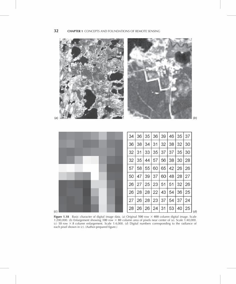
(a) (b)

(c) (d)

Figure 1.18 Basic character of digital image data. (a) Original 500 row 3 400 column digital image. Scale1:200,000. (b) Enlargement showing 100 row 3 80 column area of pixels near center of (a). Scale 1:40,000.(c) 10 row 3 8 column enlargement. Scale 1:4,000. (d) Digital numbers corresponding to the radiance ofeach pixel shown in (c). (Author-prepared figure.)


“brightness value” or “pixel value”—corresponding to the average radiance mea-sured in each pixel shown in (c). These values result from quantizing the originalelectrical signal from the sensor into positive integer values using a process calledanalog-to-digital (A-to-D) signal conversion. (The A-to-D conversion process is dis-cussed further in Chapter 4.)

Whether an image is acquired electronically or photographically, it may con-tain data from a single spectral band or from multiple spectral bands. The imageshown in Figure 1.18 was acquired using a single broad spectral band, by inte-grating all energy measured across a range of wavelengths (a process analogousto photography using “black-and-white” film). Thus, in the digital image, there isa single DN for each pixel. It is also possible to collect “color” or multispectralimagery, whereby data are collected simultaneously in several spectral bands. Inthe case of a color photograph, three separate sets of detectors (or, for analogcameras, three layers within the film) each record radiance in a different range ofwavelengths.

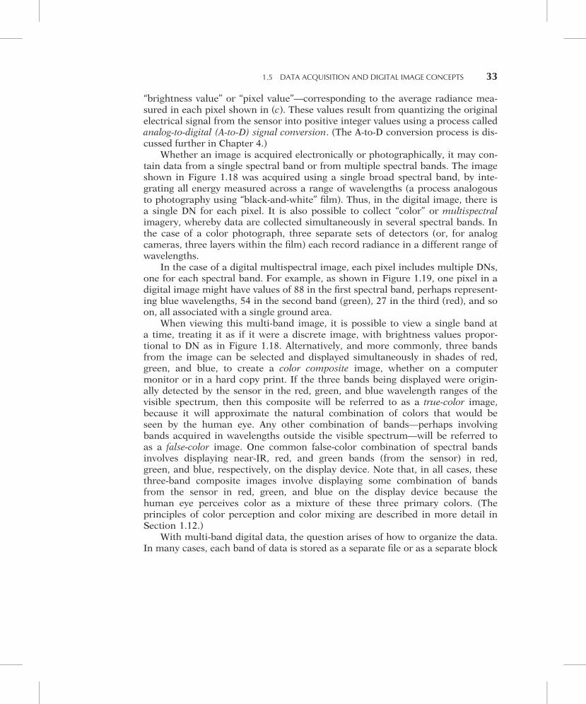
In the case of a digital multispectral image, each pixel includes multiple DNs,one for each spectral band. For example, as shown in Figure 1.19, one pixel in adigital image might have values of 88 in the first spectral band, perhaps represent-ing blue wavelengths, 54 in the second band (green), 27 in the third (red), and soon, all associated with a single ground area.

When viewing this multi-band image, it is possible to view a single band ata time, treating it as if it were a discrete image, with brightness values propor-tional to DN as in Figure 1.18. Alternatively, and more commonly, three bandsfrom the image can be selected and displayed simultaneously in shades of red,green, and blue, to create a color composite image, whether on a computermonitor or in a hard copy print. If the three bands being displayed were origin-ally detected by the sensor in the red, green, and blue wavelength ranges of thevisible spectrum, then this composite will be referred to as a true-color image,because it will approximate the natural combination of colors that would beseen by the human eye. Any other combination of bands—perhaps involvingbands acquired in wavelengths outside the visible spectrum—will be referred toas a false-color image. One common false-color combination of spectral bandsinvolves displaying near-IR, red, and green bands (from the sensor) in red,green, and blue, respectively, on the display device. Note that, in all cases, thesethree-band composite images involve displaying some combination of bandsfrom the sensor in red, green, and blue on the display device because thehuman eye perceives color as a mixture of these three primary colors. (Theprinciples of color perception and color mixing are described in more detail inSection 1.12.)

With multi-band digital data, the question arises of how to organize the data.In many cases, each band of data is stored as a separate file or as a separate block


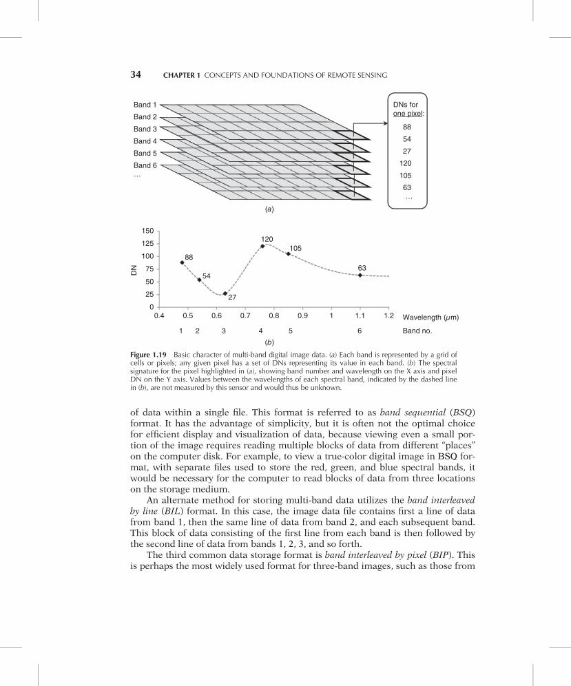
of data within a single file. This format is referred to as band sequential (BSQ)format. It has the advantage of simplicity, but it is often not the optimal choicefor efficient display and visualization of data, because viewing even a small por-tion of the image requires reading multiple blocks of data from different “places”on the computer disk. For example, to view a true-color digital image in BSQ for-mat, with separate files used to store the red, green, and blue spectral bands, itwould be necessary for the computer to read blocks of data from three locationson the storage medium.

An alternate method for storing multi-band data utilizes the band interleavedby line (BIL) format. In this case, the image data file contains first a line of datafrom band 1, then the same line of data from band 2, and each subsequent band.This block of data consisting of the first line from each band is then followed bythe second line of data from bands 1, 2, 3, and so forth.

The third common data storage format is band interleaved by pixel (BIP). Thisis perhaps the most widely used format for three-band images, such as those from

Band 6

Band 5

Band 4

Band 3

Band 2

Band 1

…

DNs for

one pixel:

63

105

120

27

54

88

…

(a)

(b)

0

25

50

75

100

125

150

0.4 0.5 0.6 0.7 0.8 0.9 1 1.1 1.2

DN

Wavelength (µm)

Band no.1 2 3 4 5 6

63

105

120

27

54

88

Figure 1.19 Basic character of multi-band digital image data. (a) Each band is represented by a grid ofcells or pixels; any given pixel has a set of DNs representing its value in each band. (b) The spectralsignature for the pixel highlighted in (a), showing band number and wavelength on the X axis and pixelDN on the Y axis. Values between the wavelengths of each spectral band, indicated by the dashed linein (b), are not measured by this sensor and would thus be unknown.


most consumer-grade digital cameras. In this format, the file contains each band’smeasurement for the first pixel, then each band’s measurement for the next pixel,and so on. The advantage of both BIL and BIP formats is that a computer canread and process the data for small portions of the image much more rapidly,because the data from all spectral bands are stored in closer proximity than in theBSQ format.

Typically, the DNs constituting a digital image are recorded over suchnumerical ranges as 0 to 255, 0 to 511, 0 to 1023, 0 to 2047, 0 to 4095 or higher.These ranges represent the set of integers that can be recorded using 8-, 9-,10-, 11-, and 12-bit binary computer coding scales, respectively. (That is,28 ¼ 256, 29 ¼ 512, 210 ¼ 1024, 211 ¼ 2048, and 212 ¼ 4096.) The technical termfor the number of bits used to store digital image data is quantization level (orcolor depth, when used to describe the number of bits used to display a colorimage). As discussed in Chapter 7, with the appropriate calibration coefficientsthese integer DNs can be converted to more meaningful physical units such asspectral reflectance, radiance, or normalized radar cross section.

Elevation Data

Increasingly, remote sensing instruments are used to collect three-dimensionalspatial data, in which each observation has a Z coordinate representing elevation,along with the X and Y coordinates used to represent the horizontal position ofthe pixel’s column and row. Particularly when collected over broad areas, theseelevation data may represent the topography, the three-dimensional shape of theland surface. In other cases (usually, at finer spatial scales), these elevation datamay represent the three-dimensional shapes of objects on or above the groundsurface, such as tree crowns in a forest, or buildings in a city. Elevation data maybe derived from the analysis of raw measurements from many types of remotesensing instruments, including photographic systems, multispectral sensors,radar systems, and lidar systems.

Elevation data may be represented in many different formats. Figure 1.20ashows a small portion of a traditional contour map, from the U.S. GeologicalSurvey’s 7.5-minute (1:24,000-scale) quadrangle map series. In this map, topo-graphic elevations are indicated by contour lines. Closely spaced lines indicatesteep terrain, while flat areas like river floodplains have more widely spacedcontours.

Figure 1.20b shows a digital elevation model (DEM). Note that the white rec-tangle in (b) represents the much smaller area shown in (a). The DEM is similarto a digital image, with the DN at each pixel representing a surface elevationrather than a radiance value. In (b), the brightness of each pixel is represented asbeing proportional to its elevation, so light-toned areas are topographically higherand dark-toned areas are lower. The region shown in this map consists of highlydissected terrain, with a complex network of river valleys; one major valley runs


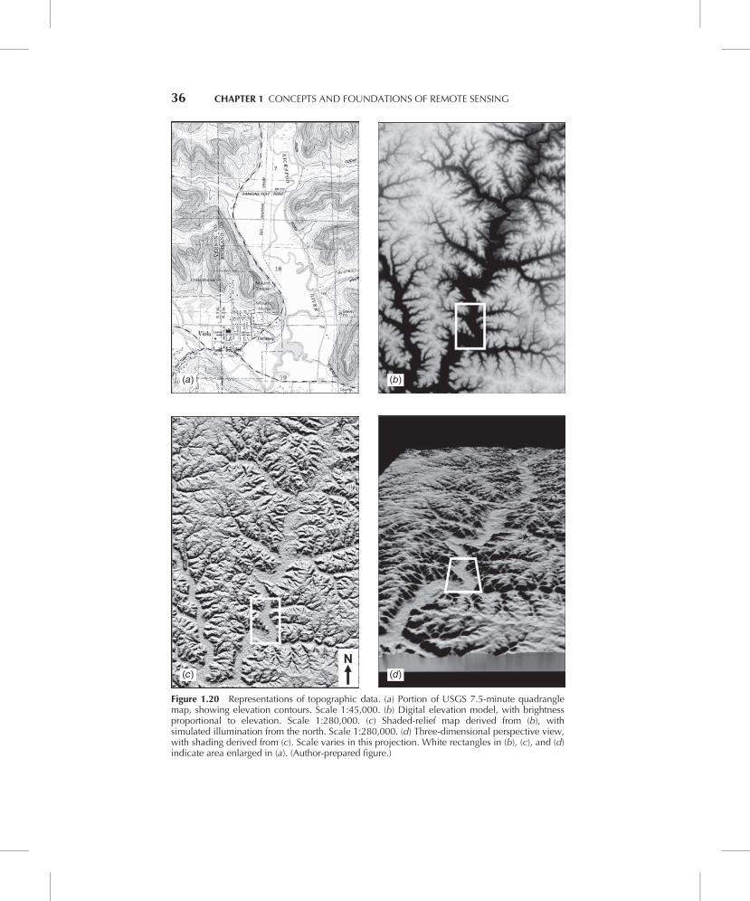
(a)

(c)

(b)

(d)

Figure 1.20 Representations of topographic data. (a) Portion of USGS 7.5-minute quadranglemap, showing elevation contours. Scale 1:45,000. (b) Digital elevation model, with brightnessproportional to elevation. Scale 1:280,000. (c) Shaded-relief map derived from (b), withsimulated illumination from the north. Scale 1:280,000. (d) Three-dimensional perspective view,with shading derived from (c). Scale varies in this projection. White rectangles in (b), (c), and (d)indicate area enlarged in (a). (Author-prepared figure.)


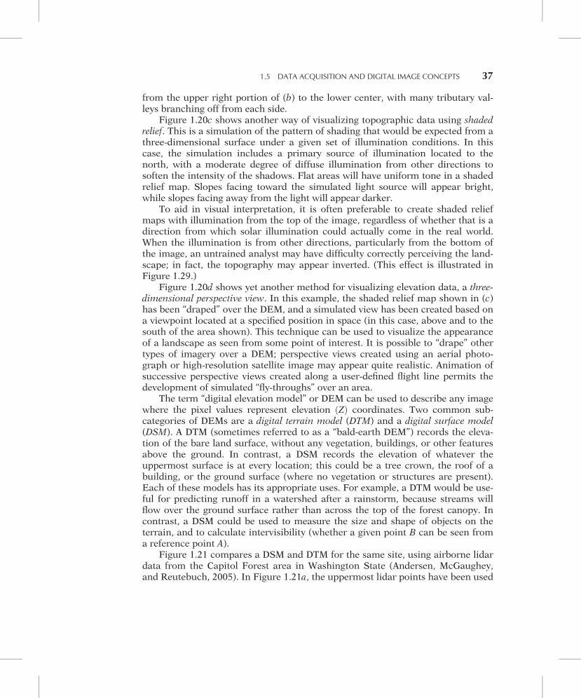
from the upper right portion of (b) to the lower center, with many tributary val-leys branching off from each side.

Figure 1.20c shows another way of visualizing topographic data using shadedrelief. This is a simulation of the pattern of shading that would be expected from athree-dimensional surface under a given set of illumination conditions. In thiscase, the simulation includes a primary source of illumination located to thenorth, with a moderate degree of diffuse illumination from other directions tosoften the intensity of the shadows. Flat areas will have uniform tone in a shadedrelief map. Slopes facing toward the simulated light source will appear bright,while slopes facing away from the light will appear darker.

To aid in visual interpretation, it is often preferable to create shaded reliefmaps with illumination from the top of the image, regardless of whether that is adirection from which solar illumination could actually come in the real world.When the illumination is from other directions, particularly from the bottom ofthe image, an untrained analyst may have difficulty correctly perceiving the land-scape; in fact, the topography may appear inverted. (This effect is illustrated inFigure 1.29.)

Figure 1.20d shows yet another method for visualizing elevation data, a three-dimensional perspective view. In this example, the shaded relief map shown in (c)has been “draped” over the DEM, and a simulated view has been created based ona viewpoint located at a specified position in space (in this case, above and to thesouth of the area shown). This technique can be used to visualize the appearanceof a landscape as seen from some point of interest. It is possible to “drape” othertypes of imagery over a DEM; perspective views created using an aerial photo-graph or high-resolution satellite image may appear quite realistic. Animation ofsuccessive perspective views created along a user-defined flight line permits thedevelopment of simulated “fly-throughs” over an area.

The term “digital elevation model” or DEM can be used to describe any imagewhere the pixel values represent elevation Zð Þ coordinates. Two common sub-categories of DEMs are a digital terrain model (DTM) and a digital surface model(DSM). A DTM (sometimes referred to as a “bald-earth DEM”) records the eleva-tion of the bare land surface, without any vegetation, buildings, or other featuresabove the ground. In contrast, a DSM records the elevation of whatever theuppermost surface is at every location; this could be a tree crown, the roof of abuilding, or the ground surface (where no vegetation or structures are present).Each of these models has its appropriate uses. For example, a DTM would be use-ful for predicting runoff in a watershed after a rainstorm, because streams willflow over the ground surface rather than across the top of the forest canopy. Incontrast, a DSM could be used to measure the size and shape of objects on theterrain, and to calculate intervisibility (whether a given point B can be seen froma reference point A).

Figure 1.21 compares a DSM and DTM for the same site, using airborne lidardata from the Capitol Forest area in Washington State (Andersen, McGaughey,and Reutebuch, 2005). In Figure 1.21a, the uppermost lidar points have been used


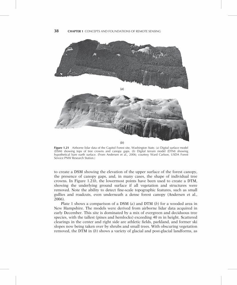
to create a DSM showing the elevation of the upper surface of the forest canopy,the presence of canopy gaps, and, in many cases, the shape of individual treecrowns. In Figure 1.21b, the lowermost points have been used to create a DTM,showing the underlying ground surface if all vegetation and structures wereremoved. Note the ability to detect fine-scale topographic features, such as smallgullies and roadcuts, even underneath a dense forest canopy (Andersen et al.,2006).

Plate 1 shows a comparison of a DSM (a) and DTM (b) for a wooded area inNew Hampshire. The models were derived from airborne lidar data acquired inearly December. This site is dominated by a mix of evergreen and deciduous treespecies, with the tallest (pines and hemlocks) exceeding 40 m in height. Scatteredclearings in the center and right side are athletic fields, parkland, and former skislopes now being taken over by shrubs and small trees. With obscuring vegetationremoved, the DTM in (b) shows a variety of glacial and post-glacial landforms, as

(b)

(a)

Figure 1.21 Airborne lidar data of the Capitol Forest site, Washington State. (a) Digital surface model(DSM) showing tops of tree crowns and canopy gaps. (b) Digital terrain model (DTM) showinghypothetical bare earth surface. (From Andersen et al., 2006; courtesy Ward Carlson, USDA ForestService PNW Research Station.)


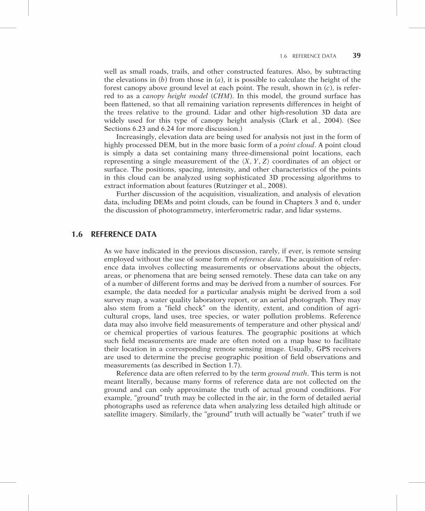
well as small roads, trails, and other constructed features. Also, by subtractingthe elevations in (b) from those in (a), it is possible to calculate the height of theforest canopy above ground level at each point. The result, shown in (c), is refer-red to as a canopy height model (CHM). In this model, the ground surface hasbeen flattened, so that all remaining variation represents differences in height ofthe trees relative to the ground. Lidar and other high-resolution 3D data arewidely used for this type of canopy height analysis (Clark et al., 2004). (SeeSections 6.23 and 6.24 for more discussion.)

Increasingly, elevation data are being used for analysis not just in the form ofhighly processed DEM, but in the more basic form of a point cloud. A point cloudis simply a data set containing many three-dimensional point locations, eachrepresenting a single measurement of the X, Y , Zð Þ coordinates of an object orsurface. The positions, spacing, intensity, and other characteristics of the pointsin this cloud can be analyzed using sophisticated 3D processing algorithms toextract information about features (Rutzinger et al., 2008).

Further discussion of the acquisition, visualization, and analysis of elevationdata, including DEMs and point clouds, can be found in Chapters 3 and 6, underthe discussion of photogrammetry, interferometric radar, and lidar systems.

1.6 REFERENCE DATA

As we have indicated in the previous discussion, rarely, if ever, is remote sensingemployed without the use of some form of reference data. The acquisition of refer-ence data involves collecting measurements or observations about the objects,areas, or phenomena that are being sensed remotely. These data can take on anyof a number of different forms and may be derived from a number of sources. Forexample, the data needed for a particular analysis might be derived from a soilsurvey map, a water quality laboratory report, or an aerial photograph. They mayalso stem from a “field check” on the identity, extent, and condition of agri-cultural crops, land uses, tree species, or water pollution problems. Referencedata may also involve field measurements of temperature and other physical and/or chemical properties of various features. The geographic positions at whichsuch field measurements are made are often noted on a map base to facilitatetheir location in a corresponding remote sensing image. Usually, GPS receiversare used to determine the precise geographic position of field observations andmeasurements (as described in Section 1.7).

Reference data are often referred to by the term ground truth. This term is notmeant literally, because many forms of reference data are not collected on theground and can only approximate the truth of actual ground conditions. Forexample, “ground” truth may be collected in the air, in the form of detailed aerialphotographs used as reference data when analyzing less detailed high altitude orsatellite imagery. Similarly, the “ground” truth will actually be “water” truth if we

1.6 REFERENCE DATA 39

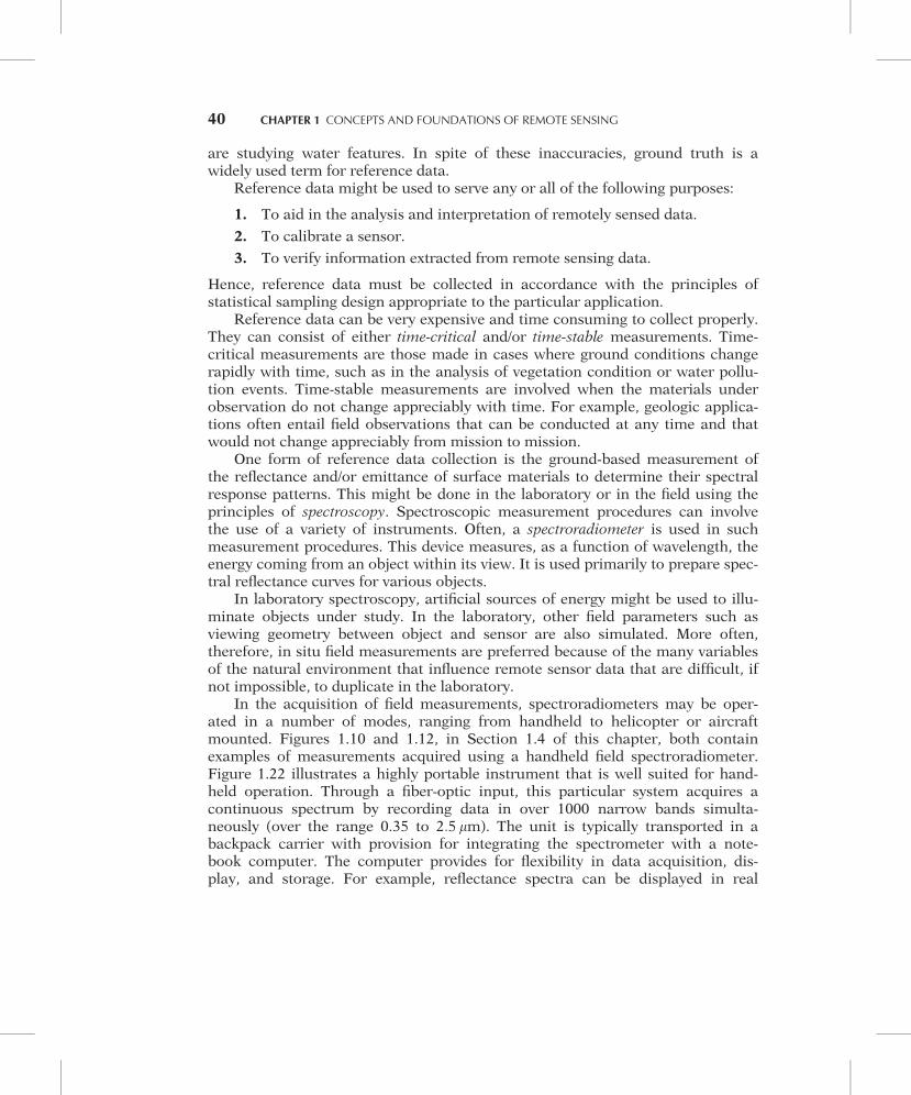
are studying water features. In spite of these inaccuracies, ground truth is awidely used term for reference data.

Reference data might be used to serve any or all of the following purposes:

1. To aid in the analysis and interpretation of remotely sensed data.

2. To calibrate a sensor.

3. To verify information extracted from remote sensing data.

Hence, reference data must be collected in accordance with the principles ofstatistical sampling design appropriate to the particular application.

Reference data can be very expensive and time consuming to collect properly.They can consist of either time-critical and/or time-stable measurements. Time-critical measurements are those made in cases where ground conditions changerapidly with time, such as in the analysis of vegetation condition or water pollu-tion events. Time-stable measurements are involved when the materials underobservation do not change appreciably with time. For example, geologic applica-tions often entail field observations that can be conducted at any time and thatwould not change appreciably from mission to mission.

One form of reference data collection is the ground-based measurement ofthe reflectance and/or emittance of surface materials to determine their spectralresponse patterns. This might be done in the laboratory or in the field using theprinciples of spectroscopy. Spectroscopic measurement procedures can involvethe use of a variety of instruments. Often, a spectroradiometer is used in suchmeasurement procedures. This device measures, as a function of wavelength, theenergy coming from an object within its view. It is used primarily to prepare spec-tral reflectance curves for various objects.

In laboratory spectroscopy, artificial sources of energy might be used to illu-minate objects under study. In the laboratory, other field parameters such asviewing geometry between object and sensor are also simulated. More often,therefore, in situ field measurements are preferred because of the many variablesof the natural environment that influence remote sensor data that are difficult, ifnot impossible, to duplicate in the laboratory.

In the acquisition of field measurements, spectroradiometers may be oper-ated in a number of modes, ranging from handheld to helicopter or aircraftmounted. Figures 1.10 and 1.12, in Section 1.4 of this chapter, both containexamples of measurements acquired using a handheld field spectroradiometer.Figure 1.22 illustrates a highly portable instrument that is well suited for hand-held operation. Through a fiber-optic input, this particular system acquires acontinuous spectrum by recording data in over 1000 narrow bands simulta-neously (over the range 0.35 to 2:5 mm). The unit is typically transported in abackpack carrier with provision for integrating the spectrometer with a note-book computer. The computer provides for flexibility in data acquisition, dis-play, and storage. For example, reflectance spectra can be displayed in real


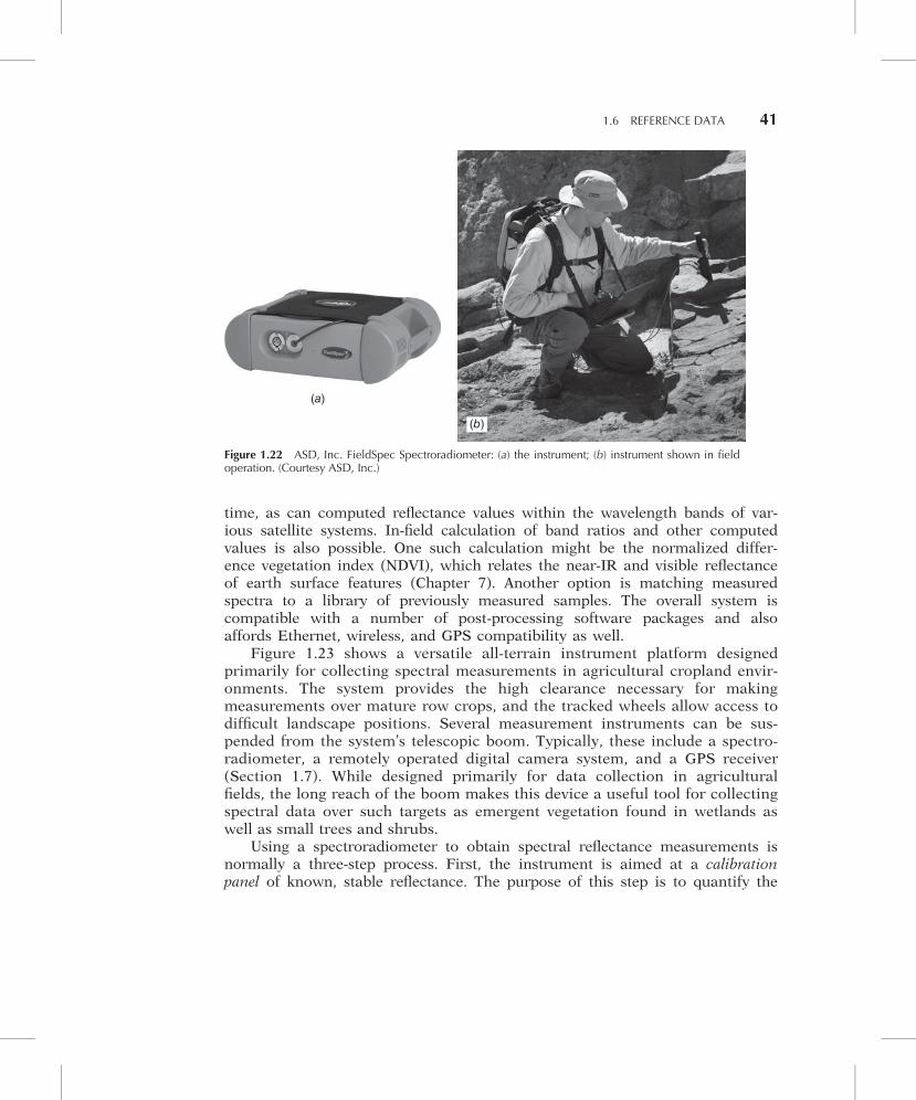
time, as can computed reflectance values within the wavelength bands of var-ious satellite systems. In-field calculation of band ratios and other computedvalues is also possible. One such calculation might be the normalized differ-ence vegetation index (NDVI), which relates the near-IR and visible reflectanceof earth surface features (Chapter 7). Another option is matching measuredspectra to a library of previously measured samples. The overall system iscompatible with a number of post-processing software packages and alsoaffords Ethernet, wireless, and GPS compatibility as well.

Figure 1.23 shows a versatile all-terrain instrument platform designedprimarily for collecting spectral measurements in agricultural cropland envir-onments. The system provides the high clearance necessary for makingmeasurements over mature row crops, and the tracked wheels allow access todifficult landscape positions. Several measurement instruments can be sus-pended from the system’s telescopic boom. Typically, these include a spectro-radiometer, a remotely operated digital camera system, and a GPS receiver(Section 1.7). While designed primarily for data collection in agriculturalfields, the long reach of the boom makes this device a useful tool for collectingspectral data over such targets as emergent vegetation found in wetlands aswell as small trees and shrubs.

Using a spectroradiometer to obtain spectral reflectance measurements isnormally a three-step process. First, the instrument is aimed at a calibrationpanel of known, stable reflectance. The purpose of this step is to quantify the

(a)

(b)

Figure 1.22 ASD, Inc. FieldSpec Spectroradiometer: (a) the instrument; (b) instrument shown in fieldoperation. (Courtesy ASD, Inc.)

1.6 REFERENCE DATA 41

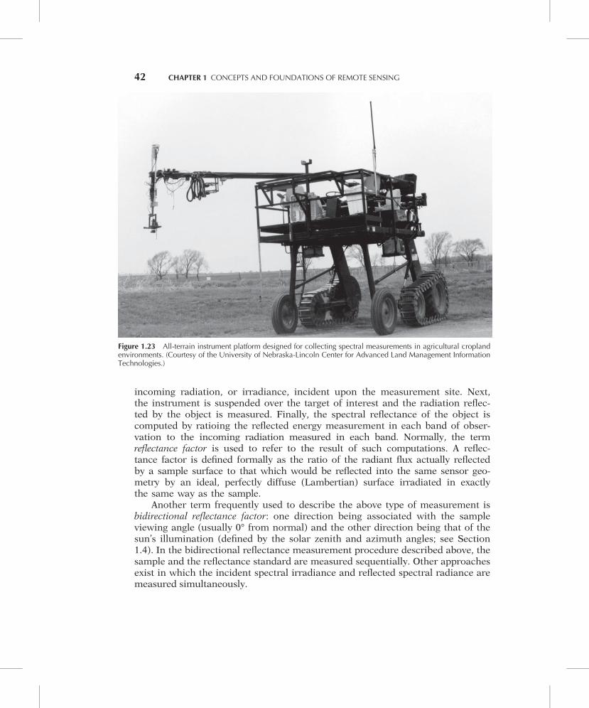
incoming radiation, or irradiance, incident upon the measurement site. Next,the instrument is suspended over the target of interest and the radiation reflec-ted by the object is measured. Finally, the spectral reflectance of the object iscomputed by ratioing the reflected energy measurement in each band of obser-vation to the incoming radiation measured in each band. Normally, the termreflectance factor is used to refer to the result of such computations. A reflec-tance factor is defined formally as the ratio of the radiant flux actually reflectedby a sample surface to that which would be reflected into the same sensor geo-metry by an ideal, perfectly diffuse (Lambertian) surface irradiated in exactlythe same way as the sample.

Another term frequently used to describe the above type of measurement isbidirectional reflectance factor: one direction being associated with the sampleviewing angle (usually 0° from normal) and the other direction being that of thesun’s illumination (defined by the solar zenith and azimuth angles; see Section1.4). In the bidirectional reflectance measurement procedure described above, thesample and the reflectance standard are measured sequentially. Other approachesexist in which the incident spectral irradiance and reflected spectral radiance aremeasured simultaneously.

Figure 1.23 All-terrain instrument platform designed for collecting spectral measurements in agricultural croplandenvironments. (Courtesy of the University of Nebraska-Lincoln Center for Advanced Land Management InformationTechnologies.)


1.7 THE GLOBAL POSITIONING SYSTEM AND OTHER GLOBALNAVIGATION SATELLITE SYSTEMS

As mentioned previously, the location of field-observed reference data is usuallydetermined using a global navigation satellite system (GNSS). GNSS technology is alsoused extensively in such other remote sensing activities as navigating aircraft duringsensor data acquisition and geometrically correcting and referencing raw image data.The first such system, the U.S. Global Positioning System (GPS) was originally devel-oped for military purposes, but has subsequently become ubiquitous in many civilapplications worldwide, from vehicle navigation to surveying, and location-based ser-vices on cellular phones and other personal electronic devices. Other GNSS “con-stellations” have been or are being developed as well, a trend that will greatly increasethe accuracy and reliability of GNSS for end-users over the next decade.

The U.S. Global Positioning System includes at least 24 satellites rotatingaround the earth in precisely known orbits, with subgroups of four or more satel-lites operating in each of six different orbit planes. Typically, these satellites revolvearound the earth approximately once every 12 hours, at an altitude of approximately20,200 km. With their positions in space precisely known at all times, the satellitestransmit time-encoded radio signals that are recorded by ground-based receiversand can be used to aid in positioning and navigation. The nearly circular orbitalplanes of the satellites are inclined about 60° from the equator and are spaced every60° in longitude. This means that, in the absence of obstructions from the terrain ornearby buildings, an observer at any point on the earth’s surface can receive the sig-nal from at least four GPS satellites at any given time (day or night).

International Status of GNSS Development

Currently, the U.S. Global Positioning System has only one operational counter-part, the Russian GLONASS system. The full GLONASS constellation consists of24 operational satellites, a number that was reached in October 2011. In addition, afully comprehensive European GNSS constellation, Galileo, is scheduled for com-pletion by 2020 and will include 30 satellites. The data signals provided by Galileowill be compatible with those from the U.S. GPS satellites, resulting in a greatlyincreased range of options for GNSS receivers and significantly improved accuracy.Finally, China has announced plans for the development of its own Compass GNSSconstellation, to include 30 satellites in operational use by 2020. The future forthese and similar systems is an extremely bright and rapidly progressing one.

GNSS Data Processing and Corrections

The means by which GNSS signals are used to determine ground positionsis called satellite ranging. Conceptually, the process simply involves measuring

1.7 THE GLOBAL POSITIONING SYSTEM 43

the time required for signals transmitted by at least four satellites to reach theground receiver. Knowing that the signals travel at the speed of light3 3 108m=sec in a vacuum� �

, the distance from each satellite to the receiver can becomputed using a form of three-dimensional triangulation. In principle, the signalsfrom only four satellites are needed to identify the receiver’s location, but in prac-tice it is usually desirable to obtain measurements from as many satellites aspractical.

GNSS measurements are potentially subject to numerous sources of error.These include clock bias (caused by imperfect synchronization between the high-precision atomic clocks present on the satellites and the lower-precision clocksused in GNSS receivers), uncertainties in the satellite orbits (known as satelliteephemeris errors), errors due to atmospheric conditions (signal velocity dependson time of day, season, and angular direction through the atmosphere), receivererrors (due to such influences as electrical noise and signal-matching errors), andmultipath errors (reflection of a portion of the transmitted signal from objects notin the straight-line path between the satellite and receiver).

Such errors can be compensated for (in great part) using differential GNSSmeasurement methods. In this approach, simultaneous measurements are madeby a stationary base station receiver (located over a point of precisely knownposition) and one (or more) roving receivers moving from point to point. Thepositional errors measured at the base station are used to refine the position mea-sured by the rover(s) at the same instant in time. This can be done either bybringing the data from the base and rover together in a post-processing modeafter the field observations are completed or by instantaneously broadcastingthe base station corrections to the rovers. The latter approach is termed real-timedifferential GNSS positioning.

In recent years, there have been efforts to improve the accuracy of GNSSpositioning through the development of regional networks of high-precision basestations, generally referred to as satellite-based augmentation systems (SBAS). Thedata from these stations are used to derive spatially explicit correction factorsthat are then broadcast in real time, allowing advanced receiver units to deter-mine their positions with a higher degree of accuracy. One such SBAS network,the Wide Area Augmentation System (WAAS), consists of approximately 25 groundreference stations distributed across the United States that continuously monitorGPS satellite transmissions. Two main stations, located on the U.S. east and westcoasts, collect the data from the reference stations and create a composited cor-rection message that is location specific. This message is then broadcast throughone of two geostationary satellites, satellites occupying a fixed position over theequator. Any WAAS-enabled GPS unit can receive these correction signals. TheGPS receiver then determines which correction data are appropriate at the cur-rent location.

The WAAS signal reception is ideal for open land, aircraft, and marine appli-cations, but the position of the relay satellites over the equator makes it difficultto receive the signals at high latitudes or when features such as trees and


mountains obstruct the view of the horizon. In such situations, GPS positions cansometimes actually contain more error with WAAS correction than without. How-ever, in unobstructed operating conditions where a strong WAAS signal is avail-able, positions are normally accurate to within 3 m or better.

Paralleling the deployment of the WAAS system in North America are theJapanese Multi-functional Satellite Augmentation System (MSAS) in Asia, theEuropean Geostationary Navigation Overlay Service (EGNOS) in Europe, and pro-posed future SBAS networks such as India’s GPS Aided Geo-Augmented Naviga-tion (GAGAN) system. Like WAAS, these SBAS systems use geostationarysatellites to transmit data for real-time differential correction.

In addition to the regional SBAS real-time correction systems such as WAAS,some nations have developed additional networks of base stations that can beused for post-processing GNSS data for differential correction (i.e., high-accuracycorrections made after data collection, rather than in real time). One such systemis the U.S. National Geodetic Survey’s Continuously Operating Reference Stations(CORS) network. More than 1800 sites in the cooperative CORS network provideGNSS reference data that can be accessed via the Internet and used in post-processing for differential correction.

With the development of new satellite constellations, and new resources forreal-time and post-processed differential correction, GNSS-based location ser-vices are expected to become even more widespread in industry, resource man-agement, and consumer technology applications in the coming years.

1.8 CHARACTERISTICS OF REMOTE SENSING SYSTEMS

Having introduced some basic concepts, we now have the elements necessary tocharacterize a remote sensing system. In so doing, we can begin to appreciatesome of the problems encountered in the design and application of the varioussensing systems examined in subsequent chapters. In particular, the design andoperation of every real-world sensing system represents a series of compromises,often in response to the limitations imposed by physics and by the current state oftechnological development. When we consider the process from start to finish,users of remote sensing systems need to keep in mind the following factors:

1. The energy source. All passive remote sensing systems rely on energythat originates from sources other than the sensor itself, typically in theform of either reflected radiation from the sun or emitted radiation fromearth surface features. As already discussed, the spectral distribution ofreflected sunlight and self-emitted energy is far from uniform. Solarenergy levels obviously vary with respect to time and location, and dif-ferent earth surface materials emit energy with varying degrees of effi-ciency. While we have some control over the sources of energy for activesystems such as radar and lidar, those sources have their own particular

1.8 CHARACTERISTICS OF REMOTE SENSING SYSTEMS 45

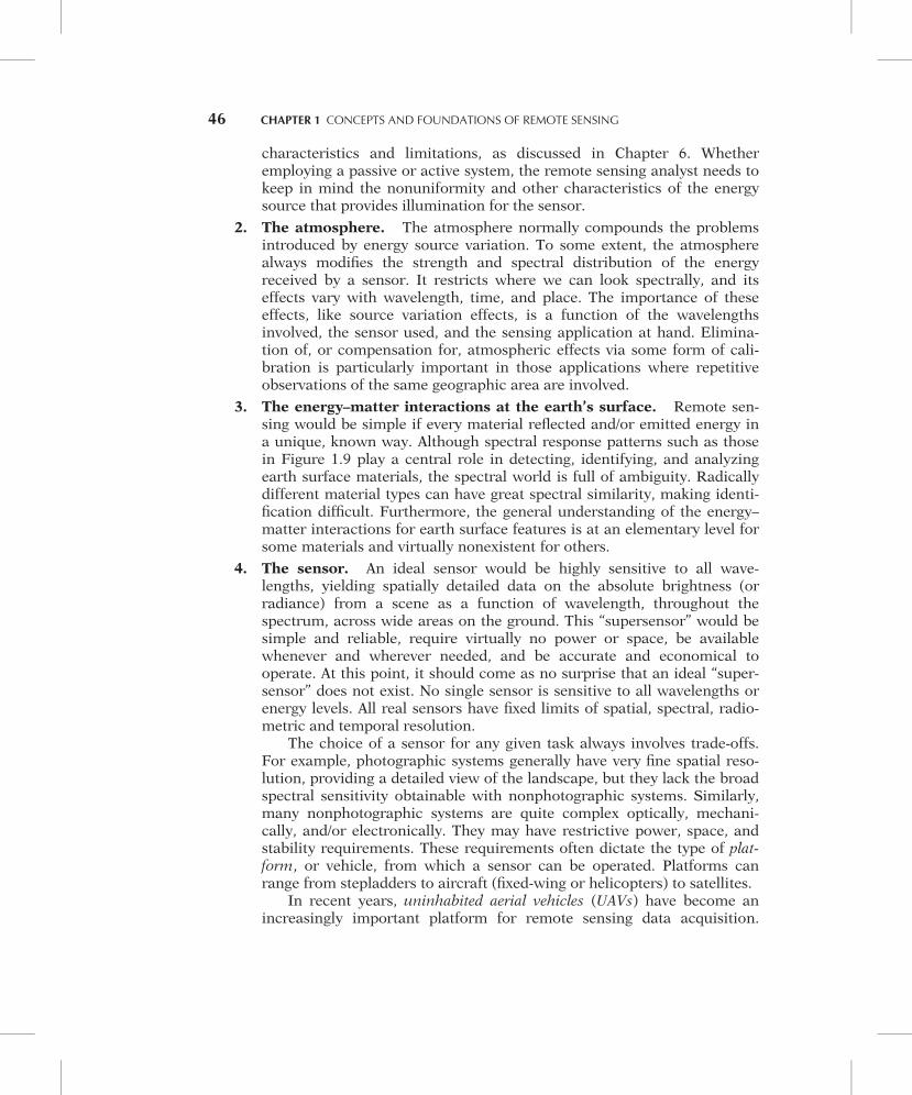
characteristics and limitations, as discussed in Chapter 6. Whetheremploying a passive or active system, the remote sensing analyst needs tokeep in mind the nonuniformity and other characteristics of the energysource that provides illumination for the sensor.

2. The atmosphere. The atmosphere normally compounds the problemsintroduced by energy source variation. To some extent, the atmospherealways modifies the strength and spectral distribution of the energyreceived by a sensor. It restricts where we can look spectrally, and itseffects vary with wavelength, time, and place. The importance of theseeffects, like source variation effects, is a function of the wavelengthsinvolved, the sensor used, and the sensing application at hand. Elimina-tion of, or compensation for, atmospheric effects via some form of cali-bration is particularly important in those applications where repetitiveobservations of the same geographic area are involved.

3. The energy–matter interactions at the earth’s surface. Remote sen-sing would be simple if every material reflected and/or emitted energy ina unique, known way. Although spectral response patterns such as thosein Figure 1.9 play a central role in detecting, identifying, and analyzingearth surface materials, the spectral world is full of ambiguity. Radicallydifferent material types can have great spectral similarity, making identi-fication difficult. Furthermore, the general understanding of the energy–matter interactions for earth surface features is at an elementary level forsome materials and virtually nonexistent for others.

4. The sensor. An ideal sensor would be highly sensitive to all wave-lengths, yielding spatially detailed data on the absolute brightness (orradiance) from a scene as a function of wavelength, throughout thespectrum, across wide areas on the ground. This “supersensor” would besimple and reliable, require virtually no power or space, be availablewhenever and wherever needed, and be accurate and economical tooperate. At this point, it should come as no surprise that an ideal “super-sensor” does not exist. No single sensor is sensitive to all wavelengths orenergy levels. All real sensors have fixed limits of spatial, spectral, radio-metric and temporal resolution.

The choice of a sensor for any given task always involves trade-offs.For example, photographic systems generally have very fine spatial reso-lution, providing a detailed view of the landscape, but they lack the broadspectral sensitivity obtainable with nonphotographic systems. Similarly,many nonphotographic systems are quite complex optically, mechani-cally, and/or electronically. They may have restrictive power, space, andstability requirements. These requirements often dictate the type of plat-form, or vehicle, from which a sensor can be operated. Platforms canrange from stepladders to aircraft (fixed-wing or helicopters) to satellites.

In recent years, uninhabited aerial vehicles (UAVs) have become anincreasingly important platform for remote sensing data acquisition.


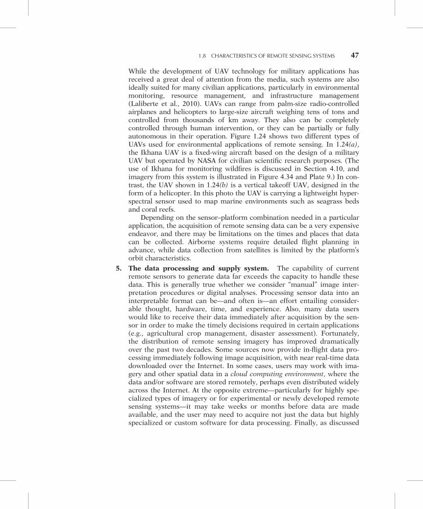
While the development of UAV technology for military applications hasreceived a great deal of attention from the media, such systems are alsoideally suited for many civilian applications, particularly in environmentalmonitoring, resource management, and infrastructure management(Laliberte et al., 2010). UAVs can range from palm-size radio-controlledairplanes and helicopters to large-size aircraft weighing tens of tons andcontrolled from thousands of km away. They also can be completelycontrolled through human intervention, or they can be partially or fullyautonomous in their operation. Figure 1.24 shows two different types ofUAVs used for environmental applications of remote sensing. In 1.24(a),the Ikhana UAV is a fixed-wing aircraft based on the design of a militaryUAV but operated by NASA for civilian scientific research purposes. (Theuse of Ikhana for monitoring wildfires is discussed in Section 4.10, andimagery from this system is illustrated in Figure 4.34 and Plate 9.) In con-trast, the UAV shown in 1.24(b) is a vertical takeoff UAV, designed in theform of a helicopter. In this photo the UAV is carrying a lightweight hyper-spectral sensor used to map marine environments such as seagrass bedsand coral reefs.

Depending on the sensor–platform combination needed in a particularapplication, the acquisition of remote sensing data can be a very expensiveendeavor, and there may be limitations on the times and places that datacan be collected. Airborne systems require detailed flight planning inadvance, while data collection from satellites is limited by the platform’sorbit characteristics.

5. The data processing and supply system. The capability of currentremote sensors to generate data far exceeds the capacity to handle thesedata. This is generally true whether we consider “manual” image inter-pretation procedures or digital analyses. Processing sensor data into aninterpretable format can be—and often is—an effort entailing consider-able thought, hardware, time, and experience. Also, many data userswould like to receive their data immediately after acquisition by the sen-sor in order to make the timely decisions required in certain applications(e.g., agricultural crop management, disaster assessment). Fortunately,the distribution of remote sensing imagery has improved dramaticallyover the past two decades. Some sources now provide in-flight data pro-cessing immediately following image acquisition, with near real-time datadownloaded over the Internet. In some cases, users may work with ima-gery and other spatial data in a cloud computing environment, where thedata and/or software are stored remotely, perhaps even distributed widelyacross the Internet. At the opposite extreme—particularly for highly spe-cialized types of imagery or for experimental or newly developed remotesensing systems—it may take weeks or months before data are madeavailable, and the user may need to acquire not just the data but highlyspecialized or custom software for data processing. Finally, as discussed

1.8 CHARACTERISTICS OF REMOTE SENSING SYSTEMS 47

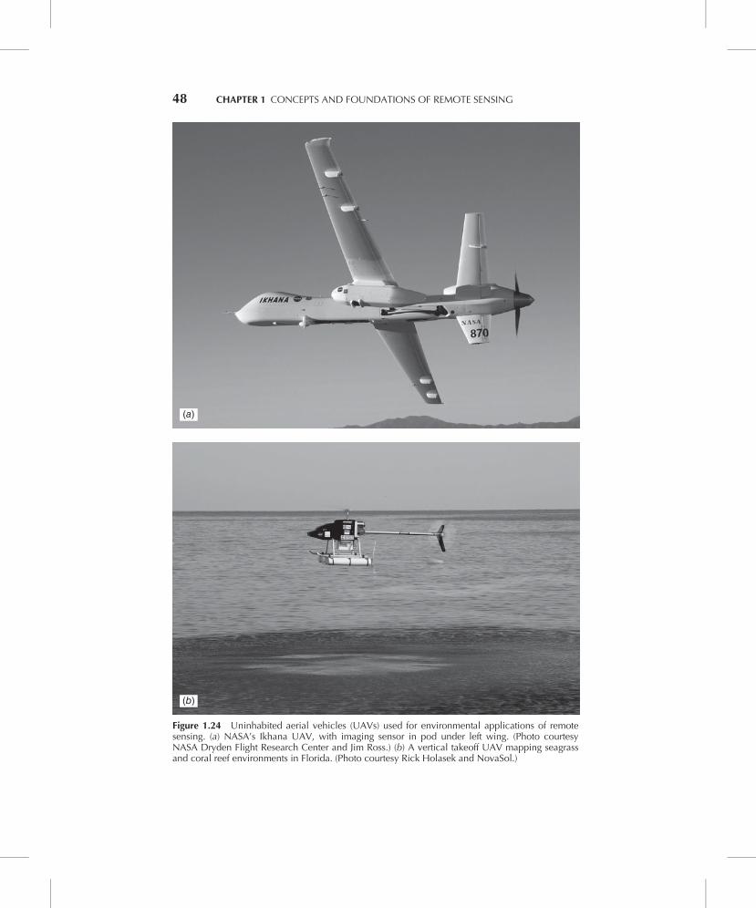
(a)

(b)

Figure 1.24 Uninhabited aerial vehicles (UAVs) used for environmental applications of remotesensing. (a) NASA’s Ikhana UAV, with imaging sensor in pod under left wing. (Photo courtesyNASA Dryden Flight Research Center and Jim Ross.) (b) A vertical takeoff UAV mapping seagrassand coral reef environments in Florida. (Photo courtesy Rick Holasek and NovaSol.)


in Section 1.6, most remote sensing applications require the collectionand analysis of additional reference data, an operation that may be com-plex, expensive, and time consuming.

6. The users of remotely sensed data. Central to the successful applica-tion of any remote sensing system is the person (or persons) using theremote sensor data from that system. The “data” generated by remotesensing procedures become “information” only if and when someoneunderstands their generation, knows how to interpret them, and knowshow best to use them. A thorough understanding of the problem at hand isparamount to the productive application of any remote sensing methodol-ogy. Also, no single combination of data acquisition and analysis proce-dures will satisfy the needs of all data users.

Whereas the interpretation of aerial photography has been used as a practicalresource management tool for nearly a century, other forms of remote sensing arerelatively new, technically complex, and unconventional means of acquiringinformation. In earlier years, these newer forms of remote sensing had relativelyfew satisfied users. Since the late 1990s, however, as new applications continue tobe developed and implemented, increasing numbers of users are becoming awareof the potentials, as well as the limitations, of remote sensing techniques. As aresult, remote sensing has become an essential tool in many aspects of science,government, and business alike.

One factor in the increasing acceptance of remote sensing imagery by end-users has been the development and widespread adoption of easy-to-use geo-visualization systems such as Google Maps and Earth, NASA’s WorldWinds, andother web-based image services. By allowing more potential users to becomecomfortable and familiar with the day-to-day use of aerial and satellite imagery,these and other software tools have facilitated the expansion of remote sensinginto new application areas.

1.9 SUCCESSFUL APPLICATION OF REMOTE SENSING

The student should now begin to appreciate that successful use of remote sensingis premised on the integration of multiple, interrelated data sources and analysisprocedures. No single combination of sensor and interpretation procedure isappropriate to all applications. The key to designing a successful remote sensingeffort involves, at a minimum, (1) clear definition of the problem at hand, (2) eva-luation of the potential for addressing the problem with remote sensing techni-ques, (3) identification of the remote sensing data acquisition proceduresappropriate to the task, (4) determination of the data interpretation procedures tobe employed and the reference data needed, and (5) identification of the criteriaby which the quality of information collected can be judged.

1.9 SUCCESSFUL APPLICATION OF REMOTE SENSING 49

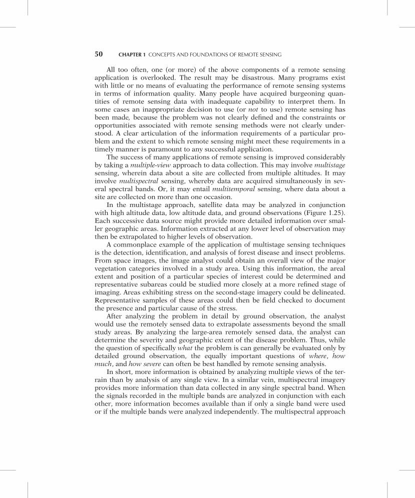
All too often, one (or more) of the above components of a remote sensingapplication is overlooked. The result may be disastrous. Many programs existwith little or no means of evaluating the performance of remote sensing systemsin terms of information quality. Many people have acquired burgeoning quan-tities of remote sensing data with inadequate capability to interpret them. Insome cases an inappropriate decision to use (or not to use) remote sensing hasbeen made, because the problem was not clearly defined and the constraints oropportunities associated with remote sensing methods were not clearly under-stood. A clear articulation of the information requirements of a particular pro-blem and the extent to which remote sensing might meet these requirements in atimely manner is paramount to any successful application.

The success of many applications of remote sensing is improved considerablyby taking a multiple-view approach to data collection. This may involve multistagesensing, wherein data about a site are collected from multiple altitudes. It mayinvolve multispectral sensing, whereby data are acquired simultaneously in sev-eral spectral bands. Or, it may entail multitemporal sensing, where data about asite are collected on more than one occasion.

In the multistage approach, satellite data may be analyzed in conjunctionwith high altitude data, low altitude data, and ground observations (Figure 1.25).Each successive data source might provide more detailed information over smal-ler geographic areas. Information extracted at any lower level of observation maythen be extrapolated to higher levels of observation.

A commonplace example of the application of multistage sensing techniquesis the detection, identification, and analysis of forest disease and insect problems.From space images, the image analyst could obtain an overall view of the majorvegetation categories involved in a study area. Using this information, the arealextent and position of a particular species of interest could be determined andrepresentative subareas could be studied more closely at a more refined stage ofimaging. Areas exhibiting stress on the second-stage imagery could be delineated.Representative samples of these areas could then be field checked to documentthe presence and particular cause of the stress.

After analyzing the problem in detail by ground observation, the analystwould use the remotely sensed data to extrapolate assessments beyond the smallstudy areas. By analyzing the large-area remotely sensed data, the analyst candetermine the severity and geographic extent of the disease problem. Thus, whilethe question of specifically what the problem is can generally be evaluated only bydetailed ground observation, the equally important questions of where, howmuch, and how severe can often be best handled by remote sensing analysis.

In short, more information is obtained by analyzing multiple views of the ter-rain than by analysis of any single view. In a similar vein, multispectral imageryprovides more information than data collected in any single spectral band. Whenthe signals recorded in the multiple bands are analyzed in conjunction with eachother, more information becomes available than if only a single band were usedor if the multiple bands were analyzed independently. The multispectral approach


forms the heart of numerous remote sensing applications involving discrimina-tion of earth resource types, cultural features, and their condition.

Again, multitemporal sensing involves sensing the same area at multipletimes and using changes occurring with time as discriminants of ground condi-tions. This approach is frequently taken to monitor land use change, such as sub-urban development in urban fringe areas. In fact, regional land use surveys mightcall for the acquisition of multisensor, multispectral, multistage, multitemporaldata to be used for multiple purposes!

In any approach to applying remote sensing, not only must the right mix ofdata acquisition and data interpretation techniques be chosen, but the right mixof remote sensing and “conventional” techniques must also be identified. The stu-dent must recognize that remote sensing is a tool best applied in concert withothers; it is not an end in itself. In this regard, remote sensing data are currently

Figure 1.25 Multistage remote sensing concept.

1.9 SUCCESSFUL APPLICATION OF REMOTE SENSING 51

being used extensively in computer-based GISs (Section 1.10). The GIS environ-ment permits the synthesis, analysis, and communication of virtually unlimitedsources and types of biophysical and socioeconomic data—as long as they can begeographically referenced. Remote sensing can be thought of as the “eyes” of suchsystems providing repeated, synoptic (even global) visions of earth resources froman aerial or space vantage point.

Remote sensing affords us the capability to literally see the invisible. Wecan begin to see components of the environment on an ecosystem basis, in thatremote sensing data can transcend the cultural boundaries within which much ofour current resource data are collected. Remote sensing also transcends dis-ciplinary boundaries. It is so broad in its application that nobody “owns” the field.Important contributions are made to—and benefits derived from—remote sensingby both the “hard” scientist interested in basic research and the “soft” scientistinterested in its operational application.

There is little question that remote sensing will continue to play an increas-ingly broad and important role in the scientific, governmental, and commercialsectors alike. The technical capabilities of sensors, space platforms, data commu-nication and distribution systems, GPSs, digital image processing systems, andGISs are improving on almost a daily basis. At the same time, we are witnessingthe evolution of a spatially enabled world society. Most importantly, we arebecoming increasingly aware of how interrelated and fragile the elements of ourglobal resource base really are and of the role that remote sensing can play ininventorying, monitoring, and managing earth resources and in modeling andhelping us to better understand the global ecosystem and its dynamics.

1.10 GEOGRAPHIC INFORMATION SYSTEMS (GIS)

We anticipate that the majority of individuals using this book will at some pointin their educational backgrounds and/or professional careers have experiencewith geographic information systems. The discussion below is provided as a briefintroduction to such systems primarily for those readers who might lack suchbackground.

Geographic information systems are computer-based systems that can dealwith virtually any type of information about features that can be referenced by geo-graphical location. These systems are capable of handling both locational data andattribute data about such features. That is, not only do GISs permit the automatedmapping or display of the locations of features, but also these systems provide acapability for recording and analyzing descriptive characteristics (“attributes”) ofthe features. For example, a GIS might contain not only a map of the locations ofroads but also a database of descriptors about each road. These attributes mightinclude information such as road width, pavement type, speed limit, number oftraffic lanes, date of construction, and so on. Table 1.1 lists other examples of attri-butes that might be associated with a given point, line, or area feature.


The data in a GIS may be kept in individual standalone files (e.g., “shape-files”), but increasingly a geodatabase is used to store and manage spatial data.This is a type of relational database, consisting of tables with attributes in columnsand data records in rows (Table 1.2), and explicitly including locational informa-tion for each record. While database implementations vary, there are certaindesirable characteristics that will improve the utility of a database in a GIS. Thesecharacteristics include flexibility, to allow a wide range of database queries andoperations; reliability, to avoid accidental loss of data; security, to limit access toauthorized users; and ease of use, to insulate the end user from the details of thedatabase implementation.

One of the most important benefits of a GIS is the ability to spatially inter-relate multiple types of information stemming from a range of sources. This con-cept is illustrated in Figure 1.26, where we have assumed that a hydrologistwishes to use a GIS to study soil erosion in a watershed. As shown, the systemcontains data from a range of source maps (a) that have been geocoded on a cell-by-cell basis to form a series of layers (b), all in geographic registration. The ana-lyst can then manipulate and overlay the information contained in, or derivedfrom, the various data layers. In this example, we assume that assessing thepotential for soil erosion throughout the watershed involves the simultaneouscell-by-cell consideration of three types of data derived from the original data lay-ers: slope, soil erodibility, and surface runoff potential. The slope information canbe computed from the elevations in the topography layer. The erodibility, whichis an attribute associated with each soil type, can be extracted from a relationaldatabase management system incorporated in the GIS. Similarly, the runoffpotential is an attribute associated with each land cover type (land cover data can

TABLE 1.1 Example Point, Line, and Area Features and Typical AttributesContained in a GISa

Point feature Well (depth, chemical constituency)Line feature Power line (service capacity, age, insulator type)Area feature Soil mapping unit (soil type, texture, color, permeability)

aAttributes shown in parentheses.

TABLE 1.2 Relational Database Table Format

ID Numbera Street Name Lanes Parking Repair Date . . .

143897834 “Maple Ct” 2 Yes 2012/06/10 . . .637292842 “North St” 2 Seasonal 2006/08/22 . . .347348279 “Main St” 4 Yes 2015/05/15 . . .234538020 “Madison Ave” 4 No 2014/04/20 . . .

aEach data record, or “tuple,” has a unique identification, or ID, number.

1.10 GEOGRAPHIC INFORMATION SYSTEMS (GIS) 53

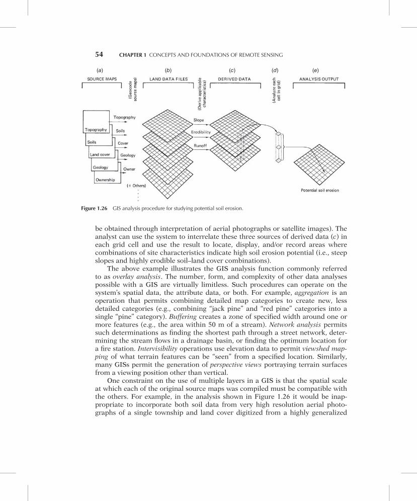
be obtained through interpretation of aerial photographs or satellite images). Theanalyst can use the system to interrelate these three sources of derived data (c) ineach grid cell and use the result to locate, display, and/or record areas wherecombinations of site characteristics indicate high soil erosion potential (i.e., steepslopes and highly erodible soil–land cover combinations).

The above example illustrates the GIS analysis function commonly referredto as overlay analysis. The number, form, and complexity of other data analysespossible with a GIS are virtually limitless. Such procedures can operate on thesystem’s spatial data, the attribute data, or both. For example, aggregation is anoperation that permits combining detailed map categories to create new, lessdetailed categories (e.g., combining “jack pine” and “red pine” categories into asingle “pine” category). Buffering creates a zone of specified width around one ormore features (e.g., the area within 50 m of a stream). Network analysis permitssuch determinations as finding the shortest path through a street network, deter-mining the stream flows in a drainage basin, or finding the optimum location fora fire station. Intervisibility operations use elevation data to permit viewshed map-ping of what terrain features can be “seen” from a specified location. Similarly,many GISs permit the generation of perspective views portraying terrain surfacesfrom a viewing position other than vertical.

One constraint on the use of multiple layers in a GIS is that the spatial scaleat which each of the original source maps was compiled must be compatible withthe others. For example, in the analysis shown in Figure 1.26 it would be inap-propriate to incorporate both soil data from very high resolution aerial photo-graphs of a single township and land cover digitized from a highly generalized

(a) (b) (c) (d) (e)

Figure 1.26 GIS analysis procedure for studying potential soil erosion.


map of the entire nation. Another common constraint is that the compilationdates of different source maps must be reasonably close in time. For example, aGIS analysis of wildlife habitat might yield incorrect conclusions if it were basedon land cover data that are many years out of date. On the other hand, since othertypes of spatial data are less changeable over time, the map compilation datemight not be as important for a layer such as topography or bedrock geology.

Most GISs use two primary approaches to represent the locational compo-nent of geographic information: a raster (grid-based) or vector (point-based) for-mat. The raster data model that was used in our soil erosion example is illustratedin Figure 1.27b. In this approach, the location of geographic objects or conditionsis defined by the row and column position of the cells they occupy. The valuestored for each cell indicates the type of object or condition that is found at thatlocation over the entire cell. Note that the finer the grid cell size used, the moregeographic specificity there is in the data file. A coarse grid requires less data sto-rage space but will provide a less precise geographic description of the originaldata. Also, when using a very coarse grid, several data types and/or attributes mayoccur in each cell, but the cell is still usually treated as a single homogeneous unitduring analysis.

The vector data model is illustrated in Figure 1.27c. Using this format, featureboundaries are converted to straight-sided polygons that approximate the originalregions. These polygons are encoded by determining the coordinates of theirvertices, called points or nodes, which can be connected to form lines or arcs.Topological coding includes “intelligence” in the data structure relative to thespatial relationship (connectivity and adjacency) among features. For example,topological coding keeps track of which arcs share common nodes and whatpolygons are to the left and right of a given arc. This information facilitates suchspatial operations as overlay analysis, buffering, and network analysis.

Raster and vector data models each have their advantages and disadvantages.Raster systems tend to have simpler data structures; they afford greater computa-tional efficiency in such operations as overlay analysis; and they represent

(a) (b) (c)

Figure 1.27 Raster versus vector data formats: (a) landscape patches, (b) landscaperepresented in raster format, and (c) landscape represented in vector format.

1.10 GEOGRAPHIC INFORMATION SYSTEMS (GIS) 55

features having high spatial variability and/or “blurred boundaries” (e.g., betweenpure and mixed vegetation zones) more effectively. On the other hand, raster datavolumes are relatively greater; the spatial resolution of the data is limited to thesize of the cells comprising the raster; and the topological relationships amongspatial features are more difficult to represent. Vector data formats have theadvantages of relatively lower data volumes, better spatial resolution, and the pre-servation of topological data relationships (making such operations as networkanalysis more efficient). However, certain operations (e.g., overlay analysis) aremore complex computationally in a vector data format than in a raster format.

As we discuss frequently throughout this book, digital remote sensing imagesare collected in a raster format. Accordingly, digital images are inherently compa-tible spatially with other sources of information in a raster domain. Becauseof this, “raw” images can be easily included directly as layers in a raster-basedGIS. Likewise, such image processing procedures as automated land cover classi-fication (Chapter 7) result in the creation of interpreted or derived data files in araster format. These derived data are again inherently compatible with the othersources of data represented in a raster format. This concept is illustrated inPlate 2, in which we return to our earlier example of using overlay analysis toassist in soil erosion potential mapping for an area in western Dane County, Wis-consin. Shown in (a) is an automated land cover classification that was producedby processing Landsat Thematic Mapper (TM) data of the area. (See Chapter 7 foradditional information on computer-based land cover classification.) To assessthe soil erosion potential in this area, the land cover data were merged with infor-mation on the intrinsic erodibility of the soil present (b) and with land surfaceslope information (c). These latter forms of information were already resident in aGIS covering the area. Hence, all data could be combined for analysis in a mathe-matical model, producing the soil erosion potential map shown in (d). To assistthe viewer in interpreting the landscape patterns shown in Plate 2, the GIS wasalso used to visually enhance the four data sets with topographic shading basedon a DEM, providing a three-dimensional appearance.

For the land cover classification in Plate 2a, water is shown as dark blue, non-forested wetlands as light blue, forested wetlands as pink, corn as orange, otherrow crops as pale yellow, forage crops as olive, meadows and grasslands asyellow-green, deciduous forest as green, evergreen forest as dark green, low-intensity urban areas as light gray, and high-intensity urban areas as dark gray. In(b), areas of low soil erodibility are shown in dark brown, with increasing soilerodibility indicated by colors ranging from orange to tan. In (c), areas of increas-ing steepness of slope are shown as green, yellow, orange, and red. The soilerosion potential map (d) shows seven colors depicting seven levels of potentialsoil erosion. Areas having the highest erosion potential are shown in dark red.These areas tend to have row crops growing on inherently erodible soils withsloping terrain. Decreasing erosion potential is shown in a spectrum of colorsfrom orange through yellow to green. Areas with the lowest erosion potential are


indicated in dark green. These include forested regions, continuous-cover crops,and grasslands growing on soils with low inherent erodibility, and flat terrain.

Remote sensing images (and information extracted from such images), alongwith GPS data, have become primary data sources for modern GISs. Indeed, theboundaries between remote sensing, GIS, and GPS technology have becomeblurred, and these combined fields will continue to revolutionize how we inven-tory, monitor, and manage natural resources on a day-to-day basis. Likewise,these technologies are assisting us in modeling and understanding biophysicalprocesses at all scales of inquiry. They are also permitting us to develop andcommunicate cause-and-effect “what-if” scenarios in a spatial context in waysnever before possible.

1.11 SPATIAL DATA FRAMEWORKS FOR GIS AND REMOTESENSING

If one is examining an image purely on its own, with no reference to any outsidesource of spatial information, there may be no need to consider the type of coor-dinate system used to represent locations within the image. In many cases, how-ever, analysts will be comparing points in the image to GPS-located referencedata, looking for differences between two images of the same area, or importingan image into a GIS for quantitative analysis. In all these cases, it is necessaryto know how the column and row coordinates of the image relate to some real-world map coordinate system.

Because the shape of the earth is approximately spherical, locations on theearth’s surface are often described in an angular coordinate or geographical sys-tem, with latitude and longitude specified in degrees (°), minutes (0), and seconds(00). This system originated in ancient Greece, and it is familiar to many peopletoday. Unfortunately, the calculation of distances and areas in an angular coordi-nate system is complex. More significantly, it is impossible to accurately representthe three-dimensional surface of the earth on the two-dimensional planar surfaceof a map or image without introducing distortion in one or more of the followingelements: shape, size, distance, and direction. Thus, for many purposes we wishto mathematically transform angular geographical coordinates into a planar, orCartesian X –Yð Þ coordinate system. The result of this transformation process isreferred to as a map projection.

While many types of map projections have been defined, they can be groupedinto several broad categories based either on the geometric models used or onthe spatial properties that are preserved or distorted by the transformation.Geometric models for map projection include cylindrical, conic, and azimuthalor planar surfaces. From a map user’s perspective, the spatial properties ofmap projections may be more important than the geometric model used. A con-formal map projection preserves angular relationships, or shapes, within local

1.11 SPATIAL DATA FRAMEWORKS FOR GIS AND REMOTE SENSING 57

areas; over large areas, angles and shapes become distorted. An azimuthal (orzenithal) projection preserves absolute directions relative to the central point ofprojection. An equidistant projection preserves equal distances, for some but notall points—scale is constant either for all distances along meridians or for all dis-tances from one or two points. An equal-area (or equivalent) projection preservesequal areas. Because a detailed explanation of the relationships among theseproperties is beyond the scope of this discussion, suffice it to say that no two-dimensional map projection can accurately preserve all of these properties, butcertain subsets of these characteristics can be preserved in a single projection.For example, the azimuthal equidistant projection preserves both direction anddistance—but only relative to the central point of the projection; directions anddistances between other points are not preserved.

In addition to the map projection associated with a given image, GIS datalayer, or other spatial data set, it is also often necessary to consider the datumused with that map projection. A datum is a mathematical definition of the three-dimensional solid (generally a slightly flattened ellipsoid) used to represent thesurface of the earth. The actual planet itself has an irregular shape that doesnot correspond perfectly to any ellipsoid. As a result, a variety of different datumshave been described; some designed to fit the surface well in one particularregion (such as the North American Datum of 1983, or NAD83) and othersdesigned to best approximate the planet as a whole. Most GISs require that both amap projection and a datum be specified before performing any coordinatetransformations.

To apply these concepts to the process of collecting and working with remo-tely sensed images, most such images are initially acquired with rows and col-umns of pixels aligned with the flight path (or orbit track) of the imagingplatform, be it a satellite, an aircraft, or a UAV. Before the images can be mapped,or used in combination with other spatial data, they need to be georeferenced. His-torically, this process typically involved identification of visible control pointswhose true geographic coordinates were known. A mathematical model wouldthen be used to transform the row and column coordinates of the raw image intoa defined map coordinate system. In recent years, remote sensing platforms havebeen outfitted with sophisticated systems to record their exact position and angu-lar orientation. These systems, incorporating an inertial measurement unit (IMU)and/or multiple onboard GPS units, enable highly precise modeling of the viewinggeometry of the sensor, which in turn is used for direct georeferencing of the sen-sor data—relating them to a defined map projection without the necessity of addi-tional ground control points.

Once an image has been georeferenced, it may be ready for use with otherspatial information. On the other hand, some images may have further geometricdistortions, perhaps caused by varying terrain, or other factors. To remove thesedistortions, it may be necessary to orthorectify the imagery, a process discussedin Chapters 3 and 7.


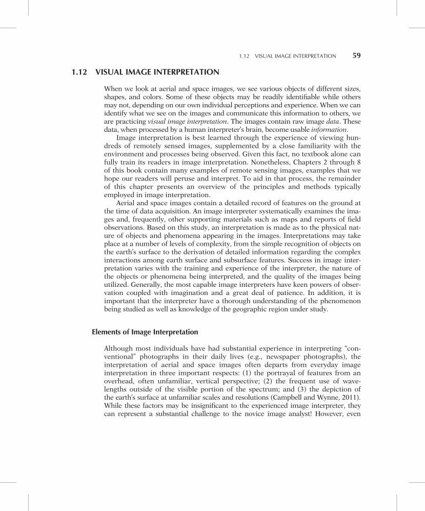
1.12 VISUAL IMAGE INTERPRETATION

When we look at aerial and space images, we see various objects of different sizes,shapes, and colors. Some of these objects may be readily identifiable while othersmay not, depending on our own individual perceptions and experience. When we canidentify what we see on the images and communicate this information to others, weare practicing visual image interpretation. The images contain raw image data. Thesedata, when processed by a human interpreter’s brain, become usable information.

Image interpretation is best learned through the experience of viewing hun-dreds of remotely sensed images, supplemented by a close familiarity with theenvironment and processes being observed. Given this fact, no textbook alone canfully train its readers in image interpretation. Nonetheless, Chapters 2 through 8of this book contain many examples of remote sensing images, examples that wehope our readers will peruse and interpret. To aid in that process, the remainderof this chapter presents an overview of the principles and methods typicallyemployed in image interpretation.

Aerial and space images contain a detailed record of features on the ground atthe time of data acquisition. An image interpreter systematically examines the ima-ges and, frequently, other supporting materials such as maps and reports of fieldobservations. Based on this study, an interpretation is made as to the physical nat-ure of objects and phenomena appearing in the images. Interpretations may takeplace at a number of levels of complexity, from the simple recognition of objects onthe earth’s surface to the derivation of detailed information regarding the complexinteractions among earth surface and subsurface features. Success in image inter-pretation varies with the training and experience of the interpreter, the nature ofthe objects or phenomena being interpreted, and the quality of the images beingutilized. Generally, the most capable image interpreters have keen powers of obser-vation coupled with imagination and a great deal of patience. In addition, it isimportant that the interpreter have a thorough understanding of the phenomenonbeing studied as well as knowledge of the geographic region under study.

Elements of Image Interpretation

Although most individuals have had substantial experience in interpreting “con-ventional” photographs in their daily lives (e.g., newspaper photographs), theinterpretation of aerial and space images often departs from everyday imageinterpretation in three important respects: (1) the portrayal of features from anoverhead, often unfamiliar, vertical perspective; (2) the frequent use of wave-lengths outside of the visible portion of the spectrum; and (3) the depiction ofthe earth’s surface at unfamiliar scales and resolutions (Campbell and Wynne, 2011).While these factors may be insignificant to the experienced image interpreter, theycan represent a substantial challenge to the novice image analyst! However, even

1.12 VISUAL IMAGE INTERPRETATION 59

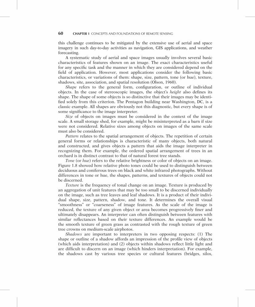
this challenge continues to be mitigated by the extensive use of aerial and spaceimagery in such day-to-day activities as navigation, GIS applications, and weatherforecasting.

A systematic study of aerial and space images usually involves several basiccharacteristics of features shown on an image. The exact characteristics usefulfor any specific task and the manner in which they are considered depend on thefield of application. However, most applications consider the following basiccharacteristics, or variations of them: shape, size, pattern, tone (or hue), texture,shadows, site, association, and spatial resolution (Olson, 1960).

Shape refers to the general form, configuration, or outline of individualobjects. In the case of stereoscopic images, the object’s height also defines itsshape. The shape of some objects is so distinctive that their images may be identi-fied solely from this criterion. The Pentagon building near Washington, DC, is aclassic example. All shapes are obviously not this diagnostic, but every shape is ofsome significance to the image interpreter.

Size of objects on images must be considered in the context of the imagescale. A small storage shed, for example, might be misinterpreted as a barn if sizewere not considered. Relative sizes among objects on images of the same scalemust also be considered.

Pattern relates to the spatial arrangement of objects. The repetition of certaingeneral forms or relationships is characteristic of many objects, both naturaland constructed, and gives objects a pattern that aids the image interpreter inrecognizing them. For example, the ordered spatial arrangement of trees in anorchard is in distinct contrast to that of natural forest tree stands.

Tone (or hue) refers to the relative brightness or color of objects on an image.Figure 1.8 showed how relative photo tones could be used to distinguish betweendeciduous and coniferous trees on black and white infrared photographs. Withoutdifferences in tone or hue, the shapes, patterns, and textures of objects could notbe discerned.

Texture is the frequency of tonal change on an image. Texture is produced byan aggregation of unit features that may be too small to be discerned individuallyon the image, such as tree leaves and leaf shadows. It is a product of their indivi-dual shape, size, pattern, shadow, and tone. It determines the overall visual“smoothness” or “coarseness” of image features. As the scale of the image isreduced, the texture of any given object or area becomes progressively finer andultimately disappears. An interpreter can often distinguish between features withsimilar reflectances based on their texture differences. An example would bethe smooth texture of green grass as contrasted with the rough texture of greentree crowns on medium-scale airphotos.

Shadows are important to interpreters in two opposing respects: (1) Theshape or outline of a shadow affords an impression of the profile view of objects(which aids interpretation) and (2) objects within shadows reflect little light andare difficult to discern on an image (which hinders interpretation). For example,the shadows cast by various tree species or cultural features (bridges, silos,


towers, poles, etc.) can definitely aid in their identification on airphotos. In somecases, the shadows cast by large animals can aid in their identification. Figure 1.28is a large-scale aerial photograph taken under low sun angle conditions that showscamels and their shadows in Saudi Arabia. Note that the camels themselves can beseen at the “base” of their shadows. Without the shadows, the animals couldbe counted, but identifying them specifically as camels could be difficult. Also, theshadows resulting from subtle variations in terrain elevations, especially in thecase of low sun angle images, can aid in assessing natural topographic variationsthat may be diagnostic of various geologic landforms.

As a general rule, the shape of the terrain is more easily interpreted when sha-dows fall toward the observer. This is especially true when images are examinedmonoscopically, where relief cannot be seen directly, as it can be in stereoscopicimages. In Figure 1.29a, a large ridge with numerous side valleys can be seen inthe center of the image. When this image is inverted (i.e., turned such that theshadows fall away from the observer), as in (b), the result is a confusing imagethat almost seems to have a valley of sorts running through the center of theimage (from bottom to top). This arises because one “expects” light sources togenerally be above objects (ASPRS, 1997, p. 73). The orientation of shadows withrespect to the observer is less important for interpreting images of buildings,trees, or animals (as in Figure 1.28) than for interpreting the terrain.

Site refers to topographic or geographic location and is a particularly impor-tant aid in the identification of vegetation types. For example, certain tree specieswould be expected to occur on well-drained upland sites, whereas other tree spe-cies would be expected to occur on poorly drained lowland sites. Also, varioustree species occur only in certain geographic areas (e.g., redwoods occur inCalifornia, but not in Indiana).

Figure 1.28 Vertical aerial photograph showing camels that cast longshadows under a low sun angle in Saudi Arabia. Black-and-whiterendition of color original. (© George Steinmetz/Corbis.)


Association refers to the occurrence of certain features in relation to others.For example, a Ferris wheel might be difficult to identify if standing in a fieldnear a barn but would be easy to identify if in an area recognized as an amuse-ment park.

Spatial resolution depends on many factors, but it always places a practicallimit on interpretation because some objects are too small or have too little con-trast with their surroundings to be clearly seen on the image.

Other factors, such as image scale, spectral resolution, radiometric resolution,date of acquisition, and even the condition of images (e.g., torn or faded historicalphotographic prints) also affect the success of image interpretation activities.

Many of the above elements of image interpretation are illustrated inFigure 1.30. Figure 1.30a is a nearly full-scale copy of a 230 3 230-mm airphotothat was produced at an original scale of 1:28,000 (or 1 cm¼ 280m). Parts (b)through (e) of Figure 1.30 show four scenes extracted and enlarged from this air-photo. Among the land cover types in Figure 1.30b are water, trees, suburbanhouses, grass, a divided highway, and a drive-in theater. Most of the land covertypes are easily identified in this figure. The drive-in theater could be difficult forinexperienced interpreters to identify, but a careful study of the elements ofimage interpretation leads to its identification. It has a unique shape and pattern.Its size is consistent with a drive-in theater (note the relative size of the cars on

(a) (b)

Figure 1.29 Photograph illustrating the effect of shadow direction on the interpretability of terrain. Islandof Kauai, Hawaii, mid-January. Scale 1:48,000. (a) Shadows falling toward observer, (b) same image turnedsuch that shadows are falling away from observer. (Courtesy USDA–ASCS panchromatic photograph.)


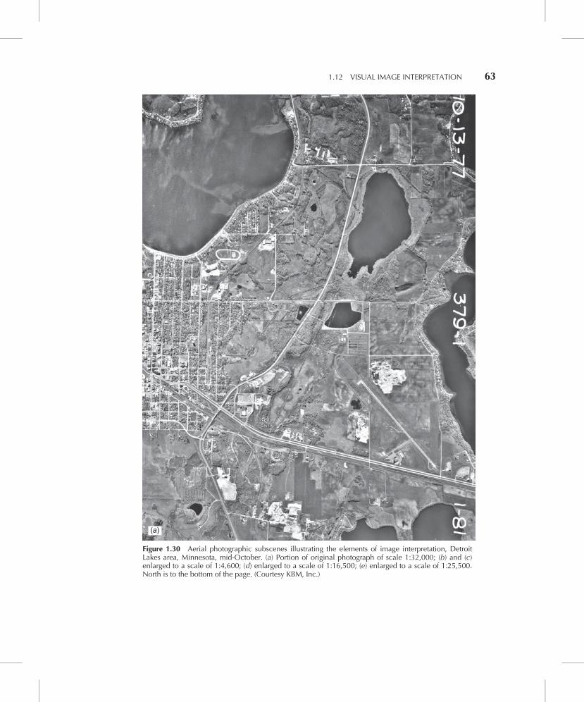
(a)

Figure 1.30 Aerial photographic subscenes illustrating the elements of image interpretation, DetroitLakes area, Minnesota, mid-October. (a) Portion of original photograph of scale 1:32,000; (b) and (c)enlarged to a scale of 1:4,600; (d) enlarged to a scale of 1:16,500; (e) enlarged to a scale of 1:25,500.North is to the bottom of the page. (Courtesy KBM, Inc.)


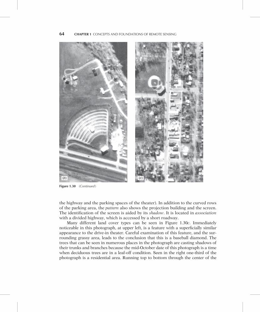
the highway and the parking spaces of the theater). In addition to the curved rowsof the parking area, the pattern also shows the projection building and the screen.The identification of the screen is aided by its shadow. It is located in associationwith a divided highway, which is accessed by a short roadway.

Many different land cover types can be seen in Figure 1.30c. Immediatelynoticeable in this photograph, at upper left, is a feature with a superficially similarappearance to the drive-in theater. Careful examination of this feature, and the sur-rounding grassy area, leads to the conclusion that this is a baseball diamond. Thetrees that can be seen in numerous places in the photograph are casting shadows oftheir trunks and branches because the mid-October date of this photograph is a timewhen deciduous trees are in a leaf-off condition. Seen in the right one-third of thephotograph is a residential area. Running top to bottom through the center of the

(b) (c)

Figure 1.30 (Continued )


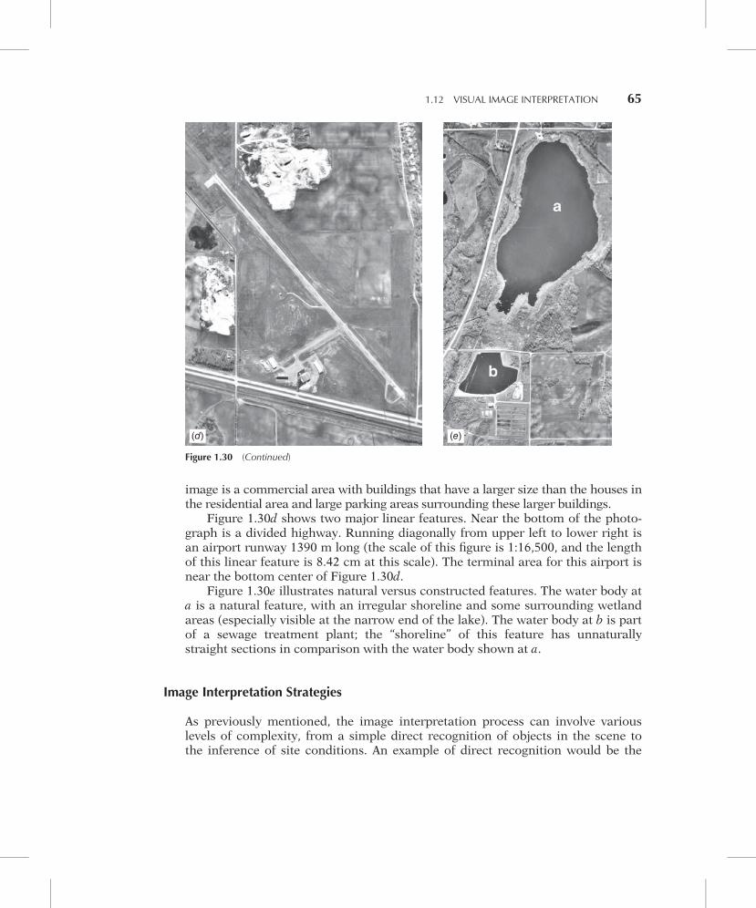
image is a commercial area with buildings that have a larger size than the houses inthe residential area and large parking areas surrounding these larger buildings.

Figure 1.30d shows two major linear features. Near the bottom of the photo-graph is a divided highway. Running diagonally from upper left to lower right isan airport runway 1390 m long (the scale of this figure is 1:16,500, and the lengthof this linear feature is 8.42 cm at this scale). The terminal area for this airport isnear the bottom center of Figure 1.30d.

Figure 1.30e illustrates natural versus constructed features. The water body ata is a natural feature, with an irregular shoreline and some surrounding wetlandareas (especially visible at the narrow end of the lake). The water body at b is partof a sewage treatment plant; the “shoreline” of this feature has unnaturallystraight sections in comparison with the water body shown at a.

Image Interpretation Strategies

As previously mentioned, the image interpretation process can involve variouslevels of complexity, from a simple direct recognition of objects in the scene tothe inference of site conditions. An example of direct recognition would be the

(d) (e)

Figure 1.30 (Continued)


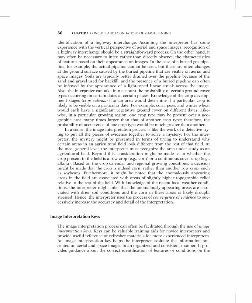
identification of a highway interchange. Assuming the interpreter has someexperience with the vertical perspective of aerial and space images, recognition ofa highway interchange should be a straightforward process. On the other hand, itmay often be necessary to infer, rather than directly observe, the characteristicsof features based on their appearance on images. In the case of a buried gas pipe-line, for example, the actual pipeline cannot be seen, but there are often changesat the ground surface caused by the buried pipeline that are visible on aerial andspace images. Soils are typically better drained over the pipeline because of thesand and gravel used for backfill, and the presence of a buried pipeline can oftenbe inferred by the appearance of a light-toned linear streak across the image.Also, the interpreter can take into account the probability of certain ground covertypes occurring on certain dates at certain places. Knowledge of the crop develop-ment stages (crop calendar) for an area would determine if a particular crop islikely to be visible on a particular date. For example, corn, peas, and winter wheatwould each have a significant vegetative ground cover on different dates. Like-wise, in a particular growing region, one crop type may be present over a geo-graphic area many times larger than that of another crop type; therefore, theprobability of occurrence of one crop type would be much greater than another.

In a sense, the image interpretation process is like the work of a detective try-ing to put all the pieces of evidence together to solve a mystery. For the inter-preter, the mystery might be presented in terms of trying to understand whycertain areas in an agricultural field look different from the rest of that field. Atthe most general level, the interpreter must recognize the area under study as anagricultural field. Beyond this, consideration might be made as to whether thecrop present in the field is a row crop (e.g., corn) or a continuous cover crop (e.g.,alfalfa). Based on the crop calendar and regional growing conditions, a decisionmight be made that the crop is indeed corn, rather than another row crop, suchas soybeans. Furthermore, it might be noted that the anomalously appearingareas in the field are associated with areas of slightly higher topographic reliefrelative to the rest of the field. With knowledge of the recent local weather condi-tions, the interpreter might infer that the anomalously appearing areas are asso-ciated with drier soil conditions and the corn in these areas is likely droughtstressed. Hence, the interpreter uses the process of convergence of evidence to suc-cessively increase the accuracy and detail of the interpretation.

Image Interpretation Keys

The image interpretation process can often be facilitated through the use of imageinterpretation keys. Keys can be valuable training aids for novice interpreters andprovide useful reference or refresher materials for more experienced interpreters.An image interpretation key helps the interpreter evaluate the information pre-sented on aerial and space images in an organized and consistent manner. It pro-vides guidance about the correct identification of features or conditions on the


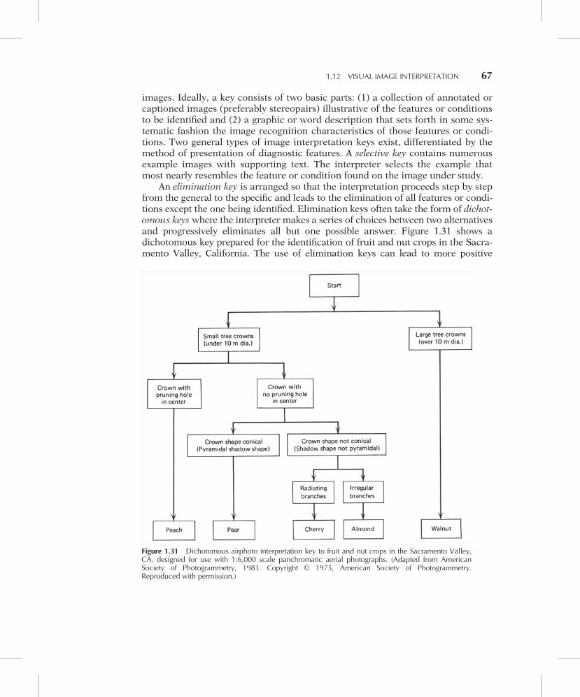
images. Ideally, a key consists of two basic parts: (1) a collection of annotated orcaptioned images (preferably stereopairs) illustrative of the features or conditionsto be identified and (2) a graphic or word description that sets forth in some sys-tematic fashion the image recognition characteristics of those features or condi-tions. Two general types of image interpretation keys exist, differentiated by themethod of presentation of diagnostic features. A selective key contains numerousexample images with supporting text. The interpreter selects the example thatmost nearly resembles the feature or condition found on the image under study.

An elimination key is arranged so that the interpretation proceeds step by stepfrom the general to the specific and leads to the elimination of all features or condi-tions except the one being identified. Elimination keys often take the form of dichot-omous keys where the interpreter makes a series of choices between two alternativesand progressively eliminates all but one possible answer. Figure 1.31 shows adichotomous key prepared for the identification of fruit and nut crops in the Sacra-mento Valley, California. The use of elimination keys can lead to more positive

Figure 1.31 Dichotomous airphoto interpretation key to fruit and nut crops in the Sacramento Valley,CA, designed for use with 1:6,000 scale panchromatic aerial photographs. (Adapted from AmericanSociety of Photogrammetry, 1983. Copyright © 1975, American Society of Photogrammetry.Reproduced with permission.)


answers than selective keys but may result in erroneous answers if the interpreter isforced to make an uncertain choice between two unfamiliar image characteristics.

As a generalization, keys are more easily constructed and more reliably uti-lized for cultural feature identification (e.g., houses, bridges, roads, water towers)than for vegetation or landform identification. However, a number of keys havebeen successfully employed for agricultural crop identification and tree speciesidentification. Such keys are normally developed and used on a region-by-region andseason-by-season basis because the appearance of vegetation can vary widely withlocation and season.

Wavelengths of Sensing

The band(s) of the electromagnetic energy spectrum selected for aerial and spaceimaging affects the amount of information that can be interpreted from the ima-ges. Numerous examples of this are scattered throughout this book. The generalconcepts of multiband imagery were discussed in Section 1.5. To explain how thecombinations of colors shown in an image relate to the various bands of datarecorded by a sensor, we next turn our attention to the principles of color, andhow combinations of colors are perceived.

Color Perception and Color Mixing

Color is among the most important elements of image interpretation. Many fea-tures and phenomena in an image can best be identified and interpreted throughexamination of subtle differences in color. As discussed in Section 1.5, multi-wavelength remote sensing images may be displayed in either true- or false-colorcombinations. Particularly for interpreting false-color imagery, an understandingof the principles of color perception and color mixing is essential.

Light falling on the retina of the human eye is sensed by rod and cone cells.There are about 130 million rod cells, and they are 1000 times more light sensi-tive than the cone cells. When light levels are low, human vision relies on the rodcells to form images. All rod cells have the same wavelength sensitivity, whichpeaks at about 0:55 �m. Therefore, human vision at low light levels is monochro-matic. It is the cone cells that determine the colors the eye sees. There are about7 million cone cells; some sensitive to blue energy, some to green energy, andsome to red energy. The trichromatic theory of color vision explains that when theblue-sensitive, green-sensitive, and red-sensitive cone cells are stimulated by dif-ferent amounts of light, we perceive color. When all three types of cone cells arestimulated equally, we perceive white light. Other theories of color vision havebeen proposed. The opponent process of color vision hypothesizes that color visioninvolves three mechanisms, each responding to a pair of so-called opposites:white–black, red–green, and blue–yellow. This theory is based on many psycho-physical observations and states that colors are formed by a hue cancellation


method. The hue cancellation method is based on the observation that when certaincolors are mixed together, the resulting colors are not what would be intuitivelyexpected. For example, when red and green are mixed together, they produce yel-low, not reddish green. (For further information, see Robinson et al., 1995.)

In the remainder of this discussion, we focus on the trichromatic theory ofcolor vision. Again, this theory is based on the concept that we perceive all colorsby synthesizing various amounts of just three (blue, green, and red).

Blue, green, and red are termed additive primaries. Plate 3a shows the effectof projecting blue, green, and red light in partial superimposition. Where all threebeams overlap, the visual effect is white because all three of the eyes’ receptor sys-tems are stimulated equally. Hence, white light can be thought of as the mixtureof blue, green, and red light. Various combinations of the three additive primariescan be used to produce other colors. As illustrated, when red light and green lightare mixed, yellow light is produced. Mixture of blue and red light results in theproduction of magenta light (bluish-red). Mixing blue and green results in cyanlight (bluish-green).

Yellow, magenta, and cyan are known as the complementary colors, or comple-ments, of blue, green, and red light. Note that the complementary color for anygiven primary color results from mixing the remaining two primaries.

Like the eye, color television and computer monitors operate on the principleof additive color mixing through use of blue, green, and red elements on thescreen. When viewed at a distance, the light from the closely spaced screen ele-ments forms a continuous color image.

Whereas color television and computer monitors simulate different colorsthrough additive mixture of blue, green, and red lights, color film photography isbased on the principle of subtractive color mixture using superimposed yellow,magenta, and cyan dyes. These three dye colors are termed the subtractive primaries,and each results from subtracting one of the additive primaries from white light.That is, yellow dye absorbs the blue component of white light. Magenta dye absorbsthe green component of white light. Cyan dye absorbs the red component of whitelight.

The subtractive color-mixing process is illustrated in Plate 3b. This plateshows three circular filters being held in front of a source of white light. The fil-ters contain yellow, magenta, and cyan dye. The yellow dye absorbs blue lightfrom the white background and transmits green and red. The magenta dyeabsorbs green light and transmits blue and red. The cyan dye absorbs red lightand transmits blue and green. The superimposition of magenta and cyan dyesresults in the passage of only blue light from the background. This comes aboutbecause the magenta dye absorbs the green component of the white background,and the cyan dye absorbs the red component. Superimposition of the yellow andcyan dyes results in the perception of green. Likewise, superimposition of yellowand magenta dyes results in the perception of red. Where all three dyes overlap,all light from the white background is absorbed and black results.

In color film photography, and in color printing, various proportions of yel-low, magenta, and cyan dye are superimposed to control the proportionate


amount of blue, green, and red light that reaches the eye. Hence, the subtractivemixture of yellow, magenta, and cyan dyes on a photograph is used to controlthe additive mixture of blue, green, and red light reaching the eye of the observer.To accomplish this, color film is manufactured with three emulsion layers thatare sensitive to blue, green, and red light but contain yellow, magenta, and cyandye after processing (see Section 2.4).

In digital color photography, the photosites in the detector array are typicallycovered with a blue, green, or red filter, resulting in independent recording of thethree additive primary colors (see Section 2.5).

When interpreting color images, the analyst should keep in mind the relation-ship between the color of a feature in the imagery, the color mixing process thatwould produce that color, and the sensor’s wavelength ranges that are assigned tothe three primary colors used in that mixing process. It is then possible to workbackwards to infer the spectral properties of the feature on the landscape. Forexample, if a feature in a false-color image has a yellow hue when displayed on acomputer monitor, that feature can be assumed to have a relatively high reflec-tance in the wavelengths that are being displayed in the monitor’s red and greencolor planes, and a relatively low reflectance in the wavelength displayed in blue(because yellow results from the additive combination of red plus green light).Knowing the spectral sensitivity of each of the sensor’s spectral bands, the analystcan interpret the color as a spectral response pattern (see Section 1.4) that ischaracterized by high reflectance at two wavelength ranges and low reflectance ata third. The analyst can then use this information to draw inferences about thenature and condition of the feature shown in the false-color image.

Temporal Aspects of Image Interpretation

The temporal aspects of natural phenomena are important for image interpreta-tion because such factors as vegetative growth and soil moisture vary during theyear. For crop identification, more positive results can be achieved by obtainingimages at several times during the annual growing cycle. Observations of localvegetation emergence and recession can aid in the timing of image acquisition fornatural vegetation mapping. In addition to seasonal variations, weather can causesignificant short-term changes. Because soil moisture conditions may change dra-matically during the day or two immediately following a rainstorm, the timing ofimage acquisition for soil studies is very critical.

Another temporal aspect of importance is the comparison of leaf-off photo-graphy with leaf-on photography. Leaf-off conditions are preferable for applica-tions in which it is important to be able to see as much detail as possibleunderneath trees. Such applications include activities such as topographic mappingand urban feature identification. Leaf-on conditions are preferred for vegetationmapping. Figure 1.32a illustrates leaf-on photography. Here considerable detailof the ground surface underneath the tree crowns is obscured. Figure 1.32b


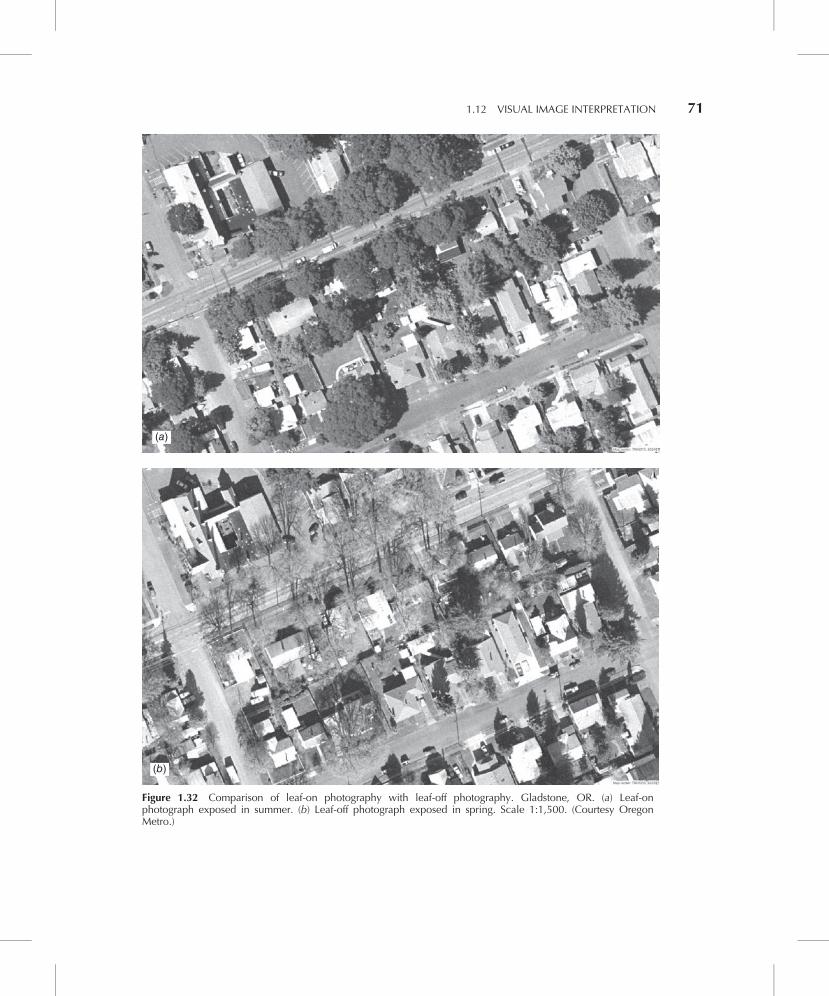
(a)

(b)

Figure 1.32 Comparison of leaf-on photography with leaf-off photography. Gladstone, OR. (a) Leaf-onphotograph exposed in summer. (b) Leaf-off photograph exposed in spring. Scale 1:1,500. (Courtesy OregonMetro.)


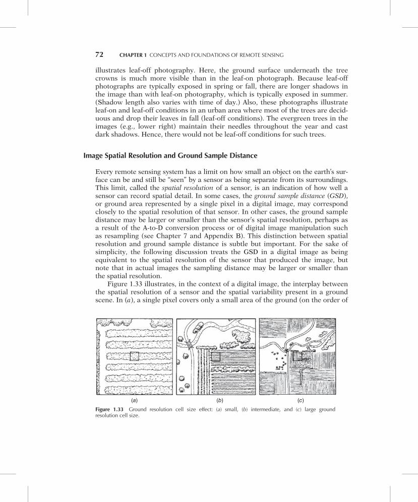
illustrates leaf-off photography. Here, the ground surface underneath the treecrowns is much more visible than in the leaf-on photograph. Because leaf-offphotographs are typically exposed in spring or fall, there are longer shadows inthe image than with leaf-on photography, which is typically exposed in summer.(Shadow length also varies with time of day.) Also, these photographs illustrateleaf-on and leaf-off conditions in an urban area where most of the trees are decid-uous and drop their leaves in fall (leaf-off conditions). The evergreen trees in theimages (e.g., lower right) maintain their needles throughout the year and castdark shadows. Hence, there would not be leaf-off conditions for such trees.

Image Spatial Resolution and Ground Sample Distance

Every remote sensing system has a limit on how small an object on the earth’s sur-face can be and still be “seen” by a sensor as being separate from its surroundings.This limit, called the spatial resolution of a sensor, is an indication of how well asensor can record spatial detail. In some cases, the ground sample distance (GSD),or ground area represented by a single pixel in a digital image, may correspondclosely to the spatial resolution of that sensor. In other cases, the ground sampledistance may be larger or smaller than the sensor’s spatial resolution, perhaps asa result of the A-to-D conversion process or of digital image manipulation suchas resampling (see Chapter 7 and Appendix B). This distinction between spatialresolution and ground sample distance is subtle but important. For the sake ofsimplicity, the following discussion treats the GSD in a digital image as beingequivalent to the spatial resolution of the sensor that produced the image, butnote that in actual images the sampling distance may be larger or smaller thanthe spatial resolution.

Figure 1.33 illustrates, in the context of a digital image, the interplay betweenthe spatial resolution of a sensor and the spatial variability present in a groundscene. In (a), a single pixel covers only a small area of the ground (on the order of

(a) (b) (c)

Figure 1.33 Ground resolution cell size effect: (a) small, (b) intermediate, and (c) large groundresolution cell size.


the width of the rows of the crop shown). In (b), a coarser ground resolution isdepicted and a single pixel integrates the radiance from both the crop rows and thesoil between them. In (c), an even coarser resolution results in a pixel measuringthe average radiance over portions of two fields. Thus, depending on the spatialresolution of the sensor and the spatial structure of the ground area being sensed,digital images comprise a range of “pure” and “mixed” pixels. In general, the largerthe percentage of mixed pixels, the more limited is the ability to record and extractspatial detail in an image. This is illustrated in Figure 1.34, in which the same areahas been imaged over a range of different ground resolution cell sizes.

Further discussion of the spatial resolution of remote sensing systems—including the factors that determine spatial resolution and the methods used formeasuring or calculating a system’s resolution—can be found in Chapter 2 (forcamera systems), Chapters 4 and 5 (for airborne and spaceborne multispectraland thermal sensors), and Chapter 6 (for radar systems).

Other Forms of Resolution Important in Image Interpretation

It should be noted that there are other forms of resolution that are importantcharacteristics of remote sensing images. These include the following:

Spectral resolution, referring to a sensor’s ability to distinguish among differentground features based on their spectral properties. Spectral resolution dependsupon the number, wavelength location, and narrowness of the spectral bands inwhich a sensor collects image data. The bands in which any sensor collects datacan range from a single broad band (for panchromatic images), a few broad bands(for multispectral images), or many very narrow bands (for hyperspectral images).

Radiometric resolution, referring to the sensor’s ability to differentiate amongsubtle variations in brightness. Does the sensor divide the range from the “bright-est” pixel to “darkest” pixel that can be recorded in an image (the dynamic range)into 256, or 512, or 1024 gray level values? The finer the radiometric resolution is,the greater the quality and interpretability of an image. (See also the discussion ofquantization and digital numbers in Section 1.5.)

Temporal resolution, referring to the ability to detect changes over shorter orlonger periods of time. Most often, this term is used in reference to a sensorthat produces a time-series of multiple images. This could be a satellite systemwith a defined 16-day or 26-day orbital repeat cycle, or a tripod-mounted camerawith a timer that collects one image every hour to serve as reference data. Theimportance of rapid and/or repeated coverage of an area varies dramatically withthe application at hand. For example, in disaster response applications, temporalresolution might outweigh the importance of some, or all, of the other types ofresolution we have summarized above.

In subsequent chapters, as new remote sensing systems are introduced anddiscussed, the reader should keep in mind these multiple resolutions that deter-mine whether a given system would be suitable for a particular application.


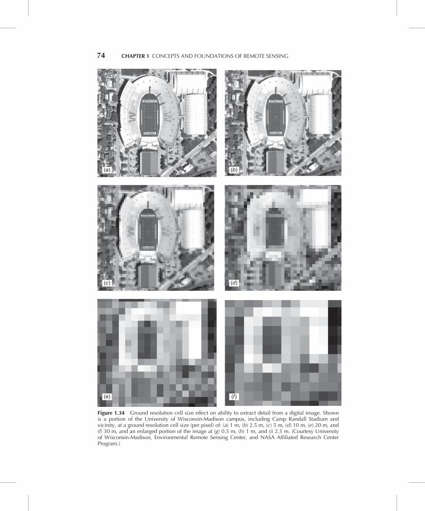
(a) (b)

(c) (d)

(e) (f)

Figure 1.34 Ground resolution cell size effect on ability to extract detail from a digital image. Shownis a portion of the University of Wisconsin-Madison campus, including Camp Randall Stadium andvicinity, at a ground resolution cell size (per pixel) of: (a) 1 m, (b) 2.5 m, (c) 5 m, (d) 10 m, (e) 20 m, and(f) 30 m, and an enlarged portion of the image at (g) 0.5 m, (h) 1 m, and (i) 2.5 m. (Courtesy Universityof Wisconsin-Madison, Environmental Remote Sensing Center, and NASA Affiliated Research CenterProgram.)


(g)

(h)

(i)

Figure 1.34 (Continued)


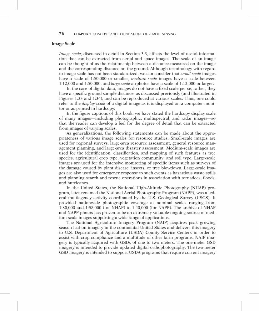
Image Scale

Image scale, discussed in detail in Section 3.3, affects the level of useful informa-tion that can be extracted from aerial and space images. The scale of an imagecan be thought of as the relationship between a distance measured on the imageand the corresponding distance on the ground. Although terminology with regardto image scale has not been standardized, we can consider that small-scale imageshave a scale of 1:50,000 or smaller, medium-scale images have a scale between1:12,000 and 1:50,000, and large-scale airphotos have a scale of 1:12,000 or larger.

In the case of digital data, images do not have a fixed scale per se; rather, theyhave a specific ground sample distance, as discussed previously (and illustrated inFigures 1.33 and 1.34), and can be reproduced at various scales. Thus, one couldrefer to the display scale of a digital image as it is displayed on a computer moni-tor or as printed in hardcopy.

In the figure captions of this book, we have stated the hardcopy display scaleof many images—including photographic, multispectral, and radar images—sothat the reader can develop a feel for the degree of detail that can be extractedfrom images of varying scales.

As generalizations, the following statements can be made about the appro-priateness of various image scales for resource studies. Small-scale images areused for regional surveys, large-area resource assessment, general resource man-agement planning, and large-area disaster assessment. Medium-scale images areused for the identification, classification, and mapping of such features as treespecies, agricultural crop type, vegetation community, and soil type. Large-scaleimages are used for the intensive monitoring of specific items such as surveys ofthe damage caused by plant disease, insects, or tree blowdown. Large-scale ima-ges are also used for emergency response to such events as hazardous waste spillsand planning search and rescue operations in association with tornadoes, floods,and hurricanes.

In the United States, the National High-Altitude Photography (NHAP) pro-gram, later renamed the National Aerial Photography Program (NAPP), was a fed-eral multiagency activity coordinated by the U.S. Geological Survey (USGS). Itprovided nationwide photographic coverage at nominal scales ranging from1:80,000 and 1:58,000 (for NHAP) to 1:40,000 (for NAPP). The archive of NHAPand NAPP photos has proven to be an extremely valuable ongoing source of med-ium-scale images supporting a wide range of applications.

The National Agriculture Imagery Program (NAIP) acquires peak growingseason leaf-on imagery in the continental United States and delivers this imageryto U.S. Department of Agriculture (USDA) County Service Centers in order toassist with crop compliance and a multitude of other farm programs. NAIP ima-gery is typically acquired with GSDs of one to two meters. The one-meter GSDimagery is intended to provide updated digital orthophotography. The two-meterGSD imagery is intended to support USDA programs that require current imagery


acquired during the agricultural growing season but do not require high hor-izontal accuracy. NAIP photographs are also useful in many non-USDA applica-tions, including real estate, recreation, and land use planning.

Approaching the Image Interpretation Process

There is no single “right” way to approach the image interpretation process. Thespecific image products and interpretation equipment available will, in part, influ-ence how a particular interpretation task is undertaken. Beyond these factors, thespecific goals of the task will determine the image interpretation processemployed. Many applications simply require the image analyst to identify andcount various discrete objects occurring in a study area. For example, counts maybe made of such items as motor vehicles, residential dwellings, recreational water-craft, or animals. Other applications of the interpretation process often involve theidentification of anomalous conditions. For example, the image analyst mightsurvey large areas looking for such features as failing septic systems, sources ofwater pollution entering a stream, areas of a forest stressed by an insect or diseaseproblem, or evidence of sites having potential archaeological significance.

Many applications of image interpretation involve the delineation of discreteareal units throughout images. For example, the mapping of land use, soil types, orforest types requires the interpreter to outline the boundaries between areas of onetype versus another. Such tasks can be problematic when the boundary is not a dis-crete edge, but rather a “fuzzy edge” or gradation from one type of area to another,as is common with natural phenomena such as soils and natural vegetation.

Two extremely important issues must be addressed before an interpreterundertakes the task of delineating separate areal units on remotely sensed images.The first is the definition of the classification system or criteria to be used to sepa-rate the various categories of features occurring in the images. For example,in mapping land use, the interpreter must fix firmly in mind what specific character-istics determine if an area is “residential,” “commercial,” or “industrial.” Similarly,the forest type mapping process must involve clear definition of what constitutes anarea to be delineated in a particular species, height, or crown density class.

The second important issue in delineation of discrete areal units on images isthe selection of the minimum mapping unit (MMU) to be employed in the pro-cess. This refers to the smallest size areal entity to be mapped as a discrete area.Selection of the MMU will determine the extent of detail conveyed by an interpreta-tion. This is illustrated in Figure 1.35. In (a), a small MMU results in a much moredetailed interpretation than does the use of a large MMU, as illustrated in (b).

Once the classification system and MMU have been determined, the inter-preter can begin the process of delineating boundaries between feature types.Experience suggests that it is advisable to delineate the most highly contrastingfeature types first and to work from the general to the specific. For example, in a


land use mapping effort, it would be better to separate “urban” from “water” and“agriculture” before separating more detailed categories of each of these featuretypes based on subtle differences.

In certain applications, the interpreter might choose to delineate photo-morphic regions as part of the delineation process. These are regions of reason-ably uniform tone, texture, and other image characteristics. When initiallydelineated, the feature type identity of these regions may not be known. Fieldobservations or other ground truth can then be used to verify the identity of eachregion. Regrettably, there is not always a one-to-one correspondence between theappearance of a photomorphic region and a mapping category of interest. How-ever, the delineation of such regions often serves as a stratification tool in theinterpretation process and can be valuable in applications such as vegetationmapping (where photomorphic regions often correspond directly to vegetationclasses of interest).

Basic Equipment for Visual Interpretation

Visual image interpretation equipment generally serves one of several funda-mental purposes: viewing images, making measurements on images, performingimage interpretation tasks, and transferring interpreted information to base mapsor digital databases. Basic equipment for viewing images and transferring inter-preted information is described here. Equipment involved in performing measur-ing and mapping tasks will be described in Chapter 3.

The airphoto interpretation process typically involves the utilization of stereo-scopic viewing to provide a three-dimensional view of the terrain. Some spaceimages are also analyzed stereoscopically. The stereo effect is possible because wehave binocular vision. That is, since we have two eyes that are slightly separated,we continually view the world from two slightly different perspectives. Whenever

(a) (b)

Figure 1.35 Influence of minimum mapping unit size on interpretation detail. (a) Foresttypes mapped using a small MMU: O, oak; M, maple; W, white pine; J, jack pine; R, redpine; S, spruce. (b) Forest types mapped using a large MMU: D, deciduous; E, evergreen.


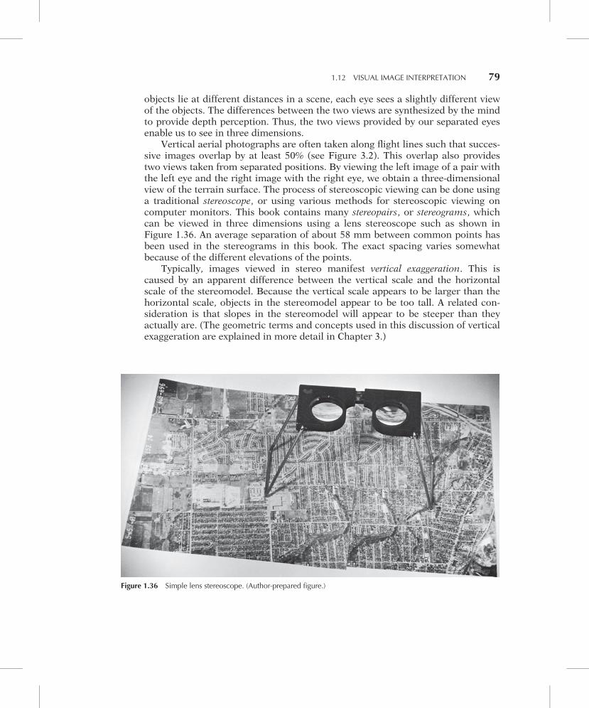
objects lie at different distances in a scene, each eye sees a slightly different viewof the objects. The differences between the two views are synthesized by the mindto provide depth perception. Thus, the two views provided by our separated eyesenable us to see in three dimensions.

Vertical aerial photographs are often taken along flight lines such that succes-sive images overlap by at least 50% (see Figure 3.2). This overlap also providestwo views taken from separated positions. By viewing the left image of a pair withthe left eye and the right image with the right eye, we obtain a three-dimensionalview of the terrain surface. The process of stereoscopic viewing can be done usinga traditional stereoscope, or using various methods for stereoscopic viewing oncomputer monitors. This book contains many stereopairs, or stereograms, whichcan be viewed in three dimensions using a lens stereoscope such as shown inFigure 1.36. An average separation of about 58 mm between common points hasbeen used in the stereograms in this book. The exact spacing varies somewhatbecause of the different elevations of the points.

Typically, images viewed in stereo manifest vertical exaggeration. This iscaused by an apparent difference between the vertical scale and the horizontalscale of the stereomodel. Because the vertical scale appears to be larger than thehorizontal scale, objects in the stereomodel appear to be too tall. A related con-sideration is that slopes in the stereomodel will appear to be steeper than theyactually are. (The geometric terms and concepts used in this discussion of verticalexaggeration are explained in more detail in Chapter 3.)

Figure 1.36 Simple lens stereoscope. (Author-prepared figure.)


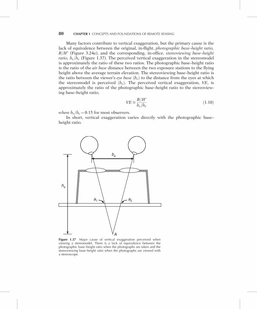
Many factors contribute to vertical exaggeration, but the primary cause is thelack of equivalence between the original, in-flight, photographic base–height ratio,B=H 0 (Figure 3.24a), and the corresponding, in-office, stereoviewing base–heightratio, be=he (Figure 1.37). The perceived vertical exaggeration in the stereomodelis approximately the ratio of these two ratios. The photographic base–height ratiois the ratio of the air base distance between the two exposure stations to the flyingheight above the average terrain elevation. The stereoviewing base–height ratio isthe ratio between the viewer’s eye base beð Þ to the distance from the eyes at whichthe stereomodel is perceived heð Þ. The perceived vertical exaggeration, VE, isapproximately the ratio of the photographic base–height ratio to the stereoview-ing base–height ratio,

VEffi B=H 0

be=heð1:10Þ

where be=he ¼ 0:15 for most observers.In short, vertical exaggeration varies directly with the photographic base–

height ratio.

Figure 1.37 Major cause of vertical exaggeration perceived whenviewing a stereomodel. There is a lack of equivalence between thephotographic base–height ratio when the photographs are taken and thestereoviewing base–height ratio when the photographs are viewed witha stereoscope.


While vertical exaggeration is often misleading to novice image interpreters, itis often very useful in the interpretation process. This is due to the fact that subtlevariation in the heights of image features is more readily discriminated when exag-gerated. As we note in Chapter 3, large base–height ratios also improve the qualityof many photogrammetric measurements made from vertical aerial photographs.

Figure 1.38 can be used to test stereoscopic vision. When this diagram isviewed through a stereoscope, the rings and other objects should appear to be atvarying distances from the observer. Your stereovision ability can be evaluated byfilling in Table 1.3 (answers are in the second part of the table). People whose eye-sight is very weak in one eye may not have the ability to see in stereo. This willpreclude three-dimensional viewing of the stereograms in this book. However,many people with essentially monocular vision have become proficient photointerpreters. In fact, many forms of interpretation involve monocular viewingwith such basic equipment as handheld magnifying glasses or tube magnifiers(23 to 103 lenses mounted in a transparent stand).

Some people will be able to view the stereograms in this book without a ste-reoscope. This can be accomplished by holding the book about 25 cm from youreyes and allowing the view of each eye to drift into a straight-ahead viewing posi-tion (as when looking at objects at an infinite distance) while still maintainingfocus on the stereogram. When the two images have fused into one, the stereo-gram will be seen in three dimensions. Most persons will find stereoviewing with-out proper stereoscopes to be a tiring procedure, producing eyestrain. It is,however, a useful technique to employ when stereoscopes are not available.

Several types of analog stereoscopes are available, utilizing lenses or a combi-nation of lenses, mirrors, and prisms. Lens stereoscopes, such as the one shown inFigure 1.36, are portable and comparatively inexpensive. Most are small instru-ments with folding legs. The lens spacing can usually be adjusted from about

Figure 1.38 Stereoscopic vision test. (Courtesy Carl Zeiss, Inc.)


45 to 75 mm to accommodate individual eye spacings. Lens magnification is typi-cally 2 power but may be adjustable. The principal disadvantage of small lens ste-reoscopes is that the images must be quite close together to be positionedproperly underneath the lenses. Because of this, the interpreter cannot view theentire stereoscopic area contained by the overlapping aerial photographs without

TABLE 1.3 Stereovision Test for Use with Figure 1.38

PART IWithin the rings marked 1 through 8 are designs that appear to be at different elevations.Using “1” to designate the highest elevation, write down the depth order of the designs. It ispossible that two or more designs may be at the same elevation. In this case, use the samenumber for all designs at the same elevation.Ring 1 Ring 6Square (2) Lower left circle ( )Marginal ring (1) Lower right circle ( )Triangle (3) Upper right circle ( )Point (4) Upper left circle ( )

Marginal ring ( )Ring 7 Ring 3Black flag with ball ( ) Square ( )Marginal ring ( ) Marginal ring ( )Black circle ( ) Cross ( )Arrow ( ) Lower left circle ( )Tower with cross ( ) Upper left circle ( )Double cross ( )Black triangle ( )Black rectangle ( )

PART IIIndicate the relative elevations of the rings 1 through 8.

( ) ( ) ( ) ( ) ( ) ( ) ( ) ( )Highest Lowest

PART IIIDraw profiles to indicate the relative elevations of the letters in the words “prufungstafel”and “stereoskopisches sehen.”

(Answers to Stereovision Test on next page)


raising the edge of one of the photographs. More advanced devices for viewinghardcopy stereoscopic image pairs include mirror stereoscopes (larger stereo-scopes that use a combination of prisms and mirrors to separate the lines of sightfrom each of the viewer’s eyes) and zoom stereoscopes, expensive precision instru-ments used for viewing stereopairs under variable magnification.

With the proliferation of digital imagery and software for viewing and analyz-ing digital images, analog stereoscopes have been replaced in the laboratory (ifnot in the field) by various computer hardware configurations for stereoviewing.These devices are discussed in Section 3.10.

TABLE 1.3 (Continued)

PART IRing 1 Ring 6Square (2) Lower left circle (4)Marginal ring (1) Lower right circle (5)Triangle (3) Upper right circle (1)Point (4) Upper left circle (3)

Marginal ring (2)Ring 7 Ring 3Black flag with ball (5) Square (4)Marginal ring (1) Marginal ring (2)Black circle (4) Cross (3)Arrow (2) Lower left circle (1)Tower with cross (7) Upper left circle (5)Double cross (2)Black triangle (3)Black rectangle (6)

PART II(7) (6) (5) (1) (4) (2)a (3)a (8)Highest Lowest

PART III

aRings 2 and 3 are at the same elevation.


Relationship between Visual Image Interpretation andComputer Image Processing

In recent years, there has been increasing emphasis on the development of quan-titative, computer-based processing methods for analyzing remotely sensed data.As will be discussed in Chapter 7, those methods have become increasinglysophisticated and powerful. Despite these advances, computers are still somewhatlimited in their ability to evaluate many of the visual “clues” that are readilyapparent to the human interpreter, particularly those referred to as image texture.Therefore, visual and numerical techniques should be seen as complementary innature, and consideration must be given to which approach (or combination ofapproaches) best fits a particular application.

The discussion of visual image interpretation in this section has of necessitybeen brief. As mentioned at the start of this section, the skill of image interpreta-tion is best learned interactively, through the experience of interpreting manyimages. In the ensuing chapters of this book, we provide many examples of remo-tely sensed images, from aerial photographs to synthetic aperture radar images.We hope that the reader will apply the principles and concepts discussed in thissection to help interpret the features and phenomena illustrated in those images.


of remote sensing - Moodle@Units

Documents

Transcript of of remote sensing - Moodle@Units