University of Groningen Osteoprotegerin in organ fibrosis: biomarker ...
Upload
khangminh22Category
view
0download
0
University of Groningen
Hot recoils from cold atomsTurkstra, Jan Willem
IMPORTANT NOTE: You are advised to consult the publisher's version (publisher's PDF) if you wish to cite fromit. Please check the document version below.
Document VersionPublisher's PDF, also known as Version of record
Publication date:2001
Link to publication in University of Groningen/UMCG research database
Citation for published version (APA):Turkstra, J. W. (2001). Hot recoils from cold atoms. s.n.
CopyrightOther than for strictly personal use, it is not permitted to download or to forward/distribute the text or part of it without the consent of theauthor(s) and/or copyright holder(s), unless the work is under an open content license (like Creative Commons).
The publication may also be distributed here under the terms of Article 25fa of the Dutch Copyright Act, indicated by the “Taverne” license.More information can be found on the University of Groningen website: https://www.rug.nl/library/open-access/self-archiving-pure/taverne-amendment.
Take-down policyIf you believe that this document breaches copyright please contact us providing details, and we will remove access to the work immediatelyand investigate your claim.
Downloaded from the University of Groningen/UMCG research database (Pure): http://www.rug.nl/research/portal. For technical reasons thenumber of authors shown on this cover page is limited to 10 maximum.
Download date: 16-02-2022
Hot recoils
fromcold atoms

Omslag: photograph taken by Dick Hutchinson of the aurora borealis. The brightobject is not a cloud of laser trapped atoms but the moon.
The work described in this thesis is part of the research program of the ’Stichtingvoor Fundamenteel Onderzoek der Materie (FOM) which is …nancially supportedby the ’Nederlandse Organisatie voor Wetenschappelijk Onderzoek’(NWO). Partof the work (chapter 4) has received support from EURATOM in the framework ofthe Association Agreement EURATOM - FOM.
Druk: van Denderen, Groningen
RIJKSUNIVERSITEIT GRONINGEN
Hot recoilsfrom
cold atoms
Proefschrift
ter verkrijging van het doctoraat in deWiskunde en Natuurwetenschappenaan de Rijksuniversiteit Groningen
op gezag van deRector Magni…cus, dr. D.F.J. Bosscher,
in het openbaar te verdedigen opvrijdag 19 oktober 2001
om 16.00 uur
door
Jan Willem Turkstra
geboren op 21 mei 1971te Beilen.

Promotor: Prof. dr. R. MorgensternCo-Promotor: Dr. ir. R. Hoekstra
Beoordelingscommissie: Prof. dr. K. JungmannProf. dr. H. Schmidt-BöckingProf. dr. P. van der Straten
aan: Opa en Oma, Pake en Beppe
Contents
1 Introduction 91.1 Introduction . . . . . . . . . . . . . . . . . . . . . . . . . . . . . . . 101.2 Motivation . . . . . . . . . . . . . . . . . . . . . . . . . . . . . . . 101.3 Outline of this work . . . . . . . . . . . . . . . . . . . . . . . . . . 12
2 Experimental techniques 132.1 Photon Emission Spectroscopy . . . . . . . . . . . . . . . . . . . . 14
2.1.1 Introduction . . . . . . . . . . . . . . . . . . . . . . . . . . 142.1.2 PES: a short historical overview . . . . . . . . . . . . . . . 142.1.3 PES: advantages and disadvantages . . . . . . . . . . . . . 152.1.4 Conclusion . . . . . . . . . . . . . . . . . . . . . . . . . . . 15
2.2 Cold Target Recoil Ion Momentum Spectroscopy . . . . . . . . . . 162.2.1 Introduction . . . . . . . . . . . . . . . . . . . . . . . . . . 162.2.2 COLTRIMS: a brief overview . . . . . . . . . . . . . . . . . 162.2.3 COLTRIMS: kinematics . . . . . . . . . . . . . . . . . . . . 172.2.4 COLTRIMS: advantages and disadvantages . . . . . . . . . 202.2.5 Conclusion . . . . . . . . . . . . . . . . . . . . . . . . . . . 20
2.3 Translational Energy Spectroscopy . . . . . . . . . . . . . . . . . . 212.3.1 Introduction . . . . . . . . . . . . . . . . . . . . . . . . . . 212.3.2 TES: a short historic overview . . . . . . . . . . . . . . . . 212.3.3 TES: advantages and disadvantages . . . . . . . . . . . . . 21
3 Theoretical methods 233.1 Atomic Orbital Close Coupling . . . . . . . . . . . . . . . . . . . . 24
5
6 Contents
3.1.1 Introduction . . . . . . . . . . . . . . . . . . . . . . . . . . 243.1.2 AO-CC calculations . . . . . . . . . . . . . . . . . . . . . . 24
3.2 Over the Barrier . . . . . . . . . . . . . . . . . . . . . . . . . . . . 253.2.1 Introduction . . . . . . . . . . . . . . . . . . . . . . . . . . 253.2.2 Final states of transferred electrons . . . . . . . . . . . . . . 263.2.3 Transversal momenta of collision partners . . . . . . . . . . 293.2.4 Conclusion . . . . . . . . . . . . . . . . . . . . . . . . . . . 33
3.3 Classical Trajectory Monte Carlo . . . . . . . . . . . . . . . . . . . 343.3.1 Introduction . . . . . . . . . . . . . . . . . . . . . . . . . . 343.3.2 CTMC calculations . . . . . . . . . . . . . . . . . . . . . . . 34
4 Lithium excitation by slow H+ and He2+ ions 374.1 Introduction . . . . . . . . . . . . . . . . . . . . . . . . . . . . . . . 384.2 Theory . . . . . . . . . . . . . . . . . . . . . . . . . . . . . . . . . . 384.3 Experimental results . . . . . . . . . . . . . . . . . . . . . . . . . . 40
4.3.1 Proton impact . . . . . . . . . . . . . . . . . . . . . . . . . 444.3.2 He2+ impact . . . . . . . . . . . . . . . . . . . . . . . . . . 47
4.4 LiI(nd-2p, n=3-9) emission: n scaling . . . . . . . . . . . . . . . . 524.5 Conclusion . . . . . . . . . . . . . . . . . . . . . . . . . . . . . . . 54
5 The Magneto Optical Trap 575.1 Introduction . . . . . . . . . . . . . . . . . . . . . . . . . . . . . . . 585.2 Laser cooling and trapping . . . . . . . . . . . . . . . . . . . . . . 585.3 Theory: trapping and cooling atoms . . . . . . . . . . . . . . . . . 615.4 Theory: trapping and cooling Na . . . . . . . . . . . . . . . . . . . 645.5 Experiment: trapping and cooling Na . . . . . . . . . . . . . . . . 655.6 Temperature, size, density and Na+
2 ions . . . . . . . . . . . . . . . 675.7 The laser . . . . . . . . . . . . . . . . . . . . . . . . . . . . . . . . 705.8 Conclusion . . . . . . . . . . . . . . . . . . . . . . . . . . . . . . . 75
6 The Recoil Ion Momentum Spectrometer 776.1 Recoil extraction . . . . . . . . . . . . . . . . . . . . . . . . . . . . 78
6.1.1 Spatial focussing . . . . . . . . . . . . . . . . . . . . . . . . 796.1.2 Time focussing . . . . . . . . . . . . . . . . . . . . . . . . . 80
6.2 time of ‡ight . . . . . . . . . . . . . . . . . . . . . . . . . . . . . . 816.3 Recoil detection: the delay line detector . . . . . . . . . . . . . . . 826.4 Recoil momentum reconstruction (theory) . . . . . . . . . . . . . . 846.5 Recoil momentum reconstruction (practice) . . . . . . . . . . . . . 856.6 Resolution . . . . . . . . . . . . . . . . . . . . . . . . . . . . . . . . 886.7 Outlook . . . . . . . . . . . . . . . . . . . . . . . . . . . . . . . . . 89

7
7 Results: Collisions of O6+ and 13C6+ with Na 917.1 Motivation . . . . . . . . . . . . . . . . . . . . . . . . . . . . . . . 927.2 Recoil charge state spectra from 16O6+ and 13C6+ impact . . . . . 927.3 Naq+(q=1..4) recoils created by 3 keV/amu O6+ impact . . . . . . 95
7.3.1 Na+ recoils . . . . . . . . . . . . . . . . . . . . . . . . . . . 967.3.2 Na2+ recoils . . . . . . . . . . . . . . . . . . . . . . . . . . . 987.3.3 Na3+ recoils . . . . . . . . . . . . . . . . . . . . . . . . . . . 1027.3.4 Na4+ recoils . . . . . . . . . . . . . . . . . . . . . . . . . . . 1057.3.5 Summary of 3 keV/amu O6+ - Na collisions . . . . . . . . 107
7.4 Naq+(q=2..4) recoils created by 4.5, 3 and 1.5 keV/amu O6+ impact 1087.4.1 Na2+ recoils . . . . . . . . . . . . . . . . . . . . . . . . . . . 1087.4.2 Na3+ recoils . . . . . . . . . . . . . . . . . . . . . . . . . . . 1117.4.3 Na4+ recoils . . . . . . . . . . . . . . . . . . . . . . . . . . . 1137.4.4 Summary of the velocity infuence . . . . . . . . . . . . . . . 115
7.5 Naq+(q=2..4) recoils created by 4.5 keV/amu 13C6+ and O6+ impact1167.5.1 Na2+ recoils . . . . . . . . . . . . . . . . . . . . . . . . . . . 1177.5.2 Na3+ recoils . . . . . . . . . . . . . . . . . . . . . . . . . . . 1187.5.3 Summary of the C6+- O6+ comparison . . . . . . . . . . . . 120
8 Summary 121
9 Nederlandse samenvatting 1259.1 Introduktie . . . . . . . . . . . . . . . . . . . . . . . . . . . . . . . 1259.2 Botsingen van atomen en ionen . . . . . . . . . . . . . . . . . . . . 1269.3 In dit werk... . . . . . . . . . . . . . . . . . . . . . . . . . . . . . 1279.4 Laserkoeling . . . . . . . . . . . . . . . . . . . . . . . . . . . 1299.5 Conclusie . . . . . . . . . . . . . . . . . . . . . . . . . . . . . . . . 130
10 Atomic units 139
11 Characteristic Na data 141
12 Dankwoord 143


1 Introduction
The work ’Hot recoils from cold atoms’ is based on the research performed in theKVI Atomic Physics group in Groningen from April 1997 to June 2001. Duringthis time I performed experiments on ions colliding with thermal and laser cooledatoms and both types of research will feature in this work. In this chapter themotivation for the research and the outline of the thesis will be given.
9
10 Introduction
1.1 IntroductionEveryone who ever saw a laser trap in action cannot help but be amazed. Andindeed, one cannot appreciate enough the beauty and even more so the importanceof laser trapping and cooling. Laser cooling techniques caused a small revolutionin the …eld of atomic physics and even gave life to a new …eld: the quantum gasesbetter known as the Bose-Einstein condensate. It was therefore ”unavoidable”that laser cooling was to be combined with the small revolution that took placein the …eld of ion-atom interactions at the same time: COld Target Recoil IonMomentum Spectroscopy, better known as COLTRIMS. The marriage betweenlaser cooling and COLTRIMS is the main topic of this work and explains the titleof this thesis: ”Hot recoils from cold atoms”.
1.2 MotivationElectron capture processes during keV collisions of highly charged ions with variousatomic and molecular targets play an important role in man-made and astrophys-ical plasmas. These processes not only strongly in‡uence the charge state balancebut also give rise to light emission. An example that recently attracted a lot ofattention is the soft X-ray emission resulting from the interaction of multi-chargedsolar wind ions with earth passing comets such as Hale-Bopp and Hyakutake (seeLisse et al.1 , Häberli et al.2 , Krasnapolski et al.3 and Beiersdorfer et al.4).The understanding and the theoretical modeling of one electron capture from one-electron targets (alkalis and atomic hydrogen) is rather well established (see Fritschand Lin5), although for multi-charged ions experimental veri…cation as a functionof impact parameter are hardly existent. The knowledge of one, two and in par-ticular many-electron transfer from multi-electron atoms and molecules, which arefor example the main constituents of the cometary tails, is basically lacking, not-withstanding the fact that a whole arsenal of experimental methods have beenapplied to study these processes.
Almost all methods are based on the detection of the charge changed projectileion or its emission of electrons and photons (Janev and Winter6). Since electronsare most often quasi-resonantly captured into excited orbitals of highly chargedions, radiative and auger processes follow the primary capture process. Thereforephoton and electron spectroscopy and charge-state measurements of the projectileions are generally just derivatives of the primary capture processes, see Cederquistet al.7 and De Nijs et al.8
The great bene…t of COLTRIMS over conventional techniques is basically thecompleteness of information about ”what is going on” in an ion-atom reaction.The experimentalist can not only see the various reaction channels directly atwork (a reaction channel being a certain change in the electronic state of the
1.2 Motivation 11
collision partners), also available is information on the particular circumstancescausing this reaction channel, or to be more precise, what is the impact parameterdependence of that reaction channel. Registering the various reaction channels atwork in an ion-atom collision can be done with various experimental techniques,however making the link between the reaction channel and its impact parameterdependence should be considered the exclusive domain of COLTRIMS. Theorycan now be tested in a more fundamental way since not only the strength ofthe various reaction channels has to be modeled correctly but also the ion-atomscattering corresponding to that channel has to be considered.
At the heart of a COLTRIMS set-up lies the cold atomic target and the conven-tional method is to use an ”ultra cold supersonic gas jet ”. Excellent COLTRIMSexperiments can be performed with such a gas jet, but there is some motivationfor trying a laser cooled target instead. First of all, employing an ultra-cold gasjet, the experimentalist are restricted to some of the noble gasses (He, Ne) andwith laser cooling many more target species (Li, Na, K, Cs, Rb, Mg, Ca, He*,Ne*,..)1 become accessible. These target species have the advantage that theycan be manipulated with laser light (otherwise one could not laser cool them) andthat the …eld of collisions of ions with laser prepared targets is then open to COL-TRIMS. Another advantage of laser cooling is that the target can in principle becooled down to much lower temperatures than with a super sonic jet. COLTRIMSexperiments with unprecedented resolution should in principle be possible.
COLTRIMS is however not the ultimate tool for all studies of all ion-atom in-teractions and this is illustrated in this work with the experiments on Li excitationby ion impact. First, the lithium target is neutral after the reaction which rulesout the recoil ion momentum spectrometry method. Second, we used the PhotonEmission Spectroscopy (PES) method for the study of Li target excitation andthis experimental method has a reaction channel selectivity which is beyond thereach of COLTRIMS or for that matter any other experimental method.
Another motivation for performing experiments on Li excitation by ion impactis the relevance of the data for the diagnostics of nuclear fusion plasmas. Theseman made plasmas emulate the sun and are created in so-called Tokamaks. Theypredominantly consist of deuterium and temperatures are so high that nuclearfusion can occur. To heat and study these fusion plasmas, beams of neutral Liare injected and the light coming from charge exchange and Lithium excitation isused for modeling the plasma. The Li excitation data presented in this work ispart of ADAS (a diagnostics program) and used at the JET (Culham, England),TEXTOR (Jülich, Germany), ASDEX upgrade (Garching).
1 In principle also H is accessible by employing magnetic trapping techniques.

12 Introduction
1.3 Outline of this workThe outline of this thesis is as follows:
² Chapter 2 introduces the three experimental methods of relevance to thiswork: i) Photo Emission Spectroscopy (PES), used in the study of Lithiumexcitation by ion impact, ii) COLTRIMS used to study electron capture fromNa and iii) Translational Energy Spectroscopy (TES), not used in this work,but a method with a very long tradition and a great complementarity toCOLTRIMS.
² Chapter 3 introduces the three theoretical methods of relevance to this work:i) Atomic Orbital Close Coupling (AO-CC), used for modeling Lithium excit-ation by ion impact, ii) Over the Barrier, used mainly to obtain an intuitiveguide to the COLTRIMS results and iii) Classical Trajectory Monte Carlo(CTMC) calculations, used for comparing with our COLTRIMS results.
² Chapter 4 presents the experimental and theoretical results on Lithium ex-citation by slow H+ and He2+ impact.
² Chapter 5 discusses the basic principles of laser cooling, and the Magneto-Optical Trap (MOT) is introduced.
² Chapter 6 discusses the Recoil Ion Momentum Spectrometer.
² Chapter 7 presents the …rst COLTRIMS results on Naq+(q=1-4) recoil ionsproduced in collisions of Na with O6+ and C6+ ions at impact energies at1.5, 3 and 4.5 keV/amu. the experimental results are compared to CTMCand Over the Barrier predictions.
² Chapter 8 contains the summary.
² This thesis concludes with the Bibliography, the Nederlandse samenvatting(Dutch summary) and the Dankwoord (acknowledgement).

2 Experimental techniques
In this section we present the principles of the experimental techniques of rel-evance to this work: Photon Emission spectroscopy (PES), COLd Target RecoilIon Momentum Spectroscopy (COLTRIMS) and Translational Energy gain Spec-troscopy (TES). PES and COLTRIMS were used in this work and as a comple-mentary technique to COLTRIMS, also TES is brie‡y discussed.
13
14 Experimental techniques
2.1 Photon Emission Spectroscopy
2.1.1 IntroductionPhoton Emission Spectroscopy (PES) makes use of the fact that ion-atom inter-actions often result in the emission of light. Target electrons can be excited bythe interaction with the ion or can be captured into excited states of the ion pro-jectile. The electrons in these excited states will decay to lower lying states byemission of (one or more) photons or electrons. By wavelength selective detectionof the photons, the electronic …nal state population resulting from the ion-atominteraction can (in principle) be reconstructed.
2.1.2 PES: a short historical overviewSpectroscopy, the frequency selective detection of light, can be traced back toIsaack Newton.9 In 1666 he showed that with the aid of a prism, sunlight couldbe decomposed into its various colours. It would however take a while beforethe infrared (1800 Herschel10) and ultra violet (1801 Ritter and Wollaston11, 12)parts of the spectrum were discovered. A decade later also the absorption linesin the solar spectrum were detected (Wollaston13) and a few years later (1814)Fraunhofer14, 15 extended these spectral measurements mainly due to improvedoptics to several hundred lines. In 1859 the connection between light emittinggasses in laboratories and the dark lines in the solar spectrum was made by Kirch-ho¤ and Bunsen.16–20 Detailed measurements on the solar spectrum would thenfollow in 1868 by Ångström21 and 1882 by Rowland22, 23 . Rowland had employeda curved grating for his measurements and this technology is still widely used inmany photon spectrometers today.
The atomic physics group in Groningen has always relied strongly on PES asone of the major techniques for studying ion-atom interactions. Collisions of ionslike He2+, C4+, C6+ on atomic and molecular hydrogen, helium and lithium wereinvestigated by Hoekstra24–28 et al. mainly in the energy range of 50 eV/amuto 12 keV/amu. Experiments on similar collision systems are still performed inour group nowadays (Bliek29, 30 , Lubinski and Juhasz31, 32) however now in theastrophysically relevant energy region of 10 eV/amu to 1 keV/amu.
Another interesting class of collision systems studied in Groningen involvesthe interaction of ions with laser prepared atoms. By optically pumping theNa(3s!3p) transition a non-isotropic m-state distribution of the Na(3p) levelis achieved. By using linearly polarized light the Na(3p) electron cloud can bealigned along the polarization axis. In this way an elongated ”dumb-bell”or”peanut ” shaped electron density is created and a dependence or anisotropy inelectron capture on the parallel or perpendicular alignment of the electron cloudwith respect to the ion beam can be measured (e.g. Schlatmann et al.33 and
2.1 Photon Emission Spectroscopy 15
Schippers et al.34, 35).
2.1.3 PES: advantages and disadvantages
PES has some distinct advantages. For once PES is highly state selective. Spec-trometers can usually resolve lines separated by a few Å and many di¤erent …nalstates can normally be distinguished. Even in case of degenerate …nal states, onecan often distinguish them, since they decay via di¤erent channels. Moreover, byemploying polarization …lters between the collision center and the detector, alsoinformation on the m-level distribution of the …nal state can be acquired.
Another advantage is that in general the experimental set-up can be kept re-latively simple. The experimental set-up used for the lithium excitation meas-urements in this work, the stripped down version of ATLAS (the set-up used bySchlatmann and Schippers), was distinctly less complex than the set-up built andused for the COLTRIMS experiments.
Some disadvantages are that the emitted light usually ranges from far infraredto soft x-rays and that a single spectrometer cannot cover this kind of a spectralrange. Another limitation of this method is the fact that some …nal state con…g-urations do not decay via photon but electron emission. The reconstruction of the…nal state population will therefore usually not be complete. Moreover it turnsout that it is very di¢cult to determine the absolute cross sections of a measuredprocess with high precision due to the large systematic uncertainties associatedwith photon spectrometers.
The combination of small solid angles of spectrometers and low detector e¢-ciencies mandates intense ion beams and/or dense targets. Last but not least noimpact parameter sensitive information (the projectile scattering angle) is obtainedwith PES.
2.1.4 Conclusion
Photon emission spectroscopy has proven over the years to be a very e¤ectivetool for the study of single electron capture and target excitation in ion-atomcollisions. Its main advantage, which can outweigh all the disadvantages, is thatit is highly state selective, and that information about the (n,l,m) population ofthe …nal states in a collision system is obtained. Two disadvantages are that i)the …nal state population determination will usually not be complete because ofgaps the spectral information and ii) no impact parameter sensitive informationis obtained.
16 Experimental techniques
2.2 Cold Target Recoil Ion Momentum Spectro-scopy
2.2.1 Introduction
In this section we introduce COLTRIMS (COld Target Recoil Ion MomentumSpectroscopy). COLTRIMS implies measuring the complete recoil momentumand subsequently reconstructing the …nal state and scattering angle distributionof an ion-atom collision. Review articles on COLTRIMS , containing many morereferences than the following brief overview, are available from Ullrich et al.,36
Dörner et al.37 and Abdallah et al.38 Technical details our COLTRIMS experimentare discussed separately in Chapter 6.
2.2.2 COLTRIMS: a brief overview
The concept and techniques of COLTRIMS were introduced by the group of Prof.H. Schmidt-Böcking (Frankfurt) just before the 1990’s and in particular with thework of J. Ullrich39 and R. Dörner. By using static 30 K (¢E =4 meV) gastargets they demonstrated40 that transverse recoil momenta could be measuredcorresponding to ¹Rad projectile scattering angles. In the 1990’s however, thereal breakthrough for COLTRIMS came with the development of the ultra-coldsupersonic gas jet (Mergel et al.41) and also with sophisticated recoil ion extractionand detection techniques by using electrostatic lenses42 (Ali et al.43 , Frohne etal.44). These two improvements pushed the resolution of helium recoils to 1.2 ¹eV(Mergel et al.42). Moreover the solid angle for recoil detection increased to 4¼:
With spectrometers installed at Kansas, Caen, Frankfurt, GSI, RIKEN, Berke-ley and Rolla major advances in the …eld of scattering angle dependent, state se-lective single and double electron capture were made (Mergel et al.41 , Abdallahet al.,45, 46 Cassimi et al.47). Kinematically complete experiments on ionization(Dörner48 et al.), capture+ionization or transfer-ionization (Mergel49 et al.) andphoto-ionization (Spielberger50, 51 et al.) were performed. In order to obtain thekinematically complete information also the momenta of one or more electronswere measured with very high precision. This last achievement was another ma-jor breakthrough, and the apparatuses capable of detecting recoil and electronmomenta are nowadays known as the reaction microscopes.
The …eld of COLTRIMS with photo-ionization saw already the introduction ofMagneto-Optically trapped targets (Wolf and Helm52) and the …eld of COLTRIMSwith ion impact is nowadays pursued by three groups: Copenhagen (Li+ +Na),Groningen (Aq++Na) and Kansas (Cs++Rb).
2.2 Cold Target Recoil Ion Momentum Spectroscopy 17
2.2.3 COLTRIMS: kinematicsIn order to understand the basic principles of COLTRIMS (and TES, next section)we look at the kinematics of an ion-atom collision. We start by writing down theenergy balance of a collision:
Ei =X
j
²j;i + Ep;i + Et;i = Ep;f + Et;f +X
j
²j;f +X
j
Ej;f = Ef (2.1)
² The labels p,t denote projectile and target,
² the labels i,f denote initial and …nal,
² E is the kinetic energy,
² ²j is the binding energy of active electron j and Ej is the energy of the(ionized) electron in the continuum.
In eq. 2.2 we de…ne the momentum balance of a collision:
Pi = Pp;f + Pt;f +X
j
Pel;j;f = Pf (2.2)
and here we used:
² Pp and Pt for the momentum vectors of projectile and target, respectively alongitudinal (Plong) and a transversal component (Ptrans), both with respectto the ion-beam direction:
² Pj Pj;el;f : the vectorial sum of all the ionized electrons’ momenta.
If we omit ionization and assume 4P=Pi ¿ 1 (i.e. the momentum change issmall compared to the total momentum in the collision) the momentum and energyconservation laws (eq. 2.1 and 2.2) can be rewritten into two elegant equations:
Plong ´ Plong;t;f = Q=v ¡ 0:5 ¢ (Nc) ¢ v (2.3)
Ptrans ´ Ptrans;t;f = Mp ¢ v ¢ £ (2.4)
where we used:
² Q =P
(²j;f ¡ ²j;i) is the change in binding energy of electrons due to theion-atom collision. A negative Q-value implies an energy gain.
² v is the velocity and Mp is the mass of the projectile.
18 Experimental techniques
² £ is the scattering angle of the projectile
The following conditions should be met in order for eq.2.3 and 2.4 to be valid:
² Et;f ¿Q and Et;f+Q¿Ep;i:
² Ptrans;p;f ¿Plong;p;f .
² mel¢Nc ¿Mp (mel= mass of the electron).
These criteria are basically speci…c cases of the already mentioned 4P=Pi ¿ 1condition. The conditions were found to be always valid in the ion-atom collisionsstudied in this work. Should this condition not be valid, then extra terms have tobe added to eq. 2.3 and the longitudinal momentum can no longer be consideredindependent from the transversal momentum. This will be illustrated in chapter3.2.2 with …gure 3.3.
Also assumed are the initial conditions: Pp;trans;i '0 (the incident ion beamhas a negligible divergence) and Pt;i '0 (the initial momentum spread of the targetis negligible). The …rst condition can be met reasonably easy in an experiment byusing small diaphragms to collimate the beam, but the second condition (Pt;i ¼0)demands a (ultra) cold target.
We now know that the longitudinal recoil momentum (eq. 2.3) is directlylinked to the collision’s Q value i.e. the change in binding energy of the activeelectrons
P(²j;f ¡ ²j;i). Capture of electron(s) into di¤erent …nal states (n,l) of
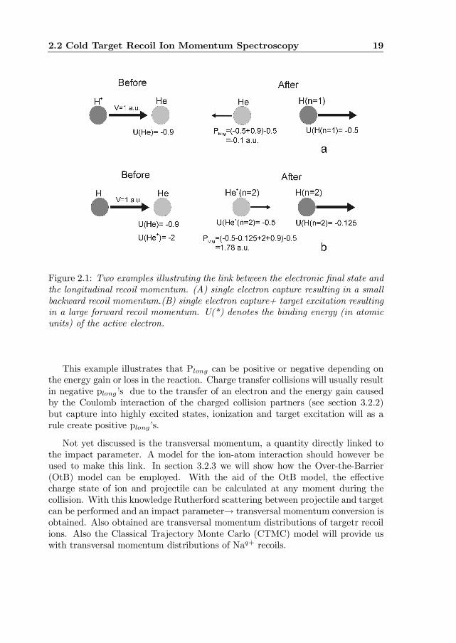
the projectile will result in di¤erent Q’s and thus, as seen in eq. 2.3, in di¤erentPlong ’s. Target excitation will also contribute to the Q and thus to Plong . We canillustrate all this with a very basic example : H+ on He (…gure 2.1 ):
2.2 Cold Target Recoil Ion Momentum Spectroscopy 19
Figure 2.1: Two examples illustrating the link between the electronic …nal state andthe longitudinal recoil momentum. (A) single electron capture resulting in a smallbackward recoil momentum.(B) single electron capture+ target excitation resultingin a large forward recoil momentum. U(*) denotes the binding energy (in atomicunits) of the active electron.
This example illustrates that Plong can be positive or negative depending onthe energy gain or loss in the reaction. Charge transfer collisions will usually resultin negative plong ’s due to the transfer of an electron and the energy gain causedby the Coulomb interaction of the charged collision partners (see section 3.2.2)but capture into highly excited states, ionization and target excitation will as arule create positive plong ’s.
Not yet discussed is the transversal momentum, a quantity directly linked tothe impact parameter. A model for the ion-atom interaction should however beused to make this link. In section 3.2.3 we will show how the Over-the-Barrier(OtB) model can be employed. With the aid of the OtB model, the e¤ectivecharge state of ion and projectile can be calculated at any moment during thecollision. With this knowledge Rutherford scattering between projectile and targetcan be performed and an impact parameter! transversal momentum conversion isobtained. Also obtained are transversal momentum distributions of targetr recoilions. Also the Classical Trajectory Monte Carlo (CTMC) model will provide uswith transversal momentum distributions of Naq+ recoils.
20 Experimental techniques
2.2.4 COLTRIMS: advantages and disadvantages
A distinct advantage of COLTRIMS over PES is that the ion-atom interaction ismeasured in a direct and complete way. Since one does not measure the decay ofthe …nal state population but the population itself, there are usually no gaps inthe measured distribution and even processes like ionization are accessible to theexperimentalist. Moreover the scattering angles involved in the various ion-atomreaction channels can be measured and a direct link to the impact parameter rangecan be made. In the case of the reaction microscopes even the ionizing collisionscan be reconstructed.
A distinct advantage of COLTRIMS is that no elaborate ion beam preparationis needed. The ion beam allowed to have an energy spread in the order of 1%without in‡uencing the experimental resolution. Moreover COLTRIMS can beused in multiple-user ion beam facilities like storage rings, quite unlike TES.
The main disadvantage is that the typical recoil energies are very small (meV inthe worst case), which makes the experiments very complicated (when compared tobasic PES set-ups) and the desired momentum resolution di¢cult to obtain. Thisdisadvantage is becoming however less of an issue since some of the most di¢cultparts of the experiment (like the ultra-cold gas jet and the 2D detectors) arenowadays commercially available. Another disadvantage is that the experiment islimited to those target species which can be prepared as cold gas or vapour targets,either by supersonic jet techniques (especially rare gases) or by laser cooling (alkali,earth-alkali and metastable rare gases).
2.2.5 Conclusion
In this section we discussed the COLTRIMS experimental technique. We discussedthe relation between the longitudinal recoil momentum and the collisional energygain and the relation between the transverse recoil momentum and the impactparameter. The main advantage of COLTRIMS is that one directly measures thephysical quantities of interest (…nal state distributions and scattering angles), thedisadvantage is that COLTRIMS experiments are (as a rule) a major technologicalchallenge.
Although we concentrated in this section on the recoil momentum, it shouldbe clear that the same information can be obtained from the momentum change ofthe projectile. To measure the very small projectile momentum changes requiresthe experimental approach called Translational Energy Spectroscopy (TES) andthis is the topic of the next section.
2.3 Translational Energy Spectroscopy 21
2.3 Translational Energy Spectroscopy
2.3.1 Introduction
In this section we will discuss brie‡y the Translational Energy Spectroscopy (TES)experimental technique. TES consists of the precise detection of the projectilesenergy (momentum) change e.g. due to electron capture. In this way one canmeasure, just like COLTRIMS, directly the …nal state distribution of an ion-atomcollision. An overview of the TES experimental technique and a more completelist of references is given in a review by Janev and Winter.6
2.3.2 TES: a short historic overview
Projectile energy loss spectroscopy has been extensively used for studying bothelastic and inelastic collisions of singly charged ions with neutrals (Ziemba et al53
et al. (1960), Aberth and Lorents54). The energy spectroscopy is in these casesperformed by a time-of-‡ight method. Measurements with doubly charged ions,which allowed an electrostatic analysis of the charge changed projectile, were per-formed by Siegel et al.55 , Kamber and Hasted,56 Huber et al.57 and McCulloughet al.58 State selective electron transfer, even with sub eV (Huber et al.:59 150meV, Kobayashi et al.60 :100 meV) resolution was eventually possible. With slow,singly charged projectiles eventually an impressive 10 meV resolution (Itoh et al.61)was achieved. The TES experimental method was also used with highly chargedions (references in Liljeby62) and just like PES, used for to studying the electroncapture and projectile scattering anisotropy from laser aligned and oriented targets(Aumayr et al.63 , Dowek et al.64, 65).
Another important application of TES can be found in the …eld of ion-solidinteraction where TES is known as Low Energy Ion Scattering (LEIS). LEIS is animportant and still developing experimental tool, but an overview on LEIS wouldbe beyond the scope of this work.
2.3.3 TES: advantages and disadvantages
The advantages are somewhat similar to the COLTRIMS experimental technique.TES gives direct and in principle complete information about the …nal state pop-ulations of an ion-atom collision system, which is an advantage over PES. AlsoTES is not (within reason) restricted in the choice of target atoms in the wayCOLTRIMS experiments are, and therefore also molecular targets are accessible(CO2 was for instance used by Itoh61 et al.). TES is however not well applicableto collisions with high energy projectiles because small energy changes of high-energy projectiles are di¢cult to identify. A major di¤erence between TES and

22 Experimental techniques
COLTRIMS is that TES can be applied in collisions of ions with surfaces andCOLTRIMS of course not.
TES usually does not provide, and this is a major disadvantage with respect toCOLTRIMS, the full kinematic information (i.e. Q-value and scattering angle) ofthe various ion-atom reaction channels. TES can provide the Q-value distributionand sometimes scattering angle distributions, but only if a time-of-‡ight techniqueis used. TES also does not provide the (n,l,m) …nal state resolution possible withPES and when compared to normal PES set-ups (as used in this work), TES canbe a quite di¢cult experiment.
3 Theoretical methods
Di¤erent theoretical methods play a part in this work, either to compare with ourexperiment or to obtain an intuitive understanding of the collision processes understudy. In this chapter we will outline the theories most relevant for this thesisnamely: the Atomic Orbital close coupling and Classical Trajectory Monte Carlowhich are used for the comparison and the Over-the-Barrier, which we employ tocreate an intuitive picture of the interactions.
23
24 Theoretical methods
3.1 Atomic Orbital Close Coupling
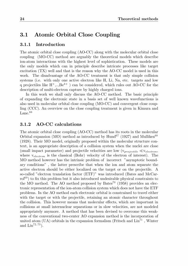
3.1.1 IntroductionThe atomic orbital close coupling (AO-CC) along with the molecular orbital closecoupling (MO-CC) method are arguably the theoretical models which describeion-atom interactions with the highest level of sophistication. These models arethe only models which can in principle describe intricate processes like targetexcitation (TX) well and that is the reason why the AO-CC model is used in thiswork. The disadvantage of the AO-CC treatment is that only simple collisionsystems (i.e. with only one active electron like H, Li, Na, etc. targets and lowq projectiles like H+,..,Be4+ ) can be considered, which rules out AO-CC for thedescription of multi-electron capture by highly charged ions.
In this work we shall only discuss the AO-CC method. The basic principleof expanding the electronic state in a basis set of well known wavefunctions isalso used in molecular orbital close coupling (MO-CC) and convergent close coup-ling (CCC). An overview on the close coupling treatment is given in Kimura andLane.66
3.1.2 AO-CC calculationsThe atomic orbital close coupling (AO-CC) method has its roots in the molecularOrbital expansion (MO) method as introduced by Hund67 (1927) and Mulliken68
(1928). Their MO model, originally proposed within the molecular structure con-text, is an appropriate description of a collision system when the nuclei are close(small impact parameter) and projectile velocities are low (vprojectile ¿velectron,where velectron is the classical (Bohr) velocity of the electron of interest). TheMO method however has the intrinsic problem of incorrect ”asymptotic bound-ary conditions” , the latter prescribe that when the ion and atom separate theactive electron should be either localized on the target or on the projectile. Aso-called ”electron translation factor (ETF)” was introduced (Bates and McCar-rol69) to …x this problem but it also introduced undesirable physical constraints tothe MO method. The AO method proposed by Bates70 (1958) provides an elec-tronic representation of the ion-atom collision system which does not have the ETFproblems. In the AO method each electronic orbital is constrained to travel eitherwith the target or with the projectile, retaining an atomic character throughoutthe collision. This however means that molecular e¤ects, which are important incollisions at small internuclear separations or in slow velocities, are not modeledappropriately anymore. A method that has been devised to overcome this weak-ness of the conventional two-center AO expansion method is the incorporation ofunited atom (UA) orbitals in the expansion formalism (Fritsch and Lin71 , Winterand Lin72, 73).

3.2 Over the Barrier 25
The basic idea of AO-CC is to expand the time-dependent electronic wavefunction of the electron active in the ion-atom collision in a basis set of target,projectile, pseudo and united atom states. The pseudo and united atom-states(PS-UA) are needed to correctly describe the electronic wave function during theinteraction and mainly serve to represent transient molecular orbitals and ioniz-ation channels. In the AO-CC calculation used for this work (chapter 4) the Litarget eigenstates (”AO’s”) were found by diagonalizing the atomic Hamiltonianwhich contains a Li model potential in a (truncated) basis set of Slater type orbitals(STO’s) de…ned by their quantum numbers n,l and charge z. This diagonaliza-tion leads to linear combinations of STO’s representing the Li states (reproducingthe Li energy levels (AO’s) within 0.3%) and a collection of additional eigenstateswith energies higher than the AO’s including several unbound states. These addi-tional eigenstates are part of the pseudo-states (PS) collection and will represent(although discrete in nature) the continuum in the collision. More details aboutpseudo-states and united-atom states used in this work will be given in chapter4.2.
Because AO-CC calculations can only be performed with the total number ofstates below »200 (simply because of computing power) a wise choice has to bemade regarding the states to be included. First of all, capture is the dominantprocess at low energies and therefore many projectile states have to be includedin the calculation, even if one is only interested in target excitation. Especiallyat low energies it is found that electron capture into projectile orbitals with highquantum number n is an important loss channel for the excited Li states of interest.Secondly, pseudo and united atom states have to be chosen in such a way thatconsistent and convergent results are obtained.
3.2 Over the Barrier
3.2.1 IntroductionThe classical Over the Barrier (OtB) model is one of the simplest models one canuse to describe ion-atom collisions. Its principles were introduced by Bohr andLindhard74 (1954) and were developed further by Ryufuku et al.,75 Bárány et al.76
and Niehaus77 . The model is extensively used since it usually describes electroncapture rather well and moreover it adds to an intuitive understanding of ion-atomcollisions. In the OtB model we discern the ”way in” of an ion, where it successivelyliberates electrons from the target into the combined ion-atom potential well, fromthe ”way out”, where it can capture electrons into the projectile potential well.As we shall see one can analytically calculate the energy gain (Q) distributionof a collision and numerically the transversal recoil momentum distribution. Forall the …gures in this section (…gure 3.1, 3.2 and 3.3), we used the same collision
26 Theoretical methods
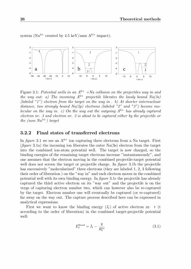
system (Na3+ created by 4.5 keV/amu A6+ impact).
Figure 3.1: Potential wells in an A6+ +Na collision on the projectiles way in andthe way out: a) The incoming A6+ projectile liberates the loosly bound Na(3s)(labeled ”1”) electron from the target on the way in . b) At shorter internucleairdistance, two strongly bound Na(2p) electrons (labeled ”2” and ”3”) become mo-lecular on the way in. c) On the way out the outgoing A6+ has already capturedelectron nr. 3 and electron nr. 2 is about to be captured either by the projectile orthe (now Na3+) target
3.2.2 Final states of transferred electronsIn …gure 3.1 we see an A6+ ion capturing three electrons from a Na target. First(…gure 3.1a) the incoming ion liberates the outer Na(3s) electron from the targetinto the combined ion-atom potential well. The target is now charged, so thebinding energies of the remaining target electrons increase ”instantaneously”, andone assumes that the electron moving in the combined projectile-target potentialwell does not screen the target or projectile charge. In …gure 3.1b the projectilehas successively ”molecularized” three electrons (they are labeled 1, 2, 3 followingtheir order of liberation ) on the ”way in” and each electron moves in the combinedpotential well with its own binding energy. In …gure 3.1c the projectile has alreadycaptured the third active electron on its ”way out” and the projectile is on theverge of capturing electron number two, which can however also be re-capturedby the target. Electron number one will eventually be captured (or re-captured)far away on the way out. The capture process described here can be expressed inanalytical expressions.
First we want to know the binding energy (It) of active electron nr. t (taccording to the order of liberation) in the combined target-projectile potentialwell:
Ebindt = It ¡ q
Rint
(3.1)
3.2 Over the Barrier 27
Ebindt consists of the original binding energy (It) and the Stark shift induced
by the projectile with charge q at distance Rint ; where the transition of electron
number t from an atomic to a quasi-moleculair orbital takes place (Note that eq.3.1 is so compact because we use atomic units).
To calculate Rint we …rst have to look more carefully at the combined projectile-
target potential:
V int (r) = ¡ q
j r j ¡ tj R ¡ r j for 0<r<R (3.2)
Following r from the projectile (r=R) to the target (r=0) we encounter a maximumdepending on R. Calculating dV in
t (r)dr = 0 yields:
V in;maxt (R) =
¡qR
¡ t + 2p
qtR
(3.3)
Electron nr. t is liberated when the barrier height (V in;maxt (R)) drops below
the Stark-shifted binding energy of the target electron (V in;maxt (R) · Ebind
t ).This will happen at the distances Rin
t ;the so called barrier crossings on the wayin:
Rint =
t + 2p
qt¡It
(3.4)
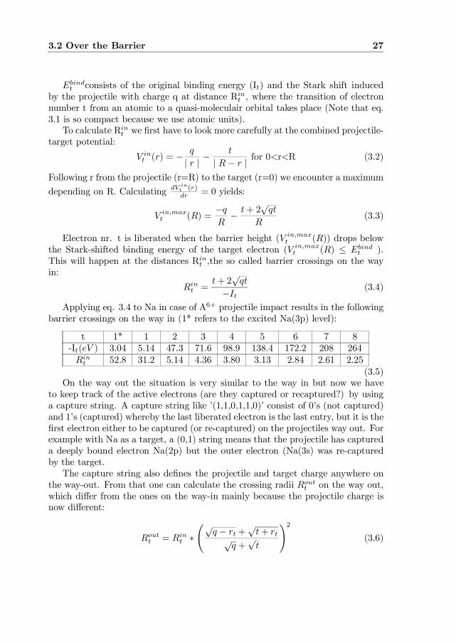
Applying eq. 3.4 to Na in case of A6+ projectile impact results in the followingbarrier crossings on the way in (1* refers to the excited Na(3p) level):
t 1* 1 2 3 4 5 6 7 8-It(eV ) 3.04 5.14 47.3 71.6 98.9 138.4 172.2 208 264
Rint 52.8 31.2 5.14 4.36 3.80 3.13 2.84 2.61 2.25
(3.5)On the way out the situation is very similar to the way in but now we have
to keep track of the active electrons (are they captured or recaptured?) by usinga capture string. A capture string like ’(1,1,0,1,1,0)’ consist of 0’s (not captured)and 1’s (captured) whereby the last liberated electron is the last entry, but it is the…rst electron either to be captured (or re-captured) on the projectiles way out. Forexample with Na as a target, a (0,1) string means that the projectile has captureda deeply bound electron Na(2p) but the outer electron (Na(3s) was re-capturedby the target.
The capture string also de…nes the projectile and target charge anywhere onthe way-out. From that one can calculate the crossing radii Rout
t on the way out,which di¤er from the ones on the way-in mainly because the projectile charge isnow di¤erent:
Routt = Rin
t ¤Ãp
q ¡ rt +p
t + rtpq +p
t
!2
(3.6)
28 Theoretical methods
Where rt is the number of electrons already captured by the projectile. Thebinding energy EA
t of a captured electron consists of Ebindt (eq. 3.1) but ”corrected”
for the Stark shift of the now charged target ( t+rtRt
out):
EAt = It ¡ q
Rint
+t + rt
Routt
(3.7)
and the energy gain/loss Q expected from the transfer of electron nr. t is simply:
Q = EAt ¡ It = ¡ q
Rint
+t + rt
Routt
(3.8)
From eq. 3.8 we see that when energy is released (an electron jumps into amore strongly bound …nal state) this results in a negative Q-value.
The energy width ¢E of the energy window, within which actually existingquantum mechanical states are likely to be populated, can be estimated by meansof the following considerations: assuming a very localized transition at a wellde…ned time t, the …nal state energy is classically well de…ned, but a lower limitfor ¢E is given by the uncertainty relation according the small ¢t: A less de…nedtransition region (and time) on the other hand, results in a broader interval ofclassically binding energies. Niehaus77 has shown that the minimum width of anenergy window compatible with these boundary conditions is given by:
¢EAt =
vuutÃpq +
pt
Rint
!2
¢ vinrad;t +
µpq ¡ rt +
pt + rt
Rint
¶2
¢ voutrad;t; (3.9)
if t < t0 then vinnoutrad;t = v0
vuut1 ¡Ã
Rinnoutto
Rinnoutt
!2
(3.10)
if t ¸ t0 then vinnoutrad;t = v0
vuut1 ¡Ã
Rinnoutt+1
Rinnoutt
!2
(3.11)
Q ¼ exp
á0:5
µE ¡ EA
t
¢EAt
¶2!
(3.12)
where t0 is the index of the …rst electron captured. The reaction window in caseof multiple electron capture is calculated by quadratic addition of the contributionsfor each captured electron.
3.2 Over the Barrier 29
The cross section for a certain string is:
¾string = ¾geo;s ¢sY
i
Wi (3.13)
where s is the number of electrons in that string, Wi is the probability to captureor recapture electron i and ¾geo the geometrical cross section for having s activeelectrons. The probability Wi in case of capture can be approximated with theratio between the number of states available to the active electron in the projectilewith respect to the total number of states in the target and projectile. Quantummechanically the degeneracy of a certain hydrogenic level is 2n2 and this leads toan estimate of the probability Wi:
Wi =n2
in2
i + m2i
(3.14)
where ni and mi correspond to the quantum number of the most likely …nal stateorbital on projectile and target respectively. This number is found by comparingthe EA
t from equation 3.7 to the actual level schemes of the O6+,O5+,... andNa+,Na2+;... respectively.
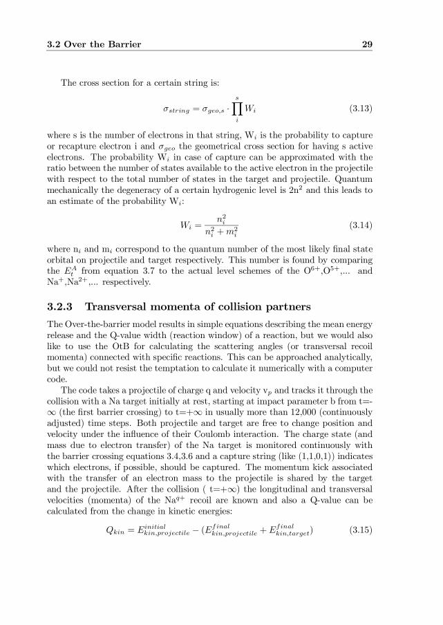
3.2.3 Transversal momenta of collision partnersThe Over-the-barrier model results in simple equations describing the mean energyrelease and the Q-value width (reaction window) of a reaction, but we would alsolike to use the OtB for calculating the scattering angles (or transversal recoilmomenta) connected with speci…c reactions. This can be approached analytically,but we could not resist the temptation to calculate it numerically with a computercode.
The code takes a projectile of charge q and velocity vp and tracks it through thecollision with a Na target initially at rest, starting at impact parameter b from t=-1 (the …rst barrier crossing) to t=+1 in usually more than 12,000 (continuouslyadjusted) time steps. Both projectile and target are free to change position andvelocity under the in‡uence of their Coulomb interaction. The charge state (andmass due to electron transfer) of the Na target is monitored continuously withthe barrier crossing equations 3.4,3.6 and a capture string (like (1,1,0,1)) indicateswhich electrons, if possible, should be captured. The momentum kick associatedwith the transfer of an electron mass to the projectile is shared by the targetand the projectile. After the collision ( t=+1) the longitudinal and transversalvelocities (momenta) of the Naq+ recoil are known and also a Q-value can becalculated from the change in kinetic energies:
Qkin = Einitialkin;projectile ¡ (Efinal
kin;projectile + Efinalkin;target) (3.15)
30 Theoretical methods
and from the longitudinal target momentum (where vp=projectile velocity andNc=number of electrons captured):
Qplong = vp ¢ plong + v2p ¢ Nc
2(3.16)
Equation 3.16 was derived in chapter 2.2.3. In …gure 3.2a,b a calculated trajectoryis displayed of a Na3+ recoil created from a string (1,1,1) in a 4.5 keV/amu A6+
collision at an impact parameter b=4 a.u.
Figure 3.2: Calculated trajectory of a Na3+ recoil created in a 4.5 keV/amu A6+
collision at impact parameter b=4 atomic units (a.u.). Longitudinal momentum=-3.72 a.u., transversal momentum=15.8 a.u. and the energy gain in the collisionwas -37.8 eV. The projectile passed by in the positive x-direction at impact para-meter y0=b=+4 a.u.
In …gure 3.2b one can see that the recoil (Na3+ created in 4.5 keV/u A6+ impactat b=4 a.u) is pushed forward by the projectiles on its way in and pushed back-wards on its way out. The longitudinal momentum directly re‡ects the delicate bal-ance between the two. The numerically calculated recoil momenta are plong=-3.78a.u, ptrans=15.8 a.u and the ”di¤erent” Q-values are Qkin=-37.8 eV(calculated
3.2 Over the Barrier 31
with eq. 3.15), Qplong=-37.6 (calculated with eq. 3.16) and Q=-38.4 (eV) (calcu-lated with eq. 3.8). Qkin is slightly smaller than Q because the simulation stoppedbefore t=+1 was e¤ectively reached and Qplong is even smaller than Qkin becauseeq. 3.16 starts to loose its validity when the recoil energy is no longer very smallas compared to Q (chapter 2.2.3). Should for instance the captured electronsnot screen the projectile charge fully then the longitudinal momentum will im-mediately increase and almost double (in our example of (1,1,1) capture1 by A6+
plong=-6.18 (no screening) instead of plong=-3.78 a.u. (full screening)).
The transversal recoil momentum however is nearly exclusively produced atthe distances of close approach and it depends therefore mainly on the impactparameter. Electron capture dynamics (taking place on the way out) will nota¤ect the transverse momentum signi…cantly (»10% depending on how close tothe target the electrons are captured). In our example of (1,1,1) capture by A6+
at an impact parameter b=4 a.u. we obtain ptrans=15.8 a.u while for the case ofno screening ptrans increases to 17.4 a.u.. For the (0,0,0) capture string, i.e. nocapture, we obtain ptrans=14 a.u..
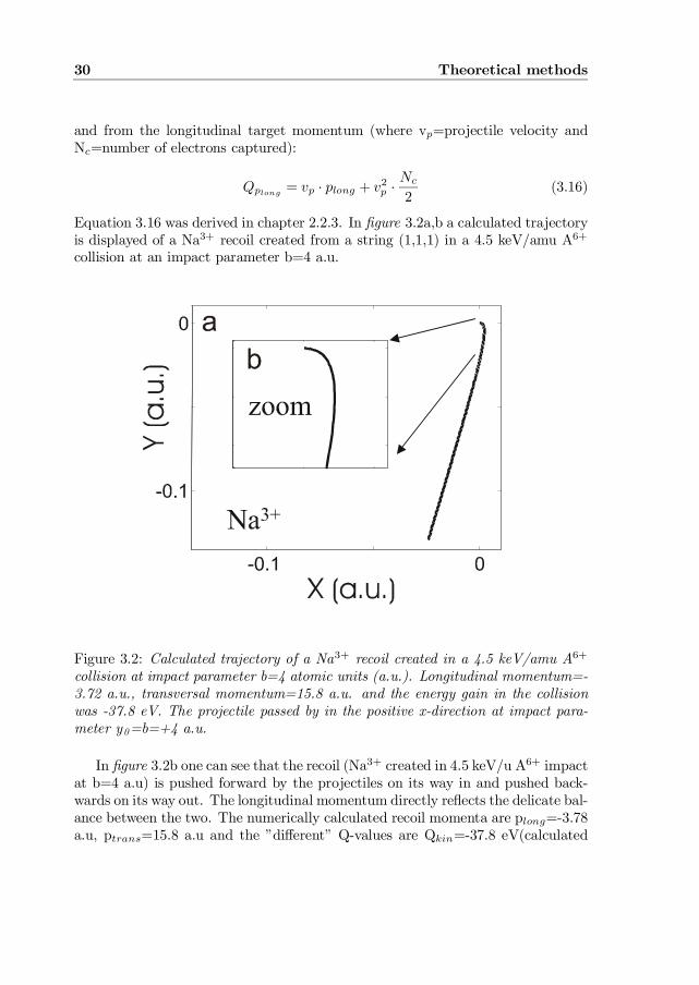
These observations support the principle already discussed in chapter 2.2.3that for ”gentle” collisions, i.e. not too many active electrons, the longitudinaland transversal momenta are independent quantities. This is (in the OtB model)because they relate to di¤erent parts of the projectile-target interaction: the in-teraction on the way out (longitudinal momentum) and the interaction at closestapproach (transverse momentum). For gentle collisions the ”way out interaction”is well separated from the ”closest approach interaction”. In a ”strong” collisionwith ’many active electrons’ capture takes place close to the target and the trans-verse momentum will show a weak dependence on the capture dynamics. Thetransition from gentle to strong collisions is further illustrated by …gure 3.3: thelongitudinal momenta of Naq+(q=2-4) recoils are not independent of the trans-versal momentum (impact parameter) but become less negative with increasingcollision strength i.e. smaller impact parameters. This ”kinematic e¤ect” wasalready touched upon in chapter 2.2.3 and is also observed in the numerical sim-ulations with the OtB computer code.
1 see section 3.2.2
32 Theoretical methods
Figure 3.3: Longitudinal momentum versus transversal momentum and im-pact parameter b for Na2+, Na3+ and Na4+ recoils produced in 4.5 keV/amuA6+collisions
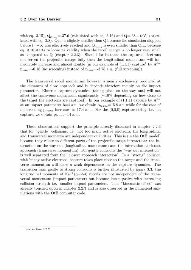
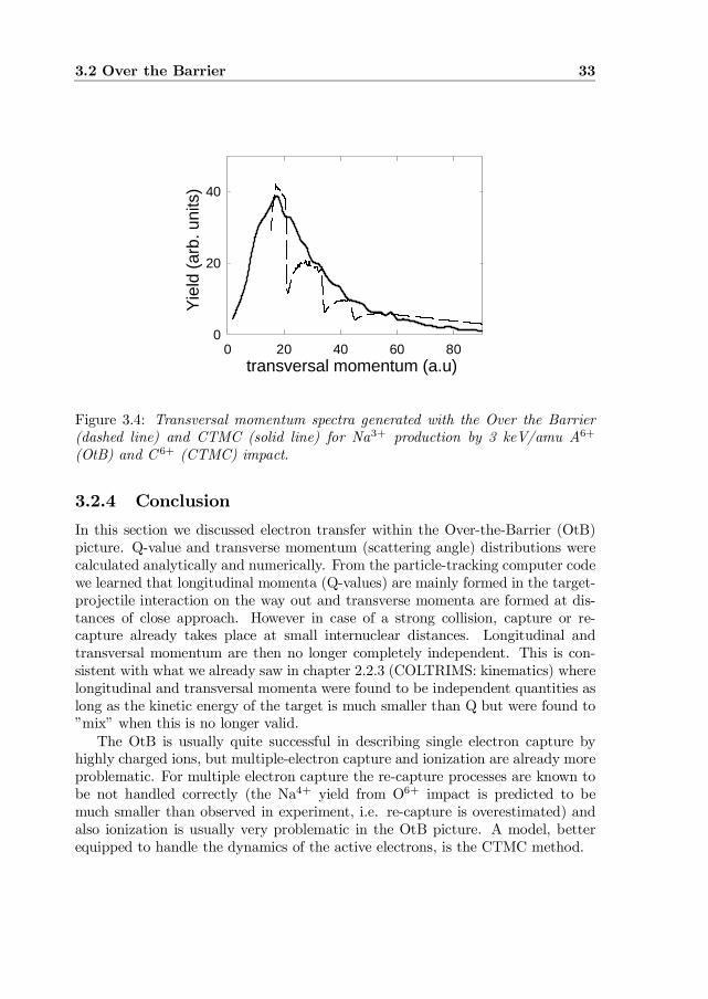
Last but not least, the code can generate transversal momentum spectra by cal-culating transversal momenta for impact parameters from bmin, bmin+¢b; ::.,bmaxfor a speci…c collision system. Each data point must be weighted with the geomet-rical cross section 2¼b¢¢b and normalized to the size of the transversal momentuminterval it represents. Figure 3.4 shows such a transversal momentum spectrum(dashed line) together with a CTMC (see next section) generated spectrum (solidline) for Na3+ recoil production by 3 keV/amu A6+ impact. The (1,1,1,0,0,..) cap-ture string was executed by the OtB code. The general trend is similar betweenthe OtB and CTMC curves but the OtB curve shows several peculiar dips. Thesedips are not caused by numerical anomalies but are created by the abrupt barriercrossings on the way in : every time a barrier is crossed an extra Na electron be-comes active and the Nar+ core changes to a Na(r+1)+. The interaction betweenthe A6+ and the Na ionic core gets an extra boost resulting in a sudden rise in thetransverse momenta. This sudden rise causes the absence (depletion) of certaintransverse momenta, resulting in a dip in the spectrum. The dips directly corres-pond to a barrier crossing (see table 3.5): the dip at Ptrans=20 a.u. is caused bythe crossing at b=4.36 a.u, dip at 35 a.u. by the one at b=3.80 a.u. etc.. In realityand indeed in the CTMC calculations one does not expect ”hard” crossings (thealready discussed ’reaction window’ in section 3.2.2 more or less already illustratedthis) and thus that the dips in the OtB are washed out in reality.
3.2 Over the Barrier 33
transversal momentum (a.u)0 20 40 60 80
Yie
ld (a
rb. u
nits
)
0
20
40
Figure 3.4: Transversal momentum spectra generated with the Over the Barrier(dashed line) and CTMC (solid line) for Na3+ production by 3 keV/amu A6+
(OtB) and C 6+ (CTMC) impact.
3.2.4 ConclusionIn this section we discussed electron transfer within the Over-the-Barrier (OtB)picture. Q-value and transverse momentum (scattering angle) distributions werecalculated analytically and numerically. From the particle-tracking computer codewe learned that longitudinal momenta (Q-values) are mainly formed in the target-projectile interaction on the way out and transverse momenta are formed at dis-tances of close approach. However in case of a strong collision, capture or re-capture already takes place at small internuclear distances. Longitudinal andtransversal momentum are then no longer completely independent. This is con-sistent with what we already saw in chapter 2.2.3 (COLTRIMS: kinematics) wherelongitudinal and transversal momenta were found to be independent quantities aslong as the kinetic energy of the target is much smaller than Q but were found to”mix” when this is no longer valid.
The OtB is usually quite successful in describing single electron capture byhighly charged ions, but multiple-electron capture and ionization are already moreproblematic. For multiple electron capture the re-capture processes are known tobe not handled correctly (the Na4+ yield from O6+ impact is predicted to bemuch smaller than observed in experiment, i.e. re-capture is overestimated) andalso ionization is usually very problematic in the OtB picture. A model, betterequipped to handle the dynamics of the active electrons, is the CTMC method.

34 Theoretical methods
3.3 Classical Trajectory Monte Carlo
3.3.1 IntroductionThe last method to be discussed in this chapter is the CTMC approach introducedin 1966 by Abrines and Percival.78 It was …rst applied extensively by Olson andSalop79 . The working area of the CTMC is e¤ectively located in between the verysophisticated AO-CC method, which can only handle simple collision systems, andthe simple Over the Barrier model, which does not handle the dynamic aspects ofan ion-atom collision very well. The CTMC method treats all ion-atom interactionsclassically and therefore it does not run into problems when for instance morethan three bodies are involved or an electron is located in a highly excited orbital.For collision systems studied in this thesis the CTMC method was applied byR.E. Olson to calculate longitudinal and transversal Naq+ recoil momenta aftercollisions with C6+ projectiles resulting in electron transfer to the projectile orinto the continuum.
3.3.2 CTMC calculationsIn CTMC electrons and ions are assumed to interact via the Coulomb potentialsand to follow classical trajectories. The initial ensemble (”microcanonical distri-bution”) of target centered electrons is constructed in such a way that it mimicsthe properties of the quantum mechanical initial state (i.e. jªi(r)j 2 and jªi(p)j2). From the initial ensemble a member is randomly picked (by a Monte Carlotechnique) just as a projectile impact parameter is chosen out of the appropriaterange.
After the interaction of the active electron(s) with the projectile and (ionic)target cores (interaction described by model (screened Coulomb) potentials ob-tained from Hartree-Fock calculations), the active electrons will most likely …ndthemselves on the projectile (capture) or moving in the continuum (ionization). Incase of capture it is usually desirable to translate the electrons motion to a properprojectile state with quantum numbers n, l and m. For this transformation theclassical principal quantum number nc is calculated from the electron’s bindingenergy Ep with:
Ep =¡q2
2n2c
(3.17)
with q the projectile charge state. These nc’s can then be binned (in case ofone active electron) according to eq. 3.18 (Olson80) to obtain their quantummechanical counterpart: the principal quantum number n.
·(n ¡ 1
2)(n ¡ 1)n
¸ 13
· nc ··(n +
12)(n + 1)n
¸ 13
(3.18)

3.3 Classical Trajectory Monte Carlo 35
Also the (normalized) classical angular momentum lc= nnc
(rxp), with r andp the classical position and momentum vectors of the electron relative to theprojectile core, can be transformed into the corresponding quantum number l:
l · lc · l + 1 (3.19)
And in a similar fashion the magnetic sub-state quantum number m can be foundby binning the classical mc = jlzc j .
m · mc · m + 1 (3.20)
In case of multiple electron capture, the electrons are binned successively.The CTMC method was e.g. quite successful in the case of single electron
capture by 1 to 50 keV/amu He2+, O6+ projectile ions from a laser prepared Natarget (Schippers et al.35 en Schlatmann et al.33).

4 Lithium excitation by slowH+ and He2+ ions
New experimental and theoretical cross sections for the excitation of groundstate Lithium by H + and He2+ impact are presented for the 2-30 keV/amu energyregime. Experimentally, absolute emission cross sections were determined with thePhoto Emission Spectroscopy (PES) method by observing the LiI(nd-2p,n=3-6)and LiI(ns-2p,n=4-6) line radiation after ion impact. Li(2s) excitation up to theLi(n=4) level was simulated by means of the Atomic Orbital Close Coupling (AO-CC) method. Furthermore a few measurements have been performed on high-nexcitation (Li(2s ! nd; n = 7 ¡ 9) by He2+ impact.
37
38 Lithium excitation by slow H+ and He2+ ions
4.1 IntroductionIn the …eld of ion-atom collisions the one electron and quasi-one-electron targets(H, Li, Na, etc.) have always received a lot of attention. Most attention wasusually directed to single electron capture, because it is a process that can be de-scribed by various models at di¤erent levels of sophistication: Over-The-Barrier75
, Multichannel Landau-Zener81 , Classical-Trajectory-Monte-Carlo (CTMC)78, 82
and Atomic Orbital Close Coupling (AO-CC)83 . However for the description oftarget excitation and ionization most models are not so well suited, mainly becauseelectron capture dominates over the other processes, especially in the low energyregion. Also there was a lack of experiments to test and improve the various mod-els. For lithium target excitation the experimental work consisted of experimentsby Kadota84 et al. and Aumayr85, 86 et al. and theoretical studies were doneby Ermolaev87 et al. and Schweinzer88 et al. Other closely related studies havebeen performed by Fritsch89 et al. , Schultz90 et al. (hydrogen excitation) andHorvath91 et al. (sodium excitation).
In this chapter we present a study on
(H+;He2+)+Li(2s) ! (H+;He2+)+Li¤(n; l) ! (H+;He2+)+Li(2s)+hv (4.1)
by means of photon emission spectroscopy (experiment) and AO-CC (theory).This work has an intended overlap with another body of work (on lithium excita-tion by ion impact) performed recently by Brandenburg et al.92 Together with thiswork a consistent, reasonably complete picture on lithium excitation can be con-structed with some unexpected features, most of them supported by the AO-CCtheory.
Another important motivation for this work was to construct a high qual-ity database of lithium excitation by ion impact to be used for the lithium beamdiagnostics of magnetically con…ned fusion plasmas93 . The previous lithium excit-ation database mainly consisted of scaled electron impact cross sections94 , whichare not likely to describe ion-atom collisions very well in the low energy region(1-20 keV/amu) because the coupling between excitation channels and electroncapture channels is not incorporated. Therefore a new database (Schweinzer etal.95) including all collision processes relevant for plasma diagnostic purposes hasbeen compiled recently. The ion-impact part of this new database is based on theAO-CC calculations presented here.
4.2 TheoryThe well-known semiclassical impact-parameter formulation of the close-coupling(CC) method for collisions with one ’active’ electron, assuming straight line tra-

4.2 Theory 39
jectories for the projectiles. The general approach has already been described byHorvath et al.91 (and ref. therein), which shall not be repeated here. Only detailsfor the particularly chosen two-center expansions will be given which are of im-portance for the discussions in the following chapters. All chosen basis sets usedin the present CC-calculation are listed in …gure 4.1.
calculation
H+
AO65-64
He2+
AO87-79
AO81-80
AO
20;n=1-4
56:n=1-6
50; n=1-5,6l<5
PS-UA
45 STO l<4
31 STO 1<l<4
AO
20; n=1-4
35; n=1-5
35; n=1-5
17 STO l<1
17 STO l <1
14 STO l<1
27 STO 2<l<4
27 STO 2<l<4
31 STO 1<l<4
PS-ST PS-UA
center on target Li+center on projectile Zq+
Figure 4.1: Basis sets used in the ao-cc simulations.
Figure 4.1 has to be regarded just as a survey, and detailed information aboutthe used basis set is available from Schweinzer (Garching). Besides atomic orbit-als (AO) on projectile and target, pseudo-states on both centers appear in theexpansion. While AO on the projectile (H+, He2+) are simply given by hydro-genic states, AOs for Li are derived by diagonalizing the atomic Hamiltonian ina truncated basis set of Slater-type orbitals (STOs, de…ned by charge z and n,lquantum numbers). The Hamiltonian on the Li center includes an analytic modelpotential (Peach96 et al.) for the interaction between the Li+ core and the ’active’electron. The diagonalization process leads to linear combinations of the originalSTOs which represent AOs in cases where the corresponding eigenvalues are closeto experimental energy levels (deviations < 0.3%). All other eigenstates of thediagonalization process are called pseudo-states (PS) and their eigenvalues covera range of energies above the highest AO state to positive values. Such statesare considered - though of discrete nature - to represent the continuum in thecalculation. One can further distinguish between such STOs optimized in order toreproduce most accurately the atomic level diagram (PS-ST, ST stands for struc-ture) and STOs with z values (not given in …gure 4.1) between the charge of theseparated atoms and the united atom (PS-UA). The latter are more appropriatefor small impact parameters to describe the motion of the active electron. Theeigenvalues of these PS-UA lie above the AO and represent higher excited boundstates as well as ionization channels. This type of states (PS-UA) is also included
40 Lithium excitation by slow H+ and He2+ ions
at the projectile center representing there capture to the continuum. All presen-ted AO-calculations (e.g. …gure 4.1) involve a considerable number of projectilecentered states representing single electron capture (SEC). The importance of suchchannels for the results of excitation cross sections has already been discussed forthe Li(2s-2p) excitation in He2+ - Li(2s) collisions (Schweinzer88 et al.). In thispure AO-CC study (no pseudo-states were included) the number of included SECchannels in‡uenced the resulting excitation cross section signi…cantly in the lowerimpact energy range. Furthermore it turned out that, in order to obtain reasonableresults, it is recommended to include SEC from the excited states under study.The AO expansion for H+- Li(2s) collisions (AO65_64 in …gure 4.1 ) has beentailored to ful…ll this rule for all excitation processes Li(2s-nl) (n=2-4, l=0-3). Aconsiderable enlargement of the basis size would have been necessary in the caseof He2+ impact (AO87_79, AO81_80 in TABLE I), but could not be realizedbecause of computational reasons. In view of this no convergent results can beexpected for Li(2s-5l) excitation cross sections, because the HeII orbitals domin-antly populated by SEC from Li(5l) will have n values of 7-9, which is beyond theones included in the present AO calculations.
These AO-CC calculations shall be compared with all available experimentaldata and available theoretical calculations. By default all theoretical curves aredisplayed as lines, even though they were all calculated for discrete energies.
4.3 Experimental results
The He2+ and H+ ions were produced by our electron cyclotron resonance ionsource (ECRIS) installed at the KVI in Groningen. The source was operated atvoltages ranging from 4 to 24 kV. We also had the possibility to post-acceleratethe ions with voltages of 30 to 100 kV. However for our experiments this optionimplied a decrease of a factor of ten loss in current. Typical currents for the He2+
and H+ ions at the collision center (non post-accelerated beams) were rangingfrom 0.5 ¹A at the lowest energies to 3 ¹A at the highest energies.
4.3 Experimental results 41
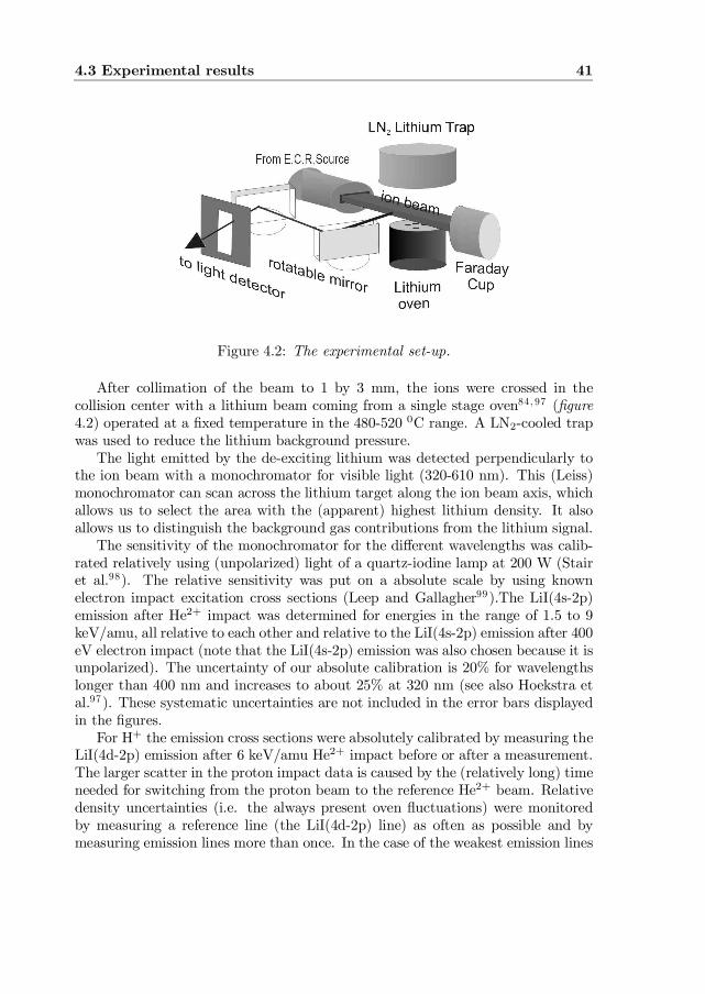
Figure 4.2: The experimental set-up.
After collimation of the beam to 1 by 3 mm, the ions were crossed in thecollision center with a lithium beam coming from a single stage oven84, 97 (…gure4.2) operated at a …xed temperature in the 480-520 0C range. A LN2-cooled trapwas used to reduce the lithium background pressure.
The light emitted by the de-exciting lithium was detected perpendicularly tothe ion beam with a monochromator for visible light (320-610 nm). This (Leiss)monochromator can scan across the lithium target along the ion beam axis, whichallows us to select the area with the (apparent) highest lithium density. It alsoallows us to distinguish the background gas contributions from the lithium signal.
The sensitivity of the monochromator for the di¤erent wavelengths was calib-rated relatively using (unpolarized) light of a quartz-iodine lamp at 200 W (Stairet al.98). The relative sensitivity was put on a absolute scale by using knownelectron impact excitation cross sections (Leep and Gallagher99).The LiI(4s-2p)emission after He2+ impact was determined for energies in the range of 1.5 to 9keV/amu, all relative to each other and relative to the LiI(4s-2p) emission after 400eV electron impact (note that the LiI(4s-2p) emission was also chosen because it isunpolarized). The uncertainty of our absolute calibration is 20% for wavelengthslonger than 400 nm and increases to about 25% at 320 nm (see also Hoekstra etal.97). These systematic uncertainties are not included in the error bars displayedin the …gures.
For H+ the emission cross sections were absolutely calibrated by measuring theLiI(4d-2p) emission after 6 keV/amu He2+ impact before or after a measurement.The larger scatter in the proton impact data is caused by the (relatively long) timeneeded for switching from the proton beam to the reference He2+ beam. Relativedensity uncertainties (i.e. the always present oven ‡uctuations) were monitoredby measuring a reference line (the LiI(4d-2p) line) as often as possible and bymeasuring emission lines more than once. In the case of the weakest emission lines

42 Lithium excitation by slow H+ and He2+ ions
(LiI(ns-2p,n=5,6)) the uncertainty in the cross section is not only determinedby the counting statistics, but also by the fact that the oven behavior was notmonitored for a relatively long period.
To compare our measurements with theory the theoretical excitation crosssections had to be transformed into emission cross sections. For this procedurethe following relations were used:
¾(3p ! 2s) = (0:215 § 0:02) ¤ (¾(3p) + 0:425¾(4s) + 0:23¾(4d)) (4.2)
¾(3d ! 2p) = ¾(3d) + 0:2¾(4p) + ¾(4f) (4.3)
¾(4s ! 2p) = 0:575(¾(4s) + 0:28¾(4p)) (4.4)
¾(4d ! 2p) = 0:77¾(4d) (4.5)
¾(5s ! 2p) = 0:48¾(5s) (4.6)
¾(5d ! 2p) = 0:71¾(5d) (4.7)
¾(6s ! 2p) = 0:43¾(6s) (4.8)
¾(6d ! 2p) = 0:65¾(6d) (4.9)
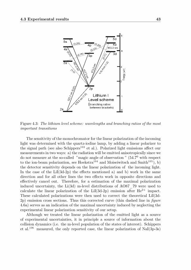
For these relations branching ratios calculated by Wiese100 et al. and Lindgårdand Nielsen101 are used (Wiese et al.: equations 4.2, 4.3, 4.4, 4.5 and Lindgårdand Nielsen: 4.6, 4.7, 4.8, 4.9. There is some uncertainty concerning the lifetimeof the Li(3p) level (see Wiese100 et al., Lindgård and Nielsen101 , Verner102 et al.)causing the 3p ! 2s branching ratio to range from 0.195 to 0.235. A more visualoverview of the most important transitions is given in …gure 4.3.
4.3 Experimental results 43
Figure 4.3: The lithium level scheme: wavelengths and branching ratios of the mostimportant transitions
The sensitivity of the monochromator for the linear polarization of the incominglight was determined with the quartz-iodine lamp, by adding a linear polarizer tothe signal path (see also Schippers103 et al.). Polarized light emissions a¤ect ourmeasurements in two ways: a) the radiation will be emitted anisotropically since wedo not measure at the so-called ”magic angle of observation ” (54.70 with respectto the ion-beam polarization, see Hoekstra104 and Moiseiwitsch and Smith105), b)the detector sensitivity depends on the linear polarization of the incoming light.In the case of the LiI(3d-2p) the e¤ects mentioned a) and b) work in the samedirection and for all other lines the two e¤ects work in opposite directions ande¤ectively cancel out. Therefore, for a estimation of the maximal polarizationinduced uncertainty, the Li(3d) m-level distributions of AO87_79 were used tocalculate the linear polarization of the LiI(3d-2p) emission after He2+ impact.These calculated polarizations were then used to correct the theoretical LiI(3d-2p) emission cross sections. Thus this corrected curve (thin dashed line in …gure4.6a) serves as an indication of the maximal uncertainty induced by neglecting theexperimental linear polarization sensitivity of our setup.
Although we treated the linear polarization of the emitted light as a sourceof experimental uncertainties, it in principle a source of information about thecollision dynamics (i.e. the m-level population of the states of interest). Schipperset al.106 measured, the only reported case, the linear polarization of NaI(3p-3s)
44 Lithium excitation by slow H+ and He2+ ions
emission in the case of Na excitation by He2+ impact. The polarization of emissionafter electron capture is however more widely studied, for example by Laulhé etal.107 (electron capture from Li) and Grego et al.108 (electron capture from Na).
4.3.1 Proton impact
In this section, the proton impact data will be discussed with their AO simulations(and other available data) as separate cases. The LiI(5d-2p) data will be shown inthis section only to get an impression of the physics of target excitation. Later on,in section 4.4, they will be evaluated more quantitatively together with the He2+
impact case.
All error bars are at least 15% because of the relative uncertainty associatedwith the calibration procedure. Some other lines LiI(3d-2p), LiI(5s-2p) and LiI(6d-2p) also have an additional 5-15% statistical uncertainty. Note that our detectoris 50 times less sensitive at the LiI(3d-2p) wavelength (610 nm) than at the LiI(4d-2p) (460 nm). Also the LiI(3p-2s) has an enhanced uncertainty of at least 10%because, at 323.3 nm, it is at the very edge of our detection range.
LiI(3d-2p) emission after proton impact
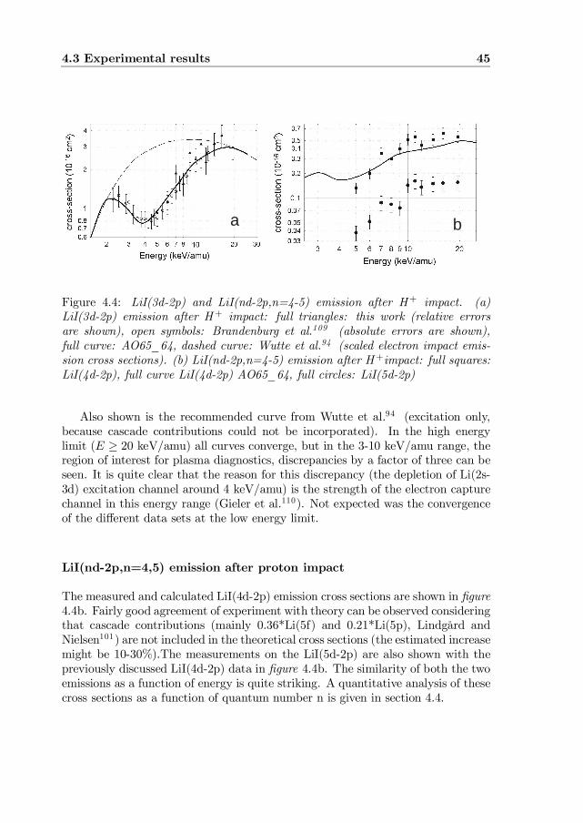
The LiI(3d-2p) emission cross section measured by us, the experimental data fromBrandenburg et al.109 (Vienna) and the AO calculations are shown in …gure 4.4a.The AO results agree well (within our experimental uncertainties) with the meas-urements. The good agreement of our LiI(3d-2p) emission cross sections withthe corresponding experimental data from Vienna con…rms the correctness of ourindependent calibration method.
4.3 Experimental results 45
a ba b
Figure 4.4: LiI(3d-2p) and LiI(nd-2p,n=4-5) emission after H+ impact. (a)LiI(3d-2p) emission after H + impact: full triangles: this work (relative errorsare shown), open symbols: Brandenburg et al.109 (absolute errors are shown),full curve: AO65_64, dashed curve: Wutte et al.94 (scaled electron impact emis-sion cross sections). (b) LiI(nd-2p,n=4-5) emission after H +impact: full squares:LiI(4d-2p), full curve LiI(4d-2p) AO65_64, full circles: LiI(5d-2p)
Also shown is the recommended curve from Wutte et al.94 (excitation only,because cascade contributions could not be incorporated). In the high energylimit (E ¸ 20 keV/amu) all curves converge, but in the 3-10 keV/amu range, theregion of interest for plasma diagnostics, discrepancies by a factor of three can beseen. It is quite clear that the reason for this discrepancy (the depletion of Li(2s-3d) excitation channel around 4 keV/amu) is the strength of the electron capturechannel in this energy range (Gieler et al.110). Not expected was the convergenceof the di¤erent data sets at the low energy limit.
LiI(nd-2p,n=4,5) emission after proton impact
The measured and calculated LiI(4d-2p) emission cross sections are shown in …gure4.4b. Fairly good agreement of experiment with theory can be observed consideringthat cascade contributions (mainly 0.36*Li(5f) and 0.21*Li(5p), Lindgård andNielsen101) are not included in the theoretical cross sections (the estimated increasemight be 10-30%).The measurements on the LiI(5d-2p) are also shown with thepreviously discussed LiI(4d-2p) data in …gure 4.4b. The similarity of both the twoemissions as a function of energy is quite striking. A quantitative analysis of thesecross sections as a function of quantum number n is given in section 4.4.
46 Lithium excitation by slow H+ and He2+ ions
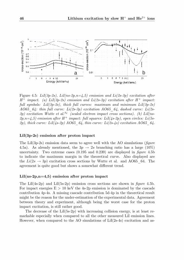
a b
Figure 4.5: LiI(3p-2s), LiI(ns-2p,n=4,5) emission and Li(2s-3p) excitation afterH+ impact. (a) LiI(3p-2s) emission and Li(2s-3p) excitation after H + impact:full symbols: LiI(3p-2s), thick full curves: maximum and minimum LiI(3p-2s)AO65_64: thin full curve: Li(2s-3p) excitation AO65_64, dashed curve: Li(2s-3p) excitation Wutte et al.94 (scaled electron impact cross sections). (b) LiI(ns-2p,n=4,5) emission after H+ impact: full squares: LiI(4s-2p), open circles: Li(5s-2p), thick curve: LiI(4s-2p) AO65_64, thin curve: Li(2s-4s) excitation AO65_64.
LiI(3p-2s) emission after proton impact
The LiI(3p-2s) emission data seem to agree well with the AO simulations (…gure4.5a). As already mentioned, the 3p ! 2s branching ratio has a large (10%)uncertainty. Two extreme cases (0.195 and 0.239) are displayed in …gure 4.5bto indicate the maximum margin in the theoretical curve. Also displayed arethe Li(2s ! 3p) excitation cross sections by Wutte et al. and AO65_64. Theagreement is quite good but shows a somewhat di¤erent trend.
LiI(ns-2p,n=4,5) emission after proton impact
The LiI(4s-2p) and LiI(5s-2p) emission cross sections are shown in …gure 4.5b.For impact energies E > 10 keV the 4s-2p emission is dominated by the cascadecontribution 4p-4s. A missing cascade contribution 5d-4p in the theoretical resultmight be the reason for the under-estimation of the experimental data. Agreementbetween theory and experiment, although being the worst case for the protonimpact excitation, is still rather good.
The decrease of the LiI(5s-2p) with increasing collision energy, is at least re-markable especially when compared to all the other measured LiI emission lines.However, when compared to the AO simulations of LiI(2s-4s) excitation and as-
4.3 Experimental results 47
suming a similarity of properties with increasing principal quantum number n, itis not so surprising. The Li(2s-4s) excitation shows a deep minimum around 15keV/amu impact energy. However this cannot be observed in LiI(4s-2p) emissionmeasurements because of the 4p cascade contribution to the Li(4s) level. Opposedto this, the LiI(5s-2p) emission does not have any signi…cant cascade contributions( Li(5p ¡! 5s) = 0:15; Li(6p ¡! 5s) » 0, Lindgård and Nielsen101) and thereforethis decrease of the cross section becomes visible.
4.3.2 He2+ impact
There are more experimental results for He2+ impact and they are more preciselycalibrated than the proton impact data, and this proved to be a real challengefor the AO-CC method. As we shall see, excellent results where obtained withthe AO87_79 and good results with the AO81_80. The AO87_79 calculationsinclude in addition to the projectile centered states of the AO81_80 the 6h state.This state was omitted only in order to reduce CPU time in the AO81_80. Thetarget centered parts of both expansions do not di¤er in the AOs included, butin the number of pseudo-states and in the details of the used STOs (see TABLE1). Especially the target centered PS-UA parts di¤er considerably between bothexpansions.
Interesting will be the lower energy range for the He2+ impact data (2-12keV/amu) as compared to the proton case (5-20 keV/amu). At these lower energiesa striking oscillatory behaviour in the excitation cross section was observed for theproton impact case (see the previous section) and similar features are expectedfor the He2+ impact case. Furthermore, there will be a few data points at muchhigher energies.
LiI(3d-2p) emission after He2+ impact
The most striking feature of the LiI(3d-2p) emission cross sections (…gure 4.6a) is,as in the proton impact case, the peak at 2.7 keV/amu, as in the protons, likely tobe caused by a depletion of the Li(3d-2p) excitation channel by electron capturechannels.

48 Lithium excitation by slow H+ and He2+ ions
a b
Figure 4.6: LiI(3d-2p) and LiI(4d-2p) emission after He2+ impact. (a) LiI(3d-2p)emission after He2+ impact: full symbols: this work (relative errors are shown),open triangles: Kadota et al.84 (absolute errors are shown), thick full curve:AO87_79, dashed thin curve: AO87_79 corrected for the polarization sensitiv-ity of the detector, thin full curve: AO81_80, thick dashed curve: schweinzer etal.88 , thick dash dot curve: Ermolaev et al.87 . (b) LiI(4d-2p) emission afterHe2+ impact: full squares: this work , thick full curve: AO87_79, thin full curve:AO81_80, dashed dotted curve: Ermolaev et al.87
Cross checking the present lithium emission after He2+ impact with electroncapture from lithium by He2+ (Hoekstra97 et al.) clearly reveals that the exper-imental HeI(n=4,l=0,1,2) (capture) levels have an enhanced population around6 keV/amu, exactly where the Li(n=3,4, l=3) (excitation) levels have reducedintensities.
We now can really see the improvements in the AO-CC method, because theLiI(3d-2p) emission after He2+ impact was studied earlier with the same method(Ermolaev et al.87 and Schweinzer et al.88) and these results are also displayedin …gure 4.6a. The previous calculation by Schweinzer et al. was good down to 4keV/amu but then failed to predict the features so striking in Li excitation by H+
and He2+ impact. The results of Ermolaev (the AO65 calculations) only agree withour data in the high energy limit (towards the Born regime). The pseudo-stateexpansion applied by Ermolaev is optimized for high impact energies. Thus onlya few projectile centered states (HeII n=2,3 + 4d and pseudo-states) were takeninto account in their calculation, leading to over-estimated excitation cross sectionsfor their lowest impact energies. On the other hand, the previous calculation bySchweinzer et al. is based on a pure AO expansion with many projectile centeredstates (HeII n=1-6) but without pseudo-states, thus completely neglecting thecoupling to ionization channels. A su¢cient representation of all inelastic reaction

4.3 Experimental results 49
channels seems to be necessary to describe excitation processes properly.Note that the inclusion of polarization e¤ects (as discussed in the experimental
results section) changes the emission cross sections only slightly.
LiI(4d-2p) emission after He2+ impact
The LiI(4d-2p) emission cross sections are shown in …gure 4.6b. The agreementbetween the AO87_79 calculation and the experimental data is very good, ex-cept maybe at 3 keV/amu where the AO81_80 agrees somewhat better with ex-periment. Di¤erences between AO87_79 and AO81_80 give an estimate of theconvergence of AO-CC results. The agreement between theory and experiment isslightly better here than for the proton impact case …gure4.4b although also heresmall cascade contributions to the theoretical emission curve were not included.Finally, the theoretical data by Ermolaev et al. (AO65 calculations) converge withour data in the high energy limit, but again are far too high at the low energies.
LiI(5d-2p) and LiI(6d-2p) emission after He2+ impact
The LiI(nd-2p,n=5,6) emission data are shown in …gure 4.7a.
a b
Figure 4.7: LiI(nd-2p,n=5,6) and LiI(3p-2s) emission after He2+ impact. (a)LiI(nd-2p,n=5,6) emission after He2+ impact: full circels: LiI(5d-2p), open tri-angles: LiI(6d-2p), thick full curve: AO87_79, thin full curve: AO81_80, dasheddotted curve: Ermolaev et al.87 . (b) LiI(3p-2s) emission after He2+impact:full symbols: LiI(3p-2s), thick full curve: LiI(3p-2s) AO87_79, thin full curve:AO81_80, dashed curve: Li(3p-2s) Schweinzer et al.88 , Dashed-dotted curve:Ermolaev et al.87 .
50 Lithium excitation by slow H+ and He2+ ions
The disagreement between the experimental LiI(5d-2p) data and the AO87_79,AO81_80 is very considerable (factor 2-3) which is most probably due to themissing high n SEC channels. As already explained in section 4.2, SEC draws‡ux from the excitation channels, thereby reducing the excitation cross sections.The predicted 2s-5d excitation cross sections are almost as large as the 2s-4d crosssections, which is very unlikely. Also Ermolaev et al. struggled with the problem ofexcessively large Li(2s-5d) excitation cross sections due to the even lower numberof SEC channels and their best results are displayed in …gure 4.7a.
Also shown are the LiI(6d-2p) emission cross sections (experiment only). It isclear that this emission line looks quite similar to the other LiI(nd-2p) emissions,although the peak structure at 3 keV/amu (minimum around 6 keV/amu) seemsto have disappeared.
LiI(3p-2s) emission after He2+ impact
For the LiI(3p-2s) emission cross section the agreement between the experimentaldata and the AO simulations, both AO87_79 and AO81_80, is reasonably good(see …gure 4.7b, a branching ratio of 0.215 was used for the theoretical curve).
LiI(4s-2p) emission after He2+ impact
We can see in …gure 4.8a that the LiI(4s-2p) emission after He2+ impact, whichis our basis of absolute calibration, agrees well with the AO-CC theory (exceptmaybe for a small structure at 3 keV/amu).
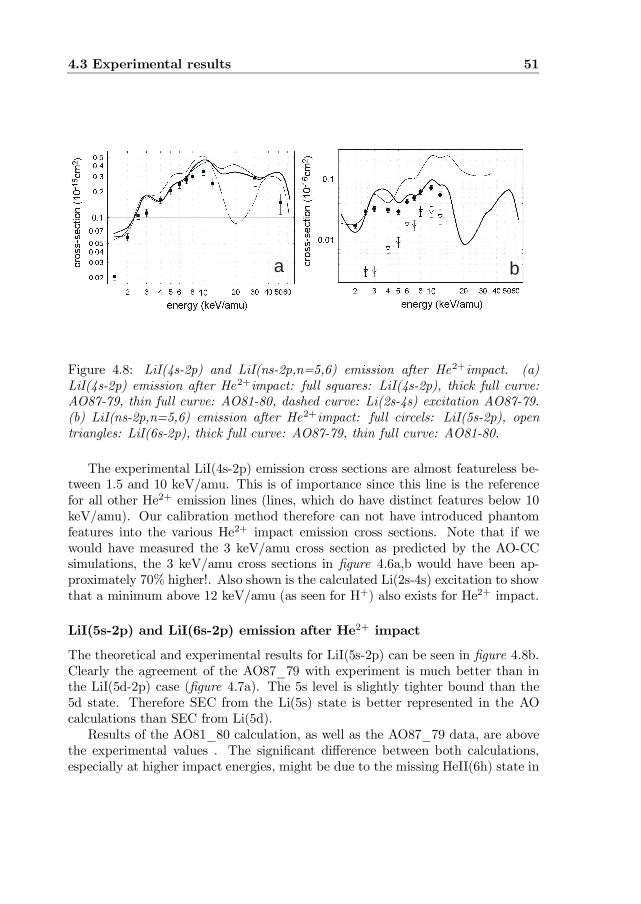
4.3 Experimental results 51
a b
Figure 4.8: LiI(4s-2p) and LiI(ns-2p,n=5,6) emission after He2+impact. (a)LiI(4s-2p) emission after He2+impact: full squares: LiI(4s-2p), thick full curve:AO87-79, thin full curve: AO81-80, dashed curve: Li(2s-4s) excitation AO87-79.(b) LiI(ns-2p,n=5,6) emission after He2+impact: full circels: LiI(5s-2p), opentriangles: LiI(6s-2p), thick full curve: AO87-79, thin full curve: AO81-80.
The experimental LiI(4s-2p) emission cross sections are almost featureless be-tween 1.5 and 10 keV/amu. This is of importance since this line is the referencefor all other He2+ emission lines (lines, which do have distinct features below 10keV/amu). Our calibration method therefore can not have introduced phantomfeatures into the various He2+ impact emission cross sections. Note that if wewould have measured the 3 keV/amu cross section as predicted by the AO-CCsimulations, the 3 keV/amu cross sections in …gure 4.6a,b would have been ap-proximately 70% higher!. Also shown is the calculated Li(2s-4s) excitation to showthat a minimum above 12 keV/amu (as seen for H+) also exists for He2+ impact.
LiI(5s-2p) and LiI(6s-2p) emission after He2+ impact
The theoretical and experimental results for LiI(5s-2p) can be seen in …gure 4.8b.Clearly the agreement of the AO87_79 with experiment is much better than inthe LiI(5d-2p) case (…gure 4.7a). The 5s level is slightly tighter bound than the5d state. Therefore SEC from the Li(5s) state is better represented in the AOcalculations than SEC from Li(5d).
Results of the AO81_80 calculation, as well as the AO87_79 data, are abovethe experimental values . The signi…cant di¤erence between both calculations,especially at higher impact energies, might be due to the missing HeII(6h) state in
52 Lithium excitation by slow H+ and He2+ ions
the AO81_80 expansion. Although this state is populated very weakly in collisionswith Li(2s) it might be of considerable importance as a SEC loss channel fromLi(5s). To test the idea that the HeII(6h) capture channel interferes with the Li(5s)excitation channel a AO87_80 (a AO81_80 plus the HeII(6h) state) calculationwas performed. This calculation did however not result in a better description ofthe Li(5s) excitation channel, implying that the AO87_79 is more successful in theprediction of Li(5s) excitation because of a better choice of pseudo-states describingthe ionization channels. The AO87_79 is de…nitely more successful when it comesdown to describing the dramatic de-coupling (de-coupling meaning: the excitationmechanism is becoming less e¤ective) of the Li(5s) excitation channel above 12keV/amu (remember, this peculiar behavior of the Li(5s) excitation was also seenfor proton impact).
Also displayed in …gure 10b are the LiI(6s-2p) emission cross sections (ex-periment only). It is clear that this excitation channel behaves di¤erently fromthe Li(5s) excitation. This indicates that a universal scaling law for describingLiI(ns-2p,n=4-6) emissions (He2+ impact) is unlikely to exist.
4.4 LiI(nd-2p, n=3-9) emission: n scaling
As far as we know the …eld of ”high n excitation by ion impact” is unknownterritory. To get some idea of the mechanisms at work some extra measurementshave been performed and a crude scaling method is introduced for the nd-states. Itis custom in the …eld of fusion plasma diagnostics to …nd scaling relations because itis a formidable (if not impossible) task to measure or calculate all the relevant crosssections for inelastic ion-atom collisions. As already mentioned before, lithium ns-state excitation by ion impact is not suitable for scaling with increasing n (thecurves in …gure 4.5b and 4.8a,b simply do not look very similar).
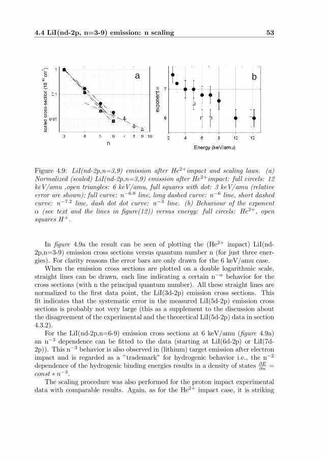
4.4 LiI(nd-2p, n=3-9) emission: n scaling 53
a b
Figure 4.9: LiI(nd-2p,n=3,9) emission after He2+impact and scaling laws. (a)Normalized (scaled) LiI(nd-2p,n=3,9) emission after He2+impact: full circels: 12keV/amu ,open triangles: 6 keV/amu, full squares with dot: 3 keV/amu (relativeerror are shown); full curve: n¡6:8 line, long dashed curve: n¡6 line, short dashedcurve: n¡7:2 line, dash dot dot curve: n¡3 line. (b) Behaviour of the exponent® (see text and the lines in …gure(12)) versus energy: full circels: He2+, opensquares H +.
In …gure 4.9a the result can be seen of plotting the (He2+ impact) LiI(nd-2p,n=3-9) emission cross sections versus quantum number n (for just three ener-gies). For clarity reasons the error bars are only drawn for the 6 keV/amu case.
When the emission cross sections are plotted on a double logarithmic scale,straight lines can be drawn, each line indicating a certain n¡® behavior for thecross sections (with n the principal quantum number). All these straight lines arenormalized to the …rst data point, the LiI(3d-2p) emission cross sections. This…t indicates that the systematic error in the measured LiI(5d-2p) emission crosssections is probably not very large (this as a supplement to the discussion aboutthe disagreement of the experimental and the theoretical LiI(5d-2p) data in section4.3.2).
For the LiI(nd-2p,n=6-9) emission cross sections at 6 keV/amu (…gure 4.9a)an n¡3 dependence can be …tted to the data (starting at LiI(6d-2p) or LiI(7d-2p)). This n¡3 behavior is also observed in (lithium) target emission after electronimpact and is regarded as a ”trademark” for hydrogenic behavior i.e., the n¡2
dependence of the hydrogenic binding energies results in a density of states @E@n =
const ¤ n¡3.The scaling procedure was also performed for the proton impact experimental
data with comparable results. Again, as for the He2+ impact case, it is striking
54 Lithium excitation by slow H+ and He2+ ions
how well the data can be …tted with these n¡® lines, even though the data spantwo orders of magnitude.
Putting the results (the exponents ®) of the n¡® …ts , both for He2+ and H+
impact, in a plot yields …gure 4.9b. The physical origin of the decrease of theexponent ® with increasing collision energy is more or less clear. It is expectedthat the higher Li(nd) states are relatively stronger populated when the projectileenergy increases. Interesting is however that the H+ and He2+ projectiles have(more or less) the same exponent (® » 6) at their highest energies, but the pro-tons reach that exponent sooner. Putting it simply: at high enough velocities,both projectiles can ’pump’ the relative nd-populations equally well; the protonshowever, can do this ’pumping’ already better at lower energies.
4.5 ConclusionIn this chapter we have seen that the AO-CC method can model the excitationof lithium atoms by H+ or He2+ with great accuracy not only for the dominantchannels (Li(2p) described in Brandenburg92 et al. and Li(3p,3d)) but also forexcitation channels that are two orders of magnitude below these channels. Bycomparing experimental data for even smaller cross sections with AO-CC calcu-lations, although already of large scale, limitations (Li(5d) excitation) have beenreached and disagreement was observed. This limitation can however most likelybe overcome by a further enlargement of the basis set. Unfortunately such anextension is not only a matter of more powerful computers, but also improvednumerical methods, because accuracy limits of the present ones are also touchedupon.
The main improvement between the old AO-CC simulations (Ermolaev et al.and Schweinzer et al.) and the new ones is that the new ones correctly predictthe features in the Li(2s-nd,n=3-4) excitation. As already mentioned in section4.3.1 (Li(3d-2p) emission after H+ impact), it is likely that these features are not”peaks around 3 keV/amu” but rather ”minima around 6 keV/amu ”. Similarstructures, resulting from the interplay between capture and excitation, have alsobeen predicted by Schultz et al.90 and Fritsch et al.89 for hydrogen excitationand experimentally seen by Aumayr et al.86 (lithium and Sodium excitation) andHorvath et al.91 (sodium excitation). The Li(2s-ns,n=4,5) excitation channels alsodisplay minima with H+ and He2+impact, but not around 5 keV/amu but around15 keV/amu for the former and 20 keV/amu for the latter. We could not …nda satisfying explanation for these depletions of the Li(4s) and Li(5s) excitationchannels above 12 keV/amu.
We would like to mention that the structures between 2-8 keV/amu were dis-cussed by Aumayr86 using the Landau-Zener picture and a pure classical inter-pretation of this structure was given by Schultz90 . Both discussions construct
4.5 Conclusion 55
a picture of the active electron oscillating (or swapping) between excitation andcapture channels, resulting in the typical structures observed. Although we clearlysaw depletion of excitation channels due to enhanced capture, we did not …nd anyevidence for the reverse process (i.e. enhanced excitation and depleted capturechannels).
We also saw that above 20-30 keV/amu the lithium excitation is governedby (Born-type) single step excitation and that below 2 keV/amu the excitationcompletely de-couples (i.e. vanishes). Remarkably, not only the high energy endbut also the low energy end can be predicted correctly by scaling electron impactexcitation cross sections.
We observed that the LiI(nd-2p,n=3-9) emission, which cannot be calculatedwhen n>5, can be described (i.e. scaled with quantum number n) quite successfullywith power law ( n¡®;¡7:5 < ® < ¡6) dependencies. The LiI(ns-2p,n=4-6) couldnot be described with similar power law dependencies.


5 The Magneto Optical Trap
In this section we introduce the basic principles of laser cooling and trapping.Also discussed in this section are the laser set-up, frequency stabilization and fre-quency manipulation schemes which use optically non-linear crystals.
57
58 The Magneto Optical Trap
5.1 Introduction
One of the most important breakthroughs in atomic physics since the developmentof the laser was the realization of laser cooling. Laser cooling gave atomic physicsunprecedented control over free atoms, culminating eventually in Bose-Einsteincondensation111 . The concepts of laser cooling were introduced in the 1970’sby Letokhov112, 113(1968) and Ashkin114, 115 (1970) and (independently from eachother) by Hänsch and Schawlow116 and Wineland and Dehmelt117 (1975). Allthese concepts make use of the fact that light carries a momentum (Einstein118
(1917)) and that atoms can be de‡ected by resonant light (Lebedev119 (1910) andFrisch120 (1933)). Laser cooling of ions con…ned in a Paul rf trap was demonstratedby Neuhauser et al.121 in 1978 and laser cooling of neutral atoms in one dimensionwas performed by Andreev et al.122 in 1981. Laser cooling in two dimensionswas experimentally demonstrated in 1984 by Balykin et al123 and in 1985, threedimensional cooling (but still no trapping) was demonstrated by Chu et al.124 . In1987 Raab125 et al. added an inhomogeneous magnetic …eld to the laser beams andcreated the Magneto-Optical Trap (MOT). The MOT was then still loaded froman atomic beam but in 1990 Monroe126 et al. demonstrated that the MOT couldalso be loaded from a background gas. The vapour cell MOT was born and it soonbecame an important workhorse in atomic physics by collecting millions of atoms(atoms like Li, Na,...,Fr, Mg, Ca,...,Ra, He*, Ne*,... (*=metastable)) per second,cooling them to sub-mK temperatures and supplying them for other experiments.For our work the MOT supplies us with a small, ultra-cold Na sample which servesas the target for projectile ions.
5.2 Laser cooling and trapping
The principle of laser cooling makes use of the facts that i) resonant light can exertan enormous force ( >50,000 times gravity) on atoms and ii) this force dependson the atoms’ velocity, both its magnitude and direction.

5.2 Laser cooling and trapping 59
ν−δν−δν−δ
ν−δν−δν−δ
ν−δν−δν−δ
ν−δν−δν−δ
v
v
v
F
F
F
a
b
c
d
Figure 5.1: The light forces on an atom depending on its velocity (laser lightdetuned by ± from the resonance frequency º). (a,b): Illustration of the light forceF of one laser beam depending on the atom velocity v. (c) Illustration of the lightforce F of two counterpropagating light beams depending on the atom’s velocity v.(d) Calculation of the typical light forces for counterpropagating laser beams (solidline) and the individual laser beams (dashed line) for Na.
Figure 5.1a illustrates the latter point: an atom moves into a laser beam whichis tuned at a frequency slightly below the atom’s resonance frequency (”red detun-ing”). However the Doppler shift due to the atom’s velocity (both magnitude anddirection) makes that the atom experiences the laser light again as resonant. Theatom absorbs photons from the laser beam and emits them again in all directions.Each absorbed photon delivers a small momentum kick to the atom in the laserbeam direction i.e. opposite the atoms direction of motion. The emitted photonshowever deliver momentum kicks in all directions and these e¤ectively cancel eachother. The net result is that the atoms motion in the direction of the laser beamis reduced (provided that this velocity was not too large in the …rst place). Figure5.1a,b illustrate that when the atoms velocity in the laser beam direction becomessmaller, the Doppler shift becomes smaller and the induced laser force gets smal-ler. Figure 5.1c shows an atom moving in between two laser beams and the forceindicated in …gure 5.1c is now slightly smaller than the force shown in …gure 5.1a.This because the laser beam in the direction of the atoms motion (i.e. ”light fromthe back”) also exerts a small force. Figure 5.1d sums up the information of …gure5.1a-c in a typical acceleration curve of an atom between two counter propagat-ing laser beams. The acceleration (solid curve) is opposite to the atom’s motionbut decreases in magnitude as the atom’s velocity becomes too high. The dashed
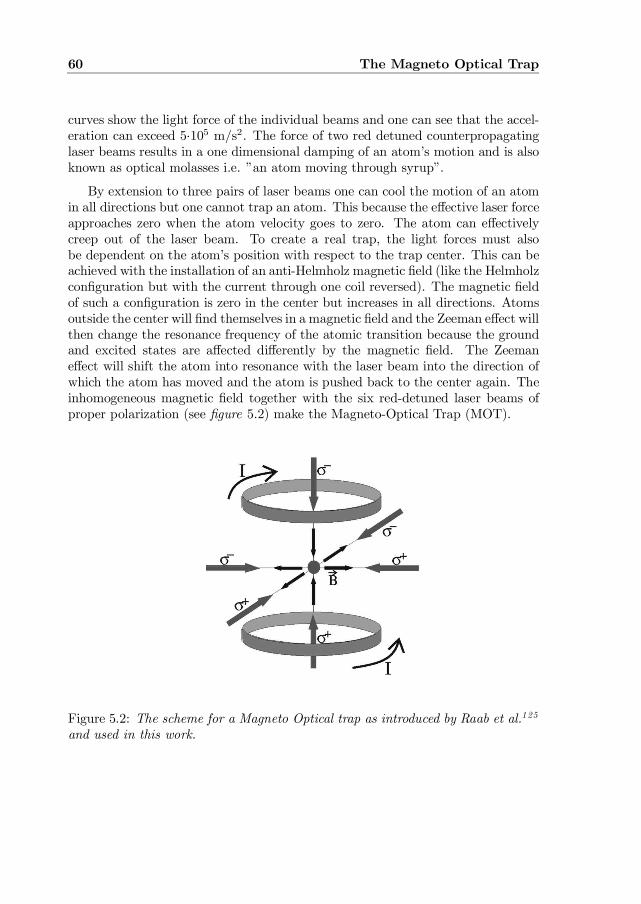
60 The Magneto Optical Trap
curves show the light force of the individual beams and one can see that the accel-eration can exceed 5¢105 m/s2. The force of two red detuned counterpropagatinglaser beams results in a one dimensional damping of an atom’s motion and is alsoknown as optical molasses i.e. ”an atom moving through syrup”.
By extension to three pairs of laser beams one can cool the motion of an atomin all directions but one cannot trap an atom. This because the e¤ective laser forceapproaches zero when the atom velocity goes to zero. The atom can e¤ectivelycreep out of the laser beam. To create a real trap, the light forces must alsobe dependent on the atom’s position with respect to the trap center. This can beachieved with the installation of an anti-Helmholz magnetic …eld (like the Helmholzcon…guration but with the current through one coil reversed). The magnetic …eldof such a con…guration is zero in the center but increases in all directions. Atomsoutside the center will …nd themselves in a magnetic …eld and the Zeeman e¤ect willthen change the resonance frequency of the atomic transition because the groundand excited states are a¤ected di¤erently by the magnetic …eld. The Zeemane¤ect will shift the atom into resonance with the laser beam into the direction ofwhich the atom has moved and the atom is pushed back to the center again. Theinhomogeneous magnetic …eld together with the six red-detuned laser beams ofproper polarization (see …gure 5.2) make the Magneto-Optical Trap (MOT).
Figure 5.2: The scheme for a Magneto Optical trap as introduced by Raab et al.125
and used in this work.
5.3 Theory: trapping and cooling atoms 61
5.3 Theory: trapping and cooling atomsFor a more analytical description of the MOT we will look at the six light forces Fi;jwhere i indicates the three dimensions (x,y,z) and j=1,2 the two counterpropagat-ing beams per dimension. When we work out the balance between stimulatedabsorption and emission per light force Fi;j (see van der Straten127, 128 and Molen-aar129) we obtain eq. 5.1 and the force of two counterpropagating laser beams Fiis given in eq. 5.2:
Fi;j =~k¡2
s0
1 + s0 + (2±i;j¡ )2
(5.1)
We see that the light forces depend on the the saturation parameter s0 (´ II0
: thelight intensity I normalized to I0 the saturation intensity of Na), the spontaneousemission rate ¡ and the detuning ±i;j( note: ±l < 0!): The detuning ±i;j = ±l ¡(kv)i;j ¡(¢Ee(B)¡¢Eg(B)
~ ) consists of the main laser de-tuning ±l, the Doppler shift(kv)i;j caused by the velocity of the atom and the Zeeman shift (¢Ee(B)¡¢Eg(B)
~ )caused by the position of the atom will be discussed in more detail later. In …rstorder approximation (small Doppler and Zeeman shifts), Fi (eq. 5.2) dependslinearly on the atom’s position x and the atom’s velocity v.
Fi ' 8~ks0±l
2¡kv + ®x
(1 + (2±l¡ )2)2
(5.2)
¼ ¡·x ¡ ¯v
The physical origin of the velocity dependence of the force (eq. 5.2) was alreadydiscussed in the introduction (see …gure 5.1d) and in …gure 5.3 we see the ingredi-ents for the position dependence of the light force. First we look at the magnetic…eld in‡uence on the excited Na levels (…gure 5.3a) and on the ground states (…g-ure 5.3b) (a level scheme of Na is given in …gure 5.3c). The energy levels show alinear increase or decrease on B (small B) depending on their magnetic sub-statemF (see …gure 5.3b: the F=1 ground state splits into its 3 mF states and eachmF state has a di¤erent energy change as a function of B. To see what two cir-cularly polarized counterpropagating laser beams will do with this Na atom, we…rst take a step back and look at an ideal 2 level (J=0,1) atom placed in a linearlyincreasing B …eld. In …gure 5.4a we see the mj sub-states of an ideal 2 level atomand indicated are the transitions that can be made with ¾¡ ; ¼ and ¾+ polarizedlight. We now put our atom (at position z) in a linearly increasing magnetic …eldand apply two counter propagating ¾+ and ¾¡ laser beams of frequency Àlaser:…gure 5.4b. The de-tuning with respect to the ¾¡ laser beam (±¡) is much smallerthan to the ¾+ laser beam (±+) and the atom will therefore absorb more photonsfrom the ¾¡ laser beam than from the ¾+ laser beam. For three pairs of counter
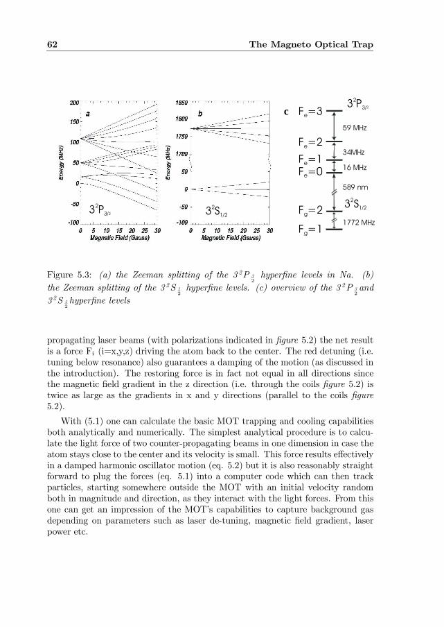
62 The Magneto Optical Trap
1772 MHz
33
SS
22 1
1/
/2
2
3
3
P
P
2
2
3
3
/
/
2
2
589 nm
59 MHz
34MHz
16 MHz
F =2g
F =0e
F =1e
F =2e
F =3e
F =1g
c
Figure 5.3: (a) the Zeeman splitting of the 3 2P 32
hyper…ne levels in Na. (b)the Zeeman splitting of the 3 2S 1
2hyper…ne levels. (c) overview of the 3 2P 3
2and
3 2S 12hyper…ne levels
propagating laser beams (with polarizations indicated in …gure 5.2) the net resultis a force Fi (i=x,y,z) driving the atom back to the center. The red detuning (i.e.tuning below resonance) also guarantees a damping of the motion (as discussed inthe introduction). The restoring force is in fact not equal in all directions sincethe magnetic …eld gradient in the z direction (i.e. through the coils …gure 5.2) istwice as large as the gradients in x and y directions (parallel to the coils …gure5.2).
With (5.1) one can calculate the basic MOT trapping and cooling capabilitiesboth analytically and numerically. The simplest analytical procedure is to calcu-late the light force of two counter-propagating beams in one dimension in case theatom stays close to the center and its velocity is small. This force results e¤ectivelyin a damped harmonic oscillator motion (eq. 5.2) but it is also reasonably straightforward to plug the forces (eq. 5.1) into a computer code which can then trackparticles, starting somewhere outside the MOT with an initial velocity randomboth in magnitude and direction, as they interact with the light forces. From thisone can get an impression of the MOT’s capabilities to capture background gasdepending on parameters such as laser de-tuning, magnetic …eld gradient, laserpower etc.
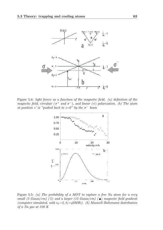
5.3 Theory: trapping and cooling atoms 63
ab
a
b
σ+ σ−
Figure 5.4: light forces as a function of the magnetic …eld. (a) de…nition of themagnetic …eld, circulair (¾+ and ¾¡); and linear (¼) polarization. (b) The atomat position z’ is ”pushed back to z=0” by the ¾¡ beam
B
0 10 20 30
0.25
0.50
0.75
1.00 a
b
Figure 5.5: (a) The probability of a MOT to capture a free Na atom for a verysmall (5 Gauss/cm) (§) and a larger (15 Gauss/cm) (N) magnetic …eld gradient(computer simulated, with s0=2, ±l=40MHz). (b) Maxwell-Boltzmann distributionof a Na gas at 330 K
64 The Magneto Optical Trap
In …gure 5.5a two curves are shown of the capture probability versus the initialparticle velocity for two di¤erent magnetic …eld gradients. These curves illustratethat with smaller gradients a larger velocity class can be captured but particleswith vi>30 m/s can usually not be captured (this is in agreement with morerealistic MOT simulations performed by Molenaar129). Comparing the captureprobabilities with the Maxwell- Boltzmann velocity distribution of Na gas at 330K (…gure 5.5b) makes clear that only a very small fraction of the background gascan be trapped by a MOT.
5.4 Theory: trapping and cooling Na
Up to now we only discussed the trapping and cooling of ideal 2-level atoms butnow we will go into the speci…c features of Na trapping and cooling. In …gure 5.3the level schemes of Na(3 2 S 1
2) and (3 2P 3
2) are shown. Important is the hyper…ne
splitting of the Na(3 2S 12) ground state with 1772 MHz. These two ground states
are coupled to each other by the laser light via the Fe=1,2 excited states sincethese excited states radiate to both ground states. Even when the trapping laserdrives the Fg=1! Fe = 0 transition then all population of the Fg=1 state wouldeventually be pumped to the Fg=2 ground state. This is caused by the fact thatthe Fg=1! Fe = 1 transition is also accidently excited due to the line-widths ofthe transition and the small Doppler and Zeeman shifts present in the MOT andthis excited state can also radiate to the Fg=2 ground state, a state not coupled tothe laser light. Similarly the Fg=1 ground state will eventually become exclusivelypopulated when the laser is tuned to the Fg=2! Fe = 3 transition. To preventthis so-called optical pumping into dark states, a ”re-pumper” should be usedi.e. a laser which pumps the dark state population back in to the main trappingtransition.
The two ground states F=1 and F= 2 turn out to allow two main frequencies tobe used for trapping and cooling, namely the Fg=2!Fe=3 + re-pumper resultingin a ”type I MOT ”129, 130”) and Fg=1! Fe = 0 + re-pumper (”type II129, 131”).The type I is common for all alkali atoms but type II is unique for Na. Bothtypes of MOT’s can be produced in our set-up but only the type (I) was used inthis work since it turned out to be much smaller (<0.5 mm) in size than the type(II) (» 5 mm). An extensive theoretical and experimental study on the variousMOT types is given by Atutov131 et al. where even a type III is introduced, whichinvolves re-pumping via the D1 (i.e. Na(3 2 S 1
2) ! Na(3 2P 1
2)) line.
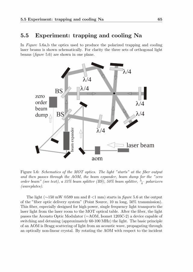
5.5 Experiment: trapping and cooling Na 65
5.5 Experiment: trapping and cooling NaIn Figure 5.6a,b the optics used to produce the polarized trapping and coolinglaser beams is shown schematically. For clarity the three sets of orthogonal lightbeams (…gure 5.6) are shown in one plane.
laser beam
λ/4
λ/4λ/4
λ/4
λ/4
λ/4
b eam
exp
a nde
r
Figure 5.6: Schematics of the MOT optics. The light ”starts” at the …ber outputand then passes through the AOM, the beam expander, beam dump for the ”zeroorder beam” (see text), a 33% beam splitter (BS), 50% beam splitter, ¸
4 polarizers(waveplates).
The light (»150 mW @589 nm and ; <1 mm) starts in …gure 5.6 at the outputof the ”…ber optic delivery system” (Point Source, 10 m long, 50% transmission).This …ber, especially designed for high power, single frequency light transports thelaser light from the laser room to the MOT optical table. After the …ber, the lightpasses the Acousto Optic Modulator (=AOM, Isomet 1205C-2) a device capable ofswitching and detuning (approximately 60-100 MHz) the light. The basic principleof an AOM is Bragg scattering of light from an acoustic wave, propagating throughan optically non-linear crystal. By rotating the AOM with respect to the incident

66 The Magneto Optical Trap
laser beam the angle of incidence is varied and 90% transmission into the …rst orderscattered beam can be obtained. The de-tuned …rst order beam can be separatedfrom the weak, un-detuned zeroth order beam and guided to the beam expanderwhich makes the ; 2 cm trapping beams. The zero order laser beam is guided intoa beam dump but could in principle also be used for additional laser preparationof the MOT cloud.
The 2 cm beam is split in three equally strong trapping beams by …rst splitting33% o¤ the main beam and then splitting the remaining beam in two equal parts.Each trapping beam is guided through a ¸
4 waveplate to produce the desired cir-cular polarization. By retro-re‡ecting the three trapping beams into themselvesthe six beams needed for a MOT are created.
Figure 5.7: Monitoring the MOT cloud: (a) A standard CCD camera ( ”MOTmonitor”) displays the MOT on a monitor in the laser room. A fast, gate-able,computer controlled CCD camera (”Master Camera”) observes the MOT from twoorthogonal directions, via 50 % beam splitters. Observations by eye can also stillbe made through the ”view ports” of the 50% beam splitters. (b) Two images ofthe same MOT taken with the imaging scheme are shown in (a).
Our MOT observation scheme is shown in …gure 5.7a: Two CCD camera areinstalled for MOT observations: a ”MOT monitor” to observe the MOT from thelaser room and a fast gate-able CCD camera (”Master camera”) with zoom lens toperform dynamic measurements on the MOT (temperature measurements). Withthe ”mirrors +50% beamsplitter scheme” shown in …gure 5.7a we can actuallyobserve the MOT from two directions by only using one CCD camera. One singleCCD image now consists of two orthogonal projections of the MOT next to eachother (…gure 5.7b, the di¤erence in height between the two MOT images is caused
5.6 Temperature, size, density and Na+2 ions 67
by a small imbalance between the two light paths and has no ”physical” origin).
The anti-Helmholz coils consist each of 20 windings, are water-cooled and canhandle over 120 A. We however use them in the 50-80 A region and this correspondsto a magnetic …eld gradients of 25-40 Gauss/cm. Also installed are so called MOTsteering coils i.e. two pairs of small Helmholtz coils ( » 30 windings;» 2A) toproduce a small additional homogeneous magnetic …eld. With these small …eldsthe position of the zero point in the magnetic …eld gradient can be moved andalong with it, the MOT cloud. The steering coils can manipulate the MOT’s yand z position in a range of »2 mm.
Some sofar unmentioned elements needed for a MOT are a Na oven and anUHV vacuum chamber. The Na oven consists of a stainless steel holder containinga few grams of Na placed in an externally heated ‡ange. The Na vapour pressurecan be monitored with a vacuum gauge (5¢10¡10 mbar additional pressure whenthe oven is on) but better still is to use the MOT itself as a Na pressure gauge(more about this in the next section). The UHV vacuum chamber is shown in…gure 6.2 in the recoil momentum spectrometer section.
5.6 Temperature, size, density and Na+2 ions
Important properties like MOT temperature, size and density were not discussedin the theoretical part. This because the simple trapping and cooling models,like the damped harmonic oscillator described in as resulting from eq. 5.2 and thevery similar computer simulation, result in a zero temperature and in…nite density.The theory so far did not consider the random walk constantly performed by thetrapped particles under in‡uence of all the laser beams. Due to the stochasticnature of the light forces, particles are also continuously heated and an equilibriumbetween cooling and heating will eventually be reached. A temperature for theMOT can be estimated127, 129, 132 . The so called Doppler limit TD is given by eq.5.3, with ¿=16 ns.
TD =~
2kb¿(5.3)
We obtain TD=300 ¹K in case of Na.
The most common way to measure the MOT temperature is using the releaseand re-capture method124, 125, 129 illustrated in …gure 5.8a-c.
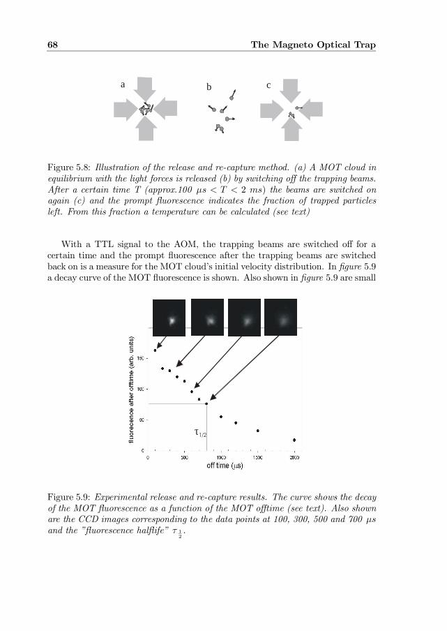
68 The Magneto Optical Trap
a b c
Figure 5.8: Illustration of the release and re-capture method. (a) A MOT cloud inequilibrium with the light forces is released (b) by switching o¤ the trapping beams.After a certain time T (approx.100 ¹s < T < 2 ms) the beams are switched onagain (c) and the prompt ‡uorescence indicates the fraction of trapped particlesleft. From this fraction a temperature can be calculated (see text)
With a TTL signal to the AOM, the trapping beams are switched o¤ for acertain time and the prompt ‡uorescence after the trapping beams are switchedback on is a measure for the MOT cloud’s initial velocity distribution. In …gure 5.9a decay curve of the MOT ‡uorescence is shown. Also shown in …gure 5.9 are small
τ1/2
Figure 5.9: Experimental release and re-capture results. The curve shows the decayof the MOT ‡uorescence as a function of the MOT o¤time (see text). Also shownare the CCD images corresponding to the data points at 100, 300, 500 and 700 ¹sand the ”‡uorescence hal‡ife” ¿ 1
2:
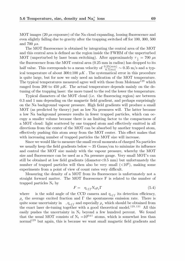
5.6 Temperature, size, density and Na+2 ions 69
MOT images (20 ¹s exposure) of the Na cloud expanding, loosing ‡uorescence andeven slightly falling due to gravity after the trapping switched o¤ for 100, 300, 500and 700 ¹s.
The MOT ‡uorescence is obtained by integrating the central area of the MOTand this central area is de…ned as the region inside the FWHM of the unperturbedMOT (unperturbed by laser beam switching). After approximately ¿ 1
2= 700 ¹s
the ‡uorescence from the MOT central area (0.25 mm in radius) has dropped to itshalf value. This corresponds to a mean velocity of 0:25(mm)
0:7(ms) » 0.35 m/s and a typ-ical temperature of about 300§100 ¹K . The systematical error in this procedureis quite large, but for now we only need an indication of the MOT temperature.The typical temperatures measured agree well with those from Molenaar129 whichranged from 200 to 450 ¹K. The actual temperature depends mainly on the de-tuning of the trapping laser: the more tuned to the red the lower the temperature.
Typical diameters of the MOT cloud (i.e. the ‡uorescing region) are between0.3 and 1 mm depending on the magnetic …eld gradient, and perhaps surprisinglyon the Na background vapour pressure. High …eld gradients will produce a smallMOT (as predicted by theory) just as low Na pressures will. The latter becausea low Na background pressure results in fewer trapped particles, which can oc-cupy a smaller volume because there is an limiting factor to the compactness ofa MOT cloud: light scattered by one trapped atom and e¤ectively emitted in alldirections from the center of the MOT can be absorbed by another trapped atom,e¤ectively pushing this atom away from the MOT center. This e¤ect makes thatwith increasing number of trapped particles the MOT size will increase.
Since we would like to measure the small recoil momenta of charged Na particleswe usually keep the …eld gradients below » 35 Gauss/cm to minimize its in‡uenceand control the MOT size mainly with the vapour pressure, whereby the MOTsize and ‡uorescence can be used as a Na pressure gauge. Very small MOT’s canstill be obtained at low …eld gradients (diameter<0.5 mm) but unfortunately thenumber of trapped particles will then also be very small (<106); making someexperiments from a point of view of count rates very di¢cult.
Measuring the density of a MOT from its ‡uorescence is unfortunately not astraight forward matter. The MOT ‡uorescence F is related to the number oftrapped particles Nt by
F = ´effNt½e¡ (5.4)
where is the solid angle of the CCD camera and ´eff its detection e¢ciency,½e the average excited fraction and ¡ the spontaneous emission rate. There isquite some uncertainty in ; ´eff and especially ½e which should be obtained fromthe exact laser de-tuning together with a good theoretical model.129, 131 All thiseasily pushes the uncertainty in Nt beyond a few hundred percent. We foundthat the usual MOT consists of Nt =106§1 atoms, which is somewhat less thannormal129 but again, this is because we want small magnetic …eld gradients and
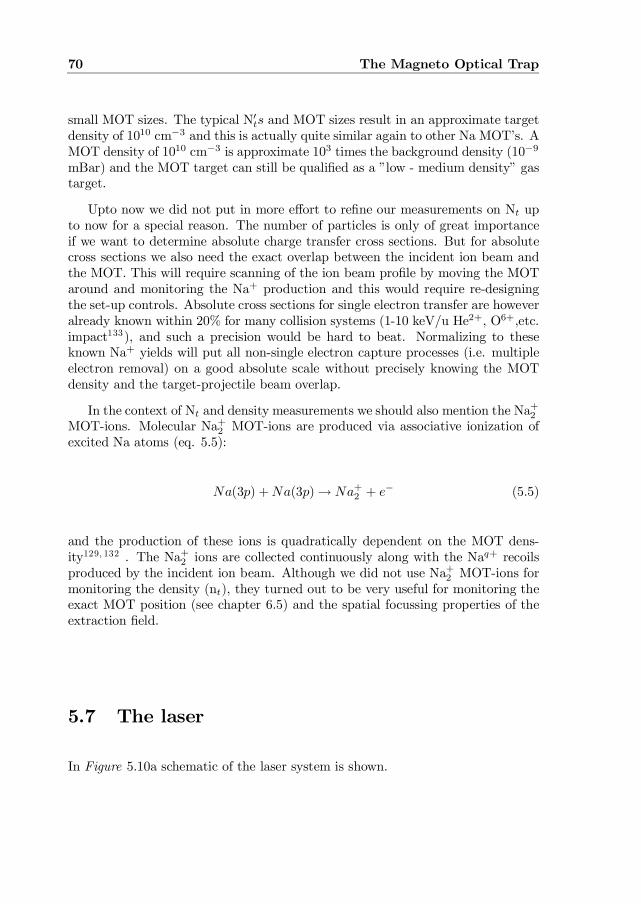
70 The Magneto Optical Trap
small MOT sizes. The typical N0ts and MOT sizes result in an approximate target
density of 1010 cm¡3 and this is actually quite similar again to other Na MOT’s. AMOT density of 1010 cm¡3 is approximate 103 times the background density (10¡9
mBar) and the MOT target can still be quali…ed as a ”low - medium density” gastarget.
Upto now we did not put in more e¤ort to re…ne our measurements on Nt upto now for a special reason. The number of particles is only of great importanceif we want to determine absolute charge transfer cross sections. But for absolutecross sections we also need the exact overlap between the incident ion beam andthe MOT. This will require scanning of the ion beam pro…le by moving the MOTaround and monitoring the Na+ production and this would require re-designingthe set-up controls. Absolute cross sections for single electron transfer are howeveralready known within 20% for many collision systems (1-10 keV/u He2+, O6+;etc.impact133), and such a precision would be hard to beat. Normalizing to theseknown Na+ yields will put all non-single electron capture processes (i.e. multipleelectron removal) on a good absolute scale without precisely knowing the MOTdensity and the target-projectile beam overlap.
In the context of Nt and density measurements we should also mention the Na+2
MOT-ions. Molecular Na+2 MOT-ions are produced via associative ionization of
excited Na atoms (eq. 5.5):
Na(3p) + Na(3p) ! Na+2 + e¡ (5.5)
and the production of these ions is quadratically dependent on the MOT dens-ity129, 132 . The Na+
2 ions are collected continuously along with the Naq+ recoilsproduced by the incident ion beam. Although we did not use Na+
2 MOT-ions formonitoring the density (nt); they turned out to be very useful for monitoring theexact MOT position (see chapter 6.5) and the spatial focussing properties of theextraction …eld.
5.7 The laser
In Figure 5.10a schematic of the laser system is shown.
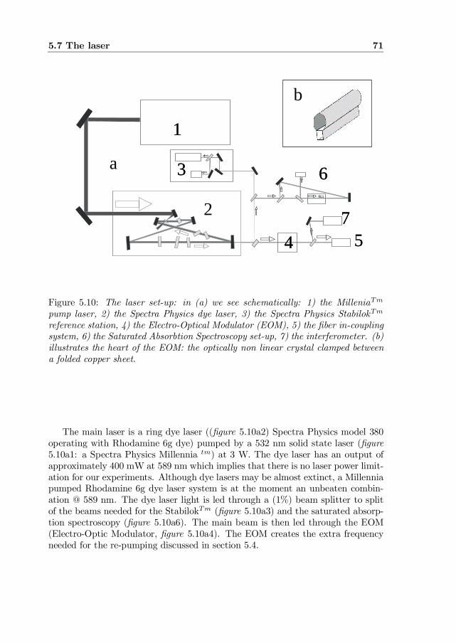
5.7 The laser 71
1
2
3
4 5
6
7
1
2
3
4 5
6
7
a
b
Figure 5.10: The laser set-up: in (a) we see schematically: 1) the MilleniaTm
pump laser, 2) the Spectra Physics dye laser, 3) the Spectra Physics StabilokTm
reference station, 4) the Electro-Optical Modulator (EOM), 5) the …ber in-couplingsystem, 6) the Saturated Absorbtion Spectroscopy set-up, 7) the interferometer. (b)illustrates the heart of the EOM: the optically non linear crystal clamped betweena folded copper sheet.
The main laser is a ring dye laser ((…gure 5.10a2) Spectra Physics model 380operating with Rhodamine 6g dye) pumped by a 532 nm solid state laser (…gure5.10a1: a Spectra Physics Millennia tm) at 3 W. The dye laser has an output ofapproximately 400 mW at 589 nm which implies that there is no laser power limit-ation for our experiments. Although dye lasers may be almost extinct, a Millenniapumped Rhodamine 6g dye laser system is at the moment an unbeaten combin-ation @ 589 nm. The dye laser light is led through a (1%) beam splitter to splitof the beams needed for the StabilokTm (…gure 5.10a3) and the saturated absorp-tion spectroscopy (…gure 5.10a6). The main beam is then led through the EOM(Electro-Optic Modulator, …gure 5.10a4). The EOM creates the extra frequencyneeded for the re-pumping discussed in section 5.4.
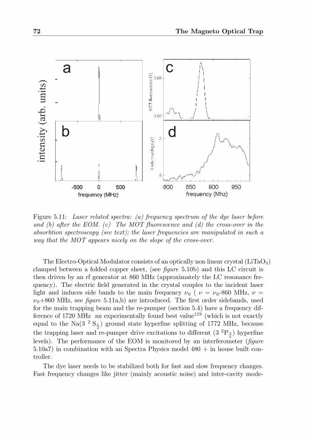
72 The Magneto Optical Trap
Figure 5.11: Laser related spectra: (a) frequency spectrum of the dye laser beforeand (b) after the EOM. (c) The MOT ‡uorescence and (d) the cross-over in theabsorbtion spectroscopy (see text); the laser frequencies are manipulated in such away that the MOT appears nicely on the slope of the cross-over.
The Electro-Optical Modulator consists of an optically non linear crystal (LiTaO3)clamped between a folded copper sheet, (see …gure 5.10b) and this LC circuit isthen driven by an rf generator at 860 MHz (approximately the LC resonance fre-quency). The electric …eld generated in the crystal couples to the incident laserlight and induces side bands to the main frequency º0 ( º = º0-860 MHz, º =º0+860 MHz, see …gure 5.11a,b) are introduced. The …rst order sidebands, usedfor the main trapping beam and the re-pumper (section 5.4) have a frequency dif-ference of 1720 MHz an experimentally found best value129 (which is not exactlyequal to the Na(3 2 S 1
2) ground state hyper…ne splitting of 1772 MHz, because
the trapping laser and re-pumper drive excitations to di¤erent (3 2P 32) hyper…ne
levels). The performance of the EOM is monitored by an interferometer (…gure5.10a7) in combination with an Spectra Physics model 480 + in house built con-troller.
The dye laser needs to be stabilized both for fast and slow frequency changes.Fast frequency changes like jitter (mainly acoustic noise) and inter-cavity mode-
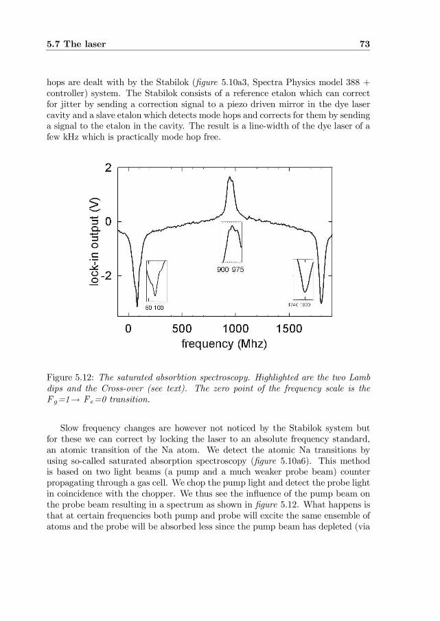
5.7 The laser 73
hops are dealt with by the Stabilok (…gure 5.10a3, Spectra Physics model 388 +controller) system. The Stabilok consists of a reference etalon which can correctfor jitter by sending a correction signal to a piezo driven mirror in the dye lasercavity and a slave etalon which detects mode hops and corrects for them by sendinga signal to the etalon in the cavity. The result is a line-width of the dye laser of afew kHz which is practically mode hop free.
Figure 5.12: The saturated absorbtion spectroscopy. Highlighted are the two Lambdips and the Cross-over (see text). The zero point of the frequency scale is theFg=1! Fe=0 transition.
Slow frequency changes are however not noticed by the Stabilok system butfor these we can correct by locking the laser to an absolute frequency standard,an atomic transition of the Na atom. We detect the atomic Na transitions byusing so-called saturated absorption spectroscopy (…gure 5.10a6). This methodis based on two light beams (a pump and a much weaker probe beam) counterpropagating through a gas cell. We chop the pump light and detect the probe lightin coincidence with the chopper. We thus see the in‡uence of the pump beam onthe probe beam resulting in a spectrum as shown in …gure 5.12. What happens isthat at certain frequencies both pump and probe will excite the same ensemble ofatoms and the probe will be absorbed less since the pump beam has depleted (via
74 The Magneto Optical Trap
optical pumping) the ground state population of those atoms. At these frequenciesa dip in the absorption is observed and these dips (approximately) correspond tothe frequencies of the Fg=1 and Fg=2 ground-states ( …gure 5.3c).
However because the pump and probe beam interact with a Na gas of 1200 C(see …gure 5.1b for a velocity distribution of Na at 600) other correlations betweenpump and probe can also occur: a Na atom moving with a certain velocity v inthe pump beam direction is also moving with a velocity -v in the probe beamdirection (the beams are counter propagating!). The atom will see the pump lightwith an º = º0(1+v/c) Doppler shift and the probe light with an º = º0(1-v/c)Doppler shift i.e. two di¤erent frequencies which can excite two di¤erent atomictransitions. For certain velocities the pump can excite a transition from groundstate Fg=1 and the probe beam a transition from the ground-state Fg=2. TheFg=1! Fe = 1 and Fg=1! Fe = 2 transitions driven by the pump will howeveralso decay to the Fg=2 ground-state. The resulting increase in Fg=2 populationresults in extra absorption of the probe light, corresponding to a peak (”the cross-over”, see Molenaar129 for detail) in the spectrum of …gure 5.12. The cross-over islocated exactly in between the Fg=1 and Fg=2 ground states and it is thereforeon the crossover where we want to ”frequency lock” our dye laser. The …rst ordersidebands of the EOM (…gure 5.11b) will then correspond to the Na Fg=2!Fe=3and Fg=1!Fe=2 transitions.
In practice one does not want to lock a laser frequency on the cross-over peakitself but on a slope of the cross-over (on a peak one can not detect small frequencychanges, on a slope one can). Here the AOM (…gure 5.6a2 ) comes to rescue byadding a 60-100 MHz de-tuning to the laser frequency allowing us to lock thelaser on a slope of the cross-over but still have light (after the AOM) of the rightfrequency.
In …gure 5.11 we can see the MOT ‡uorescence (5.11c) and the absorption spec-troscopy signal (5.11d) as a function of the laser frequency. The MOT ‡uorescenceconsists of a large peak caused by the type I MOT, (based on the Fg=2! Fe = 3transition + repumper, see section 5.4) and a small bump caused by the type IIMOT (the Fg=1! Fe = 0 transition + repumper)). The type II is in our casefainter than the type I since we use only moderate laser powers. Atutov131 etal. showed that the type II ‡uorescence depends much more strongly on the laserpower than the type I MOT and that the type II MOT ‡uorescence will evenovertake the type I ‡uorescence at approximately twice the laser power used in…gure 5.11. An order of magnitude more atoms can be trapped in a type II MOTbut the type II is also three to …ve times hotter and an order of magnitude largerin size than the type I.
The laser frequency can be locked anywhere on the cross-over slope and operatethe type I MOT at di¤erent detunings. The frequency lock is performed by acomputer program (a ”software lock”) which takes the absorption spectroscopy
5.8 Conclusion 75
signal as an input (via an ADC and BitBus) and gives a control voltage as anoutput (on a DAC). This voltage controls a subtle frequency tuning device (”thedual galvo’s”) in the dye laser cavity.
Last but not least, there is the already brie‡y mentioned …ber (section 5.5)transporting the laser light from the laser room to the MOT set-up. This systemconsists of a single mode …ber with a light incoupling system ”welded” permanentlyto it, which in turn is mounted on a precise XY manipulator. A transmission of 50% is achieved with this …ber system, leaving us with enough laser power to trapand cool Na in a type I MOT.
5.8 ConclusionIn this section we discussed all the important theoretical and experimental aspectsof our MOT set-up. The Magnetic Optical Trapping of Na is well understoodnowadays (Atutov131 et al.) but it is still important to realize that the MOT is adynamic equilibrium of six laser beams continuously heating and cooling the atomsfrom all directions. Any misalignment of the beams or laser frequency instabilitiesturns out to result in an odd shaped, moving or vibrating MOT. Aligning the laserbeams, tuning the dye laser cavity and the saturated absorption spectroscopy arethe parts of the MOT set-up which therefore demand constant attention. Howeverwith these items optimized, we are able to create stable MOT operating conditionsfor many hours.


6 The Recoil Ion MomentumSpectrometer
In this section we will discuss how recoil ion momenta are measured. The principleis fairly simple: a small electrostatic …eld extracts the recoil ion towards a posi-tion sensitive detector and from the combination of the ‡ight time and the arrivalposition on the detector, the initial velocity (momentum) vector is reconstructed.
77
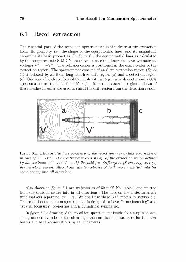
78 The Recoil Ion Momentum Spectrometer
6.1 Recoil extraction
The essential part of the recoil ion spectrometer is the electrostatic extraction…eld. Its geometry i.e. the shape of the equipotential lines, and its magnitudedetermine its basic properties. In …gure 6.1 the equipotential lines as calculatedby the computer code SIMION are shown in case the electrodes have symmetricalvoltages V¡ = ¡V+ . The collision center is positioned in the exact center of theextraction region. The spectrometer consists of an 8 cm extraction region (…gure6.1a) followed by an 8 cm long …eld-free drift region (b) and a detection region(c). One super…ne electroformed Cu mesh with a 13 ¹m wire diameter and a 88%open area is used to shield the drift region from the extraction region and two ofthese meshes in series are used to shield the drift region from the detection region.
a cb
V-V+
Figure 6.1: Electrostatic …eld geometry of the recoil ion momentum spectrometerin case of V -=-V + . The spectrometer consists of (a) the extraction region de…nedby the electrodes V + and V ¡ , (b) the …eld free drift region (8 cm long) and (c)the detection region. Also shown are trajectories of Na+ recoils emitted with thesame energy into all directions .
Also shown in …gure 6.1 are trajectories of 50 meV Na+ recoil ions emittedfrom the collision center into in all directions. The dots on the trajectories aretime markers separated by 1 ¹s. We shall use these Na+ recoils in section 6.5.The recoil ion momentum spectrometer is designed to have ”time focussing” and”spatial focussing” properties and is cylindrical symmetric.
In …gure 6.2 a drawing of the recoil ion spectrometer inside the set-up is shown.The grounded cylinder in the ultra high vacuum chamber has holes for the laserbeams and MOT-observations by CCD cameras.
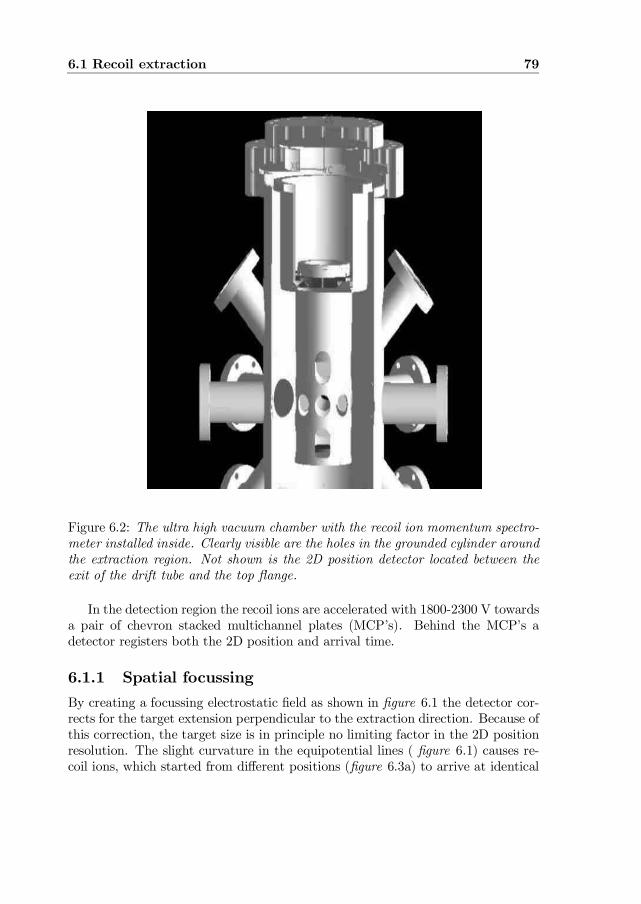
6.1 Recoil extraction 79
Figure 6.2: The ultra high vacuum chamber with the recoil ion momentum spectro-meter installed inside. Clearly visible are the holes in the grounded cylinder aroundthe extraction region. Not shown is the 2D position detector located between theexit of the drift tube and the top ‡ange.
In the detection region the recoil ions are accelerated with 1800-2300 V towardsa pair of chevron stacked multichannel plates (MCP’s). Behind the MCP’s adetector registers both the 2D position and arrival time.
6.1.1 Spatial focussingBy creating a focussing electrostatic …eld as shown in …gure 6.1 the detector cor-rects for the target extension perpendicular to the extraction direction. Because ofthis correction, the target size is in principle no limiting factor in the 2D positionresolution. The slight curvature in the equipotential lines ( …gure 6.1) causes re-coil ions, which started from di¤erent positions (…gure 6.3a) to arrive at identical
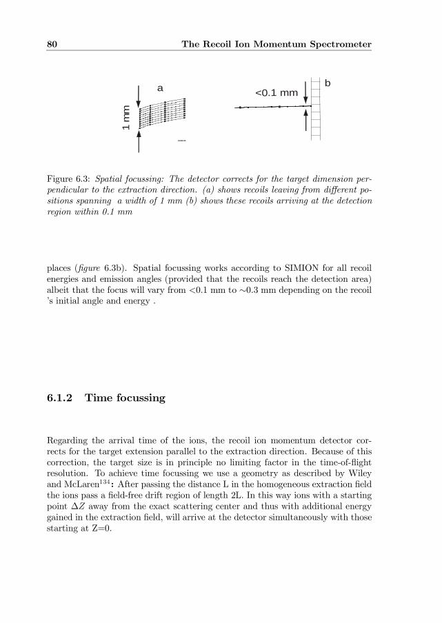
80 The Recoil Ion Momentum Spectrometer
SIMION
a
1 m
m
b<0.1 mm
Figure 6.3: Spatial focussing: The detector corrects for the target dimension per-pendicular to the extraction direction. (a) shows recoils leaving from di¤erent po-sitions spanning a width of 1 mm (b) shows these recoils arriving at the detectionregion within 0.1 mm
places (…gure 6.3b). Spatial focussing works according to SIMION for all recoilenergies and emission angles (provided that the recoils reach the detection area)albeit that the focus will vary from <0.1 mm to »0.3 mm depending on the recoil’s initial angle and energy .
6.1.2 Time focussing
Regarding the arrival time of the ions, the recoil ion momentum detector cor-rects for the target extension parallel to the extraction direction. Because of thiscorrection, the target size is in principle no limiting factor in the time-of-‡ightresolution. To achieve time focussing we use a geometry as described by Wileyand McLaren134 : After passing the distance L in the homogeneous extraction …eldthe ions pass a …eld-free drift region of length 2L. In this way ions with a startingpoint ¢Z away from the exact scattering center and thus with additional energygained in the extraction …eld, will arrive at the detector simultaneously with thosestarting at Z=0.
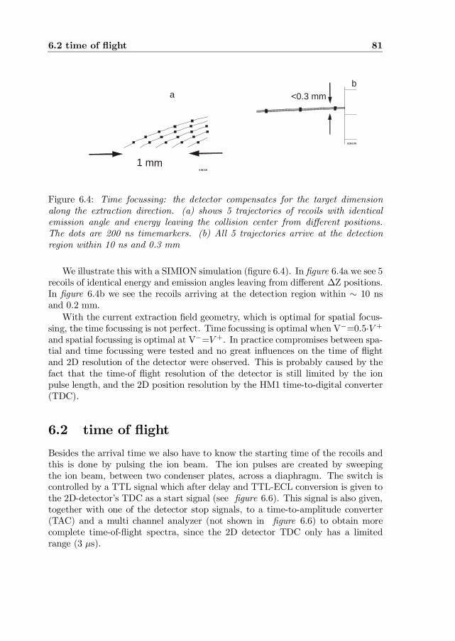
6.2 time of ‡ight 81
SIMION
b
SIMION
a
1 mm
<0.3 mm
Figure 6.4: Time focussing: the detector compensates for the target dimensionalong the extraction direction. (a) shows 5 trajectories of recoils with identicalemission angle and energy leaving the collision center from di¤erent positions.The dots are 200 ns timemarkers. (b) All 5 trajectories arrive at the detectionregion within 10 ns and 0.3 mm
We illustrate this with a SIMION simulation (…gure 6.4). In …gure 6.4a we see 5recoils of identical energy and emission angles leaving from di¤erent ¢Z positions.In …gure 6.4b we see the recoils arriving at the detection region within » 10 nsand 0.2 mm.
With the current extraction …eld geometry, which is optimal for spatial focus-sing, the time focussing is not perfect. Time focussing is optimal when V¡=0.5¢V +
and spatial focussing is optimal at V¡=V +. In practice compromises between spa-tial and time focussing were tested and no great in‡uences on the time of ‡ightand 2D resolution of the detector were observed. This is probably caused by thefact that the time-of ‡ight resolution of the detector is still limited by the ionpulse length, and the 2D position resolution by the HM1 time-to-digital converter(TDC).
6.2 time of ‡ightBesides the arrival time we also have to know the starting time of the recoils andthis is done by pulsing the ion beam. The ion pulses are created by sweepingthe ion beam, between two condenser plates, across a diaphragm. The switch iscontrolled by a TTL signal which after delay and TTL-ECL conversion is given tothe 2D-detector’s TDC as a start signal (see …gure 6.6). This signal is also given,together with one of the detector stop signals, to a time-to-amplitude converter(TAC) and a multi channel analyzer (not shown in …gure 6.6) to obtain morecomplete time-of-‡ight spectra, since the 2D detector TDC only has a limitedrange (3 ¹s).
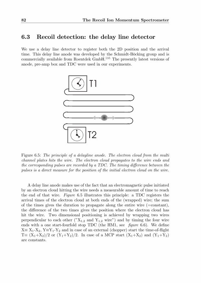
82 The Recoil Ion Momentum Spectrometer
6.3 Recoil detection: the delay line detector
We use a delay line detector to register both the 2D position and the arrivaltime. This delay line anode was developed by the Schmidt-Bocking group and iscommercially available from Roentdek GmbH.135 The presently latest versions ofanode, pre-amp box and TDC were used in our experiments.
T1
T2
Figure 6.5: The principle of a delayline anode. The electron cloud from the multichannel plates hits the wire. The electron cloud propagates to the wire ends andthe corresponding pulses are recorded by a TDC. The timing di¤erence between thepulses is a direct measure for the position of the initial electron cloud on the wire.
A delay line anode makes use of the fact that an electromagnetic pulse initiatedby an electron cloud hitting the wire needs a measurable amount of time to reachthe end of that wire. Figure 6.5 illustrates this principle: a TDC registers thearrival times of the electron cloud at both ends of the (wrapped) wire; the sumof the times gives the duration to propagate along the entire wire (=constant),the di¤erence of the two times gives the position where the electron cloud hashit the wire. Two dimensional positioning is achieved by wrapping two wiresperpendicular to each other (”X1,2 and Y1,2 wire”) and by timing the four wireends with a one start-fourfold stop TDC (the HM1, see …gure 6.6). We de…neX´ X1-X2, Y´Y1-Y2 and in case of an external (chopper) start the time-of-‡ightT´ (X1+X2)/2 or (Y1+Y2)/2. In case of a MCP start (X1+X2) and (Y1+Y2)are constants.
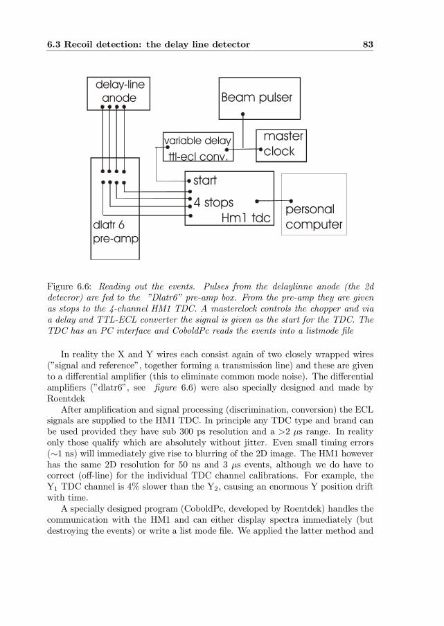
6.3 Recoil detection: the delay line detector 83
delay-line anode
dlatr 6pre-amp
Hm1 tdc4 stops
start
Beam pulser
variable delay
ttl-ecl conv.
masterclock
personalcomputer
Figure 6.6: Reading out the events. Pulses from the delaylinne anode (the 2ddetecror) are fed to the ”Dlatr6” pre-amp box. From the pre-amp they are givenas stops to the 4-channel HM1 TDC. A masterclock controls the chopper and viaa delay and TTL-ECL converter the signal is given as the start for the TDC. TheTDC has an PC interface and CoboldPc reads the events into a listmode …le
In reality the X and Y wires each consist again of two closely wrapped wires(”signal and reference”, together forming a transmission line) and these are givento a di¤erential ampli…er (this to eliminate common mode noise). The di¤erentialampli…ers (”dlatr6”, see …gure 6.6) were also specially designed and made byRoentdek
After ampli…cation and signal processing (discrimination, conversion) the ECLsignals are supplied to the HM1 TDC. In principle any TDC type and brand canbe used provided they have sub 300 ps resolution and a >2 ¹s range. In realityonly those qualify which are absolutely without jitter. Even small timing errors(»1 ns) will immediately give rise to blurring of the 2D image. The HM1 howeverhas the same 2D resolution for 50 ns and 3 ¹s events, although we do have tocorrect (o¤-line) for the individual TDC channel calibrations. For example, theY1 TDC channel is 4% slower than the Y2, causing an enormous Y position driftwith time.
A specially designed program (CoboldPc, developed by Roentdek) handles thecommunication with the HM1 and can either display spectra immediately (butdestroying the events) or write a list mode …le. We applied the latter method and
84 The Recoil Ion Momentum Spectrometer
used MATLAB for the o¤-line evaluation of the recorded events.
6.4 Recoil momentum reconstruction (theory)The …rst o¤-line transformation performed on the list mode data is the TDC calib-ration. This transformation ensures that position measurements are not in‡uencedby the total ‡ight time from target to detector. The calibration can change slightlyfrom week to week, but we can use the Na+
2 MOT-ions to re…ne the calibration(see next section). Na+
2 ions are permanently produced in associative ionizing col-lisions of excited Na(3p) atoms and are practically without kinetic energy. Theirarrival position is used to de…ne the origin (X=0,Y=0) and the (X,Y) plane istranslated accordingly. Then we reconstruct the (vx,vy,vz) with vx;y=x;y
T (withT´ Tdelay + Ttdc) and vz given by an algorithm vz(T,Ez,L) which takes the timeof ‡ight T, the extraction …eld Ez and extraction distance L as input to calculatevz. This algorithm was obtained by analytically solving the time of ‡ight of an ionwith mass m and charge q starting with velocity vz in a homogeneous extractionregion. L denotes the length of the extraction region and Ez the electric …eld inthis region. The drift region has the length 2L. The resulting function for T isgiven in eq. 6.1 and was veri…ed with SIMION simulations.
T (L;Ez; vz) =¡vz
a+
r³vz
a
´2+
2La
+2Lp
v2z + 2L ¤ a
; where: a =q ¤ Ez
m(6.1)
The expression in 6.1 can be inverted analytically with Mathematica to obtainthe function vz(T,Ez,L) which is too long and complex to be displayed here. Inorder for the vz(T,Ez,L) and vx;y functions to work we have to know however theexact Tdelay in the expression T´ Tdelay + Ttdc.
The Tdelay consists of the manually set delay (Phillips Scienti…c, model 794,the delay and TTL-ECL converter in …gure 6.6) and additional delays produced bycables, pre-amps, signal converters, etc. It can therefore not be measured directlybut has to be reconstructed. This is done by …rst using the peak separation of atleast two clearly identi…ed time-of-‡ight peaks. The peaks of the Na+ and Na2+
recoil ions usually qualify but also the H+2 peak from the background gas can
be used. The time between these peaks yields the reconstructed extraction …eldEz and this …eld is 30% smaller than the manually set …eld (V+-V¡)=2L. Thedi¤erence between the reconstructed and the set …elds is caused by the groundedcylinder around the extraction region (which is required to obtain spatial focussing)and the fact that the reconstruction algorithm assumes a homogeneous …eld whichin reality is not the case, especially near the reaction center. There is howeverno discrepancy here since the 30% di¤erence is also predicted by the SIMIONcalculations.
6.5 Recoil momentum reconstruction (practice) 85
With the exact extraction …eld Ez reconstructed Tdelay can be determined withgreat precision by demanding that the transverse velocity distribution (vy,vz)ofa Nax+ data set is symmetrical around zero. The (vy,vz) distribution will bediscussed further in the section 6.5 and examples can be seen in …gure 6.8.
With the initial recoil velocity (vx,vy,vz) reconstructed we then calculate therecoil momenta along the ion beam (Plong) and perpendicular to the ion beam(Ptrans):
Plong =vx
vo(6.2)
Ptrans =
qv2
y + v2z
v0
; (6.3)
with vo=52.8 m/s, corresponding to 1 a.u. of Na momentum.
6.5 Recoil momentum reconstruction (practice)
After the introduction in the previous section we will now show how momentaare actually reconstructed from the raw data. In …gure 6.7b,c and d the spatialdistributions at the 2D detector are shown of ions arriving at times indicated inthe time of ‡ight spectrum of …gure 6.7a, namely shortly before, exactly at andshortly after the arrival of Na2+ recoils.
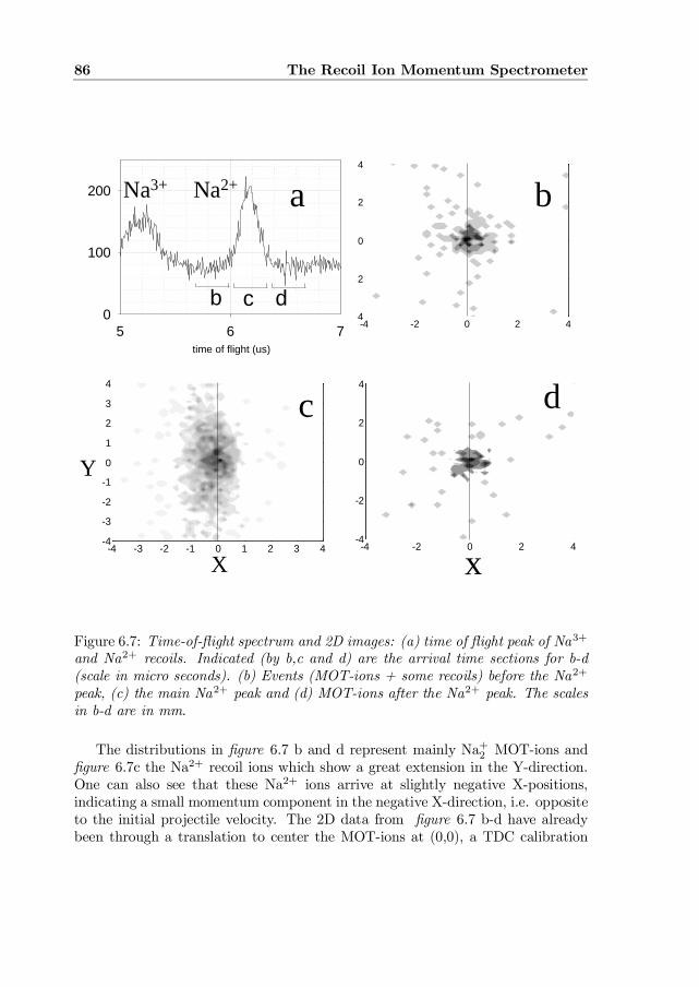
86 The Recoil Ion Momentum Spectrometer
-4 -2 0 2 4-4
-2
0
2
4
-4 -2 0 2 4-4
-2
0
2
4
-4 -3 -2 -1 0 1 2 3 4-4
-3
-2
-1
0
1
2
3
4
time of flight (us)
5 6 70
100
200
b c d
a b
c d
Y
X x
Na3+ Na2+
Figure 6.7: Time-of-‡ight spectrum and 2D images: (a) time of ‡ight peak of Na3+
and Na2+ recoils. Indicated (by b,c and d) are the arrival time sections for b-d(scale in micro seconds). (b) Events (MOT-ions + some recoils) before the Na2+
peak, (c) the main Na2+ peak and (d) MOT-ions after the Na2+ peak. The scalesin b-d are in mm.
The distributions in …gure 6.7 b and d represent mainly Na+2 MOT-ions and
…gure 6.7c the Na2+ recoil ions which show a great extension in the Y-direction.One can also see that these Na2+ ions arrive at slightly negative X-positions,indicating a small momentum component in the negative X-direction, i.e. oppositeto the initial projectile velocity. The 2D data from …gure 6.7 b-d have alreadybeen through a translation to center the MOT-ions at (0,0), a TDC calibration
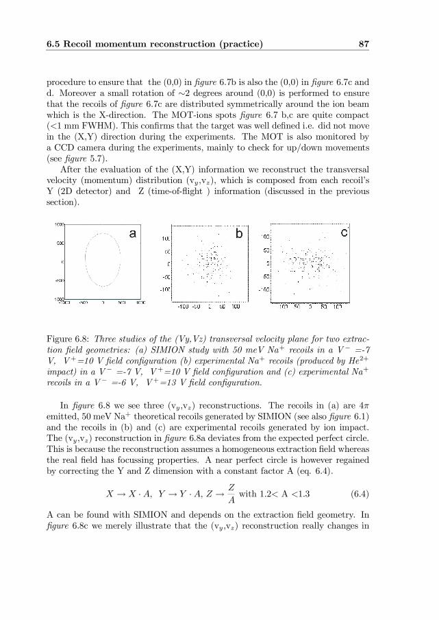
6.5 Recoil momentum reconstruction (practice) 87
procedure to ensure that the (0,0) in …gure 6.7b is also the (0,0) in …gure 6.7c andd. Moreover a small rotation of »2 degrees around (0,0) is performed to ensurethat the recoils of …gure 6.7c are distributed symmetrically around the ion beamwhich is the X-direction. The MOT-ions spots …gure 6.7 b,c are quite compact(<1 mm FWHM). This con…rms that the target was well de…ned i.e. did not movein the (X,Y) direction during the experiments. The MOT is also monitored bya CCD camera during the experiments, mainly to check for up/down movements(see …gure 5.7).
After the evaluation of the (X,Y) information we reconstruct the transversalvelocity (momentum) distribution (vy,vz), which is composed from each recoil’sY (2D detector) and Z (time-of-‡ight ) information (discussed in the previoussection).
Figure 6.8: Three studies of the (Vy,Vz) transversal velocity plane for two extrac-tion …eld geometries: (a) SIMION study with 50 meV Na+ recoils in a V ¡ =-7V, V +=10 V …eld con…guration (b) experimental Na+ recoils (produced by He2+
impact) in a V ¡ =-7 V, V +=10 V …eld con…guration and (c) experimental Na+
recoils in a V ¡ =-6 V, V +=13 V …eld con…guration.
In …gure 6.8 we see three (vy,vz) reconstructions. The recoils in (a) are 4¼emitted, 50 meV Na+ theoretical recoils generated by SIMION (see also …gure 6.1)and the recoils in (b) and (c) are experimental recoils generated by ion impact.The (vy,vz) reconstruction in …gure 6.8a deviates from the expected perfect circle.This is because the reconstruction assumes a homogeneous extraction …eld whereasthe real …eld has focussing properties. A near perfect circle is however regainedby correcting the Y and Z dimension with a constant factor A (eq. 6.4).
X ! X ¢ A, Y ! Y ¢ A, Z ! ZA
with 1.2< A <1.3 (6.4)
A can be found with SIMION and depends on the extraction …eld geometry. In…gure 6.8c we merely illustrate that the (vy,vz) reconstruction really changes in
88 The Recoil Ion Momentum Spectrometer
practice with an alteration in the extraction …eld geometry.Another concern in the reconstruction of the (vy,vz) velocity plane are the
already mentioned Na+2 MOT-ions. Na+
2 MOT-ions arriving very early and verylate in time of ‡ight simulate recoils with very large positive and negative vz com-ponents. We can remove MOT-ions from the raw data by cutting out a small (X,Y)region around (0,0)) but only if we do not remove (too many) real recoils. Howeverwhen the recoils and the MOT-ions mix then we can correct for the MOT-ions inthe momentum plots. This is possible since MOT-ions have a ”momentum …nger-print” (centered around plong=0 and stretched along the ptrans range) which canbe generated and subtracted from the combined recoils + MOT-ions momentumplot. One can generate a MOT-ion momentum plot by running the recoil recon-struction on a suitable time-of-‡ight interval containing only MOT-ions. An evenmore subtle method, investigated but not yet used in this work, is to suppress theMOT-ions experimentally by switching the trapping laser o¤ at suitable times sothat no MOT-ions arrive simultaneously with the true recoils.
Last, but not least, we have checked some of the systematical uncertaintiesin the experimental momenta by performing measurements on the same collisionsystem with very di¤erent (within reason) extraction …elds. We found that re-coil momentum spectra did not change unexpectedly, except perhaps regardingresolution.
6.6 ResolutionThe real resolution limits are discussed in the chapter 7, but here are already somegeneral remarks.
² The real detector resolution for plong can only be determined by performinga benchmark measurement i.e. an experiment with a known plong spec-trum. The ptrans resolution can basically only be optimized by looking atthe spherical symmetry in the (vy,vz) plot. If the ptrans distribution hasclear maximum at pmax 6= 0 a ring (donut) should appear in the (vy,vz)distribution.
² A theoretical limitation is the initial momentum spread (temperature) of theNa cloud. A 300 ¹K (»0.5 m/s) cloud gives a theoretical momentum limitof 0.01 a.u.. This will not restrict our experiment.
² A more realistic, yet still theoretical longitudinal momentum limit for ourdetector can easily be estimated: a separation between two recoil distribu-tions of ¢X = 0.5 mm at the 2D detector and a time of ‡ight for thesedistributions of T=50 ¹s will result in a plong resolution of ¢X=(T ¤ v0)»0.2 a.u., where v0 is 52.8 m/s: This is also the typical resolution needed for
6.7 Outlook 89
experiments involving Na+ recoils. However in order to obtain 50 ¹s ‡ight-ime very low extraction …elds have to be used and contact potentials or stray…elds will start to in‡uence the resolution.
² A more practical resolution limitation is the choice which has to be madebetween detector resolution and detector acceptance. By increasing the main‡ight time of the recoils the momentum resolution will increase (a certain¢plong;trans will result in a larger ¢(X; Y; Z)) and thus one can decreasethe in‡uence of the 2D detector resolution (0.2 mm). However, recoils withlarge momenta in X,Y direction will fall outside the 2D detector range andthe experimental data set will be incomplete.
6.7 OutlookSome suggestions for future improvements.
² The spectrometer should be modi…ed in such a way that spatial and timefocussing are optimal at the same extraction …eld geometry. This is pos-sible by adjusting the length of the drift region and/or adding …eld de…ningelements to the extraction region.
² The TDC system is under constant examination, both by us and by Roent-dek. Improvements to the TDC detection scheme are currently being invest-igated by using X1 as the common start, X2 plus cable delay as a stop (TDCchannel 1 is then directly the X direction), a delayed chopper signal as thesecond stop (TDC channel 2 is then the inverted time of ‡ight ”3 ¹s-T ”),and Y1, Y2 plus cable delays as stops three and four (TDC channel 3 minusTDC channel 4 is then the Y direction). With this scheme the position res-olution is independent of the time of ‡ight and moreover the TDC is nowonly started if a real event has occurred. The latter improves the event ratequite dramatically since the TDC is now no longer blocked or occupied bystarts which are not followed by the stops of an event. The best solutionwould however probably be to use four ultrahigh resolution TDC’s just forthe 2D detection (with a MCP start) and a …fth TDC (only ns resolutionand >5 ¹s range) for the time of ‡ight (external start, MCP stop).
² Time of ‡ight resolution would greatly bene…t from a start derived from acharge-changed projectile since these starts have a much smaller (»10 times)timing uncertainty than the ion pulse start. Furthermore much less dc ionbeam intensity would be needed (up to 1000 times) since we do not loosenearly all current in the ion pulsing process anymore. This would makemany more projectile species and energies accessible for our experiments,which can only be produced at signi…cantly lower beam intensities.

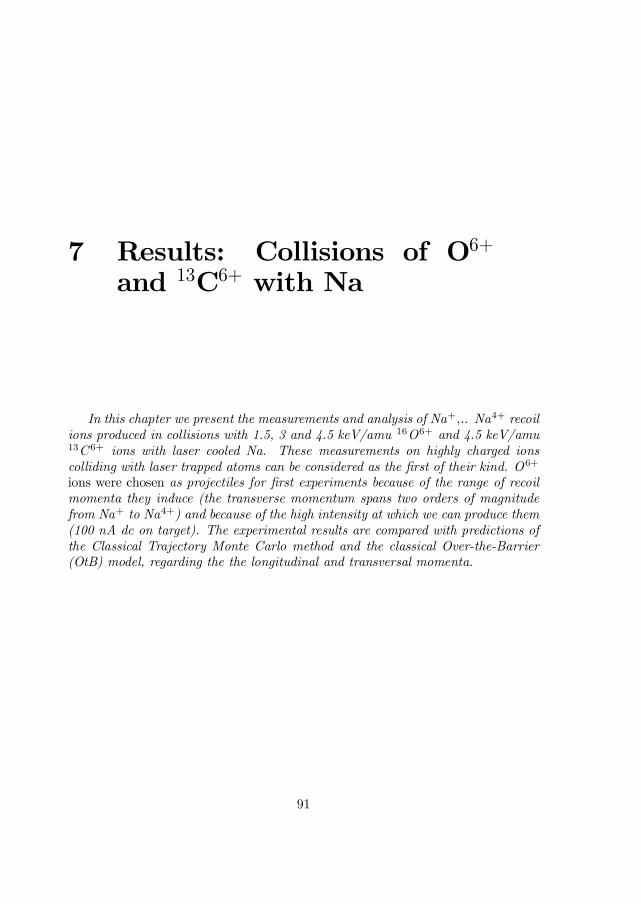
7 Results: Collisions of O6+
and 13C6+ with Na
In this chapter we present the measurements and analysis of Na+;.. Na4+ recoilions produced in collisions with 1.5, 3 and 4.5 keV/amu 16O6+ and 4.5 keV/amu13C 6+ ions with laser cooled Na. These measurements on highly charged ionscolliding with laser trapped atoms can be considered as the …rst of their kind. O6+
ions were chosen as projectiles for …rst experiments because of the range of recoilmomenta they induce (the transverse momentum spans two orders of magnitudefrom Na+ to Na4+) and because of the high intensity at which we can produce them(100 nA dc on target). The experimental results are compared with predictions ofthe Classical Trajectory Monte Carlo method and the classical Over-the-Barrier(OtB) model, regarding the the longitudinal and transversal momenta.
91

92 Results: Collisions of O6+ and 13C6+ with Na
7.1 Motivation
The main motivation for the work presented here is to demonstrate the method ofCOld Target Recoil Ion Momentum Spectroscopy (COLTRIMS) for laser-cooledtargets and its potential to study single and multiple electron transfer by highlycharged ions as a function of impact parameter. What COLTRIMS promises iscompleteness in the experimental information. This because the longitudinal andtransversal momentum components provide both Q-value, i.e. the electronic stateafter the collision, and impact parameter sensitive information. Moreover all theNaq+ recoil spectra are complete, since every Naq+ recoil ion created in a reactionis collected. The big challenge is to obtain enough signal and resolution to observeand distinguish recoils of speci…c longitudinal and transversal momentum.
7.2 Recoil charge state spectra from 16O6+ and13C6+ impact
Before we discuss the COLTRIMS results we …rst look at the time-of-‡ight distri-bution of Naq+ (q=1..4) recoils at the ion detector, shown in …gure 7.1(a-d). Inall spectra the intensity of the Na+ ions is roughly 100 times higher than that forthe other charge states. The widths of the peaks only re‡ect the collision inducedtransversal momentum ranges of the recoil ions and not the thermal spread of theNa target.
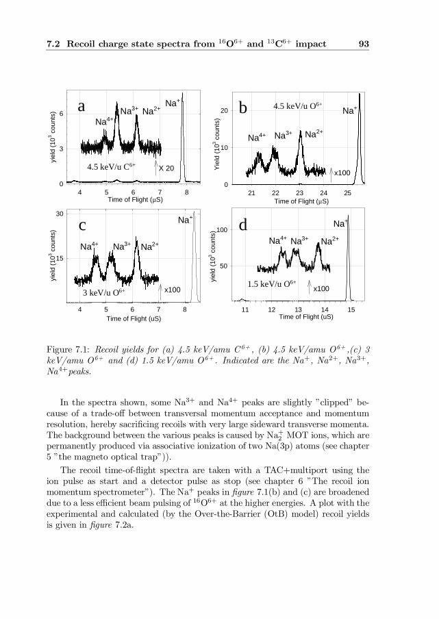
7.2 Recoil charge state spectra from 16O6+ and 13C6+ impact 93
Time of Flight (uS)4 5 6 7 8
yiel
d (1
03 cou
nts)
15
30Na+
Na2+Na3+Na4+
x100
Time of Flight (uS)11 12 13 14 15
yiel
d (1
03 cou
nts)
50
100
x100
Na4+ Na3+ Na2+
Na+
Time of Flight (µS)21 22 23 24 25
Yie
ld (
103 c
ount
s)
0
10
20
x100
Na4+ Na3+ Na2+
Na+
Time of Flight (µS)4 5 6 7 8
yiel
d (1
03 cou
nts)
0
3
6 Na2+Na3+
Na4+
Na+
X 20
a b
c d
4.5 keV/u C6+
4.5 keV/u O6+
3 keV/u O6+1.5 keV/u O6+
Figure 7.1: Recoil yields for (a) 4.5 keV/amu C 6+ , (b) 4.5 keV/amu O6+ ,(c) 3keV/amu O6+ and (d) 1.5 keV/amu O6+ . Indicated are the Na+, Na2+, Na3+,Na4+peaks.
In the spectra shown, some Na3+ and Na4+ peaks are slightly ”clipped” be-cause of a trade-o¤ between transversal momentum acceptance and momentumresolution, hereby sacri…cing recoils with very large sideward transverse momenta.The background between the various peaks is caused by Na+
2 MOT ions, which arepermanently produced via associative ionization of two Na(3p) atoms (see chapter5 ”the magneto optical trap”)).
The recoil time-of-‡ight spectra are taken with a TAC+multiport using theion pulse as start and a detector pulse as stop (see chapter 6 ”The recoil ionmomentum spectrometer”). The Na+ peaks in …gure 7.1(b) and (c) are broadeneddue to a less e¢cient beam pulsing of 16O6+ at the higher energies. A plot with theexperimental and calculated (by the Over-the-Barrier (OtB) model) recoil yieldsis given in …gure 7.2a.
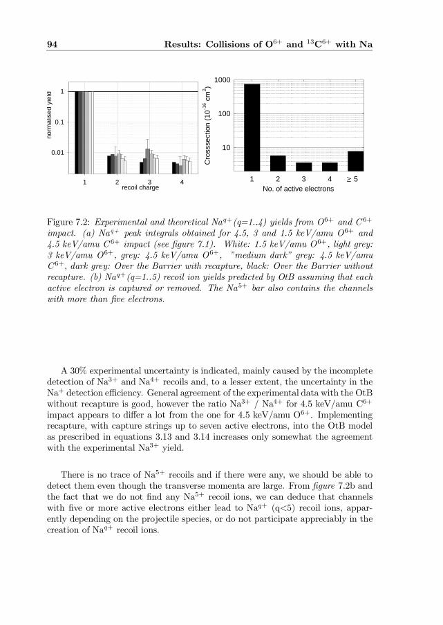
94 Results: Collisions of O6+ and 13C6+ with Na
recoil charge1 2 3 4
norm
alis
ed y
ield
0.01
0.1
1
No. of active electrons1 2 3 4 5
Cro
ssse
ctio
n (1
0-16 c
m2 )
10
100
1000
Figure 7.2: Experimental and theoretical Naq+(q=1..4) yields from O6+ and C 6+
impact. (a) Naq+ peak integrals obtained for 4.5, 3 and 1.5 keV/amu O6+ and4.5 keV/amu C 6+ impact (see …gure 7.1). White: 1.5 keV/amu O6+, light grey:3 keV/amu O6+, grey: 4.5 keV/amu O6+, ”medium dark” grey: 4.5 keV/amuC 6+; dark grey: Over the Barrier with recapture, black: Over the Barrier withoutrecapture. (b) Naq+(q=1..5) recoil ion yields predicted by OtB assuming that eachactive electron is captured or removed. The Na5+ bar also contains the channelswith more than …ve electrons.
A 30% experimental uncertainty is indicated, mainly caused by the incompletedetection of Na3+ and Na4+ recoils and, to a lesser extent, the uncertainty in theNa+ detection e¢ciency. General agreement of the experimental data with the OtBwithout recapture is good, however the ratio Na3+ / Na4+ for 4.5 keV/amu C6+
impact appears to di¤er a lot from the one for 4.5 keV/amu O6+. Implementingrecapture, with capture strings up to seven active electrons, into the OtB modelas prescribed in equations 3.13 and 3.14 increases only somewhat the agreementwith the experimental Na3+ yield.
There is no trace of Na5+ recoils and if there were any, we should be able todetect them even though the transverse momenta are large. From …gure 7.2b andthe fact that we do not …nd any Na5+ recoil ions, we can deduce that channelswith …ve or more active electrons either lead to Naq+ (q<5) recoil ions, appar-ently depending on the projectile species, or do not participate appreciably in thecreation of Naq+ recoil ions.
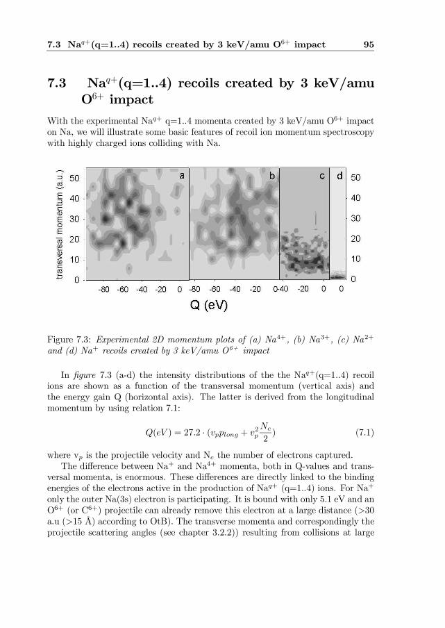
7.3 Naq+(q=1..4) recoils created by 3 keV/amu O6+ impact 95
7.3 Naq+(q=1..4) recoils created by 3 keV/amuO6+ impact
With the experimental Naq+ q=1::4 momenta created by 3 keV/amu O6+ impacton Na, we will illustrate some basic features of recoil ion momentum spectroscopywith highly charged ions colliding with Na.
Figure 7.3: Experimental 2D momentum plots of (a) Na4+, (b) Na3+, (c) Na2+
and (d) Na+ recoils created by 3 keV/amu O6+ impact
In …gure 7.3 (a-d) the intensity distributions of the the Naq+(q=1::4) recoilions are shown as a function of the transversal momentum (vertical axis) andthe energy gain Q (horizontal axis). The latter is derived from the longitudinalmomentum by using relation 7.1:
Q(eV ) = 27:2 ¢ (vpplong + v2pNc
2) (7.1)
where vp is the projectile velocity and Nc the number of electrons captured.The di¤erence between Na+ and Na4+ momenta, both in Q-values and trans-
versal momenta, is enormous. These di¤erences are directly linked to the bindingenergies of the electrons active in the production of Naq+ (q=1::4) ions. For Na+
only the outer Na(3s) electron is participating. It is bound with only 5.1 eV and anO6+ (or C6+) projectile can already remove this electron at a large distance (>30a.u (>15 Å) according to OtB). The transverse momenta and correspondingly theprojectile scattering angles (see chapter 3.2.2)) resulting from collisions at large
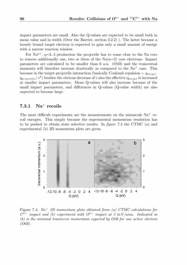
96 Results: Collisions of O6+ and 13C6+ with Na
impact parameters are small. Also the Q-values are expected to be small both inmean value and in width (Over the Barrier, section 3.2.2) ). The latter because aloosely bound target electron is expected to gain only a small amount of energywith a narrow reaction window.
For Naq+; q=2..4 production the projectile has to come close to the Na coreto remove additionally one, two or three of the Na(n=2) core electrons. Impactparameters are calculated to be smaller than 6 a.u. (OtB) and the transversalmomenta will therefore increase drastically as compared to the Na+ case. Thisbecause in the target-projectile interaction (basically Coulomb repulsion » qtarget ¢qprojectile/ r2) besides the obvious decrease of r also the e¤ective qtarget is increasedat smaller impact parameters. Mean Q-values will also increase because of thesmall impact parameters, and di¤erences in Q-values (Q-value width) are alsoexpected to become large.
7.3.1 Na+ recoils
The most di¢cult experiments are the measurements on the minuscule Na+ re-coil energies. This simply because the experimental momentum resolution hasto be pushed to obtain state selective results. In …gure 7.4 the CTMC (a) andexperimental (b) 2D momentum plots are given.
Figure 7.4: Na+ 2D momentum plots obtained from (a) CTMC calculations forC 6+ impact and (b) experiment with O6+ impact at 3 keV/amu. Indicated in(b) is the minimal transverse momentum expected by OtB for one active electron(OtB).
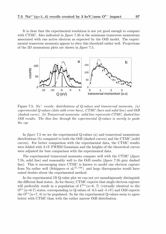
7.3 Naq+(q=1..4) recoils created by 3 keV/amu O6+ impact 97
It is clear that the experimental resolution is not yet good enough to comparewith CTMC. Also indicated in …gure 7.4b is the minimum transverse momentumassociated with one active electron as expected by the OtB model. The experi-mental transverse momenta appear to obey this threshold rather well. Projectionsof the 2D momentum plots are shown in …gure 7.5.
Q (eV)-15 -10 -5 0 5
coun
ts
0
50
100
transversal momentum (a.u)0 1 2 3
0
50
100
150a b
Figure 7.5: Na+ recoils: distributions of Q-values and transversal momenta. (a)experimental Q-values (dots with error bars), CTMC (bars and solid line) and OtB(dashed curve). (b) Transversal momenta: solid line represents CTMC, dashed lineOtB results. The thin line through the experimental Q-values is merely to guidethe eye
In …gure 7.5 we see the experimental Q-values (a) and transversal momentumdistributions (b) compared to both the OtB (dashed curves) and the CTMC (solidcurves). For better comparison with the experimental data, the CTMC resultswere folded with 3 eV FWHM Gaussians and the heights of the theoretical curveswere adjusted for best comparison with the experimental data.
The experimental transversal momenta compare well with the CTMC (…gure7.5b, solid line) and reasonably well to the OtB results (…gure 7.5b grey dashedline). This is encouraging since CTMC is known to model one electron capturefrom Na rather well (Schippers et al.35, 106) and large discrepancies would haveraised doubts about the experimental method.
In the experimental 1D Q-value plot we can not yet unambiguously distinguishthe di¤erent …nal states. As for theory, CTMC expects that single electron capturewill preferably result in a population of C5+(n=6, 7) (virtually identical to theO5+(n=6-7) states, corresponding to Q-values of -8.5 and -5 eV) and OtB expectsthe O5+(n=7, 8) to be populated. So far the experimental Q-values seem to agreebetter with CTMC than with the rather narrow OtB distribution.
98 Results: Collisions of O6+ and 13C6+ with Na
7.3.2 Na2+ recoils
In …gure 7.3 we saw already that the momenta of the Na2+ recoils are much largerthan those of the Na+; which makes them easier to detect. However, in order torecord even the largest transverse momenta, relatively high extraction …elds (>5V/cm) had to be used, thus sacri…cing some Q-value (longitudinal momentum)resolution.
The CTMC calculations for double capture by 3 keV/amu C6+are availableboth for binned and un-binned …nal states (see chapter 3.3.2). 13C6+ and 16O6+
di¤er mainly in the energy separation of the O6+(3s,p,d) levels since the 3s pen-etrates the 1s2 core, causing a 4 eV higher binding energy. The Na core electronis most likely to be captured into these (3s,p,d) levels. Because of this energyseparation the O6+ projectile o¤ers a broader, nearly continuous energy spectrumof …nal state con…gurations as compared to C6+: Binned and un-binned CTMCpredictions can di¤er signi…cantly from each other in the Q-value spectrum. Thereason for this will be explained later after we discussed the OtB model.
Also available are CTMC data on transfer ionization (capture plus ionization)by 3 keV/amu C6+ impact. At 3 keV/amu this reaction channel is estimated to bealready one third the strength of ”double capture ” (Olson, private communica-tion). The longitudinal momentum was transformed into Q by treating ionizationas capture into the continuum. Note that the strong correlation between impactparameter and transverse momentum is compromised in case of ionization sincewe are then dealing with ”three body kinematics”.
The OtB calculation predicts a mean energy gain of 24.1 eV for ”(1,1) cap-ture”1 . In the OtB model all active electrons are treated independently and thetotal Q-value is merely the sum of each electron’s individual contribution. Thewidth of the OtB Q-value distribution is calculated by adding quadratically thecontributions (reaction windows) of the two electrons.
The OtB however ignores the fact that the real two-electron …nal state distri-bution (i.e. O6+(nl,n’l’) states) is still discrete and not each Q-value is allowed.If we consider the initial and …nal state binding energies of the electrons separ-ately, we have the following situation for double electron capture: In case of (1,1)capture, the second electron (Na(2p) core electron) is predicted to gain 20 eV butactually it can only gain Q1=7 eV by transferring into the O5+(n=3) …nal state(the O5+(n=2) and O5+(n=4) result in Q–values of -50 and +20 eV respectively).The outer Na electron is predicted (by the OtB) to gain Q2=3 eV and a totalQ-value Q1+Q2=-10 eV is obtained. If the outer electron however compensatesfor the 13 eV ”missed” by the inner electron (i.e. there is a correlation betweenthe two active electrons) only then a Qtot=-24 eV would still be possible.
CTMC has the same problem to solve when going from an un-binned to a
1 see chapter 3.2.2 for the explanation of strings
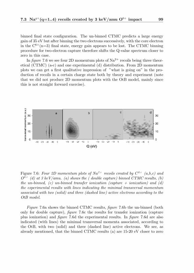
7.3 Naq+(q=1..4) recoils created by 3 keV/amu O6+ impact 99
binned …nal state con…guration. The un-binned CTMC predicts a large energygain of 35 eV but after binning the two electrons successively, with the core electronin the C6+(n=3) …nal state, energy gain appears to be lost. The CTMC binningprocedure for two-electron capture therefore shifts the Q-value spectrum closer tozero in this case.
In …gure 7.6 we see four 2D momentum plots of Na2+ recoils being three theor-etical (CTMC) (a-c) and one experimental (d) distribution. From 2D momentumplots we can get a …rst qualitative impression of ”what is going on” in the pro-duction of recoils in a certain charge state both by theory and experiment (notethat we did not produce 2D momentum plots with the OtB model, mainly sincethis is not straight forward exercise).
Figure 7.6: Four 2D momentum plots of Na2+ recoils created by C 6+ (a,b,c) andO6+ (d) at 3 keV/amu. (a) shows the ( double capture) binned CTMC results, (b)the un-binned, (c) un-binned transfer ionization (capture + ionization) and (d)the experimental results with lines indicating the minimal transversal momentumassociated with two (solid) and three (dashed line) active electrons according to theOtB model.
Figure 7.6a shows the binned CTMC results, …gure 7.6b the un-binned (bothonly for double capture), …gure 7.6c the results for transfer ionization (captureplus ionization) and …gure 7.6d the experimental results. In …gure 7.6d are alsoindicated (with lines) the minimal transversal momenta associated, according tothe OtB, with two (solid) and three (dashed line) active electrons. We see, asalready mentioned, that the binned CTMC results (a) are 15-20 eV closer to zero
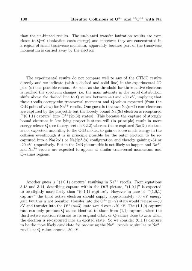
100 Results: Collisions of O6+ and 13C6+ with Na
than the un-binned results. The un-binned transfer ionization results are evencloser to Q=0 (ionization costs energy) and moreover they are concentrated ina region of small transverse momenta, apparently because part of the transversemomentum is carried away by the electron.
The experimental results do not compare well to any of the CTMC resultsdirectly and we indicate (with a dashed and solid line) in the experimental 2Dplot (d) one possible reason. As soon as the threshold for three active electronsis reached the spectrum changes, i.e. the main intensity in the recoil distributionshifts above the dashed line to Q values between -40 and -30 eV, implying thatthese recoils occupy the transversal momenta and Q-values expected (from theOtB point of view) for Na3+ recoils. One guess is that two Na(n=2) core electronsare captured by the projectile but the loosely bound Na(3s) electron is recaptured(”(0,1,1) capture” into O4+(2p,3l) states). This because the capture of stronglybound electrons in low lying projectile states will (in principle) result in moreenergy release Q (see theory, section 3.2.2) whereas the re-captured Na(3s) electronis not expected, according to the OtB model, to gain or loose much energy in thecollision eventhough it is in principle possible for the outer electron to be re-captured into a Na(2p5) or Na(2p4,3s) con…guration and thereby gaining -34 or-20 eV respectively. But in the OtB picture this is not likely to happen and Na2+
and Na3+ recoils are expected to appear at similar transversal momentum andQ-values regions.
Another guess is ”(1,0,1) capture” resulting in Na2+ recoils. From equations3.13 and 3.14, describing capture within the OtB picture, ”(1,0,1)” is expectedto be slightly more likely than ”(0,1,1) capture”. However in case of ”(1,0,1)capture” the third active electron should supply approximately -30 eV energygain but this is not possible: transfer into the O6+(n=2) state would release »-50eV and transfer into the O6+(n=3) state would cost »20 eV. The (1,1,0) capturecase can only produce Q-values identical to those from (1,1) capture, when thethird active electron returnes to its original orbit, or Q-values close to zero whenthe electron is re-captured into an excited state. So we consider (0,1,1) captureto be the most likely candidate for producing the Na2+ recoils so similar to Na3+
recoils at Q values around -30 eV.
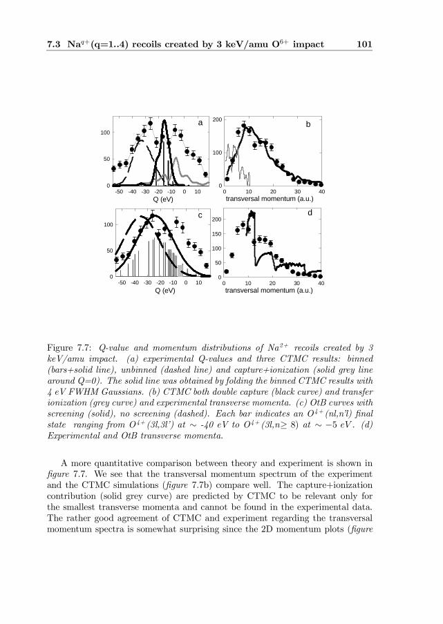
7.3 Naq+(q=1..4) recoils created by 3 keV/amu O6+ impact 101
Q (eV)-50 -40 -30 -20 -10 0 10
0
50
100
transversal momentum (a.u.)0 10 20 30 40
0
100
200
Q (eV)-50 -40 -30 -20 -10 0 10
0
50
100
transversal momentum (a.u.)0 10 20 30 40
0
50
100
150
200
a b
c d
Figure 7.7: Q-value and momentum distributions of Na2+ recoils created by 3keV/amu impact. (a) experimental Q-values and three CTMC results: binned(bars+solid line), unbinned (dashed line) and capture+ionization (solid grey linearound Q=0). The solid line was obtained by folding the binned CTMC results with4 eV FWHM Gaussians. (b) CTMC both double capture (black curve) and transferionization (grey curve) and experimental transverse momenta. (c) OtB curves withscreening (solid), no screening (dashed). Each bar indicates an O4+ (nl,n’l) …nalstate ranging from O4+ (3l,3l’) at » -40 eV to O4+ (3l,n¸ 8) at » ¡5 eV . (d)Experimental and OtB transverse momenta.
A more quantitative comparison between theory and experiment is shown in…gure 7.7. We see that the transversal momentum spectrum of the experimentand the CTMC simulations (…gure 7.7b) compare well. The capture+ionizationcontribution (solid grey curve) are predicted by CTMC to be relevant only forthe smallest transverse momenta and cannot be found in the experimental data.The rather good agreement of CTMC and experiment regarding the transversalmomentum spectra is somewhat surprising since the 2D momentum plots (…gure
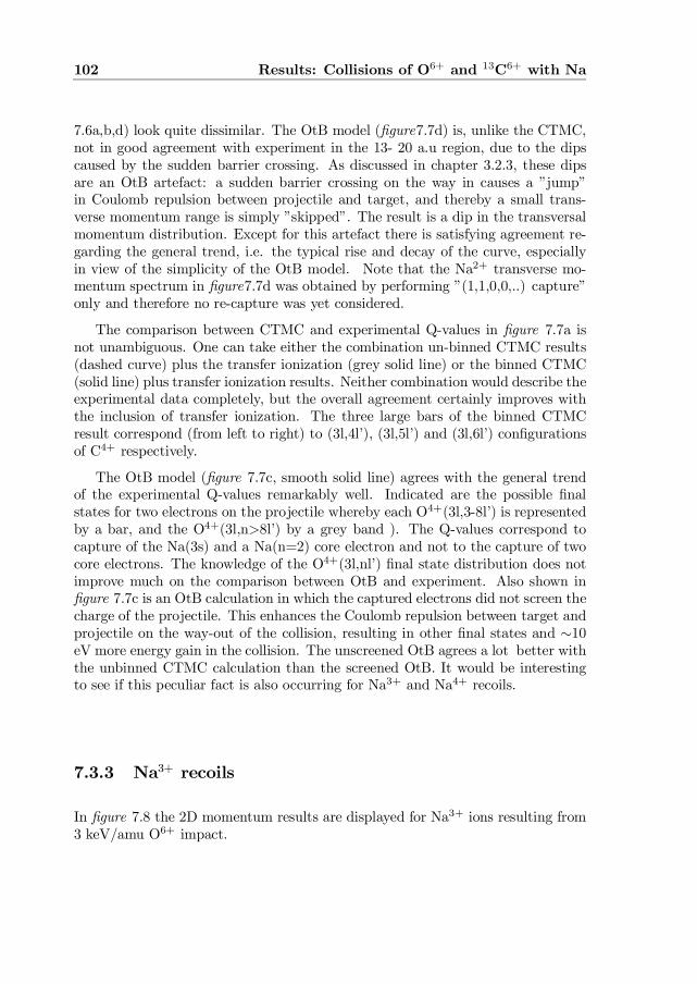
102 Results: Collisions of O6+ and 13C6+ with Na
7.6a,b,d) look quite dissimilar. The OtB model (…gure7.7d) is, unlike the CTMC,not in good agreement with experiment in the 13- 20 a.u region, due to the dipscaused by the sudden barrier crossing. As discussed in chapter 3.2.3, these dipsare an OtB artefact: a sudden barrier crossing on the way in causes a ”jump”in Coulomb repulsion between projectile and target, and thereby a small trans-verse momentum range is simply ”skipped”. The result is a dip in the transversalmomentum distribution. Except for this artefact there is satisfying agreement re-garding the general trend, i.e. the typical rise and decay of the curve, especiallyin view of the simplicity of the OtB model. Note that the Na2+ transverse mo-mentum spectrum in …gure7.7d was obtained by performing ”(1,1,0,0,..) capture”only and therefore no re-capture was yet considered.
The comparison between CTMC and experimental Q-values in …gure 7.7a isnot unambiguous. One can take either the combination un-binned CTMC results(dashed curve) plus the transfer ionization (grey solid line) or the binned CTMC(solid line) plus transfer ionization results. Neither combination would describe theexperimental data completely, but the overall agreement certainly improves withthe inclusion of transfer ionization. The three large bars of the binned CTMCresult correspond (from left to right) to (3l,4l’), (3l,5l’) and (3l,6l’) con…gurationsof C4+ respectively.
The OtB model (…gure 7.7c, smooth solid line) agrees with the general trendof the experimental Q-values remarkably well. Indicated are the possible …nalstates for two electrons on the projectile whereby each O4+(3l,3-8l’) is representedby a bar, and the O4+(3l,n>8l’) by a grey band ). The Q-values correspond tocapture of the Na(3s) and a Na(n=2) core electron and not to the capture of twocore electrons. The knowledge of the O4+(3l,nl’) …nal state distribution does notimprove much on the comparison between OtB and experiment. Also shown in…gure 7.7c is an OtB calculation in which the captured electrons did not screen thecharge of the projectile. This enhances the Coulomb repulsion between target andprojectile on the way-out of the collision, resulting in other …nal states and »10eV more energy gain in the collision. The unscreened OtB agrees a lot better withthe unbinned CTMC calculation than the screened OtB. It would be interestingto see if this peculiar fact is also occurring for Na3+ and Na4+ recoils.
7.3.3 Na3+ recoils
In …gure 7.8 the 2D momentum results are displayed for Na3+ ions resulting from3 keV/amu O6+ impact.
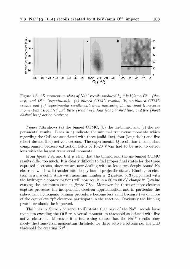
7.3 Naq+(q=1..4) recoils created by 3 keV/amu O6+ impact 103
Figure 7.8: 2D momentum plots of Na3+ recoils produced by 3 keV/amu C 6+ (the-ory) and O6+ (experiment). (a) binned CTMC results, (b) un-binned CTMCresults and (c) experimental results with lines indicating the minimal transversemomentum associated with three (solid line), four (long dashed line) and …ve (shortdashed line) active electrons
Figure 7.8a shows (a) the binned CTMC, (b) the un-binned and (c) the ex-perimental results. Lines in c) indicate the minimal transverse momenta whichregarding the OtB are associated with three (solid line), four (long dash) and …ve(short dashed line) active electrons. The experimental Q resolution is somewhatcompromised because extraction …elds of 10-20 V/cm had to be used to detections with the largest transversal momenta.
From …gure 7.8a and b it is clear that the binned and the un-binned CTMCresults di¤er too much. It is clearly di¢cult to …nd proper …nal states for the threecaptured electrons, since we are now dealing with at least two deeply bound Naelectrons which will transfer into deeply bound projectile states. Binning an elec-tron in a projectile state with quantum number n=2 instead of 3 (calculated withthe hydrogenic approximation) will now result in a 50 to 80 eV change in Q-valuecausing the structures seen in …gure 7.8a. Moreover for three or more-electroncapture processes the independent electron approximation and in particular thesubsequent hydrogenic binning procedure become less valid because two or moreof the equivalent 2p6 electrons participate in the reaction. Obviously the binningprocedure should be improved.
The lines in …gure 7.8c serve to illustrate that part of the Na3+ recoils havemomenta exceding the OtB transversal momentum threshold associated with …veactive electrons. Moreover it is interesting to see that the Na3+ recoils obeynicely the transversal momentum threshold for three active electrons i.e. the OtBthreshold for creating Na3+.
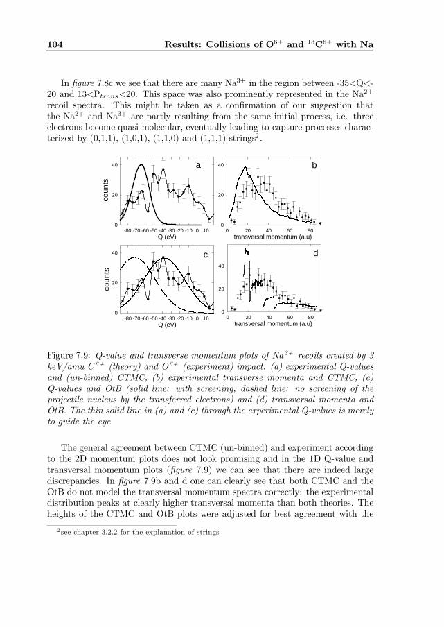
104 Results: Collisions of O6+ and 13C6+ with Na
In …gure 7.8c we see that there are many Na3+ in the region between -35<Q<-20 and 13<Ptrans<20. This space was also prominently represented in the Na2+
recoil spectra. This might be taken as a con…rmation of our suggestion thatthe Na2+ and Na3+ are partly resulting from the same initial process, i.e. threeelectrons become quasi-molecular, eventually leading to capture processes charac-terized by (0,1,1), (1,0,1), (1,1,0) and (1,1,1) strings2 .
transversal momentum (a.u)0 20 40 60 80
0
20
40
Q (eV)-80 -70 -60 -50 -40 -30 -20 -10 0 10
coun
ts
0
20
40
transversal momentum (a.u)0 20 40 60 80
0
20
40
Q (eV)-80 -70 -60 -50 -40 -30 -20 -10 0 10
coun
ts
0
20
40 a
c d
b
Figure 7.9: Q-value and transverse momentum plots of Na3+ recoils created by 3keV/amu C 6+ (theory) and O6+ (experiment) impact. (a) experimental Q-valuesand (un-binned) CTMC, (b) experimental transverse momenta and CTMC, (c)Q-values and OtB (solid line: with screening, dashed line: no screening of theprojectile nucleus by the transferred electrons) and (d) transversal momenta andOtB. The thin solid line in (a) and (c) through the experimental Q-values is merelyto guide the eye
The general agreement between CTMC (un-binned) and experiment accordingto the 2D momentum plots does not look promising and in the 1D Q-value andtransversal momentum plots (…gure 7.9) we can see that there are indeed largediscrepancies. In …gure 7.9b and d one can clearly see that both CTMC and theOtB do not model the transversal momentum spectra correctly: the experimentaldistribution peaks at clearly higher transversal momenta than both theories. Theheights of the CTMC and OtB plots were adjusted for best agreement with the
2 see chapter 3.2.2 for the explanation of strings
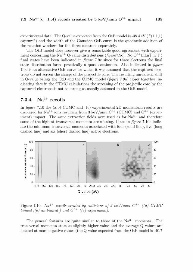
7.3 Naq+(q=1..4) recoils created by 3 keV/amu O6+ impact 105
experimental data. The Q-value expected from the OtB model is -38.4 eV ( ”(1,1,1)capture”) and the width of the Gaussian OtB curve is the quadratic addition ofthe reaction windows for the three electrons separately.
The OtB model does however give a remarkable good agreement with experi-ment concerning the Na3+ Q-value distributions (…gure7.9c). No O3+(nl,n’l’,n”l”)…nal states have been indicated in …gure 7.9c since for three electrons the …nalstate distribution forms practically a quasi continuum. Also indicated in …gure7.9c is an alternative OtB curve for which it was assumed that the captured elec-trons do not screen the charge of the projectile core. The resulting unrealistic shiftin Q-value brings the OtB and the CTMC model (…gure 7.9a) closer together, in-dicating that in the CTMC calculations the screening of the projectile core by thecaptured electrons is not as strong as usually assumed in the OtB model.
7.3.4 Na4+ recoilsIn …gure 7.10 the (a,b) CTMC and (c) experimental 2D momentum results aredisplayed for Na4+ ions resulting from 3 keV/amu C6+ (CTMC) and O6+ (exper-iment) impact. The same extraction …elds were used as for Na3+ and thereforesome of the highest transversal momenta are missing. Lines in …gure 7.10c indic-ate the minimum transversal momenta associated with four (solid line), …ve (longdashed line) and six (short dashed line) active electrons.
Figure 7.10: Na4+ recoils created by collisions of 3 keV/amu C 6+ ((a) CTMCbinned ,(b) un-binned ) and O6+ ((c) experiment).
The general features are quite similar to those of the Na3+ momenta. Thetransversal momenta start at slightly higher value and the average Q values arelocated at more negative values (the Q-value expected from the OtB model is -40.7

106 Results: Collisions of O6+ and 13C6+ with Na
eV for ”(1,1,1,1) capture”). Again we see that the binned CTMC results do notagree with the un-binned results and the experimental data.
When comparing theory and experiment for the projected distributions of Q-value and transversal momentum (…gure 7.11) it is quite a surprise to see a rathergood agreement, with the exception of …gure 7.11a . The experimental and CTMCtransversal momenta (…gure 7.11b) agree quite well. It may be somewhat acci-dental (we know that some of the highest momenta are missing) but CTMC andexperiment also agree on the rising slope and this was not the case for the Na3+
transversal momenta.
Q(eV)-100 -80 -60 -40 -20 0
0
20
40
transversal momentum (a.u.)0 20 40 60 80
0
20
Q(eV)-100 -80 -60 -40 -20 0
0
20
40
transversal momentum (a.u.)0 20 40 60 80
0
20
40
a
dc
b
Figure 7.11: Na4+ recoils created by collisions of 3 keV/amu C 6+ (theory) andO6+ (experiment). (a) experimental Q-values and CTMC (un-binned), (b) trans-versal momenta and CTMC, (c) q-values and OtB and (b) transversal momentaand OtB
Much like in the Na3+ case, the OtB model predicts the Q-value distributionquite well (…gure 7.11c, solid curve) slightly underestimating the average Q-value.CTMC (…gure 7.11a) predicts more negative Q-values, just like in the Na2+ andNa3+ case. Also, as already noticed for Na3+ and Na2+, we see that the ”un-screened OtB curve ” (…gure 7.11c dashed line) corresponds quite closely to theQ-values predicted by the un-binned CTMC.
7.3 Naq+(q=1..4) recoils created by 3 keV/amu O6+ impact 107
7.3.5 Summary of 3 keV/amu O6+ - Na collisions
In this section we presented experimental and theoretical results obtained for Naq+
(q=1-4) recoils created by O6+ (experiment) and C6+ (theory) impact. The agree-ment between theory and experiment is satisfying regarding the general trends:although the Naq+ (q=1-4) recoil momenta span two orders of magnitude andall theoretical and experimental results are ”new”, theory and experiment usuallyagree regarding the range and shape of the Naq+ momentum distributions.
As an interesting result we saw that it is possible for a theory to agree wellwith experiment with respect to one momentum distribution (either transversal orlongitudinal) and to disagree (sometimes completely) with respect to the other mo-mentum distribution. For example: the binned CTMC Q-values for Na4+ (…gure7.10a) look nothing like the experimental results (…gure 7.10c) but the transversaldistributions (…gure 7.11b) are very similar indeed.
Another interesting result is the fact that the OtB concept of active electronsseems to be con…rmed by the experimental results. All Naq+ (q=1-4) recoilsexhibit the minimum transversal momentum thresholds predicted to create theNaq+ (q=1-4) recoils. Moreover we see here that for multiple electron capturethe transverse momentum distributions of the Naq+(q=2-4) recoils exceed thetransversal momentum thresholds for more active electrons than actually captured.For instance, the Na2+ recoil momentum distributions extend into a range whereNa3+ recoils could have been produced according to the OtB model, and theNa3+ momentum plots contain recoils which were allowed to be Na4+ recoils. Inthe Na2+ momentum distribution this is most obvious: a signi…cant amount ofrecoils begins exactly at the minimum transverse momentum threshold for threeactive electrons and they have Q-values typical of Na3+ recoils. The most likelyexplanation for this is that the ”(0,1,1) capture channel ” is responsible for theseNa2+ recoils, because with (0,1,1) capture the experimentally observed Q-valuescan be explained. With (1,0,1) capture combined with the level schemes of O6+andNa3+ it is di¢cult to explain Q-values of around -30 eV (it is possible, but thatwould require a signi…cant amount of target excitation).
The ”mixing of capture channels” is perhaps the reason why it is so di¢cultfor theory (CTMC and OtB) to model the Na3+ momenta. First of all the (0,1,1)capture channel ”draws ‡ux” from the Na3+ channel while the Na3+ capturechannel ”draws” in a similar manner from the Na4+ channel.
Such a scenario was already hinted at from the recoil charge state spectra in…gure 7.1 and 7.2. Since we did not observe any Na5+ recoils experimentally, wesuspect that the Na5+ production channels might be completely depleted by theNa3+ and Na4+ channels.
108 Results: Collisions of O6+ and 13C6+ with Na
7.4 Naq+(q=2..4) recoils created by 4.5, 3 and 1.5keV/amu O6+ impact
In this section we will compare the momentum spectra of Naq+ (q=1..4) recoilscreated by O6+ impact at collision energies of 4.5, 3 and 1.5 keV/amu correspond-ing to velocities vp of 0.43, 0.35 and 0.25 a.u. respectively. By varying the energy(velocity) of the projectiles we will test two properties of ion-atom collisions. Abasic property is that the longitudinal and transversal momentum spectra shouldchange with varying projectile velocities vp because i) the longitudinal to Q-valueconversion (equation 7.1) depends on vp and ii) the transversal momentum distri-bution is predicted (by all theories) to peak at higher values with decreasing vp:The latter simply because with decreasing vp the ion-atom interaction time be-comes longer and the scattering should become stronger. A second property, whichis not merely kinematics, is that with decreasing projectile velocity vp the reactionwindow (…nal state distribution) is predicted to become narrower i.e. the num-ber of populated …nal states should decrease with decreasing vp (see also chapter3.2.2).
7.4.1 Na2+ recoils
We will compare the Na2+ recoil spectra created by 4.5, 3 and 1.5 keV/u O6+ col-lisions to CTMC and OtB like in the previous section. A disadvantage is howeverthat the quality of the 4.5 and 1.5 keV/amu experimental data is generally not asgood as that of the 3 keV/amu ones. This because the beam pulsing in the formercase was not very e¢cient and pulses were quite long, causing loss of resolution inthe transversal momenta. In case of the latter, beam currents were very low andtherefore count rates of Naq+ (q>1) recoils were also very low (»0.02 Hz). Thiscaused not only statistical problems but also some resolution problems since it isdi¢cult to keep experimental conditions as e.g. the MOT stable over many hours.
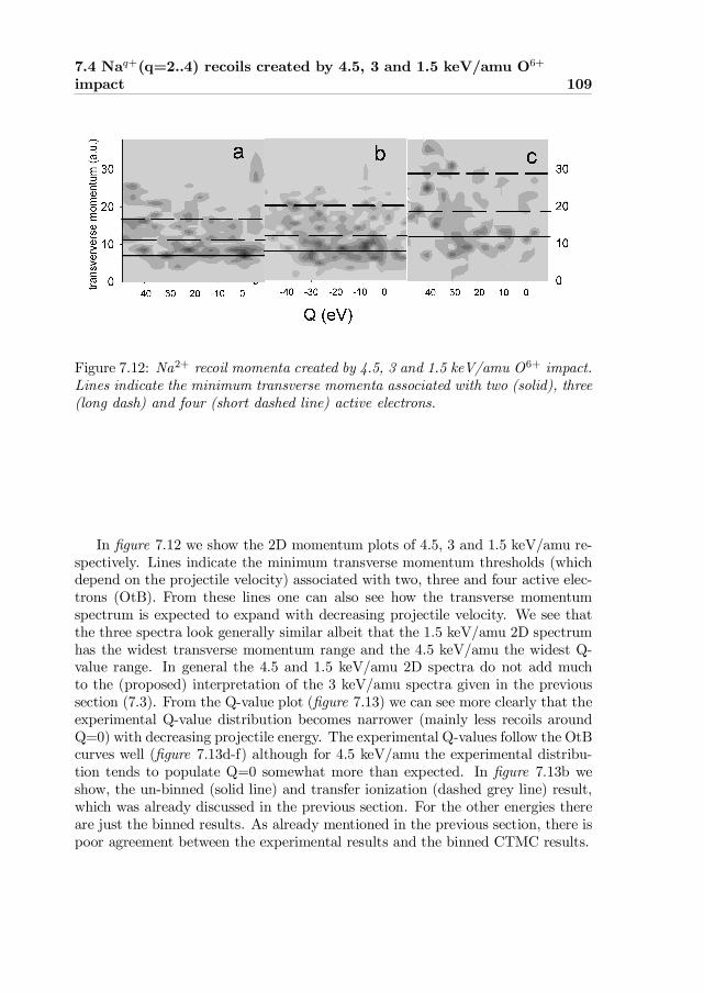
7.4 Naq+(q=2..4) recoils created by 4.5, 3 and 1.5 keV/amu O6+
impact 109
Figure 7.12: Na2+ recoil momenta created by 4.5, 3 and 1.5 keV/amu O6+ impact.Lines indicate the minimum transverse momenta associated with two (solid), three(long dash) and four (short dashed line) active electrons.
In …gure 7.12 we show the 2D momentum plots of 4.5, 3 and 1.5 keV/amu re-spectively. Lines indicate the minimum transverse momentum thresholds (whichdepend on the projectile velocity) associated with two, three and four active elec-trons (OtB). From these lines one can also see how the transverse momentumspectrum is expected to expand with decreasing projectile velocity. We see thatthe three spectra look generally similar albeit that the 1.5 keV/amu 2D spectrumhas the widest transverse momentum range and the 4.5 keV/amu the widest Q-value range. In general the 4.5 and 1.5 keV/amu 2D spectra do not add muchto the (proposed) interpretation of the 3 keV/amu spectra given in the previoussection (7.3). From the Q-value plot (…gure 7.13) we can see more clearly that theexperimental Q-value distribution becomes narrower (mainly less recoils aroundQ=0) with decreasing projectile energy. The experimental Q-values follow the OtBcurves well (…gure 7.13d-f) although for 4.5 keV/amu the experimental distribu-tion tends to populate Q=0 somewhat more than expected. In …gure 7.13b weshow, the un-binned (solid line) and transfer ionization (dashed grey line) result,which was already discussed in the previous section. For the other energies thereare just the binned results. As already mentioned in the previous section, there ispoor agreement between the experimental results and the binned CTMC results.
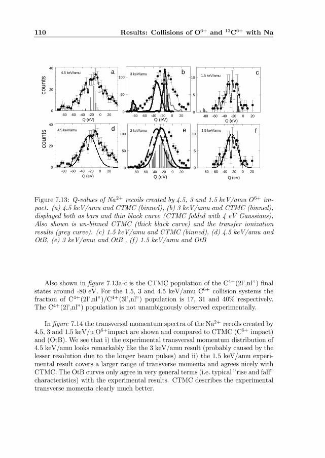
110 Results: Collisions of O6+ and 13C6+ with Na
Q (eV)-80 -60 -40 -20 0 20
0
50
100
Q (eV)-80 -60 -40 -20 0 20
0
50
100
Q (eV)-80 -60 -40 -20 0 20
coun
ts
0
20
40
Q (eV)-80 -60 -40 -20 0 20
0
5
10
Q (eV)-80 -60 -40 -20 0 20
coun
ts
0
20
40
Q (eV)-80 -60 -40 -20 0 20
0
5
10a b c
d e f
4.5 keV/amu1.5 keV/amu3 keV/amu
3 keV/amu4.5 keV/amu 1.5 keV/amu
Figure 7.13: Q-values of Na2+ recoils created by 4.5, 3 and 1.5 keV/amu O6+ im-pact. (a) 4.5 keV/amu and CTMC (binned), (b) 3 keV/amu and CTMC (binned),displayed both as bars and thin black curve (CTMC folded with 4 eV Gaussians),Also shown is un-binned CTMC (thick black curve) and the transfer ionizationresults (grey curve). (c) 1.5 keV/amu and CTMC (binned), (d) 4.5 keV/amu andOtB, (e) 3 keV/amu and OtB , (f) 1.5 keV/amu and OtB
Also shown in …gure 7.13a-c is the CTMC population of the C4+(2l’,nl”) …nalstates around -80 eV. For the 1.5, 3 and 4.5 keV/amu C6+ collision systems thefraction of C4+(2l’,nl”)/C4+(3l’,nl”) population is 17, 31 and 40% respectively.The C4+(2l’,nl”) population is not unambiguously observed experimentally.
In …gure 7.14 the transversal momentum spectra of the Na2+ recoils created by4.5, 3 and 1.5 keV/u O6+impact are shown and compared to CTMC (C6+ impact)and (OtB). We see that i) the experimental transversal momentum distribution of4.5 keV/amu looks remarkably like the 3 keV/amu result (probably caused by thelesser resolution due to the longer beam pulses) and ii) the 1.5 keV/amu experi-mental result covers a larger range of transverse momenta and agrees nicely withCTMC. The OtB curves only agree in very general terms (i.e. typical ”rise and fall”characteristics) with the experimental results. CTMC describes the experimentaltransverse momenta clearly much better.
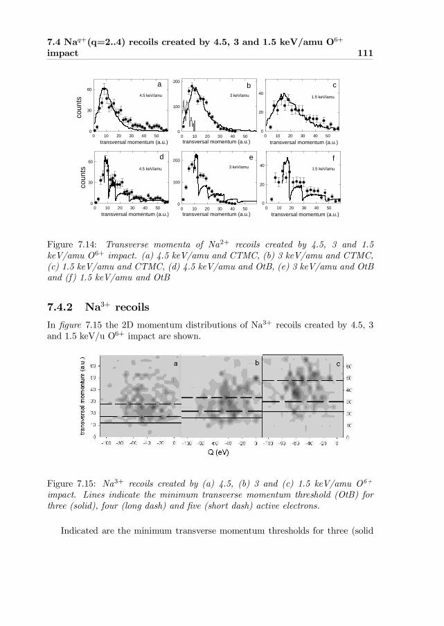
7.4 Naq+(q=2..4) recoils created by 4.5, 3 and 1.5 keV/amu O6+
impact 111
transversal momentum (a.u.)0 10 20 30 40 50
0
100
200
transversal momentum (a.u.)0 10 20 30 40 50
0
100
200
transversal momentum (a.u.)0 10 20 30 40 50
coun
ts
0
30
60
transversal momentum (a.u.)0 10 20 30 40 50
0
20
40
transversal momentum (a.u.)0 10 20 30 40 50
coun
ts
0
30
60
transversal momentum (a.u.)0 10 20 30 40 50
0
20
40
a b c
d e f
4.5 keV/amu 1.5 keV/amu3 keV/amu
3 keV/amu4.5 keV/amu 1.5 keV/amu
Figure 7.14: Transverse momenta of Na2+ recoils created by 4.5, 3 and 1.5keV/amu O6+ impact. (a) 4.5 keV/amu and CTMC, (b) 3 keV/amu and CTMC,(c) 1.5 keV/amu and CTMC, (d) 4.5 keV/amu and OtB, (e) 3 keV/amu and OtBand (f) 1.5 keV/amu and OtB
7.4.2 Na3+ recoilsIn …gure 7.15 the 2D momentum distributions of Na3+ recoils created by 4.5, 3and 1.5 keV/u O6+ impact are shown.
Figure 7.15: Na3+ recoils created by (a) 4.5, (b) 3 and (c) 1.5 keV/amu O6+
impact. Lines indicate the minimum transverse momentum threshold (OtB) forthree (solid), four (long dash) and …ve (short dash) active electrons.
Indicated are the minimum transverse momentum thresholds for three (solid
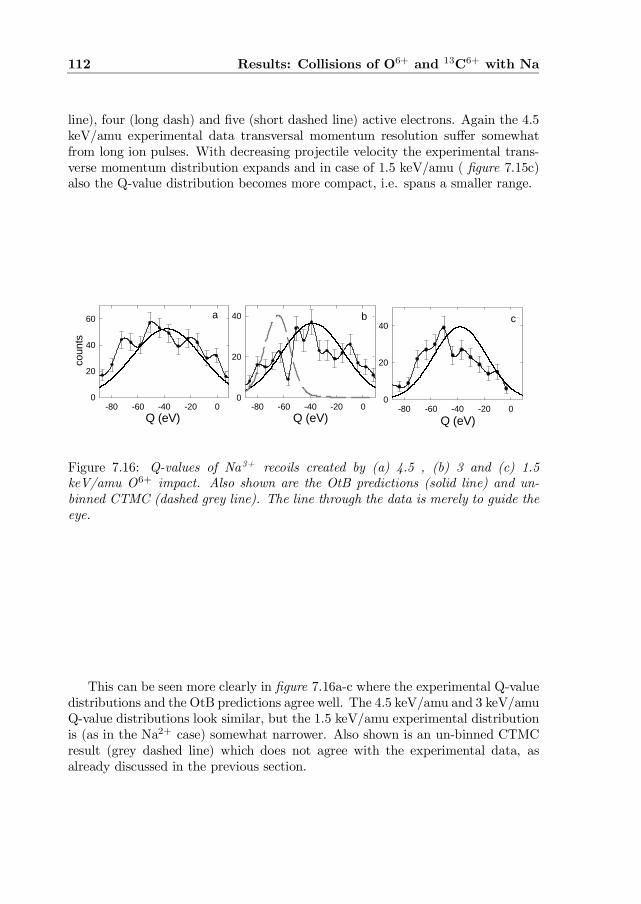
112 Results: Collisions of O6+ and 13C6+ with Na
line), four (long dash) and …ve (short dashed line) active electrons. Again the 4.5keV/amu experimental data transversal momentum resolution su¤er somewhatfrom long ion pulses. With decreasing projectile velocity the experimental trans-verse momentum distribution expands and in case of 1.5 keV/amu ( …gure 7.15c)also the Q-value distribution becomes more compact, i.e. spans a smaller range.
Q (eV)-80 -60 -40 -20 0
0
20
40
Q (eV)-80 -60 -40 -20 0
coun
ts
0
20
40
60
Q (eV)-80 -60 -40 -20 0
0
20
40a b c
Figure 7.16: Q-values of Na3+ recoils created by (a) 4.5 , (b) 3 and (c) 1.5keV/amu O6+ impact. Also shown are the OtB predictions (solid line) and un-binned CTMC (dashed grey line). The line through the data is merely to guide theeye.
This can be seen more clearly in …gure 7.16a-c where the experimental Q-valuedistributions and the OtB predictions agree well. The 4.5 keV/amu and 3 keV/amuQ-value distributions look similar, but the 1.5 keV/amu experimental distributionis (as in the Na2+ case) somewhat narrower. Also shown is an un-binned CTMCresult (grey dashed line) which does not agree with the experimental data, asalready discussed in the previous section.
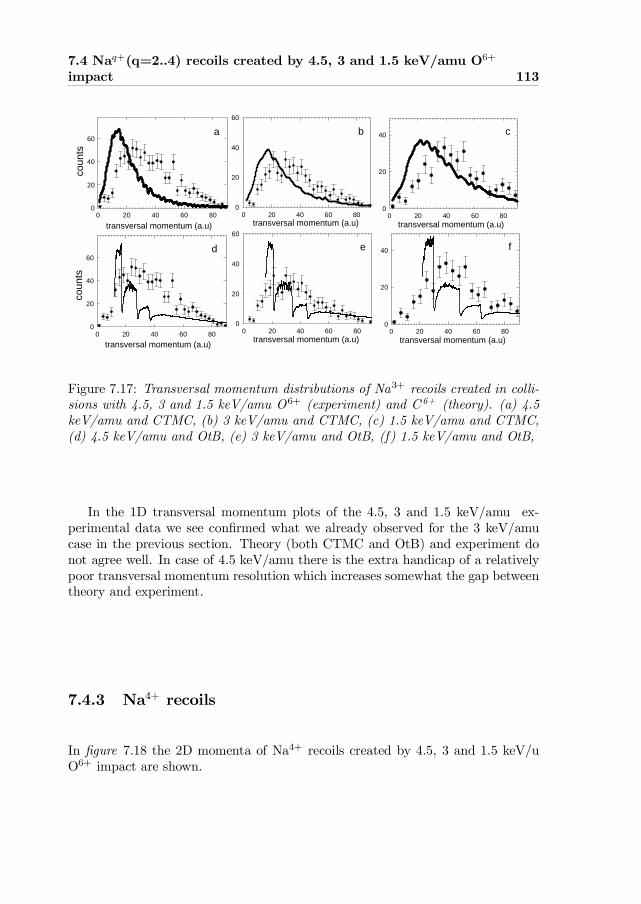
7.4 Naq+(q=2..4) recoils created by 4.5, 3 and 1.5 keV/amu O6+
impact 113
transversal momentum (a.u)0 20 40 60 80
coun
ts
0
20
40
60
transversal momentum (a.u)0 20 40 60 80
0
20
40
60
transversal momentum (a.u)0 20 40 60 80
0
20
40
transversal momentum (a.u)0 20 40 60 80
coun
ts
0
20
40
60
transversal momentum (a.u)0 20 40 60 80
0
20
40
60
transversal momentum (a.u)0 20 40 60 80
0
20
40
ba
d e f
c
Figure 7.17: Transversal momentum distributions of Na3+ recoils created in colli-sions with 4.5, 3 and 1.5 keV/amu O6+ (experiment) and C 6+ (theory). (a) 4.5keV/amu and CTMC, (b) 3 keV/amu and CTMC, (c) 1.5 keV/amu and CTMC,(d) 4.5 keV/amu and OtB, (e) 3 keV/amu and OtB, (f) 1.5 keV/amu and OtB,
In the 1D transversal momentum plots of the 4.5, 3 and 1.5 keV/amu ex-perimental data we see con…rmed what we already observed for the 3 keV/amucase in the previous section. Theory (both CTMC and OtB) and experiment donot agree well. In case of 4.5 keV/amu there is the extra handicap of a relativelypoor transversal momentum resolution which increases somewhat the gap betweentheory and experiment.
7.4.3 Na4+ recoils
In …gure 7.18 the 2D momenta of Na4+ recoils created by 4.5, 3 and 1.5 keV/uO6+ impact are shown.
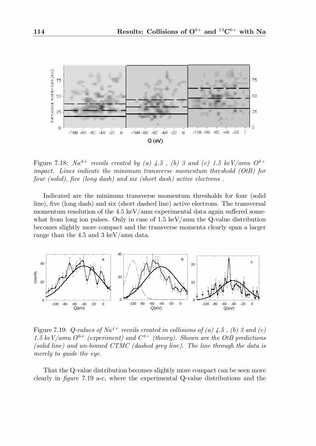
114 Results: Collisions of O6+ and 13C6+ with Na
Figure 7.18: Na4+ recoils created by (a) 4.5 , (b) 3 and (c) 1.5 keV/amu O6+
impact. Lines indicate the minimum transverse momentum threshold (OtB) forfour (solid), …ve (long dash) and six (short dash) active electrons .
Indicated are the minimum transverse momentum thresholds for four (solidline), …ve (long dash) and six (short dashed line) active electrons. The transversalmomentum resolution of the 4.5 keV/amu experimental data again su¤ered some-what from long ion pulses. Only in case of 1.5 keV/amu the Q-value distributionbecomes slightly more compact and the transverse momenta clearly span a largerrange than the 4.5 and 3 keV/amu data.
Q(eV)-100 -80 -60 -40 -20 0
coun
ts
0
20
40
Q(eV)-100 -80 -60 -40 -20 0
0
20
40
Q(eV)-100 -80 -60 -40 -20 0
0
10
20a b
c
Figure 7.19: Q-values of Na4+ recoils created in collisions of (a) 4.5 , (b) 3 and (c)1.5 keV/amu O6+ (experiment) and C 6+ (theory). Shown are the OtB predictions(solid line) and un-binned CTMC (dashed grey line). The line through the data ismerely to guide the eye.
That the Q-value distribution becomes slightly more compact can be seen moreclearly in …gure 7.19 a-c, where the experimental Q-value distributions and the
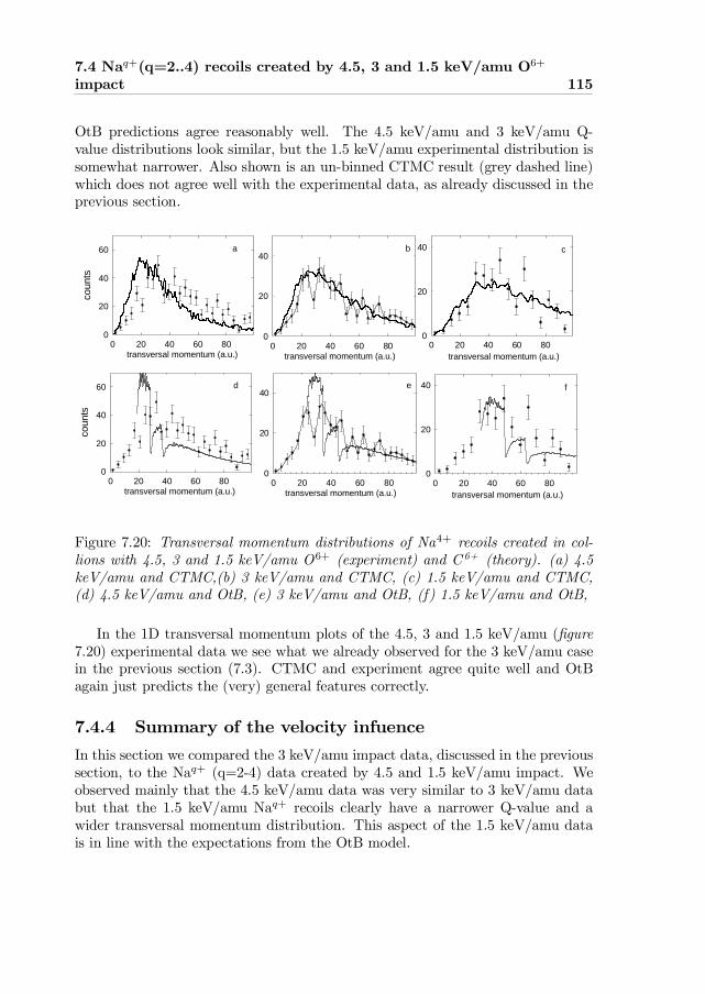
7.4 Naq+(q=2..4) recoils created by 4.5, 3 and 1.5 keV/amu O6+
impact 115
OtB predictions agree reasonably well. The 4.5 keV/amu and 3 keV/amu Q-value distributions look similar, but the 1.5 keV/amu experimental distribution issomewhat narrower. Also shown is an un-binned CTMC result (grey dashed line)which does not agree well with the experimental data, as already discussed in theprevious section.
transversal momentum (a.u.)0 20 40 60 80
coun
ts
0
20
40
60
Col 40 vs total
Col 217
transversal momentum (a.u.)0 20 40 60 80
0
20
40
transversal momentum (a.u.)0 20 40 60 80
0
20
40
transversal momentum (a.u.)0 20 40 60 80
coun
ts
0
20
40
60
transversal momentum (a.u.)0 20 40 60 80
0
20
40
transversal momentum (a.u.)0 20 40 60 80
0
20
40
a b c
d e f
Figure 7.20: Transversal momentum distributions of Na4+ recoils created in col-lions with 4.5, 3 and 1.5 keV/amu O6+ (experiment) and C 6+ (theory). (a) 4.5keV/amu and CTMC,(b) 3 keV/amu and CTMC, (c) 1.5 keV/amu and CTMC,(d) 4.5 keV/amu and OtB, (e) 3 keV/amu and OtB, (f) 1.5 keV/amu and OtB,
In the 1D transversal momentum plots of the 4.5, 3 and 1.5 keV/amu (…gure7.20) experimental data we see what we already observed for the 3 keV/amu casein the previous section (7.3). CTMC and experiment agree quite well and OtBagain just predicts the (very) general features correctly.
7.4.4 Summary of the velocity infuenceIn this section we compared the 3 keV/amu impact data, discussed in the previoussection, to the Naq+ (q=2-4) data created by 4.5 and 1.5 keV/amu impact. Weobserved mainly that the 4.5 keV/amu data was very similar to 3 keV/amu databut that the 1.5 keV/amu Naq+ recoils clearly have a narrower Q-value and awider transversal momentum distribution. This aspect of the 1.5 keV/amu datais in line with the expectations from the OtB model.
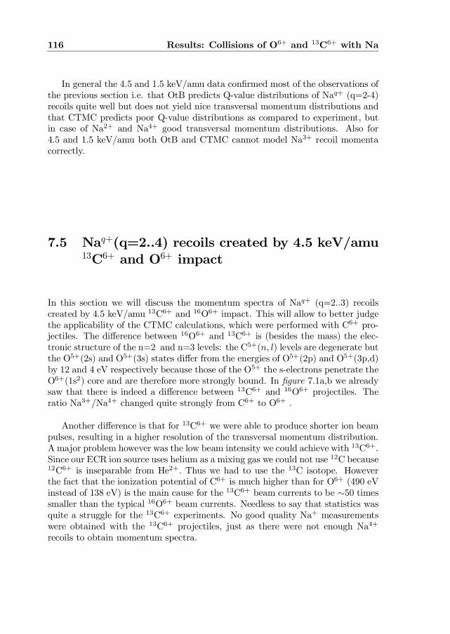
116 Results: Collisions of O6+ and 13C6+ with Na
In general the 4.5 and 1.5 keV/amu data con…rmed most of the observations ofthe previous section i.e. that OtB predicts Q-value distributions of Naq+ (q=2-4)recoils quite well but does not yield nice transversal momentum distributions andthat CTMC predicts poor Q-value distributions as compared to experiment, butin case of Na2+ and Na4+ good transversal momentum distributions. Also for4.5 and 1.5 keV/amu both OtB and CTMC cannot model Na3+ recoil momentacorrectly.
7.5 Naq+(q=2..4) recoils created by 4.5 keV/amu13C6+ and O6+ impact
In this section we will discuss the momentum spectra of Naq+ (q=2..3) recoilscreated by 4.5 keV/amu 13C6+ and 16O6+ impact. This will allow to better judgethe applicability of the CTMC calculations, which were performed with C6+ pro-jectiles. The di¤erence between 16O6+ and 13C6+ is (besides the mass) the elec-tronic structure of the n=2 and n=3 levels: the C5+(n; l) levels are degenerate butthe O5+(2s) and O5+(3s) states di¤er from the energies of O5+(2p) and O5+(3p,d)by 12 and 4 eV respectively because those of the O5+ the s-electrons penetrate theO6+(1s2) core and are therefore more strongly bound. In …gure 7.1a,b we alreadysaw that there is indeed a di¤erence between 13C6+ and 16O6+ projectiles. Theratio Na3+/Na4+ changed quite strongly from C6+ to O6+ .
Another di¤erence is that for 13C6+ we were able to produce shorter ion beampulses, resulting in a higher resolution of the transversal momentum distribution.A major problem however was the low beam intensity we could achieve with 13C6+.Since our ECR ion source uses helium as a mixing gas we could not use 12C because12C6+ is inseparable from He2+: Thus we had to use the 13C isotope. Howeverthe fact that the ionization potential of C6+ is much higher than for O6+ (490 eVinstead of 138 eV) is the main cause for the 13C6+ beam currents to be »50 timessmaller than the typical 16O6+ beam currents. Needless to say that statistics wasquite a struggle for the 13C6+ experiments. No good quality Na+ measurementswere obtained with the 13C6+ projectiles, just as there were not enough Na4+
recoils to obtain momentum spectra.
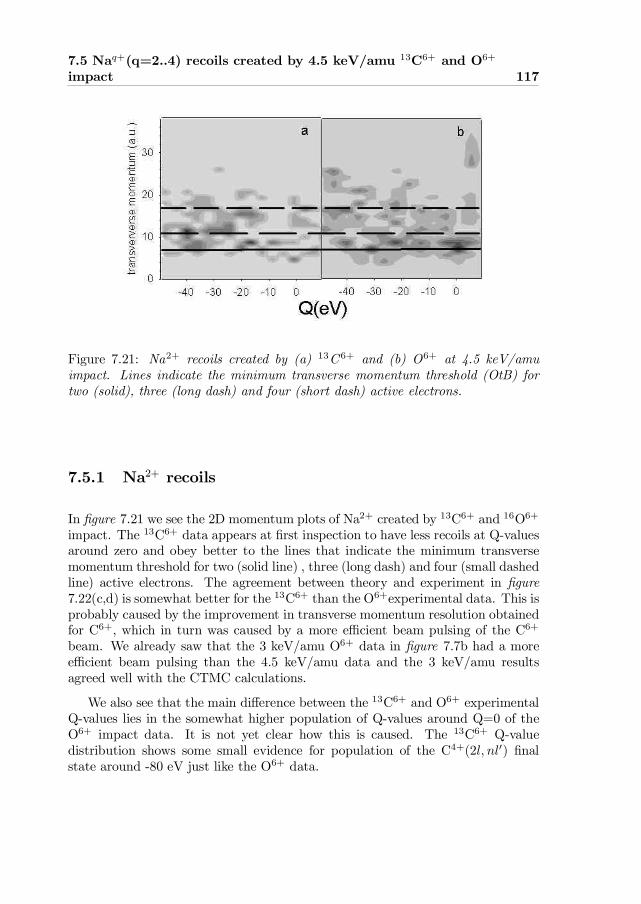
7.5 Naq+(q=2..4) recoils created by 4.5 keV/amu 13C6+ and O6+
impact 117
Figure 7.21: Na2+ recoils created by (a) 13C 6+ and (b) O6+ at 4.5 keV/amuimpact. Lines indicate the minimum transverse momentum threshold (OtB) fortwo (solid), three (long dash) and four (short dash) active electrons.
7.5.1 Na2+ recoils
In …gure 7.21 we see the 2D momentum plots of Na2+ created by 13C6+ and 16O6+
impact. The 13C6+ data appears at …rst inspection to have less recoils at Q-valuesaround zero and obey better to the lines that indicate the minimum transversemomentum threshold for two (solid line) , three (long dash) and four (small dashedline) active electrons. The agreement between theory and experiment in …gure7.22(c,d) is somewhat better for the 13C6+ than the O6+experimental data. This isprobably caused by the improvement in transverse momentum resolution obtainedfor C6+; which in turn was caused by a more e¢cient beam pulsing of the C6+
beam. We already saw that the 3 keV/amu O6+ data in …gure 7.7b had a moree¢cient beam pulsing than the 4.5 keV/amu data and the 3 keV/amu resultsagreed well with the CTMC calculations.
We also see that the main di¤erence between the 13C6+ and O6+ experimentalQ-values lies in the somewhat higher population of Q-values around Q=0 of theO6+ impact data. It is not yet clear how this is caused. The 13C6+ Q-valuedistribution shows some small evidence for population of the C4+(2l; nl0) …nalstate around -80 eV just like the O6+ data.
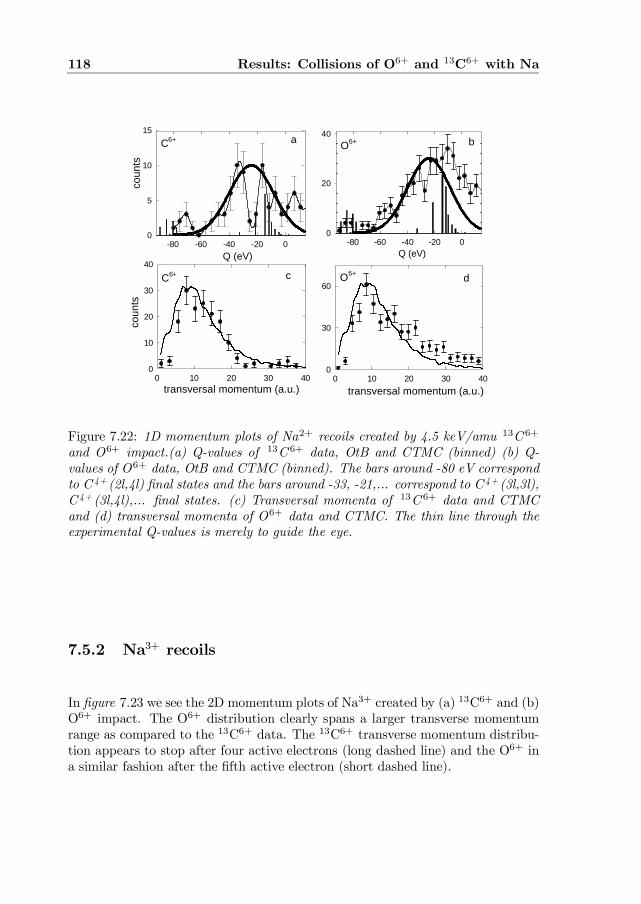
118 Results: Collisions of O6+ and 13C6+ with Na
transversal momentum (a.u.)0 10 20 30 40
0
30
60
transversal momentum (a.u.)0 10 20 30 40
coun
ts
0
10
20
30
40Q (eV)
-80 -60 -40 -20 0
coun
ts
0
5
10
15
Q (eV)-80 -60 -40 -20 0
0
20
40a b
c d
C6+O6+
O6+C6+
Figure 7.22: 1D momentum plots of Na2+ recoils created by 4.5 keV/amu 13C 6+
and O6+ impact.(a) Q-values of 13C 6+ data, OtB and CTMC (binned) (b) Q-values of O6+ data, OtB and CTMC (binned). The bars around -80 eV correspondto C 4+ (2l,4l) …nal states and the bars around -33, -21,... correspond to C 4+ (3l,3l),C 4+ (3l,4l),... …nal states. (c) Transversal momenta of 13C 6+ data and CTMCand (d) transversal momenta of O6+ data and CTMC. The thin line through theexperimental Q-values is merely to guide the eye.
7.5.2 Na3+ recoils
In …gure 7.23 we see the 2D momentum plots of Na3+ created by (a) 13C6+ and (b)O6+ impact. The O6+ distribution clearly spans a larger transverse momentumrange as compared to the 13C6+ data. The 13C6+ transverse momentum distribu-tion appears to stop after four active electrons (long dashed line) and the O6+ ina similar fashion after the …fth active electron (short dashed line).
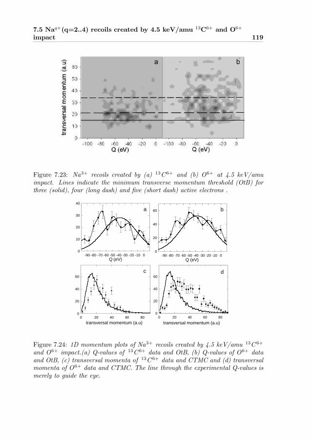
7.5 Naq+(q=2..4) recoils created by 4.5 keV/amu 13C6+ and O6+
impact 119
Figure 7.23: Na3+ recoils created by (a) 13C 6+ and (b) O6+ at 4.5 keV/amuimpact. Lines indicate the minimum transverse momentum threshold (OtB) forthree (solid), four (long dash) and …ve (short dash) active electrons .
transversal momentum (a.u)0 20 40 60 80
0
20
40
60
Q (eV)-90 -80 -70 -60 -50 -40 -30 -20 -10 0
0
10
20
30
40
transversal momentum (a.u)0 20 40 60 80
0
20
40
60
Q (eV)-90 -80 -70 -60 -50 -40 -30 -20 -10 0
0
20
40
60a b
c d
Figure 7.24: 1D momentum plots of Na3+ recoils created by 4.5 keV/amu 13C 6+
and O6+ impact.(a) Q-values of 13C 6+ data and OtB, (b) Q-values of O6+ dataand OtB, (c) transversal momenta of 13C 6+ data and CTMC and (d) transversalmomenta of O6+ data and CTMC. The line through the experimental Q-values ismerely to guide the eye.
120 Results: Collisions of O6+ and 13C6+ with Na
The 1D momentum plots in …gure 7.24 con…rm the larger transverse momentumrange of the O6+ distribution once more. The transversal momentum distributionof the 13C6+ ( …gure 7.24c) agrees now much better with the CTMC calculationsthan the O6+ experimental data (except perhaps on the position of the maximumof the Na3+ transversal momentum distribution, …gure 7.24d). Q-value distribu-tions of both 13C6+ and O6+are very similar (…gure 7.24 a,b).
7.5.3 Summary of the C6+- O6+ comparisonIn this section we compared the momentum spectra of Naq+ (q=2,3,4) recoilscreated by either 4.5 keV/amu 13C6+ or O6+ impact. We saw that CTMC agreesslightly better with the Na2+ transverse momenta when measured with 13C6+
instead of O6+ projectiles. Most likely reason for this is the improved transversemomentum resolution for the 13C6+ collision system, just as the 3 keV/amu datawas already observed to have a higher transverse momentum resolution.
Slight di¤erences in Na2+ Q-value spectra were observed. The O6+ impactdata seems to peak more around Q=0 values. This can even be seen in the raw 2Ddetector data: the Na2+ recoils created by 16O6+ impact are not so much locatedat backward positions as is the case for the other O6+ impact energies and the13C6+ impact case. Future experiments should reveal more clearly what is goingon.
A more dramatic change in transverse momentum spectra was observed forthe Na3+ recoils created by 13C6+ as compared to O6+ impact. It appears thatthe 13C6+ transverse momentum data (…gure 7.21a) ”misses” the part associated(according too the OtB) with four or more active electrons (i.e. in …gure 7.21:everything above the long dashed line). The O6+ impact data (…gure 7.21b) stillshows a large population above this line. As a direct consequence we see that the13C6+ Na3+ 1D transverse momentum spectrum (…gure 7.24c) now agrees muchbetter with the CTMC theoretical data.
The experimental evidence seems to indicate that the C6+ projectile cannotcapture the fourth (or …fth) active electron, whereas the O6+ still can with quitean e¢ciency. To model Na3+ with 13C6+ impact, only (1,1,1) capture3 channelsappear to be really important (perhaps competing with a channel like (0,1,1)capture), whereas Na3+ from 16O6+ impact seems to include capture channels like(0,1,1,1). This would at least explain why we do not see (many) Na4+ recoils andlarge transverse momenta in the 13C6+ distribution.
3 see chapter 3.2.2 for the explanation of strings
8 Summary
In this thesis a novel experimental method is introduced to study, on an impactparameter dependent basis, electron transfer processes in highly charged ion-atominteractions. This technique combines a cold target of atoms, trapped and cooledin a Magneto-Optical Trap (MOT), with Recoil Ion Momentum Spectroscopy. As aproof of principle we have applied the method to study (multiple) electron capturefrom sodium by O6+ and C6+ impact. Theoretical results were obtained withthe Classical Trajectory Monte Carlo (CTMC) and the Over-the-Barrier method.Besides the presentation of the experimental and theoretical results this workalso contains a detailed discussion of the Magneto Optical Trap (MOT) and therecoil ion momentum spectrometer, both as used in our COld Target Recoil IonMomentum Spectroscopy (COLTRIMS) experiments.
Also discussed in this work are results of lithium target excitation by slowH+ and He2+ impact obtained with the Photon Emission Spectroscopy (PES) ex-perimental and the Atomic Orbital Close Coupling (AO-CC) theoretical method(Chapter 4). These data were taken with an existing set-up during the design andconstruction phase of our COLTRIMS experiment. With the semi-quantummecha-nical AO-CC theory we obtained excellent agreement with experiment and intric-ate ion-atom collision dynamics were observed. We saw that the Li de-excitationspectra after H+ and He2+ impact displayed a behaviour which can be ascribed tothe competition of electron excitation and capture channels i.e. the former loosing‡ux to the latter.
In Chapter 5 we discuss the principles of laser cooling in general and ourMagneto-Optical Trap (MOT) in particular. Our MOT was found to be similarto those described in literature albeit that our MOT operates at somewhat lowerlaser powers. Temperatures were determined to be 300§100 ¹K, the number of
121
122 Summary
trapped atoms in the order of 106§1 and the MOT size in the order of 0.5 mm.These numbers correspond to a typical target density of about 1010 atoms/cm3:
The MOT cloud is located at the heart of our recoil ion momentum spectro-meter. We show in Chapter 6 that our recoil spectrometer has spatial and timefocussing properties and moreover that it is ”self calibrating”, i.e. its character-istics can be reconstructed completely from experimentally obtained information.We can for example determine Naq+ recoil momenta from …rst principles by us-ing Na+
2 MOT-ions as the zero-momentum marker. This eliminates to a largeextent the need for a ”benchmark collision experiment” to be part of the detectorcalibration, as was common in the COLTRIMS experiments up to now.
In Chapter 7 we discuss the …rst results of COLTRIMS with a laser cooled Natarget. Na is an alkali metal with one very loosely bound outer electron and this isdirectly re‡ected in the very small momenta of the Na+ recoils. The longitudinaland transversal momenta were found to be typically …ve times smaller than thosequoted for singly charged noble gas recoils. The transversal momentum spectrumof Na+ created by 3 keV/amu O6+ impact however agreed well with the CTMCcalculations, whereas the longitudinal momentum resolution needs some furtherattention.
Multiple electron capture from Na by O6+ and C6+ involves the capture of oneor more core electrons and this implies much more ”violent” ion-atom collisions.The typical longitudinal and transversal momenta are therefore much higher (upto two orders of magnitude as compared to Na+ recoils). We compared the exper-imentally found …nal state (or Q-value) distributions to those predicted by CTMCand the Over-the-Barrier model. Both methods yield classical (continuous) …nalstate distributions. In the CTMC method procedures have been developed to pro-ject these continuous distributions on the real (discrete) …nal state distribution.Although proven to be successful for one-electron processes, the consecutive use ofthe so-called binning procedures for many electron processes seems to lead to pe-culiar, unrealistic distributions. The unbinned CTMC Q-value distributions agreemuch better with our experiments, albeit that the mean Q-value of the CTMCcalculation is somewhat larger than the mean Q-value we found experimentally. Apossible cause for this larger Q-value was argued to be a reduction in the screen-ing of the projecile charge by captured electrons in the CTMC calculations. TheOver-the-Barrier model predictions agreed well with the experimental Q-value dis-tributions.
Besides the comparison of theoretical and experimental …nal state (Q-value)distributions we also compared theoretical and experimental transverse momentumdistributions. By doing this, we compared the predicted impact parameter depend-ence of the various Naq+ (q=2-4) reaction channels to experiment. We found thatCTMC (binned and unbinned) usually agreed very well with the experimentallyfound transversal momentum distributions. There were basically only discrep-
123
ancies between the theoretical Na3+ transversal momentum distribution and theexperimentally found Na3+ momenta. Explanations for these discrepancies wereobtained by using the concept of target electrons becoming active in the collisionsuccessively at smaller and smaller impact parameters. Also the experimentallyfound change in recoil yield when switching the projectile species from O6+ to C6+
is understandable in the context of active electrons. In collisions of O6+ with Namore Na(2p) electrons were found to become active as compared to C6+ projectilesand these extra active electrons than feed the Na3+ and Na4+ reaction channels.The end result is that O6+ produce signi…cantly more Na4+ than C6+ projectiles.
For future developments we will be mainly looking for a higher experimentalresolution (especially for the momenta of the Na+ recoils) and an improvementin theoretical methods. The former will be realized by for example increasing thepath length of the spectrometer and the latter mainly by improving the CTMCbinning procedure. Also considered for the future are collision experiments onNa(3p) atoms, optically pumped into a non-isotropic m-state distribution. Even astudy on intense non-resonant light interacting with the ion-atom collision complexmay one day be within the grasp of the experimental physicist.

9 Nederlandse samenvatting
9.1 IntroduktieIn dit proefschrift staat zowel de interactie tussen ionen en atomen als de interactietussen atomen en licht centraal. Ionen zijn elektrisch geladen en atomen neutraalen als een ion en een atoom elkaar ”ontmoeten” dan zal het ion trachten eenof meerdere elektronen van het atoom in te vangen. Echter vanwege de typischkorte duur van de ion-atoominteractie (een miljoenste van een miljardste seconde)zal de overdracht van elektronen slordig verlopen: het elektroneninvangstproceszal af en toe mislukken waardoor elektronen aangeslagen op het atoom achterkunnen blijven (excitatie). In dit werk staan elektronenoverdracht en de mislukteelektronoverdracht (excitatie) centraal. Excitatieprocessen zijn bestudeerd meteen relatief traditionele methode maar de elektronenoverdracht is bestudeerd meteen nieuwe experimentele methode.
De nieuwe methode is gebaseerd op het gebruik van een zogenaamde MOT(Magneto-Optical Trap), een val voor atomen. De val berust op het principe datlicht van precies de juiste frekwentie (kleur) op een atoom een enorme kracht,ongeveer 100.000 maal de zwaartekracht, kan uitoefenen. Met behulp van laser-bundels kunnen daardoor atomen vast gehouden worden en bovendien kan ookiedere beweging van de verzamelde atomen worden onderdrukt tot ze nagenoegstilstaan (met minder dan 2 km per uur heen en weer bewegen). Het gevolg isdan een ”wolkje” van 10 tot 100 miljoen atomen, minder dan één millimeter indiameter groot, en gekoeld tot beneden eenduizendste graad boven het absolutenulpunt.
125

126 Nederlandse samenvatting
De motivatie voor de nieuwe methode bestaat daaruit dat nu de volledige inter-actie van ion en atoom gemeten kan worden. Behalve de vraag ”welke processengebeuren er”, kan nu ook de vraag ”hoe kwamen deze processen tot stand” beant-woord worden. De vragen worden beantwoord door de volledige impuls (snelheid)te meten van de deeltjes die ten gevolge van elektroninvangstprocessen uit deMOT gestoten worden door projektielionen. Theoretische modellen moeten nubeide vragen bevredigend beantwoorden en worden daardoor fundamenteel diepergetest op hun fysische inhoud.
Deze Nederlandse samenvatting bestaat uit een sectie die het nut van ion-atoomonderzoek toelicht (Botsingen van atomen en ionen ), een sectie die deexperimentel resultaten samenvat ( in dit werk... ), een sectie die het principe vanlaserkoeling uitlegt ( Laserkoeling ) en een korte conclusie (Conclusie).
9.2 Botsingen van atomen en ionenIn de inleiding is al aangegeven wat er gebeurt als ionen en atomen botsen. Depositief geladen ionen zullen proberen een of meerdere elektronen van een atoom inte vangen om weer neutraal te worden. De ingevangen elektronen zullen zich vaakin aangeslagen toestanden bevinden en deze toestanden zullen in één of meerderestappen naar de grondtoestand vervallen. De daarbij vrijkomende energie wordtuitgezonden in de vorm van licht (fotonen) of andere elektronen (twee aangeslagenelektronen (A en B) kunnen een deal maken: A gaat naar de grondtoestand en Bverlaat met behulp van de energie van A het ion). Echter ook als het elektronenin-vangst proces mislukt kunnen de achtergebleven aangeslagen toestanden vervallenwaardoor fotonen en elektronen uitgezonden (i.e. ionisatie) kunnen worden.
De licht- en elektronenspectra die op deze manier ontstaan zijn speci…ek voorelk ion en atoom. De spectra verraden welke atomen en ionen met elkaar botsten enzelfs bij welke temperatuur (snelheid) de botsingen plaatsvonden. En dat leidt totde voornaamste motivatie voor ion-atoombotsingenonderzoek: de diagnostiek vanplasma’s. Een plasma is (algemeen gesproken) een gas dat zo heet is dat de atomenelektronen verliezen (en dus ion worden) in de botsingen met andere elektronen,atomen en ionen. Een plasma bestaat dus uit een mix van atomen, ionen en vrijeelektronen die constant met elkaar botsen en dus licht uitzenden (de uitgezondenelektronen komen vaak niet ver). Aan de hand van het lichtspectrum kan men veelbelangrijke eigenschappen van het plasma (temperatuur, samenstelling) te wetenkomen.
Er zijn in wezen twee soorten plasma’s: ”man made” plasma’s (gemaakt inlaboratoria) en natuurlijke plasma’s bijvooorbeeld in de interstellaire ruimte ofsterren. Een gedeelte van dit werk was ook van direkte relevantie voor een bijzon-der type ”man made” plasma: de thermo-nucleaire (fusie) plasma’s waarin gepro-beerd wordt de zon na te bootsen. Deze plamas bestaan voornamelijk uit waterstof
9.3 In dit werk... 127
(beter gezegd: deuterium en tritium) en zijn zo heet dat kernfusie optreed. Omzo’n plasma beter te kunnen begrijpen wordt er een bundel neutrale lithiumatomenin het plasma geschoten. De lithiumatomen botsen met de ionen van het plasmaen licht wordt uitgezonden. Met dit licht kan, mede dankzij de gedetaileerde ken-nis van lithium-ioninteracties opgedaan in dit werk, het plasma geanalyseerd engemodeleerd worden.
Een klassiek voorbeeld van licht veroorzaakt door natuurlijke ion-atoom botsing-en is het Aurora Borealis fenomeen, oftewel noorderlicht (zie ook de omslag vandit boek). Noorderlicht wordt veroorzaakt door botsingen van ionen uit de zon-newind (bestaande voornamelijk uit protonen maar ook uit relatief snelle hoogge-laden ionen) met de atomen in de bovenste aardatmosfeer waarbij licht vrijkomt.Andere voorbeelden van natuurlijke plasma’s zijn de zon, sterren en vaak ookinterstellaire gasnevels. In de licht spectra van al deze fenomenen zit een grote ho-eveelheid informatie betre¤ende samenstelling en temperatuur opgesloten. Dezeinformatie kan echter alleen ontcijfered worden met een zeer gedegen begrip vanion-atoom botsingen.
9.3 In dit werk...In dit werk is de interactie tussen ionen en atomen bestudeerd met twee exper-imentele methoden en vergeleken met drie theoretische modellen. Met een be-wezen experimentele techniek (fotonenemissiespectroscopie) is atomaire ‡uores-centie door aanslag met ionen (zeer) precies gemeten en vergeleken met een van demeest ver…jnde theoretische model (de kwantummechanische Atomic Orbital CloseCoupling (AO-CC) beschrijving). Met een nieuw ontwikkelde techniek (recoil mo-mentum spectroscopie met behulp van laser gekoelde atomen) is ladingsoverdrachtvan natrium naar hooggeladen ionen (O6+) gemeten en vergeleken met het ”over-the-barrier” (OtB) model en het meer ver…jnde ”Classical Trajectory Monte Carlo”(CTMC) (beide echter niet kwantummechanisch).
Met behulp van fotonenemissiespectroscopie hebben we de excitatie (betergezegd: de de-excitatie) van lithium na interactie met protonen en alfadeeljes(He2+) bestudeerd. Dit onderzoek is niet alleen van algemeen fysisch belang (hetbeter begrijpen en modeleren van ion-atoombotsingen) maar ook belangrijk voorde diagnostiek van fusieplasmas. Excitatieprocessen zijn echter moeilijk theore-tisch te modeleren. Elektronoverdracht lukt volgens eenvoudige modellen namelijkaltijd (mits ion en atoom dicht genoeg bij elkaar komen) en alleen de meest ver-…jnde modellen kunnen het ”mislukken” van elektron overdracht voorspellen.De goede overeenkomsten tussen de gemeten en berekende lithiumexcitatie pro-cessen geven echter aan dat voor eenvoudige botsings processen (protonen, He2+
en lithium behoren tot de minst gecompliceerde ionen en atomen die er zijn) eentheoretisch model als AO-CC tot in ongekend veel detail de ion-lithium interacties
128 Nederlandse samenvatting
kan berekenen.Helaas vallen veel ion-atoombotsingen niet in de catagorie ”eenvoudig” en dan
is de AO-CC methode niet te gebruiken. Zodra er meer dan één elektron actiefis in een botsing (”meervoudige elektroneninvangst”) of de lading van het ionhoog is (meer dan zesvoudig geladen) is een kwantummechaniche modellering vande botsing niet meer mogelijk (”de matrices worden te groot”). Daarom is hetnoodzakelijk om theoretische methodes (verder) te ontwikkelen die wel met meer-voudige elektroneninvangst en hooggeladen ionen kunnen omgaan.
Voor de verdere ontwikkeling van deze theoretische methodes is het wenselijkom als uitgangspunt een experimentele methode te hebben die op meer dan het”black box principe” berust. Met het ”black box principe” bedoelen we dat er aande ene kant ionen (en atomen) het experiment ingaan en er aan de andere kantlicht uit komt. Men weet dan wel precies hoeveel licht en van welke kleur gemaaktwordt in de ion-atoombotsingen maar niet hoe dit precies tot stand is gekomen.Het zou bijvoorbeeld interessant zijn te weten hoe dicht ion en atoom bij elkaarzijn geweest (de botsingsparameter) om een bepaald proces te laten gebeuren. Opdeze manier zijn theorie en experiment op een meer fundamentele manier metelkaar te vergelijken.
Een experimentele methode die dit voor ons kan doen is Recoil Ion MomentumSpectroscopy oftewel: spectroscopie gebaseerd op de impuls van het teruggestotendeeltje. Het idee berust hierop dat een atoom van impuls (snelheid) verandertdoor zijn interactie met een ion. Na de botsing zal het teruggestoten deeltjesnelheidscomponenten hebben in de twee richtingen, gede…nieërd ten opzichte vanrichting van de projectielen: naar voren/achteren, de zogenaamde longitudinalerichting, en naar links/rechts, de transversale richting. De impuls van het terug-gestoten deeltje in transversale richting komt direkt overeen met de verstrooiingvan het ion en atoom en deze is weer direkt gecorreleerd aan de afstand vandichtste benadering in de botsing. De impuls in de voor of achterwaardse richtinggeeft direkt aan of er energie verloren of gewonnen is in de ion-atoominteractie:als er energie verloren is zal het teruggestoten deeltje naar voren bewegen en bijenergie winst zal een teruggestoten deeltje naar achteren bewegen. De energiewinstof verlies wordt echter geheel veroorzaakt door elektonen die van toestand zijnveranderd door de botsing en de longitudinale impuls komt dus direkt overeen metde toestand van de elektronen na de botsing. Samengevat: de longitudinale impulsvan het teruggestoten deeltje verteld ons wat er is gebeurt tijdens de botsing,kortom welke elektronische transities er plaatsvonden, en de transversale impulsvertelt ons bij welke impact parameter dit is gebeurd.
De gemeten longitudinale en transversale impulsen van Na+, Na2+,.. Na4+
teruggestoten deeltjes (recoils) gemaakt in botsingen met O6+ zijn vergeleken methet eenvoudige Over-the-Barrier (OtB) en meer het ver…jnde CTMC model. Deuitkomsten zijn verrassend te noemen. Het eenvoudige OtB model kon de lon-
9.4 Laserkoeling 129
gitudinale impuls spectra voor Na+, Na2+,.. Na4+ recoils goed voorspellen daarwaar CTMC (vooral bij de Na3+ en Na4+ ) behoorlijk afweek van het experiment.De transversale spectra van het CTMC model kwamen daarintegen behoorlijkgoed overeen met het experiment, met uitzondering misschien van de Na3+: HetOtB model is wat minder geschikt voor het voorspellen van transversale impulsenmaar sloot toch altijd goed aan met het CTMC model en kon de Na3+ transversaleimpulsen dus ook niet bevredigend voorspellen.
De hoofdoorzaak in de verschillen tussen de theorie voor meervoudige elektron-eninvangst en experiment moet waarschijnlijk gezocht worden in de correkte model-ering van het grote aantal elektronen dat actief lijkt te zijn in deze botsing. Zo geefthet experiment bijvoorbeeld aan dat in de productie van Na3+ recoils door O6+
ionen tenminste vijf elektronen beschouwd moeten worden, waarvan dan slechtsdrie elektronen dus daadwerkelijk het natrium zullen verlaten. Van het OtB modelis echter bekend dat het de ”mislukte elektroneninvangst” min of meer intuïtiefbeschrijft en van CTMC is bekend dat het moeilijk vele (diep gebonden) elektronenjuist kan modeleren. Dit werk lijkt dat nogmaals te hebben aangetoond.
We zijn tot nu toe voorbij gegaan aan het feit dat vooral de impulsen vanNa+ erg moeilijk te meten zijn. De impulsen van het natrium na de botsing zijnnamelijk te verwaarlozen in vergelijking met de typische snelheden van atomenbij kamertemperatuur. Bovendien is het ook essentieël dat het volume waarin deinteractie van de projectielionen met het natrium plaatsvindt zeer klein is, omdatwe de positie van het natrium voor de botsing heel exakt moeten weten. Deatomen moeten dus in de gas fase gekoeld worden tot vrijwel het absolute nulpunten bovendien ook nog beperkt worden tot minder dan een kubieke millimeter. Eentypische klus voor laserkoeling dus...
9.4 LaserkoelingKoelen met lasers lijkt een tegenspraak in termen maar dat is het niet. Het zalduidelijk zijn dat laserlicht in dit werk fundamenteel anders gebruikt wordt danwaar lasers door staalplaten snijden. Licht bestaat uit heel veel energie en eenklein beetje impuls wat zich ergens laat vergelijken met een handgranaat die lang-zaam over de vloer rolt. Voor het verhitten van materiaal wordt de energie vande granaat gebruikt en voor het koelen van atomen wordt alleen de rollende bewe-ging van de granaat gebruikt. Laserbundels (met precies de juiste eigenschappen)kunnen atomen stilzetten door enkel en alleen impuls overdracht (de terugstoot)van de lichtdeeltjes fotonen te gebruiken.
natriumatomen absorberen alleen geel licht (bekent van straatlantaarnen) alshet exact de juiste frekwentie heeft. Als de frekwentie iets te laag is maar hetatoom beweegt echter tegen de richting van de licht in, dan kan het atoom het lichttoch nog als van de juiste kleur zijnde ervaren en het absorberen (het beroemde
130 Nederlandse samenvatting
Doppler e¤ect: de geluiden van een aankomende trein of auto klinken hoger danze eigenlijk zijn). Door nu de atomen van uit alle richtingen met laserlicht vaniets te lage frekwentie te beschijnen zullen alleen de atomen die tegen een laserbundel in bewegen het licht absorberen. De atomen zullen vrijwel onmiddelijkna de absorbtie het licht wel weer (in alle richtingen) uitzenden, maar de impulsvermindering tegen hun bewegingsrichting in zullen ze gemiddeld behouden. Opdeze manier wordt elke beweging van de atomen onderdrukt door de laserbundelstotdat de atomen nog met minder dan 0.5 m/s (»milli Kelvin) bewegen.
9.5 ConclusieWe hebben in dit werk gezien hoe met een nieuwe experimentele methode, ge-baseerd op koelen van atomen met laserlicht, interacties van ionen met atomen opeen completere wijze met theorie vergeleken kunnen worden dan met conventionelemethoden mogelijk was. We stelden vast dat het moeilijk is voor theoretischemodelen ( ”OtB en CTMC ”) om zowel de ion-atoomverstrooiing (equivalent met”hoe kwamen deze processen tot stand”) als de toestand van elektronen na eenbotsing (”welke processen gebeuren er”) juist te voorspellen. In de nabije toekomstmag men een verbetering in de theoretische modellen verwachten, maar mede teverwachten is ook een grote toename in de experimentele resolutie...

Bibliography
[1] C.M. Lisse, K. Dennerl, J. Englhauser, M. Harden, F.E. Marshall, M.J.Mumma, R. Petre, J.P. Pye, M.J. Rickets, J. Schmitt, and J. Tr .
[2] R.M. Häberli, T.I. Gombosi, D.L. de Zeeuw, M.R. Combi, and K.G. Powell,Science 276, 939 (1997).
[3] V.A. Krasnopolsky, M.J. Mumma, M. Abbott, B.C. Flynn, K.J. Meech, D.K.Yeomans, P.D. Feldman, and C.B. Cosmovici, Science 277, 1488 (1997).
[4] P. Beiersdorfer, C.M. Lisse, R.E. Olson, G.V. Brown, and H. Chen, J. Appl.Phys. in press, (2001).
[5] W. Fritsch and C.D. Lin, Phys. Rep. 202, 1 (1991).
[6] R.K. Janev and HP. Winter, Phys. Rep. 117, 267 (1985).
[7] H. Cederquist et al, Phys. rev. A 61, 022712 (2000).
[8] G. de Nijs, R.Hoekstra, and R. Morgenstern, J. Phys. B: At. Mol. Phys. 29,2614 (1996).
[9] I. Newton, Phil. Trans. 1, 128 (1672).
[10] W. Herschel, Phil. Trans. 255 (1800).
[11] J.W. Ritter, Ann. d. Physik 7, 527 (1801).
[12] J.W. Ritter, Ann. d. Physik 12, 409 (1803).
131

132 Bibliography
[13] W.H. Wollaston, Phil. Trans. Roy. Soc. 92, 365 (1802).
[14] J. Franck and G. Hertz, Verh. Deutsch. Phys. Ges. 16, 512 (1914).
[15] J. Fraunhofer, Ann. d. Physik 56, 264 (1817).
[16] G.R. Kirchho¤, Monatsber. Akad. Wiss. 662 (1859).
[17] G.R. Kirchho¤, Pogg. Ann. 109, 148 (1860).
[18] G.R. Kirchho¤, Pogg. Ann. 109, 275 (1860).
[19] G.R. Kirchho¤, Ann. Chim. et Phys. 58, 124 (1860).
[20] G.R. Kirchho¤, Ann. Chim. et Phys. 59, 254 (1860).
[21] A. J. Angström, Recherches sur le spectre solaire Uppsala, (1868).
[22] H.A. Rowland, Philos. Mag. 13, 469 (1882).
[23] H.A. Rowland, Nature 26, 211 (1882).
[24] R. Hoekstra, F.J. de Heer, and HP. Winter, Nucl. Instr. Meth. B 23, 104(1987).
[25] R. Hoekstra, A.R. Schlatmann, F.J. de Heer, and R. Morgenstern, J. Phys.B: At. Mol. Opt. Phys. 22, L603 (1989).
[26] R. Hoekstra, J.P.M. Beijers, A.R. Schlatmann, and R. Morgenstern, Phys.Rev. A 41, 4800 (1990).
[27] R. Hoekstra, R.E. Olson, H.O. folkerts, E. Wolfrum, J. Pascale, F.J. de Heer,R. Morgenstern, and H. Winter, J. Phys. B: At. Mol. Opt. Phys. 26, 2029(1993).
[28] R. Hoekstra, H.O. Folkerts, J.P.M. Beijers, R. Morgenstern, and F.J.de Heer, J. Phys. B: At. Mol. Opt. Phys. 27, 2021 (1994).
[29] F.W. Bliek, G.R. Woestenenk, R. Hoekstra, and R. Morgenstern, Hyperf.Int. 108, 121 (1997).
[30] F.W. Bliek, G.R. Woestenenk, R. Hoekstra, and R. Morgenstern, Phys. Rev.A 57, 221 (1998).
[31] G. Lubinski, Z. Juhász, R. Morgenstern, and R. Hoekstra, Phys. Rev. Lett.86, 616 (2001).
133
[32] G. Lubinski, Z. Juhász, R. Morgenstern, and R. Hoekstra, J. Phys. B.: At.Mol. Opt. Phys. 33, 5276 (2000).
[33] A.R. Schlatmann, R. Hoekstra, R. Morgenstern, R.E. Olson, and J. Pascale,Phys. Rev. Lett. 71, 513 (1993).
[34] S Schippers, Nucl. Instr. Meth. B 98, 177 (1995).
[35] S Schippers, A.R. Schlatmann, W. P. Wiersema, R. Hoekstra, and R. Mor-genstern, Phys. Rev. Lett. 72, 1628 (1994).
[36] J. Ullrich, R. Moshammer, R. Dörner, O. Jagutzki, V. Mergel, H. Schmidt-Böcking, and L. Spielberger, J. Phys. B: At. Mol. Opt. Phys 30, 2917 (1997).
[37] R. Dörner, V. Mergel, O. Jagutzki, L. Spielberger, J. Ullrich, R. Mossham-mer, and H. Schmidt-B .
[38] M.A. Abdallah, A. Landers, M. Singh, W. Wol¤, H.E. Wolf, E.Y. Kamber,and M. St .
[39] Joachim Ullrich, Ph.D. thesis, Johann Wolfgang Goethe Uni. Frankfurt,1987.
[40] R. Dörner, V. Mergel, O. Jagutzki, L. Spielberger, J. Ullrich, R. Moshammer,and H. Schmidt-B .
[41] V. Mergel et al, Phys. Rev. Lett 74, 2200 (1995).
[42] V. Mergel et al, Nucl. Instr. Meth. B 96, 593 (1995).
[43] R. Ali, V. Frohne, C.L. Cocke, M Stöckli, S. Cheng, and L.A. Raphaelian,Phys. Rev. Lett. 69, 2491 (1992).
[44] V. Frohne, S. Cheng, R. Ali, M.Raphaelian, C.L. Cocke, and R.E. Olson,Phys. Rev. Lett. 71, 696 (1993).
[45] M.A. Abdallah, W. Wol¤, H.E. Wolf, E. Sidky, E.Y. Kamber, M. Stöckli,C.D. Lin, and C.L. Cocke, Phys. Rev. A. 57, 4373 (1998).
[46] M.A. Abdallah, W. Wol¤, H.E. Wolf, E.Y. Kamber, M. Stöckli, and C.L.Cocke, Phys. Rev. A. 58, 2911 (1998).
[47] A. Cassimi, S. Duponchel, X. Flechard, P. Jardin, P. Sortais, D. Hennecart,and R.E. Olson, Phys. Rev. Lett. 76, 3676 (1996).
[48] R. Dörner et al., Phys. Rev. Lett 72, 3166 (1994).
[49] V. Mergel et al, Phys. Rev. Lett 86, 2257 (2001).
134 Bibliography
[50] L. Spielberger et al, Phys. Rev. Lett 74, 4615 (1995).
[51] L. Spielberger et al, Phys. Rev. Lett 76, 4685 (1996).
[52] S. Wolf and H. Helm, Phys. Rev. A 62, 1 (2000).
[53] G.H. Morgan F.P. Ziemba G.J. Lockwood and E. Everhard, Phys. Rev. 118,1552 (1960).
[54] W. Aberth and D.C. Lorents, Phys. Rev. 144, 109 (1966).
[55] M.W. Siegel, Y.H. Chen, and J.W. Boring, Phys. Rev. Lett. 28, 465 (1972).
[56] E.Y. Kamber and J.B. Hasted, J. Phys. B. At. Mol. Phys. 16, 3025 (1983).
[57] B.A. Huber, J. Phys. B: At. Mol. Phys. 13, 809 (1980).
[58] R.W. McCullough, M. Lennon, F.G. Wilie, and H.B. Gilbody, Nucl. Instr.Meth. 98, 199 (1995).
[59] B.A. Huber and H.J. Kahlert, J. Phys. B: At. Mol. Phys. 17, L69 (1984).
[60] N. Kobayashi, T. Nakamura, and Y. Kaneko, J. Phys. Soc. Japan 52, 2684(1983).
[61] Y.Itoh, N. Kobayashi, and Y. Kaneko, J. Phys. Soc. Japan 51, 2977 (1982).
[62] L. Liljeby, Phys. Scr. T3, (1983).
[63] F. Aumayr, M. Gielera, J. Schweinzer, HP. Winter, and J.P. Hansen, Phys.Rev. Lett. 68, 3277 (1992).
[64] D. Dowek et al, Phys. Rev. Lett 64, 1713 (1990).
[65] J.C. Houvier, D. Dowek, C. Richter, and N. Andersen, Phys. Rev. Lett 68,162 (1992).
[66] M. Kimura and N. F. Lane, Adv. in at. mol. Opt. Phys. 26, 79 (1990).
[67] F. Hund, Z. Phys. 40, 742 (1927).
[68] R.S. Mulliken, Phys. Rev. 32, 186 (1928).
[69] D.R. Bates and R. McCaroll, Proc. Roy. Soc. (London) A247, 158 (1958).
[70] D.R. Bates, Proc. Roy. Soc. (London) A274, 294 (1958).
[71] W. Fritsch and C.D. Lin, J. Phys. B: At. Mol. Phys. 15, 1255 (1982).
135
[72] T.G. Winter and C.D. Lin, Phys. Rev. A 29, 567 (1984).
[73] T.G. Winter and C.D. Lin, Phys. Rev. A 29, 3071 (1984).
[74] N. Bohr and J. Lindhard, K. Dan. Vidensk. Selsk. Mat. Fys. Medd. 28, 7(1954).
[75] H. Ryufuku, K. Sasaki, and T. Watanabe, Phys. Rev. A 21, 745 (1980).
[76] A. Bárány, G. Astner, H. Cederquist, H. Danared, S. Huldt, P. Hvelplund,A. Johnson, H. Knudsen, L. Liljeby, and K.G. Rensfelt, Nucl. Instr. Meth.B 9, 397 (1985).
[77] A. Niehaus, J. Phys. B: At. Mol. Phys. 19, 2925 (1986).
[78] R. Abrines and I. Persival, Proc. Phys. Soc 88, 861 (1966).
[79] R.E. Olson and A. Salop, Phys. Rev. A. 16, 531 (1977).
[80] R.E. Olson, Phys. Rev. A. 24, 1726 (1981).
[81] L. D. Landau, J. Phys. (USSR) 2, 46 (1932).
[82] R.E. Olson, J. Pascale, and R. Hoekstra, J. Phys. B: At. Mol. Phys. 25, 4241(1992).
[83] J.P. Hansen, L. Kocbach, S.A. Synnes, J.B. Wang, and A. Dubois, Phys.Rev. A 57, 4086 (1998).
[84] K. Kadota, D. Dijkkamp, R.L. van der Woude, Pan Guang Yan, and F.J.de Heer, J. Phys. B: At. Mol. Phys. 15, 3297 (1982).
[85] F. Aumayr, M. Fehringer, and HP. Winter, J. Phys. B: At. Mol. Opt. Phys.17, 4185 (1984).
[86] F. Aumayr, G. Lakits, and HP. Winter, Z. Phys. D 6, 145 (1987).
[87] A.M. Ermolaev, R.N. Hewitt, R. Shingal, and M.R. McDowell, J. Phys. B:At. Mol. Phys. 20, 4507 (1987).
[88] J. Schweinzer, D. Wutte, and HP. Winter, J Phys. B. 20, 137 (1994).
[89] W. Fritsch, R. Shingal, and C.D. Lin, Phys. Rev. A 44, 5686 (1994).
[90] D.R. Schultz, C.O. Reinhold, and P.S. Krstic, Phys. Rev. Lett. 78, 2720(1997).
136 Bibliography
[91] G. Horvath, J. Schweinzer, HP. Winter, and F. Aumayr, Phys. Rev. A 54,3022 (1996).
[92] R. Brandenburg, J. Schweinzer, F. Aumayr, and HP. Winter, J. Phys. B:At. Mol. Phys. 31, 2585 (1998).
[93] J. Schweinzer, E. Wolfrum, F. Aumayr, M. Pöckl, H.P. Winter, R. P. Schorn,E. Hintz, and A. Unterreiter, Plasma Phys. Controlled Fusion 34, 1173(1992).
[94] D. Wutte, R.K. Janev, F. Aumayr, M. Schneider, J. Schweinzer, J. J. Smith,and HP. Winter, Atomic and Nucl. data tables 65, 155 (1997).
[95] J. Schweinzer, R. Brandenburg, I. Bray, R. Hoekstra, F. Aumayr, R.K.Janev, and HP. Winter, Ato. and Nucl. Data Tab. 72, 239 (1999).
[96] G. Peach, H. E. Saraph, and M. J. Seaton, J. Phys. B: At. Mol. Phys. 21,3669 (1998).
[97] R. Hoekstra, E. Wolfrum, J. P. M. Beijers, HP. Winter, and R. Morgenstern,J. Phys. B: At. Mol. Phys 25, 2587 (1992).
[98] R. Stair, W.E. Schneider, and J. K. Jackson, Appl. Opt. 11, 1151 (1963).
[99] D. Leep and A. Gallagher, Phys. Rev. A 10, 1084 (1974).
[100] W.L. Wiese, M.W. Smith, and B.M. Glennon, Atomic transition probabilities(NSRDS-NBS4) Vol 1 (US Govt PrintingO¢ce, ADDRESS, 1966).
[101] A. Lindgard and S.E. Nielsen, At. Nucl. Data Tables 19, 533 (1977).
[102] D.A. Verner, E.M. Verner, and G.F. Ferland, Atomic and Nucl. Data Tab.64, (1996).
[103] S. Schippers, P. Boduch, J. van Buchem, F.W. Bliek, R. Hoekstra, R. Mor-genstern, and R.E. Olson, J. Phys. B. 28, 3271 (1995).
[104] Ronnie Hoekstra, Ph.D. thesis, Rijksuniversiteit Groningen, 1990.
[105] B.L. Moiseiwitsch and S.J. Smith, Rev. Mod. Phys. 40, 238 (1968).
[106] S. Schippers, R. Hoekstra, R. Morgenstern, and R.E. Olson, J. Phys. B: At.Mol. Phys. 29, 2819 (1996).
[107] C. Laulhé, E. Jaquet, P. Boduch, M. Chantepie, G. Cremer, N. Gherardi,X. Husson, D. Lecler, and J. Pascale, J. Phys. B: At. Mol. Phys. 30, 1517(1997).
137
[108] S. Grego, J. Salgado, J.W. Thomsen, M. Machholm, S.E. Nielsen, and N.Andersen, J Phys. B. 31, 3419 (1998).
[109] R. Brandenburg, J. Schweinzer, S. Fiedler, F. Aumayr, and HP. Winter,Plasma Phys. Controlled Fusion 41, 471 (1999).
[110] M.Gieler, F. Aumayr, P. Ziegelwanger, and HP. Winter, Phys. Rev. A 43,127 (1991).
[111] M.H. Anderson, J.R. Enser, M.R. Matthews, C. Wieman, and E.A. Cornell,Science 269, (1995).
[112] V.S. Letokhov, Pis’ma Zh. Eksp. Teor. Fiz. 7, 348 (1968).
[113] V.S. Letokhov, JETP Lett. 7, 272 (1968).
[114] A. Ashkin, Phys. Rev. Lett. 24, 156 (1970).
[115] A. Ashkin, Phys. Rev. Lett. 25, 1321 (1970).
[116] T.W. Hänsch and A.L. Schawlow, Opt. Comm. 13, 68 (1975).
[117] D. Wineland and H. Dehmelt, Bull. Am. Phys. Soc. 20, 637 (1975).
[118] A. Einstein, Physik. Z. 18, 121 (1917).
[119] P.N. Lebedev, Ann. d. Phys. 32, 411 (1910).
[120] R. Frisch, Z. Phys. 86, 42 (1933).
[121] W. Neuhauser, M. Hohenstatt, P. Toschek, and H. Dehmelt, Phys. Rev. Lett.41, 233 (1978).
[122] S.V. Andreev, V.I. Balykin, V.S. Letokhov, and V.G. Minogin, JETP Lett.34, 442 (1981).
[123] V.I. Balykin, V.S. Letokhov, and A.I. Sidorov, JETP Lett. 40, 1149 (1984).
[124] S. Chu, L. Hollberg, J.E. Bjorkholm, A. Cable, and A. Ashkin, Phys. Rev.Lett. 55, 48 (1985).
[125] E.L. Raab, M. Prentiss, A. Cable, S. Chu, and D.E. Pritchard, Phys. Rev.Lett. 59, 2631 (1987).
[126] C. Monroe, W. Swann, H. Robinson, and C. Wiemann, Phys. Rev. Lett. 65,1571 (1990).

138 Bibliography
[127] P. van der Straten, H. Beijerink, and H. Rudolph, Lasercooling: Principleand Practice (Rijksuniversiteit utrecht, Utrecht, 1993).
[128] P. van der Straten and Harold J. Metcalf, Laser Cooling and Trapping(Springer Verlag, New York Berlin Heidelberg, 1999).
[129] Peter A. Molenaar, Ph.D. thesis, Rijksuniversiteit Utrecht, 1996.
[130] M. Prentiss, A. Cable, J.E. Bjorkholm, S. Chu E.L. Raab, and D.E.Pritchard, Opt. Lett. 13, 452 (1988).
[131] S.N. Atunov et al, Eur. Phys. J. D 13, 71,82 (2001).
[132] Arjen Amelink, Ph.D. thesis, Rijksuniversiteit Utrecht, 2000.
[133] Bart Schlatman, Ph.D. thesis, Rijksuniversiteit Groningen, 1993.
[134] W.C. Wiley and L.H. Mclaren, Rev. Sci. Instrum. 26, 1150 (1955).
[135] www.roentdek.de.
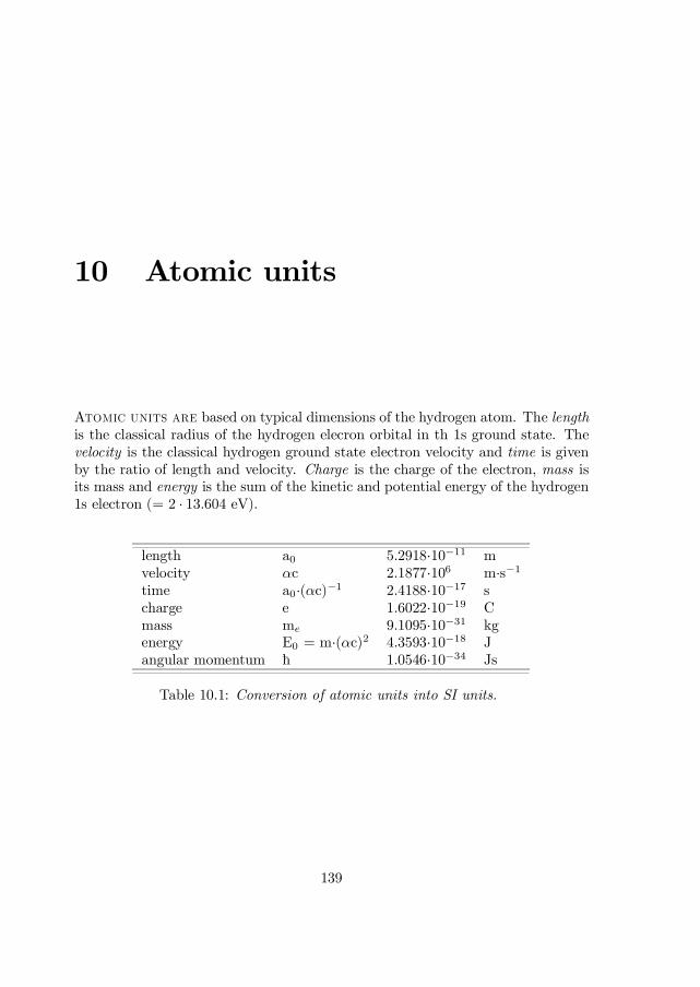
10 Atomic units
Atomic units are based on typical dimensions of the hydrogen atom. The lengthis the classical radius of the hydrogen elecron orbital in th 1s ground state. Thevelocity is the classical hydrogen ground state electron velocity and time is givenby the ratio of length and velocity. Charge is the charge of the electron, mass isits mass and energy is the sum of the kinetic and potential energy of the hydrogen1s electron (= 2 ¢ 13:604 eV).
length a0 5.2918¢10¡11 mvelocity ®c 2.1877¢106 m¢s¡1
time a0¢(®c)¡1 2.4188¢10¡17 scharge e 1.6022¢10¡19 Cmass me 9.1095¢10¡31 kgenergy E0 = m¢(®c)2 4.3593¢10¡18 Jangular momentum h 1.0546¢10¡34 Js
Table 10.1: Conversion of atomic units into SI units.
139

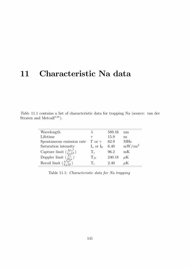
11 Characteristic Na data
Table 11.1 contains a list of characteristic data for trapping Na (source: van derStraten and Metcalf128).
Wavelength ¸ 589.16 nmLifetime ¿ 15.9 nsSpontaneous emission rate ¡ or ° 62.9 MHzSaturation intensity Is or I0 6.40 mW/cm2
Capture limit ( M°2
kBk2 ) Tc 96.2 mKDoppler limit ( ~°
2kB) TD 240.18 ¹K
Recoil limit ( ~2k2
kBM ) Tr 2.40 ¹K
Table 11.1: Characteristic data for Na trapping
141

12 Dankwoord
Het was ergens in mei 1997 toen ik op een ”summer school” Mike van derPoel uit Kopenhagen tegenkwam. Hij vertelde me over zijn plannen om ionenop lasergekoelde natriumatomen te schieten en ik wenste hem glimlachend veelsucces. Zo’n half jaar later kreeg ik echter te horen dat ik samen met een postdoc(Dirk ”oh my God, I can’t believe this ” Meyer) ook ionen op lasergekoelde atomenzou gaan schieten. Dirk sloeg aan het ontwerpen en ik ondertussen lithium aan.Een jaar later hadden we onze MOT aan de praat en vol goede moed begonnenwe aan de spectrometer, waarvan eigenlijk alleen de positiedetektor aan de praatmoest worden gebracht. Een half jaar later hadden we het idee dat ie ’t deeden vervolgens had ik nog een half jaar de tijd om een proefschrift en een PRLpublikatie bij elkaar te meten.
Er zijn drie mensen die ik in het bijzonder moet bedanken. Het grote aandeelvan Dirk in het succes van dit werk moge duidelijk zijn. Many thanks Dirk, forall the hard work you put in and all the great fun we had. Ook essentieël voordit werk was de inzet van Reinhard. Bedankt dat je er altijd was om een oio metzijn grote (pomplasers) en kleine problemen (welke trein moet ik nemen ...) tehelpen. Tja, en dan Ronnie, wiens bijdrage aan dit werk moeilijk te omschrijvenis, behalve dan dat die heel groot was. Dankzij jouw technische en natuurkundigekennis, grenzenloos optimisme en goed humeur is het toch nog goed gekomen metdie Turkstra.
Also crucial for the success of this work was the dedication of Ron Olson. Notonly the calculations reported in this work but also the ones you ran (consumingcountless hours of CPU time) just so that I could understand what I was doing,are very much appreciated. Let’s hope that theory and experiment will uncovergreat physics in the near future. Also very much appreciated were the lithium
143
144 Dankwoord
excitation calculations performed by Joe Schweinzer. Because of your e¤ort I hadsomething to compare my data to.
Verder moet ik nog een aantal bijzondere KVI’ers noemen die ook hun steentjeaan dit werk hebben bijgedragen. Hans voor de fabricage van de spectrometer,Ferdinand voor al het nodige laswerk en Imco en Jan ( ”..en waneer moet datklaar?”) voor de vele kleinere klussen. Ook Bert, Gerrit, Tjalling, Hans, Theréseen de rest van de elektronika-afdeling wil ik graag bedanken voor al hun inzet.En verder natuurlijk onze to¤e tukker Jan Mulder voor de uitlijning van mijnopstelling, Jans voor alle (soms ongevraagde, maar altijd nuttige) adviesen enHenk en Jelke voor hun inzet bij het leegpompen van mijn opstelling.
Also many thanks to Prof. Horst Schmidt-Böcking, Prof. Klaus Jungmann andProf. Peter van der Straten for ploughing through my thesis during the holidayseason and giving me some suggestions for re…nements.
Ik moet tot slot mijn opvolger Steven Knoop even sterkte wensen met de zwaretaak die hem wacht. Moge je MOT stabiel en je 2D spectra streperig zijn. Ennatuurlijk wil ik mijn collega’s Zoltán, Danyal, Omar, Marcel, Steven, Stefania,Rimco, Jur, Rian, Lubi, Thomas, Hocine, Céline, Fritsie (No Television but Tur-bovision!), Mark, Volker, Hans B. (wat liet jij je toch lekker stangen, Hans), HansW.(jou wil get het right somedag, keep oefenen), Hans F. (KVI lijkt wel een HanseHogeschool) en de rest van het KVI bedanken voor de geweldige werksfeer en allegezelligheid.
Copyright © 2022 FDOKUMEN