thesis.pdf - Rijksuniversiteit Groningen
98
University of Groningen Conserving approximations in nonequilibrium green function theory Stan, Adrian IMPORTANT NOTE: You are advised to consult the publisher's version (publisher's PDF) if you wish to cite from it. Please check the document version below. Document Version Publisher's PDF, also known as Version of record Publication date: 2009 Link to publication in University of Groningen/UMCG research database Citation for published version (APA): Stan, A. (2009). Conserving approximations in nonequilibrium green function theory. s.n. Copyright Other than for strictly personal use, it is not permitted to download or to forward/distribute the text or part of it without the consent of the author(s) and/or copyright holder(s), unless the work is under an open content license (like Creative Commons). The publication may also be distributed here under the terms of Article 25fa of the Dutch Copyright Act, indicated by the “Taverne” license. More information can be found on the University of Groningen website: https://www.rug.nl/library/open-access/self-archiving-pure/taverne- amendment. Take-down policy If you believe that this document breaches copyright please contact us providing details, and we will remove access to the work immediately and investigate your claim. Downloaded from the University of Groningen/UMCG research database (Pure): http://www.rug.nl/research/portal. For technical reasons the number of authors shown on this cover page is limited to 10 maximum. Download date: 28-05-2022
-
Upload
khangminh22 -
Category
Documents
-
view
3 -
download
0
Transcript of thesis.pdf - Rijksuniversiteit Groningen

University of Groningen
Conserving approximations in nonequilibrium green function theoryStan, Adrian
IMPORTANT NOTE: You are advised to consult the publisher's version (publisher's PDF) if you wish to cite fromit. Please check the document version below.
Document VersionPublisher's PDF, also known as Version of record
Publication date:2009
Link to publication in University of Groningen/UMCG research database
Citation for published version (APA):Stan, A. (2009). Conserving approximations in nonequilibrium green function theory. s.n.
CopyrightOther than for strictly personal use, it is not permitted to download or to forward/distribute the text or part of it without the consent of theauthor(s) and/or copyright holder(s), unless the work is under an open content license (like Creative Commons).
The publication may also be distributed here under the terms of Article 25fa of the Dutch Copyright Act, indicated by the “Taverne” license.More information can be found on the University of Groningen website: https://www.rug.nl/library/open-access/self-archiving-pure/taverne-amendment.
Take-down policyIf you believe that this document breaches copyright please contact us providing details, and we will remove access to the work immediatelyand investigate your claim.
Downloaded from the University of Groningen/UMCG research database (Pure): http://www.rug.nl/research/portal. For technical reasons thenumber of authors shown on this cover page is limited to 10 maximum.
Download date: 28-05-2022

Conserving Approximations inNonequilibrium Green Function Theory
Adrian Stan

The Zernike Institute for Advanced Materials, PhD theses seriesISBN: 978-90-367-3852-1
Adrian Stan,
Conserving Approximations in Nonequilibrium Green Function Theory,
Proefschrift Rijksuniversiteit Groningen.
Copyright c©2009, Adrian StanAll right reserved. No part of this book can be reproduced or transmitted in any form or by any mean,without permission from the author.
Printed by the Facilitair Bedrijf RuG, The Netherlands.

Rijksuniversiteit Groningen
Conserving Approximations
in
Nonequilibrium Green Function Theory
Proefschrift
ter verkrijging van het doctoraat in deWiskunde en Natuurwetenschappenaan de Rijksuniversiteit Groningen
op gezag van deRector Magnificus, dr F. Zwarts,in het openbaar te verdedigen op
maandag 25 mei 2009om 11.00 uur
door
Adrian Stan
geboren op 8 Februari 1980te Brasov, Roemenie

Promotores: Prof. dr. R. van LeeuwenProf. dr. R. Broer
Beoordelingscommissie: Prof. dr. M. BonitzProf. dr. A. SchindlmayrProf. dr. J. Knoester

Stellingenbehorende bij het proefschrift
Conserving Approximations in
Nonequilibrium Green Function Theoryvan
Adrian StanGroningen, 10 juni 2008
1. Total energies, ionization potentials and two-electron removal energies, obtained with our partially self-consistent GW approximation (i.e. the GWfc approximation), are in very good agreement with fully self-consistent GW results, while requiring only a fraction of the computational cost.1
Chapter 4 of this thesis
2. Fully self-consistent and partially self-consistent schemes provide ionization energies of similar quality as theG0W0 values, when calculated within the Extended Koopmans Theorem, but yield better total energies andenergy differences than G0W0 calculated using the Galitskii-Migdal formula.1
Chapter 3 of this thesis
3. [...] the Kadanoff-Baym equations can be used as a practical method to calculate the nonequilibrium propertiesof a wide variety of many-body quantum systems, ranging from atoms and molecules to quantum dots andquantum wells.
Chapter 5 of this thesis
4. Any Ξ-derivable theory is also Φ-derivable and therefore respects the conservation laws.
Chapter 7 of this thesis
5. Due to nonlinearity of the Kadanoff-Baym equations, the existence of bi-stable solutions and hence differentsteady states, may be possible.
Chapter 6 of this thesis
6. A physica ex machina2 approach renders the scientific method as no more than a simple task to obtainnumbers. It is too often forgotten that without understanding the path that lead to a result, the interpretationis meaningless.
7. Without a careful comprehension of the wellsprings of the claimed environmental threats, substituting thefossil fuel industry with any other type of industry, e.g., solar, hydrogen based, etc., will not solve the possibleenvironmental issues. It will just replace them with similar ones.
8. For nothing but egalitarian reasons, the Rijksuniversiteit Groningen should instate a James Watson & FrancisCrick fellowship, next to the Rosalind Franklin fellowship.
1This statement refers to the calculations on small atoms and diatomic molecules presented in this thesis.2Since at the time of publication of this thesis, a bibliographic search for the exact syntax ”physica ex machina” returned
no results, I use it here to single out a computational approach in the absence of a careful understanding of the methodused and hence lacking a lucid interpretation. I translate this syntax as ”physics from the machine” and I imply anallegorical relation with the expression ”deus ex machina” as used in Horace’s Ars Poetica. This statement is also meantto be generalized beyond its present connection to the field of physics.

6

Contents
1 Anteloquy 9
2 Theory of many-particle systems.
The Green function method. 11
2.1 Second quantization . . . . . . . . . . . . . . . . . . . . . . . . . . . . . . . . . . . . . . . 122.2 Evolution of ensembles . . . . . . . . . . . . . . . . . . . . . . . . . . . . . . . . . . . . . . 122.3 The Green function . . . . . . . . . . . . . . . . . . . . . . . . . . . . . . . . . . . . . . . . 132.4 Self-energy approximations . . . . . . . . . . . . . . . . . . . . . . . . . . . . . . . . . . . 13
2.4.1 The second Born approximation . . . . . . . . . . . . . . . . . . . . . . . . . . . . 152.4.2 The GW approximation . . . . . . . . . . . . . . . . . . . . . . . . . . . . . . . . . 15
2.5 Conserving approximations . . . . . . . . . . . . . . . . . . . . . . . . . . . . . . . . . . . 16References . . . . . . . . . . . . . . . . . . . . . . . . . . . . . . . . . . . . . . . . . . . . . . . . 17
3 Fully self-consistent GW calculations for atoms and molecules 19
3.1 Introduction . . . . . . . . . . . . . . . . . . . . . . . . . . . . . . . . . . . . . . . . . . . . 203.2 General formulation . . . . . . . . . . . . . . . . . . . . . . . . . . . . . . . . . . . . . . . 203.3 Results . . . . . . . . . . . . . . . . . . . . . . . . . . . . . . . . . . . . . . . . . . . . . . . 223.4 Conclusions . . . . . . . . . . . . . . . . . . . . . . . . . . . . . . . . . . . . . . . . . . . . 23
Appendices 25
A Basis Sets . . . . . . . . . . . . . . . . . . . . . . . . . . . . . . . . . . . . . . . . . . . . . 25References . . . . . . . . . . . . . . . . . . . . . . . . . . . . . . . . . . . . . . . . . . . . . . . . 29
4 Levels of self-consistency in the GW approximation 31
4.1 Introduction . . . . . . . . . . . . . . . . . . . . . . . . . . . . . . . . . . . . . . . . . . . . 324.2 General formalism . . . . . . . . . . . . . . . . . . . . . . . . . . . . . . . . . . . . . . . . 334.3 The GW approximation at different levels of self-consistency . . . . . . . . . . . . . . . . 34
4.3.1 Fully self-consistent GW . . . . . . . . . . . . . . . . . . . . . . . . . . . . . . . . . 344.3.2 The G0W0 and GW0 approximations . . . . . . . . . . . . . . . . . . . . . . . . . . 344.3.3 The GWfc approximation . . . . . . . . . . . . . . . . . . . . . . . . . . . . . . . . 35
4.4 Computational method . . . . . . . . . . . . . . . . . . . . . . . . . . . . . . . . . . . . . . 354.4.1 Numerical solution of the Dyson equation . . . . . . . . . . . . . . . . . . . . . . . 354.4.2 Numerical calculation of the screened potential: The product basis technique . . . 36
4.5 Results . . . . . . . . . . . . . . . . . . . . . . . . . . . . . . . . . . . . . . . . . . . . . . . 384.6 Summary and conclusions . . . . . . . . . . . . . . . . . . . . . . . . . . . . . . . . . . . . 41
7

8 CONTENTS
Appendices 43
A Ionization potentials from the Extended Koopmans Theorem . . . . . . . . . . . . . . . . 43B The Uniform Power Mesh . . . . . . . . . . . . . . . . . . . . . . . . . . . . . . . . . . . . 43References . . . . . . . . . . . . . . . . . . . . . . . . . . . . . . . . . . . . . . . . . . . . . . . . 43
5 Time propagation of the Kadanoff-Baym equations for inhomogeneous systems 47
5.1 Introduction . . . . . . . . . . . . . . . . . . . . . . . . . . . . . . . . . . . . . . . . . . . . 485.2 Theory . . . . . . . . . . . . . . . . . . . . . . . . . . . . . . . . . . . . . . . . . . . . . . . 485.3 Self-energy approximations . . . . . . . . . . . . . . . . . . . . . . . . . . . . . . . . . . . 505.4 Time-propagation of the Kadanoff-Baym equations . . . . . . . . . . . . . . . . . . . . . . 525.5 Summary and conclusions . . . . . . . . . . . . . . . . . . . . . . . . . . . . . . . . . . . . 54References . . . . . . . . . . . . . . . . . . . . . . . . . . . . . . . . . . . . . . . . . . . . . . . . 54
6 A many-body approach to quantum transport dynamics: Initial correlations and
memory effects 57
6.1 Introduction . . . . . . . . . . . . . . . . . . . . . . . . . . . . . . . . . . . . . . . . . . . . 586.2 General formalism . . . . . . . . . . . . . . . . . . . . . . . . . . . . . . . . . . . . . . . . 586.3 Results . . . . . . . . . . . . . . . . . . . . . . . . . . . . . . . . . . . . . . . . . . . . . . . 596.4 Conclusions . . . . . . . . . . . . . . . . . . . . . . . . . . . . . . . . . . . . . . . . . . . . 62References . . . . . . . . . . . . . . . . . . . . . . . . . . . . . . . . . . . . . . . . . . . . . . . . 62
7 Total energies from variational functionals of the Green function and the renormal-
ized four-point vertex 65
7.1 Introduction . . . . . . . . . . . . . . . . . . . . . . . . . . . . . . . . . . . . . . . . . . . . 667.2 Defining equations . . . . . . . . . . . . . . . . . . . . . . . . . . . . . . . . . . . . . . . . 677.3 Hedin’s equations . . . . . . . . . . . . . . . . . . . . . . . . . . . . . . . . . . . . . . . . . 697.4 Construction of a variational functional . . . . . . . . . . . . . . . . . . . . . . . . . . . . 717.5 Structure of the Ξ-functional . . . . . . . . . . . . . . . . . . . . . . . . . . . . . . . . . . 747.6 Ξ-derivable theories are conserving . . . . . . . . . . . . . . . . . . . . . . . . . . . . . . . 787.7 Approximations using the Ξ-functional . . . . . . . . . . . . . . . . . . . . . . . . . . . . . 78
7.7.1 Practical use of the variational property . . . . . . . . . . . . . . . . . . . . . . . . 787.7.2 Approximate Ξ-functionals . . . . . . . . . . . . . . . . . . . . . . . . . . . . . . . 79
7.8 Practical evaluation of the functional . . . . . . . . . . . . . . . . . . . . . . . . . . . . . . 807.8.1 Evaluation of the traces . . . . . . . . . . . . . . . . . . . . . . . . . . . . . . . . . 807.8.2 Evaluation of the L′ = 0-functional . . . . . . . . . . . . . . . . . . . . . . . . . . . 81
7.9 Conclusions . . . . . . . . . . . . . . . . . . . . . . . . . . . . . . . . . . . . . . . . . . . . 83
Appendices 85
A A generating functional for the Green function . . . . . . . . . . . . . . . . . . . . . . . . 85B The equation of motion of Gu,V . . . . . . . . . . . . . . . . . . . . . . . . . . . . . . . . . 86C Feynman rules for the two-particle Green function . . . . . . . . . . . . . . . . . . . . . . 88References . . . . . . . . . . . . . . . . . . . . . . . . . . . . . . . . . . . . . . . . . . . . . . . . 88
Epilogue 91
Samenvatting 93
Rezumat 95
List of publications 97

Chapter 1Anteloquy
The subject of this thesis lies in the field of many-body theory. This field emerged from the aim tounderstand the behavior and characterize the properties of many-body systems. When the systems con-sidered are large, the interactions between the elementary constituents of these systems can constructphenomena which may be very different from the behavior of the constituents considered as separated.In an attempt to describe these large systems, these very interactions complicate the description farbeyond the computational possibilities. In order to study the collective behavior of the interactingelementary constituents, the complexity of the interaction between them calls for simplifications. Allphysical approximations made in order to advance in understanding the behavior of many-body systemsconstitute the field of many-body physics.Within the field of many-body physics, the Green Function Theory describes the behavior and theproperties of a system with the aid of an object called the Green function. The Green function is theprobability amplitude of finding a particle that has been inserted in the system at (r′, t′) and removedat (r, t). Since between addition and removal the particle propagated through the system interactingwith all other particles, the Green function contains information about its properties. In the GreenFunction Theory, the interactions of an electronic system i.e. the effects of exchange and correlation,are incorporated into the so called self-energy operator. There are different possible approximations ofthe self-energy and they completely determine the properties of the system.One of the most widely used approximations of the self-energy is the GW approximation. In this approx-imation, the self-energy operator is the product of the Green function that describes the propagationof particles and holes in the system, and the dynamically screened interaction which describes how thebare interaction between electrons is modified due to the presence of the other electrons.
The first objective of this thesis is to investigate the ground state properties of finite inhomogeneoussystems, within the GW approximation of the self-energy. The most significant aspect here, is the studyof the effects of self-consistency of the Dyson equation on the observables of a given system. We per-form GW calculations at different levels of self-consistency on atoms and diatomic molecules and weinvestigate the effects of self-consistency on total energies, ionization potentials and on particle numberconservation. The different levels of self-consistency are, in fact, simplified GW schemes, character-ized by different constrains in self-consistency. We propose a new partially self-consistent GW scheme,labeled GWfc, in which the correlation part of the the self-energy is kept fixed throughout the self-consistency cycle. This approximation is compared to the fully self-consistent GW , the GW0 and theG0W0 approximations. Total energies, ionization potentials and two-electron removal energies obtainedwith the GWfc approximation, are in excellent agreement with fully self-consistent GW results whilerequiring only a fraction of the computational effort. This approximation can prove to be a valuable tool
9

10 ANTELOQUY
to get further insight into the performance of self-consistent GW for a large class of extended systemse.g. solid state systems for which self-consistent GW calculations are difficult to perform due to thelarge computational effort.Furthermore, we compare total energies obtained from the Luttinger-Ward functional with simple, ap-proximate Green functions as input, and we find them to be in excellent agreement with the self-consistentGW results, for atoms and molecules. We so demonstrate the usefulness of the Luttinger-Ward methodfor testing the merits of different self-energy approximations without the need to solve the Dyson equationself-consistently.
The second objective of this thesis is to discuss in detail the time-propagation of nonequilibriumGreen functions. After the Green function describing the equilibrium system has been obtained, itstime evolution in the presence of different electric fields, can be studied. This is achieved throughtime-propagation of the Kadanoff-Baym equations. We have developed a time propagation scheme forthe Kadanoff-Baym equations for general inhomogeneous systems. These equations describe the timeevolution of the nonequilibrium Green function for interacting many-body systems in the presence oftime-dependent external fields. The external fields are treated nonperturbatively whereas the many-bodyinteractions are incorporated perturbatively using Φ-derivable self-energy approximations that guaranteethe satisfaction of the macroscopic conservation laws of the system.
The third objective of this thesis, is the study of time dependent transport in a correlated model systemby means of time-propagation of the Kadanoff-Baym equations. We consider an initially contactedequilibrium system with a correlated central region coupled to tight-binding leads. Subsequently a time-dependent bias is switched on, after which we follow in detail the time-evolution of the system. With thisapproach we examine the ultrafast dynamics of transients and the inclusion of exchange and correlationeffects. We find that initial correlation and memory terms due to many-body interactions have a largeeffect on the transient currents. Further, the value of the steady state current is found to be stronglydependent on the approximation used to treat the electronic interactions.
In the last part of the thesis, we derive variational expressions for the grand potential or action interms of the many-body Green function G - which describes the propagation of particles - and therenormalized four-point vertex Γ - which describes the scattering of two particles in many-body systems.The main ingredient of the variational functionals is a term we denote as the Ξ-functional. We showthat any Ξ-derivable theory is also Φ-derivable and therefore respects the conservation laws. We set up acomputational scheme, aimed to obtain accurate total energies from our variational functionals, withouthaving to solve computationally expensive sets of self-consistent equations. The input of the functionalis an approximate Green function G and an approximate four-point vertex Γ obtained at a relativelylow computational cost. The functionals that we will consider for practical applications correspond toinfinite order summations of ladder and exchange diagrams and are therefore particularly suited forapplications to highly correlated systems.
The thesis is organized as follows: In Chapter 2 we discuss the general formalism of nonequilibriumGreen functions. We further introduce here the different conserving approximations used in the thesis.In Chapter 3-4 we describe in detail the GW approximation and we discuss the different levels of self-consistency. Further, a discussion of the computational scheme employed in the ground state calculationsis presented. We then, in Chapter 5, give the computational details of the time-propagation scheme forthe Kadanoff-Baym equations for general inhomogeneous systems and in Chapter 6 we apply this schemefor the study of the time-dependent quantum transport through a correlated double quantum dot system.Finally, in Chapter 7 we derive variational expressions for the grand potential or action in terms of themany-body Green function G and the renormalized four-point vertex Γ.
Chapter 2Theory of many-particle systems.The Green function method.
Abstract
In this chapter we introduce the fundamental concepts behind the Green Function Theory. We start from a descriptionof the second quantization method and then, after introducing the ensemble average of an operator, we define the mainobject of the theory, the Green function. Further on, after obtaining the equation of motion for the Green function, weintroduce the self-energy operator and we discuss the Hartree-Fock approximation, the second-Born approximation andthe GW approximation to the self-energy.
11
12 THE GREEN FUNCTION METHOD
2.1 Second quantization
Let us consider a system of N identical, non-relativisticparticles. The physical state of each particle j is de-scribed by the label xj . The wave function for thissystem is Ψ(x1 . . . xN). If the particles are identical,then the probability density |Ψ(x1 . . . xN)|2 must be un-changed under arbitrary exchanges of the labels we useto identify each particle. If the system is described by ascalar1 Ψ must transform according to a 1-D represen-tation of the permutation group. Hence, for the systemunder consideration, we have two cases: a) Ψ is evenunder permutation (PΨ = Ψ); and b) Ψ is odd underpermutation (PΨ = −Ψ). The latter case represents asystem of bosons and the former a system of fermions.Since in this work we are only concerned with fermionicparticles, we will neglect the bosonic case hereafter.While the usual representation of quantum mechan-ics [1] can be used to represent the full Hilbert space ofmany-body quantum mechanics, it proves to be quitecumbersome. Moreover, the usual representation issuited for problems with a fixed particle number N anddoes not allow for fluctuations. This can constitute atoo tight constrain and so it is convenient to work ina grand canonical formulation [2], where the particlenumber is allowed to fluctuate. In line with this lastconstrain, for practical purposes, one would should beable to determine the amplitude for adding a particleto the system at a certain space-time coordinate, say,(x1, t1), followed by its removal at (x2, t2).The method which removes all these shortcomings isthe second quantization [3, 4]. Within this method theoperator ψ†(x) is called creation operator and the oper-ator ψ(x) is called annihilation operator. By applyinga creation operator, a particle is added to the systemand by applying an annihilation operator, the particle isremoved [3]. These operators satisfy the commutationrelations
ψ†(x)ψ(x′) + ψ(x′)ψ†(x) = δ(x − x′), (2.1)
ψ(x)ψ(x′) + ψ(x′)ψ(x) = 0. (2.2)
Using the definitions of the field operators and theircommutation relations 2.1 and 2.2 we can express theusual operators in terms of field operators. If we con-sider a general one-body operator
O =
Zdxψ†(x)o(x)ψ(x), (2.3)
and the two-particle interaction
W =1
2
Z Zdx1dx2ψ
†(x1)ψ†(x2)w(r1, r2)ψ(x2)ψ(x1),
(2.4)
1For higher order objects, such as tensors, higher orderrepresentations of the permutation group are possible.
one can easily write the general Hamiltonian in the sec-ond quantization form
H =
Zdxψ†(x)h(r, t)ψ(x) (2.5)
+1
2
Z Zdx1dx2ψ
†(x1)ψ†(x2)w(r1, r2)ψ(x2)ψ(x1),
where w(r1, r2) = 1|r1−r2|
and where the one-body partof the Hamiltonian is
h(r, t) = −1
2∇2 + v(r, t) − µ. (2.6)
In Eq. 2.6 we introduced the chemical potential µ andthe external potential v(r, t) which will be switched onat t = t0. Hence, for t < t0 the Hamiltonian is time-independent.Using the above considerations, we can now define ourstrategy and set up further the formalism. We wantto study the time-evolution of a many-particle fermionsystem, after it has been perturbed from the groundstate, or statistical equilibrium. We have seen thatthe formalism of the second quantization is appropri-ate since it allows for extending quantum mechanicsto macroscopic number of particles and to describe thedynamical response and internal correlations of largesystems. In the next section we will briefly go throughthe steps to determine the time-dependent expectationvalue for an operator in the grand canonical ensemble.
2.2 Evolution of ensembles
In the grand canonical ensemble [5, 2], the expectationvalue of an operator O, for a system at temperature Twith the chemical potential µ, is
〈O〉 =
Pi〈Ψi|O|Ψi〉e−βEi
Pi e
−βEi, (2.7)
where |Ψi〉 is a complete set of states in the Fockspace, β = 1/kBT , with kB the Boltzmann constantand Ei are the eigenvalues of the Hamiltonian H. Notethat the chemical potential is included in the one-bodypart. If the system evolves in time, the expectationvalue becomes [2]
〈O(t)〉 = TrρO(t), (2.8)
where the statistical operator ρ acts as a weight func-tion for the Heisenberg representation of the operatorO, i.e.
OH(t) = U(t0, t)OU(t, t0), (2.9)
and where U is an evolution operator.Because the time-dependent quantities are switched on
2.4. SELF-ENERGY APPROXIMATIONS 13
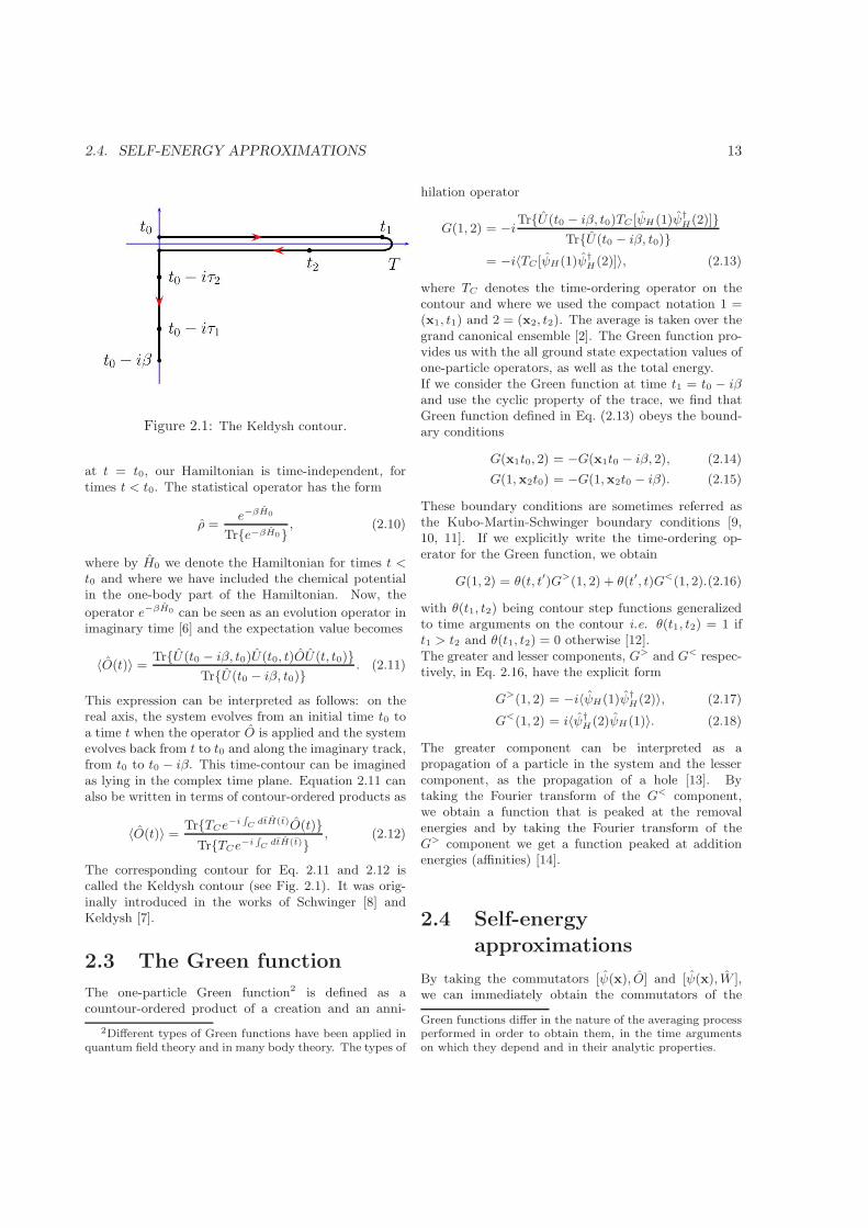
Figure 2.1: The Keldysh contour.
at t = t0, our Hamiltonian is time-independent, fortimes t < t0. The statistical operator has the form
ρ =e−βH0
Tre−βH0, (2.10)
where by H0 we denote the Hamiltonian for times t <t0 and where we have included the chemical potentialin the one-body part of the Hamiltonian. Now, the
operator e−βH0 can be seen as an evolution operator inimaginary time [6] and the expectation value becomes
〈O(t)〉 =TrU(t0 − iβ, t0)U(t0, t)OU(t, t0)
TrU(t0 − iβ, t0). (2.11)
This expression can be interpreted as follows: on thereal axis, the system evolves from an initial time t0 toa time t when the operator O is applied and the systemevolves back from t to t0 and along the imaginary track,from t0 to t0 − iβ. This time-contour can be imaginedas lying in the complex time plane. Equation 2.11 canalso be written in terms of contour-ordered products as
〈O(t)〉 =TrTCe
−iR
CdtH(t)O(t)
TrTCe−iR
CdtH(t)
, (2.12)
The corresponding contour for Eq. 2.11 and 2.12 iscalled the Keldysh contour (see Fig. 2.1). It was orig-inally introduced in the works of Schwinger [8] andKeldysh [7].
2.3 The Green function
The one-particle Green function2 is defined as acountour-ordered product of a creation and an anni-
2Different types of Green functions have been applied inquantum field theory and in many body theory. The types of
hilation operator
G(1, 2) = −iTrU(t0 − iβ, t0)TC [ψH(1)ψ†H(2)]
TrU(t0 − iβ, t0)= −i〈TC [ψH(1)ψ†
H(2)]〉, (2.13)
where TC denotes the time-ordering operator on thecontour and where we used the compact notation 1 =(x1, t1) and 2 = (x2, t2). The average is taken over thegrand canonical ensemble [2]. The Green function pro-vides us with the all ground state expectation values ofone-particle operators, as well as the total energy.If we consider the Green function at time t1 = t0 − iβand use the cyclic property of the trace, we find thatGreen function defined in Eq. (2.13) obeys the bound-ary conditions
G(x1t0, 2) = −G(x1t0 − iβ, 2), (2.14)
G(1,x2t0) = −G(1,x2t0 − iβ). (2.15)
These boundary conditions are sometimes referred asthe Kubo-Martin-Schwinger boundary conditions [9,10, 11]. If we explicitly write the time-ordering op-erator for the Green function, we obtain
G(1, 2) = θ(t, t′)G>(1, 2) + θ(t′, t)G<(1, 2).(2.16)
with θ(t1, t2) being contour step functions generalizedto time arguments on the contour i.e. θ(t1, t2) = 1 ift1 > t2 and θ(t1, t2) = 0 otherwise [12].The greater and lesser components, G> and G< respec-tively, in Eq. 2.16, have the explicit form
G>(1, 2) = −i〈ψH(1)ψ†H(2)〉, (2.17)
G<(1, 2) = i〈ψ†H(2)ψH(1)〉. (2.18)
The greater component can be interpreted as apropagation of a particle in the system and the lessercomponent, as the propagation of a hole [13]. Bytaking the Fourier transform of the G< component,we obtain a function that is peaked at the removalenergies and by taking the Fourier transform of theG> component we get a function peaked at additionenergies (affinities) [14].
2.4 Self-energy
approximations
By taking the commutators [ψ(x), O] and [ψ(x), W ],we can immediately obtain the commutators of the
Green functions differ in the nature of the averaging processperformed in order to obtain them, in the time argumentson which they depend and in their analytic properties.
14 THE GREEN FUNCTION METHOD
field operators with the Hamiltonian, [ψ(x), H ] and[ψ†(x), H]. Further we have the equation of motionfor the field operators
i∂t1 ψ(1) = [ψ(1), H(1)] = h(1)ψ(1)
+
Zd2w(1, 2)ψ†(2)ψ(2)ψ(1), (2.19)
i∂t1 ψ†(1) = [ψ†(1), H(1)] = −h(1)ψ†(1)
−Zd2w(1, 2)ψ†(1)ψ(2)ψ(2), (2.20)
with w(1, 2) = δ(t1, t2)/|r1 − r2| being the Coulombinteraction. If we take the derivative of the Greenfunction 2.16, in respect to t1 and t2, and we use 2.19and 2.20 respectively, we obtain the equation of motionfor the Green function
i∂t1G(1, 2) = δ(1, 2) + h(1)G(1, 2) (2.21)
−iZd3w(1+, 3)〈TC [ψ(1)ψ†(2)ψ†(3)ψ(3)]〉,
− i∂t2G(1, 2) = δ(1, 2) + h(2)G(1, 2) (2.22)
−iZd3w(2+, 3)〈TC [ψ†(2)ψ(1)ψ(3)ψ†(3)]〉.
The product of field operators in the last term of 2.21and 2.22 is the two particle Green function which de-scribes the propagation of two particles, two holes or aparticle and a hole through the system. We rewrite theEqs. 2.21-2.22 as3
i∂t1 G(1, 2) = δ(1, 2) (2.23)
+h(1)G(1, 2) − i
Zd3w(1+, 3)G2(1, 3, 3
+, 2),
−i∂t2 G(1, 2) = δ(1, 2) (2.24)
+h(2)G(1, 2) − i
Zd3w(2+, 3)G2(1, 3, 3
+, 2).
where G2 is the two particle Green function was definedfrom the n-particle Green function
Gn (1, . . . , n, 1′, . . . , n′) = (2.25)
(−i)n〈TC [ψ(1), . . . , ψ(n), ψ†(1′), . . . , ψ†(n′)]〉,
It can be proved by induction that the n-body Greenfunction depends on the n+1-body Green function [10,3]. At the first level, the truncation of this hierarchyis performed by introducing the self-energy operator Σ
3The notation + means that the limit is taken from aboveon the contour, i.e., 1+ = x1, t1 + δ.
such that −iG2v = ΣG [14]. In other words, we definethe self-energy Σ and its adjoint Σ by
Zd2Σ(1, 2)G(2, 1′) = −i
Zd2w(1+, 2)G2(1, 2, 2
+, 1′),
Zd2G(1, 2)Σ(2, 1′) = −i
Zd2w(1′+, 2)G2(1, 2, 2
+, 1′).
One can show that for initial equilibrium conditions theself-energy operator Σ and its adjoint Σ are the same.From here on we will assume that this is the case.With the considerations above, the equations of motionof the Green function will be written as [12]
i∂t1G(1, 2) = δ(1, 2) + h(1)G(1, 2)
+
Zd2Σ(1, 3)G(3, 2), (2.26)
−i∂t2G(1, 2) = δ(1, 2) + h(2)G(1, 2)
+
Zd2G(1, 3)Σ(3, 2). (2.27)
If we take the functional derivative of the Green func-tion in respect to the external field, we find that thetime ordered product of four field operators equals thefunctional derivative of the one-particle Green functionplus the product of the expectation value of the densityoperator and the one-particle Green function
−i〈TC [ψ(1)ψ†(2)ψ†(3)ψ(3)]〉 = iδG(1, 2)
δv(3)(2.28)
+〈nH(3)〉G(1, 2).
This follows directly from the equation of motion for theevolution operator. Making use of the definition of theinverse Green function
RG(1, 2)G−1(2, 1) = δ(1, 2), we
obtain an expression for the functional derivative of theone-particle Green function in respect to the externalpotential
δG(1, 2)
δv(3)= −
Zd4d5G(1, 4)
δG−1(4, 5)
δv(3)G(5, 2).(2.29)
If we define
− δG−1(4, 5)
δv(3)= Γ(45; 3) (2.30)
to be the vertex function. Further, making use Eq. 2.29and of
G−1(1, 2) = (i∂t1 − h(1))δ(1, 4) − Σ(1, 4), (2.31)
we write the vertex function Γ in the form
Γ(14; 3) = δ(1, 2)δ(1, 4) +δΣ(1, 4)
δv(3). (2.32)
2.4. SELF-ENERGY APPROXIMATIONS 15
By inserting 2.29, with 2.32, into 2.28, we can rewritethe equation of motion for the one-particle Green func-tion as
[i∂t1 − h(1)]G(1, 1′) = δ(1, 1′)
+
Zd4
hi
Zd2d3G(1, 3)w(1+, 2)Γ(34; 2)
+δ(1, 4)δ(3, 2)w(4, 3)〈n(3)〉iG(4, 1′). (2.33)
Using the expression for the density 〈n(3)〉 =−iG(3, 3+) together with Eqs. 2.26 and 2.23, we canidentify the self-energy as
Σ(1, 4) = i
Zd2d3
hG(1, 3)w(1, 2)Γ(34; 2)
−δ(1, 2)δ(3, 2)w(1, 3)G(3, 3+)i. (2.34)
We can now use the expression for the vertex Γ inEq. 2.32 together with Eq. 2.34 to generate higher orderapproximations. If we insert 2.32 in 2.34 we have
Σ(1, 4) = iG(1, 2)w(1+, 2)
− iδ(1, 2)
Zd3w(1, 3)G(3, 3+)
+ i
Zd4d3G(1, 3)w(1+, 4)
δΣ(3, 2)
δv(4).(2.35)
If we consider in the equation 2.35 only the first orderterms in w, we obtain the Hartree-Fock self-energy
Σ(1, 2) = iG(1, 2)w(1+, 2)−iδ(1, 2)Zd3w(1, 3)G(3, 3+).
(2.36)This approximation is the lowest order approximationfor the many-body effects.
2.4.1 The second Born approxima-
tion
Inserting 2.36 back into 2.35 leads to the second Bornapproximation to the self-energy. By keeping the termsto second-order in w we have
Σ(1, 2) = ΣHF (1, 2) + Σ(2)(1, 2), (2.37)
where ΣHF is the HF part of the self energy 2.36 andΣ(2) = Σ(2a) + Σ(2b) is the sum of the two terms
Σ(2a) (1, 2) = −i2G(1, 2)
Zd3 d4w(1, 3)
×G(3, 4)G(4, 3)w(4, 2), (2.38)
Σ(2b) (1, 2) = i2Zd3 d4G(1, 3)w(1, 4)G(3, 4)
×G(4, 2)w(3, 2). (2.39)
These terms are usually referred to as the second-orderdirect and exchange terms. They can be representeddiagramatically as the two diagrams to second order inthe two-particle interaction [15, 16].Further iterations of Eq. 2.35 lead to higher orderapproximations.
2.4.2 The GW approximation
In the GW approximation the self-energy is expandedin terms of the Green function and the dynamicallyscreened interaction W [17]. The screened interactionW describes the dynamical shielding in the Coulombpotential. Including the effective interaction of the elec-trons, the screened interaction is defined as
W (1, 2) =
Zd3w(1, 3)
δV (2)
δv(3), (2.40)
where
V (2) = v(2) +
Zd4w(2, 4)〈n(4)〉, (2.41)
and describes the effects of a test charge at point 2 onthe potential at point 1. By substituting 2.41 in 2.40and taking the functional derivative, we can use theidentity
δ
v(1)=
Zd2δV (2)
δv(1)
δ
δV (2), (2.42)
to obtain
W (1, 2) =
Zd3w(1, 3) (2.43)
×"δ(2, 3) +
Zd4d5w(2, 4)
δ〈n(4)〉δV (5)
δV (5)
δv(3)
#,
In Eq.2.43 we identify the irreducible polarizability
P (4, 5) =δ〈n(4)〉δV (5)
, (2.44)
as the density response to the effective field. We takethe functional derivative of the Green function with re-spect to V (2) and we obtain
δG(1, 2)
δV (3)= −
Zd4d5G(1, 4)
δG−1(4, 5)
δV (3)G(1, 5), (2.45)
where, using the definition of the inverse Green func-tion, we define the vertex Γ as
Γ(12; 3) = − δG−1(1, 2)
δV (3)= δ(1, 2)δ(1, 3) +
δΣ(1, 2)
δV (3).
(2.46)Note that this vertex is different form the vertex inEq. 2.32. From the definition of the density 〈n(4)〉 =
16 THE GREEN FUNCTION METHOD
−iG(4, 4+) we can rewrite the irreducible polarizabilityas
P (4, 7) = i
Zd5d6G(4, 5)
δG−1(5, 6)
V (7)G(6, 4), (2.47)
and we can use the vertex function 2.46 to write it inthe form
P (4, 7) = i
Zd5d6G(4, 5)Γ(56, 7)G(6, 4). (2.48)
From Eq. 2.21 and 2.28 we identify the self-energy as
Σ(1, 2) = −iδ(1, 2)Zd3w(1, 3)G(3, 3+) (2.49)
−iZd3d4w(1, 3)G(1, 4)
δG−1(4, 2)
δv(3)
where the first term on the right hand side is theHartree term and the second term represents theexchange-correlation part. We can express the self-energy in terms of screened interaction and vertex func-tion by using the identity 2.42. We obtain
Σ(1, 2) = iδ(1, 2)
Zd3w(1, 3)G(3, 3+)
+i
Zd3d4W (1, 3)G(1, 4)Γ(42; 3).(2.50)
Finally, we apply the chain rule in the last term ofEq. 2.46 and we obtain a self-consistent expression forthe vertex function
Γ(12; 3) = − δG−1(1, 2)
δV (3)= δ(1, 2)δ(1, 3) (2.51)
+
Zd4d5d6d7
δΣ(1, 2)
δG(4, 5)G(4, 6)Γ(67; 3)G(7, 5),
which together with the self-energy 2.50, the irreduciblepolarizability 2.48 and the screened interaction
W (1, 2) = w(1, 2) + i
Zd3d4d5d7w(2, 4)W (1, 7)P (4, 7)
(2.52)
constitute the Hedin equations [17]. We have achieveda systematic expansion of the self-energy in G and W .This is preferable for extended systems with long rangeinteractions, where W is usually much smaller thanthe bare interaction w [18]. These equations are to besolved iteratively to obtain the self-energy Σ. However,such a calculation is, in principle, not possible even forvery simple systems, mainly due to the presence of thevertex. We can take the simplest approximation tothe vertex function 2.51, i.e., Γ(12; 3) = δ(1, 2)δ(1, 3)and obtain the GW approximation [17]. With this ap-proximation to the vertex Γ, the self-energy depends onthe self-consistent Green function and the screened po-tential W , calculated from the full Green function andtherefore the equations must be solved self-consistently.
2.5 Conserving
approximations
One of the most important issues when making an ap-proximation is the satisfaction of the conservation laws.In Green Function Theory it is possible to guaranteethat the macroscopic conservation laws, such as thoseof particle, momentum and energy conservation, areobeyed.Baym showed [19] how the macroscopic conservationlaws are related to the invariant properties of a func-tional Φ 4. If we know the Green function, we cancalculate the density and the current density from
〈n(1)〉 = iG(1, 1+) (2.55)
〈j(1)〉 = −i»
∇1
2i− ∇1′
2i
–G(1, 1+)
ff
1′=1+
.(2.56)
These two quantities must satisfy the continuity equa-tion
∂t1〈n(1)〉 + ∇ · 〈j(1)〉 = 0, (2.57)
which relates the accumulation of charge in a spacialregion to the current flow in that region. This can bereadily proved by subtracting 2.26 and 2.27 (with 2 →1+)
[i∂1 − i∂1+ − h(1) + h(1+)]G(1, 1+) = (2.58)Zd1[Σ(1, 1)G(1, 1+) −G(1, 1)Σ(1, 1+)].
If the system is perturbed by a potential correspondingto a gauge transformation, the one body part of theHamiltonian becomes
hg(1) =1
2[∇− i∇Λ]2 + i
∂Λ(1)
∂t+ v(1) − µ. (2.59)
With this form of the single-particle Hamiltonian, andthe conservation of particles at vertices [16], we can
4Luttinger and Ward [20] have constructed a functionalΦ of G by summing over all irreducible self-energy diagramsclosed with an additional Green function and multiplied byspecific numerical factors. This functional can be written as
Φ[G] =X
n,k
1
2nTr[Σ
(n)k G] (2.53)
where n indicates the number of interaction lines and theindex k labels topologically different self-energy diagrams.The trace implies a summation over all indices and a fre-quency integration. In other words they proved that for theexact self-energy there is a functional Φ of G such that
Σ(1, 2) =δΦ
δG(2, 1). (2.54)

2.5. REFERENCES 17
show that for the interacting Green function and theself-energy we have the transformations
G(1, 2; Λ) = e−iΛ(1)G(1, 2)eiΛ(2), (2.60)
Σ(1, 2; Λ) = e−iΛ(1)Σ(1, 2)eiΛ(2). (2.61)
This solutions obey the boundary condition if we as-sume Λ(t0) = Λ(t0 − iβ). A first order change in G dueto the gauge transformation is
δG(1, 2) = −i(δΛ(1) − δΛ(2))G(1, 2). (2.62)
The exponential factors cancel at the internal vertices ofΣ because factors from the particles entering a vertexcancel the factors from outgoing particles. The onlyfactors remaining are those at external vertices. Thecorresponding change in the functional Φ is given by
δΦ = i
Zd1d2Σ(2, 1)G(1, 2)(δΛ(2) − δΛ(1))
= i
Zd1d2Σ(2, 1)G(1, 2) − Σ(1, 2)G(2, 1)δΛ(2).
On the other hand, from the fact that Φ[G(Λ)]=Φ[G] wehave δΦ/δΛ = 0 and therefore from Eq. 2.63 it followsthat
Zd2Σ(2, 1)G(1, 2) −G(2, 1)Σ(1, 2) = 0. (2.63)
So the integral part of the right hand term of Eq. 2.58is zero. From Eq. 2.58 and Eq. 2.55-2.56 it follows thatthe continuity equation is satisfied
∂1〈n(1)〉 = −∇1〈j(1)〉. (2.64)
The conservation law for momentum follows from con-sidering a translation of the coordinate system by avector R(t). This implies an observer whose origin ofcoordinates is at the time varying point R(t) and whowill describe the system with an extra term of the firstorder in R added to the Hamiltonian. In analogy withthe above considerations for particle conservation, weobtain the equation
d
dt〈P〉 = −
Zdx1〈n(1)〉∇1w(1). (2.65)
The proof for energy conservation involves the descrip-tion for the Φ-invariance when the system is describedby an observer with a ”rubbery clock” [19], since theenergy conservation requires time-translational invari-ance. Following the same lines as for momentum con-servation proof, we obtain
d
dt〈H0〉 = −
Zdx1〈j(1)〉 · (−∇1v(1)). (2.66)
where H0 represents the system without the addedfield 〈H0〉 = 〈H − V 〉. In Ref. [19], Baym has shownthat the condition for a self-energy approximationto be conserving is that is has to be Φ-derivable.This means that for the approximate self-energythere is a functional Φ such that the equation (2.54)is obeyed. Such approximations to the self-energyare called conserving or Φ-derivable approximations.Well-known conserving approximations are the Hartreeapproximation – where Φ = 0 –, the Hartree-Fock ap-proximation [16], the second Born [15] approximation,the GW approximation [17] and the T -matrix [15]approximation.
References
[1] Arno Bohm. Quantum Mechanics: Foundationsand Applications. Springer-Verlag, New York,2001.
[2] Dimitrii Nikolaevich Zubarev. Nonequilibrium Sta-tistical Thermodynamics. Consultants Bureau,New York, 1974.
[3] Eberhard K. U. Gross, Erich Runge, and OlleHeinonen. Many-Particle Theory. Verlag AdamHilger, Bristol, 1991.
[4] Feliks Aleksandrovich Berezin. The Method of Sec-ond Quantization. Academic Pressr, New York,1966.
[5] Arnold Munster. Statistical Thermodynamics.Springer-Verlag, Berlin, Heidelberg, 1969.
[6] Robert Mills. Propagators for many-particle sys-tems. Gordon and Breach Science Publishers, NewYork, 1969.
[7] Leonid Veniaminovich Keldysh. Zh. Eksp. Teor.Fiz., 47:1515, 1964. [Sov. Phys. JETP, 20, 1018(1965)].
[8] Julian Schwinger. J. Math. Phys., 2:407, 1961.
[9] Ryogo Kubo. J. Phys. Soc. Jpn., 12:570, 1957.
[10] Paul C. Martin and Julian Schwinger. Phys. Rev.,115:1342, 1959.
[11] Nils Erik Dahlen, Adrian Stan, and Robert vanLeeuwen. J. Phys. Conf. Ser., 35:324, 2006.
[12] Pawel Danielewicz. Ann. Phys. (N. Y.), 152:239,1984.
18 THE GREEN FUNCTION METHOD
[13] Philippe Nozieres. Theory of interacting fermi sys-tems. W. A. Benjamin, New York, 1964.
[14] Alexander L. Fetter and John Dirk Walecka.Quantum Theory of Many-Particle Systems.McGraw-Hill, New York, 1971.
[15] Leo P. Kadanoff and Gordon Baym. Quantum Sta-tistical Mechanics. W. A. Benjamin, Inc., NewYork, 1962.
[16] Gordon Baym and Leo P. Kadanoff. Phys. Rev.,124:287, 1961.
[17] Lars Hedin. Phys. Rev., 139:A796, 1965.
[18] Lars Hedin and Stig Olov Lundqvist. Solid StatePhysics, 23:1, 1969.
[19] Gordon Baym. Phys. Rev., 127:1391, 1962.
[20] Joaquin Mazdak Luttinger and John Clive Ward.Phys. Rev., 118:1417, 1960.
Chapter 3Fully self-consistent GW calculations foratoms and molecules
Adrian Stan, Nils Erik Dahlen and Robert van Leeuwen
1Rijksuniversiteit Groningen, Materials Science Centre, Theoretical Chemistry,Nijenborgh 4, 9747AG Groningen, The Netherlands.
Europhysics Letters 76, 298 (2006)
Abstract
We solve the Dyson equation for atoms and diatomic molecules within the GW approximation, in order to elucidatethe effects of self-consistency on the total energies and ionization potentials. We find GW to produce accurate energydifferences although the self-consistent total energies differ significantly from the exact values. Total energies obtainedfrom the Luttinger-Ward functional ELW[G] with simple, approximate Green functions as input, are shown to be inexcellent agreement with the self-consistent results. This demonstrates that the Luttinger-Ward functional is a reliablemethod for testing the merits of different self-energy approximations without the need to solve the Dyson equation self-consistently. Self-consistent GW ionization potentials are calculated from the Extended Koopmans Theorem, and shownto be in good agreement with the experimental results. We also find the self-consistent ionization potentials to be oftenbetter than the non-self-consistent G0W0 values. We conclude that GW calculations should be done self-consistently inorder to obtain physically meaningful and unambiguous energy differences.
19

20 SC-GW CALCULATIONS FOR ATOMS AND MOLECULES
3.1 Introduction
Green function methods have been used with great suc-cess to calculate a wide variety of properties of elec-tronic systems, ranging from atoms and molecules tosolids. One of the most successful and widespreadmethods has been the GW approximation (GWA) [1],which has produced excellent results for band gaps andspectral properties of solids [2, 3], but so far has notbeen explored much for atoms and molecules, althoughit has been known that for atoms the core-valence in-teractions are described much more accurately by GWthan Hartree-Fock (HF) [4]. Moreover, theGW calcula-tions are rarely carried out in a self-consistent manner,and the effect of self-consistency is for this reason stilla topic of considerable debate [5, 6]. In this paper wepresent self-consistent all-electron GW (SC-GW ) cal-culations for atoms and diatomic molecules. The rea-son for doing these calculations is two-fold: Firstly wewant to study the importance of self-consistency withinthe GW scheme. Such calculations are usually avoideddue to the rather large computational effort involved.It has been suggested that self-consistency will in factworsen the spectral properties, though calculations onsilicon and germanium crystals indicate that this is notalways the case [5]. The second reason is that we aim tostudy transport through large molecules and molecularchains, where it is essential to account for the screen-ing of the long range of the Coulomb interaction. Thecalculations on diatomic molecules are the first step inthis direction.
TheGWA is obtained by replacing the bare Coulombinteraction v in the exchange self-energy with the dy-namically screened interaction W , such that Σ =−GW . The screened interaction also depends on theGreen function, and one thus needs to solve a set of cou-pled equations for G and W . One usually goes throughonly a single iteration of this scheme. With an initialGreen function G0 calculated from, e.g., the local den-sity approximation (LDA), one calculates W and Σ,and subsequently obtains a new Green function fromthe Dyson equation. This scheme, known as the G0W0
approximation, has produced good results for a widevariety of systems [2], but suffers from a dependence onthe choice of the initial G0. Moreover, observables likethe total energy are not unambiguously defined, andcan be calculated in several different ways. These prob-lems can be cured by performing self-consistent calcula-tions [7], since theGWA is a Φ-derivable approximation(see Fig. 3.1). The fact that self-consistency removesthese ambiguities does not imply that the results arenecessarily closer to the exact values. For the electrongas it was shown that self-consistency actually worsensthe spectral properties, while the total energy is in ex-
cellent agreement with Monte-Carlo results [8]. On theother hand, for a system of very localized interactions,SC-GW produced poor results for both total energiesand spectral properties [3]. Furthermore, Delaney et al.[6] recently published SC-GW results for the ionizationpotential of the Be atom that were worse than thoseof G0W0. Calculations on the Si and Ge crystals have,however, shown that self-consistency leads to improvedband gaps [5].
3.2 General formulation
In this paper, we study the importance of self-consistency in GW for atoms and diatomic molecules.We compare the self-consistent total energies to thoseobtained from the Luttinger-Ward (LW) functional [9]which was earlier used to estimate the GW total energyfor atoms [10] and the electron gas [11]. The LW func-tional ELW[G] is a variational energy functional in thesense that δELW[G]/δG = 0, when G is a self-consistentsolution of the Dyson equation. This variational prop-erty suggests that evaluating ELW on an approximateGreen function obtained from, e.g., HF or LDA calcula-tions will give a result very close to the self-consistentvalue. This was earlier shown to be the case for thesecond-order self-energy [12], and investigating the sta-bility of the LW functional also for the GWA is animportant goal of this paper. The previously publishedLW calculations [10] indicated that the GW total en-ergies are not very accurate, but the essential questionis rather whether total energy differences are producedaccurately. We have for this reason also calculated thebinding curve of the H2 molecule and two-electron re-moval energies ∆E = EN−2 −EN .
We use the finite temperature formalism, with a tem-perature T (we are only considering the limit T → 0)and a chemical potential µ. The Green function de-pends on the imaginary time coordinate τ , in the range−β ≤ τ ≤ β ≡ 1/kBT , where kB is the Boltzmannconstant. It satisfies the Dyson equation
"− ∂τ +
∇2
2−w(r) − vH(r) + µ
#G(x,x′; τ ) =
= δ(τ )δ(x− x′) +
Z β
0
dτ1
Zdx1Σ[G](x,x1; τ − τ1)
×G(x1,x′; τ1), (3.1)
where x = (r, σ) denotes the space- and spin coor-dinates, w(r) is the external potential, Σ[G](x,x′; τ )is the self-energy and vH(r) is the Hartree potential.The last two objects are functionals of the Green func-tion, and the Dyson equation should therefore be solved

3.2. General formulation 21
ΦGW = −1
2 −1
4 −1
6 + . . .
ΣGW = + + + . . .
Figure 3.1: The GW self-energy Σ is the functionalderivative of a functional Φ[G].
self-consistently, together with the boundary condi-tions G(x,x′, τ − β) = −G(x,x′; τ ) and G(x,x′; 0+) −G(x,x′; 0−) = −δ(x− x′).
In the GWA (Fig. 3.1) the electronic self-energy isgiven by Σ = −GW using the screened interactionW = v + vPW , where v is the bare Coulomb inter-action 1/|r − r′| and P = GG is the polarizability [1].The Green function is transformed into a τ -dependentmatrix by expanding it in a basis of molecular orbitalsobtained from an initial HF calculation. These molec-ular orbitals are linear combinations of Slater functionslocated on the atomic centers (See Appendix A). TheGreen function, the Σ[G] and the W are peaked aroundthe endpoints (τ = 0 and τ = ±β) [12, 5] so their rep-resentation on an even-spaced grid is inconvenient. In-stead, we used a mesh which is dense around the endpoints [5].
Since we calculate the Green function on the imagi-nary time axis, it is inconvenient to calculate the ioniza-tion potentials by finding the poles of the Green func-tion in frequency space, G(ω). We have instead used theextended Koopmans theorem (EKT) [13] where the ion-ization potentials are found from the eigenvalue equa-tion X
ij
∆ijumj = −λm
X
j
ρijumj , (3.2)
where ∆ij = −∂τGij(τ )|τ=0, the density matrix is givenby ρij = Gij(0
−) and the matrix indices refer to themolecular orbital basis [12]. The eigenvalues λm areinterpreted as λm = EN−1
m − EN0 + µ, i.e. the ioniza-
tion potentials plus the chemical potential. The EKTis known to be exact for the lowest ionization ener-gies, if the exact ∆ and ρ matrices are given [14]. Forthe HF approximation, the EKT eigenvalues obviouslyagree with the poles of the HF Green function, and itis an unproven conjecture that these two methods willgive the same value for the first ionization potentialwhen the Green function is calculated self-consistentlywithin a conserving approximation. The EKT has re-cently been used to calculate ionization potentials foratoms and molecules from a self-consistent Green func-
tion using the second order diagrams [12].To calculate the SC-GW total energy E = T +Vne +
U0 +Uxc, we use the fact that the exchange-correlationpart of the interaction energy is given by
Uxc =1
2
X
ij
Z β
0
dτΣij(−τ )Gji(τ ), (3.3)
and the kinetic energy T , nuclear-electron attractionenergy Vne and Hartree energy U0 are trivially obtainedfrom the density matrix ρ. There are many other waysto calculate the total energy from a given Green func-tion, but only for a self-consistent solution of the Dysonequation will these methods give the same result [7].One alternative is to calculate the energy from vari-ational functionals of the Green function. LW haveshown [9] that the total energy can be written as
ELW[G] = Φ[G]−U0 −Tr˘ΣG
¯−Tr ln[Σ−G−1
H ] + µN(3.4)
where GH is the Hartree Green function, and Σ =δΦ/δG. The trace indicates an integration over thespatial coordinates and τ [10], see also Eq. (4.11). Itis easily verified that δELW/δG = 0 when G is aself-consistent solution of the Dyson equation (4.9).Hence, if we evaluate the LW functional on a simpleinput Green function, we obtain a result close to theself-consistent energy, since we make an error only tosecond-order in the deviation from the self-consistentG. This means that we have a computationally cheapway of obtaining self-consistent total energies.
The quality of the energies will ultimately be deter-mined by the chosen self-energy approximation.
Within a molecular orbital basis, the Dyson equation(4.9) becomes a matrix equation. We introduce a refer-ence Green function G0 in order to write the equationon integral form,
Gij(τ ) = δijG0,i(τ ) +
Z β
0
dτ1
Z β
0
dτ2X
k
G0,i(τ − τ1)
×Σik(τ1 − τ2)Gkj(τ2), (3.5)
where Σ = Σ[G] − Σ0, and Σ0 is the self-energy cor-responding to G0 [12]. We take G0 and Σ0 to be theHF Green function and self-energy, but this choice isarbitrary. Using, e.g., LDA instead would not changeany of the results. The inverse temperature is chosento have a sufficiently large value, typically larger than100 a.u.. The value of the chemical potential is some-what arbitrary, but should be in the gap between thehighest occupied and the lowest unoccupied orbital. Wechecked that the observables calculated from the result-ing Green function did not depend on the choice of βand µ. The calculations on the molecules were done atthe experimental bond lengths.

22 SC-GW CALCULATIONS FOR ATOMS AND MOLECULES
Table 3.1: Total energies (in Hartrees) calculated from SC-GW compared to CI values and results from the LWfunctional and Galitskii-Migdal formula evaluated on GHF.
System EGWSC EGW
LW [GHF] EGM[GHF] CIHe -2.9278 -2.9277 -2.9354 -2.90371
Be -14.7024 -14.7017 -14.7405 -14.66741
Be2+ -13.6885 -13.6885 -13.6929 -13.65561
Ne -129.0499 -129.0492 -129.0885 -128.93761
Mg -200.1762 -200.1752 -200.2924 -200.0531
Mg2+ -199.3457 -199.3453 -199.3785 -199.22041
H2 -1.1887 -1.1888 -1.1985 -1.1332
LiH -8.0995 -8.0997 -8.1113 -8.0403
1From Ref. [15]. 2From Ref. [16]. 3From Ref. [17].
3.3 Results
In Table 4.1 we show the SC-GW total energies of someatoms and small molecules. We have also included theELW[GHF] results, which are in spectacular agreementwith the SC-GW values. This agreement is indepen-dent of the chosen basis set, and was earlier observedalso for the second-order diagrams [12]. The third col-umn shows the total energy calculated from GHF us-ing the Galitskii-Migdal [18] formula. In contrast tothe LW results, these are not in good agreement withthe self-consistent energies. This clearly demonstratesthat different total energy functionals will not producethe same results when evaluated on a non-selfconsistentGreen function (in this case, GHF), and it also demon-strates the importance of using the variational func-tionals for obtaining a result in agreement with theself-consistent values.
As a further test of the total energy functionals, wehave calculated the total energy of the H2 molecule fora range of internuclear separations. Figure 3.2 showsthe SC-GW results together with the ELW[GHF] en-ergy. The curves agree closely up to R ≈ 5 a.u., andthe deviation remains small even at R = 8. The grad-ual increase in the deviation is due to the fact that theinput GHF differs increasingly from the self-consistentGreen function at large separations, making the vari-ational property of ELW less reliable. We also plot-ted benchmark configuration-interaction (CI) resultsand the binding curve obtained from the self-consistentGreen function within the second-order self-energy ap-proximation [12], which we were able to calculate up toR = 6. The second-order results are closer to the exactresults than the GW curve around the equilibrium dis-tance. This was to be expected, since the main featureof GWA is to screen the long range interactions. For
atoms or small molecules it is more important to takeboth direct and exchange diagrams into account to thesame order. Also for the atoms, the SC-GW results arenot particularly close to the CI results, as seen in Table4.1. It should be noticed, however, that the shapes ofthe GW and the second-order curves are similar to eachother and to the CI curve around the equilibrium bonddistance. We finally note that, like the HF method, self-consistent GW is not a size-consistent method, i.e. thetotal energy calculated at large separations will not con-verge to the sum of the total energy of the fragments.This is not surprising, since the GWA is similar to HFin that the bare interaction in the exchange self-energyis replaced by a screened interaction and this screeningis not sufficient to alleviate the deficiency of HF. Thisis an obvious problem when calculating molecular bind-ing energies, and has been discussed in more detail inRef. [19].
Let us now turn to calculations of atomic energy dif-ferences. It is evident from the shape of the bindingcurves around the equilibrium separation in Fig. 3.2,that SC-GW can produce accurate total energy dif-ferences. Calculations on atoms using the LW func-tional have also shown that two-electron removal ener-gies, ∆E = EN−2 − EN , can be very accurately givenwithin the GW approximation [10]. We therefore cal-culated the SC-GW removal energies of Be and Mg,as shown in Table 4.2. We find excellent agreementwith the experimental results for both Mg and Be, thedeviation being ten times smaller than those from theHF calculations. This improvement is in keeping withthe results obtained by Shirley and Martin for G0W0
calculations on atoms [4].
In Table 4.3, we show the ionization potentials ob-tained from the EKT, both from the SC-GW and thenon-selfconsistent G0W0 Green function. The latter is

3.4. Conclusions 23
1 2 3 4 5 6 7 8R (a.u.)
-1.15
-1.1
-1.05
-1
-0.95
-0.9
-0.85
-0.8
Ene
rgy
(a.u
.)
LWGWSecond-orderCIHF
Figure 3.2: The total energy of the H2 molecule, as function of the interatomic distance, calculated within thesecond order, the self-consistent GWA, the EGW
LW [GHF] functional and CI (from Ref. [16]). For comparison, theHF results are also presented.
Table 3.2: Two-electron removal energies EN−2 −EN
(in eV) calculated from SC-GW , compared to HF val-ues and the experimental values.
System SC-GW HF Expt.1
Mg - Mg2+ 22.59 21.33 22.68Be - Be2+ 27.59 26.17 27.53
1From Ref. [20].
obtained by iterating the Dyson equation once, startingfrom an LDA or HF Green function.
For most of the systems, the SC-GW ionization po-tentials are in good agreement with the experimentalvalues, and in several cases better than those of G0W0.This is in contrast to the results for the electron gas,where self-consistency worsens the spectral properties[8].
The results for beryllium differ from those recentlypublished by Delaney et al. [6]. We find a smaller differ-ence between the SC-GW and the G0W0(LDA) results,and the latter value is also further away from the ex-act value than reported in Ref. [6]. One explanationfor this deviation may be that while we obtained theionization potentials from the EKT, Delaney et al. cal-culated them from the poles of the Fourier transformedfunction G(ω). For the self-consistent ionization poten-tials, these methods should give the same result (theydo in fact only differ with 0.2 eV), but for the G0W0
Green function it is not obvious that the results should
agree. Another difference is that we have carried outour calculations in a basis of Slater functions, whilethe orbitals in Ref. [6] are represented on a grid. TheSlater basis was systematically extended until reach-ing convergence with respect to the total energy. Weinclude HF orbitals with very large eigenenergies, e.g.,for Be states up to 843 Hartree, while for Ne the highestorbital energy was 976 Hartree. We found good agree-ment between second-order Møller-Plesset calculationswith our basis sets and highly converged results fromthe literature [21]. This does not imply simultaneousconvergence of other properties such as the ionizationpotential. In Table 3.4, we illustrate the convergenceof the beryllium atom for two different basis sets. Themain difference between the sets is that basis I containsSlater functions optimized for HF calculations [22].
The uncertainty of ∼ 0.02 eV in the ionization poten-tial indicated in Table 3.4 is typical for the calculationson atoms presented in Table 4.3.
3.4 Conclusions
In summary, we have solved the Dyson equation withinGWA to self-consistency for a number of atoms anddiatomic molecules. We have shown that SC-GW givesgood total energy differences and ionization potentials,significantly improving the HF results. We demon-strated that self-consistency improves the G0W0 ion-ization potentials for most systems studied and has theadditional advantage of providing unambiguous results.

24 SC-GW CALCULATIONS FOR ATOMS AND MOLECULES
Table 3.3: Ionization potentials (eV) calculated from the EKT, using the self-consistent Green function and theGreen function calculated from one iteration of the Dyson equation, starting from GLDA and GHF.
System G0W0 (LDA) G0W0 (HF) GW Expt.1
He 23.65 24.75 24.56 24.59Be 8.882 9.19 8.662 9.32Ne 21.06 21.91 21.77 21.56Mg 7.52 7.69 7.28 7.65H2 15.92 16.52 16.22 15.43LiH 6.87 8.19 7.85 7.9
1From Ref. [20]2To be compared with the G0W0 value 9.25 and the SC-GW value 8.47, reported in Ref. [6].
Table 3.4: Convergence of the beryllium ionization potential, IP, (in eV) and total energy (in Hartrees) for twodifferent basis sets. The value of lmax indicates the maximum angular momentum quantum number used in thebasis.
lmax = 2 lmax = 3 lmax = 4 lmax = 5 lmax = 6 lmax = 7IP: Basis I 8.552 8.602 8.625 8.636 8.641 8.644IP: Basis II 8.439 8.615 8.637 8.649 8.654 8.656E: Basis I -14.6954 -14.6999 -14.7016 -14.7024 -14.7028 -14.7028E: Basis II -14.6807 -14.6998 -14.7015 -14.7024 -14.7027 -14.7028
Moreover, we have shown that the LW functional givestotal energies in excellent agreement with the SC-GWenergies, at a fraction of the computing time. Thisdemonstrates the considerable usefulness of the LWfunctional for estimating the accuracy of various self-energy approximations.
We would like to thank Ulf von Barth for useful dis-cussions.

A. Basis Sets 25
A Basis Sets
Slater basis functions rn−1e−λrY lm.
For the atoms and ions He, Be, Be2+, Ne, Mg, Mg2+, the following sets of Slater basis functions were used. Them quantum numbers run from m = −l to m = +l, i.e., 2l+1 states.

26 SC-GW CALCULATIONS FOR ATOMS AND MOLECULES
(a) For He, a setof 43 Slater ba-sis functions wasused.n l λ
1 0 1.430001 0 2.441501 0 4.099501 0 6.484301 0 0.797801 0 12.000002 0 6.000003 0 6.000004 0 6.000002 1 4.000003 1 4.000004 1 4.000005 1 4.000006 1 4.000007 1 4.000003 2 4.000004 2 4.000005 2 4.000006 2 4.000007 2 4.000008 2 4.000004 3 6.000005 3 6.000006 3 6.000007 3 6.000008 3 6.000009 3 6.000005 4 4.000006 4 4.000007 4 4.000008 4 4.000009 4 4.000006 5 4.000007 5 4.000008 5 4.000009 5 4.000007 6 4.000008 6 4.000009 6 4.0000010 6 4.000008 7 4.000009 7 4.0000010 7 4.00000
(b) For Be, a setof 54 Slater ba-sis functions wasused.n l λ
1 0 3.471161 0 6.368611 0 19.102452 0 0.77822 0 0.940672 0 1.487252 0 2.71833 0 1.72 1 1.052 1 1.052 1 1.052 1 5.382 1 5.382 1 5.383 1 2.63 1 2.63 1 2.64 0 1.94 1 2.54 1 2.54 1 2.55 1 2.45 1 2.45 1 2.46 1 2.56 1 2.56 1 2.53 2 1.053 2 1.053 2 1.053 2 1.053 2 1.054 2 1.64 2 1.64 2 1.64 2 1.64 2 1.65 2 2.55 2 2.55 2 2.55 2 2.55 2 2.56 2 2.86 2 2.86 2 2.86 2 2.86 2 2.84 3 1.654 3 1.654 3 1.654 3 1.654 3 1.654 3 1.654 3 1.65
(c) For Be2+, aset of 47 Slaterbasis functionswas used.n l λ
1 0 3.4203401 0 4.8275001 0 8.3266801 0 1.8314801 0 12.000002 0 2.0000003 0 2.0000002 0 8.0000003 0 8.0000002 0 0.3000002 1 2.0000003 1 2.0000004 1 2.0000005 1 2.0000002 1 8.0000003 1 8.0000004 1 8.0000005 1 8.0000003 2 2.0000004 2 2.0000005 2 2.0000006 2 2.0000003 2 8.0000004 2 8.0000005 2 8.0000006 2 8.0000004 3 2.0000005 3 2.0000006 3 2.0000007 3 2.0000004 3 8.0000005 3 8.0000006 3 8.0000005 4 2.0000006 4 2.0000007 4 2.0000005 4 8.0000006 4 8.0000007 4 8.0000006 5 2.0000007 5 2.0000006 5 8.0000007 5 8.0000007 6 2.0000008 6 2.0000007 6 8.0000008 6 8.000000

A. Basis Sets 27
(d) For Ne, a setof 62 Slater ba-sis functions wasused.n l λ
1 0 9.5735001 0 15.449601 0 1.200002 0 1.955002 0 2.8462002 0 4.774602 0 7.713102 0 15.00003 0 7.500004 0 7.600003 0 3.200002 1 1.470002 1 2.371702 1 4.454502 1 9.455002 1 15.00003 1 6.500004 1 6.000004 1 3.000004 1 2.000003 2 2.000004 2 2.000005 2 2.000003 2 8.000004 2 8.000005 2 8.000006 2 8.000007 2 8.000008 2 8.000004 3 2.000005 3 2.000006 3 2.000004 3 8.000005 3 8.000006 3 8.000007 3 8.000005 4 2.000006 4 2.000007 4 2.000005 4 8.000006 4 8.000007 4 8.000008 4 8.000006 5 2.000007 5 2.000006 5 8.000007 5 8.000008 5 8.000009 5 8.000007 6 2.000008 6 2.000007 6 8.000008 6 8.000009 6 8.000008 7 2.000009 7 2.000008 7 8.000009 7 8.000008 8 2.000009 8 2.000008 8 8.000009 8 8.00000
(e) For Mg, a setof 58 Slater ba-sis functions wasused.n l λ
1 0 12.000003 0 13.555203 0 9.2489003 0 6.5517003 0 4.2008003 0 2.4702003 0 1.4331003 0 0.8783002 0 12.000004 0 8.0000004 0 5.0000002 1 6.0000004 1 7.9884004 1 5.3197004 1 3.7168004 1 2.5354005 1 16.000004 1 6.2000004 1 2.0000004 1 1.5000003 2 2.0000004 2 2.0000005 2 2.0000006 2 2.0000003 2 1.0000003 2 8.0000004 2 8.0000005 2 8.0000006 2 8.0000007 2 8.0000004 3 2.0000005 3 2.0000006 3 2.0000007 3 2.0000004 3 8.0000005 3 8.0000006 3 8.0000007 3 8.0000005 4 2.0000006 4 2.0000007 4 2.0000005 4 8.0000006 4 8.0000007 4 8.0000006 5 2.0000007 5 2.0000008 5 2.0000006 5 8.0000007 5 8.0000008 5 8.0000007 6 2.0000008 6 2.0000007 6 8.0000008 6 8.0000008 7 2.0000009 7 2.0000008 7 8.0000009 7 8.000000
(f) For Mg2+, aset of 56 Slaterbasis functionswas used.n l λ
1 0 11.1173001 0 17.3427002 0 4.7433402 0 11.2543002 0 3.3231102 0 0.5000003 0 4.4000003 0 2.7000003 0 14.0000002 1 3.4200302 1 6.0307402 1 2.4720602 1 12.5886003 1 15.0000003 1 9.0000003 1 2.0000004 1 2.0000003 2 2.0000004 2 2.0000005 2 2.0000006 2 2.0000007 2 2.0000003 2 8.0000004 2 8.0000005 2 8.0000006 2 8.0000004 3 2.0000005 3 2.0000006 3 2.0000007 3 2.0000004 3 8.0000005 3 8.0000006 3 8.0000007 3 8.0000005 4 2.0000006 4 2.0000007 4 2.0000005 4 8.0000006 4 8.0000007 4 8.0000006 5 2.0000007 5 2.0000008 5 2.0000006 5 8.0000007 5 8.0000008 5 8.0000007 6 2.0000008 6 2.0000009 6 2.0000007 6 8.0000008 6 8.0000009 6 8.0000008 7 2.0000009 7 2.0000008 7 8.0000009 7 8.000000

28 SC-GW CALCULATIONS FOR ATOMS AND MOLECULES
(g) For H2, a set of 50 Slaterbasis functions was used.n l m λ
1 0 0 4.011999934200001 0 0 2.359999895100001 0 0 1.388235193500001 0 0 0.816608914400001 0 0 0.480358171500001 0 0 0.282563622400002 1 -1 2.89000016210002 1 0 2.890000162100002 1 1 2.890000162100002 1 -1 1.70000004770002 1 0 1.700000047700002 1 1 1.700000047700002 1 -1 1.000000000000002 1 0 1.000000000000002 1 1 1.000000000000003 2 -2 2.60768099870003 2 -1 2.60768099870003 2 0 2.607680998700003 2 1 2.607680998700003 2 2 2.607680998700003 2 -2 1.53392995620003 2 -1 1.533929956200003 2 0 1.533929956200003 2 1 1.533929956200003 2 2 1.533929956200001 0 0 -4.01199993420001 0 0 -2.359999895100001 0 0 -1.388235193500001 0 0 -0.816608914400001 0 0 -0.480358171500001 0 0 -0.282563622400002 1 -1 -2.89000016210002 1 0 -2.890000162100002 1 1 -2.890000162100002 1 -1 -1.70000004770002 1 0 -1.700000047700002 1 1 -1.700000047700002 1 -1 -1.00000000000002 1 0 -1.000000000000002 1 1 -1.000000000000003 2 -2 -2.607680998700003 2 -1 -2.607680998700003 2 0 -2.607680998700003 2 1 -2.607680998700003 2 2 -2.607680998700003 2 -2 -1.53392995620003 2 -1 -1.533929956200003 2 0 -1.533929956200003 2 1 -1.533929956200003 2 2 -1.53392995620000
(h) For LiH, a set of 46 Slaterbasis functions was used.n l m λ
1 0 0 4.695300000000001 0 0 2.473600000000002 0 0 1.635000000000002 0 0 1.498100000000002 0 0 0.537700000000002 0 0 0.268100000000002 1 -1 3.71440000000002 1 0 3.714400000000002 1 1 3.714400000000002 1 -1 2.332600000000002 1 0 2.332600000000002 1 1 2.332600000000003 1 -1 0.88090000000003 1 0 0.880900000000003 1 1 0.880900000000003 1 -1 0.52910000000003 1 0 0.529100000000003 1 1 0.529100000000004 1 -1 5.68780000000004 1 0 5.687800000000004 1 1 5.687800000000003 2 -2 0.69890000000003 2 -1 0.698900000000003 2 0 0.698900000000003 2 1 0.698900000000003 2 2 0.698900000000004 2 -2 7.54960000000004 2 -1 7.549600000000004 2 0 7.549600000000004 2 1 7.54960000000004 2 2 7.549600000000001 0 0 -2.35999989509531 0 0 -1.388235193470361 0 0 -0.816608914430241 0 0 -0.480358171485282 1 -1 -2.216528911026842 1 0 -2.216528911026842 1 1 -2.216528911026842 1 -1 -1.303840499326402 1 0 -1.303840499326402 1 1 -1.303840499326403 2 -2 -2.000000000000003 2 -1 -2.000000000000003 2 0 -2.000000000000003 2 1 -2.000000000000003 2 2 -2.00000000000000
REFERENCES 29
References
[1] Lars Hedin. Phys. Rev., 139:A796, 1965.
[2] Ferdi Aryasetiawan and Olle Gunnarsson. Rep.Prog. Phys, 61:237, 1998.
[3] Arno Schindlmayr, Thomas J. Pollehn, andRex William Godby. Phys. Rev. B, 58:12684, 1998.
[4] Eric L. Shirley and Richard M. Martin. Phys. Rev.B, 47:15404, 1993.
[5] Wei Ku and Adolfo G. Eguiluz. Phys. Rev. Lett.,89:126401, 2002.
[6] Kris Delaney, Pablo Garcıa-Gonzalez, Angel Ru-bio, Patrick Rinke, and Rex William Godby. Phys.Rev. Lett., 93:249701, 2004.
[7] Gordon Baym. Phys. Rev., 127:1391, 1962.
[8] Bengt Holm and Ulf von Barth. Phys. Rev. B, 57:2108, 1998.
[9] Joaquin Mazdak Luttinger and John Clive Ward.Phys. Rev., 118:1417, 1960.
[10] Nils Erik Dahlen and Ulf von Barth. Phys. Rev.B, 69:195102, 2004.
[11] Carl-Olof Almbladh, Ulf von Barth, and Robertvan Leeuwen. Int. J. Mod. Phys. B, 13:535, 1999.
[12] Nils Erik Dahlen and Robert van Leeuwen. J.Chem. Phys., 122:164102, 2005.
[13] Darwin W. Smith and Orville W. Day. J. Chem.Phys., 62:113, 1975.
[14] Jacob Katriel and Ernest R. Davidson. Proc. Natl.Acad. Sci., USA, 77:4403, 1980.
[15] Subhas J. Chakravorty, Steven R. Gwaltney,Ernest R. Davidson, Farid A. Parpia, and Char-lotte Froese Fischer. Phys. Rev. A, 47:3649, 1993.
[16] Robert van Leeuwen. Kohn-Sham potentials indensity functional theory. PhD thesis, Vrije Uni-versiteit, Amsterdam, 1994.
[17] Xiangzhu Li and Josef Paldus. J. Chem. Phys.,118:2470, 2003.
[18] Viktor Mikhailovich Galitskii and Arkadii Bei-nusovich Migdal. Zh. Eksp. Teor. Fiz., 34:139,1958. [Sov. Phys. JETP, 7, 96 (1958)].
[19] Nils Erik Dahlen, Robert van Leeuwen, and Ulfvon Barth. Phys. Rev. A, 73:012511, 2006.
[20] Lias S. G., Levin R. D., and Kafafi S. A. Ionenergetics data in nist chemistry web-book. InLinstrom P. J. and Mallard W. G., editors,NIST Standard Reference Database Number, vol-ume 69. U.S. GPO, Gaithersburg MD, 20899 USA(http://webbook.nist.gov), 2003.
[21] Volker Termath, Wim Klopper, and WernerKutzelnigg. J. Chem. Phys., 94:2002, 1990.
[22] Enrico Clementi. Tables of atomic functions.IBM Journal of Research and Development, Spe-cial Supplement, 9, 1965.

30 SC-GW CALCULATIONS FOR ATOMS AND MOLECULES

Chapter 4Levels of self-consistency in the GW
approximation
Adrian Stan, Nils Erik Dahlen and Robert van Leeuwen
1Rijksuniversiteit Groningen, Materials Science Centre, Theoretical Chemistry,Nijenborgh 4, 9747AG Groningen, The Netherlands.
2Department of Physics, Nanoscience Center, FIN 40014, University of Jyvaskyla, Jyvaskyla, Finland.3European Theoretical Spectroscopy Facility (ETSF).
Journal of Chemical Physics, 130, 114105 (2009)
Abstract
We perform GW calculations on atoms and diatomic molecules at different levels of self-consistency and investigate theeffects of self-consistency on total energies, ionization potentials and on particle number conservation. We further proposea partially self-consistent GW scheme in which we keep the correlation part of the self-energy fixed within the self-consistency cycle. This approximation is compared to the fully self-consistent GW results and to the GW0 and theG0W0 approximations. Total energies, ionization potentials and two-electron removal energies obtained with our partiallyself-consistent GW approximation are in excellent agreement with fully self-consistent GW results while requiring only afraction of the computational effort. We also find that self-consistent and partially self-consistent schemes provide ionizationenergies of similar quality as the G0W0 values but yield better total energies and energy differences.
31
32 LEVELS OF SELF-CONSISTENCY IN THE GW APPROXIMATION
4.1 Introduction
Green function methods [1, 2] have been very succesfulin the description of various properties of many-electronsystems, ranging from atoms and molecules to solids[3, 4]. Within the Green function approach, these prop-erties are completely determined by the self-energy op-erator Σ, which incorporates all the effects of exchangeand correlation in a many-particle system [1]. One ofthe most widely used approximations to the self-energyis theGW approximation (GWA) [5]. In theGWA, theself-energy operator has the simple form Σ = −GW ,where G is the Green function that describes the prop-agation of particles and holes in the system, and Wis the dynamically screened interaction. This quantitydescribes how the bare interaction v between electronsis modified due to the presence of the other electronsand appears as a renormalized interaction in terms ofFeynman diagrams. In extended systems the screenedinteraction is much weaker than the bare interaction,and therefore it is much more natural to expand theself-energy in terms of the screened interaction than interms of the bare interaction. The lowest order in thisexpansion [5] is the GWA.Calculations within the GWA are usually done in twosteps. First, a density functional theory (DFT) [6] cal-culation is performed and the DFT orbitals and eigen-values are used to construct a first guess G0, for theGreen function and a first guess W0, for the screened in-teraction. In a second step, the self-energy Σ = −G0W0
is constructed and the Dyson equation is solved for theGreen function. In principle, this new Green functionshould be used to calculate a new self-energy and thisprocess should be iterated to self-consistency [5]. How-ever, one usually stops after the first iteration. Thecorresponding approximation for the Green function isknown as the G0W0 approximation and has becomeone of the most accurate methods for the calculationof spectral properties and band gaps of solids [3, 4].One reason for not going beyond the first iteration ofthe G0W0 method is the large computational cost in-volved. There are further indications that a full self-consistent solution would worsen the spectral proper-ties as a consequence of a cancellation between dress-ing of Green functions and vertex corrections [7]. Thiswas investigated for the electron gas [8] and the Hub-bard model [9]. However, this problem has not beeninvestigated in detail for real systems mainly due tothe computational cost involved.The G0W0 approximation has, however, two unsatisfac-tory aspects. The first aspect is related to the satisfac-tion of conservation laws. Baym [10] has shown that theself-energy expressions that can be obtained as a func-tional derivative of a functional Φ[G] of the Green func-
tion, i.e. Σ = δΦ/δG, have the important property thatthey lead to conserving many-body approximations.These approximations obey basic conservation laws,like the ones for particle number, momentum, angularmomentum and energy. The GWA is one of these con-serving schemes [11, 12, 13]. However, the Φ-derivableapproximations are only conserving when the Dysonequation for the Green function is solved fully self-consistently. A lack of full self-consistency will gen-erally result in a violation of the conservation laws. Forthis reason the use of conserving approximations, suchas GW , is crucial in obtaining a correct description oftransport phenomena within a nonequilibrium Greenfunction approach [14, 15, 16, 17, 18]. Since it is one ofour research goals to study quantum transport, it willbe necessary to consider the fully self-consistent GW(SC-GW ) approximation [8, 19, 20, 21, 22, 23, 24].A second unsatisfactory aspect of nonself-consistentschemes, such as G0W0, is that the values of the ob-servables depend on the way they are calculated. Forinstance, the total energy can be calculated in dif-ferent ways from the Green function and the self-energy: using the Galitskii-Migdal formula [25], a cou-pling constant integration [22], a Luttinger-Ward ex-pression [26, 27, 13, 28] or various other expressions.For nonself-consistent calculations all these expressionslead to different results and therefore to ambiguityin the value of the energy. It was, however, demon-strated in the work of Baym [10] that self-consistentΦ-derivable approximations are not only conserving butalso have the property that all the various ways in whichthe observables are calculated provide the same result.This is another motivation for considering fully self-consistent many-body schemes.We can therefore conclude that self-consistency is im-portant to obtain conserving and unambiguous results.However, the large computational cost of self-consistentschemes makes them unattractive for the calculation ofthe properties of large and extended systems. In orderto lower the computational effort it is possible to usepartial self-consistency which may result in a less severeviolation of conservation laws. One can, for instance,keep the screened interaction fixed during iteration ofthe Dyson equation. This leads to a scheme that can beshown to still conserve the particle number and that hasbeen tested on the electron gas [29, 23]. Another ap-proach in which the self-consistency is constrained is theso-called quasi-particle self-consistent GW (QSGW )method [30, 31, 32, 33]. In this approach a frequencyindependent self-energy of GW -form is constructed andused to solve a quasi-particle equation from which theGreen function and the screened interaction are con-structed iteratively. Due to the Hermitian nature ofthe self-energy the method leads to an orthonormal

4.2. General formalism 33
set of quasi-particle states and thereby restricts theform of the Green function and the screened interac-tion. This method has been succesful in improving theG0W0 band gaps and band widths for a large rangeof solids [32]. One could further consider similar otherapproximations within a quasi-particle framework [34].Such approximations have been shown to improve theband structure when local density approximation is apoor starting point. These methods are, however, notΦ-derivable and are in general not conserving. Extend-ing methods based on quasi-particle equations to thetime-dependent case is not as straightforward as for theSC-GW , GW0 and G0W0 methods, which are insteadbased on an equation of motion for the Green function.For the same reason the computational schemes usedin this paper (which aims at an extension to the time-dependent case) would need to be modified in order todo QSGW calculations. We therefore did not considerthe QSGW method in this work. However, we proposeanother partially self-consistent scheme which is com-putationally cheaper than the GW0 method. In thisapproximation the correlation part of the self-energy isfixed during the iteration cycle while only the Hartreeand exchange parts are updated self-consistently. Inthis paper we investigate this approximation and otherGW schemes at different levels of self-consistency andtest them on atoms and diatomic molecules. We alsopresent in more detail the computational method be-hind the self-consistent GW calculations that we de-scribed briefly in an earlier Letter [35]. The paper isdivided as follows: In Sec. 4.2 we briefly present thegeneral formalism and in Sec. 4.3 we describe in de-tail the GW approximation at different levels of self-consistency. We then present in Sec. 4.4 the detailsof our computational procedure. Finally, in Sec. 4.5,we will discuss the results obtained with the GWA atdifferent levels of self-consistency for atoms and somediatomic molecules. These systems are well-suited totest the GW at different levels of self-consistency, butwe are ultimately interested in applications in quantumtransport theory for molecules attached to macroscopicleads. In such applications the long range screening ef-fects, as incorporated in the GWA, are important. Theinvestigations in this paper are a first step in this direc-tion and aim to get further insight into various aspectsof the GWA that are relevant in quantum transporttheory.
4.2 General formalism
We study finite many-particle systems using the Mat-subara formalism [1, 36] which can easily be extendedto a nonequilibrium version of the theory [37, 38, 39].
We consider a many-body system in thermal equilib-rium at a temperature T and chemical potential µ, andwith the Hamiltonian (in second quantization [1])
H =
Zdx ψ†(x)h(r)ψ(x) + (4.1)
+1
2
Z Zdx1dx2ψ
†(x1)ψ†(x2)v(r1, r2)ψ(x2)ψ(x1).
Here x = (r, σ) denotes the space- and spin coordinates.The two-body interaction v is taken to be of Coulombicform v(r1, r2) = 1/|r1 − r2|. We use atomic units ~ =m = e = 1 throughout this paper. The single particlepart of the Hamiltonian h(r) has the explicit form
h(r) = −1
2∇2 + w(r) − µ, (4.2)
where w(r) is the external potential and where we ab-sorbed the chemical potential µ into h. The equilibriumexpectation value of an operator O in the grand canon-ical ensemble is then given by
〈O〉 = Tr ρO, (4.3)
where ρ = e−βH/Tr e−βH is the statistical operator,β = 1/kBT the inverse temperature and kB is theBoltzmann constant. The trace is taken over all statesin Fock space [1]. The Green function is then definedas
G(xτ1,x′τ2) = −θ(τ1 − τ2)〈ψH(xτ1)ψ
†H(x′τ2)〉
+ θ(τ2 − τ1)〈ψ†H(x′τ2)ψH(xτ1)〉, (4.4)
where we define the Heisenberg form of the operators in
this equation to be OH = eτHOe−τH . Since the Hamil-tonian is time-translation invariant, the equilibriumGreen function only depends on the difference betweenthe time coordinates: G(xτ1,x
′τ2) = G(x,x′; τ1 − τ2).The Green function satisfies the equation of motion
h− ∂τ − h(r)
iG(x,x′; τ ) =
= δ(τ )δ(x− x′) + (4.5)
Z β
0
dτ1
Zdx1Σ[G](x,x1; τ − τ1)G(x1,x
′; τ1),
where the self-energy Σ[G](x,x′; τ ) incorporates themany-body interactions of the system. The self-energycan be approximated with the usual diagrammaticmethods [1, 2]. Since Σ[G] is a functional of the Greenfunction Eq.(5.8) must be solved self-consistently. Theself-energy is usually split into a Hartree part and anexchange-correlation part, according to
Σ[G](x1,x2; τ ) = δ(τ )δ(x1−x2)vH(r1)+Σxc[G](x1,x2; τ ),(4.6)

34 LEVELS OF SELF-CONSISTENCY IN THE GW APPROXIMATION
ΦGW = −1
2 −1
4 −1
6 + . . .
ΣGW = + + + . . .
Figure 4.1: The GW self-energy Σ is the functionalderivative of a functional Φ[G].
where the Hartree potential is defined as the potentialdue to the electron charge by
vH(r) =
Zdx′n(x′)v(r, r′), (4.7)
where we introduced the electron density
n(x) = limη→0
G(x,x;−η). (4.8)
The main task is now to find an approximation for thisexchange-correlation part Σxc of the self-energy and tosolve Eq.(5.8). We convert Eq.(5.8) to integral form [40]
G(x1,x2; τ ) = G0(x1,x2; τ )
+
Z β
0
dτ1dτ2
Zdx3dx4G0(x1,x3; τ − τ1)
× (Σ[G](x3,x4; τ1 − τ2) − δ(τ1 − τ2)Σ0(x3,x4))
× G(x4,x2; τ2). (4.9)
Here we introduced a static reference self-energy Σ0 anda reference Green function G0 which is defined by theequation
h− ∂τ − h(r)
iG0(x,x
′; τ ) = (4.10)
= δ(τ )δ(x− x′) +
Zdx1Σ0(x,x1)G0(x1,x
′; τ ).
In practice we solve first Eq.(4.11) for G0 and then wesolve Eq.(4.9) for G. It is clear from Eq.(5.8) that a fullyself-consistent solution of Eq.(4.9) does not depend onthe reference Green function G0. In this work we choosefor Σ0 a Hartree-Fock (HF) or a density functional self-energy. In the first case Σ0 = vH [G0] + Σx[G0], con-sisting of Hartree and exchange parts, whereas in thesecond case Σ0 = δ(x − x′)vHxc[G0](x), where vHxc(x)is the sum of the Hartree and the exchange-correlationpotential [6].
From the Green function several observables canbe calculated. To calculate the total energy E =
T + Vne + U0 + Uxc we use the fact that the exchange-correlation part Uxc of the interaction energy is givenby [1, 2]
Uxc =1
2
Z β
0
dτ
Zdx1
Zdx2Σxc(x1,x2;−τ )G(x2,x1; τ ).
(4.11)The kinetic energy T , the nuclear-electron attrac-tion energy Vne, and the Hartree energy U0 =1/2
Rdrdr′n(r)v(r, r′)n(r′) can all be calculated di-
rectly from the Green function. To calculate the ion-ization potentials from the Green function we used theextended Koopmans theorem [41, 42, 43, 44, 45], a shortderivation of which is given in Appendix B.
4.3 The GW approximation
at different levels of self-
consistency
4.3.1 Fully self-consistent GW
Within the GWA the exchange-correlation part of theself-energy has the explicit form [5, 46, 47]
Σxc(x1,x2; τ ) = −G(x1,x2; τ )W (x1,x2; τ ), (4.12)
in which W is a dynamically screened interaction corre-sponding to an infinite summation of bubble diagrams(see Fig. 4.1). From this figure we see that this self-energy is given as a functional derivative of a functionalΦ[G] with respect to G and hence represents a conserv-ing approximation [10]. From the diagrammatic struc-ture we see that the screened potential W satisfies theequation
W (x1,x2; τ ) = v(r1, r2)δ(τ ) +
+
Zdx3dx4
Z β
0
dτ ′v(r1, r3)P (x3,x4; τ − τ ′)
×W (x4,x2; τ′), (4.13)
where v is the bare Coulomb interaction and P is theirreducible polarization
P (x1,x2; τ ) = G(x1,x2; τ )G(x2,x1;−τ ). (4.14)
The problem is now completely defined. Equations(4.13) and Eq.(4.14) need to be solved self-consistentlytogether with Eqs.(5.47), (4.6) and (4.9).
4.3.2 The G0W0 and GW0
approximations
The G0W0 approximation, as mentioned before, isobtained from a single iteration of the Dyson equa-tion Eq.(4.9), starting from a refence Green function

4.4. Computational method 35
G0. For this approximation the self-energy is given asΣxc[G0] = −G0W0 where W0 is calculated by insert-ing G0 into Eq.(4.14) and solving Eq.(4.13) with thisirreducible polarization. The Dyson equation (4.9) isthen solved with this self-energy to obtain an improvedGreen function G from which spectral properties arecalculated. In principle one should insert this Greenfunction into the self-energy and solve the Dyson equa-tion again for a new Green function. This procedureshould be continued until self-consistency is achieved,but this is rarely done in practice for the reasons men-tioned in the introduction.We further consider a partially self-consistent scheme inwhich we write the self-energy as Σxc[G,G0] = −GW0,where the Green function G is determined fully self-consistently by repeated solution of the Dyson equa-tion and where W0 is calculated from G0 in the sameway as for the G0W0 approximation. This reducesthe computational cost considerably as it avoids theself-consistent calculation of the screened interactionW . The corresponding approximation is known asthe GW0 approximation [29, 48]. This approximationwas shown to be number conserving by Holm and vonBarth [49] for the case of homogeneous systems. Moreprecisely they derived that theGW0 approximation sat-isfies the Hugenholtz-van Hove theorem [50] for the ho-mogeneous electron gas. However, one can readily de-rive the number conserving property for the inhomoge-neous and time-dependent case. This requires nonequi-librium Green functions in the proof, but this extensionis straightforward [51]. If we regard W0 as a given po-tential (albeit nonlocal in space and time), it is clearthat Σ = δΦ/δG for Φ[G,W0] = −1/2trGGW0, wherethe trace denotes integration over space-time variables.Since this Φ is invariant under gauge transformations(the phases cancel at each vertex of Φ), we can fol-low the proof of Baym [10] and derive that GW0 isparticle conserving. However, for time-dependent andinhomogeneous systems W0 is not invariant under spa-tial and time-translations, unlike the bare interactionv that usually appears in the functional Φ[G]. There-fore the GW0 approximation will not be momentum orenergy conserving.
4.3.3 The GWfc approximation
The most time-consuming part of the GW0 calculationis the evaluation of the correlation part of the self-energy which is nonlocal in time. We therefore proposeanother partial self-consistent scheme in which we onlyevaluate the time-local Hartree and exchange parts ofthe self-energy in a self-consistent manner. We there-fore split the self-energy as follows
Σ[G,G0] = ΣHF [G] + Σc[G0]. (4.15)
The first term in this equation represents the Hartree-Fock part of the self-energy
ΣHF [G] = vH[G] + Σx[G], (4.16)
which consists of a Hartree part and an exchange partΣx[G] = −Gv. The last term in Eq.(4.15) representsthe correlation part of the self-energy and has the ex-plict form
Σc[G0] = −G0(W0 − v), (4.17)
where W0 is calculated from G0 in the same way as forthe G0W0 approximation. The approximation for theself-energy of Eq.(4.15) will be denoted as the GWfc
approximation (where fc stands for fixed correlation).This approximation is not conserving but, as we will seelater, nevertheless produces observables in very closeagreement with those obtained from a fully SC-GWcalculation.
4.4 Computational method
4.4.1 Numerical solution of the
Dyson equation
In the following, we will describe the computationalmethods that we employed for calculating the Greenfunction and the screened interaction W . We considerthe case of spin-unpolarized systems where the Greenfunction has the form
G(x,x′; τ ) = δσσ′G(r, r′; τ ). (4.18)
The calculations are carried out using a set of basisfunctions such that the spin-independent part of theGreen function is expressed as
G(r, r′; τ ) =X
ij
Gij(τ )φi(r)φ∗j (r
′). (4.19)
The basis functions φi are represented as linear combi-nations of Slater functions ψi(r) = rni−1e−λirY mi
li(Ω)
which are centered on the different nuclei and are char-acterized by quantum numbers (ni, li,mi) and an ex-ponent λi. In these expressions and Y mi
li(Ω) are the
usual spherical harmonics. The molecular orbitals φi
and eigenvalues ǫi are obtained from a Hartree-Fock orDFT Kohn-Sham calculation in this basis. The parti-cle number N is determined by the chemical potential.Since we consider closed shell systems we haveN/2 dou-bly occupied HF or Kohn-Sham levels ǫi (some of whichmay be degenerate). We therefore choose µ such thatei = ǫi − µ < 0 for i ≤ N/2 and ei > 0 for i > N/2.In the zero-temperature limit (we used β = 100) theobservables are insensitive to the value of µ, providedǫN/2 < µ < ǫN/2+1. The reference Green function G0

36 LEVELS OF SELF-CONSISTENCY IN THE GW APPROXIMATION
corresponding to the Hamiltonian h0 + Σ0 (either HFor DFT) is diagonal in the basis φi i.e. in matrixform we have Gij,0(τ ) = δijGi,0(τ ), where
Gi,0(τ ) = θ(τ )(n(ei) − 1)e−eiτ + θ(−τ )n(ei)e−eiτ ,(4.20)
and n(ej) = (eβej + 1)−1 is the Fermi-Dirac distribu-tion. The Dyson equation of Eq.(4.9) in basis represen-tation has the form
G(τ ) = G0(τ )+ (4.21)Z β
0
dτ ′Z β
0
dτ ′′G0(τ − τ ′)Σc[G,G0](τ′ − τ ′′)G(τ ′′),
where we denote
Σc[G,G0](τ ) = Σ[G](τ ) − δ(τ )Σ0[G0], (4.22)
and where all quantities are matrices. Since in the limitτ → 0−, G yields the density matrix, it is convenientto solve the Dyson equation for negative τ–values. Wetherefore rewrite Eq. (4.22) as
Gij(τ ) = δijGi,0(τ )+ (4.23)
X
k
Z 0
−β
dτ1
Z 0
−β
dτ2Gi,0(τ − τ1)Σcik(τ1 − τ2)Gkj(τ2),
with τ ∈ [−β, 0] where we changed variables τ1 =τ ′ − β, τ2 = τ ′′ − β, and used G0(τ ) = −G0(τ + β)with the same relation for G [40]. We now discretizeEq. (4.24) using a trapezoidal rule on a time grid(τ (0) = 0, τ (1) . . . , τ (m) = −β). Since the Green func-tions behave exponentially near the endpoints of theimaginary time interval [−β, 0], we used a uniformpower-mesh [20]. We briefly describe this mesh in Ap-pendix B. The discretized version of Eq. (4.24) attainsthe form
δijGi,0(τ(p)) = (4.24)
X
k,q
»δikδpq − ∆τ (q)
2Zik(τ (p), τ (q))
–Gkj(τ
(q)),
where we defined Zik as
Zik(τ (p), τ (q)) =
Z 0
−β
dτGi,0(τ(p) − τ )Σc
ik(τ − τ (q)).
(4.25)The time steps are positive, where ∆τ (q) = τ (q−1) −τ (q+1) except at the endpoints where ∆τ (0) = τ (0)−τ (1)
and ∆τ (m) = τ (m−1) − τ (m). For a fixed j, Eq. (4.25)represents a set of linear equations of the form
X
Q2
AQ1,Q2 · x(j)Q2
= b(j)Q1, (4.26)
where
AQ1,Q2 = A(ip)(kq) = δikδpq − ∆τ (q)
2Zik(τ (p), τ (q))
and the vectors x(j)Q2
, b(j)Q1
are defined to be
x(j)Q2
= x(j)kq = Gkj(τ
(q))
b(j)Q1
= b(j)ip = δijGi,0(τ
(p)).
The self-energy Σc of Eq.(4.22) has the form
Σcij(τ ) = Σc,ij [G](τ ) + δ(τ )
hΣHF
ij [G(0−)] − Σ0ij
i,
(4.27)where ΣHF is the Hartree-Fock part of the self-energydefined in Eq.(5.16) and Σc[G] the remaining correla-tion part. The convolution integral (4.25) can thereforebe simplified to
Zik(τ (p), τ (q)) =
Gi,0(τ(p) − τ (q))
hΣHF
ik [G(0−)] − Σ0ik
i
+
Z 0
−β
dτGi,0(τ(p) − τ )Σc,ik(τ − τ (q)). (4.28)
When we specify the explicit form of Σc, the solutionof the Dyson equation is reduced to a calculation ofEq.(4.28) together with the linear system of equations(4.26). What remains to be discussed is the calculationof the self-energy itself. This is discussed in the nextsection.
4.4.2 Numerical calculation of the
screened potential: The prod-
uct basis technique
To calculate the self-energy we need to solve the equa-tion for the screened interaction. The screened interac-tion has a singular time-local part representing the bareinteraction v. It is therefore convenient to subtract vfrom W and to treat its contribution to the self-energyexplicitly (this is simply the exchange part of the self-energy). From the remaining time nonlocal part of W ,
given by fW (r1, r2; τ ) = W (r1, r2; τ )− δ(τ )v(r1, r2), wecan calculate the correlation part of the self-energy
Σc(r1, r2; τ ) = −G(r1, r2; τ )fW (r1, r2; τ ). (4.29)
After this quantity has been calculated it can then sim-ply be added to the Hartree-Fock part of the self-energyto obtain the full self-energy Σ[G]. The time-nonlocal
part fW of the screened interaction satisfies the equation
fW (r1, r2; τ ) =
Zdr3 dr4v(r1, r3)P (r3, r4; τ )v(r4, r2) +
+
Z β
0
dτ ′Zdr3dr4v(r1, r3)P (r3, r4; τ − τ ′)fW (r4, r2; τ
′)(4.30)
where
P (r1, r2; τ ) = 2G(r1, r2; τ )G(r2, r1;−τ ). (4.31)

4.4. Computational method 37
The factor of 2 in this expression results from spin-integrations in the equation of W using the form ofthe Green function of Eq.(4.18). We now insert intoEq.(4.31) the basis set expansion for the Green functionof Eq.(5.60), to obtain
P (r1, r2; τ ) =X
ijkl
Pijkl(τ )φi(r1)φ∗j (r2)φk(r2)φ
∗l (r1)
(4.32)where Pijkl = 2Gij(τ )Gkl(−τ ). By defining the two-electron integrals
fWpqrs(τ ) =
Zdr1 dr2φ
∗p(r1)φ
∗q(r2)fW (r1, r2; τ )φr(r2)φs(r1)
vpqrs =
Zdr1 dr2φ
∗p(r1)φ
∗q(r2)v(r1, r2)φr(r2)φs(r1)
we transform Eq.(4.30) into the equation
fWpqrs (τ ) =X
ijkl
vplisPijkl(τ )vjqrk +
X
ijkl
Z β
0
dτ ′vplisPijkl(τ − τ ′)fWjqrk(τ ′).(4.33)
If we use the multi-indices Q1 = (ps), Q2 = (rq), Q3 =(il) and Q4 = (jk), then we can write this equation ina more convenient form as
fWQ1Q2(τ ) =X
Q3Q4
vQ1Q3PQ3Q4(τ )vQ4Q2+ (4.34)
X
Q3Q4
Z β
0
dτ ′ vQ1Q3PQ3Q4(τ − τ ′)fWQ4Q2(τ′),
where we defined vil,kj = vijkl and similarly for fWand Pil,jk = Pijkl. We have now obtained an equationwhich we can solve with the same algorithm we usedfor the Dyson equation.
Note that in this case we effectively use a productbasis fq(r) = φi(r)φ
∗j (r), where q = (ij) is a multi-
index. This product basis is nonorthogonal and its sizeis in general much larger than we need in practice dueto linear dependencies. We thus follow a technique de-veloped by Aryasetiawan and Gunnarsson [52], whichallows to reduce significantly the size of the productbasis fq(r) and the computational cost.The overlap matrix S for the set of orbitals fq(r)
Sqq′ = 〈fq |fq′〉, (4.35)
is diagonalized by a unitary matrix U
X
q1q2
U†qq1 〈fq1 |fq2〉Uq2q′ = σqδqq′ , (4.36)
where the eigenvalues σq are positive since S is a pos-itive definite matrix. We now define a new set of or-thonormal orbitals gq as
gq(r) =1√σq
X
q′
Uq′qfq′(r), (4.37)
with 〈gq|gq′〉 = δqq′ . Our strategy is use the orbitalsgq as a new basis and discard the functions that corre-spond to σq < ǫ (we used ǫ = 10−6). This leads to amuch reduced basis as compared to the set of all func-tions fq. As described in Ref. [52], this corresponds todiscarding functions that are nearly linearly dependentand contribute little in the expansion. The quantitiesΣ, fW and P will be represented in this new basis using
fq(r) =X
q′
gq′(r)√σq′U
†q′q . (4.38)
For the irreducible polarization we then find fromEq. (4.32) that
P (r1, r2; τ ) =X
qq′
Pqq′(τ )fq(r1)f∗q′(r2) = (4.39)
=X
q1q2
24 X
qq′
U†q1qPqq′(τ )Uq′q2
35√
σq1σq2gq1(r1)g∗q2(r2),
wherePqq′(τ ) = 2Gij(τ )Gkl(−τ ). (4.40)
With q = (il) and q′ = (jk) we have
P (r1, r2; τ ) =X
q1q2
ePq1q2gq1(r1)g∗q2(r2), (4.41)
whereePq1q2 =
h√σU†P (τ )U
√σ
iq1q2
, (4.42)
and√σ is the diagonal matrix (
√σ)pq = δpq
√σq. To
calculate the screened potential we now insert Eq.(4.41)into Eq.(4.30) and readily obtain the matrix product
fWqq′(τ ) =hv eP (τ )v
iqq′
+hv eP (τ − τ ′)fW (τ ′)
iqq′,
(4.43)where we defined the matrices
fWqq′ =
Zd3
r1d3r2 g
∗q (r1)fW (r1, r2; τ )gq′(r2) (4.44)
and
vqq′ =
Zd3
r1d3r2 g
∗q (r1)v(r1, r2)gq′(r2). (4.45)
It is important to note that in Eq.(4.41) and Eq.(4.43)the summation only runs over the indices q for whichσq > ǫ. We see from Eq.(4.42) that terms with σq < ǫ

38 LEVELS OF SELF-CONSISTENCY IN THE GW APPROXIMATION
contribute little to the total sum. This leads to a con-siderable reduction of the number of matrix elementsfor v, P and fW . Finally the correlation part of theself-energy of Eq.(4.29) is given by
Σc,ij(τ ) =
Zd3
r1
Zd3
r2φ∗i (r1)Σc(r1, r2; τ )φj(r2)
= −X
kl
Gkl(τ )X
pq
fWpq(τ )
Zd3
r1φ∗i (r1)φk(r1)gp(r1)
×Zd3
r2φj(r2)φ∗l (r2)g
∗q (r2)
= −X
kl
Gkl(τ )Zik,jl, (4.46)
where
Zik,jl =X
pq
√σpUik,p
fWpq(τ )U†q,jl
√σq. (4.47)
We can summarize our procedure as follows: in the firststep the overlap matrix Sqq′ of Eq.(4.35) is obtained anddiagonalized. Further, using and Eq.(4.37) and (4.45)the two-electron integrals in the new basis vpq are con-structed for p and q such that σp, σq > ǫ. Subsequently,for the same values of p and q the matrix ePpq(τ ) is
constructed from Eq.(4.42) and fWpq(τ ) is solved fromEq.(4.43). In the last step, the matrix (4.47) is ob-tained and the self-energy is calculated from Eq.(4.46)and further used in the solution of the Dyson equation.
4.5 Results
The various GW schemes described in section 4.3 areapplied to a set of atoms and diatomic molecules usingthe computational method of section 4.4. Details onthe basis sets are provided in Ref. [53]. In general wefound that, in single processor calculations, the com-putational cost of the GWfc method is comparable tothat of the G0W0 method, and roughly twice as fastas the GW0 method. The the fully self-consistent GWcalculations were the most time-consuming.Particle number conservation. We start by investigat-ing the number conservation property of the differentGW schemes. In Fig. 4.2 we display the particle num-ber obtained from the trace of the Green function forthe case of the hydrogen molecule H2 for different sepa-rations of the nuclei. We display results for the case ofSC-GW , GW0, GWfc and G0W0, in which the referenceGreen function G0 is obtained from a Hartree-Fock cal-culation. We see that the SC-GW and GW0 schemesyield an integer particle number of N = 2 for all in-ternuclear separations. This is a consequence of thenumber conserving property of both approximations.This can be seen as follows. If we would adiabatically
switch-on the two-particle interactions from zero to fullcoupling strength within a conserving scheme then theparticle number would be conserved during the switch-ing. This is because the conserving property is inde-pendent of the strenght of the interaction and followsfrom the structure of the Φ-functional only. Thereforethe particle number of the final correlated state will bethe same as the particle number of the initially non-interacting system. Hence conserving schemes alwaysyield integer particle number for finite systems at zerotemperature. For the case of the hydrogen moleculethis is N = 2 for all bond distances. For the caseof G0W0 we see that the particle number conserva-tion is violated as the particle number deviates fromN = 2 for all bond distances, the largest deviationsoccuring for the larger bond distances. For the largerseparations left-right correlation [54] in the hydrogenmolecule, not incorporated in the Hartree-Fock part ofthe self-energy, become increasingly important. Thisputs more demands on the quality of the correlationpart of the self-energy and consequently nonconserva-tion of the particle number becomes more apparent atlonger bond distances. Although the violation seemssmall (about 0.01 electron at R = 4.5) it should beemphasized that a change in particle number of 0.05can give large changes in the spectral features and con-ductive properties for molecules attached to leads. Aclear example of this is presented in the work of Thyge-sen [16]. For the GWfc (See sec. 4.3.3) we also observe aviolation of the number conservation law with increas-ing error for larger internuclear separations. The errorwith respect to G0W0 is however reduced by a factor of3 at R = 5.5 as a consequence of a partial inclusion ofself-consistency.
Ground state energies. For the various GW schemesof section 4.3 we calculated the total energies of someatoms and diatomic molecules from Eq.(4.11). Thereference Green function G0 for the nonself-consistentschemes was obtained from a Hartree-Fock calculation.In Table 4.1 we show the results. From comparison withbenchmark configuration interaction (CI) results we seethat the total energies of atoms and molecules calcu-lated within all schemes are not very accurate. How-ever, as we will see later, energy differences are muchbetter produced. We can nevertheless make a num-ber of useful observations from the total energies. Wefirst note that all approximations produce a total en-ergy that is lower than the benchmark CI result, withthe G0W0 generally producing the lowest and therebythe worst values. Both theGW0 and theGWfc methodsyield total energies in excellent agreement with SC-GWresults, where for most systems the difference is 10−3
Hartree or less. This means that both the GW0 and theGWfc methods can be used to make an accurate pre-
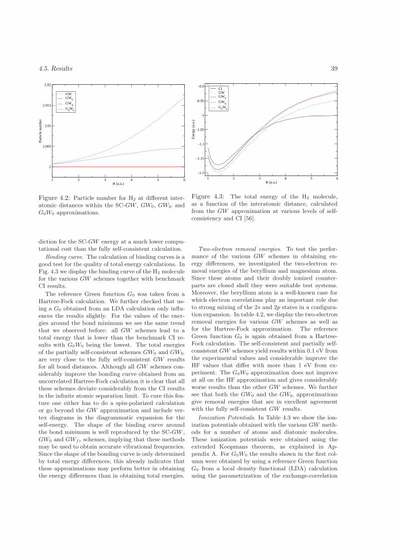
4.5. Results 39
1 2 3 4 5 6R (a.u.)
2
2.005
2.01
2.015
2.02
Part
icle
num
ber
GWGW
0
GWfc
G0W
0
Figure 4.2: Particle number for H2 at different inter-atomic distances within the SC-GW , GW0, GWfc andG0W0 approximations.
diction for the SC-GW energy at a much lower compu-tational cost than the fully self-consistent calculation.
Binding curve. The calculation of binding curves is agood test for the quality of total energy calculations. InFig. 4.3 we display the binding curve of the H2 moleculefor the various GW schemes together with benchmarkCI results.
The reference Green function G0 was taken from aHartree-Fock calculation. We further checked that us-ing a G0 obtained from an LDA calculation only influ-ences the results slightly. For the values of the ener-gies around the bond minimum we see the same trendthat we observed before: all GW schemes lead to atotal energy that is lower than the benchmark CI re-sults with G0W0 being the lowest. The total energiesof the partially self-consistent schemes GW0 and GWfc
are very close to the fully self-consistent GW resultsfor all bond distances. Although all GW schemes con-siderably improve the bonding curve obtained from anuncorrelated Hartree-Fock calculation it is clear that allthese schemes deviate considerably from the CI resultsin the infinite atomic separation limit. To cure this fea-ture one either has to do a spin-polarized calculationor go beyond the GW approximation and include ver-tex diagrams in the diagrammatic expansion for theself-energy. The shape of the binding curve aroundthe bond minimum is well reproduced by the SC-GW ,GW0 and GWfc schemes, implying that these methodsmay be used to obtain accurate vibrational frequencies.Since the shape of the bonding curve is only determinedby total energy differences, this already indicates thatthese approximations may perform better in obtainingthe energy differences than in obtaining total energies.
1 2 3 4 5 6R (a.u.)
-1.2
-1.15
-1.1
-1.05
-1
-0.95
-0.9
Ene
rgy
(a.u
.)
CIGWGW
0
GWfc
G0W
0
Figure 4.3: The total energy of the H2 molecule,as a function of the interatomic distance, calculatedfrom the GW approximation at various levels of self-consistency and CI [56].
Two-electron removal energies. To test the perfor-mance of the various GW schemes in obtaining en-ergy differences, we investigated the two-electron re-moval energies of the beryllium and magnesium atom.Since these atoms and their doubly ionized counter-parts are closed shell they were suitable test systems.Moreover, the beryllium atom is a well-known case forwhich electron correlations play an important role dueto strong mixing of the 2s and 2p states in a configura-tion expansion. In table 4.2, we display the two-electronremoval energies for various GW schemes as well asfor the Hartree-Fock approximation. The referenceGreen function G0 is again obtained from a Hartree-Fock calculation. The self-consistent and partially self-consistent GW schemes yield results within 0.1 eV fromthe experimental values and considerable improve theHF values that differ with more than 1 eV from ex-periment. The G0W0 approximation does not improveat all on the HF approximation and gives considerablyworse results than the other GW schemes. We furthersee that both the GW0 and the GWfc approximationsgive removal energies that are in excellent agreementwith the fully self-consistent GW results.
Ionization Potentials. In Table 4.3 we show the ion-ization potentials obtained with the various GW meth-ods for a number of atoms and diatomic molecules.These ionization potentials were obtained using theextended Koopmans theorem, as explained in Ap-pendix A. For G0W0 the results shown in the first col-umn were obtained by using a reference Green functionG0 from a local density functional (LDA) calculationusing the parametrization of the exchange-correlation
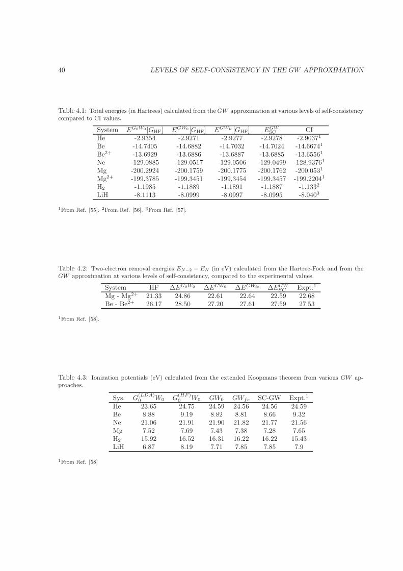
40 LEVELS OF SELF-CONSISTENCY IN THE GW APPROXIMATION
Table 4.1: Total energies (in Hartrees) calculated from theGW approximation at various levels of self-consistencycompared to CI values.
System EG0W0 [GHF] EGW0 [GHF] EGWfc [GHF] EGWSC CI
He -2.9354 -2.9271 -2.9277 -2.9278 -2.90371
Be -14.7405 -14.6882 -14.7032 -14.7024 -14.66741
Be2+ -13.6929 -13.6886 -13.6887 -13.6885 -13.65561
Ne -129.0885 -129.0517 -129.0506 -129.0499 -128.93761
Mg -200.2924 -200.1759 -200.1775 -200.1762 -200.0531
Mg2+ -199.3785 -199.3451 -199.3454 -199.3457 -199.22041
H2 -1.1985 -1.1889 -1.1891 -1.1887 -1.1332
LiH -8.1113 -8.0999 -8.0997 -8.0995 -8.0403
1From Ref. [55]. 2From Ref. [56]. 3From Ref. [57].
Table 4.2: Two-electron removal energies EN−2 − EN (in eV) calculated from the Hartree-Fock and from theGW approximation at various levels of self-consistency, compared to the experimental values.
System HF ∆EG0W0 ∆EGW0 ∆EGWfc ∆EGWSC Expt.1
Mg - Mg2+ 21.33 24.86 22.61 22.64 22.59 22.68Be - Be2+ 26.17 28.50 27.20 27.61 27.59 27.53
1From Ref. [58].
Table 4.3: Ionization potentials (eV) calculated from the extended Koopmans theorem from various GW ap-proaches.
Sys. G(LDA)0 W0 G
(HF )0 W0 GW0 GWfc SC-GW Expt.1
He 23.65 24.75 24.59 24.56 24.56 24.59Be 8.88 9.19 8.82 8.81 8.66 9.32Ne 21.06 21.91 21.90 21.82 21.77 21.56Mg 7.52 7.69 7.43 7.38 7.28 7.65H2 15.92 16.52 16.31 16.22 16.22 15.43LiH 6.87 8.19 7.71 7.85 7.85 7.9
1From Ref. [58]

4.6. Summary and conclusions 41
functional due to Vosko et al. [59]. In all other cases weused a reference Green function from a Hartree-Fockcalculation. We see that the ionization potentials offully self-consistent GW agree well with the experimen-tal values, the main exceptions being the H2 moleculeand the Be atom, which show a deviation of respec-tively 0.8 and 0.5 eV. The other partially self-consistentapproaches GW0 and GWfc yield results that are veryclose to the fully self-consistent results. The G0W0 ap-proximation based on the LDA reference Green func-tion performs a bit worse than the self-consistent GWscheme. For He and LiH there is an error of about 1eV and for Ne and H2 an error of about 0.5 eV. Per-forming a G0W0 calculation based on a HF referenceG0 instead improves the results for several systems butworsens the agreement for H2 which is 1.1 eV in error.The dependence on the reference Green function G0
within the G0W0 method is clearly unsatisfactory. Thepartially self-consistent approximations suffer much lessfrom this problem. For those schemes we found thatchanging the reference Green function from a HF oneto an LDA one, only slightly changes the results.
4.6 Summary and conclusions
We investigated the performance of the GW at differ-ent levels of self-consistency for the case of atoms anddiatomic molecules. Our main motivation for studyingfully self-consistent Φ-derivable schemes was that theyprovide unambiguous results for different observablesand the fact that they satisfy important conservationlaws that are important in future nonequilibrium appli-cations of the theory [18]. We addressed the questionto what extent partially self-consistent schemes can re-produce the results of a fully self-consistent GW cal-culation. We found that both the GW0 method, aswell as the GWfc scheme proposed by us, yield re-sults in close agreement with fully self-consistent GWcalculations. We further checked the number conser-vation properties of the various schemes. The fullyself-consistent GW scheme being Φ-derivable does sat-isfy all conservation laws, but also the partially self-consistent GW0 approximation was shown to be num-ber conserving. The nonself-consistent G0W0 and thepartially self-consistent GWfc approximations both vio-late the number conservation laws but, due to the par-tial self-consistency in GWfc, the errors are much re-duced in this scheme. A major advantage of the latterscheme is, however, that it produces results that areclose to the fully self-consistent GW results at a muchlower computational cost. It will therefore be very valu-able to test this method on solid state systems for whichself-consistent GW calculations are difficult to perform
due to the large computational effort. In this way it willbe possible to get further insight into the performanceof self-consistent GW for a large class of extended sys-tems. Work on application of the fully self-consistentGW method to transport phenomena is in progress [18].

42 LEVELS OF SELF-CONSISTENCY IN THE GW APPROXIMATION

B. The Uniform Power Mesh 43
A Ionization potentials from
the Extended Koopmans
Theorem
Here we give a brief description on the way we extractthe ionization energies from the Green function usingthe extended Koopmans theorem [41, 42, 43, 44, 45].As input, this method only needs the Green functionand its time derivative at τ = 0− on the imaginarytime axis. We define an N − 1 particle state
|ΦN−1[ui] > =
Zdxui(x)ψ(x)|ΨN
0 >, (A-1)
where ui(x) is determined by requiring the functional
EN−1[ui] =〈ΦN−1[ui]|H |ΦN−1[ui]〉〈ΦN−1[ui]|ΦN−1[ui]〉
, (A-2)
which describes the energy of the N−1 particle system,to be stationary with respect to variations in ui. Thisamounts to minimizing the energy of the N − 1 systemby choosing an optimal value for ui. We find
Zdx〈ΨN
0 |ψ†(x′)ˆψ(x), H
˜|ΨN
0 〉ui(x) =
(EN0 − EN−1
i )
Zdx〈ΨN
0 |ψ†(x′)ψ(x)|ΨN0 〉ui(x),(A-3)
where the last term contains the density matrix. Thisquantity is easily obtained from the Green function as
ρ(x,x′) = 〈ψN0 |ψ†
H(x′τ )ψH(xτ )|ΨN0 〉 = lim
η→0G(x,x′,−η)
(A-4)i.e. ρ(x,x′) = G(x,x′; 0−) or ρij = Gij(0
−) in molecu-lar orbital basis [40]. Also the expectation value underthe integral on the righthand side of Eq.(A-3), is easilyobtained from the Green function
−∂τG(x,x′; τ )|τ=0− = 〈ΨN0 |ψ†(x′)
ˆψ(x), H
˜|ΨN
0 〉= ∆(x,x′). (A-5)
In this derivation we used a zero-temperature formu-lation but making a connection to the finite tempera-ture formalism is straightforward. When we take intoaccount that, in the finite temperature formalism, weincluded the chemical potential in the one-body partof the Hamiltonian (see Eq.(4.2), then from (A-3) and(A-5) we obtain the eigenvalue equation
Zdx ∆(x,x′)ui(x) =
= (EN0 − EN−1
i − µ)
Zdx ρ(x,x′)ui(x), (A-6)
where ρ and ∆ are calculated according to Eq.(A-4,A-5). A similar equation for the electron affinities can
similarly be derived starting from an N+1-state. Sinceboth matrices ρ and ∆ are easily evaluated from theGreen function, Eq.(A-6) provides an easy way to ex-tract removal energies from knowledge of the Greenfunction on the imaginary time axis.
For completeness we mention that the extendedKoopmans method also provides a simple way to ex-tract quasiparticle or Dyson orbitals [45] and to con-struct the Green function on the real frequency axis.The Dyson orbitals are given by
fi(x) = 〈ΦN−1i |ψ(x)|ΨN
0 〉 =
=
Zdx′ u∗
i (x′)〈ΨN |ψ†(x′)ψ(x)|ΨN
0 〉 =
=
Zdx′ ρ(x,x′)u∗
i (x′). (A-7)
In terms of these orbitals and the extended Koopmanseigenvalues the hole-part of the Green function is thengiven on the real frequency axis as
G(x,x′;ω) =X
n
fn(x)f∗n(x′)
ω − (EN0 − EN−1
n + µ) + iη.
Similar derivations can be carried out for the affinitiesand the corresponding Dyson orbitals from which theparticle-part of the Green function can be constructedon the real axis.
B The Uniform Power Mesh
The uniform power mesh (UPM) [20] is a one-dimensional grid on an interval [0, β] which becomesmore dense at the endpoints. Therefore, it is well-suitedto describe the Green function on the imaginary timeaxis, since it behaves exponentially around τ = 0 andτ = ±β [40, 20]. The UPM is defined by two integers uand p and the length of the interval β. The procedure toconstruct it is simple: we consider the 2(p−1) intervals[0, βj ] and [β−βj , β] for j = 1, . . . , p−1 with βj = β/2j ,and divide each of these intervals in 2u subintervals ofequal lenght. The endpoints of all these intervals defineour grid which has 2pu+ 1 grid points.
References
[1] Alexander L. Fetter and John Dirk Walecka.Quantum Theory of Many-Particle Systems.McGraw-Hill, New York, 1971.
[2] Eberhard K. U. Gross, Erich Runge, and OlleHeinonen. Many-Particle Theory. Verlag AdamHilger, Bristol, 1991.
44 LEVELS OF SELF-CONSISTENCY IN THE GW APPROXIMATION
[3] Ferdi Aryasetiawan and Olle Gunnarsson. Rep.Prog. Phys, 61:237, 1998.
[4] Wilfried G. Aulbur, Lars Jonsson, and John War-ren Wilkins. Solid State Physics, 54:1, 2000.
[5] Lars Hedin. Phys. Rev., 139:A796, 1965.
[6] Reiner M. Dreizler and Eberhard K. U. Gross.Density Functional Theory, An Approach to theQuantum Many-Body Problem. Springer-Verlag,Berlin, 1990.
[7] Gerald. D. Mahan. Comm. Cond. Mat. Phys., 16:333, 1994.
[8] Bengt Holm and Ulf von Barth. Phys. Rev. B, 57:2108, 1998.
[9] Thomas J. Pollehn, Arno Schindlmayr, andRex William Godby. J. Phys.: Condens. Matter,10:1273, 1998.
[10] Gordon Baym. Phys. Rev., 127:1391, 1962.
[11] Gordon Baym and Leo P. Kadanoff. Phys. Rev.,124:287, 1961.
[12] M. Bonitz, K. Balzer, and Robert van Leeuwen.Phys. Rev. B, 76:045341, 2007.
[13] Carl-Olof Almbladh, Ulf von Barth, and Robertvan Leeuwen. Int. J. Mod. Phys. B, 13:535, 1999.
[14] Kristian Sommer Thygesen and Angel Rubio.Phys. Rev. B, 77:115333, 2008.
[15] Kristian Sommer Thygesen and Angel Rubio. J.Chem. Phys., 126:091101, 2007.
[16] Kristian Sommer Thygesen. Phys. Rev. Lett., 100:166804, 2008.
[17] Xin Wang, Catalin D. Spataru, Mark S. Hybert-sen, and Andrew J. Millis. Phys. Rev. B, 77:045119, 2008.
[18] Petri Myohanen, Adrian Stan, Gianluca Ste-fanucci, and Robert van Leeuwen. Europhys. Lett.,84:67001, 2008.
[19] Arno Schindlmayr and Rex William Godby. Phys.Rev. Lett, 80:1702, 1998.
[20] Wei Ku and Adolfo G. Eguiluz. Phys. Rev. Lett.,89:126401, 2002.
[21] Kris Delaney, Pablo Garcıa-Gonzalez, Angel Ru-bio, Patrick Rinke, and Rex William Godby. Phys.Rev. Lett., 93:249701, 2004.
[22] Bengt Holm. Phys. Rev. Lett., 83:788, 1999.
[23] Pablo Garcıa-Gonzalez and Rex William Godby.Phys. Rev. B, 63:075112, 2001.
[24] Bengt Holm and Ulf von Barth. Physica Scripta,T109:135, 2004.
[25] Viktor Mikhailovich Galitskii and Arkadii Bei-nusovich Migdal. Zh. Eksp. Teor. Fiz., 34:139,1958. [Sov. Phys. JETP, 7, 96 (1958)].
[26] Nils Erik Dahlen, Robert van Leeuwen, and Ulfvon Barth. Phys. Rev. A, 73:012511, 2006.
[27] Robert van Leeuwen, Nils Erik Dahlen, and AdrianStan. Phys. Rev.B, 74:195105, 2006.
[28] M. P. Agnihotri, W. Apel, and W. Weller. Phys.Stat. Sol. B, 245:421, 2008.
[29] Ulf von Barth and Bengt Holm. Phys. Rev. B, 54:8411, 1996.
[30] Takao Kotani and Mark van Schilfgaarde. SolidSt. Comm., 121:461, 2002.
[31] Sergey V. Faleev, Mark van Schilfgaarde, andTakao Kotani. Phys. Rev. Lett., 93:126406, 2004.
[32] Mark van Schilfgaarde, Takao Kotani, andS. Faleev. Phys. Rev. Lett., 96:226402, 2006.
[33] Sergey V. Faleev, Mark van Schilfgaarde,Takao Kotani, Fran cois Leonard, and MichaelP.Desjarlais. Phys.Rev. B, 74:033101, 2006.
[34] Fabien Bruneval, Nathalie Vast, and Lucia Rein-ing. Phys.Rev. B, 74:045102, 2006.
[35] Adrian Stan, Nils Erik Dahlen, and Robert vanLeeuwen. Europhys. Lett., 76:298, 2006.
[36] Takeo Matsubara. Progr. Theoret. Phys, 14:351,1955.
[37] Leonid Veniaminovich Keldysh. Zh. Eksp. Teor.Fiz., 47:1515, 1964. [Sov. Phys. JETP, 20, 1018(1965)].
[38] Pawel Danielewicz. Ann. Phys. (N. Y.), 152:239,1984.
[39] Mathias Wagner. Phys. Rev. B, 44:6104, 1996.
[40] Nils Erik Dahlen and Robert van Leeuwen. J.Chem. Phys., 122:164102, 2005.
[41] Jacob Katriel and Ernest R. Davidson. Proc. Natl.Acad. Sci., USA, 77:4403, 1980.
REFERENCES 45
[42] Orville W. Day, Darwin W. Smith, and Robert C.Morrison. Extension of koopmans’ theorem. ii. ac-curate ionization energies from correlated wave-functions for closed-shell atoms. J. Chem. Phys.,62(1):115–119, 1975. doi: 10.1063/1.430254.
[43] Darwin W. Smith and Orville W. Day. Ex-tension of koopmans’ theorem. i. derivation.J. Chem. Phys., 62(1):113–114, 1975. doi:10.1063/1.430253.
[44] Dage Sundholm and Jeppe Olsen. The exactnessof the extended koopmans’ theorem: A numericalstudy. J. Chem. Phys., 98(5):3999–4002, 1993. doi:10.1063/1.464028.
[45] Robert C. Morrison and Paul W. Ayers. J. Chem.Phys., 103:6556, 1995.
[46] L. Hedin, A. Johansson, B. I. Lundqvist,S. Lundqvist, and V. Samathiyakanit. Arkiv forFysik, 39:97, 1968.
[47] H. N. Rojas, Rex William Godby, and R. J. Needs.Phys. Rev. Lett., 74:1827, 1995.
[48] Carsten Fortmann. J. Phys. A: Math. Theor., 41:445501, 2008.
[49] Bengt Holm. Self-Consistency and the GW Ap-proximation. PhD thesis, Lund University, Swe-den, 1997.
[50] Nicolaas M. Hugenholtz and Leon Van Hove. Phys-ica, 24:363, 1958.
[51] Nils Erik Dahlen, Adrian Stan, and Robert vanLeeuwen. J. Phys. Conf. Ser., 35:324, 2006.
[52] Ferdi Aryasetiawan and Olle Gunnarsson. Phys.Rev. B, 49:16214, 1994.
[53] See EPAPS document for basis sets.
[54] Evert Jan Baerends and Oleg V. Gritsenko. J.Phys. Chem. A, 101:5383, 1997.
[55] Subhas J. Chakravorty, Steven R. Gwaltney,Ernest R. Davidson, Farid A. Parpia, and Char-lotte Froese Fischer. Phys. Rev. A, 47:3649, 1993.
[56] Robert van Leeuwen. Kohn-Sham potentials indensity functional theory. PhD thesis, Vrije Uni-versiteit, Amsterdam, 1994.
[57] Xiangzhu Li and Josef Paldus. J. Chem. Phys.,118:2470, 2003.
[58] S.G. Lias, R.D. Levin, and S.A. Kafafi, IonEnergetics Data in NIST Chemistry Web-Book, NIST Standard Reference Database Num-ber 69, Eds. P.J. Linstrom and W.G. Mal-lard, March 2003, National Institute of Stan-dards and Technology, Gaithersburg MD, 20899(http://webbook.nist.gov).
[59] S. H. Vosko, L. Wilk, and M. Nusair. Can. J.Phys., 58:1200, 1980.

46 LEVELS OF SELF-CONSISTENCY IN THE GW APPROXIMATION

Chapter 5Time propagation of the Kadanoff-Baymequations for inhomogeneous systems
Adrian Stan, Nils Erik Dahlen and Robert van Leeuwen
1Rijksuniversiteit Groningen, Materials Science Centre, Theoretical Chemistry,Nijenborgh 4, 9747AG Groningen, The Netherlands.
2Department of Physics, Nanoscience Center, FIN 40014, University of Jyvaskyla, Jyvaskyla, Finland.3European Theoretical Spectroscopy Facility (ETSF).
Journal of Chemical Physics, accepted (2009)
Abstract
We have developed a time propagation scheme for the Kadanoff-Baym equations for general inhomogeneous systems.These equations describe the time evolution of the nonequilibrium Green function for interacting many-body systems inthe presence of time-dependent external fields. The external fields are treated nonperturbatively whereas the many-bodyinteractions are incorporated perturbatively using Φ-derivable self-energy approximations that guarantee the satisfactionof the macroscopic conservation laws of the system. These approximations are discussed in detail for the time-dependentHartree-Fock, the second Born and the GW approximation.
47
48 TIME-PROPAGATION OF THE KB EQUATIONS
5.1 Introduction
The recent developments in the field of molecular elec-tronics have emphasized the need for further develop-ment of theoretical methods that allow for a systematicstudy of dynamical processes like relaxation and de-coherence at the nanoscale. Understanding these pro-cesses is of utmost importance for making progress inmolecular electronics, whose ultimate goal is to mini-mize the size and maximize the speed of integrated de-vices [1]. To study these phenomena, theoretical meth-ods must allow for the possibility to study the ultrafasttransient dynamics [2, 3] up to the picosecond [4, 5] andfemtosecond timescale, while including Coulomb inter-actions, without violating basic conservation laws suchas the continuity equation [6]. A theoretical frame-work that incorporates these features is the nonequi-librium Green function approach based on the real-time propagation of the Kadanoff-Baym (KB) equa-tions [7, 8, 9, 10, 11, 12, 13, 14]. This method allowsfor systematic inclusion of electron interactions whileproviding results in agreement with the macroscopicconservation laws of the system [7, 6]. In two recentLetters [8, 11] we applied the KB equations to investi-gate the short time dynamics of atoms and moleculesin time-dependent external fields, as well as the trans-port dynamics of double quantum dot devices. It isthe aim of this paper to describe in detail the under-lying method that was only briefly described in thoseLetters. This includes both a description of the theoryas well as the time-propagation algorithm. We furthergeneralize the equilibrium method, described in two re-cent papers [15, 16], to the nonequilibrium domain.We also extend earlier work on the time-propagationmethod of the KB equations for homogeneous sys-tems [17, 18] to the case of inhomogeneous systems. Inthe inhomogeneous case we can not take advantage ofFourier transform techniques anymore. The KB equa-tions become time-dependent matrix equations instead,in which the matrices are indexed by basis function in-dices. The time-stepping algorithm has to take intoaccount the special double-time structure of the equa-tions which are furthermore nonlinear, inhomogeneousand non-Hermitian. Therefore, several standard time-propagation methods can not be used. Our approachis different from the one presented in Refs. [17, 18] byincorporating correlated initial states and the memorythereof, which is described in terms of Green functionswith mixed real and imaginary time arguments. Tosimplify the time-stepping procedure, we make use ofseveral symmetry relations of the Green function.The paper is divided as follows: in section II wepresent the KB equations and their symmetry prop-erties. In section III we discuss the conserving self-
energy approximations that we use, and in section IVwe present the time-propagation method that we de-veloped for systems described within a general basisset representation. Finally in section V we present asummary and conclusions.
5.2 Theory
We consider a many-body system that is initially inequilibrium at a temperature T and with a chemicalpotential µ. At an initial time t0 the system is ex-posed to a time-dependent external field. This externalfield can, for instance, be a bias voltage in a quan-tum transport case, or a laser pulse. The field forcesthe system out of equilibrium and we aim to describethe time-evolution of this nonequilibrium state. In sec-ond quantization the time-dependent Hamiltonian ofthe system reads (throughout this paper we use atomicunits ~ = m = e = 1)
H(t) =
Zdx ψ†(x)h(x, t)ψ(x) + (5.1)
+1
2
Z Zdx1dx2ψ
†(x1)ψ†(x2)v(r1, r2)ψ(x2)ψ(x1),
where x = (r, σ) denotes the space- and spin coordi-nates. The two-body interaction will, in general, be aCoulombic repulsion of the form v(r1, r2) = 1/|r1−r2|.The one-body part of the Hamiltonian is
h(x, t) = −1
2∇2 + w(x, t) − µ, (5.2)
where w(x, t) is a time-dependent external potential.The chemical potential µ of the initial equilibrium sys-tem is absorbed in the one-body part of the Hamil-tonian. The expectation value of an operator O, for asystem initially in thermodynamic equilibrium (t < t0),is given by
〈O〉 = Tr ρO, (5.3)
where ρ = e−βH0/Tr e−βH0 is the statistical operator,H0 is the time-independent Hamiltonian that describesthe system before the time-dependent field is appliedand β = 1/kBT is the inverse temperature. The tracehere represents a summation over a complete set ofstates in Fock space [19]. After the time-dependentexternal field is switched on at time t0, the expectationvalue is given by
〈O(t)〉 =TrU(t0 − iβ, t0)OH(t)
Tr U(t0 − iβ, t0), (5.4)
where OH(t) = U(t0, t)OU(t, t0) is the opera-tor O in the Heisenberg picture and U(t2, t1) =

5.2. Theory 49
Figure 5.1: Keldysh contour. The depicted contourallows for the calculation of observables for times t0 ≤t ≤ T . The initial Green function is calculated on theimaginary track [t0, t0 − iβ]. As we propagate the KBequations in time, for real times t > t0, the turningpoint of the time-contour at t = T moves to the rightalong the real time axis.
T [exp(−iR t2
t1dtH(t))] is the time-ordered evolution op-
erator of the system. We further wrote exp(−βH0) =U(t0 − iβ, t0) as an evolution operator in imaginarytime. If we read the time arguments in Eq.(5.4) fromright to left we see that they follow a time-contouras displayed in Fig.7.1. This contour is also knownas the Keldysh contour [20, 21]. A more detailed in-spection of Eq.(5.4) then shows that the expectationvalue can also be written as a contour-ordered prod-uct [21, 22, 23, 24, 25]. The one-particle Green func-tion is then defined as a countour-ordered product of acreation and an annihilation operator
G(1, 2) = −i〈TC [ψH(1)ψ†H(2)]〉, (5.5)
where TC denotes the time-ordering operator on thecontour and where we used the compact notation 1 =(x1, t1) and 2 = (x2, t2). If we consider the Greenfunction at time t1 = t0 − iβ and use the cyclicproperty of the trace, we find that G(x1t0 − iβ, 2) =−G(x1t0, 2) [24]. Hence, the Green function defined inEq. (5.5) obeys the boundary conditions
G(x1t0, 2) = −G(x1t0 − iβ, 2), (5.6)
G(1,x2t0) = −G(1,x2t0 − iβ). (5.7)
The Green function satisfies the equation of motion
[i∂t1 − h(1)]G(1, 2) = δ(1, 2) +
Z
C
d3Σ(1, 3)G(3, 2),
(5.8)
as well as a corresponding adjoint equation [9, 24]. InEq.(5.8) the time-integration is carried out along thecontour C. The self-energy Σ incorporates the effectsof exchange and correlation in many-particle systemsand is a functional of the Green function that can bedefined diagrammatically [9, 19]. The Green functioncan be written as
G(1, 2) = θ(t, t′)G>(1, 2) + θ(t′, t)G<(1, 2), (5.9)
where θ is a step function generalized to arguments onthe contour i.e. with θ(t, t′) = 1 if t is later on thecontour than t′ and zero otherwise [9]. The greater andlesser components G> and G< respectively, have theexplicit form
G>(1, 2) = −i〈ψH(1)ψ†H(2)〉, (5.10)
G<(1, 2) = i〈ψ†H(2)ψH(1)〉. (5.11)
When one of the arguments is on the vertical track ofthe contour, we adopt the notation [22]
G⌉(1,x2,−iτ2) = G<(1,x2, t0 − iτ2), (5.12)
G⌈(x1,−iτ1, 2) = G>(x1, t0 − iτ1, 2). (5.13)
Finally, for the case when both time arguments are onthe imaginary track of the contour, we have the so-called Matsubara Green function iGM [19]
iGM (x1τ1,x2τ2) = G(x1t0 − iτ1,x2t0 − iτ2), (5.14)
which is a well-known object from the equilibrium the-ory. The factor i in the definition of Eq.(5.14) is aconvention which ensures that GM is a real function.The self-energy Σ has a similar general structure as theGreen function
Σ(1, 2) = ΣHF (1, 2) + θ(t, t′)Σ>(1, 2) + θ(t′, t)Σ<(1, 2).(5.15)
The main difference with Eq.(5.9) is the appearance ofthe term ΣHF which is proportional to a contour deltafunction δ(t1, t2) in the time coordinates [9]. This termhas the explicit form
ΣHF [G](1, 2) = δ(t1, t2)ΣHF (x1,x2, t1), (5.16)
where
ΣHF (x1,x2, t) = iG<(x1t,x2t)v(x1,x2)
−iδ(x1 − x2)
Zdx3v(x1,x3)G
<(x3t,x3t).(5.17)
The structure of this self-energy is that of the Hartree-Fock (HF) approximation. However, in general we willevaluate this expression for Green functions G obtainedbeyond HF level (see section 5.3). Using the form of theself-energy of Eq.(5.15) the contour integrations can be
50 TIME-PROPAGATION OF THE KB EQUATIONS
readily carried out [9, 21] and we find separate equa-tions for the different Green functions G≶ , G⌉⌈ and GM .To display their temporal structure more clearly wesuppress the spatial indices of the Green functions andself-energies. Alternatively, these quantities may be re-garded as matrices [8]. On the imaginary track of thecontour we obtain
[−∂τ − h]GM (τ ) = δ(τ ) +
Z β
0
dτΣM (τ − τ)GM (τ ),
(5.18)where the Green function and the self-energy are func-tions of the time-differences only, i.e. iGM (τ1 − τ2) =G(−iτ1,−iτ2) and iΣM (τ1 − τ2) = Σ(−iτ1,−iτ2), sincethe Hamiltonian is time-independent (and equal to H0)on the imaginary track. Equation (5.18), which deter-mines the Green function of the equilibrium system,has been treated in detail in references [15, 16]. For theother Green functions we obtain
i∂tG≶(t, t′) = hHF (t)G≶(t, t′) + I
≶1 (t, t′),
(5.19)
−i∂t′G≶(t, t′) = G≶(t, t′)hHF (t′) + I
≶2 (t, t′),
(5.20)
i∂tG⌉(t,−iτ ) = hHF (t)G⌉(t,−iτ ) + I⌉(t,−iτ ),
(5.21)
−i∂tG⌈(−iτ, t) = G⌈(−iτ, t)hHF (t) + I⌈(−iτ, t),
(5.22)
where hHF (t) = h(t) + ΣHF (t) and ΣHF (t) is given byEq.(5.17). The retarded and advanced functions for Gand Σ are defined according to
FR/A(t, t′) = ±θ(±t∓ t′)[F>(t, t′)−F<(t, t′)], (5.23)
with F replaced by G and Σ respectively. The so-calledcollision terms I≶ and I⌉⌈ have the form
I≶1 (t, t′) =
Z t
0
dtΣR(t, t)G≶(t, t′)
+
Z t′
0
dtΣ≶(t, t)GA(t, t′)
+1
i
Z β
0
dτ Σ⌉(t,−iτ)G⌈(−iτ , t′), (5.24)
I≶2 (t, t′) =
Z t
0
dtGR(t, t)Σ≶(t, t′)
+
Z t′
0
dtG≶(t, t)ΣA(t, t′)
+1
i
Z β
0
dτ G⌉(t,−iτ)Σ⌈(−iτ , t′), (5.25)
I⌉(t,−iτ ) =
Z t
0
dtΣR(t, t)G⌉(t,−iτ )
+
Z β
0
dτ Σ⌉(t,−iτ )GM (τ − τ ), (5.26)
I⌈(−iτ, t) =
Z t
0
dtG⌈(−iτ, t)ΣA(t, t)
+
Z β
0
dτ GM (τ − τ )Σ⌈(−iτ , t). (5.27)
These equations are readily derived using the conver-sion table of Ref. [21]. From the symmetry relations
G≶(t, t′)† = −G≶(t′, t), (5.28)
Σ≶(t, t′)† = −Σ≶(t′, t), (5.29)
it follows that we only need to calculate G>(t, t′) andΣ>(t, t′) for t > t′ and G<(t, t′) and Σ<(t, t′) for t ≤ t′.
These equations imply that I≶1,2(t, t
′) = −I≶2,1(t
′, t)†.We further have
G⌈(−iτ, t) = G⌉(t,−i(β − τ ))†, (5.30)
Σ⌈(−iτ, t) = Σ⌉(t,−i(β − τ ))†. (5.31)
The symmetry relations (5.28) and (5.30) for the Greenfunction follow directly from its definition, whereas thesymmetry relations (5.29) and (5.31) for the self-energyfollow from Eqs.(3.19) and (3.20) of Ref. [9]. An-other consequence of equations (5.30) and (5.31) is that
I⌈(−iτ, t) =hI⌉(t,−i(β − τ ))
i†
, which means that in
practice it is sufficient to calculate only I>1 , I
<2 and I⌉.
Eqs.(5.19) to (5.22) are known as the Kadanoff-Baymequations [7, 9].Once the Matsubara Green function GM (τ ) is obtainedfrom Eq.(5.18), the Green functions Gx(x =≶, ⌉⌈) canbe calculated by time propagation. Their initial condi-tions are
G>(0, 0) = iGM (0+), (5.32)
G<(0, 0) = iGM (0−), (5.33)
G⌉(0,−iτ ) = iGM (−τ ), (5.34)
G⌈(−iτ, 0) = iGM (τ ). (5.35)
The KB equations, together with the initial conditions,completely determine the Green functions for all timesonce a choice for the self-energy has been made. Theform of the self-energy will be the topic of the nextsection.
5.3 Self-energy
approximations
In the applications of the KB equations it is possibleto guarantee that the macroscopic conservation laws,
5.3. Self-energy approximations 51
such as those of particle, momentum and energy con-servation, are obeyed. Baym [6] has shown that thisis the case whenever the self-energy is obtained from afunctional Φ[G], such that
Σ(1, 2) =δΦ
δG(2, 1). (5.36)
Such approximations to the self-energy are called con-serving or Φ-derivable approximations. Well-knownconserving approximations are the Hartree-Fock, thesecond Born [7], the GW [26], and the T -matrix [7]approximation. In our work we implemented the firstthree of these.The second Born approximation – This approximationfor the self-energy consists of the two diagrams to sec-ond order in the two-particle interaction [7, 27]
Σ(1, 2) = ΣHF (1, 2) + Σ(2)(1, 2), (5.37)
where ΣHF is the HF part of the self energy of Eq.(5.16)and Σ(2) = Σ(2a) + Σ(2b) is the sum of the two terms
Σ(2a) (1, 2) = −i2G(1, 2)
Zd3 d4 v(1, 3)
×G(3, 4)G(4, 3)v(4, 2), (5.38)
Σ(2b) (1, 2) = i2Zd3 d4G(1, 3)v(1, 4)G(3, 4)
×G(4, 2)v(3, 2), (5.39)
where v(1, 2) = v(x1,x2)δ(t1, t2). These terms are usu-ally referred to as the second-order direct and exchangeterms. This approximation to the self-energy has beendiscussed in detail for the equilibrium case in Ref. [15].For the nonequilibrium case we need to calculate thevarious components Σx(x =≶, ⌉⌈). These are explicitlygiven by
Σ(2a),≶ (1, 2) = −i2G≶(1, 2)
Zd3 d4 v(1, 3)
×G≶(3, 4)G≷(4, 3)v(4, 2), (5.40)
Σ(2a),⌉⌈ (1, 2) = −i2Zd3 d4G⌉⌈(1, 2)v(1, 3)
×G⌉⌈(3, 4)G⌈⌉(4, 3)v(4, 2), (5.41)
for the direct diagram, and
Σ(2b),≶ (1, 2) = i2Zd3 d4G≶(1, 3)v(1, 4)G≷(3, 4)
×G≶(4, 2)v(3, 2), (5.42)
Σ(2b),⌉⌈ (1, 2) = i2Zd3 d4G⌉⌈(1, 3)v(1, 4)G⌈⌉(3, 4)
×G⌉⌈(4, 2)v(3, 2), (5.43)
for the second-order exchange diagram. These expres-sions follow immediately from Eqs.(5.38) and (5.39)
with help of the conversion table of Ref. [21].The GW approximation – In the GW approximationthe exchange-correlation part of the self-energy is givenas a product of the Green function G with a dynami-cally screened interaction W [26] . The screened inter-action W satisfies the equation
W (1, 2) = v(1, 2) +
Zd3d4v(1, 3)P (3, 4)W (4, 2).
(5.44)Here, v is the bare Coulomb interaction, and
P (1, 2) = −iG(1, 2)G(2, 1), (5.45)
is the irreducible polarization [26]. However, since thefirst term in Eq.(5.44) is singular in time (proportionalto a delta function) it is convenient, for numerical pur-poses, to define its time-nonlocal part W = W − v [16].From Eq.(5.44) it follows that
W (1, 2) =
Zd3d4v(1, 3)P (3, 4)v(4, 2)
+
Zd3d4v(1, 3)P (3, 4)W (4, 2). (5.46)
In terms of W , the self-energy has the form [26]
Σ(1, 2) = ΣHF (1, 2) + iG(1, 2)W (1, 2). (5.47)
The part Σc = iGW represents the correlation part ofthe self-energy and has the components
Σ≶c (1, 2) = iG≶(1, 2)W≷(2, 1), (5.48)
Σ⌉⌈c (1, 2) = iG⌉⌈(1, 2)W ⌈⌉(2, 1). (5.49)
From the fact that W (1, 2) has the same symmetriesas the contour-ordered density response function [26]χ(1, 2) = −i〈TC [nH (1)nH(2)]〉, where n is the densityoperator, it follows that
W≶(2, 1) = W≷(1, 2) = −[W≷(2, 1)]∗, (5.50)
W ⌉(1, 2) = W ⌈(2, 1). (5.51)
In the following, we will again surpress the spatial coor-dinates in order to display the temporal structure of theequations more clearly. From the symmetry relations(5.50), (5.51), (5.48) and (5.49), and the fact that weonly need Σ>(t, t′) for t > t′ and Σ<(t, t′) for t ≤ t′, itfollows that we only need to calculate W ⌉(t,−iτ ), andW<(t, t′) for t ≤ t′. The latter obey the equations:
W<(t, t′) = vP<(t, t′)v + vX<(t, t′), (5.52)
W ⌉(t,−iτ ) = vP ⌉(t,−iτ )v + vX⌉(t,−iτ ), (5.53)
where
P<(t, t′) = −iG<(t, t′)G>(t′, t), (5.54)
P ⌉(t,−iτ ) = −iG⌉(t,−iτ )G⌈(−iτ, t), (5.55)
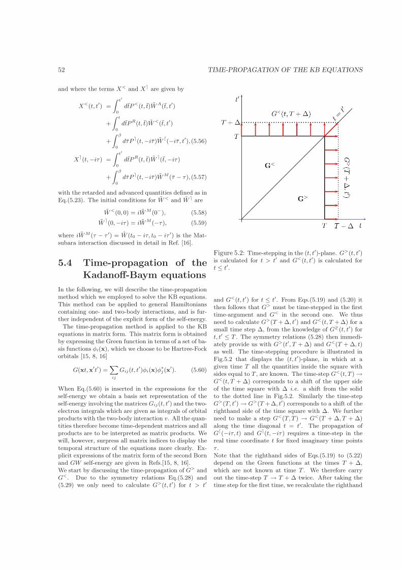
52 TIME-PROPAGATION OF THE KB EQUATIONS
and where the terms X< and X⌉ are given by
X<(t, t′) =
Z t′
0
dtP<(t, t)WA(t, t′)
+
Z t
0
dtPR(t, t)W<(t, t′)
+
Z β
0
dτP ⌉(t,−iτ)W ⌈(−iτ , t′), (5.56)
X⌉(t,−iτ ) =
Z t′
0
dtPR(t, t)W ⌉(t,−iτ )
+
Z β
0
dτP ⌉(t,−iτ)WM(τ − τ ),(5.57)
with the retarded and advanced quantities defined as inEq.(5.23). The initial conditions for W< and W ⌉ are
W<(0, 0) = iWM (0−), (5.58)
W ⌉(0,−iτ ) = iWM (−τ ), (5.59)
where iWM (τ − τ ′) = W (t0 − iτ, t0 − iτ ′) is the Mat-subara interaction discussed in detail in Ref. [16].
5.4 Time-propagation of the
Kadanoff-Baym equations
In the following, we will describe the time-propagationmethod which we employed to solve the KB equations.This method can be applied to general Hamiltonianscontaining one- and two-body interactions, and is fur-ther independent of the explicit form of the self-energy.
The time-propagation method is applied to the KBequations in matrix form. This matrix form is obtainedby expressing the Green function in terms of a set of ba-sis functions φi(x), which we choose to be Hartree-Fockorbitals [15, 8, 16]
G(xt,x′t′) =X
ij
Gij(t, t′)φi(x)φ∗
j (x′). (5.60)
When Eq.(5.60) is inserted in the expressions for theself-energy we obtain a basis set representation of theself-energy involving the matrices Gij(t, t
′) and the two-electron integrals which are given as integrals of orbitalproducts with the two-body interaction v. All the quan-tities therefore become time-dependent matrices and allproducts are to be interpreted as matrix products. Wewill, however, surpress all matrix indices to display thetemporal structure of the equations more clearly. Ex-plicit expressions of the matrix form of the second Bornand GW self-energy are given in Refs.[15, 8, 16].We start by discussing the time-propagation of G> andG<. Due to the symmetry relations Eq.(5.28) and(5.29) we only need to calculate G>(t, t′) for t > t′
Figure 5.2: Time-stepping in the (t, t′)-plane. G>(t, t′)is calculated for t > t′ and G<(t, t′) is calculated fort ≤ t′.
and G<(t, t′) for t ≤ t′. From Eqs.(5.19) and (5.20) itthen follows that G> must be time-stepped in the firsttime-argument and G< in the second one. We thusneed to calculate G>(T + ∆, t′) and G<(t, T + ∆) for asmall time step ∆, from the knowledge of G≷(t, t′) fort, t′ ≤ T . The symmetry relations (5.28) then immedi-ately provide us with G>(t′, T + ∆) and G<(T + ∆, t)as well. The time-stepping procedure is illustrated inFig.5.2 that displays the (t, t′)-plane, in which at agiven time T all the quantities inside the square withsides equal to T , are known. The time-step G<(t, T ) →G<(t, T + ∆) corresponds to a shift of the upper sideof the time square with ∆ i.e. a shift from the solidto the dotted line in Fig.5.2. Similarly the time-stepG>(T, t′) → G>(T +∆, t′) corresponds to a shift of therighthand side of the time square with ∆. We furtherneed to make a step G<(T, T ) → G<(T + ∆, T + ∆)along the time diagonal t = t′. The propagation ofG⌈(−iτ, t) and G⌉(t,−iτ ) requires a time-step in thereal time coordinate t for fixed imaginary time pointsτ .Note that the righthand sides of Eqs.(5.19) to (5.22)depend on the Green functions at the times T + ∆,which are not known at time T . We therefore carryout the time-step T → T + ∆ twice. After taking thetime step for the first time, we recalculate the righthand

5.4. Time-propagation of the Kadanoff-Baym equations 53
sides of Eqs.(5.19) to (5.22) and repeat the time-stepT → T+∆ using an average of the old and new collisionand HF terms. Since the term hHF (t) in Eqs.(5.19) to(5.22) can attain large values, it is favorable to elimi-nate this term from the time-stepping equations. Foreach time-step T → T+∆ we therefore absorb the termin a time-evolution operator of the form
U(t) = e−ihHF(T )t, (5.61)
where hHF (T ) = h(T +∆/2)+ΣHF (T ), where h is theone-body part of the Hamiltonian of Eq.(5.2). The one-body Hamiltonian h(t) is explicitly known as a func-tion of time and can be evaluated at half the time-step.The term ΣHF is only known at time T and will berecalculated in the repeated time-step. In terms of theoperator U(t) of (5.61) we define new Green functionmatrices gx(x =≶, ⌉⌈), as
G≶(t1, t2) = U(t1)g≶(t1, t2)U
†(t2), (5.62)
G⌉(t1,−iτ2) = U(t1)g⌉(t1,−iτ2), (5.63)
G⌈(−iτ1, t2) = g⌉(−iτ1, t2)U†(t2). (5.64)
We can now transform Eqs.(5.19) to (5.22) into equa-tions for gx. For instance, g> satisfies the equation
i∂tg>(t, t′) = U†(t)(hHF (t) − hHF )G>(t, t′)U(t′)
+U†(t)I>1 (t, t′)U(t′). (5.65)
Since hHF ≈ hHF (t) for times T ≤ t ≤ T + ∆, we canneglect for these times the first term on the right handside of Eq.(5.65). We then find
G>(T + ∆, t2) = U(T + ∆)g>(T + ∆, t2)U†(t2) =
= U(T + ∆)
»g>(T, t2) +
Z T+∆
T
dt∂tg>(t, t2)
–U†(t2)
≈ U(∆)G>(T, t2) −
iU(∆)
Z T+∆
T
dt eihHF(t−T )
ffI>1 (T, t2)
= U(∆)G>(T, t2) − V (∆)I>1 (T, t2), , (5.66)
where V (∆) is defined as
V (∆) = (hHF)−1[1 − e−ihHF∆]. (5.67)
Similarly for G<, which is propagated using Eq.(5.20),we find the equation
G<(t1, T + ∆) = G<(t1, T )U†(∆)
−I<2 (t1, T )V †(∆). (5.68)
For time-stepping along the time-diagonal we use
i∂tG<(t, t) = [hHF (t), G<(t, t)]
+I<1 (t, t) − I<
2 (t, t), (5.69)
which follows directly from a combination of the equa-tions for G< of Eqs.(5.19) and (5.20). The correspond-ing equation for g<(t, t) on the time diagonal then be-comes
i∂tg<(t, t) = U†(t)[hHF (t) − hHF , G<(t, t)]U(t)
+U†(t)(I<1 (t, t) − I<
2 (t, t))U(t). (5.70)
From this equation we then obtain
G<(T + ∆, T + ∆) =
= U(T + ∆)g<(T + ∆, T + ∆)U†(T + ∆)
= U(∆)G<(T, T )U†(∆) −
iU(∆)
»Z ∆
0
dtU†(t)I12U(t)
–U†(∆), (5.71)
where we defined I12 = I<1 (T, T ) − I<
2 (T, T ). By usingthe operator expansion
eABe−A = B + [A,B] +1
2[A, [A,B]]
+1
3[A,
1
2[A, [A,B]]] + . . . , (5.72)
it follows that
−iZ ∆
0
dt U†(t)I12U(t) =∞X
n=0
C(n), (5.73)
where
C(n) =i∆
n+ 1[hHF , C(n−1)], (5.74)
and C(0) = −i∆I12. If we insert Eq.(5.73) intoEq.(5.71) we finally obtain
G<(T+∆, T+∆) = U(∆)
"G<(T, T ) +
∞X
n=0
C(n)
#U†(∆)
(5.75)We found that keeping terms for n ≤ 3 only, yields suf-ficient accuracy. We now consider the time propagationfor the mixed real and imaginary time Green functions.For g⌉ we have the equation
i∂tg⌉(t,−iτ ) = U(t)†(hHF (t) − hHF )G⌉(t,−iτ )
+U(t)†I⌉(t,−iτ ). (5.76)
This yields, similarly as in Eq.(5.66) and (5.68)
G⌉(T + ∆,−iτ2) = U(∆)G⌉(T,−iτ2)−V (∆)I⌉(T,−iτ2). (5.77)
Finally, for G⌈ we have
G⌈(−iτ1, T + ∆) = G⌈(−iτ1, T )U(∆)†
−I⌈(−iτ1, T )V (∆)†. (5.78)

54 TIME-PROPAGATION OF THE KB EQUATIONS
The Eqs. (5.66), (5.68), (5.71), (5.77) and (5.78) formthe basis of the time-stepping algorithm. At each time-step, it requires the construction of the step operatorsU(∆) and V (∆) and therefore the diagonalizationof hHF for every time-step. As mentioned before,the righthand sides of Eqs.(5.19) to (5.22) depend onthe Green functions at the times T + ∆ which arenot known at time T . We therefore carry out thetime-step T → T+∆ twice. The procedure is as follows:
(1) The collision integrals and hHF at time Tare calculated from the Green functions for timest, t′ ≤ T .(2) A step in the Green function G(T ) → G(T + ∆)is taken according to Eqs.(5.66), (5.68), (5.71), (5.77)and (5.78).(3) New collision integrals I>
1 (T + ∆, t), I>2 (t, T +
∆), I⌉(T + ∆,−iτ ) and I⌈(−iτ, T + ∆) are calcu-lated by inserting the new Green functions for timest, t′ ≤ T + ∆ into Eqs.(5.24) to (5.27).(4) The values of the collision integrals andthe Hartree-Fock self-energy are approxi-mated by I = (I(T ) + I(T + ∆))/2 andΣHF = (ΣHF (T ) + ΣHF (T + ∆))/2 where I(T )and I(T + ∆) are the collision terms calculated underpoints (1) and (3).(5) The Green function is then propagated fromG(T ) → G(T + ∆) using the average values I andhHF = h(T +∆/2)+ ΣHF in Eqs.(5.66), (5.68), (5.71),(5.77) and (5.78).
This concludes the general time-stepping proce-dure for the Green functions.We finally consider the calculation of W< and W ⌉
from Eqs. (5.52) and (5.53). As a consequence of thesymmetry relation (5.50), we only need to calculateW<(t, t′) for t < t′. In a time step from T to T +∆ weneed to calculate W<(t, T + ∆) for t ≤ T + ∆ from theknown values of W<(t, T ) for t ≤ T . The first termon the righthand side of Eq.(5.52) can be calculateddirectly from G<(t, T +∆) and G>(T +∆, t). However,the last term X<(t, T + ∆) of Eq.(5.52) depends onthe, still undetermined, values W<(t, T + ∆). Wetherefore employ an iterative scheme. As a first guessfor W<(t, T + ∆) we take W<(t, T + ∆) = W<(t, T )for t ≤ T and W<(T + ∆, T + ∆) = W<(T, T ). Wetherefore use the values of W< on the known sides ofthe time square at time T (solid lines in Fig.5.2) asinitial guesses for the stepped sides (dotted lines inFig.5.2) at T + ∆. As an initial guess for the valueof W< at the new diagonal point (T + ∆, T + ∆), wetake the value at the previous diagonal point (T, T ).We then calculate the quantity X<(t, T + ∆) fort ≤ T + ∆ and obtain a new value for W<(t, T + ∆)
from Eq.(5.52). This value is then inserted back intothe righthand side of Eq.(5.52) and the process isrepeated until convergence is reached. Similarly weinitialize W ⌉(T + ∆,−iτ ) = W ⌉(T,−iτ ) and solveEq.(5.53) in the same manner as for W<.This concludes our derivation of the time-steppingalgorithm of the KB equations. The propagationmethod described here has been used in two recentLetters [8, 11] where also values for the numericalparameters are given. It is clear that the choice ofthese parameters depends strongly on the type ofsystem considered, and on the strength of the appliedexternal fields.
5.5 Summary and conclusions
We presented a detailed account of the KB equationsand discussed in detail their structure, initial condi-tions and symmetries. We developed an algorithm forthe time-propagation of the KB equations in which thesymmetry relations for the Green functions were usedto reduce the set equations that needed to be solved. Intwo recent Letters [8, 11] we applied the method to thecase of atoms and molecules in external time-dependentfields and to the case of transient transport dynamicsof double quantum dots. We therefore conclude thattime-propagation of the KB equations can be used as apractical method to calculate the nonequilibrium prop-erties of a wide variety of many-body quantum systems,ranging from atoms and molecules to quantum dots andquantum wells. Moreover, the present work can bereadily extended to other Green function formalisms,such as the Nambu formalism [28, 29] for superconduct-ing systems. Also future extension to bosonic systems isstraightforward. Work along these lines is in progress.
References
[1] Gianaurelio Cuniberti, Giorgos Fagas, and KlausRichter, editors. Introducing Molecular Electron-ics, volume 680. Springer, New York, 2005.
[2] Toshiki Hayashi, Toshimasa Fujisawa, H. D.Cheong, Yoon Hee Jeong, and Yoshiro Hirayama.Phys. Rev. Lett., 91:226804, 2003.
[3] J. M. Elzerman, R. Hanson, L. H. Willems vanBeveren, B. Witkamp, L. M. K. Vandersypen, andL. P. Kouwenhoven. Nature, 430:431, 2003.
[4] Jagdeep Shah, editor. Ultrafast Spectroscopyof Semiconductors and Semiconductor Nanostruc-tures. Springer, Berlin, 1999.

REFERENCES 55
[5] M. Merano, S. Sonderegger, A. Crottini, S. Collin,P. Renucci, E. Pelucchi, A. Malko, M.H. Baier,E. Kapon, B. Deveaud, and J. D. Ganiere. Nature,438:479, 2007.
[6] Gordon Baym. Phys. Rev., 127:1391, 1962.
[7] Leo P. Kadanoff and Gordon Baym. Quantum Sta-tistical Mechanics. W. A. Benjamin, Inc., NewYork, 1962.
[8] Nils Erik Dahlen and Robert van Leeuwen. Phys.Rev. Lett., 98:153004, 2007.
[9] Pawel Danielewicz. Ann. Phys. (N. Y.), 152:239,1984.
[10] Nai-Hang Kwong and Michael Bonitz. Phys. Rev.Lett., 84:1768, 2000.
[11] Petri Myohanen, Adrian Stan, Gianluca Ste-fanucci, and Robert van Leeuwen. Europhys. Lett.,84:67001, 2008.
[12] W. Schafer. J. Opt. Soc. Am., B13:1291, 1996.
[13] Michael Bonitz, Dietrich Kremp, D. C. Scott,Rolf Binder, Wolf-Dietrich Kraeft, and H. SigurdKohler. J. Phys. Cond. Matter, 8:6057, 1996.
[14] Rolf Binder, H. Sigurd Kohler, Michael Bonitz,and Nai-Hang Kwong. Phys. Rev., B55:5110, 1997.
[15] Nils Erik Dahlen and Robert van Leeuwen. J.Chem. Phys., 122:164102, 2005.
[16] Adrian Stan, Nils Erik Dahlen, and Robert vanLeeuwen. J. Chem. Phys., 130:114105, 2009.
[17] H. Sigurd Kohler, Nai-Hang Kwong, andHashim A Yousif. Comp. Phys. Comm., 123:123,1999.
[18] Michael Bonitz and Dirk Semkat. In MichaelBonitz and Dirk Semkat, editors, Introduction toComputational Methods in Many-Body Physics,page 171. Rinton Press, Princeton, 2006.
[19] Alexander L. Fetter and John Dirk Walecka.Quantum Theory of Many-Particle Systems.McGraw-Hill, New York, 1971.
[20] Leonid Veniaminovich Keldysh. Zh. Eksp. Teor.Fiz., 47:1515, 1964. [Sov. Phys. JETP, 20, 1018(1965)].
[21] Robert van Leeuwen, Nils Erik Dahlen, Gian-luca Stefanucci, Carl-Olof Almbladh, and Ulf vonBarth. In Miguel A. L. Merques, Carsten A.Ullrich, Fernando Nogueira, Angel Rubio, KieronBurke, and Eberhard K. U. Gross, editors, Time-dependent Density Functional Theory, page 33.Springer, Berlin Heidelberg, 2006.
[22] Gianluca Stefanucci and Carl-Olof Almbladh.Phys. Rev. B, 69:195318, 2004.
[23] Mathias Wagner. Phys. Rev. B, 44:6104, 1996.
[24] Nils Erik Dahlen, Adrian Stan, and Robert vanLeeuwen. J. Phys. Conf. Ser., 35:324, 2006.
[25] Nils Erik Dahlen, Robert van Leeuwen, and AdrianStan. J. Phys. Conf. Ser., 35:340, 2006.
[26] Lars Hedin. Phys. Rev., 139:A796, 1965.
[27] Gordon Baym and Leo P. Kadanoff. Phys. Rev.,124:287, 1961.
[28] Yoichiro Nambu. Phys. Rev., 117:648, 1960.
[29] John Robert Schrieffer. Theory of Superconductiv-ity. Addison-Wesley, 1988.

56 TIME-PROPAGATION OF THE KB EQUATIONS
Chapter 6A many-body approach to quantumtransport dynamics: Initial correlations andmemory effects
Petri Myohanen1, Adrian Stan1, Gianluca Stefanucci2,3 and Robert van Leeuwen1,3
1Department of Physics, Nanoscience Center, FIN 40014, University of Jyvaskyla, Jyvaskyla, Finland, EU2Dipartimento di Fisica, Universita di Roma Tor Vergata - Via de la Ricerca Scientifica 1, I-00133 Rome, Italy, EU
3European Theoretical Spectroscopy Facility (ETSF).
Europhysics Letters, 84, 67001 (2008)
Abstract
We study time-dependent quantum transport through a correlated double quantum dot (DQD) model system by meansof time-propagation of the nonequilibrium many-body Green’s function. The theory is an extension of the Kadanoff-Baymapproach for finite inhomogeneous systems [Phys. Rev. Lett. 98, 153004 (2007)] to open inhomogeneous systems andgeneralizes the Meir-Wingreen formula to include initial correlations and memory effects. Important features of the theoryare 1) the possibility to study the ultrafast dynamics of transients and other time-dependent regimes and 2) the inclusionof exchange and correlation effects in a conserving approximation scheme. We calculate time-dependent local currentsand densities for different many-body approximations and highlight the role of initial correlations and memory effects onthe transient dynamics. Furthermore we show that coherent charge oscillations on the DQD are strongly affected by theconfined Coulomb interaction and can be directly related to the local equilibrium spectral density.
57

58 MANY-BODY APPROACH TO QUANTUM TRANSPORT
6.1 Introduction
In this Letter we propose a many-body approach thatcan deal with both electronic interactions and time de-pendence in quantum transport. Within such a frame-work one can systematically study dynamical processeslike relaxation and decoherence at the nanoscale. Un-derstanding these processes is of utmost importancein molecular electronics [1] whose ultimate goal is tominiaturize the size and maximize the speed of inte-grated devices. Important features of our method are1) the possibility to study the ultrafast transient dy-namics [2, 3, 4] up to the picosecond [5, 6] and fem-tosecond timescale and 2) the inclusion of Coulombinteractions without violating the continuity equation[7]. Feature 1) was incorporated in some recently pro-posed one-particle frameworks and was exploited to ad-dress several issues in time-dependent (TD) quantumtransport (QT) [8, 9, 10, 11, 12]. These frameworkscan, in principle, be combined with TD density func-tional theory [13, 14, 15], thus providing a route toinclude Coulomb interactions (possibly in a conserv-ing way [16]). Feature 2) is a pivotal requirement asrealistic time evolutions must preserve basic conser-vation laws. Conserving approximations [7] like, e.g.self-consistent Hartree-Fock (HF), second Born (2B) orGW , have recently been employed in the context of QTbut the implementations have been, sofar, restricted tosteady-state regimes [17, 18, 19, 20, 21].
We propose an approach which combines both fea-ture 1) and 2) and which is based on the real-timepropagation of the Kadanoff-Baym (KB) equations[22, 23, 24, 25] for open and interacting systems in anout of steady-state regime. Below we describe the the-oretical framework and employ it to perform ultrafasttransport spectroscopy simulations in double quantumdot (DQD) model devices.
6.2 General formalism
The KB equations are equations of motion for thenonequilibrium Green function from which basic prop-erties of the system can be calculated. We consider a setα of noninteracting electronic reservoirs connectedvia a tunneling Hamiltonian to an interacting many-body quantum system C. The Green function G(z, z′)(we suppress basis indices) projected on C obeys theequation of motion [22]
[i∂z − h(z)]G(z, z′) = δ(z, z′) +
Z
c
dz Σ(z, z)G(z, z′)
(6.1)where z and z′ are time-coordinates on the Keldysh con-tour c [24]. We consider systems initially (times t < 0)
contacted and in equilibrium at inverse temperature βand chemical potential µ. The corresponding contour isdescribed in Refs. [14] and [22]. In Eq.(6.1), h(z) is theone-body Hamiltonian of the interacting system C andΣ is the time-nonlocal self-energy. The latter describesthe effects of many-body interactions and embedding ofthe system and is the sum of a many-body self-energyΣMB[G] and an embedding self-energy Σemb. The for-mer is a functional of the projected Green function Gonly and can be expressed in terms of Feynman dia-grams while the latter is a sum Σemb =
Pα Σemb,α
where
Σemb,α(z, z′) = tCα(z)gα(z, z′)tαC(z′). (6.2)
In Eq.(6.2) gα is the Green function of the uncontactedlead α and matrices tCα and tαC describe the cou-plings of system C to the leads. The TD equationsobtained from Eq.(6.1) by restricting time-argumentsto different parts of the Keldysh contour are known asthe Kadanoff-Baym equations [23, 22, 24, 25] and arethe main tools of this work. As the system is driven outof equilibrium by a TD bias voltage, the current flowinginto lead α is obtained by taking the time derivative ofthe total number of particles in α [26] and reads
Iα(t) = −2ReTrC [G< · ΣAα,emb +GR · Σ<
α,emb](t, t)
−2ReTrC [G⌉ ⋆ Σ⌈α,emb](t, t) (6.3)
where the trace is taken over the central region indicesand the products · and ⋆ denote integrations over thereal and imaginary tracks of the contour (see Ref. [14]for details). The objects superindexed with ≶, ⌉⌈ cor-respond to time arguments on different parts of theKeldysh contour [14, 22] and R/A denote the retardedand advanced components. The last term in Eq.(6.3)explicitly accounts for the effects of initial correlationsand initial-state dependence. If one assumes that bothdependencies are washed out in the long-time limit(t→ ∞) then the last term in Eq.(6.3) vanishes and theMeir-Wingreen formula [26] is recovered. The KB ap-proach provides a natural tool to investigate the validityof this assumption which has remained unexplored so-far, and that we partly address below.Using the KB equations we first solve the embedded andcorrelated equilibrium problem and then propagate thesystem in time after applying a time-dependent bias (cf.Fig. 1 of Ref. [22]). For this we extend the implemen-tation of Ref. [22] to open systems, i.e., by replacingΣMB[G] with ΣMB[G] + Σemb. Different TD perturba-tions allow us to address several open issues in corre-lated TD-QT. 1) We can set the tunneling Hamiltonianto zero at the initial time [27] or not [28] (C initiallyuncontacted or contacted) and study the effects of theinitial conditions. 2) Many-body interactions can be

6.3. Results 59
included in equilibrium (t < 0) or switched on at latertimes and the effects of initial correlations [24] on tran-sient and steady-state properties can be highlighted. 3)Due to the nonlinearity of the problem and possibly tothe nonlocality in time of ΣMB[G] phenomena like bista-bility, hysteresis, etc. may occur. 4) We can study acbiases, pulses or other kind of TD biases as well as TDgate voltages and TD contacts in correlated QT. Westress that for a given approximate ΣMB[G] all kinds ofTD perturbations within the KB approach require thesame computational effort.
We employ the KB approach to study an interact-ing DQD model device coupled to noninteracting one-dimensional leads. Time-dependent currents and den-sities are calculated and several of the issues mentionedin points 1)-4) above are addressed. The full system isdescribed by:
H(t) =X
ij,σα
[tαij + δijUα(t)]c†iσαcjσα +
X
ij,σ
tij d†iσdjσ +
1
2
X
ij,σσ′
vij d†iσ d
†jσ′ djσ′ diσ +
X
ij,σα
Vi,jα[d†iσ cjσα + c†jσαdiσ] (6.4)
where i, j are site indices, σ, σ′ spin indices and wherec†, c and d†, d are the creation and annihilation oper-ators for leads and device respectively. The first termin Eq.(6.4) describes the leads with a TD bias Uα(t)while the second and third term describe the one-bodyand many-body interactions of the device. Finally thelast term describes the coupling between the leads andthe device. Since we consider semi-infinite leads, theenergy band of the leads is continuous with a finiteband width and we therefore do not employ the oftenused wide band limit approximation. We stress thatthe KB approach is not limited to 1-D leads as theleads enter only via the embedding self-energy.
6.3 Results
The system consists of a two-level DQD coupled toa left and right lead (i.e. α = L,R). We use theparameters t11 = t22 = 0 and t12 = t21 = −1. For themany-body interactions we take v11 = v22 = 2 andv12 = v21 = 1. The chemical potential µ for the wholeinitial equilibrium system is set at the middle of the HFgap and is determined by a Hartree-Fock calculationon the uncontacted but correlated central region whichyields the value µ = 2 with the parameters describedabove. For the semi-infinite leads we use t
L/Rii = µ and
tL/Rij = −1.5 if i and j are neighboring sites and zero
otherwise. The leads are coupled to the central regionby coupling elements V1,jL = V2,jR = V when j is thefirst site on the left or right lead and zero otherwise(we use V = 0.5 and V = 0.8). We further take β = 90(zero temperature limit). All quantities are expressedin atomic units. For ΣMB we employ the HF, 2B andGW approximations which have also been used inearlier transport studies [20, 21]. The GW approxima-tion includes the dynamical screening of the electroninteraction whereas 2B includes all Feynman diagramsto second order in the bare interaction. In the smallsystem that we study here the second order exchangediagram (incorporated in 2B but not in GW ) is notnegligible and therefore the 2B approximation givesprobably the most accurate description of electroniccorrelations.Correlations in transients. In Fig.6.1 we show thetransient currents flowing into the right lead andthe spectral functions for the HF, 2B and GWapproximations. The system is driven by a symmet-rically switched bias UL(t) = −UR(t) = Uθ(t) withU = 1.0, where θ(t) is a Heaviside function, i.e. we con-sider a sudden switch on of the bias at t = 0. Resultsare displayed for weak (V = 0.5) and strong coupling(V = 0.8) of the central region to the leads. We firstconsider the spectral functions which are defined asA(T,ω) = −Tr Im
Rdt eiωt[G> − G<](T + t
2, T − t
2)
where T = (t1 + t2)/2 and t = t1 − t2. We find thatafter the steady state has been reached the spectralfunctions do not depend on T anymore. In equilibriumthe spectral peaks are at ǫ01,2 = 0.5, 3.5 for HF, 2Band GW . For the biased system (Fig.1c and inset ofFig.1b) the electron correlations beyond HF lead to anarrowing of the gap between the spectral peaks anda broadening of the spectral function. This bias de-pendent gap closing mechanism was recently identifiedby Thygesen [21]. The positions ǫ1,2 of the spectralpeaks strongly affect the final steady state currents asthey are largest when both spectral peaks enter thebias window, i.e. for biases such that µ ± U ≈ ǫ1,2.This condition is much better satisfied for 2B and GWthan for HF and explains the higher values in 2B (thehighest) and GW (top panels of Fig.6.1). Let us nowfocus on the temporal structure of the transients. Thetransient currents show an oscillation that becomesmore pronounced when we weaken the coupling fromV = 0.8 to V = 0.5. The modulus of the Fouriertransform of the current (minus its steady state value)is displayed in the inset of Fig.1c. There is a frequencypeak at 2.5 in all many-body approximations andfor HF also one at 0.5 (for 2B and GW there is abroad peak around zero). These frequencies cannotbe directly related to the spectral functions of Fig.6.1as those correspond to the steady state limit when
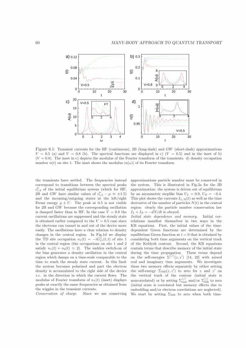
60 MANY-BODY APPROACH TO QUANTUM TRANSPORT
0
0.04
0.08
0.12
0 10 20 30
I(t)
t
V=0.5HF2B
GW 0
0.1
0.2
0.3
0 10 20 30
I(t)
t
V=0.8 0
8
0 2 4
A(ω
)
0
5
10
15
20
0 1 2 3 4
A(ω
)
ω
V=0.5
0 2 4
FT
0.95
1
0 10 20 30
n(t)
t
V=0.5
0 2 4
|n(ω
)|
a) b)
c) d)
Figure 6.1: Transient currents for the HF (continuous), 2B (long-dash) and GW (short-dash) approximationsV = 0.5 (a) and V = 0.8 (b). The spectral functions are displayed in c) (V = 0.5) and in the inset of b)(V = 0.8). The inset in c) depicts the modulus of the Fourier transform of the transients. d) density occupationnumber n(t) on site 1. The inset shows the modulus |n(ω)| of its Fourier transform
the transients have settled. The frequencies insteadcorrespond to transitions between the spectral peaksǫ01,2 of the initial equilibrium system (which for HF,2B and GW have similar values of ǫ01,2 − µ ≈ ±1.5)and the incoming/outgoing states at the left/rightFermi energy µ ± U . The peak at 0.5 is not visiblefor 2B and GW because the corresponding oscillationis damped faster than in HF. In the case V = 0.8 thecurrent oscillations are suppressed and the steady stateis obtained earlier compared to the V = 0.5 case sincethe electrons can tunnel in and out of the device moreeasily. The oscillations have a clear relation to densitychanges in the central region. In Fig.1d we displaythe TD site occupation n1(t) = −iG<
11(t, t) of site 1in the central region (the occupations on site 1 and 2satisfy n1(t) + n2(t) ≃ 2). The sudden switch-on ofthe bias generates a density oscillation in the centralregion which damps on a time-scale comparable to thetime to reach the steady state current. In this limitthe system becomes polarized and part the electrondensity is accumulated to the right side of the devicei.e. in the direction in which the current flows. Themodulus of Fourier transform of n1(t) (inset) displayspeaks at exactly the same frequencies as obtained fromthe wiggles in the transient currents.Conservation of charge. Since we use conserving
approximations particle number must be conserved inthe system. This is illustrated in Fig.2a for the 2Bapproximation: the system is driven out of equilibriumby an asymmetric steplike bias UL = 0.9, UR = −0.4.This plot shows the currents IL/R(t) as well as the timederivative of the number of particles N(t) in the centralregion: clearly the particle number conservation lawIL + IR = −dN/dt is obeyed.Initial state dependence and memory. Initial cor-relations manifest themselves in two ways in theKB equations. First, the initial values of the time-dependent Green functions are determined by theequilibrium Green function at t = 0 that is obtained byconsidering both time arguments on the vertical trackof the Keldysh contour. Second, the KB equationscontain terms that describe memory of the initial stateduring the time propagation. These terms dependon the self-energies Σ⌉/⌈(z, z′) [14, 22] with mixedreal and imaginary time arguments. We investigatethese two memory effects separately by either settingthe self-energy ΣMB(z, z′) to zero for z and z′ onthe vertical track of the contour (initial state is
noncorrelated) or by setting Σ⌉/⌈emb and/or Σ
⌉/⌈MB to zero
(initial state is correlated but memory effects due toembedding and/or electron correlations are neglected).We start by setting ΣMB to zero when both time-

6.3. Results 61
-0.08
-0.04
0
0.04
0 10 20
I(t)
t
V=0.5
ILIR
IL+IR-dN/dt
0
0.1
0.2
0.3
0.4
0 10 20 30
I(t)
t
V=0.5
2B2B0
0
0.05
0.1
0 10 20
I(t)
t
V=0.5
2B2B 12B 2
HFHF 1
0
0.1
0 10 20 30 40
I(t)
t
V=0.5
StepErf
Sin2
a) b)
c) d)
Figure 6.2: a) Transient currents for asymmetric bias (see text). b) Transient currents for 2B with and with-out the initially interacting ground state (2B and 2B0 correspondingly).c) Transient currents in HF and 2B
approximations with and without the memory terms Σ⌉/⌈emb/MB (see text). d) Transient currents for different
bias-switchings. All panels correspond to V = 0.5
arguments are on the vertical track of the contour fora situation in which we propagate an unbiased systemfrom time t = 0 to a finite time t0 at which timewe switch on a sudden symmetric bias, i.e. we useUL(t) = −UR(t) = θ(t − t0)U . Since electron correla-tions are taken into account in the time propagationbut not in the initial state there will be a chargeredistribution for times t > 0. The result is comparedto an initially correlated KB propagation. We taket0 = 20 and U = 1.0. The noninteracting systemat t = 0 has spectral peaks at energies ǫ01,2 = ±1.0(i.e. below the chemical potential at µ = 2). As aresult of electron interactions for t > 0 we find upwardshifts in the spectral peaks yielding one peak aboveand one peak below µ. As a consequence a chargeof about 2 electrons is pushed into the leads. Thecorresponding current, shown in Fig.2b for the 2Bapproximation, is saturated before the bias voltageis switched on at time t0. For later times t > t0 thetransient currents with inclusion and with neglect ofinitial correlations are indistinguisable. We thereforeconclude that the initially uncorrelated system hasrelaxed to a correlated state when the bias is switchedon.To study how initial states are remembered duringtime-propagation we compare full solutions of the KB
equations to ones in which we neglect the terms Σ⌉/⌈emb
and/or Σ⌉/⌈MB. However, at the initial time t = 0 we
still employ the fully correlated embedded equilibriumGreen function. The results are displayed in Fig.2c forthe HF and 2B approximations. We find that neglectof the memory terms Σ⌉/⌈ has a considerable effecton the transient currents. In the HF case these termsonly contain the embedding self-energy Σ
⌉/⌈emb (as ΣMB
of HF is purely local in time) and therefore the termdescribes memory of the initial contacting of leads.Neglect of this term leads to the curve labeled HF 1in Fig.2c. For the 2B case there is also a dependencyon the many-body self-energy Σ
⌉/⌈MB. We therefore have
two curves for 2B, one in which we neglect only Σ⌉/⌈MB
(labeled 2B 1) and one in which we neglect both Σ⌉/⌈emb
and Σ⌉/⌈MB (labeled 2B 2). We see that neglect of Σ
⌉/⌈emb
has a considerable effect on the transients while neglectof only Σ
⌉/⌈MB has a smaller but still noticeable effect.
We further see that the same steady state currentdevelops as with the memory terms included andtherefore conclude that the memory terms eventuallydie out in the long-time limit. This is in agreementwith the memory loss theorem proven in Refs.[14]for the case of Green functions that are sufficientlysmooth. We finally note that there are situations forwhich the Green function is not a smooth function
62 MANY-BODY APPROACH TO QUANTUM TRANSPORT
in which case persistent oscillations may appear, seeRef.[29].Time dependence of applied bias. We finally in-vestigate the dependence of the transient currentson various forms of the time-dependent bias. InFig.2d we show the 2B transient currents driven bydifferent TD symmetric biases: UL(t) = −UR(t).We take UL(t) = U θ(t), UL(t) = U Erf(ω1t) andUL(t) = U sin2(ω2t) for t ≤ π/(2ω2) and UL(t) = Ufor t > π/(2ω2) with U = 1.0, ω1 = 0.5 and ω2 = 0.1.We observe that the sudden switch-on produces rapidoscillations. They are more damped with slower switchon of the bias voltage. The steady state currents are,however, the same for all three cases. However, due tononlinearity of the KB equations existence of bistablesolutions and hence different steady states may bepossible for different biases. This will be part of futureinvestigations.
6.4 Conclusions
In conclusion we have proposed a flexible formalismto study correlated quantum transport in real time.The method allows for systematic inclusion of many-body correlations while satisfying important conserva-tion laws. We also have shown how to generalize theMeir-Wingreen formula to account for initial-state de-pendence and memory dependence. We found thatmany-body interactions have large effects on steady-state and transient currents. The temporal features inthe transients and density distributions were analyzedin detail and related to level structure displayed in thespectral functions, a study of utmost importance to in-terpret transport spectroscopy experiments. We fur-ther showed that memory terms have large effects onthe time-dependent currents.
References
[1] Gianaurelio Cuniberti, Giorgos Fagas, and KlausRichter, editors. Introducing Molecular Electron-ics, volume 680. Springer, New York, 2005.
[2] Toshiki Hayashi, Toshimasa Fujisawa, H. D.Cheong, Yoon Hee Jeong, and Yoshiro Hirayama.Phys. Rev. Lett., 91:226804, 2003.
[3] J. M. Elzerman, R. Hanson, L. H. Willems vanBeveren, B. Witkamp, L. M. K. Vandersypen, andL. P. Kouwenhoven. Nature, 430:431, 2003.
[4] R. Hanson, L. H. Willems van Beveren, I. T. Vink,J. M. Elzerman, W. J. M. Naber, F. H. L. Kop-
pens, L. P. Kouwenhoven, and L. M. K. Vander-sypen. Phys. Rev. Lett., 94:196802, 2005.
[5] Jagdeep Shah, editor. Ultrafast Spectroscopyof Semiconductors and Semiconductor Nanostruc-tures. Springer, Berlin, 1999.
[6] M. Merano, S. Sonderegger, A. Crottini, S. Collin,P. Renucci, E. Pelucchi, A. Malko, M.H. Baier,E. Kapon, B. Deveaud, and J. D. Ganiere. Nature,438:479, 2007.
[7] Gordon Baym. Phys. Rev., 127:1391, 1962.
[8] Stefan Kurth, Gianluca Stefanucci, Carl-Olof Alm-bladh, Angel Rubio, and Eberhard K. U. Gross.Phys. Rev. B, 72:035308, 2005.
[9] Yu Zhu, Joseph Maciejko, Tao Ji, Hong Guo, andJian Wang. Phys. Rev. B, 71:075317, 2005.
[10] Danqiong Hou, Yuhui He, Xiaoyan Liu, JinfengKang, Jie Chen, and Ruqi Han. Physica E, 31(2):191, 2006.
[11] Valeriu Moldoveanu, Vidar Gudmundsson, andAndrei Manolescu. Phys. Rev. B, 76(8):085330,2007.
[12] Antti-Pekka Jauho, Ned S. Wingreen, and YigalMeir. Phys. Rev. B, 50(8):5528, 1994.
[13] Erich Runge and Eberhard K. U. Gross. Phys.Rev. Lett., 52:997, 1984.
[14] Gianluca Stefanucci and Carl-Olof Almbladh.Phys. Rev. B, 69:195318, 2004.
[15] Massimiliano Di Ventra and Tchavdar N. Todorov.Journal of Physics: Condensed Matter, 16(45):8025, 2004.
[16] Ulf von Barth, Nils Erik Dahlen, Robert vanLeeuwen, and Gianluca Stefanucci. Phys. Rev. B,72(23):235109, 2005.
[17] Kristian Sommer Thygesen and Angel Rubio. J.Chem. Phys., 126:091101, 2007.
[18] Pierre Darancet, Andrea Ferretti, Didier Mayou,and Valerio Olevano. Phys. Rev. B, 75:075102,2007.
[19] Xin Wang, Catalin D. Spataru, Mark S. Hybert-sen, and Andrew J. Millis. Phys. Rev. B, 77:045119, 2008.
[20] Kristian Sommer Thygesen and Angel Rubio.Phys. Rev. B, 77:115333, 2008.

REFERENCES 63
[21] Kristian Sommer Thygesen. Phys. Rev. Lett., 100:166804, 2008.
[22] Nils Erik Dahlen and Robert van Leeuwen. Phys.Rev. Lett., 98:153004, 2007.
[23] Leo P. Kadanoff and Gordon Baym. Quantum Sta-tistical Mechanics. W. A. Benjamin, Inc., NewYork, 1962.
[24] Pawel Danielewicz. Ann. Phys. (N. Y.), 152:239,1984.
[25] Nai-Hang Kwong and Michael Bonitz. Phys. Rev.Lett., 84:1768, 2000.
[26] Yigal Meir and Ned S. Wingreen. Phys. Rev. Lett.,68:2512, 1992.
[27] C. Caroli, R. Combescot, P. Nozieres, andD. Saint-James. Journal of Physics C, 4:916, 1971.
[28] Michele Cini. Phys. Rev. B, 22:5887, 1980.
[29] Gianluca Stefanucci. Physical Review B (Con-densed Matter and Materials Physics), 75:195115,2007.

64 MANY-BODY APPROACH TO QUANTUM TRANSPORT

Chapter 7Total energies from variational functionals ofthe Green function and the renormalizedfour-point vertex
Robert van Leeuwen, Nils Erik Dahlen and Adrian Stan
1Rijksuniversiteit Groningen, Materials Science Centre, Theoretical Chemistry,Nijenborgh 4, 9747AG Groningen, The Netherlands.
2Department of Physics, Nanoscience Center, FIN 40014, University of Jyvaskyla, Jyvaskyla, Finland.3European Theoretical Spectroscopy Facility (ETSF).
Physical Review, B74, 195105 (2006)
Abstract
We derive variational expressions for the grand potential or action in terms of the many-body Green function G whichdescribes the propagation of particles and the renormalized fourvertex Γ which describes the scattering of two particles inmany-body systems. The main ingredient of the variational functionals is a term we denote as the Ξ-functional which playsa role analogously to the usual Φ-functional studied by Baym (G.Baym, Phys.Rev. 127, 1391 (1962)) in connection with theconservation laws in many-body systems. We show that any Ξ-derivable theory is also Φ-derivable and therefore respectsthe conservation laws. We further set up a computational scheme to obtain accurate total energies from our variationalfunctionals without having to solve computationally expensive sets of self-consistent equations. The input of the functionalis an approximate Green function G and an approximate fourvertex Γ obtained at a relatively low computational cost. Thevariational property of the functional guarantees that the error in the total energy is only of second order in deviationsof the input Green function and vertex from the self-consistent ones that make the functional stationary. The functionalsthat we will consider for practical applications correspond to infinite order summations of ladder and exchange diagramsand are therefore particularly suited for applications to highly correlated systems. Their practical evaluation is discussedin detail.
65

66 THE RENORMALIZED FOUR-POINT VERTEX
7.1 Introduction
Total energy calculations play an important role in con-densed matter physics and quantum chemistry. Forsolid state physicists they are essential in predictingstructural changes and bulk moduli in solids. In chem-istry molecular bonding curves and potential energysurfaces are essential to understand phenomena likemolecular dissociation and chemical reactions. How-ever, accurate total energy calculations are notoriouslydifficult and computationally demanding. In quantumchemistry there are advanced wavefunction methodslike configuration interaction and coupled cluster the-ory [1] to calculate energies but they can only be ap-plied to relatively small molecules. In solid state physicsmost total energy calculations for crystals or surfacesare based on density functional theory [2] where thedensity functionals are mostly based on the local den-sity approximation (LDA) and generalized gradientapproximations (GGA) [3]. These functionals have hadgreat success but there are many cases where the func-tionals fail, in which case there is no clear systematicroute to improvement. We have therefore recently ad-vanced a different scheme which involves variational en-ergy functionals of the many-body Green function andapplied it succesfully to atoms, molecules [4, 5, 6, 7, 8]and the electron gas [9]. A variety of such functionalscan be systematically contructed using diagrammaticperturbation theory in which the different functionalscorrespond to different levels of perturbation theory.For these functionals we use input Green functions thatare relatively easy to obtain at low computational cost,for instance from a local density or Hartree-Fock calcu-lation. The variational property of the functional thenassures that the errors in the energy are only of secondorder in the difference between our approximate Greenfunction and the actual Green function that makes thefunctional stationary. This is the essential feature thatallows one to obtain accurate total energies at a rela-tively low computational cost. The remaining questionis then how to select approximate variational function-als that yield good total energies.
In a diagrammatic expansion in many-body pertur-bation theory the building blocks are Green functionlines G which describe the propagation of particles andholes and interaction lines v which in electronic sys-tems is represented by the Coulomb repulsion betweenthe electrons. From this diagrammatic structure onecan proceed to construct variational functionals in sev-eral ways. First of all we can renormalize the Greenfunction lines. This leads to a functional that has beenintroduced by Luttinger and Ward [10] and leads to afunctional we will call the Φ-functional Φ[G, v], depend-ing on the dressed Green function and the bare two-
particle interaction v. The Luttinger-Ward functionalhas been applied, with great success, to the calculationof total energies of the electron gas [11, 9], and atomsand molecules [4, 5, 6, 7, 8, 12]. This type of function-als has also received considerable attention for Hubbardlattice type systems [13, 14, 12, 15, 16, 17]. Apart fromrenormalization of the Green function lines, we can alsodecide to renormalize the interaction lines by replac-ing the bare interaction by a dynamically screened one,usually denoted by W . This leads to the functionalΨ[G,W ] first introduced in a paper by Hedin [18] andelaborated upon by Almbladh et al.[11, 9] which hasbeen applied with succes to calculations of the totalenergy of the electron gas [11, 9] and atoms [5]. Thistype of functionals has also received considerable at-tention in the Dynamical Mean Field Theory (DMFT)community [19, 20, 21]. The natural place to use thisfunctional is in extended systems in which screening ofthe long range Coulomb interaction is essential. Finallythere is also the possibility to renormalize the four-vertices and replace them by a renormalized fourver-tex Γ. In this work we will concentrate on this type offunctionals.
The natural place for variational functionals of theGreen function G and the fourvertex Γ is in systemswhere short range correlations play an important rolesuch as in highly correlated systems. Such a type oftheory was recently discussed in work of Janis [13, 14]on the Hubbard model in which it was demonstratedhow to derive the so-called parquet approximation froma functional of the Green function and the fourver-tex. Furthermore Katsnelson and Lichtenstein [22] haveconsidered the electronic structure of correlated met-als in which the building blocks of the theory are anapproximate T -matrix and a bare or noninteractingGreen function (or a bare Green function in an effectivecorrelated medium when using Dynamical Mean FieldTheory[23]). For describing the structural properties ofsuch materials it would therefore be of great importanceto be able to calculate the total energy from variationalenergy expressions in terms of the Green function andthe fourvertex where we use an approximate G and Γas an input. The variational property then guaranteesthat the errors in the energy are only of second orderin the deviations of the input Green function and ver-tex from the true quantities that make the functionalstationary.
The construction of energy functionals in terms ofG and Γ is most naturally done by the use of theHugenholtz diagram technique [24, 25, 26, 27] whichhas the bare four-vertex as a diagrammatic buildingblock. This procedure has been carried out, initially byDe Dominicis [28, 29] and later in more generality by DeDominicis and Martin [30, 31] and leads to a functional

7.2. Defining equations 67
we will call the Ξ-functional Ξ[G,Γ]. In the latter worksthe derivation has been carried out for a very generalmany-body system with not only one- and two-bodyinteractions but also with 1
2-body and 3
2-body interac-
tions that describe Bose-condensed and superconduct-ing phases. Unfortunately this leads to rather involvedequations and disguises the simpler case in which thereare only one and two-body interactions. For instance, inthe general Bose-condensed and super-conducting caseno particle-particle and particle-hole contributions tothe fourvertex can be distinguished. The work of DeDominicis and Martin was aimed at demonstrating thatone could express all thermodynamic quantities com-pletely in terms of distribution functions rather thanat a practical application of the formalism. In theirwork there is, therefore, no discussion of approximatefunctionals and of ways of evaluating them. However,nowadays the functionals can be subjected to numeri-cal computation and it is therefore timely to discuss theformalism from this point of view and to present com-putational schemes to evaluate the functionals. This isexactly the purpose of this work.
If we consider the first of the two papers of De Do-minicis and Martin [30] we see that they use a purelyalgebraic approach to construct their functional whichis not capable of displaying its full structure. Their sec-ond paper [31] uses a purely diagrammatic approach toderive in much more detail the structure of the func-tional but the derivation is quite difficult due to nu-merous intricate topological theorems that need to bediscussed in order to avoid double counting of the dia-grams. However, we found that a combination of bothmethods discussed in these two papers leads to a muchquicker derivation of the final results. Therefore, inthis work we derive, in a as simple as possible man-ner, a variational energy or action functional for normalsystems using a purely algebraic method in combina-tion with a diagrammatic analysis. We use, however,one generalization of the formalism of DeDominicis andMartin: since the Green functions are generated bydifferentiation of our functionals with respect to time-nonlocal potentials, the most natural framework to useis the Keldysh Green function technique [32, 33, 34, 35].We therefore consider generally time-dependent sys-tems that are initially in thermodynamic equilibrium.This has two other advantages. Firstly it allows foran elegant discussion of conservation laws which, aswas shown by Baym [36], are closely connected to Φ-derivability. Such conservation laws were earlier dis-cussed for variational energy and action functionalswithin the Φ- and Ψ-formalism in connection with time-dependent density-functional theory [37]. In particularwe will in this paper show that also Ξ-derivable theoriesare conserving. Secondly, the use of finite temperature
allows for an elegant treatment of the boundary condi-tions on the Green functions. These are, for instance,essential in going from the equations of motion for theGreen function to the Dyson equation which will playan important role in our derivations.
The paper is divided as follows. We first discuss somedefinitions that form the basis of our subsequent analy-sis. We then derive self-consistent equations that relatethe Green function and the renormalized fourvertex.Then we provide a general construction of the varia-tional functional using purely algebraic methods andwe subsequently analyze the structure of the functionalusing diagrammatic methods. We then briefly discussthe conserving properties of the functional. Finally wediscuss approximate functionals with details for theirpractical evaluation and present our conclusions andoutlook.
7.2 Defining equations
In the following we will consider a many-body systeminitially in thermodynamic equilibrium. At an initialtime t0 the system is subjected to a time-dependentexternal field. The Hamiltonian of the system in antime-dependent external potential w(xt) is (in atomicunits) given by
H(t) = h0(t) + V (7.1)
where in the usual second quantization notation theone- and two-body parts of the Hamiltonian are givenby
h0(t) =
Zdxψ†(x)h0(xt)ψ(x) (7.2)
V =1
2
Zdxdx′v(r, r′)ψ†(x)ψ†(x′)ψ(x′)ψ(x). (7.3)
Here x = (r, σ) is a space-spin coordinate. The two-body interaction will usually be taken to be a Coulom-bic repulsion, i.e. v(r, r′) = 1/|r − r′|. The one-bodypart of the Hamiltonian has the explicit form
h0(xt) = −1
2∇2 + w(xt) − µ. (7.4)
We further introduced the chemical potential µ in theone-body part of the Hamiltonian of Eq.(7.4) in antic-ipation of a finite temperature treatment of the sys-tem. We first consider the expectation value of anoperator O for the case that the system is initiallyin an equilibrium state before a certain time t0. Fort < t0 the expectation value of operator O in theSchrodinger picture is then given by 〈O〉 = TrρOwhere ρ = e−βH0/Tre−βH0 is the density matrix andH0 is the time-independent Hamiltonian that describesthe system before the perturbation is switched on. We

68 THE RENORMALIZED FOUR-POINT VERTEX
(t0,−iβ)
t0t2
t1
-
6
Figure 7.1: The Keldysh contour drawn in the complextime plane
further defined β = 1/kBT , with kB the Boltzmannconstant, to be the inverse temperature, and the traceinvolves a summation over a complete set of states inthe Hilbert space. After we switch on the field theexpectation value becomes a time-dependent quantitygiven by
〈O〉(t) = TrnρOH(t)
o(7.5)
where OH(t) = U(t0, t)O(t)U(t, t0) is the operator inthe Heisenberg picture. The evolution operator U ofthe system is defined as the solution to the equations
i∂tU(t, t′) = H(t)U(t, t′) (7.6)
i∂t′ U(t, t′) = −U(t, t′)H(t′) (7.7)
with the boundary condition U(t, t) = 1 . The formalsolution of Eq. (7.6) can be obtained by integration toyield U(t, t′) = T exp (−i
R t
t′dτH(τ )) for t > t′ with a
similar expression with anti-chronological time-ordering
for t′ > t. The operator e−βH0 can now be regardedas an evolution operator in imaginary time, i.e. U(t0 −iβ, t0) = e−βH0 , if we define H(t) to be equal to H0
on the contour running straight from t0 to t0 − iβ inthe complex time plane. We can therefore rewrite ourexpression for the expectation value as
〈O〉(t) =Tr
nU(t0 − iβ, t0)U(t0, t)OU(t, t0)
o
TrnU(t0 − iβ, t0)
o (7.8)
If we read the time arguments of the evolution operatorsin the numerator of this expression from left to right wemay say that the system evolves from t0 along the realtime axis to t after which the operator O acts. Thenthe system evolves back along the real axis from time tto t0 and finally parallel to the imaginary axis from t0to t0 − iβ. This observation motivates us to define thefollowing action functional (compare with the actionfunctionals used in Refs.[36, 38])
Y = i lnTrnU(t0 − iβ, t0)
o, (7.9)
where we define the evolution operator on the contouras
U(t0 − iβ, t0) = TC exp(−iZdtH(t)). (7.10)
Here the integral is taken on the contour and TC de-notes time-ordering along the contour [33, 35]. Whenwe evaluate this quantity for the equilibrium system wesee that
iY = − ln Trne−βH0
o= βΩ (7.11)
where Ω is the grand potential. Therefore the totalenergy E of the system is obtained from the zero-temperature limit
limT→0
iY
β= lim
T→0Ω = E − µN (7.12)
where N denotes the number of particles in the system.Let us now see how this functional can be used as agenerating functional by making variations with respectto parameters in the Hamiltonian. To do this one needsto consider changes in the evolution operator U whichare readily evaluated using Eqs.(7.6) and (7.7). Forinstance, when we make a perturbation δV (t) in theHamiltonian we have using Eq.(7.6)
i∂t δU(t, t′) = δV (t)U(t, t′) + H(t)δU(t, t′) (7.13)
with a similar differential equation with respect to t′
and boundary condition δU(t, t) = 0. The solution tothis equation is given by
δU(t, t′) = −iZ t
t′dτU(t, τ )δV (τ )U(τ, t′) (7.14)
from which variations in the action can be calculated.For instance, if we choose the perturbation to be a time-dependent and spatially nonlocal potential of the form
δV (t) =
Zdx1dx2 δu(x1,x2, t)ψ
†(x1)ψ(x2) (7.15)
we obtain the time-dependent one-particle density ma-trix as a functional derivative with respect to Y
〈ψ†(x1)ψ(x2)〉(t) =δY
δu(x1,x2, t). (7.16)
Similarly, when we consider a time-dependent two-bodypotential of the form
δV (t) =
Zd(x1x2x3x4) δV (x1x2x3x4, t)
×ψ†(x1)ψ†(x2)ψ(x3)ψ(x4) (7.17)
we obtain the time-dependent two-particle density ma-trix as a derivative
〈ψ†(x1)ψ†(x2)ψ(x3)ψ(x4)〉(t)
=δY
δV (x1x2x3x4, t)(7.18)

7.3. Hedin’s equations 69
Note that in order to derive Eqs.(7.16) and (7.18) wehad to make variations δu and δV for time-variableson the contour. After the variation is made all observ-ables are, of course, evaluated for physical quantitiesthat are the same on the upper and lower branch ofthe contour. In the remainder of the paper we willheavily use the action functional as a generating func-tional for the many-body Green functions. To do thiswe have to generalize the time-local potentials u andV to time-nonlocal ones, such that the derivatives of Ywith respect to these potentials become time-orderedexpectation values that we can identify with the one-and two-particle Green functions G and G2. By a sub-sequent Legendre transform we then can construct avariational functional in terms of G and G2. Let usstart out by defining the n-body Green function as
Gn(1 . . . n, 1′ . . . n′) = (7.19)
(−i)n〈TC [ψH(1) . . . ψH(n)ψ†H(1′) . . . ψ†
H(n′)]〉
where we introduced the short notation 1 = (x1t1) andwhere we defined the expectation value of a Heisenbergoperator as
〈O〉 =Tr
nU(t0 − iβ, t0)OH(t)
o
TrnU(t0 − iβ, t0)
o . (7.20)
The many-body Green functions satisfy the followinghierarchy equations [39, 40] which connect the n-bodyGreen function to the n + 1 and n − 1 body Greenfunction:
(i∂t1 − h0(1))Gn(1 . . . n, 1′ . . . n′) =nX
j=1
δ(1j′)(−1)n−jGn−1(2 . . . n, 1′ . . . j′ − 1, j′ + 1 . . . n′)
−iZdxv(x1,x)Gn+1(1 . . . n,xt1,xt
+1 , 1
′ . . . n′). (7.21)
These equations follow directly from the definition ofthe Green functions, the anti-commutation relations ofthe field operators and the equations of motion of theevolution operators in Eq.(7.6) and (7.7). The Greenfunctions are defined for time-arguments on the timecontour. Such contour Green functions were first in-troduced by Keldysh [32] and are often denoted asKeldysh Green functions [33, 34, 35] and play an impor-tant role in nonequilibrium systems. The one-particleGreen function G1 = G obeys the boundary conditionG(x1t0, 2) = −G(x1t0 − iβ, t2) as is readily derivedusing the cyclic property of the trace. The propertyG(1,x2t0) = −G(1,x2t0 − iβ) for the other argumentis likewise easily verified as well as similar relations for
V0(1234) = 4 3
1 2
= 4 3
1 2
− 4 3
1 2
Figure 7.2: Vertex corresponding to the Hugenholtzdiagram technique.
the n-body Green functions. These boundary condi-tions are sometimes referred to as the Kubo-Martin-Schwinger conditions [41, 39] and are essential in solv-ing the equations of motion for the Green function [35].After these preliminaries we are now ready to derive theequations that connect the one- and two-body Greenfunctions which we will use to construct the variationalfunctional Y .
7.3 Hedin’s equations
In order to derive a variational energy functional interms of the Green function G and the renormalizedfour-vertex Γ we start out by deriving coupled equa-tions between these quantities, similar to the familiarHedin equations [18]. However, instead of the usualcoupled equations in terms of the Green function Gand the screened interaction W we have equations interms of the Green function G and the fourvertex Γ.Since our aim is to derive equations in terms of therenormalized fourvertex it is advantageous to write ourequations in terms of the bare fourvertex first. This ismost conveniently done within the Hugenholtz diagramtechnique [24, 25, 26, 27]. We will therefore first rewritethe two-particle interaction as a fourpoint function as
V =1
2
Zdxdx′v(r, r′)ψ†(x)ψ†(x′)ψ(x′)ψ(x)
=1
4
Zd(x1x2x3x4)V0(x1x2x3x4)
×ψ†(x1)ψ†(x2)ψ(x3)ψ(x4) (7.22)
where we defined
V0(x1x2x3x4) = v(r1, r2)[δ(x2 − x3)δ(x1 − x4)
−δ(x1 − x3)δ(x2 − x4)] (7.23)
This term is used as a basic entity in the Hugenholtzdiagram technique and is displayed pictorially in fig.7.2.We now make use of the fact that the Green functioncan be obtained as a derivative of the functional
iY [u] = − ln Tr U [u](t0 − iβ, t0) (7.24)

70 THE RENORMALIZED FOUR-POINT VERTEX
with respect to a nonlocal (in space and time) potentialu(12), where
U [u](t0 − iβ, t0) = TC exp(−iZdtH(t)−
i
Zd1
Zd2 ψ†(x1)u(12)ψ(x2)) . (7.25)
Since this expression contains a double time-integralone has to define precisely how the time-ordering in thisequation is defined. The details of this are presented inAppendix A where we further show that
G(12) = iδY [u]
δu(21). (7.26)
By a subsequent differentiation (see Appendix A ) wecan obtain the two-particle Green function as
G2(1234) = − δG(14)
δu(32)+G(14)G(23). (7.27)
If the derivatives are taken at u = 0 we obtain theGreen functions as defined in Eq.(7.20). If the deriva-tive is taken at nonzero u then there is no direct relationbetween the Green function and expectation values oftime-ordered field operators. However, as shown in theAppendix A the Green functions in the presence of anonlocal potential u still satisfy a set of hierarchy equa-tions. The first ones are
(i∂t1 − h(1))G(11′) = δ(11′)
+
Zd2u(12)G(21′)
− i
2
Zd(234)V (1234)G2(4321
′) (7.28)
and its adjoint
(−i∂t′1− h(1′))G(11′) = δ(11′)
+
Zd2G(12)u(21′)
− i
2
Zd(234)G2(1234)V (4321′) (7.29)
Here we defined
V (1234) = v(r1, r2)δ(t1, t2)[δ(23)δ(14)
−δ(13)δ(24)]θ1234 (7.30)
where δ(ij) = δ(ti, tj)δ(xi − xj) and θ1234 = 1 ift1 > t2 > t3 > t4 (on the contour) and zero other-wise. The function θ1234 therefore ensures that the op-erators have the proper time-ordering before the equaltime limits, described by the delta functions, are taken.In the next section we will also allow for more generalforms of V (1234) in order to obtain the two-particle
Green function as a functional derivative with respectto V . The higher order hierarchy equations relate thetwo-particle Green function to the one- three-particleGreen function and so on. To cut this hierarchy chainit is customary to introduce the self-energy operator Σand its adjoint Σ by the equations
Zd2Σ(12)G(21′) =
− i
2
Zd(234) V (1234)G2(4321
′) (7.31)
Zd2G(12)Σ(21′) =
− i
2
Zd(234)G2(1234)V (4321′) (7.32)
such that we have the equations of motion
(i∂t1 − h(1))G(11′) = δ(11′)
+
Zd2(u(12) + Σ(12))G(21′) (7.33)
(−i∂t′1− h(1′))G(11′) = δ(11′)
+
Zd2G(12)(u(21′) + Σ(21′)). (7.34)
In order to derive a self-consistent set of equations wehave to give a relation between the two-particle Greenfunction and the self-energy. We first note that Σ = Σ.This can derived by applying to Eq.(7.32) the operator(i∂t1 − h(1)) and to Eq.(7.31) the operator (−i∂t′
1−
h(1′)). With the use of the equations of motion of theone- and two-particle Green functions from Eq.(7.21)the result then follows. As a remark we note that formore general initial conditions Σ is not longer equal toΣ [42]. From the equality of Σ and Σ it follows thatthe Green function has a unique inverse given by theDyson equation
G−1(12) = (i∂t1 − h(1))δ(12) − u(12) − Σ(12)
= G−10 (12) − u(12) − Σ(12) (7.35)
which satisfies
Zd2G−1(12)G(21) =
Zd2G(12)G−1(21′) = δ(11′)
(7.36)For later reference we also defined the inverse G−1
0 ofthe noninteracting Green function in Eq.(7.35). We arenow ready to express the two-particle Green functionin terms of the self-energy. If we differentiate Eq.(7.36)with respect to u we obtain
δG(14)
δu(32)= −
Zd(56)G(15)
δG−1(56)
δu(32)G(64) (7.37)

7.4. Construction of a variational functional 71
Σ = + Γ
Γ = − δΣδG+ δΣδG Γ
Figure 7.3: Graphical display of the Hedin equationsthat relate the selfenergy Σ to the vertex Γ.
If we subsequently differentiate Eq.(7.35) with respectto u we have
δG−1(56)
δu(32)= −δ(35)δ(26) − δΣ(56)
δu(32)(7.38)
and we see that the combination of Eqs.(7.37), (7.38)and (7.27) gives an expression for the two-particleGreen function in terms of the self-energy
G2(1234) = G(14)G(23) −G(13)G(24)
−Zd(56)G(15)G(64)
δΣ(56)
δu(32)(7.39)
The first line in Eq.(7.39) is simply the Hartree-Fock ap-proximation to the two-particle Green function whereasthe second line describes the higher order terms. If wedefine the renormalized fourvertex Γ by the equation
δΣ(56)
δu(32)= −
Zd(78) Γ(5786)G(27)G(83) (7.40)
then the two-particle Green function has the form
G2(1234) = G(14)G(23) −G(13)G(24)
+
Zd(5678)G(15)G(27)Γ(5786)G(83)G(64) (7.41)
This expression is displayed pictorially in Fig.7.4. Thefourvertex Γ has the interpretation of a renormalizedinteraction that describes the scattering of two particlesand will play an important role in our energy functionallater. From Eqs.(7.31) and (7.41) we see that we canwrite the self-energy in terms of Γ as
Σ(18) = −iZd(23)V (1238)G(32)
− i
2
Zd(234567)V (1234)G(36)
× G(45)Γ(5678)G(72) (7.42)
where in the derivation we used that V (1234) =−V (1243). To close the set of equations we finally note
that
δΣ(12)
δu(34)=
Zd(56)
δΣ(12)
δG(56)
δG(56)
δu(34)
= −Zd(5678)
δΣ(12)
δG(56)G(57)
δG−1(78)
δu(34)G(86)
=
Zd(56)
δΣ(12)
δG(56)G(53)G(46) +
Zd(5678)
δΣ(12)
δG(56)G(57)G(86)
δΣ(78)
δu(34)(7.43)
Therefore from Eq.(7.43) and (7.40) we obtain
Γ(1234) = − δΣ(14)
δG(32)+
Zd(5678)
δΣ(14)
δG(65)G(67)G(85)Γ(7238) (7.44)
The Eqns.(7.42) and (7.44), which are pictorially dis-played in Fig.7.3, represent a self-consistent set of equa-tions, equivalent to the so-called Hedin equations [18],that generate the perturbation series for the self-energyΣ[G, V ] in terms of the Green function and the inter-action V . For instance, if one starts by taking Γ = 0 inEq.(7.42) then from Eq.(7.44) one obtains an improvedfourvertex Γ which inserted in Eq.(7.42) leads to an im-proved self-energy. In the next section we will show howthe equations derived here can be used to construct theaction or grand potential in terms of G and Γ.
7.4 Construction of a varia-
tional functional
In this section we will construct a variational energy oraction functional of the dressed Green function G andthe renormalized four-vertex Γ. The main reason for in-vestigating such a functional is to obtain in a simple waycontributions to the total energy that correspond to theinfinite summation of ladder-type diagrams. Such dia-grams correspond to an infinite number of terms in theΦ or Ψ-functional. In the new variables G and Γ wehave a corresponding functional Ξ[G,Γ] . In order toderive the Ξ-functional, which we will denote as the DeDominicis functional [28, 29, 30, 31, 43], we start withthe action functional
iY [u, V ] = − ln Tr U [u, V ](t0 − iβ, t0) (7.45)

72 THE RENORMALIZED FOUR-POINT VERTEX
which we will regard as a functional of u and V , wherewe defined
U [u, V ](t0 − iβ, t0) = TC exp(−iZdtH0(t)
−iZd1
Zd2 ψ†(x1)u(12)ψ(x2)
− i
4
Zd(1234)V (1234)
×ψ†(x1)ψ†(x2)ψ(x3)ψ(x4)) (7.46)
Here V (1234) is a general time-dependent two-body in-teraction which we require to have the following sym-metry properties
V (1234) = −V (2134) = −V (1243) = V (2143) (7.47)
This will guarantee that the Feynman rules of theHugenholtz diagram method are satisfied. Eventually,when we have derived our equations, we will set V equalto expression V0 of (7.30). To give precise meaning toexpression Eq.(7.46) we again have to specify how thetime-ordering is defined when we expand the exponent.This is done in Appendix B where we show that
iδY
δu(21)= G(12) (7.48)
iδY
δV (4321)= − i
4G2(1234) (7.49)
In Appendix B it is further demonstrated that theseone- and two-particle Green functions are related bythe equations of motion of Eq.(7.28) and (7.29). By aLegendre transform we can now construct a functionalof G and G2
F [G,G2] = iY [u[G,G2], V [G,G2]]
−Zd(12)u(21)G(12)
+i
4
Zd(1234)V (4321)G2(1234) (7.50)
where we now regard u and V as functionals of G andG2. This functional satisfies
δF
δG(12)= −u(21) (7.51)
δF
δG2(1234)=i
4V (4321). (7.52)
Therefore the functional
iY [G,G2] = F [G,G2]
+
Zd(12)u(21)G(12)
− i
4
Zd(1234)V (4321)G2(1234) (7.53)
G2(1234) = 4 3
1 2
+ 4 3
1 2
+ Γ
4
1
3
2
Figure 7.4: Definition of the renormalized fourvertexΓ
for fixed u and V is a stationary functional of G andG2, i.e.
iδY
δG(12)= 0 (7.54)
iδY
δG2(1234)= 0 (7.55)
where we will eventually be interested in the case u =0 and V = V0. We can now modify the functionalY [G,G2] such that, rather than the two-particle Greenfunction, we can use the renormalized fourvertex Γ asa basic variable. For this purpose we use Eq.(7.41)which is displayed pictorially in fig.7.4 and which givesG2[G,Γ] as an explicit functional of G and Γ. We thendefine the functional
H [G,Γ] = F [G,G2[G,Γ]] (7.56)
which is a functional of the Green function G and thefourvertex Γ. Then for fixed Γ we have
δH
δG(12)=
δF
δG(12)+
Zd(3456)
δF
δG2(3456)
δG2(3456)
δG(12)
= −u(21) − Σ(21) − ΣC(21) (7.57)
where we defined
Σ(12) = ΣHF (12) + ΣC(12) (7.58)
ΣHF (14) = −iZd(23)V (1234)G(32) (7.59)
ΣC(18) = − i
2
Zd(234567)V (1234)G(36)
×G(45)Γ(5678)G(72) (7.60)
ΣC(18) = − i
2
Zd(234567)Γ(1234)G(36)
×G(45)V (5678)G(72) (7.61)
From Eq.(7.33) we recognize these terms as selfenergydiagrams. They are displayed graphically in Fig. 7.5.We recognize the first term in Eq.(7.59) for V = V0
as the Hartree-Fock part of the self-energy. The sec-ond part ΣC of Eq.(7.60) involving the fourvertex Γdescribes the time-nonlocal correlation part of the self-energy. The third part ΣC on Eq.(7.61) is the adjointcorrelation part of the self-energy. As mentioned earlier
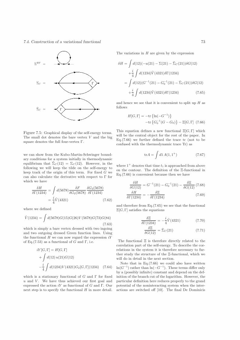
7.4. Construction of a variational functional 73
ΣHF = ΣC =Γ
ΣC =ΓFigure 7.5: Graphical display of the self-energy terms.The small dot denotes the bare vertex V and the bigsquare denotes the full four-vertex Γ.
we can show from the Kubo-Martin-Schwinger bound-ary conditions for a system initially in thermodynamicequilibrium that ΣC(12) = ΣC(12). However, in thefollowing we will keep the tilde on the self-energy tokeep track of the origin of this term. For fixed G wecan also calculate the derivative with respect to Γ forwhich we have
δH
δΓ(1234)=
Zd(5678)
δF
δG2(5678)
δG2(5678)
δΓ(1234)
=i
4V (4321) (7.62)
where we defined
V (1234) =
Zd(5678)G(15)G(26)V (5678)G(73)G(84)
(7.63)which is simply a bare vertex dressed with two ingoingand two outgoing dressed Green function lines. Usingthe functional H we can now regard the expression iYof Eq.(7.53) as a functional of G and Γ, i.e.
iY [G,Γ] = H [G,Γ]
+
Zd(12)u(21)G(12)
− i
4
Zd(1234)V (4321)G2[G,Γ](1234) (7.64)
which is a stationary functional of G and Γ for fixedu and V . We have thus achieved our first goal andexpressed the action iY as functional of G and Γ. Ournext step is to specify the functional H in more detail.
The variations in H are given by the expression
δH =
Zd(12)(−u(21) − Σ(21) − ΣC(21))δG(12)
+i
4
Zd(1234)V (4321)δΓ(1234)
=
Zd(12)(G−1(21) −G−1
0 (21) − ΣC(21))δG(12)
+i
4
Zd(1234)V (4321)δΓ(1234) (7.65)
and hence we see that it is convenient to split up H asfollows
H [G,Γ] = −tr˘ln(−G−1)
¯
−tr˘G−1
0 (G−G0)¯− Ξ[G,Γ] (7.66)
This equation defines a new functional Ξ[G,Γ] whichwill be the central object for the rest of the paper. InEq.(7.66) we further defined the trace tr (not to beconfused with the thermodynamic trace Tr) as
trA =
Zd1A(1, 1+) (7.67)
where 1+ denotes that time t1 is approached from aboveon the contour. The definition of the Ξ-functional inEq.(7.66) is convenient because then we have
δH
δG(12)= G−1(21) −G−1
0 (21) − δΞ
δG(12)(7.68)
δH
δΓ(1234)= − δΞ
δΓ(1234)(7.69)
and therefore from Eq.(7.65) we see that the functionalΞ[G,Γ] satisfies the equations
δΞ
δΓ(1234)= − i
4V (4321) (7.70)
δΞ
δG(12)= ΣC(21) (7.71)
The functional Ξ is therefore directly related to thecorrelation part of the self-energy. To describe the cor-relations in the system it is therefore necessary to fur-ther study the structure of the Ξ-functional, which wewill do in detail in the next section.
Note that in Eq.(7.66) we could also have writtenln(G−1) rather than ln(−G−1). These terms differ onlyby a (possibly infinite) constant and depend on the def-inition of the branch cut of the logarithm. However, theparticular definition here reduces properly to the grandpotential of the noninteracting system when the inter-actions are switched off [10]. The final De Dominicis

74 THE RENORMALIZED FOUR-POINT VERTEX
G2(1234) = 4 3
1 2
+ 4 3
1 2
+ 4 3
1 2
(a) (b) (c)
+1 2
4 3
+ 1 2
4 3
+ 1 2
4 3
+ . . .
(d) (e) (f)
Figure 7.6: Expansion of the 2-particle Green functionG2 in terms of the full G. The dot denotes the barevertex V .
functional (for u = 0 ) is thus given from Eq.(7.64) and(7.66) by
iY [G,Γ] = −tr˘ln(−G−1)
¯− tr
˘G−1
0 (G−G0)¯
−Ξ[G,Γ]
− i
4
Zd(1234)V0(1234)G2[G,Γ](4321) (7.72)
We can check that in the absence of interactions we haveiY = −tr ln−G−1
0 which yields the grand potential ofthe noninteracting system, as we will discuss in moredetail later. Let us now check the variational property.The derivatives of iY with respect to G and Γ are givenby
iδY
δΓ(1234)=i
4(V (4321) − V0(4321)) (7.73)
iδY
δG(12)= G−1(21) −G−1
0 (21) − ΣC(21; V )
+Σ(21; V0) + ΣC(21; V0) (7.74)
where we used that
− i
4
δ
δG(56)
Zd(1234)V0(1234)G2[G,Γ](4321)
= Σ(65; V0) + ΣC(65;V0)(7.75)
The variational equations that are obtained by puttingthe derivatives (7.73) and (7.74) equal to zero, are obvi-ously solved for the G and Γ that self-consistently solvethe equations
G−1 = G−10 − Σ[G,Γ] (7.76)
V0 = V [G,Γ] (7.77)
where Σ is calculated from Eqs.(7.59) and Eq.(7.60).Therefore the functional Y [G,Γ] is stationary when-ever the Dyson equation is obeyed and whenever the
electron-electron interaction expanded in G and Γ isequal to the specified interaction V0. Equation (7.72)for the variational functional Y [G,Γ] is the first basicresult of this work. However, before it can be usedin actual calculations we have, among others, to spec-ify the specific structure of the functional Ξ[G,Γ]. Wewill show that for several infinite series of diagrammaticterms contributing to this functional we can find ex-plicit expressions in terms of G and Γ. To do this wefirst have to study the functional V [G,Γ] of Eq.(7.77).This is the topic of the next section.
7.5 Structure of the Ξ-
functional
In this section we analyze in more detail the diagra-matic structure of the fourvertex Γ and the functionalV [G,Γ] of Eq.(7.77) which will allow us to obtain moreexplicit expressions for the functional Ξ. These quanti-ties can be directly obtained from a diagrammatic ex-pansion of the two-particle Green function. If we ex-press the diagrams in terms of the fully dressed Greenfunction G we only need to consider diagrams that donot contain any self-energy insertions. Since differentauthors use different definitions and drawing conven-tions for the two-particle Green function, it is impor-tant to be clear about them. We strictly follow thesign, loop rule and drawing conventions of reference [40]with the small difference that we use Hugenholtz dia-grams [24, 25, 26, 27]. For clarity our Feynman rulesare given in Appendix C. In fig. 7.6 we show the firstand second order Hugenholtz diagrams in terms of thefully dressed Green function G that contribute to thetwo-particle Green function G2. We see that we canwrite Γ as a sum of four classes of diagrams. There arethree classes of the form (ab, cd) which denote diagramswhich by removal of two internal Green function linescan separate the diagram into two parts, one part beingconnected to the external points ab and one part beingconnected to points cd. The class (12, 34) contains di-agrams of the particle-particle type, such as diagram(d) in fig.7.6, and will be denoted by Γpp. There aretwo classes of particle-hole type, namely (14, 32) and(13, 24) which will be denoted by ΓA
ph and ΓBph. Exam-
ples of diagrams of these types are diagrams (e) and(f) in fig.7.6. The remaining diagrams which do notfall into one of these classes are denoted by Γ0 (such asdiagram (c) in fig.7.6). We can therefore write
Γ(1234) = Γpp(1234) + ΓAph(1234)
+ΓBph(1234) + Γ0(1234) (7.78)
The simplest diagram in class Γ0 is simply the barevertex iV (1234) (i.e.diagram (c) in fig.7.6, the factor i

7.5. Structure of the Ξ-functional 75
follows from the Feynman rules in Appendix C). Sincethis diagram is special we separate it off from Γ0 anddefine the remaining diagrams Γ′
0 by the equation
Γ0(1234) = Γ′0(1234) + iV (1234) (7.79)
Using Eq.(7.78) we can then write
−iV (1234) = Γpp(1234) + ΓAph(1234)
+ΓBph(1234) + Γ′
0(1234) − Γ(1234) (7.80)
We will now first show how all the terms on the right-hand side of this equation can be constructed as a func-tional of Γ. When we have done this we can insert thisfunctional into Eq.(7.70) and perform the integrationwith respect to Γ and thereby construct our desiredfunctional Ξ[G,Γ].Let us start with the particle-particle diagrams Γpp.The contribution of all diagrams for Γpp can be writ-ten as sums of blocks of diagrams J connected withtwo parallel Green function lines (see fig.7.7 ). Each ofthese blocks J contains diagrams which cannot discon-nect points (12) and (34) by cutting two Green functionlines (such blocks are called simple with respect to (12)and (34) in the terminology of De Dominicis) and there-fore each J-block does not contain diagrams of the typeΓpp. We thus have
J(1234) = Γ(1234) − Γpp(1234) (7.81)
We introduce a convenient matrix notation
〈12|J |34〉 = J(1234) (7.82)
〈12|GG|34〉 = G(13)G(24) (7.83)
Within this notation we can, for instance, convenientlywrite C = AB instead of
C(1234) = 〈12|AB|34〉
=
Zd(56)〈12|A|56〉〈56|B|34〉
=
Zd(56)A(1256)B(5634) (7.84)
If we use this notation, then from the Feynman rulesin Appendix C one can readily convince oneself that inmatrix notation we simply have
Γ = J + Γpp
= J +1
2JGGJ + (
1
2)2JGGJGGJ + . . .
= J +1
2JGGΓ (7.85)
where for every pair of Green function lines we haveto add a factor of 1
2(see [25, 26, 27, 43]). This fol-
lows because for any diagram contributing to J , the
Γ(1234) = J1 2
4 3+J
J
4 3
21
+
J
J
J
4 3
21
+ . . .
Figure 7.7: Expression of Γ in terms of J-blocks
diagram with outgoing lines interchanged leads to thesame diagram for Γ (for the simple diagram iV in J itfollows from Feynman rule 5 in Appendix C). RelationEq.(7.85) allows us to express Γpp in terms of Γ. Wehave
J = Γ(1 +1
2GGΓ)−1 (7.86)
In combination with Eq.(7.81) this then gives
Γpp = Γ − Γ(1 +1
2GGΓ)−1 (7.87)
which expresses Γpp in terms of Γ. Let us now do thesame for the particle-hole diagrams. Since
ΓBph(1234) = −ΓA
ph(2134) (7.88)
we only need to construct ΓAph as a functional of Γ. For
the particle-hole diagrams ΓAph we can follow a similar
reasoning as for Γpp and we first write Γ in terms ofrepeated blocks I given by
I(1234) = Γ(1234) − ΓAph(1234). (7.89)
The expression for Γ in terms of I is displayed in fig.7.8.If we use the notation
〈41|I |23〉 = I(1234) (7.90)
〈12|dGG|34〉 = G(31)G(24) (7.91)
where in the first term we defined a new matrix I bya cyclic permutation of the indices, then (again usingthe Feynman rules of Appendix C) we have in matrixnotation
Γ = I + ΓAph
= I − IdGGI + IdGGIdGGI − . . .
= I − IdGGΓ (7.92)
where the alternating signs in Eq.(7.92) are related toFeynman rule 4 in Appendix C. As a remark we note
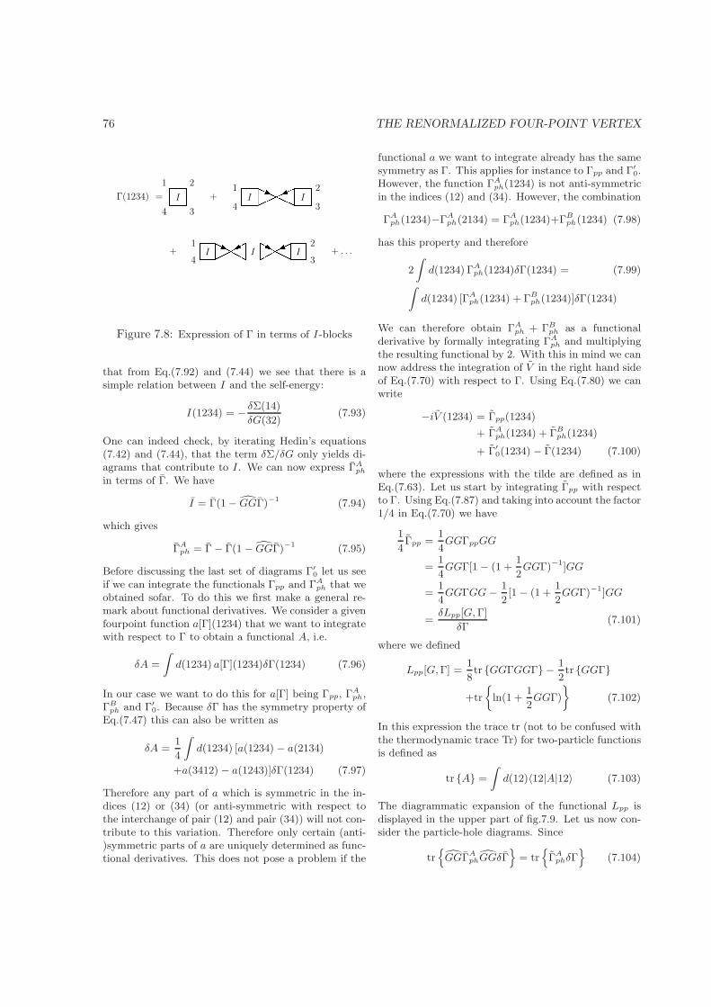
76 THE RENORMALIZED FOUR-POINT VERTEX
Γ(1234) = I1 2
4 3
+
I I
4
1
3
2
+
I I I
4
1
3
2+ . . .
Figure 7.8: Expression of Γ in terms of I-blocks
that from Eq.(7.92) and (7.44) we see that there is asimple relation between I and the self-energy:
I(1234) = − δΣ(14)
δG(32)(7.93)
One can indeed check, by iterating Hedin’s equations(7.42) and (7.44), that the term δΣ/δG only yields di-agrams that contribute to I . We can now express ΓA
ph
in terms of Γ. We have
I = Γ(1 − dGGΓ)−1 (7.94)
which gives
ΓAph = Γ − Γ(1 − dGGΓ)−1 (7.95)
Before discussing the last set of diagrams Γ′0 let us see
if we can integrate the functionals Γpp and ΓAph that we
obtained sofar. To do this we first make a general re-mark about functional derivatives. We consider a givenfourpoint function a[Γ](1234) that we want to integratewith respect to Γ to obtain a functional A, i.e.
δA =
Zd(1234) a[Γ](1234)δΓ(1234) (7.96)
In our case we want to do this for a[Γ] being Γpp, ΓAph,
ΓBph and Γ′
0. Because δΓ has the symmetry property ofEq.(7.47) this can also be written as
δA =1
4
Zd(1234) [a(1234) − a(2134)
+a(3412) − a(1243)]δΓ(1234) (7.97)
Therefore any part of a which is symmetric in the in-dices (12) or (34) (or anti-symmetric with respect tothe interchange of pair (12) and pair (34)) will not con-tribute to this variation. Therefore only certain (anti-)symmetric parts of a are uniquely determined as func-tional derivatives. This does not pose a problem if the
functional a we want to integrate already has the samesymmetry as Γ. This applies for instance to Γpp and Γ′
0.However, the function ΓA
ph(1234) is not anti-symmetricin the indices (12) and (34). However, the combination
ΓAph(1234)−ΓA
ph(2134) = ΓAph(1234)+ΓB
ph(1234) (7.98)
has this property and therefore
2
Zd(1234) ΓA
ph(1234)δΓ(1234) = (7.99)
Zd(1234) [ΓA
ph(1234) + ΓBph(1234)]δΓ(1234)
We can therefore obtain ΓAph + ΓB
ph as a functionalderivative by formally integrating ΓA
ph and multiplyingthe resulting functional by 2. With this in mind we cannow address the integration of V in the right hand sideof Eq.(7.70) with respect to Γ. Using Eq.(7.80) we canwrite
−iV (1234) = Γpp(1234)
+ ΓAph(1234) + ΓB
ph(1234)
+ Γ′0(1234) − Γ(1234) (7.100)
where the expressions with the tilde are defined as inEq.(7.63). Let us start by integrating Γpp with respectto Γ. Using Eq.(7.87) and taking into account the factor1/4 in Eq.(7.70) we have
1
4Γpp =
1
4GGΓppGG
=1
4GGΓ[1 − (1 +
1
2GGΓ)−1]GG
=1
4GGΓGG− 1
2[1 − (1 +
1
2GGΓ)−1]GG
=δLpp[G,Γ]
δΓ(7.101)
where we defined
Lpp[G,Γ] =1
8tr GGΓGGΓ − 1
2tr GGΓ
+tr
ln(1 +
1
2GGΓ)
ff(7.102)
In this expression the trace tr (not to be confused withthe thermodynamic trace Tr) for two-particle functionsis defined as
tr A =
Zd(12)〈12|A|12〉 (7.103)
The diagrammatic expansion of the functional Lpp isdisplayed in the upper part of fig.7.9. Let us now con-sider the particle-hole diagrams. Since
trn
dGGΓAph
dGGδΓo
= trn
ΓAphδΓ
o(7.104)

7.5. Structure of the Ξ-functional 77
Lpp[G, Γ] =1
3
1
23 −1
4
1
24 +1
5
1
25 − . . .
2 Lph[G, Γ] = −1
3 −1
4 −1
5 − . . .
Figure 7.9: Expansion of the functionals Lpp and Lph
in diagrams. The fourvertex Γ is denoted with a bigblack dot.
it is sufficient to integrate dGGΓAph
dGG with respect toΓ. We have using Eq.(7.95)
1
4˜ΓA
ph =1
4dGGΓA
phdGG
=1
4dGGΓ[1 − (1 − dGGΓ)−1]dGG
=1
4dGGΓA
phdGG+
1
4[1 − (1 − dGGΓ)−1]dGG
=1
2
δLph[G,Γ]
δΓ(7.105)
where we defined the functional
Lph[G,Γ] =1
4tr
ndGGΓdGGΓ
o+
1
2tr
ndGGΓ
o
+1
2tr
nln(1 − dGGΓ)
o(7.106)
The diagrammatic expansion of the functional Lph isdisplayed in the lower part of fig.7.9. Now since
trn(ΓA
ph + ΓBph)δΓ
o= 2 tr
nΓA
phδΓo
= 2 trn
dGGΓAph
dGGδΓo(7.107)
we obtain
1
4(ΓA
ph + ΓBph) =
δLph[G,Γ]
δΓ(7.108)
We now collect our results and define
L[G,Γ] = Lpp[G,Γ] + Lph[G,Γ]
−1
8tr GGΓGGΓ (7.109)
This functional L has the property
δL
δΓ=
1
4(Γpp + ΓA
ph + ΓBph − Γ) (7.110)
Using this functional we can now split up the functionalΞ further as
Ξ[G,Γ] = L[G,Γ] + L′[G,Γ] (7.111)
This defines a new functional L′[G,Γ]. Then fromEq.(7.70) we see that if we differentiate both sides ofEq.(7.111) with respect to Γ we obtain
δΞ
δΓ= − i
4V =
1
4(Γpp + ΓA
ph + ΓBph − Γ) +
δL′
δΓ(7.112)
We therefore see by comparing to Eq.(7.80) that thefunctional L′ must satisfy
1
4Γ′
0 =δL′[G,Γ]
δΓ(7.113)
This functional can not be written out explicitly, butsince Γ′
0 is well-defined diagrammatically the functionalL′ does have a diagrammatic expansion. The first termin this expansion is displayed in fig.7.10 together withits functional derivative. Note that the derivative yieldsfour diagrams in accordance with Eq.(7.97). We canfurther consider the functional derivative of the func-tional Ξ[G,Γ] with respect toG. According to Eq.(7.71)this yields self-energy diagrams, as is also seen fromthe diagrammatic expansion of Ξ. The G-derivativesof Lpp, Lph and L′ lead to correlation self-energy dia-grams ΣC,pp[G,Γ], ΣC,ph[G,Γ] and Σ′
C [G,Γ] in termsof G and Γ that fall into different topological classes.
We now again collect our results and find fromEq.(7.72) that the final De Dominicis functional (foru = 0 ) is given by
iY [G,Γ] = −tr˘ln(−G−1)
¯− tr
˘G−1
0 (G−G0)¯
−L[G,Γ] − L′[G,Γ] − i
4tr V0G2[G,Γ](7.114)
We finally write the functional in a different form usingthe Dyson equation of Eq.(7.35)
iY [G,Γ] = −tr˘ln(Σ −G−1
0 )¯− tr ΣG
−L[G,Γ] − L′[G,Γ] − i
4tr V0G2[G,Γ](7.115)
We can readily check the variationally property of thisfunctional. We then find that
iδY = −tr˘[(Σ −G−1
0 )−1 +G]δΣ¯
−trn[Σ(V ) − Σ(V0) + ΣC(V ) − ΣC(V0)]δG
o
+i
4tr
n(V − V0)δΓ
o= 0 (7.116)
whenever V [G,Γ] = V0 for a self-consistent solution ofthe Dyson equation. The variational functional (7.115)together with the variational property (7.116) is thecentral result of this work. In the next sections wewill investigate the practical evaluation of this func-tional. It is important to note that although thefunctionals in Eq.(7.114) and (7.115) are equivalentwhen evaluated on the fully self-consistent G and Γ

78 THE RENORMALIZED FOUR-POINT VERTEX
L′[G, Γ] =1
5 + . . .
δL′
δΓ[G, Γ] =
1
41 2
4 3
+1
42 1
4 3
+1
42 1
3 4
+1
41 2
3 4
+ . . .
Figure 7.10: The first term in the expansion of the L′-functional and its functional derivative with respect toΓ. For clarity in drawing the diagrams for δL′/δΓ weinterchanged the endpoint labels rather than makingthe outgoing lines cross.
obtained from the Dyson equation and V [G,Γ] = V0
this is not true anymore when evaluated at approxi-mate G and Γ. In accordance with ref.[5] the func-tional forms in Eqs.(7.114) and (7.115) will be denotedas the Klein-form and Luttinger-Ward-form of the func-tional Y . It was demonstrated in the Φ-formalism thatthe Luttinger-Ward form of the functional is more sta-ble (has a smaller second derivative) when used for thecalculation of total energies [8]. We will therefore inthe following use the Luttinger-Ward form of the func-tional.
7.6 Ξ-derivable theories are
conserving
In this section we will show that any approximate Ξ-functional leads to a corresponding Φ-functional. Sincewe know from the work of Baym [36] that any Φ-derivable theory is conserving it follows that also Ξ-derivable theories are conserving, i.e. they respect themacroscopic conservation laws, such a momentum, en-ergy and particle number conservation and related con-straints such as the virial theorem [7]. Consider anyapproximate Ξ-functional. Then from the variationalequation
δΞ[G,Γ]
δΓ= − i
4V0 (7.117)
we can construct Γ[G, V0] as a functional of G and thebare interaction V0 (some examples of this procedure
are given in the next section). With the functionalΓ[G, V0] defined in this way we define the following Φfunctional
Φ[G, V0] = −Ξ[G,Γ[G, V0]] − i
4tr V0G2[G,Γ[G, V0]]
(7.118)and the action functional
iY [G,V0] = −tr˘ln(Σ −G−1
0 )¯− tr ΣG + Φ[G, V0]
(7.119)where in this expression self-energy Σ[G,Γ[G, V0]] mustalso be regarded as a functional of G and V0. From thedefinition of Φ it then follows directly that
δΦ = −trnΣCδG
o+i
4tr
nV0δΓ
o
+ trn(Σ + ΣC)δG
o− i
4tr
nV0δΓ
o
= tr ΣδG (7.120)
We therefore obtain the result
δΦ
δG(12)= Σ(21) (7.121)
We further have that the functional Y [G, V0] ofEq.(7.119) is stationary when
0 = −tr˘((Σ −G−1
0 )−1 +G)δΣ¯
−tr
(Σ − δΦ
δG)δG
ff(7.122)
i.e. whenever the Dyson equation is obeyed for a Φ-derivable self-energy. On the basis of the work ofBaym [36] we can therefore conclude that Ξ-derivabletheories are conserving.
7.7 Approximations using the
Ξ-functional
7.7.1 Practical use of the variational
property
After having discussed the general properties of thefunctional Y [G,Γ] we will discuss its use in practicalapproximations. For a given approximation to Ξ[G,Γ]the stationary point of the functional Y corresponds toan approximation for the self-energy and the fourver-tex obtained from a solution of the Dyson equation andof an equation of Bethe-Salpeter type, both of whichneed to be solved to self-consistency. The solution ofthese equations for general electronic systems is compu-tationally very expensive or impossible. However, if weuse the variational property of Y we can save greatlyin computational cost as the full self-consistency step

7.7. Approximations using the Ξ-functional 79
can then be skipped. To illustrate this we let G and Γbe self-consistent solutions to the variational equationsand we let G and Γ be approximations to G and Γ.Then we have that
Y [G, Γ] = Y [G,Γ] +1
2tr
δ2Y
δGδG∆G∆G
ff
+ tr
δ2Y
δGδΓ∆G∆Γ
ff
+1
2tr
δ2Y
δΓδΓ∆Γ∆Γ
ff+ . . . (7.123)
where ∆G = G − G and ∆Γ = Γ − Γ are the devi-ations from the Green function and fourvertex to theself-consistent ones. We see that the error we make inY is only of second order in ∆G and ∆Γ. We maytherefore obtain rather accurate energies from rathercrude inputs. These expectations were indeed borneout by our earlier calculations within the Φ-formalismon atoms and molecules [8]. Obviously the actual errorwe make also depends on how large the second deriva-tives of functional Y are. For this reason the Kleinand Luttinger-Ward forms of the functional performdifferently. In fact, experience within the Φ-functionalformalism has shown that the Luttinger-Ward is morestable than the Klein functional with respect to changesof the input Green function [8].
7.7.2 Approximate Ξ-functionals
In the following we study some approximate schemesusing the Ξ-functional in order to illustrate the for-malism discussed in the preceeding sections. We re-strict ourselves here to the two most simplest examples,the self-consistent second order approximation and theself-consistent T -matrix approximation. A more ad-vanced approximation, also involving the particle-holediagrams, is discussed in the section on the practicalevaluation of the Ξ-functional.
The very simplest nontrivial approximation to the wecan make to the Ξ-functional is to take Lpp = Lph =L′ = 0. This yields the functional
iY2[G,Γ] = −tr˘ln(Σ −G−1
0 )¯− tr ΣG
+1
8tr GGΓGGΓ − i
4tr V0G2[G,Γ] (7.124)
which we will denote by Y2 since it only involves secondorder diagrams. The variational equations yield
G−1 = G−10 − Σ[G,Γ] (7.125)
0 =1
4Γ − i
4V0 (7.126)
which simply implies that Γ = iV0 and that
Σ[G, V0](11′) = −i
Zd(23)V0(1231
′)G(32)
+1
2
Zd(234567)V0(1234)G(36)G(45)
×V0(5671′)G(72) (7.127)
This amounts to a self-consistent solution of the Dysonequation with only second order diagrams. A fully self-consistent solution of these equations for molecules wasrecently carried out by us [7]. One of the next simplestapproximations is obtained by taking L′ = Lph = 0which yields the functional
iYpp[G,Γ] = −tr˘ln(Σ −G−1
0 )¯− tr ΣG
−Lpp[G,Γ] +1
8tr GGΓGGΓ
− i
4tr V0G2[G,Γ] (7.128)
The variational equations correspond to
G−1 = G−10 − Σ[G,Γ] (7.129)
0 = − δLpp
δΓ+
1
4Γ − i
4V0 (7.130)
where Σ is calculated from Eqs.(7.59) and Eq.(7.60).The second variational Eq.(7.130) corresponds to
iV0 = Γ(1 +1
2GGΓ)−1. (7.131)
This equation can be inverted to give
Γ = (iV0)(1 − 1
2GG(iV0))
−1 (7.132)
and expresses the renormalized four-vertex as a sum ofparticle-particle (direct and exchange) ladder diagramsin terms of the bare potential V0. The correspondingself-energy is then readily obtained from Eqs.(7.59) and(7.60) by inserting the Γ of Eq.(7.132) in Eq.(7.60).This approximation is equivalent to the self-consistentT -matrix approximation. It is clear that the set ofapproximations can be made more and more advancedby using more sophisticated approximations for the Ξ-functional. In the following sections we will discuss thenumerical evaluation of iY . We will then among otherthings, consider an approximate fourvertex obtainedfrom the T -matrix approximation as an approximateinput for the evaluation of the energy functional iY ata more sophisticated level of perturbation theory.
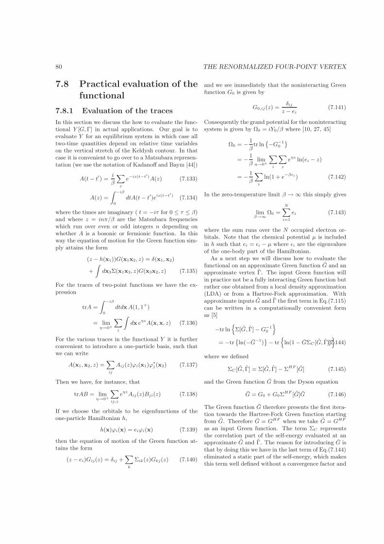
80 THE RENORMALIZED FOUR-POINT VERTEX
7.8 Practical evaluation of the
functional
7.8.1 Evaluation of the traces
In this section we discuss the how to evaluate the func-tional Y [G,Γ] in actual applications. Our goal is toevaluate Y for an equilibrium system in which case alltwo-time quantities depend on relative time variableson the vertical stretch of the Keldysh contour. In thatcase it is convenient to go over to a Matsubara represen-tation (we use the notation of Kadanoff and Baym [44])
A(t− t′) =i
β
X
z
e−iz(t−t′)A(z) (7.133)
A(z) =
Z −iβ
0
dtA(t− t′)eiz(t−t′) (7.134)
where the times are imaginary ( t = −iτ for 0 ≤ τ ≤ β)and where z = inπ/β are the Matsubara frequencieswhich run over even or odd integers n depending onwhether A is a bosonic or fermionic function. In thisway the equation of motion for the Green function sim-ply attains the form
(z − h(x1))G(x1x2, z) = δ(x1,x2)
+
Zdx3Σ(x1x3, z)G(x3x2, z) (7.135)
For the traces of two-point functions we have the ex-pression
trA =
Z −iβ
0
dtdxA(1, 1+)
= limη→0+
X
z
Zdx eηzA(x,x, z) (7.136)
For the various traces in the functional Y it is furtherconvenient to introduce a one-particle basis, such thatwe can write
A(x1,x2, z) =X
ij
Aij(z)ϕi(x1)ϕ∗j (x2) (7.137)
Then we have, for instance, that
trAB = limη→0+
X
ij,z
eηzAij(z)Bji(z) (7.138)
If we choose the orbitals to be eigenfunctions of theone-particle Hamiltonian h,
h(x)ϕi(x) = eiϕi(x) (7.139)
then the equation of motion of the Green function at-tains the form
(z − ei)Gij(z) = δij +X
k
Σik(z)Gkj(z) (7.140)
and we see immediately that the noninteracting Greenfunction G0 is given by
G0,ij(z) =δij
z − ei(7.141)
Consequently the grand potential for the noninteractingsystem is given by Ω0 = iY0/β where [10, 27, 45]
Ω0 = − 1
βtr ln
˘−G−1
0
¯
= − 1
βlim
η→0+
X
i
X
z
eηz ln(ei − z)
= − 1
β
X
i
ln(1 + e−βei) (7.142)
In the zero-temperature limit β → ∞ this simply gives
limβ→∞
Ω0 =
NX
i=1
ei (7.143)
where the sum runs over the N occupied electron or-bitals. Note that the chemical potential µ is includedin h such that ei = ǫi − µ where ǫi are the eigenvaluesof the one-body part of the Hamiltonian.
As a next step we will discuss how to evaluate thefunctional on an approximate Green function G and anapproximate vertex Γ. The input Green function willin practice not be a fully interacting Green function butrather one obtained from a local density approximation(LDA) or from a Hartree-Fock approximation. Withapproximate inputs G and Γ the first term in Eq.(7.115)can be written in a computationally convenient formas [5]
−tr lnnΣ[G, Γ] −G−1
0
o
= −tr˘ln(−G−1)
¯− tr
nln(1 − GΣC [G, Γ])
o(7.144)
where we defined
ΣC [G, Γ] = Σ[G, Γ] − ΣHF [G] (7.145)
and the Green function G from the Dyson equation
G = G0 +G0ΣHF [G]G (7.146)
The Green function G therefore presents the first itera-tion towards the Hartree-Fock Green function startingfrom G. Therefore G = GHF when we take G = GHF
as an input Green function. The term ΣC representsthe correlation part of the self-energy evaluated at anapproximate G and Γ. The reason for introducing G isthat by doing this we have in the last term of Eq.(7.144)eliminated a static part of the self-energy, which makesthis term well defined without a convergence factor and
7.8. Practical evaluation of the functional 81
also makes it decay much faster for large frequencieswhich is computationally advantageous as was shownin Ref. [5]. The first term in Eq.(7.144) can be evalu-ated analytically to give
iY0 = −tr˘ln(−G−1)
¯= −
X
i
ln(1 + e−βei) (7.147)
where ei = ǫi−µ and ǫi are the eigenvalues the Hartree-Fock equations with a nonlocal self-energy ΣHF [G]. Inpractice (for instance for LDA input Green functions)these eigenvalues are close to the true Hartree-Fockeigenvalues. Now the functional Y [G, Γ] can be writ-ten as
iY [G, Γ] = iY0
−trnln(1 − GΣC [G, Γ])
o− tr
nΣ[G, Γ]G
o
−L[G, Γ] − L′[G, Γ] − i
4tr
nV0G2[G, Γ]
o(7.148)
The second term can be evaluated by diagonalizationof GΣC since for a matrix A(z) we have
tr ln(1 − A) = limη→0+
X
z,i
eηz ln(1 − λi(z)) (7.149)
where λi(z) are the eigenvalues of A(z). This completesone part of the evaluation of the functional Y .
7.8.2 Evaluation of the L′ = 0-functional
Let us now discuss the evaluation of the L[G,Γ] andL′[G,Γ] functionals. The evaluation of even the lowestorder term of the L′-functional will be computationallyvery difficult in practice. The first term in the expan-sion of L′ is the pentagon of Fig.(7.10) containing fivefourvertices Γ. Since every fourvertex depends on fourspace-time coordinates the pentagon is (apart from thespin summations) formally an 80-dimensional integral.Fortunately, even the approximation L′ = 0 representsa very sophisticated many-body approximation. Wewill therefore in the following concentrate on this caseand consider the evaluation of the functional
iY [G,Γ] = iY0 − tr˘ln(1 − GΣC [G,Γ])
¯− tr ΣG
−L[G,Γ] − i
4tr V0G2[G,Γ] (7.150)
The evaluation of the first terms in this expression hasbeen discussed in the preceding subsection and we willtherefore concentrate on evaluation of L[G,Γ]. In thisterm the trace is taken over two-particle functions andits evaluation will therefore be slightly different fromthe case discussed above.
As our approximate Γ we will take the sum of allparticle-particle and exchange ladders in terms of V0 forwhich we will eventually take the zero-frequency limit.This is the approximate T -matrix used in Ref. [22].This approximate Γ we will denote as Γ. This approx-imate Γ will be expressed in terms of our approximateGreen function which we will denote with G. Thenfrom Eq.(7.85) we have
Γ = iV0 +i
2V0GGΓ (7.151)
If we write
V0(1234) = δ(t1, t2)δ(t1, t4)δ(t2, t3)V0(x1x2x3x4)(7.152)
with V0(x1x2x3x4) explicitly given in Eq.(7.23), we seethat we can write
Γ(1234) = δ(t1, t2)δ(t3, t4)γ(x1x2x3x4; t1t3) (7.153)
If we further expand γ in a basis as
γ(x1x2x3x4; t1t3) =X
ijkl
γijkl(t1t3)
× ϕ∗i (x1)ϕ
∗j (x2)ϕk(x3)ϕl(x4) (7.154)
then from Eq.(7.151) we see that γ satisfies
γijkl(t1t3) = iδ(t1, t3)V0,ijkl
+i
2
X
pqrs
Z −iβ
0
dt2V0,ijpq
×Gqr(t1, t2)Gps(t1, t2)γrskl(t2t3) (7.155)
which in frequency space attains the form
γijkl(z) = iV0,ijkl −1
2β
X
z1
X
pqrs
V0,ijpq
×Gqr(z1)Gps(z − z1)γrskl(z) (7.156)
(note that for γ we have to sum over the even Mat-subara frequencies). For simple approximate Greenfunctions G of Hartree-Fock or local density type thefrequency sum over z1 is readily evaluated. We arenow ready to evaluate the functionals Lpp[G, Γ] andLph[G, Γ]. They are given by the expressions
Lpp = tr ln(1 + A) − tr A +1
2tr
˘A2
¯(7.157)
Lph =1
2tr ln(1 −B) +
1
2tr B +
1
4tr
˘B2
¯(7.158)
where A = GGΓ and B = dGGΓ. Therefore in order tocalculate Lpp and Lph we have to diagonalize A and B

82 THE RENORMALIZED FOUR-POINT VERTEX
in a two-particle basis. Let us start by the calculationof A. We have for our approximate Γ and G :
Aijkl(t1t2t3t4) = δ(t3, t4)X
pq
Z −iβ
0
dt5Gip(t1, t5)
×Gjq(t2, t5)γpqkl(t5t3) (7.159)
Because of the equal-time delta function in Eq.(7.159)we find that
tr An =
=
Zd(11′ . . . nn′)〈11′|A|22′〉 . . . 〈nn′|A|11′〉
=X
p1...pn
Z −iβ
0
d(t1 . . . tn)Ap1p2(t1, t2) . . . Apnp1(tn, t1)
= limη→0+
X
z
eηzAp1p2(z) . . . Apnp1(z) (7.160)
where pk = (ikjk) are multi-indices and where we de-fined
Aijkl(t1t3) =X
pq
Z −iβ
0
dt5Gip(t1, t5)
×Gjq(t1, t5)γpqkl(t5t3) (7.161)
which in frequency space attains the form
Aijkl(z) =i
β
X
z1,pq
Gip(z1)Gjq(z − z1)γpqkl(z)(7.162)
From diagonalization of Apq(z) where p = (ij) and q =(kl) we then immediately obtain
Lpp[G, Γ] =X
z,p
(ln(1 + λp(z)) − λp(z) +1
2λ2
p(z)) (7.163)
where λp(z) are the eigenvalues of A(z). Let us finallyconcentrate on the evaluation of B. This expression isgiven by
Bijkl(t1t2t3t4) =X
pq
Gqi(t4, t1)
×Gjp(t2, t3)γpklq(t3t4) (7.164)
This expression depends on three relative times whichmakes it awkward to evaluate the logarithm. We there-fore follow reference [22] and replace in frequency spaceγijkl(z) by its zero-frequency limit γijkl(0),
γijkl(t3t4) = γijkl(0)δ(t3, t4) (7.165)
such that
Bijkl(t1t2t3t4) = δ(t3t4)X
pq
Gqi(t4, t1)
×Gjp(t2, t3)γpklq(0) (7.166)
Then, similarly as for the quantity A we have
tr Bn = limη→0+
X
z
eηzBp1p2(z) . . . Bpnp1(z)(7.167)
where
Bijkl(z) =i
β
X
z1,pq
Gqi(z1)Gjp(z1 + z)γpklq(0) (7.168)
Now B(z) is readily diagonalized with respect to itstwo-particle indices to give
Lph[G, Γ] =X
z,p
(1
2ln(1 − λp(z)) +
1
2λp(z) +
1
4λ2
p(z))(7.169)
where λp(z) are the eigenvalues of B(z). The full func-tional L[G, Γ] is then constructed as
L[G, Γ] = Lpp[G, Γ] + Lph[G, Γ] − 1
8tr
˘A2¯
(7.170)
where the last term is easily found by summing thesquares of the eigenvalues of A and performing a fre-quency sum. It finally remains to calculate an explicitexpression for Σ[G, Γ] and to evaluate the last term inEq.(7.150). The self-energy is readily calculated fromEqs.(7.59) and (7.60) to be
Σij(z) = ΣHFij + Σij,C(z) (7.171)
where
ΣHFij =
1
βlim
η→0+
X
z
V0,ipqjGqp(z) (7.172)
and
Σij,C(z) =i
2β
X
z1,z2
X
pqrstu
V0,ipqrGrs(z1)Gqt(z2)
×Gup(z1 + z2 − z)γstuj(0) (7.173)
This expression is, of course, considerably simplifiedwhen we use a diagonal input Green function. Thisfinally concludes the discussion on the practical evalu-ation of the functional.
In summary: evaluation of the functional Y inpractice therefore essentially involves the diagonaliza-tion of the one-particle matrix A(z) of Eq.(7.149) andthe diagonalization of the matrices A(z) and B(z) ofEqns.(7.161) and (7.168) in a two-particle basis followedby a frequency summation. This is, for instance withinthe DMFT approach used by Katsnelson and Lichten-stein [22], a numerically quite feasible procedure.

7.9. Conclusions 83
7.9 Conclusions
In this work we studied variational functionals of theGreen function and the renormalized fourvertex in or-der to calculate total energies for strongly correlatedsystems. The variational functionals were derived byLegendre transform techniques starting from an expres-sion of the action (or grand potential) defined on theKeldysh contour. The structure of the functionals wasfurther analyzed by means of diagrammatic techniques.We finally gave a detailed discussion of the practical useand evaluation of these for different approximate func-tionals. Future applications along the lines describedare intended.
Finally we comment on further applications of thevariatonal functionals. It was found that the Φ andthe Ψ-formalism could be succesfully used to derive ex-pressions for response functions within time-dependentdensity-functional theory (TDDFT) [37]. This wasdone by inserting approximate Green functions G[v],coming from a noninteracting system with a local po-tential v, into the variational functionals. Then thepotentials were optimized by requiring that δY/δv =0. Due to the one-to-one correspondence between thedensity and the potential (as follows from the time-dependent generalization of the Hohenberg-Kohn the-orem [2]) this then implies that we are optimizing atime-dependent density functional. The optimized po-tentials are then to be interpreted as Kohn-Sham po-tentials. In this way one obtains a density functionalfor every diagrammatic expression from the Φ- or Ψ-functional. A similar procedure can now be carried outfor the Ξ-functional.
A further point of future investigation is concernedwith finding the variationally most stable functional. Itwas already mentioned that the Klein and Luttinger-Ward (LW) forms of the functional lead to differentresults. The Luttinger-Ward form was found to be morestable. This is probably due to the fact that the secondderivatives of the LW functional are smaller than thoseof the Klein functional. However, it is very well possiblethat one could derive a better functional that wouldmake the second derivatives even smaller or make themvanish. In that case the errors we make would be onlyto third order in the deviation ∆G of the input Green tothe true self-consistent one. This still remains an issuefor future investigations. Finally we mention that workon implementation of the formalism discussed here is inprogress.
We like to thank Prof. M. I. Katsnelson and Prof.A. I. Lichtenstein for useful discussions and for interestin this work.

84 THE RENORMALIZED FOUR-POINT VERTEX

A. A generating functional for the Green function 85
A A generating functional for
the Green function
In order to obtain the Green functions as variationalderivatives we define [36] an evolution operator in termsof a time- and space nonlocal potential u(12)
U [u](t0 − iβ, t0) = TC exp(−iZdtH(t)−
i
Zd1
Zd2 ψ†(x1)u(12)ψ(x2)) (A-1)
where we used the compact notation 1 = (x1, t1). Sincewe have now two times in the exponent this expressiononly has meaning if we define how the time-ordering isspecified if we expand this expression. It is defined asfollows:
U [u](t0 − iβ, t0) ≡ U [u = 0](t0 − iβ, t0)+∞X
n=1
(−i)n
n!
Zd(11′ . . . nn′)u(1′1) . . . u(n′n)
×〈TC [ψ†H(1′)ψH(1) . . . ψ†
H(n′)ψH(n)]〉 (A-2)
where the expectation values under the integral sign areaverages (as in Eq.(7.8)) in the absence of the nonlocalfield u. This definition agrees in the limit of a time-localpotential, i.e. u(12) = u(x1t1,x2t1)δ(t
+1 , t2), with an
expression that can be derived directly from the time-dependent Schrodinger equation. We now define thefunctionals
Z[u] = Tr U [u](t0 − iβ, t0) (A-3)
iY [u] = − lnZ[u] (A-4)
Then the one-particle Green function in the presence ofthe nonlocal field u is defined as:
Gu(11′) ≡ iδY
δu(1′1)= − 1
Z[u]
δZ
δu(1′1)(A-5)
When evaluated at u = 0 the Green function reducesto the familiar one
Gu=0(11′) = −i〈TC [ψ†
H(1)ψ(1′)]〉 (A-6)
Let us note that one should be careful with dealingwith time-nonlocal potentials. It would, for instance,be tempting to think that Gu would be given by theexpression
Gu(11′) =
−iTr
nU [u](t0 − iβ, t0)TC [ψ†
H(1′)ψH(1)]o
Tr U [u](t0 − iβ, t0)(A-7)
where the Heisenberg operators in the presence of uwould be given by OH = U [u](t0, t)OU [u](t, t0). How-ever, this expression is not valid if u is nonlocal in time.
For instance, when expanding Eq.(A-5) and (A-7) inpowers of u using Eq.(A-2) one immediately sees thatcertain time-orderings of the field operators in Eq.(A-5)are absent in Eq.(A-7). Similarly the evolution operatorU [u](t, t′) does not satisfy a simple equation of motion.However, we can still derive the equations of motionfor Gu on the basis of the hierarchy equations of then-body Green functions in the absence of the nonlocalfield u, as we will show below.More generally we can now define n-body Green func-tions Gn,u from a repeated differentiation of Z[u], i.e.
1
Z[u]
δnZ
δu(1′1) . . . δu(n′n)
= ǫnGn,u(1 . . . n, 1′ . . . n′) (A-8)
where ǫn = (−1)n(n+1)/2. The prefac-tor ǫn results from reordering the opera-tor product 〈TC [ψ†(1′)ψ(1) . . . ψ†(n′)ψ(n)]〉 to〈TC [ψ(1) . . . ψ(n)ψ†(1′) . . . ψ†(n′)]〉 as is easily verifiedby induction. One can readily check that for u = 0Eq.(A-8) agrees with our previous definition of then-body Green function of Eq.(7.20). From Eq.(A-8)we further immediately obtain that
δGu(14)
δu(32)=
δ
δu(32)
`− 1
Z[u]
δZ
δu(41)
´
=1
Z2
δZ
δu(14)
δZ
δu(32)− 1
Z
δ2Z
δu(41)δu(32)
= Gu(14)Gu(23) −G2,u(1234) (A-9)
This is Eq.(7.27) used in section 7.3. As a next step wederive the hierarchy equations for the Green functionsGn,u. From Eq.(A-8) we see that we can expand thefunctional Z[u] as a Taylor series expansion in u as
Z[u] = Z[0]∞X
n=0
ǫnn!
Zd(11′ . . . nn′)
×Gn(1 . . . n, 1′ . . . n′)u(1′1) . . . u(n′n) (A-10)
where the term with n = 0 is just defined to be one.The Green functions Gn are the Green functions in theabsence of the field u. The one-body and n-body Greenfunctions can therefore be expressed in terms on thefield-free Green functions using Eqs.(A-5), (A-8) and
86 THE RENORMALIZED FOUR-POINT VERTEX
(A-10). One obtains for Gu and G2,u the equations
Z[u]
Z[0]Gu(11′) = G(11′)
−∞X
n=2
ǫn(n− 1)!
Zd(22′ . . . nn′)
×Gn(1 . . . n, 1′ . . . n′)u(2′2) . . . u(n′n) (A-11)
Z[u]
Z[0]G2,u(12; 1′2′) = G(12; 1′2′)
−∞X
n=3
ǫn(n− 2)!
Zd(33′ . . . nn′)
×Gn(1 . . . n, 1′ . . . n′)u(3′3) . . . u(n′n) (A-12)
From these expressions we see that Gu and G2,u inheritthe Kubo-Martin-Schwinger boundary conditions fromthe Gn. If we act with the operator i∂t1 − h0(1) onboth sides of Eq.(A-11) and use the Martin-Schwingerhierarchy equations Eq.(7.21) for the Green functionsGn in the absence of the u-field together with Eq.(A-12) we obtain, after slightly tedious but straightforwardmanipulations, the equation of motion for Gu
(i∂t1 − h0(1))Gu(11′) = δ(11′)
+
Zd2u(12)Gu(21′)
−iZdxv(x1,x)G2,u(1,xt1,xt
+1 , 1
′) (A-13)
By functional differentiation with respect to u we cangenerate equations of motion for the higher-order Greenfunctions. To see this we first multiply (A-13) by Z[u]to obtain
(i∂t1 − h0(1))(−i)〈11′〉 = δ(11′)Z[u]
+
Zd1u(11)(−i)〈11′〉
−iZdxv(x1,x)(−i)2〈1,xt1,xt+1 , 1′〉 (A-14)
where we introduced the simplified notation
〈1 . . . n; 1′ . . . n′〉 = Z[u]Gn,u(1 . . . n, 1′ . . . n′)(A-15)
We use the convention that the primed variables arealways associated with creation operators and that theunprimed variables are always associated with the an-nihilation operators. Taking the functional derivativeof Eq.(A-14) with respect to u(2′2) then gives
(i∂t1 − h0(1))(−i)2〈11′2′2〉 = δ(11′)(−i)〈2′2〉+δ(12′)(−i)〈21′〉
+
Zd1u(11)(−i)2〈11′2′2〉
−iZdxv(x1,x)(−i)3〈1,xt1,xt+1 , 1′2′2〉 (A-16)
Reordering the indices and dividing by Z[u] then gives
(i∂t1 − h0(1))G2,u(121′2′) =
−δ(11′)Gu(22′) + δ(12′)Gu(21′)
+
Zd1u(11)G2,u(121′2′)
−iZdxv(x1,x)G3,u(12,xt1,xt
+1 , 1
′2′) (A-17)
By continued differentiation we obtain the general hi-erarchy equations for Gn,u
(i∂t1 − h0(1))Gn,u(1 . . . n, 1′ . . . n′)
=nX
j=1
δ(1j′)(−1)n−jGn−1,u(2 . . . n, 1′ . . . j′ − 1, j′ + 1 . . . n′)
+
Zd1u(11)Gn,u(12 . . . n, 1′ . . . n′)
−iZdxv(x1,x)Gn+1,u(1 . . . n,xt1,xt
+1 , 1
′ . . . n′) (A-18)
These equations are readily checked by induction if wemultiply them by Z[u] and take the functional deriva-tive with respect to u(n′ + 1, n+ 1). We have thereforeestablished that Green functions Gn,u satisfy an ob-vious generalisation of the hierarchy equations. Therelation Eq.(A-18) is the main result of this Appendixand will be essential to the derivation in the next sec-tion. Note further that Eq.(A-18) can be used to derivea Wick’s theorem in the presence of the nonlocal fieldu. If we put w = 0 we find that the noninteractingn-body Green functions Gn,u satisfy Eq.(A-18) if theyare written as determinants in terms of Gu.
B The equation of motion of
Gu,V
The main goal in this Appendix is to derive the equa-tion of motion Eq.(7.28) for the Green function in thepresence of the a nonlocal one-body potential u(12)and a nonlocal two-body potential V (1234). As in Ap-pendix A the main difficulty is caused by the fact thatu and V are nonlocal in time. Our final result can beobtained with help of Eq.(A-18). Let Z[u, V ] be givenby
Z[u, V ] = TrnU [u, V ](t0 − iβ, t0)
o(B-1)
B. The equation of motion of Gu,V 87
where
U [u, V ](t0 − iβ, t0) = TC exp(−iZdtH0(t)
−iZd1
Zd2 ψ†(x1)u(12)ψ(x2)
− i
4
Zd(1234)V (1234)
×ψ†(x1)ψ†(x2)ψ(x3)ψ(x4)) (B-2)
Due to the multiple time-integrals this expression hasonly meaning when we define how the time-ordering isspecified when we expand this expression. We define
U [u, V ](t0 − iβ, t0) ≡ U [0, 0](t0 − iβ, t0)+∞X
n,m=1
(−i)n+m
n!m!4m
Zd(y1 . . . yn)d(X1 . . .Xm)
×u1 . . . unV1 . . .XmTC [y1 . . . ynX1 . . . Xm] (B-3)
where for the coordinates we introduced the short no-tation
yi = (i′, i) (B-4)
Xi = ((2i− 1)′, (2i)′, 2i− 1, 2i) (B-5)
and we further defined
ui = u(yi) (B-6)
yi = ψ†H (i′)ψH (i) (B-7)
Vi = V (Xi) (B-8)
Xi = ψ†H((2i− 1)′)ψ†
H((2i)′)ψH(2i− 1)ψH (2i)(B-9)
where the Heisenberg representation of the operatorsis defined with respect to H0. We then define the n-particle Green function Gn,u,V in the presence of thetime-nonlocal fields u and V as
ǫnGn,u,V (1 . . . n; 1′ . . . n′) ≡1
Z[u, V ]
δnZ[u, V ]
δu(1′1) . . . u(n′n)(B-10)
where ǫn = (−1)n(n+1)/2. For V = 0 this definitionagrees with the definition (A-8) in Appendix A in theabsence of two-particle interactions. Now from Eq.(B-3) one can readily derive that
δkZ[u, V ]
δV1 . . . δVk=
(−i)k
4k
δ2kZ[u, V ]
δu(1′1) . . . u((2k)′, 2k)(B-11)
With this equation we find that we can express theGreen functions equivalently as
G2n,u,V (1 . . . 2n; 1′ . . . (2n)′)
=4n(−i)n
Z[u, V ]
δkZ[u, V ]
δV1 . . . δVn(B-12)
G2n+1,u,V (1, 1, . . . 2n; 1′, 1′ . . . (2n)′)
= −4n(−i)n
Z[u, V ]
δ2n+1Z[u, V ]
δu1V1 . . . Vn(B-13)
As a particular case we have
Gu,V (11′) = − 1
Z[u, V ]
δZ[u, V ]
δu(1′1)(B-14)
G2,u,V (121′2′) = − 4i
Z[u, V ]
δZ[u, V ]
δV (1′2′12)(B-15)
These equations are two basic starting equations Eq.(7.48) and (7.49) of section 7.4. It remains to showthat they are related by an equation of motion as inEq.(7.28). From Eqs.(B-12) and (B-13) we see thatZ[u, V ] has the following Taylor expansion around V =0.
Z[u, V ]
Z[u, 0]=
∞X
n=0
in
n!4n
Zd(X1 . . . Xn)
×G2n,u(1 . . . 2n; 1′ . . . 2n′)V1 . . . Vn (B-16)
where we denote Gn,u = Gn,u,V =0. Similarly for Gu,V
we have from Eq.(B-13) the Taylor series expansion
Z[u, V ]
Z[u, 0]Gu,V (11′) = Gu(1, 1′)
+∞X
n=1
in
n!4n
Zd(X1 . . .Xn)
×G2n+1,u(11 . . . 2n; 1′1′ . . . 2n′)V1 . . . Vn(B-17)
and for the two-particle Green function from Eq.(B-12)
Z[u, V ]
Z[u, 0]G2,u,V (12, 1′2′) = G2,u(12, 1′2′)
− i∞X
n=2
in
4n−1(n− 1)!
Zd(X1 . . .Xn−1)
×G2n,u(1212 . . . 2(n− 1); 1′2′1′2′ . . . 2(n− 1)′)
×V1 . . . Vn−1 (B-18)
To obtain an equation of motion of Gu,V we can use thehierarchy equations for Gn,u of Eq.(A-18) for w = 0
(i∂t1 − h(1))Gn,u(1 . . . n, 1′ . . . n′)
=
n−1X
j=0
δ(1j′)(−1)n−j
×Gn−1,u(2 . . . n, 1′ . . . (j − 1)′, (j + 1)′ . . . n′)
+
Zd1u(11)Gn,u(12 . . . n, 1′ . . . n′) (B-19)

88 THE RENORMALIZED FOUR-POINT VERTEX
If we act with i∂t1 − h(1) on both sides of Eq.(B-17)and subsequently use Eqs.(B-19),(B-16) and (B-18) weobtain
(i∂t1 − h(1))Gu,V (11′) = δ(11′)
+
Zd2u(12)Gu,V (21′)
− i
2
Zd(234)V (1234)G2,u,V (4321′) (B-20)
This is the equation of motion Eq.(7.28) for the Greenfunction used in section 7.4. Again by differentiatingthis equation with respect to u we obtain the hierarchyequations for the higher order Green functions Gn,u,V .
C Feynman rules for the two-
particle Green function
In this section we give a brief summary of the Feynmanrules for the two-particle Green function G2 within theHugenholtz diagram technique [24, 25, 26, 27]. Thegeneral structure of the two-particle Green function isas given in Fig.(7.4). The Green function G2(1234) iswritten with the points (1234) positioned clockwise onfour corners of the diagram where corners 1 and 2 areconnected to outgoing lines and corners 3 and 4 areconnected to ingoing lines. If one expands the evolu-tion operators in the definition of G2 in powers of theinteraction V one finds for the diagrams the followingrules
1. Every Green function line (contraction accordingto Wick’s theorem) gives a factor iG .
2. Every vertex gives a factor −iV .
3. Every closed loop of Green function lines gives aminus sign, i.e. we have a factor (−1)l where l isthe number of closed loops. To find the numberof loops one must replace the Hugenholtz vertexby the first term on the right hand side of Fig.7.2(with the same labeling) and count the number ofloops that appear in this way.
4. A line starting at 3 and ending at 1 gives a minussign, i.e. we have a factor (−1)L13 where L13 = 1when 1 and 3 are connected and zero otherwise.To determine the connectivity it is necessary thatone again first replaces the Hugenholtz vertex bythe first term on the right hand side of Fig.7.2 (seealso [26]).
5. Two Green function lines (so-called equivalentlines) starting from a given vertex and ending bothon the same vertex give a factor 1
2, i.e. we have
a factor 2−p where p is the number of equivalentlines.
6. There is a factor (−i)2 from the definition of G2.
From these rules we find that the overall pref-actor of a G2-diagram with n vertices is given byin(−1)l+L132−p. For example, diagrams (a) − (f) inFig.7.6 have prefactors 1,−1, i,− 1
2, 1 and −1 respec-
tively.
References
[1] Trygve Helgaker, Poul Jørgensen, and JeppeOlsen, editors. Molecular Electronic-StructureTheory. Wiley, 2000.
[2] Reiner M. Dreizler and Eberhard K. U. Gross.Density Functional Theory, An Approach to theQuantum Many-Body Problem. Springer-Verlag,Berlin, 1990.
[3] John P. Perdew and Stefan Kurth. A primerin density functional theory. In Carlos Fiolhais,Fernando Nogueira, and Miguel A. L. Marques,editors, A Primer in Density Functional Theory.Springer Verlag, Berlin Heidelberg, 2003.
[4] Nils Erik Dahlen and Ulf von Barth. J. Chem.Phys., 120:6826, 2004.
[5] Nils Erik Dahlen and Ulf von Barth. Phys. Rev.B, 69:195102, 2004.
[6] Nils Erik Dahlen, Robert van Leeuwen, and Ulfvon Barth. Int. J. Quantum Chem., 101:512, 2005.
[7] Nils Erik Dahlen and Robert van Leeuwen. J.Chem. Phys., 122:164102, 2005.
[8] Nils Erik Dahlen, Robert van Leeuwen, and Ulfvon Barth. Phys. Rev. A, 73:012511, 2006.
[9] Carl-Olof Almbladh, Ulf von Barth, and Robertvan Leeuwen. Int. J. Mod. Phys. B, 13:535, 1999.
[10] Joaquin Mazdak Luttinger and John Clive Ward.Phys. Rev., 118:1417, 1960.
[11] Mikael Hindgren. Model Vertices Beyond the GWApproximation. PhD thesis, Lund University,1997.
[12] Ferdi Aryasetiawan, T. Miyake, and K. Terakura.Phys. Rev. Lett., 88:166401, 2002.
[13] Vaclav Janis. cond-mat/9806118 (unpublished).
[14] Vaclav Janis. Phys. Rev. B, 60:11345, 1999.
[15] Michael Potthoff. Eur. Phys. J., B32:429, 2003.

REFERENCES 89
[16] Michael Potthoff, Markus Josef Aichhorn, andCristopher Dahnken. Phys. Rev. Lett, 91:206402,2003.
[17] Vaclav Janis. J. Phys. Cond. Matt., 15:L311, 2003.
[18] Lars Hedin. Phys. Rev., 139:A796, 1965.
[19] R. Chitra and Gabriel Kotliar. Phys. Rev. B, 63:115110, 2001.
[20] Sergej Y. Savrasov and Gabriel Kotliar. Phys. Rev.B, 69:245101, 2004.
[21] Ning-Hua Tong. Phys. Rev. B, 72:115104, 2005.
[22] Mikhail I. Katsnelson and Alexander I. Lichten-stein. Eur. Phys. J., B30:9, 2002.
[23] Antoine Georges, Gabriel Kotliar, Werner Krauth,and Marcelo J. Rozenberg. Rev. Mod. Phys., 68:13, 1996.
[24] N. M. Hugenholtz. Physica, 23:481, 1957.
[25] Philippe Nozieres. Theory of interacting fermi sys-tems. W. A. Benjamin, New York, 1964.
[26] John W. Negele and Henri Orland, editors. Quan-tum Many-Particle Systems. Addison-Wesley,1998.
[27] Jean-Paul Blaizot and Georges Ripka. QuantumTheory of Finite Systems. MIT Press, Cambridge,MA, 1986.
[28] Cyrano De Dominicis. J. Math. Phys., 3:983, 1962.
[29] Cyrano De Dominicis. J. Math. Phys., 4:255, 1963.
[30] Cyrano De Dominicis and Paul C. Martin. J.Math. Phys., 5:14, 1964.
[31] Cyrano De Dominicis and Paul C. Martin. J.Math. Phys., 5:31, 1964.
[32] Leonid Veniaminovich Keldysh. Zh. Eksp. Teor.Fiz., 47:1515, 1964. [Sov. Phys. JETP, 20, 1018(1965)].
[33] Pawel Danielewicz. Ann. Phys. (N. Y.), 152:239,1984.
[34] Michael Bonitz. Quantum Kinetic Theory. B. G.Teubner, Stuttgart; Leipzig, 1998.
[35] Robert van Leeuwen, Nils Erik Dahlen, Gian-luca Stefanucci, Carl-Olof Almbladh, and Ulf vonBarth. In Miguel A. L. Merques, Carsten A.Ullrich, Fernando Nogueira, Angel Rubio, KieronBurke, and Eberhard K. U. Gross, editors, Time-dependent Density Functional Theory, page 33.Springer, Berlin Heidelberg, 2006.
[36] Gordon Baym. Phys. Rev., 127:1391, 1962.
[37] Ulf von Barth, Nils Erik Dahlen, Robert vanLeeuwen, and Gianluca Stefanucci. Phys. Rev. B,72(23):235109, 2005.
[38] Robert van Leeuwen. Phys. Rev. Lett., 80:1280,1998.
[39] Julian Schwinger. Proc. Nat. Acad. Sci. USA, 37:451, 1951.
[40] Eberhard K. U. Gross, Erich Runge, and OlleHeinonen. Many-Particle Theory. Verlag AdamHilger, Bristol, 1991.
[41] Ryogo Kubo. J. Phys. Soc. Jpn., 12:570, 1957.
[42] Dirk Semkat, Dietrich Kremp, and Michael Bonitz.Phys. Rev. E, 59:1557, 1999.
[43] Claude Bloch. In J. de Boer and G. E. Uhlenbeck,editors, Studies in Statistical Mechanics. North-Holland, Amsterdam, 1965.
[44] Leo P. Kadanoff and Gordon Baym. Quantum Sta-tistical Mechanics. W. A. Benjamin, Inc., NewYork, 1962.
[45] K. Orlewicz. Acta Phys. Pol., A72:357, 1987.

90 THE RENORMALIZED FOUR-POINT VERTEX
Epilogue
Green function methods have been used with great success to calculate a wide variety of properties ofelectronic systems, ranging from atoms and molecules to solids. Within the Green function approach,these properties are completely determined by the self-energy operator Σ, which incorporates all the ef-fects of exchange and correlation in a many-particle system. One of the most successful and widespreadmethods has been the GW approximation. In the GWA, the self-energy operator has the simple formΣ = −GW , where G is the Green function that describes the propagation of particles and holes in thesystem, and W is the dynamically screened interaction. This quantity describes how the bare interactionv between electrons is modified due to the presence of the other electrons and appears as a renormalizedinteraction in terms of Feynman diagrams. In extended systems the screened interaction is much weakerthan the bare interaction, and therefore it is much more natural to expand the self-energy in termsof the screened interaction than in terms of the bare interaction. The GWA has produced excellentresults for band gaps and spectral properties of solids but so far has not been explored much for atomsand molecules. However, GW calculations have been – to the present time – rarely carried out in aself-consistent manner, and the effect of self-consistency is, for this reason, still a topic of considerabledebate.At the core of this thesis lay the self-consistent all-electron GW calculations for atoms and diatomicmolecules. We solve the Dyson equation for atoms and diatomic molecules within the GW approxima-tion, in order to elucidate the effects of self-consistency and the importance of the electron correlationterm of the self-energy in a self-consistent approach. In this respect, we investigated the performance ofthe GW at different levels of self-consistency for the case of atoms and diatomic molecules. Our mainmotivation for studying fully self-consistent Φ-derivable schemes was that they provide unambiguousresults for different observables and the fact that they satisfy important conservation laws that are im-portant in future nonequilibrium applications of the theory. We addressed the question to what extentpartially self-consistent schemes can reproduce the results of a fully self-consistent GW calculation. Inthe Chapter 4 of this thesis, we proposed a new partially self-consistent scheme, called GWfc, and wefound that, together with the well known GW0 method, it yields results in very close agreement withfully self-consistent GW calculations. A major advantage of the proposed scheme, i.e., GWfc, is that itproduces results that are close to the fully self-consistent GW results at a much lower computationalcost (comparable with the widely used G0W0 scheme). It will therefore be very valuable to test thismethod on solid state systems for which self-consistent GW calculations are difficult to perform due tothe large computational effort. In this way it will be possible to get further insight into the performanceof self-consistent GW for a large class of extended systems. The nonself-consistent G0W0 and the par-tially self-consistent GWfc approximation, both violate the number conservation laws but, due to thepartial self-consistency in GWfc, the errors are much reduced in this scheme.After a thorough investigation of the ground state properties of small atoms and diatomic molecules,
91
92 EPILOGUE
within the GW approximation, we have developed a time-propagation scheme for the Kadanoff-Baymequations for general inhomogeneous systems. These equations describe the time evolution of thenonequilibrium Green function for interacting many-body systems in the presence of time-dependentexternal fields. Our main motivation for developing such a scheme was the recent advancements in thefield of molecular electronics which have emphasized the need for further development of theoreticalmethods that allow for a systematic study of dynamical processes like relaxation and decoherence atthe nanoscale. Understanding these processes is of utmost importance for making progress in molecularelectronics. We applied this time propagation scheme for the Kadanoff-Baym equations to the studyof a double quantum dot and we analyzed in detail the ultrafast dynamics of transients and densitydistributions, relating them to the level structure displayed in the spectral functions. This study enablesa clear interpretation of the transport spectroscopy experiments. Moreover, we showed that the initialcorrelations and the memory terms present in the Kadanoff-Baym equations, have large effects on time-dependent currents.The time-propagation scheme for the Kadanoff-Baym equations can be used to further study electrontransport through correlated systems considering the effects of correlated leads (two or three dimen-sional). It is also worthwhile to explore, for example, the dynamics of excitons in polymer chains likepolyacetylene or the effect of electron-ellectron scattering on (non)equilibrium properties of a few electronquantum dots and quantum rings.
Samenvatting
Het onderwerp van dit proefschrift betreft het gebied van de veeldeeltjestheorie. Dit onderzoeksgebiedheeft zich ontwikkeld met als doel het gedrag en de eigenschappen van veeldeeltjessystemen te beschri-jven. Wanneer systemen als groot beschouwd kunnen worden, kunnen de wisselwerkingen tussen desamenstellende delen van deze systemen leiden tot verschijnselen die erg verschillen van de eigenschap-pen van de samenstellende delen afzonderlijk. Deze wisselwerkingen maken het zeer ingewikkeld omberekeningen te doen aan deze systemen. Het is daarom nodig vereenvoudigingen aan te brengen om hetgemeenschappelijk gedrag van de samenstellende delen te beschrijven. De verzameling van benaderingendie nodig zijn om vooruitgang te boeken in het begrijpen van veeldeeltjessystemen vormen samen hetonderzoeksgebied van de veeldeeltjesfysica.
Greenfunctietheorie is een methode in de veeldeeltjesfysica die het gedrag en de eigenschappen van eensysteem beschrijft met behulp van een grootheid die de Greenfunctie wordt genoemd. De Greenfunctieis een waarschijnlijksheidsamplitude behorende bij een proces waarbij een deeltje aan het systeem wordttoegevoegd op ruimte-tijdpunt (r′, t′) en weggehaald wordt op ruimte-tijdpunt (r, t). In de Greenfuncti-etheorie worden de wisselwerkingen tussen de deeltjes, ofwel de gevolgen van uitwisseling en correlatie,beschreven met behulp van de zogenaamde zelfenergieoperator. Een van de meest gebruikte benaderin-gen voor de zelfenergie is de GW -benadering. In deze benadering is de zelfenergieoperator het productvan de Greenfunctie, die de propagatie van deeltjes en gaten in het systeem beschrijft, en de dynamischafgeschermde wisselwerking die de effektieve wisselwerking tussen elektronen beschrijft tengevolge vande aanwezigheid van andere elektronen.
Het eerste doel van dit proefschrift is om de grondtoestandseigenschappen van eindige inhomogenesystemen te beschrijven met behulp van de GW -benadering voor de zelfenergie. Er wordt hierbij vooralgekeken naar de gevolgen van zelfconsistentie in de Dysonvergelijking op de waarneembare groothedenvan een gegeven systeem. We doen GW -berekeningen met verschillende graden van zelfconsistentie aanatomen en tweeatomige moleculen en onderzoeken de gevolgen van zelfconsistentie op totale energien,ionisatie-energien en deeltjesaantalbehoud. De verschillende graden van zelfconsistentie zijn feitelijkvereenvoudigde GW -methoden waarbij verschillende beperkingen worden opgelegd op de zelfconsistentie.We ontwikkelen een nieuwe gedeeltelijk zelf-consistente GW -methode met de naam GWfc waarbij het cor-relatiedeel van de zelfenergie vastgehouden wordt gedurende de zelfconsistentie-iteratie. Deze benaderingwordt vergeleken met de volledig zelfconsistente GW -methode, en de GW0- en G0W0-benaderingen. Detotale energien, de ionisatie-energien en de twee-elektronverwijderingsenergien verkregen met de GWfc-benadering zijn in zeer goede overeenstemming met de volledig zelfconsistente GW -benadering, terwijlze maar een klein gedeelte van de rekentijd van de laatstgenoemde benadering vergen.
We vergelijken verder de totale energien verkregen met de Luttinger-Ward-functionaal, waarbij als ar-gument eenvoudige benaderde Greenfuncties worden gebruikt, en vinden dat deze in uitstekende overeen-stemming zijn met die van de volledig zelfconsistente GW -benadering voor atomen en moleculen. We
93

94 SAMENVATTING
tonen hierbij dus het nut aan van de Luttinger-Ward-methode voor het testen van zelfenergiebenaderin-gen zonder de Dysonvergelijking zelfconsistent te hoeven oplossen.
Het tweede doel van dit proefschrift is om in detail de tijdpropagatie van nietevenwichts-Greenfunctieste beschrijven. Nadat de Greenfunctie voor het evenwichtssysteem is verkregen, kan zijn tijdsuitbreidingin de aanwezigheid van verschillende electromagnetische velden worden onderzocht. Dit wordt gedaanmet behulp van de Kadanoff-Baym-vergelijkingen. Deze vergelijkingen beschrijven de tijdsuibreidingvan nietevenwichts-Greenfuncties voor wisselwerkende veeldeeltjessystemen in de aanwezigheid van tijd-safhankelijke externe velden. De externe velden worden exact behandeld, terwijl de veeldeeltjeswisselw-erkingen worden behandeld met storingsrekening met behulp van Φ-afleidbare zelfenergiebenaderingendie verzekeren dat aan de behoudswetten van het systeem voldaan wordt. We hebben een tijdspropa-gatiemethode ontwikkeld voor de Kadanoff-Baym-vergelijkingen voor algemene inhomogene systemen.
Het derde doel van dit proefschrift is het onderzoek van tijdsafhankelijk transport in een wisselwerk-end model, met behulp van tijdspropagatie van de Kadanoff-Baym-vergelijkingen. We beschouwen eensysteem, aanvankelijk in evenwicht, dat bestaat uit een wisselwerkend middengebied gekoppeld aan elek-troden die worden behandeld in de dichte-binding-benadering. Vervolgens wordt een tijdsafhankelijkespanning aangelegd waarna we het systeem in detail volgen in de tijd. Met deze methode onderzoekenwe zeer snelle aanschakelverschijnselen en de invloed van uitwissel- en correlatie-effekten. We vindendat aanvankelijke correlaties, en geheugentermen tengevolge van veeldeeltjeswisselwerkingen, een groteinvloed hebben op de aanschakelstromen. Ook de waarde van de stationaire-toestandsstroom hangt sterkaf van de gebruikte benadering voor de veeldeeltjeswisselwerkingen.
In het laatste gedeelte van dit proefschrift leiden we variationele uitdrukkingen af voor de grootkanon-ische potential, of actie, in termen van de veeldeeltjes-Greenfunctie G, die de uitbreiding van deeltjesbeschrijft, en de gerenomaliseerde vierpuntsvertex Γ, die de verstrooiing van twee deeltjes beschrijft ineen veeldeeltjessysteem. Het belangrijkste ingredient van de variationele functionalen is een term diewe aanduiden met Ξ-functionaal. We laten zien dat elke Ξ-afleidbare theorie ook Φ-afleidbaar is endus voldoet aan de behoudswetten. We stellen een rekenmethode voor die het mogelijk maakt totaleenergien te berekenen, zonder rekentechnisch dure zelfconsistente vergelijkingen te hoeven oplossen. Deargumenten van de functionaal zijn een benaderde Greenfunctie G en een benaderde vierpuntsvertex Γdie met lage rekenkosten verkregen kunnen worden. De functionalen die we in de praktijk beschouwenworden verkregen middels oneindige sommen van ladder- en uitwisselingsdiagrammen en zijn daarom inhet bijzonder geschikt voor toepassingen op sterkwisselwerkende systemen.
Rezumat
Subiectul tezei de fata se ıncadreaza ın teoria sistemelor cu mai multe corpuri. Acesta disciplina areca scop descrierea comportamentului si caracterizarea proprietatilor sistemelor cu mai multe corpuri.In cazul ın care sistemele considerate sunt formate dintr-un numar mare de constituenti elementari,interactiunile dintre acestia pot construi fenomene diferite de cele observate atunci cand constituentii el-ementari nu interactioneaza. In ıncercarea de a descrie aceste sisteme, interactiunile dintre constituentiielementari complica descrierea sistemelor dincolo de posibilitatile de calcul. Pentru a studia comporta-mentul colectiv al constituentilor in prezenta interactiunilor, forma acestei interactiuni trebuie simplifi-cata. Toate aproximatiile facute pentru a ıntelege comportamentul sistemelor cu mai multe particule seconstituie ın fizica sistemelor cu mai multe corpuri.In cadrul fizicii sistemelor cu mai multe particule, Teoria Functiilor Green descrie comportamentul siproprietatile unui sistem prin intermediul functiei Green. Functia Green este amplitudinea probabilitatiide a gasi o particula care a fost introdusa ın sistem la coordonatele (r′, t′) si scoasa la coordonatele (r, t).Intre momentul introducerii ın sistem si momentul scoaterii acesteia din sistem, particula se propagaın sistem interactionand cu toate celelalte particule, iar functia Green care descrie aceasta propagarecontine informatii despre proprietatile sistemului. In Teoria Functiilor Green, interactiunile din sistem,i.e., efectele de schimb si corelatie, sunt ıncorporate ın asa-zisul operator de energie-proprie. Acest oper-ator determina complet proprietatile unui sistem si are diferite forme ın functie de aproximatia folosita.Una dintre cele mai raspandite aproximatii ale operatorului de energie-proprie este aproximatia GW .In aceasta aproximatie, operatorul de energie-proprie este format din produsul dintre functia Green,care descrie propagarea particulelor si golurilor ın sistem, si potentialul dinamic ecranat care descriemodificarea interactiunii pure dintre eletroni datorata prezentei celorlalti electroni din sistem.
Primul obiectiv al acestei teze este acela de a investiga proprietatile starii de baza a unui sistem finitsi neomogen, ın cadrul aproximatiei GW a energiei-proprii. In acest cadru, aspectul cel mai semnificativıl ocupa studiul efectelor de auto-consistenta ale ecuatiei Dyson asupra observabilelor unui sistem dat.In lucrarea de fata, efectuam calcule pe sisteme atomice si molecule diatomice ın aproximatia GW ladiferite niveluri de auto-consistenta, investigand efectul acesteia asupra energiei totale, a potentialului deionizare si asupra conservarii numarului de particule. De fapt, nivelurile diferite de auto-consistenta suntscheme GW simplificate, caracterizate prin diferite constrangeri aplicate auto-consistentei. In teza defata propunem o noua schema cu auto-consistenta partiala, numita GWfc, ın care componenta corelatieidin operatorul de energie-proprie este fixata pe parcursul ciclului de auto-consistenta. Efectuam ocomparatie directa a rezultatelor obtinute ın aceasta aproximatie, i.e. GWfc, cu rezultatele obtinute ıncazul auto-consistentei complete a aproximatiei GW si cu rezultatele obtinute ın cadrul aproximatiilorGW0 si G0W0. Energiile totale, potentialele de ionizare si energiile de scoatere a doi electroni din sistem,obtinute ın aproximatia GWfc, sunt extrem de aproape de cele obtinute ın cadrul aproximatiei GW cuauto-consistenta completa, necesitand doar o fractiune din efortul computational. Aceasta aproximatie
95
96 REZUMAT
poate fi aplicata unei clase largi de sisteme extinse, permitand estimarea rezultatelor obtinute ın cazulfolosirii de auto-consistentei complete ın aproximatia GW , e.g., sisteme solide pentru care calculelecomplet auto-consistente ın aproximatia GW sunt dificil de efectuat datorita costului computationalridicat.In cadrul aceluiasi prim obiectiv, comparam si energiile totale obtinute cu o functionala Luttinger-Ward,avand ca input functii Green simple, aproximative, cu energiile totale obtinute printr-un calcul completauto-consistent ın aproximatia GW , si, pentru sistemele atomice si moleculare considerate, gasim operfecta concordanta ıntre cele doua rezulate numerice. Demonstram astfel utilitatea metodei Luttinger-Ward ın testarea meritelor diferitelor aproximatii ale energiei proprii, fara a fi nevoie de rezolvareaauto-consistenta a ecuatiei Dyson.
Al doilea obiectiv al acestei teze este descrierea ın detaliu a schemei de propagare ın timp a functiilorGreen de neechilibru. Dupa obtinerea functiei Green care descrie starea de echilibru a sistemului, putemstudia evolutia acestuia ın timp. Acest lucru se poate face prin propagarea ın timp a ecuatiilor Kadanoff-Baym. In cadrul acestui proiect am dezvoltat si implementat o schema pentru rezolvarea ecuatiilorKadanoff-Baym pentru cazul unui sistem general, neomogen. Aceste ecuatii descriu evolutia ın timp afunctiei Green pentru un sistem cu interactiuni, ın prezenta unor campuri externe dependente de timp.Campurile externe sunt tratate nonperturbativ iar interactiunile multi-particula sunt ıncorporate pertur-bativ folosind aproximatii Φ-derivabile ale energiei-proprii, i.e., aproximatii care garanteaza satisfacerealegilor de conservare macroscopice pentru sistemul ın cauza.
Al treilea obiectiv al prezentei teze este studiul ın timp al fenomenului de transport ıntr-un sistem ıncare am inclus interactiunile de corelatie, prin propagarea ın timp a ecuatiilor Kadanoff-Baym. Con-sideram un sistem format dintr-o regiune centrala care, ın starea initiala, este racordata la doua contactemodelate ın cadrul unei aproximatii cu legaturi stranse. Acestui sistem ıi este aplicata o tensiune depolarizare si urmarim evolutia sistemului ın timp. Studiem astfel dinamica ultrarapida a curentilor descurta durata si influenta pe care o are considerarea efectelor de schimb si corelatie. Observam ca atatincluderea corelatiilor initiale cat si termenii de memorie datorati interactiunilor multi-particula au unefect considerabil asupra curentilor de scurta durata. Mai mult, valoarea starii stabile a curentuluidepinde foarte mult de aproximatia ın care tratam interactiunile electronice.
In ultima parte a tezei obtinem o expresie variationala pentru macropotential sau actiune, dependentade functia Green multi-particula G - care descrie propagarea particulelor - si vertexul patru-punct Γ - caredescrie ciocnirile a doua particule ıntr-un sistem multi-particula. Cantitatea principala a functionalelorvariationale este un termen pe care ıl numim functionala Ξ. Aratam ca orice teorie Ξ-derivabila estesi Φ-derivabila si de aceea respecta legile de conservare. In aceasta parte a tezei, stabilim o schemacomputationala care are drept scop obtinerea cu acuratete a energiilor totale din functionale variationale,suntand costul computational al rezolvarii auto-consistente a unor ecuatii. Inputul functionalei este ofunctie Green aproximativa G si un vertex patru-punct Γ obtinut cu un cost computational relativmodest. Functionalele pe care le vom considera pentru aplicatiile practice corespund sumarii de ordininfinit a diagramelor de tip scara si a diagramelor de schimb, fiind potrivite pentru aplicatiile ın caresunt considerate sisteme puternic corelate.
Teza este organizata astfel: In Capitolul 2 discutam formalismul general al functiilor Green si in-troducem diferitele aproximatii conservative folosite ın lucrarea de fata. In Capitolele 3-4 descriem ındetaliu aproximatia GW pentru energia-proprie si discutam diferitele niveluri de auto-consistenta. Inclu-dem ın aceste capitole si o discutie a schemei computationale folosite pentru a obtine starea de echilibrua sistemului. Mai continuare, ın Capitolul 5, expunem detaliile computationale ale schemei folositepentru propagarea ın timp a ecuatiilor Kadanoff-Baym, iar ın Capitolul 6 aplicam aceasta schema lastudiul transportului cuantic dependent de timp printr-un sistem de doua puncte cuantice corelate. Infinal, ın Capitolul 7, obtinem expresii variationale pentru macropotential dependente de functia Greenmulti-particula G si vertexul patru-punct Γ.

List of publications
1. Adrian Stan, Nils Erik Dahlen and Robert van Leeuwen, Time-propagation of the Kadanoff-Baym
equations for inhomogeneous systems, Journal of Chemical Physics (accepted)
2. Adrian Stan, Nils Erik Dahlen and Robert van Leeuwen, Levels of self-consistency in the GW
approximation, Journal of Chemical Physics 130, 114105 (2009)
3. Karsten Balzer, Michael Bonitz, Robert van Leeuwen, Nils Erik Dahlen, Adrian Stan,Nonequilibrium Green’s functions approach to strongly correlated few-electron quantum dots, (submitted2008) (arXiv:0810.2425v1)
4. Petri Myohanen, Adrian Stan, Gianluca Stefanucci, and Robert van Leeuwen, Conserving
approximations in time-dependent quantum transport: Initial correlations and memory effects,Europhysics Letters 84, 67001 (2008)
5. Adrian Stan, Nils Erik Dahlen and Robert van Leeuwen, Fully self-consistent GW calculations for
atoms and molecules, Europhysics Letters 76, 298 (2006)
6. Robert van Leeuwen, Nils Erik Dahlen and Adrian Stan, Total energies from variational functionals
of the Green function and the renormalized four-point vertex, Physical Review B 74, 195105 (2006)
7. Nils Erik Dahlen, Adrian Stan and Robert van Leeuwen, Nonequilibrium Green function theory for
excitation and transport in atoms and molecules, Journal of Physics, Conf.Ser. 35, 324 (2006)
8. Nils Erik Dahlen, Robert van Leeuwen and Adrian Stan, Propagating the Kadanoff-Baym equations
for atoms and molecules, Journal of Physics, Conf.Ser. 35, 340 (2006)
97