Full thesis.pdf - Cranfield University

CRANFIELD UNIVERSITY

HEATHER SKIPWORTH

THE APPLICATION OF FORM POSTPONEMENT IN

MANUFACTURING

SCHOOL OF MANAGEMENT

PhD THESIS

CRANFIELD UNIVERSITY

SCHOOL OF MANAGEMENT

PhD THESIS

Academic Year 2002/3

HEATHER SKIPWORTH

The Application of Form Postponement in Manufacturing

Supervisor: Professor Alan Harrison

September 2003

© Cranfield University 2003. All rights reserved. No part of this publication may be reproduced without the written permission of the copyright holder.

i

Abstract

Postponement is widely recognised as an approach that can lead to superior supply

chains, and its application is widely observed as a growing trend in manufacturing.

Form postponement (FPp) involves the delay of final manufacturing until a customer

order is received and is commonly regarded as an approach to mass customisation.

However, while much is written in the literature on the benefits and strategic impact of

FPp, little is still known about its application. Thus this research project aims to address

how FPp is applied in terms of the operational implications within the manufacturing

facility. Here the ‘postponed’ manufacturing processes are performed in the factory

where the preceding processes are carried out.

An in-depth case study research design was developed and involved case studies at

three manufacturing facilities, which provided diverse contexts in which to study FPp

applications. Each case study incorporated multiple units of analysis which were based

around product groups subject to different inventory management policies – FPp, make

to order (MTO) and make to stock (MTS). The same research design was used in each

study and involved both qualitative and quantitative evidence. Qualitative evidence was

gathered via structured interviews and included the operational changes required to

apply FPp in a previously MTO and MTS environment. Eleven quantitative variables,

providing a broad based measurement instrument, were compared across the three units

of analysis to test the hypotheses. This combination of qualitative and quantitative

evidence in the case studies helped to triangulate the research findings. Comparison

between the three case studies provided further conclusions regarding operational

implications that were context specific and those which were not.

The research concludes that the manufacturing planning system presents a major

obstacle to the application of FPp in a MTO and MTS environment. In spite of this, and

even when the FPp application is flawed, the benefits of FPp still justify its application.

The research also contributes two frameworks: one which determines when FPp is a

viable alternative to MTO or MTS; and another that illustrates the major operational

implications of applying FPp to a product exhibiting component swapping modularity.

ii

ACKNOWLEDGEMENTS

Completing a PhD whilst having two children is by far the most challenging yet

rewarding task I have ever undertaken. The contrast between becoming a Mother and

studying for a PhD could not be sharper. My rather unusual circumstances have

necessitated unusually high levels of domestic support. So first and foremost I must

thank both my parents, and parents-in-law, for providing me with nothing short of

selfless devotion. Without their help completing this PhD would have remained a pipe

dream.

There are many more to thank. In particular thanks must go to my Supervisor Alan

Harrison who has educated me in the case study approach - I hope I do justice to his

tuition. His encouragement, support and in particular advice (normally borne of

experience) have been invaluable in ensuring I did not fall prey to the countless pitfalls

in the PhD process. Also I want to thank Colin New, who was originally my supervisor,

for continuing to review my work after his retirement. I am grateful for his frank and

enlightening comments. Richard Saw and Keith Goffin were members of my academic

review panel at Cranfield and I am thankful for their constructive discussion.

I am especially grateful to BICC for providing me with the EPSRC Industrial Case

Award to fund this research. In particular my whole-hearted gratitude goes to Pat

German, Mike Butchard and Dave Green at Thomas Bolton (ex-BICC factory) who

freely shared their knowledge with me during the Pilot study. Also I am forever

indebted to managers, at the other two industrial sponsors, who were remarkably helpful

and who encouraged my work with their own commitment to their factories.

Outstanding people included: Richard Whitehouse, Zoe Crooke and Peter Dyde at

Brook Crompton; and Richard Mayall, Nigel Green and Keith Timberlake at Dewhurst.

I must also thank Cranfield University support staff for their excellent assistance in

particular Anita Beale at the library, Wendy Habgood in the Research Office and Suzie

Chadwick in the Computer Centre.

iii

Last but by no means least a big thank you to my husband Rade who initially

encouraged me to embark on a PhD and I’m sure at times has regretted this. Thank you

for your encouragement and steadfast support throughout this testing time.

Heather Skipworth

Cranfield School of Management

September, 2003.

iv

Table of Contents

CHAPTER ONE: INTRODUCTION TO THE RESEARCH 1

1.1 Research Rationale 1

1.2 The Form Postponement Concept 3

1.2.1 Logistical or Form Postponement 3

1.2.2 Defining Form Postponement 5

1.2.3 Dichotomy in manufacturing 8

1.3 Research Agenda 11

1.3.1 Research Objectives 12

1.3.2 Contribution of Research to Operations Management Literature 13

1.3.3 Contribution of Research to Logistics literature 15

1.4 Structure of Thesis 15

CHAPTER TWO: LITERATURE REVIEW 17

2.1 Defining Form Postponement 20

2.1.1 Diverse Understandings of Postponement 21

2.1.2 Defining FPp 23

2.1.3 Types of Form Postponement 26

2.2 Logistics Literature on Form Postponement 28

2.2.1 Supply Chain Re-Configuration for Form Postponement 28

2.2.2 Form Postponement as a Logistics Strategy 30

2.3 Logistical Implications of Form Postponement 36

2.3.1 Supply Chain Management and Demand Amplification 36

2.3.2 Inbound and Outbound Logistics 41

2.3.3 Information Systems and Technology 44

2.4 Operations Management Literature Related to Form Postponement 47

2.4.1 Non-MTS Approach 48

2.4.2 Mass Customisation 52

2.4.3 Form Postponement as an Operations Strategy 56

2.5 Operational Implications of Form Postponement 59

2.5.1 Leagility 59

v

2.5.2 Manufacturing flexibility 62

2.5.3 Throughput time and Order lead-time 65

2.5.4 Manufacturing Planning and Scheduling 67

2.5.5 Capacity Planning 71

2.5.6 Production Variety Funnel 75

2.6 Engineering Implications 77

2.6.1 Delayed Product Differentiation 77

2.6.2 Product and Process Modularity 78

2.6.3 Product Standardisation and Component Commonality 83

2.6.4 Manufacturing Process Configuration 85

2.7 Conceptual Model of Form Postponement 87

2.8 Theoretical Framework 88

2.9 Conclusion 90

CHAPTER THREE: RESEARCH DESIGN CONSIDERATIONS 93

3.1 Research Design 94

3.1.1 Research Questions and Hypotheses 94

3.1.2 Internal and External Variables 97

3.1.3 Case Study Framework 101

3.1.4 Units of Analyses and the Study Boundaries 103

3.2 Justification for Case Study Approach 105

3.3 Research Perspective 109

3.3.1 Philosophical position 109

3.3.2 Research Strategy 113

3.4 Rigour in Case Studies 114

3.4.1 Triangulation (leading to construct validity) 115

3.4.2 Analytic Strategy (leading to internal validity) 117

3.4.3 Case selection (leading to external validity) 119

3.5 Operationalisation of the Research Design 120

3.5.1 Case Selection 120

3.5.2 Data Collection 123

3.6 Limitations of the Research Design 125

vi

CHAPTER FOUR: PILOT STUDY AT THOMAS BOLTON 127

4.1 Context 128

4.1.1 Product Design 129

4.1.2 Manufacturing Processes 130

4.1.3 Reasons for Applying Form Postponement 131

4.2 Applying the Research Design 133

4.2.1 Identification of Units of Analysis 133


4.3 Change Content 137

4.3.1 Product and Customer Selection for Form Postponement 137

4.3.2 Inventory management 139


4.4 Outcome Variables 145

4.4.1 Demand Profile 145

4.4.2 Demand Amplification 147

4.4.3 Customer Service 149

4.4.4 Product Modularity 152

4.4.5 Product Standardisation 153

4.4.6 Excess Capacity 155

4.4.7 Throughput Efficiency 157

4.4.8 The Production Variety Funnel 159

4.5 Case Analysis 160

4.5.1 Why the FPp Application Deteriorated 160

4.5.2 Hypotheses Testing 162

4.6 Conclusions 166

CHAPTER FIVE: STUDY AT BROOK CROMPTON 168

5.1 Context 169






vii
















5.5.1 Removing Added Value 206


5.6 Conclusions 212

CHAPTER SIX: STUDY AT DEWHURST 213

6.1 Context 214













viii









6.5.1 Not the Planned Ideal FPp Application 249


6.6 Conclusions 255

CHAPTER SEVEN: CROSS-CASE COMPARISONS 256

7.1 Introduction 256

7.2 Contextual Considerations 257

7.3 Change Content & Flaws in the Applications 259


7.4.1 Units of Analyses 265

7.4.2 Demand Profile (H1 and H2) 266

7.4.3 Customer Service and Demand Amplification (H3 and H4) 268

7.4.4 Product Modularity and Standardisation (H5) 271

7.4.5 Capacity Utilisation and Throughput Efficiency (H6) 273

7.4.6 Production Variety Funnel 275

7.5 Conclusions 276

CHAPTER EIGHT: CONCLUSIONS 279

8.1 Summary of the Project 279

8.1.1 Research Strategy 280

8.1.2 Measuring Form Postponement 281

8.1.3 Rigour in Case Study Design 283

8.2 Contribution to Knowledge 284

8.2.1 Inventory Management Policy Decision Framework 286

8.2.2 Practical Implications of Form Postponement 289

ix

8.2.3 Obstacles to the application of FPp 293

8.2.4 Is Form Postponement worth it? 294

8.3 Research Limitations 297

8.3.1 Case Selection 297

8.3.2 Form Postponement Applications Studied 298

8.3.3 Data Availability 299

8.3.4 Generalisability of the findings 299

8.4 Further Research 300

Acronyms used in this Paper 302

References 303

Appendix 1 - Glossary 316

Appendix 2 - Interviews 322

Appendix 3 – TB Change Content Data 331

Appendix 4 – TB Chronology of FPp Application 334

Appendix 5 – TB Cables in the Units of Analysis 335

Appendix 6 – TB Cable Sales by Customer 336

Appendix 7 – TB Demand Measures 337

Appendix 8 – TB Demand Amplification Charts 340

Appendix 9 – TB Customer Service Measures 342

Appendix 10 – TB Degree of Commonality Calculations 343

Appendix 11 – TB Throughput Efficiency Measure 344

Appendix 12 – BC Change Content Data 346

Appendix 13 – BC Demand Measures 350

Appendix 14 – BC Demand Amplification Charts 356

Appendix 15 – BC Customer Service Measures 359

x

Appendix 16 – BC BOM Analysis 361

Appendix 17 – BC Degree of Commonality Calculations 365

Appendix 18 – BC Capacity Utilisation Measure 366

Appendix 19 – BC Throughput Efficiency Measure 367

Appendix 20 – BC Production Variety Funnels 368

Appendix 21 – Dewhurst Change Content Data 370

Appendix 22 – Dewhurst Manufacturing Data 379

Appendix 23 – Dewhurst Demand Measures 382

Appendix 24 – Dewhurst Demand Amplification Charts 387

Appendix 25 – Dewhurst BOM Analysis Parts 391

Appendix 26 – Dewhurst Degree of Commonality Calculations 394

Appendix 27 – Dewhurst Capacity Utilisation Calculations 395

xi

Table of Figures

Figure 1.1: A schematic illustrating the location of the Customer Order Decoupling

Point for form and logistical postponement 4

Figure 1.2: A matrix of generic postponement-speculation strategies (adapted from

Pagh and Cooper 1998) 7

Figure 1.3: Process types in manufacturing operations (Slack et al. 1998). 8

Figure 1.4: Different locations for the decoupling point and its effect on demand

(Naylor et al. 1999) 10

Figure 2.1: Literature review structure. 17

Figure 2.2: Total and immediate supply networks (Slack et al. 1998) 37

Figure 2.3: Customer service versus inventory level trade-off curves for FPp and MTS

approaches (adapted from Jones and Riley 1985) 38

Figure 2.4: The ‘forrester flywheel effect’ (Houlihan 1987) 40

Figure 2.5: Stage wise evolution through postponed purchasing and postponed

manufacturing (van Hoek and Weken 1998a) 42

Figure 2.6: Continuum of Strategies (Lampel and Mintzberg 1996) 54

Figure 2.7: The two distinct manufacturing stages in a FPp application if leaglity

(Naylor et al. 1999a) is applied 60

Figure 2.8: Balance between flexibility and uncertainty (Newman et al. 1993) 62

Figure 2.9: The manufacturing planning and control system (Vollman et al. 1992) 67

Figure 2.10: Throughput efficiency, capacity utilisation and lead-time (New 1993) 74

Figure 2.11: Production Variety Funnel for mens underwear manufacture (New 1993)

75

Figure 2.12: Different shapes of product structure (Slack et al. 1998) 76

Figure 2.13: Illustration of the six types of modularity identified by Pine (1993) 81

Figure 2.14: Conceptual model of FPp 87

Figure 2.15: The theoretical framework for the application of FPp. 89

xii

Figure 3.1: Basic types of designs for case studies (Yin 2003) 93

Figure 3.2: Meta level framework for the case studies. 102

Figure 3.3: The scope of the case studies in terms of the business processes 104

Figure 3.4: Framework for research methods (Meredith et al. 1989) 111

Figure 3.5: Combining Inductive and Deductive Strategies (Wallace 1971 quoted in

Blaikie 1993) 113

Figure 4.1: Diagram illustrating the structure of the case study chapters 127

Figure 4.2: A time line for the FPp inventory management policy 141

Figure 4.3: A data flow diagram showing the Manufacturing Planning Process 143

Figure 4.4: Demand amplification measured at a daily level for the FPp UoA 148

Figure 4.5: The general indented BOM for the 3183Y1.00 cable 152

Figure 4.6: The weekly ‘planned out’ capacity measured in km of finished 3183Y1.00

cable for each process between 4th January and 28th March 1999 156

Figure 4.7: The production variety funnels for the three UoA 160


Figure 5.2: Cross-sectional drawing of a large DC motor showing major components

170

Figure 5.3: Indented BOM showing only major components at all six levels (shaded

areas represent those sections of the BOM detailed on the Cincom BOMs) 193

Figure 5.4: The weekly capacity utilisation for selected cells for the six month period

January to June 2002 exclusively 200

Figure 5.5: The Production Variety Funnel for the ETO UoA (contract motors) 204

Figure 5.6: The Production Variety Funnel for the FPp UoA (modified UK stock

motors). 205


Figure 6.2: Picture of the steel keytip variant of the EPP keyad. 215

xiii

Figure 6.3: Demand Amplification measured at a daily level for steel EPP keypads due

between 28th October and 29th November ’02 231

Figure 6.4: Demand Amplification charts for the ‘2N/O’ PB body 232

Figure 6.5: Indented BOM showing the main components at all six levels 237

Figure 6.6: Charts showing the variation in weekly capacity utilisation for the EPP

keypad cells 243

Figure 6.7: The Production Variety Funnels 247

Figure 8.1: Framework for the application of FPp. 290

xiv

Table of Tables

Table 1.1: Physically efficient versus market-responsive supply chains (Fisher 1997)

9

Table 2.1: Types of FPp summarised from Zinn and Bowersox (1988). 26

Table 2.2: Types of FPp summarised from Lee and Billington (1994). 27

Table 2.3: FPp classification used for this thesis. 27

Table 2.4: The impact of product brand, formulation, and peripherals on postponement

strategies for global products (Cooper 1993) 33

Table 2.5: Market, product and process characteristics that favour postponed

manufacturing (van Hoek 1998a). 34

Table 2.6: Conflicting goals of lean logistics (Inger et al. 1995) 37

Table 2.7: Route map for integrating leanness and agility (Naylor et al. 1999b) 59

Table 2.8: Rules to streamline material flow and reduce the Bullwhip Effect (Towill

and McCullen 1999). 61

Table 2.9: Four types of manufacturing flexibility (Slack 1987) 63

Table 2.10: Summary of the six types of modularity identified by Pine (1993) 80

Table 3.1: Concepts featuring in the hypotheses and their respective measures

including typical sources of evidence. 96

Table 3.2: The key features of the positivist and phenomenological paradigms

(Easterby-Smith et al. 1991) 109

Table 3.3: Identification of companies applying FPp output from the FAME database

searches 122

Table 4.1: A flow process chart for cables manufactured in the Volume Flex area 131

Table 4.2: Sales volumes for cables produced in the Volume Flex area and despatched

between January and July 1999. 135

Table 4.3: The main features of the inventory management policies compared for the

UoA. 140

xv

Table 4.4: Main features of manufacturing planning compared for MTO and FPp.

144

Table 4.5: The demand measures compared for the UoA. 146

Table 4.6: The order lead-time measures for the FPp and MTO UoA. 150

Table 4.7: The delivery reliability and stock availability measures for the FPp and

MTO UoA. 151

Table 4.8: Product standardisation measures compared for the UoA 154

Table 4.9: Capacity measures for each process between 4th January and 28th March

1999. 155

Table 4.10: The capacity in terms of processing rate of finished cable at each process..

157

Table 4.11: Throughput efficiency measured from input at core extrusion to output at

sheath extrusion for selected FPp and MTO orders. 158

Table 5.1: A flow process chart for LDC area 172

Table 5.2: Industrial LDC motors due for despatch between 01/07/01 and 30/06/02

175


three UoA. 180

Table 5.4: Main features of manufacturing planning compared for MTO, MTS and

FPp. 183

Table 5.5: The demand measures compared for the UoA 185

Table 5.6: The order lead-time and delivery reliability measures for all UoA. 190


Table 5.8: Capacity measures for selected LDC production cells (listed in order of

production flow) for the six month period 1st January to 30th June 2002. 199

Table 5.9: Throughput efficiency measures for the UoA. 202

Table 6.1: Flow process charts with operations summarised 217

xvi

Table 6.2: Unit of analysis orders due for despatch between 01/10/02 and 31/01/03

221


UoA. 224

Table 6.4: Main features of manufacturing planning compared for stock replenishment

orders, MTO and FPp. 226

Table 6.5: The demand measures compared for the UoA 228

Table 6.6: The order lead-time and delivery reliability measures for all UoA. 234


Table 6.8: Capacity measures for the EPP and MA production cells for the study

period 30th September 2002 to 31st January 2003. 242

Table 6.9: Throughput efficiency measures for the UoA. 245

Table 7.1: Cross-case comparison of contextual data relating to the FPp applications

258

Table 7.2: Cross-case comparison of the ‘change content’ data for the FPp applications.

260

Table 7.3: Cross-case comparison of the UoAs used in the case studies 265

Table 7.4: Cross-case comparison of the demand profile measures related to

hypotheses H1 and H2. 267

Table 7.5: Cross-case comparison of the customer service and demand amplification

measures related to hypotheses H3 and H4. 269

Table 7.6: Cross-case comparison of the product modularity and standardisation

measures related to hypothesis H5. 271

Table 7.7: Cross-case comparison of the excess capacity and throughput efficiency

measures related to hypothesis H6. 273

Table 8.1: Inventory Management Decision Framework for unicentric FPp. 287

Chapter One

1

CHAPTER ONE

1 Introduction to the Research

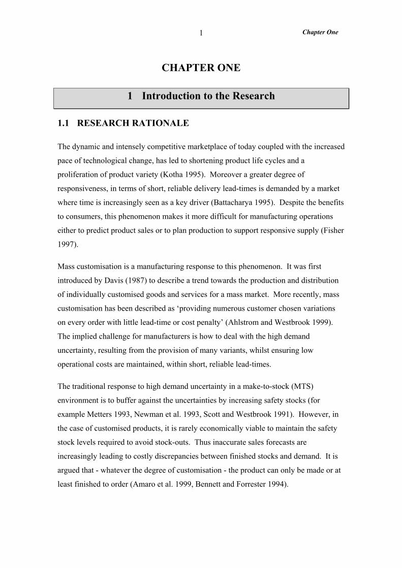
1.1 RESEARCH RATIONALE

The dynamic and intensely competitive marketplace of today coupled with the increased

pace of technological change, has led to shortening product life cycles and a

proliferation of product variety (Kotha 1995). Moreover a greater degree of

responsiveness, in terms of short, reliable delivery lead-times is demanded by a market

where time is increasingly seen as a key driver (Battacharya 1995). Despite the benefits

to consumers, this phenomenon makes it more difficult for manufacturing operations

either to predict product sales or to plan production to support responsive supply (Fisher

1997).

Mass customisation is a manufacturing response to this phenomenon. It was first

introduced by Davis (1987) to describe a trend towards the production and distribution

of individually customised goods and services for a mass market. More recently, mass

customisation has been described as ‘providing numerous customer chosen variations

on every order with little lead-time or cost penalty’ (Ahlstrom and Westbrook 1999).

The implied challenge for manufacturers is how to deal with the high demand

uncertainty, resulting from the provision of many variants, whilst ensuring low

operational costs are maintained, within short, reliable lead-times.

The traditional response to high demand uncertainty in a make-to-stock (MTS)

environment is to buffer against the uncertainties by increasing safety stocks (for

example Metters 1993, Newman et al. 1993, Scott and Westbrook 1991). However, in

the case of customised products, it is rarely economically viable to maintain the safety

stock levels required to avoid stock-outs. Thus inaccurate sales forecasts are

increasingly leading to costly discrepancies between finished stocks and demand. It is

argued that - whatever the degree of customisation - the product can only be made or at

least finished to order (Amaro et al. 1999, Bennett and Forrester 1994).

Chapter One

2

Form postponement has been proposed as one of the more effective approaches to mass

customisation (for example Amaro et al. 1999, Bowersox and Closs 1996, Pine 1993,

van Hoek 1998, van Hoek et al. 1996 and 1998, Zinn and Bowersox 1988).

Postponement, in general terms, seeks to delay final formulation, or movement, of a

product until after customer orders are received (Zinn and Bowersox, 1988). In contrast

the MTS approach aims to conduct final manufacturing, and most inventory movement,

in anticipation of customer orders - normally to sales forecasts. Thus postponement

reduces the risk of improper manufacture or inventory distribution associated with

MTS. At the other extreme, make-to-order (MTO) is where the manufacturer takes no

action until receipt of a customer order. Therefore the entire production process is

order driven. In practice this is rarely practicable and many raw materials are

purchased in anticipation of customer orders. Postponement compared to MTO

improves responsiveness and still enables a high level of customisation. It should be

noted that here, and throughout this thesis, responsiveness is the ability to respond to

fluctuating customer demand in terms of delivery speed or order lead-time. This is an

element of responsiveness as described by the framework developed by Kritchanchai

and MacCarthy (1999). Not the Matson and McFarlane (1999) definition of production

responsiveness as the ability of a production system to achieve its goals in the presence

of disturbances.

Postponement is thus widely recognised as an approach that can lead to superior

logistics systems or supply chains (for example Cooper 1993, Jones and Riley 1985,

Scott and Westbrook 1991, Shapiro and Heskett 1985). Further, the application of

postponement has been observed as a growing trend in manufacturing and distribution

by various surveys (CLM 1995, Ahlstrom and Westbrook 1999) and prominent

researchers (Christopher 1998, Lampel and Mintzberg 1996).

Yang and Burns (2003) point out that ‘postponement fosters a new way of thinking

about product design, process design and supply chain management. For example it

encourages companies to decide which components will be modular, standard and

customisable….where and which inventories are justified, and what activities are based

on forecast (or order)’. However Yang and Burns (2003) further comment that

Chapter One

3

‘although much is written in the literature on the benefits of postponement… little is

still known about the implementation of postponement’.

Before considering the research project it is necessary first to explore the concept of

form postponement to enable an appreciation of the operational implications in applying

it.

1.2 THE FORM POSTPONEMENT CONCEPT

This section introduces the concept of form postponement by considering form (or

manufacturing) postponement and logistical (or time) postponement - the two main

types of postponement. A definition of form postponement is provided and the

dichotomy in manufacturing arising from the application of form postponement is

discussed.

1.2.1 Logistical or Form Postponement

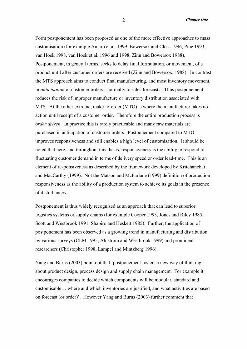
The key distinction between logistical and form postponement is the extent to which the

manufacturing process is driven by customer orders rather than by forecasts. In turn

this hinges on the location of the Customer Order Decoupling Point (CODP) as

illustrated in Figure 1.1. The CODP is the point in the chain of value adding processes

where a product is linked to a specific customer order, therefore downstream from this

point production is order-driven and upstream it is forecast-driven (Browne et al. 1996,

Hoekstra and Romme 1992, Van Veen 1992). This usually means that the CODP

coincides with the final speculative stock point.

In the case of form postponement the CODP is at the semi-finished product stage, where

the product or component modules are in a generic form. The final manufacturing

which differentiates the product is performed to specific customer orders (Zinn and

Bowersox 1988, Bowersox and Closs 1996).

Bowersox and Closs (1996) offer the following definition of logistical postponement:

‘The basic notion of logistical or time postponement is to maintain a full line anticipatory inventory at one or a few strategic locations. Forward deployment of inventory is postponed until customer orders are received.’

Chapter One

4

The CODP, therefore, is positioned at the finished product stage (Bowersox and Closs

1996, van Hoek et al. 1996 and 1998).

LOGISTICAL POSTPONEMENT

FORM POSTPONEMENT

CODP is the Customer Order Decoupling Point

CODP

BASIC MANUFACTURING

Generic product

CODP

Forecast-driven Order-driven

FINAL MANUFACTURING DISTRIBTUION

BASIC MANUFACTURING

FINAL MANUFACTURING DISTRIBTUION

FINISHEDGOODSSTOCK

GENERICPRODUCT

STOCKFinished product

Finished product

Finished product

Generic product

Generic product

indicates a stock position

Forecast-driven Order-driven

Figure 1.1: A schematic illustrating the location of the Customer Order Decoupling Point for form and logistical postponement

The benefits of logistical postponement are widely professed in the logistics literature.

For instance Bowersox and Closs (1996) claim it improves customer service and lowers

overall inventory investment, whilst preserving mass manufacturing economies of scale

in their entirety. Van Hoek (1998b) suggests that the centralisation of inventories in

European Distribution Centres (that service a number of countries from one location) is

a practical example of logistical postponement. However many applications of

logistical postponement involve service supply parts, where critical and high cost parts

are maintained in a central inventory to ensure availability to all potential users

(Bowersox and Closs 1996). When demand for a part occurs shipments are made

directly to the service facility using fast, reliable transportation.

Volvo GM Heavy Truck Corporation applied logistical postponement to the supply of

commercial truck parts for emergency roadside repairs in the United States (Narus and

Anderson 1996). The initiative was prompted by the discovery that inventories at the

Chapter One

5

dealers were exceptionally high but the parts actually needed were rarely in stock.

Volvo set up a national warehouse stocking the full line of truck parts and used FedEx

Logistics to ship parts within 24 hours to the roadside repair site. This had the effect of

both dramatically reducing parts inventory and improving service.

Logistical postponement is basically confined to the design of distribution networks.

New and Skipworth (2000) conclude that it is concerned with ‘the issue of where to

hold finished stock in a distribution system in order to minimise stock holding but

maintain a high level of customer responsiveness. This has been one of the classic

problems of inventory theory for most of the last century and the solution involves

balancing lead-time response, inventory location and transportation costs’. Logistical

postponement is outside the scope of this research project which is principally

concerned with the postponement of manufacturing transformation processes. These by

definition involve the use of resources to change the state or condition of materials to

produce goods (Slack et al. 1998). Thus this research project focuses exclusively on

form postponement. The abbreviation FPp will be used for form postponement from

this point on.

FPp enables the supply of a broad product line ‘without the risks associated with

building large finished inventories in anticipation of uncertain demand for specific

items’ (New and Skipworth 2000). It also partly preserves the mass manufacturing

economies of scale arising from the MTS approach. This is illustrated by a well known

example of FPp, which was applied in the Benetton clothing factory in Italy (Harvard

Business School 1985, Dapiran 1992). In response to highly volatile demand for the

different coloured jumpers Benetton postponed the dying process. The result was that

the jumpers were manufactured in high volume from bleached yarn thus creating high

manufacturing economies of scale, and only dyed upon the receipt of customer orders

based on actual jumper sales. Consequently finished jumper inventory levels and the

associated carrying costs, both at the factory and at the retailers, were radically reduced.

1.2.2 Defining Form Postponement

There are many FPp examples in the logistics and operations literature illustrating its

benefits, but crucial to this research is a precise and clear understanding of what FPp is.

Chapter One

6

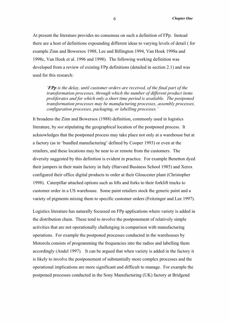
At present the literature provides no consensus on such a definition of FPp. Instead

there are a host of definitions expounding different ideas to varying levels of detail ( for

example Zinn and Bowersox 1988, Lee and Billington 1994, Van Hoek 1998a and

1998c, Van Hoek et al. 1996 and 1998). The following working definition was

developed from a review of existing FPp definitions (detailed in section 2.1) and was

used for this research:

‘FPp is the delay, until customer orders are received, of the final part of the transformation processes, through which the number of different product items proliferates and for which only a short time period is available. The postponed transformation processes may be manufacturing processes, assembly processes, configuration processes, packaging, or labelling processes.’

It broadens the Zinn and Bowersox (1988) definition, commonly used in logistics

literature, by not stipulating the geographical location of the postponed process. It

acknowledges that the postponed process may take place not only at a warehouse but at

a factory (as in ‘bundled manufacturing’ defined by Cooper 1993) or even at the

retailers, and these locations may be near to or remote from the customers. The

diversity suggested by this definition is evident in practice. For example Benetton dyed

their jumpers in their main factory in Italy (Harvard Business School 1985) and Xerox

configured their office digital products to order at their Gloucester plant (Christopher

1998). Caterpillar attached options such as lifts and forks to their forklift trucks to

customer order in a US warehouse. Some paint retailers stock the generic paint and a

variety of pigments mixing them to specific customer orders (Feitzinger and Lee 1997).

Logistics literature has naturally focussed on FPp applications where variety is added in

the distribution chain. These tend to involve the postponement of relatively simple

activities that are not operationally challenging in comparison with manufacturing

operations. For example the postponed processes conducted in the warehouses by

Motorola consists of programming the frequencies into the radios and labelling them

accordingly (Andel 1997). It can be argued that when variety is added in the factory it

is likely to involve the postponement of substantially more complex processes and the

operational implications are more significant and difficult to manage. For example the

postponed processes conducted in the Sony Manufacturing (UK) factory at Bridgend

Chapter One

7

involved fitting PCBs and other components to the ‘Eurochassis’ (common to all

products) which then underwent final assembly (Ferguson 1989).

Full Speculation

Logistical Postponement

DistributionForm

Postponement

UnicentricForm

Postponement

N/a FullPostponement

Man

ufac

turin

gLogistics

Speculation

Speculation

Postponement

Postponement

Decentralised Inventories

Centralised inventoriesand direct distribution

Make –to-stock(MTS)

FormPostponement

(FPp)

Engineer/Make-to-order

(ETO/MTO)

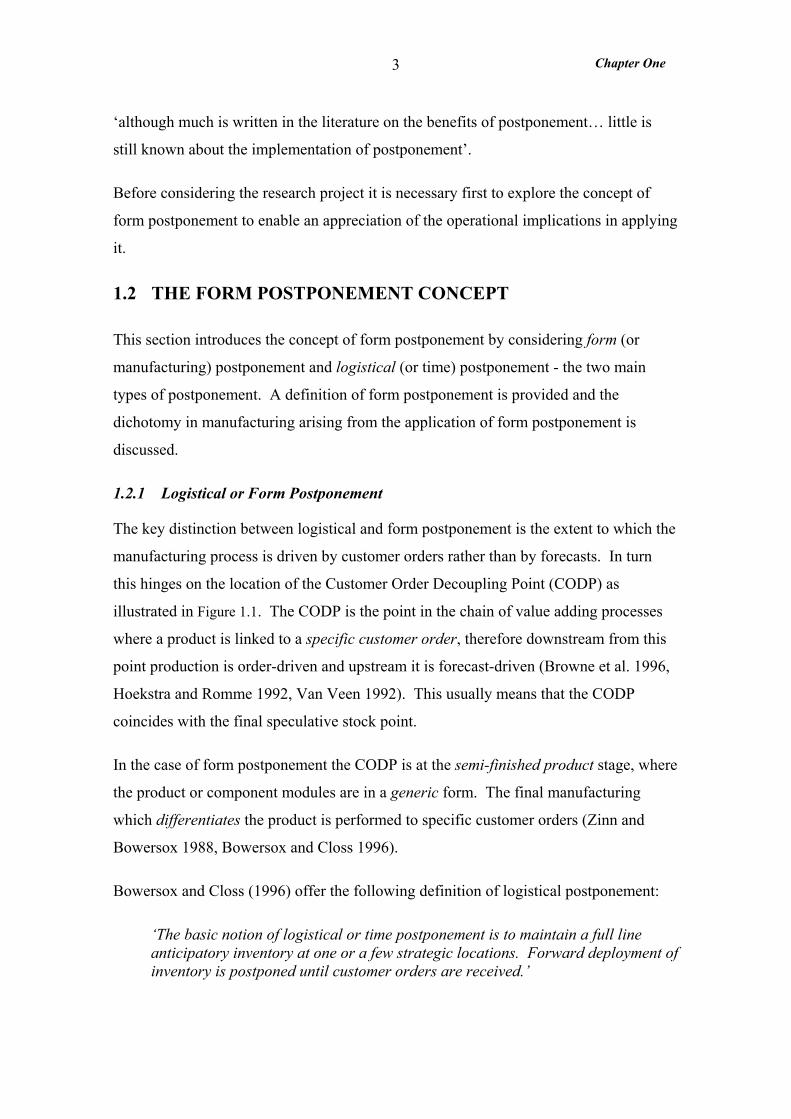
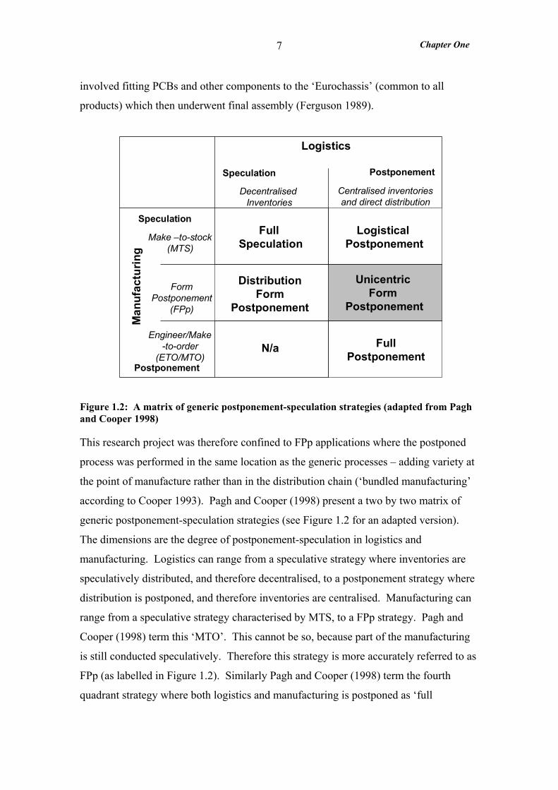
Figure 1.2: A matrix of generic postponement-speculation strategies (adapted from Pagh and Cooper 1998)

This research project was therefore confined to FPp applications where the postponed

process was performed in the same location as the generic processes – adding variety at

the point of manufacture rather than in the distribution chain (‘bundled manufacturing’

according to Cooper 1993). Pagh and Cooper (1998) present a two by two matrix of

generic postponement-speculation strategies (see Figure 1.2 for an adapted version).

The dimensions are the degree of postponement-speculation in logistics and

manufacturing. Logistics can range from a speculative strategy where inventories are

speculatively distributed, and therefore decentralised, to a postponement strategy where

distribution is postponed, and therefore inventories are centralised. Manufacturing can

range from a speculative strategy characterised by MTS, to a FPp strategy. Pagh and

Cooper (1998) term this ‘MTO’. This cannot be so, because part of the manufacturing

is still conducted speculatively. Therefore this strategy is more accurately referred to as

FPp (as labelled in Figure 1.2). Similarly Pagh and Cooper (1998) term the fourth

quadrant strategy where both logistics and manufacturing is postponed as ‘full

Chapter One

8

postponement’. It can be argued that ‘full postponement’ would be ETO or MTO

(depending upon the type of product) where all activities are postponed, therefore

another row has been added to the matrix to represent this.

The term ‘unicentric FPp’ is given to applications where the postponed process is

performed in the same location as the generic processes (normally the factory) – adding

variety at the point of manufacture rather than in the distribution chain. Alternatively

the term ‘distribution FPp’ is given where the postponed process takes place in the

distribution chain. This research project is confined to ‘unicentric FPp’ highlighted by

the shaded box in Figure 1.2.

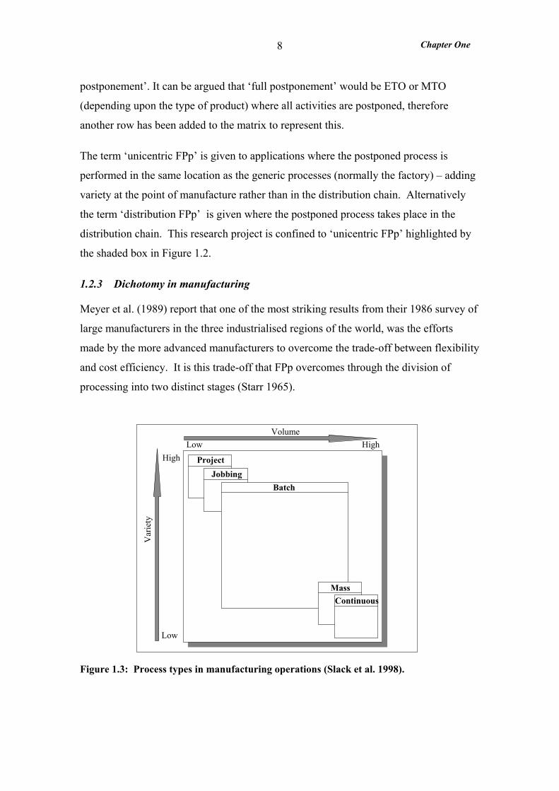
1.2.3 Dichotomy in manufacturing

Meyer et al. (1989) report that one of the most striking results from their 1986 survey of

large manufacturers in the three industrialised regions of the world, was the efforts

made by the more advanced manufacturers to overcome the trade-off between flexibility

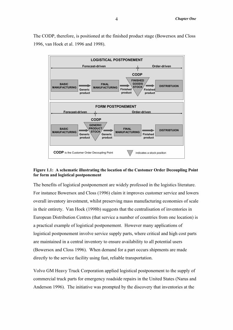
and cost efficiency. It is this trade-off that FPp overcomes through the division of

processing into two distinct stages (Starr 1965).

Figure 1.3: Process types in manufacturing operations (Slack et al. 1998).

ProjectJobbing

Batch

MassContinuous

Low

Low

HighHigh

Volume

Var

iety

Chapter One

9

The first stage involves the forecast driven production of the relatively narrow range of

base products or modules. The second stage involves the order driven production of the

broad range of finished product. Therefore the two processing stages are fundamentally

different, the first stage requiring an approach akin to efficient ‘mass production’, and

the second stage more of a flexible ‘jobbing shop’ approach as illustrated by the

diagram in Figure 1.3.

The FPp approach contributes to manufacturing flexibility and cost efficiency by

overcoming the trade-offs inherent in MTO and MTS. High manufacturing flexibility is

achieved through overcoming the customisation versus order lead-time trade-off

(Amaro et al. 1999) by retaining the opportunity to customise whilst minimising the

order lead-time. High cost efficiency is achieved by overcoming the trade-off between

the high economies of scale of speculative manufacture, and the low inventory costs and

risks, associated with processing to order (Bowersox and Closs 1996).

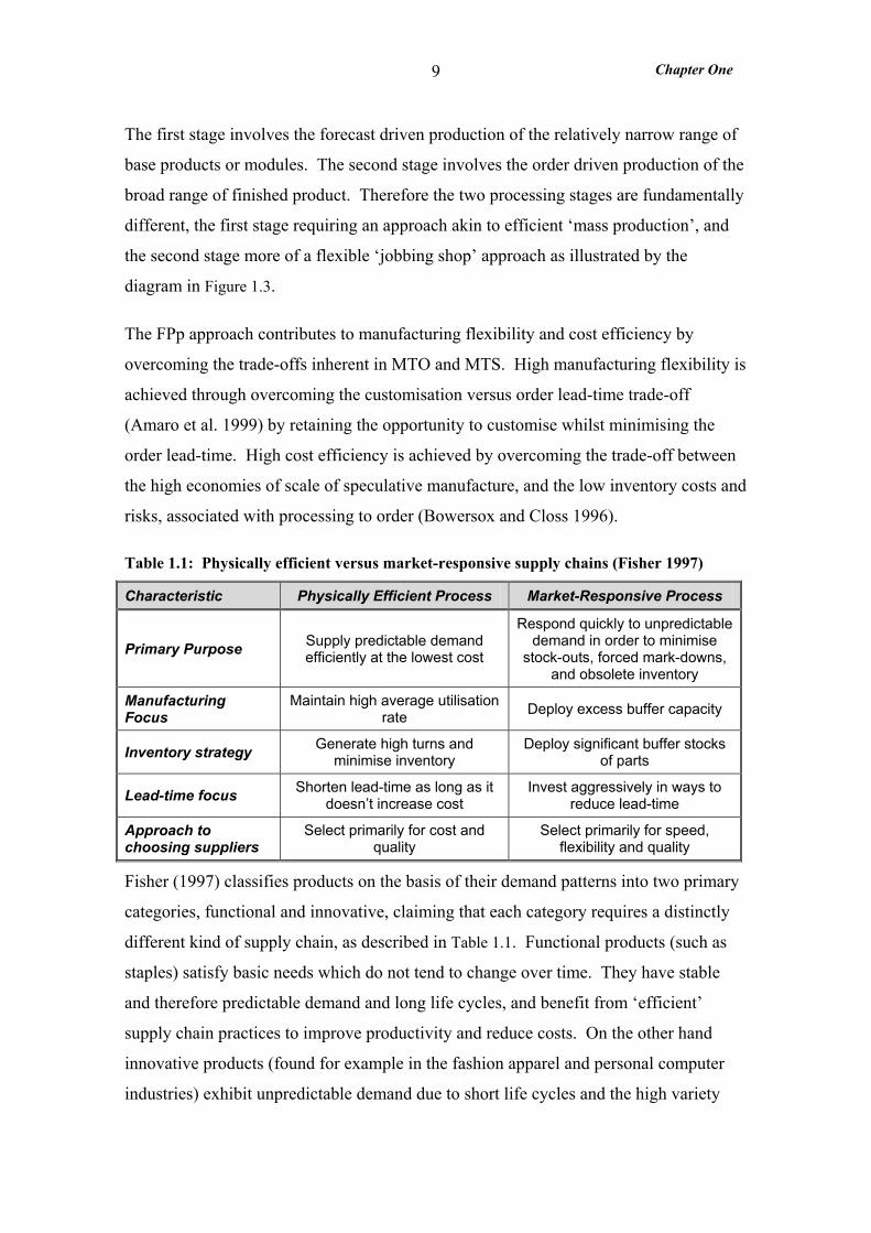
Table 1.1: Physically efficient versus market-responsive supply chains (Fisher 1997)

Characteristic Physically Efficient Process Market-Responsive Process

Primary Purpose Supply predictable demand efficiently at the lowest cost

Respond quickly to unpredictable demand in order to minimise

stock-outs, forced mark-downs, and obsolete inventory

Manufacturing Focus

Maintain high average utilisation rate Deploy excess buffer capacity

Inventory strategy Generate high turns and minimise inventory

Deploy significant buffer stocks of parts

Lead-time focus Shorten lead-time as long as it doesn’t increase cost

Invest aggressively in ways to reduce lead-time

Approach to choosing suppliers

Select primarily for cost and quality

Select primarily for speed, flexibility and quality

Fisher (1997) classifies products on the basis of their demand patterns into two primary

categories, functional and innovative, claiming that each category requires a distinctly

different kind of supply chain, as described in Table 1.1. Functional products (such as

staples) satisfy basic needs which do not tend to change over time. They have stable

and therefore predictable demand and long life cycles, and benefit from ‘efficient’

supply chain practices to improve productivity and reduce costs. On the other hand

innovative products (found for example in the fashion apparel and personal computer

industries) exhibit unpredictable demand due to short life cycles and the high variety

Chapter One

10

typical of these products. They therefore benefit from ‘responsive’ supply chain

practices that are geared to responding quickly to the unpredictable demand in order to

minimise stock-outs, forced mark-downs, and obsolete inventory. The base product or

modules in a FPp application can be likened to the ‘functional’ products and the

finished product likened to the ‘innovative’ products. Hence, the implication for FPp is

that the two types of supply chain can co-exist in series in the same factory (see CODP

discussion in section 1.2.1).

The two processing stages could equally be labelled as ‘lean manufacture’ and ‘agile

supply’ respectively. Agile supply assumes that the marketplace demands are volatile,

whereas in a lean manufacturing environment the demand should be smooth leading to a

level schedule.

MTS

FPp

MTO

ETO

Production based on forecasts

Production based on customer orders

Customer Order Decoupling Point (CODP)

Raw materials Components

Semi-finishedProducts

FinishedProducts

Demand downstream from decoupling point

Demand upstream from decoupling point

Supp

liers

Cus

tom

ers

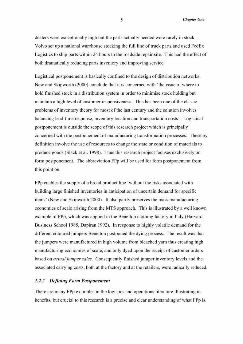
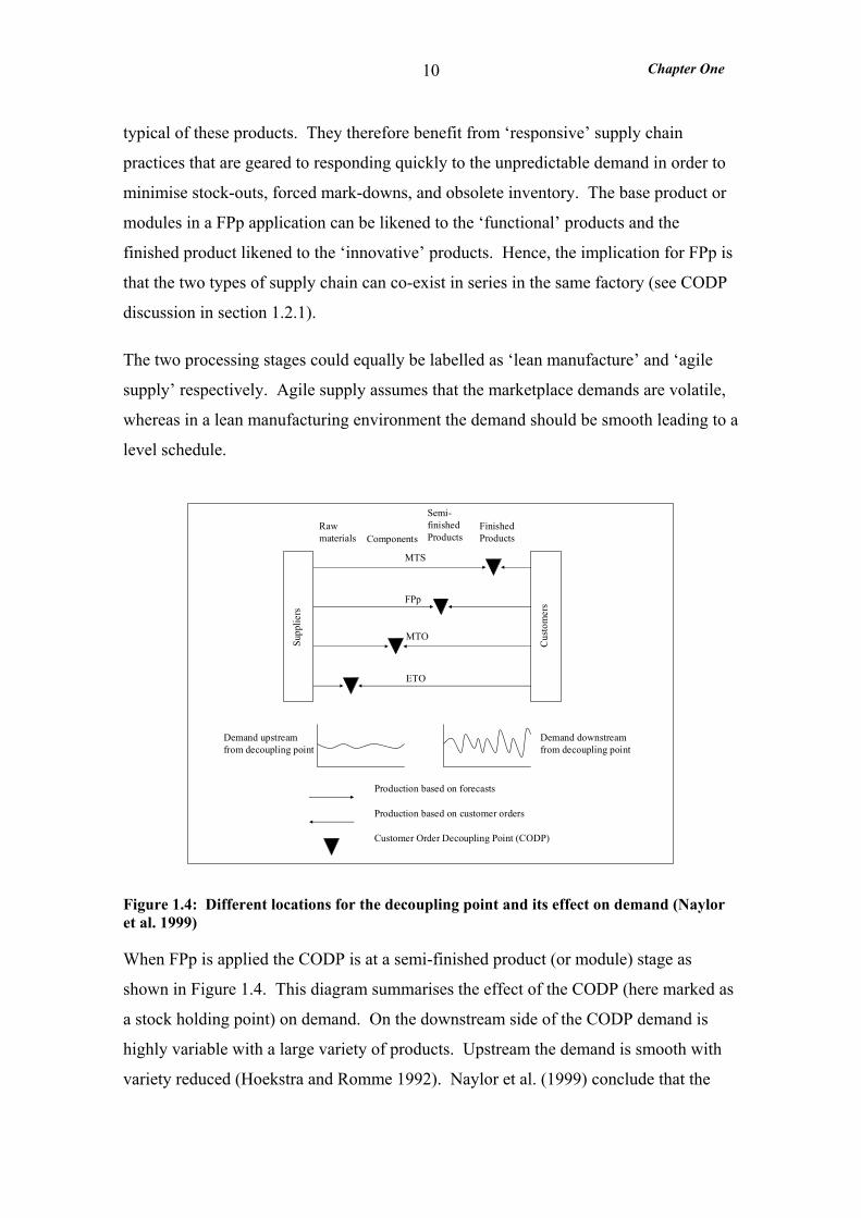
Figure 1.4: Different locations for the decoupling point and its effect on demand (Naylor et al. 1999)

When FPp is applied the CODP is at a semi-finished product (or module) stage as

shown in Figure 1.4. This diagram summarises the effect of the CODP (here marked as

a stock holding point) on demand. On the downstream side of the CODP demand is

highly variable with a large variety of products. Upstream the demand is smooth with

variety reduced (Hoekstra and Romme 1992). Naylor et al. (1999) conclude that the

Chapter One

11

lean paradigm can be applied to the supply chain upstream of the decoupling point as

demand is smooth and standard products are produced. Conversely the agile paradigm

should be applied downstream from the decoupling point as demand is variable and the

product variety increased. Combining agility and leanness in one supply chain with the

strategic use of a decoupling point has been termed ‘leagility’ (Naylor et al. 1999a) and

the literature relating to this is reviewed in section 2.5.1.

The dichotomy in manufacturing described here forms the basis of many of the

logistical and operational implications of applying FPp as discussed in the literature

review (Chapter 2). Managing this dichotomy in manufacturing within the same factory

is a major challenge.

1.3 RESEARCH AGENDA

The principle of postponement has its roots in marketing (Alderson 1950) which is

reviewed further in section 2.1. It has been developed in the logistics literature (for

example Bowersox and Closs 1996) which has differentiated between the postponement

of distribution (logistical postponement) and transformation processes (FPp). FPp is

commonly cited in the logistics literature as contributing to improved supply chains and

logistics systems (for example Scott and Westbrook 1991). In the operations

management (OM) literature it is recognized as a method of achieving mass

customization (for example Amaro et al. 1999) and more recently a new way of

thinking about product design, process design and supply chain management (Yang and

Burns 2003).

FPp is a phenomenon truly at the ‘interface’ (as understood by Voss 1995) between OM

and logistics employing supply chain and manufacturing systems thinking. However, as

is argued in the literature review in Chapter 2, the interface between these two

disciplines has become blurred, so my perspective on OM and logistics needs to be

stated. Here OM is primarily concerned with the development and management of

value adding processes and the tools and techniques to support them (Harrison 1996).

For this research project ‘value adding processes’ are confined to manufacturing

transformation processes (as defined by Slack et al. 1998). Logistics on the other hand

Chapter One

12

is primarily ‘concerned with getting products [and services] where they are needed

when they are needed’ (Bowersox and Closs 1996).

This research project is confined to FPp applications where both postponed and generic

processes are performed in the same location normally a factory. In this case two types

of supply chain exist in series in the factory. The production of the generic product or

modules is akin to an ‘efficient’ supply chain with the aim of lean manufacture. In

contrast the postponed customisation is akin to a ‘responsive’ supply chain with the aim

of agile supply. This introduces difficulties peculiar to FPp particularly in terms of

manufacturing planning and inventory management which are normally geared towards

MTO and/or MTS.

The benefits of FPp are widely appreciated and documented. However much less has

been said about applying it. This research is primarily concerned with how FPp is

applied within a manufacturing facility in terms of operations such as product design,

process design, inventory management, location of CODP and manufacturing planning.

This research is positioned at the interface between OM and logistics literature and

therefore makes a contribution to both fields. It aims to provide managers with

guidelines which indicate when FPp is justified and how it can be applied effectively.

1.3.1 Research Objectives

Six objectives were identified which reflect the overriding goal of this project, which is

to understand the operational implications of applying FPp in a manufacturing facility.

The objectives have guided the execution of this research project and they are:

• To understand the reasons for the application of FPp as an alternative to MTO or

MTS.

• To establish how products are selected for FPp - rather than MTO or MTS -

particularly in relation to products demand profiles (demand mix, volume demand

and demand variability) and production variety

Chapter One

13

• To determine the impact of FPp on customer service (order lead-time, ex-stock

availability and delivery reliability) and demand amplification relative to MTO and

MTS.

• To determine the product design implications of FPp particularly in terms of

product modularity and standardisation.

• To identify and understand other major operational implications for a

manufacturing facility which applies FPp. Particularly in terms of inventory

management and the manufacturing planning and control system.

• To identify operational obstacles to the application of FPp in manufacturing

facilities.

The objectives cover a broad field of enquiry which is both explanatory and exploratory

in nature and is supported by the case study research design detailed in Chapter 3.

1.3.2 Contribution of Research to Operations Management Literature

This research project aims to contribute knowledge to three areas of OM: non-MTS;

mass customisation; and postponement.

Most OM literature classifies non-MTS companies into three types: assemble-to-order

(ATO), MTO and engineer-to-order (ETO) (see for example New and Schejczewski

1995, Vollman et al. 1992). Clearly the key distinction between FPp and ETO or MTO

is the location of the CODP (as discussed in section 1.2.1.). There are four key

distinctions between FPp (as defined for this research) and ATO - although these two

categories overlap. Amaro et al. (1999) point out that ‘the literature addressing the

needs of companies which produce in response to customers’ orders is astonishingly

modest’. The needs of the non-MTS sector have been neglected. However, over the

four years since the Amaro et al. (1999) paper this sector appears to have received more

attention.

Much of non-MTS literature addresses the needs of the traditional MTO sector and the

bulk of these publications address issues related to manufacturing planning and control

(for example Marucheck and McClelland 1986, Hendry and Kingsman 1989, Yeh 2000,

Chapter One

14

Segerstedt 2002). A good proportion of the publications on MTO use mathematical

models to address specific planning and control issues (for instance He and Jewkes

2000, He et al. 2002, Webster 2002). Very few papers address the specific needs of

ETO (for example Eloranta 1992) or ATO (for example Wemmerlov 1984). Further in

this literature MTO and ATO are considered not to be responsive - orders are promised

on the basis of the availability of components and/or capacity rather than on the basis of

a short, often standard, quoted lead-time as for FPp.

Mass customisation has been defined as ‘providing numerous customer chosen

variations on every order with little lead-time or cost penalty’ (Ahlstrom and Westbrook

1999). Most of the literature on mass customisation is concerned with its strategic

impact (for example Gilmore and Pine 1997, Pine et al. 1993 and 1995, Lampel and

Mintzberg 1996, Kotha 1995, Westbrook and Williamson 1993). There are few

publications concerning the operational implications of mass customisation (for

example Pine 1993, Ahlstrom and Westbrook 1999, Swaminathan 2001, MacCarthy et

al. 2003).

Recently a small body of OM literature has emerged that addresses postponement. A

theoretical paper (Yang and Burns 2003) reviews research on postponement and

concludes that still little is known about its application. Most of the OM literature on

FPp uses mathematical or inventory models of postponement applications (for example

Van Mieghem and Dada 1999, Aviv and Federgruen 2001a and 2001b, Ma et al. 2002,

Ernst and Kamrad 2000). Most of these models consider delayed product

differentiation applied to MTS approaches and are therefore not directly applicable to

FPp. With the introduction of a CODP at the generic product stage they could be very

useful in understanding some of the operational implications of FPp, such as capacity

planning. This thesis contributes to this OM literature by using a case study research

design to address ‘how’ FPp is applied.

This thesis aims to contribute knowledge to OM by considering the operational issues of

applying FPp. This is a specific and responsive non-MTS approach to mass

customisation distinct from existing documented categories, ETO, MTO and ATO.

Unlike earlier literature this thesis focuses on the specific operational implications of

mass customisation achieved by applying FPp within a manufacturing facility. A case

Chapter One

15

study research design has been used to address the complexities of applying FPp. This

exploratory work could aid the development of variable oriented inventory or

mathematical models to simulate FPp and its operational implications. On a strategic

level this research determines the reasons for applying FPp rather than MTO or MTS

and how products (and customers) are selected.

1.3.3 Contribution of Research to Logistics literature

This research project aims to contribute to our understanding of the conditions under

which FPp is justified and specification of the appropriate FPp strategy (for example

Zinn and Bowersox 1988, Zin, 1990a, Cooper 1993, Pagh and Cooper 1998, van Hoek

1998a, van Hoek et al. 1998). In this literature FPp is considered as an alternative

strategy to MTS - not to MTO - and the guidelines are restricted to deciding an

appropriate postponement strategy rather than its application. In general only FPp

applications where the postponed processes are conducted in the distribution chain have

so far been considered. When postponed processes are brought back into the factory

substantially more complex processes are likely to be capable of postponement, as

supported by the survey of companies in Holland conducted by Van Hoek (1998c).

This thesis aims to contribute to logistics knowledge by considering FPp applications

where postponed processes are performed in the same location as the generic processes

This research considers when FPp is a justified alternative to either MTS or MTO and

the impact of FPp on customer service and demand amplification - both important

supply chain issues. Further contributions are made by addressing the complex

operational issues arising from taking the postponed processes back into the factory.

1.4 STRUCTURE OF THESIS

The literature review is presented in Chapter 2 and covers literature related to the

application of FPp from three different fields - logistics, operations and engineering.

The logistics and operations literature specifically addressing FPp (to which this

research contributes) is reviewed separately. This chapter culminates in a conceptual

model of FPp and a theoretical model predicting the outcome of applying FPp. Chapter

3 presents the hypotheses - extracted from the theoretical framework - which address

the research question. This chapter also describes and justifies the research design in

Chapter One

16

terms of the strategy and how it was operationalised. It concludes with the limitations

of the design. Chapters 4, 5 and 6 detail the application of the research design in three

different case companies. Chapter 4 describes the Pilot Study at Thomas Bolton which

was conducted to develop the research methods and to firm up the hypotheses. Chapter

5 describes the case study at Brook Crompton where the three inventory management

policies used in the manufacture of Direct Current motors were compared. Chapter 6

presents the study at Dewhurst which involved comparing the manufacture of three

different products. The three case studies are compared in Chapter 7 in terms of their

contexts, how FPp was applied, the flaws in the applications and the outcomes of

applying FPp. The thesis ends with Chapter 8 which provides a summary of the

research project, the contribution to knowledge made by the research and a discussion

of the research limitations.

Chapter Two

17

CHAPTER TWO

2 Literature Review

The principle of postponement has its roots in marketing. It has been developed in the

logistics literature, where FPp is commonly cited as contributing to more responsive

supply chains. In the OM literature FPp is widely recognized as a method of achieving

mass customization and more recently as an approach to product, process and supply

chain design. FPp is a phenomenon which is positioned at the overlap of a number of

subject areas and draws on a number of disciplines. Thus this research is positioned

between logistics and OM and so employs supply chain and manufacturing systems

thinking. It also draws on engineering literature which addresses product and process

design for postponement - ‘delayed product differentiation’ (DPD). Hence three bodies

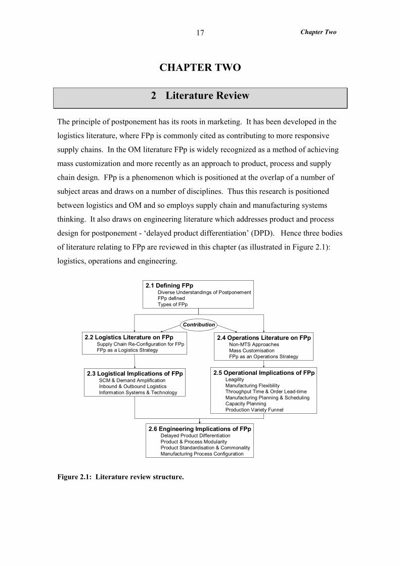
of literature relating to FPp are reviewed in this chapter (as illustrated in Figure 2.1):

logistics, operations and engineering.

2.1 Defining FPpDiverse Understandings of PostponementFPp definedTypes of FPp

2.2 Logistics Literature on FPpSupply Chain Re-Configuration for FPpFPp as a Logistics Strategy

2.3 Logistical Implications of FPpSCM & Demand AmplificationInbound & Outbound LogisticsInformation Systems & Technology

2.4 Operations Literature on FPpNon-MTS ApproachesMass CustomisationFPp as an Operations Strategy

2.5 Operational Implications of FPpLeagilityManufacturing FlexibilityThroughput Time & Order Lead-timeManufacturing Planning & SchedulingCapacity PlanningProduction Variety Funnel

2.6 Engineering Implications of FPpDelayed Product DifferentiationProduct & Process ModularityProduct Standardisation & CommonalityManufacturing Process Configuration

Contribution

Figure 2.1: Literature review structure.

Chapter Two

18

The purpose of this literature review is to:

• develop a working definition of FPp (section 2.1.2)

• identify gaps in the literature where a contribution could be made (sections 2.2

and 2.4)

• review the implications of applying FPp with a view to developing a conceptual

model and theoretical framework from which the hypothesise can be extracted.

The literature review is structured as illustrated in Figure 2.1. An attempt has been

made to distinguish between logistics and OM literature. However particularly in recent

years the line between these two disciplines has become blurred. OM has become

concerned with supply chain management (for example Yang and Burns 2003) and

logistics is addressing product customisation (for example Walker et al. 2000). Journal

subject classifications and an interpretation of OM and logistics have been used to guide

the categorisation of the literature. Literature primarily concerned with ‘the

development and management of value adding processes and the tools and techniques to

support them’ (Harrison 1996) has been classified as OM literature. Literature

primarily ‘concerned with getting products [and services] where they are needed when

they are needed’ (Bowersox and Closs 1996) has been classified as logistics.

Section 2.1 provides a brief history of postponement and a critical review of existing

postponement definitions which was the basis for the working definition of FPp used for

this research.

Section 2.2 reviews logistics research addressing FPp which can be split into two areas.

The first addresses the configuration of supply chains for FPp where factories and

warehouses are treated as ‘black boxes’. The second area is a small body of research

addressing when FPp is the justified approach by considering the product, market and

process characteristics that favour FPp. This thesis contributes to the latter area - but

not the former - since it is concerned with the operational implications within the

factory, but not the configuration of factory and warehouse sites.

Chapter Two

19

Logistics research associated with the implications of applying FPp is reviewed in

section 2.3. FPp is viewed in the context of Supply Chain Management (SCM), in

particular its effects on demand amplification. The implications for both inbound and

outbound logistics are also considered focusing mainly on the postponed process.

Finally the information system and technology implications of FPp are considered.

Section 2.4 reviews OM research addressing concepts closely related to FPp. The first

part reviews research on non-MTS approaches, of which FPp is an example. The

second part considers research on mass customization, for which FPp is widely

recognized as a possible approach. In the third part recent research is reviewed which

considers the application of postponement as an operations strategy. This thesis makes

a contribution to all three areas of OM research.

Section 2.5 reviews the OM research relating to the various operational implications of

applying FPp. Manufacturing flexibility in its various forms is considered - in

particular mix flexibility required for the postponed process. Throughput time and

order lead-time are discussed in relation to throughput efficiency. Approaches to

manufacturing planning and production scheduling suitable for FPp applications are

presented. Capacity planning issues are addressed particularly with respect to the

provision of excess capacity at the postponed process. Finally the production variety

funnel, central to the conceptual model, of FPp is introduced.

Engineering research relating to FPp is reviewed in section 2.6. Delayed product

differentiation (DPD), which can be an approach to product and process re-design for

FPp, is introduced. The three approaches to DPD are discussed in relation to FPp:

product and process modularity; product standardization and component commonality;

and manufacturing process re-structuring.

This chapter concludes with the conceptual model of FPp, the theoretical framework

and the gaps in logistics and OM research to which this thesis makes a contribution.

Chapter Two

20

2.1 DEFINING FORM POSTPONEMENT

This section provides a brief history of postponement and a critical review of existing

postponement definitions which was the basis for the working definition of FPp used for

this research.

The concept of postponement is first introduced in marketing by Alderson (1950) who

argues that postponement could be used to reduce risk and uncertainty costs associated

with the differentiation of goods. He claims that differentiation could occur in the

product itself or the geographical dispersion of the inventories and offers the principle

of postponement, which advocates:

‘postpone changes in form and identity to the latest possible point in the marketing flow; postpone changes in inventory location to the latest possible point in time.’

Alderson (1950) argues that savings in costs related to uncertainty would be achieved

‘by moving the differentiation nearer to the time of purchase’, where demand

presumably would be more predictable. Later Bucklin offers the converse of

postponement, the principle of speculation, which states:

‘changes in form, and the movement of goods to forward inventories, should be made at the earliest possible time in the marketing flow in order to reduce the costs of the marketing system.’

Bucklin (1965) recognises that postponement has its limitations and there are trade-offs

to consider. He argues that speculation permits the goods to be ordered in large

quantities therefore improving the economies of scale for manufacturing. To express

the limitation of postponement he proposes a combined principle of postponement-

speculation:

‘a speculative inventory will appear at each point in a distribution channel whenever its costs are less than the net savings to both buyer and seller from postponement.’

Following the work of Alderson and Bucklin it was some time before postponement

was practised. There are a number of theories as to why this was the case. Van Hoek

(1998a) concludes that new technologies (information and communication technology),

Chapter Two

21

operating circumstances (deregulation in Europe), and new organisational forms

(integrated networks) have recently enabled the application of postponement (van Hoek

et al. 1996 and 1998).

2.1.1 Diverse Understandings of Postponement

In the late 1980s postponement became known as a logistics strategy (Cooper 1993).

Subsequently much of the research over the last decade of the 20th century regarding

postponement appears in the logistics literature. In a key paper by Zinn and Bowersox

(1988) which attempted to operationalise the postponement-speculation principle the

following definition of postponement was given:

‘Postponement consists of delaying movement or final formulation of a product until after customer orders are received.’

This definition is more specific than Alderson’s stating that the postponed activities

should take place after the receipt of customer orders. Two main types of

postponement (implied by Alderson’s original definition) are defined, ‘form or

manufacturing postponement’ and ‘logistical or time postponement’. As discussed in

Chapter 1 logistical postponement falls outside the scope of this research therefore this

chapter focuses on form postponement.

Zinn and Bowersox (1988) offer the following definition of FPp:

‘Form Postponement proposes that under specific situations that the least risky procedure may be to send products to the warehouses in a semi-finished state for final processing after the customer order is received.’

This definition is narrow in scope stipulating that the postponed process takes place in a

warehouse and is restricted to final processing. ‘Postponed manufacturing’ (van Hoek,

1998a) is a very similar concept to this, but requires that the postponed process take

place in a ‘facility close to the customer separated from the manufacturing of semi-

finished or generic products or components’. The requirement that the postponed

process take place in the distribution chain, normally a warehouse, is the inherent

weakness in these definitions as argued in section 2.1.1 below.

The engineering literature has a very different view of logistical postponement and FPp.

Lee and Billington (1994) define logistical postponement in the same way as Zinn and

Chapter Two

22

Bowersox (1988) define FPp. Further ‘form’ postponement is defined to exist only

when the product design is standardised so the differentiation step no longer exists and

therefore differentiation is effectively postponed. The engineering literature which

focuses on design for postponement (for example, Lee and Tang 1997, Garg and Tang

1997, Lee 1996) uses the term ‘delayed product differentiation’. This can be achieved

through standardisation, modular production, or process restructuring and is reviewed in

detail in section 2.6.

Recently a host of new postponement definitions have emerged in the OM literature.

For example Brown et al. (2000) define ‘product postponement’ as ‘products are

designed so that the product’s specific functionality is not set until after the customer

receives it’. This involves the customer configuring a standardised product upon receipt

and is classified as a ‘standardisation’ strategy (as described in section 2.6.3). Brown et

al. (2000) also use the term ‘process postponement’ to describe the creation of a generic

part in the initial stages of the manufacturing process which is later customised to give

the finished product. This fits well with the working definition of FPp used for this

research unlike other definitions in the OM literature. For example Van Mieghem and

Dada (1999) consider postponement of different operational decisions: ‘price

postponement’ involves delaying setting the price; and ‘production postponement’

involves delaying production until an order has been received (MTO).

In the logistics literature the definition of ‘FPp’ is considerably extended by Van Hoek

(van Hoek 1998c, van Hoek et al. 1996 and 1998):

‘Form Postponement involves the delaying of activities that determine the form and function of products until orders are received’

Later Van Hoek (2001) states:

‘postponement means delaying activities in the supply chain until customer orders are received with the intention of customising products, as opposed to performing those activities in anticipation of future orders’.

These definitions do not specify the location of the postponed process therefore these

activities may take place at the manufacturing plant or in the distribution chain. Further

the postponed processes are described as ‘activities that determine the form and function

Chapter Two

23

of products’ or customising activities. For any given product the most upstream activity

that may be postponed is the engineering or design of the product. Therefore these

definitions include ETO and MTO (as defined by Amaro 1999, Browne et al. 1996) as

approaches to postponement. This appears to be a commonly used understanding of

postponement in the OM literature (see for example Yang and Burns 2003).

2.1.2 Defining FPp

The literature provides no consensus on a clear definition of FPp, instead there is a host

of definitions expounding different ideas. Much of the research on FPp uses one of two

FPp definitions neither of which appears appropriate. The Zinn and Bowersox (1988)

definition requires the postponed process to take place in the distribution chain and the

van Hoek (1998c, 2001) definition encapsulates ETO and MTO as approaches to FPp.

First consider the Zinn and Bowersox (1988) definition. The requirement that the

postponed process take place in the distribution chain, normally a warehouse, is an

inherent weakness for three reasons.

Firstly this definition does not reflect what several manufacturing companies are

actually doing – for instance many manufacturers conduct the postponed process in the

same location as the generic processes:

• Sony Manufacturing (UK) at Bridgend applied FPp to television manufacture

(Ferguson 1989) by designing a ‘Eurochassis’ (the base of the television to

which the PCBs and other components were fitted) which was common to all its

products. Only at a late stage in the manufacturing was the Eurochassis tailored

specifically for individual customer orders.

• Courtaulds Hosiery (Aristoc plant in Northern Ireland) manufactured tights in

two gauges of yarn, in five sizes and in twelve colour shades to provide 120

different variants (New and Skipworth 2000). FPp was applied to both the tights

themselves and the packaging. The tights were knitted from natural yarn and

over-dyed to customer order, and the packaging (which suffered from the same

level of variety) was standardised and over printed to order.

Chapter Two

24

• Xerox applied FPp to their office digital products in 1997 at the Gloucester plant

(Christopher 1998). A minimal level of ‘neutral’ finished goods were made to

stock and only configured to customer order.

• Benetton knitted the jumpers in natural yarn to stock and subsequently dyed

them to customer order all in their main plant in Italy (Harvard Business School

1985).

Other examples of FPp require the postponed process be performed at the retailers.

Instead of stocking the full range of paint colours for each variant some retailers stock

the generic paint with a variety of pigments and mix them to specific customer orders

(Feitzinger and Lee 1997). Sunoco gasoline stations apply a similar principle

(Bowersox and Closs 1996). Here a standard low octane gasoline was stocked and

mixed with additives to customer order to make higher octane grades of unleaded petrol.

Secondly conducting postponed processes in warehouses tends to restrict such processes

to extremely simple ones for two main reasons. Firstly they would be required to take

place at multiple sites ensuring that only low capital manufacturing installations are

viable. Secondly the lack of proximity to the main manufacturing plant, and the

expertise it offers, would dissuade many manufacturers from conducting highly

technical or critical processes in a warehouse. Many examples support this view:

• the postponed process conducted in the warehouses by Motorola consists of

programming the frequencies into the radios and labelling them accordingly

(Andel 1997).

• Hewlett-Packard manufactured generic Deskjet Printers at their Vancouver plant

and shipped them to there distribution centres (Europe, Asia etc.) for

‘localisation’ (Lee et al. 1993). Here the printers were merely ‘box kitted’ with

the correct power supply module and manual to order (Davis and Sasser 1995).

• Caterpillar developed a manufacturing and distribution system whereby fork lift

trucks were produced offshore and options, such as lifts and forks later attached

against customer orders in a US warehouse.

Chapter Two

25

Thirdly this narrow definition is flawed because it may not be necessary to perform the

postponed processes in a warehouse, which offers greater proximity to the customers

than the manufacturing facility. The key is getting the ‘time’ right between

commencing the postponed process and the receipt of the product by the customer not

the ‘distance’. Therefore, the appropriate location for these processes depends on the

customer required order lead-time and the speed of final distribution transport according

to the ‘point of fulfilment’ described by Inger et al. (1995).

Considering the van Hoek’s (1998c, 2001) definition which encapsulates ETO and

MTO as approaches to FPp, it is acknowledged that:

‘the vision of manufacturing postponement is one of products being manufactured an order at a time with no preparatory work or component procurement until exact customer specifications are fully known and purchase commitment is received’ (Bowersox and Closs 1996).

However, in practice there is a trade-off between the high economies of scale achievable

through speculative manufacture and the low inventory costs and risks resulting from

processing to order - if the required responsiveness is to be achieved without sacrificing

efficiency (Bowersox and Closs 1996). Bowersox and Closs (1996) state that the ideal

application of postponement is to manufacture a standard base product in sufficient

quantities to realise economies of scale, while deferring finalisation of features (such as

colour) until customer commitments are received. ETO and MTO are not encapsulated

by this understanding of FPp.

The above arguments culminated in the following working definition that has been used

for this research:

‘FPp is the delay, until customer orders are received, of the final part of the transformation processes, through which the number of different product items proliferates and for which only a short time period is available. The postponed transformation processes may be manufacturing processes, assembly processes, configuration processes, packaging, or labelling processes.’

It broadens the Zinn and Bowersox (1988) definition by not stipulating the geographical

location of the postponed process. It acknowledges that the postponed process may take

place not only at a warehouse but at a factory (as in ‘bundled manufacturing’ defined by

Cooper 1993) or even at the retailers, and these locations may be near to or remote from

Chapter Two

26

the customers. Yet it is more restricting than the van Hoek (1998c) definition by

confining FPp to the postponement of ‘the final part of the transformation process’.

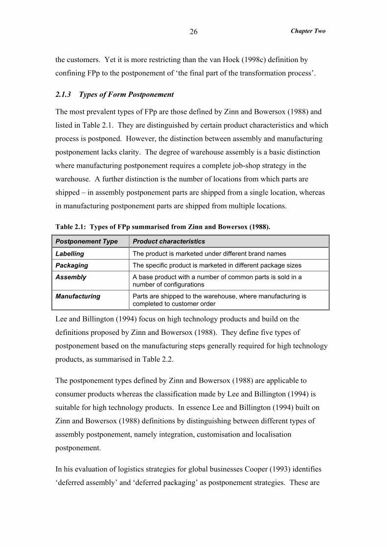
2.1.3 Types of Form Postponement

The most prevalent types of FPp are those defined by Zinn and Bowersox (1988) and

listed in Table 2.1. They are distinguished by certain product characteristics and which

process is postponed. However, the distinction between assembly and manufacturing

postponement lacks clarity. The degree of warehouse assembly is a basic distinction

where manufacturing postponement requires a complete job-shop strategy in the

warehouse. A further distinction is the number of locations from which parts are

shipped – in assembly postponement parts are shipped from a single location, whereas

in manufacturing postponement parts are shipped from multiple locations.

Table 2.1: Types of FPp summarised from Zinn and Bowersox (1988).

Postponement Type Product characteristics

Labelling The product is marketed under different brand names

Packaging The specific product is marketed in different package sizes

Assembly A base product with a number of common parts is sold in a number of configurations

Manufacturing Parts are shipped to the warehouse, where manufacturing is completed to customer order

Lee and Billington (1994) focus on high technology products and build on the

definitions proposed by Zinn and Bowersox (1988). They define five types of

postponement based on the manufacturing steps generally required for high technology

products, as summarised in Table 2.2.

The postponement types defined by Zinn and Bowersox (1988) are applicable to

consumer products whereas the classification made by Lee and Billington (1994) is

suitable for high technology products. In essence Lee and Billington (1994) built on

Zinn and Bowersox (1988) definitions by distinguishing between different types of

assembly postponement, namely integration, customisation and localisation

postponement.

In his evaluation of logistics strategies for global businesses Cooper (1993) identifies

‘deferred assembly’ and ‘deferred packaging’ as postponement strategies. These are

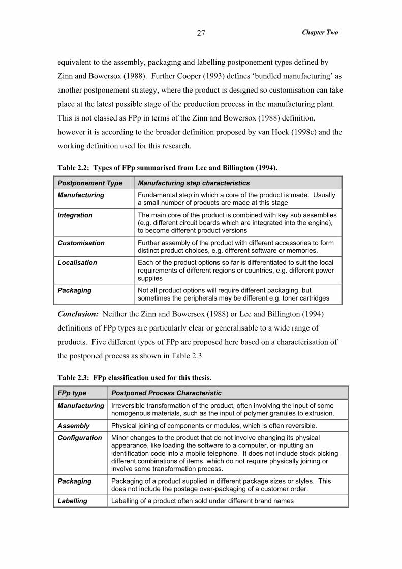
Chapter Two

27

equivalent to the assembly, packaging and labelling postponement types defined by

Zinn and Bowersox (1988). Further Cooper (1993) defines ‘bundled manufacturing’ as

another postponement strategy, where the product is designed so customisation can take

place at the latest possible stage of the production process in the manufacturing plant.

This is not classed as FPp in terms of the Zinn and Bowersox (1988) definition,

however it is according to the broader definition proposed by van Hoek (1998c) and the

working definition used for this research.

Table 2.2: Types of FPp summarised from Lee and Billington (1994).

Postponement Type Manufacturing step characteristics

Manufacturing Fundamental step in which a core of the product is made. Usually a small number of products are made at this stage

Integration The main core of the product is combined with key sub assemblies (e.g. different circuit boards which are integrated into the engine), to become different product versions

Customisation Further assembly of the product with different accessories to form distinct product choices, e.g. different software or memories.

Localisation Each of the product options so far is differentiated to suit the local requirements of different regions or countries, e.g. different power supplies

Packaging Not all product options will require different packaging, but sometimes the peripherals may be different e.g. toner cartridges

Conclusion: Neither the Zinn and Bowersox (1988) or Lee and Billington (1994)

definitions of FPp types are particularly clear or generalisable to a wide range of

products. Five different types of FPp are proposed here based on a characterisation of

the postponed process as shown in Table 2.3

Table 2.3: FPp classification used for this thesis.

FPp type Postponed Process Characteristic

Manufacturing Irreversible transformation of the product, often involving the input of some homogenous materials, such as the input of polymer granules to extrusion.

Assembly Physical joining of components or modules, which is often reversible.

Configuration Minor changes to the product that do not involve changing its physical appearance, like loading the software to a computer, or inputting an identification code into a mobile telephone. It does not include stock picking different combinations of items, which do not require physically joining or involve some transformation process.

Packaging Packaging of a product supplied in different package sizes or styles. This does not include the postage over-packaging of a customer order.

Labelling Labelling of a product often sold under different brand names

Chapter Two

28

2.2 LOGISTICS LITERATURE ON FORM POSTPONEMENT

This section reviews the logistics literature addressing FPp which can be split into two

areas. The first addresses the configuration of supply chains for FPp where

manufacturing sites (factories or warehouses) are treated as ‘black boxes’. The second

area is a small body of literature addressing when FPp is the justified approach by

considering the product, market and process characteristics that favour FPp.

2.2.1 Supply Chain Re-Configuration for Form Postponement

The appropriate location for the postponed process (and the associated speculative

aggregate inventory) is determined not only by supply chain design but also by the

design of the product (New and Skipworth 2000). In a theoretical study Cooper (1993)

evaluated postponement strategies for global brands. He made deductions regarding

supply chain configuration for FPp in relation to product design or variety:

• where the formulation and peripherals are global FPp is not favoured, because

the product line is very narrow.

• where the formulation differs from market to market, but the peripherals are

standard, FPp taking place in the factory is favoured – ‘bundled manufacturing’

• where the peripherals differ from market to market FPp is favoured where the

postponed processing is performed in the distribution chain.

Cooper (1993) assumes that the peripherals significantly increase the product volume,

and therefore transportation costs are reduced, by transporting products without

peripherals to the warehouse and packaging them there.

Supply chain design issues which determine the location of the postponed process

include the Portfolio Effect which means that centralising inventories in fewer locations

always results in a reduction of safety stocks. Zinn (1990a) shows that the Portfolio

Effect is maximised whenever the sales correlation between two inventory locations is

highly negative, and the proportional difference in demand variability is small.

However Inger et al. (1995) claims that the location of the postponed process or ‘point

Chapter Two

29

of fulfilment’ is still critically dependant on the lead-time the customer is prepared to

accept.

Van Hoek (1998a and 1998b) and Van Hoek et al. (1996 and 1998) built on the ideas

put forward by Cooper (1993) in a major study into the application of ‘postponed

manufacturing’ (FPp where postponed processing is performed in the distribution chain)

in European supply chains. This study involved eight case studies and provided three

major contributions concerned with the reconfiguration of the supply chain for FPp:

• Firstly customer service and responsiveness considerations are usually the primary

drivers for postponed manufacturing applications. The implementation of

‘postponed manufacturing’ requires the reconfiguration and design of the outbound

logistics or downstream supply chain. The starting point in the change process and

organisational heritage (particularly whether the company is American or European)

has a significant effect on the supply chain reconfiguration process.

• Secondly a postponement trade-off framework was developed. It suggests what

types of postponement are viable in relation to: the position in the supply chain of

the manufacturing company; and the geographical scale at which final

manufacturing takes place. This framework did not however consider FPp where all

processing takes place in the factory as an option.

• Thirdly a number of tools and methods are provided to aid the reconfiguration of

supply chains for ‘postponed manufacturing’. For European companies a

calculation model is suggested while the logistics strategy framework developed by

O’Laughlin et al. (1993) is proposed for American companies.

Conclusion: so far the literature has treated manufacturing sites (factories or

warehouses) as ‘black boxes’. Further it largely ignores FPp in the factory and focuses

on cases where variety is added in the distribution chain. This thesis is concerned with

operations within the factory - rather than the configuration of manufacturing in

warehouse facilities - therefore it makes no contribution to this literature.

Chapter Two

30

2.2.2 Form Postponement as a Logistics Strategy

A small body of logistics literature addresses the various characteristics – such as

product, market, demand - that favour FPp. It is argued that FPp is not always the most

cost-effective approach to manufacturing and distribution, and the identification of

characteristics that favour FPp will provide managers with guidelines as to when FPp is

justified (Zinn and Bowersox 1988).

A leading article by Zinn and Bowersox (1988) explores the impact of changes in

physical and demand product characteristics, on the cost of distribution (inventory

carrying plus transportation costs) using FPp, compared with using MTS with

anticipatory distribution. Four normative cost models were used, each based on one of

the four types of FPp defined by Zinn and Bowersox (1988): manufacturing, assembly,

packaging and labelling (see section 2.1.3.). Demand uncertainty, product value,

product variety, and in the case of postponed assembly, the cube or volume reduction

(obtained by transporting products unassembled to the warehouse), were all found to

favour FPp. Only volume demand at generic level showed little or no significant

support for FPp. Zinn (1990b) summarised this contribution by stating that generally

postponement opportunities ‘emerge as large errors in demand forecasting increasing

the cost of distribution’, and are ‘greater for products of high unit value, because such

products have high inventory carrying cost’.

A number of assumptions are made in the Zinn and Bowersox (1988) study that limit its

generalisability:

• First, and most notably the data used concerned products from the same

company, which appear from the data to be of a similar nature, however details

regarding product type is not given.

• Second, the segment of the distribution channel covered by the cost models is

from the manufacturing plant exit to the warehouse exit. Therefore, the

modelling assumes that the product design does not change and it does not take

into account the effect on manufacturing costs of relocating production into

warehouses. It is impossible to judge if this is realistic, however it is possible to

Chapter Two

31

say that this assumption limits the generalisability of the study to cases where

this assumption holds.

• Third, it is assumed that postponing either the assembly, or manufacturing

processes until an order is received, results in an increase in average delivery

time (order lead-time), and subsequently lost sales. It can be argued that the

increased availability of product variants – a potential benefit of FPp (due to

customising only to order) - may negate the effects of lost sales due to increases

in order lead-time.

The study by Zinn and Bowersox (1988) may be difficult to generalise. However their

findings that demand uncertainty, product value, and product variety favour FPp is

supported by other work (Zinn 1990a, Cooper 1993, van Hoek 1998a). Zinn (1990a)

further explores the impact of product demand characteristics on the viability of FPp by

developing heuristics to estimate the impact of FPp on safety stocks. Risk pooling

techniques are used because the risk related to the demand uncertainty for each product

item is pooled together when FPp is applied. The heuristics developed indicate that

safety stock savings from FPp are higher when:

• demand for individual items is independent of each other or negatively

correlated,

• the number of products in the product line is greater, (however the savings

stabilise when the number of items exceeds eight) or

• the standard deviation of demand for items in the product line are approximately

equal.

Lee and Billington (1994) also showed that inventory savings are greater where the

demands for different products are negatively correlated.

In the above studies ‘demand variability’ is used to indicate ‘demand uncertainty’ (Zinn

and Bowersox (1988), and Zinn (1990). Here standard deviation of demand is used as a

measure of ‘demand uncertainty’. Bhattacharya et al. (1995) clearly distinguishes

between variability and uncertainty of demand. Variability measures the changes in

Chapter Two

32

demand over a given sequence of time buckets, forecasted at a given point in time. It

can be measured using the coefficient of variation (CV), the ratio of the standard

deviation to the average demand. Uncertainty measures the changes in demand for a

given time bucket as it moves in time and approaches the delivery due date. This raises

the question whether it is valid to use demand variability as an indication of uncertainty.

However setting aside this consideration existing theory supports the proposal that

demand uncertainty at finished product level favours FPp. Traditionally in a MTS

situation finished inventory is used as a buffer against demand uncertainty (Newman et

al. 1993). FPp eliminates this finished product safety stock, therefore the greater the

demand uncertainty the greater the reduction in safety stock due to FPp.

Chiou et al (2002) empirically examine four types of FPp proposed by Zinn and

Bowersox (1988) (manufacturing, assembly, packaging and labelling) against

Taiwanese Information Technology (IT) firms. They find that these FPp types are

practiced by the Taiwanese IT firms and that:

• products characterised by high levels of customisation and modular designs

benefit from assembly FPp

• products with expensive key components benefit from labelling and packaging

FPp but not necessarily assembly or manufacturing FPp

• products with short product life cycles benefit from manufacturing FPp

In a theoretical study Cooper (1993) evaluates postponement strategies for products

with global brands. He explores the impact of two further product characteristics on the

application of FPp as shown in Table 2.4.

Cooper (1993) argues that where either the formulation or peripherals, or both, are not

global (i.e not common to all markets) FPp is favoured. When the product formulation

differs from market to market, but the peripherals are standard, ‘bundled manufacturing’

is favoured - where the postponed processes take place in the factory. However when

the peripherals are not standard ‘deferred FPp’ is favoured, where the postponed process

takes place in the theatre warehouse. Cooper (1993) assumes that the peripherals

significantly increase the product cube or volume, and therefore transportation costs are

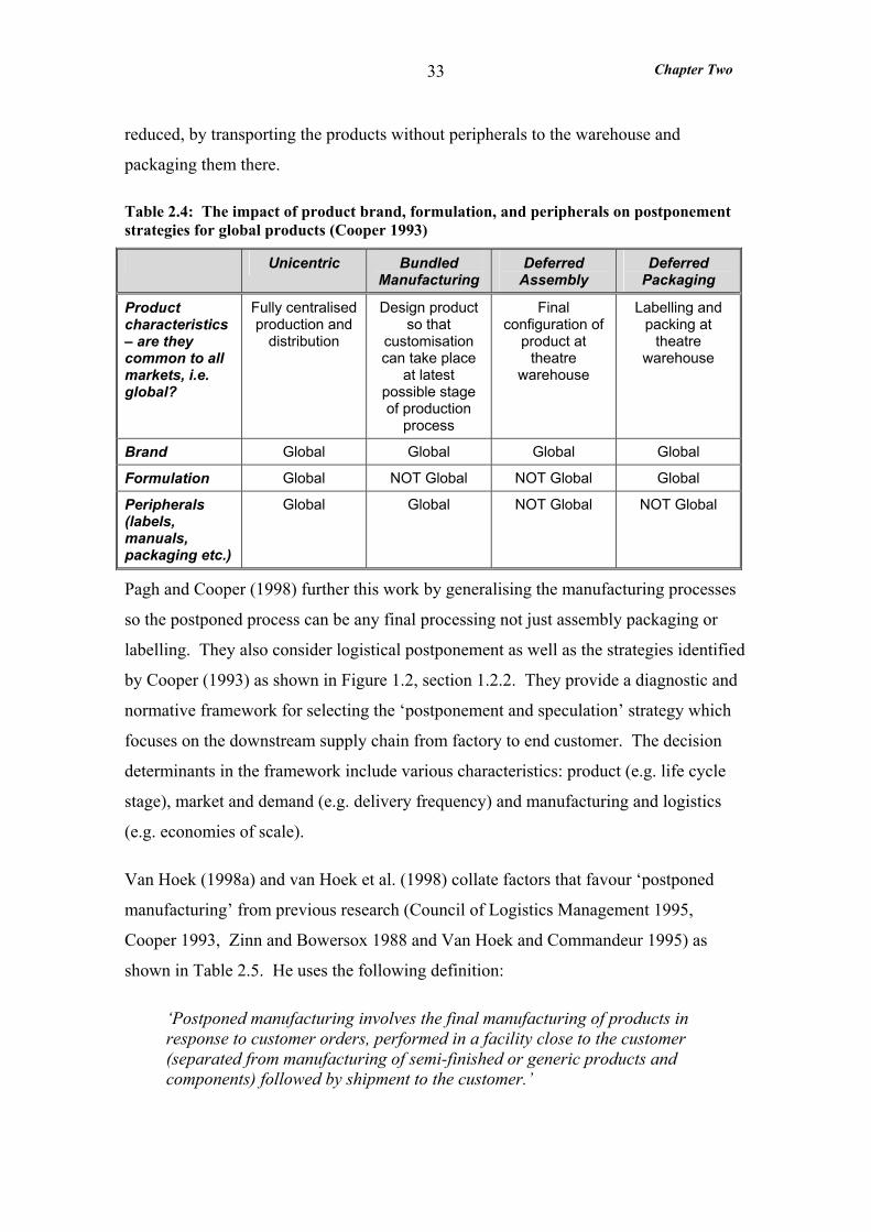
Chapter Two

33

reduced, by transporting the products without peripherals to the warehouse and

packaging them there.

Table 2.4: The impact of product brand, formulation, and peripherals on postponement strategies for global products (Cooper 1993)

Unicentric Bundled Manufacturing

Deferred Assembly

Deferred Packaging

Product characteristics – are they common to all markets, i.e. global?

Fully centralised production and

distribution

Design product so that

customisation can take place

at latest possible stage of production

process

Final configuration of

product at theatre

warehouse

Labelling and packing at

theatre warehouse

Brand Global Global Global Global

Formulation Global NOT Global NOT Global Global

Peripherals (labels, manuals, packaging etc.)

Global Global NOT Global NOT Global

Pagh and Cooper (1998) further this work by generalising the manufacturing processes

so the postponed process can be any final processing not just assembly packaging or

labelling. They also consider logistical postponement as well as the strategies identified

by Cooper (1993) as shown in Figure 1.2, section 1.2.2. They provide a diagnostic and

normative framework for selecting the ‘postponement and speculation’ strategy which

focuses on the downstream supply chain from factory to end customer. The decision

determinants in the framework include various characteristics: product (e.g. life cycle

stage), market and demand (e.g. delivery frequency) and manufacturing and logistics

(e.g. economies of scale).

Van Hoek (1998a) and van Hoek et al. (1998) collate factors that favour ‘postponed

manufacturing’ from previous research (Council of Logistics Management 1995,

Cooper 1993, Zinn and Bowersox 1988 and Van Hoek and Commandeur 1995) as

shown in Table 2.5. He uses the following definition:

‘Postponed manufacturing involves the final manufacturing of products in response to customer orders, performed in a facility close to the customer (separated from manufacturing of semi-finished or generic products and components) followed by shipment to the customer.’

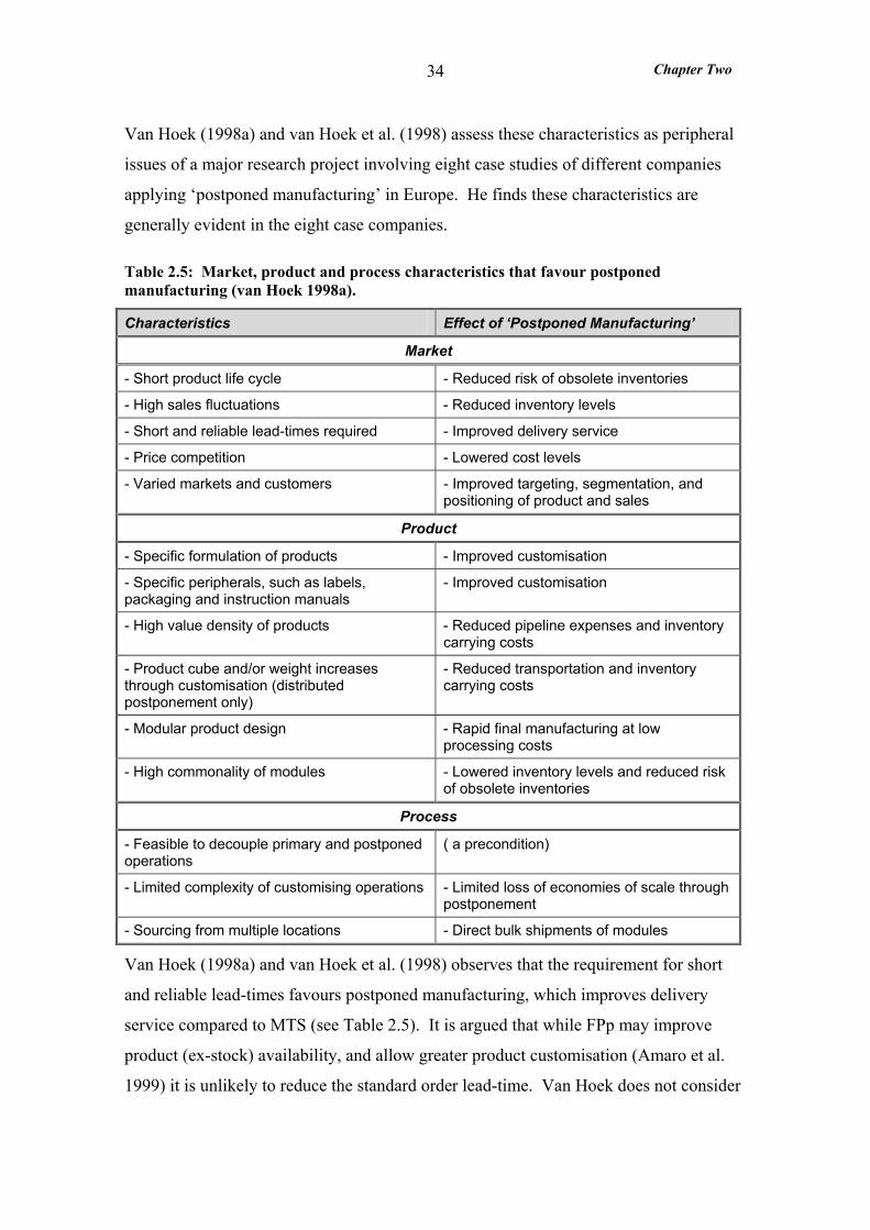
Chapter Two

34

Van Hoek (1998a) and van Hoek et al. (1998) assess these characteristics as peripheral

issues of a major research project involving eight case studies of different companies

applying ‘postponed manufacturing’ in Europe. He finds these characteristics are

generally evident in the eight case companies.

Table 2.5: Market, product and process characteristics that favour postponed manufacturing (van Hoek 1998a).

Characteristics Effect of ‘Postponed Manufacturing’

Market

- Short product life cycle - Reduced risk of obsolete inventories

- High sales fluctuations - Reduced inventory levels

- Short and reliable lead-times required - Improved delivery service

- Price competition - Lowered cost levels

- Varied markets and customers - Improved targeting, segmentation, and positioning of product and sales

Product

- Specific formulation of products - Improved customisation

- Specific peripherals, such as labels, packaging and instruction manuals

- Improved customisation

- High value density of products - Reduced pipeline expenses and inventory carrying costs

- Product cube and/or weight increases through customisation (distributed postponement only)

- Reduced transportation and inventory carrying costs

- Modular product design - Rapid final manufacturing at low processing costs

- High commonality of modules - Lowered inventory levels and reduced risk of obsolete inventories

Process

- Feasible to decouple primary and postponed operations

( a precondition)

- Limited complexity of customising operations - Limited loss of economies of scale through postponement

- Sourcing from multiple locations - Direct bulk shipments of modules

Van Hoek (1998a) and van Hoek et al. (1998) observes that the requirement for short

and reliable lead-times favours postponed manufacturing, which improves delivery

service compared to MTS (see Table 2.5). It is argued that while FPp may improve

product (ex-stock) availability, and allow greater product customisation (Amaro et al.

1999) it is unlikely to reduce the standard order lead-time. Van Hoek does not consider

Chapter Two

35

FPp as an alternative to MTO. However, it can be argued that FPp will reduce the order

lead-time and improve delivery reliability because only the final processing is ‘to-order’

reducing the risk of lateness.

Six out of the eight case studies (van Hoek 1998a and van Hoek et al. 1998) exhibit

customisation processes of low complexity. Van Hoek argues that the more complex

the postponed processes the greater the losses in economies of scale by only processing

to order (refer to Table 2.5). Therefore limited complexity of the postponed

customisation process favours ‘postponed manufacturing’. However, in the survey of

companies based in Holland conducted by van Hoek (1998c) and reviewed below a

positive correlation between final manufacturing complexity and application of FPp was

found. This is most likely attributable to the use of a broader definition of ‘form

postponement’ in this survey. Here FPp includes ETO and MTO and also applications

where the postponed process takes place in the factory. It is argued that for FPp

applications where the postponed process is performed in the distribution chain (van

Hoek’s ‘postponed manufacturing’) the postponed activities are relatively simple.

Conversely when the postponed processes are brought back into the factory it is argued

that substantially more complex processes are likely to be postponed.

Van Hoek (1998c) studied characteristics that favour ‘form postponement’ in a survey

of companies based in Holland from the electronic, automotive, food and clothing

industries. As expected various characteristics such as product modularity, high

commonality of components, demand uncertainty and variability positively correlate to

the extent of FPp application. Surprisingly, however, the ‘changes in competition and

production’ indicated by such items as ‘short product life cycles’, and ‘competitors

actions are difficult to predict’, and product cube and variety increase during final

manufacturing are negatively correlated with postponement. These findings contradict

previous research. Once again this is most likely attributable to the use of the broader

definition of ‘form postponement’ which is significantly different to the concept of FPp

used by previous research (Zinn and Bowersox 1988, Zinn 1990, Cooper 1993).

Conclusions: Characteristics that favour FPp are identified to provide managers with

guidelines as to when it is justified and what is the right FPp strategy. However FPp is

only considered as an alternative strategy to MTS (not MTO) and the guidelines are

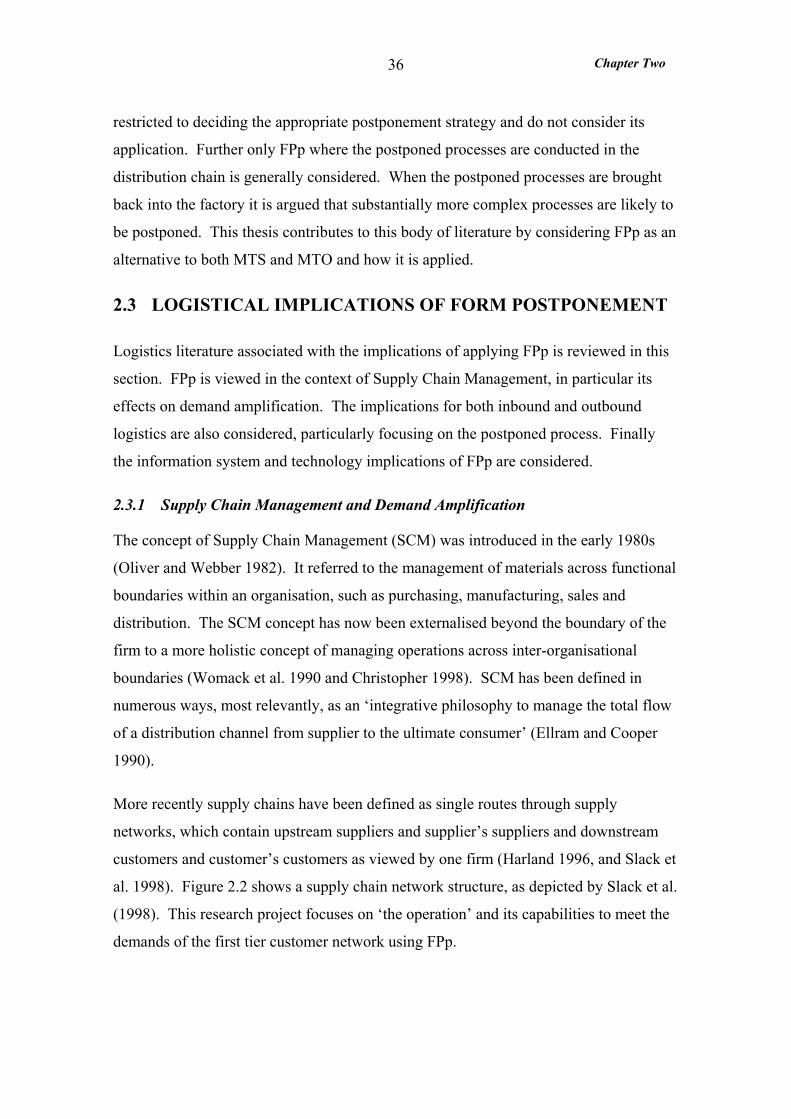
Chapter Two

36

restricted to deciding the appropriate postponement strategy and do not consider its

application. Further only FPp where the postponed processes are conducted in the

distribution chain is generally considered. When the postponed processes are brought

back into the factory it is argued that substantially more complex processes are likely to

be postponed. This thesis contributes to this body of literature by considering FPp as an

alternative to both MTS and MTO and how it is applied.

2.3 LOGISTICAL IMPLICATIONS OF FORM POSTPONEMENT

Logistics literature associated with the implications of applying FPp is reviewed in this

section. FPp is viewed in the context of Supply Chain Management, in particular its

effects on demand amplification. The implications for both inbound and outbound

logistics are also considered, particularly focusing on the postponed process. Finally

the information system and technology implications of FPp are considered.

2.3.1 Supply Chain Management and Demand Amplification

The concept of Supply Chain Management (SCM) was introduced in the early 1980s

(Oliver and Webber 1982). It referred to the management of materials across functional

boundaries within an organisation, such as purchasing, manufacturing, sales and

distribution. The SCM concept has now been externalised beyond the boundary of the

firm to a more holistic concept of managing operations across inter-organisational

boundaries (Womack et al. 1990 and Christopher 1998). SCM has been defined in

numerous ways, most relevantly, as an ‘integrative philosophy to manage the total flow

of a distribution channel from supplier to the ultimate consumer’ (Ellram and Cooper

1990).

More recently supply chains have been defined as single routes through supply

networks, which contain upstream suppliers and supplier’s suppliers and downstream

customers and customer’s customers as viewed by one firm (Harland 1996, and Slack et

al. 1998). Figure 2.2 shows a supply chain network structure, as depicted by Slack et al.

(1998). This research project focuses on ‘the operation’ and its capabilities to meet the

demands of the first tier customer network using FPp.

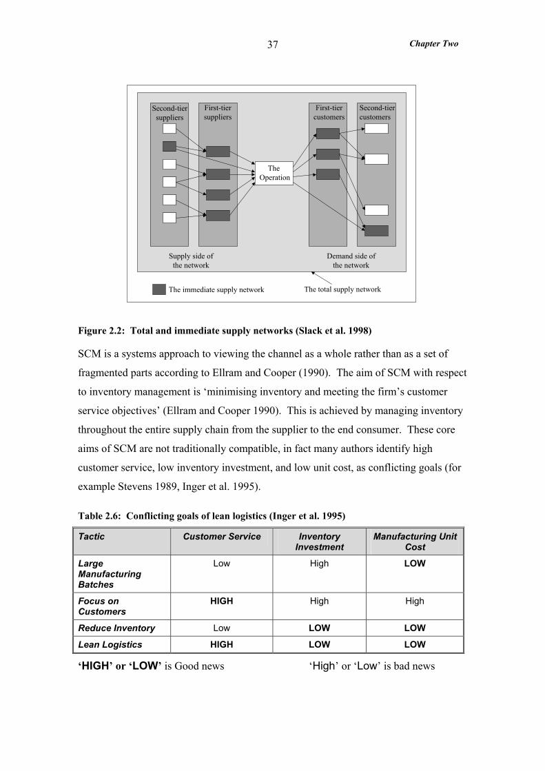
Chapter Two

37

Second-tiersuppliers

First-tiersuppliers

The Operation

First-tiercustomers

Second-tiercustomers

Supply side ofthe network

Demand side ofthe network

The immediate supply network The total supply network

Figure 2.2: Total and immediate supply networks (Slack et al. 1998)

SCM is a systems approach to viewing the channel as a whole rather than as a set of

fragmented parts according to Ellram and Cooper (1990). The aim of SCM with respect

to inventory management is ‘minimising inventory and meeting the firm’s customer

service objectives’ (Ellram and Cooper 1990). This is achieved by managing inventory

throughout the entire supply chain from the supplier to the end consumer. These core

aims of SCM are not traditionally compatible, in fact many authors identify high

customer service, low inventory investment, and low unit cost, as conflicting goals (for

example Stevens 1989, Inger et al. 1995).

Table 2.6: Conflicting goals of lean logistics (Inger et al. 1995)

Tactic Customer Service Inventory Investment

Manufacturing Unit Cost

Large Manufacturing Batches

Low High LOW

Focus on Customers

HIGH High High

Reduce Inventory Low LOW LOW

Lean Logistics HIGH LOW LOW

‘HIGH’ or ‘LOW’ is Good news ‘High’ or ‘Low’ is bad news

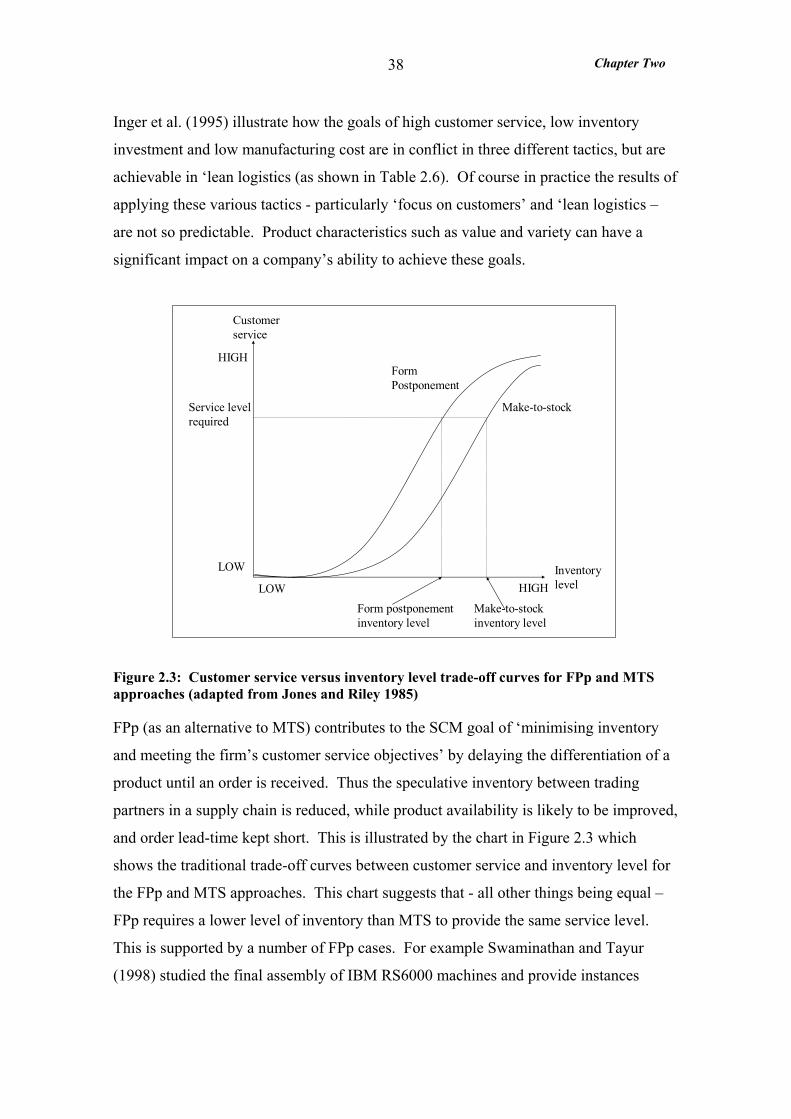
Chapter Two

38

Inger et al. (1995) illustrate how the goals of high customer service, low inventory

investment and low manufacturing cost are in conflict in three different tactics, but are

achievable in ‘lean logistics (as shown in Table 2.6). Of course in practice the results of

applying these various tactics - particularly ‘focus on customers’ and ‘lean logistics –

are not so predictable. Product characteristics such as value and variety can have a

significant impact on a company’s ability to achieve these goals.

Customerservice

Inventory level

Form Postponement

Make-to-stockService levelrequired

Form postponementinventory level

Make-to-stockinventory level

LOW

HIGH

HIGHLOW

Figure 2.3: Customer service versus inventory level trade-off curves for FPp and MTS approaches (adapted from Jones and Riley 1985)

FPp (as an alternative to MTS) contributes to the SCM goal of ‘minimising inventory

and meeting the firm’s customer service objectives’ by delaying the differentiation of a

product until an order is received. Thus the speculative inventory between trading

partners in a supply chain is reduced, while product availability is likely to be improved,

and order lead-time kept short. This is illustrated by the chart in Figure 2.3 which

shows the traditional trade-off curves between customer service and inventory level for

the FPp and MTS approaches. This chart suggests that - all other things being equal –

FPp requires a lower level of inventory than MTS to provide the same service level.

This is supported by a number of FPp cases. For example Swaminathan and Tayur

(1998) studied the final assembly of IBM RS6000 machines and provide instances

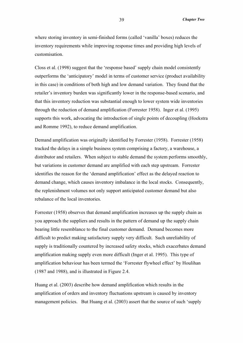
Chapter Two

39

where storing inventory in semi-finished forms (called ‘vanilla’ boxes) reduces the

inventory requirements while improving response times and providing high levels of

customisation.

Closs et al. (1998) suggest that the ‘response based’ supply chain model consistently

outperforms the ‘anticipatory’ model in terms of customer service (product availability

in this case) in conditions of both high and low demand variation. They found that the

retailer’s inventory burden was significantly lower in the response-based scenario, and

that this inventory reduction was substantial enough to lower system wide inventories

through the reduction of demand amplification (Forrester 1958). Inger et al. (1995)

supports this work, advocating the introduction of single points of decoupling (Hoekstra

and Romme 1992), to reduce demand amplification.

Demand amplification was originally identified by Forrester (1958). Forrester (1958)

tracked the delays in a simple business system comprising a factory, a warehouse, a

distributor and retailers. When subject to stable demand the system performs smoothly,

but variations in customer demand are amplified with each step upstream. Forrester

identifies the reason for the ‘demand amplification’ effect as the delayed reaction to

demand change, which causes inventory imbalance in the local stocks. Consequently,

the replenishment volumes not only support anticipated customer demand but also

rebalance of the local inventories.

Forrester (1958) observes that demand amplification increases up the supply chain as

you approach the suppliers and results in the pattern of demand up the supply chain

bearing little resemblance to the final customer demand. Demand becomes more

difficult to predict making satisfactory supply very difficult. Such unreliability of

supply is traditionally countered by increased safety stocks, which exacerbates demand

amplification making supply even more difficult (Inger et al. 1995). This type of

amplification behaviour has been termed the ‘Forrester flywheel effect’ by Houlihan

(1987 and 1988), and is illustrated in Figure 2.4.

Huang et al. (2003) describe how demand amplification which results in the

amplification of orders and inventory fluctuations upstream is caused by inventory

management policies. But Huang et al. (2003) assert that the source of such ‘supply

Chapter Two

40

chain dynamics’ is ‘mainly due to the lack of sharing of production information,

including delays and feedback in the decision rules between enterprises in the supply

chain’.

Figure 2.4: The ‘forrester flywheel effect’ (Houlihan 1987)

Lee et al. (1997) have made extensive studies of the distortion of demand information

from one end of the supply chain to the other and have termed it ‘the Bullwhip Effect’.

They identify four major causes of the Bullwhip effect: demand forecast updating, order

batching, price fluctuation and rationing and shortage gaming. Johansson et al. (2000)

further this work by using a four echelon simulation model (retailer, warehouse,

distribution centre and factory) to demonstrate the importance of time buckets to supply

chain performance. They conclude that poor synchronisation of time buckets (normally

inherent in the MRP system) upstream in the supply chain can result in product

shortages down stream and increased inventory costs upstream.

It is argued that FPp reduces demand amplification compared to MTS in two ways.

Firstly, the demand variability that the supply chain is subject to is reduced. This is

achieved by keeping speculative stocks of the undifferentiated generic products rather

than the broad range of finished products. At the generic level demand is less variable

(Inger et al. 1995, Zinn 1990a). Secondly, FPp links the point of differentiation (or

customisation) to the point of sale, by differentiating the product to customer order,

Shortages

Overordering

Unreliable delivery

Safetystockincrease

Demanddistortion

Capacityrequired

Real

Apparent

Time

Chapter Two

41

thereby eliminating anticipatory finished product stocks in the distribution chain.

Christopher (1998) suggests that the ‘tidal wave effect’ experienced by Forrester’s

channel participants, in the face of demand variability, can be subdued dramatically by

this approach. Further by only customising the products to order many of the causes of

the Bullwhip effect (Lee et al. 1997) are reduced.

Postponement is thus widely recognised as an approach that can lead to superior

logistics systems or supply chains (Cooper 1993, Jones and Riley 1985, Scott and

Westbrook 1991, Shapiro and Heskett 1985). Further, the application of postponement

has been observed as a growing trend in manufacturing and distribution by various

surveys (CLM 1995, Ahlstrom and Westbrook 1999) and prominent researchers

(Christopher 1998, Lampel and Mintzberg 1996).

Conclusions: FPp contributes to achieving the core goals of SCM, or lean logistics, by

reducing the inventory level required by the anticipatory approach (MTS) to support a

given customer service level. In addition it is argued that FPp reduces demand

amplification in the supply chain resulting from the anticipatory approach - MTS. This

is achieved by reducing the demand variability that the system is subject to and linking

the point of differentiation to the point of sale.

2.3.2 Inbound and Outbound Logistics

The implications for outbound and inbound logistics of applying FPp are addressed in

this section, which focuses on the flow of materials into and out of the postponed

process.

Van Hoek and Weken (1998) conducted a highly significant study in the automotive

industry addressing how modular production can contribute to the integration of

inbound and outbound logistics with the manufacturing plant. It was found that

modular production allows manufacturers to further involve suppliers and distributors in

the supply, assembly and distribution of products. Postponed purchasing is combined

with postponed manufacturing as illustrated in Figure 2.5. This increases the

integration of supply and assembly on the one hand and assembly and distribution on

the other.

Chapter Two

42

According to the definition of FPp a proportion (in fact possibly all) of the components

or modules required by the postponed process, will be manufactured in the focal factory

and therefore not be subject to inbound logistics at this stage. Other components,

supplied by external sources, are subject to inbound logistics. The availability of these

components into the postponed process is critical to ensure quoted order lead-time can

be achieved. Cox (1989) and Slack (1988) identify that short order lead-times on

purchased items support mix flexibility, as required by the postponed process. If the

purchased items can be ordered within the order lead-time offered to customers they do

not constrain the flexibility of the Master Production Schedule (MPS) as they can be

purchased to customer order (Browne et al. 1996).

Figure 2.5: Stage wise evolution through postponed purchasing and postponed manufacturing (van Hoek and Weken 1998a)

Van Hoek and Weken (1998) revealed ‘postponed purchasing’ of many modules subject

to inbound logistics. This leaves suppliers in charge and possession of goods until they

are actually needed in the assembly process, normally the postponed process. This is

similar to Vendor Managed Inventory (VMI), which involves the vendors assuming

total responsibility for the entire ‘replenishment-of-stocks’ process (Peck 1998). The

vendor manages the ‘goods receivable’ inventory dedicated to one customer, at a

location convenient for the customer, which may be on their site.

Purchasing Primary manufacturing

Final manufacturing Distribution

Modules

Supply chain

OutputsInputs

Stage:

In progress:

Inputs/modules/products in progress

Postponedpurchasing

Postponedmanufacturing

Chapter Two

43

Like ‘postponed purchasing’ VMI supports FPp by allowing the postponement of goods

receipt until the factory (applying FPp) are in receipt of a customer order. Whether

‘postponed purchasing’ or VMI is applied to inbound logistics, inventory is still the

responsibility of the factory and it is in their interest to ensure inventory is minimised to

reduce risk of obsolescence from new product transitions (Magretta, 1998). Therefore

the accuracy of the forecasts for components, which is used to determine order

quantities, is still critical.

Alternatively JIT may be a suitable approach to inbound logistics for modules or

components sourced externally. Schonberger’s (1982) seventh lesson in simplicity,

‘travel light and make numerous trips’ encourages:

• more frequent deliveries in smaller quantities,

• rationalised supplier bases and

• location of suppliers nearby as described by van Hoek and Weken (1998).

This results in reduced safety stocks of modules and components. Swenseth and Buffa

(1991) argue for great care in drastically reducing safety stocks. They point out that as

cycle time is reduced under JIT conditions, the effect of inbound variability is very

important, because of the increased delivery frequencies and lower shipping weights.

They further claim that some means to reduce the variability of vendor delivery

performance should be implemented in conjunction with JIT. JIT is also inappropriate

if demand for the components, or modules, is variable as it requires a level schedule

(Slack et al. 1998, Vollman et al. 1992). For instance demand for ‘option’ modules is

likely to be significantly more variable than that for ‘common’ modules (Browne et al.

1996). Therefore JIT is not viable and higher safety stocks may be required.

Van Hoek and Weken (1998a and 1998b) noted that the incidence of doorstep JIT

suppliers being opened next to the manufacturer appears to be growing. However, they

observe that these suppliers may not be (physically) close enough to the manufacturer.

In fact the new first tier suppliers may be called ‘zero level or zero tier’ suppliers. Here

the suppliers move into the factory to conduct assembly of modules - they are no longer

Chapter Two

44

an outside supplier but become integral partners that control a significant amount of the

value adding process (Van Hoek and Weken 1998).

The outbound logistical implications of applying FPp originate from the requirement to

deliver-to-order a broad range of products to a possibly fragmented market, in an

efficient manner, whilst providing required customer service. Van Hoek and Weken’s

(1998) automotive manufacturing case studies reveal that product modularity enables

the rapid and easy final modification to customer order, of the vehicle, in the

distribution channel, termed ‘postponed manufacturing’. Further, van Hoek (1998) and

van Hoek et al. (1996 and 1998) recently carried out a major study into the application

of ‘postponed manufacturing’ in European supply chains. This study is concerned with

postponement as a method for achieving a balance between globalisation (global

efficiency) and localisation (local responsiveness) as addressed by Craig and Douglas

(1996). The study found that the implementation of ‘postponed manufacturing’ requires

the reconfiguration and design of the outbound logistics or downstream supply chain.

The starting point in the change process was found to have a significant effect on the

supply chain reconfiguration process. For example the European companies tended to

start with nation-based supply chains, and the change process focussed on centralising

operations in order to enhance global efficiency.

Conclusions: Those components, supplied by external sources into the postponed

processes, are subject to inbound logistics. The availability of these components into

the postponed process is critical to ensure quoted order lead-time can be achieved.

Accordingly a number of tactics for inbound logistics are identified including purchase

on a very short lead-time; postponed purchasing; VMI; and JIT supply. The suitability

of these approaches depends on the component demand variability, volume demand and

the suppliers lead-times. Outbound logistics is not of great significance to this study

and therefore is only briefly addressed.

2.3.3 Information Systems and Technology

Literature addressing the logistical implications for the information systems and

technologies of applying FPp are reviewed here.

Chapter Two

45

Management information systems are concerned with the movement, manipulation, and

presentation of information for use in the management of organisations (Slack et al.

1998). This is distinct from information technology, which is concerned with the

configuration of the physical system, the information processing devices, such as

computers, and the telecommunications, such as Electronic Data Interchange (EDI)

(Slack et al. 1998).

A response based system, like that required to support FPp, substitutes information for

inventory enabling the entire system to react more readily to changes in demand than

the anticipatory system (Closs et al. 1998). In a response based system each supply

chain entity must be able and willing to share critical, timely information (for example

sharing customer order information with suppliers) in order for the benefits of improved

co-ordination and efficiency to be realised (Lee et al. 1997). Scott and Westbrook

(1991) claim that JIT supplies will typically not be viable without the regular and

reliable issue of sales forecasts on which the suppliers can base their plans. This

implies that sales forecasts, for modules and components supplied to the postponed

process, must be shared with the respective suppliers.

Massey Ferguson failed to share final assembly schedules with their supplier. This

coupled with cumbersome forecasting and planning systems seriously impaired their

responsiveness. In 1986 Massey-Ferguson in the UK took six weeks to convert a sales

forecast into a supplier schedule, but within the factory they planned production on

actual customer orders only three to four weeks ahead. Massey Ferguson failed to make

the final assembly schedule available to the suppliers (Harrison and Voss, 1990)

Stalk and Hout (1990) warn of the dangers of slow information lead-time - ‘the

underlying problem here is that once information ages, it loses value…old data causes

amplifications, delay and overhead’. Forrester (1958) identifies the reason for the

‘demand amplification’ effect as the delayed reaction to demand change, which can be

caused by old information. Naylor et al. (1999), describing the integration of lean and

agile paradigms, identifies ‘Information Enriched’ supply chains (Mason-Jones and

Towill 1997) where each member receives the marketplace information (commonly

consumer demand) directly. They claim this increases transparency, reduces distortions

and reduces lead-times.

Chapter Two

46

Droge et al. (1995) conducted a sample survey of Council of Logistics Management

members, and found that FPp is associated with a more intensive formal control system.

Firms applying FPp are pressured to operate JIT delivery systems that require tight

control of costs and service levels both to customers and from suppliers. Droge et al.

(1995) concludes by stating that all requisites of this operating environment could be

met by an information system that: (1) has built-in formal control mechanisms that

renders obsolete information processing middle managers; and 2) seamlessly connects

the firm to suppliers and customers (through EDI for example).

Van Hoek (1998) and van Hoek et al. (1996 and 1998) note that advances in

information technology are an important enabling factor for companies wishing to

implement postponement strategies. Especially as they can reduce transaction costs

associated with the control of goods in supply chains, and enable rapid response to

customer orders. Modern information technology can now ‘orchestrate’ the revolution

of operations from a ‘push’ to a ‘pull’ system required for postponement (CLM 1995).

Closs et al. (1998) claims that investment in information technology ‘makes the

response-based system viable’. In a study comprising a survey of companies based in

Holland from the electronic, automotive, food and clothing industries Van Hoek

(1998c) found a positive correlation between the external application of Information and

Communication Technology (ICT) and the application of FPp. This indicates that using

ICT to link production upstream with suppliers, and downstream with logistics service

suppliers and customers, supports FPp.

Electronic Data Interchange (EDI), which is the use of data exchange networks to

transmit information relating to inter-operation trade (Slack et al. 1998) is a prominent

example of ICT. EDI can be used to transmit orders, make payments, communicate

stock availability amongst other information. In this way lead-times are reduced

through the shortened transaction times of a paperless system (Scott and Westbrook

1991, Slack et al. 1998). In a study conducted by Naylor et al. (1999) the application of

FPp in an electronics products supply chain, advocated linking suppliers and customers

via EDI such that all orders are communicated this way.

Chapter Two

47

Advancing the idea of EDI connections with customers one step further, Dell Computer

Corporation sells directly to individual customers through the Internet and call centres

allowing the customer to configure their requirements themselves (Magretta, 1998).

Similarly, Van Hoek and Weken (1998) report in a case study on the SMART car

(manufactured by Micro Compact Car AG) that mutli-media systems are used to enable

clients to ‘build’ their car in the showroom.

It appears that the Internet provides an opportunity for the application of FPp, since

purchasing on the Internet is, like mail order – it always involves an order lead-time.

Whether the manufacturer uses the order lead-time to finish the goods, as in the case of

Dell Computer Corporation (Magretta 1998), or simply transports the goods ex-stock is

not of interest to the consumer as long as they receive the customer service they expect.

Conclusions: A response based information system, like that required to support FPp,

substitutes information for inventory enabling the entire system to react more readily to

changes in demand than the anticipatory system. This involves supply chain entities

sharing critical, timely information in order for the benefits of improved co-ordination

and efficiency to be realised. Advances in information and communication technology

(ICT) are an important enabling factor for companies wishing to implement FPp. They

can reduce transaction costs associated with the control of materials and enable rapid

response to customer orders. Electronic Data Interchange (EDI) is a prominent example

of ICT and can be used to transmit orders, make payments and communicate stock

availability amongst other information.

2.4 OPERATIONS MANAGEMENT LITERATURE RELATED TO

FORM POSTPONEMENT

This section reviews the OM literature addressing concepts closely related to FPp. The

first part reviews literature on non-MTS approaches, of which FPp is an example. The

second part considers literature on mass customization, for which FPp is widely

recognized as a possible approach. In the final part a more recent body of literature is

reviewed which considers the application of postponement as an operations strategy.

Chapter Two

48

2.4.1 Non-MTS Approach

In a review of OM and production literature on non-MTS approaches Amaro et al.

(1999) observes that most of this literature classifies the non-MTS companies into three

types: ATO, MTO and ETO (see for example Marucheck and McClelland 1986, Hendry

and Kingsman 1989, New and Schejczewski 1995, Vollman et al. 1992). These types

are defined below:

• ATO production. The final products offered to customers, although presenting

some degree of customisation, are produced with (common) standardised parts,

which can be assembled into a range of product variants. The receipt of an order

initiates the assembly of the component parts which may be purchased or

manufactured internally.

• MTO production. Most or all operations necessary to manufacture the product

are only performed after receipt of the customer order. Indeed sometimes

materials are purchased to customer order. Here the capability for customisation

is greater than in ATO.

• ETO production. Products are manufactured to meet a specific customer’s

needs and so require unique engineering design or significant customisation.

The key distinction between FPp and MTO or ETO is clearly the location of the CODP

as previously discussed. When FPp is applied the bulk of manufacturing is conducted

speculatively and only the customising processes are performed after receipt of a

customer order, thus enabling the responsive supply of a customised product.

Though clearly distinct from ETO and MTO, FPp is not entirely distinct from ATO -

there is an overlap between these two categories. Where ATO involves the rapid

assembly of components (the bulk of which are manufactured to stock in-house) to

provide a wide variety of finished products, then this specific instance of ATO can also

be categorised as FPp. However FPp is distinct from ATO in four key respects:

• Source of components supplied to the postponed process: In ATO all the

components required for assembly may be purchased, whereas for FPp the bulk

Chapter Two

49

of the components, and particularly the basic or generic product (if it exists), are

manufactured in-house.

• Nature of the postponed process: The postponed process (in FPp) is not

confined to assembly in fact it may be any type of transformation process

including manufacturing, assembly, configuration, packaging, or labelling as

defined in section 2.1.2.

• Responsiveness of the postponed process: Only a ‘short time period’ is

available for the postponed process – it must be responsive. Whereas this is not

necessarily the case for ATO.

• Variety of finished products: FPp is specifically for the manufacture of

products exhibiting high variety whereas ATO may be applied to standard

products. ‘For example some companies offering high priced standard items for

which the demand is intermittent choose to make [or assemble] them only to a

customer’s order rather than to stock’ (Amaro et al. 1999).

Amaro et al. (1999) comment that the ATO, MTO and ETO categories of non MTS

approaches are ‘very broad and imprecise’ and they propose a new taxonomy for non-

MTS companies. However, ATO is still only split into two broad categories on the

basis of degree of customisation. It is argued that FPp (as defined for this research) is

specifically an approach to mass customisation (as discussed in section 2.4.2). Further

although FPp overlaps with the ATO category on the whole it is quite distinct from, and

more specific than, ATO as it is generally understood.

Amaro et al. (1999) points out that ‘the literature addressing the needs of companies

which produce in response to customers’ orders is astonishingly modest’. Most of the

published research in the OM area has tended to treat all companies the same as MTS

companies and has neglected the needs of the non-MTS sector. However there are

exceptions and over the four years since the Amaro et al. (1999) paper the non-MTS

sector appears to have received more attention. This literature is reviewed here using

the traditional non-MTS classifications as defined above.

Chapter Two

50

Most of the publications on non-MTS approach address the needs of the traditional

MTO sector that manufactures a high variety of customer-specific products not – as is

becoming known as MTO – the manufacture of fairly standard products on a MTO

basis. The bulk of these publications address issues related to the manufacturing

planning and control for MTO for example:

• Marucheck and McClelland (1986) address strategic trade-offs in MTO

manufacturing that influence customer service performance. They stress the

importance of investment in safety stock and the investment of time, money and

support into a Computer Integrated Manufacturing System, which can aid the firm

in setting promise dates and in managing production.

• Hendry and Kingsman (1989) identify production planning system requirements for

the MTO sector by reviewing existing research on production scheduling, capacity

control and the setting of delivery dates. They conclude that more research on

production planning systems specifically for the MTO sector is needed. In answer

Yeh (2000) develops a customer focussed approach to effective production planning

and scheduling in a MTO environment. The approach is described in section 2.5.4.

• Segerstedt (2002) conducts a study of the production and inventory control at ABB

Motors (Vastera) and Volvo Wheel Loaders (Eskilstuna) where significant

proportions of production are MTO or ATO. The findings are presented in section

2.5.4.

Quite a number of the publications on MTO use mathematical models to address

specific planning and control issues, for instance:

• He and Jewkes (2000) and later He et al. (2002) develop algorithms to compute the

average total cost per product for a MTO inventory management system. They

examine several raw material stock replenishment policies and select the optimal

which minimises the average total cost per product.

• Webster (2002) uses a simple mathematical model of a MTO firm and examines

policies for adjusting price and capacity in response to periodic and unpredictable

Chapter Two

51

shifts in how the market values price and lead-time. The findings are discussed in

section 2.5.5 on capacity management.

Muda and Hendry (2002a and 2002b) develop a comprehensive model comprising 14

principles which offer a way to look at the strengths of a company and identify areas for

potential improvement. They use Schonberger’s (1986, 1996) world-class

manufacturing model as a starting point and argue that this model applies to the MTO of

relatively standard products rather than the MTO of a high variety of customer specific

products (as in the traditional MTO sector).

Very few papers address the specific needs of ETO or ATO. Eloranta (1992) focuses on

the problems and potential of one-of-a-kind production of non-standard products (ETO).

Here some amount of product design and engineering work are needed for every

customer order. The development needs in product design, engineering and also in

production system design are emphasised.

Wemmerlov (1984) examines manufacturing planning and control for ATO ‘for which

parts and sub-assemblies are made according to forecasts while the final assembly of the

products is delayed until customer orders are received.’ This appears particularly

relevant to FPp as Wemmerlov’s (1984) understanding of ATO is more specific than

normal and is closer to the FPp definition used for this research. However in common

with the general understanding of ATO he does not consider ATO to be very responsive

offering only a ‘medium’ order lead-time. He describes how orders are promised on the

basis of the availability of components rather than on the basis of a short standard

quoted lead-time as for FPp.

The findings from many of these studies that pre-date 1990 have been superseded by

text books such as Vollman et al. (1992) reviewed in section 2.5.4.

Conclusion: Much of the published OM research addresses the needs of the MTS

companies and neglects the needs of the non-MTS sector. There are exceptions and

much of this literature considers the traditional MTO sector. Extraordinarily little

research has been conducted on ATO which (like MTO) is considered not to be

responsive - orders are promised on the basis of the availability of components and/or

Chapter Two

52

capacity rather than on the basis of a short often standard quoted lead-time as for FPp.

This thesis contributes to this body of literature by considering the operational issues of

FPp, a specific non-MTS approach distinct from the existing categories, ETO, MTO and

ATO.

2.4.2 Mass Customisation

The concept of mass customisation was first introduced by Davis (1987) to describe a

trend towards the production and distribution of individually customised goods and

services for a mass market. Later the term was fully expounded by Pine (1993) based

on a survey of US firms, and he specifically defined it as ‘a tremendous increase in

variety and customisation without a corresponding increase in costs’. More recently,

mass customisation has been described as ‘providing numerous customer chosen

variations on every order with little lead-time or cost penalty’ (Ahlstrom and Westbrook

1999). The implied challenge for manufacturers is how to deal with high demand

uncertainty at finished item level (which results from the provision of many variants,

Inger et al. 1995) whilst ensuring low operational costs are maintained and short,

reliable lead times.

Many of the operational challenges of mass customisation originate from the need to

manufacture a broad product line. Pine et al. (1993) points out that this can be

dangerously expensive. However, a study of over 1,400 business units (Kekre and

Srinivasan 1990) indicates that significant market share benefits - and increases in firms

profitability - result from broad product lines. This explains the strong motivation for

companies to successfully apply mass customisation.

The traditional response to high demand uncertainty, in a MTS environment, is to buffer

against them by increasing safety stocks (for example Metters 1993, Newman, et al.

1993, Scott and Westbrook 1991). However, in the case of customised products, it is

rarely economically viable to maintain the safety stock levels required to avoid stock-

outs. Thus inaccurate sales forecasts are increasingly leading to costly discrepancies

between finished stocks and demand. It is argued whatever the degree of customisation

the product can only be made or at least finished to order (Amaro et al. 1999, Bennett

and Forrester 1994).

Chapter Two

53

At the other extreme MTO is where the manufacturer takes no action (except for the

purchase of materials) until an actual customer order is received, therefore more

customising options can be offered (for example New and Szwejczewski 1995, Vollman

et al. 1992). However, the more activities postponed until after receipt of customer

orders the less responsive MTO is compared to MTS (Amaro et al. 1999).

As illustrated there is a trade-off inherent in the MTO and MTS approaches between

customisation level and order lead-time. FPp mitigates this trade-off by retaining the

opportunity to customise whilst minimising the order lead-time (Amaro et al. 1999).

FPp has been widely proposed as one approach to mass customisation (for example

Bowersox and Closs 1996, Pine 1993, van Hoek 1998, van Hoek et al. 1998, Zinn and

Bowersox 1988).

The literature concerning mass customisation is extensive and can be split into that

concerned with the strategic impact of mass customisation and that addressing the

operational implications or the ‘how’ of mass customisation. First a selection of the

more prominent publications concerned with the strategic impact of mass customisation

are reviewed.

A number of publications consider the overall strategies required to achieve mass

customisation from both a marketing and organisational perspective (for example Pine

et al. 1993 and 1995). Gilmore and Pine (1997) go on to identify four approaches to

mass customisation, collaborative, adaptive, cosmetic and transparent. The

collaborative approach is most often associated with the term mass customisation, and

often involves products where many features are offered in a number of configurations,

such as a car. To be precise this is ‘mass configuration’, rather than mass

customisation, as the customer cannot independently specify his requirements, but must

choose from an array of predefined ‘options’. Even though thousands of configurations

may be on offer, the customer is still constrained to certain choices. It is argued that

FPp is more suited to mass configuration than customisation because the optional

components required for a mass configured product are predefined. Therefore in

general it is easier to ensure immediate availability of components supplied into the

postponed process.

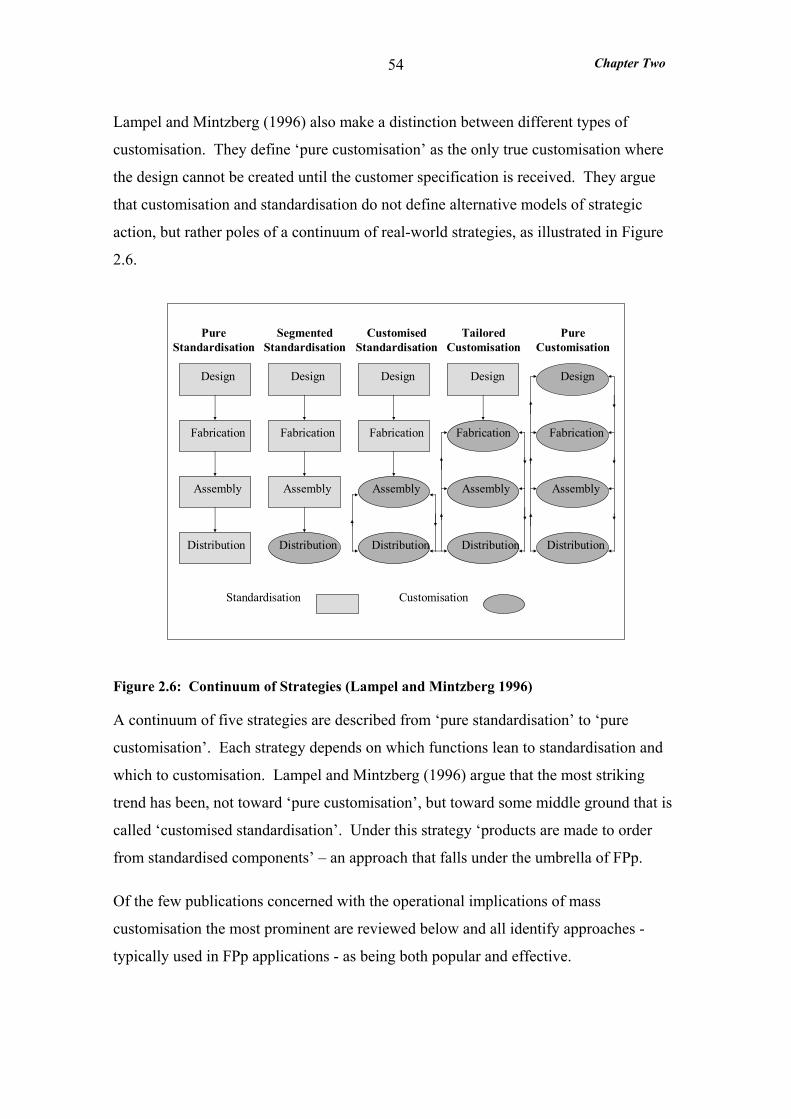
Chapter Two

54

Lampel and Mintzberg (1996) also make a distinction between different types of

customisation. They define ‘pure customisation’ as the only true customisation where

the design cannot be created until the customer specification is received. They argue

that customisation and standardisation do not define alternative models of strategic

action, but rather poles of a continuum of real-world strategies, as illustrated in Figure

2.6.

Design

Fabrication

Assembly

Distribution

Standardisation Customisation

DesignDesignDesignDesign

FabricationFabricationFabricationFabrication

AssemblyAssemblyAssemblyAssembly

DistributionDistributionDistributionDistribution Distribution

Assembly

Fabrication

Design

PureStandardisation

SegmentedStandardisation

CustomisedStandardisation

TailoredCustomisation

PureCustomisation

Figure 2.6: Continuum of Strategies (Lampel and Mintzberg 1996)

A continuum of five strategies are described from ‘pure standardisation’ to ‘pure

customisation’. Each strategy depends on which functions lean to standardisation and

which to customisation. Lampel and Mintzberg (1996) argue that the most striking

trend has been, not toward ‘pure customisation’, but toward some middle ground that is

called ‘customised standardisation’. Under this strategy ‘products are made to order

from standardised components’ – an approach that falls under the umbrella of FPp.

Of the few publications concerned with the operational implications of mass

customisation the most prominent are reviewed below and all identify approaches -

typically used in FPp applications - as being both popular and effective.

Chapter Two

55

Pine (1993) conducts a survey of US firms to explore the application of mass

customisation. Five fundamental methods for achieving mass customisation of products

and services are described. He claims that ‘the best method of minimising costs whilst

maximising individual customisation is by creating modular components that can be

configured into a wide variety of end products’. He goes on to define six different

types of modularity which are discussed in section 2.6.2.

Ahlstrom and Westbrook (1999) conducted a survey of UK manufacturing companies

concerning the operational implications of mass customisation. Out of seven alternative

approaches assembly of core modules was found to be the most used method of

achieving customisation. Once again this may be a FPp approach. Various other

findings were presented regarding broad operational implications such as the need for

improved dialogue between manufacturing and marketing to achieve mass

customisation.

Swaminathan (2001) identified three standardisation strategies for mass customisation:

part standardisation, process standardisation and procurement standardisation. This was

based on six years of detailed analytical and empirical analysis of operational strategies

for managing mass customisation with several firms (for example Swaminathan and

Tayur 1998 and 1999). A two by two matrix was developed for choosing the

appropriate standardisation strategy on the basis of product and process modularity.

‘Process standardisation’ (FPp) where an inventory of semi-finished products is

maintained, and customisation postponed until order receipt, was recommended where

both the product and process was modular.

Conclusions: The literature concerning mass customisation is extensive, however that

concerning the operational implications or the ‘how’ of mass customisation is

considerably less. Most of it is concerned with the strategic impact of mass

customisation and only a few publications address the operational implications of mass

customisation. This thesis contributes to this body of literature by addressing ‘how’

mass customisation can be achieved through the application of FPp.

Chapter Two

56

2.4.3 Form Postponement as an Operations Strategy

Recently a small body of literature has emerged in the OM field that deals with

postponement and a selection of the papers are reviewed here. It should be noted that

although this literature is not concerned with ‘logistical postponement’ and therefore

focuses on FPp the understanding of FPp tends to vary a great deal as previously

discussed in section 2.1.1.

Yang and Burns (2003) present a theoretical paper which discusses the implications of

postponement for the supply chain. Here postponement is understood in its broadest

terms including at one extreme ETO as ‘pure postponement’ and at the other extreme

MTS with distribution to order as ‘logistical postponement’. They identify factors from

the literature that influence the location of the CODP such as the extent to which

manufacturing processes are associated with the customer order. However they point

out that ‘little attention has been directed to how these factors can be balanced’.

Yang and Burn (2003) observe that with the high degree of uncertainty, it is a natural

option to postpone activities. On the other hand, the implementation typically leads to

reducing economies of scale and increasing cycle times. They call for more research on

‘how various types of postponement are linked to different types of uncertainty’.

Van Mieghem and Dada (1999) show how demand uncertainty influences the strategic

capacity investment decision of the firm. They compare different postponement

strategies using a two stage decision model where firms make three decisions: capacity

investment, inventory quantity and price. However the postponement strategies consist

of ‘production postponement’ which here is MTO and ‘price postponement’ which is

MTS with the price decision postponed. The models are by their own admission very

simple but show that: typically capacity investment is made while the demand curve is

uncertain; and the relative value of operational postponement techniques seems to

increase as the industry becomes more competitive.

Aviv and Federgruen (2001a) perform simulations using a far more complicated

analytical model of delayed product differentiation (DPD which is fully discussed in

section 2.6.1) which is a design for postponement approach. This model is much closer

to FPp as defined for this research however there is no CODP at generic product stage

Chapter Two

57

instead it the MTS approach is assumed. The model assumes a common intermediate

product is manufactured to stock in the first phase with the differentiating options and

features postponed until the second phase and each phase has a lead-time. Production

volumes in the first stage are bounded by given capacity limits but there is always

sufficient capacity to satisfy demand. The multi-item inventory model is subject to

random and seasonally fluctuating demand and the findings regarding cost savings (in

terms of production, inventory holding, capacity provision) of FPp are as follows:

• as capacity becomes more limited (i.e. capacity utilisation increases) the cost

savings of delaying product differentiation (rather than immediately

differentiating) reduces. They comment that ‘there is less to be saved when

capacity is limited because.... the factory must produce at capacity nearly all of

the time, regardless of the demand stream’.

• When there is strong seasonality, compared to no seasonality, the cost savings

of DPD increases.

• The later the differentiating process is delayed within the total production lead-

time the greater the savings from DPD. Differentiating the products after the 1st

(2nd, 3rd, 4th) week of a five-week total lead-time reduces costs by 4% (9%,

14%, 20%) when compared to the case where differentiation is not delayed at

all. In practice the order lead-time in a FPp application tends to be so short the

option of delaying the differentiating process by varying degrees does not exist.

• The less the correlation between end item demands the greater the cost saving

due to DPD. The cost savings are least with positively correlated demands,

medium with independent demand and greatest with negatively correlated

demands, which supports Zinn (1990a) work on risk pooling reviewed in

section 2.2.2.

Finally the model used by Aviv and Federgruen (2001a) assumes ‘that all demand

distribution are perfectly known from the outset’ which is not realistic even for MTS.

A further similar model to that described above was developed by Aviv and Federgruen

(2001b) to characterise the cost savings of FPp when subject to demand distributions

Chapter Two

58

which are not known with accuracy but are subject to the ‘learning effect’. The

‘learning effect’ refers to the generation of significantly more accurate forecasts of

future demand distributions which allows the differentiation of the products (second

phase) to more closely reflect demand. Therefore here the entire production process in

forecast driven. They find that the learning effect always results in increased cost

savings of DPD.

Ma et al. (2002) model a multi-stage assembly line with multiple products and random

demands to explore the dynamics between processing times and component

procurement lead-times and their impact on the application of DPD. They conclude that

delaying product differentiation by applying component commonality (standardising the

product) is usually preferred in the early stages due to lead-time dynamics in the system.

Ernst and Kamrad (2000) use an analytical framework to calculate the costs of four

different supply chain structures. Their findings suggest that vertical integration is not

desirable – it is better to outsource module manufacture and allow logistics providers to

conduct packaging in the distribution chain (distribution FPp). These are interesting

results but the framework is limited to postponed packaging and therefore probably

consumer products. Further these decisions are dependant on many other variables such

as order lead-time, geographical locations of market, factory etc.

Conclusions: A theoretical paper (Yang and Burns 2003) reviewing research on

postponement concludes that little is known about its application. Much of the OM

literature on FPp uses mathematical or inventory models of postponement applications.

Most these models consider delayed product differentiation applied to MTS approaches

and therefore are not directly applicable to FPp. With the introduction of a CODP at the

generic product stage they could be very useful in understanding some of the

operational implications of FPp such as capacity planning. This thesis contributes to

this body of literature by addressing ‘how’ FPp is applied using the case study research

design.

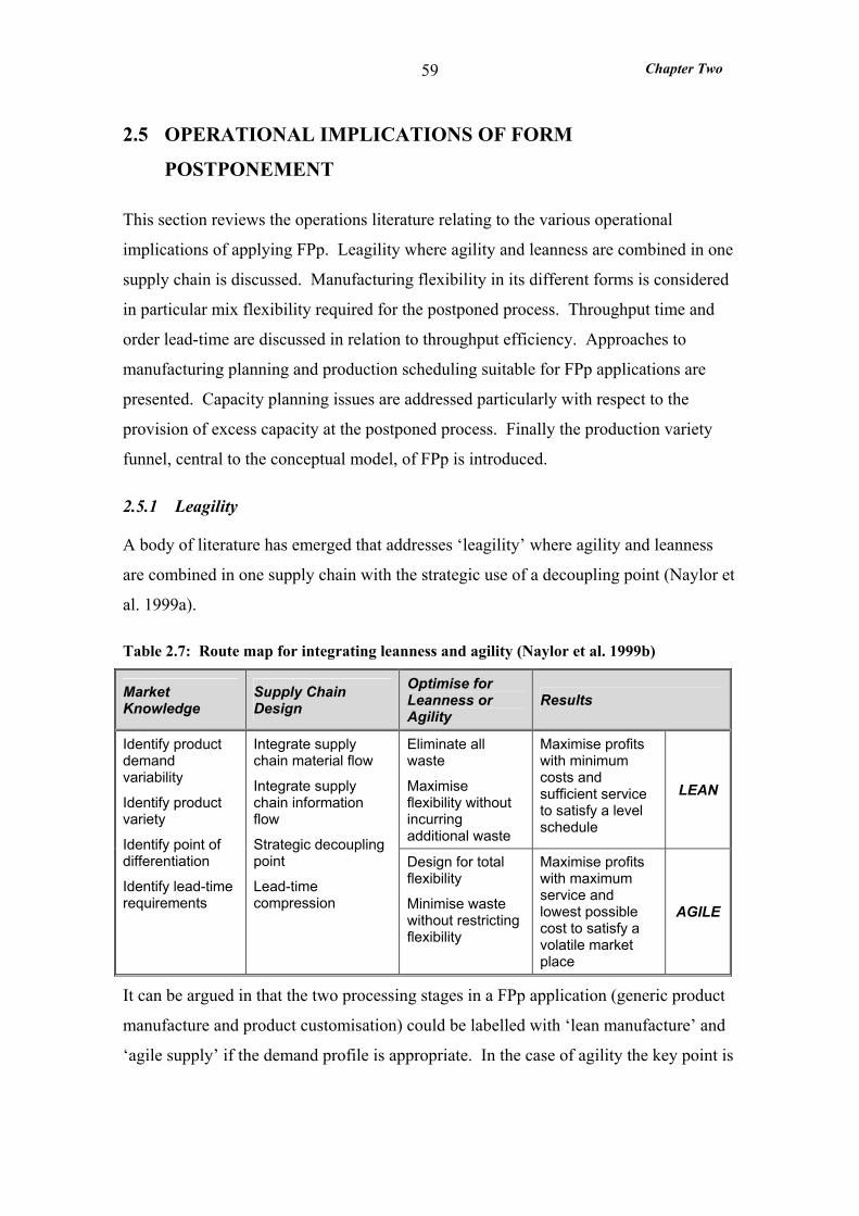
Chapter Two

59

2.5 OPERATIONAL IMPLICATIONS OF FORM

POSTPONEMENT

This section reviews the operations literature relating to the various operational

implications of applying FPp. Leagility where agility and leanness are combined in one

supply chain is discussed. Manufacturing flexibility in its different forms is considered

in particular mix flexibility required for the postponed process. Throughput time and

order lead-time are discussed in relation to throughput efficiency. Approaches to

manufacturing planning and production scheduling suitable for FPp applications are

presented. Capacity planning issues are addressed particularly with respect to the

provision of excess capacity at the postponed process. Finally the production variety

funnel, central to the conceptual model, of FPp is introduced.

2.5.1 Leagility

A body of literature has emerged that addresses ‘leagility’ where agility and leanness

are combined in one supply chain with the strategic use of a decoupling point (Naylor et

al. 1999a).

Table 2.7: Route map for integrating leanness and agility (Naylor et al. 1999b)

Market Knowledge

Supply Chain Design

Optimise for Leanness or Agility

Results

Eliminate all waste

Maximise flexibility without incurring additional waste

Maximise profits with minimum costs and sufficient service to satisfy a level schedule

LEAN

Identify product demand variability

Identify product variety

Identify point of differentiation

Identify lead-time requirements

Integrate supply chain material flow

Integrate supply chain information flow

Strategic decoupling point

Lead-time compression

Design for total flexibility

Minimise waste without restricting flexibility

Maximise profits with maximum service and lowest possible cost to satisfy a volatile market place

AGILE

It can be argued in that the two processing stages in a FPp application (generic product

manufacture and product customisation) could be labelled with ‘lean manufacture’ and

‘agile supply’ if the demand profile is appropriate. In the case of agility the key point is

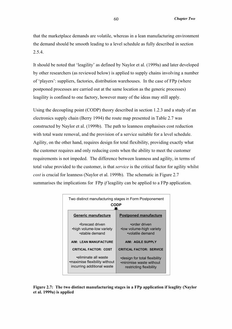
Chapter Two

60

that the marketplace demands are volatile, whereas in a lean manufacturing environment

the demand should be smooth leading to a level schedule as fully described in section

2.5.4.

It should be noted that ‘leagility’ as defined by Naylor et al. (1999a) and later developed

by other researchers (as reviewed below) is applied to supply chains involving a number

of ‘players’: suppliers, factories, distribution warehouses. In the case of FPp (where

postponed processes are carried out at the same location as the generic processes)

leagility is confined to one factory, however many of the ideas may still apply.

Using the decoupling point (CODP) theory described in section 1.2.3 and a study of an

electronics supply chain (Berry 1994) the route map presented in Table 2.7 was

constructed by Naylor et al. (1999b). The path to leanness emphasises cost reduction

with total waste removal, and the provision of a service suitable for a level schedule.

Agility, on the other hand, requires design for total flexibility, providing exactly what

the customer requires and only reducing costs when the ability to meet the customer

requirements is not impeded. The difference between leanness and agility, in terms of

total value provided to the customer, is that service is the critical factor for agility whilst

cost is crucial for leanness (Naylor et al. 1999b). The schematic in Figure 2.7

summarises the implications for FPp if leagility can be applied to a FPp application.

Generic manufacture

•forecast driven•high volume-low variety

•stable demand

AIM: LEAN MANUFACTURE

CRITICAL FACTOR: COST

•eliminate all waste•maximise flexibility without incurring additional waste

Postponed manufacture

•order driven•low volume-high variety

•volatile demand

AIM: AGILE SUPPLY

CRITICAL FACTOR: SERVICE

•design for total flexibility•minimise waste without

restricting flexibility

CODPTwo distinct manufacturing stages in Form Postponement

Figure 2.7: The two distinct manufacturing stages in a FPp application if leaglity (Naylor et al. 1999a) is applied

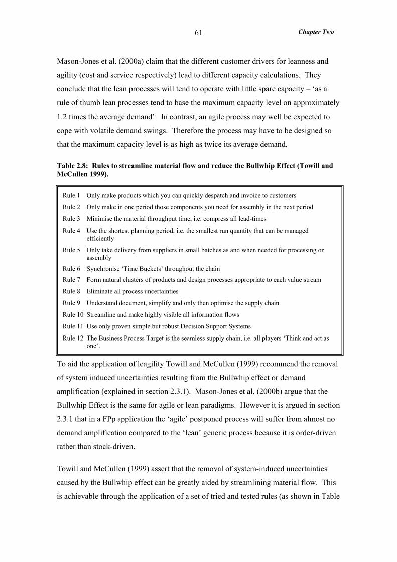
Chapter Two

61

Mason-Jones et al. (2000a) claim that the different customer drivers for leanness and

agility (cost and service respectively) lead to different capacity calculations. They

conclude that the lean processes will tend to operate with little spare capacity – ‘as a

rule of thumb lean processes tend to base the maximum capacity level on approximately

1.2 times the average demand’. In contrast, an agile process may well be expected to

cope with volatile demand swings. Therefore the process may have to be designed so

that the maximum capacity level is as high as twice its average demand.

Table 2.8: Rules to streamline material flow and reduce the Bullwhip Effect (Towill and McCullen 1999).

To aid the application of leagility Towill and McCullen (1999) recommend the removal

of system induced uncertainties resulting from the Bullwhip effect or demand

amplification (explained in section 2.3.1). Mason-Jones et al. (2000b) argue that the

Bullwhip Effect is the same for agile or lean paradigms. However it is argued in section

2.3.1 that in a FPp application the ‘agile’ postponed process will suffer from almost no

demand amplification compared to the ‘lean’ generic process because it is order-driven

rather than stock-driven.

Towill and McCullen (1999) assert that the removal of system-induced uncertainties

caused by the Bullwhip effect can be greatly aided by streamlining material flow. This

is achievable through the application of a set of tried and tested rules (as shown in Table

Rule 1 Only make products which you can quickly despatch and invoice to customers

Rule 2 Only make in one period those components you need for assembly in the next period

Rule 3 Minimise the material throughput time, i.e. compress all lead-times

Rule 4 Use the shortest planning period, i.e. the smallest run quantity that can be managed efficiently

Rule 5 Only take delivery from suppliers in small batches as and when needed for processing or assembly

Rule 6 Synchronise ‘Time Buckets’ throughout the chain

Rule 7 Form natural clusters of products and design processes appropriate to each value stream

Rule 8 Eliminate all process uncertainties

Rule 9 Understand document, simplify and only then optimise the supply chain

Rule 10 Streamline and make highly visible all information flows

Rule 11 Use only proven simple but robust Decision Support Systems

Rule 12 The Business Process Target is the seamless supply chain, i.e. all players ‘Think and act as one’.

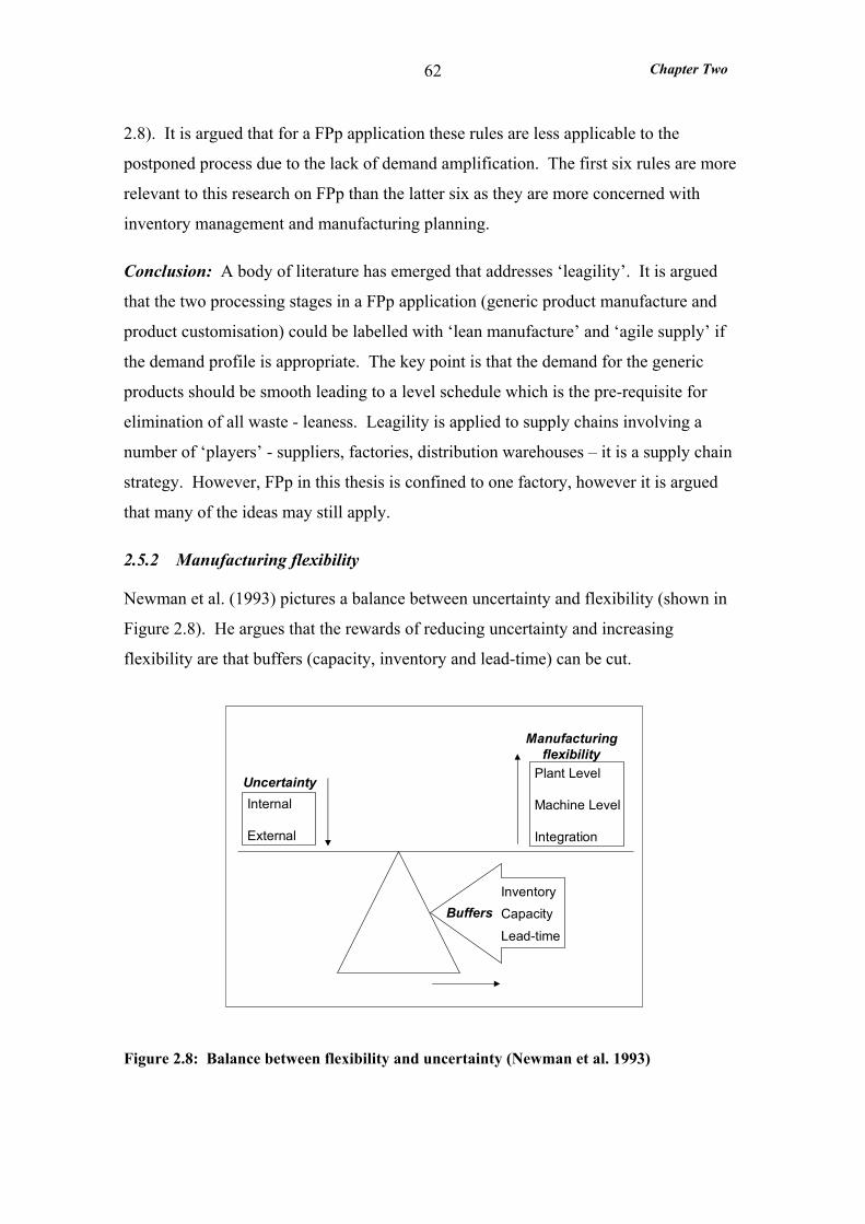
Chapter Two

62

2.8). It is argued that for a FPp application these rules are less applicable to the

postponed process due to the lack of demand amplification. The first six rules are more

relevant to this research on FPp than the latter six as they are more concerned with

inventory management and manufacturing planning.

Conclusion: A body of literature has emerged that addresses ‘leagility’. It is argued

that the two processing stages in a FPp application (generic product manufacture and

product customisation) could be labelled with ‘lean manufacture’ and ‘agile supply’ if

the demand profile is appropriate. The key point is that the demand for the generic

products should be smooth leading to a level schedule which is the pre-requisite for

elimination of all waste - leaness. Leagility is applied to supply chains involving a

number of ‘players’ - suppliers, factories, distribution warehouses – it is a supply chain

strategy. However, FPp in this thesis is confined to one factory, however it is argued

that many of the ideas may still apply.

2.5.2 Manufacturing flexibility

Newman et al. (1993) pictures a balance between uncertainty and flexibility (shown in

Figure 2.8). He argues that the rewards of reducing uncertainty and increasing

flexibility are that buffers (capacity, inventory and lead-time) can be cut.

Internal

External

Plant Level

Machine Level

Integration

Uncertainty

Manufacturingflexibility

BuffersInventoryCapacity

Lead-time

Figure 2.8: Balance between flexibility and uncertainty (Newman et al. 1993)

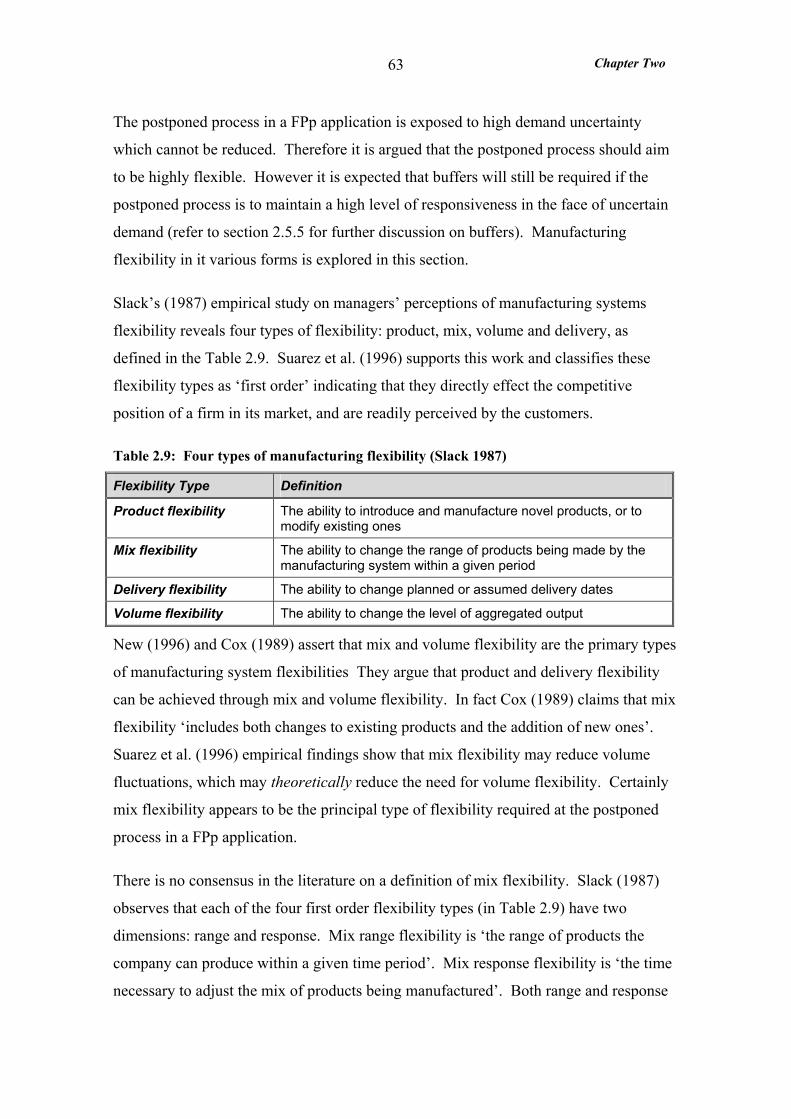
Chapter Two

63

The postponed process in a FPp application is exposed to high demand uncertainty

which cannot be reduced. Therefore it is argued that the postponed process should aim

to be highly flexible. However it is expected that buffers will still be required if the

postponed process is to maintain a high level of responsiveness in the face of uncertain

demand (refer to section 2.5.5 for further discussion on buffers). Manufacturing

flexibility in it various forms is explored in this section.

Slack’s (1987) empirical study on managers’ perceptions of manufacturing systems

flexibility reveals four types of flexibility: product, mix, volume and delivery, as

defined in the Table 2.9. Suarez et al. (1996) supports this work and classifies these

flexibility types as ‘first order’ indicating that they directly effect the competitive

position of a firm in its market, and are readily perceived by the customers.

Table 2.9: Four types of manufacturing flexibility (Slack 1987)

Flexibility Type Definition

Product flexibility The ability to introduce and manufacture novel products, or to modify existing ones

Mix flexibility The ability to change the range of products being made by the manufacturing system within a given period

Delivery flexibility The ability to change planned or assumed delivery dates

Volume flexibility The ability to change the level of aggregated output

New (1996) and Cox (1989) assert that mix and volume flexibility are the primary types

of manufacturing system flexibilities They argue that product and delivery flexibility

can be achieved through mix and volume flexibility. In fact Cox (1989) claims that mix

flexibility ‘includes both changes to existing products and the addition of new ones’.

Suarez et al. (1996) empirical findings show that mix flexibility may reduce volume

fluctuations, which may theoretically reduce the need for volume flexibility. Certainly

mix flexibility appears to be the principal type of flexibility required at the postponed

process in a FPp application.

There is no consensus in the literature on a definition of mix flexibility. Slack (1987)

observes that each of the four first order flexibility types (in Table 2.9) have two

dimensions: range and response. Mix range flexibility is ‘the range of products the

company can produce within a given time period’. Mix response flexibility is ‘the time

necessary to adjust the mix of products being manufactured’. Both range and response

Chapter Two

64

mix flexibility is desirable in the postponed process such that a wide range of products

can be produced in a responsive manner. Mix flexibility can be achieved in a number of

ways for example: set-up time reduction (Cox 1989, New 1998, Slack 1988), work-in-

progress inventory reduction (Cox 1989), and production cycle time reduction (Cox

1989). Further a number of process technology characteristics have been identified that

enable high mix flexibility. The extent to which equipment is programmable or is

general purpose promotes mix flexibility according to Cox (1989) and Suarez et al.

(1996). Slack (1988) adds that equipment with a high range of process capability

enables mix flexibility.

New (1998) states any plant can change from one product to another, but the challenge

is to achieve this without a loss of efficiency. Upton (1994) supports this view

requiring ‘little penalty in time, effort, cost or quality performance’ in his definition of

flexibility. However, as discussed earlier, flexibility (in terms of range and response) is

a higher priority than efficiency if the postponed process in a FPp application is to be

agile – ‘minimise waste without restricting flexibility’ (Naylor et al. 1999).

The volume demand variability at generic product (or aggregate) level is always less

than that at finished product level (Zinn 1990a). However, there always remains at least

some volume demand variability at generic level and in many cases this variability is

significant. Therefore volume flexibility, as well as mix flexibility is normally desirable

at the postponed process. However it can be argued that demand variability, in terms of

both mix and volume, is generally so high at the postponed process that the provision of

buffers is essential to maintain responsiveness. It can be further argued that the only

buffer available is excess capacity (see section 2.5.5).

Conclusions: The postponed process in a FPp application is exposed to high demand

uncertainty which cannot be reduced therefore a high level of manufacturing flexibility

is desirable in this process. It can be argued that mix and volume flexibility are

desirable in the postponed process, both in terms of range and response. But that

demand variability - in terms of both mix and volume - is generally so high at the

postponed process that the provision of buffers is essential to maintain responsiveness

as discussed in section 2.5.5.

Chapter Two

65

2.5.3 Throughput time and Order lead-time

The ‘throughput time’ is ‘how long the operation takes to obtain the resources, produce

and deliver the product’ (Slack et al. 1998). This is the same as the ‘composite lead-

time’, which is the difference in time between the final due date for a finished item and

the date when the first action must be taken in order to get it made (New 1977). It is

important to note that here the throughput time is that for a single company unlike the

‘composite manufacturing/procurement lead-time’ (New, 1993), which applies to the

entire supply chain and is measured from the acquisition of the original raw material.

The order lead-time (referred to by Slack as ‘demand time’) is ‘the time customers have

to wait between asking for the product and receiving it’ (Slack et al. 1998). Clearly the

order lead-time should not be greater than that required by the customer. For a FPp

application the location of the CODP in the manufacturing process flow strongly

influences the order lead-time achievable since it determines the manufacturing

processes that are order driven.

Slack et al. (1998) suggest that the P:D (throughput time to order lead-time) ratio

indicates the degree of speculation. Therefore the P:D ratio is an indication of the risks

inherent in forecasting. Reducing throughput time (P) is a way of reducing the risks. It

is argued that for FPp the risks involved in making to stock the generic product (or

modules) are already low because demand is relatively stable at this level. Therefore

forecasts are relatively accurate (Zinn 1990a) and the risk of obsolescence is low since

they are undifferentiated generic products.

What appears to be more crucial for FPp is reducing the order lead-time, as Fisher

(1997) advocates for a responsive supply chain ‘invest aggressively in ways to reduce

lead-time’. This requires that the manufacturing lead-time for the postponed processes

is minimised and the throughput efficiency (New 1993) maximised:

Throughput Efficiency = Work Content Elapsed Time Taken

Here ‘work content’ is the time taken for the value adding activities to be performed on

either a batch quantity, order quantity or single item. The elapsed time taken can be

measured from release of the factory order to the despatch, or booking into the

Chapter Two

66

warehouse, of the finished order. The elapsed time is the time the factory is available to

add value and therefore must be measured over the factory’s operating hours (New

1993).

It follows that reducing the cost adding, or non-value adding activities, will improve

throughput efficiency. Toyota identified seven wastes or non value adding activities:

overproduction; waiting; transportation; processing itself; inventory; movement; and

making defective products (Shingo 1981, Ohno 1988). Furthermore, the reduction of

many of the non-value added activities also improves mix flexibility previously

identified as particularly desirable for the postpone process (in section 2.5.2).

Level of postponement is a concept closely related to order lead-time and throughput

time. Bucklin (1965) states that operationally, postponement may be measured by the

notion of ‘delivery time’, which is equivalent to ‘order lead-time’. He goes on to say

for the seller postponement increases, as delivery time lengthens, whereas for the buyer,

postponement increases as delivery time shortens. Slack et al. (1998) suggests that the

P:D ratio indicates the degree of speculation, conversely the D:P (order lead-time to

throughput time) ratio may be a measure of postponement for the manufacturer (seller).

However in FPp applications it is desirable to minimise the order lead-time and this

reduces the level of postponement according to the D:P ratio. Possibly a better measure

would relate to the level of manufacturing processes postponed may be in terms of

value added time.

Conclusion: Throughput time is how long the operation takes to obtain the resources,

produce and deliver the product. Order lead-time is the time between the customers

asking for the product and receiving it. For a FPp application the location of the CODP

in the manufacturing process flow strongly influences the order lead-time achievable.

The P:D (throughput time to order lead-time) ratio indicates the degree of speculation,

and therefore the risks inherent in forecasting. Reducing throughput time (P) is a way

of reducing the risks. It is argued that for FPp the risks involved in making to stock the

generic product are already low because the volume demand variability at this level is

relatively low. What appears to be more crucial for FPp is reducing the order lead-time.

This requires that the manufacturing lead-time for the postponed processes is minimised

and the throughput efficiency maximised.

Chapter Two

67

2.5.4 Manufacturing Planning and Scheduling

The Master Production Schedule (MPS) is a statement of what the company plans to

manufacture. It is the planned build schedule by quantity and date, for top level items,

either finished products or high level configurations of material (Vollman et al. 1992

and Brown et al. 1996). The MPS seeks to balance incoming customer orders and

forecast requirements with available material and capacity (Brown et al. 1996). An

effective master schedule provides the basis for making customer delivery promises,

utilising plant capacity effectively, and resolving trade-offs between manufacturing and

marketing (Vollman et al. 1992). The diagram in Figure 2.9 shows how the MPS links

with the rest of the manufacturing planning and control system (Vollman et al. 1992).

Figure 2.9: The manufacturing planning and control system (Vollman et al. 1992)

The MPS drives the Material Requirement Planning (MRP) and is thus the key input

into the MRP process. Any errors within it, such as poor forecasts, cannot be

compensated for by sophisticated MRP analysis (Brown et al. 1996). This is

particularly significant in the case of FPp where order lead-times are short - only the

MPS in the near term is dominated by customer orders leaving the MPS heavily

dependant on sales forecasts input.

Resource Planning

ProductionPlanning

DemandManagement

Rough-cutcapacity planning

Capacity requirements

planning

Finiteloading

Input/outputanalysis

Masterproductionscheduling

Detailedmaterialplanning

Shop-floorsystems

Vendor systems

Long range

Medium range

Short range

Capacity Planning

Chapter Two

68

Vollman et al. (1992) claim that the distinction between the three classic types of MPS

approaches - MTS, MTO and ATO - is largely based on the production unit used for the

MPS. Ling and Widmer (1979) and Proud (1981) suggest the unit is generally at the

level in the product structure that provides the greatest flexibility and best control. This

is often at the level in the product structure which contains the smallest number of items

(Marucheck and McClelland 1986, Brown et al. 1996). For a FPp application this is

likely to be at the generic product (or module) level where the CODP is located.

Vollman et al. (1992) asserts that the ATO firm is typified by an almost limitless

number of possible end item configurations, all assembled to order from combinations

of basic components or subassemblies in a similar way to FPp. Vollman et al. (1992)

describes how the ATO firm typically does not master production schedule end items

but the modules to be assembled which are exploded into component requirements

using ‘planning bills of material’.

According to Vollman the bill of material (BOM) is narrowly considered to be an

engineering document that specifies the ingredients or subordinate components required

to physically make each part number or assembly. The ‘planning BOM’ is any use of

‘BOM approaches’ for planning only. As opposed to the ‘indented BOM’ which is used

for building products (Vollman et al. 1992). The ‘modular BOM’ and the ‘super BOM’

are the two principal types of planning BOM (Brown et al. 1996).

The modular BOM is used where the product structure is of the ‘X’ or ‘hour glass type.

Each module is defined as a single level BOM, which links components to modules but

doesn’t link either components or modules to end items. Effectively it treats the

modules as end items (Vollman et al. 1992) and translates the MPS module units into

subordinate component requirements. Sales forecasting is aided by the use of super

BOMs (defined in the glossary in Appendix 1). Marketing forecast total sales of the

product family and make best estimates on the average decimal usage of the ‘options’.

The requirements for the modules are calculated by multiplying forecast total sales of

the product family by the decimal usage (Browne et al. 1996).

Clearly an MRP system alone cannot manage manufacturing planning and control.

Segerstedt (2002) conducts a study at ABB Motors (Vastera) and Volvo Wheel Loaders

(Eskilstuna) where significant proportions of production are MTO or ATO. He finds

Chapter Two

69

where the number of end items is high, the company ATO or MTO and additions to

pure MRP are necessary. He describes the use of planning BOMs (super and modular),

normal BOM with ‘adding BOMs’, a MPS planning system with an available-to-

promise function and a home made system for modules available-to-promise.

Yeh (2000) develops a customer focussed approach to effective production planning

and scheduling in a MTO environment. This may be relevant to the postponed process

in FPp because the MTO environment is characterised by small orders placed by a wide

variety of customers. Yeh (2000) uses an integrated BOM and routing data structure.

This facilitates the creation of production jobs (with varying routing and material

requirements) in response to customers’ product specifications. Where the postponed

process involves either more than one process or a variety of processes this could be an

effective approach.

When considering the manufacturing planning and scheduling implications for FPp

applications it is necessary to appreciate the dichotomy in manufacturing (as illustrated

in Figure 2.7, section 2.5.1). As described in the introduction chapter the two

processing stages either side of the CODP can be appropriately labelled ‘lean

manufacture’ and ‘agile supply’. ‘Leanness’ is desirable for generic product

manufacture, whereas ‘agility’ is the aim for postponed processing.

Consider first the implications for generic product or module manufacture. The Just In

Time (JIT) philosophy founded on eliminating waste from manufacturing (Slack et al.

1998, Vollman et al. 1992 for example) is clearly compatible with leanness. Here

leanness means developing a value stream to eliminate all waste in the production

system - be it in the form of materials, labour or plant capacity - and to ensure a level

schedule (Naylor et al. 1999, Katayma and Bennett 1999). Harrison (1992) states that

for JIT implementations ‘manufacture needs to be in small batches with short set-ups

and with rapid delivery from one activity to the next’. Thus production can change

from one item to another and large batch production avoided (Bennett and Forrester

1994). This is of course very different from the traditional approach to manufacturing

items with level demand, which advocates high capacity utilisation through large batch

manufacture. This results in high inventories throughout the system and sluggish

response flexibility.

Chapter Two

70

However Inger et al. (1995) suggest the decoupling point is where the supply chain

moves from forecast-push of material to demand-pull, based on actual customer orders.

This would suggest that a push system is appropriate for generic product manufacture.

However the work conducted by Slack and Correa (1992) on the flexibilities of push

and pull systems suggests that a push system (in this case a conventional MRP system)

demonstrates great range flexibility, but at the expense of response flexibility. Ideally

high range flexibility is not required for the production of the generic modules therefore

an MRP push system is inappropriate. Further push systems are not ideal since they

tend to exhibit greater waste than pull systems - the emphasis is on capacity utilisation

instead of overall waste minimisation.

The flexibility of a JIT pull system is mainly associated with faster response, as opposed

to the ability to produce a wide range of products required for high variety production

(Bennett and Forrester 1994, Slack and Correa 1992). This is supported by the nature of

the best known JIT examples from firms with high volume repetitive manufacturing

methods, such as the classic case of Toyota (Vollman et al. 1992). In fact JIT is not

suitable for supplying broad product ranges where demand is highly variable, it requires

a level, stable schedule (Slack et al. 1998, Vollman et al. 1992). This implies for FPp

applications that where a level capacity plan (as discussed in section 2.5.5) can be

established the JIT pull system is suitable.

Agility seeks to cope with demand volatility (Kidd, 1994) and requires design for total

flexibility, only reducing costs when the ability to meet the customer requirements is

not impeded (Naylor et al., 1999). For the postponed process to be ‘agile’ high mix

flexibility is desirable (as discussed in section 2.5.2). This will enable the provision of a

broad product range, in a responsive manner, offering short, reliable lead-times (Naylor

et al., 1999). Mix flexibility can be achieved in a number of ways which are often

methods of reducing waste and therefore achieving leanness – for example set-up

reduction. However at the postponed process the guiding principle remains that

manufacturing flexibility is a priority over waste reduction.

Conclusions: Ideally the MPS production unit for FPp is the generic products or

modules. The MPS drives the MRP and any errors within it, such as poor forecasts,

cannot be compensated for by sophisticated MRP analysis. This is particularly

Chapter Two

71

significant in the case of FPp where the MPS is dominated by sales forecasts. Planning

BOMs such as the ‘modular BOM’ and the ‘super BOM’ can be used in conjunction

with the MPS. Manufacturing scheduling implications of FPp arise from the dichotomy

in manufacturing. Ideally a JIT pull system is suitable for ‘lean’ generic product

manufacture. However where a ‘level capacity plan’ cannot be established then a MRP

push system may be preferable. A demand-pull system based on actual customer orders

is necessary for the postponed process which aims to be ‘agile’ and therefore requires

high mix flexibility as discussed in section 2.5.2.

2.5.5 Capacity Planning

Vollman et al. (1992) state that the managerial objective in planning capacity is to

ensure the match between capacity available in specific work centres and capacity

needed to achieve planned production. Alternatively Slack et al. (1998) state that

capacity planning and control is the task of setting the effective capacity of the

operation so that it can respond to the demands placed on it, and involves deciding how

the operation should react to fluctuations in demand. Clearly providing appropriate

capacity is very important to the companies performance (Slack et al. 1998).

Insufficient capacity quickly leads to deteriorating delivery performance, escalating

work-in-progress inventories, and frustrated manufacturing personnel. On the other

hand, excess capacity might be a needless expense that can be reduced (Vollman et al.

1992).

Distinctions are often made between long, medium, and short range capacity planning

as shown in Figure 2.9. This thesis is concerned mainly with long range capacity

planning, which involves resource and rough-cut capacity planning (Vollman et al.

1992). Resource planning involves calculating resource requirements such as labour,

floor space and machine hours from the production plan (Vollman et al. 1992), and

introducing or deleting major increments of this physical capacity (Slack et al. 1998).

Clearly this level of planning can involve new capital expansion, machine tools,

warehouse space and so on, which requires a time horizon of months or years.

Rough cut capacity planning involves a relatively quick check on a few key resources

required to implement the master schedule, in order to ensure that the MPS is feasible

Chapter Two

72

from a capacity point of view (Browne et al. 1996). If this reveals that the MPS, as

proposed is infeasible then either the MPS must be revised or alternatively more

resources must be acquired. The key resources used for capacity planning are those that

are constrained and therefore are the first to be expanded when more capacity is

required. However as Browne et al. (1996) point out the key constraining resources are

not always easy to identify as they often change with product mix.

The product mix, transformed by the postponed process in a FPp application, maybe

highly volatile since the demand for each of the finished items is highly variable

(Hoekstra and Romme 1992). Required capacity in part depends on product mix (Slack

et al. 1998) therefore required capacity is likely to be highly variable even when volume

demand at aggregate (generic product) level is stable. However these fluctuations in

required capacity can be reduced by increasing mix flexibility as discussed in section

2.5.2. As argued previously as well as high product mix variability there is always at

least some aggregate volume demand variability at the postponed process which leads

to further variations in required capacity.

The options for capacity planning, in the face of demand fluctuations (product mix or

aggregate volume demand) as outlined by Slack et al. (1998) and Vollman et al. (1992)

are: level capacity plan, chase demand plan, and demand management. Each of these

options is evaluated, with respect to their suitability for the postponed process in a FPp

application. The implications for each of the three buffers against demand uncertainty

(identified by Newman et al. 1993) – inventory, lead-time and capacity – are

considered:

• FPp operates without finished inventory therefore inventory cannot be use as a

buffer. This rules out a ‘level capacity plan’ where according to Slack et al.

(1998) the capacity is set at a uniform level throughout the planning period

regardless of fluctuations in forecast demand. This approach requires finished

inventory to act as a buffer between mismatched supply and demand.

• Similarly, there is little slack in the order lead-time offered since FPp is

normally applied to improve the responsiveness of the system (Van Hoek 1998a

and 1998b). Therefore ‘demand management’, where the objective is to transfer

Chapter Two

73

customer demand from peak periods to quiet periods so demand is more uniform

(Slack et al. 1998), is not a favourable option.

• Capacity (at the postponed process) is probably the only buffer, which is not

fundamentally limited in the FPp approach. In this situation Slack et al. (1998)

advocates a ‘chase demand plan’ where capacity is adjusted to reflect the

fluctuations in demand. This involves the provision of different quantities of

resource such as labour, and equipment in adjacent time periods and can lead to

volume flexibility as discussed in section 2.5.2.

Conversely both inventory and lead-time buffers are available for the manufacture of

the generic products, however ‘demand management’ is not an option. A ‘level

capacity planning’ approach would be suitable here. This would depend on the

establishment of the correct level of generic product inventory to buffer between the

mismatched supply of and demand for the generic products. Where this is possible

capacity can be set at a uniform level and a JIT pull system is more likely to be viable as

described in section 2.5.4.

In addition to using the ‘chase demand’ approach to capacity planning for the postponed

process strategic ‘excess capacity’ is desirable, to enable production to respond to the

high demand fluctuations. Plossl (1985) points out that excess capacity is essential if

fast reaction to change is an important competitive requirement as is the case for FPp

applications. Steele and Parke-Shields (1993) state that excess capacity creates capacity

slack, a strategic weapon that can reduce lead-time and inventory. Similarly many

writers (for example South 1985) point out that excess capacity can significantly reduce

the level of queue work-in-progress inventory which adversely affects order lead-times.

More recently Webster’s (2002) analysis using a mathematical model of a MTO firm

suggests that maintaining a fixed capacity while using lead-time and/or price to absorb

changes in the market results in lower profits particularly when the market is volatile.

He finds that from a pure profit maximisation perspective it is best to strive for short

and reliable lead-times by adjusting both capacity and price in response to market

changes.

Chapter Two

74

Clearly if high throughput efficiency is a strategic aim (as described in section 2.5.3) the

likelihood is that capacity utilisation will reduce (as illustrated by the graph in Figure

2.10) and excess capacity will be a necessity.

Figure 2.10: Throughput efficiency, capacity utilisation and lead-time (New 1993)

South and Hixson (1988) suggest that safety stock requirements are not as great when

there is excess capacity available to respond to fluctuations in demand. Mapes (1992)

demonstrates that as capacity utilisation approaches 100% substantial increases in safety

stock are necessary in order to maintain customer service levels. Clearly, in the case of

FPp, where finished safety stocks are absent, if excess capacity is not provided customer

service levels will suffer.

Conclusions: This thesis is concerned mainly with long range capacity planning, which

involves resource and rough-cut capacity planning. Rough cut capacity planning

involves a relatively quick check on a few key resources required to implement the

MPS, in order to ensure that the MPS is feasible. Theses key resources normally

change with product mix variations, typical of the postponed process. Demand, and

therefore required capacity, at the postponed process tends to be highly variable due to

volatile product mix and at least some variations in aggregate volume demand. On the

basis of available buffers it is argued that a ‘level capacity plan’ is suitable for generic

processes whereas a ‘chase demand plan’ is more appropriate at postponed processes.

The level capacity plan (which supports the application of a JIT pull system) depends

on the establishment of the correct level of generic product inventory to buffer between

the mismatched supply and demand. In addition to using the ‘chase demand’ capacity

Nominal Capacity

0“Empty Shop”

Level of work in process workload

Capacity Utilisation (%)

Throughput Efficiency (%)

100%

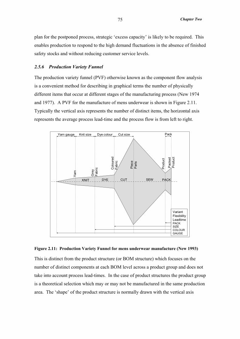
Chapter Two

75

plan for the postponed process, strategic ‘excess capacity’ is likely to be required. This

enables production to respond to the high demand fluctuations in the absence of finished

safety stocks and without reducing customer service levels.

2.5.6 Production Variety Funnel

The production variety funnel (PVF) otherwise known as the component flow analysis

is a convenient method for describing in graphical terms the number of physically

different items that occur at different stages of the manufacturing process (New 1974

and 1977). A PVF for the manufacture of mens underwear is shown in Figure 2.11.

Typically the vertical axis represents the number of distinct items, the horizontal axis

represents the average process lead-time and the process flow is from left to right.

Yar

n

Gre

yFa

bric C

olou

red

Fabr

ic

Pie

ceP

arts

Pro

duct

Pac

ked

Pro

duct

KNIT DYE CUT SEW PACK

Yarn gauge Knit size Dye colour Cut size Pack

VariantFlexibilityLeadtimePACKSIZECOLOURGAUGE

Figure 2.11: Production Variety Funnel for mens underwear manufacture (New 1993)

This is distinct from the product structure (or BOM structure) which focuses on the

number of distinct components at each BOM level across a product group and does not

take into account process lead-times. In the case of product structures the product group

is a theoretical selection which may or may not be manufactured in the same production

area. The ‘shape’ of the product structure is normally drawn with the vertical axis

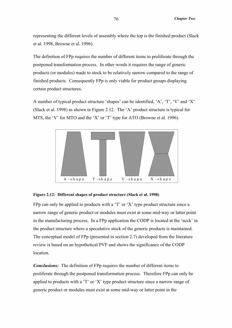
Chapter Two

76

representing the different levels of assembly where the top is the finished product (Slack

et al. 1998, Browne et al. 1996).

The definition of FPp requires the number of different items to proliferate through the

postponed transformation process. In other words it requires the range of generic

products (or modules) made to stock to be relatively narrow compared to the range of

finished products. Consequently FPp is only viable for product groups displaying

certain product structures.

A number of typical product structure ‘shapes’ can be identified, ‘A’, ‘T’, ‘V’ and ‘X’

(Slack et al. 1998) as shown in Figure 2.12. The ‘A’ product structure is typical for

MTS, the ‘V’ for MTO and the ‘X’ or ‘T’ type for ATO (Browne et al. 1996).

A - s h a p e T - s h a p e V - s h a p e X - s h a p e

Figure 2.12: Different shapes of product structure (Slack et al. 1998)

FPp can only be applied to products with a ‘T’ or ‘X’ type product structure since a

narrow range of generic product or modules must exist at some mid-way or latter point

in the manufacturing process. In a FPp application the CODP is located at the ‘neck’ in

the product structure where a speculative stock of the generic products is maintained.

The conceptual model of FPp (presented in section 2.7) developed from the literature

review is based on an hypothetical PVF and shows the significance of the CODP

location.

Conclusions: The definition of FPp requires the number of different items to

proliferate through the postponed transformation process. Therefore FPp can only be

applied to products with a ‘T’ or ‘X’ type product structure since a narrow range of

generic product or modules must exist at some mid-way or latter point in the

Chapter Two

77

manufacturing process. In a FPp application the CODP is located at the ‘neck’ in the

product structure where a speculative stock of the generic products is maintained. The

conceptual model of FPp is based on an hypothetical PVF which are distinct from

product structures in that they consider process lead-times.

2.6 ENGINEERING IMPLICATIONS

Engineering literature relating to FPp is reviewed in this section. Delayed product

differentiation (DPD), which can be an approach to product and process re-design for

FPp, is introduced. The three approaches to DPD are discussed in relation to FPp:

product and process modularity; product standardization and component commonality;

and manufacturing process re-structuring.

2.6.1 Delayed Product Differentiation

The engineering literature, (Lee and Tang 1997, Garg and Tang 1997, Lee 1996)

considers how a product or production process can be re-designed ‘so that the point of

differentiation is delayed as much as possible’.

Here the ‘point of differentiation’ is ‘the stage after which the products assume their

unique identities’ or the point where a ‘generic product is customised into different end

products’ using ‘specialised components or processes’ (Lee and Tang 1997). This

approach is given the term ‘delayed product differentiation’ (DPD). DPD is viewed as

an approach to reducing finished goods inventory in a MTS situation – sometimes this

involves introducing generic product stocks. The aim of DPD is to maintaining the

product in an undifferentiated state for as much of the manufacturing process as

possible, therefore it ultimately leads to a standardised product. This is distinct from

FPp which is only applicable to customised or highly differentiated products which are

stocked in generic form and customised to order. FPp aims to postpone differentiation

processes until after the customer orders are received while maintaining responsiveness

provided to customers.

Clearly DPD can support FPp where the finished product is not standardised (i.e.

remains differentiated) and the remainder of the engineering literature reviewed focuses

on this aspect. Lee and Tang (1997) formalise three basic approaches to DPD that some

Chapter Two

78

companies have used: standardisation, modular design and process re-structuring.

Standardisation refers to ‘using common components or processes’ and is covered in

section 2.6.3 on product standardisation. Modular design (discussed in section 2.6.2)

refers to ‘decomposing the complete product into sub-modules that can be easily

assembled together’ such that ‘the assembly of certain product-specific modules can be

delayed’. Finally process re-structuring refers to re-sequencing process steps such that

the differentiating processes are performed last (discussed in section 2.6.4).

The costs and benefits of DPD have been explored using inventory modelling with

multi-echelon systems. Some research is intended for strategic planning rather than

tactical and therefore simplifies the situation dramatically - Lee and Tang (1997)

consider a single point of differentiation whereas Garg and Tang (1997) consider

products with two points of differentiation. Other research is directed at strategic

decisions within a specific company, therefore it has very limited generalisability (Lee

and Sasser 1995).

Conclusion: DPD is an approach to product and process re-design such that the point

of differentiation is delayed. It reduces finished goods inventory in a MTS situation and

can involve the introduction of generic product stocks. The aim of DPD is to maintain

the product in an undifferentiated state for as much of the manufacturing process as

possible – ultimately this leads to a standardised product. DPD is distinct from FPp

which is only applicable to highly differentiated products which are stocked in generic

form and customised to order. FPp aims to postpone differentiation processes while

maintaining the responsiveness required by customers. Nevertheless DPD can support

FPP when the finished product is not standardised (i.e. remains differentiated) and the

remainder of the engineering literature reviewed focuses on these aspects.

2.6.2 Product and Process Modularity

The idea of modular products can be traced back to Starr (1965) who identified the

emerging ‘consumer’s demand for maximum product variety’. He describes how this

can be achieved by designing and manufacturing parts, or modules, which can be

combined in numerous ways to produce different product variants. From an

engineering perspective product modularity arises from the physical division of a

Chapter Two

79

product into independent components, and is frequently stated as a goal of good design

practice (Ulrich 1994, Lee 1996, He and Kusiak 1996).

Starr (1965) observed that modular production breaks down the manufacturing process

into two main stages, the manufacture of the modules through some transformation

process, and the assembly of the modules into a wide range of configurations:

‘It is the essence of the modular concept to design, develop, and produce those parts (modules) which can be combined in the maximum number of ways.’

More recently it has been observed that the modules may be inventoried, and the

products assembled-to-order, radically reducing the order lead-time, compared to the

alternative MTO approach (Ulrich 1994, Feitzinger and Lee 1997). This strategy has

been called the ‘mushroom approach’, because the product variety ‘mushrooms’ at or

near final assembly (Ulrich 1994).

A range of authors present the benefits of modularity most notably that it enables many

variants of a product to be constructed from a much smaller set of different modules

(Ulrich 1994, Lee 1996, He and Kusiak 1996). Ulrich (1994) and Pine (1993) claim

that this variety arises from the ability to use one of several alternative component

options to implement a function element of the design. The product can be designed so

that physical and functional interfaces between components are the same for all versions

of each component (He and Kusiak 1996), such that they are completely

interchangeable. Modularity has many other benefits: it offers improved ease of

product changes (Baldwin and Clark 1997, Ulrich 1994); and it enables simultaneous

design and manufacture of modules such that total lead-time can be shortened (Ulrich

1994, Feitzinger and Lee 1997).

Product modularity also provides companies with the opportunity to rationalise or

standardise components (Feitzinger and Lee 1997, Ulrich 1994, He and Kusiak 1996).

Ulrich and Tung (1991) argue that it is the ‘independence of the components’ that

allows standardisation and interchangeabilty of components, thus their rationalisation.

This results in increased component commonality (Collier 1981, Baker 1985) as


Chapter Two

80

Product modularity is not without its costs. Firstly, modularity assumes a product’s

functional and physical architecture is static which may be an obstacle to architectural

innovation (Ulrich 1994). Secondly, the product performance tends to be compromised

by modularity. It is said that the technical performance of a product can always be

improved by reducing modularity (Pine 1993, Ulrich 1994), or increasing ‘integration’

the converse of modularity (Erens and Verhulst 1997). Thirdly, since the physical

structure of a modular product is similar to a schematic diagram of its function

competitors can more easily reverse engineer the product (Pine 1993, Ulrich 1994).

Table 2.10: Summary of the six types of modularity identified by Pine (1993)

Modularity type Description

Component-sharing The same component is used across multiple products

Component-swapping

Different components are paired with the same basic product. This is the complement of component sharing and the distinction between the two is a matter of degree at what point does the ‘shared component’ become the basic product in ‘component swapping’, e.g. General Motors (Vollman et al. 1992) make a basic J-body car and combine this with a range of different door ‘options’, cylinder ‘options’ etc.

Cut-to-fit One or more of the components is continually variable, e.g. the National Bicycle industrial Company in Japan (Kotha 1995) cuts the bicycle frames to fit the individual customer.

Mix

Uses any of the above modularity types, with the clear distinction that the components are so mixed together that they themselves become something different, e.g. Mexican restaurants create an incredible variety of meals from relatively few components: tortillas, beans various meats, and sauces

Bus Different components are attached to a standard structure

Sectional Allows the configuration of any number of different types of components in arbitrary ways as long as each component connects to another at standard interfaces, e.g. Lego building blocks with their locking cylinder interfaces

Ulrich (1994) states that the degree of modularity depends on:

• the similarity between the physical and functional architecture of the design

(Huang and Kusiak 1998) and

• the degree to which the interactions between physical components are critical to

the function of the product (Ulrich 1994).

Chapter Two

81

Erens and Verhulst (1997) support this view of modularity stating that ‘in general a

modular design is considered to be a design in which a restricted number of functions is

allocated to a module’. Ulrich (1994) argues that modularity is a relative property –

products cannot be classified as either modular or not but rather exhibit more or less

modularity in design. This is a view supported by Baldwin and Clark (1997).

Ulrich (1994) concludes – ‘a completely modular design embodies a one-to-one

correspondence between each functional element and physical component, in which

every interaction between components is critical to the function of the system’. Here a

product can be described functionally by a collection of functional elements linked

together by exchanges of signals, material and power - frequently called a schematic

description. No products achieve complete modularity, although some electronic

products exhibit relatively high modularity.

Component-sharing modularity

Component-swapping modularity

Cut-to-fit modularity

Mix modularity

Bus modularity

Sectional modularity

Figure 2.13: Illustration of the six types of modularity identified by Pine (1993)

Pine (1993) conducts a study of the different types of modularity and identifies six types

(as shown in Figure 2.13 and defined in Table 2.10: Summary of the six types of

modularity identified by Pine (1993)) which are very similar to those previously

identified by Ulrich and Tung (1991). ‘Component swapping’ is the complement of

Chapter Two

82

‘component sharing’ and is where different components are paired with the same basic

product creating as many products as there are components to swap (Pine 1993). In

many cases the distinction between component sharing and component swapping is a

matter of degree. Consider Swatch watches: are the basic watch elements a component

shared across all the fashion products (component sharing)? Or are the watch parts the

basic product and the incredible variety of face styles the components (component

swapping)? Component swapping is often associated with the creation of product

variety as perceived by the customer (Ulrich and Tung 1991) – highly customised

products. In fact Pine (1993) claims that

‘true individual customisation comes when there are an infinite number of components to be swapped or….at least as many as there are people to buy the product or service’.

Component sharing on the other hand is

‘the kind of modularity that never results in true individual customisation…. but allows the low cost production of a great variety of products and services’.

Very little research relates product modularity to FPp applications. Van Hoek (1998a)

and van Hoek et al. (1998) identify product modularity as a characteristic that favours

FPp. However the results from van Hoek’s cases studies were not conclusive - only two

of the four companies applying postponement produced modular products. Van Hoek

and Weken (1998) conduct a study in the automotive industry addressing how modular

production can contribute to the integration of inbound and outbound logistics with the

manufacturing plant (as reviewed in section 2.3.2).

Conclusion: Product modularity arises from the physical division of a product into

independent components which can be combined in numerous ways to produce different

variations of the product. Modules can be manufactured to stock and then assembled-

to-order called the ‘mushroom approach’ or FPp. The degree of modularity depends on:

the similarity between the physical and functional architecture of the design; and the

degree to which the interactions between physical components are critical to the

function of the product. However modularity is a relative property – products cannot be

classified as either modular or not but rather exhibit more or less modularity in design.

Six types of modularity are identified and a range of authors present the costs and

Chapter Two

83

benefits of modularity, however very little research relates product modularity to FPp

applications.

2.6.3 Product Standardisation and Component Commonality

Product standardisation arises from the design of a product to maximise the number of

constituent components identical across many (or preferably all) of the product variants

within a product family. Product standardisation can be an alternative to FPp but still

categorised as DPD. For example Hewlett Packard (Feitzinger and Lee 1997, Lee and

Sasser 1995, Lee and Tang 1997) adopted the ‘standardisation strategy’ for their Laser

Jet Printer sold into Europe and North America. Formerly two different power supply

modules providing 110 volts and 220 volts respectively were required. After the

standardisation exercise a single, intelligent power supply module was installed, which

automatically adjusted itself to the supply voltage. This could be called a ‘Chameleon

product’ since it changes to suit its environment but is always the same underneath.

Another similar example was found in the semiconductor firm Xilinx (Brown et al.

2000). Here the products were programmable, allowing the customers to fully

configure the function of the integrated circuit using software. Once again the product

had been standardised and therefore was not in anyway differentiated when the

customer received it.

When product standardisation is confined to the generic product or modules it can

support FPp. Van Hoek (1998a) and van Hoek et al. (1998) suggests that component

commonality favours FPp although the results from his cases studies are not conclusive

and no measures of commonality are taken. Product standardisation results in

component rationalisation and increased component commonality which can be

measured by the Degree of Commonality Index. The Degree of Commonality Index, C,

derived by Collier (1981) is an analytical index which measures the degree of

component part commonality for any set of items, commonly a product family. Given

that a BOM is a formal statement of parent-component relationships for product items, a

component part can be any inventory item, (other than an end item) that goes into

higher level items, possibly a sub-assembly.

Chapter Two

84

C is calculated as: C = N/c

Where N = the sum of immediate parents for all distinct components over a set of end items or product structure levels

c = the total number of distinct components in the set of end items or product structure levels

The Degree of Commonality Index is the average number of common parent items per

distinct component part (Collier 1981 and 1982). Or put another way the average

number of incidences of the distinct component parts across the set of parent items.

In a simulation study Collier (1982) demonstrated that in an MRP environment

increasing the degree of commonality reduces the aggregate safety stock levels required

to support a given service level. McClain et al. (1984) challenge Colliers results

claiming that the simulation was invalid as a test of generality because it only tested

special cases where the relationship holds exactly. Baker (1985) claims that the

presence of component commonality makes it difficult to determine safety stocks

accurately. He demonstrates that commonality destroys the relationship between safety

factor and service level.

It is argued that for a FPp application if the degree of component commonality in the

generic product or modules is increased the number of Stock Keeping Units (SKUs) is

reduced and demand uncertainty pooled (Zinn 1990a). Hence generic or aggregate

safety stock levels can be reduced to support a given service level. Lee and Tang

(1997) support this view claiming that component commonality increases the flexibility

of the aggregate inventories which reduces the risk associated with speculative

production of generic products or modules. In addition a greater volume of any one

component is used therefore the manufacturing economies of scale are increased and the

unit cost reduced (Ulrich 1994, Pine 1993).

Module or component standardisation is not without its costs. Increases in design, and

subsequently material costs, often accompany the standardisation of components, since

they tend to require excess capability to perform across a wider product range (Ulrich

1994). Ulrich (1994) and Pine (1993) note that products may be perceived by the

customer, as excessively similar, so it is advisable to limit standardisation to

Chapter Two

85

components that are hidden. Ealey et al. (1996) claim that automotive manufacturers

will ‘strive for increasing commonality of all components that are invisible to the

customer’.

Conclusion: Product standardisation is an approach to DPD which involves the

maximisation of the number of constituent components identical across many of the

product variants. When it involves the standardisation of customising components it

represents an alternative to FPp. Alternatively when standardisation is confined to the

generic product or modules it supports FPp. Product standardisation leads to increased

component commonality which can be measured by the Degree of Commonality Index.

This is the average number of common parent items per distinct component part. Many

authors document the benefits and costs of component commonality. It is argued that

for FPp applications if component commonality in the generic products is increased the

number of SKUs is reduced, demand uncertainty pooled and generic safety stock levels

reduced.

2.6.4 Manufacturing Process Configuration

The final approach to DPD is the re-configuration of the manufacturing processes. It is

argued that where customisation occurs early in manufacturing, it may be necessary to

re-sequence the processes to ensure that the product can be customised-to-order within a

short ‘order lead-time’ (Feitzinger and Lee 1997, Lee and Tang 1997). Benetton used

this approach in order to apply FPp to their sweater manufacturing operations in Italy

(Harvard Business School 1985, Dapiran 1992). Originally the manufacturing process

began with dying the wool into a wide variety of colours. Unfortunately the subsequent

knitting process was an extremely lengthy one, necessitating that the retailers forecast

sales, by colour, 6 months in advance. Naturally these forecasts were notoriously

inaccurate resulting in high inventory at the retailers (to buffer against these

inaccuracies), forced mark downs and product shortages.

Benetton applied FPp to their most popular lines (which constituted about 20% by

volume) by re-sequencing the processes and postponing dying until after the jumpers

had been knitted. They were then able to offer a 5 week lead-time on orders by colour

such that the retailers’ sales forecasts were based largely on actual sales.

Chapter Two

86

Re-sequencing manufacturing processes can be aided by their modularisation. Bennett

and Forrester (1994) state that in ‘high variety - low volume’ manufacture the benefits

of modularised product design can be greatly enhanced by also modularising the

production processes. He and Kusiak (1998) propose an approach for the design of

assembly lines for modular products exhibiting component-swapping modularity (Pine

1993). This approach divides the assembly line into two subassembly lines: the first

assembles those modules common to all the product variants in the product family; and

the latter conducts those assembly operations involving optional components.

Inventory models are widely used to assist in the design of manufacturing processes for

DPD. However these often consider the CODP to be at the finished good stage (MTS)

and some level of finished good stock to always be maintained (Garg and Tang 1997 for

example). An exception to this was the Lee and Tang (1997) model of the Benetton

manufacturing process reversal. They made the general conclusion that for this

approach to be effective the postponed process should be a ‘high value added process’.

It is argued that this is not so and what is crucial is the variety produced by the

postponed process which, when high, creates high demand uncertainty. In the Benetton

case the benefits of FPp were largely derived from the dying process being based on

actual sales information (when postponed) rather than long term sales forecasts.

Conclusion: The final approach to DPD is the re-configuration of the manufacturing

processes. It is argued that where customisation occurs early in manufacturing, it may

be necessary to re-sequence the processes to ensure that the product can be customised-

to-order within a short ‘order lead-time’. Benetton used this approach in order to apply

FPp to their sweater manufacturing operations in Italy. Re-sequencing manufacturing

processes can be aided by their modularisation. Inventory models are widely used to

assist in the design of manufacturing processes for DPD. However these often consider

the CODP to be at the finished good stage (MTS) and those that don’t still suffer from

over-simplification which can lead to dubious results.

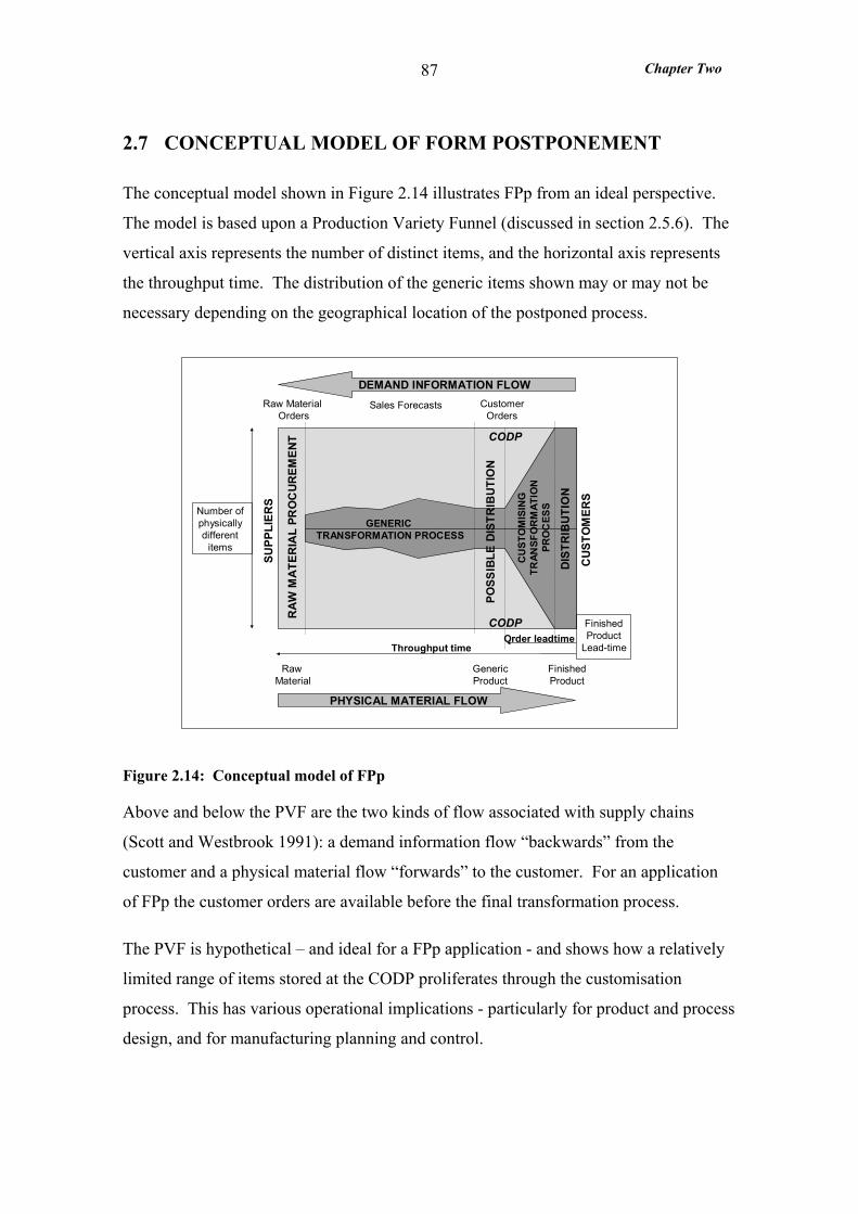
Chapter Two

87

2.7 CONCEPTUAL MODEL OF FORM POSTPONEMENT

The conceptual model shown in Figure 2.14 illustrates FPp from an ideal perspective.

The model is based upon a Production Variety Funnel (discussed in section 2.5.6). The

vertical axis represents the number of distinct items, and the horizontal axis represents

the throughput time. The distribution of the generic items shown may or may not be

necessary depending on the geographical location of the postponed process.

PHYSICAL MATERIAL FLOW

DEMAND INFORMATION FLOW

CODPNumber ofphysicallydifferent

items

FinishedProduct

Lead-timeThroughput timeOrder leadtime

SUPP

LIER

S

CU

STO

MER

S

POSS

IBLE

DIS

TRIB

UTI

ON

DIS

TRIB

UTI

ON

RA

W M

ATE

RIA

L PR

OC

UR

EMEN

T

CU

STO

MIS

ING

TRAN

SFO

RM

ATIO

NPR

OC

ESS

GENERIC TRANSFORMATION PROCESS

Raw Material Orders

CustomerOrders

Sales Forecasts

Raw Material

GenericProduct

FinishedProduct

CODP

CODP

Figure 2.14: Conceptual model of FPp

Above and below the PVF are the two kinds of flow associated with supply chains

(Scott and Westbrook 1991): a demand information flow “backwards” from the

customer and a physical material flow “forwards” to the customer. For an application

of FPp the customer orders are available before the final transformation process.

The PVF is hypothetical – and ideal for a FPp application - and shows how a relatively

limited range of items stored at the CODP proliferates through the customisation

process. This has various operational implications - particularly for product and process

design, and for manufacturing planning and control.

Chapter Two

88

The focus of product and process design is to minimise both the stock keeping units

(SKUs) at the CODP and the lead-time required for the customising processes - whilst

ensuring that the required range of finished products can be supported. The challenge

for manufacturing planning and control is to optimise the two contrasting stages of

manufacture (pre- and post- CODP). The first stage involves the forecast-driven

production of a relatively narrow range of generic items that are subject to relatively

stable demand. The second stage is the order-driven production of a broad range of

finished products that are each subject to uncertain demand. This implies that the first

stage of manufacturing should aim to be ‘lean’ - where minimising cost, and therefore

waste (such as excess capacity) is the critical factor. In contrast the second stage should

focus on ‘agile supply’ - where maximising customer service in terms of short, reliable

order lead-times is the key factor (Naylor et al. 1999).

2.8 THEORETICAL FRAMEWORK

A theoretical framework (shown in Figure 2.15) was deduced from the previous

logistics, OM and engineering research, reviewed in this chapter, on the basis of an

ideal FPp application (as illustrated by the conceptual model of FPp). The theoretical

framework addresses the research question by illustrating how FPp is applied in terms

of a wide range of variables relative to MTS and MTO. This section summarises how

this framework was deduced.

Cost models developed by Zinn and Bowersox (1988) and reviewed in section 2.2.2

analysed the impact of various product characteristics on the cost of distribution using

FPp where the postponed processes are conducted in the distribution chain. The cost

models showed that increases in product variety and demand variability favoured FPp

against MTS whereas increases in volume demand at generic level showed no support

for FPp. It is argued that these findings, supported by other work (for example, Cooper

1993 and van Hoek 1998a) will apply when the postponed process is brought back into

the factory. Further it is considered that low volume demand at end item level will

favour FPp compared to MTS while high volume demand at generic level will favour

FPp compared to MTO.

Chapter Two

89

represents the Customer Order Decoupling Point

Make-To-Order Form Postponement Make-To-Stock

SUPPLIERS

CUSTOMERS

Raw materials Semi-finishedproduct

Finished product

Ex-stock AvailabilityHigh MediumN/a

Demand Amplification Low HighNone

Order Lead-time Short Short

Delivery Reliability High N/a

Long

Low

Product Standardisation Low Medium

Product Modularity Low High

Excess CapacityHigh Low

Throughput EfficiencyHigh Low

High

Low

Demand Mix High Low

Demand Variability High Low

High

High

Volume Demand Low Low High

Volume Demand (generic) Low High High

H1

H2

H3

H4

H5

H6

Figure 2.15: The theoretical framework for the application of FPp.

In section 2.2.2 it is also discussed how Van Hoek (1998a) and van Hoek et al. (1998)

observe that the requirement for short and reliable lead-times favours postponed

manufacturing, which in turn improves delivery service compared to MTS. It is argued

that while FPp may improve product (or ex-stock) availability, and allow greater

product customisation (Amaro et al. 1999) it is unlikely to reduce order lead-time. It is

further argued that FPp, compared to MTO, will reduce order lead-time and improve

delivery reliability because only the final processing is ‘to-order’ reducing risk of

lateness.

Demand amplification is caused by a delayed reaction to demand changes (Forrester

1958) commonly caused by inventory management policies (Huang et al. 2003) as

discussed in section 2.3.1. It is argued that FPp reduces demand amplification

compared to MTS approaches by reducing the demand variability that the system is

subject to, and linking the point of differentiation to the point of sale. Conversely as an

alternative to MTO, FPp introduces demand amplification by introducing a speculative

generic stock.

Chapter Two

90

In section 2.6.3 it is argued that high levels of standardisation (or component

commonality) in the generic products supports FPp by reducing the number of generic

product variants which pools demand uncertainty and allows reduction of safety stocks.

It is further argued that higher levels of standardisation - not confined to generic

modules - favour MTS while lower levels of standardisation involving only components

supports MTO. Product modularity is commonly associated with assemble to order as

discussed in section 2.6.2 where the modules are inventoried and assembled upon

receipt of a customer order (for example Ulrich 1994, Feitzinger and Lee 1997). It is

argued therefore that products which are subject to FPp will tend to exhibit a relatively

high degree of modularity compared to products which are MTO or MTS.

For a FPp application demand at the postponed process is highly volatile. It is argued in

section 2.5.5. that, in this case, strategic ‘excess capacity’ (Steele and Park-Shields

1993) is required to enable production to respond to the high demand fluctuations, in the

absence of finished safety stocks, while maintaining responsive supply. It is further

argued in section 2.5.3 that the high levels of responsiveness require short postponed

manufacturing lead-times and high throughput efficiency. This is loosely illustrate in

the theoretical framework by comparing using MTO and MTS to represent the order

driven postponed processes and the stock driven generic processes respectively.

2.9 CONCLUSION

A working definition of FPp was developed which more closely reflects what

manufacturers are actually doing. This definition encapsulates FPp applications where

the postponed process is performed at the factory, a warehouse or a retailer. This

research is restricted to cases where the postponed process is performed in the factory.

The literature review identified gaps in both OM and logistics knowledge related to how

FPp is applied. Three areas of OM research were related to FPp: non-MTS, mass

customisation and postponement itself. Much of the published OM research addresses

the needs of the MTS companies and neglects the needs of the non-MTS sector. The

exceptions tend to address the planning and control systems and consider MTO

approaches rather than other non-MTS approaches such as ATO or FPp. Furthermore

Chapter Two

91

the non-MTS approaches considered are typically assumed to be unresponsive in

contrast to FPp which is a responsive non-MTS approach.

The OM literature concerning mass customisation is extensive. However much of it is

concerned with the strategic impact of mass customisation and only a few publications

address its operational implications or the ‘how’ of mass customisation. Consequently

mass customisation remains largely at the conceptual level and, though the logistical

and operational implications are considerable, there has been little practical input from

either discipline.

In general the OM literature on FPp uses variable oriented models of delayed product

differentiation applied to MTS approaches. Therefore these models are not directly

applicable to FPp. With the introduction of a CODP at the generic product stage they

could be very useful in understanding some of the operational implications of FPp.

This thesis contributes to OM knowledge related to FPp by addressing the operational

implications of FPp - a responsive non-MTS approach to mass customisation. The

thesis focuses on the operational implications within the factory including inventory

management, product design, production variety, manufacturing and planning and

scheduling.

The literature review identified a gap in the logistics knowledge related to FPp. The

existing logistics literature in this area considers the conditions under which FPp is

justified and the specification of the appropriate FPp strategy. Here FPp is only

considered as an alternative strategy to MTS - not to MTO - and the guidelines are

restricted to deciding an appropriate postponement strategy rather than its application.

In general only FPp applications where the postponed processes are conducted in the

distribution chain have so far been considered. As a consequence the postponed

processing tends to be relatively simple or trivial. This thesis contributes to this body of

literature by considering the application of FPp where the postponed processes are

brought back into the factory. Under this scenario substantially more complex

processes, than considered in the existing logistical literature, are likely to be capable of

postponement.

Chapter Two

92

In addition to identifying gaps in the knowledge related to FPp the literature review

identified many of the logistical, operational and engineering implications of applying

FPp. This resulted in two main outputs: the conceptual model of FPp (presented in

section 2.7); and the theoretical framework (presented in section 2.8). The conceptual

model of FPp illustrates product design, process design, and manufacturing planning

and control implications for an ideal FPp application. While the theoretical framework

addresses the research question by illustrating how FPp is ideally applied in terms of a

wide range of variables relative to MTS and MTO. In the next Chapter describing the

research methodology the hypotheses are extracted from this theoretical framework.

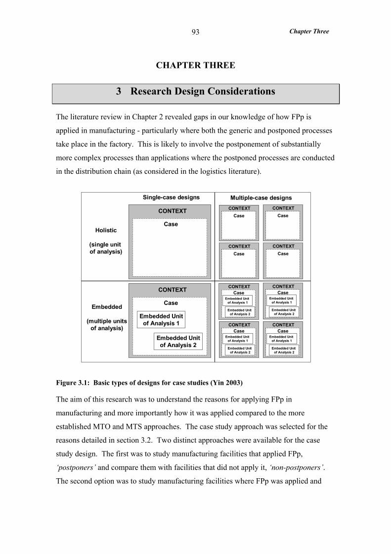
Chapter Three

93

CHAPTER THREE

3 Research Design Considerations

The literature review in Chapter 2 revealed gaps in our knowledge of how FPp is

applied in manufacturing - particularly where both the generic and postponed processes

take place in the factory. This is likely to involve the postponement of substantially

more complex processes than applications where the postponed processes are conducted

in the distribution chain (as considered in the logistics literature).

CONTEXTCase

CONTEXTCase

CONTEXTCase

CONTEXTCase

CONTEXTCase

Embedded Unit of Analysis 1


CONTEXTCase



CONTEXTCase



CONTEXTCase



CONTEXT

Case

CONTEXT

Case

Embedded Unitof Analysis 1

Embedded Unitof Analysis 2

Multiple-case designsSingle-case designs

Holistic

(single unit of analysis)

Embedded

(multiple unitsof analysis)

Figure 3.1: Basic types of designs for case studies (Yin 2003)

The aim of this research was to understand the reasons for applying FPp in

manufacturing and more importantly how it was applied compared to the more

established MTO and MTS approaches. The case study approach was selected for the

reasons detailed in section 3.2. Two distinct approaches were available for the case

study design. The first was to study manufacturing facilities that applied FPp,

‘postponers’ and compare them with facilities that did not apply it, ‘non-postponers’.

The second option was to study manufacturing facilities where FPp was applied and

Chapter Three

94

compare units of analysis based around product groups subject to different inventory

management policies – FPp, MTO and MTS. Here Yin (2003) describes the unit of

analysis as ‘subunits’ within a single case – effectively cases within a case. The term

units of analysis (abbreviated to UoA) will be used to refer to these ‘subunits’ to bring

clarity to the research design.

It was concluded that the design incorporating multiple UoA within a case had a major

advantage over the ‘postponers’ versus ‘non-postponers’ approach in that it would

screen out the contextual differences between factories that are not the subject of this

study. For instance it was expected that within a single manufacturing facility the

management team, information systems, manufacturing databases, to name but a few

aspects, would apply to the whole product range. These contextual aspects would be

different between autonomous manufacturing facilities introducing a host of new

variables when comparing FPp with non-FPp approaches (i.e. MTO or MTS).

Further, if one restricted the study to manufacturing facilities where at least a proportion

of the product range was subject to FPp, one could be assured that the organisation was

aware of FPp and had made a deliberate decision as to which products to apply it to.

This cannot be said of facilities where FPp had not been applied. At these facilities they

may have been totally unaware of the FPp approach, or have some prejudice against it,

or simply have never seriously considered it. In conclusion the case study design

incorporated multiple cases each with three UoA, as indicated by the fourth quadrant in

Figure 3.1.

3.1 RESEARCH DESIGN

3.1.1 Research Questions and Hypotheses

The aim of this research was to understand the reasons for applying FPp in

manufacturing and more importantly how it was applied compared to the more

established MTO and MTS approaches. The research question was:

Why and how is form postponement applied in manufacturing?

Chapter Three

95

Yin (2003) states that research questions tend not to isolate what you should study and

the evidence required. He maintains that only stating hypotheses will focus the

research. Consistent with this approach a theoretical framework (shown in Figure 2.15)

was deduced in Chapter 2 from previous logistics, OM and engineering research on the

basis of an ideal FPp application (as illustrated by the conceptual model of FPp

presented in Figure 2.14). The theoretical framework addresses the research question

by illustrating how FPp is applied in terms of a wide range of variables relative to MTS

and MTO. The hypotheses were extracted from the theoretical framework as indicated

down the left side of Figure 2.15. Each hypothesis compares FPp with either MTO or

MTS with respect to each of the variables as presented below:

What is the demand profile of products selected for manufacture under FPp? H1: Products are selected for manufacture under FPp rather than MTS when they exhibit high demand mix, high demand variability, and low volume demand at finished product level.

H2: Products are selected for manufacture under FPp rather than MTO/ETO when they exhibit high volume demand at generic product level.

What is the impact on customer service of FPp? H3: FPp considered as an alternative to MTS increases ex-stock availability.

H4: FPp considered as an alternative to MTO/ETO reduces order lead-times and increases delivery reliability but introduces demand amplification

What are the product design implications of applying FPp? H5: Product families subject to FPp will have a higher level of standardisation and modularity than product families subject to MTO/ETO

What are the manufacturing planning and scheduling implications of applying FPp? H6: Capability of the postponed transformation process to respond to high demand variability requires excess capacity and high throughput efficiency

Much quantitative evidence was gathered on the concepts featuring in the hypotheses,

however substantial qualitative evidence was also collected via numerous interviews

with key personnel (as detailed in section 3.5.2). Here qualitative evidence is ‘words’

and quantitative evidence ‘numbers’ as distinguished by Eisenhardt (1989) and

explained in section 3.4.1. The qualitative evidence included contextual data such as

the business environment and the reasons for applying FPp. It also incorporated data

regarding how FPp was applied such as product selection and manufacturing planning

system changes. Further detail is provided on the qualitative data in section 3.1.3.

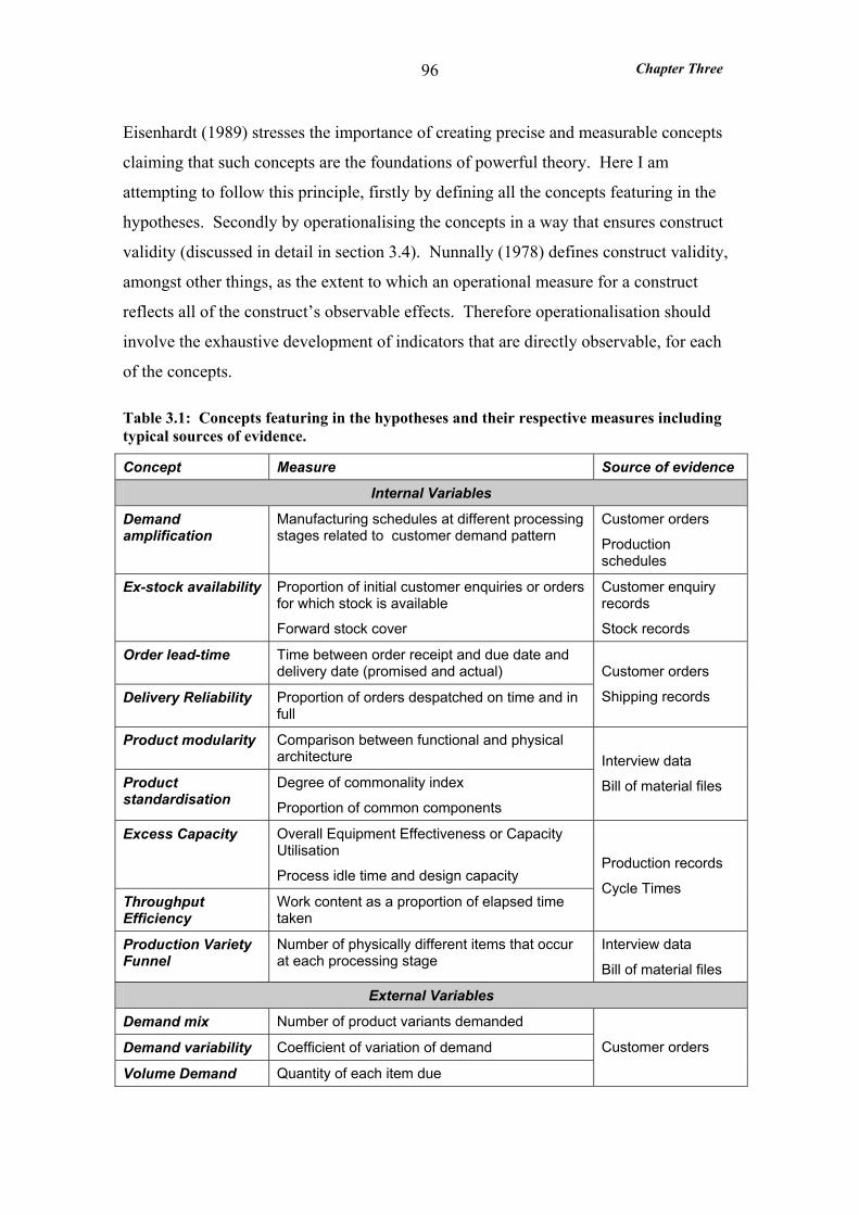
Chapter Three

96

Eisenhardt (1989) stresses the importance of creating precise and measurable concepts

claiming that such concepts are the foundations of powerful theory. Here I am

attempting to follow this principle, firstly by defining all the concepts featuring in the

hypotheses. Secondly by operationalising the concepts in a way that ensures construct

validity (discussed in detail in section 3.4). Nunnally (1978) defines construct validity,

amongst other things, as the extent to which an operational measure for a construct

reflects all of the construct’s observable effects. Therefore operationalisation should

involve the exhaustive development of indicators that are directly observable, for each

of the concepts.

Table 3.1: Concepts featuring in the hypotheses and their respective measures including typical sources of evidence.

Concept Measure Source of evidence

Internal Variables

Demand amplification

Manufacturing schedules at different processing stages related to customer demand pattern

Customer orders

Production schedules

Ex-stock availability Proportion of initial customer enquiries or orders for which stock is available

Forward stock cover

Customer enquiry records

Stock records

Order lead-time Time between order receipt and due date and delivery date (promised and actual)

Delivery Reliability Proportion of orders despatched on time and in full

Customer orders

Shipping records

Product modularity Comparison between functional and physical architecture

Product standardisation

Degree of commonality index

Proportion of common components

Interview data

Bill of material files

Excess Capacity Overall Equipment Effectiveness or Capacity Utilisation

Process idle time and design capacity

Throughput Efficiency

Work content as a proportion of elapsed time taken

Production records

Cycle Times

Production Variety Funnel

Number of physically different items that occur at each processing stage

Interview data

Bill of material files

External Variables

Demand mix Number of product variants demanded

Demand variability Coefficient of variation of demand

Volume Demand Quantity of each item due

Customer orders

Chapter Three

97

The respective measures and indicators used, and typical sources of evidence, are

summarised in Table 3.1 for each of the concepts or variables featured in the

hypotheses. The twelve variables were not intended to form a comprehensive

description of the FPp application but to focus a broad based measurement of the UoA

to identify the differences between FPp, MTO and MTS. In operationalising the

research design some variables were grouped together because they used the same data

and were strongly related. Ex-stock availability, order lead-time and delivery reliability

were grouped under ‘customer service’ and the three external demand variables were

grouped under ‘demand profile’.

3.1.2 Internal and External Variables

Before considering the entire study framework it is appropriate to first define the

concepts and measures (in Table 3.1 and defined in the glossary, Appendix 1) which

were used to study FPp in each of the three case studies:

Demand amplification: Demand amplification is the effect where variations in

customer demand are amplified with each step upstream in the supply chain, such that

the pattern of demand upstream bears little resemblance to the final customer demand

(Forrester 1958). It results in the amplification of orders and inventory fluctuations

upstream and is caused by inventory management policies (Huang et al. 2003), demand

forecast updating, order batching, price fluctuation and rationing and shortage gaming

(Lee et al. 1997). Demand amplification can be illustrated using a mapping approach

described by Bicheno (1998) which can be used in two ways: for a single member of a

supply chain and for the complete supply chain. The former approach was used for this

study where the chart shows plots of actual customer orders (demand imposed on the

manufacturing system), manufacturing orders and orders placed on the next stage of

manufacture (the manufacturing process schedule) plotted against time.

Ex-stock availability: is the proportion of initial customer requests (enquiries or orders)

for which the correct product is available ex-stock in sufficient quantities (New and

Szwejczewski 1995). It only applies to MTS and FPp, not MTO where no product

stock is normally kept. For MTS it is measured ex-finished goods stock and for FPp it

Chapter Three

98

is measured ex-generic stock. Stock levels, in terms of forward cover, combined with

delivery reliability were sometimes used as indicators of ex-stock availability.

Order lead-time: is the time between the customer ordering the product and receiving it.

The promised and actual order lead-times were measured from the receipt of the

customer order to the respective delivery dates. In the absence of delivery-to-the-

customer dates the ex-works dates were used with the proviso that transit times were not

taken into account.

Delivery reliability: is the ability of the operating facility to meet the agreed terms of

delivery with respect to the product type, the quantity ordered and the due date

(Hoekstra and Romme 1992). Delivery reliability was measured by comparing actual

delivery dates and quantities with promised due dates and quantities, normally detailed

on the customer order. In the absence of delivery-to-the-customer dates the actual and

promised ex-works dates were compared. The delivery reliability measure culminated

in the calculation of: the proportion of orders delivered on or before the last committed

delivery date (on time); and the proportion of orders where the quantity and type

delivered were correct to the order (in full). These measures were combined to give the

on time in full (OTIF) measure.

Product Modularity: arises from the physical division of a product into independent

components (Ulrich 1994, Lee 1996) which can be combined in numerous ways to

produce different variations of the product (Starr 1965, Pine 1993). According to

Ulrich (1994) the degree of product modularity depends on the similarity between the

physical and functional architecture of the design and the degree to which the

interactions between physical components are critical to the function of the product. He

argues that modularity is a relative property – products cannot be classified as either

modular or not but rather exhibit more or less modularity in design. He concludes that a

completely modular design embodies a one-to-one correspondence between each

functional element and physical component, in which every interaction between

components is critical to the function of the system. Here a product can be described

functionally by a collection of functional elements linked together by exchanges of

signals, material and power - frequently called a schematic description (Ulrich and

Seering 1989).

Chapter Three

99

Product standardisation: arises from the design of a product such that the maximum

number of constituent components are identical across many (preferably all) of the

product variants within a product group. It results in component rationalisation, or

commonality, which can be indicated by two measures: the proportion of components

common to all variants in the product group and the degree of commonality index. The

latter is the average number of common parent items per distinct component part

(Collier 1981 and 1982). Or put another way the average number of incidences of the

distinct component parts across the parent items. It is calculated by dividing the sum of

immediate parents for all distinct components by the total number of distinct

components over a set of end items or product structure levels.

The higher the degree of commonality index the greater the overall level of component

commonality. However, viewing this measure in isolation is not sufficient it must be

considered in relation to its upper bound. The upper bound is when all distinct

components are common across all the end items (Collier 1982) and is therefore equal

to the number of end items. Accordingly the commonality index was interpreted as a

percentage of the number of end items in the product group.

Excess Capacity: is the percentage amount that available capacity exceeds demand. It

can be argued that the manifestation of excess capacity is dependant on whether the

process is order-driven or stock-driven at a given point in time. In an order-driven

situation excess capacity manifests itself as ‘process idle time’, which is the time when

the process could be producing but is idle because the current load does not require this

capacity. In a stock-driven situation excess capacity may manifest itself as both process

idle time and stock awaiting further processing (or despatch) because load can be

created without demand.

Process idle time was used as an indication of excess capacity together with capacity

provision or design capacity and capacity utilisation. Two measures of capacity

utilisation were used – Overall Equipment Effectiveness (OEE) and the ratio of actual

output to design capacity.

OEE was used where capacity was equipment driven which was only in the Thomas

Bolton case study (Chapter 4). In this case OEE (the only measure of capacity

Chapter Three

100

utilisation used at TB) was measured by the factory routinely during the study period

therefore the OEE evidence was readily available in an established database. Further it

provided a good indication of excess capacity because the ‘planned out’ time -

equivalent to process idle time - was recorded separately and excluded from the OEE

measure (as the OEE definition detailed in the glossary, Appendix 1, dictates). To

summarise the main objective of OEE is to quantify the six big losses of capacity,

which can be reduced through improved equipment maintenance (Nakajima 1988).

OEE is calculated by multiplying three separate factors: availability, performance and

quality rate:

• ‘Availability’ measures downtime losses such as machine breakdowns and set-

ups;

• ‘performance’ measures speed losses caused by minor stoppages and slow

running; and

• ‘quality rate’ measures losses through defects such as scrapped production and

re-work.

Actual output as a proportion of design capacity (Slack et al. 1998), which is similar to

OEE, was the measure of capacity utilisation used for the other two cases (Brook

Crompton and Dewhurst). It was used as an indication of excess capacity – the lower it

was the more likely excess capacity existed. Further the relative design capacities of the

generic and postponed manufacturing processes were also used to indicate excess

capacity – where design capacities were higher excess capacity was more likely to exist.

Here design capacity was the theoretical capacity of an operation not usually achieved

in practice.

It was argued that using a different measure of capacity utilisation in the TB case did

not invalidate the cross-case comparison. The measure was used to indicate the relative

excess capacity at the postponed processes compared to the generic processes, not as an

absolute measure.

Throughput Efficiency: is the work content as a proportion of total elapsed time taken,

where the work content is the time taken for the value adding activities to be performed

Chapter Three

101

on an order quantity. The elapsed time is the time the factory was available to add value

and therefore must be measured over the factory’s operating hours (New 1993). It was

measured from release of the factory order to the despatch, or booking into the

warehouse, of the finished order.

Production Variety Funnel (PVF): is a convenient method for describing in graphical

terms the number of physically different items that occur at different stages of the

manufacturing process. Typically the vertical axis represents the number of distinct

items, the horizontal axis represents the average process lead-time and the process flow

is from left to right (New 1974 and 1977). The PVF is the only variable listed in Table

3.1 that does not feature in a hypothesis. Instead the PVF was plotted because it was

central to the conceptual model of FPp and the shape of the PVF should be strongly

related to the inventory management policy. It was a good indicator of whether FPp

could have been applied to other products (currently MTO or MTS) and whether the

CODP could have been better located for the FPp application.

Demand profile: included three external variables: demand mix, demand variability

and volume demand. Demand was quantified from customer order due dates and

quantities. Demand mix was the number of variants subject to demand. Demand

variability is the changes in demand over a given sequence of time buckets (Battacharya

et al., 1995). It can be measured using the coefficient of variation (CV) - the ratio of

standard deviation to average. Volume demand is the quantity of a given item

demanded.

3.1.3 Case Study Framework

The internal and external variables described in the previous section (and shown in

Table 3.1) effectively described the outcome of applying FPp in terms of a wide range

of measures such as demand amplification, customer service, and excess capacity.

Mapped onto Pettigrew’s (1990 and 1992) ‘meta level’ analytical framework these

measures constituted the ‘outcome variables’ as shown in Figure 3.2 and are highly

quantitative measures.

Pettigrew’s framework enables change to be studied in different environments without

theory limitations in comparative case study research. There are three primary

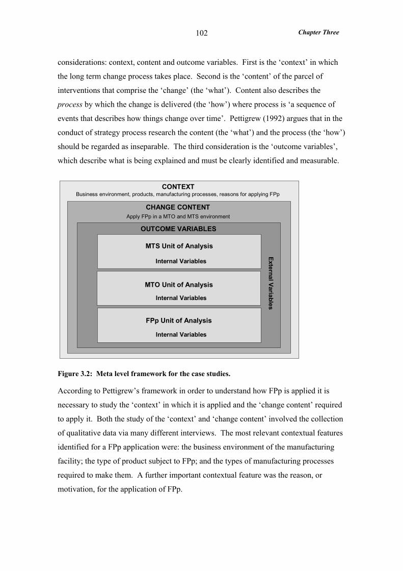
Chapter Three

102

considerations: context, content and outcome variables. First is the ‘context’ in which

the long term change process takes place. Second is the ‘content’ of the parcel of

interventions that comprise the ‘change’ (the ‘what’). Content also describes the

process by which the change is delivered (the ‘how’) where process is ‘a sequence of

events that describes how things change over time’. Pettigrew (1992) argues that in the

conduct of strategy process research the content (the ‘what’) and the process (the ‘how’)

should be regarded as inseparable. The third consideration is the ‘outcome variables’,

which describe what is being explained and must be clearly identified and measurable.

OUTCOME VARIABLES

CHANGE CONTENTApply FPp in a MTO and MTS environment

External Variables

MTS Unit of Analysis

MTO Unit of Analysis

FPp Unit of Analysis

Internal Variables

Internal Variables

Internal Variables

CONTEXTBusiness environment, products, manufacturing processes, reasons for applying FPp

Figure 3.2: Meta level framework for the case studies.

According to Pettigrew’s framework in order to understand how FPp is applied it is

necessary to study the ‘context’ in which it is applied and the ‘change content’ required

to apply it. Both the study of the ‘context’ and ‘change content’ involved the collection

of qualitative data via many different interviews. The most relevant contextual features

identified for a FPp application were: the business environment of the manufacturing

facility; the type of product subject to FPp; and the types of manufacturing processes

required to make them. A further important contextual feature was the reason, or

motivation, for the application of FPp.

Chapter Three

103

The ‘change content’ was the application of FPp in a previously MTO and MTS

environment. The operations which may be subject to change were identified from the

literature review. Clearly products (or customers) are selected to be manufactured using

the FPp approach and possibly the product design and manufacturing processes are

changed. Inventory management in terms of order processing and the subsequent

control of stocks must be changed to apply FPp. Also inherent in the inventory

management approach is the Customer Order Decoupling Point (CODP) which is

naturally relocated when FPp is applied. Manufacturing planning and scheduling in

terms of the process from orders being present on the Master Production Schedule to

jobs being scheduled through the operations was also likely to be changed. To complete

the picture qualitative evidence was collected on problems encountered with the FPp

application and potential improvements.

Evidence was gathered on all the operational features and variables in the study

framework for each of the three case studies. Where possible the same type of evidence

was used, for example the same measures were used to indicate the variables. The

remainder of this Chapter fully details the research design with regard to data collection

and analysis.

3.1.4 Units of Analyses and the Study Boundaries

As described the case study design incorporated multiple cases each incorporating three

UoA to enable FPp to be compared with MTO and MTS in the same context. Each

UoA was based around a product group subject to a particular inventory management

policy and included the associated customer orders due for delivery within a certain

time frame. Three distinct dimensions highlighted in italics defined the UoA. Clearly

in practice identifying such UoAs was not easy. For example in the case of the pilot

study no one product group was exclusively manufactured according to one inventory

management policy.

The product groups selected for the three UoAs were as similar as possible in terms of

general design and manufacturing processes. This ensured that the comparison between

the different inventory management policies in terms of the various outcome variables

(or measures) screened out product specific factors. Thus, the explanation regarding

Chapter Three

104

how FPp was applied and its impact on performance was more easily discernible

through comparison.

Product Specs.

ProcessSpecs.

Manufacturing Planning

ProductionScheduling

CustomerOrder

Processing

Stock Control Production

OutboundLogistics

Pro

duct

Dat

a

Billsof

Material

Processroutings

Duration,frequency,

capacity plan

Production line

schedules

Deliveryschedule

Replenishmentfactoryorders

Productionlinerecords

Ex-worksrecords

Production Equipment

Facilities Mode of transport

Proj

ect B

ound

ary

Project Boundary

Figure 3.3: The scope of the case studies in terms of the business processes

All three studies were conducted retrospectively - not in real time. Therefore the time

period, spanned by each UoA, was prior to the commencement of the study (but always

within the previous 18 months). Retrospective studies enabled longer study durations

than a real time study would have allowed. Further the completeness or reliability of

the data was not harmed by their retrospective nature as discussed under data collection

(section 3.5.2). Care was taken to ensure that, in each case study, all three UoA

spanned the same time period. This was an important consideration because the within-

case analysis required the comparison of the three UoA.

In this research design, defining the UoA is not sufficient to determine the boundary of

the research. According to Harrison (2002) ‘a problem in conducting case study

research is where to draw the line’. He observes that ‘in practice, the boundary will

often define itself reasonably well if you have clarified your research design’. This was

true of this research which, like Harrison’s (2002) study at Rover Cars, focussed on the

processes which convert data into products as illustrated by the fishbone diagram in

Figure 3.3. This diagram shows which processes fell within the boundary of the study

Chapter Three

105

and therefore were included in each case. Also, it shows any associated processes,

which were ruled out of the study. For instance process specifications in terms of

processing rate and routings were ruled in the study but the design of the processing

equipment was ruled out.

3.2 JUSTIFICATION FOR CASE STUDY APPROACH

At the heart of the justification for case based research is the relevance versus validity

argument. Swamidass (1991) analysed OM papers published in eight relevant journals.

He concluded that in 85% of these papers, none field-based operations research, or

management science methods (including computer simulation experiments) had been

applied to OM problems to derive prescriptive solutions. He concludes that

‘practitioners consider most OM research to be irrelevant, narrow, trivial and

unrealistic’. He is not alone in this view. Meredith et al. (1989) reviewed the

shortcomings of OM research identified by a number of critics. He concluded that ‘OM

research has failed to be integrative, is less sophisticated in its research methodologies

than the other functional fields of business, and is, by and large, not very useful to

operations managers and practitioners’. Moreover, the need for more descriptive,

empirically based research is argued by a number of authors (Flynne et al. 1990,

Mintzberg 1979, Meredith 1993).

This body of literature reviewing past OM research forms a theme which is commonly

expressed by researchers who are interested in improving the practical significance of

OM research. However there are concerns about the rigour of empirically based more

descriptive research. Daft and Lewin (1990) highlight one such concern saying it

‘requires comprehensive understanding of a specific situation that is often not

generalisable to other settings’. Ragin (1987) has expressed similar views in relation to

research on sociology. He draws distinctions between variable oriented research and

case-orientated research. On the one hand variable oriented research is based on the

application of multivariate statistical techniques, delivers broad generalisations and

seeks average influence across a variety. But conclusions tend to be vague and abstract

and have an ‘unreal quality’. In contrast case-orientated research is based on the

application of multiple methods which seek to account for all deviating cases creating a

Chapter Three

106

rich dialogue between theory and evidence. However here there are few general

conclusions which tend to be specific to the relatively few cases studied. Clearly

whichever approach taken there are shortcomings that must be acknowledged.

Variable oriented OM research includes computer simulation modelling and large

sample survey based research which has become the favoured method for much

influential research in OM. For example Ahlstrom and Westbrook’s (1999) survey to

explore operational issues surrounding mass customisation and New and

Schejczewski’s (1995) study on the relationship between performance measurement and

the focussed factory using the best factory award survey data.

It is true that large sample surveys compared to small sample case studies gain on

validity in terms of statistical significance and generalisability however they lose on

relevance. Lawler (1985) states:

‘Organisations are studied by researchers that never see them! The result is rather antiseptic descriptions of organisations and the development of theories from these. To a degree broad brush is the enemy of research that influences practice’

Starbuck (1995) continues on this theme and raises some poignant issues regarding

large sample statistical studies:

• A true statement about a population may not apply to any individual case:

statistically significant but with no meaning

• Generalising impedes true understanding: properties shared by all organisations

are superficial obvious or unimportant

• Following averages can mislead us into thinking how organisations are the

same, when what matters is how they are different

The key strength of the case study approach is that it does not isolate the phenomenon

under study from the context in which it exists. On the contrary it allows the

phenomenon to be studied in relation to its context. This is a consideration that is

largely ignored by more variable oriented approaches, such as surveys or modelling, and

results in many of the identified weaknesses of this approach. Ragin (1987) states that

Chapter Three

107

case-orientated research is based on the application of multiple methods which seek to

account for all deviating cases, and therefore creates a rich dialogue between theory and

evidence. This is particularly significant for the proposed research concerning the

application of FPp because this body of research is still small - especially that which

considers the operational implications. It is said that in an area such as this where the

theoretical base is weak ‘field based approaches are the best ways to find out about the

issues, describe the problems, discover solutions and generally ground our theory in the

complex, messy world of real organisations’ (McCutcheon and Meredith 1993).

Eisenhardt (1989) notes that one advantage of field-based research techniques such as

case studies is that operational measures are more likely to be measurable and usable in

hypothesis testing because of their grounded nature. This makes case study research

especially valuable in developing, testing and refining operational measures for

constructs. This is a necessary precursor to theory testing and therefore particularly

important for my research.

The issue of using operational measures for constructs is also one which disqualifies the

survey approach for this research. A postal survey in particular would be an

inappropriate approach because many of the concepts, such as FPp itself and

modularity, are not generally understood and open to misinterpretation. An

administered survey would also have proved insufficient because many of the variables

are too involved to understand without close scrutiny of company records, special data

collection exercises and prolonged enquiry with informants. Many of the measures for

example demand amplification and variability are unlikely to be measured by a

manufacturing facility and therefore require a special data collection exercise. While

other measures such as delivery reliability are likely to be measured by the factory, but

are unlikely to be administered in the same way and with the rigour required. Most

importantly the artificial disaggregation of variables into questions, necessary for a

survey, denies the dynamic and holistic nature of operations systems. As a result

surveys fail to address the interconnections involved. These problems are compounded

by the relative remoteness of the researcher who may only pay occasional visits to

participating companies.

Chapter Three

108

Voss et al. (2002) argue that ‘case research has consistently been one of the most

powerful research methods in OM, particularly in the development of new theory’.

Harrison (2002) states that ‘case study research is of particular value where the theory

base is weak and the environment under study is messy’ as is the case in the research of

FPp. Finally Yin (2003) has provided guidelines on the appropriate research strategy

depending on:

• the form of the research question;

• whether the researcher has control of, or access to, the actual behavioural events

under study;

• the degree of focus on contemporary, as opposed to historical, events.

My research involves a how and why question and therefore is explanatory in nature.

Such questions deal with operational links which need to be traced over time rather than

mere frequencies or incidences. Therefore the survey approach is not suitable. FPp was

a phenomenon that the researcher had no control over, but access to, because it is a

contemporary phenomena. Therefore experiments and histories were eliminated from

the possible research strategies and the case study approach emerged once again as the

most suitable strategy.

Finally I acknowledge that there are different approaches to case studies. Action

research is one approach that at first glance appeared to have great potential for studying

how FPp was applied. However this approach was rejected because of numerous

envisaged practical difficulties. Firstly, the identification of a manufacturing operation

that was planning to implement FPp in the near future, and was willing to participate in

the research. Secondly, the application of FPp involves a change in strategy and

sometimes the redesign of the product and manufacturing processes, and therefore is a

lengthy process. Further, the risk of FPp not being fully implemented was high which

would have prevented the outcome of a FPp application being researched. The view

was held that it was more practical and equally meaningful to study a company that was

already in the business of applying FPp.

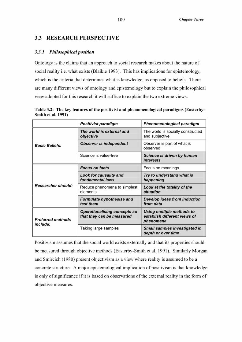
Chapter Three

109

3.3 RESEARCH PERSPECTIVE

3.3.1 Philosophical position

Ontology is the claims that an approach to social research makes about the nature of

social reality i.e. what exists (Blaikie 1993). This has implications for epistemology,

which is the criteria that determines what is knowledge, as opposed to beliefs. There

are many different views of ontology and epistemology but to explain the philosophical

view adopted for this research it will suffice to explain the two extreme views.

Table 3.2: The key features of the positivist and phenomenological paradigms (Easterby-Smith et al. 1991)

Positivist paradigm Phenomenological paradigm

The world is external and objective

The world is socially constructed and subjective

Observer is independent Observer is part of what is observed Basic Beliefs:

Science is value-free Science is driven by human interests

Focus on facts Focus on meanings

Look for causality and fundamental laws

Try to understand what is happening

Reduce phenomena to simplest elements

Look at the totality of the situation

Researcher should:

Formulate hypothesise and test them

Develop ideas from induction from data

Operationalising concepts so that they can be measured

Using multiple methods to establish different views of phenomena Preferred methods

include: Taking large samples Small samples investigated in

depth or over time

Positivism assumes that the social world exists externally and that its properties should

be measured through objective methods (Easterby-Smith et al. 1991). Similarly Morgan

and Smircich (1980) present objectivism as a view where reality is assumed to be a

concrete structure. A major epistemological implication of positivism is that knowledge

is only of significance if it is based on observations of the external reality in the form of

objective measures.

Chapter Three

110

Phenomenology, on the other hand, assumes that reality is socially constructed and

given meaning by people (Husserl 1946). Subjectivism is a similar ontological view

where reality is a projection of human imagination (Morgan and Smircich 1980). This

view assumes that human action arises from the sense that people make of different

situations, rather than a direct response from different stimuli (Easterby-Smith et al.,

1991). Therefore in this case the task of the social scientist should not be to gather facts

and measure how often certain patterns occur (as is the approach under positivism), but

to appreciate the different constructions and meanings that people place upon the

experience.

Easterby-Smith et al. (1991) provide a useful comparison between positivism and

phenomenology with respect to: the basic beliefs of the researcher; the research

strategy; and the preferred research methods (as summarised in Table 3.2). The

paradigm assumed for this research is identified by the shaded boxes.

My own beliefs are basically positivist - not surprising when one considers my

background in engineering. My natural inclination to the positivist view undoubtedly

influenced my choice of research topics but more significantly the research focus,

strategy and methods. The main research question was ‘how is FPp applied in

manufacturing?’ One of the choices I made was to study the ‘hard’ issues such as the

manufacturing planning systems, delivery reliability and capacity utilisation - rather

than issues related to human constructs such as decision processes, personal motivations

and change management.

However, the approach to the research deviated from the pure positivist approach in a

number of aspects as illustrated in Table 3.2 where the position of this research is

indicated by the shaded boxes. In fact no fewer than six aspects commonly associated

with the phenomenological paradigm were adopted. This was largely a result of the

selection of the case-oriented approach in preference to the variable oriented approach.

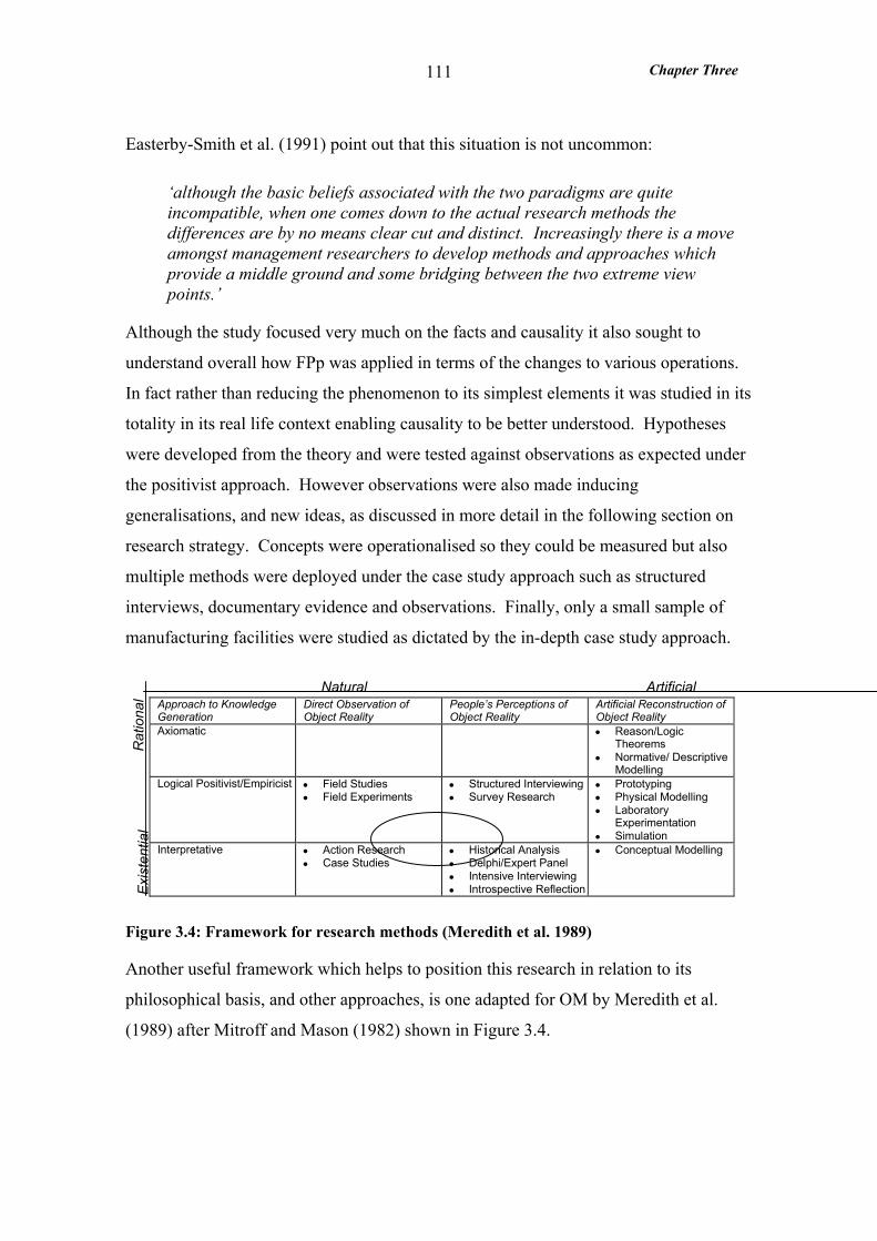
Chapter Three

111

Easterby-Smith et al. (1991) point out that this situation is not uncommon:

‘although the basic beliefs associated with the two paradigms are quite incompatible, when one comes down to the actual research methods the differences are by no means clear cut and distinct. Increasingly there is a move amongst management researchers to develop methods and approaches which provide a middle ground and some bridging between the two extreme view points.’

Although the study focused very much on the facts and causality it also sought to

understand overall how FPp was applied in terms of the changes to various operations.

In fact rather than reducing the phenomenon to its simplest elements it was studied in its

totality in its real life context enabling causality to be better understood. Hypotheses

were developed from the theory and were tested against observations as expected under

the positivist approach. However observations were also made inducing

generalisations, and new ideas, as discussed in more detail in the following section on

research strategy. Concepts were operationalised so they could be measured but also

multiple methods were deployed under the case study approach such as structured

interviews, documentary evidence and observations. Finally, only a small sample of

manufacturing facilities were studied as dictated by the in-depth case study approach.

Approach to KnowledgeGeneration

Direct Observation ofObject Reality

People’s Perceptions ofObject Reality

Artificial Reconstruction ofObject Reality

Axiomatic • Reason/LogicTheorems

• Normative/ DescriptiveModelling

Logical Positivist/Empiricist • Field Studies• Field Experiments

• Structured Interviewing• Survey Research

• Prototyping• Physical Modelling• Laboratory

Experimentation• Simulation

Interpretative • Action Research• Case Studies

• Historical Analysis• Delphi/Expert Panel• Intensive Interviewing• Introspective Reflection

• Conceptual Modelling

Exis

tent

ial

Rat

iona

l

Natural Artificial

Figure 3.4: Framework for research methods (Meredith et al. 1989)

Another useful framework which helps to position this research in relation to its

philosophical basis, and other approaches, is one adapted for OM by Meredith et al.

(1989) after Mitroff and Mason (1982) shown in Figure 3.4.

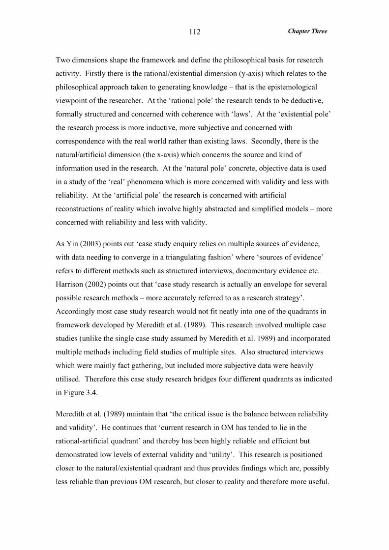
Chapter Three

112

Two dimensions shape the framework and define the philosophical basis for research

activity. Firstly there is the rational/existential dimension (y-axis) which relates to the

philosophical approach taken to generating knowledge – that is the epistemological

viewpoint of the researcher. At the ‘rational pole’ the research tends to be deductive,

formally structured and concerned with coherence with ‘laws’. At the ‘existential pole’

the research process is more inductive, more subjective and concerned with

correspondence with the real world rather than existing laws. Secondly, there is the

natural/artificial dimension (the x-axis) which concerns the source and kind of

information used in the research. At the ‘natural pole’ concrete, objective data is used

in a study of the ‘real’ phenomena which is more concerned with validity and less with

reliability. At the ‘artificial pole’ the research is concerned with artificial

reconstructions of reality which involve highly abstracted and simplified models – more

concerned with reliability and less with validity.

As Yin (2003) points out ‘case study enquiry relies on multiple sources of evidence,

with data needing to converge in a triangulating fashion’ where ‘sources of evidence’

refers to different methods such as structured interviews, documentary evidence etc.

Harrison (2002) points out that ‘case study research is actually an envelope for several

possible research methods – more accurately referred to as a research strategy’.

Accordingly most case study research would not fit neatly into one of the quadrants in

framework developed by Meredith et al. (1989). This research involved multiple case

studies (unlike the single case study assumed by Meredith et al. 1989) and incorporated

multiple methods including field studies of multiple sites. Also structured interviews

which were mainly fact gathering, but included more subjective data were heavily

utilised. Therefore this case study research bridges four different quadrants as indicated

in Figure 3.4.

Meredith et al. (1989) maintain that ‘the critical issue is the balance between reliability

and validity’. He continues that ‘current research in OM has tended to lie in the

rational-artificial quadrant’ and thereby has been highly reliable and efficient but

demonstrated low levels of external validity and ‘utility’. This research is positioned

closer to the natural/existential quadrant and thus provides findings which are, possibly

less reliable than previous OM research, but closer to reality and therefore more useful.

Chapter Three

113

3.3.2 Research Strategy

The research strategy is about how the research questions can be answered. As Blaikie

(1993) states ‘the crucial issue for the researcher is how to discover, describe, explain

and intervene in the phenomena under investigation’. Two of the best known strategies

are induction and deduction. Induction moves from observations to the development of

general hypothesise, while deduction uses general statements to explain particular

instance. It has long been debated how these two approaches relate to each other and

Blaikie (1993) asks ‘is it possible to combine these two strategies and thereby capitalise

on their strengths and minimise their weaknesses?’

Theories

Forming concepts:developing &

arranging propositions

Deducingconsequences;

making predictions

Empiricalgeneralisations Tests Hypotheses

Inducinggeneralisations:estimating populationparameters

Observations

Drawing samples& devisingmeasuringinstruments

INDUCTIVE METHODS DEDUCTIVE METHODS

THEO

RIS

ING

DO

ING

EM

PIR

ICAL

RES

EAR

CH

Figure 3.5: Combining Inductive and Deductive Strategies (Wallace 1971 quoted in Blaikie 1993)

Wallace’s (1971) cyclical approach, shown in Figure 3.5, combines inductive and

deductive methods over the ‘theorising’ and ‘doing empirical research’ activities.

Blaikie (1993) notes that although Wallace’s scheme covers inductive theorising

‘Wallace appears to have underestimated the complexity of this process which can

hardly be called inductive’. Blaikie (1993) concluded that ‘Wallace’s scheme remains

within the confines of a Positivist’ ontology which is compatible with this research

This research employed mainly a deductive strategy and an element of induction

although no inductive theorising was attempted. It is possible to begin research at any

point in the cycle and this research began with the deduction of six hypotheses from the

Chapter Three

114

theory. The concepts in the hypotheses were translated into measurement procedures

and the hypotheses were tested against new observations. The observations were far

broader than necessary to test the hypotheses and various empirical generalisations,

regarding how FPp was applied, were induced. According to Wallace’s (1971) view

these empirical generalisation are regarded as summaries of observed uniformities not

universal laws.

3.4 RIGOUR IN CASE STUDIES

Case studies have traditionally been viewed as a somewhat problematic form of enquiry

compared to other empirical methods such as surveys or experiments. A number of

concerns are put forward but the most common appears to be a lack of rigour (Yin,

2003, Hartley, 1994). Yin (2003) suggests that too many times, the case study

researcher has been sloppy and allowed equivocal evidence or biased views to influence

the direction of the findings and conclusions. Supporting this view Swamidass (1991)

states: ‘an inspection of published field-based empirical articles by OM researchers

shows that they are predominantly exploratory and use the most rudimentary form of

analysis’. However, McCutcheon and Meredith (1993) claim that misapplications of

the term ‘case study’ has also affected the reputation of the research method, for

instance in OM descriptions of implementations of new techniques are often called

‘case studies’.

A second commonly cited weakness concerns the population to which the findings can

be generalised – external validity. Conventional wisdom claims that case studies,

compared with quantitative statistical studies, are weak in their capacity to generalise to

other situations. In quantitative studies it is possible to statistically generalise from the

data by the detailed analysis of means, correlation’s and other methods (Hartley 1994)

whereas in case studies no statistical sample is taken therefore this is not possible.

However McCutcheon and Meredith (1993) claim that:

‘no empirical study offers certainty that its findings are valid for other populations. Although field studies and surveys may control for some factors and thereby better define a specific population over which results might be statistically generalised, external validity (the applicability of findings beyond the group) is still an issue for them.’

Chapter Three

115

In order that rigour in case studies can be improved it must be tested. Yin (2003)

proposes four tests to establish the quality of empirical social research:

Construct validity: establishing correct operational measures for the concepts being studied

Internal validity (for explanatory or causal studies only, and not for descriptive or exploratory studies): establishing a causal relationship, whereby certain conditions are shown to lead to other conditions, as distinguished from spurious relationships

External validity: establishing the domain to which a studies findings can be generalised

Reliability: demonstrating that the operations of a study – such as the data collection procedures can be repeated, with the same results

In this section the tactics employed to improve the validity of the FPp case studies are

explained and discussed:

• triangulation of evidence - a tactic for construct validity

• a number of with-in case and cross-case analytic strategies designed to enhance

internal validity

• case selection using replication not sampling logic - a tactic described by Yin

(2003) for external validity.

The issue of reliability in data collection is discussed in section 3.5.2 in the

operationalisation of the research design.

3.4.1 Triangulation (leading to construct validity)

Triangulation is broadly defined by Denzin (1978) as ‘the combination of

methodologies in the study of the same phenomena’. It relies on the principle that

collecting different kinds of data bearing on the same phenomena will improve the

accuracy of studies if they independently reach similar conclusions, or in other word

‘converge’. Similarly Jick (1979) claims it is largely a vehicle for cross validation

stating when two or more distinct methods are found to be congruent and yield

comparable data on a phenomenon the results are more valid.

Chapter Three

116

Denzin (1978) argues that ‘it is conventionally assumed that triangulation is the use of

multiple methods in the study of the same object……but it is only one form of the

strategy’. Denzin (1978) and Patton (1987) define four different types of triangulation

for doing evaluation, the triangulation:

1) of data sources (data triangulation)

2) among different evaluators (investigator triangulation)

3) of perspectives on the same data set (theory triangulation) and

4) of methods (methodological triangulation)

Two types of triangulation were applied in this research - methodological and data

triangulation. Denzin (1978) defined two types of methodological triangulation:

‘within-method’ and ‘between-method’. This research employs the latter ‘between-

method’ approach which Denzin (1978) argues is ‘a much more satisfactory form of

method triangulation combining dissimilar methods to measure the same unit’. He

continues that ‘ the rationale for this strategy is that the flaws of one method are often

the strengths of another; and by combining methods observers can achieve the best of

each while overcoming their unique deficiencies.’ Three methods were deployed in this

research: structured interviews, company documents and field observations. Although

it was not possible to use all three methods to collect data on all the concepts a

minimum of two methods were always used.

Data triangulation, which involves the use of different sources of data, was the second

triangulation type used in this research. Multiple informants were used wherever

possible, consequently many of the interviews were repeated with different employees.

This was always the case where questions were opinion, rather than fact, based.

Documentary evidence was often corroborated by evidence from a computer database

or management system to improve its validity.

Eisenhardt (1989) suggests that qualitative evidence is ‘words’ and quantitative

evidence ‘numbers’ and claims that this combination of data types can be highly

synergistic. Mintzberg (1979) described this synergy as follows:

Chapter Three

117

‘For while systematic data create the foundation for our theories, it is the anecdotal data that enable us to do the building. Theory building seems to require rich description, the richness that comes from anecdote. We uncover all kinds of relationships in our hard data, but it is only through the use of this soft data that we are able to explain them.’

This study involved both quantitative and qualitative evidence (according to

Eisenhardt’s 1989 definitions). The qualitative evidence was largely ‘fact-based’, and

therefore objective, rather than ‘opinion based’ and subjective. It corroborated the

quantitative evidence, provided a description of how in practical terms FPp was applied

and gave explanations for the differences in the outcome variables between the UoAs.

For example the qualitative evidence regarding the manufacturing planning and

scheduling systems often contributed to an explanation for the differences in order lead-

time, demand amplification and excess capacity. Conversely quantitative evidence was

often used to support qualitative evidence especially where it was opinion based. For

example quantitative evidence was used to support interview evidence regarding

problems encountered with the FPp applications. This combination of qualitative and

quantitative evidence in the case studies helped to triangulate the research findings

The practical considerations of applying triangulation are addressed in section 3.5.2 on

data collection.

3.4.2 Analytic Strategy (leading to internal validity)

Explanatory studies like this one, require internal validity, such that causal relationships

(as opposed to spurious relationships) are established whereby certain conditions are

shown to lead to other conditions. Accordingly two analytic strategies were applied to

this study: pattern matching (Campbell 1975) and Pettigrew’s meta-level framework

(1990 and 1992).

Yin (2003) identifies a number of tactics for internal (and external validity) and

describes pattern matching as ‘one of the most desirable strategies’. Pattern matching

involves the comparison of an empirically based pattern with a predicted one. If the

patterns coincide the results can help a case study strengthen its internal validity. In

each of the case studies reported here three units of analysis (UoA) (defined in detail in

section 3.1.4) were identified. Each UoA was based around product groups subject to

Chapter Three

118

one of three inventory management policies – MTO, FPp and MTS. The measures

relating to each of the three UoA were compared and the results compared with those

predicted by the hypotheses.

The case study research design maps onto Pettigrew’s ‘meta-level’ analytical

framework as explained in section 3.1.3 and shown in Figure 3.2. Pettigrew’s

framework enables change to be studied in different environments without theory

limitations in comparative case study research. There are three primary considerations:

context, content and outcome variables as described previously. The outcome variables

describe what it is that is being explained. In this study they are the concepts featuring

in the hypotheses and described the different outcomes which resulted from applying

the three inventory management policies (FPp, MTO and MTS). The change content

(the interventions that comprise the change) described what had changed to apply FPp

to the original MTO and MTS environment. This provided explanations for why the

outcome variables for each UoA were different and why results sometimes deviated

from the predicted results.

The Pettigrew framework not only offered a very useful perspective on within case

comparisons but also facilitated cross-case comparisons by providing a consistent and

meaningful structure for data collection. Cross-case analysis consisted of a search for

similarities and differences between the cases (Eisenhardt 1989) in terms of context,

change content and outcome variables. Naturally the distinctions between the cases far

outweighed the commonalities. This was a feature of the research design which aimed

to compare the application of FPp in diverse contexts in order to improve the

generalisability of the findings (as discussed in the following section). However in

order to advance theories in OM it was necessary to rationalise these differences and

seek out commonalities.

As explained for each case the outcome variables were compared with the predicted

results defined in the hypotheses through a process known as pattern matching. Some

of the hypotheses were not supported by all of the cases. Ragin’s (1987) view on this is

that probabilistic relationships are not accepted in case studies and that all deviating

cases must be accounted for. He advises that where cases deviate the evidence collected

must be such that the deviation can be explained. In this study a number of deviations,

Chapter Three

119

for one particular case were explained by unusual circumstances. However other

deviations from predicted results could not be explained so easily and presented a

fundamental challenge to hypotheses – disproving the hypotheses even where only one

case deviated.

3.4.3 Case selection (leading to external validity)

To what extent are the findings from a case study generalisable beyond the immediate

cases – external validity. Yin (2003) explains - that whilst findings from a survey may

be generalisable to the population from which the sample was taken - in a case study

situation the cases are few, and not statistically sampled, therefore this approach cannot

apply. Rather than statistical generalisation, case studies rely on analytic

generalisation, where the researcher attempts to generalise a particular set of results to

some broader theory.

Case selection, much like in the development of experiments, relies on replication logic

rather than sampling logic. Here replication means that individual cases can be used for

independent corroboration of specific hypotheses (Eisenhardt 1991). As Ragin (1987)

states ‘notions of sampling and sampling distributions are less relevant to the case study

approach because it is not concerned with the relative distribution of cases with

different patterns of causes and effects.’ This is precisely why case study research

cannot accept probabilistic relationships and instead depends on all deviating cases

being accounted for (Ragin 1987). As Harrison (2002) states ‘one non-conforming case

is sufficient to challenge a theory that should encompass it!’

Ragin (1987) claims in case selection ‘more important than relative frequency is the

variety of meaningful patterns of causes and effects that exist.’ In fact Pettigrew (1990)

noted that given the limited number of studies which can usually be completed, it makes

sense to choose cases such as extreme situations and polar types. Yin (2003)

recommends that each case be carefully selected so that it either predicts similar results

(literal replication) or produces contrasting results but for predictable reasons

(theoretical replication). In this study case selection was on the basis of literal

replication since the hypotheses were predicted to be true in all cases.

Chapter Three

120

Finally Eisenhardt (1989) maintains that even in case study research:

‘the concept of a population is crucial, because the population defines the set of entities from which the research sample is to be drawn. Also selection of an appropriate population controls extraneous variation and helps to define the limits for generalising the findings’.

The above discussion describes the approach used for case selection in this research and

section 3.5.1 describes how this translated into the practical selection of cases.

3.5 OPERATIONALISATION OF THE RESEARCH DESIGN

3.5.1 Case Selection

The cases were selected from the domain of manufacturing facilities in England with

the aim of providing diverse contexts in which to study the application of FPp.

Diversity was sought in terms of the industry and the complexity of the product. As

discussed if literal replication was achieved the context diversity would increase the

analytic generalisability of the findings. The research design required that during the

study period the manufacturing facilities were applying FPp (according to the working

definition), MTO (or ETO) and MTS approaches to the manufacture of their products.

A pilot study was required to trial the research design (particularly the use of units of

analysis), to firm up the hypotheses and to develop measures or indicators for the

concepts featuring in the hypotheses. The Thomas Bolton Flexible Cable factory (TB)

in Melling (near Liverpool) was selected. This factory had been part of the BICC

Group (my previous employer) and I had worked on a manufacturing improvement

project at this factory some 3 years earlier. Naturally this was an ideal site for a pilot

study. My existing product and process knowledge, combined with my familiarity with

the personnel, enabled me to devote more effort to the design of the study itself.

An initial visit revealed that since my involvement with the factory the FPp approach

had been applied to a selection of TB’s products. What was not initially clear was that

the present day application could no longer be defined as FPp. This was very

disappointing and almost prompted me to abandon the study. However after further

investigation it was apparent that the data was available to conduct a retrospective

Chapter Three

121

study, rather than the planned real-time study. Moreover this study provided the

opportunity to examine the demise of a FPp application, which contributed greatly to

knowledge on how FPp was applied. In addition it demonstrated the robustness of the

research methodology and flexibility of the research design. It set a precedent for the

two following cases, in that they were also retrospective studies, even though these

manufacturing facilities were applying FPp at the time the study was conducted. The

research design did not change in any major way following the pilot study - it followed

the research design described in this chapter. Thus the pilot study was treated as a fully

validated case study consistent with the two subsequent studies.

Pettigrew (1990) discusses the process of selecting cases:

‘there is an intentional or design component in the process of choosing and gaining access to research sites, but the practicalities of the process are best characterised by the phrase ‘planned opportunism’.

This is an honest assessment of the approach to case selection for this research.

Identifying, and gaining access to, manufacturing facilities in England that were

applying FPp, MTO and MTS to significant proportions of their manufacturing proved

to be quite a challenge.

At the time of case selection (the year 2001) the application of postponement had been

observed as a growing trend in manufacturing and distribution by various surveys

(CLM 1995, Ahlstrom and Westbrook 1999). However specific companies - or indeed

industry sectors - applying FPp were not identified. Therefore from a study of

anecdotal articles, past winners of the UK Best Factory Award (Cranfield School of

Management) and various Cranfield academic’s industrial contacts a number of

companies were identified that were supposed to be applying FPp. Unfortunately

further investigation revealed that either:

• the company had ceased to apply FPp,

• the application could not be defined as FPp according to my working definition,

• the company was too small to sustain a study, or

• the timing was wrong for a study.

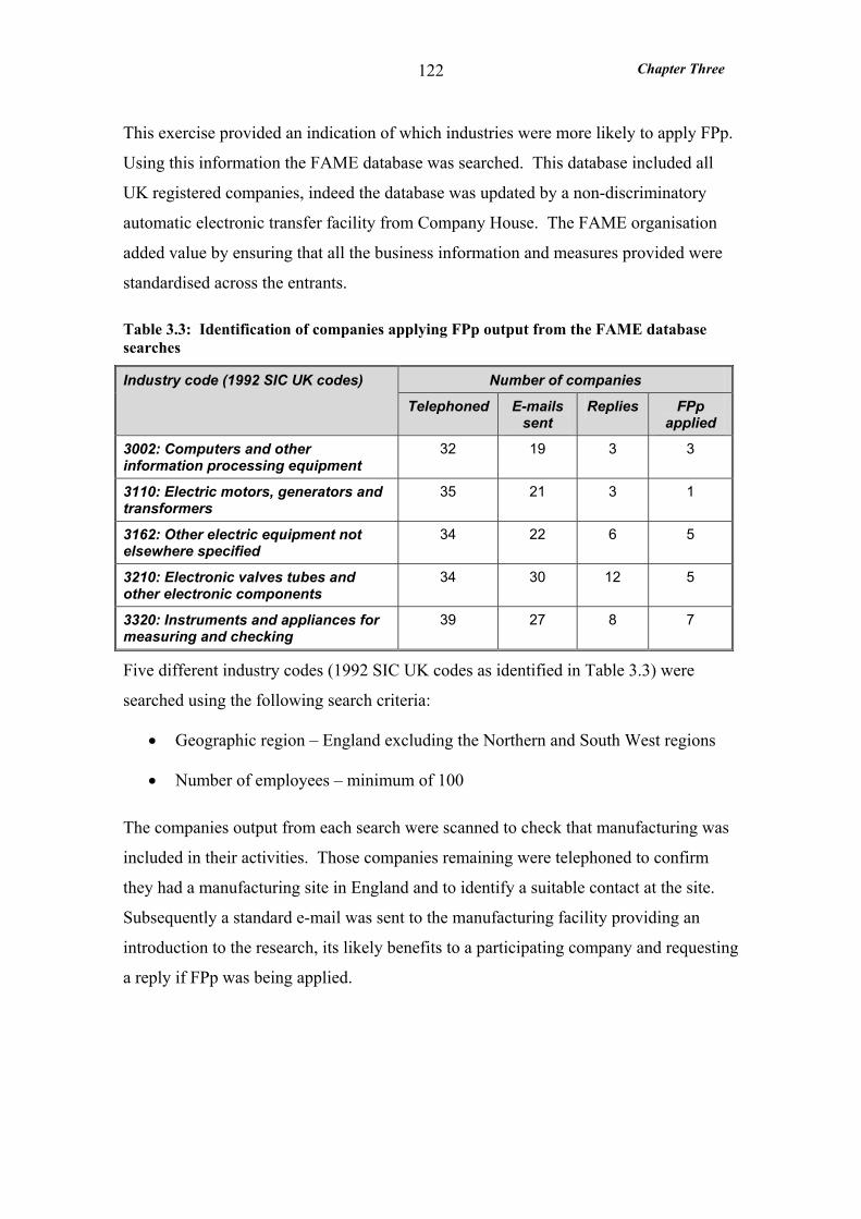
Chapter Three

122

This exercise provided an indication of which industries were more likely to apply FPp.

Using this information the FAME database was searched. This database included all

UK registered companies, indeed the database was updated by a non-discriminatory

automatic electronic transfer facility from Company House. The FAME organisation

added value by ensuring that all the business information and measures provided were

standardised across the entrants.

Table 3.3: Identification of companies applying FPp output from the FAME database searches

Number of companies Industry code (1992 SIC UK codes)

Telephoned E-mails sent

Replies FPp applied

3002: Computers and other information processing equipment

32 19 3 3

3110: Electric motors, generators and transformers

35 21 3 1

3162: Other electric equipment not elsewhere specified

34 22 6 5

3210: Electronic valves tubes and other electronic components

34 30 12 5

3320: Instruments and appliances for measuring and checking

39 27 8 7

Five different industry codes (1992 SIC UK codes as identified in Table 3.3) were

searched using the following search criteria:

• Geographic region – England excluding the Northern and South West regions

• Number of employees – minimum of 100

The companies output from each search were scanned to check that manufacturing was

included in their activities. Those companies remaining were telephoned to confirm

they had a manufacturing site in England and to identify a suitable contact at the site.

Subsequently a standard e-mail was sent to the manufacturing facility providing an

introduction to the research, its likely benefits to a participating company and requesting

a reply if FPp was being applied.

Chapter Three

123

A surprisingly high number of replies were received and many of them claimed to be

applying FPp as Table 3.3 shows. Unfortunately in many of the cases where FPp was

‘found’:

• it was applied to an insignificant proportion of production,

• MTO nor MTS were applied,

• it was applied intermittently, or

• the company was not interested in participating in the study.

Finally after a number of factory visits Brook Crompton, an electric motor manufacturer

and Dewhurst, a manufacturer of control systems were found to satisfy all the criteria

and agreed to be studied.

3.5.2 Data Collection

All three studies were conducted retrospectively as explained when defining the UoA

(section 3.1.4). Most of the data related to a time period within the 18 month period

previous to the commencement of the case study. This raised questions regarding

reliability of the data. Interview data was required to converge with documentary or

database evidence in a triangulating fashion (as described in section 3.4.1). Fortunately,

in all three case studies, all the informants were not only still employed at the factory,

but in the same roles as for the study period. Therefore all the informants had first hand

experience and knowledge of the time period in question. Further the high availability

of historic data meant that the retrospective nature of the studies did not harm the

completeness of the studies as discussed in further detail within each case study chapter

under ‘data collection’.

The data to be collected for this research fell into the three categories in Pettigrew’s

(1990) meta-level framework (as explained in section 3.1.3) context, change content and

outcome variables. The data was largely factual although some opinion based data was

sought. The ‘context’ data was largely qualitative and related to the manufacturing

facility and the FPp application itself. This data included opinion based data regarding

the motivation for applying FPp. The ‘change content’ data included the operational

changes made to apply FPp in the MTO and MTS environment. This included the more

Chapter Three

124

opinion based evidence regarding product selection for FPp and problems encountered

in applying FPp. Finally the outcome variable data was number based and consisted of

a wide range of measures which gauged the outcome of applying FPp.

The initial phase of data collection consisted of interviews (displayed in Appendix 2)

with all managers and some other personnel involved with the business processes within

the scope of the case studies (indicated in Figure 3.3). Commonly 30 interviews were

required with 15 different informants. The interviews were designed to collect the

contextual and change content data. In addition they identified other sources of

evidence, such as documents, archives and databases which corroborated the interview

data and provided further numbers based evidence (indicating the outcome variables).

An interview approach was selected which was appropriate for the nature of the

evidence collected. Yin (2003) describes three different types of interviews:

• first is open-ended in which key respondents are asked for facts and opinions

about events.

• second is a focussed interview in which the respondent is interviewed for a

short period of time normally using a predefined set of questions. These may

still be open ended and assume a conversational manner.

• third type of interview is that required for a survey where respondents are

required to fill in a questionnaire. This can either be administered by an

interviewer or via a postal survey.

The open-ended interview was not appropriate for this research since it largely involved

the collection of factual data. On the other hand many of the concepts were sufficiently

complex, and open to misinterpretation, that a postal questionnaire was not a reliable

data collection method. The most appropriate interview approach appeared to be

somewhere between a focussed interview and an administered survey. The interviews

were highly structured like a survey but also include some open-ended questions such

as ‘what were the problems experienced with FPp?’ - the answers to which were

normally followed by further questioning.

Chapter Three

125

The interviews involved some concepts that were likely to be unfamiliar to the

respondents and others which were complex and open to misinterpretation. To avoid

misunderstanding of such concepts (which leads to misinterpretation of the questions)

care was taken to ensure that the interviewees had a common and accurate

understanding. The glossary in Appendix 1 was at hand throughout the interviews to

ensure that the interviewees understood the concepts as intended.

The interviewees were selected on the basis of their knowledge of the processes within

the UoA, as illustrated by the fishbone diagram in Figure 3.3. Generally, corroboration

between informants was sought when one of the following situations arose:

• the interviewee’s knowledge of the subject matter was insufficient, normally

not detailed enough

• the data being collected was more subjective or opinion-based

In the former further informants were interviewed until the data was complete. In the

latter case all employees that had sufficient knowledge to give a valid response were

interviewed. In addition the interviewees were asked to check the interview transcript.

All interviews were taped to ensure that no information was missed and to free the

interviewer to concentrate on the interview. Subsequently the interviews were

transcribed and compiled whilst not losing the identity of the informants.

3.6 LIMITATIONS OF THE RESEARCH DESIGN

No research design is without its limitations. In selecting the multiple case design the

study found ‘why FPp is applied’ and thereby excluded a consideration of why FPp was

not applied at all in many manufacturing facilities. Other limitations relating to the

case orientated approach, such as generalisability, have already been dealt with in

section 3.4.

Past research in OM has been largely non-field based and variable oriented. Case based

research on the other hand has been criticised for being ‘predominantly exploratory and

use the most rudimentary form of analysis’. This is not a result of limitations in the

case based approach rather a result of relatively weak case study research design in the

Chapter Three

126

OM discipline. This study aims to apply the case study approach to provide explanatory

findings using a rigorous research design employing sound data gathering techniques

and analytical strategies.

The case studies were designed to be broad-based and in-depth taking around five

months for data collection and analysis. They involved about thirty interviews with

around fifteen different informants to gather the qualitative data and identify sources for

the quantitative data. Given the expansive nature of the studies, and the use of three

UoAs in each study totalling nine mini case studies, it was decided that three case

studies would be sufficient. Only a few case studies were required because case

selection, much like in the development of experiments, relies on replication logic

rather than sampling logic (as discussed in section 3.4.3). Here replication means that

individual cases can be used for independent corroboration of specific hypotheses

(Eisenhardt, 1991). In practice 3 cases proved to be sufficient as by the third and final

study theoretical saturation was reached indicated by recurring themes previously found

in one of the earlier studies.

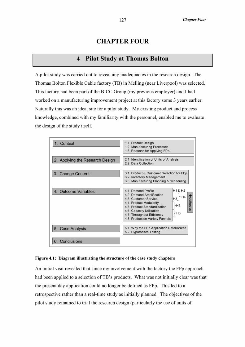
Chapter Four

127

CHAPTER FOUR

4 Pilot Study at Thomas Bolton

A pilot study was carried out to reveal any inadequacies in the research design. The

Thomas Bolton Flexible Cable factory (TB) in Melling (near Liverpool) was selected.

This factory had been part of the BICC Group (my previous employer) and I had

worked on a manufacturing improvement project at this factory some 3 years earlier.

Naturally this was an ideal site for a pilot study. My existing product and process

knowledge, combined with my familiarity with the personnel, enabled me to evaluate

the design of the study itself.

1. Context

2. Applying the Research Design

4. Outcome Variables

5. Case Analysis

6. Conclusions

1.1 Product Design1.2 Manufacturing Processes1.3 Reasons for Applying FPp

2.1 Identification of Units of Analysis2.2 Data Collection

4.1 Demand Profile4.2 Demand Amplification4.3 Customer Service4.4 Product Modularity4.5 Product Standardisation4.6 Capacity Utilisation4.7 Throughput Efficiency4.8 Production Variety Funnels

5.1 Why the FPp Application Deteriorated5.2 Hypotheses Testing

Hypotheses

H1 & H2

H3 H4

H5

H6

3. Change Content 3.1 Product & Customer Selection for FPp3.2 Inventory Management3.3 Manufacturing Planning & Scheduling

Figure 4.1: Diagram illustrating the structure of the case study chapters

An initial visit revealed that since my involvement with the factory the FPp approach

had been applied to a selection of TB’s products. What was not initially clear was that

the present day application could no longer be defined as FPp. This led to a

retrospective rather than a real-time study as initially planned. The objectives of the

pilot study remained to trial the research design (particularly the use of units of

Chapter Four

128

analysis), to firm up the hypotheses and to develop measures or indicators for the

concepts featuring in the hypotheses.

In common with the other case study chapters this is structured according to the

diagram in Figure 4.1. The contextual features relating to FPp are presented in the first

part which includes descriptions of the products subject to FPp, the manufacturing

processes used to make them and the reasons for applying FPp. The key aspects of how

the research design was applied in this specific study are described in the second part.

The ‘change content’ when FPp was applied in a previously MTO and MTS

environment is described in the third section. This includes selection of products and

customers for FPp, changes to inventory management and manufacturing planning. In

the fourth section the ‘outcome variables’, which are the quantitative concepts tested in

the hypotheses, are presented. The case analysis is presented in the fifth section which

includes an evaluation of the major flaws in the FPp application and testing of the

hypotheses against the findings. The chapter closes with conclusions from the study.

4.1 CONTEXT

TB designed, manufactured and supplied flexible cables for transmission of information

and energy. However, the bulk of cable was low voltage flexible energy cables. TB

had a turnover of around £18 million and employed 124 people - 55% of whom were

direct manufacturing labour. The financial performance of the factory in 1999 (the year

studied) was poor with no profit to report.

The Melling cable factory had been in operation for over 50 years and had been part of

the BICC Group - a large multinational corporation supplying cables world-wide.

However, in July 1998 the Melling factory was sold to the Thomas Bolton Group, a

small group of diverse factories, which was in stark contrast to the large well-

established multinational BICC group. The impact on the TB management was

dramatic.

The Group Operations Director together with other senior managers believed that the

major impact was on cash management. In BICC the main concern was profit (cash

flow to a lesser extent) due to the huge resource provided by the BICC Group.

Chapter Four

129

However, in Thomas Bolton Group Ltd cash flow was critical as the Group Operations

Director commented, ‘if we run out of cash one month we won’t be able to pay our

suppliers who will cut off supply’. The cash flow issue focussed attention on the

working capital employed by inventory particularly finished inventory, which was the

most valuable. This was the major impetus for the application of FPp.

TB’s largest customer was Volex Powercords (VP), a supplier of power leads situated

within an hour’s drive of TB. VP accounted for 22% of sales in 1999 - 35% if sales to

VP’s overseas sites in Asia and Mexico were included. Clearly TB was heavily

dependent on this business and it was to this supply that they initially applied FPp in

November 1998. At this time the dependence was mutual as the recent cable industry

restructure had reduced VP’s cable suppliers to TB and one other. Further, TB was

VP’s preferred supplier and in 1997 accounted for 85% of VP’s cable supply. VP’s

dependence on TB was compounded by the fact that VP’s manufacturing was limited to

cable cutting and adding plugs. Consequently cable supply was a very high proportion

of incoming materials.

TB’s long-term plans were to expand the FPp application to other customers and

products when the VP supply was established. However, as this case study details, a

number of problems created a barrier to this expansion and culminated in the demise of

the FPp application after 9 months.

4.1.1 Product Design

The cable group studied was described as a ‘3183Y1.00’ cable which was circular

shaped with 3 cores (refer to Appendix 3 for a cross sectional diagram). Each core was

made up of a copper conductor (cross sectional area 1mm2 ) which was insulated with

PVC to a thickness suitable for ordinary voltage. The three cores were twisted together

to make a ‘laid-up’ cable and then extrusion coated with a PVC sheath. Finally the

cable was packed, which sometimes involved rewinding the cable onto despatch reels

and loading onto pallets.

Variety in the finished cable was generated from variations in the PVC sheathing

compound, winding reel and other packaging materials. The application of FPp

involved making the standardised laid-up cable to stock and postponing the extrusion of

Chapter Four

130

the sheath coating (and subsequent packing processes) until receipt of a customer order.

The sheathing compound was available in 100 different colours and around 10 PVC

types. The reels onto which the cable was wound for despatch were either ‘direct

wound’ reels or despatch reels. The ‘direct wound’ reels were standardised metal reels

and (as the name suggests) were designed to be wound with cable directly from the

sheath extruder. The despatch reel was available in a range of materials, cardboard,

plywood or steel and in many different sizes to accommodate different cable lengths.

4.1.2 Manufacturing Processes

The process of cable making could be described as ‘a semi-continuous process’ in that

length - as opposed to discrete parts - is processed. Cable length could be an additional

variable at each stage of the manufacturing process. At TB cable length was

standardised at each process. However cable length remained a variable at the finished

product stage where the customer specified a certain reel length.

The flow process chart in Table 4.1 shows the processes required to make the cables

studied. Copper rod was drawn into multi-end wire which was subsequently bunched

(twisted together) to form the conductor. The conductor was extruded with a layer of

PVC to make the cores – each of a different colour. Then the cores were laid up

(twisted together) to give the laid up cable - the generic stock for the FPp approach.

Finally the cable was extruded with a final layer of PVC called the sheath. Cable that

was ‘direct wound’ (DW) was wound directly onto a despatch reel from the sheath

extruder thereby eliminating the rewinding process. This applied to all the cables in the

FPp UoA and all but eight cables in the MTO and MTS UoAs.

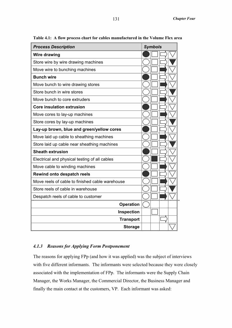
Chapter Four

131

Table 4.1: A flow process chart for cables manufactured in the Volume Flex area

Process Description Symbols

Wire drawing

Store wire by wire drawing machines

Move wire to bunching machines

Bunch wire

Move bunch to wire drawing stores

Store bunch in wire stores

Move bunch to core extruders

Core insulation extrusion

Move cores to lay-up machines

Store cores by lay-up machines

Lay-up brown, blue and green/yellow cores

Move laid up cable to sheathing machines

Store laid up cable near sheathing machines

Sheath extrusion

Electrical and physical testing of all cables

Move cable to winding machines

Rewind onto despatch reels

Move reels of cable to finished cable warehouse

Store reels of cable in warehouse

Despatch reels of cable to customer

Operation

Inspection

Transport

Storage

4.1.3 Reasons for Applying Form Postponement

The reasons for applying FPp (and how it was applied) was the subject of interviews

with five different informants. The informants were selected because they were closely

associated with the implementation of FPp. The informants were the Supply Chain

Manager, the Works Manager, the Commercial Director, the Business Manager and

finally the main contact at the customers, VP. Each informant was asked:

Chapter Four

132

Why was FPp applied - what were the drivers?

The initiative to apply FPp came from TB who applied it to selected cables for VP. The

main reason for its application (quoted by all interviewees including the VP

representative) was to increase responsiveness of cable supply. It was envisaged that

this would enable finished stocks at TB to be reduced by improving the match between

TB cable supply and VP demand. The Supply Chain Manager described the original

vision:

‘the Thomas Bolton factory was to become so responsive that the end of Thomas Bolton production line would be the start of Volex’s production line’.

Matching TB’s cable supply to VP’s demand was not easy, in part because demand was

extremely variable. This was exacerbated by the fact that TB was one of only two cable

suppliers to VP. The other supplier was Ericsson in Sweden who due to its remoteness

and inherent lack of responsiveness was only awarded 15% of VP’s business.

Moreover as admitted by the VP representative:

‘the orders placed with Ericsson were firm monthly orders whilst TB absorbed the variability in demand’

The VP representative described the problems with the cable supply from TB:

‘in the past the supply of cables [MTO] from Thomas Bolton had led to either ‘feast’ [excessive stock] or ‘famine’ [insufficient stock] of different cables.’

Within the three-week order lead-time the trend in demand for a given cable could

reverse. While the stocks of a cable were being ramped down the demand could

increase leading to chronic shortages.

The VP representative described the impact on VP of applying FPp to the manufacture

of the cables:

‘it brought the ordering horizon in from next month to next week so cable stocks at TB could be controlled with more certainty - less reliant on sales forecasts and more reliant on our [VP] customer’s orders.’

The TB Supply Chain Manager claimed the application of FPp was driven by increased

competition for the VP business and the need to reduce cable stocks. First consider the

Chapter Four

133

competitive issue. VP (including Asia and Mexico) was TB’s biggest customer and

accounted for 35% by volume of sales so it was imperative that their custom was

retained. European overseas cable manufacturers were planning to set up a cable

warehouse in the UK so, as the Supply Chain Manager commented:

‘FPp was Thomas Bolton’s answer to that threat, making it very difficult for the competing overseas cable suppliers to offer the same responsiveness’.

With regards to finished stock cash flow had become critical when the Melling factory

was bought by a small company (Thomas Bolton). As a result there was intense

pressure to reduce the working capital employed by finished inventory.

Summary: the reason for applying FPp according to both TB and VP was to increase

responsiveness so that the TB cable supply more closely matched VP’s demand for

cable. However the two companies were driven by different motives. VP on the one

hand wanted to avoid the ‘feast and famine’ supply associated with MTO. TB on the

other hand wanted to fight off competition for the VP business and at the same time

reduce the very high levels of finished stock they held.

4.2 APPLYING THE RESEARCH DESIGN

The identification of the units of analysis and the various issues concerned with data

collection at TB are addressed in this section.

4.2.1 Identification of Units of Analysis

In TB there were two main manufacturing areas:

• one which had the capability to produce the full range of cables and

manufactured the low volume, specialised cables, and

• the ‘Volume Flex’ area, which had limited capability but manufactured the high

volume products, including almost all the cables supplied to VP.

Both these areas were supplied by copper conductors from the ‘Conductor Forming’

area and cable produced in them was sometimes rewound onto despatch reels in the

‘Winding’ area.

Chapter Four

134

All the products subjected to FPp were manufactured exclusively in the Volume Flex

area. Here cables were made according to a number of inventory management policies.

As a result the study was confined to the Volume Flex area. The Conductor Forming

area was scoped out of the study since the copper wire was drawn speculatively (to a

common stock for all cables) regardless of inventory management policy. However, the

Winding area was scoped into the study, because rewinding the cables onto smaller

reels was a manufacturing process - commonly performed to customer order - but

sometimes speculatively.

Each UoA was based around a product family subject to a particular inventory

management policy (FPp, MTO/ETO, and MTS) and the respective customer orders due

for delivery within a certain time frame. Considering the time frame dimension first.

FPp was initially applied in November 1998 and customer order records showed that the

approach was properly established by the beginning of January 1999. The chronology

of changes to the FPp application (Appendix 4) shows that by mid-September 1999 the

order lead-time had been extended, such that it could no longer be defined as FPp.

Accordingly the time period for the study was limited to between 1st January and 1st

September 1999.

During the first week in June 1999 there was a factory shutdown and the new integrated

business system went ‘live’. The new system caused major disruption particularly to

records such as customer orders. Further, the finished stock records for cables subject

to FPp (Appendix 3) show that stock levels were generally higher in the second half,

than the first half, of 1999. Consequently the period from 1st January to 31st May 1999

was studied.

Identifying the appropriate product families for each UoA was not easy, because no one

product family was exclusively manufactured according to one inventory management

policy (as Table 4.2 illustrates). Inventory management policies at TB were normally

dictated by the customer, rather than set by product. The MTS approach was split

between make-to-dedicated stock and make-to-speculative stock. However, during the

study period the make-to-speculative-stock approach only accounted for about 4% of

the volume manufactured in the Volume Flex area - an insufficient volume for a UoA.

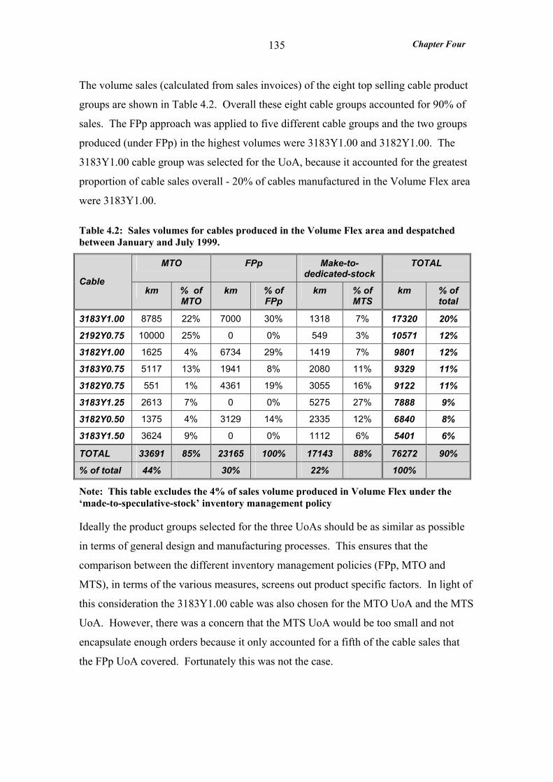
Chapter Four

135

The volume sales (calculated from sales invoices) of the eight top selling cable product

groups are shown in Table 4.2. Overall these eight cable groups accounted for 90% of

sales. The FPp approach was applied to five different cable groups and the two groups

produced (under FPp) in the highest volumes were 3183Y1.00 and 3182Y1.00. The

3183Y1.00 cable group was selected for the UoA, because it accounted for the greatest

proportion of cable sales overall - 20% of cables manufactured in the Volume Flex area

were 3183Y1.00.

Table 4.2: Sales volumes for cables produced in the Volume Flex area and despatched between January and July 1999.

MTO FPp Make-to-dedicated-stock

TOTAL

Cable km % of

MTO km % of

FPp km % of

MTS km % of

total

3183Y1.00 8785 22% 7000 30% 1318 7% 17320 20%

2192Y0.75 10000 25% 0 0% 549 3% 10571 12%

3182Y1.00 1625 4% 6734 29% 1419 7% 9801 12%

3183Y0.75 5117 13% 1941 8% 2080 11% 9329 11%

3182Y0.75 551 1% 4361 19% 3055 16% 9122 11%

3183Y1.25 2613 7% 0 0% 5275 27% 7888 9%

3182Y0.50 1375 4% 3129 14% 2335 12% 6840 8%

3183Y1.50 3624 9% 0 0% 1112 6% 5401 6%

TOTAL 33691 85% 23165 100% 17143 88% 76272 90%

% of total 44% 30% 22% 100%

Note: This table excludes the 4% of sales volume produced in Volume Flex under the ‘made-to-speculative-stock’ inventory management policy

Ideally the product groups selected for the three UoAs should be as similar as possible

in terms of general design and manufacturing processes. This ensures that the

comparison between the different inventory management policies (FPp, MTO and

MTS), in terms of the various measures, screens out product specific factors. In light of

this consideration the 3183Y1.00 cable was also chosen for the MTO UoA and the MTS

UoA. However, there was a concern that the MTS UoA would be too small and not

encapsulate enough orders because it only accounted for a fifth of the cable sales that

the FPp UoA covered. Fortunately this was not the case.

Chapter Four

136

To conclude the finished product items to be included in each UoA were those

31813Y1.00 cables due for delivery between 1st January and 31st May 1999 (as listed in

Appendix 5). Comparing FPp with the MTO approach for cables supplied to VP is a

‘before and after’ type comparison because, prior to the application of FPp, all VP

orders were MTO.

Before leaving the identification of the UoA it is useful to view them in terms of the

customers they involved. The top eleven customers, by sales value, are shown in

Appendix 6 and seven of these were included in the UoA.


This was a retrospective study where the majority of the data collected applied to the

period between 1st January and 31st May 1999 - about 18 months before the study was

conducted (July to October 2000). This raised questions regarding the reliability of the

data. Interview data required support from documentary evidence, and fortunately all

the interviewees were not only still employed at the factory but in the same roles as for

the study period. This meant that all the informants had first hand experience and

knowledge of the time period in question.

A particularly pertinent archival document was a report written by the Supply Chain

Manager at the time of the initial implementation of FPp. It described the application of

FPp in detail and substantiated much of the interview evidence regarding inventory

management and manufacturing planning and scheduling procedures.

Unfortunately just after the study period, 1st June 1999, the new integrated business

system went ‘live’ and the old business system (including the OMAC MRP system) was

rendered obsolete and inaccessible. This meant that electronic data on customer order

processing was unavailable and instead the study relied on the availability of hard

copies of customer orders and call offs. Generally this documentary evidence was

available. However some customer orders were missing as detailed in section 4.4.

A particularly fruitful source of evidence for the performance measures was the

Production Monitoring and Control System (PMCS), which allowed the sequencing and

allocation of jobs onto individual machines and monitored their progress through the

Chapter Four

137

factory. PMCS covered all processes within the study scope and provided the

production schedules and shipping records necessary to measure demand amplification,

order lead-time and delivery reliability. With regards to reliability the data retrieved

from PMCS was no less reliable (or accessible) during the study than when it was

generated.

The retrospective nature of the study did have some drawbacks. It was not possible to

measure demand amplification, ex-stock availability and throughput efficiency for the

MTS UoA. Conversely the retrospective approach offered benefits. During the study

period a manufacturing database measuring Overall Equipment Effectiveness (a

measure of capacity utilisation) was maintained. This database fell into disuse the year

after and therefore would not have been available for a real time study. A further

benefit of the retrospective study was the opportunity to examine the deterioration of a

FPp application.

Overall the reliability and completeness of the data were only marginally affected by the

retrospective nature of the study.

4.3 CHANGE CONTENT

In this section the changes required to apply FPp in a MTS and MTO environment are

described including: product and customer selection, inventory management and

manufacturing planning and scheduling changes.

4.3.1 Product and Customer Selection for Form Postponement

In common with ‘the reasons for applying FPp’, how products and customers were

selected for FPp was the subject of interviews with five different informants (previously

listed in section 4.1.3). The two questions asked of all informants, and their collective

answers, are presented below:

Was the FPp approach limited to certain customer, and if so why?

TB limited the application of FPp to cables supplied to VP because of problems

adapting the existing production scheduling system to support FPp (refer to section

4.3.3 for a detailed discussion).

Chapter Four

138

The first problem was the control of the generic cable stock levels. This was critical - a

shortage in these stocks would almost certainly have resulted in a late delivery. No

Kanban system or forecasting package was used to control the stock levels. The

Scheduling Manager simply anticipated laid up cable requirements based on his view of

laid up cable consumption or gut feeling. It was ‘not scientific’. This was difficult

enough for one customer and it was felt it would be impossible for more than one.

The second problem concerned the limitation of the scheduling system to weekly time

buckets rather than daily, as required for FPp. This necessitated the use of a very

simple manual planning board for scheduling FPp customer orders through the

postponed sheathing process. The expectation was that this planning board would prove

inadequate for the task of scheduling multiple customers and a larger, more complex,

planning board would be required.

Was the FPp approach limited to certain product specifications, and if so

why?

The finished cables subject to FPp were largely selected by VP on the basis of the

volume they consumed. Those used at the highest rates - categorised as ‘runners’ - were

selected.

When TB first approached VP about FPp TB were supplying about 50 different finished

cables to VP. The VP representative split these cables into three categories ‘runners’,

‘repeaters’ and ‘strangers’ according to the volume (average weekly useage) and

frequency of useage at VP (daily, weekly etc).

• runners were the high volume cables that were used by VP daily

• repeaters were used weekly

• strangers were only occasionally used and were generally cables required for a

specific VP customer.

Data used by VP to conduct this analysis was unavailable. However the report

describing the application of FPp (written by the Supply Chain Manager) provided

some relevant sales data for the year prior to the FPp implementation. This data showed

Chapter Four

139

that four out of five of the cable groups selected for FPp were in the top six selling

cables of 1997, which accounted for 85% by volume of the 1997 sales.

In general the cables classed as ‘runners’ were selected for manufacture under the FPp

approach. Cables were categorised by VP according to useage at finished cable level

not at cable group (or the generic) level. For a given generic cable, some finished cable

variants were therefore subjected to FPp whilst others, with only a different sheath

colour, were supplied under the MTO approach.

Given the improved responsiveness why was FPp only applied to ‘runners’, why not

‘repeaters’ and ‘strangers’ that used the same generic cable? The answer lay in the

supply of the sheathing compound used in the postponed process. For all cables subject

to FPp the sheathing compound was required on consignment stock. This involved the

supplier maintaining a stock of compound specifically for TB such that it was available

within 24 hours. TB purchased upon consumption, however a consignment stock was

not without risk for TB as they were committed to purchase it within a certain time

period. As a consequence where cables were not categorised as ‘runners’ the risk of

obsolescence (or the supplier refusing to provide a consignment stock) was high hence

TB did not offer FPp. Exceptionally the white cable subject to FPp was not categorised

as a ‘runner’. However, the white sheathing compound was already available on

consignment stock.

4.3.2 Inventory management

Inventory management encompassed order processing and the subsequent control of

stocks, including laid-up cables and finished cables. Also considered in this section -

and inherent in the inventory management approach - is the Customer Order

Decoupling Point (CODP) location.

Evidence for inventory management was gathered from interviews with the Commercial

Director, Sales Manager, Supply Chain Manager and the two Customer Service

Assistants dealing with the respective customers. The key features of the three

inventory management policies studied are presented in Table 4.3.

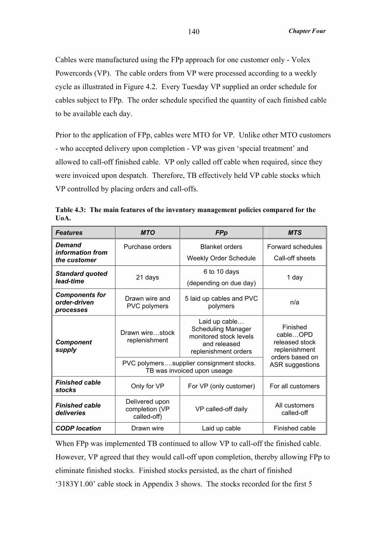
Chapter Four

140

Cables were manufactured using the FPp approach for one customer only - Volex

Powercords (VP). The cable orders from VP were processed according to a weekly

cycle as illustrated in Figure 4.2. Every Tuesday VP supplied an order schedule for

cables subject to FPp. The order schedule specified the quantity of each finished cable

to be available each day.

Prior to the application of FPp, cables were MTO for VP. Unlike other MTO customers

- who accepted delivery upon completion - VP was given ‘special treatment’ and

allowed to call-off finished cable. VP only called off cable when required, since they

were invoiced upon despatch. Therefore, TB effectively held VP cable stocks which

VP controlled by placing orders and call-offs.

Table 4.3: The main features of the inventory management policies compared for the UoA.

Features MTO FPp MTS

Demand information from the customer

Purchase orders

Blanket orders

Weekly Order Schedule

Forward schedules

Call-off sheets

Standard quoted lead-time 21 days

6 to 10 days

(depending on due day) 1 day

Components for order-driven processes

Drawn wire and PVC polymers

5 laid up cables and PVC polymers n/a

Drawn wire…stock replenishment

Laid up cable… Scheduling Manager

monitored stock levels and released

replenishment orders Component supply

PVC polymers….supplier consignment stocks. TB was invoiced upon useage

Finished cable…OPD

released stock replenishment

orders based on ASR suggestions

Finished cable stocks Only for VP For VP (only customer) For all customers

Finished cable deliveries

Delivered upon completion (VP

called-off) VP called-off daily All customers

called-off

CODP location Drawn wire Laid up cable Finished cable

When FPp was implemented TB continued to allow VP to call-off the finished cable.

However, VP agreed that they would call-off upon completion, thereby allowing FPp to

eliminate finished stocks. Finished stocks persisted, as the chart of finished

‘3183Y1.00’ cable stock in Appendix 3 shows. The stocks recorded for the first 5

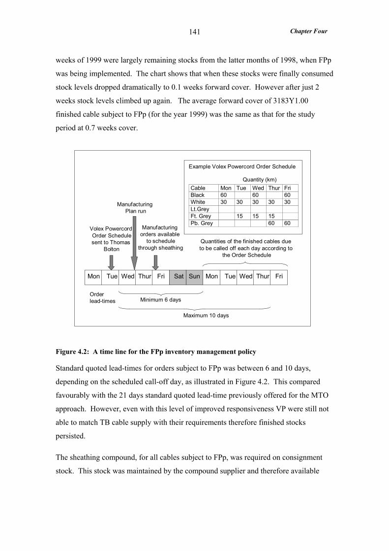
Chapter Four

141

weeks of 1999 were largely remaining stocks from the latter months of 1998, when FPp

was being implemented. The chart shows that when these stocks were finally consumed

stock levels dropped dramatically to 0.1 weeks forward cover. However after just 2

weeks stock levels climbed up again. The average forward cover of 3183Y1.00

finished cable subject to FPp (for the year 1999) was the same as that for the study

period at 0.7 weeks cover.

Cable Mon Tue Wed Thur FriBlack 60 60 60White 30 30 30 30 30Lt.GreyFt. Grey 15 15 15Pb. Grey 60 60

Mon Tue Wed Thur Fri Sat Sun Mon Tue Wed Thur Fri

Volex PowercordOrder Schedulesent to Thomas

Bolton

Manufacturing Plan run

Manufacturing orders available

to schedulethrough sheathing

Quantities of the finished cables due to be called off each day according to

the Order Schedule

Minimum 6 days

Maximum 10 days

Orderlead-times

Quantity (km)

Example Volex Powercord Order Schedule

Figure 4.2: A time line for the FPp inventory management policy

Standard quoted lead-times for orders subject to FPp was between 6 and 10 days,

depending on the scheduled call-off day, as illustrated in Figure 4.2. This compared

favourably with the 21 days standard quoted lead-time previously offered for the MTO

approach. However, even with this level of improved responsiveness VP were still not

able to match TB cable supply with their requirements therefore finished stocks

persisted.

The sheathing compound, for all cables subject to FPp, was required on consignment

stock. This stock was maintained by the compound supplier and therefore available

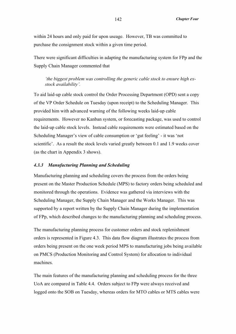
Chapter Four

142

within 24 hours and only paid for upon useage. However, TB was committed to

purchase the consignment stock within a given time period.

There were significant difficulties in adapting the manufacturing system for FPp and the

Supply Chain Manager commented that

‘the biggest problem was controlling the generic cable stock to ensure high ex-stock availability’.

To aid laid-up cable stock control the Order Processing Department (OPD) sent a copy

of the VP Order Schedule on Tuesday (upon receipt) to the Scheduling Manager. This

provided him with advanced warning of the following weeks laid-up cable

requirements. However no Kanban system, or forecasting package, was used to control

the laid-up cable stock levels. Instead cable requirements were estimated based on the

Scheduling Manager’s view of cable consumption or ‘gut feeling’ - it was ‘not

scientific’. As a result the stock levels varied greatly between 0.1 and 1.9 weeks cover

(as the chart in Appendix 3 shows).


Manufacturing planning and scheduling covers the process from the orders being

present on the Master Production Schedule (MPS) to factory orders being scheduled and

monitored through the operations. Evidence was gathered via interviews with the

Scheduling Manager, the Supply Chain Manager and the Works Manager. This was

supported by a report written by the Supply Chain Manager during the implementation

of FPp, which described changes to the manufacturing planning and scheduling process.

The manufacturing planning process for customer orders and stock replenishment

orders is represented in Figure 4.3. This data flow diagram illustrates the process from

orders being present on the one week period MPS to manufacturing jobs being available

on PMCS (Production Monitoring and Control System) for allocation to individual

machines.

The main features of the manufacturing planning and scheduling process for the three

UoA are compared in Table 4.4. Orders subject to FPp were always received and

logged onto the SOB on Tuesday, whereas orders for MTO cables or MTS cables were

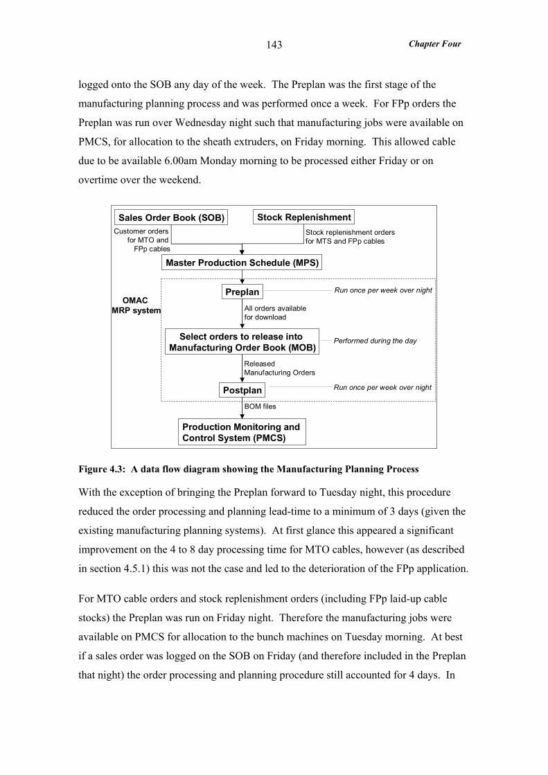
Chapter Four

143

logged onto the SOB any day of the week. The Preplan was the first stage of the

manufacturing planning process and was performed once a week. For FPp orders the

Preplan was run over Wednesday night such that manufacturing jobs were available on

PMCS, for allocation to the sheath extruders, on Friday morning. This allowed cable

due to be available 6.00am Monday morning to be processed either Friday or on

overtime over the weekend.

Sales Order Book (SOB)

Preplan

Select orders to release into Manufacturing Order Book (MOB)

Postplan

Production Monitoring and Control System (PMCS)

Customer orders for MTO and

FPp cables

All orders available for download

Released Manufacturing Orders

BOM files

Run once per week over night

Run once per week over night

Performed during the day

OMAC MRP system

Stock ReplenishmentStock replenishment orders for MTS and FPp cables

Master Production Schedule (MPS)

Figure 4.3: A data flow diagram showing the Manufacturing Planning Process

With the exception of bringing the Preplan forward to Tuesday night, this procedure

reduced the order processing and planning lead-time to a minimum of 3 days (given the

existing manufacturing planning systems). At first glance this appeared a significant

improvement on the 4 to 8 day processing time for MTO cables, however (as described

in section 4.5.1) this was not the case and led to the deterioration of the FPp application.

For MTO cable orders and stock replenishment orders (including FPp laid-up cable

stocks) the Preplan was run on Friday night. Therefore the manufacturing jobs were

available on PMCS for allocation to the bunch machines on Tuesday morning. At best

if a sales order was logged on the SOB on Friday (and therefore included in the Preplan

that night) the order processing and planning procedure still accounted for 4 days. In

Chapter Four

144

the worst case where orders were received on the Monday the procedure accounted for 8

days.

Table 4.4: Main features of manufacturing planning compared for MTO and FPp.

Features Stock

Replenishment Orders

MTO FPp

Manufacturing Orders Processed by MRP system driven by one week period MPS

Customer Orders entered onto SOB n/a Anytime during the

week Tuesday morning

Preplan run once each week Friday night Wednesday night

Manufacturing orders released onto PMCS Tuesday morning Friday morning

Duration of manufacturing planning process

84 hours over 4 nights (due to weekend)

36 hours over 2 nights

Order processing and manufacturing planning lead-time

n/a

4 to 8 days (depending on day of week order was

received)

3 days (excludes possible waiting time of 6 days)

Once manufacturing jobs were available on PMCS the Scheduling Manager batched

similar jobs together to minimise changeovers. Batching was very pronounced at the

bunching process. However it reduced with increases in variety and at the sheathing

process was minimal (refer to Appendix 3 for batching procedures).

There were significant difficulties adapting the production scheduling process for FPp.

These difficulties limited the application of FPp to one customer as described in section

4.3.1. Controlling the laid-up cable stock (as described in the previous section) was one

problem and the limitation of the manufacturing planning system to due weeks, rather

than due days, was another. This was a procedural, rather than software, limitation

attributable to the weekly time buckets used in the MRP system. The implications for

the FPp application were two-fold:

• Firstly, the Scheduling manager did not know the daily due dates (only the due

weeks) from PMCS. Therefore OPD was required to send a copy of the VP Order

Schedule upon receipt. This procedure had the added benefit of by-passing the

lengthy manufacturing planning process, and providing the Scheduling Manager

with advance warning of the following weeks requirements.

Chapter Four

145

• Secondly, scheduling orders through the postponed sheathing process was not

possible using PMCS alone. A very simple manual planning board was also used.

4.4 OUTCOME VARIABLES

The measures taken will be presented and compared for the three UoAs over the

following eight sub-sections. The first section presents the demand profile measures,

demand volume, mix and variability. In the second section the demand amplification

plots are discussed. The customer service measures including ex-stock availability,

order lead-time and delivery reliability are analysed in the third section. The fourth and

fifth sections address product modularity and standardisation. Capacity utilisation

measures and throughput efficiency measures are presented in the next two sections and

finally the production variety funnels are compared.

4.4.1 Demand Profile

Evidence for the three demand measures was gathered from archived customer order

and call off documents. It was important for measuring demand variability (and

amplification) that the demand placed on the manufacturing system by both domestic,

and export, orders was measured in the same time frame. Therefore the ex-works due

date was taken as the delivery due date for all orders with the proviso that for export

there was a transit time (refer to Appendix 7 for a detailed explanation).

To check that the archived customer order evidence was complete all factory orders for

the UoA were identified on PMCS. It was found that all archived customer order

documents were available for the FPp UoA however for the MTO UoA 21 out of the

total of 79 customer order documents were missing. Fortunately the factory order due

dates into despatch were known from PMCS and were generally the Saturday before the

ex-works due week. Therefore it was possible to estimate the ex-works due date for the

missing orders as detailed in Appendix 7.

About half the archived customer call-off documents, for the MTS UoA, were missing.

However, the actual ex-works dates for these call-offs were available on PMCS.

Further, comparison with existing call-off records revealed that these dates were

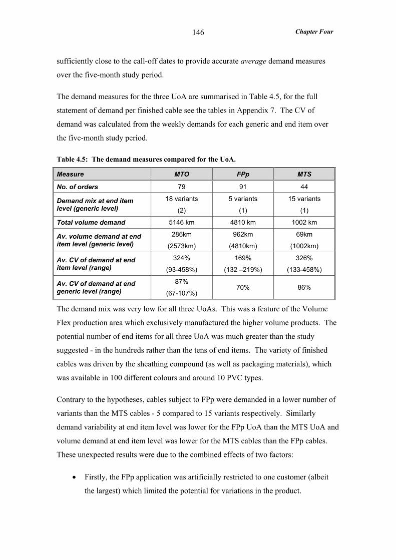
Chapter Four

146

sufficiently close to the call-off dates to provide accurate average demand measures

over the five-month study period.

The demand measures for the three UoA are summarised in Table 4.5, for the full

statement of demand per finished cable see the tables in Appendix 7. The CV of

demand was calculated from the weekly demands for each generic and end item over

the five-month study period.

Table 4.5: The demand measures compared for the UoA.

Measure MTO FPp MTS

No. of orders 79 91 44

Demand mix at end item level (generic level)

18 variants

(2)

5 variants

(1)

15 variants

(1)

Total volume demand 5146 km 4810 km 1002 km

Av. volume demand at end item level (generic level)

286km

(2573km)

962km

(4810km)

69km

(1002km)

Av. CV of demand at end item level (range)

324%

(93-458%)

169%

(132 –219%)

326%

(133-458%)

Av. CV of demand at end generic level (range)

87%

(67-107%) 70% 86%

The demand mix was very low for all three UoAs. This was a feature of the Volume

Flex production area which exclusively manufactured the higher volume products. The

potential number of end items for all three UoA was much greater than the study

suggested - in the hundreds rather than the tens of end items. The variety of finished

cables was driven by the sheathing compound (as well as packaging materials), which

was available in 100 different colours and around 10 PVC types.

Contrary to the hypotheses, cables subject to FPp were demanded in a lower number of

variants than the MTS cables - 5 compared to 15 variants respectively. Similarly

demand variability at end item level was lower for the FPp UoA than the MTS UoA and

volume demand at end item level was lower for the MTS cables than the FPp cables.

These unexpected results were due to the combined effects of two factors:

• Firstly, the FPp application was artificially restricted to one customer (albeit

the largest) which limited the potential for variations in the product.

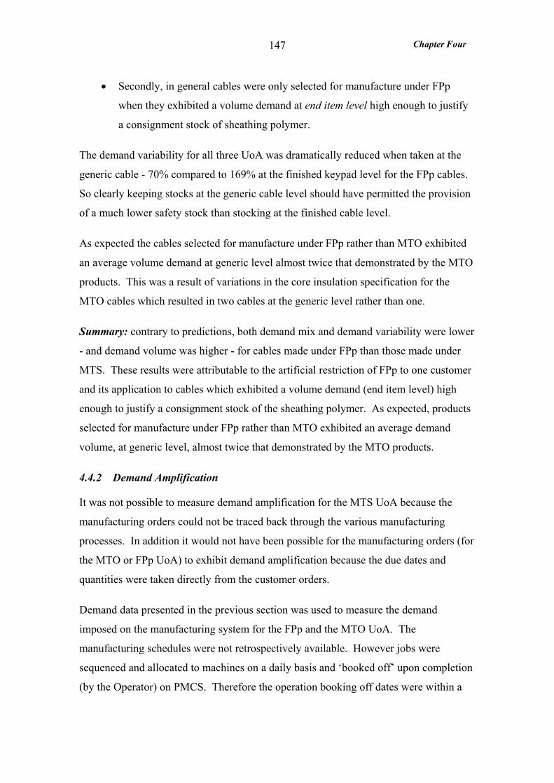
Chapter Four

147

• Secondly, in general cables were only selected for manufacture under FPp

when they exhibited a volume demand at end item level high enough to justify

a consignment stock of sheathing polymer.

The demand variability for all three UoA was dramatically reduced when taken at the

generic cable - 70% compared to 169% at the finished keypad level for the FPp cables.

So clearly keeping stocks at the generic cable level should have permitted the provision

of a much lower safety stock than stocking at the finished cable level.

As expected the cables selected for manufacture under FPp rather than MTO exhibited

an average volume demand at generic level almost twice that demonstrated by the MTO

products. This was a result of variations in the core insulation specification for the

MTO cables which resulted in two cables at the generic level rather than one.

Summary: contrary to predictions, both demand mix and demand variability were lower

- and demand volume was higher - for cables made under FPp than those made under

MTS. These results were attributable to the artificial restriction of FPp to one customer

and its application to cables which exhibited a volume demand (end item level) high

enough to justify a consignment stock of the sheathing polymer. As expected, products

selected for manufacture under FPp rather than MTO exhibited an average demand

volume, at generic level, almost twice that demonstrated by the MTO products.

4.4.2 Demand Amplification

It was not possible to measure demand amplification for the MTS UoA because the

manufacturing orders could not be traced back through the various manufacturing

processes. In addition it would not have been possible for the manufacturing orders (for

the MTO or FPp UoA) to exhibit demand amplification because the due dates and

quantities were taken directly from the customer orders.

Demand data presented in the previous section was used to measure the demand

imposed on the manufacturing system for the FPp and the MTO UoA. The

manufacturing schedules were not retrospectively available. However jobs were

sequenced and allocated to machines on a daily basis and ‘booked off’ upon completion

(by the Operator) on PMCS. Therefore the operation booking off dates were within a

Chapter Four

148

day or two of the scheduled output dates and accurately represented the scheduled

sequence of jobs at each process. This revealed the level to which similar jobs were

‘batched’ together - important to show demand amplification.

Figure 4.4: Demand amplification measured at a daily level for the FPp UoA

The demand amplification charts for the FPp and MTO UoA are shown in Appendix 8.

The plots in each chart span the same weekly time buckets and use the same scale so the

relative amplitude of demand can be easily compared. Each chart shows the weekly

demand for the cables and the process schedules for sheathing, laying up and core

extrusion (in equivalent finished cable length).

Demand amplification was not evident in the charts for either the FPp or MTO UoA

when measured at a weekly level. The peaks in demand were of a similar amplitude to

the peaks in each of the process schedules. In fact the pattern of demand was quite

accurately reflected in the process schedules particularly at laying up and core

extrusion.

Daily Demand

0

20

40

60

80

100

120

140

04/01

/99

06/01

/99

08/01

/99

10/01

/99

12/01

/99

14/01

/99

16/01

/99

18/01

/99

20/01

/99

22/01

/99

24/01

/99

26/01

/99

28/01

/99

Day Due

Qua

ntity

Due

(km

)

Daily Laying Up Schedule

0

20

40

60

80

100

120

140

04/01

/99

06/01

/99

08/01

/99

10/01

/99

12/01

/99

14/01

/99

16/01

/99

18/01

/99

20/01

/99

22/01

/99

24/01

/99

26/01

/99

28/01

/99

Day dueQ

uani

tty

due

(km

)

Daily Sheathing Schedule

0

20

40

60

80

100

120

140

04/01

/99

06/01

/99

08/01

/99

10/01

/99

12/01

/99

14/01

/99

16/01

/99

18/01

/99

20/01

/99

22/01

/99

24/01

/99

26/01

/99

28/01

/99

Day Due

Qua

ntity

Due

(km

)

Daily Core Extruding Schedule

0

20

40

60

80

100

120

140

04/01

/99

06/01

/99

08/01

/99

10/01

/99

12/01

/99

14/01

/99

16/01

/99

18/01

/99

20/01

/99

22/01

/99

24/01

/99

26/01

/99

28/01

/99

Day Due

Qua

ntity

due

(km

)

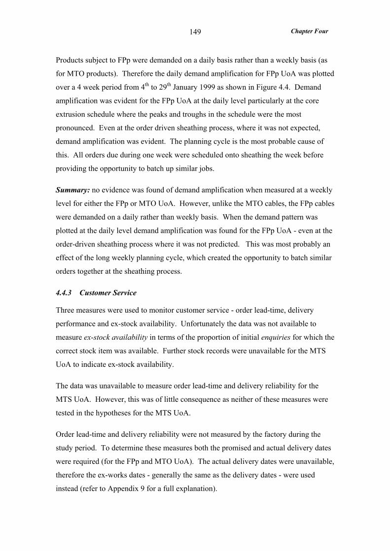
Chapter Four

149

Products subject to FPp were demanded on a daily basis rather than a weekly basis (as

for MTO products). Therefore the daily demand amplification for FPp UoA was plotted

over a 4 week period from 4th to 29th January 1999 as shown in Figure 4.4. Demand

amplification was evident for the FPp UoA at the daily level particularly at the core

extrusion schedule where the peaks and troughs in the schedule were the most

pronounced. Even at the order driven sheathing process, where it was not expected,

demand amplification was evident. The planning cycle is the most probable cause of

this. All orders due during one week were scheduled onto sheathing the week before

providing the opportunity to batch up similar jobs.

Summary: no evidence was found of demand amplification when measured at a weekly

level for either the FPp or MTO UoA. However, unlike the MTO cables, the FPp cables

were demanded on a daily rather than weekly basis. When the demand pattern was

plotted at the daily level demand amplification was found for the FPp UoA - even at the

order-driven sheathing process where it was not predicted. This was most probably an

effect of the long weekly planning cycle, which created the opportunity to batch similar

orders together at the sheathing process.

4.4.3 Customer Service

Three measures were used to monitor customer service - order lead-time, delivery

performance and ex-stock availability. Unfortunately the data was not available to

measure ex-stock availability in terms of the proportion of initial enquiries for which the

correct stock item was available. Further stock records were unavailable for the MTS

UoA to indicate ex-stock availability.

The data was unavailable to measure order lead-time and delivery reliability for the

MTS UoA. However, this was of little consequence as neither of these measures were

tested in the hypotheses for the MTS UoA.

Order lead-time and delivery reliability were not measured by the factory during the

study period. To determine these measures both the promised and actual delivery dates

were required (for the FPp and MTO UoA). The actual delivery dates were unavailable,

therefore the ex-works dates - generally the same as the delivery dates - were used

instead (refer to Appendix 9 for a full explanation).

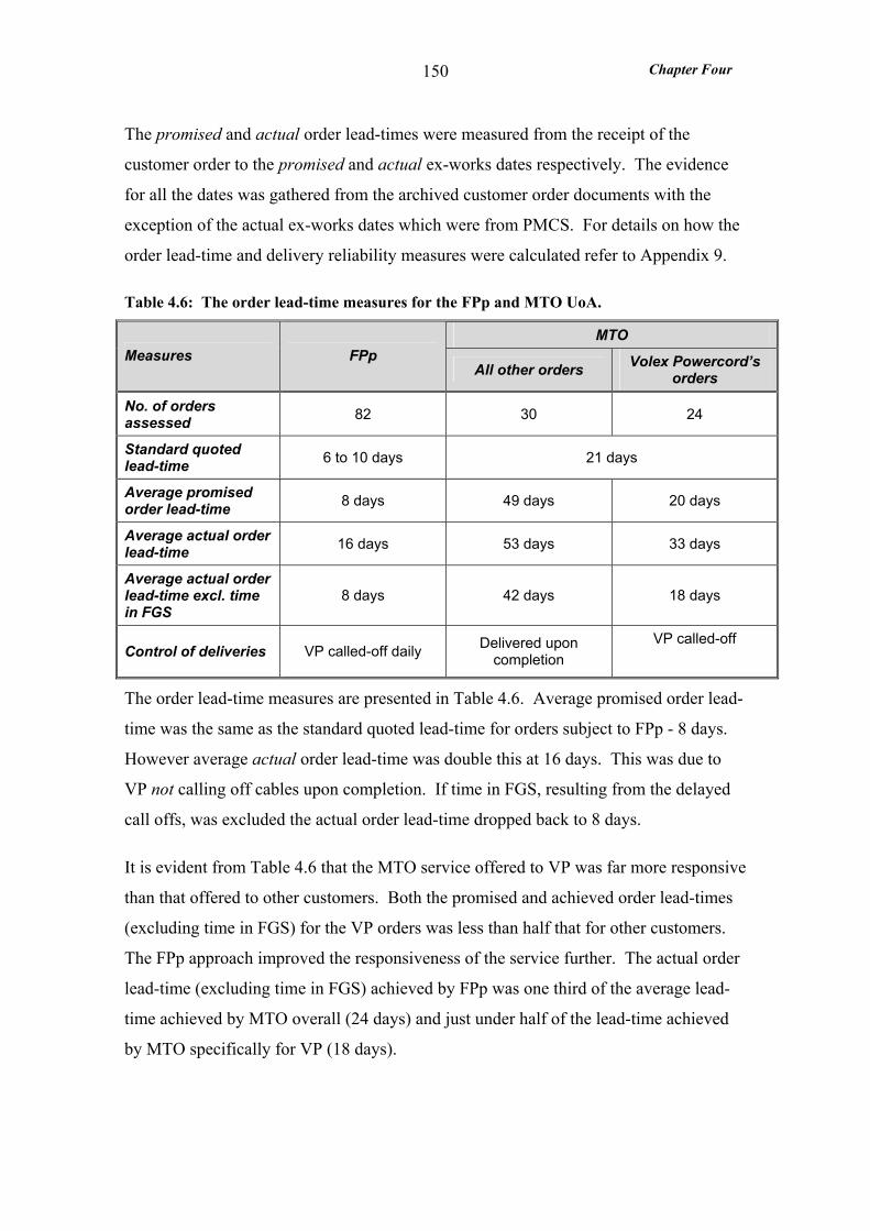
Chapter Four

150


customer order to the promised and actual ex-works dates respectively. The evidence

for all the dates was gathered from the archived customer order documents with the

exception of the actual ex-works dates which were from PMCS. For details on how the

order lead-time and delivery reliability measures were calculated refer to Appendix 9.

Table 4.6: The order lead-time measures for the FPp and MTO UoA.

MTO Measures FPp

All other orders Volex Powercord’s orders

No. of orders assessed 82 30 24

Standard quoted lead-time 6 to 10 days 21 days

Average promised order lead-time 8 days 49 days 20 days

Average actual order lead-time 16 days 53 days 33 days

Average actual order lead-time excl. time in FGS

8 days 42 days 18 days

Control of deliveries VP called-off daily Delivered upon completion

VP called-off

The order lead-time measures are presented in Table 4.6. Average promised order lead-

time was the same as the standard quoted lead-time for orders subject to FPp - 8 days.

However average actual order lead-time was double this at 16 days. This was due to

VP not calling off cables upon completion. If time in FGS, resulting from the delayed

call offs, was excluded the actual order lead-time dropped back to 8 days.

It is evident from Table 4.6 that the MTO service offered to VP was far more responsive

than that offered to other customers. Both the promised and achieved order lead-times

(excluding time in FGS) for the VP orders was less than half that for other customers.

The FPp approach improved the responsiveness of the service further. The actual order

lead-time (excluding time in FGS) achieved by FPp was one third of the average lead-

time achieved by MTO overall (24 days) and just under half of the lead-time achieved

by MTO specifically for VP (18 days).

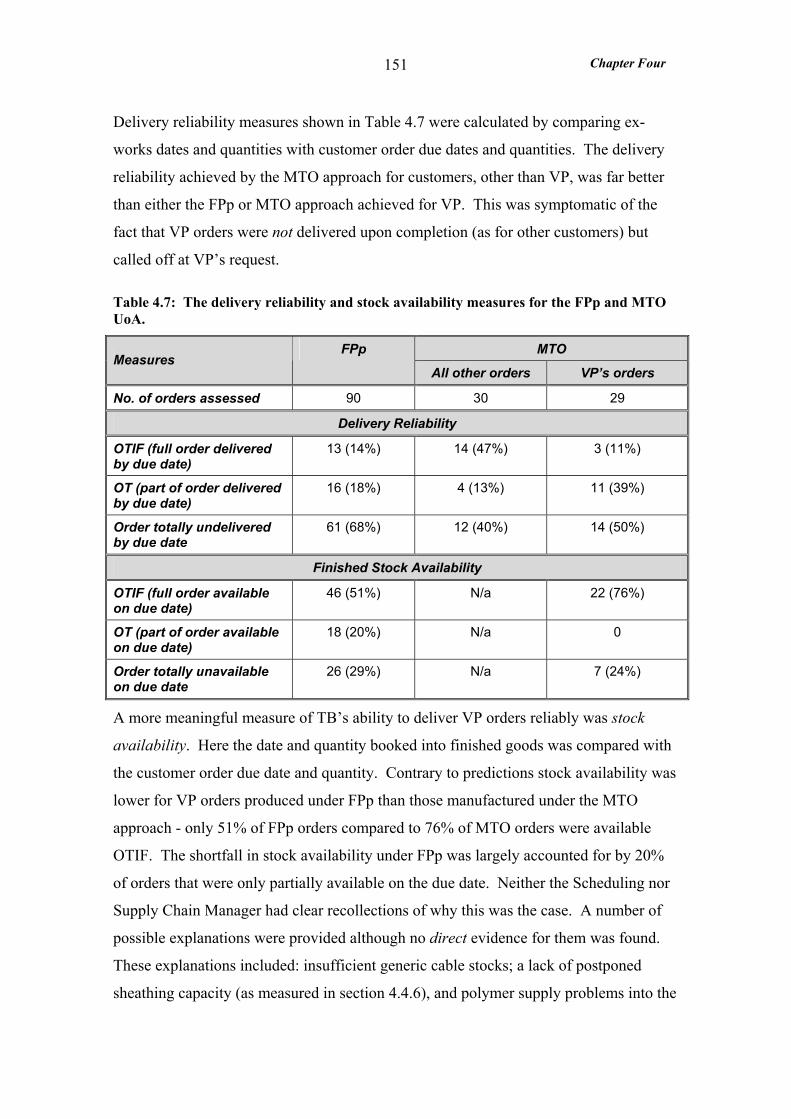
Chapter Four

151

Delivery reliability measures shown in Table 4.7 were calculated by comparing ex-

works dates and quantities with customer order due dates and quantities. The delivery

reliability achieved by the MTO approach for customers, other than VP, was far better

than either the FPp or MTO approach achieved for VP. This was symptomatic of the

fact that VP orders were not delivered upon completion (as for other customers) but

called off at VP’s request.

Table 4.7: The delivery reliability and stock availability measures for the FPp and MTO UoA.

MTO Measures

FPp

All other orders VP’s orders


Delivery Reliability

OTIF (full order delivered by due date)

13 (14%) 14 (47%) 3 (11%)

OT (part of order delivered by due date)

16 (18%) 4 (13%) 11 (39%)

Order totally undelivered by due date

61 (68%) 12 (40%) 14 (50%)

Finished Stock Availability

OTIF (full order available on due date)

46 (51%) N/a 22 (76%)

OT (part of order available on due date)

18 (20%) N/a 0

Order totally unavailable on due date

26 (29%) N/a 7 (24%)

A more meaningful measure of TB’s ability to deliver VP orders reliably was stock

availability. Here the date and quantity booked into finished goods was compared with

the customer order due date and quantity. Contrary to predictions stock availability was

lower for VP orders produced under FPp than those manufactured under the MTO

approach - only 51% of FPp orders compared to 76% of MTO orders were available

OTIF. The shortfall in stock availability under FPp was largely accounted for by 20%

of orders that were only partially available on the due date. Neither the Scheduling nor

Supply Chain Manager had clear recollections of why this was the case. A number of

possible explanations were provided although no direct evidence for them was found.

These explanations included: insufficient generic cable stocks; a lack of postponed

sheathing capacity (as measured in section 4.4.6), and polymer supply problems into the

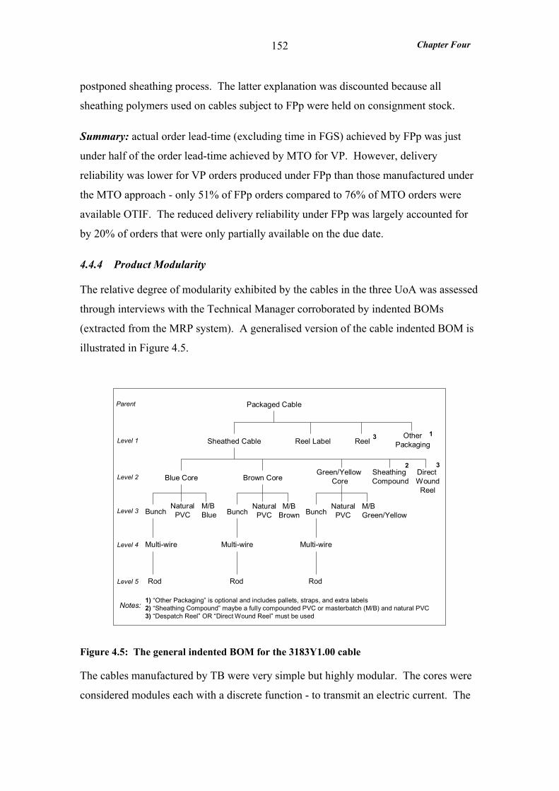
Chapter Four

152

postponed sheathing process. The latter explanation was discounted because all

sheathing polymers used on cables subject to FPp were held on consignment stock.

Summary: actual order lead-time (excluding time in FGS) achieved by FPp was just

under half of the order lead-time achieved by MTO for VP. However, delivery

reliability was lower for VP orders produced under FPp than those manufactured under

the MTO approach - only 51% of FPp orders compared to 76% of MTO orders were

available OTIF. The reduced delivery reliability under FPp was largely accounted for

by 20% of orders that were only partially available on the due date.

4.4.4 Product Modularity

The relative degree of modularity exhibited by the cables in the three UoA was assessed

through interviews with the Technical Manager corroborated by indented BOMs

(extracted from the MRP system). A generalised version of the cable indented BOM is

illustrated in Figure 4.5.

Packaged Cable

Sheathed Cable Reel Label ReelOther

Packaging

Blue Core

Parent

Level 1

Level 2

Level 3

Level 4

Level 5

Brown CoreGreen/Yellow

CoreSheathing Compound

Direct Wound

Reel

BunchNatural

PVCM/BBlue Bunch

NaturalPVC

M/BBrown Bunch

NaturalPVC

M/BGreen/Yellow

Multi-wire Multi-wire Multi-wire

Rod Rod Rod

Notes:1) “Other Packaging” is optional and includes pallets, straps, and extra labels2) “Sheathing Compound” maybe a fully compounded PVC or masterbatch (M/B) and natural PVC3) “Despatch Reel” OR “Direct Wound Reel” must be used

3

3

1

2

Figure 4.5: The general indented BOM for the 3183Y1.00 cable

The cables manufactured by TB were very simple but highly modular. The cores were

considered modules each with a discrete function - to transmit an electric current. The

Chapter Four

153

sheath also was a module with one function - to mechanically protect the cores. The

core could be split into two modules: the copper conductor (or bunch) that transmitted a

specific level of electric current; and the PVC coating which insulated the conductor to

a specified rating. Finally each of the various items of packaging, such as the reels,

fulfilled a single function

With regard to the second characteristic of modularity there was one interference

between the modules that was not critical to the function of the product. Adhesion

between the core insulation and the sheath coating was ‘positively undesirable’ since the

sheath coating must strip away easily from the cores. This unwanted interference was

rectified by the application of chalk to discourage the adhesion. Consequently it was

only occasionally a problem.

The type of modularity exhibited by the cables was ‘component swapping’ modularity

(Pine, 1993). Different components, in this case sheathing polymers, were paired with

the same basic product, a laid-up cable, to produce variety in the finished product.

Summary: not only was the entire range of cables equally modular but also highly

modular. The generic cable was modular to the same high level as the customising

components such as the sheath coating and packaging.

4.4.5 Product Standardisation

The level of product standardisation was indicated by two measures: the proportion of

components common to all variants in the UoA and the degree of commonality index.

The full indented BOMs sourced from the MRP BOM module were analysed for the

3183Y1.00 cables within each of the UoA. These BOMs had five levels. Levels 4 and

5 were excluded from the analysis because they were only concerned with the

manufacture of one conductor specification (common to all cores in all the cables under

study).

A summary of the product standardisation measures is shown in Table 4.8. The number

of components in each cable was very similar – 17 or 18. The proportion of common

components was highest for the FPp UoA. In fact only two components varied – the

polymer and pigment to make the sheath. The MTO UoA had the lowest proportion of

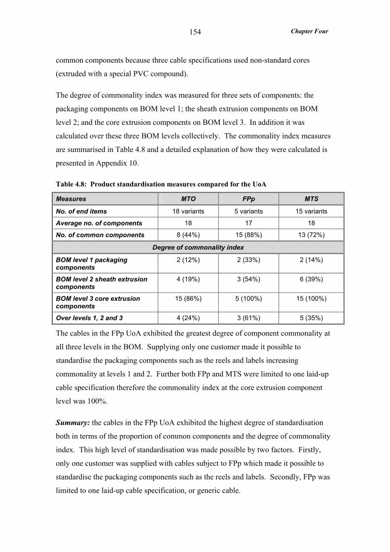
Chapter Four

154

common components because three cable specifications used non-standard cores

(extruded with a special PVC compound).

The degree of commonality index was measured for three sets of components: the

packaging components on BOM level 1; the sheath extrusion components on BOM

level 2; and the core extrusion components on BOM level 3. In addition it was

calculated over these three BOM levels collectively. The commonality index measures

are summarised in Table 4.8 and a detailed explanation of how they were calculated is

presented in Appendix 10.

Table 4.8: Product standardisation measures compared for the UoA

Measures MTO FPp MTS

No. of end items 18 variants 5 variants 15 variants

Average no. of components 18 17 18

No. of common components 8 (44%) 15 (88%) 13 (72%)


BOM level 1 packaging components

2 (12%) 2 (33%) 2 (14%)

BOM level 2 sheath extrusion components

4 (19%) 3 (54%) 6 (39%)

BOM level 3 core extrusion components

15 (86%) 5 (100%) 15 (100%)

Over levels 1, 2 and 3 4 (24%) 3 (61%) 5 (35%)

The cables in the FPp UoA exhibited the greatest degree of component commonality at

all three levels in the BOM. Supplying only one customer made it possible to

standardise the packaging components such as the reels and labels increasing

commonality at levels 1 and 2. Further both FPp and MTS were limited to one laid-up

cable specification therefore the commonality index at the core extrusion component

level was 100%.

Summary: the cables in the FPp UoA exhibited the highest degree of standardisation

both in terms of the proportion of common components and the degree of commonality

index. This high level of standardisation was made possible by two factors. Firstly,

only one customer was supplied with cables subject to FPp which made it possible to

standardise the packaging components such as the reels and labels. Secondly, FPp was

limited to one laid-up cable specification, or generic cable.

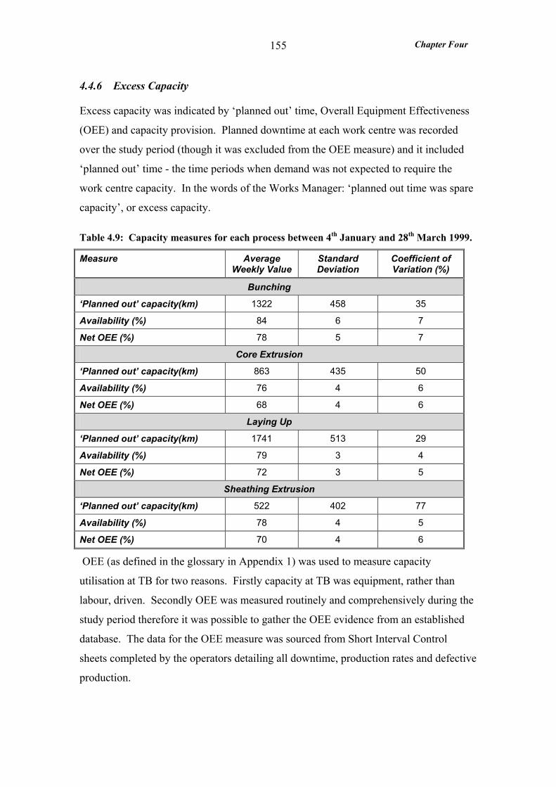
Chapter Four

155

4.4.6 Excess Capacity

Excess capacity was indicated by ‘planned out’ time, Overall Equipment Effectiveness

(OEE) and capacity provision. Planned downtime at each work centre was recorded

over the study period (though it was excluded from the OEE measure) and it included

‘planned out’ time - the time periods when demand was not expected to require the

work centre capacity. In the words of the Works Manager: ‘planned out time was spare

capacity’, or excess capacity.

Table 4.9: Capacity measures for each process between 4th January and 28th March 1999.

Measure Average Weekly Value

Standard Deviation

Coefficient of Variation (%)

Bunching

‘Planned out’ capacity(km) 1322 458 35

Availability (%) 84 6 7

Net OEE (%) 78 5 7

Core Extrusion



Net OEE (%) 68 4 6

Laying Up



Net OEE (%) 72 3 5

Sheathing Extrusion



Net OEE (%) 70 4 6

OEE (as defined in the glossary in Appendix 1) was used to measure capacity

utilisation at TB for two reasons. Firstly capacity at TB was equipment, rather than

labour, driven. Secondly OEE was measured routinely and comprehensively during the

study period therefore it was possible to gather the OEE evidence from an established

database. The data for the OEE measure was sourced from Short Interval Control

sheets completed by the operators detailing all downtime, production rates and defective

production.

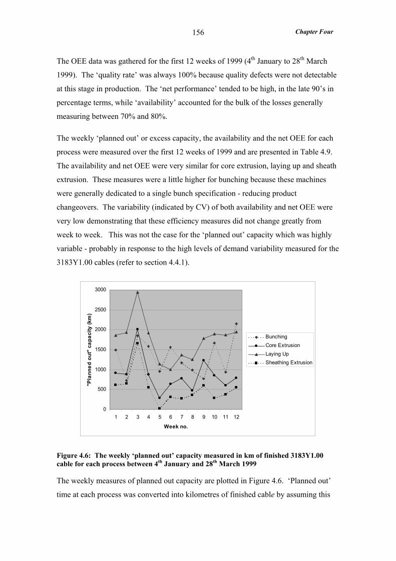
Chapter Four

156

The OEE data was gathered for the first 12 weeks of 1999 (4th January to 28th March

1999). The ‘quality rate’ was always 100% because quality defects were not detectable

at this stage in production. The ‘net performance’ tended to be high, in the late 90’s in

percentage terms, while ‘availability’ accounted for the bulk of the losses generally

measuring between 70% and 80%.

The weekly ‘planned out’ or excess capacity, the availability and the net OEE for each

process were measured over the first 12 weeks of 1999 and are presented in Table 4.9.

The availability and net OEE were very similar for core extrusion, laying up and sheath

extrusion. These measures were a little higher for bunching because these machines

were generally dedicated to a single bunch specification - reducing product

changeovers. The variability (indicated by CV) of both availability and net OEE were

very low demonstrating that these efficiency measures did not change greatly from

week to week. This was not the case for the ‘planned out’ capacity which was highly

variable - probably in response to the high levels of demand variability measured for the

3183Y1.00 cables (refer to section 4.4.1).

0

500

1000

1500

2000

2500

3000

1 2 3 4 5 6 7 8 9 10 11 12

Week no.

"Pla

nned

out

" ca

paci

ty (k

m)

BunchingCore ExtrusionLaying UpSheathing Extrusion

Figure 4.6: The weekly ‘planned out’ capacity measured in km of finished 3183Y1.00 cable for each process between 4th January and 28th March 1999

The weekly measures of planned out capacity are plotted in Figure 4.6. ‘Planned out’

time at each process was converted into kilometres of finished cable by assuming this

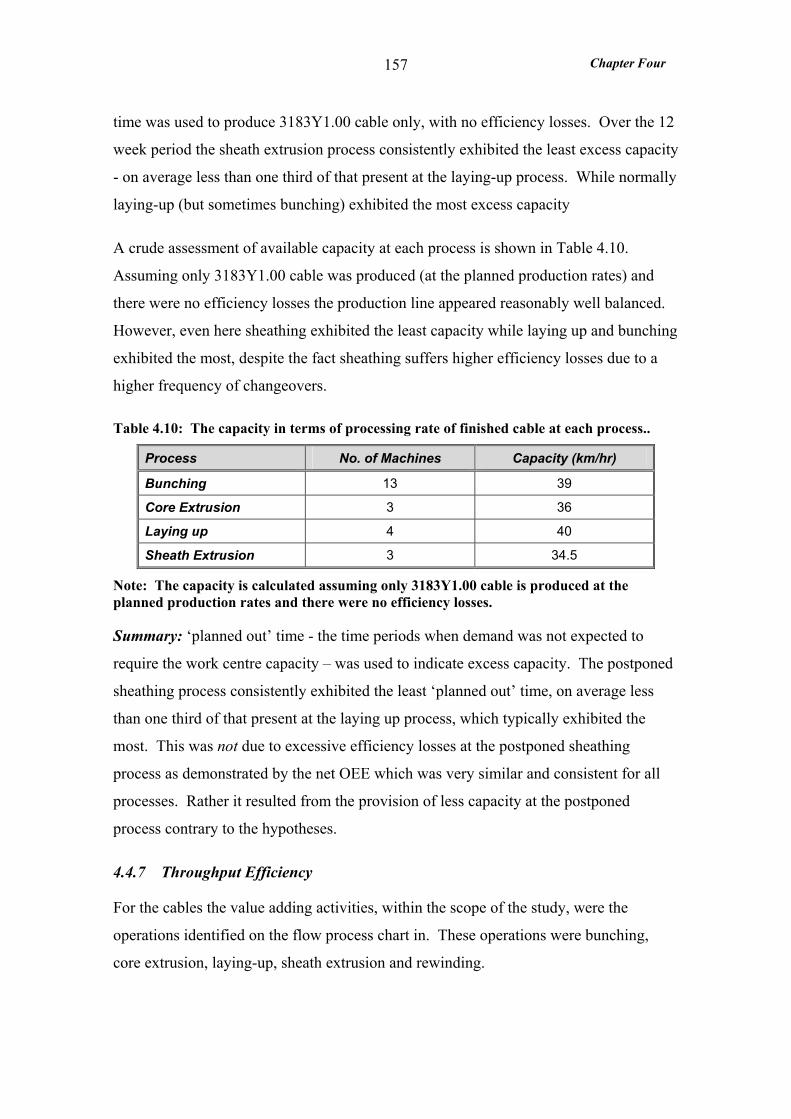
Chapter Four

157

time was used to produce 3183Y1.00 cable only, with no efficiency losses. Over the 12

week period the sheath extrusion process consistently exhibited the least excess capacity

- on average less than one third of that present at the laying-up process. While normally

laying-up (but sometimes bunching) exhibited the most excess capacity

A crude assessment of available capacity at each process is shown in Table 4.10.

Assuming only 3183Y1.00 cable was produced (at the planned production rates) and

there were no efficiency losses the production line appeared reasonably well balanced.

However, even here sheathing exhibited the least capacity while laying up and bunching

exhibited the most, despite the fact sheathing suffers higher efficiency losses due to a

higher frequency of changeovers.

Table 4.10: The capacity in terms of processing rate of finished cable at each process..

Process No. of Machines Capacity (km/hr)

Bunching 13 39

Core Extrusion 3 36

Laying up 4 40

Sheath Extrusion 3 34.5

Note: The capacity is calculated assuming only 3183Y1.00 cable is produced at the planned production rates and there were no efficiency losses.

Summary: ‘planned out’ time - the time periods when demand was not expected to

require the work centre capacity – was used to indicate excess capacity. The postponed

sheathing process consistently exhibited the least ‘planned out’ time, on average less

than one third of that present at the laying up process, which typically exhibited the

most. This was not due to excessive efficiency losses at the postponed sheathing

process as demonstrated by the net OEE which was very similar and consistent for all

processes. Rather it resulted from the provision of less capacity at the postponed

process contrary to the hypotheses.

4.4.7 Throughput Efficiency

For the cables the value adding activities, within the scope of the study, were the

operations identified on the flow process chart in. These operations were bunching,

core extrusion, laying-up, sheath extrusion and rewinding.

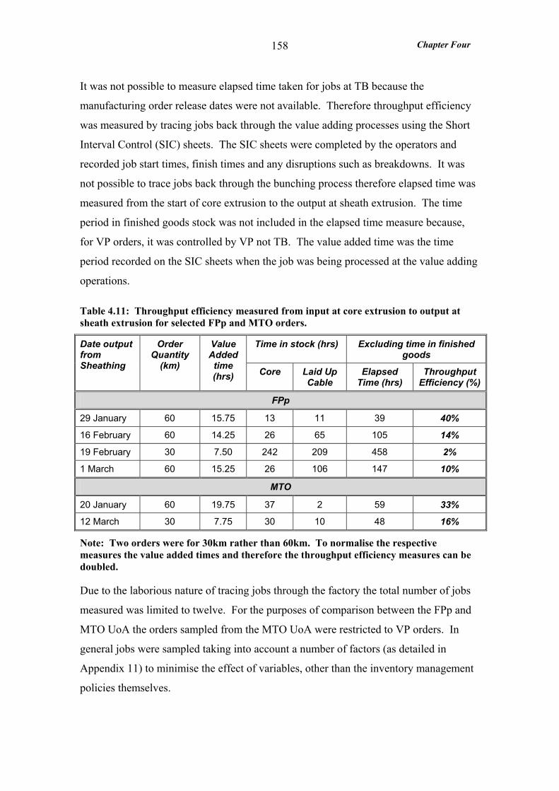
Chapter Four

158

It was not possible to measure elapsed time taken for jobs at TB because the

manufacturing order release dates were not available. Therefore throughput efficiency

was measured by tracing jobs back through the value adding processes using the Short

Interval Control (SIC) sheets. The SIC sheets were completed by the operators and

recorded job start times, finish times and any disruptions such as breakdowns. It was

not possible to trace jobs back through the bunching process therefore elapsed time was

measured from the start of core extrusion to the output at sheath extrusion. The time

period in finished goods stock was not included in the elapsed time measure because,

for VP orders, it was controlled by VP not TB. The value added time was the time

period recorded on the SIC sheets when the job was being processed at the value adding

operations.

Table 4.11: Throughput efficiency measured from input at core extrusion to output at sheath extrusion for selected FPp and MTO orders.

Time in stock (hrs) Excluding time in finished goods

Date output from Sheathing

Order Quantity

(km)

Value Added time (hrs) Core Laid Up

Cable Elapsed

Time (hrs) Throughput

Efficiency (%)

FPp

29 January 60 15.75 13 11 39 40%

16 February 60 14.25 26 65 105 14%

19 February 30 7.50 242 209 458 2%

1 March 60 15.25 26 106 147 10%

MTO

20 January 60 19.75 37 2 59 33%

12 March 30 7.75 30 10 48 16%

Note: Two orders were for 30km rather than 60km. To normalise the respective measures the value added times and therefore the throughput efficiency measures can be doubled.

Due to the laborious nature of tracing jobs through the factory the total number of jobs

measured was limited to twelve. For the purposes of comparison between the FPp and

MTO UoA the orders sampled from the MTO UoA were restricted to VP orders. In

general jobs were sampled taking into account a number of factors (as detailed in

Appendix 11) to minimise the effect of variables, other than the inventory management

policies themselves.

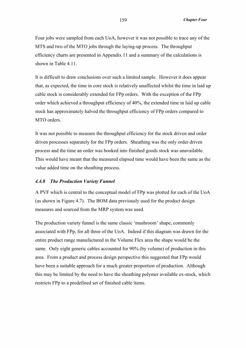
Chapter Four

159

Four jobs were sampled from each UoA, however it was not possible to trace any of the

MTS and two of the MTO jobs through the laying-up process. The throughput

efficiency charts are presented in Appendix 11 and a summary of the calculations is

shown in Table 4.11.

It is difficult to draw conclusions over such a limited sample. However it does appear

that, as expected, the time in core stock is relatively unaffected whilst the time in laid up

cable stock is considerably extended for FPp orders. With the exception of the FPp

order which achieved a throughput efficiency of 40%, the extended time in laid up cable

stock has approximately halved the throughput efficiency of FPp orders compared to

MTO orders.

It was not possible to measure the throughput efficiency for the stock driven and order

driven processes separately for the FPp orders. Sheathing was the only order driven

process and the time an order was booked into finished goods stock was unavailable.

This would have meant that the measured elapsed time would have been the same as the

value added time on the sheathing process.

4.4.8 The Production Variety Funnel

A PVF which is central to the conceptual model of FPp was plotted for each of the UoA

(as shown in Figure 4.7). The BOM data previously used for the product design

measures and sourced from the MRP system was used.

The production variety funnel is the same classic ‘mushroom’ shape, commonly

associated with FPp, for all three of the UoA. Indeed if this diagram was drawn for the

entire product range manufactured in the Volume Flex area the shape would be the

same. Only eight generic cables accounted for 90% (by volume) of production in this

area. From a product and process design perspective this suggested that FPp would

have been a suitable approach for a much greater proportion of production. Although

this may be limited by the need to have the sheathing polymer available ex-stock, which

restricts FPp to a predefined set of finished cable items.

Chapter Four

160

4Average Process Leadtime (working days)

End item

Num

ber

of p

hysi

cally

diff

eren

t ite

ms

FORM POSTPONEMENT

MTS

MTO

0 2 6 8 10

Process 1 Process 2 Postponed process

7 62

2218

25

18

6 31

8 6 5

6 31

1215

2115

Process 3

1

1

1

CODP

CODP

CODP

Figure 4.7: The production variety funnels for the three UoA

Considering the FPp application there is only one generic cable at the CODP which is

transformed into five finished cables. However, a further seven components (sheathing

polymer variants and a reel) supplied into the postponed sheathing process must be

stocked, therefore there are eight SKUs at the CODP to service only five finished items.

Moreover this is an accurate reflection of the number of finished items that are produced

given that this product is restricted to one customer.

4.5 CASE ANALYSIS

In this section the results of the case analysis are presented: first the major flaws in the

FPp application are discussed, and second the findings are compared with the

hypotheses.

4.5.1 Why the FPp Application Deteriorated

In this section the major problems experienced with the FPp application, and the

changes made to it, are presented. From this and the evidence thus far presented an

explanation of why the application deteriorated has been developed.

Chapter Four

161

A chronology of the changes to the FPp application (presented in Appendix 4) was

compiled from interview evidence and a complete set of VP Order Schedules (sent to

TB between November 1998 and the end of 1999). The interviews were with the

Supply Chain Manager, the Sales Manager, the Works Manager and the VP

representative.

Originally VP agreed to call-off orders subject to FPp, in full, upon completion -

leaving no finished stock at TB. However as the chart of finished cable stock in

Appendix 3 shows this was not the case - why? Clearly VP’s requirements changed

within the order lead-time and the VP representative explained why. The VP

Manufacturing Plan was released every Tuesday for the next week and cable orders

placed with TB to meet the plan. The Manufacturing Plan was fixed and available four

working days before commencing. Unfortunately VP deviated from the plan.

According to the VP representative:

‘it was not uncommon for around 50% of the manufacturing plan to change before implementation’.

The VP representative gave two reasons why VP deviated from plan. Firstly Production

would invariably start producing jobs early. Secondly, VP’s customers were regularly

offered 7 day order lead-times rather than the standard quoted lead-time of 14 days due

to the absence of strategic finished stocks. In either of these cases it was impossible for

TB to supply cable on a short enough lead-time to meet VP’s new requirements. For

example, taking the second case where a 7 day order lead-time was required for a VP

customer. TB’s order lead-time was between 6 and 10 days. At best VP could place the

order on Tuesday and receive it on Monday. But that only left VP with 24 hours to

produce, and deliver, the leads. Moreover the probability of it being Tuesday when the

order was placed with VP was only 20%!

The order lead-time offered by TB on the FPp cables was largely the result of two major

shortfalls in the planning system. Firstly the duration of the planning run was 36 hours

over 2 nights, which added a minimum of 2 days to the manufacturing lead time.

Secondly the frequency of the planning run was only once per week, which added a

potential 6 days of waiting time before new orders could be processed. In the worst

case this resulted in a 9 day lead-time before manufacturing could be started - 6 days

Chapter Four

162

waiting plus 3 days planning. In effect the planning lead-time for FPp orders had not

been reduced at all compared to that for MTO orders. An attempt had been made to

synchronise the TB planning system with the VP planning system. This did not take

into account the high level of changes typically made to the VP manufacturing plan

between generation and implementation.

The FPp approach allowed the order lead-time to be more than halved compared to

MTO. However this was not sufficiently responsive to enable elimination of the

finished cable stock. Indeed after 9 months (September 1999) the order lead-time was

extended by one week. The existence of high levels of finished goods stock meant it no

longer made sense to maintain a generic cable stock in order to manufacture on a short

order lead-time. The extended order lead-time meant that even the manufacture of the

generic cable was effectively customer-order-driven. This changed the FPp application

to a slightly more responsive MTO application

Conclusion: TB’s manufacturing planning system was too inflexible to support the FPp

application without the support of finished cable buffer stocks. There were two major

shortfalls in the planning system: a planning time of 2 days; and a manufacturing

planning frequency of once per week - adding a potential 6 days of waiting time before

new orders could be processed. In effect the planning lead-time for FPp orders had not

been reduced at all compared to that for MTO orders. TB’s and VP’s planning systems

were synchronised but this did not take into account VP’s high level of deviation from

their manufacturing plan.

4.5.2 Hypotheses Testing

The findings from the TB case study were not as predicted by the six hypotheses - one

hypothesis was challenged (H1) and three further hypotheses were challenged in part

(H4, H5 and H6). One hypothesis remained untested (H3) and another hypothesis was

untested in part (H6).

Chapter Four

163



Hypothesis H1 was challenged by the study findings. Both demand mix and demand

variability were lower - and volume demand was higher - for cables made under FPp

compared with those made under MTS. These unexpected findings were the result of

unusual circumstances, rather than being a fundamental challenge to the hypothesis.

There were two unusual circumstances in this case that influenced the demand profile

measures:

• Firstly, the FPp application (unlike MTS) was artificially restricted to one

customer which limited the potential for variations in the product and hence

demand mix.

• Secondly, in general, cables were only selected for manufacture under FPp when

they exhibited volume demand at end item level high enough to justify a

consignment stock of the polymer used in the postponed sheathing process.

Again this limited demand mix and increased volume demand at end item level.

As predicted by H2, the products selected for manufacture under FPp rather than MTO

exhibited an average volume demand, at generic level, almost twice that demonstrated

by the MTO cables. This was a result of variations in the MTO generic cable

specification that did not exist in the FPp generic cable.



Hypothesis H3 remains untested because it was not possible to measure ex-stock

availability for either FPp or MTS approaches.

Hypothesis H4 was fully tested but only partially supported by the findings. Demand

amplification was measured at a weekly level for FPp and MTO orders but it was not

Chapter Four

164

detected for either approach. However, cables subject to FPp were demanded on a daily

basis, rather than a weekly basis, and at this level demand amplification was detected

for the FPp orders. Unexpectedly amplification was detected at the order-driven

sheathing process, as well as the stock-driven processes (albeit to a lesser extent). This

resulted from the long weekly planning cycle, which created the opportunity to batch

similar customer orders together. These findings support hypothesis H4 showing that

applying FPp introduced a degree of demand amplification which did not exist for the

MTO approach.

The actual order lead-time achieved by FPp was just under half of the order lead-time

achieved by MTO supporting hypothesis H4. As expected this was in part because the

laid-up cable was manufactured speculatively to stock rather than to order. However

the synchronisation of the weekly manufacturing planning process at TB’s and VP’s

factories also contributed to the reduction in order lead-time.

Contrary to the predictions made in hypothesis H4 delivery reliability achieved by FPp

was lower - rather than higher - than that achieved by MTO. Only 51% of FPp orders

compared to 76% of MTO orders were available OTIF. The reduced delivery reliability

under FPp was largely accounted for by 20% of orders that were only partially available

on the due date. Two possible explanations were advanced for the poor delivery

reliability exhibited by FPp: a lack of postponed sheathing capacity (as suggested by the

excess capacity measure in hypothesis H6); and insufficient generic cable stock.

Though these fundamental factors no doubt contributed to the poor delivery reliability it

appeared that the underlying cause was the unusual circumstances of this case. In

particular VP (the customer of all cables subject to FPp) was allowed to call-off finished

cables rather than have them delivered upon completion. Therefore finished cable stock

existed which provided a buffer against poor delivery reliability. Had this not been the

case TB would have been forced to address the poor deliver reliability and as a result it

would have almost certainly been higher.

Chapter Four

165


Hypothesis H5 was only partially supported by the findings. As predicted, the cables

subject to FPp exhibited greater product standardisation than those made under MTO -

both in terms of common components and the degree of commonality index. Overall

the commonality index for the FPp UoA was two and a half times that for the MTO

UoA and it was higher at every level in the BOM. At the lower BOM levels this was

due to the use of a single generic laid-up cable for FPp. However at the sheathing and

packaging levels (postponed processes) it was due to the restriction of FPp to one

customer. This enabled the standardisation of packaging components (such as reels and

labels) and limited the range of sheathing compounds.

Contrary to hypothesis H5 all cables, regardless of inventory management policy,

exhibited the same high level of modularity. The generic cable as well, as the

customising components (such as the sheath coating and packaging), were all highly

modular. However, rather than being the result of a deliberate product design initiative,

modularity was an incidental characteristic of the product.


Contrary to expected findings, the postponed sheathing process consistently exhibited

the least excess capacity - on average less than one third of that present at the stock

driven laying up process, which typically exhibited the most. This was not attributable

to excessive efficiency losses, as net OEE was very similar and consistent for all

processes. Instead, the lack of excess capacity resulted from the provision of less

capacity at the postponed process. It was most probable that, rather than being a

fundamental challenge to hypothesis H6, this was a result of unusual circumstances at

TB. The lack of excess sheathing capacity probably contributed to the poor delivery

reliability achieved by FPp which itself challenged hypothesis H4. As previously

discussed for hypothesis H4 the existence of finished cable stocks (created by VP’s

delayed call-offs) provided a buffer against the poor delivery reliability. This allowed

the low sheathing capacity to persist unaddressed. Had the finished cable buffer stocks

Chapter Four

166

not existed TB would have been forced to address the poor deliver reliability, and

probably would have increased sheathing capacity as a result.

It was not possible to measure the throughput efficiency through the postponed process.

However, it was possible to conclude that the overall throughput efficiency was reduced

by the application of FPp, when compared to MTO, due to the extended time in generic

cable stock.

Production Variety Funnel: The number of SKUs at the CODP was greater than the

number of finished cable variants demanded – eight SKUs compared to five finished

cables. This is contrary to the original conceptual model of FPp which predicted the

number of SKUs at the CODP to be substantially less than the number of finished items.

Even if FPp had not been restricted to one customer this situation would probably have

persisted because sheathing polymers were the main differentiating component - for

every new cable variant a new sheathing polymer was likely to be required.

Nevertheless locating the CODP at generic cable level (rather than at finished cable

level) still provided benefits for TB - the generic cable and sheathing polymers were

more flexible than finished cable and certainly of lower value.

4.6 CONCLUSIONS

The FPp application at TB was flawed to the extent that after nine months it could no

longer be defined as FPp. The finished cable stocks controlled by the customer

persisted due to the mismatch between cable supply and demand. This meant that it no

longer made sense to maintain a generic cable stock to enable supply on a short lead-

time and the order lead-time was extended by one week. As a result of the various

flaws in the FPp application many of the hypotheses were challenged. The planning

system was too inflexible to support the FPp application without the support of finished

cable buffer stocks. The planning lead-time for FPp orders had not been reduced

compared to that for orders subject to MTO. Instead TB’s planning system was

synchronised with their customer’s system, but this did not take into account the

customer’s high level of deviation from their manufacturing plan.

Chapter Four

167

The flaws in the FPp application resulted in anomalies in the findings which challenged

three hypotheses. The challenge to the demand profile hypothesis (H1) was the

combined result of two factors. Firstly the FPp application (unlike MTS) was restricted

to one customer. Secondly in general only high volume end item cables were selected

for FPp to justify a consignment stock of the sheathing polymer. The challenges to the

delivery reliability and excess capacity hypotheses (H4 and H6) were attributable to the

existence of finished cable stocks which themselves were attributable to the mismatch

between supply and demand (the customer delayed call-offs). The finished cable stocks

provided a buffer against poor delivery reliability and allowed the lack of postponed

sheathing capacity to go unnoticed.

The product modularity findings fundamentally challenged the hypothesis – these

findings were not influenced by flaws in the FPp application. Contrary to predictions

product modularity was not related to the inventory management policy. All the cables

demonstrated very high levels of modularity which were incidental to the product rather

than being the result of a deliberate product design initiative.

Chapter Five

168

CHAPTER FIVE

5 Study at Brook Crompton

The study at Brook Crompton was particularly challenging due to the relatively

complex nature of the product - the Large Direct Current motors frequently required in

excess of 200 distinct components. Moreover the variety was such that over the one

year study period less than two motors (on average) were demanded in each variant. In

addition orders for motors manufactured under FPp were processed, scheduled and even

fulfilled largely outside the existing systems complicating the study further.

1. Context



5. Case Analysis

6. Conclusions




5.1 Removing Added Value5.2 Hypotheses Testing

Hypotheses

H1 & H2

H3 H4

H5

H6









Chapter Five

169







5.1 CONTEXT

Brook Crompton was Britain’s largest manufacturer of industrial electrical motors and a

leading manufacturer of electric motors world-wide. In 2002 Invensys sold Brook

Crompton to the Lindeteves-Jacoberg (L-J) Group, an international group of companies

focused on motor production. Brook Crompton made over one million motors per year

and were the largest single company in the L-J group, which also included Schorch of

Germany and Australian manufacturer Western Electric.

Brook Crompton manufactured a wide range of motors from small alternating current

(AC) motors to large direct current (LDC) motors. The motors were employed in a

diverse range of industrial applications, such as mining, water treatment, paper mills

and manufacturing to name a few. At the time of the study Brook Crompton occupied

three sites in the UK: Guiseley (Leeds); Blackheath (West Midlands); and Huddersfield.

However, the Huddersfield site had recently ceased to manufacture and was the UK

distribution centre.

The LDC motors manufactured at the Blackheath site were the focus of this study.

Demanded in exceptionally high variety the LDC motors had been manufactured using

the FPp approach for many years. The LDC manufacturing capability was moved from

the Bull Electric plant at Ipswich to Brook Crompton, Blackheath (BC) towards the end

of 1999. By 2002 the LDC motors accounted for approximately half of the £17 million

turnover at BC.


The LDC motor comprised a central shaft upon which two main cylindrical components

were assembled as illustrated in the cross sectional drawing in Figure 5.2. The

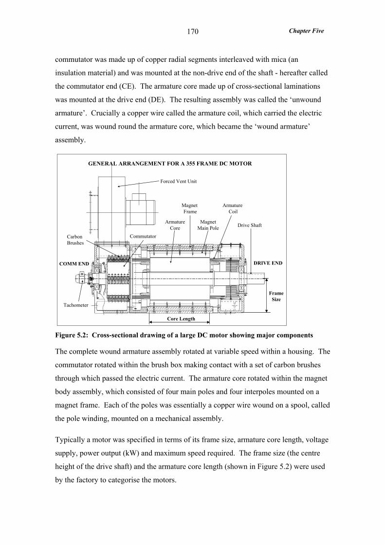
Chapter Five

170

commutator was made up of copper radial segments interleaved with mica (an

insulation material) and was mounted at the non-drive end of the shaft - hereafter called

the commutator end (CE). The armature core made up of cross-sectional laminations

was mounted at the drive end (DE). The resulting assembly was called the ‘unwound

armature’. Crucially a copper wire called the armature coil, which carried the electric

current, was wound round the armature core, which became the ‘wound armature’

assembly.

Figure 5.2: Cross-sectional drawing of a large DC motor showing major components

The complete wound armature assembly rotated at variable speed within a housing. The

commutator rotated within the brush box making contact with a set of carbon brushes

through which passed the electric current. The armature core rotated within the magnet

body assembly, which consisted of four main poles and four interpoles mounted on a

magnet frame. Each of the poles was essentially a copper wire wound on a spool, called

the pole winding, mounted on a mechanical assembly.

Typically a motor was specified in terms of its frame size, armature core length, voltage

supply, power output (kW) and maximum speed required. The frame size (the centre

height of the drive shaft) and the armature core length (shown in Figure 5.2) were used

by the factory to categorise the motors.

Core Length

Forced Vent Unit

Drive Shaft

Commutator

ArmatureCore

Armature Coil

Tachometer

COMM END DRIVE END

Carbon Brushes

Magnet Frame

MagnetMain Pole

FrameSize

GENERAL ARRANGEMENT FOR A 355 FRAME DC MOTOR

Chapter Five

171

The application of FPp required that thirty UK standard motors were made-to-stock and

subsequently modified to specific customer orders (refer to Appendix 12 for

modification details). The modifications commonly involved peripheral components

such as tachometers mounted on the shaft, forced vent units or mounting brackets.

However just over one third of the motors modified also required far more invasive

modifications requiring a change to the magnet components (as detailed in Appendix

12). Although the peripheral components generated significant variety much of the

variety in the LDC motors was generated from the magnet body and armature assembly

specifications. This is analysed fully in section 5.4.5 on product standardisation and

illustrated by the production variety funnels in section 5.4.8.


The flow process chart in Table 5.1 generally applied to motor manufacture in the LDC

area of the factory. The chart describes the main process flow from the manufacture of

the commutator to the final assembly of the motor. It also shows the process flow for

the manufacture of the magnet body assembly - shown separately since it is conducted

in parallel with the manufacture of the armature.

Manufacture of the motor began with the commutator. The coppers and mica adhesive

coated laminates were assembled radially and then put through a pressure-oven cycle

until they were the right dimension. After this the commutator was machined smooth,

fully assembled and grooves machined in the copper laminate sections for wire.

The armature core was built up from cross sectional laminates, a key way cut, then the

shaft was pressed into the armature core. The commutator - together with various other

components designed to hold the commutator and armature in place - were assembled

onto the shaft to make the ‘unwound armature’ assembly.

The armature coil was prepared and wound via a lengthy manual operation onto the

armature core. The armature was then electrically tested, the coil connections soldered

on an automatic rotating machine, and finally the armature was insulated and re-tested.

The re-test triggered the assembly of the poles into the magnet frame to ensure that the

magnet body was ready for final assembly upon completion of the armature.

Chapter Five

172

Table 5.1: A flow process chart for LDC area


Main process flow incl. Armature Manufacture

Manufacture commutator > SLIT COMM.

Store commutators.

Build armature core

Armature core, comm. and other components assembled on shaft > UNWOUND ARMATURE

Move armature assy. to winding trolleys

Wind armature coil onto core

Electrically test armature

Solder and insulate armature

Electrically test armature (triggers magnet pole-up) > TESTED WOUND ARMATURE

Move armature assy. to impregnation area

Impregnate armature assy.

Move armature assy. to armature finishing area

Paint armature and machine comm. mica

Balance armature > FINISHED ARMATURE

Move armature assy. to final assy area

Assemble motor

Test motor

Spray paint motor > FINISHED MOTOR

Move finished motor to warehouse

Magnet Body Manufacture

Prepare pole windings

Pole up magnet and assemble magnet body

Prepare compensated winding (frames 280 & 355)

Connect compensated winding (frames 280 & 355)

Impregnate magnet body assy. > MAGNET BODY

Operation

Inspection

Transport

Storage

Chapter Five

173

Following the successful completion of the electrical tests the armature was

impregnated with resin by repeating a lengthy dipping-oven cycle. The armature was

then painted (to repel the carbon fibres from the brushes) and the mica machined away

so the brushes could make contact with the copper. The armature assembly was then

balanced in rotation to give the ‘armature’ assembly.

Finally the armature, magnet body and numerous peripheral components were

assembled in an enclosure. The complete motor – regardless of whether it was made to

a customer order or to UK stock - was then fully tested, sprayed with two coats of paint

and transported to the finished goods warehouse.

UK standard motors to be modified under the FPp approach were taken from stock and

modified, not on the LDC section, but in the Service and Repairs (S&R) section. The

modifications varied greatly from the simple change of a data plate taking 10 minutes to

the change of a magnet pole involving a motor strip-down and taking up to 3 working

days (as detailed in Appendix 12). Further, depending upon the modification the motor

sometimes required re-testing and re-spraying.


The reason for applying FPp (and how it was applied) was the subject of interviews

with three different informants. The informants were selected because of their close

involvement with the relocation of LDC manufacture to BC, and their knowledge

regarding the wider issues surrounding the FPp approach. The informants were the

Production Engineering Manager, LDC Product Manager and DC Sales Manager. Each

informant was asked:

Why was FPp applied - what were the drivers?

The industrial LDC motors had been manufactured using the FPp approach at the Bull

Electric factory for many years. BC continued to use FPp when LDC motor

manufacture was transferred to BC at the beginning of the year 2000. All informants

testified that LDC motors were subject to FPp in order to provide a more responsive

supply than the manufacturing lead-time would otherwise allow. The need to be more

Chapter Five

174

responsive was attributed to the type of market the LDC motors were supplied to - the

motor replacement market.

The DC Sales Manager had a long history with this particular range of LDC motors -

employed as a Design Engineer when they were originated back in the 1970s - he had a

unique and highly informed perspective. He described the industrial LDC motor as a

‘sunset’ product and explained that:

‘for around the last 15 years the LDC motor has been generally supplied as a motor replacement, rather than a motor for new installations. The AC motor technology has advanced and now tends to be the preferred solution for new installations. At BC we only supply four companies with LDC motors for new installations in the UK. Whereas the motor replacement market is very large with thousands of LDC motors in use and - due to their long life expectancy - it is expected to remain so for many years.’

According to the DC Sales Manager the order winner for standard LDC motors was

‘availability on a short lead-time’. He elaborated:

‘the motor replacement market is not price sensitive and quality is no longer an order winner. Quite often the existing motor, requiring replacement, is no longer reliable, and should it breakdown the subsequent downtime is likely to be worth many times the motor’s value.’

Although the motors were sometimes supplied to distributors, even these customers

required a short lead-time since the motor’s high value deterred stock keeping. The DC

Sales Manager concluded:

‘the current BC standard quoted lead-time of 10-14 weeks is satisfactory for special motors, as the sales testify. However, when the motor is based on a standard specification, the UK customers expect a 3-4 week lead-time, which BC has found can be achieved using the FPp approach.’

The customer service measures endorsed this claim and - on average the motors

manufactured using the FPp approach achieved a 3 week lead-time.



collection are addressed in this section.

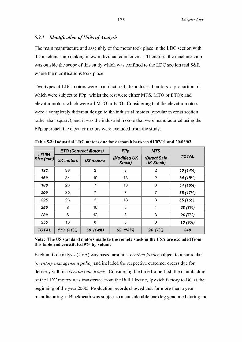
Chapter Five

175


The main manufacture and assembly of the motor took place in the LDC section with

the machine shop making a few individual components. Therefore, the machine shop

was outside the scope of this study which was confined to the LDC section and S&R

where the modifications took place.

Two types of LDC motors were manufactured: the industrial motors, a proportion of

which were subject to FPp (whilst the rest were either MTS, MTO or ETO); and

elevator motors which were all MTO or ETO. Considering that the elevator motors

were a completely different design to the industrial motors (circular in cross section

rather than square), and it was the industrial motors that were manufactured using the

FPp approach the elevator motors were excluded from the study.

Table 5.2: Industrial LDC motors due for despatch between 01/07/01 and 30/06/02

ETO (Contract Motors) Frame

Size (mm) UK motors US motors

FPp (Modified UK

Stock)

MTS (Direct Sale UK Stock)

TOTAL

132 36 2 8 2 50 (14%)

160 34 10 13 2 64 (18%)

180 26 7 13 3 54 (16%)

200 30 7 7 7 58 (17%)

225 26 2 13 3 55 (16%)

250 8 10 5 4 28 (8%)

280 6 12 3 3 26 (7%)

355 13 0 0 0 13 (4%)

TOTAL 179 (51%) 50 (14%) 62 (18%) 24 (7%) 348

Note: The US standard motors made to the remote stock in the USA are excluded from this table and constituted 9% by volume

Each unit of analysis (UoA) was based around a product family subject to a particular

inventory management policy and included the respective customer orders due for

delivery within a certain time frame. Considering the time frame first, the manufacture

of the LDC motors was transferred from the Bull Electric, Ipswich factory to BC at the

beginning of the year 2000. Production records showed that for more than a year

manufacturing at Blackheath was subject to a considerable backlog generated during the

Chapter Five

176

transfer. Further, even when production had settled, relatively low volumes of the

industrial LDC motors were manufactured (as illustrated in Table 5.2). There was a

need to study a reasonable number of orders, such that the measures would achieve an

acceptable degree of statistical significance. In consideration of these factors the most

recent 12-month period, for which records were available (1st July ’01 to 30th June ’02)

was the identified study period.

The manufacture of the industrial LDC motors was split between four different

inventory management policies, depending on the motor specification:

• Contract motors were engineered to order (ETO)

• Modified UK stock motors were form postponed (FPp)

• UK stock motors were made to stock (MTS)

• US standard motors were made to remote stock

These four product groups were used for the UoA, however only three are presented

here. The US standard motors were excluded from the thesis, because they could not be

satisfactorily classified as MTO or MTS, and only served to confuse the analysis of the

different inventory management policies. They were manufactured in a range of US

standard designs exclusively for Brook Incorporated USA, who maintain a stock of

these motors in the USA and modify them if required. Although classed as MTO by BC

(because their manufacture was covered by an order), they were effectively made-to-

remote-stock, since they were destined to replenish the USA stock. This was evident

from the very small range of variants manufactured - 14 in total - and the comparatively

high volumes.

In view of the relatively low demand for industrial LDC motors the UoAs were not

restricted to particular frame sizes but rather spanned the whole range. Therefore the

three product groups shown in Table 5.2 and the associated orders due for despatch

during the selected one-year period were studied.

Chapter Five

177

The majority of LDC motors (65%) were ETO and the bulk of these motors were made

to metric dimensions and therefore termed ‘UK motors’. The ‘US motors’ were

basically metric motors with an imperial frame size, which dictated that a small

proportion of the motor’s component parts were in imperial sizes.

The second largest product group were modified UK stock motors. These were the UK

standard motors made-to-stock and subsequently modified to specific customer orders

in accordance with the FPp approach. This UoA was further subdivided for the purpose

of certain measures (demand amplification, customer service and throughput

efficiency), since around a third of the motors were modified in production rather than

from stock (as explained in sections 5.3.2 and 5.3.3).

The final, and smallest division of products, were the UK stock motors sold ex-stock

without any modifications and these will form the MTS UoA.


In order to study a sufficient number of customer orders it was necessary to study a one

year period as argued in the previous section. Insufficient time was available to conduct

a real time one-year study therefore - considering the plentiful historical data available -

a retrospective study was conducted. The majority of the data collected applied to the

period between 1st July ’01 and 30th June ’02 and the study was conducted between July

and October 2002.

A retrospective study can raise questions regarding the reliability of the data. Interview

data naturally required support from documentary or database evidence, and fortunately

all the interviewees were not only still employed at the factory, but in the same roles, as

for the study period. Fortunately, therefore all the informants had first hand experience

and knowledge of the time period in question.

A good source of evidence for customer service and demand profile measures was the

Order Log access database. This was automatically updated on a nightly basis with

factory order progress data, including despatch dates, originating from the MRP system,

JBA. Unfortunately the MRP operation booking dates were found to be unreliable

because the Planner did not use the MRP system to monitor job progress. Instead she

Chapter Five

178

preferred to use a purpose designed Excel spreadsheet named the ‘LDC Tracker’ (as

explained in section 5.3.3.). Therefore for the purpose of measuring demand

amplification and throughput efficiency the MRP booking dates were corroborated by

dates on the Excel LDC Tracking spreadsheet. With regards to general reliability the

data retrieved from the MRP system and the ‘LDC Tracker’ was no less reliable or

accessible during the study than when it was generated.

The retrospective nature of the study did have one draw back the data was not available

to measure ex-stock availability in terms of the proportion of enquiries for which the

correct UK stock motor was available. However, two alternative sources of data were

available which gave a good indication of the ex-stock availability measure for both the

motors subject to FPp and MTS.



5.3 CHANGE CONTENT






selected for FPp was the subject of interviews with three different informants

(previously listed in section 5.1.3). The two questions asked of all informants, and their

collective answers, are presented below:

Was the ‘stock modification’ (FPp) approach limited to certain customers, and

if so why?

No. Stock modifications were carried out for any customer that required a standard UK

stock motor with modifications.

Chapter Five

179

Was the ‘stock modification’ (FPp) approach limited to certain motor

specifications, and if so why?

Yes, the stock modification approach was limited to 30 recognised standard UK motor

specifications, each demanded by multiple customers. Bull Electric at Ipswich selected

these motors (prior to the relocation of LDC motor manufacture to BC) therefore it was

not possible to confirm how the selection was made.

It was possible that these motor specifications were selected for the FPp application by

volume demand. However during the study period 4 of the 30 UK stock motors were

not subjected to demand and the demand on the remainder accounted for 52% (86

motors) of the UK specification motors ordered (the others were ETO). The DC Sales

Manager believed that the range of standard UK motors stocked should have covered all

combinations of the standard frame sizes, core lengths and wiring specifications

totalling 66 motor specifications. He argued that ‘Brook Crompton is not competitive

on lead-time for many of the standard UK motors and sales are lost as a result’. He

continues:

‘the LDC motor was designed to be stocked in component form as far back as the armature laminates when they are more flexible. If this were the case for the full range of standard motors the stock levels required would be no higher than the current levels required to support the 30 motor specifications.’

This argument was supported by evidence showing that many components exhibited

commonality across the standard motors. The degree of commonality index showed

that on average distinct components (within the armature assembly and magnet body of

generic stock motors) are common across 10% of the 30 motor specifications.



motor stocks, both generic and finished. Also considered in this section – and inherent

in the inventory management approach - is the Customer Order Decoupling Point

(CODP) location. Evidence for inventory management was gathered from interviews

with the LDC Sales Co-ordinator, LDC Planner, Product Engineering Manager and

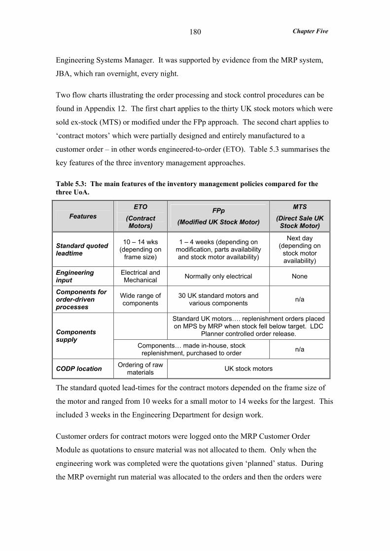
Chapter Five

180

Engineering Systems Manager. It was supported by evidence from the MRP system,

JBA, which ran overnight, every night.

Two flow charts illustrating the order processing and stock control procedures can be

found in Appendix 12. The first chart applies to the thirty UK stock motors which were

sold ex-stock (MTS) or modified under the FPp approach. The second chart applies to

‘contract motors’ which were partially designed and entirely manufactured to a

customer order – in other words engineered-to-order (ETO). Table 5.3 summarises the

key features of the three inventory management approaches.

Table 5.3: The main features of the inventory management policies compared for the three UoA.

Features ETO

(Contract Motors)

FPp (Modified UK Stock Motor)

MTS (Direct Sale UK

Stock Motor)

Standard quoted leadtime

10 – 14 wks (depending on

frame size)

1 – 4 weeks (depending on modification, parts availability and stock motor availability)

Next day (depending on

stock motor availability)

Engineering input

Electrical and Mechanical Normally only electrical None

Components for order-driven processes

Wide range of components

30 UK standard motors and various components n/a

Standard UK motors…. replenishment orders placed on MPS by MRP when stock fell below target. LDC

Planner controlled order release. Components supply

Components… made in-house, stock replenishment, purchased to order n/a

CODP location Ordering of raw materials UK stock motors

The standard quoted lead-times for the contract motors depended on the frame size of

the motor and ranged from 10 weeks for a small motor to 14 weeks for the largest. This

included 3 weeks in the Engineering Department for design work.

Customer orders for contract motors were logged onto the MRP Customer Order

Module as quotations to ensure material was not allocated to them. Only when the

engineering work was completed were the quotations given ‘planned’ status. During

the MRP overnight run material was allocated to the orders and then the orders were

Chapter Five

181

available for manufacture on the one week period MPS. The LDC Planner controlled

when the orders were released into the factory.

The flow chart for the UK stock motors covers modified stock (FPp) and direct sale

stock (MTS). For both cases two eventualities were covered: when stock was available

in the warehouse; and when no stock was available but the required motor was in

production. The latter case was relatively frequent because motor stocks were

maintained at only 50-70% of target. In the case of modified stock motors around a

third of motors were modified in production.

The quoted lead-time for stock motors (modified or direct sale) depended on their

availability or status in production. In addition the lead-time for modified motors was

dependant on the modification itself and part availability. However it was questionable

whether the salesmen did check part availability prior to providing a quote.

Although the UK motor stock levels were monitored by the LDC Planner the target

levels had not been reviewed or changed since LDC motor production was transferred

from Bull Electric (Ipswich) to BC at the beginning of 2000. The MRP system

automatically generated a stock replenishment order during its overnight run as soon as

the stock levels fell below target. However, the LDC Planner controlled order release

(timing and quantity), and thereby controlled the stock levels. The LDC Product

Manager admitted that it was very difficult to control the stock levels as sales were so

erratic. This was compounded by the high value of the motors - a strong deterrent

against stock build-up. Consequently the LDC Planner was restricted to a

replenishment quantity of one motor. The interviews with the Planner and Product

Manager suggested that stock motors were manufactured whenever capacity existed

over and above that required to manufacture the contract motors.

For contract motors the entire motor manufacture was driven by a customer order, and

indeed the purchase of many of the raw materials, therefore the CODP was located at

raw material ordering. In contrast the entire manufacture of the UK stock motors was

stock driven, therefore in the case of the direct sale motors the CODP was at the

finished motor. Whereas, the modifications were driven by customer orders, therefore

the CODP for modified motors was at the standard motor. However, should the motor

Chapter Five

182

be modified in production, the CODP was located at the point in manufacturing where

the motor was allocated to the order, and therefore variable.

The factory orders for stock modifications largely by-passed the MRP system as

illustrated by the flow chart in Appendix 12. The Order Processing Department (OPD)

advised either the warehouse or the LDC section (depending on the motor availability)

that the motor required modification. Further, OPD ensured the modification

instructions were sent to the section which would perform the modifications. The only

‘knowledge’ the MRP system had of a stock modification order was the requirement of

a UK stock motor. Consequently the MRP system was not able to provide OPD with

progress data only a despatch date.


Manufacturing planning and scheduling covers the process from the orders being

present on the MPS to the jobs being scheduled and monitored through the operations.

Evidence was gathered from interviews with the LDC Planner, the LDC Product

Manager, Customer Service & Warranty Officer and the After Sales Service Manager.

The latter two informants had involvement with the stock modifications only.

Whether the motors were ETO or MTS made little difference to the way the LDC

section planned and scheduled production as illustrated by the flow chart in Appendix

12. With the exception that motors covered by a customer order (contract motors) were

given priority throughout their production.

The main features of manufacturing planning are compared for the MTO, MTS and FPp

approaches in Table 5.4. The LDC Planner scrutinised the orders daily on the one week

period MPS and released them on the basis of raw material availability, capacity

availability and the due date. A limit of 25 motors per week (based on the armature

impregnation capacity) had been placed on the number of LDC motors launched. This

was broken down by frame size based solely on the tooling available for commutator

and armature building - not a true reflection of capacity.

The LDC Planner raised the Works Orders for the parts to be manufactured in the

machine shop and on the LDC section (commutator, armature core, etc). The MRP

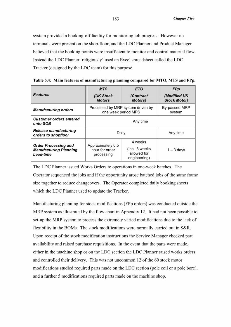
Chapter Five

183

system provided a booking-off facility for monitoring job progress. However no

terminals were present on the shop-floor, and the LDC Planner and Product Manager

believed that the booking points were insufficient to monitor and control material flow.

Instead the LDC Planner ‘religiously’ used an Excel spreadsheet called the LDC

Tracker (designed by the LDC team) for this purpose.

Table 5.4: Main features of manufacturing planning compared for MTO, MTS and FPp.

Features MTS

(UK Stock Motors

ETO (Contract Motors)

FPp (Modified UK Stock Motor)

Manufacturing orders Processed by MRP system driven by one week period MPS

By-passed MRP system

Customer orders entered onto SOB Any time

Release manufacturing orders to shopfloor Daily Any time

Order Processing and Manufacturing Planning Lead-time

Approximately 0.5 hour for order

processing

4 weeks

(incl. 3 weeks allowed for

engineering)

1 – 3 days

The LDC Planner issued Works Orders to operations in one-week batches. The

Operator sequenced the jobs and if the opportunity arose batched jobs of the same frame

size together to reduce changeovers. The Operator completed daily booking sheets

which the LDC Planner used to update the Tracker.

Manufacturing planning for stock modifications (FPp orders) was conducted outside the

MRP system as illustrated by the flow chart in Appendix 12. It had not been possible to

set-up the MRP system to process the extremely varied modifications due to the lack of

flexibility in the BOMs. The stock modifications were normally carried out in S&R.

Upon receipt of the stock modification instructions the Service Manager checked part

availability and raised purchase requisitions. In the event that the parts were made,

either in the machine shop or on the LDC section the LDC Planner raised works orders

and controlled their delivery. This was not uncommon 12 of the 60 stock motor

modifications studied required parts made on the LDC section (pole coil or a pole bore),

and a further 5 modifications required parts made on the machine shop.

Chapter Five

184

The Service Manager cited:

‘the acquiring of parts for stock modifications to be the main problem. Whereas the LDC section was supplied via Kanbans or kits from stores, stock modifications were not, they were treated as a hindrance, although they were still a sale’.

S&R transported the motor from the warehouse and picked all the bought-in parts from

stores. Clearly the whole process of acquiring parts for stock modifications was very

inefficient and entirely manual to the extent that even the purchase requisitions were

hand written.

S&R order priorities were agreed at the Weekly S&R Planning Meeting, attended by

both the Warranty Officer and the Service Manager. Stock modifications were treated

like service and repair jobs and given priority on the basis of the due date.

About one third of stock modifications studied were performed by the LDC section on

UK stock motors in production. Upon receipt of the stock modification instruction

sheet the LDC Planner allocated the motor to the order and changed the materials

requirements in the MRP system accordingly. Thereafter the motor was scheduled and

monitored through the LDC section as previously described.

The LDC section approach to controlling stock modifications was more efficient than

the S&R approach in part because material acquisition and control was conducted

within the MRP system. However, once a motor was released and materials allocated to

the order it was not easy for the LDC Planner to change material requirements (the

MRP system was not designed to be flexible in this way). It required careful

manipulation of the JBA system to ensure that stock records remain accurate.








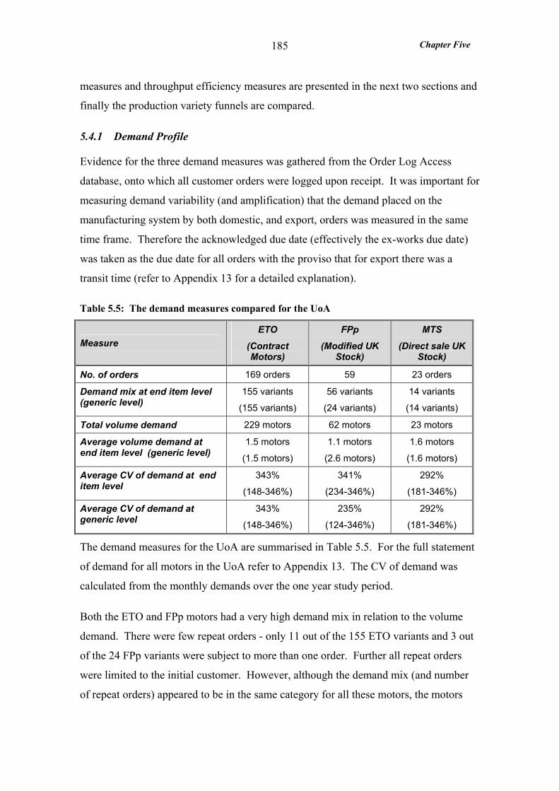
Chapter Five

185




Evidence for the three demand measures was gathered from the Order Log Access

database, onto which all customer orders were logged upon receipt. It was important for

measuring demand variability (and amplification) that the demand placed on the

manufacturing system by both domestic, and export, orders was measured in the same

time frame. Therefore the acknowledged due date (effectively the ex-works due date)

was taken as the due date for all orders with the proviso that for export there was a

transit time (refer to Appendix 13 for a detailed explanation).

Table 5.5: The demand measures compared for the UoA

Measure ETO

(Contract Motors)

FPp (Modified UK

Stock)

MTS (Direct sale UK

Stock)

No. of orders 169 orders 59 23 orders


155 variants

(155 variants)

56 variants

(24 variants)

14 variants

(14 variants)

Total volume demand 229 motors 62 motors 23 motors

Average volume demand at end item level (generic level)

1.5 motors

(1.5 motors)

1.1 motors

(2.6 motors)

1.6 motors

(1.6 motors)

Average CV of demand at end item level

343%

(148-346%)

341%

(234-346%)

292%

(181-346%)

Average CV of demand at generic level

343%

(148-346%)

235%

(124-346%)

292%

(181-346%)

The demand measures for the UoA are summarised in Table 5.5. For the full statement

of demand for all motors in the UoA refer to Appendix 13. The CV of demand was

calculated from the monthly demands over the one year study period.

Both the ETO and FPp motors had a very high demand mix in relation to the volume

demand. There were few repeat orders - only 11 out of the 155 ETO variants and 3 out

of the 24 FPp variants were subject to more than one order. Further all repeat orders

were limited to the initial customer. However, although the demand mix (and number

of repeat orders) appeared to be in the same category for all these motors, the motors

Chapter Five

186

subject to FPp were not customised to the same extent as the ETO motors. Just over a

quarter of the FPp motor variants (16 out of 56) were UK stock motors with merely a

customised dataplate added (refer to section 5.4.5 for more details).

As predicted the demand mix for the MTS motors was less than those subject to FPp.

In fact only 14 of the 30 UK stock motors were sold ex-stock (MTS). Further the

average volume demand at finished motor level was the lowest for those motors subject

to FPp - an indication of the great variety in these finished motors.

The average volume demand at the generic motor level was highest for the FPp motors.

For the ETO motors, the variety in the generic motors (which was indicated by the

armature assembly specifications) was the same as the variety at the finished motor

level. Therefore the volume demand at generic level was no higher than at finished

motor level.

The demand variability was very high for all UoA reflecting the high variety-low

volume at end item level. Even at the generic UK stock motor level demand was very

variable at 235% CV. To ensure high ex-stock availability a high safety stock would

have been required – this was discouraged because of the high value of the motors.

It should be noted that 346% variability which features as the upper bound for all three

UoA represents the situation where only one motor of a particular variant was

demanded over the whole year. As you might expect this was a very common

occurrence particularly for the ETO motors, and FPp motors, both of which exhibited

the highest demand variability.

Overall the demand analysis showed that the industrial LDC motors were required in

extremely high variety in relatively low volumes. In total a volume of 347 motors were

ordered in 238 variants, an average of 1.5 motors per variant. Two-thirds (229) of these

motors were manufactured as contract motors (ETO).

Summary: the industrial LDC motors in general were required in extremely high variety

and relatively low volumes, resulting in very high demand variability. The demand mix

for the motors manufactured under FPp was four times higher than that for the MTS

motors, 56 compared to 14 variants. As a result the demand variability at finished

Chapter Five

187

motor level was higher for the FPp motors at 341% compared to 292% for those motors

MTS. The average volume demand for finished motors was lower for the FPp motors

than for the MTS motors, 1.1 compared to 1.6 motors. Finally the average volume

demand at generic motor level for the FPp motors, was higher than that demonstrated by

the ETO motors 2.6 compared to 1.5 motors.


The demand data presented in the previous section was used to measure the demand

imposed on the manufacturing system. The manufacturing orders were the motor works

orders released into the factory as recorded on the LDC Tracker sheet.

The manufacturing schedules were not retrospectively available. However jobs were

sequenced on each work station on a daily basis by the operator and ‘booked off’ upon

completion by the LDC Planner on the LDC Tracker sheet. Further only one motor was

produced under each works order. Therefore the operation booking off dates were

within a day or two of the scheduled output dates and accurately represented the

scheduled sequence of jobs at each process and therefore the batching - important to

show demand amplification.

The demand amplification charts for the ETO and MTS UoA are shown in Appendix

14. The plots in each chart span the same weekly time buckets and use the same scale

so the relative amplitude of demand can be easily compared. Each chart shows: the

weekly demand for the motors (due between 1 July ’01 and 30 April ’02); the motor

works orders released; and the manufacturing schedules for the finished commutator,

the balanced armature and the finished motors shipped into the warehouse. In this case

study illustrating demand at a weekly level was the highest resolution possible because

all motor orders were given due weeks rather than due days.

From the production records available it was not possible to split the UK stock motor

production between those motors that were subsequently modified (FPp), and those that

were sold direct ex-stock (MTS). Therefore, the UK stock motor demand amplification

chart in Appendix 14 is for all UK stock motors.

Chapter Five

188

There are no obvious signs of demand amplification for the ETO UoA. Each plot

shows peaks and troughs of similar amplitude to those evident on the plot of customer

demand. Particularly towards the latter half of the time period analysed the patterns of

motors scheduled and works orders released reflects the pattern of demand quite

accurately. The patterns on the plots are staggered due to the 6-week manufacturing

lead-time required for these motors.

The chart for the UK stock motors showed a degree of demand amplification. The

peaks in demand were particularly amplified at the balanced armature schedule and the

shipped to warehouse schedule. However the pattern of motors released and the

commutator schedule exhibited a lower degree of demand amplification. The obvious

peak in motors released around week 33 was probably an effort to boost depleted motor

stocks. This explanation was supported by the relatively high level of modifications

performed in production between weeks 27 and 33, a scenario which only occurs in the

absence of the appropriate stock motors.

It was possible to split the demand for UK stock motors between those that were

modified (from stock and in production) and those that were sold ex-stock.

Subsequently the demand for modifications satisfied from stock was compared with the

S&R modification schedule (effectively the modification completion dates recorded on

the LDC Stock Modification Record), as the chart in Appendix 14 illustrates. As

expected no demand amplification was evident for the order-driven modifications.

Summary: there were no obvious signs of demand amplification for the ETO UoA. The

demand amplification chart for all the UK stock motors (modified and sold ex-stock),

showed a degree of demand amplification, particularly at the balanced armature

schedule and the shipped to warehouse schedule. The demand for the modified from

stock motors was compared with the S&R modification schedule and as expected no

demand amplification was evident for the order-driven modifications.



performance and ex-stock availability. Unfortunately the hypothesis featuring ex-stock

availability pre-supposed that orders subject to FPp and MTS did not pull from the same

Chapter Five

189

stock, however in the BC study this was the case. Nevertheless ex-stock availability

was measured for the FPp and MTS UoA and details are presented in Appendix 15. It

was only possible to measure ex-stock availability in terms of the proportion of orders

(rather than orders and enquiries) for which the correct stock motor was available.

Consequently this measure ignored the many enquiries which did not translate into

orders because the stock motor was not available. However, even using this extremely

lenient measure of ex-stock availability only 63% of FPp orders could be satisfied from

stock (while the remainder were modified in production). This was in part because the

UK motor stock levels were deliberately maintained at only 50% to 70% of the

established target level due to their high value and unpredictable, erratic demand.

For the order lead-time and delivery reliability measures it was relevant whether an

order was satisfied from stock or production. Clearly, if a motor was in the early stages

of production, rather than being available ex-stock a longer lead-time would be

required. For this reason the FPp UoA was split into two sub-units those orders

satisfied by motors from stock, and those orders satisfied by motors in production.

Neither order lead-time or delivery reliability to the customer were being measured by

the factory during the period of the study. To determine these measures both the

promised and actual order delivery dates to the customer were required.

The actual delivery dates to the customer were unavailable, however the ex-works dates

were available. For export orders the promised ex-works dates were available providing

a good measure of delivery reliability. However for domestic orders only promised

delivery – rather than promised ex-works dates - were available and the transit time was

normally in excess of 24 hours. Therefore the delivery reliability measure was rendered

slightly lenient for domestic orders. Refer to Appendix 15 for a detailed explanation of

the dates used for the order lead-time and delivery reliability measures.


customer order to the promised delivery and ex-works dates respectively. These

measures were made with the proviso that transit times were not taken into account

except for on the promised order lead-times for domestic orders.

Chapter Five

190

The evidence for all dates was found on the Order Log. The vast majority of customer

orders were for one motor and the largest order due during the study period was for six

contract motors. Therefore both the order lead-time and delivery measures were taken

for each motor rather than order. The delivery reliability to the customer measure was

effectively the proportion of motors despatched before, or on, the acknowledged due

date. Whereas the delivery reliability into the warehouse was the proportion of motors

shipped into the warehouse before, or on, the due into warehouse date (which was one

week prior to the acknowledged due date to allow for distribution). The evidence for

both these dates was taken from the LDC Tracker sheet.

Table 5.6: The order lead-time and delivery reliability measures for all UoA.

Measures ETO

(Contract Motors)

FPp (Modified in Production)

FPp (Modified from

Stock)

MTS (Direct sale UK

Stock)

No. of motors assessed 219 19 35 23

Av. promised order lead-time 14.2 wks 2.4 wks 3.4 wks 0.2 wks

Av. actual order lead-time 13.9 wks 2.6 wks 3.0 wks 0.1 wks

Engineering input?

Electrical and Mechanical

Normally only electrical

Normally only electrical No

6.6 wks 0.1 wks 0.5 wks Av. leadtime prior to…. .works order

release ..booking out of engineering N/a

7.3 wks Av. order lead-time measured from….. .works order

release

2.5 wks

..booking out of engineering N/a


Delivery reliability into warehouse

61% Insufficient

data available

34%

N/a

Delivery reliability to the customer

63% 79% 66% 96%

Av. lateness to the customer 1.8 wks 1.7 wks 1 wk N/a

The order lead-time and delivery reliability measures for each UoA are presented in

Table 5.6. The promised and actual order lead-times for the FPp motors were less than

Chapter Five

191

a quarter of that for the ETO motors at around 3 weeks. This was due to both a

reduction in the lead-time prior to manufacturing and the manufacturing lead-time itself.

On average the ETO motors required a 6.6 weeks lead-time prior to the release of the

works order into manufacturing compared to a mere 3 or 4 days for FPp motors. The

lengthy delay on works order release for ETO motors was due - not only to engineering

work - but also the long lead-time on various non-standard bought-in parts (such as the

shaft and copper segments for the commutator). The manufacturing lead-time for

motors subject to FPp was only one third of that for an ETO motor, 2.5 weeks compared

to 7.3 weeks.

The delivery reliability to the customer for ETO motors was 63% compared with 70%

for the FPp motors. Curiously, however, the FPp motors were generally shipped to the

warehouse later than the contract motors as the delivery reliability into the warehouse

measure shows. Only around 34 % of the modified-from-stock motors compared with

61% of the ETO motors were shipped to the warehouse before, or on, the due-into-

warehouse date (one week prior to the acknowledged due-to-the-customer date).

The FPp approach only provided a modest improvement in delivery reliability

compared to the ETO approach and in general delivery reliability was poor especially

when it was considered that the measure was slightly lenient (on domestic orders as

discussed). There are a number of possible explanations for the poor delivery

performance of FPp:

• Firstly, it was claimed that when a part made in the BC machine shop was

required for a stock modification, the required part was not given priority.

However only 5 (8%) of the 60 motors subject to FPp required such parts.

• Secondly, the quoted lead-times for the FPp motors did not take into account

parts availability, and few bought-in parts required for modifications were

stocked. In addition the process of acquiring these parts was very laborious as


• Thirdly, only very limited capacity was available in S&R, this coupled with the

fact that S&R was primarily tasked with service and repairs probably resulted in

Chapter Five

192

modifications being performed in an unresponsive manner. This is supported by

the lower delivery reliability achieved by motors modified from stock (in S&R)

compared to those modified in production (66% compared with 79%).

• Finally low standard motor stocks may have contributed to the poor delivery

reliability achieved by FPp. However this does not seem to be the case when it

is considered that higher delivery reliability was achieved by those motors

modified in production than those modified from stock (79% compared to 66%).

This suggested that the absence of motor stocks improved delivery reliability.

Comparing the two approaches to FPp, modified in production and modified from

stock, the former appears to achieve a shorter actual order lead-time and a significantly

higher delivery reliability. The actual order lead-time provided by the modified in

production approach was 2.6 weeks compared with 3.0 weeks for modified from stock.

The reduction in lead-time appears to be due to the 0.4 weeks reduction in engineering

time (see lead-time prior to booking out of engineering) which is a feature of the

modification type. Of the modified in production motors 50% involved a data plate re-

stamp only (the most trivial modification requiring virtually no engineering time)

whereas only 13 % of the modified from stock motors involved such a trivial

modification.

This disparity in modification types may also have contributed to the higher delivery

reliability achieved by the modified in production approach, 79% compared with only

66% for the modified from stock approach. None of the motors, which received a data

plate re-stamp only, whether modified in production or from stock, were delivered late.

In short the apparent improved customer service offered by the modified in production

approach may be due to the disparity of modification types rather than the operation of

the inventory management approach itself.

Summary: the hypothesis on ex-stock availability pre-supposed that orders subject to

FPp and MTS did not pull from the same stock, however in the BC study this was the

case. The average actual order lead-times for the FPp motors were less than a quarter of

that for the ETO motors at around 3 weeks. This was due to both a reduction in

engineering and bought-in parts lead-time, and the manufacturing lead-time itself (7.3 to

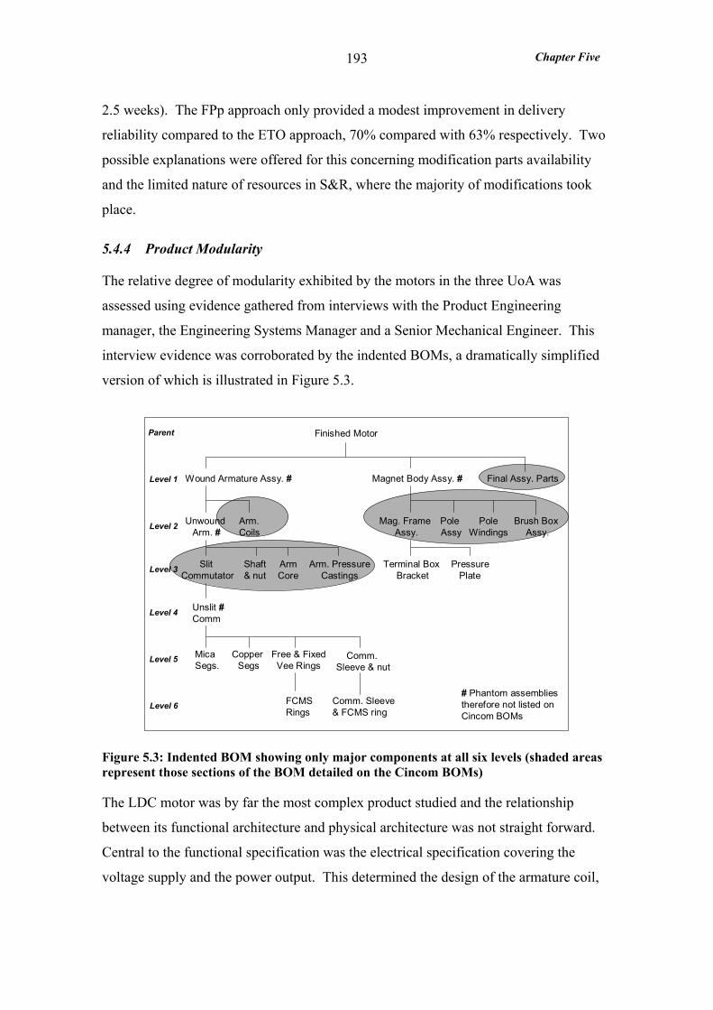
Chapter Five

193

2.5 weeks). The FPp approach only provided a modest improvement in delivery

reliability compared to the ETO approach, 70% compared with 63% respectively. Two

possible explanations were offered for this concerning modification parts availability

and the limited nature of resources in S&R, where the majority of modifications took

place.


The relative degree of modularity exhibited by the motors in the three UoA was

assessed using evidence gathered from interviews with the Product Engineering

manager, the Engineering Systems Manager and a Senior Mechanical Engineer. This

interview evidence was corroborated by the indented BOMs, a dramatically simplified

version of which is illustrated in Figure 5.3.

Parent

Level 1

Level 2

Level 3

Level 4

Level 5

Level 6

Final Assy. Parts

Slit Commutator

Brush Box Assy.

Finished Motor

Wound Armature Assy. #

Unwound Arm. #

Arm. Coils

Magnet Body Assy. #

Mag. Frame Assy.

Pole Assy

Terminal Box Bracket

Shaft& nut

ArmCore

Arm. PressureCastings

PressurePlate

PoleWindings

Unslit #Comm

MicaSegs.

Copper Segs

Free & FixedVee Rings

Comm. Sleeve & nut

FCMSRings

Comm. Sleeve& FCMS ring

# Phantom assemblies therefore not listed on Cincom BOMs

Figure 5.3: Indented BOM showing only major components at all six levels (shaded areas represent those sections of the BOM detailed on the Cincom BOMs)

The LDC motor was by far the most complex product studied and the relationship

between its functional architecture and physical architecture was not straight forward.

Central to the functional specification was the electrical specification covering the

voltage supply and the power output. This determined the design of the armature coil,

Chapter Five

194

armature core, the magnet pole windings (interpole and main pole), commutator, and

the brush ring assembly. It was clear from the previous description of the motors

structure (section 5.1.1) and the cross sectional drawing in Figure 5.2 that these

components were dispersed round the motor in different major sub-assemblies: the

wound armature assembly, the magnet body assembly and the brush box assembly.

Therefore the functional electrical element corresponded with numerous physical

components dispersed through the motor. This was supported by evidence from the

Cincom configurator (a proprietor knowledge based system) which established the

physical configuration of the parts in the BOM from the user specification and

engineering data. The Cincom BOM was split into sections called 'configuration

elements', which grouped together components relating to a particular functional

element. One such element was the ‘armature electrical element’, which grouped

together the aforementioned (physically dispersed) components relating to it.

From the Cincom BOMs it was evident that many other elements of the functional

architecture did correspond to particular sub-assemblies or components. Generally

these were assembled in the final stages of manufacturing and included essential

functional elements such as the motor enclosure, temperature protection, and the

terminal box. They also included a number of optional functional elements such as

forced ventilation unit, air pressure switch, brakes, heaters, coolers, and tachometers.

Further it appeared that there was little in terms of unwanted interactions between these

modules.

Many of the stock motor modifications (35 out of 60) involved only the highly modular

final assembly components. However a substantial number (25 out of 60) involved

components within the magnet body assembly. Over half of these modifications (14 out

of 25) involved a change of thermistors which are separate physical components

providing temperature protection and assembled in the magnet body assembly.

Therefore just under a quarter of the stock motor modifications (11 out of 60) involved

the main magnet pole and brushes which demonstrated a relatively low degree of

modularity.

The type of modularity exhibited by the motors was ‘component swapping’ modularity

(Pine, 1993). Different components, in this case various peripheral components, were

Chapter Five

195

paired with the same basic product, a UK stock motor, to produce variety in the finished

product.

Summary: all motors regardless of inventory management policy exhibited the same

level of modularity. The major sub-assemblies in the LDC motor exhibited a very low

degree of modularity. However peripheral components and sub-assemblies - generally

involved in final assembly - did correspond to particular functional elements on a one-

to-one basis thereby exhibiting a high degree of modularity. Just over half of the stock

modifications involved only the highly modular peripheral components, and a further

quarter involved a modular component embedded within the magnet body assembly.

Therefore just under a quarter of the stock motor modifications involved components

which demonstrated a relatively low degree of modularity.




Initially it was envisaged that the evidence required for the product standardisation

measures would be collected from the full indented BOMs on the MRP system.

However, these BOMs were unavailable due to system changes. Moreover, the MRP

BOMs were not in a standardised format (manually transferred from the Cincom

Configurator), which would have hampered the analysis of specific parts across a set of

BOMs. In light of this it was decided to use the BOMs generated by the Cincom

configurator which are in fact used to populate the MRP BOMs.

The Cincom BOMs had the advantage of being in a standardised format and were also

accessible using the Microsoft Excel spreadsheet application. However, they had a

number of limitations (refer to Appendix 16 for a full explanation) the most significant

of which was that they only covered levels 1, 2 and 3 of the full indented BOM, which

had six levels (as illustrated in Figure 5.3). Generally the lower couple of levels from

each major sub assembly - wound armature, magnet body and final assembly

components - were missing. Fortunately, however these levels covered mainly raw

materials for components manufactured by the machine shop, which was not within the

scope of this study, therefore these components were not subject to analysis. The only

Chapter Five

196

significant exceptions were the missing commutator components on level 5, which were

assembled by the LDC section. With consideration to time constraints it was decided

that it was necessary to exclude these from the product design measures, however the

variety of these components was estimated for the production variety funnel (presented

in section 5.4.8).

LDC motors contained many distinct or different parts, for instance a 180 frame size

UK stock motor required 157 different parts, and a 355 frame contract motor required

around 230 different parts. This demonstrated the extent to which the BOM in Figure

5.3 had been simplified. However, many of these parts were trivial raw material parts

such as cables and sealing plugs stocked on the production line (90 in the case of the

aforementioned UK stock motor) therefore it was necessary to scope the analysis to

include only significant parts. Refer to Appendix 16 for full details on the selection of

parts and a list of the part types analysed for each UoA. All parts with T* part numbers

were analysed because these were the most significant parts and featured in the original

LDC motor design. The T* parts included all parts made by BC and many of the MRP

purchased parts. In fact wherever possible all MRP purchased parts were included in

the analysis.

The components used in the UK stock modifications were not available on the Cincom

BOMs instead the Stock Mod Instruction Sheets were the source of this information.

Before considering the product standardisation measures a few basic facts illustrate the

difference between the three UoA. The UK stock motors were all supplied with

housings offering the standard International Protection level (IP23), were all made to

operate at the standard maximum speed and the majority of them require a standard

voltage power supply. In contrast the contract motors varied with respect to each of

these fundamental characteristics and in addition could be either UK or US motors.

A summary of the product standardisation measures is shown in Table 5.7. The average

number of distinct components analysed for each motor was very similar for all three

UoA, around 52 components. For any given UoA very few components were found to

be common, in fact no components were found to be common across the ETO motors.

The roller bearing data plate was common across the FPp and MTS motors and the two

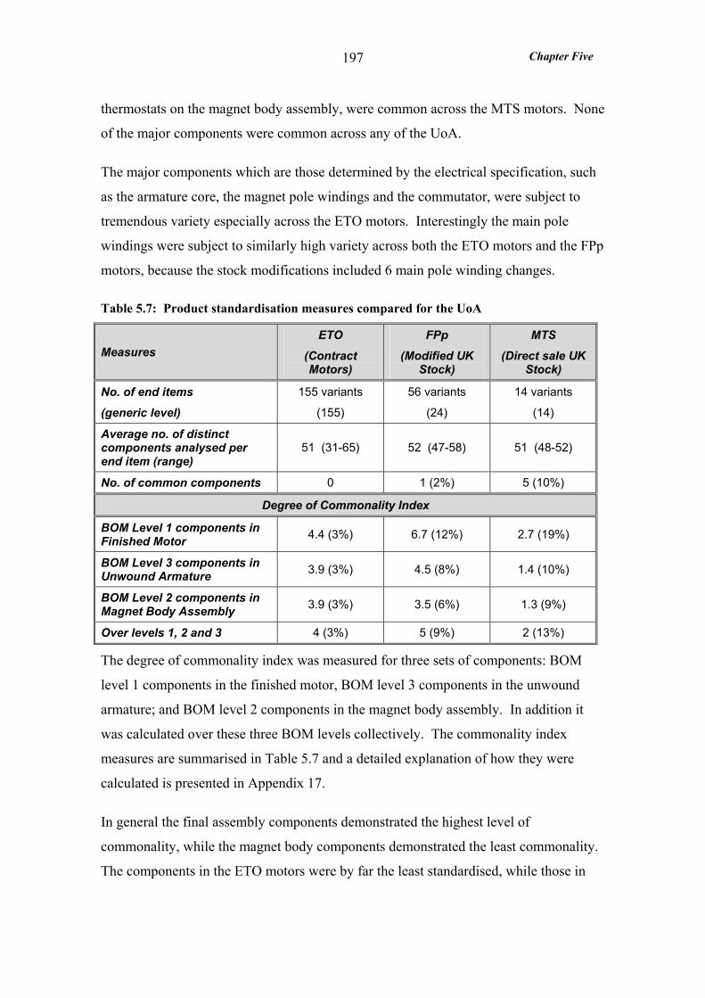
Chapter Five

197

thermostats on the magnet body assembly, were common across the MTS motors. None

of the major components were common across any of the UoA.

The major components which are those determined by the electrical specification, such

as the armature core, the magnet pole windings and the commutator, were subject to

tremendous variety especially across the ETO motors. Interestingly the main pole

windings were subject to similarly high variety across both the ETO motors and the FPp

motors, because the stock modifications included 6 main pole winding changes.


Measures ETO

(Contract Motors)

FPp (Modified UK

Stock)

MTS (Direct sale UK

Stock)

No. of end items (generic level)

155 variants

(155)

56 variants

(24)

14 variants

(14)

Average no. of distinct components analysed per end item (range)

51 (31-65) 52 (47-58) 51 (48-52)

No. of common components 0 1 (2%) 5 (10%)

Degree of Commonality Index

BOM Level 1 components in Finished Motor 4.4 (3%) 6.7 (12%) 2.7 (19%)

BOM Level 3 components in Unwound Armature 3.9 (3%) 4.5 (8%) 1.4 (10%)

BOM Level 2 components in Magnet Body Assembly 3.9 (3%) 3.5 (6%) 1.3 (9%)

Over levels 1, 2 and 3 4 (3%) 5 (9%) 2 (13%)

The degree of commonality index was measured for three sets of components: BOM

level 1 components in the finished motor, BOM level 3 components in the unwound

armature; and BOM level 2 components in the magnet body assembly. In addition it

was calculated over these three BOM levels collectively. The commonality index

measures are summarised in Table 5.7 and a detailed explanation of how they were

calculated is presented in Appendix 17.

In general the final assembly components demonstrated the highest level of

commonality, while the magnet body components demonstrated the least commonality.

The components in the ETO motors were by far the least standardised, while those in

Chapter Five

198

the MTS motors provided the highest level of commonality. The components in the

motors subject to FPp were found to have a lower commonality index than the MTS

motors particularly the components in the magnet body assembly. The explanation for

this lies in the fact that out of the 56 finished motor specifications, 23 involved invasive

modifications to the magnet body assemblies, such as main pole winding changes,

thermostat changes, and main pole bore changes (refer to Appendix 12 for details). The

component commonality for the FPp motors could easily have been lower, however 16

of the stock modifications were limited to a change of data plate only, a component so

trivial that it does not even fall within the scope of this analysis.

Summary: only very few minor components were found to be common across each

UoA - in fact no components were found to be common across the ETO motors. At

each BOM level the ETO motors exhibited the lowest degree of commonality index –

on average just one third of the commonality demonstrated by the FPp motors. The

MTS motors exhibited the highest level of commonality. For each UoA the final

assembly components (commonly the subject of postponed modifications) demonstrated

the highest level of commonality, while the magnet body components demonstrated the

least.


No production record was made of downtime due to the lack of demand defined as

excess capacity. Therefore, it was not possible to measure excess capacity directly.

Instead the ratio of actual output to design capacity (capacity utilisation) was used as an

indication of excess capacity – the lower it was the more likely excess capacity existed.

Further, no data regarding design capacity or planned downtime was available for S&R

where most of the UK stock modifications were carried out. Fortunately, however, 6 of

the 38 UK stock motors modified from stock, and all of the 22 motors modified in

production, were modified in the final assembly cell in the LDC area. Therefore, the

final assembly cell - and the subsequent motor test and paint spray cells - were order-

driven a greater proportion of the time than all the previous cells.

For the study period BC was not measuring capacity utilisation - simply all cells were

envisaged to have a weekly capacity of 25 motors. Fortunately, the actual output for

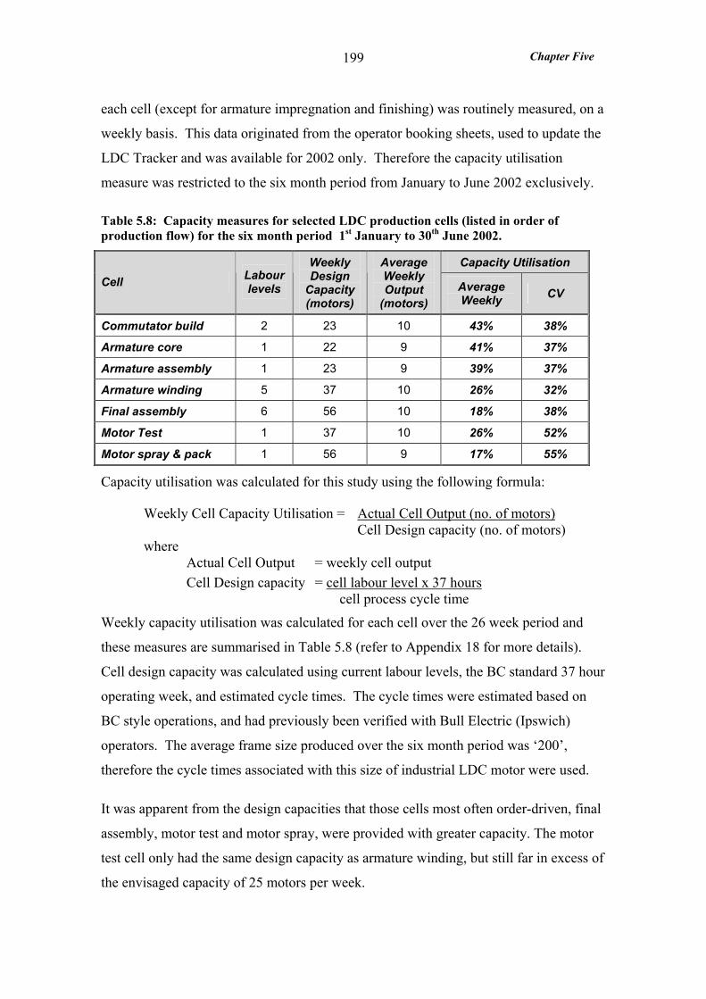
Chapter Five

199

each cell (except for armature impregnation and finishing) was routinely measured, on a

weekly basis. This data originated from the operator booking sheets, used to update the

LDC Tracker and was available for 2002 only. Therefore the capacity utilisation

measure was restricted to the six month period from January to June 2002 exclusively.

Table 5.8: Capacity measures for selected LDC production cells (listed in order of production flow) for the six month period 1st January to 30th June 2002.

Capacity Utilisation Cell Labour

levels

Weekly Design

Capacity (motors)

Average Weekly Output

(motors) Average Weekly CV

Commutator build 2 23 10 43% 38%

Armature core 1 22 9 41% 37%

Armature assembly 1 23 9 39% 37%

Armature winding 5 37 10 26% 32%

Final assembly 6 56 10 18% 38%

Motor Test 1 37 10 26% 52%

Motor spray & pack 1 56 9 17% 55%

Capacity utilisation was calculated for this study using the following formula:

Weekly Cell Capacity Utilisation = Actual Cell Output (no. of motors) Cell Design capacity (no. of motors)

where Actual Cell Output = weekly cell output Cell Design capacity = cell labour level x 37 hours

cell process cycle time

Weekly capacity utilisation was calculated for each cell over the 26 week period and

these measures are summarised in Table 5.8 (refer to Appendix 18 for more details).

Cell design capacity was calculated using current labour levels, the BC standard 37 hour

operating week, and estimated cycle times. The cycle times were estimated based on

BC style operations, and had previously been verified with Bull Electric (Ipswich)

operators. The average frame size produced over the six month period was ‘200’,

therefore the cycle times associated with this size of industrial LDC motor were used.

It was apparent from the design capacities that those cells most often order-driven, final

assembly, motor test and motor spray, were provided with greater capacity. The motor

test cell only had the same design capacity as armature winding, but still far in excess of

the envisaged capacity of 25 motors per week.

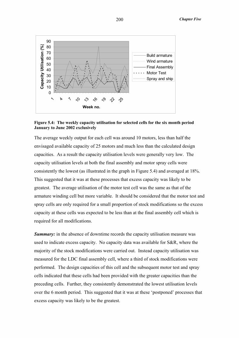
Chapter Five

200

0102030405060708090

1 4 7 10 13 16 19 22 25

Week no.

Cap

acity

Util

isat

ion

(%)

Build armatureWind armatureFinal AssemblyMotor TestSpray and ship

Figure 5.4: The weekly capacity utilisation for selected cells for the six month period January to June 2002 exclusively

The average weekly output for each cell was around 10 motors, less than half the

envisaged available capacity of 25 motors and much less than the calculated design

capacities. As a result the capacity utilisation levels were generally very low. The

capacity utilisation levels at both the final assembly and motor spray cells were

consistently the lowest (as illustrated in the graph in Figure 5.4) and averaged at 18%.

This suggested that it was at these processes that excess capacity was likely to be

greatest. The average utilisation of the motor test cell was the same as that of the

armature winding cell but more variable. It should be considered that the motor test and

spray cells are only required for a small proportion of stock modifications so the excess

capacity at these cells was expected to be less than at the final assembly cell which is

required for all modifications.

Summary: in the absence of downtime records the capacity utilisation measure was

used to indicate excess capacity. No capacity data was available for S&R, where the

majority of the stock modifications were carried out. Instead capacity utilisation was

measured for the LDC final assembly cell, where a third of stock modifications were

performed. The design capacities of this cell and the subsequent motor test and spray

cells indicated that these cells had been provided with the greater capacities than the

preceding cells. Further, they consistently demonstrated the lowest utilisation levels

over the 6 month period. This suggested that it was at these ‘postponed’ processes that

excess capacity was likely to be the greatest.

Chapter Five

201


The value adding activities at BC were the operations identified on the flow process

chart in Table 5.1. To calculate throughput efficiency the flow of material, with the

longest lead-time, was followed through commutator manufacture, the armature

assembly, motor assembly, motor test and motor spray. Therefore, the following

processes performed in parallel were not measured: armature core manufacture,

armature coil preparation, pole winding, and the magnet body assembly and

impregnation.

The value added times for each motor were calculated from the estimated processing

times based on BC style operations, and verified with Bull Electric, Ipswich operators

(refer to Appendix 19). The processing times and the elapsed times were measured over

the factory operating hours. Therefore the armature impregnation and motor painting

processes (each estimated at 1.5 days) were equivalent to 11 hours operating time.

The total value added times for the smallest and largest motors differed by only 3 hours

(8%). Given that the total elapsed time (which was the denominator in the throughput

efficiency calculation) was measured in weeks rather than hours this differential was

judged to be negligible. Therefore, the total value added time for the average sized

motor demanded during the study period, frame size ‘200’, was used. The precise stock

modification carried out on each FPp order was detailed on the Instruction sheets. The

associated processing times were estimated by the Service Manager, who had 20 years

experience with DC motors and was responsible for S&R (including stock

modifications).

The elapsed time was measured from the motor works order release into the factory to

the despatch, and booking into the warehouse, of the finished order. The works order

release off the MPS and the booking into warehouse dates were sourced from the LDC

Tracker sheet. The despatch dates were taken from the Order Log and cross-referenced

with despatch notes. The elapsed time for the stock modifications was measured from

the date the orders left mechanical engineering (as recorded on the Order Log) at which

time they were available for manufacture.

Chapter Five

202

A summary of the throughput efficiency measures is presented in Table 5.9. In

common with the customer service measures it was necessary to split the FPp UoA into

those motors modified in production, and those modified from stock. Unfortunately the

required data was only available for 6 of the 22 motors modified in production therefore

these results were excluded. Further it was not possible to link the production records

for a particular UK stock motor to the customer order for it (modified from stock or ex-

stock). Therefore the despatch date, and duration in the warehouse, was not known for

UK stock motors. The throughput efficiency for UK stock motor works orders released

between 1st May ’01 and 31st April ’02 was assessed. There was a high probability that

these motors had been used for customer orders (stock modifications or ex-stock) due

for delivery during the study period (1st July ‘01 to 30th June ’02).

Table 5.9: Throughput efficiency measures for the UoA.

Order Driven Stock Driven

Average Values ETO (Contract Motors)

FPp (Stock

Modifications)

All UK stock motors MTS

No. of motors assessed 188 35 106

Value added time 37 hrs 6.4 hrs 37 hrs

Time in warehouse 0.4 wks 0.6 wks No data

Elapsed time (excluding time in Warehouse) 6.3 wks 1.9 wks 10.8 wks

Throughput Efficiency (including time in warehouse) 16% 14% No data

Average 17% 21% 10%

CV 22% 127% 30%

Throughput Efficiency (excluding time in warehouse)

Range 9 – 26% 0.2 – 98% 4 – 20%

The elapsed time (or manufacturing lead-time) for the order-driven contract motors was

much shorter than for the stock-driven UK motors - 6 compared with 10 weeks. The

time in the finished goods warehouse was typically less than 1 week. However the UK

stock motors were probably stored in the warehouse for much longer but, as explained,

this data was unavailable. For the ETO motors the time in the finished goods

warehouse had little impact on the throughput efficiency. However in the case of stock

modifications the manufacturing lead-time was much shorter - 1.8 weeks. Therefore the

Chapter Five

203

0.6 weeks in the warehouse had a greater impact on throughput efficiency and reduced

it from 26% to 16%. Considering these issues, particularly the absence of despatch

dates for UK stock motors, throughput efficiency measure excluded time in the finished

goods warehouse.

The stock driven production of the UK stock motors achieved an average throughput

efficiency of 10% compared with the 17% and 21% efficiencies achieved by the order-

driven manufacture of the ETO motors and stock modifications respectively. As

expected the stock modifications achieved higher throughput efficiency than the

manufacture of the UK stock motors – almost double. However, the throughput

efficiency achieved by the stock modifications was highly variable from order to order

as the coefficient of variation (CV) of 127% shows. In fact on some orders where the

modification was minor the throughput efficiency was as little as 0.2% lower than that

achieved by any of the ETO or MTS orders. The main factor driving the variability in

throughput efficiency was the variety of modifications which required anything from 10

minutes to 26 working hours.

The most striking difference between generic stock motor manufacture and the

postponed modifications was not the throughput efficiencies but the manufacturing

lead-times. Postponed modification was clearly more responsive with a manufacturing

lead-time equivalent to only 18% of that for the generic stock motors.

Summary: the stock driven production of the UK stock motors achieved a throughput

efficiency of 10% compared with the 17% and 21% efficiencies achieved by the order-

driven manufacture of the ETO motors and stock modifications respectively. As

predicted the throughput efficiency achieved by the order driven modifications was

higher than (double) that achieved by the manufacture of the UK stock motors.

However the most striking difference was not the throughput efficiencies but

manufacturing lead-times - 1.9 weeks for the modification compared to 10.8 weeks for

the stock motors.

Chapter Five

204


A PVF central to the conceptual model of FPp was drawn for each of the UoA. The

PVFs for the ETO and the FPp UoA are shown in Figure 5.5 and Figure 5.6 respectively

while the PVF for the MTS UoA is in Appendix 20.

The BOMs previously analysed for the product design measures (refer to section 5.4.5

for details) were used to plot the PVFs. The commutator parts were not available on the

Cincom BOMs, therefore the variety in these parts was estimated using evidence from

interviews with mechanical motor design engineers (refer to Appendix 20 for details).

MotorRelease

0 5 6 7 8 9 10 11 12 13 14 15 16 17 18 19 20 21 22 23

Production Variety for the Contract Motors

206

COMMUTATORparts

64

366

SLIT

CO

MM

UTA

TOR

UN

WO

UN

DAR

MAT

UR

E

154

249

155

522

309

885TE

STED

WO

UN

DAR

MAT

UR

E

ARM

ATU

RES

&M

AGN

ET B

OD

IES

FINISHEDMOTORS

ARMATUREParts

ARMATURECOILS

MAGNETBODYparts

FINALASSEMBLY

parts

155

CODP

Average Process Leadtime (working days)

Figure 5.5: The Production Variety Funnel for the ETO UoA (contract motors)

The average process lead-times used for the PVFs were sourced from a lead-time

analysis conducted by the LDC section in April ’02 and are measured in working days.

This evidence was corroborated by interviews with the LDC Planner and LDC Product

Manager.

The PVF for the magnet body assembly is overlaid on that for the armature from the

point where the armature completes testing - and triggers the magnet body assembly - to

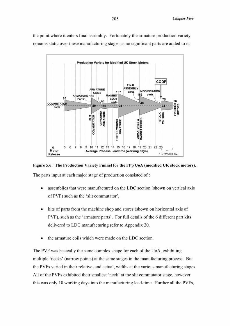
Chapter Five

205

the point where it enters final assembly. Fortunately the armature production variety

remains static over these manufacturing stages as no significant parts are added to it.

MotorRelease

0 5 6 7 8 9 10 11 12 13 14 15 16 17 18 19 20 21 22 23Average Process Leadtime (working days)

Production Variety for Modified UK Stock Motors

SLIT

CO

MM

UTA

TOR

UN

WO

UN

DAR

MAT

UR

E

TEST

ED W

OU

ND

ARM

ATU

RE

ARM

ATU

RES

&M

AGN

ET B

OD

IES

STO

CK

MO

TOR

S

ARMATURE Parts

ARMATURECOILS

MAGNETBODYparts

FINALASSEMBLY

parts

CODP

1-2 weeks av.

95

20

132

2448

24

197

48

162

24

75 56

FIN

ISH

EDM

OTO

RS

MODIFICATIONparts

COMMUTATORparts

Figure 5.6: The Production Variety Funnel for the FPp UoA (modified UK stock motors).

The parts input at each major stage of production consisted of :

• assemblies that were manufactured on the LDC section (shown on vertical axis

of PVF) such as the ‘slit commutator’,

• kits of parts from the machine shop and stores (shown on horizontal axis of

PVF), such as the ‘armature parts’. For full details of the 6 different part kits

delivered to LDC manufacturing refer to Appendix 20.

• the armature coils which were made on the LDC section.

The PVF was basically the same complex shape for each of the UoA, exhibiting

multiple ‘necks’ (narrow points) at the same stages in the manufacturing process. But

the PVFs varied in their relative, and actual, widths at the various manufacturing stages.

All of the PVFs exhibited their smallest ‘neck’ at the slit commutator stage, however

this was only 10 working days into the manufacturing lead-time. Further all the PVFs,

Chapter Five

206

except that for the modified stock UoA, were widest at the input to the final assembly of

the motor. For the ETO motors 885 distinct components were supplied to the final

assembly, to make 155 finished motor variants.

The PVF for the motors subject to FPp covered the postponed modification process.

The CODP was located at the standard UK stock motor which was the final ‘neck’ in

the PVF and was of a similar size (in terms of the number of standard motors) to the

smallest ‘neck’ at the slit commutator. In contrast the ‘neck’ in the ETO PVF at the

generic motor specification stage (indicated by the number of tested wound armature

specifications) was almost 2.5 times wider than the smallest neck at the slit commutator

stage. Further it was equal to the number of finished motors, in other words even at the

wound armature stage the motor were customised. This suggests that the modified

motor approach was not suitable for the ETO motor range.

Considering the FPp application there are 24 generic motors at the CODP and a further

51 modifying components are supplied into the postponed assembly process. However

many of these components are purchased against the customer order due to their high

variety. Therefore the number of SKUs at the CODP is less than the 56 finished motor

variants.

5.5 CASE ANALYSIS

In this section the results of the case analysis are presented: first the major flaws in this


hypotheses.

5.5.1 Removing Added Value

All modifications involved the removal of parts (as well as adding new ones) which

resulted in the removal of previously added value. Modifications commonly involved

peripheral components such as tachometers mounted on the shaft, forced vent units or

mounting brackets. The modifications required up to 4 hours. However almost half the

motors modified (25 out of 60) also required far more invasive modifications involving

changes to the magnet body components. This commonly involved a motor strip down

which could take up to 3 working days depending upon the size of the motor.

Chapter Five

207

Clearly the extent of added value removed was not insignificant and was far from ideal.

The modifications were such that the variety in the magnet bodies in the finished motors

(subject to FPp) was much greater than the number of UK standard motor variants (24) -

probably closer to the finished motor variety of 56. The armature, however, was not

subject to any modifications (following impregnation this was not possible) and its

variety remained at 24 in the finished motors.

This suggested that the CODP would be better located further up stream in the

manufacturing processes to avoid the removal of added value. A more suitable location

for the CODP would be at the balanced armature stage, but before the magnet body was

assembled. The manufacturing lead-time for the magnet body assembly and motor final

assembly was just 8 working days. Therefore it would still be possible to provide

modified standard motors on a 3 to 4 week lead-time.

This approach would have the added benefit of reducing the stock value from that of

finished standard motors to balanced armatures. Alternatively the stock levels could be

increased to improve ex-stock availability from 63% (percentage of orders for modified

stock motors which were satisfied from stock). This would be advisable because the

number of generic SKU would remain at the same level – the variety in the armatures is

the same as the variety in the finished motors. Therefore the demand variability at

generic level would remain high, so ex-stock availability would not be improved

without higher stock levels.

The improved FPp application proposed above would naturally take the postponed

motor customisation away from the S&R section (which had extremely limited

resources and was primarily tasked with service and repairs) and relocate it back in the

main LDC manufacturing section. Here the final assembly area, where motor

customisation would take place, was shown to have substantial excess capacity.


All hypotheses, except H3, were fully tested in the BC case study and the findings were

largely as predicted by the six hypotheses. However one hypothesis was challenged in

part (H5).

Chapter Five

208



The findings fully supported both hypotheses H1 and H2. The motors manufactured

under FPp were demanded in four times as many variants as the MTS motors, 56

compared to 14 variants. As a result the average demand variability at finished motor

level was higher for the FPp motors at 341% compared to 292% for those motors MTS.

The average volume demand for finished motors was lower for the motors

manufactured by the FPp approach than by MTS, 1.1 compared to 1.6 motors. The

demand analysis showed that overall the industrial LDC motors were required in

extremely high variety and relatively low volumes, resulting in very high demand

variability. A total of 347 LDC motors were ordered in 238 variants over the one-year

study period, an average of 1.5 motors per variant. Two-thirds of these motors were

manufactured as ETO motors.

As expected the average volume demand at generic level for the FPp motors was higher

than that demonstrated by the ETO motors 2.6 compared to 1.5 motors. This was

because the generic level FPp motors were recognised standard UK specification motors

demanded by multiple customers, whereas the generic level ETO motors were non-

standard motors demanded by one customer. This indicated that the 30 UK stock motor

specifications were selected for the FPp application by specification and possibly

demand volume. However, it was not possible to confirm this, because Bull Electric

made the selection prior to the relocation of LDC manufacture to BC.



Hypothesis H3 remains untested. This hypothesis pre-supposes that orders subject to

FPp and MTS do not pull from the same product stocks, however in the BC study this

was the case. Further, it was only possible to measure ex-stock availability in terms of

the proportion of orders (rather than orders and enquiries) for which the correct stock

Chapter Five

209

motor was available. Consequently this measure ignored the many enquiries which did

not translate into orders because the stock motor was not available. However, even

using this extremely lenient measure of ex-stock availability only 63% of FPp orders

could be satisfied from stock (while the remainder were modified in production). This

was because the UK motor stock levels were maintained at only 50% to 70% of target

due to their high value and unpredictable, erratic demand.

The study findings fully endorsed hypothesis H4. Demand amplification was measured

for all UoA and as expected was not detected for the ETO UoA. A degree of demand

amplification was found for the manufacture of the generic stock motors, particularly at

the balanced armature and the shipped to warehouse schedules. As expected no demand

amplification was detected for the order-driven stock modifications. These findings

support hypothesis H4 showing that applying FPp introduced a degree of demand

amplification which did not exist for the ETO approach.

The average order lead-time achieved by orders using the FPp approach was 3 weeks,

less than a quarter of that achieved by ETO orders. As expected this was in part

because much of the UK standard motor was manufactured speculatively to stock rather

than to order. This reduced the manufacturing lead-time from 7.3 to 2.5 weeks.

However dramatic reductions in both engineering and bought-in parts lead-times also

contributed to the reduction in order lead-time.

As predicted by hypothesis H4 the delivery reliability demonstrated by FPp orders was

higher than for ETO orders, 70% compared to 63% respectively. However, the

improvement in delivery reliability provided by FPp was unexpectedly modest.

There are three possible explanations:

• quoted lead-times for the modified motors (FPp) did not take into account the

availability of parts required for modifications and few of these parts were

stocked. In addition the process of acquiring parts was very laborious, since

modifications were managed outside the MRP system,

• the extremely limited nature of resources in S&R (where the majority of motor

modifications took place), coupled with the fact that S&R were primarily tasked

Chapter Five

210

with service and repairs, may have led to the unresponsive execution of

modifications.

• low standard motor stocks, providing only 63% availability for modified motor

orders, may have extended the manufacturing lead-time and reduced delivery

reliability.


Hypothesis H5 was only partially supported by the findings. As predicted by the motors

subject to FPp exhibited greater product standardisation than those ETO both in terms

of common components and the degree of commonality index. Only minor components

were found to be common across each UoA and in fact no components were common

across the ETO UoA. Overall the commonality index for the FPp UoA was three times

that for the ETO UoA and it was higher at every level in the BOM. At the lower BOM

levels this was due to the use of standard UK motors for FPp however at the level where

modifications normally took place it was simply due to the customers’ requirement for

less variety.

Contrary to hypothesis H5, all motors, regardless of inventory management policy,

exhibited the same level of modularity. The major sub-assemblies in the LDC motors

exhibited a very low degree of modularity as dictated by the basic design of the motor.

However groups of peripheral components and sub-assemblies - generally involved in

final assembly - did correspond to particular functions on a one-to-one basis, thereby

exhibiting a high degree of modularity. The majority of the stock modifications

involved only highly modular components, many of which were peripheral. However

about a quarter involved components which demonstrated a relatively low degree of

modularity and were embedded within a major sub-assembly.


The findings supported hypothesis H6. In the absence of planned downtime records the

capacity utilisation measure was used to indicate excess capacity. No capacity data was

Chapter Five

211

available for S&R where the majority of the stock modifications were carried out.

Instead the capacity utilisation measure was applied to the LDC final assembly cell,

where a third of stock modifications were performed. The design capacities of this cell

- and the subsequent motor test and spray cells - indicated that these cells had been

provided with greater capacities than preceding cells. Further they consistently

demonstrated the lowest utilisation levels over the 6 month period measured. This

suggested that it was at these ‘postponed’ processes that excess capacity was likely to

be the greatest.

As predicted by hypothesis H6 the throughput efficiency for the postponed

modifications (conducted in S&R from stock) was higher than (double) that achieved by

the stock-driven manufacture of the generic stock motors. The modifications achieved

21% throughput efficiency compared to 10% achieved by the manufacture of the

generic motors. However, the throughput efficiency achieved by the postponed

modifications was highly variable from order to order (four times more variable than for

manufacture of the generic stock motors) as the coefficient of variation of 127%

demonstrates. The main factor driving the variability in throughput efficiency was the

variety of modifications, which required anything from 10 minutes to 26 working hours.

The most striking difference between generic stock motor manufacture and the

postponed modifications was not the throughput efficiencies but the manufacturing

lead-times. Postponed modification was clearly more responsive with a manufacturing

lead-time equivalent to only 18% of that for the generic stock motors.

Production Variety Funnel: The number of SKUs at the CODP was less than the

number of finished motors demanded. However, this was only the case because many

of the components supplied into the postponed process were purchased against the

customer order due to their high variety. This supported the original conceptual model

of FPp which predicted the number of SKUs at the CODP to be less than the number of

finished items.

Chapter Five

212

5.6 CONCLUSIONS

At BC the FPp application was sustainable and provided the level of responsiveness

required by customers. However it was not an ideal application. Despite this the

hypotheses remained largely unchallenged. The customising process involved the

removal of previously added components, which suggested that the CODP would be

better located further up stream in the manufacturing process. A more suitable location

for the CODP is proposed which would still enable the required order lead-time to be

met. This approach would have the added benefit of allowing generic stock levels to be

increased to improve ex-stock availability without increasing stock value. Further the

postponed process would naturally be re-located to the main production area where

substantial excess capacity exists.

Despite the flaws in the FPp application at BC no hypotheses were challenged as a

result of anomalies in the findings. However the product modularity findings

fundamentally challenged the hypothesis. Contrary to predictions product modularity

was not related to the inventory management policy. All the motors demonstrated the

same levels of modularity.

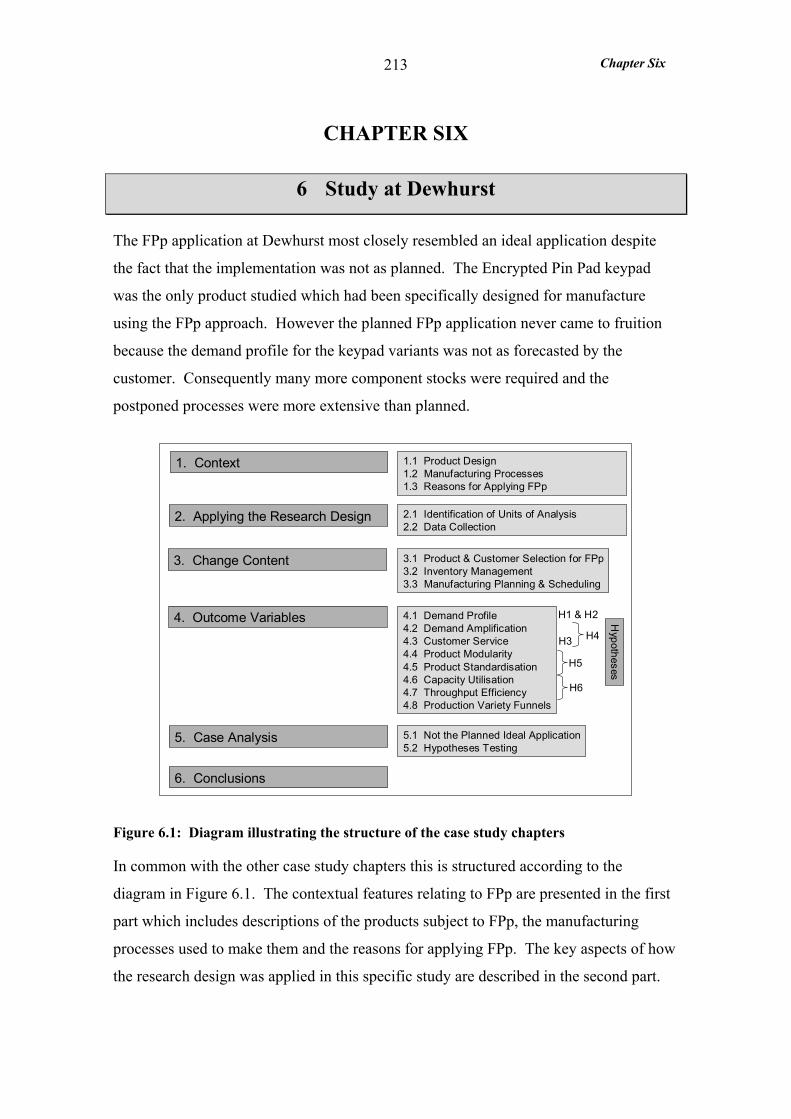
Chapter Six

213

CHAPTER SIX

6 Study at Dewhurst

The FPp application at Dewhurst most closely resembled an ideal application despite

the fact that the implementation was not as planned. The Encrypted Pin Pad keypad

was the only product studied which had been specifically designed for manufacture

using the FPp approach. However the planned FPp application never came to fruition

because the demand profile for the keypad variants was not as forecasted by the

customer. Consequently many more component stocks were required and the

postponed processes were more extensive than planned.

1. Context



5. Case Analysis

6. Conclusions




5.1 Not the Planned Ideal Application5.2 Hypotheses Testing

Hypotheses

H1 & H2

H3 H4

H5

H6








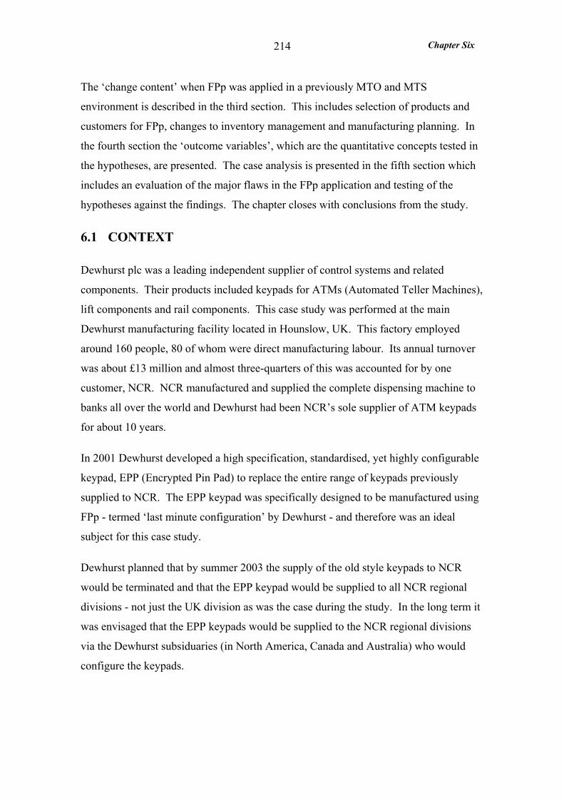
Chapter Six

214








6.1 CONTEXT

Dewhurst plc was a leading independent supplier of control systems and related

components. Their products included keypads for ATMs (Automated Teller Machines),

lift components and rail components. This case study was performed at the main

Dewhurst manufacturing facility located in Hounslow, UK. This factory employed

around 160 people, 80 of whom were direct manufacturing labour. Its annual turnover

was about £13 million and almost three-quarters of this was accounted for by one

customer, NCR. NCR manufactured and supplied the complete dispensing machine to

banks all over the world and Dewhurst had been NCR’s sole supplier of ATM keypads

for about 10 years.

In 2001 Dewhurst developed a high specification, standardised, yet highly configurable

keypad, EPP (Encrypted Pin Pad) to replace the entire range of keypads previously

supplied to NCR. The EPP keypad was specifically designed to be manufactured using

FPp - termed ‘last minute configuration’ by Dewhurst - and therefore was an ideal

subject for this case study.

Dewhurst planned that by summer 2003 the supply of the old style keypads to NCR

would be terminated and that the EPP keypad would be supplied to all NCR regional

divisions - not just the UK division as was the case during the study. In the long term it

was envisaged that the EPP keypads would be supplied to the NCR regional divisions

via the Dewhurst subsiduaries (in North America, Canada and Australia) who would

configure the keypads.

Chapter Six

215


The EPP keypad, shown in Figure 6.2 consisted of a die cast body within which was

assembled die cast keytip holders (termed keyskirts), a shim, a rubber mat, a PCB, and a

resistor assembly. The keypad was enclosed by a screw-down backplate. This stage in

the manufacturing was known as an ‘unconfigured keypad’ because the keypad had not

yet been populated by the configuration of keytips required by the specific bank. The

keytips, ten numeric and up to six function keys, were glued into the keyskirts.

Crucially the keytips were demanded in high variety which was generated by variations

in the keytip material, legend, and embossing.

Figure 6.2: Picture of the steel keytip variant of the EPP keyad.

Two other products were also studied to enable the comparison between FPp and MTO

and MTS. The MA keypad appeared very similar to the EPP keypad, as illustrated in

Figure 6.2, however there were two crucial differences. Firstly, the MA keypad was

available in 3 different layouts: the MA11 had sixteen keys like the EPP keypad; the

MA10 had twelve keys; and the MA12 had four keys. Further a special range of MA

keypads had been developed for the biggest customer Fujitsu. The implications for the

MA keypad range were that the keypad body was required in six different designs,

whereas the EPP keypad body was only required in one generic design. The second

crucial difference was in the way the keytips were secured, the MA keytips were

secured by metal studs welded to the back, whereas the EPP keytips were secured by

glue. This meant that the MA keytips had to be assembled first, whereas the

Chapter Six

216

opportunity was available to assemble the EPP keytips last, and postpone the

configuration of the keypad until a customer order had been received.

The third product studied was the lift pushbutton (PB) body. This was quite a different

product to either of the keypads, however it too required a manual assembly process.

The PB body consisted of a body moulding within which was assembled a pair of

contacts with moulded covers, illumination terminals and main power terminals. The

contacts were made up of an intricate assembly of mechanical components such as

springs, flexing arms and moulded plungers. The variety in the PB body was driven by

a number of options: the body type (switch or just indicator), whether it was to be

illuminated or not; the configuration of the pair of contacts (normally open or normally

closed); and the type of power terminals.


The flow process chart in Table 6.1 shows a summary of the manufacturing processes

required to make each of the products studied. For the full breakdown of keypad

operations refer to Appendix 21.

A number of general observations can be made about the manufacturing processes:

• the three product groups were manufactured at different work centres,

• manufacturing processes consisted of assembly operations except for the PB

body plastic components which were injection moulded,

• assembly processes were manual, and machines only employed for the gluing of

the EPP keytips and the laser marking of the plastic EPP keytips.

The production arrangement for each of the three products was different. The MA

keypads were fully assembled at individual work stations whereas the PB bodies were

assembled by a production line albeit consisting of only two people. The production

arrangement for the EPP keypads was more complex as detailed in Appendix 22.

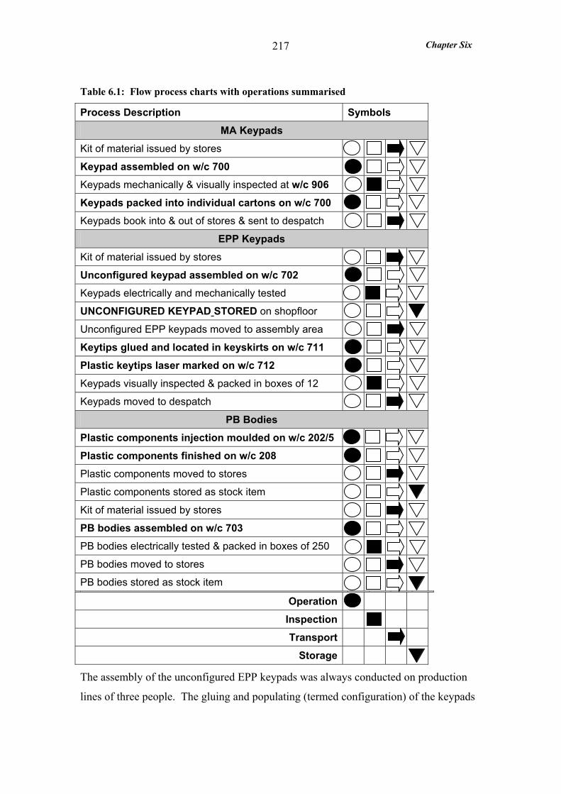
Chapter Six

217

Table 6.1: Flow process charts with operations summarised


MA Keypads

Kit of material issued by stores

Keypad assembled on w/c 700

Keypads mechanically & visually inspected at w/c 906

Keypads packed into individual cartons on w/c 700

Keypads book into & out of stores & sent to despatch

EPP Keypads


Unconfigured keypad assembled on w/c 702

Keypads electrically and mechanically tested

UNCONFIGURED KEYPAD STORED on shopfloor

Unconfigured EPP keypads moved to assembly area

Keytips glued and located in keyskirts on w/c 711

Plastic keytips laser marked on w/c 712

Keypads visually inspected & packed in boxes of 12

Keypads moved to despatch

PB Bodies

Plastic components injection moulded on w/c 202/5

Plastic components finished on w/c 208

Plastic components moved to stores

Plastic components stored as stock item


PB bodies assembled on w/c 703

PB bodies electrically tested & packed in boxes of 250

PB bodies moved to stores

PB bodies stored as stock item

Operation

Inspection

Transport

Storage

The assembly of the unconfigured EPP keypads was always conducted on production

lines of three people. The gluing and populating (termed configuration) of the keypads

Chapter Six

218

was initially conducted at individual work stations. However about 1.5 months into the

study period a gluing machine was commissioned which meant that the gluing and

populating operations had to be divided. Accordingly a configuration production line of

three people was established. Both the assembly and configuration lines employed

single piece flow and the operations were balanced to synchronise work flow.


The reasons for applying FPp (and how it was applied) was the subject of interviews

with six different informants. The informants were selected because of their close

involvement with the development of the EPP keypad and the establishment of its

manufacture. The informants were the Keypads Account Director, Works Manager,

Planning Manager, Process Engineering Manager, Design Project Leader and Materials

Manager. Each informant was asked:

Why was form postponement applied - what were the drivers?

The Keypads Account Director maintained that it was Dewhurst who (from as early as

1998) persuaded NCR that if one keypad design could be created, to replace the existing

proliferation of designs, this would have significant benefits for both companies:

‘Dewhurst sold the idea of ‘one size fits all’ to NCR over a period of time which saw increased demands on the keypad technology and the need for reduced lead-times’

Managing the different keypad models for NCR created significant problems for

Dewhurst as the Keypads Account Director explained:

‘The seven different keypad models were required in potentially hundreds of variants on a short lead-time. Not only did this drive component inventories to a very high level, but it proved complex to manage.’

The keypads were MTO, but to reliably meet the lead-times demanded by NCR, it was

necessary to maintain stocks of all the keypad components. The problem of high

component inventory was compounded by NCR’s requirement of increased

responsiveness. This formed part of NCR’s effort to offer reduced lead-times to their

ATM customers - the banks. In 1998 Dewhurst were supplying the keypads on a 10 day

lead-time. However this was halved to 5 days by the middle of 2001.

Chapter Six

219

Dewhurst argued that a ‘one-size fits all’ approach would allow the number of different

components (and their associated inventories) to be radically reduced. More importantly

to NCR it would enable ‘last minute configuration’ and potentially an even more

responsive supply.

From NCR’s point of view there were a number of converging factors that persuaded

them that the standardised EPP keypad was of benefit. Firstly, they required a more

responsive supply of keypads as discussed. Secondly, there was pressure in the ATM

market for significant improvements in keypad technology, which meant that NCR

would be forced to redesign their range of keypads. The required technology

improvements included a change in cryptographic requirements driven by Visa, where

the cryptographic module processes the PIN number. Further more stringent security

standards had been set by ZKA a German organisation that regulates security on

keypads.

Summary: the key drivers for applying FPp to the manufacture of the EPP keypad were

to improve responsiveness while reducing the high component inventory levels

associated with the MTO of multiple keypad designs. Responsiveness was improved

from the minimum standard lead-time of 5 working days to an average order lead-time

of 3 working days. This was, in spite of the fact, that the FPp application was not as

originally intended and required more customer order driven processes as later

described in section 6.5.1.



collection at Dewhurst are addressed in this section.


Similarly to the previous studies each unit of analysis (UoA) was based around a

product group subject to a particular inventory management policy (FPp, MTO or

MTS). In contrast to the previous two case studies, an entire product group was

manufactured using FPp at Dewhurst, therefore it was necessary to select three different

product groups for the UoAs.

Chapter Six

220

All EPP keypads manufactured by Dewhurst for NCR were subject to FPp. Dewhurst

manufactured unconfigured keypads (and associated keytips) speculatively to stock, and

subsequently populated the keypads with keytips to specific customer orders. As

discussed in the context section the keypads supplied to NCR accounted for three-

quarters of Dewhurst’s turnover and were scheduled to replace the existing range of

NCR keypads. Understandably this made the EPP keypad a very significant and

important product for Dewhurst, and an ideal product group for the FPp UoA.

Ideally the product groups selected for the three UoAs should be as similar as possible

in terms of general design and manufacturing processes. This ensures that the

comparison between the different inventory management policies (FPp, MTO and

MTS) screens out product specific factors. Therefore the MA keypad range was chosen

for the MTO UoA. This range had a very similar design to the EPP keypad, but differed

in that it was developed and manufactured by Dewhurst for sale to a variety of

customers. The MA keypad was highly configurable and also used in ATMs, as well as

other applications such as access systems.

Unfortunately no keypads were made-to-stock (MTS). The closest product, in terms of

manufacturing processes (which was produced in sufficient volumes) was the body

component for the ‘Compact 2’ range of lift pushbuttons (PB). The PB body

component was MTS by Dewhurst in a number of variants and was chosen for the MTS

UoA.

The keytips for both MA and EPP keypads, although of a slightly different design, were

manufactured to Kanban stocks using the same manufacturing processes. It was

decided therefore, that keytip manufacture should be ruled outside the scope of the

study and keytips treated as an outside component supply to the manufacture of the two

keypads.

Each PB body incorporated around four different plastic components injection moulded

to stock by Dewhurst. The manufacture of these components was included in the study

because their manufacture was part of the stock-driven processing of the PB bodies.

Chapter Six

221

Each UoA was based around one of the three product groups selected and included the

respective customer orders due for delivery within a certain time period. Considering

the appropriate time period, the EPP keypad was developed in 2001 and first supplied to

NCR in May 2002. However the keypad specification continued to be subject to minor

changes by NCR until the beginning of September 2002 - this disrupted the supply of

materials. Further, the stocks of unconfigured keypads were not established until the

end of September 2002. Therefore, it was appropriate that the study period should

begin on 1st October 2002, when the FPp approach to the manufacture of the EPP

keypads was established and stable. Given the high volumes of orders for the EPP

keypad it was determined that four months would be a sufficient time period for the

study.

Table 6.2: Unit of analysis orders due for despatch between 01/10/02 and 31/01/03

Product Group Orders Volume

EPP (FPp) 598

(56% steel)

26890 units

(24% steel)

MA Keypads (MTO) 45 1154 units

PB bodies (MTS) 89 44035 units

Table 6.2 shows the orders and volume of products due between 1st October 2002 and

31st January 2003. The lowest number of orders due was for the MA keypads, however

it was judged that 45 orders provided sufficient data for the customer service measures.


In order to study a sufficient number of customer orders it was necessary to study a

four-month period as argued during the identification of the UoA. In view of the ready

availability of historic data it was decided to conduct a retrospective study. The

majority of the data was collected for the four-month period between 1st October ’02

and 31st January ‘03.

A retrospective study can raise questions regarding the reliability of the data. Interview

data naturally required support from documentary and/or database evidence, and

fortunately all the interviewees were not only still employed at the factory, but in the

same roles, as for the study period. This meant that all the informants had first hand

experience and knowledge of the time period in question.

Chapter Six

222

A particularly productive source of evidence for demand profile, customer service and

product design measures was the fully integrated MRPII system, MAPICS. Several

modules had been implemented, including the main inventory management module

around which various other modules operated: the bill of material module; the material

purchasing module; the customer order module; the manufacturing order module; and

the capacity planning module. Within the manufacturing order module the shop tools

module interfaced with PMCS (described in section 6.3.3) and updated MAPICS minute

by minute with job progress data.

With regards to reliability the data retrieved from MAPICS was no less reliable or

accessible during the study than when it was generated. However, the retrospective

nature of the study meant that data was not available to measure ex-stock availability in

terms of the proportion of enquiries for which the correct product was available.

However, a stock level history was available providing an indication of this measure for

both the EPP keypads subject to FPp and the PB bodies sold direct ex-stock.



6.3 CHANGE CONTENT






selected for FPp was the subject of interviews with six different informants (previously

listed in section 6.1.3). The two questions asked of all informants, and their collective

answers, are presented below:

Chapter Six

223

Was the ‘last minute configuration’ (FPp) approach limited to certain

customers, and if so why?

Yes, FPp was limited to NCR because the EPP keypad - manufactured using the FPp

approach - was exclusively designed and produced for NCR.

Was the ‘last minute configuration’ (FPp) approach limited to certain product

specifications, and if so why?

Yes, FPp was limited to the EPP keypad and was not applied to Dewhurst’s MA keypad

range because the MA keypad design did not permit ‘last minute configuration’. Both

MA and EPP keypad variety was generated by keytip configurations and the keypad

body was relatively standardised.

The crucial difference between the EPP and the MA keypads was in their construction.

The MA keytips were secured in position by metal studs welded to the back of the

keytips, rather than glue or clips used for the EPP keytips. This necessitated that the

MA keytips be assembled first, ruling out the possibility of ‘last minute configuration’

because configuring the keytips was the first operation. Conversely the EPP keytips

could be glued or clipped into the keyskirts during the final operation after the keypad

body had been assembled.

Although all EPP keypads were selected for FPp, it could only be applied to a

predefined list of finished keypad part numbers. This was because the manufacture of

the keytips required numerous distinct processes therefore a long lead-time (steel

keytips) or a high batch quantity. Therefore only keypads using the keytips stocked in

Kanbans could be offered on a short lead-time.



stocks, including keypad keytips, unconfigured EPP keypads and finished PB bodies.

Also considered in this section - and inherent in the inventory management approach -

is the Customer Order Decoupling Point (CODP) location.

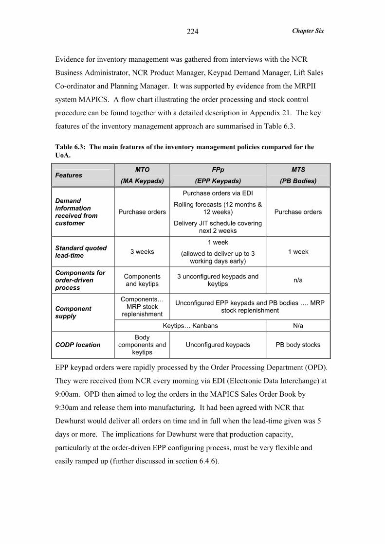
Chapter Six

224

Evidence for inventory management was gathered from interviews with the NCR

Business Administrator, NCR Product Manager, Keypad Demand Manager, Lift Sales

Co-ordinator and Planning Manager. It was supported by evidence from the MRPII

system MAPICS. A flow chart illustrating the order processing and stock control

procedure can be found together with a detailed description in Appendix 21. The key

features of the inventory management approach are summarised in Table 6.3.

Table 6.3: The main features of the inventory management policies compared for the UoA.

Features MTO

(MA Keypads) FPp

(EPP Keypads) MTS

(PB Bodies)

Demand information received from customer

Purchase orders

Purchase orders via EDI

Rolling forecasts (12 months & 12 weeks)

Delivery JIT schedule covering next 2 weeks

Purchase orders

Standard quoted lead-time 3 weeks

1 week

(allowed to deliver up to 3 working days early)

1 week

Components for order-driven process

Components and keytips

3 unconfigured keypads and keytips n/a

Components… MRP stock

replenishment

Unconfigured EPP keypads and PB bodies …. MRP stock replenishment Component

supply Keytips… Kanbans N/a

CODP location Body

components and keytips

Unconfigured keypads PB body stocks

EPP keypad orders were rapidly processed by the Order Processing Department (OPD).

They were received from NCR every morning via EDI (Electronic Data Interchange) at

9:00am. OPD then aimed to log the orders in the MAPICS Sales Order Book by

9:30am and release them into manufacturing. It had been agreed with NCR that

Dewhurst would deliver all orders on time and in full when the lead-time given was 5

days or more. The implications for Dewhurst were that production capacity,

particularly at the order-driven EPP configuring process, must be very flexible and

easily ramped up (further discussed in section 6.4.6).

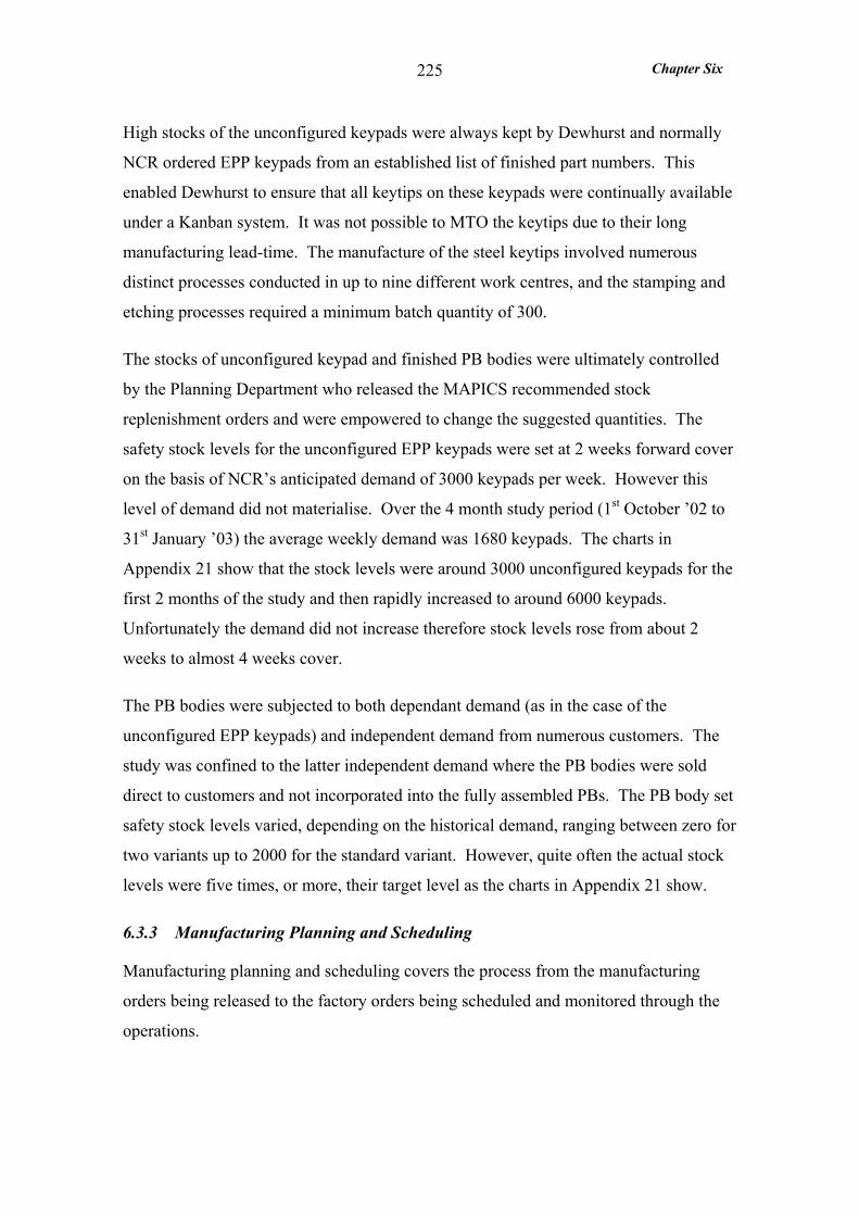
Chapter Six

225

High stocks of the unconfigured keypads were always kept by Dewhurst and normally

NCR ordered EPP keypads from an established list of finished part numbers. This

enabled Dewhurst to ensure that all keytips on these keypads were continually available

under a Kanban system. It was not possible to MTO the keytips due to their long

manufacturing lead-time. The manufacture of the steel keytips involved numerous

distinct processes conducted in up to nine different work centres, and the stamping and

etching processes required a minimum batch quantity of 300.

The stocks of unconfigured keypad and finished PB bodies were ultimately controlled

by the Planning Department who released the MAPICS recommended stock

replenishment orders and were empowered to change the suggested quantities. The

safety stock levels for the unconfigured EPP keypads were set at 2 weeks forward cover

on the basis of NCR’s anticipated demand of 3000 keypads per week. However this

level of demand did not materialise. Over the 4 month study period (1st October ’02 to

31st January ’03) the average weekly demand was 1680 keypads. The charts in

Appendix 21 show that the stock levels were around 3000 unconfigured keypads for the

first 2 months of the study and then rapidly increased to around 6000 keypads.

Unfortunately the demand did not increase therefore stock levels rose from about 2

weeks to almost 4 weeks cover.

The PB bodies were subjected to both dependant demand (as in the case of the

unconfigured EPP keypads) and independent demand from numerous customers. The

study was confined to the latter independent demand where the PB bodies were sold

direct to customers and not incorporated into the fully assembled PBs. The PB body set

safety stock levels varied, depending on the historical demand, ranging between zero for

two variants up to 2000 for the standard variant. However, quite often the actual stock

levels were five times, or more, their target level as the charts in Appendix 21 show.


Manufacturing planning and scheduling covers the process from the manufacturing

orders being released to the factory orders being scheduled and monitored through the

operations.

Chapter Six

226

Evidence for manufacturing planning and scheduling was gathered from interviews with

the NCR Business Administrator, NCR Product Manager, Keypad Demand Manager,

Lift Sales Co-ordinator and Planning Manager. It was supported by evidence from the

MAPICS MRPII system.

A flow chart illustrating the manufacturing planning and scheduling process, together

with a detailed description, can be found in Appendix 21 and a summary of the main

features is presented in Table 6.4. Manufacturing orders for order driven production of

the finished MA and EPP keypads were raised by OPD and automatically released.

Prior to this - in the case of MA keypads - OPD checked material and capacity

availability to ensure the lead-time could be met. However both material and

production capacity were assumed to be available for the configuration of the EPP

keypads.

Table 6.4: Main features of manufacturing planning compared for stock replenishment orders, MTO and FPp.

Features Stock

Replenishment Orders

MTO (MA Keypads)

FPp (EPP Keypads)

Manufacturing orders

Processed by MRP system driven by one

week period MPS

Processed by MRP system

By-passed MRP system

Customer orders entered onto SOB n/a Any time Daily 9:00am

Release manufacturing orders to shopfloor

Weekly by Planning Manager

3 times daily automatically

Daily at 10:30am manually

Order processing and manufacturing planning lead-time

1 week 11 working hours

(average measured) 1.5 working hours

No stock replenishment manufacturing orders (including those for generic EPP

keypads) were automatically released instead the MRP system made recommendations

and the Planning Manager released orders into the factory. Available capacity was

determined by a Work Centre Load Analysis generated by MAPICS. However the

Planning Manager only intervened when there was a significant change in a work centre

overload. Effectively production planning assumed the availability of infinite capacity.

Chapter Six

227

Released manufacturing orders were downloaded three times daily from MAPICS to

PMCS (Production Monitoring and Control System) with the exception of finished EPP

keypad orders which are discussed later in this section. For MA keypad orders this

ensured an average delay of 4 hours, and a worst case delay of 8 hours, between the

manufacturing order being created by OPD and being available on PMCS for

manufacturing. PMCS was a shop-floor computerised system which monitored job

progress using an operation booking system. It provided each work centre with a ‘load

sheet’ listing jobs in due date order. The Operators were able to view the load sheet and

normally processed the jobs in the sequence recommended.

Finished EPP keypad manufacturing orders, once created by OPD, by-passed the MRP

system and PMCS to ensure a rapid response from production. Hard copies of the EPP

keypad manufacturing orders were passed to the Keypad Demand Manager checked and

delivered to Production typically by 10.30am - only 1.5 hours after the customer orders

were sent via EDI to Dewhurst. Once in production the EPP orders were immediately

kitted and then processed in due date order according to the Sales Order Book.

Summary: in general the manufacturing planning and scheduling system at Dewhurst

was very responsive. The MRP system was run on a nightly basis and released

manufacturing orders were downloaded 3 times each day to PMCS which automatically

scheduled jobs in due date order. Nevertheless the finished EPP keypad manufacturing

orders were given special treatment and by-passed the MRP system and PMCS to

ensure a rapid response from production.










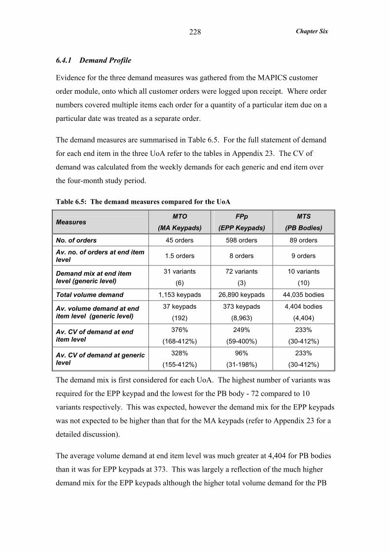
Chapter Six

228


Evidence for the three demand measures was gathered from the MAPICS customer

order module, onto which all customer orders were logged upon receipt. Where order

numbers covered multiple items each order for a quantity of a particular item due on a

particular date was treated as a separate order.

The demand measures are summarised in Table 6.5. For the full statement of demand

for each end item in the three UoA refer to the tables in Appendix 23. The CV of

demand was calculated from the weekly demands for each generic and end item over

the four-month study period.

Table 6.5: The demand measures compared for the UoA

Measures MTO

(MA Keypads) FPp

(EPP Keypads) MTS

(PB Bodies)

No. of orders 45 orders 598 orders 89 orders

Av. no. of orders at end item level 1.5 orders 8 orders 9 orders


31 variants

(6)

72 variants

(3)

10 variants

(10)

Total volume demand 1,153 keypads 26,890 keypads 44,035 bodies

Av. volume demand at end item level (generic level)

37 keypads

(192)

373 keypads

(8,963)

4,404 bodies

(4,404)

Av. CV of demand at end item level

376%

(168-412%)

249%

(59-400%)

233%

(30-412%)

Av. CV of demand at generic level

328%

(155-412%)

96%

(31-198%)

233%

(30-412%)

The demand mix is first considered for each UoA. The highest number of variants was

required for the EPP keypad and the lowest for the PB body - 72 compared to 10

variants respectively. This was expected, however the demand mix for the EPP keypads

was not expected to be higher than that for the MA keypads (refer to Appendix 23 for a

detailed discussion).

The average volume demand at end item level was much greater at 4,404 for PB bodies

than it was for EPP keypads at 373. This was largely a reflection of the much higher

demand mix for the EPP keypads although the higher total volume demand for the PB

Chapter Six

229

bodies will also have made a small contribution to this difference. The average volume

demand at generic level was much higher for the EPP keypads than for the MA

keypads. This was due to two factors:

• EPP keypads were demanded in much higher volumes overall,

• the number of MA generic keypads was double that for the EPP keypads.

Further, it should be considered that in the case of the MA keypads the generic keypad

bodies (e.g. MA10, MA11, MA12) did not physically exist at any stage in the

manufacturing process.

Surprisingly the demand variability (CV of demand) at end item level was not much

lower for the PB bodies than for the EPP keypads - only 233% compared to 249%

respectively. The explanation for this was related to the number of orders at end item

level – about nine on average for both the EPP keypads and the PB bodies. In fact half

of the ten stocked PB bodies were only subject to one or two orders over the study

period and therefore exhibited a very high CV of demand, in excess of 300%. If these

PB bodies were excluded, demand variability dropped to 97%.

The demand variability for EPP keypads was dramatically reduced when taken at the

unconfigured, or generic, keypad level - 96% compared to 249% at the finished keypad

level. So clearly keeping stocks at the generic level should have permitted the provision

of a much lower safety stock than stocking at the finished item level.

Summary: as expected the demand mix was higher for the EPP keypads than for the PB

bodies - 72 compared to 10 variants respectively. The average volume demand at end

item level was much greater at 4,404 for PB bodies than it was for EPP keypads at 373.

This was largely because the demand mix for the EPP keypads was much higher. The

average volume demand at generic level was much higher for the EPP keypads than for

the MA keypads. Surprisingly the demand variability at end item level was not much

lower for the PB bodies than for the EPP keypads, 233% compared to 249%

respectively.

Chapter Six

230


The demand data, in terms of the promised due dates and quantities, presented in the

previous section was used to measure the demand imposed on the manufacturing

system. The manufacturing orders would have provided a very similar demand plot to

the process schedules because manufacturing orders, covering only one operation, were

scheduled in due date order, and each order was manufactured continuously until

completed. Consequently it was decided to plot the process schedules only, since they

reflected more closely the timing of demand on the particular manufacturing process.

The manufacturing process schedules were available to the operator at each work centre

on PMCS (refer to Appendix 21 for details). The operator ‘booked on’ jobs as they

were started and ‘booked off’ jobs as they were completed. Unfortunately the work

centre schedules were not retrospectively available on PMCS, however the ‘booking’

dates were available. The ‘booking on’ dates were used because they accurately reflect

the scheduled sequence and timing of jobs at each process and therefore any batching

which may have occurred.

The demand amplification charts for the EPP keypads and MA keypads are shown in

Appendix 24. The plots in each chart span the same weekly time buckets and use the

same scale so the relative amplitude of demand can be easily compared. Separate charts

were plotted for the plastic and steel EPP keypads since three times as many plastic

keypads were demanded as steel keypads. This may have resulted in the pattern of

replenishment of the unconfigured keypad stocks being quite different. Each chart

showed the weekly demand for the EPP keypads, the keypad configuring schedule and

the unconfigured keypad assembly schedule. Demand amplification was not evident in

either of the charts for the EPP keypads when measured at a weekly level. The peaks in

demand were similar in amplitude to the peaks in the process schedules.

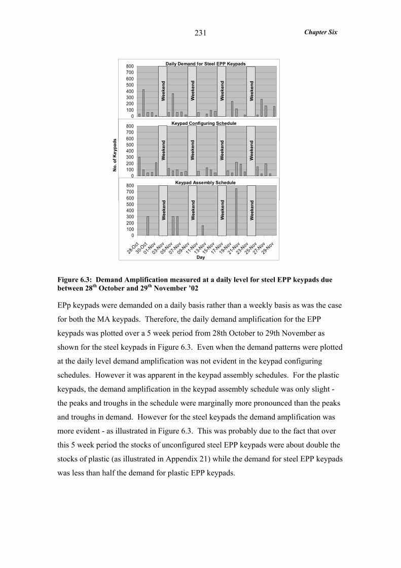
Chapter Six

231

0100200300400500600700800

28-Oct

30-Oct

01-Nov

03-Nov

05-Nov

07-Nov

09-Nov

11-Nov

13-Nov

15-Nov

17-Nov

19-Nov

21-Nov

23-Nov

25-Nov

27-Nov

29-Nov

0100200300400500600700800

28-Oct

30-Oct

01-Nov

03-Nov

05-Nov

07-Nov

09-Nov

11-Nov

13-Nov

15-Nov

17-Nov

19-Nov

21-Nov

23-Nov

25-Nov

27-Nov

29-Nov

Daily Demand for Steel EPP Keypads

Keypad Assembly Schedule

No.

of K

eypa

ds

Keypad Configuring Schedule

0100200300400500600700800

28-Oct

30-Oct

01-Nov

03-Nov

05-Nov

07-Nov

09-Nov

11-Nov

13-Nov

15-Nov

17-Nov

19-Nov

21-Nov

23-Nov

25-Nov

27-Nov

29-Nov


Day

Wee

kend

Wee

kend

Wee

kend

Wee

kend

Wee

kend

Wee

kend

Wee

kend

Wee

kend

Wee

kend

Wee

kend

Wee

kend

Wee

kend

Figure 6.3: Demand Amplification measured at a daily level for steel EPP keypads due between 28th October and 29th November ’02

EPp keypads were demanded on a daily basis rather than a weekly basis as was the case

for both the MA keypads. Therefore, the daily demand amplification for the EPP

keypads was plotted over a 5 week period from 28th October to 29th November as

shown for the steel keypads in Figure 6.3. Even when the demand patterns were plotted

at the daily level demand amplification was not evident in the keypad configuring

schedules. However it was apparent in the keypad assembly schedules. For the plastic

keypads, the demand amplification in the keypad assembly schedule was only slight -

the peaks and troughs in the schedule were marginally more pronounced than the peaks

and troughs in demand. However for the steel keypads the demand amplification was

more evident - as illustrated in Figure 6.3. This was probably due to the fact that over

this 5 week period the stocks of unconfigured steel EPP keypads were about double the

stocks of plastic (as illustrated in Appendix 21) while the demand for steel EPP keypads

was less than half the demand for plastic EPP keypads.

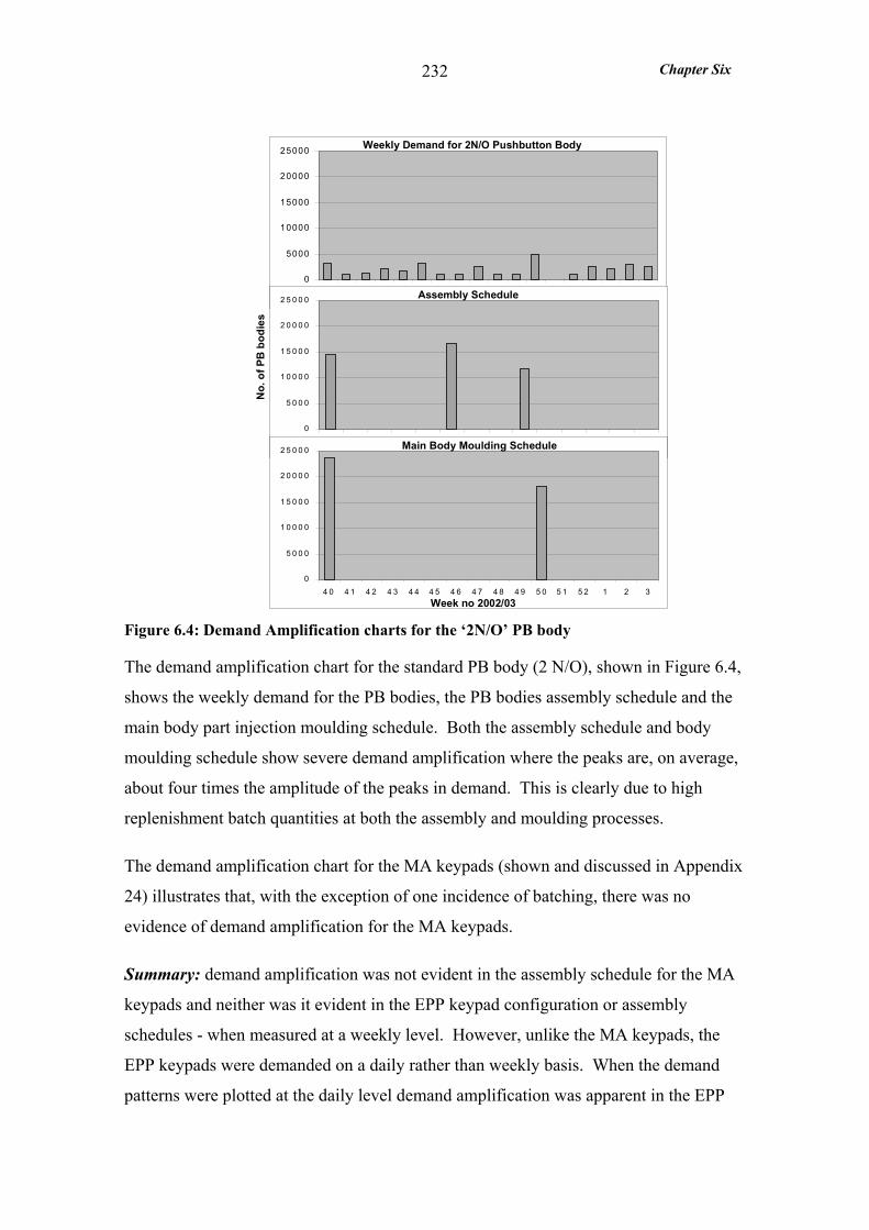
Chapter Six

232

Figure 6.4: Demand Amplification charts for the ‘2N/O’ PB body

The demand amplification chart for the standard PB body (2 N/O), shown in Figure 6.4,

shows the weekly demand for the PB bodies, the PB bodies assembly schedule and the

main body part injection moulding schedule. Both the assembly schedule and body

moulding schedule show severe demand amplification where the peaks are, on average,

about four times the amplitude of the peaks in demand. This is clearly due to high

replenishment batch quantities at both the assembly and moulding processes.

The demand amplification chart for the MA keypads (shown and discussed in Appendix

24) illustrates that, with the exception of one incidence of batching, there was no

evidence of demand amplification for the MA keypads.

Summary: demand amplification was not evident in the assembly schedule for the MA

keypads and neither was it evident in the EPP keypad configuration or assembly

schedules - when measured at a weekly level. However, unlike the MA keypads, the

EPP keypads were demanded on a daily rather than weekly basis. When the demand

patterns were plotted at the daily level demand amplification was apparent in the EPP

0

5000

10000

15000

20000

25000

40 41 42 43 44 45 46 47 48 49 50 51 52 1 2 3 4 5

0

5 0 0 0

1 0 0 0 0

1 5 0 0 0

2 0 0 0 0

2 5 0 0 0

4 0 4 1 4 2 4 3 4 4 4 5 4 6 4 7 4 8 4 9 5 0 5 1 5 2 1

0

5 0 0 0

1 0 0 0 0

1 5 0 0 0

2 0 0 0 0

2 5 0 0 0

4 0 4 1 4 2 4 3 4 4 4 5 4 6 4 7 4 8 4 9 5 0 5 1 5 2 1 2 3

Weekly Demand for 2N/O Pushbutton Body

Assembly Schedule

Main Body Moulding Schedule

No.

of P

B b

odie

s

Week no 2002/03

Chapter Six

233

keypad assembly schedules particularly for the steel keypads. Severe demand

amplification was evident in both the assembly schedule and body moulding schedule

for the PB bodies.



performance and ex-stock availability. Unfortunately, data were unavailable to measure

ex-stock availability in terms of the proportion of initial enquiries and orders for which

the correct stock item was available. Therefore stock records (plotted in Appendix 21)

for both the unconfigured EPP keypads and the PB bodies were used to indicate ex-

stock availability. Data for the EPP keypad stock levels were sourced from the EPP

Production Supervisor who recorded stock levels each morning and the PB body stock

records were sourced from the MAPICS Transaction History module.

The unconfigured EPP keypad stock levels varied between 0.5 and 6.2 weeks forward

cover (on the basis of the average demand over the study period) and no stock outs were

recorded. Further it was known that there were no enquiries only firm orders with a

non-negotiable lead-time and that the delivery performance on these orders was

extremely high, 98% on time in full. Therefore, it was fair to assume that ex-stock

availability for the unconfigured keypads was no less than 98%.

Stock outs were recorded for three of the PB bodies and this alone reduced delivery

reliability to 94%. Three PB body orders were delivered short and an analysis of the

stock levels suggests that in all 3 cases this was due to insufficient stocks being

available. Also 6 orders were delivered late and in two cases this appears to have been

due to stock outs. Further, in addition to orders, PB bodies were subject to enquiries for

which the ex-stock availability was not recorded. Therefore it was fair to conclude that

the ex-stock availability for the PB bodies was at best 94% and therefore lower than for

the EPP unconfigured keypads.

Neither order lead-time nor delivery reliability to the customer were measured by

Dewhurst during the study period. However NCR measured the delivery performance

of the EPP keypads and according to the Keypads Account Director a late delivery was

an ‘event’. Also it was extremely rare for MA keypads to be delivered late because in

Chapter Six

234

the words of the NCR Business Administrator ‘a safety margin is normally allowed

when specifying the due-to-be-delivered date’. Finally the PB bodies were despatched

ex-stock so delivery performance should not have been an issue.

Table 6.6: The order lead-time and delivery reliability measures for all UoA.

Measure MTO

(MA Keypads) FPp

(EPP Keypads) MTS

(PB Bodies)


Standard quoted lead-time 3 wks 1 wk (5 wkg days) 1 wk

Order Lead-time

Av. Promised order lead-time 3.8 wks

1.2 wks

(6 wkg days)

12.6 wks

(2.8wks excl. Dupar)

Av. Actual order lead-time 2.8 wks

0.6 wks

(3 wkg days)

11.4 wks

(2 wks excl. Dupar)

Av. Leadtime prior to factory order release 7 hours 0.5 hours N/a


OTIF (full order delivered by due date) 36 (80%) 586 (98%) 80 (90%)

OT (part of order delivered by due date) 37 (82%) 590 (99%) 83 (93%)

IF (full order delivered) 44 (98%) 594 (99%) 86 (97%)

To determine the order lead-time and delivery reliability measures both promised and

actual ex-works dates were required. Ex-works dates rather than delivery-to-the-

customer dates were used because all Dewhurst’s customers were responsible for

arranging transport of the goods from the Dewhurst factory. Therefore Dewhursts

responsibility ended upon despatch of the order. The promised and actual order lead-

times were measured from receipt of the customer order to promised and actual ex-

works dates respectively. The evidence for all dates was gathered from the MAPICS

Customer Order Module.

The order lead-time and delivery reliability measures for each UoA are presented in

Table 6.6. The standard quoted lead-time for the EPP keypads was 5 working days

equivalent to 1 week, however the average promised lead-time was 1.2 weeks. The

Chapter Six

235

promised lead-time for EPP keypads was always what the customer (NCR) requested.

This suggested that, on average, NCR did not require a lead-time as short as 1 week.

Further, the actual order lead-time achieved was only 0.6 weeks, equivalent to 3

working days, demonstrating that Dewhurst were delivering keypads to NCR with

double the responsiveness requested by them.

As expected the order lead-time achieved for the EPP keypads was only about one fifth

of that achieved for the MA keypads. This was in part due to the different approach to

manufacturing but also to the more responsive approach to order processing and

manufacturing planning used for the EPP keypads (as explained in sections 6.3.2 and

6.3.3). On average MA keypad orders required 7 hours in Order Processing before the

manufacturing orders were released, whereas EPP keypads orders only required 0.5

hour. Further, released MA keypad manufacturing orders were downloaded three times

each day to PMCS which ensured an average delay of 4 hours between order release by

OPD and availability for manufacturing. Released EPP keypad manufacturing orders

by-passed PMCS to ensure a rapid response from production. Hard copies of the EPP

manufacturing orders were passed to Production, via the Keypad Demand Manager,

typically by 10.30am - only 1 hour after the manufacturing order was released.

The actual order lead-times for the PB bodies supplied ex-stock was 11.4 weeks, against

a standard quoted lead-time of 1 week. This was, at least in part, explained by the fact

that two thirds of the orders were for Dupar (the Dewhurst Canadian subsidiary) who

requested an 18 week lead-time on average. Excluding Dupar orders reduces the lead-

time to 2 weeks still significantly longer than the lead-times for the EPP keypad.

Delivery reliability was very high for the EPP keypads, 98% of orders were delivered

On Time In Full. Only 4 out of the 598 orders were delivered short and 8 orders

delivered late. The high delivery reliability was no doubt due to high ex-stock

availability of the unconfigured keypad (and the keytips) together with the highly

responsive approach to order processing, manufacturing planning and keypad

configuration. As expected delivery performance for the MA keypads was lower at

80%. Only 1 order out of 45 orders was delivered short however 8 orders were

delivered late. The most likely explanation for this poor delivery reliability lay in the

extremely high demand variability for the MA keypads far higher than for the finished

Chapter Six

236

EPP keypads – 376% compared with 249%%. This resulted in highly variable demand

on the MA keypad assembly cell as the capacity utilisation measure demonstrates (refer

to section 6.4.6). Although the average utilisation is low at 27% this assumes the

maximum labour level of 2 men was always available. However in practice it was

probably only occasionally that 2 men worked at this cell simultaneously. Therefore the

capacity utilisation figures for the MA keypad cell were probably much higher (almost

double) but as variable as the graph in Appendix 27 indicates.

Summary: ex-stock availability as indicated by stock records was higher for EPP

keypads than for PB bodies. As expected the order lead-time achieved for the EPP

keypads was only one fifth of that achieved for the MA keypads. Further, the actual

order lead-time achieved for EPP keypads was only 0.6 weeks, on average double the

responsiveness requested on a day to day basis by NCR, the EPP keypad customer.


On Time In Full and as expected the delivery performance for the MA keypads was

lower at 80%.


The relative degree of modularity exhibited by the three products studied was assessed

using evidence gathered from interviews with the Design Project Leader, the Process

Engineering Manager and a Process Engineer. This interview evidence was

corroborated by the indented BOMs, which were extracted from the MAPICS MRP

system. Simplified versions of the indented BOMs are illustrated in Figure 6.5.

The relationship between the functional architecture and the physical architecture of

both the EPP and MA keypads was quite transparent. The keytips performed a

particular function therefore each keytip was a module - available in many variants

which could be combined to provide numerous keypad configurations (or layouts).

Also there were no incidental interactions between the keytips therefore the keytips

were highly modular.

Behind the keys the keypad body displayed a lesser degree of modularity with a number

of components providing the electronic keypad functionality and the mechanism for the

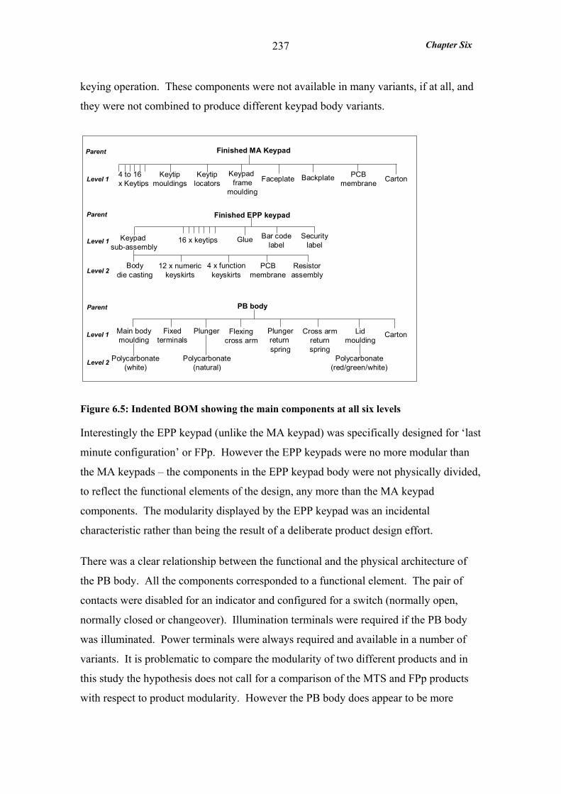
Chapter Six

237

keying operation. These components were not available in many variants, if at all, and

they were not combined to produce different keypad body variants.

Parent

Level 1

Parent

Level 1

Level 2

Parent

Level 1

Finished MA Keypad

Level 2

4 to 16x Keytips

Keytipmouldings

Keytiplocators

Keypad frame

moulding

Faceplate Backplate PCBmembrane Carton

Finished EPP keypad

Keypad sub-assembly

Bodydie casting

12 x numerickeyskirts

4 x functionkeyskirts

PCBmembrane

Resistorassembly

16 x keytips Glue Bar codelabel

Securitylabel

PB body

Main bodymoulding

Fixedterminals

Plunger Flexingcross arm

Plungerreturn spring

Cross armreturnspring

Lidmoulding

Carton

Polycarbonate(white)

Polycarbonate(natural)

Polycarbonate(red/green/white)

Figure 6.5: Indented BOM showing the main components at all six levels

Interestingly the EPP keypad (unlike the MA keypad) was specifically designed for ‘last

minute configuration’ or FPp. However the EPP keypads were no more modular than

the MA keypads – the components in the EPP keypad body were not physically divided,

to reflect the functional elements of the design, any more than the MA keypad

components. The modularity displayed by the EPP keypad was an incidental

characteristic rather than being the result of a deliberate product design effort.

There was a clear relationship between the functional and the physical architecture of

the PB body. All the components corresponded to a functional element. The pair of

contacts were disabled for an indicator and configured for a switch (normally open,

normally closed or changeover). Illumination terminals were required if the PB body

was illuminated. Power terminals were always required and available in a number of

variants. It is problematic to compare the modularity of two different products and in

this study the hypothesis does not call for a comparison of the MTS and FPp products

with respect to product modularity. However the PB body does appear to be more

Chapter Six

238

modular than the EPP keypad since each component corresponds to a functional

element.

The type of modularity exhibited by the EPP keypads was ‘component swapping’

modularity (Pine, 1993). Different components, in this case keytips, were paired with

the same basic product, an unconfigured keypad, to produce variety in the finished

product.

Summary: The EPP keypads and MA keypads exhibited the same degree of

modularity. Each keytip performed a particular function and there were no incidental

interactions between them therefore the keytips were highly modular. The EPP and MA

keypad bodies displayed a lesser degree of modularity with a number of components

providing the electronic keypad functionality and the mechanism for the keying

operation. Interestingly although the EPP keypad (unlike the MA keypad) was

specifically designed for ‘last minute configuration’ (or FPp) its modularity was an

incidental characteristic rather than being the result of a deliberate design effort.




The full indented BOMs (sourced from the MAPICS BOM module) were analysed for

products within each of the UoA (refer to Appendix 25 for a full list of analysed parts).

In accordance with the scope of the study both the EPP and MA keytip components

were excluded from this analysis. Unfortunately the BOMs for 6 MA keypad variants

were not available because they were classed as ‘specials’ and used configurable

BOMs. ‘Specials’ were MA keypads which used standard keypad bodies, but were

subject to one small order. Therefore their exclusion from this analysis had only a

minor impact on the product standardisation measures.

The product standardisation measures are summarised in Table 6.7. The number of end

items for each UoA was the number of variants subject to demand during the study

period, or the demand mix. The number of distinct components in each end item was

very similar for the two keypads (around 30 components). However the PB body

contained, on average, 13 distinct components.

Chapter Six

239

Only the polycarbonate for the main body moulding was common to all 10 variants of

the PB bodies. Similarly only the keytip moulding body component was common to all

31 variants of the MA keypads. In contrast 14 of the EPP keypad components were

common to all the variants (all body components). In fact the only EPP keypad body

components that weren’t common were the keyskirts, a reflection of the variety in the

keytip material and depth. Naturally no keytips were common across either the EPP or

MA keypads.


Measures MTO (MA Keypads)

FPp (EPP Keypads)

MTS (PB Bodies)

No. of end items (generic level)

31 variants

(6)

72 variants

(3)

10 variant

(10)

Average no. of distinct components analysed per end item (range)

31 (15-38) 29 (23-35) 13 (7-17)

No. of common components (proportion) 1 (3%)

14 (48%)

components in key body

1 (8%)

body moulding poly carbonate


BOM Level 1 components 6 (24%)

(body assembly)

5 (7%)

(keytips)

5 (45%)

(body assembly)

BOM Level 2 components 3 (14%)

(keytips)

57 (79%)

(body assembly)

7 (70%)

(moulded parts)

Over both level 1 and 2 5 (15%) 10 (14%) 5 (50%)

The degree of commonality index was measured for two sets of components, the BOM

level 1 and BOM level 2 components. In the case of the MA keypads the BOM only

had one level since the components were all assembled in one operation. Since the

keytips were assembled first, they were dropped to a notional BOM level 2. This

enabled comparisons to be made between keytip and body component commonality in

MA and EPP keypads. The commonality index measures are summarised in Table 6.7

and a detailed explanation of how they were calculated is presented in Appendix 26.

Overall the EPP and MA keypads exhibited a very similar degree of component

commonality - 14% and 15% respectively. However the source of the commonality

was quite different. The degree of component commonality in the keypad body parts

Chapter Six

240

was much greater for the EPP keypad than the MA keypad - 79% compared to 24%.

While the degree of component commonality in the keytips was higher for the MA

keypad than the EPP keypad - 14% compared to7%.

Lack of commonality in the MA keypad body parts was due to two sources of variety

not present for the EPP keypad. Firstly, the MA keypads were demanded in three

different sizes - 16 keys, 12 keys and 4 keys. Secondly, a special range of MA keypads

had been developed for Fujitsu (Spain). Historically the biggest customer, and these

keypads incorporated a completely different body design with special keytips.

Interestingly over the study period Fujitsu only placed 5 orders for these keypads

accounting for only 5% of the MA keypad volume demand.

Lack of commonality in the EPP keytips was due to high variety in keytips, even in

terms of their material. The MA keytip material was standardised as brushed stainless

steel whereas the EPP keytips were available in plastic or steel. Further the steel EPP

keytips were subject to variety of a similar magnitude to that found in the MA keytips.

Summary: a much greater proportion of the EPP keypad components was common to

all variants than MA components - 48% compared with 3% respectively. All the

common components were keypad body parts. Overall the EPP and MA keypads

exhibited a very similar degree of component commonality - 14% and 15%

respectively. However the source of the commonality was quite different -

commonality in the keypad body parts was greater for the EPP keypads whereas

commonality in the keytips was higher for the MA keypads.


No production record was made of downtime due to the lack of demand defined as

excess capacity. Therefore, it was not possible to measure excess capacity directly.

Instead the ratio of actual output to design capacity (capacity utilisation) was used as an

indication of excess capacity – the lower it was the more likely excess capacity existed.

Over the study period Dewhurst was not measuring capacity utilisation. Although the

Capacity Resource Planning module calculated available capacity and capacity overload

Chapter Six

241

at each cell, these calculations were based on inaccurate labour levels and cycle times.

Capacity utilisation was calculated for this study using the following formula:

Weekly Cell Capacity Utilisation = Actual Cell Output (man hours) Cell Design Capacity (man hours)

where Actual Cell Output = weekly cell output x unit processing time Cell Design Capacity = available labour level x weekly operating hours

The production cells engaged in the manufacture of the PB bodies also manufactured

many other products. Unfortunately neither the total output figures, nor a breakdown of

labour dedicated to PB body production, were available. Therefore it was not possible

to measure capacity utilisation for this UoA.

The production capacity of the EPP manufacturing cell was extremely flexible because,

in the words of the Production Engineering Manager:

‘the EPP keypad is a relatively simple product requiring manual assembly processes which can be broken down into small simple operations. An EPP assembly line can be rapidly established and people can be quickly trained to man the line, even temporary employees.’

In fact between 14th October and 20th December thirteen temporary staff were assigned

to the NCR production cell and all were dedicated to the manufacture of the EPP

keypad. A full account of the changes in EPP labour levels is detailed in Appendix 22.

The maximum available labour levels were used to calculate design capacity for the

EPP and MA keypad assembly cells. In the case of the MA cell a maximum of 2 men

were available, however in practice it was probably only occasionally that 2 men

worked at this cell simultaneously (during my visits I only ever observed one man).

Therefore the capacity utilisation figures for the MA keypad cell were an underestimate

in comparison to those for the EPP keypad cell.

Cell output for a given week was calculated using job booking-on times rather than

booking-off because they were known to be more reliable. The unit processing times

for both the keypads (detailed in Appendix 22) were sourced from the MAPICS BOM

module. These times were validated through interviews with the respective production

supervisors, all of whom had many years experience with these types of processes.

Chapter Six

242

Processing times for the EPP configuring cell remained constant at 4.5 man minutes,

despite the introduction of a gluing machine during November 2002. However

processing times for the assembly of the unconfigured EPP keypad changed over the

study period, as Flow Process Charts (recorded by the production team) testified. This

was due to changes in the method of moving the work piece down the assembly line as

detailed in Appendix 22. The conveyor belt was found to be too restrictive. Operators

complained that it was too stressful when the pace of work was dictated by the speed of

the belt. Removing the conveyor belt reduced unit processing times from 8.5 to 5.5

man minutes and - with further work on balancing the operations - the processing time

was reduced further to 4.5 man minutes by 20th January.

Table 6.8: Capacity measures for the EPP and MA production cells for the study period 30th September 2002 to 31st January 2003.

Average Values

Cell Labour levels

Weekly Design

Capacity (man

hours)

Processing Time (man

minutes)

Weekly Output (man

hours)

Weekly Capacity

Utilisation

CV

EPP Keypad Assembly 7.7 288 6.8 212 71% 38%

EPP Keypad Configuring 4.9 185 4.5 115 62% 51%

MA Keypad Assembly 2 75 15 20 27% 111%

Capacity utilisation calculations are summarised in Table 6.8 (refer to Appendix 27 for

details). The design capacity of the two EPP keypad cells appears different because its

expressed in man hours. Actually, design capacity of the assembly cell was very similar

to that of the configuration cell - 68 keypads per hour compared with 66.

Average weekly capacity utilisation for the stock-driven assembly of the keypads was

higher (and less variable) than that demonstrated by the order-driven keypad

configuration, as demonstrated by the charts in Figure 6.6. Capacity utilisation for the

keypad assembly cell was on average 71% compared to 62% for the keypad

configuration cell. The variability (CV) of the weekly capacity utilisation was only

38% for keypad assembly compared to 51% for keypad configuration.

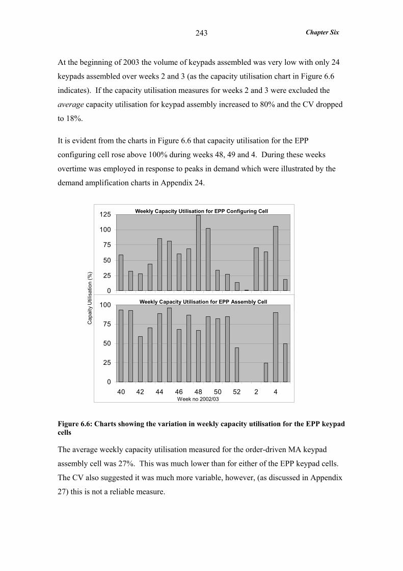
Chapter Six

243

At the beginning of 2003 the volume of keypads assembled was very low with only 24

keypads assembled over weeks 2 and 3 (as the capacity utilisation chart in Figure 6.6

indicates). If the capacity utilisation measures for weeks 2 and 3 were excluded the

average capacity utilisation for keypad assembly increased to 80% and the CV dropped

to 18%.

It is evident from the charts in Figure 6.6 that capacity utilisation for the EPP

configuring cell rose above 100% during weeks 48, 49 and 4. During these weeks

overtime was employed in response to peaks in demand which were illustrated by the

demand amplification charts in Appendix 24.

0

25

50

75

100

125

40 42 44 46 48 50 52 2 4

0

25

50

75

100

40 42 44 46 48 50 52 2 4

Weekly Capacity Utilisation for EPP Configuring Cell

Weekly Capacity Utilisation for EPP Assembly Cell

Week no 2002/03

Cap

aity

Util

isat

ion

(%)

Figure 6.6: Charts showing the variation in weekly capacity utilisation for the EPP keypad cells

The average weekly capacity utilisation measured for the order-driven MA keypad

assembly cell was 27%. This was much lower than for either of the EPP keypad cells.

The CV also suggested it was much more variable, however, (as discussed in Appendix

27) this is not a reliable measure.

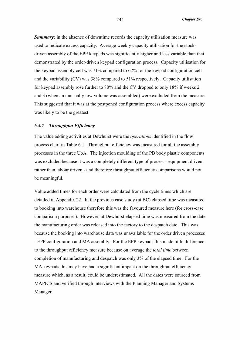
Chapter Six

244

Summary: in the absence of downtime records the capacity utilisation measure was

used to indicate excess capacity. Average weekly capacity utilisation for the stock-

driven assembly of the EPP keypads was significantly higher and less variable than that

demonstrated by the order-driven keypad configuration process. Capacity utilisation for

the keypad assembly cell was 71% compared to 62% for the keypad configuration cell

and the variability (CV) was 38% compared to 51% respectively. Capacity utilisation

for keypad assembly rose further to 80% and the CV dropped to only 18% if weeks 2

and 3 (when an unusually low volume was assembled) were excluded from the measure.

This suggested that it was at the postponed configuration process where excess capacity

was likely to be the greatest.


The value adding activities at Dewhurst were the operations identified in the flow

process chart in Table 6.1. Throughput efficiency was measured for all the assembly

processes in the three UoA. The injection moulding of the PB body plastic components

was excluded because it was a completely different type of process - equipment driven

rather than labour driven - and therefore throughput efficiency comparisons would not

be meaningful.

Value added times for each order were calculated from the cycle times which are

detailed in Appendix 22. In the previous case study (at BC) elapsed time was measured

to booking into warehouse therefore this was the favoured measure here (for cross-case

comparison purposes). However, at Dewhurst elapsed time was measured from the date

the manufacturing order was released into the factory to the despatch date. This was

because the booking into warehouse data was unavailable for the order driven processes

- EPP configuration and MA assembly. For the EPP keypads this made little difference

to the throughput efficiency measure because on average the total time between

completion of manufacturing and despatch was only 3% of the elapsed time. For the

MA keypads this may have had a significant impact on the throughput efficiency

measure which, as a result, could be underestimated. All the dates were sourced from

MAPICS and verified through interviews with the Planning Manager and Systems

Manager.

Chapter Six

245

Table 6.9: Throughput efficiency measures for the UoA.

Order Driven Stock Driven Average Values MA Keypad

Assembly EPP Keypad

Configuration EPP Keypad

Assembly PB body

Assembly

No. of orders assessed 38 596 61 20

Value added time 7.9 hrs

(1 wkg day)

2.6 hrs

(0.3 wkg day)

20.7 hrs

(2.7 wkg day)

30.5 hrs

(4.1 wkg day)

Elapsed time prior to start of manufacturing 2.8 wkg day 2.6 wkg day 9.6 wkg day 12.5 wkg day

Total Elapsed Time 21.1 wkg day 3.0 wkg day 17.5 wkg day 23.1 wkg day

Average 6.5% 11% 27% 17%

CV 114% 167% 93% 125%

Range 0.04 – 33% 0.2 – 98% 1.5 – 97% 0.3 – 72% Throughput Efficiency

Notes (including time in the finished goods warehouse)

(excluding time in the finished goods warehouse)

A summary of the throughput efficiency measures is presented in Table 6.9. Measures

for the two EPP processes are compared first - the order driven keypad configuration

and the stock driven keypad assembly. Contrary to predictions the throughput

efficiency was higher for the stock driven EPP assembly than it was for the postponed

configuration - 27% compared to 11%. This was in spite of the fact that manufacturing

lead-times for the postponed configuration process were considerably shorter than for

the keypad assembly process - 3 compared to 17.5 working days respectively. There

were two explanations for the unexpectedly low throughput efficiency at the postponed

configuration process:

• the size of the customer orders for configured keypads were on average much

smaller than the size of the EPP assembly manufacturing orders – 45 compared

with 520 respectively

• the keypad configuration manufacturing lead-time was extended (by 85% of the

lead-time) by queuing caused by capacity restrictions at this process. However,

the order lead-times required by the EPP customer, NCR, were being reliably

satisfied as illustrated by the customer service measures in section 6.4.3.

Therefore it appeared that a shorter manufacturing lead-time - or higher

throughput efficiency - was not needed.

Chapter Six

246

In addition to the throughput efficiency at the EPP configuration process being low it

was also highly variable from order to order (almost twice as variable as at the EPP

assembly process) as the CV of 167% demonstrates. The main factor driving the

variability in throughput efficiency was the customer order sizes which varied from 1 to

840 configured keypads.

The most striking difference between EPP assembly and the postponed configuration

was - not the throughput efficiencies - but the manufacturing lead-times. Keypad

configuration was clearly more responsive with a manufacturing lead-time equivalent to

only 17% of the keypad assembly lead-time.

In general there was a trend for throughput efficiencies at the two EPP cells to fall over

the study period due to reductions in cycle times which were not matched by reductions

in manufacturing lead-times.

MA keypad assembly and PB body assembly also demonstrated throughput efficiencies

contrary to expectations. However the throughput efficiency measure for the MA

keypads was probably grossly underestimated, in comparison to the PB body measure,

as explained earlier.

Summary: Contrary to expected results the throughput efficiency was higher for the

stock driven EPP assembly than it was for the order driven configuration - 27%

compared to 11%. This was in spite of the fact that manufacturing lead-times for the

postponed configuration process, were considerably shorter than for the keypad

assembly process - 3 compared to 17.5 working days respectively. There were two

explanations for the unexpectedly low throughput efficiency at the postponed

configuration process. Firstly the size of the customer orders for configured keypads

were much smaller than the EPP assembly manufacturing orders - 45 compared with

520 respectively. Secondly the keypad configuration manufacturing lead-time was

extended (by 85% of the lead-time) by queuing at this process.


A PVF central to the conceptual model of FPp was plotted for each UoA, as shown in

Figure 6.7. The BOM data previously used for the product design measures and

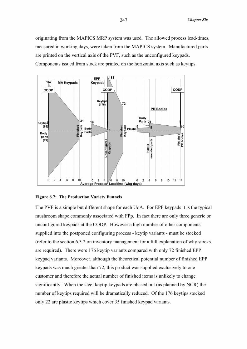
Chapter Six

247

originating from the MAPICS MRP system was used. The allowed process lead-times,

measured in working days, were taken from the MAPICS system. Manufactured parts

are printed on the vertical axis of the PVF, such as the unconfigured keypads.

Components issued from stock are printed on the horizontal axis such as keytips.

Average Process Leadtime (wkg days)40 2 6 8 10 12 1440 2 6 8 10 40 2 6 8 10

MA KeypadsEPP

Keypads

PB Bodies

Keytips(88)

Body parts

(79)

167

31

BodyParts

19

3

183

72Keytips

(176)U

ncon

figur

edK

eypa

ds

Fini

shed

Key

pads 5 8

2110

BodyParts

Plas

ticm

ould

ed p

arts

Fini

shed

PB b

odie

s

Plastic

CODP CODP CODP

Fini

shed

Key

pads

Figure 6.7: The Production Variety Funnels

The PVF is a simple but different shape for each UoA. For EPP keypads it is the typical

mushroom shape commonly associated with FPp. In fact there are only three generic or

unconfigured keypads at the CODP. However a high number of other components

supplied into the postponed configuring process - keytip variants - must be stocked

(refer to the section 6.3.2 on inventory management for a full explanation of why stocks

are required). There were 176 keytip variants compared with only 72 finished EPP

keypad variants. Moreover, although the theoretical potential number of finished EPP

keypads was much greater than 72, this product was supplied exclusively to one

customer and therefore the actual number of finished items is unlikely to change

significantly. When the steel keytip keypads are phased out (as planned by NCR) the

number of keytips required will be dramatically reduced. Of the 176 keytips stocked

only 22 are plastic keytips which cover 35 finished keypad variants.

Chapter Six

248

The PVF for MA keypads is an ‘A’ shape (when turned through 90 degrees with the end

item uppermost), typical of a MTS product. However the MA keypad was MTO as the

CODP indicates. The reason for not using the MTS approach was three fold:

• Firstly, MA keypads were only occasionally demanded in one of the three

standard specifications. Almost all the MA keypad orders were for highly

customised keypads and therefore unique to the particular customer. In fact the

potential variety in the finished MA keypads was much greater than the PVF

shows. This is in contrast to the PVF for the EPP keypads, which shows the full

variety likely to be demanded.

• Secondly, the number of repeat orders for MA keypads was very low, on

average only 1.5 orders were placed for each MA keypad item over the 4 month

study period.

• Thirdly, it appeared that the market accepted the 3 week lead-time readily and

there was no need for a more responsive supply.

FPp was not a suitable approach for the production of the MA keypads. This can be

illustrated by splitting the manufacturing process into three consecutive stages:

configuring the keytips, assembling the keypad body and packing. At no stage does the

number of distinct items drop below the number of finished keypads, 31. Configuring

the keytips was the main differentiating process and once this was completed the

number of distinct sets of keytips was the same as the number of end items.

Assembling the body and the packaging did not further differentiate the product.

The variety of components required to make the PB bodies was much less than for the

keypads. This was because each body required less than half the distinct components

required for the keypads and the finished bodies were demanded in fewer variants. The

PVF for the PB bodies is the ‘A’ shape commonly associated with MTS. However

more variety in the components is normal to justify a finished stock. There were only

21 distinct components in the 10 PB bodies as a result of a deliberate effort to

standardise the components across the different variants.

Chapter Six

249

6.5 CASE ANALYSIS

In this section the results of the case analysis are presented: first the major flaws in the


hypotheses.

6.5.1 Not the Planned Ideal FPp Application

Originally it was planned that the EPP keypad would (after a very short time) be largely

supplied in the plastic keytip variant and the steel keytip variant would be supplied in

minimal volumes, if at all. Further it was envisaged that the number of keytip colour

configurations would be limited to a handful, say five, and that only stocks of these

keypad variants would be maintained. The principal benefit being that only the laser

marking of the legend on the keytips would be performed to specific customer orders.

Therefore no components stocks would be required and the keypads could be supplied

on a very short lead-time.

However, the demand for EPP keypads was not as NCR forecasted in three respects:

• Firstly the steel keytip keypads continued to be demanded in very significant

volumes forcing Dewhurst to maintain a stock of the unconfigured steel

keypad. In fact over the four-month study period the steel tipped EPP keypad

accounted for over a quarter of the volume.

• Secondly, the plastic keypad was demanded in eighteen - rather than five -

different keytip colour configurations.

• Thirdly, the total EPP keypad sales volume was heavily overestimated.

The operational implications were that the CODP had to be located further upstream

than planned and the unconfigured keypads together with many variants of the keytips

(plastic and steel) had to be stocked. In addition - rather than merely laser marking -

gluing and populating of the keytips onto the keypads also had to be performed to

customer order. This reduced the potential for lead-time and component stock

reduction. Finally the overestimated EPP keypad sales forecasts lead to excessive

unconfigured keypad stocks.

Chapter Six

250

Indeed it can be argued that given the low value adding time to manufacture the

unconfigured keypads (4.5 minutes) it was possible for Dewhurst to assemble the

keypads entirely to order. This would still require the application of FPp but the CODP

would be moved upstream so only the keytips are manufactured to stock. There was no

possibility of making the keytips to order because they required a long manufacturing

lead-time.

The main implication of moving the CODP was that the buffer stock of unconfigured

keypads would be lost. This protected the unconfigured keypad assembly process from

the high demand variability - both in terms of volume demand variability at finished

keypad level (or varying demand mix) and at generic keypad level. Without the generic

keypad buffer stock the assembly of the unconfigured keypad – as well as the gluing

and populating of the keypads - would require excess capacity to cope with the high

demand variability.


All six hypotheses were fully tested in the Dewhurst case study and the findings were

largely as predicted by the six hypotheses. However two hypotheses were challenged in

part (H5 and H6).

What is the demand profile of products selected for manufacture under FPp? H1: Products are selected for manufacture under FPp rather than MTS when they exhibit high demand mix, high demand variability and low volume demand at finished product level.


The findings support both hypotheses H1 and H2. The EPP keypads manufactured

under FPp were demanded in seven times as many variants as the MTS PB bodies - 72

compared to 10 variants. As a result the average demand volume at finished item level

was much lower for the FPp EPP keypads than the MTS PB bodies - 373 compared to

4404 items.

As expected the average demand variability at finished item level was higher for the

FPp EPP keypads than for the MTS PB bodies. However the difference in variability

was only marginal 249% compared to 233%. The explanation for this was related to the

Chapter Six

251

number of orders at end item level – about nine on average for both the EPP keypads

and the PB bodies. In fact half of the ten stocked PB bodies were only subject to one or

two orders over the study period and therefore exhibited a very high CV of demand, in

excess of 300%. If these PB bodies were excluded demand variability dropped to 97%.

As predicted by hypothesis H2 the average volume demand at generic level was much

higher for the FPp EPP keypads than for the MTO MA keypads - 8,963 compared to

192 keypads. This was due to two factors:

• the number of MA generic keypads was double that for the EPP keypads

• EPP keypads were demanded in much higher volumes than the MA keypads.

Further, it should be considered that in the case of the MA keypads the generic keypad

bodies did not physically exist at any stage in the manufacturing process.



The findings support H3, however data were unavailable to measure ex-stock

availability in terms of the proportion of enquiries and orders for which the correct

stock item was available. Therefore stock records for both the generic EPP keypads

(subject to FPp) and the PB bodies (subject to MTS) were used to indicate ex-stock

availability. No stock outs were recorded for the generic EPP keypads. Further, there

were no enquiries for EPP keypads, only firm orders with a non-negotiable lead-time

for which the delivery performance was extremely high - 98% on time in full.

Therefore, it was fair to assume that ex-stock availability was no less than 98% and

most probably 100%.

Stock outs were recorded for three of the MTS PB bodies and this alone reduced

delivery reliability to 94% on time in full. Unlike the EPP keypads PB bodies were

subject to enquiries for which the ex-stock availability was not recorded. Therefore it

was fair to conclude that ex-stock availability for the PB bodies was at best 94% and

therefore lower than for the EPP unconfigured keypads.

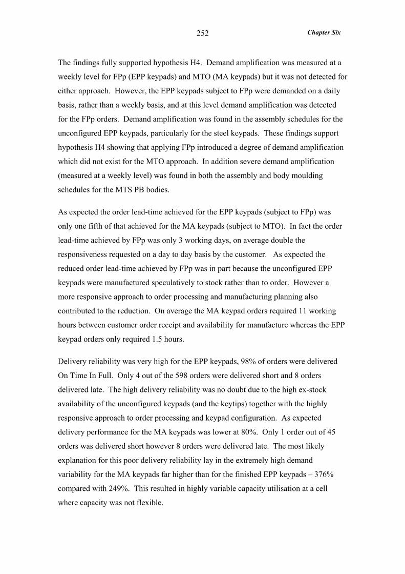
Chapter Six

252

The findings fully supported hypothesis H4. Demand amplification was measured at a

weekly level for FPp (EPP keypads) and MTO (MA keypads) but it was not detected for

either approach. However, the EPP keypads subject to FPp were demanded on a daily

basis, rather than a weekly basis, and at this level demand amplification was detected

for the FPp orders. Demand amplification was found in the assembly schedules for the

unconfigured EPP keypads, particularly for the steel keypads. These findings support

hypothesis H4 showing that applying FPp introduced a degree of demand amplification

which did not exist for the MTO approach. In addition severe demand amplification

(measured at a weekly level) was found in both the assembly and body moulding

schedules for the MTS PB bodies.

As expected the order lead-time achieved for the EPP keypads (subject to FPp) was

only one fifth of that achieved for the MA keypads (subject to MTO). In fact the order

lead-time achieved by FPp was only 3 working days, on average double the

responsiveness requested on a day to day basis by the customer. As expected the

reduced order lead-time achieved by FPp was in part because the unconfigured EPP

keypads were manufactured speculatively to stock rather than to order. However a

more responsive approach to order processing and manufacturing planning also

contributed to the reduction. On average the MA keypad orders required 11 working

hours between customer order receipt and availability for manufacture whereas the EPP

keypad orders only required 1.5 hours.


On Time In Full. Only 4 out of the 598 orders were delivered short and 8 orders

delivered late. The high delivery reliability was no doubt due to the high ex-stock

availability of the unconfigured keypads (and the keytips) together with the highly

responsive approach to order processing and keypad configuration. As expected

delivery performance for the MA keypads was lower at 80%. Only 1 order out of 45

orders was delivered short however 8 orders were delivered late. The most likely

explanation for this poor delivery reliability lay in the extremely high demand

variability for the MA keypads far higher than for the finished EPP keypads – 376%

compared with 249%. This resulted in highly variable capacity utilisation at a cell

where capacity was not flexible.

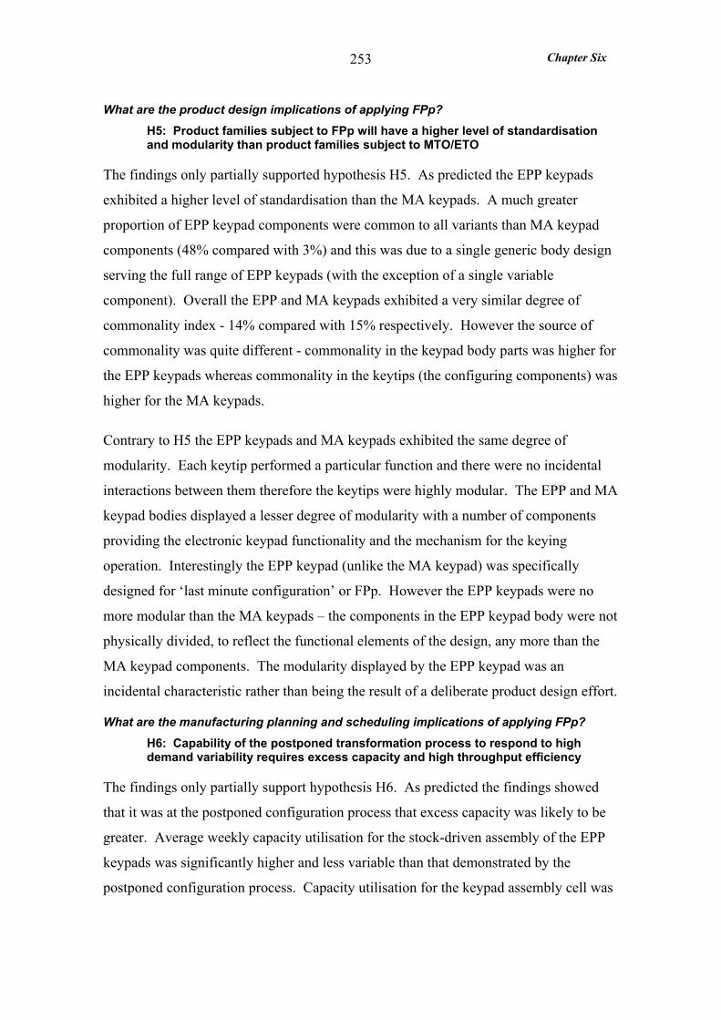
Chapter Six

253


The findings only partially supported hypothesis H5. As predicted the EPP keypads

exhibited a higher level of standardisation than the MA keypads. A much greater

proportion of EPP keypad components were common to all variants than MA keypad

components (48% compared with 3%) and this was due to a single generic body design

serving the full range of EPP keypads (with the exception of a single variable

component). Overall the EPP and MA keypads exhibited a very similar degree of

commonality index - 14% compared with 15% respectively. However the source of

commonality was quite different - commonality in the keypad body parts was higher for

the EPP keypads whereas commonality in the keytips (the configuring components) was

higher for the MA keypads.

Contrary to H5 the EPP keypads and MA keypads exhibited the same degree of

modularity. Each keytip performed a particular function and there were no incidental

interactions between them therefore the keytips were highly modular. The EPP and MA

keypad bodies displayed a lesser degree of modularity with a number of components

providing the electronic keypad functionality and the mechanism for the keying

operation. Interestingly the EPP keypad (unlike the MA keypad) was specifically

designed for ‘last minute configuration’ or FPp. However the EPP keypads were no

more modular than the MA keypads – the components in the EPP keypad body were not

physically divided, to reflect the functional elements of the design, any more than the

MA keypad components. The modularity displayed by the EPP keypad was an

incidental characteristic rather than being the result of a deliberate product design effort.


The findings only partially support hypothesis H6. As predicted the findings showed

that it was at the postponed configuration process that excess capacity was likely to be

greater. Average weekly capacity utilisation for the stock-driven assembly of the EPP

keypads was significantly higher and less variable than that demonstrated by the

postponed configuration process. Capacity utilisation for the keypad assembly cell was

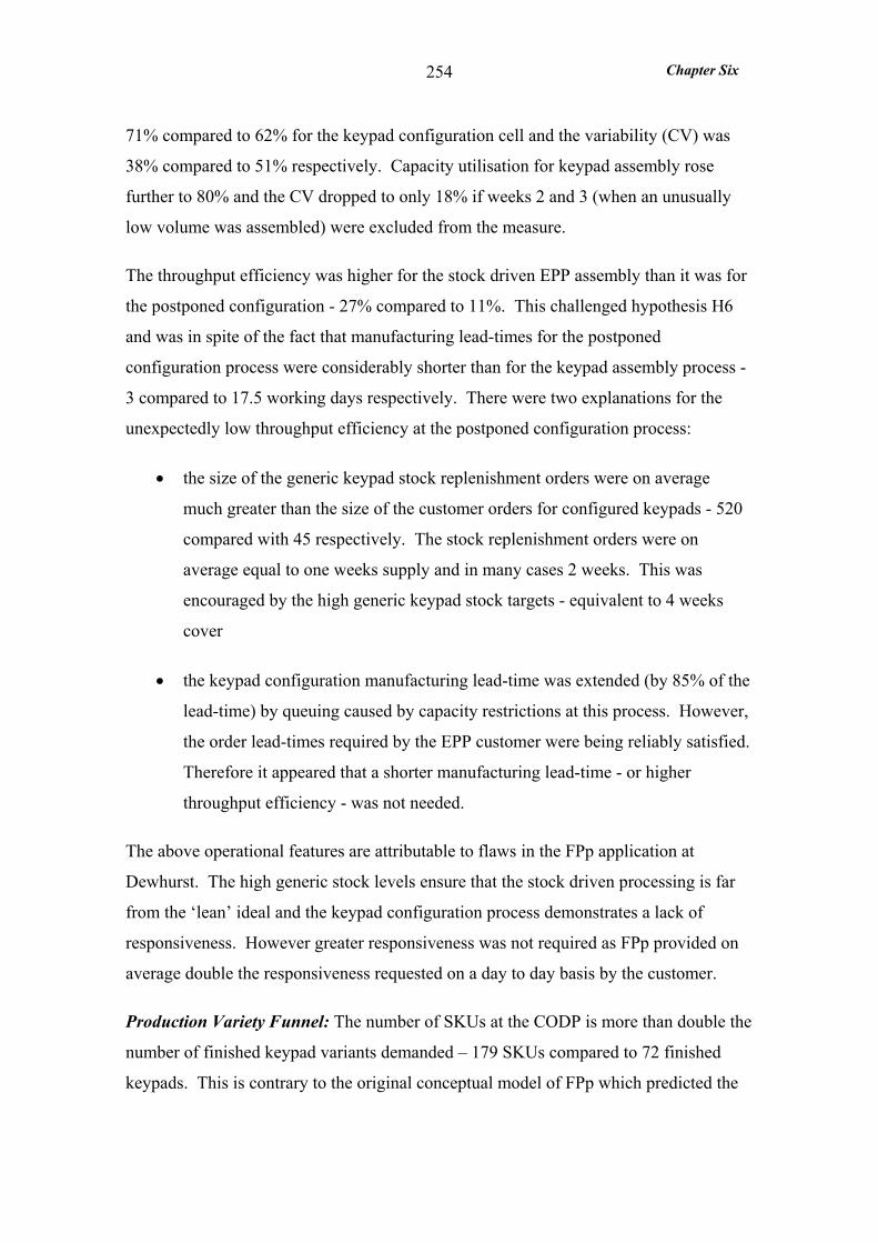
Chapter Six

254

71% compared to 62% for the keypad configuration cell and the variability (CV) was

38% compared to 51% respectively. Capacity utilisation for keypad assembly rose

further to 80% and the CV dropped to only 18% if weeks 2 and 3 (when an unusually

low volume was assembled) were excluded from the measure.

The throughput efficiency was higher for the stock driven EPP assembly than it was for

the postponed configuration - 27% compared to 11%. This challenged hypothesis H6

and was in spite of the fact that manufacturing lead-times for the postponed

configuration process were considerably shorter than for the keypad assembly process -

3 compared to 17.5 working days respectively. There were two explanations for the

unexpectedly low throughput efficiency at the postponed configuration process:

• the size of the generic keypad stock replenishment orders were on average

much greater than the size of the customer orders for configured keypads - 520

compared with 45 respectively. The stock replenishment orders were on

average equal to one weeks supply and in many cases 2 weeks. This was

encouraged by the high generic keypad stock targets - equivalent to 4 weeks

cover

• the keypad configuration manufacturing lead-time was extended (by 85% of the

lead-time) by queuing caused by capacity restrictions at this process. However,

the order lead-times required by the EPP customer were being reliably satisfied.

Therefore it appeared that a shorter manufacturing lead-time - or higher

throughput efficiency - was not needed.

The above operational features are attributable to flaws in the FPp application at

Dewhurst. The high generic stock levels ensure that the stock driven processing is far

from the ‘lean’ ideal and the keypad configuration process demonstrates a lack of

responsiveness. However greater responsiveness was not required as FPp provided on

average double the responsiveness requested on a day to day basis by the customer.

Production Variety Funnel: The number of SKUs at the CODP is more than double the

number of finished keypad variants demanded – 179 SKUs compared to 72 finished

keypads. This is contrary to the original conceptual model of FPp which predicted the

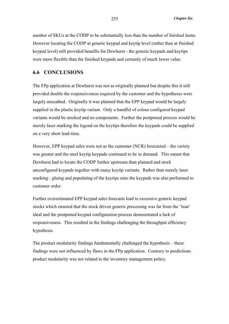
Chapter Six

255

number of SKUs at the CODP to be substantially less than the number of finished items.

However locating the CODP at generic keypad and keytip level (rather than at finished

keypad level) still provided benefits for Dewhurst - the generic keypads and keytips

were more flexible than the finished keypads and certainly of much lower value.

6.6 CONCLUSIONS

The FPp application at Dewhurst was not as originally planned but despite this it still

provided double the responsiveness required by the customer and the hypotheses were

largely unscathed. Originally it was planned that the EPP keypad would be largely

supplied in the plastic keytip variant. Only a handful of colour configured keypad

variants would be stocked and no components. Further the postponed process would be

merely laser marking the legend on the keytips therefore the keypads could be supplied


However, EPP keypad sales were not as the customer (NCR) forecasted – the variety

was greater and the steel keytip keypads continued to be in demand. This meant that

Dewhurst had to locate the CODP further upstream than planned and stock

unconfigured keypads together with many keytip variants. Rather than merely laser

marking - gluing and populating of the keytips onto the keypads was also performed to

customer order.

Further overestimated EPP keypad sales forecasts lead to excessive generic keypad

stocks which ensured that the stock driven generic processing was far from the ‘lean’

ideal and the postponed keypad configuration process demonstrated a lack of

responsiveness. This resulted in the findings challenging the throughput efficiency

hypothesis.

The product modularity findings fundamentally challenged the hypothesis – these

findings were not influenced by flaws in the FPp application. Contrary to predictions

product modularity was not related to the inventory management policy.

Chapter Seven

256

CHAPTER SEVEN

7 Cross-Case Comparisons

7.1 INTRODUCTION

In bringing together the key operational features of the various cases it is helpful to first

consider the major elements in common between the cases analysed: Thomas Bolton

(TB - Chapter 4), Brook Crompton (BC - Chapter 5) and Dewhurst (Chapter 6). The

manufacturing facilities were of a similar size - between 120 and 200 employees and an

annual turnover between £13 and £18 million.

In all three cases FPp had been applied some two years prior to the study, in order to

improve responsiveness and in each case the FPp application was not ideal. In the BC

and Dewhurst cases FPp continued to be applied, but in the TB case FPp had been

abandoned by the time the study was conducted. All three studies were retrospective

and focussed on a time period of at least 4 months. Each study compared three UoAs –

product groups subject to MTO (ETO in the BC case), FPp and MTS.

In the cases of TB and Dewhurst, FPp was applied to products destined for a single

customer. In both cases this was their biggest customer accounting for a high

proportion of the facility’s turnover and, with whom, there was a high degree of mutual

dependence.

As discussed above, and later in this chapter, there were a number of highly significant

commonalities between the cases in particular all three companies had applied FPp

(according the definition used for this research). However there were also many

distinctions between the cases. This was a feature of the research design which aims to

compare the application of FPp in diverse contexts in order to extend the

generalisability of the findings. In order to advance theories in OM it is necessary to

seek out both the differences and commonalities between cases. Thus the key

distinctions and similarities between the three case studies are presented in this chapter.

Chapter Seven

257

This chapter begins by highlighting the diverse nature of the three FPp applications

studied in a comparison of contextual considerations including the reasons for the

application of FPp. The second section addresses how FPp was applied and the main

flaws in its application to provide generaliseable findings. The third section compares

the key measures, in relation to the six hypotheses to reveal which, are fundamentally

and consistently challenged across the three case studies. The chapter ends with a

concluding section.

7.2 CONTEXTUAL CONSIDERATIONS

The three products subject to FPp were all industrial products made in medium sized

companies in England. They all exhibited ‘component swapping’ modularity (Pine,

1993) where ‘different components are paired with the same basic product’ to provide

high variety in the finished product (as discussed in section 2.6.2). All three companies

manufactured and stocked the generic or basic product (TB: laid up cable, BC: standard

motor, Dewhurst: unconfigured keypad) and then combined them with various

differentiating components in the postponed process. These components were

sometimes manufactured in-house (Dewhurst keytips and some of BC motor

components) or bought-in (many of the BC components and TB polymers).

Apart from these commonalities the three cases of FPp were very different, as the data

in Table 7.1 illustrates. The products varied greatly in complexity. The cables made by

TB were simple products requiring only 18 distinct components. The keypads made by

Dewhurst required 30 distinct components, but the BOM had fewer levels than that for

the TB cables. In contrast the motors made at BC were the most complex products

studied, requiring on average 160 distinct components and frequently in excess of 200.

Volume versus variety: The EPP keypads manufactured by Dewhurst were mass

customised for the High Street banks, as expected in a product subject to FPp. The EPP

keypads exhibited high variety at finished product level and high volume at generic

product level. In comparison the motors subject to FPp at BC were manufactured in

similar variety but very low volumes even at generic product level. The TB cables,

though produced in high volumes, exhibited an unexpectedly low level of variety – far

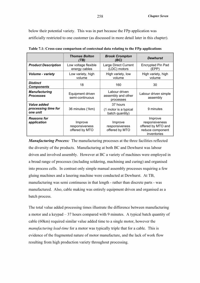
Chapter Seven

258

below their potential variety. This was in part because the FPp application was

artificially restricted to one customer (as discussed in more detail later in this chapter).

Table 7.1: Cross-case comparison of contextual data relating to the FPp applications

Thomas Bolton (TB)

Brook Crompton (BC) Dewhurst

Product Description Low voltage flexible energy cables

Large Direct Current (LDC) motors

Encrypted Pin Pad (EPP)

Volume - variety Low variety, high volume

High variety, low volume

High variety, high volume

Distinct Components 18 160 30

Manufacturing Processes Equipment driven

semi-continuous

Labour driven assembly and other

processes

Labour driven simple assembly

Value added processing time for one unit

36 minutes (1km) 37 hours

(1 motor is a typical batch quantity)

9 minutes

Reasons for application Improve

responsiveness offered by MTO

Improve responsiveness offered by MTO

Improve responsiveness

offered by MTO and reduce component

inventories

Manufacturing Process: The manufacturing processes at the three facilities reflected

the diversity of the products. Manufacturing at both BC and Dewhurst was labour

driven and involved assembly. However at BC a variety of machines were employed in

a broad range of processes (including soldering, machining and curing) and organised

into process cells. In contrast only simple manual assembly processes requiring a few

gluing machines and a lasering machine were conducted at Dewhurst. At TB,

manufacturing was semi continuous in that length - rather than discrete parts - was

manufactured. Also, cable making was entirely equipment driven and organised as a

batch process.

The total value added processing times illustrate the difference between manufacturing

a motor and a keypad – 37 hours compared with 9 minutes. A typical batch quantity of

cable (60km) required similar value added time to a single motor, however the

manufacturing lead-time for a motor was typically triple that for a cable. This is

evidence of the fragmented nature of motor manufacture, and the lack of work flow

resulting from high production variety throughout processing.

Chapter Seven

259

Reasons for applying FPp: In all three cases FPp was seen as an alternative to

MTO/ETO. MTS was not considered an option for the products subject to FPp.

Accordingly FPp was applied to reduce the order lead-time achieved by MTO and

thereby to improve responsiveness. In the case of TB there was a need to improve the

match between cable supply and their biggest customer’s demand, and to avoid the

‘feast and famine’ supply experienced with MTO. At BC, UK customers expected that

motors based on a standard specification would be available on a 3 to 4 week lead-time

– not the 10 to 14 week lead-time achieved by ETO.

At Dewhurst the EPP keypad was the only product to be specifically designed for “last

minute configuration” (FPp). In common with the other cases a reason for applying

FPp was to improve the responsiveness of supply to their biggest customer NCR. Vital

to Dewhurst was the opportunity to do this without incurring the high component stocks

that had plagued the MTO of the previous NCR keypad range.

7.3 CHANGE CONTENT & FLAWS IN THE APPLICATIONS

In this section the application of FPp across the three firms is compared with respect to

product (and customer) selection, inventory management, manufacturing planning and

the main flaws in its application. The highlights are presented in Table 7.2.

Selection of products and customers: In both the TB and the Dewhurst cases FPp was

applied exclusively to products for their biggest customers – Volex Powercords (VP)

and NCR respectively. FPp provided these customers with an especially high level of

responsiveness not afforded to other customers. At TB, the restriction to one customer

was artificial – FPp could have been equally well applied to many other cables

(withstanding the production scheduling system issues). At Dewhurst the EPP keypad

was designed exclusively for NCR, therefore its manufacture using the FPp approach

was also exclusive.

At BC the products to be subject to FPp were selected at the generic level (30 UK

standard motors) and any motor variants based on these standard specifications were

subject to FPp. At Dewhurst only a predefined list of finished EPP keypad items were

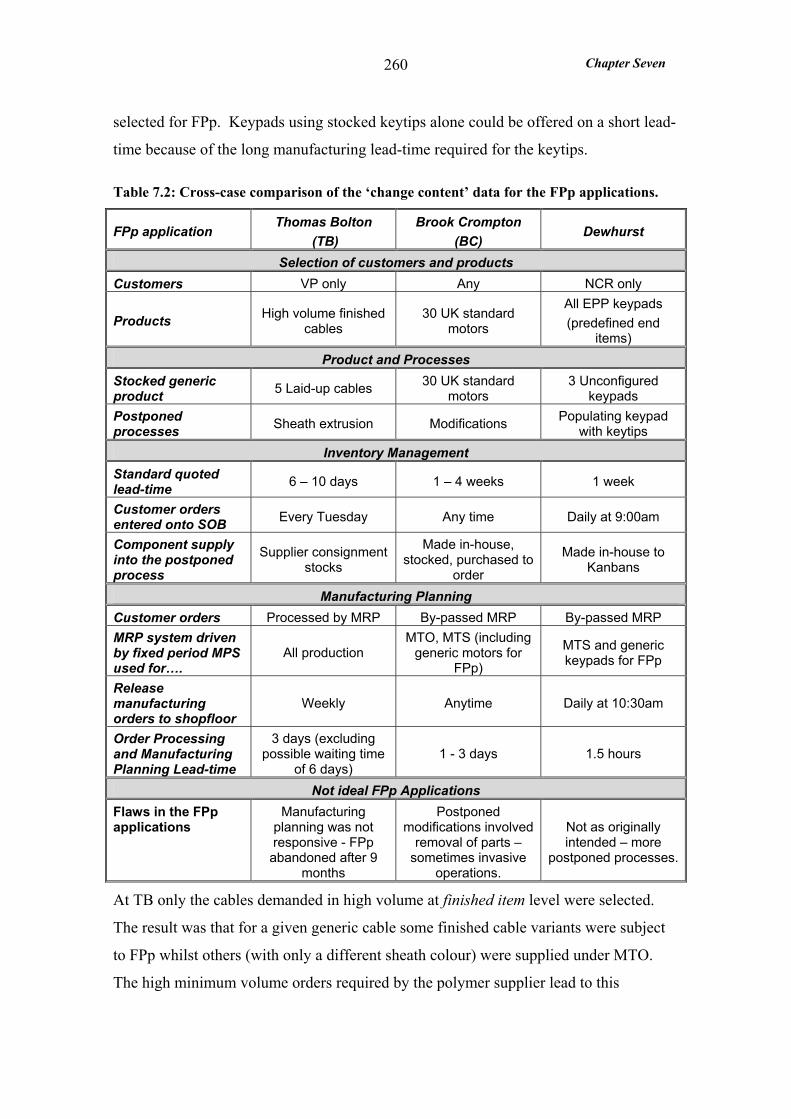
Chapter Seven

260

selected for FPp. Keypads using stocked keytips alone could be offered on a short lead-

time because of the long manufacturing lead-time required for the keytips.

Table 7.2: Cross-case comparison of the ‘change content’ data for the FPp applications.

FPp application Thomas Bolton

(TB) Brook Crompton

(BC) Dewhurst

Selection of customers and products Customers VP only Any NCR only

Products High volume finished cables

30 UK standard motors

All EPP keypads (predefined end

items) Product and Processes

Stocked generic product 5 Laid-up cables 30 UK standard

motors 3 Unconfigured

keypads Postponed processes Sheath extrusion Modifications Populating keypad

with keytips Inventory Management

Standard quoted lead-time 6 – 10 days 1 – 4 weeks 1 week

Customer orders entered onto SOB Every Tuesday Any time Daily at 9:00am

Component supply into the postponed process

Supplier consignment stocks

Made in-house, stocked, purchased to

order

Made in-house to Kanbans

Manufacturing Planning Customer orders Processed by MRP By-passed MRP By-passed MRP MRP system driven by fixed period MPS used for….

All production MTO, MTS (including

generic motors for FPp)

MTS and generic keypads for FPp

Release manufacturing orders to shopfloor

Weekly Anytime Daily at 10:30am

Order Processing and Manufacturing Planning Lead-time

3 days (excluding possible waiting time

of 6 days) 1 - 3 days 1.5 hours

Not ideal FPp Applications Flaws in the FPp applications

Manufacturing planning was not responsive - FPp abandoned after 9

months

Postponed modifications involved

removal of parts – sometimes invasive

operations.

Not as originally intended – more

postponed processes.

At TB only the cables demanded in high volume at finished item level were selected.

The result was that for a given generic cable some finished cable variants were subject

to FPp whilst others (with only a different sheath colour) were supplied under MTO.

The high minimum volume orders required by the polymer supplier lead to this

Chapter Seven

261

restriction. The sheathing polymer supplied into the postponed process was required on

consignment stock to ensure it was available within 24 hours. This was only possible

for high volume cables otherwise it was judged that the risk of obsolescence, or the

supplier refusing to provide a consignment stock, was too high.

BC and Dewhurst did not have this problem with the supply of components into the

postponed process. BC did not provide such a responsive supply to customers and

therefore time was available to purchase, or make, many modification components to

order. Dewhurst required immediate availability of the keytips for the postponed

keypad configuration, however the keytips were made in-house to Kanbans and

therefore volume was not a major issue.

Inventory Management: Order promising for BC motors was mainly based on the

modification and part availability hence the relatively long and variable quoted lead-

time. This was attributable to the high variety of components required, many of which

were purchased (or occasionally made at BC) to order. At TB and Dewhurst a standard

order lead-time was agreed and - while the required order lead-time did not fall below

this - delivery was promised on time, in full. Components and manufacturing capacity

was assumed to be available at TB and at Dewhurst. Where the product is truly

customised (i.e. the customer’s choices are not confined by predefined lists of options

but are truly free choices) as at BC, it is probably not possible to give a standardised

order lead-time. Instead the lead-time must be determined on the basis of the

customisation ordered. However it should still be short compared to the order lead-time

required for the complete order driven manufacture of the product.

At BC customer orders were communicated by either hard copy purchase orders or fax

depending on the customer. At TB customer orders were communicated by fax every

Tuesday. At Dewhurst, customer orders were communicated by EDI every morning at

9:00 am and Dewhurst sales administrators were waiting to process the orders upon

transmission. This allowed rapid reliable communication of the orders and included bar

code identification for each order so that barcode keypad labels could be printed at

Dewhurst. EDI thus appears to be the most efficient way to communicate orders but is

only practical when the customer places orders at regular intervals. Further the

Chapter Seven

262

improved responsiveness offered by EDI transmission of orders can best be realised if

orders are processed upon arrival.

Manufacturing Planning: All three facilities employed MRP systems driven by fixed

period MPS for manufacturing planning and control. At Dewhurst and BC the MRP

systems were relatively responsive – compiled nightly. However at TB the MRP

system was only compiled weekly (as it required two full days for compilation). At BC

and Dewhurst, released manufacturing orders were downloaded from the MRP systems

to the shopfloor nightly and three times daily respectively - compared with the weekly

download at TB. However, even though the manufacturing planning systems at BC and

Dewhurst were more responsive the customer orders for products subject to FPp

completely by-passed the MRP systems.

At TB the lack of responsiveness - inherent in the MRP system - restricted the customer

to placing weekly orders every Tuesday. The associated manufacturing orders were

subsequently released to the shop-floor every Friday morning. This approach to

manufacturing planning for FPp eventually lead to its demise, as discussed later in this

section.

At BC, manufacture of the generic motors and ETO motors was planned using the MRP

system driven by a one week fixed period MPS. However it had not been possible to

set up the MRP system to process the proliferation of postponed modifications due to

lack of flexibility in the BOMs. Therefore special instruction sheets were established to

control materials for the modifications and the modifications themselves. The acquiring

of parts for modifications was cited as a laborious procedure involving manual stock

checking and hand written purchase requisitions. Hence from a material control

perspective BC would have benefited from the use of an MRP system with configurable

BOMs if the time buckets were small - or better still the MRP system was bucketless.

At Dewhurst manufacturing orders subject to MTO were raised by sales, simultaneously

released into the factory and downloaded onto the shopfloor three times per day. This

ensured a maximum delay of 8 hours between creation of the manufacturing order and

availability for manufacture. However this was not considered responsive enough for

the EPP keypad orders subject to FPp. Once communicated by EDI to Dewhurst these

Chapter Seven

263

orders were logged on the manufacturing order system, hard copies printed and

manually transferred to the shopfloor – 1.5 hours from order receipt to availability for

manufacture. At Dewhurst only stock replenishment orders (including generic keypads

for FPp) were planned using a fixed period MPS.

None of the FPp applications studied were ideal. The application at TB was so flawed

that it was eventually abandoned. The application at BC incurred unnecessary

manufacturing costs, but was still workable and offered benefits compared to MTO. At

Dewhurst the FPp application was not as originally intended on the basis of the

customer’s sales forecast. The flaws in each of the FPp applications, a brief description

of the ideal applications and the potential benefits are discussed in greater detail below.

Flaws in the FPp application at TB: TB’s manufacturing planning system was too

inflexible to support the FPp application without the support of finished cable buffer

stocks. There were two major shortfalls in the planning system: a planning time of two

days; and a MRP regeneration frequency of once per week. This added a potential six

days waiting time before new orders could be processed. In effect the planning lead-

time for FPp orders had not been reduced at all compared to that for orders subject to

MTO. Instead TB’s and VP’s planning systems were synchronised but this did not take

into account VP’s high level of deviation from their manufacturing plan.

Flaws in the FPp application at BC: All modifications involved the removal of parts

resulting in increased manufacturing costs. In fact almost half the motors modified

required invasive modifications involving changes to the magnet body components.

This commonly involved a motor strip down which could take up to 3 working days.

This suggested that the CODP would be better located further up stream in the

manufacturing process. A more suitable location for the CODP would be at the

balanced armature stage since the armature was not subject to any modifications.

The magnet body assembly and motor final assembly would be postponed and

conducted to customer orders. With a manufacturing lead-time of just 8 working days it

would still be possible to provide modified standard motors on a 3 to 4 week lead-time.

Though this approach would not reduce the number of generic SKUs it would reduce

their value and allow generic stock levels to be increased to improve ex-stock

Chapter Seven

264

availability without increasing stock value. Further it would naturally take the

postponed motor customisation away from the S&R section (which had extremely

limited resources and was primarily tasked with service and repairs) and relocated it

back in the main LDC manufacturing section. Here the final assembly area, where

motor customisation would take place, was shown to have substantial excess capacity.

Flaws in the FPp application at Dewhurst: Originally it was planned that the EPP

keypad would be largely supplied in the plastic keytip variant rather than the steel

alternative. Further it was envisaged that the number of plastic keytip colour

configurations would be limited to a handful, say five, and that only stocks of these

keypad variants would be maintained. The principal benefit was that only the laser

marking of the legend on the keytips would be performed to specific customer orders.

Therefore no component stocks would be required, and the keypads could be supplied


However, the demand for EPP keypads was not as the customer (NCR) forecasted. The

steel keytip keypads continued to be demanded in high volumes and the plastic keypad

was demanded in eighteen - rather than five - different keytip colour configurations.

This meant that Dewhurst had to locate the CODP further upstream than planned and

stock the unconfigured keypads together with the many variants of keytips (plastic and

steel). The implications of this for processing were that - rather than merely laser

marking - gluing and populating of the keytips onto the keypads was also performed to

customer order. In addition the overestimated EPP keypad sales forecasts led to

excessive unconfigured keypad stocks.

Given the low value adding time (4.5 minutes) to total manufacturing lead-time of the

unconfigured keypads it would have been possible for Dewhurst to assemble the

keypads entirely to order. This would still require the application of FPp but only the

keytips would be manufactured to stock. However by doing this Dewhurst would have

lost the buffer stock of unconfigured keypads which protected the generic keypad

assembly process from the high demand variability. Consequently the generic keypad

assembly process – as well as the gluing and populating process - would have required

excess capacity to cope with the high demand variability.

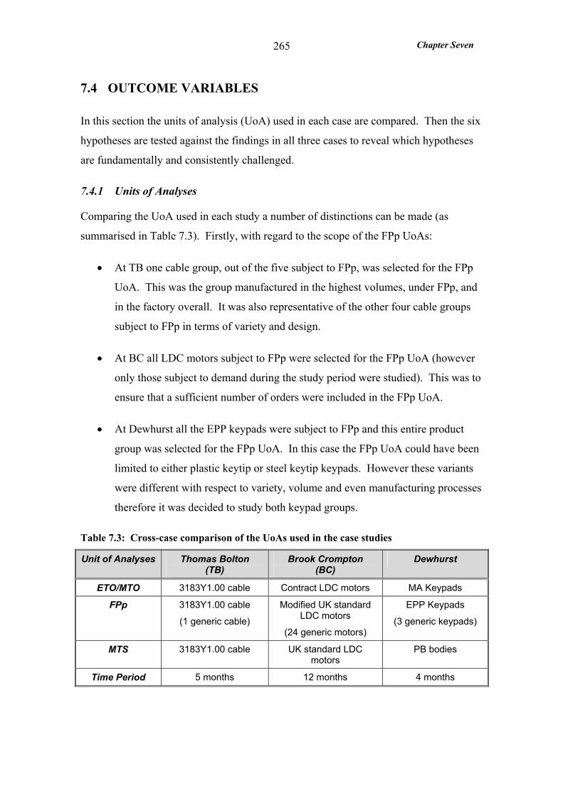
Chapter Seven

265


In this section the units of analysis (UoA) used in each case are compared. Then the six

hypotheses are tested against the findings in all three cases to reveal which hypotheses

are fundamentally and consistently challenged.

7.4.1 Units of Analyses

Comparing the UoA used in each study a number of distinctions can be made (as

summarised in Table 7.3). Firstly, with regard to the scope of the FPp UoAs:

• At TB one cable group, out of the five subject to FPp, was selected for the FPp

UoA. This was the group manufactured in the highest volumes, under FPp, and

in the factory overall. It was also representative of the other four cable groups

subject to FPp in terms of variety and design.

• At BC all LDC motors subject to FPp were selected for the FPp UoA (however

only those subject to demand during the study period were studied). This was to

ensure that a sufficient number of orders were included in the FPp UoA.

• At Dewhurst all the EPP keypads were subject to FPp and this entire product

group was selected for the FPp UoA. In this case the FPp UoA could have been

limited to either plastic keytip or steel keytip keypads. However these variants

were different with respect to variety, volume and even manufacturing processes

therefore it was decided to study both keypad groups.

Table 7.3: Cross-case comparison of the UoAs used in the case studies

Unit of Analyses Thomas Bolton (TB)

Brook Crompton (BC)

Dewhurst

ETO/MTO 3183Y1.00 cable Contract LDC motors MA Keypads

FPp 3183Y1.00 cable

(1 generic cable)

Modified UK standard LDC motors

(24 generic motors)

EPP Keypads

(3 generic keypads)

MTS 3183Y1.00 cable UK standard LDC motors

PB bodies

Time Period 5 months 12 months 4 months

Chapter Seven

266

Secondly, the three UoA selected for each case are distinct with regard to the similarity

of the product groups selected:

• At TB the three UoA were all the same cable group, because any one cable

group was manufactured under various inventory management policies – these

were dictated by the customer rather than the product group.

• At BC the ETO UoA consisted of different LDC motors to the FPp and MTS

UoAs which were both based on the UK standard motor specifications.

• At Dewhurst keypad products were selected for both the FPp and MTO UoA.

However, a different product (a pushbutton body) was selected for the MTS

UoA because no keypads were MTS.

The net result was that the three UoAs in each case study included products of very

similar design. This ensured that the comparison between the different approaches

(FPp, MTO and MTS), in terms of the various measures, screened out product-specific

factors. The only exception was the MTS UoA in the Dewhurst case - this was not a

keypad product like the FPp and MTO UoA. However the complexity of the product

and the manufacturing processes were very similar to that for the keypads. The analysis

takes this exception into consideration.

7.4.2 Demand Profile (H1 and H2)

The research questions and respective hypotheses relating to the demand profile

measures (demand mix, demand variability and volume demand) are:



The results from the three case studies are summarised in Table 7.4. Both hypotheses

H1 and H2 were tested and supported by all three case studies with the exception of H1

which was challenged by the findings from the TB case study.

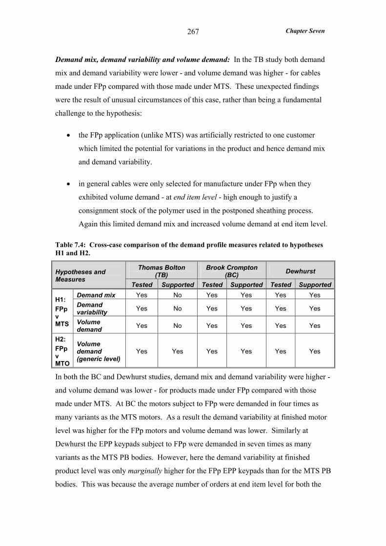
Chapter Seven

267

Demand mix, demand variability and volume demand: In the TB study both demand

mix and demand variability were lower - and volume demand was higher - for cables

made under FPp compared with those made under MTS. These unexpected findings

were the result of unusual circumstances of this case, rather than being a fundamental

challenge to the hypothesis:

• the FPp application (unlike MTS) was artificially restricted to one customer

which limited the potential for variations in the product and hence demand mix

and demand variability.

• in general cables were only selected for manufacture under FPp when they

exhibited volume demand - at end item level - high enough to justify a

consignment stock of the polymer used in the postponed sheathing process.

Again this limited demand mix and increased volume demand at end item level.

Table 7.4: Cross-case comparison of the demand profile measures related to hypotheses H1 and H2.

Thomas Bolton (TB)

Brook Crompton (BC) Dewhurst Hypotheses and

Measures Tested Supported Tested Supported Tested Supported

Demand mix Yes No Yes Yes Yes Yes Demand variability Yes No Yes Yes Yes Yes

H1: FPp v MTS Volume

demand Yes No Yes Yes Yes Yes

H2: FPp v MTO

Volume demand (generic level)

Yes Yes Yes Yes Yes Yes

In both the BC and Dewhurst studies, demand mix and demand variability were higher -

and volume demand was lower - for products made under FPp compared with those

made under MTS. At BC the motors subject to FPp were demanded in four times as

many variants as the MTS motors. As a result the demand variability at finished motor

level was higher for the FPp motors and volume demand was lower. Similarly at

Dewhurst the EPP keypads subject to FPp were demanded in seven times as many

variants as the MTS PB bodies. However, here the demand variability at finished

product level was only marginally higher for the FPp EPP keypads than for the MTS PB

bodies. This was because the average number of orders at end item level for both the

Chapter Seven

268

EPP keypads and the PB bodies was very similar. In fact half of the ten stocked PB

bodies were only subject to one or two orders over the study period and therefore

exhibited a very high CV of demand. It is questionable if these PB bodies should have

been MTS. If they were excluded from the analysis demand variability dropped

significantly.

Volume demand at generic level: As predicted by H2 in all three cases the generic

products selected for manufacture under FPp exhibited higher volume demand than

those which were MTO. This was attributable to variations in the MTO generic product

specification that did not exist in the FPp generic product. In the TB study there were

two generic cables in the MTO UoA compared to one in the FPp UoA. In the BC study

there were 155 generic motors in the ETO UoA compared to only 24 generic motors in

the FPp UoA. Finally in the Dewhurst study there were six generic keypads in the

MTO UoA compared to three in the FPp UoA.

7.4.3 Customer Service and Demand Amplification (H3 and H4)

The research questions and respective hypotheses relating to the customer service

measures (ex-stock availability, order lead-time and delivery reliability) and the demand

amplification measure are:



The results from the three case studies are summarised in Table 7.5. Hypothesis H3

was not tested by either the TB or the BC case studies. However it was tested by the

Dewhurst study and the findings supported hypothesis H3. Hypothesis H4 was tested

and supported by all three case studies with the exception of the delivery reliability

findings from the TB study which challenged H4.

Ex-stock Availability: Hypothesis H3 remained untested in the TB study due to a lack

of appropriate data. This was also partially true of the BC study. However the principal

reason for hypothesis H3 not being tested at BC was that H3 pre-supposed that orders

subject to FPp and MTS did not pull from the same product stocks as they did at BC.

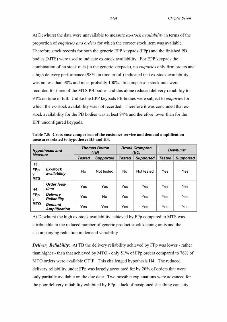
Chapter Seven

269

At Dewhurst the data were unavailable to measure ex-stock availability in terms of the

proportion of enquiries and orders for which the correct stock item was available.

Therefore stock records for both the generic EPP keypads (FPp) and the finished PB

bodies (MTS) were used to indicate ex-stock availability. For EPP keypads the

combination of no stock outs (in the generic keypads), no enquiries only firm orders and

a high delivery performance (98% on time in full) indicated that ex-stock availability

was no less than 98% and most probably 100%. In comparison stock outs were

recorded for three of the MTS PB bodies and this alone reduced delivery reliability to

94% on time in full. Unlike the EPP keypads PB bodies were subject to enquiries for

which the ex-stock availability was not recorded. Therefore it was concluded that ex-

stock availability for the PB bodies was at best 94% and therefore lower than for the

EPP unconfigured keypads.

Table 7.5: Cross-case comparison of the customer service and demand amplification measures related to hypotheses H3 and H4.

Thomas Bolton (TB)


Measure Tested Supported Tested Supported Tested Supported

H3: FPp v MTS

Ex-stock availability No Not tested No Not tested Yes Yes

Order lead-time Yes Yes Yes Yes Yes Yes

Delivery Reliability Yes No Yes Yes Yes Yes

H4: FPp v MTO Demand

Amplification Yes Yes Yes Yes Yes Yes

At Dewhurst the high ex-stock availability achieved by FPp compared to MTS was

attributable to the reduced number of generic product stock keeping units and the

accompanying reduction in demand variability.

Delivery Reliability: At TB the delivery reliability achieved by FPp was lower - rather

than higher - than that achieved by MTO - only 51% of FPp orders compared to 76% of

MTO orders were available OTIF. This challenged hypothesis H4. The reduced

delivery reliability under FPp was largely accounted for by 20% of orders that were

only partially available on the due date. Two possible explanations were advanced for

the poor delivery reliability exhibited by FPp: a lack of postponed sheathing capacity

Chapter Seven

270

(as suggested by the excess capacity measure in hypothesis H6); and insufficient generic

cable stock. The underlying cause of these factors was the unusual circumstances of

this case. In particular the customer of cables subject to FPp was allowed to call-off

finished cables rather than have them delivered upon completion. Therefore finished

cable stock existed which provided a buffer against poor delivery reliability such that it

was not noticed. Had this not been the case TB would have been forced to address poor

delivery reliability and as a result this would no doubt have improved.

In both the BC and Dewhurst studies delivery reliability was higher for products subject

to FPp than the MTO products. However at BC the improvement in delivery reliability

provided by FPp was unexpectedly modest. There are three possible explanations:

• Often quoted lead-times for the modified motors (FPp) did not take into account

availability of modification parts. Also the process of parts acquisition was very

laborious and outside the MRP system.

• Extremely limited resources where two thirds of the modifications took place,

coupled with the fact that this section was primarily tasked with service and

repairs, may have led to the unresponsive execution of modifications (as

suggested by the lower delivery reliability measure for this area).

• Low standard motor stocks, providing only 63% ex-stock availability for

modified motor orders, may have extended the manufacturing lead-time.

Order Lead-time: In all three case studies the order lead-time achieved by the FPp

approach was substantially less than that achieved by MTO, supporting hypothesis H4.

As expected this was in part because much of the manufacturing was conducted

speculatively to stock rather than to order. However other factors also contributed to

the reduction in order lead-time achieved by FPp. At TB the order lead-time achieved

by FPp was just under half of the order lead-time achieved by MTO. This was partially

due to the synchronisation of the weekly manufacturing planning process at TB’s and

their customer’s factories. At BC the order lead-time achieved by FPp was less than a

quarter of that achieved by ETO orders. This was in part due to dramatic reductions in

engineering and bought-in parts lead-times. At Dewhurst the order lead-time achieved

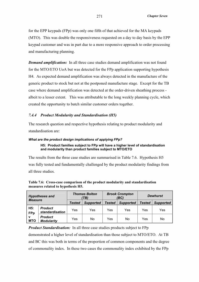
Chapter Seven

271

for the EPP keypads (FPp) was only one fifth of that achieved for the MA keypads

(MTO). This was double the responsiveness requested on a day to day basis by the EPP

keypad customer and was in part due to a more responsive approach to order processing

and manufacturing planning.

Demand amplification: In all three case studies demand amplification was not found

for the MTO/ETO UoA but was detected for the FPp application supporting hypothesis

H4. As expected demand amplification was always detected in the manufacture of the

generic product to stock but not at the postponed manufacture stage. Except for the TB

case where demand amplification was detected at the order-driven sheathing process -

albeit to a lesser extent. This was attributable to the long weekly planning cycle, which

created the opportunity to batch similar customer orders together.

7.4.4 Product Modularity and Standardisation (H5)

The research question and respective hypothesis relating to product modularity and

standardisation are:



was fully tested and fundamentally challenged by the product modularity findings from

all three studies.

Table 7.6: Cross-case comparison of the product modularity and standardisation measures related to hypothesis H5.

Thomas Bolton (TB)



Product standardisation Yes Yes Yes Yes Yes Yes H5:

FPp v MTO

Product Modularity Yes No Yes No Yes No

Product Standardisation: In all three case studies products subject to FPp

demonstrated a higher level of standardisation than those subject to MTO/ETO. At TB

and BC this was both in terms of the proportion of common components and the degree

of commonality index. In these two cases the commonality index exhibited by the FPp

Chapter Seven

272

UoA was almost three times higher than that for the MTO UoA and it was higher at

every level in the BOM. At the lower BOM levels this was due to FPp being applied to

fewer generic products than MTO/ETO. At the higher BOM levels, relating to the

postponed processes, the high commonality was for different reasons. At TB it was due

to the restriction of FPp to one customer which enabled the standardisation of packaging

components and limited the range of sheathing compounds. At BC it was simply due to

the customers’ requirement for less variety in the peripheral components of motors

subject to FPp.

At Dewhurst a much greater proportion of EPP keypad components were common to all

variants than MA keypad components (48% compared with 3%) and this was due to a

single generic body design serving the full range of EPP keypads (with the exception of

a single variable component). Unexpectedly the EPP and MA keypads exhibited a very

similar degree of commonality index overall - 14% compared with 15% respectively.

However the source of commonality was quite different - commonality in the generic

keypad was higher for the EPP keypads whereas commonality in the keytips (the

configuring components) was higher for the MA keypads.

Product Modularity: In all three cases the degree of modularity exhibited by the

products subject to FPp was the same as – rather than higher than - that exhibited by the

products subject to MTO/ETO. All the cables manufactured by TB were highly

modular. The generic cable, as well as the components supplied to the postponed

process, displayed a high degree of modularity. The keypads manufactured by

Dewhurst exhibited a lower degree of modularity than the cables due to the lack of

modularity in the generic keypad bodies. However the keytips – the only customising

component required - were highly modular. The BC motors, the most complex product

studied, exhibited the lowest degree of modularity. The major sub-assemblies in the

motors exhibited a low degree of modularity, although peripheral components (involved

in final assembly) exhibited a high degree of modularity. The majority of the

customising components were highly modular and many were peripheral.

The customising components required by all three products subject to FPp were highly

modular except for some of the components required for the BC motor modifications.

Just under a quarter of the motor modifications required customising components which

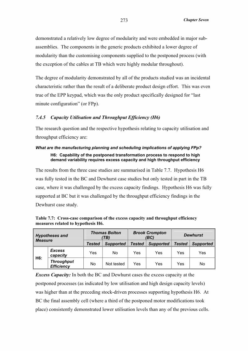
Chapter Seven

273

demonstrated a relatively low degree of modularity and were embedded in major sub-

assemblies. The components in the generic products exhibited a lower degree of

modularity than the customising components supplied to the postponed process (with

the exception of the cables at TB which were highly modular throughout).

The degree of modularity demonstrated by all of the products studied was an incidental

characteristic rather than the result of a deliberate product design effort. This was even

true of the EPP keypad, which was the only product specifically designed for “last

minute configuration” (or FPp).

7.4.5 Capacity Utilisation and Throughput Efficiency (H6)

The research question and the respective hypothesis relating to capacity utilisation and

throughput efficiency are:



was fully tested in the BC and Dewhurst case studies but only tested in part in the TB

case, where it was challenged by the excess capacity findings. Hypothesis H6 was fully

supported at BC but it was challenged by the throughput efficiency findings in the

Dewhurst case study.

Table 7.7: Cross-case comparison of the excess capacity and throughput efficiency measures related to hypothesis H6.

Thomas Bolton (TB)



Excess capacity Yes No Yes Yes Yes Yes

H6: Throughput Efficiency No Not tested Yes Yes Yes No

Excess Capacity: In both the BC and Dewhurst cases the excess capacity at the

postponed processes (as indicated by low utilisation and high design capacity levels)

was higher than at the preceding stock-driven processes supporting hypothesis H6. At

BC the final assembly cell (where a third of the postponed motor modifications took

place) consistently demonstrated lower utilisation levels than any of the previous cells.

Chapter Seven

274

At Dewhurst the average capacity utilisation was significantly lower for the EPP keypad

configuration cell than the stock driven EPP assembly cell.

In the TB study the postponed sheathing process consistently exhibited the least excess

capacity compared to the preceding processes challenging hypothesis H6. This was

attributable to the provision of less capacity at the postponed process which was due to

the unusual circumstances at TB. The lack of sheathing capacity contributed to the poor

delivery reliability achieved by FPp, which itself challenged hypothesis H4. As

previously discussed for hypothesis H4 the existence of finished cable stocks (created

by VP’s delayed call-offs) provided a buffer against poor delivery reliability. This

allowed the low sheathing capacity to persist unaddressed. Had the finished cable

buffer stocks not existed TB would have been forced to address poor delivery

reliability, and would have probably increased sheathing capacity.

Throughput Efficiency: Hypothesis H6 was not tested with respect to the throughput

efficiency measure in the TB case study because it was not possible to take this measure

for the postponed process.

In the Dewhurst study the throughput efficiency was higher for the stock driven EPP

assembly than it was for the postponed configuration - 27% compared to 11%. This

challenged hypothesis H6 and was in spite of the fact that manufacturing lead-times for

the postponed configuration process were considerably shorter than for the keypad

assembly process - 3 compared to 17.5 working days respectively. There were two

explanations for the unexpectedly low throughput efficiency at the postponed

configuration process:

• high generic keypad stock targets - equivalent to 4 weeks cover – encouraged

large generic keypad stock replenishment orders. These were much greater than

the size of the customer orders for configured keypads - 520 compared with 45

respectively. The stock replenishment orders were on average equal to one

weeks supply and in many cases 2 weeks.

• queuing caused by capacity restrictions at the postponed configuration process

extended the manufacturing lead-time by over 500%. However, the order lead-

Chapter Seven

275

times required by the EPP customer were being reliably satisfied. Therefore it

appeared that a shorter manufacturing lead-time - or higher throughput

efficiency - was not needed.

These problems were due to flaws in the FPp application at Dewhurst. The high generic

stock levels ensured that the stock driven generic processing was far from the ‘lean’

ideal and the postponed keypad configuration process demonstrated a lack of

responsiveness. However greater responsiveness was not required as the FPp

application already provided double the responsiveness (on average) requested on a day

to day basis by the customer.

The findings from the BC study supported hypothesis H6. The throughput efficiency

for the postponed modifications was double that achieved by the stock-driven

manufacture of the generic stock motors (21% compared to 10%). However, as in the

Dewhurst case, the throughput efficiency measured for the postponed process was

highly variable from order to order giving a coefficient of variation of 127% (four times

that for generic motor manufacture). The main factor driving the variability in

throughput efficiency was the variety of modifications which required anything from 10

minutes to 26 working hours.

In both the Dewhurst and BC case studies the most striking difference between generic

product manufacture and the postponed processes was not the throughput efficiencies

but the manufacturing lead-times. Postponed processes were clearly more responsive

with a manufacturing lead-time equivalent to only 18% of the generic product

manufacturing lead-times in both cases.

7.4.6 Production Variety Funnel

At TB and Dewhurst the number of SKUs at the CODP was greater than the number of

finished product variants demanded - eight SKUs compared to five finished cables at

TB and 179 SKUs compared to 72 finished keypads at Dewhurst. This is contrary to

the original conceptual model of FPp which predicted the number of SKUs at the CODP

to be substantially less than the number of finished items (see section 2.7).

Chapter Seven

276

In both cases this situation was not a feature of the duration of the study but a feature of

the product. At TB even if FPp had not been restricted to one customer this situation

would have persisted because for every new finished cable variant a new sheathing

polymer was likely to be required. At Dewhurst, although the theoretical potential

number of finished EPP keypads was much greater than 72, this product was supplied

exclusively to one customer and therefore the actual number of finished items was

unlikely to change significantly.

At TB and Dewhurst FPp was applied to a set of predefined finished product variants

therefore MTS was an option. However, in spite of the increased SKU’s required to

support FPp (compared to MTS) it still provided benefits - the generic product and

component stocks were more flexible than finished product stocks (ensuring lower stock

levels) and certainly of much lower value.

The situation was different at BC. Although 24 generic motors were stocked and 51

different components were supplied into the postponed process, the number of SKUs at

the CODP was still less than the 56 finished motor variants demanded. This was

because many of the components were purchased to customer order which was

attributable to two features of the FPp application at BC. Firstly the finished motor

specifications were not predefined (as at TB and Dewhurst) instead the motors were

truly customised. Therefore to predict and stock the full array of modifying

components was impossible. Secondly BC did not need to provide such a responsive

supply to their customers (as at TB and Dewhurst) and therefore there was sufficient

manufacturing lead-time to purchase (or make) the components to customer order.

7.5 CONCLUSIONS

Important commonalities were observed between the three cases of FPp. All involved

industrial products exhibiting ‘component swapping’ modularity (Pine, 1993) where

‘different components are paired with the same basic product’ to produce high variety in

the finished product (as discussed in section 2.6.2).

In all three cases the FPp applications were not ideal and this created anomalies in the

findings. The FPp application in the initial study at Thomas Bolton was flawed to the

Chapter Seven

277

extent that after nine months it could no longer be defined as FPp. At Brook Crompton

the FPp application was sustainable, however the customising process involved the

removal of previously added components. Finally the FPp application at Dewhurst

most closely resembled an ‘ideal’ application, however it was not the planned ideal

application!

The anomalies in the findings (caused by the flaws in the FPp applications) resulted in a

number of hypotheses being challenged - not the predicted results but for predictable

reasons. The hypotheses were deduced on the basis of an ideal FPp application,

therefore some hypotheses were challenged when tested against less than ideal

applications. When the complete picture was built up of how FPp was applied in each

case study the challenges to the hypotheses were understandable and predictable.

Literal replication (Yin, 2003) was sought (as described in section 3.4.3) where results

were predicted to be similar for each case. This was not achieved for some hypotheses

instead ‘theoretical replication’ resulted where cases produced contrasting findings but

for predictable reasons (Yin, 2003).

In the TB case three hypotheses were challenged (one in its entirety and two in part) as

a result of anomalies in the findings. The challenge to the demand profile hypothesis

was the result of the FPp application being restricted to one customer and only

applicable to high volume end item cables (to justify a consignment stock of the

sheathing polymer). The challenges to the delivery reliability and excess capacity

hypotheses were attributable to the existence of finished cable stocks. These provided a

buffer against poor delivery reliability and allowed the lack of postponed process

capacity to go unnoticed.

In the BC case no hypotheses were challenged as a result of anomalies in the findings.

However in the Dewhurst case the throughput efficiency hypothesis was challenged.

High generic stock levels ensured that the stock driven generic processing was far from

the ‘lean’ ideal and the postponed process demonstrated a lack of responsiveness.

However greater responsiveness was not required as the FPp application already

provided double the responsiveness requested by the customer.

Chapter Seven

278

Taking into account the anomalies in the findings the hypotheses remain largely

unscathed. Only the product modularity findings fundamentally challenged the

hypotheses. In all three cases product modularity was not related to the inventory

management policy – the products in the three UoA demonstrated very similar levels of

modularity.

The elusiveness of an ideal FPp application is evidence of the major operational

challenges involved in its application and ensures that FPp as envisaged remains at the

conceptual level. The broader implications - revealed by this study - for applying FPp

in practice are discussed in the next and final chapter.

Chapter Eight

279

CHAPTER EIGHT

8 Conclusions

The purpose of this concluding chapter is to summarise the research project, to describe

the contribution to knowledge in the context of the research objectives and to make

proposals for further research.

8.1 SUMMARY OF THE PROJECT

Postponement is widely recognised as an approach that can lead to superior supply

chains, and the application of postponement has been observed as a growing trend in

manufacturing and distribution by various surveys and prominent researchers.

However, although much is written in the literature on the benefits of postponement,

little is still known about its application.

FPp is a phenomenon truly at the ‘interface’ between logistics and OM employing

supply chain and manufacturing systems thinking. The logistics literature considers

conditions when FPp is the appropriate strategy. Here FPp tends to be limited to

applications where the postponed processes are conducted in the distribution chain and

the practical implications of applying FPp are not considered. In terms of the OM

literature FPp is a responsive non-MTS approach to mass customisation. However

empirical research addressing the needs of non-MTS companies is astonishingly modest

and tends not to consider responsive approaches like FPp. FPp is a major enabler to

satisfying the more fragmented markets of the future variously described as ‘mass

customisation’. The literature concerning mass customisation is extensive but much

less has been written about its operational implications. Recently a small body of OM

literature has emerged that addresses FPp. However it is dominated by mathematical

and inventory models which consider delayed product differentiation applied to MTS

approaches and therefore is not directly applicable to FPp. With the introduction of a

CODP at the generic product stage these models could be very useful in understanding

some of the operational implications of FPp.

Chapter Eight

280

Thus this research project aims to address how FPp is applied in terms of the

operational implications within the manufacturing facility. Here the generic and

postponed processes are performed in the same location, normally a factory. The

review of logistics, operations and engineering literature related to FPp revealed a

number of key operational implications. These concerned product selection, product

design, process configuration, inventory management, CODP location, manufacturing

planning, demand amplification and customer service. This thinking lead to the

development of a theoretical framework, on the basis of an ideal FPp application, from

which the following hypotheses were taken:







Though the hypotheses provide a focus for the study they do not encapsulate it. In

addition to the quantitative evidence required to test the hypotheses much qualitative

evidence (words rather than numbers) was collected and analysed to address the

overriding research question - ‘why and how is FPp applied in manufacturing?’

8.1.1 Research Strategy

Much of the research related to FPp has involved either computer simulation modelling

or large sample surveys. Exploring the complex operational issues arising from the

application of FPp, requires in-depth case studies of the phenomenon in relation to its

real life context. The case-oriented approach seeks to account for all deviating cases,

Chapter Eight

281

and therefore creates a rich dialogue between theory and evidence (Ragin, 1987). This

is particularly significant for this research as the theoretical base is weak. It is said that

in an area such as this ‘field based approaches are the best ways to find out about the

issues, describe the problems, discover solutions and generally ground our theory in the

complex, messy world of real organisations’ (McCutcheon and Meredith, 1993).

The multiple case study design where each case incorporated multiple units of analysis

(UoA) - effectively mini cases within a case - was chosen. The UoAs were based

around product groups subject to different inventory management policies – FPp, MTO

and MTS. Comparing UoAs within each case enabled the contextual differences

between manufacturing facilities (which were not the subject of this study) to be

screened out. The cases were selected from the domain of manufacturing facilities in

England with the aim of providing diverse contexts in which to study the application of

FPp. Diversity was sought in terms of industry and product complexity such that the

analytic generalisability of the findings could be extended. The research design was

first developed and tested in a pilot study at Thomas Bolton Flexible Cable factory (TB)

in Melling where I had worked some 3 years earlier. The two main case studies were

conducted at Brook Crompton (BC, electric motor manufacture) and Dewhurst (control

systems manufacture). UoAs at TB were from the same cable group, at BC were

different LDC motors, and at Dewhurst were EPP keypads, MA keypads and

pushbutton bodies.

In all three cases FPp had been applied some two years prior to the study in order to

improve customer responsiveness. The operational implications of applying FPp were

explored using structured interviews supported by documentary evidence. A set of

quantitative variables were compared across the three UoA and the results compared

with those predicted by the hypotheses in a strategy called ‘pattern matching’

(Campbell, 1975).

8.1.2 Measuring Form Postponement

Based on the literature review and the pilot study at TB a number of internal and

external variables which measure the outcome of applying FPp were developed.

Predictions were made about these variables in the hypotheses therefore the variables

Chapter Eight

282

were developed to be precise and measurable to enable predictions to be tested against

findings. The outcome variables are briefly defined below:

Demand amplification: the amplification of customer demand in the process schedules

within a manufacturing facility.

Ex-stock availability: is the proportion of initial customer requests (enquiries or orders)

for which the correct product is available ex-stock in sufficient quantities.

Order lead-time: is the time between the customer ordering the product and receiving it.

Delivery reliability: is the ability of the operating facility to meet the agreed terms of

delivery with respect to the product type, the quantity ordered and the due date

Product Modularity (degree of): depends on the degree to which the physical product

design reflects the functional architecture of the product.

Product standardisation: results in component commonality measured by the

proportion of common components in all variants and the degree of commonality index.

Excess Capacity: is the amount that available capacity exceeds demand and manifests

itself as ‘process idle time’ when the process could be producing but the current load

does not require this capacity.

Production Variety Funnel: describes in graphical terms the number of physically

different items that occur at different stages of the manufacturing process.

Demand mix: number of product items subject to demand.

Demand variability: changes in demand over a given sequence of time buckets

measured using the coefficient of variation.

Volume demand: quantity of a given item demanded.

In operationalising the research design some variables were grouped together because

they used the same data and were strongly related. Ex-stock availability, order lead-

time and delivery reliability were grouped under ‘customer service’. The three external

Chapter Eight

283

demand variables – demand mix, demand variability and volume demand - were

grouped under ‘demand profile’.

Qualitative evidence was also collected via numerous structured interviews with key

personnel. The qualitative evidence included contextual data such as business

environment, reasons for applying FPp and product type. But the majority of the

qualitative evidence concerned the ‘change content’ required to apply FPp in a

previously MTO and MTS environment. This included product (or customer) selection,

inventory management, CODP relocation and manufacturing planning and scheduling.

To complete the picture qualitative evidence was collected on problems encountered

with the FPp application and potential improvements.

The eleven outcome variables defined were not intended to form a comprehensive

description of the FPp application but to focus a broad based measurement of the UoA

to identify the differences between FPp, MTO and MTS. The qualitative data

corroborated this quantitative evidence (and visa versa), gave explanations for the

differences in the outcome variables between the UoAs and provided a description of

how in practical terms FPp was applied. This combination of qualitative and

quantitative evidence in the case studies helped to triangulate the research findings.

8.1.3 Rigour in Case Study Design

Case studies have traditionally been viewed as a somewhat problematic form of enquiry

compared to other empirical methods and the most common concern is lack of rigour in

the research design. Yin (2003) proposes four tests to establish the quality of empirical

social research. How the research design addresses each test is described below:

Construct validity: FPp was precisely defined and various indicators and measures were established and tested in the pilot study. In addition both methodological and data triangulation was used to improve construct validity.

Internal validity: the variables were compared between the UoA within each case to screen out contextual differences between manufacturing facilities and show the outcome of applying FPp. The results of the comparison were compared with those predicted in the hypotheses using the pattern matching strategy.

Chapter Eight

284

External validity: case selection relied on replication logic rather than sampling logic. Here replication means that individual cases can be used for independent corroboration of specific hypotheses as with experiments. In this study the cases were selected to provide variety but each case was expected to support the hypotheses (literal replication). Analytic generalisation, where the researcher attempts to generalise a particular set of results to some broader theory was sought rather than statistical generalisation where the findings apply to a population.

Reliability: the quantitative measures and the qualitative interviews were developed and tested in the pilot study. These were documented and repeated in the two main case studies. The same approach to case analysis was used in all cases: pattern matching for the quantitative evidence; and compiling interview transcripts without losing informants identity for the qualitative evidence. Where opinion based evidence was gathered this was validated by the informant.

A second commonly cited weakness of the case study research concerns the population

to which the findings can be generalised – external validity - which is dealt with as

described above. Consequently case selection in this research sought to extend analytic

generalisability by studying FPp in diverse contexts. This was achieved in terms of

product complexity, industry and type of customisation as explained in section 8.3

describing the contribution.

8.2 CONTRIBUTION TO KNOWLEDGE

This thesis makes a contribution to both logistics and OM knowledge. The contribution

to OM is in three areas: non-MTS approaches, mass customisation and postponement.

Amaro et al (1999) points out that ‘the literature addressing the needs of companies

which produce in response to customers’ orders is astonishingly modest’. The needs of

the non-MTS sector have been neglected. FPp is distinct from the established non-MTS

categories (ATO, MTO and ETO) in a number of ways but particularly in terms of its

responsiveness. The research addressing non-MTS approaches tends to consider ATO,

MTO and ETO not to be responsive - orders are promised on the basis of the

availability of components and/or capacity rather than on the basis of a short often

standard quoted lead-time as for FPp (for example Hendry and Kingsman, 1989, Yeh,

2000, Segerstedt, 2002).

Chapter Eight

285

Mass customisation has been defined as ‘providing numerous customer chosen

variations on every order with little lead-time or cost penalty’ (Ahlstrom and

Westbrook, 1999). Most of the research on mass customisation is concerned with its

strategic impact (for example Gilmore and Pine, 1997, Pine et al, 1993, 1995, Lampel

and Mintzberg, 1996, Kotha, 1995, Westbrook and Williamson, 1993). There are few

publications concerning the operational implications of mass customisation (for

example Pine, 1993, Ahlstrom and Westbrook, 1999, Swaminathan, 2001, MacCarthy

et al. 2003).

Recently a small body of OM research has emerged that addresses postponement. A

theoretical paper (Yang and Burns, 2003) reviews research on postponement and

concludes that still little is known about its application. Most of the OM research on

FPp uses variable-oriented models of postponement applications (for example Van

Mieghem and Dada, 1999, Aviv and Federgruen, 2001a and 2001b, Ma et al., 2002,

Ernst and Kamrad, 2000). Most of these models consider delayed product

differentiation applied to MTS approaches and therefore are not directly applicable to

FPp.

This thesis contributes to OM knowledge by considering the operational issues of

applying FPp. This is a specific and responsive non-MTS approach to mass

customisation distinct from existing documented categories, ETO, MTO and ATO. A

case study design has been used to address the complexities of applying FPp. This

exploratory work could aid the development of variable-oriented models to simulate

FPp and its operational implications. On a strategic level this research contributes an

inventory management decision framework (shown in Table 8.1) to determine when

FPp is a viable alternative to either MTS or MTO on the basis of the product’s demand

profile, customer service provided and demand amplification. Also it is concluded that

even when a FPp application is flawed as it was in all three case studies it is still worth

applying.

Unlike earlier research on mass customisation or postponement this research focuses on

the specific operational implications within the manufacturing facility. A second

framework is developed (shown in Figure 8.1), which provides practical guidance on

how FPp can be applied in terms of product design, inventory management,

Chapter Eight

286

manufacturing planning and scheduling operations. In addition obstacles to the

application of FPp are identified.

This research project contributes to our understanding of the conditions under which

FPp is justified and specification of the appropriate FPp strategy (for example Zinn and

Bowersox, 1988, Zinn, 1990a, Cooper, 1993, Pagh and Cooper, 1998, van Hoek, 1998a,

van Hoek et al. 1998). Previous research considers FPp as an alternative strategy to

MTS - not to MTO - and the guidelines are restricted to deciding an appropriate

postponement strategy rather than its application. In general only FPp applications

where the postponed processes are conducted in the distribution chain have so far been

considered. When postponed processes are brought back into the factory it is argued

that substantially more complex processes are likely to be capable of postponement, as

supported by Van Hoek’s, (1998c) survey of companies in Holland.

This research extends logistics knowledge on FPp by considering FPp applications

where postponed processes are performed in the same location as the generic processes,

normally in a factory (termed ‘unicentric’ FPp). This tends to involve the postponement

of more complex processes than previously considered in logistics research. This

research contributes an inventory management decision framework (shown in Table

8.1) which considers when FPp is a viable alternative to either MTS or MTO on the

basis of the product’s demand profile, customer service provided and demand

amplification - all important supply chain issues. Further contributions are made by

addressing the complex operational implications (such as process design and

manufacturing planning) arising from taking the postponed processes back into the

factory. Two main factors contribute to these operational issues. First, increased

complexity of the postponed processes and second the requirement that the factory

adapt to the FPp strategy. A strategy which incorporates aspects of both MTO and

MTS but also has additional specific requirements.

8.2.1 Inventory Management Policy Decision Framework

The inventory management decision framework shown in Table 8.1 shows when FPp is

a viable alternative to either MTS or MTO on the basis of the product’s demand profile

(at generic and end item level), customer service provided and demand amplification.

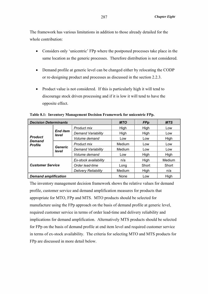
Chapter Eight

287

The framework has various limitations in addition to those already detailed for the

whole contribution:

• Considers only ‘unicentric’ FPp where the postponed processes take place in the

same location as the generic processes. Therefore distribution is not considered.

• Demand profile at generic level can be changed either by relocating the CODP

or re-designing product and processes as discussed in the section 2.2.3.

• Product value is not considered. If this is particularly high it will tend to

discourage stock driven processing and if it is low it will tend to have the

opposite effect.

Table 8.1: Inventory Management Decision Framework for unicentric FPp.

Decision Determinants MTO FPp MTS Product mix High High Low Demand Variability High High Low End item

level Volume demand Low Low High Product mix Medium Low Low Demand Variability Medium Low Low

Product Demand Profile Generic

level Volume demand Low High High Ex-stock availability n/a High Medium Order lead-time Long Short Short Customer Service Delivery Reliability Medium High n/a

Demand amplification None Low High

The inventory management decision framework shows the relative values for demand

profile, customer service and demand amplification measures for products that

appropriate for MTO, FPp and MTS. MTO products should be selected for

manufacture using the FPp approach on the basis of demand profile at generic level,

required customer service in terms of order lead-time and delivery reliability and

implications for demand amplification. Alternatively MTS products should be selected

for FPp on the basis of demand profile at end item level and required customer service

in terms of ex-stock availability. The criteria for selecting MTO and MTS products for

FPp are discussed in more detail below.

Chapter Eight

288

MTO products suitable for manufacture under the FPp approach should meet the

following criteria:

• Generic product variants which are subject to low demand variability and high

volume demand (as in TB and Dewhurst cases). If this is not so then it may be

possible to achieve this by standardising the early (or generic) processes,

increasing component commonality and reducing the number of generic product

variants.

• Products that require high delivery reliability and an order lead-time

considerably shorter than that achievable using MTO. A more responsive

product supply may be needed to improve competitiveness.

• Component suppliers that can manage levels of demand amplification likely to

be introduced by the application of FPp.

MTS products suitable for manufacture under the FPp approach should meet the

following criteria

• Products which exhibit high product mix (or potentially high product mix), high

demand variability and low volume demand at end item level. This may be

indicated by inaccurate sales forecasting causing large discrepancies between

available stock and demand evidenced by stock outs and excessive stocks.

• Products which require high ex-stock availability. Stock outs may be critical

and not tolerable by the customer as was the case at Dewhurst.

• Products for which demand amplification is high and causing component supply

problems.

• Postponed processes, necessary to apply FPp, must not extend the order lead-

time beyond the existing lead-time unless acceptable to the customer.

In conclusion opportunities for applying FPp to MTO products depends on the demand

profile at generic level. If this is not appropriate it may be possible to re-design the

Chapter Eight

289

product through process and component standardisation to create a narrow range of

generic products demanded in sufficient volumes for the application of FPp.

Opportunities for applying FPp to MTS products depend on the demand profile for the

finished products and are indicated by inaccurate sales forecasting, stock outs and

excessive stocks. In this case it still may be necessary to re-design the product to

establish a narrow range of generic products demanded in sufficient volumes to enable

the application of FPp.

8.2.2 Practical Implications of Form Postponement

The main contribution to knowledge of this research project is the practical implications

of applying FPp within a manufacturing facility. A framework is developed which

provides practical guidance on how FPp can be applied in terms of product design,

inventory management, manufacturing planning and scheduling operations.

The original conceptual model of FPp (presented in section 2.7) has been revised and

the main conclusions from this research added to it to give the framework shown in

Figure 8.1. It applies to ‘unicentric FPp’ applications (i.e. where the postponed

processes take place in the same location as the generic processes) where the product

exhibits component swapping modularity. The framework illustrates the major

operational implications of applying FPp which are described in this section.

The PVF in the original conceptual model was found not to be suitable for products

exhibiting component swapping modularity. In this case the number of SKUs at the

CODP could be greater than the number of finished product variants and there still be

benefits to be gained from FPp over MTS. The PVF in the framework (Figure 8.1)

illustrates that, although the number of generic products items at the CODP is always

small compared to the number of finished product items, the total number of

components supplied into the postponed process may not be. Indeed this was true in all

three case studies, and at TB and Dewhurst the total number of SKUs at the CODP was

greater than the number of finished product items. In spite of this FPp still provided

advantages in inventory management over MTS because the SKUs at the CODP were

more flexible – not yet committed to a specific end item.

Chapter Eight

290

A final point about the framework – the number of finished product items is not the

theoretical potential never to be realised, but the number of finished items that are going

to be produced in the foreseeable future. In the case where the product is not truly

customised (i.e. the customer either selects finished items or optional modules from

predefined lists) this is easily calculable so that the PVF demonstrates the SKUs

required for a FPp application compared to MTS.

CODP

CODP

Few generic product variants

Many generic components

Low Excess Capacity

Fixed Period Scheduling

High component commonality

High Excess Capacity

Bucketless Scheduling

High modularity

Generic Product Manufacture Postponed Processes

Ope

ratio

nal

Impl

icat

ions

Num

ber o

f ite

ms

Average Lead-times

CODPlocation

CU

STO

MER

S

RA

W M

ATE

RIA

L PR

OC

UR

EMEN

T

Minimise orderlead-time

Minimise manufacturing

unit costs

Short postponed value adding time

High proportion of product is generic

Minimise inventory

Maximise customisation

GOALS GOALS

Com

pone

nts

Fini

shed

Pro

duct

s

Gen

eric

Pro

duct

s

Distribution

Customer Orders

Figure 8.1: Framework for the application of FPp.

Locating the CODP: The CODP should be located at a ‘neck’ in the Production

Variety Funnel as illustrated in the framework (Figure 8.1). This is typically at the

generic product stage such that:

• no previously added value is removed during the postponed process (as it was at

BC) i.e. no removal of components or rework as this adds to the cost of the

product

• the postponed value added processing time is short compared to total value

adding process time required to manufacture the product to ensure a short order

lead-time

Chapter Eight

291

• number of generic product variants are kept to a minimum and are each subject

to high volume demand and low volume demand variability (CV) relative to the

end items.

Product Design: A high proportion of the product should be standardised whilst

ensuring that the required customisation levels can still be achieved. Standardisation

that involves material redundancy should not be sought (unless absolutely necessary)

instead these differentiations should remain and be postponed. The stocked generic

products should exhibit a very high level of component commonality. Whilst this is

also desirable for any differentiating components supplied into the postponed process,

here component commonality must not reduce the achievable customisation level below

that required.

Ideally components supplied to the postponed process should be highly modular such

that: a one-to-one correspondence exists between each functional element and physical

component (or module); and every interaction between components is critical to the

function of the system. This enables components to be combined in numerous ways to

produce a wide range of product variants.

Inventory Management: Requirements related to order processing and inventory

control have been identified:

• EDI is a rapid and reliable way of transmitting customer orders particularly

when electronic data such as bar codes are required. However EDI is only

practical when the customer places orders at regular intervals. Further the

improved responsiveness offered by EDI transmission of orders can best be

realised if orders are processed upon arrival. If these conditions do not apply

and orders can be placed anytime then some type of broadcasting mechanism

must be deployed for the orders upon receipt. This may involve Kanbans been

faxed by the customer.

• Generic product stock level should provide forward cover that takes into account

volume demand variability (CV) at this level.

Chapter Eight

292

• If demand for the generic products and components is stable enough (i.e.

demand variability is low enough) generic product and the components can be

supplied to the postponed process under Kanban control. This was the case for

the keytips at Dewhurst.

• Components into postponed process must be available on a short enough lead-

time. In practice this implies that components are available ex-stock. However

this is not possible when a product is truly customised since the customising

components cannot be predefined (as at BC). In this case it must be ensured that

suppliers can deliver to order on a short lead-time. This is often not possible and

leads to FPp being limited to a set of predefined end items (as at TB and

Dewhurst).

• Generally standard quoted lead-times which apply to all orders are only possible

where FPp is applied to a predefined set of end items (as at TB and Dewhurst).

Where products are truly customised quoted lead-times must depend on

component availability and are difficult to standardise and keep short as the BC

case demonstrated.

Manufacturing Planning and Control: A number of requirements related to the

manufacturing planning systems and the capacity management are identified:

• The order processing and manufacturing planning systems for the postponed

process must be highly responsive. This often requires a real time planning

system – a fixed period MRP system for the postponed processing does not

support FPp applications for two reasons. Firstly the order processing time from

order logging to availability for manufacture tends not to be short enough, in

part due to the regeneration frequency of fixed period MRP systems. Secondly

fixed period MRP systems restrict due dates to typically weekly time buckets,

not appropriate for most FPp applications. Only in the TB case was a fixed

period MRP system used for the finished product and the failure of FPp, in this

case, was mainly attributable to this. At Dewhurst the existing planning system

was by-passed for the FPp application by real time manual planning procedures

Chapter Eight

293

to provide the required responsiveness. However bucketless MRP systems

(described by Vollman et al. 1992) could provide the required responsiveness.

• Where the postponed process is more complex and especially where the product

is truly customised (as was the case at BC) an MRP system may be desirable.

However configurable BOMs will be required such that any potential finished

product BOM can be quickly established for an order. At BC this was not the

case, infact it was not possible to configure the BOMs at all. Therefore the

existing planning system was by-passed for the FPp application by real time

manual planning procedures.

• Substantial excess capacity should be provided at the postponed process to

enable it to remain responsive when subjected to high demand variability in

terms of product mix and also to a lesser extent volume (i.e. demand variability

at generic level). Where sufficient excess capacity is not provided delivery

reliability can suffer (as at TB or BC).

• Throughput efficiency is not the crucial issue at the postponed process - it tends

to be highly variable. This is largely attributable to variations in value added

processing time due to variability in order sizes (as at Dewhurst) or

customisations required (as at BC). The crucial aim is to ensure that, even for

those orders which involve the highest levels of postponed value added time, the

manufacturing lead-time is sufficiently short to satisfy the customer required

order lead-times. This may imply limitations to the quantities or customisations

that can be delivered within the standard quoted lead-time for FPp.

8.2.3 Obstacles to the application of FPp

Product design: The extent to which it is possible to standardise the product to provide

few generic products and modularise the customising components. This is dependant

on the demand profile as well as the product characteristics themselves. At Dewhurst

the demand profile was such that it was not possible to standardise the colour

configured keypad, however by moving the CODP upstream a more standardised

generic product was identified. At BC the generic motor was demanded in 24 variants

and even moving the CODP upstream would not reduce this number.

Chapter Eight

294

Manufacturing Planning and Control: In general the mindsets associated with MTO

and MTS present an obstacle to FPp. Both approaches tend not to require either

manufacturing planning or manufacturing processes themselves to be responsive.

The existing order processing and manufacturing planning systems are obstacles to the

application of FPp as all three cases demonstrate. In both the TB and Dewhurst cases

the fixed period MRP systems were found to be insufficiently responsive to process

customer orders for FPp products. This manifested itself in two ways: firstly long

order processing times, extended in the TB case by infrequent MRP regeneration;

secondly time buckets restricting due dates to due weeks rather than days.

In the BC case the MRP system was responsive enough but the BOMs lacked

flexibility. It was not possible to configure the BOMs to reflect the modification of a

standard motor and this prevented BC from using the MRP system for orders subject to

FPp.

Postponed Process Capacity: Postponed process capacity presents an obstacle to the

application of FPp when it is insufficient to maintain the required responsiveness in

terms of short, reliable lead-times. At TB a lack of excess capacity at the postponed

process was a major contributing factor to the reduced delivery reliability provided by

FPp compared to MTO. Also at BC the lack of resource and focus in the department

performing the postponed modifications was a strong contributing factor to the poor

delivery performance.

8.2.4 Is Form Postponement worth it?

The operational requirements and obstacles inherent in the application of ‘unicentric

FPp’ detailed in the previous section represent a major challenge for a manufacturing

facility that previously made to order and made to stock. Given the formidable list of

changes required the question arises: ‘is it worth it?’ or would efforts be better invested

in improving the existing MTO and MTS approaches.

Each of the three case studies are considered to evaluate this question. At TB the

benefits of FPp were never realised because the application was fundamentally flawed.

Chapter Eight

295

However, at BC and Dewhurst, though the FPp applications were not ideal, benefits

over MTO and MTS were realised but were they worth the effort?

At BC the finished motor specifications subject to FPp were not predefined. Instead the

motors were truly customised. Therefore MTS was not an option because it was not

possible to predict and stock the full array of finished motors. MTO on the other hand

would not have enabled the motors to be delivered within the 3 to 4 weeks lead-time

expected by UK customers (for modified standard motors) - the best achievable by

MTO was 6 to 10 weeks depending on motor size. In conclusion if Brook Crompton

wanted to sell modified standard motors to UK customers the only option was FPp.

At Dewhurst FPp was applied to a set of predefined finished product variants therefore

MTS was an option. However this would have required very high finished stock levels

to ensure stock availability in the face of such high demand variability. Moreover the

customer did not need immediate availability and was satisfied with a 5 working day

lead-time. MTO on the other hand was not a possibility because keytip manufacture

involved numerous distinct processes, and a high minimum batch quantity, resulting in

a long manufacturing lead-time. Applying FPp by making at least the keytips to a

speculative stock was the only approach that minimised inventory whilst enabling the

customer service need to be met.

At TB if the difficulties with the manufacturing planning and scheduling system had

been overcome substantial benefits could have been realised. The design of the

majority of TB’s cables was ideal for FPp and presented no obstacles. The MTO lead-

time of 3 weeks could have been slashed to 3 days enabling cable supply to be matched

with the customers demand and all finished stocks eliminated. This would have

provided TB with the ability to provide exceptionally responsive service without the

need for high value finished goods stock.

Chapter Eight

296

The conclusion is that FPp is worth applying where:

• there is a need for greater responsiveness, in terms of shorter order lead-times,

than the MTO approach can deliver.

• product variety is such that the stock keeping units required to support a FPp

application enable inventory carrying cost reductions - compared to a MTS

application - without increasing the order lead-time beyond that required by the

customer.

This study reveals that even flawed FPp applications offer significant benefits and are

worth applying the question remains ‘is it worth applying FPp in an ideal way?’

Certainly in the BC case improvements in the FPp application would have delivered

reduce manufacturing costs and improvements in delivery reliability without reducing

responsiveness or increasing inventory costs. However, at Dewhurst, FPp was already

providing double the responsiveness requested by the customer and delivery reliability

was very high. Therefore there were no advantages to be gained through customer

service improvement. Generic product inventory on the other hand was high and this

could have been reduced with improvements to the FPp application – either moving the

CODP further upstream or reducing the stock levels through increased leanness of the

generic processes.

In conclusion improvements in a FPp application are subject to the same criteria as

other manufacturing operation improvements – they are only worth implementing if

they deliver either reductions in manufacturing costs or improvements in customer

service that will provide competitive advantage.

Chapter Eight

297

8.3 RESEARCH LIMITATIONS

No research design is without its limitations and this research is no exception. Upon

reflection of the entire research process three aspects stand out as limiting the findings.

These aspects are all related to the chosen case study approach and are discussed below.

8.3.1 Case Selection

Identifying suitable manufacturing facilities for the case studies proved to be

extraordinarily difficult and time consuming. Pettigrew (1990) discusses the process of

selecting cases:

‘there is an intentional or design component in the process of choosing and gaining access to research sites, but the practicalities of the process are best characterised by the phrase ‘planned opportunism’.

This is an honest assessment of the approach to case selection for this research which

was challenging for many reasons. Not only were the manufacturing facilities required

to have applied FPp (according to the working definition), but the research design

necessitated that both MTO and MTS approaches must have been applied during the

same time period. In addition all three inventory management policies were required to

have been applied to products of a similar nature in the manufacture of significant

proportions of the facility’s production.

Following the pilot study and a failed attempt to identify the remaining cases using

anecdotal articles, contacts and the like, a systematic approach was adopted. This

involved searching the FAME database of all UK registered companies to identify

companies from different industries that could potentially be applying FPp. About 120

introductory letters were sent to previously identified contacts to ascertain which

companies were applying FPp and interested in participating in the research. A

surprisingly high number of replies were received and many of them claimed to be

applying FPp. Unfortunately in many of the cases where FPp was ‘found’: it was

applied to an insignificant proportion of production; MTO nor MTS were applied; it

was applied intermittently; or the company was not interested in participating in the

study.

Chapter Eight

298

Finally after a number of factory visits Brook Crompton, an electric motor manufacturer

and Dewhurst, a manufacturer of control systems were found to satisfy all the criteria

and agreed to be studied. The three manufacturing facilities selected were not only

individually suitable, but also provided the intended diversity in terms of industry,

product complexity and even the nature of the manufacturing processes. Therefore,

although the process of case selection was somewhat laborious, the case studies were in

keeping with the research design.

8.3.2 Form Postponement Applications Studied

In all three cases the FPp applications were not ideal. In practice, or at least during this

research, an ideal FPp application could not be found. The FPp application in the initial

study at Thomas Bolton was flawed to the extent that after 9 months it could no longer

be defined as FPp. At Brook Crompton the FPp application was sustainable, however

the customising process involved the removal of previously added components. Finally

at Dewhurst an example of FPp was studied which most closely resembled the ideal

application, however flaws still remained.

The flaws in the FPp applications created anomalies in the findings which resulted in a

number of hypotheses being challenged - not the predicted results but for predictable

reasons. The hypotheses were deduced on the basis of an ideal FPp application (in part

depicted by the conceptual model of FPp), therefore some hypotheses were challenged

when tested against less than ideal applications. When the complete picture was built

up of how FPp was applied in each case study the challenges to the hypotheses were

understandable and predictable. Literal replication (Yin, 2003) was sought (as

described in section 3.4.3) where results were predicted to be similar for each case.

This was not achieved for some hypotheses instead ‘theoretical replication’ resulted

where cases produced contrasting findings but for predictable reasons (Yin, 2003).

The anomalies in the findings highlighted the effect of various flaws in the FPp

applications on the hypotheses. This revealed important links between poor delivery

reliability and lack of excess capacity at the postponed process and also suggested that

in practice throughput efficiency is not a crucial measure. Taking into account the

Chapter Eight

299

anomalies in the findings the hypotheses remain largely unscathed except for that

regarding product modularity which was fundamentally challenged by each study.

The elusiveness of an ideal FPp application is evidence of the major operational

challenges involved in its application and ensures that FPp, as envisaged, remains at the

conceptual level. Though limited in its generalisability this project reveals when FPp is

the preferred approach as an alternative to MTO or MTS and some of the major

operational implications of applying FPp in practice.

8.3.3 Data Availability

A total of twelve variables were measured in each case study and this presented major

challenges for data collection. Wherever possible the same type of evidence was used

for the measures in each of the three cases however each case presented its own unique

challenges and opportunities (as discussed in each case study chapter). In some cases

the measure was already taken and data was readily available in the correct form -

although this was rare. In most cases the measure had never been taken and raw data

had to be compiled and analysed. It was not possible to collect the ideal data for all the

measures in any of the case studies. However there was only one measure where the

ideal data was never available - the ex-stock availability measure. This measure would

have required a special data gathering exercise - not possible in a retrospective study.

Although the retrospective nature of the studies prevented special data gathering

exercises it sometimes provided data which would have been unavailable in a real-time

study. For example the capacity utilisation data in the TB case study was systematically

collected and analysed during the study period but by the time the study was conducted

the database had lapsed into disuse.

8.3.4 Generalisability of the findings

FPp was studied in three very different contexts with regard to industry and product

complexity. Another distinction that extends the generalisability of the findings is the

nature of the postponed ‘customisation’. At BC the products were truly customised,

that is the customers choices were not confined by pre-defined lists of options but were

truly free choices. In the other two cases the products could be more accurately

Chapter Eight

300

described as ‘configured’ to order where the customer selected finished products from a

pre-defined list of finished items.

The three cases exhibited certain commonalities that limit the generalisability of the

findings. The manufacturing facilities were all medium sized (between 120 and 200

employees and an annual turnover between £13 and £18 million) and manufactured

industrial products. Previous to applying FPp both MTO and MTS approaches were

used. In all three cases the products subject to FPp exhibited ‘component swapping’

modularity (Pine, 1993) where ‘different components are paired with the same basic

product’ to provide high variety in the finished product (as discussed in section 2.6.2).

8.4 FURTHER RESEARCH

The body of knowledge addressing the application of FPp is still small so there are

many opportunities for further research. Below four areas for research are identified

starting with an expansive survey:

1) Survey to assess the extent to which FPp is being applied: to identify in which

industries FPp is being applied to the greatest extent and why. Which industry

sectors appear particularly successful at applying FPp and why. Conversely

which sectors are not applying FPp and why – is it not viable or is there a lack of

awareness. From my contacts with companies during the case selection exercise

I noted a range of attitudes towards FPp. There were companies that had applied

FPp successfully in the past but had reduced total manufacturing lead-time to the

extent that the MTO approach was now responsive enough. Equally there were

those that perceived benefits in the FPp approach and wanted to apply it to their

manufacturing in the future but lacked the ‘know-how’. The results of a

comprehensive survey would contribute to industry specific knowledge on the

application of FPp. In addition it could be used to direct further case study work

to compare contrasting industry sectors where FPp is being applied very

successfully and where it is not.

Chapter Eight

301

2) Assess the opportunities for FPp provided by outsourcing of module

manufacture by ATO companies: Many companies who mass customise their

products do so by ATO of bought in modules or components as illustrated by

NCR (Dewhurst’s main customer). This is often the case for consumer products

such as PCs e.g. Dell Computer Corporation ATO PCs (Magretta, 1998). Their

core processes are therefore, understanding the customers’ needs and design of

the product – manufacturing just allows the company to keep control of quality

and supply. In this situation the bulk of manufacturing is left to the suppliers

who take on the challenge of providing a responsive supply of a broad variety of

components. The question arises - are these companies applying FPp, as

Dewhurst did, to enable them to meet this challenge, and if not why not?

3) Assess the opportunities for FPp provided by the internet. A number of articles

describe how mass customised products are being sold on the Internet. For

example McCarthy (2000) describes an internet site where one can obtain

customised watches at the same cost as a standard watch sold in retail stores. In

contrast to the traditional retailer - which supplies the product immediately ex-

stock - purchase from the internet necessitates a lead-time and therefore the

opportunity to apply FPp instead of the MTS approach. The question arises - is

FPp being applied by companies that manufacture products and sell them on the

internet, or are they still supplying from stock or MTO?

4) The implications of ‘true customisation’ for FPp: Many companies who claim

to mass customise are ‘mass configuring’ their products. The customer selects

either finished products or optional modules from predefined lists and therefore

their choice is restricted. This is perfectly acceptable for many products, indeed

beneficial for both manufacturer and customer. However for some products this

simply is not possible. In the case of BC’s LDC motors the modifications

required depended on the customer’s specific use of the motor and therefore

were not predefined. This has many implications for the application of FPp

some of which were identified in this research. However further studies are

required on responsive manufacturers that are truly customising their products

using FPp to fully understand the implications.

302

Acronyms used in this Paper AC Alternating current BC Brook Crompton, Blackheath site BOM Bill of Material CV Coefficient of Variation CODP Customer Order Decoupling Point DPD Delayed Product Differentiation DC Direct Current EDI Electronic Data Interchange EPP Encrypted Pin Pad ETO Engineer-to-order FGS Finished Goods Stock FPp Form Postponement ICT Information and Communication Technology IT Information Technology LDC Large direct Current MOB Manufacturing Order Book MPS Master Production Schedule MTO Make-to-order MTS Make-to-stock OEE Overall Equipment Effectiveness OM Operations Management OPD Order Processing Department OTIF On Time and In Full PMCS Production Monitoring and Control System PVF Production Variety Funnel PB Push Button SOB Sales Order Book S&R Service and Repair Department, Brook Crompton, Blackheath SKU Stock Keeping Units SCM Supply Chain Management TB Thomas Bolton Flexible Cables Ltd., Melling site UoA Unit of Analysis VP Volex Powercords, UK

303

References

AHLSTROM, P. and WESTBROOK, R., (1999) Implications of Mass Customisation for Operations Management, International Journal of Operations and Production Management, 19, (3).

ALDERSON, W., (1950) Marketing Efficiency and the Principle of Postponement, Cost and Profit Outlook, 3, September issue.

AMARO, G., HENDRY, L. and KINGSMAN, B., (1999) Competitive Advantage, customisation and a new taxonomy for Non Make-to-stock Companies, International Journal of Operations and Production Management, 19, (4).

ANDEL, T., (1997) Warehousing in Manufacturing: From Inventory Holding to Product Moulding, Transportation and Distribution, 38, (9), pp. 80-84.

AVIV, Y. and FEDERGRUEN, A., (2001a) Capacitated Multi-Item Inventory Systems with Random and Seasonally Fluctuating Demands: Implications for Postponement Strategies, Management Science, 47, (4), pp. 512-531.

AVIV, Y. and FEDERGRUEN, A., (2001b) Design for Postponement: A comprehensive Characterisation of its Benefits Under Unknown Demand Distributions, Operations Research, 49, (4), pp. 578-598.

BAKER, K.R., (1985) Safety Stocks and Component Commonality, Journal of Operations Management, 6, (1), pp. 13-22.

BALDWIN, C.Y. and CLARK, K.B., (1997) Managing in an Age of Modularity, Harvard Business Review, 75, Sept-Oct, pp. 84-93.

BENNETT, D., and FORRESTER, P, (1994) Product Variety and Just-in-Time: Conflict and Challenge, The International Journal of Logistics Management, 5, (1).pp. 73-80.

BERRY, D., (1994) The Analysis, Modelling and Simulation of a Re-engineered PC Supply Chain, PhD Thesis, University of Whales, College of Cardiff.

BHATTACHARYA, A.K., JINA, J., and WALTON, A.D., (1995) Turbulence in Manufacturing Systems: its identification and management, Proceedings of IMC 12 Conference, University College Cork, September 1995, pp.637-44.

BICHENO, J., (1998) The Lean Toolbox, Picsie Books, Buckingham, England.

BLAIKIE, N., (1993) Approaches to Social Enquiry, Polity Press.

BOWERSOX, D.J. and CLOSS, D.J., (1996) Logistical Management: the Integrated Supply Chain Process, McGraw-Hill.

BUCKLIN, L., (1965) Postponement, Speculation and the Structure of Distribution Channels, Journal of Marketing Research, 2, February issue.

304

BROWN, A.O., LEE, H.L. and PETRAKIAN, R., (2000) Xilinx Improves Its Semiconductor Supply Chain Using Product and Process Postponement, Interfaces, 30, (4), pp.65-80.

BROWNE, J., HARHEN, J. and SHIVNAN, J., (1996) Production Management systems: the Integrated Perspective, Addison Wesley.

CAMPBELL, D.T., (1975) Degrees of Freedom and the Case Study, Comparative Political Studies, 8, pp. 178-193.

CHIOU, J.S., WU, L.Y. AND HSU, J.C., (2002) The Adoption of Form Postponement Strategy in a Global Logistics System: The Case of Taiwanese Information Technology Industry, Journal of Business Logistics, 23, (1), pp.107-124.

CHRISTOPHER, M., (1998) ‘Logistics and Supply Chain Management’ 2nd ed. Burr Ridge, IL: Financial Times.

CLOSS, D.J., ROATH, A.S., Goldsby, T.J., ECKERT, J.A., and SWARTZ, S.M., (1998) An Empirical Comparison of Anticipatory and Response-Based Supply Chain Strategies, The International Journal of Logistics Management, 9, (2).pp. 21-33.

COLLIER, D.A., (1981) The Measure and Operating Benefits of Component Part Commonality, Decision Science, 12, (1).

COLLIER, D.A., (1982) Aggregate Safety Stock Levels and Component Part Commonality, Management Science, 28, (11), pp. 1296-1303.

COOPER, J. C., (1993) Logistics Strategies for Global Businesses, International Journal of Physical Distribution and Logistics Management, 23, (4).

COUNCIL OF LOGISTICS MANAGEMENT, (1995), World Class Logistics: the Challenge of Managing Continuous Change, Oakbrook IL, CLM.

COX, T., (1989) Toward the Measurement of Manufacturing Flexibility, Production and Inventory Management Journal, 1st Quarter, pp.68-72.

CRAIG, C.S. and DOUGLAS, S.P., (1996) ‘Responding to the Challenges of Global Markets: Change Complexity, Competition and Conscience’, Columbia Journal of World Business, 31, p.6-18.

DAFT, R.L. and LEWIN, A.Y., (1990) Can Organisation Studies Begin to Break Out of the Normal Science Straitjacket, Organisation Science, 1, (1), pp.1-19.

DAPIRAN, P., (1992) Benetton – Global Logistics in Action, Asia Pacific International Journal of Business Logistics, 5, (3), pp. 7-11.

DAVIS, S., (1987) Future Perfect, Addison-Wesley, Reading, MA.

DAVIS, T. and SASSER, M., (1995), Postponing Product Differentiation, Mechanical Engineering, November issue.

305

DENZIN, N.K., (1978) The Research Act, 2nd edition, McGraw-Hill, New York.

DROGE, C., GERMAIN, R. and SPEARS, N.E., (1995) Form Postponement as a Strategic Initiative Affecting Organisational Design, American Marketing Association, Summer issue.

EALEY, L., ROBERTSON, D., and SINCLAIR, J., (1996) Beyond supplier tiers: facing the platform strategy, Motor Business International, 1st Quarter, pp. 107-120.

EASTERBY-SMITH, M., THORPE, R. and LOWE, A., (1991) Management Research: An Introduction, Sage.

EISENHARDT, K.M., (1989) Building Theories From Case Study Research, Academy of Management Review, 14 (4), pp 532-550.

EISENHARDT, K.M. (1991) Better Stories and Better Constructs: the Case for Rigour and Comparative Logic, Academy of Management Review, 16 (3), pp 620-627.

ELLRAM, L.M., and COOPER, M., (1990) Supply Chain Management, Partnerships, and the Shipper – Third Party Relationship, The International Journal of Logistics Management, 1, (2).pp. 1-10.

ELORANTA, E., (1992) The Future Factory: Challenge for one-of-a-kind production, International Journal of Production Economics, 28, pp. 131-142.

ERENS, F. and VERHULST, K., (1997) Architectures for Product Families, Computers in Industry, 33, pp.165-178.

ERNST, R. and KAMRAD, B., (2000) Evaluation of supply chain structures through modularization and postponement, European Journal of Operational Research, 124, (3), pp.495-510.

FEITZINER, E. and LEE, H. L., (1997) Mass Customisation at Hewlett-Packard: the Power of Postponement, Harvard Business Review, 75, (1)

FERGUSON, A., (1989) Britain’s Best Factories, Management Today, November issue.

FISHER, M.L., (1997) What is the Right Supply Chain for Your Product?, Harvard Business Review, March-April, pp. 105-116.

FLYNN, B.B., SAKAKIBURA, S., SCHROEDER, R.G., BATES, K.A. and FLYNN, E.J., (1990) Empirical Research Methods in Operations Management, Journal of Operations Management, 9 (2), pp. 250-284.

FORRESTER, J.W., (1958) Industrial Dynamics, Harvard Business Review, July-August, pp. 37-60.

GARG, A. and TANG, C. S., (1997) On Postponement Strategies for Product Families with Multiple Points of Differentiation, IIE Transactions, 29, (8).

306

GILMORE, J. H. and PINE II, B. J., (1997) The Four Faces of Mass Customisation, Harvard Business Review, January – February.

HARLAND, C.M., (1996) Supply Chain Management: Relationships, Chains and Networks, British Journal of Management, 7, Special Issue, S63-S80.

HARRISON, A., (1992) Just-in-Time Manufacturing in Perspective, Prentice Hall: Hemel Hempstead, UK.

HARRISON, A., (1996) Investigation of Enablers and Inhibitors to the Flow of Materials in Different Operations Contexts, PhD Thesis, Cranfield University, School of Management.

HARRISON, A.S., (2002) Case Study Research in D. Partington (ed) Essential Skills for Management Research, Sage.

HARRISON, A.S., and VOSS, C.A., (1990) Issues in Setting up JIT Supply, International Journal of Operations and Production Management, 10, (2), pp.84-93

HARTLEY, J.F., (1994) Case Studies in Organisational Research in Cassell, C and Symon, G (eds) Qualitative Methods in Organisational Research: A Practical Guide, Sage, pp 259-279.

HARVARD BUSINESS SCHOOL, (1985) Benetton (A) Teaching Note.

HE, D.W., and KUSIAK, A., (1996) Performance of Modular Products, International Journal of Production Research, 34, (1), pp. 253-272.

HE, D.W., and KUSIAK, A., (1998) Designing an Assembly Line for Modular Products, Computers and Industrial Engineering, 34, (1), pp. 37-52

HE, Q.M. and JEWKES, E.M., (2000) Performance Measures of a Make-to-Order Inventory-Production System, IIE Transactions, 32, pp. 409-419.

HE, Q.M., JEWKES, E.M. and BUZACOTT, J., (2002) Optimal and Near Optimal Inventory Control Policies for a Make-to-Order Inventory-Production System, European Journal of Operational Research, 141, pp. 113-132.

HENDRY, L.C. and KINGSMAN, B.G. (1989) Production Planning Systems and their applicability to make-to-order companies, European Journal of Operational Research, 40, (1), pp. 1-15.

HOEKSTRA, S. and ROMME, J., (1992) Integral Logistics Structures (Developing Customer Oriented Goods Flow), McGraw Hill: London.

HOULIHAN, J.B., (1985) International Supply Chain Management, International Journal of Physical Distribution and Materials Management, 15, (1), pp. 22-38.

HOULIHAN, J.B., (1987) International Supply Chain Management, International Journal of Physical Distribution and Materials Management, 17, (2), pp. 51-66.

307

HOULIHAN, J.B., (1988) International Supply Chains: A New Approach, Management Decisions, 26, (3), pp. 13-19.

HUANG, C.C., and KUSIAK, A., (1998) Modularity in Design of Products and Systems, IEEE Transactions on Systems, Management, and Cybernetics – Part A: Systems and Humans, 28, (1), pp. 66-77.

HUANG, G.Q., LAN, S.K.L., and MARK, K.L. (2003): The Impacts of sharing Production Information on Supply Chain Dynamics: a Review of the Literature, International Journal of Production Research, 41, (7), pp. 1483-1517.

HUSSERL, E., (1946) Phenomenology, in Encyclopaedia Britannica, 14th edition, 17, pp. 699-702.

INGER, R. BRAITHWAITE, A., and CHRISTOPHER, M., (1995) Creating a Manufacturing Environment that is in Harmony with the Market – the ‘how’ of Supply Chain Management, Production Planning and Control, 6, (3), pp. 246-257.

JICK, T.D., (1979) Mixing Qualitative and Quantitative Methods: Triangulation in Action, Administrative Science Quarterly, 24, pp. 602-611.

JOHANSSON, M., COWLING, P. and MACCARTHY, B., (2000) Synchronous Supply, Manufacturing Engineer, February issue, pp.36-40.

JONES, T.C. and RILEY, D.W. (1985) Using Inventory for Competitive Advantage Through Supply Chain Management, The International Journal of Physical Distribution and Materials Management, 15, (5), pp. 16-26.

KATAYAMA, H, and BENNETT, D., (1999) Agility, Adaptibility and Leanness: A Comparison of Concepts and a Study of Practice, International Journal of Production Economics, 60-61, pp. 43-51.

KEKRE, S. and SRINIVASAN, K., (1990) Broader Product Line: a Necessity to Achieve Success?, Management Science, 36, (10).

KIDD, P., (1994) Agile Manufacturing: Forging New Frontiers, Addison-Wesley: Wokingham, UK.

KOTHA, S., (1995) Mass Customisation: Implementing the Emerging Paradigm for Competitive Advantage, Strategic Management Journal, 16, pp. 21-42.

KRITCHANCHAI, D and MACCARTHY, B., (1999) Responsiveness of the Order Fulfilment Process, International Journal of Operations and Production Management, 19, (8), pp. 812-833.

LAMPEL, J. and MINTZBERG, H., (1996) Customizing Customization, Sloan Management Review, Fall issue.

LAWLER, E.E., (1985) Doing Research that is Useful in Theory and Practice in Challenging Traditional Research Assumptions, Jossey Bass, San Francisco, pp. 1-17.

308

LEE, H.L., (1996) Effective Inventory and Service Management Through Product and Process Redesign, Operations Research, 44, (1), pp. 151-159.

LEE, H. L. and BILLINGTON, C. (1994) Designing Products and Processes for Postponement, in Management of Design: Engineering and Management Perspectives, Kluwer Academic Publishers, Boston.

LEE, H. L., BILLINGTON, C. AND CARTER, B., (1993) Hewlett-Packard Gains Control of Inventory and Service through Design for Localisation, Interfaces, 23, (4) pp. 1-11.

LEE, H.L., and SASSER, M.M., (1995) Product Universality and Design for Supply Chain Management, Production Planning and Control, 6, (3), pp. 270-277.

LEE, H.L., and TANG, C.S., (1997) Modelling the Costs and Benefits of Delayed Product Differentiation, Management Science, 43, (1), pp. 40-53.

LEE, H. L., PADMANABHAN, V. and WHANG, S., (1997a) The Bullwhip Effect in Supply Chains, Sloan Management Review, 38, (3), Spring issue, pp.93-102.

LEE, H. L., PADMANABHAN, V. and WHANG, S., (1997b) Information Distortion in a Supply Chain: The Bullwhip Effect, Management Science, 43, (4), pp. 546-548.

LING, R.C. and WIDMER, K., (1979) Master Scheduling in a Make-to-Order Plant, APICS Conference Proceedings

MA, S, WANG, W AND LIU, L., (2002) Commonality and postponement in multistage assembly systems, European Journal of Operational Research, 142, (3), pp.523-538.

MACCARTHY, B., BRABAZON, P.G. and BRAMHAM, J., (2003) Fundamental Modes of Operation for Mass Customisation, International Journal of Production Economics, 85, (3), pp. 289-304.

MAGRETTA, J., (1998) The Power of Virtual Integration: An Interview with Dell Computer’s Michael Dell, Harvard Business Review, March-April.

MAPES, J., (1992) The Effect of Capacity Limitations on Safety Stock, International Journal of Operations and Production Management, 13, (10), pp. 26-33..

MARUCHECK, A.S., and McCLELLAND, M.K., (1986) Strategic Issues in Make-to-order Manufacturing, Production and Inventory Management, 2nd Qtr.

MASON-JONES, R., and TOWILL, D.R., (1997) Information Enrichment: Designing the Supply Chain for Competitive Advantage, Supply Chain Management, 2, (4), pp.137-148.

MASON-JONES, R., NAYLOR, B. and TOWILL, D.R, (2000a) Engineering the Leagile Supply Chain, International Journal of Agile Supply Chains, 2, (1), p. 54.

309

MASON-JONES, R., NAYLOR, B. and TOWILL, D.R, (2000b) Lean, Agile or Leagile? Matching Your Supply Chain to the Marketplace, International Journal of Production Research, 38, (17), pp. 4061-4070.

MATSON, J.B. AND MCFARLANE, D.C., (1999) Assessing the Responsiveness of Existing Production Systems’, International Journal of Production and Operations Management, 19, (8), pp. 765-784.

McCARTHY, F.T., (2000) All Yours, The Economist, 1st April issue.

McCLAIN, J.O., MAXWELL, W.L., MUCKSTADT, J.A., THOMAS, L.J., and WEISS, E.N., (1984) Comment on ‘Aggregate Safety Stock Levels and Component Part Commonality, Management Science, 30, (6), pp.772-774.

McCUTCHEON, D.M. and MEREDITH, J.R., (1993) Conducting Case Study Research in Operations Management, Journal of Operations Management, 11, pp. 239-256.

MEREDITH, J.R., (1993) Theory Building Through Conceptual Methods, International Journal of Operations and Production Management, 13, (5), pp. 3-11.

MEREDITH, J.R., RATURI, A., AMOAKO-GYAMPAH, K and KAPLAN, B., (1989) Alternative Research Paradigms in Operations, Journal of Operations Management, 8, (4), pp. 297-326.

METTERS, R.D., (1993) A Method for Achieving Better Customer Service, Lower Costs, and Less Instability in Master Production Schedules, Production and Inventory Management Journal, 4th Quarter, pp. 61-65.

MEYER, A., NAKANE, J., MILLER, J.G., and FERDOWS, K., (1989) Flexibility: the Next Competitive Battle the Manufacturing Futures Survey, Strategic Management Journal, 10, pp. 135-144.

MINTZBERG, H., (1979) An Emerging Strategy of ‘Direct’ Research, Administrative Science Quarterly, 24, (4) pp. 582-589.

MITROFF, I.T and MASON, R.O., (1982) Business Policy and Metaphysics: Some Philosophical Considerations, Academy of Management Review, 7, (3), pp. 361-371.

MORGAN, G. and SMIRCICH, L., (1980) The Case for Qualitative Research, Academy of Management Review, 5, pp. 491-500.

MUDA, S. and HENDRY, L., (2002a) Proposing a World-Class Manufacturing Concept for the Make-to-Order Sector, International Journal of Production Research, 40, (2), pp. 353-373.

MUDA, S. and HENDRY, L., (2002b) Developing a new World-Class Model for Small and Medium sized Make-to-Order Companies, International Journal of Production Economics, 78, pp. 295-310.

310

NAKAJIMA, S., (1988) Introduction to Total Productivity Maintenance (TPM), Productivity Press, Cambridge, Massachusetts.

NARUS, J.A. and ANDERSON, J.C., (1996) Rethinking Distribution: Adaptive Channels, Harvard Business Review, July-August, pp 112-120.

NAYLOR, J.B., NAIM, M.M., BERRY, D., (1999a) Leagility: Integrating the lean and agile manufacturing paradigm in the total supply chain, International Journal of Production Economics, 62, (1), pp. 107-118.

NAYLOR, B., MASON-JONES, R., TOWILL, D.R., and CHILDERHOUSE, P., (1999b) Integrating Lean Manufacture and Agile Supply, Logistics in the Information Age, 4th ISL, Florence, Italy.

NEW, C., (1974) Production Funnels, Management Decision, 12, (3), pp. 67-178.

NEW, C., (1977) Managing the Manufacture of Complex Products, London, Business Books.

NEW, C., (1993) The Use of Throughput Efficiency as a Key Performance Measure for the New Manufacturing Era, The International Journal of Logistics Management, 4, (2), pp. 95-104.

NEW, C., (1996) The Building Blocks of Manufacturing Excellence, GEC Journal of Research, 13, (2).

NEW, C., (1998) Mix Flexibility: Breaking the Mould, Manufacturing Excellence, issue 4, July.

NEW, C. and SKIPWORTH, H.D., (2000) Understanding Mass Customisation, Manufacturing and Supply Chain Excellence by Management Today, issue 6, August

NEW, C. and SZWEJCZEWSKI, M., (1995) Performance Measurement and the Focussed Factory: Empirical Evidence, International Journal of Operations and Production Management, 15, (4), pp. 63-79.

NEWMAN, W.R., HANNA, M., and MAFFEI, M.J., (1993) Dealing with the Uncertainties of Manufacturing: Flexibility, Buffers and Integration, International Journal of Operations and Production Management, 13, (1), pp. 19-34.

NUNNALY, J., (1978) Psychometric Theory, McGraw-Hill, New York.

O’LAUGHLIN, K.A., COOPER, J. and CABOCEL, E., (1993) Reconfiguring European Logistics Systems, CLM, Oak Brook II.

OHNO, T, (1988) Toyota Production System: Beyond Large Scale Production, Productivity Press, Portland

311

OLIVER, R.K. and WEBBER, M.D., (1982) ‘Supply Chain Management: Logistics Catches up with Strategy, in Christopher, M. (1992) ‘Logistics: The Strategic Issues’, Chapman and Hall, London, UK, pp63-75.

PAGH, J.D. and COOPER, M.C., (1998) Supply Chain Postponement and Speculation Strategies: How to Choose the Right Strategy, Journal of Business Logistics, 19, (2), pp. 13-33.

PATTON, M.Q., (1987) How to Use Qualitative Methods in Evaluation, Sage, Newbury Park, CA.

PECK, H., (1998) The Development and Implementation of Co-managed Inventory Agreements in the UK Brewing Industry, Cranfield School of Management Working Paper Series, 3/98.

PETTIGREW, A.M., (1990) Longitudinal Field Research on Change: Theory and Practice, Organisational Science, 1, (3), August, pp. 267-292.

PETTIGREW, A.M., (1992) The Character and Significance of Strategy Process Research, Strategic Management Journal, 13, pp. 5-16.

PINE II, B. J., (1993) Mass Customisation, the New Frontier in Business Competition, Harvard Business School Press, Boston.

PINE II, B.J., VICTOR, B. and BOYNTON, A.C., (1993) Making Mass Customisation Work, Harvard Business Review, September-October issue.

PINE II, B.J., PEPPERS, D. AND ROGERS, M., (1995) Do You Want to Keep Your Customers Forever?, Harvard Business Review, March-April issue.

PLOSSL, G.W., (1985) Production and Inventory Control Principles and Techniques, 2nd ed., Prentice-Hall, Englewood Cliffs, NJ.

PROUD, J.F., (1981) Controlling the Master Schedule, Production and Inventory Management, 21, (2), pp.78-90.

RAGIN, C.C., (1987) The Comparative Method, University of California Press.

SCHONBERGER, R.J., (1982) Japanese Manufacturing Techniques – Nine Hidden Lessons in Simplicity, Free Press, New York.

SCHONBERGER, R.J., (1986) World Class Manufacturing: the Lessons of Simplicity Applied, Free Press, New York.

SCHONBERGER, R.J., (1996) World Class Manufacturing: the Next Decade, Free Press, New York.

SCOTT, C. and WESTBROOK, R., (1991) New Strategic Tools for Supply Chain Management, Physical Distribution and Logistics Management, 21, (1), pp. 23-33.

312

SEGERSTEDT, A., (2002) Production and Inventory Control at ABB Motors and Volvo Wheel Loaders, two examples of MRP in practical use, Production Planning and Control, 13, (3), pp. 317-325.

SHAPIRO, R.D., and HESKETT, J.L., (1985) Logistics Strategy: Cases and Concepts, West Publishing Company, St Paul, MN.

SHINGO, S., (1981) Study of Toyota Production System from Industrial Engineering Viewpoint, Tokyo, Japan Management Association.

SLACK, N., (1987) Manufacturing Systems Flexibility: Ten Empirical Observations, Management Research Papers, Templeton College, The Oxford Centre for Management Studies MRP/87/9.

SLACK, N., (1988) Manufacturing Systems Flexibility an assessment procedure, Computer Integrated Manufacturing Systems, 1, (1).

SLACK, N., and CORREA, H., (1992), The Flexibilities of Push and Pull, International Journal of Operations and Production Management, 12, (4), pp. 82-92.

SLACK, N., CHAMBERS, S., HARLAND, C., HARRISON, A., and JOHNSTON, R., (1998) Operations Management, 2nd edition, Financial Times, Pitman Publishing.

SOUTH, J., (1985) Continuous Excess Capacity Versus Intermittent Extra Capacity to Control Average Queue Size in a Random Environment, Production and Inventory Management Journal, 1st Qtr, pp103-110.

SOUTH, J.B., and HIXSON, R., (1988) Excess Capacity versus Finished Goods Safety Stock, Production and Inventory Management Journal, 3rd Qtr.

STALK, Jr, G., and HOUT, T.M., (1990) Competing Against Time: How Time-based Competition is Reshaping Global Markets, New York: The Free Press.

STARBUCK, W., (1995) Learning from Accidents and Extreme Cases, keynote address to BAM conference, Sheffield.

STARR, M.K., (1965) Modular Production, a New Concept, Harvard Business Review, Nov-Dec, 53, pp. 131-142.

STEELE, D.C. and PAPKE-SHIELDS K.E., (1993) Capacity Slack: Strategic Alternative to Lead-time, Production and Inventory Management Journal, 4th Qtr, pp.1-5.

STEVENS, G.C., (1989) Integrating the Supply Chain, The International Journal of Physical Distribution and Materials Management, 19, (8)

SUAREZ, F. F., CUSUMANO, M. A., and FINE, C. H., (1996) Empirical Study of Manufacturing Flexibility in Printed Circuit Board Assembly, Operations Research, 44, (1).

313

SWAMIDASS, P.M., (1991) Empirical Science: New Frontier in Operations Management Research, Academy of Management Review, 16, (4), pp. 793-814.

SWAMINATHAN, J.M. and TAYUR, S.R., (1998) Managing Broader Product Lines Through Delayed Differentiation using Vanilla Boxes, Management Science, 44, (12.2), December special issue, pp. 161-172.

SWAMINATHAN, J.M. and TAYUR, S.R., (1999) Managing Design of Assembly Sequences for Product Lines that Delayed Product Differentiation, IIE Transactions, 31, (4), pp.1015-1026.

SWAMINATHAN, J.M., (2001) Enabling Customisation Using Standardised Operations, Californian Management Review, 43, (3), pp. 125-135.

SWENSETH, S.R., and BUFFA, F.P., (1991) Implications of Inbound Lead-time Variability for JIT Manufacturing, International Journal of Operations and Production Management, 11, (7), pp. 37-48.

TOWILL, D.R. and McCULLEN, P., (1999) The Impact of an Agile Manufacturing Programme on Supply Chain Dynamics, International Journal of Logistics in Manufacturing, 10, (1), pp. 83-96.

ULRICH, K.T., (1994) Fundamentals of Product Modularity, in Management of Design: Engineering and Management Perspectives, Kluwer Academic Publishers, Boston.

ULRICH, K.T. and SEERING, W.P., (1989) Synthesis of Schematic Descriptions in Mechanical Design, Research in Engineering Design, 1, pp. 3-18.

ULRICH, K.T., and TUNG, K., (1991) Fundamentals of Product Modularity, in Issues in Design/Manufacture Integration, New York: ASME

UPTON, D.M., (1994) The Management of Manufacturing Flexibility, Californian Management Review, 36, (2).

VAN HOEK, R.I., (1998a) Postponed Manufacturing in European Supply Chains: A Triangular Approach, University Utrecht.

VAN HOEK, R.I., (1998b) Reconfiguring the Supply Chain to Implement Postponed Manufacturing, The International Journal of Logistics Management, 9, (1).

VAN HOEK, R. I., (1998c) Logistics and Virtual Integration: Postponement Outsourcing and the Flow of Information, International Journal of Physical Distribution and Logistics Management, 28, (7)

VAN HOEK, R.I., and COMMANDEUR, H.R., (1995) Het verVAL van de logistiek. In: Handboek Logistiek, Alphen a.d.Rijn:Samson.

314

VAN HOEK, R.I., and WEKEN, H.A.M., (1998a) How Modular Production can Contribute to Integration in Inbound and Outbound Logistics, International Journal of Logistics: Research and Applications, 1, (1).

VAN HOEK, R.I., and WEKEN, H.A.M., (1998b) The Impact of Modular Production on the Dynamics of Supply Chains, International Journal of Logistics Management, 9, (2).

VAN HOEK, R.I., COMMANDEUR, H.R. and VOS, B., (1996) The Impact of Postponement Strategies on Supply Chain Integration, American Marketing Association, Summer issue.

VAN HOEK, R.I., COMMANDEUR, H.R. and VOS, B., (1998) Reconfiguring Logistics Systems Through Postponement Strategies, Journal of Business Logistics, 19, (1).

VAN HOEK, R.I., (2001) The Rediscovery of Postponement a Literature Review and Directions for Research, Journal of Operations Management, 19, pp. 161-184.

VAN MIEGHEM, J.A. and DADA, M., (1999) Price Versus Production Postponement: Capacity and Competition, Management Science, 45, (12), pp. 1631-1649.

VAN VEEN, E., (1992) Modelling Product Structures by Generic Bills of Material, Elsevier, Amsterdam.

VOLLMAN, T., BERRY, W. and WHYBARK, D., (1992) Manufacturing Planning and Control Systems, Irwin, Homewood, IL.

VOSS, C.A., (1995) Operations Management – from Taylor to Toyota – and Beyond?, British Journal of Management, 6, December special issue, S17-S29.

VOSS, C., TSIKRIKTSIS, N. AND FROHLICH, M., (2002) ‘Case Research in Operations Management’, International Journal of Operations and Production Management, 22, (2), pp. 195-219.

WALKER, M.A, DABHOLKAR, P.A. and GENTRY, J.J., (2000) Postponement, Product Customisation and Market-oriented Supply Chain Management, Journal of Business Logistics, 21, (2), pp. 133- 159.

WEBSTER, S., (2002) Dynamic Pricing and Lead-Time Policies for Make-to-Order Systems, Decision Sciences, 33, (4), pp. 579-599.

WEMMERLOV, U., (1984) Assemble-to-Order Manufacturing: Implications for Materials Management, Journal of Operations Management, 4, (4), pp. 347-368.

WESTBROOK, R. AND WILLIAMSON, P., (1993) Mass Customisation: Japans New Frontier, European Management Journal, 11, (1), pp. 38-45.

WOMACK, J.P., JONES, D.T. and ROOS, D., (1990) The Machine that Changed the World, Macmillan International.

315

YANG, B. and BURNS, N., (2003) Implications of Postponement for the Supply Chain, International Journal of Production Research, 41 (9), pp. 2075-2090.

YIN, R.K., (2003) Case Study Research: Design and Methods, 3rd edition, Sage, London.

YEH, C.H., (2000) A Customer-focussed Planning Approach to Make-to-Order Production, Industrial Management and Data Systems, 100, (4), pp. 180-187.

ZINN, W., (1990a) Developing Heuristics to Estimate the Impact of Postponement on Safety Stock, The International Journal of Logistics Management, 1, (2).

ZINN, W., (1990b) Should You Assemble Products Before an Order is Received? Business Horizons, 33, (2).

ZINN, W. and BOWERSOX, D. J., (1988) Planning Physical Distribution with the Principle of Postponement, Journal of Business Logistics, 9, (2)

Appendix 1

316

Appendix 1 - Glossary

Attachment component/module is an “add on” option module which may or may not be selected to build the finished product. Examples include maintenance kit and spare parts (Brown et al., 1996, Hoekstra and Romme, 1992).

Bill of Material (BOM) is considered to be an engineering document that specifies the ingredients or subordinate components required to physically make each part number or assembly (Vollman et al, 1992).

Capacity Planning is the task of setting the effective capacity of the operation so that it can respond to demands placed on it, and involves deciding how the operation should react to fluctuations in demand. (Slack et al, 1998)

Capacity utilisation is the actual output of a process as a proportion of its design capacity (Slack et al, 1998):

Capacity Utilisation = Actual Output Design Capacity

where

Actual Output is the actual production achieved measured in either units produced or standard man hours

Design Capacity is the theoretical capacity of an operation not usually achieved in practice. It can be calculated for a production line by multiplying its design speed by the operating time of the plant (Slack et al, 1998). Like actual output it can be measured in units produced or standard man hours.

Coefficient of variation (CV) is the ratio of the standard deviation to the average.

Common component/module is found in all product variants within the product family or model (Brown et al., 1996).

Commonality index (degree of) is the average number of common parent items per distinct component part (Collier, 1981, 1982). Or put another way the average number of incidences of the distinct component parts across the parent items.

C = N c

where

N = the sum of immediate parents for all distinct components over a set of end items or product structure levels

c = the total number of distinct components in the set of end items or product structure levels

Appendix 1

317

The higher the degree of commonality index the greater the overall level of component commonality. However, viewing this measure in isolation is not sufficient it must be considered in relation to it’s upper bound. The upper bound is when all distinct components are common across all the end items (Collier, 1982) and is therefore equal to the number of end items. Accordingly the commonality index should be interpreted as a percentage of the number of end items in the product group.

Customer Order Decoupling Point (CODP) is the point in a value adding process where the product is linked to a specific customer order (Brown et al., 1996, Hoekstra and Romme, 1992, Van Veen, 1992)

Delivery reliability. The ability of the operating facility to meet the agreed terms of delivery with respect to the product type, the quantity ordered and the due date (Hoekstra and Romme, 1992). Measured by the On Time In Full(OTIF) measure.

Demand amplification was first identified by Forrester (1958) and is the effect where variations in customer demand are amplified with each step upstream in the supply chain, such that the pattern of demand upstream bears little resemblance to the final customer demand (Forrester, 1958). It results in the amplification of orders and inventory fluctuations upstream and is caused by inventory management policies (Huang et al., 2003), demand forecast updating, order batching, price fluctuation and rationing and shortage gaming (Lee et al., 1997). Demand amplification can be illustrated using a mapping approach described by Bicheno (1998) which can be used in two ways: for a single member of a supply chain and for the complete supply chain. The former approach is applicable for this study where the chart shows actual customer orders (demand), manufacturing orders and orders placed on the next stage of manufacture, plotted against time.

Demand mix is the number of variants subject to demand.

Demand uncertainty is the changes in demand for a given time bucket as it moves in time and approaches the delivery due date (Battacharya et al., 1995) where demand is the forecasted and actual customer order due dates and quantities.

Demand variability is the changes in demand over a given sequence of time buckets (Battacharya et al., 1995) where demand is the customer order (or in the case of MTS call-off) due dates and quantities. It can be measured using the coefficient of variation (CV), the ratio of the standard deviation to the average demand.

Efficiency is the actual output of a process as a proportion of its effective capacity (Slack et al, 1998):

Efficiency = Actual Output Effective Capacity

where

Actual Output is the actual production achieved measured in either units produced or standard hours. It is the effective capacity minus the

Appendix 1

318

unplanned losses, which are those that are avoidable such as absenteeism, breakdowns, rework, and unplanned slow running.

Effective Capacity is the design capacity minus the planned losses, which are those that are unavoidable such as vacations, maintenance, set-ups, and planned slow running. Planned losses also include planned downtime due to lack of demand, see excess capacity.

Excess Capacity is the percentage amount that available capacity exceeds demand. It can be argued that the manifestation of excess capacity is dependant on whether the process is order-driven (e.g. MTO) or stock-driven (e.g. MTS). In an order-driven situation excess capacity manifests itself as process idle time. In a stock-driven situation excess capacity may manifest itself as both process idle time and stock awaiting further processing or despatch because load can be created without demand. Here process idle time is the time when the process could be producing but idle because the current load does not require this capacity.

Ex-stock availability is the proportion of initial customer requests, whether this is enquiries or orders, for which the correct product is available ex-stock in sufficient quantities. It only applies to MTS and form postponement, not MTO where no product stock is normally kept. For MTS it is measured ex-finished goods stock and for FPp it is measured ex-generic stock.

Flow Process Charts document the flow of material through the various processes and also use a number of different symbols to identify the different activities: an operation; a movement of materials from one place to another; an inspection of materials; and a storage or inventory of materials (Slack, 1998)

Form postponement is the delay, until customer orders are received, of the final part of the transformation processes, which may be manufacturing processes, assembly processes, configuration processes, packaging, or labelling processes, through which the number of different items proliferates

Indented BOM is a list of components from the end item all the way down to the raw materials showing the components of the components and how the product can be built (Vollman et al, 1992)

Master Production Schedule (MPS) is a statement of what a company plans to manufacture by quantity and date, for top level items, either finished products or high level configurations of materials (Vollman et al., 1992 and Brown et al., 1996)

Mix flexibility is the ability to change the range of products (or product mix) being made by the manufacturing system within a given time period (Slack, 1987)

Modular BOM is one of the principal types of planning BOM used where the product structure is of the “X” or hour glass shape. Each module is defined as a single level BOM linking the components to modules, but in this type of BOM neither the components nor modules are linked to the end items. (Vollman et al, 1992)

Appendix 1

319

On Time In Full measure (OTIF) = on time orders + in full orders total orders evaluated

Where

On time orders are those where the actual delivery date was before or on the last committed delivery date.

In full orders are those where the actual quantity and type delivered was correct to the order.

Option component/module belongs to a group, from which one of the options in the group must be selected to assemble or build the finished product (Brown et al., 1996, Hoekstra and Romme, 1992).

Order lead-time. The time between the customer ordering the product and receiving it.

Overall Equipment Effectiveness (OEE) is a measure of the six big losses of capacity which can be reduced through improved equipment maintenance. The maximisation of OEE is central to the philosophy of Total Productive Maintenance (TPM) (Nakajima, 1988, Bicheno, 1998). OEE is calculated by multiplying three separate factors:

OEE = availability x performance x quality rate

Where “availability” measures downtime losses such as machine breakdowns and set-ups; “performance” measures speed losses caused by minor stoppages and slow running; and “quality rate” measures losses through defects such as scrapped production and re-work

Availability = Operation Time Total available time when needed

Where

“Operation time” is “total available time when needed” minus unplanned downtime such as breakdowns, changeovers, time awaiting work or material.

“Total available time when needed” excludes the time when it is planned not to operate for various reasons such as planned maintenance or because no demand is expected

Performance = Actual Production Maximum possible production at Design Rate

Where “design rate” is the maximum rate the equipment was designed to run at for this product specification. Since this rate is rarely achievable even when the equipment is new because of quality issues this rate is often substituted by the “planned rate” to give the Net Performance measurement and ultimately Net OEE.

Quality Rate = Good Quality Production Total Actual Production

Appendix 1

320

Planning BOM is any use of Bill of Materials (BOM) approaches for planning purposes only, such as translating the Master Production Schedule (MPS) into subordinate component requirements (Vollman et al, 1992). There are two types of modular BOMs, see modular BOM and super BOM.

Product family is a group of products (possibly a particular model) where the different variants are characterised by one or several features. It may be that the products form a coherent set of commercial product versions destined for a particular market segment (Hoekstra and Romme, 1992).

Product modularity arises from the physical division of a product into independent components (Ulrich, 1994, Lee, 1996) which can be combined in numerous ways to produce different variations of the product (Starr, 1965, Pine, 1993)

Product modularity (degree of) depends on the similarity between the physical and functional architecture of the design and the degree to which the interactions between physical components are critical to the function of the product (Ulrich, 1994). He argues that modularity is a relative property – products cannot be classified as either modular or not but rather exhibit more or less modularity in design. A completely modular design embodies a one-to-one correspondence between each functional element and physical component, in which every interaction between components is critical to the function of the system. Here a product can be described functionally by a collection of functional elements linked together by exchanges of signals, material and power. This kind of description is frequently called a schematic description.

Product standardisation arises from the design of a product such that the maximum number of constituent components are identical across many (preferably all) of the product variants within a product family. It results in component rationalisation or commonality which can be measured with the degree of commonality index.

Product structure otherwise known as the BOM structure shows the distinct or different components and parts used at each assembly level of the BOM and how they are put together. The ‘shape’ of the product structure is normally drawn with the vertical axis representing the different levels of assembly where the top is the finished product (Slack et al, 1998, Browne et al, 1996).

Production variety funnel is a convenient method for describing in graphical terms the number of physically different items that occur at different stages of the manufacturing process. Typically the vertical axis represents the number of distinct items, the horizontal axis represents the average process lead-time and the process flow is from left to right (New, 1974, 1977)

Responsiveness is the ability to respond to fluctuating customer demand in terms of delivery speed or order lead-time. This is an element of responsiveness as defined by MacCarthy’s (1998) framework rather than the Matson and McFarlane (1999) definition of production responsiveness as the ability of a production system to achieve its goals in the presence of disturbances.

Appendix 1

321

Single level BOM shows only those subordinate components that are immediately required (Vollman et al, 1992). Both the principal planning BOMs (super and modular) are single level BOMS.

Super BOM is the most widely used planning BOM. An average end item is defined as a single level BOM showing the average decimal useage of each module (Vollman et al, 1992). The average decimal useage represents the proportion of the total forecast sales for the product family (Brown et al., 1996). This BOM links modules to an average end item, for a product family. The average end item is impossible to build, however sales forecasting is aided by the use of super BOMs. Marketing forecast total sales of the product family and make best estimates on the average decimal usage of the ‘options’. The requirements for the modules are calculated by multiplying forecast total sales of the product family by the decimal usage. (Browne et al, 1996).is the most widely used planning BOM.

Throughput efficiency is: work content elapsed time taken

Where the work content is the time taken for the value adding activities to be performed on a batch quantity, order quantity or single item. Elapsed time taken can be measured from release of the factory order to the despatch, or booking into the warehouse, of the finished order. The elapsed time is the time the factory was available to add value and therefore must be measured over the factory’s operating hours (New, 1993). .

Throughput efficiency at corporate level is:

“empty plant” process time total days cover

where “empty plant” process time is the time taken for the value adding activities assuming an average batch size and the total days cover is the raw material, in-process and finished goods stock measured in time to consume (New, 1993).

Throughput time is the difference in time between the final due date of a finished item and the date when the first action must be taken. It therefore includes the time taken to obtain the raw materials, produce and deliver the products (Slack et al, 1998).

Appendix 2

322

Appendix 2 - Interviews

General Context

1) How long have you worked in this role?

2) Which company owns this factory and for how long?

3) If there has been a recent change in ownership what was the impact of the change?

4) Give me a description of the company, how many factories, where located, what products do they produce, and is there any overlap? (check subsids and trading addresses on FAME)

5) How long has this factory been in operation?

6) What industry does this factory belong to, how is this industry structured and where does this factory fit in?

Documents: Industry Reports

7) What products are manufactured at this factory? Can you give me a break down of the product groups in terms of volume-variety, value, revenue split, and inventory management policy?

8) What is the annual revenue and profit of this factory? (refer to FAME)

Documents: Company Annual Profit and Loss Sheet

9) How many employees on the site and what proportion is direct labour? (refer to FAME)

10) What’s the organisation structure and the operating hours?

Documents: Organisation Chart

11) What are the Key Performance Indicators reported on a regular basis at site level and department level?

Documents: Performance Reports

12) With respect to ownership, organisation, man management, products, manufacturing processes, manufacturing planning, quality management, plant maintenance, supplier base, customer base: What have been the major changes? What are the current problems and the future plans?

Appendix 2

323

Market Context

1) What markets are the product families supplied to, where are they geographically located and what type are they (final users or industrial)?

2) What level of customer service to the markets demand and how close is this company to delivering this?

3) Who are the major customers and what’s the relationship with them? Development of partnerships, sole suppliers.

4) What market share does the factory have?

5) Is the market expanding, stable or contracting?

Identification of UoA and the FPp Application

1) What happens to the product after it leaves the factory? Are any further transformations performed on it by the company?

2) Describe each of the inventory management policies (MTS, FPp, MTO) used for each of the product groups? When is FGS kept and what are the standard quoted lead-times?

3) What determines which inventory management policy is used and consequently how is production split between the different approaches (by product, by customer, by market)?

4) What is the volume demand (customer order due dates and quantities) for products by inventory management policy, and customer over the past year?

5) How variable is demand over a year period, is there any pattern is it seasonal?

6) For the FPp application only:

- the generic stock that is subsequently differentiated to finished product customer order and what demand information drives its production?

- the respective generic processes and postponed processes?

- the promised and actual order lead-times?

- is the manufacture of all products based on the generic product subject to the same inventory management policy?

7) When did you start applying FPp and why – what was the driver? Opinion

Appendix 2

324

8) Why was FPp applied to some product orders and not to others? Why these customers and these product specifications? Opinion

9) What problems have you encountered applying FPp? Opinion

10) When, how and why has the application of FPp changed? Opinion

11) What other products are you planning (short and long term) to apply FPp to, is it in the same way, what’s the timing and why these products?

Inventory Management Process

1) Can you describe the order processing procedure for the different inventory management policies from receipt of the customer orders/call-offs to raising factory orders and controlling stock levels. Check list:

Order Processing:

a) What is the demand information, in terms of product breakdown, due date, due quantity and level of commitment provided by the customer (blanket purchase order, individual purchase orders, forward schedules, call offs)?

b) What are the standard quoted leadtimes and the approach to order changes?

Outbound logistics:

c) What are the finished stock agreements and is there any finished stock?

d) How are the customer deliveries controlled – products delivered upon completions or called of by the customer

e) Does the customer always receive the delivery the same day it is despatched/shipped from the factory? (need for delivery reliability measure)

f) How is customer invoicing triggered?

Generic and Finished stock control:

g) How is the generic stock controlled? How are the replenishment factory orders put on the system and what demand information are they based on (FPp only)?

h) How is the finished stock controlled? How are the replenishment factory orders put on the system and what demand information are they based on (normally MTS only)?

Appendix 2

325

i) How are the factory orders put on the system and how are the quoted leadtimes determined on these orders (MTO and FPp only)?

2) For any given inventory management policy does the inventory management process (as described above) vary from customer to customer? If so, the questions above will need to be asked for each customer/UoA combination

3) Is there a point in the manufacturing process where production is linked to a specific customer order, i.e. where is the CODP?

Product Design (Standardisation and Modularity)

1) What is Product Engineering’s involvement in each customer order?

2) From the manufacturing perspective, as opposed to the customer/end application perspective, can the products be split into product groups or models and how can the products be further classified?

Documents: Product Classification

3) What does a customer specification normally cover and how does this relate to design?

Documents: Product Drawing

4) Has there been an effort to rationalise/standardise the product range manufactured?

5) Are indented BOM available for the finished products showing how all the different components are assembled? What format?

6) Can you provide me with a generalised indented BOM for the product group so I can appreciate the product make-up?

Documents: Generalised or example indented BOM

7) Is the product/BOM structure for the different product groups known, i.e. what documents (possibly BOMs) are available that show all the distinct/different components/modules at each assembly level?

Documents: BOM Structure

8) How do I identify the common, option and attachment components in the BOM?

9) Of all the common components have any been deliberately standardised for manufacture or put another way would it improve the product design (from a performance or material requirement perspective) if some of the common components were differentiated?

Appendix 2

326

10) Why were these components standardised and what were the implications for the customer?

11) Is the product modular to any degree, i.e. can the product be divided into independent components that can be combined in numerous ways?

12) What are the modules and their functions? This involves a comparison between the functional architecture of the products and the physical architecture.

Documents: Functional architecture

13) What is the unwanted interference between the modules, i.e. that interference that’s not critical to the function of the product?

14) At what level in the BOM structure are the modules, are they at a single level or on multiple levels?

15) How long have these product groups been produced?

16) With respect to product design in terms of its modularity, standardisation or variety provided: What have been the major changes? What are the current problems and the future plans?

Process Design

1) Describe the sequence of manufacturing processes including the transport, storage and inspection processes starting with the initial raw material delivery?

Documents: Process routings

2) What are the process routings in terms of works stations and how are these determined: fixed or variable?

3) Described how the product variety is generated through the processes, what are the variables and their possible values at each process?

Documents: BOM files

4) What are the average leadtimes for each process which when added together give roughly the expected average throughput time?

5) How are the work stations arranged, in groups (work centres) as in a process layout, in cells or product lines?

Documents: Factory layout

6) How many work stations at each process and how are they identified (background for production scheduling)?

Appendix 2

327

Documents: Work station list

7) To what level are the different processes automated: is the capacity equipment or labour driven?

8) How does individual machine capability differ at each process in terms of which products they are able to process? Are some products only produced on certain machines (background for production scheduling)?

9) With respect to the manufacturing process design particularly sequence, layout, capacity/speed and automation: What have been the major changes? What are the current problems and the future plans?

Manufacturing Planning and Scheduling

1) What are the manufacturing planning and control systems used (OPT, MRP, JIT)?

2) Describe the process of manufacturing planning from orders being present on the SOB to job operations being allocated to work stations (include the duration of each main step)? Does this vary with inventory management policy (i.e. MTO, MTS or FPp)?

3) How frequently is a manufacturing plan generated?

4) Describe the process of scheduling production for each of the processes and controlling job progress through the factory – is push (e.g. using production line schedules) or pull (e.g. Kanbans) scheduling used? Does this vary with inventory management policy (i.e. MTO, MTS or FPp)?

5) How can demand amplification and throughput efficiency be measured? Record of the release dates for factory orders? Record of operation schedules or alternatively finish/output dates for operations on particular factory orders?

6) What are the allowed lead-times for each process used for planning or scheduling purposes and does it depend on the product? (need for Production Variety Funnel and to understand control)

7) Which resources are the bottlenecks, how was this determined and how are they treated differently?

8) What are the batch quantities and are Economic / Minimum Order Quantities used?

9) How is the FPp generic stock level controlled? (check for Inventory Management Process Interview)?

10) How are the stock levels of inbound raw materials to the order driven processes controlled (VMI, postponed purchasing, Kanbans)?

Appendix 2

328

11) With respect to production scheduling: What have been the major changes? What are the current problems and the future plans ?

Master Production Schedule

1) Is a MPS used in planning production and what production is planned on it? Master Production Schedule

2) What is the production unit in the MPS and what are the time buckets?

3) How is it generated (manually, by computer) and what are the inputs?

4) How frequently is it generated?

5) Are planning BOM’s used? May be they are used to translate the MPS into subordinate component requirements? Planning BOMs

6) To what extent is the MPS sales forecast driven or order driven?

7) What is the forecast horizon?

Capacity Planning (required for Capacity Utilisation measure)

8) What is the capacity planning strategy, level capacity plan, chase demand plan or demand management?

9) How is capacity planned, is a rough cut capacity plan developed for the MPS? Rough Cut Capacity Plan

10) What are the key resources used for the rough cut capacity plan, are these the bottlenecks (Cross check with Manufacturing Scheduling) and how do you know this?

12) Is a finite or infinite capacity assumed and if a finite capacity is assumed how is available capacity calculated, are efficiency losses taken into account?

12) Are the processes scheduled such that a reserve of excess capacity exists (e.g. available capacity deliberately planned out) if so which ones and how much?

13) What’s the approach to providing high capacity flexibility (in terms of mix or volume) - short set-ups, multi skilled labour, flexible machinery, committed hours, overtime?

Appendix 2

329

Customer Service

Order lead-time

1) Are the actual order lead-times (i.e. time between the customer ordering the product and receiving it) measured and if so how?

2) What are the planned and actual order lead-times (see Inventory Management Interview for details)?

3) What are the reasons for the current order lead-times, and why can’t they be shorter? Opinion

4) How can I measure the promised and actual order lead-times?

Data required: Date ordered, due/actual delivery dates/quantities


5) Is delivery reliability measured and if so how (On Time In Full, no. of on-time orders, no. of late orders)?

6) How would you describe delivery reliability performance and why is it at this level? Opinion

7) How can I measure delivery reliability (OTIF)?

Data required: Due/actual delivery dates/quantities, reason for lateness/quantity

shortfall.

Ex-stock availability

8) Is ex-stock availability (proportion of initial enquiries for which stock is available - ex- finished stock for MTS and ex- aggregate stock for FPp) measured if so how?

9) How would you describe ex-stock availability performance? Opinion

10) How can I measure ex-stock availability performance?

Data required: Initial enquiry date and delivery date/quantity, quantity of stock

available for due date, request accepted as order or refused, reason for refusal

Appendix 2

330

Capacity Utilisation

1) Is capacity utilisation measured for each process if so how? If OEE is used how is availability, performance and quality rate measured? If Capacity Utilisation how is actual output and design capacity calculated and which losses are planned?

2) What are the capacity utilisation target levels and how can I access the data?

Documents: Production Records

3) What are the design, planned and actual production rates? Are these rates different if so why?

4) How does the capacity utilisation measure currently account for process idle time, i.e. time when the process could be producing but is idle because the current level of demand does not require this capacity, e.g. planned out time?

5) If capacity utilisation is not measured how can I measure capacity utilisation (actual output/design capacity) for each process?

Documents: Production records

Data required: design and planned production rates for each product/process

combination, operating times, actual output.


1) Is throughput efficiency measured if so how and what is the target level?

2) What are the value adding activities the products undergo in the factory (see Process Design Interview)?

3) What are the operation cycle times?

4) What are the non-value adding activities the products undergo in the factory (see Process Design Interview)?

5) Do the inventory levels of raw material, in-process and finished goods vary according to any particular pattern or cycle?

6) How can I measure the process throughput efficiency for particular orders?

work content

elapsed time taken

Data required: Time periods in value added activities and total operating time

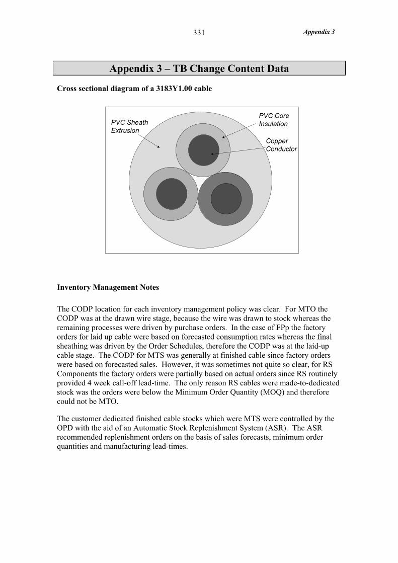
Appendix 3

331

Appendix 3 – TB Change Content Data

Cross sectional diagram of a 3183Y1.00 cable

Inventory Management Notes

The CODP location for each inventory management policy was clear. For MTO the CODP was at the drawn wire stage, because the wire was drawn to stock whereas the remaining processes were driven by purchase orders. In the case of FPp the factory orders for laid up cable were based on forecasted consumption rates whereas the final sheathing was driven by the Order Schedules, therefore the CODP was at the laid-up cable stage. The CODP for MTS was generally at finished cable since factory orders were based on forecasted sales. However, it was sometimes not quite so clear, for RS Components the factory orders were partially based on actual orders since RS routinely provided 4 week call-off lead-time. The only reason RS cables were made-to-dedicated stock was the orders were below the Minimum Order Quantity (MOQ) and therefore could not be MTO.

The customer dedicated finished cable stocks which were MTS were controlled by the OPD with the aid of an Automatic Stock Replenishment System (ASR). The ASR recommended replenishment orders on the basis of sales forecasts, minimum order quantities and manufacturing lead-times.

PVC Sheath Extrusion

PVC CoreInsulation

CopperConductor

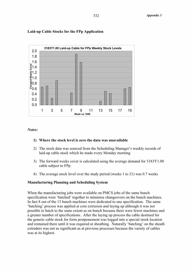
Appendix 3

332

Laid-up Cable Stocks for the FPp Application

0.00.20.40.60.81.01.21.41.61.82.0

1 3 5 7 9 11 13 15 17 19

3183Y1.00 Laid-up Cable for FPp Weekly Stock Levels

Forw

ard

Wee

ks C

over

Week no 1999

Notes:

1) Where the stock level is zero the data was unavailable

2) The stock data was sourced from the Scheduling Manager’s weekly records of laid-up cable stock which he made every Monday morning

3) The forward weeks cover is calculated using the average demand for 3183Y1.00 cable subject to FPp

4) The average stock level over the study period (weeks 1 to 21) was 0.7 weeks

Manufacturing Planning and Scheduling System

When the manufacturing jobs were available on PMCS jobs of the same bunch specification were ‘batched’ together to minimise changeovers on the bunch machines. In fact 8 out of the 13 bunch machines were dedicated to one specification. The same ‘batching’ process was applied at core extrusion and laying up although it was not possible to batch to the same extent as on bunch because there were fewer machines and a greater number of specifications. After the laying up process the cable destined for the generic cable stock for form postponement was logged into a special stock location and remained there until it was required at sheathing. Naturally ‘batching’ on the sheath extruders was not as significant as at previous processes because the variety of cables was at its highest.

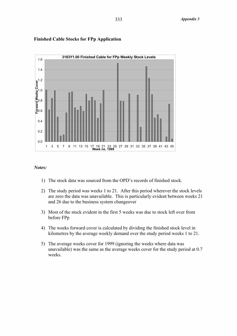
Appendix 3

333

Finished Cable Stocks for FPp Application

0.0

0.2

0.4

0.6

0.8

1.0

1.2

1.4

1.6

1 3 5 7 9 11 13 15 17 19 21 23 25 27 29 31 33 35 37 39 41 43 45Week no. 1999

Forw

ard

Wee

ks C

over

3183Y1.00 Finished Cable for FPp Weekly Stock Levels

Notes:

1) The stock data was sourced from the OPD’s records of finished stock.

2) The study period was weeks 1 to 21. After this period wherever the stock levels are zero the data was unavailable. This is particularly evident between weeks 21 and 26 due to the business system changeover

3) Most of the stock evident in the first 5 weeks was due to stock left over from before FPp

4) The weeks forward cover is calculated by dividing the finished stock level in kilometres by the average weekly demand over the study period weeks 1 to 21.

5) The average weeks cover for 1999 (ignoring the weeks where data was unavailable) was the same as the average weeks cover for the study period at 0.7 weeks.

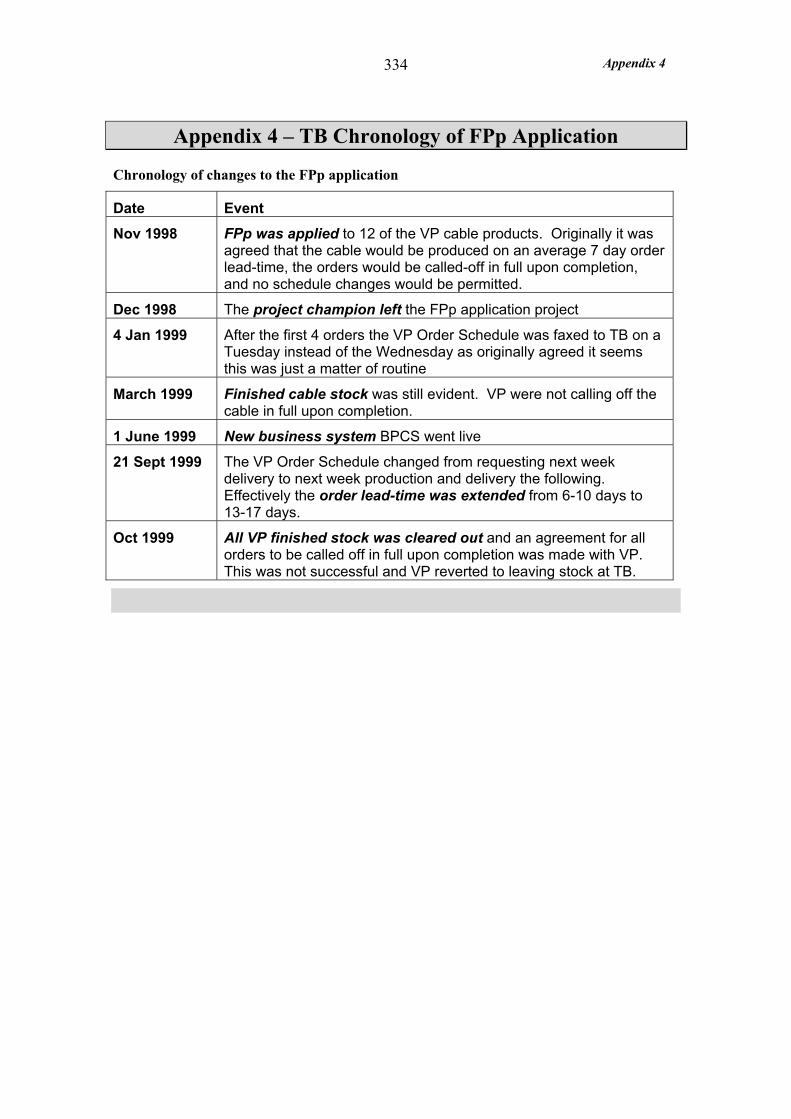
Appendix 4

334

Appendix 4 – TB Chronology of FPp Application

Chronology of changes to the FPp application

Date Event

Nov 1998 FPp was applied to 12 of the VP cable products. Originally it was agreed that the cable would be produced on an average 7 day order lead-time, the orders would be called-off in full upon completion, and no schedule changes would be permitted.

Dec 1998 The project champion left the FPp application project

4 Jan 1999 After the first 4 orders the VP Order Schedule was faxed to TB on a Tuesday instead of the Wednesday as originally agreed it seems this was just a matter of routine

March 1999 Finished cable stock was still evident. VP were not calling off the cable in full upon completion.

1 June 1999 New business system BPCS went live

21 Sept 1999 The VP Order Schedule changed from requesting next week delivery to next week production and delivery the following. Effectively the order lead-time was extended from 6-10 days to 13-17 days.

Oct 1999 All VP finished stock was cleared out and an agreement for all orders to be called off in full upon completion was made with VP. This was not successful and VP reverted to leaving stock at TB.

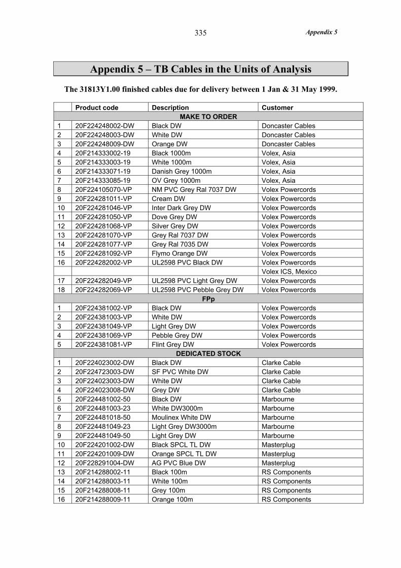
Appendix 5

335

Appendix 5 – TB Cables in the Units of Analysis

The 31813Y1.00 finished cables due for delivery between 1 Jan & 31 May 1999.

Product code Description Customer MAKE TO ORDER

1 20F224248002-DW Black DW Doncaster Cables 2 20F224248003-DW White DW Doncaster Cables 3 20F224248009-DW Orange DW Doncaster Cables 4 20F214333002-19 Black 1000m Volex, Asia 5 20F214333003-19 White 1000m Volex, Asia 6 20F214333071-19 Danish Grey 1000m Volex, Asia 7 20F214333085-19 OV Grey 1000m Volex, Asia 8 20F224105070-VP NM PVC Grey Ral 7037 DW Volex Powercords 9 20F224281011-VP Cream DW Volex Powercords 10 20F224281046-VP Inter Dark Grey DW Volex Powercords 11 20F224281050-VP Dove Grey DW Volex Powercords 12 20F224281068-VP Silver Grey DW Volex Powercords 13 20F224281070-VP Grey Ral 7037 DW Volex Powercords 14 20F224281077-VP Grey Ral 7035 DW Volex Powercords 15 20F224281092-VP Flymo Orange DW Volex Powercords 16 20F224282002-VP UL2598 PVC Black DW Volex Powercords Volex ICS, Mexico 17 20F224282049-VP UL2598 PVC Light Grey DW Volex Powercords 18 20F224282069-VP UL2598 PVC Pebble Grey DW Volex Powercords

FPp 1 20F224381002-VP Black DW Volex Powercords 2 20F224381003-VP White DW Volex Powercords 3 20F224381049-VP Light Grey DW Volex Powercords 4 20F224381069-VP Pebble Grey DW Volex Powercords 5 20F224381081-VP Flint Grey DW Volex Powercords

DEDICATED STOCK 1 20F224023002-DW Black DW Clarke Cable 2 20F224723003-DW SF PVC White DW Clarke Cable 3 20F224023003-DW White DW Clarke Cable 4 20F224023008-DW Grey DW Clarke Cable 5 20F224481002-50 Black DW Marbourne 6 20F224481003-23 White DW3000m Marbourne 7 20F224481018-50 Moulinex White DW Marbourne 8 20F224481049-23 Light Grey DW3000m Marbourne 9 20F224481049-50 Light Grey DW Marbourne 10 20F224201002-DW Black SPCL TL DW Masterplug 11 20F224201009-DW Orange SPCL TL DW Masterplug 12 20F228291004-DW AG PVC Blue DW Masterplug 13 20F214288002-11 Black 100m RS Components 14 20F214288003-11 White 100m RS Components 15 20F214288008-11 Grey 100m RS Components 16 20F214288009-11 Orange 100m RS Components

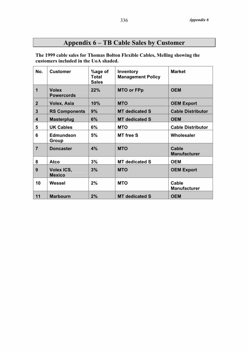
Appendix 6

336

Appendix 6 – TB Cable Sales by Customer

The 1999 cable sales for Thomas Bolton Flexible Cables, Melling showing the customers included in the UoA shaded.

No. Customer %age of Total Sales

Inventory Management Policy

Market

1 Volex Powercords

22% MTO or FPp OEM

2 Volex, Asia 10% MTO OEM Export

3 RS Components 9% MT dedicated S Cable Distributor

4 Masterplug 6% MT dedicated S OEM

5 UK Cables 6% MTO Cable Distributor

6 Edmundson Group

5% MT free S Wholesaler

7 Doncaster 4% MTO Cable Manufacturer

8 Atco 3% MT dedicated S OEM

9 Volex ICS, Mexico

3% MTO OEM Export

10 Wessel 2% MTO Cable Manufacturer

11 Marbourn 2% MT dedicated S OEM

Appendix 7

337

Appendix 7 – TB Demand Measures

Delivery due date

At TB the transit time for domestic cable orders was less than 24 hours therefore the delivery due date, as stated on the customer order, was the same as the ex-works due date. However, for the export orders in the MTO UoA the transit times were 4 or 5 weeks. Therefore the ex-works due date was taken as the delivery due date for all orders with the proviso that for export there was a transit time

Estimation of Ex-works Due Date for Unavailable MTO Customer Orders

21 out of a total of 79 customer order documents were missing for the MTO UoA. However, the factory order due dates into despatch were known from PMCS and an analysis of the existing customer orders revealed that generally this date is the Saturday before the ex-works due week. Therefore it was possible to estimate the ex-works due date for the missing orders. A total of 80 orders in the MTO UoA were due for despatch between 1 January and 31 May 1999. The customer order document giving the customer due delivery date (and the order date) could not be found for 21 of the orders (all 12 Volex ICS, 2 Volex Asia, 2 Volex Powercords and 5 Doncaster). For all orders the factory order due date into despatch was known and generally this date is the Saturday before the ex-works due week. This is supported by the 59 customer orders that are available 42 had been given a factory order due date which was the Saturday before the week it was due. The remaining 17 were all Volex Asia orders of which there was a total of 26. The factory order due date was generally 1 or 2 weeks before the customer ex-works due week (8 orders had a PMCS due date 2 weeks before, 5 orders 1 week before, 9 orders the Saturday before and 4 orders had a PMCS due date the Saturday at the end of the week due). On average for Volex Asia orders the factory order due date was either the Saturday before it was due to be despatched or 1 week before. From the interview with the respective customer service assistant it is most probable that the ex-works due dates for the other export customer Volex ICS will have a similar relationship with the factory order due dates. Therefore for the 21 missing customer orders the due ex-works date is assumed to be the week after the factory order due date. Of course in reality for all 14 missing export orders the ex-works due date may have been 1 or 2 weeks later.

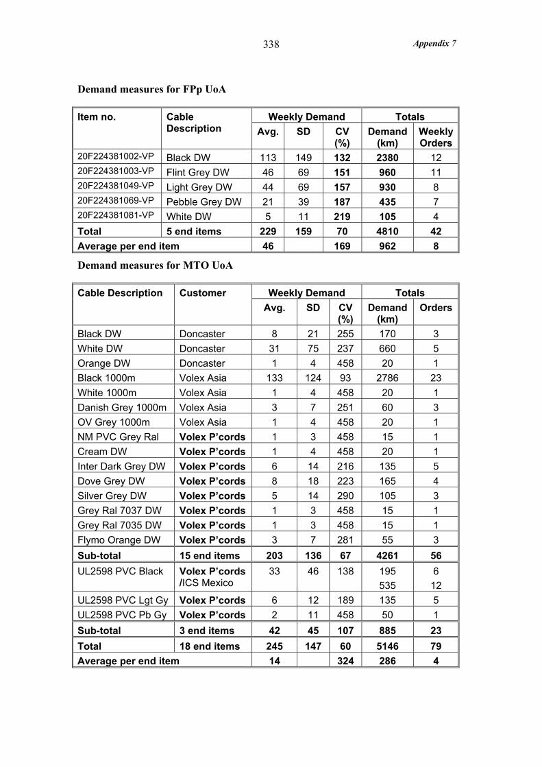
Appendix 7

338

Demand measures for FPp UoA

Weekly Demand Totals Item no. Cable Description Avg. SD CV

(%) Demand

(km) WeeklyOrders

20F224381002-VP Black DW 113 149 132 2380 12 20F224381003-VP Flint Grey DW 46 69 151 960 11 20F224381049-VP Light Grey DW 44 69 157 930 8 20F224381069-VP Pebble Grey DW 21 39 187 435 7 20F224381081-VP White DW 5 11 219 105 4 Total 5 end items 229 159 70 4810 42 Average per end item 46 169 962 8

Demand measures for MTO UoA

Weekly Demand Totals Cable Description Customer Avg. SD CV

(%) Demand

(km) Orders

Black DW Doncaster 8 21 255 170 3 White DW Doncaster 31 75 237 660 5 Orange DW Doncaster 1 4 458 20 1 Black 1000m Volex Asia 133 124 93 2786 23 White 1000m Volex Asia 1 4 458 20 1 Danish Grey 1000m Volex Asia 3 7 251 60 3 OV Grey 1000m Volex Asia 1 4 458 20 1 NM PVC Grey Ral Volex P’cords 1 3 458 15 1 Cream DW Volex P’cords 1 4 458 20 1 Inter Dark Grey DW Volex P’cords 6 14 216 135 5 Dove Grey DW Volex P’cords 8 18 223 165 4 Silver Grey DW Volex P’cords 5 14 290 105 3 Grey Ral 7037 DW Volex P’cords 1 3 458 15 1 Grey Ral 7035 DW Volex P’cords 1 3 458 15 1 Flymo Orange DW Volex P’cords 3 7 281 55 3 Sub-total 15 end items 203 136 67 4261 56 UL2598 PVC Black Volex P’cords

/ICS Mexico 33 46 138 195

535 6

12 UL2598 PVC Lgt Gy Volex P’cords 6 12 189 135 5 UL2598 PVC Pb Gy Volex P’cords 2 11 458 50 1 Sub-total 3 end items 42 45 107 885 23 Total 18 end items 245 147 60 5146 79 Average per end item 14 324 286 4

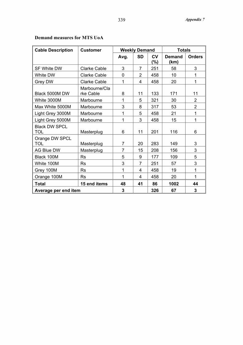
Appendix 7

339

Demand measures for MTS UoA

Weekly Demand Totals Cable Description Customer Avg. SD CV

(%) Demand

(km) Orders

SF White DW Clarke Cable 3 7 251 58 3 White DW Clarke Cable 0 2 458 10 1 Grey DW Clarke Cable 1 4 458 20 1

Black 5000M DW Marbourne/Clarke Cable 8 11 133 171 11

White 3000M Marbourne 1 5 321 30 2 Max White 5000M Marbourne 3 8 317 53 2 Light Grey 3000M Marbourne 1 5 458 21 1 Light Grey 5000M Marbourne 1 3 458 15 1 Black DW SPCL TOL Masterplug 6 11 201 116 6 Orange DW SPCL TOL Masterplug 7 20 283 149 3 AG Blue DW Masterplug 7 15 208 156 3 Black 100M Rs 5 9 177 109 5 White 100M Rs 3 7 251 57 3 Grey 100M Rs 1 4 458 19 1 Orange 100M Rs 1 4 458 20 1 Total 15 end items 48 41 86 1002 44 Average per end item 3 326 67 3

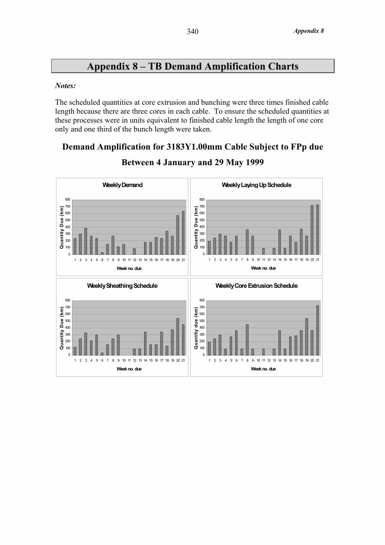
Appendix 8

340

Appendix 8 – TB Demand Amplification Charts

Notes:

The scheduled quantities at core extrusion and bunching were three times finished cable length because there are three cores in each cable. To ensure the scheduled quantities at these processes were in units equivalent to finished cable length the length of one core only and one third of the bunch length were taken.

Demand Amplification for 3183Y1.00mm Cable Subject to FPp due

Between 4 January and 29 May 1999

Weekly Demand

0

100

200

300

400

500

600

700

800

1 2 3 4 5 6 7 8 9 10 11 12 13 14 15 16 17 18 19 20 21

Week no. due

Qua

ntity

Due

(km

)

Weekly Sheathing Schedule

0

100

200

300

400

500

600

700

800

1 2 3 4 5 6 7 8 9 10 11 12 13 14 15 16 17 18 19 20 21

Week no. due

Qua

ntity

Due

(km

)

Weekly Laying Up Schedule

0

100

200

300

400

500

600

700

800

1 2 3 4 5 6 7 8 9 10 11 12 13 14 15 16 17 18 19 20 21

Week no. due

Qua

ntity

Due

(km

)

Weekly Core Extrusion Schedule

0

100

200

300

400

500

600

700

800

1 2 3 4 5 6 7 8 9 10 11 12 13 14 15 16 17 18 19 20 21

Week no. due

Qua

ntity

due

(km

)

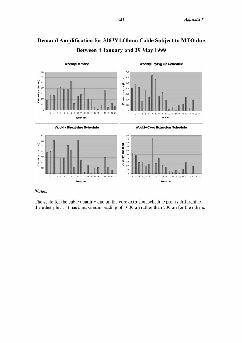
Appendix 8

341

Demand Amplification for 3183Y1.00mm Cable Subject to MTO due

Between 4 January and 29 May 1999

Notes:

The scale for the cable quantity due on the core extrusion schedule plot is different to the other plots. It has a maximum reading of 1000km rather than 700km for the others.

Weekly Demand

0

100

200

300

400

500

600

700

1 2 3 4 5 6 7 8 9 10 11 12 13 14 15 16 17 18 19 20 21

Week no.

Qua

ntity

due

(km

)

Weekly Sheathing Schedule

0

100

200

300

400

500

600

700

1 2 3 4 5 6 7 8 9 10 11 12 13 14 15 16 17 18 19 20 21

Week no.

Qua

nitit

y du

e (k

m)

Weekly Laying Up Schedule

0

100

200

300

400

500

600

700

1 2 3 4 5 6 7 8 9 10 11 12 13 14 15 16 17 18 19 20 21

Week no.

Qua

nitit

y du

e (k

m)

Weekly Core Extrusion Schedule

0

100

200

300

400

500

600

700

800

900

1000

1 2 3 4 5 6 7 8 9 10 11 12 13 14 15 16 17 18 19 20 21

Week no.

Qua

ntity

due

(km

)

Appendix 9

342

Appendix 9 – TB Customer Service Measures

• At TB the transit time for domestic cable orders was less than 24 hours therefore the delivery due date, as stated on the customer order, was the same as the ex-works due date. However, for the export orders in the MTO UoA the transit times were 4 or 5 weeks. Therefore the ex-works due date was taken as the delivery due date for all orders with the proviso that for export there was a transit time

• A number of the archived customer orders subject to MTO were missing. Further, other MTO order were excluded from the order lead-time measure because they were ordered before Christmas and due after therefore the order lead-time would have been artificially long.

• When measuring the order lead-time and delivery reliability a tolerance of 5% was allowed on the quantity delivered. Therefore the order was only considered delivered when 95% of the order quantity had been delivered or, in the case where 95% was never delivered, when the last delivery had been made on the order. .

Appendix 10

343

Appendix 10 – TB Degree of Commonality Calculations

The Degree of commonality index (as defined in the glossary Appendix 1) was calculated across each UoA for BOM levels 1, 2 and 3 components. The following formula was used based on Collier’s formula:

The average number of incidences of the distinct component parts at BOM level ‘x’ for a particular UoA

= total no. of incidences of BOM level ‘x’ components across end items no of distinct components at BOM level ‘x’ across end items

The table below shows the degree of commonality index calculations for each UoA

MTO FPp MTS

Total no. of incidences of BOM Level 1 components

56 10 43

No of distinct components at BOM level 1

25 6 21


90 27 71


26 10 12


108 30 90


7 6 6


BOM level 1 packaging components

2 (12%) 2 (33%) 2 (14%)

BOM level 2 sheath extrusion components

4 (19%) 3 (54%) 6 (39%)

BOM level 3 core extrusion components

15 (86%) 5 (100%) 15 (100%)

Over levels 1, 2 and 3 4 (24%) 3 (61%) 5 (35%)

Upper Bound - no. of end items

18 5 15

Appendix 11

344

Appendix 11 – TB Throughput Efficiency Measure

Sampling jobs for Throughput Efficiency Measurement

Due to the laborious nature of tracing jobs through the factory the total number of jobs to be traced was limited to twelve. For the purposes of comparison between the FPp and MTO UoA the jobs sampled from the MTO UoA were restricted to those supplied to VP. In general jobs were sampled taking into account a number of factors to minimise the effect of variables, other than the inventory management policies themselves:

• To avoid the effect of the Christmas vacation but still focus on the early application of FPp the jobs sampled were output from sheathing towards the end of January, through February and beginning of March.

• To account for the variable nature of the WIP levels it was attempted to sample jobs from all three UoA that were output from sheathing at the same time in the month, approximately end of January, middle of February and beginning of March.

• The quantity ordered was between 30 and 60 km, well in excess of the 15 km MOQ.

Notes on Throughput Efficiency Calculation

• The elapsed time was measured over the factory operating hours from 7:00am Monday to 7:00am Saturday

• The three cores are often core extruded simultaneously. In this situation it is advisable when calculating throughput efficiency to take the longest processing time. Therefore the processing time for the green yellow core was used because it is normally processed at the slowest rate.

• The date the finished cable was booked into stores was available for the cables subject to FPp but not for those subject to MTO. Further the time of booking into finished goods stores was not known therefore this data could not be used for calculating elapsed time excluding time in finished good stock.

• Only the date, not the time, of despatch was known so for every order it was assumed that it was despatched at 12 noon. Further, where an order was despatched in two lots the date of the last despatch was taken to calculate the elapsed time.

Appendix 11

345

Example of throughput efficiency measurement sheet:

Unit of Analysis: Form Postponement Customer VOLEX P'CORDS

Product description: 3183Y1.00FTGY-VP Product code 20F224381081-VP

Quantity ordered: 60km Factory order HO27687/0104

Due Delivery Day: Friday 29 January

Duration CommentsDescription of work Time Date Time Date (hours)Extrude cores 2:00 28-Jan-99 4:00 28-Jan-99 2.00Transport to Laying UpStore at Laying Up 12.50Lay up cores 16:30 28-Jan-99 23:00 28-Jan-99 6.50

7:15 29-Jan-99 9:15 29-Jan-99 2.00Transport to SheathingStore at Sheathing 10.75Sheath laid up cable 11:45 29-Jan-99 17:00 29-Jan-99 5.25Test cableTransport to WarehouseStore in warehouse 30-Jan-99 w/e is 30/31 JanDespatch to customer 01-Feb-99 60km 19.00

OperationInspection Total value added time (hrs) 15.75

Transport Total time elapsed (hrs) 58Storage Throughput Efficiency 27%

Excluding time in finished goodsTotal time elapsed (hrs) 39Throughput Efficiency 40%


Start End

Appendix 12

346

Appendix 12 – BC Change Content Data

Stock Modification Details

The stock modifications normally involved removing parts, which clearly was removing value already added. Indeed, as the summary of modifications in the table below illustrates, almost half (24) of the 60 motors subjected to stock modifications involved motor strip-downs. Motor strip-downs required between 4 hours and 3 working days depending on the precise modification and the motor size. Commonly these modifications involved a magnet main pole winding change or fitting thermistors.

Summary of the 60 stock modifications due between 01/07/01 and 30/06/02

Parts involved Stock Mod Type No. of Motors

Strip-down?

Data plate only Re-stamp data plate only 16 No

Main pole coil change 8 Yes

Main pole bore change 4 Yes

Pre-wire for brush detection system

2 Yes

Brushes change 1 No

Magnet body assembly parts (25 motors)

Thermistor change 14 Yes

Final assembly parts only

Various 19 No

Appendix 12

347

Is a UK

stock motor available

in warehouse ?

Yes

No

YesN

o

Arem

odificationsrequired?

Can a UK

stock motor

satisfy enquiry?

Launch replenishment

order off MP

S

Is a UK

stock motor

in production ?

Quote appropriate leadtim

e

Order received & entered onto

JBA S

ystem and Access O

rder Log

OP

D send e-m

ail to LDC

advising motor to be m

odifiedduring productionO

rder booked out of OP

D

Order returned to O

PD

OP

D send S

tock Mod Instruction

sheet together with part details to S

/R

Electrical engineering check stock

mod and provide part details

(Mech. E

ng. may/m

ay not be required) Order Processing for U

K Stock M

otors

Motor allocated

and stock level deducted

IF stock level falls below target,

replenishment order placed on M

PS

for 1 motor

JBA

MR

P overnight run


e

OP

D send fax to w

arehouseadvising stock m

otor requires m

od prior to despatch

Yes

No

No

Yes

Go to O

rder Processing

for Contract M

otorsN

o

Is a UK

stock motor

in production?


e

OP

D send e-m

ail to LDC

advising motor sold

No

Yes

Launch replenishment

order off MP

S

Order received & entered onto

JBA S

ystem and Access O

rder Log

Is a UK

stock motor available

in warehouse ?

Quote im

mediately available

Yes

LDC

change material requirem

ents

OP

D send S

tock Mod Instruction

sheet together with part details to LD

C

Shaded boxes indicate procedures that

are not covered by the JBA M

RP

system

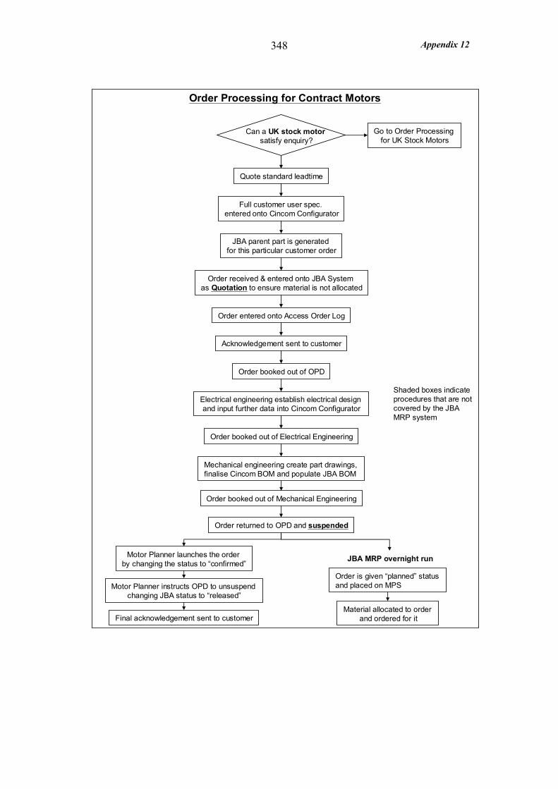
Appendix 12

348

Order Processing for Contract Motors

Can a UK stock motorsatisfy enquiry?

Quote standard leadtime

Full customer user spec. entered onto Cincom Configurator

JBA parent part is generated for this particular customer order

Order received & entered onto JBA System as Quotation to ensure material is not allocated

Order entered onto Access Order Log

Electrical engineering establish electrical design and input further data into Cincom Configurator

Order booked out of Electrical Engineering

Mechanical engineering create part drawings, finalise Cincom BOM and populate JBA BOM

Order booked out of Mechanical Engineering

Order returned to OPD and suspended

Motor Planner launches the order by changing the status to “confirmed”

Motor Planner instructs OPD to unsuspendchanging JBA status to “released”

Final acknowledgement sent to customer

JBA MRP overnight run

Order is given “planned” status and placed on MPS

Material allocated to order and ordered for it

Order booked out of OPD

Acknowledgement sent to customer

Go to Order Processing for UK Stock Motors

Shaded boxes indicate procedures that are not covered by the JBA MRP system

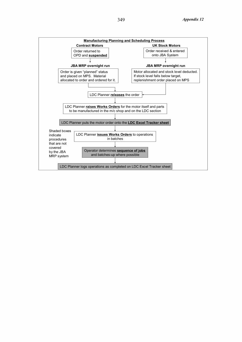
Appendix 12

349

LDC Planner releases the order


Order is given “planned” status and placed on MPS. Material allocated to order and ordered for it.

Order returned to OPD and suspended

LDC Planner raises Works Orders for the motor itself and parts to be manufactured in the m/c shop and on the LDC section

LDC Planner puts the motor order onto the LDC Excel Tracker sheet

Contract Motors

LDC Planner issues Works Orders to operations in batches

Order received & entered onto JBA System

UK Stock Motors

Motor allocated and stock level deducted.If stock level falls below target, replenishment order placed on MPS


Operator determines sequence of jobsand batches-up where possible

LDC Planner logs operations as completed on LDC Excel Tracker sheet

Shaded boxes indicate procedures that are not covered by the JBA MRP system

Manufacturing Planning and Scheduling Process

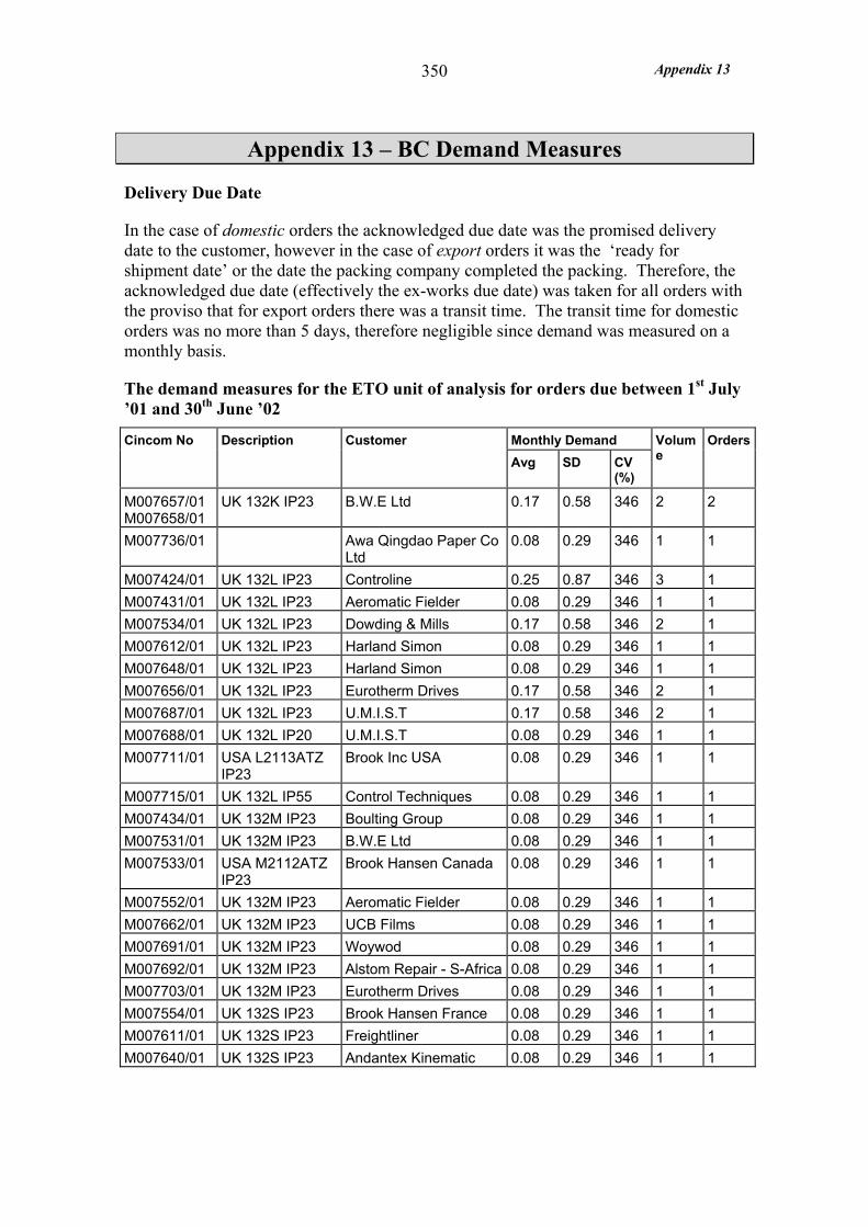
Appendix 13

350

Appendix 13 – BC Demand Measures

Delivery Due Date

In the case of domestic orders the acknowledged due date was the promised delivery date to the customer, however in the case of export orders it was the ‘ready for shipment date’ or the date the packing company completed the packing. Therefore, the acknowledged due date (effectively the ex-works due date) was taken for all orders with the proviso that for export orders there was a transit time. The transit time for domestic orders was no more than 5 days, therefore negligible since demand was measured on a monthly basis.

The demand measures for the ETO unit of analysis for orders due between 1st July ’01 and 30th June ’02

Monthly Demand Cincom No Description Customer Avg SD CV

(%)

Volume

Orders

M007657/01 M007658/01

UK 132K IP23 B.W.E Ltd 0.17 0.58 346 2 2

M007736/01 Awa Qingdao Paper Co Ltd

0.08 0.29 346 1 1

M007424/01 UK 132L IP23 Controline 0.25 0.87 346 3 1 M007431/01 UK 132L IP23 Aeromatic Fielder 0.08 0.29 346 1 1 M007534/01 UK 132L IP23 Dowding & Mills 0.17 0.58 346 2 1 M007612/01 UK 132L IP23 Harland Simon 0.08 0.29 346 1 1 M007648/01 UK 132L IP23 Harland Simon 0.08 0.29 346 1 1 M007656/01 UK 132L IP23 Eurotherm Drives 0.17 0.58 346 2 1 M007687/01 UK 132L IP23 U.M.I.S.T 0.17 0.58 346 2 1 M007688/01 UK 132L IP20 U.M.I.S.T 0.08 0.29 346 1 1 M007711/01 USA L2113ATZ

IP23 Brook Inc USA 0.08 0.29 346 1 1

M007715/01 UK 132L IP55 Control Techniques 0.08 0.29 346 1 1 M007434/01 UK 132M IP23 Boulting Group 0.08 0.29 346 1 1 M007531/01 UK 132M IP23 B.W.E Ltd 0.08 0.29 346 1 1 M007533/01 USA M2112ATZ

IP23 Brook Hansen Canada 0.08 0.29 346 1 1

M007552/01 UK 132M IP23 Aeromatic Fielder 0.08 0.29 346 1 1 M007662/01 UK 132M IP23 UCB Films 0.08 0.29 346 1 1 M007691/01 UK 132M IP23 Woywod 0.08 0.29 346 1 1 M007692/01 UK 132M IP23 Alstom Repair - S-Africa 0.08 0.29 346 1 1 M007703/01 UK 132M IP23 Eurotherm Drives 0.08 0.29 346 1 1 M007554/01 UK 132S IP23 Brook Hansen France 0.08 0.29 346 1 1 M007611/01 UK 132S IP23 Freightliner 0.08 0.29 346 1 1 M007640/01 UK 132S IP23 Andantex Kinematic 0.08 0.29 346 1 1

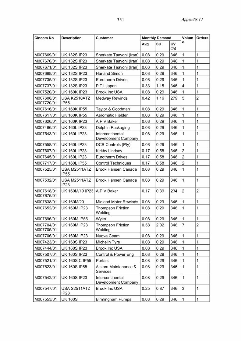
Appendix 13

351


(%)

Volume

Orders

M007669/01 UK 132S IP23 Sherkate Taavoni (Iran) 0.08 0.29 346 1 1 M007670/01 UK 132S IP23 Sherkate Taavoni (Iran) 0.08 0.29 346 1 1 M007671/01 UK 132S IP23 Sherkate Taavoni (Iran) 0.08 0.29 346 1 1 M007698/01 UK 132S IP23 Harland Simon 0.08 0.29 346 1 1 M007735/01 UK 132S IP23 Eurotherm Drives 0.08 0.29 346 1 1 M007737/01 UK 132S IP23 P.T.I Japan 0.33 1.15 346 4 1 M007520/01 UK 160K IP23 Brook Inc USA 0.08 0.29 346 1 1 M007608/01 M007720/01

USA K2510ATZ IP55

Medway Rewinds 0.42 1.16 279 5 2

M007616/01 UK 160K IP55 Taylor & Goodman 0.08 0.29 346 1 1 M007617/01 UK 160K IP55 Aeromatic Fielder 0.08 0.29 346 1 1 M007626/01 UK 160K IP23 A.P.V Baker 0.08 0.29 346 1 1 M007466/01 UK 160L IP23 Dolphin Packaging 0.08 0.29 346 1 1 M007543/01 UK 160L IP23 Intercontinental

Development Company 0.08 0.29 346 1 1

M007558/01 UK 160L IP23 DCB Controls (Pty) 0.08 0.29 346 1 1 M007607/01 UK 160L IP23 Kirkby Lindsey 0.17 0.58 346 2 1 M007645/01 UK 160L IP23 Eurotherm Drives 0.17 0.58 346 2 1 M007717/01 UK 160L IP55 Control Techniques 0.17 0.58 346 2 1 M007525/01 USA M2511ATZ


M007532/01 USA M2511ATZ IP23

Brook Hansen Canada 0.08 0.29 346 1 1

M007618/01 M007675/01

UK 160M/19 IP23 A.P.V Baker 0.17 0.39 234 2 2

M007638/01 UK 160M/20 Midland Motor Rewinds 0.08 0.29 346 1 1 M007652/01 UK 160M IP23 Thompson Friction

Welding 0.08 0.29 346 1 1

M007696/01 UK 160M IP55 Wyko 0.08 0.29 346 1 1 M007704/01 M007705/01

UK 160M IP23 Thompson Friction Welding

0.58 2.02 346 7 2

M007706/01 UK 160M IP23 Nuova Ceam 0.08 0.29 346 1 1 M007423/01 UK 160S IP23 Michelin Tyre 0.08 0.29 346 1 1 M007444/01 UK 160S IP23 Brook Inc USA 0.08 0.29 346 1 1 M007507/01 UK 160S IP23 Control & Power Eng 0.08 0.29 346 1 1 M007521/01 UK 160S C IP55 Portals 0.08 0.29 346 1 1 M007523/01 UK 160S IP55 Alstom Maintenance &

Services 0.08 0.29 346 1 1

M007542/01 UK 160S IP23 Intercontinental Development Company

0.08 0.29 346 1 1

M007547/01 USA S2511ATZ IP23

Brook Inc USA 0.25 0.87 346 3 1

M007553/01 UK 160S Birmingham Pumps 0.08 0.29 346 1 1

Appendix 13

352


(%)

Volume

Orders

M007694/01 UK 160S IP23 Aeromatic Fielder 0.08 0.29 346 1 1 M007345/01 USA L2813ATZ, Eaton Cutler Hammer 0.08 0.29 346 1 1 M007548/01 USA L2813ATZ

IP23 Brook Inc USA 0.25 0.87 346 3 1

M007619/01 UK 180L IP23 Carrington Wire 0.25 0.87 346 3 1 M007621/01 UK 180L IP23 Fenner 0.08 0.29 346 1 1 M007664/01 UK 180L IP55 Cegelec Maintenance &

Services 0.17 0.58 346 2 1

M007716/01 UK 180L IP55 Control Techniques 0.17 0.58 346 2 1 M007740/01 UK 180L IP23 Georgia-Pacific 0.08 0.29 346 1 1 M007445/01 UK 180M IP23 Brook Inc USA 0.08 0.29 346 1 1 M007467/01 UK 180M IP23 Hull Bulk Handling 0.08 0.29 346 1 1 M007536/01 UK 180M IP23 Eurotherm Drives 0.08 0.29 346 1 1 M007551/01 UK 180M IP23 Eurotherm Drives 0.08 0.29 346 1 1 M007646/01 UK 180M IP23 Eurotherm Drives 0.17 0.58 346 2 1 M007683/01 USA M2812ATZ . Brook Inc USA 0.08 0.29 346 1 1 M007684/01 UK 180M IP23 Brook Inc USA 0.08 0.29 346 1 1 M007714/01 UK 180M IP55 Control Techniques 0.08 0.29 346 1 1 M007422/01 UK 180S Brook Inc USA 0.08 0.29 346 1 1 M007430/01 USA S2811ATZ

IP23 Brook Inc USA 0.17 0.58 346 2 1

M007435/01 UK 180S IP23 Aeromatic Fielder 0.08 0.29 346 1 1 M007469/01 UK 180S IP23 Controline 0.17 0.58 346 2 1 M007625/01 UK 180S IP23 Parkgate & Co 0.08 0.29 346 1 1 M007643/01 UK 180S IP55 Capitan (Europe) 0.17 0.58 346 2 1 M007732/01 UK 180S Brook Inc USA 0.17 0.58 346 2 1 M007427/01 UK 200L IP23 Hall Rewinds 0.08 0.29 346 1 1 M007428/01 UK 200L IP23 Rexnord - Stephan

Werke 0.08 0.29 346 1 1

M007465/01 UK 200L IP23 Dolphin Packaging 0.08 0.29 346 1 1 M007541/01 UK 200L IP23 Michelin Tyre 0.08 0.29 346 1 1 M007544/01 UK 200L IP23 Intercontinental

Development Company 0.08 0.29 346 1 1

M007559/01 UK 200L IP23 IMI Yorkshire Copper Tube

0.08 0.29 346 1 1

M007628/01 UK 200L IP23 Nuova Ceam 0.08 0.29 346 1 1 M007661/01 UK 200L IP23 B.W.E Ltd 0.08 0.29 346 1 1 M007667/01 UK 200L IP23 Sherkate Taavoni (Iran) 0.17 0.58 346 2 1 M007699/01 UK 200L IP23 Brook Hansen Canada 0.08 0.29 346 1 1 M007708/01 UK 200L IP23 Brook Inc USA 0.08 0.29 346 1 1 M007495/01 UK 200M IP23 Unico 0.08 0.29 346 1 1 M007538/01 USA M3212ATZ


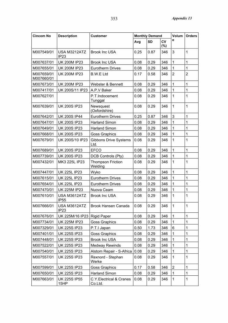
Appendix 13

353


(%)

Volume

Orders

M007549/01 USA M3212ATZ IP23

Brook Inc USA 0.25 0.87 346 3 1

M007637/01 UK 200M IP23 Brook Inc USA 0.08 0.29 346 1 1 M007655/01 UK 200M IP23 Eurotherm Drives 0.08 0.29 346 1 1 M007659/01 M007660/01

UK 200M IP23 B.W.E Ltd 0.17 0.58 346 2 2

M007673/01 UK 200M IP23 Webster & Bennett 0.08 0.29 346 1 1 M007417/01 UK 200S/11 IP23 A.P.V Baker 0.08 0.29 346 1 1 M007627/01 P.T.Indocement

Tunggal 0.08 0.29 346 1 1

M007639/01 UK 200S IP23 Newsquest (Oxfordshire)

0.08 0.29 346 1 1

M007642/01 UK 200S IP44 Eurotherm Drives 0.25 0.87 346 3 1 M007647/01 UK 200S IP23 Harland Simon 0.08 0.29 346 1 1 M007649/01 UK 200S IP23 Harland Simon 0.08 0.29 346 1 1 M007668/01 UK 200S IP23 Goss Graphics 0.08 0.29 346 1 1 M007679/01 UK 200S/10 IP23 Gibbons Drive Systems

Ltd. 0.08 0.29 346 1 1

M007689/01 UK 200S IP23 EFCO 0.08 0.29 346 1 1 M007739/01 UK 200S IP23 DCB Controls (Pty) 0.08 0.29 346 1 1 M007432/01 MK3 225L IP23 Thompson Friction

Welding 0.08 0.29 346 1 1

M007447/01 UK 225L IP23 Wyko 0.08 0.29 346 1 1 M007615/01 UK 225L IP23 Eurotherm Drives 0.08 0.29 346 1 1 M007654/01 UK 225L IP23 Eurotherm Drives 0.08 0.29 346 1 1 M007470/01 UK 225M IP23 Nuova Ceam 0.08 0.29 346 1 1 M007610/01 USA M3612ATZ

IP55 Brook Inc USA 0.08 0.29 346 1 1

M007666/01 USA M3612ATZ IP23

Brook Hansen Canada 0.08 0.29 346 1 1

M007676/01 UK 225M/16 IP23 Rigid Paper 0.08 0.29 346 1 1 M007734/01 UK 225M IP23 Goss Graphics 0.08 0.29 346 1 1 M007329/01 UK 225S IP23 P.T.I Japan 0.50 1.73 346 6 1 M007401/01 UK 225S IP23 Goss Graphics 0.08 0.29 346 1 1 M007448/01 UK 225S IP23 Brook Inc USA 0.08 0.29 346 1 1 M007522/01 UK 225S IP23 Medway Rewinds 0.08 0.29 346 1 1 M007540/01 UK 225S IP23 Alstom Repair - S-Africa 0.08 0.29 346 1 1 M007557/01 UK 225S IP23 Rexnord - Stephan

Werke 0.08 0.29 346 1 1

M007599/01 UK 225S IP23 Goss Graphics 0.17 0.58 346 2 1 M007650/01 UK 225S IP23 Harland Simon 0.08 0.29 346 1 1 M007663/01 UK 225S IP55

15HP C.Y.Electrical & Cranes Co.Ltd.

0.08 0.29 346 1 1

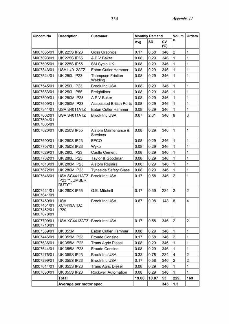
Appendix 13

354


(%)

Volume

Orders

M007685/01 UK 225S IP23 Goss Graphics 0.17 0.58 346 2 1 M007693/01 UK 225S IP55 A.P.V Baker 0.08 0.29 346 1 1 M007695/01 UK 225S IP55 SM Cyclo UK 0.08 0.29 346 1 1 M007343/01 USA L4012ATZ Eaton Cutler Hammer 0.08 0.29 346 1 1 M007524/01 UK 250L IP23 Thompson Friction

Welding 0.08 0.29 346 1 1

M007545/01 UK 250L IP23 Brook Inc USA 0.08 0.29 346 1 1 M007653/01 UK 250L IP55 Freightliner 0.08 0.29 346 1 1 M007509/01 UK 250M IP23 A.P.V Baker 0.08 0.29 346 1 1 M007609/01 UK 250M IP23 Associated British Ports 0.08 0.29 346 1 1 M007341/01 USA S4011ATZ Eaton Cutler Hammer 0.08 0.29 346 1 1 M007602/01 M007604/01 M007605/01

USA S4011ATZ Brook Inc USA 0.67 2.31 346 8 3

M007620/01 UK 250S IP55 Alstom Maintenance & Services

0.08 0.29 346 1 1

M007690/01 UK 250S IP23 EFCO 0.08 0.29 346 1 1 M007707/01 UK 250S IP23 Wyko 0.08 0.29 346 1 1 M007629/01 UK 280L IP23 Castle Cement 0.08 0.29 346 1 1 M007702/01 UK 280L IP23 Taylor & Goodman 0.08 0.29 346 1 1 M007613/01 UK 280M IP23 Alstom Repairs 0.08 0.29 346 1 1 M007672/01 UK 280M IP23 Tyneside Safety Glass 0.08 0.29 346 1 1 M007546/01 USA SC4411ATZ

IP23 **LUMBER DUTY**

Brook Inc USA 0.17 0.58 346 2 1

M007421/01 M007641/01

UK 280X IP55 G.E. Mitchell 0.17 0.39 234 2 2

M007450/01 M007451/01 M007452/01 M007678/01

USA XC4413ATDZ IP20

Brook Inc USA 0.67 0.98 148 8 4

M007709/01 M007710/01

USA XC4413ATZ Brook Inc USA 0.17 0.58 346 2 2

M007339/01 UK 355M Eaton Cutler Hammer 0.08 0.29 346 1 1 M007446/01 UK 355M IP23 Froude Consine 0.17 0.58 346 2 1 M007636/01 UK 355M IP23 Trans Agric Diesel 0.08 0.29 346 1 1 M007644/01 UK 355M IP23 Froude Consine 0.08 0.29 346 1 1 M007276/01 UK 355S IP23 Brook Inc USA 0.33 0.78 234 4 2 M007299/01 UK 355S IP23 Brook Inc USA 0.17 0.58 346 2 2 M007614/01 UK 355S IP23 Trans Agric Diesel 0.08 0.29 346 1 1 M007630/01 UK 355S IP23 Rockwell Automation 0.08 0.29 346 1 1 Total 19.08 10.07 53 229 169 Average per motor spec. 343 1.5

Appendix 13

355

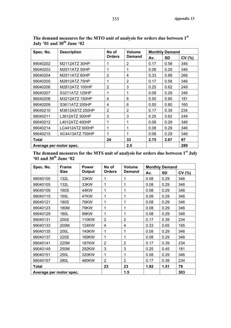
Appendix 13 355

The demand measures for the MTO unit of analysis for orders due between 1st July ’01 and 30th June ‘02

Monthly Demand Spec. No. Description No of Orders

Volume Demand Av. SD CV (%)

99040202 M2112ATZ 30HP 1 2 0.17 0.58 346 99040203 M2511ATZ 50HP 1 1 0.08 0.29 346 99040204 M2511ATZ 60HP 2 4 0.33 0.89 266 99040205 M2812ATZ 75HP 1 2 0.17 0.58 346 99040206 M2812ATZ 100HP 2 3 0.25 0.62 249 99040207 S3211ATZ 125HP 1 1 0.08 0.29 346 99040208 M3212ATZ 150HP 4 6 0.50 0.90 181 99040209 S3611ATZ 200HP 4 6 0.50 0.80 160 99040210 M3612ASTZ 250HP 2 2 0.17 0.39 234 99040211 L3612ATZ 300HP 3 3 0.25 0.62 249 99040212 L4012ATZ 400HP 1 1 0.08 0.29 346 99040214 LC4412ATZ 600HP 1 1 0.08 0.29 346 99040215 XC4413ATZ 700HP 1 1 0.08 0.29 346 Total 24 33 2.75 2.67 97 Average per motor spec. 2.5 289

The demand measures for the MTS unit of analysis for orders due between 1st July ’01 and 30th June ‘02

Monthly Demand Spec. No. Frame Size

Power Output

No of Orders

Volume Demand Av. SD CV (%)

99040105 132L 33KW 1 1 0.08 0.29 346 99040105 132L 33KW 1 1 0.08 0.29 346 99040109 160S 44KW 1 1 0.08 0.29 346 99040115 160L 47KW 1 1 0.08 0.29 346 99040121 180S 76KW 1 1 0.08 0.29 346 99040123 180M 79KW 1 1 0.08 0.29 346 99040129 180L 99KW 1 1 0.08 0.29 346 99040131 200S 110KW 2 2 0.17 0.39 234 99040133 200M 124KW 4 4 0.33 0.65 195 99040135 200L 140KW 1 1 0.08 0.29 346 99040137 225S 169KW 1 1 0.08 0.29 346 99040141 225M 187KW 2 2 0.17 0.39 234 99040149 250M 292KW 3 3 0.25 0.45 181 99040151 250L 320KW 1 1 0.08 0.29 346 99040157 280L 480KW 2 2 0.17 0.39 234 Total 23 23 1.92 1.51 79 Average per motor spec. 1.5 303

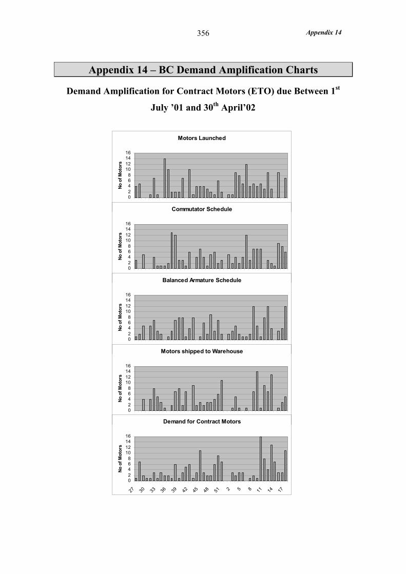
Appendix 14 356

Appendix 14 – BC Demand Amplification Charts

Demand Amplification for Contract Motors (ETO) due Between 1st

July ’01 and 30th April’02

Motors Launched

02468

10121416

27 30 33 36 39 42 45 48 51 2 5 8 11 14 17

No o

f Mot

ors

Commutator Schedule

02468

10121416

27 30 33 36 39 42 45 48 51 2 5 8 11 14 17

No o

f Mot

ors

Balanced Armature Schedule

02468

10121416

27 30 33 36 39 42 45 48 51 2 5 8 11 14 17

No o

f Mot

ors

Motors shipped to Warehouse

02468

10121416

27 30 33 36 39 42 45 48 51 2 5 8 11 14 17

No o

f Mot

ors

Demand for Contract Motors

02468

10121416

27 30 33 36 39 42 45 48 51 2 5 8 11 14 17

No o

f Mot

ors

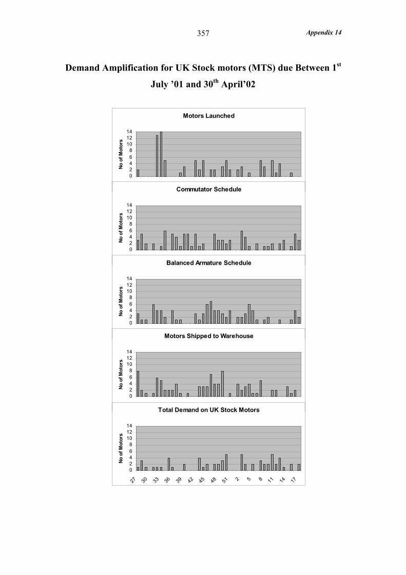
Appendix 14 357

Demand Amplification for UK Stock motors (MTS) due Between 1st

July ’01 and 30th April’02

Motors Launched

02468

101214

27 30 33 36 39 42 45 48 51 2 5 8 11 14 17

No o

f Mot

ors

Commutator Schedule

02468

101214

27 30 33 36 39 42 45 48 51 2 5 8 11 14 17

No o

f Mot

ors

Balanced Armature Schedule

02468

101214

27 30 33 36 39 42 45 48 51 2 5 8 11 14 17

No o

f Mot

ors

Motors Shipped to Warehouse

02468

101214

27 30 33 36 39 42 45 48 51 2 5 8 11 14 17

No o

f Mot

ors

Total Demand on UK Stock Motors

02468

101214

27 30 33 36 39 42 45 48 51 2 5 8 11 14 17

No o

f Mot

ors

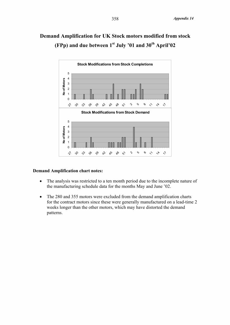
Appendix 14 358

Demand Amplification for UK Stock motors modified from stock

(FPp) and due between 1st July ’01 and 30th April’02

Stock Modifications from Stock Completions

0

1

2

3

4

5

27 30 33 36 39 42 45 48 51 2 5 8 11 14 17

No o

f Mot

ors

Stock Modifications from Stock Demand

0

1

2

3

4

5

27 30 33 36 39 42 45 48 51 2 5 8 11 14 17

No o

f Mot

ors

Demand Amplification chart notes:

• The analysis was restricted to a ten month period due to the incomplete nature of the manufacturing schedule data for the months May and June ’02.

• The 280 and 355 motors were excluded from the demand amplification charts for the contract motors since these were generally manufactured on a lead-time 2 weeks longer than the other motors, which may have distorted the demand patterns.

Appendix 15 359

Appendix 15 – BC Customer Service Measures

Ex-stock Availability

The data was not available to measure ex-stock availability in terms of the proportion of enquiries for which the correct UK stock motor was available. However, two sources of data were available which gave a good indication of this measure. The first was the number of orders for UK stock motors, which were satisfied with motors from stock. Of the 59 orders for modified UK stock (FPp) motors 37 (63%) appeared on the LDC Stock Mod Record, indicating that they were satisfied with motors from stock. The remaining 22 orders were satisfied with motors in production indicating that for these orders stock motors were not available. Therefore, the ex-stock availability for the modified stock motors was 63% or less, since this measure does not take into account enquiries received, which were not converted into orders because the stock was not available.

Of the direct ex-stock (MTS) orders none appeared to be fulfilled by a motor in production (as indicated by the absence of these customer orders on the LDC Tracker sheet). Therefore, it was assumed that the correct stock motor was always available. This assumption was supported by the consistently short order lead-time, on average no more than a day, suggesting that all the motors were immediately available. Therefore, the ex-stock availability for the direct ex-stock orders (MTS) was 100% or less, since this measure did not take into account enquiries received, which were not converted into orders because the stock was not available. This appeared much higher than the ex-stock availability measured for the modified stock motors (FPp). However, the disparity in the ex-stock availability measure was difficult to explain when it was considered that the modified and direct sale motors drew from the same motor stocks. One probable explanation was that if a standard UK motor was not immediately available for a direct ex-stock sale the sale was more likely to be lost because these motors were more widely available ex-stock.

The second source of evidence showed that many enquiries did not become orders because the stock motor was not available. This evidence was supplied by the LDC Sales Manager and was the orders lost due to the non-availability of UK stock motors. Between January and November 2002, 31 orders were lost. This was less than a year period but the lost orders still equated to about half of the 59 modified stock orders, or over 100% of the 23 direct ex-stock motor orders received over the year period of the study. However, it should be noted that these lost orders are the total across both the modified stock motors and the ex-stock motors and it is not possible to apportion them between the two.

Dates for Measuring Order Lead-time and Delivery Reliability

In the case of export orders the acknowledged due date, found on the Order Log, is the ‘ready for shipment date’ or the date the packing company is due to completed the packing. Fortunately, the recorded despatch date on the Order Log, for export orders, is the date the order leaves the packer, therefore comparing this date with the acknowledged due date will be a good measure of delivery reliability.

Appendix 15 360

In the case of domestic orders the acknowledged due date is the promised delivery date to the customer, whereas the despatch date, recorded on the Order Log, is the date the motor is received by the transport company. Unfortunately, the transit time is often in excess of 24 hours since it depends upon whether the despatch address falls within the Blackheath or Huddersfield area. For the domestic orders I was able to cross reference the despatch dates on the Order Log with the despatch dates on the despatch notes and quite often, regardless whether the motor was distributed via Huddersfield or not, the motor would spend 3 or 4 days in transit. Sadly, the despatch notes were not available for a good proportion of the orders and even when they were available the customer receipt dates were not reliably available. Suffice it to say that comparing the recorded despatch date with the acknowledged due-to-customer date is a lenient measure of delivery reliability. Similarly this applies to using the despatch date to measure order lead-time. However, the degree of leniency is similar across all UoA.

Appendix 16 361

Appendix 16 – BC BOM Analysis

Cincom BOM limitations

The Cincom BOMs were structured by functional elements rather than by BOM levels. This was overcome by transposing the components onto a spreadsheet, and reorganising them according to BOM level, which was indicated on the Cincom BOM.

There were no part descriptions on the Cincom BOMs therefore it was only possible to recognise parts from their part numbers and locations in a particular configuration element. The T* part numbers were standardised in generic groupings (eg all T018 numbers refer to the shaft part). However all other part numbers were not identifiable.

The Cincom BOMs only covered levels 1, 2 and 3. Infact for the magnet body assembly they did not cover 3 and for the final assembly parts they did not cover 2 or 3. The full indented BOMs had 6 levels for the commutator, 4 levels for the rest of the wound armature assembly, 4 levels for the magnet body assembly and 2 levels for the final assembly parts. The lower BOM levels for each major sub-assembly were missing, the implications were:

• All parts that were required for the commutator were missing therefore it was not possible to analyse the variety in the commutator parts. This was estimated by interviewing engineer and assessing variety in these parts for the Production Variety Funnel.

• Level 4 raw material parts required to make the unwound armature were missing. These were mostly raw materials (code 4, stocked and back-flushed) converted by the machine shop, with the notable exception of the armature laminates (code 8 MRP purchased). Therefore it was possible to analyse the armature parts from machine shop and stores with the exception of armature laminates. Instead the armature core part, made up from the armature laminates was analysed.

• Level 3 and 4 parts required to make the magnet body assembly were missing. These parts make up the magnet frame assembly and pole windings, both of which are supplied fully assembled to the magnet body assembly area. The magnet frame assembly was supplied fully assembled by machine shop and the windings were supplied by the LDC pole winding cell ready made, therefore the level 2 magnet body parts accurately represented the parts and sub-assemblies delivered to the magnet body assembly area

• Level 2 final assembly parts were missing. These were raw materials subsequently converted by the machine shop. Therefore the level 1 final assembly parts accurately represented the parts delivered to the final assembly area.

Appendix 16 362

Selection of parts for Product Design and Production Variety analysis

A copy of the full indented BOM off the JBA MRP system was obtained for the UK stock motor 180S 76kW output (99040121). This was a standard motor and one of the most popular frame sizes overall therefore understanding the make up of this motor was particularly relevant. The equivalent Cincom BOM was detailed with part descriptions and material codes. Parts were then selected in the following way:

• All DLF (Direct Line Feed ) parts were excluded since these were trivial parts such as standard washers, and screws. DLF parts were used in high volumes normally on every motor and the supplier directly serviced the stock kept on the line.

• Material code 4 parts were excluded since they tended to be trivial such as cables, Dowel pins, and sealing plugs. Code 4 parts were raw materials kept in stock room and issued to the line in bulk. The volume useage of these parts did not warrant DLF but did justify the maintenance of a stock on the line. There were two notable exceptions the balance discs (T025) and the pole shims (sheet steel/brass used to pack back of main pole) (T046). These were included in the anlaysis because they had T* part numbers as explained below. Further, the code 4 parts in the commutator, mica vee ring and sheet were included in the production variety funnel.

• All parts with T* number were selected regardless of whether they were part of the essential basic motor or part of an optional attachment element such as the heaters, or brakes. The T* parts were the most significant parts and featured on the original design of the LDC motor. The T* parts included all parts made by Brook Crompton whether they were made in the machine shop (code 5 or Kanban parts) or made on the LDC section (code L parts). The T* parts also included many of the MRP purchased parts (code 8).

• Other MRP purchased parts with a non T* part number were also selected because quite often significant parts relating to a particular configuration element (normally an optional attachment element such as the forced vents brake or pipe adaptors) were bought-in parts with a non T* part number. The only MRP purchased parts that were deliberately excluded were the circlip extension (part of the mechanical armature), and the ball bearings at the commutator end and drive end (part of the final assembly). These parts were excluded because they could not be reliably identified by their location in the Cincom BOM.

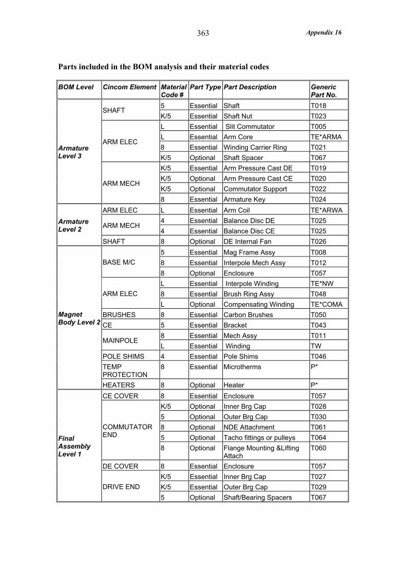
Appendix 16 363

Parts included in the BOM analysis and their material codes

BOM Level Cincom Element Material Code #

Part Type Part Description Generic Part No.

5 Essential Shaft T018 SHAFT

K/5 Essential Shaft Nut T023 L Essential Slit Commutator T005 L Essential Arm Core TE*ARMA 8 Essential Winding Carrier Ring T021

ARM ELEC

K/5 Optional Shaft Spacer T067 K/5 Essential Arm Pressure Cast DE T019 K/5 Optional Arm Pressure Cast CE T020 K/5 Optional Commutator Support T022

Armature Level 3

ARM MECH

8 Essential Armature Key T024 ARM ELEC L Essential Arm Coil TE*ARWA

4 Essential Balance Disc DE T025 ARM MECH

4 Essential Balance Disc CE T025 Armature Level 2

SHAFT 8 Optional DE Internal Fan T026 5 Essential Mag Frame Assy T008 8 Essential Interpole Mech Assy T012 BASE M/C 8 Optional Enclosure T057 L Essential Interpole Winding TE*NW 8 Essential Brush Ring Assy T048 ARM ELEC L Optional Compensating Winding TE*COMA

BRUSHES 8 Essential Carbon Brushes T050 CE 5 Essential Bracket T043

8 Essential Mech Assy T011 MAINPOLE

L Essential Winding TW POLE SHIMS 4 Essential Pole Shims T046 TEMP PROTECTION

8 Essential Microtherms P*

Magnet Body Level 2

HEATERS 8 Optional Heater P* CE COVER 8 Essential Enclosure T057

K/5 Optional Inner Brg Cap T028 5 Optional Outer Brg Cap T030 8 Optional NDE Attachment T061 5 Optional Tacho fittings or pulleys T064

COMMUTATOR END

8 Optional Flange Mounting &Lifting Attach

T060

DE COVER 8 Essential Enclosure T057 K/5 Essential Inner Brg Cap T027 K/5 Essential Outer Brg Cap T029

Final Assembly Level 1

DRIVE END 5 Optional Shaft/Bearing Spacers T067

Appendix 16 364

BOM Level Cincom Element Material Code Part Type Part Description Generic

Part No. 5 Essential Bracket T044 8 Optional Enclosure T057 DRIVE END 5/8 Optional Arm Locking Clamp T063 8 Optional Unit P* 8 Optional Filter P* 8 Optional Cover T057 8 Optional Unit and fittings T068

FORCED VENT

8 Optional Sub Assy T077 8 Optional Forced Vent Arrangement T078 8 Optional Tube B* AIR PRESSURE

SWITCH 8 Optional Switch P*

BRAKE 8 Optional Brake P* 8 Optional Heater P*

HEATERS 8 Optional Pipe Vents T068 8 Optional Cooler P*

COOLERS 8 Optional Adaptor T068

NAMEPLATE 8 Essential Lub Roller Bearing B 8 Optional Enclosure T057 PIPE ADAPTORS 8 Optional Pipe vents T068 8 Optional Shaft Key Ext B *

SHAFT 8 Optional Shaft Key T058

TACHO 8 Optional Tacho 7.8751* 8 Essential Terminal Box Assy

Complete T073

8 Essential Base and Mounting Brkt T052 8 Essential Centre Plate Earthing Strip T053 8 Essential Lid T054 8 Essential Terminal Block T056

Final Assembly Level 1

TERMINAL BOX

8 Essential Enclosure and Gasket T057

Material Code Definition L Parts made on the LDC section DLF (Direct Line Feed )

Parts used in high volumes normally on every motor and the supplier directly services the stock kept on the line

4 Raw materials kept in stock room and issued to line in bulk. The volume useage of these parts does not warrant DLF but does justify the maintenance of a stock on line

5 Parts made in the machine shop K Parts made in the machine shop and kept in Kanbans 8 Parts MRP purchased

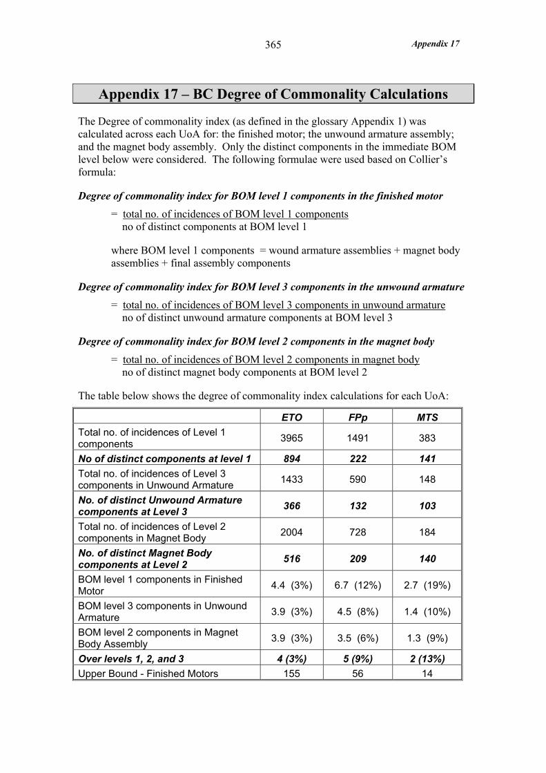
Appendix 17 365

Appendix 17 – BC Degree of Commonality Calculations

The Degree of commonality index (as defined in the glossary Appendix 1) was calculated across each UoA for: the finished motor; the unwound armature assembly; and the magnet body assembly. Only the distinct components in the immediate BOM level below were considered. The following formulae were used based on Collier’s formula:

Degree of commonality index for BOM level 1 components in the finished motor = total no. of incidences of BOM level 1 components no of distinct components at BOM level 1

where BOM level 1 components = wound armature assemblies + magnet body assemblies + final assembly components

Degree of commonality index for BOM level 3 components in the unwound armature = total no. of incidences of BOM level 3 components in unwound armature no of distinct unwound armature components at BOM level 3

Degree of commonality index for BOM level 2 components in the magnet body = total no. of incidences of BOM level 2 components in magnet body no of distinct magnet body components at BOM level 2

The table below shows the degree of commonality index calculations for each UoA:

ETO FPp MTS Total no. of incidences of Level 1 components 3965 1491 383

No of distinct components at level 1 894 222 141 Total no. of incidences of Level 3 components in Unwound Armature 1433 590 148

No. of distinct Unwound Armature components at Level 3 366 132 103

Total no. of incidences of Level 2 components in Magnet Body 2004 728 184

No. of distinct Magnet Body components at Level 2 516 209 140

BOM level 1 components in Finished Motor 4.4 (3%) 6.7 (12%) 2.7 (19%)

BOM level 3 components in Unwound Armature 3.9 (3%) 4.5 (8%) 1.4 (10%)

BOM level 2 components in Magnet Body Assembly 3.9 (3%) 3.5 (6%) 1.3 (9%)

Over levels 1, 2, and 3 4 (3%) 5 (9%) 2 (13%) Upper Bound - Finished Motors 155 56 14

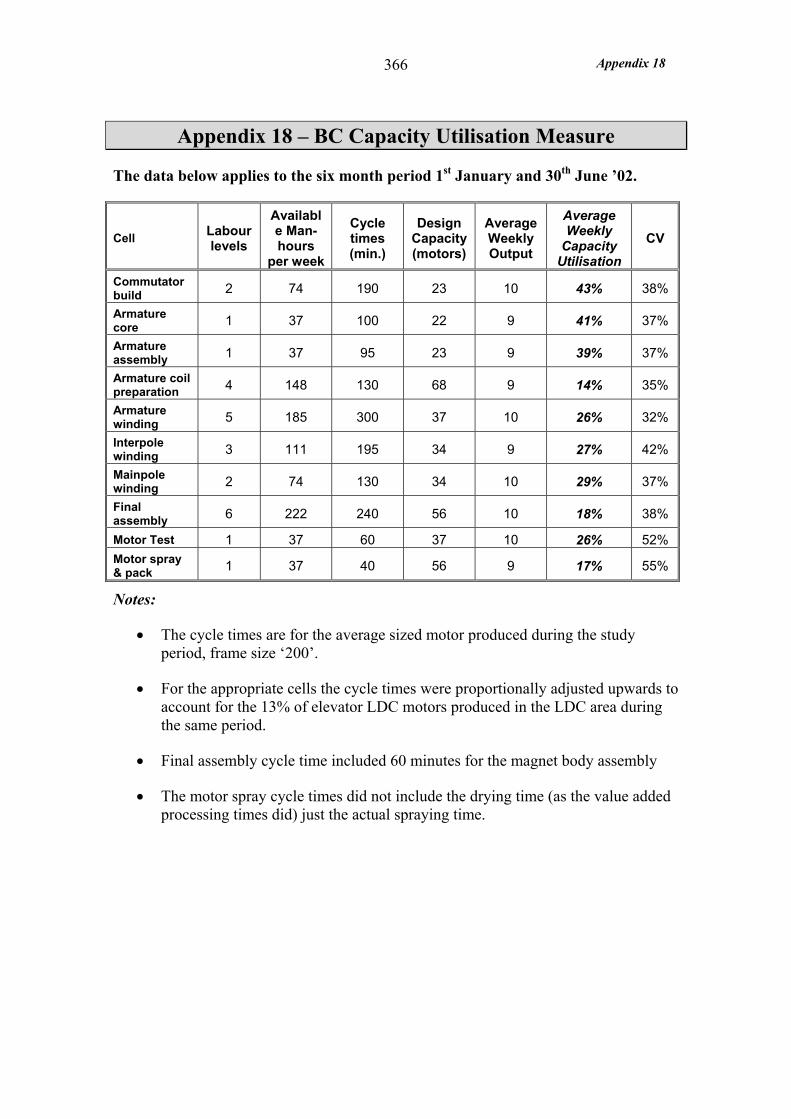
Appendix 18 366

Appendix 18 – BC Capacity Utilisation Measure

The data below applies to the six month period 1st January and 30th June ’02.

Cell Labour levels

Available Man-hours

per week

Cycle times (min.)

Design Capacity (motors)

Average Weekly Output

Average Weekly


CV

Commutator build 2 74 190 23 10 43% 38%

Armature core 1 37 100 22 9 41% 37%

Armature assembly 1 37 95 23 9 39% 37%

Armature coil preparation 4 148 130 68 9 14% 35%

Armature winding 5 185 300 37 10 26% 32%

Interpole winding 3 111 195 34 9 27% 42%

Mainpole winding 2 74 130 34 10 29% 37%

Final assembly 6 222 240 56 10 18% 38%

Motor Test 1 37 60 37 10 26% 52% Motor spray & pack 1 37 40 56 9 17% 55%

Notes:

• The cycle times are for the average sized motor produced during the study period, frame size ‘200’.

• For the appropriate cells the cycle times were proportionally adjusted upwards to account for the 13% of elevator LDC motors produced in the LDC area during the same period.

• Final assembly cycle time included 60 minutes for the magnet body assembly

• The motor spray cycle times did not include the drying time (as the value added processing times did) just the actual spraying time.

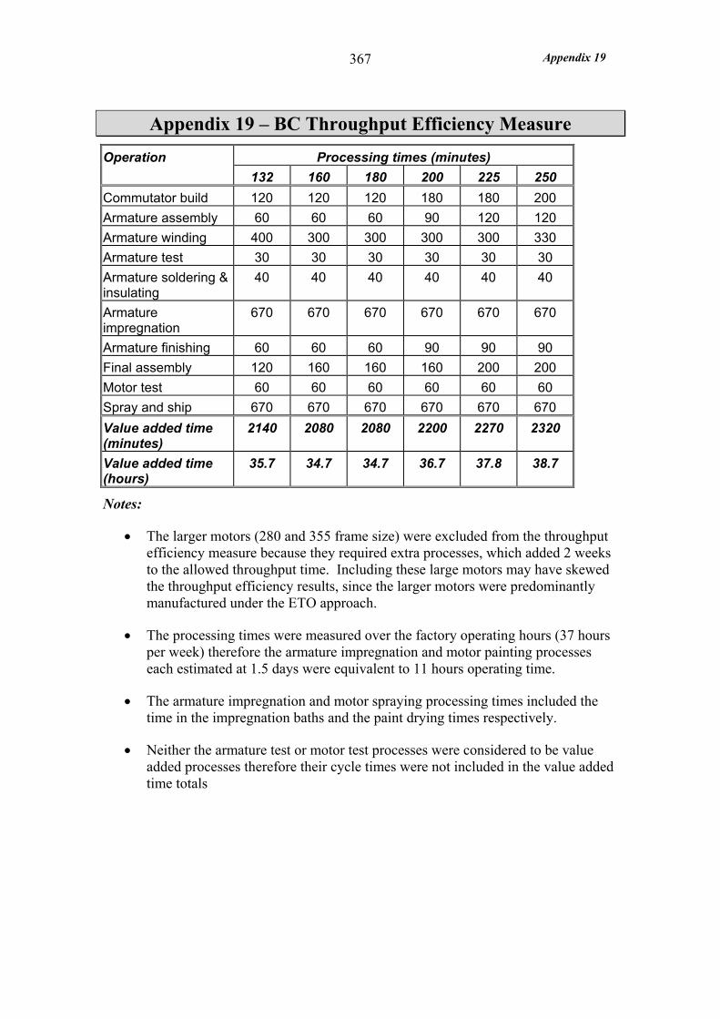
Appendix 19 367

Appendix 19 – BC Throughput Efficiency Measure Processing times (minutes) Operation

132 160 180 200 225 250 Commutator build 120 120 120 180 180 200 Armature assembly 60 60 60 90 120 120 Armature winding 400 300 300 300 300 330 Armature test 30 30 30 30 30 30 Armature soldering & insulating

40 40 40 40 40 40

Armature impregnation

670 670 670 670 670 670

Armature finishing 60 60 60 90 90 90 Final assembly 120 160 160 160 200 200 Motor test 60 60 60 60 60 60 Spray and ship 670 670 670 670 670 670 Value added time (minutes)

2140 2080 2080 2200 2270 2320

Value added time (hours)

35.7 34.7 34.7 36.7 37.8 38.7

Notes:

• The larger motors (280 and 355 frame size) were excluded from the throughput efficiency measure because they required extra processes, which added 2 weeks to the allowed throughput time. Including these large motors may have skewed the throughput efficiency results, since the larger motors were predominantly manufactured under the ETO approach.

• The processing times were measured over the factory operating hours (37 hours per week) therefore the armature impregnation and motor painting processes each estimated at 1.5 days were equivalent to 11 hours operating time.

• The armature impregnation and motor spraying processing times included the time in the impregnation baths and the paint drying times respectively.

• Neither the armature test or motor test processes were considered to be value added processes therefore their cycle times were not included in the value added time totals

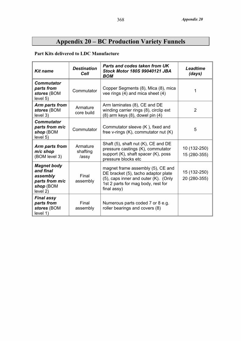
Appendix 20 368

Appendix 20 – BC Production Variety Funnels

Part Kits delivered to LDC Manufacture

Kit name Destination Cell

Parts and codes taken from UK Stock Motor 180S 99040121 JBA BOM

Leadtime (days)

Commutator parts from stores (BOM level 5)

Commutator Copper Segments (8), Mica (8), mica vee rings (4) and mica sheet (4) 1

Arm parts from stores (BOM level 3)

Armature core build

Arm laminates (8), CE and DE winding carrier rings (8), circlip ext (8) arm keys (8), dowel pin (4)

2

Commutator parts from m/c shop (BOM level 5)

Commutator Commutator sleeve (K ), fixed and free v-rings (K), commutator nut (K) 5

Arm parts from m/c shop (BOM level 3)

Armature shafting

/assy

Shaft (5), shaft nut (K), CE and DE pressure castings (K), commutator support (K), shaft spacer (K), poss pressure blocks etc

10 (132-250) 15 (280-355)

Magnet body and final assembly parts from m/c shop (BOM level 2)

Final assembly

magnet frame assembly (5), CE and DE bracket (5), tacho adaptor plate (5), caps inner and outer (K). (Only 1st 2 parts for mag body, rest for final assy)

15 (132-250) 20 (280-355)

Final assy parts from stores (BOM level 1)

Final assembly

Numerous parts coded 7 or 8 e.g. roller bearings and covers (8)

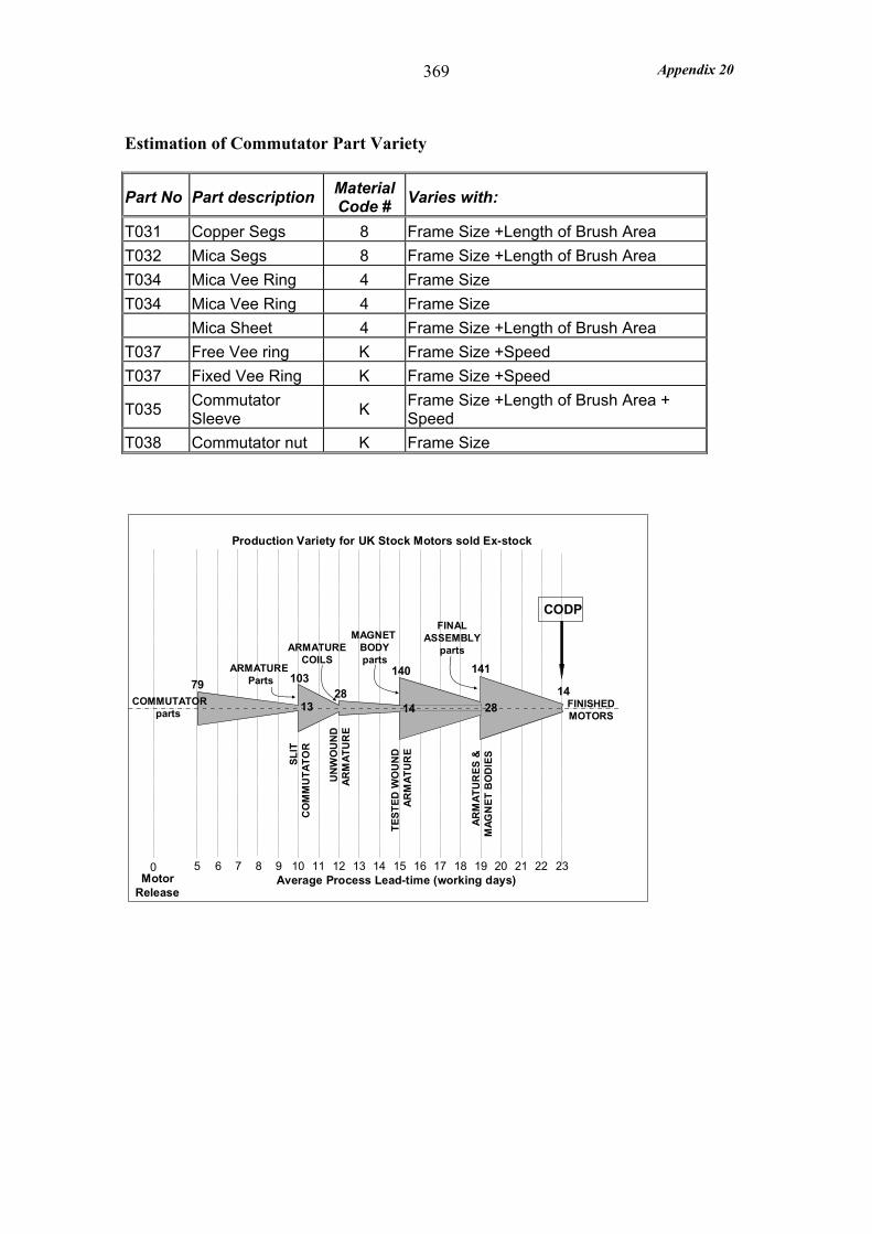
Appendix 20 369

Estimation of Commutator Part Variety

Part No Part description Material Code # Varies with:

T031 Copper Segs 8 Frame Size +Length of Brush Area T032 Mica Segs 8 Frame Size +Length of Brush Area T034 Mica Vee Ring 4 Frame Size T034 Mica Vee Ring 4 Frame Size Mica Sheet 4 Frame Size +Length of Brush Area T037 Free Vee ring K Frame Size +Speed T037 Fixed Vee Ring K Frame Size +Speed

T035 Commutator Sleeve K Frame Size +Length of Brush Area +

Speed T038 Commutator nut K Frame Size

TEST

ED W

OU

ND

ARM

ATU

RE

MotorRelease

0 5 6 7 8 9 10 11 12 13 14 15 16 17 18 19 20 21 22 23

Production Variety for UK Stock Motors sold Ex-stock

79COMMUTATOR

parts

103

SLIT

CO

MM

UTA

TOR

UN

WO

UN

DAR

MAT

UR

E

28

140 141

ARM

ATU

RES

&M

AGN

ET B

OD

IES

FINISHEDMOTORS

ARMATURE Parts

ARMATURECOILS

MAGNET BODYparts

FINALASSEMBLY

parts

14281413

CODP

Average Process Lead-time (working days)

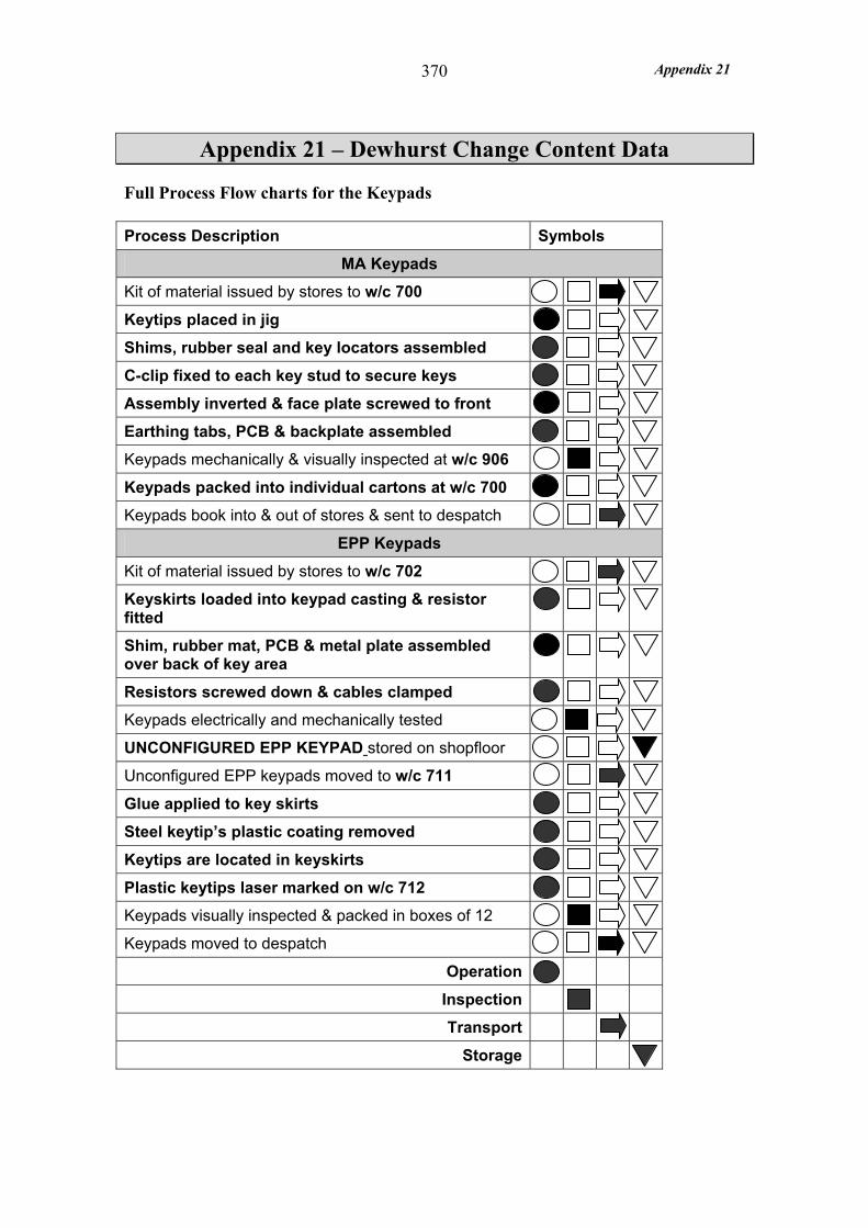
Appendix 21 370

Appendix 21 – Dewhurst Change Content Data

Full Process Flow charts for the Keypads


MA Keypads

Kit of material issued by stores to w/c 700

Keytips placed in jig

Shims, rubber seal and key locators assembled

C-clip fixed to each key stud to secure keys

Assembly inverted & face plate screwed to front

Earthing tabs, PCB & backplate assembled

Keypads mechanically & visually inspected at w/c 906

Keypads packed into individual cartons at w/c 700

Keypads book into & out of stores & sent to despatch

EPP Keypads

Kit of material issued by stores to w/c 702

Keyskirts loaded into keypad casting & resistor fitted

Shim, rubber mat, PCB & metal plate assembled over back of key area

Resistors screwed down & cables clamped

Keypads electrically and mechanically tested

UNCONFIGURED EPP KEYPAD stored on shopfloor

Unconfigured EPP keypads moved to w/c 711

Glue applied to key skirts

Steel keytip’s plastic coating removed

Keytips are located in keyskirts

Plastic keytips laser marked on w/c 712

Keypads visually inspected & packed in boxes of 12

Keypads moved to despatch

Operation

Inspection

Transport

Storage

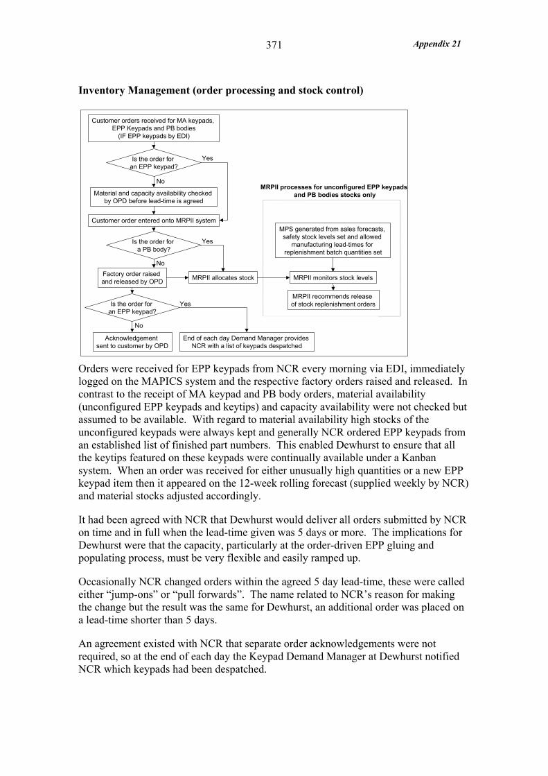
Appendix 21 371

Inventory Management (order processing and stock control)

Orders were received for EPP keypads from NCR every morning via EDI, immediately logged on the MAPICS system and the respective factory orders raised and released. In contrast to the receipt of MA keypad and PB body orders, material availability (unconfigured EPP keypads and keytips) and capacity availability were not checked but assumed to be available. With regard to material availability high stocks of the unconfigured keypads were always kept and generally NCR ordered EPP keypads from an established list of finished part numbers. This enabled Dewhurst to ensure that all the keytips featured on these keypads were continually available under a Kanban system. When an order was received for either unusually high quantities or a new EPP keypad item then it appeared on the 12-week rolling forecast (supplied weekly by NCR) and material stocks adjusted accordingly.

It had been agreed with NCR that Dewhurst would deliver all orders submitted by NCR on time and in full when the lead-time given was 5 days or more. The implications for Dewhurst were that the capacity, particularly at the order-driven EPP gluing and populating process, must be very flexible and easily ramped up.

Occasionally NCR changed orders within the agreed 5 day lead-time, these were called either “jump-ons” or “pull forwards”. The name related to NCR’s reason for making the change but the result was the same for Dewhurst, an additional order was placed on a lead-time shorter than 5 days.

An agreement existed with NCR that separate order acknowledgements were not required, so at the end of each day the Keypad Demand Manager at Dewhurst notified NCR which keypads had been despatched.

Customer orders received for MA keypads, EPP Keypads and PB bodies

(IF EPP keypads by EDI)

Material and capacity availability checked by OPD before lead-time is agreed

Customer order entered onto MRPII system

Acknowledgement sent to customer by OPD

MPS generated from sales forecasts, safety stock levels set and allowed

manufacturing lead-times for replenishment batch quantities set

MRPII monitors stock levels

MRPII recommends release of stock replenishment orders

Factory order raised and released by OPD

MRPII processes for unconfigured EPP keypads and PB bodies stocks only

MRPII allocates stock

Is the order for an EPP keypad?


End of each day Demand Manager provides NCR with a list of keypads despatched

Yes

No

Yes

No

Is the order for a PB body?

Yes

No

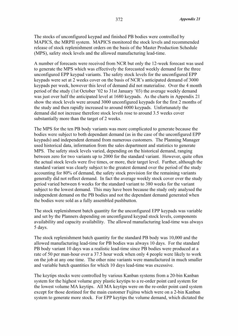
Appendix 21 372

The stocks of unconfigured keypad and finished PB bodies were controlled by MAPICS, the MRPII system. MAPICS monitored the stock levels and recommended release of stock replenishment orders on the basis of the Master Production Schedule (MPS), safety stock levels and the allowed manufacturing lead-time.

A number of forecasts were received from NCR but only the 12-week forecast was used to generate the MPS which was effectively the forecasted weekly demand for the three unconfigured EPP keypad variants. The safety stock levels for the unconfigured EPP keypads were set at 2 weeks cover on the basis of NCR’s anticipated demand of 3000 keypads per week, however this level of demand did not materialise. Over the 4 month period of the study (1st October ’02 to 31st January ’03) the average weekly demand was just over half the anticipated level at 1680 keypads. As the charts in Appendix 21 show the stock levels were around 3000 unconfigured keypads for the first 2 months of the study and then rapidly increased to around 6000 keypads. Unfortunately the demand did not increase therefore stock levels rose to around 3.5 weeks cover substantially more than the target of 2 weeks.

The MPS for the ten PB body variants was more complicated to generate because the bodies were subject to both dependant demand (as in the case of the unconfigured EPP keypads) and independent demand from numerous customers. The Planning Manager used historical data, information from the sales department and statistics to generate MPS. The safety stock levels varied, depending on the historical demand, ranging between zero for two variants up to 2000 for the standard variant. However, quite often the actual stock levels were five times, or more, their target level. Further, although the standard variant was clearly subject to the greatest demand over the period of the study accounting for 80% of demand, the safety stock provision for the remaining variants generally did not reflect demand. In fact the average weekly stock cover over the study period varied between 6 weeks for the standard variant to 380 weeks for the variant subject to the lowest demand. This may have been because the study only analysed the independent demand on the PB bodies and not the dependant demand generated when the bodies were sold as a fully assembled pushbutton.

The stock replenishment batch quantity for the unconfigured EPP keypads was variable and set by the Planners depending on unconfigured keypad stock levels, components availability and capacity availability. The allowed manufacturing lead-time was always 5 days.

The stock replenishment batch quantity for the standard PB body was 10,000 and the allowed manufacturing lead-time for PB bodies was always 10 days. For the standard PB body variant 10 days was a realistic lead-time since PB bodies were produced at a rate of 50 per man-hour over a 37.5 hour week when only 4 people were likely to work on the job at any one time. The other nine variants were manufactured in much smaller and variable batch quantities for which 10 days lead-time was excessive.

The keytips stocks were controlled by various Kanban systems from a 20-bin Kanban system for the highest volume grey plastic keytips to a re-order point card system for the lowest volume MA keytips. All MA keytips were on the re-order point card system except for those destined for the main customer Fujitsu which were on a 2-bin Kanban system to generate more stock. For EPP keytips the volume demand, which dictated the

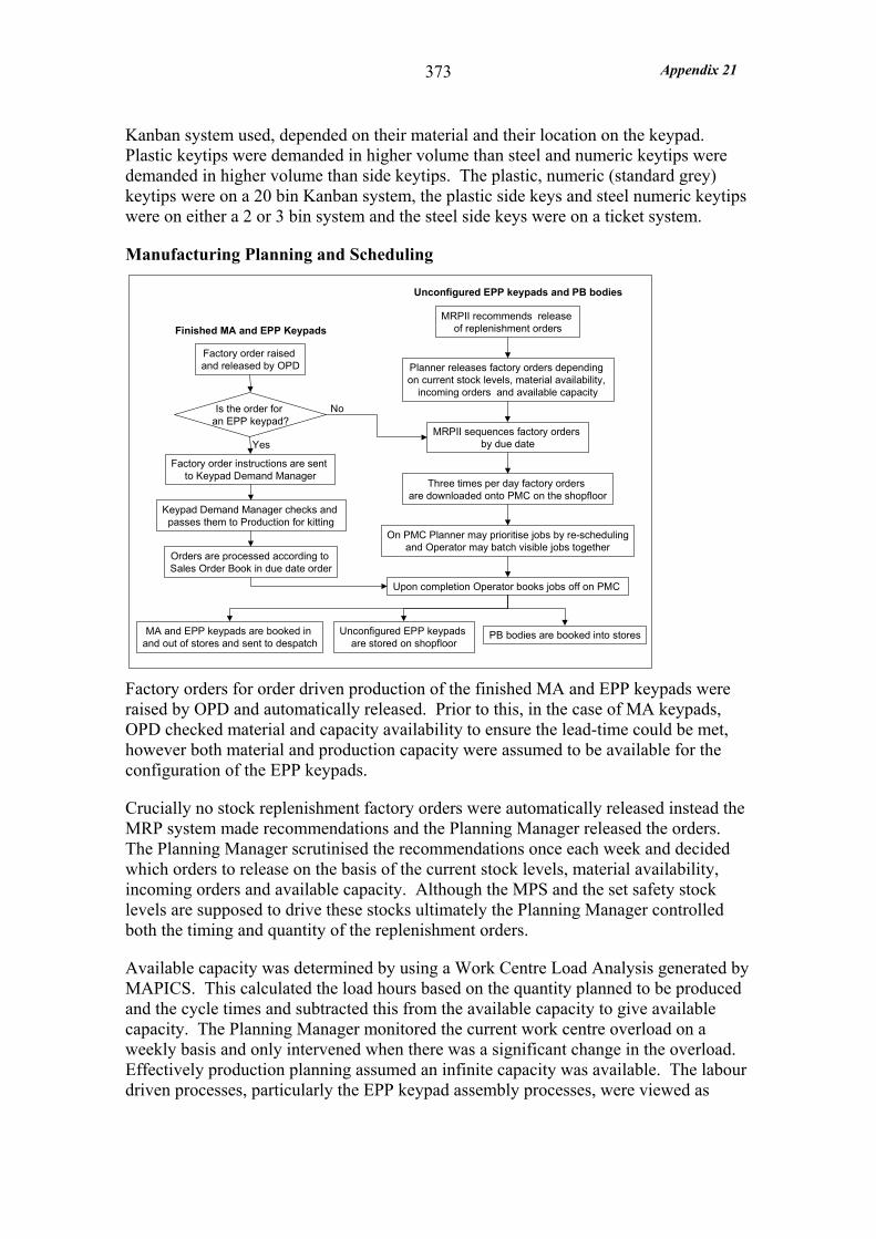
Appendix 21 373

Kanban system used, depended on their material and their location on the keypad. Plastic keytips were demanded in higher volume than steel and numeric keytips were demanded in higher volume than side keytips. The plastic, numeric (standard grey) keytips were on a 20 bin Kanban system, the plastic side keys and steel numeric keytips were on either a 2 or 3 bin system and the steel side keys were on a ticket system.

Manufacturing Planning and Scheduling

Factory orders for order driven production of the finished MA and EPP keypads were raised by OPD and automatically released. Prior to this, in the case of MA keypads, OPD checked material and capacity availability to ensure the lead-time could be met, however both material and production capacity were assumed to be available for the configuration of the EPP keypads.

Crucially no stock replenishment factory orders were automatically released instead the MRP system made recommendations and the Planning Manager released the orders. The Planning Manager scrutinised the recommendations once each week and decided which orders to release on the basis of the current stock levels, material availability, incoming orders and available capacity. Although the MPS and the set safety stock levels are supposed to drive these stocks ultimately the Planning Manager controlled both the timing and quantity of the replenishment orders.

Available capacity was determined by using a Work Centre Load Analysis generated by MAPICS. This calculated the load hours based on the quantity planned to be produced and the cycle times and subtracted this from the available capacity to give available capacity. The Planning Manager monitored the current work centre overload on a weekly basis and only intervened when there was a significant change in the overload. Effectively production planning assumed an infinite capacity was available. The labour driven processes, particularly the EPP keypad assembly processes, were viewed as

Factory order raised and released by OPD

MRPII recommends release of replenishment orders

Planner releases factory orders depending on current stock levels, material availability,

incoming orders and available capacity

Finished MA and EPP Keypads

Unconfigured EPP keypads and PB bodies

MRPII sequences factory orders by due date

Three times per day factory orders are downloaded onto PMC on the shopfloor

Upon completion Operator books jobs off on PMC

MA and EPP keypads are booked in and out of stores and sent to despatch

Unconfigured EPP keypads are stored on shopfloor

PB bodies are booked into stores

On PMC Planner may prioritise jobs by re-schedulingand Operator may batch visible jobs together

Factory order instructions are sent to Keypad Demand Manager

Keypad Demand Manager checks and passes them to Production for kitting


No

Yes

Orders are processed according to Sales Order Book in due date order

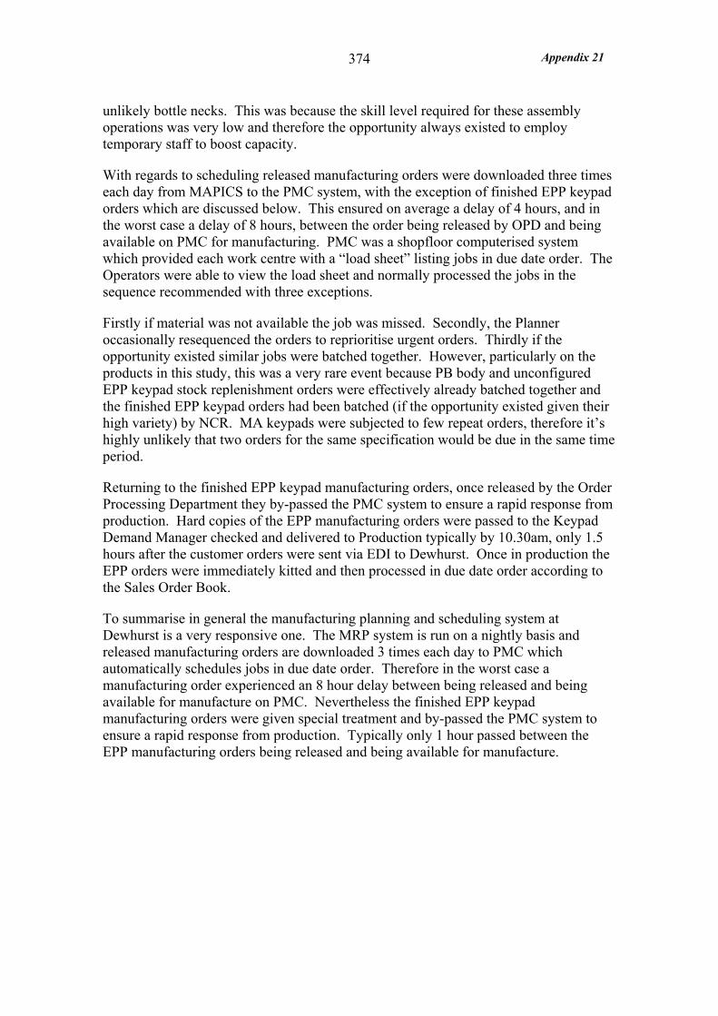
Appendix 21 374

unlikely bottle necks. This was because the skill level required for these assembly operations was very low and therefore the opportunity always existed to employ temporary staff to boost capacity.

With regards to scheduling released manufacturing orders were downloaded three times each day from MAPICS to the PMC system, with the exception of finished EPP keypad orders which are discussed below. This ensured on average a delay of 4 hours, and in the worst case a delay of 8 hours, between the order being released by OPD and being available on PMC for manufacturing. PMC was a shopfloor computerised system which provided each work centre with a “load sheet” listing jobs in due date order. The Operators were able to view the load sheet and normally processed the jobs in the sequence recommended with three exceptions.

Firstly if material was not available the job was missed. Secondly, the Planner occasionally resequenced the orders to reprioritise urgent orders. Thirdly if the opportunity existed similar jobs were batched together. However, particularly on the products in this study, this was a very rare event because PB body and unconfigured EPP keypad stock replenishment orders were effectively already batched together and the finished EPP keypad orders had been batched (if the opportunity existed given their high variety) by NCR. MA keypads were subjected to few repeat orders, therefore it’s highly unlikely that two orders for the same specification would be due in the same time period.

Returning to the finished EPP keypad manufacturing orders, once released by the Order Processing Department they by-passed the PMC system to ensure a rapid response from production. Hard copies of the EPP manufacturing orders were passed to the Keypad Demand Manager checked and delivered to Production typically by 10.30am, only 1.5 hours after the customer orders were sent via EDI to Dewhurst. Once in production the EPP orders were immediately kitted and then processed in due date order according to the Sales Order Book.

To summarise in general the manufacturing planning and scheduling system at Dewhurst is a very responsive one. The MRP system is run on a nightly basis and released manufacturing orders are downloaded 3 times each day to PMC which automatically schedules jobs in due date order. Therefore in the worst case a manufacturing order experienced an 8 hour delay between being released and being available for manufacture on PMC. Nevertheless the finished EPP keypad manufacturing orders were given special treatment and by-passed the PMC system to ensure a rapid response from production. Typically only 1 hour passed between the EPP manufacturing orders being released and being available for manufacture.

Appendix 21 375

Stock Records for Unconfigured EPP Keypads and PB Bodies

Note: The zero stock level recorded for the Canadian plastic keypads over the first few weeks was before they were made available.

0

1000

2000

3000

4000

5000

6000

7000

8000

40 42 44 46 48 50 52 2 4

No.

of E

PP K

eypa

ds

Week no 2002/03

Unconfigured EPP Keypad Total Weekly Stock Levels

0

1000

2000

3000

4000

5000

40 42 44 46 48 50 52 2 4

Steel

StandardPlasticCanadianPlastic

Week no 2002/03

No.

of E

PP K

eypa

ds

Unconfigured EPP Keypad Weekly Stock Levels

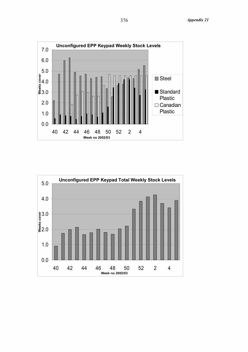
Appendix 21 376

0.0

1.0

2.0

3.0

4.0

5.0

6.0

7.0

40 42 44 46 48 50 52 2 4

Steel

StandardPlasticCanadianPlastic

Unconfigured EPP Keypad Weekly Stock Levels

Week no 2002/03

Wee

ks c

over

0.0

1.0

2.0

3.0

4.0

5.0

40 42 44 46 48 50 52 2 4

Unconfigured EPP Keypad Total Weekly Stock Levels

Week no 2002/03

Wee

ks c

over

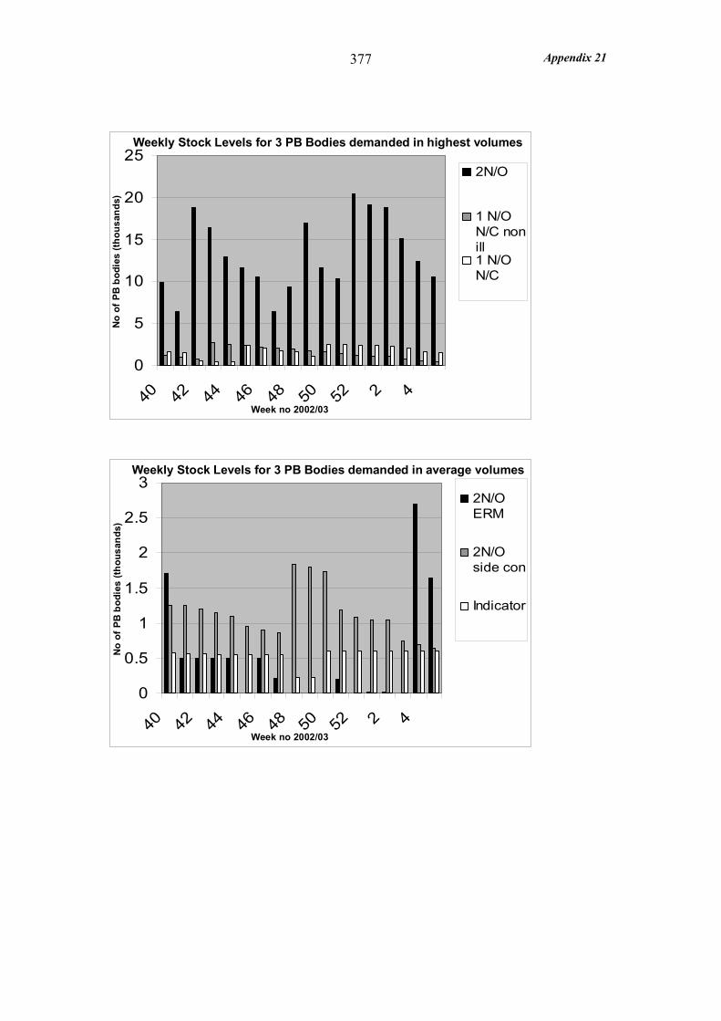
Appendix 21 377

0

5

10

15

20

25

40 42 44 46 48 50 52 2 4

2N/O

1 N/ON/C nonill1 N/ON/C

Weekly Stock Levels for 3 PB Bodies demanded in highest volumes

Week no 2002/03

No

of P

B b

odie

s (th

ousa

nds)

0

0.5

1

1.5

2

2.5

3

40 42 44 46 48 50 52 2 4

2N/OERM

2N/Oside con

Indicator

Weekly Stock Levels for 3 PB Bodies demanded in average volumes

No

of P

B b

odie

s (th

ousa

nds)

Week no 2002/03

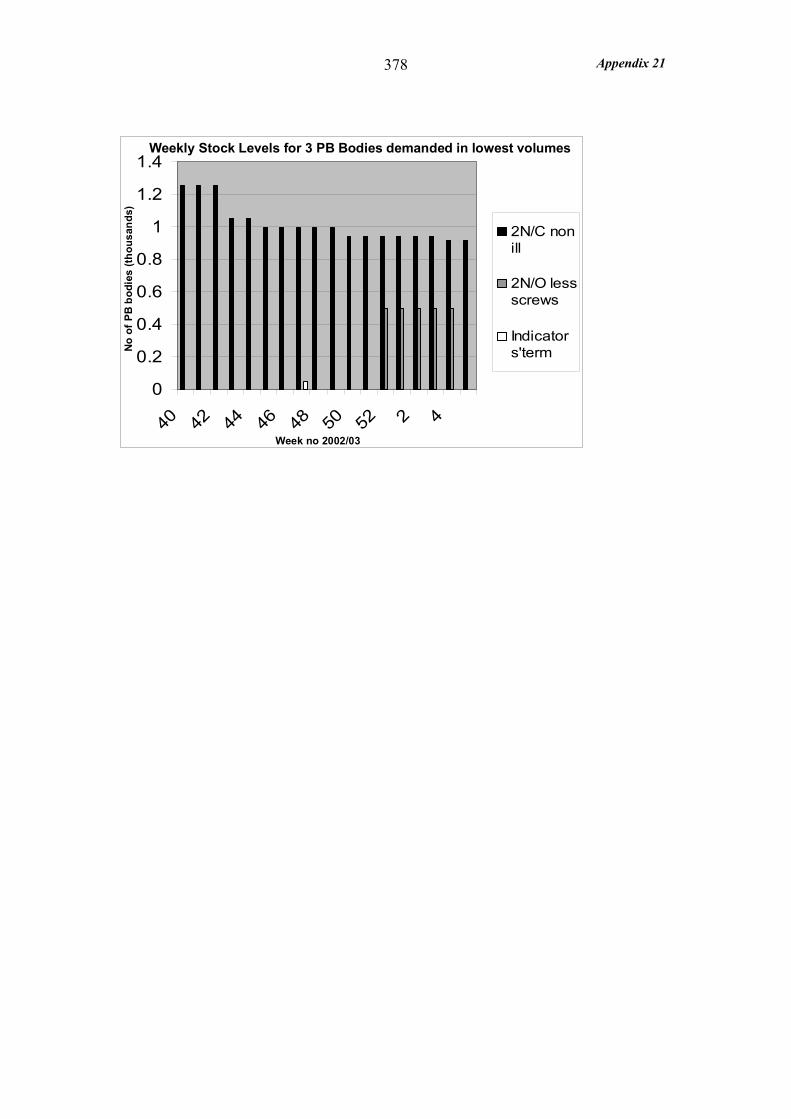
Appendix 21 378

0

0.2

0.4

0.6

0.8

1

1.2

1.4

40 42 44 46 48 50 52 2 4

2N/C nonill

2N/O lessscrews

Indicators'term

Weekly Stock Levels for 3 PB Bodies demanded in lowest volumesN

o of

PB

bod

ies

(thou

sand

s)

Week no 2002/03

Appendix 22 379

Appendix 22 – Dewhurst Manufacturing Data

The operating hours for the Dewhurst factory were 37.5 hours per week. Below are details of the production arrangements, labour levels, unit processing times and cycle times for the EPP keypads, MA keypads and PB bodies, where:

• unit processing time is measured in man minutes and is the time required to complete the assembly process on 1 unit.

• cycle time is measured in minutes and is the time period between units being completed on a production cell.

The cycle times were calculated from a knowledge of the production arrangement (i.e. production lines or individual work stations) and the unit processing times. Where only one man is involved in the assembly of each unit (i.e. an individual work station) processing and cycle times are the same. However where more than one man was involved in the assembly of each unit (i.e. a production line) then the cycle time is less than the processing time by a factor of the number of people on the line.

EPP Keypad

• Between 1st October and 20th December the unit processing times for the assembly of the EPP keypad depended on whether the belt line was used. According to Flow Process Charts recorded by Production if the belt line was used the processing time was 8.5 man minutes, however if it wasn’t used the processing time was 5.5 man minutes. The keypad assembly processing times in the table below are adjusted according to the number of belt lines used.

• Initially the configuring of the keypads was conducted by work stations where a single person conducted all operations manually. After 18th November a gluing machine was commissioned and a configuring line was established requiring 3 people. However, this did not reduce the processing times but did reduce the cycle time by a factor of 3, the number of people on the line. The keypad configuring cycle times in the table below are adjusted according to the number of gluing stations versus gluing lines.

• For both the keypad assembly and the keypad configuration process cycle times dropped over the study period. In the case of keypad assembly this was due to the gradual change to non-belt assembly lines and in the case of keypad configuration it was due to the gradual change from individual “gluing” stations to “gluing” lines. However, in both cases the elapsed time, or manufacturing lead-times, remained about the same. Therefore the trend was for throughput efficiency to drop over the study period.

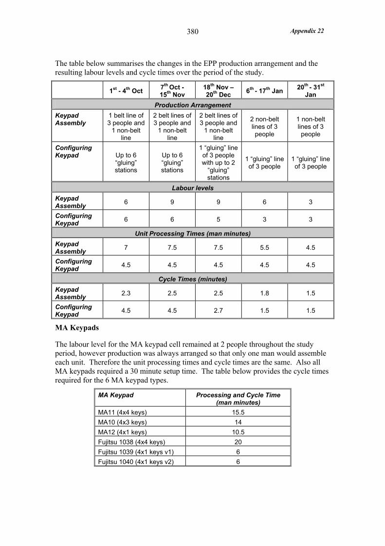
Appendix 22 380

The table below summarises the changes in the EPP production arrangement and the resulting labour levels and cycle times over the period of the study.

1st - 4th Oct 7th Oct - 15th Nov

18th Nov – 20th Dec 6th - 17th Jan 20th - 31st

Jan Production Arrangement

Keypad Assembly

1 belt line of 3 people and

1 non-belt line

2 belt lines of 3 people and

1 non-belt line

2 belt lines of 3 people and

1 non-belt line

2 non-belt lines of 3 people

1 non-belt lines of 3 people

Configuring Keypad Up to 6

“gluing” stations

Up to 6 “gluing” stations

1 “gluing” line of 3 people with up to 2

“gluing” stations

1 “gluing” line of 3 people

1 “gluing” line of 3 people

Labour levels Keypad Assembly 6 9 9 6 3

Configuring Keypad 6 6 5 3 3

Unit Processing Times (man minutes) Keypad Assembly 7 7.5 7.5 5.5 4.5

Configuring Keypad 4.5 4.5 4.5 4.5 4.5

Cycle Times (minutes) Keypad Assembly 2.3 2.5 2.5 1.8 1.5

Configuring Keypad 4.5 4.5 2.7 1.5 1.5

MA Keypads

The labour level for the MA keypad cell remained at 2 people throughout the study period, however production was always arranged so that only one man would assemble each unit. Therefore the unit processing times and cycle times are the same. Also all MA keypads required a 30 minute setup time. The table below provides the cycle times required for the 6 MA keypad types.

MA Keypad Processing and Cycle Time (man minutes)

MA11 (4x4 keys) 15.5 MA10 (4x3 keys) 14 MA12 (4x1 keys) 10.5 Fujitsu 1038 (4x4 keys) 20 Fujitsu 1039 (4x1 keys v1) 6 Fujitsu 1040 (4x1 keys v2) 6

Appendix 22 381

PB Bodies

The assembly of the switch bodies was normally performed by a production line of 2 men therefore the cycle time is half the processing time. The Assembly of all PB bodies required a 15 minute setup time. The table below provides the times required for the 2 types of PB bodies

PB body Assembly Processing Time (man minutes) Assembly Cycle Time (minutes)

PB switch 1.2 (50/man hour) 0.6 (100/hour) PB indicator 0.5 (120/man hour) 0.5 (120/hour)

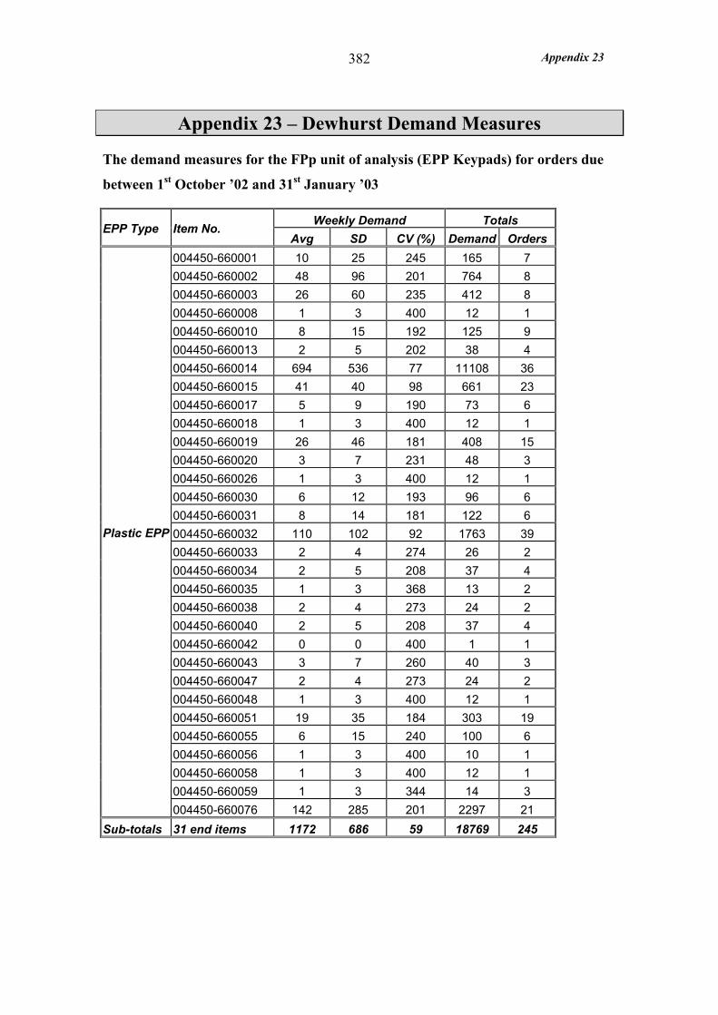
Appendix 23 382

Appendix 23 – Dewhurst Demand Measures

The demand measures for the FPp unit of analysis (EPP Keypads) for orders due

between 1st October ’02 and 31st January ’03

Weekly Demand Totals EPP Type Item No. Avg SD CV (%) Demand Orders

004450-660001 10 25 245 165 7 004450-660002 48 96 201 764 8 004450-660003 26 60 235 412 8 004450-660008 1 3 400 12 1 004450-660010 8 15 192 125 9 004450-660013 2 5 202 38 4 004450-660014 694 536 77 11108 36 004450-660015 41 40 98 661 23 004450-660017 5 9 190 73 6 004450-660018 1 3 400 12 1 004450-660019 26 46 181 408 15 004450-660020 3 7 231 48 3 004450-660026 1 3 400 12 1 004450-660030 6 12 193 96 6 004450-660031 8 14 181 122 6 004450-660032 110 102 92 1763 39 004450-660033 2 4 274 26 2 004450-660034 2 5 208 37 4 004450-660035 1 3 368 13 2 004450-660038 2 4 273 24 2 004450-660040 2 5 208 37 4 004450-660042 0 0 400 1 1 004450-660043 3 7 260 40 3 004450-660047 2 4 273 24 2 004450-660048 1 3 400 12 1 004450-660051 19 35 184 303 19 004450-660055 6 15 240 100 6 004450-660056 1 3 400 10 1 004450-660058 1 3 400 12 1 004450-660059 1 3 344 14 3

Plastic EPP

004450-660076 142 285 201 2297 21 Sub-totals 31 end items 1172 686 59 18769 245

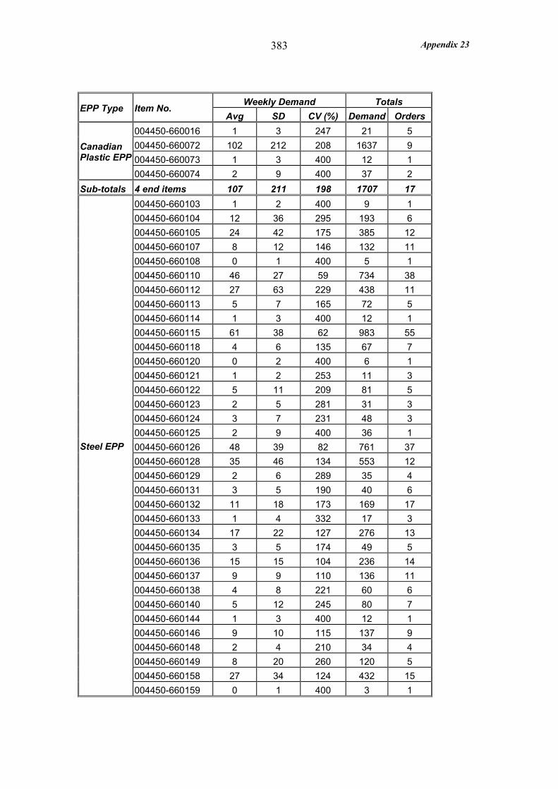
Appendix 23 383

Weekly Demand Totals EPP Type Item No.

Avg SD CV (%) Demand Orders 004450-660016 1 3 247 21 5 004450-660072 102 212 208 1637 9 004450-660073 1 3 400 12 1

Canadian Plastic EPP

004450-660074 2 9 400 37 2 Sub-totals 4 end items 107 211 198 1707 17

004450-660103 1 2 400 9 1 004450-660104 12 36 295 193 6 004450-660105 24 42 175 385 12 004450-660107 8 12 146 132 11 004450-660108 0 1 400 5 1 004450-660110 46 27 59 734 38 004450-660112 27 63 229 438 11 004450-660113 5 7 165 72 5 004450-660114 1 3 400 12 1 004450-660115 61 38 62 983 55 004450-660118 4 6 135 67 7 004450-660120 0 2 400 6 1 004450-660121 1 2 253 11 3 004450-660122 5 11 209 81 5 004450-660123 2 5 281 31 3 004450-660124 3 7 231 48 3 004450-660125 2 9 400 36 1 004450-660126 48 39 82 761 37 004450-660128 35 46 134 553 12 004450-660129 2 6 289 35 4 004450-660131 3 5 190 40 6 004450-660132 11 18 173 169 17 004450-660133 1 4 332 17 3 004450-660134 17 22 127 276 13 004450-660135 3 5 174 49 5 004450-660136 15 15 104 236 14 004450-660137 9 9 110 136 11 004450-660138 4 8 221 60 6 004450-660140 5 12 245 80 7 004450-660144 1 3 400 12 1 004450-660146 9 10 115 137 9 004450-660148 2 4 210 34 4 004450-660149 8 20 260 120 5 004450-660158 27 34 124 432 15

Steel EPP

004450-660159 0 1 400 3 1

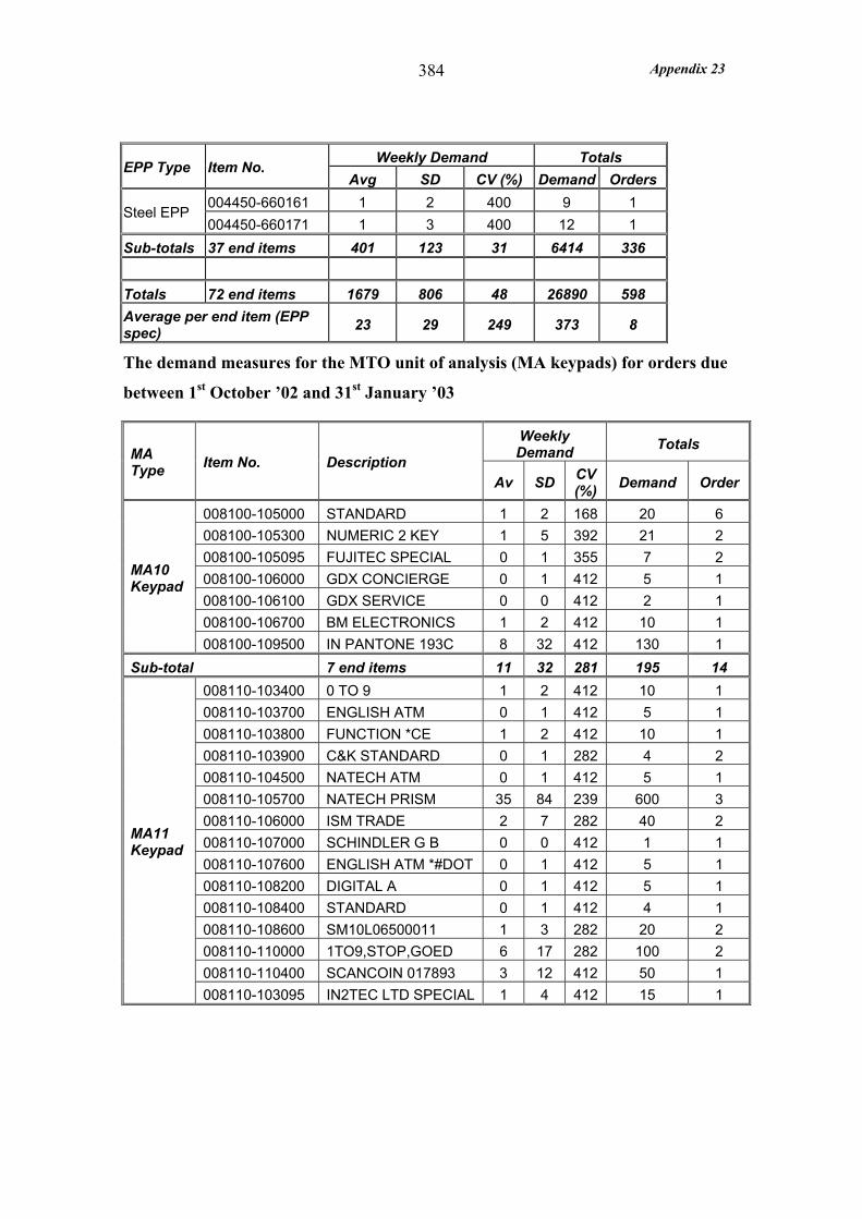
Appendix 23 384

Weekly Demand Totals EPP Type Item No.

Avg SD CV (%) Demand Orders 004450-660161 1 2 400 9 1

Steel EPP 004450-660171 1 3 400 12 1

Sub-totals 37 end items 401 123 31 6414 336 Totals 72 end items 1679 806 48 26890 598 Average per end item (EPP spec) 23 29 249 373 8

The demand measures for the MTO unit of analysis (MA keypads) for orders due

between 1st October ’02 and 31st January ’03

Weekly Demand Totals MA

Type Item No. Description Av SD CV

(%) Demand Order

008100-105000 STANDARD 1 2 168 20 6 008100-105300 NUMERIC 2 KEY 1 5 392 21 2 008100-105095 FUJITEC SPECIAL 0 1 355 7 2 008100-106000 GDX CONCIERGE 0 1 412 5 1 008100-106100 GDX SERVICE 0 0 412 2 1 008100-106700 BM ELECTRONICS 1 2 412 10 1

MA10 Keypad

008100-109500 IN PANTONE 193C 8 32 412 130 1 Sub-total 7 end items 11 32 281 195 14

008110-103400 0 TO 9 1 2 412 10 1 008110-103700 ENGLISH ATM 0 1 412 5 1 008110-103800 FUNCTION *CE 1 2 412 10 1 008110-103900 C&K STANDARD 0 1 282 4 2 008110-104500 NATECH ATM 0 1 412 5 1 008110-105700 NATECH PRISM 35 84 239 600 3 008110-106000 ISM TRADE 2 7 282 40 2 008110-107000 SCHINDLER G B 0 0 412 1 1 008110-107600 ENGLISH ATM *#DOT 0 1 412 5 1 008110-108200 DIGITAL A 0 1 412 5 1 008110-108400 STANDARD 0 1 412 4 1 008110-108600 SM10L06500011 1 3 282 20 2 008110-110000 1TO9,STOP,GOED 6 17 282 100 2 008110-110400 SCANCOIN 017893 3 12 412 50 1

MA11 Keypad

008110-103095 IN2TEC LTD SPECIAL 1 4 412 15 1

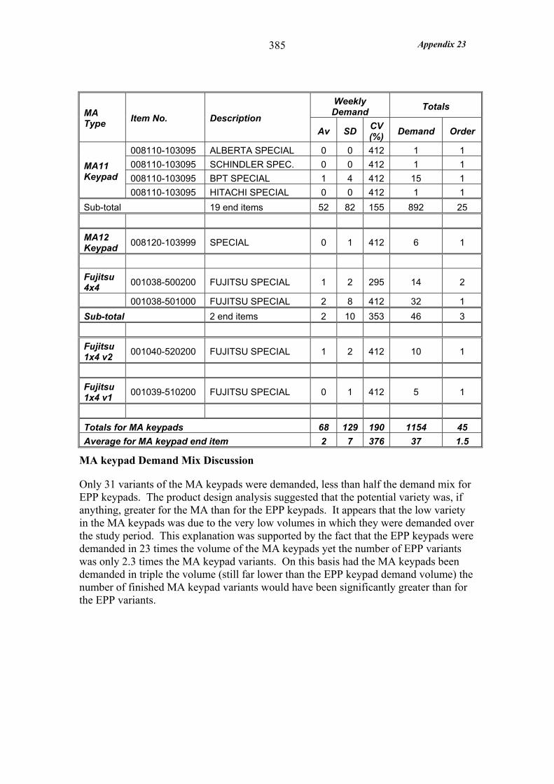
Appendix 23 385

Weekly Demand Totals MA

Type Item No. Description Av SD CV

(%) Demand Order

008110-103095 ALBERTA SPECIAL 0 0 412 1 1 008110-103095 SCHINDLER SPEC. 0 0 412 1 1 008110-103095 BPT SPECIAL 1 4 412 15 1

MA11 Keypad

008110-103095 HITACHI SPECIAL 0 0 412 1 1 Sub-total 19 end items 52 82 155 892 25 MA12 Keypad 008120-103999 SPECIAL 0 1 412 6 1

Fujitsu 4x4 001038-500200 FUJITSU SPECIAL 1 2 295 14 2

001038-501000 FUJITSU SPECIAL 2 8 412 32 1 Sub-total 2 end items 2 10 353 46 3 Fujitsu 1x4 v2 001040-520200 FUJITSU SPECIAL 1 2 412 10 1

Fujitsu 1x4 v1 001039-510200 FUJITSU SPECIAL 0 1 412 5 1

Totals for MA keypads 68 129 190 1154 45 Average for MA keypad end item 2 7 376 37 1.5

MA keypad Demand Mix Discussion

Only 31 variants of the MA keypads were demanded, less than half the demand mix for EPP keypads. The product design analysis suggested that the potential variety was, if anything, greater for the MA than for the EPP keypads. It appears that the low variety in the MA keypads was due to the very low volumes in which they were demanded over the study period. This explanation was supported by the fact that the EPP keypads were demanded in 23 times the volume of the MA keypads yet the number of EPP variants was only 2.3 times the MA keypad variants. On this basis had the MA keypads been demanded in triple the volume (still far lower than the EPP keypad demand volume) the number of finished MA keypad variants would have been significantly greater than for the EPP variants.

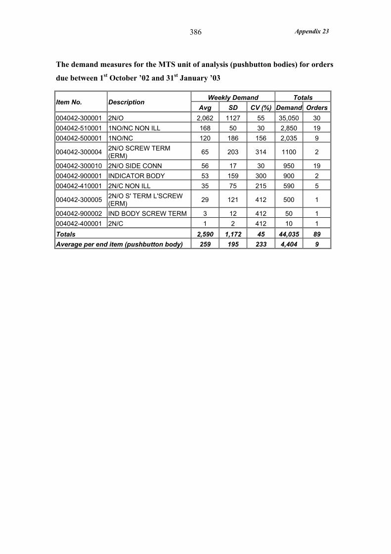
Appendix 23 386

The demand measures for the MTS unit of analysis (pushbutton bodies) for orders

due between 1st October ’02 and 31st January ’03

Weekly Demand Totals Item No. Description Avg SD CV (%) Demand Orders

004042-300001 2N/O 2,062 1127 55 35,050 30 004042-510001 1NO/NC NON ILL 168 50 30 2,850 19 004042-500001 1NO/NC 120 186 156 2,035 9

004042-300004 2N/O SCREW TERM (ERM) 65 203 314 1100 2

004042-300010 2N/O SIDE CONN 56 17 30 950 19 004042-900001 INDICATOR BODY 53 159 300 900 2 004042-410001 2N/C NON ILL 35 75 215 590 5

004042-300005 2N/O S' TERM L'SCREW (ERM) 29 121 412 500 1

004042-900002 IND BODY SCREW TERM 3 12 412 50 1 004042-400001 2N/C 1 2 412 10 1 Totals 2,590 1,172 45 44,035 89 Average per end item (pushbutton body) 259 195 233 4,404 9

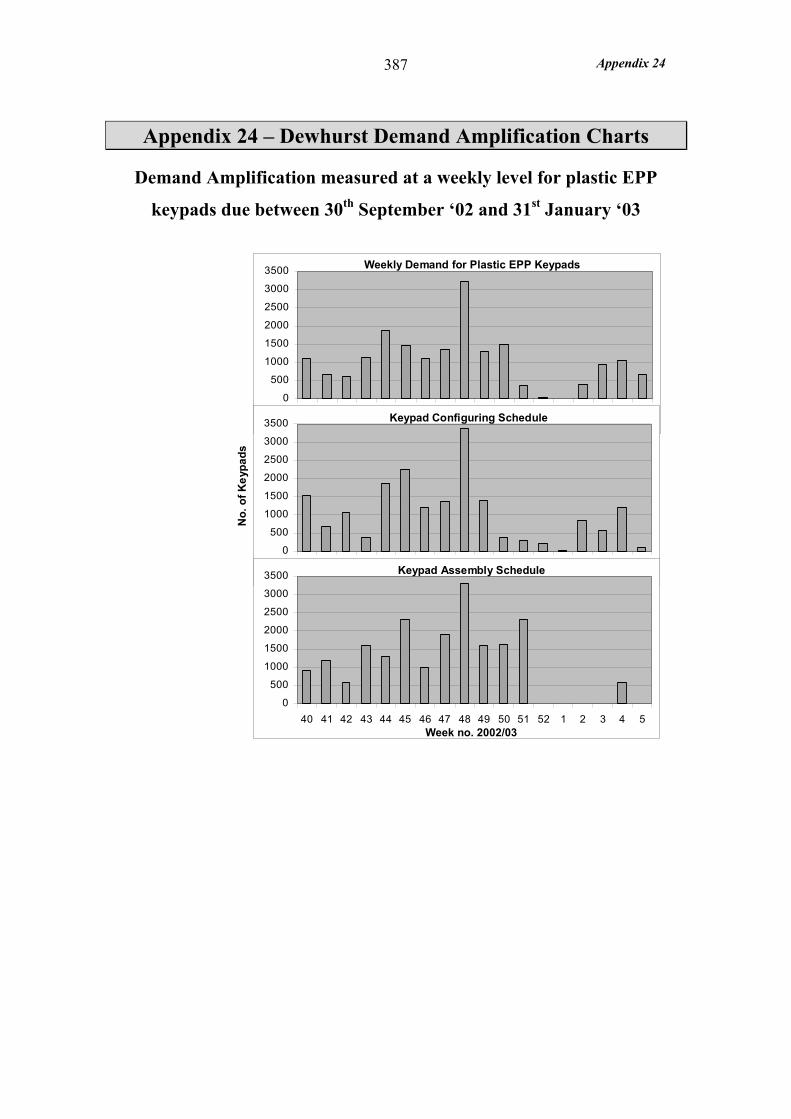
Appendix 24 387

Appendix 24 – Dewhurst Demand Amplification Charts

Demand Amplification measured at a weekly level for plastic EPP

keypads due between 30th September ‘02 and 31st January ‘03

0

500

1000

1500

2000

2500

3000

3500

40 41 42 43 44 45 46 47 48 49 50 51 52 1 2 3 4 5

0

500

1000

1500

2000

2500

3000

3500

40 41 42 43 44 45 46 47 48 49 50 51 52 1 2 3 4 5

0

500

1000

1500

2000

2500

3000

3500

40 41 42 43 44 45 46 47 48 49 50 51 52 1 2 3 4 5

Weekly Demand for Plastic EPP Keypads



No.

of K

eypa

ds

Week no. 2002/03

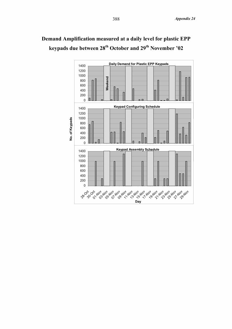
Appendix 24 388

Demand Amplification measured at a daily level for plastic EPP

keypads due between 28th October and 29th November ’02

0200400600800

100012001400

28-Oct

30-Oct

01-Nov

03-Nov

05-Nov

07-Nov

09-Nov

11-Nov

13-Nov

15-Nov

17-Nov

19-Nov

21-Nov

23-Nov

25-Nov

27-Nov

29-Nov

0200400600800

100012001400

28-Oct

30-Oct

01-Nov

03-Nov

05-Nov

07-Nov

09-Nov

11-Nov

13-Nov

15-Nov

17-Nov

19-Nov

21-Nov

23-Nov

25-Nov

27-Nov

29-Nov

0200400600800

100012001400

28-Oct

30-Oct

01-Nov

03-Nov

05-Nov

07-Nov

09-Nov

11-Nov

13-Nov

15-Nov

17-Nov

19-Nov

21-Nov

23-Nov

25-Nov

27-Nov

29-Nov

Daily Demand for Plastic EPP Keypads



No.

of K

eypa

ds

Day

Wee

kend

Appendix 24 389

Demand Amplification measured at a weekly level for steel EPP

keypads due between 30th September ‘02 and 31st January ‘03

0200400600800

10001200140016001800

40 41 42 43 44 45 46 47 48 49 50 51 52 1 2 3 4 5

0200400600800

10001200140016001800

40 41 42 43 44 45 46 47 48 49 50 51 52 1 2 3 4 5

0200400600800

10001200140016001800

40 41 42 43 44 45 46 47 48 49 50 51 52 1 2 3 4 5

Weekly Demand for Steel EPP Keypads



No.

of K

eypa

ds

Week no. 2002/03

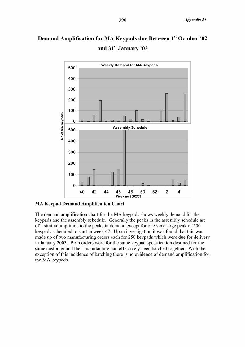
Appendix 24 390

Demand Amplification for MA Keypads due Between 1st October ‘02

and 31st January ’03

0

100

200

300

400

500

40 42 44 46 48 50 52 2 4

Weekly Demand for MA KeypadsN

o of

MA

Key

pads

0

100

200

300

400

500

40 42 44 46 48 50 52 2 4Week no 2002/03

Assembly Schedule

MA Keypad Demand Amplification Chart

The demand amplification chart for the MA keypads shows weekly demand for the keypads and the assembly schedule. Generally the peaks in the assembly schedule are of a similar amplitude to the peaks in demand except for one very large peak of 500 keypads scheduled to start in week 47. Upon investigation it was found that this was made up of two manufacturing orders each for 250 keypads which were due for delivery in January 2003. Both orders were for the same keypad specification destined for the same customer and their manufacture had effectively been batched together. With the exception of this incidence of batching there is no evidence of demand amplification for the MA keypads.

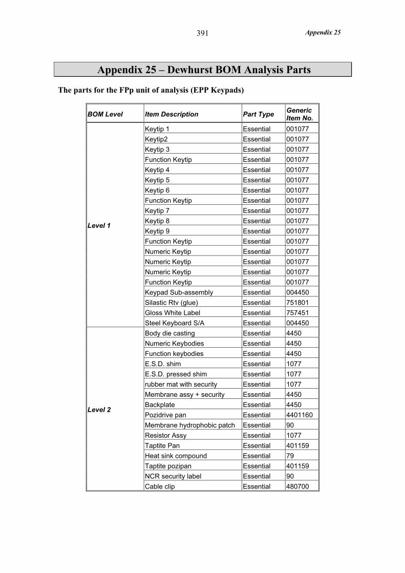
Appendix 25 391

Appendix 25 – Dewhurst BOM Analysis Parts

The parts for the FPp unit of analysis (EPP Keypads)

BOM Level Item Description Part Type Generic Item No.

Keytip 1 Essential 001077 Keytip2 Essential 001077 Keytip 3 Essential 001077 Function Keytip Essential 001077 Keytip 4 Essential 001077 Keytip 5 Essential 001077 Keytip 6 Essential 001077 Function Keytip Essential 001077 Keytip 7 Essential 001077 Keytip 8 Essential 001077 Keytip 9 Essential 001077 Function Keytip Essential 001077 Numeric Keytip Essential 001077 Numeric Keytip Essential 001077 Numeric Keytip Essential 001077 Function Keytip Essential 001077 Keypad Sub-assembly Essential 004450 Silastic Rtv (glue) Essential 751801 Gloss White Label Essential 757451

Level 1

Steel Keyboard S/A Essential 004450 Body die casting Essential 4450 Numeric Keybodies Essential 4450 Function keybodies Essential 4450 E.S.D. shim Essential 1077 E.S.D. pressed shim Essential 1077 rubber mat with security Essential 1077 Membrane assy + security Essential 4450 Backplate Essential 4450 Pozidrive pan Essential 4401160 Membrane hydrophobic patch Essential 90 Resistor Assy Essential 1077 Taptite Pan Essential 401159 Heat sink compound Essential 79 Taptite pozipan Essential 401159 NCR security label Essential 90

Level 2

Cable clip Essential 480700

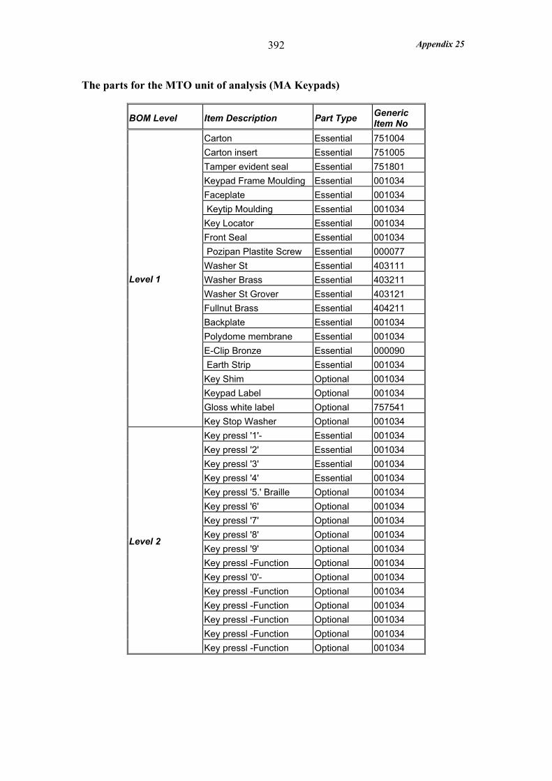
Appendix 25 392

The parts for the MTO unit of analysis (MA Keypads)

BOM Level Item Description Part Type Generic Item No

Carton Essential 751004 Carton insert Essential 751005 Tamper evident seal Essential 751801 Keypad Frame Moulding Essential 001034 Faceplate Essential 001034 Keytip Moulding Essential 001034 Key Locator Essential 001034 Front Seal Essential 001034 Pozipan Plastite Screw Essential 000077 Washer St Essential 403111 Washer Brass Essential 403211 Washer St Grover Essential 403121 Fullnut Brass Essential 404211 Backplate Essential 001034 Polydome membrane Essential 001034 E-Clip Bronze Essential 000090 Earth Strip Essential 001034 Key Shim Optional 001034 Keypad Label Optional 001034 Gloss white label Optional 757541

Level 1

Key Stop Washer Optional 001034 Key pressl '1'- Essential 001034 Key pressl '2' Essential 001034 Key pressl '3' Essential 001034 Key pressl '4' Essential 001034 Key pressl '5.' Braille Optional 001034 Key pressl '6' Optional 001034 Key pressl '7' Optional 001034 Key pressl '8' Optional 001034 Key pressl '9' Optional 001034 Key pressl -Function Optional 001034 Key pressl '0'- Optional 001034 Key pressl -Function Optional 001034 Key pressl -Function Optional 001034 Key pressl -Function Optional 001034 Key pressl -Function Optional 001034

Level 2

Key pressl -Function Optional 001034

Appendix 25 393

The parts for the MTS unit of analysis (lift PB bodies)

BOM Level Item Description Part Type Generic Item no

Main Body Moulding Essential 004042 Fixed Terminal Optional 003042 Screw Terminal Clamp Optional 004042 Comp2 Nylon Spacer Optional 004042 Plunger Optional 004042 Flexing Crossarm Optional 004042 Plunger Return Spring Optional 004042 Crossarm Return Spring Optional 004042 Lid Moulding Essential 004042 Terminal R/Conn Reinforced Optional 002087 Scr St Ch Hd Optional 401103 Illumination Terminal Optional 004042

Level 1

Plain White S/Adh label Optional 757541 Main body mould Polycarbonate Essential 322055 Plunger Delrin Acetal Optional 322091 Lid Moulding Polycarbonate Essential 322057

Level 2

Terminal Strip Optional 135042

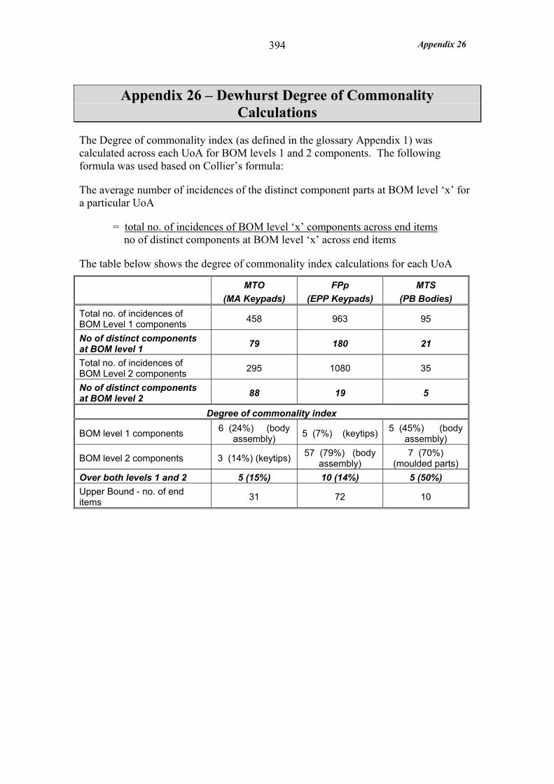
Appendix 26 394

Appendix 26 – Dewhurst Degree of Commonality Calculations

The Degree of commonality index (as defined in the glossary Appendix 1) was calculated across each UoA for BOM levels 1 and 2 components. The following formula was used based on Collier’s formula:

The average number of incidences of the distinct component parts at BOM level ‘x’ for a particular UoA

= total no. of incidences of BOM level ‘x’ components across end items no of distinct components at BOM level ‘x’ across end items

The table below shows the degree of commonality index calculations for each UoA

MTO

(MA Keypads) FPp

(EPP Keypads) MTS

(PB Bodies) Total no. of incidences of BOM Level 1 components 458 963 95

No of distinct components at BOM level 1 79 180 21

Total no. of incidences of BOM Level 2 components 295 1080 35

No of distinct components at BOM level 2 88 19 5


BOM level 1 components 6 (24%) (body assembly) 5 (7%) (keytips) 5 (45%) (body

assembly)

BOM level 2 components 3 (14%) (keytips) 57 (79%) (body assembly)

7 (70%) (moulded parts)

Over both levels 1 and 2 5 (15%) 10 (14%) 5 (50%) Upper Bound - no. of end items 31 72 10

Appendix 27 395

Appendix 27 – Dewhurst Capacity Utilisation Calculations

Calculation of the cell design capacity for the MA and EPP keypads depended on a knowledge of the available labour levels at these cells. In the case of MA keypads this was clear because the cell was dedicated to their manufacture however in the case of EPP keypads this was not the case. The cell manufacturing EPP keypads (made up of work centres 702, 711 and 712) was dedicated to the customer NCR rather than the EPP keypads therefore it also manufactured the old range of NCR keypads. Fortunately the labour available for the production of the EPP keypads was recorded by production for the study period and split between the keypad assembling and configuring processes as detailed in Appendix 22.

EPP Keypad Assembly Cell

Wk. no

Week comm.

Keypad Assembly

Output (keypads)

Processing Time

(man min.)

Cell Output (man

hours)

Labour level

Design Capacity

(man hours)

Cap. Utilis.

(%)

40 30-Sep 1800 7 210 6 225 93 41 7-Oct 2500 7.5 313 9 338 93 42 14-Oct 1600 7.5 200 9 338 59 43 21-Oct 1900 7.5 238 9 338 70 44 28-Oct 2400 7.5 300 9 338 89 45 4-Nov 2600 7.5 325 9 338 96 46 11-Nov 1850 7.5 231 9 338 69 47 18-Nov 2350 7.5 294 9 338 87 48 25-Nov 1800 7.5 225 9 338 67 49 2-Dec 2300 7.5 288 9 338 85 50 9-Dec 2215 7.5 277 9 338 82 51 16-Dec 2300 7.5 288 9 338 85 52 23-Dec 1200 7.5 150 9 338 44 1 30-Dec 0 7.5 0 9 338 0 2 6-Jan 0 5.5 0 6 225 0 3 13-Jan 600 5.5 55 6 225 24 4 20-Jan 1350 4.5 101 3 113 90 5 27-Jan 750 4.5 56 3 113 50 Averages 1770 6.8 212 7.7 288 71 Standard Deviation 27

Coeff of Variation (%) 38

Notes:

The average, standard deviation and coefficient of variation calculations exclude the Christmas vacation weeks 52 and 1.

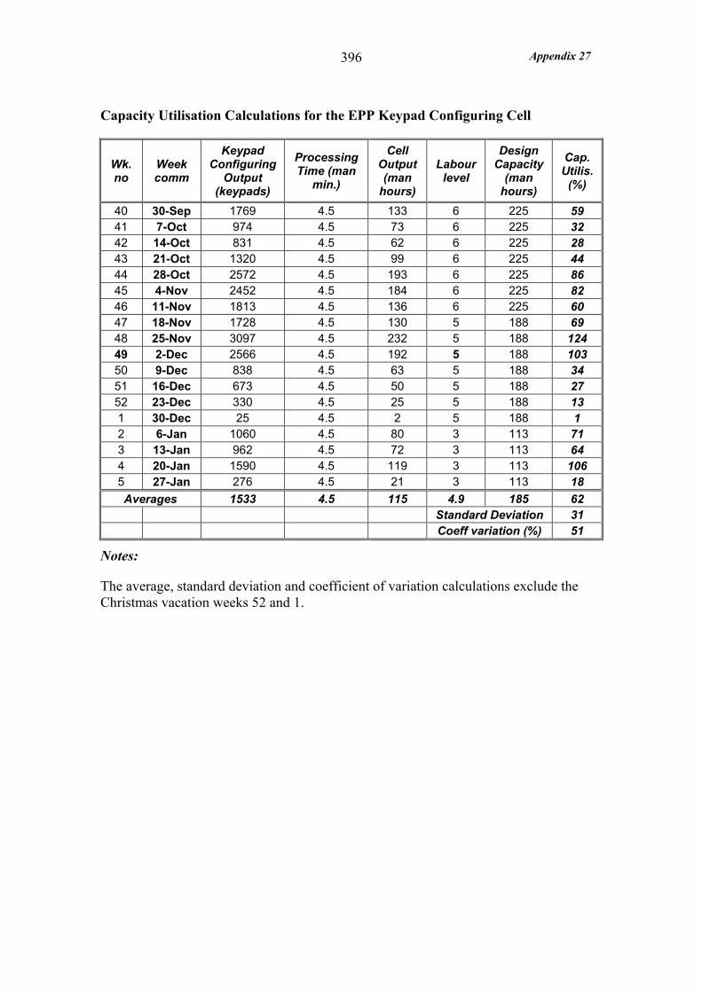
Appendix 27 396

Capacity Utilisation Calculations for the EPP Keypad Configuring Cell

Wk. no

Week comm

Keypad Configuring

Output (keypads)

Processing Time (man

min.)

Cell Output (man

hours)

Labour level

Design Capacity

(man hours)

Cap. Utilis.

(%)

40 30-Sep 1769 4.5 133 6 225 59 41 7-Oct 974 4.5 73 6 225 32 42 14-Oct 831 4.5 62 6 225 28 43 21-Oct 1320 4.5 99 6 225 44 44 28-Oct 2572 4.5 193 6 225 86 45 4-Nov 2452 4.5 184 6 225 82 46 11-Nov 1813 4.5 136 6 225 60 47 18-Nov 1728 4.5 130 5 188 69 48 25-Nov 3097 4.5 232 5 188 124 49 2-Dec 2566 4.5 192 5 188 103 50 9-Dec 838 4.5 63 5 188 34 51 16-Dec 673 4.5 50 5 188 27 52 23-Dec 330 4.5 25 5 188 13 1 30-Dec 25 4.5 2 5 188 1 2 6-Jan 1060 4.5 80 3 113 71 3 13-Jan 962 4.5 72 3 113 64 4 20-Jan 1590 4.5 119 3 113 106 5 27-Jan 276 4.5 21 3 113 18 Averages 1533 4.5 115 4.9 185 62 Standard Deviation 31 Coeff variation (%) 51

Notes:

The average, standard deviation and coefficient of variation calculations exclude the Christmas vacation weeks 52 and 1.

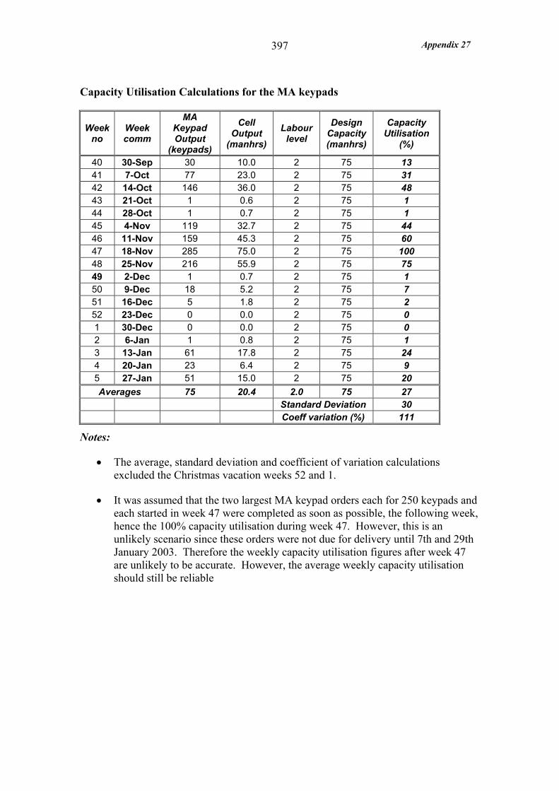
Appendix 27 397

Capacity Utilisation Calculations for the MA keypads

Week no

Week comm

MA Keypad Output

(keypads)

Cell Output

(manhrs) Labour

level Design

Capacity (manhrs)


(%)

40 30-Sep 30 10.0 2 75 13 41 7-Oct 77 23.0 2 75 31 42 14-Oct 146 36.0 2 75 48 43 21-Oct 1 0.6 2 75 1 44 28-Oct 1 0.7 2 75 1 45 4-Nov 119 32.7 2 75 44 46 11-Nov 159 45.3 2 75 60 47 18-Nov 285 75.0 2 75 100 48 25-Nov 216 55.9 2 75 75 49 2-Dec 1 0.7 2 75 1 50 9-Dec 18 5.2 2 75 7 51 16-Dec 5 1.8 2 75 2 52 23-Dec 0 0.0 2 75 0 1 30-Dec 0 0.0 2 75 0 2 6-Jan 1 0.8 2 75 1 3 13-Jan 61 17.8 2 75 24 4 20-Jan 23 6.4 2 75 9 5 27-Jan 51 15.0 2 75 20 Averages 75 20.4 2.0 75 27 Standard Deviation 30 Coeff variation (%) 111

Notes:

• The average, standard deviation and coefficient of variation calculations excluded the Christmas vacation weeks 52 and 1.

• It was assumed that the two largest MA keypad orders each for 250 keypads and each started in week 47 were completed as soon as possible, the following week, hence the 100% capacity utilisation during week 47. However, this is an unlikely scenario since these orders were not due for delivery until 7th and 29th January 2003. Therefore the weekly capacity utilisation figures after week 47 are unlikely to be accurate. However, the average weekly capacity utilisation should still be reliable

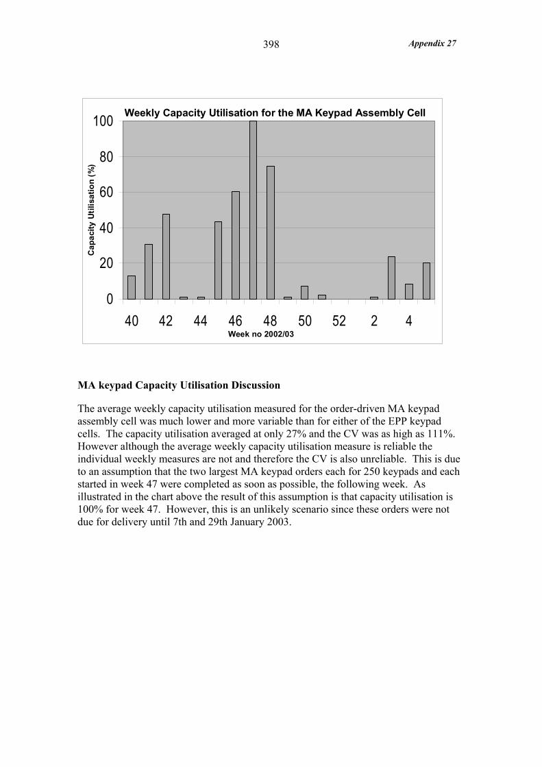
Appendix 27 398

0

20

40

60

80

100

40 42 44 46 48 50 52 2 4

Weekly Capacity Utilisation for the MA Keypad Assembly Cell

Cap

acity

Util

isat

ion

(%)

Week no 2002/03

MA keypad Capacity Utilisation Discussion

The average weekly capacity utilisation measured for the order-driven MA keypad assembly cell was much lower and more variable than for either of the EPP keypad cells. The capacity utilisation averaged at only 27% and the CV was as high as 111%. However although the average weekly capacity utilisation measure is reliable the individual weekly measures are not and therefore the CV is also unreliable. This is due to an assumption that the two largest MA keypad orders each for 250 keypads and each started in week 47 were completed as soon as possible, the following week. As illustrated in the chart above the result of this assumption is that capacity utilisation is 100% for week 47. However, this is an unlikely scenario since these orders were not due for delivery until 7th and 29th January 2003.

Full thesis.pdf - Cranfield University

Documents

Transcript of Full thesis.pdf - Cranfield University