Cranfield University

Adrian James Clarke

The Conceptual Design of Novel Future UAV’s Incorporating Advanced Technology Research Components

School of Engineering

Doctor of Philosophy (PhD) Thesis

Cranfield University

School of Engineering

Doctor of Philosophy (PhD) Thesis

2011

Adrian James Clarke

The Conceptual Design of Novel Future UAV’s Incorporating Advanced Technology Research Components

Supervisor: Prof. J. P. Fielding

Academic Year 2010 to 2011

This thesis is submitted in partial fulfilment of the requirements for the degree of Doctor of Philosophy (PhD)

© Cranfield University, 2011. All rights reserved. No part of this publication may be

reproduced without the written permission of the copyright holder.

Abstract

There is at present some uncertainty as to what the roles and requirements of the next generation of UAVs might be and the configurations that might be adopted. The incorporation of technological features on these designs is also a significant driving force in their configuration, efficiency, performance abilities and operational requirements. The objective of this project is thus to provide some insight into what the next generation of technologies might be and what their impact would be on the rest of the aircraft. This work involved the conceptual designs of two new relevant full-scale UAVs which were used to integrate a select number of these advanced technologies. The project was a CASE award which was linked to the Flaviir research programme for advanced UAV technologies. Thus, the technologies investigated during this study were selected with respect to the objectives of the Flaviir project. These were either relative to those already being developed as course of the Flaviir project or others from elsewhere. As course of this project, two technologies have been identified and evaluated which fit this criterion and show potential for use on future aircraft. Thus we have been able to make a contirubtion knowledge in two gaps in current aerospace technology. The first of these studies was to investigate the feasibility of using a low cost mechanical thrust vectoring system as used on the X-31, to replace conventional control surfaces. This is an alternative to the fluidic thrust vectoring devices being proposed by the Flaviir project for this task. The second study is to investigate the use of fuel reformer based fuel cell system to supply power to an all-electric power train which will be a means of primary propulsion. A number of different fuels were investigated for such a system with methanol showing the greatest promise and has been shown to have a number of distinct advantages over the traditional fuel for fuel cells (hydrogen). Each of these technologies was integrated onto the baseline conceptual design which was identified as that most suitable to each technology. A UCAV configuration was selected for the thrust vectoring system while a MALE configuration was selected for the fuel cell propulsion system. Each aircraft was a new design which was developed specifically for the needs of this project. Analysis of these baseline configurations with and without the technologies allowed an assessment to be made of the viability of these technologies. The benefits of the thrust vectoring system were evaluated at take-off, cruise and landing. It showed no benefit at take-off and landing which was due to its location on the very aft of the airframe. At cruise, its performance and efficiency was shown to be comparable to that of a conventional configuration utilizing elevons and expected to be comparable to the fluidic devices developed by the Flaviir project. This system does however offer a number of benefits over many other nozzle configurations of improved stealth due to significant exhaust nozzle shielding.

i

The fuel reformer based fuel cell system was evaluated in both all-electric and hybrid configurations. In the ell-electric configuration, the conventional turboprop engine was completely replaced with an all-electric powertrain. This system was shown to have an inferior fuel consumption compared to a turboprop engine and thus the hybrid system was conceived. In this system, the fuel cell is only used at loiter with the turboprop engine being retained for all other flight phases. For the same quantity of fuel, a reduction in loiter time of 24% was experienced (compared to the baseline turboprop) but such a system does have benefits of reduced emissions and IR signature. With further refinement, it is possible that the performance and efficiency of such a system could be further improved. In this project, two potential technologies were identified and thoroughly analysed. We are therefore able to say that the project objectives have been met and the project has proven worthwhile to the advancement of aerospace technology. Although these systems did not provide the desired results at this stage, they have shown the potential for improvement with further development. Keywords: Thrust vectoring, fuel cells, fuel processing, alternative fuels, aircraft performance

ii

iii

Acknowledgements

This thesis is dedicated to Frank Clarke. My great uncle, who worked in Woomera Australia as a designer of the Black Arrow Rocket and then worked on the subsequent missile projects. He has always been somebody to look up to and his work has been an inspiration for my own career.

The author would like to thank the following people for their continual help and support during my studies,

• Prof. Fielding (my supervisor) – For his continued support and advise, especially through the most difficult times.

• My family – For their love, support and patience. • BAE Systems (Case Award sponsors) - For their financial support, without

which this project would not have been possible. • The 2007-2008 Flaviir Team – Especially, Craig Lawson, Robert Jones and

Andrew Mills. It was a very interesting and rewarding year and I was proud to be a key part of the original team which turned the project around and tuned it in to an ultimate success.

• The library staff – Especially Tricia Fountain and Sharon Hinton for their warm welcome, help and for always being there when I really needed somebody to talk to. Additional thanks is also due for them always being kind enough to remove the continual bar on my library account (for never returning books on time).

• Thanks also goes out to a special group of people who helped me through the darkest times. Any time, day or night, they were always there to turn to and always willing to give up hours of their time to listen to others and offer their comfort and support. I am glad to be part of the group and am now pleased to be able play an active part in helping others in the same situation.

We are pressed on every side by troubles, but we are not crushed. We are perplexed, but not driven to despair. We are hunted down, but never abandoned by god. We get knocked down, but we are not destroyed. - 2 Corinthians 4:8 Fairy Tales are more than true; not because they tell us that dragons exist, but because they tell us that dragons can be beaten. - G. K. Chesterton

Table of Contents Abstract.............................................................................................................................. i Acknowledgements ......................................................................................................... iii 1 Introduction .............................................................................................................. 1

1.1 Project objectives.............................................................................................. 1 1.2 Work on the Flaviir project .............................................................................. 2 1.3 Summary of work ............................................................................................. 2 1.4 Thesis structure................................................................................................. 3

2 Initial literature review ............................................................................................. 4 2.1 A review of aircraft design methodologies....................................................... 4

2.1.1 An overview of the aircraft design process ..................................................... 4 2.1.2 A closer look at the conceptual design phase .................................................. 5 2.1.3 The aircraft design process applicable to UAV’s............................................ 6

2.2 Review of existing UAVs and down-selection of the baseline configurations 6 3 Baseline UAV design ............................................................................................... 7

3.1 Design requirements and design flight profiles................................................ 7 3.1.1 UCAV design requirements ............................................................................ 7 3.1.2 MALE design requirements ............................................................................ 8

3.2 The conceptual design of the baseline configurations...................................... 8 3.2.1 The conceptual design of the UCAV............................................................... 9 3.2.2 The conceptual design of the MALE............................................................. 10

3.3 Details of the final baseline configurations .................................................... 11 3.3.1 The UCAV configuration .............................................................................. 12 3.3.2 The MALE configuration .............................................................................. 13

3.4 The final layout of the baseline configurations .............................................. 13 3.4.1 The baseline MALE UAV configuration ...................................................... 13 3.4.2 The baseline UCAV configuration................................................................ 14

3.5 Analysis of the baseline configurations.......................................................... 15 3.5.1 Longitudinal static stability ........................................................................... 15 3.5.2 Aerodynamic characteristics ......................................................................... 16 3.5.3 High lift devices ............................................................................................ 16 3.5.4 Landing gear layout and analysis .................................................................. 17 3.5.5 Control surface sizing and analysis for the MALE ....................................... 18 3.5.6 Control surface sizing and analysis for the UCAV ....................................... 18 3.5.7 Refined drag predictions................................................................................ 20 3.5.8 Refined mass estimations .............................................................................. 20 3.5.9 Refined performance predictions................................................................... 21 3.5.10 Dynamic stability analysis of the UCAV .................................................... 21 3.5.11 Propeller analysis for the MALE................................................................. 22

4 Technologies selection ........................................................................................... 24 4.1 Identification of potential UAV technologies ................................................ 24 4.2 The down-selection of potential technologies ................................................ 24

4.2.1 The QFD down-selection process.................................................................. 25 4.2.2 The QFD methodology.................................................................................. 25 4.2.3 The QFD process applied to this project ....................................................... 26

4.3 The final selected technologies and rationale................................................. 27 4.3.1 Rationale for low cost mechanical thrust vectoring systems......................... 27

iv

4.3.2 Rationale for the use of fuel cells for propulsion .......................................... 28 4.3.3 Matching of the selected technologies to the baseline aircraft ...................... 28

5 Thrust vectoring literature review .......................................................................... 29 5.1 What is thrust vectoring?................................................................................ 29 5.2 The dawn of thrust vectoring - VTOL and STOL.......................................... 29 5.3 Thrust vectoring as an alternative means of aircraft control .......................... 31

5.3.1 The limitations of conventional control surfaces .......................................... 31 5.3.2 Thrust vectoring for aircraft trim................................................................... 31 5.3.3 The advantages of using thrust vectoring for aircraft control ....................... 32 5.3.4 The disadvantages of using thrust vectoring for aircraft control................... 33 5.3.5 The special case of the pure sideslip manoeuvre........................................... 34

5.4 Different thrust vectoring approaches ............................................................ 34 5.4.1 Pure vs. partially vectored aircraft................................................................. 34 5.4.2 Internal vs. external thrust vectoring ............................................................. 35 5.4.3 Axi-symmetric vs. rectangular thrust vectoring nozzles ............................... 35 5.4.4 Single vs. multi-axis thrust vectoring............................................................ 36

5.5 An overview thrust vectoring theoretical principles....................................... 36 5.6 The impact of engine and nozzle technology developments.......................... 37

5.6.1 Engine control developments ........................................................................ 37 5.6.2 Material advancements .................................................................................. 37

5.7 Stealth and survivability considerations ......................................................... 38 5.7.1 Aircraft agility ............................................................................................... 38 5.7.2 Survivability .................................................................................................. 39 5.7.3 Radar cross section and IR signatures ........................................................... 39

5.8 Future development opportunities .................................................................. 39 5.9 Fluidic thrust vectoring concepts.................................................................... 40

5.9.1 Co-flow thrust vectoring................................................................................ 40 5.9.2 Counter-flow thrust vectoring ....................................................................... 41 5.9.3 Pulsed jet actuators ........................................................................................ 42 5.9.4 Shock vector thrust vectoring........................................................................ 43 5.9.5 Sonic throat skewing (shifting) ..................................................................... 43

6 Thrust vectoring studies and examples................................................................... 45 6.1 Existing thrust vectoring research effort and thrust vectored aircraft ............ 45 6.2 Internal mechanical thrust vectoring concepts ............................................... 45

6.2.1 PYBBN nozzle .............................................................................................. 45 6.2.2 Axi-symmetric Vectoring Exhaust Nozzle (AVEN) ..................................... 46 6.2.3 ADEN nozzle................................................................................................. 47 6.2.4 Lyulka Saturn AL-31FU/P ............................................................................ 47

6.3 Mechanical thrust vectoring research projects ............................................... 48 6.3.1 McDonnell Douglas F-15 S/MTD (STOL and Manoeuvre Technology Demonstrator)......................................................................................................... 48 6.3.2 NASA F-15 Advanced Control Technology for Integrated Vehicles (ACTIVE) programme ........................................................................................... 48 6.3.3 General Dynamics F-16 Multi-Axis Thrust Vectoring (MATV) programme49 6.3.4 NASA F/A-18 High Angle of Attack Research Vehicle (HARV) programme................................................................................................................................ 49 6.3.5 The STOL Exhaust Nozzle (STOLEN) Concepts Program .......................... 50 6.3.6 Rockwell-MBB X-31 .................................................................................... 51

v

6.3.7 Boeing X-32 .................................................................................................. 52 6.3.8 Lockheed Martin X-35 .................................................................................. 52 6.3.9 McDonnell Douglas X-36 ............................................................................. 53 6.3.10 Lockheed Martin X-44 MANTA................................................................. 54 6.3.11 Mitsubishi ATD-X....................................................................................... 54 6.3.12 Harrier.......................................................................................................... 55 6.3.13 Grumman X-29A......................................................................................... 55 6.3.14 F-22 Raptor.................................................................................................. 56 6.3.15 X-45............................................................................................................. 56 6.3.16 Thrust vectoring for the Eurofighter............................................................ 56 6.3.17 The B2 ......................................................................................................... 57 6.3.18 Sukhoi-37 .................................................................................................... 57

6.4 Fluidic thrust vectoring research effort .......................................................... 57 6.4.1 Fluidic research at NASA.............................................................................. 58 6.4.2 The Flaviir project ......................................................................................... 58 6.4.3 The Cirrus Vision aircraft and the Williams Exact nozzle............................ 59

7 Design and integration considerations for thrust vectoring systems ...................... 61 7.1 An overview of the fundamental concepts ..................................................... 61

7.1.1 An overview of exhaust nozzles.................................................................... 61 7.1.2 The engine and exhaust nozzle sizing process .............................................. 61

7.2 Thrust vectoring nozzle design and integration.............................................. 62 7.2.1 Thrust vectoring nozzle design requirements................................................ 62 7.2.2 Exhaust system layout ................................................................................... 63 7.2.3 Jet pipe design ............................................................................................... 63 7.2.4 Cooling requirements .................................................................................... 64 7.2.5 Weight and centre of gravity considerations ................................................. 64 7.2.6 Metallurgical considerations ......................................................................... 65 7.2.7 Afterburners................................................................................................... 65 7.2.8 The relationship between engine and nozzle................................................. 65 7.2.9 Stability and control and aerodynamic considerations .................................. 66 7.2.10 Detailed nozzle design................................................................................. 66 7.2.11 Integration of the next generation of technology......................................... 67 7.2.12 Airframe considerations .............................................................................. 67 7.2.13 Safety considerations................................................................................... 68 7.2.14 A note on engine inlets for thrust vectoring systems .................................. 69 7.2.15 Flight and propulsion control systems......................................................... 69 7.2.16 Modification of existing aircraft.................................................................. 70 7.2.17 Integration of high aspect ratio nozzles....................................................... 70

8 Sizing and integration of the UCAV thrust vectoring system................................ 71 8.1 Thrust vectoring system requirements for the UCAV.................................... 71 8.2 Selection of the candidate thrust vectoring system ........................................ 71 8.3 An overview of the final thrust vectoring system........................................... 72 8.4 Design and sizing the vectoring and pitch control systems............................ 73

8.4.1 The inter-relation with the engine performance ............................................ 73 8.4.2 Sizing the thrust vectoring system................................................................. 73 8.4.3 Design of the nose jet pitch control system................................................... 74

8.5 The analysis of the vectoring and control systems ......................................... 74 8.6 Integration of the vectoring and pitch control systems................................... 76

vi

8.6.1 The integration of the thrust vectoring system .............................................. 76 8.6.2 The integration of the nose jet pitch control system...................................... 77

9 Fuel cells literature review ..................................................................................... 78 9.1 An overview of fuel cells and their working principles ................................. 78

9.1.1 What is a fuel cell? ........................................................................................ 78 9.1.2 Fuel cell working principles .......................................................................... 78 9.1.3 The potential benefits of fuel cells ................................................................ 79 9.1.4 Challenges still to be overcome..................................................................... 80 9.1.5 Rival hydrogen powered propulsion systems................................................ 80

9.2 The different types of fuel cells...................................................................... 81 9.2.1 Electrolytes and membranes of the different fuel cell types ......................... 81 9.2.2 Recommended systems suitable for propulsion ............................................ 83

9.3 The PEM fuel cell in greater detail................................................................. 83 9.3.1 Predicting the efficiency of a fuel cell........................................................... 83 9.3.2 An introduction to fuel cell operating characteristics.................................... 84 9.3.3 Impact of pressure and concentration on fuel cell performance.................... 85 9.3.4 The impact of fuel and air quality on fuel cell performance ......................... 85 9.3.5 Water management ........................................................................................ 85 9.3.6 Thermal management .................................................................................... 86

9.4 Fuel cell construction ..................................................................................... 87 9.4.1 The main parts of a fuel cell .......................................................................... 87 9.4.2 Fuel cell electrodes ........................................................................................ 87 9.4.3 Fuel cell membranes...................................................................................... 88 9.4.4 Fuel cell manufacture and construction......................................................... 88

9.5 High altitude fuel cell operation ..................................................................... 90 9.5.1 Introduction ................................................................................................... 90 9.5.2 Low pressure fuel cell applications ............................................................... 90 9.5.3 De-rate performance prediction methods ...................................................... 90 9.5.4 Current low pressure operation research efforts............................................ 90 9.5.5 Fuel cells – Design for high altitude operation.............................................. 93

10 Fuel cell research projects .................................................................................. 94 10.1 An overview of fuel cell development ........................................................... 94 10.2 Automotive research effort............................................................................. 94 10.3 Current PEM fuel cell developers .................................................................. 95 10.4 Other applications of fuel cells....................................................................... 95 10.5 Aerospace research projects ........................................................................... 95

10.5.1 DLR Antares DLR-H2 fuel cell airplane..................................................... 96 10.5.2 FASTec/ATP fuel cell E-plane.................................................................... 97 10.5.3 ENFICA Rapid 200-FC fuel cell hybrid airplane........................................ 97 10.5.4 Boeing fuel cell demonstrator airplane........................................................ 99 10.5.5 Design study of a fuel cell powered aircraft – Menard ............................. 100 10.5.6 Conceptual design of a Fuel Cell Powered Aircraft – Bekiaris................. 102

11 Alternative fuels literature review .................................................................... 105 11.1 The need for alternative fuels ....................................................................... 105

11.1.1 An overview of current fossil fuels ........................................................... 105 11.1.2 Diminishing fuel supplies.......................................................................... 106 11.1.3 What about natural and nuclear energy sources? ...................................... 106 11.1.4 Pollution factors associated with existing fossil fuels ............................... 107

vii

11.1.5 What is the contribution of transportation to these problems?.................. 107 11.1.6 Existing fuel infrastructures ...................................................................... 108

11.2 An overview of alternative fuels .................................................................. 108 11.2.1 Bio-fuels .................................................................................................... 108 11.2.2 Alcohol fuels ............................................................................................. 108

11.3 Hydrogen as a fuel........................................................................................ 109 11.3.1 The current availability of hydrogen ......................................................... 110 11.3.2 Hydrogen fuel infrastructures.................................................................... 110 11.3.3 Hydrogen production................................................................................. 110 11.3.4 Liquefied hydrogen.................................................................................... 111 11.3.5 The outlook for using hydrogen as a fuel .................................................. 111

11.4 Hydrogen storage considerations.................................................................. 111 11.4.1 Compressed storage................................................................................... 112 11.4.2 Liquefied storage ....................................................................................... 113 11.4.3 Metallurgical considerations...................................................................... 114 11.4.4 Other storage methods ............................................................................... 114

11.5 Methanol in depth review............................................................................. 116 11.5.1 Methanol as a fuel ..................................................................................... 116 11.5.2 The manufacture of methanol.................................................................... 116 11.5.3 The use of methanol within traditional IC engines ................................... 117 11.5.4 Material compatibility issues..................................................................... 118 11.5.5 Methanol and DME storage and distribution ............................................ 118 11.5.6 Methanol price and availability ................................................................. 119 11.5.7 Methanol safe handling practices .............................................................. 119 11.5.8 Environmental considerations ................................................................... 120 11.5.9 The prospect of the manufacture of methanol by CO2 recycling .............. 120

11.6 Fuel study conclusion ................................................................................... 120 12 Fuel processing................................................................................................. 122

12.1 An overview of fuel processing.................................................................... 122 12.2 Steam reforming ........................................................................................... 122 12.3 Partial oxidation reforming........................................................................... 125 12.4 Autothermal reforming ................................................................................. 126 12.5 Electrolysers ................................................................................................. 127 12.6 Additional clean-up phases........................................................................... 127 12.7 Fuel processor requirements and selection................................................... 128 12.8 Fuel processor performance prediction (fuel cell reforming book for references) ................................................................................................................ 129 12.9 Methanol and DME reforming for hydrogen fuel cells................................ 130

13 A review of existing fuel processors ................................................................ 131 13.1 Methanol fuel processors.............................................................................. 131

13.1.1 Xcellsis-Ballard fuel processors ................................................................ 131 13.1.2 DaimlerChrysler methanol vehicles .......................................................... 132 13.1.3 Hyundai “Santa Fe” project....................................................................... 133 13.1.4 Other mobile methanol fuel processor projects......................................... 133 13.1.5 Johnson Matthey HotSpot reactor ............................................................. 135

13.2 Gasoline fuel processors............................................................................... 135 13.2.1 General motors research efforts................................................................. 136 13.2.2 Renault research efforts ............................................................................. 136

viii

13.3 Diesel and Kerosene fuel processors ............................................................ 137 13.4 Multi-fuel processors.................................................................................... 137

14 Design and integration considerations for fuel cell systems ............................ 138 14.1 Introduction .................................................................................................. 138 14.2 What is balance of plant? ............................................................................. 138 14.3 Fuel cell system design considerations and requirements ............................ 139 14.4 Fuel supply ................................................................................................... 140

14.4.1 Direct hydrogen fuel supply ...................................................................... 141 14.4.2 Hydrogen fuel supply via a fuel processor ................................................ 142

14.5 Oxidant supply.............................................................................................. 142 14.5.1 Using air instead of oxygen ....................................................................... 143 14.5.2 Air compressors......................................................................................... 143 14.5.3 Turbines and expanders ............................................................................. 145

14.6 Humidification requirements and water management.................................. 145 14.7 Thermal management and the cooling system ............................................. 146 14.8 Electrical energy storage .............................................................................. 147 14.9 Costs ............................................................................................................. 147 14.10 Safety considerations................................................................................ 148 14.11 Fuel cell durability and reliability ............................................................ 148 14.12 Future outlook and challenges for fuel cells............................................. 149 14.13 Traction motors for electric vehicles ........................................................ 149

14.13.1 An overview of electric traction motors .................................................. 149 14.13.2 Motor cooling requirements .................................................................... 151 14.13.3 Motor requirements and selection ........................................................... 151 14.13.4 Associated regulators and controllers...................................................... 152

15 Sizing and integration of the fuel reformer based MALE fuel cell system...... 153 15.1 Selection of the fuel cell type and candidate fuel......................................... 153 15.2 An overview of the all-electric propulsion system....................................... 153 15.3 The influence of fuel cell operating parameters ........................................... 154 15.4 The influence of the fuel processor .............................................................. 155 15.5 Overall sizing of the all-electric propulsion system ..................................... 155 15.6 The analysis of the final system ................................................................... 156 15.7 The selection of a suitable compressor-turbine unit..................................... 156 15.8 Sizing and integration of the fuel cell system components .......................... 157 15.9 Sizing and integration of the cooling system ............................................... 158 15.10 Selection, sizing and integration of the electric powertrain ..................... 159 15.11 Design considerations for the use of methanol......................................... 161 15.12 The impact of the systems on the aircraft configuration .......................... 161 15.13 Sizing and integration of the hybrid systems............................................ 163

16 Evaluation of the technologies ......................................................................... 164 16.1 Thrust vectoring take-off performance analysis........................................... 164

16.1.1 An overview of the analysis procedure ..................................................... 164 16.1.2 Final results for the thrust vectored aircraft configuration ........................ 165 16.1.3 Comparison with conventional elevons..................................................... 165 16.1.4 The influence of landing gear setting angle............................................... 166 16.1.5 Investigation into possible wing size reduction......................................... 167

16.2 Thrust vectoring cruise performance analysis .............................................. 168 16.3 Thrust vectoring landing performance analysis............................................ 168

ix

x

16.3.1 Results ....................................................................................................... 169 16.3.2 The influence of initial vertical descent velocity....................................... 169

16.4 Fuel cell powered MALE performance analysis .......................................... 170 16.4.1 Analysis of the autothermal and steam reformer based fuel cell systems . 171 16.4.2 Analysis of the hybrid autothermal and steam reformer based fuel cell systems ................................................................................................................. 171 16.4.3 Final results ............................................................................................... 171 16.4.4 Investigation into the use of oxygen injection........................................... 172

17 Discussion......................................................................................................... 173 17.1 A review of the MALE and UCAV baseline designs................................... 173 17.2 The identification and selection of the technologies .................................... 173 17.3 The feasibility of low cost mechanical thrust vectoring............................... 174

17.3.1 Thrust vectoring for take-off ..................................................................... 174 17.3.2 Thrust vectoring for cruise ........................................................................ 176 17.3.3 Thrust vectoring for landing...................................................................... 177 17.3.4 Significant integration considerations for this system............................... 177 17.3.5 Comparison with other thrust vectoring systems ...................................... 177

17.4 The feasibility of fuel cell systems for propulsion ....................................... 178 17.4.1 Fuel choices ............................................................................................... 178 17.4.2 Fuel processors .......................................................................................... 179 17.4.3 All-electric propulsion systems ................................................................. 180 17.4.4 Hybrid propulsion systems ........................................................................ 180 17.4.5 Significant integration considerations for this system............................... 180

17.4.6 Evaluation of the overall system propulsive efficency.............................. 180 17.4.7 Evaluation of the direct operating costs .................................................... 183 18 Conclusions and recommendations .................................................................. 184

18.1 Thrust vectoring conclusions and recommendations.................................... 184 18.1.1 The thrust vectoring technology gap and contribution to knowledge ....... 184 18.1.2 Project outcome and lessons learnt for low cost mechanical thrust vectoring.............................................................................................................................. 185

18.2 Fuel cells conclusions and recommendations............................................... 187 18.2.1 The fuel cell propulsion system technology gap and contribution to knowledge............................................................................................................. 187 18.2.2 Project outcome and lessons learnt for fuel reformer based fuel cell systems for primary propulsion.......................................................................................... 188

18.3 Fulfilment of project objectives.................................................................... 189 18.4 Recommendations for future work............................................................... 189

References .................................................................................................................... 192 Bibliography ................................................................................................................. 194

1.1 Bibliography for baseline aircraft design study............................................ 194 1.2 Bibliography for thrust vectoring study ....................................................... 195 1.3 Bibliography for fuel cell system study........................................................ 201

Additional Table of Contents for the Appendices A Baseline UCAV and MALE performance............................................................ 211

A1.1 Baseline aircraft performance analysis an overview .................................... 211 A1.2 Take-off performance analysis ..................................................................... 212

A1.2.1 Take-off ground roll ............................................................................. 212 A1.2.2 Take-off rotation................................................................................... 213 A1.2.3 Take-off climb out ................................................................................ 213 A1.2.4 Second segment climb.......................................................................... 214

A1.3 Climb performance analysis ......................................................................... 215 A1.3.1 UCAV climb......................................................................................... 216 A1.3.2 MALE first climb stage ........................................................................ 216 A1.3.3 MALE second stage ............................................................................. 217

A1.4 Cruise and loiter performance analysis ........................................................ 218 A1.5 Descent performance analysis ...................................................................... 219

A1.5.1 UCAV descent...................................................................................... 219 A1.5.2 MALE first descent stage ..................................................................... 220 A1.5.3 MALE second descent stage ................................................................ 221

A1.6 Landing performance analysis...................................................................... 222 A1.6.1 Landing approach and flare .................................................................. 222 A1.6.2 Landing ground roll .............................................................................. 224

A1.7 UCAV fuel consumption, weight variation and engine characteristics........ 224 A1.8 MALE fuel consumption, weight variation and engine characteristics........ 225 A1.9 General terms used ....................................................................................... 226

B1 Thrust vectoring source data................................................................................. 227 B1.1 NASA vectored nozzle test results ............................................................... 227 B1.2 NASA test results with no vanes installed ................................................... 228 B1.3 Geometric data of the vectoring system ....................................................... 228

B2 Rescaling the NASA test data .............................................................................. 229 B2.1 Assumptions and limitations ........................................................................ 229 B2.2 Background to the approach......................................................................... 229 B2.3 The data for the un-vectored baseline engine nozzle ................................... 229 B2.4 Rescaling the NASA data to suit the baseline engine nozzle ....................... 230 B2.5 Matching the nozzle data to the engine operating data ................................ 231 B2.6 Dealing with vast quantities of data ............................................................. 234 B2.7 Formatting the results ................................................................................... 235 B2.8 Final results for the engine-nozzle in take-off conditions ............................ 236 B2.9 Final results for the engine-nozzle in cruise conditions ............................... 237 B2.10 Variation of Thrust and TSFC with Mach number during the take-off phase 238

B3 Deriving a general expression for the engine throttle setting at cruise ................ 239 B4 Deriving a general expression for the thrust specific fuel consumption at cruise 242 B5 Analysis of the nose jet pitch control system ....................................................... 245

B5.1 An overview of the system ........................................................................... 245 B5.2 Analysis of the system.................................................................................. 245

B5.2.1 Flow conditions at the engine bleed port exit (at station 1).................. 246 B5.2.2 Bleed elbow loss factor (between stations 1 and 2).............................. 247 B5.2.3 Control valve loss factor (between stations 2 and 3)............................ 248

xi

B5.2.4 Front to rear ducting loss factor (between stations 3 and 4)................. 248 B5.2.5 Nozzle elbow bend loss factor (between stations 4 and 5)................... 248 B5.2.6 Nozzle contraction loss factor (between stations 5 and 6) ................... 248 B5.2.7 Total system pressure loss (between stations 1 and 7) ......................... 249 B5.2.8 Nozzle throat sizing (station 6)............................................................. 249 B5.2.9 Flow conditions at the nozzle throat (station 6) ................................... 250 B5.2.10 Analysis of the nozzle divergent section (stations 6 to 7) .................... 250

B5.3 Calculation of the gross thrust from the pitch control jet ............................. 252 B5.4 Final results .................................................................................................. 252 B5.5 Mach number scale factors ........................................................................... 253

C1 Initial propulsion system considerations .............................................................. 255 C1.1 A brief review of engine exhaust nozzles..................................................... 255 C1.2 A brief note on engine intakes...................................................................... 256 C1.3 Engine nozzle sizing for conceptual design studies ..................................... 256 C1.4 Engine intake sizing for conceptual design studies ...................................... 257

C2 An overview of engine design methodology........................................................ 258 C2.1 Engine design specifications and parameter predictions.............................. 258

C2.1.1 Engine performance targets .................................................................. 258 C2.1.2 Engine component technology level prediction ................................... 259 C2.1.3 Engine parameters – design choices..................................................... 259 C2.1.4 Off the shelf engines vs. new developments ........................................ 263

C2.2 An overview of the engine design and sizing process.................................. 264 C2.2.1 Engine design methodology ................................................................. 264 C2.2.2 The on-design design stage .................................................................. 264 C2.2.3 The off-design sizing stage................................................................... 265

C2.3 Station numbering ........................................................................................ 266 C3 Practical software based engine design ................................................................ 267

C3.1 Engine design with the AEDsys software suite............................................ 267 C3.1.1 On-Design parametric analysis with the ONX module ........................ 267 C3.1.2 Off-Design engine analysis with the engine cycle deck....................... 268

C3.2 Design of the baseline engine....................................................................... 269 C3.2.1 Design point parametric analysis.......................................................... 269 C3.2.2 Verifying the final configuration.......................................................... 270 C3.2.3 Refined engine intake and nozzle sizing .............................................. 271

C3.3 The analysis of thrust vectoring nozzles....................................................... 271 C3.4 Datasets for take-off and cruise conditions .................................................. 272

C3.4.1 Take-off analysis datasets..................................................................... 272 C3.4.2 Cruise analysis datasets ........................................................................ 276

C3.5 Refined engine nozzle analysis with the Nozzle module ............................. 277 C3.5.1 Cruise analysis nozzle results ............................................................... 277 C3.5.2 Take-off analysis nozzle results ........................................................... 277

C4 Detailed nozzle design an overview ................................................................. 279 C4.1 Nozzle design requirements.......................................................................... 279 C4.2 An overview of nozzle operation.................................................................. 279 C4.3 Engine back-pressure control ....................................................................... 280 C4.4 Exhaust nozzle area ratio.............................................................................. 280 C4.5 Thrust reversers ............................................................................................ 281 C4.6 Nozzle design parameters............................................................................. 281

xii

C4.6.1 Total pressure loss ................................................................................ 281 C4.6.2 Gross thrust and discharge coefficients ................................................ 281 C4.6.3 Velocity coefficient .............................................................................. 282 C4.6.4 Angularity coefficient (CA) .................................................................. 282

C4.7 One dimensional flow approximation .......................................................... 282 C4.8 General relation for nozzle performance ...................................................... 283 C4.9 Installation considerations ............................................................................ 283

C4.9.1 Revised inlet and exhaust installation loss factors ............................... 283 C4.9.2 Inlet installation loss factor .................................................................. 284 C4.9.3 Nozzle installation loss factor .............................................................. 284 C4.9.4 Predicting the drag due to a thrust vectoring nozzle ............................ 286

C4.10 Stealth design requirements...................................................................... 286 D1 General terms for the performance analyses .................................................... 287

D1.1 Basic terms ................................................................................................... 287 D1.2 Analysis of the ground effect for the take-off analysis ................................ 287 D1.3 The effect of deploying the Kruger flaps...................................................... 288 D1.4 Variation in the aircraft centre of gravity with fuel burn ............................. 289 D1.5 Aircraft drag increase in the landing configuration...................................... 290 D1.6 Control characteristics of the elevons........................................................... 290

D1.6.1 Contribution to lift due to elevon deflection ........................................ 290 D1.6.2 Contribution to pitching moment due to elevon deflection.................. 291 D1.6.3 Contribution to drag due to elevon deflection...................................... 292

D2 Cruise analysis.................................................................................................. 294 D2.1 Analysis parameters...................................................................................... 294

D2.1.1 The engine throttle setting of the thrust vectored engine ..................... 294 D2.1.2 Specific fuel consumption of the thrust vectored configuration........... 294 D2.1.3 Specific fuel consumption of the conventional configuration.............. 295

D2.2 Thrust vectored cruise analysis .................................................................... 295 D2.2.1 Derivations ........................................................................................... 295 D2.2.2 Analysis approach ................................................................................ 297 D2.2.3 Analysis stage 1 – Solution for required engine thrust......................... 297 D2.2.4 Analysis stage 2 – Solution for nozzle vectoring angle........................ 298

D2.3 Conventional elevons configuration cruise analysis .................................... 299 D2.3.1 Derivations ........................................................................................... 299 D2.3.2 Analysis approach ................................................................................ 300 D2.3.3 Analysis stage 1 – Solution for required engine thrust......................... 301 D2.3.4 Analysis stage 2 – Solution for elevon deflection ................................ 302

D3 Take-off analysis .............................................................................................. 304 D3.1 Analysis parameters...................................................................................... 304

D3.1.1 Engine parameters ................................................................................ 304 D3.1.2 Vectored thrust components ................................................................. 305 D3.1.3 Nose-jet control terms .......................................................................... 305 D3.1.4 Presentation of the results..................................................................... 306 D3.1.5 Effect of thrust vectoring on the landing gear ...................................... 306

D3.2 Numerical analysis to determine the final solution ...................................... 307 D3.3 Take-off analysis – Lift limit........................................................................ 308

D3.3.1 Derivations ........................................................................................... 308 D3.3.2 Analysis approach ................................................................................ 309

xiii

D3.3.3 Finding the final solution...................................................................... 310 D3.4 Take-off analysis – Thrust vectoring control limit....................................... 310

D3.4.1 Derivations ........................................................................................... 311 D3.4.2 Analysis approach ................................................................................ 312 D3.4.3 Finding the final solution...................................................................... 313

D3.5 Take-off analysis – Conventional elevons control limit............................... 314 D3.5.1 Derivations ........................................................................................... 314 D3.5.2 Analysis approach ................................................................................ 314 D3.5.3 Finding the final solution...................................................................... 315

D3.6 Finding the final overall solution ................................................................. 316 D4 Landing analysis ............................................................................................... 317

D4.1 Analysis parameters...................................................................................... 317 D4.1.1 Engine specific fuel consumption ........................................................ 317

D4.2 Landing approach analysis ........................................................................... 317 D4.2.1 Derivations ........................................................................................... 317 D4.2.2 Analysis approach ................................................................................ 318 D4.2.3 Analysis stage 1 – Descent angle ......................................................... 320 D4.2.4 Analysis stage 2 – Aircraft weight ....................................................... 321 D4.2.5 Analysis stage 3 – Wing-fuselage pitching moment ............................ 322 D4.2.6 Analysis stage 4 – Aircraft pitching moment ....................................... 322 D4.2.7 Analysis stage 5 – Nose lift jet force.................................................... 323 D4.2.8 Analysis stage 6 – Solution for angle of attack .................................... 324 D4.2.9 Analysis stage 7 – Solution for thrust................................................... 325 D4.2.10 Analysis stage 8 – Time to touchdown............................................. 326 D4.2.11 Analysis stage 9 – Distance covered ................................................ 327

D4.3 Landing ground run analysis ........................................................................ 328 D4.3.1 Derivations ........................................................................................... 328 D4.3.2 Analysis approach ................................................................................ 329

D4.4 Aircraft carrier landing analysis ................................................................... 330 D5 Wing size reduction investigation .................................................................... 331

D5.1 Wing resizing................................................................................................ 331 D5.2 Take-off analyses.......................................................................................... 332

E1 Fuel cell system design requirements............................................................... 333 E1.1 An overview of the fuel cell system power train.......................................... 333 E1.2 Commercially available traction motors....................................................... 334 E1.3 Commercially available traction motor controllers ...................................... 334 E1.4 Fuel cell power requirements ....................................................................... 335 E1.5 Results for fuel cell system power output required ...................................... 336

E2 An overview of the fuel cell systems................................................................ 337 E2.1 An overview of the main fuel cell system .................................................... 337 E2.2 An overview of the fuel cell powered aircraft powertrain............................ 339 E2.3 An overview of an example fuel cell control system ................................... 339

E3 An overview of the fuel processors .................................................................. 341 E3.1 An overview of the autothermal based fuel processor ................................. 341 E3.2 An overview of the steam reformer based fuel processor ............................ 342

E4 Sizing the fuel cell stacks ................................................................................. 343 E4.1 Fuel cell system design requirements........................................................... 343 E4.2 Sizing the fuel cell stacks ............................................................................. 343

xiv

E4.3 The cell active area and total bi-polar plate area .......................................... 344 E4.4 The overall stack geometry........................................................................... 346 E4.5 The cell flow field geometry ........................................................................ 347 E4.6 The fuel cell control unit .............................................................................. 349

E5 Sizing the fuel processor .................................................................................. 350 F Evaluation of the NFCC altitude predictions ................................................... 351

F1.1 Derivation of a general relation .................................................................... 351 F1.2 Evaluation of the results ............................................................................... 352

G1 Derivation of equations for the fuel cell........................................................... 353 G2 Derivation of the equations for the analysis of the autothermal reformer........ 356 G3 Derivation of the equations for the analysis of the steam reformer.................. 360 G4 Derivation of equations for the burner analysis................................................ 362

G4.1 Products entering the burner......................................................................... 362 G4.2 Products leaving the burner .......................................................................... 364

G5 Derivation of a general relation to determine the fuel cell output voltage ....... 366 H Analysis of the fuel cell system........................................................................ 373

H1.1 Analysis block A – Fuel cell operating environment ................................... 374 H1.1.1 Atmospheric variables .......................................................................... 374

H1.2 Other useful fuel cell system analysis fluid parameters ............................... 374 H1.2.1 Cooling system parameters................................................................... 374 H1.2.2 Specific heats........................................................................................ 375 H1.2.3 Other useful parameters........................................................................ 375

H1.3 Analysis block B – Fuel cell operating conditions ....................................... 376 H1.3.1 Theoretical background ........................................................................ 376 H1.3.2 Analysis to determine of the operational fuel cell voltage ................... 377 H1.3.3 Pressure at the fuel cell exit.................................................................. 380

H1.4 Analysis block C – Fuel cell humidification ................................................ 385 H1.4.1 Simplified representation of the humidification system....................... 387

H1.5 Analysis block D – Burner operating conditions ......................................... 388 H1.5.1 Mass flow of the products entering the burner ..................................... 388 H1.5.2 Mass flow rate of the products leaving the burner ............................... 389 H1.5.3 Mass flow rate of products recovered by the separators ...................... 390 H1.5.4 Enthalpy of the products entering the burner ....................................... 390 H1.5.5 Enthalpy of the products leaving the burner......................................... 392 H1.5.6 Enthalpy difference between burner entry and exit.............................. 393 H1.5.7 Properties of the exhaust gas leaving the burner .................................. 393

H1.6 Analysis block E – Compressor and turbine analysis .................................. 396 H1.7 Analysis block F – Fuel cell air and fuel requirements ................................ 397

H1.7.1 Fuel cell system with autothermal fuel processor ................................ 397 H1.7.2 Fuel cell system with steam reformer fuel processor ........................... 398

H1.8 Analysis block G - Analysis solution procedure .......................................... 399 H1.9 Analysis block H – Heat removal requirements........................................... 400

H1.9.1 Mass flow rate of products entering and leaving the fuel cell.............. 400 H1.9.2 Quantity of waste heat to be removed by the cooling system .............. 401

H1.10 Analysis block I – Cooling system requirements ..................................... 404 H1.11 Analysis block J – Cooling system analysis............................................. 407

H1.11.1 Heat exchanger air side heat transfer coefficient.............................. 407 H1.11.2 Heat exchanger coolant side heat transfer coefficient ...................... 409

xv

H1.11.3 Determination of the total heat exchanger heat transfer rate............ 410 H1.11.4 Pressure drop within the matrix coolant passages ............................ 412 H1.11.5 Determination of the pressure drop and velocity of the air passing through the air side of the heat exchanger matrix ................................................ 413 H1.11.6 Mass flow rate of coolant in the by-pass pipe work ......................... 414 H1.11.7 Simplified representation of the cooling system .............................. 415 H1.11.8 Heat exchanger properties ................................................................ 415

H1.12 Analysis block K – Cooling system pumping requirements .................... 416 H1.12.1 Pressure drop across the fuel cell stack coolant channels ................ 416 H1.12.2 Cooling pump power requirements .................................................. 418

H1.13 Analysis block L – Fuel system pumping requirements .......................... 420 I1 Sizing the cooling system................................................................................. 421

I1.1 Layout of the cooling system ....................................................................... 421 I1.2 Analysis of the cooling system..................................................................... 422 I1.3 The impact of the fuel cell operating parameters on the cooling system ..... 422 I1.4 Heat exchanger selection.............................................................................. 424 I1.5 Sizing the external heat exchangers.............................................................. 425 I1.6 Integrating the tailboom heat exchangers..................................................... 426 I1.7 Integrating the fuselage heat exchanger ....................................................... 426

I2 Sizing of miscellaneous components................................................................ 427 I2.1 Radiator mass estimation.............................................................................. 427 I2.2 Feed pipe sizing for a split radiator system .................................................. 430 I2.3 Heat transfer from aircraft wing fuel tanks .................................................. 431 I2.4 Liquid-liquid heat exchanger sizing ............................................................. 434

I2.4.1 Liquid-liquid heat exchanger integration ............................................. 437 I2.5 Fuel cell intake sizing................................................................................... 437

J Fuel cell powered MALE performance analysis .............................................. 439 J1.1 Autothermal reformer system performance analysis.................................... 439

J1.1.1 System analysis .................................................................................... 439 J1.1.2 Analysis results..................................................................................... 441 J1.1.3 Derivation of a general relation from the analysis data........................ 441 J1.1.4 Derivation of a low power relation....................................................... 444

J1.2 Steam reformer system performance analysis .............................................. 445 J1.2.1 Analysis results..................................................................................... 446 J1.2.2 Derivation of a general relation from the analysis data........................ 446 J1.2.3 Derivation of a low power relation....................................................... 447

J1.3 Hybrid autothermal reformer system performance analysis......................... 447 J1.4 Hybrid steam reformer system performance analysis .................................. 448 J1.5 Investigation into the use of oxygen injection.............................................. 449

J1.5.1 System description................................................................................ 450 J1.5.2 Analysis of the mixing chamber........................................................... 450 J1.5.3 System performance prediction at loiter............................................... 451

xvi

Notation

1.1 Notation for baseline aircraft design studies AR - Wing aspect ratio b - Wing span

DZC - Zero lift drag coefficient

LC - Lift coefficient

LpC - Rolling moment derivative

αLC - Lift curve slope

mC - Pitching moment coefficient

0mC - Zero lift pitching moment coefficient

βnC - Yawing moment derivative

PC - Propeller power coefficient

RootC - Wing root chord

TC - Propeller thrust coefficient

TipC - Wing tip chord J - Propeller advance ratio K - Lift induced drag coefficient

nK - Static stability static margin D

L - Lift to drag ratio

δL - Rolling moment control power coefficient N - Load factor nD - Propeller tip speed factor

ξN - Yawing control power coefficient

EngineP - Engine design power output S - Reference wing area SP - Structural parameter

EngineT - Engine design thrust

ct - Wing thickness to chord ratio W

T - Thrust loading V - Aircraft velocity

StallV - Aircraft stalling speed

eW - Aircraft empty weight

fW - Fuel weight

0W - All-up aircraft mass S

W - Wing loading

ACX - Location of aerodynamic centre α - Angle of attack

xvii

L0α - Wing angle of zero lift Γ - Wing dihedral

tε - Wing twist

41Λ - Quarter chord sweep angle

λ - Wing taper ratio φ - Roll angle

1.2 Additional notation for performance analysis studies a - Speed of sound Alt - Altitude AR - Aspect ratio

Xa - Acceleration in the x-direction

Za - Acceleration in the z-direction c - Speed and altitude scaled specific fuel consumption c′ - Design specific fuel consumption c - Mean aerodynamic chord of the wing

DiCΔ - Increment in lift induced drag due to elevon deflection

( )GEDiCΔ - Increment in lift induced drag due to the ground effect

DZCΔ - Increment in zero lift drag due to elevon deflection

)(LandingDZCΔ - Increment in zero lift drag of the aircraft in the landing configuration

)(BasicLC - Lift coefficient of an aircraft operating away from the ground

( )GELCΔ - Increment in lift coefficient due to the ground effect

(incGELC ) - Lift coefficient including the ground effect

(max)LC - Maximum wing lift coefficient

0LC - Lift coefficient at zero angle of attack

)(elevonsMC - The pitching moment due to deflection of the elevons

)(HTMC - Moment due to the horizontal component of deflected thrust

)(0 KrugersmC - Moment due to deflection of the kruger flaps

)(LWMC - Moment due to the lift of the wing

)(0 wfMC - The zero lift pitching moment of the wing-fuselage

)(TotalMC - Sum of moments acting about the aircraft centre of gravity

)(VTMC - Moment due to the vertical component of deflected thrust

αmC - Pitching moment coefficient as a function of angle of attack D - Drag force

RF - Friction force

XF - Resultant force in the x-direction

ZF - Component of thrust acting in the z-direction g - Acceleration due to gravity

xviii

H - Height Wi - Incidence of the wing

BasicK - Lift induced drag of an aircraft operating away from the ground

(incGEK ) - Lift induced drag including the ground effect L - Lift force

LΔ - Lift coefficient increment due to high lift devices DragL - Component of drag acting in the z-direction

LiftL - Component of aerodynamic lift acting in the z-direction

NJL - Resultant thrust from the nose jet

)2.0(@ MNJL - Resultant thrust from the nose jet at Mach 0.2

NoseJetL - Component of thrust from the nose jet acting in the z-direction

ThrustL - Component of deflected thrust acting in the z-direction

TotalL - Total lift acting on the aircraft

ACm - Aircraft mass q - Dynamic pressure

fQ - Mass flow rate of fuel per unit time R - Resultant force, bypass ratio

gearMainR − - Reaction force acting on the main gear, similar for the nose gear

MachNJScale − - Nose jet thrust scale factor for Mach number effects SFC - Specific fuel consumption at off-design thrust conditions

2.0MSFC - Take-off specific fuel consumption at Mach 0.2

ScaleMSFC − - Take-off SFC scale factor for Mach number effects

TOSFC - Specific fuel consumption at take-off

GS - Ground run distance t - Time T - Thrust

T% - Throttle setting AvailableT - Available thrust for climb

DragT - Component of drag acting in the x-direction

XEngineT − - Component of deflected thrust acting in the x-direction

)(VectoredEngineT - Vectored engine thrust

LiftT - Component of deflected thrust acting in the z-direction

MaxT - Design thrust

2.0MT - Available take-off thrust at Mach 0.2

ScaleMT − - Thrust scale factor for Mach number effects

NoseJetT - Component of thrust from the nose jet acting in the x-direction

TOT - Available take-off thrust Temp - Temperature of surrounding air

xix

XT - Component of deflected thrust acting in the x-direction

ZT - Component of deflected thrust acting in the z-direction

1V - Take-off decision speed

ApproachV - Landing approach speed

LOFV - Take-off lift off speed

FinalV - Touchdown speed

RV - Take-off rotation speed

XV - Velocity component in the x-direction

ZV - Velocity component in the z-direction

)0(ZV - Initial vertical descent velocity W - Weight

ACWX - Location of the aerodynamic centre of the wing

CGX - Location of the aircraft centre of gravity from the aircraft reference point

InertiaX - Inertia acting in the x-direction

MACX - Location of the mean aerodynamic chord of the wing from the aircraft ref. point

InertiaZ - Inertia acting in the z-direction β - Flight path angle

fδ - Elevon deflection γ - Flight path angle

Bμ - Friction coefficient due to the application of the aircraft brakes

Rμ - Friction coefficient ρ - Density σ - Density ratio τ - Thrust scaling factor φ - Engine plume deflection angle

1.3 Additional notation for thrust vectoring analysis studies CA - Inlet capture area

AC - Nozzle angularity coefficient

DC - Nozzle discharge coefficient

fgC - The nozzle thrust loss factor

VC - Nozzle velocity coefficient dA - The deflection angle of the thrust vectoring vanes

InletD - Inlet drag

NozzleD - Nozzle drag dR - The deflection of the exhaust jet plume

ne - Nozzle polytropic efficiency

TotalK - Coefficient for total losses in the nose jet system

xx

0m - Engine mass flow rate

8m - Mass flow rate of exhaust gases through the nozzle throat

Bleedm - Mass flow rate of engine bleed

Coolingm - Mass flow rate of engine cooling air

Enginem - Engine mass flow rate

Inletm - Total inlet mass flow rate - The nozzle pressure ratio NPR

tP - Total pressure

8tP – Total pressure of the exhaust gases at the nozzle throat SF - Engine sizing scale factor

ThrustSF - Engine thrust scale factor for Mach number effects

TSFCSF - Thrust specific fuel consumption scale factor for Mach number effects

4tT - Turbine entry temperature

8tT – Total temperature of the exhaust gases at the nozzle throat TR - Throttle ratio TSFC - Thrust specific fuel consumption α - Engine bypass ratio

A6γ - Ratio of specific heats of the gases at the nozzle entry (mixer exit) ε - Engine cooling air requirements

Nozzleη - Nozzle efficiency

Cπ - Compressor pressure ratio

Componentπ - Component total pressure ratio

fπ - Fan pressure ratio

Inletφ - Inlet installation loss factors

Nozzleφ - Nozzle installation loss factors

1.4 Additional notation for fuel cell system studies A - Area

MatrixAR - Aspect ratio of heat exchanger matrix C - Sutherland’s constant, equation constant

PC - Specific heat at constant pressure

PC - Specific heat at constant pressure on a molar basis

RateC - Heat exchanger capacity rate

VC - Specific heat at constant volume on a molar basis D - Diameter, depth E – Potential f - Friction factor, fuel flow rate on a molar basis F - Shape factor (taken as 1), faraday constant, fuel cell power output g - Acceleration due to gravity (9.81 m/s^2) G - Mass velocity, gibbs free energy of formation

xxi

H - Geopotential altitude, enthalpy, higher heating value h - Convection coefficient, height

fgh - Heat of evaporation

HHVh - Higher heating value i - Current density I - Current k - Ratio of specific heats, thermal conductivity K - Loss factor L - Length, temperature gradient LPM - Litres per minute m - Mass flow rate m - Mass

0m - Mean molecular mass m,n,p – Number of moles of each element M – Molecular mass, mass N - Number of. NTU - NTU number n - Number of cells in a fuel cell stack nu - Viscosity Nu - Nusselt number P - Pressure, power output, perimeter Pr - Prandtl number Q - Volumetric flow rate, heat output/input r - Gas concentration R - Gas constant Ra - Rayleigh number

ConR - Convective thermal resistance Re - Reynolds number

Hr - Hydraulic radius

RdvR - Radiative thermal resistance

ThR - Combined thermal resistance

uR - Universal gas constant S - Stoichiometric ratio, separation SLPM - Standard litres per minute T - Temperature t - Temperature, thickness u - Velocity

AirU - Overall heat transfer coefficient V - Voltage, velocity, volume

0V - Freestream velocity w - Width W - Width, work output/input χ - Quantity of oxygen to attain desired reforming reaction X - Fraction of water recovered

xxii

HTX - Heat exchanger heat transfer relation y - Molar fraction α - Ratio of free flow area to frontal area, thermal diffusitivity β - Gas concentration, thermal expansion coefficient

Finβ - Fin area ratio γ - Ratio of specific heats ε - Equivalence ratio for autothermal reforming, heat transfer epsilon factor η - Efficiency μ - Dynamic viscosity ν - Kinematic viscosity ρ - Density σ - Stefan-Boltzman constant (5.67E-8 Wm-2K-4) φ - Relative humidity ω - Humidity ratio

xxiii

xxiv

1 Introduction

1.1 Project objectives This project was a CASE award which was partly funded by the EPSRC and BAE Systems and linked to the Flaviir project. The project definition laid down at the start of the project was: ‘To perform a number of new conceptual designs of relevant full-scale UAVs which will each integrate a number of advanced technologies, selected from either those which are currently being developed within the FLAVIIR research programme or others from elsewhere’. The Flaviir project is a £6.5M BAE Systems/EPSRC funded research project whose aim is to investigate technologies which could possibly be used for the next generation of UAVs. Those being investigated range from low cost manufacturing methods, “flapless” controls, novel control algorithms to prediction methods to enhance the design cycle. 11 universities are involved in the research effort with Cranfield being responsible for the design and development of an advanced demonstrator UAV. This demonstrator is used to integrate and evaluate in-flight the technology components developed by the partner universities. In particular, this is used to test fluidic thrust vectoring and circulation control systems for flapless pitch and roll control respectively. At present there is little published work being carried out to investigate what the next generation of UAVs might look like, the roles they might be able to perform and the additional markets (civil and military) that they could be expected to fill. This area has therefore been identified as a technology gap, which was the foundation of this research project. Work in this area will not only contribute to the evolution of the next generation of unmanned air vehicles but may also increase the future potential for the work of the FLAVIIR programme. Throughout the course of this project, the complexity, cost and time to develop viable solutions incorporating a number of these technologies was explored. This led to an assessment of the viability of these technologies. The current range of UAV designs and the design methodologies used to create them can be restrictive in the sense that they are biased towards conventional configurations and the integration of existing technology. When these traditional procedures are applied to the design of novel UAV configurations utilising advanced concepts, there are concerns that the optimal solution could be either dismissed or overlooked. There is also an increasing risk that current design practices could even deem a good concept either non-viable or not cost-effective. Throughout the course of the project, new UAV designs were developed which were purposely designed around a number of the newly emerging technologies. As this will use new concepts, rather than the adaptation of existing designs, this will give a more realistic perspective of the viability of these technologies.

1

1.2 Work on the Flaviir project During the course of these studies as well as working on this PhD, the author also had the opportunity to become involved in the development of the flying demonstrator for the industry-based Flaviir research programme. This work was not only an opportunity for the author to gain valuable industrial experience but to also gather insight which will contribute to the development of new UAV designs incorporating these technologies. The roles held by the author on the Flaviir project are, • 10/2007-10/2008 (Full-time) Lead Structural Designer. Work involved extensive

design work and close liaison with others to progress the demonstrator UAV from a conceptual design through the preliminary design, detail design and airframe manufacturing phases. In particular this has involved the design of external shell panels, main structure detail, patterns for mould tools, payload bay structure, nose and main landing gears and attachments, engine and APU installation and cowlings, intakes and mountings, wing tips, trailing edge devices and mountings, component positioning, pipe work and wiring routing, fuel tank sizing and integration., fuel tank supporting structure, centre of gravity and weight estimation.

• 10/2005-10/2007 (Part-time) Design/Systems Integration Engineer and CAD Manager. Work involved investigating possible system configurations and their layout within the airframe.

This project was an excellent opportunity for the author to put into practice many skills within a real world environment as well as work alongside other engineers and learn many new skills. This also gave a good context for the work carried out for this PhD.

1.3 Summary of work This work was carried out over four phases. This project began by investigating the current UAV market as well as typical aircraft design flight profiles and specifications. Past and current aircraft design methodologies were then researched and an optimisation tool developed for the design and evaluation of future designs. This work enabled areas to be identified in the design process where it may prove to be inefficient and need to be adapted in order to be able to cater for new technologies and unconventional aircraft. The first phase of this project concluded with the design and analysis of a baseline MALE and UCAV UAV which will be used to integrate new technologies. The second phase of the project involved a broad literature search for possible technologies, which generated a list of over 100 candidate technologies. This list was down-selected to just two by marking each technology against selection criteria which were chosen in accordance with the initial project goals and requirements. Low-cost mechanical thrust vectoring and fuel cell propulsion were selected as candidate technologies by means of this process. The third and fourth phases of the project commenced with an extensive literature review of each of the technologies. In the case of mechanical thrust vectoring, this has encompassed a survey of the different forms of mechanical and fluidic thrust vectoring. Whilst the fuel cell study has covered the review of fuel cell systems, alternative fuels and fuel reformers. Each of these technologies were then sized and integrated on the corresponding baseline UAV designs. This was followed by an analysis of the performance of each of the

2

3

modified UAV designs which could then be compared to the performance of the baseline configuration. The work finally concluded with a review of the integration issues encountered and a study of the benefits and drawbacks of these new technologies. Suggestions were then made as to the applicability and benefits of these technologies to other UAV types within both the civil and military markets. In conjunction with the research work, significant time was invested gathering the skills and tools required in order to able to fulfil the objectives of this project. As an example of this, the integration of the thrust vectoring system on the UCAV required detailed knowledge of engine operating characteristics. This necessitated the need to build the skills and knowledge required in order to be able to perform the conceptual design a turbofan engine which is sufficient to provide the required data. This PhD has therefore not only given the author the opportunity to make significant contribution to knowledge but also the opportunity to develop and put into practice the skills and understanding needed to be an aircraft designer.

1.4 Thesis structure This section gives an overview of the structure of the thesis and how this relates to the work carried out in the different phases of the project. Chapters 2 and 3 cover Phase 1 of the project. Specifically, Chapter 2 gives an outline of the initial literature review which covers aircraft design methodologies and the selection of a baseline UAV configuration from a review of existing UAVs. Chapter 3 then discusses the design of the 2 baseline UAV configurations which is based on design requirements from similar existing designs. Phase 2 of the work is described in Chapter 4 which covers the selection of 2 technologies from an extensive literature review of potential technologies. . Phase 3 of the project which involved the study of the thrust vectoring system, commenced with an extensive literature review given in Chapters 5 and 6. An overview of the sizing and integration of this system on the UCAV is then given in Chapters 7 and 8. The detailed calculations for this are given in Appendices B and C which covers the conceptual design of an engine and the rescaling of thrust vectoring nozzle test data to suit. This phase concludes with a performance analysis of the modified aircraft which is described in Chapter 16, the methodology for which is given in Appendix D. Phase 4 of the project involved a study of the use of fuel cells as a primary propulsion source. This commenced with a review of fuel cell systems and fuel processors as given in Chapters 9, 10, 12 and 13, which was carried out in conjunction with a review of alternative fuels as given in Chapter 11. An overview of the sizing and integration of this system on the MALE is then given in Chapters 14 and 15. The detailed calculations for which are given in Appendices E through to I. Appendix E derives the fuel cell requirements and gives and overview of the fuel cell and fuel processor systems. Appendix H gives the methodology used to design and analyses the system while Appendix I works through the process used to size some of the ancillary equipment. Appendices F and G cover the derivation of the equations used in the analysis and are included purely for reference. This project phase concludes with a performance analysis of the modified aircraft which is described in Chapter 16, the methodology for which is given in Appendix J.

2 Initial literature review

2.1 A review of aircraft design methodologies The aim of this research study was to summarise the different aircraft design methods proposed in the literature and their applicability to the design of UAVs. The actual process followed to design an aircraft will be specific to the type of aircraft and will also vary from one company to another, as well as from one designer to another. There are therefore many different aircraft design approaches and it has been necessary to limit this study to those found in the main texts on the subject. This encompassed those methods proposed by Howe [1], Jenkinson [2], Raymer [3], Stinton [4], Loftin [5], Roskam [6-13] and Torenbeek [14].

2.1.1 An overview of the aircraft design process The design process begins with a customer or executive design brief which is a brief statement of what is needed and an invitation for proposals. The next stage is the initial project study phase which involves a review of the current market and similar aircraft to enable a design specification and flight profile to be drawn up. At this stage, an assessment is also made of emerging technologies which could be incorporated on the design. The project will then enter the conceptual design phase where a variety of design solutions are brainstormed and a small number of the most viable solutions are down-selected. At this stage, the designer is working with basic estimation methods based on statistical data. These do not offer results of great detail but are sufficient to be able to make first pass estimates of the size, mass, performance and layout of the configurations. At this stage in the process, an assessment is being made of the feasibility of a number of configurations and it is important that to keep the analyses as simple as possible so that costs and time invested are kept to a minimum. The configurations are therefore simplistic with components being represented by points, lines and boxes. The results from this phase enable the final configuration to be down-selected from a trade-off of the different designs. At this point, the project will be subject to a review to ensure its viability and protect any financial investment. The most promising design will then enter the initial preliminary design phase, during which more detail will be added to the design. The design will also be subjected to more detailed and time consuming analysis methods for aerodynamics, stability, mass and performance. At this stage, consideration is also given to the layout of the structure and the size and location of the systems. The external profile of the aircraft will at this point be frozen following the completion of design review. Other design teams will now be becoming more involved in the design process. The structures team will be deriving the airframe loads and estimating the size of the structural members while the aerodynamics team will be carrying out detailed CFD and wind tunnel testing.

4

The final design stage is the detail design phase where the structural components evolve from blocks to fully detailed assemblies which are stressed and tested. The systems team will source the components and sub-systems, design the circuits and test the systems on an iron bird test rig. The flight dynamics team will build a flight simulator model to test the flight characteristics of the aircraft using aerodynamic and stability coefficients derived by the aerodynamics team. The design will finally enter the manufacturing phase where a prototype will be manufactured often by very manual processes. This test vehicle is used for a phase of full-scale testing which will test the flight characteristics and structural strength of the aircraft. This may be followed by a phase of evaluation and design revision in which any critical parts will be redesigned, pilot opinion ratings collated and aerodynamic fixes added where necessary. Successful completion of the prototype testing will ultimately lead to the aircraft being certified by the necessary body, its mass production and its entry to service. As the design progresses through the different stages above, more and more specialised departments join the project and the amount of financial injection required increases as a result. From the discussion above, it is clear to see how the success of the project is pinned on the work of the conceptual design team and therefore the following section will take a closer look at this crucial design stage.

2.1.2 A closer look at the conceptual design phase Any new aircraft design commences with the conceptual design phase which develops the lines and size of an aircraft from a blank sheet of paper. This process begins with sketches of possible design configurations which the designer believes that the final aircraft form may follow. At this point in the design process, the designer is working from their experience and a review of existing aircraft designed to meet a similar role. The most promising of these designs are selected by means of an initial design review and then further analysed by the conceptual design analysis process. This process enables the feasibility of each design to be assessed and therefore enables a selection of the final configuration to be made. During the conceptual design phase, statistical estimations are used to size a design and predict how it might perform in its final form. A process known as parametric analysis enables the design parameters to be varied to determine the range of parameters which are able to meet the specified performance constraints. This process ensures that the design is able to meet all the performance criteria early on in the process, which can reduce the design man hours required. Where time is critical, such an analysis can utilise non-dimensionalised parameters and charts but where greater accuracy is required calculations based on detailed flight performance derivations can be used. Within these performance boundaries, the baseline as-drawn design can then be optimised in terms of its mass, cost or some other parameter. Having decided upon what appears to be a feasible solution, the design will then be further analysed with more detailed methods to make a better prediction of its mass, performance and stability. It may be necessary to return to an earlier stage in the design to modify the configuration if the design proves inadequate in these later stages. Where more than one design has been analysed in parallel, at this point a selection of the final design can be made.

5

6

2.1.3 The aircraft design process applicable to UAV’s As already mentioned the aircraft design process will differ according to the class of aircraft as well as differing from company to company and designer to designer. For example, the payload provision and design mission will be specific to the aircraft and each design will also have a different design focal point. In the case of a civil airliner, the design focal point is likely to be to carry as much cargo and as many people as you can as fastly and as cheaply as you can over as long a range as is possible. A military aircraft might instead focus on being able to move as quickly as it can with the smallest possible Radar Cross-Section and its economy moves further down the list of design priorities. The methodology presented above is not definitive but is an example of what a designer’s typical design process might consist of and could easily be debated. The design process for a UAV is expected to be in some ways similar to that used for a manned aircraft. Since there are no life forms aboard the aircraft, the following differences are expected.

• No cockpit or cabin is required. • A smaller environmental control system can be used, whose purpose is to

maintain a reasonable operating environment for the avionics. • Significant more flexibility is available in the design of the aircraft since it no

longer has to accommodate a large cabin or cockpit. Smaller and slender configurations can be used as a result with better aerodynamic characteristics.

• In some cases, the aircraft may be able to be designed for a shorter service life since they may be used for shorter periods. In such cases, the airframe will be subjected to less flight hours and therefore fatigue may be less of an issue. Military units may be packed away in crates during peace time.

• Safety and redundancy constraints may also be less of an issue since there are no souls on board. The concern to protect an expensive aircraft, people on the ground and valuable on-board equipment is still an issue though.

2.2 Review of existing UAVs and down-selection of the baseline configurations

A review of existing UAVs involved a stage of information gathering and familiarisation with the current UAV market. The UAVs collated where then categorised according to their size and intended mission. This gave an opportunity to narrow down the vast UAV market, to be able to identify the UAVs that are of most relevance to this particular project. Two distinct categories were felt to be most applicable to this project as well as being of interest to current UAV customers and developers. The first is those covered those under the title UCAV (Unmanned Combat Air Vehicle), such as the X-45 family (A, B and C variants), X-47 family (A and B variants) and the EADS Barracuda. The second category is those under the title MALE (Medium Altitude Long Endurance) such as the Predator family (RQ-1, MQ-1 and B), Hermes 1500, Heron, Hunter and BAE Herti. Since information on these existing UAVs is readily available elsewhere, data for these will not be included here.

3 Baseline UAV design Thesis size limitations necessitate that the description of the design process followed for the baseline configurations is kept as brief as possible. This section will therefore be kept as concise as possible with a very brief outline of the processes followed and only the most important results included. Where possible references for the methods used will be included to enable the reader to follow the methodology used if they so wish. The layout of this section follows the same course as that used to design aircraft. It progresses from the initial sizing of the aircraft through to the more detailed methods.

3.1 Design requirements and design flight profiles Before any air vehicle can be designed, design requirements and a design flight profile are required. The design flight profile is an idealic representation of a typical mission which the aircraft would be required to complete while the design requirements are used to specify other parameters such as field length. These are a critical part of the design process and are used to specify the required operating characteristics and can therefore dictate the eventual commercial success of the aircraft in relation to its competetors. These are normally specified by either the customer or the companies executives. In the case of this project a small selection of vehicles were identified upon which the new design will be based. The specifications of these not only give an indication of the size of this design but can also be used to define typical design requirements and design flight profiles. These will be presented in the following sections.

3.1.1 UCAV design requirements The design objective for the UCAV was to deliver a lethal payload of 2x GBU-31 JDAM bombs of a weight of 2000lb each to a target. Design flight profiles of simular existing UCAV designs were not available in the public domain and one from the Cranfield U-99 TUAV [15] group design project had to be used instead. Although two flight profiles had been defined for the U-99 project, its primary flight profile was sufficient for the needs of this project. The design cruise speed was however increased to M0.9 for the purposes of this project. Although a weapons release is dictated in the mission profile, it was decided not to incorporate this in the aircraft design work. The rationale for this is that it may be necessary to bring the expensive and deadly weapons home if the target cannot be identified.

7

High Altitude Deep Penetration (Primary Mission) Mission Segment Description Altitude (ft) Speed (Mach) Distance (nm) 1 - 2 Engine start, Taxi and Take-off 2 - 3 Climb and Accelerate ≈0 to 40,000 ≈0 to ≥0.7 (0.8 Typical) 3 - 4 Cruise segment 1 (outbound leg) 40,000 ≥0.7 (0.8 Typical) ≥750 4 - 5 Weapon release (454kg) (at appropriate altitude and speed with 1.5 turns) 5 - 6 Cruise segment 2 (inbound leg) 40,000 ≥0.7 (0.8 Typical) ≥750 6 - 7 Descent 40,000 to ≈0 ≥0.7 (0.8 Typical) to ≈0 7 - 8 Landing, Taxi and shutdown (6% fuel remaining (includes useable fuel) at point 8)

• Payload = 4000lb• Mission radius = ≥ 750nm• Field performance (take-off and landing) = ≤ 3500ft • Cruise speed = ≤ M0.9• Cruise altitude = 40,000ft

g q• Design max. Mach no. (MD) = 0.95• Limit manoeuvre factors at combat mass = +7.5 and – 3 • Airframe life = 500hrs

Design requirements

1

2

34,5

6

7

81

2

34,5

6

7

8

UCAV design flight profile and design requirements(Modified version of the Cranfield U-99 TUAV requirements)

Figure 3-1

3.1.2 MALE design requirements In the case of the MALE UAV, there was fortunatly a design flight profile available in the public domain for the simular existing MQ-9B Predator B UAV which was sufficent for the needs of this project.

• Internal payload = 800lb• External payload = 3,000lb • Endurance (clean) = 35 hrs • Max level speed = 240kt • Cruising speed = 210kt • Max rate of climb at S.L. = 2,500ft/min • Max operating altitude = 51,000ft • Max range = 6,622nm • Field performance (take-off and landing) = ≤ 5000ft (1524m) • Limit load factors (as for GA Utility Aircraft) = +4.4 to -1.8

Predator (Tier II) Mission Profile Mission Segment Description Altitude (ft) Speed (Mach) Distance 1 - 2 Engine start, Taxi and Take-off 0 to 50 2650ft 2 - 3 Climb 50 to 15,000 60nm max. 3 - 4 Cruise Climb Ingress 15,000 to 25,000 500nm 4 - 5 Loiter 25,000 24 hour 5 - 6 Egress 25,000 to 15,000 500nm 6 - 7 Descent 15,000 to S.L. 60nm max. 7 - 8 Reserve Loiter Sea Level 1 hour 8 - 9 Landing, Taxi and Shutdown Sea Level 2650ft

1

2

34 5

6

7 8

91

2

34 5

6

7 8

9

Design requirements

MALE UAV design flight profile and design requirements(Modified version of the MQ-9B Predator B requirements)

Figure 3-2

3.2 The conceptual design of the baseline configurations At the conceptual design stage we are using statistical sizing relations to explore a number of different design concepts before we make our final selection. The parametric analysis carried out as part of this work not only verifies that the design is able to meet our performance requirements but also gives us a insight into the optimal size of the wing and engine to meet our needs. This ensures that the design is able to meet all of the performance constraints and neither the wing nor engine is unnecessarily oversized with

8

the optimal being one which is just able to meet the most prominent performance constraints. This work necessitated the need for an optimisation tool which would enable optimal design choices to be made within our performance constraints. In the absence of such a ready made tool, a 25 point spreadsheet based optimisation tool was developed specifically for this task by the author. The parametric analysis part of the tool is able to analyse the performance of an aircraft for a range of values of wing loading (weight/wing area) and thrust loading (thrust/weight) and then express the results graphically so the boundaries of the solution space can be clearly identified. The optimisation part then allows the optimal size of each component to be determined at this design point. This enables a range of wing design values such as aspect ratio and thickness/chord ratio to be explored to determine the configuration with minimal mass. Such a process is a complex trade-off between structural weight and the mission fuel requirements via the drag of the configuration. An additional capability of the tool is its ability to perform sensitivity studies of the T/W and W/S parameters by imposing lines of constant mass on the parametric output chart. The differences in the designs meant that the tool had to be specifically tailored towards the design of the UCAV and MALE respectively. In each case, a variety of aircraft design relations were used from Howe [1], Mattingly [16] and Raymer [3].

3.2.1 The conceptual design of the UCAV The design brief for the UCAV was to design a stealthy configuration which is able to efficiently deliver a lethal payload over a long range. The final UCAV design was based on a true delta planform with a straight wing trailing edge. Such a configuration may not have normally been regarded as being stealthy, but developments in this area have seen the introduction of designs such as the Eurofighter with such a wing planform. As the aircraft is only required to operate at transonic speed, aerodynamic requirements would dictate only a small amount of sweep but in this example, it is dictated by centre of gravity requirements instead. A particular feature of a true delta is that wing sweep can be shown to be related to the aspect ratio, whereby a reduction in aspect ratio will result in an increase in wing sweep. This not only has the desired effect of shifting the wing fuel tanks and therefore the aircraft centre of gravity aft but also shifts the aerodynamic centre of the wing aft although at a lesser rate. By modelling a number of different configurations of different aspect ratio a relationship between aspect ratio and centre of gravity was determined. In conjunction with a relationship for the aerodynamic centre of the wing as a function of wing sweep, the solution for neutral stability (when the two parameters coincide) can be determined. This gave an aspect ratio of 2.54 and quarter chord wing sweep of 44º. A taper ratio of 0.1 was selected to retain good stall characteristics while keeping the shape of the delta. The resulting parametric chart for this configuration is presented below, from which the optimal configuration can be seen to lie within the boundaries of the landing and specific excess power constraints. This results in the solution W/S = 1588.6, T/W = 0.62 and W0 = 8650.5kg. Other specifications are, t/c = 0.12, We = 4523.5kg, Wf = 2312.6kg, S = 53.42m2, b = 11.65m, CRoot = 8.34m, L/DMax = 11.0, TEngine = 52.73kN.

9

Constraint Analysis - Delta

0.45

0.5

0.55

0.6

0.65

0.7

0.75

1000 1200 1400 1600 1800 2000 2200 2400 2600 2800 3000

W/S

T/W

Max. Level Speed Constraint (Low)Sustained Turn Rate ConstraintSpecific Excess Power ConstraintTake-Off Distance ConstraintInstantaneous Turn Rate ConstraintLanding ConstraintMax. Level Speed Constraint (High)Cruise ConstraintAcceleration ConstraintGust Sensitivity (0m)Gust Sensitivity (6096m) Gust Sensitivity (12192m)M=7000kgM=7150kgM=7300kgM=7450kgM=7600kgM=7750kgM=7900kgM=8050kgM=8200kgM=8350kgM=8500gM=8650kgM=8800kgM=8950kgM=9100kgM=9250kgM=9400kgM=9550kgM=9700kg

Chart 3-1

3.2.2 The conceptual design of the MALE The design brief for the MALE was, to design a configuration which is able to efficiently loiter for long periods at medium altitudes. It should also have sufficient operational flexibility and be capable of delivering a lethal payload as required. The optimiser tool highlighted the potential of using a wing with the highest aspect ratio possible as used on sailplane. Within the methodology, an additional constraint known as the structural parameter had to be incorporated to take into account the structural limitations of such wing designs. This parameter is used to restrict the maximum aspect ratio to a realistic value with respect to our wing thickness from the relation below.

( ) 4.0

8.0

6.1

4 ⎟⎠⎞

⎜⎝⎛⋅

Λ⋅=

ct

N

CosSPAR

C

Eq 3-1

The value of the structural parameter for this study was estimated as 24.5 from similar existing designs such as the Predator B. When combined with a t/c figure of 17% from the optimiser, this gave a maximum realistic wing aspect ratio of 16.83. Wing sweep was not required for this low speed design but it was deemed good practice to incorporate a straight rear spar and thus a straight trailing edge device hinge line. The remaining unknown was the wing taper ratio which was assumed a value of 0.45 to correspond to the equivalent elliptical planform of a wing with zero sweep. The resulting parametric chart for this configuration is presented below, from which the optimal configuration can be seen to lie within the boundaries of the high altitude maximum lift coefficient (CL = 0.8) and high altitude cruise power constraints. This results in the solution W/S = 1408.9, T/W = 0.295 and W0 = 3428.7kg (unarmed). Other

10

design specifications are, We = 1054.5kg, Wf = 2011.4kg, S = 23.87m2, b = 20.04m, CRoot = 1.64m, L/DMax = 21.3, PEngine = 591.0kW.

Constraint Analysis - MALE

0.15

0.2

0.25

0.3

0.35

0.4

0.45

800 1200 1600 2000 2400 2800

W/S

T/W

Cruise Constraint (4572m)Sustained Turn Rate ConstraintLoiter Constraint (7620m)Take-Off Distance ConstraintStall Condition Constraint Take-offLanding ConstraintCruise Constraint (6096m)Cruise Constraint (7620m)Maximum Ceiling (15544.8m)Gust Sensitivity (0m)Gust Sensitivity (4572m) Gust Sensitivity (7620m)Loiter Constraint (Sea Level)Buffet Constraint 4572mBuffet Constraint 6096mBuffet Constraint 7620mCL Constraint 7620m LoiterGust Sensitivity (Loiter phase)M=2500kgM=2625kgM=2750kgM=2875kgM=3000kgM=3125kgM=3250kgM=3375kgM=3500kgM=3625kgM=3750kgM=3875kgM=4000kgM=4125kgM=4250kgM=4375kgM=4500kgM=4625kg

Chart 3-2

3.3 Details of the final baseline configurations At this stage it was sufficient to represent the internal components as simple boxes, whose size were estimated during the conceptual design phase. The layout of the aircraft had to be carried out in conjunction with the static stability analysis to achieve a centre of gravity relative to the desired degree of stability. The consumption of fuel means that the centre of gravity and the stability will however be variable and so a number of points throughout the flight must be analysed. Integration of the fuel system at was limited to consideration of the size, shape and location of the fuel tanks. This is a particularly exhausting task since they have to be designed around centre of gravity and geometrical imitations. Integration of the engine not only had to take into account its location but also clearance requirements for cooling and maintenance. The physical size and mass of an engine were determined as a function of output power by means of rubber engine sizing relations. The engine intakes were sized using relations from Roskam [7] which determine the total intake mass flow rate required as the sum of that for engine and that for engine cooling. The final intake size is determined from the analysis of a number of different flight conditions to find the critical condition. At this stage, the aerodynamic surfaces also became better defined with the selection of airfoils, high lift devices, control surfaces, washout and dihedral. The details of the high lift devices and control surfaces will be covered in later sections. At the conceptual design phase it is sufficient to make a selection from existing airfoils which will be better tailored to the design by the aerodynamics team at a later stage. Selection of the

11

right starting airfoil needed to take into account the operating regime and desired performance of the aerodynamic surfaces. The correct selection of an initial airfoil proved to be vital to making the best possible aircraft performance predictions as early as possible in the design process.

3.3.1 The UCAV configuration The aerodynamic design of the wing for a tailless aircraft is a balance of flight performance, stability, control and stall behaviour. The absence of a tail and therefore longitudinal dihedral (generated by the setting angles of the wing and stabiliser) means that the wing has to not only generate lift but also provide a means of controlling and stabilising the aircraft. Swept back flying wing typically utilise the combination of a number of aerodynamic design features to generate such longitudinal balance. This can include, sweep and washout, tailored wing sections, the deflection of elevator flaps and reflexed airfoil sections at the wing root. It can be summarised that the secret of a flying wing lies merely in its lift distribution, which can be analysed as three separate distributions - basic, washout and flap deflection. The tailless transonic configuration of the UCAV dictated the need for high speed/low pitching moment airfoils. The high wing sweep and taper meant that wing tip stall would be a problem and an airfoil with smooth stalling characteristics was required for the wing tips. The high speed NACA 6A (straight trailing edge) series of airfoils offered the best design flexibility for such an application. At the highly loaded wing root, a cambered NACA 65A112 was selected to meet the design lift coefficient. This was blended out to a NACA 64A012 give the lift performance required at the root along with good stall characteristics at the tip. Wing tip elevons were selected for this design as these not only provide the best roll moment arm but can also increase the wash-out at the wing tips. When deflected upwards, these can reduce the aerodynamic load on the wing tips and are therefore beneficial to the stall characteristics of the wing. A statistical estimate of 2º was used for the dihedral of an equivalent straight wing. However, since 10º of sweep results in 1º of effective dihedral, the effective dihedral of this wing (44º sweep) was 4.4º and so 2.4º of anhedral was used. The airfoil choices resulted in = -0.016 and = 0, which meant that wash-out was required to generate the positive overall pitching moment required for stability. The amount of wash-out required was determined from the equation below taken from Roskam [11].

rmC 0 tmC 0

( )( ) t

t

mtmrmwm

CCCCosA

CosAC ε

ε⋅⎟⎟

⎠

⎞⎜⎜⎝

⎛ Δ+

+⋅

Λ⋅+

Λ⋅= 000

2

0 224

1

41 Eq 3-2

Early work indicated that a value of 0.006 was desirable which meant a value of wmC 0

tε = -6.17° was required. These results were validated with a wing lift distribution using the methods of ESDU 83040 [17] and further validated with a vortex lattice analysis. Using the methods of Roskam [11], the wing zero lift angle was determined as 1.95º at M0.15 and 1.88º at M0.9. The size and location of the wing fuel tanks is consistent with the conceptual design work to align the centre of gravity and aerodynamic centre.

12

3.3.2 The MALE configuration The low speed medium altitude operation of the MALE dictated the need for airfoils optimised for loiter periods. Since the parametric analysis indicated a root t/c of 17% was required the LS(1)-0417 was the perfect candidate. This was complimented with the 13% t/c LS(1)-0413 at the tip with a smooth blend between. This combination is well established and has seen use on similar designs such as the Predator. A statistical estimate of 3º wash-out was incorporated to prevent the adverse effects of wing tip stall by shifting the lift distribution inwards. A statistical estimate of 2º wing dihedral was also incorporated to improve the lateral stability characteristics of the aircraft. The considerably large fuel requirement of the MALE necessitated the need to utilise as much space as possible for the stowage of fuel. The final configuration has consisted of as much fuel as possible being held in the wings with the remainder being held in a fuselage fuel tank.

3.4 The final layout of the baseline configurations

3.4.1 The baseline MALE UAV configuration

Figure 3-3 – The final MALE configuration

8 9

7

4 1

3 2

6 5

Figure 3-4 – Internal view of the final MALE UAV configuration

13

Baseline MALE component breakdownItem Description

1 Propellor2 Turboprop engine3 Turboprop pitot air inlet4 Fuselage fuel tank5 Wing fuel tanks6 Wing hard points7 Main landing gear8 Location of systems9 Nose landing gear

Table 3-1 – Component breakdown for the MALE UAV

3.4.2 The baseline UCAV configuration

Figure 3-5, 3-6, 3-7 – The final Delta UCAV configuration

14

4

3

2

1

8

6 7

9

5

Figure 3-8 – Internal view of the final Delta UCAV configuration

Baseline UCAV component breakdown

Item Description1 Elevons2 Drag rudders3 Main engine jet pipe4 Low by-pass ratio turbofan engine5 Main landing gear6 JDAMS (2 off)7 Location of systems8 S-duct inlet9 Nose landing gear

Table 3-2 – Component breakdown for the Delta UCAV

3.5 Analysis of the baseline configurations

3.5.1 Longitudinal static stability Longitudinal static stability is the ability of an aircraft to return to its undisturbed flight state following a disturbance around the pitch axis. This is however the starting point when designing a stable aircraft configuration and the lateral and dynamic characteristics must be verified soon after. Since the static stability of the aircraft is dependant on the centre of gravity, its analysis was carried out in conjunction with the general layout of the aircraft. It should be noted that a trade-off exists between static stability and manoeuvrability and the degree of stability or manoeuvrability required is relative to the role of the aircraft. The stability if an aircraft is usually expressed by the static margin (K). This is by definition the distance from the neutral point to the centre of gravity expressed as a percentage of the MAC, as given by the equation below.

( ) OO

cgnp XXK 100×−= Eq 3-3

15

The neutral point is the centre of gravity location where the aircraft pitching moment remains constant for a variation in the angle of attack and can be regarded as the aerodynamic centre. The location of this point was determined by an expression given by Raymer [3] which is derived from the derivative of the sum of the moments acting on the aircraft with respect to its angle of attack. The results are presented below. Static stability results

MALE Kn (%)UCAV Kn (%) End of take-off 7.3End of take-off 2.0 Start of cruise 1 7.0Start of cruise outbound 5.3 Start of loiter 7.1Start of cruise inbound 5.5 End of loiter 6.5End of cruis inbound 5.7 End of cruise 2 6.2Start of landing 2.4 Start of landing 6.4 Table 3-3

3.5.2 Aerodynamic characteristics Predictions of the zero lift and lift induced drag components were made during the conceptual design work for each configuration. A polynomial equation was fitted to each set of data to arrive at the expressions given below. Also included is curve fit expressions obtained for data obtained from ESDU 70011 [18] for the wing lift curve slope and aerodynamic centre.

0128.00162.01067.03926.07388.06863.02493.0 23456 +−+−+−= MMMMMMCDZ

1677.0011.00551.01134.00882.0 234 +−+−= MMMMK

UCAV

MALE0217.00044.00002.0 2 +−= MMCDZ

0237.00002.00016.00048.00055.0 234 +−+−= MMMMK

8036.20231.10877.59647.79629.4 234 +−+−= MMMMCLα

3333.00471.02405.03881.02472.0 234 +−+−= MMMMX AC

2085.5236.05794.38586.32681.5 234 +−+−= MMMMCLα

2445.00233.01115.02036.01399.0 234 ++−+−= MMMMX AC Eq 3-4 to 3-11

3.5.3 High lift devices The trailing edge devices of the MALE and UCAV were selected and sized to meet the lift enhancement requirements specified in the conceptual design analysis work. In the case of the MALE, simplistic trailing edge plain flaps located inboard of the ailerons proved to be more able to meet the required lift increment. Statistical methods were deemed sufficient for MALE, to roughly size the devices. This resulted in flaps with a width of 20% of the wing chord and a length of 8 to 50% of the wing semi-span. Of the high lift devices studied, the Kruger flap was selected as the device most suited to the UCAV. As the trailing edge of the wing already incorporates drag rudders and elevons, the addition of a further device would reduce the space available for these. Whereas trailing edge devices can have a negative effect on the pressure gradient across the top surface of the wing, leading edge devices offer a means of increasing the flow

16

over the top surface of the wing. This has the effect of adding energy to the flow and therefore delaying the onset of flow separation, which results in a much higher operating angle of attack. Although the use of a leading edge device means that the aircraft must operate at higher angles of attack (since they have the effect of increasing the angle of zero lift), this is not considered a problem for unmanned aircraft. They also have the additional benefit of the potential for increased manoeuvrability at transonic speeds by having a positive effect on the buffet characteristics. The first stage in sizing the Kruger flaps was to estimate maximum lift available from the clean wing. The best method for this task was found to be the advanced leading edge sharpness parameter method from Raymer [3], which is specifically aimed at low aspect ratio wings. This chart based approach gave a value of 0.9 for our wing. Using the estimate of maximum lift coefficient from the conceptual design work, including an allowance of 5% for the loss of lift due to trimming, the total lift enhancement required is 0.221. A first pass estimate of the performance of Kruger flaps (from Roskam [11]), sufficient for sizing work is,

MaxLC −

( ) ( 22

411.7 cCos

bb

cc

Ce

leflefKrugerMaxL Λ⋅⎟⎟

⎠

⎞⎜⎜⎝

⎛⋅⎟⎟

⎠

⎞⎜⎜⎝

⎛⋅=Δ − ) Eq 3-12

To be able to use this expression, estimates of the geometry were made from similar configurations and ESDU 94027 [19] to give the following. The setback of the Kruger flap hinge line from the leading edge = 2%. The chord of the Kruger flap = 5%. The backwards deflection angle of the Kruger flap from the wing chord line = 35°. An iterative process was used to size the devices to meet the desired value of lift enhancement. The final configuration extends from 30 to 55% of the semi-span to give a lift increment of 0.235. The aircraft pitching moment increment due to the deflection of these devices was determined by methods of Roskam [11]. This method gives the increment in pitching moment, as a function of the configuration geometry, aircraft pitching moment (also determined by Roskam methods); aircraft lift coefficient and the location of the centre of gravity. Since the Kruger flaps are only deployed during the take-off and landing phase, only these flight phases were analysed to give, = -0.001 and = -0.00125. )( offTakemC −Δ )(LandingmCΔ

3.5.4 Landing gear layout and analysis For these studies, a conceptual design of the landing gear was sufficient to determine its geometry, longitudinal and lateral location, tyre sizes and interaction with the runway surface. As the centre of gravity is a function of this process, it is also dependent on other design stages. This work followed the methodology of Raymer [3]. The ground handling is a function of the longitudinal and lateral location of the landing gear. The longitudinal location was set so that the nose gear load fraction lies between the preferred ranges of 8-20%. The lateral location of the main gear was set so that the overturn angle was kept within the 63 degrees limit. The design work had to also take into account its retraction and length which had to sufficient to ensure there was adequate clearance during take-off and landing rotation. The tyres were selected from the Goodyear Aircraft Tire Data Book to be capable of carrying the aircraft static and dynamic ground loads. An analysis of the aircraft flotation characteristics for the given

17

tyre/landing gear configuration was given by the Load Classification Number (LCN). These were compared to specified ranges for different runway surfaces to determine the aircraft’s suitability to operate from a range of airfields. A summary of the results for the UCAV and MALE are given in the table below. Landing gear configuration details

UCAV MALEMax. static nose gear load fraction (%) 20.0 13.5Min. static nose gear load fratction (%) 15.1 11.5Overturn angle (deg) 48.7 54.0Nose gear tyre type (Goodyear) 461B-3072-TL 504T41-2Main gear tyre type (Goodyear) 461B-3356-TL 708C01-1LCN nose gear 5.9 1.7LCN main gear 11.1 5.7 Table 3-4

3.5.5 Control surface sizing and analysis for the MALE As the MALE was not intended to be used for any detailed control analysis work, statistical methods were sufficient to roughly size the control surfaces as follows.

• Ailerons – Width of 20% of the wing chord and with a length of 50 to 95% of the wing semi-span.

• Elevator – Width of 25% of the horizontal tail chord and with a length of 100% of the horizontal tail span.

• Rudder – Width of 25% of the vertical tail chord and with a length of 14% to 92% of the vertical tail span.

In a similar way, the horizontal and vertical tail surfaces were roughly sized using tail volume coefficients, respective of this class of aircraft. It was still advantageous to carry out a carpet plot analysis to explore the effect of variations in centre of gravity and tail area on the tail plane setting angle to trim. This enabled the angle of the horizontal tail plane to be set so that the elevator deflection and trim drag is kept to a minimum. The result is a tail plane setting angle of -2 deg. A further analysis was carried out to verify that there is sufficient elevator deflection available to trim the aircraft at various points throughout its flight. The results below show the maximum elevator deflection of -15.4º during landing approach to be well within acceptable limits. During the loiter phase, the elevator deflection ranges from -5.1 to 4.0º which indicates that the tail plane is correctly set.

3.5.6 Control surface sizing and analysis for the UCAV In the case of the UCAV, an in-depth analysis of its control characteristics was required for later work. This involved an analysis of the roll, pitch and yaw requirements and analytical sizing of the corresponding control surfaces. The control configuration of the UCAV consists of,

• Elevons – These are located outboard on the wing which deflected differentially provides roll control and deflected collectively provides pitch control.

• Drag-rudders – These are located inboard of the elevons and can open and close to provide a means of yaw control. When closed, they can also work as a plain flap trailing edge high lift device for take-off and landing.

18

The yaw control power required to meet airworthiness requirements was determined as ςξ ⋅−N = 0.004189, to counteract a 15.43m/s cross-wind at 1.3 VStall. The aircraft was

approximated as a flying wing and Datcom methods [20] were used to determine the yawing moment derivative (in wind axes). Assuming a maximum deflection of 60° an expression from Roskam [21] was used to size the drag rudders. The result was drag rudders of 8% constant chord (measured at the mid point of the drag rudder) which extend from 28% to 60% of the wing half span to give

βnC

ξN− = 0.00443. The roll performance requirement of 0-45 degrees in 1.4 seconds and at a speed of 1.3VStall from the MIL Type A, Level 1 airworthiness requirements was deemed applicable for the UCAV. The aircraft was approximated as a flying wing and the method of ESDU 06.01.01 [22] used to determine the rolling moment derivative (in wind axes). When transformed into dimensional American notation the result was

= -1.065 (1/s). Assuming that the maximum deflection of the control surface is 16º, the control power derivative required can then be determined by solving the expression below from Roskam [21].

LpC

)(DimPL

( 1)(2

−⋅⎪⎭

⎪⎬⎫

⎪⎩

⎪⎨⎧ ⋅

+⋅⎭⎬⎫

⎩⎨⎧ ⋅

−= ⋅tLp

PPe

L

Lt

LL

tδδ

φ δδ ) Eq 3-13

This gave an American dimensional derivative value of 455.4)( =DimLδ or a value of in non-dimensional format. An iterative process was then used to size

the elevons using ESDU 88013 [23]. The final elevon has a constant chord of 15% (measured at the mid point of the elevon) and extends from 60% to 93% of the wing half span to gives a control power derivative of = -0.0725. In a separate analysis, the size of the elevons was also shown to be sufficient for pitch control at their critical phases and they were therefore fixed at this value.

0703.0== δδ LCL

ξL

In the case of the pitch control surfaces, the airworthiness requirements simply state that there must be sufficient control authority available at all phases during a flight. The take-off rotation phase when the aircraft is flying at a low speed and the high lift devices are extended proved to be the most control power critical. This analysis was based on the sum of moments about the main wheel ground contact points at the point of initiation of the take-off rotation. At this instant, the nose wheel is just resting on the ground and the aircraft has an angular acceleration of 8 deg/sec2 about the ground contact point. The rotational inertia of the aircraft was based on a statistical estimate from Roskam [10], modified with the parallel axis theorem. This analysis was complicated by the number of design variables involved such as, landing gear setting angle, wing setting angle, take-off speed, landing gear location and length. Each of these needed to be properly explored in order to arrive at the best compromise of design choices and a landing gear setting angle of 5º was finally selected. The elevon size could finally be determined and its range of deflection verified at other flight phases via more straight forward trim analyses. In this case, moments were taken about the centre of gravity. This analysis is complicated by the fact that deflection of the elevon will not only modify the wing pitching moment but also the lift coefficient. The results showed a deflection of -3.5º during landing approach and a range of -0.19 to 0.17º during cruise confirmed that the aerodynamic characteristics of the aircraft are well balanced.

19

3.5.7 Refined drag predictions The original drag estimates from the conceptual design phase were based on statistical predictions which required only a rough estimate of the aircraft configuration. As the design became more defined, a better estimate of the drag components could be made. Since the lift induced drag component is primarily based on the primary lifting surface, the original subsonic-transonic predictions were still adequate. In the later design stages, the aircraft is sufficiently detailed to make a better estimate of the profile drag using the methods of Raymer [3]. The nature of the flow in the transonic regime meant that to obtain a drag estimate in this regime, it was necessary to graphically interpolate between estimates for the subsonic and supersonic regimes. This process involved determining the profile drag of each of the component parts that makes up the external surface. For each component, a flat-plate skin-friction drag coefficient is used to estimate its surface friction and a form factor to estimate its pressure drag due to viscous separation. These are then factored to allow for component interference and multiplied by the component wetted area to give the drag for that part. The sum of these, including additional allowances for miscellaneous drag items, leakages and protuberances allows us to arrive at the total drag of the aircraft. In the supersonic regime, an additional term known as the wave drag is included to account for the pressure drag due to shock wave formation on the surface of the aircraft. This term is directly related to the volume distribution of the aircraft but there was insufficient time to carry out an analysis to optimise this term. In the case of the supersonic analysis, the component interference and form factors are included within the wave drag term. Thesis size limitations have meant that it has not been possible to include the resulting drag polars here. As these refined results were similar to the original estimates, the original predictions were retained in the later performance analysis work.

3.5.8 Refined mass estimations As for the drag estimates, the estimates from the conceptual design work were sufficient to give a first pass estimate with minimal knowledge of the final configuration. As the design becomes more defined, these figures can be verified with more detailed methods such as the mass prediction formulae from Howe [1]. These predict of the mass of the aircraft on a component level, which results in a greater degree of accuracy but requires component level knowledge of the aircraft. Since many of the different component masses are determined as functions of the gross aircraft mass, the process is iterative and time consuming. The results for the MALE and UCAV are presented below, but due to the size of the full results, only the results for each assembly subset are given. Also included are the earlier conceptual design estimates for comparison. Component level mass estimation Conceptual estimates Refined estimates

UCAV MALE UCAV MALEWing (kg) 661.4 208.7 991.8 283.3Fuselage (including emenage and undercariage) (kg) 1319.0 246.7 1168.1 287.3Installed powerplant (kg) 1505.1 222.0 1314.9 367.9Systems (kg) 1038.1 377.2 1225.5 423.0Payload for primary mission (kg) 1814.4 362.9 1814.4 362.9Fuel (including allowance and reserve) (kg) 2312.6 2011.4 2312.6 2011.4Total all-up mass (kg) 8650.5 3428.7 8827.1 3735.7 Table 3-5

20

3.5.9 Refined performance predictions During the conceptual design phase, we have relied upon weight fractions to determine the fuel burn and the constraint analysis to ensure our engine meets our performance requirements. It was however essential that these results were verified by more advanced analytical methods which are able to predict the performance of the aircraft throughout its flight. This not only verified that the engine was able to deliver the required performance but also provided better estimates of fuel consumption. This work was based on direct derivations of aircraft performance from first principles which were incorporated into macro driven spreadsheets. This work eventually became the basis for later work and because of this a separate section has been devoted to its discussion within the appendices [Appendix A]. The fuel consumption results for the MALE and UCAV are presented below. Fuel consumption estimates from conceptual and refined analyses

Original RefinedOriginal Refined MALE mf (kg) mf (kg)

UCAV mf (kg) mf (kg) Take-off 68.6 1.8Take-off 259.5 23.4 Climb and accelerate 16.3 50.4Climb and accelerate 190.9 363.2 Cruise outbound 151.2 237.6Cruise outbound 887.6 1023.4 Loiter (35 hours) 1555.0 1417.3Weapons release 0.0 0.0 Cruise inbound 74.1 196.1Cruise inbound 791.6 970.0 Descent 7.8 14.4Descent 32.6 130.5 Loiter sea level (1 hour) 13.8 16.1Landing 19.5 3.0 Landing 10.8 0.0Reserve (additional 6%) 130.9 150.8 Reserve (additional 6%) 113.9 116.0Total fuel estimate 2312.6 2664.3 Total fuel estimate 2011.4 2049.6 Table 3-6

3.5.10 Dynamic stability analysis of the UCAV Although the static stability of the UCAV was favourable, it was necessary to verify its dynamic stability characteristics. Its unconventional configuration meant that simplistic reduced order analytical models could not be used and a more complete analysis was required. The Class II, CAT A, Level 1 airworthiness requirements were identified as being most applicable to the size and mission requirements of this aircraft. The space state format of the decoupled equations of longitudinal and lateral motion referred to the body axes were used for this analyses as given by Cook [24]. This relies on two matrices of derivatives in concise form, one for aerodynamic terms (body axes) and the other for control terms. Determination of the stability derivates was lengthy and followed the methods of Datcom [20]. Various transformation stages were required to obtain their required concise form. These were obtained for a range of speeds from Mach 0.15 to 0.9 and also at three flight phases to allow for centre of gravity variations. Matlab was used to carry out the matrix algebra to determine the transfer function matrix of the system in the Laplace ‘S’ domain format. The numerator of this gives the control response transfer functions and the denominator ( )sΔ is the characteristic polynomial. When the characteristic polynomial is set to zero, the resulting characteristic equation can be used to find the open loop stability of the aircraft. In the case of the longitudinal motion, this factors in to two pairs of complex roots representing the phugoid and the short period oscillation. The undamped natural frequency and damping ratio can finally be determined for each mode. For the lateral case, the characteristic equation factors into a complex pair of roots and two real roots

21

which represent the dutch roll, spiral and roll subsidence modes respectively. To be stable, real roots must be negative and complex roots must have negative real parts The results for the longitudinal analysis gave negative real parts for both pairs of complex roots which imply that the aircraft is stable in both the phugoid and short period oscillation longitudinal stability modes. In the case of the lateral analysis, negative real roots implied a stable configuration for the spiral mode and the roll subsidence modes. The complex pair of roots however has positive real parts which imply that the aircraft is unstable in the dutch roll mode. This is to be expected however due to the absence of a vertical tail and the solution to this would be to use a yaw damper.

3.5.11 Propeller analysis for the MALE In the constraint analysis work, estimates of the thrust required from the propeller were made. To be able to determine the input power required to drive the propeller, it is necessary to determine the efficiency of the propeller at a number of flight conditions. This is a measure of the propellers ability to transform power into thrust. CFD and experimental data for an actual propeller design give the best results but the design of a propeller is a complex, time consuming and costly process. The design process typically begins with an analytical methods based on a combination of momentum and blade element theories. Each theory on its own is insufficient to fully describe the actual characteristics of the propeller but an analysis using a combination of the two has shown to produce very good results. Such an analysis is also beyond the scope of this work. Instead, relations from Howe [1] based on statistical data were used to first roughly size the propeller. As this design uses a turboprop engine allowance had to be made for the additional component of thrust from its jet exhaust. This was assumed to be 5% of the total thrust due to the possible complexity of a suitable exhaust system and will obviously not exist for an electric propulsion system. The number of propeller blades required was predicted from similar existing designs as 3. These expressions also relied on estimates of tip speed factor nD (taken as 75), engine power off takes (taken to be 5%) and maximum tip speed (taken as Mach 0.85). The final size of the propeller must be verified at different flight conditions to determine the critical design condition which in this case is high altitude cruise condition. Generalised propeller charts where then used (as can be obtained from manufacturer’s data and research papers) to determine the performance of a typical propeller. Such charts eliminate the need for detailed knowledge of factors such as blade shape, blade twist and the blade airfoils. The Hamilton Standard charts [25] as used for this work are available for a range of values of a parameter known as the activity factor. This is related to the shape of the blade and is an indicator of the amount of power the propeller blade absorbs. The activity factor is typically related to the type and size of the aircraft with a value of 100 being a good estimate for a light aircraft similar to the MALE. To be able to use charts we also need to make an estimate of the design lift coefficient of the blade airfoils. A figure of 0.5 was deemed typical for a light aircraft propeller and therefore suitable for this work. The charts are based on the advance ratio (J) which is analogous to the angle of attack of a wing and the power and thrust coefficients (CP and CT) which are a function of the power absorbed and thrust produced. As an estimate of

22

the propeller input power is required to be able to use the charts, input to the process, either a graphical or iterative solution is required. The absence of forward speed during take-off results in an advance ratio of zero and therefore a set of static propeller charts were used instead (based on the ratio of thrust coefficient to power coefficient). The efficiency figure obtained from the charts must finally be factored to take account of installation losses. In the case of a pusher propeller like this, a loss of efficiency is experienced due to the wake of the wing and blockage from the presence of the fuselage. Determination of the actual figure can be quite complex and must be verified by experimentation. Typical figures range from 2-5% and our design is assumed to lie in the middle of this range. The final results are presented in the figure below for the range of flight conditions experienced by the aircraft. This includes data for both the turboprop and fuel cell powered aircraft, denoted by TP and FC respectively.

Installed propellor efficency

0.6

0.65

0.7

0.75

0.8

0.85

0.9

0 1 2 3 4 5 6 7 8 9 10 11 12

Flight segment (N)

Effic

ency

TP climbFC climbTP outboundFC outboundTP loiterFC loiterTP inboundFC inboundTP descentFC descent

Take-off Climb and accelerate Cruise outbound Loiter Cruise inbound Descent

Chart 3-3

23

4 Technologies selection The goal of this PhD is to perform a number of new conceptual designs of full-scale UAVs which will each integrate a selected number of advanced technologies. The choice of technologies includes those technologies which were being developed a part of the FLAVIIR (Flapless Air Vehicles Integrated Industrial Research) research programme as well as a choice of others from elsewhere. To be able to complete this task it was necessary to carry out a literature review of current technologies and down-select this list to those most relevant to this project. This section discusses the process followed to determine the technologies to be integrated.

4.1 Identification of potential UAV technologies An extensive literature review was carried out to survey the possible technologies that could be implemented on the aircraft. The number of advanced projects and emerging technologies reported in the literature proved vast, some of which had a reasonable amount of data available while others had very little. At this stage only a very brief study of each technology was carried out which was sufficient enough to identify their key points without any in-depth detail. This was, however, sufficient to select those with the greatest potential to this project. This review was time consuming and the final list of possible technologies amounted to 100+.

4.2 The down-selection of potential technologies The purpose of the technology selection process was to identify those forthcoming technologies from the list of 100+ technologies which are most closely matched to the project objectives. The time limitations of this project meant that there was only sufficient time carry out an in-depth study of 2 technologies. It would have been possible to study more but the time invested in each would have been much less. This would have led to a less detailed study with the risk of important design considerations being overlooked. It was therefore felt that an in-depth study of 2 technologies was the best option. Within this section, an overview is given of the down-selection methodology employed in the search for these 2 ideal technologies. Potential technologies should meet a number or all of the following requirements and should:

• Be applicable to the class of aircraft which the technologies are being applied to, which in this case is one or both of the baseline UAVs.

• Ideally have some relevance to the goals of the FLAVIIR programme although the project objectives states that others outside the programme can also be used.

• Have a realistic chance of success. • Be of interest to both commercial as well as academic parties both within and

outside the project and possibly lead on to further research studies both at Cranfield and elsewhere.

• Offer a significant operational benefit to the aircraft in terms of performance, cost, maintenance etc.

• Project timescales imply that there should be sufficient literature available to implement the technologies on the baseline designs without further extensive experimental or theoretical development of the technologies.

24

4.2.1 The QFD down-selection process A number of different methods were briefly reviewed for the down-selection process but many of these proved very time consuming or relied upon third party computer programs which were not available. The ideal method had to be an easy to understand and implement method which could effectively match the list of technologies to the requirements. The method finally employed was the QFD (Quality Function Deployment) method which is based on the familiar graphical ‘House of Quality’ decision making process. This process is defined as the objective comparison of a number of different systems or processes, the results of which are stored logically within a results matrix. This decision tool was selected in preference to other methods as it is able to offer the following benefits:

• The output is the well-known graphical ‘House of Quality’ format which can be easily interpreted by many people from different disciplines

• The relatively simple process can be easily incorporated into a spreadsheet with no extra programs or tools being required.

• Participant inputs can be scaled according to their experience and specialism. • Customer requirements are easily changed as required. • The layout of the matrix produces a record of the many decisions and therefore

generates a valuable audit trail of events. • The process can also be used to consider the interactions that exist between each

of the separate parameters themselves. A good example of the method in use is reported by Boeing Phantom Works in their technology selection work on the 1997 FATE programme [26].

4.2.2 The QFD methodology The construction of a QFD matrix involves the following stages:

1. Each of the different systems/processes must be accurately defined. Collectively the competing solutions/processes are known as the ‘HOWs’.

2. The customer requirements must be identified and clearly defined. These are known as the ‘WHATs’, which will be used to quantatively compare the ‘HOWs’. Examples include, an performance increase or reductions in mass, cost or weight.

3. The customer requirements must be prioritised by means of weighting factors known as WHYs.

4. The HOWs, WHYs and WHATs are used along with some simple QFD maths to generate ‘HOW MUCHes. The HOW MUCHes are a scoring system for each system/process solution which indicate how successful each solution is at meeting the customer requirements (WHATs).

The standard QFD matrix presented above can also be extended with an optional correlation of the systems/processes being considered. This is recognised as the roof section of a standard house of quality diagram which is used to identify relationships that exist between the competing systems/processes. This allows the full effect of the addition of more than one system or process to be accounted for. To produce more reliable and accurate results the expert’s input into the matrix can also be weighted to take account of their experience and specialism.

25

The Technology Selection Methodology

HOWs(systems/processes being down-selected)

WHATs(selection criteria)

WHYs(selection criteria priority weighting)

Correlate the systems/processes being down-selected

HOW MUCHes(evaluation of systems/processes being down-selected)

HOWs(systems/processes being down-selected)

WHATs(selection criteria)

WHYs(selection criteria priority weighting)

Correlate the systems/processes being down-selected

HOW MUCHes(evaluation of systems/processes being down-selected)

Weighted scoring from specialist groups

Sum of systems/processes results column above with each cell factored by its appropriate priority weighting

HOWs(systems/processes being down-selected)

WHATs(selection criteria)

WHYs(selection criteria priority weighting)

Correlate the systems/processes being down-selected

HOW MUCHes(evaluation of systems/processes being down-selected)

HOWs(systems/processes being down-selected)

WHATs(selection criteria)

WHYs(selection criteria priority weighting)

Correlate the systems/processes being down-selected

HOW MUCHes(evaluation of systems/processes being down-selected)

Weighted scoring from specialist groups

Sum of systems/processes results column above with each cell factored by its appropriate priority weighting

QFD scoring system

• 0-No relationship exists• 1-Weak relationship exists• 2-Moderate relationship exists• 3-Strong relationship exists

Quality Function Deployment (QFD)

•Well known ‘House of Quality’ output•No additional software required•Spreadsheet approach•Successfully used by Boeing Phantom Works on the 1997 FATE programme•Participants inputs can be scaled according to their specialism and experience•Complete record of decisions automatically generated.•Interactions between HOWscan be examined

Figure 4-1 The scoring system used for the QFD matrix enables a representation of whether and if so how much the proposed systems/processes (HOWs) influence the customer requirements (WHATs). A standard linear scoring system with a scale of 0 to 3 is sufficient to represent a range of relationships from none to strong. Although a non-linear scoring system is recommended by Boeing Phantom Works, the linear system ensures that less favourable technologies are not dismissed too early in the project.

4.2.3 The QFD process applied to this project This section gives an overview of the application of the QFD process to this project. The HOWs (competing systems and processes) is the extensive list of 100+ potential technologies identified in the broad technology review. These were categorised according to the flight vehicle areas influenced by the technologies which ranges from stability and control to stealth and operation. It has been impossible to include the complete list of technologies within this thesis due to the limitation on its size. The WHATs (customer or design board requirements) were carefully selected in accordance with the project objectives. Since the project is directly related to the FLAVIIR programme, the requirements where selected in accordance with the criteria laid down in the BAE Systems ‘grand challenge’ statement. ‘To develop technologies for a maintenance free, low cost UAV without conventional control surfaces and without performance penalty over conventional craft.’ This led to the specification of requirements which were categorised under the headings of performance and cost.

26

The WHYs (requirements priority weights) were carefully selected in accordance with the project objectives. This enabled the list of requirements to be skewed towards the BAE ‘grand challenge’ statement and project objectives.

The Technology Selection Process Inputs

Technology categories

• Stability and control• Configuration design• Materials• Design methods• Aerodynamics• Subsystems and

avionics• Structures• Propulsion• Manufacturing• Performance• Cost• Armament• Maintainability• Reliability• Weight estimation• Stealth• Safety• Operation• Environmental impart• Other

Performance Weight Factor

Payload capability increase 7 Mission Radius/Endurance increase 7 Field Performance. Take-off and landing distance decrease 4 Cruise speed/loiter time increase 3 Cruise/loiter altitude increase 3 Agility increase 4

Capability

Autonomy increase 5 Systems mass decrease 6 Powerplant mass decrease 6

Mass

Structural mass decrease 6 Suscepability decrease 5 Vulnerability decrease 5 Durability increase 10 Reparability increase 9 Environmental impact decrease 2

Operational

Transportability increase 7 Technology risk/readiness level decrease 7 Development Project intellectual assets increase 8

Costs Maintenance and support costs decrease 10 Operational costs Design mission fuel costs decrease 9 Research, Development, Test & Evaluation (RDT&E) costs decrease 8 Component manufacturing costs decrease 10

Program costs

Air vehicle assembly costs decrease 10 End of life costs Final disposal costs decrease 3

HOWs(The competing systems and processes)

WHYs(Requirements priority weights)

WHATs(Customer or design board requirements)1. To satisfy the project objectives.2. To meet the criteria laid down by the BAE Systems ‘Grand

Challenge’ [To develop technologies for a maintenacne free, low cost UAV without conventional control surfaces and without performance penalty over conventional craft].

Figure 4-2 The HOW MUCHes (results from the selection phase) enabled the list of technologies to be short-listed to the 10 most relevant to this project. The full ‘House of Quality’ results matrix for this project is too big to be included in this thesis. These 10 were manually further down-selected to just 2. This manual selection process enabled additional requirements to be accounted for in the selection process.

4.3 The final selected technologies and rationale The two technologies selected for investigation in this project are:

• Low cost mechanical thrust vectoring approaches • Fuel cells as a primary propulsion sources

The rationale for their selection will be given in the following sections.

4.3.1 Rationale for low cost mechanical thrust vectoring systems Recently, there has been significant interest in the use of thrust vectoring systems to replace conventional flight control surfaces. Such a system would enable the aircraft to be controlled and/or trimmed by vectoring the engine exhaust gases. Conventional control surfaces are well known for their contribution to drag of and where they are used for trim considerable trim drag can also result. Such conventional devices also require regular maintenance and the radar cross-section of the aircraft is also increased as a result of their presence. The elimination of such devices is therefore expected to result in an increase in the performance of the aircraft and a reduction in maintenance.

27

28

The idea of using thrust vectoring for control and/or trim is not new and a small number of research studies have already been carried out in this area. Until now this has concentrated on the use of fluidic thrust vectoring devices for this purpose. Although fluidic devices have a number of benefits associated with them compared to mechanical thrust vectoring devices, they also come with their own set of problems. In particular, the research work of the Flaviir project has shown them to have considerable air flow demands necessary for their operation. Although mechanical thrust vectoring has traditionally been disregarded for such roles due to their cost, complexity and weight, there are a number of low cost devices receiving interest lately. Such low cost devices have traditionally been proposed as a means to improve the manoeuvrability of an aircraft and this project aims to investigate their viability for control and/or trim instead.

4.3.2 Rationale for the use of fuel cells for propulsion Since the advent of the industrial revolution, the world’s power requirements have seen continual growth. This is not only to meet the needs of mass manufacturing but to also satisfy the needs of the revolution in personal transport. This need has until now been met with the combustion of hydrocarbon based fossil fuels such as coal and oil derived products. The rapidly diminishing finite supply of fossil fuels as well as the degenerative environmental impact associated with their use, means that alternatives are being sought. Aircraft as well as other forms of transport are seeking alternative means. The dependency of current aerospace propulsion devices on fuels derived from crude oil has made them vulnerable to rising oil prices and fuel availability. Air transport is reported to be responsible for about 10% of global warming via the greenhouse gas CO2. With a further increase in air transport expected over the next few years, the level of pollution will increase accordingly. Research is underway to determine ways to improve the fuel efficiency and reduce the emissions from conventional aircraft engines. A number of alternative studies are also underway into the use of alternative fuels such as hydrogen and alternative power sources such as fuel cells. The studies carried out to date have dismissed the commercial use of fuel cells onboard aircraft due to problems of weight and hydrogen storage. The aim of this project is thus to investigate the current level of technology of fuel cells and the fuel choices available for such devices.

4.3.3 Matching of the selected technologies to the baseline aircraft The selected technologies can clearly be seen to be more appropriate to one type of aircraft than the other and as a result, the technologies have been paired to the baseline aircraft accordingly.

• Low cost mechanical thrust vectoring – Most suited to the UCAV. The MALE UAV is not suitable because of its propeller configuration.

• Fuel cells for propulsion – Most suited to the MALE. The UCAV is not suitable because of its high thrust requirements necessitating the need for jet propulsion.

In the case of the thrust vectoring system we have the choice of a pitch only, pitch and yaw or pitch, roll and yaw system. It has been decided to opt for a pitch only system to replace the function of the elevators in the first instance, to keep the analysis to a manageable level. The UCAV is however well suited to the future integration of a pitch and yaw system, in which case it would replace the elevators and drag rudders.

5 Thrust vectoring literature review

5.1 What is thrust vectoring? On a conventional aircraft, the line of action of the thrust from its engines is typically approximately parallel to the centreline of the aircraft. Thrust vectoring is a technique whereby the thrust line is deflected away from the centreline. When resolved into its components, this deflected thrust generates an additional component of thrust perpendicular to the centreline. This can have many benefits, the most common of these being reduced take-off and landing field length and/or improved manoeuvring capabilities. An obvious drawback to deflecting the thrust is that the resolved component of thrust along the aircraft centreline is reduced as the thrust vectoring angle increases. This necessitates the need to increase the engine thrust in order to maintain the momentum of the aircraft parallel to its axis.

5.2 The dawn of thrust vectoring - VTOL and STOL Thrust vectoring first appeared when the idea of an aircraft being able to take-off and land vertically was first conceived. Although helicopters already have this inherent ability, they also have a number of drawbacks including lower achievable flight speeds. There was therefore a need for a hybrid between the two different craft, and thrust vectoring offered a solution to extending the capabilities of a fixed wing aircraft. A variation of the vertical take-off and landing (VTOL) concept is the short take-off and landing (STOL) concept. Where as VTOL aircraft do not require a runway, STOL aircraft still require a runway, although a much shorter one than would be required for the same size and weight of aircraft. This gives STOL aircraft an obvious operational advantage of being able to operate from an increased number of airfields. STOL as opposed to VTOL has the additional benefit of significantly reduced vertical thrust requirements. Extending the concept even further, a hybrid of the VTOL and STOL concepts is known as, STOVL (short take-off and vertical landing). This concept is not only capable of short take-off but also has the capability of a vertical landing. Since the landing weight is always significantly less than the take-off weight, the vertical thrust requirements are significantly reduced for such a concept. It should be noted that a VTOL aircraft is also STOL and STOVL capable but is less efficient. Since the thrust requirements for vertical lift are dominant for a VTOL aircraft, the engine is oversized (larger and heavier than is required) for all other flight phases. Afterburners have been explored to provide the additional thrust required for these critical phases but the excessive heat from the impinging hot exhaust gases can however damage the runway surface. Over the years, a number of methods have been explored to give an aircraft VTOL capability, all of which have the same goal of generating the vertical thrust required. Some of the concepts explored are grouped into the categories below:

29

• Swivelling the whole engines – Rather than deflecting the thrust, the wing tip mounted jet engines rotate through 90º. A variant of this is the tilt-rotor which uses two wing mounted turboprop engines fitted with hybrid propeller/rotors. When airborne, the engines return to their normal forward position. Since the take-off and landing phases are no longer critical constraints for wing size, a smaller wing can be used. This concept can become complex when consideration is given to the engines ancillaries, off-takes and the many connections required (electrical/pneumatic/hydraulic/fuel), which all have to rotate as well. Safety considerations dictate that a minimum of two engines must be used for such a concept.

• Using vertically aligned secondary engines - whose sole purpose is to provide vertical thrust during take-off and landing and are switched off at all other times. The downside of this is their dead weight and volume during normal flight.

• Deflecting the thrust of the main engines – Swivel/rotating nozzles and/or vanes allow the exhaust gases of a turbofan engine to be deflected by up to 90º.

• Using ducted high energy gas – either bled from the engine or generated by engine shaft driven remote lift fans.

A selection of common deflector nozzle configurations which includes, switch-in deflector nozzle, swivelling nozzle and contra-rotating nozzle, are presented in the figures below. .

Figure 5-1 and 5-2 – Common deflector nozzle configurations [27]

Figure 5-3 and 5-4 – More common deflector nozzle configurations [27]

With all the VTOL thrust vectoring concepts mentioned above, it should be noted that additional systems are required to provide aircraft control since the conventional aerodynamic flight control surfaces are ineffective during such manoeuvres. This increases the complexity of the system even further. Examples of such control approaches include differential engine throttling and reaction control jets.

30

5.3 Thrust vectoring as an alternative means of aircraft control Besides offering the benefits of VTOL and STOL capability mentioned above, thrust vectoring systems are also able to offer an alternative means of aircraft control. Since the dawn of aviation, conventional aircraft have until recently relied heavily upon aerodynamic control surfaces for control about their three axis (pitch, roll and yaw axis). The ailerons, elevators and rudder (or in some cases the elevons, ruddervator or flapperons) have been until now regarded as the life-lines of the aircraft from a control perspective. Although these control methods have stood the test of time, they are not, however, without their drawbacks as will be discussed below.

5.3.1 The limitations of conventional control surfaces The control force attainable (LC) from conventional aerodynamic control devices can be shown to be proportional to and limited by:

• V2 - The square of the aircraft’s speed. This shows the strong dependence of the control force on the flight speed. At low flight speeds this nay result in only marginal control power being available while at high subsonic speeds the control surfaces may prove to be oversized and merely adding drag to the aircraft. At supersonic speeds the onset of shock waves produces a completely different flow system in which subsonic control surfaces will prove to be inadequate

• ρ - The density of the surrounding atmosphere. A decrease in ρ at high altitudes will result in a decrease in the control force attainable.

• dCL/dη - The change in lift curve slope of a lifting surface with respect to the deflection of its control surface. The product dCL/dη*η, can be thought of as a means of altering the camber of the wing (and therefore altering the zero lift angle of the wing) to give a ΔCL. This will however also have either a positive or negative impact on the stall margin of the wing with control deflection.

• η - The deflection angle of a control surface. This is typically limited by aerodynamic and aero-elastic effects

• SC - The planform area of the control surface. The perfect balance of control surface size is difficult to achieve since the control surface will either be either marginal or oversized under different conditions

This list is by no means exhaustive, but the main parameters listed here are sufficient for some of the limitations of conventional control surfaces to be highlighted. Summarising the points above, the conventional control surfaces can be seen to lose effectiveness while flying at either high altitudes, low speeds or high angles of attack close to the stall. Fortunately, thrust vectoring offers a means to be able to overcome some of these problems by replacing or supplementing the control force from a conventional control surface with the thrust components from a vectored exhaust jet.

5.3.2 Thrust vectoring for aircraft trim As well as extending the control envelope of an aircraft, thrust vectoring has also been proposed as a means of improving the cruise efficiency by eliminating the need to trim the aircraft by means of the elevator. Since the associated elevator trim drag can reduce the efficiency noticeably it has been proposed that thrust vectoring can be used to trim

31

the aircraft instead. Such a configuration is being investigated in the SAX-40 design project, which has shown that the trim drag associated with conventional aircraft can be almost eliminated.

5.3.3 The advantages of using thrust vectoring for aircraft control The benefits available from the incorporation of thrust vectoring on an aircraft are:

1. Increase in aircraft efficiency. Thrust vectoring has been shown to improve the efficiency of an aircraft as a whole when used control or trim

2. Reduction in control surface size for conventional flight. When used for control, the additional control power available from the thrust vectoring enables conventional control surfaces to be significantly reduced in size or even eliminated. This can lead to a reduction in drag, weight, maintenance, cost and radar vulnerability of the aircraft.

3. Expansion of the control envelope. Where manoeuvrability and agility are important, thrust vectoring allows the control envelope of the aircraft to be expanded, especially in the low speed and/or high angle of attack regimes. Since thrust vectoring systems do not have the same aerodynamic limitations as conventional control surfaces, we are now also able to extend our manoeuvring capabilities into the “post-stall” regime. Such manoeuvring abilities do not however impose any extra load on the aircraft structure, since the aerodynamic surfaces in a post-stall manoeuvre are operating beyond their stall margins and therefore lower ‘g’ loads are experienced.

4. Low speed manoeuvre capabilities. Although speed is the key for a fighter pilot, there are instances where low speed flight is inevitable. Studies have identified this as being the regime where thrust vectoring is most beneficial to a fighter pilot.

5. Reduction in control surface size for manoeuvrability. It can be shown that the pitch and yaw control requirements increase with an increase in the aircrafts angle of attack. It can also been noted that for a given roll rate, the pitch and yaw requirements increase exponentially with angle of attack. This would normally imply the need for exceptionally large and heavy conventional control surfaces for aircraft operating at low speeds and high angles.

6. Reduction in lifting surface size. The vectored exhaust jet can also supplement the lift from the wings or other lifting surfaces, allowing them to be reduced in size.

7. Reduction in field length. The vectored exhaust jet is reported to be able to supplement the lift from the wings during take-off and landing and thereby reducing the field length. This has is also particularly attractive for carried based aircraft. In cases when aerodynamic control surfaces are retained for control, sufficient forward speed may be required before adequate control power is available.

8. Provide lift in the ‘post-stalled’ domain. The vectored exhaust jet is able to provide a means of lift when the aircraft is operating in flight regimes where the lifting surfaces have stalled.

9. Possibility of the complete elimination of control surfaces. In the case of pure vectored aircraft, the control surfaces and their associated actuators can be completely eliminated. This has many benefits including a reduction in mass and

32

maintenance requirements, which is offset to some extent by the increases in mass and maintenance of the engine nozzle.

10. Reduced roll inertia. Elimination of ailerons in favour of thrust vectoring roll control can improve the roll inertia as a result of the aircraft’s mass becoming more concentrated on it longitudinal axis.

11. Large control forces are possible. Especially at high throttle settings, large control forces and therefore very rapid manoeuvres are possible.

12. Improved combat manoeuvring. Combat manoeuvre analysis studies have shown thrust vectoring to offer improved turn rates and smaller minimum turn radiuses in the post-stalled domain.

5.3.4 The disadvantages of using thrust vectoring for aircraft control The drawbacks of incorporating of thrust vectoring on an aircraft are:

1. Cost, complexity and mass. Existing thrust vectoring systems have proven to be heavy, complex and costly systems.

2. Systems can be application specific. Particular thrust vectoring systems do not have the same benefits for all aircraft configurations. Certain systems might prove to be vital to the survival of combat aircraft but may have little benefit on a recreational aircraft.

3. Dependency on engine power. Loss of engine power can lead to complete loss of control power for pure vectored aircraft and degradation of control power for partially vectored aircraft.

4. Aft fuselage located heavy mass. Existing mechanical thrust vectoring nozzles have proven to be heavy (~50% heavier than conventional nozzles). Since nozzles are located at the very rear of an aircraft, the centre of gravity of the aircraft is offset to the rear with an increase in the pitch inertia of the aircraft.

5. Dependency on engine operating conditions. Control power is engine thrust dependant, which itself is altitude and speed dependant.

6. Lack of control power for landing. During landing the engine is throttled back and their may be insufficient control power for a pure vectored aircraft. It may be necessary to increase the engine thrust during the landing approach to overcome this problem.

7. Engine lag influence. As thrust vectoring is thrust dependant, control power may also be subject to the thrust build-up lag often experienced with jet engines.

8. Control system complexity. A complex control system is required which can take into account altitude, speed, thrust variations and vectoring requirements.

9. Engine thrust – vectoring angle interdependence. When the thrust is deflected, the component of thrust parallel to the aircraft centre-line is reduced which results in a loss of momentum of the aircraft. A control system is required which is capable of increasing the engine thrust to compensate.

10. Maintenance. Existing thrust vectoring systems have proven to be very complex, particularly the multi-axis vectoring systems which contain a large number of moving parts. This necessitates an increase in maintenance.

33

5.3.5 The special case of the pure sideslip manoeuvre A pure sideslip manoeuvre is one where the aircraft translates sideways without any change in the pitch or roll of the aircraft. In their simplest form they can be generated in a twin engine aircraft by deflecting the thrust on one engine while reducing the thrust on the other to prevent any unwanted aircraft yaw. Alternatively, both engines can be vectored in the desired direction. Vectored canard and extended nose vectoring jet configurations are also able to perform pure sideslip manoeuvres by deflecting all of their jets in one direction. The deflection angle of each jet must however take into account the thrust level and moment arm of each jet to keep the aircraft in balance.

5.4 Different thrust vectoring approaches As will be presented later, considerable research effort has already been expended in investigating different approaches to deflecting thrust for purpose of aircraft control. The extent of thrust vectoring onboard the aircraft, the propulsion system used and its vectoring capabilities allow the system to be categorised as follows. The aircraft may be categorised as either pure vectored or partially vectored. The propulsion system, including the thrust vectoring nozzle, may be categorised as either internal or external thrust vectoring. Finally, the vectoring capabilities allow the system to be categorised as either 1-D or 2-D. These terms will be explained in more detail in the sections below.

5.4.1 Pure vs. partially vectored aircraft A pure vectored aircraft is defined as one whose entire set of traditional aerodynamic control surfaces has been replaced with a thrust vectoring system capable of providing pitch, roll and yaw aircraft control. Such a configuration has a fully movable exhaust nozzle which allows the engine exhaust to be deflected in multiple directions. This sometimes also includes thrust reversal capability. The elimination of flight control surfaces can sometimes be extended to the elimination of stabiliser surfaces as well to create a pure flying wing. It should be noted however that a sophisticated flight and propulsion control system is required for such a configuration. Since the control power moment available is a direct consequence of the length of the moment arm, vectoring jets located outboard on the wings offer the best control authority for yaw and roll control. There are also some aerodynamic benefits to such a configuration. In particular, the wing area in vicinity of wing mounted thrust vectoring nozzles is influenced by super-circulation effects. In such a pure vectored configuration, the control authority can be further increased with the addition of differentially vectored canards or nose jets. In such an arrangement, the canards can be fixed or variable and typically use bleed air from the low pressure fan of a turbofan engine. In some cases, these are a necessity to balance some of the adverse moments that can be encountered. The partially vectored aircraft is a hybrid between a conventional aircraft with aerodynamic control surfaces and the pure vectored aircraft discussed above. Not all of the conventional control surfaces (rudders, ailerons, elevators etc) may be present on a

34

partially vectored aircraft and the addition of any one or more of these on a purely vectored aircraft is regarded as a partially vectored aircraft. Since externally vectored aircraft are also to some extent affected by the surrounding flow environment (and therefore susceptible to certain aerodynamic limitations), these aircraft can also be classified as partially vectored. One of the main drawbacks of such a configuration is the need for a considerably more complex control system than for a purely vectored aircraft due to the phasing of aerodynamic and thrust vectoring control.

5.4.2 Internal vs. external thrust vectoring External thrust vectoring (also referred to as post-nozzle or impingement) uses obstructions in the exhaust jet such as post-exit single or multi-axis paddles to deflect the exhaust jet from an axi-symmetric nozzle. An example of this is the paddles vectoring system as used on the X-31, which will be covered in more detail in a later section. Such an arrangement does however require heavy hydraulic actuators to operate the paddles. This type of system is capable of providing either pitch only, yaw-pitch or yaw-pitch-roll control. The benefits of this system are its simplicity and its ease of incorporation on existing aircraft. This can however experience considerable thrust losses, and it therefore less efficient than some other thrust vectoring approaches. The large gaps between the paddles also result in an additional inefficiency since a significant portion of the jet flow is able to escape un-deflected. As already mentioned, due to the protrusion of the paddles into the surrounding flow, the behaviour of the system is also influenced by the external flow. The additional length of the paddles results in a longer overall propulsion system and aircraft. Such a system is however designed around axi-symmetric nozzles, which means that super-circulation lift-gains can not be achieved. From a stealth perspective, the IR signature of the aircraft is increased as a result of the hot exhaust gases impinging on the paddles and heating them up. Three and four vane derivatives of this thrust vectoring system are available, though the three vane has received the most attention due to the weight saving in comparison with the four vane version. Internal thrust vectoring nozzles (also known as annular nozzles) are more complex and heavier than their external vectoring counterparts. Within such a nozzle, the exhaust jet is turned within the actual nozzle and therefore they exhibit a greater efficiency. They do however sometimes require a significant number of large hydraulic rams and actuators which contributes to their weight and complexity.

5.4.3 Axi-symmetric vs. rectangular thrust vectoring nozzles The obvious difference between the axi-symmetric (circular) and rectangular nozzles is in their cross-section. As will be discussed, each has their own merits and limitations. Rectangular nozzles can either be of low aspect ratio and located on the aircraft mid-plane or of high aspect ratio and blended into the trailing edge of the wing. The rectangular shape offers improved exhaust gas cooling and therefore lower exhaust gas IR signatures. The high aspect ratio nozzles offer improved wing aerodynamic efficiency (by means of super-circulation), improved yaw and roll vectoring capability and structural integration. They do however have problems associated with uneven internal flow and distortion due to temperature gradients.

35

The axi-symmetric nozzles are typically located on the aircraft mid-plane (in the case of a single engine aircraft). Their complex construction typically consists of a large number of smaller movable metal flaps around its perimeter, that can be simultaneously deflected together to deflect the thrust line. These nozzles can be configured to provide both yaw and pitch control but are limited to low deflection angles. Although these nozzles can exhibit high thrust efficiencies, the large number of flaps has the drawbacks of gas leakage and thrust losses as well as velocity and thermal boundary layers. As with any axi-symmetric nozzle, super-circulation lift gains are not possible (since the nozzle must be fully integrated with the trailing edge for such benefit). The IR signatures of these nozzles are higher than some of the high aspect ratio diverging nozzles.

5.4.4 Single vs. multi-axis thrust vectoring Single-axis thrust vectoring is limited to providing control about only one of the aircrafts axis, which is typically pitch or yaw. In contrast, multi-axis thrust vectoring is able to provide control about two or all three of the aircraft’s axes. Multi-axis thrust vectoring has received extensive study (in the form of analytical evaluations and simulator and flight evaluations) over the past years to assess its benefits for combat aircraft. In contrast to pitch control/thrust reversing systems, thrust vectoring about the yaw/pitch axes was determined to have better agility payoffs.

5.5 An overview thrust vectoring theoretical principles When the exhaust gases are deflected by an angle θ, a force perpendicular to the aircrafts longitudinal axis and a moment about the centre of gravity is produced which are proportional to Sin θ. At the same time a loss in axial thrust is experienced which is proportional to (1-Cos θ). When the exhaust gases are vectored, losses are encountered within the nozzle as a result of the turning process. These are accounted for by a slight reduction in gross thrust coefficient as a function of vector angle, which are characteristic of each particular nozzle. The components of thrust along the X,Y,Z (forward, sideslip, heave) axes for a pitch and yaw thrust vectoring nozzle can then be determined from the relations below,

yzifgx CosCosTCT δδ ⋅⋅⋅= Eq 5-1

yzifgy SinCosTCT δδ ⋅⋅⋅= Eq 5-2

yzifgz CosSinTCT δδ ⋅⋅⋅= Eq 5-3 Where zδ and yδ are the deflection angles of the thrust line in the pitch and yaw directions respectively. is the nozzle thrust coefficient, which is used to take account of thrust losses due to the configuration of the nozzle as well as the turning of the flow within the nozzle. The final term is the ideal un-vectored thrust from the nozzle which is given by,

fgC

iT

36

21

1

11

2

⎥⎥⎥

⎦

⎤

⎢⎢⎢

⎣

⎡

⎟⎟⎟

⎠

⎞

⎜⎜⎜

⎝

⎛

⎭⎬⎫

⎩⎨⎧

−−

=

−γ

γ

γγ

T

aTactuali P

PRTmT Eq 5-4

The terms in this expression are, • Pa – Ambient pressure • PT – Total pressure at the nozzle throat • T – Total temperature at the nozzle throat T

• actualm - The actual mass flow rate through the nozzle • R and γ – Gas constant and ratio of specific heats of the exhaust gases

5.6 The impact of engine and nozzle technology developments In the design of any new fighter engine, its demanding relationship with other systems now dictates a ‘whole system engineering’ approach in which engines are no longer considered as separate units. A particularly close relationship exists between the engine and exhaust nozzle and any engine developments will have a considerable impact on the performance of the exhaust nozzle. An example of this is the ‘Variable Cycle Engine’ concept which is being actively chased by engine companies. This operates as a turbofan during subsonic flight and a turbojet during supersonic flight and is able to cater for both high and low jet velocities requirements. Such a propulsion unit is able to offer significant improvements in efficiency throughout the flight envelope. Such a development would however require a nozzle which has the flexibility to be able to adapt to the wide variation in engine operating conditions if the full potential of such a configuration is to be realised.

5.6.1 Engine control developments Of benefit to the development of thrust vectoring system is the progressive change from hydro-mechanical to FADEC (Full Authority Digital Electronic Control) engine control systems. The advantage of such systems is that they are fully integrated with the aircraft flight controls and is therefore especially useful to bring together the different control systems necessary for a pure or partially vectored aircraft. The FADEC systems are currently considered the best solution for advanced fighters as they are able to significantly reduce the workload that the pilot has to cope with.

5.6.2 Material advancements The advent of new materials such as RCC composites and other ceramic/ceramic composites are expected to allow engines to be able to operate at temperatures up to 4000°F. This is expected to offer major improvements to the SFC and thrust of the engine. The use of RCC materials is however not limited to engine components and thrust vectored nozzles/transition ducts are expected to be manufactured from these materials as well. These materials have the ability to maintain their strength at temperatures in excess of 4000ºF (limits of 1600ºF are typical for conventional metallic materials). This means that no cooling is required to protect the RCC materials. They also offer the benefit of having negligible thermal expansion compared to the metallic

37

equivalents which results in increased durability and reliability. From a stealth perspective, RCC materials also have an excellent ability to absorb radar waves. The current major difficulty associated with RCC materials is the current lack of efficient manufacturing processes available, although development work is underway. RCC materials must also be impregnated with carbides etc to prevent oxidation of the carbon fibres and the matrix at elevated temperatures. This is inarguably the best treatment for RCC materials since no surface coatings are able to offer the same durability and oxidation protection. Another similar material development is ‘single crystal turbine blades’ which are formed from super-alloys. These are directly applicable to aircraft engines and offer the benefits of increased turbine durability, improved cycle performance. They are also able to cater for advanced internal cooling methods. However, such developments are likely to increase the turbine entry temperature of the engine, which the exhaust nozzle must also ultimately bear.

5.7 Stealth and survivability considerations Studies have identified thrust vectoring as one of the essential technologies for the next generation of high performance stealth aircraft. Some of its benefits for a combat aircraft are discussed in the sections below.

5.7.1 Aircraft agility Aircraft agility is important to the survival of a combat aircraft especially during ‘energy and angles’ fights and can be divided into 2 areas, that of manoeuvrability and that of controllability. Agility can also be further separated into pitch, torsional and axial agility. Thrust vectoring is a tool which is able to add super-manoeuvrability and super-controllability abilities to combat aircraft. These are attributes which enable the aircraft to perform complex post-stall, de-coupled (sharp translations independent of other manoeuvres) and controlled side-slip manoeuvres. The maximum turn rate of an aircraft is also significantly improved along with its ability to sustain high turn rate manoeuvres with thrust vectoring. This improved manoeuvring effectiveness means that the duration of high ‘g’ manoeuvres is also considerably reduced. It is worth noting that the pure vectored aircraft have a greater manoeuvrability and post-stall super-manoeuvrability capability than their partially vectored relatives. This is due to their complete elimination of control surfaces and in some cases stabiliser surfaces. Even so, pilots have reported that multi-axis thrust vectoring is a tool which is very effective under specific circumstances but does not need to be used at every opportunity. Such enhanced manoeuvring capabilities must also be accompanied by efficient and precise controllability of the aircraft during all phases. This necessitates the need for adequate control power and precise aircraft handling qualities. Since thrust vectoring also enables the different means of control (such as pitch and yaw vectoring combined

38

with thrust reversal) to be combined, the execution of such complex manoeuvres is now realistically possible.

5.7.2 Survivability In a combat situation, enhanced manoeuvring capabilities result in the higher probability of a kill and therefore reduced combat engagement times. Manoeuvres such as the ability of the aircraft to point in one direction while translating in another direction not only allow the aircraft to out manoeuvre other aircraft and missiles, but capture and maintain a target in its sights (rapid nose pointing and shooting). Partially vectored aircraft have a distinct advantage over pure vectored aircraft, since the survivability of a partially vectored aircraft is higher than for a pure vectored aircraft due to the additional flight control redundancy. In the event of the failure or damage of a flight control system or surface, the aircraft has a much greater chance of still being able to complete its mission.

5.7.3 Radar cross section and IR signatures In cases where the empennage/control surfaces have been reduced/eliminated, as on partially/pure vectored aircraft, there is an accompanying significant reduction in the number of RADAR reflecting edges, discontinuities and flat surfaces on the aircraft surface. Complex thrust vectoring exhaust nozzle with lots of surfaces, edges and moving parts, are however detrimental to the RCS signatures. In general however; the stealth characteristics of a pure vectored aircraft are improved. The propulsion system of any aircraft is well known for its contribution to the RCS and IR signatures of an aircraft. This can however be improved by shielding the engine inlets and nozzles from below. S-duct inlets are effective at shielding the engine compressor from the front, as these are able to trap any radar waves inside the inlet. Such design features do however have an impact on the installed engine performance and therefore the performance of an attached nozzle. In cases where a reduced IR signature is paramount, higher rates of nozzle cooling are required to cool the exhaust gases. This does however dictate the need for a larger engine

5.8 Future development opportunities Studies have shown that substantial thrust penalties could be present with certain thrust vectoring nozzles due to coolant bypass flow and leakage. Further development work is therefore necessary in order to overcome these problems. The evolution of the next generation of UAVs incorporating this technology needs to continue the evolutional process used so far, whereby current partially vectored aircraft help pave the way for pure vectored aircraft. It is however necessary to develop the experience and tools required before these more advanced concepts can become reality.

39

Studies have shown that the use of thrust reversal is not essential for vectored combat manoeuvres; it is the combined use of pitch and yaw vectoring which is most significant. It has therefore been concluded that in-flight thrust reversal capability is becoming a less attractive option on today’s aircraft with its only real benefit being to the landing field length. The elimination of these devices can actually have a positive impact with weight and cost savings as well as a reduction in the complexity of the nozzle. There are also stealth benefits to be gained by its removal, as a result of the accompanying reduction in the number of edges and crevices that can contribute to the RCS signature of the nozzle.

5.9 Fluidic thrust vectoring concepts Fluidic flow control of an exhaust nozzle was originally conceived in the 1950/60’s as a means of controlling the nozzle throat area of rocket engines. Such thrust vectoring systems involve the manipulation of a primary exhaust flow with a secondary air stream. This secondary air stream typically uses bleed air from the engine compressor or fan, which moves their operating point from the optimum and therefore has an impact on engine performance. Both pitch and yaw vectoring is possible with these systems. A number of different fluidic thrust vectoring approaches have been investigated over time such as,

• Co-flow • Counter-flow • Synthetic jet actuators • Shock vector control • Sonic throat skewing

These will be briefly discussed in the sections which follow.

5.9.1 Co-flow thrust vectoring Co-flow thrust vectoring works on the coanda principle in which a jet remains attached to and is deflected around a convex surface. This effect can be increased by passing a thin layer of high velocity turbulent air tangentially to the surface. This particular system works by blowing a secondary air stream (momentum injection) across the coanda surface. This secondary air flow follows the profile of the coanda surface and entrains the primary flow (from the engine exhaust) into a curved path. Although the coanda principle has proven to be effective for blown high lift devices, its use as a means of vectoring and exhaust jet has previously been fraught with difficulties. Early research work reported such a system as being very difficult to control with the recommendation that variable coanda surfaces were required to achieve linear control. Early systems were limited to vectoring angles of about 9º. Interest in co-flow thrust vectoring was revived by M.S.Mason [28], who concluded that the maximum vectoring angle could be increased to about 12.5º by further increasing the secondary mass flow rate. At this point however, the system is considered saturated and no further deflection is possible. The secondary flow required was however considerable, with at least 5% being required to initiate system operation. Although the

40

control in linear, an initial dead zone exists and therefore a certain amount continual blowing is required to overcome this problem. Co-flow systems have also been investigated as part of the Flaviir project. The system consisted of a high aspect ratio nozzle with thin secondary slots. Secondary air supply was from a compressor constructed from a turbocharger compressor wheel. Early studies investigated the effect of secondary gap height and coanda surface diameter, as well as other geometric variable. This led to the development of an early system whose effectiveness was demonstrated on model aircraft. These where however of very low wing loading and therefore there may be a noticeable difference in effectiveness on actual aircraft. Later on, a swept exhaust nozzle was also tested, which demonstrated better efficiency, better vectoring performance and retained the linear control characteristics with no control dead zone. This early research work did however only demonstrate the effectiveness of this system for low subsonic primary jet Mach numbers [Ref. 29]. It was also reported that “the system becomes increasingly inefficient for high primary jet Mach numbers which require supersonic secondary flow for adequate control effectiveness”. Even under the early tests, secondary jet Mach numbers of up to 0.73 were tested.

Figure 5-5 – The coflow thrust vectoring principle [28]

5.9.2 Counter-flow thrust vectoring Counter-flow thrust vectoring works on a simulate principle to a co-flow thrust vectoring system as shown in the figure below. The main difference being that in this system, the secondary flow is sucked (momentum removal) rather than then blown across the coanda surface and therefore in a counter direction to that of the primary flow. The mechanics of vectoring the primary flow in this system are a result of asymmetric separation in the interaction zone between the primary and secondary flows. The counteracting secondary suction flow acts to alter the region of separation in the nozzle and therefore influences the angle at which the primary jet leaves the nozzle.

41

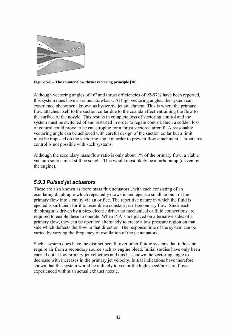
Figure 5-6 – The counter-flow thrust vectoring principle [30]

Although vectoring angles of 16º and thrust efficiencies of 92-97% have been reported, this system does have a serious drawback. At high vectoring angles, the system can experience phenomena known as hysteretic jet attachment. This is where the primary flow attaches itself to the suction collar due to the coanda effect entraining the flow to the surface of the nozzle. This results in complete loss of vectoring control and the system must be switched of and restarted in order to regain control. Such a sudden loss of control could prove to be catastrophic for a thrust vectored aircraft. A reasonable vectoring angle can be achieved with careful design of the suction collar but a limit must be imposed on the vectoring angle in order to prevent flow attachment. Throat area control is not possible with such systems. Although the secondary mass flow ratio is only about 1% of the primary flow, a viable vacuum source must still be sought. This would most likely be a turbopump (driven by the engine).

5.9.3 Pulsed jet actuators These are also known as ‘zero mass flux actuators’, with each consisting of an oscillating diaphragm which repeatedly draws in and ejects a small amount of the primary flow into a cavity via an orifice. The repetitive nature in which the fluid is ejected is sufficient for it to resemble a constant jet of secondary flow. Since each diaphragm is driven by a piezoelectric driver no mechanical or fluid connections are required to enable these to operate. When PJA’s are placed on alternative sides of a primary flow, they can be operated alternately to create a low pressure region on that side which deflects the flow in that direction. The response time of the system can be varied by varying the frequency of oscillation of the jet actuators. Such a system does have the distinct benefit over other fluidic systems that it does not require air from a secondary source such as engine bleed. Initial studies have only been carried out at low primary jet velocities and this has shown the vectoring angle to decrease with increases in the primary jet velocity. Initial indications have therefore shown that this system would be unlikely to vector the high speed/pressure flows experienced within an actual exhaust nozzle.

42

5.9.4 Shock vector thrust vectoring In this system, a secondary flow is injected asymmetrically into the divergent section of a convergent-divergent nozzle. This creates a low pressure region downstream of the injection port which is seen as a disturbance by the flow and results in a strong oblique shock wave being formed. The change in flow properties which are typical across a shock wave, causes the flow to change direction and be vectored away from the injection port as it passes through the oblique shock. Since vectoring takes place at supersonic speeds, thrust losses can occur as a result of the primary flow passing through the oblique shock which has a knock on effect on the thrust efficiency. Vectoring angles of more than 19º have been achieved in static tests. In practice, the resulting freestream velocities are seen to vary the pressure differential at the nozzle exit, which moves the shock wave attachment point further into the nozzle. This has the effect of reducing the effectiveness of the nozzle. This system is reported to have a greater efficiency than equivalent mechanical systems with a secondary mass flow requirement of 6-10%. The drawback of such a system is when the oblique shock wave becomes too strong and its other end impinges on the opposite nozzle wall. When this happens, a reflected shock wave of reduced intensity is generated which vectors the primary flow in the opposite direction. This results in a degradation of thrust vectoring performance and thrust efficiency. Another problem with this system is, in order to achieve large vectoring angles; the system must operate at highly over-expanded conditions which results in over-expansion loses. The throat area remains unaffected by this thrust vectoring method but can be varied by mechanical means if required.

Figure 2-7 – The shock vector thrust vectoring principle [30]

Thrust vectoring efficiencies of 0.9-4 deg per percent of flow injection and thrust efficiencies of 0.86-0.94 have been demonstrated.

5.9.5 Sonic throat skewing (shifting) In this system, secondary flow is injected into either the throat or divergent section of a supersonic convergent-divergent nozzle to vector the flow. The working principle here is the creation of virtual aerodynamic surfaces which have the same function as mechanical surfaces. The conventional throat of the nozzle and its shock wave is skewed (shifted) to the new minima of these virtual surfaces. Since the vectoring takes place on he subsonic side of the nozzle throat shockwave and therefore at lower speeds, the thrust losses due to vectoring are lower. The injection points are typically located at different points long the nozzle axis which has the effect of skewing the sonic plane

43

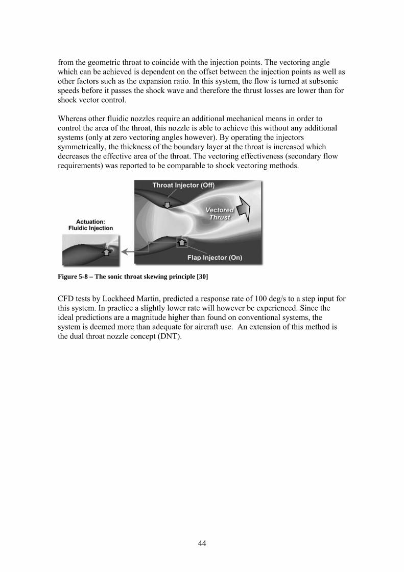
from the geometric throat to coincide with the injection points. The vectoring angle which can be achieved is dependent on the offset between the injection points as well as other factors such as the expansion ratio. In this system, the flow is turned at subsonic speeds before it passes the shock wave and therefore the thrust losses are lower than for shock vector control. Whereas other fluidic nozzles require an additional mechanical means in order to control the area of the throat, this nozzle is able to achieve this without any additional systems (only at zero vectoring angles however). By operating the injectors symmetrically, the thickness of the boundary layer at the throat is increased which decreases the effective area of the throat. The vectoring effectiveness (secondary flow requirements) was reported to be comparable to shock vectoring methods.

Figure 5-8 – The sonic throat skewing principle [30]

CFD tests by Lockheed Martin, predicted a response rate of 100 deg/s to a step input for this system. In practice a slightly lower rate will however be experienced. Since the ideal predictions are a magnitude higher than found on conventional systems, the system is deemed more than adequate for aircraft use. An extension of this method is the dual throat nozzle concept (DNT).

44

6 Thrust vectoring studies and examples

6.1 Existing thrust vectoring research effort and thrust vectored aircraft

A significant amount of research effort has been expended to thrust vectoring over the last few years. Some of the effort has not progressed beyond the experimental stage, while at the other end of the scale, a handful of thrust vectored production aircraft exist. A number of these developments are listed below and have been categorised according to their thrust vectoring abilities.

Manufacturer Model Main Engine Additional NotesBell/Boeing V-22 Osprey 2xTurboprop TiltrotorBoeing X-32 P&W F135 A/BDornier Do31 2xPegasus +8x RB162 lift enginesEWR VJ 101 4xRB-145 (rotating) +2x RB145 in fuselageBAE Harrier RR PegasusLockheed Martin F-35B JSF F135/F136 A/B + Low pressure shaft driven lift fan for liftVFW VAC 191B RR RB 193-12 +2x RR RB162-81 lift enginesYakovlev YAK-38 R-28 V-300 +2x RD-38 lift enginesLockheed Martin F-22 Raptor 2x P&W F119-PW-100 A/B Pitch only vectoring (+/- 20 deg)McDonnell Douglas F-15 S/MTD P&W F-100-PW-200 A/B P&W 2-d TV Nozzle (+/- 20 deg)McDonnell Douglas X-36 Williams F112 Yaw onlyBoeing X-45A Yaw onlySukhoi Su-30 2x AI-31FL A/B 2-d (+/-15 deg)Sukhoi Su-35 2x Saturn 117S A/BSukhoi Su-37 2x AI-31FU 2-d (+/-15 deg)Lockheed Martin F-16 MATV GE F110-GE-100 A/BMcDonnell Douglas F-15 ACTIVE 2x P&W F-100-PW-200 A/B P&W P/YBBN TV Nozzles (20 deg 3-d)McDonnell Douglas F-18 HARV 2x GE F404-GE-400 A/BMitsubishi ATD-X 2x IHI XF5 A/B 3 paddlesMikoyan MiG-29OVT 2x Klimov RD-33MK A/BRockwell MBB X-31 GE F404-GE-400 3 paddles for pitch and yawSukhoi Su-35BM 2x Saturn 117S A/BLockheed Martin X-44 Full pitch/yaw/roll TV control

VTO

L/ST

OL

2-d

Man

euve

r3-

d M

aneu

ver

Table 6-1

6.2 Internal mechanical thrust vectoring concepts Numerous thrust vectoring nozzle configurations have been explored over time. Many of these are however quite old compared to the configurations discussed below and there are a number for which little information is available. This review will thus be restricted to the most current concepts which have shown the most promise.

6.2.1 PYBBN nozzle The axi-symmetric PYBBN (Pitch Yaw Balanced Beam Nozzle) nozzle is able to vector the thrust by 20° within a full 360° envelope. It was tested on a F100-PW-229 engine which was fitted to redundant MATV project test aircraft, but can be retrofitted to any F100 engine. The redundancy of the system is also good with duplex actuators being used for the engine-nozzle system. The balanced beam configuration is a means to

45

reduce the forces required to deflect the nozzle and thus reduce the size of any the accompanying actuators.

Figure 6-1 and 6-2 [Ref 31]

6.2.2 Axi-symmetric Vectoring Exhaust Nozzle (AVEN) The General Electric AVEN nozzle program was born around a requirement to provide a simple means of multi-axis thrust vectoring which could be retro-fitted to any F-16 with a digital flight control. The nozzle was coupled to a GE F110-GE-100 engine and tested as part of the VISTA and MATV programmes. Although this was designed around a F110 engine, it is adaptable to other engine designs, including the very similar F404. The nozzle has the ability to be vectored in any direction by over 20° and has a low external profile, but is heavy and a significant amount of ballast is required in the nose of the aircraft to compensate. The AVEN nozzle was derived from a standard convergent-divergent F110 nozzle by replacing the compression links with a load carrying flap/frame system which was connected to a movable ring. This could be either tilted to vector the thrust or translated fore and aft to adjust the exhaust area. The position of the ring is maintained relative to the engine centreline with three ring support mechanisms. Thermal resistant seals also had to be included between the divergent flaps of the nozzle to maintain its efficiency. Nozzle vectoring requirements are passed from a digital Vector Electronic Control Unit to a Nozzle Control Valve (which is a set of electro-hydraulic servo valves). The divergent section of the nozzle is then manipulated via three equally spaced actuators and the throat area by four actuators (which are adoptions of the F110 hydraulic nozzle actuators). The layout of the nozzle is shown in the figure below.

Figure 6-3 and 6-4 [Ref 32]

46

Since the thrust is vectored in the divergent section of the nozzle, aft of the chocked nozzle throat, the engine is unaffected by pressure fluctuations from the nozzle.

6.2.3 ADEN nozzle The ADEN nozzle is a 2-d thrust vectoring nozzle which can be extended to include directional thrust vectoring with the addition of articulated sidewalls. In its simplest format this nozzle consists of a variable external expansion ramp (VEER) which is rotated in the vertical direction to control longitudinal thrust vectoring angle. The resulting exhaust flow field from this nozzle is rectangular.

Figure 6-5 [Ref 33]

6.2.4 Lyulka Saturn AL-31FU/P The Lyulka Saturn AL-31P and AL-31FU are thrust vectoring capable production versions of the AL-31 range of military turbojet engines. The AL-31 range of engine are reported as having high gas dynamic stability and strength and able to maintain reliable engine performance in extreme conditions of inlet distortion. Such an engine has thus until now been an excellent choice for a highly manoeuvrable aircraft. The AL-37FU engine is fitted with a 2-d (pitch) afterburning-articulating/steerable nozzle and is currently fitted to the Su-37 and Su-47 aircraft. This titanium nozzle has the ability to deflect the thrust by ±15° at a rate of 30°/sec. When fitted to twin engined aircraft, the nozzles can be deflected collectively, differentially or even unsymmetrically. The 83kN AL-31FP engine, which is fitted with a prototype 3-d vectoring nozzle, is only 110kg heavier and 0.4m longer than the baseline AL-31F engine with the same thrust output. The AL-31F family of engines (plus the improved 117S) are upgradeable to the AL-31FP at any time without any changes to the airframe. The AL-31FP is currently used in the SU-30MKI and has demonstrated vectoring capabilities 32 degrees in the horizontal plane and 15 degrees in the vertical plane.

47

Figure 6-6, 6-7, 6-8 [Ref 34]

6.3 Mechanical thrust vectoring research projects

6.3.1 McDonnell Douglas F-15 S/MTD (STOL and Manoeuvre Technology Demonstrator)

The goal of the S/MTD programme was to demonstrate six emerging technologies, which include thrust vectoring, integrated flight propulsion control systems, enhanced lift systems, enhanced avionics systems, low grade runway landing gear and advanced post stalled engine intakes (which reduce flow distortion). An F-15 airframe (capable of Mach 2.1) was used as a test bed, which was fitted with canards, derived from the stabiliser of an F/A-18. This was fitted with two P&W F-100-PW-200 turbofan engines which were fitted with 2-d converging-diverging thrust vectoring nozzles. A combination of movable nozzles and vanes in the jet pipe was able to produce deflection angles of +/-20°. The complex flight control system allowed the thrust vectoring nozzle to be integrated with the operation of the canards and elevators to provide enhanced manoeuvrability. The work investigated ways to reduce the field length required by the aircraft to increase its operational flexibility, by means of the combined operation of thrust reversing, thrust vectoring and canards. This allowed the take-off rotation speed to be reduced to 43mph, the take-off roll distance to be reduced by 25% and the landing field length to be reduced from 2,300m to just 500m. The work also investigated some of the enhanced manoeuvres which could be possible with such a configuration. This included rapid in-flight deceleration with thrust reversal and using the canards as airbrakes as well as controlled flight at angles of attack of about 85° (without tail surfaces).

6.3.2 NASA F-15 Advanced Control Technology for Integrated Vehicles (ACTIVE) programme

The 1993-1999 ACTIVE programme was a research collaboration between a number of parties to enhancing the performance and manoeuvrability of future aircraft (civil and military). Of particular interest was the feasibility of replacing conventional aerodynamic with multi-axis thrust vectoring nozzles. This project reused the aircraft of the earlier S/MTD programme with replacement P&W F-100-229 engines fitted, along with newly developed 3-d P&W PYBBN axi-symmetric thrust vectoring nozzles. These

48

nozzles enable the thrust to be vectored by 20° in both the pitch and yaw directions or any combination of these, while retaining an acceptable top speed of Mach 2.0. Such a configuration required a control system capable of controlling the nozzle, engine and conventional control surfaces. The flight tests demonstrated both pitch and yaw vectoring at speeds up to Mach 2. Yaw vectoring of the aircraft while at 30° angle of attack was also successfully demonstrated. Finally, an adaptive performance software program (developed as part of the project) was demonstrated which could optimise the nozzle and control surface deflections for minimum drag. The aircraft later went on to be reused once again in the 1999 IFCS (Intelligent Flight Control System) programme as well as also being able to lend itself to other research activities outside the ACTIVE programme.

6.3.3 General Dynamics F-16 Multi-Axis Thrust Vectoring (MATV) programme

The goal of the MATV programme was to investigate high angle of attack flight at altitudes above 20,000ft with Multi-Axis Thrust-Vectoring. The aircraft used was a modified F-16 which originated from the 1988 VISTA (Variable stability In-flight Simulator Test Aircraft) programme, where it was originally used to perform variable stability test flights. The variable stability computers and controls were removed for the MATV project and the aircraft was fitted with a P&W F100-PW-220 turbofan engine (with afterburner) and AVEN thrust vectoring nozzle. This enabled the aircraft to perform super-manoeuvres in the post-stalled domain, while also being able to fly at speeds in excess of Mach 2. The same aircraft was also used for testing the P&W PYBBN.

6.3.4 NASA F/A-18 High Angle of Attack Research Vehicle (HARV) programme

The NASA HATP (High Angle-of-Attack Technology Program) used a HARV (High Alpha Research Vehicle) F-18 aircraft to investigate controlled flight at high angles of attack. This 1987-96 project was the first NASA project to demonstrate mechanical thrust vectoring and high alpha flight at subsonic speeds. The X-31 and F-15 ACTIVE projects later went on demonstrate high alpha flight at supersonic speeds. The test aircraft was fitted with two modified GE-F404-400 turbofan engines in which the divergent sections of each nozzle was removed and three inconel paddles were externally mounted around each exhaust. This configuration allowed pitch and yaw vectoring of the aircraft from coordinated deflection of the vanes into the thrust stream. Removal of the nozzle divergent section meant that the aircraft was limited to subsonic flight. Hinged forebody strakes were also added which were able to provide control at high angles of attack by interacting with vortices generated in this domain. Flight control system improvements included new control laws to integrate the thrust-vectoring nozzle with the existing control surfaces to achieve the optimal benefit from each device. In total, the aircraft modifications added 3,750lbs to the weight of the aircraft

49

Controlled flight at 70° angle of attack and high roll rates at 65° alpha were demonstrated. However, there were a number of disadvantages associated with this system and as a result, internal thrust vectoring concepts were given preference in subsequent NASA research efforts.

Figure 6-9 [Ref 35]

6.3.5 The STOL Exhaust Nozzle (STOLEN) Concepts Program The objective of the 1980s STOLEN project was to investigate a number of potential exhaust vectoring concepts suitable for STOL. The specifications for the project were to devise advanced tactical fighter concepts able to meet a field length requirement of either 700 or 1000ft. This necessitated the need for high vector angles to reduce the axial thrust and increase lift. The STOL concepts investigated were based on variants of existing VTOL and CTOL nozzle designs and included, both side and rear exhaust vectoring systems with axi-symmetric and non axi-symmetric nozzles. These were fitted to either a RB406-03 military turbofan (with a variable area mixed exhaust) or a RB420-02 separate flow engine (where the bypass fan flow exhausts through two variable area side nozzles and the core flow is exhausted through a single variable area rear nozzle). The thrust from the core flow was supplemented with an afterburner and that of the side nozzles was supplemented with a plenum chamber burner (located just before each side nozzle). Four aircraft configurations were studied, Aero Balanced Deflected Thrust (ABDT), Jet Balanced Deflected Thrust (JBDT), Vectored Fan Thrust (VFT), Vectored Total Thrust (VTT). These investigated the use of blown canards and a fan air driven pitch pipe to counteract the pitching moment due to the thrust vectoring nozzle as well as investigating the use of front nozzles for thrust vectoring. The thrust vectoring nozzles used were, VACS, RAMP, 2D-CD and CRD TRBPN. These ranged from rotating side mounted elbow ducts with variable area nozzles to movable plates and deflector doors and allowed the thrust to be deflected by up to 70º. The conclusion was that side mounted ducts gave the shortest ground roll results. Adding STOL capabilities to a tactical aircraft was estimated to incur a mere 3% increase in TOGW.

50

6.3.6 Rockwell-MBB X-31 Following on from the HARV programme, was the NASA X-31 Enhanced Fighter Manoeuvrability (EFM) programme, in which the aircraft was used to test the tactical benefits of thrust vectoring. Thrust vectoring was combined with a sophisticated coupled flight control system to enable the effectiveness of controlled manoeuvres at high angles of attack to be tested while in an air combat situation. The horizontal tail surfaces were removed and the single thrust vectoring nozzle was supplemented with canards and aft fuselage fixed strakes to further increase its manoeuvrability and stability. The three paddle thrust vectoring system (as fitted to the F-18 HARV) was fitted to the exhaust of a GE F404-GE-400 turbofan engine. The carbon-carbon composite paddles (capable of withstanding temperatures of up to 1500ºC) were mounted directly to the airframe and provided both pitch and yaw control. Although the design speed of the X-31 was Mach 0.9 (40,000ft), the thrust vectoring system was tested at Mach 1.28 (35,000ft). The design of the X-31 demonstrator aircraft descended from the earlier HiMAT and (Highly Manoeuvrable Aircraft Technology Program) in which tests were carried on a remotely piloted research vehicle. The design of the thrust vectoring system was built on experience gained from the SNAKE programme (Super Normal Attitude Kinetic Enhancement) which investigated the use of paddles as a low cost means of thrust vectoring. In the development of the multi-axis X-31 thrust vectoring system, 498 paddle and nozzle configurations were tested and then used to down select the final configuration. Initial tests revealed a weakness in the post-stalled pitch control of the aircraft, which was fixed with the addition of aft fuselage strakes to the aircraft. The X-31 programme successfully demonstrated controlled flight at 70° AoA and the execution of a Herbst manoeuvre (rapid 180° turn using a post stalled manoeuvre). The X-31 has since been involved in the NASA Vectoring, Extremely Short Take-off and Landing, Control and Tailless Operation Research (VECTOR) project. This goal of this project was to research the autonomous short landing of an aircraft at a high angle of attack. As well as building on the work of the X-31 programme, this project integrated a modified EuroJet EJ200 engine with a novel axi-symmetric thrust vectoring nozzle. The nozzle was developed by Industria de Turbo Propulsores (Spain) and is able to offer multi-axis vectoring capability while being capable of varying its throat and exit areas with a minimal number of control actuators.

51

Figure 6-10 [Ref 36] and 6-11 [Ref 37]

6.3.7 Boeing X-32 The Boeing X-32 was a Mach 1.6 capable (at altitude) direct lift STOVL demonstrator aircraft, designed around the requirements of the Joint Strike Fighter competition. The aircraft used three-poster thrust vectoring system, powered by a P&W F135 afterburning turbofan engine located in the forward fuselage. The exhaust gases were directed to lift nozzles at the rear of the engine and a pitch axis thrust vectoring nozzle (via a afterburner) at the rear of the aircraft. The three lifting nozzles are fixed and do not rotate, instead the exhaust gases are ducted to them. During testing, it was noted that the hot exhaust gases had a tendency to get sucked back into the engine, which caused it to overheat along with a loss in thrust. The contract was ultimately lost to the Lockheed Martin X-35 and the X-32 was retired to a museum.

Figure 6-12 and 6-13 [Ref 38]

6.3.8 Lockheed Martin X-35 The X-35 was the Mach 1.6 capable rival to the X-32 and winner in the JSF competition. The aircraft later went on to production with the F-35 designation. The aircraft comes in three variants, a conventional fighter, a STOVL fighter and a carrier capable fighter. The STOVL variant, as is discussed here, is the baseline of the three

52

configurations. The carrier capable variant of the aircraft was given a bigger wing and tail surfaces as well as a strengthened landing gear. The conventional fighter configuration variant of the aircraft enables the lift fan to be replaced with a large fuel tank for increased range. The Lockheed Martin lift system consisted of a vertical contra-rotating lift fan which was situated at the middle of the aircraft (just behind the cockpit) and shaft driven from a P&W F119 engine. Propulsive lift comes from a combination of thrust from the lift fan and vectored exhaust gases from a three bearing pitch-axis vectoring main engine nozzle. The shaft-driven fan arrangements ability to move a large mass of slower moving air made it more efficient than other concepts and is able to support almost half of the aircrafts weight. As it does not use high velocity hot exhaust gases it is also less likely to damage runway surfaces. During normal flight, the lift fan is disengaged and the lift fan bay concealed with upper and lower clamshell doors. At low speeds, a further set of doors open to uncover an auxiliary intake for the engine. Roll control is provided by roll-post nozzles located on each wing tip, which uses air from the LP turbine of the main engine. Although the lift system is unnecessary weight during normal flight, it has the added benefit of enabling heavier payloads to be carried while still achieving a satisfactory field length. Although the X-35 was designed with stealth in mind, the unshielded circular nozzle does make the aircraft vulnerable from the rear.

Figure 6-14 [Ref 39] and 6-15 [Ref 40]

6.3.9 McDonnell Douglas X-36 The unmanned X-36 was a 28% scale prototype of a possible low-observable fighter configuration, which was used to research tailless fighter agility. Its low observable features included, no tail, aligned edges, a wide flat exhaust. Conventional control surfaces were eliminated with aircraft control being instead achieved with: all moving canards, split ailerons and an advanced thrust vectoring. The thrust vectoring system was only used to supplement the directional control from the drag rudders on the wing tips. It used a Williams F112 turbofan engine and was reported to be capable of 234mph but unstable in the pitch and yaw axes, necessitating the need for an advanced flight control system. During flight testing, the aircraft demonstrated, stable flight at 40° AoA, 360° rolls at 15° AoA and rapid turning/rolling manoeuvres at 35° AoA. At the end of the project

53

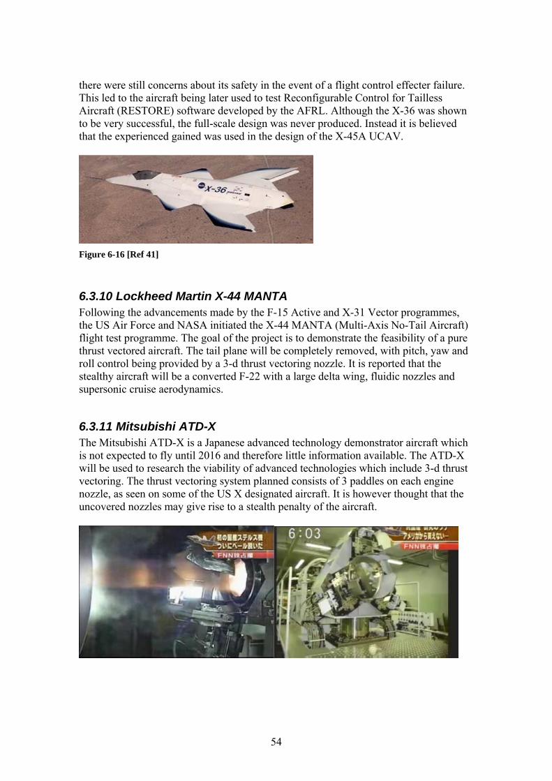
there were still concerns about its safety in the event of a flight control effecter failure. This led to the aircraft being later used to test Reconfigurable Control for Tailless Aircraft (RESTORE) software developed by the AFRL. Although the X-36 was shown to be very successful, the full-scale design was never produced. Instead it is believed that the experienced gained was used in the design of the X-45A UCAV.

Figure 6-16 [Ref 41]

6.3.10 Lockheed Martin X-44 MANTA Following the advancements made by the F-15 Active and X-31 Vector programmes, the US Air Force and NASA initiated the X-44 MANTA (Multi-Axis No-Tail Aircraft) flight test programme. The goal of the project is to demonstrate the feasibility of a pure thrust vectored aircraft. The tail plane will be completely removed, with pitch, yaw and roll control being provided by a 3-d thrust vectoring nozzle. It is reported that the stealthy aircraft will be a converted F-22 with a large delta wing, fluidic nozzles and supersonic cruise aerodynamics.

6.3.11 Mitsubishi ATD-X The Mitsubishi ATD-X is a Japanese advanced technology demonstrator aircraft which is not expected to fly until 2016 and therefore little information available. The ATD-X will be used to research the viability of advanced technologies which include 3-d thrust vectoring. The thrust vectoring system planned consists of 3 paddles on each engine nozzle, as seen on some of the US X designated aircraft. It is however thought that the uncovered nozzles may give rise to a stealth penalty of the aircraft.

54

Figure 6-17 to 6-20 [Ref 42]

6.3.12 Harrier No study of thrust vectoring systems is complete without mentioning the Harrier since this lead the way in the development of vectored propulsion theory and practice. The Harrier relies on its four poster thrust vectoring system for VTOL capabilities rather than super-manoeuvrability. During take-off and landing, the four nozzles of the Pegasus engine thrust are rotated to deflect the thrust downwards. During normal flight, the nozzles return to their normal position for forward propulsion of the aircraft. Pitch and roll control was achieved with reaction control valves (which used air bled from the engine) located on the nose, tail and wing tips of the aircraft.

Figure 6-21 [Ref 39] and 6-22 [Ref 27]

6.3.13 Grumman X-29A The initial goal of the cancelled X-29A project was to evaluate a forward swept winged aircraft at an angle of attack up to 40º without thrust vectoring and up to 90º with multi-axis thrust vectoring. The aircraft was a close coupled variable incidence lifting canard design in which the flow field of the canard and wing interact favourably with each other. The relaxed stability aircraft (35% statically unstable) relies upon a full authority digital fly-by-wire flight control system. The partially thrust vectored aircraft used an ADEN (Augmented Deflector Exhaust Nozzle) thrust vectoring nozzle fitted to a GE F404-GE-400 engine and retained the original aerodynamic flight control surfaces. Lateral-directional manoeuvres which were not possible at high angle of attack

55

manoeuvres for the normal aircraft (due to masking of the rudder by the fuselage) could be successfully carried out with directional thrust vectoring. The benefits of longitudinal thrust vectoring were assessed as a 17% reduction in take-off speed, 37% reduction in take-off distance and 20% reduction in take-off time.

6.3.14 F-22 Raptor The F-22 raptor used the first ever production thrust vectoring nozzles fitted to two P&W F119-100 engines. The pitch only mechanical vane thrust vectoring system is capable of delivering up to 20 degrees pitch vectoring to enhance the maneuverability of the aircraft.

Figure 6-23 [Ref 43 and 6-24 [Ref 44]

6.3.15 X-45 Little in known about the X-45 thrust vectoring system except that it builds on the experience of the X-36 aircraft, is an internal thrust vectoring system and is used for yaw control only.

6.3.16 Thrust vectoring for the Eurofighter The European fighter aircraft (EFA) is not currently equipped with any form of thrust vectoring and concerns have been raised that this may make the aircraft vulnerable. As a result, on-going research work is being carried out to investigate a modified nozzle which could be used to add thrust vectoring capability to the aircraft. The convergent-divergent thrust vectoring nozzle which was developed by ITP has the ability to vector the thrust by 30º in three dimensions. This nozzle is based on three concentric rings enabling it to offer variable area control for the throat and exit areas to further improve its efficiency. It is also claimed to be the lightest in its category.

56

Figure 6-25 and 6-26 [Ref 45]

6.3.17 The B2 To reduce the radar signature of this stealth aircraft, there is no conventional tail and alternative means of aircraft control have been incorporated. Pitch and roll control are achieved with three elevons located on each side of the aircraft. Yaw control is achieved with the use of drag rudders located at the extremities of each wing and are able to function as both an airbrake and rudder as required. Unfortunately, the drag rudders are inoperative at deflections below 5º and therefore have to be left slightly open in flight. As this is detrimental to the stealth characteristics of the aircraft, differential engine operation is used for yaw control instead where possible. Although this is not thrust vectoring in the true sense it is still worth including in any study.

6.3.18 Sukhoi-37 This uses two Lyulka Saturn AL-31FU thrust vectored engines to enhance its maneuverability. These 2-d nozzles are able to vector by -15º to +15º in the pitch plane but can also be deflected differentially or collectively to achieve the desired control. Although they are integrated into the digital flight control system, they can be operated either automatically by the FCS of manually by the pilot.

6.4 Fluidic thrust vectoring research effort A number of research studies have been carried out in to fluidic thrust vectoring. The key players in this field to date have been NASA but another significant contribution has been made by the recent Flaviir project. In addition, there has been a number of smaller research efforts conducted at many of the universities such as the Florida State University. The only commercial non-mechanical thrust vectoring nozzle reported to date is the Exact nozzle as developed by Williams for the Cirrus aircraft [46]. There is however expected to be other non-commercial nozzles in use on military aircraft but as to be expected no information is available.

57

6.4.1 Fluidic research at NASA NASA has been actively researching fluidic thrust vectoring for some time with reports being available which date back to the early 1990’s. The objective of their research efforts was to evaluate the use of fluidic thrust vectoring nozzles as a means to reduce the weight and observability of an aircraft. A range of fluidic concepts were explored which were able to offer, thrust-vector angle control, throat area control and expansion control. The fluidic thrust vectoring concepts being researched by NASA were:

• Shock vector control method • Throat shifting method • Counter flow method

These were tested and evaluated by a range of both computational and experimental studies at NASA Langley Research Centre. The latest update on fluidic thrust vectoring within NASA dates however back to 2003 with no more up to date information being available. It is therefore unknown whether NASA is still active in this research area.

6.4.2 The Flaviir project Amongst other technologies, the Flaviir project investigated the viability of replacing conventional control surfaces with fluidic devices. Fluidic circulation control devices were retro-fitted in place of conventional ailerons and a fluidic thrust vectoring nozzle replaced a conventional straight through jet pipe. The fluidic thrust vectoring nozzle was based on the co-flow concept, which differs from the counter-flow concept by the direction of the secondary flow. The secondary air is therefore blown out of the nozzle instead of being sucked in a direction against the primary flow. The research effort was initiated by Mark Mason [28] and the concept further developed by later students after it became part of the Flaviir project sponsored by BAE/EPSRC. Development followed a series of computation and experimental studies, in which the control and flow characteristics were evaluated and refined. The concept was finally evaluated on a series of model aircraft with promising resulting being reported. A larger scale nozzle was then built and tested, which unfortunately highlighted a number of problems at this larger scale and the nozzle was never tested on the Flaviir flying demonstrator. The nozzle does show promise but possibly only for smaller air vehicles. The problems highlighted in its development are control instability, control dead-zones, manufacturing difficulties due to the required tolerances and the provision of a large amount of the secondary jet. The greatest difficulty for the flying demonstrators proved to be the provision of a mass flow rate of air sufficient for the secondary jet. The only practical way to achieve this was to use engine bleed air but the amount of bleed required would have been too detrimental to the performance of the main engine. Therefore, a secondary engine was used whose sole purpose was to supply bleed air.

58

Figure 6-27 – Configuration of the Flaviir Demon demonstrator UAV

Figure 6-28 and 6-29 – The co-flow thrust vectoring nozzle developed as part of the Flaviir project [Courtesy of Manchester University]

Figure 6-30 – Cross-section through the co-flow thrust vectoring nozzle developed as part of the Flaviir project [Courtesy of Manchester University]

6.4.3 The Cirrus Vision aircraft and the Williams Exact nozzle The Exact nozzle developed by Williams for the Cirrus Vision aircraft is reported as being a pressure ratio thrust vectoring nozzle [46]. This nozzle allows the thrust from the top mounted engine to be vectored as required to increase the cruise speed and improve the pitch-thrust coupling effect and thus the handling at low speeds. The most significant vectoring takes place at low altitudes and low speeds with it being straighter at high altitude cruise. The nozzle was developed specifically for the Cirrus Vision aircraft with several nozzle geometry configurations being tested on the aircraft to arrive at the optimal geometry to achieve the best handling characteristics.

59

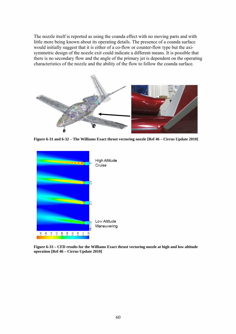
The nozzle itself is reported as using the coanda effect with no moving parts and with little more being known about its operating details. The presence of a coanda surface would initially suggest that it is either of a co-flow or counter-flow type but the axi-symmetric design of the nozzle exit could indicate a different means. It is possible that there is no secondary flow and the angle of the primary jet is dependent on the operating characteristics of the nozzle and the ability of the flow to follow the coanda surface.

Figure 6-31 and 6-32 – The Williams Exact thrust vectoring nozzle [Ref 46 – Cirrus Update 2010]

Figure 6-33 – CFD results for the Williams Exact thrust vectoring nozzle at high and low altitude operation [Ref 46 – Cirrus Update 2010]

60

7 Design and integration considerations for thrust vectoring systems

7.1 An overview of the fundamental concepts

7.1.1 An overview of exhaust nozzles The simplest of all the exhaust nozzles is the convergent nozzle. Their performance is limited, but with careful design, they are able to offer satisfactory performance up to transonic speeds. They are, however, only efficient over a narrow operating range but this can be expanded with a variable area configuration. When it is necessary to meet high speed and performance requirements, full expansion from a convergent nozzle can not always be achieved, and in such cases a convergent-divergent nozzle is required. Variable geometry derivatives are able to offer the benefits of higher performance and efficiencies throughout a wider aircraft flight envelope. When the performance of the convergent-divergent nozzle (including the thrust vectoring variants) configurations needs to be extended for short periods, an afterburner can be used. These are fitted upstream of the nozzle and typically necessitate the need for a variable geometry nozzle to allow the nozzle throat area to be increased (to maintain constant flow and the correct back pressure). A more detailed overview of the common exhaust nozzles is given in Appendix C and the reader is advised to refer to this section for more information. Thrust vectoring nozzles do share similarities with other exhaust nozzles and can still be categorised as being convergent or convergent-divergent according to their operating requirements. The internal vectoring nozzles for example can be seen to retain their convergent-divergent geometry when vectored, although now with a deflected flow path. It is possible to offer convergent nozzles with thrust vectoring capabilities, but their performance will be limited. The majority of thrust vectoring nozzles are therefore of the convergent-divergent type and are categorised as 2-d or 3-d according to their vectoring abilities. As to be expected, the mass, cost and complexity of the nozzle will however be increased somewhat as a result of increasing nozzle performance abilities. Therefore, the use of a convergent-divergent configuration, afterburners and/or thrust vectoring should be justified otherwise a more simplistic approach should be adopted.

7.1.2 The engine and exhaust nozzle sizing process In order to maximise its performance, exhaust nozzles should be designed to achieve full expansion. However, since the performance of an exhaust nozzle is directly related to the performance of the accompanying engine, the design of the nozzle is complex and must be integral with the design of the engine. The final nozzle configuration is therefore a trade-off between many requirements. For example, nozzles can be designed purely to achieve maximum possible thrust but this can lead to problems of high temperatures, pressures and possible engine surge. A more detailed overview of the engine and exhaust nozzle sizing process is given in Appendix C and the reader is advised to refer to this section for more information.

61

7.2 Thrust vectoring nozzle design and integration This discussion builds on the discussion for the design and integration of a general exhaust nozzle as given in Appendix C and the reader is advised to refer to this section for background reading. It should be noted that the scale of the benefits attainable from a thrust vectoring system is dependent on many design factors. In order to reap the most benefit from such a system, it must be integrated into the design as early as possible, preferably at the conceptual design stage. An example of this is that conventional control surfaces will be redundant and only act to hinder aircraft performance on an aircraft which uses thrust vectoring as its primary means of flight control. The class of aircraft on to which the system is to be fitted, must also be considered since a thrust vectoring system designed for a combat aircraft is unlikely to realise its potential on a reconnaissance aircraft. Since the design and integration of an exhaust nozzle can be considerably complex and encompass so many different streams of aeronautical engineering, it is not possible to go into great depth within the constraints of this thesis. Therefore only an overview of some of the design and integration considerations will be given in the sections below.

7.2.1 Thrust vectoring nozzle design requirements As with any other part of the aircraft, any exhaust nozzle will be designed to meet design requirements laid down by the airworthiness regulations, customer and other internal design groups. A thrust vectoring nozzle will be subject to additional design requirements such as:

• Max sustainable TV angle. This will always be less than the nozzle deflection angle. (20-25 degrees is reasonable for a mechanical paddle system)

• Total system weight. This includes all the actuators, control systems, hydraulic pumps and other ancillary equipment.

• Nozzle efficiency when vectored. This accounts for losses in engine thrust due to vectoring.

• Thrust vectoring efficiency. The deflection angle of the thrust line of action will be less than the nozzle deflection angle, which is accounted for by this term.

• Complexity and Maintainability. The higher moving part count of thrust vectoring nozzles makes them more complex than other nozzles and they require more frequent maintenance as a result.

• Safety. This includes the ability to vector the thrust in a controlled manner without failure as well as the controllability of an aircraft in the event of engine failure/flame-out.

• Observability. This covers the effect of the system on RADAR and infrared signatures. One method of reducing the radar cross-section of the nozzle is by shaping to a flattened arrowhead shape (as used on the X-45A). One of biggest infrared emitters is hot exhaust gases which heat up the metal parts, which can be reduced by nozzle cooling or shielding.

• Operational Effectiveness. How will the thrust vectoring nozzle affect the rest of the aircraft, engine and aircraft systems. This includes factors such as boat-tail drag, super-circulation lift gains (from integrated high aspect ration nozzles) and the impact on engine performance as a result of bleed air and power off-takes.

62

As a result of their extended manoeuvring capabilities, post-stalled manoeuvre capable aircraft are subject to additional design requirements. Research by Herbst determined the following requirements in such cases:

• Adequate control power must be available about all 3 axes for Mach numbers down to 0.1 and angles of attack up to 70 degrees.

• Sufficient aircraft stability and engine intake performance is necessary for Mach numbers up to 0.6 and angles of attack up to 70 degrees.

• The aircraft thrust loading (T/W) should ideally be no less then 1.2. • Intelligent flight control systems are required which are capable of calculating

the control inputs required for coordinated flight manoeuvres with regards to the main velocity vector.

7.2.2 Exhaust system layout As shown in the figure below, the exhaust nozzle of a buried installation is only one part of the exhaust system. The propelling nozzle is located at the very rear of the aircraft and is connected to the exhaust cone of the main engine via a jet pipe. The total length of the exhaust system is dictated by the layout of the aircraft configuration and in particular the positioning of the engine within the fuselage. The respective lengths of the jet pipe and nozzle are, however, design choices. The length of a thrust vectoring nozzle for example is a trade-off between the weight savings possible with a short nozzle and the nozzle length required to overcome internal flow problems such as separation, non-uniformity and swirl.

Figure 7-1 – A typical buried engine complete exhaust system [27]

7.2.3 Jet pipe design The jet pipe may at first sight appear to be a simple transition section connecting the propelling nozzle to the exhaust cone but its design is, however, more complex. For example, its area is gradually increased in order to be able to act as a diffuser to reduce the speed of the high speed gases entering the jet pipe. This helps to reduce friction losses associated with the gases moving through the exhaust system. Since the gases pass through flow straighteners before entering the exhaust system, losses due to swirl are less of a problem. When high aspect ratio nozzles are used, the jet pipe becomes a circular to rectangular transition duct, which must be designed so that the exit velocity profile remains as uniform as possible in order to minimise pressure losses.

63

7.2.4 Cooling requirements The high temperature of the exhaust gases passing through the nozzle necessitates the need for high temperature materials and appropriate cooling methods. The nozzle components which are directly impinged on by the hot exhaust gasses have the most severe cooling requirements. This means that thrust vectoring nozzles have significantly greater cooling requirements than conventional nozzles and typically use film cooling methods. The shape and therefore the internal surface area of a nozzle also have an impact on cooling requirements (as is the case for 2-d vectoring nozzles which are usually rectangular). It should also be noted that the temperature across the surface of a nozzle may not be uniform (especially in the case of 2-d nozzles which experience a non uniform field in mid flap compared to the corners). These temperature fields can result in internal stresses and distortion of the nozzle and therefore the nozzle must be cooled in accordance. Since engine bleed air is used for cooling the nozzle, the engine size and weight or even influence the choice of engine cycle selected is influenced by the nozzle cooling requirements. There is a perfect balance with regards the amount of cooling air to use. There must be sufficient cooling air to protect the structural integrity of the nozzle but not too much which would result in a significant detriment in engine thrust. A solution to the cooling flow requirements of nozzles may be the use of an ejector system, which may also result in an improved propulsion system. This does, however, have the disadvantage of complicating the propulsion system installation as in-depth consideration of the inlet and nozzle installations is required. The cooling of very high temperature can be further improved by using a double wall construction for the nozzle walls. This has an added benefit that the external wall also acts like an insulating blanket to reduce noise. In such an arrangement, cooling air is drawn between the nozzle walls by the ejector principle. Although cooling is a major problem for current thrust vectoring nozzles, this will be less of an issue for the next generation of nozzles manufactured from RCC materials. Such materials are able to maintain their shape and structural integrity at higher temperatures and therefore have lower cooling requirements. These are, however, still in the early stages of development.

7.2.5 Weight and centre of gravity considerations The weight of a nozzle is relative to its functional ability and its complexity and thrust vectoring nozzles can be considerably heavy. Although the weight of the aircraft is increased as a result, of greater concern is the location of this additional mass at the rear of the aircraft. This not only shifts the centre of gravity rearwards but also increases the pitch inertia of the aircraft. Potential weight savings are available with the advent of new mechanical thrust vectoring nozzle concepts as well as the use of novel materials. The new class of fluidic thrust vectoring nozzles are also reported to offer significant weight savings but these are still in their infancy. In the case of 2-d rectangular converging-diverging nozzles, weight savings may be made by designing the nozzle so that the sidewalls are cut back to be shorter than the diverging flaps. The amount of side wall that can be cut back can be determined by examination of the Mach lines within the nozzle exit as shown in the figure below.

64

Figure 7-2 – Guidelines for potential nozzle cut-back for weight saving [47]

7.2.6 Metallurgical considerations A well known restriction in the technological expansion of engines is the temperature limits imposed by current materials. Since increases in engine operating temperature are also imposed on the exhaust system, the exhaust system is also subject to material limitations. Current exhaust systems have to be manufactured from nickel or titanium and use some form of cooling to withstand the high temperatures currently experienced. A new breed of Reinforced Carbon-Carbon composite materials are being developed which are able to reduce the amount of cooling required for intended hot engine components such as turbine blades and exhaust nozzles. As well as being able to reduce cooling requirements, nozzles constructed from these materials also offer reductions in leakage losses. Overall this leads to an improvement in performance of the propulsion system. These new materials also offer significant weight reductions and enable complex assemblies to be co-formed, which reduced part counts and assembly times. Such materials also have stealth benefits as they are reported be excellent absorbers of electromagnetic waves.

7.2.7 Afterburners Where an afterburner is required, the complexity, mass and cost of the nozzle can increase considerably. The increase in exhaust gas temperature and thrust associated with afterburners demands the use of a more robust nozzle able to withstand the higher internal stresses and temperatures. It should be remembered that these higher temperatures will also dictate the need for a means of increased nozzle cooling. The incorporation of an afterburner will also have the impact of lengthening the complete engine exhaust and may therefore lengthen and increase the mass of the rear fuselage.

7.2.8 The relationship between engine and nozzle The inter-relation between engine and nozzle is complicated with many factors to consider. The performance of the nozzle is dependant on factors such as engine throttle setting, nozzle pressure ratio (NPR) and exhaust gas composition (which is dependant on the air/fuel ratio and the combustion efficiency). Engine swirl can have a considerable impact on the performance of a nozzle, which is overcome with flow straighteners. The behaviour of the flow within the engine and nozzle can be complex and the exact performance of a nozzle can only be properly investigated experimentally.

65

When designing a thrust vectoring system for agility, we also need to give consideration to the response time of the engine. Many current engines are reported to fall short of this requirement and engine developments are required in this area, especially to compressor stall margins and digital flight control systems. This short fall in requirements is not necessarily a design restriction, however, since performance limitations are sometimes imposed by a manufacturer to preserve engine life. Modifications may be required to an engine which is fitted with a thrust vectoring nozzle since the operation of the nozzle will generate pressure distortions within the engine. When the distance between the engine and nozzle is short, this can cause the fan and turbine blades to vibrate. In such an event, snubbers can be fitted to the fan blades and shrouds to the turbine tips. This is however not an issue for convergent-divergent nozzles since the pressure fluctuations are prevented from being reflected back to the engine by the shock wave at the nozzle throat.

7.2.9 Stability and control and aerodynamic considerations As already discussed, the installation of a thrust vectoring nozzle will move the aircraft centre of gravity and increase the pitch inertia of the aircraft. In addition to this, the rear of the fuselage may have to be increased to accommodate the nozzle, which will have an impact on the aerodynamic pitch damping of the aircraft. Collectively, these will have an impact on the aircraft static and dynamic stability and control characteristics. The aerodynamics of the aircraft can also be significantly affected by a thrust vectoring nozzle and in particular the boat-tail drag of the aircraft will be affected by increases in the rear fuselage. In the case of high aspect ratio nozzles, it is possible to carefully blend them in to the trailing edge of a lifting surface to create phenomena known as super-circulation. In such a situation the aircraft aerodynamics are improved due to the generation of favourable interference effects between the exhaust flow and the airflow over the lifting surface. In cases where thrust vectoring is used to contribute to the lift produced by the wings, it is possible to reduce the size of the wings and their accompanying drag.

7.2.10 Detailed nozzle design The detail design of mechanical thrust vectoring nozzles is a complex process which encompasses many of the different branches of mechanical engineering. Some of the engineering design parameters which need to be considered include:

• Engine operational factors – Thrust requirements, efficiency, engine technology limits, aero-thermodynamics, IR and heat transfer variables

• Design and manufacture - Structural and materials technology limits, manufacturing constraints, mass, installation considerations and cost

• Operational factors - Reliability, durability, safety, cost and maintenance In particular, careful selection of nozzle materials and its structural layout is essential to prevent distortion of the nozzle. Installation and assembly of the exhaust system must also take into account the expansion and contraction of the different sections, which

66

requires careful design of the joints and mounts. Failure to do so can result in severe distortion and damage to the nozzle and surrounding structure.

7.2.11 Integration of the next generation of technology Integration is a discipline which is continually changing as new technologies and engineering approaches are evolving. The integration of a propulsion unit into an airframe has traditionally dealt with aspects such as:

• Space allocation within the airframe and optimisation of the surrounding aircraft aft-body profile.

• Aircraft configuration considerations. The aircraft configuration may have to be modified to compensate for the rearward shift of the centre of gravity by shifting the aerodynamic centre of the aircraft. The easiest way to achieve this is by repositioning the wings on the fuselage.

• Weight and centre of gravity considerations. • Aerodynamic considerations. • Stability and control considerations. • Engine-inlet matching. This takes into consideration airflow requirements and

distortion effects. • Engine bleed air and power extraction requirements.

The advent of new technologies has considerably increased the complexity of airframe/engine integration. For example, the incorporation of electronic control systems (instead of the earlier mechanical inputs) require numerous inputs from the pilot, environment, airframe and engine in order to optimise the performance of the engine/airframe combination. Thrust vectoring has been noted to be one of the most extreme cases of airframe/propulsion integration and the design and integration of the next generation of exhaust nozzles is not straightforward. In such cases, there are barriers which still have to be overcome such as:

• The desires to maintain inter-changeability between engines from different manufacturers.

• Negative views of highly integrated systems being risky. • Contractual working environments between engine and airframe manufacturers

where teamwork is often not viable. • Difficulties in the exchange of data between airframe and engine manufacturers. • The need to recognise the airframe/engine assembly as a single system.

7.2.12 Airframe considerations An important consideration when integrating a thrust vectoring nozzle into an airframe is ensuring that that there is sufficient strength within the airframe to withstand additional loads generated. Such a task does, however, require prior knowledge of the loads likely to be experienced. Whereas the loads generated by a conventional nozzle are primarily parallel to the axis of the aircraft, a thrust vectoring nozzle is able to generate considerable loads perpendicular to the aircraft axis.

67

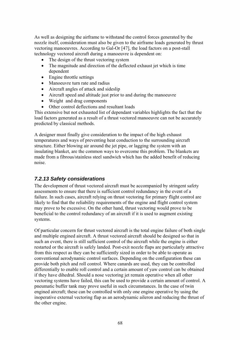
As well as designing the airframe to withstand the control forces generated by the nozzle itself, consideration must also be given to the airframe loads generated by thrust vectoring manoeuvres. According to Gal-Or [47], the load factors on a post-stall technology vectored aircraft during a manoeuvre is dependent on:

• The design of the thrust vectoring system • The magnitude and direction of the deflected exhaust jet which is time

dependent • Engine throttle settings • Manoeuvre turn rate and radius • Aircraft angles of attack and sideslip • Aircraft speed and altitude just prior to and during the manoeuvre • Weight and drag components • Other control deflections and resultant loads

This extensive but not exhausted list of dependant variables highlights the fact that the load factors generated as a result of a thrust vectored manoeuvre can not be accurately predicted by classical methods. A designer must finally give consideration to the impact of the high exhaust temperatures and ways of preventing heat conduction to the surrounding aircraft structure. Either blowing air around the jet pipe, or lagging the system with an insulating blanket, are the common ways to overcome this problem. The blankets are made from a fibrous/stainless steel sandwich which has the added benefit of reducing noise.

7.2.13 Safety considerations The development of thrust vectored aircraft must be accompanied by stringent safety assessments to ensure that there is sufficient control redundancy in the event of a failure. In such cases, aircraft relying on thrust vectoring for primary flight control are likely to find that the reliability requirements of the engine and flight control system may prove to be excessive. On the other hand, thrust vectoring would prove to be beneficial to the control redundancy of an aircraft if it is used to augment existing systems. Of particular concern for thrust vectored aircraft is the total engine failure of both single and multiple engined aircraft. A thrust vectored aircraft should be designed so that in such an event, there is still sufficient control of the aircraft while the engine is either restarted or the aircraft is safely landed. Post-exit nozzle flaps are particularly attractive from this respect as they can be sufficiently sized in order to be able to operate as conventional aerodynamic control surfaces. Depending on the configuration these can provide both pitch and roll control. Where canards are used, they can be controlled differentially to enable roll control and a certain amount of yaw control can be obtained if they have dihedral. Should a nose vectoring jet remain operative when all other vectoring systems have failed, this can be used to provide a certain amount of control. A pneumatic buffer tank may prove useful in such circumstances. In the case of twin engined aircraft; these can be controlled with only one engine operative by using the inoperative external vectoring flap as an aerodynamic aileron and reducing the thrust of the other engine.

68

7.2.14 A note on engine inlets for thrust vectoring systems Any engine/nozzle system must consider the effect which large pitch, yaw and sideslip angles have on the performance of engine intakes, since this will ultimately affect the performance of the engine. This is especially an issue for thrust vectored aircraft due to the increase of this effect during super manoeuvres and their reliant on engine power for aircraft control. The design of the intake needs to give consideration to the behaviour of the flow field surrounding the aircraft since this can have a significant impact on its performance. This is a particular problem or thrust vectored aircraft executing complex large angle of attack manoeuvres, since the flow field can become extremely distorted and complex. In such cases, a post-stall capable engine intake must be used since the engine is extremely susceptible to engine stall at these extreme flight conditions. Such inlet configurations are of variable geometry and be able to supply air from the upper and lower wing surfaces.

7.2.15 Flight and propulsion control systems The benefits of thrust vectoring are dependant on the effective control of the engine and nozzle in relation to the pilot’s requirements and the aircraft operating conditions. A selection of some of the requirements which such a flight/engine control systems must meet are,

• A properly designed flight and propulsion control system must be tailored to maintain the correct load/acceleration proportions relative to the pilot’s requirements.

• Thrust vectoring control forces must be governed to ensure aircraft and inhabitant limitations are not exceeded.

• Vectoring capability should be selectable by the pilot but then become transparent and its control integrated within the flight control system.

• Thrust losses due to vectoring must be accounted for by increasing the engine thrust as required.

• Allowance must be made for compressor stall margins since engine operating conditions can be directly affected by nozzle geometry via reflected pressure fluctuations.

• Allowance must be made for altitude effects which result in a reduction of engine power and therefore thrust vectoring control power.

• Partially vectored aircraft control systems must make allowance for the control force generated by the aerodynamic control surfaces.

• The thrust vectoring control system must take into account discrepancies between the deflection angles of the exhaust nozzle and exhaust plume.

• The effectiveness of the thrust vectoring system will be dependant on the aircraft operating conditions which must be allowed for.

• Allowance must be made for the response rate of the engine as well as that of the thrust vectoring nozzle to ensure that the system is able to act within the desired timeframe.

• Coupling effects must be allowed for between the payload, weapons, propulsion system and airframe. In such cases, the flight dynamics of an aircraft with and without external payload will be different and need to be accounted for.

69

A simplistic layout of such a control system is shown in the figure below, which highlights some of the interactions between the different systems.

Figure 7-3 [Ref 32]

7.2.16 Modification of existing aircraft Existing aircraft modified to incorporate thrust vectoring systems a subject to the same design considerations as those listed above. In this case however, the engineer must work within the constraints of the existing airframe which include volume, propulsion, mass and centre of gravity and flight control system constraints. For example, the addition of a heavy nozzle at the rear of the aircraft will need to be counteracted with ballast at its nose. The existing flight control system must also be replaced with one able to co-ordinate the control of the thrust vectoring nozzle with the conventional aerodynamic flight controls. Extensive testing of the modified aircraft configuration will then be required since the flight dynamics will be affected by the interaction with other components such as the wings. As already discussed, external vectoring systems will also work as aerodynamic control devices as well as being influenced by the external flow.

7.2.17 Integration of high aspect ratio nozzles High aspect ratio nozzles are able to offer benefits of super-circulation, reduced boat-tail drag and lower IR signatures. The nozzle aspect ratio has been shown by experimental testing to be the most important parameter for the performance of these nozzles. To be able to take advantage of the super-circulation phenomena, the nozzle must be integrated into the trailing edge of the wing. In such cases, the nozzle can be integrated in to the wing structure to reduce weight, with the wing skin and structure forming part of the nozzle. Streamlined-flow-distributors/struts may be required inside such nozzles to distribute the flow evenly, reduce swirl across the throat and exit areas and improve the structural strength. NAR does however have an impact on the overall length of the exhaust system, since the circular to rectangular transition sections will have to be extended to maintain a favourable internal flow distribution. Due to their increased heat transfer area, the transition ducts may require significant cooling. This can however be improved by the use of internal wing mixers and inlet passages for cooling airflows

70

8 Sizing and integration of the UCAV thrust vectoring system

8.1 Thrust vectoring system requirements for the UCAV Recent proposals have been made to utilise fluidic thrust vectoring devices for control and trim. Such a proposal is intended to reduce the trim drag associated with conventional control surfaces. Fluidic devices were envisioned as a means of being able to utilise the benefits of thrust vectoring without the many drawbacks associated with mechanical devices. However these devices have proven to be fraught with their own problems. These include unstable control regions, control dead zones and high secondary air flow requirements. The co-flow devices in particular have been shown to require a significant amount of secondary air which can only practically be obtained from engine bleed air. The use of engine bleed air is however accompanied with a decrease in engine performance and an increase in fuel consumption. This has raised the question whether such a task could be accomplished with a refined mechanical thrust vectoring system. Mechanical thrust vectoring systems have traditionally been envisioned as a means of generating vertical lift or enhancing the manoeuvring capabilities of an aircraft. The primary objective of this work is however to investigate the effectiveness of mechanical thrust vectoring systems for aircraft control and trim. The ideal mechanical thrust vectoring system is one which:

• Is mechanical and not fluidic. • Has a response time which is sufficient to meet aircraft control and dynamic

stability requirements. • Is able to offer a performance advantage compared to a conventional aircraft. • Preferably is light weight, low cost and simplistic. • Is safe and reliable • Has a sufficient degree of accuracy and repeatability

8.2 Selection of the candidate thrust vectoring system Our earlier review of existing thrust vectoring systems highlighted the fact the majority of mechanical thrust vectoring systems have a number of associative drawbacks. These include mass, complexity, maintenance requirements and cost. It is these drawbacks that prompted the research and development of fluidic devices. Since many of these mechanical devices were intended to enhance lift and/or manoeuvrability, they may be over-engineered for less demanding aircraft control and trim tasks. The result is that these systems will be overly complex, expensive and heavy. A system of particular interest to this study is the low cost paddles vectoring system as investigated by NASA for their X-31 and F/A-18 aircraft. This utilises post-exit paddles which are deflected into the exhaust flow in order to change the direction of the resultant thrust. This system was tested extensively on the X-31 and F/A-18, but was

71

later abandoned, probably with the advent of more refined devices which offered improved manoeuvrability. This system has however recently been receiving renewed interest on the Mitsubishi ATD-X as a low-cost mean to enhance the manoeuvrability of the aircraft. Compared to other mechanical thrust vectoring concepts, this system offers distinct benefits of being low cost and light weight. This work aims to answer the question, ‘can such a system be utilised to control and/or trim an aircraft and if so what are the benefits/penalties associated with it’.

8.3 An overview of the final thrust vectoring system The thrust vectoring system envisioned for this project is a re-scaled variant of that used for the X-31 and F/A-18. This consists of three large external thrust vectoring paddles which are equally spaced around the circumference of the exhaust nozzle exit. Each of these paddles is connected to a heavy duty hydraulic actuator which deflects the paddle into and out of the exhaust flow as required. The range of movement of each paddle is +35º to -60º. The control of each actuator must therefore be integrated into the flight control system if it is to be transparent to the pilot/operator. The paddle shells are constructed from a RCC (reinforced carbon-carbon) material which is affixed to a metallic (Nimonic) backing structure which is used to transfer loads to and from the mountings and actuator. A more detailed overview of the system will follow. Only the pitch control aspect of this system will be investigated as part of this study. This is however not restricted to control about the pitch axis and is also able to deliver yaw control by means of the simultaneous deflection of two paddles. The system is however unable to offer any significant roll control due to the lack of any significant moment arm and thus and alternative roll control device is required. A four paddle variant of this system was also investigated by NASA which utilised four equally spaced paddles instead of three. Although this is potentially easier to control with the need to deflect only 1 vane at a time, this was abandoned in favour of the lighter three paddle variant. While in flight, the thrust vectoring system can be shown to have sufficient control power to be able to moments about the aircraft’s centre of gravity which are sufficient to manoeuvre and trim the aircraft. During take-off and landing however it was envisioned that the thrust vectoring system would be used to generate an additional component of lift. In such cases an alternative means of aircraft control is required such as conventional aerodynamic control surfaces. If we are to meet the objectives of the BAE Grand Challenge (to eliminate conventional flight control surfaces), we must find a means to be able to dispense with conventional control surface. The aircraft was thus equipped with a nose jet control system which is intended to replace the function of the conventional aerodynamic pitch control surfaces. This system is only active during take-off and landing with the thrust vectoring system being used for control during all other flight phases. The nose jet pitch control system utilises engine bleed air to generate a downward thrust from two downward jets of air located at the nose of the aircraft. The downward thrust is generated by a pair of convergent-divergent nozzles which are located on either side of the nose landing gear within the nose gear bay. Upon retraction of the nose gear, the

72

nozzles are covered by the nose landing gear bay doors to reduce the drag of the aircraft. The nozzles are connected to the engine bleed port via ducting which runs down each side of the aircraft. The quantity of bleed entering each duct is regulated with a butterfly valve at the bleed port exit. The reader is advised to refer to Appendix B for a more detailed breakdown of the system components.

8.4 Design and sizing the vectoring and pitch control systems It the sections which follow, an overview will be given of the design process for the thrust vectoring and nose jet control systems. An introduction will also be given to the impact of these systems on the engine performance, which will give the reader an appreciation of the complexity of the design process. Included in Appendix C is an overview of detailed nozzle and inlet design which have been included to give the reader an appreciation of the complexity of the engine nozzle design task. We will however be utilising an existing nozzle concept for this study and will be concentrating on the integration considerations.

8.4.1 The inter-relation with the engine performance Neither the thrust vectoring nor pitch control system can be considered in isolation of each other or in isolation of the engine. In the case of the thrust vectoring system, each deflection of the exhaust nozzle results in a different exhaust nozzle configuration with different internal flow characteristics. This is however further complicated by the fact that the performance of a typical engine can also be shown to be influenced by the characteristics of the exhaust nozzle configuration. The engine configuration and its resulting performance will thus be dependent on the deflection of the thrust vectoring nozzle. In the case of the pitch control system, the total control force from the nose jet nozzles is dependent on the mass flow rate of engine bleed. The performance of the engine is however also dependent on the fraction of engine bleed. Thus, the performance of the engine is dependant on the total control force from the nose jets. Taking into consideration the relations discussed above, we can see that the thrust vectoring nozzle and nose jet will also be related via the engine performance. The reader is advised to refer to Appendices B and C for further details of these relationships.

8.4.2 Sizing the thrust vectoring system To be able to utilise the test results from NASA, it was essential that the geometry of the thrust vectoring system retains the original proportions specified by NASA. The approach adopted here for sizing the system was to generate a model of the system to the exact dimensions specified by NASA. This was then re-scaled so that the diameter of the jet pipe of the NASA model matches that of the UCAV. It should be noted that the loss coefficient of a duct will only be affected by variations in the geometry and/or flow conditions. It is therefore possible to linearly scale an existing duct design without affecting its loss coefficient. Thus, by linearly scaling the NASA thrust vectoring system, the original NASA test results will remain unaffected.

73

These results are however only valid for the flow conditions investigated in the NASA experiments. Although NASA did test the system over a range of flow conditions with the intention of covering all eventualities. However, a problem was uncovered when trying to utilise this data for this particular study. It was discovered that was a mis-match between characteristics of the unvectored nozzles (with no vectoring paddles installed) of the NASA test rig and the engine of our UCAV. Therefore, it was necessary to rescale the NASA test results so that the data for the unvectored test rig nozzle matches the characteristics of the unvectored nozzle of the UCAV. The reader is advised to refer to Appendix B for further details of this process.

8.4.3 Design of the nose jet pitch control system As already discussed, the pitch control system utilises air bled from the main engine to generate a vertical thrust at the nose of the aircraft. The system utilises an arrangement of valves and ducting to deliver the bleed in a controllable manner from the main engine to the convergent-divergent nozzles located in the nose landing gear bay. Butterfly valves located at the engine bleed port exits were selected as the best means of regulating the flow to the nozzles. Such valves offer benefits of precise control and fast response times. As a result of the range of operating conditions that the nozzle has to operate over, a variable area nozzle would have provided the best solution to keep the system as efficient as possible. However, such a nozzle would result in additional mass, volume and complexity and thus it was decided to opt for a fixed nozzle arrangement instead. The various components in the system were sequentially sized by an iterative process to achieve the desired flow conditions in each component. However, a full description of this complex design process is beyond the scope of this discussion and the reader is advised to refer to Appendix B for further details. An important design consideration is the point along the main engine at which the air is bled from. This not only influences the performance of the pitch control system but also the performance of the engine. Bleeding from the LP compressor is less detrimental to engine performance but the low pressure air does necessitate the need for large mass flow rates to achieve the desired control system thrust. This implies the need for large diameter ducting which has a greater weight and occupies more space within the aircraft. The low temperatures involved however mean that it may be possible to utilise composite sandwich ducting, in which case the sandwich core also acts as an insulation material. Bleeding from the HP compressor on the other hand generates higher pressure air which implies a smaller mass flow rate and thus smaller diameter ducting. This is however more detrimental to the engine thrust. The bleed air is however at a higher temperature which necessitates the need for high temperature ducting such as Nimonic Alloy 75. This ducting must however also incorporate expansion joints to relieve thermal stresses and be well insulated to protect surrounding equipment and structure. Insulation will however add weight and occupy a significant amount of space. The convergent-divergent nozzles are envisioned to be constructed from a nickel alloy.

8.5 The analysis of the vectoring and control systems The analysis of the thrust vectoring is concerned with determining whether such a system is able to offer any benefits in performance at the take-off, cruise and landing

74

phases. In the case of the take-off and landing phases, we are primarily interested in whether the take-off and landing field lengths could be reduced. At cruise we are interested in whether a reduction in the drag and thus the fuel consumption of the aircraft could be realised. The reader is advised to refer to the evaluation section of this thesis for a more detailed discussion of this analysis work. In order to be able to carry out these evaluative studies, we need to generate a number of representative analytical models to determine:

• The specific fuel consumption of the engine as a function of the nozzle vectoring angle and nose jet force at take-off and landing conditions.

• The maximum available engine thrust as a function of the nozzle vectoring angle and nose jet force (via the engine bleed) at take-off and landing conditions.

• The vertical thrust from the nose jet pitch control system as a function of engine bleed at take-off and landing conditions.

• The engine throttle setting as a function of the nozzle vectoring angle and engine thrust at cruise conditions.

• The specific fuel consumption of the engine as a function of the nozzle vectoring angle and engine throttle setting at cruise conditions.

The generation of such analytical models requires detailed knowledge of the engine operating characteristics and how these are affected by variations in parameters such as the nozzle characteristics and engine bleed setting. Such engine data can however only be realistically be predicted from an engine simulation model due to the complexity of the inter-relation between all the different engine components. One such engine simulation model is the AEDsys package developed by Mattingly [16], as was used for this study. This is an engine conceptual design package which requires minimal component level knowledge of the engine. It has proven to be sufficient to predict the performance of the engine over a range of engine operating conditions (off-design conditions) and is thus well suited to this study. The engine analysis work utilised a baseline engine performance model which was representative of the unvectored engine configuration. This model could then be modified as required to take into account the variations in each of the engine parameters being studied. At cruise for example we would have a different engine model for each nozzle vectoring angle (and thus nozzle configuration) being investigated. The analysis is somewhat more complicated at take-off and landing as we will have a different model for each nozzle deflection angle and each engine bleed setting. Each on-design model can finally be tested over the range of off-design flight conditions of interest to generate the required database of test results. The required analytical models can finally be generated by fitting a polynomial expression to each data set in the database. In the case of take-off and landing, it was necessary to derive additional correction factors to take into account for variations in engine performance as a result of variations in the speed of the aircraft. The reader is advised to refer to Appendix C for further details of the engine design and analysis work.

75

8.6 Integration of the vectoring and pitch control systems This section gives an overview of the integration of the thrust vectoring and nose jet pitch control systems. As with the modification of any aircraft configuration or integration of any systems, consideration needs to be given to general design considerations. These include aircraft stability and control, component positioning and space allocation within the airframe, mass, aircraft performance and additional power-off takes. An overview of initial engine installation considerations has been included in appendix C as background reference material for the reader.

8.6.1 The integration of the thrust vectoring system As already mentioned, the thrust vectoring system was sized by rescaling a model of the system proposed by NASA. The model was constructed to the exact dimensions specified by NASA and then re-scaled to match the diameter of the jet pipe of the UCAV. This system was then integrated onto the aircraft whilst keeping the same relative position of the paddles with respect to the jet pipe as specified by NASA. The most significant integration consideration which had to be taken into account was the additional length of the paddles. If the paddles were to be simply retro-fitted on the end of the nozzle of the conventional UCAV then there is a risk that they could come into contact with the ground during high angle of attack manoeuvres. The aft fuselage thus needed to be shortened so that the aft point of the paddles is within the bounds of the original length of the fuselage. The other main integration consideration is the provision of sufficient surrounding aircraft structure to provide mountings for the vectoring paddles and hydraulic paddles actuators. The degree of any elasticity in the structure must be determined and accounted for by the thrust vectoring control system.

Figure 8-1 to 8-4 – External views of the paddles thrust vectoring system installed in the UCAV

76

Figure 8-5 to 8-8 – The accompanying paddles supporting structure, alignment relative to the jet pipe and an exploded and sectional view of the assembly

8.6.2 The integration of the nose jet pitch control system Integration of the nose jet pitch control system is primarily concerned with determining the most efficient ducting runs between the main engine and the pitch control nozzles at the front of the aircraft. The high temperature of the ducting means that particular consideration needs to be given to routing it away from sensitive equipment. Allowance also needs to be made for the volume occupied by any insulation material. The two nozzles are themselves located one on either side of the nose landing gear, within the nose gear bay. As the nozzles are only required for take-off and landing, they are thus concealed for all other flight phases to keep the drag of the aircraft to a minimum. The most significant sources of loads in this system are expected to be due to pressure and momentum changes at bends and regions of cross-sectional area changes. In addition, allowance needs to be made for the hoop stress in the ducting due to the internal pressure. Thermal loads can be assumed to be insignificant due to the incorporation of expansion joints into the ducting runs.

Figure 8-9 and 9-10 – The layout of the pitch control system and location of the nose jets

77

9 Fuel cells literature review

9.1 An overview of fuel cells and their working principles

9.1.1 What is a fuel cell? Fuel cells were invented in about 1840 but have recently been revived as an ideal candidate in the search for an alternative power source. These electrochemical devices generate an electric current as a result of a chemical reaction between a fuel (typically hydrogen) and an oxidant with the only by-products of the process being heat and water. Since no combustion takes place, efficiencies of more than twice that of a conventional IC engine are possible. As shown in the figure below, a fuel cell system consists of a stack of identical cells which are combined to achieve the desired power output. Each individual cell assembly consists of an electrolyte membrane which is sandwiched between two catalyst impregnated anode and cathode electrodes. This basic cell is further sandwiched between two bipolar plates which are used to deliver the reactants to the working fuel cell. The sizing of a fuel cell stack is considerably simpler than for an IC engine since the power output of the stack is simply a function of the number of cells used.

Figure 9-1 - The components of a fuel cell stack [48]

9.1.2 Fuel cell working principles It should be noted that the electrochemical reactions which take place at each electrode vary according to the fuel cell type and therefore the electrolyte used. This discussion will however be restricted to the most common type of fuel cell, which is the acid electrolyte hydrogen fuel cell. The working principles of a fuel cell are best understood by examining a cross-section through an anode/membrane/cathode cell assembly as shown in the figure below.

78

Figure 9-2 – Fuel cell electrochemical reactions [49, p84]

The overall chemical reaction for a hydrogen fuel cell is 2H2 + O2 → 2H2O which is the result of the separate chemical reactions at the anode and cathode. At the anode there is the chemical reaction 2H2 → 4H+ + 4e- which ionises the hydrogen to release electrons and create H+ ions. At the cathode, there is the reaction O2 + 4e- + 4H+ → 2H2O where H+ ions from the electrolyte and electrons from the anode react with oxygen to form water. In order to sustain the chemical reactions, an external electrical circuit is required to supply a continual supply of electrons at the cathode from the anode. This external flow of electrons can be utilised by connecting an external load across the electrodes. The H+ ions required from the anode are transported to the cathode through the electrolyte which is sandwiched between the two electrodes. In this case, two hydrogen molecules are required for each oxygen molecule in order to maintain the reaction process.

9.1.3 The potential benefits of fuel cells Fuel cell systems have many benefits in comparison to conventional internal combustion engines, as discussed below,

• Higher efficiency – Fuel cells have been shown to be considerably more efficient than IC engines (approx. 50% vs. 15%). Their efficiency is expected to rise to about 60% in the future, as a result of their ongoing development.

• Wider efficiency band – The maximum efficiency of an IC engine is limited to a narrow operating range, but fuel cell engines show flatter results with a high efficiency being possible of a wide range of operating conditions.

• Modularity – IC engines are of fixed size and require considerable design effort to rescale them to meet different power requirements. Fuel cell stacks can, however, easily cater for a wide range of power requirements by varying the number of cells within the stack. Where required, more than one fuel cell stack can be used which gives an endless range of possibilities.

• Safety – The modularity of fuel cell assemblies means that failure of a single cell will only result in a small degradation of performance and not total loss.

• Fuel flexibility – Fuel cells are not restricted to pure hydrogen and with the necessary additional equipment they are capable of handling a wide variety of hydrogen based fuels including conventional hydrocarbons.

• Zero emissions when using hydrogen – The emissions from a fuel cell operating directly on hydrogen are zero but the environmental impact of the production of the hydrogen must be taken into account.

79

• Low emissions when using fuel reformers - The use of on-board reformers to generate hydrogen still show considerably lower emissions compared to IC engines. CO2 is typically a third of that of an IC engine and other emissions such as CO, NOX, SOX, and HC are reduced to levels that are undetectable

• Low noise – Since the basic fuel cell has no moving parts and its function does not involve a combustion process, their noise output is less than that of an IC engine. The main sources of noise within a fuel cell system originate from the accompanying balance of plant such as compressors.

• Ready supply of waste heat - A by-product of the electrochemical process is heat, which can then be used for other processes or for onboard equipment such as fuel reformers. The utilisation of this waste heat can increase the efficiency of the system as a whole and reduce emissions.

• Rapid load following capability – Fuel cells are capable of immediate response to changes in demand.

9.1.4 Challenges still to be overcome The cost, size and weight of fuel cells and their associated systems is at present inferior to conventional IC engines. The current technical progress of fuel cells is a major drawback for their vehicular use and additional research effort is required. To reduce costs current manufacturing processes must also be reviewed. Pure hydrogen is the preferential fuels but practical constraints dictate the use of other fuels which can be vulnerable to fuel tolerance issues. These are a major cause for concern since fuel contaminants can have a direct impact on fuel cell performance and lifespan. The use of other fuels also dictates the need for a fuel reformer but such systems are not as efficient as using pure hydrogen systems and further development work is required. Although the emissions from fuel cells are low, their operation at high altitudes can still present environmental issues since the water by-product (in a steam state) has been shown to be a greenhouse gas in itself. One approach to prevent this would be to fly at a lower altitude so that the output steam is able to return to its liquid state in the atmosphere. Where this is not possible, the water can be captured and stored. This will increase the landing weight of an aircraft but it may be possible to utilise some of the water onboard the aircraft or dump it just before landing.

9.1.5 Rival hydrogen powered propulsion systems Hydrogen can not only be used as a fuel in fuel cell engines but also as a fuel in conventional IC engines. In such engines, emissions such as CO, CO2 and HC are negligible with only NOX remaining. When allowance is made for power off-takes, the efficiency of a fuel cell is less than initially predicted and a hydrogen IC engine with a hybrid power train could prove to be a considerably competitive alternative. Such engines would also offer the benefits of technological maturity, reduced cost and complexity. Fuel cells however still offer a better efficiency and lower emissions making them the ultimate long term solution. In the short term however, hydrogen fuelled IC engines are a logical step in the right direction.

80

9.2 The different types of fuel cells

9.2.1 Electrolytes and membranes of the different fuel cell types Numerous different fuel cells have been explored over time which can be characterised according to the electrolyte that they use and the accompanying reactions. The most common fuel cells types and their application in industry are summarised below.

Table 7-1 – A summary of the different fuel cell types [49, p85]

The electrolyte used will influence the nature of the reactions which take pace as well as the type of fuel which can be used. The most effective electrolytes to use are those with free H+ ions, such as acids. Certain polymers called ‘proton exchange membranes’ also contain mobile H+ ions and work in a similar way to the acids. Such electrolytes are fundamental to the operating principle of the fuel cell as only the H+ ions are able to pass through and not electrons. This forces the electrons travel around the electrical circuit as opposed to through the electrolyte in order to complete the reaction. An overview of the common fuel cell types is given in the sections below.

9.2.1.1 Alkaline fuel cell (AFC) The low operating temperatures (less than 100˚C) of alkaline fuel cells has made them particularly attractive for vehicular use. They have already been successfully used in a number of demonstrator vehicles as well as on both the Apollo and the Shuttle orbiters. They however suffer from slow reaction rates and electrodes with an embedded platinum catalyst are typically used as a result. Both of the reactant gas streams must also be scrubbed before entering the fuel cell in order to remove carbon compounds. This typically involves passing the gases through precious metal membranes which requires a considerable pressure difference and adds additional complexities to the system. Compared to PEM fuel cells, the alkaline fuel cell is considerably cheaper but their power output is lower and PEM fuel cells are more favourable as a result.

9.2.1.2 Phosphoric acid fuel cell (PAFC) These were the first commercial fuel cells and there are currently many PAFC systems successfully operating in Europe and the USA. Their higher operating temperatures (of about 220˚C) result in start/stop and high thermal inertia problems. These systems have

81

proved their worth in fixed applications which require a steady continual operation such as generators for decentralised stationary power systems. They can also be used in ships and locomotives but are not a particularly viable solution for other vehicles.

9.2.1.3 Solid oxide fuel cell (SOFC) SOFC’s consist of a solid zirconia based electrolyte sandwiched between a nickel and YSZ (yttria-stabilised zirconia) anode and a LaSr (strontium and lanthanum) and magnesium oxide cathode. They have a high power density and typically operate at temperatures in the region of 600-1000˚C while remaining in a solid state. Their high temperature makes them more tolerant to fuel impurities and means that they are able use hydrocarbon fuels directly without a reformer. This also allows high reaction rates to be achieved with expensive catalysts. They are currently being used for stationary power applications (up to 10MW) but are also currently being investigated a replacement for aircraft APU’s (as a result of their ability to run directly on kerosene). The SOFC unfortunately needs to be manufactured from ceramic materials which makes them expensive to manufacture and causes handling problems. Their high operating temperature means that longer starting times are required and PEM fuel cells are more favourable for vehicle applications. A variant of the SOFC is the protonic ceramic fuel cell but this is not common.

9.2.1.4 Molten carbonate fuel cell (MCFC) The MCFC is set apart from the other fuel cell types in that it typically operates with carbon dioxide. This is another high temperature fuel cell which uses a corrosive complex lithium, potassium and sodium carbonate electrolyte mixture and is only really suitable for large systems of continual operation. The high operating temperature means that expensive catalysts are not required to achieve high reaction rates and conventional gases can be used without an onboard fuel reformer. They have the same response characteristics as the PAFC and are well suited to the same stationary and steady operation applications.

9.2.1.5 Polymer electrolyte membrane fuel cell (PEMFC) PEM fuel cells are one of the simplest types of fuel cell. They use a solid polymer (mobile proton) electrolyte which results in a reaction process the same as that for an acid electrolyte fuel cell. Their low operating temperature necessitates the need for novel electrodes and catalysts to overcome otherwise slow reaction rates. Very small amounts of platinum are typically used as the catalyst with effort being expended to reduce the amount required and therefore further reduce the costs. Of particular concern to these fuel cells is the presence of CO which is damaging to the platinum catalyst and new platinum-ruthenium-tungsten catalyst compounds are being developed to overcome this problem. A more recent novel technique involves using electrical pulses to raise the potential of the anode which oxidises the absorbed CO into CO2. Water management is also difficult especially with larger stacks, which can limit the size of a stack. These were originally used for the short Gemini space missions but early problems associated with their extended use led to the use of alkaline fuel cells for the Apollo and

82

Space Shuttle missions. They have since seen considerable improvement and the added benefit of a solid electrolyte has led to them being the most commonly used type for vehicular applications. As a result of the impressive recent developments, NASA has decided to replace the AFC systems on the space shuttle with PEMFC systems.

9.2.1.6 Direct methanol fuel cells (DMFC) Methanol has recently been considered as a particularly attractive alternative to pure hydrogen. Its use within indirect methanol fuel cells necessitates the need for an accompanying fuel reformer to extract the hydrogen. Direct methanol fuel cells have the ability to use the liquid methanol directly without having to extract the hydrogen first. The fuel system is therefore much simpler and humidification and thermal management systems are not required either since a controlled mixture of methanol and water is used as both the fuel and coolant. They are not as efficient as other fuel cell types due to fuel being able to travel straight through the membrane without reacting by means of concentration gradient diffusion and proton migration electro-osmotic drag (fuel crossover). A suitable catalyst is also required as a result of sluggish kinetics. DMFC’s are not as developed as other systems and are only currently of very low power output and therefore only suitable for low power applications such as portable electronic equipment. Daimler has however already successfully tested a 3kW go-kart and they do show potential to be used in vehicles in the future with further development work.

9.2.2 Recommended systems suitable for propulsion As well as being the most technically advanced, the PEM fuel cell has for some time been regarded as the type currently showing most promise for mobile applications. Compared to other types, they offer benefits of low operational temperatures (40-100 degrees), short transient and start-up periods and respectable efficiencies. The SOFC has also received significant interest for vehicles as a result of their higher efficiency and better tolerance of fuel impurities. They are however presently not viable due to their higher operating temperature and lower power densities. However, on-going development work may make them more viable in the near future. At present, the majority of fuel cell powered cars use the PEM fuel cells and they have also been shown to be an excellent choice for the aerospace industry.

9.3 The PEM fuel cell in greater detail

9.3.1 Predicting the efficiency of a fuel cell In this analysis, the fuel cell can be considered as a black box with hydrogen and oxygen entering and electrical energy, heat and water leaving. In such studies, it is typical to use a parameter known as the Gibbs free energy which is defined as the energy available to do external work. The Gibbs energy, which is dependant on the temperature and state of a substance, is determined for the reactants entering and the products leaving the fuel cell. The energy released from the fuel cell is then taken as the difference between the Gibbs input and the Gibbs output. In order to be able to accurately compare the efficiency of a fuel cell with that of an IC engine, the change in enthalpy of formation of the products is typically used instead. This the electrical

83

energy output of the fuel cell to be compared to the heat that would be produced if the fuel was burnt as in an IC engine. The comparable efficiency of the fuel cell can then be determined as the ratio of the electrical energy produced per mole of fuel to the change in enthalpy of formation. The change in enthalpy of formation is dependant on weather the final state of the products of the reactions are a liquid or gas. The maximum efficiency of the fuel cell (comparable IC engine carnot limit) can be determined for a fuel cell from the following equation, which assumes that the electrical energy equals the Gibbs energy.

%100)( ⋅ΔΔ

=HG

MaxFuelCellη Eq 9-1

This is dependant on the operating temperature of the fuel cell with a drop in efficiency and EMF typically being experienced with an increase in temperature. The operating temperature must therefore be chosen with care with a figure of 80ºC being typical for vehicular PEM fuel cells. In the ideal case of 100% efficiency, the maximum voltage obtainable for a single cell is 1.48V for the higher heating value (HHV) of hydrogen or 1.25V for the lower heating value (LHV). The efficiency of a single cell can then be determined by inputting the average voltage of one cell into the equation below.

%)100(Cell

CellFuelCell V

V=η Eq 9-2

The maximum voltage of a fuel cell is obtained when 100% of the Gibbs free energy is converted into electrical energy as given by the equation below (F = Faraday constant).

FGVMax ⋅

Δ=

2 Eq 9-3

9.3.2 An introduction to fuel cell operating characteristics The operating characteristics of a fuel cell are governed by internal resistances which cause a voltage drop proportional to the current being drawn. An example of typical fuel cell operating characteristics is shown in the figure below.

Figure 9-3 - Typical fuel cell polarization curve [Ref 49]

84

Three characteristic operating regions are apparent from the voltage drop curve in the above graph, which are.

1. The initial rapid voltage drop at low currents is referred to as the activation energy, which is the energy required to maintain the reactions at the electrodes.

2. The steady linear voltage drop which dominates the fuel cell characteristics is referred to as the ohmic voltage loss, which is a result of the resistance of the electrolyte and electrodes.

3. The increased voltage drop at high currents is referred to as the ‘concentration voltage loss’. This results from a reduction in available oxygen to complete the reaction as a result of a build-up of remnant nitrogen from the air.

Continual research and development effort is aiming towards a reduction in these voltage losses but at present a typical fuel cell voltage is approximately 0.65-0.7 V (for currents up to 1A per cm2). This corresponds to an efficiency of about 50% (HHV) which is further reduced when allowance is made for balance of plant power off-takes. In contrast to an IC engine, as can be seen from above, a fuel cell is capable of high efficiencies at low power outputs and therefore has a wider useful operating range.

9.3.3 Impact of pressure and concentration on fuel cell performance In addition to operating temperature, the performance of a fuel cell is also affected by operating pressure, which also has an impact on the values of Gibbs free energy. Likewise, gas concentration will also have a similar impact on the Gibbs free energy. For a pressure change from P1 to P2, the resulting voltage change can be predicted by the Nernst equation below.

⎟⎟⎠

⎞⎜⎜⎝

⎛⋅

⋅⋅

=Δ1

2ln4 P

PFTRV Eq 9-4

This expression is however most suited to high temperature fuel cells as it under predicts the voltage drop of low temperature fuel cells (such as PEM). This discrepancy is related to activation energy which has in this case been shown to be influenced by both pressure and concentration. In practice, allowance must also be made for the power off-take of an air compressor which is required to generate the pressure and thus voltage increase. Fuel cells intended for vehicle applications generally operate at pressures of 1.5 - 2.0 bars primarily to aid the balance of water within the cell.

9.3.4 The impact of fuel and air quality on fuel cell performance In addition to temperature, pressure and gas concentration, other factors which are likely to result in degradation in fuel cell output voltage and therefore performance are,

• The use of air instead of pure oxygen. • The use of hydrogen based fuels as opposed to pure hydrogen. The hydrogen

obtained from reforming fuels such as methanol is typically diluted with CO2.

9.3.5 Water management The fuel cell cathode is not only used to deliver oxygen to the fuel cell membrane but is also used to expel the water which is formed as a by-product of the electrochemical

85

process. The continual flow of air that is fed to the electrode evaporates off and then carries the excess water out of the fuel cell. It is however critical that the level of hydration in a PEM fuel cell is carefully maintained at the correct level to avoid a degradation in its performance. It can be shown that the proton conductivity of the electrolyte is directly proportional to the electrolyte water content and insufficient water will result in a loss in performance. Too much water on the other hand will block the pores in the electrodes or the gas diffusion layer as a result of flooding which will also result in a loss in performance. In a small number of situations water, which is produced at the cathode, is able to diffuse through the thin electrolyte membrane and keep the whole system suitably hydrated. This is, however, difficult to control due to water molecules migrating in the opposite sense by electro-osmotic drag and the drying effect of fuel cell operating temperatures. In practical PEM fuel cell systems however, the air and/or hydrogen are humidified by injecting water in to them prior to them entering the fuel cell. It is necessary to use pure water for this process and it is typical to condense and recirculate water from the water vapour exhausted from the fuel cell. Fortunately, higher operating pressures not only increase the performance of the fuel cell but also slightly alleviate the problem of electrolyte drying. This means that less additional water vapour is required to keep the electrolyte hydrated.

9.3.6 Thermal management Compared to IC engines, fuel cells are more efficient and generate less heat but have more waste heat to dispose of. Whereas IC engines are able to dispense an significant proportion of their waste heat via their exhaust, the waste air exiting the fuel cell will only be at about 85ºC and will therefore carry little waste heat. IC engines are also able to dispense heat by forced convection and radiation from the external surfaces; this is however less effective for fuel cells due to their cooler external surfaces. There are therefore fewer mechanisms for the removal of excess heat from a fuel cell compared to an IC engine and the performance requirements of a fuel cell cooling system are greater as a result. Small fuel cells (up to 100W) can be sufficiently cooled by supplying excess air to the cathode to remove the waste heat. At higher powers the cooling air flow requirements become excessive leading to excess water evaporation and unfavourable drying of the electrodes and electrolyte. Alternative cooling methods are therefore required for larger fuel cell systems. Medium sized fuel cells (up to 2-3kW) may be cooled by passing an additional cooling air flow through dedicated cooling passages in the bipolar plates. Such an arrangement is shown in the figure below.

86

Figure 9-4 – The arrangement of reactant and coolant passages in a stack [49]

In the case of large fuel cells (over 2-3kW) the cooling air is substituted with cooling fluids (such as water), in order to maintain even cooling. The cooling water is re-circulated through a radiator which considerably larger than for an IC engine since typically twice as much heat needs to be dispersed.

9.4 Fuel cell construction

9.4.1 The main parts of a fuel cell Each single fuel cell assembly consists of membrane electrolyte sandwiched between anode and cathode electrodes. These are typically 1mm thick, which is made up from:

• 0.03mm thick anode and cathode electrode plates • 0.2 – 0.5mm anode and cathode gas diffusion layers. • A 0.05 to 0.1mm sandwich layer of electrolyte.

The most common arrangement for a fuel cell stack consists of a series of flat plates which are clamped and sandwiched together. To alleviate the sealing problems associated with the planar designs the different layers can be built as a series of concentric circles to create a tubular design. The planar configurations typically have higher power densities and will be the only type considered here.

9.4.2 Fuel cell electrodes The reactions which take place between all the fuel cell elements take place on the electrode surfaces. These reactions are however typically too slow to produce a significant current and therefore power output, which must be improved by:

• Increasing the area of the electrodes. For this reason, the performance of a fuel cell is typically expressed in terms of the current per cm3. Porous surfaces enable the electrode area to be increased when viewed on a microscopic level.

• Increasing the operating temperature of the fuel cell. This is beneficial to the reactions but long start-up times are required and the transient operation is poor.

• Coating the electrodes with a catalyst layer to provoke the reaction. The catalyst required is specific to the fuel cell, with platinum typically being used for PEM

87

cells. Catalysts can however (especially platinum) be very expensive and it is necessary to use them sparingly.

Within PEM fuel cells, very fine particles of the catalyst are typically supported within a surface layer of carbon particles which is connected to the electrode surface by means of a porous but highly conductive gas diffusion layer. This allows the contact between the reactants and catalyst to be maximised while maintaining a good electrical contact between the parts of the electrode. At the cathode, the gas diffusion layer also allows the water by-product to be removed. Carbon based materials such as carbon felt or carbon paper are normally used for this purpose. A certain amount of the electrodes typically extends beyond the catalyst to further increase the contact with the reactants.

9.4.3 Fuel cell membranes The best and most common material used for the polymer electrolyte membranes of PEM fuel cells is the fluoroethylene material Nafion. Fluoroethylene materials are particularly suited to such an application since:

• They offer a high resistance to chemical attack • They offer good mechanical strength and durability, which allows them to be

manufactured in very thin films of down to 50μm • They are good proton conductors. When the material is kept well hydrated the

H+ ions are able to freely move within the material. • They are highly hydrophobic. This material property is particularly beneficial to

operation of fuel cells as it promotes the expulsion of water from electrodes and therefore helps to prevent flooding.

The main disadvantages of the material are, it is expensive to manufacture and must be kept sufficiently hydrated for the electrolyte to function properly.

9.4.4 Fuel cell manufacture and construction The construction of a fuel cell stack consists of the assembly of a number of repeating fuel cell units to achieve the desired power output. The cells in a stack are connected in series whereby the anode of one cell is connected to the cathode of the next and so on Careful connection between the cells is however required if significant voltage drops as a result of the connections between cells is to be avoided. The layout of a single cell within a stack is shown below, which shows the grooved backing plates which are used to channel the gases and make electrical connection with the electrodes.

88

Figure 9-5 – Reactant channelling within a stack [49]

The backing plates are typically manufactured from either Stainless Steel or Graphite. These materials each have their benefits and drawbacks: Stainless Steel plates face problems of corrosion while Graphite plates are brittle and require careful manufacture. When used within a stack, they have grooves on both sides to produce a ‘bipolar plate’ which is used to link the anode and cathode of adjacent cells, while keeping the supply gases safely separated. A bi-polar plate is typically made larger than the electrodes and also used to channel the gases though the complete stack. This significantly simplifies connections to the fuel cell stack, as only electrical and gas connections need to be made on the end plates of the stack. The porosity of the electrodes results in an additional complication when fuel cells are clamped together within a stack, since gas leakage will occur if the edges of the electrodes are not properly sealed. It is typical to increase the size of the electrolyte layer and use a sealing gasket around the edges of the electrodes to prevent such leakage, as shown in the figure below.

Figure 9-6 – Exploded view of a fuel cell membrane-electrode assembly [49]

89

The complexity of the bi-polar plates is further increased when additional passages are incorporated for a cooling medium. In such cases, each bi-polar plate normally has to be manufactured in two halves in order to be able to manufacture the cooling channels which results in an increase in cost, weight, size, complexity and the number of component joints.

9.5 High altitude fuel cell operation

9.5.1 Introduction Until now the use of fuel cells has been primarily limited to sea level applications. Operation of a fuel cell at higher than atmospheric pressures is already well understood for its performance benefits. Until now, there has been little research effort for cases where they are operated at lower than standard sea level atmospheric pressure conditions. This is because until now fuel cells have only been used for sea level installations and since degradation in performance is expected at such operating conditions, they have generally been avoided. Along with the interest in the use of fuel cells in the aerospace industry is the need to investigate their performance under low pressure conditions. The research efforts that have been carried out in this area will be discussed in a later section.

9.5.2 Low pressure fuel cell applications There are already a small number of fuel cell installations which operate within low pressure environments such as on the Apollo and space shuttle orbiters and the Boeing fuel cell demonstrator aircraft. These have however relied on high pressure bottled oxygen and hydrogen and thus have ignored the problem of low pressure operation. GA aircraft and UAVs operating at low altitudes are unlikely to see a serious deterioration in the performance of a fuel cell using atmospheric air. The effect of much higher altitudes will be more significant and any performance degradation can no longer be ignored. Operation under such conditions is likely to necessitate the need for a larger fuel cell, resulting in increased cost, complexity, volume and weight.

9.5.3 De-rate performance prediction methods A number of manufacturers currently specify altitude ‘de-rate’ factors for the un-pressurised operation of their fuel cells at altitude. An example of such a de-rate factor would be a power output decrease of 1.5% per 1000ft for altitudes above 1000ft. These are however generally only applicable for altitudes up to 10,000ft and therefore are not applicable to typical aircraft cruising altitudes of 20,000+ft.

9.5.4 Current low pressure operation research efforts It is evident that, for fuel cell powered aircraft to become viable some form of reliable analytical method is required to predict the performance of a fuel cell at high altitudes. Such a tool would enable the performance of the fuel cell to be accurately predicted not only at high altitudes but throughout the complete flight profile. In order to meet

90

airworthiness requirements, fuel cells must also demonstrate that they are reliably able to produce sufficient power even under the most hostile of environments. Three research efforts which have been aimed at bridging this gap in knowledge will be discussed in the sections below.

9.5.4.1 Cessna-Boeing aircraft battery replacement research In this project, fuel cells were investigated as a replacement for the batteries used on-board aircraft. Experimental tests were carried out on a Ballard Nexa 1.2kW PEM fuel cell within a basic altitude test chamber, which showed a net power decrease from 1300W at sea level conditions to 970W at 5000ft. The air supply was identified as being responsible for the power loss.

9.5.4.2 U.S. Environmental Protection Agency high altitude fuel cell bus operation

This research was conducted as was part of phase 2 of the Ballard fuel cell bus research programme. Its powerplant consisted of 20 13kW PEM fuel cells which were tested at an altitude of 7400ft in Mexico City. Operation at this altitude showed a 24% decrease in current compared to equivalent operation at sea level conditions. The research also identified the air supply system to be responsible for the power loss.

9.5.4.3 General high altitude research by the National Fuel Cell Centre (NFCC) The aim of this project was to investigate how the performance of a fuel cell is affected by variations in both ambient pressure and oxygen concentration. This is the most significant contribution to high altitude fuel cell operation. A summary of this research is presented below but further details can be obtained from Ref [50].

9.5.4.3.1 Experimental testing and analysis This involved the experimental testing of an annular type PEM fuel cell (supplied by DCH Enable Fuel Cell Corp.) at a range of pressures from 0 to 53,500ft within a vacuum chamber. The air was cooled by means of cold boil-off nitrogen gas fed to a flat plate heat exchanger and the relative humidity was controlled by means of a desiccant dryer system. Ultra-high purity hydrogen was used. The results were later compared to current theoretical analyses to offer possible explanations for the mechanisms that govern such behaviour. The results presented a distinction between voltage losses due to concentration changes and voltage losses due to total pressure reductions. For the same percentage reduction, total pressure reductions are shown to have the greater effect on performance. The concentration of oxygen in air is constant for altitudes up to 262,000ft and total pressure is typically the main contributor to reduced performance. Limitations of the analysis methods meant that the results were only analysed up to 35,000ft. Oxygen concentration was varied by changing the airflow and thus the stoichiometric ratio but this is complicated by the fact that it is also dependant on the water content of the

91

cathode. In these experiments, neither of these varied by an amount considered to be significant.

9.5.4.3.2 Results The results obtained are valid for the 15-70% humidity range and inlet air temperature range of -60 to +20˚C. The results were initially obtained as a number of voltage vs. current curves for a number of different pressure and airflow combinations. In such tests, the fuel cell was operating in the transition region, where its characteristics are dominated by activation and ohmic losses. These results showed airflow to have little effect at high pressures but a large effect at low pressures, which led to the development of the Air Flow – Pressure interaction contour graph below.

Figure 9-7 – Results from the study into the performance of fuel cell at high altitudes [50]

As can be seen, this voltage drop with decreasing airflow can be considered to be less significant at high pressure than low pressure conditions.

9.5.4.3.3 Theoretical analysis The effect of high altitude conditions on a fuel cell are thought to be a result of variations of both the Nernst potential and cell polarizations which will reduce the voltage and efficiency of the fuel cell for a given power setting. The theoretical analysis is based on a form of the Nernst equation below, which is presented in terms of the total pressure of the anode and cathode. This expression shows the performance of the fuel cell to be dependant on partial pressure, which itself is dependant on both concentration and total pressure.

( )OpH

pOpHnFRTEE

2

21

220 ln+= Where, TPxOpO 22 = Eq 9-5 and 9-6

92

93

The Nernst equation is insufficient on its own and irreversible losses such as activation, ohmic and mass diffusion also need to be accounted for. These are however dependant on the regime within with the fuel cell operates and have also been shown to have an effect on whether it is the concentration or total pressure that is the most relevant. Total pressure has been shown to be more significant than concentration at low current densities. The theoretical analysis predicts that the voltage loss should be equally affected by either a change in the total pressure or concentration. This is however not what has been observed in practice, with total pressure having a greater influence on the voltage than the oxygen partial pressure. Reductions in both concentration and total pressure also gave rise to losses greater than predicted and further work is required in this area. Experimental results therefore remain the most reliable at present.

9.5.4.3.4 Evaluation of the research effort The author of this thesis conducted an in-depth review of the results presented for this research effort with a view to fitting a convenient analytical expression to the results. In the process however it was discovered that the results were unreliable due to temperature variations during testing. These results were therefore not used for this project. Full details of the evaluation of the results and the derivation of the general analytical expression are given in Appendix F.

9.5.5 Fuel cells – Design for high altitude operation Where fuel cells are operated under high altitude conditions a number of design features can be implemented to tailor them for improved performance under such conditions. Such modifications include:

• Modifying the electrolyte concentration in the catalyst layer to improve mass diffusion at low pressures.

• Optimise the catalyst layer thickness for low pressure conditions. The design operating region on the V-i curve not only has an impact on the reaction rate but also has a significant impact on the optimal catalyst layer design. Thicker catalyst layers are favourable for low current operation but result in increased total pressure losses and are therefore less suitable for low pressure operation. Thinner catalyst layers are favourable for high current operation and low pressure operation but result in lower reaction rates.

• Design of the fuel cell backing layer with respect to oxygen concentration. It is independent of total operating pressure.

10 Fuel cell research projects

10.1 An overview of fuel cell development The first serious use of mobile fuel cells was for space missions onboard the 1960’s Apollo Orbiter. More recently fuel cell technology has received serious interest for stationary power generation, automotive propulsion and small scale electrical equipment power supply. Their continual development has resulted in significant improvements in performance, weight, volume and cost. Their continued improvement has now reached a stage where the readiness of the technology and the power/weight of these units have reached levels which are attractive for use in the aerospace sector. Fuel cell technology is not without its problems, but it is currently considered to be the best replacement for oil dependant propulsion systems and is being eagerly followed up by many sectors.

10.2 Automotive research effort Within the automotive industry fuel cells are seen as serious contenders to IC engines and the majority of major motor companies are investing considerable time and money to advance the technology for vehicular use. To-date fuel cells have been demonstrated in a number of concept cars, which have proven the capability of the technology with very respectable performance figures. There are many challenges which still need to be overcome before they can become commercially widespread but their development is advancing at a respectable rate. It is fair to say that the application of fuel cells in the automotive industry may always be ahead of the aerospace industry since the development of these vehicles is not held back by strict airworthiness requirements. The most recent developments in the automotive industry are summarised in the table below. Automotive research efforts - Copied from www.fuelcells2000.org carchartManufacturer Vehicle Year Propulsion Fuel cell size/type FC Mfr. Fuel typeAudi Q5 HFC 2010 FC/Batt. hybrid 131 bhp N/A Comp. hydrogen

A2 2004 FC/Batt. hybrid 66kW PEM Ballard Comp. hydrogenBMW FC hybrid 1-series 2009 FC/Batt. hybrid 5kW PEM UTC Power N/ADaihatsu MOVE FCV-K II 2001 FC/Batt. hybrid 30kW PEM Toyota Comp. hydrogenDaimler M' -Benz F-800 2010 FC/Batt. hybrid N/A N/A Comp. hydrogen

B-Class Zero F-Cell 2009 FC/Batt. hybrid 90kW PEM N/A Comp. hydrogenBlue Zero F-Cell 2009 Fuel Cell N/A N/A N/AEcoVoyager 2008 FC/Batt. hybrid 45kW PEM N/A Comp. hydrogen

Fiat Panda 2007 Fuel Cell 60kW PEM Nuvera Comp. hydrogenFord Airstream/HySeries 2007 FC/plug-in hybrid HySeries Drive Ballard N/A

Explorer 2006 FC/Batt. hybrid 60kW PEM Ballard Comp. hydrogenGM Provoq 2008 FC/Batt. hybrid 88kW PEM GM Comp. hydrogen

HydroGen4 2007 FC/Batt. hybrid 93kW PEM N/A N/AEquinox FCEV 2006 FC/Batt. hybrid 93kW PEM N/A N/A

Honda FC Sport 2008 Fuel Cell PEM Honda Comp. hydrogenFCX Clarity 2007 Fuel Cell 100kW PEM Honda Comp. hydrogenPUYO 2007 Fuel Cell N/A N/A N/AFCX 2006 Fuel Cell 100kW PEM Honda Comp. hydrogen

Hyundai Tucson ix35 FCEV 2010 FC/SuperCap. 100kW PEM N/A Comp. hydrogeni-Blue 2007 Fuel Cell 100kW PEM N/A Comp. hydrogenTuscon II 2007 FC/Batt. hybrid 100kW PEM Kia Comp. hydrogen

Kia Borrego/Mojave 2008 FC/Batt. hybrid 115kW PEM Kia Comp. hydrogenSportage II 2008 FC/Batt. hybrid 100kW PEM Kia Comp. hydrogen

Peugeot-Citroen 307cc FiSyPAC 2009 FC/Batt. hybrid N/A N/A N/AH2 Origin Van 2008 FC/Batt. hybrid 10kW PEM Intelligent Energy Comp. hydrogen

Renault Scenic FCV H2 2008 FC/Batt. hybrid 90kW Nissan N/ASuzuki SX4-FCV 2008 Fuel Cell 80kW PEM GM Comp. hydrogenToyota FCHV-adv 2008 FC/Batt. hybrid Toyota FC Stack N/A N/AVolkswagen Passat Lingyu 2008 FC/Batt. hybrid 55kW PEM SAIC N/A

Tiguan HyMotion 2008 FC/Batt. hybrid 80kW HTFC VW N/ASpace-Up Blue 2007 FC/Batt. hybrid 45kW PEM VW N/ATouran HyMotion 2007 FC/Batt. hybrid 80kW PEM VW N/A Table 10-1

94

Work in the automotive industry has however not been limited to cars and vans with fuel cell buses, trucks and scooters also being developed. Compared to other vehicles, buses have the benefit of virtually continual operation which can relieve some of the problems experienced with other vehicles. These include long periods of on-board hydrogen storage, long warm-up and shut down cycles and cost recuperations. As a result, hydrogen buses have already been successfully used in several major cities.

10.3 Current PEM fuel cell developers Of all the fuel cell types, the PEM fuel cell is one of the most mature and is showing the most promise for vehicles. These have the advantages of low operating temperature (60-80ºC), compact size, low weight, high efficiency and quick start-up times. PEM fuel cells have not always been attractive candidates however, due to their use of platinum, but, fortunately, recent research effort has reduced the platinum content making them more cost effective than in the 1970’s. To date these fuel cells have typically used hydrogen, but systems coupled to methanol fuel processors are also showing promise. Automotive PEM fuel cells are currently being developed by a number of companies, such as Ballard, GM, Nuvera, UTC and VW. Ballard was at one time considered to be the leaders in this field with their Mk900 series fuel cells being incorporated in the majority of early automotive research projects.

10.4 Other applications of fuel cells Fuel cells have not only been considered for use within aircraft and cars and a number of other research projects have investigated their use within:

• Marine Vehicles – Such as boats, submarines and yachts. Fuel cell systems up to 300kW have been developed for such applications.

• Utility vehicles – Such as trucks, tractors and forklifts. The most relevant vehicles in this area have been 65kW aircraft tow tractors developed by Entwhistle and Hydrogenics.

• Motorcycles and scooters – The majority of these demonstrator projects have been in the low power range with the biggest being the ECN Fresco scooter which uses a 12kW PEM fuel cell.

• Unmanned Aerial Vehicles – The most significant demonstrator vehicles in this area have been the Aerovironment Puma and DLR HyFish, each with a 1kW fuel cell. Other projects have been on a much smaller scale and are not relevant to this project.

• Other vehicles – Such as all-terrain vehicles, wheelchairs, trains and golf carts. The most relevant development in this area has been the 10kW Quantum Aggressor ATV vehicle. Other systems have been of low power.

10.5 Aerospace research projects

95

10.5.1 DLR Antares DLR-H2 fuel cell airplane This demonstrator aircraft was developed as part of the Fuel Cell Labs research project run by DLR to develop fuel cells to be used as reliable on-board power supplies in civil aviation applications. This aircraft is to be used as a flying test bed aircraft for the development of fuel cells for such purpose, and will optimise the time needed for testing of the much larger Airbus A320 ATRA research aircraft also being used by DLR. On the ATRA aircraft, fuel cells have been implemented as an auxiliary power supply for hydraulic pumps used for steering. Plans are already in place to extend their use as an on-board power supply for wide body airliners. The DLR-H2 aircraft is based on the self-launching Antares 20E single seater motor glider built by Lange Aviation. This production glider with a 20m wingspan and weight of 660kg already uses a battery powered electrical propulsion system which made it the ideal candidate for this project. The aircraft was retrofitted with a 25kW fuel cell system specially prepared as a collaborative effort between DLR Institute of Technical Thermodynamics, BASF Fuel Cells and Serenergy A/S. The fuel cell is used as the primary power source for propulsion and delivers sufficient power to enable it to take-off using fuel cell power alone. The propulsion system enables the aircraft to fly at a maximum speed of 170km/h but in normal straight and level flight, only 10kW is required, enabling the fuel cell to operate at an efficiency of 52%. The aircraft wings were strengthened to enable an external pod to be added underneath each wing with the left pod housing the fuel cell system and the right pod housing the hydrogen tank. The power train consisting of the motor, controller and propeller was specifically developed by Lange Aviation. In 2010 the aircraft made history as the first aircraft to take-off using power from the fuel cells, as well as setting an altitude record of 2560m.

Figure 10-1, 10-2 and 10-3 – The DLR Antares fuel cell airplane [51]

96

Although the design range and endurance of the Antares DLR-H2 is a respectable 700km and 5 hours respectively, DLR is developing an improved performance version, the DLR-H3 in collaboration with Lange Aviation. The DLR-H3 will use four external pods to give it a design range and endurance of 6km and 50 hours respectively. The wingspan and weight have increased to 23m and 1250kg respectively, but it is also capable of carrying payloads up to 200kg. First flight of this aircraft is expected in 2011 and it is intended to become the first piloted aircraft to perform a complete powered flight by fuel cell alone.

10.5.2 FASTec/ATP fuel cell E-plane This project was lead by the Foundation for Advanced Science and Technology Education organisation with the aim of converting a 2 seater composite DynAero Lafayette III aircraft to electric power. Development of the E-plane was to be carried out over three phases. The first phase will focus on converting the aircraft to electrical power using lithium ion batteries and a brushless permanent magnet motor from UQM which will give the aircraft a range of 100 miles. In the second project phase a 10-15kW fuel cell will be used to augment the batteries to give it a range of 250 miles. In this configuration, the fuel cell will provide power for the steady cruise phases, with additional power coming from the batteries as required. In its final phase, a larger fuel cell will be used to replace all the batteries, which is capable of delivering a 500 mile range. In this configuration, a number of batteries will be carried on-board solely to provide power in the event of emergency. The E-Plane was intended to be used to demonstrate emerging technologies in worldwide education programs, but the project has been relatively quiet since late 2003 when they were actively seeking sponsors.

Figure 10-4 and 10-5 – The FASTec/ATP fuel cell E-plane [Ref Unknown]

10.5.3 ENFICA Rapid 200-FC fuel cell hybrid airplane This aircraft was developed by the ENFICA-FC (ENvironmentally Friendly Inter City Aircraft powered by Fuel Cells) research consortium which consists of 9 industrial and academic partners. The objective of this 4.5M€, 3 year program was aimed at investigating the use of fuel cells as a means of propulsion for more/all electric aircraft. Such work is aimed at the development of the next generation of commuter airplanes which are characterised by low noise and low emissions which will make them more

97

desirable for operation from urban airfields. This would involve the development and evaluation of a fuel cell system within an aerospace environment. Specifically this project will bring together the experience of the partners in the fields of fuel cell systems and hydrogen storage systems in the development of this demonstrator aircraft. The baseline production aircraft selected for this project was the two seater Rapid 200 manufactured by Jihlavan Aircraft. This light sport aircraft, with a wingspan of 10m and weight of 500kg, was selected for its low power requirement at low speed flight. Partners Intelligent Energy developed the 20kW fuel cell system which uses centrifugal compressors to enable it to operate at elevated pressures. Hydrogen for the fuel cells is stored at 350 bars within two 26 litre Dynatec L026 tanks which are installed in the baggage compartment behind the pilot. The power from the fuel cell is supplemented with two Lithium Polymer battery packs which are able to deliver an additional 20kW for take-off and climb. This battery/fuel cell combination was selected to minimise the weight of the fuel cell system. In order to preserve battery life, the fuel cell has priority as the primary power source and as a result it serves as the sole power source during the cruise and descent flight phases. A complex control system is used to switch between the power sources and then deliver the power to a 46kW commercial air cooled brushless motor manufactured by Phase Motion Control. The fuel cell system was continually tested for more than 6 hours by the manufacturer to assert its reliability, within which time it showed no degradation in performance. The system was then installed on the aircraft and extensively tested before the aircraft made its maiden flight in May 2010. The completed aircraft was flight tested as proof of functionality of fuel cell systems for the next generation of inter-city aircraft. During this in-flight testing, an endurance of 40 minutes was obtained which was limited by the water consumption and the size of the water tank (not the hydrogen tank). The results showed the performance of the fuel cell aircraft to be inferior to the original aircraft along with a reduction in payload capacity. A recommendation was made for further development work to reduce the weight of the systems to improve its performance. For example, to be able to carry 1.2kg of hydrogen currently requires a 52kg storage system.

Figure 10-6 and 10-7 – The ENFICA fuel cell airplane [52]

98

10.5.4 Boeing fuel cell demonstrator airplane The aim of the fuel cell demonstrator airplane was to provide an insight into fuel cell technology with a view to using fuel cells to replace large aircraft APUs. This work is coincident with the significant amount of work already being carried out to reduce the emissions and improve the fuel economy of commercial aircraft engines. Although the APU is not the largest contributor of emissions it is still an area which needs to be addressed. The 20kW fuel cell used for this project will give valuable insight into the use of larger 130kW to 600kW fuel cells to replace the APU in the tail of large commercial aircraft. The experience gained from this project will highlight any potential problems which will need to be addressed if fuel cells are to be used in aerospace applications. This case study will also help new airworthiness regulations to be defined and will give valuable insight into the problems of hydrogen fuel handling. The airplane used was a refitted commercially available two seater Diamond Dimona powered glider. The low cruise speed of this aircraft implied low power requirements (high glide ratio) which were a particularly attractive feature to keep the fuel cell system to a sensible size. The existing engine was replaced with a PEM fuel cell, batteries and an electric motor which was used to drive a conventional propeller. The fuel cell was sized for cruise with the power required being a function of the cruise speed. This resulted in a power of 15kW being required to achieve a cruise speed of 60kts. During cruise, the electric motor is powered solely by the fuel cell but this has insufficient power for the take-off and climb phases. For the needs of these more demanding short period flight phases, the fuel cell power output was supplemented by a bank of batteries, which keeps the fuel cell to a sensible size. The batteries will also be used to supply start-up power for the fuel cell as well as begin able to provide emergency power in the event of failure of the fuel cell. Since the range of the aircraft is small (100nmi typically), the hydrogen and air required by the fuel cell were supplied in gaseous form. For this purpose, a number of on-board composite filament wound fuel tanks were connected together and used to supply low pressure hydrogen to the fuel cell, via a regulator. The motors and controllers used in electric powered cars were shown to be able to meet these requirements and were adapted for this project. An efficient low speed motor was envisioned to provide 50kW peak power and a continuous speed range of 2200-2500 rpm during cruise, rising to 2500-2800 rpm during take-off and climb. A large heat exchanger was also required to be installed in order to disperse the heat generated by the fuel cell, motor and controller. The most efficient location for this is just aft of the propeller where it is able to make use of the higher velocity air, as shown in the figure below.

Figure 10-8 – The Boeing fuel cell demonstrator fuel cell installation [48]

99

A mass budget of 247kg was available which was made up of the mass of the conventional engine and fuel system which have been removed and that which would normally be available for gasoline, a passenger and any baggage. The majority of this mass budget is taken up by the fuel cell, batteries and motor. The remainder is taken up by the controller, fuel tanks, hydrogen fuel, heat exchanger and balance of plant. The PEM fuel cells which are supplied by the UK manufacturer Intelligent Energy function at higher than atmospheric pressures to improve their efficiency. The controller and power conditioner used to regulate the power delivery from the batteries and fuel cell was developed by Boeing. The initial layout of the aircraft as of 2003 is shown in the figure below.

Figure 10-9 [Ref Unknown]

At the time of the initial study for this project, it was felt that fuel cells were still too immature for them to be feasible to replace the APU. This study suggested a further development time of 10-15 years from year 2003 was before they become feasible.

10.5.5 Design study of a fuel cell powered aircraft – Menard This was a Cranfield University MSc project [53], whose aim was to investigate the feasibility of using a fuel cell to power a light reconnaissance aircraft. The project gave an overview of the use of fuel cells and the problems associated with the storage of large quantities of hydrogen onboard the aircraft. The project initially investigated the implications of installing a fuel cell into two different aircraft types. These were:

1. Reconnaissance airplane - This was based around the 1970s ducted fan Edgley Optica which is low powered and quiet. The powerplant was to be replaced with a DC fuel cell, converter and AC motor. Three different fuel cell types were investigated for this aircraft, scaled-up Ballard Mark 902, modular Ballard Mark 9 SSL and a high power non-commercial research unit

2. 4 seat general aviation aircraft - This was based around the Cessna 172 Skyhawk. Again three different fuel cell options were investigated, 6x Ballard Mark 9 SSL stacks, a GM designed fuel cell stack and a high power non-commercial research unit

100

This initial study showed fuel cells to be less able than piston engines to meet the performance demands of these aircraft. The four seat high wing reconnaissance aircraft was selected as the final aircraft configuration for further analysis due to its lower thrust requirements. This configuration also had plenty of space available in the fuselage for the fuel cell system and extra fuel in addition to that already stored in the wings. It used two pusher propellers which were driven by motor located in under-wing nacelles. The layout of the aircraft and the various internal components is shown in the figure below. This also shows a cross-section through the wing and wing fuel tanks as will be discussed below.

Figure 10-10 and 10-11 – MSc design study of a fuel cell powered aircraft [53]

The unconventional nature of the powerplant installation meant that the aircraft had to be designed from scratch to ensure it was able to meet all of the design requirements. A spreadsheet approach was used for this task which was able to be adapted to take account of the output power and weight of the fuel cell propulsion system. This identified the need for 8x water cooled 21kW Ballard Mark 9 SSL PEM fuel cell stacks in order to meet the design requirements. To meet the requirements of an 800 km range at 190km/h, the amount of hydrogen that needed to be carried onboard the aircraft was determined as 55kg. Due to the low density of hydrogen, liquid hydrogen was considered the only viable storage option. This would consist of integral wing tanks situated between front and rear spars at 15% and 60% respectively, which would be wrapped in aluminium foil based insulation to minimise boil off. The actual thickness of the insulation was determined from a trade-off study of weight penalty, volume stored and hydrogen losses. The fuel tanks were designed as a series of overlapping cylinders which were intended to be the optimal configuration to withstand the 20 PSI pressure of the hydrogen. When extended to the full span, the tanks have the potential to carry 132kg of hydrogen. The tanks were perceived as being constructed as either a one piece unit or from upper and lower shells which can be accessed by removing the wing skins. A schematic of the propulsion system is shown below.

101

Figure 10-12 [53]

The components selected for the system are: • A scaled up TIM-600 inverter capable of handling 168kW for a weight of

16.8kg. • A Zytec motor capable of handling 100kW for a weight of 21kg with an

efficiency of 93%.. • A 58.6 litre/min water pump which uses 400W and weighs 6.8kg. A total figure

of 12kg was assumed for the complete cooling system including heat exchanger and cooling fluids.

• A Eaton M62 supercharger which requires 22kW to operate at 8600 rpm for a weight of 21kg.

• Batteries manufactured by aircraft battery specialists SAFT, which are used to provide additional power for take-off and power in an emergency.

The validity of the results obtained are however dependant on the initial assumptions which had to be made about certain parameters (such as fuel cell efficiency, whose exact values were not available at the time of the project). As a result, although this project forms gave a reasonable introduction, the results obtained should not be relied upon and future work should strive to obtain more accurate predictions.

10.5.6 Conceptual design of a Fuel Cell Powered Aircraft – Bekiaris This was another Cranfield University MSc project [54] aimed at investigating the feasibility of using a fuel cell to power a light aircraft. Time constraints meant that a conventional baseline configuration designed to meet VLA requirements was opted for. This was a low wing monoplane with 2 seats in tandem and a conventional tail. An Xcellsis PEM fuel cell engine was selected for the aircraft which was predicted to occupy a large part of the total volume of the fuselage. Data relating to the operating performance of such a unit was scarce but necessary to predict its performance over a range of operating conditions. Bekiaris therefore opted to define a basic system

102

schematic using what data could be collected for the Xcellsis HY-75. The remaining data came from its relative the Ballard Mark 902 fuel cell. The basic schematic was used to construct a basic analytical model which could be used to predict the performance of the fuel cell aircraft throughout the aircraft flight. This involved defining analytical and empirical performance models to estimate the performance and efficiency of the various components and the interaction between them. Collectively, these would then used to build a very basic overall fuel cell engine performance model. The objective was to create a simple black box representation of the complete system which can be easily incorporated into an aircraft conceptual design process. Bekiaris was however only able to build an engine specific fuel consumption model within the time allocated. This model was developed directly from theory. This made use of expressions for the ideal voltage which was corrected to take account of loses such as polarisations. The effect of non-standard pressures was then accounted for with a simplified form of the Nernst equation. When compared with experimental data, it was evident that better theoretical correlations between the pressure and temperature conditions at the various voltage losses are required as a result of discrepancies. Liquid hydrogen storage within integral wing tanks was favoured over compressed hydrogen for this project since it would offer the same amount of energy for a smaller volume. The use of liquid hydrogen was however shown to be accompanied by its own set of problems. Two options were proposed for the construction of the tanks. The first option was the vaulted composite panel construction used on the multi-lobed hydrogen tanks of the Lockheed Martin X-33 which would be wrapped with insulation. The second option was a system proposed by Linde AG to reduce hydrogen boil-off and enables liquid hydrogen to be stored for a period of two weeks without significant vapour loss. In this system, a heat exchanger transfers heat from the hydrogen being drained to air to be fed into a cavity making up the inner and outer skins of a hydrogen tank. The use of liquid hydrogen means that fuel pre-heaters are required. Its high pressure means that no fuel pump is required; an ejector pump is still however required to re-circulate the hydrogen. Within the aircraft, the fuel cell is located aft of the cockpit along with its associated equipment. Its DC power output is converted to AC through and inverter/controller and then fed to an electrical motor and gearbox located ahead of the cockpit. A liquid cooled brushless AC racing motor by Zytec was considered to be the best for this application with a specific power rating of 4.76kW/kg. A matching liquid cooled Zytec inverter/controller was scaled up to match the motor with a specific power rating of 14.58kW/kg. A reduction gearbox is a necessity to enable the high motor speeds (necessary for high efficency) to be reduced to 1000-2000 rpm suitable for the propeller. An inline split path planetary gearbox was selected as the best for this application in terms of its specific power requirements, efficiency and external

Figure 10-13 [54]

103

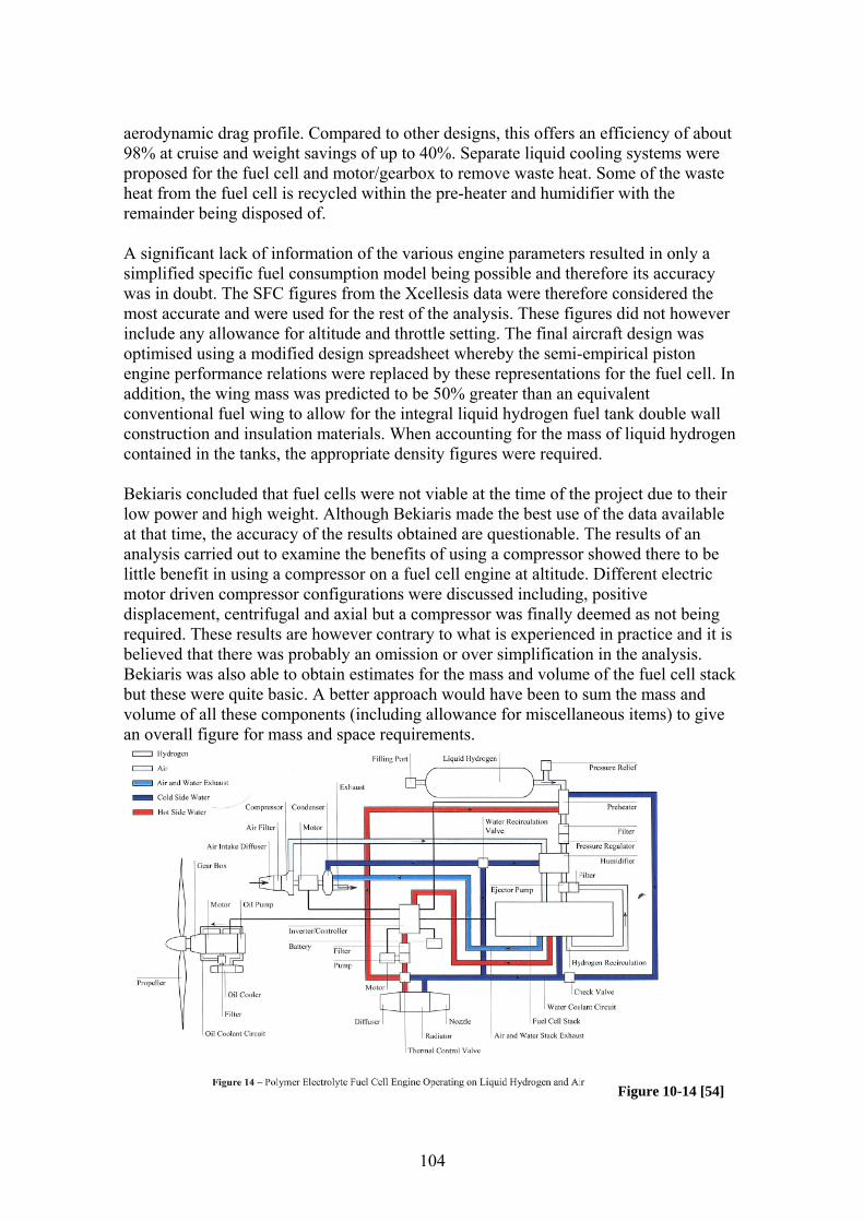
aerodynamic drag profile. Compared to other designs, this offers an efficiency of about 98% at cruise and weight savings of up to 40%. Separate liquid cooling systems were proposed for the fuel cell and motor/gearbox to remove waste heat. Some of the waste heat from the fuel cell is recycled within the pre-heater and humidifier with the remainder being disposed of. A significant lack of information of the various engine parameters resulted in only a simplified specific fuel consumption model being possible and therefore its accuracy was in doubt. The SFC figures from the Xcellesis data were therefore considered the most accurate and were used for the rest of the analysis. These figures did not however include any allowance for altitude and throttle setting. The final aircraft design was optimised using a modified design spreadsheet whereby the semi-empirical piston engine performance relations were replaced by these representations for the fuel cell. In addition, the wing mass was predicted to be 50% greater than an equivalent conventional fuel wing to allow for the integral liquid hydrogen fuel tank double wall construction and insulation materials. When accounting for the mass of liquid hydrogen contained in the tanks, the appropriate density figures were required. Bekiaris concluded that fuel cells were not viable at the time of the project due to their low power and high weight. Although Bekiaris made the best use of the data available at that time, the accuracy of the results obtained are questionable. The results of an analysis carried out to examine the benefits of using a compressor showed there to be little benefit in using a compressor on a fuel cell engine at altitude. Different electric motor driven compressor configurations were discussed including, positive displacement, centrifugal and axial but a compressor was finally deemed as not being required. These results are however contrary to what is experienced in practice and it is believed that there was probably an omission or over simplification in the analysis. Bekiaris was also able to obtain estimates for the mass and volume of the fuel cell stack but these were quite basic. A better approach would have been to sum the mass and volume of all these components (including allowance for miscellaneous items) to give an overall figure for mass and space requirements.

Figure 10-14 [54]

104

11 Alternative fuels literature review

11.1 The need for alternative fuels Any fuel can be simply regarded as an energy carrier, currently the majority of which are hydrocarbon based and obtained from fossil sources. Although they have been in widespread use for many years, there are a number of drawbacks associated with their use and as a result alternative fuels are actively being sought. This section will firstly present an overview of the different fuels that are currently available before discussing their availability and the impacts associated with their use.

11.1.1 An overview of current fossil fuels The majority of current fossil fuels are hydrocarbon based and are categorised according to their hydrocarbon composition, which includes,

11.1.1.1 Petroleum based fuels Petroleum based fuels (kerosene, diesel, gasoline etc) currently make up about one half of the global energy supply. These are obtained from hydrocarbon based chemical compounds from sedimentary rock deposits such as wells, tar sands and oil shale which are refined through various stages into petroleum based fuels and other products by means of distillation processes. The quantity of fuel obtained (per unit of crude oil) is dependant on the origin of the crude oil. Gasoline is normally blended with other compounds to achieve the different octane rating blends as well as including various additives to improve combustion and engine life etc.

11.1.1.2 Liquefied petroleum gas (LPG) This is a by-product of the refining of petroleum derived fuels and is suitable as a fuel for both IC engines and fuel cells. This will be discussed in more detail later.

11.1.1.3 Coal This is the most abundant of all the fossil fuels and is graded according to its composition and the degree of impurities present. It can be processed to obtain various liquids, gases and other compounds (carbonisation processing and later gasification processes were used to obtain town gas in the nineteenth century). Such processing requires temperatures of over 1200˚C and additional clean-up stages due to the number of contaminants. Numerous research studies have been carried out to investigate the benefits of operating a fuel cell on such gases.

11.1.1.4 Natural gas Natural gas is a mixture of hydrocarbons including methane, ethane, propane as well as other gases such as nitrogen, CO2, helium and sulphur compounds. It is typically found in porous rocks and more commonly in the vicinity of oil reservoirs and its composition can vary from source to source as well as being dependant on the seasonal climate. It can however be blended to achieve a desired composition to meet specified

105

requirements. Its variable composition makes it difficult to be able to use within fuel cell systems since the catalyst used can be severely affected by such variations.

11.1.1.5 The limitations of fossil fuels for fuel cell systems It is possible to use fossil fuel fuels to power fuel cells but the fuel processing required to extract the hydrogen can make this uneconomical. Since high temperatures can be required along with various additional clean up stages to remove traces of other unwanted compounds (such as sulphur and nitrogen which may affect the performance or life of a fuel cell). They are therefore not really suitable for mobile applications.

11.1.2 Diminishing fuel supplies If examine the world’s predicted fuel demands and the viability of meeting these demands with existing fossil fuel sources, the need for alternative fuels is apparent. Since this study is biased towards transportation fuels, this discussion will be limited to oil which is the primary source. Although the transportation is the largest user of the world oil (60.3% - 2007 Key world energy statistics [55]) it is not the only consumer. An increasing world population along with an increasing demand for fuel, as a result of increases in standards of living and energy demands is putting considerable demands on the world’s few existing finite oil reserves. This has resulted in cost increases, not only for transportation but also for domestic tasks such as heating and cooking. Whereas coal reserves are estimated to be sufficient for another 200-300 years, the oil and gas reserves are however only sufficient for about the next 100 years (assuming that we are able to tap into new oil reserves). At our current rate of consumption, our easy to access oil reserves will only be sufficient for 70 years, which does not take into account our ever increasing population. Natural gas reserves on the other hard will give us between 80 and 100 years. The demand for oil is predicted to increase even more over the coming years and our diminishing oil reserves may not even last this long. Alternative hydrocarbon fuel sources are available such as heavy oil deposits, oil shale or tar sand deposits but the extraction of fuel from these sources is difficult, costly and limited. With time oil is proving harder to obtain with new techniques and technologies being developed to enable oil wells to be utilised which were previously inaccessible. This includes deep sea oil drilling techniques, which have in recent times shown to have significant difficulties and risks associated with them. Another difficulty is that 61.5% of the world’s existing oil sources are reportedly located in the Middle East with the rest coming from US, Africa, Europe and Asia. Mans thirst for energy and oil puts pressure on international relations, possibly being one of the driving forces for recent conflicts (the next generation of beasts wild with hunger? [Nostradamus quatrain]). It is evident that we need to be concentrating on finding alternative energy sources in preparation for the inevitable.

11.1.3 What about natural and nuclear energy sources? The use of natural energy sources such as hydro, geothermal, solar, wind, tidal and waves are slowly being exploited but are facing obstacles such as public opposition. This is to be expected however since it is unfair to expect a quaint village to redevelop

106

its landscape in order to find ways to meet the power demands of adjacent towns. A better solution would be to put the responsibility on individuals to meet their own power demands. No solar panels or wind turbines equals no energy. Alternative energy sources are however unlikely to be able to fulfil all our energy needs and are unlikely to be suitable for transportation which means that fossil fuels may still remain in the loop for a while longer. The progressive increase in the use of alternative fuels will however lead to them being phased out with time. The manufacture of numerous chemical and materials is also reliant on oil and gas and so alternative sources must be sought for these as well. Atomic energy has been explored for some time but has proven to have catastrophic impacts in the event of a failure as was evident in the melt down of the power station in Chernobyl Russia. This disaster saw the atomic reactions running away uncontrollably, with many lives being sacrificed and radioactive clouds coving the whole of Europe. The reactor was eventually entombed in concrete but is predicted to take many years to cool down. This disaster has made the surrounding environment inhabitable since and people and animals still have to deal with the impact of the radiation. The disposal of radioactive waste is an additional problem with high risk waste currently being entombed in concrete deep within purpose built landfill sites. Atomic energy has too many drawbacks for its use to be further widespread. Either of these energy sources is particularly well suited to the generation of electricity. The transformation of an energy source into electrical energy does enable the efficient transportation of energy but the problem of the storage of large quantities of electric makes this form of energy less attractive. For this reason, they are not well suited to mobile applications.

11.1.4 Pollution factors associated with existing fossil fuels As will be discussed, the use of fossil fuel fuels has serious pollution implications. The combustion of hydrocarbon based fossil fuels results in the carbon being converted to carbon dioxide and the hydrogen to water. Of concern is the 24% increase in CO2 in the environment in the last 50 years which has been shown to be directly related to the increase in oil usage. CO2 is not solely responsible but has been shown to be the major contributing (63% - IPCC Fourth Assessment Report Climate Change 2007 [55]) greenhouse gas responsible for global warming. A 2007 study to determine the CO2 emissions in grams output per tonne carried and kilometre travelled showed aviation to be the worst of all the forms of transport (673-867g tkm). But in actual fact 90% of the world’s trade is moved by shipping which amounts to 3% of the total global CO2 production the lack of emission regulations for shipping is a particular concern.

11.1.5 What is the contribution of transportation to these problems? It is a common myth that aviation is one of the biggest energy consumers within the transportation sectors. In-fact the world cars and trucks are the collectively the largest at about 80% with the remaining 20% being consumed by rail, sea and air transport. It is sensible to target the biggest energy consumers but any additional improvements made by other consumers will definitely help and pave the way for others.

107

11.1.6 Existing fuel infrastructures The current fuel infrastructure has seen continual growth since the widespread introduction of the internal combustion engine at the turn of the 20th century when petroleum fuels were supplied by local chemist shops. Prior to this, the distribution of fossil fuels was predominantly intended for heating homes etc. Our modern dependence on fuels means that a fuel distribution infrastructure is a necessity which is applicable to the alternative fuels being used. Ideally the current petroleum fuel infrastructure could be adapted to cater for an alternative fuel but where this is not possible, a new infrastructure will have to be put in place, but at what cost?

11.2 An overview of alternative fuels There are numerous alternative fuels available which include Hydrogen, Alcohol fuels and Bio fuels which will be introduced below. Hydrogen will be covered in depth in a later section and a brief overview of Bio and Alcohol fuels will be presented below.

11.2.1 Bio-fuels These are derived from natural organic material, which includes a wide range of living organisms from algae, plants and trees through to animal flesh and waste. It has high energy content and can be utilised as a fuel by either direct combustion or conversion to biogas, ethanol, syngas, methanol, ammonia or other liquid hydrocarbon fuels. Potential sources are the 150 giga-tonnes of vegetable bio matter generated worldwide on an annual basis or the refuse digestion within landfill sites. Such bio-gases will contain high levels of nitrogen and carbon oxides which make them undesirable for typical gas fuelled engines but are less of a problem for a number of fuel cells. Bio-fuels can also be used to obtain alcohol fuels. Methanol can be synthesised from syngas, which itself can be obtained from biomass (in addition to natural gas) and ethanol can be obtained by fermentation of biomass.

11.2.2 Alcohol fuels Alcohol fuels were the first fuels to be used within IC engines but lost their popularity due to the advent of cheap post-war oil. Since they are able to be distilled from crops, they are however still used within countries which with no oil reserves. They are well suited for use within modern IC engines and have been shown to be less polluting than gasoline. Ethanol and Methanol are the most popular of these fuels. Methanol is available at a lower cost than Ethanol since it is able to be manufactured from a number of sources and has a greater flexibility within IC engines. The octane of gasoline can be increased by blending it with methanol and ethanol to improve the performance of an IC engine. Ethanol is probably the best known of the alcohol fuels and is available from a number of sources such as fermented corn, sugarcane or the bio-conversion of other natural materials. Ethanol is less toxic and less aggressive to metals and polymers than methanol and has slightly higher hydrogen content. Ethanol is however only suitable in countries where its production is not likely to be detrimental to food supply and even in

108

these cases, it is only able to meet a small fraction of fuel demands. Other fuels such as methanol are better suited in this case since they are not dependant on these agricultural sources. Alcohol fuels continue to receive renewed interest during times of high oil prices and as a result of pollution concerns. The 1975 National Alcohol Program (NPA) of Brazil, lead to the widespread use of sugarcane derived ethanol alcohol vehicles. In the early-mid 80s the Bank of America who converted their 200+ fleet to pure methanol, which showed benefits of reduced engine wear, pollution and cost compared to the use of gasoline. Since the end of the 80’s concerns about air pollution have led to the development of cars (20,000 in 1997) able to utilise such fuels. The majority of these are in California which use an 85/15 methanol/gasoline fuel blend called M85. To overcome concerns about fuel availability, these vehicles were also fuel flexible. More recently, a number of car manufacturers have still been actively perusing methanol and this has led to developments such as the Exige 270E ‘tri-flex-fuel’ car from Lotus, which is capable of using any mixture of methanol, gasoline or ethanol.

11.3 Hydrogen as a fuel Hydrogen has recently received considerable interest and research effort recently as a clean fuel which has led to proposals for a ‘Hydrogen Economy’. Hydrogen has significant environmental benefits with water being the only by-product of a combustion process. Although it has a significantly high value of energy per kilogram (or specific energy) it has the lowest molecular weight of all the gases making it more likely to leak and therefore requires careful handling and costly specialised fuel tanks. As shown in the chart below, the energy content per unit volume of hydrogen is considerably less than for other fuels which means that considerably larger fuel tanks are also required in order to carry the same total energy content.

. Figure 11-1 – Volumetric energy content of hydrogen compared to other fuels [55]

It has very low ignition temperatures and is therefore extremely volatile. Although a hydrogen and air mixture is able to detonate, a high fuel concentration of about 18% is required. It is safer than similar alternatives such as Methane and Propane but its higher proneness to leaking means that systems should be designed and monitored accordingly.

109

11.3.1 The current availability of hydrogen Hydrogen is already used in large quantities in the order of 50 million tons, 35% of which is used as a chemical reagent (mainly for oil refining and petroleum processing) and 51% being used for the manufacture of ammonia (as used for the manufacture of fertiliser). 8% is also used for the production of methanol. It is therefore already produced on a mass scale in order to be able to meet these demands

11.3.2 Hydrogen fuel infrastructures The hydrogen fuel infrastructure currently in place is to meet the needs of the refining and ammonia production industries. Presently, the only hydrogen vehicles in regular use are buses with a number of dedicated hydrogen refilling stations located in various cities worldwide (47 in 2004 [55]). Recommendations were made to put more in place by a number of countries to extend the use of such vehicles, of which Iceland appears to be the most committed with deadlines being put in place. There is however significant cost penalties associated with the development of an accompanying infrastructure. In the short term, fuel reformers could be used on-board hydrogen powered vehicles to enable them to extract the hydrogen from existing fuels such as petrol and kerosene. The aviation industry is unlikely to adapt hydrogen as a fuel until dedicated hydrogen infrastructures have reached sufficient maturity. Local filling stations can utilise hydrogen manufactured by present production methods but this requires the large scale storage of hydrogen either directly in compressed or liquefied form or retained in a hydrogen absorber. Alternatively, man-made hydrogen rich carrier fuels can be used (such as methanol and ammonia) which are made from mass produced hydrogen and can be reformed as required. Alternatively, the hydrogen can be manufactured on site. The volatile nature of hydrogen means it must be kept separate from oxygen at all times which means that nitrogen must also be readily available at all times at any refuelling station to take the place of air in any system.

11.3.3 Hydrogen production Hydrogen is not a naturally occurring gas and therefore must be extracted from other fuels (such as fossil or bio fuels) or from the electrolysis of water. Electrolysis requires a considerable amount of electricity from the national grid and is therefore reliant on fossil fuels. Such a process could however become carbon dioxide neutral if electricity from renewable sources or other similar processes was used instead. The extraction of hydrogen from fossil fuels tends to result in a large amount of unwanted residual carbon dioxide greenhouse gas as a by-product. Novel hydrogen production methods are being explored which involve the use of biological methods such as enzymes, bacteria or even light to break down fuels. These are applicable to both fossil and bio fuels but as yet these they are still in their infancy and are not commercially available. The manufacture of hydrogen is currently heavily reliant on fossil fuels with natural gas accounting for 48%, liquid hydrocarbons 30%, coal 18% and only 4% from water electrolysis. This is contrary to our goal to reduce our dependence on the use of fossil fuels. The processing of these also requires energy intensive reforming processes which offset the benefit of the clean burning hydrogen fuel. Future manufacturing processes

110

are predicted to rely on the increased use of water electrolysis and a process known as thermo-chemical water dissociation. When powered by renewable energy sources hydrogen will be more viable as a replacement fuel.

11.3.4 Liquefied hydrogen To liquefy it, hydrogen has to be cooled to about 22K which can require a considerable external energy input equivalent to at least 25 - 45% of the hydrogen’s heating value. This is normally carried out over three stages, initial compression, cooling to about 78K with liquid nitrogen and final cooling by expansion through a turbine. When the energy of manufacture is taken into account, liquefied hydrogen proves to be an inefficient means of storage. The low temperatures involved also present their own problems not only due to risks of frostbite but also due to air condensing to a liquid on exposed surfaces which can ignite certain materials. Any equipment must therefore be sufficiently insulated. The use of liquid hydrogen would not only have implications on fuel infrastructures but also on the refuelling procedures which must prevent the cryogenic fluids coming into contact with the skin or other disasters. Re-education of the public may be required to be able to use such specialised refuelling systems.

11.3.5 The outlook for using hydrogen as a fuel This review has shown hydrogen to be less desirable than initially thought when the energy required during its manufacture is taken into account. Alternative manufacturing processes are being investigated but these are still in the early stages of development. Since the Hindenburg disaster, the public has a negative view of hydrogen but subsequent research has shown it to be no more dangerous than methane and propane which are already being widely used. Public opinion is therefore an obstacle which must be overcome if hydrogen is going to receive serious consideration for use as a fuel. The widespread introduction of hydrogen as a fuel requires a significant investment in a dedicated fuel infrastructure which has cost implications. In the US, the DOE made the decision in May 2009 to cut funding for research into the use of hydrogen for automotive fuel cells as a result of it bleak outlook.

11.4 Hydrogen storage considerations A major drawback of using hydrogen as a fuel is its low density (0.084kgm-3 STP) which makes it difficult to efficiently store. To store it directly its energy density must therefore be increased by either compressing or liquefying the gas. More efficiently it can be used to manufacture hydrogen rich man made fuels or chemicals. Novel methods such as carbon nano-fibres and metal hydrides have also been receiving considerable interest recently. The most appropriate hydrogen storage solution is a trade-off of efficiency, mass, practicality, cost and safety. The storage of gaseous hydrogen on-board vehicles is a particular problem since its low energy density per unit volume means that very large storage tanks are required. It can be stored in a liquid form but the low temperatures required bring about its own set of problems. The very small size of hydrogen molecules mean that it will leak 3.3 times faster than air. This is particularly concerning when we consider the ease of which hydrogen can be

111

easily ignited and the difficulty of detecting it when alight as a result of it burning with a clear flame. Fortunately its low density means that any leaking fuel can also quickly dissipate into the environment. Even so, any system will require high integrity seals in order to safely contain the fuel. The volatile nature of hydrogen/air mixtures means that any storage tank must also remain air free at all times and should be purged with nitrogen when empty.

11.4.1 Compressed storage If stored in its gaseous format, the low density of hydrogen implies that it must be stored at very high pressures to make its use viable. Pressurised cylinders are favourable when hydrogen is required in small quantities due to its simplicity. In such cases, steel alloy cylinders may be sufficient but they do have significant weight penalties associated with them. Composite tanks are a lighter alternative and have already seen use on vehicles. An example of such was the composite tanks fitted in the roof of a bus which consisted of a aramide and epoxy composite outer shell which encompassed a 6mm aluminium inner shell. This combination gave an efficient cylinder with good burst characteristics although the cylinder was only operating with a maximum working pressure of a quarter of its design value. An example of a high pressure cylinder used onboard a hydrogen powered car is shown in the figure below.

Figure 11-2 – Typical high pressure hydrogen storage cylinder for vehicles [49]

The shape of high pressure tanks also makes them good candidates for aircraft external fuel tanks. When the full extent of the weight of such a hydrogen storage system is taken into account the hydrogen stored typically amounts to less than 2% of the total mass. Of high importance are the burst characteristics of such a compressed cylinder. The occurrence of a leak, leading to fracture can lead to large forces being generated in the vicinity of the defect. Any sudden decompression will result in highly explosive volatile gas regions as the gas mixes with the surrounding air. Safety devices such as burst disks (to safely vent the gas in a controlled manner) and flame traps (fitted to pressure regulators to prevent flame back-flow into a cylinder) must therefore be used.

11.4.2 Liquefied storage The very low density of hydrogen means that it is not practical to liquefy it just by compressing it, as it down with other gases (kinetic theory). Instead its temperature has

112

to be reduced instead to about -253ºC to store it as a cryogenic liquid, known as LH2. This method is the most common method of storing large amounts of hydrogen for industrial applications but after liquefaction the density is still only 71kgm-3. Smaller scale LH2 tanks have already been approved for vehicular use with two types being common, vacuum wall and solid insulated wall. These are considered safer than compressed gas alternatives, since failure of the tank does not result in sudden decompression. In the event of failure, the liquid fuel will remain in place and slowly evaporate. It should be noted that the liquid fuel from a LH2 tank will need to be preheated to convert it to a gas before it can be used in a fuel cell. Waste heat can be used for this purpose but a heat exchanger is still required. Reinforced cylindrical vacuum wall tanks are the most effective cryogenic tanks. These typically consist of two 3cm thick walls, each with 70 aluminium foil/fibre glass layers. An alternative is solid insulated wall tanks which use solid insulation materials combined with a reflective layer. Solid insulation materials used include, foam, glass and aluminium mixtures. The results of a study carried out into the effectiveness of a number of these materials for cryogenic tanks are presented below.

Figure 11-3 – Insulation material properties [54]

The temperature of liquid hydrogen needs to be maintained at about -253ºC to keep it in its liquid state which is difficult with even the best insulation materials. When not in use, LH2 will still slowly evaporate and any tank will need to be fitted with a pressure release to prevent the pressure exceeding a specified level (typically 3 bar). This not only wastes fuel but also creates a dangerous situation due to the escaping volatile vapours. It is therefore unsafe to allow a liquid hydrogen tank to stand for long periods (a limit of 5 hours has been estimated for a full tank). This is not an issue when in use since this hydrogen vapour would normally be consumed by the fuel cell. This reduces the practicality of liquid hydrogen fuelled vehicles since they must be de-fuelled after use and then refuelled before the next trip.

11.4.3 Metallurgical considerations The design of suitable storage devices is further complicated by the fact that hydrogen is known to react with certain metals. The small molecular nature of hydrogen means that

113

it is able to diffuse into certain normally impermeable materials and can even pass through microscopically porous materials. This includes carbon composite materials which are not hydrogen proof. The dissociation of the hydrogen molecules in close contact with the materials surface can also severely affect the mechanical properties of the material which can result in blistering and cracking of the material. Another phenomenon that a designer needs to be aware of is hydrogen embitterment in which the carbon in carbon based materials reacts with hydrogen to form voids of CH4 in the material. Gas pressure within the voids then leads to internal stresses in the blisters and cracks. Hydrogen damage is therefore more likely to occur for materials with high carbon content. Non-ferrous metals are less susceptible and certain chromium based steels and alloys are known to be resistant to this phenomenon. Cryogenic fuels present their own problems due to the extremely low temperatures involved, which can seriously affect the strength and fatigue properties of materials. The varying thermal stresses due to fuelling/de-fuelling temperature changes can lead to fatigue problems and stresses in tank mounting etc. As a result, only materials than remain ductile at low temperatures can be used which includes, aluminium, titanium, nickel alloys and austenitic stainless steels. The tensile properties of alloys are known to improve at cryogenic temperatures whereas the properties of a quasi-isotropic laminate get worse. The magnesium based alloys tend to see an improvement in their fatigue properties with opposite being true for steel. The fatigue properties of plastics are dependant on weather they are thermoplastic (improved properties) or thermosetting (degraded properties). The lower molecular kinetic energy of the substance means that hydrogen embrittlement is also less of a problem.

11.4.4 Other storage methods

11.4.4.1 Reversible metal hydrides Certain metals and alloys known as reversible metal hydrides are able to easily react with hydrogen to create a storage solution. Due to their small size, the hydrogen molecules are able to be absorbed in-between the molecules of these hydrogen absorbers. The exothermic hydride formation process can be easily reversed by supplying heat to the hydride. The exact nature of the reaction is dependant on the material involved as well as its operating temperature and pressure. Since the rate of hydrogen release is dependant on the heat supplied, the process is easy to control. The volumetric efficacy of such a system is comparable to liquid hydrogen but at a less attractive gravitational efficiency. Only hydrogen with a very high purity can be used (otherwise the material will be damaged by impurities) and a refill time of 1 hour is currently typically required for a 5kg system. These systems exhibit good safety characteristics since any leak will be accompanied by a temperature drop which will inhibit the hydrogen release reaction.

11.4.4.2 Carbon nanofibres A revolutionary hydrogen storage method is carbon nanofibres. These are reported to be able to store 67% of their own weight in hydrogen though the results are in question. This system is still in its infancy and therefore not a practical consideration at present.

114

11.4.4.3 Hydrogen carrier fuels These are man-made fuels which are manufactured to hold large quantities of hydrogen in comparison to their mass. A number of criteria exist for these fuels,

1. It must be easy to extract the hydrogen from the fuel. 2. Manufacture of the fuel must be easy and efficient. 3. The fuel must pass certain safety consideration.

These most promising of these are Methanol and Ethanol which are discussed in a dedicated separate section.

11.4.4.4 Alkali metal hybrids Alkali metal hybrids are chemical hydrogen absorbers which are similar to reversible metal hydrides but water instead of heat is used to promote the release of hydrogen. Such a substance is calcium hydride which when reacted with water it reverts to calcium hydroxide and hydrogen. This is already available commercially as polythene Powerballs which are held under water and simply cut open as required. A control system regulates the frequency that the balls are cut open and therefore the hydrogen supply. This system is heavier than the reversible metal hydrides since allowance must also be made to carry a large quantity of water (typically 3 times as much as is required for the reaction) and the waste sodium hydroxide/water solution. Manufacture of the hydride is energy intensive and certain batteries are preferable.

11.4.4.5 Sodium borohydride Sodium borohydride is a stable hydrogen carrier which has been around since 1943 and is currently manufactured from borax in quantities of 5000 tonnes per year. With the aid of a suitable catalyst, it controllably reacts with water to generate hydrogen. Only pure hydrogen is produced which is diluted with water vapour. This has shown promising results and a number of hydrogen powered vehicles have already been built by Millennium Cell Corporation utilising this. This is also available as solid form which is formed from sodium borohydride and a suitable catalyst and only needs water to generate hydrogen. A more practical derivative is sodium borohydride in solution form which does not require a separate water supply and only needs to be bought into contact with a suitable catalyst and is easy to control. Recirculation systems are the most common but the solution cannot be replaced or replenished until all the sodium borohydride has been used up and then it must be completely renewed. The Hydrogen on Demand System developed by Millennium Cell Corporation is more refined single pass concept. Solution based sodium borohydride is safe to transport, generates only pure hydrogen and no extra energy is required to promote the reaction. The fuel solution is upto100 times more expensive than hydrogen produced by other means due to the extreme manufacturing energy requirements required which far exceed those of methanol.

11.4.4.6 Ammonia Ammonia is a toxic gas with high hydrogen content. It is currently produced at a rate of 100 million tonnes (by energy intensive steam reforming of methane) for the

115

manufacture of fertiliser and explosives and is competitively priced and readily available. It is easy to liquefy by either cooling it to -33ºC or compressing it to 8 bar but requires large amounts of energy to enable it to vaporise back into a gas. Its dissociation back to hydrogen is energy intensive and requires an inexpensive catalyst and reaction temperatures of 800-900ºC. Ammonia based fuels can cause permanent damage to PEM fuel cells (is only suitable for alkaline fuel cells) and generate a corrosive mixture when dissolved in water.

11.5 Methanol in depth review

11.5.1 Methanol as a fuel Methanol (methyl alcohol) is a liquid oxygenated hydrocarbon fuel which was first discovered in 1661 by Robert Boyle. It is colourless and water soluble with a mild alcoholic odour. It has a simple chemical composition and is the simplest of all alcohols containing only one carbon atom. It has a freezing to boiling temperature range of 97.6 to 64.4 ºC and a typical density of 791 kgm-3 (20 ºC). A downside is that it contains only about half the energy density of gasoline. The attractiveness and low cost of this fuel has however led to the proposal of a ‘Methanol Economy’. Methanol is regarded as a safe and efficient hydrogen carrier and energy storage medium. When conventional transportation means are unavailable, other fuels such as natural gas can be safely and easily transported by converting them into methanol. Volatile hydrogen can also be effectively tamed by combining it with CO2 into easy to handle and store liquid methanol. As a transportation fuel it does not need to be pressurised or liquefied (in contrast to hydrogen) and can be easily distributed, handled and stored (especially on-board vehicles). It also already has a proven track record of being able to be safely carried on-board vehicles as it is currently already used in a number of IC engined vehicles. Low cost fuel grade methanol can also be used within existing natural gas powered turbines for power generation. Only minor modifications are required and a higher power output can be achieved along with lower NOX and zero SOX emissions (since methanol is sulphur free). Methanol and DME can also be used as household fuels and methanol cooking stoves have already been developed.

11.5.2 The manufacture of methanol Methanol first obtained as a by-product from the charcoal manufacturing process. This was later replaced by the use of coal based processes during the industrial revolution and then much later by synthetic processes. It can be manufactured from a number of sources including fossil fuels but at present, syn-gas is the worldwide adopted approach. Research has however been invested in the low-pressure synthesis of carbon oxides and hydrogen which have been refined to produce a selectivity of 99.8% at a process efficiency of 75%. It is however the intention that methanol will eventually become the ultimate green fuel with the carbon coming from the chemical conversion of atmospheric CO2 and the hydrogen being obtained by the electrolysis of water (using renewable energies for the process). The demand for methanol has progressively

116

increased over the years which have led to a number of mega methanol production plants being created. Methanol is manufactured worldwide but China is currently the largest methanol producer. Unfortunately, they rely on coal for its manufacture as a result of its availability and low cost which not environmentally friendly.

11.5.3 The use of methanol within traditional IC engines The excellent combustion characteristics of Methanol (octane rating of 100) and its Dimethyl Ether (DME) derivative have drawn particular attention to their use as fuels in IC engines. Conventional IC engines can easily be adapted to use this fuel. As a fuel, methanol can be used either neat or blended with conventional fuels as an oxygenated additive. Typically twice as much methanol is however required to achieve the same quantity of stored energy as gasoline due to its lower energy density. This is however offset by the fact that the higher octane rating of methanol allows an engine to be operated at higher compression ratios (10-11:1 vs 8-9:1 for a gasoline engine) making them more efficient. Methanol also has higher flame speed and therefore the combustion process will be more complete. As a result, less than double the amount methanol is actually required to achieve the same power output. The low volatility of pure methanol makes the fuel much safer than gasoline but can lead to cold start problems and the need to use volatile additives or blend it with gasoline (as with M85 blends). Its lower volatility and improved performance have made methanol the fuel of choice for the Indianapolis races since the 1960’s. Methanol can be used directly within a diesel engine but its cetane number of 3 (the ability of a fuel to self ignite at high pressures which is 40-55 for diesel) necessitates the need to adapt the engines. Nitrogen based ignition improving additives are also used to increase the cetane number. The use of methanol as opposed to diesel is able to reduce the two main sources of pollution commonly associated with diesel engines. There are no particulates and the amount of NOx generated is minimal because of its lower combustion temperature. The energy content of diesel is about 2.2 times greater than methanol meaning a much greater fuel tank is required. The dehydration of methanol results in a fuel more suitable for use within diesel engines due to its much higher cetane number of 55-60, known as Dimethyl Ether. DME shares the same benefits as methanol of zero particulates and low NOx along with a reduction in engine noise. The low energy density of DME means that the fuel tank must be twice the size of a diesel tank. DME has a low lubricity and lower viscosity making the fuel system more susceptible to leakage and wear. DME is also known to be incompatible with a number of plastics and rubbers and PTFE and Buna-N are often used. DME is already produced in large quantities (4 million tonnes a year in China in 2008) and is regarded as the most attractive contender for the replacement of diesel fuel. Refined DME engines and vehicles are currently being developed. Research has shown that DME can also be used as a substitute for LPG and is comparable to natural gas, for use within power generation gas turbines. The low octane number of 35 RON of DME means it can not be used within spark ignition engines. This can be improved by mixing it with 20% LPG.

117

11.5.4 Material compatibility issues Care needs to be taken when designing new systems or adapting existing systems to use methanol since it is the worst of the pure alcohols for attacking metals and polymers. Such design precautions are not expected to have any serious cost implications. Methanol vapour is reported to be worse than methanol liquid for corrosion with a high electrical conductivity which promotes a corrosive reaction. Magnesium is the worst corroded with aluminium, copper, brass, zinc and bronze also being affected. Aluminium is also rapidly corroded this has the added complication that the resultant products (gelatinous precipitates) are known to be sufficient to clog filters etc. Stainless steel is more resistant to methanol than some of the other metals but incurs a weight penalty. Nickel coatings are reported to be the most effective of the metallic coatings to resist methanol. This can be applied to the inside surface of an aluminium fuel tank to provide a light weight solution but joints would still present a sealing problem. The molecular nature of methanol is also known to cause problems with certain polymers resulting in swelling/shrinking, hardening/softening or cracking of the material. The polymers offering the best methanol resistance are those with high fluorine content (such as Teflon) and it may be possible to use these as a barrier coating. Since traditional fibre reinforced polymers can soften and delaminate, a group of methanol resistant polymers have be developed but their use is limited to static storage tanks at this stage. Methanol incompatibility also extends to engine lubricants and specific formulations must be used.

11.5.5 Methanol and DME storage and distribution Significant progress has already been made in the development of methanol fuelled vehicles but for these to become more widespread they need to be accompanied by an increase in the distribution of the fuel. 100 or so methanol refilling stations have already been built in California to satisfy the needs of the many flexible fuel vehicles already in service. These distribute either M100 (100% methanol) or M85 (85% methanol/15% gasoline), or both. These are similar to conventional fuel refilling stations with similar handling precautions. Although the construction of dedicated methanol refilling stations is straightforward, the conversion of existing refilling stations to cater for methanol is the most cost effective solution. In such cases, a small number of modifications are required to make the equipment compatible with methanol. In comparison, the costs of developing a hydrogen refilling station are considerably more than for methanol as a result of the much more specialised equipment which is required (both for high pressure and cryogenic systems). The liquid state of methanol allows it to be easily distributed by rail, road and sea as is the case already for 500,000 tons per year in the US. Distribution by pipeline has also been demonstrated and the storage of large quantities is also viable. DME on the other hand has similar physical properties to LPG and therefore the existing LPG infrastructure and refilling stations can be used with minor modifications.

118

11.5.6 Methanol price and availability Methanol is currently manufactured in the order of 40 million tonnes (2007 figures) as an ingredient for the production of various chemicals and products either in its direct form or following conversion into synthetic hydrocarbons. Only 7% of this methanol was destined for fuel use. Methanol production from natural gas is at present the most cost effective approach as production from other sources often requires further processing stages. The cost of DME is slightly higher since further methanol refining stages a required in its manufacture but is still considerably less than diesel. Since natural gas is the main ingredient of methanol, the price of methanol is dependant on the price of this. The 2007 mass production cost of methanol was estimated to be below 30 cents per gallon and even taking into account its lower energy content, it is still competitive with gasoline and diesel.

11.5.7 Methanol safe handling practices Methanol is non-toxic and is actually already present in small quantities in a number of consumer products such as windscreen washer fluid, de-icer, antifreeze and many more. It also occurs in very small quantities naturally in our bodies and in our food and a daily intake of up to 500mg, taken in this way is considered perfectly safe. Methanol can be difficult to detect due to it being colourless and only having a mild alcoholic odour but with the correct precautions in place, it is not any more dangerous than any of the existing fuels. The same handling precautions as gasoline have been shown to be sufficient. In the long term, methanol is better than gasoline as it does not present the same carcinogenic risk. DME is similar to methanol, being non-toxic and non-carcinogenic having a mild odour and burning with a visible blue flame. As for similar fuels, a certain amount of careful handling is required. Fuel refilling carries the greatest risk of methanol being absorbed into the body by ingestion, inhalation or skin contact. The fatal limit for ingestion of methanol is about 1g per kg of body mass which is 25-90mL as opposed to 120-300mL for gasoline but antidotes are available to treat cases of methanol poisoning. The inclusion if dyes and odour/taste agents in the fuel and anti-siphoning measures on vehicles will all help prevent the accidental ingestion of methanol. The levels of methanol inhalation during normal refuelling present no risk but as an added precaution, vapour recover systems can be used. The risk of skin contact can be significantly reduced with the use of spill-free nozzles. Fire risk for methanol is significantly less than for gasoline as a result of its lower volatility and the vapour concentration must be four times as much to be ignitable. In the event of a methanol fire, it burn with a visible light blue flame, produces little smoke (improving visibility and reducing smoke inhalation) and can be easily extinguished (even with water). Since methanol burn at an eighth of the heat output and at a quarter of the speed of gasoline, fires are considerably safer as they less eagerly spread to surrounding combustible materials. It is estimated that gasoline based fires could be reduced by 90% with the use of methanol which is one of the reasons why methanol is regarded as one of the safest fuels and has been used for Indianapolis-type race cars since the 1960s (as well as the superior performance benefits).

119

11.5.8 Environmental considerations The continual development of IC engines has lead to a significant reduction in their emissions which has made them competitive with alternative fuelled vehicles. However they are susceptible to an increase in emissions as a result of age and poor maintenance, whereas the emissions from a methanol fuelled IC engine will continue to be low throughout its life. The incomplete combustion of methanol in IC engines can result in formaldehyde production, which can however be treated with a catalytic muffler. DME fuelled CI engines will also benefit from significantly reduced exhaust emissions and significantly less complicated exhaust after treatment systems are required. The absence of sulphur from DME means that no emissions are produced and since there are no C-C bonds in the make up of DME, particulates are also virtually eliminated. Methanol spills do not present any risk to the environment as it is easily degraded by photo-oxidation and biodegradation and is used in windscreen washer fluids for this very reason. Methanol is already currently used within sewerage plants to accelerate the bacterial treatment process and so there is little risk to water treatment either. Since methanol is miscible with water, any major spill would be conveniently diluted and biodegraded by micro-organisms in just a few days. This is in contrast to the scale of disaster experienced with crude oil spills. A similar situation exists for DME, which is non-toxic, water soluble and easily broken down by micro-organisms.

11.5.9 The prospect of the manufacture of methanol by CO2 recycling

At present fossil fuels are used for the manufacture of syn-gas and methanol. Natural gas is preferred in terms of efficiency, cost and emissions, while coal is noted to be the most unfriendly in terms of CO2 production. If we take into account the CO2 generated from the manufacture of methanol, the CO2 emissions from methanol fuelled vehicles will only be slightly lower than their gasoline counterparts. This can be significantly improved if we are able to manufacture methanol with renewable sources instead. The manufacture of methanol from chemically recycled CO2, obtained from chimneys of power and manufacturing plants has been proposed. When this CO2 is combined with hydrogen generated from water by renewable energy sources these fuels can become environmentally CO2 neutral. In such cases, fossil fuels may not longer be required.

11.6 Fuel study conclusion This study highlighted the limitations of conventional fuels before investigating a number of alternative fuels which have the potential to eventually cut our ties with the almost exhausted fossil fuels. Hydrogen and the hydrogen carrier fuel methanol were identified as the best contenders as fuels most suitable for a fuel cell vehicle. Hydrogen was however shown to have significant difficulties in terms of its storage and distribution due to its volatile nature. Methanol on the other hand, is in a normally liquid state at standard conditions and much safer to handle. Compared to gasoline, methanol has only half the energy density but liquid hydrogen has half that of methanol and gaseous hydrogen only a sixth. The low energy density of these fuels is offset to some extent by the fact that the fuel consumption of a fuel cell engine is only a third of a

120

121

gasoline engine. If we also take into account the total cost of hydrogen and methanol after production, transportation and storage, methanol wins again. The manufacture of methanol by CO2 recycling also has the potential to alleviate the problems of global warming. Methanol is not limited to use as a fuel and can also replace oil and gas as a vital ingredient for the manufacture of synthetic hydrocarbons and their products. In this study methanol has been shown to be the best substitute for non-renewable fossil fuels and is already mass produced in large quantities. With only a few years supply of fossil fuels still remaining, the time to implement such a change is now. The switch to alternative fuels will however be progressive, with alternative fuels supplementing fossil fuels initially before eventually completely replacing them. This has been shown to be straightforward with conventional gasoline and diesel engine being easily adapted to use methanol with a number of minor modifications. A more long term challenge will be the introduction of fuel cell vehicles. In the short term, hydrocarbon based fuels can be utilised within such a vehicle by means of a fuel processor but alcohol fuels are more attractive even for this due to their lower energy requirement for such a process. Methanol reformer equipped fuel cell powered vehicles, have already been shown to have emissions which are considerably less than the very strict limits laid down for SULEV (super ultra low emission vehicles) vehicles in California. The methanol derivative DME is expected to be similar. In order for a fuel to be able to become widespread, as well as having the backing of sufficiently large manufacturing plants, it must also have a suitable distribution infrastructure. At the end of the distribution network, there must be refilling stations which can be easily and safely used by the customer. Existing fuels have always benefited from being sufficiently safe and easy to distribute with a vast distribution infrastructure already in existence. Although past experience has shown the general public to be more than capable of handling specialised fuels such as LPG, the ideal replacement fuel will be similar to existing fuels. Methanol has a distinct benefit in this area of being able to utilise existing refilling stations with a number of modifications. Since hydrogen is significantly different to conventional fuels a new fuel infrastructure would be required. A small number of hydrogen outlets already exist but a new and costly infrastructure would have to be developed for hydrogen to be widespread as a fuel. A number of regulations would also have to be overcome for such an infrastructure to become reality. In particular, a US NFPA regulation prohibits a hydrogen pump from being installed within 25m of gasoline pumps, making the integration of hydrogen pumps into existing refilling stations difficult. From a financial perspective, hydrogen an unviable option due to the cost of developing such a new infrastructure and a number of hydrogen fuel studies have recently been abandoned for this reason. Hydrogen is still attractive as a fuel but only for specialised applications requiring a limited distribution infrastructure.

12 Fuel processing

12.1 An overview of fuel processing Since hydrogen rich fuels contain more hydrogen per volume than pure hydrogen in its most dense liquid state they are becoming increasingly attractive for fuel cell systems. The use of such fuels also has other practical benefits over hydrogen such as storage and distribution. It is however necessary to use a fuel processor to extract the hydrogen from them as required by a fuel cell. This way, fuel cell vehicles are able to utilise existing fuels in the short term until pure hydrogen becomes more viable. In this way, hydrogen is able to be extracted from a range of fuels such as petrol, kerosene, propane and methanol but the exact process used is specific to the fuel. The reaction temperatures required for theses chemical conversion processes can be high and therefore catalysts are often used. The three main fuel reforming approaches are steam, partial oxidation and autothermal, each of which will be discussed below. The hydrogen output from the main reformer is however typically polluted with other unwanted substances such as CO, CO2 and H2O. Some of which act as mere dilutants with a fuel cell but others must be removed by additional clean-up stages such as desulphurisation, shift reaction and gas clean-up. The exact nature of the process is dependant on the type if fuel cell used. Other stages required are those to vaporise liquid fuels into the required gaseous form and preheat the reactants (fuel and air) before they enter the fuel reformer. These normally require additional heat input which must be allowed for. The numerous stages involved each have their own optimal operating conditions as well as being dependant on the composition of the gasses, reactor operating temperature and supply feeds. Collectively, control of the complete process can be complex.

12.2 Steam reforming Steam reforming is widely used and is the most common fuel reforming approach. The process involves two reforming (oxygenolysis) reactions and a water-gas shift reaction as given in the example below for methane.

224 3HCOOHCH +⎯→⎯+ Eq 12-1

22188 1788 HCOOHHC +⎯→⎯+ Eq 12-2

222 HCOOHCO +⎯→⎯+ Eq 12-3 The two reforming reactions indicate that the output from the reformer is a mix of CO, CO2 and H2 as well as fuel and steam. The exact output from the reformer is governed by operating conditions such as temperature, pressure, fuel and steam content. As shown in the figure below, the reaction temperature needs to be high enough to achieve full conversion of the fuel for all hydrocarbon and alcohol fuels with temperatures of up to 700ºC being the most desirable for the production of hydrogen. These can be reduced with the use of a catalyst and temperatures of about 500ºC are typically used in conjunction with a Nickel catalyst.

122

Figure 12-1 Output concentrations from a steam reformer as a function of temperature [56]

This process is endothermic and an external heat source is required to sustain the reaction. This is typically achieved by the combustion of an additional amount of fuel within a burner which is thermally coupled to the reformer. The steam reforming reactions are separate from the combustion reactions in the burner, except for thermal conduction between the two and thus will be reversible and not include any nitrogen. The steam reforming of Naphtha is a special case which is initially endothermic but becomes exothermic as the temperature is lowered but these lower temperatures will favour the production of methane as opposed to hydrogen. Other fuels such as alcohols can be reformed in a similar way as for the example given for methane above. The reaction for methanol is given below.

2223 3 COHOHOHCH +⎯→⎯+ Eq 12-4 Methanol has the distinct advantage over other fuels in that much lower temperatures are required. Since a certain amount of unconverted methanol within the reformate is also tolerable within phosphoric and PEM fuel cells lower temperatures can be used. High operating temperatures are however still desirable to prevent carbon formation. With the aid of copper and zinc oxide catalysts, temperatures of the order of 250ºC are typically used. A distinct advantage for PEM fuel cells is than CO is not shown as a product of the process. Although not shown, traces of CO are still present. The theoretical efficiency which is taken as the ratio of the heating value of hydrogen produced to the total fuel consumed in both of the reactions is 100% for a steam reforming process. The actual efficiency will be less than this as a result of heat losses and incomplete reactions. A certain amount of CO will also be included in the output from the reactor and further processing will be required when it is destined for use in certain fuel cells such as the PEM. Two of the most common methods used will be discussed in the sections which follow.

123

12.2.1.1 Steam reforming and shift reactions This process involves an additional shift reactor stage in which the CO in the reformate reacts with extra steam to produce additional hydrogen and CO2. More than one shift reactor may be required and both high temperature and low temperature reactors can be used. As shown in the schematic below, these are typically followed by a preferential oxidation stage in which any remaining CO is oxidised with oxygen (usually with the aid of a suitable catalyst).

Figure 12-2 – Steam reforming process [57]

12.2.1.2 Steam reforming and membrane separation This uses a metal membrane which will only allow hydrogen to pass through, with the result being a product gas consisting of mainly high purity hydrogen. The reformate products that were unable to pass through the membrane are combusted within the burner instead. This process has proven to be very efficient, but large pressure differentials are required across the metal membrane in order to make it work. As a result it is better suited to compressed and liquid fuels (such as methanol) which do not require significant additional compression. The schematic is shown below.

Figure 12-3 –Steam reforming with membrane separation [57]

124

12.2.1.3 Variants of steam reforming Dry reforming (also known as CO2 reforming), as defined by the following reaction can be used when there is no available steam source. Such systems rely on the recirculation of water and CO2 from the exhaust into the inlet.

224 22 HCOCOCH +⎯→⎯+ Eq 12-5 A hybrid approach between the steam and dry reforming methods which uses both steam and CO2 is also possible. In either approach care needs to be taken since the nickel catalysts are easily damaged by carbon formation. When high temperature fuel cells are used, the heat required to maintain an endothermic reforming process can be supplied by heat generated by the fuel cell stack instead of being supplied by an external source. The heat generated by the fuel cell is typically twice that required to sustain the steam reforming reactions. Such systems also reduce the cooling requirements, increase the overall efficiency of the system and reduce the system cost. The are two variants of this system. In the direct arrangement, the reforming is performed within the anode chamber and therefore is able to utilise the already available steam. In the indirect arrangement, the reformer is placed in close thermal contact with the fuel cell.

12.3 Partial oxidation reforming Partial oxidation is effectively a less than stoichiometric combustion process, in which CO and hydrogen are produced instead of the products normally associated with a typical combustion process. It is an exothermic reforming process which is faster than steam reforming but operates at temperatures of 1200 - 1500ºC (without a catalyst) and is therefore impractical for mobile applications. These systems are much simpler than steam reformers since they do not require an external heat or steam supply. The reaction can however be difficult to control and the process is less efficient than steam reforming and therefore produces less hydrogen per mole of fuel. This is made worse by the use of air instead of pure oxygen. The reformate gas also contains a large amount of nitrogen, which reduces the hydrogen content of the gas. As with a steam reformer, shift reactor and partial oxidation stages are required to complete the process. An example reaction for methane and schematic of the process is given below.

2221

4 2HCOOCH +⎯→⎯+ Eq 12-6

22188 984 HCOOHC +⎯→⎯+ Eq 12-7

Figure 12-4 – Partial oxidation reforming process [57]

125

A derivative of this is known as Catalytic Partial Oxidation which enables the temperature requirements to be reduced with a catalyst such as platinum or nickel. There are numerous CPO reactors in development which are applicable to both stationary and mobile applications. The best know of these is the Johnson Matthey HotSpot reactor which will be discussed in more detail in a later section. As with other reformers, methanol has a distinct advantage over other fuels in that the reactions are able to proceed at much lower temperatures, which results in a much simpler design. An experimental unit has been developed which uses a methanol/water mix and controlled air flow in an ignitor. This arrangement means that only a small fraction of the methanol is burnt and the heat produced is sufficient to vaporise the remaining water and methanol, which is then fed to a catalyst (supported on a honeycomb monolith) reactor.

12.4 Autothermal reforming Autothermal reforming is a hybrid between partial oxidation and steam reforming in which the endothermic steam reforming and exothermic partial oxidation reactions occur simultaneously. Both steam and an oxidant are used along with a catalyst to react with the fuel. Depending on the amount of oxygen which is introduced to the system the process can be endothermic, exothermic or neutral. An autothermal process has a theoretical efficiency of 100% and exists when the system is neutral and there is no net heat transfer. The amount of oxygen required to achieve such a situation is different for every fuel (X=0.23 in the case of methanol). In practice however, it is typical to use slightly more oxygen than is theoretically required along with additional steam (to give a steam to carbon ratio of approx. 2-3), in order to reduce the risk of carbon formation within the fuel processor. Although this results in a reduction in efficiency the service life of the fuel processor is increased. The amount of steam required is less than with a standard steam reformer since the heat required is generated by partial combustion of the fuel. A schematic of the process is given below.

Figure 12-5 – Autothermal reforming process [57]

As with other fuel processors, additional processing is required to remove unwanted elements. The shift reactor used consists of a high temperature (400-500˚C) and low temperature stage (200-250˚C) which allows each stage to utilise a catalyst optimised for that particular temperature range. The output still has a CO content of about 1% which must be further reduced by either preferential or selective oxidation.

126

12.5 Electrolysers Although not strictly a fuel reforming process, water can be divided into hydrogen and oxygen by passing electricity through it. The reaction is reverse to that encountered in a fuel cell. Efficiencies of 60 to 70% have been reported for such units and they can be operated at higher pressures if so desired. Pure forms of hydrogen are generated but with the presence of significant amounts of water vapour. Such a system can also be used to store surplus electrical energy as was successfully demonstrated on the NASA Helios hybrid UAV project. This aircraft was equipped with solar panels to provide power during the day as well as generate hydrogen to power fuel cells at night.

12.6 Additional clean-up phases Any fuel processor typically relies on additional processing stages to support the reformer. The stages required are dependent on the reformer and fuel used and the reformate composition required by the fuel cell. Desulphurisation is the first stage of a fuel processor. It is used to remove the traces of sulphur that are commonly found in a number of fuels such as natural gas, gasoline and diesel. This is necessary to prevent premature degradation of the catalysts used and poisoning of PEM fuel cell anodes. The sulphur content will vary from fuel to fuel and this stage may not be required in all cases. A hydrodesulpharisation (HDS) reactor is typically used for this stage which operates on recirculated hydrogen gas. These use nickel-molybdenum or cobalt-molybdenum catalysts to convert any sulphur compounds into hydrogen sulphide which is followed by the conversion to zinc sulphide, by absorbing this into a bed of zinc oxide. Alternatives to the HDS are absorbents such as activated carbon and molecular sieves. The output from such devices is however very low and regular maintenance is required. Pre-reforming to prevent carbon formation. Carbon formation is a problem in areas where hot fuel gases are present or when nickel based catalysts and materials are used. Higher hydrocarbons are at a greater risk and thus liquid petroleum fuels are particularly vulnerable. This can be minimised by adding steam to the fuel stream, which promotes reactions to counteract this effect with a steam/carbon ratio of 2-3 being typical. Careful control of a fuel processor is also required to prevent the sometimes very rapid growth of carbon deposits. The use of a low temperature steam reforming phase (250-500˚C) prior to the main reforming phase can be used as a further preventative step. Shift reaction is a post-reformer stage. This used to reduce the CO content of the reformate and depending on the process involved, more than one stage may be used. In the case of a normal steam reformer, higher reaction temperatures not only favour the production of hydrogen but also increase the CO content. One way of dealing with the CO is to convert it into CO2. This is done by cooling the reformer output gases and then using one or more catalyst reactors to invoke a shift reaction. These units are however excessively large, have a number of safety hazards and the catalysts are easily poisoned by sulphur. Methanol reformers have the advantage of being able to dispense with the extra shift reactors.

127

Gas clean-up is the final gas processing stage. This is used to further reduce the CO content which can cause a drop in performance or even permanently damage a fuel cell. Methanol reformers have a low CO output of only about 0.1% (when operating at 200˚C), but this is still too high for PEM fuel cells. The output from shift reactors is also far too high. One of a number of different methods can be adopted for this stage which includes preferential oxidation, CO methanation, palladium/platinum membrane separation, selective oxidation, or pressure swing absorption. Each of these suffers from the same cost, complexity and volumetric penalties. However, preferential oxidation seems to be receiving considerable interest. This involves the controlled combustion of CO and excess oxygen (a stiochiometric ratio of 2-3.5 is typically used) on a noble metal catalyst which is biased towards CO. As the excess oxygen also reacts with some of the hydrogen, a reduction is efficiency is experienced (which is dependant on the stoiciometric ratio) and careful control is required to prevent combustion of the hydrogen.

12.7 Fuel processor requirements and selection The required output from a fuel processor is dependant on the fuel cell type and its operating conditions. Low temperature fuel cells are for example intolerant of a number of fuel contaminants and therefore have stricter fuel processor requirements associated with them. As shown in the table below, the gas species typically found in a reformate can act as either a fuel, diluent or poison depending on the type of fuel cell being used.

Table 12-1 – Fuel requirements for the different fuel cell types [56]

It is important that any poisons in the reformate are reduced to permitable levels since they can cause considerable damage to the fuel cell. CO in particular must be kept below 10ppm otherwise it can ruin the catalyst on the electrodes of the fuel cell. This is less of a problem for fuel cells operating at higher temperatures (>120-130˚C in the case of a PEM fuel cell) but certain fuel cell membranes are temperature limited. The use of PtRu catalysts and a process known as air bleed can also help. Diluents such as CO2, will not damage a fuel cell but their presence will dilute the hydrogen content in the fuel and therefore reduce its performance. Although not listed in the table above, the reformate will also contain concentrations of steam. Although this is a diluent, it is however actually beneficial to the fuel cell by keeping it hydrated. Since variations in reformate composition can affect a fuel cells output potential as well as its lifespan and performance, careful control of the fuel processor is required.

128

The actual reformate composition from the fuel processor is dependant on a number of factors such as fuel type, reformer type and fuel processor efficiency. Typical reformate compositions for a number of combinations of fuel and reformer types are given in the following table for reference.

Table 12-2 – Typical reformate compositions for the different fuel reformers [57]

Since the energy requirements of the reforming processes are affected by fuel choice, this is the basis of the primary selection of the most appropriate fuel reforming process. The total energy of the fuel processor including energy for steam generation and fuel evaporation processes must however be taken into account, especially where reformate is used to meet this demand. In some cases however, the hydrogen is not completely consumed with the fuel cell and can be fed back to the processor to provide this energy. High temperature fuel cells may be able to meet some of the energy demand by utilising excess heat from the fuel cell. It is worth noting that methanol reformers have the lowest energy demands of all the reformers. Additional consideration must also be given to other factors such as, reformate requirements, application, physical constraints, complexity, costs, operation and maintenance. For instance, partial oxidation offers the benefit of simplicity while steam reformers offer a higher level of efficiency.

12.8 Fuel processor performance prediction Fuel conversion efficiency is one of the most important measures of the performance of a fuel processor, which is defined as the ratio of the output and input products. This can be determined by the expression below which takes into account the effect of all the compounds as well as any reformate which is re-circulated back to the fuel processor.

( ) ( ) ( )( ) ( ) ( ) ( )[ ]

circulatedCHCOHFuel

CHCOHocessorFuel nCHLHVnCOLHVnHLHVnFuelLHV

nCHLHVnCOLHVnHLHV

Re42

42Pr

42

42

+++

++=η

Eq 12-8 In the case of a PEM fuel cell, CO and methane are not utilised by the fuel cell and therefore these terms are eliminated from the above equation. In addition to this, the total efficiency must account for operational factors which affect the performance of the fuel processor. These include heat losses and the heat generated by the condensation of steam. These can be used to give an expression for operational efficiency as below.

129

( ) ( ) Fuel

LossesCondFPOperationocessorFuel nFuelLHV

QQ _1Pr −=η Eq 12-9

The total efficiency of the fuel processor will then be the product of these as below.

( )OperationocessorFuelocessorFuelTotalocessorFuel PrPr)(Pr ηηη ⋅= Eq 12-10 The total efficiency of a fuel processor-fuel cell combination will be the ratio of the fuel cell power output to the fuel input into the fuel processor.

12.9 Methanol and DME reforming for hydrogen fuel cells Of all the liquid fuels, methanol is the safest and is showing the most promise for transportation fuel cells and is the only fuel which has been developed for such purpose. Methanol reformers are not limited to on-board applications and can be used for the generation of hydrogen at refilling stations via methanol-to-hydrogen units (MTH) for hydrogen powered vehicles. Although still costly, Methanol and DME steam reformers typically operate at efficiencies of 80-90% and at temperatures of 250-350ºC and are therefore well suited to on-board applications. A typical steam reformer has an output of 0.14kg of hydrogen for each kg of methanol can be assumed for a hydrogen utilisation of 75%. The lower reformer temperatures mean that less CO is produced and no nitrogen oxides are produced. This means that only 1 CO processing stage is required compared to the 4 stages typically used for reforming other fuels. Autothermal reformers as being developed by Johnson-Matthey are also becoming popular and are currently showing the most promise for on-board applications due to their size. A DME reformer involves two stages. In the first stage, the DME is hydrolyzed to methanol with the aid of a catalyst (mildly acidic). The second stage then utilizes a typical methanol reformer.

130

13 A review of existing fuel processors The majority of commercially available fuel processors are aimed at stationary systems. Steam reformers have been in service for many years in an industrial context as a means of generating hydrogen on a large scale. Such units have however typically been burdened with problems such as cost, size, weight and operating requirements. Natural gas is fuel of choice for these systems because of its availability and ease of processing. Alternatively, partial oxidation systems can be used such as compact regenerative, plate, membrane, plasma reformers. The requirements of vehicles (especially their range), indicates that on-board fuel processing is the only really viable solution to supply hydrogen. Such vehicular based reformers are currently being investigated to generate hydrogen for both fuel cell and IC engine applications. The difference between the systems is relative to the fuel being used and the level of purity of hydrogen required. These have more stringent requirements than their stationary counterparts such as, mass, volume, efficiency, cost, start-up, transient behaviour and low levels of CO and other pollutants. Mobile fuel processors are not limited to vehicular use and are also used for portable power generation. Steam, CPO or autothermal are typically reforming approaches. Methanol, gasoline, diesel, kerosene and multi-fuel fuel processors are receiving the most interest.

13.1 Methanol fuel processors These have undergone a significant amount of development work recently and are now more realistic compared to what they used to be. The key developers are, Excellsis (DaimlerChrysler), GM, Honda, International fuel cells, Mitsubishi, Nissan, Toyota and Johnson Matthey. Steam reforming seems to be the preferred approach but partial oxidation is also received significant interest. Research has also shown the emissions from methanol reformer equipped fuel cell powered vehicles to be considerably less than the very strict limits laid down for SULEV (super ultra low emission vehicles) vehicles in California. Some of these fuel processors will be discussed below.

13.1.1 Xcellsis-Ballard fuel processors This is an integrated autothermal fuel processor which is able to provide a hydrogen output of 1.2m3h-1 for a weight of 1.8kg and a volume of 0.5L, as shown below. Reactions take place through a porous copper/zinc catalyst based sintered reactor. After which, the reformate passes through a mixing zone (where air was added) before it was treated in a preferential oxidation zone. The pressure drop over the complete unit at full load was 200mbar. Almost complete conversion was shown at an operating temperature of 280˚C and a methanol feed rate of 15molh-1 with just 0.9% (vol.) methanol remaining and a CO content of 0.1% (vol.). During start-up an excess amount of air is supplied to the fuel processor to achieve total combustion of the methanol within the preferential oxidation stage which provides the start-up energy required. A start-up time of 10mins is typical.

131

Figure 13-1 – Internal components within a Ballard fuel processor [58]

13.1.2 DaimlerChrysler methanol vehicles The biggest breakthrough in vehicle methanol reformers came from the 50kW NeCar 3 and the more advanced 75kW NeCar 5 projects. A catalytic afterburner and thermal oil cycle was used to meet the energy requirements as well as heating a micro structured heat–exchanger evaporator. A water cooled preferential oxidation unit was used for CO removal. Two of these processors were later incorporated into a methanol fuelled bus. They were switched in parallel to supply six Ballard Mark 7 stacks, which gave a net continuous power output of 100kW. Air was supplied from a two stage air compressor with heat and pressure energy recovery. The characteristics of the fuel processor are given below along with a representation of its space requirements within the NeCar3.

Figure 13-2 and 13-3 NeCar 3 specifications [56]

Following the success of the NeCar3, DaimlerChrysler and Excellsis joined forces with BASF to develop the ME 75-5 advanced fuel processor. The catalytic reformer and preferential oxidation reactions were combined into one and the evaporator was integrated into the catalytic afterburner. System start-up was aided by the novel reactor which could be operated either in combustion mode, autothermal or steam reforming mode. This complete fuel processor package was used in the NeCar5 (with a 75kW Ballard Mk9 stack) and Jeep Commander research projects. The NeCar5 eventually became famous for being the first methanol fuelled car to cross the US. The complete fuel cell drive system of the NeCar5 has the same space requirements as the drive assembly of a conventional gasoline vehicle. In contrast to the much larger system used

132

in the NeCar3, all of the interior space of the car was able to be retained. The ME 75-5 fuel processor is shown below along with a picture of it installed in the NeCar5.

Figure 13-4 [58] and 13-5 [49] – The NeCar 5 fuel processor

13.1.3 Hyundai “Santa Fe” project ch was developed by SK Corp and

wer

0˚C

%

This project used a 25kW fuel processor whidesigned to fit in a Hyundai “Santa Fe” car. It consisted of a steam reformer withmembrane separation technology and was reported to be able to deliver very pure hydrogen. Instead of a compressor/expander unit, this used a high performance bloto supply air to the system. The only feeds to the system were water and methanol, which were pre-heated and evaporated with heat from the catalytic burner. A 300-35membrane separator was then used to purify the reformate, in which 70-75% (vol.) of hydrogen permeated through the membrane. The remaining reformate products were combusted in the burner to supply the energy for the steam reforming and membrane separation processes. The final fuel processor, as shown below had an efficiency of 75and a start-up time of 15 mins.

Figure 13-6 – Early development of the Hyundai el processor [58]

13.1.4 Other mobile methanol fuel processor projects elled fuel cell

fu

A number of other car manufacturers developed their own methanol fuvehicles, although little is known about these projects. Toyota developed a 50kW vehicle with a methanol steam reformer and water-gas shift/preferential oxidation

133

catalytic clean up. GM developed a 30kW methanol vehicle in the 1990’s which ustheir own methanol reformer. This had a specific power of 0.44kWeL-1, a power density of 0.5kWekg-1, an efficiency of 82-85% and a conversion rate of >99%. Oslightly larger scale, a 75kW methanol fuel processor/fuel cell combination was developed by Yan. This used an autothermal fuel processor along with a catalyticclean-up unit (water-gas shift/preferential oxidation) to generate 120m3h-1 of reformatewhich contained 53% (vol.) hydrogen and less than 30ppm of CO during stationary operation (which peaked to in excess of 100ppm during peak operation).

ed

n a

CO

Figure 13-7 – A 75kW fuel processor developed by Yan [58]

he UK ‘Mercatox’ project aimed to develop an on-board methanol steam reformer a

t the top end of the scale, a 240kW methanol system has been developed for naval

mW

Tspecifically for automotive use. The concept was similar to that of a plate reformer incompact aluminium heat exchanger arrangement, with a separate gas clean-up unit of a similar arrangement. The design targets were, suitable for a 50-kWe, volume of 49L, mass of 50kg and a warm-up and response times of less than 5s. Aapplications. While at the other end of the scale miniature reformers are being developed to replace batteries in portable electronic equipment such as the 2.5Wreformer by CASIO. The smallest methanol steam reformer is suitable for 50-500applications and fits two evaporators/pre-heaters, a reformer and a burner into a volume of less than 0.2cm3.

Figure 13-8 and 13-9 – Small scale fuel processors [58]

134

13.1.5 Johnson Matthey HotSpot reactor This originated in the 1980’s as a form of catalytic partial oxidation reforming. The reactor consisted of a platinum/chromium oxide catalyst within a ceramic support. It received its name because of the 600˚C hot spot generated by the injection of the air and hydrocarbon mixture into the centre of the reactor. This early design took 25-30mins to become fully operational and the hydrogen output was only 12L. A later development of the HotSpot reactor saw it move over to autothermal reforming (although partial oxidation was still used for system start-up) which enabled it to handle the reforming of methanol for both residential and automotive applications. This reactor provided an output of 2.4mol of hydrogen per mol of methanol at a much lower maximum temperature of 400˚C. The power density of the complete system was 0.75kWL-1 (including manifolds and CO clean-up). The latest development saw it expanded to an eight unit device which is able to produce more than 6000L of hydrogen per hour while weighing 8.8kg and occupying a volume of 6L. It works in partial oxidation mode for start-up before switching to autothermal reforming. The unit is fully operational after 50-170s and has an overall efficiency of 95.4%. Its modularity allows it to be easily adapted to different sizes and enables units to be switched off when not required. An add-on known as the Demonox system was developed to reduce the CO content in the reformate but a PROX can also be used..

Figure 13-10 and 13-11 – The HotSpot fuel processor [56]

The HotSpot fuel processor is not limited to methanol and can be made in a number of different forms to cater for other fuels such as methane and gasoline.

13.2 Gasoline fuel processors There has been considerable interest in gasoline fuel processors especially in the automotive industry for supplementing the power of electric vehicles. The use of gasoline fuel processors also allows fuel cell vehicles to take advantage of conventional fuels and therefore be introduced into the market place sooner. The onboard reforming of gasoline is capable of achieving efficiencies of 80%, its drawbacks being start-up time, cost and the high temperatures involved. In order for gasoline reforming to become viable development work is required in these areas. These include start-up and transient behaviour, afterburner design, tolerance to fuel additives and sulphur removal techniques. Additional CO removal and desulphurisation stages are also required if they

135

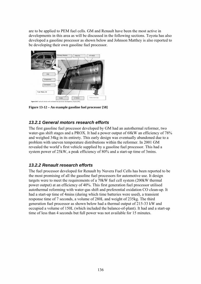
are to be applied to PEM fuel cells. GM and Renault have been the most active in developments in this area as will be discussed in the following sections. Toyota has also developed a gasoline processor as shown below and Johnson Matthey is also reported to be developing their own gasoline fuel processor.

Figure 13-12 – An example gasoline fuel processor [58]

13.2.1 General motors research efforts The first gasoline fuel processor developed by GM had an autothermal reformer, two water-gas shift stages and a PROX. It had a power output of 68kW an efficiency of 78% and weighed 34kg in its entirety. This early design was eventually abandoned due to a problem with uneven temperature distributions within the reformer. In 2001 GM revealed the world’s first vehicle supplied by a gasoline fuel processor. This had a system power of 25kW, a peak efficiency of 80% and a start-up time of 3mins.

13.2.2 Renault research efforts The fuel processor developed for Renault by Nuvera Fuel Cells has been reported to be the most promising of all the gasoline fuel processors for automotive use. It design targets were to meet the requirements of a 70kW fuel cell system (200kW thermal power output) at an efficiency of 40%. This first generation fuel processor utilised autothermal reforming with water-gas shift and preferential oxidation CO clean-up. It had a start-up time of 4mins (during which time batteries were used), a transient response time of 7 seconds, a volume of 280L and weight of 235kg. The third generation fuel processor as shown below had a thermal output of 215-33 kW and occupied a volume of 150L (which included the balance-of-plant). It had and a start-up time of less than 4 seconds but full power was not available for 15 minutes.

136

Figure 13-13 – A gasoline fuel processor developed by Nuvera for Renault [58]

13.3 Diesel and Kerosene fuel processors The reforming of jet fuel (kerosene) results in unwanted CO and sulphur by-products which necessitates additional fuel reforming stages which add cost, complexity, mass etc to the overall system. Diesel fuel processors are currently receiving interest for cars and auxiliary power sources in trucks. The catalytic partial oxidation and autothermal reforming of diesel (as well as JP-8, natural gas and gasoline) is being investigated by Delphi for use with their range of solid oxide fuel cells. Volkswagen has also joined forces with IdaTech to develop a diesel fuel processor/fuel cell system. Both Airbus and Boeing are investing the use of fuel cells to replace APU’s. These would consist of a solid oxide fuel cell fed by a kerosene fuel processor (using either partial oxidation or autothermal reforming). The anode waste gases would then be fed to an afterburner to generate power for the compressor. On a very large scale, studies are also being carried out with regards the development of 2.5MW fuel processor/fuel cell system for submarines.

13.4 Multi-fuel processors The ideal fuel processor would be one which is able to cater for a number of different fuels. This would make it not only future safe but also operationally flexible. Research is underway to develop such a system, which is able to provide the level of efficiency and reliability found in fuel processors which have been tailored to specific fuels. The fuel processor developed by Nuvera (already listed in the gasoline reformer section) is able to meet such requirements and able to handle gasoline, alcohols, natural gas, diesel and jet fuel. So far this has demonstrated a good efficiency and low CO content. Another key player in this area is International Fuel Cells who been developing a fuel processor which has a power equivalent to 50kW. This unit used an autothermal reformer, catalytic CO removal and feed desulphurisation and is able to cater for both methanol and gasoline.

137

14 Design and integration considerations for fuel cell systems

14.1 Introduction There are still a number of problems which have to be overcome before fuel cells can become commercially widespread within vehicles. Some of these which are associated with their start-up and shut-down and the onboard storage for fuels for long periods have proven to be less of an issue for vehicles such as buses. Since aircraft are characterised by similar steady operation over long periods, fuel cells are also expected to be well suited to operation within aircraft. This section will give an overview of what makes a complete fuel cell system and some the factors which need to be considered when integrating such systems.

14.2 What is balance of plant? The balance of plant is the significant amount of additional ancillaries which are required to enable a fuel cell to function. A complete fuel cell system including all ancillaries is a complex and difficult to manufacture system which must include the following sub-systems.

• Fuel supply – As will be discussed later, the fuel system can take a number of different forms depending on the fuel used. Pumps and regulators will generally be required to maintain a continual supply of fuel. Fuel pre-heaters and humidifiers may also be required to condition the fuel before it enters the fuel cell. Depending on the system, some form or recirculation may also be used.

• Air supply – This must be sufficient to maintain a continuous supply of air to the fuel cell. Systems can range from blowers for smaller fuel cells to compressors for larger systems typically found on vehicles or in some cases even bottled oxygen is used. This is usually linked with the humidification system.

• Humidification system – This is a necessity to keep the fuel cell sufficiently hydrated. A certain amount of product water from the fuel cell outlet is usually recovered and injected back into the fuel cell inlet for this purpose.

• Cooling system – This is necessary to maintain the heat balance of the plant. • Fuel cell operation - Various miscellaneous monitoring and control systems are

required in order to maintain the correct operation of the fuel cell. This includes systems to maintain the correct water balance and temperature etc.

• Power conditioning - Simple voltage regulators or DC/DC converters are used for this task to transform the DC output into a useable form.

• Electronic control system – This is required to monitor numerous sensors and maintain the fuel cell operating conditions via a numerous pressure regulators, control valves and pumps.

• Fuel cell start-up and shut-down systems - Additional valves and heaters may be required for these stages along with additional controller stages.

138

The balance of plant can add a significant amount of extra weight and occupy a considerable volume and as shown in the figure below which shows the complete Xcellsis HY-80 80kW fuel cell system used for the Ford Focus FCV. In this figure, the fuel cell is the box in the centre with the remainder being the balance of plant and PDU.

Figure 14-1 – Complete Ballard fuel cell system (including balance of plant) [59]

The balance of plant can consume an appreciable amount of power from the fuel cell output which reduces the overall efficiency of the complete fuel cell system and therefore careful integration of the different systems is required. Isolated fuel cells can be seen to be most efficient at the lower end of their operating range but when the power requirements of the ancillaries are taken into account a more constant efficiency over a wide operating range is apparent. An overview of a number of these sub-systems will be given in the sections below.

14.3 Fuel cell system design considerations and requirements As with any other more traditional propulsion system, fuel cell systems will be designed to meet design requirements laid down by the airworthiness regulations, customer and other internal design groups. Design considerations of particular relevance for fuel cell systems include:

• Fuel cell volume and mass – Which is usually expressed in terms of specific power and power density which are measures of the volume and mass respectively as a function of the fuel cell power output.

• Fuel processor mass and volume – Which are usually expressed as a function of either the hydrogen output or the power output of a fuel cell which it is sufficient to supply.

• Operating conditions – Consideration needs to be given to the temperature and pressure of the fuel cell operating environment. These will have a notable impact on the performance of the fuel cell, fuel processor and compressor as well as other systems such as the cooling.

• Compressor requirements – Consideration needs to be given to its mass, volume, input power requirements and efficiency which are normally derived as a function of its pressure ratio and flow rate.

139

• Reactant consumption of the fuel cell – Where hydrogen is used as the fuel, this will dictate the quantity which needs to be carried on-board the vehicle. When oxygen is used instead of air, this will also need to be carried on-board.

• Fuel consumption of the fuel processor – Where a fuel processor is used, its consumption dictates the quantity of fuel required to produce the desired quantity of hydrogen.

• Cooling system heat exchanger requirements – Its frontal area will not only dictate its heat removal capacity but since it interacts with the free-stream air, it will also contribute to the drag f the vehicle.

• Manoeuvring loads – The effect of g-loads could have a significant impact on the performance of a fuel cell. Such loads may result in a displacement of water within the fuel cell significant enough to locally dehydrate the cell and could thus result in degradation in performance or even permanent damage.

• Cost – The acquisition and operating costs need to be competitive with traditional propulsion systems to avoid their dismal on the basis of cost.

• Technology readiness – A limiting factor in fuel cell development is financial investment. Fuel cell systems need to be implemented at the early stage in order to generate a return on the existing developments.

• Start-up and shut-down – Certain fuel cell systems make take a long time to become fully operational and in such conditions, power from an alternative source is required.

• Transient performance – The response time of some fuel cell systems may be unsuitable for certain vehicles but this is less of a problem for continual operation vehicles such as aircraft, trains and buses.

• Lifespan and Maintenance – The lack of moving parts in a fuel cell gives them a competitive edge compared to IC engines. There is however a significant number of seals between the different fuel cell layers which will require careful inspection. The delicate construction of the fuel cell stack will require specialist tools and processes in order to carry out any repairs. In the event of any problems, maintenance engineers are not likely to be able to carry out such repairs and exchange units are likely to be used instead.

• Safety – The construction of a fuel cell stack means that failure of a single cell will not result in complete failure of a stack and will only result in degradation in performance. Since hydrogen fires burn with a virtually invisible flame, hydrogen leaks from seals are of particular concern. Suitable hydrogen leak detection and fire extinguisher systems are therefore required to reduce the risk.

14.4 Fuel supply The hydrogen and oxidant reactants which enter the fuel cell are distributed over the surface of the electrodes by means of a large number of passages in the backing plates. A number of different passage patterns have been explored to distribute the reactants as evenly as possible over the surfaces but it is inevitable that concentration gradients will still exist. It is typical for there to be a high concentration of reactants at the centre of the fuel cell which diminishes towards the edges. This also results in voltage gradients within the fuel cell plates but this subject is beyond the extent of this study. If we consider a simple straight channel with a reactant fed at one end as an example, as the

140

reactant travels along the channel it is also slowly absorbed into the fuel cell electrodes. By the time the reactant reaches the end of the channel, its concentration is considerably diminished. At these extremities, there is also likely to be a significant build up of impurities in the remaining reactants. It is therefore necessary to supply the reactants to the fuel cell in excess of what is actually required. In this context we are able to define an utilisation factor, which is a measure of the amount of hydrogen or oxidant which is actually converted within a fuel cell to that which is actually supplied. Fuel cells generally use hydrogen as their fuel which can be supplied directly from an onboard hydrogen source or extracted from another fuel such as methanol. An overview of each of these approaches will be given in the sections which follow.

14.4.1 Direct hydrogen fuel supply This is the simplest means of fuel supply in which hydrogen is held onboard the vehicle directly by means of some form of hydrogen storage. The most common approaches are compressed or liquefied tanks but other approaches such as hydrogen absorbers are also receiving considerable interest. In a typical system utilising compressed hydrogen from a high pressure cylinder, a pressure regulator is used to control the pressure of the hydrogen entering the fuel cell. Incidentally, the pressure of the hydrogen must balance that of the oxidant as a pressure differential across the membrane will result in its damage. As already discussed, the hydrogen is supplied to the fuel cell in excess of what is actually required and one of the three approaches below is typically used to utilise as much of this as possible to maintain a high economy.

• Dead end with purge – In this system, the fuel cell hydrogen exit is blocked off so that the hydrogen is retained within the stack until it is consumed by the fuel cell. Even bottled hydrogen is not 100% pure and impurities can build up within the fuel cell which is in addition to the water vapour which the hydrogen can collect. These dilatants can decrease its performance and it is necessary to purge such a system at regular intervals. For such purposes a purge valve at the fuel cell exit which is regularly opened. The downside of this being that hydrogen is wasted each time the system is purged.

• Closed loop with purge – This is an improvement over the previous system in which the hydrogen is able to freely pass through the stack. Upon its exit from the stack, it passes through a water separator to remove the excess water. The remaining dry hydrogen is then returned to the fuel cell inlet via a circulation pump or ejector pump. Such a system will still require purging but at less frequent intervals and is thus more economical.

• Straight through with a tail gas burner – In this system, the hydrogen passes through the stack just once. Upon its exit from the fuel cell, the remaining hydrogen passes through a water separator before being burnt in a tail gas burner. The pressure and temperature gases from the burner can be used to drive a compressor or heat another system. In such a system, the flow rate of hydrogen fed to the stack requires careful control to prevent wastage.

141

14.4.2 Hydrogen fuel supply via a fuel processor Instead of having to store large quantities of hydrogen, it is sometime more efficient to extract hydrogen from a hydrogen rich fuel instead. Such a process requires the integration of a fuel processor into the fuel cell system. The exact nature of each fuel processor is different but they typically include a reforming stage followed by several gas clean-up stages. When we consider that each stage has its own air, steam and heat requirements, the complexity of the integration of such a system soon becomes apparent. Fuel processors are complex in their own right and their design involves careful planning of the layout of the different components and the flows between them. In addition to this, the design of a fuel processor needs to also encompass the fuel cell system with a view to providing some commonality between the two systems. This would enable heat, air, water and coolant to be shared between the systems and thus reduce the number of components required. The design target for such a system is a high efficiency, minimal content of CO and other by-products and sufficient flexibility to meet its demands. Due to their complexity, it is typical for a fuel processor to use a dedicated control system for control of the temperature and all the air, fuel and steam supplies. An example of an integrated fuel cell/fuel processor system is shown below.

Figure 14-2 – An example complete fuel cell system with integrated fuel processor [57]

The reformate from a fuel processor typically contains significant proportions of carbon dioxide and nitrogen in addition to hydrogen which act as dilutants in the fuel cell. In such systems, any unused reformate which leaves the fuel cell is typically burnt within a tail gas burner to generate heat for the fuel processor. Since the reformate already leaves the fuel processor in a hot and saturated state, there is no need for an anode humidifier as used on direct hydrogen systems. A cooler and water separator is still required however to reduce the temperature and water content of the reformate.

14.5 Oxidant supply The oxidant used with a fuel cell is either oxygen from a compressed source or atmospheric air. As with the fuel supply, the oxidant must be supplied to the fuel cell in

142

excess of that required to ensure there is a sufficient concentration across the surface of the fuel cell. This is defined by the stoichiometric ratio with a value of 2 or above being typical. Where oxygen is used, it is typical to use a closed loop with purge system as for the hydrogen supply. When air is used, there is no need to re-circulate the oxidant and a straight through system can be used. In such systems, the air is driven through the fuel cell with the aid of a blower or air compressor. The oxygen depleted air leaving the fuel cell has a high water content which is usually recovered with a water separator to be used elsewhere within the fuel cell system. Where the air is compressed before entering the fuel cell, an expander can be used at the fuel cell exit to recover some of this energy. In systems where a burner is employed, the excess oxidant is used in the burner to compliment the excess hydrogen from the fuel supply.

14.5.1 Using air instead of oxygen Systems using air are less efficient that those using oxygen since only 21% of air is oxygen. This means that considerably more air needs to be delivered to the fuel cell to supply the same quantity of oxygen. When we take into account the excess defined by the stoichiometric ratio, the quantity of air must be ratioed by the same amount and thus the quantity of air required can be considerable. Supplying too much air to the fuel cell is however not only a waste of energy required for the compressor or blower but can also carry too much heat away from the fuel cell. In small systems, air can be supplied at higher stoichiometric ratios to cool the fuel cell. Although such an approach is insufficient to completely cool a larger fuel cell, it could bring the temperature down below what is required. Where air is used, some form of air cleaner must also be incorporated into the air supply to remove particles and other unwanted substances.

14.5.2 Air compressors As already discussed fuel cells are typically operated at higher than ambient pressures to increase performance and improve water balance (1.5 bar being a typical figure). This thus necessitates the need for some form of air compressor. The incorporation of an air compressor into the system does however increase the cost and complexity of the system. Allowance must also be made for the power-off take required to drive the compressor which can have a considerable impact on the actual fuel cell output. It is possible to run a fuel cell at near atmospheric pressures but some level of compression is still required to overcome the pressure drop within the fuel cell. The type of compressors used is however relative to the application and larger fuel cells may require an extensive device while a simple blower may be sufficient for smaller fuel cells. Blowers are only suitable for small to medium sized fuel cells which require low pressures. No single type of compressor can thus cater for the range of fuel cell sizes encountered in practice. The selection of a suitable compressor is based on the following requirements. Although it will not be possible to fulfil all of these, the ideal is device is one which offers the best balance of all of these parameters.

• Desired pressure ratio and mass flow rate – As required by the fuel cell. • Good efficiency - Over the operating range encountered from partial to full load.

143

• Heating effect of the compressor – This is related to the efficiency of the compressor. Higher heating dictates the need for additional cooling stages to bring the temperature of the air down to a level suitable for entry to the fuel cell.

• Noise and vibration – Important for any aircraft. The compressor is the major source of noise within a fuel cell system and can be influenced by other system components.

• Low mass and volume – Important for any aircraft. • Low cost – Including initial outlay and subsequent maintenance costs. • Durability and lifespan – Crucial for the safety and reliability of any system. • Outlet air purity – The outlet air must be free from contaminants such as oil • Transient response – The device must be able to meet the fuel cell demands.

There are four main types of compressor commonly encountered in reasonable sized fuel cell systems dictating the need for a high mass flow rate. These are given below and can be categorised as positive displacement or aerodynamic compressors.

• Roots compressor – These are cheap and work over a wide range of flow rates but only achieve reasonable efficiencies for small pressure differentials.

• Lysholm (screw) compressor – These provide good efficiency over a wide range of flow rates but are expensive to manufacture. By changing the length and pitch of the screws, these can be designed to provide a wide range of compression ratios.

• Centrifugal (radial) compressor – These are common, inexpensive, reliable and a wide range of units are available to suit a variety of flow rates. They offer good efficiency but only within well defined pressure and flow rate limits and are not suitable for low flow rates. These units also require careful lubrication due to the high rotor speeds of typically 80,000rpm. Care must be taken during their operation to avoid surge, a condition where the compressor becomes unstable. To achieve optimum efficency, the operating pressure must increase/decrease in accordance with increases/decreases in flow rate.

• Axial compressor – These offer good efficiency but only over a narrow range of flow rates and are expensive to manufacture.

The selection of a suitable air compressor has traditionally been made from existing units. Although these units are mature, they were however designed specifically for other applications. For example, the majority of compressors which operate with pressure ratios between 1.4 and 3 have been designed for IC engines. An example of such a unit this is the Eaton supercharger which is well suited for applications with a pressure ratio between 1.35 and 1.7. The smallest unit in this range is able to deliver flow rates of 50 to 100Ls-1 and thus these are only suitable for large fuel cell systems over 50kW. Compressors for systems of less than 50kW are significantly more difficult to obtain. Systems operating at higher pressures ratios between 1.6 and 3 also experience difficulties in finding a suitable unit. The Lysholm compressor is the most suitable in this case but these are designed for high flow rates. The smallest unit corresponds to mass flow rates up to 0.12kgs-1 which corresponding to systems of about 100kW.

144

More recently, a number of companies such as Opcon Autorotor, Eaton and Rotrex have started to develop air compressors specifically aimed at fuel cell systems. The correct selection of such devices does however require the use of manufacturer’s performance charts in terms of the ‘non-dimensional’ mass flow and rotational speed factors. These can however be difficult to obtain and in some cases custom compressor units may have to be developed to meet the needs of a particular application. A characteristic of any compression process is that the air is heated as a result of the process and thus the air may need to be cooled before it can be safely used within the fuel cell. An intercooler (using free-stream air) can be used for this task or alternatively a heat exchanger can be used to transfer the heat to the incoming hydrogen flow. If the fuel cell and fuel processor are designed to operate at similar pressures, then the same compressor unit can be used to deliver air to both.

14.5.3 Turbines and expanders These are used for the recovery of power from high pressure air leaving the fuel cell or hot exhaust gases leaving a burner. Although these are not used for oxidant supply, they are relatives of the air compression devices and thus worth a mention here. Because of the nature of the expansion process, these units also enable the exhaust gases to be cooled sufficient for later water recovery stages. The preferred choice of turbine for use in fuel cell systems is the centripetal (radial) turbine which can be likened to the centrifugal compressor. These do however operate at extremely high speeds which means that they are unsuitable for driving lower speed compressors such as the screw compressor. Their speed is thus well matched to driving centrifugal compressors as is done in a turbocharger. Such turbocharger units are readily available in a range of sizes but are only suitable for fuel cells over 50kW. It is however possible to combine two positive displacement devices in the same way. In such turbocharger units, the energy of the exhaust gases must be increased with the use of a tail gas burner which uses either an additional supply of hydrogen or the excess from the fuel cell. Compared to turbochargers, mechanical superchargers offer benefits of an improved transient response but at the expense of NHV behaviour, power demands and efficiency. Waste gates, variable turbine geometries and turbine inlet throttles can be used to balance the compressor and turbine power requirements and demands respectively. The advent of fuel cells has promoted the development of compressor/expander units specifically for fuel cells. Key players in this field are Honeywell and Vairex. These units are however currently only aimed at 50kW fuel cell vehicles. For larger systems, automotive turbochargers remain the best option.

14.6 Humidification requirements and water management A criterion for a PEM fuel cell is that its electrolyte membrane is kept sufficiently hydrated. Failure to do so will result in the electrolyte drying out which is accompanied by a degradation in fuel cell performance and the risk of permanent damage to the fuel cell. The flow of air entering the fuel cell has a drying effect on the membrane, which is another reason why air cooling is not used in larger fuel cells. Although the atmospheric air entering the fuel cell will have some humidity, this will be insufficient to meet the

145

needs of the fuel cell. To overcome this, the intake air must be maintained at a high level of humidity which is typically achieved by means of injection of water under high pressure into a cathode air supply humidifier. An additional complexity when fuel cells are used in vehicles is the influence of external forges which can cause movement of the water within the fuel cell leading to humidity gradients within the membrane. It is also usual to hydrate the hydrogen entering the system as well but this is usually less than for the air side of the fuel cell. The water used for hydration must be of high purity to prevent the fuel cell from being contaminated and water obtained from the fuel cell exit as a by-product of the reaction is used for this purpose The water captured at the fuel cell exit is not only used for hydration but is also required for other systems such as the fuel processor (to generate steam for the reformer and shift reactors). The total balance of water within the system is more complex than this in reality since water is also generated by the tail gas combustor and preferential oxidation units. In addition, the quantity of water that initially enters the fuel cell along with the air is also dependent on environmental conditions. Any unused water can either be dumped or left to exit the system in its vapour state (which can be beneficial to increase the mass flow rate through any expander such as a turbine).

14.7 Thermal management and the cooling system In any fuel cell system it is necessary to make provision for adequate cooling of the system. This needs to be sufficient to not only cool the fuel cell but also all the associated ancillaries such as the fuel processor. Fortunately, some of this waste heat can be reused within other components such as fuel pre-heaters and vaporisers. Drive components such as traction motors and controllers also require cooling but they typically use their own cooling circuit. In small systems, the power is usually low enough that air cooling is sufficient in which excess air is supplied to the fuel cell to remove the waste heat. This is however insufficient for higher powered systems and a liquid cooling system is typically used instead. Although IC engines operate at higher temperatures than fuel cells, the heat load on their cooling system is less since a significant proportion of their waste heat is carried out the engine by the hot exhaust gases. The cooler exhaust gases of a fuel cell means that the proportion of heat retained within the fuel cell which must be removed by the cooling system is higher. Within a fuel cell system, surplus heat is typically removed by a combination of an exhaust gas condenser and a radiator type heat exchanger. The actual ratio of heat removed by the condenser to that removed by the radiator is however dependant on the operating temperature and pressure of the system. Heat removal by the condenser is more favourable at higher temperatures and lower pressures with the radiator being more favourable in the opposite sense. The working principle of using a condenser for cooling is that a portion of the waste heat is consumed by the phase change that takes place (the condensation of steam into water). Such units do however have lower heat transfer coefficients that their radiator counterparts which imply the need for larger heat exchange areas and thus a large unit when subject to the same heat load. The dependency of the effectiveness of a radiator on

146

temperature means that at low operating temperatures (as encountered with PEM fuel cells) larger radiators are required in order to be able to remove sufficient heat. Automotive radiators are typically used for this purpose because of their compactness (producing heat exchange areas of greater that 1000m2/m3) but even this may prove to be insufficient in some cases the size of fuel cell may be limited by the cooling system. Although the cooling system could utilise water recovered from the fuel cell, a separate water circuit is typically used to cool both the fuel cell stack and fuel processor. The cooling circuit encompasses many components within the fuel cell system as some of these have also have cooling needs while it is possible to utilise some of the waste heat elsewhere within others (such as the air humidifiers). This allows antifreeze and coolant additives to be used which prevent freezing and offer improved heat capacity. The figure included in the hydrogen supply section gives and example of such a system.

14.8 Electrical energy storage It is necessary to provide some means of energy storage onboard a fuel cell powered vehicle to provide an alternative source of energy to meet the following requirements.

• Start-up – It may take a few minutes for a fuel cell to become fully operational during which time power is required for pre-heaters, pumps, sensors, control systems. This is however less of a concern for a aircraft as a ground cart could be used as for the start-up of a conventional aircraft.

• Short term high power demands – In the case of an aircraft, such instances will be experienced during take-off and acceleration. For continual high power operation, it will be necessary to use a larger fuel cell but for short periods, an additional energy supply can be used to boost the power from the fuel cell.

• Transient operation – Fuel cells will not be as responsive as IC engines and therefore a means of smoothing out the power distribution is required.

• Back-up power – In the event of failure of the fuel cell, there must be sufficient power available to be able to safely bring the vehicle to rest.

Batteries are the commonest way to provide additional electrical power but super capacitors have also been receiving considerable interest. A pack of super capacitors has been shown to be an efficient means of storing a large quantity of energy for a short period of time. Tests on such a pack of 90 super capacitors showed it was able to provide 50kW over a 15 second period for a weight penalty of 168kg. The short duration of such units is however less likely to be sufficient for providing back-up power and batteries may still be required for such needs.

14.9 Costs At their current level of technology, fuel cells are considerably more expensive than a comparable IC engine. The main cost drivers for fuel cells are the fuel cell manufacturing processes and the system ancillary equipment required. Cost will unfortunately be one of the main deciding factors as to the initial success of a fuel cell powered aircraft and we are unlikely to see such aircraft entering production in the short term as a result. Such units are more likely to be realised in the automotive industry first

147

which and their costs are expected to come down as a result of the increases in production. The US DOE set a target price of 45$/kW for a fuel cell in the year 2010 which was backed by a Ballard’s 2010 predictions of 45$/kW. Although system costs will be higher, fuel costs will during our time of rising fuel costs, makes fuel cell powered aircraft a significant long term investment. As an example, a study carried out in 2006 predicted the cost of fuel for a Cessna 172 in 2010-2015 to be 50.56$/h (assuming a price of 5$/gallon). Oil prices have however risen considerably greater than these predictions in recent years and they are expected to continue to do so in the next few years. An equivalent fuel cell with an assumed hydrogen consumption of 9kg/h (with a predicted hydrogen price for the 2012-2015 period of between 2.35$/kg to 6.97$/kg) is expected to have a fuel cost of between 18$/h and 63$/h. The maintenance costs are expected to be slightly higher due to the complexity and specialist nature of the systems but the US DOE has set a service life target of 5000 hours by the year 2010.

14.10 Safety considerations The greatest risk within a fuel cell system is that of hydrogen leaks which can result in a dangerous hydrogen/oxygen gas mixture. The dangerous nature of a leaked gas mixture means that the fault tolerance of such a system is low and careful manufacture, assembly, testing and maintenance is necessary. Problematic areas within a fuel cell are couplings, joints and the mating faces between plates and electrodes. Although bi-polar plates are designed with a layout to reduce the risk of leaks at the edges, leaks are still problematic. The porous nature of the electrodes is also an area of concern especially its edges, where a gasket is normally used. Adequate means of detecting hydrogen leaks must be incorporated into a fuel cell system to prevent a disaster. Another concern for any propulsion system is that of loss of power in the event of a failure. As discussed, the construction of a fuel cell stack means that failure of a single cell will not result in complete failure of a stack. In such cases, the loss of an individual cell will only result in degradation in performance which is in contrast to an IC engine.

14.11 Fuel cell durability and reliability The lifespan of a fuel cell is an important consideration which must be thoroughly evaluated if fuel cells are to be accepted as primary sources of power for propulsion. A significant amount of experimental testing is required to determine the lifetime of a fuel cell system. Such testing is costly and is sometimes impractical. Typical figures suggest an operating lifetime of between 3000 and 5000 for automotive applications and up to 20,000 hours for buses. Such studies are however are carried out for the use of air and pure hydrogen with little information being available for the use of reformed fuels. In such studies water management and been shown to be a major contributor to the lifespan and performance of a fuel cell. Excess water can lead to impurities being deposited on the catalysts or membrane and thus poisoning of the fuel cell. In the case of methanol reformer systems, it is important to keep the quantity of unreacted methanol to a minimum as this can diffuse to the cathode and contaminate the catalyst. A number of preventative measures can be used to preserve the life of a fuel cell. Such measures include, the injection of oxygen into the fuel stream to remove contaminants

148

by oxidation and regular reactant chamber purging with an inert gas. Other measures include the operation at lower pressures and temperatures and the maintenance of a correct water balance. The performance of any fuel cell in a stack can be carefully monitored by assessing its electrical or thermal response. Such data can be fed back to the fuel cell control unit to adjust the flow rate of reactants or humidity to that cell. The reader is advised to refer to ‘Failure Analysis of Polymer Electrolyte Fuel Cells’ by Pratap Rama et al [60] for a theoretical analysis of fuel cell failure.

14.12 Future outlook and challenges for fuel cells There is a definite market for fuel cell powered aircraft but there are a number of barriers preventing the realisation of such an aircraft in the short term. These have already been mentioned in the discussion above but to summarise, these are, cost, specific power and power density, fuel choice and safety. These areas have already been highlighted as long term goals for further development of fuel cell system and so improvements are expected within the next few years.

14.13 Traction motors for electric vehicles Electric motors are a key component within any electric vehicle and selection of the correct motor is vital to the performance and efficiency of the vehicle. There are many different types of motors available with the best one to use being dependent on the application. A high efficiency motor is desirable to ensure that its power demands and thus the size of the accompanying batteries or fuel cell and ultimately the weight of the vehicle are kept to a minimum. Since a reduction in the weight of the vehicle will result in a reduction in the power demands, a converging design spiral results. Selection of the best motor will however involve a trade-off of a range of requirements such as efficiency, power output, operating range, weight, size, cooling requirements, maintenance and cost.

14.13.1 An overview of electric traction motors Selection of the right motor does require some knowledge of the characteristics of the different motors. An overview of the most common motor types is given below, each of which works in a slightly different way.

• Permanent magnet brushed DC motor – These traditional motors use fixed permanent magnets, a multiple coil wound rotating core and brushes. The torque is dependant on the current, which is dependent on the supply voltage and the resistance of the armature. The presence of back EMF results in maximum torque when the armature is stationary with a progressive drop in current and thus torque with increasing motor speeds. A controller is required at low speeds to limit the current and thus prevent damage to the motor. These motors have been replaced by more sophisticated types for vehicle traction applications but are still very popular for general purpose applications.

149

• Electro-magnet brushed DC motor – These are a more sophisticated form of the motor above whereby the magnetic field is generated by electro-magnets (field windings) instead. Field windings are more efficient and cheaper way to generate a strong magnetic field and also enable the magnetic field strength to be varied for better motor control. Such motors do however generate additional heat and thus require improved cooling. The field windings in the series and shunt wound variants are fitted in series and parallel to the motor core and are thus dependent on the operating characteristics of the core, resulting in limited control of the motors speed and torque. The field windings in the separately excited motor are part of a separately controlled circuit which allows independent control of the magnetic flux and thus allows greater control of the motor torque at any speed. As a result, these motors are a popular choice for electric vehicles.

Brushless motor were envisioned to overcome the problems of friction, heat and wear associated with the contact between brushes and the commutator in traditional motors. They are also typically arranged so that the majority of heat is generated in the outer part of the motor and is therefore easier to dispense. The three most common types of brushless motors used in electric vehicles are briefly discussed below.

• Brushless DC motor (self-synchronous AC motor) – This is an AC motor which consists of a permanent magnet rotor which is surrounded by a number of stator coils. The stator coils are successively energised to induce magnetic fields in the stator which interact with the magnetic field of the rotor and generate a torque. They use DC power which is converted to AC by the motor controller but have operating characteristics similar to that of a traditional DC motor. Back EMF in the stator coils reduces the magnetic field strength and thus torque as the speed increases. Sophisticated versions of this motor are well suited for high power and traction applications. Compared to similar motors, the permanent magnet rotor does increase the cost of the motor but it also increases its efficiency and specific power.

• Switched reluctance motor – This consists of a cheap plain iron rotor which is

surrounded by a number of stator lobes which are successively magnetised by coils. Induced magnetic fields in the rotor and stator generate a force of attraction between the two components to bring them in-line. Successive switching of the stator coils enables an angular momentum of the rotor to be maintained. The speed is controlled by the duration that each stator coil is switched on for and thus a microcontroller is required. The elimination of permanent magnets and back EMF means that higher speeds can be achieved. These motors offer benefits of higher torque per unit volume and higher speeds and thus higher power densities. Their peak efficiency is lower but more desirable efficiencies can be obtained over much wider operating band.

• Induction motors – These consist of a linked rod rotor which is surrounded by a

number of equally spaced stator coils. When connected to a three phase AC supply, an anti-clockwise rotating magnetic field is generated by the stator coils. A corresponding current is generated in the rotor rods and force which prompts

150

the rotor to follow the rotating field. The maximum torque that can be obtained is dependent on the strength of the magnetic field from the coils. The number of stator coils (poles) defines the design speed of the motor but variation of the frequency of the three phase supply enables the speed of the motor to be controlled. An inverter is required in order to be able to connect these motor to a DC system. These motors are very slightly less efficient than similar types but have a number of advantages which has resulted in their widespread use.

14.13.2 Motor cooling requirements There are four main sources of loses within a motor, copper losses, iron losses, friction and windage and constant losses. These motor losses are dependent on its torque and speed and thus its efficiency is also dependent on these. Such losses are accompanied by a generation of heat and sufficient heat removal methods are required to prevent an excess build up of heat which can lead to its failure. Motors are able to safely exceed their rated power output for transient short periods but should not do so for extended periods when they are likely to overheat. The power output of the motor is thus limited as a result of its cooling effectiveness. Configurations in which the losses and heat are generated in the outer components instead of the core have proven to be easier to cool due to their greater surface area. Air cooling is generally the preferred method of heat removal but liquid cooling can be used for high power motors where this is insufficient.

14.13.3 Motor requirements and selection Size and mass are particularly important requirements for traction motors and typical measured in terms of power density (power per unit volume) and specific power (power per kilogram mass). For DC systems, AC motors are generally lighter than their DC counterparts but an inverter is required. The method of cooling can be seen to have a significant impact on its specific power with liquid cooling enabling an equivalent power to be extracted from a much smaller motor. These motors do however have the additional weight of the cooling system. Efficiency is also a particularly important parameter which is influenced by,

• The type of motor - Brushless motor types can achieve slightly higher efficiencies due to lower losses in the rotor.

• Operating speed - Motor losses are related to its torque and thus speed, with high speed low torque motors being the most efficient.

• Cooling - Since the resistance of the motor windings increases with temperature. • Size of the motor – The efficiency can be seen to increase with size for induction

motors. • Operating conditions – A wide operating efficiency band is important for motors

which are subject to variable speed/torque conditions as with reluctance motors. It is worth noting that the size of a motor can be shown to be governed by its torque requirements and not power requirements. This means that high speed low torque requirements will only require a small motor. A high speed motor/gearbox combination will thus sometimes be more compact and lighter than an equivalent low speed motor for low speed applications. A next generation improved motor has been proposed called the HTS motor (High Temperature Superconductor) which uses superconductor alloys

151

152

instead of traditional copper windings. Their main drawback is the need for a complex cooling system to maintain low operating temperatures of about 50ºK.

14.13.4 Associated regulators and controllers The voltage output from sources such as fuel cells can vary with respect to time, temperature and current leading to an impractical very wide voltage range. The first stage in such a circuit is thus a voltage regulator, which is used to transform unsteady voltages into a more practical and regulated form. Batteries are able to deliver a well regulated voltage output but even this has to be varied when controlling equipment such as motors. It is typical to incorporate electronic switching circuits for such purposes to either drop or boost the voltage output to achieve either a fixed or variable voltage as desired. The requirements of electric vehicles mean that custom DC/DC converters and step-up/step-down chopper circuits may be required. When a AC motor is to be driven from a DC supply an inverter is also required. Motor controllers are vital to the efficient operation of any motor. In the case of basic DC motors, these may be simple units which use step-up and step-down regulators to vary the supply voltage and thus torque. In the case of more sophisticated motors, an additional control is achieved by varying the magnetic field via field windings. A combination of both flux and voltage control enable a motor to work over a wider range of torque and speed conditions but requires a complex electronic control system.

15 Sizing and integration of the fuel reformer based MALE fuel cell system

This section gives an overview of the selection, sizing and integration of the fuel cell propulsion system which is being investigated to replace the conventional turboprop engine of the MALE UAV. The enormity of the system selection and sizing work meant that it was necessary to incorporate as much as possible of this work into the accompanying appendices and other thesis sections. This section will thus only give an overview of each of these stages and point the reader to the relevant sections for further information. The main focus of the discussion contained in this section will thus be on the integration of the system into the aircraft.

15.1 Selection of the fuel cell type and candidate fuel The study into different fuel cell types showed the PEM fuel cell to have benefits of low operational temperatures, short transient and start-up periods and respectable efficiencies. They are thus regarded as the fuel cell of choice for use in the majority of other fuel cell powered vehicles. As a result, they have received considerable investment from developers and are thus currently the most technically advanced. The PEM fuel cell has thus been highlighted as being most appropriate for this project. The study into alternative fuels has focused on an in-depth review of hydrogen and methanol. Hydrogen is the most appropriate fuel for use in fuel cells with its pure form currently regarded by many as the fuel of choice for fuel cell vehicles. Hydrogen is however accompanied with storage and operational problems which have proven to be one of the bottle necks in the development of fuel cell vehicles. An alternative approach to the use of pure hydrogen is to extract it on-demand from a hydrogen rich fuel which can be more likened to conventional fuels. Such a process does however necessitate the need for additional equipment to reform the fuel which adds cost, weight and complexity to the system. This is however offset by the fact that more conventional fuel tanks and fuel delivery equipment can be used. In this study methanol was shown to be the best synthetic hydrogen carrier fuel for this purpose. Its benefits include the requirement of a low reforming temperature, already being mass produced in large quantities and the potential to adapt existing fuel infrastructures for its use.

15.2 An overview of the all-electric propulsion system The all-electric propulsion system which was devised for this project can be broken down into two sub-systems as given below.

• The fuel reformer based fuel cell system – This system utilises a fuel cell and its associated balance of plant to generate DC electrical power for the electric powertrain. This is accompanied by a fuel processor which is integrated into the system and used to extract hydrogen on-demand from the methanol fuel. The system also incorporates an air compressor which is used to improve the performance of the system. The power demands of the compressor are met by

153

burning excess hydrogen in a tail-gas burner to generate hot gases to drive a turbine which is directly coupled to the compressor.

• The all-electric power train – This system utilises 2 large traction motors and their associated controllers to transform electrical power into mechanical shaft power. The traction motors are linked via a 2 into one reduction gearbox, the output from which drives the aircraft propeller. Also incorporated into the system are regulators and inverters which are used to stabilise and transform the output voltage from the fuel cell system.

A more in-depth description of these systems is given in Appendix E and the reader is advised to refer to this section for further details.

15.3 The influence of fuel cell operating parameters The performance and efficiency of the fuel cell system is directly related to the numerous system variables. This includes a range of parameters such as operating temperature and pressure, fuel and air flow, system humidity, output current, reformate composition and many more. It can be shown however that many of these parameters are inter-related and the number of actual independent variables is significantly reduced. For the purpose of this work, an extensive spreadsheet was developed to analyse the complete fuel reformer based fuel cell system. This was able to automate the optimisation of the majority of the variables with the only unknowns being operating pressure ratio and desired output power. A breakdown of the different stages that make up the complete analysis spreadsheet is given in Appendix H with the accompanying equation derivations given in Appendix G. These sections also include a thorough discussion of the relationships that exist between the different operating parameters. The reader is thus advised to review these sections for a better understanding of the function of the different fuel cell operating parameters. The hydrogen and oxygen stoichiometric ratios are particularly important as these have a strong influence on the fuel consumption of the system. The stoichiometric ratio is by definition the ratio of the actual quantity of hydrogen or oxygen delivered to the theoretically required quantity. In this particular system, the excess hydrogen leaving the fuel cell is utilised in the burner to generate hot gases to drive the turbine. Thus the careful control of the hydrogen stoichiometric ratio enables the power out of the turbine to be regulated to match power requirement of the compressor. In a similar way, the oxygen stoichiometric ratio is regulated according to the water content of the air. Too much air not only requires excess fuel to drive the compressor but also has a drying effect on the fuel cell and thus should be avoided. Too little air can result in their being either insufficient air in the burner or the fuel cell becoming flooded. The operating temperature of the fuel cell can be shown to be directly related to the pressure by the requirement to keep the fuel cell exit gases in a two phase state. This implies that the exit gases must be kept within the thermodynamic vapour dome. The final operating parameter is the compressor pressure ratio, which can be shown to be an independent design variable. As a result, it is not influenced by other parameters but does have a considerable impact on the performance of the whole system. In particular, this affects the operating pressure and thus the performance of the fuel cell and fuel

154

processor over the range of altitudes experienced. To determine the best pressure ratio, the system was tested at two different values to arrive at the results below.

Comparison of fuel consumption at different pressure ratios

0

0.01

0.02

0.03

0.04

0.05

0.06

0.07

0.08

0 1 2 3 4 5 6 7 8

Flight phase

m-d

ot fu

el in

(kg/

s)

PR 3

PR 4

Chart 15-1 – Fuel consumption at different pressure ratios

Flight phase points 1-3 is climb start to end, 3-5 is cruise outbound start to end and 5-7 is loiter start to end. Point 7 also represents the start of cruise inbound. These trends show us that there is a slight fuel consumption advantage at loiter in terms of using a pressure ratio of 4 as opposed to 3. The reverse can be seen to be true at start-mid cruise but since the aircraft spends the majority of its time at loiter it makes sense to optimise the fuel consumption for this phase. Although it is possible to use even higher values of pressure ratio, to do so would require a significantly more demanding compressor unit. The pressure ratio has thus been fixed at a value of 4 for this system. As will be discussed elsewhere, operation at a higher pressure ratio also results in a smaller required radiator size. This has the added benefits of reductions in mass and drag.

15.4 The influence of the fuel processor In this analysis we are considering two types of fuel processor, the autothermal reformer based unit and the steam reformer based unit. As is discussed in a different section, each unit has its own advantages and disadvantages and thus it is worth assessing the performance of each one. Values of typical reformate compositions for each unit are given in the table below. Typical reformate compositions

H2 CO2 N2Methanol autothermal reformer 0.50 0.20 0.30Methanol steam reformer 0.70 0.29 0.01 Table 15-1

15.5 Overall sizing of the all-electric propulsion system The fuel cell system and powertrain must be sized to be able to deliver sufficient power to the propeller at the most demanding flight phase. There will however be a number of losses in the components that make up the powertrain which must be taken into account.

155

To compensate, the power delivered by the fuel cell must therefore be more than that required at the propeller shaft. The methodology used to size the fuel cell system was apropeller back approach, whereby our starting point is the propeller thrust requirements.The overall efficiency of our powertrain is thus taken to include the efficiency of the propeller, gearbox, motors and motor controllers. Additional losses due to other components within the powertrain are considered negligible compared to these. Treader is advised to refer to Appendix E for further details of the derivation of the fuecell system power requirements.

he l

can be shown that the propeller is the source of the greatest loss within the t and

is

15.6 The analysis of the final system rily interested in evaluating the

e.

d

e but

r a

he analytical expressions discussed above were shown to give very good results for

ht

15.7 The selection of a suitable compressor-turbine unit An overview of the different compressor types and their suitability for fuel cell systems was given in the integration consideration section. The analysis of the reformer based

Itpowertrain. Its efficiency is dependent on its size, operating speed, power inpulocation on the aircraft. The importance of correct propeller matching can thus not beunderestimated. A detailed description of the determination of the propeller efficiency given in the baseline design section of the main text of this thesis.

For the purpose of this feasibility study we are primaspecific fuel consumption of the installed system throughout the flight profile of the aircraft. This required the construction of an analytical model of the fuel cell system which gives the fuel consumption as a function of power output and operating altitudThis model was based on test data obtained from the fuel cell design and analysis spreadsheet described in Appendix H. Using this spreadsheet, the system was testeover a range of combinations of fuel cell power output and altitude to generate an extensive database of results. This raw data can then be converted more manageablcomplex analytical expression with the aid of various stages of numerical analysis. The result is a polynomial expression to determine the fuel consumption as a function of the fuel cell power output. The constants of this expression are themselves determined by expressions which are functions of the operating altitude. This process is repeated to obtain two expressions, one for an autothermal based fuel cell system and the other fosteam reformer based system. A more detailed description of this procedure and the resulting expressions are given in Appendix J. Tmedium to high power settings as encountered in the take-off to descent flight phase. These were however less satisfactory for low power settings as encountered in the sealevel loiter and landing phases. An alternative low power expression was thus derived for these phases following a similar process as above utilising low power data at sea level conditions from the design and analysis spreadsheet. Since these low power fligphases are at sea level conditions, the resulting quadratic expressions are much simpler that before with fixed constants. These analytical models can finally integrated into the existing performance analysis spreadsheets used for the baseline aircraft as discussed in the evaluation section and Appendix J.

156

fuel cell system at different conditions showed the maximum required mass flow rate of

l

ited to

t

this study it was sufficient to represent the main components of the reformer based fuel cell system as boxes. The main purpose of this work being to ensure that there is

d itu

air to be 0.6397 kg/s at the top of climb. Using the density of air at this condition, this gives a required volumetric flow rate of 829.94 litres/s. Since our system utilises four independently controlled reformer-fuel cell units, it makes sense to use a separate compressor-turbine unit for each. If we were to use a single compressor to supply air to all four fuel cells then a wide variation in the flow rate would be experienced if any of the fuel cell units were shut down. Thus the use of a dedicated compressor for each fuecell enables each compressor to operate in the highest efficiency regime. The required mass flow rate through compressor will then be 207.49 litres/s. From the earlier discussion, a centrifugal compressor–radial turbine turbo-compressor arrangement is clearly the best solution to meet the desired mass flow rates and pressure

tios. Compared to other types, the centrifugal compressor is also well surameeting the required compressor ratio value of 4. The Autorotor twin screw compressors would also provide a good solution for the air compressor side of the system but would be difficult to link to a suitable turbine. The selection of an off the shelf compressor-turbine unit is however fraught with difficulty due to the lack ofavailable manufacturers data. The analysis for such a unit needs to take into accounpower requirements, efficiency and the impact of altitude and is thus clearly not possible within the timeframe of this project.

15.8 Sizing and integration of the fuel cell system components In

sufficient space available within the aircraft and to determine the best location of each component with respect to the centre of gravity of the aircraft. The mass of each component must thus also be determined. For the purpose of this work it is sufficient toconcentrate on the fuel cell and reformer modules with other components being less critical in comparison. The mass and volume of each is determined from statistical estimates of the specific power and power density as is discussed in Appendix E. An example of a modern methanol reformer module, the ME-75-6 (typical of that usein this project) is shown in the figure below. The accompanying figure shows it in s

the Xcellsis ME-75-6 fuel cell engine. in

Figures 15-1 and 15-2 – The Xcellsis fuel processor in situ [59]

157

The fuel cell system air intake and exhaust must also be given careful consideration for the integration of the system. These are sized according to the methods of Appendix I. The final routing and layout of these is decided by designer’s eye.

15.9 Sizing and integration of the cooling system The design and sizing of the cooling system involved an extensive analysis of the complete system based on the first law of thermodynamics. Due to its close relationship with the fuel cell operating conditions, the cooling system analysis was incorporated into the fuel cell system design and analysis spreadsheet. Due to the scale of the task,

the cooling system is given in

anger which is e fuselage and used to transfer some of the waste heat to the fuel held in the

nt of the aircraft drag due an

essor of

the description of the selection, sizing and integration ofAppendix I. The final system consists of a large 3-row air-liquid heat exchanger located in the aft fuselage which is used to dispense 65% of the waste heat. The remaining heat is dispensed of predominantly by smaller 3-row air-liquid heat exchangers located in ach tailboom. These are supplemented with a liquid-liquid heat exche

located in thwing fuel tanks and thus also prevent the fuel from freezing. Each air-liquid heat exchanger must be accompanied by an intake and exhaust which were sized according to the following guidelines.

• Duct entrance area = One third of the heat exchanger matrix frontal area. • Duct exit area = 115% of the duct entrance area. • Length of the entrance and exit ducts = Equivalent to the radiator height.

The boom radiators utilise a pitot type intake located at the front of the boom and a straight-out exit underneath the boom. The fuselage radiator utilises a flush NACA inleton each side of the aft fuselage and an exit aperture located at the very rear of the fuselage just below the propeller shaft. In each case, fairly complex ducting is used to channel the flow to and from the internal heat exchanger housing. Time constraints have

eant that it has not been possible to determine the componemto the presence of the heat exchanger inlets and exhausts. This is however a importantconsideration for any design incorporating such units and is thus left by the author as area for further research investigation. Not included in this work are the cooling requirements of the vaporiser, fuel procand other components. These are however expected to balance the heat requirementscomponents such as fuel pre-heaters and such like. An extensive analysis would be required to predict the cooling/heat transfer requirements of such units and is beyond the scope of this work. There effect is however expected to be negligible in comparisonwith the main cooling system components such as the fuel cell and heat exchangers.

158

Figure 15-3 and 15-4 – The location and configuration of the tail boom and fuselage heat exchanger inlets and exhausts and an uninstalled view of a heat exchanger

Figure 15-5 and 15-6 – Views of the internal positioning and ducting for the fuselage and tail boom heat exchangers

or the purpose of this study, it was preferential to select the powertrain components o enabled us pendix E, an

mmercially available traction motors and motor controllers was n

ng nit which is capable of meet the needs of this project. Consideration was giving to

s

15.10 Selection, sizing and integration of the electric powertrain

Ffrom current off the shelf components. This not only simplified task but alsto obtain the best possible estimates of size and weight. As discussed in Apextensive review of cocarried out. The motor deemed the most suitable for this project was the AC PropulsioAC-200. This motor was selected in preference to other designs for its long and narrow geometry which enabled it to be easily integrated into the aft fuselage. An additional benefit was that it was air cooled and thus offered a reduction in weight, cost and complexity. The motor controllers used were the accompanying AC Propulsion AC-200 controllers which were designed specifically for the AC-200 motor. Power requirementsdictate the use of a dedicated controller for each motor and thus two are required. The final stage of the powertrain is a 2 into 1 reduction gearbox which couples the two parallel motors to the propeller shaft and reduces the speed of the output shaft to a value suitable for the propeller. A review of such gearboxes showed there to be no existiumaking an statistical estimate from existing units. The only existing units were howeverprimarily aimed at heavy duty applications which were not weight critical and thus were not representative of gearboxes for aerospace applications. The best approach was thuto produce a conceptual design of such a unit which could be used to determine the

159

volume and mass of each component and the complete assembly. The resulting gearbox assembly is shown below which is accompanied by a table giving a mass breakdown.

Figure 15-7 to 15-11 – Views of the electric powertrain assembly Gearbox assembly item Quantity Volume (m3) Material Density (kg/m3) Mass (kg)Prop gear 1 9.215E-04 Alloy Steel 7750 7.1Motor gear 2 3.182E-04 Alloy Steel 7750 4.Motor shaft 2 2.636E-04 Medium Steel 7860 4.

800 1.7Prop shaft 1 6.663E-04 Medium Steel 7860 5.2Prop gear bearings 2 1.119E-04 Chromium Steel 7800 1.7Motor shaft oil seals 2 8.985E-06 Fluoroelastomer 1840 0.0Prop shaft oil seal 1 1.225E-05 Fluoroelastomer 1840 0.0Gear box end mount 2 1.026E-05 Mild Steel 7860 0.2Gearbox front casing 1 7.903E-04 Magnesium RZ5 1840 1.5Gearbox rear casing 1 1.235E-03 Magnesium RZ5 1840 2.3Assembly backing plate 1 1.315E-03 Magnesium RZ5 1840 2.4Top and bottom mountings 1 6.255E-05 Mild Steel 7860 0.5Mounting structure 1 1.014E-03 Mild Steel 7860 8.0Drive motor 2 N/A N/A N/A 100.0

Total mass (kg) 139.7

91

Motor gear bearings 4 5.519E-05 Chromium Steel 7

Table 15-2 – Gearbox mass estimate

160

15.11 Design considerations for the use of methanol The use of methanol as a fuel requires certain design modifications to prevent components of the aircraft being attacked by the methanol. In particular, fuel system components must be manufactured from metals, plastics and rubbers which are resistant to the fuel. Such modifications are however not expected to have a significant effect on the overall aircraft. Of greater concern are composite materials which can be attacked by methanol if they come into direct contact with the fuel. A particular problem with respect to this phenomenon is the storage of methanol within our composite wing-box. Research into this identified the best solution to be the use of a fuel bladder material within the tank which is resistant to methanol. The lightest and thinnest material capable of this task is manufactured by Aero Tech Laboratories, which is 1.2mm ick and has a

eduction due to this material is thus neg igible but the additional weight penalty will need to be taken into account. A fuel tank liner for both

. A liner for

.

nalysis of is modified configuration gave the longitudinal static stability results presented in the

thldensity of 0.8kgm2. The volume r

wing fuel tanks with a total surface area of 23.913m2 has a mass of 0.023kgthe fuselage tank with a surface area of 6.833m2 will have a mass of 0.007kg. A final consideration for the use of methanol is the freezing and flash points of the fuel in comparison with traditional Jet A fuel. In the case of methanol, these are -97.7°C and 12°C while for Jet A, these are -40°C and 38°C. From these figures we can seen that methanol is more suitable for low temperature applications such as high altitude flightIts lower flash point however necessitates the need for additional safety precautions.

15.12 The impact of the systems on the aircraft configuration The final mass breakdown for the MALE configuration with the fuel cell system integrated is given in the table below. Integration of the fuel cell propulsion system intothe MALE configuration did however require a wing shift of 620mm towards the nose of the aircraft in order to keep the centre of gravity within acceptable limits. Athtable below for a number of different points throughout the flight profile.

Figure 15-12 View of the fuel cell powered MALE

161

Figure 15-3 – View of the fuel cell powered MALE configuration

Figure 15-14 – Internal view of the fuel cell powered MALE configuration

Fuel cell powered MALE component breakdown

Item Description1 Propellor2 Electric power train (including motor, gearbox and frame)3 Fuselage heat exchanger4 Fuel cell stacks (4 off)5 Motor controllers (2 off)6 Fuel cell pitot air inlet7 Tail boom heat exchanger (2 off)8 Fuselage fuel tank9 Wing fuel tanks

10 Fuel syst liquid-liquid heat exchanger11 Fuel cell s k contro it (4 off)12 Fuel processor (4 off)

emtac l un

Table 15-3 – Breakdown of fuel cell components

2

3 4 5

6 7

1

8

9

10

11

12

162

Component level mass estimation - Conceptual estimates Static stability results

Genral items relative to both configurations Mass (kg) MALE - Fuel Cell Kn (%)Wing 208.7 End of take-off 5.6Fuselage (including emenage and undercariage) 246.7 Start of cruise 1 5.5Systems 377.2 Start of loiter 6.4Payload for primary mission 362.9 End of loiter 12.1Fuel (including allowance and reserve) 2011.4 End of cruise 2 13.1

Start of landing 13.7Items specific to the turboprop configuration Mass (kg)Installed powerplant 222.0 MALE - Original Kn (%)Total all-up mass 3428.7 End of take-off 7.3

Start of cruise 1 7.0Items specific to the fuel cell configuration Mass (kg) Start of loiter 7.1Electric powertrain assembly 139.8 End of loiter 6.5Fuselage radiator 8.3 End of cruise 2 6.2Tail boom radiators - 2 off (total) 5.4Fuel cell stack - 4 off (total) 333

Start of landing 6.4.2

ethanol fuel processor - 4 off (total) 353.7otor controller - 2 off (total) 60.0

Fuel cell control unit - 4 off (total) 4.0Fuel tank liner - wings and fuselage 0.0Total all-up mass 4111.2

MM

Table 15-4 – Component level mass estimation and static stability results for the fuel cell powered MALE configuration

15.13 Sizing and integration of the hybrid systems The hybrid propulsion system was envisioned as a means of reducing the fuel consumption of the fuel cell powered aircraft. Such a configuration utilises a turboprop/fuel cell propulsion system combination. The turboprop engine is retained for all but the loiter phase and thus retains its original size. During loiter, power for propulsion comes solely from the electric powertrain and fuel cell system combination. In this case, the fuel cell system will thus be sized to meet the demands of the loiter phase only. An estimate of the mass for this configuration is given in the table below. This was obtained by scaling the mass of each of the all-electric components by the ratio of required power output of each system. This ratio of 414.55/156.16 gives us a scale factor of 37.67%. Component level mass estimation - Conceptual estimates

Genral items relative to all MALE configurations Mass (kg)Sum of wing/fueselage/systems/payload/fuel 3206.8

Items specific to the hybrid fuel cell configuration Mass (kg)Installed turboprop powerplant 222.0Electric powertrain assembly - excluding motors 139.8Traction motor 37.7Fuselage radiator 5.2Tail boom radiators 0.0Fuel cell stack - 1 off 125.5Methanol fuel processor - 1 off 133.3Motor controller - 1 off 22.6Fuel cell control unit - 1 off 1.5Fuel tank liner - wings and fuselage 0.0Total all-up mass (kg) 3672.3 Table 15-5

163

16 Evaluation of the technologies This section contains a brief overview of the procedures used to analyse the thrust vectoring and fuel cell systems along with a summary of the most results obtained. References will be given in the text to more detailed description of the analysis procedures which are included in the appendices. Where required, the benchmark figures for this work are those determined for the baseline aircraft.

16.1 Thrust vectoring take-off performance analysis The purpose of this analysis is to determine the point during the take-off ground run

is sufficient lift and control authority to be able to safely rotate the nose of the aircraft. It would have been preferable to analyse the complete take-off phase encompassing the rotation, transition and climb-out segments but it was only possible to analyse the ground run within the time available. The error in doing so is however small since the ground run segment can be seen to be the biggest contributor to the total take-off distance. The main focus of this work was to identify a trend between the exhaust plume deflection angle and the ground run required which can be used to asses the viability of the system. A similar analysis was also carried out for a conventional configuration utilising elevons, which was more detailed than that encountered in the baseline performance analysis. These results enable us to make a more accurate assessment between the two systems. The work carried out up to this point had identified the landing gear setting angle as being an important parameter which could potentially also have a considerable impact on take-off performance. An analysis was therefore carried out to assess the influence of landing gear setting angle. Since the vectored thrust can be seen to contribute to the lift of the aircraft, a final analysis was carried out to investigate the potential of reducing the size of the wing. Each stage of this work will be discussed in the sections which follow which will also include a summary of the results obtained.

16.1.1 An overview of the analysis procedure The thrust vectored take-off performance study utilises two analyses, the first of which is to determines the point during the ground run where there is sufficient speed and thus life to commence the rotation phase. The other analysis is used to determine the point where there is sufficient control authority to safely control the aircraft. This process is repeated for a number of plume deflection angles and engine bleed settings to arrive at a set of curves as shown in the figure below, which form the boundaries of the solution space. The point of intersection between these two curves gives us the optimal engine bleed setting when there is just enough lift and control authority to be able to rotate the nose of the aircraft. Although it is possible to operate the aircraft at any other point within the solution space, a performance penalty will occur due the degradation in engine performance and thus thrust due to excessive engine bleed. The procedure to derive each data point used to construct the boundaries is beyond the scope of this discussion and the reader is advised to refer to Appendix D for further details.

when there

164

Lift limit and control limit trends as a function of engine bleed

340

240

250

9 10 11 12 13 14 15 16 17 18 19

Engine bleed (%)

290

300

310

320

330

SG (m

)

Solution Space

Optimum solution

10

10 CL

270

280 Poly. (10 CL)Lift limit boundary

Poly. (10)Control limit boundary

260

Chart 16-1

16.1.2 Final results for the thrust vectored aircraft configuration ion The final lift boundary and control boundary results for a range of plume deflect

angles from 0 to 20º in 2.5º steps are given in the figure below. A further analysis was carried out to determine the intersection of each of the curves, the results of which are presented in the influence of the landing gear setting angle section below.

Lift limit and control limit trends as a function of engine bleed

240

250

260

270

9 10 11 12 13 14 15 16 17 18 19

Engine bleed (%)

280

SG

290 (m)

300

310

320

330

340

02.557.51012.51517.5202.5 CL5 CL7.5 CL10 CL12.5 CL15 CL17.5 CL20 CLPoly. (2.5 CL)Poly. (5 CL)Poly. (7.5 CL)Poly. (10 CL)Poly. (12.5 CL)Poly. (15 CL)Poly. (17.5 CL)Poly. (20 CL)Poly. (20)Poly. (17.5)Poly. (15)Poly. (12.5)Poly. (10)Poly. (7.5)Poly. (0)Poly. (5)P l (2 5)

rol

Chart 16-2

16.1.3 Comparison with conventional elevons An analysis similar to that for the thrust vectoring system was carried out for a moreconventional configuration utilising elevons for control instead of the nose jet contsystem. As before, this analysis was carried out for a range of plume deflection angles

165

from 0 to 20º in 2.5º steps, as given in the figure below. The advantage of such a system is that since there is no additional engine bleed as before then there is no accompanying degradation in engine performance. The procedure to derive each data point used to construct the boundaries is beyond the scope of this discussion and the reader is advised to refer to Appendix D for further details.

Elevon lift and control limit trends as a function of plume deflection angle

200

500

600

700

800

900

1000

1100

SG (m

)

0% bleedElevons

Control limit boundary

Lift limit boundary

300

400

100

00 2.5 5 7.5 10 12.5 15 17.5 20

Plume angle (deg)

Chart 16-3

16.1.4 The influence of landing gear setting angle In our work so far, the setting angle was assumed to be 5º. The purpose of this work was to investigate the influence of landing gear setting angle on the take-off performance of the thrust vectored aircraft. The analysis follows exactly the same procedure as given above for the thrust vectored configuration with the only difference being the landing gear setting angle. During this work, a range of values were explored from 4 to 10º.

The influence of landing gear setting angle

260

280

290

300

310

320

330

340

SG (m

)

4 LG5 LG6 LG7 LG8 LG9 LG10 LGLinear (4 LG)Linear (5 LG)Linear (6 LG)Linear (7 LG)Linear (8 LG)270Linear (9 LG)Linear (10 LG)

2500 5 10 15 20

Plume angle (deg)

Chart 16-4

166

16.1.5 Investigation into possible wing size reduction As course of the studies of take-off performance, the question was raised whether the incorporation of a thrust vectoring system would enable a smaller wing to be used. The rationale was that the vertical component of vectored thrust along with the thrust from the nose jet will contribute to the lift of the wing. The purpose of this work is therefore

examine the impact of reducing the size of the wing on the take-off performance. The approach adopted in this study was to test a number of variants of the thrust vectored aircraft by the same procedure as before, each with a different wing size. This gives us similar results as before with results for the 80% wing presented below. The reader is advised to refer to Appendix D for further details of the analysis procedure.

to

Lift and control limit trends as a function of engine bleed

2909 10 11 12 13 14 15 16 17 18 19

Engine bleed (%)

02.557.5

310

350

370

390

410

430

SG (m

)

1012.51517.5202.5 CL5 CL7.5 CL10 CL12.5 CL15 CL17.5 CL20 CLPoly. (20 CL)Poly. (17.5 CL)Poly. ( L)15 CPoly. ( CL)12.5Poly. ( L)10 C

330 Poly. (7.5 CL)Poly. (5 CL)Poly. (2.5 CL)Poly. (20)Poly. (17.5)Poly. (15)Poly. (12.5)Poly. (10)Poly. (7.5)Poly. (0)Poly. (2.5)

Chart 16-5 As before, the intersection between the curves gives us the optimal solution, from which

e can generate the set of optimal solution curves as presented below for a range of wing sizes from 50 to 100% in 10% steps.

w

Investigation into the reduction of wing size

0

100

200

300

400

500

600

700

0 2.5 5 7.5 10 12.5 15 17.5 20

Plume angle (deg)

SG (m

)

100%90%80%70%60%50%

Chart 16-6

167

These results show the take-off distance of the aircraft to be significantly hindered by a

e

16.2 Thrust vectoring cruise performance analysis The purpose of this analysis is to asses the benefits of using a low cost thrust vectoring system to trim the aircraft during cruise as opposed to the conventional elevons. The cruise phase is particularly important as this has the largest fuel demands. It was proposed that the efficiency of an aircraft can be increased by eliminating conventional aerodynamic control surfaces and thus the additional drag penalty associated with their use. The purpose of this analysis is thus to make a comparison between the fuel consumption at cruise of the thrust vectored and conventional elevon configurations. It was therefore necessary to carry out two analyses, one for the thrust vectored proposal and the other for a conventional aircraft configuration utilising elevons. Compared to those used for the baseline aircraft, these analyses are considerably more detailed and need to take into account the plume angle or elevon deflection required to trim the aircraft. The reader is advised to refer to Appendix D for further details of the analysis

The results for fuel consumption are given below along with the range of on required to trim throughout the flight phase and the

reduction in the size of wing. This is a situation which can be seen to be made worse with the use of vectored thrust, with the best results being obtained for zero nozzle deflection. There are however still a number of benefits to be realised with a reduction in wing size during other flight phases. This thrust vectoring system has however proven to be incapable of compensating for the reduction in wing lift as a result of this reduction in wing size. The main difficult can be shown to lie in generating a control moment which is sufficient to counteract the additional moment due to the deflected exhaust thrust. This is a problem which is inherent to all aft located thrust vectoring systems, with a thrust vectoring system located at the centre of gravity expected to giv

ore desirable results. m

procedure.lume angle or elevon deflectip

resulting range of thrust specific fuel consumption. Cruise results - thrust vectored aircraft

Fuel used - mf (kg) Plume angle range (deg) TSFC range (mg/Ns)Outbound 966.5 -4.2 to -0.1 24.5 to 23.1 Inbound 913.3 -0.1 to 4.2 23.1 to 24.6

Cruise results - conventional elevon aircraft

Fuel used - mf (kg) Elevon angle range (deg) TSFC range (mg/Ns)Outbound 946.3 -0.2 to -0.0 23.2 to 23.2Inbound 895.5 -0.0 to 0.2 23.2 to 23.1 Table 16-1

16.3 Thrust vectoring landing performance analysis Since the landing approach and ground run are both significant contributors to the total landing distance, it was necessary to analyse the performance of the aircraft throughout the complete landing phase. This analysis was broken down in two stages as follows.

168

• Approach and flare – This covers the flight path from the screen height to the point where the vertical velocity is zero and the aircraft is firmly on the groundThis complex analysis involves finding the simultaneous solutions to the balof the forces and moments acting on the aircraft for a range of vectoring angles.

• Ground run – This is a continuation of the last stage and covers the grounddistance required to bring the aircraft to rest. This analysis is a less complex balance of the deceleration forces acting on the aircraft.

The reader is advised to refer to Appendix D for further details of the analysis procedures. A variant of the landing

. ance

analysis was carried out to investigate the potential of landing e aircraft on an aircraft carrier. This analysis follows the same procedure as above

e t to an

d

thwith the only difference being a lower landing approach speed which becam

StallApproach VV ⋅= 15.1 . In reality however, a carrier aircraft is likely to be subjecadditional braking force due to an arresting hook. We have however assumed that an arresting hook is not used and are thus assessing the viability of landing an unmodifieland based aircraft on an aircraft carrier.

16.3.1 Results he final results for the approach, flare and ground run stages of the landing phase are T

given in the table below for the baseline case which has an initial descent speed of 5m/s. Landing results - Descent speed 5m/s

Landing approach Flare out Ground run TotalPhi Lift wing (N) Lift thrust (N) Lift nose jet (N) Distance (m) V-td (m/s) time (s) Distance (m) Distance (m) Distance (m30 49625.7 16367.5 10810.4 269.1 40.7 2 81.3 221.8 572.225 50350.6 13008.3 8174.6 270.6 41.0 2 81.9 224.7 577.120 50921.6 10424.2 6160.3 271.9 41.2 2 82.4 226.9 581.115 51389.9 8357.4 4560.8 273.1 41.4 2 82.7 228.7 584.510 51786.2 6652.9 3251.9 274.2 41.5 2 83.1 230.2 587.55 52130.0 5211.6 2153.8 275.3 41.7

)

2 83.3 231.6 590.20 52434.2 3967.0 1212.9 276.3 41.8 2 83.6 232.7 592.6

Table 16-2

16.3.2 The influence of initial vertical descent velocity To investigate the influence of initial vertical descent velocity, the process above was repeated for a range values to generate the results presented below for the total landing distance.

169

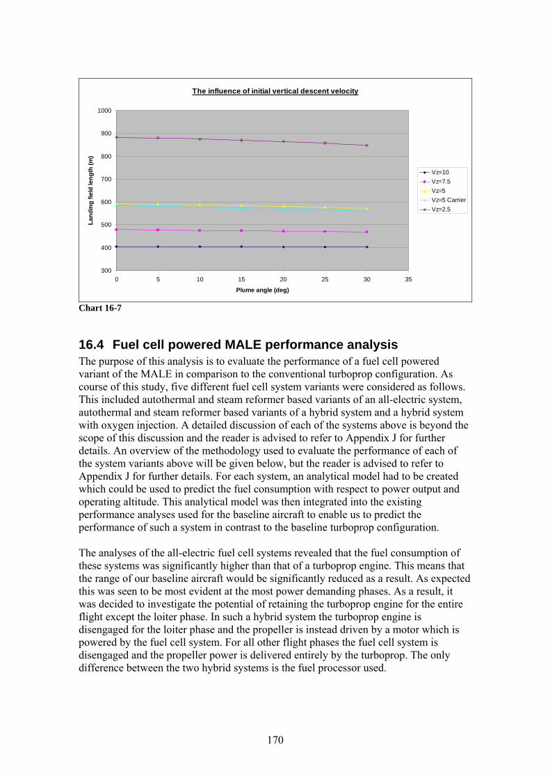
The influence of initial vertical descent velocity

1000

300

400

500

0 5 10 15 20 25 30 35

Plume angle (deg)

Land

in

600g f

700

ield

leng

th

800

900

(m)

Vz=10Vz=7.5Vz=5Vz=5 CarrierVz=2.5

hart 16-7

ariant of the MALE in comparison to the conventional turboprop configuration. As course of this study, five different fuel cell system variants were considered as follows. This included autothermal and steam reformer based variants of an all-electric system, autothermal and steam reformer based variants of a hybrid system and a hybrid system with oxygen injection. A detailed discussion of each of the systems above is beyond the scope of this discussion and the reader is advised to refer to Appendix J for further details. An overview of the methodology used to evaluate the performance of each of the system variants above will be given below, but the reader is advised to refer to Appendix J for further details. For each system, an analytical model had to be created

ld be used to predict the fuel consumption with respect to power output and perating altitude. This analytical model was then integrated into the existing

ance analyses used for the baseline aircraft to enable us to predict the figuration.

of our baseline aircraft would be significantly reduced as a result. As expected is was seen to be most evident at the most power demanding phases. As a result, it

was decided to investigate the potential of retaining the turboprop engine for the entire flight except the loiter phase. In such a hybrid system the turboprop engine is disengaged for the loiter phase and the propeller is instead driven by a motor which is powered by the fuel cell system. For all other flight phases the fuel cell system is disengaged and the propeller power is delivered entirely by the turboprop. The only difference between the two hybrid systems is the fuel processor used.

C

16.4 Fuel cell powered MALE performance analysis The purpose of this analysis is to evaluate the performance of a fuel cell powered v

which couoperformperformance of such a system in contrast to the baseline turboprop con The analyses of the all-electric fuel cell systems revealed that the fuel consumption of these systems was significantly higher than that of a turboprop engine. This means that he range t

th

170

16.4.1 Analysis of the autothermal and steam reformer based fuel cell systems

The performance analysis for the all-electric autothermal and steam reformer based systems followed the same procedure as for the conventional turboprop engined aircraft configuration. The only difference being that the spreadsheets are modified to include the new expressions for fuel consumption. The results of these analyses are given below alongside the results for the original turboprop configuration, for comparison. To provide a ‘like for like’ comparison, the fuel tanks have been assumed to retain their original size as determined for the baseline turboprop configuration. It has therefore been necessary to reduce the loiter time of the aircraft for each variant accordingly in order to meet this constraint. Since the density of methanol of 0.796kg/m3 at 15ºC lies within the range 775 to 840kg/m3 for Jet A fuel at 15ºC the weight of the two fuels is thus comparable. In the case of the autothermal reformer, this meant that the loiter time had to be reduced from 35 hours to 9.15 hours. Likewise for the steam reformer, the loiter time was reduced to 18.03 hours.

6.4.2 Analysis of the hybrid autothermal and steam reformer based

he baseline fuel

ts

r

e

engine is f cruise

cell stem in conjunction with the turboprop engine at these most demanding phases. The

s

rcraft due to the dditional mass of the fuel cell system. If it were possible to reduce the weight of the

1fuel cell systems

In the case of the analysis of the hybrid systems, only the loiter phase of tturboprop performance analysis is modified to incorporate the characteristics of thecell system. The remainder of the baseline performance analysis is retained. The resulof these analyses are given below alongside the results for the original turboprop configuration, for comparison. As before, the total volume of the fuel tanks is assumed to be fixed at the value determined for the baseline aircraft design. As a result, the loitertime has been reduced accordingly. In the case of the autothermal reformer, the loiter time had to be reduced from 35 hours to 17.96 hours while that of the steam reformewas reduced to 26.45 hours. In the analysis of these hybrid systems we have assumed that the turboprop engine is thsole means of propulsion at all flight phases other than the loiter phase. During these flight phases the fuel cell system is assumed to be switched off. The turbopropthus sized to meet the most critical thrust requirements which were at the end ooutbound and the start of cruise inbound. A possibility would be to operate the fuelsypower output from the traction motor (connected to the fuel cell) would thus be used tosupplement that from the turboprop engine. The result would be that a smaller and lighter turboprop engine could be utilised which would result in a reduction in the weight of the aircraft and thus a reduction in the mission fuel consumption. There waunfortunately insufficient time to investigate this proposal and this task is thus reserved for future work.

16.4.3 Final results The results in the table below include the increase in the mass of the aia

171

172

.7kg then an improvement in the loiter time could be realised. rs

fuel cell systems so that the mass of the aircraft were to retain its same value as the original estimate of 3428For the autothermal and steam reformer systems, loiter times of 13.99 and 24.21 houcould be achieved respectively. In the case of the hybrid autothermal and steam reformer based systems, loiter times of 19.19 and 28.20 hours could be respectively. Also included in this table are the initial and refined baseline fuel consumption figures. The difference between these two sets is due to the vagueness of fuel consumption

redictions with weight fractions, especially for unconventional aircraft like UAVs. p Fuel mass used for the different variants of the MALE UAV

Segment fuel consumption (kg)Flight phaseTake-off ground roll 17.1 1.1 1.2 0.9 1.1 1.1Take-off rotation 17.1 0.4 0.6 0.5 0.4 0.4Take-off climb out 17.1 0.4 0.6 0.5 0.4 0.4Second segment climb 17.1 0.0 0.1 0.1 0.0 0.0Climb 16.3 50.4 92.7 67.3 50.6 50.6Cruise egress 151.2 237.

Hybrid autothermal

Hybrid steam

Conceptual design

Refined baseline

Autothermal reformer

Steam reformer

6 680.3 509.5 253.5 253.5ter at altitude 1555.0 1417.3 680.2 996.1 1344.8 1356.9

Cruise ingress 74.1 196.1 381.4 279.4 197.6 197.6

5.4 0.0 0.0 0.0 0.0 0.0

Loi

Descent 7.8 14.4 11.2 8.4 12.9 12.9Loiter sea level 13.8 16.1 49.1 35.1 36.2 24.0Landing approach and flareLanding ground roll 5.4 0.0 0.0 0.0 0.0 0.0

Total fuel used for the mission 1897.5 1933.6 1897.5 1897.5 1897.5 1897.5Reserve (6% of the total) 113.9 116.0 113.9 113.9 113.9 113.9Total fuel (mission and reserve) 2011.4 2049.6 2011.4 2011.4 2011.4 2011.4

Loiter time at altitude (hours) 35.00 35.00 9.15 18.03 17.96 26.45

all of the systems above, we have to supply an excess amount of hydrogen to the fuel

e to

nds of the fuel cell system meant that it was unlikely that sufficient xygen can be carried on-board the aircraft to meet our needs. Such a system would

therefore supplement the oxygen obtained from the air. A liquefied oxygen source was practical means of meeting our needs for this application. The

fuel mass saved with the use of such a system. Such a system is therefore not viable.

Table 16-3

16.4.4 Investigation into the use of oxygen injection Incell so that the waste leaving the fuel cell can be burned to generate the power needed for the air compressor. An additional quantity of fuel is therefore consumed in order tobe able to deliver oxygen at the desired quantity and pressure for the fuel cell. Taking into consideration that air is made up of approximately only 21% oxygen, then a significant amount of energy is being wasted to deliver the remaining 79% which is predominantly nitrogen and serves no other purpose than to act as a dilutant. We are therefore expending work and fuel to deliver it to the fuel cell in order to throw it away! It was therefore proposed that the use of oxygen from a purer source would give risa reduction in the fuel consumption of the system. The only realistic means of achievingthis would be to carry a compressed or liquefied source of oxygen on-board the aircraft. The oxygen demao

considered to be the only feasibility of such a system is considered in detail in Appendix J. This showed that the mass of the liquid oxygen which must be carried on-board the aircraft far exceeds the

17 Discussion

17.1 A review of the MALE and UCAV baseline designs The MALE and UCAV configurations selected for use as baseline designs for this sare in-line with current UAV designs. Each design was only developed to a level

tudy

fficient for this work and further refinements are to be expected for such designs to become more realistic. They did however prove to be more than satisfactory for the needs of this project without devoting too much time to their design and development. The main difficulty with the MALE was the provision of fuel tanks of sufficient size to be able to hold sufficient fuel to meet the mission requirements. This necessitated the need for a large fuselage fuel tank and thus a fuselage which is larger than desired. In the case of the UCAV, a large amount of sweep was required to get the centre of gravity in the desired location for stable flight. The desired slenderness of the configuration also presented its own problems with undesirable blisters in the wing surface being incorporated to accommodate the landing gear and lethal payload. A simplistic means of landing gear retraction was opted for to keep in-line with the theme of reduced cost UAVs but a better option would be increase the complexity of this slightly so that the associated blisters can be eliminated.

17.2 The identification and selection of the technologies int in the project, the questions which looms is, ‘Did we select the best ndidate technologies to make the best possible contribution to knowledge?’

vast and a real engineer only has to open his eyes to other engineering

su

At this poossible cap

The choice of technologies was find possible technologies. Examples can be found everywhere fromstreams, our natural environment and even in the minds of a science fiction writer. For example, 30 years ago it was laughable that the James Bond movies depicted mobile communication devices small enough to fit in wrist watches, but now? The children’s toy cars the ‘Hot Wheels Colour Shifters’ are another excellent example. These toys change colour by simply immersing them in hot or cold water respectively. What benefit would such paint have to a stealth aircraft which can change the colour of theaircraft from white on a hot day to black on a cold night? The recognition of future concepts and how to apply them in an engineering concept has been the ultimate test for entenaries to distinguish the notable scientists and engineers from the rest. Something c

as simple as watching a pot boiling led to the development of the IC engine. The really worthy engineers and scientists will only see a world full of possibilities. As the focus of this project is on the integration and not the development of technologies then we are restricted to utilising existing technologies. Our goal here is thus to identify new openings and opportunities for these systems. The technologies selected for this project were low cost mechanical thrust vectoring and fuel cell systems. The thrust vectoring system was selected to keep in-line with the focus of Flaviir project and to evaluate an alternative to the fluidic devices being proposed. The fuel cell systemwas selected to explore the viability of fuel cells in aerospace applications. Currently,

173

anybody who is anybody in engineering has got a fuel cell development project. These nge of applications from golf karts to ships with minimal raft. The best technologies were therefore selected in-line

ith the theme of this PhD.

s

concerned with and thus these differences are not ritical for the purpose of this study.

for of

y

the

f vectored

have already seen use in a rarogress being made for aircp

w

17.3 The feasibility of low cost mechanical thrust vectoring This study investigated the feasibility of using a low cost thrust vectoring system utilising post exit paddles for the trim and control of a large UAV. The system used wathat originally investigated by NASA for their X-31 and F/A-18 aircraft, which was escaled to suit our application. This system was analysed at a number of different flightr

phases to assess the benefits of the system under a number of different conditions. The results of this work, as presented in the evaluation section, will be now discussed in the sections which follow. During the performance evaluation work, the mass of the thrust vectoring system was assumed to be negligible in comparison with the mass of the aircraft. This is probably an over-simplification but to be able to make an reasonable estimate of the complete thrust vectoring system would have required more detailed knowledge of the different components. This would have involved a lengthy process to size the actuators and nosejet pneumatic system components, a process we did not have sufficient time for. It is

owever the trends which we are most hc As will be discussed in the following section, the main difficulty with this systemtake-off is its location on the aft fuselage. The result is that a downward deflectionthe nozzle is accompanied by a large increase in the nose down pitching moment of the aircraft. This moment must be counteracted by either the pneumatic pitch control system or the elevons and the take-off must be delayed until there is sufficient control power available. As a minimum, the solution to this problem would be to relocate the vertical component of vectored thrust to the same location at the main gear wheels. Anpossibility to locate the vectored thrust forward of this point would contribute to the nose up pitching moment and thus reduce the control power for rotation. A similar situation exists for landing. Examples of this design practice can clearly be seen onHarrier Jump Jet and similar STOL/VTOL designs. These systems are however not without their own penalties with weight being a particular problem.

17.3.1 Thrust vectoring for take-off During this part of the study, an investigation was carried out into the use othrust to contribute to the lift of the aircraft during the take-off phase and thus reduce the take-off distance. An additional component of vertical thrust from the nose jet control system not only provided pitch control but also contributed to the lift of the aircraft. The analysis described in the evaluation section is used to determine the optimal engine bleed setting and point during the ground run when there is just enough lift and control power available to be able to rotate the nose of the aircraft. At this optimal condition the ground run distance is at its minima. By collating these points for a number of plume angles we are able to obtain a single curve for the optimal ground

174

run as a function of plume deflection angle. This process was repeated for a number of different landing gear setting angles to test the influence of this parameter. The results are presented in the ‘influence of landing gear setting angle’ chart, where the baseline landing gear setting angle is taken to be 5º.

Inspection of the results shows us that that the ground run distance required increases of

tion

uces in proportion to the cosine of the deflection angle. ollectively, this means that the propulsive thrust is reduced as the vectoring angle is

he reasoning is that as the vertical component of vectored thrust increases, the aircraft r. to

t

g

to 280.9m . The effect is thus marginal and would be insignificant if we were to take into

angle of attack.

.

t 0º

with exhaust plume deflection angle. Although the lift due to the vertical componentthrust increases with vectoring angle, a number of other factors also increase in relato the vectoring angle, which are detrimental to the performance. As is discussed in the appendices, each nozzle deflection angle corresponds to a different exhaust nozzle configuration which gives rise to a different engine operating condition. Deflection of the nozzle thus moves the operating point of the engine away from its design condition resulting in a reduction in available thrust. This is combined with the fact the horizontal component of thrust redCincreased, which results in a decrease in the acceleration and thus the speed of the aircraft. Since the lift of the wing is proportional to the square of the speed then for thesame point along the runway, the wing lift will decrease as the vectoring angle increases. The additional components of lift from the nose jet and vectored thrust have proven to be insufficient to meet this shortfall. If we now review the results from a control perspective, it was seen that the control force required to rotate the nose of the aircraft increases with plume deflection angle. Texperiences an increase in the nose down pitching moment about the main landing geaAlthough the horizontal component of thrust reduces in relation, the moment arm due the vertical component of thrust is greater than the horizontal component and thus has a greater influence. As a result, an increase in control force is required for an increase in the plume deflection angle. Considering the moments acting on the aircraft, we arrive aanother important consideration. It can be seen that the lift from the wing contributes ina positive way to the rotation of the nose of the aircraft about the main wheels. Thus, the control power requirements of the nose jet or the elevons are reduced as the aircraft gains speed. This highlights the importance of speed and wing lift during take-off. A further investigation was carried out to explore the influence of landing gear settinangle on the take-off ground run. For a plume deflection angle of 10º, this showed a ecrease in the ground run from 284.3m at a landing gear setting angle of 5ºd

at 10ºaccount the increase in drag due to the higher The final stage of work involved an investigation into a possible reduction in wing sizeThe results of this study showed a considerable increase in the take-off field length as a result of a reduction in wing size. As can be seen, for a 50% reduction in wing size aplume angle, the take-off ground run required increases from 250.9m to 480.1m corresponding to a 91% increase. At 10º plume angle, the distance increases by 95% and at 20º also by 95%. Thus the lift from the thrust vectoring system has been shown tobe unable to match the lift generated by the wing and in this case there appears to be no substitute for wing size.

175

At this point we can ask the question, ‘how does this compare to the conventional configuration with elevons?’. If we first examine the trends for the control and lift limitboundaries of the elevons, we can see that the ground run distance is dictated by the control limit. This can however also be seen

to increase with deflection in plume angle nd thus there is no benefit in using deflected thrust for this configuration. At 0º plume

ing

d er

ted.

ke-off

control jet used to supplement the ontrol power of the elevons. If it is necessary to eliminate the elevons completely then

and rust

ectoring system was used to determine the plume deflection angle required to trim the

l component due to the

levons. In actual fact, for the complete cruise phase we saw a 2% increase from 1841.8

ugh to e.

aangle this gives us a ground run distance of 324.9m. The configuration using the nosejet shows a similar trend with 0º plume angle giving the best figure of 250.9m, in which case the nose jet is replacing the function of the elevons. Thus a 22.8% reduction in the ground run distance can be achieved with the use of just the nose jet system as opposed to the conventional elevons. We could improve the conventional elevons by increastheir size until we match the lift limit boundary of 223.7m but this would result in performance problems at other flight phases. In this study, the two systems have been considered in isolation but the take-off performance could be further improved by using the nose jet system to supplement the conventional elevons. Such a system woulrequire less engine bleed for the nose jet (the current figure being 8.2%) and thus furthimprove the acceleration of the aircraft and the point at which rotation can be initia To summarise, for this particular aircraft and thrust vectoring system, the best taperformance can be achieved with the nose jet alone. The thrust vectoring nozzle wouldthus remain in its undeflected state and the nosecthe thrust vectoring nozzle should remain in its undeflected state during take-off.

17.3.2 Thrust vectoring for cruise During this part of the study, an investigation was carried out into the use of vectored thrust to trim the aircraft at cruise as opposed to using conventional elevons. The intention being to reduce the trim drag. This study utilised the performance analysis spreadsheets used for the baseline study which were extended to include aircraft control terms. In the case of the conventional elevons, additional terms were added to determine the elevon deflection angle required to balance the moments acting on the aircraft and thus trim the aircraft. This analysis also had to take into account the variations in lift drag of the aircraft due to the deflection of the elevons. A similar analysis for the thvaircraft. In this case, the analysis had to account for the variations in lift and thrust due to deflection of the exhaust plume. It was hoped that the thrust vectoring system would give rise to a reduction in the fueconsumption at cruise as a result of the elimination of the drageto 1879.9kg. In the case of the conventional elevons, we require an elevon deflection range between -0.18 and 0.16 deg to trim the aircraft, in which case the component of drag due to their deflection is small. In the case of the thrust vectoring system however, the plume deflection range is between -4.18 and 4.23 deg, which is sufficient enohave a knock on effect on the performance and thus the fuel consumption of the enginThe decrease in fuel consumption at cruise is however only 2% and could be easily catered for if required.

176

17.3.3 Thrust vectoring for landing During this part of the study, an investigation was carried out into the use of vectored thrust to contribute to the lift of the aircraft during the landing phase and thus reduce thelanding distance. As for the take-off case, the lift from the wing is supplemented by additional components of lift from the vectored thrust and the pitch control nose jet. Theactual analysis was a very complex balance of the forces and moment acting on the aircraft over the landing approach, flare out and ground run phases. Although the baseline vertical descent velocity was taken to be 5m/s, a range of other values were explored to examine the influence of this parameter. In addition, an aircraft carrier variant was explored with a slightly slower approach speed. The results showed the vertical descent velocity to have considerable impact on the on the total landing field length with a 16.0% reduction being achieved for an increase from 5 to 7.5m/s and a 31.7% reduction for an increase from 5 to 10m/s. The effect of a reduction in approach speed was however less pronounced with only a 1.7% reduction in the landing field length.

ed quired. This means that some form deflector is required to reverse the thrust. Our

to be sufficient control authority available landing field length of 577.86m. The

deflect when a load is applied, the elastic

ompare to other thrust vectoring systems? No analysis was arried out of other thrust vectoring systems but we are able to draw up some

The results for the effect of thrust vectoring showed less promise with only a 1.6% reduction being achieved between a vectoring angle of 0 and 15deg and 3.4% being achieved between 0 and 30deg. This analysis does however assume that we are utilising the nose jet system for pitch control, in which case the engine needs to be spooled up to generate the engine blereoriginal control analysis work showed therethroughout the landing phase with a requiredconventional configuration utilising elevons is thus comparable to the thrust vectored system with there being little benefit in using such a system.

17.3.4 Significant integration considerations for this system As with any thrust vectoring nozzle, we have to take into account the impact which the nozzle has on the operating characteristics of the engine. We also need to take into account the effect of variations in the mass, centre of gravity, lift and drag of the whole aircraft. Of particular importance to this system however is the need to provide structural attachment points for the paddles and the accompanying hydraulic rams. As any aircraft structure can be seen to deformation of the structure needs to be accounted for in the design and in the flight control system commands. From a more general design perspective, allowance needs tobe made for the additional length of the vectoring paddles. In particular the designer needs to ensure that they do not come into contact with the ground during the high angle of attack take-off rotation and landing approach flare phases. As this is often a critical consideration in the design of the tail of many aircraft, the integration of such a system on an existing aircraft may prove troublesome.

17.3.5 Comparison with other thrust vectoring systems ow does this system cH

c

177

conclusions on the lessons learnt in this project. Inspection of published data for other s

lts

s. utothermal reformer based fuel cell system – In this system, the turboprop

engine has been replaced with an all electric powertrain which was powered by

as electric powertrain which is powered by the steam

reformer based fuel cell system. ft st

red

eption that a steam reformer is used instead.

same t the

hich

ses

uration vehicles, it is sufficient to use ottled supplies of hydrogen and oxygen, as is the case with a number of existing

ties of the upply of

systems showed the internal vectoring concepts to have lower flow turning thrust losseassociated with them. These systems are thus expected to offer better performance but at the expense of mass, cost and complexity. Fluidic devices are another form of thrust vectoring which is considered to offer great potential. These devices do however require large amounts of engine bleed air to operate, which would result in a considerable reduction in engine performance and increase in fuel consumption. Thus similar resuto those found in this analysis are expected for such fluidic devices.

17.4 The feasibility of fuel cell systems for propulsion This study investigated the feasibility of using a fuel cell system as the primary propulsion system of a MALE UAV in contrast to a more conventional turboprop. As course of this study, five different fuel cell system variants were considered as follow

• A

an autothermal reformer based fuel cell system. • Steam reformer based fuel cell system - In this system, the turboprop engine h

been replaced with an all

• Hybrid autothermal reformer based fuel cell system – In this system, the aircrahas been retrofitted with a hybrid electric/turboprop powertrain. During the modemanding flight phases, the turboprop is responsible for delivering the requipower. Whilst during the loiter phase, the turboprop is switched off and the fuelcell system has sole responsibility for meeting the power demands.

• Hybrid steam reformer based fuel cell system – This system adopts the same approach as the hybrid autothermal system with the exc

• Hybrid fuel cell system with oxygen injection – This system adopts theapproach as the two other hybrid systems above with the exception thaoxygen in the air is supplemented with additional oxygen.

A detailed discussion of each of the systems above is beyond the scope of this discussion and the reader is advised to refer to Appendix J for further details. This work involved the development of an analytical model representative of each system wcould be used to predict the fuel consumption with respect to its operating conditions. The integration of these analytical models into the baseline performance analyenabled the performance of an aircraft incorporating such a system to be evaluated incontrast to the baseline turboprop configuration.

17.4.1 Fuel choices Fuel cells need a ready supply of hydrogen and oxygen in order to complete the associated electro-chemical reaction. For short dbresearch vehicles. More practical systems however require larger quantireactants and thus alternative sources are required. Fortunately, a ready soxygen is available from the atmospheric air, although a decrease in performance is

178

experienced as a result of the presence of nitrogen. A ready supply of hydrogen on the other hand is more problematic due to its low density which has traditionally necessitated the need for large compressed hydrogen storage tanks. Cryogenic storage tanks have also received considerable interest for the direct storage of hydrogen but these have proven to present their own set of problems. The problem of sufficient hydrogen storage has thus been one of the bottle necks in the development of fuel cell powered vehicles. An alternative solution to this problem is to xtract the hydrogen on demand from a hydrogen rich fuel such as methanol. Such an

approach does however necessitate the need for additional equipment to process the fuel uch as

fuel s

.

ll.

wn etermine

g

tional amount of fuel but this reduces . In the case of this particular system, we are already

erate the power required to drive the compressor. Thus, if we e the

rtial ny

e

in situ. The advantage of such an approach is that a liquid hydrogen carrier smethanol is easier to store and provides a good hydrogen yield. Studies into suchreformer based fuel cell systems for automotive applications have highlighted problemwith transient performance and start-up times. Such system behaviour is however less likely to be such of a problem for steady state applications such as aircraft propulsionAlthough it is possible to extract hydrogen from any hydrogen based fuel such as the natural hydrocarbon based fuels, the more synthetic fuels such as methanol are easier. The criteria for the selection of a suitable fuel for a reformer based system is based on a number of considerations including, availability, ease of storage, required reforming temperature, the content of impurities and the hydrogen yield of the fuel. Of all the fuels considered, methanol has proven to be the most suitable for this application with all the desired qualities of yield, availability, storage and low reforming temperature.

17.4.2 Fuel processors Mobile fuel processing is an area which has been receiving considerable interest recently, especially for fuel cell systems. Such fuel processors would have once filled the entire boot of a car but there now exists units which take up virtually no space at aTwo fuel processing approaches have almost dominated the market for mobile applications, these being steam and autothermal reforming. Each of these has their obenefits and drawbacks and thus it was necessary to explore each approach to dthe best system for this application. Steam reformers are the most efficient of all the fuel processors but are generally heavier and bulkier due to the additional accompanying equipment. These units also require external sources of heat and steam, which are required to promote the reforminreactions. The main problem with these is the generation of the required heat. This is ypically achieved with the combustion of an addit

the overall efficiency of the systemburning excess fuel to genare able to locate this burner in close proximity to the fuel processor we can utiliswaste heat from the external surface of the burner within the fuel processor. The result is a fuel processor which is capable of achieving a high level of efficiency. Autothermal reformers generate the heat required for reforming internally by the pacombustion of a small amount of the fuel being reformed. Such units do not require aadditional steam or heat inputs and are generally lighter and smaller than their steam

179

180

ver an

7.4.3 All-electric propulsion systems

n figure

hile enjoying the benefits of a quiet and environmentally friendly propulsion system lowing the same procedure as before, the loiter time of autothermal system is reduced by 48.7% to 17.96 hours,

urs.

has to take in to account usual considerations

y

y

reformer relatives. These units are however less efficient than the steam reformer counterparts. Their ability to function as a self contained compact unit is howeextremely attractive feature which offsets some of the other problems.

1In the all-electric propulsion systems, the turboprop engine has been completely removed and replaced with two powerful traction motors which are used to drive the propeller instead. The power to drive the motors is generated by a fuel cell system which utilises hydrogen from either a steam reformer based or autothermal reformer based fuel processor. To enable a equal comparison to be made between the systems, it was assumed that the aircraft fuel tanks have been retained at their original size determined for the turboprop engine and thus the loiter time was reduced accordingly from the original figure of 35 hours. In the case of the autothermal reformer, the loiter time of the aircraft was reduced by 73.9% to 9.15 hours, while that of the steam reformer based aircraft was reduced by 48.5% to 18.03 hours.

17.4.4 Hybrid propulsion systems The hybrid propulsion system was envisioned to improve the fuel consumption of the aircraft propulsion system by retaining the turboprop engine for all but the loiter phase. During loiter, the turboprop is disengaged and power is delivered by a smaller variant ofthe fuel cell systems above. Such a system retains a reasonable fuel consumptiowfor its lengthy loiter phase. Folthe aircraft utilising an hybrid while that of the hybrid steam reformer system was reduced by 24.4% to 26.45 hoThe hybrid steam reformer based system is thus the best choice for our application. A loiter of 28.20 hours can however be achieved if the system mass could be reduced

17.4.5 Significant integration considerations for this system The integration of the fuel cell systemsuch as centre of gravity, space allocation and the provision of inlet and exhaust apertures. The main difficulty in the integration of this system was the provision of sufficiently large heat exchangers for cooling. A number of locations were explored for these units with the final configuration being a large unit in the aft fuselage and two smaller units located in the tailbooms. Each unit requires its own inlet an exhaust which contributes to the drag of the aircraft. This is however less of a problem for the smaller hybrid system, in which a single heat exchanger located in the aft fuselage, will be sufficient.

17.4.6 Evaluation of the overall system propulsive efficiencThe overall efficiency of a system is typically used as a means of comparing the overall performance of a number of different systems which are intended to fulfil the same task. The efficiency of the system cannot however be considered in isolation when selecting a system and other factors must be taken into consideration. In this section, the efficienc

of the turboprop and fuel cell system variants is calculated at a number of key pointhroughout the flight profile. The results of this analysis will then form a means of evaluating each system in addition to the other factors being considered

ts

such as loiter me, practicality and cost.

o of the useful energy output to the

ti

The efficiency of any system is defined as the ratitotal energy input required, as follows.

InputquiredOutputDesired_Re

_=η Eq 17

In this particular study, this equates to the ratio of the propulsive power output of the propulsion device to the energy input of the fuel consumed by the system. In this study we have assumed that each system shares a common propeller and therefore it is justified to determine the efficiency of each system in terms of the propeller shaft inpupower. This assumption holds true as long as the speed and therefore the efficiency of the propeller remains the same, which will be pre-set by the gearbox in each systeach case, any error due to any small deviations is however expe

-1

t

em. In cted to be negligible.

The efficiency of the propulsion system can then be determined from the expression.

Propulsive device (Turboprop or fuel cell system)

ftopellorShaWPrFuelE

inputenergyfuelofRatepowerinputftopellorSha____

__Pr=η Eq 17

In cases where a combustion process takes place, the energy of the fuel is based on the heating value of the fuel (HV), which is a measure of the amount of the total quantity o

eat released when a unit quantity of the fuel is burned under controlled conditions.

-2

f

his is also known as the enthalpy of combustion reaction. Two versions of the HV ependent

e f

the

hTvalue exist, a higher heating value (HHV) and a lower heating value (LHV), don whether the by-product water leaves the system as liquid or vapour. The differencbetween the two values is thus the product of the quantity of water and the enthalpy ovaporisation of water. The efficiency of IC engines for example is determined usingLHV since the water exists as a vapour in the exhaust gases. In the case of fuel cells however, where no combustion process takes place, the overall reaction of hydrogen within the fuel cell is the same as a that for a hydrogen combustion process ( OHOH 222

12 →+ ). In this case, the heating value of the fuel is therefore still

a valid measure of the energy of the fuel entering the system. For a PEM fuel cell onwn, its low

its temperature means that either the LHV or HHV values can be used. Since

e system proposed in this study incorporates a tail-gas burner then the water will leave h the

oththe system as a vapour and thus the LHV should be used. The efficiency of botturboprop and fuel cell systems can then be determined from the expression.

LHVmW

Fuel

opShaft

⋅= Prη Eq 17-3

181

The terms opShaftWPr and Fuelm have already been determined for the complete flightprofile from our analysis work on each system. The remaining term LHV for the two

ifferent fuels used is then,

In this analysis, it wasthe highest fuel burn which includes climb, cruise egress, high altitude loiter, cruise

g

d• Methanol = 20.07 MJ/kg • Jet A = 42.80 MJ/kg

only deemed necessary to concentrate on those flight phases with

ingress, descent and sea level loiter. With start, mid and end points of each phase beinconsidered to get a full appreciation of the conditions at each stage, the results of which are presented in the table below.

b se e

gres

s

se e

gres

s

e eg

ress

at a

ltitu

de

alti

tude

er a

t alti

tude

e in

gres

s

ngre

ss

e in

gres

s

ent

cent en

t

r sea

leve

l

er s

ea le

vel

loite

r

A comparision between the efficency of the baseline turboprop and fuel cell system variants at a number of different flight points

Star

t clim

Mid

clim

b

End

clim

b

Star

t cru

i

Mid

cru

i

End

crui

s

Star

t loi

ter

Mid

loite

r at

End

loit

Star

t cru

is

Mid

cru

ise

i

End

crui

s

Star

t des

c

Mid

des

End

desc

Star

t loi

te

Mid

loit

End

loite

r

mf (g/s) 53.97 36.50 30.74 35.12 27.55 23.02 13.30 11.09 9.69 18.94 23.56 29.31 22.34 7.91 0.17 4.49 4.48 4.46Prop Shaft Pwr (kW) 516.62 355.8 7.26 104.87 91.76 205.25 257.51 321.02 244.68 72.44 1.25 35.23 35.08 34.93Fuel TypeLHV (MJ/kg)Efficency (%) 22.12 25.32 25.54 25.59 25.59 21.39 16.96 18.31 18.31 18.31

mf (g/s) 80.09 65.54 62.67 192.63 64.89 50.83 22.47 20.51 19.16 37.77 45.86 56.04 35.91 7.72 18.10 13.77 13.63 13.50Prop Shaft Pwr (kW) 344.82 344.82 344.82 461.22 356.43 292.88 133.65 120.99 112.05 215.86 264.27 324.80 211.00 49.66 3.25 64.35 63.80 63.26

35

mf (g/s) 57.72 47.65 45.69 143.37 48.70 38Prop Shaft Pwr (kW) 344.82 344.82 344.82 462.95 360.43 298Fuel TypeLHV (MJ/kg)Efficency (%) 29.77 36.05 37.60 16.09 36.88 38.94 40.30 39.94 39.42 38.61 39.07 39.50 40.16 43.71 1.26 32.37 32.40 32.43

10.65

6.63

Jet A

turb

opro

per

eam

re

form

er

Methanol (CH3OH)20.07

9 340.66 389.19 306.80 255.25 12

Ref

ined

22.36 22.78 25.89 25.89 26.02 25.90 22.35 22.09

Flig

ht p

oint

42.80

l

Fuel TypeLHV (MJ/kg)Efficency (%) 21.45 26.22 27.42 11.93 27.37 28.71 29.64 29.40 29.13 28.48 28.72 28.88 29.28 32.05 0.89 23.29 23.32 23.Au

tot

refo

rmherm

a

Methanol (CH3OH)20.07

.21 17.36 15.18 13.77 27.64 33.61 40.96 26.27 5.70 12.96 9.81 9.74 9.68

.60 140.42 121.70 108.98 214.16 263.52 324.69 211.73 50.02 3.27 63.76 63.37 62.98

St

mf (g/s) 54.20 36.53 30.74 37.43 29.40 24.62 24.31 20.50 18.20 19.19 23.73 29.42 21.08 6.87 0.39 10.14 10.05 9.96Prop Shaft Pwr (kW) 516.14 355.67 340.66 414.71 327.36 272.85 134.67 111.61 97.33 207.98 259.40 322.20 230.93 62.89 2.85 46.15 45.79 45.43Fuel TypeLHV (MJ/kg)Efficency (%) 22.25 22.75 25.89 25.89 26.02 25.90 27.61 27.12 26.65 25.32 25.54 25.59 25.59 21.39 16.96 10.63 10.64

mf (g/s) 54.20 36.53 30.74 37.43 29.40 24.62 16.67 14.04 12.45 19.18 23.72 29.41 21.13 6.91 0.39 6.71 6.67Prop Shaft Pwr (kW) 516.14 355.67 340.66 414.71 327.36 272.85 134.67 111.43 97.08 207.86 259.32 322.14 231.48 63.27 2.80 45.69 45.45 45.21Fuel TypeLHV (MJ/kg)Efficency (%) 22.25 22.75 25.89 25.89 26.02 25.90 40.25 39.54 38.85 25.32 25.54 25.59 25.59 21.39 16.96 15.90 15.91 15.92

Jet A20.07 42.80H

ybrid

au

toth

erm

al

Jet A Methanol (CH3OH)

Hyb

rid s

team

42.80 20.07 42.80Jet A Methanol (CH3OH) Jet A

42.80

ve a much better

ive for the hybrid systems aphase on these sy

Table 17-1

rom the results above, the fuel cell systems can be seen to haF

efficiency compared to the baseline turboprop engine. The high altitude loiter flight phase in particular has proven to be the most fuel demeaning in all cases and thus it is desirable to achieve the highest propulsive efficiency at this stage when designing a system. The mid-loiter at altitude results in the table above showed a definitive increase in efficiency of 17.4% (from 22.1% to 39.5%) between the baseline turboprop and the hybrid steam reformer. Similarly, attractive increases in efficiency of 5.1%, 17.9% and 7.0% were shown for the hybrid autothermal, all-electric steam reformer and all-electric autothermal systems respectively at the same mid-loiter point. Although a similar comparison could be made at other flight phases, the results are less comparat

t these phase since the fuel cell system is only utilised during the loiter stems.

182

183

he rationale for the higher efficiencies encountered with the fuel cell systems is that d l

lf of that of conventional fuels. This means that a quired to achieve the same energy content of fuel.

tly offset by higher efficiency of the fuel cell systems

ating costs anned aircraft are defined as those costs which are

incurred for each hour that the aircraft flies and will typically consist of, • Fuel costs • Maintenance and repair costs (labour and parts) • Flight related charges (landing fees etc)

Due to the relative newness of fuel cell vehicles, it is unfortunately not possible to make an accurate prediction of the maintenance and repair costs for such a propulsion system. These are however expected to be significantly lower than its IC engine competitor due to the lack of moving parts which would otherwise be susceptible to wear. Here, we are therefore only able to make a realistic comparison of fuel costs. As of December 2011, the US trade prices of methanol and jet fuel were,

• Jet fuel – $2.87/gallon • Methanol - $1.38/gallon

As can be seen from these figures, there is a considerable cost saving associated with the use of methanol instead of jet fuel. This equates to a 51.9% saving on the trade price of fuel.

ass approximation, the densities of methanol and jet fuel are roughly e at about 800kg/m3. In such case, the fixed total mission fuel mass of

011.3kg equates to a volumetric quantity of 664.2 US Gallons (where, 1m3 = 264.2 US s cost

the

r

e

Tmore of the energy of the fuel is utilised within the system as opposed to being ejecteout of the exhaust as hot gases, as with the turboprop. The main downside of methanobased propulsion systems however, is the low energy content of the fuel, which, as canbe s nee from above, is roughly hahigher mass flow rate of fuel is reThis is unfortunately only parcompared to the turboprop engine. As a result, even though the fuel cell systems have a higher efficiency, a higher fuel flow rate will be required for thee systems because of their fuel.

17.4.7 Evaluation of the direct operThe direct operating cost of an unm

As a first pcomparabl2Gallons). A tank full of methanol for an all-electric propulsion system would thu$916.6 as opposed to $1906.2 for a tank full of jet fuel for the baseline turboprop. In case of the hybrid steam reformer system, 1356.9kg of methanol would be required forthe fuel cell system (for the loiter phase) and 654.4kg of jet fuel for the turboprop (foall other flight phases). This equates to 216.1 US Gallons of jet fuel at a cost of $620.2 and 448.1 US Gallons of methanol at a cost of $618.4, which gives a total fuel cost of $1238.6. There is thus a significant cost saving to be made with both the all-electric andhybrid propulsion systems in comparison with the baseline turboprop configuration. It should however be re-emphasised that the fuel prices quoted are trade prices and arthus subject to additional cost factors.

18 Conclusions and recommendations This project aims to contribute to knowledge in two gaps in current aerospace technology. The technology areas identified for study were;

• Low cost mechanical thrust vectoring systems - To investigate the feasibilityusing low cost mechanical thrust vectoring systems to replace conventional control surfaces. This is also an alternative to the fluidic thrust vectoring devicesproposed by the Flaviir project.

• Fuel reformer based fuel cell propulsion

of

systems - To investigate the use of a fuel reformer based fuel cell system to supply power to an all-electric power

ese iguration which was identified

ectoring system

ions

ctoring has traditionally been achieved with the use of mechanical thrust ectoring nozzles. Although a variety of concepts have evolved over time, these have

st

anoeuvrability of aircraft. Even more recently owever, interest has been expressed in its use as a means to trim an aircraft and thus duce the trim drag associated with conventional control surfaces. Such work has until

ow primarily been biased towards the use of fluidic devices because of the weight and

train which will be a means of primary propulsion. The main conclusions for each of these studies will be given below but the reader is advised to refer to preceding sections for more in-depth details. Each of thtechnologies was integrated onto a baseline aircraft confas the configuration most suitable to each technology.

• A UCAV configuration - For the thrust v• A MALE configuration - For the fuel cell propulsion system.

Each aircraft was a new design, which was sized and developed from a blank sheet of paper to a level of detail sufficient for the needs of this project. Each design is therefore not fully developed in areas not required for this project.

18.1 Thrust vectoring conclusions and recommendat

18.1.1 The thrust vectoring technology gap and contribution to knowledge

Thrust vevhowever proven to be heavy and complex devices. As a result, alternative thrust vectoring concepts such as fluidic devices have been receiving considerable interelately. These fluidic devices are however not without their own problems and have proven to suffer with unstable operating regimes and require large amounts of engine bleed to operate. A few years ago, NASA was carrying out investigations into a low cost mechanical thrust vectoring system which used post-exit paddles that deflected intothe exhaust flow to change the direction of the flow. Although this system was tested extensively on the X-31 and F/A-18, the concept was later abandoned, probably becauseof the advent of fluidic devices. This system has however recently been receiving renewed interest on the Mitsubishi ATD-X. Thrust vectoring originated as a means of providing vertical lift capability and more recently as a means of increasing the mhren

184

complexity penalties associated with traditional mechanical devices. As already lems and thus

ctoring concepts interest dy else

ons learnt for low cost mechanical

terested in verifying that re

ve the efficiency of

ff phase are; • This thrust vectoring system is not able to reduce to the ground run distance

lift from the nose jet and the vertical component of vectored thrust, the overall ion of t as a

d

s th

mentioned however, these fluidic devices are not without their own probhe purpose of this study was to review alternative mechanical thrust vet

to assess their viability to control and trim an aircraft. The system of particular in this study is the paddles vectoring system as used on the X-31. To-date, nobohas investigated the use of this system to trim an aircraft or even considered the application of this system to a UAV.

18.1.2 Project outcome and lessthrust vectoring

Three flight phases were investigated as part of this analysis work, these being; • Take-off and landing - During these phases we are in

the system has sufficient control power to rotate the nose of the aircraft. We aalso interested in finding the optimal combination of operating parameters to achieve the shortest possible take-off or landing field length.

• Cruise - During the cruise phase, our objective is to use the thrust vectoring system to replace the conventional elevons and thus improthe aircraft by reducing the trim drag.

18.1.2.1 Conclusion for the take-off analysis he important points noted from the analysis of the take-oT

required to rotate the nose of the aircraft. • Although the thrust vectoring system did provide two additional components of

lift of the aircraft was reduced as a result. The reasoning being that deflectthe thrust vectoring nozzle was seen to result in a reduction in engine thrusresult of engine bleed, nozzle deflection and engine operating characteristics. The result is that the acceleration and thus the forward speed of the aircraft arereduced. Since the lift of the wing is proportional to the square of the speed, theloss in lift can be seen to quite substantial and the lift from the nose jet anthrust vectoring nozzle was insufficient to compensate.

• The amount of engine bleed must also be increased relative to the nozzle deflection angle. This is in order to generate the control power required to counteract the additional moments about the main wheels and thus enable the nose wheel to be rotated. This further worsens the take-off performance as a result of a further loss in engine performance.

• The best take-off performance was obtained for zero nozzle deflection angle with just the nose jet part of the system in use.

The analysis of a configuration utilising elevons showed the required ground run to be dictated by the control power requirements with the lift limit boundary far exceeded. Abefore, the best take-off performance was obtained for zero nozzle deflection angle wia distance of 324.9m being achieved. The optimal system would thus be one in which

185

the nozzle has a deflection angle of zero and the nose jet is used on conjunction welevons to match the lift limit boundary figure of 223.7m. It was also proven in a further analysis that the thrust vectoring system was insufficient to enable the wing size to be reduced. The final conclusion from this analysis is thus;

• There is no gain to be made in using the thrust vectoring nozzle during ta• The nose jet system on its own

ith the

ke-off. however has the greatest potential to reduce the

take-off distance when used in conjunction with the elevons.

landing analysis

nit would be required to dispose of the engine thrust, which would prevent the aircraft from being slowed.

• The final conclusion is therefore that there is no benefit to be gained in the use ding.

nding the er

system in employed or not.

he e in

e

g such a system at cruise was

a conventional aircraft configuration.

18.1.2.2 Conclusion for the The important points noted from the analysis of the landing phase are;

• This thrust vectoring system is not able to reduce the landing field length. • Because the analysis is a complex balance of forces and moments it is difficult

to pin-point the exact cause of the characteristics responsible for the landing performance associated with this system.

• It was evident from the analysis that that the engine had to be spooled up in order to generate the engine bleed mass flow rate required by the nose jet system. This meant that an additional u

of this thrust vectoring system during lan• It was however shown that that there was a potential benefit of la

aircraft at an higher initial vertical descent velocity but such a result is howevindependent on whether a thrust vectoring

18.1.2.3 Conclusion for the cruise analysis The important points noted from the analysis of the cruise phase are;

• The aircraft configuration utilising thrust vectoring for trim will have comparable performance with a conventional configuration utilising elevons.

• Whereas the elevons only required minimal deflection to generate the trim forces required, the required deflection of the exhaust plume was a more significant ± 4.2º.

• The main drawback of this thrust vectoring system is that a deflection of tnozzle is accompanied by a reduction in engine performance and an increasspecific fuel consumption. Thus, although the drag of the aircraft is reduced, thengine experiences an overall reduction in performance.

• The final conclusion was that the benefit of usinquestionable.

18.1.2.4 The overall viability of this thrust vectoring system The final conclusion for this thrust vectoring system is thus;

• This system has been shown to offer no benefit during take-off and landing • The added cost and complexity of the system for trim at cruise is not viable for

186

• Such a system would however offer a number of IR reduction benefits to reconnaissance, bomber and attack aircraft. The large external thrust vectoring paddles would act as a shield to conceal the engine exhaust as would normally

raft by reducing its RCS signature.

• If utilised on an attack aircraft, such a system would also offer the additional

ower to

tion. Bottled supplies of the

oard the ircraft. In previous research efforts, the mass storage of hydrogen has proven to be

pressed hydrogen or cryogenic each of which however have their own

he ever

s such as poor transient performance and

number of light aircraft and small UAV demonstrator vehicles ave been built to study the viability of using fuel cells as a means of generating power

for the primary propulsion of such craft. These demonstrator vehicles have however te nobody else has;

mary propulsion fuel cell

be seen by an observer on the ground. • The use of the thrust vectoring system does however also offer the potential to

reduce the size of or even eliminate the conventional control surface. Such an action would have the benefit of reducing the number of and size of the free edges and thus increasing the stealth characteristics of the airc

benefit of improved manoeuvrability.

18.2 Fuel cells conclusions and recommendations

18.2.1 The fuel cell propulsion system technology gap and contribution to knowledge

Recently, fuel cells have been receiving considerable interest as a means of generatingelectrical power for numerous applications ranging from portable electrical ppropulsion. In order for a fuel cell to operate, a ready supply of hydrogen and oxygen ishowever required to complete the electro-chemical reacreactants have proven to be sufficient for demonstration systems but more practicalsystems require more substantial supplies. Although oxygen is readily available from the atmospheric air, a sufficient supply hydrogen must however be carried on baproblematic due to its low density and thus large comstorage tanks have traditionally been required,set of problems. An alternative source of hydrogen, as studied here, is its extraction on demand from hydrogen rich fuels. Although this necessitates the need for additional equipment, tcarrier fuels are typically much easier to handle and store. Such systems have howto-date proven to be burdened with problemlong start-up times making them less desirable for automotive applications. This is however less likely to be such of a problem for more steady state applications such as aircraft propulsion. This project thus aimed to try to utilise the automotive research effort in this field in a more applicable application. To-date, only a small h

been reliant upon bottled sources of hydrogen and oxygen. To-da• Investigated the use of a methanol reformer based pri

system for a light aircraft or large UAV. • Investigated for use of a methanol reformer based fuel cell system at high

altitude conditions.

187

18.2.2 Project outcome and lessons learnt for fuel reformer basefuel cell systems for primary propulsion

The systems studied can be categorised as either all-electric or hybrid and further rised as autothermal or steam reformer ba

d

ses

• All of the systems studied showed there to be a performance penalty in

as a means to be able to utilise the best benefits of each system while keeping the fuel economy to a reasonable level.

variants were studied, each of which has

ver

ult

further study was carried out to investigate potential candidate fuels, the important

to

to d has the lowest content of CO in

the reformate.

a

benefits such as;

catego sed. In the all-electric systems, the turboprop engine was replaced with two large traction motors which are powered by a fuel reformer based fuel cell system. The hybrid system was conceived as a means to improve the fuel economy of the all-electric systems. This system configuration utilithe fuel cell system for loiter and the turboprop engine for all other flight phases. The important points noted from the analysis of the different fuel cell system variantsstudied here are;

comparison with conventional turboprop propulsion. • The hybrid fuel cell/turboprop propulsion system was conceived

As course of this work, two fuel processor their own benefits and drawbacks. These being;

• A steam reformer base system – This is generally the more efficient of the twobut requires an external source of heat. The need for an external heat source is a considerable drawback of the steam reformer and sometimes required the combustion of an additional amount of fuel. In the systems studied here howeit was proposed to utilise the waste heat from the burner, which itself is used togenerate power for the turbine.

• An autothermal reformer based system – This is a more self contained unit which generates its own heat by means of partial internal combustion. The resis that it has a lower overall efficiency.

Apoints from the study being;

• The traditional fuel of choice for fuel cells has been hydrogen which has provento be difficult to store in sufficient quantities.

• Although hydrogen carrier fuels such as methanol do require a fuel reformer toextract the hydrogen, they offer distinct benefits of being considerably easierhandle and store

• Of the carrier fuel studied, methanol has the distinct advantage of being able be reformed at relatively low temperatures an

• The additional benefits of widespread availability and cost were prompted methanol to be selected as the fuel of choice for this project.

The final system of choice was a hybrid fuel cell system which utilises methanol and steam reformer. Although this system results in a reduction in the loiter time from 35 to26.45 hours, such a system does offer a number of

188

189

h are emitted directly into

nd

project, the success of the ultimate project can only be assessed by

l xt generation of UAVs. As course of this

roject, two technologies have been identified and evaluated which fit this criterion and hat

ect has proven worthwhile to the

ts of this project. More accurate results can

ing too heavy and complex, it would lso be worthwhile analysing these existing systems in order to obtain a baseline for

studied here but also proposed a 4 vane system. The 4

ever be interesting to revisit the

ooking a potentially good thrust vectoring

the not in further

udies. Based on what learnt in this study, it is in this author’s opinion that the paddles

eriods such as to gain a manoeuvring advantage over an opponent. This study has however shown it to less desirable for use for longer periods such as for trimming an aircraft, due to its

• Since we are solely reliant on the fuel cell system at high altitude loiter, we areable to reduce the quantity of greenhouse gases whicthe higher layers of the atmosphere.

• Other benefits offered by this system are a reduction in noise, IR signature athe ability to utilise a range of alternative fuels.

It is this author’s opinion that utilising today’s technology methanol and fuel cells are the best way forward to meet the need of our future energy demands for transportation.

18.3 Fulfilment of project objectives At the end of this answering the questions;

• ‘Have we achieved what we set out to achieve?’ - • ‘Has the project been worthwhile?’

At the start of this project we set out to identify and investigate a number of novetechnologies which could be utilised on the nepshow potential for use on future aircraft. We are therefore able to say without doubt tthe project objectives have been met and the projadvancement of aerospace technology.

18.4 Recommendations for future work The analysis of the thrust vectoring system utilised the best analytical methods which were available within the time constrainhowever be obtained with the use of more refined methods such as more refined experimental models or CFD analysis tools. Although conventional mechanical thrust vectoring systems are nowadays regarded as beacomparison. The original NASA work, upon which this study was based, not only investigated the 3 vane systemvane system was however later abandoned in favour of the 3 vane system, primarily due to its reduction in weight and complexity. It would how4 vane system in greater depth in a future study to make a more refined evaluation of itsperformance in comparison to the 3 vane system. This study would not only be key to ensuring ourselves that we are not overlsystem but may also further our understanding of the 3 vane system and how it could berefined. At the end of this feasibility study for the thrust vectoring system we are faced withdecision whether to continue to peruse this thrust vectoring system orstthrust vectoring system does show significant promise as a simplistic, light weight and cost effective means of enhancing the manoeuvrability of an aircraft. In earlier studies, it has already proven itself to be very effective when used for short p

detrimental effect on engine thrust and engine performance. The system does however offer the potential of being a simplistic addition to any combat aircraft for which a complex conventional thrust vectoring nozzle would not be cost effective or viable. A

ot required. Such a solution

erformance, efficiency and range of the aircraft for all other flight phases.

d fuel cell system showed the most

rid system is thus still one le to completely dispense

m

y of as a blend of methanol) which yields an higher

nergy content (more comparable with that of conventional fuels) would also have great system.

e the

t

ing

ple of this being the potential risk of ice formation within existing air supply

lls

potential future development of the system could even be retractable thrust vectoring vanes which could be retracted into the airframe when nwould have the benefit of reducing the additional afterbody drag of the aircraft associated with these normally exposed thrust vectoring vanes and thus improve the p

Of all the fuel cell system variants studied, the hybripromise as an alternative propulsion system. This system still however utilises a conventional IC engine in conjunction with the fuel cell system and thus is still dep den ent on traditional hydrocarbon based fuels. The hyb

em which is abstep away from the idealistic propulsion systwith these fossil based fuels. Although the all-electric variants of the fuel cell systefall under this idealistic umbrella, they are however burdened with other problems such as inferior fuel consumption. Therefore, although the hybrid system has proven to be a good step in the right direction, it is however only a foundation upon which further development work should be carried out in our quest for the ideal all-electric system. This further development work is however not restricted to improving the efficienche fuel cell system as a new fuel (such t

ebenefit in reducing the fuel consumption of the fuel cell Any such fuel cell system variant would however require significantly more research and development to gain a better understanding of the real-world characteristics of thmany components which make up the system. Such work would also necessitate development of an experimental test rig which would not only verify the results obtained as part of analytical studies but also gain some insight into how the differencomponents interact with each other in a real-world system. At present, there is also asignificant lack of good quality data which is able to help us better understand the behaviour of fuel cell systems which operate for long periods at high altitude conditions. The development of such a system to safely operate under these conditions would therefore necessitate the need for further good quality studies in this area. On a component level, there are also a number of obstacles which would need to be overcome for such a fuel cell system to become reality. Many of these are associated with the lack of availability of purpose built components and the lack of understandof the characteristics of off the shelf components operating within these environments. An examcomponents which have be utilised from a conventional internal combustion engine and ultimately exposed to high altitude conditions. One particular hurdle in this context is the availability of a suitable air compressor which is able to deliver air at the desiredpressure and mass flow rate. Such a unit would probably have to be purposely developed for this purpose. Although fuel cells have seen significant advancements in the past few years, there is still some way to go before they evolve to a level which makes them more viable for many more general roles. The main burdens in the widespread realisation of fuel ce

190

191

As

re. igher

l to a d to a

ch

nly and

are, cost, manufacturability, maintenance, mass, volume, fuels and availability. These are all areas which also present opportunities for future fuel cell development work.with any system, there will always be on-going work to increase the efficiency of the system. In a fuel cell, although the theoretical cell potential decreases with increasing operating temperatures, the operation cell potential actually increases with temperatuThis is a result of internal voltage losses within the fuel cell which decrease at htemperatures. Thus if we could find a way to decrease these losses at lower temperatures then we could see a further improvement in its efficiency. With respect to this particular fuel cell system, hydrogen is being accurately fed to the fuel cell in excess of that required by the fuel cell in order to supply sufficient fuetail gas burner. The hot gases from which, drive a turbine which is directly linkecompressor which supplies air to the fuel cell. Therefore, the fuel efficiency of the system is directly related to the quantity of air demanded by the fuel cell. This in itselfis fixed by the need to achieve a sufficient concentration of oxygen over the face of eafuel cell membrane in the stack. As well as this, there also needs to be a sufficient excess of oxygen leaving the fuel cell to achieve complete combustion in the tail gas burner. A major difficulty is this study was the prediction of the actual oxygen stoichiometric ration required by the fuel cell to meet these conditions. This is however an area which required a more detailed analysis of the flow conditions within each bi-polar plate and is thus a definite area for future work. Optimisation of the oxygen stoichiometric ratio would thus ultimately lead to a significant improvement in the fuel efficiency of the complete system as a whole. On a final note, the reliability of current fuel cell systems also needs to be thoroughly investigated if fuel cell systems are to be proved that they are capable of meeting airworthiness requirements. This work would require significant research effort not ointo the endurance of these systems but would also require a thorough reliability failure analysis to ensure that any power loss due to failure would be partial and not total.

References

1. Howe, D. (2000), Aircraft conceptual design synthesis, Professional Engineering Publishing, London.

2. Jenkinson, L.R. et al. (1999), Civil jet aircraft design, Arnold, London 3. Raymer, D.P. (1999), Aircraft design: a conceptual approach, third edition, AIAA

series, Reston 4. Stinton, D. (2001), The design of the aeroplane, second edition, Blackwell sci

education

ence, Oxford.

,

n

ic

Lift-curve slope and aerodynamic centre position of wings in inviscid subsonic flow, ESDU 70011.

19. Increments in aerofoil lift coefficient at zero angle of attack and in maximum lift coefficient due to deployment of various leading-edge high-lift devices at low speeds, ESDU 94027.

20. Hoak, D. E., et al., The USAF Stability and Control DATCOM, Air Force Wright Aeronautical Laboratories, Oct. 1960 (Revised 1978).

21. Roskam, J. (1979), Airplane flight dynamics and automatic flight controls, Roskam Aviation and Engineering Corporation, Ottawa, Kansas.

22. Stability derivative LP, rolling moment due to rolling for swept and tapered wing, ESDU Aircraft 06.01.01.

23. Rolling moment derivative, Lξ for plain ailerons at subsonic speeds, ESDU 88013. 24. Cook, M. V. (2007), Flight dynamics principles: a linear systems approach to aircraft stability

and control, Elsevier, Amsterdam. 25. Lan, C. E. (1981), Airplane aerodynamics and performance, Roskam Aviation and Engineering,

Ottawa, Kansas. 26. Cupstid, J. (1999), Future aircraft technology enhancements – Block 1, Air Force Research

Laboratory, Report No. AFRL-VA-WP-TR-1999-3061. 27. Rolls Royce plc (1996), The jet engine, 5th ed, Rolls Royce plc, Derby. 28. Mason, M.S. (2002), “Fluidic thrust vectoring of low observable aircraft”, CEAS Aerospace

Research Conference, 10-12 June 2002, Cambridge. 29. Mason, M.S. (2004), Fluidic thrust vectoring of low observable air vehicles, AIAA 2004-2210. 30. Joslin, R. D. and Miller, D. N. (2009), Fundamentals and applications of modern flow control,

American Institute of Aeronautics and Astronautics, Reston, Va.

5. Loftin, L.K. (1980), Subsonic aircraft: Evolution and the matching of size to performance, NASA-RP-1060.

6. Roskam, J. (1990), Airplane Design Part I: Preliminary Sizing or Airplanes, Roskam Aviation and Engineering Corporation, Ottawa, Kansas.

7. Roskam, J. (1990), Airplane Design Part II: Preliminary Configuration Design and Integrationof the Propulsion System, Roskam Aviation and Engineering Corporation, Ottawa, Kansas.

8. Roskam, J. (1990), Airplane Design Part III: Layout Design of Cockpit, Fuselage, Wing and Empennage, Roskam Aviation and Engineering Corporation, Ottawa, Kansas.

9. Roskam, J. (1990), Airplane Design Part IV: Layout Design of Landing Gear and SystemsRoskam Aviation and Engineering Corporation, Ottawa, Kansas.

10. Roskam, J. (1990), Airplane Design Part V: Component Weight Estimation, Roskam Aviatioand Engineering Corporation, Ottawa, Kansas.

11. Roskam, J. (1990), Airplane Design Part VI: Preliminary Calculation of Aerodynamic, Thrust and Power Characteristics, Roskam Aviation and Engineering Corporation, Ottawa, Kansas.

12. Roskam, J. (1990), Airplane Design Part VII: Determination of Stability, Control and Performance Characteristics, Roskam Aviation and Engineering Corporation, Ottawa, Kansas.

13. Roskam, J. (1990), Airplane Design Part VIII: Airplane Cost Estimation, Roskam Aviation and Engineering Corporation, Ottawa, Kansas.

14. Torenbeek, E. (1982), Synthesis of subsonic airplane design, Martinus Nijhoff Publishers, Holland.

15. U-99 Cranfield GDP project specifications report. 16. Mattingly, J.D. et al. (2002), Aircraft engine design, 2nd ed., American Institute of Aeronautics

and Astronautics, Reston, VA. 17. Method for the rapid estimation of spanwise loading of wings with camber and twist in subson

attached flow, ESDU 83040. 18.

192

31. http://www.dfrc.nasa.gov/PAO/PIAS/HTML/FS-048-DFRC.html Wilkinson, T. (1992), Emerging airframe/propulsion integration technologies at ic, AIAA 92-3335.

33. Klafin, J.F. (1988), Integrated thrust vectoring on the X-29A, AIAA 88-4499.

.nasa.gov/centers/dryden/news/FactSheets/FS-002-DFRC.html ml

balsecurity.org/military/systems/aircraft/x-32.htm

/wiki/McDonnell_Douglas_X-36

g-nozzles-california-capital-airshow-photo-

craft, Land

rom: www.cirrusaircraft.com. w

titude

at wered by fuel cells, 27 ICAS 2010.

ered aircraft, MSc thesis, Cranfield

design of a fuel cell powered aircraft, MSc thesis, Cranfield

nd oil and gas: the methanol economy, 2 ed, Wiley-VCH,

Dicks, A. (2003), Fuel cell systems explained, 2 edition, Wiley, Chichester.

a world presentation May 10-11 2006.

tion of the thrust vectoring system of the F /A-18

. and Pahle, J. (1996), Thrust vectoring on the NASA F-18 high alpha research

hicle, NASA TM 101741.

he F-18 High-Alpha Research Vehicle at Angles of Attack from 0 deg to 70

el results of axial thrust loss caused

U 74028.

7.

32. Mishler, R. & General Electr

34. http://vayu-sena.tripod.com/info-su30mki.html#11 35. http://www36. http://www.nasa.gov/centers/dryden/news/FactSheets/FS-009-DFRC.ht37. http://oea.larc.nasa.gov/PAIS/Partners/X_31.html 38. http://www.glo39. http://www.aerospaceweb.org/question/planes/q0042.shtml 40. http://www.fas.org/man/dod-101/sys/ac/jsf.htm 41. http://en.wikipedia.org42. http://www.youtube.com/watch?v=495b5SVXJUA 43. http://www.kbvp.com/photo/f-22-thrust-vectorin

gallery 44. http://science.howstuffworks.com/f-22-raptor5.htm 45. .Ikaza, D. (2001), "Thrust Vectoring Nozzle for Modern Military Aircraft", Active Control

Technology for Enhanced Performance Operational Capabilities of Military AirVehicles and Sea Vehicles; 01 June 2001.

46. Black, G. (2010), Cirrus Vision Update: October 2010. Available f47. Gal-Or, B. (1990), Vectored propulsion, supermaneuverability and robot aircraft, Springer, Ne

York. 48. Friend, M.G. and Daggett, D.L. (2003), Fuel cell demonstrator airplane, AIAA 2003-2868. 49. Larminie, J. and Lowry, J. (2003), Electric vehicle technology explained, Wiley, New York. 50. Pratt, J. W. et al. (2007), "Performance of proton exchange membrane fuel cell at high-al

conditions", Journal of Propulsion and Power, vol. 23, no. 2, pp. 437-444. 51. Unknown. (2008), Antares DLR-H2: New DLR research aircraft takes off using fuel cell

propulsion, available at: www.dir.de (accessed 02/10/2009). 52. Romeo, G. et al. (2010), ENFICA-FC: Design, realization and flight test of all electric 2-se

aircraft po th

53. Menard, E. (2006), Design study of a fuel cell - powUniversity.

54. Bekiaris, N. (2002), Conceptual University.

55. Olah, G.A. et al. (2009), Beyo nd

Weinheim. 56. Larminie, J. and nd

57. Barbir, F. (2005), PEM fuel cells: theory and practice, Elsevier, Amsterdam. 58. Kolb, G. (2008), Fuel processing for fuel cells, Wiley-VCH, New York. 59. Ballard Power Systems (2006), CUTE – A fuel cell bus project for Europe: lessons learnt from

fuel cell perspective, Power to change the th

60. Rama, P. et al. (2008), Failure analysis of polymer electrolyte fuel cells, SAE 2008-01-0634. 61. Mason, M.L. et al. (1992), A static investiga

high-alpha research vehicle, NASA-TM-4359. 62. Bowers, A

vehicle, NASA TM 4771. 63. Bowers, A. et al. (1991), Multiaxis thrust vectoring using axisymmetric nozzles and postexit

vanes on an F/A-18 configuration ve64. Asbury, S.C. and Capone, F.J. (1995), Multiaxis Thrust-Vectoring Characteristics of a Model

Representative of tdeg, NASA-TP-3531.

65. Johnson, S.A. (1992), Aircraft ground test and subscale modby thrust vectoring using turning vanes, NASA-TM-4341.

66. Introductory memorandum on the pressure losses in internal flow systems, ESDU FMI1. 67. One-dimensional compressible gas flow in ducts, ESD68. Properties of a standard atmosphere, ESDU 77021. 69. Pressure losses in curved ducts: single bends, ESDU 83037. 70. Friction losses for fully-developed flow in straight pipes, ESDU 6602

193

71. Pressure losses in valves, ESDU 69022. 72. Jet flow parameters, ESDU 67035. 73. Mattingly, J.D. (2002), ONX Program User Guide.

. als properties and

Crc, Boca Raton, FL. atlab, Academic

solutions, Wiley, New York. changers, 3rd edition, Kreiger

4042. Selection and costing of heat exchangers – Shell and tube type.

f tailless

aft

nd

s –

lysis of alternatives and .

, 24th ICAS 2004.

74. Mattingly, J.D. (2002), AEDsys Program User Guide. 75. Mattingly, J.D. (2002), Nozzle Program User Guide76. Wilkinson, D.P. et al. (2009), Proton exchange membrane fuel cells: materi

performance, CRC Press. 77. Hoogers, G. (2003), Fuel cell technology handbook, 78. Spiegel, C. (2008), PEM fuel cell modeling and simulation using M

Press/Elsevier, Amsterdam/Boston. 79. Bagotsky, V.S. (2009), Fuel cells: problems and80. Kays, W. M. and London, A. L. (1998), Compact heat ex

Publishing Company, Malabar. 81. ESDU 92013. Selection and costing of heat exchangers. 82. ESDU 9

Bibliography

Bibliography for baseline aircraft design study Tailless aircraft design considerations

Lee, G.H. (1947), “Taille1. ss aircraft design problems”, J. of the Royal Aero Soc., 1947. 2. Lippisch, A. (1981), The delta wing, IOWA State University Press.

Nickel, K. (1994), T3. ailless aircraft: in theory and practice, Edward Arnold, London. 4. Valiyff, A. and Arjomandi, M. (2009), An investigation into the aerodynamic efficency o

aircraft, AIAA 2009-1436. 5. Weyl, A.R. (1945), “Tailless aircraft and flying wings”, Aircraft engineering, February 1945.

and controStability l considerations 6. Altman, A. (2002), A comparative study to identify the propeller-driven MALE UAV

configuration with the maximum endurance performance, AIAA 2002-3468. ge of Aeronautics 7. Castro, H. V. (2001), The longitudinal static stability of tailless aircraft, Colle

Report. Cranfield University. 8. Esteban, A. (2001), Static and dynamic analysis of an unconventional plane: flying wing, AIAA

2001-4010. 9. Joubert, J. W. J. (1996), Flying qualities of an advanced combat wing fighter aircraft, MSc

thesis, Cranfield University. 10. Mennicken, P. (2001), The stability control and flying qualities of the small scale tailless aircr

for UAV application, Thesis, Cranfield University. 11. Notation for aircraft dynamics, ESDU 67022.

Pamadi, B. N. (2004), Pe12. rformance, stability, dynamics, and control of airplanes, 2 edition,American Institute of Aeronautics and Astronautics, Reston, VA. Perkins, C. D. and Hage, R. E. (1949), 13. Airplane performance stability and control, Wiley, NewYork.

Aircraft configuration considerations 14. Goraj, Z. and Frydrychewicz, A. (2004), Development approach of the PW 103 – an increased

reliability MALE UAV, 24th ICAS 2004. 15. Nangia, R.K. and Palmer, M.E. (2005), A comparative study of UCAV type wing planform

A 2005-5078. aero performance & stability considerations, AIAnce UAV ana16. Nickol, C.L. et al. (2007), High altitude long endura

TP-20technology requirements development, NASA 07-21486117. Tsach, S. et al. (2004), History of UAV development in IAI & road ahead

194

18. Yenne, B. (2004), Attack of the drones – a history of unmanned aerial combat, Zenith Press, St.

hnologies on aircraft structural mass:

ned aerial vehicle (UAV), 25 ICAS 2006.

, AIAA

trainer”, Aircraft

olutionary propulsion systems for 21 century aviation,

ssions aircraft, NASA TM-2009-215487.

perational considerations 25. Dollmayer, J. and Carl, U.B. (2006), Consideration of fuel consumption caused by aircraft

systems in aircraft design, 25th ICAS 2006. eir requirements 005), Power system comparisons for a high altitude long endurance (HALE)

remotely operated aircraft (ROA), AIAA 2005-7401. 27. Colozza, A.J., Effect of power system technology and mission requirements on high altitude long

28. Abbott, I. H. and Von Doenhoff, A. E. (1959), Theory of wing sections, including a summary of ition, Dover Publications, New York.

t of

thesis,

DU

udy

and,

l

Paul USA. Weight estimation for next generation technology

19. Eustance, P.A. (2000), Predicting the effects of new tecUCAV case study, ICAS 2000.

20. Zhang, Y. and Heping, W (2006), A study of structure weight estimating for high altitude long endurance (HALE) unman th

Propulsion systems 21. Campbell, D.J. (2003), Revolutionary propulsion and power for 21st century aviation

2003-2561. 22. Kong, C. (2000), “Propulsion system integration of turboprop aircraft for basic

engineering and aerospace technology, Vol. 72, No. 6, Pg. 524-536. 23. Sehra, A.K. and Shin, J. (2003), Rev st

NASA TM-2003-212615. 24. Snyder, C.A. et al. (2009), Propulsion investigation for zero and near-zero emi

O

On-board systems and th26. Atreya, S et al. (2

endurance aircraft, NASA CR-194455. Aircraft conceptual design

airfoil data, corrected version ed. 29 Aerofoil and wing pitching moment coefficient at zero angle of attack due to deploymen

leading-edge high-lift devices, ESDU 00029. 30. Altman, A. (2000), A conceptual design methodology for low speed HALE UAVs, PhD

Cranfield University. 31. Clarke, A. (2006), Nine month review, Cranfield University. 32. Clarke, A. (2007), Twenty one month review, Cranfield University

tion to aircraft design, Cambridge University Press, Cambridge. 33. Fielding, J.P. (1999), Introduc. 34 Information on the use of data items on high-lift devices, ESDU 97002.

35. Maximum lift of wings with leading-edge devices and trailing-edge flaps deployed, ES92031.

36. Pitching moment of low-aspect-ratio cropped-delta wings up to high angles of attack at subsonicspeeds, ESDU 95022.

37. Properties of a standard atmosphere, ESDU 77021. 38. Take-off performance of vectored-jet-thrust V/STOL aircraft, ESDU 87037. 39. The maximum lift coefficient of plain wings at subsonic speeds, ESDU 89034. 40. Thomas, F. (1999), Fundamentals of sailplane design, 3rd Ed, College Park Press. 41. Wing angle of attack for zero lift at subcritical Mach number, ESDU 87031.

Additional bibliography for thrust vectoring st Engine design

42. Mattingly, J.D. (1992), Improvements in teaching aircraft engine design, AIAA 92-3758. 43. Mattingly, J.D. (1999), New software to support systems approach to conceptual design of

aircraft engines, AIAA 99-2849. 44. Stricker, J. M. (1999), “The Gas Turbine Engine Conceptual Design Process: An Integrated

Approach”, NASA Center for AeroSpace Information, 7121 Standard Dr , Hanover, Maryl21076-1320, USA.

45. Woodford, S. (1999), The minimisation of combat aircraft life cycle cost through conceptuadesign optimisation, PhD thesis, Cranfield University.

195

Additional nozzle design references 46. Crown, J.C. (1948), Supersonic nozzle design, NACA TN 1651.

analogy”, J. of Aircraft, Vol. 14, No. 4, pg. 409-

s .

American Institute of and Astronautics, New York.

ridge.

As. ments of gas turbine propulsion, McGraw-Hill, New York.

f cs, Reston, VA.

), Elements of propulsion, American Institute of Aeronautics and

gas turbine and rocket propulsion, 3 ed, d Astronautics, Reston, PA.

ngine technology, 2 ed, Glencoe, New York. cher, P. (2004), Gas turbine performance, 2nd edition, Blackwell Science,

.

ology for advanced fighter aircraft, SAE

Improved agility for modern fighter aircraft. II - Thrust vectoring engine , 8th, Cincinnati, OH, Proceedings;

ll gimes, NASA TM-2000-209021.

oring nozzles”, Int. J. of Turbo and Jet Engines, 9, 29-48. oring for supersonic business jet, 26th ICAS

g thrust

ics”, J. of Aircraft, Vol. 44, No. 6, Pg. 1877-1888.

Thrust vectored aircraft and research projects – General mensional

71. Capone, F. et al. (1992), Comparative investigation of multiplane thrust vectoring nozzles, AIAA 3.

1), Static internal performance of an axisymmetric nozzle

rimental investigation of static internal performance for an axisymetric

47. Viets, H. (1977), “Thrust augmenting ejector411.

Gas turbine and thrust vectoring book48. Boyce, M.P. ( 2006), Gas turbine engineering handbook, 3rd ed., Gulf Professional Pub., Boston49. Covert, E. E. (1985), Thrust and drag: its prediction and verification,

Aeronautics 50. Flack, R. D. (2005), Fundamentals of jet propulsion with applications, Cambridge University

Press, Camb51. Hüenecke, K. (1997), Jet engines: fundamentals of theory, design and operation, Airlife

Publications, Shrewsbury. 52. Kerrebrock, J. L. (1992), Aircraft engines and gas turbines, 2nd ed, MIT Press, Cambridge, M53. Mattingly, J. D. (1996), Ele54. Mattingly, J. D. (2006), Elements of propulsion: gas turbines and rockets, American Institute o

Aeronautics and Astronauti55. Mattingly, J.D. (2006

Astronautics, Reston, Va. 56. Oates, G. C. (1997), Aerothermodynamics of rd

American Institute of Aeronautics an57. Oates, G.C. (1989), Aircraft propulsion systems technology and design, American Institute of

Aeronautics and Astronautics, Washington, DC. 58. Saravanamuttoo, H. I. H. et al. (2001), Gas turbine theory, 5th ed, Prentice Hall, Harlow. 59. Treager, I. E. (1994), Aircraft gas turbine e nd

60. Walsh, P. P. and FletOxford.

61. Zucrow, M. J. (1958), Aircraft and missile propulsion, Wiley, New YorkThrust vectoring system benefits

62. Alexander, M.G. et al. (1992), Maneuvering techn921984.

63. Geidel, H. A. (1987), "nozzles", International Symposium on Air Breathing EnginesUNITED STATES; 14-19 June 1987. ISABE 87-7062.

64. Ghosh, K. et al. (2006), Effect of thrust vectoring on aircraft post-stall trims, stability and manoeuvre, AIAA 2006-6486.

65. Gilyard, G.B. and Bolonkin, A. (2000), Optimal pitch thrust-vector angle and benefits for aflight re

66. Herrick, P.W. (1992), “Fighter aircraft affordability, survivability and effectiveness through multi-function thrust-vect

67. Horinouchi, S. (2008), Noise reduction by thrust vect2008.

68. Hreha, M. et al. (1994), An approach to aircraft performance optimisation usinvectoring, AIAA 94-3361.

69. Wang, Z. et al. (2007), “Effect of thrust-vectoring jet on delta wing aerodynam

70. Bare, E. and Reubush, D.E. (1987), Static internal performance of a two-diconvergent-divergent nozzle with thrust vectoring, NASA-TP-2721.

92-32672. Capone, F.J. (1978), Static performance of five twin-engine nonaxisymmetric nozzles with

vectoring and reversing capability, NASA-TP-1224. 73. Carson, G.J. and Capone, F.J. (199

with multiaxis thrust-vectoring capability, NASA-TM-4237. 74. http://en.wikipedia.org/wiki/Thrust_vectoring, (accessed 04/12/2008). 75. Jie, J. et al. (2000), Expe

vectoring exhaust nozzle, ICAS 2000.

196

76. Lamb, M. (1995), Internal performance characteristics of thrust-vectored axisymmetric ejector

own, “New nozzle design aimed at F-15, F-16 aircraft”, AW&ST, Sept. 13 1982. Pg. 70-

-xis thrust vectoring, NASA-TP-2800.

texit ration vehicle, NASA-TM-101741.

Space

fighter aircraft, propulsion package

-3360. ents of the F-15 active

profession; SETP Symposium, 40th, Beverly Hills, CA; UNITED STATES; Sept. 1996.

, (accessed 09/12/2008).

. and Dickinson, R. (1990), Flight test results of the F-15 SMTD thrust vectoring/thrust

essons learned from the STOL &

arch vehicle V,

72. ic

le F-18 prototype airplane model, NASA-TP-1638

ry/pastprojects/HARV/index.html

th the ch Center, Fourth High

ikipedia.org/wiki/F-16_VISTA

lti-axis thrust vectoring program", Israel

SA. Dryden Flight Research Center, Fourth High Alpha Conference, Volume 2 19 p (SEE N95-14239 03-02); UNITED STATES.

nozzles, NASA-TM-4610. 77. Unknown (1994), “Thrust vectoring trio”, Air international journal, July 1994, pg. 22-24. 78. Unkn th

73. 79. Wing, D.J. and Capone, F.J. (1993), Performance characteristics of two multiaxis thrust-

vectoring nozzles at Mach numbers up to 1.28, NASA-TP-3313. Thrust vectoring – post exit vanes

80. Berrier, B.L. and Mason, M.L. (1988), Static performance of an axisymmetric nozzle with postexit vanes for multia

81. Bowers, A.H. et al. (1991), Multiaxis thrust vectoring using axisymmetric nozzles and posvanes on an F/A-18 configu

Thrust vectoring - Eurofighter 82. Ikaza, D. and Rausch, C. (2000), "Thrust vectoring for eurofighter - the first steps", Air &

Europe, vol. 2, no. 1, pp. 92-95. 83. Jimenez, A. (2001), Thrust vectoring for advance

development, ITP Spain, AIAA 2001-3991. Thrust vectoring – F-15 ACTIVE

84. Doane, P. et al. (1994), F-15 Active: A flexible propulsion integration testbed, AIAA 9485. Orme, J.S. and Sims, R.L. (1999), “Selected performance measurem

axisymmetric thrust-vectoring nozzle”, ISABE - International Symposium on Air Breathing Engines, 14th, Florence, Italy, 5-10 Sept. 1999.

86. Orme, J.S. et al. (1998), Initial Flight Test Evaluation of the F-15 ACTIVE Axisymmetric Vectoring Nozzle Performance, NASA/TM-1998-206558.

87. Smolka, J. W. et al. (1996), "F-15 ACTIVE flight research program", 1996 report to the aerospace

Thrust vectoring – Su-27 88. www.sci.fi/~fta/Su-27.htm

Thrust vectoring – F-15 SMTD 89. Bursey, R

reversing exhaust nozzle, AIAA 90-1906. 90. Laughreu, J.A. (1991), Use of thrust vectoring and reversing on the S/MTD, SAE 911173. 91. Moorhouse, D.J. and Laughrey J.A. (1991), Results and l

maneuver demonstration program, SAE 912005. Thrust vectoring - F-18 high alpha rese

92. Asbury, S. C. and Capone, F. J. (1994), High-alpha vectoring characteristics of the F-18/HARAIAA 92-3095

93. Ashby, S.C. and Capone, F.J. (1992), Thrust vectoring characteristics of the F-18 high alpharesearch vehicle at angles of attack from 0° to 70°. AIAA 92-3095.

94. Bowers, A.H. et al. (1996), An overview of the NASA F-18 high alpha research vehicle, NASA TM 47

95. Capone, F.J. and Berrier, B.L. (1980), Investigation of axisymmetric and nonaxisymmetrnozzles installed on a 0.10 sca

96. http://en.wikipedia.org/wiki/High_Alpha_Research_Vehicle 97. http://www.nasa.gov/centers/dryden/histo

Thrust vectoring – F-16 MATV 98. Anna, P.D. and Kidman, D.S. (1994), “Flight test results of the F-16 aircraft modified wi

axisymmetric vectoring exhaust nozzle”, NASA Dryden Flight ResearAlpha Conference, Volume 2 (SEE N95-14239 03-02).

99. http://en.w100. http://www.f-16.net/f-16_versions_article19.html 101. Sweeney, J. E. and Gerzanics, M. A. (1994), "F-16 mu

Annual Conference on Aerospace Sciences, 34th, Tel Aviv, Proceedings; ISRAEL; 16-17 Feb.1994.

102. www.acesaero.com/dreammachine.pdf (details of MATV project) 103. Zwerneman, W.D. and Eller, B.G. (1994), “Vista/F-16 Multi-Axis Thrust Vectoring (MATV)

control law design and evaluation”, NA

197

Thrust vectoring - X-31 104. http://en.wikipedia.org/wiki/Rockwell-MBB_X-31

ring - X-35

.htm

id=358

e

35.

le technology, AIAA 84-1175. Nozzle concepts for STOL Tactical Aircraft, AIAA 83-1226.

thrust

Aerodynamic development and effectiveness evaluation of the X-31A thrust ASA Dryden Flight Research Centre,

12-14 1994.

e X-31A an advanced maneuverability aircraft,

for STOL tactical aircraft, AIAA 83-1226. concepts for tactical STOL, AIAA 83-2129.

L Aerodyn. 36 p (SEE N84-25625 16-01).

. and Clark, J.W. (1965), Investigation into the use of vectored thrust during carrier

Past, present, EE N84-25625 16-01).

mbat Aircraft,

al aircraft with thrust vectoring nozzles,

hitney's multi-axis thrust vectoring engine

orence, Italy, 5-10 Sept. 1999.

Thrust vectoring - X-32 105. http://en.wikipedia.org/wiki/Boeing_X-32

Thrust vecto106. http://en.wikipedia.org/wiki/Lockheed_Martin_X-35 107. http://www.aeroflight.co.uk/types/usa/lockheed_martin/x-35/X-35

Thrust vectoring - X-36 108. http://www.nasa.gov/centers/dryden/news/FactSheets/FS-065-DFRC.html 109. http://www.nationalmuseum.af.mil/factsheets/factsheet.asp?

Thrust vectoring - ATD-X 110. http://en.wikipedia.org/wiki/Mitsubishi_ATD-X

Thrust vectoring - ADEN Nozzl111. Mishler, R. and Wilkinson, T. (1992), Emerging Airframe/Propulsion Integration Technologies

at General Electric, AIAA 92-33Thrust vectoring - STOLEN Project

112. Barnes, G.R. (1984), Vectoring exhaust nozz113. Curry, S.G. (1983), Exhaust

Thrust vectoring - Saturn AL-31 114. http://en.klimov.ru/production/aircraft/tvn/ 115. http://en.wikipedia.org/wiki/AL-31 116. http://warfare.ru/?catid=341&linkid=2493 117. http://www.airforce-technology.com/projects/su37/

X-31 thrust vectoring system 118. Berrier, B.L. and Mason, M.L. (1987), Static investigation of post-exit vanes for multiaxis

vectoring, AIAA 87-1834. 119. Georg, H. (1994), “

vectoring system”, Fourth high alpha conference, NEdwards, California, July

120. Powers, S. and Schellenger, H. (1989), The X-31: High performance at low cost, AIAA 89-2122. 121. Robinson, M.R. and Herbst, W.B. (1990), Th

ICAS-90-0.4. Thrust vectoring for VTOL/STOL

122. Curry, S.G. et al. (1983), Exhaust nozzle concepts 123. Eckard, G.J. and Poth, G.E. (1983), Innovative 124. Flethcher, J. (1984), "Layout considerations and types of V/STOL aircraft", AGARD Spec.

Course on V/STO125. Hutchinson, J. (2004), “Going vertical – developing a short take-off, vertical landing system”,

Ingenia - Issue 20, Aug 2004, pg. 25-30. 126. Kentfield, J.A.C, (1967), “Nozzles for jet lift V/STOL aircraft”, J. of aircraft, July/Aug 1967. 127. Miller, D.P

landings, AIAA 65-792. 128. Nelms, W. P. and Anderson, S. B. (1984), "V/STOL concepts in the United States:

and future", AGARD Spec. Course on V/STOL Aerodyn. 44 p (S129. Probert, B. (1998), Aspects of Wing Design for Transonic and Supersonic Co

NASA no. 19990036209. 130. Raymer, D. P. (1988), The impact of VTOL on the conceptual design process, AIAA 88-4479. 131. Tape, R. F. et al. (1983), "Vectoring exhaust systems for STOL tactical aircraft". 132. Tape, R.F. et al. (1987), STOL characteristics of a tactic

AIAA 87-1835. 133. Wood, C. B. and Berger, C. W. (1999), "Pratt & W

exhaust nozzle design, development, flight test techniques and results", International Society forAir Breathing Engines - ISOABE, ISABE - International Symposium on Air Breathing Engines,14th, Fl

Engine and nozzle integration 134. Henderson, W. P. (1991), Airframe propulsion integration at transonic speeds. 135. Henderson, W.P. (1989), Propulsion integration for military aircraft, SAE 892234.

198

136. Henderson, W.P. and Berrier, B.L. (1989), Airframe/propulsion integration characteristics at plication, and Experiment, Volume 1, Part 1

14-02). pulsion integration – A General Dynamics

92-3332. /propulsion integration – A Wright

erg, G. (1992), Fighter airframe/propulsion integration – a McDonnell aircraft

n integration – A Rockwell 2-3334.

le/airframe integration technology an

o. 3, Pg. 380-386.

-GE-400 turbofan

d selection d design criteria, AIAA 2004-3923.

ign of a distributed propulsion thrust vectoring system, MSc

for a next generation fighter ranfield University.

lsion and Power, Vol. 11, No. 3, Pg. 427-432.

3), “Jet engines as prime flight effectors in future tailless, vectored, stealthy air ules”, International journal of turbo and jet engines, 20, 297-305.

,

al design references

eveloped flow in straight pipes of constant cross section – subsonic

ring devices, ESDU 66030.

damental concepts of vectored propulsion”, J. of Propulsion, Vol. 6, No.

tests”, J. of Propulsion and Power, Vol. 9, No. 1. Pg. 51-58.

transonic speeds, Transonic Symposium: Theory, Ap(SEE N89-20925

137. Kitowski, J.V. (1992), Fighter airframe/properspective, AIAA

138. Liston, G.W. and Small, L.L. (1992), Fighter airframeLaboratory perspective, AIAA 92-3337.

139. Mace, J. and Nybperspective, AIAA 92-3333.

140. Powers, S.A. and Robinson, M.R. (1992), Fighter airframe/propulsioperspective, AIAA 9

141. Richey, G.K. et al. (1977), Two-dimensional nozzoverview, AIAA 77-839.

142. Sanghi, V. et al. (1998), “Engine-airframe integration during conceptual design for military application”, J. of Aircraft, Vol. 35, N

Engine performance considerations 143. Yuhas, A. (1992), Effects of bleed air extraction on thrust levels of the F404

engine, AIAA 92-3092. Thrust vectoring system design an

144. Gamble, E. et al. (2004), Nozzle selection an145. Glenet, S. J. (2006), Preliminary des

thesis, Cranfield University. 146. Lewis, R. (2004), Optimisation of a thrust vectoring system

aircraft, MSc thesis, C147. Moron, L. et al. (2007), Design and analysis of a planar 2-d nozzle for a small jet engine, GT

2007-28115. Thrust vectoring control

148. Cornelius, K.C. and Lucius, G.A. (1995), “Thrust vectoring control from convergent nozzles with translating side walls”, J. of Propu

149. Curtin, R.J. (1997), Thrust vectoring for longitudinal flight control, MSc thesis, Cranfield University.

150. Gal-Or, B. (200vehicles: the first key design r

151. Simon, J.M. et al. (1993), Control concepts for a vertical tailless fighter, AIAA 93-4000. 152. Snow, B.H. (1990), Thrust vectoring control concepts and issues, SAE 901848 153. Snow, B.H. (1991), “The key thrust vectoring issue: control”, Aerospace Engineering Journal

August 1991. 154. Vinelli, G. (2000), Modelling of the control of a thrust vectored aircraft, ICAS 2000.

Thrust vectoring and pitch control system gener155. Flow through sudden contractions of duct area: pressure losses and flow characteristics, ESDU

05024. 156. Friction losses for fully-d

compressible flow of gases, ESDU 74029. 157. Munson, B. R. et al. (1998), Fundamentals of fluid mechanics, 3rd ed, Wiley, New York. 158. One-dimensional isentropic gas flow, ESDU S.00.03.07. 159. Pressure losses in flowmete160. Scott, M. L. (1981), S80 Roll control and remote augmented lift systems, MSc thesis, Cranfield

University. 161. Specific heat capacities and their ratio as functions of temperature for several common gases,

ESDU 00.01.08. Thrust vectoring general

162. Barnes, G.R. et al. (1984), Vectoring exhaust nozzle technology, AIAA 84-1175. 163. Friehmelt, H. (1996), Thrust vectoring and tailless aircraft design – review and outlook, AIAA

96-3412-CP. 164. Gal-Or, B. (1990), “Fun

6, Pg. 747-757. 165. Gal-Or, B. and Sherbaum, V. (1993), “Thrust vectoring: theory, laboratory and flight

199

166. Gill, J.C. (1974), “Advanced technology thrust vectoring exhaust systems”, J. of Aircraft, Vol. 11, No. 12, Pg. 764-770.

167. Herbst, W.B. (1980), “Future fighter technologies”, J. of Aircraft, Vol. 17, No. 8, Pg. 561-566. Vthrust

nal journal of turbo and jet engines, 15, 91-94.

in multiaxes using confined shear layers”, ASME J. of

ulti-directional Co-flow fluidic thrust vectoring intended for a

Aerodynamic jet vectoring using steady blowing and suction,

ary of fluidic thrust vectoring research conducted at NASA Langley

dual throat fluidic thrust vectoring 2.

t, AIAA 2006-3516. study of a dual- throat fluidic thrust-vectoring nozzle

A 2006-3701. tion

less UAVs, AIAA 2007-7726. ), “Modelling and robust control of fluidic thrust vectoring and circulation

, Canadian aeronautics and space journal, Vol 48, No. 2, June 2002.

oring using

Performance studies of shock vector control fluidic thrust vectoring,

coanda effect”,

, M. et al. (2006), Development of a dynamic wind tunnel model for demonstration of

low fluidic thrust vectoring requirements for

thrust vectoring of a gas turbine, PhD

2006-6916. g

trator, CEIAT 2005-xxxx. eree, K.A. (2003), Experimental and computational investigations of

g, AIAA

et al. (2007), Integrated design of a model-scale gas turbine powered flapless

nd Vittal, B.R. (2002), Fluidic thrust vectoring and throat control exhaust

168. Sherbaum, V. and Lichtsinder, M. (1998), “Jet deflection angles in military, civil and RPvectoring aircraft”, Internatio

Fluidic thrust vectoring concepts 169. Alvi, F.S. et al. (2000), “Vectoring thrust

Fluids Engineering, Vol. 122. 170. Banazadeh, A. et al. (2007), M

small gas turbine, AIAA 2007-2940. 171. Bettridge, M.W. et al. (2004),

AIAA 2004-0921. 172. Deere, K.A. (2003), Summ

Research Centre, AIAA 2003-3800. 173. Deere, K.A. et al. (2005), A computational study of a new

nozzle concept, AIAA 2005-350174. Dores, D. et al. (2006), Characterization of a counterflow thrust vectoring scheme on a gas

turbine engine exhaust je175. Flamm, J.D. et al. (2005), Experimental

concept, AIAA 2005-3503. 176. Flamm, J.D. et al. (2006), Design enhancements of the two-dimensional, dual throat fluidic

vectoring nozzle concept, AIA177. Forliti, D.J. and Diaz-Guardamino, I.E. (2008), Thrust vector control using trasverse injec

and countercurrent shear, AIAA 2008-3879. 178. Gill, K. et al. (2007), Development of an integrated propulsion and pneumatic power supply

system for flap179. Gu, D. et al. (2008

control for unmanned air vehicles”, University of Leicester, Special issue paper 333, Proc. IMechE Vol. 222 Part I: J. Systems and Control Engineering.

180. Kowal, H.J (2002), “Advances in thrust vectoring and the application of flow-control technology”

181. Lim, C. et al. (2006), Studies on thrust vector control using a fluidic counter-flow concept, AIAA 2006-5204.

182. Lord, W.K. (2000), Flow control opportunities in gas turbine engines, AIAA 2000-2234. 183. Nabavi, Y. and Calisal, S.M. (2006), An innovative design for fluidic thrust vect

smart structure materials, AIAA 2006-4978. 184. Neely, A.J. et al. (2007),

AIAA 2007-5086. 185. Panitz, T. and Wasan, D.T. (1972), “Flow attachment to solid surfaces: the

AIChE Journal, Vol. 18, No. 1, Pg. 51-57. 186. Pilmoor

flow control manoeuvre effectors, AIAA 2006-3507. 187. Saghafi, F. and Banazadeh, A. (2006), Co-f

longitudinal and lateral trim purposes, AIAA 2006-4980. 188. Santos, M.M. (2005), Experimental study on counter-flow

thesis, Florida State University. 189. Sobester, A. and Keane, A.J. (2006), Multi-objective optimal design of a fluidic thrust vectoring

nozzle, AIAA190. Sparks, R. et al. (2005), Development of an integrated circulation control/fluidic thrust vectorin

flight test demons191. Waithe, K.A. and D

multiple injection ports in a convergent-divergent nozzle for fluidic thrust vectorin2003-3802.

192. Wilde, P.I.A. demonstrator aircraft: a case study, AIAA 2007-7727.

193. Williams, R.G. anozzle, AIAA 2002-4060.

200

Additional bibliography for fuel cell system study Fuel cells - introduction and general concepts

194. Ballard PEM fuel cell product portfolio, www.ballard.com. 195. Barbir, F. (2007), Fuel cells for clean power generation: Status and perspectives.

Research, vol. 32, no. 5, pp. 369-378.

cells and hydrogen technology”, Engineering science and

Stationary and transportation fuel cell applications”, First international

ation process 'fuel cell vehicle': What strategy promises to

al .

l , no. 15, pp. 6005-6020.

es Technology Laboratory.

ns from a methanol-fueled “electrochemical

generation for fuel cell-powered vehicles: The use

s”, Fuel cells for transportation,

stem,

Moran, M. J. (2004), "Proton exchange membrane (PEM) fuel cell-powered rgy,

ing effects on the performance of proton exchange f

, no. 3, pp. 191-196. icles,

E

e

n Energy, vol. 33, no. 23, pp. 7062-7073.

r Sources, vol. 102, no. 1-2, pp. 1-15.

p. 1-15.

et al. (2000), Characteristics of an indirect-methanol fuel cell system, AIAA 2000-

ted gasoline, Johnson Matthey

ompact methanol reformer test for fuel-cell powered light-duty vehicles”, Journal of Power Sources, vol. 71, no. 1-2, pp. 288-293.

196. Barbir, F. and Yazici, S. (2008), "Status and development of PEM fuel cell technology", International Journal of Energy

197. Burke, K.A. (2003), Fuel cells for science applications, AIAA 2003-5938. 198. Cook, B. (2002), “Introduction to fuel

education journal, December 2002, Pg. 205-216. 199. Isbii, R.K. (2008), “

conference on energy efficiency and conservation, Hong Kong, 15-17 January 2003. 200. Schneider, M. T. et al. (2004), "Innov

be most successful?", Technology Analysis and Strategic Management, vol. 16, no. 2, pp. 147-172.

201. Stumper, J. and Stone, C. (2008), "Recent advances in fuel cell technology at Ballard", Journof Power Sources, vol. 176, no. 2, pp. 468-476

202. Thomas, C. E. (2009), "Fuel cell and battery electric vehicles compared", International Journaof Hydrogen Energy, vol. 34

203. U.S. Department of Energy (2004), Fuel cell handbook, 7th Edition, EG&G Technical ServicInc, Office of Fossil Energy, National Energy

Fuel processing and reformer based fuel cell systems 204. Amphlett, J.C. et al. (1995), Predicted emissio

automobile engine” based on a PEM fuel cell, SAE 952374. 205. Avci, A. K. et al. (2003), “On-board hydrogen

of methanol and propane”, Topics in Catalysis, vol. 22, no. 3-4, pp. 359-367. 206. Barbir, F. et al. (1999), “Development of advanced low-cost PEM fuel cell stack and system

design for operation on reformate used in vehicle power systemFY 1999 progress report.

207. Bhatia, K.K. (2004), Study of a methanol reforming polymer electrolyte fuel cell syPennsylvania State University PhD Thesis.

208. Boettner, D. D. andvehicle performance using direct-hydrogen fueling and on-board methanol reforming", Enevol. 29, no. 12-15, pp. 2317-2330.

209. Boettner, D.D. et al. (2002), "On-board reformmembrane (PEM) fuel cell vehicles", Journal of Energy Resources Technology, Transactions othe ASME, vol. 124

210. Bowers, B.J. et al. (2004), Development of an onboard fuel processor for PEM fuel cell vehSAE 2004-01-1473.

211. Bowers, B.J. et al. (2007), Multi-fuel fuel processor and PEM fuel cell system for vehicles, SA2007-01-0692.

212. Carpenter, I. et al. (1999), On-board hydrogen generation for PEM fuel cells in automotivapplications, SAE 1999-01-1320.

213. Chuang, C. et al. (2008), “Optimal design of an experimental methanol fuel reformer”, International Journal of Hydroge

214. Danial, D.E. et al. (2001), "Fuel processors for automotive fuel cell systems: a parametric analysis", Journal of Powe

215. Doss, E. et al. (2001), "Fuel processors for automotive fuel cell systems: a parametric analysis", Journal of Power Sources, vol. 102, no. 1-2, p

216. Edwards, N. et al. (1998), “On-board hydrogen generation for transport applications: the HotSpot™ methanol processor”, Journal of Power Sources, vol. 71, no. 1-2, pp. 123-128.

217. Eggert, A.R.3040.

218. Ellis, S.R. et al. (2001), Hotspot processor for reformulaTechnology Centre, ETSU F/02/00143/REP, DTI/Pub URN 01/958.

219. Emonts, B. et al. (1998), “C

201

220. Ersoz, A. et al. (2006), “Reforming options for hydrogen production from fuel cells”, Journal of Power Sources, vol. 154, no. 1, pp. 67-73.

fossil fuels for PEM

221. European commission, On-board gasoline reforming for fuel cell vehicles (PROFUEL), FP5 – opment research programme.

ars - a simulation study", ngineering,

or technologies”,

1-

E 1-0421.

tal, vol. 56, no. 1-2, pp. 149-169

reformers for hydrogen production”, Report to

oceedings of the

ard hydrogen generation for fuel cell powered electric cars: A review . 349-

processors for fuel cell application: A review", Fuel

S Division of Fuel Chemistry, Preprints, Vol. 48, pp.

), Warm-up strategies for a methanol reformer fuel cell vehicle, SAE

al. (2005), "A reformer performance model for fuel cell applications", Journal

gasoline fuel processor for passenger vehicle APU", Journal

cell vehicle fuel

novatek.com.

n applications”, Proceedings of 219,

s, vol. 162, no. 2, pp. 1265-1269.

ge, dispensing and vehicle

energy, environment and sustainable devel222. Fischer, K. et al. (2005), "Performance of gasoline fuel cell c

Proceedings of the Institution of Mechanical Engineers D, Journal of Automobile Evol. 219, no. D7, pp. 889-896.

223. Garland, N. L. et al. (2002), “Recent development of automotive fuel processACS Division of Fuel Chemistry, Preprints, Vol. 47, pp. 538.

224. Golunski, S. (1998), “HotSpot™ fuel processor: Advancing the case for fuel cell powered cars”, Platinum Metals Review, vol. 42, no. 1, pp. 2-7.

225. Hagan, M. et al. (2000), Automotive fuel processing systems for PEM fuel cells, SAE 2000-00007.

226. Hung, T.C. (2006), Fuel reforming for fuel cell application, Hong Kong University Thesis. 227. Hwang, I. et al. (2003), Development of fuel cell hybrid electric vehicle fueled by methanol, SA

2003-0228. Lattner, J. R. and Harold, M. P. (2005), "Comparison of methanol-based fuel processors for

PEM fuel cell systems", Applied Catalysis B: Environmen229. Megede, D. (2002), “Fuel processors for fuel cell vehicles”, Journal of Power Sources, vol. 106,

no. 1-2, pp. 35-41. 230. Moore, R.M. (2000), Indirect-methanol and direct-methanol fuel cell vehicles, AIAA 2000-

3038. 231. Ogden, J.M. (2001), “Review of small stationary

the international energy agency, Centre for energy and environmental studies, Princeton University.

232. Panik, F. et al. (2002), Concept study of a methanol fuel cell vehicle, SAE 2002-21-0069. 233. Park, J. et al. (2005), "PEMFC operation with methanol reforming process", Pr

3rd International Conference on Fuel Cell Science, Engineering, and Technology, 2005, pp. 767.

234. Prigent, M. (1997), “On boof various available techniques”, Revue de l'Institut Francais du Petrole, vol. 52, no. 3, pp360.

235. Privette, R. M. et al. (1999), Compact Fuel Processor for Fuel Cell-Powered Vehicles, SAE 1999-01-0536.

236. Qi, A. et al. (2007), "Integrated fuel Processing Technology, vol. 88, no. 1, pp. 3-22.

237. Ramaswamy, S. et al. (2003), “On-board hydrocarbon fuel processors for fuel cell vehicles: Performance and system interactions”, AC697.

238. Sadler, M. et al. (20002000-01-0371.

239. Sandhu, S. S. etof Power Sources, vol. 140, no. 1, pp. 88-102.

240. Severin, C. et al. (2005), "Compactof Power Sources, vol. 145, no. 2, pp. 675-682.

241. Sundaresan, M. et al. (2003), "Catalytic burner for an indirect methanol fuel processor", Journal of Power Sources, vol. 113, no. 1, pp. 19-36.

242. Unknown, Specifications for InnovaGen 5 fuel processor, www.in243. Virji, M. B. V. and Thring, R. H. (2005), “Analysis of a 50 kWe indirect methanol proton

exchange membrane fuel cell (PEMFC) system for transportatiothe Institution of Mechanical Engineers, Part D: Journal of Automobile Engineering, vol.no. 8, pp. 937-950.

244. Yan, X. et al. (2006), “A 75-kW methanol reforming fuel cell system”, Journal of Power Source

Alternative fuels general overview 245. Bechtold, R. L. (1997), Alternative fuels guidebook: properties, stora

facility modifications, Society of Automotive Engineers, Warrendale, PA.

202

246. Berlowitz, P.J. and Darnell, C.P. (2000), Fuel choices for fuel cell powered vehicles, SAE 2000-01-003.

247. Daggett, D. et al. (2006), Alternative fuels and their potential impact on aviation, 25th ICAS 2006.

248. Ogden, J. M. et al. (1999), “A comparison of hydrogen, methanol and gasoline as fuels cell vehicles: implications for vehicle design and infrastructure development”, Journal of PowerSources, vol. 79, no. 2, pp. 143-16

for fuel

8.

. 6, pp. 551-567.

ambridge. m,

l. (2008), An overview of hydrogen fuel for vehicular application, SAE 2008-

-

996), Comparison of onboard hydrogen storage for fuel cell vehicles, Final

G. (2006), Hydrogen technology – ready for take-off – hydrogen applications in the

rnal of es, vol. 106, no. 1-2, pp. 353-363.

ance

, M.J. (2005), Hydrogen aircraft concepts & ground support, PhD thesis, Cranfield

epartment of Transportation (2007), Guidelines for use of hydrogen fuel in commercial

, Fuel cells and hydrogen: the path forward – a comprehensive strategy for

aete, D. (2009), The potential of liquid hydrogen for long range aircraft propulsion, PhD

2005), Hydrogen fuelled general aviation airplanes, AIAA 2005-7324.

electric and fuel cell vehicles: fundamentals,

a, air and space vehicles,

ectric and hybrid vehicles: design fundamentals, CRC Press.

ells: emerging technologies and applications, Elsevier,

249. Thomas, C. E. et al. (2000), “Fuel options for the fuel cell vehicle: hydrogen, methanol or gasoline?”, International Journal of Hydrogen Energy, vol. 25, no

250. Thomas, C.E. et al. (1998), Societal impacts of fuel options for fuel cell vehicles, SAE 982496. Hydrogen fuel considerations

251. Ball, M. (2009), The hydrogen economy: opportunities and challenges, Cambridge University Press, C

252. Battipede, M. et al. (2008), Innovative hydrogen storage tank for flying fuel cell power systeAIAA 2008-5730.

253. Carvalho, L. et a36-0322.

254. Colozza, A.J. (2002), Hydrogen storage for aircraft applications overview, NASA CR-2002211867.

255. James, B.D. et al. (1report, prepared for Ford Motor Company.

256. Klein, aerospace industry, 25th ICAS 2006.

257. Mercuri, R. et al. (2002), “Options for refuelling hydrogen fuel cell vehicles in Italy”, JouPower Sourc

258. Millis, M.G. et al. (2009), Hydrogen fuel system design trades for high-altitude long-endurremotely-operated aircraft, NASA TM 2009-215521.

259. Raman, V. (1999), The hydrogen fuel option for fuel cell vehicle fleets, SAE 1999-01-0529. 260. Sefain

University. 261. Smith, T.D., Hydrogen-powered flight, NASA report, Source unknown. 262. U.S. D

vehicles, Final Report, Federal Motor Carrier Safety Administration. 263. Unknown (2003)

federal investment in fuel cell technology and fuel infrastructure, available at: www.fuelcellpath.org.

264. Unknown (2009), Worldwide hydrogen fueling stations, fuel cells 2000, available at: www.fuelcells.org.

265. Verstrthesis, Cranfield University.

266. Wentz, W.H. et al. (267. Wyczalek, F.A. (2004), Hydrogen fuel – defining the future, AIAA 2004-5606.

Fuel cell books 268. Barclay, F.J. (2006), Fuel cells, engines and hydrogen – an exergy approach, Wiley. 269. Ehsani, M. et al. (2009), Modern electric, hybrid

theory and design, 2nd Edition, CRC Press. 270. Emadi, A. et al. (2004), Vehicular electric power systems – land, se

Marcel Dekker Inc, New York. 271. Gou, B. et al. (2009), Fuel cells: modeling, control and applications, CRC Press. 272. Hodkinson, R. and Fenton, J. (2001), Lightweight electric/hybrid vehicle design, Butterworth

Heinemann. 273. Husain, I. (2003), El274. Sammes, N. (2006), Fuel cell technology: reaching towards commercialization, Springer. 275. Sorensen, B. (2005), Hydrogen and fuel c

2005, Amsterdam. 276. Westbook, M.H. (2001), The electric and hybrid electric car, Society of Automotive Engineers.

203

Balance of plant 277. Fuber, R. and Weber, O. (2000), Air intake and exhaust systems in fuel cell engines, SAE 2000-

(2004), Peripheral systems for a fuel cell powered vehicle, SAE 2004-01-1010.

0-01-0380.

Pierre, J. (2003), Durability, in: Handbook of fuel cells – fundamentals,

2002), Cost modeling of PEM fuel cell systems for automobiles, SAE 2002-

and Kalinoski, J. (2009), Automotive fuel cell system cost trends and predictions, Fuel

and Kalinoski, J. (2009), Mass production cost estimation for direct H PEM fuel cell

irected technologies, Future car congress 2002, 4 June

g cost estimates for polymer electrolyte

ons, 1-3200.

design for high

n of an air-breathing

uel cell at high AIAA Aerospace Sciences Meeting and Exhibit - Meeting Papers, pp.

999), "Fuel cell bus operation at high altitude", Proceedings of the .

e

applications of fuel cells l of Power

evelopment at Hyundai-Kia Motors”, IEEE, 2006.

cts of different fuel cell technologies for vehicle applications”,

s, Ohio State University.

No.4 April 2007, Pg. 704-718.

303. Fuel cells 2000 (2011), Fuel cell specialty vehicles, available at: www.fuelcells.org.

01-0381. 278. He, X. et al. 279. Pischinger, S. and Lang, O. (2003), “Air-supply components”, in: Handbook of fuel cells –

fundamentals, technology and applications, Volume 4: Fuel cell technology and applications, Edited by Vielstich, W.

280. Semenov, S.Y. (2009), Lightweight planar heat pipe for fuel cell cooling, AIAA 2009-4654. 281. Wiartalla, A et al. (2000), Compressor expander units for fuel cell systems, SAE 200

Operational aspects 282. Wilkinson, D.P. and St-

technology and applications, Volume 3: Fuel cell technology and applications, Edited by Vielstich, W.

Fuel cell costs 283. Carlson, E.J. et al. (

01-1930. 284. James, B.

cell seminar 2009 presentation, GHT 41, Directed technologies. 285. James, B. 2

systems for automotive applications: 2008 update, Directed technologies, Report for the U.S. Dept. of energy.

286. James, B.D. et al. (2002), “DFMA cost estimates of fuel-cell/reformer systems at low/medium/high production rates”, D2002.

287. Lomax, F.D. et al. (1998), Detailed manufacturinmembrane (PEM) fuel cells for light duty vehicles, Directed technologies, Report for Ford Motor Company.

High altitude fuel cell operation 288. Chang, V. and Gallman, J. (2004), Altitude testing of fuel cell systems for aircraft applicati

SAE 2004-0289. Himansu, A. et al. (2006), "Hybrid solid oxide fuel cell/gas turbine system

altitude long endurance aerospace missions", Star, vol. 44, no. 15. 290. Pratt, J. et al. (2005), Experimental evaluation and computer simulatio

PEM fuel cell at aircraft flight altitudes, AIAA 2005-953. 291. Pratt, J. W. et al. (2005), "Experimental performance of an air-breathing PEM f

altitude conditions", 43rd9363.

292. Spiegel, R. J. et al. (1Institution of Mechanical Engineers, Part A: Journal of Power and Energy, vol. 213, no. A1, pp57-68.

293. Tarroja, B. et al. (2009), Thermodynamic design analysis of a solid oxide fuel cell gas turbinhybrid system for high-altitude applications, AIAA 2009-4526.

General vehicle 294. Ahluwalia, R. K. et al. (2004), "Fuel economy of hydrogen fuel cell vehicles", Journa

Sources, vol. 130, no. 1-2, pp. 192-201. 295. Ahn, B.K. et al. (2006), “Fuel cell vehicle d296. Aso, S. et al. (2007), “Development of fuel cell hybrid vehicles in Toyota”, IEEE, 2007. 297. Bernay, C. et al. (2002), “Prospe

Journal of power sources, 108 (2002) 139-152. 298. Bork, C. (2009), Development and testing of a PEM fuel cell system for an electric land speed

vehicle, Thesi299. Bosco, A, Hy-Wire – General motors fuel cell research, Source unknown. 300. Cantemir, C. et al. (2004), High performance fuel cell sedan, SAE 2004-01-1003. 301. Chan, C.C. (2007), “The state of the airt of electric, hybrid and fuel cell vehicles”, Proceedings

of the IEEE, Vol. 95302. Eichenberg, D.J. (2005), The fuel cell powered club car carryall, NASA TM-2005-214024.

204

304. Fuel cells 2000 (2011), Fuel cell vehicles (from Auto Manufacturers), available at:

n University, Advanced vehicle development – The fuel cell bus program,

5), “Fuel cell buses in the Stockholm CUTE project – first experiences

amburg, May 10 2006.

onceptual design and modeling of a fuel cell scooter for urban Asia”, Journal er sources, 86 (2000) 202-213.

and applications, Volume 4: Fuel cell technology and applications, Edited by

ging the future closer", Journal

ries (ORNL). 00-01-0369.

ful future”, in: Handbook of fuel cells – fundamentals, technology and applications,

amentals, technology and applications, Volume 4: Fuel cell technology and elstich, W.

2001-01-2508.

003.

an Methanol Institute, Beyond the internal combustion engine – the promise of methanol

(2009), Can methanol really make a dent in US oil demand?, available at: www.energy

y Alliance Consulting

, no. 1, pp. 97-105.

kipedia.org/wiki/Alcohol_fuel, (accessed

/en.wikipedia.org/wiki/Methanol. (accessed 16/03/2010).

cles, Masters Thesis, University of

ctric helicopter”, Journal of aircraft, 2007, Vol. 44 No. 6.

www.fuelcells.org. 305. Georgetow

http://fuelcellbus.georgetown.edu/. 306. Gurski, S. and Nelson, D.J. (2002), Design and integration challenges for a fuel cell hybrid

electric sport utility vehicle, SAE 2002-01-0095. 307. Haraldsson, K. et al. (200

from a climate perspective”, Journal of power sources, 145 (2005) 620-631. 308. Kohler, H. (2006), “Making sustainable transport a reality – a carmaker’s view”, Cute

thconference, H309. Kohout, L.L. (2002), “Fuel cell activities at the NASA Glann Research Centre”, Presentation at

the Ohio Technical College, July 10, 2002. 310. Lin, B. (2000), “C

of pow311. Matsuo, S. (2003), “Honda fuel cell activities”, in: Handbook of fuel cells – fundamentals,

technologyVielstich, W.

312. Panik, F. (1998), "Fuel cells for vehicle applications in cars - brinof Power Sources, vol. 71, no. 1-2, pp. 36-38.

313. Perez-Davis, M.A. (2002), Fuel cell research at NASA GRC, Report prepared for OakRidge National Laborato

314. Rajashekara, K. (2000), Propulsion system strategies for fuel cell vehicles, SAE 20315. Rodrigues, A. et al. (2003), “General Motors/OPEL fuel cell activities – driving towards a

successVolume 4: Fuel cell technology and applications, Edited by Vielstich, W.

316. Schmid, H.P. and Ebner, J. (2003), “Daimler-Chrysler fuel cell activities”, in: Handbook of fuel cells – fundapplications, Edited by Vi

317. Tran, D. and Cummins, M. (2001), Development of the jeep commander 2 fuel cell hybrid electric vehicle, SAE

318. Truckenbrodt, A. (2004), Fuel cell vehicles for future car concepts, SAE 2004-21-0081. 319. U.S. Department of Energy (2004), Fuel cell vehicle world survey 2320. US fuel cell council (2001), Fuel cell power for vehicles, www.usfcc.com.

Methanol fuel considerations 321. Allard, M. (2000), Issues associated with widespread utilization of methanol, SAE 2000-01-

0005. 322. Americ

fuel cell vehicles, www.methanol.org. 323. American Methanol Institute, Methanol: an ideal hydrogen carrier, www.methanol.org. 324. Lynn, J.

tribune.com/articles.cfm?aid=2131, (accessed 07/04/2010). 325. Methanol institute (2008), Methanol safe handling manual, prepared b

International. 326. Nichols, R. J. (2003), "The methanol story: A sustainable fuel for the future", Journal of

Scientific and Industrial Research, vol. 62327. Nowell, G.P., The promise of methanol fuel cell vehicles, American Methanol Institute. 328. Panik, F. (2002), Concept study of a methanol fuel cell vehicle, SAE 2002-21-0069. 329. The American Methanol Institute, Methanol fuel cell vehicles, www.methanol.org. 330. Unknown, Alcohol fuel, available at: http://en.wi

07/04/2010). 331. Unknown, Methanol, available at: http:/332. Unknown, Spill free and secure refueling by Identic.

Fuel cell system mass and volume considerations 333. Das, S. (2005), Lightweight opportunities for fuel cell vehicles, SAE 2005-01-0007. 334. Fluiter, T. (2008), Design of lightweight electric vehi

Waikato. 335. Guinea, D.M. et al. (2007), “Specific weight: A challenge for a fuel-cell-powered ele

205

Fuel cell system design, simulation, operation and integration 336. Abul-Hawa, A.A. et al., Control strategy for polymer electrolyte membrane fuel cell systems,

odelling of proton exchange membrane fuel cell 7-

lifornia State Univ

of a 250 kW diesel fuel processor/PEM fuel cell

deling of the Ballard Mark IV solid polymer

iety, pp. 9-15.

on of Fuel Chemistry, Preprints, vol. 44, no. 4,

sign considerations”, AICHE spring national meeting,

PEM 39.

e PEM fuel cell

uel 55, no. 2, pp. 272-285.

otive of Energy Resources Technology, Transactions of the

ressure operation of

06), "Fuel cell airframe integration study for short-range aircraft, volume

sson, K. and Alvfors, P. (2005), "Effects of ambient conditions on fuel cell vehicle

nse of an indirect-methanol fuel cell vehicle, SAE 2000-

ngs of the Institution of Mechanical Engineers, Journal of Power and Energy,

n exchange membrane fuel cell

o. 4, pp.

al. (2003), “System design for vehicle applications: DaimlerChrysler”, in:

ichiometric ratio λ on the performance of a polymer

l”, in: of fuel cells – fundamentals, technology and applications, Volume 4: Fuel cell

Source unknown. 337. Al-Baghdadi, M. A. R. S. (2005), "M

performance based on semi-empirical equations", Renewable Energy, vol. 30, no. 10, pp. 1581599.

338. Amphlett, J. C. et al. (1995), "A practical PEM fuel cell model for simulating vehicle power sources", Annual Battery Conference on Applications and Advances, 10th, Ca, Long Beach, CA.

339. Amphlett, J. C. et al. (1998), "Simulation system", Journal of Power Sources, vol. 71, no. 1-2, pp. 179-184.

340. Amphlett, J. et al. (1995), “Performance moelectrolyte fuel cell I. Mechanistic model development”, Journal of the Electrochemical Society, vol. 142, no. 1, pp. 1-8.

341. Amphlett, J. et al. (1995), “Performance modeling of the Ballard Mark IV solid polymer electrolyte fuel cell II. Empirical model development”, Journal of the Electrochemical Socvol. 142, no. 1,

342. Balasubramanian, B. et al. (1999), "Optimal operating temperature and pressure of PEM fuel cell systems in automotive applications", ACS Divisipp. 977-981.

343. Barbir, F. (2002), “PEM fuel cell stack deMarch 2002, New Orleans, pg 520-530.

344. Barbir, F. et al. (1999), “Trade-off design analysis of operating pressure and temperature infuel cell systems”, Proceedings of the ASME, Advanced energy systems division, 1999, Vol.

345. Barbir, F. et al. (2000), Design and operational characteristics of automotivstacks. SAE 2000-01-0011.

346. Benziger, J. B. et al. (2006), "The power performance curve for engineering analysis of fcells", Journal of Power Sources, vol. 1

347. Boettner, D. D. et al. (2002), "Proton exchange membrane fuel cell system model for automvehicle simulation and control", JournalASME, vol. 124, no. 1, pp. 20-27.

348. Cunningham, J.M. et al. (2001), A comparison of high-pressure and low-pPEM fuel cell systems, SAE 2001-01-0538.

349. Gummalla, M. et al. (201, aircraft propulsion and subsystems integration evaluation", Star, vol. 44, no. 23.

350. Haraldperformance", Journal of Power Sources, vol. 145, no. 2, pp. 298-306.

351. Hauer, K. et al. (2000), Dynamic respo01-0370.

352. Heinzel, A. et al. (1998), "Membrane fuel cells - concepts and system design", Electrochimica Acta, vol. 43, no. 24, pp. 3817-3820.

353. Kazim, A. and Lund, P. (2006), "Basic parametric study of a proton exchange membrane fuelcell", Proceedivol. 220, no. A8, pp. 847-854.

354. Khater, H.A. et al. (2009), Modeling of a methane fuelled protosystem, AIAA 2009-4589.

355. Kolavennu, P. K. et al. (2006), "Design of a Fuel Cell Power System for AutomotiveApplications", International Journal of Chemical and Reactor Engineering, vol. 4, n1310.

356. Konrad, G. et Handbook of fuel cells – fundamentals, technology and applications, Volume 4: Fuel cell technology and applications, Edited by Vielstich, W.

357. Kulikovsky, A. A. (2004), "The effect of stoelectrolyte fuel cell", Electrochimica Acta, vol. 49, no. 4, pp. 617-625.

358. Masten, D.A. and Bosco, A.D. (2003), “System design for vehicle applications: GM/OpeHandbooktechnology and applications, Edited by Vielstich, W.

206

359. Miller, A. R. et al. (2007), "System design of a large fuel cell hybrid locomotive", Journal of

0), Systems integration, modeling and validation of a fuel cell hybrid electric

l ource unknown.

8), Control challenges and methodologies in fuel cell vehicle development,

r.

08.

of Power Sources, vol. 171, no. 2, pp. 793-801.

ydlo-Moore, J (2007), Fuel cells for commercial transport airplanes needs and

ight and optimized fuel cells for space and aircraft

e 1: ystems integration evaluation, NASA CR-2006-214457/VOL1.

to

07), An analysis of fuel cell options for an all-electric

aircraft applications, Source unknown.

raft

ly/Aug 2008.

nal, vol. 112, no. 1134, pp. 459-467.

S. (2004), Preliminary design considerations for zero

s - small UAV research effort IAA

, T.H. et al. (2008), Design studies for hydrogen fuel cell powered unmanned aerial

small-scale PEM fuel cell long endurance aircraft, AIAA 2006-7701.

Power Sources, vol. 173, no. 2, pp. 935-942. 360. Ogburn, M.J. (200

vehicle, Masters Thesis, Virginia Polytechnic and State University. 361. Perez-herranz, V. et al., Effect of stoichiometric ratio on the performance of a 3kW PEM fuel cel

stack, s362. Sharma, R.et al. (2004), Water balance limitations in transportation PEM fuel cell systems,

AIAA 2004-5608. 363. Yang, W. et al. (199

SAE 98C054. Fuel cell opportunities and challenges

364. Emadi, A. and Williamson, S.S., Fuel cell vehicles: Opportunities and challenges, IEEE pape365. Stobart, R. (2008), Fuel cell systems: a review of current issues, Presentation to IET/IMechE

seminar, 3rd December 20Aerospace applications of fuel cells – general

366. Bradley, T. H. et al. (2007), "Development and experimental characterization of a fuel cell powered aircraft", Journal

367. Bradley, T.H. (2008), Modeling, design and energy management of fuel cell systems for aircraft, PhD thesis, Georgia Institute of Technology.

368. Breit, J. and Szopportunities, AIAA 2007-1390.

369. Fenton, J. et al. (2009), Compact, lightwepower, NASA CR-2009-215441.

370. Galvao, F.L. (2007), Long range aircraft, an ideal case for fuel cell power, SAE 2007-01-2957. 371. Gummalla, M. (2006), Fuel cell airframe integratrion study for short-range aircraft – Volum

Aircraft propulsion and subs372. Hiebel, V. (2006), Fuel cell systems for aeronautic applications – a clean way from kerosene

energy, Airbus, ICAS 2006. 373. Himansu, A. (2006), Hybrid solid oxide fuel cell/gas turbine system design for high altitude long

endurance aerospace missions, NASA TM-2006-214328. 374. Kohout, L.L. and Schmitz, P.C. (20

unmanned aerial vehicle, NASA TM-2007-214699. 375. Liang, A., Emerging fuel cell developments at NASA for376. Oman, H. (2004), “Fuel-cell powered airplane propulsion”, IEEE AESS Systems magazine,

January 2004. 377. Ordonez, J. and Luongo, C. (2009), Modeling and optimization of fuel cell systems for airc

applications, NASA CR-2009-215441. 378. Rajashekara, K. et al. (2008), “Hybrid fuel cell power in aircraft”, IEEE industry applications

magazine, Ju379. Santin, M. et al. (2008), "Technological aspects of gas turbine and fuel cell hybrid systems for

aircraft: A review", Aeronautical Jour380. Upton, E. and Mavris, E. (2006), Quiet, clean and efficient, but heavy – concerns for future fuel

cell powered personal air vehicles, SAE 2006-01-2436. 381. Wentz, W.H. and Mohamed, A.

greenhouse gas emission airplanes, SAE 2004-01-1803. Aerospace applications of fuel cell

382. Bradley, T.H. et al. (2007), Flight test results for a fuel cell unmanned aerial vehicle, A2007-32.

383. Bradleyvehicles, AIAA 2008-6413.

384. Chiang, C. et al. (2008), Systems integration of a hybrid PEM fuel cell/battery powered endurance UAV, AIAA 2008-151.

385. Herweth, C. et al. (2006), Development of a fuel cell powered UAV for environmental research, AIAA 2006-237.

386. Moffitt, B.A. et al. (2006), Design and performance validation of a fuel cell unmanned aerial vehicle, AIAA 2006-823.

387. Moffitt, B.A. et al. (2006), Design space exploration of

207

388. Ofoma, U.C. and Wu, C.C. (2005), Design of a fuel cell powered UAV for environmental research, AIAA 2004-6384.

389. Soban, D.S. and Upton, E. (2005), Design of a UAV to optimize use of fuel cell propulsion technology, AIAA 2005-7135.

Aerospace applications of fuel cells – general aviation and larger UAVs 390. Balaba, D. et al. (2008), A general aiviation aircraft retrofit with a PEM fuel cell, SAE 2008-01-

Fuel cell powered electric propulsion for HALE aircraft, ASME 92-GT-404.

d Schmitz, P.C. (2003), Fuel cell propulsion systems for an all-electric personal

lectric propulsion”, AIRTEC 2 Int. Conf. “Supply on the wings”, ermany.

red

g-endurance unmanned airplanes incorporating

U replacement

APU’s in commercial aircraft – an assessment of SOFC and

Coolant controls of a PEM fuel cell system", Journal of Power

port, Washington, D.C.

15. D. and Hucho W.H. (1974), A rational approach to automotive radiator systems

l vehicle thermal management system simulation in

. (1944), Note on the radiator requirements for high powered liquid-

inum radiators for

ization, SAE 840380.

ed 06/05/2010). nes with special reference to

. "A review of liquid cooled aircraft engine installation aerodynamics", 1986 AIAA

ooling radiators, SAE 670525.

99.

ources, vol. 195, no. 15, pp. 4743-4752.

1-12, pp. 2033-2043.

pp. 339-346.

2914. 391. Bentz, J.C. (1992), 392. Dornheim, M.A. (2005), “Fuel-cell flier”, Aviation week and space technology, June 27th 2005. 393. Kohout, L.L. an

air vehicle, AIAA-2003-2867 394. Lapena-Rey, N. et al. (2007), The Boeing fuel cell demonstrator airplane, SAE 2007-01-3906. 395. Romeo, D et al. (2005), “ENFICA-FC: Environmental friendly inter-city aircraft and 2-seat

aircraft powered by fuel cells e nd

24-25 October 2005, Frankfurt/Main, G396. Romeo, G. et al. (2007), ENFICA-FC: Preliminary survey & design of 2-seat aircraft powe

by fuel cells electric propulsion, AIAA 2007-7754. 397. Unknown (2009), “Fuel cells take off”, Eureka on campus magazine, Summer 2009, Pg. 12-13. 398. Youngblood, J.W. et al. (1984), Design of lon

solar and fuel cell propulsion, AIAA 84-1430. Aerospace applications of fuel cells – AP

399. Daggett, D.L. et al. (2003), Fuel cell APU for commercial aircraft, AIAA 2003-2660. 400. Eelman, S. et al. (2004), Fuel cell

PEMFC concepts, 24th ICAS 2004. 401. Pachidis, V. (2001), Cryoplane-Parts 1 and 2: investigation of a fuel cell as an aircraft APU,

MSc thesis, Cranfield University. Cooling system design and analysis

402. Ahn, J. and Choe, S. (2008), "Sources, vol. 179, no. 1, pp. 252-264.

403. Brevoort, M. J. and Naca (1941), Radiator design, NACA re404. Callister, J.R. et al. (1997), The design of automobile and racing car cooling systems, SAE

971835. 405. Dong, J. et al. (2007), "Heat transfer and pressure drop correlations for the multi-louvered fin

compact heat exchangers", Energy Conversion and Management, vol. 48, no. 5, pp. 1506-15406. Emmenthal, K.

design, SAE 740088. 407. Hager, J. and Schickmair, L. (2005), Fuel cel

contrast to conventional vehicle concepts, SAE 2005-01-2050. 408. Hartshorn, A. S., Seddon, J

cooled engines. RAE TN Aero 1418 409. Kern, J. and Eitel, J. (1993), State of the art and future developments of alum

cars and trucks, SAE 931092. 410. Kroger, D.G. (1984), Radiator characterization and optim411. Mayer, H., Cooling systems for automotive conversions, available at:

www.ch601.org/resources/cooling_systems1.htm. (access412. Meredith, F. W. (1935), Note on the cooling of aircraft engi

ethylene glycol radiators enclosed in ducts. R&M No. 1683 413. Miley, S. J

General Aviation Technology Conference; Anaheim, CA; Sep 29-Oct 1. 414. Morse, J.D. (1967), Engine c415. Nenden, J. and Sunden B. (1999), A method to determine the thermal characteristics of

radiators, IMechE Report C543/102/416. Nolan, J. and Kolodziej, J. (2010), "Modeling of an automotive fuel cell thermal system",

Journal of Power S417. Oliet, C. et al. (2007), "Parametric studies on automotive radiators", Applied Thermal

Engineering, vol. 27, no. 1418. Renn, V. and Gilhaus, A. (1986), "Aerodynamics of vehicle cooling systems", J.Wind

Eng.Ind.Aerodynamics, vol. 22, no. 2-3,

208

419. Rubert, K. F., Knopf, G. S. (1942), A method for the design of cooling systems for aircraftpower-plant installations; NA

CA ARC 5842

design and installation - 2, NACA report. lection charts for heat

G. P. and Brevoort, M. J. (1943), Design, selection, and installation of aircraft heat

engineer's data handbook, Butterworth-Heinemann, Boston.

Springer-Verlag, Berlin, Heidelberg.

land Park, N.J.

temporal changes of relative humidity and osfera, 1991, pg. 257-264.

– Introduction, ESDU 80030.

a design framework for all-electric aircraft propulsion 49.

Pg. 1340-1353. rworth-

(2003), Electric and hybrid vehicles: design fundamentals, CRC Press, Boca Raton Fl.

tive Engineers, London.

ybrid and fuel cell vehicles”,

“Comparative study of using different electric motors in

.S. (1991), A comparative study of various motor drive systems

eristics of motor drives

001-

, ucks, buses and cars,

-0567. ctance and PM motors for electric vehicles”, Power

r electric vehicles”, 2008 AUPEC

fuel-cell powered DC electric vehicle motor”,

420. Srun, N. (1999), A simple engine cooling system simulation model, SAE 1999-01-0237. 421. Tifford, A. N. (1942), Radiator 422. Tifford, A. N. and Wood, G. P. (1942), Generalized equations for se

exchangers in aircraft, NACA ACR 5953. 423. Wood,

exchangers, NACA report. General reference data for fuel cell system design and integration

424. Brooks, C. and Huff, I. (2006), The effect of altitude in relative humidity. Source unknown. 425. Carvill, J. ( 1994), Mechanical426. Dorf, R.C. (2004), Handbook of engineering tables, CRC Press, Washington. 427. Dudley, D. (1994), Handbook of practical gear design, CRC Press, Boca Raton, Fl. 428. Garrett, D. F. (1992), Aircraft systems and components, Iap, Casper,WY. 429. Gülich, J.F. ( 2010), Centrifugal pumps, 2nd ed., 430. Hoerner, S. F. (1965), Fluid-dynamic drag: practical information on aerodynamic drag and

hydrodynamic resistance, 1965 edition, The Author, Mid431. Incropera, F.P. and DeWitt, D.P. (2001), Fundamentals of heat and mass transfer, 5th ed, Wiley,

New York. 432. Labajo, J.L. et al. (1991), “An equation relating

temperature: case of variable intervals in time”, Atm433. Lombardo, D. A. (1993), Advanced aircraft systems, Tab Books, Blue Ridge Summit. 434. Ozisik, M.N. (1985), Heat transfer a basic approach, McGraw-Hill, New York. 435. Radial, mixed and axial-flow pumps

Electric vehicle design background 436. Choi, T.P. et al. (2005), Creation of

architectures, AIAA 2005-55437. Gur, O. and Rosen, A. (2009), “Optimising electric propulsion systems for unmanned aerial

vehicles”, J. of Aircraft, Vol. 46, No. 4,438. Hodkinson, R. and Fenton, J. (2001), Lightweight electric/hybrid vehicle design, Butte

Heinemann, Oxford. 439. Husain, I.440. Nam, T. et al. (2005), A generalized aircraft sizing method and application to electric aircraft,

AIAA 2005-5574. 441. Westbrook, M. H. (2001), The electric and hybrid electric car, Institute of Electrical Engineers

and Society of AutomoTraction components an overview and selection

442. Burke, A.F. (2007), “Batteries and ultracapacitors for electric, hProceedings of the IEEE, Vol. 95, No. 4, April 2007.

443. Hashemnia, N. and Asaei, B. (2008), the electric vehicles”, Proceedings of the 2008 International conference on electrical machines.

444. Krishnan, R. and Bharadwaj, Afor aircraft applications, IEEE paper.

445. Nanda, G. and Kar, N.C. (2006), “A survey and comparison of charactused in electric vehicles”, IEEE CCECE/CCGEI, Ottawa, May 2006.

446. Perez-Davis, M.A. et al. (2001), Energy storage for aerospace applications, NASA TM-2211068.

447. Posma, B.W. (2002), “Saminco 220 kW traction drive for fuel cell and diesel electric vehicles”Presented at: HEV market TOPTEC: Challenges and opportunities for trJune 26-27 2002, Florida.

448. Satoh, H. et al. (2004), Development of traction motor for fuel cell vehicle, SAE 2004-01449. West, J.G.W. (1994), “DC, induction, relu

Engineering Journal 1994, Pg. 77-88. 450. Xue, X.D. et al. (2008), “Selection of electric motor drives fo

Conference. 451. Zenith, F. and Skogestad, S. (2005), “Control of a

AiChE Annual Meeting 2005.

209

210

solid oxide fuel cell designs as energy source for

A’s high specific

lid oxide fuel cells to aircraft", Proceedings -

007), "Recent anode advances in solid oxide fuel cells", Journal of

n

o 43rd

60. d associated power

002), “Fuel cells power aerospace vehicles”, IEEE AESS Systems magazine,

08-8954.

dy to go commercial?", Fuel 11, pp. 12-17.

Canada, June 10 1997.

Solid oxide fuel cells 452. Bundschuh, N. et al. (2006), A comparison of

the all-electric aircraft, 25th ICAS 2006. 453. Cable, T.L. and Sofie, S.W. (2007), A symmetrical planar SOFC design for NAS

power density requirements. Source unknown. 454. Mehdi, I. S. et al. (2005), "Application of so

Electrochemical Society, Vol. PV 2005-07, pp. 249. 455. Sun, C. and Stimming, U. (2

Power Sources, vol. 171, no. 2, pp. 247-260. Regenerative fuel cells and solar power

456. Bents, D.J. (2006), “Hydrogen-oxygen PEM regenerative fuel cell development at NASA GlenResearch Centre”, Prepared for 2006 fuel cell seminar, Honolulu.

457. Bents, D.J. (2007), “Solar airplanes and regenerative fuel cells”, NASA presentation tannual I.R.I.S. show, Mayfield, Oct 9th 2007.

458. Dornheim, M.A. (2005), “Perpetual motion”, AW&ST, June 27th 2005, Pg 48-50. 459. Fellner, J.P. (2000), Primary and regerative fuel cells for UAV applications, SAE 2000-01-36460. Hall, D.W. et al. (1983), A preliminary study of solar powered aircraft an

trains, NASA CR-3699. 461. Oman, H. (2

February 2002. 462. Ross, H. (2008), Fly around the world with a solar powered airplane, AIAA 20463. Unknown, Solar powered multipurpose remotely powered aircraft, NASA N93-29722.

Direct methanol fuel cells 464. Apanel, G. and Johnson, E. (2004), "Direct methanol fuel cells – rea

Cells Bulletin, vol. 2004, no. 465. Halpert, G. et al. (1997), “An update of direct methanol fuel cell technology”, JPL, Windsor

workshop of transportation fuels, th

466. Halpert, G. et al. (1999), “Direct methanol, liquid-feed fuel cell progress and prospects”, Presented at IMTOF ’99, Colorado, June 21st 1999.

467. Narayanan, S.R. et al. (2003), Status of direct methanol fuel cells, AIAA 2003-5943.

A1 Baseline UCAV and MALE performance This section gives an overview of the methods used to analyse the performance of the baseline UCAV and MALE designs. The analysis methods presented enable the optimal thrust requirements to be determined at each stage in the flight, which in turn is used to determine the engine fuel consumption. These results can also be used to determine that there is sufficient thrust available from the engine at all phases throughout the flight.

A1.1 Baseline aircraft performance analysis an overview The performance analysis for the baseline UCAV is broken down into the following stages corresponding to its design flight profile.

1. Take-off ground roll 2. Take-off rotation 3. Take-off climb out – To clear a screen height of 10.668m. 4. Take-off second segment climb – To achieve a vertical velocity of 12.5m/s. 5. Climb – Climb and accelerate to an altitude of 12.192km and speed of Mach 0.9.

at a constant vertical velocity of 12.5m/s. 6. Cruise outbound – Cruise at Mach 0.9 and 12.192km over a distance of 1389km. 7. Cruise inbound – Cruise Mach 0.9 and 12.192km over a distance of 1389km. 8. Descent - Descend to an altitude of 15.24m and decelerate to a speed of Mach

0.1764 at a constant vertical descent speed of 10m/s. 9. Landing approach and flare - Descend from a screen height of 15.24m. 10. Landing ground run – To bring the aircraft to rest.

In a similar way, the performance analysis for the baseline MALE is broken down into the following stages corresponding to its design flight profile.

1. Take-off ground roll 2. Take-off rotation 3. Take-off climb out – To clear a screen height of 10.668m. 4. Take-off second segment climb – To achieve a vertical velocity of 6.1m/s. 5. Climb phase 1 – Climb and accelerate to an altitude of 4.572km and speed of

Mach 0.3488 over a distance of 111.12km. 6. Climb phase 2 – Climb to 7.620km at Mach 0.3488 over a distance of 926km. 7. Loiter – Loiter for 35 hours at an altitude of 7.620km and speed of Mach 0.2507. 8. Descent phase 1 – Descend to 4.572km at Mach 0.3488 over a distance 926km. 9. Descent phase 2 – Descend to sea level and decelerate to a speed of Mach

0.1073 over a distance of 111.12km. 10. Loiter (reserve) – Loiter for 1 hour at sea level and a speed of Mach 0.1046. 11. Landing approach and flare – Descend from a screen height of 10.668m. 12. Landing ground run – To bring the aircraft to rest.

The different performance conditions of each flight phase necessitate the need for a different analysis for each phase as will be discussed in the sections that follow. At the heart of each analysis is fundamental equations derived from Newton’s second law for the resultant forces acting in the aircraft in the X and Z directions respectively. To

211

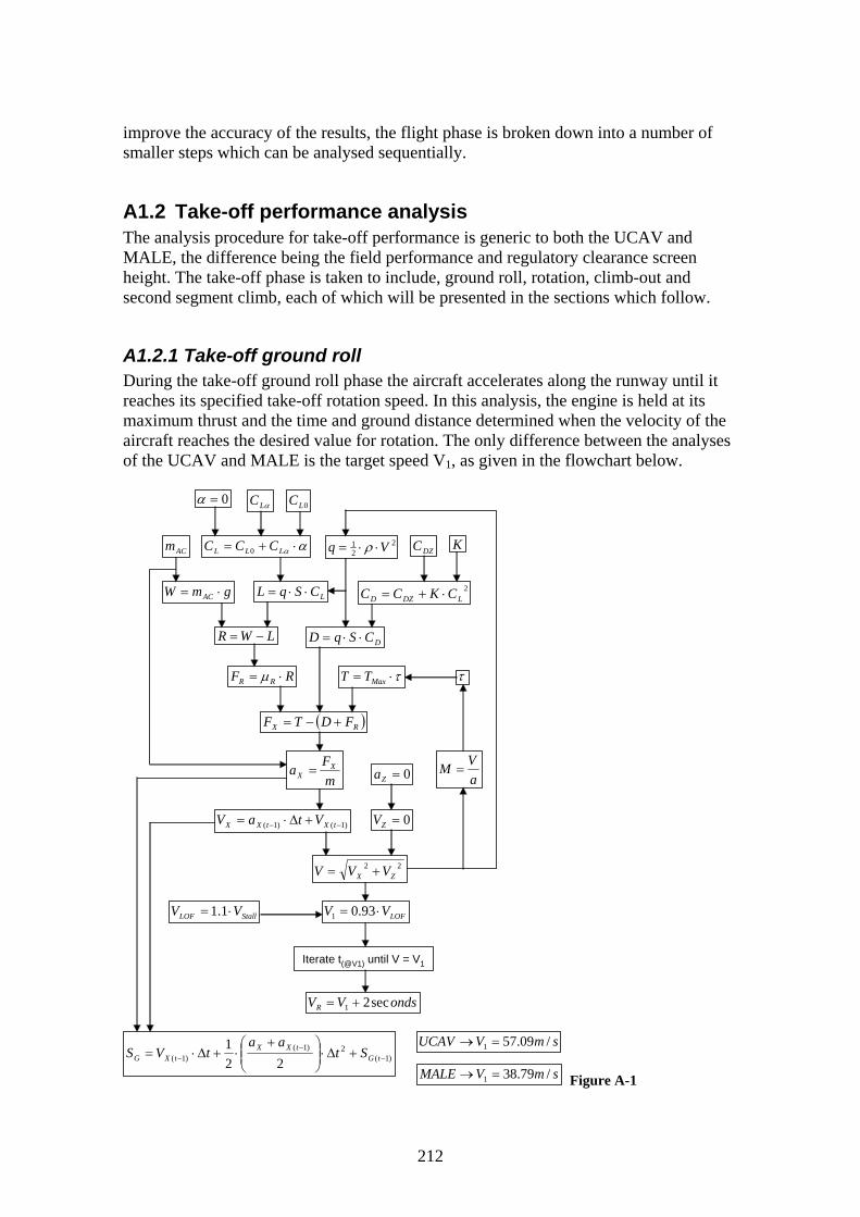
improve the accuracy of the results, the flight phase is broken down into a number of smaller steps which can be analysed sequentially.

A1.2 Take-off performance analysis The analysis procedure for take-off performance is generic to both the UCAV and MALE, the difference being the field performance and regulatory clearance screen height. The take-off phase is taken to include, ground roll, rotation, climb-out and second segment climb, each of which will be presented in the sections which follow.

A1.2.1 Take-off ground roll During the take-off ground roll phase the aircraft accelerates along the runway until it reaches its specified take-off rotation speed. In this analysis, the engine is held at its maximum thrust and the time and ground distance determined when the velocity of the aircraft reaches the desired value for rotation. The only difference between the analyses of the UCAV and MALE is the target speed V1, as given in the flowchart below.

22ZX VVV +=

LOFVV ⋅= 93.01StallLOF VV ⋅= 1.1

ondsVVR sec21 +=

0=α

LWR −=

RF RR ⋅= μ τ⋅= MaxTT

( )RX FDTF +−=

mFa X

X = 0=Za

0=ZV

)1(2)1(

)1( 221

−−

− +Δ⋅⎟⎟⎠

⎞⎜⎜⎝

⎛ +⋅+Δ⋅= tG

tXXtXG St

aatVS

)1()1( −− +Δ⋅= tXtXX VtaV

LCSqL ⋅⋅=

DCSqD ⋅⋅=

gmW AC ⋅=

ACm αα ⋅+= LLL CCC 0

2LDZD CKCC ⋅+=

DZC K

αLC 0LC

221 Vq ⋅⋅= ρ

Iterate t(@V1) until V = V1

aVM =

τ

smVUCAV /09.571 =→

smVMALE /79.381 =→ Figure A-1

212

A1.2.2 Take-off rotation During the take-off rotation phase, the aircraft gradually rotates about its main wheels to raise the nose of the aircraft. During this time, the angle of attack of the wings and thus the lift gradually increases until the entire weight of the aircraft is supported by the wings. In this analysis, the aircraft angle of attack is assumed to increase by 1 degree per second until the weight of the aircraft is supported by the wings. The time and ground distance covered until this condition is satisfied can be determined respectively. This analysis is identical for the MALE and UCAV as presented in the flowchart below.

22ZX VVV +=

LWR −=

RF RR ⋅= μ τ⋅= MaxTT

( )RX FDCosTF +−⋅= α

mFa X

X = 0=Za

0=ZV

)1(2)1(

)1( 221

−−

− +Δ⋅⎟⎟⎠

⎞⎜⎜⎝

⎛ +⋅+Δ⋅= tG

tXXtXG St

aatVS

)1()1( −− +Δ⋅= tXtXX VtaV

( ) ZL FCSqL +⋅⋅=

DCSqD ⋅⋅=

gmW AC ⋅=

ACm αα ⋅+= LLL CCC 0

2LDZD CKCC ⋅+=

DZC K

αLC 0LC

221 Vq ⋅⋅= ρ

Iterate t(Final) until (L-W) = 0

aVM =

τ

αSinTFZ ⋅=

Increase α by 1 deg/s from initial value of 0

Figure A-2

A1.2.3 Take-off climb out During the take-off climb out phase the aircraft initially climbs to a height sufficient to clear a screen height specified by the airworthiness regulations. In this analysis, the aircraft is assumed to maintain the angle of attack attained at the end of the take-off rotation. The time and ground distance covered until the aircraft reaches the screen

213

height can then be determined. This analysis is identical for the MALE and UCAV as presented in the flowchart below.

22ZX VVV +=

τ⋅= MaxTT

( ) βββα CosDSinLCosTFX ⋅−⋅−+⋅=

)1(2)1(

)1( 221

−−

− +Δ⋅⎟⎟⎠

⎞⎜⎜⎝

⎛ +⋅+Δ⋅= tG

tXXtXG St

aatVS

)1()1( −− +Δ⋅= tXtXX VtaV

LCSqL ⋅⋅=

DCSqD ⋅⋅=

gmW AC ⋅=

ACm αα ⋅+= LLL CCC 0

2LDZD CKCC ⋅+=

DZC K

αLC 0LC

221 Vq ⋅⋅= ρ

mF

a XX =

Iterate t(Final) until H = 10.668m

aVM =

τ

α = Value fixed at end of take-off rotation

( ) WSinDCosLSinTFZ −⋅−⋅++⋅= βββα

mF

a ZZ =

)1()1( −− +Δ⋅= tZtZZ VtaV

⎟⎟⎠

⎞⎜⎜⎝

⎛=

X

Z

VV

ATANβ

)1(2)1(

)1( 221

−−

− +Δ⋅⎟⎟⎠

⎞⎜⎜⎝

⎛ +⋅+Δ⋅= t

tZZtZ Ht

aatVH

Figure A-3

A1.2.4 Second segment climb The second segment climb phase is the final take-off stage, during which the aircraft attains a desired aircraft vertical velocity in preparation for the main climb phase. In this analysis, the aircraft is assumed to maintain the angle of attack attained during the initial take-off climb out phase. The time and ground distance covered to complete this phase can then be determined as the condition when the desired vertical velocity is met. The only difference between the analyses of the UCAV and MALE is the target vertical velocity VZ as given in the flowchart below.

214

22ZX VVV +=

τ⋅= MaxTT

( ) βββα CosDSinLCosTFX ⋅−⋅−+⋅=

)1(2)1(

)1( 221

−−

− +Δ⋅⎟⎟⎠

⎞⎜⎜⎝

⎛ +⋅+Δ⋅= tG

tXXtXG St

aatVS

)1()1( −− +Δ⋅= tXtXX VtaV

LCSqL ⋅⋅=

DCSqD ⋅⋅=

gmW AC ⋅=

ACm αα ⋅+= LLL CCC 0

2LDZD CKCC ⋅+=

DZC K

αLC 0LC

221 Vq ⋅⋅= ρ

mF

a XX =

Iterate t(Final) until VZ = VZ(Final)

aVM =

τ

α = Value fixed at end of take-off climb out

( ) WSinDCosLSinTFZ −⋅−⋅++⋅= βββα

mF

a ZZ =

)1()1( −− +Δ⋅= tZtZZ VtaV

⎟⎟⎠

⎞⎜⎜⎝

⎛=

X

Z

VV

ATANβ

)1(2)1(

)1( 221

−−

− +Δ⋅⎟⎟⎠

⎞⎜⎜⎝

⎛ +⋅+Δ⋅= t

tZZtZ Ht

aatVH VZ(0) from take-off climb-out

smVUCAV FinalZ /5.12)( =→

smVMALE FinalZ /1.6)( =→

Figure A-4

A1.3 Climb performance analysis The analysis procedure is different for the climb performance of the UCAV and MALE configurations. In the case of the UCAV, the aircraft not only climbs to the desired cruise altitude but also accelerates to the desired cruise speed. In the case of the MALE, the climb phase is broken down into 2 stages. During the first stage the aircraft climbs to an intermediate altitude and accelerates to its cruise speed. In the second stage, the aircraft climbs at a constant speed climb to its final loiter altitude. The analysis procedure for each of these will be discussed in the sections which follow.

215

A1.3.1 UCAV climb During the climb phase, the UCAV climbs and accelerates to its cruise altitude and speed of 12.192km and Mach 0.9 respectively. During this analysis, the flight path of the aircraft is fixed and the angle of attack of the aircraft is treated as a variable which is iterated to find the optimal solution corresponding to minimum thrust. The total altitude attained and distance covered can also be determined for each step to verify the results. The accuracy of the solution can be seen to be dependent on the number of steps used and the corresponding time interval of each step. The analysis is presented in the flowchart below.

( ) ( )22 WCosLSinDmaSinLCosDT X +⋅−⋅++⋅+⋅= ββββ

Variable=α

LCSqL ⋅⋅= DCSqD ⋅⋅=

gmW AC ⋅=

ACm

αα ⋅+= LLL CCC 02

LDZD CKCC ⋅+=

DZC KαLC 0LC

221 Vq ⋅⋅= ρ

Iterate α to find minimum value for T

⎟⎟⎠

⎞⎜⎜⎝

⎛=

X

Z

VV

ATANβ

aMVX ⋅=

smVZ /5.12=

ndSpeedOfSou

sMachXX a

aa )/(=

sMa sMachX /0006.0)/( =

1)/)(1( −− += tsMachtX MaM

)1(2)1(

)1( 221

−−

− +Δ⋅⎟⎟⎠

⎞⎜⎜⎝

⎛ +⋅+Δ⋅= tG

tXXtXG St

aatVS

)1(2)1(

)1( 221

−−

− +Δ⋅⎟⎟⎠

⎞⎜⎜⎝

⎛ +⋅+Δ⋅= t

tZZtZ Ht

aatVH

0=Za 0)0( =H

Iterate tFinal until HFinal = 12192m

)(Hfna ndSpeedOfSou =

Figure A-5

A1.3.2 MALE first climb stage During the first climb phase, the MALE climbs to an intermediate altitude of 4.572km and accelerates to the desired second climb phase speed of Mach 0.3488. During this analysis, the angle of attack of the aircraft is treated as a variable which is iterated to find the optimal solution corresponding to minimum thrust. This flight phase has proven to be the most critical phase with respect to thrust requirements and a second solution

216

stage iterates the climb angle to find to optimal flight path to meet the thrust requirements. As it is not sensible to operate an engine at full power for long periods, a percentage of the full power is also assumed (which is 97.5% in this analysis). The total altitude attained and distance covered can also be determined for each step to verify the results. The analysis is presented in the flowchart below.

( ) ( )22 WCosLSinDmaSinLCosDT X +⋅−⋅++⋅+⋅= ββββ

Variable=α

LCSqL ⋅⋅= DCSqD ⋅⋅=

gmW AC ⋅=

ACm

αα ⋅+= LLL CCC 02

LDZD CKCC ⋅+=

DZC KαLC 0LC

221 Vq ⋅⋅= ρ

Iterate α to find minimum value for T

Variable=β

aMV ⋅=

tVV

a tXXX Δ

−= − )1(

0

0)/( tt

MMa

Final

FinalsMachX −

−=

( ) 1)/)(1( −− +Δ⋅= tsMachtX MtaM

)1(0

tan −+Δ⋅−

= tFinal

Total Distttt

DistceDis

)1()1(

2 −− +Δ⋅

+= t

tZZ AlttVV

Altitude

0=Za 0)0( =H

)(Hfna ndSpeedOfSou =

βCosVVX ⋅=

βSinVVZ ⋅=

( )τ⋅⋅= DesignAvailable TFullPowerT %

ActualAvailableThrust TTError −=

Iterate β until ErrorThrust = 0

)(Hfn=σ

5.0

02.012.0 στ ⋅+

=MDesignT

Figure A-6

A1.3.3 MALE second stage During the second climb phase, the MALE climbs to its final loiter altitude of 7.620km at a constant climb speed of Mach 0.3488. During this analysis, the angle of attack of the aircraft is treated as a variable which is iterated to find the optimal solution corresponding to minimum thrust. In contrast to the last stage, the climb angle attains a fixed value in this analysis. The analysis is presented in the flowchart below.

217

( ) ( )22 WCosLSinDmaSinLCosDT X +⋅−⋅++⋅+⋅= ββββ

Variable=α

LCSqL ⋅⋅= DCSqD ⋅⋅=

gmW AC ⋅=

ACm

αα ⋅+= LLL CCC 02

LDZD CKCC ⋅+=

DZC KαLC 0LC

221 Vq ⋅⋅= ρ

Iterate α to find minimum value for T

Fixed=β

aMV ⋅=

tVV

a tXXX Δ

−= − )1(

0

0)/( tt

MMa

Final

FinalsMachX −

−=

( ) 1)/)(1( −− +Δ⋅= tsMachtX MtaM

)1(0

tan −+Δ⋅−

= tFinal

Total Distttt

DistceDis

)1(0

−+Δ⋅−

= tFinal

Total Altttt

AltAltitude

0=Za 0)0( =H

)(Hfna ndSpeedOfSou =

βCosVVX ⋅=

βSinVVZ ⋅=

τ⋅= DesignAvailable TT

)(Hfn=σ

5.0

02.012.0 στ ⋅+

=MDesignT

⎟⎟⎠

⎞⎜⎜⎝

⎛=

Total

Total

DistAlt

ATANβ

Figure A-7

A1.4 Cruise and loiter performance analysis The analysis procedure for the cruise and loiter phases of the UCAV and MALE configurations respectively is essentially the same. In the case of the UCAV, we have an outbound and inbound cruise phase, both of which are at an altitude of 12.192km and speed of Mach 0.9. In the case of the MALE, the main loiter phase is at an altitude of 7.62km, and at a speed of Mach 0.2507 for 35 hours. In addition, to this there is a 1 hour loiter phase at sea level and a speed of Mach 0.1046. Both the cruise and loiter phases follow the same analysis procedure whereby the flight phase is fixed and the aircraft angle of attack is a variable which is iterated to find the minimum value of engine thrust. This procedure is presented in the flowchart below, with the only

218

difference between the analyses of the UCAV and MALE being the flight speed and altitude.

( )22 LWDT −+=

Variable=α

LCSqL ⋅⋅= DCSqD ⋅⋅=

gmW AC ⋅=

ACm

αα ⋅+= LLL CCC 02

LDZD CKCC ⋅+=

DZC KαLC 0LC

221 Vq ⋅⋅= ρ

Iterate α to find minimum value for T

tVceDis X Δ⋅=tan Figure A-8

A1.5 Descent performance analysis The analysis procedure to determine the descent performance is different for the UCAV and MALE configurations. In the case of the UCAV, the aircraft descends to its approach altitude at a constant vertical descent velocity while decelerating to its approach speed. In the case of the MALE, the descent phase is broken down into 2 stages. The first stage involves a constant speed descent to an intermediate altitude. The second stage then involves a simultaneous descent to sea level and a deceleration. The analysis procedure for each of these will be discussed in the sections which follow.

A1.5.1 UCAV descent During the descent phase, the UCAV descends from its cruise altitude to a landing approach altitude of 15.24m at a constant vertical velocity of 10m/s. During this time it also decelerates from its cruise speed to an approach speed of Mach 0.1764. During this analysis, the flight path of the aircraft is fixed and its angle of attack is treated as a variable which is iterated to find the optimal solution corresponding to minimum thrust. The total altitude lost and distance covered can also be determined for each step to verify the results. The analysis is presented in the flowchart below.

219

( ) ( )22 ββββ CosLSinDWmaSinLCosDT X ⋅−⋅−++⋅−⋅=

Variable=α

LCSqL ⋅⋅= DCSqD ⋅⋅=

gmW AC ⋅=

ACm

αα ⋅+= LLL CCC 02

LDZD CKCC ⋅+=

DZC KαLC 0LC

221 Vq ⋅⋅= ρ

Iterate α to find minimum value for T

⎟⎟⎠

⎞⎜⎜⎝

⎛−=

X

Z

VV

ATANβ

aMVX ⋅=

smVZ /10−=

ndSpeedOfSou

sMachXX a

aa )/(=

1)/)(1( −− += tsMachtX MaM

)1(2)1(

)1( 221

−−

− +Δ⋅⎟⎟⎠

⎞⎜⎜⎝

⎛ +⋅+Δ⋅= tG

tXXtXG St

aatVS

)1(2)1(

)1( 221

−−

− +Δ⋅⎟⎟⎠

⎞⎜⎜⎝

⎛ +⋅+Δ⋅= t

tZZtZ Ht

aatVH

0=Za 12192)0( =H

Iterate tFinal until HFinal = 15.24m

)(Hfna ndSpeedOfSou =

0)/( tt

MMa

Final

ApproachCruisesMachX −

−=

Figure A-9

A1.5.2 MALE first descent stage During the first descent phase, the MALE descends from its loiter altitude to an intermediate altitude of 4.572km at a constant speed of Mach 0.3488. During this analysis, the flight path of the aircraft is fixed and the angle of attack of the aircraft is treated as a variable which is iterated to find the optimal solution corresponding to minimum thrust. The analysis is presented in the flowchart below.

220

( ) ( )22 ββββ CosLSinDWmaSinLCosDT X ⋅−⋅−++⋅−⋅=

Variable=α

LCSqL ⋅⋅= DCSqD ⋅⋅=

gmW AC ⋅=

ACm

αα ⋅+= LLL CCC 02

LDZD CKCC ⋅+=

DZC KαLC 0LC

221 Vq ⋅⋅= ρ

Iterate α to find minimum value for T

Fixed=β

aMV ⋅=

tVV

a tXXX Δ

−= − )1(

0)/( =sMachXa

FixedM =

)1(0

tan −+Δ⋅−

= tFinal

Total Distttt

DistceDis

)1(0

−+Δ⋅−

= tFinal

Total Altttt

AltAltitude

0=Za 0)0( =H

)(Hfna ndSpeedOfSou =

βCosVVX ⋅=

βSinVVZ ⋅=

τ⋅= DesignAvailable TT

)(Hfn=σ

5.0

02.012.0 στ ⋅+

=MDesignT

⎟⎟⎠

⎞⎜⎜⎝

⎛=

Total

Total

DistAlt

ATANβ

Figure A-10

A1.5.3 MALE second descent stage During the second descent phase, the MALE descends from its intermediate altitude of the first descent stage to sea level while decelerating to a speed of Mach 0.1073. During this analysis, the angle of attack of the aircraft is treated as a variable which is iterated to find the optimal solution corresponding to minimum thrust. The total altitude lost and distance covered can also be determined for each step to verify the results. The analysis is presented in the flowchart below.

221

( ) ( )22 ββββ CosLSinDWmaSinLCosDT X ⋅−⋅−++⋅−⋅=

Variable=α

LCSqL ⋅⋅= DCSqD ⋅⋅=

gmW AC ⋅=

ACm

αα ⋅+= LLL CCC 02

LDZD CKCC ⋅+=

DZC KαLC 0LC

221 Vq ⋅⋅= ρ

Iterate α to find minimum value for T

Fixed=β

aMV ⋅=

tVV

a tXXX Δ

−= − )1(

0

0)/( tt

MMa

Final

FinalsMachX −

−=

)1(0

tan −+Δ⋅−

= tFinal

Total Distttt

DistceDis

)1(0

−+Δ⋅−

= tFinal

Total Altttt

AltAltitude

0=Za 0)0( =H

)(Hfna ndSpeedOfSou =

βCosVVX ⋅=

βSinVVZ ⋅=

τ⋅= DesignAvailable TT

)(Hfn=σ

5.0

02.012.0 στ ⋅+

=MDesignT

⎟⎟⎠

⎞⎜⎜⎝

⎛=

Total

Total

DistAlt

ATANβ

1)/)(1( −− += tsMachtX MaM

Figure A-11

A1.6 Landing performance analysis The analysis procedure for landing performance is generic to both the UCAV and MALE, the difference being the field performance, approach speed and regulatory clearance screen height. The landing phase is taken to include: landing approach, flare and ground run, each of which will be presented in the sections which follow.

A1.6.1 Landing approach and flare The landing approach and flare phase starts at the regulatory screen height and approach speed. The aircraft then descends at a vertical descent velocity specific to that configuration while decelerating to its touchdown speed. As the aircraft speed is reduced, the aircraft angle of attack must be increased accordingly in order to maintain sufficient lift to maintain the desired descent velocity. This gives rise to the characteristic landing flare manoeuvre, whereby the nose of the aircraft is rotated as the

222

aircraft approaches the ground. This manoeuvre also ensures that the main landing gear wheel makes contact with the ground first to bear the impact of the landing. During this analysis, the angle of attack of the aircraft is treated as a variable which is iterated to find the optimal solution corresponding to minimum thrust. The total altitude lost and distance covered can also be determined for each step. This phase ends when the aircraft velocity equals the touchdown velocity. The only difference between the analyses of the UCAV and MALE is the vertical decent velocity VZ and the approach screen height as given in the flowchart below

22ZX VVV +=

)1(2)1(

)1( 221

−−

− +Δ⋅⎟⎟⎠

⎞⎜⎜⎝

⎛ +⋅+Δ⋅= tG

tXXtXG St

aatVS

)1()1( −− +Δ⋅= tXtXX VtaV

LCSqL ⋅⋅=

DCSqD ⋅⋅=

gmW AC ⋅=

ACm αα ⋅+= LLL CCC 0

2LDZD CKCC ⋅+=

DZC K

αLC 0LC

221 Vq ⋅⋅= ρ

0

)0()(

ttVV

aFinal

XFinalXX −

−=

Iterate α to find the minimum value for T

( ) ( )22ZX maSinDCosLWmaSinLCosDT +⋅−⋅−++⋅−⋅= ββββ

tVV

a iZZZ Δ

−= − )1(

ZV

⎟⎟⎠

⎞⎜⎜⎝

⎛=

X

Z

VV

ATANβ

)1(2)1(

)1( 221

−−

− +Δ⋅⎟⎟⎠

⎞⎜⎜⎝

⎛ +−⋅+Δ⋅= t

tZZtZ Ht

aatVH

VZ(0) from take-off climb-out

)0(H mH Final 0)( = VX(0) from take-off climb-out

StallTouchdownFinalX VVV ⋅== 1.1)(

0)( =FinalZVIterate tFinal until H = 0 when VX(Final) = VTouchdown

⎟⎠⎞

⎜⎝⎛

Δ−=→

tsmVVUCAV ZZ

/1)0(

smVMALE Z /1−=→

mHUCAV 24.15)0( =→

mHMALE 668.10)0( =→ Figure A-12

223

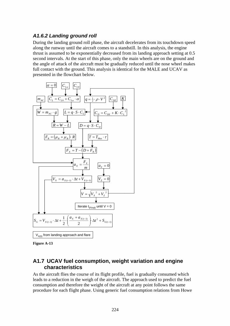
A1.6.2 Landing ground roll During the landing ground roll phase, the aircraft decelerates from its touchdown speed along the runway until the aircraft comes to a standstill. In this analysis, the engine thrust is assumed to be exponentially decreased from its landing approach setting at 0.5 second intervals. At the start of this phase, only the main wheels are on the ground and the angle of attack of the aircraft must be gradually reduced until the nose wheel makes full contact with the ground. This analysis is identical for the MALE and UCAV as presented in the flowchart below.

22ZX VVV +=

0=α

LWR −=

( ) RF BRR ⋅+= μμ τ⋅= MaxTT

( )RX FDTF +−=

mFa X

X = 0=Za

0=ZV

)1(2)1(

)1( 221

−−

− +Δ⋅⎟⎟⎠

⎞⎜⎜⎝

⎛ +⋅+Δ⋅= tG

tXXtXG St

aatVS

)1()1( −− +Δ⋅= tXtXX VtaV

LCSqL ⋅⋅=

DCSqD ⋅⋅=

gmW AC ⋅=

ACm αα ⋅+= LLL CCC 0

2LDZD CKCC ⋅+=

DZC K

αLC 0LC

221 Vq ⋅⋅= ρ

Iterate t(Final) until V = 0

VX(0) from landing approach and flare

Figure A-13

A1.7 UCAV fuel consumption, weight variation and engine characteristics

As the aircraft flies the course of its flight profile, fuel is gradually consumed which leads to a reduction in the weigh of the aircraft. The approach used to predict the fuel consumption and therefore the weight of the aircraft at any point follows the same procedure for each flight phase. Using generic fuel consumption relations from Howe

224

[1], this process can be seen to be a function of the aircraft speed, altitude and engine thrust as presented in the flowchart below.

( ))0()0( FuelFuelACAC mmmm −−=

)1()1( −− +Δ⋅= tFueltfFuel mtQm

SFCTQ f ⋅=

EngineT

gmW AC ⋅=

( ) ( )[ ] 08.02265.0 063.0128.0115.01' σ⋅⋅⋅+⋅+⋅⋅−⋅= MRRcc

)/(104.2' 5 Nskgc −⋅=

⎥⎥⎦

⎤

⎢⎢⎣

⎡⎟⎟⎠

⎞⎜⎜⎝

⎛−⋅+⋅= 101.01

TT

cSFC Design

NTDesign 77.52730=

)(0

Altitudefn==ρρσ Mach

Figure A-14 The maximum achievable value of engine thrust as required for critical flight phases can be determined from a generic relation from Howe as a function of aircraft altitude and speed, as given in the flowchart below. In this case, the design value of thrust is taken to be the maximum value of thrust when the aircraft is at sea level and stationary, as was determined in the conceptual design studies.

( )[ ] *4321

SMRKKRKKF στ τττττ ⋅⋅⋅++⋅+⋅=

225

DesignMax TT ⋅= τ NTDesign 77.52730= Equation A-1 and Table A-1 [38] The constants in the expression above can be determined from the accompanying table from Howe for a dry engine with a bypass ratio of 0.8 and Mach number up to 0.9.

A1.8 MALE fuel consumption, weight variation and engine characteristics

As for the UCAV, the approach used to predict the fuel consumption and therefore the weight of the aircraft at any point, follows the same procedure for each flight phase. Using a relation from Mattingly [16] for a turboprop engine, this process can be seen to be a function of the aircraft speed, altitude (via the temperature ratio) and engine thrust as presented in the flowchart below.

( ))0()0( FuelFuelACAC mmmm −−=

)1()1( −− +Δ⋅= tFueltfFuel mtQm

SFCTQ f ⋅=EngineT

gmW AC ⋅=

( ) 6132.288.018.0

5.0

ETempTempMachSFC

Std

⋅⎥⎥⎦

⎤

⎢⎢⎣

⎡⎟⎟⎠

⎞⎜⎜⎝

⎛⋅⋅+=

)(AltitudefnTempTemp

Std

=

Figure A-15

Once again, the maximum achievable value of engine thrust as required for critical flight phases can be determined from a generic relation from Mattingly as a function of aircraft altitude and speed, as given in the flowchart below. As before, the design value of thrust is taken to be the maximum value of thrust when the aircraft is at sea level and stationary, as was determined in the conceptual design studies.

)(0

Altitudefn==ρρσ

5.0

02.012.0 στ ⋅⎥⎦

⎤⎢⎣⎡

+=

Mach

DesignMax TT ⋅= τ NTDesign 11.9925=

Figure A-16

A1.9 General terms used The majority of the expressions used in these analyses are self explanatory and will be familiar to any aerospace student. General aerodynamic terms such as CDZ, K, CLα and XAC are presented as convenient polynomial expressions in the baseline aircraft design section of this thesis. Atmospheric terms of particular importance within these analyses are the speed of sound and density of surrounding air. This data, as is readily available from any aerodynamic textbook has been adapted into convenient polynomial expressions as given below, where H is the altitude in km.

5.34002.4 +−= HaAir Eq A-2 2239.11152.00035.0 2 +−= HHAirρ Eq A-3

226

B1 Thrust vectoring source data Two different data sets were available from NASA for the external vanes vectoring system - that for a military power nozzle and that for a max nozzle (which is aimed at nozzles incorporating an afterburner). Since our engine does not use an afterburner, we will thus only concentrate on the data for the military power engine nozzle. There were also a number of different paddle sizes investigated by NASA but here we are concentrating on the same configuration as that used on the X-31 with a large top vane and two smaller vanes. The test results for the vectored nozzle and baseline nozzle with no vanes installed is given in the sections below. An additional section gives the geometry of the system as tested by NASA.

B1.1 NASA vectored nozzle test results The results obtained from the NASA tests on the thrust vectoring system are given in the table below at a number of specified values of nozzle pressure ratio and paddle deflection angle. In this work, we are primarily interested in the pitch control of the system and thus only results for deflection of the top vectoring paddle have been included. The two lower vanes are thus assumed to be in their fully retracted position of -10°. These results were taken directly from page 109 to 129 of NASA TM 4359 [61]. Data for the vectored NASA nozzle from tests at different paddle angles

δC (deg) -10 δB (deg) -10

δA (deg) NPR test NPR wp/wi F/Fi Fr/Fi δP (deg) δY (deg) δR (deg) Cfg10 2.0016 2 0.886 0.9973 0.9973 0.27 -0.21 0.342053 0.997310 3.0014 3 0.9282 0.9967 0.9967 0.69 -0.2 0.718401 0.996710 4.0037 4 0.9358 0.9861 0.9862 0.92 -0.15 0.932148 0.986210 5.0024 5 0.9283 0.9684 0.9689 1.75 -0.12 1.754109 0.968910 6.0004 6 0.9284 0.9529 0.9541 2.86 -0.16 2.864472 0.954115 2.0069 2 0.8864 0.9844 0.9848 1.58 -0.31 1.610124 0.984815 3.0044 3 0.9268 0.9819 0.9825 2.14 -0.24 2.153416 0.982515 4.0049 4 0.9359 0.9693 0.9704 2.82 -0.24 2.830194 0.970415 5.0016 5 0.9285 0.9472 0.9499 4.3 -0.34 4.313421 0.949915 6.0038 6 0.9285 0.9286 0.9338 5.99 -0.44 6.006139 0.933820 3.0063 3 0.9248 0.9297 0.9362 6.75 -0.45 6.764983 0.936220 4.0049 4 0.9349 0.9171 0.9258 7.84 -0.62 7.864477 0.925820 4.9997 5 0.9284 0.8999 0.9121 9.34 -0.73 9.368484 0.912120 5.997 6 0.9283 0.8856 0.9022 10.97 -0.86 11.00366 0.902225 1.996 2 0.8853 0.8867 0.9019 10.51 -0.62 10.52827 0.901925 3.006 3 0.9245 0.8759 0.8948 11.74 -0.96 11.77919 0.894825 4.002 4 0.9349 0.8655 0.8877 12.8 -1.16 12.85246 0.887725 5.0013 5 0.9285 0.8554 0.8808 13.72 -1.23 13.77502 0.880825 5.9986 6 0.9282 0.8461 0.8754 14.83 -1.24 14.88175 0.875430 2.011 2 0.8875 0.8161 0.8531 16.9 -1.29 16.94916 0.853130 2.9988 3 0.9291 0.8011 0.8431 18.09 -1.62 18.16239 0.843130 3.9973 4 0.9361 0.7992 0.8435 18.61 -1.44 18.66563 0.843530 4.9858 5 0.9303 0.7974 0.8428 18.84 -1.48 18.89804 0.842830 5.9901 6 0.9285 0.794 0.8415 19.28 -1.64 19.34963 0.841535 2.0002 2 0.8881 0.7475 0.8088 22.27 -3.15 22.49167 0.808835 2.999 3 0.9255 0.7352 0.7997 23 -3.17 23.21743 0.799735 4.0014 4 0.9355 0.7375 0.8001 22.6 -3.48 22.86636 0.800135 4.9983 5 0.9288 0.741 0.8002 21.94 -3.73 22.25481 0.800235 6.0032 6 0.9283 0.7419 0.7987 21.43 -4.07 21.81306 0.7987

Table 1-1

227

B1.2 NASA test results with no vanes installed The results obtained from NASA TM 4359 [61] pages 97 to 98 for the baseline nozzle with no vanes installed is given in the table below. Data for the baseline NASA nozzle with no vanes installed(Averaged values of all the test runs)

NPR NPR test wp/wi F/Fi Fr/Fi dP (deg) dY (deg) dR (deg) Cfg2 2.00128 0.88614 0.99994 0.99996 0.01 -0.178 0.178281 0.999963 2.99998 0.92822 0.9992 0.9992 0.276 -0.076 0.286273 0.99924 4.00185 0.935183 0.989133 0.989133 0.323333 -0.03667 0.325406 0.9891335 4.99076 0.93238 0.97814 0.97814 0.324 0.01 0.324154 0.978146 5.99996 0.92848 0.96856 0.96858 0.292 0.04 0.294727 0.96858

Table 1-2

B1.3 Geometric data of the vectoring system Data for the geometry of the system taken from NASA TM 4359 [61] pages 133 to 134 is given below. Additional data can also be obtained from NASA TM 4771 [62], TM 101741 [63], TM 3531 [64] and TM 4341 [65] where required.

Figures 1-1, 1-2, 1-3

228

229

B2 Rescaling the NASA test data

B2.1 Assumptions and limitations In this work, we were fortunate enough to have access to test data for the X-31 thrust vectoring system from NASA studies. These tests were however carried out on a scale model of the system and under laboratory conditions. Whilst we can make some attempt to rescale the data to match it to a different nozzle, the data itself makes no allowance for the interaction of external flow conditions on the system. To clarify this point, the installed nozzle performance will be dependent on the flight speed and altitude, giving different results for each case. The performance of the nozzle will also be dependent on its installation within the airframe. In particular, the aircraft after-body will affect the flow field surrounding aircraft and thus the nozzle. We are therefore somewhat restricted as to the accuracy of the results that can be achieved from this study. This work is however considered sufficient for conceptual design and feasibility studies.

B2.2 Background to the approach In its original format, the NASA test data is only valid for the nozzle on which the original experimental tests were carried out. Since it is not practical to build and test our own nozzle within the time-frame of this project, we have to find a way to adapt the original data to match a different nozzle. Since the terms in the data which govern the flow conditions are non-dimensional, matching of the scale test data to a full scale nozzle should be likened to the matching of models to full scale bodies of other fluid flow studies. This system consists of a simple nozzle which is surrounded by external vectoring vanes, which deflect into the flow stream as required. In its un-vectored state when all the vanes are fully retracted, the nozzle could be viewed in the same way as a standard engine nozzle. Comparison of the operating characteristics of the un-vectored NASA test nozzle with those of our baseline engine did however highlight a mis-match between the two. In the absence of a better method, the approach adopted here was to rescale the NASA test data in accordance with the differences between the un-vectored nozzles used for the NASA tests and our baseline engine. Some error is expected with this approach but it is expected to serve as a good first approximation. To be able to obtain a better approximation, it would be necessary to carry out more scale tests on a like for like un-vectored nozzle and/or use a CFD model. Either of these approaches would however be time consuming and costly and beyond the scope of these feasibility studies.

B2.3 The data for the un-vectored baseline engine nozzle In this work, an engine nozzle with PI value of 0.98 was selected as the baseline (un-vectored) configuration. Using the AEDsys software suite, data was generated for this baseline engine-nozzle combination at a number of different engine conditions for cruise and take-off conditions. The full details of this are included with in the engine design section.

B2.4 Rescaling the NASA data to suit the baseline engine nozzle

As mentioned above, a mis-match exists between the operating data of the un-vectored NASA test nozzle and our baseline nozzle. We therefore need to rescale the NASA data to match the characteristics of our nozzle. If we know how much the un-vectored NASA nozzle has to be re-scaled by in order to match the baseline nozzle of our engine, then the vectored data for the NASA nozzle can be rescaled by the same amount. This involves the manipulation of the following parameters from the NASA data:

• Cfg – The nozzle thrust loss factor • NPR – The nozzle pressure ratio • dA – The deflection angle of the thrust vectoring vanes • dR – The deflection of the exhaust jet plume

The NASA data was categorised according to the deflection angle of the vectoring vanes and nozzle pressure ratio (NPR). The NPR parameter is dependent on the nozzle configuration and the engine operating condition and it is therefore difficult to maintain a specific value. Fortunately though, the test conditions for the NASA nozzle were carefully maintained to produce results for a range of fixed NPR and dA values. This simplifies our analysis somewhat as we have fixed points to interpolate between. Since NPR and dA can be regarded as input variables, only Cfg and dR require rescaling. The rescaling process for the parameter Cfg is presented in the flow chart below. Each data set has been clearly identified by subscripts referring to the NASA or baseline engine data and the vectored or no vanes installed nozzle configurations respectively.

( ) )()( NoVanesNASAfgVectoredNASAfgNASAfg CCC −− −=Δ

)(

)(

NoVanesNASAfg

NASAfgfg C

CCF

−

Δ=Δ

( ) )(()(Re NoVanesBLfgNoVanesBLfgfgscaledfg CCCFC −− +⋅Δ=

Data from NASA tests

Rescaled data

( ) )()( NoVanesNASAfgVectoredNASAfgNASAfg CCC −− −=Δ

)(

)(

NoVanesNASAfg

NASAfgfg C

CCF

−

Δ=Δ

( ) )(()(Re NoVanesBLfgNoVanesBLfgfgscaledfg CCCFC −− +⋅Δ=

Data from NASA tests

Rescaled data

In the first stage of this process, we determine the change in the values that is experienced as a result of deflecting the vanes in to the engines jet stream. In the next stage, we assume that these changes are directly related to the operating characteristics of the nozzle to obtain a relation to rescale the data. Since Cfg is the most widely used standard nozzle parameter amongst propulsion engineers it is reasonable to use this parameter to rescale the changes in the NASA test data. Using these fractional values, we can reverse the process using the Cfg value of the baseline nozzle in place of that of the no-vanes NASA data to obtain the revised and rescaled data. The parameter dR is rescaled by the same process, as presented in the flow chart below. Here, the dR(no-vanes) value is omitted when the data is rescaled to the new nozzle. In the case of the NASA nozzle, this figure was used to make allowance for the test rig set-up and nozzle manufacturing tolerances. In the case of our nozzle, these are assumed to be negligible since it is not possible to make a realistic prediction for them.

230

)()( NoVanesNASAVectoredNASA dRdRdR −− −=Δ

)(

)(

NoVanesNASAfg

NASA

CdR

dRF−

Δ=Δ

)()(Re NoVanesBLfgscaled CdRFdR −⋅Δ=

Data from NASA tests

Rescaled data

)()( NoVanesNASAVectoredNASA dRdRdR −− −=Δ

)(

)(

NoVanesNASAfg

NASA

CdR

dRF−

Δ=Δ

)()(Re NoVanesBLfgscaled CdRFdR −⋅Δ=

Data from NASA tests

Rescaled data The procedures above are repeated for each combination of vane vectoring angle and NPR to generate a revised set of data for our nozzle. An example set of results for a NPR of 3 is presented below with similar results for NPR values of 2, 4, 5 and 6.

NPR 3

dA (deg) dR (deg) Cfg Δ dR (deg) Δ Cfg FΔdR (deg) FΔCfg Δ dR (deg) Δ Cfg dR (deg) Cfg10 0.718401 0.9967 0.4321284 -0.0025 43.247438 -0.2502 0.4203199 -0.00243 0.42032 0.96946415 2.153416 0.9825 1.8671433 -0.0167 186.86382 -1.67134 1.8161211 -0.01624 1.816121 0.95565220 6.764983 0.9362 6.4787108 -0.063 648.38979 -6.30504 6.3016712 -0.06128 6.301671 0.91061725 11.77919 0.8948 11.492912 -0.1044 1150.2114 -10.4484 11.178853 -0.10155 11.17885 0.87034830 18.16239 0.8431 17.87612 -0.1561 1789.0432 -15.6225 17.387631 -0.15183 17.38763 0.82006135 23.21743 0.7997 22.931154 -0.1995 2294.9514 -19.966 22.304529 -0.19405 22.30453 0.777847

Original untouched test data for the NASA nozzle

Incremental changes in new nozzle data

Final resized data for new nozzle

Fractional changes for original NASA data

Incremental changes in original NASA data

Table 2-1

B2.5 Matching the nozzle data to the engine operating data The data rescaling process above, gives us a number of tables of results for nozzle pressure ratios from 2 to 6 in unit steps. Within these are a range of vane deflection angles from 10 to 35 degrees in 5 degree steps. An example of such data is below. Results for nozzle pressure ratio = 2 Results for nozzle pressure ratio = 3

dA NPR Cfg (Scl'd) dR (Scl'd) dA NPR Cfg (Scl'd) dR (Scl'd)10 2 0.962961 0.158133 10 3 0.969454 0.42031615 2 0.950891 1.382542 15 3 0.955642 1.81610320 2 0.910869 5.688082 20 3 0.910608 6.30160825 2 0.870846 9.993621 25 3 0.87034 11.1787430 2 0.823726 16.19343 30 3 0.820053 17.3874635 2 0.780951 21.5451 35 3 0.777839 22.3043 Table 2-2

From our engine design work, we have a number of data sets for the baseline engine. Each set corresponds to the engine operating condition such as a different thrust ratio or percentage of bleed. Within each data set, are results corresponding to a number of values of nozzle isentropic stagnation pressure ratio, designated as (π). Is should be emphasised that this is different to the nozzle pressure ratio (NPR). NPR is the ratio of the total to static pressure at the nozzle throat, whereas π is the ratio of the total pressure entering the nozzle to that leaving the component. The NPR of the engine has proven to be invaluable for stitching the engine and nozzle data sets together. Fortunately, this was obtained from the engine design process, as included within our engine data sets. For the take-off work, we have a number of tables of data for the engine as tested at a range of Pi-Nozzle values from 0.995 to 0.6 in 0.05 steps and engine bleed from 0% to 20% in 2.5% steps. An example take-off analysis data set is given below.

231

Results for 5% engine bleed Results for 10% engine bleed

% Thrust Pi-Nozzle Cfg (Eng) NPR (Eng) % Thrust Pi-Nozzle Cfg (Eng) NPR (Eng)100 0.995 0.978 3.217542 100 0.995 0.9777 2.898816100 0.95 0.961 3.217542 100 0.95 0.9588 2.898816100 0.9 0.9405 3.217542 100 0.9 0.9359 2.898816100 0.85 0.918 3.217542 100 0.85 0.9107 2.898816100 0.8 0.8932 3.217542 100 0.8 0.8827 2.898816100 0.75 0.8655 3.217542 100 0.75 0.8514 2.898816100 0.7 0.8343 3.217542 100 0.7 0.8159 2.898816100 0.65 0.7987 3.217542 100 0.65 0.775 2.898816100 0.6 0.7575 3.217542 100 0.6 0.7276 2.903511 Table 2-3

. A similar set of data exists for the cruise work. In this case we have a number of tables of data for the engine as tested at a range of Pi-Nozzle values from 0.995 to 0.84 in 0.02 steps and engine throttle settings from 45 to 65% in 5% steps. An example cruise analysis data set is given below. Results for 50% engine thrust Results for 60% engine bleed

% Thrust Pi-Nozzle Cfg (Eng) NPR (Eng) % Thrust Pi-Nozzle Cfg (Eng) NPR (Eng)50 0.995 0.9783 3.831136 60 0.995 0.9785 4.26483550 0.98 0.9736 3.837729 60 0.98 0.9742 4.2703350 0.96 0.9673 3.847253 60 0.96 0.9684 4.27948750 0.94 0.9607 3.857143 60 0.94 0.9624 4.28717950 0.92 0.9539 3.867399 60 0.92 0.9562 4.29487250 0.9 0.9464 3.878022 60 0.9 0.9498 4.30329750 0.88 0.9398 3.890842 60 0.88 0.9432 4.31208850 0.86 0.9324 3.902564 60 0.86 0.9364 4.32124550 0.84 0.9247 3.914652 60 0.84 0.9294 4.331136 Table 2-4

The next stage in this work is to stitch together the data sets for the engine and nozzle, with the aid of linear interpolation techniques. During this process, each engine operating point is interpolated between the corresponding rescaled nozzle data sets to generate a set of data specific to the NPR being analysed. This process is shown diagrammatically below. As a result of the vast amount of data that needed to be analysed, this process was automated with spreadsheet functions to filter and interpolate the data. This automated process will be discussed in more detail in a later section.

For an example 15% engine bleed data point at a NPR = 2.584

% Thrust Pi-Nozzle Cfg (Eng) NPR (Eng)100 0.9 0.9296 2.583764

Rescalled nozzle test data for NPR = 2 Rescalled nozzle test data for NPR = 3

dA NPR Cfg (Scl'd) dR (Scl'd) dA NPR Cfg (Scl'd) dR (Scl'd)10 2 0.962961 0.158133 10 3 0.969454 0.42031615 2 0.950891 1.382542 15 3 0.955642 1.81610320 2 0.910869 5.688082 20 3 0.910608 6.30160825 2 0.870846 9.993621 25 3 0.87034 11.1787430 2 0.823726 16.19343 30 3 0.820053 17.3874635 2 0.780951 21.5451 35 3 0.777839 22.3043

Interpolated nozzle test data for NPR = 2.5

dA NPR Cfg (Scl'd) dR (Scl'd)10 2.583764 0.966751 0.31118615 2.583764 0.953665 1.63563920 2.583764 0.910716 6.04623625 2.583764 0.87055 10.6854530 2.583764 0.821582 16.8904635 2.583764 0.779135 21.9883 Figure 2-1

232

A similar process exists for the cruise analysis, in which case the data is given as a function of engine throttle ratio instead of bleed. The equations used for the interpolation of Cfg and dR values are given below. The engine subscript refers to the engine data point being investigated, which would be NPREngine = 2.584 in the example above. The subscripts 1 and 2 refer to upper and lower rescaled nozzle data sets respectively, which would be NPR1 = 2 and NPR2 = 3 in the example above.

( ) )1()1()2(12

1fgfgfg

Enginefg CCC

NPRNPRNPRNPR

C +−⋅⎟⎟⎠

⎞⎜⎜⎝

⎛−

−= Eq 2-1

( ) 11212

1 dRdRdRNPRNPR

NPRNPRdR Engine +−⋅⎟⎟

⎠

⎞⎜⎜⎝

⎛−

−= Eq 2-2

At this stage in the process we now have a table of data points from the rescaled nozzle data, at the NPR point which is being investigated for our engine. The next stage is to further narrow down this data set to the value of Cfg at the engine operating point being investigated. This involves a second stage of interpolation as shown in the figure below.

% Thrust Pi-Nozzle Cfg (Eng) NPR (Eng)100 0.9 0.9296 2.583764

dA NPR Cfg (Scl'd) dR (Scl'd)10 2.583764 0.966751 0.31118615 2.583764 0.953665 1.635639 dA NPR Cfg (Scl'd) dR (Scl'd)20 2.583764 0.910716 6.046236 17.8016 2.583764 0.9296 4.10698225 2.583764 0.87055 10.6854530 2.583764 0.821582 16.8904635 2.583764 0.779135 21.9883

Upper bound of result

Lower bound of result

Final results for the NPR and Cfg values under consideration

Interpolated nozzle test data for NPR = 2.584

For an example 15% engine bleed data point at a NPR = 2.584

Figure 2-2 As before, a similar process exists for the cruise analysis. The accompanying equations for this interpolation stage are given below for dA and dR respectively, where the subscripts adopt the same terminology as before.

( ) 112)1()2(

)1()( dAdAdACC

CCdA

fgfg

fgEnginefgEngine +−⋅⎟

⎟⎠

⎞⎜⎜⎝

⎛

−

−= Eq 2-3

( ) 112)1()2(

)1()( dRdRdRCC

CCdR

fgfg

fgEnginefgEngine +−⋅⎟

⎟⎠

⎞⎜⎜⎝

⎛

−

−= Eq 2-4

Using the process above, we are able to merge the rescaled nozzle data with that for our engine operating at a number of different conditions. The results thus allow us to predict the impact which deflecting the vanes will have on the performance of the engine. Especially in terms of the gross thrust and thrust specific fuel consumption.

233

B2.6 Dealing with vast quantities of data As to be expected, it is not practical to manually manipulate the vast quantity of nozzle data for every single engine data point and some form of automation was required. For the range of NPR values encountered in this work, 3 rescaled nozzle NPR datasets were sufficient to cover the entire range of data points. The automation process here utilises a series of tests to filter out the final solution as shown in the example.

Rescaled nozzle data set for NPR=2

Rescaled nozzle data set for NPR=4

Rescaled nozzle data set for NPR=3

Rescaled nozzle data set interpolated between NPR = 2 and 3 for actual NPR to generate new Cfgand dR data set

Rescaled nozzle data set interpolated between NPR = 3 and 4 for actual NPR to generate new Cfgand dR data set

Interpolate each value in the new data set in accordance with the actual Cfg value to generate a final set of Cfg and dR values

Interpolate each value in the new data set in accordance with the actual Cfg value to generate a final set of Cfg and dR values

Test 1: If NPR(engine) < 3 then the value of test1 = 1 otherwise its value = 0

Test 1: If NPR(engine) > 3 then the value of test1 = 1 otherwise its value = 0

Test 2: If Cfg(nozzle) < Cfg(engine) then the value of test2 = 1 otherwise its value = 0

Test 2: If Cfg(nozzle) < Cfg(engine) then the value of test2 = 1 otherwise its value = 0

Test 3: If Cfg(nozzle@i-1) < Cfg(engine@i) then the value of test3 = 1 otherwise its value = 0

Test 3: If Cfg(nozzle@i-1) < Cfg(engine@i) then the value of test3 = 1 otherwise its value = 0

Filter the dA values for NPR 2-3 to find the final value using the equation for dA2-3.

Filter the dA values for NPR 3-4 to find the final value using the equation for dA3-4.

Filter the dR values for NPR 2-3 to find the final value using the equation for dR2-3.

Filter the dR values for NPR 3-4 to find the final value using the equation for dR3-4.

Filter the final dR values for the actual NPR with the dRFinal equation

Filter the final dR values for the actual NPR with the dRFinal equation Figure 2-3

234

The accompanying equations to find dA are:

( )∑=

− ⋅⋅⋅=n

iidAtesttesttestdA

132 321 AND ( )∑

=− ⋅⋅⋅=

n

iidAtesttesttestdA

143 321

Eq 2-5, 2-6 Likewise, the equations for dR are:

( )∑=

− ⋅⋅⋅=n

iidRtesttesttestdR

132 321 AND ( )∑

=− ⋅⋅⋅=

n

iidRtesttesttestdR

143 321

The final equations for dR and dA are then: Eq 2-7, 2-8 4332 −− += dAdAdAFinal Eq 2-9

4332 −− += dRdRdRFinal Eq 2-10 An example of this process as used in the actual analysis is given below. Example data analysis

NPR 2dA (deg) dR (deg) Cfg CFG NPR dA (deg) dR (deg)

10 0.158133 0.962961 0.8973 3.376089 21.75133 8.43694815 1.382542 0.95089120 5.688082 0.91086925 9.993621 0.870846 NPR 3.376089 Cfg 0.897330 16.19343 0.823726 dA (deg) dR (deg) Cfg Test 1 Final figures35 21.5451 0.780951 10 0.51892 0.971896 0 dA (deg) dR (deg) Test 2 Test 3 dA (deg) dR (deg)

15 1.97916 0.957429 0 35.78133 8.048307 0 1 0 0NPR 3 20 6.532348 0.91051 0 21.40772 7.814273 0 1 0 0dA (deg) dR (deg) Cfg 25 11.62445 0.870149 0 21.63647 8.198967 1 1 0 0

10 0.420316 0.969454 30 17.83652 0.818671 0 22.36286 8.348038 1 0 0 015 1.816103 0.955642 35 22.58983 0.776669 0 20.64004 8.93834 1 0 0 020 6.301608 0.910608 sum 0 025 11.17874 0.87034 NPR 3.376089 Cfg 0.897330 17.38746 0.820053 dA (deg) dR (deg) Cfg Test 1 Final figures35 22.3043 0.777839 10 0.486969 0.970129 1 dA (deg) dR (deg) Test 2 Test 3 dA (deg) dR (deg)

15 2.060828 0.95566 1 35.16644 8.408656 0 1 0 0NPR 4 20 6.724018 0.911043 1 21.5401 8.160377 0 1 0 0dA (deg) dR (deg) Cfg 25 11.6144 0.871807 1 21.75133 8.436948 1 1 21.75133 8.436948

10 0.597544 0.971249 30 17.64121 0.824062 1 22.33036 8.396511 1 0 0 015 2.466815 0.955688 35 22.26478 0.781649 1 21.36592 9.657153 1 0 0 020 7.424775 0.911764 sum 21.75133 8.43694825 12.33713 0.87424230 18.06218 0.83071235 22.19922 0.78797

Inputs from engine data points

Results from vectoring analysis

Figure 2-4

The example above is for just one data point and this process must thus be repeated for each of the engine data points to produce a complete table of data. In it entirety, the process completely stitches together the data sets for the engine conditions with the data sets for the rescaled thrust vectoring nozzle.

B2.7 Formatting the results At this stage in our work, we now have a number of tables of data for the engine and nozzle combination at a number of different vane deflection angles. Each of the tables of data corresponds to a different engine operating condition such as throttle ratio or bleed. An example of such a data table is presented below for a take-off case of 5% bleed. Similar tables exist for the cruise cases within which each data table corresponds to a different throttle ratio. With the data in this format, it is possible to plot the results of each parameter, from each results table. This enables us to fit a polynomial expression to each plot, which puts the data in a format more applicable to analytical analyses. These results are presented in the following sections.

235

Table of results for 0% bleed

Table of results for 2.5% bleed

Table of results for 5% bleed

Table of results for 20% bleed

Pi-N % bleed % Thrust Thrust (N) TSFC (mg/N-s) NPR Cfg dA (deg) dR (deg)0.995 5 100 50322.735 22.9473 3.217542 0.978 0 00.95 5 100 49353.023 23.397747 3.217542 0.961 13.11596 1.3929030.9 5 100 48183.141 23.964347 3.217542 0.9405 16.69137 3.50976

0.85 5 100 46902.053 24.621603 3.217542 0.918 19.20294 5.8145160.8 5 100 45483.07 25.386513 3.217542 0.8932 22.22575 8.720408

0.75 5 100 43903.951 26.298739 3.217542 0.8655 25.58264 12.141970.7 5 100 42129.111 27.409275 3.217542 0.8343 28.77826 16.04286

0.65 5 100 40109.618 28.788946 3.217542 0.7987 32.79619 20.189050.6 5 100 37774.301 30.56807 3.217542 0.7575 0 0

Figure 2-5

B2.8 Final results for the engine-nozzle in take-off conditions The analyses of the previous sections, gives us the following results for the engine-nozzle combination operating at its take-off condition. The results presented in this section are given at a number of different engine bleed settings, as a function of plume deflection angle. Those results of particular importance to this work are the maximum available thrust and thrust specific fuel consumption as presented in the charts below. Other useful results but which are not required for this work are, required vanes deflection to achieve a desired plume deflection and required exhaust nozzle exit area. These have thus not been included here due to thesis size limitations.

Engine take-off thrust vs. dR

y = 2.3421x2 - 560.32x + 54601y = 2.3373x2 - 535.45x + 50024y = 3.8825x2 - 524.57x + 45304y = 2.9695x2 - 467.32x + 40335

y = 2.7429x2 - 415.5x + 35107

y = 2.2378x2 - 546.96x + 52330y = 2.3983x2 - 521.48x + 47673y = 3.4031x2 - 496.54x + 42847y = 3.5186x2 - 452.13x + 37779

20000

25000

30000

35000

40000

45000

50000

55000

60000

0 5 10 15 20 25

dR (deg)

T-O

Thr

ust (

N)

0% Bleed5% Bleed10% Bleed15% Bleed20% Bleed2.50%7.50%12.50%17.50%Poly. (0% Bleed)Poly. (5% Bleed)Poly. (10% Bleed)Poly. (15% Bleed)Poly. (20% Bleed)Poly. (2.50%)Poly. (7.50%)Poly. (12.50%)Poly. (17.50%)

Chart 2-1

236

Take-off conditions TSFC vs. dR

y = 0.0016x2 + 0.3201x + 27.1

y = 0.0014x2 + 0.2935x + 25.268

y = 0.0008x2 + 0.2795x + 23.992

y = 0.0018x2 + 0.2445x + 23.089

y = 0.0015x2 + 0.2284x + 22.395

y = 0.0009x2 + 0.3143x + 26.078y = 0.0011x2 + 0.2867x + 24.575

y = 0.0018x2 + 0.2546x + 23.515

237

y = 0.0017x2 + 0.236x + 22.716

20

22

24

26

28

30

32

34

0 5 10 15 20 25

dR (deg)

TSFC

(mg/

N-s

)

0% Bleed5% Bleed10% Bleed15% Bleed20% Bleed2.5% Bleed7.5% Bleed12.5% Bleed17.5% BleedPoly. (20% Bleed)Poly. (15% Bleed)Poly. (10% Bleed)Poly. (5% Bleed)Poly. (0% Bleed)Poly. (17.5% Bleed)Poly. (12.5% Bleed)Poly. (7.5% Bleed)Poly. (2.5% Bleed)

Chart 2-2

B2.9 Final results for the engine-nozzle in cruise conditions Analysis of the engine-nozzle combination operating at cruise conditions gives us the following results. As for the take-off condition, these are given as a function of plume deflection angle and at a number of different engine thrust settings. Those of particular interest are, engine thrust and thrust specific fuel consumption as presented in the charts below. Other useful results but which are not required for this work are, required vanes deflection to achieve a desired plume deflection and required exhaust nozzle exit area.

Thrust vs. Phi

y = -0.4115x2 - 90.489x + 9339.8

y = -0.6389x2 - 81.607x + 8624.3

y = -0.6822x2 - 73.223x + 7901.6

y = -0.6015x2 - 64.497x + 7181.1

y = 0.0002x2 - 62.86x + 6473.4

6000

6500

7000

7500

8000

8500

9000

9500

0 1 2 3 4 5 6 7

Phi (deg)

Thru

st (N

)

6560555045Poly. (65)Poly. (60)Poly. (55)Poly. (50)Poly. (45)

Chart 2-3

TSFC vs. Phi

y = 0.0077x2 + 0.3685x + 23.042

y = 0.0095x2 + 0.3304x + 23.052

y = 0.0079x2 + 0.3203x + 23.073

y = 0.0076x2 + 0.303x + 23.13

y = 0.0066x2 + 0.2917x + 23.202

23

23.5

24

24.5

25

25.5

26

0 1 2 3 4 5 6 7

Phi (deg)

TSFC

(mg/

N-s

)

6560555045Poly. (45)Poly. (50)Poly. (55)Poly. (60)Poly. (65)

Chart 2-4

B2.10 Variation of Thrust and TSFC with Mach number during the take-off phase

A significant complication in the take-off analysis is due to the fact that the velocity of the aircraft is continually changing as it accelerates down the runway. The problem is that the performance of the engine is also a function of the aircraft velocity and altitude, amongst other parameters. Since the altitude is assumed to be fixed at standard sea level conditions, we only need to consider the velocity effects. The engine performance data used for the take-off analysis was thus derived at an average aircraft take-off speed of Mach 0.2 (assumed to be typical for this type of aircraft). The velocity effects could be accounted for by repeating the complete engine-nozzle analysis at a number of Mach numbers and interpolating between the data points. This would however require the analysis to be repeated a large number of times, which would prove to be very time consuming. The final result would also be a particularly complicated expression which is a function of plume angle, engine bleed and aircraft velocity. A much simpler approach is to account for the velocity effects with a scale factor. This was generated with ONX and AEDsys [16], which was used to determine the effect of velocites up to Mach 0.4 on the un-vectored baseline configuration (Pi = 0.98) with zero nose jet engine bleed. The Mach 0.2 results were then taken as the baseline values (as presented in the results section above), and all other conditions scaled with reference to this condition. At Mach 0.2, the scale factor thus equals 1. Plotting the results enables us to fit polynomial expressions as a function of Mach number. As given below, these can then be used to the scale the data for thrust and thrust specific fuel consumption.

0804.13575.07693.0459.37672.3 234 +−−+−= MMMMSFThrust Eq 2-11

9196.03014.09856.004.31881.3 234 +++−= MMMMSFTSFC Eq 2-12

238

B3 Deriving a general expression for the engine throttle setting at cruise

The purpose of this work is to transform the thrust vectored engine-nozzle data as obtained in the data rescaling section, into a more manageable format for analytical work. The result is an analytical expression for the engine throttle setting as a function of the resultant engine thrust and engine plume deflection angle. The final expression enables us to determine the thrust specific fuel consumption, given as a function of the throttle ratio. A summary of the procedure used is shown in the flow chart below. The accompanying equations, charts and tables for this process are also given below.

Obtain rescaled test data for the engine and nozzle combination under consideration at the flight conditions under investigation. This will consist of a number of data sets for different throttle settings such as 65%, 60%, 55%, 50% and 45%.

Plot the rescaled engine test data to generate a chart of different T vs. Phi curves for each throttle setting – (AA1)

Fit quadratic curves to obtain trends for the curves plotted in the T vs. Phi chart – (AA1)

Tabulate the equation constants for the quadratic curves of the form AX2+BX+C obtained from the T vs. Phi chart – (AA2)

Using the relation T=Aφ2+Bφ+C along with the constants above, generate a table of results for engine thrust at number of different combinations of throttle setting and phi – (AA3)

Plot a chart of throttle setting vs. thrust for a number of different vectoring angles – (AA4)

Fit linear expressions to obtain trends for the curves plotted in the throttle setting vs. thrust chart – (AA4)

Tabulate the equation constants for the linear expressions of the form AX+B obtained from the throttle setting vs. thrust chart – (AA5)

Plot the equation constants to generate a chart of A vs. Phi for the linear expressions from the throttle setting vs. thrust chart – (AA6)

Plot the equation constants to generate a chart of B vs. Phi for the linear expressions from the throttle setting vs. thrust chart – (AA7)

Fit quadratic curves to obtain trends for the curves plotted in the constant A vs. Phi chart – (AA6)

Fit quadratic curves to obtain trends for the curves plotted in the constant B vs. Phi chart – (AA7)

The expression can be used to determine the throttle setting at any value of resultant thrust by using the expressions for constants A and B – (AA8)

Using the tables of results from the thrust vectored engine-nozzle analysis; we are able to obtain the thrust versus vectoring angle plots given in chart AA1 below. As shown, we are then able to fit a quadratic expression to each curve which corresponds to a different engine throttle setting.

239

Thrust vs. Phi

y = -0.4115x2 - 90.489x + 9339.8

y = -0.6389x2 - 81.607x + 8624.3

y = -0.6822x2 - 73.223x + 7901.6

y = -0.6015x2 - 64.497x + 7181.1

y = 0.0002x2 - 62.86x + 6473.4

6000

6500

7000

7500

8000

8500

9000

9500

0 1 2 3 4 5 6 7

Phi (deg)

Thru

st (N

)

6560555045Poly. (65)Poly. (60)Poly. (55)Poly. (50)Poly. (45)

Chart 3-1 (AA3)

The constants from the quadratic expressions can then be tabulated as in AA2 below.

Throttle settings (%)65 60 55 50 45

A -0.4115 -0.6389 -0.6822 -0.6015 0.0002B -90.489 -81.607 -73.223 -64.497 -62.86C 9339.8 8624.3 7901.6 7181.1 6473.4C

onst

ants

Constants A,B,C for the quadratic expressions of the Thrust vs. Phi plots at different throttle setti

Table 3-1 (AA2)

ngs

Using the expression below we are able to generate the results in table AA3 for engine thrust at a number of different combinations of throttle setting and vectoring angle.

CBAT +⋅+⋅= φφ 2

Table 3-2 (AA3)

Throttle setting (% - x100)6500 6000 5500 5000 4500

0 9339.8 8624.3 7901.6 7181.1 6473.41 9248.9 8542.054 7827.695 7116.002 6410.542 9157.176 8458.53 7752.425 7049.7 6347.6813 9064.63 8373.729 7675.791 6982.196 6284.8224 8971.26 8287.65 7597.793 6913.488 6221.9635 8877.068 8200.293 7518.43 6843.578 6159.1056 8782.052 8111.658 7437.703 6772.464 6096.247

Values of un-vectotred thrust at different combinations of throttle setting and vectoring angle

Phi

(deg

)

The results from table AA3 can then be plotted out to produce chart AA4 below and a linear expression fitted to each curve as shown.

240

Chart of throttle setting vs. unvectored thrust

y = 0.6968x - 7.2072

y = 0.7039x - 11.232

y = 0.7115x - 15.996

y = 0.7193x - 21.544 y = 0.7275x - 27.917

y = 0.7361x - 35.156

y = 0.7451x - 43.2944000

4500

5000

5500

6000

6500

7000

5500 6000 6500 7000 7500 8000 8500 9000 9500

Thrust (N)

Thro

ttle

set

ting

(% -

x100

)

0 deg1 deg2 deg3 deg4 deg5 deg6 degLinear (0 deg)Linear (1 deg)Linear (2 deg)Linear (3 deg)Linear (4 deg)Linear (5 deg)Linear (6 deg)

Chart 3-2 (AA4)

The constants from the expressions in the chart AA4 can then be tabulated as in table AA5 below. Where, each linear expression is in the format,

( ) BThrustAThrottle +⋅=%

ConstantsA B

0 0.6968 -7.20721 0.7039 -11.2322 0.7115 -15.9963 0.7193 -21.5444 0.7275 -27.9175 0.7361 -35.1566 0.7451 -43.294

Phi (

deg)

Constants A,B for the linear expressions of the throttle setting vs. unvectored thrust

Table 3-3 (AA5) Each of the columns of constants from the table above can finally be plotted in separate charts and a quadratic expression fitted to each. This gives us equations AA6 and AA7 below for equation constants A and B respectively.

2482.75303.34118.0 2 −⋅−⋅−= φφB Eq 3-1 (AA6)

8.6969536.61821.0 2 +⋅+⋅= φφA Eq 3-2 (AA7) The general expression for the engine throttle setting with respect to the resultant engine thrust is then given by the expression AA8 below. Where, the constants A and B are determined by equations AA6 and AA7 respectively as a function of engine plume deflection angle.

( )1000

% tanRe BTAThrottle tsul +⋅

= Eq 3-3 (AA8)

241

B4 Deriving a general expression for the thrust specific fuel consumption at cruise

The purpose of this work is to transform the thrust vectored engine-nozzle data as obtained in the data rescaling section, into a more manageable format for analytical work. The result is an analytical expression for the thrust specific fuel consumption as a function of engine throttle setting and engine plume deflection angle. A summary of the procedure used is shown in the flow chart below. The accompanying equations, charts and tables for this process are also given below.

Obtain rescaled test data for the engine and nozzle combination under consideration at the flight conditions under investigation. This will consist of a number of data sets for different throttle settings such as 65%, 60%, 55%, 50% and 45%.

Plot the rescaled engine test data to generate a chart of different TSFC vs. Phi curves for each throttle setting – (AB1)

Fit quadratic curves to obtain trends for the curves plotted in the TSFC vs. Phi chart – (AB1)

Tabulate the equation constants for the quadratic curves of the form AX2+BX+C obtained from the TSFC vs. Phi chart – (AB2)

Using the relation T=Aφ2+Bφ+C along with the constants above, generate a table of results for engine TSFC at number of different combinations of throttle setting and phi – (AB3)

Plot a chart of TSFC vs. throttle setting for a number of different vectoring angles – (AB4)

Fit quadratic expressions to obtain trends for the curves plotted in the TSFC vs. throttle setting chart – (AB4)

Tabulate the equation constants for the quadratic expressions of the form AX2+BX+C obtained from the TSFC vs. throttle setting chart – (AB5)

Plot the equation constants to generate a chart of A vs. Phi for the quadratic expressions from the TSFC vs. throttle setting chart – (AB6)

Plot the equation constants to generate a chart of B vs. Phi for the quadratic expressions from the TSFC vs. throttle setting chart – (AB7)

Fit quadratic curves to obtain trends for the curves plotted in the constant A vs. Phi chart – (AB6)

Fit quadratic curves to obtain trends for the curves plotted in the constant B vs. Phi chart – (AB7)

The expression can be used to determine the TSFC at any value of throttle setting by using the expressions for constants A, B and C – (AB9)

Plot the equation constants to generate a chart of C vs. Phi for the quadratic expressions from the TSFC vs. throttle setting chart – (AB8)

Fit quadratic curves to obtain trends for the curves plotted in the constant C vs. Phi chart – (AB8)

242

Using the tables of results from the thrust vectored engine-nozzle analysis; we are able to obtain the TSFC versus vectoring angle plots given in chart AB1 below. As shown, we are then able to fit a quadratic expression to each curve which corresponds to a different engine throttle setting.

TSFC vs. Phi

y = 0.0077x2 + 0.3685x + 23.042

y = 0.0095x2 + 0.3304x + 23.052

y = 0.0079x2 + 0.3203x + 23.073

y = 0.0076x2 + 0.303x + 23.13

y = 0.0066x2 + 0.2917x + 23.202

23

23.5

24

24.5

25

25.5

26

0 1 2 3 4 5 6 7

Phi (deg)

TSFC

(mg/

N-s

)

6560555045Poly. (45)Poly. (50)Poly. (55)Poly. (60)Poly. (65)

Chart 4-1 (AB1) The constants from the quadratic expressions can then be tabulated as in AB2 below.

Throttle settings (%)65 60 55 50 45

A 0.0066 0.0076 0.0079 0.0095 0.0077B 0.2917 0.303 0.3203 0.3304 0.3685C 23.202 23.13 23.073 23.052 23.042

Constants A,B,C for the quadratic expressions of the TSFC vs. Phi plots at different throttle settings

Con

stan

t

Table 4-1 (AB2)

s

The expression below we are then able to generate the results in table AB3 for engine TSFC at a number of different combinations of throttle setting and vectoring angle.

CBATSFC +⋅+⋅= φφ 2

Table 4-2 (AB3)

Throttle setting (% - /100)65 60 55 50 45

0 23.202 23.13 23.073 23.052 23.0421 23.5003 23.4406 23.4012 23.3919 23.41822 23.8118 23.7664 23.7452 23.7508 23.80983 24.1365 24.1074 24.105 24.1287 24.21684 24.4744 24.4636 24.4806 24.5256 24.63925 24.8255 24.835 24.872 24.9415 25.0776 25.1898 25.2216 25.2792 25.3764 25.5302

Values of TSFC at different combinations of throttle setting and vectoring angle

Phi

(deg

)

The results from table AB3 can then be plotted out to produce chart AB4 below and a quadratic expression fitted to each curve as shown.

243

TSFC vs. Throttle

y = 8.1029x2 - 10.584x + 28.649

y = 8.1286x2 - 10.16x + 27.999

y = 7.9086x2 - 9.4826x + 27.3

y = 7.4429x2 - 8.5509x + 26.553

y = 6.7314x2 - 7.3654x + 25.758

y = 5.7743x2 - 5.9259x + 24.914

y = 4.5714x2 - 4.2326x + 24.02222.5

23

23.5

24

24.5

25

25.5

26

0.2 0.3 0.4 0.5 0.6 0.7

Throttle (% - /100)

TSFC

(mg/

N-s

)

0123456Poly. (6)Poly. (5)Poly. (4)Poly. (3)Poly. (2)Poly. (1)Poly. (0)

Chart 4-2 (AB4) Chart 4-2 (AB4) The constants from the quadratic expressions in chart AB4 can then be tabulated as in table AB5 below. Where, each quadratic expression is in the format, The constants from the quadratic expressions in chart AB4 can then be tabulated as in table AB5 below. Where, each quadratic expression is in the format,

( ) ( ) CThrottleBThrottleATSFC +⋅+⋅= %% 2( ) ( ) CThrottleBThrottleATSFC +⋅+⋅= %% 2

Constant

Table 4-3 (AB5) Table 4-3 (AB5)

sA B C

0 4.5714 -4.2326 24.0221 5.7743 -5.9259 24.9142 6.7314 -7.3654 25.7583 7.4429 -8.5509 26.5534 7.9086 -9.4826 27.35 8.1286 -10.16 27.9996 8.1029 -10.584 28.649

Constants A,B,C for the linear expressions of the TSFC vs. throttle setting

Phi

(deg

)

Each of the columns of constants from the table above finally be plotted in separate charts and a quadratic expression fitted to each. This gives us equations AB6, AB7 and AB8 below for equation constants A, B and C respectively.

Each of the columns of constants from the table above finally be plotted in separate charts and a quadratic expression fitted to each. This gives us equations AB6, AB7 and AB8 below for equation constants A, B and C respectively.

5714.43257.11229.0 2 +⋅+⋅−= φφA Eq 4-1 (AB6)

2326.48203.1127.0 2 −⋅−⋅= φφB Eq 4-2 (AB7)

022.249163.00242.0 2 +⋅+⋅−= φφC Eq 4-3 (AB8) The general expression for the thrust specific fuel consumption with respect to engine throttle setting is then given by the expression AB9 below. Where, the constants A, B and C are determined from equations AB6, AB7 and AB8 respectively as a function of engine plume deflection angle.

CTBTATSFC +⎭⎬⎫

⎩⎨⎧

⎟⎠⎞

⎜⎝⎛⋅+

⎪⎭

⎪⎬⎫

⎪⎩

⎪⎨⎧

⎟⎠⎞

⎜⎝⎛⋅=

100%

100% 2

Eq 4-4 (AB9)

244

B5 Analysis of the nose jet pitch control system

B5.1 An overview of the system The layout of the nose jet control system is presented in the figure below.

Nozzle divergent sectionG

Nozzle convergent sectionF

Nozzle elbowE

Front to rear ductingD

Bleed valveC

Bleed outlet elbowB

Engine bleed portA

DescriptionItem

Nozzle divergent sectionG

Nozzle convergent sectionF

Nozzle elbowE

Front to rear ductingD

Bleed valveC

Bleed outlet elbowB

Engine bleed portA

DescriptionItem

Figure 5-1 This system uses high pressure air which is bled directly from the engine via a bleed port and is connected to a control valve by means of a 90 degree elbow. The air leaving the control valve at the desired flow rate is then ducted to the front of the aircraft before passing through a 90 degree elbow, to interface with the downward pointing nozzle. The convergent-divergent nozzle, which is conveniently located within the nose gear bay, accelerates the flow to generate a reaction force which can be used to lift the nose of the aircraft and thus rotate the aircraft. The control valve is able to regulate the quantity of air which is bled from the engine and thus the reaction force that is generated by the nozzle. This will inevitably be linked into the flight control system. As can be seen in the figure above, the system is symmetrical about the aircraft centreline and thus there will be two nozzles located on either side of the nose landing gear bay.

B5.2 Analysis of the system In the analysis which follows, the total losses in the system must be determined in order to calculate the flow conditions at the nozzle and thus the reaction force generated. This is achieved by analysing each of the component parts separately. The analysis then involves determining the flow conditions at a number of points along the system and the losses between them. An exploded view of the system is shown below with the reference points used in this analysis marked.

Nozzle exit7

Nozzle throat6

Nozzle elbow exit5

Front to rear ducting exit4

Bleed valve exit3

Bleed outlet elbow exit2

Engine bleed port exit1

DescriptionStation

Nozzle exit7

Nozzle throat6

Nozzle elbow exit5

Front to rear ducting exit4

Bleed valve exit3

Bleed outlet elbow exit2

Engine bleed port exit1

DescriptionStation

Figure 5-2

245

5.2.1 Flow conditions at the engine bleed port exit (at station 1) The results from the ONX\AEDsys analyses at the engine condition under investigation gives us the total temperature, total pressure, ratio of specific heats and bleed mass flow rate at the bleed port exit. As there are two bleed ports (one on each side of the engine), the bleed flow through each port will therefore be half of this value. For the work which follows, we also need to know the Mach number of the flow leaving the bleed port. This is determined with a parameter known as the mass flow function (MFP) which is related to the local Mach number of the flow at any cross section. This is determined with the relation below from ESDU FMI1 [66] as a function of total temperature and pressure.

Eq 5-1 Fortunately, we have all the terms to be able to calculate the function on the left side of the expression and the only unknown on the right side of the expression is the Mach number. The Mach number can thus be determined by making an initial estimate and iterating this value until the left and right sides of the expression are equal. We are now able to determine the static temperature and pressure with the expressions below, obtained from ESDU 74028 [67].

Eq 5-2

Eq 5-3 The density and speed of sound of the gas can be determined with the expressions for the equation of state of a perfect gas from ESDU 74028.

RTp

=ρ Eq 5-4

TRa ⋅⋅= γ Eq 5-5 The velocity of the flow can then finally be determined from the expression,

aMV ⋅= Eq 5-6 The final fluid property required is the viscosity of the air, which can be determined from the relation below, from ESDU 77021 [68].

4.11010458.1 2

36

+⋅⋅

=−

TTμ Eq 5-7

We now have all the necessary terms to be able to calculate the Reynolds number of the flow, as given by the expression,

μρ DV ⋅⋅

=Re Eq 5-8

The result of this stage is a table of parameters for flow at the bleed port exit, which will be utilised in the analyses which follow.

246

5.2.2 Bleed elbow loss factor (between stations 1 and 2) The loss factor for the bleed port exit elbow can be determined by the method given in ESDU 83037 [69]. This method is based on a generic circular arc bend, the geometry of which is defined in figure below.

Figure 5-3 [69] In this study, the important parameters are the pipe diameter, mean bend radius and the turning angle of the bend. The upstream and downstream tangent lengths are assumed to be zero as these are accounted for elsewhere. The elbow diameter is assumed to be the same as the bleed port exit diameter of 50.5mm. The turning angle is 90º and the mean bend radius is assumed to be twice the exit diameter at 101mm. The procedure followed is that given for turbulent flow (Re≥4000) through short circular arc bends, where the gross static elbow loss factor is determined from,

Eq 5-9 Where, Kb is the loss component due to friction in the bend, which is determined from,

Eq 5-10 This relation makes use of the fanning friction factor (f) for fully developed flow in a straight pipe. This can be approximated with the relation below from ESDU 66027 [70], which is valid for the 104<Re<2.5x108 range.

Eq 5-11 Kc is the loss component due to bend curvature, which can be determined from,

Eq 5-12 In this relation, ε is the effective roughness height of the surface. A value of 0.0015mm was chosen as being a typical value for this application. Finally, Kd is the loss component due to flow recovery in the downstream tangent. This can be determined by the relation below, which is valid for R/D≥1.

Eq 5-13 Where, 1φ is the Reynolds number correction factor as given by the relation,

Eq 5-14 2φ is the downstream tangent correction factor as given by the relation below. As the

length of our downstream tangent is assumed to be zero, the relation reduces to 1.

247

Eq 5-15 Finally 5φ , is the bend angle correction factor, which is given by the expression below as a function of the bend angle. For a 90º bend, this has a value of 1.

Eq 5-16

5.2.3 Control valve loss factor (between stations 2 and 3) The loss factor for the control valve can be determined by the method given in ESDU 69022 [71]. This empirical chart based method is based the loss for a typical butterfly valve, whereby the corrected pressure loss coefficient is given by the relation below.

Eq 5-17 Where, CK’ is the basic loss coefficient for a fully open valve with a Re>4000. This can be determined from figure 4 of ESDU 69022, where t/D is taken to equal 0.1. α1 is a correction factor for a partially open valve and can be determined from figure 12 of ESDU 69022. In this analysis, the valve is assumed to be fully open in order to generate maximum reaction thrust from the nose jet. In this case, α1 is taken to be 1. The final term α2, is a correction factor for flows with a Re<4000 as given by figure 16 of ESDU 69022. Since we are operating in conditions well above Re=4000, this equals 1.

5.2.4 Front to rear ducting loss factor (between stations 3 and 4) The loss factor for the front to rear ducting can be determined by the method given in ESDU 66027 [70]. The general equation for the friction losses for fully developed flow within a straight pipe is given below.

DLfK f ⋅⋅= 4 Eq 5-18

Where, L and D and the length and diameter of the pipe respectively and f is the fanning friction factor which can be approximated with expression below.

Eq 5-19

5.2.5 Nozzle elbow bend loss factor (between stations 4 and 5) The analysis for the nozzle bend loss factor follows exactly the same procedure as that used for the bleed elbow. The only difference being the nozzle elbow has a smaller bend radius and is taken to be equal to the pipe diameter with a value of 50.5mm. The pipe diameter has remained constant up to this point in the system.

5.2.6 Nozzle contraction loss factor (between stations 5 and 6) To determine the nozzle contraction loss factor, reference was made to a similar study which itself referred to an obsolete ESDU data sheet. In the absence of a better approach, the same methodology was adopted here and since the nozzles were of similar geometry, the required coefficients were also considered valid.

248

Following this approach, the contraction loss coefficient is given by,

ttCon A

AKK 2⋅⋅= λ Eq 5-20

Where, the constants λ and were both taken as 0.1. A2 is the nozzle elbow exit area, which is the same as the bleed port exit area and At is the nozzle throat area, which is determined in a later section.

tK

5.2.7 Total system pressure loss (between stations 1 and 7) We now have estimates for the loss coefficient of each of the components that make up the system. The total loss coefficient for the system between the bleed port exit and the nozzle throat will then be the sum of these, as in the equation below.

ConNozzleElbowNozzleDuctingValveElbowBleedTotal KKKKKK −−− ++++= Eq 5-21 Using the relations from ESDU FMI1 [66], the total pressure drop between the bleed port outlet and the nozzle throat can then be found from the following relation.

TotalKVP ⋅⋅⋅=Δ −2

21

71 ρ Eq 5-22 Finally, the total pressure at the nozzle throat can be determined from the relation below, where Pt3 is the total pressure at the bleed port exit.

713 −− Δ−= PPP tThroatt Eq 5-23

5.2.8 Nozzle throat sizing (station 6) To determine the size of the nozzle throat, we make use of a non-dimensional expression for the mass flow rate from ESDU 67035 [72], as given below.

Eq 5-24 The terms used in this relation are defined in the figure below. In our analysis, pH and TH are the total temperature and pressure of the flow leaving the nozzle elbow.

Figure 5-4 [72] Fortunately, for high pressure ratios where ( )*00 pppp HH ≥ this equation reduces to the relation below. ( )*0ppH is the critical pressure ratio, which is the condition at which sonic velocity first occurs at the exit of the convergent nozzle. In other words, we are assuming that that at the nozzle throat, the Mach number is always 1.

249

Eq 5-25 At this stage, we already have all the necessary terms to be able to calculate the function on the right side of the above expression. In accordance with the continuity of mass, the mass flow rate through the system remains constant and therefore we can use the value calculated at the bleed port exit here. The total temperature is also assumed to remain constant through the system and the value at the bleed port exit is used here, the same being true for the ratio of specific heats. The total pressure at the nozzle throat, taking into account the pressure losses in the system, was determined in the previous section. The only unknown on the left side of the expression is the nozzle throat area. The nozzle throat area could therefore be found directly from this expression. However, the throat area is required in an earlier section which also an impact on these results and therefore an iterative solution process is required. Firstly, we make an initial estimate of the area, which is used to determine the nozzle contraction loss factor and so forth and then iterate this value until the estimated and calculated values are equal. The nozzle throat diameter can then be determined from the following simple expression.

πt

tA

D⋅

=4

Eq 5-26

5.2.9 Flow conditions at the nozzle throat (station 6) Fortunately, we have already determined a number of the conditions at the nozzle throat in the work so far. In this section, we determine the remaining terms as required for the following sections. The static pressure and temperature can be determined from the respective relations below, from ESDU 74028 [67]. The reader is reminded that flow at the nozzle throat is sonic and therefore the Mach number at the throat is 1.

Eq 5-27

Eq 5-28 The density of the gas and speed of sound of the gas can be calculated with the expressions below from the equation of state for a perfect gas from ESDU 74028.

RTp

=ρ Eq 5-29

TRa ⋅⋅= γ Eq 5-30 The velocity of the flow can finally be determined from the expression,

aMV ⋅= Eq 5-31

5.2.10 Analysis of the nozzle divergent section (stations 6 to 7) The layout of a typical convergent-divergent nozzle is presented in the figure below. An important parameter with respect to the nozzle divergent section is the semi-angle Divθ

250

which is important with respect to maintaining attached flow in the nozzle. In this system, Divθ was taken to be 12.5º, in accordance with similar nozzles.

Divθ

251

Convergent Divergent

Nozzle throat

Divθ

Convergent Divergent

Figure 5-5 Nozzle throat

With knowledge of the static temperature at the nozzle throat, as determined in the previous section we are able to calculate a revised figure for the ratio of specific heats. For this, we are able to make use of the following curve fitted expression.

( ) 434.10001 +⋅= −ThroatStThroat T.0−γ Eq 5-32 At this point in our analysis, it is worth double checking our earlier assumption that we are operating in excess of the critical pressure ratio. Where, the critical pressure ratio can be determined from the following expression from ESDU 67035 [72].

Eq 5-33 The actual pressure ratio can be determined from the expression below, where P0 is the ambient pressure (taken as 101.32 kPa).

00 PP

pp Throatt

Nozzle

=H −⎟⎟⎠

⎞⎜⎜⎝

⎛ Eq 5-34

In the design of a convergent-divergent nozzle which is operating with a throat Mach number of 1, the divergent section exit area should be correctly matched to the area of the throat for its operating pressure ratio. The nozzle exit area (A1) to satisfy this requirement can be predicted with the relation below where A* is the nozzle throat area.

Eq 5-35 The diameter of the nozzle exit can then be found from the following relation.

π⋅4 t

ExitA

D = Eq 5-36

The final Mach number of the flow at the exit plane of the nozzle (M2) can then be found from the expression below, from ESDU 74028 [67]. Where, P2 is the atmospheric pressure at the nozzle exit and P1 is the total pressure at the nozzle throat.

Eq 5-37 If we assume that the flow is fully expanded at the nozzle exit then the static temperature at the nozzle exit can then be determined from the relation below. In this

case, the total temperature is taken to be that at the bleed port exit and the Mach number is that at the nozzle exit.

Eq 5-38 Finally, we are able to calculate the density and speed of sound of the gas with the expression for the equation of state for a perfect gas from ESDU 74028. Since the flow is assumed to be fully expanded then the pressure at the nozzle exit will be the same as the atmospheric pressure.

RTp

=ρ Eq 5-39

TRa ⋅⋅= γ Eq 5-40 The velocity of the flow can finally be determined from expression,

aMV ⋅= Eq 5-41

B5.3 Calculation of the gross thrust from the pitch control jet The gross thrust from each nozzle can finally be determined from the expression below.

Eq 5-42 Using the results from the previous sections, we are able to calculate the function on the right hand side of the expression above. In this expression, P0 is the ambient pressure and A1 is the nozzle exit area (also referred to as A3 in the analyses above). The thrust from the nozzle can then be determined from the left hand side of the expression above as,

( 0301

PApA

FFNozzle ⋅⋅⎥⎦

⎤⎢⎣

⎡⋅

= ) Eq 5-43

Since we have two pitch control nozzles at the front of the aircraft (one at either side of the nose landing gear), the total force at the nose of the aircraft will be twice the value obtained above as below. Eq 5-44 NozzleTotal FF ⋅= 2

B5.4 Final results Following the procedure above, we are able to obtain a complete set of results for the engine operating at its take-off condition, as a function of engine bleed as given in the following chart.

252

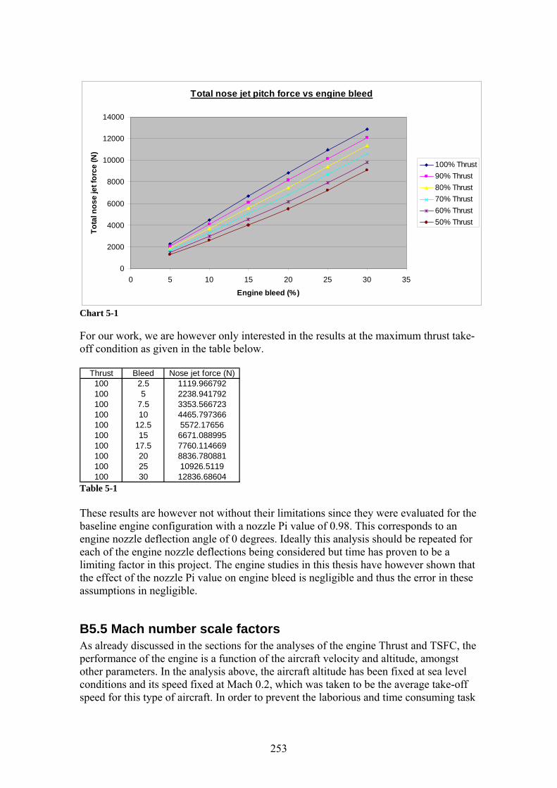
Total nose jet pitch force vs engine bleed

0

2000

4000

6000

8000

10000

12000

14000

0 5 10 15 20 25 30 35

Engine bleed (%)

Tota

l nos

e je

t for

ce (N

)

100% Thrust90% Thrust80% Thrust70% Thrust60% Thrust50% Thrust

Chart 5-1 For our work, we are however only interested in the results at the maximum thrust take-off condition as given in the table below.

Thrust Bleed Nose jet force (N)100 2.5 1119.966792100 5 2238.941792100 7.5 3353.566723100 10 4465.797366100 12.5 5572.17656100 15 6671.088995100 17.5 7760.114669100 20 8836.780881100 25 10926.5119100 30 12836.68604

Table 5-1 These results are however not without their limitations since they were evaluated for the baseline engine configuration with a nozzle Pi value of 0.98. This corresponds to an engine nozzle deflection angle of 0 degrees. Ideally this analysis should be repeated for each of the engine nozzle deflections being considered but time has proven to be a limiting factor in this project. The engine studies in this thesis have however shown that the effect of the nozzle Pi value on engine bleed is negligible and thus the error in these assumptions in negligible.

B5.5 Mach number scale factors As already discussed in the sections for the analyses of the engine Thrust and TSFC, the performance of the engine is a function of the aircraft velocity and altitude, amongst other parameters. In the analysis above, the aircraft altitude has been fixed at sea level conditions and its speed fixed at Mach 0.2, which was taken to be the average take-off speed for this type of aircraft. In order to prevent the laborious and time consuming task

253

of having to repeat the above analysis at a number of different Mach numbers, a scale factor has been applied to the results to account for the ever changing speed of the aircraft during the take-off phase. In order to generate these scale factors, the analysis above was repeated at a number of different Mach numbers. The un-vectored baseline configuration (Pi = 0.98) with zero nozzle deflection angle was used for this analysis to give the results below. Nose jet force (N)

BleedMach 2.5 5 7.5 10 12.5 15 17.5 20

0 1109.322 2217.201 3322.676 4423.732 5519.019 6607.29 7684.903 8749.1350.1 1112.146 2222.846 3331.139 4435.45 5533.666 6624.86 7705.384 8773.3630.2 1119.967 2238.942 3353.567 4465.797 5572.174 6671.089 7760.113 8836.7820.3 1133.154 2265.301 3394.106 4520.713 5638.025 6750.832 7853.945 8944.0050.4 1152.219 2302.972 3450.916 4595.045 5735.446 6868.448 7992.667 9103.337

Table 5-2 If the Mach 0.2 results are taken as the baseline values (as presented in the results section above), then a scale factor with reference to this condition can be determined. The results of this analysis are presented below for a number of different values of engine bleed.

Nose jet Mach number scale factor

y = 0.1218x3 + 0.1807x2 + 0.0084x + 0.9901

y = 0.1143x3 + 0.1851x2 + 0.0068x + 0.9903

y = 0.1151x3 + 0.1811x2 + 0.007x + 0.9904

y = 0.1153x3 + 0.1781x2 + 0.0074x + 0.9905

y = 0.0147x3 + 0.2308x2 + 0.0012x + 0.9906

y = 0.0573x3 + 0.2101x2 + 0.0024x + 0.9908

y = 0.0321x3 + 0.2178x2 + 0.0035x + 0.9903

y = 0.0655x3 + 0.2021x2 + 0.0044x + 0.9905

0.985

0.99

0.995

1

1.005

1.01

1.015

1.02

1.025

1.03

1.035

0 0.05 0.1 0.15 0.2 0.25 0.3 0.35 0.4 0.45

Mach

Scal

e fa

ctor

2.5% bleed5% bleed7.5% bleed10% bleed12.5% bleed15% bleed17.5% bleed20% bleedPoly. (20% bleed)Poly. (17.5% bleed)Poly. (15% bleed)Poly. (12.5% bleed)Poly. (10% bleed)Poly. (7.5% bleed)Poly. (5% bleed)Poly. (2.5% bleed)

Chart 5-2

254

C1 Initial propulsion system considerations

C1.1 A brief review of engine exhaust nozzles The role of the exhaust nozzle is to accelerate the engine exhaust gases generated by the gas generator proportion of the engine to a high velocity and thus generate a propulsive thrust. The engine nozzle can in some cases be required to satisfy other requirements such as stealth requirements or even augment lift by deflecting the thrust. This section givens an overview of some the common nozzle types, which can be arranged into one of the main groups,

• Convergent nozzles - This is the oldest type of engine nozzle which simply consists of a fixed convergent duct. Its exit area is typically selected for optimal cruise. It is still widely used on subsonic aircraft and in cases when the nozzle pressure ratio is less than about 4. Their simplicity and light-weight has helped them retain their popularity.

• Convergent-divergent nozzles - These were developed to overcome the limitations of convergent nozzles, which become chocked when the exit gases reach Mach 1. The addition of a divergent section nozzle downstream of the nozzle throat allows the gases to further accelerate in this section to values in excess of Mach 1. Variable geometry variants allow the nozzle throat to be varied to match the engine operating conditions and thus increase their operational flexibility. When afterburners are used, the operating characteristics of the afterburner can be isolated from the engine by means of the nozzle throat. Even more refined variants allow the nozzle exit area to be varied as well. These nozzles have typically seen application on high performance engines in supersonic aircraft or in cases where the nozzle pressure ratio is greater than about 4.

• Ejector nozzle - An additional airflow from the outside of the nozzle is ejected into the exhaust flow to alter the flow characteristics of the exhaust flow at the nozzle exit. These are not only restricted to use on convergent nozzles but have also been developed as a convergent-divergent configuration. A refinement of this is the two-stage ejector nozzle in which some of the external flow passes through the nozzle. Such a concept allows the nozzle areas to be varied independently.

• Variable geometry nozzle - Such configurations enable the engine to operate more effectively over a wider operating range. The first generation of variable convergent nozzles (as were developed for the early transonic fighters) consisted of flaps which deflected into the flow. Other variants include the translating plug and the later more efficient converging iris designs.

• Thrust vectored nozzle - A detailed description of a number of common thrust vectoring nozzles is presented in the main text. In addition to those discussed, other older configurations include, vectoring flaps, rotating sections, side elbow, bucket and ventral designs.

255

C1.2 A brief note on engine intakes Intake design is not the focus of this study but will be briefly mentioned since it can have a considerable impact on engine and nozzle performance. The role of the engine intake is to not only deliver sufficient air to the engine at all flight regimes but also slow the air to prevent breakdown of the flow within the compressor. Other design requirements for an inlet are to minimise pressure losses, flow distortion and swirl. An engine intake consists of two parts, an inlet front face and a diffuser. The free-stream flow is initially slowed outside the inlet and then further slowed within the diffuser. The most common types of subsonic intake are plenum, straight through, podded nacelle, pitot, flush NACA and S-duct. Supersonic inlets include pitot, external compression and mixed compression (internal and external). The location of the engine inlets is an important consideration to prevent problems with inlet distortion. The shape of the aircraft fore-body will being a particular problem. For buried installations, intake locations include, chin, over-fuselage, over-wing, fuselage side and many more. The intake design must also incorporate a means of boundary layer removal to prevent large pressure recovery losses. This can consist of either a boundary layer diverter or a means of bleeding the boundary layer from the inlet entrance. The engine inlet is sized to be able to deliver sufficient air to the engine at the most critical design condition. As the inlet is responsible for the biggest contribution to propulsion system drag, the designer must ensure that it is not oversized. At other conditions, the excess air will spill around the outside of the intake which results in a drag component called ‘additive drag’. This is due to the loss in momentum of the air approaching the inlet, which is slowed and compressed by the inlet but not used by the engine. This can be offset by cowl-lip suction, which is a result of the turning of the flow around the edge of the engine cowl. Alternatively, the excess air can be ducted and dumped, which results in by-pass drag, but this will still considerably less than the additive drag. A final form of drag within the inlet system arises from the removal of the turbulent boundary layer. Calculation of these drag terms involves complex analytical and empirical tools which are a function of the flow field around the aircraft.

C1.3 Engine nozzle sizing for conceptual design studies The design of an engine nozzle is a complex process involving numerous trade-offs to deliver the best balance of performance over the flight profile. During aircraft conceptual design studies, an initial estimate of nozzle area will enable the designer to predict components such as wave drag and boat-tail drag. If an existing engine is to be used, this can be easily determined from engine data, otherwise we have to rely on more general statistical relations. A very crude approximation of nozzle area can be made with respect to the capture area of the engine. For the two types of nozzle commonly encountered, the exit area can be determined as,

• Convergent nozzle = 0.5 to 0.7 times the capture area • Convergent-divergent nozzle = 0.5 to 0.7 times the capture area in the closed

position and 1.2 to 1.6 times the capture area in the fully open position. Where, the engine capture area is determined in the conceptual intake sizing section. The drag component of particular concern in initial studies is boat-tail drag, which results from flow separation on the aft part of the nozzle or fuselage fairing. For a

256

protruding nozzle, initial guidelines are that the angle of the aft fuselage in this location should not be greater than 15º or 20º.

C1.4 Engine intake sizing for conceptual design studies As for the exhaust nozzle, the design of an engine intake is a complex and time consuming process which has to take into account factors such as, flow distortion, pressure recovery losses and other pressure losses. Such a process is not viable for conceptual design work. The methods presented in this section relate the mass flow rate of air passing through the engine to the thrust produced. At high subsonic speeds, ram effects can increase the mass flow rate of air into the engine, but these are often offset by a drop in performance in the exhaust nozzle. Up to the transonic regime, the velocity effects can be assumed to cancel out, resulting in relatively linear thrust characteristics. The exception to this is where a supersonic nozzle is used, where ram effects are not offset by the nozzle. Pressure losses in the inlet will however eventually prevail, leading to a loss in engine performance. Inlet pressure recovery is a complex function of flow behaviour and flight Mach number. In conceptual design work, the internal pressure recovery may be approximated as, straight duct = 0.96, S duct = 0.94 and podded nacelle = 0.98. The intake capture area for a subsonic jet engine can be estimated from the expression below from Roskam [51], where the density and velocity are relative to the flight condition being studied.

Vm

A InletC ⋅=ρ

Eq 1-1

Where, the total inlet mass flow rate is the sum of that required by the engine and that required for cooling, as given by the expression below from Roskam [7].

CoolingEngineInlet mmm += Eq 1-2 The air flow requirements of the engine can be determined from the expression below from Roskam [7] as a function of the engine thrust.

Tkm GasEngine ⋅= Eq 1-3 The factor in this expression is a function of the engine by-pass ratio as below: Gask

• 0.0003 for 0 ≤ BPR ≤ 1 • 0.0007 for 1 ≤ BPR ≤ 2 • 0.0009 for 2 ≤ BPR ≤ 4 • 0.0011 for 4 ≤ BPR ≤ 6

Likewise, the cooling air requirements can be estimated by the expression below from Roskam [7],

EngineCooling mm ⋅= 06.0 Eq 1-4 The final inlet size is then the largest area determined from a number of flight phases tested. For most subsonic aircraft this is usually to meet low speed requirements.

257

C2 An overview of engine design methodology

C2.1 Engine design specifications and parameter predictions Any engine design process begins with performance targets. In industry, these will be specified by the aircraft design department or customer. In this study, these were specified in our aircraft conceptual design studies. We also need to make predictions as to the characteristics of the different engine components, relative to the level of technology incorporated in the engine. Data from existing designs enables us to establish technology based trends, which can be used for this purpose.

C2.1.1 Engine performance targets The engine performance targets of particular importance for the design of a new engine are thrust and specific fuel consumption. The targets for this study are given below.

2.1.1.1 Thrust design targets The installed thrust requirements for our engine were determined from the constraint analysis used to size the aircraft. These results are however for the engine thrust referred back to standard sea level conditions (SSL). For engine design work; we prefer to have the actual thrust requirements of our engine at their corresponding altitude and speed. These can be easily determined with the thrust scaling and weight scaling factors used in the constraint analysis. As the engine will be designed in isolation from the airframe, we need to factor these results for installation losses to determine the uninstalled values. A figure of 5% has been assumed here as being typical for the losses for a buried engine installation. The table below gives these results in both British and SI units.

Installed thrust values Uninstalled thrust valuesDesign case T (N) SSL T (N) True T (lbf) True T (N) True T (lbf) TrueMax. Level Speed Constraint (Low) 36309.5484 31910.94551 7173.864558 33590.46896 7551.436377Max. Level Speed Constraint (High) 27901.8796 6127.323276 1377.476806 6449.813974 1449.975585Sustained Turn Rate Constraint 51890.94 45852.4075 10308.02929 48265.6921 10850.55715Specific Excess Power Constraint 52730.7736 44115.38305 9917.530737 46437.24532 10439.50604Take-Off Distance Constraint 26604.9163 25838.69475 5808.768544 27198.62605 6114.493204Cruise Constraint (start of cruise outboard) 36361.71 7941.999429 1785.432155 8359.999399 1879.402269Acceleration Constraint 47189.527 37334.59428 8393.149071 39299.57292 8834.893759Cruise Constraint (end of cruise inboard) 32967.6161 7200.673133 1618.775406 7579.655929 1703.974112Cruise Constraint (end of outboard/start of inboard) 34471.0838 7529.055364 1692.598654 7925.321436 1781.682794

(assume 5% installation loss) Table 2-1

These results show the sustained turn rate and specific excess power thrust requirements to be the most critical design constraints. In the design work, it is however also worthwhile checking the take-off and cruise constraints.

2.1.1.2 Specific fuel consumption design targets During our conceptual design work, we had assumed an installed specific fuel consumption value of 0.88 at cruise for our engine. This is therefore the target value for our engine design, to ensure we are able to meet our original requirements. As for the thrust requirements, this figure needs to be expressed as an uninstalled value for engine

258

design work. Assuming an installation loss of 5%, the uninstalled specific fuel consumption target of our engine is thus 0.84.

C2.1.2 Engine component technology level prediction Utilising trends for past, current and future engine proposals, we are able to predict the characteristics of the engine components according to the level of technology we are striving for. Although an engine utilising all components with the highest levels of technology will offer the best performance, the development timescale and cost of such an engine will be high. The technology requirements should therefore be kept to a sensible level. A typical list of engine component parameters at different technology levels is given in the figure below from Mattingly [16]. In this study, we are interested in a mix of level 3 and level 4 technologies corresponding to current and future engine designs. This will give us a realistic engine design with a number of high technology features which can be developed within a realistic budget and timeframe.

Table 2-2 [16]

C2.1.3 Engine parameters – design choices In this section, we give an overview of a number of the design parameters utilised in the engine design work. This includes parameters for component behaviour, component efficiencies and engine operating temperatures. The initial prediction of these parameters is one of the most important stages in the design process as the engine configuration is designed according to these values. These design choices also become the design targets which the later component level designers must endeavour to meet. Failure to meet these targets later on in the development process may render the final engine configuration unable to meet our original design requirements. These parameters must therefore be selected with care.

259

2.1.3.1 Component total pressure ratios (Pi value) The parameter is defined as the ratio of the total (isentropic stagnation) pressures across a component as given by the relation,

)()(

mponentEnteringCoPponentLeavingComP

Total

TotalComponent =π Eq 2-1

The Pi value of the exhaust nozzle is of particular importance in this study, which is the ratio of the total pressures at the nozzle exit and entry . 9tP 7tP

2.1.3.2 Solution boundaries Typical ranges of the engine parameters for a number of different engine configurations are given in the chart below from Mattingly [16]. As this chart is based on data collated from existing engine designs, it gives a useful reality check for any engine design. It also serves as an indication of the boundaries between which our solution is expected to lie, unless we are dealing with an advanced configuration.

Table 2-3 [16] Thus, in this particular design study, the parameters for our turbofan engine with no afterburner are thus expected to lie between the following boundaries,

• Compressor pressure ratio – 20 to 30 • Turbine inlet temperature – 2000 to 3000ºR • Specific thrust – 23 to 84 (depending on Tt4) • Specific fuel consumption – 0.85 to 1.5 (depending on Tt4)

These figures are however, applicable to current technology engine configurations. For next generation developments, we need to make comparisons with similar designs.

2.1.3.3 Comparison with similar designs - UCAV design example Fortunately, for this study the results for a similar UCAV engine design are available from Mattingly [16]. This was designed to cruise at M0.8 and 40,00ft with a specific fuel consumption goal of 0.76 1/h, which is not too far from our requirements. A mixed flow turbofan with a high bypass ratio engine was chosen to deliver high propulsion efficiency. A throttle ratio of 1 was assumed and the maximum turbine inlet temperature taken to be 3200ºR (which when corrected for control system constraints at cruise, equals 2714ºR). Other engine parameters are given in the table below.

260

Table 2-4 [16] This gave a final engine configuration of, α =1.236, Cπ =36, fπ =3.5, =107.1 lThe sim

0m bm/s. ilarity between the design requirements of this and our study mean that these

2.1.3.4 Maximum turbine entry temperature (TET) ine is limited by the maximum

t

2.1.3.5 Operating turbine entry temperature k, Tt4 will be limited by the engine

The

figures also serve as useful guidelines for our design. Our engine is still expected to differ somewhat primarily due to different specific fuel consumption constraints.

The maximum turbine entry temperature (Tt4) of an engmetallurgical temperature and the method of cooling adopted for the turbine. As seen from the Brayton cycle, increasing the TET temperature does however offer the benefiof improved efficiency. Ingenious cooling methods are therefore employed to enable an engine to operate at temperatures beyond which the turbine would normally be able to withstand. Technological advancements in engine materials are also enabling engineersto push these boundaries even further.

As will be discussed in the section for theta breacontrol system to values below the maximum TET to prevent damage to the engine. free-stream total temperature can be shown to have a strong influence on the behaviour of the engine throughout its flight. This is usually expressed as a ratio of the standard sea level static temperature to arrive at the dimensionless form 0θ . To summarise frombelow, the actual value of Tt4 will be limited to values less than t4max for flight conditions where 0

T

θ is less than the throttle ratio (TR). Beyond this limit, Tt4 will aits maximum value and the engine will be limited by other components instead. The

ttain

261

value of Tt4 for flight conditions below 0θ can be determined from the relation below as a function of either the engine throttle ratio or theta break.

MaxtBreak

Mastt TTTR

T 40

40

4 ⋅=⋅=θθθ

Eq 2-2

Where 0θ , is given by the expression,

Std

C

Std

t

T

MT

TT

⎟⎠⎞

⎜⎝⎛ −+⋅

==

200

00

21

1γ

θ Eq 2-3

In our study, the throttle ratio was fixed at 1. Using the expression above, the turbine inlet temperature was determined for a number of different flight cases as:

• Sustained turn rate = 3507.556ºR – At M0.7 and 250ft • Specific excess power = 3188.897ºR – At M0.4 and 5,000ft • Take-off = 3200.064ºR – At M0.01 and 0ft • Cruise = 2795.753ºR – At M0.9 and 40,000ft

2.1.3.6 Turbine cooling air requirements Turbine cooling air is required to maintain the temperature of the turbine at an acceptable level. It may not be required however for low temperature engine designs. An estimate of the cooling air requirements can be determined from the following design trends:

• For cases where Tt4 ≤ 2400ºR, the cooling air requirements are typically zero so that, 021 == εε

• For cases where Tt4>2400ºR, the cooling air requirements can be predicted from

the expression, 2400

160004

21−

== MaxtTεε Eq 2-4

In this study, where , the cooling requirements are RT Maxt °= 32004 %521 == εε

2.1.3.7 Component efficiencies Within the engine parametric analysis, the efficiency of a number of the engine components must be defined. These are characterised as:

• Polytrophic efficiencies - Used to describe the process efficiency of devices such as compressors and turbines. These account for the deviation of the behaviour of an actual fluid device from the polytrophic idealisation.

• Mechanical efficiencies - Used to account for mechanical inefficiencies such as friction between moving components, windage and seal drag.

• Burner (combustion) efficiency – This is defined as the degree to which complete combustion is achieved. It is calculated as the ratio of the actual thermal rise to the maximum theoretically available thermal energy.

• Nozzle expansion characteristics - The nozzle expansion characteristics are usually quoted as the ratio P0/P9 and is used to indicate whether we are dealing with under-expansion, ideal-expansion, over-expansion etc.

These efficiencies vary according to the design and operation of the engine and the components and technological advancements incorporated in its design. Their values

262

263

r

eak and the throttle ratio Theta break and throttle ratio are properties of the engine control system which impose

ngine. To prevent the risk of damage to

vary between different engine designs and are best predicted by inspection of similacurrent designs.

2.1.3.8 Theta br

limits on the operating characteristics of the ethe engine by it exceeding its operating boundaries, the control system is designed to limit the maximum allowable values of Cπ and 4tT with respect to its operating conditions. The figure below from Mattingly [16], is an example of the control systemcharacteristics applicable to an engine co presso

In

m r.

this figure, we can see that for low values of 0θ , T must be limited to t4

prevent the compressor exceeding MaxC−π an thus stalling. At higher

values of 0

dθ , Cπ must be limited to

prevent m−T from being exceeded. Theta break is the point where the control logic switches between limiting C

ax4t

π and Tt4. At values of 0θ less than reakBθ , Tt4 is less than

max4−tT w results in a loss inspecific thrust. Likewise, at valu

0

hich es of

θ greater than Breakθ , Cπ is less than MaxC−π and the specific fuel consumption is higher that its optimal. akBreθ is thus selected by the designer to achieve the best balance of performance throughout the flight profile. For cases where an aircraft is flown with a value of 10 =θ (as in traditional designs), the engine is designed with 1=Breakθ . The throttle ratio is the ratio of the maximum total temperature of gases leaving the

g main burner at a particular flight condition to the total temperature of the gases leavinthe burner at sea level static conditions. This can also be shown to be equal to Breakθ and therefore, the two terms can be used interchangeably, which gives, BreakTR θ= . A number of advanced engines with throttle ratios greater than one arefor future supersonic aircraft. Most current engines are however designed to have a throttle ratio of one, which will also be used for this study.

being developed

2.1.4 Off the shelf engines vs. new developments ble of designing a

e

CWith so many existing engines to choose from, why go to the trounew engine? Off the shelf engines do offer benefits of immediate availability and reduced cost, but there is unlikely to be one that fits our design requirements exactly.Even after it has been tailored to suit our needs, some compromises would also be required. Existing engine manufacturers are also unlikely to supply such detailed engin

264

e the

2.2 An overview of the engine design and sizing process ew with

2.2.1 Engine design methodology , has a level of detail which is sufficient predict parameters such as available

ble el

t the

gine.

2.2.2 The on-design design stage our design requirements

ber of the engine components. During

or our analysis. Fortunately this is ents.

e f

to

data as required by this project. Therefore a new engine design was considered to bbest approach for this project to generate the required detailed engine data.

CThe engine design and sizing process is a very detailed subject and only an overviwill be given here. During these studies, a baseline engine was designed and sizeda level of detail sufficient for later analyses. Component level design was not requiredfor this work. In this section, we will therefore only give a brief overview of the subject which is sufficient enough for the reader to understand the engine design process.

CThe engine model developed for these studiesenough for our needs. This proved adequate tothrust and specific fuel consumption, as well as the flow conditions at a number of points within the engine. With our estimates for general engine parameters, we are ato carry out the conceptual design and initial sizing of an engine and analytical modwith a level of detail sufficient for our needs. As will be discussed in the following sections, the conceptual engine design process consists of two stages as follows:

• On-design – This stage is used to determine the optimal combination of the unknown engine parameters to meet the needs of our design condition. Aend of this stage, all of our engine design parameters are fixed.

• Off-design – This stage is used to test the engine in conditions other than our design condition and will ultimately determine the size of our en

CThis is the first stage in the design process, which begins with and predictions for the characteristics of a numthis stage, we use parametric analysis techniques to explore the undetermined engine parameters and ultimately determine the optimal engine configuration to meet our needs. Such parametric studies can include the investigation of the parameters:

• Turbine inlet temperature- For this study, this has already been fixed in accordance with current metallurgical limits.

• Compressor pressure ratio – This is a design variable for our analysis. • Fan pressure ratio – This is a design variable f

automatically adjusted within the software to meet our engine requirem• Bypass ratio – For our study, this was fixed at the conceptual design stage.

The only unknown in this study is therefore the engine compressor ratio, which will bthe focus of our parametric analysis. This process involves the generation of plots ouninstalled thrust specific fuel consumption versus uninstalled specific thrust for a rangeof compressor pressure ratio values, as in the example below. These can then be used establish a trend between the engine performance and the compressor pressure ratio, which will help us identify the optimal solution. Our primary goal here is to optimise the engine at its design point, such as cruise. It is important however that it retains acceptable performance characteristics over the other flight conditions. This involves

265

ch as repeating the parametric analysis at a range of thrust critical flight points such as sutake-off, cruise and specific excess power.

Chart 2-1 The parametric trend for the critical d nables us to determine the maximum ompressor ratio to meet our requirements such as fuel consumption at that point. Once

e

it is in our

2.2.3 The off-design sizing stage e an engine configuration whose parameters t. The final size of the engine however

to

esign point ecwe have fixed the compressor ratio and the design point, we need to verify this result within the trends generated for the other critical flight points. This ensures that the engine retains acceptable performance characteristics over our entire flight profile. Thfinal result may prove to be a trade-off between the difference performance requirements. The ideal engine is one whose key parameters are within their best ranges for all the critical engine operating points. When making our final selection, best interest to keep the specific thrust as high as possible for the most demanding flight conditions as this is related to the final size of our engine. Keeping the specific thrust ashigh as possible will ensure that the size, weight and cost of the final engine are kept to a minimum. At the end of this stage, all of our engine design parameters will have been fixed with the aid of the parametric trends but the actual size of the engine is still variable. The result is thus a rubber engine which has been optimised for our design requirements.

CAt the end of the on-design analysis, we havhave been fixed with respect to a design poinremains undetermined, which is represented by the mass flow rate of air passing through it ( 0m ).The engine performance parameters we have been using in our on-design analysis were independent of the size of the engine and with 0m we are abledetermine the actual engine parameters. An iterative process is used to determine the final engine size which begins with an assumed value of 0m . The engine is then tested at various critical flight points to determine the critical value of 0m , which is used to size our engine. The flight phases of particular interest include:

• Flight phases which have a high fuel consumption • Conditions with demanding thrust requirements • Other extreme operating conditions

266

to determine the final engine to meet all of our performance

est the

haracteristics of our engine at our reference design point (used for the on-design

he ign

re ible in

2.3 Station numbering study is consistent with the ARP755A

as given below.

The assumed value of 0m can then re-scaled accordinglysize which is able to deliver sufficient thrustrequirements. With its size fixed, the performance of the final engine configuration can be determined within its entire operating envelope. We are also then able to tengine at different engine throttle settings, which is particularly useful for this study. The off-design analysis is named as such, since we not only measure the performance canalysis) but also at a number of other flight conditions throughout its operating envelope. It is typical to study more that one potential engine configuration up to toff-design stage and then use these results to establish further trends between deschoices and therefore further optimise the final engine configuration. The result is an engine with the best balance of performance over the complete flight profile. In this study, our off-design has been based on assumed typical values for the engine installation allowances. We can however, also use an off-design analysis to study modetailed intake and nozzle installation models. This has however not been possthis study due to the project time constraints.

CThe engine station numbering used in thisaerospace recommended practice,

267

C3 Practical software based engine design

C3.1 Engine design with the AEDsys software suite The conceptual design of an engine can be a very labour intensive activity due to the vast number of relations which are required and the simultaneous solution of each of these. Fortunately, we are able to make use of a reliable software suite called AEDsys, which has already been developed for such purpose by Mattingly [16]. As will be discussed in the sections below, this software is sufficient to be able to handle the on-design and off-design stages as well as perform more detailed analysis of the various components. Only an overview of the programs as applied to this project will be given here and the reader is advised to consult the program user guides for more information.

C3.1.1 On-Design parametric analysis with the ONX module The ONX module [73] allows the user to define a number of component level engine characteristics and then test the remaining engine parameters over a range of values to erform a parametric analysis. For this study, we opted for the following user selections

guration

IR signature and increasing the stealth of the aircraft. his has been

s .

• Aircraft operating environment – Mach number, Altitude, Temperature, etc

opic stagnation pressure ratios (Pi) – Diffuser, Burner, Nozzle

y are shown in the figure

the figure. The compressor ratio input box is

pfrom the main window:

• Type of cycle – Turbofan with mixed exhaust. The mixed exhaust confiis particularly good for cooling the hot exhaust gases and therefore reducing the

• Ideal gas model – The Modified Specific Heat (MSH) Model as tshown to give the best results.

• Unit system – The English unit system was used as a program used later on waonly able to cope with these units and this enabled the results to be used directly

• Iteration variable – Our parametric analysis is based on Compressor Pressure Ratio, which is the only unknown design variable. In this work a range of CPRvalues between 10 and 40, in 0.25 steps were tested.

The component level engine characteristics are finally defined within the engine data nput box, which includes choices for: i

• Fuel characteristics – Heating value • Burner exit temperature – Tt4 • Air off-take requirements – Includes bleed and cooling air requirements • Power off-take requirements • Component isentr• Component polytrophic efficiencies – Fan, Compressors and Turbines • Component efficiencies – Burner, Spools, etc

The values selected for each of these components for this studbelow. It should be noted that a Pi-Nozzle value of 0.98 was used for the baseline engine and not the figure of 0.9 shown in also normally left black for these parametric analyses. The value of -1 used for the fan pressure ratio enables the software to automatically find the best solution for this

268

t

th the engine cycle deck the best rubber engine configuration from

focused on one particular engine operating ables us to determine the most critical

examining its of other off-design conditions. The engine

in window of AEDsys on start-up by default. It the engine pull-down menu, this then

ed for the off-design

variable. The majority of these variables remain fixed during our tests. Under differentest conditions, Mach number, Altitude and Tt4 must however be adjusted accordingly.

Figure 3-1 – ONX data input window

C3.1.2 Off-Design engine analysis wiThe on-design work enabled us to determine parametric studies, which where primarily point. The AEDsys engine cycle deck [74] enmass flow rate requirements and thus the size of the engine byperformance at the design point and a range cycle deck is not available within the mamust be activated by selecting Cycle Deck fromputs two additional buttons on the main window, which are usanalysis work. The first of these is the Engine Data button, which is used to define the

in the program. The second is the Engine Testreference engine configuration with off-design condition.

ly from the ONX module by the defines the engine configuration at its design

ondition. To generate a reference file within ONX, we need to select the Single Point

button, which is used to test the reference engine at any

3.1.2.1 Defining the engine with ONX reference files Fortunately, the engine data can be transferred directcreation of a reference file, which cCalculation option from the main window. The compressor pressure ratio will now be fixed at its final value of 27 within the view data form. Since the single point calculation is based on an actual engine size, the user must define the mass flow rate of the engine

269

at its design point. The final engine mass flow rate is however determined by aniterative process and thus we begin by making an initial estimate, which is refined later. The reference file can then be entered into the cycle deck via the Engine Data form. This form has additional options for engine installation allowances, but since these havalready been factored into our work, the default constant loss model is retained. Theother features within this input window will retain their default values for our work.

3.1.2.2 Engine testing within the cycle deck We are finally able to test the engine under a variety of off-design test conditions via th

e

e Engine Test form. The off-design engine test inputs within this window allow us tomodify a variety of operating parameters but for this study we will concentrate on the

ach number, Altitude and Throttle ratio. After testing, the results can be retrieved in either a summary of the main results or a more detailed format (which gives the

d.

M

operating conditions at each engine station).

3.1.2.3 Selecting the final engine size The process to determine the final size of the engine involves an iterative process between ONX and AEDsys, as follows:

1. Within ONX, create a single point reference file using an initial estimate for the engine mass flow rate. In this analysis, a value of 100 lbm/sec was assume

2. Within AEDsys, test this reference engine at each of the critical design points to determine the thrust available at each condition.

3. At each critical design point determine the ratio of required thrust to available thrust from the scale factor relation below.

Available

quiredTSF Re= Eq 3-1

Tcordance with the most critical condition 4. Rescale the engine mass flow rate in ac

from above, as given by the relation below. GuessNew mSFm ⋅= Eq 3-2

5. Repeat the process above to verify the new results. In this study, the sustained turn rate was identified as the most critical condition, whichgave a mass flow rate of 59.48 lbm/sec for the final engine size.

3.2 Design of the baseline engine tionale for the selection of the final baseline

onsiderable impact on the d

s the largest consumer of fuel, it makes sense to select this as the design point or on-design condition for the parametric

CThis section gives an overview of the raengine configuration, which is used for further analysis work in this project.

C3.2.1 Design point parametric analysis In this study, the parametric analysis focused on determining the optimal compressor pressure ratio for the engine. This parameter can have a cthrust and specific fuel consumption characteristics of the final engine configuration anmust be selected with care. Since the cruise phase i

270

analysis. ONX was used to test a range of compressor ratios and thus generate the parametric trend belo

r

e of

ve ine. As can be

thrust specific fuel point too low down on

ling rapidly. Selection of the final engine

nstalled cruise specific fuel rked on the parametric analysis NX raw data, corresponds to a

situated at an excellent location on the d at this value.

section, the engine compressor ratio was selected to deliver the best erformance at cruise. It is essential however to verify this design choice at other

w of output parameters of most concern to us.

Chart 3-1 With reference to the figure above, there are two possible solutions for the specific thrust, at higher and lower values of specific fuel consumption. The final compressopressure ratio should be selected at a point sufficiently below the knee of the curve. This ensures that any deviation in the engine operating point does not stray above the knethe curve and therefore into the unnecessarily higher SFC operating regime. At the sametime, we should aim to achieve the highest specific thrust possible, which would hasmaller airflow requirements and thus result in a smaller and lighter engseen from the figure, this would however be at the expense ofconsumption. We must however also be careful not to select a the curve for which the specific thrust is falconfiguration is therefore a trade-off of many factors. In this study, our configuration was selected to meet our uniconsumption design target of 0.84. This point is macurve above, which when traced back within our Ocompressor ratio of 27. Since this point was alsoparametric curve, our final engine configuration was fixe

C3.2.2 Verifying the final configuration In the lastpcritical flight conditions, to ensure the engine retains good performance at these conditions. The flight conditions examined in this way were:

• Specific excess power requirements – At Mach 0.4 and 5,000ft. • Sustained turn rate requirements – At Mach 0.7 and 250ft. • Take-off requirements – At Mach 0.01 and 0ft.

ONX is used to generate a parametric curve for each one as presented below, to which the point corresponding to a compressor pressure ratio of 27 has been added.

271

oint is

• Flow area at 0 (engine intake) = 5.703ft – To m• Flow area at 9 (engine nozzle) = 2.777ft2 – To m

C3.3 The analysis of thrust vectoring nozzles The work carried out so far has focused on a fixed geomcharacteristics. In this study, the nozzle isentropic stagnation prefixed at 0.98 for our baseline design. In the case of variab the value of Pi will be related to its internal flow characterdependent on the nozzle geometry amongst othegeometry of the nozzle is varied. This concept is illustrated b

at a number of different nozzle deflection angles. It should be noted

Figure 3-2 – Relationship between nozzle vectoring angle and its Pi value

Chart 3-2, 3-3, 3-4 Within each of the analyses above, the engine is shown to operate at a favourable palong the curve with a compressor pressure ratio of 27 and so it will be fixed at thvalue for the baseline engine.

C3.2.3 Refined engine intake and nozzle sizing Within the results generated by the AEDsys software are the intake and exhaust areas required for the engine at each flight condition. These were determined as:

2 eet the SEP requirements eet the cruise requirements

etry nozzle with fixed operating ssure ratio (Pi) was

le geometry nozzles however,istics, which in turn will be

r factors. Pi will therefore vary as the elow for a thrust vectoring

nozzle operating that the values quoted in this figure are arbitrary values to illustrate the concept.

272

n engine will be It should be re-emphasised that the operating characteristics of aaffected by nozzle, by means of the back pressure it generates. This means that, if each of the nozzle configurations above were coupled to an identical engine, its operating characteristics would be different for each case. For a thrust vectoring nozzle, the engine characteristics will therefore vary according to the engine plume deflection angle. In our work so far, we have concentrated on the baseline engine with an un-vectored nozzle ( °= 0φ ). Our next step is to examine the behaviour of our baseline engine when the characteristics of the engine nozzle are varied. Later on in our work, we can use this data to pair our engine to an existing nozzle and predict its performance.

C3.4 Datasets for take-off and cruise conditions At this stage in our work we need to gather data which will help us to predict the behaviour of our baseline engine when the nozzle characteristics are varied. Fortunately, we are able to use the AEDsys software suite for this task but even so, a significant amount of work is still required. This process involves the analysis of many different engine configurations at a number of different operating conditions. The difference between each is the nozzle, which is accounted for via the value of PiNozzle, which itself is a function of the plume deflection angle. In this work, we are primarily interested in the analysis of the engine at take-off and cruise. Using the process described in the following sections, we are able to test our engine with a number of different nozzles, to

generate a set of data for each. The results of most importance to us are: • Engine thrust (lbf) • Thrust specific fuel consumption ((lbm/hr)/lbf) • 0m (lbm/s) - Mass flow rate of air through the engine intake • Tt4 (Rankine) – Total temperature at the burner exit • 8m (lbm/s) – Mass flow rate of exhaust gases through the nozzle throat • Pt8 (Psia) – Total pressure of the exhaust gases at the nozzle throat • Tt8 (Rankine) – Total temperature of the exhaust gases at the nozzle throat • A6γ - Ratio of specific heats of the gases at the nozzle entry (mixer exit) • A9 (ft2) – Required area at the exhaust nozzle exit

this result is given in e test results)

ew reference cle deck. The process used

s:

• A9/A8 – Ratio of areas at the nozzle throat and nozzle exit (the main window of the AEDsys engine test form and not th

An overview of the process and the results are given in the sections which follow.

C3.4.1 Take-off analysis datasets During take-off, the engine thrust is assumed to be held at its maximum value. In this analysis, we also need to consider the effect of engine bleed on engine performance, (which will be used for a pitch control device located at the nose of the aircraft). The amount of bleed required is not known at this stage and our analysis is thus repeated at anumber different engine bleed settings to establish a trend. When using AEDsys, engine bleed is fixed for the on-design testing and therefore we have to create a nfile within ONX for each test point before we can use the cyto build such a dataset for the take-off phase is as follow

273

he original ONX data file same.

original of

esign with fixed values of,

or the

his gives us the table of results as presented in the first table below.

operties of the air which is bled from the ,

is

1. Modify the value of PiNozzle and engine bleed within tfor the configuration being tested. All the other parameters remaining the

2. Generate a single point engine reference file within ONX, using the reference engine mass flow rate value of 59.48 lbm/sec. The modified form our baseline engine becomes a new on-design test configuration.

3. Input the ONX reference file into AEDsys and test the engine at the off-dconditions being investigated. Here we are workingAltitude = 0m, Mach number = 0.2 and Throttle setting = 100%.

4. Record the required results and then return to step 1 to repeat the process fnext combination of PiNozzle and engine bleed being tested.

T

The second table gives the results for the prengine to supply air to the nose pitch control device. Calculation of the rate of air bleedas is fed to the nose pitch control device, is as follows. The total quantity of air whichbled from the high pressure compressor is determined as the sum of the quantity of airrequired for the pitch control device and that required for cooling. The cooling air requirements were defined in our original engine requirements as:

• %51 =−Coolingm • %52 =−Coolingm

The total percentage air bleed, is then given by, 21 %%%% −− ++= CoolingCoolingNoseJetTotal BleedBleedBleedBleed Eq 3-3

low The actual bleed mass flow rate (lbm/s) can then be determined from the total mass frate of air leaving the high pressure compressor, as given by the expression,

⎥⎦⎤⎡%Bleed

⎢⎣⋅=

1003)(Total

TotalBleed mm Eq 3-

The mass flow rate of air being fed to the pitch control device can finally be dete

4

rmined from the expression,

⎥⎦

⎢⎣ Total

TotalBleedNoseJetBleed Bleedmm

%)()( ⎤⎡

⋅= NoseJetBleed%Eq 3-5

Test variables Engine properties results Nozzle properties resultsPi-Nozzle % Bleed % Thrust Thrust TSFC

0.995 0 100 12334 0.78660.995 2.5 100 11828 0.7975 179 3200 179.15 49.615 1543.56 1.3379 2.178 1.1597

0.8608 179.11 3200 169.05 40.279 1433.7 1.3405 2.264 1.07660.995 15 100 9149 0.8839 179.13 3200 166.52 37.971 1404.02 1.3412 2.301 1.0580.995 17.5 100 8574 0.9119 179.15 32000.995 20 100 7979 0.9461 179.18 32000.95 0 100 12119 0.8006 178.97 3200 181.66 51.932 1568.94 1.3373 2.229 1.21450.95 2.5 100 11611 0.8123 179 3200 179.15 49.615 1543.56 1.3379 2.241 1.19310.95 5 100 11095 0.8259 179.02 3200 176.62 47.285 1517.38 1.3385 2.258 1.17190.95 7.5 100 10569 0.8415 179.06 3200 174.11 44.947 1490.36 1.3391 2.279 1.15120.95 10 100 10031 0.8599 179.09 3200 171.59 42.601 1462.45 1.3398 2.306 1.13110.95 12.5 100 9482 0.8812 179.11 3200 169.05 40.279 1433.7 1.3405 2.339 1.11220.95 15 100 8920 0.9067 179.13 3200 166.52 37.971 1404.02 1.3412 2.38 1.09470.95 17.5 100 8340 0.9374 179.15 3200 163.99 35.666 1373.32 1.3419 2.432 1.0790.95 20 100 7739 0.9755 179.18 3200 161.47 33.369 1341.54 1.3427 2.499 1.06580.9 0 100 11859 0.8181 178.97 3200 181.66 51.932 1568.94 1.3373 2.304 1.25560.9 2.5 100 11351 0.831 179 3200 179.15 49.615 1543.56 1.3379 2.319 1.23460.9 5 100 10832 0.8459 179.02 3200 176.62 47.285 1517.38 1.3385 2.339 1.21390.9 7.5 100 10303 0.8632 179.06 3200 174.11 44.947 1490.36 1.3391 2.363 1.19390.9 10 100 9762 0.8835 179.09 3200 171.59 42.601 1462.45 1.3398 2.395 1.17480.9 12.5 100 9209 0.9074 179.11 3200 169.05 40.279 1433.7 1.3405 2.433 1.1570.9 15 100 8642 0.9358 179.13 3200 166.52 37.971 1404.02 1.3412 2.481 1.1410.9 17.5 100 8055 0.9706 179.15 3200 163.99 35.666 1373.32 1.3419 2.541 1.12740.9 20 100 7446 1.0138 179.18 3200 161.47 33.369 1341.54 1.3427 2.619 1.1170.85 0 100 11576 0.8381 178.97 3200 181.66 51.932 1568.94 1.3373 2.389 1.3020.85 2.5 100 11065 0.8525 179 3200 179.15 49.615 1543.56 1.3379 2.407 1.28160.85 5 100 10544 0.8691 179.02 3200 176.62 47.285 1517.38 1.3385 2.431 1.26170.85 7.5 100 10012 0.8884 179.06 3200 174.11 44.947 1490.36 1.3391 2.46 1.24270.85 10 100 9466 0.9112 179.09 3200 171.59 42.601 1462.45 1.3398 2.497 1.22480.85 12.5 100 8908 0.938 179.11 3200 169.05 40.279 1433.7 1.3405 2.542 1.20870.85 15 100 8335 0.9703 179.13 3200 166.52 37.971 1404.02 1.3412 2.598 1.19490.85 17.5 100 7740 1.01 179.15 3200 163.99 35.666 1373.32 1.3419 2.669 1.1840.85 20 100 7121 1.0601 179.18 3200 161.47 33.369 1341.54 1.3427 2.761 1.17750.8 0 100 11263 0.8614 178.97 3200 181.66 51.932 1568.94 1.3373 2.487 1.35510.8 2.5 100 10749 0.8775 179 3200 179.15 49.615 1543.56 1.3379 2.509 1.33560.8 5 100 10225 0.8961 179.02 3200 176.62 47.285 1517.38 1.3385 2.537 1.31680.8 7.5 100 9689 0.918 179.06 3200 174.11 44.947 1490.36 1.3391 2.572 1.29920.8 10 100 9138 0.9438 179.09 3200 171.59 42.601 1462.45 1.3398 2.616 1.28310.8 12.5 100 8574 0.9746 179.11 3200 169.05 40.279 1433.7 1.3405 2.67 1.26930.8 15 100 7993 1.0118 179.13 3200 166.52 37.971 1404.02 1.3412 2.736 1.25840.8 17.5 100 7388 1.0582 179.15 3200 163.99 35.666 1373.32 1.3419 2.821 1.25150.8 20 100 6756 1.1174 179.13 3200 161.41 33.375 1341.77 1.3427 2.93 1.250.75 0 100 10916 0.8888 178.97 3200 181.66 51.932 1568.94 1.3373 2.6 1.41670.75 2.5 100 10399 0.9071 179 3200 179.15 49.615 1543.56 1.3379 2.627 1.39840.75 5 100 9870 0.9283 179.02 3200 176.62 47.285 1517.38 1.3385 2.661 1.38120.75 7.5 100 9329 0.9534 179.06 3200 174.11 44.947 1490.36 1.3391 2.703 1.36560.75 10 100 8771 0.9833 179.09 3200 171.59 42.601 1462.45 1.3398 2.756 1.3520.75 12.5 100 8199 1.0191 179.11 3200 169.05 40.279 1433.7 1.3405 2.821 1.34150.75 15 100 7608 1.063 179.13 3200 166.52 37.971 1404.02 1.3412 2.902 1.33480.75 17.5 100 6991 1.1184 179.12 3200 163.96 35.671 1373.5 1.3419 3.006 1.33330.75 20 100 6342 1.1909 178.56 3200 160.84 33.453 1344.76 1.3424 3.126 1.33330.7 0 100 10526 0.9216 178.97 3200 181.66 51.932 1568.94 1.3373 2.733 1.48920.7 2.5 100 10005 0.9427 179 3200 179.15 49.615 1543.56 1.3379 2.767 1.47280.7 5 100 9471 0.9675 179.02 3200 176.62 47.285 1517.38 1.3385 2.809 1.45790.7 7.5 100 8923 0.9968 179.06 3200 174.11 44.947 1490.36 1.3391 2.861 1.44520.7 10 100 8357 1.0321 179.09 3200 171.59 42.601 1462.45 1.3398 2.926 1.43530.7 12.5 100 7774 1.0748 179.11 3200 169.05 40.279 1433.7 1.3405 3.007 1.42950.7 15 100 7170 1.128 179.08 3200 166.47 37.981 1404.33 1.3412 3.106 1.42860.7 17.5 100 6537 1.1966 178.52 3200 163.35 35.765 1376.76 1.3417 3.22 1.42860.7 20 100 5874 1.2873 177.16 3200 159.41 33.647 1352.14 1.3419 3.349 1.42860.65 0 100 10086 0.9619 178.97 3200 181.66 51.932 1568.94 1.3373 2.893 1.57640.65 2.5 100 9558 0.9868 179 3200 179.15 49.615 1543.56 1.3379 2.935 1.56270.65 5 100 9017 1.0162 179.02 3200 176.62 47.285 1517.38 1.3385 2.988 1.55120.65 7.5 100 8460 1.0514 179.06 3200 174.11 44.947 1490.36 1.3391 3.054 1.54290.65 10 100 7882 1.0943 179.09 3200 171.59 42.601 1462.45 1.3398 3.137 1.53870.65 12.5 100 7286 1.1471 178.98 3200 168.92 40.305 1434.47 1.3404 3.236 1.53850.65 15 100 6667 1.2139 178.33 3200 165.71 38.11 1408.47 1.3409 3.345 1.53850.65 17.5 100 6022 1.3008 176.98 3200 161.78 36.006 1385.15 1.3411 3.468 1.53850.65 20 100 5347 1.4173 174.7 3200 156.9 33.994 1365.42 1.341 3.606 1.53850.6 0 100 9579 1.0128 178.97 3200 181.66 51.932 1568.94 1.3373 3.09 1.68380.6 2.5 100 9044 1.0429 179 3200 179.15 49.615 1543.56 1.3379 3.145 1.67440.6 5 100 8492 1.079 179.02 3200 176.62 47.285 1517.38 1.3385 3.214 1.66830.6 7.5 100 7922 1.227 179.05 3200 174.09 44.95 1490.43 1.3391 3.299 1.66670.6 10 100 7331 1.1769 178.77 3200 171.26 42.67 1464.37 1.3397 3.398 1.66670.6 12.5 100 6723 1.2444 177.96 3200 167.88 40.5 1440.27 1.3401 3.505 1.66670.6 15 100 6094 1.3304 176.51 3200 163.85 38.43 1418.75 1.3402 3.624 1.66670.6 17.5 100 5441 1.4437 174.24 3200 158.98 36.448 1400.58 1.34 3.757 1.66670.6 20 100 4761 1.5979 170.91 3200 153.01 34.557 1387.05 1.3394 3.907 1.6667

m-dot 0 Tt4 m-dot 8 Pt8 Tt8 Gamma 6A A9 A9/A8178.97 3200 181.66 51.932 1568.94 1.3373 2.168 1.1814

0.995 5 100 11313 0.81 179.02 3200 176.62 47.285 1517.38 1.3385 2.193 1.13820.995 7.5 100 10789 0.8244 179.06 3200 174.11 44.947 1490.36 1.3391 2.211 1.1170.995 10 100 10253 0.8412 179.09 3200 171.59 42.601 1462.45 1.3398 2.235 1.09630.995 12.5 100 9707

163.99 35.666 1373.32 1.3419 2.347 1.0409161.47 33.369 1341.54 1.3427 2.405 1.0259

Table 3-1 – Engine and nozzle data from engine tests at take-off conditions

274

Test variables Engine Properties at station 3 Bleed flow calculationsPi-Nozzle % bleed % Thrust m-dot 0 m-dot 3 Gamma 3 Pt3 Tt3 % bleedTotal m-dot bleedTotal m-dot bleedNoseJet

0.995 0 100 178.97 98.99 1.4 359.585 1478.86 10 9.899 00.995 2.5 100 179 99 1.4 359.599 1478.87 12.5 12.375 2.4750.995 5 100 179.02 99.02 1.4 359.613 1478.89 15 14.853 4.9510.995 7.5 100 179.06 98.98 1.4 359.637 1478.91 17.5 17.3215 7.42350.995 10 100 179.09 99 1.4 359.655 1478.93 20 19.8 9.90.995 12.5 100 179.11 99.01 1.4 359.684 1478.97 22.5 22.27725 12.376250.995 15 100 179.13 99.02 1.4 359.72 1479.01 25 24.755 14.8530.995 17.5 100 179.15 99.03 1.4 359.758 1479.06 27.5 27.23325 17.330250.995 20 100 179.18 99.05 1.4 359.8 1479.11 30 29.715 19.810.95 0 100 178.97 98.99 1.4 359.585 1478.86 10 9.899 00.95 2.5 100 179 99 1.4 359.599 1478.87 12.5 12.375 2.4750.95 5 100 179.02 99.02 1.4 359.613 1478.89 15 14.853 4.9510.95 7.5 100 179.06 98.98 1.4 359.637 1478.91 17.5 17.3215 7.42350.95 10 100 179.09 99 1.4 359.655 1478.93 20 19.8 9.90.95 12.5 100 179.11 99.01 1.4 359.684 1478.97 22.5 22.27725 12.376250.95 15 100 179.13 99.02 1.4 359.72 1479.01 25 24.755 14.8530.95 17.5 100 179.15 99.03 1.4 359.758 1479.06 27.5 27.23325 17.330250.95 20 100 179.18 99.05 1.4 359.8 1479.11 30 29.715 19.810.9 0 100 178.97 98.99 1.4 359.585 1478.86 10 9.899 00.9 2.5 100 179 99 1.4 359.599 1478.87 12.5 12.375 2.4750.9 5 100 179.02 99.02 1.4 359.613 1478.89 15 14.853 4.9510.9 7.5 100 179.06 98.98 1.4 359.637 1478.91 17.5 17.3215 7.42350.9 10 100 179.09 99 1.4 359.655 1478.93 20 19.8 9.90.9 12.5 100 179.11 99.01 1.4 359.684 1478.97 22.5 22.27725 12.376250.9 15 100 179.13 99.02 1.4 359.72 1479.01 25 24.755 14.8530.9 17.5 100 179.15 99.03 1.4 359.758 1479.06 27.5 27.23325 17.330250.9 20 100 179.18 99.05 1.4 359.8 1479.11 30 29.715 19.810.85 0 100 178.97 98.99 1.4 359.585 1478.86 10 9.899 00.85 2.5 100 179 99 1.4 359.599 1478.87 12.5 12.375 2.4750.85 5 100 179.02 99.02 1.4 359.613 1478.89 15 14.853 4.9510.85 7.5 100 179.06 98.98 1.4 359.637 1478.91 17.5 17.3215 7.42350.85 10 100 179.09 99 1.4 359.655 1478.93 20 19.8 9.90.85 12.5 100 179.11 99.01 1.4 359.684 1478.97 22.5 22.27725 12.376250.85 15 100 179.13 99.02 1.4 359.72 1479.01 25 24.755 14.8530.85 17.5 100 179.15 99.03 1.4 359.758 1479.06 27.5 27.23325 17.330250.85 20 100 179.18 99.05 1.4 359.8 1479.11 30 29.715 19.810.8 0 100 178.97 98.99 1.4 359.585 1478.86 10 9.899 00.8 2.5 100 179 99 1.4 359.599 1478.87 12.5 12.375 2.4750.8 5 100 179.02 99.02 1.4 359.613 1478.89 15 14.853 4.9510.8 7.5 100 179.06 98.98 1.4 359.637 1478.91 17.5 17.3215 7.42350.8 10 100 179.09 99 1.4 359.655 1478.93 20 19.8 9.90.8 12.5 100 179.11 99.01 1.4 359.684 1478.97 22.5 22.27725 12.376250.8 15 100 179.13 99.02 1.4 359.72 1479.01 25 24.755 14.8530.8 17.5 100 179.15 99.03 1.4 359.758 1479.06 27.5 27.23325 17.330250.8 20 100 179.13 99.05 1.4 359.817 1479.14 30 29.715 19.810.75 0 100 178.97 98.99 1.4 359.585 1478.86 10 9.899 00.75 2.5 100 179 99 1.4 359.599 1478.87 12.5 12.375 2.4750.75 5 100 179.02 99.02 1.4 359.613 1478.89 15 14.853 4.9510.75 7.5 100 179.06 98.98 1.4 359.637 1478.91 17.5 17.3215 7.42350.75 10 100 179.09 99 1.4 359.655 1478.93 20 19.8 9.90.75 12.5 100 179.11 99.01 1.4 359.684 1478.97 22.5 22.27725 12.376250.75 15 100 179.13 99.02 1.4 359.72 1479.01 25 24.755 14.8530.75 17.5 100 179.12 99.02 1.4 359.773 1479.08 27.5 27.2305 17.32850.75 20 100 178.56 99.09 1.4 360.04 1479.42 30 29.727 19.8180.7 0 100 178.97 98.99 1.4 359.585 1478.86 10 9.899 00.7 2.5 100 179 99 1.4 359.599 1478.87 12.5 12.375 2.4750.7 5 100 179.02 99.02 1.4 359.613 1478.89 15 14.853 4.9510.7 7.5 100 179.06 98.98 1.4 359.637 1478.91 17.5 17.3215 7.42350.7 10 100 179.09 99 1.4 359.655 1478.93 20 19.8 9.90.7 12.5 100 179.11 99.01 1.4 359.684 1478.97 22.5 22.27725 12.376250.7 15 100 179.08 99.05 1.4 359.746 1479.05 25 24.7625 14.85750.7 17.5 100 178.52 99.12 1.4 360.031 1479.41 27.5 27.258 17.3460.7 20 100 177.16 99.02 1.4 360.606 1480.15 30 29.706 19.8040.65 0 100 178.97 98.99 1.4 359.585 1478.86 10 9.899 00.65 2.5 100 179 99 1.4 359.599 1478.87 12.5 12.375 2.4750.65 5 100 179.02 99.02 1.4 359.613 1478.89 15 14.853 4.9510.65 7.5 100 179.06 98.98 1.4 359.637 1478.91 17.5 17.3215 7.42350.65 10 100 179.09 99 1.4 359.655 1478.93 20 19.8 9.90.65 12.5 100 178.98 99.05 1.4 359.75 1479.05 22.5 22.28625 12.381250.65 15 100 178.33 99.13 1.4 360.09 1479.49 25 24.7825 14.86950.65 17.5 100 176.98 99.32 1.4 360.716 1480.29 27.5 27.313 17.3810.65 20 100 174.7 99.54 1.4 361.672 1481.52 30 29.862 19.9080.6 0 100 178.97 98.99 1.4 359.585 1478.86 10 9.899 00.6 2.5 100 179 99 1.4 359.599 1478.87 12.5 12.375 2.4750.6 5 100 179.02 99.02 1.4 359.613 1478.89 15 14.853 4.9510.6 7.5 100 179.05 99.03 1.4 359.644 1478.92 17.5 17.33025 7.427250.6 10 100 178.77 99.04 1.4 359.827 1479.15 20 19.808 9.9040.6 12.5 100 177.96 99.2 1.4 360.253 1479.7 22.5 22.32 12.40.6 15 100 176.51 99.39 1.4 360.975 1480.62 25 24.8475 14.90850.6 17.5 100 174.24 99.68 1.4 362.037 1481.99 27.5 27.412 17.4440.6 20 100 170.91 100.06 1.4 363.522 1483.88 30 30.018 20.012

Table 3-2 – Engine bleed data from engine tests at take-off conditions

275

276

C3.4.2 Cruise analysis datasets During the cruise phase, the engine thrust is an extra variable in our analysis which is constantly changing throughout the flight phase. We therefore need to test our engine at a number of different throttle ratios for a range of nozzles. Fortunately, the throttle ratio is defined within AEDsys cycle deck, used for off-design testing. The process used to build such a dataset for the cruise phase is as follows:

1. Modify the value of PiNozzle being tested within the original ONX data file. All the other parameters remaining the same.

2. Generate a single point engine reference file within ONX, using the original reference engine mass flow rate value of 59.48 lbm/sec. The modified form of our baseline engine becomes a new on-design test configuration.

3. Input the ONX reference file into AEDsys and test the engine at the off-design conditions being investigated. Here we are working with fixed values of, Altitude = 40kft, Mach number = 0.9 and fixed engine bleed for cooling only.

4. Record the required results and then return to step 1 to repeat the process for the next value of PiNozzle being tested.

This gives us the table of results as presented below. Test variables Engine properties results Nozzle properties resultsPi-Nozzle % Bleed % Thrust Thrust TSFC m-dot 0 Tt4 m-dot 8 Pt8 Tt8 Gamma 6A A9 A9/A8

0.995 0 65 2105 0.8154 48.1 2446.13 48.58 12.228 1197.71 1.3398 2.385 1.3110.995 0 60 1943 0.8129 46.36 2386.39 46.8 11.643 1168.53 1.3403 2.33 1.28110.995 0 55 1782 0.8108 44.6 2323.71 45 11.056 1138.11 1.3408 2.274 1.25120.995 0 50 1620 0.8096 42.8 2256.92 43.16 10.459 1105.9 1.3414 2.217 1.22080.995 0 45 1458 0.8095 40.96 2186.27 41.29 9.859 1072.11 1.3421 2.16 1.19040.98 0 65 2095 0.821 48.14 2447.4 48.62 12.241 1198.33 1.3398 2.406 1.32220.98 0 60 1933 0.8188 46.4 2387.92 46.84 11.658 1169.27 1.3403 2.35 1.29250.98 0 55 1773 0.8171 44.65 2325.53 45.05 11.073 1138.99 1.3408 2.294 1.26260.98 0 50 1611 0.8163 42.85 2259.05 43.22 10.477 1106.92 1.3414 2.238 1.23240.98 0 45 1451 0.8167 41.03 2188.76 41.36 9.879 1073.29 1.3421 2.181 1.20210.96 0 65 2080 0.8289 48.19 2449.16 48.67 12.259 1199.19 1.3398 2.434 1.33780.96 0 60 1921 0.827 46.47 2390.4 46.91 11.683 1170.53 1.3402 2.379 1.30840.96 0 55 1760 0.8259 44.72 2328.03 45.12 11.096 1140.2 1.3408 2.323 1.27850.96 0 50 1600 0.8257 42.93 2261.99 43.3 10.503 1108.33 1.3414 2.267 1.24840.96 0 45 1441 0.8268 41.11 2192.19 41.44 9.908 1074.93 1.342 2.211 1.21830.94 0 65 2065 0.8371 48.24 2450.99 48.72 12.277 1200.09 1.3397 2.464 1.3540.94 0 60 1907 0.8357 46.54 2392.59 46.98 11.704 1171.6 1.3402 2.409 1.32470.94 0 55 1747 0.8351 44.79 2330.63 45.2 11.12 1141.46 1.3408 2.353 1.2950.94 0 50 1588 0.8355 43.01 2265.05 43.38 10.53 1109.8 1.3413 2.297 1.26510.94 0 45 1430 0.8374 41.21 2195.76 41.54 9.937 1076.63 1.342 2.241 1.23530.92 0 65 2049 0.8457 48.3 2452.9 48.78 12.296 1201.02 1.3397 2.495 1.37080.92 0 60 1892 0.8448 46.6 2394.87 47.04 11.725 1172.71 1.3402 2.44 1.34170.92 0 55 1734 0.8447 44.87 2333.32 45.28 11.144 1142.77 1.3407 2.385 1.31220.92 0 50 1576 0.8458 43.1 2268.23 43.47 10.558 1111.33 1.3413 2.329 1.28250.92 0 45 1419 0.8485 41.3 2199.48 41.63 9.968 1078.39 1.342 2.274 1.2530.9 0 65 2033 0.8548 48.36 2454.89 48.84 12.316 1201.99 1.3397 2.527 1.38850.9 0 60 1877 0.8543 46.67 2397.25 47.12 11.748 1173.86 1.3402 2.472 1.35960.9 0 55 1720 0.8549 44.94 2336.14 45.35 11.17 1144.13 1.3407 2.417 1.33020.9 0 50 1564 0.8567 43.19 2271.55 43.56 10.587 1112.92 1.3413 2.362 1.30080.9 0 45 1408 0.8602 41.4 2203.35 41.74 10.001 1080.24 1.3419 2.307 1.2715

0.88 0 65 2016 0.8643 48.42 2456.96 48.9 12.337 1203.01 1.3397 2.56 1.40690.88 0 60 1862 0.8644 46.74 2399.73 47.19 11.772 1175.07 1.3402 2.506 1.37820.88 0 55 1706 0.8656 45.03 2339.09 45.44 11.198 1145.56 1.3407 2.452 1.3490.88 0 50 1552 0.8681 43.29 2275.42 43.66 10.622 1114.85 1.3413 2.397 1.32010.88 0 45 1396 0.8726 41.5 2207.38 41.84 10.034 1082.16 1.3419 2.343 1.29090.86 0 65 1999 0.8744 48.48 2459.08 48.97 12.358 1204.07 1.3397 2.596 1.42620.86 0 60 1846 0.8751 46.82 2402.32 47.27 11.797 1176.33 1.3401 2.542 1.39770.86 0 55 1692 0.877 45.11 2342.16 45.52 11.226 1147.05 1.3407 2.488 1.36880.86 0 50 1539 0.8802 43.38 2279.03 43.76 10.654 1116.58 1.3412 2.434 1.34010.86 0 45 1384 0.8857 41.61 2211.59 41.95 10.07 1084.17 1.3418 2.38 1.31130.84 0 65 1981 0.8851 48.55 2461.35 49.04 12.381 1205.17 1.3397 2.633 1.44650.84 0 60 1829 0.8864 46.9 2405.03 47.35 11.824 1177.65 1.3401 2.579 1.41820.84 0 55 1676 0.889 45.2 2345.37 45.61 11.256 1148.6 1.3406 2.526 1.38960.84 0 50 1525 0.8931 43.49 2282.79 43.87 10.687 1118.39 1.3412 2.472 1.36120.84 0 45 1372 0.8996 41.73 2215.99 42.07 10.107 1086.27 1.3418 2.419 1.3328

Table 3-3 – Analysis dataset at cruise conditions

C3.5 Refined engine nozzle an

277

alysis with the Nozzle module

sis is sufficient for our studies as

he only unknowns being:

A component level analysis of the nozzle can be carried out with the Nozzle module [75] within AEDsys. In particular, this enables us to determine the nozzle gross thrust coefficient (Cfg) using the engine-nozzle results obtained above. This parameter is the ratio of the actual gross thrust to the ideal gross thrust and as particularly important forfurther analysis work. A one dimensional nozzle analyis selected within the main window. The majority of the input parameters have already been determined from our engine analysis work, t

• Gas constant – This has a fixed value for air. • Static pressure – This is the ambient pressure at the flight condition.

Discharge coefficient – This is a function of the nozzle geometry a• nd was givena value of 0.98 in all of our test cases, which is typical for this type of nozzle.

After entering all the required parameters, the results can be obtained from the DesignCalc b

utton and are displayed in the main window.

C3.5.1 Cruise analysis nozzle results The results from the Nozzle program for the cruise phase are presented below along with the nozzle pressure ratio (NPR) which can be determined from the expression below.

0

8

PP

NPR t= Eq 3-6

Pi-Nozzle % Bleed % Thrust Cfg NPR Pi-Nozzle % Bleed % Thrust Cfg NPR

0.995 0 65 0.9785 4.479121 0.9 0 65 0.9509 4.5113550.995 0 60 0.9785 4.264835 0.9 0 60 0.9498 4.3032970.995 0 55 0.9784 4.049817 0.9 0 55 0.9485 4.0915750.995 0 50 0.9783 3.831136 0.9 0 50 0.9464 3.8780220.995 0 45 0.9782 3.611355 0.9 0 45 0.9452 3.663370.98 0 65 0.9744 4.483883 0.88 0 65 0.9446 4.5190480.98 0 60 0.9742 4.27033 0.88 0 60 0.9432 4.3120880.98 0 55 0.9739 4.056044 0.88 0 55 0.9417 4.1018320.98 0 50 0.9736 3.837729 0.88 0 50 0.9398 3.8908420.98 0 45 0.9733 3.618681 0.88 0 45 0.9377 3.6754580.96 0 65 0.9688 4.490476 0.86 0 65 0.938 4.526740.96 0 60 0.9684 4.279487 0.86 0 60 0.9364 4.3212450.96 0 55 0.9679 4.064469 0.86 0 55 0.9345 4.1120880.96 0 50 0.9673 3.847253 0.86 0 50 0.9324 3.9025640.96 0 45 0.9666 3.629304 0.86 0 45 0.9299 3.6886450.94 0 65 0.963 4.49707 0.84 0 65 0.9312 4.5351650.94 0 60 0.9624 4.287179 0.84 0 60 0.9294 4.3311360.94 0 55 0.9616 4.07326 0.84 0 55 0.9272 4.1230770.94 0 50 0.9607 3.857143 0.84 0 50 0.9247 3.9146520.94 0 45 0.9597 3.639927 0.84 0 45 0.9219 3.7021980.92 0 65 0.9571 4.5040290.92 0 60 0.9562 4.2948720.92 0 55 0.9551 4.0820510.92 0 50 0.9539 3.8673990.92 0 45 0.9525 3.651282

Table 3-4 – Nozzle analysis results at cruise conditions

C3.5.2 Take-off analysis nozzle results The results from the Nozzle program for the take-off phase are presented below along with the nozzle pressure ratio (NPR).

Pi-Nozzle % Bleed % Thrust Cfg NPR Pi-Nozzle % Bleed % Thrust Cfg NPR0.995 0 100 0.9782 3.533751 0.75 0 100 0.8759 3.5337510.995 5 100 0.978 3.217542 0.75 5 100 0.8655 3.2175420.995 10 100 0.9777 2.898816 0.75 10 100 0.8514 2.8988160.995 15 100 0.9774 2.583764 0.75 15 100 0.8317 2.5837640.995 20 100 0.9768 2.270618 0.75 20 100 0.8034 2.2763340.95 0 100 0.9627 3.533751 0.7 0 100 0.8478 3.5337510.95 5 100 0.961 3.217542 0.7 5 100 0.8343 3.2175420.95 10 100 0.9588 2.898816 0.7 10 100 0.8159 2.8988160.95 15 100 0.9558 2.583764 0.7 15 100 0.7898 2.5844450.95 20 100 0.9513 2.270618 0.7 20 100 0.753 2.2895350.9 0 100 0.944 3.533751 0.65 0 100 0.8159 3.5337510.9 5 100 0.9405 3.217542 0.65 5 100 0.7987 3.2175420. 100 0.775 2.8988169 10 100 0.9359 2.898816 0.65 100.9 15 100 0.9296 2.583764 0.65 15 100 0.7424 2.5932230.

0.8 15 100 0.8682 2.5837640.8 20 100 0.8459 2.271026

9 20 100 0.9201 2.270618 0.65 20 100 0.6992 2.3131460.85 0 100 0.9235 3.533751 0.6 0 100 0.7793 3.5337510.85 5 100 0.918 3.217542 0.6 5 100 0.7575 3.2175420.85 10 100 0.9107 2.898816 0.6 10 100 0.7276 2.9035110.85 15 100 0.9006 2.583764 0.6 15 100 0.6894 2.6149970.85 20 100 0.8852 2.270618 0.6 20 100 0.6408 2.3514560.8 0 100 0.9009 3.5337510.8 5 100 0.8932 3.2175420.8 10 100 0.8827 2.898816

Table 3-5 – Nozzle analysis results at take-off conditio

ns

278

279

C4 Detailed nozzle design an overview

C4.1 Nozzle design requirements The function of a typical exhaust nozzle is to:

1. Accelerate the exhaust gases to a high velocity – Primary function of the nozzle. 2. Collect the gas flow into a single jet plume – The exhaust gases are typically

collated from more than one engine stage into a single exhaust plume. In the case of a mixed flow exhaust, this may be the mixing of the fan and core flows. A two-exhaust turbofan will retain separate core and fan exhaust flows.

3. Straighten the exhaust flow – The rotating parts of the engine, impart a rotary component to the flow passing through it. As the preference is for a uniform exhaust flow, some method of straightening the flow is required.

4. Fully expand the exhaust gases as much as possible - To extract the maximum amount of energy from them.

terburners - For a cor ctly sized nozzle throat area; the characteristics downstream of the throat of a convergent-divergent nozzle are completely independent of those upstream. This useful engine operating regime can be extended with the use of a variable throat nozzle.

6. Provide capability for cooling the nozzle walls where required. 7. Provide capability for the use of thrust reversing systems. 8. Provide a means to suppress engine noise from the jet 9. For stealth applications, the nozzle should be able to provide means of reducing

the infra-red signature and radar reflection. Such techniques do typically impart an engine performance penalty.

10. Provide capability for the use of thrust vectoring systems. 11. Minimise boat-tail drag – This is related to the external geometry of the nozzle. 12. Maintain a high level of engine reliability

he design engineer has the difficult task of meeting all of these requirements at inimum cost, weight, development time and complexity and with minimum total

ressure loss.

4.2 An overview of nozzle operation he primary function of a propulsive gas turbine nozzle is to generate a high velocity xhaust jet and thus thrust to propel the aircraft. It is thus a means of converting the xcess enthalpy from the gas generator into an exhaust stream of high kinetic energy. he efficiency of a nozzle is by definition, the ratio of the actual performance of the ozzle to the performance of an ideal isentropic expansion process. Since the velocity of e gases entering the nozzle can be neglected in comparison to those leaving the

ozzle, this reduces to the ratio of actual to ideal exhaust velocities squared as given elow. The expression for the polytrophic efficiency of the nozzle is also given.

5. Reduce the impact on engine operation of af re

Tmp

CTeeTnthnb

( )( )[ ]

( )tie

tienn PP

PPe

ln11ln

1

/1 γγηγγ −−−

⋅−

= 2

2

Ideal

ActialNozzle V

V=η Eq 4-1, 4-2

280

ressure ratio. verned by the

ressure ratio across the nozzle. The ideal case to achieve maximum thrust is when the erefore careful control of the pressure ance. In this optimum operating

e

rk.

n

perature

rea

rdance with the throat area. Such configurations are particularly useful for afterburning e gines but have be considerably x.

An important parameter with respect to nozzle operation is the nozzle pThis is related to the expansion of the gases through the nozzle and is gopexit pressure equals the ambient pressure and thratio is required to maintain favourable performcondition, the gases leaving the exhaust are fully expanded and we are therefore able to extract the maximum possible amount of energy out of the exhaust gases.

C4.3 Engine back-pressure control ndary function of the nozzle is engine back pressure. This is used to retainA seco som

of the energy of the burner gases to power the turbine and thus the compressor. Engine back-pressure is an important parameter in any engine design and analysis wo

aintained by the area of the throat of the nozzle and is related to the thrusIt is m t and fuel consumption characteristics of the engine. In this context, the inter-relation betwee

ine and its nozzle is clearly appan eng arent and neither the engine nor nozzle can therefore be considered in isolation. The nozzle throat area is therefore an important design variable which affects the performance of both the engine and the nozzle. The throat area is typically fixed for on-design conditions, with respect to the mass flow rate

engine at its design condition. This is thus ultimately one of the main contributors of the to the off-design performance of the engine. Nozzle with a variable throat area offer benefits of a wider operating range and thus improved off-design performance. The capability to increase the mass flow rate through the engine as desired can also reduce the risk of compressor surge. Such a nozzle is

l for engines fitted with an afterburner, to cater for the large temessentiachanges involved. The ability to reduce the engine back pressure can also make engine starting significantly easier. Such nozzles do however come at a price in terms of incr is of such engine-nozzle combinations is considerably more complicated since each discrete value of throat arepresents a different engine with different on-design and off-design operating characteristics.

eased cost, complexity and weight. The analys

C4.4 Exhaust nozzle area ratio The flow conditions at the nozzle exit are particularly important with respect to the performance of the engine. The ideal condition for any nozzle is when the flow is fullyexpanded at the nozzle exit. In such case, the nozzle exit pressure equals the ambient and the resultant thrust is at its maximum. A loss in engine performance will be experienced for conditions of under-expansion or over-expansion. The performance of a nozzle can however be improved by varying the nozzle exit area with respect to the throat area. The ultimate configuration is thus one whose throat area can be varied to control engine back pressure and the exit area varied in acco

n proven to comple

281

C4.5 Thrust reversers Thrust reversers have traditionally been used during the landing ground run to slow the aircraft but they can also be used to improve the manoeuvrability of fighter aircraft. Theclam-shell and the cascade-blocker and the two types most common. The use of a reverser does however have an impact of engine operation and it is sometimes necessaryto increase the nozzle throat area to prevent fan and compressor stall. Since this is not the objective our study they will not be discussed in detail here.

C4.6 Nozzle design parameters The sections which follow give an introduction to a number of common nozzle design parameters. Terms relating to the nozzle geometry are defined in the figure below.

Figure 4-1 – Nozzle geometric parameters [16]

C4.6.1 Total pressure loss The biggest contribution to the total pressure loss is viscous effects, which can be determined from the following relation for one-dimensional flow. Where, WP is thwetter perimeter and fC is the friction coefficient.

e

dxP

CMPdP W

ft

t ⋅⋅⋅⋅−= 2

2γ

AEq 4-3

he pressure loss of two-dimensional nozzle can be determined relative to a circular the aspect ratio (Width/Height)

Tnozzle via following relation. Where, AR is

( )( ) ARCircularn

gularcn

⋅=

− ππAR +− π 11

1tanRe Eq

C4.6.2 Gross thrust and discharge coefficients The dimensionless gross thrust and discharge coefficients are the two main parameteused to assess nozzle performance. The gross thrust coefficient is a measure of the nozzle efficiency, expressed as the ratio of actual to ideal gross thrust.

4-4

rs

Idealg

Actualgfg F

FC

−

−= Eq 4-5

The parameter is particularly important as it used to account for losses from: • Exhaust velocity angularity

282

e to boundary layer friction

e ratio of the actual ass flow to the ideal mass flow for the nozzle, which is also equal to the ratio of the

effective 1-D to the ideal throat area as given by the expression,

• Reduction in velocity du• Mass flow leakage thorough the nozzle walls • Flow non-uniformities

This parameter can differ between companies according to the method adopted. The discharge coefficient is particularly important to determine the required nozzle throat area to pass a specified mass flow rate. This parameter is thm

eeiD AAVm 88888 ⋅⋅

AAVmC 88888 =

⋅⋅==ρρ

The maximum value of CD is achieved when the nozzle is choked and is a function

Eq 4-6

of the half angle of the nozzle convergent section. In the case of a convergent nozzle, any NPR below this value sees a reduction in CD. A convergent-divergent nozzle sees a reduction in CD for an increase in NPR beyond that for CDmax.

C4.6.3 Velocity coefficient The velocity coefficient is the ratio of the actual to the ideal velocity of the exhaust gases as given by the expression below.

IdealV V −9

ActualVC −= 9 Eq 4-7

his parameter is a function of the geometry of the nozzle and is related to the adiabatic o represents friction losses in the boundary layer of ain the alternative expression for adiabatic efficiency.

4-8

C4.6.4 Angularity coefficient (C ) The angularity coefficient is

ds

C4.7 One dimensional flow approximation or the preliminary analysis of a nozzle, a one-dimensional adiabatic flow analysis is a

reasonable approximation. In such case, the nozzle flow coefficients reduce to the

Tefficiency of the nozzle since it alsthe nozzle. We are thus able to obt

2VNozzle C=η Eq

A

used to account for the thrust loss due to the non-axial component of the exhaust gases leaving the nozzle. Analytical and chart based methocan be used to determine CA as a function of nozzle half angle and nozzle area ratio.

F

simpler formats, 1=AC and 78 ttD PPC = . Eq 4-9

. Using relations for ideal gross thrust as a function of isentropic exit velocity and treating the exhaust as a calorically perfect gas, we are able to obtain the expression

( )( )

( )( ) ( )( ) ⎪⎪⎬

⎪⎪⎨

−

−⋅

⋅−

+⋅⎪⎬

⎪⎨−

⋅ −− 11

211 /1

90/1

0

8

γγγγ γγ

PPPP

P

Pt Eq 4-10 ⎭

⎫

⎩

⎧

⎪⎭⎪⎩

−⋅=

1

1

99

CCCtP

VDfg

⎫⎧ − 21

/19

γγP i

8t

For ideal expansion (P9 = P0), this reduces to VDfg CCC ⋅= Eq 4-11

283

ncorporated into the

4.8 General relation for nozzle performance

Fortunately, all of the expressions above have already been iAEDsys Nozzle program.

CThe complete general relation for the gross thrust coefficient incorporating all of thenozzle coefficients above is given below.

( )fg

S

iCiAVfg C

gVmAPPgVmCC

C Δ−C

⋅−+⋅⋅⋅= 90997 Eq 4-12

7

Where, is the actual mass f7m low rate entering the nozzle, iV9 and iP9 are the ideal velocity and pressure at the nozzle exit and fgCΔ is the sum of the losses due to leakagand changes in the cooling air flow. Thrust losses due to under or over expansion are not included in these expressions and are instead accounted for in the ‘off-design’ engine analysis. These analytical expressions are however only approximate and the

sults must be verified by experiment and/or CFD modelling. In this stud

e

y, the 1-ensional analysis incorporated into the Nozzle program is sufficient for our needs.

The final size of an engine is based on uninstalled thrust requirements, which require knowledge of

contribution its own right since the presence of the engine, inlet, nozzle and even the exhaust

stream can have an impact on the flow field and pressure distribution around the

e constraints of this project. Therefore, only an overview of the nozzle and intake ance on making sensible

installed thrust of engine can be predicted by the expression,

redim

C4.9 Installation considerations

the engine installation losses. For initial design work, it is sufficient to assume a typical loss factor but more detailed estimates are required for later studies. The main contributors to these losses are the engine intake and exhaust and therefore careful design of these is required. This design work is not limited to the internal profile of the inlet and exhaust as their external profile can also provide a significant

to the total drag of the aircraft. Such an analysis is however a field of study in

aircraft. A further complication is a phenomenon known as throttle dependant drag, in which the engine throttle setting has a considerable impact on the external drag characteristics of

e inlet and nozzle. Due to its complexity, such an analysis is not feasible within the thtiminstallation considerations will be given here to provide guiddesign choices. Since our work is primarily focused on the integration of exhaust nozzles, this will be the main focus of this discussion.

C4.9.1 Revised inlet and exhaust installation loss factors During initial design work, we can assume an installation loss of 5% and thus the

95.0⋅= FT . Where T and F refer to the installed and uninstalled engine thrust respectivelestimate for the installed engine thrust (as used for later design work) is given by the

y. A more refined

expression,

( )InletmFmT φ −−⋅⎟⎟⎠

⎞⎜⎜⎝

⎛⋅= 10 Nozzleφ

0

Eq 4-13

Where, is the engine mass flow rate and

284

0m ( )0mF the specific thrust of the engine, as obtained from the parametric engine design work. Inletφ and Nozφ zle are inlet and nozzle

dition and throttle setting. The internal behaviour of the inlet and nozzle has already beenwork, by means of the engine component paramet

new

for

5. Return to step 2 and determine the installation loss at this new mass flow rate. 6. Repeat steps 2-5 until the solution converges.

more depth in the sections that follow.

installation loss factors, expressed as a function of the uninstalled thrust. These are themselves complex functions of flight con

accounted for in our engine design ers. These loss factors are thus used to

account for losses primarily due to external flow behaviour. The engine design process incorporating this model is modified as such:

1. Make an estimate of the size of the critical mass flow rate of the engine. 2. Determine the inlet and nozzle installation loss factors at this mass flow rate

a number of critical design conditions. 3. Determine the thrust of the engine at these conditions 4. Re-scale the mass flow rate until the engine thrust requirements are met.

The installation loss factors will be discussed in

C4.9.2 Inlet installation loss factor The inlet installation loss factor can be determined by the following expression as a function of the uninstalled thrust and the drag.

FDInlet

Inlet =φ Eq 4-14

The effects of external friction are not included in this expression and should be covby the aerodynamics design team instead. The propulsive aspect of inlet drag (oftreferred to

ered en

as the additive inlet drag) can be determined from the expression below,

he nozzle installation loss factor can be determined by the following expression as a

( ) dAPPD AdditiveInlet ∫ ⋅−=0 0)( Eq 4-15

Where, station 1 is taken at the inlet lip and 0 is the free-stream. A number of analyticalexpressions can be determined according to the inlet configuration adopted, either subsonic or supersonic. The reader is advised to consult the literature for more details.

C4.9.3 Nozzle installation loss factor

1

Tfunction of the uninstalled thrust and the drag.

FNozzle =φ Eq

As for the inlet, the effects of external friction are not included in this expression and are covered by the aerodynamics team instead. The propulsive aspect of nozzle drag iassociated with separation of the boundary layer on the nozzle afterbody, which resultin a pressure

DNozzle 4-16

s s

drag on the nozzle. The geometry of the nozzle as well as a representation of the region of flow separation is presented in the figure below.

Figure 4-2 – Nozzle boat-tail drag geometric parameters [16] The propulsive aspect of nozzle drag can be determined from the expression below,

Eq 4-17

gime (up to Mach 0.8) is given below.

( ) dAPPDN ∫ ⋅−=9

mozzle 0

Fortunately, simplified empirical expressions exist for determining the nozzle loss factors. One such expression for the subsonic re

( )

285

( )09100 2=φ

/

00/ amgFNozzle ⋅⋅ Eq 4-1

AAAC

M D −⋅⋅8

C

the transonic and supersonic regimes, (0.8 ≤ Mach ≥For 1.2), we have the expression.

( )00/ am0

100 2 A

M D⎟⎟⎠

⎜⎜⎝⋅⎟⎠

⎜⎝⋅

Eq 4-19

ure ach ≤ 1.2, (CD) can be determined

from the figu

gF CNozzle ⋅⋅

=φ

AC ⎞⎛⎞⎛

For the speed regime 0 < Mach < 0.8, the drag coefficient (CD) can be found from fig4-3 below from Mattingly. For the speed 0.8 ≤ M

re 4-4 below from Mattingly, as a function of M0 and L/D10.

Figure 4-3 nd 4-4 – Boat-tail drag coefficients [16] a The parameter IMS in figure 6.8 is the ‘Integral Mean Slope’ which is a function of the nozzle geometry. This complex function requires detailed knowledge of the nozzle geometry but for initial design work, the simplified approximation below is used.

⎟⎟⎠

⎞⎜⎜⎝

⎛−⋅⎟

⎠⎞

⎜⎝⎛ −⋅≈

10

9910 18.1DD

LDD

IMS Eq 4-20

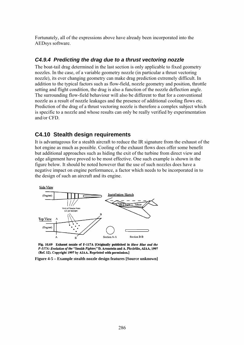
286

Fortunately, all of the expressions above have already been incorporated into the AEDsys software.

C4.9.4 Predicting the drag due to a thrust vectoring nozzle The boat-tail drag determined in the last section is only applicable to fixed geometry nozzles. In the case, of a variable geometry nozzle (in particular a thrust vectoring nozzle), its ever changing geometry can ma e drag prediction extremely difficult. In

geometry and position, throttle tting and flight condition, the drag is also a function of the nozzle deflection angle.

nozzle as a result of noPrediction of the drag o

ion

C4.10 Stealth design ree

but additional approaches such as hiding the exit of the turbine from direct view and edge alignment have provefigure below. It should be noted however th

kaddition to the typical factors such as flow-field, nozzleseThe surrounding flow-field behaviour will also be different to that for a conventional

zzle leakages and the presence of additional cooling flows etc. f a thrust vectoring nozzle is therefore a complex subject which

is specific to a nozzle and whose results can only be really verified by experimentatand/or CFD.

quirements It is advantageous for a stealth aircraft to reduce the IR signature from the exhaust of thhot engine as much as possible. Cooling of the exhaust flows does offer some benefit

d to be most effective. One such example is shown in the at the use of such nozzles does have a

negative impact on engine performance, a factor which needs to be incorporated in to the design of such an aircraft and its engine.

Figure 4-5 – Example stealth nozzle design features [Source unknown]

D1 General terms for the performance analyses This section is a reference for some of the general analysis terms used within the following thrust vectored aircraft performance analyses. Some of these expressions are common to more than one analysis while others are specific to just one.

D1.1 Basic terms The general aerodynamic terms such as CDZ, K, CLα and XAC as used in the baseline performance analysis work remain valid for this work. These are presented as convenient polynomial expressions in the baseline aircraft design section of this thesis. Other useful basic terms included in the analyses are:

• The basic lift coefficient, for an aircraft operating away the ground is given by, )LW(LBasicL iCC 0)( ααα −+⋅= Eq 1-1

• The dynamic pressure (q) of the flow is a common term within the analyses and is given by, 2

21 Vq ⋅⋅= ρ Eq 1-2

D1.2 Analysis of the ground effect for the take-off analysis Any aircraft operating in a close vicinity to the ground (as in the take-off phase) will experience a phenomena known as the ground effect. The presence of the ground can be considered as a mirror line which reflects the system of vortices and therefore modifies the aerodynamic characteristics of the aircraft. Analytical approaches model the effect of the ground as a reflected set of vortices below the ground with their own sets of sources, sinks and doublets. For this work however, we are merely concerned with the effect that this has on the aerodynamic characteristics of the aircraft. The most common way to account for this effect is to treat the ground effect as a virtual increase in the wing aspect ratio as will be used here. The aerodynamic parameters will then be modified in the same way as for an actual increase in the wing aspect ratio with and KV being the most affected. When operating away from the ground these retain their standard notation , and . It is worth noting that the aerodynamic centre of the aircraft remains unaffected. Rather than recalculating and KV of the virtual wing, analytical approximations can be used to determine the increase of these parameters for the actual wing.

αLC

αLC DZC BasicK

αLC

Since has a direct impact on the lift coefficient, it is viable to account for a variation in the lift coefficient instead, as below.

αLC

( ) ( ) (GELBasicLincGEL CCC )Δ+= Eq 1-3 This increase in lift coefficient can be obtained from below, taken from Datcom [20].

⎟⎟⎠

⎞⎜⎜⎝

⎛−⋅⎟⎟

⎠

⎞⎜⎜⎝

⎛⋅

⋅⋅=Δ

G

LBasicLGEL A

AAR

CCC 13.57 )(

)( πα Eq 1-4

The parameters used in this expression and the accompanying chart are:

287

1. ( )BasicLC - The basic lift coefficient of a wing operating away from the ground. 2. αLC - The basic lift curve slope of a wing operating away from the ground. 3. AR – The actual wing aspect ratio (not the virtually increased value). 4. A/AG – Ratio of the actual to the virtual aspect ratio as given by the chart below. 5. H – This is the height of the 25% MAC point of the wing above the ground. 6. b – This is the actual wing span of the wing (not the virtually increased value).

Figure 1-1 [20] In a similar way, the variation in the lift induced drag is determined as the sum of the basic value and a change due to the ground effect as below.

( ) (GEDiBasicincGE CKK Δ+= ) Eq 1-5 This increase in lift induced drag can be obtained from below, taken from Nicolai.

( )2

LBasicGEDi CKC ⋅⋅′−=Δ σ Eq 1-6 The parameter σ ′ is determined by the relation below, where h is the height of the wing above the ground and b is the actual wing span.

((

))bh

bh/4.705.1

/32.11'⋅+⋅−

=σ Eq 1-7

D1.3 The effect of deploying the Kruger flaps The Kruger flaps are deployed during the take-off and landing phases to extend the useable angle of attack of the aircraft. Although the leading edge Kruger flaps are not camber changing devices, they can still add an extra component of zero lift pitching moment to the aircraft when deployed. The method from Roskam [11] is used to determine this extra component, which consists of a variable expression (Part A) and a fixed expression (Part B) as given below.

BKrugersmAKrugersmKrugersm CCC −− Δ+Δ= )()()(0 Eq 1-8 Part B of the expression is dependent on the centre of the gravity of the aircraft and was determined by the expressions from Roskam as:

• In the landing configuration 004292488.0)( −=Δ −BKrugersmC • In the take-off configuration 004319778.0)( −=Δ −BKrugersmC

Part A of the expression is more variable and is dependent on the aircraft wing-fuselage pitching moment and lift coefficient as given by the relation below.

KKK

LK

mAKrugersm ccc

ccC

ccCC η⋅

⎥⎥⎦

⎤

⎢⎢⎣

⎡⎟⎟⎠

⎞⎜⎜⎝

⎛

⎭⎬⎫

⎩⎨⎧ −′⋅

′⋅⋅+

⎟⎟

⎠

⎞

⎜⎜

⎝

⎛

⎪⎭

⎪⎬⎫

⎪⎩

⎪⎨⎧

−⎟⎠⎞

⎜⎝⎛ ′

⋅=Δ − 75.012

)( Eq 1-9

288

The parameters used in this expression are: 1. Cm – Wing-fuselage pitching moment 2. '

Kc - Mean aerodynamic chord of the flapped wing section (determined for this configuration as 5.315m)

3. c – The chord of the un-flapped wing at the location of the mean aerodynamic chord for the flapped wing section (determined for this configuration as 5.206m)

4. CL – Lift coefficient of the wing 5. ηΔ - The span of the Kruger flap as a fraction of the wing semi-span

(determined for this configuration as 0.25) Determination of the wing-fuselage pitching moment followed the method given by Roskam which can be complex as it is dependent on many other parameters. To clarify the process to determine the Kruger pitching moment, it is presented in the easy to follow flowchart format below. If relevant, the ground effect must be included in the analysis, but should be omitted if not required.

LL

mm C

CC

C ⋅=

( )πα

α

180⋅=

L

m

L

m

CC

CC

αLC

⎟⎠⎞

⎜⎝⎛ ⋅⋅⎟

⎠

⎞⎜⎝

⎛⋅⎟⎟⎠

⎞⎜⎜⎝

⎛−=

παα180

LRoot

Root

AC

Root

CGm C

cC

CX

CX

C

[ ]( )Root

MACACW

Root

AC

CXccX

CX +⋅

=

ACWX1000/

10001000

2

⎥⎥⎦

⎤

⎢⎢⎣

⎡+⎟⎟

⎠

⎞⎜⎜⎝

⎛⋅+⎟⎟

⎠

⎞⎜⎜⎝

⎛⋅= C

MB

MAX AircraftAircraft

CG

AKrugersmC −Δ )(

BKrugersmAKrugersmKrugersm CCC −− Δ+Δ= )()()(0

)(0)(0)(0 KrugersmfuselageWingmTotalm CCC += −

BKrugersmC −Δ )(

)(0 fuselageWingmC −

( ) ( ) ( )GELBasicLincGEL CCC Δ+=

⎟⎟⎠

⎞⎜⎜⎝

⎛−⋅⎟⎟

⎠

⎞⎜⎜⎝

⎛⋅

⋅⋅=Δ

G

LBasicLGEL A

AAR

CCC 13.57 )(

)( πα

( )LWLBasicL iCC 0)( ααα −+⋅=

LL

mm C

CC

C ⋅=

( )πα

α

180⋅=

L

m

L

m

CC

CC

αLC

⎟⎠⎞

⎜⎝⎛ ⋅⋅⎟

⎠

⎞⎜⎝

⎛⋅⎟⎟⎠

⎞⎜⎜⎝

⎛−=

παα180

LRoot

Root

AC

Root

CGm C

cC

CX

CX

C

[ ]( )Root

MACACW

Root

AC

CXccX

CX +⋅

=

ACWX1000/

10001000

2

⎥⎥⎦

⎤

⎢⎢⎣

⎡+⎟⎟

⎠

⎞⎜⎜⎝

⎛⋅+⎟⎟

⎠

⎞⎜⎜⎝

⎛⋅= C

MB

MAX AircraftAircraft

CG

AKrugersmC −Δ )(

BKrugersmAKrugersmKrugersm CCC −− Δ+Δ= )()()(0

)(0)(0)(0 KrugersmfuselageWingmTotalm CCC += −

BKrugersmC −Δ )(

)(0 fuselageWingmC −

( ) ( ) ( )GELBasicLincGEL CCC Δ+=

⎟⎟⎠

⎞⎜⎜⎝

⎛−⋅⎟⎟

⎠

⎞⎜⎜⎝

⎛⋅

⋅⋅=Δ

G

LBasicLGEL A

AAR

CCC 13.57 )(

)( πα

( )LWLBasicL iCC 0)( ααα −+⋅=

D1.4 Variation in the aircraft centre of gravity with fuel burn As fuel is consumed, both the weight and centre of gravity of the aircraft will change as a result of this weight loss and a shift in the weight distribution. Fortunately, an expression for the location of the aircraft centre of gravity as a function of the aircraft mass was analytically derived from the conceptual design work, as given below.

289

1000/6.43161000

427.291000

3116.12

⎥⎥⎦

⎤

⎢⎢⎣

⎡+⎟⎟

⎠

⎞⎜⎜⎝

⎛⋅+⎟⎟

⎠

⎞⎜⎜⎝

⎛⋅−= AircraftAircraft

CG

MMX Eq 1-10

This value is measured from the nose of the aircraft (the aircraft reference point). It is common to also quote this value relative to the mean aerodynamic chord of the wing. In such cases this can be found from the expression below, where is the location of the start of the mean aerodynamic chord as measured from the aircraft nose.

MACX

CXX

X MACCGCG

−= Eq 1-11

D1.5 Aircraft drag increase in the landing configuration When in its landing configuration, the aircraft will experience an increase in drag due to the deployment of high lift devices and the extension of the landing gear. The impact of leading edge devices is typically negligible in comparison with trailing edges devices and so only the trailing edge devices are included here. In such cases, the contribution to the lift induced drag is negligible compared to that due to the zero lift drag. The expression below from Howe [1] proved to be sufficient to predict the increase in the zero lift drag of the aircraft in the landing configuration.

)(33.0)(15.0

LandingDLF

LandingDZ CAR

FC +⎟⎠⎞

⎜⎝⎛ ⋅

=Δ Eq 1-12

The first part of this expression accounts for the deployed high lift devices and the second the extended landing gear. The parameters used in this expression are:

1. AR – Wing aspect ratio 2. FF – Flap drag factor which is taken as 1.0 for a single slotted trailing edge flap. 3. )(LandingDL - The drag coefficient of an extended landing gear. This is assumed

to have a value of 0.03, typical for this type of aircraft. C

D1.6 Control characteristics of the elevons As part of the analysis work, the effectiveness of the thrust vectoring system for aircraft pitch control was compared to that of conventional elevons control surfaces. In order to be able to carry out such an analysis, we need to predict the impact which the deflection of the elevons will have on the lift, drag and pitching moment of the aircraft.

D1.6.1 Contribution to lift due to elevon deflection If we treat the elevon as a plain flap, the variation in lift due to elevon deflection can be determined from the expression below from Raymer [3].

( ) FlapFlap

LFlapL d

dCC δδ

⋅=Δ Eq 1-13

The terms required in the determination of this expression are:

290

1. FlapL ddC δ/ - Lift increment for plain flaps as determined by the expression below from Raymer [3]. This is a function of the elevon geometry with this arrangement having a Sflapped/S ratio of 0.1869 and 1=ΛHL . Cos

HLflapped

f

lf

f

L CosS

SddC

KddC

Λ⋅⋅⎟⎟⎠

⎞⎜⎜⎝

⎛⋅⋅=

δδ9.0 Eq 1-14

2. fl ddC δ/ - The 2-dimensional lift increment for plain flaps which is determined from the chart below. For this arrangement, we have a t/c value of 0.0894 at the mid-elevon point and a cf/c ratio of 0.15 which gives us 1.3/ =fl ddC δ

Figure 1-2 [3] 3. Kf – Flap correction factor for large flap deflection angles. As we are operating

at angles of 10 degrees and less, Kf=1. 4. Flapδ - Flap deflection angle measured in radians.

This gives us a value of 521451.0/ =FlapL ddC δ for our configuration. As required, the expression for the total wing lift coefficient then becomes,

( )[ ] (FlapLLLL CCC Δ+−⋅= 0 )ααα Eq 1-15

D1.6.2 Contribution to pitching moment due to elevon deflection The pitching moment coefficient due to elevator deflection can be determined by the expression below from Raymer [3].

( )CGFlapCPFlapFlap

LFlapelevonsM XX

ddCKC −⋅⋅⋅−= )()( δδ

Eq 1-16

The terms required in the determination of this expression are: 1. FlapL ddC δ/ - Lift increment for plain flaps as determined above. 2. Flapδ - Flap deflection angle measured in radians.

3. )(FlapCPX - Location of the centre of pressure of the flap relative to the aircraft reference point as a fraction of the MAC of the wing. The location of the centre of pressure of the flap with respect to the mean aerodynamic chord of the flapped area can be determined from the chart below. Knowing the location of the flapped MAC with respect to the aircraft reference point we are able to convert this to the aircraft reference point. For our configuration this was determined as 7311.0 . =CPX

291

Figure 1-3 and 1-4 [3] 4. CGX - Location of the aircraft centre of gravity as measured from the aircraft

reference point, as a fraction of the MAC of the wing.

D1.6.3 Contribution to drag due to elevon deflection The total drag coefficient of the aircraft including the components due to elevon deflection can be determined from the modified drag coefficient expression below.

( )( ) ( )( )[ ]20 LFlapDiFlapDDZD CCKCCC ⋅Δ++Δ+= Eq 1-17

The contributions due to zero lift drag and lift induced drag are given in sections below.

D1.6.3.1 Contribution to zero lift drag The variation in the zero lift drag due to elevon deflection is determined by the expression below taken from Stinton [4].

( ) BSCFlapDC εεε ⋅⋅=Δ 0 Eq 1-18 The terms required in the determination of this expression are:

1. Cε - This is a factor to account for the elevon chord in relation to the wing chord as determined from the figure below. This was determined as 75.0=Cε .

2. Sε - This is a factor to account for the area of the flap in relation to the total area of the wing as determined from the figure below. This was determined as

475.0=Sε for 33.0=bb f . 3. Sε - This is a factor to account for flap deflection as determined from the figure

below. To save time and effort, an expression was derived from the results for Sε for this configuration as a function of the absolute value of flap deflection measured in degrees.

( ) 31/2696.20065.02

EffB δδε ⋅+⋅= Eq 1-19

292

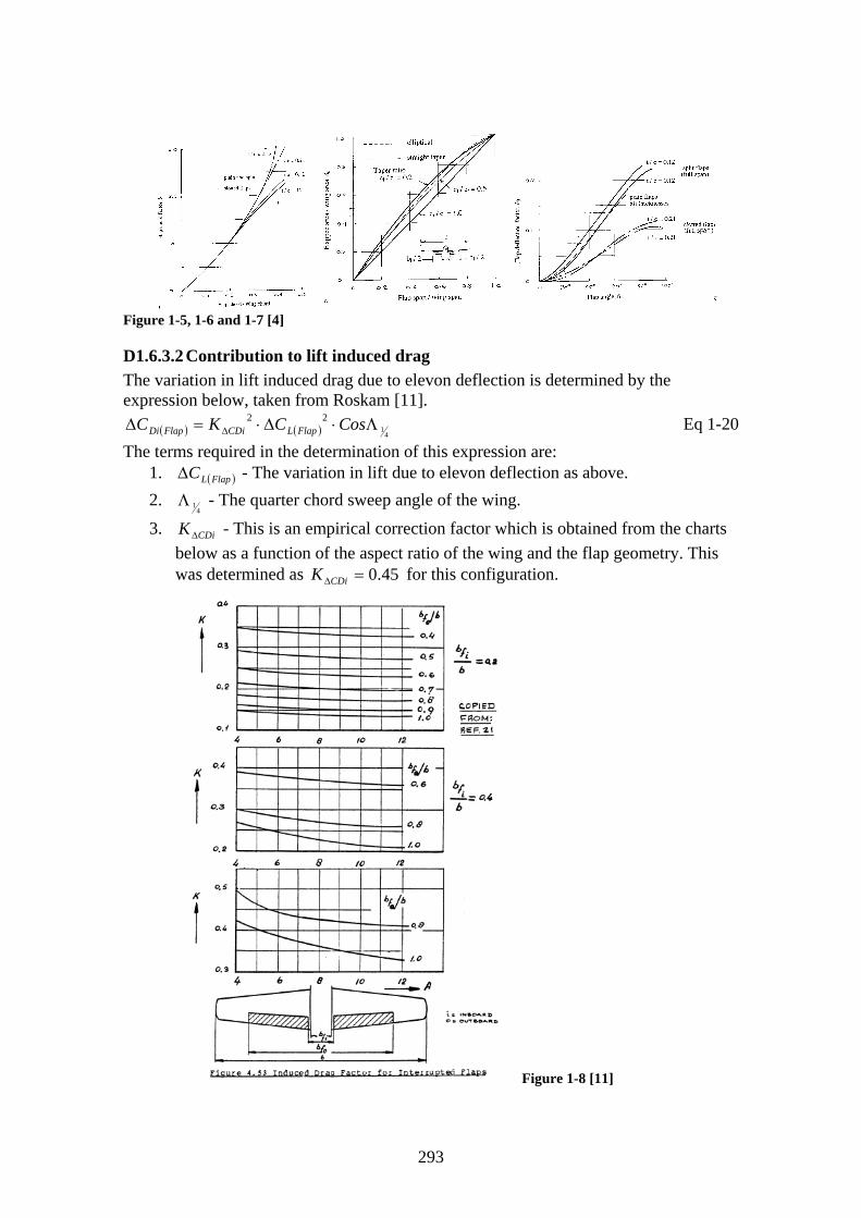
Figure 1-5, 1-6 and 1-7 [4]

D1.6.3.2 Contribution to lift induced drag The variation in lift induced drag due to elevon deflection is determined by the expression below, taken from Roskam [11].

( ) ( ) 41

22 Λ⋅Δ⋅=Δ Δ CosCKC FlapLCDiFlapDi Eq 1-20 The terms required in the determination of this expression are:

1. ( )FlapLCΔ - The variation in lift due to elevon deflection as above. 2.

41Λ - The quarter chord sweep angle of the wing.

3. CDiKΔ - This is an empirical correction factor which is obtained from the charts below as a function of the aspect ratio of the wing and the flap geometry. This was determined as 45.0= for this configuration. ΔCDiK

Figure 1-8 [11]

293

D2 Cruise analysis The purpose of this analysis is to asses the benefits of using a low cost thrust vectoring system to replace the conventional elevons on an aircraft during the cruise phase. It is hoped that by replacing the elevons, the additional drag penalty associated with their use will also be eliminated. The result is an increase in the aerodynamic efficiency of the aircraft. Since the cruise phase has the largest fuel demands, this will be the key indicator of the viability of such a proposal. This section describes two studies, one for the thrust vectored proposal and the other for a conventional aircraft configuration utilising elevons. A comparison between these results will enable the feasibility of using such a system for trimming an aircraft to be assessed.

D2.1 Analysis parameters Presented in this section are the parameters required for these analyses. During these analyses, the aircraft is in a clean cruise configuration. As fuel is consumed, the centre of gravity of the aircraft will be displaced as discussed in the general terms section. In the case of the conventional configuration, deflection of the elevons will result in a variation in lift, drag and pitching moment due to their deflection. This is discussed in greater depth in the general terms section.

D2.1.1 The engine throttle setting of the thrust vectored engine In contrast to a standard fixed configuration engine, the analysis of a thrust vectoring engine-nozzle combination is complicated by the fact that the engine configuration is a function of thrust vectoring nozzle deflection and therefore variable. To cater for this, an expression was derived as part of the engine analysis work which gives the specific fuel consumption as a function of the engine throttle ratio. To be able to use this, we make use of an expression also derived in the engine analysis work for the engine throttle ratio as a function of engine thrust, as given below.

( )31

%E

BTAT +⋅= Eq 2-1

The coefficients used in this expression are themselves functions of the absolute value of thrust vectoring angle as given by the following relations.

318.6969536.61821.0 2

EA

+⋅+⋅=

φφ Eq 2-2

2483.75303.34118.0 2 −⋅−⋅−= φφB Eq 2-3

D2.1.2 Specific fuel consumption of the thrust vectored configuration

The expression for the specific fuel consumption of the engine as determined from our engine analysis work is given below. As already stated, this is a function of the engine throttle setting determined above.

294

( ) ( )[ ]61

%% 2

ECTBTASFC +⋅+⋅

= Eq 2-4

The coefficients used in this expression are themselves functions of the absolute value of thrust vectoring angle as given by the following quadratic relations.

5714.43257.11229.0 2 +⋅+⋅−= φφA Eq 2-5

2326.48203.1127.0 2 −⋅−⋅= φφB Eq 2-6

022.249163.00242.0 2 +⋅+⋅−= φφC Eq 2-7

D2.1.3 Specific fuel consumption of the conventional configuration In the case of the conventional fixed configuration engine, an expression for the specific fuel consumption was also derived in our engine work. The resulting expression is a direct function of engine thrust as given below.

611000100010001000

234

−⋅⎥⎥⎦

⎤

⎢⎢⎣

⎡+⎟

⎠⎞

⎜⎝⎛⋅+⎟

⎠⎞

⎜⎝⎛⋅+⎟

⎠⎞

⎜⎝⎛⋅+⎟

⎠⎞

⎜⎝⎛⋅= EETDTCTBTASFC Eq 2-8

The corresponding coefficients are given in the following table.

Coefficents A B C D EValue -0.0007 0.0175 -0.1262 0.1578 23.895

D2.2 Thrust vectored cruise analysis The function of this analysis is to investigate the cruise performance of a thrust vectored variant of the UCAV. During this flight phase, the aircraft is assumed to be flying at a constant speed and attitude and the thrust vectoring system is utilised solely for trim. As the specific fuel consumption is dependent on the engine configuration, this will change throughout the flight phase as the centre of gravity of the aircraft and thus the trim requirements varies.

D2.2.1 Derivations The arrangement of the aircraft in its cruise configuration is given in the figure below along with the system of forces acting on it. This figure also includes the definitions of the characteristic lengths required to determine the moment coefficients.

295

Figure 2-1 As the aircraft will approach the oncoming airflow at an angle of attack, the thrust required to maintain flight will be the resultant of the forces acting on the aircraft in the X and Z directions. Applying Newton’s second law of motion to the aircraft we are able to derive a suitable expression as follows. Summing forces along the x-axis, we obtain,

DTmax −= αcos . Eq 2-9 As the aircraft is moving with constant velocity, ax = 0, so that the above reduces to,

DT =αcos Eq 2-10 In a similar way, summing the forces along the y-axis, we obtain,

WLTmaz −+= αsin . Eq 2-11 As the aircraft is maintaining a constant altitude, az = 0, so that the above reduces to,

LWT −=αsin Eq 2-12 Solving the above equations simultaneously, we are able to obtain the expression below for the thrust. This is the fundamental equation for the first part of this analysis.

22 )( LWDT −+= Eq 2-13 Summing the moments acting on the aircraft about its centre of gravity, we obtain,

( )VTMHTMLWMwfMTotalM CCCCC +++= )()()(0)( Eq 2-14 Each of the components in the expression above can be derived from inspection of the figure above. The dimensions are given as a fraction of the wing mean aerodynamic chord, denoted as ‘bar’ values. The resulting expressions are given below:

1. )(0 wfMC - The zero lift pitching moment of the wing-fuselage

2. ( )ACWCGLLWM XXCC −⋅=)( - Due to the lift of the wing Eq 2-15

3. ( )CGX− - Due to the vertical component of deflected

thrust. Eq 2-16

NozzZ

VTM XSq

TC ⋅⋅

−=)(

4. NozzX

HTM ZSq

TC ⋅⋅

−=)( - Due to the horizontal component of deflected thrust.

Eq 2-17 The horizontal and vertical components of deflected thrust can be determined from the simple relations below as a function of vectoring angleφ .

( )φSinTT VectoredEngineZ ⋅= )( Eq 2-18 ( )φCosTT VectoredEngineX ⋅= )( Eq 2-19

296

The thrust of the exhaust plume will encounter thrust losses due to deflection of the nozzle which have already been incorporated into the engine performance relations. These relations will now be put into practice in the analyses that follow.

D2.2.2 Analysis approach The nature of this analysis meant that it had to be broken down into two stages as follows,

1. This stage is used to determine the optimal angle of attack of the aircraft which gives us the minimum thrust requirements at that instance in time.

2. This stage is used to determine the thrust vectoring plume angle required to trim the aircraft and that instance in time.

An iterative solution process is required to solve each analysis. An added complication to this is however the fact that the two analyses are inter-related by means of the engine thrust term. It is therefore necessary to keep alternatively iterating each solution until both solutions converge. This process is summarised below.

Solution procedure for the cruise analysis Stage 1 – Iterate α to determine the minimum value for T Stage 2 – Iterateφ until 0=mC Repeat Stage 1 and Stage 2 until both of the solutions converge

Since many of the parameters are continually changing during the cruise phase, it is necessary to break the flight phase down into a number of steps. The accuracy of the analysis increases as the number of time steps used increases. As the number of time steps increase, the corresponding decrease in the interval of each time step therefore reduces the step wise nature of the parameters used. The analysis process described above is then repeated at each of the time steps being analysed. The two analysis stages are discussed in the sections below.

D2.2.3 Analysis stage 1 – Solution for required engine thrust The analysis process to determine the optimal aircraft angle of attack and thus the thrust is presented in the easy to follow equation flow chart below. This process is repeated for each time step with macros being used to automate the Microsoft Excel Solver function used for the iteration process.

297

( ) ( )[ ]61

%% 2

ECTBTASFC +⋅+⋅

=

)1(Variable=α

)2(VariableNozzle =φ

( )LLL CC 0ααα −⋅= 2LDZD CKCC ⋅+=

LCSqL ⋅⋅= DCSqD ⋅⋅=

221 Vq ⋅⋅= ρ

( )22 LWDT −+=

Iterate alpha to find the solution for minimum thrust

gMW AircraftAircraft ⋅=

( )00 −−−= fuelfuelAircraft mmMM

( ) ( )11 −− +−⋅= tfueltffuel mttQm

SFCTQ f ⋅=

Additionally, L, D, T and W are used to find L/D and T/W ratios

From analysis stage 2

( )31

%E

BTAT +⋅=

31

2

EFED

A+⋅+⋅

=φφ

IHGB +⋅+⋅= φφ 2

( ) ( )[ ]61

%% 2

ECTBTASFC +⋅+⋅

=

)1(Variable=α

)2(VariableNozzle =φ

( )LLL CC 0ααα −⋅= 2LDZD CKCC ⋅+=

LCSqL ⋅⋅= DCSqD ⋅⋅=

221 Vq ⋅⋅= ρ

( )22 LWDT −+=

Iterate alpha to find the solution for minimum thrust

gMW AircraftAircraft ⋅=

( )00 −−−= fuelfuelAircraft mmMM

( ) ( )11 −− +−⋅= tfueltffuel mttQm

SFCTQ f ⋅=

Additionally, L, D, T and W are used to find L/D and T/W ratios

From analysis stage 2

( )31

%E

BTAT +⋅=

31

2

EFED

A+⋅+⋅

=φφ

IHGB +⋅+⋅= φφ 2

D2.2.4 Analysis stage 2 – Solution for nozzle vectoring angle The analysis process to determine the nozzle vectoring angle required to trim the aircraft is presented in the easy to follow equation flow chart below. This process is repeated for each time step with macros being used to automate the Microsoft Excel Solver function used for the iteration process.

298

MAircraft from analysis stage 1

1000/10001000

2

⎥⎥⎦

⎤

⎢⎢⎣

⎡+⎟⎟

⎠

⎞⎜⎜⎝

⎛⋅+⎟⎟

⎠

⎞⎜⎜⎝

⎛⋅= C

MB

MAX AircraftAircraft

CG

CXX

X MACCGCG

−=

)2(VariableNozzle =φ

( )ACWCGLLWM XXCC −⋅=)()(0 wfMC

( )VTMHTMLWMwfMTotalM CCCCC +++= )()()(0)(

Iterate φNozzle to find the solution for CM(Total) = 0

Return the result for φNozzle to the stage 1 analysis

CL from analysis stage 1 ACWX

( )φCosTTX ⋅=

( )φSinTTZ ⋅=

NozzX

HTM ZSq

TC ⋅

⋅−

=)(

( )CGNozzZ

VTM XXSq

TC −⋅

⋅−

=)(

MAircraft from analysis stage 1

1000/10001000

2

⎥⎥⎦

⎤

⎢⎢⎣

⎡+⎟⎟

⎠

⎞⎜⎜⎝

⎛⋅+⎟⎟

⎠

⎞⎜⎜⎝

⎛⋅= C

MB

MAX AircraftAircraft

CG

CXX

X MACCGCG

−=

)2(VariableNozzle =φ

( )ACWCGLLWM XXCC −⋅=)()(0 wfMC

( )VTMHTMLWMwfMTotalM CCCCC +++= )()()(0)(

Iterate φNozzle to find the solution for CM(Total) = 0

Return the result for φNozzle to the stage 1 analysis

CL from analysis stage 1 ACWX

( )φCosTTX ⋅=

( )φSinTTZ ⋅=

NozzX

HTM ZSq

TC ⋅

⋅−

=)(

( )CGNozzZ

VTM XXSq

TC −⋅

⋅−

=)(

D2.3 Conventional elevons configuration cruise analysis The function of this analysis is to investigate the cruise performance of the conventional UCAV utilising elevons. As before, the aircraft is assumed to be flying at a constant speed and attitude, with the elevons being utilised solely for trim. In this case, as the engine configuration is fixed, the specific fuel consumption will remain constant throughout the flight phase. The elevon deflection required will however vary as the centre of gravity of the aircraft and thus the trim requirements varies.

D2.3.1 Derivations The arrangement of the conventional aircraft in its cruise configuration is given in the figure below along with the system of forces acting on it. Also shown are the characteristic lengths required to determine the moment coefficients.

299

Figure 2-2 The derivations of the forces and moments follow the same procedure as for the thrust vectored variant of the aircraft. Following the same procedure to determine the required thrust from the engine, we obtain the same fundamental equation as before. As before, this is the foundation of the first part of this analysis.

22 )( LWDT −+= Eq 2-20 In the case of the moments acting on the aircraft about its centre of gravity, the relation for the conventional elevons configuration becomes,

)()()(0)( elevonsMLWMwfMTotalM CCCC ++= Eq 2-21 As before, each of the components in the expression above can be derived by inspection of the figure above with each of the dimensions being quoted as ‘bar’ values. This results in the expressions given below:

5. )(0 wfMC - The zero lift pitching moment of the wing-fuselage

6. ( )ACWX− - Due to the lift of the wing Eq 2-22 CGLLWM XCC ⋅=)(

7. )(elevonsM - The pitching moment due to deflection of the elevons as determined by the relations presented in the general terms section. C

These relations will now be put into practice in the analyses that follow.

D2.3.2 Analysis approach The analysis for the conventional elevons configuration follows a very similar approach to that presented for the thrust vectored aircraft. As before, the nature of the analysis meant that it had to be broken down into two parts as follows,

1. This stage is used to determine the optimal angle of attack of the aircraft which gives us the minimum thrust requirements at that instance in time.

2. This stage is used to determine the elevon deflection angle required to trim the aircraft and that instance in time.

An iterative solution process is required to solve each analysis. An added complication to this is however the fact that the two analyses are inter-related by means of the engine thrust term. As before, it is therefore necessary to keep alternatively iterating each solution until both solutions converge. This process is summarised below.

300

Repeat Stage 1 and Stage 2 until both of the solutions converge

Solution procedure for the cruise analysis Stage 1 – Iterate α to determine the minimum value for T Stage 2 – Iterate fδ until 0=mC

As before, since many of the parameters are constantly changing during the cruise phase, it is necessary to break the flight phase down into a number of steps in order to increase the accuracy of the analysis. The analysis process described above is then repeated at each of the time steps being analysed. The two analysis stages are discussed in the sections below.

D2.3.3 Analysis stage 1 – Solution for required engine thrust The analysis process to determine the optimal aircraft angle of attack and thus the thrust is presented in the easy to follow equation flow chart below. Compared to the analysis for the thrust vectored aircraft, here we have to take account of the additional aerodynamic effects which arise as a result of deflecting the elevons, which includes increases in lift and drag. The process given below is repeated for each time step with macros being used to automate the Microsoft Excel Solver function used for the iteration process.

301

)1(Variable=α )2(VariableFlap =δ

( ) FlapFlap

LFlapL d

dCC δδ

⋅=Δ( ) ( ) 4

122 Λ⋅Δ⋅=Δ Δ CosCKC FlapLCDiFlapDi

( ) BSCFlapDC εεε ⋅⋅=Δ 0( )[ ] ( )FlapLLLL CCC Δ+−⋅= 0ααα

( )( ) ( )( )[ ]20 LFlapDiFlapDDZD CCKCCC ⋅Δ++Δ+=

LCSqL ⋅⋅= DCSqD ⋅⋅=

221 Vq ⋅⋅= ρ

( )22 LWDT −+=

Iterate alpha to find the solution for minimum thrust

gMW AircraftAircraft ⋅=

( )00 −−−= fuelfuelAircraft mmMM

( ) ( )11 −− +−⋅= tfueltffuel mttQm

SFCTQ f ⋅=

SFC

Additionally, L, D, T and W are used to find L/D and T/W ratios

From analysis stage 2)1(Variable=α )2(VariableFlap =δ

( ) FlapFlap

LFlapL d

dCC δδ

⋅=Δ( ) ( ) 4

122 Λ⋅Δ⋅=Δ Δ CosCKC FlapLCDiFlapDi

( ) BSCFlapDC εεε ⋅⋅=Δ 0( )[ ] ( )FlapLLLL CCC Δ+−⋅= 0ααα

( )( ) ( )( )[ ]20 LFlapDiFlapDDZD CCKCCC ⋅Δ++Δ+=

LCSqL ⋅⋅= DCSqD ⋅⋅=

221 Vq ⋅⋅= ρ

( )22 LWDT −+=

Iterate alpha to find the solution for minimum thrust

gMW AircraftAircraft ⋅=

( )00 −−−= fuelfuelAircraft mmMM

( ) ( )11 −− +−⋅= tfueltffuel mttQm

SFCTQ f ⋅=

SFC

Additionally, L, D, T and W are used to find L/D and T/W ratios

From analysis stage 2

D2.3.4 Analysis stage 2 – Solution for elevon deflection The analysis process to determine the elevon deflection required to trim the aircraft is presented in the easy to follow equation flow chart below. This follows a similar approach to that used for the thrust vectored aircraft, the main difference between that the thrust vectoring moment terms are replaced with the moment term due to elevon deflection. This process given below is repeated for each time step with macros being used to automate the Microsoft Excel Solver function used for the iteration process.

302

MAircraft from analysis stage 1

1000/10001000

2

⎥⎥⎦

⎤

⎢⎢⎣

⎡+⎟⎟

⎠

⎞⎜⎜⎝

⎛⋅+⎟⎟

⎠

⎞⎜⎜⎝

⎛⋅= C

MB

MAX AircraftAircraft

CG

CXX

X MACCGCG

−=

)2(VariableFlap =δ

( )CGFlapCPFlapFlap

LFlapelevonsM XX

ddCKC −⋅⋅⋅−= )()( δδ

( )ACWCGLLWM XXCC −⋅=)()(0 wfMC

)()()(0)( elevonsMLWMwfMTotalM CCCC ++=

Iterate δf to find the solution for CM(Total) = 0

Return the result for δf to the stage 1 analysis

CL from analysis stage 1 ACWX

MAircraft from analysis stage 1

1000/10001000

2

⎥⎥⎦

⎤

⎢⎢⎣

⎡+⎟⎟

⎠

⎞⎜⎜⎝

⎛⋅+⎟⎟

⎠

⎞⎜⎜⎝

⎛⋅= C

MB

MAX AircraftAircraft

CG

CXX

X MACCGCG

−=

)2(VariableFlap =δ

( )CGFlapCPFlapFlap

LFlapelevonsM XX

ddCKC −⋅⋅⋅−= )()( δδ

( )ACWCGLLWM XXCC −⋅=)()(0 wfMC

)()()(0)( elevonsMLWMwfMTotalM CCCC ++=

Iterate δf to find the solution for CM(Total) = 0

Return the result for δf to the stage 1 analysis

CL from analysis stage 1 ACWX

303

D3 Take-off analysis The complete take-off phase typically consists of four phases, ground roll, rotation, transition to climb and take-off climb-out. The results of the baseline performance studies showed the contribution of the, rotation, transition and take-off climb out phases to the complete take-off to be small in comparison to the ground run phase. Time constraints have dictated the depth of study which can be achieved and in this analysis it is reasonable to merely concentrate on the ground roll. The work consists of three analyses, the first of which determines the point where there is sufficient speed and thus lift to commence the rotation. The other two analyses determine the point at which there is sufficient control authority available to safely control the aircraft, one of which is for the thrust vectoring system and the other for conventional elevons. These results are finally merged to find the optimal point when the aircraft has sufficient lift and control.

D3.1 Analysis parameters Presented in this section are the parameters required for this analysis. During this analysis, the aircraft is in its take-off configuration with the Kruger flaps deployed. Its close proximity to the ground means that ground effect is also important. Both of these are discussed in the general terms section.

D3.1.1 Engine parameters The engine characteristics such as available thrust and thrust specific fuel consumption were determined in the engine analysis work at a number of engine operating points. This covered a range of engine bleed settings and thrust vectoring nozzle deflection angles. A complication comes from the fact that the speed of the aircraft is constantly changing during the take-off run, which will also affect the engine operating parameters. To overcome this, all the parameters were evaluated at an average take-off speed of M0.2, to which a scale factor was applied to account for the Mach number variations. This is given by the respective relations below for thrust and specific fuel consumption.

ScaleMMTO TTT −⋅= 2.0 Eq 3-1

ScaleMMTO SFCSFCSFC −⋅= 2.0 Eq 3-2 The accompanying Mach number scale factors are given by the expressions below. It should be re-emphasised that these are independent of thrust vectoring angle and bleed.

( ) ( ) ( ) ( ) 0804.13575.07693.0459.37672.3 234 +−−+−=− MMMMT ScaleM Eq 3-3 ( ) ( ) ( ) ( ) 9196.03014.09856.004.31881.3 234 +++−=− MMMMSFC ScaleM Eq 3-4

The available engine thrust at M0.2 is determined from the following relation where the vectoring angle of the engine plumeφ is in degrees and the thrust is in Newtons.

( ) ( ) CBAT MTO +⋅+⋅=− φφ 22.0 Eq 3-5

The constants in this expression are different for each engine bleed setting as given in the table below. Each set of constants being valid for a range of vectoring angles within that engine bleed setting.

304

Thrust at M0.20 2.5 5 7.5 10 12.5 15 17.5 20

Constant A 2.3421 2.2378 2.3373 2.3983 3.8825 3.4031 2.9695 3.5186 2.7429Constant B -560.32 -546.96 -535.45 -521.48 -524.57 -496.54 -467.32 -452.13 -415.5Constant C 54601 52330 50024 47673 45304 42847 40335 37779 35107

Bleed setting (%)

Table 3-1 In a similar way, the thrust specific fuel consumption at M0.2 is determined by the relation below where once again,φ is in degrees and SFC is in kg/Ns (x1E-6).

( ) ( ) CBASFC MTO +⋅+⋅=− φφ 22.0 Eq 3-6

As before, the constants in this expression are different for each engine bleed setting as given in the table below. TSFC at M0.2

0 2.5 5 7.5 10 12.5 15 17.5 20Constant A 0.0015 0.0017 0.0018 0.0018 0.0008 0.0011 0.0014 0.0009 0.0016Constant B 0.2284 0.236 0.2445 0.2546 0.2795 0.2867 0.2935 0.3143 0.3201Constant C 22.395 22.716 23.089 23.515 23.992 24.575 25.268 26.078 27.1

Bleed setting (%)

Table 3-2 Collectively, these relations enable us to predict the thrust and specific fuel consumption of the engine over a range of bleed settings, plume deflection angles and speeds. These have provided a valuable tool for this performance analysis work but they are however only applicable to this particular engine. The reader is advised to refer to the engine design section for further details of their derivation.

D3.1.2 Vectored thrust components The layout of the thrust vectoring system is shown in the figure below along with expressions for the horizontal and vertical components of thrust. The thrust of the engine plume is the vectored thrust which includes the thrust loss is associated with the vectoring action. In this figure,φ is defined as the angle that the engine’s exhaust plume and thus the engine thrust is deflected from the engine centre-line.

305

( )φCosTT VectoredEngineX ⋅= )( ( )φSinTT VectoredEngineZ ⋅= )(

Eq 3-7 and 3-8 Figure 3-1

D3.1.3 Nose-jet control terms The function of the nose jet is to generate a pitch force sufficient to rotate the nose of the aircraft at take-off and therefore replace the conventional elevator control surfaces. In such cases, the deflection of the elevons will therefore be zero ( 0=Flapδ ). In the nose jet analysis section, it was shown that the thrust generated by the nose jet is primarily a function of engine bleed. We could be misled into thinking that the nose jet force would also be a function of the engine vectoring angle, since this has a knock on effect on the engine. However, since the mass flow rate of air through the engine remains the same, the bleed remains unaffected. The nose jet analysis gave us a useful table of results for the nose jet force at M0.2 and at a number of engine bleed settings as presented below.

0 2.5 5 7.5 10 12.5 15 17.5 20L-NJ at M0.2 (N) 0 1119.967 2238.942 3353.567 4465.797 5572.177 6671.089 7760.115 8836.781

Bleed setting (%)

Table 3-3

As with the engine analyses, these figures are for an average take-off speed of M0.2 and it is necessary to apply a scale factor to account for Mach number effects. The resulting thrust from the nose jet can be determined from the relation below.

MachNJMNJNJ ScaleLL −⋅= )2.0(@ Eq 3-9 The scale factor for the aircraft speed is given by the relation below whose constants are given in the accompanying table for a range of engine bleed settings.

( ) ( ) ( ) DMCMBMAScale MachNJ +⋅+⋅+⋅=−23 Eq 3-10

ScaleNJ-Mach

0 2.5 5 7.5 10 12.5 15 17.5 20Constant A 0 0.0655 0.0321 0.0573 0.0147 0.1153 0.1151 0.1143 0.1218Constant B 0 0.2021 0.2178 0.2101 0.2308 0.1781 0.1811 0.1851 0.1807Constant C 0 0.0044 0.0035 0.0024 0.0012 0.0074 0.007 0.0068 0.0084Constant D 0 0.9905 0.9903 0.9908 0.9906 0.9905 0.9904 0.9903 0.9901

Bleed setting (%)

Table 3-4

D3.1.4 Presentation of the results At the point of initiation of rotation of the aircraft, we are able to determine a number of other parameters. In particular, the distance covered during the ground run can be determined from the relation below. It is important to evaluate this expression over a number of small time steps to account for the ever changing velocity and acceleration.

( ) ( ) )1(2

1)1()(

1 221

−−−

− +−⎟⎟⎠

⎞⎜⎜⎝

⎛ +⋅+−= tGi

tXtXiXG Stt

aattVS Eq 3-11

We are also able to determine the contribution to the total lift from the different lifting mechanisms as given by the relation below. This includes that from the wings, the vertical component of vectored thrust and the lift from the nose jet.

NJZTotal LTLL ++= Eq 3-12

D3.1.5 Effect of thrust vectoring on the landing gear When the engine plume is deflected downwards, an additional nose down pitching moment is generated about the main landing gear wheels. This will increase the nose gear load fraction and will thus change the ground handling characteristics of the aircraft. As a result, the nose steering could become too heavy to be able to be used safely. The opposite being true if the engine thrust is instead deflected upwards, which could give rise to steering which is too light with the risk of drift. Knowing the total pitching moment of the aircraft, as given by analyses which follow, we are able to determine the landing gear reaction forces from the relations below. The terms and are the locations of the main gear and nose gear respectively, as measured from the reference point of the aircraft.

gearMainX − gearNoseX −

( )gearNosegearMain

TotalmgearNose XX

cSqCR

−−− −

⋅⋅−= )( Eq 3-13

gearNoseTotalgearMain RRR −− −= Eq 3-14 The nose gear and main gear load fractions can finally be determined from the normal landing gear analysis methods.

306

D3.2 Numerical analysis to determine the final solution As will be seen in the sections which follow, the solution to these analyses is found at the point of intersection of two curves. For example, in the case of the control limit analysis, this will be intersection of curves for the control power required and control power available. Although it is possible to estimate these intersection points graphically, numerical interpolation techniques were employed instead to improve the accuracy and automate the process. The system devised was integrated within the analysis spreadsheets to filter out the closest solution points either side of the location of the final solution and then linearly interpolate between these to obtain the final solution. The first step in this process is to filter out the upper and lower solution boundaries between which the final solution lies from the mass of data within the spreadsheet. Assuming that our two parameters are X and Y (control power required and control power available), the two spreadsheet functions below can be used to fill two auxiliary columns of either ones or zeros depending on where each corresponding data point lies in relation to the final solution. Top solution filter: Eq 3-15 )0,1,( )1(@)1(@ −− >= ttTop YXIFFilterBottom solution filter: )0,1,( )(@)(@ ttBottom YXIFFilter <= Eq 3-16 The multiplication of these two rows as given in the function below will pinpoint the upper and lower solution boundaries. Solution filter: BottomTopSelector FilterFilterFilter ⋅= Eq 3-17 By multiplying the solution filter by the original results, the top and bottom boundaries of each analysis solution can be determined as given below. Top solution boundary: )1(@1 +⋅= tFilterVariableBoundary Eq 3-18 Bottom solution boundary: )(@2 tFilterVariableBoundary ⋅= Eq 3-19 The final solution can finally be determined by linearly interpolating between the boundaries with the expression below.

( ) )1(@)1(@)2(@12

1)(@ ttt

SolutiontSolution VariableVariableVariable

tttt

Variable +−⎥⎦

⎤⎢⎣

⎡−−

=−

Eq 3-20 For small time steps, the result curves are sufficiently linear for the error in using a linear interpolation method to be negligible. With the solution part of the spreadsheet set up as above, all that remains is to determine time domain solution where the 2 curves intersect (tSolution). An iterative solution process was used for this purpose as given by the steps below.

1. Assume a value for the input t-solution, which lies between boundaries 1 and 2. 2. Using the assumed value for t-solution, linearly interpolate variables X and Y

between the boundaries 1 and 2. 3. Determine the error between the solutions for X and X. YX Error −=4. Iterate the assumed value for t-solution with Solver until the error equals zero.

Using the final value for t-solution and the location of the top and bottom solution boundaries, the remaining analysis parameters can be linearly interpolated by the same expression above. As well as the variables X and Y, we are interested in solutions for

307

time, mass of fuel consumed, ground run, Mach number and the fractions of lift from the nose jet, vertical component of vectored thrust and wing.

D3.3 Take-off analysis – Lift limit The function of this analysis is to determine the point during the ground run when there is sufficient lift for the aircraft to be able to begin the rotation phase. The total lift acting on the aircraft during this phase is the sum of that due to the wings, control nose jet and vertical component of the deflected engine thrust. To be able to safely initiate the rotation, the aircraft must be moving at a speed of 110% of the stall speed of the wing. The stall speed of the wing will be relative to the load acting on the wing and thus allowance needs to be made for the contribution from the other lifting devices. To improve the accuracy of the results, the flight phase is broken down into a number of smaller steps which can be analysed sequentially. In cases where an iterative solution process is required, this is automated with the Solver function of Microsoft Excel.

D3.3.1 Derivations The arrangement of the aircraft in its take-off configuration is given in the figure below along with the system of forces acting on it.

Figure 3-2

308

)

Summing the forces acting in the horizontal direction, we obtain the relation below for the resultant force. Here, we are assuming that the angle of the nose jet thrust from the vertical is negligible and therefore does not contribute any horizontal force.

( RXTOX FDTF +−= − Eq 3-21 The rolling resistance of the wheels is given by the expression RF RR ⋅= μ , where Rμ is assumed to have a value of 0.02. The term R is the total reaction force acting on the landing gear wheels, which includes components due to weight, lift and the vertical components of thrust, as given by the relation below.

ZFLWR −−= Eq 3-22 The vertical components of thrust consist of that from the vectored engine thrust and the thrust from the nose jet as given by the expression below.

NJZTOZ LTF += − Eq 3-23 These relations will now be put into practice in the analyses that follow.

D3.3.2 Analysis approach This analysis is broken down into two stages, the first being to determine the actual aircraft speed and the second to determine the required aircraft speed. Each process is presented in easy to follow flowchart format in the sections which follow. The result of the analysis being the point of intersection between these two curves.

D3.3.2.1 Actual aircraft speed

22ZXR VVV +=

0=ZV( ) )1(1 −− +−⋅= tXtxX VttaV

mF

a Xx =

( )RXTOX FDTF +−= −TaxiStartConsumedFuelTOAircraft mmmm +−−= )(

( ) )1@(1)( −− +−⋅= tConsFueltFConsFuel mttQm RF RR ⋅= μ

)(2

21

GEDCSVD ⋅⋅⋅⋅= ρTOTOF SFCTQ ⋅=

ScaleMDesignTO SFCSFCSFC −⋅=

ScaleMMTO TTT −⋅= 2.0

2)()()( GELGEGEDZGED CkCC +=

ZFLWR −−=

gmW AircraftAircraft ⋅=

)(2

21

GELCSVL ⋅⋅⋅⋅= ρ

NJZTOZ LTF += −

)(φSinTT TOZTO ⋅=−

)(φCosTT TOXTO ⋅=−

)(2.0 ScaleMNJMNJNJ LLL −− ⋅=φ=angleVectoring _

22ZXR VVV +=

0=ZV( ) )1(1 −− +−⋅= tXtxX VttaV

mF

a Xx =

( )RXTOX FDTF +−= −TaxiStartConsumedFuelTOAircraft mmmm +−−= )(

( ) )1@(1)( −− +−⋅= tConsFueltFConsFuel mttQm RF RR ⋅= μ

)(2

21

GEDCSVD ⋅⋅⋅⋅= ρTOTOF SFCTQ ⋅=

ScaleMDesignTO SFCSFCSFC −⋅=

ScaleMMTO TTT −⋅= 2.0

2)()()( GELGEGEDZGED CkCC +=

ZFLWR −−=

gmW AircraftAircraft ⋅=

)(2

21

GELCSVL ⋅⋅⋅⋅= ρ

NJZTOZ LTF += −

)(φSinTT TOZTO ⋅=−

)(φCosTT TOXTO ⋅=−

)(2.0 ScaleMNJMNJNJ LLL −− ⋅=φ=angleVectoring _

309

D3.3.2.2 Required aircraft speed

StallRotate VV ⋅= 1.1

( ))(

2

MaxL

ZStall CS

FgmV

⋅⋅−⋅⋅

=ρ

Aircraftm

LCOSARC MaxL Δ+⎟⎟⎠

⎞⎜⎜⎝

⎛⎟⎠⎞⎜

⎝⎛Λ⋅=

41)( 2 NJZTOZ LTF += −

)(φSinTT TOZTO ⋅=−

)(2.0 ScaleMNJMNJNJ LLL −− ⋅=ScaleMMTO TTT −⋅= 2.0

φ=angleVectoring _

StallRotate VV ⋅= 1.1

( ))(

2

MaxL

ZStall CS

FgmV

⋅⋅−⋅⋅

=ρ

Aircraftm

LCOSARC MaxL Δ+⎟⎟⎠

⎞⎜⎜⎝

⎛⎟⎠⎞⎜

⎝⎛Λ⋅=

41)( 2 NJZTOZ LTF += −

)(φSinTT TOZTO ⋅=−

)(2.0 ScaleMNJMNJNJ LLL −− ⋅=ScaleMMTO TTT −⋅= 2.0

φ=angleVectoring _

D3.3.3 Finding the final solution The solution to this analysis corresponds to the intersection between the curves for the required aircraft speed and the actual aircraft speed as shown in the example below. The actual value of this point is determined by numerical analysis techniques.

Lift limit analysis results

0

20

40

60

80

100

120

140

160

180

200

0 5 10 15 20 25 30 35 40 45 50

Time (s)

Spee

d (m

/s)

V-AircraftV-Rotate

Bottom solution boundary

Top solution boundary

Chart 3-1

D3.4 Take-off analysis – Thrust vectoring control limit The function of this analysis is to determine the point during the ground run when there is sufficient control authority available from the nose jet control system to be able to safely rotate the nose of the aircraft. To be able to rotate the nose of the aircraft, there needs to be a control moment acting about the main wheel which is sufficient to counteract the sum of the other moments acting on the aircraft. This includes the

310

angular inertia to initiate a rotational acceleration as specified by the airworthiness regulation. Since the moment due to thrust vectoring is dependent on the deflection of the exhaust plume, the analysis is repeated for a range of thrust vectoring angles. As before, to improve the accuracy of the results, the flight phase is analysed as a number of sequential steps. Iterative solutions are automated with the Excel Solver function.

D3.4.1 Derivations

311

)

The arrangement of the aircraft in its take-off configuration is given in the figure below. This shows the system of forces acting on the aircraft as well as their locations as measured from the aircraft reference point. Each of these lengths being expressed as a fraction of the mean aerodynamic chord of the wing, denoted as a ‘bar’ value. The sum of the forces acting in the horizontal direction is given by the expression used earlier.

( RXTOX FDTF +−= − Eq 3-24 The force required to rotate the nose of the aircraft is determined from the sum of the moments acting on the aircraft about the main landing gear wheels. Each of these being determined from inspection of the figure which gives the forces and characteristic lengths used to arrive at the moment expressions below.

Figure 3-3 The total zero lift pitching moment is the sum of that due to the wing-fuselage and that due to the deflection of the leading edge Kruger flaps as given by,

)(0)(0)(0 KrugersMfuselageWingMTotalM CCC += − Eq 3-25 The moment due to the lift from the wing-fuselage combination is given by,

( ACWMGGELLWM XXCC −⋅= )()( ) Eq 3-26 The moment due to the vertical component of vectored engine thrust is given by,

( MGNOZZZ

TZM XXSq

TC −⋅

−=)( ) Eq 3-27

The moment due to the horizontal component of vectored engine thrust is given by,

( NOZZMGX

TXM ZZSq

TC +⋅

−=)( ) Eq 3-28

The moment due to the drag of the wing-fuselage combination is given by, MGDDM ZCC ⋅=)( Eq 3-29

The moment due to the inertia of the accelerating aircraft, which is assumed to act at the centre of gravity of the aircraft, is given by,

MGXAircraft

axM ZSq

amC ⋅⎟⎟

⎠

⎞⎜⎜⎝

⎛⋅

⋅=)( Eq 3-30

The moment due to the vertical thrust from the nose jet is given by,

( NJMGNJ

NJM XXSq

LC −⋅

⋅=)( ) Eq 3-31

The moment due to the weight of the aircraft acting at its centre of gravity is given by,

( CGMGmgM XXSqgmC −⋅

⋅⋅−

=)( ) Eq 3-32

The final moment contribution acting on the aircraft is the rotational inertia of the aircraft at the point of rotation of the nose. This required the second moment of area of the aircraft about the main landing gear wheels which was approximated

from statistical methods from Roskam [10] as . is the rotational acceleration of the aircraft at the initial point of rotation as specified by airworthiness requirements. In this example, this was taken as which is consistent with this size of aircraft. The rotational inertia moment can then be determined from,

)(MainGearYYI

)(MainGearYY = 440692mI

8=θ

θ

deg/ 2s

( )cSq

IC MainGearYY

RIM ⋅⋅

⋅⋅−=

180/)()(

πθ Eq 3-33

The total moment acting on the aircraft is the sum of all the components above. From this we are able to determine the nose jet force required to rotate the nose of the aircraft as given by the expression below.

⎟⎟⎠

⎞⎜⎜⎝

⎛−⋅

⋅−=NJMG

TotalmqdNJ XXSqCL )()(Re Eq 3-34

These relations will now be put into practice in the analyses that follow

D3.4.2 Analysis approach This analysis is broken down into two stages, the first being to determine the available nose jet force and the second to determine the required nose jet force. Each process is presented in the sections which follow. The result of the analysis being the point of intersection between these two curves.

D3.4.2.1 Available nose jet force The available nose jet force is given by the expression below from the nose jet control terms given in the analysis parameters section of this appendix.

312

)(2.0)( ScaleMNJMNJAvailableNJ LLL −− ⋅= Eq 3-35

D3.4.2.2 Required nose jet force The process to find the required nose jet force is presented in easy to follow flowchart format below utilising the expressions derived above.

)()()()()()()()()(0)( EMRIMmgMNJMaxMDMTXMTZMLWMMTotalM CCCCCCCCCCC +++++++++=

⎟⎟⎠

⎞⎜⎜⎝

⎛−⋅

⋅−=NJMG

TotalMqdNJ XXSqCL )()(Re

( )φSINTT TOZ ⋅=

( )φCOSTT TOX ⋅=

2)()()( GELGEGEDZGED CKCC ⋅+=

mF

a Xx =

( )RXTOX FDTF +−= −

RF RR ⋅= μ

)(2

21

GEDCSVD ⋅⋅⋅⋅= ρ

)(φCOSTT TOXTO ⋅=−

MGXAircraft

axM ZSq

amC ⋅

⋅

⋅=)(

( )NJMGNJ

NJM XXSq

LC −⋅

⋅=)(

( )CGMGmgM XXSqgmC −⋅

⋅⋅−

=)(

( )cSq

IC MainGearYY

RIM ⋅⋅

⋅⋅−=

180/)()(

πθ

( )CGCPEff

LfEM XX

ddCKC −⋅⎟

⎠⎞

⎜⎝⎛ ⋅⋅⋅−= )()( 180

πδδ

)(0)(00 KrugersMFuselageWingMM CCC += −

⎟⎠⎞

⎜⎝⎛ −⋅=

cX

XCC ACWMGGELLWM )()(

( )MGNozzZ

TZM XXSq

TC −⋅

⋅−

=)(

( )NozzMGX

TXM ZZSq

TC +⋅

⋅−

=)(

MGDDM ZCC ⋅=)(

)()()()()()()()()(0)( EMRIMmgMNJMaxMDMTXMTZMLWMMTotalM CCCCCCCCCCC +++++++++=

⎟⎟⎠

⎞⎜⎜⎝

⎛−⋅

⋅−=NJMG

TotalMqdNJ XXSqCL )()(Re

( )φSINTT TOZ ⋅=

( )φCOSTT TOX ⋅=

2)()()( GELGEGEDZGED CKCC ⋅+=

mF

a Xx =

( )RXTOX FDTF +−= −

RF RR ⋅= μ

)(2

21

GEDCSVD ⋅⋅⋅⋅= ρ

)(φCOSTT TOXTO ⋅=−

mF

a Xx =

( )RXTOX FDTF +−= −

RF RR ⋅= μ

)(2

21

GEDCSVD ⋅⋅⋅⋅= ρ

)(φCOSTT TOXTO ⋅=−

MGXAircraft

axM ZSq

amC ⋅

⋅

⋅=)(

( )NJMGNJ

NJM XXSq

LC −⋅

⋅=)(

( )CGMGmgM XXSqgmC −⋅

⋅⋅−

=)(

( )cSq

IC MainGearYY

RIM ⋅⋅

⋅⋅−=

180/)()(

πθ

( )CGCPEff

LfEM XX

ddCKC −⋅⎟

⎠⎞

⎜⎝⎛ ⋅⋅⋅−= )()( 180

πδδ

)(0)(00 KrugersMFuselageWingMM CCC += −

⎟⎠⎞

⎜⎝⎛ −⋅=

cX

XCC ACWMGGELLWM )()(

( )MGNozzZ

TZM XXSq

TC −⋅

⋅−

=)(

( )NozzMGX

TXM ZZSq

TC +⋅

⋅−

=)(

MGDDM ZCC ⋅=)(

)(0)(00 KrugersMFuselageWingMM CCC += −

⎟⎠⎞

⎜⎝⎛ −⋅=

cX

XCC ACWMGGELLWM )()(

( )MGNozzZ

TZM XXSq

TC −⋅

⋅−

=)(

( )NozzMGX

TXM ZZSq

TC +⋅

⋅−

=)(

MGDDM ZCC ⋅=)(

D3.4.3 Finding the final solution The solution to this analysis corresponds to the intersection between the curves for the nose jet lift required and the nose jet lift available as shown in the example below. The actual value of this point is determined by numerical analysis techniques.

313

Control limit analysis results

-6000

-4000

-2000

0

2000

4000

6000

8000

10000

12000

0 5 10 15 20 25 30 35 40 45 50

Time (s)

Forc

e (N

)

LNJ-RequiredLNJ-Available

Top solution boundary

Bottom solution boundary

Chart 3-2

D3.5 Take-off analysis – Conventional elevons control limit The function of this analysis is to determine the point during the ground run when there is sufficient control authority available from conventional elevons to be able to safely rotate the nose of the aircraft. This analysis allows us to determine the effect of using the elevons for pitch control as opposed to using the thrust vectoring/nose jet system. For a true comparison, the elevon control requirements were analysed at a number of different engine plume deflection angles. As before, to improve the accuracy of the results, the flight phase is analysed as a number of sequential steps. Iterative solutions are automated with the Microsoft Excel Solver function

D3.5.1 Derivations For this analysis, we make use of the expression for pitching moment due to elevon deflection as given below and discussed in the general terms section.

( CGECPff

LfEM XX

ddCKC −⋅⎟

⎠⎞

⎜⎝⎛ ⋅⋅⋅−= )()( 180

πδδ

) Eq 3-36

Upon rearranging this expression, we are able to determine the elevator deflection required to rotate the nose of the aircraft as a function of the resultant moment acting on the aircraft as given below.

( ) πδ

δ 180

)(

)()( ⋅

−⋅⋅−=

CGECPf

Lf

TotalmRotateE

XXddCK

C Eq 3-37

D3.5.2 Analysis approach This analysis is broken down into two stages, the first being to determine the maximum elevon available elevon deflection and the second to determine the required elevon deflection. Each process is presented in the sections which follow. The result of the analysis being the point of intersection between these two curves.

314

D3.5.2.1 Maximum available elevon deflection In this analysis, the maximum elevon deflection during take-off has been assumed to be 10 degrees. Although it is possible for a conventional control surface to effectively exceed this figure, this figure makes allowance for reserve control authority for roll control as may be required.

D3.5.2.2 Required elevon deflection The analysis to determine the required elevon deflection follows the same process as used for the nose jet control force with the elevon deflection becoming the objective variable instead as given below. All the other parameters remain the same.

)()()()()()()()()(0)( EMRIMmgMNJMaxMDMTXMTZMLWMMTotalM CCCCCCCCCCC +++++++++=

Flap

L

ddCδ

FlapK

( ) πδ

δ 180

)(

)()( ⋅

−⋅⋅−=

CGECPf

Lf

TotalmRotateE

XXddC

K

C

)()()()()()()()()(0)( EMRIMmgMNJMaxMDMTXMTZMLWMMTotalM CCCCCCCCCCC +++++++++=

Flap

L

ddCδ

FlapK

( ) πδ

δ 180

)(

)()( ⋅

−⋅⋅−=

CGECPf

Lf

TotalmRotateE

XXddC

K

C

D3.5.3 Finding the final solution The solution to this analysis corresponds to the intersection between the curves for the elevon deflection required and the maximum elevon deflection as shown in the example below. The actual value of this point is determined by numerical analysis techniques.

Conventional elevons control limit analysis results

-10

0

10

20

30

40

50

0 5 10 15 20 25 30 35 40 45 50

Time (s)

Elev

on d

efle

ctio

n (d

eg)

Elevon max.Elevon req'd

Top solution boundary

Bottom solution boundary

Chart 3-3

315

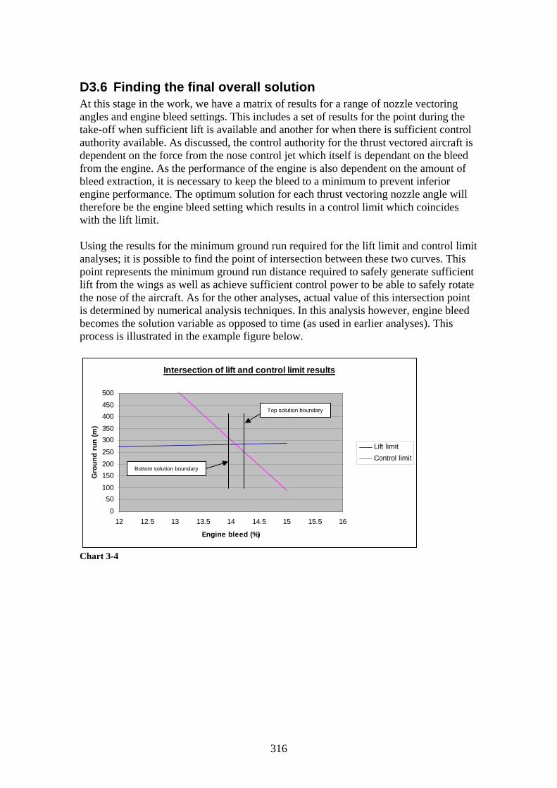
D3.6 Finding the final overall solution At this stage in the work, we have a matrix of results for a range of nozzle vectoring angles and engine bleed settings. This includes a set of results for the point during the take-off when sufficient lift is available and another for when there is sufficient control authority available. As discussed, the control authority for the thrust vectored aircraft is dependent on the force from the nose control jet which itself is dependant on the bleed from the engine. As the performance of the engine is also dependent on the amount of bleed extraction, it is necessary to keep the bleed to a minimum to prevent inferior engine performance. The optimum solution for each thrust vectoring nozzle angle will therefore be the engine bleed setting which results in a control limit which coincides with the lift limit. Using the results for the minimum ground run required for the lift limit and control limit analyses; it is possible to find the point of intersection between these two curves. This point represents the minimum ground run distance required to safely generate sufficient lift from the wings as well as achieve sufficient control power to be able to safely rotate the nose of the aircraft. As for the other analyses, actual value of this intersection point is determined by numerical analysis techniques. In this analysis however, engine bleed becomes the solution variable as opposed to time (as used in earlier analyses). This process is illustrated in the example figure below.

Intersection of lift and control limit results

0

50100

150200

250

300350

400450

500

12 12.5 13 13.5 14 14.5 15 15.5 16

Engine bleed (%)

Gro

und

run

(m)

Lift limitControl limit

Bottom solution boundary

Top solution boundary

Chart 3-4

316

D4 Landing analysis The complete landing phase typically consists of three phases, approach, flare and ground run. In this work, the flare has been integrated into the landing approach analysis resulting in two analyses to describe the landing performance of the aircraft. The first of these analyzes the flight path from the screen height to the point where the vertical velocity is zero and the aircraft is firmly on the ground. The second then analyzes the ground run to bring the aircraft to rest. The landing approach analysis is an iterative solution process involving a complex balance of the forces and moments acting on the aircraft, within which a range of vectoring angles and initial descent velocities are explored. The ground run analysis is a less complex balance of the deceleration forces acting on the aircraft. An additional analysis has investigated the potential of landing on an aircraft carrier, by means of a lower landing approach speed.

D4.1 Analysis parameters Presented in this section are the parameters required for these analyses. During these analyses, the aircraft is in its landing configuration with the Kruger flaps deployed and landing gear extended. These are discussed in the general terms section.

D4.1.1 Engine specific fuel consumption During the landing phases, the engine is throttled back and it is sufficient to use a typical figure of (kg/Ns) for the specific fuel consumption. This figure is however relative to the engine operating at its design condition, when it is delivering a thrust of 52730.77N. When the engine is operated at partial load, the SFC will vary from its design value as can be predicted by the expression below. Here T is the thrust of the engine at the off-design condition.

51010.2' −×=c

⎟⎟⎠

⎞⎜⎜⎝

⎛

⎥⎥⎦

⎤

⎢⎢⎣

⎡

⎭⎬⎫

⎩⎨⎧

−⋅+⋅= 101.01'T

TcSFC Design Eq 4-1

D4.2 Landing approach analysis The function of this analysis is to determine the performance of the aircraft during the landing approach phase. The exact process is a complex balance of the forces and moments acting on the aircraft to arrive at a solution for the performance of the aircraft at any instant.

D4.2.1 Derivations The arrangement of the aircraft in its descent configuration is given in the figure below along with the system of forces acting on it.

317

318

Figure 4-1 Summing the forces acting in the vertical direction, we obtain the relation below for the resultant force. ∑ ++−−+−= NoseJetInertiaDragLiftThrustZ LZLLWLF Eq 4-2 Inspection of the above figure, allows us to derive relations for each component as given below. As the aircraft is descending, the flight path angle in this analysis is negative. This results in the need for an extra minus sign in the relations.

1. ( ))( γφα −−+⋅= SinTLThrust Eq 4-3 2. gm Eq 4-4 W ⋅=3. ( )γCos Eq 4-5 LLLift ⋅=

4. ( )γSin Eq 4-6 DLDrag ⋅=

5. ZInertia amZ ⋅= Eq 4-7 6. ( )( )γα −−⋅= CosLL NJNoseJet Eq 4-8

In a similar way, summing the forces acting in the horizontal direction allows us to obtain the relation below for the resultant force. ∑ ++++= − NoseJetInertiaDragLiftXEngineX TXTTTF Eq 4-9 This is made up of the following components as derived from the figure above.

1. ( ))( γφα −−+⋅=− CosTT EngineXEngine Eq 4-10 2. ( )γSin Eq 4-11 LTLift ⋅=

3. ( )γCosDTDrag ⋅−= Eq 4-12 4. X Eq 4-13 Inertia amX ⋅−=5. ( ))( γα −− Eq 4-14 ⋅−= SinLT NJNoseJet

These relations will now be put into practice in the analyses that follow

D4.2.2 Analysis approach The complexity of this analysis has necessitated the need to break it down into a number of smaller sections in order to be able to present the procedure here. This is shown in the diagram below, which is intended to help the reader trace their steps. This diagram not only presents the function of each block but also highlights their inputs/outputs so that the inter-relation between the blocks can be better understood. Due to the complexity of the analysis, it is not possible to illustrate all the links between the blocks, as this could potentially obscure the function of the diagram. Instead, arrows between each block are used to remind the reader that a complex network of links exists.

Analysis 1 – Descent angle (γ)

Analysis 2 – Aircraft weight (W)

Analysis 3 – Wing-fuselage pitching moment (CM)

Analysis 4 – Aircraft pitching moment (CM(Untrimmed))

Analysis 5 – Nose jet lift force (LNosejet)

Analysis 6 – Solution for α for ΣFZ = 0

Analysis 7 – Solution for T for ΣFX = 0

Analysis 8 – Solution for tTouchdown for H = 0

Analysis 9 – Distance covered

tTouchdown

VZ

γ

T W

α Cm

α φ

T Cm

Cm(untrimmed)

Cm(untrimmed)

α

LNJ

T αφ

LNJ aZ m

LNJaX m

φ α T

VZtTouchdown

α

tTouchdown

VZ X

Analysis inputs – φ , VZ(0) , VApproach

Analysis outputs – X , tTouchdown , VTouchdown , mTouchdown

Analysis 1 – Descent angle (γ)

Analysis 2 – Aircraft weight (W)

Analysis 3 – Wing-fuselage pitching moment (CM)

Analysis 4 – Aircraft pitching moment (CM(Untrimmed))

Analysis 5 – Nose jet lift force (LNosejet)

Analysis 6 – Solution for α for ΣFZ = 0

Analysis 7 – Solution for T for ΣFX = 0

Analysis 8 – Solution for tTouchdown for H = 0

Analysis 9 – Distance covered

tTouchdown

VZ

γ

T W

α Cm

α φ

T Cm

Cm(untrimmed)

Cm(untrimmed)

α

LNJ

T αφ

LNJ aZ m

LNJaX m

φ α T

VZtTouchdown

α

tTouchdown

VZ X

Analysis inputs – φ , VZ(0) , VApproach

Analysis outputs – X , tTouchdown , VTouchdown , mTouchdown To be able to solve this analysis, an iterative solution process is required for the aircraft angle of attack and the engine thrust. The solution for the aircraft angle of attack is found as that value which gives a resultant vertical force of zero. In a similar way, the solution for the engine thrust is found as that value which gives a resultant horizontal force of zero. As an added complication, the angle of attack and engine thrust can be seen to be related to each other and it is therefore necessary to keep alternatively iterating each solution until both solutions converge. This process is summarised below.

Solution procedure for the landing approach analysis

Stage 1 – Iterate a until ΣFZ = 0Stage 2 – Iterate T until ΣFX = 0

Repeat Stage 1 and Stage 2 until ΣFZ and ΣFX = 0 This analysis is repeated for an array of combinations of the input parameters being investigated. This includes variations of the parameters:

1. φ - Thrust vectoring nozzle deflection angle 2. VZ(0) - Initial vertical descent velocity of the aircraft at the screen height 3. VApproach - Approach speed of the aircraft at the screen height

319

The approach speed (VApproach) is different for land based and carrier based aircraft. In this particular analysis, the aircraft is assumed to be land based but a carrier variant is considered in a later section. In this analysis, the approach speed is StallApproach VV ⋅= 2.1 .The array of values of φ and VZ(0) investigated in this analysis are presented in the table below which gave a total of 28 analysis cases for each combination of input variables.

Vectoring angle (φ) Inputs 0 5 10 15 20 25 30

2.5 C1 C2 C3 C4 C5 C6 C7 5 C8 C9 C10 C11 C12 C13 C14

7.5 C15 C16 C17 C18 C19 C20 C21 VZ(0)

10 C22 C23 C24 C25 C26 C27 C28 Table 4-1 The analysis outputs of particular importance include:

• X – Ground distance covered to the point of touchdown. • tTouchdown – The time taken until the vertical descent velocity equals zero. • VTouchdown – The aircraft velocity at the point when the vertical velocity is zero. • mTouchdown – The aircraft mass at the point when the vertical velocity equals zero.

In the sections which follow, each of the individual analysis blocks making up the complete analysis will be presented to the reader in an easy to follow flow chart format. To improve the accuracy of the results, the flight phase is broken down into a number of smaller steps which can be analysed sequentially. In cases where an iterative solution process is required, this is automated with the Solver function of Microsoft Excel.

D4.2.3 Analysis stage 1 – Descent angle The function of this stage of the analysis is to determine the descent angle of the aircraft at each time step, as required by the other analysis stages. In this flight phase, the descent angle not fixed and can be seen to vary throughout the flight stage in relation to the changes in the aircraft X and Z velocity components. The solution to this stage is therefore a function of the horizontal and vertical velocity components as is presented in the equation flowchart below.

320

⎟⎟⎠

⎞⎜⎜⎝

⎛=

X

Z

VV

ATANγ

( ) ( )11)1(

2 −−− +−⎟⎟⎠

⎞⎜⎜⎝

⎛ += iXi

iXXX Vtt

aaV

( ) ( )11)1(

2 −−− +−⎟⎟⎠

⎞⎜⎜⎝

⎛ +−= iZi

iZZZ Vtt

aaV

StartEnd

StartXEndXX tt

VVa

−

−= )()(

StartEnd

StartZEndZZ tt

VVa

−

−−= )()(

2)0(

20)0( ZX VVV −=FixedInputVZ =)0(

2)(

2)( FinalZFinalFinalX VVV −=

StallApproach VV ⋅= 2.1StallFinal VV ⋅= 1.1

StallV

0)( =FinalZV

StallCarrierApproach VV ⋅= 15.1)(⎟⎟⎠

⎞⎜⎜⎝

⎛=

X

Z

VV

ATANγ

( ) ( )11)1(

2 −−− +−⎟⎟⎠

⎞⎜⎜⎝

⎛ += iXi

iXXX Vtt

aaV

( ) ( )11)1(

2 −−− +−⎟⎟⎠

⎞⎜⎜⎝

⎛ +−= iZi

iZZZ Vtt

aaV

StartEnd

StartXEndXX tt

VVa

−

−= )()(

StartEnd

StartZEndZZ tt

VVa

−

−−= )()(

2)0(

20)0( ZX VVV −=FixedInputVZ =)0(

2)(

2)( FinalZFinalFinalX VVV −=

StallApproach VV ⋅= 2.1StallFinal VV ⋅= 1.1

StallV

0)( =FinalZV

⎟⎟⎠

⎞⎜⎜⎝

⎛=

X

Z

VV

ATANγ

( ) ( )11)1(

2 −−− +−⎟⎟⎠

⎞⎜⎜⎝

⎛ += iXi

iXXX Vtt

aaV

( ) ( )11)1(

2 −−− +−⎟⎟⎠

⎞⎜⎜⎝

⎛ +−= iZi

iZZZ Vtt

aaV

StartEnd

StartXEndXX tt

VVa

−

−= )()(

StartEnd

StartZEndZZ tt

VVa

−

−−= )()(

2)0(

20)0( ZX VVV −=FixedInputVZ =)0(

2)(

2)( FinalZFinalFinalX VVV −=

StallApproach VV ⋅= 2.1StallFinal VV ⋅= 1.1

StallV

0)( =FinalZV

StallCarrierApproach VV ⋅= 15.1)(

D4.2.4 Analysis stage 2 – Aircraft weight The function of this stage of the analysis is to determine the mass and weight of the aircraft at each time step, as required by the other analysis stages. The solution is directly related to the engine thrust and specific fuel consumption, as presented in the flow chart below. As clarification, is the mass of the aircraft at the start of the approach phase and is the total mass of fuel used up to that point.

)0(ACm

)0(Fuelm

321

gmW ⋅=

( ))0()0( FuelFuelACAC mmmm −−=

( ) ( )11 −− +−= iFueliFFuel mttQm

SFCTQF ⋅=

⎟⎟⎠

⎞⎜⎜⎝

⎛

⎥⎥⎦

⎤

⎢⎢⎣

⎡

⎭⎬⎫

⎩⎨⎧

−⋅+⋅= 101.01'T

TcSFC Design

)0(ACm )0(Fuelm

VariableT =

gmW ⋅=

( ))0()0( FuelFuelACAC mmmm −−=

( ) ( )11 −− +−= iFueliFFuel mttQm

SFCTQF ⋅=

⎟⎟⎠

⎞⎜⎜⎝

⎛

⎥⎥⎦

⎤

⎢⎢⎣

⎡

⎭⎬⎫

⎩⎨⎧

−⋅+⋅= 101.01'T

TcSFC Design

)0(ACm )0(Fuelm

VariableT =

D4.2.5 Analysis stage 3 – Wing-fuselage pitching moment The function of this stage of the analysis is to determine the wing-fuselage pitching moment coefficient at each step, as presented in the flow chart below. The solution is a function of the variable aircraft angle of attack, as required by analysis stage 4 to determine the untrimmed pitching moment of the aircraft.

LL

mm C

CC

C ⋅=

( )πα

α

180⋅=

L

m

L

m

CC

CC

αLC

⎟⎠⎞

⎜⎝⎛ ⋅⋅⎟

⎠

⎞⎜⎝

⎛⋅⎟⎟⎠

⎞⎜⎜⎝

⎛−=

παα180

LRoot

Root

AC

Root

CGm C

cC

CX

CX

C

[ ]( )Root

MACACW

Root

AC

CXccX

CX +⋅

=

ACWX1000/

10001000

2

⎥⎥⎦

⎤

⎢⎢⎣

⎡+⎟⎟

⎠

⎞⎜⎜⎝

⎛⋅+⎟⎟

⎠

⎞⎜⎜⎝

⎛⋅= C

MB

MAX AircraftAircraft

CG

( )LWLL iCC 0ααα −+⋅=

Variable=α

LL

mm C

CC

C ⋅=

( )πα

α

180⋅=

L

m

L

m

CC

CC

αLC

⎟⎠⎞

⎜⎝⎛ ⋅⋅⎟

⎠

⎞⎜⎝

⎛⋅⎟⎟⎠

⎞⎜⎜⎝

⎛−=

παα180

LRoot

Root

AC

Root

CGm C

cC

CX

CX

C

[ ]( )Root

MACACW

Root

AC

CXccX

CX +⋅

=

ACWX1000/

10001000

2

⎥⎥⎦

⎤

⎢⎢⎣

⎡+⎟⎟

⎠

⎞⎜⎜⎝

⎛⋅+⎟⎟

⎠

⎞⎜⎜⎝

⎛⋅= C

MB

MAX AircraftAircraft

CG

( )LWLL iCC 0ααα −+⋅=

Variable=α

D4.2.6 Analysis stage 4 – Aircraft pitching moment The function of this stage of the analysis is to determine the total aircraft pitching moment coefficient at each time step, as presented in the flow chart below. The solution, which is a function of α, φ and T as well as the wing-fuselage pitching

322

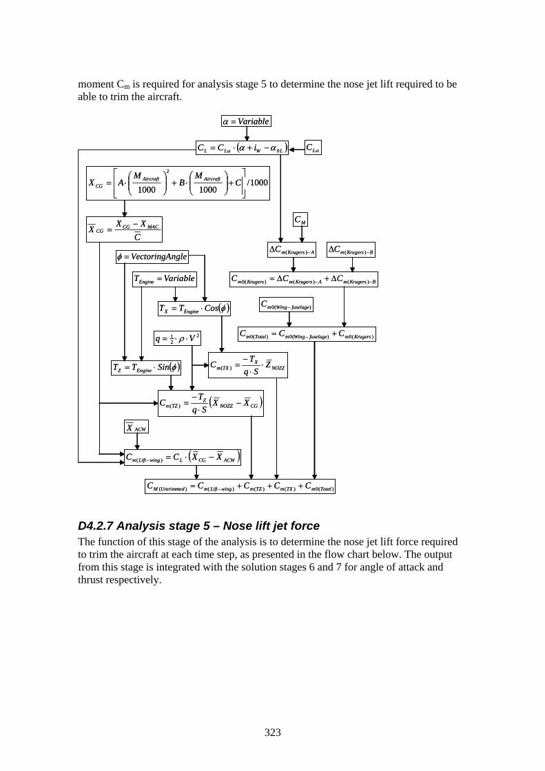
moment Cm is required for analysis stage 5 to determine the nose jet lift required to be able to trim the aircraft.

( )LWLL iCC 0ααα −+⋅=

AKrugersmC −Δ )(

BKrugersmAKrugersmKrugersm CCC −− Δ+Δ= )()()(0

)(0)(0)(0 KrugersmfuselageWingmTotalm CCC += −

( )φCosTT EngineX ⋅=

( )φSinTT EngineZ ⋅= NOZZX

TXm ZSq

TC ⋅⋅

−=)(

( )CGNOZZZ

TZm XXSq

TC −

⋅−

=)(

ACWX

( )ACWCGLwingLiftm XXCC −⋅=− )(

221 Vq ⋅⋅= ρ

1000/10001000

2

⎥⎥⎦

⎤

⎢⎢⎣

⎡+⎟⎟

⎠

⎞⎜⎜⎝

⎛⋅+⎟⎟

⎠

⎞⎜⎜⎝

⎛⋅= C

MB

MAX AircraftAircraft

CG

)(0)()()()( TotalmTXmTZmwingLiftmUntrimmedM CCCCC +++= −

CXX

X MACCGCG

−=

BKrugersmC −Δ )(

VariableTEngine =

ngleVectoringA=φ

MC

Variable=α

)(0 fuselageWingmC −

αLC( )LWLL iCC 0ααα −+⋅=

AKrugersmC −Δ )(

BKrugersmAKrugersmKrugersm CCC −− Δ+Δ= )()()(0

)(0)(0)(0 KrugersmfuselageWingmTotalm CCC += −

( )φCosTT EngineX ⋅=

( )φSinTT EngineZ ⋅= NOZZX

TXm ZSq

TC ⋅⋅

−=)(

( )CGNOZZZ

TZm XXSq

TC −

⋅−

=)(

ACWX

( )ACWCGLwingLiftm XXCC −⋅=− )(

221 Vq ⋅⋅= ρ

1000/10001000

2

⎥⎥⎦

⎤

⎢⎢⎣

⎡+⎟⎟

⎠

⎞⎜⎜⎝

⎛⋅+⎟⎟

⎠

⎞⎜⎜⎝

⎛⋅= C

MB

MAX AircraftAircraft

CG

)(0)()()()( TotalmTXmTZmwingLiftmUntrimmedM CCCCC +++= −

CXX

X MACCGCG

−=

BKrugersmC −Δ )(

VariableTEngine =

ngleVectoringA=φ

MC

Variable=α

)(0 fuselageWingmC −

αLC

D4.2.7 Analysis stage 5 – Nose lift jet force The function of this stage of the analysis is to determine the nose jet lift force required to trim the aircraft at each time step, as presented in the flow chart below. The output from this stage is integrated with the solution stages 6 and 7 for angle of attack and thrust respectively.

323

NJCG

UntrimmedMNJ XX

SqCL

−

⋅⋅−= )(

( )( )γα −−⋅= CosLL NJNoseJet

221 Vq ⋅⋅= ρ

1000/10001000

2

⎥⎥⎦

⎤

⎢⎢⎣

⎡+⎟⎟

⎠

⎞⎜⎜⎝

⎛⋅+⎟⎟

⎠

⎞⎜⎜⎝

⎛⋅= C

MB

MAX AircraftAircraft

CG

CXX

X MACCGCG

−= )(UntrimmedMC

Variable=αNJCG

UntrimmedMNJ XX

SqCL

−

⋅⋅−= )(

( )( )γα −−⋅= CosLL NJNoseJet

221 Vq ⋅⋅= ρ

1000/10001000

2

⎥⎥⎦

⎤

⎢⎢⎣

⎡+⎟⎟

⎠

⎞⎜⎜⎝

⎛⋅+⎟⎟

⎠

⎞⎜⎜⎝

⎛⋅= C

MB

MAX AircraftAircraft

CG

CXX

X MACCGCG

−= )(UntrimmedMC

Variable=α

D4.2.8 Analysis stage 6 – Solution for angle of attack The function of this stage is to determine the solution for the optimal angle of the aircraft at each time step, as presented in the flow chart below. The solution is a function of the input parameters T, φ, LNJ, az and m, which are used to determine the sum of the vertical force components acting on the aircraft at any moment in time. By iterating the input variable α, we are able to determine the value required to achieve a resultant vertical force of zero. This analysis block is therefore the basis of the first stage of the solution process.

324

∑ ++−−+−= NoseJetInertiaDragLiftThrustZ LZLLWLF

( )( )γφα −−+⋅= SinTLThrust

gmW ⋅=

( )γCosLLLift ⋅=

( )γSinDLDrag ⋅=

DCSVD ⋅⋅⋅⋅= 221 ρ

LCSVL ⋅⋅⋅⋅= 221 ρ

22ZX VVV +=

( )LWLL iCC 0ααα −+⋅=

αLC

( )2)( LLandingDZD CKCC ⋅+=

K)()()( LandingDZBasicDZLandingDZ CCC Δ+=

)(33.0)(15.0

LandingDLF

LandingDZ CAR

FC +⎟⎠⎞

⎜⎝⎛ ⋅

=Δ

ZInertia amZ ⋅=

)(BasicDZC

( )( )γα −−⋅= CosLL NJNoseJetAircraftm

Variable=α

VariableT =

NJL

Za

ngleVectoringA=φ

∑ ++−−+−= NoseJetInertiaDragLiftThrustZ LZLLWLF

( )( )γφα −−+⋅= SinTLThrust

gmW ⋅=

( )γCosLLLift ⋅=

( )γSinDLDrag ⋅=

DCSVD ⋅⋅⋅⋅= 221 ρ

LCSVL ⋅⋅⋅⋅= 221 ρ

22ZX VVV +=

( )LWLL iCC 0ααα −+⋅=

αLC

( )2)( LLandingDZD CKCC ⋅+=

K)()()( LandingDZBasicDZLandingDZ CCC Δ+=

)(33.0)(15.0

LandingDLF

LandingDZ CAR

FC +⎟⎠⎞

⎜⎝⎛ ⋅

=Δ

ZInertia amZ ⋅=

)(BasicDZC

( )( )γα −−⋅= CosLL NJNoseJetAircraftm

Variable=α

VariableT =

NJL

Za

ngleVectoringA=φ

D4.2.9 Analysis stage 7 – Solution for thrust The function of this stage is to determine the solution for the optimal engine thrust of the aircraft at each time step, as presented in the flow chart below. The solution is a function of the input parameters α, φ, LNJ, ax and m, which are used to determine the sum of the horizontal force components acting on the aircraft at any moment in time. By iterating the input variable Τ, we are able to determine the value of Τ required to achieve a resultant horizontal force of zero. This analysis block is therefore the basis of the second stage of the solution process.

325

∑ ++++= − NoseJetInertiaDragLiftXEngineX TXTTTF

( )( )γφα −−+⋅=− CosTT EngineXEngine

( )γSinLTLift ⋅=

( )γCosDTDrag ⋅−=

XInertia amX ⋅−=

( )( )γα −−⋅−= SinLT NJNoseJet

DCSVD ⋅⋅⋅⋅= 221 ρ

LCSVL ⋅⋅⋅⋅= 221 ρ

22ZX VVV +=

( )LWLL iCC 0ααα −+⋅=

αLC

( )2)( LLandingDZD CKCC ⋅+=

K)()()( LandingDZBasicDZLandingDZ CCC Δ+=

)(33.0)(15.0

LandingDLF

LandingDZ CAR

FC +⎟⎠⎞

⎜⎝⎛ ⋅

=Δ)(BasicDZC

Aircraftm

Variable=α

VariableT =

NJL

Xa

ngleVectoringA=φ

∑ ++++= − NoseJetInertiaDragLiftXEngineX TXTTTF

( )( )γφα −−+⋅=− CosTT EngineXEngine

( )γSinLTLift ⋅=

( )γCosDTDrag ⋅−=

XInertia amX ⋅−=

( )( )γα −−⋅−= SinLT NJNoseJet

DCSVD ⋅⋅⋅⋅= 221 ρ

LCSVL ⋅⋅⋅⋅= 221 ρ

22ZX VVV +=

( )LWLL iCC 0ααα −+⋅=

αLC

( )2)( LLandingDZD CKCC ⋅+=

K)()()( LandingDZBasicDZLandingDZ CCC Δ+=

)(33.0)(15.0

LandingDLF

LandingDZ CAR

FC +⎟⎠⎞

⎜⎝⎛ ⋅

=Δ)(BasicDZC

Aircraftm

Variable=α

VariableT =

NJL

Xa

ngleVectoringA=φ

D4.2.10 Analysis stage 8 – Time to touchdown The function of this stage is to determine the total time taken to complete the approach phase of the complete landing phase, as is presented in the flow chart below. This is based on the time taken to descent from the screen height, utilising expressions to determine the altitude at each time step. The time to touchdown is not only the time taken to descend from the screen height but also the time to reach the point where the vertical velocity equals zero. A particularly important factor within this analysis is the initial vertical descent velocity, which is one of the input variables under investigation.

326

( ) ( ) ( )12

1)1(

1 221

−−−

− +−⎟⎟⎠

⎞⎜⎜⎝

⎛ +−⋅+−⋅= ii

iZZiZ Htt

aattVH

StartEnd

StartZEndZZ tt

VVa

−

−−= )()(

( ) mH 24.150 =

riableAnalysisVaVZ =)0(

0)( =FinalZV

( ) mH Final 0=

( ) ( )11)1(

2 −−− +−⎟⎟⎠

⎞⎜⎜⎝

⎛ +−= iZi

iZZZ Vtt

aaV

( ) Solutiont Final =

( ) ( ) ( )12

1)1(

1 221

−−−

− +−⎟⎟⎠

⎞⎜⎜⎝

⎛ +−⋅+−⋅= ii

iZZiZ Htt

aattVH

StartEnd

StartZEndZZ tt

VVa

−

−−= )()(

( ) mH 24.150 =

riableAnalysisVaVZ =)0(

0)( =FinalZV

( ) mH Final 0=

( ) ( )11)1(

2 −−− +−⎟⎟⎠

⎞⎜⎜⎝

⎛ +−= iZi

iZZZ Vtt

aaV

( ) Solutiont Final =

D4.2.11 Analysis stage 9 – Distance covered The function of this stage is to determine the total horizontal distance covered during the approach phase as presented in the flow chart below. This process enables the distance to be determined at each time step which collectively gives the total distance covered. The total distance in this flight phase is the horizontal distance flown between the point of the screen height and the point where the vertical velocity equals zero. The input variables in this analysis are α, VZ and tTouchdown (from the previous analysis stages) and the output X is one of the final analysis solutions.

327

)(

2

MaxLStall CS

LV⋅⋅⋅

=ρ

2)0(

2)0( ZApproachX VVV −=

( ) ( )11)1(

2 −−− +−⎟⎟⎠

⎞⎜⎜⎝

⎛ += iXi

iXXX Vtt

aaV

( ) StallFinal VV ⋅= 1.1 ( ) mX 00 =

riableAnalysisVaVZ =)0(

( ) ( ) ( )12

1)1(

1 221

−−−

− +−⎟⎟⎠

⎞⎜⎜⎝

⎛ +⋅+−⋅= ii

iXXiX Xtt

aattVX

StartEnd

StartXEndXX tt

VVa

−

−= )()(

2)(

2)( FinalZFinalFinalX VVV −=

0)( =FinalZV

StallApproach VV ⋅= 2.1

LCSVL ⋅⋅⋅⋅= 221 ρ

)(MaxLC

( )LWLL iCC 0ααα −+⋅=

( ) SolutionX Final =StallCarrierApproach VV ⋅= 15.1)(

Variable=α

VariabletFinal =

)(

2

MaxLStall CS

LV⋅⋅⋅

=ρ

2)0(

2)0( ZApproachX VVV −=

( ) ( )11)1(

2 −−− +−⎟⎟⎠

⎞⎜⎜⎝

⎛ += iXi

iXXX Vtt

aaV

( ) StallFinal VV ⋅= 1.1 ( ) mX 00 =

riableAnalysisVaVZ =)0(

( ) ( ) ( )12

1)1(

1 221

−−−

− +−⎟⎟⎠

⎞⎜⎜⎝

⎛ +⋅+−⋅= ii

iXXiX Xtt

aattVX

StartEnd

StartXEndXX tt

VVa

−

−= )()(

2)(

2)( FinalZFinalFinalX VVV −=

0)( =FinalZV

StallApproach VV ⋅= 2.1

LCSVL ⋅⋅⋅⋅= 221 ρ

)(MaxLC

( )LWLL iCC 0ααα −+⋅=

( ) SolutionX Final =StallCarrierApproach VV ⋅= 15.1)(

Variable=α

VariabletFinal =

D4.3 Landing ground run analysis The function of this analysis is to determine the performance of the aircraft during the landing ground run phase. The starting point for this analysis is the results from the landing approach phase. This process is however a less complex balance of the deceleration forces acting on the aircraft.

D4.3.1 Derivations The arrangement of the aircraft in its landing ground run configuration is given in the figure below along with the system of forces acting on it.

328

329

Figure 4-2 In this analysis, the aircraft is assumed to have all its wheels in contact with the ground and the vertical acceleration . We have also assumed that the engine is at idle and therefore any thrust is negligible. Since no pitch control is required, the lift force from the nose jet is assumed to be zero. At this stage we could be misled into thinking that the lift from the wings is zero since the angle of attack of the aircraft is assumed to be zero. This is not the case however since the wing is still being presented to the airflow at an angle due to the setting angle of the landing gear as well as the angle of zero lift for the wing. This can be observed in the relation for CL,

0=Za

( )LWLL iCC 0ααα −+⋅= . In reality however, the effect of the landing gear setting angle is likely to be less than that assumed here. The forward inertia of the aircraft as a result of the aircraft braking will generate a moment about the rear wheels which will compress the nose landing gear strut and therefore reduce the setting angle. Inspection of the forces acting on the aircraft in the vertical direction gives the expression, LWR −= . Here R is the ground reaction from the wheels which is directly related to the aircraft braking force . In a similar way, the forces acting in the aircraft in the horizontal direction, gives the expression,

RF( )RX FDTF +−= Eq 4-15

This is made up of the following components: 1. 0@ = IdleEngineT

2. )(2

21

LandingDCSVD ⋅⋅⋅⋅= ρ Eq 4-16 3. ( ) RF BRR ⋅+= μμ Eq 4-17

RF is the total horizontal decelerating friction force, which is the sum of that due to the rolling friction of the tyres ( 03.0=Rμ ) and that due to the application of the brakes ( 3.0=Bμ ). These relations will now be put into practice in the analyses that follow.

D4.3.2 Analysis approach The analysis for the landing ground run is considerably less complex than that for the landing approach phase as given by the flowchart below. As with the landing approach analyses, to improve the accuracy of the results, the flight phase is broken down into a number of smaller steps which can be analysed sequentially. Where required, the Solver function Microsoft Excel is used for iterative solutions. By this method, the summation of the ground run distance as determined at each time step gives the total ground distance covered until the aircraft comes to a rest.

Although the aircraft is on the ground, the setting angle of the landing gear means that the wing is still generating a small amount of lift, which will affect the vertical reaction force on the wheels and thus the decelerating force. The input parameters for this phase are the output parameters from the previous landing approach flight phase. The ones of particular concern here are VTouchdown and mTouchdown. The parameter mTouchdown is assumed to remain constant during this phase since no (or negligible) fuel is being consumed when the engine is at idle.

( ) ( ) ( )12

1)1(

1 221

−−−

− +−⎟⎟⎠

⎞⎜⎜⎝

⎛ +⋅+−⋅= iGi

iXXiXG Stt

aattVS

( ) ( )11)1( −−− +−= iXiiXX VttaVAircraft

XX m

Fa =

( )RX FDTF +−=

DCSVD ⋅⋅⋅⋅= 221 ρ ( ) RF BRR ⋅+= μμ

22ZX VVV +=

( )2)( LLandingDZD CKCC ⋅+=

)()()( LandingDZBasicDZLandingDZ CCC Δ+=

)(33.0)(15.0

LandingDLF

LandingDZ CAR

FC +⎟⎠⎞

⎜⎝⎛ ⋅

=Δ

LWR −=

LCSVL ⋅⋅⋅⋅= 221 ρ

( )LWLL iCC 0ααα −+⋅=

αLC

K

0=ZV

)(BasicDZC

gmW ⋅=

FixedmAircraft =

0=α deg5=Wi

StallTouchdown VVV ⋅== 1.10

0=T

0=Za

( ) ( ) ( )12

1)1(

1 221

−−−

− +−⎟⎟⎠

⎞⎜⎜⎝

⎛ +⋅+−⋅= iGi

iXXiXG Stt

aattVS

( ) ( )11)1( −−− +−= iXiiXX VttaVAircraft

XX m

Fa =

( )RX FDTF +−=

DCSVD ⋅⋅⋅⋅= 221 ρ ( ) RF BRR ⋅+= μμ

22ZX VVV +=

( )2)( LLandingDZD CKCC ⋅+=

)()()( LandingDZBasicDZLandingDZ CCC Δ+=

)(33.0)(15.0

LandingDLF

LandingDZ CAR

FC +⎟⎠⎞

⎜⎝⎛ ⋅

=Δ

LWR −=

LCSVL ⋅⋅⋅⋅= 221 ρ

( )LWLL iCC 0ααα −+⋅=

αLC

K

0=ZV

)(BasicDZC

gmW ⋅=

FixedmAircraft =

0=α deg5=Wi

StallTouchdown VVV ⋅== 1.10

0=T

( ) ( ) ( )12

1)1(

1 221

−−−

− +−⎟⎟⎠

⎞⎜⎜⎝

⎛ +⋅+−⋅= iGi

iXXiXG Stt

aattVS

( ) ( )11)1( −−− +−= iXiiXX VttaVAircraft

XX m

Fa =

( )RX FDTF +−=

DCSVD ⋅⋅⋅⋅= 221 ρ ( ) RF BRR ⋅+= μμ

22ZX VVV +=

( )2)( LLandingDZD CKCC ⋅+=

)()()( LandingDZBasicDZLandingDZ CCC Δ+=

)(33.0)(15.0

LandingDLF

LandingDZ CAR

FC +⎟⎠⎞

⎜⎝⎛ ⋅

=Δ

LWR −=

LCSVL ⋅⋅⋅⋅= 221 ρ

( )LWLL iCC 0ααα −+⋅=

αLC

K

0=ZV

)(BasicDZC

gmW ⋅=

FixedmAircraft =

0=α deg5=Wi

StallTouchdown VVV ⋅== 1.10

0=T

0=Za

D4.4 Aircraft carrier landing analysis In the case of the analysis for landing on an aircraft carrier, the only difference is the landing approach speed which now becomes StallApproach VV ⋅= 15.1 . This is considered to be the only variation between the land based and carrier base analyses. In reality however, a carrier aircraft is unlikely to be subject to the requirement to clear a landing approach screen height. In addition, there is likely to be an additional braking force due to an arresting hook. In this analysis however we have assumed that an arresting hook is not used. We are therefore making an assessment of the viability of landing a land based aircraft on an aircraft carrier without any modifications to the aircraft.

330

331

D5 Wing size reduction investigation The take-off analysis studies carried out on the thrust vectored variant of the baseline aircraft raised the question whether the incorporation of such a system would enable a smaller wing to be used. The rationale for this is that, compared to the baseline aircraft, the thrust vectored aircraft has additional components of lift from the thrust vectoring system. These include the vertical components of thrust from the deflected thrust vectoring nozzle and the thrust from the nose jet. Our initial thoughts are that these additional components of lift should mean that the lift requirements of our wing during the take-off phase are reduced. The same argument is also true for the aircraft during the landing phase. If we refer back to the constraint analysis which was carried out for our baseline design, we can see that the final size of a wing is typically governed by either the take-off or landing boundaries. Our initial thoughts are therefore that the addition of a thrust vectoring system would result in our wing being oversized to meet our original requirements. The aim of this study was therefore to test these predictions and examine the impact of reducing the size of the wing and how this compares with the performance of our baseline design. The approach adopted in this study was to test a number of variants of the thrust vectored aircraft, each with a different wing size. The results of which will enable us to establish a trend between wing size and take-off performance for the thrust vectored aircraft.

D5.1 Wing resizing As mentioned above, the approach adopted in this study was to analyse the performance of a number of variants of the baseline design. Each of which has a different wing size and therefore different characteristics. If we take another look at the aircraft conceptual design process, we will see that a reduction in the wing area is accompanied by variations in:

• Aircraft mass (empty and take-off) • Mission fuel requirements (as result of revised L/D characteristics) • Drag (lift induced drag and zero lift) • Wing geometry • T/W and W/S boundaries

Since the wing area has such a considerable impact on many other parts of the aircraft and its characteristics, it was necessary to repeat the conceptual design process for each aircraft variant. This process is discussed below. Although variations in wing area will have a considerable impact on the vast majority of the aircraft parameters, some of these are expected to retain their original figures as derived for the baseline design. This includes:

• Fuselage mass – Fixed at 1318.99kg • Systems mass – Fixed at 1038.06kg • Powerplant mass – Fixed at 1505.06kg • Take-off thrust – Fixed at 52730.77N

• Wing t/c ratio – Fixed at 12% • Wing aspect ratio – Fixed at 2.54

The process followed was to fix the aircraft wing area at a number of values, which were a fraction of the original wing area as given by the following expression. The values tested in this study were, 50-100% in 10% steps. Where, . 24194.53 mSBaseline =

100% )(

)(iVariant

BaselineiVariant

SSS ⋅= Eq 5-1

This design exercise gave us the following results for the different variants. Aircraft configurations

%SVariant(i) SVariant (m2) Mo (kg) MEmpty (kg) MFuel (kg) MWing (kg) CdzCruise KvCruise L/DCruise

100 53.4194034 8650.487 4523.54385 2312.574 661.43728 0.010393 0.177667 9.57268290 48.077463 8616.954 4490.71431 2311.871 628.60774 0.010503 0.177667 9.52238580 42.7355227 8582.28 4456.10471 2311.806 593.99814 0.010628 0.177667 9.46647170 37.3935824 8546.323 4419.35347 2312.6 557.2469 0.010771 0.177667 9.40347860 32.051642 8508.921 4379.96049 2314.591 517.85392 0.010938 0.177667 9.33127950 26.7097017 8469.896 4337.19993 2318.327 475.09336 0.011139 0.177667 9.246601

Table 5-1

Wing geometry for aicraft confiurations

%SVariant(i) SVariant (m2) CRoot (m) b (m) MAC (m)

100 53.4194034 8.338155 11.6484 5.60930490 48.077463 7.910268 11.05065 5.32145380 42.7355227 7.457873 10.41865 5.01711470 37.3935824 6.976201 9.745753 4.69308160 32.051642 6.458707 9.022814 4.34494850 26.7097017 5.895966 8.236665 3.966377

Table 5-2

D5.2 Take-off analyses Since the take-off phase is the critical flight phase with respect to lift requirements, this study is limited to this phase. The take-off performance analysis, as performed on each of the variants being studied, follows exactly the same process as that used in the thrust vectoring take-off performance analysis. The obvious difference being the substitution of different aircraft parameters as determined above. To reiterate, the analyses covered by this study includes:

1. Lift limit analysis 2. Thrust vectoring control limit 3. Conventional elevons control limit

Whereas, the original take-off analysis study also considered the effect of varying the landing gear setting angle, it is assumed to be fixed at 5 degrees in this study.

332

E1 Fuel cell system design requirements In our baseline aircraft constraint analysis, we determined the thrust required from our propeller to meet our performance constraints. As part of our design work, we were also able to predict the propeller efficiency, which enables us to determine the propeller input shaft power required. The purpose of this section is to determine the fuel cell system power requirements, taking into account losses within the power train. This includes all the losses between the fuel cell output and the propeller. In this analysis we are particularly interested in those losses from, the propeller, gearbox and controller. Losses from other power train components are assumed to be negligible in comparison.

E1.1 An overview of the fuel cell system power train A schematic of the fuel cell system power train is presented below to help the reader familiarise themselves with the power train.

Motor 1

Motor 2

Motor 1

Motor 2

Controller 1Controller 1

Controller 2Controller 2

InverterDC/ACInverterDC/AC

ConverterDC/DCConverterDC/DC

BatteryBattery

Fuel Cell

Anode

Cathode

Fuel Cell

Anode

Cathode

1122

33

44

55

66

77

88

991010

1111

1212

Power off-takes for other aircraft external loads12

Power off-takes for fuel cell system balance of plant11

Battery for system start-up and back-up10

Aircraft propeller9

2 into 1 reduction drive gearbox8

Drive motor 27

Drive motor 16

Controller for drive motor 25

Controller for drive motor 14

DC/AC inverter for drive power output3

DC/DC inverter for auxiliary system loads2

Fuel cell1

DescriptionNo.

Power off-takes for other aircraft external loads12

Power off-takes for fuel cell system balance of plant11

Battery for system start-up and back-up10

Aircraft propeller9

2 into 1 reduction drive gearbox8

Drive motor 27

Drive motor 16

Controller for drive motor 25

Controller for drive motor 14

DC/AC inverter for drive power output3

DC/DC inverter for auxiliary system loads2

Fuel cell1

DescriptionNo.

Figure 1-1 The power delivered by the fuel cell is DC and must therefore first pass through an inverter to change it to the AC power required by the electrical traction components. This AC power is then fed to the AC traction motor via a motor controller, which is used to regulate the speed and torque of the motor. As can be seen from the figure, there is also the need to draw DC power from the fuel cell output, which is used for power off-takes such as auxiliary equipment and other aircraft loads. A DC/DC converter is included in the system in order to condition and regulate this DC power off-take. Also included in this circuit is a battery which will be used to aid system start-up and supply power to the essential systems in the event of a failure. The most suitable battery for this

333

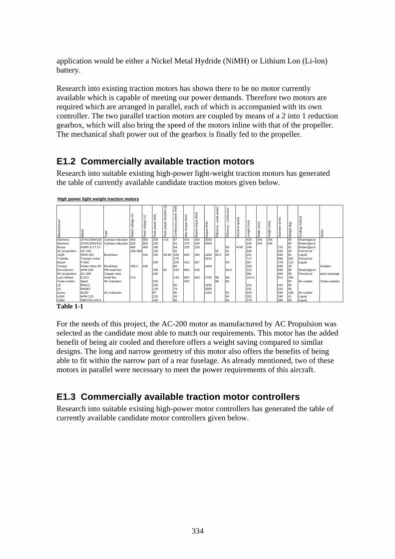
application would be either a Nickel Metal Hydride (NiMH) or Lithium Lon (Li-lon) battery. Research into existing traction motors has shown there to be no motor currently available which is capable of meeting our power demands. Therefore two motors are required which are arranged in parallel, each of which is accompanied with its own controller. The two parallel traction motors are coupled by means of a 2 into 1 reduction gearbox, which will also bring the speed of the motors inline with that of the propeller. The mechanical shaft power out of the gearbox is finally fed to the propeller.

E1.2 Commercially available traction motors Research into suitable existing high-power light-weight traction motors has generated the table of currently available candidate traction motors given below. High power light weight traction motors

Man

ufac

ture

r

Mod

el

Type

Rat

ed v

olta

ge (V

)

Pea

k vo

ltage

(V)

Pea

k po

wer

(kW

)

Pea

k po

wer

dur

atio

n (s

)

Con

tinuo

us p

ower

(kW

)

Max

torq

ue (N

m)

Rat

ed to

rque

(Nm

)

Rat

ed R

PM

Effi

cenc

y - p

eak

pow

er

Effi

cenc

y - c

ontin

uous

Nom

inal

spe

ed

Leng

th (m

m)

Wid

th (m

m)

Hei

ght (

mm

)

Dia

met

er (m

m)

Wei

ght (

kg)

Coo

ling

met

hod

Not

es

Siemens 1PV5135WS28 3-phase induction 650 900 200 <15 67 430 160 3500 425 245 245 90 Water/glycolSiemens 1PV5135WS24 3-phase induction 520 900 150 61 370 160 3500 425 245 245 90 Water/glycolBrusa HSM1-6.17.12 400 400 108 64 220 130 95 4700 245 270 51 Water/glycolAC propulsion AC-150 336-360 150 50 91 91 350 245 50 Forced airUQM HPM-150 Brushless 420 150 30-90 100 650 400 1650 92.5 95 241 405 91 LiquidToshiba Traction motor 275 3010 717 458 392 Forced airRaser P-200 200 100 415 207 93 457 279 112 LiquidYuneec Power drive 60 Brushless 166.5 190 60 2400 209 280 30 AviationEvo Electric AFM-240 PM axial flux 335 60 150 800 440 96.5 222 400 80 Water/glycolAC propulsion AC-200 Copper rotor 200 381 305 50 Forced air tzero packageLynx Motion E-813 Axial flux 574 130 900 450 2750 98 98 162.4 813 295Tesla motors Sport AC induction 215 400 80 90 52 Air cooled Tesla roadsterLE M40L2 140 90 3250 191 410 90LE M40B2 120 78 3000 191 510 95Azure AC90 AC-induction 97 50 1350 92 520 394 189 Air cooledUQM HPM 125 125 45 94 252 280 41 LiquidUQM SMP218-143-3 145 85 94 279 280 50 Liquid Table 1-1 For the needs of this project, the AC-200 motor as manufactured by AC Propulsion was selected as the candidate most able to match our requirements. This motor has the added benefit of being air cooled and therefore offers a weight saving compared to similar designs. The long and narrow geometry of this motor also offers the benefits of being able to fit within the narrow part of a rear fuselage. As already mentioned, two of these motors in parallel were necessary to meet the power requirements of this aircraft.

E1.3 Commercially available traction motor controllers Research into suitable existing high-power motor controllers has generated the table of currently available candidate motor controllers given below.

334

Controllers suitable for high power traction motors

Manufacturer Evisol Raser UQM AC propulsion Centric-AutoMotive Saminco AC propulsion AzureModel PCU-200 DD45-500L AC-150 Gen-2 EVI-200 M600 AC-200 DMOC645Peak power (kW) 200 215 150 220 200 97Continuous power (kW) 110Efficency 94-95 95-98Nominal voltage (V) 750-DC 240-420 750Max voltage (V) 900-DC 340-420 900Output form 3-phase 3-phaseLength (mm) 224x330x358 380 186x313x760 585x470x215 186x313x760 585Width (mm) 365 260Height (mm) 119 310Weight (kg) 24 36 15.9 30 24 58 30 27.5Cooling method Water/glycol Liquid Liquid Forced air Water/glycol Liquid Forced air Air cooledNotes Dual control 300kW cont capable tzero package Table 1-2 For the needs of this project, the AC-200 motor controller as manufactured by AC Propulsion was selected as candidate most able to match our requirements. This controller also has the benefit of being designed specifically for the AC-200 traction motor selected above and has the same benefits of air cooling. Two of these controllers are required to meet our power demands with one being allocated to each motor.

E1.4 Fuel cell power requirements The analysis described in this section is used to determine the fuel cell system output power required to be able to meet the performance constraints of the aircraft, whilst making allowance for losses in the aircraft power train. The analytical procedure is summarised in the following flow chart. The accompanying equations are also given below.

Select a number of cruise and loiter conditions for investigation

Determine the installed propeller efficiency at each of the points being investigated

Use the efficiencies for the gearbox, motor and controller to find the total power delivery efficiency – (P44)

Determine the required propeller shaft input power at each of the points being investigated

Determine the required fuel cell power output at each of the points being investigated – (P45)

The total efficiency of the fuel cell power train, between the fuel cell output and the propeller, is determined from equation P44 below. This is made up of the following component efficiencies:

• Gearboxη - Efficiency of the 2 into 1 reduction gearbox (which is taken to be 0.98) • Motorη - Efficiency of the traction motors (which is taken to be 0.93) • Controllerη - Efficiency of the motor controllers (which is taken to be 0.97) • opellerPrη - Efficiency of the propeller (which is determined by the methods

presented in the baseline aircraft design section)

335

opellerControllerMotorGearboxDeliveryTotal Prηηηηη ⋅⋅⋅=− Eq 1 (P44)

The required fuel power output can finally be determined from equation P45, which is analysed at a number of flight conditions to determine the most critical constraint.

DeliveryTotal

InputopellerFuelCellOutput

PP

−

−− =

ηPr Eq 2 (P45)

E1.5 Results for fuel cell system power output required The final results for the required fuel cell system power output (taking into account the power train losses) for this project are presented in the figure below for the range of flight conditions experienced by the aircraft.

Fuel cell system power output required

0

50

100

150

200

250

300

350

400

450

500

0 1 2 3 4 5 6 7 8 9 10 11 12

Flight segment (N)

Pow

er (k

W)

FC climbFC outboundFC loiterFC inboundFC descentFC take-off

Take-off Climb and accelerate Cruise outbound Loiter Cruise inbound Descent

Chart 1-1 From the chart above, the most critical points in terms of fuel cell power requirements can be easily identified, which are:

• End of climb/start of cruise outboard = 414.51kW. This will be the design condition to ensure that a fuel cell system is capable of delivering sufficient power at out most demanding flight condition.

• Start of loiter = 156.16kW. This will be the design condition for a fuel cell system which is capable of delivering sufficient power for the loiter phase only.

336

337

E2 An overview of the fuel cell systems The objective of this section is to introduce the reader to the various systems designed by the author for a methanol fuelled fuel cell powered aircraft. The systems which are of particular importance to this study and are thus presented here are:

• The main fuel cell system – This system is responsible for generating the DC power used to supply the aircraft electric powertrain.

• The aircraft electric powertrain – This system is responsible for converting the electrical power from the fuel cell into thrust via the propeller.

• Fuel cell powered aircraft control systems – These systems are responsible for controlling the various components of the fuel cell system to meet the flight commands.

Each of these systems will be discussed in more detail in the sections that follow.

E2.1 An overview of the main fuel cell system The schematic for the main fuel cell system is shown overleaf. The reader is advised to familiarise themselves with this system in order to be able to understand the fuel cell system analysis work which follows in the rest of this thesis. The complete system can be broken down into a number of subsystems which are each identified by a different colour in the schematic. These are:

1. Air supply – This includes an air compressor which is used to pressurise the air entering the fuel cell and a humidifier to control the air quality.

2. Fuel supply – This includes the methanol delivery circuit and the fuel processor, as well as means of cooling and recovering water from the reformate.

3. Exhaust stream power recovery – This includes a burner and turbine to generate mechanical power using the excess hydrogen leaving fuel cell. This mechanical power is used to power the air compressor via a direct mechanical connection. The hydrogen flow rate entering the fuel cell is carefully controlled so that there is only just sufficient excess hydrogen and thus turbine power output to meet the demands of the compressor.

4. Water recovery and humidification – This includes separators which are used to recover water from the anode and cathode streams. This recovered water is then re-circulated to the fuel processor and humidifier.

5. Cooling system – This includes a pumped coolant circuit which is used to remove waste heat from the various components. Where possible, this heat is reused within the system and aircraft for de-icing and other heating needs. The excess waste heat is dispensed into the atmosphere by means of a air/water heat exchanger.

Further details of these systems will be presented later on in the thesis, in the sections which make up the fuel cell system analysis.

338

339

E2.2 An overview of the fuel cell powered aircraft powertrain The aircraft electric powertrain converts the electrical power output from the fuel cell into mechanical power at the propeller input shaft and ultimately thrust. This system has already been extensively discussed in the fuel cell system requirements section of this thesis and the reader is advised to refer to this for further details.

E2.3 An overview of an example fuel cell control system The schematic of an example control system for a fuel cell powered aircraft is shown overleaf. This system is not necessarily right or wrong but serves the purpose of giving the reader an idea of the scale of the task required to integrate a fuel cell system into an aircraft. This is made up of the following parts:

1. Flight control unit – This compares flight commands from the pilot with data for the aircraft flight conditions to devise the action required to ensure that the pilots commands are met. In the case of an autonomous aircraft, this is also responsible for the generation of an aircraft flight path.

2. Power delivery unit – This is used to compare the power needs of the motors with the power output from the fuel cell. It is then able to make a decision as to whether the fuel cell output needs to be increased, decreased or maintained at its current value.

3. Fuel cell control unit – This is used to control the power output from the fuel cell to meet the needs of the output demanded from the power delivery unit. This control unit authorises the fuel processor control unit and air delivery unit to supply air and fuel in the proportions required to maintain the power output of the fuel cell.

4. Fuel processor control unit – This is used to regulate the output from the fuel processor and its associated ancillary equipment to generate the hydrogen flow rate demanded by the fuel cell control unit.

5. Air delivery unit – This is used to regulate the quantity of air delivered to the fuel processor and fuel cell, as demanded by the fuel cell control unit.

6. Power switching and conditioning unit – This is used to condition the DC power output from the fuel cell and convert it the AC format required by the motors. This unit also allows the power supply to be switched between a battery supply for starting and in the event of an emergency. Under normal operating conditions, any excess power from the fuel cell is used to charge the battery.

7. Motor controllers – These are used to control the speed and torque of the AC traction motors.

As already stated, this is just one example of a possible fuel cell control system and many other different variants are possible. Hopefully however, it will have given the reader an appreciation of the complexity of such a control system.

340

E3 An overview of the fuel processors In the schematic of the complete fuel cell system, the fuel processor was represented as a simple block but it is actually a system in its own right. The purpose of this section is to give the reader a brief overview of the fuel processor used in this project; they are however advised to refer to the analysis for further details. The two fuel processors discussed briefly in the sections below are the autothermal and the steam reformer.

E3.1 An overview of the autothermal based fuel processor The layout of the autothermal based fuel processor is presented in the figure below, which also shows the composition of the reformate at each stage within the fuel processor.

Autothermal Reformer

ShiftReactor

PreferentialOxidation

Air(O2, N2)

Fuel(CH3OH)

H2O(Steam)

H2O(Steam)

Air(O2, N2)

H2, N2, CO, CO2H2COCO2N2

H2CON2

Autothermal reformer - Methanol

Figure 3-1 The fuel processor block within our complete fuel cell system schematic, then becomes as in the figure below, in which we are merely concerned with the inputs and outputs of the fuel processor.

Fuel processor

AutothermalReformerAutothermalReformer

ShiftReactorShiftReactor

PreferentialOxidationPreferentialOxidation

VaporiserVaporiser

Steam Steam

H2, CO, N2

H2, COCO2, N2

H2, COCO2, N2

CH3OHMethanol

Air(O2, N2)

Water Figure 3-2

341

E3.2 An overview of the steam reformer based fuel processor The layout of the steam reformer based fuel processor is presented in the figure below, which also shows the composition of the reformate at each stage within the fuel processor.

Burner

Steam Reformer

ShiftReactor

PreferentialOxidation

Heat

Air(O2, N2)

Excess H2N2, CO2, CO

Fuel(CH3OH)

H2O(Steam)

H2O(Steam)

Air(O2, N2)

H2, N2, CO, CO2H2COCO2

H2CO

Steam reformer - Methanol

Exhaust

Figure 3-3 The fuel processor block within our complete fuel cell system schematic, then becomes as in the figure below, in which we are merely concerned with the inputs and outputs of the fuel processor.

Burner

Steam Reformer

ShiftReactor

PreferentialOxidation

Heat

Air(O2, N2)

Excess H2N2, CO2, CO

Fuel(CH3OH)

H2O(Steam)

H2O(Steam)

Air(O2, N2)

H2, N2, CO, CO2H2COCO2

H2CO

Exhaust

Fuel processor

Figure 3-4

342

E4 Sizing the fuel cell stacks

E4.1 Fuel cell system design requirements In the fuel cell system requirements section, the end of climb was identified as the most critical point in terms of fuel cell power requirements. This gave us a power demand of 414.51 kW, which our fuel cell system must be sized to meet.

E4.2 Sizing the fuel cell stacks Since each fuel cell stack is built up of a number of cells which are connected in series, the desired output voltage is achieved by using a relative number of cells in the stack. Each cell is able to deliver the same voltage and thus the total number of cells required in all the stacks to meet our requirements can be determined from the expression below.

)()(

MaxPCellMaxP

MaxTotalCells VI

PN

⋅= Eq 4-1

The terms included in this expression are: • MaxP - The maximum power output demands (414.51 kW in this system). • MaxPI - Typical total system current at maximum power. In this system, a value

of 300A was assumed which is consistent with similar existing fuel cell systems (as used by the Ballard Mk 902).

• )(MaxPCell - Typical cell voltage at maximum power. In this system, a value of 0.65V was assumed which is consistent with similar existing fuel cells. V

When rounded up to the nearest whole number, a total number of cells of 2126 are required in order to be able to meet our power requirements. It is however not practical to construct a single fuel cell stack from so many cells and so this number of cells must be divided over a number of separate stacks instead. This gives us added benefits of:

• Better fuel cell performance – Since there will be a better distribution of reactants within a smaller stack and thus they are more likely to be able to reach each of the separate cells.

• Maintainability – Smaller stacks are more easily removed from the aircraft and rebuilt.

• Operational aspects – A number of the stacks can be shut-down when they are not required. This not only increases the lifespan of the fuel cell stacks but also gives better fuel cell performance, since we are able to avoid low power operation where the internal fuel cell losses (activation losses) are greatest.

• Safety – A system built from a number of separate stacks, enables an individual stack to be safely shut-down in the event of a catastrophic failure. It should be pointed out that a fuel cell system will normally continue to operate with one or more failed cells, although at a much lower power output. Only a serious failure would necessitate the need to shut-down the complete stack.

• Installation – Smaller stacks can be more readily installed within any space requirements, since they are able to be stacked on top of each other if required.

343

A review of comparable existing fuel cell stacks indicated that a figure of about 600 cells per stack is typical for larger fuel cell stacks. Thus, the number of stacks required to meet our requirements can then be determined from the expression below.

600)(TotalCells

Stacks

NN = Eq 4-2

When rounded up to the nearest whole number, this gives us a number of fuel cell stacks of 4. The actual number of cells in each stack is then given by the equation.

Stacks

TotalCellsStackCells N

NN )(

)( = Eq 4-3

When rounded up, this gives us a figure of 532 cells per stack and the total number of cells in all the stacks becomes 2128. The maximum power output required from each stack can finally be determined by the equation.

Stacks

MaxStack N

PP = Eq 4-4

This gives us a power output requirement of 103.63 kW per stack.

E4.3 The cell active area and total bi-polar plate area The fuel cell active area is simply the working area of the fuel cell plate, on which the electro-chemical reactions take place to generate the output power. This is an important design parameter within any fuel cell system, which not only defines the maximum power output of each cell but also its size. The layout of a typical fuel cell bi-polar plate is shown in the figure below, with an indication of the fuel cell active area highlighted.

Figure 4-1 – Fuel cell active area representation [76]

Representation of the fuel cell active area with relation to the size of a bi-polar plate

It should be noted that the bi-polar plate does not actually have an active area but since its flow field pattern comes into contact with the active area then this gives a reasonable representation. This concept can be seen in the figure below which shows how the flow field plate makes contact with the anode/membrane/cathode assembly and is therefore a reasonable representation of the fuel cell active area.

344

Figure 4-2 – Fuel cell stack construction [77]

The fuel cell active area is a design variable, the selection of which is influenced by requirements such as power output, voltage, efficiency and physical factors (such as size and mass). A large active area is however not always desirable since this implies a greater current (which leads to bigger connecting cables) and larger fuel cell plates. Another limiting factor with large plates is that it can prove difficult to generate uniform flow conditions within each cell, which can affect fuel cell performance. At the other extreme, a small active area would imply the use of a large number of cells to achieve the same power output. The sheer number of cells required for a large system would make assembly of such a unit difficult. Such a unit would also have problems with reactant distribution and large internal pressure drops within long distribution channels. Typical trends for fuel cell active area with respect to the total number of cells in the stack and the stack power output are presented in the figure below.

Figure 4-3 – Fuel cell active area [57]

In our example, the stack power output and number of cells in the stack is beyond the extremities of the chart above and therefore we must make an estimate from comparable sized existing stacks. A review of similar sized existing stacks manufactured by Ballard

345

and GM, indicated a active area of 400cm2. The curves in the above figure also tend towards this value for a large numbers of cells. An estimate of total area of the bi-polar plate can be made by including an allowance for sufficient overhang around the perimeter of the active area. This overhang is required for sealing the edge of the flow field, aligning and clamping the stack and for distribution of the reactants. In the case of the cells within the Ballard MK4 stacks, the active area was 31% of the electrode area. This figure was increased by a considerable amount to 56% in the Ballard MK5 stacks. As a guideline, the ratio of total plate area to cell active area as used in existing designs is in the range 1.4 to 1.8, though newer designs are likely to be significantly less than this.

E4.4 The overall stack geometry The procedure used to determine the size and mass of the stack is based on predictions from similar existing designs. In particular, we make use of the parameters, power density and specific power, which are measures of the power per unit volume and power per unit mass respectively. The figures for a number of exiting designs are given in the table below, which also includes some target figures for future fuel cell designs.

Manufacturer Model Power density (kW/l) Specific power (kW/kg)GM Gen 7 1.1 0.47GM Stack 2000 1.6 0.94GM Stack 2001 1.75 1.22

Ballard Mk 902 1.13 0.8854Nucellsys HY80 0.9 N/A

Ballard Targets for 2010 2.5 N/AU.S. DOE Targets for 2010 2 N/A Table 4-1

The data from this table shows the Stack 2001 as manufactured by GM to be most representative of the current level of fuel cell system technology. The Ballard and U.S. DOE targets show slightly better figures for the power density but in the absence of more accurate data, these may prove to be too optimistic. As development targets are not always achieved by manufacturers, it seems more sensible to rely on actual figures. In our configuration, we have assumed a fuel cell total area/active area ratio of 1.435 which corresponds to the figures reported for Stack 2001 developed by GM. For a fuel cell active area of 400cm2 (0.04m2), this gives us a total cell area of 0.0574m2. If we also adopt the power density figures reported for Stack 2001 of 1.75 kW/l, then the total volume of each of the four stacks can be determined as below.

305922.075.1

63.103 mtyPowerDensi

PV Stack

Stack === Eq 4-5

Using our estimate of total cell area from above, the stack length is as below.

mA

VL

TotalCell

StackStack 03166.1

0574.005922.0

)(

=== Eq 4-6

If we assume that each cell is square, then the height and width of each cell can be determined from the total cell area as below.

346

mmAHW TotalCellTotalCellTotalCell 6.239)()()( === Eq 4-7 Design recommendations in the literature suggest that the maximum number of cells in a stack is typically between 200 and 250. Therefore, in this design we have opted for two rows of cells in our stack in order to make the required number of 532 cells per stack. This gives us the final stack configuration below.

Figure 4-4 In a similar way, the mass of the stack can be predicted from the specific power figures of similar existing units. Using the figures from GM for their Stack 2001, the specific power was estimated to be 1.2439 kW/kg. The stack mass was thus determined as.

kgwerSpecificPo

PM Stack

Stack 31.832439.1

63.103=== Eq 4-8

E4.5 The cell flow field geometry Any fuel cell must have some sort of flow field pattern cut into the bi-polar plate in order to distribute the reactants to the fuel cell anode and cathode. Some of the patterns commonly encountered include, parallel channel, serpentine flow field (patented by Ballard), mirrored flow field (patented by GM), interdigitated flow field and mesh. This list is by no way exhaustive and there are numerous different patterns available, each of which has its own advantages and disadvantages. Important considerations for flow field designs are:

• Adequate membrane electrode assembly support – Sufficient support must be available to securely hold the MEA.

• Ability to distribute the reactants effectively and uniformly – There must be an adequate distribution of reactants to all parts of the fuel cell. This distribution should also be as uniform as possible to prevent an undesired mix of concentration hot spots and concentration depleted areas which would result in undesirable voltage variations across the fuel cell.

• Blockage – The layout of the flow field should be able to prevent blockage of the channel due to factors such as a build-up of the by-product of water.

• Manufacture – More complex flow field patterns can be significantly more complicated and timely to manufacture and are therefore more costly.

In these studies, we have opted for a multiple parallel serpentine design as used by Ballard, which is illustrated in the figure below.

347

Figure 4-5 – Flow field channel design [78]

To further aid visualisation of the concept, a cross section of serpentine anode and cathode flow channels in contact with the fuel cell is given in the figure below.

Figure 4-6 – Flow field cross section [79]

As well as the design of the flow field, the dimensions of the flow field channels have an important influence on the performance of the fuel cell. Large channels are able to distribute the reactants effectively but offer little support for the fuel cell. At the other end of the scale, small channels are more susceptible to blockages. For square channel profiles, channels with dimensions of 1mm by 1mm (width by depth) with 1mm spacing between channels are typically used in current designs. Studies have however reported that channels with dimensions of 1.5mm by 1.5mm with 0.5mm spacing between the channels are the optimal configuration. These dimensions have thus been taken as the next generation of technology within the fuel cell industry and have been used for the purposes of our high technology studies. These larger reactant channels will be especially useful in our configuration since they will help to reduce the pressure drop across the channels. This is especially important for high altitude and low pressure operation as with our design and will reduce our compressor power requirements.

348

As well as being able to distribute the oxygen and hydrogen reactants, the bi-polar plate must also have sufficient provision for cooling. In small fuel cell systems, cooling can be achieved by supplying an excess of air to the fuel cell. In larger systems however an additional means of cooling must be used, which is typically achieved by passing coolant through the bi-polar plate as well. An example of such a configuration is shown in the figure below.

Figure 4-7 – Cross section through fuel cell assembly [76]

E4.6 The fuel cell control unit In the absence of better data the fuel cell control unit of the NuCellSys HY-80 was scaled up with respect to the ratio of fuel cell power outputs (from 68kW to 103.63kW). The unit was therefore scaled up from 80x181x168mm to 92x208x193mm.

349

E5 Sizing the fuel processor The fuel processor must be sized to be able to deliver sufficient hydrogen to the fuel cell to enable it to operate effectively at its maximum power condition. Since our system utilises four separate fuel cell units, it makes sense to use four separate fuel processors as well. As such, each fuel cell unit has its own corresponding fuel processor. As for the fuel cell units, such a configuration enables the fuel processors that are not required to be shut down in order to improve the efficiency of the system. In practice, a fuel processor would be sized according to the maximum hydrogen output it must be able to deliver. Such hydrogen flow rate data is readily available for our analysis but is not so readily available for existing fuel processors. Fortunately, it is now convention for the size and mass of a fuel processor to be defined with respect to the maximum power output of the fuel cell which it supplies hydrogen to. We are therefore able to determine the size and mass of the fuel processor using statistical estimates from existing designs. The parameters of particular importance are the power density and specific power, which are measures of the power per unit volume and power per unit mass respectively. The figures for a number of exiting designs are given in the table below, which also includes targets for future fuel processor designs.

Manufacturer Model Power density (kW/l) Specific power (kW/kg)U.S. DOE Targets for 2010 0.8 0.8

Ballard ME-75-6 1.172 N/ADaimler Necar 3 1.1 0.44

GM Fuel Processor 0.5 0.44 Table 5-1 Since the Ballard ME-75-6 is a current unit, it is reasonable to use these figures for our system. In the absence of a specific power figure from the literature, this has been assumed to be the same as the figure for the power density, which correlates with the figures given for the U.S. DOE 2010 targets. Using the power density figures reported for the Ballard ME-75-6 the total volume of each of the four fuel processors can be determined as below.

308843.0172.1

63.103 mtyPowerDensi

PV Stack

Stack === Eq 5-1

In a similar way, the mass of each fuel processor can be determined from the Ballard ME-75-6 specific power estimate as given below.

kgwerSpecificPo

PM Stack

Stack 43.88172.1

63.103=== Eq 5-2

If the dimensions of the ME-75-6 fuel processor are rescaled in the correct proportions, to achieve the volume figures predicted above, the final dimensions of each of the four fuel processors will be as given in the figure. Figure 5-1

350

F1 Evaluation of the NFCC altitude predictions

F1.1 Derivation of a general relation The purpose of this work was to convert the experimental test results from the AIAA paper [50], as given below, into a format more suitable for analytical work. We are able to use this chart to generate a table of Flow vs. Pressure, which enables the data to be re-plotted as stack voltage vs. airflow at a number of pressures, as below.

Stack voltage as a function of pressure and airflow

8

9

10

11

12

13

14

15

16

0 1 2 3 4 5 6 7 8 9 10

Airflow (SLPM)

Stac

k vo

ltage

(V)

4.654.554.454.354.254.154.053.953.853.753.653.553.453.353.253.15Test

Figure 1 [50] and Chart 2 – Voltage vs. airflow

To each of the curves in the chart above, a trend line can be fitted and a polynomial expression obtained. Examination of the coefficients of each of these polynomial expressions then enables us to determine a global expression for the stack. The voltage of a single cell within the 23 cell experimental stack as a function of atmospheric pressure and flow rate can then determined from,

( ) ( ) ( ) [ ]2091.5ln3395.41273.1ln232.0231

−++−= PAFPVCell Eq 1

Where ln P is given by the relation below and H is the altitude in meters.

( ) ( ) ⎟⎟

⎠

⎞

⎜⎜

⎝

⎛⎥⎦

⎤⎢⎣

⎡−⋅−

⋅=− 25588.5

35.615.28815.288201325.1lnln

EHEP Eq 2

Using this expression, the variation in voltage due to either a change in pressure from P1 to P2 or a change in airflow from AF1 to AF2 can be determined as the ratio of V2 and V1. After simplifying, the voltage variation from sea level conditions becomes,

( ) ( ) ( ) ( ) 8322.1405585.0

2091.5ln3395.41273.1ln232.0 2222

+−++−

=AF

PAFPVV

SL

Eq 3

The term AF in the above relations is the equivalent airflow given in standard litres per minute at 20ºC and 1atm. This can be converted in to actual LPM with the expression,

SLPMTT

PP

LPMC

Actual

Actual

Atm ⋅⎟⎟⎠

⎞⎜⎜⎝

⎛⋅⎟⎟⎠

⎞⎜⎜⎝

⎛=

°20

1 Eq 4

351

F1.2 Evaluation of the results There were plans to convert the expressions above to use stoichiometric ratio instead of the airflow rate and thus be in a format more general to any fuel cell. However, such a task would require knowledge of the operational characteristics of the fuel cell at any given point. In particular, to be able to determine the stoichiometric ratio, we need to be able to determine the theoretical airflow. This is however dependent on parameters such as pressure, concentration, temperature and current density. In the original experiments, the tests were carried out with a fixed external resistance load and thus if the voltage across the resistor in known, the current through it can be easily determined. The concentration can be assumed to be constant since atmospheric air was used and the operating pressure is also known (being an experiment variable). The only temperature given in the results is that of the air entering the fuel cell, which is not indicative of fuel cell operating temperature. The operating temperature is thus an unknown. Using a number of ball-park assumptions and a first pass analysis, it was believed that the temperature was variable throughout the experiments, as shown below. This is to be expected since operation at high stoichiometric ratios is known to have a cooling effect.

Ball-park prediction of fuel cell operating temperature

0

20

40

60

80

100

120

140

0 10 20 30 40 50 60 70 80 90 100

Stoichiometric ratio

Tem

pertu

re (D

eg C

)

Figure 2 – Ballpark predictions for the effect of temperature If we were to test a fuel cell at standard conditions over a range of temperatures, the dependency of the output voltage on the operating temperature would be apparent. The results from the AIAA study are thus deemed questionable. This study also makes reference to another research paper which discusses the effect that variations in stoichiometric ratio can have on fuel cell output voltage. The AIAA study however was for an estimated range of stoichiometric ratios from 3 to 60 and the research paper referred to is only valid for stoichiometric ratios up to 3. Although the results in the AIAA paper showed initial promise, the author of this thesis had no further choice but to abandon the use of the data. Much later on in this project, the author of the AIAA paper finally responded to questions put to him about his work and produced additional data which was not included in the AIAA paper. This data did confirm that considerable variations in the operating temperature of the fuel cell were experienced during testing. There is therefore a strong possibility that the voltage variations experienced are predominantly due to variation in operating temperature and not pressure and airflow. It was however unfortunately too late in this project to be able to revisit this work and alternative theoretical approaches had already been adopted.

352

G1 Derivation of equations for the fuel cell In order to be able to derive the equations required for the analysis of the fuel cell it is necessary to understand the electrochemical reactions taking place. The process typically involves simultaneous reactions at the anode and cathode as given below for a hydrogen fuel cell. The anode reaction: Eq 1-1 −+ +→ eHH 222

The cathode reaction: OHeHO 2221 22 →++ −+ Eq 1-2

The combined reaction is then: OHOH 2221

2 →+ Eq 1-3 Air requirements From inspection of the cathode reaction it is evident that 4 electrons must travel around the electrical circuit for each mole of oxygen used in order to complete the reaction. The quantity of charge transferred is then as below, where F is the Faraday Constant (which is the charge on one mole of electrons) and is the flow rate of moles per second. N

24 ONFQ ⋅⋅= Eq 1-4 For a stack of n cells, the oxygen usage then becomes,

FInNO 42 = Eq 1-5

Using the relation below for the power of a fuel cell stack, a more convenient form of the equation above can be obtained on a molar mass basis as given below. Power of a fuel cell stack: nIVP CellSt ⋅⋅= Eq 1-6

The mass flow rate of oxygen: 22 4 OCell

StO M

FVP

m ⋅⋅⋅

= Eq 1-7

Air is however typically used instead of O2 for practical reasons and allowance must be made in the equations by including an oxygen fraction. As well as this, it is also practical to supply air in excess of that predicted by theory, which is defined by an oxygen stoichiometric ratio. The final form of the equation then becomes.

22

2

4 OO

O

Cell

StAir M

rS

FVP

m ⋅⋅⋅⋅

= Eq 1-8

Hydrogen requirements From inspection of the cathode reaction, it is apparent that in order to complete the reaction 2 electrons must travel around the circuit for each mole of hydrogen. By following the same procedure as before, the mass flow rate of hydrogen is obtained. In this case, direct hydrogen is used which for practical reasons must also supplied in excess, as is defined by a hydrogen stoichiometric ratio.

222 2 HHCell

StH MS

FVP

m ⋅⋅⋅⋅

= Eq 1-9

Water production in the fuel cell The equation for the production of water in the fuel cell is derived by the same process as for the air and hydrogen requirements. In this case however, examination of the

353

cathode reaction shows that 2 electrons must travel around the circuit for each mole of water produced. The required equation is then as below.

OHCell

GenFCOH MFV

Pm22 2)( ⋅

⋅⋅=− Eq 1-10

Quantity of nitrogen entering the fuel cell from the air The derivation for the quantity of nitrogen entering the fuel cell is the same as that for the air but with the addition of the fraction of nitrogen present in the air as below.

( )2

2

22)(2

14 N

O

OO

CellinairN M

rr

SFV

Pm ⋅−

⋅⋅⋅⋅

=− Eq 1-11

Quantity of water vapour entering the fuel cell from the air

The definition of humidity ratio gives us: a

w

mm

=ω Eq 1-12

Where the subscripts w and a represent water and air respectively. Noting that the mass of an element is the product of its partial pressure and molecular mass, this gives us.

aa

ww

MPMP⋅⋅

=ω Eq 1-13

Here, we also make use of the definition of relative humidity, which is a function of the partial pressure of water (Pw) and the saturated vapour pressure of the water (PSat).

The relative humidity is defined as: Sat

w

PP

=φ Eq 1-14

It should be noted that the partial pressure of air can also be obtained from the total pressure of air and the partial pressure of water as below.

wa PPP −= Eq 1-15 Substitution of these into the humidity ratio then gives us.

( )Sata

Satw

a

w

PPMPM

mm

⋅−⋅⋅⋅

==φ

φω Eq 1-16

After rearranging, the above becomes.

( ) aSata

Satww m

PPMPM

m ⋅⋅−⋅

⋅⋅=

φφ

Eq 1-17

Substitution for the mass flow of air entering the fuel cell we then finally obtain.

)(@)(@

)()(

)()()(

2

2inFCVSAmbinFC

inFCVSAmb

Air

OHinFCAirinAirFCOH TPP

TPMM

mm⋅−

⋅⋅⋅= −−− φ

φ Eq 1-18

The total volumetric flow rate of humid air entering the fuel cell can then be obtained by dividing the derivations for air and water vapour entering the fuel cell by the density of humid air. The result is as given below.

6

)()()(

)(

2

2 10)(@4⋅

⋅−

⋅⋅⎟⎟⎠

⎞⎜⎜⎝

⎛⋅

⋅⋅=

inFCVSinFCinFC

inFC

O

O

CellStack TPP

TRrS

FVPQ

φ Eq 1-19

Saturated vapour pressure at the exit of a operational fuel cell One of the problems associated with fuel cell operation at low pressures is an increase in water content of the air at these conditions. This can result in a decrease in

354

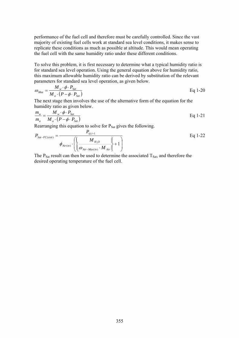
performance of the fuel cell and therefore must be carefully controlled. Since the vast majority of existing fuel cells work at standard sea level conditions, it makes sense to replicate these conditions as much as possible at altitude. This would mean operating the fuel cell with the same humidity ratio under these different conditions. To solve this problem, it is first necessary to determine what a typical humidity ratio is for standard sea level operation. Using the general equation above for humidity ratio, this maximum allowable humidity ratio can be derived by substitution of the relevant parameters for standard sea level operation, as given below.

355

)( Sata

SatwMax PPM

PM⋅−⋅

⋅⋅=

φφ

ω Eq 1-20

The next stage then involves the use of the alternative form of the equation for the humidity ratio as given below.

( )Sata

Satw

a

w

PPMPM

mm

⋅−⋅⋅⋅

=φ

φ Eq 1-21

Rearranging this equation to solve for PSat gives the following.

⎟⎟⎠

⎞⎜⎜⎝

⎛+

⎪⎭

⎪⎬⎫

⎪⎩

⎪⎨⎧

⋅⋅

=

−

−−

1)(

)(

1@)(

2

AirinMaxAir

OHinAir

iexitFCSat

MM

PP

ωφ

Eq 1-22

The PSat result can then be used to determine the associated TSat, and therefore the desired operating temperature of the fuel cell.

G2 Derivation of the equations for the analysis of the autothermal reformer

Analysis of the autothermal reformer The overall equation for an autothermal process (including shift reaction) is,

( ) 2222 22

222 HpnmmCOOHpmOOHC pnm ⎟⎠⎞

⎜⎝⎛ −−++→−−++ χχχ Eq 2-1

Where χ represents the quantity of oxygen (in moles of oxygen per mole of fuel) which is required to attain either an endothermic, exothermic or thermoneutral reaction (autothermal). Since χ varies with fuel composition, the standard practice is to use an equivalence ratio, as defined below.

χε 24

pnm −+= Eq 2-2

The equivalence ratio is directly related to the efficiency of the reforming process with a gain in hydrogen output being experienced with an increase in the equivalence ratio. The theoretical efficiency limit is 100% but there is a practical limit to prevent carbon formation in the fuel processor. As a result, the equivalence ratio used is always less than the theoretical value required to achieve an autothermal process. Incorporating the equivalence ratio, the equation for an autothermal process becomes.

( )( )2222

112

2221

24 HpnmmCOOH

npmO

pnmOHC pnm ⎟

⎠⎞

⎜⎝⎛ −⎟⎠⎞

⎜⎝⎛ −++→

−−−+

−++

εε

ε

ε Eq 2-3 In addition to operation at lower values of equivalence ratio, the problem of carbon formation can be alleviated somewhat by adding excess steam to the reaction. A steam to carbon ratio σ (molar fraction of steam to carbon in the fuel) in the range of 2-3 is typically used for this purpose. In an actual reforming process, allowance also needs to be made for other limiting factors such as the composition of air, fuel slip and incomplete reactions. An actual reforming reaction including all these factors can thus be defined as.

OgHfHeNdCOcCObCHOHaC

OHN

pnm

rr

O

pnmOHC

pnm

O

Opnm

22224

222

22

24124

++++++→

+−+−

+−+

+ σεε Eq 2-4

The output from an actual reactor can thus be seen to consist of following elements (as defined by their coefficients). Also listed is the role of each of the elements within a PEM fuel cell. a – Fuel slip b – Incomplete reactions (dilutant) c – Carbon dioxide (dilutant) d – Carbon monoxide (poisonous to a PEM fuel cell)

356

e – Nitrogen (from the air) (dilutant) f – Hydrogen (fuel) g – Water (dilutant) In the case of methanol (CH3OH) as used in this study, the actual reforming reaction will be as given below, where the composition for methanol is, m=1, n=4 and p=1. The fuel slip in this case is typically minimal in comparison to the other elements and is often disregarded.

OgHfHeNdCOcCObCHOHNr

rOOHCH

O

O2222422

2

223

5.115.1+++++→+

−++ σ

εε Eq 2-5 The equation above can be solved by means of an atom balance of the constituent parts, in order to determine the different reformate quantities leaving the reformer. Carbon balance: dcb ++=1

Oxygen balance: gdc ++=+ 23 σε

Hydrogen balance: gfb 23424 ++=+ σ

Nitrogen balance: ⎟⎟⎠

⎞⎜⎜⎝

⎛ −=

2

215.1

O

O

rr

eε

The atom balances above gives four of the six equations needed to solve the six unknown coefficients in the equation above. The remaining two equations required can be found from the required hydrogen and carbon monoxide content in the dry reformate gas, as given below.

CO content: fedcb

drCO ++++= Eq 2-6

By substitution of the relations for the carbon and nitrogen into the expression above, this reduces to the form below. An operating requirement of PEM fuel cells is that the carbon monoxide in any reformate must be kept below 1% to prevent the fuel cells from being poisoned. Substitution of this figure thus enables the equation to be solved.

01.015.11

2

2

=+⎟⎟

⎠

⎞⎜⎜⎝

⎛ −+

=f

rr

dr

O

OCO

ε

Eq 2-7

In a similar way, the hydrogen content in the dry reformate gas gives.

fr

rfr

O

OH

+⎟⎟⎠

⎞⎜⎜⎝

⎛ −+

=

2

22 15.11

ε

Eq 2-8

From the definition of fuel processor efficiency, the hydrogen output can be determined as below.

2H

FuelActual H

Hf

ΔΔ

=η Eq 2-9

In cases where the hydrogen fraction is known, then the equation for hydrogen content can be solved for the hydrogen output as below.

357

2

2

22

1

15.11

H

O

OH

rr

rr

f−

⎟⎟⎠

⎞⎜⎜⎝

⎛⎥⎦

⎤⎢⎣

⎡ −+⋅

=ε

Eq 2-10

Solving for the other unknown constants gives, 0=a Eq 2-11

⎟⎟⎠

⎞⎜⎜⎝

⎛ −=

2

215.1

O

O

rr

eε

Eq 2-12

⎟⎟⎠

⎞⎜⎜⎝

⎛+⎥

⎦

⎤⎢⎣

⎡ −+= f

rr

rdO

OCO

2

215.11ε

Eq 2-13

8

6228ε

−−−=

dfb Eq 2-14

8

626 dfc

−+= ε Eq 2-15

2

23 dfg

+−+=

σε Eq 2-16

The quantity of hydrogen required by the fuel cell (on a molar basis) is given by the expression below from the fuel cell derivations.

FVPSNCell

HH ⋅⋅⋅=222 Eq 2-17

Multiplication of this result by the molar mass of hydrogen gives the result on a mass flow basis instead. This result can then be used to find the mass flow rate of methanol entering the reformer by using from above, the reciprocal of which gives the moles of methanol required to achieve the required hydrogen output.

f

fM

FVPSm Fuel

CellHFuel ⋅

⋅⋅⋅=22 Eq 2-18

The quantity of air required for the fuel processor can be seen to be proportional to the mass flow rate of methanol entering the system. The relationship between these can be obtained from the general form of the actual reforming relation given above. This also includes an O2 fraction to allow for the use of air as opposed to oxygen.

22)(

2412 O

Air

CellHinFPAir r

Mpnm

fFVPSm ⋅

−+⋅⋅

⋅⋅⋅=− ε

Eq 2-19

Water consumed by the fuel processor is once again relative to the rate of methanol entering the system. In this case however, for simplicity the relationship is obtained from the ideal relation for an autothermal process. The error in doing so can be considered minimal.

358

( )( )OH

CellHConsFPOH M

npm

fFVPSm

22

221122)( ⋅

−−−⋅⋅

⋅⋅⋅=− ε

ε Eq 2-20

Analysis of the preferential oxidation unit The purpose of the preferential oxidation unit is to reduce the CO content of the reformate and therefore the air for the unit will be proportional to the CO content. This process is defined by the reaction 222

1 COOCO →+ . Eq 2-21 The first part of the derivation below presents the CO flow rate as a function of the hydrogen flow rate and then the remaining part takes into account the air requirements as a function of the CO rate. Here, the divisor of 2 relates to the PROX reaction of moles of air per mole of CO. The PROX stoichiometric ratio (SPROX) ensures that there is sufficient O2 for the reaction and as before the O2 fraction allows for the use of air instead of O2.

22

22)( 2

12412 O

AirPROX

O

OCO

CellHinPROXAir r

MSf

rr

pnm

fr

FVPSm ⋅⋅

⎟⎟⎟

⎠

⎞

⎜⎜⎜

⎝

⎛+

−⋅

−++⋅⋅

⋅⋅⋅=− ε

Eq 2-22 Water generated by the preferential oxidation unit is derived in a similar way as for the air requirement of the PROX unit but with a different final relation in accordance with the PROX reaction.

( ) OHPROXO

OCO

CellHGenPROXOH MSf

rr

pnm

fr

FVPSm

221

12412 2

22)( ⋅−⋅

⎟⎟⎟

⎠

⎞

⎜⎜⎜

⎝

⎛+

−⋅

−++⋅⋅

⋅⋅⋅=− ε

Eq 2-23 Other elements included in the composition of the reformate The other elements which leave the fuel processor along with the hydrogen include nitrogen, water vapour, carbon monoxide and carbon dioxide. Since the water vapour and CO are typically small in comparison to the other elements, these are however often neglected. Using the derivation above for the hydrogen output from the fuel processor, the total reformate output can be obtained. Division of the hydrogen output by the hydrogen fraction leaving the fuel processor gives the result below (on a molar basis).

2

2Re 2 H

H

Cellformate r

SFV

PN ⋅⋅⋅

= Eq 2-24

The mass flow rate of nitrogen leaving the fuel reformer is easily obtained from the product of the total reformate output, the nitrogen fraction for the reformate and the molar mass of nitrogen. This gives the result as follows.

222

2)(2 2 NN

H

H

CellinfuelN Mr

rS

FVPm ⋅⋅⋅

⋅⋅=− Eq 2-25

In a similar way, mass flow rate of carbon dioxide can be derived as.

222

2)(2 2 COCO

H

H

CellinfuelCO Mr

rS

FVPm ⋅⋅⋅

⋅⋅=− Eq 2-26

359

G3 Derivation of the equations for the analysis of the steam reformer

Analysis of the steam reformer fuel processor The overall equation for a steam reforming process is,

( ) 222 2HnmpCOCOpmHeatOmHOHC SRpnm ⎟⎠⎞

⎜⎝⎛ +++−→++ Eq 3-1

The steam reforming process must be preceded by a gas shift reaction, given below. ( ) GSRHeatHCOgOHCO ++→+ 222 Eq 3-2

The combined reaction for the complete fuel processor including the steam reforming process and the gas shift reaction is then.

( ) 222 222 HpnmmCOXOHpmOHC Heatpnm ⎟

⎠⎞

⎜⎝⎛ −++→+−+ Eq 3-3

In the case of systems which use an additional quantity of fuel (k) to generate the steam for the process, the additional combustion process is given by.

Heatpnm XOHnkkmCOOpnmkOHkC +⎟⎠⎞

⎜⎝⎛+→⎟

⎠⎞

⎜⎝⎛ −++ 222 24

Eq 3-4

In this case, the efficiency of the steam reforming process is,

( ) Fuel

H

HH

k

pnm

ΔΔ

⋅+

⎟⎠⎞

⎜⎝⎛ −+

= 2

12

2η Eq 3-5

Where the steam for the process is obtained from some source other than the combustion of additional fuel, the efficiency becomes.

Fuel

H

HHpnm

ΔΔ

⋅⎟⎠⎞

⎜⎝⎛ −+= 2

22η Eq 3-6

Keeping the same convention as for the autothermal reformer, the output from a steam reformer can be obtained from inspection of the reaction above, as given below.

pnmf −+=2

2 Eq 3-7

As before, the fuel input required to achieve a desired hydrogen output is given by the equation below.

fM

FVPSm Fuel

CellHFuel ⋅

⋅⋅⋅=22 Eq 3-8

As can be seen from the reaction above, the reforming reaction does not involve any combustion process and thus no oxygen input is required, as defined below.

0)( =− inFPAirm Eq 3-9 The water quantity required for the fuel processor can be derived as for the autothermal reformer. In this case, the water quantity required is obtained from the relation above on a molar basis and the required substitution made to derive the equation below.

360

( ) OHCell

HConsFPOH MpmfFV

PSm22

2122)( ⋅−⋅⋅

⋅⋅⋅=− Eq 3-10

Analysis of the PROX unit Air for the preferential oxidation unit is derived in a similar way as for the autothermal reforming process. The difficulty here is that CO does not appear as an output component in the steam reforming reaction that we have been using so far. For the autothermal process we utilised the actual reaction but this is not possible here due to the complexity of the steam reforming process. An actual steam reforming analysis can however be seen to include reverse reactions which are responsible for the generation of the traces of CO. In this study, it is reasonable to assume that the CO output is comparable with that of an autothermal reformer, as given below.

01.015.11

2

2

=+⎟⎟

⎠

⎞⎜⎜⎝

⎛ −+

=f

rr

dr

O

OCO

ε

Eq 3-11

In the case of an autothermal reformer, the middle function in the denominator can be traced back to the oxygen leaving the reformer. For a steam reformer, this term will become zero and thus the relation can be reduced as below.

fdrCO +

=1

Eq 3-12

After rearranging the above relation, the CO content per unit fuel input can be determined as below.

( frd CO += 1 ) Eq 3-13 This finally gives us an estimate for the air requirement for the PROX unit as given below. The error in such an assumption is considered to be minimal with a better estimate only really be obtainable by experimentation.

( )2

2)( 21

2 O

AirPROXCO

CellHinPROXAir r

MSff

rFV

PSm ⋅⋅+⋅⋅⋅⋅

⋅=− Eq 3-14

In a similar way, the relation for water generation from the autothermal reformer can be modified to arrive at the relation below.

( ) ( ) OHPROXCO

CellHGenPROXOH MSf

fr

FVPSm

2211

22)( ⋅−⋅+⋅⋅⋅⋅

⋅=− Eq 3-15

361

G4 Derivation of equations for the burner analysis

In this analysis it is assumed that only the excess hydrogen from the fuel cell is utilised in the burner, other flammable components such as fuel slip and incomplete reformate are considered to be of negligible quantity. Other reformate components are therefore treated as dilatants in the combustion process with their only effect being to reduce the temperature of the combustion process.

G4.1 Products entering the burner Stoichiometric ratio The reaction for the combustion of hydrogen is as given below.

HeatOHOH +→+ 222 22 Eq 4-1 Inspection of this reaction shows us that the minimum quantity of O2 required for complete combustion is ½ of the H2 available. Referring back to the derivations for the fuel cell, the mass flow rate of O2 required is thus as given below.

( ) AirCell

HdqO MFV

PSm ⋅⋅⋅

⋅−⋅=− 21

21

2'Re2 Eq 4-2

In a similar way, the quantity of O2 that is available at the burner can be shown to be.

( ) AirCell

OAvaO MFV

PSm ⋅⋅⋅

⋅−=− 4122 Eq 4-3

The stoichiometric ratio of the O2 at the burner is finally given by the expression below.

11

2

2

'Re −−

==−

−

H

O

dqAir

AvaAirBurner S

Smm

S Eq 4-4

Quantity of water generated by combustion The quantity of water which is generated in the burner as a result of the combustion process can be derived from inspection of the reaction above. This shows us that one mole of water is generated for each mole of hydrogen burnt. Incorporating the hydrogen mass flow rate entering the burner into this definition gives us the following result.

( ) OHCell

HGenBURNOH MFV

PSm22 2

12)( ⋅⋅⋅

−=− Eq 4-5

Quantity of hydrogen entering the burner Since there are no losses between the fuel cell and burner, the mass flow rate of hydrogen entering the burner will be the same as that of the unused hydrogen leaving the fuel cell. For reference, the hydrogen entering the fuel cell is given below.

222 2 HHCell

H MSFV

Pm ⋅⋅⋅⋅

= Eq 4-6

The quantity of unused hydrogen leaving the fuel cell will be the difference between that entering the fuel cell (as defined by the hydrogen stoichiometric ratio) and that

362

consumed by the fuel cell (as defined by a hydrogen stoichiometric ratio of 1). This leads us to the derivation below.

22)(2 )1(2 HH

CellinfuelH MS

FVPm ⋅−⋅

⋅⋅=− Eq 4-7

Quantity of oxygen entering the burner In a similar way as for the derivation of hydrogen entering the burner, the quantity of oxygen entering the burner can be derived as below.

22)(2 )1(4 OO

CellinairO MS

FVPm ⋅−⋅

⋅⋅=− Eq 4-8

Quantity of nitrogen entering the burner Since nitrogen does not play an active part in any of the reactions with the fuel cell, it merely acts as a dilutant and passes straight through the fuel cell and thus into the burner untouched. The quantity of nitrogen entering the burner will thus be the sum of that entering the fuel cell from the air and that from the fuel processor as below.

)(2)(2)(2 inFCFuelNinFCAirNinBurnN mmm −−−−− += Eq 4-9 The mass flow rate of nitrogen entering the fuel cell is given in the relevant sections for fuel cell derivations. Quantity of water vapour entering the burner along with the oxygen depleted air This derivation is based on the fact that the air enters the fuel cell with a standard atmospheric composition and leaves the fuel cell in an oxygen depleted state as a result of the oxygen being consumed within the fuel cell. This leads to the following result for the oxygen depleted air leaving the fuel cell.

⎟⎟⎠

⎞⎜⎜⎝

⎛−⋅

⋅⋅=− 1

4 2

2)(

O

O

CellinburnAir r

SFV

PN Eq 4-10

From the fuel cell derivations, the following result can be used to find the mass flow rate of water vapour at any point in a system as a function of the mass flow rate of air and the operating conditions at that point.

( ) aSata

Satww m

PPMPM

m ⋅⋅−⋅

⋅⋅=

φφ

Eq 4-11

Combining the two results above, gives us the derivation below. This can also be seen to include a fraction factor to account for the quantity of water recovered by the water separator. The remainder of this fraction as given by the expression below gives us the quantity of water remaining in the air stream.

)1()(@

)(@1

4 22)()()(

)()(

2

2)( FractAirOH

inBurnVSoutFCinBurn

inBurnVSoutFC

O

O

CellinairOH XM

TPPTP

rS

FVPm −− −⋅⋅

⋅−

⋅⋅⎟⎟⎠

⎞⎜⎜⎝

⎛−⋅

⋅⋅=

φφ

Eq 4-12 Quantity of water vapour entering the burner along with the hydrogen input From above, the quantity of hydrogen leaving the fuel cell is given as.

22)(2 )1(2 HH

CellinfuelH MS

FVPm ⋅−⋅

⋅⋅=− Eq 4-13

363

Following the same process as in the previous section and thus combining this result with the derivation for the mass flow rate of water as a function of the mass flow rate of air, the following result is obtained. As before, a fraction is included to account for the quantity of water recovered by the water separator located in the fuel cell hydrogen output stream.

( ) )1()(@

)(@1

2 2)()()(

)()(2)(2 22 FractHOH

inBurnVSoutFCinBurn

inBurnVSoutFCH

CellinHOH XM

TPPTP

SFV

Pm −− −⋅⋅⋅−

⋅⋅−⋅

⋅⋅=

φφ

Eq 4-14

G4.2 Products leaving the burner Quantity of unused oxygen leaving the burner The quantity of unused oxygen leaving burner will be the remainder of that entering the burner and that consumed by the combustion process in the burner. From above, the quantity of oxygen entering the burner is as follows.

22)(2 )1(4 OO

CellinairO MS

FVPm ⋅−⋅

⋅⋅=− Eq 4-15

Also from above, the quantity of oxygen consumed in the burner is.

( ) AirCell

HdqO MFV

PSm ⋅⋅⋅

⋅−=− 412'Re2 Eq 4-16

The quantity of oxygen is then given by. )(2)(2)(2 ConsumedBurnOinBurnOoutBurnO mmm −−− −= Eq 4-17

Substitution of the above equations, allows us to arrive at the following result.

222)(2 )(4 OHO

CelloutBurnO MSS

FVPm ⋅−⋅

⋅⋅=− Eq 4-18

Quantity of nitrogen leaving the burner Since nitrogen only serves as a dilutant within the burner, the quantity of nitrogen leaving the burner will be the same as that entering the burner. This in turn will be the same as the sum of that entering the fuel cell, as given below.

)(2)(2)(2 inFCFuelNinFCAirNinBurnN mmm −−−−− += Eq 4-19 From the fuel cell derivations, the nitrogen entering the fuel cell with the air can be determined from.

( )2

2

22)(2

14 N

O

OO

CellinairN M

rr

SFV

Pm ⋅−

⋅⋅⋅⋅

=− Eq 4-20

Likewise, the nitrogen entering the fuel cell from the fuel processor is given by.

222

2)(2 2 NN

H

H

CellinfuelN Mr

rS

FVPm ⋅⋅⋅

⋅⋅=− Eq 4-21

Substitution of these terms into the equation above leads to the following expression.

22

22

2

22)(2

122 N

O

OO

H

NH

CelloutBurnN M

rrS

rr

SFV

Pm ⋅⎟⎟⎠

⎞⎜⎜⎝

⎛

⎭⎬⎫

⎩⎨⎧

⎥⎦

⎤⎢⎣

⎡ −⋅+

⎭⎬⎫

⎩⎨⎧

⋅⋅⋅

=− Eq 4-22

364

Quantity of carbon dioxide leaving the burner As for the nitrogen passing through the system, the carbon dioxide is a mere dilutant, therefore the quantity of CO2 leaving the burner is the same as that entering the fuel cell. The main source of CO2 entering the system is from the fuel processor as derived in the fuel processing section and reiterated below.

222

2)(2 2 COCO

H

H

CelloutBurnCO Mr

rS

FVPm ⋅⋅⋅

⋅⋅=− Eq 4-23

Quantity of water leaving the burner As for the N2 and CO2 passing through the system, any water vapour in the system will also act as a mere dilutant. The total quantity of water leaving the burner will therefore be the sum of:

• The water that enters the burner with the air and is not removed by the air water separator. As derived above.

• The water that enters the burner with the hydrogen and is not removed by the hydrogen water separator. As derived above.

• The water generated by combustion in the burner. As derived above. This leads to the result below.

)(2)(2)( 22221

2 inHOHinAirOHOHHCell

outBurnOH mmMSFV

Pm −−− ++⎟⎟⎠

⎞⎜⎜⎝

⎛⋅−⋅

⋅⋅= Eq 4-24

Quantity of water vapour leaving the burner with the exhaust gases As for the water vapour entering the burner, the following relation can be used to determine the quantity of water present in vapour form in the exhaust gas flow.

( ) aSata

Satww m

PPMPM

m ⋅⋅−⋅

⋅⋅=

φφ

Eq 4-25

In this case, the mass flow rate of air becomes the mass flow rate of exhaust gases leaving the burner and the molar mass of air becomes the composite molar mass of the exhaust gases. This leads us to the result below.

)(@)(@

)()(

)()()(

2

2OutExhVSExhOutExh

OutExhVSExh

Exh

OHOutExhOutExhOH TPP

TPMM

mm⋅−

⋅⋅⋅=− φ

φ Eq 4-26

365

G5 Derivation of a general relation to determine the fuel cell output voltage

This section will give an overview of the derivation of a simple expression which is capable of predicting the voltage output from a fuel cell as a function of its power output and operating temperature. The first stage in this work is to predict the fuel cell output voltage at a number of different values of operating temperature and over a range of current densities. Knowledge of the current and voltage then allows us to determine the output power at each point and ultimately the point of maximum power. We are then able to plot relations for fuel cell output voltage versus output power fraction at a number of different operating temperatures. By fitting polynomial expressions to these relations we are then able to derive a global relation by examination of the coefficients. A summary of the analytical procedure is shown in the flow chart below. The accompanying equations and background to the analysis procedure is also given below.

Theoretical fuel cell voltage as a function of operating temperature – (M1)

Exchange current density as a function of temperature – (M2)

Open circuit fuel cell voltage as a function of temperature – (M3)

Tafel equation constant A – (M4)

Tafel equation constant B [Tafel slope] – (M5)

Activation losses from the Tafel equation – (M6)

Ohmic losses – (M7)

Concentration losses – (M8)

Practical fuel cell potential – (M9)

Fuel cell current – (M10)

Fuel cell power output – (M11)

Fuel cell power fraction – (M12)

Global relation for fuel cell voltage as a function of power output and operating temperature

The first stage in this analysis is to determine the theoretical fuel cell voltage from the reactions involved. As a reminder, the general reaction for a hydrogen fuel cell is,

OHOH 2221

2 →+ Eq 5-1

366

If we consider the chemistry of the reaction in greater detail, we will see that there is an energy change associated with the reaction. For our purposes, it is most convenient to express this change as the change in the Gibbs free energy of formation. This is the difference between the Gibbs energy of the reactants and products as below.

tsacfoductsf GGG tanRePr −− −=Δ Eq 5-2 These values are typically determined on a molar basis as denoted by a bar value. The value of the change in Gibbs free energy of formation can be seen to be dependant on the temperature of the reaction and final state of the products and is thus variable. Calculation of the molar specific change in Gibbs free energy of formation can be a lengthy process. Fortunately, for the basic hydrogen fuel cell reaction above the data is already available in a tabulated format for a number of different conditions as given below. The sign convention used is consistent with energy being released.

Table 5-1 – Change in Gibbs free energy of formation [56]

If we look back at the working principles of the fuel cell, we can see that in order to complete the reaction, two electrons must pass round the external circuit per mole of hydrogen. Each electron will carry a charge as predicted by the Faradays constant F. The electrical work done to move this charge around the circuit is then determined as the product of the charge and voltage. If we assume that the reaction is reversible and therefore there are no losses in the fuel cell, this electrical work done will equal the change in Gibbs free energy of the reaction as below

EFvoltageechg f ⋅−=×=Δ 2arg Eq 5-3 By rearranging the equation above, we have a method of predicting the reversible open circuit voltage of the fuel cell, as below.

Fg

E f

2Δ−

= Eq 5-4

If we then use the above relation to determine the EMF at a number of different operating temperatures, we are then able to plot the results and obtain a relation for EMF versus operating temperature as given below.

367

Theoretical E vs Operating Temp

y = -0.0838x + 1.4796

1.16

1.17

1.18

1.19

1.2

1.21

1.22

1.23

1.24

2.9 3.1 3.3 3.5 3.7 3.9

Operating Temp (/100) (K)

Eth

(V)

Eq 5-5 (M1) The next stage in the work is to predict the actual open circuit voltage of the fuel cell by taking into account the operating losses. The first part of this analysis is to determine the exchange current density i0 from equation M2 as a function of operating temperature. The exchange current density is a particularly important parameter which can be deemed as a measure of the readiness of the electrode to proceed with the electrochemical reaction. A higher exchange current density implies a more active electrode surface and thus higher currents can be generated for any over potential.

Equation M2: ⎥⎥⎦

⎤

⎢⎢⎣

⎡⎟⎟⎠

⎞⎜⎜⎝

⎛−−⎟

⎟⎠

⎞⎜⎜⎝

⎛⋅⋅⋅=

−−

f

c

fr

rccf T

TRTE

PPLaii

ReReRe00 1exp

γ

Eq 5-6 (M2)

The terms included in the above equation are:

• fi Re0− - This is the exchange current density at a reference condition (typically 25°C and 1atm). This is normally quoted per unit catalyst surface area (with the units Acm-2Pt). Determination of this parameter will be discussed further below.

• ca - This is the catalyst specific area. Modern catalysts have a value which lies between 600 and 1000cm2mg-1. In the absence of better data, an average value of 800cm2mg-1 has been assumed for this analysis.

• cL - This is the catalyst loading. Modern electrodes have a value which lies between 0.3 and 0.5mgPtcm-2. In the absence of better data, an average value of 0.4mgPtcm-2 has been assumed for this analysis.

• Pr – This is the reactant partial pressure, measured in kPa. This is assumed to be 1atm in this analysis.

• Prref – This is the reference pressure, measured in kPa. This is assumed to be 1atm in this analysis.

• γ – This is the pressure coefficient which can be anywhere between 0.5 and 1.0 but in this analysis a value of 1 is used.

• Ec – This is the activation energy and is assumed to have a value of 66kJmol-1 for oxygen reduction on a Pt catalyst.

• R – This is the standard gas constant which has a value of 8.314Jmol-1K-1. • T and Tref – This is the temperature and reference temperature (at 25°C) in K.

The temperature being the independent variable in this analysis.

368

The reference exchange current density can be determined from a standard value of exchange current density with the following relation. A standard value of 0.001 has been assumed for i0 in this analysis which is consistent with data obtained for a modern Ballard fuel cell.

ccf La

ii

⋅=−

0Re0 Eq 5-7

The denominator of the relation above is the product of the catalyst specific area and the catalyst loading, which is also known as the electrode roughness. Using the figures above, a value of 3.125E-6 was determined for i0.

cc La

The practical open circuit voltage can then be determined from the theoretical open circuit voltage with Equation M3. The unknown parameters in this equation are:

• lossi - This is the loss in current density due to internal currents and fuel crossover through the polymer membrane electrolyte. Examination of analysis data for existing fuel cells has deemed a value of 3mAcm-2 as being a typical.

• α – This is the charge transfer coefficient which typically assumes a value of 1.

⎥⎦

⎤⎢⎣

⎡⎟⎟⎠

⎞⎜⎜⎝

⎛⋅

⋅⋅

−=0

lni

iFTREE loss

athOC α

Eq 5-8 (M3)

Until now we have only considered the open circuit voltage for the fuel cell. The next stage of the analysis is to determine the losses which are encountered as a result of useful current being drawn. We will then finally be able to determine the actual fuel cell output voltage in the presence of an external load. The fuel cell working losses are characterised as, activation, ohmic and concentration as will be examined below. Activation losses are associated with the anode and cathode electrode kinetics and the initiation of the electrochemical reaction. These are related to the exchange current density with lower losses being experienced at higher values of exchange current density. Activation losses can be determined from the Butler-Volmer equation but are most effectively predicted by equation M6 which is known as the Tafel equation. The equation coefficients A and B are given by equations M4 and M5 respectively. Where

is the exchange current density and i is the current density (mA/cm2), which is obtained by dividing the current by the fuel cell active area. The fuel cell active area is a design variable for fuel cells with a value of 400cm2 being assumed for this analysis.

0i

( )0log3.2 iFTRA

aAct ⋅

⋅⋅

⋅−=α

Eq 5-9 (M4)

FTRB

aAct ⋅

⋅⋅=α

3.2 Eq 5-10 (M5)

( )iBAV ActActAct log⋅+=Δ Eq 5-11 (M6)

369

The ohmic losses are not only a result of the resistance of the flow of electrons in the conductive components but also the resistance of the flow of ions in the electrolyte. These losses can be predicted with equation M7, which has values of R between 0.1 and 0.2Ωcm2. In this analysis, an average value of 0.15Ωcm2 has been assumed.

RiVOhm ⋅=Δ Eq 5-12 (M7) The final source of losses is the concentration losses, which result from concentration gradients at the fuel cell electrodes due to the rapid consumption of reactants at various points on the electrodes. These are best predicted by the empirical relation M8, with typical values of C = 3E-5V and D = 0.125Acm-2 being assumed for this analysis.

⎟⎠⎞

⎜⎝⎛⋅=Δ

DiCVConc exp Eq 5-13 (M8)

The final voltage output from a fuel cell, which is being subjected to an external load, is given by equation M9.

ConcOhmActOCCell VVVEV Δ−Δ−Δ−= Eq 5-14 (M9) The process presented above is repeated for a range of values of current density to produce a plot of VCell against current density (i). If equation M10 is used to determine the current from the current density, the fuel cell power output can be determined from equation M11. The term in equation M10 is the fuel cell active area, which as mentioned above has been assumed to be 400cm2 in this analysis.

ActCellA −

1000ActCell

CellAi

I −⋅= Eq 5-15 (M10)

CellCellCell IVP ⋅= Eq 5-16 (M11)

The results of equation M11 can then be used to generate a plot of power against current, from which the maximum value of power output can then be determined. Using equation M12, we are then finally able to generate another plot of percentage maximum power output against current.

)(

%MaxCell

Cell

PP

P = Eq 5-17 (M12)

This whole process is then repeated for a range of fuel cell operating temperatures and for values of current density up to that for the maximum power. The results are finally plotted against percentage power output to generate something similar to the plot shown in figure 5-1 below. This shows the characteristic fuel cell polarization curves for a number of different operating temperatures from 30 to 100°C.

370

Effect of operating temperature on cell voltage

0.5

0.6

0.7

0.8

0.9

1

1.1

0 0.1 0.2 0.3 0.4 0.5 0.6 0.7 0.8 0.9 1

Power output (%)

Cel

l vol

tage

10090807060504030

Figure 5-1

The final stage in this analysis is to transform the results given in the above chart into a more easily manageable format for use within the main spreadsheet. Step one of this process is to fit a polynomial expression to each of the curves in the above plot. We are then able to examine the trend between coefficients of each expression to arrive at the global expression given by equation M13. The accompanying coefficients can be determined from equations M14 through to M18.

( ) ( ) ( ) ( ) CPwrXPwrXPwrXPwrXBasicCell CFCFCFCFCV +⋅+⋅+⋅+⋅=−2

23

34

4 Eq 5-18 (M13)

8708.01000

5486.14 −⋅−= FCX

TC Eq 5-19 (M14)

7465.11000

6579.23 −⋅= FCX

TC Eq 5-20 (M15)

2305.11000

2895.12 −⋅−= FCX

TC Eq 5-21 (M16)

1772.01000

2492.01000

4107.02

+⋅−⎟⎠⎞

⎜⎝⎛⋅= FCFC

XTT

C Eq 5-22 (M17)

6517.01000

0758.2 +⋅= FCC

TC Eq 5-23 (M18)

371

372

H1 Analysis of the fuel cell system Due to its size, it has been necessary to break this analysis down into a number of smaller sections so that the procedure can be presented here in an easy to understand format. This process is shown in the diagram below to help the reader trace their steps. It has not however been possible to illustrate all the links between the blocks in this diagram due to the complexity of the analysis and the risk of obscuring the meaning of the diagram.

Analysis block A - Fuel cell operating environment and requirements

Analysis block B - Fuel cell operating conditions

Analysis block C – Fuel cell humidification

Analysis block D – Burner operating conditions

Analysis block E – Compressor and turbine unit

Analysis block F – Fuel cell fuel and air flow

Analysis block G – Analysis solution

Analysis block H – Heat removal requirements

Analysis block I – Cooling system requirements

Analysis block J – Cooling system analysis

Analysis block K – Cooling system pumping requirements

Analysis block L – Fuel system pumping requirements Each of the blocks in the chart above represents a complex analysis for a particular part of the fuel cell system or an operating condition. This includes analysis of the system operating environment, operating conditions (including the analysis of flows entering and leaving the system) and auxiliary systems used to regulate the operating conditions of the system (such as the cooling and humidification systems). Each of these blocks will be discussed in depth in the sections which follow.

373

H1.1 Analysis block A – Fuel cell operating environment

H1.1.1 Atmospheric variables Within this section the relations will be presented which are used to determine the properties of the atmosphere at the altitudes under consideration. These relations, as given below, were obtained from ESDU 77021 [68] and the reader is advised to refer to this data sheet for further information.

( HLTT ii ⋅+= ) Eq A-1

iRLmg

ii T

TPP

00

⎟⎠⎞

⎜⎝⎛⋅= Eq A-2

TRmP⋅⋅

= 0ρ Eq A-3

4.11010458.1 2

36

+⋅⋅

=−

TTμ Eq A-4

H1.2 Other useful fuel cell system analysis fluid parameters

H1.2.1 Cooling system parameters The kinematic viscosity (nu) and thermal diffusivity (α) of the ambient air are given by the polynomial expressions below which were obtained by fitting curve-fit expressions to existing data. Where, H is the altitude in km and T is the temperature in Kelvins.

( ) 61/725.146524.03195.00412.00023.0 234 EHHHH +++−=υ Eq A-5 ( ) ( ) ( )50654.188197.8111018.9 2 −−⋅−+⋅−= ETETEα Eq A-6

Also required for the cooling system analysis are the Cp and k values of air which can be determined from the relations below. Where, TAir is the temperature of the air in the immediate vicinity of the fuel cell in Kelvins and the accompanying constants are given in the table below.

10001000100010001000

)(234

⋅⎥⎥⎦

⎤

⎢⎢⎣

⎡+⎟

⎠⎞

⎜⎝⎛⋅+⎟

⎠⎞

⎜⎝⎛⋅+⎟

⎠⎞

⎜⎝⎛⋅+⎟

⎠⎞

⎜⎝⎛⋅= E

TD

TC

TB

TAairCp AirAirAirAir Eq A-7

Constants A B C D ECp (W/mdegC) 13.333 -15.259 6.7556 -1.3456 1.1066

( )

⎟⎠⎞

⎜⎝⎛ ⋅+

⋅−=

−AirT

Air

AitAir

T

TEk

12

23

10245

3648151.2 Eq A-8

The fuel cell coolant is assumed to be a mix of 30% glycol and 70% water, the properties of which can be determined from the expression below developed by the

374

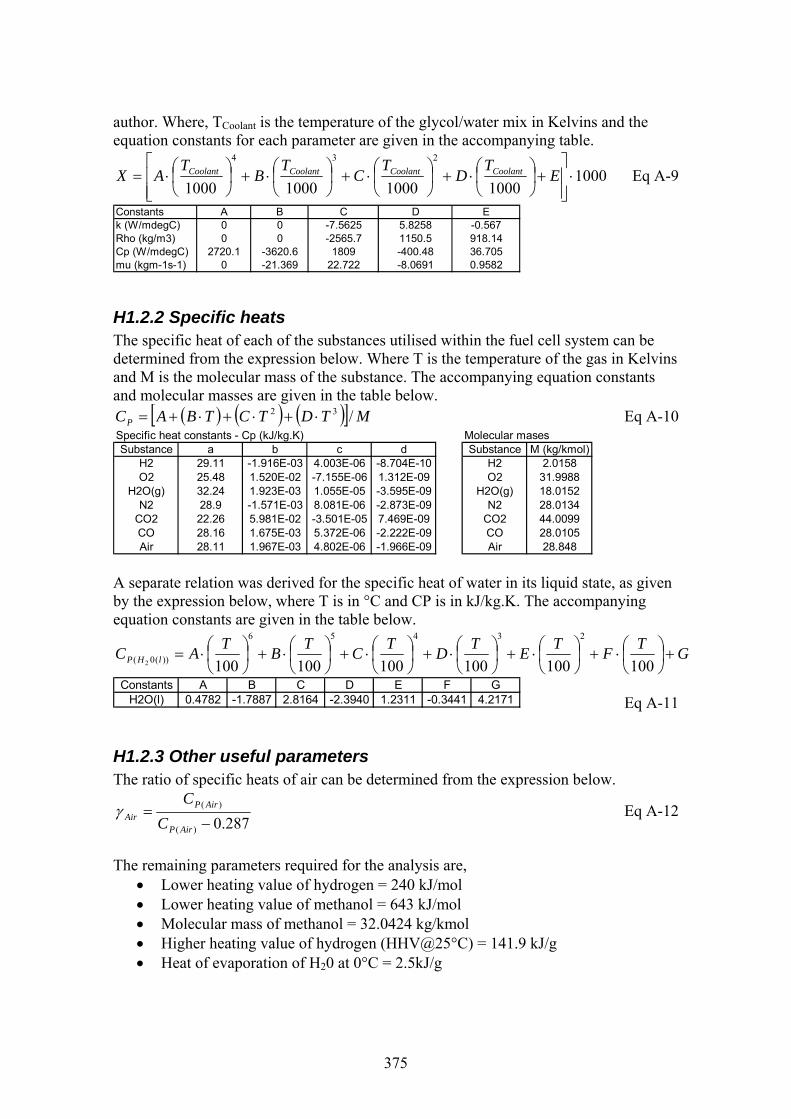
author. Where, TCoolant is the temperature of the glycol/water mix in Kelvins and the equation constants for each parameter are given in the accompanying table.

10001000100010001000

234

⋅⎥⎥⎦

⎤

⎢⎢⎣

⎡+⎟

⎠⎞

⎜⎝⎛⋅+⎟

⎠⎞

⎜⎝⎛⋅+⎟

⎠⎞

⎜⎝⎛⋅+⎟

⎠⎞

⎜⎝⎛⋅= E

TD

TC

TB

TAX CoolantCoolantCoolantCoolant Eq A-9

Constants A B C D Ek (W/mdegC) 0 0 -7.5625 5.8258 -0.567Rho (kg/m3) 0 0 -2565.7 1150.5 918.14Cp (W/mdegC) 2720.1 -3620.6 1809 -400.48 36.705mu (kgm-1s-1) 0 -21.369 22.722 -8.0691 0.9582

H1.2.2 Specific heats The specific heat of each of the substances utilised within the fuel cell system can be determined from the expression below. Where T is the temperature of the gas in Kelvins and M is the molecular mass of the substance. The accompanying equation constants and molecular masses are given in the table below.

( ) ( ) ( )[ ] MTDTCTBACP /32 ⋅+⋅+⋅+= Eq A-10 Specific heat constants - Cp (kJ/kg.K) Molecular masesSubstance a b c d Substance M (kg/kmol)

H2 29.11 -1.916E-03 4.003E-06 -8.704E-10 H2 2.0158O2 25.48 1.520E-02 -7.155E-06 1.312E-09 O2 31.9988

H2O(g) 32.24 1.923E-03 1.055E-05 -3.595E-09 H2O(g) 18.0152N2 28.9 -1.571E-03 8.081E-06 -2.873E-09 N2 28.0134

CO2 22.26 5.981E-02 -3.501E-05 7.469E-09 CO2 44.0099CO 28.16 1.675E-03 5.372E-06 -2.222E-09 CO 28.0105Air 28.11 1.967E-03 4.802E-06 -1.966E-09 Air 28.848

A separate relation was derived for the specific heat of water in its liquid state, as given by the expression below, where T is in °C and CP is in kJ/kg.K. The accompanying equation constants are given in the table below.

GTFTETDTCTBTAC lHP +⎟⎠⎞

⎜⎝⎛⋅+⎟

⎠⎞

⎜⎝⎛⋅+⎟

⎠⎞

⎜⎝⎛⋅+⎟

⎠⎞

⎜⎝⎛⋅+⎟

⎠⎞

⎜⎝⎛⋅+⎟

⎠⎞

⎜⎝⎛⋅=

100100100100100100

23456

))(0( 2

Constants A B C D E F GH2O(l) 0.4782 -1.7887 2.8164 -2.3940 1.2311 -0.3441 4.2171 Eq A-11

H1.2.3 Other useful parameters The ratio of specific heats of air can be determined from the expression below.

287.0)(

)(

−=

AirP

AirPAir C

Cγ Eq A-12

The remaining parameters required for the analysis are,

• Lower heating value of hydrogen = 240 kJ/mol • Lower heating value of methanol = 643 kJ/mol • Molecular mass of methanol = 32.0424 kg/kmol • Higher heating value of hydrogen (HHV@25°C) = 141.9 kJ/g • Heat of evaporation of H20 at 0°C = 2.5kJ/g

375

H1.3 Analysis block B – Fuel cell operating conditions

H1.3.1 Theoretical background It should be noted that the operational temperature of a fuel cell is actually not an independent parameter and is dependant on the fuel cell operating pressure and humidification requirements. In this analysis, the fuel cell can be considered to be a constant volume device within a control volume as shown in figure 1 below.

Fuel Cell

Control Volume

Air-in Air-outFuel Cell

Control Volume

Air-in Air-out

Figure B-1 In order for the fuel cell to operate effectively, its water content must be kept within carefully controlled limits. If there is too much water, the reactant channels will become flooded and if there is insufficient water, the membrane will dry out. In either case, a serious reduction in performance will occur. The optimum operating condition is when the oxygen depleted air leaves the fuel cell with an average relative humidity of 0.9 (within the limits of 80 to 100%). In other words, the exhaust air must be 90% saturated. From a thermodynamics perspective of a constant volume device, this would imply that the operating temperature of the fuel cell must be carefully maintained to keep its operating point within the saturated vapour dome. This concept is clarified in the P-V diagram of figure 2 below.

Constant VolumeOperating Line

Operating Point at T1

Operating Point at T2

Constant VolumeOperating Line

Operating Point at T1

Operating Point at T2

Figure B-2 In the P-V diagram above, we can see that the operating temperature of a fixed volume fuel cell would have to be decreased from temperature T2 to T1 in order to move its operating point from the superheated region to within the desired saturated vapour region (to within the vapour dome). It is also evident that if the relative humidity of the air is known then the temperature required to achieve this condition can be determined.

376

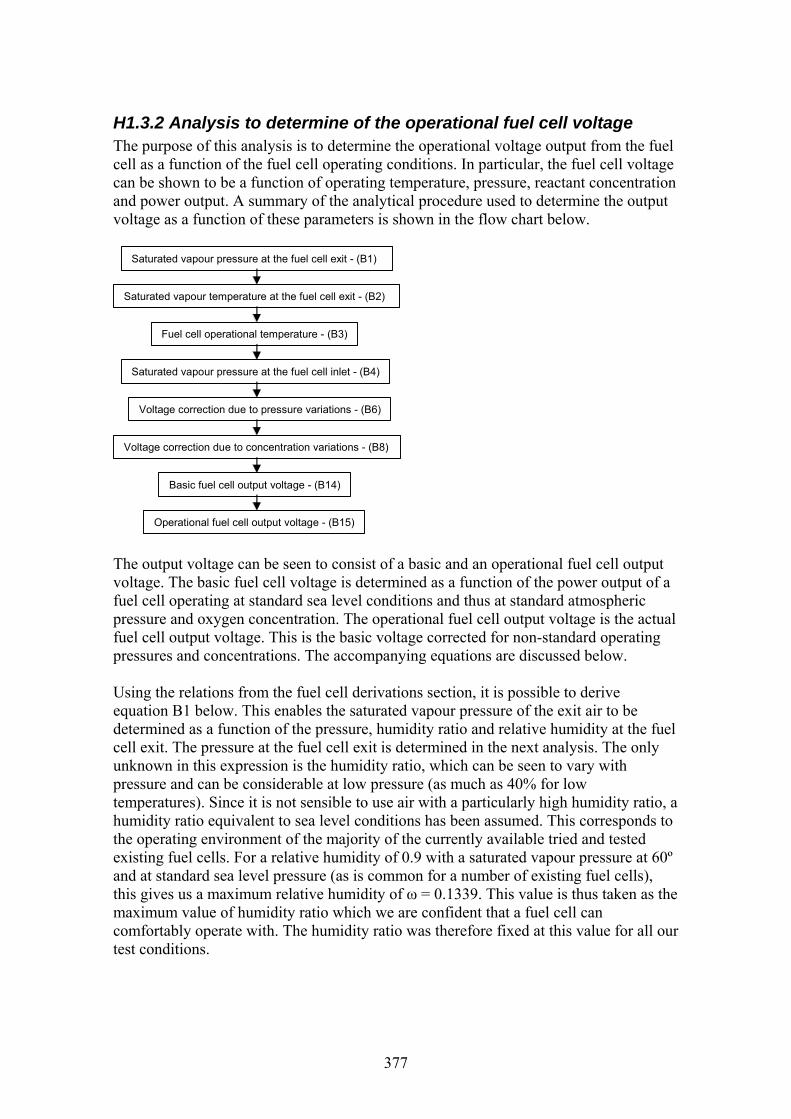
H1.3.2 Analysis to determine of the operational fuel cell voltage The purpose of this analysis is to determine the operational voltage output from the fuel cell as a function of the fuel cell operating conditions. In particular, the fuel cell voltage can be shown to be a function of operating temperature, pressure, reactant concentration and power output. A summary of the analytical procedure used to determine the output voltage as a function of these parameters is shown in the flow chart below.

Saturated vapour pressure at the fuel cell exit - (B1)

Saturated vapour temperature at the fuel cell exit - (B2)

Fuel cell operational temperature - (B3)

Saturated vapour pressure at the fuel cell inlet - (B4)

Voltage correction due to pressure variations - (B6)

Voltage correction due to concentration variations - (B8)

Basic fuel cell output voltage - (B14)

Operational fuel cell output voltage - (B15) The output voltage can be seen to consist of a basic and an operational fuel cell output voltage. The basic fuel cell voltage is determined as a function of the power output of a fuel cell operating at standard sea level conditions and thus at standard atmospheric pressure and oxygen concentration. The operational fuel cell output voltage is the actual fuel cell output voltage. This is the basic voltage corrected for non-standard operating pressures and concentrations. The accompanying equations are discussed below. Using the relations from the fuel cell derivations section, it is possible to derive equation B1 below. This enables the saturated vapour pressure of the exit air to be determined as a function of the pressure, humidity ratio and relative humidity at the fuel cell exit. The pressure at the fuel cell exit is determined in the next analysis. The only unknown in this expression is the humidity ratio, which can be seen to vary with pressure and can be considerable at low pressure (as much as 40% for low temperatures). Since it is not sensible to use air with a particularly high humidity ratio, a humidity ratio equivalent to sea level conditions has been assumed. This corresponds to the operating environment of the majority of the currently available tried and tested existing fuel cells. For a relative humidity of 0.9 with a saturated vapour pressure at 60º and at standard sea level pressure (as is common for a number of existing fuel cells), this gives us a maximum relative humidity of ω = 0.1339. This value is thus taken as the maximum value of humidity ratio which we are confident that a fuel cell can comfortably operate with. The humidity ratio was therefore fixed at this value for all our test conditions.

377

⎟⎟⎠

⎞⎜⎜⎝

⎛+

⎪⎭

⎪⎬⎫

⎪⎩

⎪⎨⎧

⋅⋅

=

−

−−

1)(

)(

1@)(

2

AirinMaxAir

OHinAir

iexitFCSat

MM

PP

ωφ

Eq B-1

By plotting the saturated vapour temperature verses the saturated vapour pressure of air; it is possible to obtain the relation given in equation B2. This relation enables us to determine the saturated vapour temperature of the air leaving the fuel cell, with respect to the saturated vapour pressure determined in the relation above. For our work, an accuracy of 1 decimal place is deemed sufficient.

( ) ( ) ( ) ZPLOGYPLOGXPLOGWT SatSatSatexitFCSat +++=− )()()( 23)( Eq B-2

The constants for equation B2 are given in the table below. Constant W X Y Z Value 1.2166 -7.0857 43.351 -92.121

It should be noted that there is a limit to the actual operating temperature which a fuel cell can operate at, which is dictated by the material limits of the components that make up the fuel cell assembly. Since 80ºC is generally regarded as the maximum allowable temperature for a PEM fuel cell, this figure is adopted here. The operating temperature of the fuel cell can then thus be determined from equation B3 below as the lesser of the saturated vapour temperature and the maximum allowable limit.

),,( )()( MatMaxSatMatMaxSatlOperationaFC TTTTIFT <=− Eq B-3 In a similar way as above, the saturated vapour pressure of the air entering the fuel cell can be determined from the curve fitted expression given in equation B4 below.

( ) ( ) ( ) ( ) ( )( )[ ]TfTeTdTcbTaEXPP AirSat ln321)( ⋅+⋅+⋅+⋅++⋅= − Eq B-4

The constants for equation B4 are given in the table below.

Constant a b c d e fValue -5.800E+03 1.391E+00 -4.864E-02 4.176E-05 -1.445E-08 6.546E+00

The effect of variations in fuel cell operating pressure is traditionally predicted by the analytical Nernst equation given below.

⎟⎟⎠

⎞⎜⎜⎝

⎛⋅

⋅⋅

=Δ Δ1

2ln4 P

PF

TRE FC

P

This relation has been shown to give reasonable results for high temperature fuel cells operating at temperatures of about 1000ºC. In the case of low temperature fuel cells however, a significant error between those figures predicted by this relation and those reported in practice, is evident. To overcome this problem, the author of this thesis has derived a fudge factor from analytical and experimentally reported data, to correct the predictions made by the Nernst equation. This is given in equation B5 as a function of temperature, since the error is proportional to the operating temperature of the fuel cell.

378

( ) 4535.80108.0 +⋅−=Δ FCP TFud Eq B-5

The corrected Nernst equation to predict the effect of pressure variations is then given by equation B6 below.

PFC

P FudPP

FTR

E ΔΔ ⋅⎟⎟⎠

⎞⎜⎜⎝

⎛⋅

⋅⋅

=Δ1

2ln4

Eq B-6

In a similar way as for the relation to predict the effect of pressure changes, an alternative form of the Nernst equation can be used to predict concentration changes as given below.

⎟⎟⎠

⎞⎜⎜⎝

⎛⋅

⋅⋅

=Δ Δ1

2ln4 β

ββ F

TRE FC

As before, there is some disagreement between those values predicted by this analytical expression and those reported in practice and so another fudge factor was derived by the author of this thesis to correct for this effect. This is given by equation B7 below.

( 122743.5 )βββ −⋅=ΔFud Eq B-7 The corrected Nernst equation to predict the effect of concentration variations is then given by equation B8 below.

ββ ββ

ΔΔ ⋅⎟⎟⎠

⎞⎜⎜⎝

⎛⋅

⋅⋅

=Δ FudF

TRE FC

1

2ln4

Eq B-8

Using the global analytical relation derived by this author in the fuel cell operating temperature relations derivations section, we are able to determine the basic fuel cell voltage. This is given by equation B14 as a function of the fuel cell output power fraction. The corresponding equation constants are given by equations B9 through to B13 as a function of the fuel cell operating temperature.

8708.01000

5486.14 −⋅−= FCX

TC Eq B-9

7465.11000

6579.23 −⋅= FCX

TC Eq B-10

2305.11000

2895.12 −⋅−= FCX

TC Eq B-11

1772.01000

2492.01000

4107.02

+⋅−⎟⎠⎞

⎜⎝⎛⋅= FCFC

XTT

C Eq B-12

6517.01000

0758.2 +⋅= FCC

TC Eq B-13

( ) ( ) ( ) ( ) CPwrXPwrXPwrXPwrXBasicCell CFCFCFCFCV +⋅+⋅+⋅+⋅=−2

23

34

4 Eq B-14

379

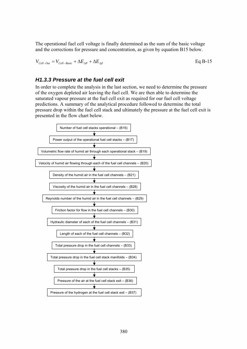
The operational fuel cell voltage is finally determined as the sum of the basic voltage and the corrections for pressure and concentration, as given by equation B15 below.

βΔΔ−− Δ+Δ+= EEVV PBasicCellOutCell Eq B-15

H1.3.3 Pressure at the fuel cell exit In order to complete the analysis in the last section, we need to determine the pressure of the oxygen depleted air leaving the fuel cell. We are then able to determine the saturated vapour pressure at the fuel cell exit as required for our fuel cell voltage predictions. A summary of the analytical procedure followed to determine the total pressure drop within the fuel cell stack and ultimately the pressure at the fuel cell exit is presented in the flow chart below.

Number of fuel cell stacks operational – (B16)

Power output of the operational fuel cell stacks – (B17)

Volumetric flow rate of humid air through each operational stack – (B19)

Velocity of humid air flowing through each of the fuel cell channels – (B20)

Density of the humid air in the fuel cell channels – (B21)

Viscosity of the humid air in the fuel cell channels – (B28)

Reynolds number of the humid air in the fuel cell channels – (B29)

Friction factor for flow in the fuel cell channels – (B30)

Hydraulic diameter of each of the fuel cell channels – (B31)

Length of each of the fuel cell channels – (B32)

Total pressure drop in the fuel cell channels – (B33)

Total pressure drop in the fuel cell stack manifolds – (B34)

Total pressure drop in the fuel cell stacks – (B35)

Pressure of the air at the fuel cell stack exit – (B36)

Pressure of the hydrogen at the fuel cell stack exit – (B37)

380

381

hich

of 4, then the forth is ut-down and the remaining 3 are run at a higher and more efficient power output. The

16 below as a function of the power output required and the maximum power output each stack is able to deliver (which is 103.63kW in this analysis).

As is mentioned elsewhere in this thesis, it is more efficient to operate fuel cells at higher rather than lower power outputs. This is due to fuel cell activation losses ware predominant at low currents. For this reason, the fuel cell system in this study has been designed to shut-down any fuel cell stack not required. For example, if it is possible to achieve the same power output from 3 stacks insteadshaccompanying equations for this analysis are discussed below. The number of fuel cell stack which are operational can be determined from equation B

⎟⎠

⎜⎝

⎟⎠

⎜⎝ )(MaxStack

StacksOp P

⎟⎞

⎜⎛

⎟⎞

⎜⎛

=− 0,OutPROUNDUP Eq B-16

he power output and the percentage of maximum power of each operational fuel cell stack can then be determ

N

Tined from equations B17 and B18 respectively.

StacksOp

OutStack N

PP

−

= Eq B-17

100%)(MaxStack

Stack P The total volumetric flow rate of the humid air passing through each operational fuel cell stack is given by equat

⋅= StackPP Eq B-18

ion B19 below. This is derived from expressions for the total ass flow rate of air entering the fuel cell and the density of the air with respect to its

temperature and pressure.

m

6

)()()(2 )(@4 ⋅−⎟⎠

⎜⎝⋅⋅ inFCVSinFCinFCOCell

Stack TPPrFV φ The velocity of the humid air flowing through each channel on the bi-polar plate can be determined from equation B20 as a function of the internal geometry of the fuel cell stack. This requires knowledge of the number of cells in the stack (532 in this analy

)(2 10⋅⋅

⋅⎟⎞

⎜⎛⋅= inFCO TRSP Eq B-19

sis), e number of parallel serpentine channels on each bi-polar plate (10 in this analysis)

and the cross-sectional area of 2

Q

th each reactant channel (0.0225cm in this analysis).

ChCellChCellCellCh ANN ⋅⋅ −

−

StackQ= Eq B-20

he density of the humid air entering the fuel cell can then be determined from equation B21 as a function of the temperature and pressure of the air.

V

T

( )1000)(

)()()( 2

⋅⋅

⋅+⋅−=−

inFC

OHinSatAirinSatinFCHumidAir TR

MPMPPρ Eq B-21

Determination of the viscosity of the humid air entering the fuel cell is more complexthan for the other parameters and is typically determined as a composition of its omponent parts (air and water vapour). This first stage is to determine the viscosity of

r at the temperature of the humid air. The viscosity of air and water vapour is typically given at a reference temdetermined at the required temperature from equa

cthe air and water vapou

perature of 25, which can then be tions B22 and B23.

23

25

)(

)(

25)25())((1 ⎟⎟

⎠

⎞⎜⎜⎝

⎛⋅

++

⋅=−− TT

CTCT inFC

AirinFC

AirAirinFCTAir μμ Eq B-22

23

)(25 ⎟⎞

⎜⎛⋅

+⋅

TCT inFCWVμμ25)(

)25())((2 ⎟⎠

⎜⎝+

=−− TCT WVinFCWVinFCTWV Eq B-23

The parameters and constants used in these relations are,

Parameter Value Descriptionmu-air 25 (kgm-1s-1) 0.0000181 Viscosity of air at 25 deg C

Sutherlands constant for airC-water vapor 660 Sutherlands constant for water vapor

mu-wv 25 (kgm-1s-1) 0.0000163 Viscosity of water vapor at 25 deg CC-air 120

The next stage is to determiequations B24 and B25 respectively.

ne the volume fractions of air and water vapour present from

)(

))((@)(1

inFC

inFCTVSinFCAir P

Pr −−

⋅=φ

Eq B-24

( ))(

))((@)()(2

inFC

inFCTVSinFCinFCWV P

PPr −

−

⋅−=

φ Eq B-25

We are then able to determine the functions required fofor the air and water vapour, from equations B26 and B

r the next stage of the analysis, 27 respectively.

5.0

2

1

225.0

1

2

5.0

2

11 11

42

−

−

−

−

−

−

−− ⎟⎟

⎠

⎞⎜⎜⎝

⎛+

⎥⎥⎦

⎤

⎢⎢⎣

⎡⎟⎟⎠

⎞⎜⎜⎝

⎛⎟⎟⎠

⎞⎜⎜⎝

⎛+=Ψ

WV

Air

Air

WV

WV

AirAir r

rrr

μμ

Eq B-26

5.0

2

25.0

2

1

5.0

1

22 11

42

−

−

−

−

−

−− ⎟

⎞⎜⎜⎝

⎛+

⎥⎥⎦

⎤

⎢⎢⎣

⎡⎟⎟⎠

⎞⎜⎜⎝

⎛⎟⎟⎠

⎞⎜⎜⎝

⎛+=Ψ WV

WV

Air

Air

WVWV r

rrr

μμ

Eq B-27 1

2

−⎟⎠Air

The viscosity of the humid air mixture can finallyfunction of the parameters determined above.

be determined from equation B28 as a

382

WV

AirWV

WV

WVAir

AirHumidAir

MM

MM −

−

−

−−

−−

Ψ++

Ψ+=

12

2

21

1

11

μμμ Eq B-28

Air −− 21

The Reynolds number of the fbe determined from equation B29. The characteristic dimension in this expression is the

ydraulic diameter of each of the channels, as will be determined below.

low within the bi-polar plate serpentine channels can then

h

HumidAir

ChHChHumidAir DV− ⋅⋅Ch

−

−=μ

ρRe Eq B-29

The friction factor for steady laminar flow in a channel can be determined from the xpression below where has a constant value of 56 for a square channel. f−Ree

383

ChCh

fRe−=f

Re Eq B-30

The hydraulic diameter of the reactant channels can be determined from equation B31 s a function of width and depth of the channel (taken as 0.15 x 0.15 cm in this study). a

ChCh

ChChH DW

D+

=− Ch DW ⋅⋅2Eq B-31

of the serpentine channels can be determined from equation B32,

• - Number of parallel serpentine channels in each bi-polar plate (10 in this example)

• - Width of a c• - Separation between the serpentine channels (0.05cm in this example)

The length of eachwhere the parameters used in this relation are,

2• )( ActCellA - Cell active area (400cm in this example)

)(PChN

ChW hannel (0.15cm in this example)

ChS

( )ChChPCh

ActCellCh SWN

AL

+⋅=

)(

)( Eq B-3

The pressure drop in each of the serpentine channels can then be determined from equ on

2

ce

• - Local loss factor (in this analysis, this is given a value of 30 for each of the 90º bends in the serpentine path)

• - The number of 90º bends in the serpentine path (18

ati B33. This expression can be seen to consist of two parts. The first of these is used to determine the pressure drop in the straight sections of the serpentine channel.

cond paThe se rt of this expression gives the additional pressure drop due to the presenof local loss a factors such as bends and obstructions. Many of the parameters in this expression have already been defined with the exception of,

LK

BendsN in this example)

384

• - Friction factor (assumed to be the same as for the straight channel lengths) f

( )∑ −−

−−

−

⋅⋅⋅+⋅⋅⋅=Δ22

22CellCh

HAirLCellCh

HAirChH

ChChCh

VfK

VDL

fP ρρ Eq B-33

ince each of the cells in our stack are in parallel and in addition, each of the serpentine channels are parallel, theto the result fo

e fuel cell stack manifolds can be determined from equation B34 in which it is

S total pressure drop across the fuel cell stack is therefore equal

r the pressure drop in an single serpentine channel. The pressure drop in thassumed to be 10% of the total pressure drop in the fuel cell stack channels.

10Ch

ManP

PΔ

=Δ Eq B-34

he total pressure drop in the complete fuel cell stack assembly is then given by

is

Eq

B-36

a fuel cell, it is important that the pressure is balanced on either side of the bipolar late, to prevent damage to the membrane. Therefore the pressure at the hydrogen side xit will the same as for the air side exit, as given by equation B37.

Eq B-37

Tequation B35. Since the assembly of fuel cell stacks are in parallel, the pressure drop the same for each stack and all the operational stacks collectively.

ManChStack PPP Δ+Δ=Δ B-35 The pressure of the air at the fuel cell stack exit is then given by equation B36 as the difference between the air entering the fuel cell and the pressure drop.

Δ−= Eq StackAirOpStackOutAirFC PP −− )()(P

Inpe

)()(2 OutAirFCOutHFC P −− =P

385

se of this nalysis is to determine the quantity of water that has to be recovered from the fuel cell

output streams, to feed the fuel processor and hydrate the fuel cell. A summary of the analytical procedure is shown in the flow chart below. A simplified representation of the humidification system is included at the end of this section for reference.

H1.4 Analysis block C – Fuel cell humidification As already discussed, it is important that the fuel cell is kept with sufficient hydration limits, as failure to do so will cause the performance to be severely impaired. In this system, fuel cell humidification is achieved by humidifying the air supply stream ntering the fuel cell with water recovered from the fuel cell outlet. The purpoe

a

Mass flow rate of water vapour entering the fuel cell with the air – (C1)

Mass flow rate of water generated by the fuel cell reactions – (C2)

Mass flow rate of water generated by the preferential oxidation unit – (C3)

Mass flow rate of water consumed by the fuel processor – (C4)

Total mass flow rate of exhaust products leaving the system – (C5)

Mass flow rate of water vapour leaving the system with the exhaust products – (C6)

Mass flow rate of water vapour generated by the burner – (C7)

Mass flow rate of water vapour entering the burner with the air – (C8)

Mass flow rate of water vapour entering the burner with the H2 – (C9)

Mass flow rate of water vapour captured by the separator from the air – (C10)

Mass flow rate of water vapour captured by the separator from the H2 – (C11)

Total mass flow rate of water vapour required to leave the fuel cell – (C12)

Total mass flow rate of water vapour injection required – (C13) The accompanying equations are given below. A certain amount of water enters the

stem along with the ambient air via the air supply, as given by equation C1. sy

)(@)(@ )(

)()(2 inFCVSAmbOH

inFCAirinAirFCOH

TPMmm

)()(2

inFCVSAmbinFCAir TPPM ⋅−

⋅⋅⋅= −−− φ

φ Eq C-1

Other sources of water in the system are, that generated by the fuel cell reaction and that enerated by the PROX unit of the fuel processor, as given by C2 and C3 respectively.

g

OHCell

GenFCOH MFV

Pm22 2)( ⋅

⋅⋅=− Eq C-2

( ) OHPROXOCell

HGenPROXOH rfFV2 2 22)(

⎟⎠

⎜⎝

⋅⋅− ε

OCO MSfr

pnmrPS2

11241 2 ⋅−⋅⎟

⎟⎞

⎜⎜⎛

+−

⋅−+

+⋅⋅⋅=

Eq C-3 Now we know how much water is available, the next stage is to

emands of the fuel processor as given by C4.

m

determine the water d

( )( )OH

CellHConsFPOH M

npm

fFVPSm

22

221122)( ⋅

−−−⋅⋅

⋅⋅⋅=− ε

ε Eq C-4

The mass flow rate of dry exhaust products leaving the burner can be determined from equation C5, which is determ lance of the products entering, leaving and generated by the system as given by

ined from the ba∑ ∑ ∑+= GenOutI mmm . Where, n

∑ −− +++= INJOHFPOHAirFuelIn mmmmm22

∑ −+= SeperatorOHExhOut mmm2

∑ PROXOHBurnOHFCOHGen mmmm −−− ++=222

INJOHFPOHPROXOHBURNOHFCOHAirFuelOutExh mmmmmmmm −−−−− ++−−−+=22222)(

Eq C-5

we know the temperature, pressure and the relative humidity of the exhaust gas then the mass flow rate of water leaving the system with the burnerdetermined from C6.

If

exhaust gases can be

)(@)(@

)()(

)()()(

2

2OutExhVSExhOutExh

OutExhVSExh

Exh

OHOutExhOutExhOH TPP

TPMM

mm⋅−

⋅⋅⋅=− φ

φ Eq C-6

The majority of the terms used in equation C5 have already been derived in earlier nalyses. The excepti

on to this being the quantity of water generated in the burner as a y-product of the combustion process and the quantity of water required to be injected

into the air stream for humidification. The be derived from C7.

ab

quantity of water generated in the burner can

( ) OHCell

HGenBURNOH MFV

PSm22 2

12)( ⋅⋅⋅

−=− Eq C-7

rom earlier work, we know how much water must leave the fuel cell in order to keep iF

sufficiently hydrated. Wt

e also know how much water is generahow much enters the fuel cell along with the reactants. The req

e injected into the air stream for hydration can then be determined from equation C8.

ted in the fuel cell and uired quantity of water to

b

386

)()(2)()( 22222 GenFCOHinHOHinAirOHOutFCOHINJOH mmmmm −−−−− −−−= Eq C-8

equation C8, the quantity of water leaving the fuel cell is equal to the sum of that entering the burner with the reactant streams and that recovered by the separators as in quation C9.

In

e

)2()2()()()( 22222 InHSEPOHInHBURNOHInAirSEPOHInAirBURNOHOutFCOH mmmmm −−−−−−−−− +++= Eq C The terms in equation C9 can be determined from the relations C10 to C13. Where X inhe relatio

-9

ns is the fraction of water recovered by each of the separators. In particular

11 and C13 give the quantity of water recovered fromand C12 then give the remainder of water that estreams.

tC the fuel and air streams. C10

nters the burner along with each of the

)1()()( 22 FAiroutAirFCOHInAirBURNOH Xmm −−−−− −⋅= Eq C-10 ract

)()()( 22 FractAiroutAirFCOHInAirSEPOH Xmm −−−−− ⋅= Eq C-11 )1( 2)2()2( 22 FractHoutHFCOHInHBURNOH Xmm −−−−− −⋅= Eq C-12

Eq C-13

H1.4.1 Simplified representation of the humidification system

)( 2)2()2( 22 FractHoutHFCOHInHSEPOH Xmm −−−−− ⋅=

FuelProcessorFuelProcessor

Fuel Cell

Anode

Cathode

Fuel Cell

Anode

Cathode

WaterTankWaterTank

BurnerBurner

MMM

Fuel side water separator

Air side water separatorH2 supply water separator

Humidification water pump

Air supply humidifier

Air supply

H2 supply

Figure C-1

387

388

ns

1.5.1 Mass flow of the products entering the burner This part of the analysis is used to determine the mass flow rate of the products entering the burner. A summary of the analytical procedure is shown in the flow chart below.

H1.5 Analysis block D – Burner operating conditio

H

Mass flow rate of H2 entering the burner from the fuel – (D1)

Mass flow rate of N2 entering the burner from the fuel – (D2)

Mass flow rate of CO2 entering the burner from the fuel – (D3)

Mass flow rate of O2 entering the burner from the air – (D4)

Mass flow rate of N2 entering the burner from the air – (D5)

Mass flow rate of H2O entering the burner from the air – (D6)

Mass flow rate of H2O entering the burner from the fuel – (D7) The accompanying equations are given below. The reader is advised to refer to the

ction on derivation of burner equations for further details of the terms used in these equations. The mass flow rate of hydrogburner from the fuel supply is given by equations D1 to D3 respectively.

seen, nitrogen and carbon dioxide entering the

22)(2 )1(2 HH

CellinfuelH MS

FVPm ⋅−⋅

⋅⋅=− Eq D-1

222

2)(2 2 NN

H

H

CellinfuelN Mr

rS

FVPm ⋅⋅⋅

⋅⋅=− Eq D-2

222

2)(2 2 COCO

H

H

CellinfuelCO Mr

rS

FVPm ⋅⋅⋅

⋅⋅=− Eq D-3

The mass flow rate of oxygen and nitrdepleted air supply is given by equations D4 and D5 respectively.

ogen entering the burner from the oxygen

22)(2 )1(4 OO

CellinairO MS

FVPm ⋅−⋅

⋅⋅=− Eq D-4

( )2

2

22)(2

14 N

O

OO

CellinairN M

rr

SFV

Pm ⋅−

⋅⋅⋅⋅

=− Eq D-5

The mass flow rate of water which accompanies the air and fuel streams entering the burner is given by equations D6 and D7 respectively.

)1()(@

)(@1

4 22)()()(

)()(

2

2)( FractAirOH

inBurnVSoutFCinBurn

inBurnVSoutFC

O

O

CellinairOH XM

TPPTP

rS

FVPm −− −⋅⋅

⋅−

⋅⋅⎟⎟⎠

⎞⎜⎜⎝

⎛−⋅

⋅⋅=

φφ

Eq D-6

( ) )1(

389

)(@2 )(

)(@1 2

)()(FractHO

inBurnVSoutFC XMTP

SPm −−⋅⋅)()(

2)(2 22 HinBurnVSoutFCinBurn

HCell

inHOH TPPFV− ⋅−

⋅⋅−⋅=

⋅⋅ φφ

1.5.2 Mass flow rate of the products leaving the burner This part of the analysis is used to determine the mass flow rate of the products leaving the burner. A summary of the analytical procedure is shown in the flow chart below.

Eq D-7

H

Mass flow rate of O2 leaving the burner – (D8)

Mass flow rate of N2 leaving the burner – (D9)

Mass flow rate of CO2 leaving the burner – (D10)

Mass flow rate of H2O leaving the burner – (D11) The accompanying equations are given below. The reader is advised to refer to the

ction on derivation of burner equations for further details of the terms used in these equations. The mass flow rate of oxygen, nitrogen and carbon dioxide leaving the burner is given by equations D8 to D10 resppresence of any carbon monoxide to be minimal.

se

ectively. This analysis assumes that the

222)(2 )(4 OHO

CelloutBurnO MSS

FVPm ⋅−⋅

⋅⋅=− Eq D-8

22

22

2

22)(2

1 r ⎞⎫⎤⎡ −22 N

O

OO

H

NH

CelloutBurnN M

rS

rr

SFV

Pm ⋅⎟⎟⎠

⎜⎜⎝

⎛

⎭⎬

⎩⎨⎧

⎥⎦

⎢⎣⋅+

⎭⎬⎫

⎩⎨⎧

⋅⋅⋅

=− Eq D-9

222

)(2 2 COCOH

outBurnCO MrrS

FVPm ⋅⋅⋅

⋅⋅=−

2HCell

Eq D-10

The mass flow rate of water leaving the burner, as given by equation Dbe the same as that entering the burner as it merely acts as a dilutant.

11, is assumed to

)(2)(2)( 22221

2 inHOHinAirOHOHHoutBurnOH mmMSFV

Pm −−− ++⎟⎟⎞

⎜⎜⎛

⋅−⋅⋅⋅

= Eq D-11 Cell ⎠⎝

390

H1.5.3 Mass flow rate of products recovered by the separators This part of the analysis is used to determine the mass flow rate of the water which has been recovered by the separators, for reuse within the fuel cell system. A summary of the analytical procedure is shown in the flow chart below.

Mass flow rate of H2O recovered from the air entering the burner – (D12)

Mass flow rate of H2O recovered from the fuel entering the burner – (D13)

Total mass flow rate of H2O recovered by the air and fuel separators – (D14) The accompanying equations are given below. If we refer back to the relations to etermine the mass flow rate of water entering the burner we will see that this is

governed by the fraction (1-X). Where X is the fraction of water captured by each of the separators and is assumed to be the same for each in this analysis. If we therefore

d

replace the (1-X) simply with X then we obtain the quantity of water captured by each f the separators, as given by equations D12 and D13. o

FractAirOHinBurnVSoutFCinBurnOCell TPPrFV ⋅−⎠⎝⋅⋅ 22 )(@4 )()()(2 φ

inBurnVSoutFCOSEPairOH XM

TPSPm −− ⋅⋅⋅

⋅⎟⎟⎞

⎜⎜⎛

−⋅=)(@

1 )()(2)(

φ

Eq D-12

( ) FractHOHBurn

inBurnVSoutFC

Cell

XMTPPFV −⋅⋅

⋅−HSEPHOH

TPSP

−

⋅⋅−⋅= 1

inBurnVSoutFCin⋅⋅ 2(

)()(2)(2 22 )(@

)(@2 φ

mφ

)()()

Eq

The total amount of water recovered is then the sum of that from the fuel and air stream

D-14

H1.5.4 Enthalpy of the products entering the burner This part of the analysis is used to determine the enthalpy of the products entering the burner. A summary of the analytical procedure is shown in the flow chart below.

D-13

separators, as given by equation D14.

)(2)()( 222 SEPHOHSEPAirOHtotalSEPOH mmm −−− += Eq

Higher heating value of hydrogen at reference temperature – (D15)

Enthalpy of unburnt dry hydrogen entering the burner – (D16)

Enthalpy of O2 depleted dry air entering the burner – (D17)

Enthalpy of H2O vapour in O2 depleted air entering the burner – (D18)

Enthalpy of H2O vapour in H2 fuel entering the burner – (D19)

Enthalpy of N2 entering the burner from the fuel – (D20)

Enthalpy of CO2 entering the burner from the fuel – (D21)

Total enthalpy of the products entering the burner – (D22) The accompanying equations are given below. The enthalpy of a gas or liquid can be determined by one of four ways according to its properties, as given below.

1) In the case of dry gases – The enthalpy is given by the relation t where m is the mass flow rate, pC is the specific heat and

CmH p ⋅⋅=

t is the temperature. 2) In the case of combustible gases – Since any combustible gas has a heating

value, this must be included in the enthalpy calculation which is given by ( )( )0HHVp htCmH +⋅⋅=

3) In the case of liquid water – The enthalpy is determined from tCm with the corresponding values used for water in its liquid state.

H p ⋅⋅=

4) In the case of water vapour – The enthalpy of the water will now include an extra term fgh to allow for the heat of evaporation. When taken at 0°C this has a value of 2500jg-1. The relation then becomes ( ))0(fgp htCmH +⋅⋅=

It should be noted that the higher heating value parameter is temperature dependent. The values quoted in the literature are typically given at 25°C but for the expressions here we require them to be referenced to 0°C. This can be achieved with equation D15.

2521

)(2

22

22)25()0( 2

2 ⋅⎟⎟⎠

⎞⎜⎜⎝

⎛−+−= −−− lOHP

H

OHOP

H

OHPHHVHHV C

MM

CMM

Chh Eq D-15

Since hydrogen is a combustible gas then its enthalpy is given by the relation of D16. This relation also includes and efficiency factor Burnη to allow for combustion inefficiencies in the burner. In the absence of better information, a value of 0.9925 was assumed for this value which is in line with the efficiency of the burner of a gas turbine.

( ) BurnHHVinBurnHHPinBurnHinBurnH htCmH η⋅+⋅⋅= −−−− )0()(22)(2)(2 Eq D-16

391

The air entering the burner will be oxygen depleted since some of this will have been used up in the fuel cell. The most efficient way to determine the enthalpy of this is to break it down into its major component parts (oxygen and nitrogen), as in D17.

( ) ( ))(22)(2)(22)(2)(22 inairBurnNNPinairBurnNinairBurnOOPinairBurnOinairBurnON tCmtCmH −−−−−−−−−−−−+ ⋅⋅+⋅⋅= Eq D-17 The water that enters the burner does so along with the fuel and air streams. Since this water is in vapour form, its enthalpy can be determined from equations D18 and D19.

( ))0()()()()()( 2222 fginAirBurnOHgOHPinAirBurngOHinAirBurnOH htCmH +⋅⋅= −−−−−−− Eq D-18 ( ))0()2()()2()()2( 2222 fginHBurnOHgOHPinHBurngOHinHBurnOH htCmH +⋅⋅= −−−−−−− Eq D-19

The enthalpy of the remaining dry gases which originate from the reformed fuel (nitrogen and carbon dioxide) can be determined from equations D20 and D21.

( ))(22)(2)(2 infuelBurnNNPinfuelBurnNinfuelBurnN tCmH −−−−−−− ⋅⋅= Eq D-20 ( ))(22)(2)(2 infuelBurnCOCOPinfuelBurnCOinfuelBurnCO tCmH −−−−−−− ⋅⋅= Eq D-21

The total enthalpy of the products entering the burner is finally the sum of the components above, as given in equation D22.

)(2)()2()(2)(22)(2)( 22 fuelNAirOHHOHfuelCOAirONfuelHinBurn HHHHHHH +++++= +∑ Eq D-22

H1.5.5 Enthalpy of the products leaving the burner This part of the analysis is used to determine the enthalpy of the products leaving the burner. A summary of the analytical procedure is shown in the flow chart below.

Enthalpy of unused O2 leaving the burner – (D23)

Enthalpy of N2 leaving the burner – (D24)

Enthalpy of CO2 leaving the burner – (D26)

Enthalpy of H2O vapour leaving the burner – (D25)

Total enthalpy of the products leaving the burner – (D27) The accompanying equations are given below. The dry gases leaving the burner are unused oxygen, nitrogen and carbon dioxide and their enthalpies are determined from D23, D24 and D26 respectively. Since the water leaving the burner is in vapour form, it can be determined from equation D25.

392

( ))(22)(2)(2 outBurnOOPoutBurnOoutBurnO tCmH −−−− ⋅⋅= Eq D-23 ( ))(22)(2)(2 outBurnNNPoutBurnNoutBurnN tCmH −−−− ⋅⋅= Eq D-24

( ))0()()()()()( 2222 fgoutBurnOHgOHPoutBurngOHoutBurnOH htCmH +⋅⋅= −−−− Eq D-25 ( ))(22)(2)(2 outBurnCOCOPoutBurnCOoutBurnCO tCmH −−−− ⋅⋅= Eq D-26

The summation of the enthalpy of the products leaving the burner is finally given by equation D27.

)()(2)(2)(2)( 2 outBurnOHoutBurnCOoutBurnNoutBurnOoutBurn HHHHH −−−− +++=∑ Eq D-27

H1.5.6 Enthalpy difference between burner entry and exit This part of the analysis determines the difference in the enthalpy of the products entering and leaving the burner and forms part of the solution process. In this analysis, the burner temperature is an unknown and the analysis must be solved by iterating an initial estimate until the enthalpy difference across the burner is zero. The enthalpy of the water captured by the air and fuel stream separators is also determined at this point but is required in a different analysis. A summary of the analytical procedure is shown in the flow chart below.

Difference in enthalpy between products entering and leaving the burner – (D28)

Enthalpy of H2O recovered from the air entering the burner – (D29)

Enthalpy of H2O recovered from the fuel entering the burner – (D30) The accompanying equations are given below. The difference in enthalpy between the products entering and leaving the burner can be determined from equation D28.

∑∑ −=Δ )()( outBurninBurn HHH Eq D-28 Equations D29 and D30 give the enthalpy of the water vapour captured by the air and fuel stream water separators respectively. Although the water will be in liquid form when it leaves the separator and not vapour form, it is useful for a later analysis to determine the enthalpy loss as a result of the initial recovery of the water vapour.

( ))0()()()()()( 2222 fgAirSEPOHgOHPAirSEPgOHAirSEPOH htCmH +⋅⋅= −−−− Eq D-29 ( ))0()2()()2()()2( 2222 fgHSEPOHgOHPHSEPgOHHSEPOH htCmH +⋅⋅= −−−− Eq D-30

H1.5.7 Properties of the exhaust gas leaving the burner The purpose of this final stage of the analysis is to determine the composition and thus the properties of the exhaust gas leaving the burner. Of most importance are the specific heat (constant pressure) and the ratio of specific heats which are used in a different

393

section for the analysis of turbine output power. A summary of the analytical procedure is shown in the flow chart below.

Specific heat (pressure) of products leaving the burner [molar] – (D31)

Molar flow rate of products leaving the burner – (D32)

Molar fraction of products leaving the burner – (D33)

Specific heat (volume) of products leaving the burner [molar] – (D34)

Total mass flow rate of products leaving the burner – (D35)

Total molar flow rate of products leaving the burner – (D36)

Total molar mass of products leaving the burner – (D37)

Cumulative specific heat (pressure) of products leaving the burner [molar] – (D38)

Cumulative specific heat (volume) of products leaving the burner [molar] – (D39)

Cumulative specific heat (pressure) of products leaving the burner – (D40)

Cumulative specific heat (volume) of products leaving the burner – (D41)

Cumulative ratio of specific heats of products leaving the burner – (D42) The accompanying equations to determine the properties of each of the products leaving the burner are given below. The specific heat at constant pressure is given by equation D31 on a molar basis.

( ) ( ) ( 32 tdtctbaCPi ⋅+⋅+⋅+= ) Eq D-31 The constants for the above equation are given in the following table for each of the components that make up the exhaust gases

a b c dO2 25.48 1.52E-02 -7.16E-06 1.31E-09N2 28.9 -1.57E-03 8.08E-06 -2.87E-09H2O (vapour) 32.24 1.92E-03 1.06E-05 -3.60E-09CO2 22.26 5.98E-02 -3.50E-05 7.47E-09

To be able to make use of the above expression, it is necessary to change the mass flow rates into molar flow rates, with equation D32.

i

ii M

mN = Eq D-32

394

The molar fraction of each of the products leaving the burner can be determined from equation D33, where the denominator is the sum of the moles of all the gases.

∑=

i

ii N

Ny Eq D-33

The specific heat of each of the products at constant volume can be determined from equation D34, where Ru is the universal gas constant. (Ru = 8.3143 kJ/kmol.K)

uPiVi RCC −= Eq D-34 The total mass flow rate of the gases leaving the burner can then be determined from equation D35 and the total molar flow rate from equation D36.

∑= iTotal mm Eq D-35

∑= iTotal NN Eq D-36 The total molar mass of the exhaust gas mixture leaving the burner can be determined as the sum of the products of the molar mass of each of the individual gases and their molar fraction. This is given by equation D37.

(∑ ⋅= iiTotal yMM ) Eq D-37 In a similar way, the specific heats at constant pressure and volume for the exhaust gas mixture on a molar basis are given by equations D38 and D39 respectively.

( )∑ ⋅= iPiPm yCC Eq D-38

( )∑ ⋅= iViVm yCC Eq D-39 The specific heat at constant pressure and constant volume for the exhaust gas mixture can then be converted to a mass basis with equations D40 and D41.

Total

PmPm M

CC = Eq D-40

Total

VmVm M

CC = Eq D-41

Finally, the ratio of specific heats (also referred to as gamma) is given by equation D42.

Vm

Pm

CC

k = Eq D-42

395

H1.6 Analysis block E – Compressor and turbine analysis The purpose of this analysis is to determine the power demands of the compressor and the power available from the turbine. The solution for our system is found when the power available from the turbine exactly matches the demands of the compressor. For our work, it is also necessary to determine the temperatures of the gasses leaving the compressor and turbine. The outlet temperature of the compressor gives an indication of the demands of a charge cooler, required to bring the temperature inline with that of the fuel cell inlet. The exit temperature of the turbine is used to determine the quantity of water leaving the system, if required. The relevant equations are given below but since these are standard equations for compressors and turbines, they will not be discussed in detail here. The outlet temperature of the compressor can be determined from equation E1 and its power demands from equation E2. In each case, the efficiency Compη is taken to be 0.65, which is a typical figure for an air compressor.

)(

1

)()( 1 inComp

In

Out

Comp

inCompOutComp T

PPT

T +⎥⎥⎥

⎦

⎤

⎢⎢⎢

⎣

⎡−⎟⎟

⎠

⎞⎜⎜⎝

⎛=

−γγ

η Eq E-1

CompIn

Out

Comp

inCompAirPComp m

PPT

CW ⋅⎥⎥⎥

⎦

⎤

⎢⎢⎢

⎣

⎡−⎟⎟

⎠

⎞⎜⎜⎝

⎛⋅=

−

1

1

)()(

γγ

η Eq E-2

In the case of the turbine, its outlet temperature and power output can be determined from equations E3 and E4 respectively. In each case, the efficiency Turbη is taken to be 0.65, which again is a typical figure for a turbine.

)(

1

)()( 1 inTurbIn

OutTurbinTurbOutTurb T

PP

TT +⎥⎥⎥

⎦

⎤

⎢⎢⎢

⎣

⎡−⎟⎟

⎠

⎞⎜⎜⎝

⎛⋅⋅=

−γγ

η Eq E-3

TurbIn

OutinTurbTurbExhPTurb m

PP

TCW ⋅⎥⎥⎥

⎦

⎤

⎢⎢⎢

⎣

⎡−⎟⎟

⎠

⎞⎜⎜⎝

⎛⋅⋅=

−

1

1

)()(

γγ

η Eq E-4

396

H1.7 Analysis block F – Fuel cell air and fuel requirements

H1.7.1 Fuel cell system with autothermal fuel processor The purpose of this analysis is to determine the mass flow rate of air and fuel, which is required by the complete fuel cell system. A summary of the analytical procedure is shown in the flow chart below. The accompanying equations are also given below. The reader is however advised to refer to the sections on fuel cell derivations and fuel processor derivations for further details of the terms included in the expressions.

Mass flow rate of air required by the fuel cell – (F1)

Mass flow rate of air required by the fuel processor – (F2)

Mass flow rate of air required by the preferential oxidation unit – (F3)

Mass flow rate of air required for air bleed – (F4)

Total mass flow rate of air required by the complete system – (F5)

Ratio of moles of H2 produced per mole of fuel – (F6)

Mass flow rate fuel required by the fuel processor – (F7) The theoretical mass flow rate of air required by the fuel cell is given by equation F1.

AirCellO

OinFCAir M

FVP

rS

m ⋅⋅⋅

⋅=− 42

2)( Eq F-1

The additional air required for the autothermal fuel processor and PROX clean up unit can be determined from equations F2 and F3 respectively.

22)(

2412 O

Air

CellHinFPAir r

Mpnm

fFVPSm ⋅

−+⋅⋅

⋅⋅⋅=− ε

Eq F-2

22

22)( 2

12412 O

AirPROX

O

OCO

CellHinPROXAir r

MSf

rr

pnm

fr

FVPSm ⋅⋅

⎟⎟⎟

⎠

⎞

⎜⎜⎜

⎝

⎛+

−⋅

−++⋅⋅

⋅⋅⋅=− ε

Eq F-3 As already discussed, to reduce carbon formation, a small amount of air is typically bled from the air supply and fed into the fuel cell along with the hydrogen supply. This is typically 2% of the hydrogen flow rate as given by equation F4.

397

AirCellH

HBleedAir M

FVP

rSm ⋅

⋅⋅⋅⋅=− 2

02.02

2 Eq F-4

The total mass flow rate of air required by the fuel cell system can then be determined from equation F5 as the sum of the terms above.

BleedAirinPROXAirinFPAirinFCAirinTotalAir mmmmm −−−−− +++= )()()()( Eq F-5 From our earlier analyses, we know what the theoretical flow rate of hydrogen for the fuel cell is. Equation F6 from the autothermal fuel processor derivations section then allows us to determine the molar mass flow rate of fuel required to achieve a unit hydrogen output.

2

2

22

1

15.11

H

O

OH

rr

rr

f−

⎟⎟⎠

⎞⎜⎜⎝

⎛⎥⎦

⎤⎢⎣

⎡ −+⋅

=ε

Eq F-6

Using the expression for the flow rate of hydrogen for the fuel cell, the required mass flow rate of fuel can be determined as in equation F7, which incorporates equation F6.

fM

FVPSm Fuel

CellHFuel ⋅

⋅⋅⋅=22 Eq F-7

H1.7.2 Fuel cell system with steam reformer fuel processor In the case of a fuel cell system with a steam reformer based fuel processor, the same analysis approach is adopted as given above but some of the equation will differ. The reader is advised to refer to the sections on fuel processor derivations for more details. In this case, equation F2 will be replaced by F8, F3 by F9 and F6 by F10.

0)( =− inFPAirm Eq F-8

( )2

2)( 21

2 O

AirPROXCO

CellHinPROXAir r

MSf

fr

FVPSm ⋅⋅+⋅⋅

⋅⋅⋅=− Eq F-9

pnmf −+=2

2 Eq F-10

It is also worth noting that the water generated and consumed by the fuel processor will also be different to the autothermal system, as is required for another analysis section. Where, the replacement expressions are given by equations F10 and F12 below.

( ) ( ) OHPROXCO

CellHGenPROXOH MSf

fr

FVPSm

2211

22)( ⋅−⋅+⋅⋅⋅⋅

⋅=− Eq F-11

( ) OHCell

HConsFPOH MpmfFV

PSm22

2122)( ⋅−⋅⋅

⋅⋅⋅=− Eq F-12

398

H1.8 Analysis block G - Analysis solution procedure In the fuel cell system analysis overview section, the reader was given an introduction to the complexity of this analysis. The true complexity of the complete analysis however soon becomes evident when we consider the links between the blocks that make up the analysis. Within this analysis, there are a number of variables which have to be solved one-by-one in order to find the global solution, as shown in the flowchart below. This process is however very tedious since each of the variables also have an impact on each other and thus an iterative solution within an iterative solution must be adopted as shown in the figure below. The global solution therefore involved a slowly converging spiral of the solution variables. The author developed a macro based Microsoft Excel spreadsheet for the very purpose of solving this analysis, but this still took a reasonable amount of time to find the final solution for each operating point being tested. Thus, many hours were devoted to determining all the results required at the different power requirements and flight conditions being studied.

Stage 1Iterate the burner temperature until the enthalpy of the components entering the burner equals the enthalpy of the components leaving the burner

Stage 2Iterate the hydrogen stoichiometric ratio until the power output from the turbine exactly equals the compressor power requirement

Stage 3Iterate the trial and error solution for the pressure at the fuel cell exit

Stage 4Iterate the solution for the water recovery fraction required to keep the system properly humidified

Stage 5Iterate the oxygen stoichiometric ratio in conjunction with the water recovery solution

Stage 6Iterate the solution for the mass flow rate through the radiator until the radiator heat removal exactly equals the heat removal required

Error for solver stages 1 to 6 equal to zero ?Error for solver stages 1 to 6 equal to zero ?

EndEnd

Yes

No

399

H1.9 Analysis block H – Heat removal requirements

H1.9.1 Mass flow rate of products entering and leaving the fuel cell This part of the analysis is used to determine the mass flow rate of the products entering and leaving the fuel cell. A summary of the analytical procedure is shown in the flow chart below. The accompanying equations are also given below.

First estimate heat removal requirements – (H1)

Mass flow rate of H2 entering the fuel cell – (H2)

Mass flow rate of N2 entering the fuel cell from the fuel – (H3)

Mass flow rate of CO2 entering the fuel cell from the fuel – (H4)

Mass flow rate of H2O entering the fuel cell with the H2 – (H5)

Mass flow rate of H2O entering the fuel cell with the air – (H7)

Mass flow rate of air entering the fuel cell – (H6)

Mass flow rate of H2O entering the fuel cell for humidification – (H8)

Mass flow rate of substances leaving the fuel cell are the same as those entering the burner – (Burner analysis)

A first pass estimate of the waste heat generated by a fuel cell can be obtained from consideration of the inefficiencies within an operational fuel cell which is drawing power. This is given by equation H1 below.

⎟⎟⎠

⎞⎜⎜⎝

⎛−⋅= 125.1

CellHeating V

PQ Eq H-1

This is however a very basic first approximation and does not give a very accurate estimate of the waste heat which has to be removed by the cooling system. To obtain a better estimate, we must also take into account the heat which is being taken into and out of the system by the reactants and products which enter and leave the system respectively. To be able to carry out such an analysis, it is first necessary to determine the mass flow rate of the products entering and leaving the system. The reader is advised to refer to the section on fuel cell derivations for further details of the terms used in the following equations. The mass flow of hydrogen entering the fuel cell is given by equation H2.

222 2 HHCell

H MSFV

Pm ⋅⋅⋅⋅

= Eq H-2

400

Since nitrogen and carbon dioxide are not involved in the fuel cell reactions, they merely pass straight through and act as dilutants. The mass flow rate of these products leaving the fuel cell and entering the burner will therefore be identical to that entering the fuel cell. The mass flow rate of the products entering the burner can be obtained from the burner analysis section. The quantity of N2 and CO2 entering the fuel cell from the fuel can be determined from equations H3 and H4 respectively.

)(:2)(:2 inFuelBurnNinFuelFCN mm −− = Eq H-3

)(:2)(:2 inFuelBurnCOinFuelFCCO mm −− = Eq H-4 The hydrogen entering the fuel cell is assumed to be dry and therefore any water attached to this stream will be zero as defined in equation H5.

0)(2:2=− inHFCOHm Eq H-5

The mass flow rate of air entering the fuel cell can be determined from equation H6 and any water attached to it can be determined from equation H7.

AirCellO

OinFCAir M

FVP

rS

m ⋅⋅⋅

⋅=− 42

2)( Eq H-6

)(@)(@

)()(

)()()(

2

2inFCVSAmbinFC

inFCVSAmb

Air

OHinFCAirinAirFCOH TPP

TPMM

mm⋅−

⋅⋅⋅= −−− φ

φ Eq H-7

The water entering the fuel cell will also be supplemented with an additional mass flow rate of water as required for the humidification of the fuel cell. This is given by equation H8, which is used to decipher positive mass flow rates only.

)0,,0(222 INJOHINJOHINJOH mmIFm −−− >= Eq H-8

The mass flow rates of other products leaving the fuel cell are identical to those entering the burner and the reader should refer to this section for more details. The reader should however be aware of the presence of the water separators. The mass flow rate of water leaving the fuel cell will thus also include that captured by the separators.

H1.9.2 Quantity of waste heat to be removed by the cooling system This part of the analysis is used to determine the quantity of waste heat which must be removed by the cooling system, from a first law of thermodynamics analysis of the system. A summary of the analytical procedure is shown in the flow chart below. The accompanying equations are also given below.

401

Higher heating value of hydrogen at reference temperature – (H9)

Enthalpy of the dry hydrogen entering the fuel cell – (H10)

Enthalpy of N2 entering the fuel cell – (H11)

Enthalpy of H2O vapour in air entering the fuel cell – (H14)

Enthalpy of H2O vapour in H2 fuel entering the fuel cell – (H13)

Enthalpy of air entering the fuel cell – (H15)

Enthalpy of CO2 entering the fuel cell – (H12)

Total enthalpy of the products entering the fuel cell – (H17)

Enthalpy of H2O entering the fuel cell for humidification – (H16)

Enthalpy of substances leaving the fuel cell are the same as those entering the burner – (Burner analysis). With the exception of water vapour removed by the separators.

Total enthalpy of the products leaving the fuel cell – (H18)

Total waste heat to be removed from the fuel cell – (H19) Determination of the enthalpy of the fuel cell gases follows the same procedure as used in the burner analysis section, in accordance with the properties of the gases. As a refresher, there are four possible cases for, dry gases, combustible gases, liquid water and water vapour. To prevent the discussion being repeated here, the reader is advised to refer to the burner analysis section for further details. As before, the higher heating value of hydrogen figures given in the literature at 25ºC must be converted to values at 0ºC. This can be performed with equation H9.

2521

)(2

22

22)25()0( 2

2 ⋅⎟⎟⎠

⎞⎜⎜⎝

⎛−+−= −−− lOHP

H

OHOP

H

OHPHHVHHV C

MM

CMM

Chh Eq H-9

The N2, CO2 and Air entering the fuel cell are taken as dry gases whose enthalpies can be determined from equations H11, H12 and H14 respectively. The only combustible gas entering the fuel cell is the H2 which is given by equation H10. The total water vapour entering the fuel cell consists of that from the fuel and air streams and that injected into the air stream for humidification, as given by equations H13, H15 and H16 respectively.

( ))0()(22)(2)(2 HHVinFCHHPinFCHinH htCmH +⋅⋅= −−− Eq H-10

402

( ))(22)(2)(2 inFCNNPinFCNinN tCmH −−− ⋅⋅= Eq H-11

( ))(22)(2)(2 inFCCOCOPinFCCOinCO tCmH −−− ⋅⋅= Eq H-12

( ))0()()()()()( 2222 fginFuelFCOHgOHPinFuelFCgOHinFuelOH htCmH +⋅⋅= −−−−−− Eq H-13

( ))()()( inFCAirAirPinFCAirinAir tCmH −−− ⋅⋅= Eq H-14

( ))0()()()()()( 2222 fginAirFCOHgOHPinAirFCgOHinAirOH htCmH +⋅⋅= −−−−−− Eq H-15

( ))0()()()( 2222 fgInjOHgOHPInjgOHInjOH htCmH +⋅⋅= −−− Eq H-16 The total enthalpy entering the fuel cell can then be determined as the sum of above, as given by equation H17.

)()()()()(2)(2)(2)( 222 INJOHAirOHinAirfuelOHinCOinNinHinFC HHHHHHHH ++++++= Eq H-17 The total enthalpy of the products leaving the fuel cell can be determined from equation H18, which is the sum of the enthalpy of the products entering the burner and the enthalpy of the water vapour captured by the separators. The enthalpy of the products entering the burner was determined in the burner analysis and the enthalpy of the water vapour captured by the separators was determined in the humidification analysis.

∑++= −−−− )():2():()( 22 inBurnOutFCHSEPOHOutFCAirSEPOHoutFC HHHH Eq H-18 The total heat output can finally be determined from the first law of thermodynamics as applied to the fuel cell. After dropping unwanted terms and rearranging, this gives us equation H19, where Q is the heat output and P is the fuel cell power output.

PHHQ outFCinFCHeat −−= )()( Eq H-19

403

H1.10 Analysis block I – Cooling system requirements The purpose of this analysis is to obtain an estimate of the waste heat which must be removed by the radiator/s. This analysis first determines the quantity of heat with is lost from the fuel cell by radiation and conduction, the remaining waste heat in the fuel cell must then be removed the cooling system. A summary of the analytical procedure is shown in the flow chart below. The accompanying equations are also given below.

Repeat steps above for stack top and bottom making the following substitutions

Radiative thermal resistance for stack sides (including top and bottom) – (I1)

Rayleigh number for each stack side – (I2)

Nusselt number for each stack side – (I3)

Convection coefficient for each stack side – (I4)

Convective thermal resistance for each stack side – (I5)

Combined thermal resistance for each stack side – (I6)

Total heat transfer from each stack side – (I7)

Nusselt number for the stack top – (I8)

Nusselt number for the stack top – (I9)

Total heat dissipated by each stack – (I10)

Total heat to be rejected by the cooling system – (I11)

Average coolant temperature within the stack – (I12)

Total mass flow rate of coolant around the stack – (I13)

Total volumetric flow rate of coolant around the stack – (I14) In this work, each of the stack external surfaces is assumed to be of the same size. The radiative thermal resistance for each can then be determined from equation I1.

( )( )22

1

AirStAirStStRdv TTTTAF

R++⋅⋅⋅

=σ

Eq I-1

We will now turn our attention to determining the terms for the convective heat transfer. We start by analysing the sides of the stack, the analysis for the top and bottom uses

404

slightly different expressions for the Nusselt number as will be discussed below. The Rayleigh number, Nusselt number and finally the convection coefficient can be determined from equations I2 to I4 respectively. It should be noted that the expression given for the Nusselt in equation I3 is for the vertical stack sides only.

( )α

β⋅

⋅−⋅⋅=

nuLTTg

Ra ChAirSt3

Eq I-2 25.056.0 RaNuSides ⋅= Eq I-3

NuLkhCh

⋅= Eq I-4

The convective thermal resistance for each stack side can be obtained from equation I5. The combined thermal resistance for convection and radiation can then be determined from equation I6.

StCon Ah

R⋅

=1 Eq I-5

RdvCon

Th

RR

R11

1

+= Eq I-6

The heat transfer from each of the stack sides by dissipation can finally be determined by equation I7.

Th

AirStDis R

TTQ

−= Eq I-7

The procedure to determine the heat transfer by dissipation from the stack top and bottom surfaces is the same as for that used for the stack sides, the only difference being the expression used for the Nusselt number. Where, the Nusselt number for the stack top and bottom is given by equations I8 and I9 respectively.

Eq I-8 25.054.0 RaNuTop ⋅=25.025.0 RaNuBottom ⋅= Eq I-9

The total heat loss from all the surfaces of all the operational fuel cell stacks is then given by equation I10.

( )[ ]bottomDistopDissideDisOpStackstotalDis QQQNQ −−−−− ++⋅⋅= 2 Eq I-10 The waste heat to be removed by the cooing system is finally determined from equation I11, where the heat output from the cooling system was determined in the previous heat removal requirements analysis.

outHeatQ −

405

totalDisoutHeatCooling QQQ −− −= Eq I-11 To be able to determine the mass flow rate of coolant required to meet this cooling requirement, it is necessary to estimate the coolant temperature change as it passes through the fuel cell CoolingTΔ . Which is assumed to be 10ºC in this analysis. The average temperature of the coolant within the fuel cell is then given by equation I12.

2Cooling

FCAvCoolant

TTT

Δ−=− Eq I-12

Along with the specific heat capacity of the coolant, the coolant temperature drop can be used to determine the total mass flow rate of coolant required through the operational fuel cell stacks. This is given by equation I13 and the corresponding volumetric flow rate is given by equation I14.

TCQ

mCoolantP

CoolingFCC Δ⋅

=−

Eq I-13

Coolant

FCCFCC

mQ

ρ= Eq I-14

The characteristic lengths which are required for the analysis are given by equations I15 and I16. The characteristic length of the sides is equal to the width of a cell which itself is equal to the height of a cell. The characteristic length of the top and bottom stack surfaces is determined by the area/perimeter ratio for the surface as given by the bi-polar plate geometry. Finally, the area of each stack surface can be determined from equation I17.

CellsidesCh WL =− Eq I-15

Cell

CellbottomtopCh W

AL

⋅=− 4& Eq I-16

StackCellSt LWA ⋅= Eq I-17 The air properties, kinematic viscosity (nu) and thermal diffusivity (α) as required for this analysis are defined in the parameters section. The exception to this is the thermal expansion coefficient of the ambient air which is simply the inverse of the temperature in Kelvins, as given by equation I18.

T1

=β Eq I-18

406

H1.11 Analysis block J – Cooling system analysis This section is used to analyse the heat transfer properties of the cooling system heat exchanger as well as the pressure drop in its matrix and connecting pipe work. A simplified representation of the cooling system is presented at the end of this section for reference. In this work, the radiator is analysed as a number of repeating blocks whose properties were defined in Kays and London [80] and have been included at the end of this section for reference. In a different section, the radiator is sized according to the number of repeating blocks required to meet our heat transfer requirements. During this study, a two row and a three row radiator configuration were investigated in parallel to determine the optimal configuration for our needs, as will be discussed later section.

H1.11.1 Heat exchanger air side heat transfer coefficient This part of the analysis is used to determine the heat transfer coefficient for the air side of the heat exchanger matrix. A summary of the analytical procedure is shown in the flow chart below. The accompanying equations are also given below.

Volumetric flow rate of coolant flowing through the radiator – (J1)

Maximum allowable mass velocity through the air side of the matrix – (J2)

Velocity of the air at the maximum G – (J3)

Equivalent free stream air speed – (J4)

Mass velocity of the air at free stream conditions – (J5)

Operational mass velocity through the air side of the matrix – (J6)

Reynolds number of air through the air side of the matrix – (J7)

Non-dim heat transfer function for the air side of the matrix – (J8)

Prandtl number for the air side of the matrix – (J9)

Heat transfer coefficient for the air side of the matrix – (J10) The radiator volumetric flow rate is determined from J1, which is a function of the radiator mass flow rate , which itself is determined by Stage 6 of the solver block. Equation J2 is then used to determine the maximum value of mass velocity consistent with the maximum Reynolds number for the heat exchanger. The velocity of the air passing through the matrix at this condition can then be determined by equation J3 below.

Radm

407

Coolant

RadRad

mQ

ρ= Eq J-1

)(

)()(

Re

Airh

AirMaxAirMaxAir D

Gμ⋅

= Eq J-2

Air

AirMaxAirMaxGAir

GV

ρσ⋅

= )():( Eq J-3

This analysis uses the equivalent air speed, as derived from J4, which is a function of the true airspeed as determined above.

5.0

)()( ⎟⎟⎠

⎞⎜⎜⎝

⎛⋅=−

SLFlightAirFlightEASAir VV

ρρ Eq J-4

The free stream mass velocity as determined by equation J5 is used unless the maximum limit is reached. In which case, the value of maximum mass velocity is used as defined by equation J6 below.

Air

FlightEASAirAirFreeAir

VG

σρ )(

)(−⋅

= Eq J-5

),,( )()()()()( FreeAirMaxAirMaxAirFreeAirUsedAir GGGGIFG >= Eq J-6 Equation J7 then determines the Reynolds number corresponding to the actual value of mass velocity used.

Air

AirhUsedAirUsedAir

DGμ

)()()(Re

⋅= Eq J-7

By fitting a polynomial curve to the non-dimensional heat exchanger data given at the end of this section, a cubic relation can be obtained as given by equation J8.

( )[ ] ( )[ ] ( )[ ] 1000/ReReRe 23RRRRHT DLOGCLOGBLOGAX +⋅+⋅+⋅= Eq J-8

In this analysis, curves have been fitted to the data for both the 2-row and 3-row heat exchanger configurations. The above relation is applicable to both of the configurations and the equation constants are given in the table below. Config/Const AR BR CR DR 2-Row -1.9141 21.579 -84.051 117.26 3-Row -6.0672 67.857 -256.24 332.68

The Prandtl number, as given by equation J9 below is actually a fluid property and is independent of the heat exchanger configuration.

408

Air

AirAirPAir k

C μ⋅= )(Pr Eq J-9

The air side heat transfer coefficient is finally obtained from equation J10 below.

32

)()(

PrAir

AirPUsedAirHTAir

CGXh

⋅⋅= Eq J-10

H1.11.2 Heat exchanger coolant side heat transfer coefficient This part of the analysis is used to determine the heat transfer coefficient for the coolant side of the heat exchanger matrix. A summary of the analytical procedure is shown in the flow chart below. The accompanying equations are also given below.

Coolant side frontal area – (J11)

Maximum velocity of the coolant in the matrix coolant passages – (J12)

Reynolds number of the flow in the matrix coolant passages – (J13)

Prandtl number of the flow in the matrix coolant passages – (J14)

Heat transfer coefficient for the coolant side of the matrix – (J15) The first stage of the analysis is to determine the total frontal area of the coolant side of the heat exchanger matrix as given by equation J11 below. The velocity of the coolant in each of the coolant passages can then be determined from the mass flow rate of the coolant in each of the coolant passages, as in J12. This includes the necessary terms to determine the total coolant passage area from the coolant side frontal area.

MatrixMatrixCoolantfr dwA ⋅=)( Eq J-11

)((max)

CoolantfrCoolantCoolant

RadCPRad A

mu

⋅⋅=− σρ

Eq J-12

The Reynolds number for the flow is given by equation J13. As before, the Prandtl number is a fluid property which is determined for the coolant from equation J14.

Coolant

CPRadhCPRadCoolantCPRad

Duμ

ρ )((max)Re −−−

⋅⋅= Eq J-13

Coolant

CoolantCoolantPCoolant k

C μ⋅= )(Pr Eq J-14

If we use the Dittus-Boelter equation to determine the Nusselt number, the coolant side heat transfer coefficient can finally be determined from equation J15 below.

409

4.08.0

)(

PrRe023.0 CoolantCPRadCPRadh

CoolantCoolant D

kh ⋅⋅⋅= −

−

Eq J-15

H1.11.3 Determination of the total heat exchanger heat transfer rate This part of the analysis is used to determine the total heat transfer coefficient rate for the heat exchanger matrix. A summary of the analytical procedure is shown in the flow chart below. The accompanying equations are also given below.

Fin efficiency – (J17)

Area weighted fin efficiency – (J18)

Overall air side heat transfer coefficient – (J20)

Air side frontal area – (J21)

Mass flow rate through the air side of the matrix – (J22)

Volumetric flow rate through the air side of the matrix – (J23)

Capacity rate of air – (J24)

Capacity rate of coolant – (J25)

Volume of heat exchanger matrix – (J28)

Heat exchanger matrix air side heat transfer area – (J29)

Heat exchanger air side NTU number – (J30)

Effective heat transfer capacity rate – (J31)

Air side heat transfer epsilon factor – (J32)

Heat exchanger heat transfer rate – (J33) Equation J16 below is used to determine a function required for the fin efficiency relation as given by J17 below.

PlateEffFinMetal

Air Ltk

hmL −⋅

⋅⋅

=2

Eq J-16

( )mL

mLFin

tanh=η Eq J-17

410

The fin efficiency from J17 must then be corrected for the geometry being used with the area-related expression J18 below. This requires the fin area ratio given by J19 below.

411

)( FinFinFinW ηβη −−=− 11 Eq J-18

Total

FinFin A

A=β Eq J-19

The overall heat transfer coefficient, which includes the effect of the matrix fins, is then given by equation J20 below.

( ) CoolantAirCoolantAirFinWAir hhU ⋅+

⋅=

− ααη /111 Eq J-20

The air side total frontal area is determined from equation J21 below, which is used in equation J22 to determine the mass flow rate of air passing through the heat exchanger. The volumetric flow rate can then be determined from equation J23 below.

MatrixMatrixAitfr hwA ⋅=)( Eq J-21

)()( AirfrAirUsedAirAir AGm ⋅⋅= σ Eq J-22

1000⋅=Coolant

AirAir

mQ

ρ Eq J-23

The next stages of the analysis require knowledge of the maximum and minimum values of the heat exchanger capacity rates for the air and coolant fluids, as given by equations J24 to J27.

)( AirPAirairRate CmC ⋅=− Eq J-24

)(CoolantPRadcoolantRate CmC ⋅=− Eq J-25 ( coolantRateairRateMin CCMinC −−= , )

) Eq J-26

( coolantRateairRateMax CCMaxC −−= , Eq J-27 The heat exchanger matrix total volume and air side free flow area are then given by equations J28 and J29 respectively and the heat transfer NTU number is given by J30.

MatrixAirfrMatrix dAV ⋅= )( Eq J-28

MatrixAirAirHT VA ⋅= σ)( Eq J-29

Min

AirAirHT

CUA

NTU⋅

= )( Eq J-30

To determine the heat transfer epsilon factor as given by equation J32, we require the effective heat transfer rate which is given by equation J31.

Max

MinEff C

CC = Eq J-31

(⎥⎥⎦

⎤

⎢⎢⎣

⎡−⋅−⋅⋅−= 1exp1exp1 78.022.0 NTUCNTU

C EffEff

ε ) Eq J-32

With the relations above, the heat exchanger heat transfer rate can finally be determined from Equation J33 below. The temperatures are a function of the operating environment and fuel cell operating conditions and are incorporated in the analysis solution process.

( ))()( incinhMinHeat TTCQ −⋅⋅= ε Eq J-33

H1.11.4 Pressure drop within the matrix coolant passages This part of the analysis is used to determine the total pressure drop within the coolant passages the heat exchanger matrix. A summary of the analytical procedure is shown in the flow chart below. The accompanying equations are also given below.

Mass flow rate through the matrix coolant passages – (J34)

Reynolds number of flow through the matrix coolant passages – (J35)

Laminar friction factor for flow in the matrix coolant passages – (J36)

Turbulent friction factor for flow in the matrix coolant passages – (J37)

Actual friction factor within the matrix coolant passages – (J38)

Pressure drop within the matrix coolant passages – (J39) Equations J34 and J35 give the mass velocity and Reynolds number respectively for the flow through the coolant side of the heat exchanger.

CoolantCoolantfr

RadCoolant A

mG

σ⋅=

)(

Eq J-34

Coolant

CoolanthCoolantCoolant

DGμ

)(Re⋅

= Eq J-35

The friction factor for the coolant flow passages is determined from equation J38 in accordance with the Reynolds number of the flow regime being encountered. The flow is considered turbulent for flows above 4000 and laminar in other cases. The laminar and turbulent friction factors are given by equations J36 to J38 respectively.

Re64

min =arLaf Eq J-36

412

25.0Re079.0 −⋅=Turbulentf Eq J-37 ),,4000(Re min arLaTurbulentCoolantActual ffIFf >= Eq J-38

The pressure drop across the coolant passages within the fuel cell can finally be determined from equation J39.

⎟⎟⎠

⎞⎜⎜⎝

⎛⋅

⋅⋅=Δ

HCoolant

CoolantActualCoolant r

LGfP

ρ2

2

Eq J-39

H1.11.5 Determination of the pressure drop and velocity of the air passing through the air side of the heat exchanger matrix

This part of the analysis is used to determine the pressure drop and velocity of the air passing through the air side of the heat exchanger matrix. A summary of the analytical procedure is shown in the flow chart below. The accompanying equations are also given below.

Friction factor for flow across the air side of the matrix – (J40)

Pressure drop across the air side of the matrix – (J41)

Velocity of the air passing through the air side of the matrix – (J42) The flow conditions across the air side of the heat exchanger matrix have already been determined. The remaining unknown required to be able to determine the pressure drop across the air side is the friction factor, which is determined from the heat exchanger data. By fitting a polynomial curve to the non-dimensional heat exchanger data given at the end of this section, a cubic relation can be obtained as given by equation J40.

( )[ ] ( )[ ] ( )[ ] 1000/ReReRe 23MMMMMatrix DLOGCLOGBLOGAf +⋅+⋅+⋅=

Eq J-40 In this analysis, curves have been fitted to the data for both the 2-row and 3-row heat exchanger configurations. The above relation is then applicable to both of the configurations, where the equation constants are given in the table below. Config/Const AM BM CM DM 2-Row -18.629 206.44 -770.96 991.16 3-Row -31.797 347.99 -1280.7 1610.6

The pressure drop across the air side of the heat exchanger matrix and the velocity of the air passing through it can finally be found from Equations J41 and J42 respectively.

⎟⎟⎠

⎞⎜⎜⎝

⎛⋅

⋅⋅=Δ

MinAir

AirActualAir A

AGfP

ρ2

2

Eq J-41

413

Air

AirAirMatrixAir

GV

ρσ⋅

=− Eq J-42

H1.11.6 Mass flow rate of coolant in the by-pass pipe work This part of the analysis is used to determine the final geometry of the heat exchanger matrix from the number of repeating blocks required, as determined by the cooling system solution. This also determines the mass flow rate of coolant which by-passes the radiator. A summary of the analytical procedure is shown in the flow chart below. The accompanying equations are also given below.

Width of the matrix – (J43)

Height of the matrix – (J44)

Frontal area of the matrix – (J45)

Heat transfer rate error – (J46)

Mass flow rate of coolant in the by-pass pipe work – (J47) Equations J43 to J45 are used to determine the final geometry of the heat exchanger matrix from the geometry of a single repeating block, the number of repeating blocks and the heat exchanger aspect ratio.

BlocksBlockMatrix Nww ⋅= Eq J-43

Matrix

MatrixMatrix AR

wh = Eq J-44

MatrixMatrixMatrix hwA ⋅= Eq J-45 Equation J46 is used as part of the solution procedure, in which the mass flow through the radiator is iterated until the error reduces to zero. In other words, the coolant mass flow is set so that the heat removal required by the radiator exactly equals the heat removal actually achieved.

)()()( RadiatorHeatCoolingHeatErrorHeat QQQ −= Eq J-46 The mass flow rate of coolant which passes through the by-pass circuit is then given by equation J47. This is the difference between that leaving the fuel cell and that passing through the heat exchanger.

RadiatorCoolantFCPassBy mmm −= −− Eq J-47

414

H1.11.7 Simplified representation of the cooling system

Fuel Cell

Anode

Cathode

Fuel Cell

Anode

Cathode

RadiatorRadiatorRadiator CoolantTankCoolantTank

MMM

By-pass circuit By-pass valve Cooling system pump Figure J-1

H1.11.8 Heat exchanger properties Data for the 2 and 3 row heat exchanger configurations used in this analysis is given in the respective figures below, from Kays and London [80] Figures 10.95 and 10.96.

Figure J-2 Data for the heat exchangers as used in the analysis work is given in the table below. Parameter 2-Row Heat Ex. 3-Row Heat Ex.

)( AirhD (m) 3.60E-3 4.12E-3

Airσ 0.697 0.788

Coolantσ 0.173 0.161

)( CPRadhD − (m) 5.4838E-3 4.5776E-3

PlateEffL − (m) 4.01E-3 5.72E-3

Metalk (W/mdegC) 173 173

Fint (m) 1.02E-4 1.02E-4

AirCoolant αα / (m-1) 0.168 0.188

Matrixd (m) 6.8326E-2 6.1544E-2

)(CoolanthD 5.4838E-3 4.5776E-3

Hr (m) 1.3710E-3 1.1444E-3 Table J-1

415

H1.12 Analysis block K – Cooling system pumping requirements

H1.12.1 Pressure drop across the fuel cell stack coolant channels This part of the analysis is used to determine the pressure drop across the fuel cell coolant channels. A summary of the analytical procedure is shown in the flow chart below. The accompanying equations are also given below.

Mass flow rate of coolant through each bi-polar plate coolant channel – (K1)

Velocity of the flow through each coolant channel – (K2)

Reynolds number of the flow through each coolant channel – (K3)

Laminar friction factor for the flow in each coolant channel – (K4)

Turbulent friction factor for the flow in each coolant channel – (K5)

Actual friction factor for the flow in each coolant channel – (K6)

Pressure drop across the stack coolant channels – (K7) The first stage in this analysis is to determine the geometry of the coolant channels within each bi-polar plate, which are assumed to be of a serpentine layout to match the reactant channels. If the cross sectional area of the coolant channel is taken to be a fraction of the cross sectional area of the reactant channel, then its area can be determined from the equation below. In this particular analysis, the cross sectional area of the coolant channel is assumed to be the same as for the reactant channels.

Chtac

ChCoolantChtacChCoolant A

AAA

−

−−− ⋅=

tanRetanRe

If we assume that the coolant channels are circular, then its diameter can be determined from the equation below, otherwise we can use the equivalent diameter of the channel.

πChCoolant

ChCoolantA

D −−

⋅=

4

The mass flow rate through each of the bi-polar plate coolant channels can be determined from equation K1. In this relation, the total mass flow of coolant circulating the system is first divided by the number of operational stacks to find the coolant passing through each stack. This is then divided by the number of bi-polar plates in each stack (531 in this case) to find the coolant in each plate. This figure is finally divided again by the number of parallel serpentine channels in each bi-polar plate (10 in this case) to arrive at the mass flow rate of coolant passing through each coolant channel.

416

ChannelsBiPlatesStackOpStacks

TotalStacksFCC NNN

mm

−−−

−

⋅⋅= Eq K-1

The average velocity of the coolant in the fuel cell channel can be determined from the basic relation given in equation K2.

FCCCoolant

FCCFCC A

mV

⋅=ρ

Eq K-2

The Reynolds number of the flow can be determined from K3, in which the critical length D is the diameter of the coolant channel.

Coolant

FCCHFCCCoolantFCC

DVμ

ρ −⋅⋅=Re Eq K-3

The next stage of the analysis is to determine the friction factor for flow in the channels. In the case of the flow being laminar, equation K4 is used, otherwise in the case of turbulent flow, K5 is used. Equation K6 is used to determine the actual state of the flow, with Reynolds numbers above 4000 being turbulent, otherwise the flow is laminar.

Re64

min =arLaf Eq K-4 25.0Re079.0 −⋅=Turbulentf Eq K-5

),,4000(Re min arLaTurbulentFCCActual ffIFf >= Eq K-6 Finally, the pressure drop across each serpentine channel can be determined from equation K7. The first part of this relation determines the pressure drop due to the length of the serpentine channel, quoted as LFCC (4m in this case and can be thought of as the serpentine channel being laid out flat). The second part of the relation determines the pressure drop due to the bends in the serpentine path. In this analysis, KL is the friction factor for 90 degree bends (which was taken as 30) and N is the number of 90 degree bends (which was calculated as 26).

∑ ⋅⋅⋅+⋅⋅⋅=Δ−

NFCC

CoolantLFCC

CoolantFCCH

FCC VfK

VDL

fP1

22

22ρρ Eq K-7

Equation K7 gives us the pressure drop across a single serpentine channel, but since the channels are parallel to each other, this is same for the sum of the channels. Since each of the bi-polar plates are also parallel, then the pressure drop is also for the complete fuel cell stack. Likewise, each of the fuel cell stacks are also in parallel to each other.

417

H1.12.2 Cooling pump power requirements This part of the analysis is used to determine the power requirements of a cooling system pump. To aid understanding of this analysis a schematic of the cooling system is given below along with the key pipe dimensions.

Fuel Cell

Anode

Cathode

Fuel Cell

Anode

Cathode

RadiatorRadiatorRadiator CoolantTankCoolantTank

MMM

By-pass circuit

By-pass valve Cooling system pump

Connecting pipe 3L = 2mD = 0.08m

Connecting pipe 1L = 1mD = 0.08m

Connecting pipe 2L = 1mD = 0.08m

By-pass pipeL = 1mD = 0.06m

Figure K-1

A summary of the analytical procedure is shown in the flow chart below. The accompanying equations are also given below.

Laminar friction factor for flow through each connecting pipe – (K4)

Turbulent friction factor for flow through each connecting pipe – (K10)

Actual friction factor for flow through each connecting pipe – (K11)

Pressure drop across each connecting pipe – (K12)

Total pressure drop across the connecting pipe-work – (K13)

Velocity of the flow through each connecting pipe – (K8)

Reynolds number of the flow through each connecting pipe – (K9)

Repeat steps above to determine the pressure drop across the by-pass duct

Total pressure drop across the stack coolant manifolds – (K14)

Total pressure drop across the complete cooling system – (K15)

Total mass flow rate through the coolant pump

Coolant pump power requirement – (K16)

418

The first part of this analysis determines the pressure drop in the cooling system connecting pipe work, which is added to the pressure drop in the fuel cell coolant circuit. The result is then used along with the total coolant mass flow rate to determine the coolant pump power requirements. Equation K8 gives us the average velocity of the coolant passing through the connecting pipe work in terms of its mass flow rate.

CPWCoolant

CPWCPW A

mV

⋅=ρ

Eq K-8

The Reynolds number of the flow in the pipe is then given by equation K9, where the critical dimension D is the diameter of each connecting pipe.

Coolant

CPWCPWCoolantCPW

DVμ

ρ ⋅⋅=Re Eq K-9

The laminar friction factor can then be determined from equation K4 and the turbulent friction factor from Equation K10. Equation K10 was obtained from a curve fitted to the turbulent flow curve of a moody chart for a drawn tube of roughness 0.0015mm.

( ) ( ) ( ) ( )456.0

10

Re5596.2

2

10

Re6666.5

3

10

Re5851.5

4

10

Re0656.2 +−+−= ⎥⎦

⎤⎢⎣⎡

⎥⎦⎤

⎢⎣⎡

⎥⎦⎤

⎢⎣⎡

⎥⎦⎤

⎢⎣⎡ LOGLOGLOGLOG

f

Eq K-10 The actual friction factor expression used is relative to the Reynolds number of the flow regime as given by equation K11.

),,4000(Re min arLaTurbulentCPWActual ffIFf >= Eq K-11 The pressure drop in each of the connecting pipes can then be determined from equation K12, where L is the length of each pipe.

2

2CPW

CoolantCPW

CPW VDL

fP ⋅⋅⋅=Δ ρ Eq K-12

This process is repeated for each of the connecting pipes with the total pressure drop for all the connecting pipe work being the sum of all these, as given by equation K13.

∑Δ=Δ −

N

CPWTotalCPW PP1

Eq K-13

Each fuel cell stack will have a manifold which distributes the coolant to each of the bi-polar plates. The pressure drop in these cooling manifolds is estimated as being 10% of the total stack coolant channels pressure drop as given by equation K14.

419

10TSCS

TSCMP

PΔ

=Δ Eq K-14

The total pressure drop across the complete cooling system is finally the sum of that for the connecting pipe work, stack coolant channels, stack manifolds, external radiator and the by-pass pipe work. This is summarised in equation K15.

CSBPRadTSCMTSCSTotalCPWTCS PPPPPP Δ+Δ+Δ+Δ+Δ=Δ − Eq K-15 The power required by the cooling system pump can finally be determined from equation K16. In this analysis, the pump efficiency (η) is taken to be 0.8 which is a typical value for a centrifugal pump.

PumpCoolant

PumpTCSPump

mPW

ηρ ⋅

⋅Δ= Eq K-16

H1.13 Analysis block L – Fuel system pumping requirements This analysis is used to determine the power requirements of a fuel system pump. This follows a similar procedure as for the cooling pump power requirements analysis above. In this case, the power required is given by the expression,

PumpMethanol

FuelFuelSystemPump

mPW

ηρ ⋅

⋅Δ= Eq L-1

Here, the pump is assumed to be a centrifugal pump, in which case η is given a typical value of 0.8. is the required fuel feed to the fuel processor, which is a solution from another analysis block. The density of methanol can be determined from the expression below which was fitted to data from fuel property charts.

Fuelm

21.809100

366.80100

452.142

+⎟⎠⎞

⎜⎝⎛⋅−⎟

⎠⎞

⎜⎝⎛⋅−= MethanolMethanol

MethanolTT

ρ Eq L-2

Where, is the temperature of fuel in the fuel tanks, which is assumed to be the same as the ambient temperature for the purpose of this work.

MethanolT

The final term is the pressure differential across the fuel pump which can be determined from the expression,

FuelSystemPΔ( ) )Pr( ocessorFuelLossAmbientFuelSystemFuelPump PPPP Δ+−=Δ

The operating pressure of the fuel system is taken to be equal to the operating pressure of the air supply, in order to keep the pressures across the fuel cell membrane balanced. The final unknown )Pr( ocessorFuelLossPΔ is the pressure loss in the fuel processor. This is characteristic of the design of the fuel processor and is not possible to predict analytically. Inspection of a number of existing fuel processors enabled the Author to determine the following very approximate first pass estimate. Where, is in Pa and POutput(FuelCell) is the fuel cell power output in kW.

)Pr( ocessorFuelLossPΔ

)()Pr( 1000 FuelCellOutputocessorFuelLoss PP ⋅=Δ Eq L-4

420

I1 Sizing the cooling system This section commences with an overview of the fuel cell powered aircraft cooling system, which is followed by a description of the trade-off studies used to determine the optimal configuration. Finally, an overview is given of the procedures followed to size and integrate the cooling system.

I1.1 Layout of the cooling system The layout of the final cooling system is presented in the schematic below. It should be noted however that an actual cooling system would also be used to cool a number of additional system components besides the fuel cell. The impact of these on the cooling system is however small in comparison with the contribution from the fuel cell and have therefore been neglected from this analysis in order to keep it simple. The reader is advised to refer to the full fuel cell system schematic for further details.

Fuel Cell

Anode

Cathode

Fuel Cell

Anode

Cathode

RadiatorRadiatorRadiator

CoolantTankCoolantTank

MMM

RadiatorRadiatorRadiator

RadiatorRadiatorRadiator

MMM

Wing Fuel Tanks

By-pass ValveBy-pass Circuit

Cooling system pump

Fuselage Radiator

Tail Boom Radiator 1

Tail Boom Radiator 2

Fuel Cooling Circuit Pump

Liquid - Liquid Heat Exchanger

Fuel Cooling Circuit

Figure 1-1 To aid understanding, the cooling system can be envisioned as four interconnected flow circuits, as discussed below:

1. By-pass circuit – This is used to divert the flow from the radiators and is therefore used to control the heat load supplied to the radiators. By regulating the flow through the radiators in this way, we are able to accurately control the temperature of the fuel cell.

2. Fuselage radiator circuit – The coolant flow which is not diverted through the by-pass circuit, is split between the fuselage radiator and the tail boom radiators. The larger space available within the rear fuselage in comparison with the booms means that the fuselage radiator is the largest of all the radiators.

421

3. Tail boom radiator circuit – The remaining coolant that does not pass through either of the circuits above, passes through the radiators in the tail booms instead. Before entering the radiators, the coolant first passes through a liquid-liquid heat exchanger in which some of the heat is transferred to the fuel stored in the wing fuel tanks. This not only provides an additional means of heat dispersal but also provides a means to ensure that the temperature of the fuel is maintained at a level sufficient to prevent the risk of ice formation. After the coolant leaves the liquid-liquid heat exchanger, it is then split equally between the port and starboard heat exchangers located in the tail booms.

4. Fuel cooling circuit – This is used to circulate fuel between the wing fuel tanks and the liquid-liquid heat exchanger, used for the tail boom radiator circuit above.

The coolant flows eventually re-converge and enter the coolant tank, from which it is pumped through the fuel cell and other components not included above.

I1.2 Analysis of the cooling system If we isolate the fuel cell from the rest of the system and consider it from a first law of thermodynamics perspective, we are able to arrive at the following expression.

ConvectionRadiationOutFCOutFCInFCtemCoolingSys QPHHQ &)()()( −−−= ∑∑ Eq 1-1 This gives us the quantity of waste heat that the cooling system is required to remove. The terms that make up this expression are,

• tem - Quantity of waste heat to be removed by the cooling system CoolingSysQ

• - Total enthalpy of the reactants entering the fuel cell ∑ )( InFCH

• - Total enthalpy of the unused reactants and products leaving the fuel cell ∑ )(OutFCH

• )(OutFCP - Fuel cell electrical power output • Convection - Quantity of heat rejected from the fuel cell external surfaces

by radiation and convection RadiationQ &

Since the requirements of the cooling system are dependant on the fuel cell system operating parameters, then analysis of the cooling system must be carried out in conjunction with the analysis of the fuel cell system. In this study, the cooling system was therefore incorporated into the analysis described in Appendix H and the reader is advised to refer to this section for further details.

I1.3 The impact of the fuel cell operating parameters on the cooling system

The fuel cell system analysis described in Appendix H was used to study the impact of the fuel cell operating parameters on the cooling system. The results of this study enabled us to make the best selection of operating parameters for our fuel cell with respect to the complete installation (including the performance of the aircraft).

422

The first such analysis was to study the impact of the fuel cell pressure ratio on the minimum total radiator frontal area required to meet our cooling requirements. In this analysis, the methods of Appendix H were used to determine the radiator size required to meet our cooling demands at our most critical condition (top of climb). This was repeated for a number of fuel cell pressure ratios to generate the results below. These results are for a single large radiator and are therefore representative of the total radiator frontal area. It is worth pointing out that the final results might be slightly different to these results, but at this stage it is the trend that is most important to us. These results clearly demonstrate the benefit of operating the fuel cell system at higher pressure ratios. In this analysis, the oxygen stoichiometric ratio was fixed at 3 since this is known to have a cooling effect. An example of this is that smaller fuel cells can be cooled solely by supplying air to the fuel cell at higher flow rates.

Effect of pressure ratio on min required radiator frontal area

0

0.2

0.4

0.6

0.8

1

1.2

1 2 3 4 5 6

Pressure ratio

Min

fron

tal a

rea

(m^2

)

Chart 1-1 A separate analysis was carried out to study the impact of the oxygen stoichiometric ratio on the required minimum radiator frontal area, the results of which are given in the chart below. In this analysis, the fuel cell system was tested at its most critical condition (top of climb) for a number of different values of oxygen stoichiometric ratio. For the purposes of this analysis, the pressure ratio was fixed at a value of 3. Taking into consideration the scale used in the chart below compared to that for the pressure ratio, it is evident that the effect of oxygen stoichiometric ratio is negligible for values over 2.5.

Effect of stoichiometric ratio on min required radiator frontal area

0.72

0.74

0.76

0.78

0.8

0.82

0.84

0.86

1 2 3 4 5 6

SO2

Min

fron

tal a

rea

(m^2

)

Chart 1-2

423

I1.4 Heat exchanger selection There is an endless choice of different heat exchanger configurations available but the type most applicable to our needs is a compact air-liquid heat exchanger (as used for automotive radiators). As to be expected, the best possible configuration can only be achieved by the design and development of a purpose built unit. There is however a vast number of off the shelf compact heat exchangers already available, from which it would be possible to find a reasonable match. The difficulty in such an approach however comes from the lack of technical data available for such units, which is essential to make the correct selection. Fortunately, a number of generic relations already exist for different compact heat exchanger configurations as reported by Kays and London [80]. There are a number of different air-liquid compact heat exchanger configurations available, each with their own set of merits. The most effective of which has been reported to be the two and three row finned flat tube configurations. Fortunately, data for these is readily available from London and Kays. To make the best selection, it is necessary to test each of these configurations at a number of important points throughout the flight profile using the analysis methods of Appendix H. This enables us to determine the minimum heat exchanger frontal area required to meet our cooling needs at that point. The analysis procedure adopted was to vary the size of the heat exchanger until the mass flow rate of coolant through the by-pass circuit is zero. This process was repeated for the two and three row heat exchanger configurations at each points being analysed in the flight phase. This gives us the results in the chart below

Heat exchanger comparison and selection

0

0.1

0.2

0.3

0.4

0.5

0.6

0.7

0.8

0 1 2 3 4 5 6 7 8 9 10 11

Flight phase

Min

fron

tal a

rea

(m^2

)

2 Row Heat Ex3 Row Heat Ex

Key to flight phases 1. Climb start 2. Climb mid 3. Climb end 4. Outbound start 5. Outbound mid 6. Outbound end 7. Loiter start 8. Loiter mid 9. Loiter end 10. Inbound start

Chart 1-3 Another parameter of significant importance to our work is the air side pressure drop across the heat exchanger, since this is directly related to the drag generated by the air passing through the matrix. As before, our analysis gave us the results below for the two and three row heat exchangers at a number of different flight phases. The analysis of frontal area above has demonstrated that a two and three row heat exchanger would be of comparable size. However, a considerable reduction in the pressure drop across the air side has been demonstrated for the three row heat exchanger. On this basis, the three row heat exchanger has been selected for our system.

424

Heat exchanger air side pressure drop comparison

0

250

500

750

1000

1250

1500

1750

2000

2250

2500

0 1 2 3 4 5 6 7 8 9 10 11

Flight phase

Delta

P (P

a)

2 Row Heat Ex3 Row Heat Ex

Key to flight phases 1. Climb start 2. Climb mid 3. Climb end 4. Outbound start 5. Outbound mid 6. Outbound end 7. Loiter start 8. Loiter mid 9. Loiter end 10. Inbound start

Chart 1-4

I1.5 Sizing the external heat exchangers In our work so far, the end of climb was identified as the critical design point for our radiator. The methods of Appendix H were used to determine the minimum size of heat exchanger required to meet our needs at this design point. The procedure used involved iterating the size of the heat exchanger until the mass flow rate of coolant through the by-pass circuit is zero. The radiator is thus working at maximum capacity at this critical design point. The problem is however not as straightforward as it first seems as a number of design choices must be made, which include:

• The aspect ratio of each radiator – Long and thin or short and fat? • The proportion of the heat load carried by each radiator – Should the fuselage

radiator be doing the most work, or visa versa, or even carrying equals loads? • The orientation of each radiator – Whether the matrix tubes are arranged

horizontally or vertically when installed. • The number of repeating blocks – The radiator is built up from a number of

repeating elements, the dimensions of which are predefined. Thus, such a design process involves numerous iterations of the design choices above until a solution is found which meets all our requirements as well as fitting into the space available. The final solutions for the fuselage and tail boom radiators are given in the table below. The dimensions are defined in the figure and refer to the matrix only and therefore do not include the end manifolds or fittings. In the final configuration, 65% of the waste heat is disposed of by the fuselage radiator. The remaining 35% of which is disposed of by the fuel system heat exchanger and tailboom radiators.

425

Final radiator matrix configurations

Parameters Fuselage TailboomNo. of rads. 1 2

W (mm) 433.07 195.58H (mm) 860.2 529.7D (mm) 61.544 61.544

Aspect ratio 0.5035 0.3692N-Blocks 31 14

Figure 1-2 and Table 1-1

I1.6 Integrating the tailboom heat exchangers A number of locations were initially explored for the tailboom radiators. These locations included:

• Fore fuselage – The radiators would be located within the fuselage. Doors can be used to seal off the entry and exit ductwork to reduce aircraft drag when they are not in use. This installation has the benefits of reduced drag and increased cooling efficiency. The downsides are that the ducting would take up a lot of space within the forward fuselage and the coolant would have to be pumped a considerable distance.

• Under wing pods – In this arrangement, the radiators would be housed within pods underneath the wing. This offers the benefits of good cooling efficiency and minimal impact of the existing space within the wings and fuselage. The main drawback is increased aircraft drag.

• Internal wing installation – The radiators would be housed within the wing itself, with just an inlet and exhaust protruding from the wing surface. The radiator is located just fore of the front spar with the inlet just below the leading edge. The exhaust is located just aft of the front spar. The advantage of this arrangement is reduced drag. The disadvantages are that some of the space within the wing is taken up by the inlet and exhaust ducting and therefore there is a slight reduction in the volume of the wing fuel tanks.

• Internal tailboom installation – In this configuration, a radiator would be housed within each of the tailbooms. This arrangement has the advantage of reduced drag and has the least impact on the aircraft structure and other components and assemblies. The disadvantage of this arrangement is that the coolant has to be pumped a long way out to the tailbooms.

Of all the configurations investigated, the tailboom installation showed the most promise for our needs.

I1.7 Integrating the fuselage heat exchanger As mentioned above, the fuselage radiator is the largest of the heat exchangers and as a result is responsible for the removal of 65% of the total waste heat. This radiator is located within the aft portion of the fuselage, underneath the electric drive train. Air is supplied via flush NACA inlets which are integrated into either side of the aft fuselage. The air is then internally ducted to the radiator, after which it is expelled through a single exhaust located on the rear of the aircraft, just below the propeller drive train.

426

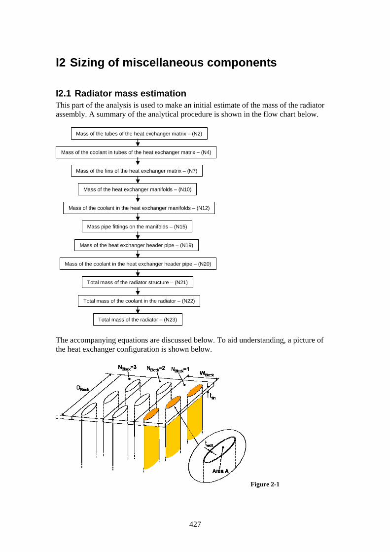
I2 Sizing of miscellaneous components

I2.1 Radiator mass estimation This part of the analysis is used to make an initial estimate of the mass of the radiator assembly. A summary of the analytical procedure is shown in the flow chart below.

Mass of the tubes of the heat exchanger matrix – (N2)

Mass of the coolant in tubes of the heat exchanger matrix – (N4)

Mass of the fins of the heat exchanger matrix – (N7)

Mass of the heat exchanger manifolds – (N10)

Mass of the coolant in the heat exchanger manifolds – (N12)

Mass pipe fittings on the manifolds – (N15)

Mass of the heat exchanger header pipe – (N19)

Mass of the coolant in the heat exchanger header pipe – (N20)

Total mass of the radiator structure – (N21)

Total mass of the coolant in the radiator – (N22)

Total mass of the radiator – (N23) The accompanying equations are discussed below. To aid understanding, a picture of the heat exchanger configuration is shown below.

Figure 2-1

427

An understanding of the heat exchanger configuration, as presented in the figure above, is valuable to aid understanding of the equations presented in this analysis. The heat exchanger is analysed as a number of N repeating identical blocks. Each block has the dimensions WxDxH, with W being the width and D the depth of the block end plates. H is the length of the tubes between end plates. The number of tubes in each block is dependant on the configuration chosen, which is 3 in this analysis (3-row heat exchanger). The total volume of the material that makes up the tubes of the matrix is given by equation N1, where P is the perimeter of a cross-section through one of the tubes and t is the wall thickness of each tube. The total mass of the tubes is given by equation N2.

WallTubeMatrixBlocksBlockTubesEachTubeMatrixTubes thNNPV −−−− ⋅⋅⋅⋅= Eq 2-1 (N1)

MatMatrixMatrixTubesMatrixTubes VM −−− ⋅= ρ Eq 2-2 (N2) An operational heat exchanger will also be completely filled with coolant and allowance must be made for this additional mass. The total volume of the coolant contained in the heat exchanger tubes can be determined from equation N3, where A is the internal cross-sectional area of one of the tubes. The mass of the coolant in the tubes can then be determined from N4.

MatrixBlocksBlockTubesTubeCSACoolantTubes hNNAV ⋅⋅⋅= −−− Eq 2-3 (N3)

CoolantCoolantTubesCoolantTubes VM ρ⋅= −− Eq 2-4 (N4) Matrix fins are used to improve the effectiveness of the heat exchanger, which are equally spaced along the entire length H of the heat exchanger tubes. For the configuration chosen, the fin pitch is defined by the data from Kays and London. The total number of fins can then simply be determined from equation N5.

( )[ ] 10, −=− FinMatrixBlockFins PitchhROUNDN Eq 2-5 (N5) The total volume of the material that makes up the fins in the heat exchanger is given by equation N6, where AFin-Block is the platform area of a single fin within each block and tFin is the material thickness of a fin. The total mass of the matrix fins can then be determined from equation N6.

EachFinBlockBlockFinsNetBlockFinFins tNNAV −−− ⋅⋅⋅= )( Eq 2-6 (N6)

MatMatrixFinsFins VM −⋅= ρ Eq 2-7 (N7)

428

Figure 2-2 The radiator end manifolds are assumed to adopt the semi-circular configuration shown in the figure above. The total volume of material making up the manifolds (one on each end of the matrix) can be determined from equation N8. As defined by equation N9, the wall thickness of the end manifolds is assumed to be twice that of the matrix tubes. The mass of the end manifolds is finally given by equation N10.

ManifoldMatrixMatrixManifold twtV ⋅⋅⋅= π Eq 2-8 (N8)

WallTubeManifold tt −⋅= 2 Eq 2-9 (N9)

MatMatrixManifoldManifold VM −⋅= ρ Eq 2-10 (N10) The volume of the coolant within the end manifolds is given by equation N11 and its mass is given by N12.

MatrixMatrix

CoolantManifold wt

V ⋅⋅

=− 4

2π Eq 2-11 (N11)

CoolantCoolantManifoldCoolantManifold VM ρ⋅= −− Eq 2-12 (N12) The general layout of the complete radiator is shown in the figure below. Besides the heat exchanger matrix and end manifold which have already been discussed, this also includes end fittings for connecting pipes. It is typical for the inlet and outlets of a heat exchanger to be at opposite corners of the matrix, to improve its performance. A header pipe can however be used so that both of the connections are at the same end, as shown.

End manifolds

End fitting

Header pipe

Heat exchanger matrix

End manifolds

End fitting

Header pipe

Heat exchanger matrix Figure 2-3 In this analysis, we have assumed that the length and diameter of the end fitting are equal, as given by equation N13. The volume of material that makes up the end fitting is

429

given by equation N14 and its mass is given by N15, where NFitting is the number of end fittings in the configuration (2 in this case).

FittingFitting DL = Eq 2-13 (N13)

FittingFittingWallFittingFitting DLtV ⋅⋅⋅= − π Eq 2-14 (N14)

MatMatrixFittingFittingFitting NVM −⋅⋅= ρ Eq 2-15 (N15) The length of the header pipe is assumed to be equal to the height of the heat exchanger, as given by equation N16. Its diameter is also assumed to be the same as that of the end fitting, as given by equation N17.

MatrixHeaderPipe hL =− Eq 2-16 (N16)

FittingHeaderPipe DD =− Eq 2-17 (N17) The volume of material that makes up the header pipe is given by N18, where

is the wall thickness of the header pipe and is assumed to be the same as the manifold wall thickness. The mass of the header pipe is then given by equation N19.

)(wallHeaderPipet −

HeaderPipeHeaderPipewallHeaderPipeHeaderPipe LDtV −−−− ⋅⋅⋅= π)( Eq 2-18 (N18)

MatMatrixHeaderPipeHeaderPipe VM −−− ⋅= ρ Eq 2-19 (N19) The mass of the coolant contained in the header pipe is given by equation N20.

CoolantHeaderPipeHeaderPipe

CoolantHeaderPipe LD

M ρπ ⋅⋅⋅= −−

− 2

2

)( Eq 2-20 (N20)

The total mass of the empty radiator can finally be determined from equation N21 as the sum of the components above. Likewise, the total mass of the coolant within the radiator is given by equation N22. The total mass of the radiator is finally determined as the sum of the empty mass and the coolant, as given by equation N24.

HeaderPipeFittingManifoldFinsMatrixTubesRadiator MMMMMM −− ++++= Eq 2-21 (N21)

)(CoolantHeaderPipeCoolantManifoldCoolantTubesRadCoolant MMMM −−−− ++= Eq 2-22 (N22)

RadCoolantRadiatorTotalRad MMM −− += Eq 2-23 (N23)

I2.2 Feed pipe sizing for a split radiator system Due to size constraints, it is necessary to use two separate radiator circuits instead of one, which will mean splitting the mass flow into two smaller diameter pipes. The cross-sectional area of each split pipe can be determined from equation N24 and its diameter from N25.

430

45.0

2Original

SplitPipe

DA ⋅⋅=− π Eq 2-24 (N24)

πSplitPipe

SplitPipe

AD −

−

⋅=

4 Eq 2-25 (N25)

I2.3 Heat transfer from aircraft wing fuel tanks This part of the analysis is used to determine the heat transfer from the wing fuel tanks, which thus reduces the quantity of heat which must be dissipated by the boom radiators. Since the depth of the wing fuel tank is small in comparison to its other dimensions, heat loss from the fuel tank is assumed to be from its upper and lower surfaces only. A summary of the analytical procedure is shown in the flow chart below. The accompanying equations are also given below.

Radiative thermal resistance for wing fuel tank top surface – (N29)

Radiative thermal resistance for wing fuel tank underside surface – (N30)

Reynolds number for wing fuel tank top surface – (N31)

Reynolds number for wing fuel tank underside surface – (N32)

Prandtl number for the aircraft operating conditions – (N33)

Nusselt number for the wing fuel tank top surface – (N34)

Nusselt number for the wing fuel tank underside surface – (N35)

Convection coefficient for the wing fuel tank top surface – (N36)

Convection coefficient for the wing fuel tank underside surface – (N37)

Convective thermal resistance for wing fuel tank top surface – (N38)

Convective thermal resistance for wing fuel tank underside surface – (N39)

Combined thermal resistance for wing fuel tank top surface – (N40)

Combined thermal resistance for wing fuel tank underside surface – (N41)

Total heat transfer from the wing fuel tank top surface – (N42)

Total heat transfer from the wing fuel tank underside surface – (N43)

Total heat transfer from the aircrafts wing fuel tanks – (N44)

431

This analysis requires knowledge of a number of properties of the atmospheric air, which are given by equations N26 to N27. It should also be noted that the fuel temperature has been fixed at 15 degrees during the analysis. This analysis follows a similar procedure to that used for heat loss from the external surfaces of a fuel cell as presented in the cooling system requirements section and so the depth of discussion will be somewhat limited here. The main difference here is that heat transfer will involve forced convection as opposed to natural convection used before.

( )TTTk 12

233

104.24510648151.2

−

−

∗+⋅∗

= Eq 2-26 (N26)

T1

=β Eq 2-27 (N27)

αααα CtBtA airair −⋅+⋅= 2 Eq 2-28 (N28) Constant Aα Bα Cα Value 9.1018E-11 8.8197E-8 -1.0654E-5

The radiative thermal resistance for the top and underside fuel tank surfaces can be determined from equations N29 and N30 respectively.

( )( )22)(1

AirFuelAirFuelTopTanktopR TTTTAF

R++⋅⋅⋅

=−σ

Eq 2-29 (N29)

( )( )22)(1

AirFuelAirFuelBottomTankbottomR TTTTAF

R++⋅⋅⋅

=−σ

Eq 2-30 (N30)

Equations N31 and N32, able us to determine the Reynolds number for the top and underside fuel tank surfaces, where L is the mean surface width and V is the free stream flight speed.

Air

TopTankAirTop

LVμ

ρ −⋅⋅= 0Re Eq 2-31 (N31)

Air

BottomTankAirBottom

LVμ

ρ −⋅⋅= 0Re Eq 2-32 (N32)

Another fluid dependant property known as the Prandtl number, as given by equation N33, is required in order to determine the Nusselt number.

Air

AirAirP

kC μ⋅

= −Pr Eq 2-33 (N33)

The Nusselt number for the top and underside fuel tank surface can then be determined from equations N34 and N35 respectively.

432

177.033.05.0 PrRe332.0 ⎟⎟

⎠

⎞⎜⎜⎝

⎛⋅⋅⋅=

air

fuelTopTop t

tNu Eq 2-34 (N34)

177.033.05.0 PrRe332.0 ⎟⎟

⎠

⎞⎜⎜⎝

⎛⋅⋅⋅=

air

fuelBottomBottom t

tNu Eq 2-35 (N35)

The convection coefficient for the top and underside surfaces can then be determined from equations N36 and N37 respectively.

TopTopTank

AirTop Nu

Lk

h ⋅=−

Eq 2-36 (N36)

BotomBottomTank

AirBottom Nu

Lk

h ⋅=−

Eq 2-37 (N37)

The convective thermal resistance for each fuel tank surface can then be obtained from equations N38 and N39. Equations N40 and N41 can then be used to find the combined thermal resistance for convection and radiation.

TopTankTopTopCon Ah

R−

− ⋅=

1 Eq 2-38 (N38)

BottomTankBottomBottomCon Ah

R−

− ⋅=

1 Eq 2-39 (N39)

TopRTopCon

TopTh

RR

R

−−

−

+=

111 Eq 2-40 (N40)

BottomRBottomCon

BottomTh

RR

R

−−

−

+=

111 Eq 2-41 (N41)

The heat transfer from each of the fuel tank surfaces by dissipation can finally be determined by equations N42 and N43. The total heat transfer for the top and underside fuel tank surfaces on both sides of the aircraft is finally given by equation N44.

TopTh

AirFuelTopDis R

TTQ

−−

−= Eq 2-42 (N42)

BottomTh

AirFuelBottomDis R

TTQ

−−

−= Eq 2-43 (N43)

( )BottomDisTopDisTotalDis QQQ −−− +⋅= 2 Eq 2-44 (N44)

433

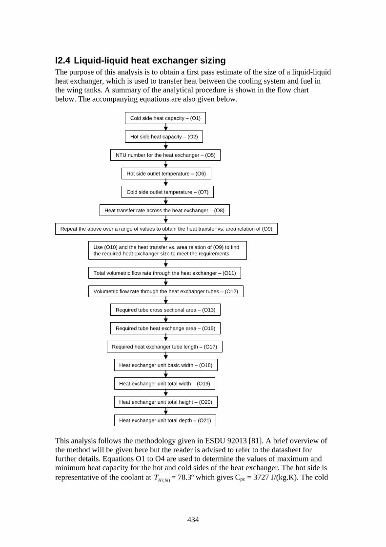
I2.4 Liquid-liquid heat exchanger sizing The purpose of this analysis is to obtain a first pass estimate of the size of a liquid-liquid heat exchanger, which is used to transfer heat between the cooling system and fuel in the wing tanks. A summary of the analytical procedure is shown in the flow chart below. The accompanying equations are also given below.

Cold side heat capacity – (O1)

Hot side heat capacity – (O2)

NTU number for the heat exchanger – (O5)

Hot side outlet temperature – (O6)

Cold side outlet temperature – (O7)

Heat transfer rate across the heat exchanger – (O8)

Repeat the above over a range of values to obtain the heat transfer vs. area relation of (O9)

Use (O10) and the heat transfer vs. area relation of (O9) to find the required heat exchanger size to meet the requirements

Total volumetric flow rate through the heat exchanger – (O11)

Volumetric flow rate through the heat exchanger tubes – (O12)

Required tube cross sectional area – (O13)

Required tube heat exchange area – (O15)

Required heat exchanger tube length – (O17)

Heat exchanger unit basic width – (O18)

Heat exchanger unit total width – (O19)

Heat exchanger unit total height – (O20)

Heat exchanger unit total depth – (O21) This analysis follows the methodology given in ESDU 92013 [81]. A brief overview of the method will be given here but the reader is advised to refer to the datasheet for further details. Equations O1 to O4 are used to determine the values of maximum and minimum heat capacity for the hot and cold sides of the heat exchanger. The hot side is representative of the coolant at = 78.3º which gives Cpc = 3727 J/(kg.K). The cold )( InHT

434

side is representative of the methanol in the wing tanks at = 15º which gives Cpc = 3727 J/(kg.K). A trial and error approach was used to determine the best balance of mass flow rates, which gave, =0.9kg/s and =0.13kg/s.

)( InCT

Cm Hm

A

CPCC mCC ⋅= Eq 2-45 (O1)

HPHH mCC ⋅= Eq 2-46 (O2) ):min( HCMin CCC = Eq 2-47 (O3) ):max( HCMax CCC = Eq 2-48 (O4)

Equation O5 gives the NTU number required, where the heat transfer coefficient

=600 W/m2K (from ESDU 94042 [82] table 12.1). is the heat transfer area which is an analysis variable, for which a range of values between 0.8 and 2m2 were explored.

mU HT

Min

mHT

CUA

NTU⋅

= Eq 2-49 (O5)

Using NTU from above and C* (C* =Cmin/Cmax) we are able to determine the effectiveness from the corresponding tables in ESDU 92013. The hot side and cold side exit temperatures can then be determined from equations O6 and O7.

( )

435

H

In)( − InCHMinInHOutH C

TTCTT )(

)()(

⋅⋅ε Eq 2-50 (O6) −=

( )C

InCIn)( −HMinInCOutC C

TTCTT )(

)()(

⋅⋅+=ε

Eq 2-51 (O7)

Finally, the heat exchanger heat transfer rate can be determined from equation O8.

( ))()( OutHInHHHeat TTCQ −⋅= Eq 2-52 (O8) After repeating the steps above at a number of different estimates of heat transfer area, the heat transfer versus area relation O9 is obtained, as shown in the chart below.

Heat Transfer vs Area Relation

y = -3.7732x2 + 16.239x + 5.522

15

16

17

18

19

20

21

22

23

24

0.6 0.8 1 1.2 1.4 1.6 1.8 2

A (m2)

Q (k

W)

2.2

Eq 2-53 (O9)

The relation O9 given above can then be solved to determine the size of heat exchanger required. In which case, the optimal configuration is one whose calculated heat transfer rate will equal the required heat transfer rate, as given in equation O10.

etTCalculatedError QQQ arg−= Eq 2-54 (O10) Relations O11 and O12 enable the volumetric flow rate through the heat exchanger and each of the flow tubes to be determined. The number of tubes used in this analysis is 4.

Coolant

HTotalFlow

mQρ

=− Eq 2-55 (O11)

Tubes

TotalFlowTubeFlow N

QQ −

− = Eq 2-56 (O12)

The cross sectional area of each of the flow tubes can be determined from equation O13 and the corresponding tube diameter from equation O14.

TubeFlow

TubeFlowTube V

QA

−

−= Eq 2-57 (O13)

πTube

TubeA

D⋅

=4

Eq 2-58 (O14)

The total heat transfer area can now be divided according to the number of tubes used in the configuration as given in equation O15.

Tubes

TotalHTTubeHT N

AA −

− = Eq 2-59 (O15)

The circumference of each of the tubes can be determined from equation O16 and then the required length of each of the tubes can be determined from equation O17.

π⋅=1000

TubeTube

DC Eq 2-60 (O16)

Tube

TubeTube C

AL = Eq 2-61 (O17)

Finally, an estimate of the unit size can be made from the results obtained above and the configuration assumed. In this case, there is assumed to be 4 shells in total with 2 tube passes in each shell, which gives a total of 8 passes for each tube. There is also assumed to be 4 parallel tubes for this arrangement. Using this data and some basic assumptions, an estimate of the unit width can be determined from equation O18.

TotalPasses

TubeUnit N

Lw

−

= Eq 2-62 (O18)

436

The dimensions of the heat exchanger can then be obtained from equations O19 to O21.

( )TubeUnitHeatEx Dww ⋅+= 4 Eq 2-63 (O19) ( )TubeTubeHeatEx DDh ⋅+⋅⋅= 234

Eq 2-64 (O20)

TubeTubeHeatEx DDd ⋅+⋅= 45 Eq 2-65 (O21)

I2.4.1 Liquid-liquid heat exchanger integration Naturally, the best location for the liquid-liquid heat exchanger is within the fuselage in close proximity to the fuel tanks. This will ensure that the power demands of the pumps required to circulate the hot and cold flows are kept to a minimum and that it is located as close as possible to the aircraft centre of gravity.

I2.5 Fuel cell intake sizing The minimum fuel cell system intake area required to meet the air supply demands can be determined from the equation below, where is determined by the analysis methods given in appendix H.

Airm

0Vm

AAir

AirIntake ⋅

=ρ

Eq 2-66

It should be emphasised however that this is the minimum size to meet the air demands of the fuel cell system only. The actual area of the intake must be larger than this to provide sufficient additional air for cooling. A cooling air requirement of 5% of the core airflow was quoted for a gas turbine engine and in the absence of a better estimate, it seems reasonable to adopt this figure for a fuel cell system. The minimum intake size for a fuel cell system then becomes.

0)( 05.1

Vm

AAir

AirTotalIntake ⋅

=ρ

Eq 2-67

437

438

J1 Fuel cell powered MALE performance analysis The purpose of this section is to present an overview of the different fuel cell system configurations which were proposed and the methodology used to evaluate their performance. This covers following fuel cell system variants:

• Autothermal reformer system • Steam reformer system • Hybrid autothermal reformer system • Hybrid steam reformer system • Fuel cell system with oxygen injection

In the sections which follow, a brief description of each of the fuel cell propulsion system variants will be given. This is followed with an overview of the procedure used to generate an analytical model which can be used to predict the fuel consumption of each system. This analytical model is finally integrated into the existing performance analyses used for the baseline aircraft to enable us to predict the performance of such a system in contrast to the baseline turboprop configuration. The final results for these analyses are presented in the evaluation section on the main text.

J1.1 Autothermal reformer system performance analysis A simplified schematic of the autothermal reformer based fuel cell system is presented in the figure below. The reader is advised to refer to the section, an overview of the fuel cell powered aircraft systems for further details of the accompanying systems.

Motor 1

Motor 2

Motor 1

Motor 2

Fuel Cell

Anode

Cathode

Fuel Cell

Anode

Cathode

Schematic of the autothermal reformer system

Comp.Comp.

Air-in

Autothermal FuelProcessorAutothermal FuelProcessor

Methanol-in

2 in to 1 reduction gearbox

Figure 1

J1.1.1 System analysis Using the analysis methods discussed in Appendix H (fuel cell system design and analysis), this system was tested over a range of combinations of fuel cell power output and altitude. The results of this analysis work are presented in the chart below as number of trends lines of fuel consumption versus power output. Each curve in this chart represents a different test altitude, which includes a range of values between sea level and the loiter altitude of 7620m.

439

Fuel consumption as a function of power and altitude

0

0.01

0.020.03

0.04

0.05

0.06

0.070.08

0.09

0.1

70 95 120 145 170 195 220 245 270 295 320 345 370 395 420

Power (kW)

m-d

ot fu

el (k

g/s)

0

2286

4572

6096

7620

1143

3429

5334

6858

Chart 1 At this point, the reader may question the irregular nature of the curves in the above chart. The shape of the curves is however correct and is a result of the operating characteristics of the fuel cell system. To explain this phenomenon, we shall take a closer look at the characteristics of one of the curves. For this discussion, the curve for the 1143m altitude condition was selected at random, as presented below. The other curves exhibit the same operating characteristics.

Fuel consumption as a function of power and altitude

0.01

0.02

0.03

0.04

0.05

0.06

0.07

0.08

0.09

0.1

0.06 0.1 0.14 0.18 0.22 0.26 0.3 0.34 0.38 0.42

Power - /1000 (kW)

m-d

ot fu

el (k

g/s)

1143

N=1

N=2

N=3

N=4

Fuel consumption as a function of power and altitude

0.01

0.02

0.03

0.04

0.05

0.06

0.07

0.08

0.09

0.1

0.06 0.1 0.14 0.18 0.22 0.26 0.3 0.34 0.38 0.42

Power - /1000 (kW)

m-d

ot fu

el (k

g/s)

1143

N=1

N=2

N=3

N=4

Chart 2 Upon close inspection of the irregular curve in the above chart, we can see that its profile actually consists of a number of steps along its length. It could in fact be considered to be constructed from four smaller segments, each of which corresponds to a different number of fuel cells in operation. For example, the first curve represents 1 of the 4 fuel cells in operation; the second curve corresponds to 2 of the 4 fuel cells in operation and so on. The characteristics are thus a function of the switching of the individual fuel cell stacks. In an actual fuel cell system, the control system will tailor the switching of each fuel cell system to deliver smoother operating characteristics for the complete system. It would therefore be reasonable to draw a best fit curve through the points which begins and end on the first and last points.

440

J1.1.2 Analysis results The raw data from our analysis for a number of different altitudes and fuel cell power outputs is given in the table below for reference. Results for autothermal reformer system

0 1143 2286 3429 4572 5334 6096 6858 762064.47933 0.011967 0.010851 0.009993 0.009314 0.009019 0.009063 0.009112 0.009165 0.00923978.7569 0.015121 0.013716 0.012638 0.011784 0.011436 0.011499 0.011567 0.011662 0.011785

101.3247 0.021567 0.019588 0.018071 0.016874 0.01649 0.016605 0.016761 0.01696 0.017175116.0628 0.021234 0.01925 0.017726 0.016519 0.015964 0.016039 0.016121 0.016211 0.016336

138.17 0.025908 0.023494 0.02164 0.020173 0.019536 0.019635 0.019744 0.019897 0.020061153.3687 0.029285 0.026562 0.024472 0.022818 0.022142 0.022261 0.022392 0.022573 0.022768175.0153 0.03456 0.03136 0.028904 0.026962 0.026224 0.026378 0.026593 0.026826 0.027077190.6746 0.039035 0.035436 0.032676 0.030496 0.02973 0.02992 0.030182 0.030466 0.030828211.8607 0.039864 0.036151 0.0333 0.031044 0.030066 0.03022 0.03039 0.030627 0.030882227.9805 0.043455 0.039413 0.036311 0.033856 0.032853 0.033028 0.033221 0.033489 0.033777248.706 0.048334 0.04385 0.040408 0.037686 0.036644 0.03685 0.037078 0.037391 0.037729

265.2864 0.052574 0.047708 0.043974 0.041022 0.0399 0.040137 0.040467 0.040824 0.041282285.5513 0.058409 0.053023 0.048893 0.04563 0.044483 0.044768 0.045159 0.045582 0.046123302.5923 0.064184 0.058292 0.053777 0.050211 0.049066 0.049406 0.049866 0.050455 0.051093322.3967 0.062221 0.056443 0.052009 0.048501 0.047073 0.047333 0.047701 0.048015 0.048526339.8982 0.066508 0.060342 0.055611 0.051869 0.05044 0.05073 0.051049 0.051486 0.052049359.242 0.071598 0.064976 0.059895 0.055878 0.054356 0.054683 0.055138 0.055629 0.056259

377.2041 0.076791 0.069706 0.064273 0.059978 0.058467 0.058837 0.059346 0.059898 0.060603396.0873 0.082933 0.075308 0.069463 0.064846 0.063242 0.063779 0.06436 0.064991 0.065793

414.51 0.089878 0.081651 0.075348 0.070373 0.068794 0.069415 0.070087 0.070944 0.071872

Altitude (m)

Pow

er (k

W)

Fuel (kg/s)

Table 1

J1.1.3 Derivation of a general relation from the analysis data The raw data from the last section needs to be converted into a more manageable format if it is to be used within our performance analysis. In this section, we describe the process followed to create a complex analytical expression from the raw data. A summary of the procedure used is shown in the flow chart below. The accompanying equations are also given below.

Test the fuel cell system at a number of different altitudes and power settings to generate a table of results – (FC1)

Use the table of results to generate a plot of fuel consumption versus power output for the system operating at a number of different altitudes – (FC2)

Generate a plot of coefficient value versus altitude for each of the polynomial coefficients – (FC4)

Test the expressions obtained and determine the error – (FC5)

Fit a polynomial expression to each of the curves generated in the stage above – (FC2)

Generate a table of coefficients for the polynomial expressions fitted to the curves generated in the stage above – (FC3)

Fit a polynomial expression to each of the curves generated in the stage above – (FC4)

441

The first stage in this work is to use the raw data from the last section to generate a number of plots of fuel consumption against fuel cell power output, with each plot corresponding to a different altitude. An example of one such plot is presented in the chart below for the 1143m altitude case.

Fuel consumption as a function of power and altitude

y = 78.044x5 - 87.508x4 + 36.764x3 - 7.0917x2 + 0.796x - 0.0195

0.01

0.02

0.03

0.04

0.05

0.06

0.07

0.08

0.09

0.1

0.06 0.1 0.14 0.18 0.22 0.26 0.3 0.34 0.38 0.42

Power - /1000 (kW)

m-d

ot fu

el (k

g/s)

1143

Theo

Poly. (1143)

Chart 3 (FC2) To this plot, we are then able to fit a polynomial best fit curve, which is taken as an average of the data points. The corresponding polynomial expression for each best fit curve takes the form given by the general expression below, which expresses the fuel consumption as a function of the fuel cell power output.

CEPX

EPX

EPX

EPX

EPXmFuel +⎟

⎠⎞

⎜⎝⎛⋅+⎟

⎠⎞

⎜⎝⎛⋅+⎟

⎠⎞

⎜⎝⎛⋅+⎟

⎠⎞

⎜⎝⎛⋅+⎟

⎠⎞

⎜⎝⎛⋅=

3131313131

2

2

3

3

4

4

5

5

Eq 1 (FC2) This process is repeated to obtain a plot and corresponding best fit polynomial expression for each of the altitudes tested. This ultimately gives us nine independent expressions, whose constants can be tabulated as in table FC3 below. Expression constants for autothermal reformer system

X5 X4 X3 X2 X C0 84.883 -95.176 39.985 -7.713 0.8683 -0.0212

1143 78.044 -87.508 36.764 -7.0917 0.796 -0.01952286 72.895 -81.735 34.339 -6.624 0.7413 -0.01823429 68.93 -77.29 32.472 -6.2639 0.6989 -0.01724572 71.124 -79.762 33.508 -6.4617 0.7116 -0.01775334 73.131 -81.933 34.39 -6.6272 0.7265 -0.01826096 75.196 -84.28 35.392 -6.8232 0.7449 -0.01876858 78.968 -88.5 37.159 -7.1643 0.7761 -0.01977620 82.035 -92.055 38.702 -7.4696 0.8046 -0.0205

Altit

ude

Expresssion constants

Table 2 (FC3) If we then generate a plot of expression coefficient versus altitude for each column of coefficients from the table above, it is possible to identify a trend with respect to altitude. An example of such a plot for the coefficients X3 is shown in the chart below.

442

Expression constant X3

y = 248.89x5 - 584.64x4 + 467.9x3 - 102.31x2 - 20.608x + 39.966

30323436384042444648

0 0.2 0.4 0.6 0.8

Altitude - /10000 (m)

Con

stan

t

Chart 4 (FC4) To this plot, we are then able to fit a polynomial best fit curve, which gives us a corresponding best fit polynomial expression. This expression takes the form given by the general expression below which gives the expression coefficient as a function of the operating altitude.

)()()(2)(3)(4)(5 4141414141 NNNNNNN DEhY

EhY

EhY

EhY

EhYX +⎟

⎠⎞

⎜⎝⎛⋅+⎟

⎠⎞

⎜⎝⎛⋅+⎟

⎠⎞

⎜⎝⎛⋅+⎟

⎠⎞

⎜⎝⎛⋅+⎟

⎠⎞

⎜⎝⎛⋅=

Eq 2 (FC4) This process is repeated to obtain a plot and corresponding best fit polynomial expression for each column of coefficients in table FC3 above. This gives us six independent expressions, whose constants can be tabulated as below. Expression constants for autothermal reformer system

Y5 Y4 Y3 Y2 Y DX5 500.67 -1204 978.28 -215.15 -43.819 84.842X4 -579.66 1375.8 -1108.4 243.04 49.053 -95.131X3 248.89 -584.64 467.9 -102.31 -20.608 39.966X2 -47.993 112.17 -89.552 19.506 3.9955 -7.7094

X (/10) 40.048 -97.985 80.697 -16.703 -5.1069 8.6793C (/100) -11.345 27.677 -22.883 5.0421 1.1134 -2.1191 Table 3 (FC4)

The corresponding expressions for each of the equation coefficients X5, X4, X3, X2, X and C can then determined from the respective relations below. Where, the corresponding expression coefficients Y5 to D are given in the table above.

DEhY

EhY

EhY

EhY

EhYX +⎟

⎠⎞

⎜⎝⎛⋅+⎟

⎠⎞

⎜⎝⎛⋅+⎟

⎠⎞

⎜⎝⎛⋅+⎟

⎠⎞

⎜⎝⎛⋅+⎟

⎠⎞

⎜⎝⎛⋅=

4141414141 23455

DEhY

EhY

EhY

EhY

EhYX +⎟

⎠⎞

⎜⎝⎛⋅+⎟

⎠⎞

⎜⎝⎛⋅+⎟

⎠⎞

⎜⎝⎛⋅+⎟

⎠⎞

⎜⎝⎛⋅+⎟

⎠⎞

⎜⎝⎛⋅=

4141414141 23454

DEhY

EhY

EhY

EhY

EhYX +⎟

⎠⎞

⎜⎝⎛⋅+⎟

⎠⎞

⎜⎝⎛⋅+⎟

⎠⎞

⎜⎝⎛⋅+⎟

⎠⎞

⎜⎝⎛⋅+⎟

⎠⎞

⎜⎝⎛⋅=

4141414141 23453

DEhY

EhY

EhY

EhY

EhYX +⎟

⎠⎞

⎜⎝⎛⋅+⎟

⎠⎞

⎜⎝⎛⋅+⎟

⎠⎞

⎜⎝⎛⋅+⎟

⎠⎞

⎜⎝⎛⋅+⎟

⎠⎞

⎜⎝⎛⋅=

4141414141 23452

443

10/4141414141 2345 ⎥

⎦

⎤⎢⎣

⎡+⎟

⎠⎞

⎜⎝⎛⋅+⎟

⎠⎞

⎜⎝⎛⋅+⎟

⎠⎞

⎜⎝⎛⋅+⎟

⎠⎞

⎜⎝⎛⋅+⎟

⎠⎞

⎜⎝⎛⋅= D

EhY

EhY

EhY

EhY

EhYX

100/4141414141 2345 ⎥

⎦

⎤⎢⎣

⎡+⎟

⎠⎞

⎜⎝⎛⋅+⎟

⎠⎞

⎜⎝⎛⋅+⎟

⎠⎞

⎜⎝⎛⋅+⎟

⎠⎞

⎜⎝⎛⋅+⎟

⎠⎞

⎜⎝⎛⋅= D

EhY

EhY

EhY

EhY

EhYC

Eqs 3 to 8 The final expression for the fuel consumption with respect to fuel cell power output is then given below. Whose constants are a function of operating altitude, as given by the expressions above.

CEPX

EPX

EPX

EPX

EPXmFuel +⎟

⎠⎞

⎜⎝⎛⋅+⎟

⎠⎞

⎜⎝⎛⋅+⎟

⎠⎞

⎜⎝⎛⋅+⎟

⎠⎞

⎜⎝⎛⋅+⎟

⎠⎞

⎜⎝⎛⋅=

3131313131

2

2

3

3

4

4

5

5 Eq 9

The final stage in our work is to test the expression at the original raw data points and thus determine the magnitude of any numerical analysis error. The error associated with this expression in respect to the source data, can be found from the expression below,

%100⋅⎟⎟⎠

⎞⎜⎜⎝

⎛ −=

Analysis

AnalysisEquation

mmm

Error Eq 10

For this study, this gave us an error range between 0.1 and 7% with an average value of 2.97%. The biggest source of error originates from the smooth curve approximation to the stepped raw data curves. In a practical fuel cell system however, the operating characteristics of the fuel cell system are likely to be tailored to match those of the smooth curve approximation and therefore the error range is not a significant problem. This expression has been shown to give very good results for medium to high power flight phases but is less satisfactory for low powers which will be covered in the next section. The expression given in this section can thus only be used with confidence within for the following phases:

• Take-off (including ground roll, rotation, climb-out and second segment climb) • Climb (stage 1 and 2) • Loiter • Descent (stage 1 and 2)

J1.1.4 Derivation of a low power relation As mentioned above, at low powers the general expression given above deviates somewhat from the raw data and thus its accuracy is questionable. In such cases, an alternative expression must be used which is applicable to the following flight phases:

• Sea level loiter • Landing (including approach and flare and ground roll)

Since the low power flight phases all take place at sea level, it is reasonable to restrict our analysis to a sea level altitude. Not only does this have the benefit of a considerably reduced workload but also results in a much simpler expression than before.

444

The derivation of such an expression utilises the methods of Appendix H to determine the low power characteristics of the fuel cell at sea level conditions. The fuel cell system is then tested at a number of low power settings to determine the fuel consumption of the fuel cell at these conditions. These results can then be used to generate a plot of fuel consumption versus power as in the chart below.

Fuel consumption for low power conditions - autothermal reformer

y = 42.965x2 + 1576.8x + 16.609

0

2000

4000

6000

8000

10000

12000

14000

0 1 2 3 4 5 6

Power - /10 (kW)

m-d

ot fu

el -

x1E6

(kg/

s)

7

Chart 5 A quadratic curve and corresponding quadratic expression can then be fitted to this chart to generate the manageable final relation below.

61/609.1610

8.157610

965.422

EPP

m kWKWFuel

⎥⎥⎦

⎤

⎢⎢⎣

⎡+⎟

⎠⎞

⎜⎝⎛⋅+⎟

⎠⎞

⎜⎝⎛⋅= Eq 11

J1.2 Steam reformer system performance analysis A simplified schematic of the steam reformer based fuel cell system is presented in the figure below. The reader is advised to refer to the section, ‘an overview of the fuel cell powered aircraft systems’ for further details of the accompanying systems.

Motor 1

Motor 2

Motor 1

Motor 2

Fuel Cell

Anode

Cathode

Fuel Cell

Anode

Cathode

Schematic of the steam reformer system

Comp.Comp.

Air-in

Methanol-in

2 in to 1 reduction gearbox

Steam Reformer FuelProcessorSteam Reformer FuelProcessor

Figure 2 As with the autothermal system, this system is tested at a number of conditions to generate a table of raw data. This raw data can then be used to generate an analytical

445

model to predict the fuel consumption of the system, which is in a format which can be easily integrated into the performance analysis work. As before, we are then able to predict the performance of such a system in contrast to other propulsion devices.

J1.2.1 Analysis results The raw data from our analysis for a number of different altitudes and fuel cell power outputs is given in the table below for reference. Results for steam reformer system

0 1143 2286 3429 4572 5334 6096 6858 762064.47933 0.011967 0.010851 0.009993 0.009314 0.009019 0.009063 0.009112 0.009165 0.00923978.7569 0.015121 0.013716 0.012638 0.011784 0.011436 0.011499 0.011567 0.011662 0.011785

101.3247 0.021567 0.019588 0.018071 0.016874 0.01649 0.016605 0.016761 0.01696 0.017175116.0628 0.021234 0.01925 0.017726 0.016519 0.015964 0.016039 0.016121 0.016211 0.016336

138.17 0.025908 0.023494 0.02164 0.020173 0.019536 0.019635 0.019744 0.019897 0.020061153.3687 0.029285 0.026562 0.024472 0.022818 0.022142 0.022261 0.022392 0.022573 0.022768175.0153 0.03456 0.03136 0.028904 0.026962 0.026224 0.026378 0.026593 0.026826 0.027077190.6746 0.039035 0.035436 0.032676 0.030496 0.02973 0.02992 0.030182 0.030466 0.030828211.8607 0.039864 0.036151 0.0333 0.031044 0.030066 0.03022 0.03039 0.030627 0.030882227.9805 0.043455 0.039413 0.036311 0.033856 0.032853 0.033028 0.033221 0.033489 0.033777248.706 0.048334 0.04385 0.040408 0.037686 0.036644 0.03685 0.037078 0.037391 0.037729

265.2864 0.052574 0.047708 0.043974 0.041022 0.0399 0.040137 0.040467 0.040824 0.041282285.5513 0.058409 0.053023 0.048893 0.04563 0.044483 0.044768 0.045159 0.045582 0.046123302.5923 0.064184 0.058292 0.053777 0.050211 0.049066 0.049406 0.049866 0.050455 0.051093322.3967 0.062221 0.056443 0.052009 0.048501 0.047073 0.047333 0.047701 0.048015 0.048526339.8982 0.066508 0.060342 0.055611 0.051869 0.05044 0.05073 0.051049 0.051486 0.052049359.242 0.071598 0.064976 0.059895 0.055878 0.054356 0.054683 0.055138 0.055629 0.056259

377.2041 0.076791 0.069706 0.064273 0.059978 0.058467 0.058837 0.059346 0.059898 0.060603396.0873 0.082933 0.075308 0.069463 0.064846 0.063242 0.063779 0.06436 0.064991 0.065793

414.51 0.089878 0.081651 0.075348 0.070373 0.068794 0.069415 0.070087 0.070944 0.071872

Fuel (kg/s) Altitude (m)

Pow

er (k

W)

Table 4

J1.2.2 Derivation of a general relation from the analysis data As for the autothermal reformer, the raw data from the last section needs to be converted into a more manageable format if it is to be used within our performance analysis. The process used to generate the complex analytical expression from the raw data is the same as that for the autothermal reformer, which enables us to arrive at the expression below.

CEPX

EPX

EPX

EPX

EPXmFuel +⎟

⎠⎞

⎜⎝⎛⋅+⎟

⎠⎞

⎜⎝⎛⋅+⎟

⎠⎞

⎜⎝⎛⋅+⎟

⎠⎞

⎜⎝⎛⋅+⎟

⎠⎞

⎜⎝⎛⋅=

3131313131

2

2

3

3

4

4

5

5

Eq 12 As before, an expression for each of the equation coefficients X5, X4, X3, X2, X and C can then determined in the form of the general relation below. The accompanying coefficients are given in the table below. As before, the constants X and C must be further divided by 10 and 100 respectively to arrive at the final answer.

)()()(2)(3)(4)(5 4141414141 NNNNNNN DEhY

EhY

EhY

EhY

EhYX +⎟

⎠⎞

⎜⎝⎛⋅+⎟

⎠⎞

⎜⎝⎛⋅+⎟

⎠⎞

⎜⎝⎛⋅+⎟

⎠⎞

⎜⎝⎛⋅+⎟

⎠⎞

⎜⎝⎛⋅=

Eq 13

446

Expression constants for steam reformer systemY5 Y4 Y3 Y2 Y D

X5 360.66 -867.72 704.05 -155.95 -29.651 60.826X4 -417.05 990.58 -797.03 175.98 33.211 -68.203X3 179.5 -421.73 336.99 -74.209 -13.942 28.654X2 -34.57 80.843 -64.455 14.141 2.7041 -5.5272

X (/10) 28.531 -70.043 57.745 -12.057 -3.4913 6.2293C (/100) -10.974 24.351 -18.439 3.8015 0.7872 -1.5194 Table 5

This expression is however, only applicable to the medium to high power flight phases, since its accuracy is questionable at the low power flight regimes. An alternative expression must therefore be used for the low power conditions.

J1.2.3 Derivation of a low power relation As before, an alternative expression was required for low power sea level flight regimes. The derivation of such an expression utilises the methods of Appendix H to generate a table of results and then generate a plot of fuel consumption versus power as given in the chart below.

Fuel consumption for low power conditions - steam reformer

y = 30.765x2 + 1137.4x + 11.899

0

1000

2000

3000

4000

5000

6000

7000

8000

9000

0 1 2 3 4 5 6 7

Power - /10 (kW)

m-d

ot fu

el -

x1E6

(kg/

s)

Chart 6 A quadratic curve and corresponding quadratic expression can then be fitted to this chart to generate the final relation below.

61/899.1110

4.113710

765.302

EPP

m kWKWFuel

⎥⎥⎦

⎤

⎢⎢⎣

⎡+⎟

⎠⎞

⎜⎝⎛⋅+⎟

⎠⎞

⎜⎝⎛⋅= Eq 14

J1.3 Hybrid autothermal reformer system performance analysis The original analysis of the fuel cell system power requirements highlighted the final climb phase as being the most critical. This flight phase will thus also be the largest consumer of methanol fuel. As discovered in the analyses carried out so far, the fuel consumption of the reformer based fuel cell systems is significantly higher than that of a turboprop engine. This means that the range of our baseline aircraft would be

447

significantly reduced as a result. To overcome this problem, in this section we investigate the potential of retaining the turboprop engine for the entire flight except the loiter phase. In such a hybrid system, the turboprop engine is disengaged for the loiter phase and the propeller is instead driven by the motor which is fed by the fuel cell system. For all other flight phases, the fuel cell system is disengaged and the propeller power is delivered entirely by the turboprop. A simplified schematic of the hybrid autothermal reformer system is presented in the figure below. As before, the reader is advised to refer to the section on an overview of the fuel cell powered aircraft systems for further details of the accompanying systems. The only difference between this and the other fuel systems is that one of the motors that feeds the 2 into 1 reduction gearbox, has been replaced with a turboprop engine. Since the loiter phase has a significantly lower power demand than the other flight phases, the size of the fuel cell system can be reduced accordingly. This weight saving is intended to offset the additional weight of the turboprop engine.

Motor 1

Turboprop Engine

Fuel Cell

Anode

Cathode

Fuel Cell

Anode

Cathode

Schematic of the hybrid autothermal reformer system

Comp.Comp.

Air-in

Autothermal FuelProcessorAutothermal FuelProcessor

Methanol-in

2 in to 1 reduction gearbox

Figure 3 Fortunately, with this system we are able to reuse the analytical model generated for the autothermal system to predict the fuel consumption of the fuel cell part of the system. The relevant expressions are thus integrated into the flight phases of the performance analysis work in which the fuel cell system is operative. The remaining flight phases retain the engine performance expressions for the baseline turboprop configuration.

J1.4 Hybrid steam reformer system performance analysis The steam reformer based hybrid system offers the same benefits as the autothermal based hybrid system in terms of a reduction in fuel consumption. As before, the turboprop engine is used to supply power to the propeller in all the flight phases except the loiter phase. In the loiter phase, the turboprop engine is disengaged and the propeller is driven by the motor which is fed by fuel cell system instead. The only difference between this and the autothermal reformer based hybrid system is the fuel processor. A simplified schematic of the hybrid steam reformer system is presented in the figure below. As before, the reader is advised to refer to the section on an overview of the fuel cell powered aircraft systems for further details of the accompanying systems. As with the hybrid autothermal system, the 2 into 1 reduction gearbox is driven by both a motor

448

and a turboprop engine. As before, the size of the fuel cell system can also be reduced, since in this configuration it only needs to meet the requirements of the loiter phase.

Motor 1

Turboprop Engine

Fuel Cell

Anode

Cathode

Fuel Cell

Anode

Cathode

Schematic of the hybrid steam reformer system

Comp.Comp.

Air-in

Methanol-in

2 in to 1 reduction gearbox

Steam Reformer FuelProcessorSteam Reformer FuelProcessor

Figure 4 Fortunately, with this system, we are able to reuse the analytical model generated for the fuel consumption of the steam reformer system. The relevant expressions are thus integrated into the flight phases of the performance analysis work in which the fuel cell system is operative. The remaining flight phases retain the engine performance expressions for the baseline turboprop configuration.

J1.5 Investigation into the use of oxygen injection In the systems above, hydrogen is being fed to the fuel cell in excess of that actually required. This is so that the excess leaving the fuel cell can be burned to generate the hot gases needed to drive a turbine, which is linked to the system air compressor. We therefore have to burn an additional quantity of fuel in order to be able to deliver oxygen in sufficient quantity and at the required pressure for the fuel cell. If we consider the fact that air is only made up of approximately only 21% oxygen, then we are wasting a significant amount of energy (via the additional amount of fuel) to deliver the fractions of air that are not actually required. In particular, the compressor has to work hard to deliver nitrogen (which makes up 79% of the air), which is not actually required. The nitrogen in the air serves no useful purpose within the fuel cell and merely acts as a dilutant which is eventually discarded. We are therefore expending work and fuel to deliver it to the fuel cell in order to throw it away. If we could find a way to either sieve the oxygen from the air before it enters the compressor or use oxygen from a purer source, then the fuel consumption of our system could be reduced. Sieving the air is however not practical since the air must be delivered to the sieve in a considerable quantity to start with. The only other option is therefore to carry either a compressed or liquefied source of oxygen on-board the aircraft. Such a oxygen supply would be able to at least in part, meet the oxygen needs of the fuel cell. Since space is at a premium inside our aircraft and liquefied oxygen takes up a significantly smaller volume than compressed oxygen, only a liquefied oxygen source will be considered here.

449

Since a large quantity of oxygen is required for a fuel cell system of this size, it was unlikely that we would be able to carry sufficient oxygen on-board the aircraft to meet our needs. There is still however benefits to be gained by using such an oxygen source to supplement the oxygen already available within the air. In such a system, the air would be mixed with pure oxygen to increase the oxygen content of the air. The feasibility of such a system is considered in the work which follows.

J1.5.1 System description A simplified schematic of a system which is able to incorporate additional oxygen is presented in the figure below. This system is the same as for a standard fuel cell system, with the exception of the addition of a mixing chamber between the fuel cell and the air compressor. Within this chamber, the air from the compressor is mixed with pure oxygen supplied from an alternative source. The reader is advised to refer to the section ‘an overview of the fuel cell powered aircraft systems’ for further details of the accompanying systems.

Fuel Cell

Anode

Cathode

Fuel Cell

Anode

Cathode

Schematic of a fuel cell system with oxygen injection

Comp.Comp.

Air-in

Fuel ProcessorFuel ProcessorMethanol-in

Mixing ChamberMixing Chamber

Compressed Oxygen

Figure 5

J1.5.2 Analysis of the mixing chamber As already stated, the mixing chamber is used to mix air from the compressor with pure oxygen from an alternative source. The output stream from the mixing chamber is thus an air stream with an higher oxygen content. In this section, we will determine the revised oxygen fraction of the air mixture for varying quantities of oxygen injection. It is a reasonable approximation that air typically consists of 21% oxygen and 79% nitrogen. This therefore gives us, 21 parts of O2 per 100 parts of air. If we now add an additional percentage of ‘X’ O2 to the air, this will give us additional ‘X’ parts of O2 out of 100. The total parts of O2 in the mixture will then become,

XOOO AdditionalAirTotal +=+= 21)(2)(2)(2 Eq 15 This gives us a mixture made up of a total number of parts,

XOAirMix AdditionalTotal +=+= 100)(2)( Eq 16

450

The total fraction of O2 in the mixture then becomes,

)(

)(22 )(

Total

Total

MixO

OFraction = Eq 17

The percentages of air and additional O2 in the mixture are then given by respective relations below.

)(

)(TotalMix

AirAirPercentage = Eq 18

)(

)(22 )(

Total

AdditionalAdditional Mix

OOPercentage =− Eq 19

Following this procedure, we are able to obtain the table of results given below. O2(Additional) (%) Parts O2(from air) Parts of air Parts O2(Additional) Parts of O2(Total) Parts Total Fraction O2(in mixture) % Air % O2(Additional)

0 21 100 0 21 100 0.21 100 05 21 100 5 26 105 0.247619048 95.2381 4.76190476210 21 100 10 31 110 0.281818182 90.90909 9.09090909115 21 100 15 36 115 0.313043478 86.95652 13.0434782620 21 100 20 41 120 0.341666667 83.33333 16.6666666725 21 100 25 46 125 0.368 80 2030 21 100 30 51 130 0.392307692 76.92308 23.0769230835 21 100 35 56 135 0.414814815 74.07407 25.9259259340 21 100 40 61 140 0.435714286 71.42857 28.5714285745 21 100 45 66 145 0.455172414 68.96552 31.0344827650 21 100 50 71 150 0.473333333 66.66667 33.3333333355 21 100 55 76 155 0.490322581 64.51613 35.4838709760 21 100 60 81 160 0.50625 62.5 37.565 21 100 65 86 165 0.521212121 60.60606 39.3939393970 21 100 70 91 170 0.535294118 58.82353 41.1764705975 21 100 75 96 175 0.548571429 57.14286 42.8571428680 21 100 80 101 180 0.561111111 55.55556 44.44444444

Table 6 In a similar way, the molecular mass of the gas mixture at different oxygen concentrations was evaluated and a linear expression fitted to the data as given below. Where, M has the units of kg/kmol and X is oxygen volume fraction.

167.288328.3 +⋅= XM Mixture Eq 20

J1.5.3 System performance prediction at loiter Since the aircraft spends the majority of its time at loiter, it makes sense to initially asses the viability of an oxygen injection system at this flight phase. This also fits in well with the proposals for a hybrid fuel cell system, in which the fuel cell is restricted to use at loiter. Since the steam reformer system has already been shown to give the best fuel consumption results, the steam reformer system will form the basis of this study. This analysis thus follows the same analysis procedure as presented for the steam reformer based fuel cell system. The only difference between this analysis and that for the standard steam reformer system is the O2 fraction of air entering the system. This was determined in the section above, as the oxygen concentration of the air leaving the mixing chamber for a number of different additional O2 injection settings.

451

This analysis utilises the methods of appendix H to give us the results for the required mass flow rate of methanol and additional injection oxygen at the mid loiter phase. The quantity of additional oxygen required in each case be then determined from the expression,

⎟⎟⎠

⎞⎜⎜⎝

⎛⋅=

100% )(2

)()(2Additional

TotalAirAdditionalO

Omm Eq 21

If we base our initial estimates on the original loiter phase duration of 35 hours, then the total mass of methanol and liquid oxygen for that flight duration can then be determined from the expression below.

eLoiterPhasactatTotaltac tmm ⋅= Re)(tanRe Eq 22 This analysis gives us the results given in the table below. Results for mid loiter Duration of loiter flight phase (s) 126000

%O2(Additional) Fraction O2(in mixture) % Air %O2(Additional) m-dot(methanol) (kg/s) m-dot(LOX) (kg/s) Mehanol(loiter) (kg) LOx(loiter) (kg)0 0.21 100 0 0.01058676 0 1333.93182 0

10 0.281818182 90.90909 9.09090909 0.010066604 0.010226248 1268.392086 1288.50725920 0.341666667 83.33333 16.6666667 0.009643394 0.018641275 1215.067662 2348.80068430 0.392307692 76.92308 23.0769231 0.009290876 0.025689793 1170.650402 3236.91397640 0.435714286 71.42857 28.5714286 0.008992716 0.031677725 1133.08226 3991.39339450 0.473333333 66.66667 33.3333333 0.008737453 0.036825896 1100.919112 4640.06284960 0.50625 62.5 37.5 0.008516657 0.041298084 1073.098792 5203.55855170 0.535294118 58.82353 41.1764706 0.00832396 0.045218359 1048.818956 5697.51320680 0.561111111 55.55556 44.4444444 0.008154455 0.048682357 1027.461377 6133.976958

Table 7 If we present these results graphically as in the chart below, we can see that a system using oxygen injection is clearly not viable. It is evident that the mass of the liquid oxygen which must be carried on-board the aircraft far exceeds the fuel mass saved with the use of such a system.

Total methanol and LOx required for loiter

0

1000

2000

3000

4000

5000

6000

7000

0 10 20 30 40 50 60 70 80 90

%O2(Additional)

Mas

s (k

g)

Methanol

LOx

Chart 7

452