CRANFIELD UNIVERSITY Rebecca L. Whetton Multi-sensor ...

i

CRANFIELD UNIVERSITY

Rebecca L. Whetton

Multi-sensor and data fusion approach for determining yield limiting factors and

for in-situ measurement of yellow rust and fusarium head blight in cereals

School of Energy Environment and Agrifood

This thesis is submitted in partial fulfilment of the requirements for the degree

of Doctor of Philosophy

PhD

23rd December 2016

Supervisor: Prof. Abdul Mounem Mouazen

Co-Supervisor: Dr Toby Waine

iii

CRANFIELD UNIVERSITY

School of Energy Environment and Agrifood

PhD

Academic Year 2013 - 2016

Rebecca L. Whetton

Multi-sensor and data fusion approach for determining yield limiting factors and

for in-situ measurement of yellow rust and fusarium head blight in cereals

Supervisor: Prof. Abdul Mounem Mouazen

Co-Supervisor: Dr Toby Waine

This thesis is submitted in partial fulfilment of the requirements for the degree

of Doctor of Philosophy

© Cranfield University 2016. All rights reserved. No part of this publication

may be reproduced without the written permission of the copyright owner.

v

"If we do not change our direction, we are likely to end up where we

are headed."

vii

ABSTRACT

The world’s population is increasing and along with it, the demand for food. A novel

parametric model (Volterra Non-linear Regressive with eXogenous inputs (VNRX)) is

introduced for quantifying influences of individual and multiple soil properties on crop yield

and normalised difference vegetation Index. The performance was compared to a random

forest method over two consecutive years, with the best results of 55.6% and 52%,

respectively. The VNRX was then implemented using high sampling resolution soil data

collected with an on-line visible and near infrared (vis-NIR) spectroscopy sensor predicting

yield variation of 23.21%.

A hyperspectral imager coupled with partial least squares regression was successfully applied

in the detection of fusarium head blight and yellow rust infection in winter wheat and barley

canopies, under laboratory and on-line measurement conditions. Maps of the two diseases

were developed for four fields. Spectral indices of the standard deviation between 500 to 650

nm, and the squared difference between 650 and 700 nm, were found to be useful in

differentiating between the two diseases, in the two crops, under variable water stress. The

optimisation of the hyperspectral imager for field measurement was based on signal-to-noise

ratio, and considered; camera angle and distance, integration time, and light source angle and

distance from the crop canopy.

The study summarises in the proposal of a new method of disease management through

suggested selective harvest and fungicide applications, for winter wheat and barley which

theoretically reduced fungicide rate by an average of 24% and offers a combined saving of

the two methods of £83 per hectare.

viii

Keywords

Yellow rust, Fusarium head blight, PLSR regressions, yield limiting factors, on-line,

precision agriculture.

ix

ACKNOWLEDGEMENTS

I would like to acknowledge the Farm FUSE project from the ICT-AGRI under the European

Commission’s ERA-NET scheme under the 7th Framework Programme, and the UK

Department of Environment, Food and Rural Affairs (contract no: IF0208), for providing

funding which made this PhD possible.

To my supervisors, Abdul Mouazen and Toby Waine, firstly thank you for giving me the

opportunity to undertake this PhD research. Abdul your guidance, and expertise in the area

has been invaluable, and your patience and drive with the project has been greatly

appreciated. Toby I’m very grateful for your guidance, suggestions and constructive

comments on the project. Without the knowledge and direction from both of my supervisors,

this project and the papers would not have been possible. Furthermore, for having made the

last three years (…3 months… and 3 weeks) at Cranfield thoroughly rewarding and

enjoyable. Involving me with other projects, collaborations, and your support for attending

conferences, has been of great use in the thesis, and I’m sure will continue to be highly

valuable, and for that I can’t express my gratitude enough. I’d also like to acknowledge and

thank Kim Blackburn for his guidance. To both Yifan and Said, it’s been a great pleasure to

work with you on the papers, and your insights and persistence towards publishing have been

greatly encouraging. To Dimitrios’ team at Aristotle University and Boyan at Cranfield thank

you, you really helped me get started with the project. I would also like to say a big thank you

to my examiners Jon and Paul. Your knowledge in the area, and detailed attention to

improving the thesis has been greatly appreciated. To you all, I’m much obliged.

x

To my thesis committee, including my subject advisor, Naresh Magan and independent

chairman, Ahmed Al-Ashaab, the guidance and constructive comments that you provided

throughout the course of this PhD were invaluable. Furthermore, to all the Cranfield staff,

both in the lab and in the office, who have helped me in my PhD studies, many thanks to you

all. I’d like to say a particular thankyou to Bob Walker without whom I don’t think this

project would ever have gotten to the field, and to Mr Maskell for giving me access to “play”

with the sensors in those fields.

Matt and Olly thank you for all your time and patience with the various software and coding.

And thankyou to Scott for always being a reference of BASIS knowledge. To all my fellow

students and friends at Cranfield, past and present, thanks for all of the distractions, coffee

breaks, great times and support. To all of my other friends, despite asking “aren’t you done

yet?” you have been there all the way. You have helped to balance out my life, reminding me

there is more to life than work, and many of you have gone out of your ways to ensure I have

eaten and slept (when I had often forgotten to).

I would like to say a big thankyou to my parents and family who throughout my PhD, (and

despite thinking I play with soil all day) have always given me their utmost support

(emotional, financial, and in cake).

And thank you to you, the reader, even if you stop here.

xi

TABLE OF CONTENTS

ABSTRACT .................................................................................................................... vii

ACKNOWLEDGEMENTS ............................................................................................. ix

TABLE OF CONTENTS ................................................................................................. xi

LIST OF FIGURES ........................................................................................................ xv

LIST OF TABLES .......................................................................................................... xx

LIST OF ABBREVIATIONS ...................................................................................... xxiv

1 Introduction .................................................................................................................... 1

1.1 Background and Context ......................................................................................... 1

1.2 Research objectives ................................................................................................. 8

Hypothesis ......................................................................................................................... 8

Aim .................................................................................................................................... 8

Objectives .......................................................................................................................... 9

1.3 Thesis structure ..................................................................................................... 10

1.4 Disclosure ............................................................................................................. 11

2 Literature review .......................................................................................................... 14

2.1 Fungal diseases ..................................................................................................... 14

2.1.1 Yellow rust .............................................................................................................. 14

2.1.2 Fusarium head blight .............................................................................................. 15

2.1.3 Fungal disease resistance ........................................................................................ 19

2.1.4 Disease distribution and spread .............................................................................. 20

2.1.5 Current approach in fungal disease control ............................................................ 26

2.1.6 Timings of fungicide applications .......................................................................... 26

2.2 Techniques for disease detection .......................................................................... 27

2.2.1 Review of optical imaging techniques of crop canopies ........................................ 30

2.2.2 Application of visible and infrared spectroscopy in disease detection ................... 32

2.2.3 Application of fluorescence spectroscopy in disease detection .............................. 34

2.2.4 Alternative spectral methods .................................................................................. 36

2.2.5 Hyperspectral and multispectral imaging ............................................................... 36

2.2.6 Optical imaging summary ....................................................................................... 39

2.3 Variability and yield limiting factors .................................................................... 42

2.4 On-line measurement of soil properties ................................................................ 43

2.5 Literature conclusions; research gaps ................................................................... 44

3 Quantification of yield limiting factors........................................................................ 46

3.1 A new non-linear parametric modelling method to quantify influence of soil

properties on crop yields: Methodology ..................................................................... 47

Abstract ............................................................................................................................ 47

3.1.1 Introduction ............................................................................................................. 48

3.1.2 Material and methods .............................................................................................. 50

3.1.3 Results and discussion ............................................................................................ 58

xii

3.2 A new non-linear parametric modelling method to quantify influence of soil

properties on crop yields: Application to on-line soil data ......................................... 74

Abstract ............................................................................................................................ 74

3.2.1 Introduction ............................................................................................................. 75

3.2.2 Materials and Methods ............................................................................................ 78

3.2.3 Results and discussion ............................................................................................ 85

3.3 Summary conclusions ......................................................................................... 103

4 Optimising the configuration of a hyperspectral imager for on-line measurement of

wheat canopies .............................................................................................................. 105

Abstract ..................................................................................................................... 105

4.1 Introduction ......................................................................................................... 106

4.2 Materials and methods ........................................................................................ 109

4.2.1 Hyperspectral configuration in the laboratory ...................................................... 109

4.2.2 On-line soil and crop measurements in the field .................................................. 113

4.2.3 Data analyses ........................................................................................................ 116

4.2.4 Mapping ................................................................................................................ 121

4.3 Results and Discussion ....................................................................................... 121

4.3.1 Spectral quality in the laboratory .......................................................................... 121

4.3.2 Hyperspectral image configuration parameters; laboratory .................................. 123

4.3.3 Hyperspectral imager; on-line measurement ........................................................ 129

4.4 Influence of soil properties on signal-to-noise ratio during the on-line measurement

................................................................................................................................... 131

4.5 Conclusions ......................................................................................................... 134

5 Hyperspectral measurements of yellow rust and fusarium head blight in cereal crops:

Part 1: Laboratory study................................................................................................ 136

Abstract .......................................................................................................................... 136

5.1 Introduction ......................................................................................................... 137


5.2.1 Wheat and Barley cultivation and inoculation ...................................................... 140

5.2.2 Disease assessments .............................................................................................. 143

5.2.3 Hyperspectral data capture .................................................................................... 146

5.2.4 Data pre-processing and modelling ...................................................................... 148

5.3 Results ................................................................................................................. 153

5.3.1 Crop canopy spectra .............................................................................................. 153

5.3.2 Model performance for yellow rust and fusarium head blight detection .............. 159

5.4 Discussion ........................................................................................................... 163

5.4.1 Crop canopy spectra .............................................................................................. 163

5.4.2 Model performance for yellow rust and fusarium head blight detection .............. 168


6 Hyperspectral measurements of yellow rust and fusarium head blight in cereal crops:

Part 2: on-line field measurement ................................................................................. 173

Abstract .......................................................................................................................... 173

xiii

6.1 Introduction ......................................................................................................... 174


6.2.1 Field sites .............................................................................................................. 177

6.2.2 Hyperspectral on-line data capture ....................................................................... 179

6.2.3 Moisture content measurement ............................................................................. 181

6.2.4 Disease recognition in the field............................................................................. 182

6.3 Data analyses. ..................................................................................................... 185

6.3.1 Crop canopy spectral data pre-processing ............................................................ 185

6.3.2 Evaluation of model performance ......................................................................... 186

6.3.3 Mapping ................................................................................................................ 192

6.4 Results ................................................................................................................. 193

6.4.1 Crop canopy spectra analysis ................................................................................ 193


6.4.3 Maps ...................................................................................................................... 199

6.5 Discussion ........................................................................................................... 208

6.5.1 Crop canopy spectra analysis ................................................................................ 208


6.5.3 Maps ...................................................................................................................... 213


7 Management zone maps for variable fungicide application and selective harvest .... 218

Abstract ..................................................................................................................... 218

7.1 Introduction ......................................................................................................... 219


7.2.1 Field site ................................................................................................................ 222

7.2.2 Disease and canopy property data collection ........................................................ 224

7.2.3 On-line soil measurement ..................................................................................... 226

7.2.4 Spectral modelling of disease and soil properties ................................................. 226

7.2.5 Mapping ................................................................................................................ 228

7.2.6 Management zone maps ........................................................................................ 228

7.2.7 Eventual calculation of cost-benefit analysis ........................................................ 229

7.3 Results and discussion ........................................................................................ 231

7.3.1 Spatial variability of different properties .............................................................. 231

7.3.2 K-means clusters ................................................................................................... 237

7.3.3 Treatment maps ..................................................................................................... 242

7.3.4 Economic benefits ................................................................................................. 247


8 Conclusions and further work .................................................................................... 255

8.1 Recent publications ............................................................................................. 255

8.2 Objectives and chapter conclusions .................................................................... 256

8.2.1 Objective 1: ........................................................................................................... 257

8.2.2 Objective 2: ........................................................................................................... 259

8.2.3 Objective 3: ........................................................................................................... 262

xiv

8.2.4 Objective 4: ........................................................................................................... 264

8.2.5 Objective 5: ........................................................................................................... 266

8.3 Hypothesis consideration .................................................................................... 268

8.4 Contributions to knowledge ................................................................................ 269

8.5 Further work ........................................................................................................ 270

8.5.1 Yield limiting factors ............................................................................................ 270

8.5.2 Hyperspectral imaging of disease ......................................................................... 271

8.5.3 Management zones ............................................................................................... 271

8.6 Concluding remarks ............................................................................................ 271

REFERENCES ............................................................................................................. 273

APPENDICES .............................................................................................................. 295

xv

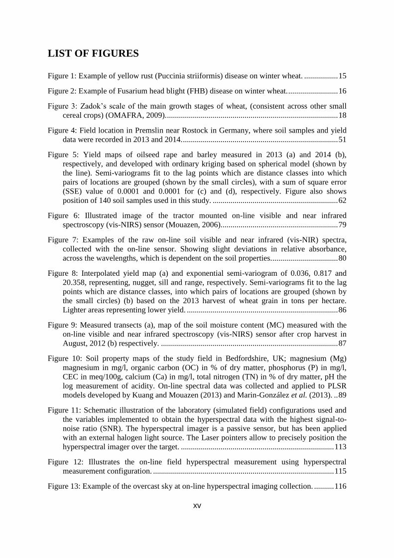
LIST OF FIGURES

Figure 1: Example of yellow rust (Puccinia striiformis) disease on winter wheat. ................. 15

Figure 2: Example of Fusarium head blight (FHB) disease on winter wheat. ......................... 16

Figure 3: Zadok’s scale of the main growth stages of wheat, (consistent across other small

cereal crops) (OMAFRA, 2009). ...................................................................................... 18

Figure 4: Field location in Premslin near Rostock in Germany, where soil samples and yield

data were recorded in 2013 and 2014. .............................................................................. 51

Figure 5: Yield maps of oilseed rape and barley measured in 2013 (a) and 2014 (b),

respectively, and developed with ordinary kriging based on spherical model (shown by

the line). Semi-variograms fit to the lag points which are distance classes into which

pairs of locations are grouped (shown by the small circles), with a sum of square error

(SSE) value of 0.0001 and 0.0001 for (c) and (d), respectively. Figure also shows

position of 140 soil samples used in this study. ............................................................... 62

Figure 6: Illustrated image of the tractor mounted on-line visible and near infrared

spectroscopy (vis-NIRS) sensor (Mouazen, 2006)........................................................... 79

Figure 7: Examples of the raw on-line soil visible and near infrared (vis-NIR) spectra,

collected with the on-line sensor. Showing slight deviations in relative absorbance,

across the wavelengths, which is dependent on the soil properties.................................. 80

Figure 8: Interpolated yield map (a) and exponential semi-variogram of 0.036, 0.817 and

20.358, representing, nugget, sill and range, respectively. Semi-variograms fit to the lag

points which are distance classes, into which pairs of locations are grouped (shown by

the small circles) (b) based on the 2013 harvest of wheat grain in tons per hectare.

Lighter areas representing lower yield. ............................................................................ 86

Figure 9: Measured transects (a), map of the soil moisture content (MC) measured with the

on-line visible and near infrared spectroscopy (vis-NIRS) sensor after crop harvest in

August, 2012 (b) respectively. ......................................................................................... 87

Figure 10: Soil property maps of the study field in Bedfordshire, UK; magnesium (Mg)

magnesium in mg/l, organic carbon (OC) in % of dry matter, phosphorus (P) in mg/l,

CEC in meq/100g, calcium (Ca) in mg/l, total nitrogen (TN) in % of dry matter, pH the

log measurement of acidity. On-line spectral data was collected and applied to PLSR

models developed by Kuang and Mouazen (2013) and Marin-González et al. (2013). .. 89

Figure 11: Schematic illustration of the laboratory (simulated field) configurations used and

the variables implemented to obtain the hyperspectral data with the highest signal-to-

noise ratio (SNR). The hyperspectral imager is a passive sensor, but has been applied

with an external halogen light source. The Laser pointers allow to precisely position the

hyperspectral imager over the target. ............................................................................. 113

Figure 12: Illustrates the on-line field hyperspectral measurement using hyperspectral

measurement configuration. ........................................................................................... 115

Figure 13: Example of the overcast sky at on-line hyperspectral imaging collection. .......... 116

file:///C:/Users/s215090/Desktop/thesis_map_corrections/ready_for_last/thesis_v_8.2_reformated.docx%23_Toc491714668





















xvi

Figure 14: Schematic illustration outlining how mean, standard deviation and signal-to-noise

ratio for wavelength (Mw, SDw, SNRw, respectively) and a spectrum (Ms, SDs, SNRs,

respectively) were calculated. ........................................................................................ 119

Figure 15: Examples of smooth (the grey line with 1.6 signal-to-noise ratio (SNR), noisy (the

black line with 1.2 SNR), and saturated (the dotted line with 1.8 SNR) spectra of wheat

canopy. The saturated spectrum flattens off at 680-750 nm and important information is

lost on the peak around 700 nm that is otherwise illustrated by the clear spectra. ........ 123

Figure 16: Principal component analysis similarity maps developed for principal components

1 and 2 (a) and for principal components 1 and 3 (b). Input variables are camera and

light height, light distance, camera angle, integration time and signal-to-noise ratio

(SNR).............................................................................................................................. 126

Figure 17: Comparison of canopy spectra of water stressed wheat crop obtained in the

laboratory (the dashed line) and on-line in the field (the dotted and grey lines). The crop

was of the same variety and at comparable growth stages. Laboratory and field scans

were collected under the suggested optimal configurations. The on-line field scans are:

1) field scan (the grey line) is of a more water stressed plant and 2) field scan (the dotted

line) is of a less water stressed plant. ............................................................................. 131

Figure 18: Maps of on-line measured soil moisture content (MC) (a) total nitrogen (TN) (b),

and the average signal-to-noise ratio (SNR) per scan (c). .............................................. 133

Figure 19: Schematic of tray replicates and treatments, showing winter barley and winter

wheat, with yellow rust and fusarium head blight (FHB) diseases, and healthy crop, both

rain fed and water stressed, in replicates of three. .......................................................... 142

Figure 20: Fusarium inoculation of wheat and barley trays in the laboratory. Inoculation took

place at the anthesis crop growth stage. ......................................................................... 143

Figure 21: Illustrating influence of foliar health on yield (HGCA, 2008) ............................. 145

Figure 22: Schematic illustration of the laboratory configurations of hyperspectral camera

and light source (Whetton et al., 2016b). ....................................................................... 148

Figure 23: Example spectra of wheat and barley canopy at growth stage 72, after white and

dark corrections. Arrows highlight areas of interest for indices to distinguish the health

of the crop. ...................................................................................................................... 153

Figure 24: Comparison of an average wheat crop canopy spectra between watered (-) and

water-stressed (----) treatments for a) healthy, b) yellow rust infected and c) fusarium

head blight (FHB) infected crop canopy. Plot (d) compares canopy spectra under

watered conditions of healthy (---), yellow rust (---) and FHB (-). ................................ 155

Figure 25: Comparison of an average barley crop canopy spectra between watered (-) and

water-stressed (----) treatments for a) healthy, b) yellow rust infected and c) fusarium

head blight (FHB) infected crop canopy. Plot (d) compares canopy spectra under

watered conditions of healthy (---), yellow rust (---) and FHB (-). ................................ 156

Figure 26: Scatter plots of predicted versus reference measured (based on 20% prediction set)

yellow rust coverage in wheat (a), yellow rust coverage in barley (b), yellow rust scale in

wheat (c), yellow rust scale in barley (d), fusarium head blight (FHB) severity in wheat




xvii

(e), FHB severity in barley (f), wheat yellow rust logit (g), barley yellow rust logit (h).

The R² report significance level of <0.01 for each regression. ...................................... 162

Figure 27: Hyperspectral imagery system mounted on a metal frame attached to the side of a

tractor, ready for on-line canopy measurement. ............................................................. 179

Figure 28: Schematic of work flow from data capture to production of PLSR models,

validation, and on-line prediction for production of maps ............................................. 180

Figure 29: on-line hyperspectral measurement lines and position of ground truth plots,

collected at five samples per ha, in the four fields. Fields 1 and 4 were validated at the

same locations at two time intervals............................................................................... 183

Figure 30: Example of photo interpretation to assess yellow rust and fusarium head blight

(FHB) coverage based on a 100-point grid. ................................................................... 185

Figure 31: Indicative spectra of wheat canopy collected at early (booting) and late (milk)

growth stages, comparing on-line and non-mobile (off-line ground truth) spectra as: (-)

late non-mobile (---) early non-mobile (…) early on-line, and ( _ _ ) late on-line. ....... 194

Figure 32: Indicative spectra of barley canopy collected at anthesis growth stage, comparing

between on-line (--) and non-mobile (-) spectra. ........................................................... 194

Figure 33: Scatter plots for the on-line predicted versus reference assessed diseseas. On-line

predictions was based on partial least squares regression model developed, based on

visual yellow rust coverage in wheat (a), visual yellow rust coverage in barley (b), visual

yellow rust scale in wheat (c), visual yellow rust scale in barley (d), image fusarium head

blight (FHB) scale in wheat (e) and image FHB scale in barley (f). .............................. 198

Figure 34: Maps of % disease cover of fusarium head blight (FHB) of ground truth data

obtained with photo interpretation at a 10 by 10 m resolution. Maps areshown for the

four experimental fields; Field 1 with wheat (a) (4 ha anthesis), field 2 with barley (b)

(10 ha anthesis), field 3 with wheat (c) (12 ha Milk), and field 4 with wheat (d) (7 ha

Milk). .............................................................................................................................. 201

Figure 35: Maps of yellow rustclassed in the 0-5 scale of ground truth data at a 10 by 10 m

resolution. Maps are shown in the four experimental fields: (a and b) refer to maps of

early stage scans in field 1 with wheat (4 ha booting) and field 3 with wheat (12 ha

booting), respectively. Maps of late stage scans are shown by (c) for field 3 with wheat

(12 ha Milk), (d) for field 4 with wheat (7 ha Milk) (e) for field 1 with wheat (4 ha

anthesis) and (f) field 2 with barley (10 ha anthesis). .................................................... 202

Figure 36: On-line measured % infection of fusarium head blight (FHB) maps using photo

interpretation in the four experimental fields; Field 1 with wheat (a) (4 ha anthesis), field

2 with barley (b) (10 ha anthesis), field 3 with wheat (c) (12 ha Milk), and field 4 with

wheat (d) (7 ha Milk)...................................................................................................... 205

Figure 37: On-line measured yellow rust maps, classed in the 0-5 scale (0 is given when no

disease is present, 1 for up to 5% cover, 2 for up to 10%, 3 for up to 30%, 4 for up to

50% and 5 for >50%) in the four experimental fields: (a and b) refer to maps of early

stage scans in field 1 with wheat (4 ha booting) and field 3 with wheat (12 ha booting),

respectively. Maps of late stage scans are shown by (c) for field 3 with wheat (12 ha



xviii

Milk), (d) for field 4 with wheat (7 ha Milk) (e) for field 1 with wheat (4 ha anthesis) and

(f) field 2 with barley (10 ha anthesis). .......................................................................... 206

Figure 38: Soil moisture content map and images of measured with the on-line visible and

near infrared spectroscopy sensor (Mouazen, 2006) in field 4. ..................................... 208

Figure 39: Images of wheat crop at the field site in Bedfordshire, UK. Wheat was at growth

stage 72 (Milk). Part A) Fusarium head blight infection (FHB), and part B) Yellow rust

infection. ......................................................................................................................... 213

Figure 40: Map of the experimental field where ground sample locations (5 per hectare,

n=60) are shown. ............................................................................................................ 225

Figure 41: Disease severity; On-line predicted maps of fusarium head blight (FHB) measured

at milk growth stage 72 (july 2015), early yellow rust measured at booting growth stage

43 (may 2015), and late yellow rust measured at milk growth stage 72 (july 2015). The

disease is classified on a 0 to 5 scale, where 0 indicates low disease presence and 5

indicates high disease. .................................................................................................... 234

Figure 42: Properties attributed to the canopy; On-line measured normalised difference

vegetation index (NDVI), along with the 60 samples based developed maps for leaf area

index (LAI), canopy air temperature and humidity. These data were all collected at the

booting growth stage 43, in May 2015. .......................................................................... 235

Figure 43: Soil properties; On-line predicted soil cation exchange capacity (CEC in

Cmol/kg), total nitrogen (TN in %), moisture content (MC in %) and organic carbon (OC

in %). The soil properties were collected before the seed was drilled in September 2014.

........................................................................................................................................ 236

Figure 44: Yield map of wheat measured in September 2015. .............................................. 237

Figure 45: K-means cluster analysis based on the on-line predicted late yellow rust and

fusarium head blight (FHB) showing two classes to be adopted for the selective harvest

(SH). ............................................................................................................................... 239

Figure 46: K-means cluster analysis for variable rate fungicide application (VRFA) at the T1

and T2 growing stages. Input data were measured normalised difference vegetation

index (NDVI), air temperature, air humidity, leaf area index (LAI), on-line predicted soil

organic carbon (OC), total nitrogen (TN), moisture content (MC) and cation exchange

capacity (CEC), and on-line predicted early yellow rust disease. .................................. 240


growing stage. Input data were measured normalised difference vegetation index

(NDVI), air temperature, air humidity, leaf area index (LAI), on-line predicted soil

organic carbon (OC), total nitrogen (TN), moisture content (MC) and cation exchange

capacity (CEC), and on-line predicted fusarium head blight (FHB) disease. ................ 242

Figure 48: Management zone (MZ) maps for selective harvest (SH), The map on the left

shows high disease infection (MZ 1) and low disease infection (MZ 2) which is obtained

by k-means clustering that included on-line predicted fusarium head blight (FHB) and

late yellow rust. With the right map showing high and low infection zones on the right,




xix

with the field being split into plots of 12 m (due to the combine harvest cutting head).

........................................................................................................................................ 244

Figure 49: Management zone (MZ) maps for variable rate fungicide application (VRFA) at

the T1 and T2 growing stages. The map on the left show low yellow rust (MZ 1) and

high yellow rust (MZ 2), which is obtained by k-means clustering that included,

measured canopy properties (normalised difference vegetation index (NDVI), air

temperature, air humidity, and leaf area index (LAI)), on-line predicted soil (organic

carbon (OC), total nitrogen (TN), moisture content (MC) and cation exchange capacity

(CEC)), and on-line predicted early yellow rust disease. With the right map showing

high and low infection zones on the right, with the field being split into plots of 24 m

(due to the boom width). ................................................................................................ 245


the T3 growing stages, The map on the left show high fusarium head blight (FHB) (MZ

1) and medium FHB (MZ 2), and high FHB (MZ3), which is obtained by k-means

clustering that included, measured canopy properties (normalised difference vegetation

index (NDVI), air temperature, air humidity, and leaf area index (LAI)), on-line

predicted soil (organic carbon (OC), total nitrogen (TN), moisture content (MC) and

cation exchange capacity (CEC)), and on-line predicted FHB. With the right map

showing high and low infection zones on the right, with the field being split into plots of

24 m (due to the boom width). ....................................................................................... 246

xx

LIST OF TABLES

Table 1: Pathogen infection and influence. The economic impact, and environmental

conditions conducive to yellow rust, fusarium head blight (FHB) infection and

associated mycotoxins. The growth stages are in reference to Zadoks scale (Zadoks et

al., 1974; De Vallavieille-Pope et al., 1995; Gilbert and Tekauz, 2000; Rossi et al., 2001;

Bravo et al., 2003; Xu, 2003; Del Ponte et al., 2007) ............................................. 23

Table 2: summary of different spectral applications to recognition of crop diseases and

associated observations and accuracies ................................................................... 41

Table 3: Statistics of measured soil properties of the 140 soil samples used as input data into

the three models. TN, OC, MC in %, P, K, Mg Na, Ca in mg/l and CEC meq/100g60

Table 4: Semi-variogram model parameters of yield maps. The best fit was achieved with

spherical models for each, showing nugget (c0), sill c, range (r m), proportion (C0/ C %),

and the sum of square error (SSE)........................................................................... 60

Table 5: Pearson correlation (r) between soil properties and yield of 2013 and 2014. .. 64

Table 6: Calculated variable importance score (MSE) of yield prediction obtained with the

random forest (RF) model, indicating contribution of each soil property to crop yield in

2013 and 2014. ........................................................................................................ 65

Table 7: Calculated individual contribution (ERRC) of each soil property and sum of

contribution (SERR) to crop yield in 2013 and 2014 cropping seasons, obtained with

Volterra Non-linear Regressive with eXogenous inputs (VNRX), accounting for both

linear and non-linear relationships (VNRX-LN)..................................................... 69


contribution (SERR) to crop yield in 2013 and 2014 cropping seasons, obtained with

Volterra Non-linear Regressive with eXogenous inputs (VNRX), accounting for linear

relationship only (VNRX-L). .................................................................................. 71

Table 9: Summaries of the statistics for the soil properties predicted in the field and the

reliabilities of the models they were predicted from. The models were developed in

Kuang and Mouazen (2013) and Marin-González et al. (2013). ............................. 90

Table 10: Pearson correlation (r) between on-line measured soil properties in 2012 and wheat

yield harvested in 2013............................................................................................ 92

Table 11: The correspondence between inputs variables in Volterra Non-linear Regressive

with eXogenous inputs (VNRX) model and soil properties ................................... 93

Table 12: The first 10 terms with corresponding error reduction ratio contribution (ERRC)

values and coefficients based on the shortest distance approximation (SDA) re-sampling

technique with a 3 m radius. .................................................................................... 95

Table 13: Error reduction ratio contribution (ERRC) contribution of each soil property (input)

to the crop yield (system output) with corresponding significance threshold based on the

shortest distance approximation (SDA) re-sampling technique with a 3 m radius. 97

xxi

Table 14: Contribution of the top three significant soil properties in terms of the sum of error

reduction ratio (SERR) on the crop yield, based on shortest distance approximation

(SDA) and (CAA) sampling techniques calculated for different radius values. ... 102

Table 15: Factors included in configuring the hyperspectral imager measured in meters (m),

degrees (°) and micro seconds (ms) (multiple configurations considered) ........... 111

Table 16: Average and standard deviation (SD) values of the highest signal-to-noise-ratios

(SNR) obtained with different integration times, camera settings and light source settings

when scanning a wheat canopy. Theoretical forward distance travelled (and captured to a

single data line) if applied on a moving platform at field scale. ........................... 124

Table 17: Statistics of samples used in the partial least squares regression (PLSR) models,

with 80% and 20% of samples were considered for cross validation and prediction,

respectively. The data has a normal distribution. Yellow rust % refers to the percent

cover of yellow rust on the leaves (used for both % and the logit transformation). Yellow

rust scale refers to classes of disease infection levels with 0 being non and 5 being

>50%. Fusarium head blight (FHB) refers to number of infected ears compared to

number of healthy ears with 0 being healthy and 2 being >50%. ......................... 151

Table 18: Classes of the ratio of prediction deviation (RPD) and their suitability for

predicting yellow rust and fusarium head blight (FHB) in cereal crops, and is based on

the classifications from Rossel et al. (2006).......................................................... 152

Table 19: Spectral differences indicated as standard deviation of the 500-650 nm range and

squared difference of 650 and 700 nm, calculated for healthy, yellow rust and fusarium

head blight (FHB) infected wheat and barley canopy under watered and water-stressed

conditions, averaged from spectra captured at growth stage 70. One average spectra were

produced per line scan, with 9 line scans being considered for each class. .......... 158

Table 20: Analysis of Variance (ANOVA) table for the analysis of transformed spectral

indices over the different treatments. Analysis of the index the squared difference of 650

and 700 nm (sqDiff) was done on the square root scale, whilst analysis of the index

standard deviation (SD) is done on of the range 500-650 nm. .............................. 159

Table 21: Summary of model prediction performance of yellow rust and barley in cross-

validation and prediction showing the R2, root mean square error of the prediction

(RMSEP) and cross validation (RMSECV), and the ratio of prediction deviation (RPD).

The three models for each are shown; yellow rust coverage (which is in two formats a %

coverage of the yellow rust disease on the leaves, and the LOGIT transformation).,

yellow rust scale (which is a class of 0 to 5 with 0 being healthy and 5 being >50%

yellow rust covered leaf area), and fusarium head blight (FHB) severity (severity and

ratio of infected ears to healthy, 0 being healthy and 2 being >50%). .................. 161

Table 22: Experimental fields, scanning time and growth stage identified according to the

Zadok’s scale (Zadoks et al., 1974). The soil type is presented for northern (N), southern

(S) or eastern (E) and western (W) parts of a field. .............................................. 178

Table 23: Explanation of validation sets, cross, non-mobile and on-line, along with the

datasets included and the methods for each. ......................................................... 187

xxii

Table 24: Summary of the models produced for the yellow rust and fusarium head blight

(FHB) models. Showing the datasets used, the achieved outcomes and validations.188

Table 25: Statistics of samples for the assessment of yellow rust in wheat used in the

validation techniques of the partial least squares (PLSR) regression analysis (which at

creation undergoes cross validation), and non-mobile and on-line predictions.

Demonstrating the number of samples (Nr), standard deviation (SD), and the max, mean,

and min of the samples considered in each model. Visual cover analysis in %, i photo

interpretation in %, and visual scale analysis on a 0-5 scale ................................. 190

Table 26: Statistics of samples for the assessment of fusarium head blight (FHB) in wheat

used in the partial least squares (PLSR) regression analysis and non-mobile and on-line

predictions. Demonstrating the number of samples (Nr), standard deviation (SD), and the

max, mean, and min of the samples considered in each model. Visual cover analysis in

%, photo interpretation in %.................................................................................. 191

Table 27: Statistics of samples used for on-line prediction of yellow rust and fusarium head

blight (FHB) in barley. Visual cover analysis in %, photo interpretationin %, and visual

scale analysis on a 0-5 scale .................................................................................. 191

Table 28: Ranges of the ratio of prediction deviation (RPD) and their suitability for predicting

yellow rust and fusarium head blight (FHB) in cereal crops, proposed by which was

proposed in Whetton et al. (2016c), and is based on the classifications from Rossel et al.

(2006). ................................................................................................................... 192

Table 29: Summary of model prediction performance of yellow rust and fusarium head blight

(FHB) in wheat in cross-validation and non-mobile independent validation. Models were

developed with the five on-line scanning occasions in three wheat fields. The five

models are presented below; FHB visual cover analysis (%), FHB photo interpretation

(%), Yellow rust visual coverage analysis (%), Yellow rust visual scale analysis (0-5)

Yellow rust photo interpretation (%). ................................................................... 196

Table 30: on-line validation based on–line spectral data collected from three wheat fields and

one barley field. The five models are presented below; Fusarium head blight (FHB)

visual cover analysis (%), FHB photo interpretation (%), Yellow rust visual coverage

analysis (%), Yellow rust visual scale analysis(0-5) Yellow rust photo interpretation (%).

............................................................................................................................... 199

Table 31: shows the summary statistics of the ground truth values for fusarium head blight

(FHB) early and late yellow rust, for each field for the two models selected for on-line

application. ............................................................................................................ 200

Table 32: Semi-variogram model parameters of each mapped disease in the four fields. The

best fit was achieved with spherical models. Yellow rust early and late and fusarium

head blight (FHB) .................................................................................................. 203

Table 33: Date of different measurement as related to crop growth stages according to the

zadok’s scale (Zadoks et al., 1974). ...................................................................... 223

Table 34: Properties of the spherical semi-variogram obtained for yellow rust early (YR

early) and late (YR late) scans, fusarium head blight (FHB), soil moisture content (MC),

organic carbon (OC), total nitrogen (TN), cation exchange capacity (CEC), leaf area

xxiii

index (LAI) and normalised difference vegetation index (NDVI), crop humidity and

temperature. ........................................................................................................... 232

Table 35: Statistics of yield and disease pressure (fusarium head blight (FHB), early and late

yellow rust (YR)) of each management zone (MZ), for the variable rate fungicide

applications (VRFA) at growing stage T1 and T2 (which consider soil properties, canopy

properties and early yellow rust), and growing stage T3 (which consider soil properties,

canopy properties, and FHB), and for the selective harvest (SH) (late yellow rust and

FHB). For the VR T1 and T2 applications two MZ are considered; MZ1 (high yellow

rust disease) and MZ2 (low yellow rust disease). For the VR T3 applications three MZ

are considered; MZ1 (high FHB disease) and MZ2 (medium FHB disease) MZ3 (low

FHB disease). SH considers two MZ; MZ1 (lower quality crop) and MZ2 (higher quality

crop)....................................................................................................................... 248

Table 36: Cost-benefit analysis results comparing the selective harvest (SH) with the

homogeneous harvest (HH), based on on-line available prices of grain (FWI, 2016).

Management zone (MZ) 2 being of high quality grain (low fusarium head blight (FHB)

spread and low mycotoxin concentration) and MZ1 being of low quality grain (high

FHB spread and high mycotoxin concentration). .................................................. 249

Table 37: Cost-benefit analysis results for variable rate fungicide application (VRFA) at T1

and T2 growth stages, and at T3 growth stage, as compared to homogeneous application

(HA). Management zones (MZs) 1, 2 and 3 refer to high dosage rate, medium rate and

low rate, respectively. Fungicide used is Proline 275 (£34 per litre) for T1 and T2

application and Adexar (£55 per litre) for T3 application. .................................... 251

xxiv

LIST OF ABBREVIATIONS

AFOLS Adaptive-forward-orthogonal least squares

ANOVA Analysis of variance

Ca Calcium

CAA Circle-based average approximation

CEC Cation exchange capacity

DGPS Differential global positioning system

DON Deoxynivalenol

ERR Error reduction ratio

ERRC Error reduction ratio contribution

FAO Food and Agriculture Organisation

FHB Fusarium head blight

FOV Field of view

GS Growth stage

HH homogenous harvest

HI Hyper spectral imager

HRFA Homogeneous rate fungicide application

HS Hyperspectral

IF Immunofluorescence

IR Infrared

K Potassium

LAI Leaf area index

MC Moisture content

Mg Magnesium

Ms Mean reflectance of spectrum

MSE Mean square error (Variable importance scores)

Mw Mean reflectance of wavelength

MZ Management zones

N Nitrogen

xxv

Na Sodium

NARMAX Non-linear auto-regressive moving model with exogenous inputs

NDVI Normalised differential vegetation index

NFIR Non-linear finite impulse response

NIR Near infrared

OC Organic carbon

OLS Orthogonal least squares

OOB Out-of-bag

P Phosphorus

PC Principal component

PCA Principal component analysis

PCR Polymerase chain reaction

pH potential of hydrogen

PLS Partial least squares regression

PLSR Partial least squares regression

QDA Quadratic discriminant analysis

RF Random forest model

RMSE Root mean square error

RMSECV Root mean square error of cross validation

RMSEP Root mean square error of prediction

RPD Ratio of prediction deviation

SD Standard deviation

SDA Shortest distance approximation

SDs Standard deviation of spectrum

SDw Standard deviation of wavelengths

SEER Sum of error reduction ratio

SH selective harvest

SNR Signal-to-noise ratio

SNRs Signal-to-noise ratio of spectrum

SNRw Signal-to-noise ratio of wavelengths

xxvi

SSE Sum of square error

STB Septoria tritici blotch

SWIR Short wavelength infrared

T0 Timing 0

T1 Timing 1

T2 Timing 2

T3 Timing3

TN Total Nitrogen

UTM Universal transverse Mercator

Vis Visible

Vis-NIR Visible near infrared

VNIR Visible and near infrared

VNRX Volterra non-linear regressive with exogenous inputs

VNRX-l Linear variability

VNRX-LN Non-linear variability

VOCIT Volatile organic compound

VOCs Volatile organic carbons

VRFA variable rate fungicide application

1

1 Introduction

Chapter Synopsis;

This chapter sets the background and scope of the research in this thesis, which is focused

towards spectral recognition of crop disease. The research presented here has been conducted

as part of the larger Farm FUSE project, which aimed to fuse a set of data on soil and crop

together with auxiliary data on topography, land use and weather to delineate management

zones for site specific, land and crop management including site specific agro-chemical

applications. The specific aims and objectives of the thesis are provided below, which are

targeted towards the recognised gaps in knowledge from literature. The thesis structure is

outlined, and a full disclosure of contribution to work in each section is given here.

1.1 Background and Context

Conventional farming relies upon the unsustainable management of external inputs, and high-

yield varieties susceptible to disease, to achieve higher yields. However, crop diseases cause

significant reductions in harvest and further financial losses from reduced quality (Hole et al.,

2005; Godfray et al., 2010). The homogenous application of inorganic, chemical, disease

control products, started more than a century ago (Oerke 2006). With the world’s population

estimated to reach 9 billion by 2050, sustainable approaches to increase crop yield are a

necessity (Hole et al., 2005). One way to achieve this is by site specific management of farm

resources. Among these, fungicide applications may well be reduced by targeted site specific

spraying. Accurate measurement of fungal diseases is a main requirement for sustainable

application of fungicides and expected to contribute to the reduction and prevention of the

spread of crop disease and the quantity and quality losses incurred from them. The thesis will

focus on the detection of crop diseases (specifically yellow rust and fusarium head blight

2

(FHB)), and consider the potential of variably applying fungicides at field scale, in response

to their severity.

Soil variability within agricultural fields differs in spatial scale, from small scales of 0.30 m

by 0.30 m grids (Raun et al., 1998), to larger scales of 2 m by 2 m grids (Dhillon et al.,

1994). Borlaug and Doswell (1994) stated that soil fertility is the single most important factor

that limits crop yields in developing countries. However, an area such as 0.30 m by 0.30 m

would only effect a few plants (depending on drill rate). From a management perspective, soil

variability on small scales (e.g. less than a few meters) cannot be variably managed on a

commercial scale, due to practicality issues and technology limitations. As much as 50% of

the increase in crop yields worldwide during the 20th century is due to the use of chemical

fertilizers (Baligar et al., 2001). Conventional farming in the UK relies on unsustainable

applications of external inputs, based on homogeneous applications of micro- and macro-

nutrients to obtain higher crop yields. These applications are made based on an average

sample collected per field or per 1-3 ha in the best scenario. Plant resistance to diseases and

pests are linked to balanced crop nutrition. A lack of different nutrients will increase the

crop’s vulnerability to specific diseases. However, an abundance of nutrients (such as

available nitrogen) are of particular interest in linking a crop’s susceptibility to various fungal

diseases, through prolonged, and denser canopies, and nitrogen availability (Huber, 1980;

Engelhard, 1989; Agrios, 1997; Fageria and Baligar, 1997; Graham and Webb, 1991;

Snoeijers et al., 2000). However, nitrogen is needed to support plants in growth and repair

and resistance from disease injury. A lack of nitrogen can leave a plant susceptible to

pathogens that are specialised in infecting weak plants (Agrios, 1997; McElhaney et al.,

1998).

3

The spatial and temporal variability of soil physical and chemical properties affect

agricultural quantitative and qualitative production (Mzuku et al., 2005). Assessment of field

variability can help identify limiting factors of crop growth and optimise agrochemical inputs

(Vrindts et al., 2003). Assessing the contribution of disease, in comparison to nutrient factors,

as a yield limiting factor has not yet been approached in the literature, and would require a

high sampling resolution of environmental parameters, crop disease, and yield mapping.

Fungal plant diseases and stressful environmental conditions can result in a significant

agronomic impact. Diseases can potentially spread over large areas through vectors and

infected plant materials (López et al., 2003; Sankaran et al., 2010). Streams can spread the

fungal spores through locations and rain through the crop canopy. Certain pathogens require a

moist leaf surface for successful infection (Bisby 1943; HGCA 2010). Through wind

dispersal, it is possible for fungal spores to be spread across and between continents (Brown

and Hovmøller, 2002). Crop diseases cause major economic and agricultural losses

worldwide by reducing both production quantity and quality (Roberts and Paul, 2006). A

greater occurrence of fungal diseases is observed in denser canopies, although a conclusive

regression through multiple years and fields has not been obtained, potentially due to the

strong influence of weather conditions (Sentelhas et al., 1993; Rozalski et al., 1998).

Cunniffe et al. (2015) have recently summarised the issues in modelling of crop

epidemiology, and the parameters considered. Therefore, the monitoring and detection of

stress and diseases in plants is vital for sustainable agriculture practice.

4

Fungal disease control is a large task for successful production of cereals worldwide. For

example, yellow rust (Puccinia. striiformis) is a foliar disease, which can reduce crop yields

by up to 7 tha-1

in severe epidemics (Bravo et al., 2003). A virulent strain of yellow rust

developed during 2009 which attacked several widely grown genetically resistant cereal crop

varieties, including Solstice (Milus et al., 2009). Another important fungal disease that

attacks cereal crops is FHB with the most aggressive and prevalent species (Fusarium

graminearum), being highly pathogenic and produces mycotoxins (Rotter et al., 1996;

Brennan et al., 2005; Desjardin, 2006; Leslie and Summerell, 2006). FHB predominantly

affects the ear of the crop and has become one of the most important pre-harvest diseases

worldwide. Similar to yellow rust, fusarium also causes a reduction in yield quantity and

quality, and when producing mycotoxins, it becomes a significant threat to both humans and

animals. Fusarium is a sporadic disease, dependent on warm and humid weather conditions,

which causes variability of disease presence and level of infection across regions, and years

(Jelinek et al., 1989; Rossi et al., 2001; Xu, 2003). Yellow rust and FHB were selected for

the thesis focus, as they have been reliably seen at the field site over numerous years.

However, diseases such as Septoria also have a high geographic distribution and are

economically important, causing significant losses of up to 50% in wheat each year (Moss,

2013; Quaedvlieg et al., 2013).

Although azole fungicides are currently widely used in wheat production, there is a risk that

these fungicides may not be available in the future (Chandler, 2008). The European and

Mediterranean Plant Protection Organization (EPPO, 2010) conclude that a diverse

availability of azoles are the major contributing factor in the successful management of

fungal pathogens. Agronomists are currently taking preventative measures not to compromise

azoles, by rotating their usage and combining them with other active ingredient based

5

fungicides (Mielecki, 2011). The potential consequences of changes in the EU Pesticide

Directive (91/414/EEC) will have considerable impacts on crop production in complying

countries, requiring the withdrawal of 20% of the active ingredients (Hillocks, 2012).

Consequently, this will result in more food having to be produced with fewer fungicides. In

the next few decades, average crop yields are predicted to continue levelling off or to decline

across many regions. Even in the most managed and irrigated cropping systems, the yield is

currently ~80% of its expected potential (at best), hence, reducing the gap between actual and

potential yields is of importance. However, no evidence exists suggesting that yields have

ever achieved >80% of their potential (Lobell et al., 2009; Fischer et al., 2014). Therefore, it

is necessary to measure and map the spatial distribution of these two diseases aiming at

optimising variable rate application of relevant fungicide for sustainable increase in crop

yield.

Limited measurement techniques of crop diseases are available at research or commercial

scales. Some of these methods provide direct quantification of crop disease spread, whereas

others rely on the measurement of a parameter linked with disease spread. A CROP-meter

(Ehlert et al., 2003) is currently sold as agricultural equipment, which can vary the

application rate of fungicide in accordance to the measurement of crop density. The CROP-

meter’s application is relevant to plant density. Plant density affects microclimates and its

conduciveness to diseases (Park et al., 1992; Murray et al., 1994; Dammer and Ehlert, 2006).

The financial benefit of the CROP-meter method is attributed to a reduction in application

rate in sparser areas. The crop density could be a reflection of multi-stresses occurring at the

same time e.g., water, nutrients, temperature, disease etc. Crop density is also dependent upon

the climatic conditions each year and associated crop variety (Cuculeanu et al., 2002).

Therefore, there is a big question mark of the applicability of the CROP-meter for disease

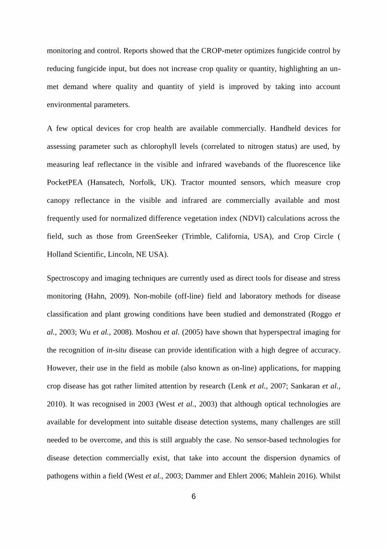
https://www.cambridge.org/core/journals/journal-of-agricultural-science/article/yield-gap-analysis-of-rainfed-wheat-demonstrates-local-to-global-relevance/086231FFEB3AE7CDA08875E79E11957A/core-reader#ref17

6

monitoring and control. Reports showed that the CROP-meter optimizes fungicide control by

reducing fungicide input, but does not increase crop quality or quantity, highlighting an un-

met demand where quality and quantity of yield is improved by taking into account

environmental parameters.

A few optical devices for crop health are available commercially. Handheld devices for

assessing parameter such as chlorophyll levels (correlated to nitrogen status) are used, by

measuring leaf reflectance in the visible and infrared wavebands of the fluorescence like

PocketPEA (Hansatech, Norfolk, UK). Tractor mounted sensors, which measure crop

canopy reflectance in the visible and infrared are commercially available and most

frequently used for normalized difference vegetation index (NDVI) calculations across the

field, such as those from GreenSeeker (Trimble, California, USA), and Crop Circle (

Holland Scientific, Lincoln, NE USA).

Spectroscopy and imaging techniques are currently used as direct tools for disease and stress

monitoring (Hahn, 2009). Non-mobile (off-line) field and laboratory methods for disease

classification and plant growing conditions have been studied and demonstrated (Roggo et

al., 2003; Wu et al., 2008). Moshou et al. (2005) have shown that hyperspectral imaging for

the recognition of in-situ disease can provide identification with a high degree of accuracy.

However, their use in the field as mobile (also known as on-line) applications, for mapping

crop disease has got rather limited attention by research (Lenk et al., 2007; Sankaran et al.,

2010). It was recognised in 2003 (West et al., 2003) that although optical technologies are

available for development into suitable disease detection systems, many challenges are still

needed to be overcome, and this is still arguably the case. No sensor-based technologies for

disease detection commercially exist, that take into account the dispersion dynamics of

pathogens within a field (West et al., 2003; Dammer and Ehlert 2006; Mahlein 2016). Whilst

7

progress has been made in disease recognition in the field, there are only a few yellow rust

specific identification systems and none for FHB. Commonly the attempts of disease

recognition using hyperspectral and multispectral imagery, are targeted to individual leaves

rather than the canopy (Bock et al., 2010a).

Although on-line applications are still rather limited, optical techniques have the potential to

be integrated with agricultural vehicles. Optical methods provide non-invasive and high

sampling resolution data necessary for monitoring and mapping of crop diseases. Among

optical sensing methods, hyperspectral and multispectral imaging techniques are the best

candidates as they have been used in disease and stress monitoring (Hahn, 2009).

Hyperspectral imaging takes near simultaneous spectral measurements along a series of

spatial positions, providing spectral features at high resolutions and with an improved

understanding of the target than multispectral imagery (Gilchrist 2006).

Spectral reflectance in vegetation canopies is dependent on several factors including the

illumination angle, the canopy architecture and the radiative properties of the plants (Pinter

and Jackson, 1985; Asner, 1998). Other factors affecting this are the integration time, light

source, and camera distance and angle. Therefore, optimising the measurement configuration

is essential before on-line field measurements using a hyperspectral imager can be

successfully carried out, which is the main target of this thesis.

8

1.2 Research objectives

There is a necessity for on-line recognition of crop disease, being both disease specific and

capable of quantifying disease presence, for site specific management and evaluation of yield

limiting factors.

Hypothesis

The project will consider the following hypotheses;

1. Proximal hyperspectral imagery is capable of detecting specific crop diseases (e.g., FHB

and yellow rust), and can be applied for on-line detection and mapping of their spatial

distribution in cereal crops.

2. Multi-sensor and data fusion of crop disease, canopy and soil properties collected at high

sampling resolutions, can be successfully used for the quantification of the yield limiting

factors.

Aim

The aim of the thesis is;

To apply a hyperspectral imager on-line application to cereal crop disease recognition,

critically appraising the existing technology. It also investigates a novel modelling approach

for quantifying the crop yield limiting factors. The key aim is to produce management zone

maps for variable rate fungicide application and selective harvest, in response to crop disease

pressures, soil characteristics and micro-climatic conditions.

9

Objectives

The objectives of the thesis are;

1. To critically appraise different approaches, and identify the best configuration for the

hyperspectral imaging systems for in-situ and on-line field measurement of crop

disease.

2. To evaluate the individual and interaction effects of parameters limiting crop growth

and yield.

3. To create a spectral library using hyperspectral data to identify and quantify specific

crop diseases (yellow rust and fusarium head blight) independent from water stresses.

4. To implement the hyperspectral imager for on-line detection and mapping of the

spatial distribution of yellow rust and fusarium head blight in winter wheat and

barley.

5. To adopt a data-fusion approach for delineation of management zones for variable

rate fungicide application and selective harvest.

10

1.3 Thesis structure

Chapter 7: Management zone maps for

variable fungicide application and selective

harvest

Chapter 3:

Yield limiting factors

Subchapter 3:1:

A new non-linear parametric

modelling method to quantify

influence of soil properties on

crop yields – Methodology.

Subchapter 3:2:

A new non-linear parametric

modelling method to quantify

influence of soil properties on

crop yields - Application to

on-line soil data.

Chapter 4:

Optimising the configuration of a hyperspectral imager for

on-line measurement of wheat canopy

Chapter 8: Conclusions and further work

Multi-sensor and data fusion approach for determining yield limiting factors and for potential in-situ

measurement of yellow rust and fusarium head blight in cereals

Chapter 2: Literature review

Chapter1: Introduction

Chapter 5:

Hyperspectral measurements of yellow rust and fusarium in

cereal crops: Part 1: Laboratory study

Chapter 6:

Hyperspectral measurements of yellow rust and fusarium in

cereal crops: Part 2: On-line field measurement

11

1.4 Disclosure

The thesis consists of 8 Chapters. Apart from Chapter 1 (Introduction), Chapter 2 (Literature

review) and Chapter 8 (Conclusions and Further work), the remaining chapters are presented

as papers (accepted or under review) and are detailed below;

Chapter 3 part 1: A new non-linear parametric modelling method to quantify influence of

soil properties on crop yields - Methodology

The study was collaborative work with Dr. Yifan Zhao and Dr. Said Nawar. The paper is

submitted to the European journal of Agronomy. The paper is presented as part 1 of chapter

3. My contribution to this work was being the lead author, and conducting all the field work

data collection, soil processing and property analysis. The majority of NARMARX modelling

was produced by Dr. Yifan Zhao, and random forest analysis By Dr. Said Nawar.

Whetton, R.L., Zhao, Y., Nawar, S., and Mouazen, A.M. (2016). A new non-linear parametric

modelling method to quantify influence of soil properties on crop yields - Methodology.

European journal of Agronomy (under review).

Chapter 3 part 2: A new non-linear parametric modelling method to quantify influence of

soil properties on crop yields - Application to on-line soil data

The study was collaborative work with Dr. Yifan Zhao, and the paper is submitted to Soil

Research. The paper presented as part 2 of chapter 3. My contribution to this work was being

the lead author, and conducting all the field work data collection, soil processing and property

analysis. I have also prepared the data layers through interpolation (kriging) and raster

analysis. The methodology and results for NARMARX modelling were produced by Dr.

Yifan Zhao.

12

Whetton, R.L., Zhao, Y. and Mouazen, A.M. (2016). A new non-linear parametric modelling

method to quantify influence of soil properties on crop yields - Application to on-line soil

data. Soil research (under review).

Chapter 4: Optimising the configuration of a hyperspectral imager for on-line field

measurement of wheat canopy

The study was first presented at ATIA, with a short paper included in the proceedings. A

more elaborated version of the work (provided in the thesis) was accepted for publication in

Biosystem Engineering. All work was my own with supervision and guidance from my

supervisors.

Whetton R.L., Waine T.W. and Mouazen, A.M. (2016). Optimising configuration of a

hyperspectral imager for on-line field measurement of wheat canopy. Biosystems

Engineering (accepted on 9th

December 2016).

10.1016/j.biosystemseng.2016.12.006.

Chapter 5: Hyperspectral measurements of yellow rust and fusarium head blight in cereal

crops: Part 1: Laboratory study.

This work was submitted to Biosystems Engineering and the work is currently in review. All

work was my own with supervision and guidance from my supervisors.

Whetton, R.L., Waine, T.W. and Mouazen, A.M. (2016). Hyperspectral measurements of

yellow rust and fusarium head blight in cereal crops: Part 1: Laboratory study. Biosystems

Engineering (under review).

13

Chapter 6: Hyperspectral measurements of yellow rust and fusarium head blight in cereal

crops: Part 2: on-line field measurement.

The study was first presented at CIGAR in June 2016, with the abstract provided in the

proceedings. A full paper was prepared and submitted to Biosystems Engineering. All work

was my own with supervision and guidance from my supervisors.

Whetton, R.L., Waine, T.W. and Mouazen, A.M. (2016). Hyperspectral measurements of

yellow rust and fusarium head blight in cereal crops: Part 2: on-line field measurement.

Biosystems Engineering (under review).

Chapter 7: Management zone maps for variable fungicide application and selective harvest

All work was my own with supervision and guidance from my supervisors.

Whetton, R.L., Waine, T.W. and Mouazen, A.M. (2016). Yellow rust and fusarium head blight

disease in winter wheat; proposed Management zones European Journal of Agronomy (under

review).

14

2 Literature review

Chapter Synopsis;

This chapter undertakes a critical review of the literature, with particular focus on cereal crop

yield limiting factors, fungal disease, soil properties, nutrient status, water stress, climate and

infection. It will also review measurement and monitoring techniques used for disease

detection.

2.1 Fungal diseases

Fungal diseases result in significant yield losses of cereal crops worldwide. Yellow rust, a

foliar disease, and fusarium, which affects the head of the crop, are two fungal infections

common on the small cereal crops, wheat and barley. Over 200 million hectares of farmland

worldwide is used to grow wheat (Triticum aestivum), which contributes to about 21% of the

world's food according to the food and agriculture organization (FAO) (Gustavsson et al.,

2011).

2.1.1 Yellow rust

Yellow rust, Puccinia striiformis, is a plant pathogen (Figure 1), causing yellow rust

(commonly in patches through a field) alternatively known as stripe rust, which produces

yellow uredo spores on the leaves. Yellow rust, is one of the most widely destructive plant

diseases in winter cereal crops (Wellings, 2011). The spores are predominantly dispersed by

the wind, and require damp or very humid conditions to infect the crop’s leaves. Disease

symptoms start with chlorosis, occurring parallel to leaf veins in a narrow 2mm wide stripe,

which develop into multiple yellow coloured rust pustules (De Vallavieille-Pope et al., 1995).

Disease presence can vary considerably between plants. In severe epidemics, the yields can

be reduced by up to 7 tonne ha-1

(Bravo et al., 2003). A virulent strain of yellow rust that

15

developed during 2009, attacked several widely grown genetically resistant cereal crop

varieties, including Solstice (Milus et al., 2009). A broad-spectrum seed dressing and

appropriate fungicide treatments should be used in areas at-risk and those with historic

infection (Blake et al., 2011).

Figure 1: Example of yellow rust (Puccinia striiformis) disease on winter wheat.

2.1.2 Fusarium head blight

Fusarium head blight (FHB) infection (Figure 2) is a major fungal disease, affecting several

hosts including wheat and barley (Parry et al., 1995). The disease occurs throughout most of

the world and is caused by the genus, Fusarium. FHB is prevalent as several species,

including; F. avenaceum, F. culmorum, F. graminearum, F. poae, F. sporotrichoides, M.

nivale and M. Majus (Parry et al., 1995; Xu et al., 2005). Fusarium fungi survive over winter

on plant residues (as mycelium), which can produce ascospores that infect the flag shoot

(Sutton, 1982; Oberti et al., 2014). FHB is a sporadic disease, severity is dependent on warm

humid weather (Rossi et al., 2001; Xu, 2003), causing variability of disease presence and

level of infection across regions and years (Jelinek et al., 1989). FHB symptoms in wheat and

16

barley appear in the head and peduncle tissues, causing discolouration and early senescence.

Early visual symptoms consist of a characteristic purple/pink discolouration. Seed from a

FHB affected crop is often shrunken, with a bleached appearance (Andersen, 1948; Parry et

al., 1995; McMullen et al., 1997; Goswami and Kistler, 2004). FHB can result in yield losses,

reduced grain, seed quality and size, causing direct economic losses. Mycotoxin

contamination (a secondary metabolite of the fusarium mould) in the grain, results in indirect

economic losses, due to market rejection or downgrading of grain quality (Sutton, 1982;

Gilbert and Tekauz, 1995; Parry et al., 1995; Goswami and Kistler, 2004). Due to legal limits

imposed by the European commission, for the fusarium mycotoxins deoxynivalenol (DON),

and zearalenone (ZON) high levels of mycotoxins in cereal grain mean that it cannot be sold

for human consumption (1250ppb for DON and 100ppb for ZON in wheat crop) but the crop

can be downgraded to cattle feed (ruminants are more resistant to mycotoxins) but at a

reduced price (HGCA 2014).

Figure 2: Example of Fusarium head blight (FHB) disease on winter wheat.

17

FHB has become one of the most important pre-harvest diseases worldwide (Magan et al.

2002). Control of fusarium and high mycotoxin contaminations are required to prevent toxic

contamination reaching the food chain either in milling grain (for human consumption) or as

cattle feed (Magan et al., 2002). F. graminearum is regarded as the most prevalent fusarium

pathogen in the UK, as it is highly pathogenic (when considering mycotoxins) with a high

genetic variation due to being a species complex (Rotter et al., 1996; Brennan et al., 2005;

Desjardin, 2006; Leslie and Summerell, 2006). Ear development is a critical growth stage for

cereal pathogen infection. Cereals are highly susceptible to fusarium infection during anthesis

(growth stage 60, Figure 3), as the anthers provide nutrients to fungal growth (Andersen,

1948; Parry et al., 1995; Lacey et al., 1999; Xu, 2003; Del Ponte et al., 2007). Imathiu et al.

(2008) found that fusarium DNA can be detected in the ‘panicle’ of the crop at the end of

anthesis (growth stage 60 – 69 illustrated in Figure 3). If the crop is infected later during

grain development, visual symptoms may not develop, though mycotoxins can still be

produced in the grain (Salas et al., 1999; Osborne and Stein, 2007).

18

Figure 3: Zadok’s scale of the main growth stages of wheat, (consistent across other small

cereal crops) (OMAFRA, 2009).

Impey (2012) confirmed the presence of fusarium leaf lesions in Herefordshire. This study

was based on leaf analysis from five sites by the Agricultural and Environmental

Consultancy. Fusarium leaf lesions found on the top two leaves is unusual but indicates the

disease’s establishment in the ear (Impey, 2012). The addition of leaf lesions reduces

photosynthesising green leaf area, contributing to a reduction in yield.

Early detection of cereal disease, which may lack obvious visual symptoms, allows for a

more effective fungicide treatment, preventing losses to crop yield and quality. Optical

sensing provides non-destructive measurements, allowing repeated data acquisition

throughout the growing season (Oberti et al., 2014). Among these optical techniques,

hyperspectral imagers show the potential for such system and are discussed later on.

http://www.sciencedirect.com/science/article/pii/S0168169914000611#b0015

19

2.1.3 Fungal disease resistance

Significant increases in cereal crop yields have been achieved over the last half-century

through changes in agronomic practice, synthetic fertilizers, pesticides, resistant and high

yielding cultivars (Bilsborrow et al., 2013). The most economical approach is to cultivate

varieties with a genetic resistance to fungal diseases. Genetically modified plants with an

increased resistance to fungal diseases are part of active research aiming to aid the reduction

of the use of chemical fungicides (Bliffeld et al., 1999; Clausen, 2000; Bieri et al., 2003).

However, resistant crops are susceptible to being overcome by fungal pathogens, due to many

resistant plant varieties relying on a few key resistance genes. Fungicide resistance has also

developed to many of the available fungicide classes (Mielecki, 2011).

Cultivating varieties with resistance genes to FHB infection can be complicated due to the

nature of the disease and the necessity to check ‘resistant’ plants at maturity for disease

expression and distinguishing them under varying and complex environmental effects as well

as the cost and time implications required for phenotyping (Bai and Shaner, 1994; Yang,

1994; Campbell and Lipps, 1998). There are varying types of resistance genes for FHB

infection in wheat and small cereal crops (Bai and Shaner, 1994; Yang, 1994; McMullen et

al., 1997). Genetic resistance to FHB is generally expressed as a quantitative trait, due to its

resistance relying on only a few genes, and their wide variation in response to environmental

conditions. Fungicide resistant pathogens, and pathogens overcoming crop genetic resistance

are both cause for concern (Wolfe 1985). With approaches to fungal disease control

becoming less effective there is pressure for new disease management strategies to be

developed. Improving disease control and the timings of application of fungicides, could

prolong certain fungicides’ effectiveness, and keep them available as a reliable method for

longer, due to reducing the chance of resistant mutants establishing (FRAC, 2010).

20

2.1.4 Disease distribution and spread

There are multiple environmental factors in addition to those of crop resistance, which

contributes to disease distribution. These include climate, humidity, weather, sources of

inoculation, and environmental stresses. Balanced nutrition has an important role in

determining plant resistance or susceptibility to diseases.

2.1.4.1 Sources of fungal disease inoculation

Theoretically, a higher disease pressure is expected to occur in fields of minimum or no

tillage (Edwards, 2007; Parikka et al., 2007; Imathiu, 2008). A regular practice in

conventional farming is to grow a wheat crop for 2 successional years without rotation, which

commonly results in a yield loss and a higher demand for fungicide (Bilsborrow et al., 2013).

Yellow rust and FHB species can survive in soil and weeds occurring in the hedgerows and

borders of a field, acting as a source of inoculum (Jenkinson and Parry, 1994; Champeil et

al., 2004; Imathiu et al., 2013). Initial infections of soil-borne pathogens, commonly result

from infected plant residues left over from the previous year’s harvest. Fusarium species

survive over winter on plant tissues and residues as mycelium (Sutton, 1982), infecting the

ear of the crop as conidia and ascospores (Osborne and Stein, 2007), even after two years on

the soil surface (Pereyra et al., 2004). Crop residue is considered a major factor for

inoculation levels (Teich and Hamilton, 1985; Dill Macky and Jones, 2000). Pathogen

survival is expected to be reduced in ploughed systems, as tillage buries residue, speeds

decomposition and reduces pathogen reproduction and survival (Khonga and Sutton, 1988;

Pereyra et al., 2004). However, stubble can have a significant impact on other fungal

diseases as well, such as Septoria tritici Blotch (STB). Zymoseptoria tritici causes STB on

wheat. STB is a highly significant disease reducing wheat yields by up to 50% in severe

epidemics on susceptible varieties (Eyal et al., 1973: Eyal et al., 1987; Fones and Gurr 2015).

http://www.sciencedirect.com/science/article/pii/S0168160507003947#bib56

http://www.sciencedirect.com/science/article/pii/S0168160507003947#bib9

21

Annual losses in the UK are around 20% of harvest (HGCA, 2012). STB poses a threat in

temperate climates around the world. Septoria shows symptoms only in the later stages of

infection, as the fungus can grow between leaf cells without causing visible damage.

However, once established, visible symptoms can occur throughout infected crops, rapidly

creating oval pale brown lesions, containing black spots (pycnidia). Lesions can form from a

single spore. In high severity, these lesions can join together, covering a large surface area of

the leaf. Airborne ascospores, rain splashed pycnidiospores (from infected plant debris), and

seed-borne infections are the main causes of STB.

There is a trade-off between preserving top soil and increasing disease presence. Stubble can

help the survival of stubble-borne pathogens, for example, Z. tritici populations can survive

between growing seasons and release spores to infect the next crop. This increased survival

can increase potential mutations, and the rate of evolution. Traditionally crop rotations and

burying infected crop residues (tillage) reduces levels of early inoculation within a field.

However, there is a large airborne source of inoculum from ascospores from neighbouring

fields (Schuh 1990). This means that tillage has little impact on STB levels later in the season

(Schuh 1990; Suffert and Sache 2011). STB control is the focus of about 70% of fungicide

applications in Europe (Eyal et al., 1973: Eyal et al., 1987). Whilst STB is not considered

further in the thesis, it would be a suitable disease for further work. The adaptability of STB

supports studies into early disease recognition, as a method of control.

The fusarium conidial spores are usually transported by rain drop splashes from the infected

tissue to plant leaves and ears, though wind and insects are also sources for its distribution.

Yellow rust infection is caused by uredospores and are predominantly dispersed by the wind

and require damp or high humid conditions to infect the crop’s leaves (De Vallavieille-Pope

22

et al., 1995; Parry et al., 1995; Sache 2000; Paul et al., 2004). This method of pathogen

transportation is more effective in sparse canopies, though in low precipitation levels, a dense

crop stand will be more infected due to higher humidity (Broscious et al., 1985; Sentelhas et

al., 1993). Cultivation practices, environmental factors such as crop density and climate

variations are important factors to consider when modelling the spread of disease. Influence

of environment on disease distribution

Epidemics of fungal diseases are strongly influenced by the local environment, persistence

and adaption of the pathogen, and the crop’s variety and physiological condition (Dammer,

2003). The climate and local weather conditions are considered a highly influential factor

regarding the distribution and severity of fungal infections in a crop stand. Warm, humid

conditions are ideal for FHB infection in crops (Rossi et al., 2001; Xu, 2003), particularly if

occurring during anthesis and early stages of kernel development (Gilbert and Tekauz, 2000).

Yellow rust infections are closely correlated with temperature, ideally between 10°C and

15°C with little infection occurring<2°C and above>23°C (Murray et al., 1994; Park et al.,

1992). Environmental conditions and the economic impact of yellow rust, FHB infection and

associated mycotoxins are highlighted in Table 1.

.

23

Table 1: Pathogen infection and influence. The economic impact, and environmental

conditions conducive to yellow rust, fusarium head blight (FHB) infection and associated

mycotoxins. The growth stages are in reference to Zadoks scale (Zadoks et al., 1974; De

Vallavieille-Pope et al., 1995; Gilbert and Tekauz, 2000; Rossi et al., 2001; Bravo et al.,

2003; Xu, 2003; Del Ponte et al., 2007)

Pathogens Growth stage Weather conditions

promoting infection

Effect on yield

Yellow rust Puccinia

striiformis.

Usually at stem

elongation and

onwards (growth

stage 30 shown in

Figure 3.

Infection pressures

correlated with

temperature, wind to

spread, moisture to

inoculate, cool moist

summers.

Reduced quality and 40-

50% reductions in yield.

The reduction can reach up

to 7 tonne ha ¯1.

FHB Several fusarium

and

Microdochium

species.

Usually at

anthesis and

onwards (growth

stage 60 shown in

Figure 3.

Variety of species

suited to varying

conditions,

predominantly ideal if

warm and humid.

40% reduction in quantity

and reduction in quality by

size, weight, shape, and

toxins. Reduced quality;

potentially toxic.

There is unequivocal evidence that the climate is changing at an increasing, and alarming rate

(Change 2007; Parry 2007). Due to the impact of climate on crop disease pressure, there is a

recognised need for a suitable crop monitoring system. F. graminearum is a dominant cause

of FHB with a broader adaption to environmental variability and climatic conditions,

compared to other species. The incidence of the disease can occur over varying temperatures

and moisture conditions, either through different regions, or from within field variability due

to e.g., soil type and moisture, and the impact of crop density on humidity and temperature

(Dammer, 2003; Backhouse 2014). Climate change could cause a population change in the

24

pathogen, allowing for a wider distribution of aggressive and virulent strains, which again

supports a need for optimisation of disease monitoring and control (Sung and Cook, 1981;

Dufault et al., 2006; Rossi et al., 2001).

2.1.4.2 Influence of canopy density on microclimate and disease spread

Under clear weather conditions in spring and summer, areas of the field with a low crop

density will warm up and cool down faster than those with dense canopies. Differences in a

wheat field’s microclimate could have an inter-canopy variation of up to 7.5°C (Dammer,

2003). Considering the influence of canopy density on environmental conditions and thus

disease distribution, the impact of crop density variation should be considered when

monitoring crop health.

2.1.4.3 Influence of rainfall on disease distribution

Imathiu et al. (2008) concluded that the closer the plant part is to the soil surface, the higher

the infection with fusarium species. It also showed a dilution effect of the inoculum away

from the soil surface and potential sources of inoculum, possibly resulting from splash

dispersal or from earlier inoculation where the disease concentration increases between

inoculation and sampling. Moisture is often required for disease infection (De Vallavieille-

Pope et al., 1995; Rossi et al., 2001; Xu, 2003). Therefore, when assessing the regional

distribution of fungal disease, the impacts of local weather conditions should be a

consideration.

25

2.1.4.4 Influence of soil characteristics

Balanced nutrition has an important role in determining plant resistance to diseases. Soil

properties can have an indirect effect on disease pressure. For example, variable soil moisture

will affect the crop microclimate, and an increase in nitrogen will increase the duration and

green area index of the canopy (Stokes et al., 1997; Sylvester-Bradley and Kindred, 2009).

Both macro (specifically nitrogen, potassium and phosphorus) and micro nutrients have an

impact on the severity of fungal diseases. A lack of different nutrients will increase the crop’s

vulnerability to specific diseases. Nutrients provide building blocks for the synthesis of plant

components (e.g., additional amino acids, proteins, chlorophyll), supporting growth, repair,

and resistance from disease (Huber, 1980; Engelhard, 1989; Graham and Webb, 1991;

Fageria and Baligar, 1997; McElhaney et al., 1998). Plant growth promoting bacteria in the

rhizosphere, can also increase the crops nutrient uptake (Amule et al., 2017). When

considering a method of disease control, it is important to acknowledge its interaction with

nitrogen. A lack of nitrogen can leave a plant susceptible to pathogens that are specialised in

infecting weak plants (Agrios, 1997; Snoeijers et al., 2000). However, increases in nitrogen

will increase the green area index and duration of the canopy (Stokes et al., 1997; Sylvester-

Bradley and Kindred, 2009). This subsequently affects the microclimate of the crop and the

effect of suitable disease control (by fungicides or genetic resistance) and prolongs the

canopy duration (Bryson et al., 1997).

Studies observed that a high increase in nitrogen application within a wheat crop led to an

increase in the disease severity due to prolonged green canopy (Leitch and Jenkins, 1995; von

Tiedemann, 1996). Ishikawa et al. (2012) argue that there is an optimum N concentration for

fungal infections to develop in wheat. The quality and nutritional content of whole grain

http://onlinelibrary.wiley.com/doi/10.1111/j.1365-3059.2010.02276.x/full#b33






26

wheat stay the same between organic and conventional farming practices though a drop in

yield may be seen under organic practices (Shier et al., 1984; Mader et al., 2002).

2.1.5 Current approach in fungal disease control

Multiple fungal pathogens commonly co-exist within a cereal field. Fungicide treatments are

often ‘broad-band’, and applied homogenously to the field, in an attempt to control the

various established plant diseases, and pre-emptively protect plants from later occurring ones

(Dammer and Ehlert, 2006). The recommended dosages of fungicide products given on the

product labels usually have a high efficacy even when subjected to environmental conditions

conducive to disease spread (FRAC, 2010). However, if there is a low disease pressure at the

time of spraying, a lower dosage is often sufficient to get the same efficacy of disease control

(Burth et al., 1990). However, crop pathogens under conditions conducive to disease can

spread very quickly, particularly if already established in the crop stand. A variable rate could

be applied to the crop stand in response to areas of high and low disease pressure. In this

instance, a sensing system of crop intensity would be valuable in optimising fungicide

application.

2.1.6 Timings of fungicide applications

Typically there are up to four timings of fungicide application to control yellow rust. T0

(Timing 0) is applied between growth stage 25 and 30 (Zadoks scale). Its application is

usually a preventative in historically problematic fields, or if an early disease is observed. T1

(GS 31-33) and T2 (GS 37-39) are applied to keep the third, second and flag leaves healthy,

as these heavily influence yield in wheat. The T3 application (GS 52-60) is usually an “ear

wash”, usually to preserve the quality of the grain. T2 is commonly considered the most

crucial application, and is the most frequently followed, due to the importance of maintaining

27

flag leaf health. T1 is considered secondary in importance followed by T3 and then T0

(HGCA 2008; Clark, 2016).

2.2 Techniques for disease detection

There are several techniques applied for disease detection. The main methods currently used

for disease recognition are based on visual assessments conducted by expert knowledge,

molecular techniques, spectroscopy, volatile organic compounds (VOC’s). There are direct

and indirect methods of fungal disease detection. Direct methods include molecular

techniques such as immunology-based methods and Polymerase chain reactions, whilst

indirect methods rely on stress based symptom detection (through imaging and spectroscopy)

and biomarker based detection (through plant metabolites, and volatile organic compound

profiling) (Ray et al., 2017).

Biosensors have been utilised for environmental monitoring. They are analytical devices,

which incorporate a biological material for recognition of a concentration of an analyte and

produce an electrical signal for the output (Tothill, 2001). In recent years, biosensors have

been used for rapid detection in quantifying and diagnosing plant diseases in the field,

detecting pathogens and aiding management decisions for the reduction of disease spread

(Ray et al., 2017). A few electrical biosensors are available, but have been advancing through

research, for example, air sampling coupled with PCR (West et al., 2008).

Molecular techniques are commonly used to confirm the presence of a disease pathogen

within a crop stand. In 2004 there were approximately 100 commercially available test kits

for the methods described above (Alvarez, 2004). These techniques are commonly based on

liquid chromatography, Polymerase Chain Reaction (PCR) and Enzyme Linked

Immunosorbent Assay (ELISA). Liquid chromatography separates a complex sample into

28

individual components through solid and liquid stages, while PCR detects a specific sequence

of DNA, and ELISA is an immunological response to detect antigenic protein. As techniques

have continued to develop in increasing the accuracy and the process speed, the number of

commercially available molecular tests have continued to grow. Next-generation sequencing

was introduced in 2005 and has rapidly developed in the area. DNA sequencing, such as that

based on nanopores, is a rapidly growing industry, which is currently making advances in

agricultural research. However, it still requires extensive sample preparation (Thate et al.,

2007). Moreover, PCR and real-time PCR detect and multiply a specific sequence of DNA

(Schaad and Frederick, 2002; and Henson and French, 1993). Other techniques available and

have applied in the field of crop disease detection include; immunofluorescence (IF),

fluorescence in-situ hybridization (FISH), flow cytometry, and DNA microarrays, loop-

mediated isothermal amplification (LAMP) assays and real-time Lamp assays (Prithiviraj et

al., 2004; Das, 2004; Saponari et al., 2008; Ruiz-Ruiz et al., 2009; Yvon et al., 2009; Bekele

et al., 2011). Molecular techniques provide a reliable and thorough evaluation of plant

pathogen presence. However, their application is generally limited due to them being time

consuming, labour-intensive, expensive and require experienced operators. Commonly, they

require preparation involving intricate procedures, equipment, and consumable pathogen

specific reagents. Therefore, they cannot realistically be used in preliminary screening of a

large quantity of samples (Sankaran et al., 2010).

An alternative approach to the molecular techniques is the recognition and distinguishing of

VOC’s. Metabolic activities within plant components (e.g. leaves, stem, and seed) release

VOC’s. Species, physiological condition and stress, age and development stage,

environmental conditions, disease pressure and any pest stress all dictate the VOC profile. A

distinct volatile biomarker identifying a specific plant and disease from that of a nutrient or

29

environmental stress is necessary to overcome the natural variation in the VOC profile within

a plant species, which can otherwise conceal the presence of stress and disease (Sankaran et

al., 2010). Potential exists for distinguishing between species of fungi based on characteristic

volatile patterns (Magan and Evans, 2000). Indirect detection methods are where disease

occurrence is predicted based on other factors, such as the density of the crop. Currently, the

market offers a method, for fungal control, which is based on crop density measurement for

optimising the application of a variable rate of fungicide (Dammer and Ehlert, 2006). This

method contributes towards real-time control of fungicide application. Spatial information

about crop density can be obtained by a CROP-Meter (Ehlert et al., 2003). The CROP-Meter

provides an indirect measurement of leaf area index (LAI) and plant mass using a pendulum,

which passes through the plant matter. Authors reported an increase in savings from CROP-

meter between 7% and 38% of fungicide costs depending on the heterogeneity of the field

and the variability and extent of the LAI, which is attributed to a reduction in application rate

in sparser areas. This success suggests an influence of LAI on the microclimate conditions

within the crop. Studies have shown a correlation of leaf rust infection with temperature

(Park et al., 1992; Murray et al., 1994; Dammer and Ehlert, 2006). However, LAI could be a

reflection of multiple stresses at the same time e.g. water, nutrients, temperature, and

diseases. Although Dammer and Ehlert (2006) report that variable-rate fungicide application

based on plant biomass is fiscally successful, it did not improve grain quality or quantity. A

direct method of specific disease detection could result in not only an economic benefit, from

reduced fungicide input (like the biomass based CROP-meter), but also lead to an increase in

yield, by reducing losses caused by disease presence.

The direct detection methods of crop diseases refer to those methods based on proximal

sensors. These include classical imaging, visible and infrared spectroscopy, fluorescence

30

spectroscopy, and hyperspectral imaging. Optical sensing performs non-destructive

measurements, allowing for repeated data acquisitions throughout the growing season

without interfering with crop growth. The capability of two commercially available optical

devices, the GreenSeeker RT100TM (Trimble, California, USA) and Crop Circle TM

(Holland Scientific, Lincoln, NE USA), which are both active sensors for measuring relative

greenness of crop, were used to discriminate levels of downy mildew (Plasmopara viticola)

infection on detached grapevine leaves. A linear relationship between disease severity and

output optical data was found from both sensors (Calcante et al., 2012). Since optical

methods based on a hyperspectral imager were used in this study, a detailed literature review

on optical methods is provided in the following section.

2.2.1 Review of optical imaging techniques of crop canopies

Originally, spectral images were sequentially taken, through a series of wavelength band pass

filters; an image is collected at one wavelength at a time in a fixed field of view (FOV). If an

object is moving or spectrally unstable, the results would be questionable. Integral spectral

images require all the wavelengths to be recorded near simultaneously. Spectroscopy (based

on the measurement of electromagnetic radiation reflectance of a targeted object) both

passive (using an external light source), and active (using its own light source e.g., a halogen

lamp), and conventional analyses have traditionally been used in the past to analyse

individual samples under off-line (non-mobile) measurement conditions, which is time and

resource consuming. Recent applications have been developing towards real-time (on-line,

mobile) measurements for use in-situ and monitoring (Gilchrist, 2006). Spectroscopic

technology has been successfully applied for plant stress detection such as water-stress and

nutrient-stress detection (Sankaran et al., 2010). Crop disease would ideally be identified in


31

spectroscopy by a wavelength range or index that is specific to a plant disease and is little

affected by environmental conditions (Griffin and Burke, 2003).

Spectral reflectance in vegetation canopies is dependent on the illumination angle of the

canopies’ architecture and the radiative properties of the plants. The most important plant

characteristics that determine reflectance are LAI and leaf pigmentation. Cell structure in the

leaves reflects near-infrared light (from 700 to 1000 nm), greater foliage has a greater effect,

and chlorophyll in plant leaves, absorbs visible light, particularly blue and red, (from 400 to

700 nm) (Campbell and Norman, 1998). Normalized Difference Vegetation Index (NDVI)

measures the visible and near-infrared sunlight reflected by the crop. For the most effective

method for measuring LAI, it can be first scanned by a proximal NDVI scanner and

calibrated for LAI, which is conducted as a commercial practice. Canopy reflectance is

dependent upon the structure and changes of the solar angle. Moreover, wind direction can

also influence reflectance due to the orientation of the leaf (Rauner, 1976). A common

approach is to include leaf angle and its effect on reflectance to derive an average leaf angle,

developing it into a conical distribution and substituting it into a radiation transfer calculation

(Monteith and Unsworth, 2008). In a homogenous canopy, the absorption of light is evenly

distributed, making an ellipsoidal distribution adequate for use in many canopy types (Jones

and Vaughan, 2010). Crop density through the use of a LAI measure is a traditional approach

to calculate how much radiation is absorbed by the canopy. The overall reflectance in a dense

canopy is less than a less-dense canopy, which is attributed to the light having passed through

more than one reflection, due to a greater capacity for absorption and light scattering (Jones

and Vaughan, 2010). The occurrences of sparse or irregular clouds affect the quality of light

incidence, so that each spectral measurement should include a sunlight irradiance

measurement (Jones and Vaughan 2010). Soil moisture can have a strong influence on

32

reflectance, related to an increase in absorption from wet soil, particularly in a sparse crop

(Jones and Vaughan, 2010).

2.2.2 Application of visible and infrared spectroscopy in disease detection

Visible and infrared (350-2500 nm) spectroscopy has been used as a rapid, non-destructive

tool for detection of plant diseases. It is cost effective and a fast developing technology

(Ramon et al., 2002; Delwiche and Graybosch, 2002; Pontius et al., 2005; Gomez et al.,

2006; Zhang et al., 2008a,b; Guo et al., 2009; Sundaram et al., 2009). Visible and infrared

spectroscopy can be applied to detect plant stress, damage and disease, and when applied to

plant disease detection it is commonly used in combination (Malthus and Madeira, 1993;

Polischuk et al., 1997; Bravo et al., 2003; Huang et al., 2004; Spinelli et al., 2006; Larsolle

and Muhammed, 2007; Naidu et al., 2009). The visible and infrared wavelengths of the

electromagnetic spectrum provide maximum information on the plant’s physiological stress

state (Muhammed, 2002, 2005; Xu et al., 2007). When specific wavebands indicative of a

disease are known, they can be applied to detect the plant disease in a crop field (West et al.,

2003). It is even feasible to detect the presence of a pathogen before visible disease

symptoms appear (Sankaran et al., 2010).

Within the visible spectrum, the radiation reflectance from an environmentally stressed plant

will increase. This is due to an increase in the incident light reflection from the leaf of a

stressed plant (Cibula and Carter, 1992). Using leaf spectral reflectance at 500, 600 and 650

nm wavelengths, Sasaki et al. (1998) classified to 90% accuracy, diseased and healthy

cucumber plants. Polischuk et al. (1997) used spectral reflectance measurements in making

an early diagnosis of Tomato mosaic tobamovirus (ToMV) infection in Debney's tobacco

(Nicotiana debneyi). Significant visual symptoms were noted three weeks after inoculation,

33

whilst a reduction in chlorophyll was detected by leaf reflectance after ten days. Similar

results were also found on barley leaves with powdery mildew (Lorenzen and Jensen, 1989).

Spinelli et al. (2006) used a NIR-based technique under greenhouse conditions for detecting

fire blight disease in pear plants. Results showed that the NIR technique alone was unable to

detect and therefore, classify the infected and healthy plants. This was attributed to the small

leaf scan area, which in this study was 2mm2. Spinelli et al. (2006) highlighted the

importance of field of view, recommending that a large area of both the diseased and healthy

plants should be considered.

Under field conditions, Naidu et al. (2009) used leaf spectral reflectance to identify viral

infections causing leaf roll disease in grapevines (Vitis vinifera L.). To assess the ability and

use of spectral reflectance in identifying a disease, discriminant analysis was performed to

classify leaves into infected and non-infected leaves. The accuracy was reached a maximum

of 75% for classifying leaf disease categories, when both the vegetative indices and

individual reflectance bands (from the green, mid infrared and near infrared spectral regions)

were used. The many successful studies on using the visible near infrared (vis-NIR)

spectroscopy for disease detection confirm the possibilities of using this technology for early

detection of diseases in field conditions. Moshou et al. (2011) introduced a prototype of an

on-line and automated multi-spectral camera (using the 495, 747 and 837 nm wavebands) for

the detection of early stages of disease in wheat crop, for both yellow rust and septoria. A

review by Mahlein (2016), discusses the use of optical sensors for the recognition of crop

disease, and the development process they must continue to undergo. Thomas et al. (2017)

recorded both reflectance and transmittance imagery in barley crop inoculated with powdery

mildew, finding that reflectance data outperformed transmission data in early disease

34

detection. They also highlight the significance of reflectance in the 580 to 650nm

wavelengths, for disease detection.

Mahlein et al. (2010) studied the potential of three spectral indices (NDVI, Anthocyanin

Reflectance Index (ARI) and modified Chlorophyll Absorption Integral (mCAI) between

400–1050 nm wavelengths, in early disease detection of sugar beets, concluding that

multiple indices would be required for an accurate distinction of diseases. Results

suggested that a distinctive differentiation of the three sugar beet diseases using spectral

vegetation indices is possible using two or more indices in combination. Rumpf et al.

(2010) used nine spectral vegetation indices (collected with hyperspectral reflectance)

relating to physiological parameters in a support vector machine learning for the

classification of specific diseases between healthy and inoculated sugar beet plants.

Discrimination between healthy and diseased leaves was successfully done with an accuracy

of 97%. These studies highlighted the potential accuracy of spectral indices in disease

recognition.

Whilst previous research has studied spectral data collected in the field and from mobile

systems, limited studies on on-line (mobile, and attached to a vehicle) captured spectral data,

for crop disease detection could be found in the literature, which is a key gap for research to

justify the novelty of this thesis.

2.2.3 Application of fluorescence spectroscopy in disease detection

Fluorescence characteristics have been used for the last twenty years in vegetation studies. It

is a method, where fluorescence is measured during excitation (Sankaran et al., 2010).

Excitation is where fluorescence occurs when a molecule absorbs light photons from the ultra

violet visible light spectrum (200-900 nm). The molecule then rapidly emits light photons and

35

returns to its previous state. A small quantity of energy is lost in heat or movement within the

molecule, so excitation energy is greater than the emitted energy. Belasque et al. (2008)

commented on how the change in blue-green fluorescence and chlorophyll florescence of

plants at excitation could be used not only to encompass the monitoring of stress on the

physiological condition of the plant, but potentially be applied in detecting and discriminating

disease stress from mechanical one (physical damage such as broken stems and damaged

leaves).

A further advancement of fluorescence spectroscopy is fluorescence imaging. Instead of

using a UV (10-400 nm) or halogen (320-1100 nm) light source for florescence excitation, a

xenon (240-1100 nm with strong peaks at 750-1000 nm) light source is becoming more

common. Fluorescence images are collected using a camera instead of a single spectrum, and

at specified wavelengths the fluorescence is recorded with use of a charge coupled device

(CCD) camera based system (Bravo et al., 2004; Lenk and Buschmann, 2006; Chaerle et al.,

2007; Lenk et al., 2007, Sankaran et al., 2010). In fluorescence imaging, the commonly used

regions of the electromagnetic spectra are blue (440 nm), green (520–550 nm), red (690 nm),

far red (740 nm), and near infrared (800 nm) (Lenk and Buschmann, 2006; Chaerle et al.,

2007). Lenk et al. (2007) described multispectral fluorescence and its possible application in

monitoring disease symptoms in plants, as well as use in fruit quality, leaf structure and

photosynthesis.

In 2007, Poutaraud et al. (2007) measured the distribution of downy mildew (P. viticola)

from grapevine stress induced secondary metabolites (stilbenic phytoalexins) using in vivo

fluorescence measurements, finding that the high intensity of blue and violet fluorescence

(near 390 nm) emitted by the metabolite could be used as a strong indicator for early onset of

disease. Also using fluorescence measurements Bélanger et al. (2008) showed that disease


36

could be quantified on detached leaves. Authors reported that the ratio between blue (near

440 nm) and green (near 520 nm) intensity between the healthy and diseased tissue was

significantly different shortly after inoculation.

2.2.4 Alternative spectral methods

There are other imaging techniques that can be applied in the detection of plant diseases, such

as x-ray imaging, terahetz spectroscopy, NMR spectroscopy and infrared thermography.

These techniques are generally not applied to plant pathology as they are expensive to run,

and so are not cost effective when compared to the potential of crop quality and yield

increase (Sankaran et al., 2010). However, Masri et al. (2017) using thermography, found

that air temperature and fusarium infected ears were negatively correlated 6 days after

inoculation.

2.2.5 Hyperspectral and multispectral imaging

Hyperspectral imaging has been developed dramatically from large, aircraft-based systems, to

a more compact (UAV connected), economic tool that can be applied in monitoring,

inspecting and diagnosing crop disease. A hyperspectral imaging instrument takes

simultaneous (or near-simultaneous) spectral measurements along a series of spatial

positions, giving both the shape and features of the spectral curve. The more spectral

wavelengths observed (resolution of wavelength nm collected), the greater is the

understanding of the sample quality (Gilchrist, 2006). Hyperspectral imaging is similar to

multispectral imaging, but differs on having a broader range of wavelengths and spectral

bands. One spectrum of different wavelengths per pixel, to form the hyperspectral image

(Sankaran et al., 2010). These wavelengths can include the visible (Vis), near infrared (NIR)

and infrared (IR) regions. Each spectral region provides information about the plant. The

reflectance at visible wavelengths is attributed to leaf pigmentation, with a low reflectance

37

indicating larger absorption of the light due to darker coloured leaves. This is attributed to the

photosynthetic pigments of the plants leaves, governed by the abundance of chlorophyll,

absorbing most of the light radiation (Gates et al., 1965; Thomas and Gausman, 1977). Leaf

reflectance in the NIR range is affected by the structure of the plant leaves (Gates et al.,

1965), and can be related to the leaf wax coating (Cameron 1970). The infrared wavelength

reflectance provides information on the physiological condition of the plant. The wavelength

measurement for the return of light intensity in hyperspectral imaging adds the multiple

wavelengths (spectrum) with its spatial position to the brightness information of the spectral

image, providing a rapid image-contrast, which would not be present in a conventional image

approach (Huang et al., 2007). Mahlein et al. (2013) used spectral vegetation indices to

differentiate between diseases on sugar beet plants and three leaf diseases. Hyperspectral

signatures of healthy and diseased sugar beet leaves were assessed, finding a single

wavelength and normalised wavelength difference between 450 to 950 nm to be most

relevant, with classification accuracies being between 85 and 92%.

In addition, the proximal applications of hyperspectral imaging have been successfully

adapted to use in remote sensing (air and satellite) applications for a range of control,

monitoring, and scientific applications. Remote-sensing based monitoring has also been used

in agriculture for detecting invasive species (Sankaran et al., 2010). Application of remote

hyperspectral sensing techniques have been aimed at supporting real-time monitoring and

inspection, in the identification, quantification and quality control (Gilchrist 2006; Sankaran

et al., 2010). Hyperspectral imaging is commonly used for monitoring food product quality

and pharmaceuticals (Mehl et al., 2004; Lee et al., 2005; Yao et al., 2005; Tallada et al.,

2006; Gowen et al., 2007; Mahesh et al., 2008; Sighicelli et al., 2009). The application of the

38

technology for use in precision agriculture and plant disease detection has been gaining

popularity (Okamoto et al., 2009).

The use of hyperspectral imaging techniques for disease identification was reported by

several researchers under non-mobile measurement conditions (Roggo et al., 2003; Wu et al.,

2008). The early success in field studies for hyperspectral detection of yellow rust focused on

detecting the presence of yellow rust (Bravo et al., 2003; Moshou et al., 2004). Bravo et al.

(2003) detected early symptoms of yellow rust (P. striiformis) on winter wheat, using a

quadratic discriminant model with an accurate classification accuracy of 92–98%. Moshou et

al. (2004) successfully detected yellow rust disease in winter wheat by using spectral

wavelengths of 460 to 900 nm, classifying individual plants into healthy and infected with

accuracies between 92.0% and 99.4%. Moshou et al. (2005) combined hyperspectral

reflectance and multispectral fluorescence imaging for the detection of yellow rust in winter

wheat, through sensory and data fusion approach. The hyperspectral imaging data collection

was obtained under ambient light conditions in winter wheat plots, whereas data for

fluorescence images was obtained through UV excitation. Moshou et al. (2005) demonstrated

that when sensory imagery was combined with quadratic discriminant analysis (QDA) based

classification, the accuracy of healthy plants improved considerably to 97% from a prior 71–

90%. Similarly, the classification accuracy of the diseased plants increased to 99.4% and

healthy plants’ classification further improved to 98.7% accuracy, when the self-organizing

map (SOM)-based neural network was used for the plant classification. More recent attempts

with hyperspectral and multispectral imagery are targeted to leaves rather than the canopy

(Bock et al., 2010). Huang et al. (2015) successfully provided quantitative assessment of

yellow rust in winter wheat, through hyperspectral measurement of individual infected

leaves. This research shows the potential application for hyperspectral imaging in the


39

application of disease recognition in-situ with resultant high accuracies. Whilst the use of

hyperspectral imaging techniques for offline disease identification has been reported by

several researchers there are few on-line (Roggo et al., 2003; Wu et al., 2008; Bock et al.,

2010).

Soil and canopy properties can vary on different scales and a greater resolution in data

collection could be more sensitive to detecting the smaller scale changes (Raun et al., 1998;

Dhillon et al., 1994; Rossi et al., 2001; Dammer, 2003; Xu, 2003). Proximal spectral data can

have a high resolution, an example of this is the on-line soil measurement platform created by

Mouazen (2006), where a spectrophotometer (Tec5 Technology for Spectroscopy, Oberursel,

Germany) was applied to a tractor travelling at a speed of 3 km h-1

and collecting spectral soil

data every second at 10 m parallel intervals. The resolution of data acquired, of course,

depends on the method of application and the make and model of the camera. Satellite data,

for example from Landsat 8, has a spatial resolution of 30 meters for the visible and NIR,

which may not detect finer spatial changes. However, the benefit of the spatial and temporal

coverage of satellite data may outweigh the negatives for certain applications (Lobell, 2013).

2.2.6 Optical imaging summary

Optical imaging techniques don’t require direct contact with samples, hence, they can be

operated at a wide range of distances. Measurements are very rapid and can be performed at

normal field vehicle operation speeds. Moshou et al. (2011) developed a prototype, tractor

mounted, hyperspectral imager demonstrating the practicality towards field-scale disease

detection of yellow rust.

Studies have considered proximal detection of diseased and healthy crops, by using sampled

leaves/ears, a summary of which can be found in Table 2. They commonly found the most



https://link.springer.com/article/10.1007/s11119-014-9365-6#CR18

40

discriminant wavelength intervals to be at green (near 500 nm) and near infrared (900 nm and

1600 – 2200 nm) (Naidu et al., 2009). Polder et al. (2005) reported successful detection of

fusarium in single kernels, by using both spectroscopy and imaging. Bauriegel et al. (2011)

successfully recognised FHB infection at growth stages 71–85, using spectral ranges of 400–

1000 nm, 500–533 nm (green), 560–675 nm (yellow), 682–733 nm (red) and 927–931 nm

(red edge). Similarly, Delwiche and Kim (2000) successfully detected FHB in wheat kernels

using a hyperspectral imager at 435 – 860 nm spectral range based on machine learning.

Oerke and Steiner (2010) detected significantly higher temperature in fusarium infected

ears, by means of an infrared thermography method for in-situ measurement of crop

canopy.

Although certain nm wavelengths can be associated to disease recognition in the spectra, the

use of a full spectral range generally produces a more reliable prediction model, due to

interactions of different properties on the spectrum. This was confirmed for the Vis-NIR

spectral analysis for the prediction of soil properties (Mouazen et al., 2005). Therefore, the

analysis of the full spectral range obtained in this study will be considered rather than

focusing on specific wavebands.

Although many studies of the use of optical methods for the recognition of crop disease can

be found in the literature, very limited research was published on the use of these optical

techniques for on-line measurements.

http://link.springer.com/article/10.1007/s10658-011-9878-z#CR35

41

Table 2: summary of different spectral applications to recognition of crop diseases and

associated observations and accuracies

Spectrum Observations and success Reference

Visible spectrum 90% accuracy for detection of environmentally stressed plant due to an

increased radiation reflectance.

Sasaki et

al.(1998)

Hyperspectral

wavelengths at 704,

1423 and 1926 nm

Quantitative assessment of yellow rust in winter wheat, through

individual infected leaves with an R² of 0.88.

Huang et

al.(2015)

Spectroscopy and

imaging.

Successful detection of fusarium in single wheat kernels, Polder et

al.(2005)

Flouresence spectrum The method could be applied in detecting and discriminating disease

stress from environmentally attributed stress.

Belasque et

al.(2008)

hyperspectral

wavelength range of

435 to 860 nm

Fusarium head blight in wheat kernels through machine learning. Delwiche and

Kim (2000)

NIR spectrum Unable to discriminate between infected and healthy plants.

Recommend a larger area of view rather than a small one.

Spinelli et

al.(2006)

NIR spectrum Maximum of 75% accuracy for classifying leaf disease categories Naidu et

al.(2009)

Vis-NIR spectral range

of 400–1000 nm

Discrimination of fusarium infected from healthy plants at growth

stages 71–85 using principal component analysis (PCA)

Bauriegel et

al. (2011)

NIR along with mid

infrared spectrum

Noticed it was more reliable than NIR spectroscopy alone for earlier

disease detection and identification

Sankaran et

al.(2010).

Vis-NIR spectrum Detecting early symptoms of yellow rust on winter wheat, with a

discrimination accuracy of 92–98% between infected and healthy

plants.

Bravo et

al.(2003)

Vis- NIR spectrum Discriminating healthy from infected individual plants with

classifications accuracies ranged between 92.0% and 99.4%.

Moshou et

al.(2004)

Infrared thermography Detected significantly higher temperature in fusarium infected ears. Oerke and

Steiner (2010)

Hyperspectral imaging Classification accuracy of the infected and healthy plants ranged

between 98.7% and 71–90%.

Moshou et

al.(2005)

Hyperspectral imaging

and fluorescence

When sensory imagery was combined with quadratic discriminant

analysis (QDA) based classification, the accuracy improved to 97% and

99.4% for healthy and infected plants.

Moshou et

al.(2005)

http://link.springer.com/article/10.1007/s10658-011-9878-z#CR35

42

2.3 Variability and yield limiting factors

The spatial variability that exists in the majority of agricultural fields requires careful

management with the aim to increase yield at reduced input cost and related environmental

impacts. Conventional management of fields relies on homogeneous applications of external

inputs. For example, current fertiliser applications are made based on an average soil sample

collected per field or 1-3 per ha in the best scenario, which ignores within field variability.

But, soil commonly varies within an agricultural field (Raun et al., 1998; Dhillon et al.,

1994). Therefore, an alternative scenario of the conventional homogeneous application is

required, namely, variable rate applications, by which the required amount of input (e.g.,

fungicide, fertilizer, etc) is applied in the right place where needed. Variable rate applications

have seen a surge of innovative technologies in recent years, relying on input data from

normalised difference vegetation index (NDVI), leaf area index (LAI), soil properties or a

combination of these (Lowenberg-DeBoer and Aghib, 1999; Maleki et al., 2008; Halcro et

al., 2013). Although precision management of farm external inputs is growing due to its

economically beneficial results (Halcro et al., 2013), quantifying the yield limiting factors is

still a crucial question to be answered, before variable rate applications can be optimised to

meet the exact crop needs.

One way to analyse and quantify the yield limiting factor is by adopting an input-output

model that describes the relationship of the inputs (e.g. crop and soil properties, topography

and terrain attributes, disease and weather conditions) and output (crop yield) of a system.

This can be achieved for example by the implementation of machine learning, multivariate

statistical analyses, random forest and others. Wang and Shen (2015) used classification and

regression tree analysis to relate soil characteristics to yield. They classified low yield areas

and could detect them based on just a few soil properties to an accuracy of 61.8%. Volterra

43

Non-linear Regressive with eXogenous inputs (VNRX) is a non-linear parametric model

(Zhao et al., 2013), which will be applied for quantifying the individual and collective

influences of soil properties on yield variability, for the first time in this thesis.

Parametric models have attracted more and more interest recently due to their limited reliance

on field calibration, less requirement of sample size and their transparent assessment of

model performance. Parametric modelling in agriculture was used to assess soil erosion as

correlated to landslide events (Pradhan et al., 2012), to assess land size for a maximum crop

output (Färe et al., 1997), water retention (Timlin et al., 2004) and soil respiration (Chen et

al., 2011). However, very few studies on the use of parametric modelling to predict yield can

be found in literature. The first successful application of parametric modelling to predict crop

yield was reported by Mkhabela et al. (2011), where NDVI was the sole input. Authors

reported difficulties associated with removing non-target crop NDVI obtained from the earth

observation satellite imagery (with a resolution of 250m). Huang et al. (2013) developed a

regression model to predict rice yield based on a direct empirical relationship established

between NDVI and rice yields, achieving some success. Whilst the relationship between

nutrients in soil and yield is widely understood, there are areas of interest where high

sampling resolution data (obtained with advanced remote and proximal sensing technologies)

could be applied.

2.4 On-line measurement of soil properties

In addition to crop disease and crop NDVI measurements, soil property data was also

collected using on-line measurement systems. Kuang et al. (2012) stated that among the

different sensing techniques for soil properties, the most applicable one for the field under

both non-mobile and on-line mobile conditions is vis-NIR spectroscopy. It has the potential

to provide a rapid, cost effective and accurate analysis of multiple soil properties. The

44

technology can be mounted on a tractor for on-line sensing, capable of collecting high

sampling resolution data e.g., >500 readings per ha (Mouazen, 2006; Maleki et al., 2008;

Kuang and Mouazen, 2011a; 2011b). The Mouazen (2006) internationally patented system

was proven by many publications to enable the measurement of key soil properties with

appreciable accuracy (Mouazen et al., 2005; Kuang and Mouazen, 2012; Kuang et al., 2015).

By utilising such a system, a greater understanding of the spatial distribution of soil

properties and their impact and correlation on crop growth and yield will be possible. This

on-line soil sensor will be a key contributor for the delineation of management zones for

selective harvest and fungicide application to be investigated in this thesis.

2.5 Literature conclusions; research gaps

The literature review confirmed that there is a need to develop and test a proximal sensor for

on-line measurement of crop diseases, e.g., yellow rust and FHB. The sensor should enable

the collection of high sampling resolution data on these diseases to enable site specific

application of fungicide or selective harvest.

The literature review has highlighted the impact of soil, canopy properties, and microclimate

conditions, on the risk of infection. It is more effective to know the location and severity of

the disease, rather than estimating the overall average for the field (Dammer, 1999; Fleischer

et al., 1999). On-line soil and crop data and micro-climatic conditions when fused with

quantitative data on crop disease may not only be beneficial for variable rate fungicide

application and selective harvest, but predicting future infection patterns.

There is a need for high sampling resolution data on soil characteristics, crop growth,

diseases, and microclimate conditions to enable understanding for managing variability that

exists in most agricultural fields. These layers could be applied to a non-linear model to

45

explore the yield limiting factors, by quantifying the individual and collective influences of

these layers on the yield variability within a field.

46

3 Quantification of yield limiting factors

Chapter Synopsis;

This chapter discusses the implementation of a new non-linear parametric modelling

approach for quantifying the yield limiting factors, by estimating the individual contributions

and interactions of soil properties to NDVI and yield.

Chapter 3 is split into two subchapters;

3.1 A new non-linear parametric modelling method to quantify influence of soil properties on

crop yields – Methodology.

3.2 A new non-linear parametric modelling method to quantify influence of soil properties on

crop yields - Application to on-line soil data.

This modelling approach is further explored with the inclusion of disease data (e.g., fusarium

head blight (FHB) and late yellow rust) with some key soil properties (TN, OC, MC, and

CEC). Results of this further analysis can be found in Appendix A.

47

3.1 A new non-linear parametric modelling method to quantify

influence of soil properties on crop yields: Methodology

Abstract

This paper aims at introducing a new non-linear parametric modelling technique based on a

Volterra Non-linear Regressive with eXogenous inputs (VNRX) model to study and quantify

the effect of soil properties on crop yield. Two versions of VNRX were implemented,

namely, VNRX-LN, accounting for both the linear and non-linear variability in the system,

and VNRX-L, accounting for linear variability only. The performance was compared with a

non-linear random forest (RF) model to predict oilseed rape (2013) and barley (2014) yields

in one field in Germany. Soil samples were collected in 2013 and analysed in the laboratory

for ten properties. These were used as system inputs for the three models and crop yield data

of 2013 (oilseed rape) and 2014 (wheat) were used as the system outputs. Results

demonstrated the individual and total contribution of soil properties on crop yield to vary

throughout different cropping seasons. Both VNRX-LN and RF models outperformed the

VNRX-L model (attributed to the ability of these models to account for non-linearity) and

explained up to 55.6% (2013) and 45.8% (2014) of yield variation for the RF model and

52.2% (2013) and 50.6% (2014) of yield variation for the VNRX-LN model. Although

VNRX-LN and RF models almost equally performed for yield prediction, the RF models

were more consistent with the soil properties ranking for describing the yield variability,

indicating a greater stability. The VNRX-LN accounted for slightly more variability over the

two years, though the ranking of properties was more variable, which could be attributed to

other parameters that have not been involved in this study.

48

Keywords

Yield prediction; yield limiting factors; soil fertility; random forest, VNRX.

3.1.1 Introduction

Quantification of soil related yield limiting factors is essential for site specific management

of farm resources and for crop yield forecast. However, the estimation of these limiting

factors is not a straightforward process, as many affecting parameters exist in a very complex

system, consisting of soil and associated micro- and macro-variability, microclimate,

topography, land use and others. Whilst the relationship between nutrients in soil and yield is

widely understood, there is little work using high sampling resolution data obtained with

advanced on-line proximal sensing technologies. Modelling approaches to predict crop yield

have been introduced (Hole et al., 2005), which included statistical, process-based numerical,

machine learning and parametric modelling approaches. Although statistical models are more

suitable for large spatio-temporal scales, they can hardly extrapolate beyond historical

extremes (Hahn, 2009). Process-based models (Fourcaud et al., 2008; Thorp et al., 2014)

emulate the main processes of crop growth and development. These models are typically

developed and tested using experimental trials, and thus offer the distinct advantage of

leveraging decades of research on crop physiology and reproduction, agronomy, and soil

science, among other disciplines. These models also require extensive input data on cultivar,

management, and soil conditions that are unavailable in many parts of the world. Apart from

overfitting issues, machine learning modelling techniques were successfully implemented

recently to predict wheat yield using proximal sensors (Pantazi et al., 2016).

49

Parametric models have attracted more and more interest recently due to their limited reliance

on field calibration, less requirement of sample size and their transparent assessment of

model performance. Very few studies on the use of parametric modelling to predict yield can

be found in literature. Assuming that regression analysis falls under parametric modelling, the

number of studies on prediction of crop yield suddenly increases. Palm (1997) produced the

simplest form of parametric modelling to estimate crop yield, in the form of a regression of

yield against rainfall. In areas where water is a limiting parameter, about 46% of yield

variability was attributed to rainfall. A simple parametric simulation of maize yields using the

standard Food and Agriculture Organisation (FAO) methodology was produced by Rijks et

al. (2003), where 73.75% of the yield variability between separate years was attributed to

evapotranspiration.

The non-linear auto-regressive moving average model with eXogenous inputs (NARMAX) is

a parametric modelling method introduced by Billings et al. (1989) and one of the most

popular classes of non-linear system identification methods for a complex system, where the

inner structure of the underlying system is unknown but only input and output observational

data are available. Comparing with machine learning methods, one of the advantages of the

NARMAX model is transparency, which means that it can be written down, can be related to

known and existing models in the literature, and also can be analysed in frequency and other

domains. This characteristic is attractive for a studying brain, climatic change or an

agriculture system that is a typical input-output system with an unknown inner structure,

because it not only allows further frequency analysis or statistical analysis based the

identified model, but also is easily understood and interpreted. A Volterra non-linear

regressive with eXogenous inputs (VNRX) is a special case of NARMAX that has been

recently introduced. Although it has been successfully applied in brain signal analysis (Zhao

50

et al., 2012; Sarrigiannis et al., 2014), climate change (Bigg et al., 2014; Zhao et al., 2016a)

and non-destructive tests (Zhao et al., 2017), its application in agriculture is novel. This non-

linear model has potential to understand how soil properties and other factors affecting the

crop yield due to its capability to reveal non-linear information whilst linear modelling

methods cannot, or would produce misleading results.

This paper aims at (1) exploring the potential of the new proposed VNRX models to quantify

soil related yield limiting factors and understand the dependence among crop yield and soil

properties within a field, (2) comparing between VNRX with random forest (RF) models for

identifying and quantifying the most influencing soil properties that affect yield variability.

All methods were tested in one arable field in Germany, throughout two cropping seasons in

2013 and 2014 with oilseed rape and wheat grown, respectively.

3.1.2 Material and methods

3.1.2.1 Study site and data collection

The study site was an arable field located in Premslin near Rostock in Germany (Figure 4),

with 11°46’2.00” E latitude and 53°6’58.00” N longitude according to the Universal

transverse Mercator (UTM) system. The field is about 33 ha in area, with an average annual

rainfall of 591 mm, an average temperature of 16.5 ºC from May through to August in the

2013 and 2014 cropping seasons. The soil type according to FAO soil classes is a

homogenous Dystric Cambisol with humic loam texture, on a sandstone rock (FAO code

Bd67-2b). Oilseed rape and barley were cultivated during the experiment in 2013 and 2014

cropping seasons, respectively.

51

Figure 4: Field location in Premslin near Rostock in Germany, where soil samples

and yield data were recorded in 2013 and 2014.

A total of 140 soil samples were collected after the harvest of the previous crop in 2013

(Figure 4). About 700 g of each soil sample was prepared as a mixture of soil collected over

1.5 m distance at about 0.15 m depth. An equal gap between neighbouring sampling lines of

12 m was selected. A differential global positioning system (DGPS) (EZ-Guide 250, Trimble,

California, USA) with sub-metre accuracy was used to record the position of each soil

sample. Soil samples were placed into tightly sealed plastic bags to hold field moisture, and

stored in a refrigerator at 4 ºC, until laboratory analysis. Yield data were collected in 2013

and 2014, at different spatial resolutions to that of the soil samples using the on-board yield

sensor of the farmer’s combine harvester (New Holland, CX8070 model).

3.1.2.2 Laboratory analysis and development of calibration models of soil properties

Each sample was air dried at a temperature not greater than 30 °C, grinded and sieved with a

2 mm sieve. Samples were then subjected to chemical analyses to determine selected soil

parameters that were likely to be limiting the yield of the oilseed rape and barley. These

parameters are pH, soil moisture content (MC), cation exchange capacity (CEC), organic

52

carbon (OC), total nitrogen (TN), and the available cations sodium (Na), potassium (K),

calcium (Ca), magnesium (Mg), and available phosphorous (P). pH was measured

potentiometrically on a suspension of soil to water ratio (1:2.5) under a controlled

temperature environment (DEFRA, 2010). MC was determined by oven drying of soil

samples at 105 ºC for 24 h. To determine CEC, soil was saturated with Sodium Acetate

(pH 7.0), and the excess acetate removed by washing with water and ethanol. The sodium

ions absorbed onto the cation exchange sites of the soil were displaced with 1.0M

Ammonium Acetate, and their concentration was determined using a Flame Photometer

(Chapman 1965). OC was determined according to the British Standard BS 7755 Section

3.8:1995 using a combustion method, which is identical to ISO 10694:1995. TN was

determined by the Dumas method, where soil samples are heated to 900 ºC in the presence

of oxygen gas as described by British Standard BS EN 13654-2:2001. Exchangeable K, Na,

Ca and Mg were extracted with 1.0 molar Ammonium Nitrate (MAFF/ADAS, 1986), and

their concentrations in the extract were determined by Agilent 240 FS AA atomic absorption

spectrophotometry (Agilent Technologies, Inc. USA). Available P was determined by

extraction from the soil at 20 °C by shaking with 0.5 M sodium bicarbonate solution at pH

8.5 and the concentration was determined by an ascorbic acid method (Olsen, 1954).

3.1.2.3 Data processing

Yield and ten soil data layers were first fitted to semi-varigrams using Vesper software

developed by the Australian Centre of Precision Agriculture (Sydney, Australia) to typify the

spatial variation. After satisfactory semi-variogram selection, semi-variogram parameters

were transferred into ArcGIS (Esri, USA) software to perform ordinary kriging to predict

values of un-sampled positions. The interpolated (through kriging) data layers were then

converted into a common 5 m2 raster grid in ArcGIS (Esri, USA) in order to assist data fusion

53

(Frogbrook and Oliver, 2007). The resulting 5 m2 raster squares of the layers were converted

into a common grid of points by extracting the value at the midpoint of each raster square.

These steps ensured that all layers consisted of common sets of 5 m2 grid points, which is

essential for running different spatial analyses. This method allowed data from a diverse

range of soil and yield surveys, measured at different resolutions, to be merged (Khosla et al.,

2008). However, it is worth to mention that transferring information of 5 m2 raster to a point

would introduce unavoidable error to the spatial distribution of data. The different soil and

crop data were subjected to the linear and non-linear VNRX, and RF modelling methods,

detailed in the following sections.

3.1.2.4 Random forest method

Random forest is a non-linear classification and regression algorithm developed first by

Breiman (2001), which can be described as follows:

Suppose we have a calibration set with and an independent

test case with predictor , the following steps can be carried out:

1) Sample the calibration set with replacement to generate bootstrap resamples

2) For each resample , grow a regression tree .

3) For predicting the test case with covariate , the predicted value by the whole RF

is obtained by combining the results given by individual trees. Let denote the

prediction of by mth

tree, the RF prediction for regression problems can then be

written as:

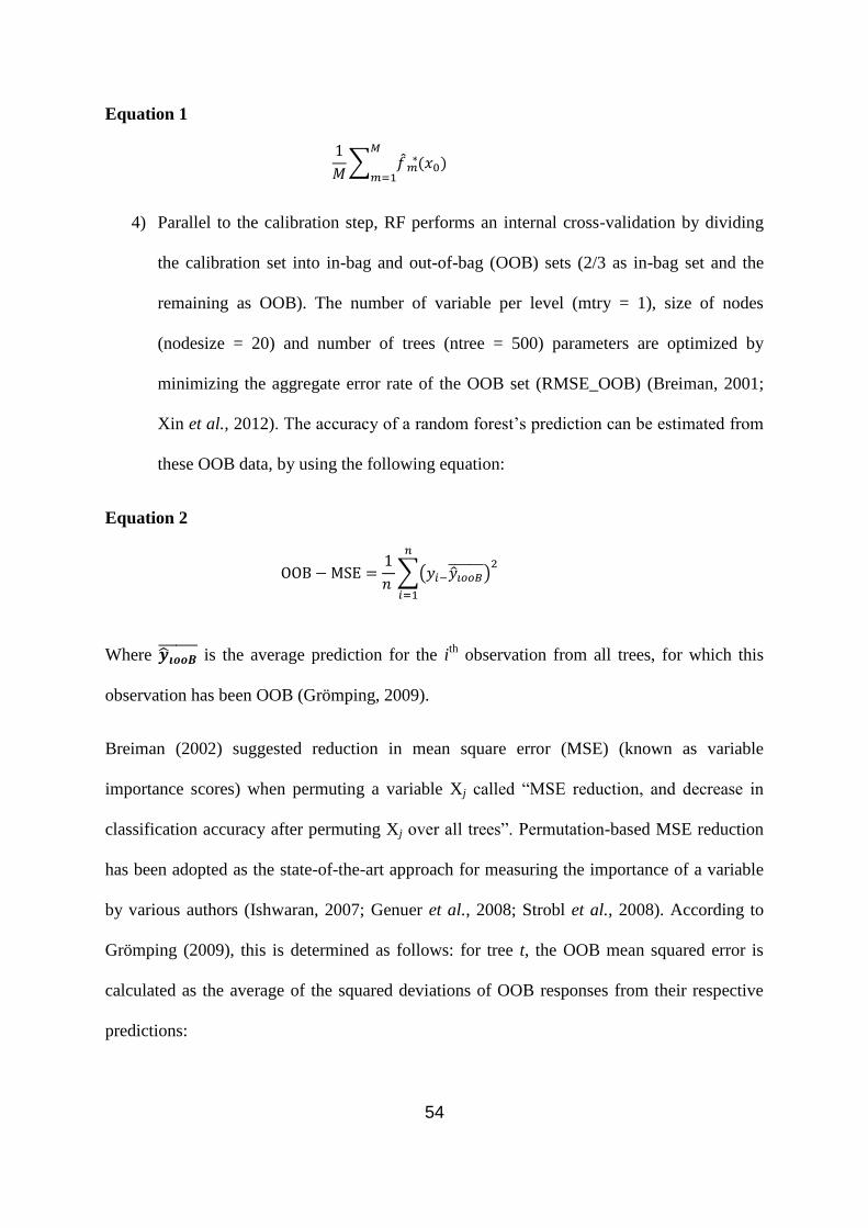
54

Equation 1

4) Parallel to the calibration step, RF performs an internal cross-validation by dividing

the calibration set into in-bag and out-of-bag (OOB) sets (2/3 as in-bag set and the

remaining as OOB). The number of variable per level (mtry = 1), size of nodes

(nodesize = 20) and number of trees (ntree = 500) parameters are optimized by

minimizing the aggregate error rate of the OOB set (RMSE_OOB) (Breiman, 2001;

Xin et al., 2012). The accuracy of a random forest’s prediction can be estimated from

these OOB data, by using the following equation:

Equation 2

Where is the average prediction for the i

th observation from all trees, for which this

observation has been OOB (Grömping, 2009).

Breiman (2002) suggested reduction in mean square error (MSE) (known as variable

importance scores) when permuting a variable Xj called “MSE reduction, and decrease in

classification accuracy after permuting Xj over all trees”. Permutation-based MSE reduction

has been adopted as the state-of-the-art approach for measuring the importance of a variable

by various authors (Ishwaran, 2007; Genuer et al., 2008; Strobl et al., 2008). According to

Grömping (2009), this is determined as follows: for tree t, the OOB mean squared error is

calculated as the average of the squared deviations of OOB responses from their respective

predictions:

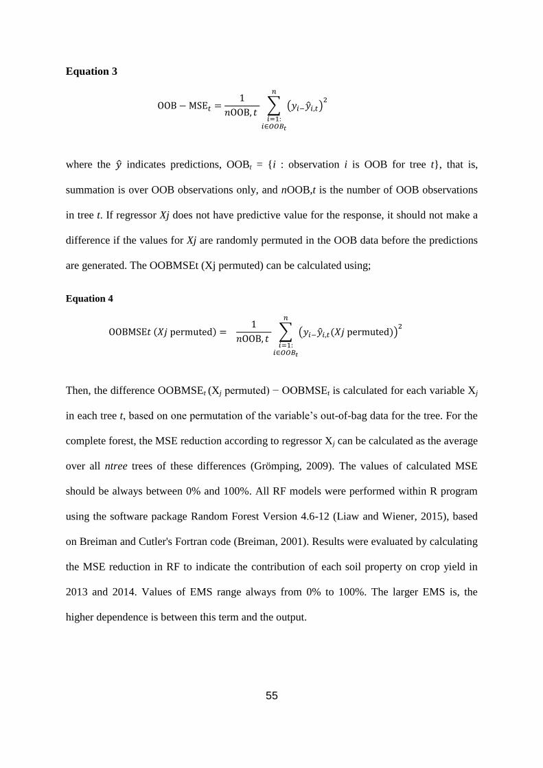
55

Equation 3

where the indicates predictions, OOBt = {i : observation i is OOB for tree t}, that is,

summation is over OOB observations only, and nOOB,t is the number of OOB observations

in tree t. If regressor Xj does not have predictive value for the response, it should not make a

difference if the values for Xj are randomly permuted in the OOB data before the predictions

are generated. The OOBMSEt (Xj permuted) can be calculated using;

Equation 4

Then, the difference OOBMSEt (Xj permuted) − OOBMSEt is calculated for each variable Xj

in each tree t, based on one permutation of the variable’s out-of-bag data for the tree. For the

complete forest, the MSE reduction according to regressor Xj can be calculated as the average

over all ntree trees of these differences (Grömping, 2009). The values of calculated MSE

should be always between 0% and 100%. All RF models were performed within R program

using the software package Random Forest Version 4.6-12 (Liaw and Wiener, 2015), based

on Breiman and Cutler's Fortran code (Breiman, 2001). Results were evaluated by calculating

the MSE reduction in RF to indicate the contribution of each soil property on crop yield in

2013 and 2014. Values of EMS range always from 0% to 100%. The larger EMS is, the

higher dependence is between this term and the output.

56

3.1.2.5 Parametric modelling

In this study, a simplified VNRX model, also known as non-linear finite impulse response

(NFIR) model, is proposed to understand and quantify the correlation between soil properties

and crop yield. This model has been commonly used to represent a multi-inputs and single-

output system, and can be expressed as:

Equation 5

where is the number of the system inputs, is some unknown linear or non-linear mapping,

which links the system output to the system inputs ; denotes the model

residual.

A commonly employed model type to specify the function in Eq. (5) is a polynomial

function (Chen and Billings, 1989; Wei et al., 2004), which can be expressed as follows:

Equation 6

where is the model term generated from all input vectors; is the corresponding

unknown parameters; is the total number of potential model terms. Note that is, in

general, non-linear. Considering a system with two inputs and , a second order

polynomial function can be written as:

Equation 7

f

57

Comparing with existing linear parametric methods, the proposed method accommodates the

non-linear relationship between the inputs and the output by introducing

terms

. Note that the candidate term in Eq. (6) can be any linear or non-

linear relationship among inputs. This paper will compare the performance of a model

accounting only for linear terms, designated as VNRX-L, with a model accounting for both

linear and non-linear terms, named VNRX-LN throughout this paper.

The next step is to estimate the parameters based on the

observations . The procedure begins by determining the structure, or the important

model terms, using the orthogonal least squares (OLS) estimation procedures. It determines

which dynamics and non-linear terms should be included in the model by computing the

contribution that each potential model term makes to the variation of the system output. The

model is to be built up term by term in a manner that exposes the significance of each new

term that is added. Once the structure of the model has been determined, the unknown

parameters can be estimated, and the procedure of model validation can ensure the model is

adequate. In this paper, a routine called adaptive-forward-orthogonal least squares (AFOLS)

was employed not only to determine the model structure but also to estimate the unknown

parameters. More detailed explanation of this method can be found in Zhao et al. (2012).

Finally, the performance of the VNRX models in the prediction of yield was evaluated. This

was done by considering the value of error reduction ratio (ERR) for each selected term

calculated from AFOLS that measures the percentage this term contributes to the system

output (Zhao et al., 2013). Values of ERR range always from 0% to 100%. The larger ERR

is, the higher dependence is between this term and the output. It is, therefore, a very

important index to indicate the importance of each term to the output.

58

To calculate the contribution of each input variable to the output, the sum of ERR values of

all selected terms, denoted as , is calculated by

Equation 8

to describe the percentage explained by the identified model to the system output, where

denotes the number of the selected terms. If the considered inputs can fully explain the

variation of system output, the value of is equal to 100%. It is an indicator of model

performance and uncertainty. The contribution of the input variable to the variation of the

system output, denoted as , is defined as the sum of ERR values of the terms that

include this input variable. Because some selected terms may involve more than one input

variable due to non-linearity, the sum of for all input variables can be greater than

. To overcome this problem, the value of is written as:

Equation 9

The value of should be always between 0% and 100%.

3.1.3 Results and discussion

In this work, the ten laboratory measured soil properties (i.e., TN, OC, Ca, CEC, Na, Mg, K,

pH, P and MC) were normalised and used as inputs to the VNRX and RF models’

establishments, whereas the model output was crop yield. The aim was to investigate the

contribution of each soil property on crop yield through two different cropping seasons.

Whilst the soil properties were collected only in 2013 the yield was collected in 2013 and

59

2014, it is assumed that soil properties may have decreased or increased in the time. The

methods used are not process based, and do not consider any temporal patterns or outline any

expected behaviours as input parameters, so the outputs cannot be considered interpretable to

other circumstances. However, they were applied in this study to understand yield variability

within a field at a given time. The knowledge gained is limited to its application in this field

and year. The study was designed to assess the models potential to explain yield variability,

particularly in non-homogenous fields.

3.1.3.1 Soil and yield data analysis

Results of the descriptive statistical analyses for soil properties are shown in Table 3, where

soil data were collected in 2013. The experimental soil ranges from strongly acidic to slightly

alkaline (pH = 5.4 to 7.7), with a mean neutral pH value of 6.63. The pH and OM conditions

were appropriate for the growth of oilseed rape and wheat (DEFRA, 2010), with a potential

pH effect on the P and Mg availability for smaller pH ranges than 6.5 (Truog, 1946,

Murrmann and Peech, 1969; Murrmann et al., 2005). Exchangeable K, Mg, Na, and Ca were

considered low for both crops, with mean values of 0.5 mg l-1

, 0.29 mg l-1

, 0.06 mg l-1

and

2.86 mg l-1

, respectively. Available P, CEC and TN were of low concentrations for oilseed

rape and wheat growth (DEFRA, 2010). P was consistently one of the largest contributors to

yield variation, this could be due to it being present in low concentrations, compared to the

crops ideal requirement (e.g., for oilseed rape the target soil index is 16-25 mg/l). However, it

was variable through the field from 9.54 mg/l to 1.34 mg/l (HGCA, 2014). These low

concentrations indicate these soil properties to be limiting of crop growth and yield.

60

Table 3: Statistics of measured soil properties of the 140 soil samples used as input data into

the three models.

TN pH P OC MC K Mg Na Ca CEC

Max 0.141 7.7 9.54 1.29 12.5 1.33 0.63 0.13 5.17 11.7

Min 0.058 5.4 1.34 0.59 6.15 0.14 0.13 0.025 1.47 6.3

Mean 0.08 6.63 2.69 0.83 8.19 0.5 0.29 0.06 2.86 8.45

SD 0.014 0.467 0.93 0.15 1.12 0.23 0.089 0.016 0.665 1.04

TN is total nitrogen, OC is organic carbon, and MC is moisture content which are all in % of dry matter; K is

exchangeable potassium in mg/l; P is extractable phosphorous in mg l-1

; CEC is cation exchange capacity in

mg100g-1

; Ca is calcium in mg l-1

; Na is sodium in mg l-1

; Mg is magnesium in mg l-1

; and pH the log

measurement of acidity.

The semi-variogram analysis of yield 2013 and 2014 shows the best fit of yield data to be

obtained with spherical models with negligible sums of squares error (SSE) values (Table 4).

Spherical models were selected as they best fit the empirical data. Spherical models are most

suitable for data with a progressive decrease in spatial autocorrelation. Selection of a suitable

model fit is important as the steepness of the curve (fitted to the empirical data) will impact

the influence of the closer data points.

Table 4: Semi-variogram model parameters of yield maps. The best fit was achieved with

spherical models for each, showing nugget (c0), sill (c), range (r m), proportion (C0/ C %),

and the sum of square error (SSE)

Variable c0 c r (m) (c0/ c) (%) (SSE)

Yield 2013 0.0021 0.007 24.38 30.0% 0.0001

Yield 2014 0.0039 0.009 40.98 43.1% 0.0001

c0 is nugget variance, c is sill, r is range and SSE is sum of squared error.

61

The ratio of nugget variance to sill variance is an important parameter to quantify short-

distance autocorrelation or the degree of spatial dependency for a variable (Cambardella et

al., 1994; Chang et al., 2014). Cambardella et al.,(1994) defined three categories of spatial

dependency of high, moderate, and week with ratios of less than 25%, between 25% and

75%, and greater than 75%, respectively. In this study, variations of the ratio of nugget

variance to sill variance of yield 2013 and 2014 are of moderate spatial dependence, with

ratios of 30.0% and 43.1%, respectively. Ranges of spatial dependence vary from 19.49 m

(yield 2013) to 0.98 m (yield 2014), which in 2013 is wider than the sampling interval of 12

m and confirming the effectiveness of geostatistical analysis adopted in this study (Chang et

al., 2014). Although the yield data in 2014 demonstrates smaller spatial variability than that

in 2014, which can be attributed to different crops and agricultural inputs (fertilisers,

pesticides and seeding rate), a different spatial distribution pattern across the study area can

be observed (Figure 5).

62

Figure 5: Yield maps of oilseed rape and barley measured in 2013 (a) and 2014 (b),

respectively, and developed with ordinary kriging based on spherical model (shown by

the line). Semi-variograms fit to the lag points which are distance classes into which

pairs of locations are grouped (shown by the small circles), with a sum of square error

(SSE) value of 0.0001 and 0.0001 for (c) and (d), respectively. Figure also shows

position of 140 soil samples used in this study.

63

3.1.3.2 Linear correlation

Examining Pearson’s correlation coefficient (r) values between pairs of soil properties

reveals few linear correlations, with the strongest correlation unsurprisingly recorded

between OC and TN (r = 0.945), which is in line with other reports (Carlyle, 1993; Kuang

and Mouazen, 2011). Other reasonable correlations can be observed between Ca and pH (r =

0.716), although those calculated between OC and MC, TN and Ca, TN and MC are of

smaller r values ranging between 0.507 and 0.559. Another interesting but negative linear

correlation (r = -0.656) is calculated between pH and CEC, explaining that pH decreases with

increasing CEC, which is true as CEC represents the soil’s ability to hold positively charged

ions e.g., exchangeable cations (Hazelton and Murphy, 2007).

The r values indicate no linear correlation could be observed between the ten soil properties

and yield in 2013 and 2014 (Table 5). The highest correlation of 0.239 is calculated between

OC and yield of 2013, which makes P the second highest correlated at 0.192, which for single

properties is very reasonable, as they are both influential soil fertility parameters (Tiessen et

al., 1994; Baligar et al., 2001; Agegnehu et al., 2016; Zhang et al., 2016). TN, Na, and pH

also make a slight correlation to yield estimation in the two years. However, collectively the

contribution is very limited and does not offer much explanation to yield variability, in either

of the years. This indicates the system complexity and non-linearity that cannot be explored

or quantified by simple linear relationships.

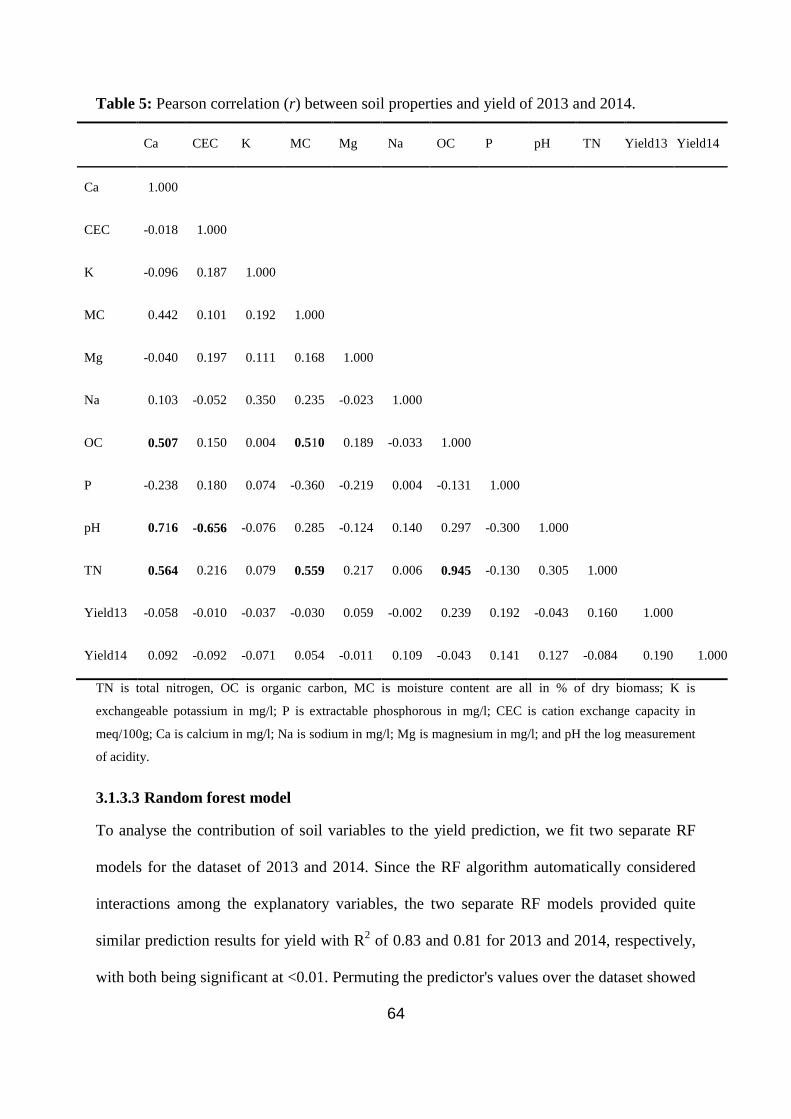
64

Table 5: Pearson correlation (r) between soil properties and yield of 2013 and 2014.

Ca CEC K MC Mg Na OC P pH TN Yield13 Yield14

Ca 1.000

CEC -0.018 1.000

K -0.096 0.187 1.000

MC 0.442 0.101 0.192 1.000

Mg -0.040 0.197 0.111 0.168 1.000

Na 0.103 -0.052 0.350 0.235 -0.023 1.000

OC 0.507 0.150 0.004 0.510 0.189 -0.033 1.000

P -0.238 0.180 0.074 -0.360 -0.219 0.004 -0.131 1.000

pH 0.716 -0.656 -0.076 0.285 -0.124 0.140 0.297 -0.300 1.000

TN 0.564 0.216 0.079 0.559 0.217 0.006 0.945 -0.130 0.305 1.000

Yield13 -0.058 -0.010 -0.037 -0.030 0.059 -0.002 0.239 0.192 -0.043 0.160 1.000

Yield14 0.092 -0.092 -0.071 0.054 -0.011 0.109 -0.043 0.141 0.127 -0.084 0.190 1.000

TN is total nitrogen, OC is organic carbon, MC is moisture content are all in % of dry biomass; K is

exchangeable potassium in mg/l; P is extractable phosphorous in mg/l; CEC is cation exchange capacity in

meq/100g; Ca is calcium in mg/l; Na is sodium in mg/l; Mg is magnesium in mg/l; and pH the log measurement

of acidity.

3.1.3.3 Random forest model

To analyse the contribution of soil variables to the yield prediction, we fit two separate RF

models for the dataset of 2013 and 2014. Since the RF algorithm automatically considered

interactions among the explanatory variables, the two separate RF models provided quite

similar prediction results for yield with R2 of 0.83 and 0.81 for 2013 and 2014, respectively,

with both being significant at <0.01. Permuting the predictor's values over the dataset showed

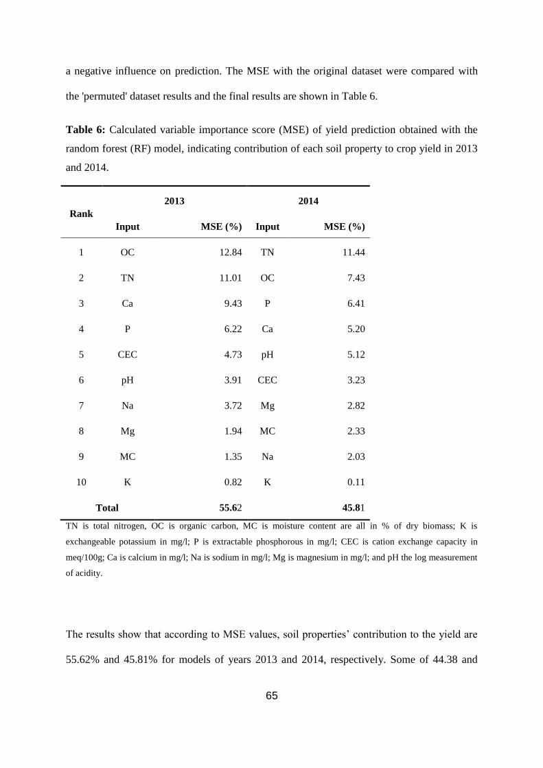
65

a negative influence on prediction. The MSE with the original dataset were compared with

the 'permuted' dataset results and the final results are shown in Table 6.

Table 6: Calculated variable importance score (MSE) of yield prediction obtained with the

random forest (RF) model, indicating contribution of each soil property to crop yield in 2013

and 2014.

Rank

2013 2014

Input MSE (%) Input MSE (%)

1 OC 12.84 TN 11.44

2 TN 11.01 OC 7.43

3 Ca 9.43 P 6.41

4 P 6.22 Ca 5.20

5 CEC 4.73 pH 5.12

6 pH 3.91 CEC 3.23

7 Na 3.72 Mg 2.82

8 Mg 1.94 MC 2.33

9 MC 1.35 Na 2.03

10 K 0.82 K 0.11

Total 55.62 45.81




of acidity.

The results show that according to MSE values, soil properties’ contribution to the yield are

55.62% and 45.81% for models of years 2013 and 2014, respectively. Some of 44.38 and

66

54.19% variation in the yield was left unexplained by both models. This result may be

explained by the fact that there are some factors could not be measured or included in the

models, such as weather conditions (Roberts et al., 2012; Lobell et al., 2014), and crop

disease (Paveley et al., 2012). The OC, TN and Ca were the top three highest contributors to

oilseed rape yield in 2013, whereas TN, OC, and P were the top three highest contributors to

barley yield in 2014. The OC has the highest variable importance score (12.84%) in 2013,

meanwhile it was the second highest variable importance score (7.43%) in 2014. This result

is expected and supported by the fact that OC can play a vital role in increasing crop yield

(Agegnehu et al., 2016), improving soil fertility (Tiessen et al., 1994; Zhang et al., 2016),

improving soil structure (Lorenz et al., 2007; Lal, 2011), and water retention (Fan et al.,

2013). Furthermore, soils with low OC contents have low crop yield and low use efficiency

of added nutrients (Agegnehu et al., 2016). Similarly, TN was the highest contributor to yield

prediction after OC in 2014 with a MSE value of 11.44%, whereas TN was the second

highest contributor in 2013 (MSE = 11.01%). Agegnehu et al. (2016) found that nitrogen

supply appeared to be a much greater factor limiting yield, which was related to the soil TN

content before planting and uptake rate by plants during the growing season. Interestingly,

they found that increases in yield and yield components were more pronounced when organic

amendments and N fertilizer were both applied, in comparison to one or the other.

Surprisingly, K had the lowest variable importance score for both RF 2013 and 2014 models

with contributions of 0.82%, and 0.11%, respectively. There was a gradual decline in soil K

levels, however, cereals remove less K compared to other crops (Malo et al., 2008). Both P

and Ca exchange the third and fourth places on the list. CEC is ranked the fifth and the sixth

in 2013 and 2014 with MSE values of 4.73% and 3.23%, respectively, whereas pH on

contrary to CEC, is ranked the sixth (3.91%) and the fifth (5.12%) on the list for 2013 and

67

2014, respectively. The remaining soil properties e.g., Na, Mg, and MC collectively

contributed to the yield of 7.01% and 7.18% for 2013 and 2014, respectively.

3.1.3.4 Parametric models

Based on Eq. (6), the following VNRX-LN model with quadratic terms was established to

relate the ten soil input variables with yield:

Equation 10

This model included 66 terms consisting of 11 linear terms and 55

non-linear terms . The VNRX-L model can be

written as:

Equation 11

The contributions of each soil property to crop yield variation were listed in Table 7 and

Table 8 for the VNRX-LN model and VNRX-L model, respectively. The VNRX-LN model

accounted for both linear and non-linear interactions, whilst the VNRX-L only considered

linear interaction. The non-linear aspect of the VNRX-LN model, permitted far more of the

yield variation to be understood, which is shown in the SERR values for 2013 and 2014 being

52.23% and 50.66%, respectively for the VNRX-LN and 19.15% and 8.5% for the VNRX-L.

This is supported by the negligible linear correlations calculated with r (Table 5). The

variation of SERR contribution between the years can be attributed to varying weather

conditions (Renouf et al., 2010; Boone et al., 2016), pests (Eberhart and Russell, 1966;

68

Paveley et al., 2012) and finally, the different crops grown, e.g., oilseed rape in 2013 and

wheat in 2014.

The output of the VNRX-LN model indicated as ERRC shows P, CEC and OC to be the top

three contributors to oilseed rape yield variability in 2013, whereas P, Na and OC were the

top three contributors to wheat in 2014. This seems logical from the soil fertility point of

view, as these (apart from Na) are all key nutrients to crop growth and development (Baligar

et al., 2001). As indicated above, OC can improve soil fertility, soil structure and water

retention, hence improve soil productivity. Na is a minor nutrient, which can have negative

effects on moisture uptake and can inhibit enzyme activities at high levels. The high yield

variability attributed to Na from the VNRX models is thus unexpected. Though there is an

optimal K:Na ratio for plant growth and yield development (Wakeel 2013). High amounts of

K have been found to reduce the occurrence of crop disease. High quantities of Na can reduce

the availability of K to plants (Perrenoud 1990; Prabhu et al., 2007). Within the studied field,

levels of K were more variable through the field than Na, the interaction between K and Na

may help explain the higher Na impact on yield variation, particularly in the non-linear

VNRX model (Baligar et al., 2001; Wakeel 2013). CEC is often used as a measurement of

soil fertility, but is not nutrient specific, whereas P is a main soil nutrient (with N and K) for

crop growth and development. CEC is also related to K content and clay particles, which all

affect available water content (Bergaya and Vayer, 1997).

Surprisingly, TN (Table 7) had a small contribution to yield variation in 2013 (ERRC =

1.23%), which may well be attributed to the small variation in nitrogen in this field (Table 3),

or to the smaller sensitivity of oilseed rape to nitrogen as compared to barley, as TN

demonstrates a higher contribution (ERRC = 5.01%) in 2014’s calculations. Both pH and Mg

69

were quite consistent contributors to 2013 and 2014 yield variability with calculated ERRC

values of 4.915 and 5.05%, respectively.


contribution (SERR) to crop yield in 2013 and 2014 cropping seasons, obtained with Volterra

Non-linear Regressive with eXogenous inputs (VNRX), accounting for both linear and non-

linear relationships (VNRX-LN).

Rank

2013 2014

Input ERRC (%) Input ERRC (%)

1 P 12.74 P 8.30

2 CEC 12.47 Na 6.77

3 OC 6.44 OC 6.71

4 pH 4.91 K 5.89

5 Ca 3.87 pH 5.05

6 Na 3.82 TN 5.01

7 Mg 3.41 MC 5.00

8 K 1.75 Mg 4.06

9 MC 1.59 CEC 2.79

10 TN 1.23 Ca 1.08

SERR 52.23 50.66




of acidity.

70

The range of soil pH in this field is between moderately basic to moderately acidic (Table 3).

Furthermore, it is interesting to see that MC has a low contribution to yield variation in 2013

(ERRC = 1.59%), with a higher contribution calculated in 2014 (ERRC = 5.0%), which may

be attributed to different crop or weather conditions across the two cropping seasons.

Reasonable contributions of K to the yield variability are calculated with the best contribution

observed in 2014. Ca was the lowest contributor in 2014 only.

The VNRX-L model (Table 8) shows different ranking results and different contributions of

individual soil properties as compared to the VNRX-LN model. With the VNRX-L model

both P and OC are the top two contributors to yield variability in both 2013 and 2014 years.

Contrary to the VNRX-LN model, TN obtained with the VNRX-L model in 2013 was of

more significant influence and got the same ranking in 2014, although the ERRC with the

VNRX-L model is smaller (e.g., 0.88) compared to the VNRX-LN model (e.g., 5.01%),

which is attributed to the larger SERR of the latter than the former approach. Ca has a

remarkably similar contribution in both 2013 and 2014, being the fourth most significant

parameter. Na was a larger contributor to yield variability in 2014 than in 2013, which is in

line with the VNRX-LN model predictions. pH varied in contribution between the two years

significantly, this could be due to the availability of nutrients detailed in Table 3, and being

reasonably neutral in acidity. Mg and MC are both insignificant contributors, which is in line

with the VNRX-LN model that accounts for both the linear and non-linear variability. K

holds a similar position in 2013 and 2014 for both parametric models investigated. CEC most

interestingly had no effect in 2013 in the VNRX-L model, opposed to the VNRX-LN model

predictions.

71


contribution (SERR) to crop yield in 2013 and 2014 cropping seasons, obtained with Volterra

Non-linear Regressive with eXogenous inputs (VNRX), accounting for linear relationship

only (VNRX-L).

Rank

2013 2014

Input ERRC (%) Input ERRC (%)

1 P 6.18 P 2.01

2 OC 5.73 OC 1.46

3 TN 3.94 Na 1.21

4 Ca 1.23 Ca 1.20

5 pH 1.09 K 1.13

6 Mg 0.53 TN 0.88

7 K 0.17 CEC 0.33

8 Na 0.15 MC 0.18

9 MC 0.13 Mg 0.07

10 CEC 0 pH 0.03

SERR 19.15 8.50




of acidity.

72

3.1.3.5 Parametric models versus random forest models

Based on results discussed above, it seems that OC always retained a high contribution to

yield variability through both years. This is true for all three models investigated in this

study. Soil OC arguably was the best single indicator of soil quality and function because of

its impact on soil physical, chemical and biological properties (Reeves, 1997; Shukla et al.,

Ebinger, 2006; D’Hose et al., 2014). Furthermore, OC is a source of plant nutrients in soils

and is vital in maintaining and improving soil structure, promoting water retention, and

reducing erosion (D’Hose et al., 2014). Therefore, it is not surprising to observe that soil OC

is a high contributor to yield variability.

P has a direct link with yield and so is expected to be a high contributor to yield variability

(Harmsen et al., 2001). P was the highest contributor to yield variability in both VNRX

models. However, with the RF model, P consistently contributed around 6% to yield

variability, being ranked as the third contributor to yield variability in 2014, and fourth in

2013. VNRX-LN presents TN as a moderate contributor, whereas the highest contribution for

TN is obtained with RF models. Since N is a key indicator for soil quality and plays a vital

role in crop production, this is an advantage of RF over VNRX (Sharma et al., 2008).

Although VNRX-LN and RF models allow the prediction of yield variability to be around

50%, with the input data from ten on-line soil properties, there is a remaining 50% of the

contribution that has not been accounted for. Kravchenko and Bullock (2000) stated that yield

variability is caused by a host of factors in addition to topographical and soil characteristics.

Therefore, it’s suggested that there are other external factors (such as diseases, pests, and

compaction) that need to be incorporated along with soil properties to allow for more

accurate assessment of the yield limiting factors and for improving the accuracy of prediction

of yield. Phosphorus along with Nitrogen are commonly added as fertilisers, and are the main

73

soil macro nutrients, affecting the severity of fungal diseases (Huber, 1980; Engelhard, 1989;

Fageria and Baligar, 1997; Graham and Webb, 1991). Whilst fungal diseases have not been

considered in this study, it would be interesting to involve them in further work, particularly

with the yield variation attributed to Na by the VNRX models.

The total contributions of the RF model to crop yield variability were 55.6% and 45.8% in

2013 and 2014 cropping seasons, respectively. The VNRX-LN model that was more

successful than the VNRX-L model in yield prediction contributed with similar percentages

(52.23% and 50.66% for years 2013 and 2014 respectively) to those of the RF models. The

total contribution of VNRX-LN models provides a greater consistency for high contribution

to yield variation. However, the RF model was more consistent on the ranking of influencing

soil properties of the yield variability. The consistency of the contribution of regression

models to predict yield was an issue raised by Kravchenko and Bullock (2000). Their

findings suggested that the capability of models to predict yield based on input soil properties

is heavily variable. Whilst successful in explaining a substantial portion of the yield in some

years, it is only capable of explaining a small portion of the yield variability in others.

Consistency of model predictions is highly valued. Each of the models demonstrated some

consistency between the two years, with RF being more consistent in ranking the influencing

soil properties on yield variability. VNRX-LN predicted a much larger contribution of K to

yield variation than the RF model, particularly in 2014. K is correlated to disease pressure,

making the VNRX-LN model an interesting concept for further work, if disease data could be

included. This study using parametric models, which could draw an understanding of ~50%

of the variabilities affecting yield in this field, in the two studied years. However, for

universal conclusions to be drawn, process based models, which consider climate data, crop

specific input parameters, and temporal patterns of parameters would be required

74

3.2 A new non-linear parametric modelling method to quantify

influence of soil properties on crop yields: Application to on-

line soil data

Abstract

There is a limited understanding of soil factors limiting crop yield, due to the complexity and

variability of the system. High spatial sampling resolution data on soil properties, may

contribute towards this, though soil properties are not the only factor affecting crop yield.

This study attempts to use a novel data mining approach, based on non-linear parametric

modelling, to study the effects of high resolution data of multiple soil properties on wheat

yield in a 22 ha field in Bedfordshire, UK. A Volterra Non-linear Regressive with eXogenous

inputs (VNRX-LN) model was introduced and tested in Part 1 of this study, where a limited

number of soil data were considered in the analysis. In Part 2, moisture content (MC) along

with the seven soil properties; total nitrogen (TN), organic carbon (OC), pH, available

phosphorous (P), magnesium (Mg), calcium (Ca), and cation exchange capacity (CEC) were

collected with an on-line (tractor mounted) visible and near infrared spectroscopy (vis-NIR)

sensor and used as multiple-input to the VNRX-LN model, while crop yield represented the

single-output in the system.

Results showed that the largest contributors to wheat yield were CEC, Mg and TN, with error

reduction ratio contribution (ERRC) values of 14.6%, 4.69% and 1%, respectively. The

overall contribution (SEER) of the soil properties considered in this study totals a value of

23.21%, which was surprisingly low as compared to 50-52% obtained in Part 1 with a limited

number of soil samples analysed with laboratory standard methods. This was attributed to a

large area of the studied field having been waterlogged, which masked the effect of soil

nutrient properties on crop yield. The study recommends further validation on a greater

75

number of fields where additional crop yield affecting parameters are taken into account e.g.,

crop disease, pests, drainage, topography, and microclimate conditions.

Keywords

Yield limiting factors; proximal soil sensing; VNRX; NARMAX; non-linear parametric

modelling.

3.2.1 Introduction

The world's population is expected to rise to 9 billion by 2050, hence, there is an increasing

demand for land for the use of biofuels, and there is already a food shortage. An increase in

yield of 60% will be required to match these requirements (Hole et al., 2005; Godfray et al.,

2010). One way to increase yield may be through precision management of farm resources.

The spatial variability in agricultural fields exists at different scales (Raun 1998; Dhillon et

al., 1994), which requires careful management with the aim to increase yield at reduced input

cost and related environmental impacts. This is hardly achievable by conventional agriculture

that relies on homogeneous applications of external inputs. For example, current fertiliser

applications are made based on an average soil sample collected per field or 1-3 ha in the best

scenario, which ignore within field variability as the fertilisers are spread homogenously.

This may result in over-application in rich zones, and under-application in poor zones in the

field (i.e., nitrogen rich areas receiving high rates of nitrogen fertiliser, due to the field having

nitrogen poor areas). In this context, recent years have seen a surge of variable-rate

application technologies where external farm inputs are applied in response to input data

from normalised difference vegetation index (NDVI), leaf area index (LAI), high resolution

soil properties or a combination of these (Lowenberg-DeBoer and Aghib, 1999; Maleki et al.,

2008; Mouazen et al., 2009; Halcro et al., 2013; Mouazen and Kuang, 2016). Commercial

fertiliser commonly contains nitrogen (N), phosphorus (P), and potassium (K). Other

76

nutrients such as, magnesium (Mg) and Calcium (Ca), are applied with less frequency. Mg

and Ca, N, P, K are used in the structural component of proteins, energy conversion, chemical

reactions in the plants, building components of the chlorophyll, respiration, and cell

membrane permeability. In non-homogenous fields, precision management of fertilisers is the

obvious way forward to increase crop yield. Understanding and quantifying the yield limiting

factors is still a crucial research question to be answered, before variable rate applications can

be optimised.

Since spatial variability in the majority of agricultural fields exist, proximal sensor

technologies are necessary to measure this variability accurately. This will require robust and

reliable sensing platforms of crop and soil. Proximal (e.g., Crop Circle ACS 470, Holland

Scientific, Lincoln, NE USA) and remote sensing (e.g., satellite imagery, unmanned aerial

vehicles or aircrafts) both can provide high resolution data on crop canopy characteristics

indicated e.g., as NDVI or LAI (Mulla, 2013; Kipp, Mistele, and Schmidhalter, 2014) and

they are commercially available. However, remote sensing methods provide data on the top

millimetres of soil and require a bare soil surface. Furthermore, due to the complex nature

and vast variability of agricultural soils, the majority of proximal soil sensors are still

premature to fulfil this requirement. Kuang et al. (2012) concluded in an extensive review

that the most promising proximal sensing technologies for quantifying soil properties are

electrochemical techniques and optical visible and near infrared (vis-NIR) spectroscopy.

Although they are limited to particular research groups worldwide, on-line vis-NIR sensors

(Shibusawa et al., 2001; Mouazen, De Baerdemaeker, and Ramon, 2006; Christy, 2008)

enable the prediction of high sampling resolution (e.g. >500 samples per ha) of key soil

properties (Kuang et al., 2012; Kodaira and Shibusawa, 2013; Kuang and Mouazen, 2013;

77

Kweon, Lund, and Maxton, 2013 Marin-González et al., 2013;), which are valuable sources

of information to be utilised for the analysis of soil related crop yield limiting factors.

The use of a simplified volterra non-linear regressive with eXogenous inputs (VNRX) model,

also known as non-linear finite impulse response (NFIR) model, was proposed and

implemented to understand the correlation between laboratory measured soil properties and

crop yield in Part 1 of this study (Whetton et al., 2016a), where on-line soil data was not

included in the analysis. In Part 1 of this study, VNRX accounting for both the linear and

non-linear (VNRX-LN) variability was compared to random forest (RF) models, and results

revealed VNRX-LN performed almost equally as good as RF in quantifying the total

contribution of soil properties on yield variation. The VNRX-LN reported interesting results

for field application. To our best knowledge, no literature about the use of a VNRX-LN

model to predict crop yield based on on-line measured soil properties can be found in the

literature. This is important to investigate, since on-line soil sensors provide high sampling

resolution data (>500 samples per ha) to enable accounting for variability that exists within

small scales (few meters), which cannot be obtained with the traditional soil sampling and

laboratory analytical methods.

The aim of this work is to explore the potential of the VNRX-LN model to quantify the

individual, interaction and collective contribution of high sampling resolution data of eight

selected soil properties collected with an on-line soil sensor on wheat yield Variability in one

site in Bedfordshire, UK. It will be based on multiple input data of soil properties (e.g., total

nitrogen (TN), organic carbon (OC), pH, available phosphorous (P), magnesium (Mg),

calcium (Ca), moisture content (MC), and cation exchange capacity (CEC), and wheat yield

used as the model output.

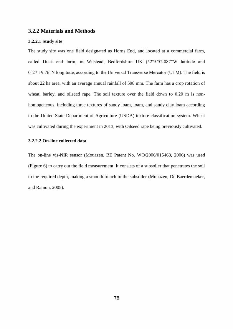
78

3.2.2 Materials and Methods

3.2.2.1 Study site

The study site was one field designated as Horns End, and located at a commercial farm,

called Duck end farm, in Wilstead, Bedfordshire UK (52°5’52.087”W latitude and

0°27’19.76”N longitude, according to the Universal Transverse Mercator (UTM). The field is

about 22 ha area, with an average annual rainfall of 598 mm. The farm has a crop rotation of

wheat, barley, and oilseed rape. The soil texture over the field down to 0.20 m is non-

homogeneous, including three textures of sandy loam, loam, and sandy clay loam according

to the United State Department of Agriculture (USDA) texture classification system. Wheat

was cultivated during the experiment in 2013, with Oilseed rape being previously cultivated.

3.2.2.2 On-line collected data

The on-line vis-NIR sensor (Mouazen, BE Patent No. WO/2006/015463, 2006) was used

(Figure 6) to carry out the field measurement. It consists of a subsoiler that penetrates the soil

to the required depth, making a smooth trench to the subsoiler (Mouazen, De Baerdemaeker,

and Ramon, 2005).

79

Figure 6: Illustrated image of the tractor mounted on-line visible and near infrared

spectroscopy (vis-NIRS) sensor (Mouazen, 2006).

The optical probe, housed in a steel lens holder, was attached to the rear of the subsoiler

chisel to acquire soil spectra in reflectance mode from the smooth bottom of the trench. The

subsoiler, retrofitted with the optical unit, was attached to a frame that was mounted onto the

three point hitch of the tractor. An AgroSpec mobile, fibre type, vis-NIR spectrophotometer

(tec5 Technology for Spectroscopy, Germany) which is an active sensor, with a measurement

range of 305-2200 nm was used to measure soil spectra in diffuse reflectance mode. A

differential global positioning system (DGPS) (EZ-Guide 250, Trimble, California, USA)

was used to record the position of the on-line measured spectra with sub-metre accuracy. A

Panasonic semi-rugged laptop was used for data logging and communication. The

spectrometer system, laptop and DGPS were powered by the tractor battery. A New Holland

80

T5000 tractor with 100 Ah battery was used. The total power consumption for all electrical

parts of the on-line vis-NIR sensor was around 60 W.

On-line soil measurement occurred in summer 2012 after the harvest of the previous crop, at

parallel transects with an average forward speed of the tractor of 2 km h-1

and the

measurement depth set at 150 mm. A few on-line collected vis-NIRS spectra are shown in

Figure 7, as an example.

Figure 7: Examples of the raw on-line soil visible and near infrared (vis-NIR) spectra,

collected with the on-line sensor. Showing slight deviations in relative absorbance, across the

wavelengths, which is dependent on the soil properties.

81

During each line measurement, two or three soil samples were collected from the bottom of a

trench and the sampling positions were carefully recorded with the DGPS. Samples collected

during the on-line measurement were analysed for calcium (Ca), cation exchange capacity

(CEC), magnesium (Mg), phosphorous (P), pH, moisture content (MC), organic carbon (OC)

and total nitrogen (TN). These samples were subjected to the same laboratory methods of soil

analysis mentioned in Part 1 of this study. The laboratory measurement techniques varied for

each value and the units they are presented in are in relation to this. MC, OC, and TN are

given in % (ISO 10694:1995; British Standard BS EN 13654-2:2001). P, Ca, and Mg is given

in mg/l (MAFF/ADAS, 198; Agilent Technologies, Inc. USA; Olsen, 1954). CEC is given in

meq/100g (Chapman 1965). pH is given in log measure (DEFRA, 2010).

Partial least squares regression (PLSR) based calibration models, developed with

Unscrambler V9.8 software (Camo Software, Norway) were used to predict all eight soil

properties using the on-line collected soil spectra (>500 samples per ha). More details about

the on-line vis-NIR sensor and accuracy of measurement can be found in Kuang and

Mouazen (2013) and Marin-González et al. (2013).

Wheat yield data was collected in August, 2013 by the on-board yield sensor and GPS system

of the farmer’s combine harvester (New Holland, CX8070 model), with a header width of

7.25 m commonly used for barley and wheat harvest. In addition, the harvest was optimised

to: I) record wheat yield when the machine header was full for the full length of the study

area, and II) avoid the bare soil in the tramlines (by collecting harvest data only from a full

header). Total yield was calculated from the mean yield (tonnes per hectare) of an area,

multiplied by the size of the area (m2), which was derived using ArcGIS (Esri, USA).

82

3.2.2.3 Data processing

Features in the environment, are the product of many interacting processes, including

physical, chemical and biological. They are determined with exceedingly complex

interactions. To overcome the difficulty of predicting this intricate distribution, it is required

to treat the variation as if it is random (Matheron, 1963). The measurement points from the

on-line soil sensor and yield sensor required a method of interpolation, to provide a

continuous data set across the locations. Kriging was selected as a non-biased approach to

predict the values between the sample points, where semi-variograms were first produced and

then applied in Kriging interpolation calculations. The interpolated data were then converted

into a common 5 m raster grid in ArcGIS (Esri, USA) in order to assist data fusion

(Frogbrook and Oliver, 2007). The raster squares of the layers were converted into this

common grid of points by extracting the value at the midpoint of each raster square. A

smaller resolution has no practical implementation, due to the limitations of the size and

response time of the precision farming equipment. The 5 m grid size provided a balance

between adequately characterising the spatial variation and practical farm management.

These steps ensured that all layers consisted of a common set of 5 m grid point-values, to

allow the application of parametric modelling to be carried out. This method allowed data

from a diverse range of soil and crop property surveys, measured at different resolutions, to

be merged (Khosla R. et al., 2008). The different soil and crop layers of a 5 by 5 m grid were

subjected to the VNRX-LN detailed in the following section.

3.2.2.4 Volterra Non-linear Regressive with eXogenous Model

In this study, the simplified VNRX-LN model, also known as NFIR model, introduced in Part

1 of this study was used, to represent a multi-inputs and single-output system:

83

Equation 12

[ 1] [ 1] [ 1]

1 2( ) = ( , ,..., ) ( )k k k

ry k f u u u k

was considered to represent a multi-inputs and single-output system, where ( =1,2,...)k k is a

time index, r is the number of the system inputs, f is some unknown linear or non-linear

mapping, which links the system output y to the system inputs 1 2, ,..., ru u u ; ( )k denotes

the model residual.

The on-line measured soil properties (i.e., TN, OC, pH, P, Mg, Ca, MC, and CEC) were

normalised and used as inputs to the VNRX-LN model, whereas the model output was wheat

yield. The analysis also included the interaction between pairs of soil properties and their

contribution to crop yield. The aim was to investigate the contribution of each soil property

and their pairwise interaction on crop yield variability.

Parameters are estimated based on the observations, and these are determined by the

structure, using the orthogonal least squares (OLS) estimation procedures. Adaptive-forward-

orthogonal least squares (AFOLS) was employed not only to determine the model structure

but also to estimate the unknown parameters. More detailed description of this method can be

found in Zhao et al.,(2012). More details about the VNRX-LN model is described in the Part

1 of this study (Whetton et al., 2016a).

Performance of VNRX-LN model output was evaluated by considering the value of error

reduction ratio (ERR) for each parameter to the prediction of yield (system outputs). Values

of ERR always range from 0% to 100%. The larger the ERR is, the higher the dependence is

between this term and the output. It is, therefore, a very important index to indicate the

84

contribution of each term to the output. To calculate the contribution of each input variable to

the output, the sum of ERR values (SERR) of all selected terms is used to describe the

percentage explained by the identified model to the system output. If the considered inputs

can fully explain the variation of system output, the value of is equal to 100%. It is an

indicator of model performance and uncertainty. The contribution of the input variable to

the variation of the system output, denoted as , is defined as the sum of ERR values of

the terms that include this input variable. The value of should be always between 0%

and 100%.

3.2.2.5 Significance Test

To determine the statistical significance of the contribution from each input to the system

output, a threshold , representing the level of contribution, above which value had less than

a 5% probability of occurring by chance, requires being determined. The conventional 95%

(0.05 significance level) confidence interval is not suitable for this study because the

distribution of ERRC value is unknown, as the condition to use 95% confidence interval is

that the value must follow the Gaussian distribution. As the distribution of ERRC value is

unknown, a 95% confidence may produce biased conclusions. For this purpose, the following

surrogate data technique was used.

Assuming the signal is a function of the signal , this sort of dependence is destroyed when

is ordered randomly in some way while keeps the same order. For this purpose, the order

of the data in was randomised by a shuffle procedure that saves the distribution properties

of the signal, but destroys the spatial relationship between and . This procedure was

repeated 100 times and then the 95% quantile was determined as the threshold. A

85

significance threshold for each term is firstly calculated, and then the significance threshold

for each input can then be derived by the same way to calculate .

3.2.2.6 Optimal spatial resolution of soil properties versus yield

Since the spatial sampling resolutions of soil properties and crop yield are different, before

applying the proposed VNRX-LN modelling method, the data must be re-sampled to

establish the correspondence between the inputs and the output. Two re-sampling techniques

have been used in this study. In the first technique, for each crop yield data on a

location , the corresponding soil properties were approximated by the properties on

the location that has the shortest distance to , which must be smaller than a radius . It

is possible that some crop yield data cannot find corresponding soil properties if is too

small, for which scenario this yield data will be discarded. In the second technique, for each

crop yield data , each corresponding soil property was approximated by the

averaging value of all values of this soil property inside a circle with a radius . A small value

of leads to more accurate correspondence between yield and properties, but a lower number

of samples included in the analysis. The former method of re-sampling is designated here as

‘shortest distance approximation (SDA)’, whereas the latter method is designated as ‘circle-

based average approximation (CAA)’.

3.2.3 Results and discussion

The yield data from the 2013 harvest is given in Figure 8, along with the semi-variogram

used for the interpolation. The yield data shows a consistently higher yield in the centre of the

field compared to the E and W edge. This variability is partially due to the field being on

reclaimed land, consisting of variable soil types as discussed earlier, but there is also an

influence from the hedgerow surrounding the field. The impact from the hedgerow was not

86

Figure 8: Interpolated yield map (a) and exponential semi-variogram of 0.036, 0.817 and 20.358,

representing, nugget, sill and range, respectively. Semi-variograms fit to the lag points which are

distance classes, into which pairs of locations are grouped (shown by the small circles) (b) based

on the 2013 harvest of wheat grain in tons per hectare. Lighter areas representing lower yield.

observed in Part 1 of this study, which used a field in Germany (Whetton et al., 2016a), due

to the field there having no hedgerow boundaries, as it was an area within a large continuous

field (with multiple crop varieties). However, anomalies in yield data can occur, particularly

towards the boundaries of the field (crop varieties) due to a decrease in combine speed,

turning, and headers being cut separately. The noise and influence of these areas were

removed from the yield data, but it is possible that there is still an artefact of this.

(a) (b)

The on-line collected soil properties (shown in Figure 9 for moisture content, and in Figure

10 for Mg, OC, P, CEC, Ca, TN, and pH) were achieved through applying PLSR models. A

summary of the statistics and model accuracy can be found in Table 9. Further details about

the development of these models can be found in Kuang and Mouazen (2013) and Marin-

87

Figure 9: Measured transects (a), map of the soil moisture content (MC) measured with

the on-line visible and near infrared spectroscopy (vis-NIRS) sensor after crop harvest

in August, 2012 (b) respectively.

González et al. (2013). The moisture content map is shown along with the measurement

transects (Figure 9), where the spectral data was collected. Whilst MC is involved in the

VNRX model this is sampled at the beginning of the growing season. The MC map highlights

the moisture distribution spatial pattern in a field although the levels will vary in short

periods of time (Vachaud et al., 1985). The studied field site has different soil property types,

as areas of the field are on reclaimed land. It was noted through the growing season that there

was a waterlogging problem on the west side of the field.

(a) (b)

Figure 10 shows the on-line predicted soil properties (i.e., Mg, OC, P, CEC, Ca, TN, and pH),

the semi-variogram results for the interpolated maps can be found in Table 9. General trends

can be seen between the soil properties, with a low strip running through the centre of the

field. The highest correlation seen is between moisture content and yield. However, Ca and

Mg (Figure 10) show this same trend, being higher in nutrients in the areas of higher moisture

88

content, associated with low yield. Total nitrogen is in the highest concentrations in the NW

of the field with a high band running through the S of the field, and phosphorus mimics this

pattern. The lowest yield and highest moisture content are found in the NW of the field.

Organic carbon appears to be homogenous through the field apart from a band in the centre,

which is notably lower, with the NE and SW edge being slightly higher. PH is the lowest in

the NW, with a low strip through the centre, but otherwise quite homogenous. A general

trend can be seen between pH and CEC. Whilst an inverted pattern can be seen between pH

and P. CEC is the highest on the SW and NE of the field. The most obvious spatial similarity

is between yield and MC, where low yield (Figure 8) was seen in areas of higher moisture

(Figure 9), suggesting a waterlogging problem effect on crop yield, which was confirmed by

the farmer.

89

Figure 10: Soil property maps of the study field in Bedfordshire, UK; magnesium (Mg)

magnesium in mg/l, organic carbon (OC) in % of dry matter, phosphorus (P) in mg/l, CEC in

meq/100g, calcium (Ca) in mg/l, total nitrogen (TN) in % of dry matter, pH the log

measurement of acidity. On-line spectral data was collected and applied to PLSR models

developed by Kuang and Mouazen (2013) and Marin-González et al. (2013).

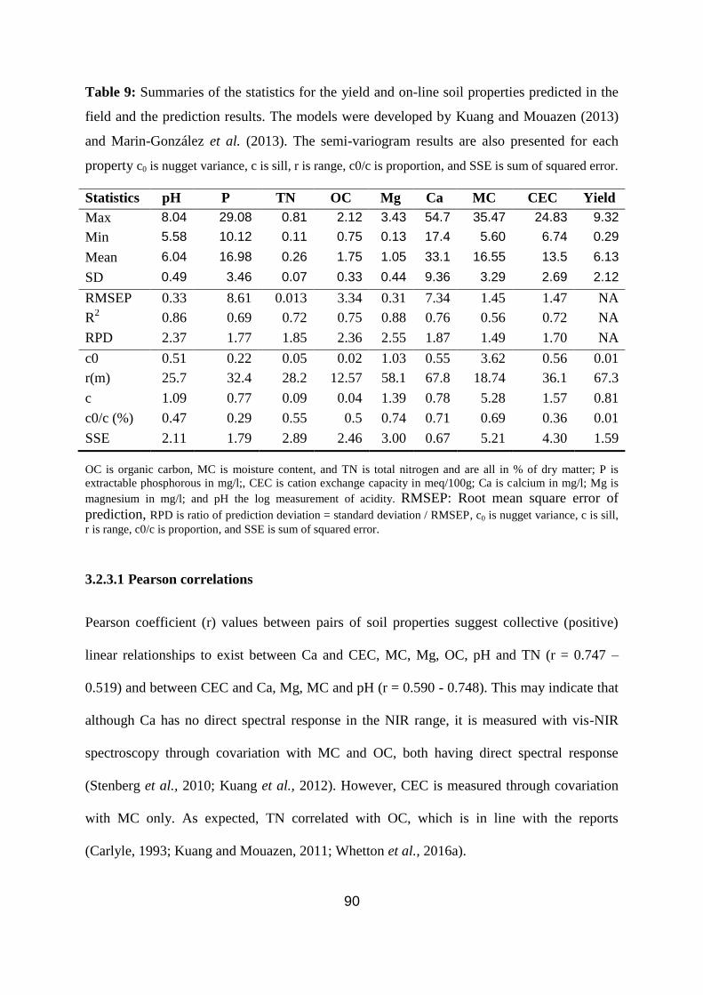
90

Table 9: Summaries of the statistics for the yield and on-line soil properties predicted in the

field and the prediction results. The models were developed by Kuang and Mouazen (2013)

and Marin-González et al. (2013). The semi-variogram results are also presented for each

property c0 is nugget variance, c is sill, r is range, c0/c is proportion, and SSE is sum of squared error.

Statistics pH P TN

(%)

OC

(%)

Mg Ca MC

(%)

CEC Yield

d Max 8.04 29.08 0.81 2.12 3.43

0

54.7

3

35.47 24.83 9.32

Min 5.58 10.12 0.11 0.75 0.13 17.4 5.60 6.74 0.29

Mean 6.04 16.98 0.26 1.75 1.05 33.1

7

16.55 13.5 6.13

SD 0.49 3.46 0.07 0.33 0.44 9.36 3.29 2.69 2.12

RMSEP 0.33 8.61 0.013 3.34 0.31 7.34 1.45 1.47 NA

R2 0.86 0.69 0.72 0.75 0.88 0.76 0.56 0.72 NA

RPD 2.37 1.77 1.85 2.36 2.55 1.87 1.49 1.70 NA

c0 0.51 0.22 0.05 0.02 1.03 0.55 3.62 0.56 0.01

r(m) 25.7 32.4 28.2 12.57 58.1

3

67.8 18.74 36.1 67.3

c 1.09 0.77 0.09 0.04 1.39 0.78 5.28 1.57 0.81

c0/c (%) 0.47 0.29 0.55 0.5 0.74 0.71 0.69 0.36 0.01

SSE 2.11 1.79 2.89 2.46 3.00 0.67 5.21 4.30 1.59

OC is organic carbon, MC is moisture content, and TN is total nitrogen and are all in % of dry matter; P is

extractable phosphorous in mg/l;, CEC is cation exchange capacity in meq/100g; Ca is calcium in mg/l; Mg is

magnesium in mg/l; and pH the log measurement of acidity. RMSEP: Root mean square error of

prediction, RPD is ratio of prediction deviation = standard deviation / RMSEP, c0 is nugget variance, c is sill,

r is range, c0/c is proportion, and SSE is sum of squared error.

3.2.3.1 Pearson correlations

Pearson coefficient (r) values between pairs of soil properties suggest collective (positive)

linear relationships to exist between Ca and CEC, MC, Mg, OC, pH and TN (r = 0.747 –

0.519) and between CEC and Ca, Mg, MC and pH (r = 0.590 - 0.748). This may indicate that

although Ca has no direct spectral response in the NIR range, it is measured with vis-NIR

spectroscopy through covariation with MC and OC, both having direct spectral response

(Stenberg et al., 2010; Kuang et al., 2012). However, CEC is measured through covariation

with MC only. As expected, TN correlated with OC, which is in line with the reports

(Carlyle, 1993; Kuang and Mouazen, 2011; Whetton et al., 2016a).

91

Examining r values between the eight on-line measured soil properties and yield, reveals

negligible (negative) relationships (Table 10), which is in-line with results of Part 1 of this

study (Whetton et al., 2016a), based on the correlation between laboratory measured soil

properties and yield. If the relationship between variables is not linear, then the correlation is

not strongly presented. The correlation could be affected by a third variable. The negative

correlations of the soil properties to the yield could be explained due to the non-linearity of a

soil system (Evans, 1996). The highest linear correlation is calculated between CEC and yield

(r = -0.349). This again proves the complexity of the system and supports the interest in

modelling techniques that account for both linear and non-linear interactions. As mentioned

earlier, the interactions of soil properties that lead to their distribution are intricate and

complex (Matheron, 1963). Ines et al. (2013) applied a simulation model where remotely

sensed soil moisture, and LAI data were used to update the model variables for yield

prediction of maize crop. Ines et al. (2013) model were process based which allowed the

consideration of a large area, over multiple years. They found that in very wet conditions, a

better accuracy was achieved with LAI parameters alone, and concluded that the water stress

influence later in the season was negligible. Involving a process model in this study could

have allowed a greater understanding and interpretation of the results, and would be

interesting to involve in further modelling studies.

92

Table 10: Pearson correlation (r) between on-line measured soil properties in 2012 and

wheat yield harvested in 2013.

Ca CEC MC Mg OC P pH TN Yield

Ca 1.000

CEC 0.733 1.000

MC 0.519 0.748 1.000

Mg 0.628 0.586 0.476 1.000

OC 0.650 0.441 0.436 0.176 1.000

P 0.163 0.216 0.019 0.042 0.027 1.000

pH 0.747 0.590 0.492 0.348 0.432 -0.013 1.000

TN 0.596 0.411 0.269 0.167 0.543 0.556 0.307 1.000

Yield -0.321 -0.349 -0.209 -0.320 -0.199 -0.000 -0.152 -0.057 1.000

TN is total nitrogen, OC is organic carbon, MC is moisture content are all in % of dry; P is extractable

phosphorous in mg/l; CEC is cation exchange capacity in meq/100g; Ca is calcium in mg/l; Mg is magnesium in

mg/l; and pH the log measurement of acidity.

3.2.3.2 Model output

The detailed correspondence between inputs variables and soil properties are described in

Table 11.

93

Table 11: The correspondence between inputs variables in Volterra Non-linear Regressive

with eXogenous inputs (VNRX) model and soil properties

Input Property Input Property Input Property Input Property

Ca CEC MC Mg

OC P pH TN




The initial full model, based on quadratic terms, was chosen in this paper, which can be

written as follows:

Equation 13

This model has 45 terms. All inputs and output were normalised (through maximum

normalisation) before being applied to the model. The proposed method was then applied to

calculate the ERRC of each term. Table 12 lists the first 10 terms selected using the SDA re-

sampling technique with a radius of 3 m. From this calculation it was observed that the

contribution of CEC to the wheat yield variability was the largest (e.g. ERRC = 15.68%)

among the 45 terms, including all soil properties and their interactions. This was followed

successively by Mg (ERRC = 3.57%) and Ca * CEC (ERRC = 1.13%) terms. This is

explained by the fact that although CEC is not a nutrient, it is a widely accepted measure to

assess the fertility of the soil. In fact, CEC represents the soil ability to hold positively

8 8 8

0

=1 =1

i i ij i j

i i j i

y u u u

94

charged ions e.g., exchangeable cations, which is directly linked to nutrients, hence, it is an

important indicator of the availability of nutrients (Hazelton and Murphy, 2007). Its

significant contribution to crop yield could be due to the quantity of nutrients being variable

through the field (Table 9), with Ca, P, MC and CEC having the highest standard deviations

successively. Mg was variable through the field with very low concentrations in some areas.

Mg contributed highly in explaining yield variability, which is understood as Mg is the

central part of a chlorophyll molecule and its availability can be limited by high availability

of other nutrients (i.e., potassium) (Holmes 1962). Whilst Mg has been influential in this

study to explaining yield variability in the field, it is not the most crucial nutrient to crop

growth (Engelhard, 1989). The high influence of Mg on yield variability observed in this

study could be attributed to it being a limiting factor in the field, rather than an essential

nutrient for crop growth. Mg influence on yield variation may also be due to its interactions

with Ca on the soil structure (with a recommended Ca:Mg ratio of around 5:1) (Rengasamy et

al., 1986; Tiwari et al., 2010).

95

Table 12: The first 10 terms with corresponding error reduction ratio contribution (ERRC)

values and coefficients based on the shortest distance approximation (SDA) re-sampling

technique with a 3 m radius.

Rank Term ERRC Coefficient

1 CEC 15.68% -0.0948

2 Mg 3.57% -0.4840

3 Ca*CEC 1.13% -0.0025

4 MC*Mg 0.72% -0.0558

5 OC 0.78% -0.2056

6 Mg*P 0.34% -0.9615

7 Mg*TN 0.78% 5.0750

8 pH*pH 0.39% -0.0670

9 constant 0.82% 0.1917

10 TN*TN 0.37% -8.5096




Furthermore, CEC is an important indicator influencing soil structure stability, nutrient

availability, soil pH and the soil’s reaction to fertilisers and other ameliorants (Hazelton and

Murphy, 2007), which as a result will have a positive influence of crop growth and yield.

Furthermore, CEC is also related to clay particles, which affect available water content

(Bergaya and Vayer, 1997), hence, influencing crop growth and development.

96

By comparing the contribution of each soil property to the wheat yield with the

corresponding significance threshold, the soil properties having significant contribution to the

crop yield variability can then be highlighted as shown in Table 13. It can be clearly observed

that among the eight studied soil properties, the following six soil properties e.g., CEC, Mg,

TN, Ca, OC and MC have all significant influence on the crop yield variability, with

declining order. However, the largest influence was attributed to CEC, followed successively

by Mg and TN.

It is worth noting that pH is normally associated with soil fertility (and CEC) but pH has one

of the lowest influence on yield variation (Hazelton and Murphy, 2007). But, pH level

directly affects nutrient availability and crop nutrient uptake (HGCA, 2014). With acidic soils

(soil pH is smaller than 5), the pH would have negative influence on nutrient uptake. It is

commonly stated in farmer’s guides that the optimum pH for soils under continuous arable

cropping of cereal crops is between 6 and 7 with 6.5 being the ideal. However, in the Horns

End experimental field, the pH value of the majority of the field area ranged between 5.6 and

8, with the average being 6.04 and a SD of 0.49, which may explain the low contribution of

pH to yield variability prediction (Bruulsema, 2015). However, all measured soil properties

were included in the model, even those with low variability across the field. The model is not

process based and does not produce universal truths, but reports the influence of influencing

factors on the yield variability for this field, in this cropping season. Similar observation can

be made for P. Although P is a key nutrient for crop growth and development, no significant

contribution to wheat yield variability was observed. Mg, Ca, N, P, and K are used in the

structural component of proteins, energy conversion, chemical reactions in the plants,

building components of the chlorophyll, respiration, and cell membrane permeability

(Epstein, 1972).

97

Table 13: Error reduction ratio contribution (ERRC) contribution of each soil property

(input) to the crop yield (system output) with corresponding significance threshold based on

the shortest distance approximation (SDA) re-sampling technique with a 3 m radius.

Rank Input ERRC (%) Significance threshold

(%)

Significant

1 CEC 14.60 0.60 Yes

2 Mg 4.69 0.52 Yes

3 TN 1.00 0.50 Yes

4 Ca 0.98 0.43 Yes

5 OC 0.68 0.49 Yes

6 MC 0.62 0.47 Yes

7 pH 0.34 0.46 No

8 P 0.30 0.56 No

Total 23.21 4.03

OC is organic carbon in % of dry matter; P is extractable phosphorous in mg/l; MC is moisture content in %;

TN is total nitrogen in % of dry matter, CEC is cation exchange capacity in meq/100g; Ca is calcium in mg/l;

Mg is magnesium in mg/l; and pH the log measurement of acidity.

This is a contradictory result to that achieved in Part 1, where the VNRX model was applied

to soil samples from a field in Germany, where P was the largest contribution soil parameter

to crop yield across the two cropping seasons studied. P is not a limiting property in the

Bedfordshire field, as manure is being frequently applied (Table 9) (Mouazen and Kuang,

2016). Another reason might that a part of the field i.e., the NW part, experienced a water

98

lodging problem associated with a poor drainage system for many years. Whilst MC was

mapped for the field prior to crop growth, the level of water will change throughout the

growing season, though the distribution pattern will stay relatively constant, so issues which

occur (such as waterlogging) after the data collection were not considered by the model. The

low yield and high moisture content is demonstrated in Figures8 and 9 respectively). This

impact could have been negated by establishing plot areas through the field, using a factorial

approach with different quantities of soil properties. This should be considered in further

work, as it could not be applied in this study, due to restrictions with it being a commercial

farm.

A multiple linear regression analyses with least square estimation conducted by Kravchenko

and Bullock (2000) found OC as the main and most consistent, positively correlated

parameter with corn and soybean yield. Interestingly, they found that the contribution from

K, CEC and P was mostly negligible, and this was attributed to K and P being ample in

abundance in the soils. This finding is in line with those of the current work regarding the

observed P values (as K was not considered in the work) However, Kravchenko and Bullock

(2000) stated that the performance of crop prediction models varies from field to field across

different cropping seasons. They could on average explain about 30% of yield variability

(results from 5 to 71%), whereas the model presented in this study explained 23.21% of the

yield variability.

TN ranked as the third largest contributor to wheat yield variability. A high influence of TN

to a field’s variability is supported by previous research. It is known that nitrogen supply is a

highly influential factor to crop yield (Agegnehu et al., 2016). The high contribution of TN to

yield variability in this study, suggests nitrogen supply was not homogenous through the

field. TN large variation is also shown by the soil maps in Figure10.

99

MC had only a minor influence on crop yield as it is ranked sixth among the eight soil

properties included in the analysis. However, the yield was thought to be considerably

impacted by the waterlogging problem associated with the poor drainage system in the NW

part of the field (Figure 9), Ines et al.(2013) found a similar issue in very wet conditions. MC

may be ranked low because it doesn’t capture the impact of water logging, and some of the

crop nutrients (such as Mg and Ca), closely mimic MC spatial distribution. This may also

explain the surprising high influence of Mg on the yield variability, which was ranked the

second most influential property for yield variance. The ratio of Mg and Ca can affect soil

conductivity (with a recommended Ca:Mg ratio of around 5:1). If Mg concentrations are high

it can cause high Flocculation in clay particles, resulting in ponding in wet conditions

(Rengasamye et al., 1986; Tiwari et al., 2010). Mg had particularly low values in some areas

of the field, with the high areas correlating well with the high areas of moisture content.

However, the high Ca areas were generally reflected in the high Mg areas, however this is not

true throughout the field, and this could have potentially contributed to Mg high impact on

yield variability.

There is an optimum for soil moisture (varying with crop growth stage) being beneficial to

crop yield. As MC increases it may become a hindrance to crop yield after reaching a

threshold. The waterlogged areas are of high MC and nutrient concentrations but low in yield

due to the water stress, which affects crop growth and yield. Waterlogged crop roots are

unable to respire, as there is too little oxygen in the soil pores (Boyer, 1982). Water logging

at grain filling stages can cause a significant loss in grain yield (Condon and Giunta, 2003).

Kravchenko and Bullock (2000) commented that the capability of models to predict yield is

heavily variable spatially and across different cropping seasons. Whilst successful in

explaining a substantial portion of the yield variability in some years, they are only capable of

100

explaining a small portion of the yield variability in others. This could be due to not using

process based models, whilst suitable in explaining the contribution of a properties variability

to the yield variability in a specific field, it does not provide universal truths. Low variability

of properties in a field, could reduce the amount of explainable yield variability.

Along with the waterlogging issue in Horns End field encountered in Part 2 of this study, this

goes further to suggest a reason why results in the Part 1 of this study (Whetton et al., 2016a)

were more successful (e.g., SERR reaching 52%). Regression analyses between cotton yield

and soil properties collected by a traditional soil sampling method (Corwin et al., 2003)

suggested that issues surrounding moisture content, salinity and pH were the most significant

influence on the yield outcome, which support the finding of the current work regarding the

water logging problem.

3.2.3.3 Model sensitivity

All results discussed above are based on the SDA re-sampling technique with a 3m radius. To

evaluate the sensitivity of the results to the selection of re-sampling technique and the size of

radius, more tests where been performed, whose results are shown in Table 14, in which only

the top 3 significant soil properties are presented. Inspection of Table 14 reveals that the top

two soil properties (e.g., CEC and Mg) showed exactly same response for all tests, appearing

at first and second factors affecting yield, respectively, whereas TN appears three times and

Ca appears once in the third position. Additionally, the CAA re-sampling technique

consistently had a larger total contribution (SERR = 22.97% for 3 m radius) to wheat yield

than that of the SDA re-sampling technique (SERR = 20.29% for 3 m radius), which

indicates the CAA technique may be more suitable for the high resolution soil and yield data,

because the identified model explains more of the system output. Also, the total contribution

to variability decreases, following the increase of the re-sampling radius, which is expected

101

because more samples in an area, should be more sensitive and indicate more spatial

variations of the underlying rule (Billings 2013).

102

Table 14: Contribution of the top three significant soil properties in terms of the sum of error

reduction ratio (SERR) on the crop yield, based on shortest distance approximation (SDA)

and (CAA) sampling techniques calculated for different radius values.

Re-sampling

technique

Re-sampling

radius

Sampled

number

Top three inputs Total Contribution

(SERR) Inputs Contribution

SDA 3 1377

CEC 14.60%

20.29% Mg 4.69%

TN 1.00%

CAA 3 1377

CEC 16.54%

22.97% Mg 4.00%

TN 2.43%

SDA 5 3605

CEC 9.20%

13.61% Mg 2.45%

TN 1.96%

CAA 5 3605

CEC 12.90%

15.87% Mg 3.02%

Ca 2.65%

OC is organic carbon in % of dry matter; P is extractable phosphorous in mg/l; MC is moisture content in %;

TN is total nitrogen in % of dry matter, CEC is cation exchange capacity in meq/100g; Ca is calcium in mg/l;

Mg is magnesium in mg/l; and pH the log measurement of acidity.

103

Results showed that the overall contribution of the eight soil properties to wheat yield

variability is 23.21%. One would expect that the contribution of soil properties to yield

should be larger than the overall calculated contribution in the current work. Nutrients are

required for healthy plants. This study has assessed the impact of the variabilities of eight soil

properties through a field. It does not report the necessity of these nutrients, but has attempted

to assess the variability of yield, attributed to the soil properties spatial variability. However,

the results obtained confirmed this to be a significant contribution, but also shows that there

is variability still at play, influencing the crop yield (e.g., crop disease, pests, topography,

micro-climatic conditions etc.). For example, whilst TN and OC should have significant

effects, and both are required by the crop for healthy growth and grain production, they can

also increase and prolong the leaf area index of the crop, which in turn increases humidity,

making the plant more susceptible to disease, hence, crop yield is negatively affected (Bryson

et al., 1997). In wheat, epidemics can cause significant crop losses, pest damage, including

weeds, and disease can result in global loss of around 50% (Bravo et al., 2003; Oerke 2006;

Moss, 2013). Further work should expand by including additional variables, to account for

more yield variability.

3.3 Summary conclusions

In part one of this study;

The results showed that over the two years the VNRX-L models produced the poorest results

for yield variability of 19.15% and 8.5% in 2013 and 2014, respectively. VNRX-LN model

accounting for both linear and non-linear interactions, which was the reason why this model

has explained 52.2% and 50.7% of yield variation in 2013 and 2014 respectively. The RF

model produced the highest contribution of 55.6% in 2013, which dropped down

considerably to 45.8% in 2014. Authors encourage further studies into the novel VNRX

104

modelling approach, for quantifying the individual and collective influences of soil properties

on yield variability.

In part two of this study;

Results showed that the overall contribution of the eight soil properties (collected at high

resolution) to wheat yield variability using a VNRX-LN model is 23.21%. There is a need for

a future work to expand on the current data mining approach to quantify yield limiting

factors, based on a greater number of fields with different crops and different agricultural

systems. The study should also account for the other affecting factors of crop yield including

crop disease, pests, topography, micro-climatic conditions etc., which was highlighted in

work by Shearman et al. (2005) and Sylvester-Bradley et al. (1999).

105

4 Optimising the configuration of a hyperspectral imager for on-

line measurement of wheat canopies

Chapter Synopsis;

This chapter concerns the laboratory-based optimisation of measurement configuration of a

hyperspectral imager for cereal crop canopy measurements. The optimal configurations are

later applied in the recognition of yellow rust and fusarium head blight (FHB) at canopy

level, under laboratory and field on-line measurement conditions to be discussed in chapters 5

and 6, respectively.

Abstract

There is a lack of information on optimal measurement configuration of hyperspectral

imagers for on-line measurement of a wheat canopy. This paper aims to identify this

configuration using a passive sensor (400-750 nm). The individual and interaction effects of

camera height (above the canopy) and angle, sensor integration time and light source distance

and height on the spectra’s signal-to-noise ratio (SNR) were evaluated under laboratory

scanning conditions, from which an optimal configuration was defined and tested under on-

line field measurement conditions. The influences of soil total nitrogen (TN) and moisture

content (MC), measured with an on-line visible and near infrared (vis-NIR) spectroscopy

sensor, on SNR were also studied. Analysis of variance and principal component analysis

(PCA) were applied to understand the effects of the laboratory considered factors and to

identify the most influencing components on SNR.

Results showed that integration time and camera height and angle are highly influential

factors affecting SNR. Among integration times of 10, 20 and 50 ms, the highest SNR was

obtained with 1.2 m, 1.2 m and 10° values of light height, light distance and camera angle,

106

respectively. The optimum integration time for on-line field measurement was 50 ms,

obtained at an optimal camera height of 0.3 m. On-line measured soil TN and MC were found

to have significant effects on the SNR with Kappa values of 0.56 and 0.75, respectively. In

conclusion, an optimal configuration for a tractor mounted hyperspectral imager was

established for the best quality of on-line spectra collected for wheat canopy.

Keywords

Hyperspectral imager, signal-to-noise ratio, wheat canopy, principal component analysis, soil

properties.

4.1 Introduction

Advanced methods for early disease detection in crops is vital for improving the efficacy of

treatment, reducing infection and minimising losses to yield and quality. Traditionally,

disease detection is carried out manually, which is costly, time consuming and requires

special expertise (Schmale and Bergstrom, 2003; Bock et al., 2010). Developments in

agricultural technology have led to demands for a non-destructive, automated approach for

crop disease detection that should be ideally rapid, disease specific, and sensitive to early

symptoms (López et al., 2003). Optical sensing methods are non-destructive, allowing

repeated data acquisition throughout the growing season without inhibiting crop growth.

Spectroscopy and imaging techniques have been used in disease and stress monitoring (Hahn,

2009). However, their in-situ application although established in other industries (e.g. health

services, pharmacology and food safety) is still rather limited. Both Lenk et al. (2007) and

Sankaran et al. (2010) focused on implementing the technology in the field, as a mobile (on-

line) application for mapping crop disease. Yuan et al. (2016) have used high spatial satellite

imagery in the detection of powdery mildew. Remote spectral sensing for identification of

107

weeds in wheat fields has been tested by means of ground collected data (Gómez-Casero et

al., 2009). Herrmann et al. (2013) have applied proximal hyperspectral imagery in the field

for weed detection (e.g., both broadleaf and grass weeds), reporting 85% accuracy. Okamoto

and Lee (2009) collected in-situ hyperspectral images for the detection of green citrus fruits,

reporting promising results for identification of citrus fruits from background objects. In

contrast, non-mobile (off-line) and laboratory methods for disease classification and plant

growing conditions have been studied and demonstrated (Roggo et al., 2003; Wu et al.,

2008).

A UAV mounted with a multi-spectral camera was successfully applied in the detection of

leaf stripe disease in grapevines when monitored with ground assessments (Di Gennaro et al.,

2016). Calderón et al. (2014) claimed accurate detection of downy mildew in opium poppy

using unmanned aerial vehicles (UAV) technology and a combination of thermal and multi-

spectral cameras. With the inclusion of fluorescence indices, Calderón et al. (2013) could

successfully detect verticillium wilt in olive trees.

Hahn (2009) claims that spectroscopic and imaging techniques could be integrated with

agricultural vehicles, providing non-invasive and reliable systems for the monitoring and

mapping of crop diseases, with further potential for early disease detection. Moshou et al.

(2005) have shown that hyperspectral imaging for the recognition of in-situ disease can

provide identification with a high degree of accuracy. Depending on the method of analysis

and data fusion, an error between 1 - 16.5% was reported.

Spectral reflectance in vegetation canopies is dependent on several factors including the

illumination angle, the canopy architecture and the radiative properties of the plants. The

reflectance of crop canopies is non-lambertian scattering, varying with the sun position, view

108

positions and meteorological conditions including cloud cover (Pinter and Jackson, 1985;

Asner, 1998). Plant species, maturity, phenology, level of foliage and nutrient status are plant

properties affecting reflectance (Asner, 1998; Coops et al., 2003; Gnyp et al., 2014).

Geometrical arrangement of objects can affect the spectral reflectance such as leaf

orientation, which cannot be controlled during on-line measurements (Asner, 1998; Coops et

al., 2003). This creates problems associated with reduced reflection from light scattering.

Shadows at small scale can be reduced by additional light sources. Barbedo et al. (2015)

found that opposing lighting can help reduce shadows. Oberti et al. (2014) argued that the

angle between the canopy and camera in the range between 0° to 60° affects the sensitivity of

a mounted on-line (mobile) sensor due to light backscattering, suggesting the potential of an

oblique camera angle, to reduce the impact on signal-to-noise ratio (SNR) variation.

A tractor mounted hyperspectral imager allows for on-line field crop canopy sensing and

mapping, however, an optimal configuration of the camera, light source and integration time

needs to be established for optimal quality of imagery and spectra to be collected. Spectral

quality is predominantly affected by sensor integration time, camera orientation, and light

height and angle from the object (leaf or canopy). Integration time is the period over which

the detector collects photons of light. The greater the integration time and light intensity, the

more reflected light is expected to be captured by the detector, providing a higher SNR and

pronunciation of the spectral peaks. Though when relying on sun light, the intensity can be

variable. Ideally the system could be run at night to exclude external variabilities, however

this solution is not practical. When applying a spectral technique to a forward moving

platform (on-line measurement) longer integration times result in an average spectrum over a

larger area, reducing the sensitivity. Furthermore, the greater the distance between the camera

and its subject, the larger the area observed and captured by a single pixel, reducing spatial

109

resolution. Therefore, optimising the measurement configuration is essential before on-line

field measurements can be successfully carried out. Furthermore, background soil influences

canopy spectra, and efforts have been made to remove this influence (Huete, 1988). Based on

remote sensing data of the surface soil, Demetriades-Shah et al. (1990) suggested using a

second order derivative to remove deviations caused by the soil background. However, none

of these studies have investigated the influences of on-line measured (at a depth of 15-20 cm)

soil properties [e.g., moisture content (MC) and total nitrogen (TN)] on the quality of crop

canopy spectra.

This paper evaluates, under laboratory conditions, the individual and interaction effects of

camera height and angle, integration time and light distance and height on the spectral SNR

of a wheat plant canopy captured with a hyperspectral line imager. Furthermore, the influence

of on-line measured soil MC and TN on SNR of plant spectra collected on-line in the field is

also assessed. This was essential to inform optimal configuration and operational conditions

for on-line field measurement of crop canopy and diseases.

4.2 Materials and methods

4.2.1 Hyperspectral configuration in the laboratory

Winter wheat Triticum sativum (Solstice variety) was grown outdoors in 600 x 400 mm trays

(depth of 120 mm) with 100 seeds evenly sown and spaced in 5 parallel lines. After seeding,

the trays were predominantly rain fed, to reduce input of excess salts from treated tap water.

As the crops were grown outside no artificial vernalisation was given. Three grams of

Nitrogen (34%) fertiliser were added to each tray, the same composition as that applied

during the field experiment (discussed below). A push broom hyperspectral imager

(spectrograph) (HS spectral camera model from Gilden Photonics Ltd., UK) was used to

capture high-resolution-line images with a resolution of 1,608 pixels over 1 second, using a

110

diode array detector. It is a 12 bit Basler piA 1600-35 gm camera, with Schneider-Kreuznach

XNP1.4/23 lens and has a pixel pitch of 7.4 μm interpolated/averaged to 0.6 nm readings

with a spectral range of 400 - 750 nm. The reflected light from the target travels through the

lens, past an entrance slit through a series of inspector optics in the spectrograph and is then

split by the prism dispersing element into different wavelengths. This sensor was chosen for

its potential for being applied to crop canopy measurements, and was of low price compared

to comparable sensors, commercially available in the market.

The data captured is in the form of a line array, with each pixel containing a spectrum and

one detector per pixel across the swath. In order to compile a full image, every line across a

target must be captured (Gilden Photonics Ltd, Glasgow, UK). When conFigured on a

consistent moving platform, the imager sweeps across an area to build up an image. Due to

practical restraints of applying a consistent moving platform, the spectraSENS v3.3 (Gilden

Photonics Ltd, Glasgow, UK) software was adapted to record a single line array, which

required an additional RGB photo taken by a 5 megapixel camera with a 3.85 mm f/2.8 lens

at the same time of image capture, so that the scanned area could be comprehended. Two

laser pointers were added at each side of the hyperspectral imager to indicate the area of the

canopy to be scanned. The laser pointers were shut off when the spectral image was captured

to remove any interference. Before data analysis, the collected scans were corrected by means

of a dark and white reference, which were collected just before spectral capture, and at 10

minute intervals until scanning was completed. The white reference used was a commercially

available Spectralon Teflon white calibration panel with 99.9% white reflectance value. The

distance of the camera was set at variable heights from the top of the canopy, so crop height

information was not included in the study.

111

Factorial analysis was undertaken to understand and quantify the influence of configuration

parameters on SNR. The wheat was at growth stage 47 according to Zadoks scale (Zadoks et

al., 1974) (whilst the head was booting, and the canopy had closed) at the time of scanning.

The studied configuration parameters are shown in Table 15.

Table 15: Factors included in configuring the hyperspectral imager measured in meters (m),

degrees (°) and micro seconds (ms) (multiple configurations considered)

The same area was scanned in triplicate for the different combination of configurations. The

laboratory (simulated-field) measurement configuration is shown in Figure 11. For the indoor

environment, two 500 watt diffused broad spectrum halogen lamps were positioned at either

end of the crop sample tray with an average Lux measurement of 1650. The additional

illumination used in the current work was shown by experience to reduce the influence of

shadow within the complex and non-homogenous canopy structure. Imagery data was then

captured at different camera and light heights, light distances, camera angles and integration

times (measured in milliseconds (ms)), as illustrated in Table 15. Light angle was kept

Camera angle,

deg °

Light height,

m

Light distance,

m

Camera height,

m

Integration time,

ms

0 0.90 0.60 0.15 10

5 1.2 0.90 0.30 20

10 - 1.2 0.45 50

- - - 0.60 1000

112

constant at 45°, which is debated as the optimal angle to provide the strongest response

(Huadong, 2001). Additional opposing lighting was used to reduce shadows (Barbedo et al.,

2015). Four integration times of 10, 20, 50 and 1000 ms were adopted as these cover the most

practical ranges. The 1000 ms integration time illustrates the highest potential time, during

which the system will absorb the reflected light hence; this is expected to give the smoothest

spectra.

Having determined a suitable configuration in the laboratory, the next experiments were

designed to apply the configurations to a field environment and assess the impact of the

environmental factors; e.g., soil moisture and total nitrogen, on SNR. Field measurements

were conducted in a 9 ha field at Duck End farm, Wilstead, Bedfordshire, UK (52°05'46.3"N

0°26'41.4"W), with an average annual rainfall of 598 mm. The farm has a crop rotation of

barley, wheat and oilseed rape. Wheat was cultivated during the experiment in the 2013

cropping season (drilled in September 2013) with canopy measurements being taken in April

2014. The dominant soil type in the field is a clay loam, but has a sand fraction due to

underlying gravel deposits.

113

Figure 11: Schematic illustration of the laboratory (simulated field) configurations used and

the variables implemented to obtain the hyperspectral data with the highest signal-to-noise

ratio (SNR). The hyperspectral imager is a passive sensor, but has been applied with an

external halogen light source. The Laser pointers allow to precisely position the hyperspectral

imager over the target.

4.2.2 On-line soil and crop measurements in the field

The on-line field measurements included crop spectra and soil MC and TN. The reason why

MC and TN were the selected soil properties, is that the former affects the soil physical and

mechanical conditions, influencing the soil dynamic behaviour below the tractor tyres during

the on-line measurement, whereas both may well be linked with crop growth (assuming that

TN is directly linked to mineral nitrogen). It is worth mentioning that mineral nitrogen (e.g.

nitrate and ammonia) cannot be measured with visible (400-780 nm) and near infrared (780-

2200 nm) (vis-NIR) spectroscopy, however analytical tests could be applied (Kuang et al.,

2012). Furthermore, the literature confirmed the potential of the vis-NIR to measure MC and

TN, which is attributed to the direct spectral response of these properties in the NIR range

114

(Stenberg et al., 2010; Kuang et al., 2012). The SNR values from the canopy’s hyperspectral

data was compared against the on-line measured soil properties at the same location via

Kappa statistics and visual comparisons. This was essential to evaluate whether or not the

optimal measurement configuration established in the laboratory was applicable in the field,

and whether modifications should be considered.

An on-line vis-NIR soil sensor developed by Mouazen (2006) was used in this study to

measure soil MC and TN, with the objective of mapping the spatial variability of these two

selected soil properties. The system consists of a subsoiler, opening a smooth trench at 15 cm

depth (Mouazen et al., 2005). The sensor was mounted on a three-point linkage of a tractor

travelling at a speed of 3 km h-1

and collecting spectral soil data at 10 m parallel intervals. In

order to measure soil spectra, an AgroSpec mobile, fibre type, vis–NIR spectrophotometer

(Tec5 Technology for Spectroscopy, Oberursel, Germany), with a measurement range of

305–2200 nm and a light source of 20W tungsten halogen lamp were used (Kuang and

Mouazen, 2013). A differential global positioning system (DGPS) (EZ-Guide 250, Trimble,

California, USA) recorded the position of the on-line spectra with sub-meter accuracy. The

collection of soil spectra and DGPS readings took place at 1 sec sampling resolution using

AgroSpec software (Tec5 Technology for Spectroscopy, Oberursel, Germany).

The same hyperspectral imager (Gilden Photonics Ltd, Glasgow, UK) as that used in the

laboratory to optimise measurement configuration was used for on-line measurement of the

wheat canopy in the field. The following hyperspectral measurement configuration was

considered: an integration time of 50 ms, a camera height of 0.3 m and light height and

distance of 1.2 m and a camera angle of 10°. The hyperspectral imager was mounted on a

tractor boom (Figure 12) traveling at approximately 4 km h-1

. The direction and angle of the

imager was kept consistent, and a day with uniformly overcast weather (complete cloud

115

cover) was selected (Figure 13), which helped prevent issues of moving shadows from lateral

sun movement on the data (West et al., 2003). Nevertheless, a handheld LUX meter (RS 180

– 7133, RS Components and Controls, India) was utilized to check the sunlight and readings

ranged between 1950 and 2000 LUX, indicating no significant difference. Alternatively, to

overcome sunlight issues the data collection could be conducted at night with the use of

broad spectrum artificial lighting. The hyperspectral camera was mounted to the side of the

tractor. It captures images of 1608 pixels per line, over a one-second interval, which is

subsequently logged and geo-located using a DGPS. The collected scans were corrected by

means of a dark and a white reference (spectralon 99% white reflectance panel). The latter

was used before spectral capture, and at a maximum of 30 minute intervals until scanning

was completed.

Figure 12: Illustrates the on-line field hyperspectral measurement using hyperspectral

measurement configuration.

116

Figure 13: Example of the overcast sky at on-line hyperspectral imaging collection.

4.2.3 Data analyses

4.2.3.1 Spectrograph spectral data processing and evaluation

Quality of the wheat canopy spectra (measured both in the laboratory and field) was

evaluated by analysing SNR. The SNR is defined here as a ratio of the signal strength to that

of unwanted interference. A strong signal devoid of interference is the desired outcome in

measurements. If the data is too noisy it can hide key features of the spectrum, and data pre-

processing such as smoothing can result in them being removed (Dasu and Johnson, 2003). A

noisy spectrum can result in poor calibration models, due to noise being considered as a

feature. There are many applications for estimating the SNR from sources such as electrical,

chemical, and spectral. Different methods are often applied to estimate the SNR value,

117

depending on the data input. Curran and Dungan (1989) used a bright homogenous surface to

estimate the SNR and produced a method termed the geostatistical method for removal of

periodic noise in images. Van der Meer (2000) used a method outlined by Lee et al. (1990)

for remote spectral sensing, to assess SNR of Landsat Thematic imagery. Analysis of image

SNR has also been conducted through production of histograms of an image (Ramamurthy et

al., 2004). A similar approach was outlined earlier by Smith (1999), where spectra were

collected from grayscale images. Smith (1999) exampled a SNR range between 0.5 and 2.0,

stating that there is only an issue if the SNR value drops below 1.0. We have used a crop

canopy in this study instead of a white or grey reference panel to calculate SNR, since the

intension was to use the optimal configuration for on-line measurement of crop canopy in the

field, where variations in canopy architecture and leaf orientation are foreseen. The same area

of the canopy was used for all individual scans. In this case, whilst uniform intensity cannot

be achieved across the spectrum in one scan, each pixel has almost the same target object

throughout all the scans. Similar to the measurements curried out in the current work,

Daumard et al. (2010) relied on crop canopy spectra to maximise SNR, although details of

the calculation of SNR were not provided. However, they considered central pixels only in

their calculations, whilst we have considered all pixels in a line image after removing non-

crop canopy spectra. The following assumptions were made in the current study to justify the

selection of a crop canopy for achieving an optimal measurement configuration:

1- Non-crop contaminated spectra including soil and soil-plant, etc. can be excluded from the

analysis. This was done by calculating normalised differential vegetation index (NDVI) of all

pixels. Spectra of pixels with NDVI values smaller than 0.3 were removed from the

calculation of SNR. This method is used by Bravo et al. (2004) and Huete (1988).

118

2- Spectra of remaining pixels contain both residual noise and canopy signal, the intensity of

which depends on the pixel position within a complex canopy structure of the crop. This will

represent the measurement of a homogenous canopy (without soil spectra).

3- Variation in position of pixels for a series of scans can be minimised by fixing the position

of crop trays, so that line images are collected from the same target area for different

measurement configurations. In this case, whilst uniform intensity cannot be achieved across

the spectrum in one scan, each pixel has almost the same target object throughout all the

scans.

The calculation of the SNR was done in this study following a similar approach adopted by

Ramamurthy et al. (2014) and described earlier by Smith (1999). As the data collected is

single line 2-dimensional captures, the data was assessed as spectra rather than images. This

method of SNR was selected as it could be used as a basis of comparison between individual

spectral data captures. We calculated the SNR of individual wavelength (SNRw) as follows:

Equation 14

SNRw = Mw/SDw

Where: Mw is the mean reflectance value of individual wavelengths through all the pixels,

and SDw is the standard deviation of mean reflectance of individual wavelengths of all pixels

explained in a schematic in Figure 14. It is worth noting that all pixels were considered

important in the current work to calculate SNR. An alternative approach to this method

would have been to select central pixels only to calculate SNR, a method applied by Daumard

et al. (2010).

The mean spectral signal describes what is being measured, whereas the standard deviation

represents noise and other interference for each pixel (Smith, 1999). Mw values for different

119

wavelengths were calculated on the remaining 583 wavebands, after removing the spectral

range outside of the 400 to 750 nm range, since they were found to be noisy. Once Mw and

SDw are calculated for each individual wavelength, the SNR for a spectrum (SNRs) was

calculated as follows (see Figure 14):

Equation 15

SNRs = Ms/SDs

Where: Ms is mean reflectance of all wavelengths in a spectrum (a scan) and SDs is mean

standard deviation of the reflectance of all wavelengths in a spectrum. The SNRs was used in

this study to evaluate the strength of scans, hence, the quality of spectral signal. It is worth

noting that SD is not important in itself, but only in comparison to the mean. Therefore, a

strong SNR with pronounced absorption peaks provides increased recognition for the

association of spectral signatures to a subject.

Figure 14: Schematic illustration outlining how mean, standard deviation and signal-to-noise

ratio for wavelength (Mw, SDw, SNRw, respectively) and a spectrum (Ms, SDs, SNRs,

respectively) were calculated.

120

A principal component analysis (PCA) was also undertaken on laboratory measured

hyperspectral data only using Statistica software (StatSoft inc., Oklahoma USA) to identify

parameters with the greatest impact on SNR. PCA is a statistical method, which analyses the

distribution of data in multidimensional space (principal components) or similarity maps,

where similarities (within groups of a variable) and differences between groups can be

evaluated (Dytham, 2011). In this instance, SNR, integration time, light height and distance,

and camera angle and height were used as input variables for the PCA analysis. Additionally,

a two-way analysis of variance (ANOVA) was carried out with RStudio software (RStudio

Boston, MA) to estimate significant influences of individual variables and interaction

between variables on SNR (Webster, 2007; Dytham, 2011).

4.2.3.2 On-line soil sensor calibration

Laboratory measurements of MC and TN were carried out using a standard reference method.

Soil MC was measured with oven drying of samples at 105ºC for 24 h, whereas TN was

measured with a TrusSpecCNS spectrometer (LECO Corporation, St. Joseph, MI, USA),

using the Dumas combustion method (Dumas, 1826 as cited by Buckee, 1994). The on-line

collected soil spectra were subjected to pre-processing before modelling. Pre-processing

included noise cut by removing wavelengths smaller than 400 nm and larger than 1900 nm.

Noise cut was followed successively by maximum normalisation, and Savitzky-Golay first

derivative and smoothing was applied. The smoothing reduces noise in the spectrum, and the

first derivative was used to eliminate the effect of the roughness of soil surface on the

spectrums absorption (Shibusawa et al., 2000;Waiser et al., 2007), Partial least squares

regression (PLSR) analysis with leave-one-out full cross-validation was carried out to

establish correlations between soil spectra and laboratory measured MC and TN. Spectra pre-

121

processing and PLSR analysis were carried out using Unscrambler 7.8 software (Camo Inc.;

Oslo, Norway).

4.2.4 Mapping

Maps for on-line vis-NIR predicted MC and TN and on-line spectrograph measured wheat

canopy reflectance were developed used ArcGIS 10 (ESRI, California, USA) software.

Kriging was used to develop maps, assuming that the distance or direction between sample

points reflects a spatial correlation that can be used to explain spatial variations. The

advanced parameters option in ArcGIS 10 software (ESRI, California, USA) allowed control

of the semi-variogram used for kriging, with spherical selected as the best fit. The semi-

variogram values were calculated in RStudio (RStudio, Boston, MA).

The similarity assessment between maps can be performed by visual inspection and statistical

tests (Tekin et al., 2013). The simplest way of comparing between maps is by visual

inspection, to conclude whether similarities may exist or not. However, this is insufficient, as

quantitative estimation of similarity is a more robust approach to adopt. To compare the

statistical relationship of pairs of maps, Kappa statistics (Cohen, 1960) analyses were

performed to calculate the Kappa value (κ), using SPSS (Statistical Package for the Social

Sciences, IBM, Armonk, New York, USA). However, before running Kappa statistics, data

was subjected to raster analyses to have the same 5 m by 5 m grid size for all maps, after

which the data underwent maximum normalisation.

4.3 Results and Discussion

4.3.1 Spectral quality in the laboratory

Typical wheat crop canopy spectra can be observed in Figure 15, which shows clear, noisy

and saturated spectra. The clear and saturated spectra can be observed to be more

pronounced, whereas a weak absorption in the spectral signature and interference in the noisy

122

spectrum leads to reduced quality, low SNR, masking detail in the signature and causing a

loss of important spectral information through the entire spectral range studied. The clear

spectrum is the best quality, and the target to be obtained. The noisy spectrum is caused by

the low integration times, and greater distance of the Halogen light source. A strong SNR

with pronounced absorption peaks would allow for a greater success in analysis of crop

assessments and disease presence. Although, pre-processing of spectral data includes

techniques such as smoothing, if the process of cleaning the data is intensive due to noisy

spectra it can lead to the loss of important spectral features, and thus impact on the success of

analysis (Dasu and Johnson, 2003).

Saturation predominantly occurs within the central pixels associated with the highest

reflectance, causing data in the peaks of the electromagnetic spectrum to be lost (starting

around 650 nm). Leaf reflectance in the NIR range is affected by the structure of the plant

leaves (Gates et al., 1965), and can be related to the leaf wax coating (Cameron 1970). In the

case of spectral saturation the data becomes unusable. In the remaining parts of the spectrum,

however, particularly the visible range (400–700 nm), there is a lower reflectance due to a

larger absorption of the light, which is attributed to the photosynthetic pigments of the plants

leaves, (Gates et al., 1965).

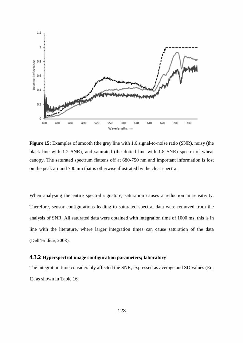
123

Figure 15: Examples of smooth (the grey line with 1.6 signal-to-noise ratio (SNR), noisy (the

black line with 1.2 SNR), and saturated (the dotted line with 1.8 SNR) spectra of wheat

canopy. The saturated spectrum flattens off at 680-750 nm and important information is lost

on the peak around 700 nm that is otherwise illustrated by the clear spectra.

When analysing the entire spectral signature, saturation causes a reduction in sensitivity.

Therefore, sensor configurations leading to saturated spectral data were removed from the

analysis of SNR. All saturated data were obtained with integration time of 1000 ms, this is in

line with the literature, where larger integration times can cause saturation of the data

(Dell’Endice, 2008).

4.3.2 Hyperspectral image configuration parameters; laboratory

The integration time considerably affected the SNR, expressed as average and SD values (Eq.

1), as shown in Table 16.

124

Table 16: Average and standard deviation (SD) values of the highest signal-to-noise-ratios

(SNR) obtained with different integration times, camera settings and light source settings

when scanning a wheat canopy. Theoretical forward distance travelled (and captured to a

single data line) if applied on a moving platform at field scale.

The longer the integration time, the greater the opportunity for more energy to be captured by

the spectrograph. The 1000 ms configuration was the highest potential integration time and

was trialled (under field simulations) to see the potential highest SNR, whilst the

manufacturer recommended around 20 ms for laboratory use. The results from the 1000 ms

integration time provided a high percentage of saturated results. The non-saturated recordings

were of the same SNR values to that of the 50 ms integration times, so integration times

higher than 50 ms were not trialled further. With varying the integration time, parameters had

constant values apart from the camera height. The optimal camera height decreases with an

increased integration time, the closer the camera to the object, the higher the integration time

required. This may mean that the most influencing parameters on the SNR were the

Average,

SNR

SD

Integration

time,

ms

Light

height,

m

Light

distance,

m

Camera

height,

m

Camera

angle,

deg

Distance

travelled,

m

1.688 0.102 1000 1.2 1.2 0.15 10 4

1.669 0.160 50 1.2 1.2 0.30 10 0.2

1.471 0.103 20 1.2 1.2 0.45 10 0.08

1.386 0.078 10 1.2 1.2 0.45 10 0.04

125

integration time and camera height. Other studies demonstrated that the movement

(adjustments, bounce or vibration) between the imager and the subject during integration time

can cause a compiled image to be warped or noisy (Zhong et al., 2011). For on-line

measurements, the easiest variable to control is integration time, as angle and height can alter

slightly as ground is uneven, crop stands vary and unavoidable movement occurs in

mountings. It becomes necessary to have the optimal configurations set initially but to

understand there would be slight deviations. A NADIR camera angle was selected, due to

reports from Oberti et al. (2014) and Van Beek et al. (2013).

ANOVA (appendix B) showed that all individual variables and interactions of variables had

significant influences on SNR at the (0.05) 5% probability level, except for the interactions of

light distance and integration time (0.01), and light distance, camera height and integration

time (0.01) (Appendix B). Therefore, the null hypothesise ‘that variables and subsequent

interactions of variables will have no significant effect on SNR’ can be rejected.

126

Figure 16: Principal component analysis similarity maps developed for principal components

1 and 2 (a) and for principal components 1 and 3 (b). Input variables are camera and light

height, light distance, camera angle, integration time and signal-to-noise ratio (SNR)

127

Principal component analysis, allows for a simpler visual understanding of a dataset as it

emphasise patterns and variations, by expressing the variation in a minimal number of

observations (Wold et al., 1987). Figure 16 illustrates the similarity maps of principal

component (PC) 1 and 2 (a), and PC1 and 3 (b) accounting for 47.62% and 42.26% of

variance, respectively. Examining the plot of PC1 vs PC2 one can observe that the integration

time, SNR and camera height are gathered in one group, which explains these to be closely

related. Integration time showed the strongest influence and correlation with SNR, whereas,

camera height demonstrated the second closest corresponding variable on SNR with the latter

having a weaker influence (Figure 16a). Light distance, light height and camera angle seem to

have a smaller influence on SNR (compared to integration time and camera height), as they

make a separate group associated with PC2 with minor variance associated with PC1.

Disregarding other variables, it becomes clear that a longer integration time and a smaller

camera height result in a higher SNR.

Although the light distance and height are strongly associated in the PCA similarity maps

(Figure 16 a and b), they have a negligible influence on the SNR. This does not mean that the

absence of light would have no effect. As long as there was ample diffused light, in order for

the detector to collect photons, light variables appeared to have little impact. Although the

influence of camera height was the second largest in the PC1-PC2 similarity map, in the PC1-

PC3 similarity map, the camera height had little influence on SNR, similarly to the light

variables. Furthermore, the close correlation between camera height and integration time

shown in the PC1-PC2 similarity map is not observed in the PC1-PC3 similarity map. In the

latter similarity map (Figure 16 b), the camera angle has the second largest influence on SNR

after the integration time. This means that both camera height and angle have strong

influences on the SNR. Under laboratory measurement conditions, larger camera angles were

128

reported to be beneficial for powdery mildew recognition in leaves of grape vines by Oberti

et al. (2014). Smaller view angles are discussed by Pisek et al. (2009) to theoretically be

better due to observing a larger area. Rautiainen et al. (2008) concluded greater nadir angles

are more suitable for viewing the top canopy and had a very limited view of the understory.

This is supported by the finding that 80% of the crop yield is calculated from the health of the

top 3 leaves (HGCA, 2008). The correlation between green leaf retention and yield has been

observed in a number of trials (Reynolds et al., 2009; Ali et al., 2010; Hunt and Poole, 2010)

and can be observed with reference to trial work in barley conducted by the authors in 2009,

where every 1% reduction in green leaf area on flag-1 at GS80 correlated to a 20 kg/ha loss in

yield. This is true when applying a camera angle. But when assessing light conditions, an off-

nadir angle can create more lighting variability, due to shady and illuminated areas of the

crop. Van Beek et al. (2013) found that for smaller off-nadir viewing angles (<20°) of the

sensor, the sun orientation was found not to be important. This, along with issues of shadow

from the infield mountings, is why small angles for the configurations were selected.

To make a decision on an optimal configuration that would result in the highest SNR, was not

a straightforward process. However, when SNR values are arranged according to the

integration time (Table 16), a clear trend is observed. For example, SNR increased with

integration time, where the highest values of SNR were obtained with an integration time of

1000 ms, however, they were only marginally higher than the SNR values at 50ms. Since

several variable combinations resulted in similar SNR values, it is perhaps premature to

suggest the optimal configuration as the single highest, so configurations with SNR

variability of less than 5% from the highest reading (of each integration time) were

considered for further evaluation. The further analysis confirms that the highest SNR occurs

with the same configurations of 1.2 m, 1.2 m, and 10° of light height, light distance and

129

camera angle, respectively. As stated earlier, the camera height is negatively correlated with

the integration time (Table 16). A possible theory for reoccurrence of these configurations

could be that they allow for the greatest amount of reflected light to be captured by the

detector. Among the integration time steps of 10, 20, 50 and 1000 ms selected, a practical

range for on-line measurement is between 10 ms and 50 ms, a range which is suggested by

the manufacturers. Assuming that the best integration time for practical on-line (mobile)

measurement in the field is 50 ms, the optimal configuration parameters of 1.2 m, 1.2 m, 0.3

m and 10° are recommended for light height, light distance, camera height, and camera angle,

respectively. The average SNR for this integration time is 1.669 (seen in Table 16), which in

reference to Smith (1999) we believe is a strong signal for a crop canopy. These optimal

configuration parameters were adopted for the on-line measurement of wheat canopy

measurement in this study.

4.3.3 Hyperspectral imager; on-line measurement

During the on-line measurement, it was noticed that there was an unavoidable bounce in the

boom observed to be at ±0.2 m of the original height of the mounting (set at 0.3 m above the

crop canopy). On inspection of the data, the camera height from the object affected the

uniformity of light intensity measured across the pixels, (particularly at the beginning and end

of the captured line). Therefore, for calibrating the on-line hyperspectral scans, it is

recommended to overcome this fluctuation by removing the first and last 320 pixels from the

spectral data. This is specific to this hyperspectral imager but is an interesting factor for

consideration.

130

Comparing the laboratory with on-line field measured canopy spectra, one can observe that

the laboratory reflectance scans are of a higher relative reflectance than the on-line scans,

specifically between 500nm and 700nm (Figure 17). The laboratory spectra are from tray

grown crops, whilst the on-line scans highlight different spatial areas of a field. The

reflectance difference between the laboratory and field scans could be also due to other

influencing factors such as water stress. The laboratory spectra shown is an average spectrum

from multiple trays. Although trays are reasonably deep (120 mm), they do not necessarily

hold as much water as in the field and this is believed to be reflected by the laboratory spectra

(Wang et al., 2014). Initially, the on-line spectra showed variation throughout the field, which

appeared to be in response to different crop spatial conditions. For example, the field scan 1,

refers to the canopy of water stressed wheat plants, whereas field scan 2 refers to healthier

wheat plants. Crops start to show yellow colour as a symptom of water stress, which leads to

reduce light absorption and increased reflectance as shown in field scan 1 (Figure 17). More

detailed analysis of crop and soil properties needs to be assessed to understand differences in

quality of canopy spectra collected in the field.

131

Figure 17: Comparison of canopy spectra of water stressed wheat crop obtained in the

laboratory (the dashed line) and on-line in the field (the dotted and grey lines). The crop was

of the same variety and at comparable growth stages. Laboratory and field scans were

collected under the suggested optimal configurations. The on-line field scans are: 1) field

scan (the grey line) is of a more water stressed plant and 2) field scan (the dotted line) is of a

less water stressed plant.

4.4 Influence of soil properties on signal-to-noise ratio during the on-line

measurement

The on-line measured soil MC and TN maps of the field provided a visual explanation

(Figure 18) for a drop in reflectance within certain areas of the field. Comparing the MC map

with the SNR map, one can draw a general conclusion that areas of low MC correspond with

areas of high SNR, and vice versa (areas of high MC being of low SNR). This can be

explained by the fact that soil deformation under the tractor tyre in wet soils is larger than

that in drier soil conditions. A larger soil deformation should result in a larger fluctuation in

camera height and angle, compared to the baseline setup, which may lead to reducing the

132

SNR. Work carried out by Söhne (1958) showed that an increase in the MC of a soil and the

increase in payload on a tyre both increase the depth of soil deformation.

Both on-line measured MC and TN were found to have significant effects on the SNR of the

wheat canopy spectra at 95% confidence. The kappa values between the SNR map and TN

and MC maps confirm spatial similarities within the field. Landis and Koch (1977) classified

Kappa values into different categories: 0–0.20, 0.21–0.40, 0.41–0.60, 0.61–0.80, and 0.81–1,

which indicate slight, fair, moderate, substantial, and almost perfect agreement, respectively.

Results show that the Kappa value between TN and SNR is rather small (kappa = 0.56),

indicating moderate similarity between these two maps. Since TN is the main source of

mineral nitrogen essential for crop growth and development, it can be influential on the

quality of the crop canopy and SNR.

133

Figure 18: Maps of on-line measured soil moisture content (MC) (a) total nitrogen (TN) (b),

and the average signal-to-noise ratio (SNR) per scan (c).

The kappa value between MC and SNR was much higher (kappa = 0.75) than that between

TN and SNR map, confirming substantial similarity between the two maps. This supports the

earlier suggestion about the influence of MC on soil deformation that changes the initial

(optimal) hyperspectral measurement configuration obtained in the laboratory and

implemented for on-line measurement in the field. To reduce the negative influence of soil

deformation on SNR due to high soil MC during on-line scanning, proper spectra pre-

processing is recommended e.g., normalisation, derivation, and multiplicative scatter

corrections. Further research is required to confirm this assumption, as when measuring on-

134

line, deviations from the optimum configuration (due to tractor vibration, bounce in the boom

and soil deformation) were unavoidable.

4.5 Conclusions

This study was undertaken to determine an optimal measurement configuration of a

hyperspectral line imager (400-750 nm). The SNR was calculated on the hyperspectral

measurement of a wheat canopy, under laboratory scanning conditions. The individual and

interaction effects of the systems configurations were evaluated for the impact on the SNR.

Optimal configuration was determined and implemented for on-line field measurement. The

influence of on-line measured soil moisture content (MC) and total nitrogen (TN) on SNR

was evaluated. Results allowed the following conclusions to be drawn:

1- The integration time followed by the camera height and camera angle appeared to have the

largest influence of the SNR. A long integration time (>50 ms) was of a negligible influence

and only slightly increased the SNR, but resulted in spectral saturation, hence should be

avoided.

2- The PCA similarity map showed that the light height and distance have a strong

correlation with each other but a minimal influence on SNR.

3- Both on-line measured MC and TN were found to have significant effects on the SNR of

the wheat canopy spectra at 95% confidence. The on-line soil measurements revealed

stronger spatial similarity between the hyperspectral SNR and MC maps (kappa value =

0.75), which was attributed to soil deformation below the tractor tyre.

4- The variable reflected light intensity captured by the different pixels across the line

imagery is an interesting factor to consider, due to the impact of varying camera height

135

during the on-line measurement. Whilst the solution suggested here is appropriate, it is

camera specific.

Further work is planned to overcome variation in SNR associated with camera height changes

(vibration, bounce in the boom, and soil deformation during the on-line measurement) by the

implementation of a proper spectra pre-processing. It is also planned to implement these

hyperspectral measurement configurations for on-line measurements of crop canopy for

detection of crop health and disease presence.

136

5 Hyperspectral measurements of yellow rust and fusarium head

blight in cereal crops: Part 1: Laboratory study

Chapter Synopsis;

This chapter focuses on the application of the hyperspectral imager with the optimised

configurations achieved in Chapter 4 for the detection of yellow rust and fusarium head blight

(FHB) in wheat and barley canopies. This was done based on PLSR models developed for

yellow rust and FHB quantitative prediction. The methods developed in this chapter will be

applied in the following chapter (6) using on-line data.

Abstract

The aim of this study was to assess the potential use of a hyperspectral camera for

measurement of yellow rust and fusarium head blight (FHB) in wheat and barley canopy

under laboratory conditions. The plants were grown in trays and inoculated with different

spore concentrations of the two studied pathogens. In order to account for water stress, trays

were water stressed at the crop growth stage 45. Visual assessment of disease was made at

four levels, namely, at the head (when present), at the flag leaves, at 2nd

and 3rd

leaves (mid

canopy), and at the lower canopy. Partial least squares regression (PLSR) was implemented

to establish calibration models to predict the percentage coverage and scale of infection (0-5

for yellow rust and 0-2 for FHB). Results showed that a hyperspectral technique coupled with

PLSR can be successfully used for the prediction of yellow rust in winter wheat and barley

canopies. Ratio of prediction deviation (RPD) values of 2.25 (equivalent to an R²= 0.8) and

1.97 (R²= 0.77) were calculated for wheat and barley based on scale measurement and 2.04

(R²=0.77) and 1.80 (R²=0.69) for percentage coverage, respectively, which were classified as

good accuracy in wheat and as moderately accurate in barley. For FHB detection, results

were less successful (RPD = 1.5 in wheat and 1.36 in barley, equivalent to an R² of 0.57 and

137

0.5, respectively). The standard deviation between 500 and 650 nm and squared difference

between 650 and 700 nm can explain differences between healthy, yellow rust and FHB

infected canopies. It is recommended to explore the potential of hyperspectral imaging for

on-line measurement of studied diseases in cereals.

Keywords

Yellow rust, fusarium head blight, wheat, barley, crop canopy, partial least squares

regression.

5.1 Introduction

With the world’s population estimated to reach 9 billion by 2050, sustainable approaches to

increase crop yield is a necessity (Hole et al., 2005; Godfray et al., 2010). The majority of

current farming practices are based on unsustainable production systems, relying on external

inputs and high-yield varieties susceptible to disease (Hole et al., 2005). Advanced

management (e.g., precision agriculture) of farm external resources such as fungicides, if

applications were site specific, could result in increasing yield at a reduced amount of input

and cost. This can be achieved by applying the full rate to areas of the field which would

benefit from the resource, and by applying a reduced rate to areas of lower demand, which

would reduce the quantity of input (Wittry and Mallarino 2004; Maleki et al., 2007). Among

these resources, fungicide application may well be reduced by targeted site specific spraying

(FRAC, 2010). However, accurate measurement of fungal diseases is a main requirement for

sustainable application of fungicides, and is expected to contribute to the reduction and

prevention of the spread of crop disease and the losses of quantity and quality incurred from

them.

138

Fungal disease control is a large task for the successful production of cereals worldwide.

Both yellow rust and fusarium head blight (FHB) are fungal diseases which infect small

cereal crops, and are responsible for causing severe yield losses (De Vallavieille-Pope et al.,

1995; Bravo et al., 2003). Disease presence can vary considerably between plants. Yellow

rust caused by Puccinia striiformis is a foliar disease, which can alone reduce crop yields by

40%. Bravo et al. (2003) stated that reductions in the yield can be as high as 7 tha-1

in severe

epidemics. Alternatively known as stripe rust, yellow rust produces yellow uredo spores on

the leaves. Following infection, the disease starts with chlorosis occurring parallel to leaf

veins, in a narrow 2 mm wide stripe, which develops later into multiple yellow coloured rust

pustules (De Vallavieille-Pope et al., 1995). FHB is one of the most important pre-harvest

diseases worldwide, reducing yield quantity and quality. The most aggressive and prevalent

fusarium species is Fusarium graminearum, which is a highly pathogenic species. The

pathogen can also produce mycotoxins, which can become a significant threat to both humans

and animals. FHB symptoms in wheat and barley appear in the head and peduncle tissues,

causing discolouration and early senescence. Legions can occur on the leaves during heavy

infection and fusarium can also cause fusarium foot rot. Disease presence can vary

considerably between plants (Rotter et al., 1996; Brennan et al., 2005; Desjardin, 2006;

Leslie and Summerell, 2006), hence, it is required to adopt site specific treatments of fungal

diseases.

Advanced methods for disease detection in crops is vital for improving the efficacy of

treatment, reducing infection and minimising the losses to yield and quality. Traditionally,

disease detection is carried out manually, which is costly, time consuming and requires

special expertise (Schmale and Bergstrom, 2003; Bock et al., 2010). Alternative methods of

detection are needed to enable mapping the spatial distribution of yellow rust and FHB.

139

Among those methods, optical sensing methods are recommended candidates since they are

non-destructive and allow for fast and repeated data acquisition throughout the growing

season without inhibiting crop growth. It was recognised by West et al. (20003) that although

optical technologies are available for development into suitable disease detection systems,

many challenges are still needed to be overcome, and this is still arguably the case.

Spectroscopy and imaging techniques have been used in disease and stress monitoring (Hahn,

2009). One of the optical methods reportedly used to measure disease in crops is

hyperspectral imagery in the visible (vis) and/or the near infrared (NIR) spectral ranges. The

reflectance in the visible wavelength range is relevant to leaf pigmentation whilst infrared

wavelength range provides information on the physiological condition of the plant. The

wavelength function for light intensity in hyperspectral imaging adds the wavelength and

spectrum (with its spatial position) to the brightness information of the spectral image,

providing a rapid image-contrast, which would not be present in a conventional image

approach (Huang et al., 2007). Within the visible spectrum, the radiation reflectance from an

environmentally stressed plant will increase. This is due to an increase in the incidence

reflection within the leaf of a stressed plant (Cibula and Carter, 1992). Bélanger et al. (2008)

showed that disease could be quantified on detached leaves, finding that the ratio between

blue (near 440 nm) and green (near 520 nm) intensity between the healthy and diseased tissue

was significantly different shortly after inoculation. Using vis-NIR imaging, Bravo et al.

(2003) detected early symptoms of yellow rust on winter wheat, with a quadratic discriminant

model analysis, reporting a correct discrimination accuracy of 92–98%. To our knowledge

none of the above studies incorporated water stress effects, in the prediction model of yellow

rust and FHB intensity in cereal crops. Some studies have focused on bringing the

technology to the field. However, the first step towards field application is to test the

140

accuracy of the methods under laboratory conditions (allowing more control and observation

of the crop), where disease and water stress are accounted for in one experiment.

The aim of this paper is to assess the potential implementation and performance of a

hyperspectral imager for recognition of yellow rust and FHB diseases in winter wheat and

winter barley under laboratory conditions, with the intention to establish calibration models

and spectral library for potential use under mobile on-line measurement conditions. Both

diseases (yellow rust and FHB) and water stress were introduced and accounted for.


5.2.1 Wheat and Barley cultivation and inoculation

Treated seeds of winter wheat Triticum sativum (Solstice variety) and winter barley Hordeum

vulgare L. (Carat Variety) were grown outdoors in 600 x 400 mm trays (depth of 120 mm),

with 100 seeds evenly sown and spaced in 5 parallel lines. After seeding, the trays were

predominantly rain fed, to reduce input of excess salts from treated tap water. Three

treatments were adopted, where each treatment was triplicated in three separate trays. A total

of 18 trays of wheat, and 18 trays of barley were grown for each of the following three

treatments (illustrated in Figure 19);

1) Treatment 1 – Naturally yellow rust infected: consisting of six trays that were not treated

with fungicide, as these were to represent the more heavily infected yellow rust trays, and

were not inoculated with fusarium.

2) Treatment 2 – Healthy: consisting of six trays of each that were kept healthy by applying a

broad spectrum fungicide, namely, Rubric (epoxiconazole) at a rate of 1 lha-1

.

3) Treatment 3 – Fusarium inoculated: consisting of six trays of each that were infected with

fusarium as the crop reached anthesis growing stage (Figure 20).

141

When the crop growth reached ‘booting’ growth stage 45 on the Zadoks scale (Zadoks et al.,

1974), half of trays in each were water stressed using a transparent tarpaulin and water

content was monitored throughout the growing season using a moisture-probe ML3 Thetakit

(Delta-T Devices Ltd, Cambridge, UK).

Yellow rust occurred naturally in the crops as early as growth stage 30. Therefore, half of the

crop trays were treated early with fungicide to fulfil treatments 2 and 3. This allowed for a

difference in intensity of yellow rust disease. Fusarium inoculation was applied to trays in

treatment 3 at the anthesis crop growth stage. The spores were first cultivated in the

laboratory by using the following method. A 2% wheat agar was produced using 100 ml

distilled water, with 2 g agar and 2 g milled wheat. This was autoclaved at 120°C. Plates

were poured to a consistent depth, and inoculated with Fusarium graminearum BFE1006

isolated from infected wheat grain. The plates were grown for 5-7 days under near UV light

as this was shown to help cause sporulation (Leach, 1967). The agar plates were subsequently

agitated with distilled water to suspend the spores with the concentration increased as

necessary by gentle use of the centrifuge. Spore concentrations were standardised at

approximately 106 ml

-1 using serial dilutions and a haemocytometer. Every 1 m

2 of crop ear

was inoculated with 100 ml of the suspension, which is an adapted method from Lacey

(1999). These trays were then kept under a high humidity conditions for 24 hours.

Whilst it has been reported that fungicide has little to no effect on crop canopy reflectance,

some azole fungicides can have a negative impact on crop growth and yield, when applied to

small plants (Geis, 2014; AHDB, 2016). In this study, the epoxiconazole fungicide was

applied at growth stage 32. Some symptoms of yellow rust disease were recorded in the

fungicide treated trays. However, the fungicide treated trays remained healthier, and these

were included in the PLSR models.

142

Figure 19: Schematic of tray replicates and treatments, showing winter barley and winter

wheat, with yellow rust and fusarium head blight (FHB) diseases, and healthy crop, both rain

fed and water stressed, in replicates of three.

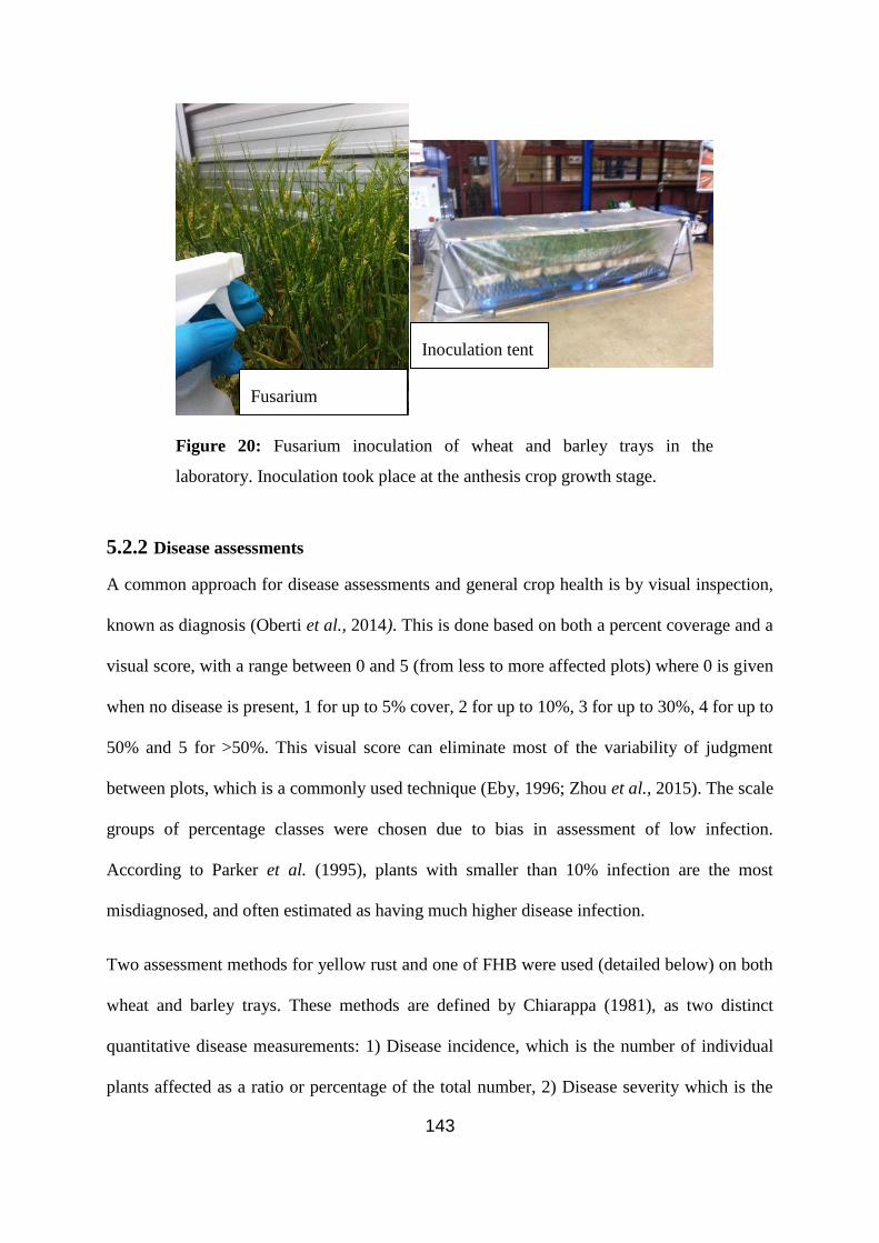
143

Figure 20: Fusarium inoculation of wheat and barley trays in the

laboratory. Inoculation took place at the anthesis crop growth stage.

5.2.2 Disease assessments

A common approach for disease assessments and general crop health is by visual inspection,

known as diagnosis (Oberti et al., 2014). This is done based on both a percent coverage and a

visual score, with a range between 0 and 5 (from less to more affected plots) where 0 is given

when no disease is present, 1 for up to 5% cover, 2 for up to 10%, 3 for up to 30%, 4 for up to

50% and 5 for >50%. This visual score can eliminate most of the variability of judgment

between plots, which is a commonly used technique (Eby, 1996; Zhou et al., 2015). The scale

groups of percentage classes were chosen due to bias in assessment of low infection.

According to Parker et al. (1995), plants with smaller than 10% infection are the most

misdiagnosed, and often estimated as having much higher disease infection.

Two assessment methods for yellow rust and one of FHB were used (detailed below) on both

wheat and barley trays. These methods are defined by Chiarappa (1981), as two distinct

quantitative disease measurements: 1) Disease incidence, which is the number of individual

plants affected as a ratio or percentage of the total number, 2) Disease severity which is the

Fusarium

suspension

Inoculation tent

144

amount of expressed disease tissue of a plant. These disease parameters can be assessed with

some objectivity, although they may well be subjected to some subjectivity. In the current

work, each tray was assessed for both diseases at four levels, namely, at the head (when

present), at the flag leaves, 2nd

and 3rd

leaves (mid canopy), and at the lower canopy

explained as follows;

1) For fusarium infection, only the head of the crop was assessed as we were assessing for

FHB, which appears in the head and peduncle tissues, causing discolouration and early

senescence. Earlier visual symptoms consist of a characteristic purple/pink

discolouration. The seeds from FHB affected crops are often shrunken, with a bleached

appearance (Andersen, 1948; Parry et al., 1995; McMullen et al., 1997; Goswami and

Kistler, 2004). Impey (2012) confirmed the presence of fusarium leaf lesions in

Herefordshire, the leaf lesions are very unusual, and found only in heavy infections. The

assessment considered both early and later symptoms, and were assessed as either a 0 for

no infection, 1 for mild infection (describing FHB symptoms on up to 50 % of the ears,

with the majority being symptoms of early infection), and a 2 for heavy infection

(describing FHB infection in over 50% of the ears with the majority being early

senescence), dependent on the ratio of occurrence of infected to healthy crops.

2) For yellow rust infection, the three foliar stages were assessed for percent coverage of

yellow rust lesions. Disease starts with chlorosis occurring parallel to leaf veins, in a

narrow 2 mm wide stripe, developing into multiple yellow coloured rust pustules (De

Vallavieille-Pope et al., 1995). Average disease coverage was given for all the plants

in the assessment area at the 3 different stages, and a visual score was also given. As

it’s needed for each ground truth plot to have a singular assessment for the later

analysis, the data from each stage was combined and weighted appropriately

145

Figure 21: Illustrating influence of foliar health on yield (HGCA, 2008)

according to HGCA (2008) recommendations; that 80% of a wheat yield can be

calculated from the top 3 leaves (Figure 21). The weighting given in this study was as

follows; flag leaf 55%, mid canopy 40%, and lower canopy 5%. This allowed a single

yellow rust assessment to be associated to a tray. This was done for both wheat and

barley crops. Barley has a much smaller flag leaf, representing about 4% of the leaf

area. However, the health of the flag leaf is still considered to be significant in

determining yield (Jebbouj and Yousfi 2006 and 2009), and due to the image being

taken from above the canopy, the flag leaf will still be highly captured. Therefore,

barley was also subjected to the same weighting. Two different quantitative

assessments were recorded, one for the percent cover on the leaves and one recorded

as a 0-5 scale, based on a similar approach to Bergamin Filho and Amorim (1996),

Godoy et al.(2006) and Huang et al.(2007).

146

5.2.3 Hyperspectral data capture

A push broom hyperspectral imager (spectrograph) (HS spectral camera model from Gilden

Photonics Ltd., UK) was used to capture high-resolution (1,608 pixels) line images over 1

second, using a diode array detector. It is a 12 bit Basler piA 1600-35 gm camera, with

Schneider-Kreuznach XNP1.4/23 lens and has a pixel pitch of 7.4 μm interpolated/averaged

to 0.6 nm readings with a spectral range of 400 - 1000 nm. The reflected light from the target

travels through the lens, past an entrance slit through a series of inspector optics in the

spectrograph and is then split by the prism dispersing element into different wavelengths.

This sensor was chosen for its potential for being applied to crop canopy measurements, and

was of a lower price compared to comparable sensors, commercially available in the market.

The spectral data was captured at three separate places along the crop tray at slightly different

positions. Captured in the form of a line array, each pixel has a spectrum and one detector per

pixel across the swath. In order to compile a full image, every line across a target must be

captured (Gilden Photonics Ltd, Glasgow, UK). When conFigured on a consistent moving

platform, the imager sweeps across an area to build up an image. Due to practical constraints

of applying a consistent moving platform, the spectraSENS v3.3 (Gilden Photonics Ltd,

Glasgow, UK) software was adapted to record a single line array, which required an

additional RGB photo taken by a 5 megapixel camera with a 3.85 mm f/2.8 lens at the same

time of image capture, so that the scanned area could be comprehended. Two laser pointers

were added at each side of the hyperspectral imager to indicate the area of the canopy to be

scanned (Figure 22). The laser pointers were shut off when the spectral image was captured

to remove any interference. The collected scans were corrected by means of a dark and a

white reference (spectralon 99% white reflectance panel) providing the relative reflectance.

147

The latter was used before spectral capture, and at 10 minute intervals until scanning was

completed.

The optimal configuration of the push broom hyperspectral imager including light sources

was optimised in the laboratory (Whetton et al., 2016b). A schematic illustration of the

configurations can be observed in Figure 22, where two 500 watt diffused broad spectrum

halogen lamps were positioned at either end of the crop sample tray. Light angle was kept

constant at 45°, which is debated as the optimal angle to provide the strongest response

(Huadong, 2001). The optimal configuration adopted included integration time, light height,

light distance, camera height, and camera angle, of 50 ms, 1.2 m, 1.2 m, 0.3 m and 10°,

respectively (Whetton et al., 2016b). These configurations were used in the current work, for

crop canopy scanning that started at booting growth stage 43 on Zadoks scale and continued

until reaching ripening at growth stage 90.

148

Figure 22: Schematic illustration of the laboratory configurations of hyperspectral camera

and light source (Whetton et al., 2016b).

5.2.4 Data pre-processing and modelling

If the spectral data is too noisy, there is a risk that key features of the spectrum will be

hidden, and data pre-processing such as smoothing is necessary to remove noise, but can

remove significant features (Dasu and Johnson, 2003). Furthermore, a noisy spectrum can

result in poor model performances, due to noise being considered as a feature. So the first

step towards successful measurement should ensure obtaining a good quality spectrum, which

was ensured in the current work by adopting the optimal configurations established in

Whetton et al. (2016b).

The spectral data were averaged to reduce the number of wavelengths (variables), which was

successively followed by maximum normalisation, Savitzky–Golay first derivative and

smoothing (Mouazen et al., 2006). Maximum normalisation is typically used to get all data to

149

approximately the same scale, or to get a more even distribution of the variances and the

average values. The maximum normalisation is a normalisation that “polarizes” the spectra.

The peaks of all spectra with positive values scale to +1, while spectra with negative values

scale to −1. Since all soil spectra in this study have positive values, the peaks of these spectra

scaled to +1. This scaled spectra between 0 and +1. Using the Savitzky–Golay first derivative

enables the computation of the first or higher-order derivatives, including a smoothing factor,

which determines how many adjacent variables will be used to estimate the polynomial

approximation used for derivatives. A second order polynomial approximation was selected.

A 2:2 smoothing was carried out after the first derivative to decrease noise from the measured

spectra. All pre-processing steps were carried out using Unscrambler 10 software (Camo Inc.;

Oslo, Norway).

Analysis of variance (ANOVA) was used to analyse two spectral indices captured at the

growth stage 72. A factorial treatment structure was incorporated to test for differences

between disease type (healthy, FHB, yellow rust), water treatment (watered, water-stressed)

and crop type (barley, wheat). In addition, a contrast was used to test for differences between

healthy and diseased trays and between the different diseases. Analysis of the index SD was

done on a log scale, whilst analysis of SQdiff was done on a sqrt scale to ensure

homoscedascity of variance. GenStat 18th

Edition (© VSN International Ltd, Hemel

Hempstead, UK) was used to compute the ANOVA tables.

PLSR analyses were applied to the hyperspectral data (Table 17) to establish quantitative

models to predict yellow rust and FHB infection. Before PLSR analysis, data were

divided into two sets of 80% (e.g., 174 samples for yellow rust and 129 for FHB) and 20%

(e.g., 43 samples for yellow rust and 32 for FHB), representing the calibration and

prediction data sets (Tables 17), respectively. The pre-processed spectra and visual

150

assessments of yellow rust and FHB of the calibration dataset were subjected to PLSR with

leave-one-out full cross-validation to establish calibration models. The performance of

these models was evaluated by predicting crop disease using the prediction dataset. Separate

models for wheat and barley were developed and evaluated for yellow rust and FHB. PLSR

analysis was carried out using Unscrambler 10 software (Camo Inc.; Oslo, Norway). The

following models were developed and validated:

1) Yellow rust prediction in wheat and barley, estimated as % of disease spread on the leaves.

This was referred to as yellow rust in %.

2) Yellow rust prediction in wheat and barley, estimated at 0 to 5 scales of the amount of

disease spread on the leaves. This was referred as yellow rust scale.

3) FHB prediction in wheat and barley estimated as either a 0 for no infection, 1 for mild

infection and a 2 for heavy infection.

For yellow rust, a LOGIT transformation of the % coverage response was also trialed to

ensure homoscedascity of variance. The inverse LOGIT function (exp(p)/(1+exp(p)) was

applied before assessment of the prediction results. PLSR analysis was carried out using

Unscrambler 10 software (Camo Inc.; Oslo, Norway). Outliers were detected and removed to

a maximum of 5% of the total input data. The model performance was evaluated in cross-

validation and prediction by means of coefficient of determination (R2), root mean square

error of prediction (RMSEP) and ratio of prediction deviation (RPD), which equals standard

deviation divided by the RMSEP. In order to compare between the performances of different

models developed, we proposed classifying RPD values into the classes mentioned in Table 18.

The entire pre-processed spectrum was used in the PLSR analyses.

151

Table 17: Statistics of samples used in the partial least squares regression (PLSR) models,

with 80% and 20% of samples were considered for cross validation and prediction,

respectively. The data has a normal distribution. Yellow rust % refers to the percent cover of

yellow rust on the leaves (used for both % and the logit transformation). Yellow rust scale

refers to classes of disease infection levels with 0 being none and 5 being >50%. Fusarium

head blight (FHB) refers to number of infected ears compared to number of healthy ears with

0 being healthy and 2 being >50%.

Wheat Barley

Yellow

rust (%)

Yellow

rust scale

FHB Yellow

rust (%)

Yellow

rust scale

FHB

Cross-

validation

Sample Nr. 174 174 129 174 174 129

Maximum 70 5 2 60 5 2

Minimum 0 0 0 0 0 0

Mean 21 2.56 0.55 21.1 1.8 0.55

SD 15 1.5 0.83 12.75 1.05 0.83

Prediction

Sample Nr. 43 43 32 43 43 32

Maximum 40 5 2 60 4 2

Minimum 1 1 0 10 0 0

Mean 12 3.09 0.87 34 1.8 0.61

SD 9.87 1.35 0.8 17 0.95 0.93

152

Table 18: Classes of the ratio of prediction deviation (RPD) and their suitability for

predicting yellow rust and fusarium head blight (FHB) in cereal crops, and is based on the

classifications from Rossel et al. (2006).

RPD range Class and prediction capability

< 1 Poor model predictions - not useful.

1-1.5 Possibility to discriminate between low and high values

1.5-2.0 Moderate prediction capability

2.0-2.5 Good prediction capability

2.5-3.0 Very good prediction capability

>3.0 Excellent prediction capability

Outliers were detected, and removed to a maximum of 5% of the total input data. These

outliers were recognised by being distant from the other observations, either due to variability

in the measurements or an error in data capture (e.g. missed in data cleaning). The model

performance was evaluated in cross-validation and prediction by means of R² and root mean

square error of prediction (RMSEP) and ratio of prediction deviation which equals standard

deviation divided by the RMSEP. In order to compare between the performances of different

models developed, we proposed classifying the ratio of prediction deviation (RPD) values

into the classes mentioned in Table 17, calculated by dividing the RMSEP by the standard

deviation of visually assessed infection. RPD values were used as they are more thorough in

reporting the reliability of a model, than R². However, R² has been referenced through the

text for use as a comparison.

153

5.3 Results

5.3.1 Crop canopy spectra

Crop canopy spectra for wheat and barley are shown in Figure 23. The spectral signatures were

selected to demonstrate clearly the variations in shape. Arrows have been added to highlight

important wavelengths, where the spectrum shows the most visible variation between the two

crops (500, 650 and 700 nm).

Figure 23: Example spectra of wheat and barley canopy at growth stage 72, after white and

dark corrections. Arrows highlight areas of interest for indices to distinguish the health of the

crop.

0

0.2

0.4

0.6

0.8

1

1.2

400 430 460 490 520 550 580 610 640 670 700 730

Rel

ativ

e R

efle

ctan

ce (

%)

Wavelengths (nm)

Barley Wheat

154

Average spectra of healthy, yellow rust and FHB infected wheat crop canopy at growth stage

72, are plotted in Figure 24, and for barley in Figure 25. While plots a, b and c compares

between watered and water stressed spectra, plot d compares between healthy and infected

canopies under watered conditions. Slight differences in the shape of the reflectance spectrum

can be observed in the healthy canopy (Figure 24 a) than in the water-stressed canopy.

However, in the healthy barley canopy, the water-stressed spectrum shows less absorption

than the watered canopy (Figure 25 a). The water-stressed spectra are less reflective than

watered spectra, particularly for the yellow rust in both wheat and barley (Figure 24 b and

Figure 25 b, respectively). Only a negligible deviation is observed between FHB infected

spectra in both wheat and barley (Figure 24 c and Figure25 c, respectively), indicating a

larger influence of yellow rust on crop canopy when combined with water stress, compared to

FHB. A closer examination of Figure 24 and 25 (d) indicates differences in spectra between

healthy, yellow rust and FHB infected crop canopy under watered conditions. Barley and

wheat canopies show a similar high reflectance for yellow rust infected canopy, compared to

those of FHB and healthy canopies.

155

Figure 24: Comparison of an average wheat crop canopy spectra between watered (-) and

water-stressed (----) treatments for a) healthy, b) yellow rust infected and c) fusarium head

blight (FHB) infected crop canopy. Plot (d) compares canopy spectra under watered

conditions of healthy (---), yellow rust (---) and FHB (-).

156

Figure 25: Comparison of an average barley crop canopy spectra between watered (-) and

water-stressed (----) treatments for a) healthy, b) yellow rust infected and c) fusarium head

blight (FHB) infected crop canopy. Plot (d) compares canopy spectra under watered

conditions of healthy (---), yellow rust (---) and FHB (-).

157

To quantify differences between healthy, yellow rust and FHB infected spectra, two indices

were considered in this study, namely, standard deviation of all wavelengths in the 500-650

nm range and squared difference of 650 and 700 nm, these areas are highlighted in Figure 23.

In table 19, where spectral areas of interest (500 to 650 and 700nm) are assessed, and indices

are created showing similar patterns in the watered and water stressed trays for each of the

yellow rust infected, FHB infected, and healthy crop. This is supported by the statistical

analysis of the indices through ANOVA. The ANOVA results are shown in Table 20, which

shows a clear difference in response, both in the different crops and the different treatments. SD

revealed significant differences in response in barley and wheat, whereas SD along with SQdiff

showed a large difference between healthy and diseased trays. SD and SQdiff both showed no

evidence of an effect of water stress.

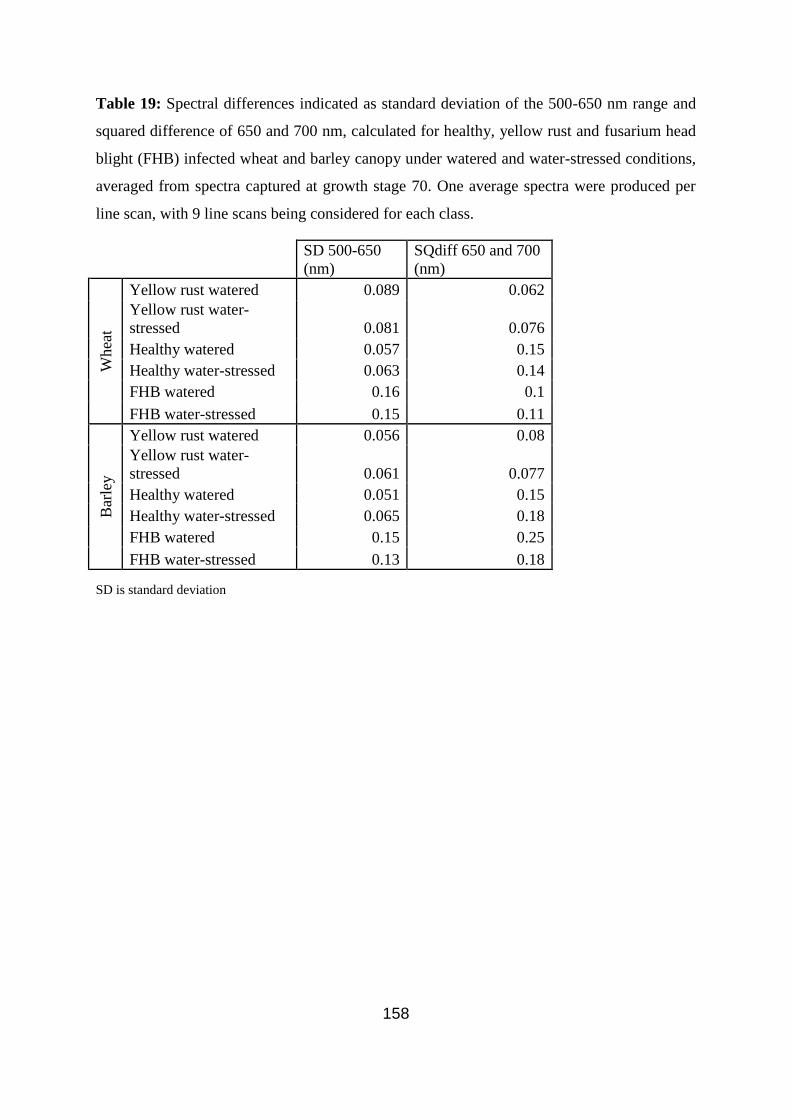
158

Table 19: Spectral differences indicated as standard deviation of the 500-650 nm range and

squared difference of 650 and 700 nm, calculated for healthy, yellow rust and fusarium head

blight (FHB) infected wheat and barley canopy under watered and water-stressed conditions,

averaged from spectra captured at growth stage 70. One average spectra were produced per

line scan, with 9 line scans being considered for each class.

SD 500-650

(nm)

SQdiff 650 and 700

(nm)

Whea

t

Yellow rust watered 0.089 0.062

Yellow rust water-

stressed 0.081 0.076

Healthy watered 0.057 0.15

Healthy water-stressed 0.063 0.14

FHB watered 0.16 0.1

FHB water-stressed 0.15 0.11

Bar

ley

Yellow rust watered 0.056 0.08

Yellow rust water-

stressed 0.061 0.077

Healthy watered 0.051 0.15

Healthy water-stressed 0.065 0.18

FHB watered 0.15 0.25

FHB water-stressed 0.13 0.18

SD is standard deviation

159

Table 20: Analysis of Variance (ANOVA) table for the analysis of transformed spectral

indices over the different treatments. Analysis of the index the squared difference of 650 and

700 nm (sqDiff) was done on the square root scale, whilst analysis of the index standard

deviation (SD) is done on of the range 500-650 nm.

d.f. s.s. m.s. v.r. F pr.

log

(SD

)

Disease Status (Healthy vs Infected) 1 7.484 7.484 874.11 <.001

Water (Watered vs Water stressed) 1 0.015 0.015 1.79 0.193

Crop (Barley vs Wheat) 1 0.810 0.810 94.59 <.001

Disease Status: Disease Class (Fusarium vs Yellow

rust) 1 10.268 10.268 1199.23 <.001

Disease Status:Water 1 0.274 0.274 31.98 <.001

Disease Status:Crop 1 0.234 0.234 27.31 <.001

Water:Crop 1 0.053 0.053 6.24 0.02

Disease Status:Disease Class:Water 1 0.055 0.055 6.37 0.019

Disease Status:Disease Class:Crop 1 0.324 0.324 37.8 <.001

Disease Status:Water:Crop 1 0.002 0.002 0.22 0.641

Disease Status:Disease Class:Water:Crop 1 0.052 0.052 6.05 0.022

Residual 24 0.205 0.009 1.05

sqrt

(SQ

dif

f)

Disease Status (Healthy vs Infected) 1 0.118 0.118 12.66 0.002

Water (Watered vs Water stressed) 1 0.001 0.001 0.07 0.799

Crop (Barley vs Wheat) 1 0.071 0.071 7.61 0.011

Disease Status:Disease Class (Fusarium vs Yellow rust) 1 0.310 0.310 33.29 <.001

Disease Status:Water 1 0.000 0.000 0.05 0.827

Disease Status:Crop 1 0.013 0.013 1.42 0.246

Water:Crop 1 0.001 0.001 0.14 0.708

Disease Status:Disease Class:Water 1 0.016 0.016 1.67 0.209

Disease Status:Disease Class:Crop 1 0.092 0.092 9.88 0.004

Disease Status:Water:Crop 1 0.012 0.012 1.31 0.264

Disease Status:Disease Class:Water:Crop 1 0.013 0.013 1.34 0.258

Residual 24 0.224 0.009 5.08

5.3.2 Model performance for yellow rust and fusarium head blight

detection

The collected spectral data and field observations were subjected to PLSR with on-leave-out

cross-validation. For the predicted results, this is data that was not included in the cross-

validation (20% of the calibration data sets size), (Figure 26). The PLSR results for yellow

160

rust detection in cross-validation and prediction are shown in Table 21. The cross-validation

results indicate good model performance for yellow rust % cover and yellow rust scale in

wheat with R2 values of 0.82 and 0.88 (significance level of <0.01), respectively, whereas

model performance for barley is less successful (R2 = 0.72 and 0.80, respectively), with a

significance level of <0.01. This is also indicated by a smaller root mean square error of

cross-validation (RMSECV) calculated for wheat % cover (6.04) and a slightly larger

RMSECV of 0.54 for yellow rust scale, as compared to barley (7.88 and 0.37, respectively).

Yellow rust is a foliar disease, the reduction in prediction performance for barley may be

attributed to the crop having smaller leaves, causing a smaller foliar area to be captured by

the hyperspectral imager.

Yellow rust % cover was also applied to the PLSR regressions after undergoing LOGIT

transformation. The LOGIT transformation resulted in the cross-validation results in wheat

being of 0.68 R², which is lower than both the yellow rust percent and the yellow rust scale.

However, using the LOGIT transformation in the percent yellow rust coverage in barley,

allowed for a slightly higher R² of 0.74, as compared to the yellow rust coverage, though it

was still lower than the yellow rust scale.

The PLSR result for FHB assessments in both wheat and barley are poor. However, much

better results can be observed in cross-validation (R2 = 0.67 for wheat and 0.54 for barley)

(Table 21). Prediction results in Table 21 demonstrate the reliability of the PLSR models

when data independent from the models creation is applied (Figure 26). The yellow rust

model performance in prediction showed a similar performance to that in cross-validation

(Table 21 and Figure 26).

161

Table 21: Summary of model prediction performance of yellow rust and barley in cross-

validation and prediction showing the R2, root mean square error of the prediction (RMSEP)

and cross validation (RMSECV), and the ratio of prediction deviation (RPD). Results are

shown for yellow rust coverage (aa % coverage and the LOGIT transformation), yellow rust

scale a class of 0 to 5 with 0 being healthy and 5 being >50% covered leaf area), and

fusarium head blight (FHB) severity (severity and ratio of infected ears to healthy, 0 being

healthy and 2 being >50%).

RMSECV is root mean square error of cross validation; RMSEP is root mean square error of prediction; RPD is

ratio of prediction deviation = standard deviation / RMSEP; The R² report significance level of <0.01 for each

regression.

Wheat Barley

Yellow

rust

coverage

Yellow

rust

coverage

Logit

Yellow

rust

scale

FHB severity

Yellow

rust

coverage

Yellow

rust

coverage

Logit

Yellow

rust

scale

FHB severity

Cross-

validation

R2 0.82 0.68 0.88 0.67 0.72 0.74 0.80 0.54

RMSECV 6.04 0.60 0.54 0.50 7.88 0.52 0.37 0.56

Prediction

R2 0.77 0.43 0.80 0.57 0.69 0.79 0.77 0.5

RMSEP 4. 84 9.76 0.6 0.54 9.49 13.7 0.48 0.68

RPD 2.04 1.2 2.25 1.50 1.80 1.4 1.97 1.36

162

Figure 26: Scatter plots of predicted versus reference measured (based on 20% prediction

set) yellow rust coverage in wheat (a), yellow rust coverage in barley (b), yellow rust scale in

wheat (c), yellow rust scale in barley (d), fusarium head blight (FHB) severity in wheat (e),

FHB severity in barley (f), wheat yellow rust logit (g), barley yellow rust logit (h). The R²

report significance level of <0.01 for each regression.

163

To compare between the performances of different models, RPD was used in this work.

According to the RPD classes proposed in the current work (Table 21), the prediction of both

the yellow rust coverage (RPD = 2.04; R²=0.77 and yellow rust scale (RPD = 2.25; R²=0.8) is

of good performance in wheat. These models again suffered deterioration in prediction

performance in barley, where moderate prediction performances are recorded (RPD = 1.80

and 1.97, and R²= 0.69 and 0.77, respectively). The R² and RPD have declined for yellow rust

coverage in wheat by applying the LOGIT function with an R² of 0.68 for cross validation

and in prediction to an R² of 0.43 and RPD of 1.2. The barley results for the LOGIT

transformation of yellow rust coverage have increased using the LOGIT for cross validation

and predictions with R² of 0.74 and 0.79 respectively. However, the RPD calculated for

prediction has declined to 1.4, indicating that the LOGIT function was only able to

distinguish between high and low yellow rust infections. The FHB prediction accuracy based

on RPD values was again of a poor result of 1.5 (R²=0.57) for wheat and 1.36 (R²=0.5) for

barley, suggesting the performance to be classified as moderately accurate and able to useful

to distinguish between high and low infection (Table 18).

5.4 Discussion

5.4.1 Crop canopy spectra

The spectra shown in Figure 23 are to clearly demonstrate the shape of the spectral

signature. The reflectance intensity between wheat and barley was witnessed to be similar

through the scans, which is also described by Wilson et al. (2014), with only minor variations

being seen in the NIR spectrum attributed to growth stage (rate of senescence) and the

physical structure of the ears. Wilson et al. (2014) also discuss that growth stages 67–73

are best for making this separation. Within the visible range of 400–550 nm, there is a low

reflectance due to a larger absorption of the light, attributed to the photosynthetic pigments of

164

the plants leaves, governed by the abundance of chlorophyll, absorbing most of the light

radiation (Gates et al., 1965; Thomas and Gausman, 1977). Both plant chlorophylls and

carotenoids have strong absorption at 480 nm, the waveband associated with blue colour

(Hunt et al., 2013). Another interesting band around 670 nm, is linked with Chlorophyll a

absorption (Hunt et al., 2013), the latter wavelength is designated as the green leaf

reflectance (Buscaglia and Varco, 2002 and Zhao et al., 2005). A small absorption appears at

the red edge around 715 nm, with deeper absorption in a barley spectrum than in wheat.

Raper and Varco (2015) found that the strongest wavelength correlations with leaf nitrogen

concentration, lint yield and plant total nitrogen content to be near 700 nm. Further analysis

of these bands, as linked with crop diseases studied, is discussed below.

In Figure 24 generally all spectra are similar, although slight differences can be observed by

close examining of individual plots (Figure 24, b and c). The water-stressed spectra are less

reflective than watered spectra, particularly for the yellow rust (Figure 24 b). Slight

differences in shape of the reflectance spectrum can be observed in the healthy canopy (a)

than in the water-stressed canopy, which is in line with the findings from Earl and Davis

(2003) who attributed these differences to alterations in leaf internal structure, variations in

leaf angle (due to wilting) and leaf area index. Smaller reflectance at the green edge (500-570

nm) and red edge (670-750 nm) can be attributed to the water stress. However, these slight

differences may indicate that water-stress has only slight influence on crop canopy

reflectance, hence, on the performance of PLSR models in predicting yellow rust and FHB.

The influence of water stress on the yellow rust infected crop canopy was more obvious,

where the water stressed spectrum is consistently of lower reflectance (higher absorption)

than the watered spectrum throughout the entire waveband (Figure 24 b). This indicates that

water stress may have a considerable influence on yellow rust prediction. However, spectra

165

pre-processing e.g., maximum normalisation used in this study will eliminate differences in

reflectance e.g., due to scattering, as all spectra will be scaled between 0-1. However, only a

negligible deviation is observed between FHB infected spectra (Figure 24 c), indicating

negligible effect of water stress on FHB prediction.

Figure 24 d shows spectra of each category (healthy, yellow rust, and FHB infected) for

watered crops. The healthy spectrum is of a lower reflectance than both infected spectra in

the range between 400 to 700 nm. The yellow rust infected crop spectra has the highest

increase between 400 and 700 nm, whilst FHB infected crop spectra has a flatter (linear)

curve in the 500 to 650 nm area.

The lower reflectance of the healthy canopy can be attributed to larger absorption by

photosynthetic pigments of the plants associated with chlorophyll (Gates et al., 1965; Thomas

and Gausman, 1977). Cibula and Carter (1992) reported larger reflectance in infected leaves

than healthy leaves, which is in line with findings of the current study. Indeed, after crop

infection by foliar pathogens such as yellow rust, noteworthy visual symptoms can usually be

observed. Early symptoms such as chlorosis, associated with a reduction in chlorophyll

results in increasing reflectance due to a reduction in light absorption (Lorenzen and Jensen,

1989). Therefore, the sharpest increase in reflectance from 650 to 700 nm takes place in the

healthy plant reflection spectrum.

Figure 25 compares between the average spectra of healthy, yellow rust and FHB infected

barley canopy at growth stage 72. The water-stressed canopy spectrum shows more reflection

or less absorption than the watered canopy spectrum for the healthy canopy in Figure 25a.

This may reflect the darker (greener) canopy of the watered canopy resulting in larger

absorption of light. This is in line with findings of other researchers, who have attributed the

increased reflectance of the healthy canopy to early senescence caused by drought, and a

166

reduction in chlorophyll absorption (Jamieson et al., 1995; Hunt et al., 2013). With the

yellow rust infected canopy (Figure 25b), the opposite trend can be observed, where higher

reflectance is shown for the water-stressed canopy. This trend is observed in both the wheat

(Figure 24b) and barley (Figure 25b) canopies, indicating a larger influence of yellow rust

on crop canopy when combined with water stress, compared to FHB (Figures 24c and 25c),

where the differences between watered and water-stressed are minimal. As for the wheat

canopy, the yellow rust infected canopy has again the highest reflectance, compared to those

of FHB and healthy canopies (Figure 25d). The % coverages of yellow rust and FHB is

larger in wheat than in barley. In wheat, the yellow rust watered canopy had an average

infection of 42%, yellow rust water stressed averaged 45%, Yellow rust watered averaged

63%, and FHB water stressed canopies averaged 66% infection, whereas, in barley, these

were 36%, 33%, 48% and 52%, respectively.

Moshou et al. (2004) recommended the use of a wavelength range between 460 and 900 nm

for successful yellow rust detection. Bauriegel et al. (2011) recommends spectral analysis

using the range intervals of 500–533 nm (green), 560–675 nm (yellow to red), 682–733 nm

(red edge) and 927–931 nm (far red) for recognition of FHB infection (in growth stages 71–

85, according to Zadoks scale). Krishna et al. (2014), suggested particularly useful spectra

wavelengths of 428, 672, and 1399, for quantitative detection of yellow rust from a healthy

crop.

Table 19 refers to two indices, SD and SQdiff. SD refers to the standard deviation of each of

the wavelengths between 500 and 650nm. SQdiff refers to the squared difference between 650

and 700nm wavelengths. These two proposed indices show clear differences in response both

in the different crops and the different treatments. The largest differences were observed

between infection type, observing a significant F statistic of F1,24=1199 (p<0.001) and F1,24=33

167

(p<0.001) for the comparison between FHB infection and yellow rust infection, for index SD

and SQdiff, respectively. Analysis of the index SD revealed significant differences in response

in barley and wheat (F1,24=94.59, p<0.001) and big differences between healthy and diseased

trays (F1,24=874.11, p<0.001). The largest differences were observed between FHB infection

and yellow rust infection (F1,24=1199.23, p<0.001). In contrast, there was no evidence of a

significant effect of water stress (F1,24= 1.79, p=0.193), meaning that on average (over all

disease types and crops) there is no evidence of a difference in the SD index for watered and

water stressed trays. However, analysis of the index SD does demonstrate a significantly

different response to water stress both within different crops and under different disease

infections (full ANOVA table is given in Table 20), i.e. the response to water stress is not the

same in the different conditions. Analysis of the index SQdiff revealed significant differences

between healthy and diseased trays (F1,24=12.66, p=0.002) and also significant differences

between FHB infection and yellow rust infection (F1,24=33.29, p <0.001). Moreover, different

responses in the different crops were observed (F1,24=7.61, p=0.011) with a significant

interaction between crop type and disease type indicating the index SQdiff responds differently

to disease type in the different crops (F1,24=9.88, p=0.004). There was no evidence to suggest a

differing response to water treatment (F1,24=0.07, p=0.799).

Although the largest SD in reflectance between 650 and 700 nm was observed for the healthy

canopy (both watered and water-stressed), the smallest SD was observed for yellow rust

(Table 19). For the barley canopy, the largest SD and SQdiff can be observed for FHB

infected canopies, indicating that these proposed two indices respond differently for different

crops (Table 19). Consequently, the two indices adopted in the current work highlight a

distinguishable difference between the yellow rust, FHB and healthy wheat and barley

crop canopies. It is important to mention that whilst these indices have worked in

168

establishing a difference between yellow rust, FHB and a healthy canopy at growth stage 72

in this work, it may be specific to the method and equipment used. Further work should be

undertaken to assess the reliability of such indices, if captured at different growth stages,

under different circumstances, with alternative equipment.

5.4.2 Model performance for yellow rust and fusarium head blight

detection

It is well known in spectral analysis that successful measurement of a concentration, be it soil

properties or other, depends on presence of variability of that said concentration. For

example, Kuang and Mouazen (2011) reported that although larger R2 and RPD values can be

obtained with larger variability in soil analysis, larger RMSEP is to be expected. The RMSEP

values in wheat were smaller for yellow rust coverage and larger for yellow rust scale

detection, as compared to the corresponding RMSEP for barley. However, RMSEP is a

valuable index for assessing individual model performance, but is not recommended to

compare between models (e.g., those for wheat and barley), due to the different data range. A

data set with a small variability, could result in a weak or even no correlation being

established with PLSR, so that no models could be developed. However, this could be

improved with the incorporation of extra data, with a larger variability. Having said that, we

believe that the scale of variability in yellow rust is small (Table 17), although a reasonably

high infection was recorded, this occurrence was infrequent, and the average was weighted

by a few heavily infected trays. The small variability may be possibly due to the experiment

being run in trays under rather controlled conditions, where only water is varied artificially.

These controlled conditions may well lead to rather small variability in yellow rust (Table

17). FHB’s result might be due to the full line scan being used, while the ear of the crop is

captured only by a small section of the line image, compared to the foliage of the crop, which

was used more successfully for yellow rust modelling and detection. This may suggest the

169

need to isolate segments in the line image that capture fusarium as the disease appears mainly

in heads (Impey, 2012). This can be potentially implemented by splitting the crop canopy

spectra into 10 cm increments, similar to the approach mentioned in Broge and Mortensen

(2002) for canopy chlorophyll density, or that of Moshou et al. (2005), for disease detection

with a data fusion technique. The few classes used for the FHB infection in the current work

(Table 17) may have also contributed to lower detection accuracy. The FHB classes were no

infection, mild infection (describing FHB symptoms on up to 50 % of the ears) and heavy

infection (describing FHB infection in over 50% of the ears with the majority showing early

senescence). The scale for FHB was classified in this manner because most ears became

infected through the inoculation process. Another reason believed to have influenced the

FHB model performance is the smaller number of data points considered in the PLSR cross-

validation modelling, as compared to yellow rust (Table 17). Fusarium symptoms appear on

crop heads at a late stage in the crop growing season (normally only after anthesis, but

potentially at head emergence), allowing for a limited number of scans to be collected.

Bauriegel et al. (2010) claimed that FHB can be detected by spectral analysis in the spectral

range of 400–1000 nm, with an identification accuracy of 87%. These authors advised that

the ideal timing for measurement was at the medium milk stage (growth stage 75), though the

scans were based on the crop ears against a black background. The scans conducted in this

study, for FHB, were taken from anthesis at growth stage 61, to grain hardening at growth

stage 90. Delwiche et al. (2011) successfully differentiated between healthy kernels from

FHB infected, reporting a 95% classification accuracy between 8 groups, containing

approximately 60 seeds each.

The percentage of disease coverage, a method discussed by Chiarappa (1981) and defined as

“disease severity”, is the amount of expressed disease tissue of a plant. This method can be

170

objective, but is not free of subjectivity. In the current study, all assessments were made by

just one individual, which increases subjectivity and potentially RMSEP for both yellow rust

and FHB detection. The more spectral wavelength indices captured and accounted for, the

greater understanding of the object (Gilchrist, 2006). However, for noisy spectra there is a

need to minimise noise in the signal, by adopting an optimised measurement configuration

(Whetton et al., 2016b) and suitable spectra pre-processing.

Furthermore, stresses in the field are combined and might include water stress, nitrogen

stress, disease stress, and other stresses that are mainly reflected on crop canopy as a

yellowing of the leaves. In the current work, we have combined water stress and yellow rust

infection in the tray experiments, to evaluate the prediction accuracy of the yellow rust

models. The result obtained is satisfactory (RPD > 2.0 for wheat and > 1.8 for barley) to

encourage exploring the goal of the current study, which is on-line measurement of yellow

rust in the field using the hyperspectral imager (400 – 750 nm). However, additional affecting

parameters exist in the field on top of the water stress accounted for in the current study,

which should also be evaluated. Using wheat trays under glass house controlled conditions,

Moshou et al. (2014) reported successful discrimination of water-stressed from healthy plants

with 99% accuracy. Their approach was based on a combination of hyperspectral (460–

900 nm) and fluorescence imagery and least squares support vectors machine learning

models, for automated recognition of different biotic and abiotic stresses, of crop canopies

under greenhouse conditions.

The early success in field studies for hyperspectral imager’s detection of yellow rust disease

such as Moshou et al. (2004) and Bravo et al. (2003), focused on the presence of yellow rust

in the field, not necessarily the severity. Commonly, disease recognition attempts with

hyperspectral and multispectral imagery are targeted to leaves rather than the canopy (Bock

171

et al., 2010). Whilst recent attempts such as Zhou et al. (2015) studying wheat resistance,

have used RGB images for quantification of disease, which is of lower cost but with larger

error margins. Compared to other studies, the current work achieved good to very good

accuracy based only on a relatively cost-effective hyperspectral camera in the visible and the

NIR range. In addition, in the current work, the effect of water stress was also taken into

consideration in the experimental trial, hence, this effect was accounted for in the PLSR

models

This study used triplicate trays of each of the considered crops, disease, and conditions, with

9 scans captured across 3 locations of each tray, through multiple growth stages. The

observations discussed in this paper for the development of FHB models, suggest the need for

a larger dataset to be accounted for in the PLSR analysis and to explore new methods of data

analysis based on machine learning and/or image processing. It is also suggested to adopt a

data fusion approach of both spectra and images, which is expected to provide improved

model prediction performance. Ideally the requirement is a method which incorporates not

just the percentage of fusarium infected heads to healthy heads, but the coverage of the plot

by the ear. A method such as a camera image with a 100-point dot grid overlay of the

assessment area, discussed by Knight et al. (2006), could be a potential method, and should

be further assessed.


A hyperspectral line image camera was implemented successfully under laboratory

conditions for the measurement of yellow rust and FHB in wheat and barley. The standard

deviation (SD) of the wavelength range from 500 to 650 nm and the squared difference

between 650 nm and 700 nm are of interest in discrimination between healthy, and yellow

rust or FHB infection in a wheat or barley canopy. Yellow rust prediction models performed

172

more accurately than FHB models. Further work needs to consider a larger dataset in the

PLSR analysis, and the exploration of new methods of data analysis based on machine

learning and/or image processing, particularly for FHB detection.

173

6 Hyperspectral measurements of yellow rust and fusarium head

blight in cereal crops: Part 2: on-line field measurement

Chapter Synopsis;

This chapter investigates the applicability of the optimal hyperspectral imaging configuration

reached in Chapter 4 for on-line measurement of yellow rust and fusarium head blight (FHB)

using PLSR analysis in three fields of winter wheat and one field with winter barley.

Abstract

This study implemented a hyperspectral line imager (spectrograph) for on-line measurement

of yellow rust and fusarium head blight (FHB) in wheat and barley fields. On-line

measurements were carried out in four arable fields in Bedfordshire, the UK. Disease

recognition consisted of visual field assessments and photo interpretation based on 100-point

grid overlaid on RGB images. The spectral data and disease assessments were subjected to

partial least squares regression (PLSR) analysis with leave-one-out cross-validation using

calibration sets, consisting of 70% of samples. The developed recognition models were then

validated with a non-mobile (25%) and mobile (5%) prediction data sets.

Results showed that yellow rust can be measured with an on-line hyperspectral imagery

system with better accuracy than FHB, and that the performance was better in wheat, as

compared to barley. It was found that photo interpretation was most applicable and accurate

for the on-line measurement of FHB, where it was classified as a good prediction accuracy in

wheat (ratio of prediction deviation (RPD) and R2 values of 2.27, and 0.82, respectively) and

a moderately accurate in barley (RPD of 1.56 and an R² of 0.61). However, visual scale

analysis was most suitable for yellow rust based models, where model performance was

174

classified as moderately accurate in barley (RPD = 1.82; R²=0.72) and good in wheat (RPD =

2.5; R²=0.81). It was recommended to adopt the proposed on-line measurement technique

coupled with PLSR to map the spatial variability in yellow rust and FHB in wheat and barley,

although further analyses that include advanced image processing or machine learning

techniques may further improve the current results.

Keywords

On-line measurement, Yellow rust, fusarium head blight, wheat, barley, mapping, and partial

least squares regression.

6.1 Introduction

Fungal disease control is a large task for the successful production of cereals worldwide. For

example, yellow rust (Puccinia striiformis) is a foliar disease, common in cool climates, one

of the most devastating diseases of wheat worldwide, and reported to reduce crop yields by

up to up to 7 tha-1

in severe epidemics (Ma et al., 2001; Bravo et al., 2003). In 2009, yellow

rust mutations have enabled the disease to attack several widely grown genetically resistant

cereal crop varieties, including Solstice (Milus et al., 2009). Another important fungal disease

that attacks cereal crops is fusarium head blight (FHB), which is caused by multiple species.

Fusarium graminearum is a highly aggressive and prevalent species. Fusarium graminearum

along with other fusarium species can cause mycotoxin production in grain (Rotter et al.,

1996; Brennan et al., 2005; Desjardin, 2006; Leslie and Summerell, 2006). Fusarium

predominantly affecting the ear of the crop, causing FHB. FHB is one of the most important

pre-harvest diseases worldwide. Like yellow rust, FHB also causes reduction in yield quantity

and quality and when producing mycotoxins, it becomes a significant threat to both humans

and animals. FHB is a sporadic disease, that is dependent on warm humid weather conditions

175

(Rossi et al., 2001; Xu, 2003), causing variability of disease presence and level of infection

across regions, and years (Jelinek et al., 1989). Both yellow rust and fusarium species can

survive in soil and weeds occurring in the hedgerows and borders of a field, fusarium also

survives within plant residues even after 2 years, acting as a source of inoculum (Jenkinson

and Parry, 1994; Champeil et al., 2004; Imathiu et al., 2013). Therefore, control of

mycotoxins caused by fusarium fungi is required to prevent toxic contamination reaching the

food chain either in milling grain (for human consumption) or as cattle feed (Magan et al.,

2002).

Traditionally, disease detection is carried out manually by human experts using visual

assessments of disease coverage throughout the field, a process that may be lengthy,

subjective and tiresome (Schmale and Bergstrom, 2003; Bock et al., 2010). These methods

are limited in providing high sampling resolution data on spatial variability of crop disease.

Therefore, on-line mobile systems are necessary to inform site specific application of

fungicides.

It has been stated that optical technologies are available for development into suitable disease

detection systems, but with many challengers still required to be overcome (West et al.,

2003). Although on-line applications are still rather limited, optical techniques have the

potential to be integrated with agricultural vehicles. Optical (both remote and proximal)

methods provide non-invasive and high sampling resolution data necessary for monitoring

and mapping of crop diseases. Among optical sensing methods, hyperspectral and

multispectral imaging techniques are the best candidates as they acquire high resolution data,

at multiple points simultaneously, and have already been used in disease and stress

monitoring (Hahn, 2009), Non-mobile (off-line) field and laboratory methods for disease

classification and plant growing conditions have been studied and demonstrated (Roggo et

176

al., 2003; Wu et al., 2008). The early success in field studies for a hyperspectral imager’s

detection of yellow rust, focused on the presence of yellow rust in the field, not necessarily

the severity. Moshou et al. (2005) implemented a data fusion approach of a hyperspectral

(450-900 nm) and flouresence (550-690 nm) imaging for yellow rust detection in winter

wheat reporting 94.5% accuracy. Other common attempts with hyperspectral and

multispectral imagery are targeted to leaves rather than the canopy (Bock et al., 2010). Huang

et al. (2015) successfully provided quantitative assessment of yellow rust in winter wheat, by

hyperspectral measurement of individual infected leaves. Zhou et al. (2015) used low cost

RGB images for quantification of yellow rust, reporting 74% and 81% detection accuracy.

Zhao et al. (2016) focused on two sensitive bands (558 nm and 856 nm) in the wavelength

ranges of 550-680 nm and 750-1300 nm to detect yellow rust with 90.6% accuracy. Krishna

et al. (2014) used remote hyperspectral data in 350 to 2500 nm range for quantitative

identification of yellow rust. Whilst mobile techniques have been successfully applied, these

were instruments attached to hand moved frames. On-line here is defined as attached to an

agriculture vehicle, where measurement is being taken on the move. Moshou et al., in 2011

looked at a wheat crop, for both yellow rust and septoria, using an on-line method with a

multi-spectral camera. To the best of our knowledge, there are few reports in the literature of

on-line (mobile, using agricultural vehicles) application of proximally captured hyperspectral

imagery, for simultaneous recognition and mapping of yellow rust and FHB in both wheat

and barley.

A hyperspectral imager was applied to winter wheat and barley plants, grown in trays under

laboratory conditions in Part 1 of this study (Whetton et al., 2016c). Plants were subjected to

variable water stress, and inoculated with yellow rust and FHB, these diseases were selected

as their presence had been reliably witnessed in previous years. Results confirmed that

177

reliable models for yellow rust detection could be produced, but highlighted an alternative

technique and modelling approach should be applied for FHB disease detection. However,

the Part 1 of this study suggested exploring the potential of this approach for on-line field

measurement. The aim of this paper is to implement a hyperspectral imager for on-line

measurement of yellow rust and FHB in wheat and barley grown commercially outdoors in

fields.


6.2.1 Field sites

Field measurements were conducted in four different field sites through the 2015 cropping

season. These sites were located at Duck End farm, Wilstead, Bedfordshire, UK

(52°05'46.3"N 0°26'41.4"W), with an average annual rainfall of 598 mm. The farm has a

three year crop rotation of oilseed rape, winter wheat and winter barley. Fields varied in size

between 12 ha, 10 ha, 7 ha and 4 ha (Table 20), to allow for pattern identification of diseases

with different field size. This is because yellow rust and FHB occurrence in the field often

begins nearer the hedgerows, and the spread pattern throughout the growing season may well

depend on the shape and size of the field. Winter wheat was grown in three fields, whereas

winter barley was grown in the 10 ha field only. The largest and smallest winter wheat fields

were scanned at two different intervals. Timing and growth stage of measurement in each

field is shown in Table 22. Growth stage in this study refers to the Zadok’s scale (Zadoks et

al., 1974). The dominant soil texture types in the fields are shown in Table 22, with sand

fractions due to underlying gravel deposits.

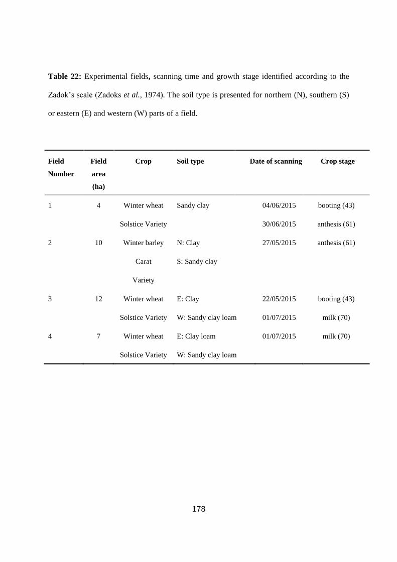
178

Table 22: Experimental fields, scanning time and growth stage identified according to the

Zadok’s scale (Zadoks et al., 1974). The soil type is presented for northern (N), southern (S)

or eastern (E) and western (W) parts of a field.

Field

Number

Field

area

(ha)

Crop Soil type Date of scanning Crop stage

1 4 Winter wheat

Solstice Variety

Sandy clay 04/06/2015

30/06/2015

booting (43)

anthesis (61)

2 10 Winter barley

Carat

Variety

N: Clay

S: Sandy clay

27/05/2015 anthesis (61)

3 12 Winter wheat

Solstice Variety

E: Clay

W: Sandy clay loam

22/05/2015

01/07/2015

booting (43)

milk (70)

4 7 Winter wheat

Solstice Variety

E: Clay loam

W: Sandy clay loam

01/07/2015 milk (70)

179

Hyperspectral imager

Laptop DGPS

Broad spectrum diffused light

source

6.2.2 Hyperspectral on-line data capture


Photonics Ltd., UK) and light source were mounted on a tractor by means of a metal frame

(Figure 27). Optimal hyperspectral measurement configurations set by Whetton et al. (2016b)

were considered in the design and manufacturing of this on-line measurement system of crop

canopy. These include an integration time of 50 ms, a camera height of 0.3 m and light height

and distance of 1.2 m and a camera angle of 10°. The on-line measurements were carried out

at a travel speed of approximately 4 km h-1

. The hyperspectral imager’s line capture occurs at

1 second intervals, which is subsequently logged and geo-located with a sub-meter accuracy,

using a differential global positioning system (DGPS) (EZ-Guide 250, Trimble, California,

USA). The direction and angle of the imager was kept consistent, and a day with uniformly

overcast weather was selected, which helped prevent issues of moving shadows from lateral

sun movement on the data (West et al., 2003).

Figure 27: Hyperspectral imagery system mounted on a metal frame attached to the

side of a tractor, ready for on-line canopy measurement.

180

The same hyperspectral imager used in Part 1 of this study was used for on-line field

measurement, along with two external halogen lamps (Figure 27). It consists of 1608 pixels,

with a spectral range of 400 - 1000 nm. More details about the hyperspectral imager’s

properties can be found in Whetton et al. (2016b). A schematic showing an overview of the

methodology can be seen in Figure 28.

Figure 28: Schematic of work flow from data capture to production of PLSR models,

validation, and on-line prediction for production of maps

In order to compile a full image from a set of line imagery, a steady moving platform is

needed to sweep across the target object to capture every line (Gilden Photonics Ltd,

Glasgow, UK). However, due to practical constraints of applying a consistent moving

platform, the spectraSENS v3.3 software (Gilden Photonics Ltd, Glasgow, UK) was adapted

to record a single line array. Before data capture, measurements from a white and dark

reference were collected, and subsequently repeated at 10 minute intervals until the scanning

181

was completed. The white reference used, was a commercially available Spectralon Teflon

white reflectance panel with 99.9% white reflectance value. The collected on-line data, was

corrected by the white and dark scans after data collection was complete, providing the

relative reflectance.

6.2.3 Moisture content measurement

An on-line visible and near infrared (vis-NIR) spectroscopy soil sensor developed by

Mouazen (2006) was used in this study to measure gravimetric soil moisture content (MC) in

field 4, with the objective of studying the influence of MC on crop disease spatial

distribution. This data was collected at beginning of the growing season in September 2014.

Although MC may change daily, the distribution pattern through the field will remain

consistent through the multiple seasons (Vachaud et al., 1985; Mouazen et al., 2005). The

system consists of a subsoiler, opening a smooth trench at 15 cm depth (Mouazen et al.,

2005). The sensor was mounted on a three-point linkage of a tractor travelling at a speed of 3

km h-1

and collecting spectral soil data at 10 m parallel intervals. In order to measure soil

spectra, an AgroSpec mobile, fibre type, vis–NIR spectrophotometer (Tec5 Technology for

Spectroscopy, Oberursel, Germany), with a measurement range of 305–2200 nm and a light

source of 20W tungsten halogen lamp were used (Kuang and Mouazen, 2013). A differential

global positioning system (DGPS) (EZ-Guide 250, Trimble, California, USA) recorded the

position of the on-line spectra with sub-meter accuracy. The collection of soil spectra and

DGPS readings took place at 1 sec sampling resolution using AgroSpec software (Tec5

Technology for Spectroscopy, Oberursel, Germany). A previously developed MC model

(Halcro et al., 2013) was used to predict MC based on on-line collected spectra in the field.

182

6.2.4 Disease recognition in the field

During field scanning with the hyperspectral imager, ground truth spots were selected

randomly, at a rate of five samples per hectare (Figure 29), and a series of five hyperspectral

images were collected per ground truth location, each covering 1 m².

The measurement position was recorded with a DGPS. The disease assessment was assigned

to each of the five scans. In order to assist in disease and crop health assessments a

photograph was collected at each position using a RGB, 5 megapixel camera with a 3.85 mm

f/2.8 lens at the same time of hyperspectral image capture. The 1 m² ground truth spots were

used for disease recognition.

183

Figure 29: on-line hyperspectral measurement lines and position of ground truth plots,

collected at five samples per ha, in the four fields. Fields 1 and 4 were validated at the same

locations at two time intervals.

Disease assessments were based on the following two methods:

1- photo interpretation: Photos collected from the ground truth plots were used in this photo

interpretation to assess crop disease coverage (severity), and incidence of disease, defined by

Chiarappa (1981) as the percentage cover of disease, and the occurrence of disease in a field,

respectively. Images were overlaid with a 100-point grid at equal spacing as illustrated in

Figure 30, adopting a similar approach to that proposed by Knight et al. (2006). At the centre

184

of each point, the object and health status were recorded and used to calculate the percent

coverage of infection, or incidence of disease. This approach was adopted for both the yellow

rust and FHB assessment.

2- Visual assessment: Although visual assessment of crop diseases was deemed to be

subjective, it is the most common and adopted by partitions. Visual assessment of both

diseases at the ground truth plots were made at four levels, namely, the head (when present),

at the flag leaves, at 2nd

and 3rd

leaves (mid canopy), and at the lower canopy. Details on this

method can be found in Part 1 of this study (Whetton et al., 2016c). Depending on the

disease, two visual assessment approaches were considered in the current work. The

assessment for FHB considered both early and later symptoms on heads, and were assessed

as either a 0 for no infection, 1 for less than 5% individual infected heads, 2 for up to 10%, 3

for up to 30%, 4 for up to 50%, and 5 being a heavy infection over 50% infected heads,

dependent on the ratio of FHB infected to healthy crops. For yellow rust, two different

quantitative assessments were recorded, one for the percent cover on the leaves and one

recorded as a 0-5 scale, which is explained by Oberti et al.(2014). The scale between 0 and 5

(from less to more affected plots) was given the same ratio as that for FHB. For example, 0 is

given when no disease is present, 1 for up to 5% cover, 2 for up to 10%, 3 for up to 30%, 4

for up to 50% and 5 for >50%.

185

Figure 30: Example of photo interpretation to assess yellow rust and fusarium head blight

(FHB) coverage based on a 100-point grid.

6.3 Data analyses

6.3.1 Crop canopy spectral data pre-processing

The first step of spectra pre-processing included removing noisy wavelengths larger than 750

nm. Following the suggestion made in Whetton et al. (2016b), the first and last 320 pixels

were removed from each line scan. Noise removal was followed successively by reducing the

number of variables by averaging three neighbouring wavelengths, maximum normalisation,

first derivative and smoothing. The first derivative was used to eliminate the effect of the

roughness of soil surface on the spectrums absorption (Shibusawa et al., 2000; Waiser et al.,

2007). All spectra pre-processing was carried out using Unscrambler 10 software (Camo Inc.;

Oslo, Norway). Although pre-processing of spectral data includes techniques such as

smoothing, if the process of cleaning the data is intensive due to noisy spectra, it can lead to

186

the loss of important spectral features, and thus impact on the success of analysis (Dasu and

Johnson, 2003). Therefore, a gentle smoothing of 2:2 was implemented during the first

derivative and smoothing using the Savitzky–Golay algorithm (Savitzky and Golay 1964).

Detailed information about the spectra pre-processing steps can be found in Martens and

Naes (1989).

6.3.2 Evaluation of model performance

For yellow rust analysis, the data from the five scans from the three wheat fields and the one

scan from the barley field was considered (Table 22). However, FHB models were developed

based on the one later data capture of each field. This is because FHB only occurs at a later

crop growth stage, when the ear emerges (growth stage 51, according to Zadok’s scale)

(Zadoks et al., 1974). The potential infections can occur when the plants are booting (growth

stage 43) by washing into the sheath (Anand et al., 2003). Five models were developed and

validated in cross-validation, non-mobile validation and on-line (mobile) validation. The

validation methods are summarised in Table 23, and the models produced are summarised in

table 24.

187

Table 23: Explanation of validation sets in cross-validation, non-mobile and on-line, along

with the datasets included and the methods for each.

Validation Dataset Method

Cross-validation 70% ground truth locations,

empirical and spectral data.

Cross-validation is included

with the PLSR models,

which is trained on all the

data except for one point

each time, and the average

errors from those

calculations, evaluates the

models.

Non-mobile validation PLSR models.

25% (model excluded)

ground truth locations,

empirical and spectral data.

The non-mobile validation

refers to the application of

excluded data to the model,

where the empirical values

are compared to the

predicted.

On-line (mobile) validation PLSR model predicted on-

line data.

5% (model excluded)

empirical ground truth

locations.

On-line (mobile) validation

refers to the use of the on-

line predicted data, (where

on-line data was applied to

the models) and compared by

location to the empirical

values of the remaining

model excluded data.

188

Table 24: Summary of the models produced for the yellow rust and fusarium head blight

(FHB) models. Showing the datasets used, the achieved outcomes and validations.

Model Dataset Outcome Validations

Yellow rust

Visual coverage

analysis (%)

Yellow rust visual assessments, as % of

disease spread on the leaves.

Spectral data from ground truth plots

On-line spectral data

Offline and on-line

PLSR model for

predicting % cover of

yellow rust

Wheat Cross validation.

Wheat non-mobile validation.

Barley and wheat on-line

validation

Yellow rust

scale (0-5)

Yellow rust visual assessments, on a 0 to 5

scale of disease severity on the leaves.



Offline and on-line

PLSR model for

predicting 0-5 scale

cover of yellow rust




validation

Yellow rust

photo

interpretation

(%)

Yellow rust assessments, from photo

interpretation for disease severity on the

leaves %.



Offline and on-line

PLSR model for


cover of yellow rust




validation

FHB Visual

coverage

analysis

(%)

Yellow rust visual assessments, as % of

disease spread on the leaves.



Offline and on-line

PLSR model for

predicting % cover of

FHB




validation.

FHB photo

interpretation

(%)

Yellow rust assessments, from photo

interpretation for disease severity on the

leaves %.



Offline and on-line

PLSR model for


cover of FHB



189

Statistics of samples used for yellow rust and FHB modelling and validation in wheat is

shown in Table 25 and Table 26, respectively. However, sample statistics of on-line dataset

in barley is shown in Table 27. Before running the analysis, each yellow rust dataset was

divided into calibration (70%, e.g., 940 samples), non-mobile validation (25%, e.g., 235

samples) and on-line validation (5%, e.g., 47 samples) sets. A Similar division of samples

was done for FHB data, although fewer samples were available, due to FHB only occurring at

a later growth stage, hence, only fewer late scans were collected (Table 26). Partial least

squares regression (PLSR) analysis with leave-one-out cross-validation was carried on

calibration datasets. The input variables to PLSR were wavelengths (400-750 nm) and

disease, assessed as coverage and category scale, as per five models described above. As for

spectra pre-processing, PLSR analyses were carried out using Unscrambler 10 software

(Camo Inc.; Oslo, Norway). Outliers were detected, and removed to a maximum of 5% of the

total input data. These outliers were recognised by being distant from the other observations,

either due to variability in the measurements or an error in data capture (e.g. missed in data

cleaning). The wheat data was used to establish the PLSR calibration models and underwent

both cross-validation and independent validations (both non-mobile and on-line). Although as

mentioned, no barley data was considered in the cross-validation, on-line predictions in

barley data were carried out using the wheat models (Table 27).

190

Table 25: Statistics of samples used for the assessment of yellow rust in wheat by partial

least squares (PLSR) regression analysis. Data is shown in cross-validation, non-mobile and

on-line predictions.

Visual coverage analysis

(%)

Visual scale analysis

(0-5)

Photo interpretation (%)

Item Cross-

val

Non-

mobile

On-

line

Cross-

val

Non-

mobile

On-

line

Cross-

val

Non-

mobile

On-

line

Nr 940 235 47 940 235 47 940 235 47

Max 90 65 50 5 4 5 60 65 50

Min 0 2 2 0 0 0 0 2 2

Mean 15 20 20 2 1.9 2.2 7 10 10

SD 17 18 13.4 1.3 1.4 1.5 14 12 16


The performance of PLSR models were validated using the remaining 20% samples, which

were not considered in the cross-validation stage. Validation was done using non-mobile

collected spectra and the on-line collected data in the field using the mounted hyperspectral

imager. For the on-line validation, predicted and assessed values were overlaid at the same

or a very close position. However, the position of the on-line data did not always perfectly

align to the ground truth spot position, due to the capture rate of the hyperspectral imager,

and the accuracy of the DPGS system. Therefore, for validating the on-line predictions, a

scanned area of 5 m² was considered, and the ground truth spot was located in the middle.

This meant that for some ground truth points there was up to 3 on-line predicted values,

where we select the point providing the greatest match. This was done with ArcGIS 10

software (ESRI, California, USA).

191

Table 26: Statistics of samples for the assessment of fusarium head blight (FHB) in wheat

used in the partial least squares (PLSR) regression analysis. Data is shown for cross-

validation, non-mobile and on-line predictions.

Visual cover analysis (%) Photo interpretation (%)

Cross-val Non-mobile On-line Cross-val Non-mobile On-line

Nr 620 155 31 620 155 31

Max 5 3 5 3 2 3

Min 0 0 0 0 0 0

Mean 0.9 0.5 0.6 0.7 0.5 0.6

SD 1.7 0.9 1.4 1.3 0.7 1.4

Table 27: Statistics of samples used for on-line prediction of yellow rust and fusarium head

blight (FHB) in barley by partial least squares (PLSR) regression analysis. Data is shown in

on-line predictions.

FHB Yellow rust

Visual

coverage

analysis (%)

Photo

interpretation

(%)

Visual coverage

analysis (%)

Visual scale

analysis

(0-5)

Photo

interpretation

(%)

Nr 50 50 50 50 50

Max 5 3 40 4 58

Min 2 1 0 0 3

Mean 2.6 1.9 5 1.9 20

SD 1.3 1.5 9 1.3 13


192

The model performance was evaluated in cross-validation, non-mobile validation and on-line

validation by means of R², root mean square error of prediction (RMSEP) and ratio of

prediction deviation (RPD), which is the standard deviation divided by RMSEP. In order to

compare between the performances of different models developed we used the classification

scale proposed by Whetton et al. (2016c) for crop disease analysis (Table 28).

Table 28: Ranges of the ratio of prediction deviation (RPD) and their suitability for

predicting yellow rust and fusarium head blight (FHB) in cereal crops, proposed by which

was proposed in Whetton et al. (2016c), and is based on the classifications from Rossel et al.

(2006).

RPD range Class and prediction capability

< 1 Poor model predictions - not useful.

1-1.5 Possibility to discriminate between low and high values

1.5-2.0 Moderate prediction capability

2.0-2.5 Good prediction capability

2.5-3.0 Very good prediction capability

>3.0 Excellent prediction capability

6.3.3 Mapping

Maps for the on-line predicted yellow rust and FHB were developed with ArcGIS 10

software (ESRI, California, USA). Kriging was used to develop maps from the data collected

from the tramlines illustrated in Figure 29, assuming that the distance or direction between

sample points reflects a spatial correlation that can be used to explain spatial variations. To

distinguish these spatial variations, semi-variograms were developed in Rstudios (RStudio,

193

Boston, MA) and then applied to the kriging by utilising the advanced parameters option in

ArcGIS 10 software (ESRI, California, USA).

6.4 Results

6.4.1 Crop canopy spectra analysis

Figure 31 and Figure 32 show typical spectra collected at early (booting) and late (milk)

growth stages of wheat and barley, respectively, comparing on-line and non-mobile (off-line,

in the field) spectra. In Figure 31, the early on-line spectra had the lowest reflectance through

the spectral signature, whilst the late non-mobile had the highest reflectance through the

spectral signature apart from that at 710nm for the early non-mobile spectra, which has the

second highest absorption at the rest of spectra. Late on-line spectra closely resemble late

non-mobile spectral signature apart from having a slightly lower reflectance between 580 and

650. The spectra of a barley canopy are shown at the anthesis growth stage for on-line and

non-mobile measurement (Figure 32), the similarity is clear although slight differences in

reflection can be observed at 520 – 550 nm and at 670 - 750 nm spectral ranges.

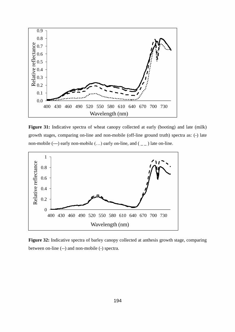
194

Figure 31: Indicative spectra of wheat canopy collected at early (booting) and late (milk)

growth stages, comparing on-line and non-mobile (off-line ground truth) spectra as: (-) late

non-mobile (---) early non-mobile (…) early on-line, and ( _ _ ) late on-line.

Figure 32: Indicative spectra of barley canopy collected at anthesis growth stage, comparing

between on-line (--) and non-mobile (-) spectra.

0.0

0.1

0.2

0.3

0.4

0.5

0.6

0.7

0.8

0.9

400 430 460 490 520 550 580 610 640 670 700 730

Rel

ativ

e re

flec

tan

ce

Wavelength (nm)

0

0.2

0.4

0.6

0.8

1

400 430 460 490 520 550 580 610 640 670 700 730

Rel

ativ

e re

flec

tan

ce

Wavelength (nm)

195


The cross-validation results (Table 29) indicate accurate predictions, with high R² values

(above 0.74), with FHB models appearing slightly higher than yellow rust, with photo

interpretation for FHB being the marginal highest at 0.87 R², and visual scale being the

highest for yellow rust at 0.82 R². The independent validation based on non-mobile collected

spectra (Table 29) in the field indicates an opposite trend to cross-validation, where

measurement of yellow rust (RPD = 1.3, 2.14, 2.55 and R² = 0.005, 0.78 and 0.82 for photo

interpretation, visual coverage in %, and visual scale, respectively) is more successful than

FHB (RPD = 1.4 (R²=0.71) and 2.31 (R²=0.85) for visual coverage in %, and image scale

analysis, respectively). The independent (non-mobile) models based on visual scale analyses,

provide improved prediction performance (RPD = 2.55, R²=0.82) for yellow rust, as

compared to the % coverage model (RPD = 2.14, R²=0.78). The image scale analysis is the

worst performing in yellow rust prediction (RPD = 1.30, R²=0.005), whereas the opposite is

true for FHB (RPD = 2.31, R²=0.85).

196

Table 29: Summary of model prediction performance of yellow rust and fusarium head

blight (FHB) in wheat in cross-validation and non-mobile independent validation. Models

were developed with the five on-line scanning occasions in three wheat fields. The five

models are; FHB visual cover analysis (%), FHB photo interpretation (%), Yellow rust visual

coverage analysis (%), Yellow rust visual scale analysis (0-5) Yellow rust photo

interpretation (%).

The R² are significant to <0.01. RMSECV is root mean square error of cross validation; RMSEP is root

mean square error of prediction; RPD is ratio of prediction deviation = standard deviation / RMSEP

Scatter plots of on-line predicted versus reference assessed (both % coverage and scale)

yellow rust and FHB (photo interpretation) are shown in Figure 33. Photo interpretation for

yellow rust and visual analysis for FHB were excluded from Figure 33, due to their poor

results, however, their results are summarised in Table 30. Table 30 also shows the PLSR

results for on-line prediction, where R², RPD, and RMSEP are provided for wheat and barley

for each model. The photo interpretation provides very poor on-line predictions of yellow

rust, as compared to those for FHB in both barley and wheat fields. The visual scale analysis

is again (like in cross-validation and non-mobile validation) more accurate for on-line yellow

FHB Yellow rust

Visual

scale

analysis

photo

interpretation

Visual

coverage

analysis

Visual

scale

analysis

photo

interpretation

Cross

validation

R² 0.86 0.87 0.79 0.82 0.74

RMSECV 0.51 0.25 8.19 0.59 8.21

Non-

mobile

validation

R² 0.71 0.85 0.78 0.82 0.005

RMSEP 0.5 0.39 8.2 0.55 9.2

RPD 1.4 2.31 2.14 2.55 1.3

197

rust prediction, which can be classified as good for wheat (RPD = 2.5, R²=0.81) and a

moderate for barley (RPD = 1.82, R²=0.72). The visual analysis of FHB is very poor (RPD =

0.47 (R²=0.09) and 0.75 (R²=0.04) for barley and wheat, respectively). The photo

interpretation model offers an improvement of model prediction performance, which can be

classified as good for wheat (RPD = 2.27, R²=0.82) and moderate for barley (RPD = 1.56,

R²=0.61). For both non-mobile and on-line validation scenarios, yellow rust models based on

visual coverage analyses outperformed the corresponding FHB models (Table 29 and Table

30). The photo interpretation is more accurate for FHB prediction, whereas both the visual

analyses are more efficient for yellow rust prediction.

198

Figure 33: Scatter plots for the on-line predicted versus reference assessed diseseas. On-line

predictions was based on partial least squares regression model developed, based on visual yellow rust

coverage in wheat (a), visual yellow rust coverage in barley (b), visual yellow rust scale in wheat (c),

visual yellow rust scale in barley (d), image fusarium head blight (FHB) scale in wheat (e) and image

FHB scale in barley (f).

199

Table 30: On-line validation results based on–line spectral data collected from three wheat

fields and one barley field. The five models are; Fusarium head blight (FHB) visual cover

analysis (%), FHB photo interpretation (%), Yellow rust visual coverage analysis (%),

Yellow rust visual scale analysis (0-5) and Yellow rust photo interpretation (%).

RMSEP is root mean square error of prediction; RPD is ratio of prediction deviation = standard deviation /

RMSEP the R² are significant to <0.01

6.4.3 Maps

Table 31 Summarises the mapped ground truth data for each field, for FHB the photo

interpretation is shown and for yellow rust the visual scale analysis is shown. The ground

truth data were interpolated through Inverse distance weighting, and extracted at a 10m by

10m resolution, and are presented as maps in Figure 34 for FHB and Figure 35 for yellow

rust. The maps use different scales to highlight the change in disease levels through the field.

If they all used the same scale, the distribution pattern would be masked. Figure 34 shows the

highest FHB infection towards the edges of the field for all fields, apart from Field 1, which

is the smallest at only 4 ha, where FHB appears towards the centre and west side. The highest

infection levels are seen in field 4 and field 3 in the NE corner.

FHB Yellow rust

Visual

coverage

analysis

Photo

interpretat

ion

Visual

coverage

analysis

Visual scale

analysis

Photo

interpretation

Wheat

R² 0.04 0.82 0.78 0.81 0.06

RMSEP 1.93 0.63 6.13 0.59 22.88

RPD 0.75 2.27 2.19 2.5 0.7

Barley

R² 0.09 0.61 0.72 0.72 0.045

RMSEP 2.69 0.93 5.39 0.69 26.59

RPD 0.47 1.56 1.67 1.82 0.49

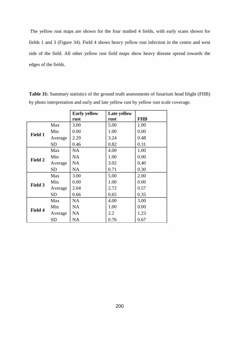
200

The yellow rust maps are shown for the four studied 4 fields, with early scans shown for

fields 1 and 3 (Figure 34). Field 4 shows heavy yellow rust infection in the centre and west

side of the field. All other yellow rust field maps show heavy disease spread towards the

edges of the fields.

Table 31: Summary statistics of the ground truth assessments of fusarium head blight (FHB)

by photo interpretation and early and late yellow rust by yellow rust scale coverage.

Early yellow

rust

Late yellow

rust FHB

Field 1

Max 3.00 5.00 1.00

Min 0.00 1.00 0.00

Average 2.29 3.24 0.48

SD 0.46 0.82 0.31

Field 2

Max NA 4.00 1.00

Min NA 1.00 0.00

Average NA 3.02 0.40

SD NA 0.71 0.30

Field 3

Max 3.00 5.00 2.00

Min 0.00 1.00 0.00

Average 2.04 2.72 0.57

SD 0.66 0.65 0.35

Field 4

Max NA 4.00 3.00

Min NA 1.00 0.00

Average NA 2.2 1.23

SD NA 0.76 0.67

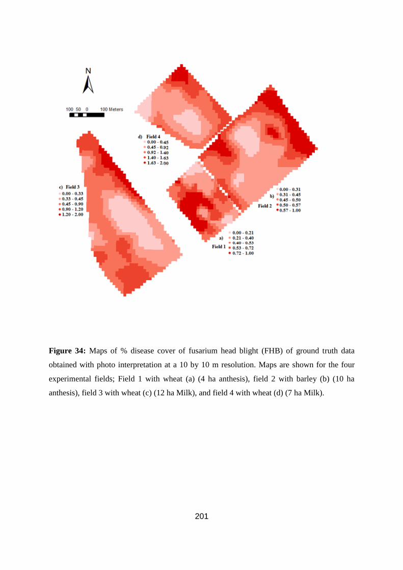
201

Figure 34: Maps of % disease cover of fusarium head blight (FHB) of ground truth data

obtained with photo interpretation at a 10 by 10 m resolution. Maps are shown for the four

experimental fields; Field 1 with wheat (a) (4 ha anthesis), field 2 with barley (b) (10 ha

anthesis), field 3 with wheat (c) (12 ha Milk), and field 4 with wheat (d) (7 ha Milk).

202

Figure 35: Maps of yellow rust classed in the 0-5 scale of ground truth data at a 10 by 10 m

resolution. Maps are shown in the four experimental fields: (a and b) refer to maps of early

stage scans in field 1 with wheat (4 ha booting) and field 3 with wheat (12 ha booting),

respectively. Maps of late stage scans are shown by (c) for field 3 with wheat (12 ha Milk),

(d) for field 4 with wheat (7 ha Milk) (e) for field 1 with wheat (4 ha anthesis) and (f) field 2

with barley (10 ha anthesis).

203

The best on-line PLSR models (e.g., photo interpretation for FHB and visual analysis for

yellow rust) were selected and used to develop corresponding maps. The best fit of the spatial

data for both diseases in all fields was obtained with spherical semi-variograms, whose

parameters are shown in Table 32.

Table 32: Semi-variogram model parameters of each mapped disease in the four fields. The

best fit was achieved with spherical models. Yellow rust early and late and fusarium head

blight (FHB), showing nugget (c0), sill (c), range (r m), proportion (C0/ C %), and the sum of

square error (SSE)

Semi-variogram parameters

c0 r (m) C (c0/c) (%) SSE

FH

B

Field 1 0.12 86.39 0.71 5.51 2.95

Field 2 0.37 99.46 0.83 1.70 1.41

Field 3 0.11 97.02 0.89 8.02 3.32

Field 4 0.04 75.62 0.77 18.98 0.01

Yel

low

ru

st e

arl

y

Field 1 0.001 77.75 0.002 1.001 3.383

Field 2 0.001 68.1 0.003 2.002 8.029

Field 3 0.0001 78.34 0.001 9.0009 2.56

Field 4 0.02 76.63 0.043 1.173 0.0021

Yel

low

ru

st

late

Field 1 0.01 77.75 0.022 1.212 2.11

Field 3 0.01 92.57 0.039 2.929 1.534

MC

Field 4 2.02 65.01 3.52 0.57 5.29

c0 is nugget variance, c is sill, r is range, c0/c is proportion, and SSE is sum of squared error.

204

The semi-variogram represents the spatial correlation of empirical values from sample points.

The empirical values of each point were plotted into lag points, and a spherical model was

fitted to them. The nugget value is attributed to small sampling intervals or measurement

errors. The sill represents the semi-variance value of when the model first flattens out. The

range reports when this sill occurs and gives the variance in meters, anything beyond the

range is not spatially correlated (Bohling, 2005). This translates into the maps shown in

Figures 36 and 37 for on-line FHB and yellow rust, respectively, where the on-line predicted

data from the hyperspectral imager is interpolated using kriging, from the spatial parameters

(nugget, range and sill) based on the semi-variagram data (Table 32).

On-line maps of FHB and yellow rust are shown in Figure 36 and Figure 37. FHB Figures

shows a clear spatial pattern of high disease towards the edge of the fields in fields 2, 3, and 4

(Figure 36). In the earlier scans of yellow rust (Figure 37), high infection along the edges of

the fields 1 and 3 is also recorded. This pattern of disease distribution is also noticed in field

2 in the later yellow rust scans. The late scans also show higher concentrations of yellow rust,

specifically in fields 1, 3 and 4. In fields 1 and 3 it’s possible to see the change in distribution

from the early infection, which is towards the edge of the field, and the later infection which

covers a larger area. However, this disease distribution pattern is not necessarily the case for

the smallest field 1 with four ha area, as in this field, significantly lower spatial variability in

disease pressure was observed, with high levels of the disease appear within the middle parts

(Figures 36 and 37).

205

Figure 36: On-line measured % infection of fusarium head blight (FHB) maps using photo

interpretation in the four experimental fields; Field 1 with wheat (a) (4 ha anthesis), field 2

with barley (b) (10 ha anthesis), field 3 with wheat (c) (12 ha Milk), and field 4 with wheat

(d) (7 ha Milk).

206

Figure 37: On-line measured yellow rust maps, classed in the 0-5 scale (0 is given when no

disease is present, 1 for up to 5% cover, 2 for up to 10%, 3 for up to 30%, 4 for up to 50%

and 5 for >50%) in the four experimental fields: (a and b) refer to maps of early stage scans

in field 1 with wheat (4 ha booting) and field 3 with wheat (12 ha booting), respectively.

Maps of late stage scans are shown by (c) for field 3 with wheat (12 ha Milk), (d) for field 4

with wheat (7 ha Milk) (e) for field 1 with wheat (4 ha anthesis) and (f) field 2 with barley

(10 ha anthesis).

207

Figures 34 and 35, and Figures 36 and 37 show maps of ground truth data, and on-line

predictions, each for FHB and yellow rust, respectively. In general, good spatial similarities

can be overserved between measured (ground truth) and on-line predicted corresponding

maps. However, the spatial resolution of the ground truth maps shown in Figures 34 and 35

are of much lower spatial resolution. The good spatial similarity is particularly true for FHB,

showing a very good comparison of high and low areas. However, the level of disease does

not match well, as the model tends to over predict FHB observations, apart from field 3,

where it was under predicted. The range of prediction to the reference values can be seen for

the online data in figure 33. The yellow rust maps also show a good similarity, with the main

difference is the central area of field 1, which seems to be healthier in the ground truth maps.

Again, different classes are used for each field and map, a decision that was attributed to the

need to show and compare the spatial variation of disease between measured and on-line

predicted maps. If all maps were on the same scale much of this detail would have been lost.

The largest yellow rust infection can be observed on the SW part of the field (Figures 35 and

37), whereas FHB spatial distribution follows an opposite trend (Figures 34 and 36), where

the highest infection is observed on the NE part of the field. The MC map in field 4 shows

higher MC in the NE part of the field compared to the SW part. The MC spatial distribution

in this field matches that of FHB. Although moisture content values will vary from day to

day, the spatial distribution pattern will remain almost constant (Vachaud et al., 1985;

Mouazen et al., 2005).

208

Figure 38: Soil moisture content map and images of measured with the on-line visible and

near infrared spectroscopy sensor (Mouazen, 2006) in field 4.

6.5 Discussion

6.5.1 Crop canopy spectra analysis

Figures 31 and 32 both showed similar spectral features to those reported by Whetton et al.

(2016c) under laboratory scanning conditions. However, the difference between 650 and 700

(nm) in field spectra is much larger than that in the laboratory spectra (in part 1 of the study),

which may indicate larger absorption in the 400-650 nm range by the darker canopy colour

associated with larger intensity of Chlorophyll in leaves. This large absorption in the 400-

650nm wavelength range is linked to absorbance from chlorophyll a (Hunt et al., 2013).

Zhang and Zhang (2016) recommend the use of the spectral range of 470 to 800 nm, which

chlorophyll is sensitive to, to monitor crop diseases. Reduced absorption can be observed for

a late stage captured spectra, as compared to an early stage, which may be attributed to a

reduction in leaf area due to increased yellow rust infection or as Xavier et al. (2006) suggest

209

it’s attributed to the increase of senescent leaves. Furthermore, both on-line and non-mobile

spectra captured late in the growing season were more similar to each other than they were to

the early spectra (Figure 31). The early spectra both on-line and non-mobile show a very

similar pattern through the spectral signature. However, a more noticeable difference in

relative reflectance can be seen from 670nm onwards. This difference could be due to the

individual plant, or the amount of foliage being captured by a moving platform, as from

700nm onwards greater foliage has a greater reflectance. This large similarity in spectra

(Figure 31) is a first indication of a good quality canopy spectra collected in this study under

mobile conditions. the high similarity between the on-line and non-mobile spectra seen in the

barley canopy (Figure 32) is a good indication of the hyperspectral system stability in

providing high quality spectra to enable modelling yellow rust and FHB with desirable

accuracy, to be evaluated in the following section. There was a slightly lower reflectance

recorded for both (early and late) non-mobile wheat spectra, however, the barley has a

slightly higher reflectance for the non-mobile spectra. The differences between the on-line

and non-mobile spectra are attributed to the moving platform. As the on-line captures are

steadily moving and thus capturing an average over a small distance, as opposed to capturing

just a small area (a line) like the non-mobile spectra. The spectra between wheat and barley

appears similar in Figures 31 and 32. Wilson et al. (2014), found only minor differences in the

spectra of wheat and barley and attributed these small differences to the physical structure of

the ears.

210


The highest independent validation of yellow rust obtained with the visual scale assessment

(RPD = 2.55, R²=0.82) can be classified as very good prediction performance, whereas the

highest performance for FHB was obtained with image scale analysis (RPD = 2.31, R²=0.85),

which can also be classified as good prediction ability (Table 28). The implication of this is

that both an image and visual assessments should be collected for accurate disease models.

An RGB image might not capture yellow rust in the low canopy layers. This is the reason

why Zhao et al. (2016) recommended investigating the disease development for different leaf

layers. FHB seems to be better captured in the RGB image than yellow rust as the disease

appears on heads that present at the top of the crop canopy; hence, FHB disease is unlikely to

be obscured like yellow rust, allowing for an accurate count and representation to be made

with the photo interpretation. The photo interpretation also removes the potential of

subjectivity between assessments. Due to yellow rust being a foliar disease and leaf

overlapping occurring in a canopy, the level of disease could be hidden in an RGB image.

Whilst it’s arguable that the RGB photograph would be representing the same area seen by

the hyperspectral imager, the latter may pick up alterations in the crop’s reflectance due to

yellow rust, which can be captured by the spectral data.

Huang et al. (2015) successfully assessed yellow rust in winter wheat, reporting a high R²

value of 0.88, based on hyperspectral measurements of individual infected leaves, which is of

limited use as compared to canopy measurement adopted in the current work. Peteinatos et al.

(2016) measured spectral reflectance using two hand-held passive spectrometers and one

fluorometer, and concluded that early detection of yellow rust was possible. Adopting a data

fusion approach of hyperspectral data (450 – 900 nm) and fluorescence data (550 – 690 nm),

Moshou et al. (2005), reported a high accuracy (94.5 %) of detecting yellow rust in winter

211

wheat. They needed two detection technologies to achieve this accuracy, increasing the cost

for field application. Similar reliable results for quantitative identification of yellow rust in

winter wheat have been demonstrated by Krishna et al. (2014), achieving high R² and RPD

values of 0.90 of 3.8, respectively. However, they have to include the entire visible and near

infrared range (e.g., visible and near infrared (VNIR) and short wavelength infrared (SWIR)

of 350 to 2500 nm) to reach this accuracy, whereas the current work achieved good (RPD =

2.14, R²=0.78) to very good (RPD = 2.55, R²=0.82) prediction accuracy, based on a mobile

relatively cost-effective hyperspectral camera, in the visible range only.

There is limited literature for FHB detection in the field, which may be attributed to the

difficult detection of symptoms appearing on ears. Polder et al. (2005) reported successful

detection of fusarium in single kernels, by using both spectroscopy and imaging. Similarly,

Delwiche and Kim (2000) successfully used a hyperspectral imager at 435 – 860 nm and

machine learning for fusarium detection in wheat kernels. Bauriegel et al. (2011) utilised a

hyperspectral imager, based on wavelength range intervals of 500–533 nm (green), 560–

675 nm (yellow to red), 682–733 nm (red edge) and 927–931 nm (NIR), to identify the

percent coverage of fusarium disease in ears, achieving average recognition accuracy of 67%

and as high as 87%. Oerke and Steiner (2010) utilised an infrared thermography method for

in-situ detection of FHB symptoms at a canopy level, by detecting a significantly higher

temperature in infected ears.

The non-mobile independent validation results (Table 29) were better than those of the on-

line validation (Table 30), particularly for yellow rust. This is expected as during on-line

measurement, uncontrollable external conditions such as vibrations and variations in camera

and light source heights and angles, negatively affect the measurement accuracy. Since

fusarium infects the ear as opposed to the foliage, the impact of fusarium symptoms on

212

spectra in less pronounced in early growing stages (Rossi et al., 2001; Xu, 2003), hence, can

only be applied to the data collected later in the season. Prediction of FHB infection in wheat

(Table 30) is more accurate than in the barley, as the wheat data for the FHB models were

collected at milk (70) in field 1 and 2 and at anthesis (61) in field 4 for wheat, compared to

just anthesis (61) for barley (Table 22). Though FHB was only detected later in the season,

its recognition can still be useful for selective harvest (see next Chapter), and perhaps for the

last fungicide application, which is usually targeted towards maintaining the health of the

crops ear (Pillinger et al., 2004).

The improved models performance is in line with the findings of Part 1 of this study

(Whetton et al.,(2016c), and could be attributed to the reduction in the subjectivity effect on

the assessments, by grouping readings within 5 different groups of infections detailed above.

The on-line prediction performance of percent coverage, obtained with the visual analysis of

FHB is very poor (RPD = 0.47 (R²=0.09) and 0.75 (R²=0.04) for barley and wheat

respectively). There is very limited literature about on-line measurement of cereal disease,

particularly for FHB. Examining the on-line validation in Table 30 suggests that FHB should

be detected by the RGB photo interpretation, whereas yellow rust by the visual analyses, both

the percent coverage and scale. This is true for both wheat and barley. On-line predictions in

wheat were better that those in the barley field, which is expected as models were created

using data from wheat fields and then applied to predict disease presence in the barley field to

test robustness.

213

6.5.3 Maps

From the maps developed, it can be generally observed that higher disease is located towards

the edges of the fields, where hedgerows and borders of a field act as a source of inoculum of

yellow rust and fusarium species (Jenkinson and Parry, 1994; Champeil et al., 2004; Imathiu

et al., 2013). Initial infections of soil-borne pathogens, commonly result from infected plant

residues left over from the previous year’s harvest. Fusarium fungi survive over winter on

plant residues (as mycelium), which can produce ascospores that infect the flag shoot (Sutton,

1982; Oberti et al., 2014). The late (second) scans of the 10 and 4 ha fields (Figure 37) show

the yellow rust spreads further towards the centre of the field. Figure 39 shows yellow rust

and FHB infection from the RGB images captured in the late scans.

A) B)

Figure 39: Images of wheat crop at the field site in Bedfordshire, UK. Wheat was at

growth stage 72 (Milk). Part A) Fusarium head blight infection (FHB), and part B)

Yellow rust infection.

214

Fields 1 and 2 (Figure 36) were classed at anthesis growth stage. FHB infection can occur at

the booting growth stage. However, it’s unlikely to see symptoms until after anthesis (Anand

et al., 2003; Reis et al., 2016). Development of crop is heavily affected by temperature,

which can vary through a field due to microclimate. The majority of the crop in field 1 and 2

was at the anthesis growth stage however, there are areas in the field that were further

developed. The infection witnessed in field 1 and 2 were the first symptoms of FHB, being a

pink tint in some of the ears. The majority of field 2 had a very low infection, particularly

towards the centre of the field. Field 1 however, had a more homogenous distribution of

FHB. (Dammer, 2003; Saiyed et al., 2009; AHDB 2015).

It is important to point out here that the 7 ha field 4 can be split according to soil type into

almost two halves, with the NE half being of a heavier soil (clay loam), whilst the other SW

half being of a much lighter soil (sandy clay loam). This field was only scanned in one

occasion at the milk (grain filling) stage on 1st July, 2015, which is quite late in the season.

The largest yellow rust infection can be observed on the SW part of the field (Figure 35),

whereas FHB spatial distribution follows an opposite trend, where the highest infection is

observed on the NE part of the field (Figure 34). Due to the dry but warm conditions of 2015

spring, FHB infection was low in general. It is of interest to mention that May according to

the UK metrological office was particularly dry, and record breaking temperatures had been

reached later on in the season. This resulted in half of the field being under substantially more

water stress (SW) than the other wetter half (NE), due to the difference in the soil type and its

ability to retain soil moisture. Subsequently, this soil type and moisture retention differences

between the two halves affected the crop canopy, and substantially impacted on the

microclimate conditions of the crop. It was reported that a variation in soil texture can lead to

variations in soil properties.

215

For example, an increase in nitrogen will increase the duration and green area index of the

canopy, which further affects the microclimate conditions (Stokes et al., 1997; Sylvester-

Bradley and Kindred, 2009). The underlying spatial distribution of moisture content in field 4

(Figure 38) confirms the NE part to have a larger moisture content than the SW part. This is

resulted as plants in the NE part being a denser, thicker and greener canopy (Part B in Figure

38), than plants in the dryer SW part (Part A in Figure 38). Whilst moisture content will vary

quickly, the underlying spatial distribution pattern of water presence will remain similar

through the season (Vachaud et al., 1985).

Local climate and weather conditions are considered the most influential factor regarding the

distribution and severity of fungal infections in a crop stand. Under clear weather conditions

in spring and summer, areas of the field with a lower crop density will warm up and cool

down faster than those with dense canopies. Temperature in a wheat field’s microclimate

could have an inter-canopy variation of up to 7.5°C (Dammer, 2003), depending on crop

canopy density and soil moisture content. Therefore, different soil texture type and

subsequently moisture content encountered in this study may have affected crop canopy

density and humidity and crop health under the exceptionally dry conditions in the spring of

2015, which led to the different disease spread pattern in among the two parts of the Field 4.

Literature demonstrates that epidemics of fungal diseases are strongly influenced by the local

environment, persistence and adaption of the pathogen and the crop’s variety and

physiological condition (Dammer, 2003). Therefore, variation in one of more of these will

possibly affect disease distribution, which we believe to be the case in the 7 ha, field 4. The

conidial fusarium spores are commonly transported by rain drop splashes, though this

depends on the species (Parry et al., 1995). Variability of disease presence is common for

FHB. This is due to infection being dependent on warm humid weather conditions, which

216

may explain why the NE part of field 4 had higher fusarium disease ranges than the dryer SW

part (Jelinek et al., 1989; Rossi et al., 2001; Xu, 2003). In the NE part, the crop canopy was

denser due to heavier texture and larger MC which resulted in a higher humidity. However,

the higher infection with yellow rust in the dryer SW part of this field can be attributed to the

fact that yellow rust spores are predominantly dispersed by wind but require moisture to

infect the crops leaves. The less dense canopy of the SW part, as compared to the NE part

(Figure 38) may have allowed for better penetration of yellow rust spores by wind, hence

increase infection rates in this part. This is an interesting point to consider in plant protection

against yellow rust and FHB, although further investigations are necessary.

Examining the spatial distribution of the on-line FHB (Figure 36) and yellow rust (Figure 37)

maps, one can observe the high infection concentrated at the hedgerows and borders of fields.

This suggests the need for site specific application of fungicides that should target these

highly infected edge parts, and that application should take place at earlier growing stages.

This will prevent or at least reduce the possibility of diseases to expand towards the inner

parts. The on-line measured disease maps become more important at late growing stages once

diseases spread over the field, and site specific spraying becomes more important to adopt.

Further work will need to use these maps for site specific fungicide applications, followed by

cost-benefit and life cycle analysis to evaluate the economic and environmental benefits as

compared to the traditional homogeneous applications adopted by majority of farmers today.

217


This Chapter introduces the work related to the on-line measurement of yellow rust and

fusarium in four fields using the optimal measurement set up of the hyperspectral line image

camera, obtained in Chapter 4. The results from this study show that on-line hyperspectral

measurement and mapping of yellow rust (using visual assessments) and FHB (using image

interpretation) is possible, with moderate accuracy in barley and good accuracy in wheat. The

spatial distribution of yellow rust, and FHB, were impacted by both soil texture and moisture

content. This will allow for future work to be carried out on on-line measurement for both

crop diseases to guide site specific fungicide application or selective harvest, to be discussed

in the next Chapter.

218

7 Management zone maps for variable fungicide application and

selective harvest

Chapter Synopsis;

This chapter focuses on data fusion of disease data (yellow rust and fusarium head blight

(FHB)), along with canopy and soil properties, to produce management zones (MZ) in winter

wheat. The chapter introduces theoretical MZ methods of selective harvest (SH) (so grain can

be separated in relation to quality) and variable fungicide application (VRFA) of application

rates dependent on the severity of disease. The MZ approaches are compared to conventional

methods by means of virtual cost-benefit analyses, under certain assumptions. The data is

collected through the methods introduced and discussed in chapters 3, 4, 5, and 6.

Abstract

Currently the majority of crop protection approaches are based on homogeneous application

of fungicides over the entire field area. With the increasing pressures on fungicide

applications, associated with increased environmental impact and cost, an alternative

approach based on site specific fungicide application and selective harvest (SH) is needed.

But, to achieve this goal high resolution data on the affecting factors in the system is needed

to allow accounting for the within field variability in the analysis. High sampling resolution

data on crop growth and diseases, soil properties and yield were subjected to k-mean cluster

analysis to develop management zone (MZ) maps for one experimental field in Bedfordshire,

UK. Cost-benefit analyses for variable rate fungicide application (VRFA) and SH were

performed at T1, T2 and T3 growth stages of wheat. Results showed that with VRFA, when

compared to homogeneous rate fungicide application (HRFA), reductions in fungicide

application of 22.24% at T1 and T2 and 25.93% at T3 are expected. SH reduced the risk of

market rejection due to low quality and high mycotoxin content. Total profit of combining

219

SH and VRFA was £83.35 per hectare, divided into £48.04 ha-1

for SH, £17.6 ha-1

for each

VRFA at T1 and T2 growth stages and £17.7 ha-1

at T3. We recommend adopting this MZ

concept for VRFA and SH, as economic and environment viability is feasible.

Keywords

Yellow rust, Fusarium head blight, Hyperspectral imager, Management zones, Cost-benefit

analysis, Selective harvest, Variable rate fungicide application, Canopy humidity, canopy

temperature, k-mean clustering.

7.1 Introduction

Ideally, high crop yields would need to be produced with minimal impact on the environment

(Pimentel et al., 1997; Tilman, 1999). Although intensive conventional agriculture based on

unsustainable management of external inputs has led to increasing yields, it has posed severe

environmental problems (Pimentel et al., 1995; Hole et al., 2005). But, varieties with high

productivity are associated with higher sensitivity to disease leading to yield loss, which

necessitates a sustainable approach for managing farm external inputs in a site specific way.

In order to achieve this goal, data on all affecting factors in the system should be collected at

high sampling resolution. This is possible today for specific diseases, crop canopy and soil

properties, using on-line crop and soil sensors (Kuang et al., 2012; Kuang and Mouazen,

2013; Whetton et al., 2016a). Fusing these different layers of information is a main

requirement for creating management zones (MZ), to explore the potential of VRFA and SH.

A balanced availability of soil nutrition contributes to disease resistance and susceptibility.

Nitrogen and phosphorus are the main soil macro nutrients affecting the severity of fungal

diseases, whilst micronutrients (e.g. Ca, Mg, Zn, B, Mn, Mo, Ni, Cu, Fe, S, and Si) are also

known to affect various diseases in plants (Engelhard, 1989; Fageria and Baligar, 1997;

220

Graham and Webb, 1991; Huber, 1980). For example, high potassium in crops reduces the

incidence of diseases (Perrenoud 1990; Prabhu et al., 2007). When considering a method for

disease control, it is important to acknowledge its interaction with nitrogen. Increases in

nitrogen will increase the green area index and duration of the canopy, which in turn affects

the microclimate of the crop and increases the likelihood of infection (Stokes et al.,

1997; Sylvester-Bradley and Kindred, 2009). Therefore, information about key soil properties

and their effect on crop disease spread is essential for site specific plant protection.

Fusarium head blight (FHB) is a sporadic disease, causing variability of disease presence and

level of infection across regions, and years (Jelinek et al., 1989). FHB can result in yield

losses, leading to both direct and indirect economic losses and negative influences on human

and animal health (Paul et al., 2005). The direct economic loss is attributed to reduced grain

quantity and size, whereas the indirect loss is due to mycotoxin contamination (a secondary

metabolite of the fusarium mould), associated with market rejection or downgrading of grain

quality (Parry et al., 1995). Yellow rust is a foliar fungal disease that is also linked with a

long history of yield loss. The loss due to yellow rust is mostly attributed to a reduction in the

number of grains per ear, and weight of the individual grains (Herrera-Foessel et al. 2006).

Across the globe, yield losses due to yellow rust are reported to be between 10 and 70%

(Chen, 2005). Doodson et al. (1964) reported yield losses of 64.5% in individual severely

infected plants. Doling and Doodson (1968) also remarked substantial yield loss, but with a

maximum of 30% reduction, which was attributed to the extensive cultivation of resistant

spring and winter wheat varieties. Singh et al. (2012) witnessed severe epidemics of yellow

rust infection in various cultivars that were formerly protected by resistance genes. It is still a

major contributor to yield loss, with large variations in yield reduction observed between

susceptible and resistant varieties, often being >50% (Safavi, 2015).

221

Fungicides can be organic (contain carbon atoms) or inorganic (do not contain carbon). Some

of the oldest fungicides were inorganic and based on heavy metals. Fungicides can be contact

or systemic. Contact fungicides (protectants) work on the surface of the plant, whereas

systemic (penetrants) are absorbed. Fungicides damage the cell membranes of fungi, or

interfere with processes (by inactivating enzymes, or prevent energy production or

respiration). Fungicides can also be grouped as narrow spectrum - affecting only a few

related pathogens and are often systemic, or broad spectrum - affecting a wide range of

pathogens and often contact based. Contacts are generally applied as preventatives, while

systemic fungicides can be applied as both preventive and curative. Contacts are often

reapplied to protect new growth of the plant. Depending on the type of fungicide, and the

targeted disease, the timings and number of fungicide applications will vary. Typically, there

are up to four timings of fungicide application to control foliar diseases of wheat, with the

fourth application also being aimed at ear diseases. T0 (Timing 0) is applied between growth

stage 25 and 30 (Zadoks scale). Its application is usually a preventative in historically

problematic fields, or if early disease is observed. T1 (GS 31-33) and T2 (GS 37-39) are

applied to keep the third, second and flag leaves healthy, as these heavily influence yield in

wheat. The T3 application (GS 52-60) can also be an “ear wash”, and is usually applied to

preserve the quality of the grain. T2 is commonly considered the most crucial application and

is the most frequently followed, due to the importance of maintaining flag leaf health. T1 is

considered secondary in importance followed by T3 and then T0 (HGCA 2008; Clark, 2016).

In some regions of Europe, there have been trials to reduce the number of fungicide

applications. The fungicide applications are applied after growth stage 31, but only if

infection levels reach a defined threshold (Verreet et al., 2000; Falisse and Meeus 2002).

222

Therefore, information about crop disease in the field, collected at high sampling resolution,

is another essential step towards site specific plant protection. But sole information about

crop disease is not sufficient for an integrated decision support system, due to the influence of

other factors e.g., relevant soil properties, microclimate conditions and crop canopy

characteristics (Huber, 1980; Engelhard, 1989; Graham and Webb, 1991; Fageria and

Baligar, 1997; Stokes et al., 1997; Sylvester-Bradley and Kindred, 2009).

The aim of this paper is to propose and implement a multi-sensor and data fusion approach

for the delineation of management zone (MZ) maps. The MZ map will be used for creating

recommendations for VRFA and SH. A cost-benefit analysis will evaluate whether this

approach has economic benefits. To our best knowledge, no reports have been produced for

assessing the environmental and economic benefits of VRFA and SH based on data fusion of

high sampling resolution spectral data, collected with on-line soil and crop sensors. This

study focuses on the potential economic benefits of non-homogenous fungicide applications

and selective harvest based on high sample data, compared to a conventional practice.

However, the study will not ask the question about when and which fungicide should be

applied.


7.2.1 Field site

One study field of 10.8 ha with cereal crop production was selected for this study. It is

located at Duck End Farm, a commercial family farm in Wilstead, Bedfordshire, UK

(52°05'46.3"N 0°26'41.4"W), with an average annual rainfall of 598 mm. The fields N part is

of a clay soil, whereas the S part is of a sandy clay soil. The farmer uses a 3-year crop

rotation of barley, wheat and oilseed rape. The experiment was carried out in 2015, when the

crop grown was winter wheat (solstice variety). Yellow rust and FHB were observed in the

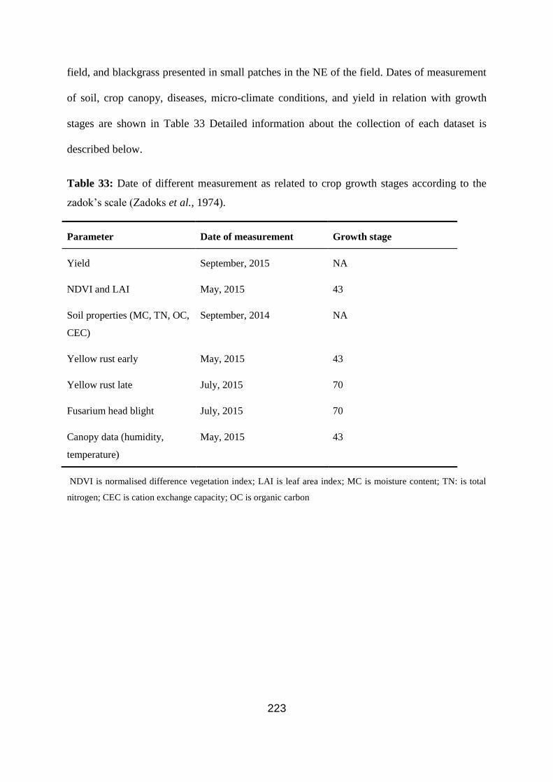
223

field, and blackgrass presented in small patches in the NE of the field. Dates of measurement

of soil, crop canopy, diseases, micro-climate conditions, and yield in relation with growth

stages are shown in Table 33 Detailed information about the collection of each dataset is

described below.

Table 33: Date of different measurement as related to crop growth stages according to the

zadok’s scale (Zadoks et al., 1974).

Parameter Date of measurement Growth stage

Yield September, 2015 NA

NDVI and LAI May, 2015 43

Soil properties (MC, TN, OC,

CEC)

September, 2014 NA

Yellow rust early May, 2015 43

Yellow rust late July, 2015 70

Fusarium head blight July, 2015 70

Canopy data (humidity,

temperature)

May, 2015 43

NDVI is normalised difference vegetation index; LAI is leaf area index; MC is moisture content; TN: is total

nitrogen; CEC is cation exchange capacity; OC is organic carbon

224

7.2.2 Disease and canopy property data collection


Photonics Ltd., UK) with a spectral range between 400 and 750 nm, and a halogen light

source were mounted on a tractor by means of a metal frame for on-line measurement of

yellow rust and FHB (Whetton et al., 2016a). Measurement was carried out at a forward

travel speed of approximately 4 km h-1

, and line images were captured at 1 sec frequency,

which was subsequently logged and geo-located with a sub-meter accuracy, using a

differential global positioning system (DGPS) (EZ-Guide 250, Trimble, California, USA).

The methodology followed the optimal configurations discussed in Whetton et al. (2016b).

These include an integration time of 50 ms, a camera height of 0.3 m and light height and

distance of 1.2 m and a camera angle of 10°.

At 5 locations per hectare, ground truth plots were selected (Figure 40), where manual

disease assessment and recognition of yellow rust and FHB were made according to methods

discussed in detail by Whetton et al. (2016a and 2016c). The assessment for FHB considered

both early and late symptoms on heads, and were assessed as either a 0 for no infection, 1 for

less than 5% individual infected heads, 2 for up to 10%, 3 for up to 30%, 4 for up to 50%,

and 5 being a heavy infection over 50% infected heads, dependent on the ratio of FHB

infected to healthy crops. Similarly, for yellow rust, a 0-5 scale was applied, similar to the

approach adopted by Oberti et al. (2014). A scale between 0 and 5 (from less to more

affected plots) was given the same ratio as that for FHB.

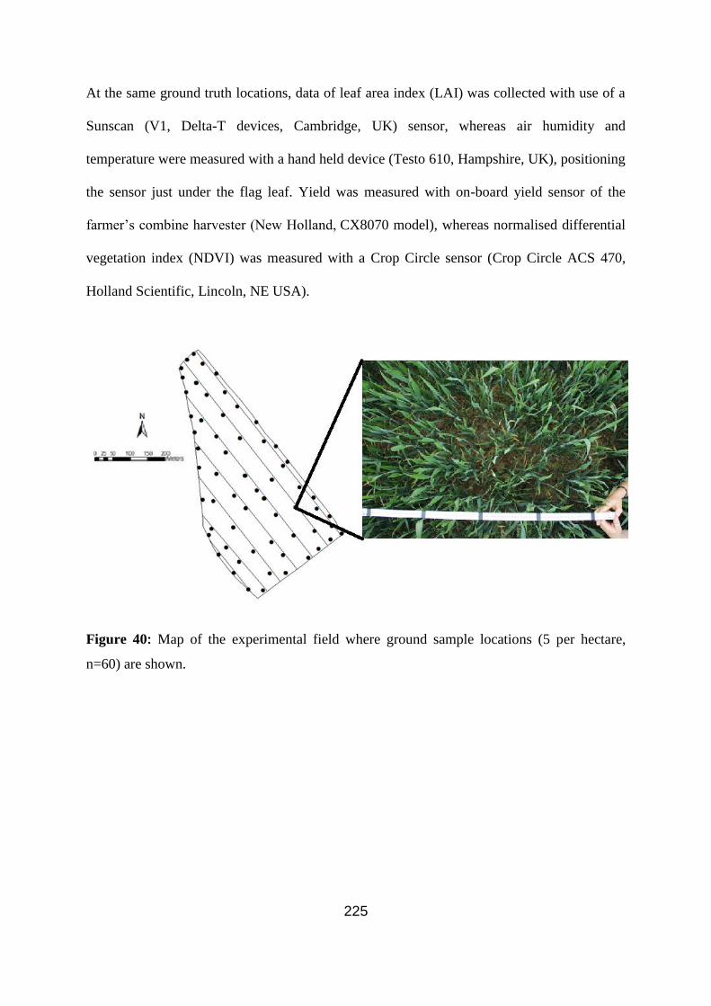
225

At the same ground truth locations, data of leaf area index (LAI) was collected with use of a

Sunscan (V1, Delta-T devices, Cambridge, UK) sensor, whereas air humidity and

temperature were measured with a hand held device (Testo 610, Hampshire, UK), positioning

the sensor just under the flag leaf. Yield was measured with on-board yield sensor of the

farmer’s combine harvester (New Holland, CX8070 model), whereas normalised differential

vegetation index (NDVI) was measured with a Crop Circle sensor (Crop Circle ACS 470,

Holland Scientific, Lincoln, NE USA).

Figure 40: Map of the experimental field where ground sample locations (5 per hectare,

n=60) are shown.

226

7.2.3 On-line soil measurement

An on-line visible and near infrared (vis-NIR) spectroscopy sensor (Mouazen, 2006) was

used for the measurement of soil total nitrogen (TN), organic carbon (OC), moisture content

(MC) and cation exchange capacity (CEC). It consists of a mobile, fibre type, AgroSpec

visible and near infrared (vis-NIR) spectrophotometer (tec5 Technology for Spectroscopy,

Germany) with a measurement range of 305-2200 nm, and a differential global positioning

system (DGPS) (EZ-Guide 250, Trimble, California, USA) to record the position of the on-

line measured spectra with sub-metre accuracy. The spectrophotometer is linked to an optical

probe by means of two optical fibres. The optical probe is attached to the back side of a

subsoiler that penetrated the soil and opened a smooth trench, which is illuminated by a 20 W

light source, while diffuse reflected spectra is collected at 1 sec frequency. A detailed

description of the system can be found in Kuang, and Mouazen, (2013). On-line measurement

was carried out in 2014, after the harvest of the previous crop at parallel transects of about 10

m apart and at 2 km forward speed, setting the sensor at 15 cm depth.

7.2.4 Spectral modelling of disease and soil properties

The pre-processing of the soil and canopy spectral data was carried out following an

approach outlined in Mouazen et al. (2006). The first step was to remove noisy wavelengths

at the two far edges of spectra, before they underwent averaging of neighbouring wavebands,

maximum normalisation, first derivative calculation and smoothing, successively. All spectra

pre-processing was carried out using Unscrambler 10 software (Camo Inc.; Oslo, Norway).

The hyperspectral imager data set was randomly divided into two sets of 80% and 20%,

representing the calibration and validation data sets, respectively. The pre-processed canopy

spectra and manual assessments of disease were subjected to partial least squares regression

227

(PLSR) analysis with full-cross validation using the calibration set (80%). PLSR analyses

were carried out using Unscrambler 10 software (Camo Inc.; Oslo, Norway). The models’

performance was evaluated using the on-line validation set (20%). More detailed information

about the calibration and validation of the FHB and yellow rust models can be found in

Whetton et al. (2016a). The same approach was used for the calibration and validation of

models to predict soil properties (e.g., MC, OC, TN and CEC). More detailed information

about the calibration and validation of these models can be found in Halcro et al. (2013) for

TN, OC and MC and Marin-González et al. (2013) for CEC.

The calibration models for FHB and yellow rust were used to predict these two diseases using

on-line collected hyperspectral data in 2015 (Table 33). Yellow rust prediction was made

twice for early scanning (May, 2015) and late scanning (July 2015), whereas FHB was

measured at the late scanning only, as this disease affects the crop heads, at a late growing

stage. The calibration models developed earlier for OC, TN and MC (Halcro et al., 2013) and

CEC (Marin-González et al., 2013) were used to predict soil properties using the on-line

measured soil spectra after crop harvest in September, 2014 (Table 33).

Since the canopy properties apart from NDVI, including LAI, humidity and temperature were

measured only at 60 locations shown in Figure 40; these limited data were used for further

analysis. However, a much larger number of data points was obtained of the on-line predicted

crop yellow rust and FHB, on-line predicted TN, OC, MC and CEC, measured NDVI and

yield.

228

7.2.5 Mapping

Maps for the measured NDVI and yield and the on-line predicted yellow rust, FHB, soil TN,

OC, MC and CEC were developed using ArcGIS 10 software (ESRI, California, USA). The

first step in the development of maps was the creation of semi-variograms in R-studio

(RStudio, Boston, MA). After an optimal semi-variogram (smallest sum of square error) was

established for a given property, kriging was applied to develop a full point map using

ArcGIS 10 software (ESRI, California, USA). A different number of data points was

considered in the semi-variogram development and kriging, hence, the quality of maps differs

among different maps, although the best fit was found with spherical semi-variogram models

for all properties investigated.

7.2.6 Management zone maps

The on-line predicted soil properties and crop diseases, measured canopy and yield and

microclimate conditions were pulled into one matrix by means of Statistica software (StatSoft

inc., Oklahoma USA), before running k-means clustering. The k-mean cluster analyses were

performed for the following applications to produce three different MZ maps, with a different

number of MZ, depending on variability resulting from the different input data used:

1) Selective harvest: In this case, only the on-line predicated FHB and late yellow rust data

were included in the k-mean clustering to produce a MZ map for SH.

2) T1 and T2 variable fungicide applications: The k-means cluster analysis here aimed at

producing MZ maps for VRFA at growth stages 31 to 39, applied as a foliar disease

preventative. In this case, the on-line predicted early yellow rust and soil properties (MC, OC,

TN and CEC) and canopy properties (NDVI, LAI, canopy humidity and temperature) were

included in the analysis.

229

3) T3 variable rate fungicide applications: The k-means cluster analysis produced a MZ map

for the growth stage 52-60, where fungicides are usually applied to preserve the grain quality.

Input data included the on-line predicted FHB and soil properties (MC, OC, TN, and CEC),

canopy properties (NDVI, LAI, canopy humidity and temperature).

7.2.7 Eventual calculation of cost-benefit analysis

The following assumptions were made in this study for the cost-benefit analyses;

1) The cost of implementing the different sensing technologies and data mining was not

taken into consideration.

2) FHB presence is directly linked to mycotoxin presence, which is in line with Paul et

al. (2005) who reported a mean correlation of R² of 0.73 between deoxynivalenol

(DON) level and fusarium observed in 163 studies in the USA. Turner and Jennings

(1997) reported the occurrence of mycotoxins in UK cereals was lower than expected

due to M. nivale (Microdochium species which hold no mycotoxin risk), which

supressed the infection of Fusarium species. However, a correlation was still

observed.

3) VRFAs would not reduce the efficiency of disease control obtained with

homogeneous applications, an assumption supported by a practical note that reduced

doses of fungicide should be applied in low disease pressure areas (FRAC, 2010) and

vice versa.

4) Wheat grain would be sold at a lower price due to fusarium contamination of

mycotoxins. This assumption is supported by the European commission imposed

upper limits of the DON mycotoxin in cereal grain for human consumption.

230

5) A uniform application of fungicide was proposed for the T0 growing stage, as it is

usually a preventive treatment and at this early growth stage disease sensing would be

difficult, as the canopy is sparse.

Two fungicides commonly used in fungicide control were selected in this study (chemical

labels are available in Appendix C). Adexar (epoxicoazole) is suitable for the treatment of

many fungal disease infections and is particularly common for FHB treatment. It is used at a

maximum of 2 litres per hectare (lha-1

), with a maximum of 2 applications per annum for

wheat in Europe. The current price is £34 per litre. Proline 275 (prothioconazole), is suitable

for many fungal disease infections but it is particularly used for treatment of early yellow

rust. It is applied at a maximum of 0.72 lha-1

per dosage, with a max total of 2.16 lha-1

per

year for wheat treatment in Europe. The current price is between £52.5 and £59 per litre1. The

following two cost-benefit analyses were carried out for the VRFA and SH;

1- The cost-benefit for the variable fungicide treatments (T1, T2 and T3) was applied using

ArcGIS 10 software (ESRI, California, USA), by dividing the field area into high infection

risk (HIR) and low infection risk (LIR) zones, taking into consideration the boom width

relative to the position of tramlines. Zones of HIR were virtually subjected to a full

application rate, whereas the LIR zones were given a 50% application rate. For T3 the

medium infection zones (MIF) were subjected to 75% dosage rate. All MZ were considered

in the analysis, and the amount of fungicide per area was calculated. The overall applied

amount of fungicide was then compared to that of a conventional full homogenous

application, and the potential savings or losses were calculated.

231

2- The cost-benefit analysis for SH was calculated in a similar manner to that of VRFA using

ArcGIS 10 software (ESRI, California, USA). MZ were classified into HIR and LIR. This

was made by proposing separate harvest of the HIR (low quality) from that of the LIR (high

quality) zones. All MZ were considered in the analysis, and their corresponding area was

calculated, so as the average yield per zone could be calculated. The total prices of wheat

grain obtained from Farmer’s Weekly (FWI 2016) were £145 and £135 per tonne, for the

high-quality and low-quality yield, respectively. The SH was compared with the

homogeneous harvest of the entire field area, sold at the lower price of £135.

7.3 Results and discussion

7.3.1 Spatial variability of different properties

The analysis for semi-variogram of different soil and crop properties indicated that the best

approximation can be achieved with spherical models, whose properties can be found in

Table 34. The largest sum of square error is calculated for TN followed by MC. The small

values of the proportion between the nugget (attributed to small sampling intervals, or

measurement errors) to sill variation (less pairs of points separated by far distances) indicate

the autocorrelation between different properties studied, because this proportion is an

important parameter to quantify short-distance autocorrelation or the degree of spatial

dependency for a variable (Cambardella et al., 1994; Chang et al., 2014). Cambardella et al.

(1994) defined three categories of spatial dependency of high, moderate, and weak with ratios

of less than 25%, between 25% and 75%, and greater than 75%, respectively. Ranges of

spatial dependency are wider than the sampling interval of on-line soil measurement (10 m),

disease, LAI, humidity and NDVI (24 m), and yield (12 m), confirming the effectiveness of

geostatistical analysis adopted in this study (Chang et al., 2014). The only exception is for the

NDVI measurement (Table 34.).

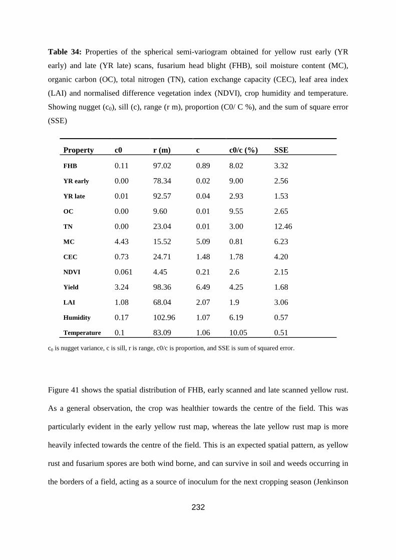
232

Table 34: Properties of the spherical semi-variogram obtained for yellow rust early (YR

early) and late (YR late) scans, fusarium head blight (FHB), soil moisture content (MC),

organic carbon (OC), total nitrogen (TN), cation exchange capacity (CEC), leaf area index

(LAI) and normalised difference vegetation index (NDVI), crop humidity and temperature.

Showing nugget (c0), sill (c), range (r m), proportion (C0/ C %), and the sum of square error

(SSE)

c0 is nugget variance, c is sill, r is range, c0/c is proportion, and SSE is sum of squared error.

Figure 41 shows the spatial distribution of FHB, early scanned and late scanned yellow rust.

As a general observation, the crop was healthier towards the centre of the field. This was

particularly evident in the early yellow rust map, whereas the late yellow rust map is more

heavily infected towards the centre of the field. This is an expected spatial pattern, as yellow

rust and fusarium spores are both wind borne, and can survive in soil and weeds occurring in

the borders of a field, acting as a source of inoculum for the next cropping season (Jenkinson

Property c0 r (m) c c0/c (%) SSE

FHB 0.11 97.02 0.89 8.02 3.32

YR early 0.00 78.34 0.02 9.00 2.56

YR late 0.01 92.57 0.04 2.93 1.53

OC 0.00 9.60 0.01 9.55 2.65

TN 0.00 23.04 0.01 3.00 12.46

MC 4.43 15.52 5.09 0.81 6.23

CEC 0.73 24.71 1.48 1.78 4.20

NDVI 0.061 4.45 0.21 2.6 2.15

Yield 3.24 98.36 6.49 4.25 1.68

LAI 1.08 68.04 2.07 1.9 3.06

Humidity 0.17 102.96 1.07 6.19 0.57

Temperature 0.1 83.09 1.06 10.05 0.51

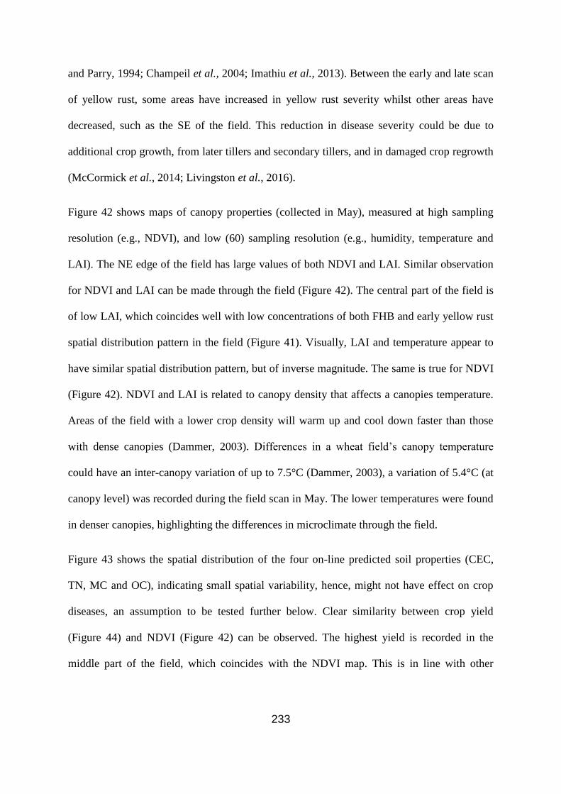
233

and Parry, 1994; Champeil et al., 2004; Imathiu et al., 2013). Between the early and late scan

of yellow rust, some areas have increased in yellow rust severity whilst other areas have

decreased, such as the SE of the field. This reduction in disease severity could be due to

additional crop growth, from later tillers and secondary tillers, and in damaged crop regrowth

(McCormick et al., 2014; Livingston et al., 2016).

Figure 42 shows maps of canopy properties (collected in May), measured at high sampling

resolution (e.g., NDVI), and low (60) sampling resolution (e.g., humidity, temperature and

LAI). The NE edge of the field has large values of both NDVI and LAI. Similar observation

for NDVI and LAI can be made through the field (Figure 42). The central part of the field is

of low LAI, which coincides well with low concentrations of both FHB and early yellow rust

spatial distribution pattern in the field (Figure 41). Visually, LAI and temperature appear to

have similar spatial distribution pattern, but of inverse magnitude. The same is true for NDVI

(Figure 42). NDVI and LAI is related to canopy density that affects a canopies temperature.

Areas of the field with a lower crop density will warm up and cool down faster than those

with dense canopies (Dammer, 2003). Differences in a wheat field’s canopy temperature

could have an inter-canopy variation of up to 7.5°C (Dammer, 2003), a variation of 5.4°C (at

canopy level) was recorded during the field scan in May. The lower temperatures were found

in denser canopies, highlighting the differences in microclimate through the field.

Figure 43 shows the spatial distribution of the four on-line predicted soil properties (CEC,

TN, MC and OC), indicating small spatial variability, hence, might not have effect on crop

diseases, an assumption to be tested further below. Clear similarity between crop yield

(Figure 44) and NDVI (Figure 42) can be observed. The highest yield is recorded in the

middle part of the field, which coincides with the NDVI map. This is in line with other

234

studies, reporting that NDVI of previous years can be used as an indicator for yield in the

following years (Mkhabela et al., 2011).

Figure 41: Disease severity; On-line predicted maps of fusarium head blight (FHB)

measured at milk growth stage 72 (july 2015), early yellow rust measured at booting growth

stage 43 (may 2015), and late yellow rust measured at milk growth stage 72 (july 2015). The

disease is classified on a 0 to 5 scale, where 0 indicates low disease presence and 5 indicates

high disease.

235

Figure 42: Properties attributed to the canopy; On-line measured normalised difference

vegetation index (NDVI), along with the 60 samples based developed maps for leaf area

index (LAI), canopy air temperature and humidity. These data were all collected at the

booting growth stage 43, in May 2015.

236

Figure 43: Soil properties; On-line predicted soil cation exchange capacity (CEC in

Cmol/kg), total nitrogen (TN in %), moisture content (MC in %) and organic carbon (OC in

%). The soil properties were collected before the seed was drilled in September 2014.

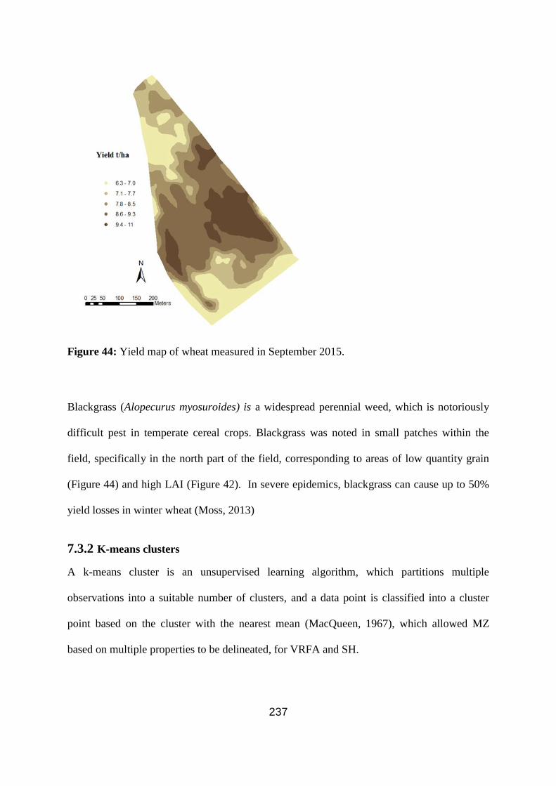
237

Figure 44: Yield map of wheat measured in September 2015.

Blackgrass (Alopecurus myosuroides) is a widespread perennial weed, which is notoriously

difficult pest in temperate cereal crops. Blackgrass was noted in small patches within the

field, specifically in the north part of the field, corresponding to areas of low quantity grain

(Figure 44) and high LAI (Figure 42). In severe epidemics, blackgrass can cause up to 50%

yield losses in winter wheat (Moss, 2013)

7.3.2 K-means clusters

A k-means cluster is an unsupervised learning algorithm, which partitions multiple

observations into a suitable number of clusters, and a data point is classified into a cluster

point based on the cluster with the nearest mean (MacQueen, 1967), which allowed MZ

based on multiple properties to be delineated, for VRFA and SH.

https://home.deib.polimi.it/matteucc/Clustering/tutorial_html/kmeans.html#macqueen

238

The K-mean clustering carried out for 1) SH, (Figure 45) 2) T1 and T2 variable fungicide

applications (Figure 46) and 3) T3 variable fungicide application resulted in different

numbers of clusters (Figure 470). For SH, where on-line predicted FHB and late yellow rust

were included in the analysis, the k-mean clustering resulted in two classes (Figure 45).

Cluster 1 (Figure 45) demonstrated high normalised means associated with high yellow rust

and FHB spread, whereas cluster 2 associated with lower spread of both diseases. Therefore,

it is a straightforward decision of be made for classifying the wheat yield into high quality

and low quality, associated with the cluster 2 and cluster 1, respectively. This classification is

made assuming that FHB presence relates to mycotoxin accumulation and can cause

downgrading of grain on the market, causing economical loss (Parry et al., 1995). Yellow

rust was included in the classification, as infection reduces quantity but also affects grain

filling. Yield losses in wheat from yellow rust infections are usually the result of reduced

kernel number per ear and low weight (Prescott et al., 1986). Small grains are associated with

low flour extraction rates (during milling), and low energy contents for livestock feed

(Gooding and Davies 1997; Rose et al., 2001). Grain protein content is often reduced with

infection by rust (Dimmock and Gooding, 2002). A higher protein content in the grain can

fetch higher prices (Devadas et al., 2014)

http://onlinelibrary.wiley.com/doi/10.1111/mpp.12116/full#mpp12116-bib-0107

239

Figure 45: K-means cluster analysis based on the on-line predicted late yellow rust and

fusarium head blight (FHB) showing two classes to be adopted for the selective harvest (SH).

The k-mean cluster analysis for T1 and T2 variable fungicide applications using on-line

predicted early yellow rust, and the four soil properties, NDVI, LAI, temperature and

humidity has resulted in two clusters (Figure 46). It was necessary to rank these two clusters

into highly and poorly infected. In cluster 1, high yellow rust is associated with low NDVI

and LAI, indicating degraded crop growth (Figure 46). A smaller crop density (smaller LAI

and NDVI) could permit a greater penetration and distribution of the yellow rust spores

(Whetton et al., 2016d). However, moisture is essential for yellow rust infection. Yellow rust

is most likely to occur in areas with a cool and moist environment during the growing season,

with the optimum temperature for urediniospore germination being between 7 and 12°C

(Schröder and Hassebrauk, 1964; Chen et al., 2014). A denser canopy is more likely to

http://onlinelibrary.wiley.com/doi/10.1111/mpp.12116/full#mpp12116-bib-0113

240

maintain a higher humidity, but to heat up and cool down slower compared to a sparse

canopy (Dammer, 2003). The cluster analysis demonstrates no influences of the on-line

predicted soil properties, as no clear differences in the normalised mean values for the four

soil properties can be observed between the two clusters. This is expected due to the small

variability measured throughout the field area. Only minor differences can be attributed to

MC and CEC. Due to the higher yellow rust spread of cluster 1, a high fungicide application

rate would be proposed, whereas a low application rate would be proposed for cluster 2.


and T2 growing stages. Input data were measured normalised difference vegetation index

(NDVI), air temperature, air humidity, leaf area index (LAI), on-line predicted soil organic


(CEC), and on-line predicted early yellow rust disease.

241

The K-mean cluster analysis for T3 variable fungicide application results in three clusters

(Figure 47). Similar to that for T1 and T2 growing stages and due to the small spatial

variability range, the effect of on-line predicted soil properties on FHB spread is negligible,

although minor differences in normalised means can be observed for MC and CEC. Again

lower LAI and NDVI (lower crop density) of cluster 1 associate with higher air temperature

and lower air humidity than those of clusters 2 and 3. This has resulted in cluster 1 having the

largest FHB pressure, and has negatively affected the crop growth indicated as low NDVI

and LAI. The clear majority of cluster 2 areas are along the edge of the field, where it is

understood that there is a higher risk of inoculation, due to the hedgerow (Jenkinson and

Parry, 1994; Champeil et al., 2004; Imathiu et al., 2013). Due to the degree of FHB pressure,

clusters, 1, 2 and 3 have been classified at the highest, medium and lowest risks for FHB

severity. Whilst soil properties have little influence on crop disease severity in this study

field, it is suggested to continue accounting for them in future, particularly in fields with high

variability in soil properties.

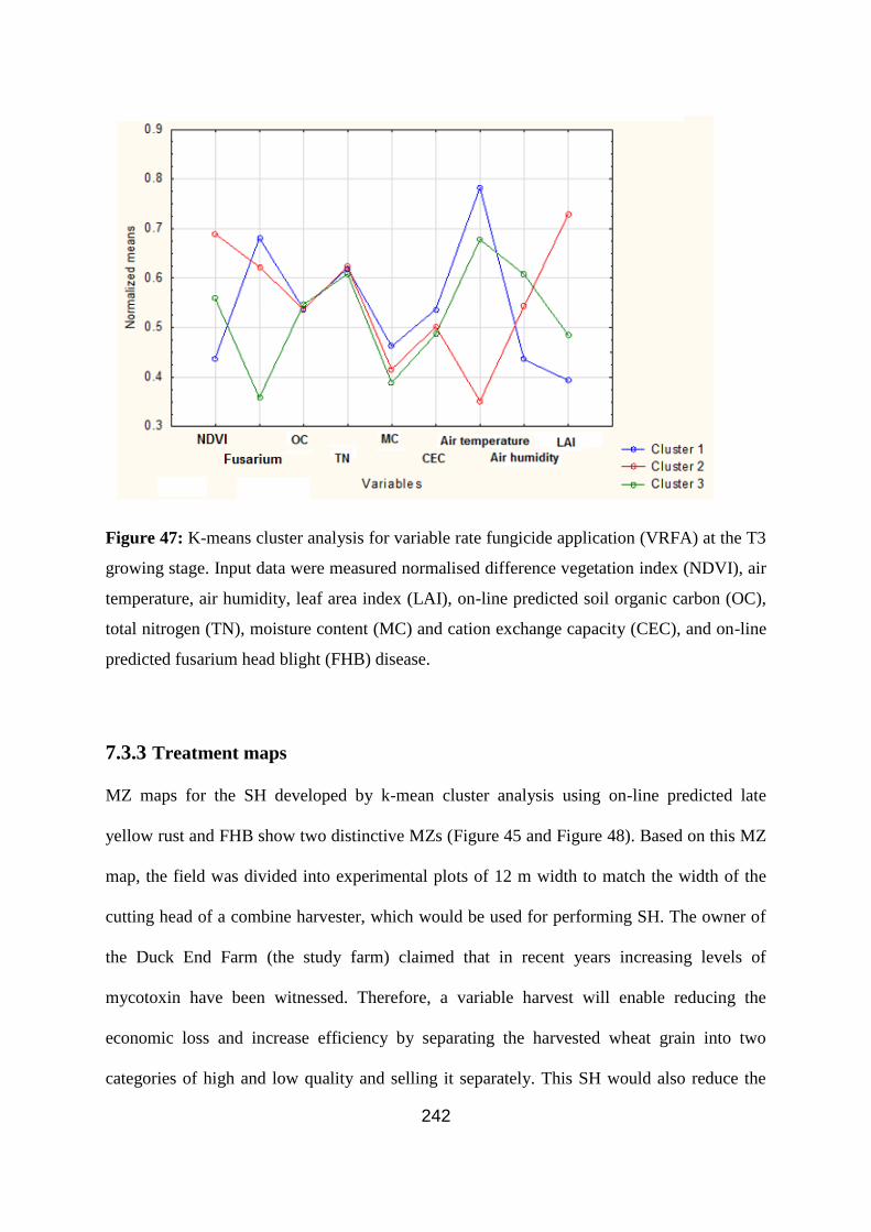
242


growing stage. Input data were measured normalised difference vegetation index (NDVI), air

temperature, air humidity, leaf area index (LAI), on-line predicted soil organic carbon (OC),

total nitrogen (TN), moisture content (MC) and cation exchange capacity (CEC), and on-line

predicted fusarium head blight (FHB) disease.

7.3.3 Treatment maps

MZ maps for the SH developed by k-mean cluster analysis using on-line predicted late

yellow rust and FHB show two distinctive MZs (Figure 45 and Figure 48). Based on this MZ

map, the field was divided into experimental plots of 12 m width to match the width of the

cutting head of a combine harvester, which would be used for performing SH. The owner of

the Duck End Farm (the study farm) claimed that in recent years increasing levels of

mycotoxin have been witnessed. Therefore, a variable harvest will enable reducing the

economic loss and increase efficiency by separating the harvested wheat grain into two

categories of high and low quality and selling it separately. This SH would also reduce the

243

mycotoxin levels in grain and toxic influences on human health. MZ1(Figure 48) associated

with cluster 1 in Figure 45 is with high FHB presence and high risk for mycotoxin presence

and toxic effects on human health, whereas MZ 2 associated with cluster 2 is of low risk of

mycotoxin presence and the grain can be sold at a higher price than that in MZ1.

Figure 49 and Figure 50 illustrate spatial distribution MZs and the division of the field area

into 24 m width plots, responding to a fungicide sprayer boom width of 12 m either side of a

tramline. West et al. (2003) discussed the highest benefit to variable fungicide applications is

in diseases, which make a small number of large areas, with a boom containing separately

controllable sections. However, at the commercial farm this technology was not available, so

the VRFA maps are based on 24m widths (with the standard being 12m on either side). MZ 2

in Figure 49, associates with cluster 2 in Figure 46 indicates low disease in the centre,

whereas MZ 1 at the field hedges linked with cluster 1 refers to high yellow rust. It’s

proposed that this MZ map is adopted for VRFA for T1 and T2 growing stages. The MZ map

(Figure 50) for VRFA for the T3 application stage shows three MZs of high (northern and

southern edge areas), medium (east and west edge areas) and low (central areas) FHB spread,

associated with cluster 1, cluster 2 and cluster 3, respectively (Figure 47). The general shape

of the MZ map here (Figure 43) is similar to that of the one developed for yellow rust for T1

and T2 application times (Figure 46), but the former is divided into three MZs not two as for

the latter map.

244

Figure 48: Management zone (MZ) maps for selective harvest (SH), The map on the left

shows high disease infection (MZ 1) and low disease infection (MZ 2) which is obtained by

k-means clustering that included on-line predicted fusarium head blight (FHB) and late

yellow rust. With the right map showing high and low infection zones on the right, with the

field being split into plots of 12 m (due to the combine harvest cutting head).

245


the T1 and T2 growing stages. The map on the left show low yellow rust (MZ 1) and high

yellow rust (MZ 2), which is obtained by k-means clustering that included, measured canopy

properties (normalised difference vegetation index (NDVI), air temperature, air humidity, and

leaf area index (LAI)), on-line predicted soil (organic carbon (OC), total nitrogen (TN),

moisture content (MC) and cation exchange capacity (CEC)), and on-line predicted early

yellow rust disease. With the right map showing high and low infection zones on the right,

with the field being split into plots of 24 m (due to the boom width).

246


the T3 growing stages, The map on the left show high fusarium head blight (FHB) (MZ 1)

and medium FHB (MZ 2), and high FHB (MZ3), which is obtained by k-means clustering

that included, measured canopy properties (normalised difference vegetation index (NDVI),

air temperature, air humidity, and leaf area index (LAI)), on-line predicted soil (organic


(CEC)), and on-line predicted FHB. With the right map showing high and low infection

zones on the right, with the field being split into plots of 24 m (due to the boom width).

Grain is commonly tested for mycotoxin content at or post-harvest, where time consuming

and expensive laboratory tests are needed (HPLC, serological rapid tests, Fast-DON-

ELISA-test) (Thate et al., 2008). Fusarium damaged wheat grains can be detected by

hyperspectral imaging with an accuracy of up to 95%. Mycotoxin content detection

depended on important wavelengths in the NIR range of 1204, 1365 and 1700 nm, whereas

spectral differences in the ranges between 1425 to 1440 nm and 1915 to 1930 nm are

247

important for the detection of mycotoxin DON in the grain (Delwiche 2003; Singh et al.,

2007; Peiris et al., 2009). However, it is uncertain to how well different fungi may be

distinguished using NIR (Peiris et al., 2009).

The downgrading of grain can be in response to a percentage of the harvested grain, which

reduces the quality or surpasses mycotoxin health limits. However, the BoMill TriQ

(Bowmill AB, Sweden) was studied and showed the capability in bulk separating good

quality wheat grain from downgraded fusarium infected grain, using crude protein content

(Kautzman et al., 2015). With the increased awareness of food security, and the knowledge

that one third of food is currently lost or wasted, innovative studies are needed to maximise

yields reaching the market (Gustavsson et al., 2011).

7.3.4 Economic benefits

Table 35 summarises the yield and average disease development in each MZ. For SH, the MZ

2 (low disease pressure shown in Figure 48 and Figure 45) associates with a higher average

yield (8.2 tha-1) and lower average late yellow rust (1.9) and FHB (0.54), as compared to MZ

1 (6.9 tha-1

, 2.9 and 0.87, respectively). Similarly, for VRFA at T1 and T2 growing stages,

MZ 2 (lower early yellow rust pressure shown in Figure 46 and Figure 49) is associated with

higher average yield (8.3 tha-1

) and lower early yellow rust pressure (1.2), as compared to MZ

1 (6.7 tha-1

and 2.2, respectively). For the variable fungicide application at the T3 growing

stage, the MZ 3 (lowest FHB pressure as shown in Figure 47 and Figure 50) has the highest

average yield (8.3 tha-1

) and lowest FHB (0.54), followed by MZ 2 and MZ 1, respectively

(Table 35). The consistent link between the yield and disease pressure in the three studied

248

cases proves the correct classification of the field area into proposed MZs, so that MZs with

high disease pressure associate with low yield and vice versa.

Table 35: Statistics of yield and disease pressure (fusarium head blight (FHB), early and late

yellow rust (YR)) of each management zone (MZ), for the variable rate fungicide

applications (VRFA) at growing stage T1 and T2 (which consider soil properties, canopy

properties and early yellow rust); at growing stage T3 (which consider soil properties, canopy

properties, and FHB); for the selective harvest (SH) (late yellow rust and FHB). For the VR

T1 and T2 applications two MZ are considered; MZ1 (high yellow rust disease) and MZ2

(low yellow rust disease). For the VR T3 applications three MZ are considered; MZ1 (high

FHB disease) and MZ2 (medium FHB disease) MZ3 (low FHB disease). SH considers two MZ;

MZ1 (lower quality crop) and MZ2 (higher quality crop).

MZ Total

cluster

area, ha

Total

yield, t

Average

Yield,

tha-1

Average

early YR

Average

late YR

Average

FHB

SH MZ1 4.5 33.2 6.9 NA 2.9 0.87

MZ2 6.3 51.9 8.2 NA 1.9 0.54

VR T1

and T2

MZ1 4.8 36.5 7.6 2.2 NA NA

MZ2 6 49.8 8.3 1.2 NA NA

VR T3 MZ1 3.6 26.3 7.3 NA NA 0.8

MZ2 3.2 25.9 8.1 NA NA 0.71

MZ3 4 33.2 8.3 NA NA 0.54

249

The cost-benefit analysis of SH based on two MZs proposed in this work (Table 36) reveals

that a total saving of £519 per field (£48.05 ha-1

) would be gained, as compared to the

homogeneous harvest of the entire field area. This is because of the higher price that the SH

could provide for almost 59% of the field area with high quality of grains (FWI, 2016)

harvested from MZ2 with low FHB spread or low mycotoxin concentration.

Table 36: Cost-benefit analysis results comparing the selective harvest (SH) with the

homogeneous harvest (HH), based on on-line available prices of grain (FWI, 2016).

Management zone (MZ) 2 being of high quality grain (low fusarium head blight (FHB)

spread and low mycotoxin concentration) and MZ1 being of low quality grain (high FHB

spread and high mycotoxin concentration).

Harvest

type

MZ Total

area,

ha

Total

yield,

t

Price,

£/t

Price

per

MZ, £

Total

field

price, £

Difference

(HH – SH)

for field, £

Difference

(HH – SH),

per ha, £

SH MZ1 4.55 33.2 135 4482 12007.5 519 48.05

MZ2 6.35 51.9 145 7525.5

HH All

field

10.8 85.1 135 11488.5 11488.5

VRFA at the T1 and T2 growth stages aimed at protecting the third, second, and flag leaves

from foliar diseases, such as yellow rust. In this study, VRFA is split into two areas of high

and low disease pressure as compared to a homogenous rate application applied as the full

dose. The calculated potential benefit of the VRFA at the T1 and T2 was £95.04 per

application for this field (£190.08 for the T1 and T2 applications), with an average saving of

£8.8 per ha per application (or £17.6 for two applications) (Table 37), compared with the

homogeneous application. This is based on the assumption that yellow rust has a direct link

250

with grain yield, and that a lower dose would not have significant negative impacts. The

homogenous rate would consume 7.776 L Proline 275 per application for the 10.8 ha field,

whereas the variable rate would need 6.048 L, suggesting a potential reduction of 1.73 L per

application (or 3.46 L for the two applications). This reduction would sum up to a 22.24%

reduction in fungicide application by adopting the variable application method, as compared

to the homogeneous application.

The VRFA at the T3 application stage is usually an ear wash aimed at preserving grain

quality from diseases such as FHB. This application in the study field would be based on 3

rates according to the three MZ delineated by the k-mean clustering (Figure 47 and Table 37).

Treatments proposed are of full dose for the heavily infected MZ1, 75% dose for the medium

infected MZ2 and 50% dose for the low infected MZ3, compared to the full dose rate for the

homogenous application proposed for the entire field area. The per field potential saving of

the VRFA at the T3 growth stage is £191.2, with an average saving of £17.7 ha-1

(Table 37).

The homogenous rate would consume 21.6 l Adexar per 10.8 ha total field area, whereas the

VRFA would consume 16 l, with a potential reduction of 5.6 l per application, or 25.93% to

be expected by adopting the VRFA, as compared to the uniform application.

251

Table 37: Cost-benefit analysis results for variable rate fungicide application (VRFA) at T1

and T2 growth stages, and at T3 growth stage, as compared to homogeneous application

(HA). Management zones (MZs) 1, 2 and 3 refer to high dosage rate, medium rate and low

rate, respectively. Fungicide used is Proline 275 (£34 per litre) for T1 and T2 application and

Adexar (£55 per litre) for T3 application.

Total

area,

ha

Total

yield

Application

rate, lha-1

Price of

chemical

l-1

, £

Price of

chemical

ha-1

, £

Cost per

treatmen

t, £

Difference

(HA –

VR) for

field, £

Difference

(HA –

VR), ha-1

,

£

T1andT

2

MZ1

high

6 46 0.72 55

39.6 237.6 95.04 8.8

MZ2

low

4.8 39.8 0.36 19.8 95.04

HA 10.8 85.8 0.72 39.6 427.68

T3 MZ1

high

3.6 26.3 2 34

68 244 191.2 17.7

MZ2

mid

3.2 25.9 1.5 51 163.2

MZ3

low

4 33.2 1 34 136

HA 10.8 85.4 2 68 734.4

By combining he SH with the VRFA at T1 and T2 and at T3 application times, a potential

saving of £900.18 is expected for this field, which is an average of £83.35 per ha. It is

possible to consider both methods as a combined economic benefit as the SH is considering

the savings from preventing down grading of the grain, if the full field were to be collected

homogenously, whilst the variable fungicide applications consider the savings from fungicide

costs compared to a full homogenous rate. VRFA are here assumed to maintain the grain

252

quality and quantity by applying higher rates on needed areas, compared to a full rate, and not

improve the quality. VRFA would only be assumed to improve grain quantity and quality if

compared to a homogenous reduced or half rate. Thus, SH would still be required to separate

the higher quality grain from the lower quality areas. The current technology of fungal

disease treatment based on the CROP-meter offers economic benefits by just reducing

fungicide input, but does not necessarily increase crop quality or quantity (Ehlert et al.,

2003). The suggested methodology in the current work may lead to not only economic, but

environmental and social benefits. The potential reduction in the amount of fungicide applied

(Table 37) would lead not only to reducing the environmental impact due to reduced soil and

water contamination, but improve the quality of grain harvest, by targeting areas of risk to

fungicide pressure with the larger fungicide concentrations. The social benefit is associated

with less mycotoxin concertation in human consumed grain obtained with SH. This could be

considered from the other perspective, that if a field has generally a low disease spread, and

the farmer or agronomist would otherwise prescribe a half dose for the field, they can add a

full dose in the areas recognised to be at risk. The reason this is of interest is better control of

the disease (by applying higher rates on risk areas than lower rates homogenously), and

lowering the chance of the efficacy of the fungicide product being reduced in the long term,

as fungal strains adapt and develop increased immunity (FRAC, 2010).

There is a need to recognise the current work’s proposed method of SH and VRFA. However,

before the current work can be adopted in practice, further work is needed to account for

cost-benefit analysis, which includes the cost of data collection and application of the

process. The costs of implementing both SH and VRFA have not been discussed. It is

important to acknowledge that initially extra costs would be incurred in fuel consumption and

grain storage. However, if such methods prove to be beneficial, agricultural equipment could

253

be modified or developed to accommodate both methods, eliminating the need for additional

driving and grain storage trailers. Purchasing the equipment would have an initial cost, which

will vary depending on the specifications of the imager (size, wavebands, resolution, etc.),

with a low spatial and spectral resolution camera being more affordable. As the field

develops, options of leasing equipment are also increasing. Details on hyperspectral imager

costs are by request and vary between suppliers. For an imager with similar spec to the one

used in this study costs of around £10,000 should be expected. Whilst the cost of the

hyperspectral equipment has not been included in this study, through further work we aim to

investigate if the economic and environmental benefits would support the expense. However,

many of the issues that West et al. (2003) highlighted with predicting economic benefit are

still relevant today, with limitations of farming equipment being common i.e., boom length

and variable section control. Furthermore, costs of fungicide and prices of grain continue to

vary (FWI 2016). Predicting economic benefit becomes further taxing when considering the

increasing legislation on the choice of fungicides, mutations of fungicide resistant disease,

and the impacts of climate change, the efficacy of disease control, and the response to

fungicide treatment (Sung and Cook, 1981; De Vallavieille-Pope et al., 1995; Rossi et al.,

2001; Xu, 2003; Dufault et al., 2006; FRAC, 2010; Mielecki, 2011).

The current work assesses the use of high spatial resolution data to compare the economic

and environmental benefit of a VRFA and a SH to a conventional homogenous practice.

Whilst the study found initial economic savings of £83.35 per ha, the results are specific to

this field, crop and year. For a decision tool that would recommend a time of spraying and

VRFA, further components would need to be considered such as the use of air sampling for

the detection of airborne pathogens. West et al. (2008) combined air sampling with

polymerase chain reaction analysis, for the quantitative identification of Pathogens. A process

254

based model including climate data would create a robust decision tool, where parameters

could be considered relating to fungicide applications. In conventional farming, fungicides

are often applied in response to agronomists’ visual assessments. An example of prescribed

fungicides can be found in Appendix D. This study has highlighted the potential economic

benefit of the disease mapping methodology for VRFA and SH, compared to conventional

methods. However, further work should consider a combination of disease mapping,

pathogen sensor technologies, and temporal data (such as plant growth, and climate data) in a

process based model, for production of a robust decision tool.


The study explores the virtual cost-benefit analysis results of variable rate fungicide

applications for yellow rust, compared to the conventional method of homogenous full rate

application. This analysis has also included selective harvest against homogeneous harvest

when fusarium head blight disease protection concerned. The virtual total calculated profit of

combining selective harvest and variable rate fungicide application is £83.35 per hectare and

an environmental benefit of fungicide reduction of was found to be around 25%. Air

sampling for pathogens should also be considered in future work for a dynamic decision tool

of disease site specific management.

255

8 Conclusions and further work

Chapter Synopsis;

This chapter includes a short discussion about some recent publications, revisits the

hypotheses, aims, and objectives of the thesis, and discusses and highlights the previous

chapter’s conclusions and further work. Drawing attention to the recognised gaps in

knowledge, and how the thesis has tried to address them. Discussing the potential further

work which could take the data introduced and discussed in this thesis, to further develop and

full fill the gaps in knowledge.

8.1 Recent publications

Bhattarai et al. (2017) used Multivariate and cluster analysis in distinguishing soil limiting

factors and grouping types of coffee farms. Where they attempted to understand variations

and yield gaps from farm resources. Highlighting multiple farm variations influencing yield

variations, soil properties were one of the major contributors in yield variability, specifically

noting the (Ca + Mg)/K ratio, and soil Fe content. However, Chenu et al. (2017), encourages

the use of process based models for understanding crop growth and yield gaps, which should

be based on worldwide climate data, soil properties and characteristics, cropping practices

and local conditions. Supporting that the studies on yield limiting factors (in chapter 3),

whilst interesting for the field studied to understand field level yield variations, process based

models are required for a more global application.

Pantazi et al. (2017) were capable of distinguishing between yellow rust and nitrogen stress at

canopy level with an accuracy of over 95% for three techniques of hierarchical self-

organizing classifiers. Which highlights the importance of distinguishing between biotic and

abiotic factors and the potential of a hyperspectral imager to do so. Masri et al. (2017) found

256

the use of thermography was useful in detecting the advancement of FHB after inoculation.

Finding that air temperature to fusarium infected ears was negatively correlated. This would

be an interesting aspect to involve and improve FHB detection which was investigated in this

thesis (chapters 5, 6 and 7).

A review by Mahlein (2016), discusses the use of optical sensors for the recognition of crop

disease. Thermography and chlorophyll fluorescence is sensitive to early stress symptoms in

plants, however, they are not alone capable of being used for specific disease detection.

Suggesting a data fusion and combined use with RGB images and hyperspectral techniques,

highlighting the development process that the imaging technologies need to undergo. This is

a subject touched upon through the thesis, particularly chapter 4, which focuses on the current

limitations of applying on-line a proximal hyperspectral imager, to a cereal crop canopy.

Mahlein (2016) encourages future use of date fusion, from different sensors in the

understanding of the plant-pathogen systems. Whilst this thesis attempted the use of multiple

sources of data, and the fusion of data (chapter 7) for a greater understanding of disease

management, there are still many more technologies that could be incorporated in future

work. It also highlights the potential use of different platforms of data, which could be

utilised to overcome some of the current limitations.

8.2 Objectives and chapter conclusions

The Introduction in Chapter 1 brings attention to areas of particular interest, which have

limited published knowledge, they are discussed further in chapter 2. This chapter aims to

summarise the conclusions found in the previous chapters and how they fulfil the highlighted

objectives.

257

The aim of this study;

To apply a hyperspectral imager on-line application to cereal crop disease recognition,

critically appraising the existing technology. It also investigates a novel modelling approach

for quantifying the crop yield limiting factors. The key aim is to produce management zone

maps for variable rate fungicide application and selective harvest, in response to crop disease

pressures, soil characteristics and micro-climatic conditions.

Yellow rust and fusarium head blight (FHB) was selected to be the two diseases studied

through the thesis, as they have a history of occurrence at the studied farm. The selection also

meant that both a significant foliar disease (yellow rust) and a significant ear disease (FHB)

could be included in the study.

This aim has been broken into five objectives, which are stated and discussed below;

8.2.1 Objective 1:

“To critically appraise different approaches, and identify the best configuration for the

hyperspectral imaging systems for in-situ and on-line field measurement of crop disease.”

Conclusions of Chapter 4;

Whilst progress has been made in disease recognition in the field, there are few on-line (in-

situ and applied with a moving platform, e.g. an agricultural vehicle) yellow rust specific

identification systems and none for fusarium head blight (FHB). Objective 1 was designed to

address this observation in literature. And is addressed within the literature review and further

assessed in chapter 4; “optimising the configuration of a hyperspectral imager for on-line

measurement of wheat canopy”. The literature review summarises the current approaches and

developments in on-line spectroscopy and hyperspectral imaging. Chapter 4 focuses

specifically on hyperspectral imaging and evaluates the individual and interaction effects of

258

the system, and the parameters that are of interest. Resulting in an optimal configuration for a

high quality spectra assessed by signal-to-noise ratio (SNR) for an on-line hyperspectral

imager, the influence of on-line measured soil moisture content (MC) and total nitrogen (TN)

on SNR was also evaluated. This allowed for the following conclusions to be drawn:

1) The integration time followed by the camera height and camera angle appeared to

have the largest influence on the SNR. As integration, increased SNR increased,

however a long integration time (>50 ms) was of a negligible influence and only

slightly increased the SNR, but result in spectral saturation, hence should be avoided.

An increase in camera angle benefitted SNR, however a decrease in camera height

benefitted SNR.

2) The PCA similarity map showed that the light height and distance have a strong

correlation with each other but a minimal influence on SNR.

3) Both on-line measured MC and TN were found to have significant effects on the SNR

of the wheat canopy spectra at 95% confidence. The on-line soil measurements

revealed stronger spatial similarity between the hyperspectral SNR and MC maps

(kappa value = 0.75), which was attributed to soil deformation below the tractor tyre.

4) The variable reflected light intensity captured by the different pixels across the line

imagery is an interesting factor to take into account, due to the impact of varying

camera height during the on-line measurement. Whilst the solution suggested here is

appropriate, it is camera specific.


(vibration, bounce in the boom, and soil deformation during the on-line measurement) by the

further investigation in spectra pre-processing. It is also planned to implement these

259

hyperspectral measurement configurations for on-line measurements of crop canopy for

detection of crop health and disease presence, which is approached in chapters 5 and 6.

8.2.2 Objective 2:

“To evaluate the individual and interaction effects of parameters limiting crop growth and

yield”.

Conclusions of chapter 3;

To the best of our knowledge, no previous studies have utilised high sampling resolution data

on multi-soil properties collected with a vis-NIRS on-line sensor to quantify crop yield

limiting soil factors using a VNRX model. Assessing the contribution of disease collected

through high resolution hyperspectral imaging, in comparison with nutrient factors collected

through high resolution vis-NIR as a yield limiting factor has not yet been approached in

literature. Whilst studies have been undertaken to assess yield limiting factors, few have used

high resolution spectroscopy. Studies in the area have historically used sub plots within a

field, as (Sylvester-Bradley and Kindred, 2009). An alternative to this would be to consider

the entire field, this, however, requires a higher sampling resolution of environmental

parameters, crop disease, and yield mapping. This is partially addressed by Objective 2,

approached in chapter 3, yield limiting factors. This chapter is presented in two parts. Part 1

“A new non-linear parametric modelling method to quantify influence of soil properties on

crop yields - Methodology”, which focused towards the quantification of soil related yield

limiting factors. This was based on a parametric modelling technique of a Volterra non-linear

regressive with eXogenous inputs (VNRX) technique which was applied and compared with

a random forest technique through two cropping seasons of 2013 and 2014. And Part 2 “A

new non-linear parametric modelling method to quantify influence of soil properties on crop

yields - Application to on-line soil data” where the parametric modelling technique of a


260

Volterra non-linear regressive with eXogenous inputs (VNRX) technique was applied to

NIR-Vis on-line collected soil data.

Concluding that;

1) The results of VNRX-LN model accounting for both linear and non-linear interactions

explained 52.2% and 50.7% of yield variation in 2013 and 2014 respectively, which

were much higher than those obtained with VNRX-L (total contributions of 19.15%

and 8.5% in 2013 and 2014, respectively), accounting for the linear interaction only.

2) The contribution of the RF model produced the highest contribution of 55.6% in

2013, which dropped down considerably to 45.8% in 2014.

3) The VNRX-LN model indicated that P, CEC and OC are the highest contributors to

oilseed rape yield variability in 2013 and P, Na and OC to wheat yield variability in

2014. TN was surprisingly a small contributor particularly in 2013. It was observed

that P and OC are consistently the highest contributors to yield variability through all

VNRX models. Light, N, P, and K are the main factors affecting crop yield, the

results in this chapter are specific to the yield variability and were attributed to the

properties being more limited in the field, it did not measure for factors that were not

limiting (such as N which was applied as ferteliser).

4) The RF analysis presented OC and TN to be the highest contributors to yield in both

studied cropping seasons.

5) The RF and VNRX-LN models were comparable in predicting contribution of soil

properties to yield variation, with VNRX-LN being slightly higher, however the RF

model provided a higher consistency for individual soil property importance.

6) Yield variability for the VNRX-LN model showed a higher variability contribution

from P and K and Na than the RF model, whilst P and K contribute to yield (P has a

261

direct link with crop yield), Na can have negative effects on moisture uptake, and can

inhibit enzyme activities.

The RF model is an established method, whilst the application of the VNRX-LN was a novel

approach introduced in this thesis. It’s for these reasons that we will conduct further studies

in quantifying yield variability with the new VNRX-LN method.

The further work highlighted in the first part of this subchapter included the use of high

resolution data on soil chemical properties, which is addressed in part two of the chapter;

which further explores the objective of yield limiting factors within the field, drawing the

following conclusions:

1. The VNRX-LN model can be successfully used to quantify the influence of multi-soil

properties, collected at high sampling resolution with an on-line soil sensor, on crop

yield.

2. The effect of soil properties on crop yield varied with soil property, with the largest

contribution observed for CEC, Mg and TN, with error reduction ratio contribution

(ERRC) values of 14.6%, 4.69% and 1%, respectively.

3. The overall contribution of the eight soil properties sums up to an ERRC value of

23.21%. This value was found to be surprisingly low, a large part of the studied field

suffers from a drainage problem, and this is thought to have masked some of the

effects of soil properties on crop yield, and contributed to the low value.

The application of a VNRX to soil property, yield and NDVI data has been applied in chapter

3 part 1 and 2. Showing there is still a significant variability in yield and NDVI, that has not

been accounted for, the further work is to apply the method to more study sites and include

other variables. Sites of variable Nitrogen should also be considered, as the model is limited

to detecting the influence of limited and variable properties on the yield. This is believed to

262

be the main reason for the impact on yield variability from Mg. Appendix A demonstrates the

initial results of disease (late yellow rust and FHB) contribution to yield and NDVI

prediction, which is the same 10 ha field considered in chapter 7. Though in this model, soil

properties were reduced to just 4 properties (OC, TN, MC, CEC) and had little impact on the

yield and NDVI predictions, this is understandable as in chapter 7 the same properties are

reviewed and had little variation through the field. Reinforcing that variable/precision

agriculture is only appropriate for non-homogenous crop stands.

8.2.3 Objective 3:

“To create a spectral library using hyperspectral data to identify and quantify specific crop

diseases (yellow rust and fusarium head blight) independent from water stresses”.

Conclusions of Chapter 5;

The monitoring and detection of stress and diseases in plants is vital for sustainable

agriculture practice. This observation was considered best approached by first developing a

technique for disease recognition independent of water stress, and is captured by objective 3

“Chapter 5; Hyperspectral measurements of yellow rust and FHB in cereal crops: Part 1:

Laboratory study”, addresses this objective by exploring the potential of a hyperspectral line

imager (400-750 nm) with the use of linear partial least squares regression (PLSR) analysis,

concluding 5 main points:

1) The standard deviation (SD) of the wavelength range from 500 to 650 nm and the

squared difference between 650 nm and 700 nm are of particular interest in

discrimination between healthy, and yellow rust or FHB infected sites in a wheat and

barley canopy. With the lowest 500-650 nm SD, and highest 650-700 nm squared

difference being attributed to healthy crop, a noticeably lower 650-700 nm squared

263

difference attributed to yellow rust infected crop, and a noticeably higher 500-650 nm

SD attributed to FHB infected crop.

2) Yellow rust models performed more accurately than FHB models, which was

attributed to the fact that yellow rust is a foliar disease, which has larger chance to be

captured by the hyperspectral line image, as compared to FHB being head disease that

appear late in the growing season.

3) Scale-based assessment of yellow rust, based on 0-5 classes, produced a marginally

more reliable model performance than the percent coverage data set.

4) Modelling of yellow rust in wheat is rather more accurate than in barley, which is

possibly due to wheat having larger leaves. Prediction results indicated moderate

prediction accuracy for barley (RPD = 1.80 - 1.97; R²= 0.69 – 0.77) and good

accuracy for wheat (RPD = 2.04 - 2.25; R²= 0.77 – 0.80). Therefore, it can be

concluded that yellow rust can be detected with appreciable accuracy and reliability in

both wheat and barley. Whilst the Logit scale applied for yellow rust for wheat and

barley was able to distinguish between high and low (RPD = 1.2 and R² = 0.43, and

RPD = 1.4 and R² = 0.79, respectively)

5) Results for FHB prediction were of moderate accuracy for wheat (RPD = 1.5; R²=

0.57) and able to distinguish between high and low values (RPD = 1.36; R²= 0.5) for

barley, suggesting the need for a more effective measurement and modelling

approaches for barley. FHB models were able to predict FHB infection severity, to an

accuracy of low and high infection. Further work should be done to enable assessment

of % FHB coverage.

The laboratory trials in this study have been designed to emulate a field. The data used in the

models was all collected from the wheat and barley trays, designed to simulate a field

264

canopy, so the variance of reflectance due to canopy is included in the models. Whilst other

properties such as illumination angle, view positions, shadows, plant species, maturity and

phenology can be controlled under the laboratory conditions, these parameters will have

considerable influences under field conditions. Their on-line application is considered in

chapter 6 which is the second part of this study.

8.2.4 Objective 4:

“To implement the hyperspectral imager for on-line detection and mapping of the spatial

distribution of yellow rust and fusarium head blight in winter wheat and barley”.


To the best of our knowledge, there are few on-line spectral recognition systems, which are

capable of being disease specific for yellow rust, and none for FHB. Presenting a gap in

knowledge for an on-line hyperspectral recognition system, capable of differentiating

between water stressed, yellow rust and FHB infected crops. In addition to the necessity of an

on-line disease recognition system, it has been reported that a greater occurrence of fungal

diseases is observed in denser canopies, although a conclusive regression has not been

obtained. This was approached in chapter 6 “Hyperspectral measurements of yellow rust and

FHB in cereal crops: Part 2: on-line field measurement” to obtain objective 4. The chapter

considers the potential of a hyperspectral line imager (400-750 nm) for the on-line

measurement and mapping of yellow rust and FHB in wheat and barley, and discusses the

impact of soil moisture and crop density on the disease distributions. Results reported

allowed the following conclusions to be made;

1. On-line hyperspectral measurement and mapping of yellow rust and FHB is possible

with moderate accuracy in barley and good accuracy in wheat.

265

2. Yellow rust is more accurately measured, based on models developed with visual

disease assessment, whereas assessment of FHB required photo interpretation to

provide more accurate measurement. This is believed to be due to fusarium symptoms

on ears being better captured in an RGB image, than yellow rust attacking the foliage.

3. Photo interpretation-based on-line measurement of FHB was classified as good in

wheat (RPD = 2.27; R²= 0.82) to moderately accurate in barley (RPD = 1.56; R²=

0.61), whereas good (RPD = 2.5; R²=0.81 in wheat) and moderate (RPD = 1.82; R²=

0.72 in barley) measurement accuracy was achieved for yellow rust by means of

visual scale assessment.

4. On-line maps developed in this study support that in large fields, disease

concentration is higher at the edges of the field and then expand towards the inner

parts through the growing season. However, the findings suggest that disease

pressures in the smaller field were more evenly distributed across the entire field area,

than the larger fields.

5. A PLSR model developed for recognition of FHB and yellow rust in wheat, can be

applied to barley with a slight reduction in accuracy.

6. Soil texture and moisture content affect and canopy density and subsequently

humidity, which in turn affect FHB and yellow rust spatial pattern.

The suggested further work highlighted by this chapter, is approached in chapter 7

“Management zone maps for variable fungicide application and selective harvest”. The

suggestions being; to evaluate the impact of on-line maps of yellow rust and FHB on site

specific recommendations of fungicides, and to adopt a management-zone concept for site

specific applications and selective harvest.

266

8.2.5 Objective 5:

“To adopt a data-fusion approach for delineation of management zones for variable rate

fungicide application and selective harvest.”


Diseases such as yellow rust can vary considerably in very short distances and reduce yields

by up to 7 tha-1

(Bravo et al., 2003). The crop density could reflect multi-stresses occurring at

the same time e.g. water, nutrients, temperature, disease etc. crop density is also dependent

upon the climatic conditions each year and associated crop variety. The CROP-meter

optimizes fungicide control by reducing fungicide input and maintains control, but does not

increase crop quality or quantity, highlighting an un-met demand where quality and quantity

of yield is improved by considering environmental parameters. To the best of our knowledge

there are no proposed methods of precise management of fungal diseases, which takes into

account a high spectral sampling resolution, of disease pressure and canopy and soil

properties. This was approached in chapter 7 “Management zone maps for variable fungicide

application and selective harvest” to obtain objective 5.

The study proposed the delineation of management zone maps for variable rate fungicide

application and selective harvest in one field with wheat subjected to yellow rust and FHB

spread. A k-mean cluster analysis was explored to divide the experimental field into

separated clusters (zones) based on on-line predicted FHB and yellow rust (measured with a

hyperspectral imager), on-line predicted soil total nitrogen (TN), organic carbon (OC),

moisture content (MC) and cation exchange capacity (CEC) (using an on-line visible and

near infrared (vis-NIR) spectroscopy sensor), measured crop canopy normalised difference

vegetation index (NDVI) and leaf area index (LAI), yield, and air humidity and temperature.

The main findings highlight the following conclusions:

267

1) The field was divided into a different number of management zones depending on the

input data layers used for the k-mean cluster analysis. Management zones with high

disease pressure associated with low NDVI and LAI, and high air temperature and

vice versa for low disease pressure management zones.

2) Average overall reductions in fungicide of 22.24% (for T1 and T2 growth stages

applications) and 25.93% (for T3 growth stage application) were calculated for the

entire field area of 10.8 ha for variable rate fungicide application as compared to

homogeneous application.

3) The selective harvest of high quality grain from low quality grain would result in less

risk of mycotoxins affecting human health.

4) The virtually total calculated profit of combining selective harvest and variable rate

fungicide application is £900.18 per field or £83.35 per hectare, divided into selective

harvest of £48.04 ha-1

, variable rate fungicide application at T1 and T2 growth stages

of £17.6 ha-1

each and; T3 £17.7 ha-1

).

Future work should focus on the implementation of the proposed methodology in the field, to

allow actual cost-benefit analysis to be carried out. The cost of collecting the multi-layer data

on crop and soil characteristics and microclimatic conditions and yield responses should be

accounted for in the cost-benefit analysis. Additional sensors could be involved, to produce a

more robust decision support tool, and additional vegetation indices could be considered.

268

8.3 Hypothesis consideration

The thesis suggested two hypotheses;

“Proximal hyperspectral imagery is capable of detecting specific crop diseases (e.g.

Fusarium head blight and yellow rust) and applied on-line can be used to quantify their

distribution pattern.”

And;

“Multi-sensor and data fusion of crop disease, and canopy and soil properties

collected at high sampling resolutions, contribute to the quantification of the yield limiting

factors, which can be utilised in variable management zones.”

The first hypothesis has been proven true for the detection of only two diseases. To fully

understand if the disease recognition is specific further diseases such as septoria should be

considered. This would allow the current system to be tested on its capability to distinguish

specific diseases, not just on the presence of a particular symptom, as septoria disease can

also cause similar chlorosis symptoms to that of yellow rust. Chapters 5 and 6 show that with

suitable disease assessments and PLS regressions, with hyperspectral data collected at an

optimal configuration (chapter4), a good accuracy of prediction can be obtained for yellow

rust infection and a moderate accuracy for FHB infection on-line.

The second hypothesis has also been found true (though some variability still needs to be

accounted for, such as disease and pest presence) through chapter 3, where VNRX modelling

was utilised on soil properties to predict Yield (and further explored in the data provided in

Appendix A), and the production of management zones through K-means clustering in

chapter 7, where the potential cost benefits of applying the selective harvests and variable

fungicide applications are discussed.

269

8.4 Contributions to knowledge

Methods of yield variability have been assessed and found a possibility of attributing 55.6%

(through VNRX modelling) and 52% (from RF modelling) of yield variability, from soil

properties alone, both having a significance level of <0.01. The further work for this is to

include disease data. Initial findings for this are provided in Appendix A, where they show a

significant contribution of yield and predictions based on NDVI can be attributed to late

yellow rust and FHB presence. A yield gap exists between current production and the

maximum yield potential of a crop. Further work with detecting and mapping the crop and

soil qualities, could help towards better management of crop limiting factors, to reduce the

current yield gap.

An optimal configuration for the application of a push broom hyperspectral imager to a cereal

crop canopy has been suggested. With configurations of 0.3 m, 1.2 m, 1.2 m and 10° values

of camera height, light height, light distance and camera angle, respectively. The optimum

integration time for on-line field measurement was 50 ms.

A hyperspectral technique coupled with PLSR can be successfully used for the estimation of

yellow rust in winter wheat and barley canopy. At tray level ratio of prediction deviation

(RPD) values of 2.25 (R²= 0.80) and 1.97 (R²=0.77) were calculated for wheat and barley

based on scale measurement, and 2.04 (R²=0.77) and 1.80 (R²=0.69) for percentage coverage,

respectively, which were classified as good accuracy in wheat and as moderately accurate in

barley. FHB detection, results were less successful RPD = 1.5 (R²=0.57) (just at the edge of

moderately accurate) in wheat and RPD= 1.36 (R²=0.5) (differentiate between high and low

values) in barley). However, the disease recognition needs further applications to establish its

reliability in the presence of additional crop diseases, such as septoria. Currently, it was

trialled upon yellow rust (a foliage disease) and FHB (an ear disease), further applications

270

should be made on detecting these whilst other diseases are known to be present. i.e.

detection of yellow rust in a yellow rust and septoria affected crop stands. This would allow

greater understanding if the system is capable of being disease specific.

It was found that photo interpretation was the most applicable and accurate for on-line

measurement of FHB, which was classified as a good to moderately accurate recognition

method, since the ratio of prediction deviation (RPD) values were 2.27 (R²=0.82) for wheat

and 1.56 (R²=0.61) for barley. For yellow rust significantly improved results for the PLSR

models were obtained when the ground truths were based on visual scale assessment, where

model performance was classified as moderately accurate in barley (RPD = 1.82; R²=0.72)

and good in wheat (RPD = 2.5; R²=0.81).

A method of selective harvest has been suggested, with potential cost benefits (under certain

assumptions) with Financial savings of £900.18 for the 10.8 ha field, with an average of

£83.35 per hectare (harvest = £48.05 ha-1

; T1andT2 = £8.8 ha-1

each and; T3 £17.70 ha-1

)

8.5 Further work

The chapters have addressed the objectives, and aimed towards contributing to the current

gaps in knowledge. However, each chapter has highlighted further work, which would

contribute to knowledge. These have not been obtained in this thesis due to either being

outside of the study’s focus, or due to time restraints. The recommended further work is

summarised in 3 parts; yield limiting factors, hyperspectral imaging of disease, and

management zones.

8.5.1 Yield limiting factors

Further work is suggested to validate the concept of Volterra Non-linear Regressive with

eXogenous inputs (VNRX) models to study and quantify the effect of soil properties on crop

271

yield, on a larger number of fields. Where other affecting parameters such as, crop diseases

(from the methods highlighted in Chapter 5), environmental factors (e.g., pests, topography,

microclimate conditions), and soil physical properties (e.g., soil compaction, hydraulic

conductivity, etc), should be considered in the analysis, to take into account the full picture of

yield limiting factors.

8.5.2 Hyperspectral imaging of disease


(vibration, bounce in the boom, and soil deformation during the on-line measurement) by

investigating further the variations of spectra pre-processing.

8.5.3 Management zones

This chapter suggests theoretical methods of selective harvest and fungicide application,

using collected data from soil and canopy properties, and disease data compared to harvest

data. Suggesting potential economic and environmental benefits under certain assumptions.

The further work will be focused on applying these methods in practice. Air sampling for

pathogens should also be considered for a dynamic decision tool, for disease management.

8.6 Concluding remarks

The homogenous application of chemicals throughout a field to control crop disease has been

in practice in agriculture for nearly a century. There is an ever-growing demand for food. As

the population growth continues to escalate, and the competition for agricultural land for

alternative use rises, the pressure for maximizing yield increases. Fungicides are being

removed from the market due to environmental concerns, they, along with disease resistant

strains of crop, are succumbing to mutating fungal strains. It has become imperative to move

away from conventional farming methods, and find a more sustainable approach. Whilst

272

research into alternative methods, such as precision agriculture is becoming more of a focus,

there are still limitations, gaps in knowledge, and the application of this knowledge. Whilst

it’s been recognised for a while that optical technologies are suitable for disease detection

systems, no sensor-based technologies for disease detection commercially exist, that are

directly related to a diseases presence within a field. This thesis has focused towards moving

the technology to the field, to understand the yield limiting factors at high sample rates,

recognise disease (yellow rust and FHB) in cereal crops (winter wheat and winter barley) and

apply the technology on-line. This has been combined into approaches of variable fungicide

applications and a selective harvest approach, which will hopefully contribute towards

confidence in variable applications, and quantify the potential environmental and economic

benefits.

273

REFERENCES

Agegnehu, G., Nelson, P., and Bird, M. (2016). Crop yield, plant nutrient uptake and soil physicochemical

properties under organic soil amendments and nitrogen fertilization on Nitisols. Soil and Tillage Research, 160,

pp. 1–13.

Agrios, G.N., (1997). Plant Pathology Academic Press San Diego. California, USA, 390.

AHDB, 2016, Fungicide performance in oilseed rape, Agriculture and Horticulture Development Board

publications

Al Masri, A., Hau, B., Dehne, H.W., Mahlein, A.K. and Oerke, E.C., (2017). Impact of primary infection site of

Fusarium species on head blight development in wheat ears evaluated by IR-thermography. European Journal of

Plant Pathology, 147(4), pp.855-868.

Ali M.A., Hussain M., Khan M.I., Ali Z., Zulkiffal M., Anwar J., Sabir W., Zeeshan M. (2010). Source-sink

relationship between photosynthetic organs and grain yield attributes during grain filling stage in spring wheat

(Triticum aestivum). International Journal of Agriculture and Biology, 12: pp. 509–515.

Alvarez, A.M., 2004. Integrated approaches for detection of plant pathogenic bacteria and diagnosis of bacterial

diseases. Annual Review of Plant Pathology 42, 339–366.

Anand, A., Zhou, T., Trick, H.N., Gill, B.S., Bockus, W.W. and Muthukrishnan, S. (2003). Greenhouse and

field testing of transgenic wheat plants stably expressing genes for thaumatin‐like protein, chitinase and

glucanase against Fusarium graminearum. Journal of Experimental Botany, 54(384), pp.1101-1111.

Andersen AL. (1948). The development of Gibberella zeae head blight of wheat. Phytopathology 38, pp.595–

611.

Asner, G. P. (1998). Biophysical and biochemical sources of variability in canopy reflectance. Remote sensing

of Environment, 64(3), pp.234-253.

Backhouse, D., (2014). Global distribution of Fusarium graminearum, F. asiaticum and F. boothii from wheat in

relation to climate. European journal of plant pathology, 139(1), pp.161-173.

Bai G, Shaner G (1994) Scab of wheat: prospects for control. Plant Dis 78: pp.760–766

Baligar, V., Fageria, N., and He, Z. (2001). Nutrient use efficiency in plants. Communications in Soil Science

and Plant Analysis, 32(7-8), pp. 921-950.

Barbedo, J. G., Tibola, C. S., and Fernandes, J. M. (2015). Detecting Fusarium head blight in wheat kernels

using hyperspectral imaging. Biosystems Engineering, 131, pp. 65-76.

Bauriegel, E., Giebel, A., Geyer, M., Schmidt, U. and Herppich, W.B. (2011). Early detection of Fusarium

infection in wheat using hyper-spectral imaging. Computers and Electronics in Agriculture, 75(2), pp. 304-312.

Bekele, G.T., (2002). Wheat diseases and pests: a guide for field identification.

Bélanger M.C., Roger J.M., Cartolaro P., Viau A.A., Bellon-Maurel V., (2008), Detection of powdery mildew

in grapevine using remotely sensed UV-induced fluorescence, Int. J. Remote Sens., 29 pp. 1707–172

Belasque, L., Gasparoto, M.C.G., Marcassa, L.G., (2008). Detection of mechanical and disease stresses in citrus

plants by fluorescence spectroscopy. Applied Optics 47

Bergamin Filho A. and Amorim, L. (1996). Doenças de plantas tropicais: epidemiologia e controle econômico.

São Paulo: Editora Agronômica Ceres Ltda.

Bergaya, F., and Vayer, M. (1997). CEC of clays:measurement by absorbtion of a copper ethylenediamine

comples. Applied clay science, 12(3), pp. 275-280.

274

Bhattarai, S., Alvarez, S., Gary, C., Rossing, W., Tittonell, P. and Rapidel, B., (2017). Combining farm typology

and yield gap analysis to identify major variables limiting yields in the highland coffee systems of Llano Bonito,

Costa Rica. Agriculture, Ecosystems and Environment, 243, pp.132-142.

Bieri, S., Potrykus, I. and Futterer, J. (2000) Expression of active barley seed ribosome-inactivating protein in

transgenic wheat.Theor. Appl. Genet. 100, 755–763.

Bigg, G. R., Wei, H. L., Wilton, D. J., Zhao, Y., Billings, S. A., Hanna, E., and Kadirkamanathan, V. (2014). A

century of variation in the dependence of Greenland iceberg calving on ice sheet surface mass balance and

regional climate change. Proceedings of the Royal Society A: Mathematical, Physical and Engineering Sciences,

470(2166), pp. 20130662.

Billings, S. A. (2013). Non-linear system identification: NARMAX methods in the time, frequency, and spatio-

temporal domains. London: John Wiley and Sons.

Billings, S., Chen, S., and Korenberg, M. J. (1989). Identification of MIMO non-linear systems using a forward

regression orthogonal estimator. International Journal of Control, 49, pp. 2157–2189.

Bilsborrow, P., Cooper, J., Tétard-Jones, C., Średnicka-Tober, D., Barański, M., Eyre, M. and Wilcockson, S.

(2013). The effect of organic and conventional management on the yield and quality of wheat grown in a long-

term field trial. European Journal of Agronomy, 51, 71-80.

Bisby, G.R., (1943). Geographical distribution of fungi. The Botanical Review, 9(7), pp.466-482

Bliffeld, M., Mundy, J., Potrykus, I. and Futterer, J. (1999) Genetic engineering of wheat for increased

resistance to powdery mildew disease. Theor. Appl. Genet. 98, 1079–1086

Bock, C. H., Graham, J. H., Gottwald, T. R., Cook, A. Z., and Parker, P. E. (2010). Wind speed effects on the

quantity of Xanthomonas citri subsp. citri dispersed downwind from canopies of grapefruit trees infected with

citrus canker. Plant Disease, 94(6), pp. 725-736.

Bock, C.H., Poole, G.H., Parker, P.E. and Gottwald, T.R. (2010a). Plant disease severity estimated visually, by

digital photography and image analysis, and by hyperspectral imaging. Critical Reviews in Plant Sciences,

29(2), pp. 59-107

Bohling, G., 2005. Introduction to geostatistics and variogram analysis. Kansas geological survey, pp.1-20.

Boone, L., De Meester, S., Vandecasteele, B., Muylle, H., Roldán-Ruiz, I., Nemecek, T., and Dewulf, J. (2016).

Environmental life cycle assessment of grain maize production: An analysis of factors causing variability.

Science of The Total Environment, 553, pp. 551-564.

Borlaug, N. E. and C. R. Doswell. (1994). Feeding a human population that increaseingly crowds a fragile

planet 15th World Cong. of Soil Sci. Acapulco, Mexico.Supplement to Trans. pp.10

Boyer, J. (1982). Plant productivity and environment. Science, 218, pp. 443–448.

Bravo, C., Moshou, D., Orberti, R., West, J., McCartney, A., Bodria, L. and Ramon, H. (2004). Foliar disease

detection in the field using optical sensor fusion. Agricultural Engineering International: CIGR Journal of

Scientific Research and Development. Manuscript FP 04 008. Vol.6, pp. 14.

Bravo, C., Moshou, D., West, J., McCartney, A., and Ramon, H. (2003). Early disease detection in wheat fields

using spectral reflectance. Biosystems Engineering, 84(2), pp. 137-145.

Breiman, L. (2001). Random forests. Machine learning, 45(1), pp. 5-32.

Breiman, L. (2002). Manual on setting up, using, and understanding random forests v3. 1. CA, USA: Statistics

Department University of California Berkeley.

Brennan, J.M., Egan, D., Cooke, B.M, Doohan, F.M. (2005). Effect of temperature on head blight of wheat

caused by Fusarium culmorum and F. graminearum. Plant Pathology 54, pp. 156.

275

Broge, N.H. and Mortensen, J.V. (2002). Deriving green crop area index and canopy chlorophyll density of

winter wheat from spectral reflectance data. Remote sensing of environment, 81(1), pp.45-57.

Broscious, S.C., Frank, J.A., and Frederick, J.R. (1985). Influence of winter wheat management practices on the

severity of powdery mildew and Septoria blotch in Pennsylvania. Phytopathology, pp. 75, pp. 538–542.

Brown, J.K. and Hovmøller, M.S., (2002). Aerial dispersal of pathogens on the global and continental scales and

its impact on plant disease. Science, 297(5581), pp.537-541.

Bruulsema, T. (2015). Plant Nutrition TODAY. Georgia USA: International Plant Nutrition Institute (IPNI).

Bryson, R., Paveley, N., Clark, W., Sylvester-Bradley, R., and Scott, R. (1997). Use of in-field measurements of

green leaf area and incident radiation to estimate the effects of yellow rust epidemics on the yield of winter

wheat. European Journal of Agronomy, 7, pp. 53-62.

BSI. (1995). Determination of organic and total carbon after dry combustion (elementary analysis), BSI 389.

Chiswick High Road, London W4 4AL, UK.: British Standard Institute (BSI).

BSI. (2007). Soil improvers and growing media: BS EN 13040:2007. Sample preparation for chemical and

physical tests, determination of dry matter content, moisture content and laboratory compacted bulk density.

UK: British Standards Institution.

Buckee, G. K. (1994). Determination of total nitrogen in barley, malt and beer by Kjeldahl procedures and the

Dumas combustion method — Collaborative trial. Journal of the Institute of Brewing 1994, 100 (2), pp. 57–64.

Burth, U., Hartleb, W., Hartmann, W., and Hamann, W. (1990). Zur variablen, situationsbezogenen Bemessung

der Aufwandmenge bei der Applikation von Pflanzenschutzmitteln (Variable situation based adaptation of the

application rate of pesticides). Nachrichtenblatt fu¨r den Pflanzenschutzdienst in der DDR, 44, 194–196.

Buscaglia, H. J., and Varco, J. J. (2002). Early detection of cotton leaf nitrogen status using leaf reflectance.

Journal of Plant Nutrition, 25, pp. 2067–2080.

Calcante, A. Mena, F. Mazzetto Evaluation of “ground sensing” optical sensors for diagnosis of Plasmopara

viticola on vines Spanish J. Agric. Res., 10 (2012), pp. 619–630

Calderón, R., Montes-Borrego, M., Landa, B.B., Navas-Cortés, J.A. and Zarco-Tejada, P.J., (2014). Detection of

downy mildew of opium poppy using high-resolution multi-spectral and thermal imagery acquired with an

unmanned aerial vehicle. Precision Agriculture, 15(6), pp.639-661.

Calderón, R., Navas-Cortés, J.A., Lucena, C. and Zarco-Tejada, P.J., (2013). High-resolution airborne

hyperspectral and thermal imagery for early detection of Verticillium wilt of olive using fluorescence,

temperature and narrow-band spectral indices. Remote Sensing of Environment, 139, pp.231-245.

Cambardella, C.A., Moorman, T.B., Parkin, T.B., Karlen, D.L., Novak, J.M., Turco, R.F.and Konopka, A.E.

(1994). Field-Scale Variability of Soil Properties in Central Iowa. Soil Science Society of America Journal 58,

pp.1501–1511.

Cameron, R. J. (1970). Light intensity and the growth of Eucalyptus seedlings: II. The effect of cuticular waxes

on light absorption in leaves of Eucalyptus species. Australian Journal of Botany, 18: pp. 275 – 284.

Campbell KAG, Lipps PE (1998) Allocation of resources: sources of variation in Fusarium head blight

screening nurseries. Phytopathology 88: pp.1078–1086

Campbell, J., and Norman, M. (1998). An Introduction to Environmental Biophysics. American: Springer-

Verlag, 97-97.

Carlyle, J. (1993). Carbon in forested sandy soils: properties, processes, and the impact of forest management.

New Zealand Journal of Forestry Science, 23(3), pp. 390-402.

Chaerle, L., Lenk, S., Hagenbeek, D., Buschmann, C., Van Der Straeten, D., (2007). Multicolor fluorescence

imaging for early detection of the hypersensitive reaction to tobacco mosaic virus. Journal of Plant Physiology

164 (3), 253–262.

276

Champeil, A., Dore, T. and Fourbet, J.F. (2004). Fusarium head blight: epidemiological origin of the effects of

cultural practices on head blight attacks and the production of mycotoxins by Fusarium in wheat grains. Plant

science, 166(6), pp. 1389-1415.

Chandler, D., (2008). The consequences of the ‘cut off’ criteria for pesticides: alternative methods of

cultivation, http://www.europarl.europa.eu/RegData/ etudes/note/agri/2008/408962/IPOL-AGRI

NT%282008%29408962 EN.pdf [accessed: 15.12.12].

Chang, D., Zhang, J., Zhu, L., Ge, S.-H., Li, P.-Y.and Liu, G.-S. (2014). Delineation of management zones

using an active canopy sensor for a tobacco field. Computers and Electronics in Agriculture, 109, pp. 172–

178.Chen, S., and Billings, S. A. (1989). Representation of non-linear systems: the NARMAX model.

International Journal of Control, 49, pp. 1013-1032.

Change, I.P.O.C., 2007. Climate change 2007: The physical science basis. Agenda, 6(07), p.333.

Chen, S. and Billings, S.A., (1989). Recursive prediction error parameter estimator for non-linear models.

International Journal of Control, 49(2), pp.569-594.

Chen, X. M. (2005). Epidemiology and control of stripe rust (Puccinia striiformis f. sp. tritici) on wheat.

Canadian Pathology, 27, pp. 314-337.

Chen, X. W., Post, W. M., Norby, R. J., and Classen, A. T. (2011). Modeling soil respiration and variations in

source components using a multi-factor global climate change experiment. Climatic Change, 107(3), pp. 459-

480.

Chen, W., Wellings, C., Chen, X., Kang, Z. and Liu, T., (2014). Wheat stripe (yellow) rust caused by Puccinia

striiformis f. sp. tritici. Molecular plant pathology, 15(5), pp.433-446.

Chenu, K., Porter, J.R., Martre, P., Basso, B., Chapman, S.C., Ewert, F., Bindi, M. and Asseng, S., (2017).

Contribution of Crop Models to Adaptation in Wheat. Trends in Plant Science.

Chiarappa L., ed. (1981). Crop Loss Assessment Methods — Supplement 3. Wallingford; CAB Interationa

Christy, C. (2008). Real-time measurement of soil attributes using on-the-go near infrared reflectance

spectroscopy. Computers and Electronics in Agriculture, 61, pp. 10-19.

Cibula WG, Carter GA. (1992). Identification of a far-red reflectance response to ectomycorrhizae in slash pine.

International Journal of Remote Sensing, 13, pp. 925–32.

Clark, B., (2016) Fungicide management: timings, Farmers Academy,

http://www.fwi.co.uk/academy/lesson/fungicide-management-timings.

Clausen, M., Krauter, R., Schachermayr, G., Potrykus, I. and Sautter,C. (2000) Antifungal activity of a virally

encoded gene in transgenic wheat. Nat. Biotechnol. 18, 446–449

Cohen, J., (1960). Kappa: Coefficient of concordance. Educational Psychologist, Measurement, 20, pp. 37

Condon, A., and Giunta, F. (2003). Yield response of restricted-tillering wheat to transient waterlogging on

duplex soils. Australian Journal of Agricultural Research, 54(10), pp. 957-967.

Contribution of Crop Models to Adaptation in Wheat. Trends in Plant Science.

Coops, N. C., Smith, M. L., Martin, M. E., and Ollinger, S. V. (2003). Prediction of eucalypt foliage nitrogen

content from satellite-derived hyperspectral data. IEEE Transactions on Geoscience and Remote Sensing, 41(6),

pp. 1338-1346.

Corwin, D., Lesch, S., Shouse, P., Soppe, R., and Ayars, J. (2003). Identifying soil properties that influence

cotton yield using soil sampling directed by apparent soil electrical conductivity. Agronomy Journal, 95(2), pp.

352-364.

Crous, P.W., (2013). Sizing up septoria.Studies in Mycology, 75, pp.307-390.

277

Cuculeanu, V., Tuinea, P. and Bălteanu, D., (2002). Climate change impacts in Romania: Vulnerability and

adaptation options. GeoJournal, 57(3), pp.203-209.

Cunniffe, N. J., Koskella, B., Metcalf, C. J. E., Parnell, S., Gottwald, T. R., and Gilligan, C. A. (2015). Thirteen

challenges in modelling plant diseases.Epidemics, 10, pp. 6-10.

Curran, P.J. and Dungan, J.L., (1989). Estimation of signal-to-noise: a new procedure applied to AVIRIS

data. IEEE Transactions on Geoscience and Remote Sensing, 27(5): pp. 620-628.

D’Hose, T., Cougnon, M., De Vliegher, A., Vandecasteele, B., Viaene, N., Cornelis, W., Reheul, D. (2014). The

positive relationship between soil quality and crop production: A case study on the effect of farm compost

application. Applied Soil Ecology, 75, pp. 189-198.

Dammer, K. H., and Ehlert, D. (2006). Variable-rate fungicide spraying in cereals using a plant cover

sensor. Precision Agriculture, 7(2), pp. 137-148.

Dammer, K.-H. (1999). Analyse und Darstellung der Dispersion von Schaderregern sowie Mo¨glichkeiten der

Stichprobennahme bei aggregiertem Auftreten (Analysis and dispersion maps of pests and samplingdesign

under their aggregated pattern). Germany: Kropsta¨dt.

Dammer, K.-H. (2003). In: Investigations into the dynamic of climatic parameters and infections with fungi

diseases in heterogeneous cereal stands, Potsdam, Germany: Jahresbericht des ATB. pp. 23.

Dammer, K.H., Wollny, J. and Giebel, A., (2008). Estimation of the Leaf Area Index in cereal crops for variable

rate fungicide spraying. European Journal of Agronomy, 28(3), pp. 351-360

Das, A.K., (2004). Rapid detection of Candidatus Liberibacter asiaticus, the bacterium associated with citrus

Huanglongbing (Greening) disease using PCR. Current Science 87 (9), pp. 1183–1185.

Dasu, T., and Johnson, T. (2003). Exploratory data mining and data cleaning (Vol. 479). John Wiley and Sons.

Daumard, F., Champagne, S., Fournier, A., Goulas, Y., Ounis, A., Hanocq, J.F. and Moya, I., (2010). A field

platform for continuous measurement of canopy fluorescence. IEEE Transactions on Geoscience and Remote

Sensing, 48(9), pp.3358-3368.

De Vallavieille-Pope, C., Ali, S., Leconte, M., Enjalbert, J., Delos, M. and Rouzet, J. (2012). Virulence

dynamics and regional structuring of Puccinia striformis f. sp. tritici in France between 1984 and 2009. Plant

Disease, 96, pp. 131-140

De Vallavieille-Pope, C., Huber, L., Leconte, M. and Goyeau, H. (1995). Comparative effects of temperature

and interrupted wet periods on germination, penetration, and infection of Puccinia recondita f. sp. tritici and P.

striiformis on wheat seedlings. Phytopathology, 85(4), pp. 409-415

DEFRA. (2010). The analysis of agriculture materials. Refrence book 427. Stationary office, London.

Del Ponte EM, Fernandes JMC, Bergstrom GC. (2007) Influence of growth stage on fusarium head blight and

deoxynivalenol production in wheat. J Phytopathol 155, pp.577–581.

Dell’Endice, F. (2008). Improving the Performance of Hyperspectral Pushbroom Imaging Spectrometers for

Specific Science Applications. In ISPRS 2008: Proceedings of the XXI Congress: Silk Road for Information

from Imagery: The International Society for Photogrammetry and Remote Sensing pp. 215-220.

Delwiche, S.R. and Kim, M.S., (2000), December. Hyperspectral imaging for detection of scab in wheat.

In Environmental and Industrial Sensing pp. 13-20. International Society for Optics and Photonics

Delwiche, S.R., (2003). Classification of scab–and other mold–damaged wheat kernels by near–infrared

reflectance spectroscopy. Transactions of the ASAE, 46(3), p.731.

Delwiche, S.R., Graybosch, R.A., (2002). Identification of waxy wheat by near-infrared reflectance

spectroscopy. Journal of Cereal Science 35 (1), pp. 29–38.

278

Delwiche, S.R., Kim, M.S. and Dong, Y. (2011). Fusarium damage assessment in wheat kernels by Vis/NIR

hyperspectral imaging. Sensing and instrumentation for food quality and safety, 5(2): pp. 63-71.

Demetriades-Shah, T.H., Steven, M.D. and Clark, J.A., (1990). High resolution derivative spectra in remote

sensing. Remote Sensing of Environment, 33(1): pp.55-64.

Desjardin, A.E. (2006). Fusarium mycotoxins. Chemistry, Genetics, and Biology. APS Press, St. Paul, MN.

Devadas, R., Simpfendorfer, S., Backhouse, D. and Lamb, D.W., (2014). Effect of stripe rust on the yield

response of wheat to nitrogen. The Crop Journal, 2(4), pp.201-206.

Dhillon, N., Samra, J., Sadana, U., and Nielson, D. (1994). Spatial variability of soil test values in a typic

Ustochrept. Soil Technology, 7, pp. 163–171.

Di Gennaro, S.F., Battiston, E., Di Marco, S., Facini, O., Matese, A., Nocentini, M., Palliotti, A. and Mugnai,

L., (2016). Unmanned Aerial Vehicle (UAV)-based remote sensing to monitor grapevine leaf stripe disease

within a vineyard affected by esca complex. Phytopathologia Mediterranea, 55(2), p.262.

Dill-Macky, R. and Jones, R.K., (2000). The effect of previous crop residues and tillage on Fusarium head

blight of wheat. Plant disease, 84(1), pp.71-76

Dimmock, J.P.R.E. and Gooding, M.J., (2002). The influence of foliar diseases, and their control by fungicides,

on the protein concentration in wheat grain: a review. The Journal of Agricultural Science, 138(04), pp.349-366

Doling, D.A. and Doodson, J.K., (1968). The effect of yellow rust on the yield of spring and winter

wheat. Transactions of the British Mycological Society, 51(3), pp. 427-434

Doodson, J.K., Manners, J.G. and Myers, A., (1964). Some effects of yellow rust (Puccinia striiformis) on the

growth and yield of a spring wheat. Annals of Botany, 28(3), pp. 459-472.

Dufault, N.S., DeWolf, E.D., Lipps, P.E., Madden, L.V., (2006). Role of temperature and moisture in the

production and maturation of Gibberella zeae perithecia. Plant Disease 90, pp. 637–644

Dytham, C. (2011). Choosing and using statistics: a biologist's guide. John Wiley and Sons.

Earl, H.J. and Davis, R.F. (2003). Effect of drought stress on leaf and whole canopy radiation use efficiency and

yield of maize. Agronomy journal, 95(3), pp. 688-696.

Eberhart, S., and Russell, W. (1966). Stability parameters for comparing varieties. Crop science, 6(1), pp. 36-40.

Eby, W.H. (1996). "Soybean cultivar 1572432." U.S. Patent 5,569,815, issued October 29.

Edwards SG. (2007) Investigation of fusarium mycotoxins in UK barley and oat production. HGCA Project

Report No. 415. HGCA, London.

Ehlert, D., Hammen, V., and Adamek, R. (2003). on-line sensor pendulum-meter for determination of plant

mass. Precision Agriculture, 4, pp. 139–148.

Engelhard, A. W. (ed.). (1989). Soil borne. Plant Pathogens. Management of Diseases with Macro-and

Microelements. The American Phytopathological Society Press. St. Paul, MN.

Epstein, E., (1972). Mineral nutrition of plants: principles and perspectives.

Eyal, Z., (1987). The Septoria diseases of wheat: concepts and methods of disease management. Cimmyt.

Eyal, Z., Amiri, Z. and Wahl, I., (1973). Physiologic specialization of Septoria tritici. Phytopathology.

Fageria, N. K., and V. C. Baligar. (1997). Phosphorous—use efficiency by corn genotypes. J. Plant Nutr. 20: pp.

1267–1277.

Fan, M., Cao, J., Wei, W., Zhang, F., and Su, Y. (2013). Managing soil organic carbon for advancing food

security and strengthening ecosystem services in China. In R. Lal, K. Lorenz, H. R.F., B. Schneider, and J. Von

279

Braun (Eds.), Ecosystem Services and Carbon Sequestration in the Biosphere pp. 419–429. Netherlands:

Springer.

Falisse A, Meeus P. (2002). Froment d’hiver. In Fumure et Protection Phytosanitaire des Cer´ eales ´ , ed. A

Falisse, P Meeus, Gembloux. Belgium: FUSAGx and CRAGx. 60 pp.

Färe, R., Grabowski, R., Grosskopf, S., and Kraft, S. (1997). Efficiency of a fixed but allocatable input: A non-

parametric approach. Economics Letters, 56(2), pp. 187-193.

Fischer, R. A., Byerlee D., AND Edmeades G. O. (2014). Crop Yields and Global Food Security: Will Yield

Increase Continue to Feed the World? ACIAR Monograph No. 158. Canberra, Australia: Australian Centre for

International Agricultural Research.

Fleischer, S. J., Blom, P. E., and Weisz, R. (1999). Sampling in precision IPM: When the objective is a

map.phytopathology, 89, pp. 1112–1118.

Fones, H. and Gurr, S., (2015). The impact of Septoria tritici Blotch disease on wheat: an EU

perspective. Fungal Genetics and Biology, 79, pp.3-7.

Fourcaud, T., Zhang, X. P., Stokes, A., Lambers, H., and Körner, C. (2008). Plant Growth Modelling and

Applications: The Increasing Importance of Plant Architecture in Growth Models. Annals of Botany, 101(8),

pp.1053–1063.

Frogbrook, Z. L., and Oliver, M. A. (2007). Identifying management zones in agricultural fields using spatially

constrained classification of soil and ancillary data. Soil Use and Management, 23(1), pp. 40-51.

Fungicide Resistance Action Committee, (2010). FRAC Recommendations for Fungicide Mixtures Designed to

Delay Resistance Evolution.

FWI (2016) Market prices Arable, Available at: http://www.fwi.co.uk/business/prices-trends/ (Accessed: 10th

November 2016).

Gates, D.M., Keegan, H.J., Schleter, J.C. and Weidner, V.R. (1965). Spectral properties of plants. Applied

optics, 4(1), pp.11-20.

Geis, J.P., (2014). Application and timing effects of QoI and DMI fungicides and a foliar fertilizer on overall

plant health and grain yield in corn.

Genuer, R., Poggi, J.-M., and Tuleau, C. (2008). Random Forests: Some Methodological Insights. Research

Report 6729. Institut National de Recherche en Informatique et en Automatique.

Gilbert J, Tekauz A (2000) Review: recent developments in research on Fusarium head blight of wheat in

Canada. Can J Plant Pathol 22 pp.1–8

Gilchrist J. R. (2006). Gilden Photonics Ltd and Timo Hyvärinen, Spectral Imaging Ltd. Hyperspectral Imaging

Spectroscopy: A Look at Real-Life Applications. Photonics.com. [On-line].

Gnyp, M.L., Miao, Y., Yuan, F., Ustin, S.L., Yu, K., Yao, Y., Huang, S. and Bareth, G. (2014). Hyperspectral

canopy sensing of paddy rice aboveground biomass at different growth stages. Field Crops Research, 155: pp.

42-55.

Godfray, H.C.J., Beddington, J.R., Crute, I.R., Haddad, L., Lawrence, D., Muir, J.F., Pretty, J., Robinson, S.,

Thomas, S.M. and Toulmin, C., (2010). Food security: the challenge of feeding 9 billion

people. science, 327(5967), pp. 812-818.

Godoy, C.V., Koga, L.J. and Canteri, M.G. (2006). Diagrammatic scale for assessment of soybean rust

severity. Fitopatologia Brasileira, 31(1), pp. 63-68.

Gómez-Casero, M.T., Castillejo-González, I., García-Ferrer, A., Peña-Barragán, J.M., Jurado-Expósito, M.,

García-Torres, L. and López-Granados, F. (2010). Spectral discrimination of wild oat and canary grass in wheat

fields for less herbicide application. Agronomy for Sustainable Development, 30(3), pp. 689-699.

280

Gooding, M.J. and Davies, W.P., (1997). Wheat production and utilization: systems, quality and the

environment. CAB international.

Goswami RS, Kistler HC. (2004). Heading for disaster: Fusarium graminearum on cereal crops. Mol Plant

Pathol 5, pp. 515–525

Gowen, A.A., O’Donnell, C.P., Cullen, P.J., Downey, G., Frias, J.M., 2007. Hyperspectral imaging—an

emerging process analytical tool for food quality and safety control. Trends in Food Science and Technology 18

(12), pp. 590–598

Graham, R. D. and M. J. Webb. (1991). Micronutirents and disease resistance and tolerance in plants. pp. 329–

370. In J. J. Mortvadt, F. R. Cox, L. M. Shuman and R. M. Welch (eds.), Micronutrients in Agriculture. 2nd ed.

Soil Science Society American Book series no. 4, Madison, WI.

Griffin, M.K. and Burke, H.H.K., (2003). Compensation of hyperspectral data for atmospheric effects. Lincoln

Laboratory Journal, 14(1), pp.29-54.

Grömping, U. (2009). Variable importance assessment in regression: Linear regression versus random forest.

The American Statistician, 63(4), pp. 308–319.

Guo, T.T., Guo, L., Wang, X.H., Li, M., (2009). Application of NIR spectroscopy in classification of plant

species. In: International Workshop on Education Technology and Computer Science, Wuhan, Hubei, China,

vol. 3, pp. 879–883.

Gustavsson, J., Cederberg, C., Sonesson, U., Van Otterdijk, R. and Meybeck, A., (2011). Global food losses and

food waste (pp. 1-38). Rome: FAO.

Hahn, F., (2009). Actual pathogen detection: Sensors and algorithms—a review. Algorithms 2, pp. 301–338.

Halcro, G., Corstanje, R., and Mouazen, A. (2013). Site-specific land management of cereal crops based on

management zone delineation by proximal soil sensing. In: J. Stafford (Ed.), Precision Agriculture pp. 475-481.

Wageningen, Neitherlands: Wageningen Academic Publishers.

Harmsen, K., Matar, A., Saxena, M., and Silim, S. (2001). Yield response to phosphorus fertilizer in a wheat-

lentil rotation in a Mediterranean environment. NJAS-Wageningen Journal of Life Sciences, 49(4), pp. 385-403.

Hazelton, P. A., and Murphy, B. W. (2007). Interpreting soil test results: what do all the numbers mean

Australia. Australia: CSIRO publisher.

Henson, J.M., French, R., (1993). The polymerase chain reaction and plant disease diagnosis. Annual Review of

Plant Pathology 31, 81–109

Herrera-Foessel, S.A., Singh, R.P., Huerta-Espino, J., Crossa, J., Yuen, J. and Djurle, A., (2006). Effect of leaf

rust on grain yield and yield traits of durum wheats with race-specific and slow-rusting resistance to leaf

rust. Plant Disease, 90(8), pp.1065-1072.

Herrmann, I., Shapira, U., Kinast, S., Karnieli, A. and Bonfil, D.J., (2013). Ground-level hyperspectral imagery

for detecting weeds in wheat fields. Precision agriculture, 14(6): pp. 637-659.

Hillocks, R.J., (2012). Farming with fewer pesticides: EU pesticide review and resulting challenges for UK

agriculture. Crop Protection 31 (1), pp. 85–93.

Hole, D., Perkins, A., Wilson, J. D., Alexander, I. H., Grice, P. V., and Evans, A. (2005). Does organic farming

benefit biodiversity? Biological Conservation, 122, pp. 113–130.

Holmes, M.R.J., (1962). The magnesium requirements of arable crops.Journal of the Science of Food and

Agriculture, 13(11), pp.553-556.

Home Grown Cereal Authority (HGCA) (2008). The spring wheat disease management guide. Warwickshire:

Home Grown Cereals Authority (HGCA Publication).

281

Home Grown Cereal Authority HGCA (2010) foliar disease. Agriculture and Horticulture Development Board.

Warwickshire: Home Grown Cereals Authority (HGCA Publication).

Home Grown Cereal Authority HGCA (2012) septoria tritici in winter wheat. Agriculture and Horticulture

Development Board. Warwickshire: Home Grown Cereals Authority (HGCA Publication).

Home Grown Cereal Authority HGCA. (2014). Oilseed rape guide. Agriculture and Horticulture Development

Board. Warwickshire: Home Grown Cereals Authority (HGCA Publication).

Huadong, G. (2001). Applications of Radar Remote Sensing in China. New York: Taylor and Francis inc. 56.

Huang, J., Wang, X., Li, X., Tian, H., and Pan, Z. (2013). Remotely sensed rice yield prediction using multi-

temporal NDVI data derived from NOAA's-AVHRR. PloS one, 8(8), e70816.

Huang, L.S., Ju, S.C., Zhao, J.L., Zhang, D.Y., Teng, L. and Yang, F. (2015). Hyperspectral Measurements for

Estimating Vertical Infection of Yellow Rust on Winter Wheat Plant. International Journal of Agriculture and

Biology, 17(6), pp. 1234-1241.

Huang, M.Y., Huang, W.H., Liu, L.Y., Huang, Y.D., Wang, J.H., Zhao, C.H., Wan, A.M., (2004). Spectral

reflectance feature of winter wheat single leaf infested with stripe rust and severity level inversion. Transactions

of the CSAE 20 (1), pp. 176– 180

Huang, W., Lamb, D.W., Niu, Z., Zhang, Y., Liu, L. and Wang, J. (2007). Identification of yellow rust in wheat

using in-situ spectral reflectance measurements and airborne hyperspectral imaging. Precision Agriculture,8(4-

5), pp. 187-197.

Huber, D. M. (1980). The role of mineral nutrition in defense. pp. 381– 406. In: J. G. Horsfall and E. B.

Cowling (eds.), Plant Pathology An Advanced Treati. Academic Press, New York, NY.

Huete, A. R. (1988). A soil vegetation adjusted index (SAVI). Remote Sensing of Environment, 25: pp. 295 –

309.

Hunt J., and Poole N. (2010). Simulating leaf area duration to predict yield response to foliar fungicide in wheat

and barley. In: Dove H, Culvenor RA, editors. Food security from. sustainable agriculture. Proceedings of 15th

Agronomy Conference; 2010 Nov; Lincoln, New Zealand.

Hunt, E.R., Doraiswamy, P.C., McMurtrey, J.E., Daughtry, C.S., Perry, E.M. and Akhmedov, B., (2013). A

visible band index for remote sensing leaf chlorophyll content at the canopy scale. International Journal of

Applied Earth Observation and Geoinformation, 21, pp.103-112

Imathiu SM. (2008) Fusarium langsethiae infection and mycotoxin production in oats. Harper Adams University

College, UK. PhD Thesis

Imathiu, S.M., Edwards, S.G., Ray, R.V. and Back, M.A. (2013). Fusarium langsethiae–a HT‐2 and T‐2 Toxins

Producer that Needs More Attention. Journal of Phytopathology, 161(1), pp.1-10

Impey, L. (2012). Fusarium found on wheat leaves in western England. Available:

http://www.fwi.co.uk/articles/19/07/2012/134000/fusarium-found-on-wheat-leaves-in-western-england.htm.

Last accessed 14/10/2013

Ines, A.V., Das, N.N., Hansen, J.W. and Njoku, E.G., (2013). Assimilation of remotely sensed soil moisture and

vegetation with a crop simulation model for maize yield prediction. Remote Sensing of Environment, 138,

pp.149-164.

Ishikawa, S., Hare, M.C., Kettkewell, P.S., (2012). Effects of strobilurin fungicide programmes and fertiliser

nitrogen rates on winter wheat:severityofSeptoriatritici, leaf senesence and yield. Journal of Agriculture Science

150, pp. 411–426.

Ishwaran, H. (2007). Variable Importance in Binary Regression Trees and Forests. Electronic Journal of

Statistics, 1, pp. 519–537.

282

Jebbouj R, El Yousfi B (2006) Effet comparé de l’inoculation par Pyrenophora teres f. Maculate et/ou la

défoliation simultanée des quatre feuilles supérieures, sur le rendement grain de l’orge. Al Awamia. 120:50-71.

Jebbouj R, El Yousfi B (2009) Barely yield losses due to defoliation of upper three leaves either healthy or

infected at boot stage by Pyrenephora teresf.teres. Eur J Plant Pathol.125:303-315.

Jelinek CF, Pohland AE, Wood GE. (1989) Worldwide occurrence of mycotoxins in foods and feeds-An update.

J AOAC Int, 72, pp. 223–230.

Jenkinson, P. and Parry, D.W. (1994). Splash dispersal of conidia of Fusarium culmorum and Fusarium

avenaceum. Mycological Research, 98(5), pp.506-510.

Jones, H. G., and Vaughan, R. A. (2010). Remote sensing of vegetation: principles, techniques, and

applications. Oxford, UK: Oxford university press.

Kautzman, M.E., Wickstrom, M.L. and Scott, T.A., (2015). The use of near infrared transmittance kernel sorting

technology to salvage high quality grain from grain downgraded due to Fusarium damage. Animal

Nutrition, 1(1), pp.41-46.

Khonga, E.B. and Sutton, J.C., (1988). Inoculum production and survival of Gibberella zeae in maize and wheat

residues. Canadian Journal of Plant Pathology, 10(3), pp.232-239. Khosla, R., Inman, D., Westfall, D. G.,

Reich, R. M., Frasier, M., Mzuku, M., Hornung, A. (2008). A synthesis of multi-disciplinary research in

precision agriculture: site-specific management zones in the semi-arid Western Great Plains of the USA.

Precision Agriculture, 9, pp. 85-100.

Kipp, S., Mistele, B., and Schmidhalter, U. (2014). The performance of active spectral reflectance sensors as

influenced by measuring distance, device temperature and light intensity. Computers and Electronics in

Agriculture, 100, pp. 24–33.

Knight, J.F., Lunetta, R.S., Ediriwickrema, J. and Khorram, S. (2006). Regional scale land cover

characterization using MODIS-NDVI 250 m multi-temporal imagery: A phenology-based approach. GIScience

and Remote Sensing, 43(1), pp.1-23.

Kodaira, M., and Shibusawa, S. (2013). Using a mobile real-time soil visible-near infrared sensor for high

resolution soil property mapping. Geoderma, 199, pp. 64-79.

Kravchenko, A., and Bullock, D. (2000). Correlation of corn and soybean grain yield with topography and soil

properties. Agronomy Journal, 92(1), pp. 75-83.

Krishna, G., Sahoo, R.N., Pargal, S., Gupta, V.K., Sinha, P., Bhagat, S., Saharan, M.S., Singh, R. and

Chattopadhyay, C. (2014). Assessing wheat yellow rust disease through hyperspectral remote sensing. The

International Archives of Photogrammetry, Remote Sensing and Spatial Information Sciences, 40(8), pp.1413.

Kuang, and Mouazen, A. M. (2013). Non-biased prediction of soil organic carbon and total nitrogen with vis-

NIR spectroscopy, as affected by soil moisture content and texture. Biosystems Engineering, 114(3), pp. 249-

258.

Kuang, B., and Mouazen, A. (2011). Calibration of a visible and near infrared spectroscopy for soil analysis at

field scales across three European farms. European Journal of Soil Science, 62(4), pp. 629-636.

Kuang, B., Mahmood, H.S., Quraishi, M.Z., Hoogmoed, W.B., Mouazen, A.M. and van Henten, E.J., (2012). 4

Sensing Soil Properties in the Laboratory, In Situ, and On-Line: A Review. Advances in Agronomy, 114(1),

pp.155-223 Kuang, B., Tekin, Y., Mouazen, A.M., (2015). Comparison between artificial neural network and

partial least squares for on-line visible and near infrared spectroscopy measurement of soil organic carbon, pH

and clay content. Soil and Tillage Research, 146(Part B), pp. 243-252.

Kweon, G., Lund, E., and Maxton, C. (2013). Soil organic matter and cation-exchange capacity sensing with on-

the-go electrical conductivity and optical sensors. Geoderma, 199, pp. 80-89.

Lacey J, Bateman GL, Mirocha CJ. (1999). Effects of infection time and moisture on the development of ear

blight and deoxynivalenol production by Fusarium species in wheat. Ann Appl Biol 134, pp. 277–283.

283

Lal, R. (2011). Sequestering carbon in soils of agro-ecosystems. Food Policy, 36, pp. 33-39.

Landis, J. R., and Koch, G. G. (1977). The measurement of observer agreement for categorical data. Biometrics,

33, pp. 159-174.

Larsolle, A., Muhammed, H.H., (2007). Measuring crop status using multivariate analysis of hyperspectral field

reflectance with application to disease severity and plant density. Precision Agriculture 8 (1–2), pp. 37–47.

Leach, C. M. (1967). Interaction of near-ultraviolet light and temperature on sporulation of the fungi Alternaria,

Cercosporella, Fusarium, Helminthosporium, and Stemphylium. Canadian Journal of Botany, 45(11), pp. 1999-

2016.

Lee, J. B., Woodhyatt, S., and Berman, M. (1990). Enhancement of high spectral resolution remote-sensing data

by a noise-adjusted principal components transform. IEEE Transactions on Geoscience and Remote Sensing, 28:

pp. 295–304

Lee, K.J., Kang, S., Kim, M.S., Noh, S.H., (2005). Hyperspectral imaging for detecting defect on apples.

ASABE Paper No. 053075, 2005 ASAE Annual International Meeting, Tampa, FL, 17–20 July, 2005.

Leitch,M.H.,Jenkins,P.D.,(1995).Influence of nitrogen on the development of Septoria epidemics in winter

wheat. The Journal of Agricultural Science Cambridge 124, pp. 361–368

Lenk, S. and Buschmann, C., (2006). Distribution of UV-shielding of the epidermis of sun and shade leaves of

the beech (Fagus sylvatica L.) as monitored by multi-colour fluorescence imaging. Journal of Plant Physiology,

163(12), pp.1273-1283.

Lenk, S., Chaerle, L., Pfündel, E.E., Langsdorf, G., Hagenbeek, D., Lichtenthaler, H.K., Van Der Straeten, D.,

and Buschmann, C., (2007). Multispectral fluorescence and reflectance imaging at the leaf level and its possible

applications. Journal of Experimental Botany 58 (4), pp. 807–814.

Leslie, J.F., Summerell, B.A. (2006). The Fusarium Laboratory Manual. Blackwell Publishing, Ames, IA

Liaw, A., and Wiener, M. (2015). Breiman and Cutler's Random Forests for Classification and Regression. R

package version n 4.6-12. Retrieved from https://cran.r-

project.org/web/packages/randomForest/randomForest.pdf

Lobell, D. B. (2013). The use of satellite data for crop yield gap analysis. Field Crops Research, 143, 56–64.

Lobell, D. B., Roberts, M. J., Schlenker, W., Braun, N., Little, B. B., Rejesus, R. M., and Hammer, G. L. (2014).

Greater Sensitivity to Drought Accompanies Maize Yield Increase in the U.S. Midwest. Science, 344(6183), pp.

516–519.

López, M.M., Bertolini, E., Olmos, A., Caruso, P., Gorris, M.T., Llop, P., Penyalver, R., and Cambra, M.,

(2003). Innovative tools for detection of plant pathogenic viruses and bacteria. International Microbiology 6, pp.

233–243.

Lorenz, K., Lal, R., Preston, C., and Nierop, K. (2007). Strengthening the soil organic carbon pool by increasing

contributions from recalcitrant aliphatic bio (macro) molecules. Geoderma, pp. 142, 1-10.

Lorenzen, B. and Jensen, A., (1989). Changes in leaf spectral properties induced in barley by cereal powdery

mildew. Remote Sensing of Environment, 27(2), pp. 201-209.

Lowenberg-DeBoer, J., and Aghib, A. (1999). Average return and risk characteristics of site specific P and K

management: eastern Corn Belt on-farm trial results. Journal of Production Agriculture, 12, pp. 276–282.

Ma, J., Zhou, R., Dong, Y., Wang, L., Wang, X. and Jia, J., (2001). Molecular mapping and detection of the

yellow rust resistance gene Yr26 in wheat transferred from Triticum turgidum L. using microsatellite

markers. Euphytica, 120(2), pp.219-226

MacQueen, J., (1967), June. Some methods for classification and analysis of multivariate observations.

In Proceedings of the fifth Berkeley symposium on mathematical statistics and probability (Vol. 1, No. 14, pp.

281-297).

https://cran.r-project.org/web/packages/randomForest/randomForest.pdf

https://cran.r-project.org/web/packages/randomForest/randomForest.pdf

284

Mader, P., Fliessbach, A., Dubois, D., Gunst, L., Fried, P., Niggli, U., (2002). Soil fertility and biodiversity in

organic farming. Science 296, pp. 1694–1697.

Magan, N., and Evans, P. (2000). Volatiles as an indicator of fungal activity and differentiation between species,

and the potential use of electronic nose technology for early detection of grain spoilage. Journal of Stored

Products Research, 36(4), pp. 319-340.

Magan, N., Hope, R., Colleate, A., and Baxter, E. S. (2002). Relationship between Growth and Mycotoxin

Production by Fusarium species, Biocides and Environment. European Journal of Plant Pathology, 108(7), pp.

685-690.

Mahesh, S., Manickavasagan, A., Jayas, D.S., Paliwal, J.,White, N.D.G., (2008). Feasibility of near-infrared

hyperspectral imaging to differentiate Canadian wheat classes. Biosystems Engineering 101 (1), pp. 50–57

Mahlein, A.K., (2016). Plant disease detection by imaging sensors–parallels and specific demands for precision

agriculture and plant phenotyping. Plant Disease, 100(2), pp.241-251.

Mahlein, A.K., Steiner, U., Dehne, H.W. and Oerke, E.C., (2010). Spectral signatures of sugar beet leaves for

the detection and differentiation of diseases. Precision Agriculture, 11(4), pp.413-431.

Maleki, M., Mouazen, A., De Keterlaere, B., Ramon, H., and De Baerdemaeker, J. (2008). On-the-go variable-

rate phosphorus fertilisation based on a visible and near infrared soil sensor. Biosystems Engineering, 99(1), pp.

35-46.

Maleki, M.R., Mouazen, A.M., Ramon, H. and De Baerdemaeker, J., (2007). Optimisation of soil VIS–NIR

sensor-based variable rate application system of soil phosphorus. Soil and Tillage Research, 94(1), pp. 239-250.

Malo, D., Logsdon, S., Clay, D., Moore, D., and Tsegaye, T. (2008). Measuring nutrient removal, calculating

nutrient budgets. In S. Logsdon, D. Clay, D. Moore, and T. Tsegaye (Eds.), Soil Science Step-by-Step Field

Analysis (pp. 158–182). Madison, USA: Soil Science Society of America.

Malthus, T.J., Madeira, A.C., (1993). High resolution spectroradiometry: spectral reflectance of field bean

leaves infected by Botrytis fabae. Remote Sensing of Environment 45, pp. 107–116.

Marin-González, O., Kuang, B., Quraishi, M., Munoz-Garcia, M., and Mouazen, A. (2013). on-line

measurement of soil properties without direct spectral response in near infrared spectral range. Soil and Tillage

Research, 132, pp. 21-29.

Martens, H. and Naes, T. (1989). Assessment, validation and choice of calibration method. Multivariate

calibration, pp. 237-266

Matheron, G. (1963). Principles of geostatistics. Economic Geology, 58, pp. 1246–1266.

McElhaney, R., Alvarez, A.M. and Kado, C.I., (1998). Nitrogen limitsXanthomonas campestrispv.

campestrisinvasion of the host xylem.Physiological and molecular plant pathology, 52(1), pp.15-24.

McMullen MP, Jones R, Gallenberg G (1997). Scab of wheat and barley: a re-emerging disease of devastating

impact. Plant Dis 81, pp. 1340–1348

Mehl, P.M., Chen, Y.R., Kim, M.S., Chan, D.E., (2004). Development of hyperspectral imaging technique for

the detection of apple surface defects and contaminations. Journal of Food Engineering 61 (1), pp. 67–81.

Mielecki, R,V. (2011). Agricultural Dialogue 14 BASF the chemical company. Available:

http://www.agro.basf.com/agr/AP-

Internet/en_GB/function/conversions:/publish/upload/news_room/agricultural_dialogue/BASF_newsletter_ENG

_low.pdf. Last accessed 10th november 2013.

Milus, E.A., Kristensen, K., and Hovmøller, M.S. (2009). Evidence for increased aggressiveness in a recent

widespread strain of Puccinia striiformis f. sp. tritici causing stripe rust of wheat. Phytopathology, 99(1), pp. 89-

94.

285

Mkhabela, M., Bullock, P., Raj, S., Wang, S., and Yang, Y. (2011). Crop yield forecasting on the Canadian

Prairies using MODIS NDVI data. Agricultural and Forest Meteorology, 151(3), pp. 385-393.

Monteith, J.L. and Unsworth, M.H., (2008). Microclimatology of radiation (iii) interception by plants and

animals. Principles of Environmental Physics, pp.116-133.

Moshou, D., Bravo, C.,West, J.,Wahlen, S., McCartney, A., Ramon, H. (2004). Automatic detection of ‘yellow

rust’ in wheat using reflectance measurements and neural networks. Computers and Electronics in Agriculture

44 (3), pp. 173–188.

Moshou, D., Bravo, C., Oberti, R., West, J., Bodria, L., McCartney, A. and Ramon, H. (2005). Plant disease

detection based on data fusion of hyper-spectral and multi-spectral fluorescence imaging using Kohonen

maps. Real-Time Imaging, 11(2), pp.75-83.

Moshou, D., Pantazi, X.E., Kateris, D. and Gravalos, I., (2014). Water stress detection based on optical

multisensor fusion with a least squares support vector machine classifier. Biosystems Engineering, 117, pp. 15-

22.

Moshou. D, Bravo. C, Oberti. R, West. J.S, Ramon H., Vougioukas S., Bochtis D., (2011). Intelligent multi-

sensor system for the detection and treatment of fungal diseases in arable crops, Biosyst. Eng., 108, pp. 311–32

Moss, S., (2013). Black-grass (Alopecurus myosuroides). A Rothamsted Research technical publication

Mouazen, A. M. (2006). Soil Survey Device. International publication published under the patent cooperation

treaty (PCT). World Intellectual Property Organization, International Bureau. International Publication Number:

WO2006/015463; PCT/BE2005/000129; IPC: G01N21/00; G01N21/00.

Mouazen, A., and Kuang, B. (2016). on-line visible and near infrared spectroscopy for in-field phosphorous

management. Soil and Tillage Research, 156, pp. 471-477.

Mouazen, A., De Baerdemaeker, J., and Ramon, H. (2005). Towards development of on-line soil moisture

content sensor using a fibre-type NIR spectrophotometer. Soil and Tillage Research, 80(1-2), pp. 171-183.

Mouazen, A., De Baerdemaeker, J., and Ramon, H. (2006). Effect of wavelength range on the measurement

accuracy of some selected soil constituents using visual-near infrared spectroscopy. Journal of Near Infrared

Spectroscopy, 14, pp. 189–199.

Mouazen, A.M., Anthonis, J., and Ramon, H., (2005). An automatic depth control system for on-line

measurement of spatial variation in soil compaction, Part 4: improvement of compaction maps by using a

proportional integrative derivative depth controller. Biosystems Engineering, 90(4), pp. 409-418.

Muhammed, H.H., (2002). Using hyperspectral reflectance data for discrimination between healthy and diseased

plants, and determination of damage-level in diseased plants. In: IEEE: Proceedings of the 31st Applied Imagery

Pattern Recognition Workshop, pp. 49–54.

Muhammed, H.H., (2005). Hyperspectral crop reflectance data for characterizing and estimating fungal disease

severity in wheat. Biosystems Engineering 91 (1), pp. 9–20.

Mulla, D. (2013). Twenty Five Years of Remote Sensing in Precision Agriculture: Key Advances and

Remaining Knowledge Gaps. Biosystems Engineering, 114, pp. 358-371.

Murray, G. M., Ellison, P. J., Watson, A., and Cullis, B. R. (1994). The relationship between wheat yield and

stripe rust as affected by length of epidemic and temperature at the grain development stage of cropgrowth.

Plant Pathology, 43, pp. 397–405.

Mzuku, M., Khosla, R., Reich, R., Inman, D., Smith, F., and MacDonald, L. (2005). Spatial variability of

measured soil properties across site-specific management zones. Soil Science Society of America Journal, 69,

pp. 1572-1579.

Naidu, R.A., Perry, E.M., Pierce, F.J., Mekuria, T., (2009). The potential of spectral reflectance technique for

the detection of Grapevine leafroll-associated virus-3 in two red-berried wine grape cultivars. Computers and

Electronics in Agriculture 66, pp. 38–45.

286

Oberti, R., Marchi, M., Tirelli, P., Calcante, A., Iriti, M., and Borghese, A. N. (2014). Automatic detection of

powdery mildew on grapevine leaves by image analysis: Optimal view-angle range to increase the

sensitivity. Computers and Electronics in Agriculture, 104, pp. 1-8.

Oerke, E.C. and Steiner, U., (2010). Potential of digital thermography for disease control. In Precision Crop

Protection-the Challenge and Use of Heterogeneity Springer Netherlands, pp. 167-182.

Oerke, E.C., (2006). Crop losses to pests. The Journal of Agricultural Science, 144(1), pp.31-43.

Oerke, E.C., (2006). Crop losses to pests. The Journal of Agricultural Science, 144(01), pp.31-43

Okamoto, H. and Lee, W.S. (2009). Green citrus detection using hyperspectral imaging. Computers and

Electronics in Agriculture, 66(2): pp.201-208.

Olsen, S.R., (1954). Estimation of available phosphorus in soils by extraction with sodium bicarbonate. United

States Department Of Agriculture; Washington

OMAFRA Staff (2009) Cereals: Planting and Crop Development, Available

at: http://www.omafra.gov.on.ca/english/crops/pub811/4planting.htm (Accessed: 30th November 2016).

Osborne L.E. and J.M. Stein, (2007). Epidemiology of Fusarium head blight on small-grain cereals.

International Journal of Food Microbiology 119 (1–2), pp. 103–108.

Palm, R. (1997). Les modèles de prévision statistique: cas du modèle Eurostat-Agromet. In B. Tychon, and V.

Tonnard (Eds.), Estimation de la production agricole à une échelle régionale Luxembourg: Official Publications

of the EU. pp. 85-108.

Pantazi, X.-E., Moshou, D., Alexandridis, T., Whetton, R., and Mouazen, A. (2016). Wheat yield prediction

using machine learning and advanced sensing technologies. Computers and Electronics in Agriculture, 121, pp.

57-65.

Pantazi, X.E., Moshou, D., Oberti, R., West, J., Mouazen, A.M. and Bochtis, D., 2017. Detection of biotic and

abiotic stresses in crops by using hierarchical self organizing classifiers. Precision Agriculture, 18(3), pp.383-

393

Parikka P, Hietaniemi V, Ram S, Jalli H. (2007) The effect of cultivation practices on Fusarium langsethiae

infection of oats and barley. Proceedings of the COST SUSVAR Fusarium Workshop –Fusarium Diseases in

Cereals. pp 15–18.

Park, R. F., Ash, G. J., and Rees, R. G. (1992). Effect of temperature on the response of some Australianwheat

cultivars to Puccinia striiformis f. sp. tritici. Mycological Research, 96, pp. 166–170

Parker, S.R., Shaw, M.W. and Royle, D.J. (1995). The reliability of visual estimates of disease severity on

cereal leaves. Plant Pathology, 44(5), pp. 856-864.

Parry DW, Jenkinson P, McLead L. (1995). Fusarium ear blight (scab) in small grain cereals-a review. Plant

Pathol 44, pp. 207–238

Parry, D.W., Jenkinson, P. and McLeod, L., (1995). Fusarium ear blight (scab) in small grain cereals—a

review. Plant pathology, 44(2), pp.207-238.

Paul, P.A., El-Allaf, S.M., Lipps, P.E. and Madden, L.V., (2004). Rain splash dispersal of Gibberella zeae

within wheat canopies in Ohio. Phytopathology,94(12), pp.1342-1349.

Paul, P.A., Lipps, P.E. and Madden, L.V., (2005). Relationship between visual estimates of Fusarium head

blight intensity and deoxynivalenol accumulation in harvested wheat grain: A meta-

analysis. Phytopathology, 95(10), pp. 1225-1236.

Paveley, N., Blake, J., Gladders, P., and Cockerell, V. (2012). Wheat disease management guide. HGCA.

Peiris, K.H., Pumphrey, M.O. and Dowell, F.E., (2009). NIR absorbance characteristics of deoxynivalenol and

of sound and Fusarium-damaged wheat kernels. Journal of Near Infrared Spectroscopy, 17(4), pp.213-221.

287

Pereyra, S.A. and Dill-Macky, R., (2008). Colonization of the residues of diverse plant species by Gibberella

zeae and their contribution to Fusarium head blight inoculum. Plant Disease, 92(5), pp.800-807. Perrenoud S

(1990) Potassium and plant health. IPI-Research Topics No. 3, 2nd edn. International Potash Institute, Basel, pp.

365

Peteinatos, G.G., Korsaeth, A., Berge, T.W. and Gerhards, R. (2016). Using Optical Sensors to Identify Water

Deprivation, Nitrogen Shortage, Weed Presence and Fungal Infection in Wheat. Agriculture, 6(2), pp. 24.

Pillinger, C., Evans, E.J., Whaley, J.M., Knight, S.M. and Poole, N., 2004. Managing early-drilled winter wheat:

seed rates, varieties and disease control. HGCA Project Report

Pimentel, D., Harvey, C., Resosudarmo, P., Sinclair, K., Kurz, D., McNair, M., Crist, S., Shpritz, L., Fitton, L.,

Saffouri, R. and Blair, R., (1995). Environmental and economic costs of soil erosion and conservation

benefits. Science-AAAS-Weekly Paper Edition, 267(5201), pp.1117-1122.

Pimentel, D., Wilson, C., McCullum, C., Huang, R., Dwen, P., Flack, J., Tran, Q., Saltman, T. and Cliff, B.,

(1997). Economic and environmental benefits of biodiversity. BioScience, 47(11), pp.747-757.

Pinter, JR, P.J. and Jackson, R.D. (1985). Sun-angle and canopy-architecture effects on the spectral reflectance

of six wheat cultivars. INT. J. REMOTE SENSING, 6(12): pp. 1813-1825.

Pisek, J., Chen, J.M., Miller, J.R., Freemantle, J.R., Peltoniemi, J.I. and Simic, A., (2010). Mapping forest

background reflectance in a boreal region using multiangle compact airborne spectrographic imager data. IEEE

Transactions on Geoscience and Remote Sensing, 48(1), pp.499-510.Polder, G., Van Der Heijden, G.W.A.M.,

Waalwijk, C. and Young, I.T., (2005). Detection of Fusarium in single wheat kernels using spectral

imaging. Seed Science and Technology, 33(3), pp. 655-668.

Polischuk, V.P., Shadchina, T.M., Kompanetz, T.I., Budzanivskaya, I.G., Sozinov, A., (1997). Changes in

reflectance spectrum characteristic of Nicotiana debneyi plant under the influence of viral infection. Archives of

Phytopathology and Plant Protection 31 (1), pp. 115–119.

Polischuk, V.P., Shadchina, T.M., Kompanetz, T.I., Budzanivskaya, I.G., Sozinov, A., (1997). Changes in

reflectance spectrum characteristic of Nicotiana debneyi plant under the influence of viral infection. Archives of

Phytopathology and Plant Protection 31 (1), pp. 115–119.

Pontius, J., Hallett, R., Martin, M., (2005). Assessing hemlock decline using visible and near-infrared

spectroscopy: indices comparison and algorithm development. Applied Spectroscopy 59 (6), pp. 836–843.

Poutaraud, A., Latouche, G., Martins, S., Meyer, S., Merdinoglu, D. and Cerovic, Z.G., (2007). Fast and local

assessment of stilbene content in grapevine leaf by in vivo fluorometry. Journal of agricultural and food

chemistry, 55(13), pp.4913-4920.

Prabhu AS, Fageria NK, Huber DM, Rodrigues FA (2007) Potassium and plant disease. In: Datnoff LE, Elmer

WH, Huber DM (eds) Mineral nutrition and plant disease. The American Phytopathological Soc Press, Saint

Paul, pp. 57– 78

Pradhan, B., Chaudhari, A., Adinarayana, J., and Buchroithner, M. (2012). Soil erosion assessment and its

correlation with landslide events using remote sensing data and GIS: a case study at Penang Island, Malaysia.

Environmental monitoring and assessment, 184(2), pp. 715-727.

Prescott, J.M., Burnett, P.A., Saari, E.E., Ransom, J.K., Bowman, J., De Milliano, W.A.J., Singh, R.P. and

Prithiviraj, B., Vikram, A., Kushalappa, A.C., Yaylayam, V., (2004). Volatile metabolite profiling for the

discrimination of onion bulbs infected by Erwinia carotovora ssp. carotovora, Fusarium oxysporum and Botrytis

allii. European Journal of Plant Physiology 110, pp. 371–377.

Quaedvlieg, W., Verkley, G.J.M., Shin, H.D., Barreto, R.W., Alfenas, A.C., Swart, W.J., Groenewald, J.Z. and

Ramamurthy, R., Canning, C. F., Scheetz, J. P., and Farman, A. G. (2004). Impact of ambient lighting intensity

and duration on the signal-to-noise ratio of images from photostimulable phosphor plates processed using

DenOptix® and ScanX® systems. Dentomaxillofac Radiol, 33(5), pp. 307-11

288

Ramon, H., Anthonis, J., Vrindts, E., Delen, R., Reumers, J., Moshou, D., Deprez, K., De Baerdemaeker, J.,

Feyaerts, F., Van Gool, L., DeWinne, R., Van den Bulcke, R., (2002). Development of a weed activated

spraying machine for targeted application of herbicides. Aspects of Applied Biology 66, pp. 147–164.

Raper T. B. and Varco J. J. (2015) Canopy-scale wavelength and vegetative index sensitivities to cotton growth

parameters and nitrogen status. Precision Agriculture, 16(1), pp. 62–76

Raun, W., Soile, J., Johnson, G., Stone, M., Whitney, R., Lees, H., Philips, S. (1998). Microvariability in soil

test, plant nutrient and yield parameters in Bermudagras. Soil Science Society of America Journal, 62, pp. 683–

690.

Rauner, J. L. (1976). Deciduous forests. Vegetation and the Atmosphere, 2, pp. 241-264.

Rautiainen, M., Lang, M., Mõttus, M., Kuusk, A., Nilson, T., Kuusk, J. and Lükk, T., (2008). Multi-angular

reflectance properties of a hemiboreal forest: An analysis using CHRIS PROBA data. Remote Sensing of

Environment,112 (5), pp. 2627-2642

Ray, M., Ray, A., Dash, S., Mishra, A., Achary, K.G., Nayak, S. and Singh, S., (2017). Fungal disease detection

in plants: Traditional assays, novel diagnostic techniques and biosensors. Biosensors and Bioelectronics, 87,

pp.708-723.

Reeves, D. (1997). The role of soil organic matter in maintaining soil quality incontinuous cropping systems.

Soil and Tillage Research, 43, pp. 131–167.

Reis, E.M., Boareto, C., Danelli, A.L.D. and Zoldan, S.M., (2016). Anthesis, the infectious process and disease

progress curves for fusarium head blight in wheat. Summa Phytopathologica, 42(2), pp.134-139.

Rengasamy, P., Greene, R.S.B. and Ford, G.W., (1986). Influence of magnesium on aggregate stability in sodic

red-brown earths. Soil Research,24(2), pp.229-237.

Renouf, M., Wegener, M., and Pagan, R. (2010). Life cycle assessment of Australian sugarcane production with

a focus on sugarcane growing. The International Journal of Life Cycle Assessment, 15(9), pp. 927–937.

Reynolds M., Foules M.J., Slafer G.A., Berry P., Parry M.A., Snape J.W., Angus W.J. (2009). Raising wheat

potential. Journal of Experimental Botany. 60: pp. 1899–1918.

Rijks, D., Rembold, F., Nègre, T., Gommes, R., and Cherlet, M. (2003). Crop and rangeland monitoring in

eastern Africa for early warning and food security. Nirobi (Kenya): International Workshop on Crop Rangeland

Monitoring in Eastern Africa for Early Warning and Food Security.

Roberts, M.R. and Paul, N.D., (2006). Seduced by the dark side: integrating molecular and ecological

perspectives on the influence of light on plant defence against pests and pathogens. New Phytologist, 170(4),

pp.677-699.

Roberts, M., Schlenker, W., and Eyer, J. (2012). Agronomic weather measures in econometric models of crop

yield with implications for climate change. American Journal of Agricultural Economics, 95(2), pp. 236–243.

Roggo, Y., Duponchel, L., and Huvenne, J.P. (2003). Comparison of supervised pattern recognition methods

with McNemar’s statistical test: application to qualitative analysis of sugar beet by near-infrared spectroscopy.

Analytica Chimica Acta, 477(2), pp. 187–200.

Rose, S.P., Pirgozliev, V.R., McCracken, K.J., McNab, J.M. and Miller, H.M., (2001). Specific weight and

quality measurements on the nutritional value of four wheat cultivars for broiler chickens. ASPECTS OF

APPLIED BIOLOGY, 64, pp.85-86.

Rossel, R.V., Walvoort, D.J.J., McBratney, A.B., Janik, L.J. and Skjemstad, J.O., (2006). Visible, near infrared,

mid infrared or combined diffuse reflectance spectroscopy for simultaneous assessment of various soil

properties. Geoderma, 131(1), pp.59-75.

Rossi V, Ravanetti A, Pattori E, Giosue S. (2001) Influence of temperature and humidity on the infection of

wheat spikes by some fungi causing fusarium head blight. J Plant Pathol 83, pp.189–198.

289

Rossi V, Ravanetti A, Pattori E, Giosue S. (2001) Influence of temperature and humidity on the infection of

wheat spikes by some fungi causing fusarium head blight. J Plant Pathol, 83, pp. 189–198.

Rotter, B.A., Prelusky, D.B., Pestka, J.J. (1996). Toxicology of deoxynivalenol (vomitoxin). Journal of

Toxicology and Environmental Health 48, pp. 1–34.

Rozalski, K., Pudelko, J., and Skrzypczak, G. (1998). Disease incidence in winter wheat and spring triticale as

influenced by crop protection and nitrogen. Progress in Plant Protection, 38, pp. S.551–S.554.

Ruiz-Ruiz, S., Ambrós, S., Carmen Vives, M., Navarro, L., Moreno, P., Guerri, J., (2009). Detection and

quantification of Citrus leaf blotch virus by TaqMan real-time RTPCR. Journal of Virological Methods 160 (1–

2), pp. 57–62.

Sache, I., (2000). Short-distance dispersal of wheat rust spores. Agronomie,20(7), pp.757-767.

Safavi, S.A., (2015). Effects of yellow rust on yield of race-specific and slow rusting resistant wheat

genotypes. Journal of Crop Protection, 4(3), pp. 395-408.

Saiyed, I.M., Bullock, P.R., Sapirstein, H.D., Finlay, G.J. and Jarvis, C.K., (2009). Thermal time models for

estimating wheat phenological development and weather-based relationships to wheat quality. Canadian Journal

of Plant Science, 89(3), pp.429-439.

Salas B., B.J. Steffenson, H.H. Casper, B. Tacke, L.K. Prom, T.G. Fetch Jr. and P.B. Swhwarz, (1999).

Fusarium species pathogenic to barley and their associated mycotoxins. Plant Disease 83, pp. 667–674.

Sankaran, S., Mishra, A., Ehsani, R., and Davis, C. (2010). A review of advanced techniques for detecting plant

diseases. Computers and Electronics in Agriculture, 72(1), pp. 1-13.

Saponari, M., Manjunath, K., Yokomi, R.K., (2008). Quantitative detection ofCitrus tristeza virusin citrus and

aphids by real-time reverse transcription-PCR (TaqMan®). Journal of Virological Methods 147 (1), pp. 43–53.

Sarrigiannis, P. G., Zhao, Y., Wei, H.-L., Billings, S. A., Fotheringham, J., and Hadjivassiliou, M. (2014).

Quantitative EEG analysis using error reduction ratio-causality test; validation on simulated and real EEG data.

Clinical Neurophysiology, 125(1), pp. 32–46.

Savitzky, A. and Golay, M.J., (1964). Smoothing and differentiation of data by simplified least squares

procedures. Analytical chemistry, 36(8), pp.1627-1639.

Schaad, N.W., Frederick, R.D., (2002). Real-time PCR and its application for rapid plant disease diagnostics.

Canadian Journal of Plant Pathology 24 (3), pp. 250–258.

Schmale, D. G., III, and Bergstrom, G. C. (2003). Fusarium head blightin wheat. The Plant Health Instructor.

http://dx.doi.org/10.1094/PHI-I-2003-0612-01.

Schröder, J., (1964). Untersuchungen über die Keimung der Uredosporen des Gelbrostes (Puccinia striiformis

West.). Technische Hochschule Carolo-Wilhelmina zu Braunschweig.

Schuh, W., (1990). Influence of tillage systems on disease intensity and spatial pattern of Septoria leaf

blotch. Phytopathology, 80(12), pp.1337-1340.

Sentelhas, P.C., Pedro, M.J., and Felicio, J.C. (1993). Effects of different conditions of irrigation and crop

density on microclimate and occurrence of spot blotch and powdery mildew. Bragantia, 52, pp. 45–52.

Sharma, K., Grace, J., Mandal, U., Gajbhiye, P., Srinivas, K., Korwar, G., Yadav, S. (2008). Evaluation of long-

termsoil management practices using key indicators and soil quality indices in asemi-arid tropical Alfisol. Soil

research, 46, pp. 368–377.

Shearman, V.J., Sylvester-Bradley, R., Scott, R.K. and Foulkes, M.J., (2005). Physiological processes

associated with wheat yield progress in the UK.Crop Science, 45(1), pp.175-185

290

Shibusawa, S., Imade Anom, S., Sato, S., Sasao, A., and Hirako, S. (2001). Soil mapping using the real-time soil

spectrophotometer. In G. Grenier, and S. Blackmore, Third European Conference on Precision Agriculture (Vol.

1, pp. 497–508). Montpellier, France: ECPA.

Shibusawa, S., Sato, H., Sasao, A., Hirako, S. and Otomo, A., (2000). A revised soil spectrophotometer. IFAC

Proceedings Volumes, 33(29), pp.231-236.

Shier, N.W., Kelman, J., Dunson, J.W., (1984). A comparison of crude protein, moisture, ash and crop yield

between organic and conventionally grown wheat. Nutrition Reports International 30, pp. 71–76.

Shukla, M., Lal, R., and Ebinger, M. (2006). Determining soil quality indicators by factoranalysis. Soil and

Tillage Research, 87, pp. 194–204.

Sighicelli, M., Colao, F., Lai, A., Patsaeva, S., (2009). Monitoring post-harvest orange fruit disease by

fluorescence and reflectance hyperspectral imaging. ISHS Acta Horticulturae 817, pp. 277–284.

Singh, C.B., Jayas, D.S., Paliwal, J. and White, N.D.G., (2007). Fungal detection in wheat using near-infrared

hyperspectral imaging. Transactions of the ASABE, 50(6), pp.2171-2176.

Singh, R.P., Duveiller, E. and Huerta-Espino, J., (2012). Virulence to yellow rust resistance gene Yr27: a new

threat to stable wheat production in Asia. In Meeting the Challenge of Yellow Rust in Cereal Crops pp. 25.

Smith, S. W. (1999). The Scientist and Engineer's Guide to Digital Signal Processing. 2nd ed. San Diego:

California Technical Publishing, Chapter 2, pp. 13-16).

Snoeijers, S.S., Pérez-García, A., Joosten, M.H. and De Wit, P.J., (2000). The effect of nitrogen on disease

development and gene expression in bacterial and fungal plant pathogens. European Journal of Plant

Pathology,106(6), pp.493-506.

Sohne, W., (1958). Fundamentals of pressure distribution and soil compaction under tractor tires. Agricultural

Engineering, 39, p.290.

Spinelli, F., Noferini, M., Costa, G., (2006). Near infrared spectroscopy (NIRs): Perspective of fire blight

detection in asymptomatic plant material. Proceeding of 10th International Workshop on Fire Blight. Acta

Horticulturae 704, pp. 87–90.

Stenberg, B., Rossel, R.A.V., Mouazen, A.M. and Wetterlind, J., 2010. Chapter five-visible and near infrared

spectroscopy in soil science. Advances in agronomy, 107, pp.163-215.

Stokes, D.T., Sylvester-Bradley, R., Clare, R., Scott, R.K., Hopkinson, J., Milford, G.F.J. and Salmon, S.E.,

1998. An integrated approach to nitrogen nutrition for wheat. HGCA Project Report (United Kingdom).

Strobl, C., Boulesteix, A., Kneib, T., Augustin, T., and Zeileis, A. (2008). Conditional Variable Importance for

Random Forests. BMC Bioinformatics, 9, pp. 307.

Suffert, F., Sache, I. and Lannou, C., (2011). Early stages of septoria tritici blotch epidemics of winter wheat:

build‐up, overseasoning, and release of primary inoculum. Plant Pathology, 60(2), pp.166-177.

Sundaram, J., Kandala, C.V., Butts, C.L., (2009). Application of near infrared (NIR) spectroscopy to peanut

grading and quality analysis: Overview. Sensing and Instrumentation for Food Quality and Safety 3 (3), pp.

156–164

sung, J.-M., Cook, R.G., (1981). Effect of water potential on reproduction and spore germination by Fusarium

roseum ‘Graminearum’, ‘Culmorum’, and ‘Avenaceum’. Phytopathology 71, pp. 499–504.

Sutton, J.C. (1982). Epidemiology of wheat head blight and maize ear rot caused by Fusarium graminearum.

Canadian Journal of Plant Pathology, 4, pp. 195.

Sylvester-Bradley R., Kindred D. (2009). Analysing nitrogen responses of cereals to prioritise routes to the

improvement of nitrogen use efficiency. Journal of Experimental Botany, 60, pp. 1939–51.

291

Sylvester‐Bradley, R., Lord, E., Sparkes, D.L., Scott, R.K., Wiltshire, J.J.J. and Orson, J., (1999). An analysis of

the potential of precision farming in Northern Europe. Soil use and management, 15(1), pp.1-8.

Tallada, J.G., Nagata, M., Kobayashi, T., (2006). Detection of bruises in strawberries by hyperspectral Imaging.

ASABE Paper No. 063014, 2006 ASABE Annual International Meeting, Portland, Oregon, 9–12 July 2006.

Teich, A.H. and Hamilton, J.R., (1985). Effect of cultural practices, soil phosphorus, potassium, and pH on the

incidence of Fusarium head blight and deoxynivalenol levels in wheat. Applied and environmental

microbiology,49(6), pp.1429-1431

Tekin, Y., Kuang, B., and Mouazen, A. M. (2013). Potential of on-line visible and near infrared spectroscopy

for measurement of pH for deriving variable rate lime recommendations. Sensors, 13(8), pp. 10177-10190.

Thate, A., Schumann, S., Hanschmann, G. and Urban, Y., (2008). Auftreten von Ährenfusariosen und

Mykotoxinen in Sachsen und Ergebnisse der Vor-und Nachernteuntersuchungen von Winterweizen

2007. Nachrichtenbl. Dtsch. Pflanzenschutzdienst, 60, p.117.

Thomas, J.R. and Gausman, H.W. (1977). Leaf reflectance vs. leaf chlorophyll and carotenoid concentrations

for eight crops. Agronomy journal,69(5), pp. 799-802

Thomas, S., Wahabzada, M., Kuska, M.T., Rascher, U. and Mahlein, A.K., (2017). Observation of plant–

pathogen interaction by simultaneous hyperspectral imaging reflection and transmission

measurements. Functional Plant Biology, 44(1), pp.23-34.

Thorp, K. R., Ale, S., Bange, M. P., Barnes, E. M., Hoogenboom, G., Lascano, R. J., White, J. W. (2014).

Development and Application of Process-based Simulation Models for Cotton Production: A Review of Past,

Present, and Future Directions. The Journal of Cotton Science, 18, pp. 10–47.

Tiessen, H., Cuevas, E., and Chacon, P. (1994). The role of soil organic matter in sustaining soil fertility.

Nature, 371, pp. 783–785.

Tilman, D., (1999). Global environmental impacts of agricultural expansion: the need for sustainable and

efficient practices. Proceedings of the National Academy of Sciences, 96(11), pp. 5995-6000

Timlin, D., Williams, R., Ahuja, L., and Heathman, G. (2004). Simple parametric methods to estimate soil water

retention and hydraulic conductivity. Developments in Soil Science, 30, pp. 71–93.

Tiwari, A.N., Nawale, V.P., Tambe, J.A. and Satyakumar, Y., (2010). Variation in calcium and magnesium ratio

with increasing electrical conductivity of groundwater from shallow basaltic aquifers of Maharashtra

(India). Journal of environmental science and engineering, 52(4), pp.311-314.

Tothill, I.E., (2001). Biosensors developments and potential applications in the agricultural diagnosis

sector. Computers and Electronics in Agriculture,30(1), pp.205-218.

Vachaud, G., Passerat de Silans, A., Balabanis, P. and Vauclin, M., (1985). Temporal stability of spatially

measured soil water probability density function. Soil Science Society of America Journal, 49(4), pp .822-828

Van Beek, J., Tits, L., Somers, B., and Coppin, P. (2013). Stem water potential monitoring in pear orchards

through WorldView-2 multispectral imagery. Remote Sensing, 5(12), pp. 6647-6666.

Van der Meer, F. and De Jong, S.M., (2000). Improving the results of spectral unmixing of Landsat Thematic

Mapper imagery by enhancing the orthogonality of end-members. International Journal of Remote

Sensing,21(15): pp. 2781-2797.

Verreet JA, Klink H, Hoffmann GM. (2000). Regional monitoring for disease prediction and optimization of

plant protection measures: the IPM wheat model. Plant Dis. 84:816–26

von Tiedemann, A., (1996). Single and combined effects of nitrogen fertilization and ozone on fungal leaf

diseases on wheat. Zeitschriftfur Planzenkrankheiten und Planzenschutz 103, pp. 409–419.

292

Vrindts, E., Reyniers, M., Darius, P., Gilot, M., Sadaoui, Y., Frankinet, M., Hanquet, B. and Destain, M.F.,

2003. Analysis of soil and crop properties for precision agriculture for winter wheat. Biosystems engineering,

85(2), pp.141-152.

Waiser, T.H., Morgan, C.L., Brown, D.J. and Hallmark, C.T., (2007). In situ characterization of soil clay

content with visible near-infrared diffuse reflectance spectroscopy. Soil Science Society of America

Journal, 71(2), pp.389-396.

Wakeel, A., (2013). Potassium–sodium interactions in soil and plant under saline‐sodic conditions. Journal of

Plant Nutrition and Soil Science, 176(3), pp.344-354.

Wang, X., Zhao, C., Guo, N., Li, Y., Jian, S. and Yu, K., (2015). Determining the canopy water stress for spring

wheat using canopy hyperspectral reflectance data in loess plateau semiarid regions. Spectroscopy

Letters, 48(7), pp.492-498.

Wang, Y.P. and Shen, Y., 2015. Identifying and characterizing yield limiting soil factors with the aid of remote

sensing and data mining techniques. Precision agriculture, 16(1), pp.99-118.

Webster, R. (2007). Analysis of variance, inference, multiple comparisons and sampling effects in soil research.

European Journal of Soil Science, 58(1), pp. 74-82.

Wei, H., Billings, S., and Liu, J. (2004). International Journal of Control. Term and variable selection for non-

linear system identification, 77, pp. 86-110.

Wellings, C.R., (2011). Global status of stripe rust: a review of historical and current threats. Euphytica, 179(1),

pp.129-141.

West, J.S., Bravo, C., Oberti, R., Lemaire, D., Moshou, D. and McCartney, H.A., (2003). The potential of

optical canopy measurement for targeted control of field crop diseases. Annual review of Phytopathology, 41(1),

pp.593-614.

West, J.S., Atkins, S.D., Emberlin, J. and Fitt, B.D., 2008. PCR to predict risk of airborne disease. Trends in

microbiology, 16(8), pp.380-387.

Whetton R.L., Waine T.W. and Mouazen, A.M. (2016b). Optimising configuration of a hyperspectral imager for

on-line field measurement of wheat canopy. Biosystems engineering (accepted).

Whetton, R., Zhao, Y., Nawar, S., and Mouazen, A. (2016a). A new non-linear parametric modelling method to

quantify influence of soil properties on crop yields. Part 1: Methodology. Soil Research, (Under review).

Whetton, R.L., Waine, T.W. and Mouazen, A.M. (2016c). Hyperspectral measurements of yellow rust and

fusarium in cereal crops: Part 1: Laboratory study Biosystems engineering (Under review).

Whetton, R.L., Waine, T.W. and Mouazen, A.M. (2016d). Hyperspectral measurements of yellow rust and

fusarium in cereal crops: Part 2: on-line field measurement Biosystems engineering (Under review)

Wilson, J.H., Zhang, C. and Kovacs, J.M., (2014). Separating crop species in northeastern Ontario using

hyperspectral data. Remote Sensing, 6(2), pp.925-945.

Wittry, D.J. and Mallarino, A.P., (2004). Comparison of uniform-and variable-rate phosphorus fertilization for

corn–soybean rotations. Agronomy Journal, 96(1), pp. 26-33.

Wold, S., Esbensen, K. and Geladi, P., 1987. Principal component analysis.Chemometrics and intelligent

laboratory systems, 2(1-3), pp.37-52.

Wolf, T. (2016). variable-rate-spraying. [ON-LINE] Available at: http://sprayers101.com/variable-rate-

spraying/. [Accessed 28 November 2016]

Wolfe, M., (1985). The current status and prospects of multiline cultivars and variety mixtures for disease

resistance. Annual review of phytopathology, 23(1), pp. 251-273.

293

Wu, D., Feng, L., Zhang, C., and He, Y., (2008). Early detection of Botrytis cinerea on eggplant leaves based on

visible and near-infrared spectroscopy. Transactions of the ASABE 51 (3), pp. 1133–1139.

Xavier, A.C., Rudorff, B.F.T., Moreira, M.A., Alvarenga, B.S., Freitas, J.G.D. and Salomon, M.V., (2006).

Hyperspectral field reflectance measurements to estimate wheat grain yield and plant height. Scientia

Agricola, 63(2), pp.130-138.

Xin, N., Gu, X.-F., Wu, H., Hu, Y.-Z., and Yang, Z.-L. (2012). Discrimination of raw and processed Dipsacus

asperoides by near infrared spectroscopy combined with least squares-support vector machine and random

forests. Spectrochimica Acta Part A: Molecular and Biomolecular Spectroscopy, 89, pp. 18-24.

Xu X.M. (2003) Effects of environmental conditions on the development of fusarium ear blight. Eur J Plant

Pathol, 109. pp. 683–689.

Xu, H.R., Ying, Y.B., Fu, X.P., Zhu, S.P., (2007). Near-infrared spectroscopy in detecting leaf miner damage on

tomato leaf. Biosystems Engineering 96 (4), pp. 447–454.

Yang ZP (1994) Breeding for resistance to Fusarium head blight of wheat in the mid- to lower Yangtze River

Valley of China. Wheat Special Report No. 27. CIMMYT, Mexico, D.F

Yao, H., Hruska, Z., DiCrispino, K., Brabham, K., Lewis, D., Beach, J., Brown, R.L., Cleveland, T.E., (2005).

Differentiation of fungi using hyperspectral imagery for food inspection. ASAE Paper No. 053127, 2005 ASAE

Annual International Meeting, Tampa, FL, 17–20 July 2005.

Yuan, L., Pu, R., Zhang, J., Wang, J. and Yang, H. (2016). Using high spatial resolution satellite imagery for

mapping powdery mildew at a regional scale. Precision Agriculture, 17(3): pp. 332-348.

Yvon, M., Thébaud, G., Alary, R., Labonne, G., (2009). Specific detection and quantification of the

phytopathogenic agent ‘Candidatus Phytoplasma prunorum’. Molecular and Cellular Probes 23 (5), 227–234.

Zadoks, J.C., Chang, T.T. and Konzak, C.F., (1974). A decimal code for the growth stages of cereals. Weed

research, 14(6), pp.415-421.

Zhang, C., Shen, Y., Chen, J., Xiao, P., Bao, J., (2008). Nondestructive prediction of total phenolics, flavonoid

contents, and antioxidant capacity of rice grain using near-infrared spectroscopy. Journal of Agricultural and

Food Chemistry 56 (18), 8268–8272.

Zhang, H., Hu, H. and Zhang, H. (2016). Monitoring Methods of Crop Diseases and Pests Based on

Hyperspectral Technology. International Journal of Simulation--Systems, Science and Technology, 17(11),

pp.2.1-2.5.

Zhang, X., Xu, M., Sun, N., Xiong, W., Huang, S., and Wu, L. (2016). Modelling and predicting crop yield, soil

carbon and nitrogen stocks under climate change scenarios with fertiliser management in the North China Plain.

Geoderma, 265, pp. 176-186.

Zhao, D., Reddy, K. R., Kakani, V. G., Read, J. J., and Koti, S. (2005). Selection of optimum reflectance ratios

for estimating leaf nitrogen and chlorophyll concentrations of field-grown cotton. Agronomy Journal, 97, pp.

89–98.

Zhao, J., Zhang, D., Huang, L., Zhang, Q., Liu, W. and Yang, H. (2016). Vertical features of yellow rust

infestation on winter wheat using hyperspectral imaging measurements. In Agro-Geoinformatics (Agro-

Geoinformatics), 2016 Fifth International Conference on (pp. 1-4). IEEE.

Zhao, Y., Bigg, G. R., Billings, S. A., Hanna, E., Sole, A. J., Wei, H., and Wilton, D. J. (2016a). Inferring the

variation of climatic and glaciological contributions to West Greenland iceberg discharge in the twentieth

century. Cold Regions Science and Technology, 121, pp. 167–178.

Zhao, Y., Billings, S. A., Wei, H., and Sarrigiannis, P. (2012). Tracking time-varying causality and

directionality of information flow using an error reduction ratio test with applications to electroencephalography

data. Physical Review E, 86, pp. 051919.

294

Zhao, Y., Billings, S. A., Wei, H., He, F., and Sarrigiannis, P. G. (2013). A new NARX-based Granger linear

and non-linear casual influence detection method with applications to EEG data. Journal of Neuroscience

Methods, 212(1), pp. 79–86.

Zhao, Y., Mehnen, J., Sirikham, A., and Roy, R. (2017). A novel defect depth measurement method based on

Non-linear System Identification for pulsed thermographic inspection. Mechanical Systems and Signal

Processing, 85, pp. 382–395.

Zhong, C., Ding, Y., and Fu, J. (2011). Image Forward Motion Compensation Method for Some Aerial

Reconnaissance Camera Based on Neural Network Predictive Control. Advanced Research on Computer

Science and Information Engineering. 152 (1), pp. 237-244.

Zhou, B., Elazab, A., Bort, J., Vergara, O., Serret, M.D. and Araus, J.L. (2015). Low-cost assessment of wheat

resistance to yellow rust through conventional RGB images. Computers and Electronics in Agriculture, 116, pp.

20-29.

295

APPENDICES

Appendix A; yield limiting factors

Yield NDVI

Soil properties 9.99% 10.09%

Soil properties and fusarium 28.24% 21.30%

Soil properties and yellow rust 26.80% 26.65%

Soil properties and fusarium and yellow

rust 39.43% 40.26%

Figure A: NARMARX model results, for soil properties and disease, for percentage

contribution to yield and NDVI.

Appendix B; ANOVA results

Df Sum Sq

Mean Sq F value Pr(>F)

light_h 1 1 1 2.81E+

01 1.14E

-07 ***

light_d 1 1706 1706 6.76E+

04 < 2e-16 ***

camera_h 1 726 726 2.87E+

04 < 2e-16 ***

camera_angle 1 1037

7 1037

7 4.11E+

05 < 2e-16 ***

integration_time 1 1688

00 1688

00 6.69E+

06 < 2e-16 ***

light_h:light_d 1 587 587 2.33E+

04 < 2e-16 ***

light_h:camera_h 1 1 1 5.81E+

01 2.48E

-14 ***

light_d:camera_h 1 1 1 2.63E+

01 2.97E

-07 ***

light_h:camera_angle 1 1889 1889 7.48E+

04 < 2e-16 ***

light_d:camera_angle 1 477 477 1.89E+

04 < 2e-16 ***

camera_h:camera_angle 1 21 21 8.39E+

02 < 2e-16 ***

light_h:integration_time 1 30 30 1.19E+

03 < 2e-16 ***

light_d:integration_time 1 0 0 7.87E+

00 0.005

02 **

camera_h:integration_time 1 126 126 5.00E+ < 2e- ***

296

03 16

camera_angle:integration_time 1 893 893 3.54E+

04 < 2e-16 ***

light_h:light_d:camera_h 1 43 43 1.70E+

03 < 2e-16 ***

light_h:light_d:camera_angle 1 325 325 1.29E+

04 < 2e-16 ***

light_h:camera_h:camera_angle 1 50 50 1.98E+

03 < 2e-16 ***

light_d:camera_h:camera_angle 1 8 8 3.11E+

02 < 2e-16 ***

light_h:light_d:integration_time 1 87 87 3.45E+

03 < 2e-16 ***

light_h:camera_h:integration_time 1 10 10 3.80E+

02 < 2e-16 ***

light_d:camera_h:integration_time 1 0 0 4.66E+

00 0.030

8 *

light_h:camera_angle:integration_time 1 316 316 1.25E+

04 < 2e-16 ***

light_d:camera_angle:integration_time 1 120 120 4.75E+

03 < 2e-16 ***

camera_h:camera_angle:integration_time 1 20 20 7.92E+

02 < 2e-16 ***

light_h:light_d:camera_h:camera_angle 1 94 94 3.72E+

03 < 2e-16 ***

light_h:light_d:camera_h:integration_time 1 1 1 4.89E+

01 2.69E

-12 *** light_h:light_d:camera_angle:integration_time me 1 73 73

2.89E+03

< 2e-16 ***

light_h:camera_h:camera_angle:integration_time ime 1 28 28

1.12E+03

< 2e-16 ***

light_d:camera_h:camera_angle:integration_time ime 1 14 14

5.59E+02

< 2e-16 ***

light_h:light_d:camera_h:camera_angle:integration_time

ratio 1 2 2

7.14E+01

< 2e-16 ***

Residuals 13892

10 3506

9 0

Figure B: ANOVA results, considering parameters of light hight and distance, integration

time, camera height and angle, for optimal configurations. Showing the significance of each

parameter and there interactions.

Appendix C: Chemical labels

297

Figure C-1: Proline 275 chemical label part 1

Figure C-2: Proline 275 chemical label part 2

298

Figure C-3: Adexar chemical label part 1

299

Figure C-4: Adexar chemical label part 2

300

Appendix D: Example of agronomists notes

Figure D: Example of Agronomy notes for the T2 application

CRANFIELD UNIVERSITY Rebecca L. Whetton Multi-sensor ...

Documents

Transcript of CRANFIELD UNIVERSITY Rebecca L. Whetton Multi-sensor ...