
Wireless Sensor Networks
518
-
Upload
khangminh22 -
Category
Documents
-
view
1 -
download
0
Transcript of Wireless Sensor Networks


Wireless Sensor Networks

IAN F. AKYILDIZ SERIES IN COMMUNICATIONS AND NETWORKING
Series Editor: Ian F. Akyildiz, Georgia Institute of Technology, USA
Advisory Board: Tony Acampora, UC San Diego, USAHamid Aghvami, King’s College London, United KingdomJon Crowcroft, University of Cambridge, United KingdomLuigi Fratta, Politecnico di Milano, ItalyNikil Jayant, Georgia Institute of Technology, USALeonard Kleinrock, UCLA, USASimon S. Lam, University of Texas at Austin, USAByeong Gi Lee, Seoul National University, South KoreaYi-Bing Lin, National Chiao Tung University, TaiwanJon W. Mark, University of Waterloo, CanadaPetri Mähönen, RWTH Aachen University, GermanyH. Vincent Poor, Princeton University, USAGuy Pujolle, University of Paris VI, FranceKrishan Sabnani, Alcatel-Lucent, Bell Laboratories, USAStephen Weinstein, Commun. Theory & Tech. Consulting, USA
The Ian F. Akyildiz Series in Communications and Networking offers a comprehensive rangeof graduate-level text books for use on the major graduate programmes in communicationsengineering and networking throughout Europe, the USA and Asia. The series providestechnically detailed books covering cutting-edge research and new developments in wirelessand mobile communications, and networking. Each book in the series contains supportingmaterial for teaching/learning purposes (such as exercises, problems and solutions, objectivesand summaries etc), and is accompanied by a website offering further information such asslides, teaching manuals and further reading.
Titles in the series:
Akyildiz and Wang: Wireless Mesh Networks, 978-0470-03256-5, January 2009Akyildiz and Vuran: Wireless Sensor Networks, 978-0470-03601-3, August 2010Akyildiz, Lee and Chowdhury: Cognitive Radio Networks, 978-0470-68852-6
(forthcoming, 2011)Ekici: Mobile Ad Hoc Networks, 978-0470-68193-0 (forthcoming, 2011)

Wireless Sensor NetworksIan F. Akyildiz
Georgia Institute of Technology, USA
Mehmet Can Vuran
University of Nebraska-Lincoln, USA
A John Wiley and Sons, Ltd, Publication

This edition first published 2010c© 2010 John Wiley & Sons Ltd.
Registered officeJohn Wiley & Sons Ltd, The Atrium, Southern Gate, Chichester, West Sussex, PO19 8SQ,United Kingdom
For details of our global editorial offices, for customer services and for information about how to applyfor permission to reuse the copyright material in this book please see our website at www.wiley.com.
The right of the author to be identified as the author of this work has been asserted in accordance withthe Copyright, Designs and Patents Act 1988.
All rights reserved. No part of this publication may be reproduced, stored in a retrieval system, ortransmitted, in any form or by any means, electronic, mechanical, photocopying, recording orotherwise, except as permitted by the UK Copyright, Designs and Patents Act 1988, without the priorpermission of the publisher.
Wiley also publishes its books in a variety of electronic formats. Some content that appears in print maynot be available in electronic books.
Designations used by companies to distinguish their products are often claimed as trademarks. Allbrand names and product names used in this book are trade names, service marks, trademarks orregistered trademarks of their respective owners. The publisher is not associated with any product orvendor mentioned in this book. This publication is designed to provide accurate and authoritativeinformation in regard to the subject matter covered. It is sold on the understanding that the publisher isnot engaged in rendering professional services. If professional advice or other expert assistance isrequired, the services of a competent professional should be sought.
Library of Congress Cataloging-in-Publication Data
Akyildiz, Ian Fuat.Wireless sensor networks / Ian F. Akyildiz, Mehmet Can Vuran.
p. cm.Includes bibliographical references and index.ISBN 978-0-470-03601-3 (cloth)
1. Wireless sensor networks. I. Vuran, Mehmet Can. II. Title.TK7872.D48A38 2010 681’.2–dc22
2010008113
A catalogue record for this book is available from the British Library.
ISBN 978-0-470-03601-3 (H/B)
Set in 9/11pt Times by Sunrise Setting Ltd, Torquay, UK.Printed and bound in Singapore by Markono Print Media Pte Ltd, Singapore.

To my wife Maria andchildren Celine, Rengin
and Corinne for their continouslove and support. . .
IFA
Hemserim’e. . .To the loving memory of my
Dad, Mehmet Vuran. . .
MCV


Contents
About the Series Editor xvii
Preface xix
1 Introduction 11.1 Sensor Mote Platforms 2
1.1.1 Low-End Platforms 21.1.2 High-End Platforms 41.1.3 Standardization Efforts 51.1.4 Software 9
1.2 WSN Architecture and Protocol Stack 101.2.1 Physical Layer 121.2.2 Data Link Layer 121.2.3 Network Layer 131.2.4 Transport Layer 131.2.5 Application Layer 14References 15
2 WSN Applications 172.1 Military Applications 17
2.1.1 Smart Dust 172.1.2 Sniper Detection System 182.1.3 VigilNet 19
2.2 Environmental Applications 212.2.1 Great Duck Island 212.2.2 CORIE 232.2.3 ZebraNet 232.2.4 Volcano Monitoring 242.2.5 Early Flood Detection 25
2.3 Health Applications 262.3.1 Artificial Retina 262.3.2 Patient Monitoring 282.3.3 Emergency Response 29
2.4 Home Applications 292.4.1 Water Monitoring 30
2.5 Industrial Applications 312.5.1 Preventive Maintenance 312.5.2 Structural Health Monitoring 322.5.3 Other Commercial Applications 33References 33

viii Contents
3 Factors Influencing WSN Design 373.1 Hardware Constraints 373.2 Fault Tolerance 393.3 Scalability 403.4 Production Costs 403.5 WSN Topology 40
3.5.1 Pre-deployment and Deployment Phase 413.5.2 Post-deployment Phase 413.5.3 Re-deployment Phase of Additional Nodes 41
3.6 Transmission Media 413.7 Power Consumption 43
3.7.1 Sensing 433.7.2 Data Processing 443.7.3 Communication 46References 49
4 Physical Layer 534.1 Physical Layer Technologies 53
4.1.1 RF 544.1.2 Other Techniques 55
4.2 Overview of RF Wireless Communication 574.3 Channel Coding (Error Control Coding) 59
4.3.1 Block Codes 594.3.2 Joint Source–Channel Coding 60
4.4 Modulation 624.4.1 FSK 644.4.2 QPSK 644.4.3 Binary vs. M-ary Modulation 64
4.5 Wireless Channel Effects 664.5.1 Attenuation 674.5.2 Multi-path Effects 684.5.3 Channel Error Rate 684.5.4 Unit Disc Graph vs. Statistical Channel Models 70
4.6 PHY Layer Standards 724.6.1 IEEE 802.15.4 724.6.2 Existing Transceivers 74References 75
5 Medium Access Control 775.1 Challenges for MAC 77
5.1.1 Energy Consumption 785.1.2 Architecture 795.1.3 Event-Based Networking 795.1.4 Correlation 79
5.2 CSMA Mechanism 805.3 Contention-Based Medium Access 83
5.3.1 S-MAC 845.3.2 B-MAC 895.3.3 CC-MAC 92

Contents ix
5.3.4 Other Contention-Based MAC Protocols 985.3.5 Summary 103
5.4 Reservation-Based Medium Access 1035.4.1 TRAMA 1035.4.2 Other Reservation-Based MAC Protocols 1065.4.3 Summary 110
5.5 Hybrid Medium Access 1105.5.1 Zebra-MAC 111References 115
6 Error Control 1176.1 Classification of Error Control Schemes 117
6.1.1 Power Control 1176.1.2 Automatic Repeat Request (ARQ) 1186.1.3 Forward Error Correction (FEC) 1196.1.4 Hybrid ARQ 119
6.2 Error Control in WSNs 1206.3 Cross-layer Analysis Model 123
6.3.1 Network Model 1246.3.2 Expected Hop Distance 1256.3.3 Energy Consumption Analysis 1276.3.4 Latency Analysis 1296.3.5 Decoding Latency and Energy 1306.3.6 BER and PER 130
6.4 Comparison of Error Control Schemes 1316.4.1 Hop Length Extension 1316.4.2 Transmit Power Control 1346.4.3 Hybrid Error Control 1346.4.4 Overview of Results 136References 137
7 Network Layer 1397.1 Challenges for Routing 139
7.1.1 Energy Consumption 1397.1.2 Scalability 1407.1.3 Addressing 1407.1.4 Robustness 1407.1.5 Topology 1417.1.6 Application 141
7.2 Data-centric and Flat-Architecture Protocols 1417.2.1 Flooding 1437.2.2 Gossiping 1437.2.3 Sensor Protocols for Information via Negotiation (SPIN) 1447.2.4 Directed Diffusion 1467.2.5 Qualitative Evaluation 148
7.3 Hierarchical Protocols 1487.3.1 LEACH 1487.3.2 PEGASIS 1507.3.3 TEEN and APTEEN 1517.3.4 Qualitative Evaluation 152

x Contents
7.4 Geographical Routing Protocols 1527.4.1 MECN and SMECN 1537.4.2 Geographical Forwarding Schemes for Lossy Links 1557.4.3 PRADA 1577.4.4 Qualitative Evaluation 159
7.5 QoS-Based Protocols 1597.5.1 SAR 1607.5.2 Minimum Cost Path Forwarding 1607.5.3 SPEED 1627.5.4 Qualitative Evaluation 163References 163
8 Transport Layer 1678.1 Challenges for Transport Layer 167
8.1.1 End-to-End Measures 1688.1.2 Application-Dependent Operation 1688.1.3 Energy Consumption 1688.1.4 Biased Implementation 1698.1.5 Constrained Routing/Addressing 169
8.2 Reliable Multi-Segment Transport (RMST) Protocol 1698.2.1 Qualitative Evaluation 170
8.3 Pump Slowly, Fetch Quickly (PSFQ) Protocol 1718.3.1 Qualitative Evaluation 175
8.4 Congestion Detection and Avoidance (CODA) Protocol 1758.4.1 Qualitative Evaluation 177
8.5 Event-to-Sink Reliable Transport (ESRT) Protocol 1778.5.1 Qualitative Evaluation 180
8.6 GARUDA 1808.6.1 Qualitative Evaluation 185
8.7 Real-Time and Reliable Transport (RT)2 Protocol 1858.7.1 Qualitative Evaluation 189References 189
9 Application Layer 1919.1 Source Coding (Data Compression) 191
9.1.1 Sensor LZW 1929.1.2 Distributed Source Coding 194
9.2 Query Processing 1959.2.1 Query Representation 1969.2.2 Data Aggregation 2009.2.3 COUGAR 2029.2.4 Fjords Architecture 2059.2.5 Tiny Aggregation (TAG) Service 2079.2.6 TinyDB 210
9.3 Network Management 2129.3.1 Management Architecture for Wireless Sensor Networks (MANNA) 2159.3.2 Sensor Network Management System (SNMS) 216References 218
10 Cross-layer Solutions 22110.1 Interlayer Effects 222

Contents xi
10.2 Cross-layer Interactions 22410.2.1 MAC and Network Layers 22410.2.2 MAC and Application Layers 22610.2.3 Network and PHY Layers 22710.2.4 Transport and PHY Layers 228
10.3 Cross-layer Module 22910.3.1 Initiative Determination 23010.3.2 Transmission Initiation 23110.3.3 Receiver Contention 23210.3.4 Angle-Based Routing 23410.3.5 Local Cross-layer Congestion Control 23610.3.6 Recap: XLP Cross-layer Interactions and Performance 239References 240
11 Time Synchronization 24311.1 Challenges for Time Synchronization 243
11.1.1 Low-Cost Clocks 24411.1.2 Wireless Communication 24411.1.3 Resource Constraints 24511.1.4 High Density 24511.1.5 Node Failures 245
11.2 Network Time Protocol 24511.3 Definitions 24611.4 Timing-Sync Protocol for Sensor Networks (TPSN) 248
11.4.1 Qualitative Evaluation 25011.5 Reference-Broadcast Synchronization (RBS) 251
11.5.1 Qualitative Evaluation 25111.6 Adaptive Clock Synchronization (ACS) 253
11.6.1 Qualitative Evaluation 25411.7 Time Diffusion Synchronization Protocol (TDP) 254
11.7.1 Qualitative Evaluation 25711.8 Rate-Based Diffusion Protocol (RDP) 257
11.8.1 Qualitative Evaluation 25811.9 Tiny- and Mini-Sync Protocols 258
11.9.1 Qualitative Evaluation 26011.10 Other Protocols 260
11.10.1 Lightweight Tree-Based Synchronization (LTS) 26011.10.2 TSync 26111.10.3 Asymptotically Optimal Synchronization 26111.10.4 Synchronization for Mobile Networks 261References 262
12 Localization 26512.1 Challenges in Localization 265
12.1.1 Physical Layer Measurements 26512.1.2 Computational Constraints 26712.1.3 Lack of GPS 26712.1.4 Low-End Sensor Nodes 267
12.2 Ranging Techniques 26812.2.1 Received Signal Strength 269

xii Contents
12.2.2 Time of Arrival 26912.2.3 Time Difference of Arrival 27012.2.4 Angle of Arrival 271
12.3 Range-Based Localization Protocols 27212.3.1 Ad Hoc Localization System 27212.3.2 Localization with Noisy Range Measurements 27512.3.3 Time-Based Positioning Scheme 27612.3.4 Mobile-Assisted Localization 279
12.4 Range-Free Localization Protocols 28012.4.1 Convex Position Estimation 28012.4.2 Approximate Point-in-Triangulation (APIT) Protocol 283References 284
13 Topology Management 28713.1 Deployment 28813.2 Power Control 289
13.2.1 LMST 29013.2.2 LMA and LMN 29113.2.3 Interference-Aware Power Control 29213.2.4 CONREAP 294
13.3 Activity Scheduling 29613.3.1 GAF 29713.3.2 ASCENT 29913.3.3 SPAN 30013.3.4 PEAS 30313.3.5 STEM 305
13.4 Clustering 30813.4.1 Hierarchical Clustering 30913.4.2 HEED 31113.4.3 Coverage-Preserving Clustering 313References 317
14 Wireless Sensor and Actor Networks 31914.1 Characteristics of WSANs 321
14.1.1 Network Architecture 32114.1.2 Physical Architecture 323
14.2 Sensor–Actor Coordination 32514.2.1 Requirements of Sensor–Actor Communication 32514.2.2 Actor Selection 32614.2.3 Optimal Solution 32814.2.4 Distributed Event-Driven Clustering and Routing (DECR) Protocol 33014.2.5 Performance 33314.2.6 Challenges for Sensor–Actor Coordination 337
14.3 Actor–Actor Coordination 33714.3.1 Task Assignment 33914.3.2 Optimal Solution 34014.3.3 Localized Auction Protocol 34314.3.4 Performance Evaluation 34314.3.5 Challenges for Actor–Actor Coordination 345

Contents xiii
14.4 WSAN Protocol Stack 34514.4.1 Management Plane 34614.4.2 Coordination Plane 34614.4.3 Communication Plane 347References 348
15 Wireless Multimedia Sensor Networks 34915.1 Design Challenges 350
15.1.1 Multimedia Source Coding 35015.1.2 High Bandwidth Demand 35115.1.3 Application-Specific QoS Requirements 35115.1.4 Multimedia In-network Processing 35215.1.5 Energy Consumption 35215.1.6 Coverage 35215.1.7 Resource Constraints 35215.1.8 Variable Channel Capacity 35215.1.9 Cross-layer Coupling of Functionalities 353
15.2 Network Architecture 35315.2.1 Single Tier Architectures 35315.2.2 Multi-tier Architecture 35415.2.3 Coverage 355
15.3 Multimedia Sensor Hardware 35715.3.1 Audio Sensors 35715.3.2 Low-Resolution Video Sensors 35815.3.3 Medium-Resolution Video Sensors 36115.3.4 Examples of Deployed Multimedia Sensor Networks 362
15.4 Physical Layer 36515.4.1 Time-Hopping Impulse Radio UWB (TH-IR-UWB) 36615.4.2 Multicarrier UWB (MC-UWB) 36715.4.3 Distance Measurements through UWB 367
15.5 MAC Layer 36715.5.1 Frame Sharing (FRASH) MAC Protocol 36915.5.2 Real-Time Independent Channels (RICH) MAC Protocol 37015.5.3 MIMO Technology 37015.5.4 Open Research Issues 371
15.6 Error Control 37115.6.1 Joint Source Channel Coding and Power Control 37215.6.2 Open Research Issues 373
15.7 Network Layer 37415.7.1 Multi-path and Multi-speed Routing (MMSPEED) Protocol 37515.7.2 Open Research Issues 378
15.8 Transport Layer 37915.8.1 Multi-hop Buffering and Adaptation 38015.8.2 Error Robust Image Transport 38015.8.3 Open Research Issues 382
15.9 Application Layer 38315.9.1 Traffic Management and Admission Control 38315.9.2 Multimedia Encoding Techniques 38415.9.3 Still Image Encoding 384

xiv Contents
15.9.4 Distributed Source Coding 38615.9.5 Open Research Issues 388
15.10 Cross-layer Design 38815.10.1 Cross-layer Control Unit 389
15.11 Further Research Issues 39215.11.1 Collaborative In-network Processing 39215.11.2 Synchronization 394References 394
16 Wireless Underwater Sensor Networks 39916.1 Design Challenges 401
16.1.1 Terrestrial Sensor Networks vs. Underwater Sensor Networks 40116.1.2 Real-Time Networking vs. Delay-Tolerant Networking 402
16.2 Underwater Sensor Network Components 40216.2.1 Underwater Sensors 40216.2.2 AUVs 403
16.3 Communication Architecture 40516.3.1 The 2-D UWSNs 40616.3.2 The 3-D UWSNs 40716.3.3 Sensor Networks with AUVs 408
16.4 Basics of Underwater Acoustic Propagation 40916.4.1 Urick Propagation Model 41116.4.2 Deep-Water Channel Model 41216.4.3 Shallow-Water Channel Model 414
16.5 Physical Layer 41416.6 MAC Layer 416
16.6.1 CSMA-Based MAC Protocols 41616.6.2 CDMA-Based MAC Protocols 42116.6.3 Hybrid MAC Protocols 425
16.7 Network Layer 42616.7.1 Centralized Solutions 42716.7.2 Distributed Solutions 42916.7.3 Hybrid Solutions 435
16.8 Transport Layer 43516.8.1 Open Research Issues 436
16.9 Application Layer 43716.10 Cross-layer Design 437
References 440
17 Wireless Underground Sensor Networks 44317.1 Applications 445
17.1.1 Environmental Monitoring 44517.1.2 Infrastructure Monitoring 44617.1.3 Location Determination of Objects 44617.1.4 Border Patrol and Security Monitoring 447
17.2 Design Challenges 44717.2.1 Energy Efficiency 44717.2.2 Topology Design 44817.2.3 Antenna Design 44917.2.4 Environmental Extremes 449

Contents xv
17.3 Network Architecture 45017.3.1 WUSNs in Soil 45017.3.2 WUSNs in Mines and Tunnels 452
17.4 Underground Wireless Channel for EM Waves 45317.4.1 Underground Channel Properties 45417.4.2 Effect of Soil Properties on the Underground Channel 45517.4.3 Soil Dielectric Constant 45517.4.4 Underground Signal Propagation 45717.4.5 Reflection from Ground Surface 45817.4.6 Multi-path Fading and Bit Error Rate 460
17.5 Underground Wireless Channel for Magnetic Induction 46317.5.1 MI Channel Model 46317.5.2 MI Waveguide 46417.5.3 Characteristics of MI Waves and MI Waveguide in Soil 466
17.6 Wireless Communication in Mines and Road/Subway Tunnels 46617.6.1 Tunnel Environment 46717.6.2 Room-and-Pillar Environment 47217.6.3 Comparison with Experimental Measurements 474
17.7 Communication Architecture 47417.7.1 Physical Layer 47417.7.2 Data Link Layer 47617.7.3 Network Layer 47717.7.4 Transport Layer 47817.7.5 Cross-layer Design 479References 480
18 Grand Challenges 48318.1 Integration of Sensor Networks and the Internet 48318.2 Real-Time and Multimedia Communication 48418.3 Protocol Stack 48518.4 Synchronization and Localization 48518.5 WSNs in Challenging Environments 48618.6 Practical Considerations 48818.7 Wireless Nano-sensor Networks 488
References 489
Index 491


About the Series EditorIan F. Akyildiz is the Ken Byers Distinguished Chair Professor with theSchool of Electrical and Computer Engineering, Georgia Institute of Technology;Director of Broadband Wireless Networking Laboratory and Chair of theTelecommunications Group. Since June 2008 he has been an Honorary Professorwith the School of Electrical Engineering at the Universitat Politècnica deCatalunya, Barcelona, Spain. He is the Editor-in-Chief of Computer NetworksJournal (Elsevier), is the founding Editor-in-Chief of the Ad Hoc NetworksJournal (Elsevier) in 2003 and is the founding Editor-in-Chief of the Physical
Communication (PHYCOM) Journal (Elsevier) in 2008. He is a past editor for IEEE/ACM Transactionson Networking (1996–2001), the Kluwer Journal of Cluster Computing (1997–2001), the ACM-SpringerJournal for Multimedia Systems (1995–2002), IEEE Transactions on Computers (1992–1996) as well asthe ACM-Springer Journal of Wireless Networks (ACM WINET) (1995–2005).
Dr Akyildiz was the Technical Program Chair and General Chair of several IEEE and ACM conferencesincluding ACM MobiCom’96, IEEE INFOCOM’98, IEEE ICC’03, ACM MobiCom’02 and ACMSenSys’03, and he serves on the advisory boards of several research centers, journals, conferencesand publication companies. He is an IEEE Fellow (1996) and an ACM Fellow (1997), and served asa National Lecturer for ACM from 1989 until 1998. He received the ACM Outstanding DistinguishedLecturer Award for 1994, and has served as an IEEE Distinguished Lecturer for IEEE COMSOC since2008. Dr Akyildiz has received numerous IEEE and ACM awards including the 1997 IEEE LeonardG. Abraham Prize award (IEEE Communications Society), the 2002 IEEE Harry M. Goode Memorialaward (IEEE Computer Society), the 2003 Best Tutorial Paper Award (IEEE Communications Society),the 2003 ACM SIGMOBILE Outstanding Contribution Award, the 2004 Georgia Tech Faculty ResearchAuthor Award and the 2005 Distinguished Faculty Achievement Award.
Dr Akyildiz is the author of two advanced textbooks entitled Wireless Mesh Networks and WirelessSensor Networks, published by John Wiley & Sons in 2010.
His current research interests are in Cognitive Radio Networks, Wireless Sensor Networks, WirelessMesh Networks and Nano-networks.

Preface
Wireless sensor networks (WSNs) have attracted a wide range of disciplines where close interactionswith the physical world are essential. The distributed sensing capabilities and the ease of deploymentprovided by a wireless communication paradigm make WSNs an important component of our dailylives. By providing distributed, real-time information from the physical world, WSNs extend the reachof current cyber infrastructures to the physical world.
WSNs consist of tiny sensor nodes, which act as both data generators and network relays. Eachnode consists of sensor(s), a microprocessor, and a transceiver. Through the wide range of sensorsavailable for tight integration, capturing data from a physical phenomenon becomes standard. Throughon-board microprocessors, sensor nodes can be programmed to accomplish complex tasks rather thantransmit only what they observe. The transceiver provides wireless connectivity to communicate theobserved phenomena of interest. Sensor nodes are generally stationary and are powered by limitedcapacity batteries. Therefore, although the locations of the nodes do not change, the network topologydynamically changes due to the power management activities of the sensor nodes. To save energy, nodesaggressively switch their transceivers off and essentially become disconnected from the network. In thisdynamic environment, it is a major challenge to provide connectivity of the network while minimizingthe energy consumption. The energy-efficient operation of WSNs, however, provides significantly longlifetimes that surpass any system that relies on batteries.
In March 2002, our survey paper “Wireless sensor networks: A survey” appeared in the Elsevier jour-nal Computer Networks, with a much shorter and concise version appearing in IEEE CommunicationsMagazine in August 2002. Over the years, both of these papers were among the top 10 downloadedpapers from Elsevier and IEEE Communication Society (ComSoc) journals with over 8000 citations intotal.1 Since then, the research on the unique challenges of WSNs has accelerated significantly. In thelast decade, promising results have been obtained through these research activities, which have enabledthe development and manufacture of sophisticated products. This, as a result, eventually created a brand-new market powered by the WSN phenomenon. Throughout these years, the deployment of WSNs hasbecome a reality. Consequently, the research community has gained significant experience through thesedeployments. Furthermore, many researchers are currently engaged in developing solutions that addressthe unique challenges of the present WSNs and envision new WSNs such as wireless underwater andunderground sensor networks. We have contributed to this research over the years through numerousarticles and four additional survey/roadmap papers on wireless sensor actor networks, underwateracoustic networks, wireless underground sensor networks, and wireless multimedia sensor networkswhich were published in different years within the last decade.
In summer 2003, we started to work on our second survey paper on WSNs to revisit the state-of-the-art solutions since the dawn of this phenomenon. The large volume of work and the interest in bothacademia and industry have motivated us to significantly enhance this survey to create this book, whichis targeted at teaching graduate students, stimulating them for new research ideas, as well as providingacademic and industry professionals with a thorough overview and in-depth understanding of the state-of-the-art in wireless sensor networking and how they can develop new ideas to advance this technologyas well as support emerging applications and services. The book provides a comprehensive coverage of
1According to Google Scholar as of October 2009.

xx Preface
the present research on WSNs as well as their applications and their improvements in numerous fields.This book covers several major research results including the authors’ own contributions as well as allstandardization committee decisions in a cohesive and unified form. Due to the sheer amount of workthat has been published over the last decade, obviously it is not possible to cover every single solutionand any lack thereof is unintentional.
The contents of the book mainly follow the TCP/IP stack starting from the physical layer and coveringeach protocol layer in detail. Moreover, cross-layer solutions as well as services such as synchronization,localization, and topology control are discussed in detail. Special cases of WSNs are also introduced.Functionalities and existing protocols and algorithms are covered in depth. The aim is to teach the readerswhat already exists and how these networks can further be improved and advanced by pointing out grandresearch challenges in the final chapter of the book.
Chapter 1 is a comprehensive introduction to WSNs, including sensor platforms and networkarchitectures. Chapter 2 summarizes the existing applications of WSNs ranging from military solutionsto home applications. Chapter 3 provides a comprehensive coverage of the characteristics, critical designfactors, and constraints of WSNs. Chapter 4 studies the physical layer of WSNs, including physicallayer technologies, wireless communication characteristics, and existing standards at the WSN physicallayer. Chapter 5 presents various medium access control (MAC) protocols for WSNs, with a specialfocus on the basic carrier sense multiple access with collision avoidance (CSMA/CA) techniquesused extensively at this layer, as well as distinct solutions ranging from CSMA/CA variants, timedivision multiple access (TDMA)-based MAC, and their hybrid counterparts. Chapter 6 focuses onerror control techniques in WSNs as well as their impact on energy-efficient communication. Alongwith Chapter 5, these two chapters provide a comprehensive evaluation of the link layer in WSNs.Chapter 7 is dedicated to routing protocols for WSNs. The extensive number of solutions at this layerare studied in four main classes: data-centric, hierarchical, geographical, and quality of service (QoS)-based routing protocols. Chapter 8 firstly introduces the challenges of transport layer solutions andthen describes the protocols. Chapter 9 introduces the cross-layer interactions between each layer andtheir impacts on communication performance. Moreover, cross-layer communication approaches areexplained in detail. Chapter 10 discusses time synchronization challenges and several approaches thathave been designed to address these challenges. Chapter 11 presents the challenges for localizationand studies them in three classes: ranging techniques, range-based localization protocols, and range-free localization protocols. Chapter 12 is organized to capture the topology management solutions inWSNs. More specifically, deployment, power control, activity, scheduling, and clustering solutions areexplained. Chapter 13 introduces the concept of wireless sensor–actor networks (WSANs) and theircharacteristics. In particular, the coordination issues between sensors and actors as well as betweendifferent actors are highlighted along with suitable solutions. Moreover, the communication issues inWSANs are discussed. Chapter 14 presents wireless multimedia sensor networks (WMSNs) along withtheir challenges and various architectures. In addition, the existing multimedia sensor network platformsare introduced, and the protocols are described in the various layers following the general structureof the book. Chapter 15 is dedicated to underwater wireless sensor networks (UWSNs) with a majorfocus on the impacts of the underwater environment. The basics of underwater acoustic propagation arestudied and the corresponding solutions at each layer of the protocol stack are summarized. Chapter 16introduces wireless underground sensor networks (WUSNs) and various applications for these networks.In particular, WUSNs in soil and WUSNs in mines and tunnels are described. The channel propertiesin both these cases are studied. Furthermore, the existing challenges in the communication layers aredescribed. Finally, Chapter 17 discusses the grand challenges that still exist for the proliferation ofWSNs.
It is a major task and challenge to produce a textbook. Although usually the authors carry the majorburden, there are several other key people involved in publishing the book. Our foremost thanks goto Birgit Gruber from John Wiley & Sons who initiated the entire idea of producing this book. TiinaRuonamaa, Sarah Tilley, and Anna Smart at John Wiley & Sons have been incredibly helpful, persistent,
Preface xxi
and patient. Their assistance, ideas, dedication, and support for the creation of this book will always begreatly appreciated. We also thank several individuals who indirectly or directly contributed to our book.In particular, our sincere thanks go to Özgur B. Akan, Tommaso Melodia, Dario Pompili, Weilian Su,Eylem Ekici, Cagri Gungor, Kaushik R. Chowdhury, Xin Dong, and Agnelo R. Silva for their help.
I (MCV) would like to specifically thank the numerous professors who have inspired me throughoutmy education in both Bilkent University, Ankara, Turkey and Georgia Institute of Technology, Atlanta,GA. I would like to thank my colleagues and friends at the University of Nebraska–Lincoln andthe Department of Computer Science and Engineering for the environment they created during thedevelopment of this book. I am especially thankful to my PhD advisor, Professor Ian F. Akyildiz,who introduced me to the challenges of WSNs. I wholeheartedly thank him for his strong guidance,friendship, and trust during my PhD as well as my career thereafter. I would also like to express mydeep appreciation to my wife, Demet, for her love, exceptional support, constructive critiques, and hersacrifices that made the creation of this book possible. I am thankful to my mom, Ayla, for the love,support, and encouragement that only a mother can provide. Finally, this book is dedicated to the lovingmemory of my dad, Mehmet Vuran (or Hemserim as we used to call each other). He was the greatestdriving force for the realization of this book as well as many other accomplishments in my life.
I (IFA) would like to specifically thank my wife and children for their support throughout all theseyears. Without their continuous love, understanding, and tolerance, none of these could have beenachieved. Also my past and present PhD students, who became part of my family over the last 25years, deserve the highest and sincerest thanks for being in my life and letting me enjoy the researchto the fullest with them. The feeling of seeing how they developed in their careers over the years isindescribable and one of the best satisfactions in my life. Their research results contributed a great dealto the contents of this book as well.
Ian F. Akyildiz and Mehmet Can Vuran


1Introduction
With the recent advances in micro electro-mechanical systems (MEMS) technology, wireless commu-nications, and digital electronics, the design and development of low-cost, low-power, multifunctionalsensor nodes that are small in size and communicate untethered in short distances have become feasible.The ever-increasing capabilities of these tiny sensor nodes, which include sensing, data processing, andcommunicating, enable the realization of wireless sensor networks (WSNs) based on the collaborativeeffort of a large number of sensor nodes.
WSNs have a wide range of applications. In accordance with our vision [18], WSNs are slowlybecoming an integral part of our lives. Recently, considerable amounts of research efforts have enabledthe actual implementation and deployment of sensor networks tailored to the unique requirements ofcertain sensing and monitoring applications.
In order to realize the existing and potential applications for WSNs, sophisticated and extremelyefficient communication protocols are required. WSNs are composed of a large number of sensor nodes,which are densely deployed either inside a physical phenomenon or very close to it. In order to enablereliable and efficient observation and to initiate the right actions, physical features of the phenomenonshould be reliably detected/estimated from the collective information provided by the sensor nodes [18].Moreover, instead of sending the raw data to the nodes responsible for the fusion, sensor nodes usetheir processing capabilities to locally carry out simple computations and transmit only the required andpartially processed data. Hence, these properties of WSNs present unique challenges for the developmentof communication protocols.
The intrinsic properties of individual sensor nodes pose additional challenges to the communicationprotocols in terms of energy consumption. As will be explained in the later chapters, WSN applicationsand communication protocols are mainly tailored to provide high energy efficiency. Sensor nodes carrylimited power sources. Therefore, while traditional networks are designed to improve performancemetrics such as throughput and delay, WSN protocols focus primarily on power conservation. Thedeployment of WSNs is another factor that is considered in developing WSN protocols. The positionof the sensor nodes need not be engineered or predetermined. This allows random deployment ininaccessible terrains or disaster relief operations. On the other hand, this random deployment requiresthe development of self-organizing protocols for the communication protocol stack. In addition tothe placement of nodes, the density in the network is also exploited in WSN protocols. Due to theshort transmission ranges, large numbers of sensor nodes are densely deployed and neighboring nodesmay be very close to each other. Hence, multi-hop communication is exploited in communicationsbetween nodes since it leads to less power consumption than the traditional single hop communication.Furthermore, the dense deployment coupled with the physical properties of the sensed phenomenonintroduce correlation in spatial and temporal domains. As a result, the spatio-temporal correlation-basedprotocols emerged for improved efficiency in networking wireless sensors.
Wireless Sensor Networks Ian F. Akyildiz and Mehmet Can Vuranc© 2010 John Wiley & Sons, Ltd

2 Wireless Sensor Networks
In this book, we present a detailed explanation of existing products, developed protocols, and researchon algorithms designed thus far for WSNs. Our aim is to provide a contemporary look at the current stateof the art in WSNs and discuss the still-open research issues in this field.
1.1 Sensor Mote PlatformsWSNs are composed of individual embedded systems that are capable of (1) interacting with theirenvironment through various sensors, (2) processing information locally, and (3) communicating thisinformation wirelessly with their neighbors. A sensor node typically consists of three components andcan be either an individual board or embedded into a single system:
• Wireless modules or motes are the key components of the sensor network as they possess thecommunication capabilities and the programmable memory where the application code resides.A mote usually consists of a microcontroller, transceiver, power source, memory unit, and maycontain a few sensors. A wide variety of platforms have been developed in recent years includingMica2 [3], Cricket [2], MicaZ [3], Iris [3], Telos [3], SunSPOT [9], and Imote2 [3].
• A sensor board is mounted on the mote and is embedded with multiple types of sensors. Thesensor board may also include a prototyping area, which is used to connect additional custom-made sensors. Available sensor boards include the MTS300/400 and MDA100/300 [3] that areused in the Mica family of motes. Alternatively, the sensors can be integrated into the wirelessmodule such as in the Telos or the SunSPOT platform.
• A programming board, also known as the gateway board, provides multiple interfaces includingEthernet, WiFi, USB, or serial ports for connecting different motes to an enterprise or industrialnetwork or locally to a PC/laptop. These boards are used either to program the motes or gatherdata from them. Some examples of programming boards include the MIB510, MIB520, andMIB600 [3]. Particular platforms need to be connected to a programming board to load theapplication into the programmable memory. They could also be programmed over the radio.
While the particular sensor types vary significantly depending on the application, a limited numberof wireless modules have been developed to aid research in WSNs. Table 1.1 captures the majorcharacteristics of popular platforms that were designed over the past few years in terms of their processorspeed, programmable and storage memory size, operating frequency, and transmission rate. The timelinefor these platforms is also shown in Figure 1.1. As can be observed, the capabilities of these platformsvary significantly. However, in general, the existing platforms can be classified into two based on boththeir capabilities and the usage. Next, we overview these existing platforms as low-end and high-endplatforms. Moreover, several standardization efforts that have been undertaken for the proliferation ofapplication development will be explained in Section 1.1.3. Finally, the software packages that have beenused within these devices are described.
1.1.1 Low-End Platforms
The low-end platforms are characterized by their limited capabilities in terms of processing, memory,and communication. These platforms are usually envisioned to be deployed in large numbers in a WSNto accomplish sensing tasks as well as providing a connectivity infrastructure. The following platformshave been mostly used in developing communication protocols recently:
Mica family: The Mica family of nodes consist of Mica, Mica2, MicaZ, and IRIS nodes and areproduced by Crossbow [3]. Each node is equipped with 8-bit Atmel AVR microcontrollers with a speedof 4–16 MHz and 128–256 kB of programmable flash. While the microcontrollers are similar, the Micafamily of nodes have been equipped with a wide range of transceivers. The Mica node includes a 916or 433 MHz transceiver at 40 kbps, while the Mica2 platform is equipped with a 433/868/916 MHz

Introduction 3
Table 1.1 Mote hardware.
CPU speed Prog. mem. RAM Radio freq. Tx. rateMote type (MHz) (kB) (kB) (MHz) (kbps)
Berkeley [3]WeC 8 8 0.5 916 10rene 8 8 0.5 916 10rene2 8 16 1 916 10dot 8 16 1 916 10mica 6 128 4 868 10/40mica2 16 128 4 433/868/916 38.4 kbaudmicaz 16 128 4 2.4 GHz 250
Cricket [3] 16 128 4 433 38.4 kbaudEyesIFX [17] 8 60 2 868 115TelosB/Tmote [3] 16 48 10 2.4 GHz 250SHIMMER [16] 8 48 10 BT/2.4 GHza 250Sun SPOT [9] 16–60 2 MB 256 2.4 GHz 250BTnode [1] 8 128 64 BT/433–915a VariesIRIS [3] 16 128 8 2.4 GHz 250V-Link [15] N/A N/A N/A 2.4 GHz 250TEHU-1121 [7] N/A N/A N/A 0.9/2.4 GHz N/ANI WSN-3202 [6] N/A N/A N/A 2.4 GHz 250Imote [3] 12 512 64 2.4 GHz (BT) 100Imote2 [3] 13–416 32 MB 256 2.4 GHz 250Stargate [3] 400 32 MB 64 MB SD 2.4 GHz Variesb
Netbridge NB-100 [3] 266 8 MB 32 MB Variesb Variesb
a BTnode and SHIMMER motes are equipped with two transceivers: Bluetooth and a low-power radio.b The transmission rate of the Stargate board and the Netbridge depends on the communication deviceconnected to it (MicaZ node, WLAN card, etc.).
Figure 1.1 Timeline for the sensor mote platforms.

4 Wireless Sensor Networks
transceiver at 40 kbps. On the other hand, the MicaZ and IRIS nodes are equipped with IEEE 802.15.4compliant transceivers, which operate at 2.4 GHz with 250 kbps data rate. Each platform has limitedmemory in terms of RAM (4–8 kB) and data memory (512 kB). Moreover, each version is equippedwith a 51-pin connector that is used to connect additional sensor boards and programming boards tothe mote.
Telos/Tmote: An architecture similar to the MicaZ platform has been adopted for the Telos motes fromCrossbow and Tmote Sky motes from Sentilla (formerly Moteiv). While the transceiver is kept intact,Telos/Tmote motes have larger RAM since an 8 MHz TI MSP430 microcontroller with 10 kB RAMis used. Furthermore, Telos/Tmote platforms are integrated with several sensors including light, IR,humidity, and temperature as well as a USB connector, which eliminates the need for additional sensoror programming boards. Moreover, 6- and 10-pin connectors are included for additional sensors.
EYES: The EYES platform has been designed as a result of a 3-year European project and is similarto the Telos/Tmote architectures. A 16-bit microcontroller with 60 kB of program memory and 2 kBdata memory is used in EYES [24]. Moreover, the following sensors are embedded with the mote:compass, accelerometer, and temperature, light, and pressure sensors. The EYES platform includes theTR1001 transceiver, which supports transmission rates up to 115.2 kbps with a power consumption of14.4 mW, 16.0 mW, and 15.0 µW during receive, transmit, and sleep modes, respectively. The platformalso includes an RS232 serial interface for programming.
In addition to these platforms, several low-end platforms have been developed with similar capabilitiesas listed in Table 1.1 and shown in Figure 1.1. An important trend to note is the appearance of proprietaryplatforms from the industry such as V-Link, TEHU, and the National Instruments motes in recent years(2008–2009).
The low-end platforms are used for sensing tasks in WSNs and they provide a connectivityinfrastructure through multi-hop networking. These nodes are generally equipped with low-powermicrocontrollers and transceivers to decrease the cost and energy consumption. As a result, they are usedin large numbers in the deployment of WSNs. It can be observed that wireless sensor platforms generallyemploy the Industrial, Scientific, and Medical (ISM) bands, which offer license-free communication inmost countries. More specifically, most recent platforms include the CC2420 transceiver, which operatesin the 2.4 GHz band and is compatible with the IEEE 802.15.4 standard. This standardization providesheterogeneous deployments of WSNs, where various platforms are used in a network. Most of thecommunication protocols discussed in this book are developed using these platforms.
1.1.2 High-End Platforms
In addition to sensing, local processing, and multi-hop communication, WSNs require additionalfunctionalities that cannot be efficiently carried out by the low-end platforms. High-level tasks such asnetwork management require higher processing power and memory compared to the capabilities of theseplatforms. Moreover, the integration of WSNs with existing networking infrastructure requires multiplecommunication techniques to be integrated through gateway modules. Furthermore, in networks whereprocessing or storage hubs are integrated with sensor nodes, higher capacity nodes are required. Toaddress these requirements, high-end platforms have been developed for WSNs.
Stargate: The Stargate board [8] is a high-performance processing platform designed for sensing, signalprocessing, control, and sensor network management. Stargate is based on Intel’s PXA-255 Xscale400 MHz RISC processor, which is the same processor found in many handheld computers including theCompaq IPAQ and the Dell Axim. Stargate has 32 MB of flash memory, 64 MB of SDRAM, and an on-board connector for Crossbow’s Mica family motes as well as PCMCIA Bluetooth or IEEE 802.11 cards.Hence, it can work as a wireless gateway and computational hub for in-network processing algorithms.

Introduction 5
When connected with a webcam or other capturing device, it can function as a medium-resolutionmultimedia sensor, although its energy consumption is still high [22].
Stargate NetBridge was developed as a successor to Stargate and is based on the Intel IXP420 XScaleprocessor running at 266 MHz. It features one wired Ethernet and two USB 2.0 ports and is equippedwith 8 MB of program flash, 32 MB of RAM, and a 2 GB USB 2.0 system disk, where the Linuxoperating system is run. Using the USB ports, a sensor node can be connected for gateway functionalities.
Imote and Imote2: Intel has developed two prototypal generations of wireless sensors, known asImote and Imote2 for high-performance sensing and gateway applications [3]. Imote is built around anintegrated wireless microcontroller consisting of an 8-bit 12 MHz ARM7 processor, a Bluetooth radio,64 kB RAM, and 32 kB flash memory, as well as several I/O options. The software architecture is basedon an ARM port of TinyOS.
The second generation of Intel motes, Imote2, is built around a new low-power 32-bit PXA271XScale processor at 320/416/520 MHz, which enables DSP operations for storage or compression, andan IEEE 802.15.4 ChipCon CC2420 radio. It has large on-board RAM and flash memories (32 MB),additional support for alternate radios, and a variety of high-speed I/O to connect digital sensors orcameras. Its size is also very limited, 48 × 33 mm, and it can run the Linux operating system andJava applications.
1.1.3 Standardization Efforts
The heterogeneity in the available sensor platforms results in compatibility issues for the realization ofenvisioned applications. Hence, standardization of certain aspects of communication is necessary. To thisend, the IEEE 802.15.4 [14] standards body was formed for the specification of low-data-rate wirelesstransceiver technology with long battery life and very low complexity. Three different bands werechosen for communication, i.e., 2.4 GHz (global), 915 MHz (the Americas), and 868 MHz (Europe).While the PHY layer uses binary phase shift keying (BPSK) in the 868/915 MHz bands and offsetquadrature phase shift keying (O-QPSK) in the 2.4 GHz band, the MAC (Medium Access Control)layer provides communication for star, mesh, and cluster tree-based topologies with controllers. Thetransmission range of the nodes is assumed to be 10–100 m with data rates of 20 to 250 kbps [14]. Mostof the recent platforms developed for WSN research comply with the IEEE 802.15.4 standard. Actually,the IEEE 802.15.4 standard, explained in Chapter 4, acquired a broad audience and became the de factostandard for PHY and MAC layers in low-power communication. This allows the integration of platformswith different capabilities into the same network.
On top of the IEEE 802.15.4 standard, several standard bodies have been formed to proliferatethe development of low-power networks in various areas. It is widely recognized that standards suchas Bluetooth and WLAN are not well suited for low-power sensor applications. On the other hand,standardization attempts such as ZigBee, WirelessHART, WINA, and SP100.11a, which specificallyaddress the typical needs of wireless control and monitoring applications, are expected to enable rapidimprovement of WSNs in the industry. In addition, standardization efforts such as 6LoWPAN are focusedon providing compatibility between WSNs and existing networks such as the Internet.
Next, three major standardization efforts will be described in detail: namely, ZigBee [13], Wire-lessHART [12], and 6LoWPAN [4]. In addition, other standardization efforts will be summarized.
ZigBee
The ZigBee [13] standard has been developed by the ZigBee Alliance, which is an international, non-profit industrial consortium of leading semiconductor manufacturers and technology providers. TheZigBee standard was created to address the market need for cost-effective, standard-based wirelessnetworking solutions that support low data rates, low power consumption, security, and reliability
DUYTAN
Highlight

6 Wireless Sensor Networks
Physical (PHY) Layer
Medium Access Control (MAC) Layer
Network (NWK) Layer
Application
Object
Application
Object
Application
Object
Application (APL) Layer
ZigBee Device Object (ZDO)
IEEE 802.15.4
ZigBee
Application Support (APS) Sub–Layer
Figure 1.2 IEEE 802.15.4 and the ZigBee protocol stack [13].
through wireless personal area networks (WPANs). Five main application areas are targeted: homeautomation, smart energy, building automation, telecommunication services, and personal health care.
The ZigBee standard is defined specifically in conjunction with the IEEE 802.15.4 standard.Therefore, both are usually confused. However, as shown in Figure 1.2, each standard defines specificlayers of the protocol stack. The PHY and MAC layers are defined by the IEEE 802.15.4 standard whilethe ZigBee standard defines the network layer (NWK) and the application framework. Applicationobjects are defined by the user. To accommodate a large variety of applications, three types of trafficare defined, Firstly, periodic data traffic is required for monitoring applications, where sensors providecontinuous information regarding a physical phenomenon The data exchange is controlled through thenetwork controller or a router. Secondly, Intermittent data traffic applies to most event-based applicationsand is triggered through either the application or an external factor. This type of traffic is handledthrough each router node. To save energy, the devices may operate in disconnected mode, whereas theyoperate in sleep mode most of the time. Whenever information needs to be transmitted, the transceiveris turned on and the device associates itself with the network. Finally, repetitive low-latency data trafficis defined for certain communications such as a mouse click that needs to be completed within a certaintime. This type of traffic is accommodated through the polling-based frame structure defined by theIEEE 802.15.4 standard.
The ZigBee network (NWK) layer provides management functionalities for the network operation.The procedures for establishing a new network and the devices to gain or relinquish membership of thenetwork are defined. Furthermore, depending on the network operation, the communication stack of eachdevice can be configured. Since ZigBee devices can be a part of different networks during their lifetime,the standard also defines a flexible addressing mechanism. Accordingly, the network coordinator assignsan address to the devices as they join the network. As a result, the unique ID of each device is not used forcommunication but a shorter address is assigned to improve the efficiency during communication. In atree architecture, the address of a device also identifies its parent, which is used for routing purposes. TheNWK layer also provides synchronization between devices and network controllers. Finally, multi-hoproutes are generated by the NWK layer according to defined protocols.

Introduction 7
As shown in Figure 1.2, the ZigBee standard also defines certain components in the applicationlayer. This layer consists of the APS sub-layer, the ZigBee device object (ZDO), and the manufacturer-defined application objects [13]. The applications are implemented through these manufacturer-definedapplication objects and implementation is based on requirements defined by the standard. The ZDOdefines functions provided by the device for network operation. More specifically, the role of devicessuch as a network coordinator or a router is defined through the ZDO. Moreover, whenever a deviceneeds to be associated with the network, the binding requests are handled through the ZDO. Finally,the APS sub-layer provides discovery capability to devices so that the neighbors of a device and thefunctionalities provided by these neighbors can be stored. This information is also used to match thebinding requests of the neighbors with specific functions.
WirelessHART
WirelessHART [12] has been developed as a wireless extension to the industry standard HighwayAddressable Remote Transducer (HART) protocol. HART is the most used communication protocolin the automation and industrial applications that require real-time support with a device count around20 million [12]. It is based on superimposing a digital FSK-modulated signal on top of the 4–20 mAanalog current loop between different components. HART provides a master/slave communicationscheme, where up to two masters are accommodated in the network. Accordingly, devices connectedto the system can be controlled through a permanent system and handheld devices for monitoring andcontrol purposes.
The WirelessHART standard has been released as a part of the HART 7 specification as the firstopen wireless communication standard specifically designed for process measurement and controlapplications [12]. WirelessHART relies on the IEEE 802.15.4 PHY layer standard for the 2.4 GHz band.Moreover, a TDMA-based MAC protocol is defined to provide several messaging modes: one-waypublishing of process and control values, spontaneous notification by exception, ad hoc request andresponse, and auto-segmented block transfers of large data sets.
The network architecture of the WirelessHART standard is shown in Figure 1.3. Accordingly, fivetypes of components are defined: WirelessHART field devices (WFDs) are the sensor and controlelements that are connected to process or plant equipment. Gateways provide interfaces with wirelessportions of the network and the wired infrastructure. As a result, host application and the controllercan interact with the WFDs. The network manager maintains operation of the network by schedulingcommunication slots for devices, determining routing tables, and monitoring the health of the network. Inaddition to the three main components, the WirelessHART adapters provide backward compatibility byintegrating existing HART field devices with the wireless network. Finally, handhelds are equipped withon-board transceivers to provide on-site access to the wireless network and interface with the WFDs.
Based on these components, a full protocol stack has been defined by the WirelessHART standard. Asexplained above, at the PHY layer, the IEEE 802.15.4 standard is employed and a TDMA-based MACprotocol is used at the data link layer. In addition, the network topology is designed as a mesh networkand each device can act as a source or a router in the network. This network topology is very similar towhat is generally accepted for WSNs.
At the network layer, table-based routing is used so that multiple redundant paths are establishedduring network formation and these paths are continuously verified. Accordingly, even if a communi-cation path between a WFD and a gateway is corrupted, alternate paths are used to provide networkreliability greater than 3σ (99.7300204%). In addition to established paths, source routing techniquesare used to establish ad hoc communication paths. Moreover, the network layer supports dynamicbandwidth management by assigning allocated bandwidth to certain devices. This is also supportedby the underlying TDMA structure by assigning appropriate numbers of slots to these devices. Thebandwidth is allocated on a demand basis and can be configured when a device joins the network.

8 Wireless Sensor Networks
Devices (WFDs)
Wireless
Handheld
HART devices
AdapterGateway
Gateway
Host Application
Process AutomationController
Network Manager
Field
Figure 1.3 WirelessHART architecture and components [12].
The transport layer of the WirelessHART standard provides reliability on the end-to-end path andsupports TCP-like reliable block transfers of large data sets. End-to-end monitoring and control ofthe network are also provided. Accordingly, WFDs continuously broadcast statistics related to theircommunication success and neighbors, which is monitored by the network manager to establishredundant routes and improve energy efficiency.
Finally, the application layer supports the standard HART application layer, where existing solutionscan be implemented seamlessly.
6LoWPAN
The existing standards enable application-specific solutions to be developed for WSNs. Accordingly,stand-alone networks of sensors can be implemented for specific applications. However, these networkscannot be easily integrated with the Internet since the protocols based on IEEE 802.15.4 are notcompliant with the IP. Therefore, sensors cannot easily communicate with web-based devices, servers,or browsers. Instead, gateways are required to collect the information from the WSN and communicatewith the Internet. This creates single-point-of-failure problems at the gateways and stresses the neighborsof the gateway.
To integrate WSNs with the Internet, the Internet Engineering Task Force (IETF) is developing theIPv6 over Low-power Wireless Personal Area Network (6LoWPAN) standard [4]. This standard definesthe implementation of the IPv6 stack on top of IEEE 802.15.4 to let any device be accessible from andwith the Internet.
The basic challenge in integrating IPv6 and WSNs is the addressing structure of IPv6, which definesa header and address information field of 40 bytes. However, IEEE 802.15.4 allows up to 127 bytes forthe whole packet including header and payload information. Accordingly, straightforward integration ofboth standards is not efficient. Instead, 6LoWPAN adds an adaptation layer that lets the radio stack andIPv6 communications operate together. A stacked header structure has been proposed for the 6LoWPANstandard [23], where, instead of a single monolithic header, four types of headers are utilized accordingto the type of packet being sent. In addition, stateless compression techniques are used to decrease thesize of the header from 40 bytes to around 4 bytes, which is suitable for WSNs.

Introduction 9
The four header types are as follows:
• Dispatch header (1 byte): This header type defines the type of header following it. The first2 bits are set to 01 for the dispatch header and the remaining 6 bits define the type of headerfollowing it (uncompressed IPv6 header or a header compression header).
• Mesh header (4 bytes): This header is identified by 10 in the first 2 bits and is used in meshtopologies for routing purposes. The first 2 bits are followed by additional 2 bits that indicatewhether the source and destination addresses are 16-bit short or 64-bit long addresses. A 4-bithop left field is used to indicate the number of hops left. Originally, 15 hops are supported but anextra byte can be used to support 255 hops. Finally, the remaining fields indicate the source andthe destination addresses of the packet. This information can be used by the routing protocols tofind the next hop.
• Fragmentation header (4–5 bytes): IPv6 can support payloads up to 1280 bytes whereas this is102 bytes for IEEE 802.15.4. This is solved by fragmenting larger payloads into several packetsand the fragmentation header is used to fragment and reassemble these packets. The first fragmentincludes a header of 4 bytes, which is indicated by 11 in the first 2 bits and by 000 in the next3 bits. This is followed by the datagram size and datagram tag fields. The following fragmentheader uses 11100 in the first 5 bits followed by the datagram size, tag, and the datagram offset.
• Header compression header (1 byte): Finally, the 40-byte IPv6 header is compressed into2 bytes including the header compression header. This compression exploits the fact thatIEEE 802.15.4 packet headers already include the MAC addresses of the source and destinationpairs. These MAC addresses can be mapped to the lowest 64 bits of an IPv6 address. As a result,the source and destination addresses are completely eliminated from the IPv6 header. Similartechniques are used to eliminate the unnecessary fields for each communication and allow thesefields to be inserted when the packet reaches a gateway to the Internet.
Header compression is not the only challenge for WSN–Internet integration. The ongoing efforts inthe development of the 6LoWPAN standard aim to address some of these challenges including routingand transport control to provide seamless interoperation of WSNs and the Internet.
Other Standardization Efforts
In addition to the above efforts, several additional platforms have been engaged with defining standardsfor WSN applications. The ISA SP100.11a standard [5] also centers around the process and factoryautomation and is being developed by the Systems and Automation Society (ISA). Moreover, theWireless Industrial Networking Alliance (WINA) [11] was formed in 2003 to stimulate the developmentand promote the adoption of wireless networking technologies and practices to help increase industrialefficiency. As a first step, this ad hoc group of suppliers and end-users is working to define end-user needs and priorities for industrial wireless systems. The standardization attempts such as ZigBee,WirelessHART, WINA, and SP100.11a, which specifically address the typical needs of wireless controland monitoring applications, are expected to enable rapid improvement of WSNs in the industry.
WSN applications have gained significant momentum during the past decade with the accelerationin research in this field. Although existing applications provide a wide variety of possibilities wherethe WSN phenomenon can be exploited, there exists many areas waiting for WSN empowerment.Moreover, further enhancements in WSN protocols will open up new areas of applications. Nevertheless,commercialization of these potential applications is still a major challenge.
1.1.4 Software
In addition to hardware platforms and standards, several software platforms have also been developedspecifically for WSNs. Among these, the most accepted platform is the TinyOS [10], which is an

10 Wireless Sensor Networks
open-source operating system designed for wireless embedded sensor networks. TinyOS incorporatesa component-based architecture, which minimizes the code size and provides a flexible platformfor implementing new communication protocols. Its component library includes network protocols,distributed services, sensor drivers, and data acquisition tools, which can be further modified or improvedbased on the specific application requirements. TinyOS is based on an event-driven execution model thatenables fine-grained power management strategies.
Most of the existing software code for communication protocols today is written for the TinyOSplatform. Coupled with TinyOS, a TinyOS mote simulator, TOSSIM, has been introduced to simplify thedevelopment of sensor network protocols and applications [21]. TOSSIM provides a scalable simulationenvironment and compiles directly from the TinyOS code. It simulates the TinyOS network stack at thebit level, allowing experimentation with low-level protocols in addition to top-level application systems.It also provides a graphical user interface tool, TinyViz, in order to visualize and interact with runningsimulations.
In addition to TinyOS, several software platforms and operating systems have been introducedrecently. LiteOS [19] is a multi-threading operating system that provides Unix-like abstractions.Compared to TinyOS, LiteOS provides multi-threaded operation, dynamic memory management, andcommand-line shell support. The shell support, LiteShell, provides a command-line interface at the userside, i.e., the PC, to provide interaction with the sensor node to be programmed.
Contiki [20] is an open-source, multitasking operating system developed for use on a variety ofplatforms including microcontrollers such as the TI MSP430 and the Atmel AVR, which are used inthe Telos, Tmote, and Mica families. Contiki has been built around an event-driven kernel but it ispossible to employ preemptive multithreading for certain programs as well as dynamic loading andreplacement of individual programs and services. As a result, compared to TinyOS, which is staticallylinked at compile-time, Contiki allows programs and drivers to be replaced during run-time and withoutrelinking. Moreover, TCP/IP support is also provided through the µIP stack.
The recent SunSPOT platform [9] does not use an operating system but runs a Java virtual machine(VM), Squawk, on the bare metal, which is a fully capable Java ME implementation. The VM executesdirectly out of flash memory.
While several operating systems with additional capabilities have become available, TinyOS is stillbeing widely used in WSN research. One of the main reasons for this popularity is the vast code spacebuilt throughout the development of WSN solutions. Clearly, it is hard to port existing applicationsand communication protocols to these new operating systems. This calls for platforms that supportinteroperability for existing code space so that additional flexibility and capabilities are provided toboth the research community and industry.
1.2 WSN Architecture and Protocol StackThe sensor nodes are usually scattered in a sensor field as shown in Figure 1.4. Each of these scatteredsensor nodes has the capability to collect data and route data back to the sink/gateway and the end-users.Data are routed back to the end-user by a multi-hop infrastructureless architecture through the sink asshown in Figure 1.4. The sink may communicate with the task manager/end-user via the Internet orsatellite or any type of wireless network (like WiFi, mesh networks, cellular systems, WiMAX, etc.), orwithout any of these networks where the sink can be directly connected to the end-users. Note that theremay be multiple sinks/gateways and multiple end-users in the architecture shown in Figure 1.4.
In WSNs, the sensor nodes have the dual functionality of being both data originators and data routers.Hence, communication is performed for two reasons:
• Source function: Source nodes with event information perform communication functionalitiesin order to transmit their packets to the sink.
• Router function: Sensor nodes also participate in forwarding the packets received from othernodes to the next destination in the multi-hop path to the sink.

Introduction 11
Task ManagerNode
User
Internet &Satellite E
D C B
A
Sensor Field
Sink
Sensor Nodes
Figure 1.4 Sensor nodes scattered in a sensor field.
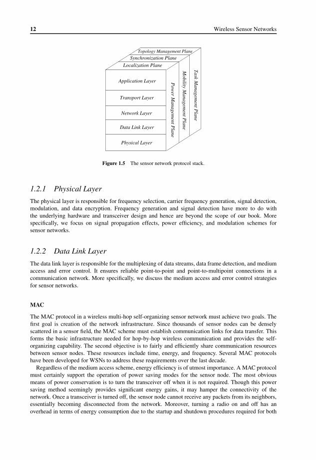
The protocol stack used by the sink and all sensor nodes is given in Figure 1.5. This protocol stackcombines power and routing awareness, integrates data with networking protocols, communicates powerefficiently through the wireless medium, and promotes cooperative efforts of sensor nodes. The protocolstack consists of the physical layer, data link layer, network layer, transport layer, application layer,as well as synchronization plane, localization plane, topology management plane, power managementplane, mobility management plane, and task management plane. The physical layer addresses the needsof simple but robust modulation, transmission, and receiving techniques. Since the environment is noisyand sensor nodes can be mobile, the link layer is responsible for ensuring reliable communicationthrough error control techniques and manage channel access through the MAC to minimize collisionwith neighbors’ broadcasts. Depending on the sensing tasks, different types of application software canbe built and used on the application layer. The network layer takes care of routing the data supplied bythe transport layer. The transport layer helps to maintain the flow of data if the sensor network applicationrequires it. In addition, the power, mobility, and task management planes monitor the power, movement,and task distribution among the sensor nodes. These planes help the sensor nodes coordinate the sensingtask and lower the overall power consumption.
The power management plane manages how a sensor node uses its power. For example, the sensornode may turn off its receiver after receiving a message from one of its neighbors. This is to avoid gettingduplicated messages. Also, when the power level of the sensor node is low, the sensor node broadcaststo its neighbors that it is low in power and cannot participate in routing messages. The remaining poweris reserved for sensing. The mobility management plane detects and registers the movement of sensornodes, so a route back to the user is always maintained, and the sensor nodes can keep track of theirneighbors. By knowing these neighbor sensor nodes, the sensor nodes can balance their power and taskusage. The task management plane balances and schedules the sensing tasks given to a specific region.Not all sensor nodes in that region are required to perform the sensing task at the same time. As aresult, some sensor nodes perform the task more than others, depending on their power level. Thesemanagement planes are needed so that sensor nodes can work together in a power-efficient way, routedata in a mobile sensor network, and share resources between sensor nodes. Without them, each sensornode will just work individually. From the standpoint of the whole sensor network, it is more efficient ifsensor nodes can collaborate with each other, so the lifetime of the sensor networks can be prolonged.
DuyTan
Highlight
DuyTan
Highlight
DuyTan
Highlight
12 Wireless Sensor Networks
Application Layer
Physical LayerP
ower
Managem
entPlane
Mobility
Managem
entPlane
Task
Managem
entPlane
Transport Layer
Network Layer
Data Link Layer
Localization Plane
Synchronization PlaneTopology Management Plane
Figure 1.5 The sensor network protocol stack.
1.2.1 Physical Layer
The physical layer is responsible for frequency selection, carrier frequency generation, signal detection,modulation, and data encryption. Frequency generation and signal detection have more to do withthe underlying hardware and transceiver design and hence are beyond the scope of our book. Morespecifically, we focus on signal propagation effects, power efficiency, and modulation schemes forsensor networks.
1.2.2 Data Link Layer
The data link layer is responsible for the multiplexing of data streams, data frame detection, and mediumaccess and error control. It ensures reliable point-to-point and point-to-multipoint connections in acommunication network. More specifically, we discuss the medium access and error control strategiesfor sensor networks.
MAC
The MAC protocol in a wireless multi-hop self-organizing sensor network must achieve two goals. Thefirst goal is creation of the network infrastructure. Since thousands of sensor nodes can be denselyscattered in a sensor field, the MAC scheme must establish communication links for data transfer. Thisforms the basic infrastructure needed for hop-by-hop wireless communication and provides the self-organizing capability. The second objective is to fairly and efficiently share communication resourcesbetween sensor nodes. These resources include time, energy, and frequency. Several MAC protocolshave been developed for WSNs to address these requirements over the last decade.
Regardless of the medium access scheme, energy efficiency is of utmost importance. A MAC protocolmust certainly support the operation of power saving modes for the sensor node. The most obviousmeans of power conservation is to turn the transceiver off when it is not required. Though this powersaving method seemingly provides significant energy gains, it may hamper the connectivity of thenetwork. Once a transceiver is turned off, the sensor node cannot receive any packets from its neighbors,essentially becoming disconnected from the network. Moreover, turning a radio on and off has anoverhead in terms of energy consumption due to the startup and shutdown procedures required for both

Introduction 13
hardware and software. In fact, if the radio is blindly turned off during each idling slot, over a periodof time the sensor may end up expending more energy than if the radio had been left on. As a result,operation in a power saving mode is energy efficient only if the time spent in that mode is greater than acertain threshold. There can be a number of such useful modes of operation for the wireless sensor node,depending on the number of states of the microprocessor, memory, A/D converter, and the transceiver.Each of these modes can be characterized by its power consumption and the latency overhead, which isthe transition power to and from that mode.
Error Control
Another important function of the data link layer is the error control of transmission data. Two importantmodes of error control in communication networks are forward error correction (FEC) and automaticrepeat request (ARQ), and hybrid ARQ. The usefulness of ARQ in sensor network applications is limitedby the additional retransmission cost and overhead. On the other hand, decoding complexity is greaterin FEC, as error correction capabilities need to be built in. Consequently, simple error control codeswith low-complexity encoding and decoding might present the best solutions for sensor networks. In thedesign of such a scheme, it is important to have a good knowledge of the channel characteristics andimplementation techniques.
1.2.3 Network Layer
Sensor nodes are scattered densely in a field either close to or inside the phenomenon as shown inFigure 1.4. The information collected relating to the phenomenon should be transmitted to the sink,which may be located far from the sensor field. However, the limited communication range of the sensornodes prevents direct communication between each sensor node and the sink node. This requires efficientmulti-hop wireless routing protocols between the sensor nodes and the sink node using intermediatesensor nodes as relays. The existing routing techniques, which have been developed for wireless ad hocnetworks, do not usually fit the requirements of the sensor networks. The networking layer of sensornetworks is usually designed according to the following principles:
• Power efficiency is always an important consideration.• Sensor networks are mostly data-centric.• In addition to routing, relay nodes can aggregate the data from multiple neighbors through local
processing.• Due to the large number of nodes in a WSN, unique IDs for each node may not be provided and
the nodes may need to be addressed based on their data or location.
An important issue for routing in WSNs is that routing may be based on data-centric queries. Basedon the information requested by the user, the routing protocol should address different nodes that wouldprovide the requested information. More specifically, the users are more interested in querying anattribute of the phenomenon rather than querying an individual node. For instance, “the areas where thetemperature is over 70 ◦F (21 ◦C)” is a more common query than “the temperature read by node #47.”
One other important function of the network layer is to provide internetworking with externalnetworks such as other sensor networks, command and control systems, and the Internet. In one scenario,the sink nodes can be used as a gateway to other networks, while another scenario is to create a backboneby connecting sink nodes together and making this backbone access other networks via a gateway.
1.2.4 Transport Layer
The transport layer is especially needed when the network is planned to be accessed through the Internetor other external networks. TCP, with its current transmission window mechanisms, does not address

14 Wireless Sensor Networks
the unique challenges posed by the WSN environment. Unlike protocols such as TCP, the end-to-endcommunication schemes in sensor networks are not based on global addressing. These schemes mustconsider that addressing based on data or location is used to indicate the destinations of the data packets.Factors such as power consumption and scalability, and characteristics like data-centric routing, meansensor networks need different handling in the transport layer. Thus, these requirements stress the needfor new types of transport layer protocols.
The development of transport layer protocols is a challenging task because the sensor nodes areinfluenced by hardware constraints such as limited power and memory. As a result, each sensor nodecannot store large amounts of data like a server in the Internet, and acknowledgments are too costly forsensor networks. Therefore, new schemes that split the end-to-end communication probably at the sinksmay be needed where UDP-type protocols are used in the sensor network.
For communication inside a WSN, transport layer protocols are required for two main functionalities:reliability and congestion control. Limited resources and high energy costs prevent end-to-end reliabilitymechanisms from being employed in WSNs. Instead, localized reliability mechanisms are necessary.Moreover, congestion that may occur because of the high traffic during events should be mitigated bythe transport layer protocols. Since sensor nodes are limited in terms of processing, storage, and energyconsumption, transport layer protocols aim to exploit the collaborative capabilities of these sensor nodesand shift the intelligence to the sink rather than the sensor nodes.
1.2.5 Application Layer
The application layer includes the main application as well as several management functionalities. Inaddition to the application code that is specific for each application, query processing and networkmanagement functionalities also reside at this layer.
The layered architecture stack has been initially adopted in the development of WSNs due to itssuccess with the Internet. However, the large-scale implementations of WSN applications reveal that thewireless channel has significant impact on the higher layer protocols. Moreover, resource constraintsand the application-specific nature of the WSN paradigm leads to cross-layer solutions that tightlyintegrate the layered protocol stack. By removing the boundaries between layers as well as the associatedinterfaces, increased efficiency in code space and operating overhead can be achieved.
In addition to the communication functionalities in the layered stack, WSNs have also been equippedwith several functionalities that aid the operation of the proposed solutions. In a WSN, each sensordevice is equipped with its own local clock for internal operations. Each event that is related tooperation of the sensor device including sensing, processing, and communication is associated withtiming information controlled through the local clock. Since users are interested in the collaborativeinformation from multiple sensors, timing information associated with the data at each sensor deviceneeds to be consistent. Moreover, the WSN should be able to correctly order the events sensed bydistributed sensors to accurately model the physical environment. These timing requirements have led tothe development of time synchronization protocols in WSNs.
The close interaction with physical phenomena requires location information to be associated inaddition to time. WSNs are closely associated with physical phenomena in their surroundings. Thegathered information needs to be associated with the location of the sensor nodes to provide an accurateview of the observed sensor field. Moreover, WSNs may be used for tracking certain objects formonitoring applications, which also requires location information to be incorporated into the trackingalgorithms. Further, location-based services and communication protocols require position information.Hence, localization protocols have been incorporated into the communication stack.
Finally, several topology management solutions are required to maintain the connectivity and coverageof the WSN. The topology management algorithms provide efficient methods for network deploymentthat result in longer lifetime and efficient information coverage. Moreover, topology control protocolshelp determine the transmit power levels as well as the activity durations of sensor nodes to minimize
DuyTan
Highlight
DuyTan
Highlight
DuyTan
Highlight
DuyTan
Highlight

Introduction 15
energy consumption while still ensuring network connectivity. Finally, clustering protocols are used toorganize the network into clusters to improve scalability and improve network lifetime.
The integration of each of the components for efficient operation depends on the applications runningon the WSN. This application-dependent nature of the WSNs defines several unique properties comparedto traditional networking solutions. Although the initial research and deployment of WSNs have focusedon data transfer in wireless settings, several novel application areas of WSNs have also emerged.These include wireless sensor and actor networks, which consist of actuators in addition to sensorsthat convert sensed information into actions to act on the environment, and wireless multimedia sensornetworks, which support multimedia traffic in terms of visual and audio information in addition to scalardata. Furthermore, recently the WSN phenomenon has been adopted in constrained environments suchas underwater and underground settings to create wireless underwater sensor networks and wirelessunderground sensor networks. These new fields of study pose additional challenges that have not beenconsidered by the vast number of solutions developed for traditional WSNs.
The flexibility, fault tolerance, high sensing fidelity, low cost, and rapid deployment characteristicsof sensor networks create many new and exciting application areas for remote sensing. In the future,this wide range of application areas will make sensor networks an integral part of our lives. However,realization of sensor networks needs to satisfy the constraints introduced by factors such as faulttolerance, scalability, cost, hardware, topology change, environment, and power consumption. Sincethese constraints are highly stringent and specific for sensor networks, new wireless ad hoc networkingtechniques are required. Many researchers are currently engaged in developing the technologies neededfor different layers of the sensor network protocol stack. Commercial viability of WSNs has also beenshown in several fields. Along with the current developments, we encourage more insight into theproblems and more development of solutions to the open research issues as described in this book.
References[1] BTnode platform. http://www.btnode.ethz.ch/.
[2] Cricket indoor location system. http://nms.lcs.mit.edu/projects/cricket.
[3] Crossbow technology. http://www.xbow.com.
[4] IPv6 over low power WPAN working group. http://tools.ietf.org/wg/6lowpan/.
[5] ISA SP100.11a working group. http://www.isa.org/ISA100.
[6] National Instruments ni wsn-3202 wireless sensor.http://sine.ni.com/nips/cds/view/p/lang/en/nid/206921.
[7] Sensicast TEHU-1121 wireless sensor. http://www.sensicast.com/wireless_sensors.php.
[8] The Stargate platform. http://www.xbow.com/Products/Product_pdf_files/Wireless_pdf/Stargate_Datasheet.pdf.
[9] SunSPOT mote specifications. http://www.sunspotworld.com.
[10] TinyOS. Available at http://www.tinyos.net/.
[11] Wireless Industrial Networking Alliance (WINA). http://www.wina.org.
[12] WirelessHART communications protocol. http://www.hartcomm2.org/index.html.
[13] ZigBee Alliance. http://www.zigbee.org/.
[14] IEEE standard for information technology – telecommunications and information exchange between systems –local and metropolitan area networks – specific requirement part 15.4: wireless medium access control (MAC)and physical layer (PHY) specifications for low-rate wireless personal area networks (WPANS). IEEE Std.802.15.4a-2007 (Amendment to IEEE Std. 802.15.4-2006), pp. 1–203, 2007.
[15] Microstrain V-Link wireless sensor. http://www.microstrain.com/v-link.aspx, 2009.
[16] Shimmer project. http://www.eecs.harvard.edu/ konrad/projects/shimmer/, 2009.
[17] EYES project. http://www.eyes.eu.org/, March 2002–February 2005.

16 Wireless Sensor Networks
[18] I. F. Akyildiz, W. Su, Y. Sankarasubramaniam, and E. Cayirci. Wireless sensor networks: a survey. ComputerNetworks, 38(4):393–422, March 2002.
[19] Q. Cao, T. Abdelzaher, J. Stankovic, and T. He. The LiteOS operating system: towards Unix-like abstractionsfor wireless sensor networks. In Proceedings of IPSN’08, pp. 233–244, St. Louis, Missouri, USA, April 2008.
[20] A. Dunkels, B. Grönvall, and T. Voigt. Contiki – a lightweight and flexible operating system for tiny networkedsensors. In Proceedings of IEEE EmNets’04, Tampa, Florida, USA, November 2004.
[21] P. Levis, N. Lee, M. Welsh, and D. Culler. Tossim: accurate and scalable simulation of entire TinyOS applica-tions. In Proceedings of ACM SenSys’03, pp. 126–137, Los Angeles, CA, USA, November 2003.
[22] C. B. Margi, V. Petkov, K. Obraczka, and R. Manduchi. Characterizing energy consumption in a visual sensornetwork testbed. In Proceedings of the IEEE/Create-Net International Conference on Testbeds and ResearchInfrastructures for the Development of Networks and Communities (TridentCom’06), Barcelona, Spain, March2006.
[23] G. Mulligan and the 6LoWPAN Working Group. The 6LoWPAN architecture. In Proceedings of EmNets’07,pp. 78–82, Cork, Ireland, June 2007.
[24] L. F. W. van Hoesel, S. O. Dulman, P. J. M. Havinga, and H. J. Kip. Design of a low-power testbed for wirelesssensor networks and verification. Technical report, University of Twente, 2003.
2WSN Applications
The emergence of the WSN paradigm has triggered extensive research on many aspects of it. However,the applicability of sensor networks has long been discussed with emphasis on potential applicationsthat can be realized using WSNs. In this chapter, we present an overview of the existing commercial andacademic applications developed for WSNs.
WSNs may consist of many different types of sensors including seismic, magnetic, thermal, visual,infrared, acoustic, and radar, which are able to monitor a wide variety of ambient conditions that includethe following [15, 26]: temperature, humidity, pressure, speed, direction, movement, light, soil makeup,noise levels, the presence or absence of certain kinds of objects, and mechanical stress levels on attachedobjects. As a result, a wide range of applications are possible. This spectrum of applications includeshomeland security, monitoring of space assets for potential and human-made threats in space, ground-based monitoring of both land and water, intelligence gathering for defense, environmental monitoring,urban warfare, weather and climate analysis and prediction, battlefield monitoring and surveillance,exploration of the Solar System and beyond, monitoring of seismic acceleration, strain, temperature,wind speed and GPS data.
These ever-increasing applications of WSNs can be mainly categorized into five categories. In thischapter, several examples are described for military (Section 2.1), environmental (Section 2.2), health(Section 2.3), home (Section 2.4), and industry (Section 2.5) applications as illustrated in Figure 2.1.
2.1 Military ApplicationsWSNs can be an integral part of military command, control, communications, computing, intelligence,surveillance, reconnaissance, and targeting (C4ISRT) systems. The rapid deployment, self-organization,and fault tolerance characteristics of sensor networks make them a very promising sensing technique formilitary C4ISRT. Since sensor networks are based on the dense deployment of disposable and low-costsensor nodes, destruction of some nodes by hostile action does not affect a military operation as muchas the destruction of a traditional sensor, which makes the sensor network concept a better approachfor battlefields. Some of the military applications of sensor networks are monitoring friendly forces,equipment, and ammunition; battlefield surveillance; reconnaissance of opposing forces and terrain;targeting; battle damage assessment; and nuclear, biological, and chemical (NBC) attack detection andreconnaissance [5, 9, 15, 29, 37]. Three of the representative military applications are discussed next.
2.1.1 Smart Dust
Smart Dust was one of the earliest applications of the WSN phenomenon. The main goal of this DARPA-funded project is to provide technologies for sensor networks that will be used for military operationsin hostile environments. The use of WSNs extend the reach by deploying these networks in areas where
Wireless Sensor Networks Ian F. Akyildiz and Mehmet Can Vuranc© 2010 John Wiley & Sons, Ltd

18 Wireless Sensor Networks
MilitarySmart Dust
Sniper detectionVigilNet
EnvironmentalGreat Duck Island
CORIE
ZebraNetVolcano monitoringFlood detection
HealthArtificial retina
Patient monitoringEmergency Response
HomeWater monitoring
IndustrialPreventive maintenance
Structucal health monitoringVigilNet
Wireless Sensor Network Applications
Figure 2.1 Main categories of WSN applications and the specific examples discussed in this chapter.
it is too dangerous for humans to operate continuously. WSNs obtain information needed to assesscritical situations by dropping a robust, self-configuring, self-organizing WSN onto the battlefield.The military applications include collecting information from enemy movements, hazardous chemicals,and infrastructure stability. The main goal of the Smart Dust project has been developing sensorplatforms in cubic millimeter packages. Instead of focusing on a particular sensor, the transceiver andmicrocontroller unit (MCU) design are performed.
The resulting sensor node is a 100 cubic millimeter prototype with two chips: a MEMS cornercube optical transmitter array and a CMOS ASIC with an optical receiver, charge pump, and simpledigital controller. The Smart Dust project has resulted in the creation of Dust Networks Inc. [9], tocommercialize this technology. Accordingly, the Smart Dust platform has been utilized in militaryapplications such as battlefield surveillance, treaty monitoring, transportation monitoring, and scudhunting. In addition, other commercial applications are also viable with this technology. As an example,a virtual keyboard is developed, where each dust mote is attached to each fingernail and the accelerationinformation is used to detect movements and convert them into key strokes. Similarly, the Smart Dustnode is used as a part of inventory control, where each item is equipped with a unique wireless sensornode that can communicate with the palette, truck, warehouse, and the Internet. Finally, Smart Dustnodes are used in product quality monitoring, where the temperature and humidity of meat, produce,and dairy products are monitored.
2.1.2 Sniper Detection System
The Boomerang sniper detection system [5] has been developed for accurate sniper location detection bypinpointing small-arms fire from the shooter. It has been used by the military, law-enforcement agencies,and municipalities. This application has been realized through two distinct architectures.
The countersniper system shown in Figure 2.2 consists of an array of microphones and can be mountedon a vehicle or worn by a soldier [5]. The system uses passive acoustic sensors to detect incoming fire.The detected audio from the microphones is processed to estimate the relative position of the shooter.The Boomerang system is helpful in urban settings, where a soldier or a vehicle can be subjected to firefrom any location. The vehicle-mounted sensors can detect the shooter even while moving.
This centralized concept has been enhanced through a distributed network of acoustic sensors for acountersniper system as shown in Figure 2.3 to combat the effects of multi-path in sound detection [37].The network consists of Mica2 nodes equipped with a custom-made sensor board. The sensor boardis embedded with a high-power DSP to provide real-time detection, classification, and correlation ofacoustic events. Once a shot has been detected by several sensors, the time and location information ofthese sensors is used to determine the trajectory of the bullet and estimate the location of the shooter. As aresult, the distributed system improves the accuracy of the centralized system. This system is suitablefor law-enforcement agencies and municipalities to provide protection during events such as speeches.

WSN Applications 19
Figure 2.2 Boomerang sniper detection system [5].
Figure 2.3 Distributed sniper detection system [37].
2.1.3 VigilNet
VigilNet [29] is a large-scale surveillance network designed for energy-efficient and stealthy targettracking in harsh environments. The design and implementation of the network were based on 70 Mica2nodes equipped with magnetic sensors that detect the magnetic field generated by the movementof vehicles and magnetic objects. The main goal of this application is to provide energy-efficientsurveillance support through distributed sensor nodes.
The lifetime of VigilNet is improved through a hierarchical structure of nodes in the network. Certainnodes denoted as sentries are responsible for maintaining the multi-hop routes and managing event-basedoperation of the non-sentry nodes, which remain in a low-power state until an event occurs. In case ofan event, e.g., a vehicle passing a group of nodes, the network is reorganized into clusters including
DUYTAN
Highlight

20 Wireless Sensor Networks
Neighbor Discovery
Event Tracking
Power Mgmt
System Initialization
RESET
Sentry Selection
Status Report
Figure 2.4 Operation phases of VigilNet [29].
the associated group of nodes with the help of sentries. This scheme provides event-based collaborativetracking with a long network lifetime.
The network operation of VigilNet is organized into several phases that are executed in a cycle asshown in Figure 2.4. The five phases are as follows:
1. System initialization: This phase includes synchronization, multi-hop backbone setup, andreconfiguration. Network-wide synchronization is essential for the accuracy of the trackingapplication. This is accomplished by broadcast messages from the sink node sent during theinitialization phase. During the propagation of the broadcast messages, a backbone of sentries isalso formed throughout the network. This backbone provides a stable path between the nodesand the sink and allows the nodes that are not part of the backbone to sleep. To avoid thediverse effects of asymmetric links between any pair of nodes, each node performs link symmetrydetection (LSD) to filter out its neighbors with highly symmetric links. The backbone is then builtusing these links. The time synchronization packets are also used to reconfigure the network ondemand. Accordingly, the operating parameters such as cycle length, duty cycle, sampling rate,and aggregation parameters are piggybacked on the synchronization packets. Finally, localizationis performed manually during this phase. During deployment, an operator equipped with a GPSunit and a transceiver programs each node with its location based on the GPS reading on site.Apart from localization, each initialization service is performed at the beginning of each cycle.
2. Neighbor discovery: The initialization phase is followed by local broadcast of HELLO messagesby each node. This message includes information about the node including its ID, whether it is asentry or not, the number of sentries it is connected to, and its location. This information is usedfor local message exchanges and sentry selection.
3. Sentry selection: The sentries remain active during the network operation and are selected at thebeginning of each cycle. Each node determines its duty as a sentry if it is part of the backboneor none of its neighbors is a sentry. This duty is communicated to other nodes using a broadcastmessage after a certain broadcast duration. Consequently, each node is guaranteed to be coveredby at least one sentry.

WSN Applications 21
4. Status report: This phase is used by each node to communicate its status to the base station usingthe backbone. The status report phase can be omitted, but is used for visualization and debuggingpurposes.
5. Power management and event tracking: The final phase of the operating cycle constitutes themajority of the lifetime of the network. Throughout the hierarchical structure, which consistsof sentry and non-sentry nodes, a significant amount of energy is saved. The sleep and wakeupcycles of the non-sentry nodes are controlled by the sentry nodes through proactive or reactivecontrol schemes. For proactive control, each sentry node broadcasts sleep beacons that let eachnon-sentry node switch to a sleep state. In case of an event, the sleep beacons are not sent and thenon-sentry nodes participate in delivering information. On the other hand, for reactive control, thesentry nodes send beacons only when an event occurs to wake up the non-sentry nodes, which,otherwise, follow a sleep/wakeup schedule. When an event occurs, the nodes that sense the eventform event-based clusters and a leader is selected. The sensed information is locally collected bythe leader, which forwards this information to the sink only after a certain confidence level hasbeen satisfied. The collected information consists of the location of the node and the timestamprelated to the sensed event. Using this information the location and speed of the moving objectare estimated.
Each cycle is periodically initiated by a reset phase followed by the system initialization phase. Thesystem spends a very short time, e.g., 2 minutes, during the first four phases (system initialization,neighbor discovery, sentry selection, and status report), which update the system-wide parameters tobe adopted in the dynamics of the network. The fifth phase (power management and event tracking)constitutes actual application operation, where the event-based tracking takes place. This phase may lastup to a day until the next cycle. This sequential operation also helps isolate one system management taskfrom another as well as the actual tracking. This helps conserve the limited resources and the wirelessbandwidth.
VigilNet illustrates how several functionalities of a WSN are integrated into a coherent framework ina practical setting. The experimental evaluations reveal that the local aggregation and the hierarchicalsleep/wakeup schemes significantly contribute to the energy efficiency of a tracking application inmilitary settings.
In addition to these specific projects, WSNs have been widely used in battlefield surveillanceapplications, where exposure of military personnel to hazardous materials and enemy attack areminimized. Furthermore, WSNs are used for target tracking, where the location of a known or a mobileobject is detected by a group of sensors and reported to the command control stations.
2.2 Environmental Applications
The autonomous coordination capabilities of WSNs are utilized in the realization of a wide variety ofenvironmental applications. Some environmental applications of WSNs include tracking the movementsof birds, small animals, and insects; monitoring environmental conditions that affect crops andlivestock; irrigation; macroinstruments for large-scale Earth monitoring and planetary exploration;chemical/biological detection; precision agriculture; biological, Earth, and environmental monitoringin marine, soil, and atmospheric contexts; forest fire detection; meteorological or geophysical research;flood detection; biocomplexity mapping of the environment; and pollution studies [6, 10, 14, 17, 18, 19,21, 30, 31, 32, 33, 34, 38, 49, 50, 51, 52, 54].
2.2.1 Great Duck Island
The Great Duck Island project [38, 50] has been developed as a collaboration between College ofthe Atlantic and the Intel Research Laboratory at Berkeley to study the distribution and abundance

22 Wireless Sensor Networks
Gateways
Tier 1:Sensor Nodes
Tier 2:
Figure 2.5 Two-tier architecture of Great Duck Island habitat monitoring network [38].
of seabirds on Great Duck Island (GDI), Maine. A network of Mica sensors is used to measure theoccupancy of nesting burrows and the role of microclimatic factors in the habitat selection of seabirds,i.e., petrels. More specifically, the occupancy of the burrows during 1–3 days is monitored as well as theenvironmental changes during the breeding season and the corresponding changes in bird behavior.
The GDI habitat monitoring network employs a two-tier hierarchical architecture as shown inFigure 2.5. In the first tier, groups of sensors are used to gather information. For this tier, Mica motesequipped with Mica Weather Boards are used, which include temperature, photoresistor, barometricpressure, humidity, and thermopile sensors. More specifically, these sensor nodes are used for twodifferent purposes: burrow motes are deployed in the burrows to detect occupancy using non-contactinfrared thermopiles and temperature/humidity sensors, while weather motes are used to monitor thesurface microclimate. Each group of sensors is connected to a gateway that collects these data and sendsthem to the second tier. The second tier consists of gateways that provide connectivity between thesensor groups in the field and the remote base station on the island through long-haul point-to-pointcommunication. Two different platforms are used for this purpose: an embedded Linux system equippedwith an IEEE 802.11 card and a 12 dBi omnidirectional antenna with a range of 1000 feet (30.5 m).Moreover, the Mica nodes are equipped with a 916 MHz directional antenna for a range of 1200 feet(365.75 m). The base station is also connected to the Internet by satellite, which enables remote accessto the WSN.
The GDI project was conducted in 2002 and provided essential information on the characteristics ofseabirds. In addition, the GDI network stands as one of the first proof-of-concept deployments of theWSN phenomenon for environmental applications.

WSN Applications 23
2.2.2 CORIE
The Columbia River Ecosystem (CORIE) [6] is an example of an environmental observation andforecasting system (EOFS) built by the Center for Coastal and Land Margin Research at the OregonGraduate Institute. It consists of sensor stations in the Columbia River estuary that carry variousenvironmental sensors. In all, 24 stations in or around the Columbia River and other Oregon estuariesare equipped with various environmental sensors to measure water velocity, water temperature, salinity,and depth. Moreover, several meteorological stations are deployed to measure wind and air properties,and determine solar radiation at different wavelengths. The information gathered from these sensors isused for online control of vessels, marine research and rescue, and ecosystem research and management.The stations communicate via a Freewave DGR-115 spread-spectrum wireless network. In addition, thetransmission of signals is accomplished by an ORBCOMM LEO satellite in case of disruptions in lineof sight. Accordingly, the observations are displayed via the World Wide Web, in near real time.
The Columbia River estuary system includes the lower river, the estuary, and the near ocean. Thegoal of the CORIE system is to combine the observed information from the sensors with numerical datamodels to characterize the physical state of this system. More specifically, the goal is to characterizethe complex circulation and mixing processes and predict any changes [24]. Since a large area of theriver is covered by a limited number of sensors, the CORIE network represents significantly differentcharacteristics than traditional sensor networks. Compared to low-cost sensor motes, the sensors used inCORIE are large complex systems that are expensive to deploy and maintain. Therefore, highly accuratedata gathering solutions with a minimum number of stations are required. This necessitates estimationmethods tailored to the data models used by the domain scientists.
2.2.3 ZebraNet
ZebraNet [33, 54] is an animal tracking system developed to investigate the long-term movementpatterns of zebras, their interactions within and between species, as well as the impacts of humandevelopment. The system was deployed in Kenya to track two species of zebras.
ZebraNet consists of collars attached to the zebras to collect location information. Each collar includesa GPS unit, associated microcontroller, two types of radios (short range and long range), a lithium-ion polymer high-energy-density battery, and a solar array for recharging the battery as shown inFigure 2.6. The attached collar logs location information through the GPS unit every 3 minutes, whichis shown through biological studies to result in statistically independent location samples that can beused to develop mobility models. This information is collected through a base station, which is keptby the researchers and used intermittently during their trips into the field. Therefore, ZebraNet canbe characterized as a highly mobile sensor network without a static sink. Accordingly, the locationinformation collected at each node is transmitted in a delay-tolerant manner, i.e., when the opportunityto communicate with the base station arises.
Since a particular node may not be within communication range of the mobile sink for a verylong time, a data sharing policy is adopted in ZebraNet so that each sensor node shares the collectedinformation with its neighbors. As a result, when one of the nodes establishes a connection with thesink, the location information of this node as well as its previous neighbors is downloaded. For datasharing, two different delay-tolerant routing protocols are used. Firstly, a simple flooding protocol isused, where each node sends its data to its neighbor whenever it detects a new neighbor. This improvesthe chance to deliver the data to the sink but increases the data overload in the network and limits thestorage space at each node. The second protocol is based on the successful sink communication historyof the nodes and assigns each node a hierarchy level [33]. If a node has recently communicated witha node it is assigned a higher level. Each node shares its location information with a node at a higherhierarchy level with higher probability.

24 Wireless Sensor Networks
Figure 2.6 The ZebraNet sensor collar attached to a zebra [54].
The location information of the zebras collected by a group of sensors provides the domain scientistswith valuable information to model the movement of these animals. In addition to its contribution to thedomain sciences, this movement information is also used to fine-tune the developed protocols accordingto the mobility patterns of the zebras. The network deployment has provided an important insight intothe operation of these networks and resulted in the development of communication protocols such asZ-MAC [47] that was devised to address the unique challenges of this application.
2.2.4 Volcano Monitoring
WSNs have also been used in extreme environments, where continuous human access is impossible.Volcano monitoring is an example of these extreme applications, where a network of sensors can beeasily deployed near active volcanoes to continuously monitor their activities and provide data at a scaleand resolution not previously possible with existing tools.
Two case studies were conducted on two volcanoes in Ecuador during 2004–2005 as a proof ofconcept of WSN applications in volcano monitoring [52]. In 2004, a small network of three sensornodes, equipped with microphones, was used to monitor an erupting volcano, i.e., Volcán Tangurahuain central Ecuador. In 2005, 16 TMote Sky nodes equipped with seismic and acoustic sensors wereused for a duration of 19 days to monitor the activities of an active volcano, Volcán Reventador, innorthern Ecuador. The sensor nodes were equipped with higher gain external antennas to improve thecommunication range and three long-haul communication nodes were used to transmit the data to acentral controller covering a 3 km array. A laptop equipped with a directional antenna was used as a sinkto collect information and manage the network remotely.
The main goal of the application was to collect seismic information based on earthquakes that occurnear the volcanoes. Since these earthquakes usually last less than 60 seconds, a high sampling rate is

WSN Applications 25
employed for the seismic sensors, i.e., 100 Hz, which limits the amount of locally stored information to20 minutes of volcanic activity. Each sensor node uses the local storage as a cyclic buffer and filters thecollected information through a short-term average/long-term average threshold detector to determinethe events related to volcanic activities. When an event is generated, it is reported to the sink. If highconfidence of an event is established through multiple event reports, the sink sends back a data collectioncommand to the network. As a response to this command, each node transmits the information stored inits memory. Consequently, a large volume of data is transmitted to the sink only if an event of interest isdetected by a smaller number of nodes. This reduces the bandwidth wastage and energy consumption atindividual nodes.
The sensor nodes are synchronized using the Flooding Time Synchronization protocol (FTSP) [40]and a GPS unit equipped with a MicaZ node to provide location information. The results of this applica-tion provide important information related to the physical processes at work within a volcano’s interior.
2.2.5 Early Flood Detection
WSNs are also used for early warning flood detection in developing countries [17]. The main challengewith existing systems is the involvement of personnel for continuous monitoring of river beds. Instead,model-based prediction systems can be used by exploiting the statistical properties of data collected bya network of sensor nodes. Such a system has been developed at MIT and tested in Honduras, wherefrequent floods significantly affect urban life.
Flood monitoring requires a large area to be covered with sensors. Considering the limited commu-nication range of individual sensors, a two-tier network topology is used as shown in Figure 2.7. Threedifferent sensors are used in the lower tier of the network for measuring rainfall, air temperature, andwater flow data. These types of data are required for the prediction model. Each closely located sensorforms a group and is connected to the second-tier computation nodes. Data collection and informationprocessing are performed at the computation nodes, which inform the third tier, i.e., control centers, incase of a potential flood. Overall, four different types of nodes are used in the system. Each node has thesame base system that includes a microcontroller and a transceiver but is enhanced with sister-boardsaccording to its function:
• Sensing node: This node is equipped with one of the sensors monitoring rainfall, air temperature,and water flow and collects information over a period on the order of minutes [17]. Each node isequipped with a 900 MHz transceiver and reports its data to the computation node in its cluster.While the rainfall and temperature sensors are located on the ground, the water flow data requiresunderwater measurements. The water level can be easily converted into water flow. To measurethe water level, a water pressure sensor is interfaced with the base board and deployed underwater.
• Computation node: Each group of closely located sensing nodes is maintained by a computationnode as shown in Figure 2.7. The computation node has two main duties in the network. Firstly,the data set collected from the group of sensors is fed into the prediction model, which estimatesthe river flow. In case the prediction confidence is not high, the computation node requestsadditional information from the sensing nodes. Secondly, the computation node provides long-haul communication between the group and the control and monitoring nodes through a 144 MHztransceiver. The information collected by different groups of sensing nodes is collected atthe interface nodes. Through long-haul communication techniques, the computation nodes candirectly reach the interface nodes. This two-tier approach improves the scalability of the system.
• Government office interface node: This node provides a user interface to the network byvisualizing data and enabling network maintenance tasks. Larger scale predictions can also beperformed using the data received from multiple sensors located at different locations.

26 Wireless Sensor Networks
Community Interface
Government Office
Computation Node
NodesSensing
Node
Figure 2.7 Sensor network architecture for flood detection [17].
• Community interface node: Finally, the flood prediction system will be connected to communityinterface nodes that inform the interested community about the results of the prediction. Thisallows the necessary action to be taken timely in the case of severe floods.
The prediction model has been validated using 7-year data collected from the Blue River, Oklahoma,through the Distributed Model Intercomparison project run by the National Oceanic and AtmosphericAdministration. Moreover, the lower tier of the system has been tested in Charles River, Massachusetts,during October–November 2007 using a group of three sensors. Finally, the flood prediction system wasdeployed in Honduras over a long period of time between January 2004 and March 2007.
2.3 Health ApplicationsThe developments in implanted biomedical devices and smart integrated sensors make the usage ofsensor networks for biomedical applications possible. Some of the health applications for sensornetworks are the provision of interfaces for the disabled; integrated patient monitoring; diagnostics;drug administration in hospitals; monitoring the movements and internal processes of insects or othersmall animals; telemonitoring of human physiological data; and tracking and monitoring doctors andpatients inside a hospital [4, 28, 34, 39, 41, 46, 51, 53].
2.3.1 Artificial Retina
The Artificial Retina (AR) project supported by the US Department of Energy aims to build achronically implanted artificial retina for visually impaired people [4]. More specifically, the projectfocuses on addressing two retinal diseases, namely age-related macular degeneration (AMD) and retinitispigmentosa (RP). AMD is an age-related disease and results in severe vision loss at the center of theretina caused by fluid leakage or bleeding in people aged 60 and above. RP, on the other hand, affects

WSN Applications 27
Figure 2.8 Operating principle of the artificial retina [4].
the photoreceptor or rod cells, which results in a loss of peripheral vision [4]. A healthy photoreceptorstimulates the brain through electric impulses when light is illuminated from the external world. Whendamaged, vision is blocked at the locations of the photoreceptors. The AR project aims to replace thesedamaged photoreceptors with an array of microsensors.
The receptors along the retina have different functionalities. The periphery is specialized on temporalevents, whereas the center of the macula is specialized on spatially oriented information. In order tomimic the functionality of the retina, the distribution and the transmission principles of smart sensors oneach segment of the retina must be tailored.
The operating principle of the AR is shown in Figure 2.8. A tiny camera placed in eyeglasses isused to capture visual information from the external world. This information is wirelessly transmittedto a microprocessor, which converts it into electrical signals. These signals are then sent to an arrayof microelectrodes, which are implanted along the retina at the locations of the photoreceptors. Themicroelectrodes then send electric impulses to the brain via the optic nerve.
So far, three models have been developed as part of the AR project. The first model, Argus I, hasbeen completely tested and implanted into six patients between 2002 and 2004. This model consists of a16-electrode array and helps the patients to detect whether lights are on or off, describe the motion of anobject, count individual items, and locate objects. The second model, Argus II, consists of a 60-electrodearray and is undergoing clinical trials. Finally, the third model, which is under development, will includemore than 200 electrodes. The ultimate goal for the prosthetic device is to create a lasting device thatwill enable facial recognition and the ability to read large print [4].

28 Wireless Sensor Networks
(a) (b)
Figure 2.9 Medical sensor nodes used in CodeBlue: (a) Telos mote with EMG sensor and (b) Mica2 mote withpulse oximeter sensor [7].
2.3.2 Patient Monitoring
The CodeBlue project at Harvard University focuses on wearable sensors that monitor vital signs ofpatients throughout their daily lives [39]. To this end, sensor boards with pulse oximeter, electrocardio-graph (EKG), and electromyograph (EMG) circuitry have been designed for MicaZ and Telos motesas shown in Figure 2.9. Accordingly, pulse rate, blood oxygen saturation, electrical activities of theheart, patient movements, and muscular activity can be monitored continuously. The CodeBlue softwareplatform enables these nodes to be operated in a networked setting, where medical personnel can monitorpatients through a PDA.
The architecture of the CodeBlue network is shown in Figure 2.10 in a hospital setting. Accordingly,sensor motes with various sensors are attached to patients for monitoring. Additional motes are deployedinside the hospital as an infrastructure to provide message delivery to/from the motes. The medicalpersonnel can access the network through either PDAs or computers. The network is based on apublish/subscribe mechanism, where the sensor motes publish the available data and the medicalpersonnel subscribe to this data based on certain conditions. The publish/subscribe mechanism isbased on the Adaptive Demand-Drive Multicast Routing (ADMR) protocol, which maintains routinginformation based on the published information. Whenever a mote publishes data, each node in thenetwork is informed about the best path to this node. Route discovery between nodes is performedperiodically through limited flooding to adapt to the changes in the wireless channel.
When a sensor is connected to the network, its capabilities are communicated to the network through adiscovery protocol. Subscribing to the published data is performed through the CodeBlue query (CBQ)layer, which specifies a query through a tuple 〈S, τ, chan, ρ, C, p〉, where S is the set of subscribednode IDs, τ is the subscribed sensor type, chan is the channel type used for routing, ρ is the samplingrate, and C is the optional maximum number of samples to be reported. To model the interests of theusers, a filter predicate, p, is also used in the query, according to which the sensor information to bereported is filtered. Accordingly, a doctor may specify a sensor connected to a particular patient andrequest to receive heartbeat information only if it exceeds normal limits.
In addition to the publish/subscribe mechanism, CodeBlue also provides a localization service througha set of nodes that periodically broadcast beacon messages. A mobile node can then estimate its locationbased on the received RF signal signature from these beacon nodes. This information is essential in

WSN Applications 29
Sensor node
Infrastructure node
PDA/Computer
Figure 2.10 CodeBlue architecture in a hospital setting.
hospitals to locate doctors, nurses, patients, and important equipment in a timely fashion. Finally, agraphical user interface (GUI) is provided to users so that medical personnel can easily utilize the system.
ALARM-NET provides similar monitoring capabilities for elderly people in assisted-living andresidential monitoring applications [53]. A hierarchical network of sensor nodes monitors environmentaland physiological data. At the lowest layer, a body sensor network (BSN) is worn by the resident(s),which collects vital signs. Moreover, emplaced sensors are deployed in the living space to senseinformation related to temperature, dust, motion, and light. Finally, the heterogeneous set of sensor nodesreports to AlarmGates, which are connected through an IP network. Accordingly, the daily activities ofresidents can be monitored and reported to the medical personnel.
2.3.3 Emergency Response
WSNs are also used in emergency response situations to automate monitoring and assessment of thevital signs of casualties [28]. The miTag platform has been developed to include several medical sensorsincluding GPS, pulse oximetry, blood pressure, temperature, and ECG. Using these sets of sensors, theemergency responders can monitor the vital signs of casualties in an accident. The miTag architectureconsists of two tiers of networks. The first tier is a body sensor network including the various sensors andthe second tier is a relay network consisting of nodes dispensed by responders on the scene. Accordingly,an ad hoc network can be formed rapidly to collect information from multiple casualties in a largedisaster or an accident.
2.4 Home Applications
As technology advances, smart sensor nodes and actuators can be buried in appliances such asvacuum cleaners, microwave ovens, refrigerators, and DVD players [43] as well as water monitoringsystems [35]. These sensor nodes inside domestic devices can interact with each other and with theexternal network via the Internet or satellite. They allow end-users to more easily manage homedevices both locally and remotely. Accordingly, WSNs enable the interconnection of various devicesat residential places with convenient control of various applications at home.

30 Wireless Sensor Networks
Main
Computation
Water Company
Meter
Node
Figure 2.11 Non-intrusive Autonomous Water Monitoring System (NAWMS) architecture [35].
2.4.1 Water Monitoring
The Nonintrusive Autonomous Water Monitoring System (NAWMS) for homes has recently beendeveloped using WSNs [35]. The main goal of NAWMS is to localize the wastage in water usage andinform tenants about more efficient usage. Since the water utility companies only provide total waterusage in a house, it is not easy to determine the individual sources that contribute to that total. Using adistributed WSN, the water usage in each pipe of the house’s plumbing system can be monitored at alow cost.
The operating principle of NAWMS is based on the fact that the water flow in a particular pipe can beestimated by measuring the vibrations of that pipe because of the proportional relationship between thetwo. Accordingly, wireless sensor nodes are attached to the water pipes to measure the vibrations throughaccelerometers. Because of the nonlinear relationship between vibration and water flow, however, eachsensor node needs to be calibrated to determine the optimal set of parameters that relate accelerationinformation to water flow. Instead of manual calibration that can be performed by individually installingwater flow sensors at each pipe, in NAWMS this calibration is performed automatically with the help ofthe main water meter.
The architecture of NAWMS is illustrated in Figure 2.11, which consists of three types of components.A wireless sensor node is attached to the main water meter to collect actual water flow information andcommunicate it to the rest of the network. Since the water meter sensor is already calibrated by the utilitycompany, this node serves as a ground truth for the rest of the system. The second type of componentis the vibration sensors, which are installed in each pipe to monitor vibrations. The distributed vibrationinformation is then sent to the central computation node, which automatically calibrates the sensorsand determines the water usage associated with each pipe. Calibration is performed through an onlineoptimization algorithm, which is based on the fact that the sum of the water flows at each non-calibratedsensor should be equal to that of the water meter, which is known to be accurate. Accordingly, thevibrations are used in a microscopic flow model to estimate the flow rate at spatially distributed locations.The system provides real-time water usage information at different locations of the water pipe system,which can be utilized to improve the efficiency of homes in the future.

WSN Applications 31
2.5 Industrial Applications
Networks of wired sensors have long been used in industrial fields such as industrial sensing andcontrol applications, building automation, and access control. However, the cost associated with thedeployment of wired sensors limits the applicability of these systems. Moreover, even if a sensorsystem were deployed in an industrial plant, upgrading this system would cost almost as much as anew system. In addition to sensor-based monitoring systems, manual monitoring has also been used inindustrial applications for preventive maintenance [36]. Manual monitoring is generally performed byexperienced personnel using handheld analyzers that are collected from a central location for analysis.While sensor-based systems incur high deployment costs, manual systems have limited accuracy andrequire personnel. Instead, WSNs are a promising alternative solution for these systems due to theirease of deployment, high granularity, and high accuracy provided through battery-powered wirelesscommunication units.
Some of the commercial applications are monitoring material fatigue; building virtual keyboards;managing inventory; monitoring product quality; constructing smart office spaces; environmental controlof office buildings; robot control and guidance in automatic manufacturing environments; interactivetoys; interactive museums; factory process control and automation; monitoring disaster areas; smartstructures with embedded sensor nodes; machine diagnosis; transportation; factory instrumentation;local control of actuators; detecting and monitoring car theft; vehicle tracking and detection; instrumen-tation of semiconductor processing chambers, rotating machinery, wind tunnels, and anechoic chambers;and distributed spectrum sensing to help realize cognitive radio networks [1, 2, 11, 12, 13, 14, 16, 20,22, 23, 25, 26, 36, 27, 34, 42, 44, 45, 46, 48, 51].
2.5.1 Preventive Maintenance
Preventive maintenance has been utilized in many large industrial plants since it provides cost-effectivesolutions to long-term operation of expensive equipment. However, existing systems cannot gain wideacceptance since the cost associated with the deployment of a preventive maintenance system outweighsthe gains. WSNs have been shown to provide cost-effective yet accurate maintenance capabilities in twocase studies: a semiconductor fabrication plant and an oil tanker [36].
The “health” of equipment can be monitored through vibration analysis techniques that requireaccelerometer sensors attached to the equipment. In Intel’s semiconductor fabs, thousands of sensorstrack the vibrations of various pieces of equipment. Based on the established science that maps aparticular signature to a well-functioning device, the machines are monitored continuously. However,the data from the sensors are collected manually by employees. In an effort to automate the datacollection, a network of Mica2 and Intel Mote sensors along with Stargate gateways, namely FabApp,has been deployed.
The FabApp architecture is shown in Figure 2.12, where the hierarchical three-tier network isillustrated. The lowest tier consists of either Mica2 or Intel motes connected to multiple accelerometersto collect vibration information. This tier is organized into clusters and each cluster is controlled bya Stargate gateway node to improve the scalability of the network. The data collection is controlled byeach gateway node through a duty cycle scheme. The gateways form the second tier, i.e., an IEEE 802.11mesh network of high-end nodes that is overlaid on the first-tier sensor network. The data collected byeach gateway are transmitted to a root node over the higher data-rate 802.11 connections. The rootnode is also connected to the enterprise network through a cable, which forms the third tier. Using thisarchitecture, the data collected by the entire network are sent to the enterprise server for analysis.
FabApp illustrates a practical implementation of the cluster-based protocols for industrial applications.The sensor node activities are controlled by the gateway to decrease the processing required at each node.Accordingly, the gateway notifies the report and sleep durations to the sensor nodes and each sensor nodewakes up at the same time to report its vibration information and switch to sleep state for the rest of the

32 Wireless Sensor Networks
EnterpriseNetwork
Primergy
NetworkEnterprise
Tier 2
NetworkGateway
NetworkSensor
Tier 1
ServerEnterprise Tier 3
Figure 2.12 FabApp architecture [36].
cycle. In addition, both sensor nodes and gateway are programmed such that the software is reset atthe end of each reset cycle. This removes any state dependency for each cycle and ensures long-termunattended operation in the network. Furthermore, several watchdog timers are implemented to ensurethe embedded devices operate properly.
The same tiered structure is also deployed in an oil tanker to monitor equipment through a WSN.While the application goals are similar to FabApp, the environmental differences significantly affect thedesign choices. Since the ship consists of steel floors and bulkheads and the compartments are dividedby hatchways, signal propagation and wireless communication are major challenges [36]. This requirespre-deployment analysis to determine suitable locations for the gateways. Moreover, a more robust datadelivery protocol is required so that data are not lost whenever hatchways are closed and the network ispartitioned. Both deployments have been operated for several days with valuable information collectedby distributed sensors and provide a proof-of-concept for industrial applications of WSNs.
2.5.2 Structural Health Monitoring
WSNs have also been used in structural health monitoring (SHM) applications, where distributed sensorstrack the spatio-temporal patterns of vibrations induced throughout the structures [23]. Accordingly,potential damage can be localized and its extent can be estimated in almost real time. Wisden [42]has been developed to address the limitations of existing SHM techniques which rely on either periodicvisual inspections or expensive wired data acquisition systems. To this end, actuators, which apply forcedexcitation to the structure, are networked with sensors, which detect the effects of these excitations.Accordingly, the challenges of intolerance to data loss, strict synchronization requirements, and largevolumes of raw data are addressed through a distributed WSN. The system has been deployed in aSHM testbed for development as well as in an abandoned building for evaluation. This system has alsobeen extended to the netSHM [22], which provides a two-level architecture such that the details of theunderlying WSN operation are hidden from the application. This provides the flexibility of using higherlevel languages such as MATLAB or C, with which domain experts are much more comfortable.

WSN Applications 33
2.5.3 Other Commercial Applications
Wireless automatic meter reading (AMR) is one of the fastest growing markets for short-range radiodevices. Wireless collection of utility meter data (electricity, water, gas) is a very cost-efficient way ofgathering consumption data for the billing system [3, 8]. Chipcon produces low-cost, low-power radiochips and transceivers for wireless AMR applications [1].
Heating, ventilating, and air-conditioning (HVAC) applications are another field where WSNs have animportant impact. In commercial buildings, it is common to control multiple spaces or rooms by a singleHVAC unit. Hence, systems configured this way are most commonly controlled by a single sensor in oneof the rooms. However, low-cost wireless sensor technology offers the opportunity to replace this singlesensor with a network of sensors where there is at least one sensor per room. ZenSys produces wirelessRF-based communications technology designed for residential and light commercial control and statusreading applications such as meter reading, lighting, and appliance control [13].
Sensicast is producing the H900 Sensor Network Platform, a wireless mesh networking system, whichcan be used in many industrial applications [11]. Moreover, SYS Technologies (formerly Xsiology)produces systems for real-time monitoring of a wide variety of remote industrial applications includingwastewater, oil and gas, utilities, and railroads [12].
Soflinx provides a perimeter security system for the real-time detection of hazardous explosive,nuclear, biological, and chemical warfare agents. Soflinx uses its Datalinx technology which pushesthe intelligence of the network closer to the source of the data by using gateways in the network edgesand enabling the individual components to automate responses to these data. Moreover, a transportablesecurity system for the detection of the above hazardous agents has also been produced [2].
References[1] Available at http://www.chipcon.com.
[2] Available at http://www.soflinx.com.
[3] Altera Corp. http://www.altera.com/.
[4] Artificial Retina project. Available at http://artificialretina.energy.gov.
[5] Boomerang shooter detection system. http://bbn.com/boomerang.
[6] Center for Coastal Margin Observation and Prediction. http://www.ccalmr.ogi.edu/corie.
[7] CodeBlue project. Available at http://fiji.eecs.harvard.edu/CodeBlue.
[8] DataRemote Inc. http://www.dataremote.com/.
[9] Dust Networks Inc. http://www.dust-inc.com.
[10] ENSCO Inc. http://www.ensco.com.
[11] Sensicast systems. Available at http://www.sensicast.com.
[12] SYS Technologies (formerly Xsiology). http://www.systechnologies.com.
[13] Zensys, Inc. http://www.zen-sys.com.
[14] J. Agre and L. Clare. An integrated architecture for cooperative sensing networks. IEEE Computer Magazine,33(5):106–108, May 2000.
[15] I. F. Akyildiz, W. Su, Y. Sankarasubramaniam, and E. Cayirci. Wireless sensor networks: a survey. ComputerNetworks, 38(4):393–422, March 2002.
[16] I.F. Akyildiz, W.-Y. Lee, M. C. Vuran, and S. Mohanty. Next generation/dynamic spectrum access/cognitiveradio wireless networks: a survey. Computer Networks, 50(13):2127–2159, September 2006.
[17] E. A. Basha, S. Ravela, and D. Rus. Model-based monitoring for early warning flood detection. In Proceedingsof ACM SenSys’08, pp. 295–308, Raleigh, NC, USA, November 2008.
[18] M. Bhardwaj, T. Garnett, and A. P. Chandrakasan. Upper bounds on the lifetime of sensor networks. InProceedings of IEEE ICC’01, volume 3, pp. 785–790, Helsinki, Finland, June 2001.
DUYTAN
Highlight

34 Wireless Sensor Networks
[19] P. Bonnet, J. Gehrke, and P. Seshadri. Querying the physical world. IEEE Personal Communications, 7(5):10–15, October 2000.
[20] N. Bulusu, D. Estrin, L. Girod, and J. Heidemann. Scalable coordination for wireless sensor networks: self-configuring localization systems. In Proceedings of the International Symposium on Communication Theoryand Applications (ISCTA’01), Ambleside, UK, July 2001.
[21] A. Cerpa, J. Elson, M. Hamilton, and J. Zhao. Habitat monitoring: application driver for wireless communica-tions technology. In Proceedings of ACM SIGCOMM’01, pp. 20–41, Costa Rica, April 2001.
[22] K. Chintalapudi, J. Paek, O. Gnawali, T. Fu, K. Dantu, J. Caffrey, R. Govindan, and E. Johnson. Structuraldamage detection and localization using NetSHM. In Proceedings of IPSN/SPOTS’06, pp. 475–482, Nashville,TN, USA, April 2006.
[23] K. Chintalapudi, J. Paek, N. Kothari, S. Rangwala, J. Caffrey, R. Govindan, E. Johnson, and S. Masri. Moni-toring civil structures with a wireless sensor network. IEEE Internet Computing, 10(2):26–34, March/April2006.
[24] T. Dang, S. Frolov, N. Bulusu, W. Feng, and A. Baptista. Near optimal sensor selection in the COlumbia RIvEr(CORIE) observation network for data assimilation using genetic algorithms. In Proceedings of DCOSS’07,pp. 253–266, Santa Fe, NM, USA, June 2007.
[25] D. Estrin, R. Govindan, and J. Heidemann. Embedding the internet. Communications of the ACM, 43(5):38–41,May 2000.
[26] D. Estrin, R. Govindan, J. Heidemann, and S. Kumar. Next century challenges: scalable coordination in sensornetworks. In Proceedings of ACM/IEEE MobiCom’99, pp. 263–270, Seattle, WA, USA, August 1999.
[27] V. Fodor, I. Glaropoulos, and L. Pescosolido. Detecting low-power primary signals via distributed sensing tosupport opportunistic spectrum access. In Proceedings of IEEE ICC’09, Dresden, Germany, June 2009.
[28] T. Gao, C. Pesto, L. Selavo, Y. Chen, J. G. Ko, J.H. Lim, A. Terzis, A. Watt, J. Jeng, B. r. Chen, K. Lorincz,and M. Welsh. Wireless medical sensor networks in emergency response: implementation and pilot results. InProceedings of IEEE International Conference on Technologies for Homeland Security, pp. 187–192, Waltham,MA, USA, May 2008.
[29] T. He, S. Krishnamurthy, J. A. Stankovic, T. Abdelzaher, L. Luo, R. Stoleru, T. Yan, L. Gu, G. Zhou, J. Hui, andB. Krogh. VigilNet: an integrated sensor network system for energy-efficient surveillance. ACM Transactionson Sensor Networks, 2(1):1–38, February 2006.
[30] W. R. Heinzelman, J. Kulik, and H. Balakrishnan. Adaptive protocols for information dissemination in wirelesssensor networks. In Proceedings of MobiCom’99, pp. 174–185, Seattle, WA, USA, August 1999.
[31] C. Intanagonwiwat, R. Govindan, and D. Estrin. Directed diffusion: a scalable and robust communicationparadigm for sensor networks. In Proceedings of MobiCom’00, pp. 56–67, Boston, MA, USA, August 2000.
[32] C. Jaikaeo, C. Srisathapornphat, and C. Shen. Diagnosis of sensor networks. In Proceedings of IEEE ICC’01,volume 5, pp. 1627–1632, Helsinki, Finland, June 2001.
[33] P. Juang, H. Oki, Y. Wang, M. Martonosi, L. S. Peh, and D. Rubenstein. Energy-efficient computing for wildlifetracking: design tradeoffs and early experiences with ZebraNet. ACM SIGOPS Operating Systems Review,36(5):96–107, 2002.
[34] J. M. Kahn, R. H. Katz, and K. S. J. Pister. Next century challenges: mobile networking for “smart dust”. InProceedings of ACM MobiCom’99, pp. 271–278, Seattle, WA, USA, August 1999.
[35] Y. Kim, T. Schmid, Z. M. Charbiwala, J. Friedman, and M. B. Srivastava. NAWMS: Nonintrusive AutonomousWater Monitoring System. In Proceedings of ACM SenSys’08, pp. 309–322, Raleigh, NC, USA, November2008.
[36] L. Krishnamurthy, R. Adler, P. Buonadonna, J. Chhabra, M. Flanigan, N. Kushalnagar, L. Nachman, andM. Yarvis. Design and deployment of industrial sensor networks: experiences from a semiconductor plant andthe North Sea. In Proceedings of SenSys’05, pp. 64–75, San Diego, CA, USA, 2005.
[37] Á. Lédeczi, A. Nádas, P. Völgyesi, G. Balogh, B. Kusy, J. Sallai, G. Pap, S. Dóra, K. Molnár, M. Maróti, andG Simon. Countersniper system for urban warfare. ACM Transactions on Sensor Networks, 1(2):153–177,November 2005.
[38] A. Mainwaring, J. Polastre, R. Szewczyk, D. Culler, and J. Anderson. Wireless sensor networks for habitatmonitoring. In Proceedings of ACM WSNA’02, Atlanta, GA, USA, September 2002.
[39] D. Malan, T. Fulford-Jones, M. Welsh, and S. Moulton. CodeBlue: an Ad Hoc sensor network infrastructure foremergency medical care. In Proceedings of Workshop on Applications of Mobile Embedded Systems (WAMES2004), Boston, MA, USA, June 2004.

WSN Applications 35
[40] M. Maroti, B. Kusy, G. Simon, and A. Ledeczi. The flooding time synchronization protocol. In Proceedings ofACM SenSys’04, Baltimore, MD, USA, November 2004.
[41] N. Noury, T. Herve, V. Rialle, G. Virone, E. Mercier, G. Morey, A. Moro, and T. Porcheron. Monitoring behav-ior in home using a smart fall sensor. In IEEE–EMBS Special Topic Conference on Microtechnologies inMedicine and Biology, pp. 607–610, Lyon, France, October 2000.
[42] J. Paek, K. Chintalapudi, J. Cafferey, R. Govindan, and S. Masri. A wireless sensor network for structural healthmonitoring: performance and experience. In Proceedings of the 2nd IEEE Workshop on Embedded NetworkedSensors (EmNetS-II), Sydney, Australia, May 2005.
[43] E. M. Petriu, N. D. Georganas, D. C. Petriu, D. Makrakis, and V. Z. Groza. Sensor-based information appli-ances. Instrumentation & Measurement Magazine, 3(4):31–35, December 2000.
[44] G. J. Pottie and W. J. Kaiser. Wireless integrated network sensors. Communications of the ACM, 43:51–58, May2000.
[45] N. Priyantha, A. Chakraborty, and H. Balakrishnan. The cricket location-support system. In Proceedings ofACM MobiCom’00, Boston, MA, USA, pp. 32–43, August 2000.
[46] J. M. Rabaey, M. J. Ammer, J. L. da Silva Jr., D. Patel, and S. Roundy. Pico radio supports ad hoc ultra-lowpower wireless networking. IEEE Computer Magazine, 33(7):42–48, 2000.
[47] I. Rhee, A. Warrier, M. Aia, and J. Min. Z-mac: a hybrid mac for wireless sensor networks. In Proceedings ofACM SenSys’05, pp. 90–101, San Diego, CA, USA, 2005.
[48] E. Shih, S. H. Cho, N. Ickes, R. Min, A. Sinha, A. Wang, and A. Chandrakasan. Physical layer driven protocoland algorithm design for energy-efficient wireless sensor networks. In Proceedings of ACM MobiCom’01,pp. 272–287, Rome, Italy, 2001.
[49] S. Slijepcevic and M. Potkonjak. Power efficient organization of wireless sensor networks. In Proceedings ofIEEE ICC’01, Helsinki, Finland, June 2001.
[50] R. Szewczyk, E. Osterweil, J. Polastre, M. Hamilton, A. Mainwaring, and D. Estrin. Application driven systemsresearch: habitat monitoring with sensor networks. Communications of the ACM Special Issue on SensorNetworks, 47(6):34–40, June 2004.
[51] B. Warneke, B. Liebowitz, and K. S. J. Pister. Smart Dust: communicating with a cubic-millimeter computer.IEEE Computer, 34(1):2–9, January 2001.
[52] G. Werner-Allen, K. Lorincz, M. Ruiz, O. Marcillo, J. Johnson, J. Lees, and M. Welsh. Deploying a wirelesssensor network on an active volcano. IEEE Internet Computing, 10(2):18–25, March/April 2006.
[53] A. Wood, G. Virone, T. Doan, Q. Cao, L. Selavo, Y. Wu, L. Fang, Z. He, S. Lin, and J. Stankovic. ALARM-NET: wireless sensor networks for assisted-living and residential monitoring. Technical report CS-2006-11,Department of Computer Science, University of Virginia, 2006.
[54] P. Zhang, C. Sadler, S. Lyon, and M. Martonosi. Hardware design experiences in ZebraNet. In Proceedings ofACM SenSys’04, Baltimore, MD, USA, November 2004.


3Factors Influencing WSN Design
The design of WSNs requires ample knowledge of a wide variety of research fields including wirelesscommunication, networking, embedded systems, digital signal processing, and software engineering.This is motivated by the close coupling between several hardware and software entities of wirelesssensor devices as well as the distributed operation of a network of these devices. Consequently, severalfactors exist that significantly influence the design of WSNs. In this chapter, the major factors aredescribed including the hardware constraints, fault tolerance, scalability, production costs, sensornetwork topology, transmission media; and power consumption. These factors have been addressed bymany researchers in a wide range of areas concerning the design and deployment of WSNs. Moreover,the integration of the solutions for these factors is still a major challenge because of the interdisciplinarynature of this research area.
3.1 Hardware ConstraintsThe general architecture and the major components of a wireless sensor device (node) are illustrated inFigure 3.1. A wireless sensor device is generally composed of four basic components: a sensing unit,a processing unit, a transceiver unit and a power unit. Moreover, additional components can also beintegrated into the sensor node depending on the application. These components as shown by the dashedboxes in Figure 3.1 include: a location finding system, a power generator, and a mobilizer. Next, eachcomponent is described in detail:
• Sensing unit: The sensing unit is the main component of a wireless sensor node that distinguishesit from any other embedded system with communication capabilities. The sensing unit maygenerally include several sensor units, which provide information gathering capabilities from thephysical world. Each sensor unit is responsible for gathering information of a certain type, such astemperature, humidity, or light, and is usually composed of two subunits: a sensor and an analog-to-digital converter (ADC). The analog signals produced by the sensor based on the observedphenomenon are converted to digital signals by the ADC, and then fed into the processing unit.
• Processing unit: The processing unit is the main controller of the wireless sensor node, throughwhich every other component is managed. The processing unit may consist of an on-boardmemory or may be associated with a small storage unit integrated into the embedded board.The processing unit manages the procedures that enable the sensor node to perform sensingoperations, run associated algorithms, and collaborate with the other nodes through wirelesscommunication.
• Transceiver unit: Communication between any two wireless sensor nodes is performed by thetransceiver units. A transceiver unit implements the necessary procedures to convert bits to betransmitted into radio frequency (RF) waves and recover them at the other end. Essentially, theWSN is connected to the network through this unit.
Wireless Sensor Networks Ian F. Akyildiz and Mehmet Can Vuranc© 2010 John Wiley & Sons, Ltd

38 Wireless Sensor Networks
Power Unit
Sensor(s) ADC
Memory
ProcessorTransceiver Antenna
Location Finding System Mobilizer
Sensing UnitProcessing
Power Generator
Unit
Figure 3.1 General hardware architecture of a sensor node.
• Power unit: One of the most important components of a wireless sensor node is the power unit.Usually, battery power is used, but other energy sources are also possible. Each component inthe wireless sensor node is powered through the power unit and the limited capacity of this unitrequires energy-efficient operation for the tasks performed by each component.
• Location finding system: Most of the sensor network applications, sensing tasks, and routingtechniques need knowledge of the physical location of a node. Thus, it is common for a sensornode to be equipped with a location finding system. This system may consist of a GPS module fora high-end sensor node or may be a software module that implements the localization algorithmsthat provide location information through distributed calculations.
• Mobilizer: A mobilizer may sometimes be needed to move sensor nodes when it is necessary tocarry out the assigned tasks. Mobility support requires extensive energy resources and should beprovided efficiently. The mobilizer can also operate in close interaction with the sensing unit andthe processor to control the movements of the sensor node.
• Power generator: While battery power is mostly used in sensor nodes, an additional powergenerator can be used for applications where longer network lifetime is essential. For outdoorapplications, solar cells are used to generate power. Similarly, energy scavenging techniques forthermal, kinetic, and vibration energy can also be used [22].
These components should also fit into a matchbox-sized embedded system [11]. For certain applica-tions, the actual size may be smaller than even a cubic centimeter [19] and weigh light enough to remainsuspended in the air. These sophisticated features and the size requirements place additional constraintson the design of wireless sensor nodes. In addition to size, there are also some other stringent constraintsfor sensor nodes. These nodes must [12]: consume extremely low power; operate in high density; havelow production cost and be dispensable; be autonomous and operate unattended; and be adaptive to theenvironment.
The main concern for the operation of WSNs is the energy consumption. For most applications, theWSN is inaccessible or it is not feasible to replace the batteries of the sensor nodes. With limited batterypower, the lifetime of the network, which is the maximum time for which network is operational, isalso limited. Because of size and cost limitations of sensor nodes, the power is a scarce resource inWSNs. As an example, the capacity of the Smart Dust mote is 33 mA h [19] as powered by a single size-5 hearing aid battery. For MicaZ and Mica2 nodes [2], which use two AA batteries, the node capacityis limited to 1400–3400 mA h. Similarly, the recent SunSPOT platform uses a 750 mA h lithium-ionbattery [5]. It is possible to extend the lifetime of the WSNs through energy scavenging [21, 22], whichis extracting energy from the environment. Solar cells are a practical and low-cost example of energy
DuyTan
Highlight

Factors Influencing WSN Design 39
scavenging. However, the amount of energy that can be extracted is still limited. Hence, WSNs areseverely constrained in terms of available energy. Moreover, a WSN is required to operate for a longtime over months or even years. Therefore, energy-efficient operation is the most important factor forthe design of WSNs.
Among the components described above, the transceiver unit is the most important part of a sensornode because it consumes the most energy and provides connectivity to the rest of the network. Thetransceiver may be a passive or active optical device as in Smart Dust motes [19] or an RF device as foundin the Mica family of nodes [2], TelosB [3], or SunSPOT [5]. RF communications require modulation,bandpass filtering, demodulation, and multiplexing circuitry, which makes them more complex andexpensive as well as energy consuming. Moreover, RF waves experience high path loss, which isproportional to the fourth-order exponent of the distance between two nodes [19, 29]. Consequently,the communication range of a low-power RF transceiver is limited to tens to hundreds of meters.Nevertheless, RF communication is preferred as the de facto standard for most sensor node prototypes.This is based on the fact that small packets can be efficiently sent through RF signals with low data ratesand the limited transmission range can be exploited for frequency reuse. Furthermore, the low startupand power-off delays of current sensor transceivers provide extensive capabilities to communicationprotocols, where low-duty-cycle operations can be implemented. In other words, a sensor transceivercan be turned off for most of the time and turned on whenever there is a packet to be sent or received.One of the major factors for transceivers is the design of low-cost, energy-efficient, and low-duty-cycleradio circuits, which is still technically challenging.
In addition to the transceiver, the sensor node is also constrained in terms of processing and memory.Although higher computational power is made available with smaller processors at low cost, theprocessing power of the current sensor nodes is significantly lower than many other embedded systemsbecause of the cost and size constraints. As an example, earlier platforms such as the Smart Dustmote prototype had a 4 MHz Atmel AVR 8535 microcontroller with 8 kB instruction flash memory,512 bytes of RAM, and 512 bytes of EEPROM [17]. These capabilities have been increased with therecent SunSPOT and Imote2 platforms. SunSPOT is equipped with a 180 MHz 32-bit ARM920T coreprocessor with 512 kB RAM and 4 MB flash [5], while the higher end Imote2 platform has a 416 MHzMarvell PXA271 XScale microcontroller with 256 kB SRAM, 32 MB flash, and 32 MB SDRAM [1].Although the capabilities of sensor node hardware are increasing, these values are still greatly belowthe current capabilities of embedded devices such as PDAs or cell phones. Consequently, the softwaredesigned for WSNs should be lightweight and the computational requirements of the algorithms shouldbe low for efficient operation in WSNs.
WSNs closely interact with their environment to gather data about various physical phenomena. Mostsensing tasks require knowledge of position. Since sensor nodes are generally deployed randomly andrun unattended, a location finding system is required. Location finding systems are also required by manyof the routing protocols developed for WSNs as explained in Chapter 7. Location information can easilybe provided by GPS, which provides an accuracy up to 10 m through the recent GPS units developed forWSNs [4]. However, the cost of these units is significantly higher than a single sensor node and, hence,equipping all sensor nodes with GPS is not viable. Instead, a limited number of nodes, which use GPSor other means to identify their location, are used to help the other nodes determine their locations. Thelocalization solutions are discussed in Chapter 12.
3.2 Fault ToleranceThe hardware constraints lead sensor nodes to frequently fail or be blocked for a certain amount of time.These faults may occur because of a lack of power, physical damage, environmental interference, orsoftware problems. The failure of a node results in disconnection from the network. Since the WSNis interested in information regarding the physical phenomenon instead of information from a singlesensor, the failure of a single node should not affect the overall operation of the network. The level offailures that is allowed by the network to adequately continue its functions defines its fault tolerance.

40 Wireless Sensor Networks
More specifically, fault tolerance is the ability to sustain sensor network functionalities without anyinterruption due to sensor node failures [10, 15, 23]. Firstly, the hardware and software componentsof a node affect the failure rate. Since the sensor nodes are embedded with low-cost devices, themajority of the failures are caused by hardware problems. Moreover, because of the limited memoryspace and processing capabilities, the software may result in a node to halt. In addition to the internalproblems, the deployment environment may also affect how a sensor works. Indoor applications resultin less interference with the sensor nodes and may not increase the failure rate. On the other hand,in applications where sensor nodes are deployed outdoors, sensor node failures also occur because ofenvironmental interference.
The protocols and algorithms designed for WSNs aim to address the frequent failures of sensor nodesthrough redundancy. The fault tolerance of a network can be improved by relying on more than a singlenode in the broadcast range of a node. As a result, even if a sensor node fails, other nodes in the broadcastrange can be utilized for connectivity to the network.
The fault tolerance of a network also depends on the application it is built for. If the environment,where the sensor nodes are deployed, has little interference, then, the protocols can be more relaxed. Forexample, if sensor nodes are being deployed in a house to keep track of humidity and temperature levels,the fault tolerance requirement may be low since this kind of sensor network is not easily damaged oraffected by environmental noise. On the other hand, if sensor nodes are being deployed on a battlefieldfor surveillance and detection, then the fault tolerance has to be high because the sensed data are criticaland sensor nodes can be destroyed by hostile action. As a result, the fault tolerance level depends on theapplication of the sensor networks, and the protocols or algorithms should be developed accordingly.
3.3 Scalability
While high-density deployment of sensor nodes in a WSN provides redundancy and improves the faulttolerance of the network, this also creates scalability challenges. The number of sensor nodes deployedfor sensing a physical phenomenon may be on the order of hundreds or thousands. Therefore, thenetworking protocols developed for these networks should be able to handle these large numbers ofnodes efficiently. The density can range from a few to hundreds of sensor nodes in a region, which canbe less than 10 m in diameter [8]. The node density depends on the application for which the sensornodes are deployed.
3.4 Production Costs
Since the sensor networks consist of a large number of sensor nodes, the cost of a single node is veryimportant to justify the overall cost of the networks. If the cost of the network is more expensive thandeploying traditional single sensor devices, then the sensor network will not be cost justified. As a result,the cost of each sensor node has to be kept low. The cost for Bluetooth is usually less than $10 [21]. Thecost of a sensor node should be less than $1 in order for sensor networks to be practically feasible [20].Current prices for sensor devices are much more higher than even for Bluetooth. Furthermore, a sensornode may also have some additional units, e.g., for sensing and processing as described in Section 3.1.Also it may be equipped with a location finding system, mobilizer, or power generator depending on theapplications of the sensor networks. These units all add to the cost of the sensor devices. As a result, thecost of a sensor node is a very challenging issue given the number of functionalities.
3.5 WSN Topology
The large number of inaccessible and unattended sensor nodes which are prone to frequent failures maketopology maintenance a challenging task. The major challenge is the deployment of these sensor nodes

Factors Influencing WSN Design 41
in the field so that the phenomenon of interest can be monitored efficiently. This constitutes the pre-deployment and deployment phase. Topology maintenance is also important after the initial deployment,i.e., the post-deployment phase, where the protocol parameters and operations can be adopted accordingto the network topology. Finally, the re-deployment phase may be necessary if several nodes fail ordeplete their energy to prolong the network lifetime. Overall, densely deploying a high number ofnodes requires careful handling of topology maintenance. We describe next issues related to topologymaintenance and change in these three phases.
3.5.1 Pre-deployment and Deployment Phase
Sensor nodes can be either thrown en masse or placed one by one in the sensor field. They can bedeployed by dropping from an aircraft; delivering by an artillery shell, rocket, or missile; placing ina factory; and placing one by one either by a human or robot. Although the sheer number of sensorsand their unattended deployment usually preclude their placing according to a carefully engineeredplan, the schemes for initial deployment must (1) reduce the installation cost; (2) eliminate the needfor any pre-organization and preplanning; (3) increase the flexibility of arrangement; and (4) promoteself-organization and fault tolerance.
3.5.2 Post-deployment Phase
After the deployment phase, the topology may vary due to changes in sensor conditions [11, 13]. Inmobile WSNs, the movements of sensors affect the topology of the network. Accordingly, significantchanges may occur in the topology for long times. Moreover, the connectivity of the nodes can changebecause of jamming, interference, noise, or moving obstacles. These factors also affect the topology ofthe network for a short time. Another cause of topology changes after deployment is due to node failures,which result in permanent changes. Finally, the topology of the network may change periodicallyaccording to the sensing tasks and the application, when certain nodes need to be turned off for a specificamount of time.
These changes result in a different operation than the initial deployment of the network. Consequently,the networking protocols should be able to adapt to these short-term, periodic, and long-term changes inthe topology.
3.5.3 Re-deployment Phase of Additional Nodes
The post-deployment phase changes may require additional nodes to be deployed if the connectivityand fault tolerance of the network are severely affected by the changes in the topology. Accordingly,additional sensor nodes can be re-deployed at any time to replace the malfunctioning nodes or due tochanges in task dynamics. The addition of new nodes poses a need to reorganize the network. Copingwith frequent topology changes in an ad hoc network that has myriads of nodes and very stringent powerconsumption constraints requires special routing protocols. This issue is examined in detail in Chapter 7.
3.6 Transmission Media
The successful operation of a WSN relies on reliable communication between the nodes in the network.In a multi-hop sensor network, nodes can communicate through a wireless medium creating linksbetween each other. These links can be formed by radio, infrared, optical, acoustic or magneto-inductivelinks. To enable interoperability and global operation of these networks, the chosen transmission mediummust be available worldwide.

42 Wireless Sensor Networks
Table 3.1 Frequency bands available for ISMapplications.
Frequency band Center frequency
6765–6795 kHz 6780 kHz13 553–13 567 kHz 13 560 kHz26 957–27 283 kHz 27 120 kHz40.66–40.70 MHz 40.68 MHz433.05–434.79 MHz 433.92 MHz902–928 MHz 915 MHz2400–2500 MHz 2450 MHz5725–5875 MHz 5800 MHz24–24.25 GHz 24.125 GHz61–61.5 GHz 61.25 GHz122–123 GHz 122.5 GHz244–246 GHz 245 GHz
A popular option for radio links is the use of ISM bands, which offer license-free communicationin most countries. The International Table of Frequency Allocations, contained in Article S5 of theRadio Regulations (Volume 1), specifies some frequency bands that may be made available for ISMapplications; they are listed in Table 3.1.
Some of these frequency bands are already being used for communication in cordless phone systemsand wireless local area networks (WLANs). For WSNs, a small-sized, low-cost, ultra low powertransceiver is required. Hardware constraints and the tradeoff between antenna efficiency and powerconsumption limit the choice of a carrier frequency for such transceivers to the ultra high frequency(UHF) range [18]. Consequently, earlier sensor nodes supported the 433 MHz ISM band in Europe andthe 915 MHz ISM band in North America. More recent sensor nodes use the 2.4 GHz band, which isalso supported by the new IEEE 802.15.4 standard [6]. The IEEE 802.15.4 standard will be explained indetail in Chapter 5.
The main advantages of using the ISM bands are the free radio, huge spectrum allocation, and globalavailability. Communication in the ISM band is not bound to a particular standard, thereby giving morefreedom for the implementation of energy-efficient networking protocols for WSNs. On the other hand,there are various rules and constraints, such as power limitations and harmful interference from existingapplications. Furthermore, since the ISM band is not regulated or assigned to a particular type of user, itcan be used by any wireless network. This increases the chance of interference to WSNs, which typicallyuse low-power communication techniques in this spectrum band.
Much of the current hardware for sensor nodes is based upon RF circuit design. The earlier µAMPSwireless sensor node uses a Bluetooth-compatible 2.4 GHz transceiver with an integrated frequencysynthesizer [24]. The MicaZ, TelosB, and SunSPOT nodes all use the same transceiver chip (CC2420),which operates in the 2.4 GHz band and supports direct sequence spread-spectrum techniques as definedby the IEEE 802.15.4 standard. It can be observed that with the wide acceptance of the IEEE 802.15.4standard, the transmission media used by WSNs are also being standardized. This provides extensivecapabilities in terms of interoperability and ease of development for sensor node design.
Another possible mode of internode communication in sensor networks is infrared. Infrared commu-nication is license free and robust to interference from electrical devices. Infrared-based transceiversare cheaper and easier to build. Many of today’s laptops, PDAs, and cell phones offer an Infrared DataAssociation (IrDA) interface. The main drawback, on the other hand, is the requirement of a line of sightbetween the sender and the receiver. This makes infrared a reluctant choice for the transmission medium
Factors Influencing WSN Design 43
in the sensor network scenario. Nevertheless, infrared can be used in harsh environments, where RFsignals suffer from high attenuation, such as underwater links, as will be described in Chapter 16.
The unusual application requirements of sensor networks make the choice of transmission mediamore challenging. For instance, marine applications may require the use of an aqueous transmissionmedium. Here, one would like to use long-wavelength radiation that can penetrate the water surface.Inhospitable terrain or battlefield applications might encounter error-prone channels and greaterinterference. Moreover, a sensor antenna might not have the height and radiation power of those in otherwireless devices. Hence, the choice of transmission medium must be supported by robust coding andmodulation schemes that efficiently model these vastly different channel characteristics. Consideringthese facts, acoustic communication techniques have recently been adopted for underwater sensornetwork applications instead of RF waves, which experience high attenuation in this environment.
3.7 Power Consumption
A wireless sensor node can only be equipped with a limited power source (<0.5 A h, 1.2 V) due to theseveral hardware constraints described in Section 3.1. Moreover, for most applications, replenishmentof power resources is impossible. WSN lifetime, therefore, shows a strong dependence on batterylifetime. Thus the sources that consume energy during the operation of each node should be analyzedand maintained efficiently.
In a multi-hop ad hoc sensor network, each node plays two separate and complementary roles:
• Data originator: Each sensor node’s primary role is to gather data from the environment throughthe various sensors. The data generated from sensing the environment need to be processed andtransmitted to nearby sensor nodes for multi-hop delivery to the sink.
• Data router: In addition to originating data, each sensor node is responsible for relaying theinformation transmitted by its neighbors. The low-power communication techniques in WSNslimit the communication range of a node. In a large network, multi-hop communication is requiredso that nodes relay the information sent by their neighbors to the data collector, i.e., the sink.Accordingly, the sensor node is responsible for receiving the data sent by its neighbors andforwarding these data to one of its neighbors according to the routing decisions.
The operations related to each role affect how the energy is consumed in a sensor node. Moreover, asexplained in Section 3.5, the failure of a few nodes can cause significant topological changes and mightrequire rerouting of packets and reorganization of the network. Hence, power conservation and powermanagement are integral parts of any communication protocol in WSNs. Consequently, the design ofpower-aware protocols and algorithms for WSNs is of paramount importance.
The main task of a sensor node in a sensor field is to detect events, perform local data processing,and then transmit the data. Power consumption can hence be divided into three domains, sensing,communication, and data processing, which are performed by the sensors, the CPU, and the radio,respectively. A breakdown of the power consumption of a MicaZ sensor node is shown in Figure 3.2 [2].It can be seen that, among these three, a sensor node expends maximum energy for data communication.The three sources of energy consumption are discussed next.
3.7.1 Sensing
The sensing unit and its components were introduced in Section 3.1. Sensing power varies with thenature of applications and the specific sensors used. Sporadic sensing might consume less power thanconstant event monitoring. The complexity of event detection also plays a crucial role in determiningenergy expenditure. Higher ambient noise levels might cause significant corruption and increasedetection complexity.

44 Wireless Sensor Networks
15
30
45
60
75
Sensor MCU TX RX Idle Sleep
Pow
er (
mW
)Radio
Figure 3.2 The breakdown of power consumption of a MicaZ node.
While the energy consumption for sensing varies significantly with the type of sensor used, the sensorsystem is generally associated with an ADC subsystem. This subsystem usually consists of the sensor,a low-noise preamplifier, an anti-aliasing filter, an ADC, and a DSP [7]. The energy consumption of anADC depends on the performance of each of these components; however, in general the power dissipatedby an ADC depends on two major factors [26]:
P ∝ FS · 2ENOB (3.1)
where FS is the sampling rate and ENOB is the effective number of bits, i.e., the resolution of the sensor.As a result, based on the application requirements, the accuracy of the sensed data can be controlled byadjusting the sampling rate or the resolution. Increased sampling rate provides better temporal resolutionof the sensed data. However, the physical properties of the sensed phenomenon may not require highsampling rates. As an example, for a temperature sensing application, a sensing rate of 1 ms will notbe required since the temperature usually changes over tens of minutes or even hours. As a result,the energy consumption of sensing can be minimized by adjusting the sampling rate according to therequirements of the application and the sensed phenomenon. The resolution, on the other hand, definesthe level of information gathered through a single sensing. Increasing the resolution from an 8-bit to 10-bit ADC provides more accurate results. However, this increase is possible through more sophisticatedADC circuitry and an increased number of operations for a single sensing. Accordingly, the energyconsumption can be increased by approximately a factor of 4 [7]. In addition to adjusting samplingfrequency and resolution, the energy management of sensors should also include sleep states. Whenever asensor is not required for a certain amount of time, it should be switched to a sleep state, which consumespower only in proportion to the leakage current. However, the overhead in turning on the sensor and theenergy consumption associated with it should also be considered to prevent frequent switches.
3.7.2 Data Processing
The energy expenditure for data processing is similar to that for sensing. However, computationrequires much less energy compared to data communication as shown in Figure 3.2. As an example,assuming Rayleigh fading and fourth-power distance loss, the energy cost of transmitting a 1 kbpacket over a distance of 100 m is approximately equal to executing 3 million instructions by a typicalmicroprocessor [19]. This drastic difference between communication and computation signifies theimportance of local data processing in minimizing power consumption in a multi-hop sensor network.
DuyTan
Highlight
Factors Influencing WSN Design 45
A sensor node has built-in computational abilities and is capable of interacting with its surroundingsthrough the transceiver. The computational abilities are provided through a microprocessor, which isbased on complementary metal oxide semiconductor (CMOS) technology because of cost and sizelimitations. While CMOS technology enables low-cost processors to be embedded into sensor platforms,this technology has inherent limitations in terms of energy efficiency. A CMOS transistor pair drawspower every time it is switched. This switching power is proportional to the clock frequency, devicecapacitance (which further depends on the area), and square of the voltage swing. Moreover, theprocessor dissipates energy due to leakage currents between the power and ground. As a result, theenergy consumption for data processing (Ep) for a single task can be represented as a sum of twocomponents as follows [27]:
Ep =N · C · V 2dd + Vdd(I0e
Vdd/n·VT )(N/f ) (3.2)
where the first term is energy dissipation as a result of transistor switches and N is the number of clockcycles per task, C is the total switching capacitance, and Vdd is the supply voltage. The second term in(3.2) is the power loss due to leakage currents, where I0 is the leakage current, n is a constant related tothe processor hardware, VT is the threshold voltage, and f is the clock frequency.
The energy consumption for data processing, as shown in (3.2), depends on the supply voltage, Vdd,and the clock frequency, f , which can be controlled, in addition to other parameters that depend on themicroprocessor architecture. More specifically, the energy consumption decreases quadratically as thesupply voltage is decreased. On the other hand, the gate delay is also dependent on the supply voltage asfollows [25, 27]:
Tg = Vdd
K(Vdd − Vth)a
(3.3)
where K and a are microprocessor-dependent variables with a ∼ 2. Therefore, decreasing the supplyvoltage increases the gate delay which can be controlled to reduce the idle time of the microprocessor.If the microprocessor is operating at a clock frequency, f , this corresponds to a gate switch for eachT0 = 1/f seconds during which the processor has a single task to process. If the gate delay, Tg , is muchless than the gate switch duration T0, then the processor is kept idle from when the task is finished towhen the next task is assigned. Therefore, the gate delay can be increased by decreasing the supplyvoltage according to (3.3) such that Tg ≤ T0 or [27]
f ≤ K(Vdd − Vth)a
Vdd. (3.4)
As shown in (3.4), for each clock frequency value, there exists a minimum supply voltage level. Reducingthe supply voltage to this level is hence an effective means of lowering power consumption withouthampering the performance. This is referred to as dynamic voltage scaling (DVS), [14, 16], where theprocessor power supply, Vdd , and the clock frequency, f , are adapted to match workloads.
When a microprocessor handles time-varying computational load, simply reducing the clock fre-quency during periods of reduced activity only affects the power loss due to leakage currents as shownin (3.2). In addition, the supply voltage can also be reduced in conjunction with the clock frequency.This results in almost quadratic savings in energy consumption and reduces the leakage current as well.While DVS provides computation energy savings, decreasing the supply voltage compromises the peakperformance of the processor. Significant energy gains can be obtained by recognizing that the peakperformance is not always desired and, therefore, the processor’s operating voltage and frequency canbe dynamically adapted to instantaneous processing requirements.
As shown in Figure 3.2, the power consumption for data processing is significantly smaller thanthat for communication. This motivates the importance of energy-efficient communication protocols.Nevertheless, each communication task is associated with a computational component. Hence, furtherenergy reductions are possible by combining energy-efficient communication techniques with adaptivecomputation such as DVS.

46 Wireless Sensor Networks
3.7.3 Communication
Of the three domains, a sensor node expends the maximum energy in data communication as shownin Figure 3.2. Communication is performed by the transceiver circuitry during both receiving andtransmitting data. The breakdown of the transceiver power consumption in Figure 3.2 shows that atransceiver expends a similar amount of energy for transmitting and receiving, as well as when it isidle. Moreover, a significant amount of energy can be saved by turning off the transceiver to a sleep statewhenever the sensor node does not need to transmit or receive any data. This provides energy savings ofup to 99.99% (from 59.1 mW to 3 µW).
A transceiver circuit consists of a mixer, frequency synthesizer, voltage-controlled oscillator (VCO),phase-locked loop (PLL), demodulator, and power amplifiers, all of which consume valuable power.For a transmitter–receiver pair, the power consumption for data communication, Pc, is a combination ofpower consumed by these components and can simply be modeled as
Pc = Po + Ptx + Prx (3.5)
where Po is the output transmit power and Ptx and Prx are the power consumed in the transmitterand receiver electronics, respectively. In other words, the first two terms in (3.5) model the powerconsumption of the transmitting party, while the last term is for the receiving party.
The major difference between transmitting and receiving is the usage of power amplifiers fortransmitting data, i.e., Po. However, for short-range communication with low radiation power (∼0 dBm),transmission and reception energy costs are nearly the same. Furthermore, with the development ofmore sophisticated modulation schemes, decoding energy dominates encoding energy and the receivepower is higher than the transmit power for MicaZ nodes. The transmission power consumption maychange according to the transmit power level set by the sensor node software, which can range from 0to −25 dBm. Accordingly, if the transmit power level is set to very low values, then the receiving powerdominates data communication in WSNs.
While the power consumption model in (3.5) includes the basic factors for energy consumption,more sophisticated models are required to accurately analyze communication energy consumption. Inaddition to the transmitting and receiving modes, a transceiver can be switched to sleep mode to saveenergy during inactive periods. However, the transition between different modes of the transceiver is notinstantaneous and consumes additional energy. The energy consumption due to the transition betweenthe sleep mode and active (transmit or receive) modes is called the startup energy consumption, which isattributed to the startup delays of the frequency synthesizer and the VCO as well as the lock time of thePLL in the transceiver. The startup time, which is on the order of hundreds of microseconds, makes thestartup energy consumption non-negligible. As the packet size is reduced, the startup power consumptionstarts to dominate the active power consumption. As a result, it is inefficient to turn the transceiver onand off frequently, due to the large amount of power spent in turning the transceiver back on each time.The startup energy consumption, Est, can be modeled as follows [28]:
Est = PLO · tst (3.6)
where PLO is the power consumption of the circuitry including the synthesizer and the VCO; tst is thetime required to start up all the transceiver components.
In addition to the energy consumed for transitioning between the sleep and active modes, energy isalso consumed when the transceiver switches from the transmit mode to receive mode. This energyconsumption, Esw, is given as
Esw = PLO · tsw (3.7)
where tsw is the switching time. Finally, the energy consumption for receive and transmit modes isrepresented as follows. In the receive mode, the transceiver uses the synthesizer, VCO, low-noiseamplifier, mixer, intermediate-frequency amplifier, and demodulator components. Since the power

Factors Influencing WSN Design 47
consumption of the synthesizer and the VCO are denoted as PLO, the energy consumption whilereceiving is given as [28]
Erx = (PLO + PRX)trx (3.8)
where PRX is the power consumption of the remaining active components, which is constant for thedata-rate values used for WSNs, and trx is the time it takes to receive a packet.
When the transceiver is switched to transmit mode, in addition to the frequency synthesizer and VCO,it uses the modulator and the power amplifier. Since the modulator’s energy consumption is negligible,the energy consumption for transmitting is given as
Etx = (PLO + PPA)ttx (3.9)
where PPA is the power amplifier’s power consumption. Contrary to the receive mode energy consump-tion, which is constant, transmit energy consumption varies with the transmit power, i.e., RF outputpower. As the desired RF output power level is increased by the system software, the power amplifierconsumes more energy, which increases the energy consumption. Consequently,
PPA = 1
ηPout (3.10)
where η is the power efficiency of the power amplifier and Pout is the desired RF output power level.As an example, for the MicaZ node [2], the transceiver consumes 52.2 mW and 33 mW for a RF outputpower of 0 dBm and −10 dBm, respectively. The RF output power level is usually controlled by higherlayer protocols such as the MAC or routing protocols to provide an acceptable communication success ata given distance d. Accordingly, the power amplifier’s power consumption can also be written in termsof this distance d as follows [28]:
PPA = 1
η· γPA · r · dn (3.11)
where r is the data rate, n is the path loss exponent of the channel, and γPA is a factor which dependson the antenna gains, wavelength, thermal noise power spectral density, as well as the desired signal-to-noise ratio (SNR) at the distance d. Since it is a function of distance d, the power amplifier’s powerconsumption, PPA is usually referred to as the distance-dependent component for energy consumption,while the other components for transmit, receive, startup, and switch energy consumption are referred toas the distance-independent components.
According to the above definitions, a detailed model for the energy consumed in communication canbe derived. A communication cycle, where a node transmits a packet to a neighbor node and receivesa response back, includes the startup of the transceiver, packet transmission, switching from transmitmode to receive mode, and packet reception. As a result, the overall energy consumption can be givenas [28]
Ec = Est + Erx + Esw + Etx (3.12)
= PLO · tst + (PLO + PRX)trx + PLO · tsw + (PLO + PPA)ttx. (3.13)
Assuming the transmit and receive durations can be represented as trx = ttx = lPKT/r , where lPKT isthe packet length, and using (3.11), the overall energy consumption is
Ec = PLO(tst + tsw)+ (2PLO + PRX)lPKT
r+ 1
η· γPA · dnttx · lPKT (3.14)
It can be seen from (3.14) that the energy consumption for communication has three main components.The first component is constant and depends on the transceiver circuitry. The second component isindependent of the communication distance, d, but can be controlled through the packet size or thetransmission rate. The first two terms in (3.14) constitute the distance-independent components of energyconsumption. The final component depends on the communication distance as well as the packet lengthand can be controlled through higher layer protocols such as the MAC and routing protocols.

48 Wireless Sensor Networks
k–bit packet k–bit packetTransmit
Electronics
TX
Amplifier
E (k) E (k,d)
e * k * delecE * k amp
E (k,d)
Transmitter
Receive
Electronics
E (k)
elecE * k
E (k)
Receiver
d
tx_amptx_elec
rx
rx_elec
tx
Figure 3.3 The simplified energy model.
Simplified Energy Model
The energy consumption model can be simplified for a transmitter–receiver pair a distance d apart asfollows:
Ec = Etx(k, d)+ Erx(k) (3.15)
where Etx(k, d) and Erx(k) are the energy consumption of the transmitter and the receiver, respectively.This simplified model is illustrated in Figure 3.3 for the transmitter–receiver pair. Accordingly, theenergy consumption at the transmitter is divided into the transmit electronics and transmitter amplifierwhile the receiver energy consumption depends on only the receiver electronics. Then, the transmitterand receiver energy consumptions are
Etx(k, d)=Etx-elec · k + eamp · k · dn (3.16)
Erx(k)=Erx-elec · k (3.17)
respectively, where Etx-elec and Erx-elec are the energy consumption per bit for the transmitter andreceiver circuitry, respectively, and eamp is the energy consumption per bit per distance for the poweramplifier.
Detailed Energy Model
Energy consumption for communication depends on various factors such as the hardware profile,packet size, transmit power level, and distance. Since energy efficiency is the most important parameterin WSNs, these various factors should be carefully chosen. It can be seen from the overall energyconsumption in (3.14) that the energy consumption directly depends on the duration over which thetransceiver is active. Consequently, one way to increase the energy efficiency of communication is toreduce the transmission time of the radio. This can be achieved by sending multiple bits per symbol,i.e., by using M-ary modulation [9]. Consequently, the effective packet size, lPKT , is decreased, whichreduces the transmit and receive times.
More specifically, to send a packet of lPKT bits, a binary modulation scheme uses lPKT symbols. Giventhe symbol duration as Ts = 1/r , the transmit time of a packet is L · Ts for binary modulation. Thisduration can be reduced through an M-ary modulation scheme, which uses b bits per symbol, where b =log2 M . Therefore, the effective packet length is Ls = lPKT/b and the transmit time can be decreased bya factor of b. While M-ary modulation decreases the transmit duration, the circuit complexity and powerconsumption of the radio are increased. Moreover, for M-ary modulation, the efficiency of the poweramplifier is also reduced. This implies that more power is needed to obtain reasonable levels of transmitoutput power for a single symbol. Therefore, using M-ary modulation, the energy consumption of thepower amplifier can be decreased at the cost of increasing the energy consumption of the transceiver

Factors Influencing WSN Design 49
circuitry. As a result, an optimal modulation level exists for a certain WSN, where the activity time isdecreased without compromising the circuit energy.
Based on the above discussion, and assuming a multilevel quadrature amplitude modulation (MQAM)scheme is used, the overall energy consumption of a pairwise communication can be represented as [9]
Ec = (1+ α)4
3Nf σ
2 2b − 1
bln
4(1− 2−b/2)bPb
Gd +PcTon + 2PsynTtr
lPKT(3.18)
where
α = ξη− 1, ξ = 3
√M − 1√M + 1
, M = 2L/(B·Ton) (3.19)
and L is the packet length, B is the channel bandwidth, Nf is the receiver noise figure, σ 2 is the powerspectrum energy, Pb is the probability of bit error, Gd is the power gain factor, Pc is the circuit powerconsumption, Psyn is the frequency synthesizer power consumption, Ttr is the frequency synthesizersettling time, Ton is the transceiver on time, and M is the modulation parameter.
The detailed energy model in (3.18) captures several factors that affect the energy consumption forcommunication. Compared to the simplified energy model in (3.16), this model provides more detail andflexibility for analyzing the energy consumption. However, for certain applications, this level of detailis not necessary. Therefore, the selection of the most appropriate energy model depends on the focus ofthe analysis.
Overall Energy Consumption
In addition to the energy consumed in a single cycle of communication as given in (3.14), its simplifiedversion in (3.16), and the detailed version in (3.18), the communication energy also depends on therate at which the transceiver is used. This rate depends on many factors including the applicationtype, transport protocol, routing protocol, as well as the MAC layer. In a monitoring application, wherefrequent information retrieval is necessary, the transceiver is more frequently used compared to an event-based application, where data are generated only if certain conditions are met and the network is idleotherwise. Similarly, the transport protocol throttles the rate at which the data should be injected into thenetwork, which determines how frequently the transceiver should be turned on. The routing protocols,on the other hand, may increase the communication rate by sensing control messages among neighborsto gather neighborhood information. The next hop selected by the routing protocol also determinesthe communication rate since multiple retransmissions may be required if a node with poor channelconditions is chosen. Finally, the MAC layer controls the channel access rate through which the nodegains access to the broadcast channel. Depending on the MAC type, this rate may change drastically.Overall, the communication energy consumption can be modeled as follows [24]:
Ec =NT [PLO(ttx + tst)+ PPA(ttx)] +NR[PR(trx + tst)] (3.20)
where PLO is the power consumed by the synchronizer and the VCO, PPA is the output power of thetransmitter, PR = (PLO + PRX) is the power consumed by the receiver, ttx and trx are the transmitter andreceiver on time, and tst is the transmitter or receiver startup time. Finally, NT and NR are the numberof times the transmitter and receiver are switched on per unit time, respectively, which depends on theapplication, transport, network, and MAC layers.
References[1] Crossbow Imote2 mote specifications. http://www.xbow.com.
[2] Crossbow MicaZ mote specifications. http://www.xbow.com.

50 Wireless Sensor Networks
[3] Crossbow TelosB mote specifications. http://www.xbow.com.
[4] Mts420 environment sensor board. Available at http://www.xbow.com.
[5] SunSPOT mote specifications. http://www.sunspotworld.com.
[6] Wireless medium access control (MAC) and physical layer (PHY) specifications for low-rate wireless personalarea networks (LR-WPANs). ANSI/IEEE Standard 802.15.4, October 2003.
[7] B. H. Calhoun, D. C. Daly, N. Verma, D. F. Finchelstein, D. D. Wentzloff, A. Wang, S.-H. Cho, and A. P.Chandrakasan. Design considerations for ultra-low energy wireless microsensor nodes. IEEE Transactions onComputers, 54(6):727–740, June 2005.
[8] S. Cho and A. P. Chandrakasan. Energy efficient protocols for low duty cycle wireless microsensor networks.In Proceedings of IEEE International Conference on Acoustics, Speech, and Signal Processing (ICASSP’01),volume 4, pp. 2041–2044, Salt Lake City, UT, USA, January 2001.
[9] S. Cui, A. J. Goldsmith, and A. Bahai. Energy-constrained modulation optimization. IEEE Transactions onWireless Communications, 4(5):2349–2360, September 2005.
[10] G. Hoblos, M. Staroswiecki, and A. Aitouche. Optimal design of fault tolerant sensor networks. In Proceedingsof IEEE International Conference on Control Applications, pp. 467–472, Anchorage, AK, USA, September2000.
[11] C. Intanagonwiwat, R. Govindan, and D. Estrin. Directed diffusion: a scalable and robust communicationparadigm for sensor networks. In Proceedings of MobiCom’00, pp. 56–67, Boston, MA, USA, August 2000.
[12] J. M. Kahn, R. H. Katz, and K. S. J. Pister. Next century challenges: mobile networking for “smart dust.” InProceedings of ACM MobiCom’99, pp. 271–278, Seattle, WA, USA, August 1999.
[13] S. Meguerdichian, F. Koushanfar, M. Potkonjak, and M. B. Srivastava. Coverage problems in wireless ad-hocsensor networks. In Proceedings of IEEE INFOCOM 2001, volume 3, pp. 1380–1387, Anchorage, AK, USA,April 2001.
[14] R. Min, T. Furrer, and A. Chandrakasan. Dynamic voltage scaling techniques for distributed microsensornetworks. In Proceedings of ACM MobiCom’95, Berkeley, CA, USA, August 1995.
[15] D. Nadig and S. S. Iyengar. A new architecture for distributed sensor integration. In Proceedings of IEEESoutheastcon’93, Charlotte, NC, USA, April 1993.
[16] T. Pering, T. Burd, and R. Brodersen. The simulation and evaluation of dynamic voltage scaling algorithms.In Proceedings of International Symposium on Low Power Electronics and Design (ISLPED’98), pp. 76–81,Monterey, CA, USA, August 1998.
[17] A. Perrig, R. Szewczyk, V. Wen, D. Culler, and J. D. Tygar. Spins: security protocols for sensor networks. InProceedings of ACM MobiCom’01, pp. 189–199, Rome, Italy, 2001.
[18] A. Porret, T. Melly, C. C. Enz, and E. A. Vittoz. A low-power low-voltage transceiver architecture suitablefor wireless distributed sensors network. In Proceedings of IEEE International Symposium on Circuits andSystems’00, volume 1, pp. 56–59, Geneva, Switzerland, 2000.
[19] G. J. Pottie and W. J. Kaiser. Wireless integrated network sensors. Communications of the ACM, 43:51–58, May2000.
[20] J. Rabaey, J. Ammer, J. L. da Silva Jr., and D. Patel. Picoradio: ad-hoc wireless networking of ubiquitouslow-energy sensor/monitor nodes. In Proceedings of the IEEE Computer Society Annual Workshop on VLSI(WVLSI’00), pp. 9–12, Orlando, FL, USA, April 2000.
[21] J. M. Rabaey, M. J. Ammer, J. L. da Silva Jr., D. Patel, and S. Roundy. Pico radio supports ad hoc ultra-lowpower wireless networking. IEEE Computer Magazine, 33(7):42–48, 2000.
[22] S. Roundy, P. K. Wright, and J. M. Rabaey. Energy Scavenging for Wireless Sensor Networks: with SpecialFocus on Vibrations. Springer, 2003.
[23] C. Shen, C. Srisathapornphat, and C. Jaikaeo. Sensor information networking architecture and applications.IEEE Personal Communications, 8(4):52–59, August 2001.
[24] E. Shih, S. H. Cho, N. Ickes, R. Min, A. Sinha, A. Wang, and A. Chandrakasan. Physical layer driven protocoland algorithm design for energy-efficient wireless sensor networks. In Proceedings of ACM MobiCom’01,pp. 272–287, Rome, Italy, 2001.
[25] A. Sinha and A. Chandrakasan. Dynamic power management in wireless sensor networks. IEEE Design andTest of Computers, 18(2):62–74, 2001.

Factors Influencing WSN Design 51
[26] R. H. Walden. Analog-to-digital converter survey and analysis. IEEE Journal of Selected Areas in Communica-tion, 17(4):539–550, April 1999.
[27] A. Wang and A. Chandrakasan. Energy-efficient DSPs for wireless sensor networks. IEEE Signal ProcessingMagazine, 43(5):68–78, July 2002.
[28] A. Y. Wang and C. G. Sodini. A simple energy model for wireless microsensor transceivers. In Proceedings ofIEEE Globecom’04, pp. 3205–3209, Dallas, TX, USA, November 2004.
[29] M. Zuniga and B. Krishnamachari. Analyzing the transitional region in low power wireless links. In Proceedingsof IEEE SECON’04, pp. 517–526, Santa Clara, CA, USA, October 2004.


4Physical Layer
The physical (PHY) layer is responsible for the conversion of bit streams into signals that are best suitedfor communication across the wireless channel. More specifically, the physical layer is responsible forfrequency selection, carrier frequency generation, signal detection, modulation, and data encryption. Thereliability of the communication depends also on the hardware properties of the nodes, such as antennasensitivity and transceiver circuitry.
Most of the unique advantages of WSNs are provided through wireless communication. Ease ofdeployment, infrastructure-free networking, and broadcast communication are some of these advantages.However, wireless communication also brings several challenges in terms of limited communicationrange, frequent errors, and interference.
It is well known that long-distance wireless communication can be expensive, in terms of both energyconsumption and implementation complexity. While designing the physical layer for sensor networks,energy minimization assumes significant importance, over and above the decay, scattering, shadowing,reflection, diffraction, multi-path, and fading effects. In general, the minimum output power requiredto transmit a signal over a distance d is proportional to dn, where 2< n < 4. The exponent n iscloser to 4 for low-lying antennas and near-ground channels [25, 27], as is typical in sensor networkcommunication. Multi-hop communication in a sensor network can effectively overcome shadowingand path loss effects, if the node density is high enough. Similarly, while propagation losses and channelcapacity limit data reliability, this very fact can be used for spatial frequency reuse.
In this chapter, physical layer issues in WSNs are discussed. In Section 4.1, major PHY layertechnologies used for wireless communication are described. An overview of RF communication,which is most frequently used in WSNs, is provided in Section 4.2. Based on this overview, channelcoding (Section 4.3) and modulation (Section 4.4) techniques are explained. Moreover, the effects ofwireless communication and wireless channel models for WSNs are discussed in Section 4.5. Finally,the IEEE 802.15.4 PHY layer standard and the platforms used in WSNs are described in Section 4.6.
4.1 Physical Layer TechnologiesThe wireless medium used in WSNs is one of most important factors, since the unique properties ofdifferent media place several constraints on the capabilities of the physical layer. In general, wirelesslinks can be formed by RF, optical, acoustic, or magnetic induction techniques. While RF communicationis generally adopted, the other communication techniques also have particular application scenarios.These physical layer techniques are described next.
Wireless Sensor Networks Ian F. Akyildiz and Mehmet Can Vuranc© 2010 John Wiley & Sons, Ltd

54 Wireless Sensor Networks
4.1.1 RF
Most of the current hardware for sensor nodes is based on RF circuit design. RF communication takesplace through electromagnetic (EM) waves that are transmitted on the RF bands, which span the 3 Hz to300 GHz spectrum. As explained in Chapter 3, for RF links, one option is to use the ISM bands, whichoffer license-free communication in most countries. Other frequency bands have also been used for thistype of communication.
The main types of technologies used for RF communication in WSNs can be classified into threeas narrow-band, spread-spectrum, and ultra-wide-band (UWB) techniques. Narrow-band technologiesaim to optimize bandwidth efficiency by using M-ary modulation schemes in a narrow band. Spreadspectrum and UWB, on the other hand, use a much higher bandwidth and spread the information onto thishigher bandwidth. Spread-spectrum techniques use chip codes of higher rate for spreading the spectrum.On the other hand, UWB accomplishes communication by relative positioning of UWB pulses withrespect to a reference time [33]. These three main RF communication techniques are described next.
Narrow-Band Communication
The earlier platforms developed for WSNs employ narrow-band communication techniques. As anexample, the Mica2 platform uses the CC1000 transceiver, which operates in 433, 868, and 915 MHzbands with a bandwidth of up to 175 kHz and data rate of 76 kbps. In addition, the low-powersensor device [32] uses a single channel RF transceiver operating at 916 MHz with a data rate of10 kbps. The wireless integrated network sensors architecture [23] also uses narrow-band RF techniquesfor communication.
Spread Spectrum
Spread-spectrum techniques have recently been used for RF communication to improve the data rate andresistance to interference. A narrow-band signal is transmitted using a spectrum that is much larger thanthe frequency content of the signal. In other words, a signal of limited bandwidth is spread over a muchlarger band using spread-spectrum techniques. Accordingly, the signal at a particular band is observedas noise, which improves the resilience to interference from other signals. Two types of spread-spectrumtechniques exist: frequency hopping spread spectrum (FHSS) and direct sequence spread spectrum(DSSS).
FHSS relies on a frequency hopping scheme, where the wide-band spectrum is divided into frequencychannels. Accordingly, the transmitter and receiver pair hops through these channels based on apredefined hopping scheme. FHSS has been mainly used in the Bluetooth standard [3]. The µAMPSwireless sensor node [26] uses a Bluetooth-compatible 2.4 GHz transceiver with an integrated frequencysynthesizer.
On the other hand, DSSS is based on pseudo-noise (PN) codes that are called chips. A stream ofchips is used to modulate the information bits to be sent. The chips have a much smaller durationcompared to a bit and, hence, each bit is modulated with a number of chips. Since the chip rate is muchhigher than the bit rate, the narrow-band information is again spread over a much larger bandwidth. Bycommunicating the sequence of PN codes to the receiver, a DSSS signal can be decoded. The DSSStechnique has become the de facto standard for WSNs with the establishment of the IEEE 802.15.4standard [4]. Accordingly, many recent sensor platforms including MicaZ, TelosB, and Imote2 employthe DSSS technique. The CC2420 transceiver chip, which is used in these platforms, operates at the2.4 GHz band with a chip rate of 2 Mchips/s and a bit rate of 250 kbps.

Physical Layer 55
Ultra Wide Band
The UWB or impulse radio has also been used as communication technology in WSN applications,especially in indoor wireless networks [22]. UWB employs baseband transmission and, thus, requires nointermediate or radio carrier frequencies. Generally, pulse position modulation (PPM) is used. The mainadvantage of UWB is its resilience to multi-path fading [10, 19]. Hence, increased reliability is possibleby exploiting the UWB techniques in sensor networks along with low transmission power and simpletransceiver circuitry. Since UWB uses bandwidth modulation, implementation costs are significantlylower than DSSS systems. UWB will be described in detail in Chapter 15 as a potential physical layertechnique for wireless multimedia sensor networks (WMSNs).
A comparison of the three RF communication techniques, i.e., narrow band, spread spectrum, andUWB, shows that narrow-band communication performs poorly in WSNs [31]. The main reason is thatthese techniques trade bandwidth efficiency for energy efficiency. More importantly, as the modulationlevel is increased, energy efficiency decreases further although bandwidth efficiency is increased. Onthe other hand, spread spectrum and UWB enable low-power communication with robustness againstmulti-path effects. In particular, spread-spectrum techniques provide robustness to other narrow-bandsignals since the communication takes place over a larger spectrum using very low power. Moreover,for a given communication success requirement, spread-spectrum techniques can afford lower transmitpower levels compared to narrow-band techniques, which is important for WSNs.
UWB, on the other hand, improves the advantages of spread-spectrum techniques since much largerspectrum bands are used for transmission. Furthermore, UWB can be transmitted at the baseband withoutrequiring intermediate-frequency (IF) transmission, which significantly decreases the complexity ofthe transceiver circuitry. However, UWB communication is limited to small communication ranges(< 10 m), which limits its applicability for WSN deployment. Furthermore, since a carrier does notexist, well-established carrier sensing (CS) techniques cannot be employed for MAC.
Compared to UWB, DSSS can provide a better packet error rate if equal bandwidth occupanciesare considered for binary modulation [33]. UWB performance is comparable to DSSS only for highermodulation schemes, which, on the other hand, increases the complexity required for a UWB transceiverand its cost. However, when multi-path effects are considered, UWB provides higher resilience whencompared to DSSS. It can be observed that spread-spectrum techniques provide a fine balance betweensystem complexity and interference mitigation compared to other RF communication techniques.
4.1.2 Other Techniques
RF communication techniques have been mostly used in WSNs. However, these techniques suffer fromlimited bandwidth and susceptibility to interference from other wireless sources. In addition to RFcommunication techniques, several other solutions have also been used for certain scenarios in WSNs.These techniques are optical (infrared), acoustic, and magnetic induction communication.
Optical Communication
Optical (or infrared) communication takes place in the band that is at the lower end of the visiblespectrum with a wavelength of 750 to 1000 nm. Infrared communication has been used mainly forshort-range communication in portable devices such as cell phones, laptops, and PDAs. A transmitterconsisting of a light-emitting diode (LED) or a laser diode (LD) is used to emit infrared light, which canbe captured by a photodiode [9, 17]. The transmitter modulates the intensity of the infrared accordingto the information content. At the receiver end, the current at the photodiode is used to decode thetransmitted information, resulting in an intensity modulation with direct detection (IM/DD) system [9].
Infrared communication can be performed in two ways as shown in Figure 4.1. The most commonlyused communication type is point-to-point communication, where the transmitter and receiver are

56 Wireless Sensor Networks
Point-to-point Communication Diffuse Communication
Figure 4.1 Infrared communication techniques.
directed to each other. Point-to-point communication requires a line of sight (LoS) between thetransmitter and the receiver. By using narrow beams, communication distances longer than 10 m canbe achieved provided that the LoS path exists. The second type of infrared communication is diffusecommunication, which does not require LoS. Instead, the communication is conducted based onreflections of the light from surrounding objects. To increase success in diffuse communication, generallywide beams at the transmitter and a wide field of view at the receiver are used. Hence, the communicationrange of diffuse systems is limited.
In addition to the infrared band, optical communication has also been performed over a largerspectrum band for communication among sensor nodes. An example is the Smart Dust mote [16], whichis an autonomous sensing, computing, and communication system that uses the optical medium fortransmission. The main goal of the Smart Dust project is the development of a cubic-millimeter sensornode [29]. Hence, size is an extremely important design parameter for this platform. RF transceivers,which provide sufficient data rates with a form factor on the order of millimeters, are not feasible.Instead, optical transmitters and receivers are used. Accordingly, Smart Dust supports two types ofoptical communication techniques: passive reflective and active-steered laser systems.
The passive reflective system is based on a corner-cube retroreflector (CCR), which consists ofthree micro-scale mirrors that are placed perpendicular to each other as the corner of a cube. Oneof the mirrors is controlled by the node to modulate an incoming light beam to transmit informationto a base station. Using this technique a data rate of 4 kbps at a range of 180 m is possible [30]. TheSmart Dust node not only includes a passive CCR system, but also integrates an active transmitter. Theactive transmitter includes a light source and a steered micro-mirror controlled by a MEMS controller.The light illuminated at the mirror is reflected in the direction selected by the controller to performcommunication between different motes. The system is shown to operate at a distance of 21.4 km using3.5 mW transmission power.
Compared to RF communication, infrared communication technologies do not suffer from electro-magnetic interference. Hence, interoperability with existing wireless systems is not an issue. Moreover,LoS communication enables simultaneous communication between multiple closely located transmitter–receiver pairs, which decreases the complexity required by MAC protocols. Although not affected byexisting electromagnetic waves, external light sources create interference to optical communication.For outdoor deployment, sunlight is an important source of interference that requires noise reductiontechniques at the receiver. On the other hand, indoor deployment is generally influenced by the periodicnoise generated by fluorescent lights, which should be combated through appropriate filters at thereceivers [9]. While the optical medium can enable ultra-low-power communication with the help ofpassive devices and mirrors on the sensor nodes, LoS requirements and robustness problems withnode position changes constitute difficulties for the deployment of WSNs. This severely limits theapplicability of optical communication technology as a transmission medium for WSNs. On the otherhand, infrared transmitter and receivers can be used as a sensor type.

Physical Layer 57
Acoustic Communication
The particular characteristics of the deployment environment also dictate the wireless communicationtechnique to be deployed for the WSN. As an example, for underwater wireless sensor networks(UWSNs), the transmission medium is the water. Since the communication ranges of RF and opticalcommunication techniques are severely limited in water, an alternative communication technique isrequired. Instead, acoustic waves that can propagate in water over very long distances are suitable forthe transmission of digital signals.
Underwater acoustic communication requires efficient microphones and receivers to establish wirelesslinks in water. Communication success is influenced by path loss, noise, multi-path, Doppler spread, andpropagation delay, all of which depend on the properties of the water, such as temperature, depth, andcomposition. Consequently, the available bandwidth and the propagation delay significantly depend ontime and frequency. While the data rate provided by acoustic communication varies according to thetarget communication range, most communication is limited to the order of tens of kilobits per secondfor existing devices. Furthermore, because of the three-dimensional nature of the underwater topology,acoustic links are also classified as vertical and horizontal, according to the direction of the sound raywith respect to the ocean bottom. Details of acoustic communication are deferred to Chapter 16 in theexplanation of UWSNs.
Magnetic Induction Communication
WSNs have also been recently deployed in underground settings, where communication is severelyaffected by underground obstacles such as soil, rocks, and tunnels. This led to the development ofwireless underground sensor networks (WUSNs). Traditional signal propagation techniques using EMwaves encounter three major problems in the soil medium [7]. Firstly, EM waves experience highlevels of attenuation due to absorption by soil, rock, and water underground. Secondly, the path lossis highly dependent on numerous soil properties such as water content, soil makeup (sand, silt, or clay),and density, and can change dramatically with time and space. Thirdly, operating frequencies in themegahertz or lower ranges are necessary to achieve a practical transmission range [6]. To efficientlytransmit and receive signals at that frequency, the antenna size would be too large to be deployed inthe soil.
Magnetic induction (MI) is an alternative signal propagation technique for underground wirelesscommunication, which addresses the challenges of dynamic channel condition and large antenna sizein the EM wave techniques. In particular, dense media such as soil and water cause little variation in theattenuation rate of magnetic fields from that of air, since the magnetic permeabilities of each of thesematerials are similar. Details of communication through magnetic induction techniques are deferred toChapter 17 in the explanation of WUSNs.
4.2 Overview of RF Wireless Communication
Despite the various short-range, low-power wireless communication techniques explained in Section 4.1,RF communication techniques are generally used in WSNs. In the rest of the chapter, we will focus onthe details of RF communication techniques.
An illustration of RF wireless communication and the general components is given in Figure 4.2.Accordingly, the following are performed to transmit information between a transmitter and a receiver:
• Source coding (data compression): At the transmitter end, the information source is firstencoded with a source encoder, which exploits the information statistics to represent the sourcewith a fewer number of bits, i.e., source codeword. Source coding is also referred to as datacompression. Source (en/de)coding is performed at the application layer as shown in Figure 4.2.

58 Wireless Sensor Networks
EncoderSource Source Codeword Channel Codeword
EncoderChannel
Modulator
DecoderSource Source Codeword Channel Codeword
DecoderChannel
Demodulator
Transmitter
Receiver
WirelessChannel
ApplicationLayer
PhysicalLayer
Figure 4.2 Overview of RF communication blocks.
• Channel coding (error control coding): The source codeword is then encoded by the channelencoder to address the wireless channel errors affecting the transmitted information. Channelcoding is also referred to as error control coding.
• Interleaving and modulation: The encoded channel symbols are then interleaved to combatthe bursty errors that can affect a large number of consecutive bits. The channel coding and theinterleaving mechanism help the receiver either to (1) identify bit errors to initiate retransmissionor (2) correct a limited number of bits in case of errors. Then, an analog signal (or a set thereof)is modulated by the digital information to create the waveform that will be sent over the channel.Finally, the waveforms are transmitted through the antenna to the receiver.
• Wireless channel propagation: The transmitted waveform, which is essentially an EM wave,travels through the channel. Meanwhile, the waveform is attenuated and distorted by severalwireless channel effects.
At the receiver end, symbol detection is performed first to lock into the sent waveform. The receiversignal is demodulated to extract the channel symbols, which are then de-interleaved and decoded by thechannel and the source decoders to determine the information sent by the transmitter.
The success of RF wireless communication depends on the techniques used for each block shown inFigure 4.2 as well as the wireless channel effects and operating parameters such as frequency, antennaproperties, and ambient noise. In addition to these fundamental parameters, wireless communicationfor WSNs is also influenced by energy efficiency. The limited energy resources and the low costrequirements of the WSN paradigm result in low-power communication techniques being employed.Furthermore, high-complexity channel codes, modulation schemes, or antenna technologies cannot beemployed. These limitations exacerbate the effects of the wireless channel. Consequently, providingenergy-efficient wireless communication is a major challenge for the PHY layer of WSNs.
The first step in information delivery in wireless systems is source coding (or data compression).These solutions rely on the statistical characteristics of information for more efficient representation.Accordingly, redundant information is compressed to decrease the data volume while preserving theinformation content. Source coding is generally performed at the application layer and will be explainedin Chapter 9.
In the remainder of this chapter, the concepts of channel coding and modulation are discussed.Furthermore, the log-normal channel model, which adequately models the effects of the wireless channelfor low-power communication, is described. Finally, the PHY layer standards and the transceiver typesused in WSN applications are introduced.

Physical Layer 59
Source
Encoder
Correlated bits
Source codeword
Control bits
Channel
Encoder
Channel codeword
Parity bits
Source stream
Figure 4.3 Source and channel coding.
4.3 Channel Coding (Error Control Coding)
Source coding techniques aim to decrease the amount of data to be transmitted by exploiting thestatistical properties of the information, as will be explained in Chapter 9. Once encoded, thisinformation needs to be transmitted reliably over the wireless channel. However, the transmittedinformation can be easily corrupted due to the adverse effects of the wireless channel. To combat theseeffects, channel coding schemes have long been investigated in the context of wireless communicationtheory. The main goal of these channel coding approaches is to exploit the statistical properties of thechannel to inject redundancy into the information to be sent. Consequently, the received information canbe decoded successfully even if certain portions of it are distorted. Channel coding is also referred to aserror control coding (ECC) or forward error correction (FEC).
The notions of source and channel coding can be more clearly seen in Figure 4.3. When a certainnumber of information bits are provided to the source encoder, an output that consists of a smallernumber of bits is created. Although compressed, if this source codeword is successfully received at thesource decoder, the original set of information bits can be decoded. In order to successfully transmit thesource codeword, the channel encoder creates an output that consists of a larger number of bits comparedto the source codeword. The redundant bits (or parity bits) are added to the source codeword to create thechannel codeword, which helps combat the wireless channel errors. Note that the resulting channel wordmay be longer or shorter than the initial information since source and channel coding are performedindependently. As a result, the reduction due to source coding depends on the properties of informationcontent whereas the increase due to channel coding depends on the channel properties.
There exist several powerful channel codes that have been developed for communication systems.These codes constitute the basis of error control techniques such as automatic repeat request (ARQ),forward error correction (FEC), and hybrid ARQ schemes as we will describe in Chapter 6. Next, wepresent some of the common channel codes that are being used in WSNs.
4.3.1 Block Codes
Block codes are generally preferred in WSNs due to their relatively simpler implementation and smallermemory requirements. A block code transforms an input message u of k bits into an output message vof n bits, n > k [20, 21]. The output message v is denoted as the channel codeword. Depending on thecomplexity of the code, each code is capable of correcting up to t bits in error. Accordingly, a block codeis identified by a tuple (n, k, t).
The error detection and error correction capabilities of block codes are determined by the minimumdistance of the code. The Hamming distance between two codewords is defined as the number of placesthey differ [20]. Accordingly, the minimum Hamming distance, dmin, is the minimum distance betweenany two words in a code. A code with minimum distance dmin can detect up to dmin − 1 errors andcorrect up to t errors such that 2t + 1≤ dmin ≤ 2t + 2.
Three main types of block codes are used in WSNs in general.

60 Wireless Sensor Networks
BCH Codes
A popular example of block codes is the Bose, Chaudhuri, and Hocquenghem (BCH) code. BCHcodes have been used in many different applications and provide both error detection and correctioncapabilities. A BCH code is identified by a tuple (n, k, t), where n is the block length, k is theinformation length, and t is the maximum number of errors that can be corrected. The following holdtrue for any BCH code:
n= 2m − 1
n− k ≤ mt (4.1)
dmin ≥ 2t + 1
The encoding and decoding operations of BCH codes are performed in a finite field GF(2m), called aGalois field, which has 2m elements [20].
RS Codes
RS (Reed–Solomon) codes are a family of BCH codes that are non-binary, i.e., the operations areperformed in GF(q), where q is a prime number. While they retain the properties of binary BCH codes,the following hold true for all RS codes:
n= q − 1
n− k = 2t (4.2)
dmin = 2t + 1
CRC Codes
CRC (Cyclic Redundancy Check) codes are a special family of BCH codes that are used to detect errorsin a packet. Irrespective of whether an error control code is used within communication, CRC codes areused in almost any communication system. The automatic repeat request (ARQ) scheme (see Chapter 6),which relies on retransmissions for reliability, is based on CRC codes. In particular, CRC codes are BCHcodes with dmin = 4. Upon decoding, CRC codes detect whether a packet is received in error or not.However, they cannot correct these errors.
Block codes are easy to implement because of the relatively simpler encoder and decoder structures.Consequently, the encoding complexity of block codes is negligible [20]. Hence, only the decodingcomplexity is considered. Accordingly, assuming software implementation, block codes can be decodedwith (2nt + 2t2) additions and (2nt + 2t2) multiplications. A more detailed description of the benefitsof block codes in communication in WSNs is provided in Chapter 6.
4.3.2 Joint Source–Channel Coding
Traditional information theory separates source and channel coding as shown in Figure 4.3. This is basedon the fact that, generally, information and channel exhibit independent characteristics. Accordingly,information content is first compressed using source coding techniques that exploit the statisticalredundancy within it. Secondly, redundant parity bits are added by channel coding techniques tothe compressed bits according to the channel characteristics. In a typical communication system, theinformation generated by the users is directly related to the applications on their devices. Hence,separation of source and channel coding is optimum for these systems.

Physical Layer 61
E
E
E
E
YM[n]
S [n]1
WirelessSensorNetwork
S
X
N
N
2
N
Y1
Y2
X1[n]
[n]S [n]2
M
N
[n]
[n]
N[n] YN[n]
S [n]
S [n]
X
XM[n]
1[n]
2
M
NN
[n]
[n]
[n]
S^D
Figure 4.4 Correlation model and architecture.
In WSNs, however, the applications generally observe physical phenomena. Since the informationgathered by sensor nodes follows the physical properties of the sensed phenomenon, the characteristicsof the source can be closely matched with the channel characteristics. Accordingly, the efficiency of jointsource–channel coding has recently been investigated in the context of WSNs [12].
In a sensor field, each sensor observes the noisy version of a physical phenomenon. The sink isinterested in observing the physical phenomenon using the observations from sensor nodes with thehighest accuracy [28]. The physical phenomenon of interest can be modeled as a spatio-temporal processs(t, x, y) as a function of time t and location (x, y).
The model for the information gathered by N sensors in an event area is illustrated in Figure 4.4. Thesink is interested in estimating the event source, S, according to the observations of the sensor nodes,ni , in the event area. Each sensor node ni observes Xi [n], the noisy version of the event information,Si [n]. The event information Si [n] is also correlated with the event source, S. In order to communicatethis observation to the sink through the WSN, each node has to encode its observation. The encodedinformation, Yi[n], is then sent to the sink through the WSN. The sink, at the other end, decodes thisinformation to get the estimate, S, of the event source S. The encoders and the decoders are labeled asE and D in Figure 4.4, respectively.
Each observed sample, Xi [n], of sensor i at time n is represented as
Xi [n] = Si[n] +Ni [n] (4.3)
where the subscript i denotes the spatial location of node ni , i.e. (xi, yi), Si [n] is the realization of thespace–time process s(t, x, y) at time t = tn and (x, y) = (xi, yi), and Ni [n] is the observation noise.{Ni [n]}n is a sequence of i.i.d. Gaussian random variables of zero mean and variance σ 2
N . We furtherassume that the noise each sensor node encounters is independent of another, i.e., Ni [n] and Nj [n] areindependent for i = j and ∀n.

62 Wireless Sensor Networks
As shown in Figure 4.4, each observation Xi[n] is then encoded into Yi[n] by the source coding at thesensor node as
Yi[n] = fi(Xi[n]) (4.4)
where fi(·) is the encoding function. The Yi[n] are then sent through the network to the sink. The sinkdecodes the received data to reconstruct an estimate S of the source S
S = g(Y1[n1], . . . , Y1[nτ ]; . . . ; YN [n1], . . . , YN [nτ ]) (4.5)
based on the data received from N nodes in the event area over a time period τ = tnτ − tn1 . The sink isinterested in reconstructing the source S according to a distortion constraint
D = E[d(S, S)]. (4.6)
In distributed networks, where the information about an event is more important than the individualreadings of each sensor, joint source–channel coding results in optimal results [13]. More specifically,in the case when source–channel coding is performed separately, the distortion in (4.6) can only bedecreased by 1/ logN , where N is the number of sensors. However, using joint source–channel coding,the observation Xi [n] can be encoded using a scalar power constraint as follows:
Yi [n] =√
PE
σ 2S+ σ 2
N
Xi[n] (4.7)
where PE is the power constraint. Accordingly, using the MMSE estimator at the sink, each sample isestimated as
Z[n] = E[S[n]Y [n]]E[Y 2[n]] Y [n]. (4.8)
For (4.7) and (4.8), the distortion in (4.6) decreases with 1/N as the number of sensors, N , thatobserve the phenomenon increases. For the case of Gaussian sensor networks, where the source andnoise statistics follow a Gaussian distribution, in addition to outperforming separation techniques, jointsource–channel coding also leads to the optimum communication solution [14].
Joint source–channel coding provides a better performance compared to traditional separationtechniques, in theory. However, existing communication platforms still follow the source–channelseparation principle since they are generally implemented in the digital domain. On the other hand,joint source–channel coding techniques require analog communication techniques, which are generallynonlinear and harder to implement [15]. Therefore, practical implementations of joint source–channelcoding techniques have not yet been realized. The existing digital source and channel coding techniquesperform well for point-to-point communication. However, the optimality of these techniques is not wellknown for networked settings and especially for sensor networks, where the information is also relatedto the physical phenomenon. Developing practical joint source–channel communication solutions forWSNs is an important challenge in this field.
4.4 ModulationSource and channel coding schemes are generally operated in the digital domain, where the informationbits that will be communicated over the wireless channel are determined. Wireless communication,however, takes place in the analog domain, where waveforms generated by the transmitter antennaare radiated. The conversion from the bit streams to the waveforms is accomplished by modulationtechniques.
In a typical modulation scheme, a waveform is a sinusoid of the form
s(t)= r(t) cos[2πfct + ψ(t)] (4.9)
which has three main components:

Physical Layer 63
0 1 0 1 0 11 0
ASK
FSK
PSK
Figure 4.5 The three basic modulation schemes: amplitude shift keying (ASK), frequency shift keying (FSK), andphase shift keying (PSK).
• Amplitude r(t): The amplitude or envelope of the waveform.
• Frequency fc: The center frequency of the waveform.
• Phase ψ(t): The phase of the waveform.
Digital information is transmitted by modifying one of these components according to the bits to betransmitted. This leads to the three main digital modulation schemes that constitute the bases of severalother modulation schemes used for wireless communication. The representation of these schemes isshown in Figure 4.5 and described as follows:
• Amplitude shift keying (ASK): As shown in Figure 4.5, the ASK modulation scheme is basedon modulating the amplitude of the waveform according to the bit to be sent. The simplest formof ASK is ON–OFF keying (OOK), which transmits a waveform for a digital 1 and keeps silentfor the duration of a digital 0. A simple signal amplitude comparison is performed at the receiverto detect the transmitted bits.
• Frequency shift keying (FSK): FSK is one of the most frequently used modulation schemes forwireless communication. As shown in Figure 4.5, the frequency, fc , of the waveform is variedbased on the information bit to be transmitted. By choosing distant frequency values, differentsignals and hence bits can be detected at the receiver.
• Phase shift keying (PSK): PSK is based on modifying the phase of the waveform, ψ(t),according to the transmitted bits as shown in Figure 4.5. Accordingly, the changes in the phase ofthe received signal can be mapped to the transmitted bits at the receiver.
The modulation schemes used for wireless communication are generally derived from the three mainschemes shown in Figure 4.5. Next, we describe two main modulation schemes used for WSN platforms:frequency shift keying (FSK) and offset quadrature phase shift keying (OQPSK). The energy efficiencyof modulation schemes is also discussed.

64 Wireless Sensor Networks
SymbolBit-to
to-ChipSymbol-
ModulatorO-QPSKBit stream
WaveformModulated-
Figure 4.6 The modulation structure in IEEE 802.15.4 [4].
4.4.1 FSK
Binary FSK has been used by early WSN platforms such as Mica2 [1]. As shown in Figure 4.5, themodulation is based on using two distinct frequency values to represent digital 1 and 0. At the receiverside, the center frequency of the received waveform is estimated to decide whether a 1 and/or 0 isreceived.
At the transmitter side, the appropriate waveform is selected to transmit the bits sequentially. Thetransmitter ensures that the phase is preserved between different bit transmissions. At the receiver side,the waveform is passed through two matched filters that operate at frequencies f1 and f2. The output ofeach filter represent the signal content at the particular center frequency, which is input to an envelopedetector. The results of the envelope detector are compared for a decision.
The bit error rate of the binary FSK modulation scheme is given by
pFSKb = 1
2exp
(− Eb
2N0
)(4.10)
where Eb/N0 is the ratio of energy per bit to noise spectral density, which represents the quality of thereceived signal at the receiver.
4.4.2 QPSK
The QPSK modulation scheme has been adopted by the IEEE 802.15.4 [4] standard to modulate thechips sent for each bit as a part of the DSSS scheme as explained in Section 4.1.1. More specifically,modulation of bits in an IEEE 802.15.4 transceiver uses offset QPSK (O-QPSK) with DSSS. Themodulation structure is shown in Figure 4.6, which consists of the conversion of bits to symbols,conversion of symbols to chips, and O-QPSK modulation for the chips.
In the IEEE 802.15.4 standard, a byte is represented by two symbols with 4 bits per symbol, whichresults in a 16-ary modulation. Each 16 symbol is represented by a combination of 32 chips. Then, eachchip is transmitted using O-QPSK modulation.
The modulation scheme used in MicaZ nodes is O-QPSK with DSSS. The bit error rate of this schemeis given by [18]
pOQPSKb
=Q(√(Eb/N − 0)DS) (4.11)
where
(Eb/N0)DS = 2N × Eb/N0
N + 4Eb/N0(K − 1)/3(4.12)
where N is the number of chips per bit, and K is the number of simultaneously transmitting users.
4.4.3 Binary vs. M-ary Modulation
The modulation schemes shown in Figure 4.5 are denoted as binary modulation schemes, since two typesof waveforms are used to represent digital 1 and 0. In addition to binary schemes, a higher number of
DUYTAN
Highlight

Physical Layer 65
waveforms can be used to improve the efficiency of the modulation scheme. These schemes are referredto as M-ary modulation schemes, where M = 2n is the number of waveforms used by the modulationscheme and n is the number of bits represented by each waveform. Using M-ary modulation, multiplebits can be sent through a single symbol, i.e., waveform. This is accomplished by parallelizing the inputdata and using these parallel data as inputs to a digital-to-analog converter (DAC). As a result, the parallelinput levels provide the in-phase and quadrature components of the modulated signal.
Binary and M-ary modulation schemes have different advantages for WSNs. An M-ary scheme cansend multiple bits per symbol, which reduces the time it takes to transmit a given set of bits. Accordingly,the transmitter can be kept on for a shorter time, which can reduce the energy consumption. On theother hand, compared to binary modulation, M-ary modulation schemes require higher complexityfor transceiver circuitry to process the transmitted and received waveforms. Moreover, compared tothe binary scheme, where two different waveforms are used to represent 1 and 0, M-ary modulationschemes use a higher number of waveforms. As the number of waveforms increases, it becomes harderto distinguish any received distorted waveform from other waveforms, which increases the decodingerrors. To combat the increased decoding errors and to achieve the same symbol error rate, M-arymodulation schemes require a higher transmit power compared to binary schemes [26]. Furthermore,withM-ary modulation, the efficiency of the power amplifier at the transmitter decreases asM increases.Consequently, to achieve the same output power level, higher power consumption is required at theamplifier. As a result, M-ary schemes decrease communication duration while increasing power, whichmay or may not decrease the overall energy consumption.
The overall energy consumptions of the binary and M-ary modulation schemes are compared next,considering the tradeoffs in terms of circuit power and transmit duration. According to the energyconsumption factors discussed in Chapter 3, for a binary modulation scheme, the energy consumption ismodeled as follows [26]:
E2 = (Pmod-B + PFS-B)Ton + PFS-BTst + Pout-BTon (4.13)
where Pmod-B is the power consumption for binary modulation circuitry, PFS-B is the power consumedat the frequency synthesizer, and Pout-B is the output transmit power consumed at the amplifier. Thedurations Ton and Tst are the transmit on time and the transceiver circuitry startup latency. While thetransmit on time, Ton, depends on the number of bits to be sent, Tst is fixed and platform specific.
For an M-ary modulation scheme, the transmit on time is shorter than that for binary modulation andis proportional to the number of bits per symbol, n= log2 M . On the other hand, the transmit powerlevels are higher. Accordingly, the energy consumption for M-ary modulation schemes is [26]
EM = (Pmod-M + PFS-M)Ton
n+ PFS-MTst + Pout-M
Ton
n(4.14)
where Pmod-M, PFS-M, and Pout-M are the corresponding power consumption at the modulation circuitry,frequency synthesizer, and amplifier, respectively. While the transmit on time is scaled by n, such a clearrelationship between the power consumption levels cannot be found easily. Instead, the ratios of powerconsumption at the modulation circuitry and the frequency synthesizer are represented as follows:
α = Pmod-M
Pmod-B(4.15)
β = PFS-M
PFS-B. (4.16)
Then, M-ary modulation is more energy efficient, i.e., EM < E2 if the following inequality holds:
α < n
[1+ PFS-B[(1− β/n)Ton + (1− β)Tst]
Pmod-BTon
](4.17)

66 Wireless Sensor Networks
Reflected rays
Refracted rays
(a)
(b) (c)
Figure 4.7 Sources of distortion in wireless communication: (a) reflection and refraction, (b) diffraction, and(c) scattering.
considering the power consumption of the amplifier is small compared to that of the frequencysynthesizer. According to (4.17), M-ary modulation is more energy efficient when the overhead ofthe modulation scheme, i.e., α and the startup power, Tst , are small. However, under startup powerdominant conditions, i.e., Tst� Ton, the effect of decreased on time is not pronounced. Instead, theoverall energy consumption increases because of the difference in the power consumed at the frequencysynthesizer for M-ary modulation, i.e., β. In this case, the binary modulation scheme is more energyefficient irrespective of the values of α. Consequently, the efficiency of M-ary modulation schemespartly depends on the circuit parameters.
4.5 Wireless Channel EffectsThe modulation schemes discussed in Section 4.4 convert a stream of bits into waveforms. Thesewaveforms are transmitted from the transceiver via EM signals through the air and received at thereceiver antenna. During this transmission, the EM waves are distorted due to several external factorsand hence may not be correctly decoded at the receiver. This results in wireless channel errors.Understanding the circumstances under which wireless channel errors occur requires accurate wirelesschannel models. Since the adverse effects of these errors influence each protocol in WSNs, capturing theeffects of the wireless channel is essential in WSNs. In the following, the wireless channel effects andthe techniques for modeling these effects for WSNs will be described.
The wireless channel distorts signals transmitted from a transceiver. The sources of this distortion canbe classified into four main phenomena:
• Attenuation: As the signal wave propagates through air, the signal strength is attenuated. Theattenuation is proportional to the distance traveled over the air. This results in path loss for radiowaves in air.
• Reflection and refraction: When a signal wave is incident at a boundary between two differenttypes of material, a certain fraction of the wave bounces off the surface, which is called reflection.Depending on the properties of the two materials, a certain fraction of the wave may also

Physical Layer 67
propagate through the boundary, which is called refraction. Reflection and refraction are usuallyobserved on the ground or the walls of a building as shown in Figure 4.7(a). As a result thereceived signal may fade based on the constructive or destructive effects of multiple waves thatare received at the receiver.
• Diffraction: A signal wave may also propagate through sharp edges such as the tip of a mountainor a building. As shown in Figure 4.7(b), this causes the sharp edge to act as a source, where newwaves are generated. In effect, the signal strength is distributed to the new generated waves.
• Scattering: Signal waves do not generally encounter perfect boundaries. Instead, when a signalwave is incident at a rough surface, it scatters in different directions as shown in Figure 4.7(c).
Next, we explain in detail the effects of each phenomenon on low-power wireless communication forWSNs.
4.5.1 Attenuation
Attenuation in air results in path loss for the EM waves. More specifically, the signal strength decreasesas a function of distance. This decrease also defines the transmission range of a node. If the signalstrength decreases below a certain threshold, the receiver cannot correctly detect the EM wave anddecode the signal. This threshold is referred to as the receiver sensitivity. The distance at which thesignal strength drops below the receiver sensitivity can be regarded as the maximum communicationdistance or the transmission range of a node.
Attenuation is generally modeled based on empirical evaluations, which show that signal strengthdecreases as a function of the distance, d, between the transmitter and the receiver. Consequently, theattenuation of the wireless channel can be generalized by representing the path loss PL(d) as the ratio ofthe transmitted power, Pt , and the received power, Pr :
Pt
Pr (d)= PL(d)= PL(d0)
(d0
d
)−η(4.18)
where PL(d) is the path loss at a distance d, PL(d0) is the received signal strength at a referencedistance d0, and η is the attenuation constant or path-loss exponent. Path loss is generally representedin logarithmic form (in dB):
PL(d)[dB] = PL(d0)[dB] + 10η log10
(d
d0
)(4.19)
where PL(d0)[dB] is the path loss at the reference distance, d0, in dB and η is the path-loss exponent.Accordingly, the relation between the transmit power, Pt , and the received signal power, Pr(d), at adistance d is given below:
Pr (d)= Pt − PL(d0)− 10η log10
(d
d0
)(4.20)
From this equation, it can be seen that as the communication range increases, the required transmitpower level should be increased for successful communication. Therefore, long-distance wirelesscommunication is expensive, in terms of both energy and cost. However, WSNs are generally deployedover large areas, where information from a single sensor node needs to be transmitted at the sink, whichmay be a long distance from the node. Since the signal strength decreases with dη, where η ≥ 2, it is moreenergy efficient to use multi-hop communication with smaller node distances. Multi-hop communicationnot only limits the maximum transmit power that needs to be used at a sensor node, but also decreasesthe overall energy consumption compared to long-haul communication.

68 Wireless Sensor Networks
4.5.2 Multi-path Effects
The path-loss model in (4.19) captures only the attenuation of the signal waves with distance. However,as explained in Section 4.5, additional factors such as reflection and scattering also affect communicationin the wireless channel. Due to the relatively short distances used for communication, diffraction is not amajor factor in low-power, short-range communication. However, the effects of reflection and scatteringshould be considered.
Reflection and scattering from a surface generally result in multiple copies of the signal being receivedat the receiver. This is mainly related to the omnidirectional propagation of signal waves from thetransmitter as shown in Figure 4.7(a). Accordingly, one can visualize multiple rays propagating awayfrom the transmitter in all directions. Because of the reflection and scattering, multiple paths existthrough which these rays can reach the receiver. The direct path between the transmitter and receiveris called the line-of-sight (LoS) path. In addition to the LoS path between a transmitter and the receiver,a group of rays may also reflect or scatter from surrounding surfaces and reach the receiver. Thesepaths are referred to as the non-line-of-sight (NLoS) paths. Those NLoS rays that encounter attenuationcomparable to the LoS path also contribute to the success of the communication. These effects are calledmulti-path effects because of the multiple rays that are received at the receiver from different paths.
The effects of NLOS paths on communication depend on both the surrounding and the operatingfrequency. Moreover, these effects vary with time since the surroundings may vary with time. Therefore,the effects cannot be accurately modeled by the attenuation formula in (4.20). Instead, experimentalevaluations show that the multi-path effects are random and can be represented by several probabilitydistribution functions depending on the communication scale, frequency, and location. For short-range communication such as in WSNs, the multi-path effects are modeled by a log-normal randomvariable [34]. As a result, the path loss formula can be rewritten as
PL(d)= PL(d0)[dB] + 10η log10
(d
d0
)+Xσ (4.21)
where Xσ is a normal random variable, N (0, σ ), with zero mean and variance σ 2.Multi-path effects effectively introduce randomness into the wireless communication. Consequently,
the success of the communication no longer depends on the distance between the transmitter and receiver.Depending on the path-loss exponent, η, and the variance due to multi-path effects, σ 2, this may lead toa highly non-deterministic wireless communication success, which should be considered in the designof higher layer protocols.
4.5.3 Channel Error Rate
The channel model developed so far captures the effects of signal propagation from a single transmitter.Using (4.18) and (4.21), the received signal strength at a receiver can be found. However, the success ofwireless communication depends not only on the received signal strength from a single transmitter butalso on the effects of transceiver noise and interference from other users. To be able to capture the channelerror rate in terms of bits that are transmitted (bit error rate (BER)) and packets that are transmitted(packet error rate (PER)), the multi-user wireless environment should be considered. Accordingly, thefollowing two additional sources of distortion should also be considered:
• Noise: The receiver electronics as well as external sources result in non-negligible noise thataffects the accuracy of signal reception. This is generally referred to as the receiver sensitivity,which is the minimum signal strength required for the receiver to decode the waveform.Noise generally depends on the particular receiver architecture, the environment, as well as thetemperature.
• Interference: The wireless channel is a multi-user environment due to its broadcast nature.As a result, more than one device may transmit at the same time, which creates co-channel

Physical Layer 69
interference. Furthermore, other devices, which emit energy at a band close to the sensornode operating frequency, may cause interference with the ongoing communication and createadjacent-channel interference. While adjacent-channel interference can be minimized throughappropriate filter design, it is still an important source of distortion for WSNs. Common sourcesof adjacent-channel interference for WSNs are WLANs and microwave ovens.
The success of wireless communication depends on decoding the received signal waveform accordingto the modulation scheme as explained in Section 4.4. In addition to the particular modulation scheme,this also depends on the received signal strength compared to the distortion caused by the noise andinterference. Accordingly, the signal-to-noise and interference ratio (SNIR) in dB is defined as follows:
SNIR [dB] = 10 log10
(Pr
N0 +∑ki=1 Ii
)(4.22)
where Pr is the received signal strength,N0 is the noise power, Ii is the interference from node i, and k isthe number of neighbors that contribute to the interference. The higher the SNIR, the better the wirelesschannel quality.
In WSNs, the communication attempts of multiple nodes are controlled through the MAC layer solu-tions as we will see in Chapter 5. Generally, these MAC protocols limit the simultaneous communicationeffects so that the interference from different nodes is minimized. Hence, co-channel interference canbe neglected for WSNs. Similarly, adjacent-channel interference can be regarded as random and, hence,modeled as additional noise. Accordingly, a simplified representation is possible through the definitionof signal-to-noise ratio (SNR) as follows:
SNR(d)=ψ(d)= Pt − PL(d)− Pn (4.23)
where Pn is the noise power (or noise floor) in dB. The noise floor depends on the environment (indoor,outdoor, factory, etc.) as well as time.
As shown in Section 4.4, the BER of a modulation scheme depends on the ratio of energy per bit tonoise spectral density, Eb/N0, which is generally expressed in terms of SNR as follows:
Eb/N0 = ψ BNR
(4.24)
where ψ is the received SNR, BN is the noise bandwidth, and R is the data rate. Accordingly, the BERfor FSK and O-QPSK modulation schemes used for Mica2 and MicaZ can be expressed as in (4.10) and(4.11), respectively.
Based on the BER pb, the PER can be calculated for different channel coding schemes as explainedin Section 4.3. For ARQ, the CRC-16 error detection mechanism is deployed. Assuming all possibleerrors in a packet can be detected, the PER of a single transmission of a packet with payload of l bits isgiven by
PERCRC(l)= 1− (1− pb)l . (4.25)
For BCH codes, assuming perfect interleaving at the transceiver, the block error rate (BLER) isgiven by
BLER(n, k, t)=n∑
i=t+1
(n
i
)pib(1− pb)n−i . (4.26)
Since a packet can be larger than the block length n, especially where small block lengths are used,the PER for FEC is given by
PERFEC(l, n, k, t)= 1− (1− BLER(n, k, t)) l/k� (4.27)
where l/k� is the number of blocks required to send l bits and ·� is the ceiling function.
DuyTan
Highlight

70 Wireless Sensor Networks
��������
����
��
����
��
��������
��
����
����
����
��
��������
����
������
������
��
����
��
����
����
��
��
��
����
(a)
Connected Region
Transitional Region
Disconnected Region
(b)
Figure 4.8 Channel models for WSNs: (a) unit disc graph model and (b) statistical channel model.
4.5.4 Unit Disc Graph vs. Statistical Channel Models
The PHY layer specializes in providing reliable wireless links for multi-hop networking in WSNs. Thewireless channel properties affect almost all operations at the higher layers. Therefore, an accurate modelof the wireless channel is essential. So far, wireless channel models in WSNs have been considered intwo main contexts: unit disc graph models and statistical channel models.
Unit Disc Graph Model
Founded on graph theory principles, the unit disc graph (UDG) model represents the range of a node asa disc centered around the node with a radius of 1 as shown in Figure 4.8(a). Accordingly, the node cancommunicate with its neighbors inside the unit disc perfectly and it is disconnected from the nodesoutside the circle. This model leads to the definition of communication range of a node as a fixeddistance, rcomm. Accordingly, the BER for the unit disc graph model, pudg
b, is represented as
pudgb={
0 if d ≤ rcomm
1 if d > rcomm(4.28)
This model is extremely useful for simplifying the analysis of large graphs, which represent theconnections between sensor nodes. Accordingly, several protocols have been created and analyzed basedon the UDG model.
Statistical Channel Models
As shown in Section 4.5.2, wireless communication exhibits non-deterministic characteristics due tothe random multi-path effects. This randomness lends itself to statistical channel models as explainedin Section 4.5. Compared to the UDG model, statistical channel models capture the randomness in thewireless channel more accurately.
Using the log-normal channel model, the SNR is given by [34]
ψ(d)= Pt − PL(d0)[dB] − 10η log10
(d
d0
)+Xσ − Pn (4.29)
which can be represented as a Gaussian random variable as follows:
�(d)=N (β(d, η), σ ) (4.30)

Physical Layer 71
where
β(d, η)= Pt − PL(d0)[dB] − 10η log10
(d
d0
)− Pn (4.31)
is the mean and σ 2 is the variance of the Gaussian random variable ψ .Through (4.10), (4.11), (4.24), and (4.25)–(4.27), we know that the PER is a function of the SNR:
π(d)= f (ψ(d)), (4.32)
where f (·) depends on the path loss, receiver electronics, modulation, and error control coding schemes.Due to the randomness in SNR, the PER is also a random variable at a given distance, d. Accordingly,the statistical channel model can be represented as in Figure 4.8(b) through three main regions [34]:
• Connected region: This is the region in which the nodes have a high probability pc of having ahigh PER (> πc).
• Disconnected region: In this region the nodes have a high probability, pd , of having a low PER(< πd ).
• Transitional region: This region resides between the connected and disconnected regions, wherethe variance of the PER is high. Consequently, nodes residing in this region may observe high-quality links for a fraction of the time.
Compared to the UDG model, where only connected and disconnected regions exist, the statisticalchannel model introduces the concept of a transitional region, where the success of the communicationhas a high variance. According to the definition of PER in (4.32), the lower (dl) and higher (dh) boundsfor the transitional region can be defined.
The connected region is defined according to the following condition:
Pr(π > πc)= Pr(ψ > ψc)= pc (4.33)
Q
(ψc − β(dmax
c )
σ
)= pc (4.34)
where πc = f (ψc), Q(x)= 1/√
2π(∫∞x e−(t2/2)) dt , and dmax
c is the maximum distance that definesthe boundary between the connected and transitional regions as shown in Figure 4.8(b). Similarly, thedisconnected region is defined as follows:
Pr(π < πd)= Pr(ψ < ψd)= pd (4.35)
Q
(ψd − β(dmin
d)
σ
)= (1− pd) (4.36)
where dmind
is the minimum distance that defines the boundary between the transitional and disconnectedregions as shown in Figure 4.8(b). Accordingly, the critical distances dmax
c and dmind
are given asfollows [34]:
dmaxc = 10ec , ec = ψc − σQ
−1(pc)− Pt + Pn + PL(d0)
−10η(4.37)
dmind = 10ed , ed = ψd − σQ
−1(1− pd)− Pt + Pn + PL(d0)
−10η. (4.38)
Since communication is still possible in the transitional region, its relation to the connected region isof interest for communication and routing in WSNs. As can be seen from Figure 4.8(b), the connectedregion has a limited range for multi-hop routing in WSNs. Exploiting the transitional region forcommunication is important since this leads to longer communication distances. In a multi-hop scenario,

72 Wireless Sensor Networks
a fewer number of hops can be utilized to transfer information from sensors to the sink. Accordingly, thetransitional region coefficient, �, is defined as follows:
� = dmind− dmin
c
dminc
(4.39)
According to (4.37)–(4.38), the transitional region coefficient decreases with the attenuation constant ηand increases with the variance, σ 2, due to multi-path effects. In other words, in an environment wherethe attenuation constant is high, the signal strength falls rapidly so that the effect of the transitional regionis small. However, as the randomness in the channel increases due to multi-path effects, the transitionalregion constitutes most of the communication range. Depending on η and σ 2, the transitional regioncoefficient, �, can be as high as 10, i.e., the transitional region length is 10 times the connected region.This fact highlights the importance of exploiting the transitional region in communication for WSNs.
It can be observed that the UDG model is a special case of the statistical channel model, wherethe length of the transitional region is zero, i.e., � = 0. In cases where �� 1, the UDG model leadsto highly pessimistic results since the communication range of a sensor node is confined to only theconnected region, which is only a fraction of the potential communication range. However, because ofthe dependency on the random SNR values, exploiting the transitional region requires channel-awarerouting protocols. Accordingly, links can be selected according to the instantaneous channel quality, i.e.,SNR, and much more efficient multi-hops can be created by using longer links. This requires cross-layersolutions as we will discuss in Chapter 10.
For the design of the physical layer for WSNs, energy minimization assumes significant importance,over and above the attenuation, reflection, refraction, diffraction, and scattering effects. For instance,multi-hop communication in a sensor network can effectively overcome shadowing and path-loss effects,if the node density is high enough. Similarly, while propagation losses and channel capacity limit datareliability, this very fact can be used for spatial frequency reuse. Moreover, network layer protocols areusually developed to provide the shortest hop routes to the packet. Although these routes may be optimalfor the network layer, the high error rates due to increased transmission range result in a penalty [11].However, with the aid of physical layer information, fewer error-prone links can be chosen providinga cross-layer energy optimization in WSNs. Energy-efficient and reliable physical layer solutions arecurrently being pursued by researchers. Although some of these topics have been addressed in theliterature, the area still remains a vastly unexplored domain of WSNs, especially in terms of power-efficient transceiver design, new modulation techniques, and the efficient implementation of low-powercommunication solutions for sensor network applications.
4.6 PHY Layer StandardsStandardization in WSNs has been a major challenge. Over the years, various types of platformshave been developed, mainly for research purposes. However, due to the independent development ofthese platforms, interdependency has been a problem among them. Recently, the IEEE has undertakena worldwide effort to develop a standard for low-power wireless communication. As a result, theIEEE 802.15.4 [4] standard was developed. Since its establishment, this standard has been adopted bythe majority of the platforms and industrial applications as the de facto standard for WSNs. In thissection, we describe the IEEE 802.15.4 standard and the existing platforms used for WSNs.
4.6.1 IEEE 802.15.4
The IEEE 802.15.4 [4] standards body was formed for the specification of low-data-rate wirelesstransceiver technology with long battery life and very low complexity. The IEEE 802.15.4 standardcan be viewed as the low-power counterpart of the IEEE 802.11 standard developed for WLANs [2].

Physical Layer 73
Full Function Device
PAN Coordinator (FFD)
Reduced Function Device
(a)
Full Function Device
PAN Coordinator (FFD)
Reduced Function Device
(b)
Full Function Device
PAN Coordinator (FFD)
Reduced Function Device
(c)
Figure 4.9 Topology structures for IEEE 802.15.4 networks: (a) star, (b) mesh, and (c) cluster tree.
The IEEE 802.15.4 standard defines the PHY and MAC layers and provides flexibility for higher layersolutions. More specifically, the wireless spectrum to be used, wireless communication techniques, andMAC algorithms are defined. This allows for compliant transceivers to communicate with each othereven though they may have been produced by different vendors.
At the PHY layer, three different bands are chosen for communication, i.e., 2.4 GHz (global),915 MHz (the Americas), and 868 MHz (Europe), in addition to larger bands reserved for UWBcommunication; 47 channels are distributed among these bands. One channel is associated with the868 MHz range with a data rate of 20–250 kbps; 30 channels are defined for the 915 MHz range and 16are used in the 2.4 GHz range. The transmission range of the nodes is assumed to be 10–100 m with datarates from 20 to 250 kbps [4]. Based on this channel allocation, six different PHY layers are defined.Among these, three PHY layer specifications are based on DSSS. In the 868/915 MHz bands, BPSK andO-QPSK are used. O-QPSK is also used in the 2.4 GHz band. In addition to these three specifications, theparallel sequence spread spectrum (PSSS) is used to define an additional PHY layer in the 868/915 MHzbands. With the recent amendments, the chirp spread spectrum (CSS) is used as an additional PHY layerdefinition for highly mobile communication devices in the 2.4 GHz band. Finally, direct sequence UWBis defined to operate in the 1, 3–5, and 6–10 GHz bands as a part of the IEEE 802.15.4a standard [4].
DUYTAN
Highlight
DUYTAN
Highlight
DUYTAN
Highlight
DUYTAN
Highlight

74 Wireless Sensor Networks
Table 4.1 Existing transceivers used in WSNs.Radio
RFM Infineon TI TI ZeevoTR1000 TDA5250 CC1000 CC2420 ZV4002
Platforms WeC, Rene eyesIFX Mica2Dot, Mica2 MicaZ, TelosB ImoteDot, Mica BTnode SunSPOT, Imote2 BTnode
Standard N/A N/A N/A IEEE 802.15.4 Bluetooth
Data rate (kbps) 2.4–115.2 19.2 38.5 250 723.2
Modulation OOK/ASK ASK/FSK FSK O-QPSK FHSS–GFSK
Radio frequency (MHz) 916 868 315/433/868/915 2.4 GHz 2.4 GHz
Supply voltage (V) 2.7–3.5 2.1–5.5 2.1–3.6 2.1–3.6 0.85–3.3
TX max (mA/dBm) 12/−1 11.9/9 26.7/10 17.4/0 32/4
TX min (mA/dBm) N/A 4.9/−22 5.3/−20 8.5/−25 N/A
RX (mA) 1.8–4.5 8.6–9.5 7.4–9.6 18.8 32
Sleep (µA) 5 9 0.2–1 0.02 3.3 mA
Startup time (ms) 12 0.77–1.43 1.5–5 0.3–0.6 N/A
The IEEE 802.15.4 standard also defines a MAC layer, which is based on a superframe structure andrelies on carrier sense multiple access with collision avoidance (CSMA/CA) techniques as explainedin Chapter 5. The MAC layer provides communication for star, mesh, and cluster tree-based topologieswith controllers. Each of these topologies is shown in Figure 4.9. As part of these topologies, two typesof devices are defined as a part of the standard. Full function devices (FFDs) are implemented with allthe functionalities defined in the standard. As shown in Figure 4.9, they can function in any topology andcan be used as a network coordinator or a router. An FFD can communicate with any other device in thenetwork. On the other hand, reduced function devices (RFDs) are defined for very simple implementationin the network. RFDs are used only as part of the star topology as shown in Figure 4.9(a). Because of thesimple implementation, they cannot perform some of the functionalities defined in the standard, such asrouting or network coordinator operations. An RFD can only communicate with a network coordinator.
Applications for the IEEE 802.15.4 standard include sensor networks, industrial sensing and controldevices, building and home automation products, and even networked toys. Most of the recent platformsdeveloped for WSN research comply with the IEEE 802.15.4 standard.
4.6.2 Existing Transceivers
The major transceiver architectures used for WSNs and their properties are listed in Table 4.1. It canbe observed that a wide variety of data rates, operating frequencies, and energy consumption levelsexist for the transceivers. Moreover, the first four columns of the table illustrate the timeline of low-power transceivers. A steady increase in data rate from 10 up to 250 kbps can be observed. Thisis, however, achieved at the cost of increased power consumption because of higher complexitymodulation schemes as well as transceiver circuitry used in the recent architectures. Nevertheless,since the transmit durations are decreased through higher data rates, recent transceiver architectures aremuch more energy efficient compared to earlier ones. An important trend is the change in the tradeoffbetween transmit and receive power. In earlier transceivers such as the RFM TR1000, transmit powerdominated energy consumption by 4 to 1, which is mainly because of the relatively simpler receiverelectronics. In this case, amplifier power consumption is higher compared to the energy consumptionof the electronics. However, in more recent platforms such as the CC1000, which is used in Mica2motes, the transmit–receive energy is almost equal. This tradeoff has recently tilted toward receiveenergy consumption in the CC2420, which has been used in many platforms and complies with theIEEE 802.15.4 standard. Due to the increased complexity with spread-spectrum techniques, receiver

Physical Layer 75
electronics dominate amplifier energy consumption, making receive energy consumption higher than thatfor transmit. This fundamental shift in energy consumption also influences the way MAC protocols haveevolved as we will discuss in Chapter 5. Another important trend in transceiver design is the decreasein sleep power as can be observed from the first four columns in Table 4.1. The significant differencein energy consumption between sleep and idle modes (∼1:1 000 000 for the CC2420) motivates moreenergy-efficient communication protocols that leave the node in sleep mode for most of the time.Furthermore, the startup time for the transceiver has considerably reduced during the last decade, whichreduces the overhead in switching to sleep state too often. These changes in transceiver capabilities alsodrive the changes in communication approaches for WSNs [5, 8, 24].
References[1] Crossbow Mica2 mote specifications. http://www.xbow.com.
[2] IEEE Std. 802.11b-1999/cor 1-2001. 2001.
[3] Specification of the Bluetooth system – version 1.1b, specification volume 1 & 2. Bluetooth SIG, February 2001.
[4] IEEE standard for information technology – telecommunications and information exchange between systems –local and metropolitan area networks – specific requirement part 15.4: wireless medium access control (MAC)and physical layer (PHY) specifications for low-rate wireless personal area networks (WPANS). IEEE Std.802.15.4a-2007 (Amendment to IEEE Std. 802.15.4-2006), pp. 1–203, 2007.
[5] A. A. Abidi, G. J. Pottie, and W. J. Kaiser. Power-conscious design of wireless circuits and systems. Proceedingsof the IEEE, 88(10):1528–1545, October 2000.
[6] I. F. Akyildiz and E. P. Stuntebeck. Wireless underground sensor networks: research challenges. Ad HocNetworks Journal, 4:669–686, July 2006.
[7] I. F. Akyildiz, M. C. Vuran, and Z. Sun. Signal propagation techniques for wireless underground communicationnetworks. Physical Communication Journal, 2(3):167–183, September 2009.
[8] B. H. Calhoun, D. C. Daly, N. Verma, D. F. Finchelstein, D. D. Wentzloff, A. Wang, S.-H. Cho, and A. P.Chandrakasan. Design considerations for ultra-low energy wireless microsensor nodes. IEEE Transactions onComputers, 54(6):727–740, June 2005.
[9] J. B. Carruthers. Wireless infrared communications. Chapter in Encyclopedia of Telecommunications. JohnWiley & Sons, Inc., 2002.
[10] R. J.-M. Cramer, M. Z. Win, and R. A. Scholtz. Impulse radio multipath characteristics and diversity reception.In Proceedings of IEEE ICC’98, volume 3, pp. 1650–1654, Atlanta, GA, USA, 1998.
[11] D. S. J. De Couto, D. Aguayo, J. Bicket, and R. Morris. A high-throughput path metric for multi-hop wirelessrouting. Wireless Networks, 11(4):419–434, 2005.
[12] M. Gastpar. Distributed source–channel coding for wireless sensor networks. In Proceedings of IEEEICASSP’04, volume 3, pp. 829–832, Montreal, Quebec, Canada, May 2004.
[13] M. Gastpar and B. Rimoldi. Source–channel communication with feedback. In Proceedings of IEEE Informa-tion Theory Workshop’03, pp. 279–282, Paris, France, March 2003.
[14] M. Gastpar and M. Vetterli. Source–channel communication in sensor networks. In Proceedings of 2ndInternational Workshop on Information Processing in Sensor Networks (IPSN’03), pp. 162–177, Palo Alto, CA,USA, April 2003.
[15] M. Gastpar, M. Vetterli, and P. L. Dragotti. Sensing reality and communicating bits: a dangerous liaison. IEEESignal Processing Magazine, 23(4):70–83, July 2006.
[16] J. M. Kahn, R. H. Katz, and K. S. J. Pister. Next century challenges: mobile networking for “smart dust”. InProceedings of ACM MobiCom’99, pp. 271–278, Seattle, WA, USA, August 1999.
[17] J. M. Kahn and J. R. Barry. Wireless infrared communications. Proceedings of the IEEE, 85(2):265–298,February 1997.
[18] M. A. Landolsi and W. E. Stark. On the accuracy of Gaussian approximations in the error analysis of DS-CDMAwith OQPSK modulation. IEEE Transactions on Communications, 50(12):2064– 2071, December 2002.
[19] H. Lee, B. Han, Y. Shin, and S. Im. Multipath characteristics of impulse radio channels. In Proceedings of IEEEVTC 2000, volume 3, pp. 2487–2491, Tokyo, Japan, May 2000.

76 Wireless Sensor Networks
[20] S. Lin and D. J. Costello Jr. Error Control Coding: Fundamentals and Applications. Prentice Hall, 1983.
[21] A. M. Michelson. Error-Control Techniques for Digital Communication. John Wiley & Sons, Inc., 1984.
[22] F. R. Mireles and R. A. Scholtz. Performance of equicorrelated ultra-wideband pulse-position-modulated signalsin the indoor wireless impulse radio channel. Proceedings of IEEE Communications, Computers and SignalProcessing, 2:640–644, August 1997.
[23] G. J. Pottie and W. J. Kaiser. Wireless integrated network sensors. Communications of the ACM, 43:51–58, May2000.
[24] J. Rabaey, J. Ammer, B. Otis, F. Burghardt, Y. H. Chee, N. Pletcher, M. Sheets, and H. Qin. Ultra-low-powerdesign. IEEE Circuits & Devices Magazine, 22(4):23–29, July/August 2006.
[25] T. Rappaport. Wireless Communications: Principles and Practice. Prentice Hall, 1996.
[26] E. Shih, S. H. Cho, N. Ickes, R. Min, A. Sinha, A. Wang, and A. Chandrakasan. Physical layer driven protocoland algorithm design for energy-efficient wireless sensor networks. In Proceedings of ACM MobiCom’01,pp. 272–287, Rome, Italy, 2001.
[27] K. Sohrabi, B. Manriquez, and G. Pottie. Near-ground wideband channel measurements. In Proceedings of theIEEE Vehicular Technology Conference (VTC), volume 1, pp. 571–574, New York, USA, 1999.
[28] M. C. Vuran, O. B. Akan, and I. F. Akyildiz. Spatio-temporal correlation: theory and applications for wirelesssensor networks. Computer Networks, 45(3):245–261, June 2004.
[29] B. Warneke, B. Liebowitz, and K. S. J. Pister. Smart Dust: communicating with a cubic-millimeter computer.IEEE Computer, 34(1):2–9, January 2001.
[30] B. A. Warneke, M. D. Scott, B. S. Leibowitz, L. Zhou, C. L. Bellew, J. A. Chediak, J. M. Kahn, B. Boser, andK. Pister. An autonomous 16 mm3 solar-powered node for distributed wireless sensor networks. In Proceedingsof the International Conference on Sensors, volume 2, pp. 1510–1515, Piscataway, NJ, USA, 2002.
[31] K. D. Wong. Physical layer considerations for wireless sensor networks. In Proceedings of the IEEE Inter-national Conference on Networking, Sensing and Control, volume 2, pp. 1201–1206, Taipei, Taiwan, March2004.
[32] A. Woo and D. Culler. A transmission control scheme for media access in sensor networks. In Proceedings ofACM MobiCom’01, Rome, Italy, July 2001.
[33] R. Ziemer, M. Wickert, and T. Williams. A comparison between UWB and DSSS for use in a multiple accesssecure wireless sensor network. In Proceedings of the IEEE Conference on Ultra Wideband Systems andTechnologies, 2003, pp. 428–432, Reston, VA, USA, November 2003.
[34] M. Zuniga and B. Krishnamachari. An analysis of unreliability and asymmetry in low-power wireless links.ACM Transactions on Sensor Networks, 3(2):1–34, June 2007.

5Medium Access Control
The wireless channel exhibits a broadcast nature, where the transmission of a sensor node can be receivedby multiple sensor nodes surrounding it. This nature results in each sensor node sharing the wirelesschannel with the nodes in its transmission range. Since the communication has to be performed throughthis broadcast wireless channel, the design of Medium Access Control (MAC) protocols is of crucialimportance in WSNs. The MAC protocols ensure communication in the wireless medium such thatthe communication links between nodes are established and connectivity is provided throughout thenetwork. Moreover, the access to the channel should be coordinated such that collisions, which occurwhen two closely located nodes transmit at the same time, are minimized or eliminated.
In addition to the traditional requirements of MAC in wireless networks, additional challenges areposed because of the limited capabilities of each sensor node, the distributed nature of the WSNs, andthe traffic properties of sensor applications. We begin this chapter by discussing these challenges andpotential solutions in detail. Accordingly, the factors that affect the design of a MAC protocol for WSNsare explained.
In order to address the unique challenges of MAC for WSNs, a large number of MAC protocolshave been developed in recent years [5, 12]. The approaches can be classified into three main classes:contention-based medium access, reservation-based medium access, and hybrid solutions that mergethese two schemes. The three main classes and the respective protocols developed for WSNs are shownin Figure 5.1. In the following sections, the MAC protocols shown in bold in Figure 5.1 are discussedin detail.
In this section, we discuss only three types of MAC techniques: contention-based, reservation-based,and hybrid solutions. These solutions depend on two fundamental multiple access schemes: carriersense multiple access (CSMA) and time division multiple access (TDMA). However, typical mediumaccess schemes also include frequency division multiple access (FDMA) [26], code division multipleaccess (CDMA) [20, 22, 29], and orthogonal frequency division multiple access (OFDMA) [10]. Thesetechniques are generally not employed in WSNs for various reasons.
FDMA techniques are not preferred due to the narrow-band nature of communication employed forWSNs. Furthermore, since the channel bandwidth is limited, FDMA schemes do not provide highefficiencies in WSNs. On the other hand, CDMA and OFDMA techniques that are successfully usedin cellular networks are not generally preferred due to cost constraints. The complexity and energyconsumption required for these schemes are high compared to the traditional requirements of WSNs.However, as the technology progresses and more cost- and energy-efficient solutions are developed,these solutions will also find their applications in WSNs.
5.1 Challenges for MACSeveral MAC protocols have already been developed and are being used in the general area ofwireless networks. These protocols focus mainly on two important performance metrics: throughput
Wireless Sensor Networks Ian F. Akyildiz and Mehmet Can Vuranc© 2010 John Wiley & Sons, Ltd
DUYTAN
Highlight
DUYTAN
Highlight
DUYTAN
Highlight

78 Wireless Sensor Networks
MAC Protocols
Contention-based Reservation-based HybridB-MAC [21] Z-MAC [25]
Crankshaft [9]IEEE 802.15.4 [1]
C-MAC [16]CC-MAC [32]
DSMAC [15]
S-MAC [34,35]RI-MAC [28]
SCP-MAC [35]Sift [13]STEM [27]T-MAC [30]WiseMAC [7]X-MAC [4]
FLAMA [23]
PEDAMACS [8]PMAC [37]
TRAMA [24]
BMA MAC [14]
CSMA-MPS [17]
-
Figure 5.1 Overview of MAC protocols.
and latency. However, these metrics are of secondary importance for WSNs. As explained in Chapter 3,thestringent energy reserves of the sensor nodes make the energy consumption of primary importance.Hence, the MAC protocols designed for WSNs need to be developed according to this unique challenge.In addition to energy consumption, more challenges exist, which are pointed out next.
5.1.1 Energy Consumption
The low cost requirements and the distributed nature of the sensor nodes constrain the energyconsumption of all the layers [2]. Hence, the energy efficiency is of primary importance for the MAClayer protocol design. The MAC layer protocol should ensure that nodes transmit their information withminimum energy consumption.
The sources of energy consumption in WSNs are the three main functionalities of sensing, processing,and communication. The sensor and the processing circuitry consume negligible amounts of powerwhen compared to the radio. Hence, communication attempts need to be coordinated carefully toprovide energy-efficient operation in WSNs. MAC layer design, in this respect, constitutes an importantchallenge since the MAC constitutes the core of the communication coordination. Accordingly, the majorsources for energy consumption during a communication attempt can be classified as follows:
• Idle listening: This refers to the cases where the radio is operated and no useful data are retrievedfrom the channel. One of the major sources of idle listening is leaving the radio on during longidle times when no sensing event happens. This may result in overhearing. When a node receivesa packet that is not destined for itself, it wastes energy while receiving this packet. All the sourcesof idle listening in WSNs should be minimized in the MAC layer design.
• Collisions: These occur when two or more closely located sensor nodes transmit packets to thesame receiver at overlapping times. The overlapped information causes the receiver not to receiveeither of the packets, leading to packet collision. Collisions constitute a major source of energyconsumption in WSNs. Since the half-duplex nature of the wireless channel prevents collisiondetection, collision avoidance techniques are usually exploited by MAC protocols.
• Protocol overhead: Another major source of energy consumption is the control overhead of thecommunication protocols. In order to coordinate communication in the wireless channel, MAC
DUYTAN
Highlight

Medium Access Control 79
protocols require control packets to be transmitted. Although these control packets provide robustoperation of MAC protocols, they need to be minimized to improve the energy efficiency.
• Transmit vs. receive power: Transmitting and receiving a packet constitute the major sources ofenergy consumption in WSNs. However, depending on the hardware architecture, transmitting orreceiving may dominate the energy consumption. While in earlier hardware architectures, suchas Mica2, transmission energy is higher than receiving energy, the opposite is true for MicaZnodes. As a result, the MAC protocol should be tailored to these relations between transmittingand receiving.
An important way to save energy in WSNs is by turning off the transceiver circuitry. The radio of asensor node can be operated in sleep mode, where all the circuitry related to the radio is switched off. Thisis especially desirable when a node has no packets to transmit or receive during a specific period. Becauseof this sleep mode, the node is said to be in “sleep” when the radio circuitry is switched off and “awake”when it is switched on. Ideally, a sensor node should be awake only during transmitting and receivingdata packets. However, this ideal behavior is hard to achieve in a distributed fashion. Since a centralizedcontroller that can manage the operations of all the nodes in the network is not practical, distributedMAC protocols are required. Therefore, these protocols introduce a control overhead in coordinating thecommunication between sensor nodes. The major goal of a MAC protocol is to minimize this overheadwhile ensuring efficient, collision-free, and reliable communication in the broadcast wireless channel.
5.1.2 Architecture
The topological awareness of the network is a major property that should be incorporated into MACprotocols. In WSNs, a large number of sensor nodes can be deployed [2]. The increasing densityincreases the number of nodes within reach of a sensor node, which can be viewed as both a disadvantageand an advantage. Higher network density results in an increase in the number of nodes contending forthe wireless channel, which results in higher collision probability. On the other hand, the connectivity ofthe network can be improved without compromising the increased transmission power due to the largenumber of neighbor nodes. Moreover, the multi-hop nature of the network needs to be exploited at theMAC layer for improved delay and energy consumption performance.
5.1.3 Event-Based Networking
The application-oriented nature of the WSNs should be exploited in order to increase the performanceof the MAC protocol. In traditional networks, per-node fairness is an important aspect of the MAC layerprotocol due to the competitive nature of the nodes. In WSNs, however, the system is interested in thecollective information provided by the sensors instead of the information sent by each node. Hence,MAC layer protocols should take a collaborative approach so that the application-specific informationis exploited to enhance the performance. As an example, for monitoring applications where the trafficfollows a periodic pattern, a reservation-based approach can be used to exploit the periodicity in thetraffic. On the other hand, in event-based applications, where bursty traffic is generated only duringevents, an access mechanism that is adaptive to the generated traffic is necessary.
5.1.4 Correlation
Due the high density of the sensor nodes, the information gathered by each node is highly correlated [31,32]. Intuitively, data from spatially separated sensors are more useful to the sink than highly correlateddata from closely located sensors. Hence, it may not be necessary for every sensor node to transmitits data; instead, a smaller number of sensor measurements might be adequate to communicate theevent features to the sink. Similarly, the nature of the sensed physical phenomenon results in sensed

80 Wireless Sensor Networks
Direct access ifmedium is freet > IFS
IFS
Medium Busy
IFS
t
Packet tx.
Contention Window(Randomized backoff)
Slot time
Figure 5.2 Basic CSMA protocol.
information being temporally correlated. Consequently, there is a fundamental limit in the rate at whichsensor samples should be taken. Exploiting the correlation between sensor nodes at the MAC layerprotocol can be a promising approach to further improve overall network performance.
5.2 CSMA MechanismMost of the MAC protocols proposed for WSNs rely on a conventional medium access scheme thathas been introduced for WLANs. This scheme is the carrier sense multiple access (CSMA) mechanism.CSMA is used extensively in many types of MAC protocols in WSNs. In contention-based protocols,CSMA is used for basic data communication. Similarly, in reservation-based protocols, slot requests aregenerally performed through CSMA. Hence, a general knowledge of how CSMA works is necessarybefore explaining the specifics of each MAC protocols for WSNs. In this section, we overview theCSMA technique along with some modifications that improve the performance of basic CSMA.
CSMA, as its name implies, relies on carrier sense. Carrier sense refers to nodes listening tothe channel for a specific amount of time to assess the activity on the wireless channel. In otherwords, CSMA is a listen-before-transmit method. The functionalities of the basic CSMA are shownin Figure 5.2. A node, first, listens to the channel for a specific time, which is generally referred to as theinterframe space (IFS). Then, the node acts based on two conditions:
• If the channel is idle for the duration of the IFS, the node may transmit immediately.
• If the channel becomes busy during the IFS, the node defers transmission and continues to monitorthe channel until the transmission is over.
EXAMPLE 5.1
The IFS duration ensures that nodes transmit only if the channel is idle and helps to preventcollisions. If the channel is sensed as busy during the IFS, it is determined that another nodeis transmitting a packet. Figure 5.3 illustrates this situation. When node A transmits a packet tonode B, the nodes C, D, and E that can hear A’s transmission will defer their transmissions if theyhave a packet to send. As an example, let us assume that all three nodes C, D, and E have a packetto transmit. Since they will sense the channel as busy during carrier sensing, they will defer theirtransmission until the end of node A’s transmission. However, at the end of node A’s transmission,all the three nodes will sense the channel as idle and will try to send their packets simultaneously.This, in turn, causes a collision at any node that can receive packets from any two of the nodes(node F). In order to prevent this collision, in CSMA nodes defer for a random amount of timebefore they transmit a packet. This is referred to as backoff.
DUYTAN
Highlight
DUYTAN
Highlight
DUYTAN
Highlight
DUYTAN
Highlight

Medium Access Control 81
A
D E
B C
F
Figure 5.3 Collision in CSMA.
The backoff mechanism of CSMA works as follows. Once the current transmission is over, the stationdelays another IFS. If the medium remains idle for this period, the node picks up a random number ofslots within a range of values to wait before transmitting its packet. This range of values is referred to asthe contention window. As an example, in WLANs, an initial contention window of 32 is used, whichmeans that a node can select a random number between 0 and 31 for its backoff. The backoff is performedthrough a timer, which reduces the backoff value for each specific duration referred to as a slot. After thenodes enter the backoff period, the first node with its clock expiring starts transmission. Other terminalssense the new transmission and freeze their backoff clocks, to be restarted after completion of the currenttransmission in the next contention period.
The random backoff mechanism of CSMA aims to prevent nodes from self-synchronizing at the endof a transmission and colliding with each other. However, it is clear that in the case of dense networks,there will be many nodes that will enter the backoff mechanism. As a result, with some probability, somenodes can select the same backoff period and collide with each other. In this case, the nodes that collidedouble their contention window, i.e., from 32 to 64, and select a new backoff period. This mechanismis referred to as the binary exponential backoff scheme. In the case of a successful communication, thecontention window is set to its initial value, e.g., 32.
So far, only the basic CSMA mechanism has been described. However, in basic CSMA, the transmitternode has no way of knowing that a packet has been successfully transmitted. It is possible that a packetmay be corrupted because of wireless channel errors or collide with another packet. In order for a node tobe informed about its transmission, an acknowledgment mechanism is incorporated into CSMA. Whena node receives a packet from the transmitter node, it waits for a smaller amount of time than the IFS,i.e., SIFS< IFS, and transmits an acknowledgment (ACK) packet back to the transmitter. On receptionof the packet, the transmitter is informed that the packet has been received correctly. The lack of an ACKpacket indicates an error in transmission.
One of the major shortcomings of the CSMA mechanism is its susceptibility to hidden terminalcollisions. The hidden terminal problem is explained through the following example.
EXAMPLE 5.2
The hidden terminal problem is depicted in Figure 5.4. When node A is transmitting a packetto node B, nodes C, D, and E can hear this transmission and defer their transmission attempts.However, nodes G, H, and I, which can hear B but not A, are not aware of this transmission sincethey cannot sense the transmission of node A. Hence, if one of these nodes starts transmittinga packet, this packet may collide with the packet that is being sent by node A, at node B. Thisphenomenon is known as the hidden terminal problem.
DUYTAN
Highlight
DUYTAN
Highlight
DUYTAN
Highlight
DuyTan
Highlight
DuyTan
Highlight

82 Wireless Sensor Networks
A
B C
F
GH
D E
I
Figure 5.4 Hidden terminal problem.
ACK
RTS
DIFS
CTSSIFS
DATASIFS
SIFS
t
Next FrameDIFS
Defer AccessBackoff after defer
Other
Source
Destination
Figure 5.5 CSMA/CA mechanism.
If the data packet being sent is long, then the probability of hidden terminal collision is high. In orderto solve this problem, the CSMA/CA scheme has been introduced in wireless networks, where CA standsfor collision avoidance. In this scheme, nodes send small packets to reserve the wireless channel prior todata transmission. The operation of CSMA/CA is illustrated in Figure 5.5. This operation of exchangingfour messages in CSMA/CA is generally referred to as four-way handshaking.
The difference between CSMA and CSMA/CA is the transmission of two reservation packets in thelatter mechanism. The channel reservation in CSMA/CA is performed through two small packets, i.e.,request to send (RTS) and clear to send (CTS). These packets are generally smaller than the actual DATApackets. The CSMA/CA mechanism is explained in the following:
EXAMPLE 5.3
As shown in Figure 5.5, the channel sensing and, if necessary, backoff procedure are performedprior to sending the RTS packet by the transmitter node. When a receiver node receives theRTS packet, it replies with a CTS packet, granting the right to send the packet. As shownin Figure 5.5, each node waits for a duration of SIFS before sending its packet in the four-way handshaking. Since SIFS< IFS, the four-way handshaking is given precedence over othertransmission attempts. Other nodes have to wait for a duration of IFS for the channel to be idle.Hence, they cannot interfere with the exchange of control and data packets in CSMA/CA.
DUYTAN
Highlight
DUYTAN
Highlight
DUYTAN
Highlight
DUYTAN
Highlight
DUYTAN
Highlight
DUYTAN
Highlight

Medium Access Control 83
ACK
RTS
DIFS
CTSSIFS
DATASIFS
SIFS
t
Other
Source
Destination
NAVNAV
Figure 5.6 NAV mechanism in IEEE 802.11.
Now, let us refer to Example 5.2 again. It can be seen in Figure 5.3 that after the CTS packetis transmitted, the neighbors of node B are informed about the ongoing transmission. Hence,the hidden node problem is partly suppressed through the four-way handshaking. However, RTScollisions are still possible in CSMA/CA. This probability is reduced through binary exponentialbackoff.
The CSMA/CA mechanism is used in everyday life quite often. The reason for this wide use is becausethis mechanism is a part of the IEEE 802.11 MAC protocol, which is the MAC protocol of almostevery WLAN card. In addition to physical channel sensing, in IEEE 802.11, virtual channel sensing isemployed as well. Virtual sensing enables nodes to store a channel occupancy schedule in their localcache. Virtual sensing is accomplished through a local table called the network allocation vector (NAV),as explained next.
EXAMPLE 5.4
The NAV operation is illustrated in Figure 5.6 according to the setup in Example 5.3. When a nodesends an RTS packet, the duration of the DATA packet that will be sent is also indicated in the RTSpacket. Moreover, the receiver node replies to this RTS with a CTS packet, copying the durationof the DATA packet. As a result, nodes that hear either the RTS or CTS packet can determinethe duration of the four-way handshaking. As a result, these nodes can refrain from continuouslysensing the channel during the transmission. NAV consists of the duration of the transmission thatis being performed and is reduced in every slot just as the backoff timer. Physical channel sensingis only performed when NAV expires.
One of the major problems of the CSMA/CA scheme is the requirement for continuous channelsensing. NAV helps, to some extent, to reduce the energy consumed for channel sensing by enablingthe nodes to sleep during an ongoing transmission until NAV expires. The NAV concept is one of themost exploited ideas in MAC protocols for WSNs. In order to further reduce energy, many solutions aimto construct logical distributed schedules at each node that helps them to sleep more and be active onlywhen required. CSMA/CA is the major building block of WSN MAC protocols. We will explore how itis exploited in the following sections.
5.3 Contention-Based Medium Access
One of the fundamental classes of MAC protocols is the contention-based protocols, which rely oncontrolled contention between nodes to establish communication links. Contention-based protocolsprovide flexibility since each node can independently perform contention decisions without the need for
DuyTan
Highlight

84 Wireless Sensor Networks
DATASYNC
Listen Interval Sleep Interval
SLEEP
Figure 5.7 Listen and sleep intervals of S-MAC.
message exchanges. As a result, contention-based protocols generally do not require any infrastructure,which is important for many applications of WSNs. Instead, each node tries to access the channel basedon the carrier sense mechanism. Contention-based protocols provide robustness and scalability to thenetwork. On the other hand, the collision probability increases with increasing node density.
The IEEE 802.11 MAC protocol, which is based on the CSMA/CA technique explained in Section 5.2,constitutes the basic building block for many of the developed protocols for WSNs. However, CSMA/CAperforms poorly in terms of energy efficiency since nodes have to listen to the channel for contentionand before transmission. Nodes also consume energy during the idle listening period [34]. In addition,as the density of the network increases, the collision avoidance mechanism becomes ineffective due tothe increased number of hidden nodes [33]. Hence, appropriate enhancements are required in the WSNscenario.
In this section, we describe the major MAC protocols developed for WSNs that address these enhance-ments to the CSMA/CA scheme to improve energy efficiency. Three main MAC protocols, i.e. SleepMAC (S-MAC) [34, 35], Berkeley MAC (B-MAC) [21], and the Correlation-based Collaborative MAC(CC-MAC) [32], are explained in detail. We also briefly describe other examples of contention-basedprotocols including Dynamic Sensor MAC (DSMAC) [15], T-MAC [30], STEM [27], WiseMAC [7],CSMA-MPS [17], and Sift [13].
5.3.1 S-MAC
The CSMA/CA technique has the disadvantage of requiring nodes to continuously sense the channelfor inactivity. This requirement results in significant energy consumption, especially when nodes do nothave any packets to transfer. In order to address this challenge, duty cycle operation has been introducedthrough the S-MAC protocol [34, 35]. Using this operation, the activity of a node is scheduled accordingto a specific amount of time, called the frame. During this frame, which is shown in Figure 5.7, a nodesleeps for a specific amount of time and listens to the wireless channel for the rest of the frame. The ratioof the listen interval and the total duration of the frame is denoted as the duty cycle. During the sleepinterval, the radio of the node is switched off to save energy. In the meantime, the particular node is alsodetached from the network.
Periodic Listen and Sleep
S-MAC is a distributed contention-based MAC protocol which relies on coordinated sleep schedules todecrease the energy consumption while trading off throughput and latency. While the protocol is basedon the CSMA/CA scheme, periodic sleep and listen cycles are introduced to reduce idle listening. Theoperation of each node is maintained during frames. Each frame consists of two intervals, listen andsleep, as shown in Figure 5.7. The listen interval is further divided into two intervals called SYNC andDATA. The main idea behind S-MAC is to construct virtual clusters of nodes that sleep and wake up atthe same time. This goal is performed through periodic synchronization messages, abbreviated as SYNCmessages. The SYNC portion of the listen interval is reserved for the exchange of these messages. Then,nodes try to find their intended receivers during the DATA interval.

Medium Access Control 85
Next Sleep TimeSender Node ID
Figure 5.8 The structure of the S-MAC SYNC packets.
Follower
Border node
Synchronizer
Figure 5.9 Virtual clusters of the S-MAC protocol.
Now, let us illustrate how the virtual schedules are established using S-MAC. S-MAC ensures thatnodes, which are in the transmission range of each other, synchronize according to a single sleepschedule. This is performed by exchanging periodic SYNC messages. The structure of a SYNC messageis shown in Figure 5.8 and consists of the ID of the sender node and the remaining time until the senderswitches to sleep mode. During protocol initialization, a node listens to the channel for a specific amountof time, long enough to receive any SYNC packets sent by its neighbors. If no SYNC packet is receivedduring this interval, the node determines its own sleep schedule and broadcasts a SYNC packet. Thisparticular node is referred to as the synchronizer. The nodes which receive this packet follow the sleepschedule of the synchronizer. The sleep schedule consists of the remaining time until the node will goto sleep. Since all the nodes are informed about the duty cycle and the frame size, this information issufficient for other nodes to synchronize. However, inaccuracies in the clocks of a sensor node preventactual time values being broadcast. Instead, a node broadcasts the remaining time to switch to sleep.
EXAMPLE 5.5
An example of the virtual cluster formation of S-MAC is shown in Figure 5.9. If a node receivesa schedule from a neighbor before choosing its own schedule, it follows this neighbor’s schedule,i.e. becomes a follower. Furthermore, the follower waits for a random delay and broadcasts thisschedule. S-MAC does not aim to globally synchronize the network such that a single scheduleis followed throughout the network. Instead, the nodes in close proximity are synchronized. Asa result, it might happen that a node receives a neighbor’s schedule after it has selected its ownschedule. In these cases, this node is referred to as the border node as shown in Figure 5.9. Bordernodes adapt to both schedules and wake up at the listen intervals of these two schedules. However,it is expected that a node adopts multiple schedules very rarely since every node tries to followexisting schedules before choosing an independent one.

86 Wireless Sensor Networks
G
HB
A
C
D
F
E
I
(a)
SYNC DATA SLEEPRTSSYNC DATA
RTSSYNC DATACTS ACKSYNC
CTS ACKSYNC
t
B
A
SYNC DATA SLEEP
SLEEP
SLEEP
C
SLEEP
SLEEP
(b)
Figure 5.10 Multi-hop awareness problem: (a) topology and (b) MAC scheme.
Overhearing Avoidance
Once a schedule is established, data packet transmissions are performed during the DATA period ofthe listen interval. For this purpose, the CSMA/CA mechanism is used. Nodes that have a packet tosend contend for the wireless medium during the DATA interval shown in Figure 5.7 through RTS–CTSexchanges. When a node transmits its RTS packet, the intended receiver sends back a CTS packet duringthe “for CTS” interval. After the RTS–CTS exchange, the transmitter node starts to transmit its DATApacket. Other nodes in the virtual cluster switch to sleep state until the end of the frame. This avoidswasting energy during idle listening and is referred to as overhearing avoidance [35]. The actual DATApacket transmission can continue during the sleep interval and only the two nodes that exchange DATAand ACK messages stay awake.
Multi-hop Awareness
A major disadvantage of the S-MAC protocol described so far is that it only controls the local interactionsof the nodes in the network. More specifically, only a single hop operation is maintained. However, themulti-hop nature of WSNs requires various enhancements to the basic CSMA/CA mechanism, whichwas originally developed for single hop WLANs. While multi-hop communication is mainly handledat the network layer in the conventional layered structure, considering this fact for MAC design bringsvarious advantages. This is commonly referred to as multi-hop awareness, which is not crucial for properoperation of the medium access scheme alone, but it is important for energy conservation and latencyreduction due to cross-layer effects of the routing on the MAC.
EXAMPLE 5.6
The multi-hop awareness problem of the basic S-MAC scheme is illustrated in Figure 5.10, wherenode A tries to send a packet to node D, through nodes B and C.

Medium Access Control 87
When node A attempts to send a packet to node B it first performs carrier sensing. If node Asuccessfully sends a packet to node B, the neighbors of nodes A and B, i.e., nodes C, H, and E,which overhear this transmission, switch to sleep state. However, in S-MAC, the RTS–CTSexchange is performed when all the nodes are awake. If a node does not receive any packetsdestined for itself during this interval, it switches to sleep state. As a result, the communicationbetween nodes A and B continues as the nodes C, H, and E switch to sleep state. When node Bsuccessfully receives the packet from node A, it will try to find node C, which is the next hopto the destination node D. However, since node C is in sleep mode, node B has to wait for thesubsequent listen interval for node C to wake up and receive an RTS packet. As a result, during asingle frame, a packet can only travel a single hop. This results in an average delay proportional tothe length of the path, which significantly affects the packet delivery delay of multi-hop networks.
The lack of multi-hop awareness results in medium access being performed for every hop independentof the multi-hop route of the packet. An ideal way would be for each next hop to wake up when thetransmission of the previous hop is finished. This would be possible in Example 5.6 if node C wakes upat the time when the transmission from node A to node B is finished. As a result, node B can send itspacket immediately to node C if there are no other nodes performing a transmission. Similarly, if node Dwakes up at the end of the transmission from node B to node C, virtually no delay would be incurreddue to the duty cycle operation of the MAC protocol.
The ideal solution for multi-hop awareness is hard to implement in a distributed network such asWSNs. Such a solution requires, firstly, a network-wide synchronization such that each node will wakeup at the exact time and, secondly, knowledge of the route a packet will take. These requirements may notbe feasible in a distributed WSN. Moreover, there will be other packets being transmitted in the network,which will contend with this packet. Instead, a localized solution, which exploits limited information,has been developed in S-MAC. This solution is referred to as adaptive listening, as explained next.
Adaptive Listening
The S-MAC protocol has been enhanced with the adaptive listening mechanism to provide multi-hopawareness [35]. Adaptive listening does not assume knowledge of the route, nor does it try to scheduleall the nodes on the route of a packet that is sent. Instead, a best effort solution is provided. Adaptivelistening allows nodes that overhear a packet transfer to wake up at the end of this transfer in case theybecome the next hop. An example of the operation of the adaptive listening mechanism is given next.
EXAMPLE 5.7
The adaptive listening mechanism of S-MAC is illustrated in Figure 5.11 based on the topologyin Example 5.6 as shown in Figure 5.10(a). Node A transmits an RTS packet to node B. Thistransmission is also overheard by node C, which switches to sleep state to save energy duringthe communication. Node C is also informed about the duration of the transmission through theduration field in the RTS and CTS packets. Accordingly, node C sets up a timer such that it wakesup for a short period of time at the end of the transmission between nodes A and B. This allowsnode B to find its next hop by transmitting an RTS packet immediately. Since node C is awake,it can respond with a CTS packet and the packet can be transmitted one additional hop during asingle frame.
Figure 5.11 shows the timeline for the adaptive listening operation. Note that node C wakesup when the communication between nodes A and B is finished. When node B transmits anRTS packet to node C, it can immediately receive the packet. This adaptive listening mechanismreduces the latency of the basic S-MAC protocol by half. However, note that the packet cannotprogress any further when the transmission between nodes B and C finishes. As a result, node Chas to wait for the next listen period in order to find the next hop (node D). Thus, adaptive listening

88 Wireless Sensor Networks
RTS DATA
SYNC CTS ACK RTS DATA
CTS ACK
SYNC
SYNC RTS DATA
CTS ACKSYNC
B
A
C
t
D
SYNC DATA SLEEP
SYNC
SYNC DATA
DATA
SYNC DATA SLEEP
SLEEP
SLEEP
SLEEP
SLEEP
SLEEP
SLEEP
SLEEP
Figure 5.11 Adaptive listening mechanism of S-MAC.
RTS DATA
ACKCTS
DATA
ACK
DATA
ACK
DATA
ACK
SYNC DATA
SYNC DATA
SYNC DATASYNC SLEEP
SYNC SLEEP
SYNC SLEEPDATA SYNC SLEEP SLEEP
Figure 5.12 Message passing mechanism of S-MAC.
provides a best effort service to minimize latency in duty cycle-based MAC protocols. However,this scheme may not always decrease the latency. Instead, energy consumption may be increasedbecause of the adaptive listening of all the neighbor nodes that overhear a transmission.
Message Passing
In certain applications, a sensor node may need to send a burst of packets to transmit a large amountof information that it has generated. If the default operation of S-MAC is used for these cases, a largeoverhead is incurred. The main reason for this overhead is the transmission of RTS–CTS packets beforeeach DATA packet. This overhead is minimized in S-MAC through the message passing procedure.In this case, when a node has a burst of packets to send, it uses the RTS–CTS exchange only for thefirst packet. Each packet is followed by an acknowledgment from the receiver. Moreover, the remainingduration of the burst transfer is included in each packet sent by the sender and the receiver nodes. In thisway, other nodes are prevented from accessing the channel. The main notion of the acknowledgmentmessages from the receiver is to prevent hidden terminal problems. The message passing procedure isexplained in the following example.
EXAMPLE 5.8
A message passing example, which includes a sender node A and a receiver node B, is illustratedin Figure 5.12. Moreover, node C is a neighbor of node B and cannot hear the transmission ofnode A. Node A starts the transmission by broadcasting an RTS packet and node B responds witha CTS packet. If node C wakes up in the middle of the transmission, it receives the ACK packetfrom node B and is informed about the duration of the transmission. In this case, it sleeps untilthe end of the transmission. This procedure prevents collisions with long packet transmissions.

Medium Access Control 89
Qualitative Evaluation
S-MAC consumes much less energy compared to the CSMA/CA protocol as a result of energysavings through the duty cycle operation. Especially for lightly loaded networks, periodic listeningplays a key role. At heavy load, on the other hand, idle listening rarely happens. As a result, energysavings from sleeping are very limited. S-MAC achieves energy savings by avoiding overhearing andefficiently transmitting long messages. Moreover, the synchronization mechanism of S-MAC results inthe formation of virtual clusters in the network. Consequently, several cluster-based protocols developedfor routing can be easily incorporated in S-MAC without explicit clustering mechanisms.
For the development of the S-MAC protocol, a network with periodic traffic is assumed. However, thefixed duty cycle operation of S-MAC cannot provide flexibility to bursty traffic since the sleep schedulesare of fixed length. When the network traffic is low, each node has to wake up at the beginning of eachframe to receive the SYNC packet sent by the synchronizer without sending any packets. As a result,S-MAC consumes a constant amount of energy due to the duty cycle structure. Moreover, if the networktraffic increases because of an event, the listen interval may not be long enough to accommodate thetraffic. This results in an increase in communication delay since a node will have to wait several framesto transmit its packets.
S-MAC trades off latency for reduced energy consumption. The virtual clustering mechanism resultsin all the nodes in a cluster sleeping at the same time and transmitting during the listen period.Consequently, the idle listening duration is reduced to save energy. However, this increases the end-to-end latency that a packet experiences, which makes S-MAC unsuitable for delay-sensitive data.Furthermore, in high-density networks or networks with high loads, S-MAC introduces an increasedcollision rate since all the nodes in the cluster are constrained to contend for the medium during thelisten interval. Consequently, these types of networks may not be supported by S-MAC.
5.3.2 B-MAC
Energy consumption is the main performance metric that drives novel medium access protocols beingdeveloped for WSNs. As we have seen in Section 5.3.1, duty cycle operation is devised throughthe S-MAC protocol to decrease energy consumption by making nodes sleep during idle periods. Inthis section, we will describe the preamble sampling mechanism and the B-MAC (Berkeley MAC)protocol [21], which has been devised to overcome two main drawbacks of this mechanism.
Duty cycle operation requires sleep–wakeup schedules to be formed such that nodes in close proximityare active at the same time. This operation has two drawbacks in terms of energy inefficiency. Firstly,nodes need to send periodic messages, such as the SYNC packets used by S-MAC in each frame.Secondly, all the nodes need to be active during the listen period to wait for a possible incoming packet.As a result, even when there is no traffic, nodes consume energy at a rate at least equal to the duty cycle.
B-MAC has been designed to provide a core MAC protocol that is simple and reconfigurable by higherlevel protocols. To this end, B-MAC provides basic CSMA mechanism to the higher layers. Furthermore,an optional link level ACK mechanism is provided without any RTS–CTS message exchanges. TheCSMA mechanism can be configured by higher layers by changing the backoff durations. Accordingly,a low-power operation and an effective collision avoidance mechanism is implemented. Furthermore,the simple implementation results in a small code space.
B-MAC is based on two mechanisms: sleep–wake scheduling using low-power listening (LPL) andcarrier sensing using clear channel assessment (CCA). Both of these mechanisms improve the energyefficiency and channel utilization. Furthermore, B-MAC has been implemented in TinyOS and providessimple interfaces for the higher layer services to easily configure the underlying MAC operation. Thisenables rapid development of cross-layer solutions, which require the basic functionalities of a MACprotocol. Through the provided interfaces, the higher layer protocols can toggle the CCA and ACK

90 Wireless Sensor Networks
SLEEP
SLEEP
SLEEP
DATA
ACK
A
B
C
TP
PREAMBLE
SLEEP SLEEP
LISTEN
Figure 5.13 Preamble sampling.
services, set backoff parameters on a per-packet basis, and change the LPL mode for transmit and receiveefficiently. Next, we explain the LPL and CCA functionalities of B-MAC.
LPL
The drawbacks of the fixed duty cycle operation of S-MAC and its derivatives can be addressed byremoving the requirement of schedule for each node. Accordingly, all the nodes in the network do notneed to wake up and sleep at the same time. Instead, each node can determine its sleep and wakeupschedule without any synchronization with the other nodes. This, however, requires transmitters tosynchronize with their intended receivers when they have a packet to send. In other words, a transmitterneeds either to wake up its intended receiver or wait for the intended receiver to wake up and send itsdata. This necessity is solved through preamble sampling [6], which is also referred to as LPL [21]. Themain idea behind LPL is to send a preamble before each packet to wake up the intended receiver withthe goal of minimizing the “listen cost” associate with the fixed duty cycle protocols. Accordingly, eachnode periodically wakes up, turns on its radio, and checks for activity on the channel. During this smallperiod, if activity is detected on the channel, the node stays in the receive mode. However, if no activityis detected, then the node switches back to sleep state.
EXAMPLE 5.9
The operation of LPL is shown in Figure 5.13 for three nodes: transmitter node A, receivernode B, and neighbor node C. In this scheme, each node in the network determines its sleepschedule. The sleep schedule frame length is determined as TP . At each TP second, the nodewakes up for a short amount of time to detect the activity of the channel. As shown in Figure 5.13,the wakeup time of each node is not synchronized with other nodes. When node A has a packet tosend to node B, it first sends a preamble of length TP to wake up the node. Note that a length ofTP is required for the preamble to wake up any node. When node B wakes up, it listens until theend of the preamble, determines that the packet is destined for itself, and does not switch to sleepstate to wait for the subsequent packet. Node A then sends the DATA packet and node B replieswith an ACK packet if the transmission is successful. Note that node C also wakes up during thepreamble transmission. However, since the packet is not destined for itself, it switches back tosleep state without consuming more energy.
The LPL mechanism removes the need to send periodic SYNC messages to form virtual clusters.However, this is achieved at the cost of transmitting a long preamble before each DATA packet. Thisapproach can be more energy consuming per packet transfer when compared to the sleep–wakeupschedule-based protocols. However, it is certainly more energy efficient for the durations with no traffic.For low traffic load, preamble sampling is, hence, more energy efficient. The channel listen interval,

Medium Access Control 91
TP , is an important variable to determine for efficient operation. The traffic pattern defines the optimallisten interval. If the listen interval is too small, then the nodes waste energy by frequently waking upand listening to the channel. On the other hand, if the listen interval is too large, energy is wastedon transmissions since long preambles need to be transmitted before each communication attempt.However, since multiple nodes consume energy during listening, it is better to use a longer preamblethan check for activity more often. The optimal listen interval value can be determined according to thetraffic load.
CCA
The success of the LPL technique, in general, relies on the accuracy in sensing the activity on the channel.Each node samples the network for a short amount of time and goes back to sleep if it does not detectany activity such as the transmission of preamble packet(s). If a node assesses that there is activity on thechannel and wakes up when there is no activity (false positive), precious energy is wasted. On the otherhand, if a node cannot detect a preamble destined for itself (detection failure), the transmitter wouldwaste energy because of the transmitted preamble and would have to wait for another sampling period tomeet the receiver, which increases end-to-end latency. Furthermore, if a transmitter inaccurately assessesthat the channel is idle when it is occupied, the transmission of a preamble would result in collisions,which reduces the capacity of the wireless channel and increases energy consumption. These problemsare addressed by the B-MAC protocol in the context of CCA [21].
The main motivation behind the design of the CCA mechanism of B-MAC is as follows. In awireless channel, the ambient noise may significantly change depending on the environment. Thisleads to frequent fluctuations in the received signal strength of a receiver even during a lack of packettransmissions. On the other hand, packet reception exhibits a fairly constant channel energy. This leadsto the conclusion that, to accurately detect activity in the channel, several channel measurements shouldbe taken over time. The main goal of the CCA mechanism is to differentiate between noise and a signalto accurately assess the channel activity. This is addressed through a software approach to estimate thenoise floor before any decisions have been made.
The CCA mechanism of B-MAC consists of two phases: noise floor estimation and signal detection.Since the channel noise varies depending on the environment, B-MAC does not assume a fixed noisefloor for CCA. Instead, signal strength samples are taken during times when the channel is assumed tobe idle, which is usually right after a packet transmission. The noise floor estimation is performed usinga first-in, first-out (FIFO) queue. Each sample is stored in the FIFO queue and the median, St , of thequeue is added to an exponentially weighted moving average with decay. Accordingly, the noise floorestimate is calculated as follows:
At = aSt + (1− a)St−1 (5.1)
where a is a parameter which controls the effect of the decay. The moving average of the noise floor isthen used for signal detection.
The traditional approach for signal detection in CSMA-based protocols is to take a single signalstrength sample and compare this value to the noise floor. This is referred to as a threshold approach.However, the threshold approach leads to many false positives. Whenever the channel is idle, thefluctuations in the noise level may result in the receiver determining that the channel is occupied. Asa result, the channel utilization is decreased. To address this issue, B-MAC follows an outlier detectionapproach, where the node searches for outliers in the received signal through multiple signal strengthmeasurements. Since the packet transmission results in a constant signal strength, if a node finds outliersamong the samples it determines that the channel is clear. On the other hand, if no outliers exist, thenthe channel is determined to be busy.
As a result, the operation of the B-MAC CCA mechanism works as follows. Following a transmission,a node first takes a sample of the channel to update its noise floor estimate. Then, before transmitting anypackets, it takes several samples of the channel to determine outliers. If an outlier is found, the channel

92 Wireless Sensor Networks
is assumed to be clear and the packet is sent. If no outlier is found, the channel is determined to be busyand the backoff mechanism is used.
B-MAC provides interfaces in TinyOS implementation so that several features can be controlled byhigher layers. As a result, the CCA mechanism can be turned on or off by higher layer protocols. Thisallows TDMA-based MAC protocols to be implemented in conjunction with the B-MAC protocol, whichprovides basic functionalities. Similarly, the backoff mechanism of B-MAC can be controlled by higherlayers through the provided interface. Whenever a channel is sensed to be busy, B-MAC sends a signalto the higher layers through this interface and the required backoff mechanism can be specified.
Qualitative Evaluation
The B-MAC protocol provides an efficient carrier sensing mechanism so that most of the false positivesare eliminated. As a result, the channel efficiency can be improved. Furthermore, the noise floorestimation mechanism enables the MAC protocol to adapt to its surroundings. Moreover, B-MAC isa simple and lightweight protocol which does not require large memory space. As a result, most of theMAC functionalities can be provided without consuming scarce memory resources. Accordingly, theinterfaces provided by the B-MAC protocol provide flexibility and interoperability for the developmentof higher layer protocols. Consequently, B-MAC can be used as a “core” MAC protocol, on which otherschemes can be built.
B-MAC implements a simple CSMA-based MAC protocol. As a result, the hidden terminal problem isnot addressed. Accordingly, the B-MAC protocol may lead to underutilization of the wireless channel inhigh-density and high-traffic networks. The LPL mechanism requires nodes to transmit long preambles,which creates significant overhead when the traffic load is high. Furthermore, this overhead increases ifthe duty cycle of the network is low and the nodes sleep for a longer time to save energy.
While trying to improve the accuracy of the carrier sense mechanism, B-MAC introduces additionalcomplexity through the CCA mechanism. Each node needs to keep track of several channel measure-ments, which may increase memory usage. Furthermore, the CCA mechanism increases the channelaccess delay since multiple measurements need to be taken before the channel is determined to be clear.
5.3.3 CC-MAC
Typical WSN applications require spatially dense sensor deployment in order to achieve satisfactorycoverage [18]. As a result, several sensor nodes record information about a single event in a sensor field.Due to the high density in the network topology, the sensor records may be spatially correlated subject toan event. Exploiting spatial correlation in the context of the collaborative nature of the WSNs can lead toa significant performance improvement in communication protocols. Spatial correlation increases whenthe distance between nodes decreases, making this phenomenon of local interest around a particularnode. Since the local interactions among nodes are resolved at the MAC layer, it is natural to exploitthis local redundancy at the MAC layer. The CC-MAC (Correlation-based Collaborative MAC) protocolaims to address this issue [32].
The operation of the CC-MAC protocol is based on a spatial correlation model, which will beexplained next. Then, the details of CC-MAC operation are described.
Spatial Correlation Model
In a sensor field, each sensor observes the noisy version of a physical phenomenon. The sink is interestedin observing this phenomenon using the observations from multiple sensor nodes with the highestaccuracy. The physical phenomenon of interest can be modeled as a spatio-temporal process s(t, x, y)as a function of time t and spatial coordinates (x, y).

Medium Access Control 93
The model for information delivery from N sensors in an event area is discussed in Chapter 4. Thesink is interested in estimating the event source, S, according to the observations of a subset ofM sensornodes in the event area (M ≤N). Each sensor node ni observes Xi [n], the noisy version of the eventinformation, Si [n], which is spatially correlated to the event source, S. This observation is then encodedin the form of Yi [n] and then sent to the sink through the WSN. The sink, at the other end, decodes thisinformation to get the estimate, S, of the event source S.
As explained above, the observations of each sensor node are correlated according to the properties ofthe physical phenomenon, which can be modeled as joint Gaussian random variables (JGRVs) at eachobservation point1 as
E{Si} = 0, i = 1, . . . , N
var{Si} = σ 2S , i = 1, . . . , N
cov{Si, Sj } = σ 2S corr{Si, Sj }
corr{Si, Sj } = ρi,j =Kϑ(di,j )=E[SiSj ]σ 2S
where di,j = ‖si − sj‖ is the distance between nodes ni and nj located at coordinates si and sj ,respectively, and Kϑ(·) is the correlation model. The covariance function is assumed to be non-negativeand to decrease monotonically with the distance d = ‖si − sj ‖, with limiting values of 1 at d = 0 and of0 at d =∞.
According to this model, each observed sample, Xi , of sensor ni is represented as
Xi = Si +Ni, i = 1, . . . , N (5.2)
where the subscript i denotes the location of node ni , i.e. (xi , yi ), Si is the realization of the space–time process s(x, y) at (x, y) = (xi , yi ), and Ni is the observation noise. {Ni}i is a sequence of i.i.d.Gaussian random variables of zero mean and variance σ2
N.
Each observation Xi [n] is then encoded into Yi[n] as
Yi =√
PE
σ 2S+ σ 2
N
Xi, i = 1, . . . , N (5.3)
where σ2S
and σ 2N
are the variances of the event information Si and the observation noiseNi , respectively.Yi is then sent to the sink through the multi-hop network. Once the sink receives this information, it isdecoded as Zi as follows:
Zi = E[SiYi]E[Y 2
i ]Yi. (5.4)
The main goal of the sensing phenomenon is to accurately reconstruct the features of the physicalphenomenon using information from a subset of M out of N sensors, where N is the total number ofsensor nodes in the event area. Accordingly, S, the estimate of S, is given as
S(M)= 1
M
M∑i=1
Zi. (5.5)
Moreover, the level error in the reconstructions, i.e., the distortion, achieved by usingM sensor nodes toestimate the event S is given as
D(M)= E[(S − S(M))2] (5.6)
1Since the spatial correlation between nodes is considered, samples are assumed to be temporally independent.

94 Wireless Sensor Networks
0 5 10 15 20 25 30 35 40 45 50
2
3
4
5
6
7
8
9
10
11
12
13
Number of Representative Nodes
Obs
erve
d E
vent
Dis
tort
ion
10 50 100 500 1000 500010000
Figure 5.14 Average distortion for different θ1 values according to changing representative node number.
where the mean-squared error is used as the distortion metric. Accordingly, the distortion functionD(M)is found to be [32]:
D(M)= σ 2S −
σ 4S
M(σ 2S+ σ 2
N)
(2M∑i=1
ρ(s,i) − 1
)+ σ 6
S
M2(σ 2S+ σ 2
N)2
M∑i=1
M∑j =i
ρ(i,j). (5.7)
EXAMPLE 5.10
D(M) shows the distortion achieved at the sink as a function of the number of nodes M that sendinformation to the sink and correlation coefficients ρ(i,j) and ρ(s,i) between nodes ni and nj , andthe event source S and node ni , respectively. The change in distortion as a function of the numberof nodes M that send information is shown in Figure 5.14 for a network of N = 50 nodes.
It can be observed that the minimum distortion is achieved when all the sensor nodes in theevent area send information to the sink, i.e., M =N = 50. However, the achieved distortion atthe sink can be preserved even though the number of representative nodes significantly decreasesfrom 50 to 15. Furthermore, there are two factors affecting the distortion other than the numberof representative nodes. Firstly, the distortion increases as the distance between the event sourceS and a node ni increases. More specifically, if a representative sensor node is chosen distantfrom the source, it observes inaccurate data resulting in higher distortion at the sink. Secondly, asthe distance between sensor nodes increases, the distortion decreases. Since sensor nodes that arefurther apart observe less correlated data, the distortion is decreased if these nodes are chosen asthe representative nodes. Accordingly, the minimum distortion can be achieved by choosing thesenodes such that (1) they are located as close to the event source S as possible, and (2) they arelocated as far apart from each other as possible.
As shown in Figure 5.15, the redundancy in the network allows a sensor node to act as a representativenode for several other sensor nodes in its vicinity. These nodes are referred to as correlation neighbors

Medium Access Control 95
Correlation Region
E-MAC
Event AreaN-MAC
Representative Node
Correlation Neighbor
Sink
Figure 5.15 Two components of the CC-MAC protocol: E-MAC and N-MAC [32].
since the information they observe is highly correlated with that of the representative node. As a result,from the standpoint of the sink, it would be enough for only one node (representative node) to send itsinformation. The area where the representative node and all its correlation neighbors reside is referredto as the correlation region. CC-MAC operation is based on the operation of two entities: the iterativenode selection (INS) algorithm that runs at the sink and the distributed CC-MAC protocol that runs ateach sensor node on the field.
Iterative Node Selection (at the sink):
The INS algorithm resides at the sink to determine the operating parameters of the distributed CC-MAC protocol. To this end, the statistical properties of the WSN topology are used as the input. Theseinclude the network density and the variance of the physical phenomenon samples and the noise. Asthe output, the INS algorithm provides the average correlation radius, rcorr, between the nodes to beused in the distributed protocol. This is the maximum distance, rcorr, at which two nodes are highlycorrelated, given a distortion requirement. More specifically, the goal is to find the minimum number ofrepresentative nodes that achieve the distortion constraint given by the sensor application:
M∗ = argminM
{DE(M) < Dmax} (5.8)
where Dmax is the maximum distortion allowed by the sensor application. Given the density of thenetwork, the distance, rcorr, is determined. The calculation of the correlation radius consists of twosteps: (1) INS performs vector quantization (VQ) techniques to form Voronoi regions. (2) The average

96 Wireless Sensor Networks
distance between the centers of these Voronoi regions are used as the correlation radius. This value isthen communicated to the sensor nodes for distributed CC-MAC operation.
Given a vector source with known statistical properties and given a distortion constraint and thenumber of code vectors, VQ algorithms try to find a codebook and a partition which result in the smallestaverage distortion. In other words, VQ algorithms represent all possible codewords in a code space by asubset of codewords. In the case of the CC-MAC protocol, the goal is to represent all the sensor nodes inan event area with a smaller number of representative nodes. If we choose two-dimensional code vectors,the code space in the VQ approach can be mapped to the network topology with the node locations as thecodeword spaces. Once the codebook is determined, VQ algorithms use Voronoi regions to determine thepartition of a code such that any information in this partition is represented by the code vector. Voronoiregions determine the areas closest to the points representing the area.
EXAMPLE 5.11
The notions of codebook and partitions are illustrated in Figure 5.16 for two correlation radii, i.e.,rcorr = 90 m in Figure 5.16(a) and rcorr = 45 m in Figure 5.16(b). Accordingly, the codebookrepresents the locations of the representative nodes (nodes filled with dots) and the partitionsrepresent the Voronoi regions, i.e., areas for which the representative nodes are responsible.
VQ algorithms require only the statistical properties of the code space, i.e., only the statisticalproperties of the topology are required at the sink. Accordingly, the INS algorithm does not need theexact locations of the nodes but only the statistical properties, which are evident from initial networkdeployment.
In addition, the statistical properties of the sensed phenomenon should be estimated to determinethe distortion in (5.7). This is performed during initialization of the protocol, when sensors send theirobservations for one cycle to the sink. Accordingly, the INS algorithm estimates the variance σ 2
Sfrom
the collected data by variance estimation techniques. The correlation parameters are estimated similarly.More specifically, the empirical correlation between two nodes is estimated according to the samplesS1, S2, . . . , SN , from each of the N nodes, as follows:
ρ(i,j) =SiSj
σS= e−d(i,j)/θ1 (5.9)
and the correlation coefficient, θ1, is estimated accordingly. This value is used in (5.7) to calculate thedistortion.
The optimum value of M∗ in (5.8) is found first by setting M =N , the total number of nodesin the event area or the whole network. Then, the distortion, D(M), given in (5.7) is calculated. IfD(M) < Dmax, thenM is decreased asM =M − k. Using the updatedM , the VQ algorithm is executedto generate multiple topologies with M nodes and find the minimum distortion, D(M). This iterationis repeated as long as D(M) < Dmax. The algorithm terminates when M∗ is found and the resultingVoronoi regions are found as shown in Figure 5.16. Accordingly, the average distance, davg, between therepresentative nodes is found, where davg = 2rcorr.
CC-MAC Protocol (at the nodes)
The CC-MAC operation is performed through two components: Event MAC (E-MAC) and NetworkMAC (N-MAC). The correlation in the region where an event occurs is handled by the E-MACcomponent. E-MAC is initiated by a first contention phase (FCP), where nodes in close proximityto each other contend to become a representative node using the RTS/CTS/DATA/ACK mechanism.Each of these nodes sets the first-hop (FH) field of the RTS packet and tries to capture the medium fortransmission.

Medium Access Control 97
–250 –200 –150 –100 –50 0 50 100 150 200 250–250
–200
–150
–100
–50
0
50
100
150
200
250
Representative Nodes: 16, Distortion: 3.1668, rcorr
= 91.68m
(a)
–250 –200 –150 –100 –50 0 50 100 150 200 250–250
–200
–150
–100
–50
0
50
100
150
200
250
Representative Nodes: 43, Distortion: 2.76, rcorr
= 46.05m
(b)
Figure 5.16 Representative nodes and Voronoi regions created by the INS algorithm of CC-MAC for (a) rcorr =90 m and (b) rcorr = 45 m [32].
When a node ni captures the channel after the first contention phase, it becomes the representativenode of the area determined by the correlation radius rcorr. The node, ni , continues to send informationto the sink as the sole representative of its correlation region. This phase is similar to the clusteringmechanisms explained in Chapter 13. Once a node becomes a representative node, it sets a first-hopbit in the transmitted packets to indicate to its correlated neighbors to drop their packets. Every otherneighbor node, nj , that listens to the RTS packet of the node ni checks the FH field and determinesthat the transmission is related to a source functionality. In addition, each node nj determines d(i,j),its distance to node ni . If d(i,j) is found to be less than the correlation radius, rcorr, then the node,nj , determines that it is a correlation neighbor of the node ni and stops its transmission. If the nodeis outside the correlation region of node ni , then it contends for the medium if it has a packet to send.

98 Wireless Sensor Networks
This operation constructs correlation clusters as shown in Figure 5.15. As a result, a lower numberof communication attempts are performed, which leads to lower contention, energy consumption, andlatency while achieving acceptable distortion for reconstructing event information at the sink.
Since the correlation is filtered in the event area, the transmitted packets will have a higher prioritythan newly generated packets. These packets are handled by the Network MAC (N-MAC) componentof CC-MAC. The relay nodes clear the FH bit on receiving a packet and relay it to indicate that thetransmitted packet is a “route-thru” packet. Consequently, a higher priority is given to the route-thrupackets. A node in a correlation region with a route-thru packet listens to the channel for a time whichis smaller than the DCF interframe space (DIFS) used by the nodes performing E-MAC. As a result,it can attempt to capture the channel earlier. Moreover, the router node uses a smaller backoff windowsize than the value used by the representative nodes. Such a principle increases the probability that therouter node captures the channel since the router node begins backoff before the representative node ofthe correlation region. As a result, the route-thru packet is given precedence.
Exploiting spatial correlation for MAC operation results in high performance in terms of energyefficiency, packet drop rate, and latency compared to MAC layer protocols designed for WSNs.Consequently, exploiting the spatial correlation results in significant energy savings in WSNs.
Qualitative Evaluation
CC-MAC exploits the spatial correlation inherent in the sensor readings to significantly improve theenergy efficiency. By restricting the communication attempts to only representative nodes, the efficiencyof the MAC protocol is improved since local contentions are minimized. This operation does not affectthe accuracy of event estimation due to the spatial correlation between closely located nodes. The E-MAC and N-MAC components of CC-MAC provide priority for the filtered traffic so that informationfrom representative nodes is not affected by local contentions. This improves the reliability of datadelivery. Furthermore, CC-MAC moves most of the complexity to the sink, where the computation-hungry INS algorithm is run. At the sensor nodes, a distributed protocol is implemented, which acceptsonly the correlation radius, rcorr, as a parameter from the sink.
CC-MAC is applicable to networks where spatial correlation is dominant. More specifically, in high-density networks, where the sensors observe correlated data, the energy savings are significant. However,CC-MAC may not provide high savings if nodes observe independent data. Similarly, the operationof CC-MAC requires locational knowledge of the neighbors of a node to determine correlation. Thisrequires either on-board GPS devices or localization techniques as discussed in Chapter 12.
5.3.4 Other Contention-Based MAC Protocols
In addition to the S-MAC, B-MAC, and CC-MAC protocols, we briefly explain next other contention-based MAC protocols developed for WSNs. More specifically, the Dynamic Sensor MAC (DSMAC)[15], T-MAC [30], STEM [27], WiseMAC [7], CSMA-MPS [17], and Sift [13] protocols are described.
DSMAC
One of the basic enhancements for fixed duty cycle operation is provided through the DSMAC (DynamicSensor MAC) protocol [15]. The main motivation behind this protocol is to minimize the mediumaccess delay that may occur due to high traffic rate. The S-MAC duty cycle allows a fixed numberof packet transmissions during the listen period. If a node generates (or receives) more packets than itcan immediately transmit, the delay that will be experienced by the packet will increase. The delay thatis incurred by the MAC protocol in transmitting a packet is generally referred to as medium access delay.Static duty cycles may result in intolerable medium access delay, which builds up the packet queue. Aswill be explained in Chapter 8, increased queue length may cause congestion in the network, leading to

Medium Access Control 99
DATASYNC SLEEP DATASYNC SLEEP
Listen Interval Sleep Interval
(a) S-MAC operation.
DATASYNCSLEEPDATASYNC SLEEPDATASYNC
Listen Interval Sleep Interval
DATASYNC SLEEPSLEEP
(b) DSMAC operation
Figure 5.17 Listen and sleep intervals of DSMAC.
������������������
������������������
������������������
������������������
SYNC DATA TX. SLEEP
Listen Interval Sleep Interval
SLEEP
TATA
Figure 5.18 Listen and sleep intervals of T-MAC.
some packets being lost. DSMAC aims to solve this problem. The solution is to double the duty cyclein case the medium access delay of a packet exceeds a pre-specified value. In order to conserve energy,a node also checks if its energy consumption is lower than a threshold value. The sleep schedule ofthe DSMAC protocol, when doubled due to high traffic load, is shown in Figure 5.17(b) along with theS-MAC sleep schedule in Figure 5.17(a). Doubling the duty cycle enables a node to receive or sendmore packets than nodes that perform the original schedule. Moreover, since every other listen intervalcoincides with the original schedule, connectivity is still established. When a node decides to double itsduty cycle, it broadcasts this value inside the SYNC packet that is sent at the beginning of each originalframe. The node also includes its intended receiver in the SYNC message. Accordingly, the receivernode, after receiving the SYNC packet, adjusts it duty cycle and wakes up at the specified time. Othernodes in the virtual cluster are not affected by this operation. As a result of doubling the duty cycle, themedium access delay can be reduced and the buffer length can be decreased.
T-MAC
Another drawback of static schedules is the waste of energy when the traffic load is low. T-MAC aims tosolve this problem by introducing an adaptive duty cycle operation [30]. The nodes start to listen to thechannel in each listen interval but time out when there is no traffic for a specific amount of time. In thisway, the duration of the listen interval is reduced in cases where there is no node in the virtual clusterto transmit a packet. The sleep–wakeup schedule of the T-MAC protocol is shown in Figure 5.18. Whenthere is no traffic, the listen time of the T-MAC protocol is lower than S-MAC’s. The timeout value,denoted by TA, is an important parameter for the T-MAC protocol. This value is determined such thatTA> C + R + T , where C is the length of the contention interval, R is the time for RTS packet transfer,and T is the turnaround time between the reception of the RTS packet and the transmission of the CTSpacket. This ensures that potential hidden neighbors of the receiver nodes are aware of the transmissionbefore switching to sleep. Although this awareness is not crucial for the communication taking place, ithas implications for multi-hop awareness of the MAC protocol.

100 Wireless Sensor Networks
SLEEP
SLEEP
SLEEP
��������������
��������������
������������������
������������������
������������
������������
������������
������������
������������
������������
��������������
��������������
����
����
��������
��������
����
����
����
����
����
����
����
����
A
B
C
TP
SLEEP SLEEP
DATA
ACK SLEEP
SLEEP
Figure 5.19 Wakeup scheme of STEM.
STEM
A problem with basic preamble sampling is that a node has to send the whole preamble even if thereceiver node wakes up at the very beginning and is ready to receive the packet. An example of thisproblem is explained next.
EXAMPLE 5.12
As shown in Figure 5.13, after node A transmits the preamble, node B wakes up in the middle ofthe transmission. However, node B still has to listen to the remaining preamble before the DATAtransmission can start. As a result, the long preamble wastes bandwidth as well as energy.
An alternative way and a solution to this problem is used in the STEM (Sparse Topology and EnergyManagement) protocol [27]. Although STEM is not a pure MAC protocol, here we will describe thewakeup scheme used in STEM. This wakeup scheme relies on successive small packets being transmittedinstead of a single long preamble. Moreover, a separate signaling channel is reserved for wakeup packets.As a result, STEM requires two radios (main and wakeup radio) to be implemented on the sensor nodes.However, this requirement can also be relaxed by using a single radio.
After transmitting each wakeup packet, the transmitter node listens to the channel for a reply from theintended receiver. On the other side, each node in the network periodically listens to the channel as inthe basic preamble sampling scheme. When a node hears a wakeup packet destined for itself, it replieswith a small packet. After packet exchange, the transmitter starts to send the DATA packet as shown inFigure 5.19. In this way, no energy is wasted once the intended receiver wakes up. Let us denote thepreamble length of the basic preamble sampling mechanism as TP s. Using the basic preamble samplingmechanism, a transmitter node has to spend a duration of TP s before each DATA packet. Accordingly,the wakeup scheme in STEM reduces this time to TP /2 on average.
WiseMAC
Another source of energy wastage of the basic preamble sampling scheme is when a transmitterimmediately starts to send the preamble once it has a DATA packet to send and the medium is idle.However, it still has to wait for a node to wake up before transmitting the DATA packet while sendingthe preamble. Since the transceiver consumes energy during this time, both bandwidth and energy arewasted. Recall that each receiver has a fixed wakeup schedule. This schedule can be exploited to schedulethe start of the preamble packet and save energy. Hence, if a node is aware of the wakeup schedule of itsintended receiver, it can wait until the intended receiver wakes up and then send the preamble packet. Inthis way, it will not waste energy by transmitting the preamble before its intended receiver can hear.

Medium Access Control 101
SLEEP
SLEEP
SLEEP������������������
������������������
DATA DATA
ACK������������
������������
ACKLISTEN
������������
������������
SLEEP������������
������������
SLEEP������������
������������
SLEEP
������������
������������
������������������������������������
������������������������������������
������������
������������
������������������
������������������
������������
������������
A
B
C
TP
PREAMBLE
SLEEP
SLEEP
Figure 5.20 Wakeup scheme of WiseMAC.
WiseMAC [7] enhances the wakeup scheme of basic preamble sampling by exploiting the wakeupschedules of a node’s neighbors, referred to as local self-synchronization. WiseMAC minimizes thelength of the wakeup preamble by exploiting knowledge of the sampling schedule of direct neighbors,reducing transmit, receive, and overhearing overheads.
EXAMPLE 5.13
The operation of WiseMAC is shown in Figure 5.20 for nodes A (transmitter), B (intendedreceiver), and C (neighbor) similar to Figure 5.13. When node A has no knowledge of the wakeupschedule of node B, WiseMAC operates similar to basic preamble sampling. When node A sendsa DATA packet to node B, node B replies with an ACK packet. In the ACK packet, the wakeupschedule information of node B is also indicated. This information consists of the next timenode B will wake up and the value of the wakeup period. Accordingly, node A will know whennode B will wake up in case it has more packets to send to it.
Sensor nodes use cheap clocks, which have a fairly significant drift. Hence, even if a node knows thewakeup schedule of its neighbor, it still may not reach the neighbor at the previously calculated wakeuptime. As a result, the preamble has to be transmitted before the calculated wakeup time and last longer.More specifically, let us assume that node A sends a packet to node B and receives the ACK packet attime t = 0. At time t = 0, node A will know about node B’s wakeup schedule. Let us further assumethat node B’s next wakeup is scheduled at t = L. If node A has more packets to send to B, it will waitL seconds and start to send the preamble. However, considering a clock drift of at most ±δ per second,the actual wakeup time of a node may drift by ±2δL. As a result, WiseMAC adjusts the length of thepreamble such that TP =min(4δL, TW ), where TW is the wakeup schedule. Consequently, as the timebetween subsequent transmission to a neighbor increases, a longer preamble is used to overcome theclock drift.
WiseMAC also addresses two of the drawbacks of the basic preamble sampling scheme. One is thepossibility of a collision between two preambles. If two nodes start to send the preamble at the same time,the preambles will collide at the receivers. Hence, WiseMAC inserts a medium reservation preamble(MRP) in front of the preambles to resolve collisions just like the RTS packets in CSMA/CA. Anotherdrawback of the basic preamble sampling scheme is the case when a node has more than one packet tosend to the same receiver. In this case, the node has to wait until the next sampling time of the receiverfor each subsequent packet. This adds latency to the end-to-end delivery performance of the protocol.However, in WiseMAC, nodes indicate subsequent packets by a “more” bit in the data header. As aresult, at the end of each ACK packet, the receiver waits for the next DATA packet. This allows thetransmission of bursty traffic with low delays. Moreover, the overhead due to transmitting a preamble isshared among multiple DATA packets.

102 Wireless Sensor Networks
SLEEP
SLEEP
SLEEP��������������
��������������
���
���
������
������
���
���
���
���
���
���
������
������
���
���
DATA DATA
ACK ACK
������������
������������
SLEEP������������
������������
SLEEP
������������
������������
������������
������������
��������������
��������������
��������
��������
��������������
��������������
����
����
A
B
C
TP
Figure 5.21 Wakeup scheme of CSMA-MPS.
CSMA-MPS
As we have seen above, STEM and WiseMAC reduce energy wastage at the two ends of the preamble.While STEM prevents preamble transmission time being longer than required, WiseMAC schedules thestart of the preamble such that longer preambles are not sent. These two improvements are combined inCSMA-MPS [17]. The medium access mechanism is shown in Figure 5.21. CSMA-MPS uses multiplesmall wakeup packets as in STEM and starts the transmission of these packets according to the scheduleinformation of the neighbors as in WiseMAC. Moreover, at the beginning of the preamble transmission,nodes introduce an additional random time Trandom to avoid collisions with other nodes that are similarlysynchronized to the receiving node and want to send at the same time.
Sift
The majority of MAC protocols proposed for WSNs rely on the CSMA/CA protocol as a buildingblock. As a result, the backoff mechanism is not altered in many proposals and the binary exponentialbackoff mechanism, which is explained in Section 5.2, is deployed. One of the drawbacks of the binaryexponential backoff occurs when the contention rate is increased, i.e., the number of nodes contendingfor the wireless channel is high. In this case, the backoff window of each node is increased due tocollisions. Consequently, the medium access latency increases, leading to high end-to-end latency inthe network. The Sift protocol has been designed to minimize the time taken to send packets in thenetwork [13]. Sift uses a fixed contention window of length CW as opposed to the variable contentionwindow used by CSMA/CA. The goal of the protocol is to minimize the time taken for R ≤N nodesto send their packets without collisions, where N is the number of nodes contending for the channelat the same time. Instead of varying the contention window size, Sift uses a non-uniform probabilitydistribution for picking a transmission slot in the contention window. The probability distribution forpicking the slot r ∈ [1, CW ] is
pr = (1− α)αCW
1− αCW α−r , for r = 1, . . . , CW, (5.10)
where 0< α < 1. This probability distribution increases exponentially with r , so the later slots havehigher probability. The reasoning behind the probability distribution can be described as follows. Whena transmission ends, each node that has a packet to send contends for the medium using the backoffstrategy. Assuming there are multiple nodes that try to access the channel, nodes pick the earlier slots ofthe contention window with low probability. If there are a high enough number of nodes in the vicinity,with some probability, a node picks the earlier slot and wins the contention. However, when no slots arebeing chosen, the probability to pick later slots increases according to the distribution function (5.10).In other words, as the slots are not chosen, each node assumes that there are a fewer nodes contendingfor the medium and tries to access the channel more aggressively. As a result, access to the channel is

Medium Access Control 103
Reservation Slots
Reservation Period Data Period
Figure 5.22 General frame structure for TDMA-based MAC protocols.
upper bounded by the fixed contention window length because, with a high probability, a node wins thecontention at the end of CW.
5.3.5 Summary
Generally, contention-based protocols provide scalability and lower delay, when compared to thereservation-based protocols that will be explained next. On the other hand, the energy consumptionis significantly higher than the reservation-based (or TDMA-based) approaches as will be explained inSection 5.4 due to collisions and collision avoidance schemes. Moreover, contention-based protocolsare more adaptive to changes in the traffic volume and hence applicable to applications with burstytraffic such as event-based applications. Furthermore, the synchronization and clustering requirementsof reservation-based protocols make contention-based ones more favorable in scenarios where suchrequirements cannot be fulfilled.
5.4 Reservation-Based Medium AccessReservation-based protocols have the advantage of collision-free communication since each nodetransmits data during its reserved slot. Hence, the duty cycle of the nodes is decreased resulting in furtherenergy efficiency. Recently, time division multiple access (TDMA)-based protocols have been proposedin the literature. Generally, these protocols follow common principles, where each node communicatesaccording to a specific superframe structure. This superframe structure, which generally consists of twomain parts, is illustrated in Figure 5.22. The reservation period is used by the nodes to reserve theirtime slots for communication through a central agent, i.e., cluster head or with other nodes. The dataperiod consists of multiple time slots that are used by each sensor for transmitting information. Amongthe proposed TDMA schemes, the contention schemes for reservation protocols, the slot allocationprinciples, the frame size, and clustering approaches differ in each protocol. We explain each protocolalong with these common features in the following.
5.4.1 TRAMA
The energy-efficient collision-free MAC protocol TRAMA is based on a time-slotted structure and uses adistributed election scheme based on the traffic requirements of each node [24]. As a result, the time slotthat a node should use is determined such that any collisions with other nodes are prevented. TRAMAis a schedule-based MAC protocol, where no central entity is required for reservations. Rather, pairwisecommunications between neighbors are performed to schedule transmission slots for the communicatingparties. Consequently, each node schedules the slots during which it will transmit or receive packets.Accordingly, the node can coordinate when it has to sleep or remain active in the network.
TRAMA consists of four main phases:
• Neighborhood discovery: In this phase, nodes need to be informed about their neighbors suchthat the potential receivers and transmitters can be determined.
DUYTAN
Highlight

104 Wireless Sensor Networks
����������������������������������������
����������������������������������������
����������������������������������������
����������������������������������������
Signaling Slots Transmission Slots
Figure 5.23 Frame structure of TRAMA.
• Traffic information exchange: During this phase, nodes inform their intended receivers abouttheir traffic information. More specifically, if a node intends to send a packet to a node, it informsthis particular node during this phase. Consequently, by collecting traffic information from othernodes, a node can form its schedule.
• Schedule establishment: Based on the traffic information from its neighbors, a node determinesthe slots for transmitting and receiving packets in a frame. These schedules are then exchangedbetween nodes.
• Data transmission: Based on the established schedule information, the nodes can switch to activemode and start communication in the specified slot.
The superframe structure of TRAMA is shown in Figure 5.23. The frame consists of signaling slots inthe reservation period and transmission slots in the data period. TRAMA operation consists of threemechanisms: the neighbor protocol (NP), schedule exchange protocol (SEP), and adaptive electionalgorithm (AEA). In summary: (1) Each node gets information about its every two-hop neighbor usingNP. (2) The traffic information of each node is gathered by SEP using signaling slots, i.e., the reservationperiod. Based on this information, (3) each node calculates its priority and decides using AEA whichtime slot to use. Nodes sleep during their allocated slots if they do not have any packets to send orreceive. We explain these three mechanisms in detail next.
NP
NP of TRAMA propagates one-hop information among neighbors. This is achieved by each nodebroadcasting its neighborhood information using signaling packets during the signaling slots. Thesignaling packets indicate the list of one-hop neighbors that a node has and carry incremental neighborupdates to keep the size of the signaling packet small. Each node sends incremental updates about itsone-hop neighborhood as a set of added and deleted neighbors. If there are no updates, signaling packetsare still sent as “keep alive” beacons. As a result, signaling packets help maintain connectivity betweenneighbors. The signaling packets inform each node about its two-hop neighborhood. If a node does nothear from a node for a certain amount of time, the neighborhood information about that node is erased.
SEP
Using the neighborhood information gathered through NP, a node determines its intended transmissionschedule based on the number of packets it has. This schedule is then communicated to the neighborsthrough SEP. Each node computes a SCHEDULE_INTERVAL (SCHED) based on the rate at whichpackets are produced. SCHED represents the number of slots for which the node can announce theschedule to its neighbors according to its current state. The node pre-computes the number of slots inthe interval [t , t+SCHED] for which it has the highest priority among its two-hop neighbors. The lastwinning slot is used for broadcasting the node’s schedule for the next interval. The node announces theintended receivers for these slots. The intended receivers are indicated through a bitmap in the schedulepackets. The format of the schedule packet is shown in Figure 5.24. If a node does not have data, it gives

Medium Access Control 105
000 0 111 1Source Addr Timeout Width NumSlots 001 1 00 1 0 00 0 0
RESERVED GIVEUPReservedfor announcingthe schedule
Figure 5.24 TRAMA schedule packet format.
up the vacant slots by indicating this through the GIVEUP field of the schedule packet. The scheduleinformation is also piggybacked to the DATA packets to maintain synchronization of the network.
AEA
The selection of the slots to transmit or receive a packet is determined through the distributed AEA ofTRAMA. According to the schedule information obtained by SEP from neighbor nodes, AEA decideseach neighbor node state as transmit (TX), receive (RX), or sleep (SL). Nodes without any data to sendare removed from the election process, thereby improving channel utilization. After NP and SEP, eachnode knows its two-hop neighborhood and the current schedules of its one-hop neighbors. Using thisinformation, the priority of each node in the schedule interval can be calculated.
This is performed as follows. A node uses identifier u and a globally known hash function h andcomputes its own priority
p(u, t)= h(u⊕ t) (5.11)
for a time slot t . This priority is computed for the next k time slots for the node itself and its two-hopneighbors. This is also performed by the other nodes. Note that schedule information is not required tocompute the priority of a node. Instead, the node identifier, u, determines the priority of nodes in differenttime instances, t , according to the hash function h(·). Then, a node uses the time slots for which it hasthe highest priority. For a given time slot t , the node is decided to be in TX state if it has the highestpriority and it has a packet to send. Accordingly, each node determines the slot it should transmit andinforms its intended receivers. Each intended receiver, when informed, is assigned to RX state for theselected slot. The other slots, when the node is not assigned to TX or RX state, are labeled as SL, duringwhich the node can sleep.
TRAMA does not require complete information regarding the schedules of nodes in the networkfor slot assignment. Instead, local information exchanges are exploited for this purpose. As a result,collisions are possible since each node selects its slots according to limited neighborhood information,i.e., two-hop neighborhood. The cases for possible collisions are resolved by calculating the relativepriorities of each neighbor among their respective neighbors. In a two-hop neighborhood of a node i,if a node j has the highest priority in a given slot, it is determined as the absolute winner. An absolutewinner has the right to transmit at a slot. We explain next a case where the absolute winner may notalways be selected.
EXAMPLE 5.14
In the network topology shown in Figure 5.25, according to node B, node D is the absolutewinner. However, node Amay not be aware of node D’s priority. As a result, according to node A,it is the absolute winner in its two-hop neighborhood. If node D does not have a packet to sendto node B, then node B may sleep during that particular slot. However, in this slot, node Ais assigned as the absolute winner by itself and can send its packet to node B. For node Bto be available at that slot, TRAMA introduces the concepts of alternate winner and possibletransmitter set. If a node may be an absolute winner in its two-hop neighborhood it is labeled asan alternate winner by its neighbors. As a result, node B labels node A as an alternate winner and
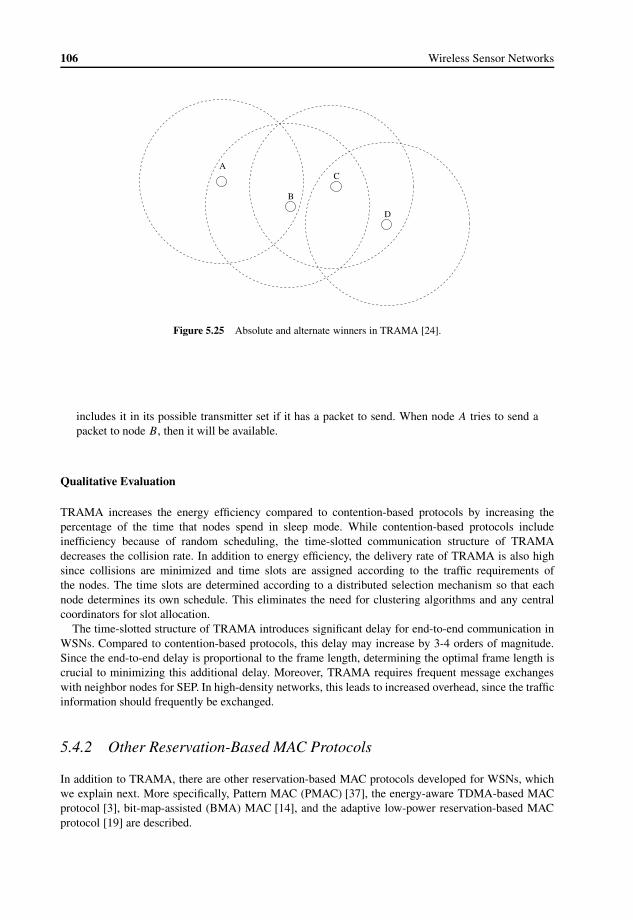
106 Wireless Sensor Networks
D
A
B
C
Figure 5.25 Absolute and alternate winners in TRAMA [24].
includes it in its possible transmitter set if it has a packet to send. When node A tries to send apacket to node B, then it will be available.
Qualitative Evaluation
TRAMA increases the energy efficiency compared to contention-based protocols by increasing thepercentage of the time that nodes spend in sleep mode. While contention-based protocols includeinefficiency because of random scheduling, the time-slotted communication structure of TRAMAdecreases the collision rate. In addition to energy efficiency, the delivery rate of TRAMA is also highsince collisions are minimized and time slots are assigned according to the traffic requirements ofthe nodes. The time slots are determined according to a distributed selection mechanism so that eachnode determines its own schedule. This eliminates the need for clustering algorithms and any centralcoordinators for slot allocation.
The time-slotted structure of TRAMA introduces significant delay for end-to-end communication inWSNs. Compared to contention-based protocols, this delay may increase by 3-4 orders of magnitude.Since the end-to-end delay is proportional to the frame length, determining the optimal frame length iscrucial to minimizing this additional delay. Moreover, TRAMA requires frequent message exchangeswith neighbor nodes for SEP. In high-density networks, this leads to increased overhead, since the trafficinformation should frequently be exchanged.
5.4.2 Other Reservation-Based MAC Protocols
In addition to TRAMA, there are other reservation-based MAC protocols developed for WSNs, whichwe explain next. More specifically, Pattern MAC (PMAC) [37], the energy-aware TDMA-based MACprotocol [3], bit-map-assisted (BMA) MAC [14], and the adaptive low-power reservation-based MACprotocol [19] are described.

Medium Access Control 107
����������������������������������������
����������������������������������������
����������������������������������������
����������������������������������������
PRTF
w
PETF
Figure 5.26 Frame structure of PMAC.
PMAC
PMAC is an adaptive MAC protocol that relies on the exchange of activity patterns and scheduledetermination [37]. The time frame structure of PMAC is shown in Figure 5.26. Each frame consistsof two periods, i.e., pattern repeat time frame (PRTF) and pattern exchange time frame (PETF), similarto data period and reservation period, respectively. Similar to TRAMA, in PMAC a node broadcasts atentative schedule for active slots during the PETF. The tentative schedule is referred to as patterns inPMAC. The patterns consist of ones and zeros for each slot, where a 1 indicates that the node intends tobe active during the slot, whereas a 0 indicates that it intends to switch to sleep state during the slot. Forexample, a pattern of 001 indicates that a node will be in sleep state for two consecutive slots and willbe active during the third slot.
The pattern only indicates the intention of the node according to its traffic load. The actual slots wherethe node will be active or sleep are determined by its schedule which is determined after the patternexchange. The PMAC pattern is a sequence of binary numbers with a maximum length ofN , which is theperiod length. Moreover, the pattern is restricted to be in the form of 0m1, where m= 0, 1, . . . , N − 1.Note that the length of a pattern can be less then N , in which case the pattern repeats itself. For example,for N = 6, a pattern of 001 corresponds to the tentative plan 001001.
A node’s pattern starts with a 1 and zeros are added in front of it, if there is no traffic. This incrementis performed in an exponential fashion. When a node does not have a packet to transmit, the patternevolves as follows: 1, 01, 021, 041, . . . , 0δ1, 0δ01, . . .. This approach of exponentially increasing thesleep time during light traffic allows the nodes to save a considerable amount of energy. Note that theexponential increase continues until the number of zeros reaches a predetermined value (δ). Then, zerosare added linearly to prevent oversleeping.
After each node exchanges its pattern during the PETF, the actual schedule determination isperformed. This is done according to the patterns of the intended receiver and the number of packetsthat a node has to transmit. More specifically, considering the pattern value for node j at slot k as P ij ,
and the corresponding value for its intended receiver (in case a data packet is to be transmitted) as P ki
,the schedule is determined as follows:
• Pkj= 1, P k
i= 1. If node j has a packet to send, it marks its schedule as 1 and transmits its packet
at time slot k. If node j does not have a packet to send, it marks its schedule as 1− indicatingthat it will wake up at slot k, wait for a specific time for any incoming packet, and switch to sleepstate if there is no activity.
• Pkj= 0, P k
i= 1. If node j has a packet to send, it marks its schedule as 1. If it does not have any
packet to send, the schedule is marked as 0 and the node j sleeps during this slot.
• Pkj = 0, P ki = 0. In this case, node j marks its schedule as 0 and waits for the next frame if it hasa packet to send to node i.
• Pkj = 1, P ki = 0. In this case, node j marks its schedule as 1− and wakes up at slot k to checkfor an incoming transmission. If it has a packet to send to node i, it waits for the next frame.
According to these rules the communication between each node is performed using CSMA/CA ineach slot.

108 Wireless Sensor Networks
Cluster Head (CH)
Cluster Node
Figure 5.27 An example of the cluster structure in WSNs.
Energy-Aware TDMA-Based MAC Protocol
The reservation-based protocols described so far enable each node to exchange its schedule informationwith its neighbors to reserve slots for transmission. As a result, a distributed reservation approach isdeveloped. This reservation approach, however, may lead to energy wastage due to collisions in messageexchanges. Moreover, since a general view of even the close vicinity of nodes cannot be generated,suboptimal schedules can be generated distributively. In order to address these inefficiencies, cluster-based protocols have also been developed for WSNs. These protocols rely on a clustered hierarchy suchthat a fraction of the nodes in the network are part of a cluster. Moreover, a cluster head (CH) organizesthe reservation of slots for efficient communication. An example of the cluster structure is also shown inFigure 5.27. In each cluster, the communication is organized by a CH.
The energy-aware TDMA-based MAC protocol [3] focuses on WSNs that are composed of clustersand gateways. Each gateway acts as a cluster-based centralized network manager and assigns slots ina TDMA frame based on the traffic requirements of the nodes in the cluster. Since, in a cluster, nodesmay need multiple hops to reach the gateway, the traffic for routing messages is also incorporated intothe TDMA frame structure. This protocol serves as another example of multi-hop awareness in WSNs.Similar to all cluster-based MAC protocols, the CH manages the slot assignments for other nodes in thecluster. This assignment informs the nodes about the slots during which they should either receive ortransmit a packet. Since multi-hop routes can also exist in a cluster as shown in Figure 5.27, the nodescan also serve as routers in addition to data generators.
The structure of the TDMA frame is shown in Figure 5.28. Both the TDMA frame and the protocolhave four phases for medium access. These four phases are refresh, event-triggered rerouting, refresh-based rerouting, and data transfer phases. The first three phases can be considered as the reservationperiod and the last phase is the data period in the context of the general structure of reservation-basedprotocols. The duration and period of each phase are fixed in the protocol. The main goal is to schedulethe active times of slots based on routing duties and the generated packets of the nodes in a cluster.Accordingly, during the refresh phase, network-related information such as residual energy, location,and state of each node is collected. The refresh slot shown in Figure 5.28 is further slotted such thateach node in the cluster has an assigned slot to transmit its information to the CH. During the event-triggered and refresh-based rerouting phases, the multi-hop routes from the nodes to the CH are updatedand the nodes, which are on these routes, are assigned slots. Accordingly, the CH manages the times ofcommunication at each hop as well as calculating paths.

Medium Access Control 109
����������������
����������������
���������������������
���������������������
������������
������������
������������
������������
Data Slots Refresh Slot
Event-basedRerouting Slots
Refresh-basedRerouting Slot
Figure 5.28 The frame structure of the energy-aware TDMA-based MAC protocol [3].
For slot assignment, two techniques, i.e., breadth and depth, are used. The breadth technique followsa breadth-first search technique to assign the slots to nodes. Accordingly, first nodes A and B send theirpackets to node C. Node C then sends these packets to node E. As a result, a node has to wait for allpackets from its children before relaying packets to its next hop. On the other hand, the depth techniquefollows a depth-first search technique such that the packets from a node that is farther away from the sinkare transmitted first. The CH informs each node of the slots it is going to receive or transmit informationusing one of these techniques.
Finally, the data phase is composed of data slots allocated to nodes with packets to send. The slotassignment performed in the rerouting phases is followed by the nodes in a cluster.
BMA-MAC
The BMA-MAC protocol is an intracluster communication protocol with an energy-efficient TDMA(E-TDMA) scheme [14]. BMA-MAC consists of a cluster setup phase and a steady state phase. In thecluster setup phase, the CH is selected based on the available energy of each node. If a node’s remainingenergy is above a certain threshold, then it can be elected as the CH. The elected nodes contend forbecoming the CH by broadcasting an advertisement message using a simple CSMA scheme. The nodesthat hear the advertisement message join the cluster of the CH. Once the clusters are built, the protocolenters the steady state phase.
In the steady state phase, an E-TDMA MAC scheme is used in each of the clusters formed by the CHs.The superframe structure of BMA-MAC is shown in Figure 5.29. In each superframe, the reservationperiod is slotted for contention. The data period is further divided into two periods, i.e., the datatransmission period and idle period. The duration of the data period is fixed and the data transmissionperiod is changed based on the traffic demands of the nodes. The slot assignment is performed by theCH according to the demands of the non-CHs during the reservation period. The reservation period isslotted and each node has a preassigned slot for its request. If a node has a packet to send, it sends a1-bit control message or remains silent if it does not have any packets. According to the requests, the CHassigns slots for each node with a packet to send in the next data period. Depending on the number ofnodes that request a slot, the duration of the data transmission period and the idle period changes. Eachnode transmits its packets to the CH during its assigned slot and sleeps during the other slots. During theidle slots, all the nodes in the cluster sleep. The BMA-MAC protocol performs the cluster setup phaseafter a specified number of rounds are performed by a CH. As a result, CH duty is exchanged by theother nodes leading to equal energy consumption.
Adaptive Low-Power Reservation-Based MAC
The adaptive low-power reservation-based MAC protocol [19] also assumes a clustered hierarchicalorganization, where the CH is chosen as a result of contention similar to the BMA-MAC protocol.

110 Wireless Sensor Networks
����������������
����������������
�������
�������
�������
�������
�������
�������
����������������������������������������
����������������������������������������
��������������������
��������������������
periodSet-upphase
Data Slots
Data Transmission Idleperiod period
Contention
Figure 5.29 Frame structure of BMA-MAC.
The reservation period is composed of three parts. In the control slot, the CH broadcasts controlinformation such as frame length and the end of cluster information. Since the role of the CH is energyconsuming, the protocol aims to assign the CH duty to several nodes. After a specific duration, theCH announces the end of its duty and the CH is chosen again. The second slot in the frame is thereservation request window. In this window, nodes in the cluster transmit their requests to the CH. Thetransmissions in this window are performed through contention, where a basic CSMA scheme is used.During the reservation confirmation slot, slot allocations are communicated to the cluster nodes by theCH. Finally, a data slot is used for the nodes to transmit their data. The frame size is adjusted accordingto the probability of transmission failures of reservation request packets. If this probability is high, theframe size is increased. On the other hand, if there are no errors for reservation request packets, theframe size is decreased.
5.4.3 Summary
TDMA-based protocols provide collision-free communication in WSNs, achieving improved energyefficiency. However, TDMA-based protocols require an infrastructure consisting of CHs, whichcoordinate the time slots assigned to each node. Although many clustering algorithms have beenproposed with these protocols, the optimality and energy efficiency of these algorithms still need tobe investigated. While TDMA schedules within a cluster can be easily devised, the problem is moreinvolved when individual CHs are not in direct range of the sink, thus necessitating intercluster multi-hop communication. An acceptable, non-overlapping slot assignment for all neighboring clusters needsto be derived in a distributed manner requiring coordination between different clusters. This problem hasbeen shown to be NP -complete [11] by reduction to an instance of graph coloring, and the developmentof efficient heuristics is an open issue.
Network scalability is another important area of research and the TDMA schedules must be able toaccommodate high node densities that are characteristic of sensor networks. As the channel capacityin TDMA is fixed, only slot durations or a number of slots in a frame may be changed keeping inmind the number of users and their respective traffic types. In addition, TDMA-based protocols resultin high latency due to the frame structure. Hence, TDMA-based MAC protocols may not be suitablefor some WSN applications where delay is important in estimating event features and the traffic hasa bursty nature. Moreover, since time-slotted communication is performed in the clusters, interclusterinterference has to be minimized such that nodes with overlapping schedules in different clusters donot collide which each other. Finally, time synchronization is an important part of the TDMA-basedprotocols and synchronization algorithms as explained in Chapter 11 are required.
5.5 Hybrid Medium AccessContention-based and reservation-based protocols provide different advantages and disadvantages in themedium access performance. Since contention-based protocols require significantly less overhead, these
Medium Access Control 111
protocols result in high utilization in cases where there is low contention. However, when the numberof nodes contending for the channel increases, channel utilization decreases since these nodes are notcoordinated. On the other hand, reservation-based protocols provide scheduled access to each node anddecrease collisions. This results in high utilization when the competition is high but also in latency andoverhead. Such a contrast produces a tradeoff between access capacity and energy efficiency. Hybridschemes in MAC protocols aim to leverage the tradeoff introduced in channel allocation by combiningrandom access schemes with reservation-based access TDMA approaches.
Hybrid solutions provide performance enhancements in terms of collision avoidance and energyefficiency due to improved channel organization and adaptivity to dynamic traffic load. Next, we describetwo hybrid solutions developed for WSNs.
5.5.1 Zebra-MAC
In order to provide an adaptive operation based on the level of contention, Zebra-MAC (Z-MAC)combines the advantages of each scheme in a hybrid MAC solution [25]. The communication structureof Z-MAC still relies on time slots similar to TDMA-based solutions. Each slot is tentatively assigned toa node. However, the difference between TDMA-based solutions is that each slot can be stolen by othernodes if it is not used by its owner. Consequently, Z-MAC behaves like CSMA under low contentionand like TDMA under high contention.
Similar to many reservation-based protocols, Z-MAC consists of a setup phase and a communicationphase. The setup phase has four main components:
• Neighbor discovery
• Slot assignment
• Local frame exchange
• Global time synchronization.
Neighbor discovery is performed once by each node to gather information about its two-hopneighborhood. During this phase, each node broadcasts its one-hop neighborhood information toits neighbors. At the end of multiple message exchanges, each node is informed about its two-hopneighborhood information. Collisions in the wireless channel affect the two-hop neighborhood of eachnode because of the hidden terminal problem.
Slot assignment is performed by the DRAND protocol [25], which ensures a broadcast schedulesuch that each node is assigned a slot that will not coincide with the slots of its two-hop neighbors.DRAND first creates a radio interference map of the network. Nodes that can interfere with each otherare connected by bidirectional links in the interference map. Slot assignment is performed iterativelyaccording to this map.
EXAMPLE 5.15
A sample topology of six nodes is shown in Figure 5.30(a), where the connectivity of each nodeis also illustrated by ellipses. According to this topology, DRAND creates the radio interferencemap as shown in Figure 5.30(b).
The case where node C needs to assign a slot to itself is depicted in Figure 5.30(c). Node Cfirst broadcasts a request message to its immediate neighbors, A, B, and D. If there is no conflict,each node responds with grant messages (Figure 5.30(d)). Accordingly, node C indicates that theparticular slot is reserved by broadcasting a release message as shown in Figure 5.30(e). Eachimmediate neighbor also communicates this slot selection to each two-hop neighbor of node C,i.e., E and F, as shown in Figure 5.30(f).
In case there is a conflict with the slot selected by node C, this is indicated by a reject messageafter the request broadcast as shown in Figure 5.30(g), where node D sends a reject message to

112 Wireless Sensor Networks
F
C
B
A
D
E
(a) Network topology
F
C
B
A
D
E
(b) Radio Interference Map
RequestC
B
A
D
E
F
(c) Broadcast request
GrantC
B
A
D
E
F
(d) Receive grants
ReleaseC
B
A
D
E
F
(e) Broadcast release
Two Hop Release
C
B
A
D
E
F
(f) Two-hop release
Grant C
B
A
D
E
F
Reject
(g) Receive reject
FailC
B
A
D
E
F
(h) Broadcast fail
Figure 5.30 Operation of the DRAND protocol.
node C. If node C does not receive a grant message from all of its neighbors, it broadcasts afail message as shown in Figure 5.30(h) to indicate that it cannot allocate the slot. As a result,collisions are prevented.
Z-MAC also introduces a local frame structure. In many TDMA-based solutions, the frame size isfixed for the whole network. While a large enough frame size is essential to accommodate all thecontending nodes in a local neighborhood, the required size may not be the same for different parts of thenetwork. Depending on the density at each location of the network, a node may have fewer neighbors tocompete with. For these cases, smaller frame sizes are more efficient since the slots can be reused morefrequently. Based on this observation, Z-MAC allows each node to specify its own local frame size.
The local frame size is selected according to the time frame rule. Accordingly, if a node i is assigneda slot si and the maximum slot number in its neighborhood is Fi , then node i’s time frame size isselected as 2a . The integer a is chosen such that 2a−1 ≤ Fi < 2a − 1. This time frame rule ensures thatif the node uses the slot si for each 2a slots, then it does not collide with any of its two-hop neighbors.After the local frame sizes are selected, this information is exchanged between neighbors to constitute astable operation.

Medium Access Control 113
End backoff
A (0)
B (1)
0 1 2
Start backoff
Figure 5.31 Adaptive channel access mechanism of Z-MAC.
The transmission structure of Z-MAC follows the frame structure described above. For each slot, anode is denoted as the owner and other nodes are non-owners. Owners have higher priority over non-owners in accessing the channel during their assigned slots. This prioritization is performed similarly toCSMA. If an owner has a packet to transmit during its slot, it first performs CCA. If the channel is idle, itwaits for a random amount of time within a time period To and transmits its packet. If the owner does nothave a packet to send, non-owners can utilize its time slot. This is performed through a different backoffmechanism. The non-owners first wait for a time period To and then back off for a random amount oftime within a time period Tno. This provides prioritization for owners and enable non-owners to stealthe slot if it is not used.
EXAMPLE 5.16
The adaptive transmission mechanism of Z-MAC is illustrated in Figure 5.31, where two nodes Aand B own slots 0 and 1, respectively. During slot 0, both nodes have packets to send and back offat the beginning of the slot. Since node A is the owner of this slot, its backoff timer expires first,it allocates the channel, and transmits its packet. On the other hand, since node B’s backoff timeexpires later, it senses the channel as busy and waits for the packet transmission. If node A haspackets to send, it can use slot 0. In the next slot, 1, node B is the owner, and can send its packetsduring this slot. The dynamic operation of Z-MAC is shown during slot 2, where node A is theowner. Node A first transmits its packet. When the transmission is over, node B starts its backofftimer and initiates transmission when the channel is idle. As a result, when node A does not haveany packet to send during its assigned slot, node B can utilize the available channel.
Z-MAC also employs a mechanism to relieve the contention around a specific node. If an ownerexperiences a high contention during its time slot, it broadcasts an explicit contention notification (ECN)message to its neighbors. The ECN message is propagated toward the two-hop neighbors on the pathto destination. The nodes receiving the ECN message switch to a high contention level (HCL) mode.Nodes in HCL mode for a specific node do not compete for the slots owned by that node. As a result,contention decreases on the path toward destination.
EXAMPLE 5.17
The ECN operation is illustrated in Figure 5.32, where node C tries to send packets to the sinkthrough nodes D and F. If node C experiences high contention, it broadcasts a one-hop ECNmessage to A, B, and D. Since nodes A and B are not on the routing path, they discard the ECNmessage. However, since node D is on the routing path, it forwards the ECN message as a two-hop

114 Wireless Sensor Networks
F
A B
C
E
D
Figure 5.32 Operation of the ECN mechanism in Z-MAC.
ECN message to nodes E and F. As a result E and F do not compete during C’s slot as non-owners.However, nodes A, B, and D are eligible to compete during C’s slot.
Qualitative Evaluation
The hybrid medium access scheme of Z-MAC provides adaptive communication if a number of sensornodes or the traffic load change. Compared to contention-based protocols, Z-MAC improves throughputwhen the traffic load is high and still maintains acceptable latency for low traffic compared to TDMA-based protocols.
Z-MAC has been developed for a specific scenario, where the sensor nodes are mobile and haveintermittent communication capabilities. Hence, it may not be applicable for a large set of WSNapplications, where the network is static.
IEEE 802.15.4
IEEE 802.15.4 was developed for low-data-rate wireless networks, and combines reservation-based andcontention-based approaches [1]. The protocol, also supported by the ZigBee consortium, introduces asuperframe structure with two disjoint periods, i.e. contention access period and contention-free period.The network is assumed to be clustered and each cluster head, i.e. PAN coordinator, broadcasts theframe structure and allocates slots to prioritized traffic in the contention-free period. In the contentionperiod, nodes contend using CSMA/CA or slotted CSMA/CA to access the channel. The winners canallocate the channel for their transmissions for a specific amount of time. This provides a flexible accessmethod for nodes with infrequent traffic. During the contention-free period, nodes with higher prioritytraffic are served by the PAN coordinator. Based on the traffic requirements, each node is assigned slotsduring the contention-free period. These slots are allocated to only one pair and channel contention isprevented to provide priority. As a result, the IEEE 802.15.4 protocol provides a hybrid operation througha CSMA-based and a TDMA-based operation. Although this protocol aims for prioritization and energyefficiency up to 1% duty cycles, it requires a cluster-based topology, which may not be applicable tosome WSN scenarios.

Medium Access Control 115
References[1] IEEE standard for information technology – telecommunications and information exchange between systems –
local and metropolitan area networks – specific requirement part 15.4: Wireless medium access control (MAC)and physical layer (PHY) specifications for low-rate wireless personal area networks (WPANS). IEEE Std.802.15.4a-2007 (Amendment to IEEE Std. 802.15.4-2006), pp. 1–203, 2007.
[2] I. F. Akyildiz, W. Su, Y. Sankarasubramaniam, and E. Cayirci. Wireless sensor networks: a survey. ComputerNetworks, 38(4):393–422, March 2002.
[3] K. A. Arisha, M. A. Youssef, and M. Y. Younis. Energy-aware TDMA-based MAC for sensor networks.Computer Networks, 43(5):539–694, December 2003.
[4] M. Buettner, G. Yee, E. Anderson, and R. Han. X-MAC: a short preamble MAC protocol for duty-cycledwireless sensor networks. In Proceedings of ACM SenSys’06, pp. 307–320, Boulder, CO, USA, October 2006.
[5] I. Demirkol, C. Ersoy, and F. Alagoz. MAC protocols for wireless sensor networks: a survey. IEEE Communi-cations Magazine, 44(4):115–121, April 2006.
[6] A. El-Hoiydi. Aloha with preamble sampling for sporadic traffic in ad hoc wireless sensor networks. InProceedings of IEEE ICC’02, volume 5, pp. 3418–3423, New York, USA, April 2002.
[7] A. El-Hoiydi and J.-D. Decotignie. WiseMAC: an ultra low power MAC protocol for the downlink ofinfrastructure wireless sensor networks. In Proceedings of the International Symposium on Computers andCommunications (ISCC’04), volume 1, pp. 244–251, Alexandria, Egypt, July 2004.
[8] S. C. Ergen and P. Varaiya. PEDAMACS: power efficient and delay aware medium access protocol in sensornetworks. IEEE Transactions on Mobile Computing, 5(7):920–930, July 2006.
[9] G. P. Halkes and K. G. Langendoen. Crankshaft: an energy-efficient MAC-protocol for dense wireless sensornetworks. In Proceedings of EWSN’07, pp. 228–224, Delft, The Netherlands, January 2007.
[10] M. Hayajneh, I. Khalil, and Y. Gadallah. An OFDMA-based MAC protocol for under water acoustic wirelesssensor networks. In Proceedings of IWCMC’09, pp. 810–814, Leipzig, Germany, June 2009.
[11] T. Herman and S. Tixeuil. A distributed TDMA slot assignment algorithm for wireless sensor networks. InProceedings of the Workshop on Algorithmic Aspects of Wireless Sensor Networks (ALGOSENSORS’04),pp. 45–58, Turku, Finland, July 2004.
[12] K. Kredo II and P. Mohapatra. Medium access control in wireless sensor networks. Computer Networks,51(4):961–994, 2007.
[13] K. Jamieson, H. Balakrishnan, and Y. C. Tay. Sift: a MAC protocol for event-driven wireless sensor networks.In Proceedings of EWSN’06, pp. 260–275, Zurich, Switzerland, February 2006.
[14] J. Li and G. Y. Lazarou. A bit-map-assisted energy-efficient MAC scheme for wireless sensor networks. InProceedings of ACM IPSN’04, pp. 55–60, Berkeley, CA, USA, April 2004.
[15] P. Lin, C. Qiao, and X. Wang. Medium access control with a dynamic duty cycle for sensor networks. InProceedings of IEEE WCNC’04, pp. 1534–1539, Atlanta, GA, USA, March 2004.
[16] S. Liu, K.-W. Fan, and P. Sinha. CMAC: an energy efficient MAC layer protocol using convergent packetforwarding for wireless sensor networks. In Proceedings of IEEE SECON’07, pp. 11–20, San Diego, CA, USA,June 2007.
[17] S. Mahlknecht and M. Bock. CSMA-MPS: a minimum preamble sampling MAC protocol for low powerwireless sensor networks. In Proceedings of the IEEE International Workshop on Factory CommunicationSystems, pp. 73–80, Vienna, Austria, September 2004.
[18] S. Meguerdichian, F. Koushanfar, M. Potkonjak, and M. B. Srivastava. Coverage problems in wireless ad-hocsensor networks. In Proceedings of IEEE INFOCOM 2001, volume 3, pp. 1380–1387, Anchorage, AK, USA,April 2001.
[19] S. Mishra and A. Nasipuri. An adaptive low power reservation based MAC protocol for wireless sensor net-works. In Proceedings of the IEEE International Conference on Performance, Computing, and Communications,pp. 731–736, Phoenix, AZ, USA, April 2004.
[20] A. Muqattash and M. Krunz. CDMA-based MAC protocol for wireless ad hoc networks. In Proceedings of ACMMobiHoc, volume 1, pp. 153–164, Annapolis, MD, USA, June 2003.
[21] J. Polastre, J. Hill, and D. Culler. Versatile low power media access for wireless sensor networks. In Proceedingsof SenSys’04, pp. 95–107, Baltimore, MD, USA, 2004.

116 Wireless Sensor Networks
[22] D. Pompili, T. Melodia, and I. F. Akyildiz. A distributed CDMA medium access control for underwater acousticsensor networks. In Proceedings of Mediterranean Ad Hoc Networking Workshop (Med-Hoc-Net), Corfu,Greece, June 2007.
[23] V. Rajendran, J. J. Garcia-Luna-Aveces, and K. Obraczka. Energy-efficient, application-aware medium accessfor sensor networks. In Proceedings of IEEE MASS’05, Washington, DC, USA, November 2005.
[24] V. Rajendran, K. Obraczka, and J. J. Garcia-Luna-Aceves. Energy-efficient, collision-free medium accesscontrol for wireless sensor networks. In Proceedings of ACM SenSys’03, Los Angeles, CA, USA, November2003.
[25] I. Rhee, A. Warrier, M. Aia, and J. Min. Z-MAC: a hybrid MAC for wireless sensor networks. In Proceedingsof ACM SenSys’05, pp. 90–101, San Diego, CA, USA, 2005.
[26] M. Salajegheh, H. Soroush, and A. Kalis. HYMAC: hybrid TDMA/FDMA medium access control protocol forwireless sensor networks. In Proceedings of IEEE PIMRC’07, pp. 1–5, Athens, Greece, 2007.
[27] C. Schurgers, V. Tsiatsis, and M. B. Srivastava. STEM: topology management for energy efficient sensornetworks. In Proceedings of the IEEE Aerospace Conference, volume 3, pp. 1099–1108, Big Sky, MT, USA,2002.
[28] Y. Sun, O. Gurewitz, and D. B. Johnson. RI-MAC: a receiver-initiated asynchronous duty cycle MAC protocolfor dynamic traffic loads in wireless sensor networks. In Proceedings of ACM SenSys’08, pp. 1–14, 2008.
[29] H.-X. Tan and W. K. G. Seah. Distributed CDMA-based MAC protocol for underwater sensor networks. InProceedings of IEEE LCN’07, pp. 26–36, Washington, DC, USA, 2007.
[30] T. van Dam and K. Langendoen. An adaptive energy-efficient MAC protocol for wireless sensor networks. InProceedings of ACM SENSYS’03, pp. 171–180, Los Angeles, CA, USA, November 2003.
[31] M. C. Vuran, O. B. Akan, and I. F. Akyildiz. Spatio-temporal correlation: theory and applications for wirelesssensor networks. Computer Networks, 45(3):245–261, June 2004.
[32] M. C. Vuran and I. F. Akyildiz. Spatial correlation-based collaborative medium access control in wireless sensornetworks. IEEE/ACM Transactions on Networking, 14(2):316–329, April 2006.
[33] Y. Wang and J. J. Garcia-Luna-Aceves. Performance of collision avoidance protocols in single-channel ad hocnetworks. In Proceedings of the IEEE International Conference on Network Protocols, pp. 68–77, Paris, France,2002.
[34] W. Ye, J. Heidemann, and D. Estrin. An energy-efficient MAC protocol for wireless sensor networks. InProceedings of IEEE INFOCOM’02, volume 3, pp. 1567–1576, New York, USA, June 2002.
[35] W. Ye, J. Heidemann, and D. Estrin. Medium access control with coordinated adaptive sleeping for wirelesssensor networks. IEEE/ACM Transactions on Networking, 12(3):493–506, June 2004.
[36] W. Ye, F. Silva, and J. Heidemann. Ultra-low duty cycle MAC with scheduled channel polling. In Proceedingsof ACM SenSys’06, Boulder, CO, USA, November 2006.
[37] T. Zheng, S. Radhakrishnan, and V. Sarangan. PMAC: an adaptive energy-efficient MAC protocol for wirelesssensor networks. In Proceedings of the IEEE International Parallel and Distributed Processing Symposium(IPDPS ’05), Denver, CO, USA, 2005.

6Error Control
WSN applications rely on multiple sensor feedback for interaction with the environment. In general,the main objectives of the data link layer in this interaction are multiplexing/ demultiplexing of data,data frame detection, medium access, and error control. In addition to the MAC layer functionalitiesdiscussed in Chapter 5, in this chapter we explain the effects of error control on communicationreliability and efficiency in WSNs.
Contrary to traditional networks, WSNs are characterized by low energy requirements and thecollaborative nature of sensors. Hence, the design of data link layer protocols encounters uniquechallenges as opposed to traditional networking protocols. While fulfilling the application’s objectives,the data link layer should provide reliable and energy-efficient point-to-point and point-to-multipointcommunication throughout the network. An overview of the data link components is shown inFigure 6.1 [16].
In WSNs, where the correlation between sensors can be exploited in terms of aggregation, collab-orative source coding, or correlation-based protocols, error control is extremely important. Since thecommunication solutions generally aim to reduce the redundancy in the traffic by filtering correlateddata or switching off redundant nodes, it is essential for each packet to be transmitted reliably. Moreover,the multi-hop features of WSNs require a unique definition of reliability other than the conventionalreliability metrics which focus on point-to-point reliability. Hence, the effects of error control schemesare analyzed using cross-layer analysis techniques to consider the effects on wireless channel, mediumaccess, and multi-hop routing.
The main purpose of the error control schemes is to provide reliable communication in the wirelesschannel. This channel has adverse effects on communication because of the fading, interference, andloss of bit synchronization as discussed in Chapter 4. This results in wireless channel errors that impactthe integrity of packets that are sent by sensor nodes. The wireless channel effects are further increasedin WSNs because of the low-power communication techniques. As a result, in addition to the physicallayer techniques that provide reliability at the bit level, error control schemes are used at the link layerto provide reliability at the packet level. Accordingly, error control schemes maintain error-free, in-sequence, duplicate-free, and loss-free communication between sensor nodes.
In general, the error control mechanisms in WSNs can be categorized into four main approaches:power control, automatic repeat request (ARQ), forward error correction (FEC), and hybrid ARQ(HARQ) as described next.
6.1 Classification of Error Control Schemes
6.1.1 Power Control
State-of-the-art transceivers such as the CC2420 used in MicaZ, TelosB, and SunSPOT nodes supportmultiple transmit power levels that can be controlled on a per-packet basis. Accordingly, the amount of
Wireless Sensor Networks Ian F. Akyildiz and Mehmet Can Vuranc© 2010 John Wiley & Sons, Ltd

118 Wireless Sensor Networks
Network Layer
MAC
LinkLayer
ErrorControl
Power
Management
Physical Layer
Figure 6.1 An overview of the data link layer providing reliability in WSNs [16].
power dissipated from the antenna can be adjusted to control the effective communication range of anode. Transmission power control can be used to achieve desired error rates in wireless communication.Higher transmit power reduces the packet error rate by improving the signal-to-noise ratio. However,energy consumption is therefore increased in addition to increased interference with other nodes. Powercontrol requires sophisticated protocols to be implemented, which requires additional memory for theimplementation. Transmit power control is generally used for long periods of time, such as topologycontrol, as will be explained in Chapter 13. However, per-packet transmit power introduces significantoverhead in the resource constraint sensor nodes. Further, as we will describe next, power control can beused in conjunction with forward error control schemes to improve energy efficiency.
6.1.2 Automatic Repeat Request (ARQ)
ARQ-based error control mainly relies on the retransmission of lost or corrupted packets to maintainreliability. For this purpose, a header is added to the payload of the packet to indicate the source nodeand a low-complexity error detection algorithm is used to calculate the checksum of the packet. Thischecksum is added to the end of the packet. Typically a cyclic redundancy check (CRC) mechanism,which is described in Chapter 4 is used. The receiver node computes the checksum of the receivedbits and compares this to the checksum of the received packet. Accordingly, the receiver can providefeedback to the source regarding the integrity of the received packet. This can be performed bysending either a positive acknowledgment (ACK) for each successfully received packet or a negativeacknowledgment (NACK) for each corrupt packet. In the case of an ACK, the sender sets a timer todetect that ACKs have not arrived. If the sender infers that a packet is corrupted it retransmits thispacket.
The main ARQ strategies can be summarized as go-back-N, selective repeat, and stop-and-wait [9, 5,4]. Go-back-N lets the sender send up to N packets. If at least a packet has not been ACKed, then allthe packets are retransmitted. For selective repeat, the sender retransmits only those packets that havenot been ACKed. Finally, the stop-and-wait strategy lets only a single outstanding packet through andtransmits the following packet after the outstanding packet is ACKed. Stop-and-wait is the most commonARQ strategy for WSNs.
ARQ-based error control mechanisms incur significant additional retransmission cost and overhead.Although these schemes are utilized at the data link layer for conventional wireless networks, theefficiency of ARQ in sensor network applications is limited due to the scarcity of the energy andprocessing resources of the sensor nodes.
DuyTan
Highlight
DuyTan
Highlight
DuyTan
Highlight
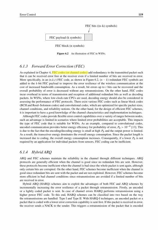
Error Control 119
FEC bits ((n–k) symbols)
FEC block (n symbols)
FEC payload (k symbols)
Figure 6.2 An illustration of FEC in WSNs.
6.1.3 Forward Error Correction (FEC)
As explained in Chapter 4, FEC codes (or channel codes) add redundancy to the transmitted packet suchthat it can be received error free at the receiver even if a limited number of bits are received in error.More specifically, in an (n,k,t) FEC code, as shown in Figure 6.2, (n− k) redundant FEC symbols areadded to the k-bit FEC payload to improve the error resilience of the wireless communication at thecost of increased bandwidth consumption. As a result, bit errors up to t bits can be recovered and theoverall probability of error is decreased without any retransmissions. On the other hand, FEC codesincur overhead in terms of transmission and reception of additional redundant bits as well as decodingpackets. In WSNs, where low-clock-rate CPUs are used, decoding energy should also be considered inassessing the performance of FEC protocols. There exist various FEC codes such as linear block codes(BCH and Reed–Solomon codes) and convolutional codes, which are optimized for specific packet sizes,channel conditions, and reliability notions. On the other hand, for the design of efficient FEC schemes,it is important to have a good knowledge of the channel characteristics and implementation techniques.
Although FEC codes provide flexible error control capabilities over a variety of ranges between nodes,such an advantage is limited in scenarios where limited error probabilities are acceptable. This impactsthe type of FEC code that is suitable for WSNs. As an example, compared to convolutional codes,uncoded communication provides better energy efficiency for probability of error, Pb > 10−4 [13]. Thisis due to the fact that the encoding/decoding energy is small at high Pb and the output power is limited.As a result, the transceiver energy dominates the overall energy consumption. Since the packet length isincreased due to coding, the overall energy consumption increases. Consequently, if a lower Pb is notrequired by an application for individual packets from sensors, FEC coding can be inefficient.
6.1.4 Hybrid ARQ
ARQ and FEC schemes maintain the reliability in the channel through different techniques. ARQprotocols are generally efficient when the channel is good since no redundant bits are sent. However,these protocols become inefficient when the channel is bad since the whole packet is sent again, althoughonly certain bits are corrupted. On the other hand, FEC schemes become inefficient when the channel isgood since redundant bits are sent with the packet and are not exploited. However, FEC schemes becomemore efficient in bad channel conditions since retransmissions are avoided if a limited number of bitsare received in error.
Hybrid ARQ (HARQ) schemes aim to exploit the advantages of both FEC and ARQ schemes byincrementally increasing the error resilience of a packet through retransmission. Firstly, an uncodedor a lightly coded packet is sent. In case of channel errors HARQ performs retransmission using ahigher power FEC code. To this end, HARQ schemes can be classified into two based on the waythe retransmissions are handled: Type I and Type II. With HARQ-I techniques, an uncoded packet or apacket that is coded with a lower error correction capability is sent first. If this packet is received in error,the receiver sends a NACK to the sender. This triggers a retransmission of the packet that is encoded
DuyTan
Highlight

120 Wireless Sensor Networks
Figure 6.3 Probability of error versus transmission power for different convolutional codes.
with a more powerful FEC code. The difference in Type II is that, for retransmissions, only the redundantbits are sent. While Type II decreases the bandwidth usage of the protocol, Type I does not require thepreviously sent packets to be stored at the receiver side.
In the following, we describe the unique aspects of using error control schemes in WSNs.
6.2 Error Control in WSNs
In WSNs, energy consumption is the most important performance metric in the design of communicationprotocols. Since the sensor nodes have stringent energy capabilities, error control protocols should alsoconsider energy efficiency as the first design goal. The sources of energy consumption in WSNs can bemainly classified into two types, namely computation power and transmission/receiving power. However,since transmission of a bit is more costly than processing power, protocols that exploit the on-boardprocessing capabilities of sensor nodes are more favorable. Consequently, the use of FEC results inhigher energy efficiency in certain situations given the constraints of the sensor nodes.
The use of FEC codes can decrease the transmit power due to the increased redundancy in theconstructed packets [13]. The performance of convolutional codes in terms of probability of error andoutput transmit power is shown in Figure 6.3 [13]. As shown in this figure, lower transmit power ispossible for a specific probability of error using FEC codes. However, the required processing powerdue to encoding/decoding of the packet increases the overall energy consumption. The required energyduring the encoding and decoding of BCH codes is shown in Figure 6.4 along with the incurredencoding/decoding latency in Figure 6.5 [10]. Moreover, the increase in packet length also incursadditional energy cost. This additional cost is due to the longer packet transmission times and, hence,the increased packet collision rate.
Although the FEC can achieve significant reduction in the bit error rate (BER) for any given valueof the transmit power, the additional processing power that is consumed during encoding and decodingmust be considered when designing an FEC scheme. FEC is a valuable asset for the sensor networks ifthe additional processing power is less than the transmission power savings. Thus, the tradeoff between

Error Control 121
Figure 6.4 Total energy consumption for encoding and decoding using BCH codes [13].
Figure 6.5 Total encoding and decoding latency using BCH codes [13].
this additional processing power and the associated coding gain needs to be optimized in order tohave powerful, energy-efficient, and low-complexity FEC schemes for error control in sensor networks.Furthermore, powerful FEC codes incur additional decoding latency which should also be considered inthe choice of error control schemes.
In addition to single-hop effects, the overall impact of error control schemes on multi-hop communica-tion should also be considered. FEC coding and HARQ schemes improve the error resilience comparedto ARQ schemes by sending redundant bits through the wireless channel. Therefore, lower SNR valuescan be supported to achieve the same error rate as an uncoded transmission. However, this advantagecomes at the cost of increased packet sizes due to the redundant bits and encoding/decoding packets. Toovercome the overhead because of increased communication and computational cost, the error resilienceof the FEC and HARQ codes can be exploited in two ways in WSNs:

122 Wireless Sensor Networks
–100 –80 –60 –40 –20 0 20 40 60 80 100–100
–80
–60
–40
–20
0
20
40
60
80
100Avg. PRR (500 samples) – ARQ (7 retx) + DSSS + OQPSK
0
0.2
0.2
0.2
0.2
0.20.
40.4
0.4
0.4
0.6
0.6
0.6
0.6
0.8
0.8
0.8
0.9
0.9
0.95
0.95
0.99
0.99
1
1
(a)
–100 –80 –60 –40 –20 0 20 40 60 80 100–100
–80
–60
–40
–20
0
20
40
60
80
100Avg. PRR (500 samples) – BCH(128, 78, 7) + DSSS + OQPSK
0.2
0.2
0.2
0.2
0.2
0.2
0.2
0.2
0.4
0.4
0.4
0.4
0.40.4
0.4
0.6
0.60.6
0.6
0.6
0.6
0.8
0.8
0.8
0.80.8
0.9
0.9
0.9
0.9
0.95
0.95
0.95
0.95
0.99
0.99
0.99
1
1
1
1
1
1
1
(b)
Figure 6.6 Two-dimensional average packet reception rate graphs for (a) ARQ (N = 7) and (b) FEC(BCH(128, 78, 7)) for MicaZ [14].
• Hop length extension: In multi-hop networks, the error resilience of FEC and HARQ schemescan be exploited to improve the effective transmission range of a node. This is illustrated inFigure 6.6. In these figures, the packet error rate (PER) contours of the ARQ and FEC codes areshown around a transmitter node. The contours show the locations where the corresponding PERis at a specific value. If we compare Figure 6.6(a) and Figure 6.6(b) for a target packet receptionrate of 90%, the average transmission range of a node is 29 m for ARQ and 42 m for FEC witha transmit power of −5 dBm. This 45% increase in effective range clearly illustrates that FECcodes can increase the effective transmission range of a node compared to ARQ by using thesame transmit power. While this property is generally not useful for single-hop communication,it is beneficial for WSNs where longer hops can be constructed in a multi-hop network suchas WSNs. The hop length extension can be achieved through channel-aware cross-layer routingprotocols.
• Transmit power control: The improved error resilience provided through FEC codes can also beexploited by reducing the transmit power. This technique is referred to as transmit power controland improves the capacity of the network by reducing the interference to other users.
EXAMPLE 6.1
The concepts of hop length extension and transmit power control for exploiting the error resilienceof FEC codes are depicted in Figure 6.7 compared to an ARQ communication. In Figure 6.7(a), atypical communication link between nodes A and B is shown for a typical ARQ communication.In this case, node A uses a transmit power of Pt,ARQ to send a packet to node B, which is at adistance dARQ away. As a result of the attenuation in the channel, this results in a SNR of SNRARQat node B. Accordingly, a target PER value of PER∗ARQ can be achieved.
Now consider the case where an FEC code is used for communication instead of ARQ. Basedon the error resilience of FEC codes, the same target PER∗ARQ can be reached through a lower SNRvalue SNRFEC < SNRARQ. This advantage can be exploited in two ways in multi-hop networks. Inthe first case, node A selects another node C that is farther from node B as the next hop as shownin Figure 6.7(b). Since the distance is increased, i.e., dFEC > dARQ, with the same transmit power,

Error Control 123
Pt,ARQ
dARQ
SNRARQ
(a) ARQ communication
Pt,ARQ
SNRFEC
dFEC
(b) Hop length extension via FEC
Pt,FEC
dARQ
SNR FEC
(c) Transmit power control via FEC
Figure 6.7 Error resilience of FEC vs. ARQ.
the received SNR value at node C is less than that at B. However, lower SNR values are adequatefor FEC codes. Hence, the same PER can still be achieved. This is called hop length extension.
The second way is depicted in Figure 6.7(c). In this case, node A uses node B as the next hopby fixing the hop distance, i.e., dFEC = dARQ. However, it uses a smaller transmit power, i.e.,Pt,FEC < Pt,ARQ, than the ARQ case to reach the node. Since attenuation is constant at the samedistance, the same target PER can be achieved with a smaller SNR. This is called transmit powercontrol.
Both hop length extension and transmit power control improve the energy efficiency of communica-tion. In hop length extension, fewer hops can be used to reach a destination, while transmit power controlreduces the transmit power level at each hop without affecting the hop distance.
In addition to the advantages, FEC and HARQ schemes improve the error resilience at the cost ofencoding/decoding energy and latency as well as communication overhead due to the transmission andreception of longer packets. As a result, the overall comparison of error control schemes requires a cross-layer analysis to weigh the advantages and disadvantages of these schemes. In the following, we presentsuch an analysis model and describe the cases where FEC or HARQ is more efficient than ARQ.
6.3 Cross-layer Analysis Model
In this section, we describe a cross-layer analysis model that will be used to investigate the tradeoffsbetween ARQ, FEC, and HARQ schemes in terms of energy consumption, latency, and end-to-end PERconsidering the hop length extension and the transmit power control techniques [14, 15]. The objectiveof this model is to determine the following metrics for the analysis:
• Expected hop distance
• End-to-end energy consumption
• End-to-end latency
• End-to-end PER.
Next, we explain the system model and describe how these metrics are calculated.

124 Wireless Sensor Networks
nj
ni
dγ
αd
R inf
d(i,j)
α
D
Sinkγ
dA
Figure 6.8 Reference model for the derivations [14].
6.3.1 Network Model
For the cross-layer analysis, consider a network composed of sensor nodes that are distributed accordingto a two-dimensional (2-D) Poisson distribution with density ρ. Duty cycle operation is deployed suchthat each node is active for a fraction δ of the time and is in sleep mode otherwise [14, 15]. The modelis based on a monitoring application such that the reporting rates of sensors are low but the messagesshould be transmitted reliably subject to a certain end-to-end PER target.
The hop length extension can be realized through a channel-aware routing algorithm, where the nexthop is determined according to the received SNR of a packet sent from a specific node i at a distance Dfrom the sink. Among the neighbors of i, the neighbor j that is closest to the sink and with SNR valuehigher than a threshold, i.e., ψj > ψTh, is selected as the next hop. The medium access is performedthrough RTS–CTS–DATA exchange in addition to ACK and retransmissions for ARQ and NACK andretransmissions for HARQ.
The model used for derivations is shown in Figure 6.8, where a sender node ni transmits a packet tothe sink through a path that involves node nj as the next hop. The log-normal shadow fading modelexplained in Chapter 4 is used for the wireless channel. In this case, the transmission range of a node isessentially infinite due to the shadow fading component. Hence, the transmission range of a node isRinf ,which is the distance at which the probability that a packet can be successfully received is negligible.Moreover, the distribution of hop distance and the associated parameters at each hop can be consideredindependent since duty cycle operation is performed. As a result, the state of the network will changeat each hop since different nodes will be awake at different times. The following cross-layer analysis isbased on a packet that is transmitted to the sink and captures the effects of neighbor nodes and wirelesschannel effects.
The cross-layer analysis framework enables a comprehensive comparison of ARQ, FEC, and HARQschemes. To illustrate specific results, block codes are considered, which are represented by (n, k, t),where n is the block length, k is the payload length, and t is the error correction capability in bits. Inthe comparisons a series of extended BCH (n, k, t) codes with n= 128 and t = {2, 3, 5, 7, 9, 13, 21}are used. Moreover, the (7, 3, 2), (15, 9, 3), and (31, 19, 6) RS codes are considered. For theHARQ schemes, three different configurations are important. For Type I HARQ (HARQ-I), first anuncoded packet is sent followed by a packet encoded by BCH codes. Furthermore, a combinationof two BCH codes is also considered for the HARQ-I. The Type II HARQ (HARQ-II) schemesnecessitate incremental error control coding since only the difference in redundant bits is sent throughretransmissions. Accordingly, the packet is encoded by a BCH code and then the payload is sent first.The receiver uses the CRC bits in the payload for decoding. In case of errors, the receiver sends a NACK

Error Control 125
packet and the transmitter sends the redundant bits for BCH decoding. The HARQ schemes are indicatedby a tuple (t1, t2), where the first parameter, t1, indicates the error correction capability of the first packetand t2 is that of the second packet. As an example, HARQ-II (0, 3) refers to the Type II HARQ, wherefirst an uncoded packet is sent, i.e., t1 = 0, and in case of channel errors, the redundant bits of the BCH(128, 106, 3) encoded packet are sent. Hence, only single retransmission is considered.
The most important performance metrics in WSNs is the energy consumption. The total energyconsumed as a result of a single flow from a source node at distance D from the sink is as follows:
Eflow(D)= E[Eh] E[nh(D)] (6.1)
where E[Eh] is the expected energy consumption per hop and E[nh(D)] is the expected hop count froma source at distance D from the sink. Similarly, the end-to-end latency of a flow is given by
Tflow(D)= E[Th] E[nh(D)] (6.2)
where E[Th] is the expected delay per hop.The expected hop count E[nh(D)] is represented as [15]
E[nh(D)] �D − Rinf
E[dh] + 1 (6.3)
where D is the end-to-end distance, Rinf is the approximated transmission range, and E[dh] is theexpected hop distance. In Sections 6.3.2, 6.3.3, and 6.3.4, we derive the expressions for the expectedhop length, E[dh], the expected energy consumption per hop, E[Eh], and the expected latency per hop,E[Th], respectively.
6.3.2 Expected Hop Distance
Let us consider the reference model in Figure 6.8, where a node j resides in the infinitesimal area dA=dγ dα at coordinates (γ, α) with respect to the sink. The distance from node j to node i is, hence,given by
d(i,j) = d(D, γ, α)=√γ 2 +D2 − 2γD cos α (6.4)
where D is the distance between the source node i and the sink, γ is the distance between the sink andthe relay node j , and the angle α is as shown in Figure 6.8.
Accordingly, the expected hop distance, E[dh], is represented as
E[dh] =∫ D
γmin
∫ αγ
−αγd(i,j) dP{Ni = j} (6.5)
where γmin =D − Rinf is the minimum distance between a potential next hop node j and the sink.Moreover, d(i,j) is the distance between nodes i and j as given by (6.4) and dP{Ni = j} is the probabilitythat the next hop Ni is selected as node j . Finally, αγ = a cos [(γ 2 +D2 − R2
inf )/(2γD)] is the limitsof the distance αγ .
In order for node j to be selected as the next hop, three conditions should hold true:
• A node exists in the infinitesimal area dA.
• The received SNR of node j satisfies ψj > ψTh.
• The received SNR, ψk , at each node, k, which is closer to the sink than node j , should be lowerthan the SNR threshold, i.e., ψk ≤ ψTh.

126 Wireless Sensor Networks
Consequently, the probability that node j is selected as the next hop is given by
dP{Ni = j} = P{NA(dγ ) = 1}P{ψj > ψTh}P{d(j,s) ≥ γ } (6.6)
where NA(dγ ) is the number of nodes in the area, dA, at distance γ from the sink. The first componentin (6.6) denotes the probability that there is a node inside the area A(dγ ). The second component,P{ψj > ψTh}, in (6.6) is the probability that the received SNR of the node j is above ψTh. Finally, thethird component, P{d(j,s) ≥ γ }, is the probability that the next hop j is at least at a distance γ fromthe sink, s. By integrating over the feasible area as indicated by the limits in the integral in (6.5), theexpected hop distance can be found.
The first component, P{NA(dγ ) = 1}, in (6.6) can be approximated by
P{NA(dγ ) = 1} � 1− e−ρδγ dγ dα as dγ → 0
� ρδγ dγ dα (6.7)
where ρ is the node density in the network and δ is the duty cycle parameter. In the last step, theapproximation e−x � 1− x is used since (ρδγ dγ dα)→ 0 as dγ → 0, dα→ 0.
For the calculation of P{ψj > ψTh} and P{d(j,s) ≥ γ } in (6.6), the log-normal channel modelintroduced in Chapter 4 is used. Accordingly, the received power at a receiver at distance d from atransmitter is given by
Pr(d)= Pt − PL(d0)− 10η log10
(d
d0
)+Xσ (6.8)
where Pt is the transmit power in dBm, PL(d0) is the path loss at a reference distance d0 in dB, η is thepath loss exponent, and Xσ is the shadow fading component, with Xσ ∼N (0, σ ). Moreover, the SNRat the receiver is given by ψ(d)= Pr (d)− Pn in dB, where Pn is the noise power in dBm.
The second term in (6.5) is the probability that ψj is above the SNR threshold, ψTh, and is found by
P{ψj > ψTh} = P{Xσ > β(d(i,j), ψTh)}
=Q(β(d(i,j), ψTh)
σ
)(6.9)
where
β(d(i,j), ψTh)= ψTh + Pn − Pt + PL(d0)+ 10η log10
(d(i,j)
d0
)(6.10)
and Q(x) = 1/√
2π(∫∞x e−(t2/2)) dt . Since the shadow fading component is a log-normal random
variable, this probability is based on the cdf of the normal random variable, which is represented bythe Q(x) function.
According to the channel model above, the probability P{d(j,s) ≥ γ } that the nodes closer to the sinkthan node j have an SNR value below the threshold can be found. Let us denote the area that consists ofnodes that are closer to the sink than node j as A(γ ). Then,
P{d(j,s) ≥ γ } =∞∑i=0
P{NA(γ ) = i}pk(γ )i
=∞∑i=0
e−M(γ )M(γ )ii! pk(γ )
i
= e−M(γ )(1−pk(γ )) (6.11)
where A(γ ) is the area of intersection of two circles with centers separated by D and with radii Rinfand γ , respectively. Consequently, NA(γ ) is the number of nodes in A(γ ) and M(γ )= ρδA(γ ) is the

Error Control 127
average number of nodes in this area. Moreover, pk(γ )= P{ψk ≤ ψTh, k ∈ A(γ )} is the probability that,for a node k in A(γ ), the received SNR is less than the SNR threshold, i.e., ψk ≤ ψTh. This can found as
pk(γ )=∫ γ
γmin
∫ αγ
−αγ
[1−Q
(β
σ
)]1
A(γ )dα dγ (6.12)
where γmin =D − Rinf .Using (6.6), (6.7), (6.9), (6.11), and (6.12) in (6.5), the expected hop distance can be calculated as
follows:
E[dh] = ρδ∫ D
γmin
∫ αγ
−αγγ d(i,j)Q
(β
σ
)e−M(γ )(1−pk(γ )) dα dγ, (6.13)
which will be used for energy consumption and latency analyses of the FEC, ARQ, and HARQ schemesaccording to (6.1), (6.2), and (6.3).
6.3.3 Energy Consumption Analysis
The expected energy consumption and latency per hop are also calculated by considering a node j asshown in Figure 6.8. The expected energy consumption between node i and node j is denoted by E[Ej ],which is a function of γ and α. Following the same derivations as in Section 6.3.2 and replacing d(i,j)by E[Ej ] in (6.13), the expected energy consumption per hop is found as
E[Eh] = ρδ∫ D
γmin
∫ αγ
−αγγE[Ej ]Q
(β
σ
)e−M(γ )(1−pk(γ )) dα dγ. (6.14)
Since a node can become a next hop if its received SNR value is above a certain threshold, the expectedenergy consumption, E[Ej ], in (6.14) can be found as
E[Ej ] =∫ ∞ψTh
Ecomm(d(i,j), ψ)f�(d(i,j), ψ) dψ (6.15)
where Ecomm(d(i,j), ψ) is the energy consumption for communication between nodes i and j given thatthey are at a distance d(i,j) and the SNR value at node j is ψ . Moreover, f�(·) is the pdf of the SNR,which is a function of d(i,j) as well. Since P(� ≤ ψ)= P(Xσ ≤ β(d(i,j), ψ)), f�(·) is found as
f�(d(i,j), ψ)= fXσ (β(d(i,j), ψ))=1
σ√
2πe−(β(d(i,j),ψ))2/2σ 2
(6.16)
where β(d(i,j), ψ) is given in (6.10).The first component, Ecomm(d(i,j), ψ), in (6.15) is the energy consumption in transmitting a packet
between two nodes at a distance d(i,j) with received SNR ψ . The energy consumption in a typical linkin WSNs has three components: the energy consumption of the sender node, the receiver node, and theneighbor nodes. Accordingly, it is given as1
Ecomm = ETX + ERX + Eneigh (6.17)
where ETX is the energy consumed by the sender node (node i), ERX is the energy consumed by thereceiver node (node j ), and Eneigh is the energy consumed by the neighbor nodes.
The three energy consumption values depend on the underlying MAC and error control schemedeployed on the nodes. Accordingly, in order to successfully transmit the packet, a node needsto complete the four-way RTS–CTS–DATA–ACK handshake for ARQ, three-way RTS–CTS–DATAhandshake for FEC codes, and RTS–CTS–DATA–NACK exchange for HARQ. Before transmitting an
1We drop the indices ψ and d(i,j) for ease of illustration.

128 Wireless Sensor Networks
RTS packet, for medium access, a node performs the carrier sense mechanism to assess the availabilityof the channel and transmits a packet thereafter.
A successful allocation of the channel depends on both successful carrier sense and the fact that thetransmission encounters no collisions. The probability of successful carrier sense, pcs, can be denotedas follows [12]:
pcs = 1− (1− pcf )K+1 (6.18)
where K is the number of re-sensings allowed for one transmission and pcf is the probability of sensingthe channel free, which is given by
pcf = e−λnet(τcs+Tcomm) (6.19)
where τcs is the carrier sense period and Tcomm is the duration of a packet transmission. After a successfulcarrier sense, a collision can only occur if another node transmits during the vulnerable period of τcs. Asa result, the probability of no collisions, pnoColl, is given by
pnoColl = e−λnetτcs . (6.20)
The term λnet that appears in both (6.19) and (6.20) refers to the overall traffic that is generated by allthe nodes inside the transmission range of a node, which is given by
λnet = λ pcs
pcomm(1− (1− pcomm)
L+1) (6.21)
where λ is the total generated traffic in the transmission range of a node and pcomm is the probability ofsuccessful transmission. Accordingly, the probability that a node can successfully acquire the channel isgiven by pcspnoColl, which can be found by solving the system of equations (6.18)–(6.21).
The total generated packet rate, λ, depends on both the generated traffic rate and the size of the packet.Let us assume that the sensor node has an average sampling rate of b bps. Denoting the length of thepacket payload as lD , on average, the packet generation rate of a node i is λii = b/lD pkts/s. Since anode will also relay packets from other nodes to the sink, the packet transmission rate of a node is higherthan this value. If a routing scheme that equally shares the network load among nodes is considered, onthe average, the packet transmission rate of a node is λi = ciλii, where ci > 1. Consequently, λ in (6.21)is given by λ=∑Mn
i=1 λi , where the number of nodes that are in the transmission range of a node isgiven by Mn − 1.
Upon accessing the channel, the energy consumption depends on the probability that a data and acontrol packet are successfully received at distance d(i,j) with SNR ψ , which are denoted as pDs (ψ)and pCs (ψ), respectively.2 The derivations of pDs (ψ) and pCs (ψ) are explained in Section 6.3.6. Inaddition, an RTS packet transmission is only successful if a node can successfully acquire the channel(given by pcspnoColl). Accordingly, ETX is given by
EARQTX = nARQ
ret {Esense + pcs(ECtx + pnoCollp
Cs E
Crx + pnoColl(p
Cs )
2EDtx + pnoColl(pCs )
2pDs ECrx
+ (1− pnoCollpCs )E
Ct/o + pnoColl(p
Cs )
2(1− pDs )EDt/o)} (6.22)
EFECTX = nFEC
ret {Esense + pcs(ECtx + pcollp
Cs (E
Crx + ECdec)+ (1− pcollp
Cs )E
Ct/o)}
+ pcspcoll(pCs )
2EDtx (6.23)
EHARQTX = nHARQ
ret {Esense + pcs(ERtx + ECrx + ECdec + ED1
tx )}+ (pCs )2(1− pD1
s )(ENrx + ECdec + ED2tx ) (6.24)
2The length of RTS, CTS, ACK, and NACK packets can be considered to be the same and the index ψ is dropped in the remainderfor clarity.

Error Control 129
for ARQ, FEC, and HARQ, respectively, where
nARQret = (1− pcs + pcspnoColl(p
Cs )
3pDs )−1 (6.25)
nFECret = nHARQ
ret = (1− pcs + pcspcoll(pCs )
2)−1 (6.26)
are the expected number of retransmissions for ARQ, FEC, and HARQ, which are further limited by theallowed maximum number of retransmissions.
In (6.22), (6.23), and (6.24), Extx and Exrx are the transmission and receiving energies for packets,where the superscripts R, C, D, and A refer to RTS, CTS, DATA, and ACK packets, respectively.
The first term in (6.22) is the expected number of retransmissions. This value is a function ofprobability of successful carrier sense, pcs, the probability of no collisions, pnoColl, and the successfultransmission probability of control and data packets. The first term in parentheses in (6.22), Esense, isthe energy consumption for sensing the region. If the channel sensing is successful, the node transmitsan RTS packet and receives a CTS packet if there is no collision and the RTS packet is successfullyreceived at the destination. Similarly, a data packet is sent if the CTS packet is received successfully,followed by an ACK packet reception. The last two terms in the parentheses are the energy consumptionfor the timeout for CTS and ACK packets in case of packet errors.
Similarly, ETX for FEC and HARQ can be found as in (6.23) and (6.24), respectively, where Exdec isthe decoding energy. Moreover, the superscripts D1 andD2 in (6.24) refer to the transmitted packets forthe first and second transmission in HARQ. Using the same approach, the energy consumption of thereceiver node, ERX in (6.17), is given as follows:
EARQRX = nARQ
ret {ERrx + ECtx +EDrx + EAtx} (6.27)
EFECRX = nFEC
ret {ERrx + ERdec + ECtx + EDrx + EDdec} (6.28)
EHARQRX = nHARQ
ret {ERrx + ERdec + ECtx } + ED1rx +ED1
dec + (pCs )2(1− pD1s )(ENtx + ED2
rx + ED2dec)
(6.29)
for ARQ, FEC, and HARQ, respectively.In wireless networks, the neighbors of the sender and receiver are also affected by the communication
due to the broadcast nature of the wireless channel. Hence, the last term in (6.17), Eneigh, is the energyconsumed by the neighbors of the transmitter and receiver nodes. This term is as follows:
EARQneigh = nARQ
ret {(ρδπR2inf − 2)ERrx + [ρδ(πR2
inf − A(D, Rinf , D))− 2]ECrx} (6.30)
EFECneigh = EHARQ
neigh = nFECret (ρδπR2
inf − 2)ERrx + [ρδ(πR2inf − A(D, Rinf , D))− 2]ECrx (6.31)
for ARQ, HARQ, and FEC codes, respectively.Using these derivations in (6.1), the end-to-end energy consumption can be calculated for each error
control technique.
6.3.4 Latency Analysis
The expression for end-to-end latency of a flow is derived using a similar approach to the above. Thedelay per hop is given by
E[Th] = ρδ∫ D
γmin
∫ αγ
−αγγE[Tj ]Q
(β
σ
)e−M(1−pk) dα dγ (6.32)
where
E[Tj ] =∫ ∞ψTh
Tcomm(ψ, d(i,j))f�(ψ, d(i,j)) dψ (6.33)

130 Wireless Sensor Networks
and Tcomm is the latency for communication given by
TARQcomm = nARQ
ret {Tsense + 2pcspnoColl(pCs )
2T Ctrl
+ pcs(1− pnoColl(pCs )
2)T Ct/o + pcspnoColl(pCs )
3pDs (TD + T Ctrl)
+ pcspnoColl(pCs )
3(1− pCs pDs )T At/o} (6.34)
T FECcomm = nFEC
ret {Tsense + 2T Ctrl + 2T Cdec + T D + T Ddec} (6.35)
THARQcomm = nHARQ
ret {Tsense + 2T Ctrl + 2T Cdec + T D1 + T D1dec }
+ (pCs )2(1− pD1s )(T Ctrl + T Cdec + T D2 + T D2
dec ) (6.36)
for ARQ, FEC, and HARQ, respectively. In these expressions, Tsense is the time spent for sensing, T Ctrl
and T D are the control and data packet transmission times, respectively, Tt/o is the timeout value, andT Ctrl
dec and T Ddec are the decoding latency for control and data packets, respectively. The derivations of(6.34), (6.35), and (6.36) follow a similar approach as in (6.22).
6.3.5 Decoding Latency and Energy
One of the major overheads of FEC codes in addition to the transmission and reception of redundantbits is the energy consumption for encoding and decoding packets as well as the delay associated withit. It is well known that the encoding energy for block codes is negligible [8]. Hence, only the decodingenergy and latency are considered in the analysis. The latency of decoding for a block code (n, k, t) isgiven as [8]
T BLdec = (2nt + 2t2)(Tadd + Tmult) (6.37)
where Tadd and Tmult are the latency for addition and multiplication, respectively, of field elements inGF(2m), m= �log2 n+ 1� [11]. Both Mica2 and MicaZ nodes are implemented with 8-bit microcon-trollers [6], which can perform addition and multiplication of 8 bits in one and two cycles, respectively.As a result,
Tadd + Tmult = 3
⌈m
8
⌉tcycle (6.38)
where tcycle is one cycle duration, which is 250 ns [6]. Consequently, the decoding energy consumptionis EBL
dec = IprocV TBLdec, where Iproc is the current for processor, V is the supply voltage, and T BL
dec is givenin (6.37).
6.3.6 BER and PER
The energy consumption and the latency depend on the PER during the communication. In this section,we derive the expressions for the BER and PER for Mica2 and MicaZ nodes. Since the modulationschemes used in these nodes are significantly different, it is necessary to investigate the effects ofFEC and HARQ on these nodes separately. Mica2 nodes are implemented with a non-coherent FSKmodulation scheme. The BER of this scheme is given by [8]
pFSKb = 1
2e−(Eb/N0)/2, Eb/N0 = ψ BN
R(6.39)
where ψ is the received SNR, BN is the noise bandwidth, and R is the data rate. The modulation schemeused in MicaZ nodes is offset quadrature phase shift keying (O-QPSK) with direct sequence spreadspectrum (DSSS). The BER of this scheme is given by [7]
pOQPSKb =Q(√(Eb/N0)DS) (6.40)

Error Control 131
where
(Eb/N0)DS = 2N × Eb/N0
N + 4(Eb/N0)(K − 1)/3where N is the number of chips per bit, and K is the number of simultaneously transmitting users.
Based on the BER pb, the PER for the error control schemes can be calculated as follows. For ARQ,the CRC-16 error detection mechanism is deployed in both Mica nodes. Assuming all possible errors ina packet can be detected, the PER of a single transmission of a packet with payload l bits is given by
PERCRC(l)= 1− (1− pb)l . (6.41)
For the BCH codes, assuming perfect interleaving at the transceiver, the block error rate (BLER) isgiven by
BLER(n, k, t)=n∑
i=t+1
(n
i
)pib(1− pb)n−i . (6.42)
The BLER for RS codes is found through simulations. More specifically, the Berlekamp–Masseyalgorithm [3] is implemented and simulated to find the relationship between the BLER and the BER.
Since a packet can be larger than the block length n, especially where small block lengths are used,the PER for FEC is given by
PERFEC(l, n, k, t)= 1− (1− BLER(n, k, t)) l/k� (6.43)
where l/k� is the number of blocks required to send l bits and ·� is the ceiling function. Using (6.41),(6.42), and (6.43), the PERs for the HARQ schemes are also found. The packet success probabilities pCsand pDs used in Section 6.3.3 and Section 6.3.4 for control and data packets can then be found by usingl = lC and l = lD , respectively.
6.4 Comparison of Error Control SchemesIn this section, we illustrate the effects of the FEC and HARQ schemes in terms of PER, energyconsumption, and end-to-end latency in a multi-hop network via numerical evaluations in MATLABand simulations. For this comparison, two sensor node architectures are considered, i.e., Mica2 [1] andMicaZ [2]. Unless otherwise noted, the parameters in Table 6.1 are used for the numerical results.
The expected hop distance dhop, which is found in (6.5), is shown in Figure 6.9(a) as a function ofthe received SNR threshold, ψTh, for different transmit power values, Pt . It can be observed that forsmall values of the received SNR threshold, ψTh, the average hop distance increases. Since lower ψThallows nodes with lower channel quality to be chosen as the next hop, further nodes may become the nexthop. Therefore, the number of hops from a node to a sink decreases for smaller ψTh values. Moreover,when the transmit power of a node is decreased, the expected hop distance decreases as expected. Thesimulation results, also shown in Figure 6.9(a), follow the theoretical results closely.
In the following, we present the effects of hop length extension and transmit power control defined inSection 6.2.
6.4.1 Hop Length Extension
In Figure 6.9(b), the end-to-end energy consumption per useful bit is shown as a function of theSNR threshold, ψTh. The energy consumption is shown for ARQ with the maximum number ofretransmissions (N = 7) and BCH(128, 78, 7) and RS(15, 9, 3) codes. The simulation results are alsoshown in Figure 6.9(b).
As shown in Figure 6.9(b), the energy consumption of a flow decreases when the ψTh value isdecreased from 15 dB. This is mainly because of the increase in expected hop distance as shown in

132 Wireless Sensor Networks
Table 6.1 Parameters [14].
D 300 m lC 8 bytesPt 0, −5, −15 dBm lD 38 bytesPLd0 55 dB tcycle 250 nsPn −105 dBm Iproc 8 mAη 3 V 3 Vσ 3.8
Mica2 MicaZ
erx 21 mJ 59.1 mJetx (Pt = 0) 24 mJ 52.2 mJetx (Pt =−5) 21.3 mJ 42 mJetx (Pt =−15) 16.2 mJ 29.7 mJtbit = 1/R 62.4µs 4µsN N/A 16 chipsK N/A 2
Figure 6.9(a). However, the energy consumption for ARQ significantly increases as ψTh is decreasedbelow a specific value, e.g., 5 dB. A lower ψTh results in nodes with lower channel quality being selectedas the next hop. As a result, retransmissions occur, which increase the energy consumption per hop.Although the expected number of hops decreases, the increase in energy consumption per hop dominatesthe total energy consumption for ARQ.
Note that, for ARQ, the energy consumption curve reaches a peak and decreases as ψTh is decreased.This point corresponds to the case where the maximum number of retransmissions is no longer sufficientfor reliable communication.
When the FEC codes are considered, the energy consumption can be decreased at lower SNR thresholdvalues. When ARQ and FEC codes are compared, for large ψTh values, ARQ clearly outperforms theFEC codes. However, the BCH(128, 78, 7) and RS(15, 9, 3) codes are more energy efficient for smallerψTh (∼ 2 dB). This figure clearly shows the energy consumption of the two schemes as a function ofψTh;the operating points of ψTh for ARQ and FEC are not the same and should be determined according tothe target PER.
The PER for ARQ and FEC codes is given in (6.41) and (6.43), respectively. Since these equationsshow the PER for a single hop, they should be extended for the multi-hop case. The relation betweenψTh and the end-to-end PER bound can be used to determine the optimal point for ψTh in Figure 6.9(b).Denoting the PER of a hop i by PERi , there exists a π such that
PERi ≤ π, for ψi ≥ψTh,
where ψi is the received SNR at the hop i and π = f (ψTh), which can be calculated using (6.39)–(6.43)by replacing ψ with ψTh in (6.39). Since the end-to-end PER is
PERe2e = 1−nh∏i=1
(1− PERi ),
where nh is the number of hops, PERe2e is bounded by
PERe2e ≤ 1− (1− π)nh , for ψi ≥ ψTh, ∀i. (6.44)
If the end-to-end PER needs to be bounded by a certain threshold, PER∗e2e , according to the application
requirements, the route selection needs to be performed such that
ψTh = f−1(1− [1− PER∗e2e]1/nh ). (6.45)

Error Control 133
–5 0 5 10 150
20
40
60
80
100
120
ψTh
(dB)
Exp
ecte
d H
op D
ista
nce
(m)
Pt = 0 dBm (th)
Pt = 0 dBm (sim)
Pt = –5 dBm (th)
Pt = –5 dBm (sim)
(a)
–5 0 5 10 150
0.5
1
1.5
2
2.5
3
3.5
ψTh
(dB)
Eflo
w (
J/bi
t)
ARQ (N=7) (th)ARQ (N=7) (sim)BCH (128,78,7) (th)BCH (128,78,7) (sim)RS (15,9,3) (th)RS (15,9,3) (sim)
(b)
–5 0 5 10 15
10–4
10–3
10–2
10–1
100
Received SNR (dB)
PE
Re2
e
ARQ (N=4)ARQ (N=7)ARQ (N=10)BCH (128,78,7)RS (15,9,3)HARQ–I (0,7)
(c)
–5 0 5 10 150
0.5
1
1.5
2
2.5
3
3.5
4
4.5
ψTh
(dB)
End
–to–
end
Late
ncy
(s)
ARQ (N=4)ARQ (N=7)ARQ (N=10)BCH (128,78,7)RS (15,9,3)
(d)
Figure 6.9 (a) Average hop distance and (b) average energy consumption of a flow vs. ψTh. (c) End-to-end PER vs.ψTh and (d) average end-to-end latency vs. ψTh (MicaZ) [15].
The relationship between the end-to-end PER, PERe2e, and received SNR is shown in Figure 6.9(c) forthe ARQ, BCH, RS, and HARQ schemes for MicaZ nodes. For RS codes, the results of the simulationsare used as explained in Section 6.3.6, whereas for ARQ, BCH, and HARQ, (6.41) and (6.43) are used.According to Figure 6.9(c), the operating point for ψTh corresponding to a target end-to-end PER canbe found.
As an example, if the target PER of an application is 10−2, the minimum value for ψTh corresponds to6.1 dB for ARQ, 3 dB for BCH(128, 78, 7), 4.8 dB for RS(15, 9, 3), and 2.5 dB for HARQ-I. As a result,it can be observed from Figure 6.9(b) that BCH(128, 78, 7) is slightly more energy efficient than ARQ.On the other hand, the RS(15, 9, 3) code results in higher energy consumption compared to the ARQscheme. It is clear that more energy is consumed per hop for FEC codes due to both the transmissionof redundant bits and decoding. However, since the error resilience is improved with FEC codes, lowerSNR values can be supported. Through a channel-aware routing protocol that exploits this property,longer hop distances can be achieved leading to lower end-to-end energy consumption.
Exploiting FEC schemes with channel-aware routing not only improves energy consumption perfor-mance, but also decreases the end-to-end latency significantly as shown in Figure 6.9(d). Both FECschemes outperform ARQ since their optimal ψTh value is lower than that of ARQ. This is due to both

134 Wireless Sensor Networks
–5 0 5 10 152
4
6
8
10
12
14
16
18
20
22
ψTh
(dB)
Eflo
w (
mJ/
bit)
ARQ (Pt = 0 dBm)
BCH (Pt = 0 dBm)
BCH (Pt = –5 dBm)
BCH (Pt = –15 dBm)
RS (Pt = 0 dBm)
RS (Pt = –5 dBm)
RS (Pt = –15 dBm)
(a)
–5 0 5 10 150
2
4
6
8
10
12
14
16
ψTh
(dB)
End
–to–
end
Late
ncy
(s)
ARQ (Pt = 0 dBm)
BCH (Pt = 0 dBm)
BCH (Pt = –5 dBm)
BCH (Pt = –15 dBm)
RS (Pt = 0 dBm)
RS (Pt = –5 dBm)
RS (Pt = –15 dBm)
(b)
Figure 6.10 (a) Average energy consumption of a flow and (b) average end-to-end latency vs. ψTh for differentvalues of transmit power (Mica2) [15].
the longer hops for FEC codes and the additional retransmissions of ARQ. Since the decoding delay ofthe FEC codes is lower than the time consumed for retransmission of a packet, FEC schemes improve thelatency performance of the WSN. Furthermore, RS codes provide slightly lower end-to-end latency whencompared to the BCH codes. This is related to the better error correction capability of RS codes whenthe same number of redundant bits is sent. Consequently, the end-to-end latency is slightly decreased.
6.4.2 Transmit Power Control
Another technique for exploiting the error resilience of FEC codes is to decrease the transmit power, Pt .In order to investigate the effect of transmit power, Pt , consider three power levels: 0,−5, and−15 dBm.Decreasing the transmit power can improve the energy efficiency of the FEC schemes since less power isconsumed for the transmission of longer encoded packets. Although the receive power is fixed, since theinterference range of a node decreases, the number of neighbors that consume idle energy also decreases.On the other hand, decreasing the transmit power increases the number of hops. In Figure 6.10(a),the energy consumption of BCH(128, 50, 13) and RS(15, 9, 3) are shown for three different transmitpower levels and ARQ at Pt = 0 dBm. Note that the decrease in transmit power decreases the end-to-end energy consumption for both BCH and RS codes, which outperform the ARQ scheme for lowertransmit power levels.
While transmit power control provides energy efficiency for particular FEC codes, its drawback isshown in Figure 6.10(b), where the end-to-end latency is shown. Contrary to the hop distance extension,since controlling transmit power has no effect on the time required for transmitting a packet, the end-to-end latency depends on the number of hops. Since transmit power control increases the number of hops,this technique introduces a significant increase in latency, which is a tradeoff for the BCH codes.
6.4.3 Hybrid Error Control
HARQ schemes exploit the advantages of both ARQ and FEC techniques. In this section, we present acomparison of the end-to-end energy consumption and the latency characteristics of these schemes withthe ARQ scheme and BCH(128, 78, 7), which is found to be the most energy-efficient FEC scheme inthe previous discussions.

Error Control 135
–5 0 5 10 150
0.5
1
1.5
2
2.5
3
3.5
ψTh
(dB)
Eflo
w (
mJ/
bit)
ARQBCH (128,78,7)HARQ–I (0,3)HARQ–I (0,7)HARQ–I (0,13)HARQ–I (3,7)HARQ–I (3,13)HARQ–I (7,13)
(a)
–5 0 5 10 150
0.5
1
1.5
2
2.5
3
3.5
ψTh
(dB)
Eflo
w (
mJ/
bit)
ARQBCH (128,78,7)HARQ–II (0,3)HARQ–II (0,7)HARQ–II (0,13)
(b)
10–4
10–3
10–2
10–1
0.2
0.3
0.4
0.5
0.6
0.7
0.8
0.9
1
1.1
1.2
Target PERe2e
Eflo
w (
mJ/
bit)
ARQBCH (128,78,7)HARQ–I (0,3)HARQ–I (0,13)HARQ–I (3,7)HARQ–I (7,13)HARQ–II (0,3)HARQ–II (0,13)
(c)
Figure 6.11 Average energy consumption vs. ψTh for HARQ (a) Type I and (b) Type II, and (c) average energyconsumption vs. target end-to-end PER (MicaZ) [15].
The energy consumption of the Type I and Type II HARQ schemes is shown in Figure 6.11(a) and (b),respectively, for MicaZ. An important result is that Type II HARQ schemes are more energy efficientthan both ARQ and FEC schemes. As shown in Figure 6.11(b), the energy consumptions of differentHARQ-II schemes are similar for a given ψTh value. However, since the error resilience of theseprotocols depends on the BCH code used, the operating points of these schemes differ based on the targetPER. It is shown in Figure 6.11(a) that the energy consumption of the HARQ-I scheme is dependent onthe error correction code used in the first transmission. Consequently, the HARQ-I (7,13) scheme resultsin slightly higher energy consumption for a given ψTh value.
The energy consumption curves in Figure 6.11(a) and (b) as a function of the SNR threshold, ψTh,illustrate the effect of this threshold on the performance of these error control schemes. However, for agiven end-to-end reliability requirement, the operating point of ψTh is different for each scheme becauseof the different error resilience. In Figure 6.11(c) the end-to-end energy consumption is shown as afunction of the target PER for MicaZ nodes. It can be observed that HARQ-II schemes outperformARQ, FEC, as well as HARQ-I schemes. This is particularly appealing since the HARQ-II scheme isimplemented through only a single BCH code. Hence, the implementation cost of the HARQ-II schemeunder consideration is also low compared to the HARQ-I case, where two different encoding schemes

136 Wireless Sensor Networks
0 2 4 6 8 10 12 14 16 18 20 220
0.5
1
1.5
2
2.5
Error Correction Capability (t)
Min
. Ene
rgy
Con
sum
ptio
n (m
J/bi
t)
ARQ (N=4)ARQ (N=7)ARQ (N=10)BCH (128,x,x)RSHARQ–I (0,x)HARQ–I (3,x)HARQ–I (7,x)HARQ–II (0,x)
(a)
0 2 4 6 8 10 12 14 16 18 20 222
3
4
5
6
7
8
9
Error Correction Capability (t)
End
–to–
end
Late
ncy
(s)
ARQ (N=4)ARQ (N=7)ARQ (N=10)BCH (128,x,x)RSHARQ–I (0,x)HARQ–I (3,x)HARQ–I (7,x)HARQ–II (0,x)
(b)
Figure 6.12 (a) Minimum energy consumption vs. error correction capability and (b) minimum end-to-end latencyvs. error correction capability for MicaZ [15].
Table 6.2 Overview of results [15].
Hop length extension Transmit power control
Energy Latency Energy Latency
Mica2 HARQ-I, II HARQ-I, II BCH ARQ(t ≥ 1)
MicaZ HARQ-II HARQ-II BCH ARQ(RS) (t ≥ 1)
need to be implemented. Furthermore, the energy efficiency of HARQ-II schemes improves when morepowerful FEC schemes are used.
6.4.4 Overview of Results
An overview of the energy and latency performance of the error control schemes is shown in Figure 6.12.In the figure, the minimum end-to-end energy consumption and latency of the ARQ, BCH, RS, HARQ-I, and HARQ-II schemes subject to an end-to-end PER target of 10−2 are shown as a function of theirerror correction capability. In particular, Figure 6.12(a) and (b), the minimum energy consumption andlatency of these schemes are shown. Accordingly, both HARQ-I and HARQ-II schemes outperformother error control schemes. Moreover, it can be observed that for both BCH and RS codes, an optimumerror correction capability, t , value can be found to minimize energy consumption and latency. Theresults reveal that HARQ-I codes are slightly inefficient in terms of energy consumption and latency.The HARQ-II scheme is more energy efficient compared to ARQ, BCH, and RS codes. Furthermore, itcan be observed from Figure 6.12(b) that RS(31, 19, 6) performs very close to the HARQ-II scheme interms of end-to-end latency, which makes both of these schemes suitable candidates for real-time traffic.
The results of the comparison of error control schemes are summarized in Table 6.2, where theefficient schemes are identified. Accordingly, hop length extension decreases both energy consumptionand end-to-end latency for certain FEC codes when compared to ARQ. On the other hand, transmit

Error Control 137
power control can be exploited in situations where energy consumption is of paramount importance andcan be traded off for end-to-end latency.
Error control constitutes an integral component of the link layer in addition to MAC protocoloperations, which are explained in Chapter 5. As we have described in this chapter, these twomain functionalities of the link layer are interdependent and should be designed and analyzed in acoherent manner.
References[1] Crossbow MICA2 mote specifications. http://www.xbow.com.
[2] Crossbow MICAz mote specifications. http://www.xbow.com.
[3] E. R. Berlekamp. Algebraic Coding Theory. McGraw-Hill, 1968.
[4] I. Chlamtac, C. Petrioli, and J. Redi. Energy-conserving go-back-N ARQ protocols for wireless data networks.In Proceedings of IEEE ICUPC’98, volume 2, pp. 1259–1263, Piscataway, NJ, USA, October 1998.
[5] I. Chlamtac, C. Petrioli, and J. Redi. Energy-conserving selective repeat ARQ protocols for wireless datanetworks. In Proceedings of the 9th IEEE International Symposium on Personal, Indoor and Mobile RadioCommunications, volume 2, pp. 836–840, Boston, MA, USA, September 1998.
[6] Atmel Corp. Atmega128 datasheet. Available at http://www.atmel.com.
[7] M. A. Landolsi and W. E. Stark. On the accuracy of Gaussian approximations in the error analysis of DS-CDMAwith OQPSK modulation. IEEE Transactions on Communications, 50(12):2064– 2071, December 2002.
[8] S. Lin and D. J. Costello Jr. Error Control Coding: Fundamentals and Applications. Prentice Hall, 1983.
[9] H. Liu, H. Ma, M. El Zarki, and S. Gupta. Error control schemes for networks: an overview. Mobile Networksand Applications, 2(2):167–182, September 1997.
[10] R. Min, M. Bhardwaj, S.-H. Cho, E. Shih, A. Sinha, A. Wang, and A. Chandrakasan. Low-power wirelesssensor networks. In Proceedings of the 14th International Conference on VLSI Design, pp. 205–210, Bangalore,India, January 2001.
[11] Y. Sankarasubramaniam, I. F. Akyildiz, and S. W. McLaughlin. Energy efficiency based packet size optimizationin wireless sensor networks. In Proceedings of the IEEE Internal Workshop on Sensor Network Protocols andApplications, pp. 1–8, Anchorage, AK, USA, 2003.
[12] K. Schwieger, A. Kumar, and G. Fettweis. On the impact of the physical layer on energy consumption in sensornetworks. In Proceedings of EWSN’05, pp. 13–24, Istanbul, Turkey, February 2005.
[13] E. Shih, S.H. Cho, N. Ickes, R. Min, A. Sinha, A. Wang, and A. Chandrakasan. Physical layer driven protocoland algorithm design for energy-efficient wireless sensor networks. In Proceedings of ACM MobiCom’01,pp. 272–287, Rome, Italy, 2001.
[14] M. C. Vuran and I. F. Akyildiz. Cross-layer analysis of error control in wireless sensor networks. In Proceedingsof IEEE SECON’06, Reston, VA, USA, September 2006.
[15] M. C. Vuran and I. F. Akyildiz. Error control in wireless sensor networks: a cross layer analysis. IEEE/ACMTransactions on Networking, 17(4):1186–1199, 2009.
[16] L. C. Zhong and J. M. Rabaey. An integrated data-link energy model for wireless sensor networks. InProceedings of IEEE ICC’04, Paris, France, June 2004.


7Network Layer
The network layer is one of the most investigated research topics in WSNs [1, 2]. Especially, manyrouting algorithms and protocols have been proposed through the development of WSNs. In this chapter,the challenges for the network layer in WSNs are described. Moreover, the solutions for routing aredescribed in detail. To provide a consistent discussion on these solutions, the routing protocols arebroken down into four groups: (1) data-centric and flat architecture, (2) hierarchical, (3) location based,and (4) QoS based. The classification of routing protocols and the particular solutions are shown inFigure 7.1.
7.1 Challenges for RoutingRouting is one of the main problems in WSNs and many solutions have been developed to address thisproblem. Ensuring efficient routing faces many challenges due to both wireless communication effectsand the peculiarities of sensor networks. These challenges preclude existing routing protocols developedfor wireless ad hoc networks from being used in WSNs. Instead, novel routing protocols are required.Next, we describe these main challenges facing routing in WSNs.
7.1.1 Energy Consumption
The main objective of the routing protocols is efficient delivery of information between sensors and thesink. To this end, energy consumption is the main concern in the development of any routing protocolfor WSNs. Because of the limited energy resources of sensor nodes, data need to be delivered in themost energy-efficient manner without compromising the accuracy of the information content. Hence,many conventional routing metrics such as the shortest path algorithm may not be suitable. Instead,the reasons for energy consumption should be carefully investigated and new energy-efficient routingmetrics developed for WSNs. The major reasons of energy consumption for routing in WSNs can beclassified as follows:
• Neighborhood discovery: Many routing protocols require each node to exchange informationbetween its neighbors. The information to be exchanged can vary according to the routingtechniques. While most geographical routing protocols require knowledge of the locations ofthe neighbor nodes, a data-centric protocol may require the information content of the observedvalues of each sensor in its surrounding. In each case, nodes consume energy in exchanging thisinformation through the wireless medium, which increases the overhead of the protocol. In orderto improve the energy efficiency of the routing protocols, local information exchange should beminimized without hampering the routing accuracy.
• Communication vs. computation: It is well known that computation is much cheaper thancommunication in terms of energy consumption. Moreover, in WSNs, the goal is to deliver
Wireless Sensor Networks Ian F. Akyildiz and Mehmet Can Vuranc© 2010 John Wiley & Sons, Ltd

140 Wireless Sensor Networks
Routing Protocols
Data-centric Hierarchical GeographicalFlooding [12] SAR [33]
Min-Cost Path [36]SPEED [10]
Gossiping [12]SPIN [14]Directed Diffusion [15]
PEGASIS [21,22]
APTEEN [24]TEEN [23]
QoS-basedLEACH [13]
SMECN [19]PRADA [25,26]
MECN [28]
Figure 7.1 Overview of routing protocols.
information instead of individual packets. Consequently, in addition to the conventional packetswitching techniques, computation should also be integrated with routing to improve energyconsumption. As an example, data from multiple nodes can be aggregated into a single packetto decrease the traffic volume without hampering the information content. Similarly, computationat each relay node can be used to suppress redundant routing information.
7.1.2 Scalability
WSNs usually consist of a large number of nodes. The need to observe physical phenomena in detailmay also require a high-density deployment of these nodes. The large number of nodes prevents globalknowledge of the network topology from being obtained at each node. Hence, fully distributed protocols,which operate with limited knowledge of the topology, need to be developed to provide scalability. Inaddition, since the density is high in the network, local information exchange should also be limitedto improve the energy efficiency of the network. Furthermore, since high-level information is moreimportant than individual pieces of information from each sensor node, the routing protocol shouldsupport in-network combination of the information from a large number of nodes without hamperingenergy consumption.
7.1.3 Addressing
The large number of sensor nodes in a network prevents unique addresses from being assigned toeach node. While local addressing mechanisms can still be used to facilitate communication betweenneighbors, address-based routing protocols are not feasible because of the large overhead required to useunique addresses for each communication. Consequently, the majority of the ad hoc routing protocolscannot be adopted for WSNs since these solutions require unique addresses for each node in the network.Furthermore, users are interested in collective information from multiple sensors regarding a physicalphenomenon instead of information from individual sensors. Consequently, new addressing mechanismsor novel routing techniques that do not require unique IDs for each node are required.
7.1.4 Robustness
WSNs rely on the nodes inside the network to deliver data in a multi-hop manner. Hence, routingprotocols operate on these sensor nodes instead of dedicated routers such as in the Internet. The low-cost components used in sensor nodes, however, may result in unexpected failures to such an extentthat the sensor node may be non-operational. As a result, routing protocols should provide robustnessto node failures and prevent single point-of-failure situations, where the information is lost if a sensor

Network Layer 141
dies. Moreover, the wireless channel results in packets being lost during communication. In addition torobustness against node failures, the routing protocol should ensure that the effectiveness of the protocoldoes not rely on a single packet that can be lost. Even under very harsh conditions with frequent channelerrors, the routing protocol should provide efficient delivery between the sensor and the sink.
7.1.5 Topology
The deployment of a WSN can be either predetermined or through a random strategy. While predeter-mined topology can be exploited to design more efficient routing protocols, this is usually not the casefor WSNs. Consequently, individual nodes are usually unaware of the initial topology of the network.However, the relative locations of the neighbors of a node and the relative location of the nodes inthe network significantly affect the routing performance. Therefore, routing protocols should providetopology-awareness such that the neighborhood of each node is discovered and the routing decisionsare made accordingly. Furthermore, the network topology can change dynamically during the lifetimeof the network. Since energy efficiency is crucial, nodes may switch off the transceiver circuitry, which,in effect, results in removing a node from the topology. Whenever the node is active again, it joins thenetwork. These changes between active and sleep states of nodes dynamically affect the neighborhoodtopology of a sensor node.
WSN topology is usually assumed to be static. However, dynamic changes due to sink mobility ortarget mobility can affect the communication structure and, hence, the routes. Consequently, the routingprotocol should also be adaptive to these changes in the network topology.
7.1.6 Application
The type of application is also important for the design of routing protocols. In monitoring applications,usually nodes communicate their observations to the sink in a periodic manner. As a result, static routescan be used to maintain efficient delivery of the observations throughout the lifetime of the network.In event-based applications, however, the sensor network is in sleep state most of the time. However,whenever an event occurs, routes should be generated to deliver the event information in a timely manner.Moreover, event location is not fixed since it is directly related to the event and, hence, new routes shouldbe generated for each event. It can be seen that the routing technique is directly related to the applicationand significantly different techniques may be required for different kinds of applications.
7.2 Data-centric and Flat-Architecture Protocols
As explained in Section 7.1, one of the major differences between WSNs and ad hoc networks is that,because of the large number of sensor nodes, it is hard to assign specific IDs to each of the sensornodes. Hence, address-based routing protocols are not preferred for WSNs. To overcome this, data-centric routing protocols have been proposed. As an example, “the areas where the temperature is over70 ◦F (21 ◦C)” is a more common query than “the temperature read by a certain node.” Attribute-basednaming is used to carry out queries by using the attributes of the phenomenon.
EXAMPLE 7.1
An example for data-centric routing is illustrated in Figure 7.2. In this case, the sink is interestedin areas where the temperature is higher than 70 ◦F. Consequently, the nodes with sensor readingsmatching this request are addressed. Note that data-centric routing provides routes according tothe query content and, hence, the nodes that send information change for each query. Moreover,

142 Wireless Sensor Networks
Sink
t=71F
t=71F
t=71F
t=72F
t=72F
t=72F
t=69Ft=69F
t=69Ft=68Ft=67F
t=63Ft=67F
t=65F
t=62F
t=69F
t=71F
(a) WSN topology with temperature reading of eachnode
t>70F
(b) Sink initiates a query (t > 70 ◦F)
t>70F
���
���
������
������
������
������
������
�������
��
���
���
���
������
������
(c) Nodes with matching readings are addressed
������
������
������
������
������
�������
��
���
���
���
������
������
t>70F
���
���
(d) Routes are generated
Figure 7.2 Illustration of data-centric routing.
using a single data-centric query, multiple nodes in distant locations can be addressed as alsoshown in Figure 7.2.
Data-centric routing refers to the type of query message initiated through the sink as described inChapter 9. Instead of node IDs, data-centric routing requires attribute-based naming [7, 8, 26, 32]. Forattribute-based naming, users are more interested in querying an attribute of the phenomenon, rather thanquerying an individual node.
Some of the protocols that may apply data-centric principles are flooding [11], gossiping [11], SPIN[13], directed diffusion [9, 14], energy-aware routing protocol [31], rumor routing [4], gradient-basedrouting [29], CADR [6], COUGAR [35], ACQUIRE [28], Shortest Path Minded SPIN (SPMS) [17], andsolar-aware routing [34].
To provide insight into these solutions, we discuss some of the data-centric routing mechanisms.

Network Layer 143
Figure 7.3 Flooding.
7.2.1 Flooding
The simplest routing algorithm, which has been developed for multi-hop networks, is the floodingtechnique. Accordingly, whenever a node receives a packet, it broadcasts this packet to all of itsneighbors. This continues until all the nodes in the network receive the packet as shown in Figure 7.3. Asa result, a packet can be flooded through the whole network. The flooding can be controlled by limitingthe rebroadcast until the packet reaches the destination or the maximum number of hops is reached.
Flooding is a reactive protocol and its implementation is fairly straightforward. The advantages offlooding are in its simplicity since a node does not require neighborhood information, and flooding doesnot require costly topology maintenance and complex route discovery algorithms. However, floodinghas several deficiencies as described below [13]:
• Implosion: The flooding mechanism does not restrict multiple nodes from broadcasting the samepacket to the same destination. As a result, duplicated messages are usually sent to the same node.As shown in Figure 7.4(a), if node A shares N neighbor nodes with another node B, the sensornode B receives N copies of the message sent by node A.
• Overlap: The information sent by the sensor nodes is closely related to their sensing regions. Asshown in Figure 7.4(b), if two nodes have overlapping sensing regions, then both of them maysense the same stimuli at the same time. As a result, neighbor nodes receive duplicated messages.
• Resource blindness: The most important resource in WSNs is the available energy, which shouldbe efficiently consumed by networking protocols. However, the flooding protocol does not takeinto account the available energy resources. An energy resource-aware protocol must take intoaccount the amount of energy available to it at all times.
7.2.2 Gossiping
One of the main inefficiencies of flooding is the implosion problem, where multiple copies of thesame packet traverse the network. This can be avoided through gossiping, which is a derivation offlooding [11]. Gossiping avoids implosion by selecting a single node for packet relaying. As a result,whenever a node receives a packet it does not broadcast the packet but selects a random node among itsneighbors and forwards the packet to that particular node. Once the neighbor node receives the packet,it randomly selects another sensor node.

144 Wireless Sensor Networks
B
A
(a) Implosion
C
BA
(b) Data overlap
Figure 7.4 Main problems with flooding.
Although gossiping avoids the implosion problem by just having one copy of a message at any node,it increases the latency in propagating the message to all sensor nodes. Since a single node at a timeis informed about the packet, the information is distributed slowly. On the other hand, since multiplecopies of a packet are prevented, the energy consumption of gossiping is lower than that of flooding.
Although simple and inefficient, flooding and/or gossiping techniques can still be used by recentrouting protocols for specific functions. As an example, during the deployment phase, the sink canuse flooding or gossiping protocols to determine the active nodes. Similarly, during sensor networkinitialization, limited flooding can be used to gather information from neighbors in close proximity.
7.2.3 Sensor Protocols for Information via Negotiation (SPIN)
SPIN is a family of routing protocols designed to address the deficiencies of flooding by negotiation andresource adaptation [13]. For this purpose, two main approaches are followed. Firstly, instead of sendingall the data, sensor nodes negotiate with each other through packets that describe the data. Consequently,the observed information is only sent to interested sensor nodes as a result of this negotiation. Secondly,each node monitors its energy resource, which is used to perform energy-aware decisions.
EXAMPLE 7.2
The negotiation mechanism of SPIN is performed through three types of messages, namelyadvertisement (ADV), request (REQ), and DATA, which are illustrated in Figure 7.5. Beforesending a DATA packet, a node advertises its intent by broadcasting an ADV packet (Step 1).The ADV packet contains a description of the DATA packet to be sent, which is much smallerin size than the DATA packet. Then, if a neighbor is interested in the ADV packet, it repliesback with a REQ message (Step 2). Finally, the DATA packet is sent to the node that requestsit (Step 3). Data propagation in WSNs is coordinated through this mechanism at each hop. Asshown in Steps 4, 5, and 6 of Figure 7.5, multiple nodes can send REQ messages back to a node,which sends DATA to each node until all the nodes get a copy. As a result of the SPIN protocol,the sensor nodes in the entire sensor network which are interested in the data will get a copy.
The basic operation explained in Example 7.2 is referred to as the point-to-point SPIN protocol (SPIN-PP). In addition to SPIN-PP, several variations have been proposed to address some of the disadvantagesof SPIN-PP. We explain these variations of SPIN next, i.e., SPIN with energy consumption awareness(SPIN-EC), SPIN for broadcast networks (SPIN-BC), and SPIN with reliability (SPIN-RL).

Network Layer 145
ADV
Step 1
REQ
Step 2
DATA
Step 3
ADV
Step 4
REQ
Step 5
DATA
Step 6
Figure 7.5 The SPIN protocol [13].
SPIN-PP does not address the resource-blindness problem of conventional flooding or gossipingprotocols. Although the DATA packet transmission is limited to nodes that provide interest, energyconsumption is still a concern. SPIN-EC addresses this through a simple energy conservation heuristicsuch that whenever the residual energy of a node is lower than a threshold, the node does not participatein the protocol operation, i.e., it does not send a REQ packet if it does not have enough energy to transmitthe REQ packet and receive a DATA packet. Since node participation is dependent on the residual energy,if a node has plenty of energy SPIN-EC behaves like SPIN-PP.
Another disadvantage of SPIN-PP is shown in Steps 5 and 6 of Figure 7.5. Whenever there is morethan one node that sends REQ packets, the DATA packet is sent to each node individually. Consideringthe broadcast nature of the wireless channel, this approach is a waste of resources since each neighbor ofa node can receive the packet in each unicast. Furthermore, SPIN-PP does not provide any mechanismto prevent collisions when multiple REQ packets are send. This is addressed through SPIN-BC, whichis developed for broadcast networks. In contrast to SPIN-PP, SPIN-BC introduces a randomized backoffmechanism for the nodes before transmitting a REQ packet. As a result, if a node has an interest in apacket but hears a REQ packet related to that particular packet, it drops its REQ packet and waits for theDATA packet. Upon receiving a REQ packet, a transmitter node broadcasts a single DATA packet whichcan be received by all the interested neighbors. As a result, SPIN-BC decreases the energy consumptionand overhead caused by multiple interested neighbors.
SPIN-RL provides a reliability mechanism to the SPIN-BC protocol such that if a node receivesan ADV packet but does not receive a DATA packet followed by it (due to wireless channel errors),it requests the DATA packet from the neighbors that may have received the DATA packet. Moreover,SPIN-RL limits the retransmission period of the nodes such that they do not retransmit a DATA packetbefore a specified period.
SPIN is based on data-centric routing [13] where the sensor nodes broadcast an advertisementfor the available data and wait for a request from interested sinks. Compared to flooding, SPIN-PPreduces energy consumption by 70% since redundant transmissions are prevented. SPIN-EC providesa further 10% increase in energy consumption, through energy-aware operation. Moreover, since localinteractions are required for routing, SPIN is also scalable. However, compared to flooding, the latencyin data dissemination is higher because of the overhead in the handshake mechanism.

146 Wireless Sensor Networks
Source
Sink
(a) Interest propagation
Source
Sink
(b) Gradient setup
Source
Sink
(c) Reinforcement
Source
Sink
(d) Data delivery
Figure 7.6 Operation of the directed diffusion protocol [14].
7.2.4 Directed Diffusion
SPIN provides efficient mechanisms for a sensor node to disseminate its observations to interested nodes.As a result, the traffic flow in SPIN is initiated from the sensors and usually ends up at the sink. However,this type of traffic may not always be preferable when the user (i.e., sink) requests specific informationfrom the sensors. The directed diffusion data dissemination paradigm has been developed to address thisrequirement [14]. Directed diffusion consists of four stages to construct routes between the sink and thesensors of interest to the sink’s request. The four stages are: (1) interest propagation, (2) gradient setup,(3) reinforcement, and (4) data delivery, as described next.
The information request is provided through interest messages initiated by the sink. Directed diffusionis initiated when the sink sends out interest messages to all sensors as shown in Figure 7.6(a). Thisphase is called interest propagation, where the interest messages flood through the network. The interestmessages act as exploratory messages to indicate the nodes with matching data for the particular task.During the task, the sink continues to periodically broadcast the interest message.
Upon receiving the interest message, each sensor node stores it in an interest cache. The interest cachehas several fields including timestamp, gradient, interval, and duration. The timestamp field indicatesthe local time when the interest is received. The gradient indicates the node from which the interest hasbeen received. This gradient field is used to form reverse paths towards the sink. Each interest is stored atthe cache for a specific time indicated by the duration field. After receiving the interest, the sensor nodeforwards the message to its downstream neighbors. This forwarding can be similar to flooding or morelimited according to the task description. Local rules can be specified to define different gradient setuptechniques. Accordingly, the gradient can be sent to the node which first sends the interest. Similarly,the gradient can be set up such that nodes with the highest remaining energy are chosen. As the interestis propagated throughout the sensor network, the gradients from the source back to the sink are set up asshown in Figure 7.6(b).
The interest messages indicate the required data at a given time from the sensor networks. Each nodechecks its sensor observations and becomes a source node if it has data matching the interest. When thesource has data for the interest, the source sends the data along the interest’s gradient path as shown inFigure 7.6(b).

Network Layer 147
Sink
Data pathSource
(a) Data path
Sink
ReinforcementNegative reinforcement
Source
(b) Negative reinforcement
New data pathSource
Sink
(c) New data path
Figure 7.7 Negative reinforcement in directed diffusion.
Since the gradient setup phase does not limit the number of gradients that a node may have, the sourcenode may have several gradients for the same interest. As a result, the data can be sent through multipleroutes to the sink. In this case, the sink can reinforce a particular path by resending the interest throughthe specified node in that path as shown in Figure 7.6(c). This path can be selected according to severalrules such as best link quality, number of packets received from a neighbor, or lowest delay. Once aspecified node is selected, the interest is sent only to that node to reinforce the path associated with thatnode. Each node along this path forwards the reinforcement to its next hop. Finally, a route between thesource and sink can be established as shown in Figure 7.6(d).
Moreover, using reinforcement, the data routes can be dynamically changed according to the changesin the WSN. In this case, the sink sends reinforcement messages through a new path other than the currentpath. Furthermore, negative reinforcement messages are sent through the current path to suppress datatransfer through that path as shown in Figure 7.7.
The interest propagation, gradient setup, reinforcement, and data propagation are performed accordingto local rules. Consequently, different local rules can result in different transmission techniques. Whilethe basic operation of directed diffusion as described above results in single path delivery, the sink mayselect multiple paths during the reinforcement stage to provide multi-path delivery, where the traffic oneach path is proportional to the gradient. Similarly, sensor information can be delivered to multiple sinksaccording to the interest propagation and gradient setup techniques.
An important overhead of the directed diffusion protocol is the flooding operation during interestpropagation. This operation is also referred to as two-phase pull since the sink initiates the communi-cation. For applications where data need to be initiated from the sensors, an extension of the directeddiffusion, i.e., push diffusion, has also been developed. Push diffusion omits the interest propagationphase and sensors advertise their data to the sink much like the operation of SPIN. Upon receivingthe advertisements, the sink sends reinforcement packets to establish routes between the sources andthe sink.

148 Wireless Sensor Networks
7.2.5 Qualitative Evaluation
Data-centric routing protocols provide application-dependent routes based on the interests of the user.A data-centric mechanism is used to determine end-points in the network, which results in a dynamicoperation. Whenever the sensor readings change, the network routes are adapted to these changes tosatisfy the user’s requests. Moreover, since a data-centric mechanism is used, a global node addressingmechanism is not required. This provides energy efficiency since the routes are constructed onlywhen there is an interest and there is no need to maintain a global network topology. Data-centricsolutions also decrease energy consumption in the network by specifying selected routes for a specificinterest from the sink. Accordingly, only those nodes that have matching information are involved ininformation generation.
A major disadvantage of the data-centric routing protocols is that they are generally based on a flattopology. This causes scalability problems as well as increased congestion among the nodes closer tothe sink. Distributed aggregation mechanisms are necessary to decrease the information content flowingin each part of the network. Moreover, protocols such as directed diffusion are applicable to a subset ofapplications in WSNs, since the communication is initiated by queries generated from the sink. This alsomakes directed diffusion not a good choice for dynamic applications, where continuous data delivery isimportant. Moreover, the query types as well as the interest matching procedures need to be definedfor each application. Furthermore, the data-centric approach results in application-dependent namingschemes. Accordingly, for each change in the application, these schemes should be defined a priori.Finally, the matching process for data and queries causes some overhead at the sensors.
7.3 Hierarchical Protocols
The data-centric and flat-architecture protocols result in the majority of the information generated atthe sensors being concentrated near the sink. As a result, flat-architecture protocols suffer from dataoverload close to the sink as the density increases. The nodes which are located near the sink route moreinformation than nodes in other parts of the network. As a result, these nodes die faster and produce adisconnection between the sink and the WSN. Consequently, flat-architecture protocols result in unevenenergy consumption throughout the network and limit the scalability of the protocols.
The disadvantages of the flat-architecture protocols can be addressed by forming a hierarchicalarchitecture, where the nodes are grouped in clusters and the local interactions between cluster membersare controlled through a cluster head as shown in Figure 7.8. Based on this architecture, severalhierarchical routing protocols have been developed to address the scalability and energy consumptionchallenges of WSNs. Sensor nodes form clusters where the cluster heads aggregate and fuse data toconserve energy. The cluster heads can also form another layer of clusters among themselves beforereaching the sink. Some of the hierarchical protocols proposed for sensor networks are the low-energyadaptive clustering hierarchy (LEACH) [12], power-efficient gathering in sensor information systems(PEGASIS) [20, 21], threshold-sensitive energy-efficient sensor network (TEEN) [22], and adaptivethreshold-sensitive energy-efficient sensor network (APTEEN) [23].
7.3.1 LEACH
The LEACH protocol aims to minimize energy consumption in WSNs through a cluster-basedoperation [12]. The goal of LEACH is to dynamically select sensor nodes as cluster heads and formclusters in the network. The communications inside the clusters are directed to the cluster head, whichperforms aggregation. Cluster heads then directly communicate with the sink to relay the collectedinformation from each cluster. LEACH also changes the cluster head role dynamically such that thehigh-energy consumption in communicating with the sink is spread to all sensor nodes in the network.

Network Layer 149
Sink
Cluster member
Cluster head
Figure 7.8 Hierarchical cluster-based architecture in WSNs.
The operation of LEACH is controlled through rounds, which consist of several phases. During eachround, each cluster formation stays the same, and the cluster heads are selected at the beginning ofeach round. A round is separated into two phases, the setup phase and steady state phase. During thesetup phase, cluster heads are selected, clusters are formed, and the cluster communication schedule isdetermined. During the steady state phase, data communication between the cluster members and thecluster head is performed. The duration of the steady state phase is longer than the duration of the setupphase in order to minimize the overhead.
The setup phase of LEACH consists of three phases: advertisement, cluster setup, and schedulecreation. LEACH aims to randomly select sensors as cluster heads during the beginning of each round.The cluster head selection is performed through the advertisement phase, where the sensor nodesbroadcast a cluster head advertisement message. Firstly, a sensor node chooses a random numberbetween 0 and 1. If this random number is less than a threshold T (n), the sensor node becomes a clusterhead. T (n) is calculated as
T (n)=
P
1− P [r mod(1/P )] if n ∈G0 otherwise
(7.1)
where P is the desired percentage to become a cluster head, r is the current round, and G is the set ofnodes that have not been selected as a cluster head in the last 1/P rounds. The selected cluster headsthen advertise to their neighbors in the network that they are the new cluster heads. For this operation,LEACH relies on a CSMA-based random access scheme to avoid advertisement collisions from multiplecluster heads.
Once the sensor nodes receive the advertisement, they determine the cluster that they belong to. If anode receives an advertisement from a single cluster head, then it automatically becomes a member ofthat cluster. However, if a sensor node receives advertisements from multiple cluster heads, the clusterselection is performed based on the signal strength of the advertisement from the cluster heads to thesensor nodes. The cluster head with the highest signal strength is selected. Consequently, the channelquality between the cluster members and the cluster head is aimed to be high.
After the advertisement phase, the sensor nodes inform the associate cluster head that they will bemembers of the cluster, which is called the cluster setup phase. Again, LEACH relies on a CSMA-based

150 Wireless Sensor Networks
Cluster member
Cluster head
Sink
0
1
2
3
4
5
6
Figure 7.9 Chain structure of PEGASIS.
random access scheme to prevent collisions between packets sent by each node. Finally, the schedulecreation phase is performed, where the cluster heads assign the time during which the sensor nodescan send data to the cluster heads. This selection is based on a time division multiple access (TDMA)approach, which is followed throughout the steady state phase.
Once the cluster formation is completed in the setup phase, LEACH switches to the steady state phase.During this phase, the sensor nodes can begin sensing and transmitting data to the cluster heads. Thecluster heads also aggregate data from the nodes in their cluster before sending these data to the sink. Atthe end of the steady state phase, the network goes into the setup phase again to enter into another roundof selecting the cluster heads. As a result, energy consumption due to the cluster head duty is equallydistributed among sensor nodes.
The cluster-based operation of LEACH improves the energy efficiency of WSNs. During the steadystate phase, only the cluster heads are active all the time. A cluster member in a cluster is active onlyduring its allocated time slot and the setup phase. Consequently, the energy consumption of a regularnode is minimized significantly. Since LEACH performs periodic cluster head selection, the energyconsumption burden of the cluster head nodes is also shared. Accordingly, LEACH provides a factor of4–8 reduction in energy consumption compared to a flat-architecture routing protocol.
7.3.2 PEGASIS
The PEGASIS protocol aims to provide improvements to the LEACH protocol [20, 21]. PEGASIS aimsto address the overhead caused by the cluster formation in LEACH by constructing chains of nodesinstead of clusters as shown in Figure 7.9. The chain construction is performed according to a greedyalgorithm, where nodes select their closest neighbors as next hops in the chain. It is assumed that thenodes have a global knowledge of the network and the chain construction starts from the nodes thatare farthest from the sink. As a result of chain operation, instead of maintaining cluster formation andmembership, each node only keeps track of its previous and next neighbor in the chain.
Communication in the chain is performed sequentially such that each node within a chain aggregatesdata from its neighbor until all the data are aggregated at one of the sensor nodes, i.e., chain leader. Thechain leader controls the communication order by passing a token among the nodes.

Network Layer 151
EXAMPLE 7.3
An example of chain communication is shown in Figure 7.9. The chain leader in this example isnode 2. Node 2 first passes the token to node 0 to initiate communication. Node 0 transmits itsdata to node 1, which aggregates these data with its own to create a packet of the same length.This packet is transmitted to node 2. Once node 2 receives the packet from node 1, it passes thetoken to the other end of the chain, i.e., node 6. Information from nodes 6, 5, 4, and 3 is alsoaggregated and sent to node 2 in the same fashion. Upon receiving the aggregated information inthe chain, node 2 uses a single hop communication to transmit the data to the sink.
PEGASIS provides performance enhancement of 100–300% over LEACH in energy consumption.This improvement is due to the limited overhead in chain communication compared to cluster formation.However, PEGASIS results in significant delays since the data have to be sequentially transmitted in thechain and the chain leader waits until all the messages are received before communicating with the sink.Moreover, PEGASIS requires all the information in the chain to be aggregated into a single packet,which may cause inaccuracy in the information sent to the sink.
7.3.3 TEEN and APTEEN
The LEACH and PEGASIS protocols support applications where information from sensor nodes isperiodically transmitted to the sink. Consequently, the information content from multiple nodes isdecreased through aggregation techniques. However, these protocols may not be responsive to event-based applications, where information is generated only when certain events occur. The TEEN protocolaims to provide event-based delivery in the network [22]. As the name implies, multi-hop routes aregenerated according to a threshold related to sensory data, which is set by the application.
The TEEN protocol organizes the sensor nodes into multiple levels of hierarchy as shown inFigure 7.10. In this hierarchical architecture, data are transmitted first by sensor nodes to cluster heads,which collect, aggregate, and transmit these data to a higher level cluster head until the base station isreached. In order to evenly distribute the energy consumption, the cluster heads are periodically changedinside the cluster.
Based on this hierarchical network structure, TEEN provides event-based communication through twothresholds: hard threshold (HT ) and soft threshold (ST ). The sensor nodes are programmed to respondto sensed-attribute changes, e.g., temperature or magnetic flux, by comparing the measured value to thehard threshold. If the hard threshold HT is exceeded, the sensor node sends its observed data to thecluster head. Consequently, data are collected only if an event of interest occurs. It is clear that eventscan last for a long time, which requires frequent data transmission. In order to reduce the redundancyin this transmission, the soft threshold ST is used. Whenever the hard threshold is exceeded, the sensornode also checks the soft threshold for consequent observations. If the difference between consecutiveobservations does not exceed the soft threshold, the sensor node does not transmit this information.This informs the cluster head that similar values are observed. New observations are only transmittedif the soft threshold is exceeded. Consequently, the hard threshold limits the transmissions to thoseobservations that match the sink’s interests (exceed the hard threshold) and the soft threshold furtherlimits the transmitted information when there is no or little change in the sensed value.
Since TEEN is based on fixed threshold limits, it is not suitable for periodic reports required by someapplications. In order to provide periodic information retrieval, the adaptive threshold-sensitive energy-efficient sensor network (APTEEN) protocol has been developed as an advancement of TEEN [23].APTEEN provides a TDMA-based structure for information transmission in each cluster. Consequently,each node transmits its information periodically to the cluster head. Moreover, the hard and soft thresholdvalues control when and how frequently to send the data. As a result, both event-based and monitoringapplications can be served.

152 Wireless Sensor Networks
Sink
Cluster member
Cluster head
Figure 7.10 Hierarchical architecture of TEEN and APTEEN.
7.3.4 Qualitative Evaluation
Hierarchical protocols, in general, provide scalability in the network by limiting most of the communi-cation inside the clusters. Consequently, the traffic generated in the network can be limited by the clusterheads. This enables large-scale networks to be deployed without traffic overload in certain parts of thenetwork. Moreover, dynamic clustering mechanisms result in better energy efficiency compared to flat-topology protocols. In event-based WSNs, where the nodes are mostly dormant, most of the sensors canbe put to sleep with the help of the cluster heads. Furthermore, most of the intelligence is passed to asmall number of cluster heads and the rest of the nodes perform simple tasks. This improves the overallnetwork lifetime.
Despite their advantages, cluster-based protocols significantly rely on cluster heads and face robust-ness issues such as failure of the cluster heads. Moreover, cluster formation requires additional signaling,which increases the overhead in case of frequent cluster head changes as will be discussed in more detailin Chapter 13. As a result, the tradeoff between increased energy consumption of the cluster heads andthe overhead in cluster formation needs to be considered for efficient operation. Furthermore, interclustercommunication is still a major challenge for many hierarchical routing protocols. Generally, clusterheads are assumed to directly communicate with the sink using higher transmit power. This limits theapplicability of these protocols to large-scale networks, where single hop communication with the sink isinfeasible. Hierarchical clustering mechanisms are generally required to provide multi-hop interclustercommunication.
7.4 Geographical Routing Protocols
Location information is essential in many applications of WSNs. Since the main interest in suchapplications is the physical phenomenon in the environment, it is important to associate the sensorobservations with the locations of the wireless sensor nodes. To provide location information to each

Network Layer 153
C
A
B
F
E
D
(a) Graph G′
C
A
B
F
E
D
(b) Subgraph G
Figure 7.11 Subgraph formation in MECN.
sensor node, GPS devices can be integrated in the embedded board. Although GPS is not envisionedfor all types of WSNs, it can still be used if stationary nodes with a large amount of energy are used.In addition, the localization protocols that will be explained in Chapter 12 provide accurate locationinformation even if not all sensor nodes are equipped with GPS.
Since location information is necessary (and usually available) for most applications, it is natural touse this information for routing as well. Location-based protocols or geographical routing protocolsexploit the location information of each node to provide efficient and scalable routing. Since thedestination in WSNs is usually fixed, the location of the destination can be used to develop localizedrules to route the data closer to that location. Geographical routing protocols provide several techniquesto route that data to improve energy efficiency or latency.
7.4.1 MECN and SMECN
The MECN (Minimum Energy Communication Network) solution computes an energy-efficient sub-network when a communication network is given [27]. The resulting subnetwork minimizes thecommunication energy consumption between any pair of nodes in the network. The solution starts witha network graph G′, where each vertex represents a node and the edges connect two nodes that cancommunicate with each other. From this network graph, G′, MECN derives a subgraph, G, with thesame number of vertices but a smaller number of edges. Consequently, the number of nodes that aparticular node can communicate with is decreased. However, if two nodes are connected in G′, theymay be connected in G through other nodes. In other words, subgraph G contains all the vertices ingraph G with fewer edges.
EXAMPLE 7.4
An example of subgraph formation is shown in Figure 7.11. In Figure 7.11(a), a portion of thegraph G′, which models the neighbors of a node A, is shown. In this graph, node A can directlycommunicate with node B. However, the power required to transmit between a pair of nodesincreases as the nth power of the distance, where n≥ 2. Consequently, it might be much moreenergy efficient for node A to use node C as a relay to reach node B. Considering the energyefficiency in communication, then, the subgraph G can be computed as shown in Figure 7.11(b).As a result, the energy required to transmit data from node A to all its neighbors in subgraph G isless than the energy required to transmit to all its neighbors in graph G′.
The power required to transmit data between node A and B is modeled as p(A, B)=td(A, B)n, where t is a constant, d(A, B) is the distance between node A and B, and n ≥ 2 is

154 Wireless Sensor Networks
A
B
F
E
C
DRelay Region
Relay RegionAsymptote
Relay Region Boundary
Figure 7.12 Relay region concept in MECN.
the path-loss exponent experienced by radio transmission. Also, the power needed to receivedata is c. Since p(A, B) increases by the nth power of the distance between node A and B, itmay take less power to relay data than directly transmit data between node A and B. The pathbetween node A (i.e., A0) and B (i.e., Ak) is represented by r , where r = (A0, A1, . . . , Ak) inthe subgraph G= (V , E) is an ordered list of nodes such that the pair (Ai, Ai+1) ∈E. Also, thelength of r is k. The total power consumption between node A0 and Ak is
C(r)=k−1∑i=0
(p(Ai, Ai+1)+ c) (7.2)
where p(Ai, Ai+1) is the power required to transmit data between node Ai and Ai+1, and c isthe power required to receive data. A path r is a minimum energy path from A0 to Ak if C(r) ≤C(r ′) for all paths r ′ between node A0 and Ak inG′. As a result, a subgraph G has the minimumenergy property if for all (A,B) ∈ V , there exists a path r in G which is a minimum energy pathinG′ between node A and B.
The operation of MECN relies on a localized search for each node through a relay region concept asshown in Figure 7.12. According to the subgraph formalization as explained in Example 7.4, the relayregion consists of nodes in a surrounding area where transmitting through those nodes is more energyefficient than direct transmission. The concept of relay region is explained in the following example.
EXAMPLE 7.5
The relay region between nodes A and C is shown in Figure 7.12. In this case, if node A wantsto communicate with node B, which is in its relay region with node C, then it is more energyefficient to use node C as the intermediate node. The same is true for any node inside the relayregion, e.g., node D or node E. The union of the relay regions with all the neighbors of a nodeconstitutes the enclosure of that node.
Based on MECN, a new algorithm called small MECN (SMECN) has been proposed to improve thechannel modeling in MECN [18]. Instead of a circular transmission range, where all the nodes in thisrange are connected all the time, SMECN also considers the obstacles between nodes, which results ina graph with fewer edges than that of MECN. SMECN also follows the minimum energy path, whichMECN uses to construct the subnetwork.

Network Layer 155
Sink
������
������
��������
��������
��������
��������
��������
��������
Feasible Area
Infeasible Area
A
Figure 7.13 Geographical routing.
7.4.2 Geographical Forwarding Schemes for Lossy Links
As explained above, the wireless channel is prone to failures and packet errors. Hence, the network graphformed by MECN or SMECN can change frequently, which necessitates frequent message exchangesbetween nodes to reconstruct the graph. Moreover, instead of constructing a network graph, which iscostly due to the overhead, it may be much more efficient to define localized rules, which all nodes inthe network follow to forward packets. In addition, energy consumption may not be the only importantmetric for establishing the route.
Based on the information used, the localized forwarding schemes can be classified mainly into twoclasses: namely, distance-based forwarding, where only the distance information is used; and reception-based forwarding, where the state of the channel is also incorporated into route decisions. Next, weexplain several variations of these techniques [30, 37]. The discussion is based on the following example.
EXAMPLE 7.6
We consider the scenario shown in Figure 7.13, where the source node A tries to forward itspacket to destination “Sink” through one of the neighbors in its transmission range, which isrepresented by the circle around node A. In any geographical routing algorithm, the area aroundnode A defined by its transmission range is divided into two regions as shown in Figure 7.13.The area where the neighbors that are farther away from the destination “Sink” than the sourcenode A reside is denoted as the infeasible region. Consequently, the nodes in this area are denotedas infeasible nodes. Similarly, the area where the neighbors that are closer to the destination thanthe source node reside is the feasible region and the neighbors in this area are feasible nodes.
Geographical routing algorithms aim to select one of the feasible nodes as the next hop to advancethe packet toward the destination. As a result, routing loops are prevented. The selection of the next hopinside the feasible region depends on the forwarding algorithm as explained next.
Greedy forwarding
The simplest geographical routing protocol is the greedy forwarding protocol, which is explained next.
EXAMPLE 7.7
According to the scenario in Example 7.6, greedy forwarding is shown in Figure 7.14(a). NodeA selects the feasible node that is closest to the destination. There exists several metrics that
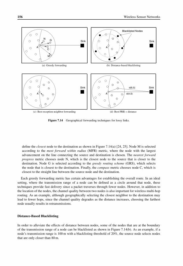
156 Wireless Sensor Networks
���
���
���
���
���
���
���
���
������������������������
������������������������
��������
������������
������������
������������
������
A
Sink
M
C
GN
(a) Greedy forwarding
Blacklisted Nodes
���
���
���
���
���
���
���
���
A
Sink
(b) Distance-based blacklisting
���
���
���
���
���
���
���
���
���
���
���
���
���
���A
Sink
(c) Best reception neighbor forwarding
d(B,S)
���
���
���
���
���
���
���
���
���
���
���
���A
Sink
d(A,S)
���
���
(d) Best PRR× distance
Figure 7.14 Geographical forwarding techniques for lossy links.
define the closest node to the destination as shown in Figure 7.14(a) [24, 25]. Node M is selectedaccording to the most forward within radius (MFR) metric, where the node with the largestadvancement on the line connecting the source and destination is chosen. The nearest forwardprogress metric chooses node N, which is the closest node to the source that is closer to thedestination. Node G is selected according to the greedy routing scheme (GRS), which selectsthe node that is closest to the destination. Finally, the compass metric chooses node C, which isclosest to the straight line between the source node and the destination.
Each greedy forwarding metric has certain advantages for establishing the overall route. In an idealsetting, where the transmission range of a node can be defined as a circle around that node, thesetechniques provide fast delivery since a packet traverses through fewer nodes. However, in addition tothe location of the nodes, the channel quality between two nodes is also important for wireless multi-hoprouting. As an example, although geographically selecting the closest neighbor to the destination maylead to fewer hops, since the channel quality degrades as the distance increases, choosing the farthestnode usually results in retransmissions.
Distance-Based Blacklisting
In order to alleviate the effects of distance between nodes, some of the nodes that are at the boundaryof the transmission range of a node can be blacklisted as shown in Figure 7.14(b). As an example, if anode’s transmission range is 100 m with a blacklisting threshold of 20%, the source node selects nodesthat are only closer than 80 m.

Network Layer 157
Reception-Based Blacklisting
The distance between two nodes does not directly relate to the channel quality. Hence, distance-basedblacklisting does not always prevent the selection of nodes with lower channel quality. Instead, theabsolute reception-based blacklisting protocol blacklists neighbors that have a packet reception ratebelow some threshold. For this purpose, each node keeps track of its packet reception rate (PRR) witheach of its neighbors. This information is then exchanged with these neighbors. As a result, when anode has a packet to send, it chooses the next hop among the feasible nodes with a PRR higher thanthe threshold.
Absolute reception-based blacklisting results may lead to disconnections in the network if none of theneighbors of a node satisfy the threshold constraint. Consequently, relative reception-based blacklistingis used, which orders the neighbors of a node according to the PRR values. Then, according to ablacklisting threshold value, the percentage of nodes with the worst PRR value is blacklisted. Thistechnique provides adaptive operation according to the neighbors of each node. A special case for theabsolute reception-based blacklisting is the best reception neighbor algorithm, where the next hop isthe neighbor with the highest PRR, as shown in Figure 7.14(c). By controlling the threshold value, theabsolute reception-based blacklisting algorithm can operate between two extremes: greedy forwardingand best reception neighbor.
Best PRR × distance
Forwarding mechanisms that rely only on the PRR suffer from increased latency. As an example,as shown in Figure 7.14(c), the best reception neighbor algorithm tends to select the node closestto the source node. As a result, a packet traverses through more hops to reach the destination. ThePRR×distance algorithm aims to exploit the tradeoff between PRR and distance.
EXAMPLE 7.8
An illustration of the algorithm is shown in Figure 7.14(d). The next hop, B, is selected such thatthe product of PRR and the distance improvement achieved by forwarding to a node is maximized.The distance improvement is found as follows:
1− d(B, S)
d(A, S)(7.3)
where d(B, S) is the distance between the neighbor, node B, and the destination “Sink” andd(A, S) is the distance between the source node, A, and the destination, “Sink.”
A comparison of these schemes shows that the PRR× distance algorithm provides the highestdelivery rate followed by the best reception, relative reception-based, absolute reception-based, distance-based, and greedy forwarding ones. Consequently, considering channel quality in geographical routingdecisions improves the performance compared to algorithms which only consider geographical location.In terms of energy efficiency, the absolute reception-based algorithm outperforms the other algorithmsfollowed by the PRR× distance, relative reception-based, best reception, distance-based, and greedyforwarding ones. As a result, considering both the channel quality and advances in geographical routingprotocols provides the most effective operation.
7.4.3 PRADA
Geographical routing protocols require neighborhood information to select the next hop according to dis-tance, PRR, etc. However, collecting this neighborhood information is costly. Moreover, neighborhoodinformation provides only a limited view of the network upon which the node has to make decisions.

158 Wireless Sensor Networks
A
Sink
Knowledge Range
Optimum Route
Route with limited knowledge range
Figure 7.15 The impact of knowledge range on geographical routing.
It can be argued that if a node has global knowledge of the network, the optimum path to the destinationcan be found. Accordingly, the next hop in this optimum route can be selected. However, in practice,global network knowledge is impossible to gather in WSNs due to the high density and associated highcost. Hence, geographical routing protocols aim to provide decision-making mechanisms using a limitedview of the network, i.e., information about neighbors of a node. In Figure 7.15, the optimum routebetween a source node A and destination S is shown with a solid line when the global knowledge of thenetwork is known. However, if each node in the network only knows the locations of their immediateone-hop neighbors, the resulting route is as shown by the dashed line. It is clear that with limited topologyknowledge, the established route deviates from the optimum route. However, the difference decreaseswhen the topology knowledge of a node increases since more informed decisions can be made. Asa result, the accuracy of the forwarding decisions is related to the topology knowledge of the node.However, to improve the topology knowledge, a node has to consume more energy.
PRADA, the probe-based distributed protocol for knowledge range adjustment [24, 25], exploits thetradeoff between the cost associated with larger topology knowledge and the accuracy of the forwardingdecision. In order to obtain larger topology knowledge, a node has to use a larger transmit powerand increase its transmission range. As a result, the cost of obtaining topology knowledge increases.However, with increased topology knowledge, routes closer to the optimum can be created which candecrease the energy consumption for data delivery.
PRADA is based on a centralized forwarding scheme called partial topology knowledge forwarding(PTKF), which aims to minimize the energy consumption for data communication as well as the costfor topology information. Accordingly, each node constructs a route based on a weighted shortest pathalgorithm with the link cost given as the energy consumption. According to this route, the next hop in itis selected and this hop calculates the route according to its topology knowledge. PTKF aims to find the

Network Layer 159
optimum set of knowledge range values, R, of each node to minimize the overall energy consumption.In other words, the objective is to minimize
CTOT =∑i∈V
(CCOMi + CINF
i ) (7.4)
where V is the set of nodes in the network, CCOMi is the communication cost for node i, and CINF
i is thetopology information cost for node i. Note that the values of CCOM
iand CINF
idepend on the knowledge
range of each node and PTKF finds the optimum set of these knowledge ranges.PRADA is a distributed version of PTKF, where each node adjusts its knowledge range according
to the feedback information it receives from neighbor nodes. PRADA first selects a random knowledgerange (KR), rcurrent, and constructs a route to the sink according to its current KR. Then, each nodeperiodically selects a certain KR, rprobe, to be probed and calculates
CTOTi (rprobe)= CINF
i (rprobe)+∑p∈Pi
cpi(rprobe) (7.5)
where cpi (rprobe) is the cost of communication for each connection p with the KR rprobe. If
CTOTi
(rprobe) < CTOTi
(rcurrent), then the knowledge range is updated as rcurrent = rprobe.PRADA converges quickly and, according to the simulations, achieves a performance very close to
the global optimum.
7.4.4 Qualitative Evaluation
Geographical routing protocols exploit local position information for routing decisions. Instead ofrouting tables that are explicitly constructed, neighborhood information is implicitly inferred from thephysical placement of nodes. This results in scalable routing protocols. Moreover, geographical protocolshave low complexity since the next hops can be selected based on local information.
On the other hand, the performance of geographical routing depends on accurate knowledge of thelocation. The error in location detection can cause an error in routing. For example, sensor nodes areprone to failure and may be deployed in a hostile environment. If the GPS or location device is damaged,sensor nodes that depend on the device are rendered useless. In addition, the monetary cost for the GPSmay be expensive for some applications. Also, the power consumption and size of the GPS may not beappropriate if sensor nodes are operated by batteries and deployed in their thousands.
7.5 QoS-Based Protocols
Many of the routing protocols explained above focus only on energy consumption in the network.Hence, route generation is performed to minimize energy consumption in the network. While energyconsumption is one of the most important performance metrics in WSNs, it is not the only one. Inparticular, the development of novel applications including multimedia communication necessitatesother performance metrics such as throughput, delay, and jitter also being considered in protocol design.Moreover, in some cases delay may be even more important than energy consumption. Hence, the qualityof service (QoS) requirements of these applications needs to be guaranteed in addition to the energyefficiency in WSNs.
Some of the routing protocols [1, 3, 5, 6, 10, 15, 16, 18, 19, 33] aim to minimize the energy consump-tion of the network by using the remaining energy of the sensor nodes as a metric of optimization.

160 Wireless Sensor Networks
7.5.1 SAR
The SAR (Sequential Assignment Routing) protocol provides a table-driven multi-path approach andwas one of the first routing protocols developed for WSNs which considers QoS requirements [33]. Themain goal of SAR is to create multiple trees originating from a root node which is one of the singlehop neighbors of the sink. Each tree grows outward from the sink while avoiding nodes with very lowQoS (i.e., low throughput/high delay) and energy reserves. Consequently, multiple paths that connectany node in the network to the sink can be created.
Each node specifies two parameters for each path to the sink:
• Energy resources: The energy resource of a path is estimated as the maximum number of packetsthat can be sent by the node, if the node has exclusive use of the path.
• Additive QoS metric: Each path is also associated with an additive QoS metric, which is relatedto the energy and delay at each link. A high QoS metric means low QoS.
Using the multiple paths, a node can select the routing path according to the QoS of each path and thepacket priority. As explained above, the QoS of a path is determined as an additive metric, which is afunction of energy and delay. As the QoS metric increases, the QoS of the route deceases. Whenever anode has a packet to send, it calculates a weighted QoS metric for the packet, which is a product of theQoS metric of the path and the priority level of the packet. As a result, paths with higher QoS are usedfor higher priority packets.
7.5.2 Minimum Cost Path Forwarding
The minimum cost path forwarding protocol combines the delay, throughput, and energy consumptioncharacteristics to establish routes between nodes in the network [36]. The protocol assigns a costfunction, which captures the delay, throughput, and energy consumption of the node, to each link.According to the cost function, the minimum cost forwarding algorithm specifies a cost field at eachnode. As a result, packets flow through the cost field, which specifies the next hop with the lowest cost.
The minimum cost path algorithm has two phases: cost field establishment and cost path forwarding.The cost field establishment phase aims to determine the minimum cost between any node and the sink.The sink broadcasts an advertisement (ADV) message with an initial cost of 0. The ADV message is thenforwarded by updating the cost. Each node j , which receives an ADV message from node i, calculatesits cost
Li + Cj,i (7.6)
where Li is the cost of node i (= 0 for the sink) and Cj,i is the cost from node j to node i. Each nodethen sets up a backoff timer proportional to its cost to node i, Cj,i , and broadcasts the ADV message.The backoff time helps the node to update its cost to the sink by selecting the node with the minimumcost to the sink.
EXAMPLE 7.9
The operation of the cost field establishment phase is shown in Figure 7.16 for nodes A, B,and C. Assume that node A has a minimum cost of LA = 0.5 to the sink and the link costsare as follows: LB,A = 1.5, LC,A = 4, and LC,B = 1, as shown in Figure 7.16(a). Node A firstbroadcasts an ADV message as shown in Figure 7.16(b) and, upon receiving the ADV message,node B updates its cost from inf to LA + LB,A = 2 and sets up its backoff timer to γLB,A, whereγ is a constant. Node C also updates its cost to LA + LC,A = 4, 5 and sets its backoff timer toγLC,A. Since node B’s backoff timer expires first, node B broadcasts an ADV with cost 2 asshown in Figure 7.16(c). Upon receiving the ADV, node C determines that its cost to the sink islower through node B than through A (LB + LC,B = 3< 4, 5) and hence updates its minimum

Network Layer 161
A
C
B
C,A
L =1.5B,A
L =1C,B
L =0.5A
L =4
(a) Minimum cost of A and linkcosts between A, B, and C
A
C
B
C
L =2B
L =0.5A
L =4.5
(b) Node A broadcasts an ADV and nodes Band C update their minimum cost
A
C
BB
L =3C
L =0.5A
L =2
(c) Node B broadcasts its ADV and node Cupdates its minimum cost
Figure 7.16 Cost field establishment procedure of minimum cost path forwarding.
cost with an updated backoff timer γLC,B , after which it also broadcasts its ADV message. Asa result of the backoff-based cost field establishment phase, each node determines its minimumcost to the sink by broadcasting a single ADV message.
In the second phase, the source node broadcasts the data message to its neighboring nodes. Themessage is routed through the cost field of the nodes. When a source node broadcasts a message,a budget for the message is also included. The budget is equal to the minimum cost of the sourceto the sink. As an example, assume that node C in Figure 7.16(c) has a packet to send to the sink.It broadcasts its message with a budget of 3. When node A receives this message, it compares itsminimum cost (0.5) plus the link cost to node C (4) to the message budget and determines that thetotal cost exceeds the budget. Consequently, it does not forward the packet. On the other hand,node B forwards the packet since it is in the optimum route from node C to the sink.
Based on the cost field concept, the messages can be routes without specific route information,neighborhood information, or node IDs. Each packet is broadcast without specifying the next hop andthe next hop is selected as a result of the budget and (minimum cost + link cost) comparison. If the cost

162 Wireless Sensor Networks
is not sufficient to reach the sink, the message is dropped; otherwise, the message is forwarded untilit reaches the sink. As a result, the minimum cost path forwarding mechanism delivers the messagesaccording to the minimum costs at each node.
7.5.3 SPEED
The QoS requirements in traditional networks are usually related to end-to-end delay and throughput.However, in WSNs, where the relative location of a node significantly affects the end-to-end perfor-mance, distance is another factor for guaranteeing QoS requirements. The SPEED protocol exploitsthis fact and aims to provide a packet guaranteed advancement at a given time (i.e., speed) [10].Consequently, the end-to-end delay experienced by the packets is proportional to the distance betweenthe source and the destination.
The SPEED protocol has several components to provide speed guarantees to the packets in thenetwork. The neighbor beacon exchange protocol is periodically run to exchange location informationbetween neighbors. As a result, each node constructs a neighbor table and stores the information aboutits neighbors with the following fields: NeighborID, Position, SendToDelay, and ExpireTime, whereSendToDelay is the estimated delay to the neighbor node and ExpireTime controls the expiration timewhen the particular entry is deleted from the table if no updates are received.
As explained above, in addition to the location, each node stores the estimated delay to its neighbors inits neighbor table. Delay estimation is performed at the sender whenever a packet is sent to the particularneighbor. The sender stores the time it takes between placing the packet in its queue and receiving theACK from its neighbors. Moreover, the receiver neighbor communicates the duration of processing forthe ACK using the ACK packet, which is subtracted from the delay estimate. In case multiple packetsare sent to the same neighbor, the moving average of the delay estimates is stored in the neighbor table.
The SendToDelay value stored for each neighbor is used for forwarding using the stateless non-deterministic geographic forwarding (SNGF) algorithm of SPEED. SNGF aims to forward the packetsto neighbors that can provide a minimum delivery speed of Ssetpoint.
EXAMPLE 7.10
The operation of SNGF is illustrated in Figure 7.17, where a sender node A aims to forward itspacket toward a destination D. Firstly, nodes that are inside the transmission range of node A andcloser to the destination D than node A are selected as forwarding candidates. In Figure 7.17,these nodes are E, F, and G. Then, the relay speed between node A and a node j ∈ {E, F, G} fordestination D is calculated for each forwarding candidate as follows:
SpeedjA(D)= dA,D − dj,D
HopDelayA,j∀j ∈ {E, F, G} (7.7)
where dA,D and dj,D are distances to destination D from nodes A and j , respectively, andHopDelayA,j is the estimated hop delay between nodes A and j .
SNGF chooses the next hop among the forwarding candidates with estimated speed higher thanSsetpoint . As a result, forwarded packets are guaranteed to reach a minimum speed. However, if nonode is found to satisfy this requirement, the packet is randomly dropped according to the neighborhoodfeedback loop (NFL).
The NFL component of SPEED controls the packet drop procedure in case no neighbor satisfyingthe minimum speed exists. For this purpose, the miss ratio of each neighbor, which is the rate at whichthe neighbor node does not satisfy the speed requirement, is calculated. Based on the miss ratio of theneighbor, the NFL determines either to drop or forward the packet.
In some cases, the packets can be routed toward hot spots, where there exists a high contention. Toprevent further packets from being forwarded to the same region, SPEED also employs a backpressure

Network Layer 163
dA,D
dE,D
B
DA
C E
FG
Figure 7.17 SNGF operation.
mechanism. Nodes which experience high miss rates send backpressure beacons to the upstream nodes.The backpressure beacons are used to remove these neighbors from the neighbor list and, as a result,packets are rerouted around the hot spots to relieve congestion.
SPEED is shown to provide lower delay and miss rates compared to the DSR and AODV protocols,which are developed for ad hoc networks. Moreover, SPEED is energy efficient because of the smalloverhead for establishing the route. One of the drawbacks of SPEED, however, is that only a single speedguarantee can be supported in the network. This prevents heterogeneous applications, where differentclasses of traffic reside in the network. SPEED is enhanced to provide multiple speed guarantees fordifferent traffic types through the MMSPEED protocol, which is described in Chapter 15.
7.5.4 Qualitative Evaluation
QoS-based routing protocols consider additional metrics in addition to energy consumption for con-structing routes. This provides additional capabilities to WSNs, where more sophisticated applicationscan be developed. However, providing additional guarantees increases the cost in terms of energyconsumption and, hence, network lifetime. The tradeoff between these additional capabilities and theircosts should be carefully tailored to the requirements of the applications.
References[1] K. Akkaya and M. Younis. A survey on routing protocols for wireless sensor networks. Ad Hoc Networks,
3(3):325–349, May 2005.
[2] J. N. Al-Karaki and A. E. Kamal. Routing techniques in wireless sensor networks: a survey. IEEE WirelessCommunications, 11(6):6–28, December 2004.
[3] J. Aslam, Q. Li, and D. Rus. Three power-aware routing algorithms for sensor networks. Wireless Communica-tions and Mobile Computing, 3(2):187–208, 2003.
[4] D. Braginsky and D. Estrin. Rumor routing algorithm for sensor networks. In Proceedings of the First Workshopon Sensor Networks and Applications (WSNA’02), pp. 22–31, Atlanta, GA, USA, September 2002.
[5] J. H. Chang and L. Tassiulas. Maximum lifetime routing in wireless sensor networks. In Proceedings of theAdvanced Telecommunications and Information Distribution Research Program (ATIRP’2000), pp. 609–619,College Park, MD, USA, March 2000.

164 Wireless Sensor Networks
[6] M. Chu, H. Haussecker, and F. Zhao. Scalable information-driven sensor querying and routing for ad hoc hetero-geneous sensor networks. International Journal of High Performance Computing Applications, 16(3):293–313,2002.
[7] J. Elson and D. Estrin. Random, ephemeral transaction identifiers in dynamic sensor networks. In Proceedingsof the 21st International Conference on Distributed Computing Systems, pp. 459–468, Mesa, AZ, USA, April2001.
[8] D. Estrin, L. Girod, G. Pottie, and M. Srivastava. Instrumenting the world with wireless sensor networks. InProceedings of ICASSP’01, volume 4, pp. 2033–2036, Salt Lake City, UT, USA, May 2001.
[9] D. Estrin, R. Govindan, J. Heidemann, and S. Kumar. Next century challenges: scalable coordination in sensornetworks. In Proceedings of ACM/IEEE MobiCom’99, pp. 263–270, Seattle, WA, USA, August 1999.
[10] T. He, J. A. Stankovic, C. Lu, and T. Abdelzaher. SPEED: a stateless protocol for real-time communicationin sensor networks. In Proceedings of the 23rd International Conference on Distributed Computing Systems,pp. 46–55, Providence, RI, USA, May 2003.
[11] S. Hedetniemi and A. Liestman. A survey of gossiping and broadcasting in communication networks. Networks,18(4):319–349, 1988.
[12] W. R. Heinzelman, A. Chandrakasan, and H. Balakrishnan. Energy-efficient communication protocol for wire-less microsensor networks. In Proceedings of the IEEE Hawaii International Conference on System Sciences,pp. 1–10, Maui, HI, USA, January 2000.
[13] W. R. Heinzelman, J. Kulik, and H. Balakrishnan. Adaptive protocols for information dissemination in wirelesssensor networks. In Proceedings of MobiCom’99, pp. 174–185, Seattle, WA, USA, August 1999.
[14] C. Intanagonwiwat, R. Govindan, and D. Estrin. Directed diffusion: a scalable and robust communicationparadigm for sensor networks. In Proceedings of MobiCom’00, pp. 56–67, Boston, MA, USA, August 2000.
[15] K. Kalpakis, K. Dasgupta, and P. Namjoshi. Maximum lifetime data gathering and aggregation in wirelesssensor networks. Technical report, University of Maryland, 2002.
[16] R. Kannan, L. Ray, R. Kalidindi, and S. S. Iyengar. Max-min length-energy-constrained routing in wirelesssensor networks. In Proceedings of the 1st European Workshop on Wireless Sensor Networks, pp. 234–249,Berlin, Germany, January 2004.
[17] G. Khanna, S. Bagchi, and Y. Wu. Fault tolerant energy aware data dissemination protocol in sensor networks.In Proceedings of the International Conference on Dependable Systems and Networks, pp. 795–804, Florence,Italy, June 2004.
[18] L. Li and J. Y. Halpern. Minimum energy mobile wireless networks revisited. In Proceedings of the IEEEInternational Conference on Communications (ICC’01), Helsinki, Finland, June 2001.
[19] Q. Li, J. Aslam, and D. Rus. Distributed energy-conserving routing protocols. In Proceedings of the 36th HawaiiInternational Conference on System Science, January 2003.
[20] S. Lindsey and C. S. Raghavendra. PEGASIS: power efficient gathering in sensor information systems. InProceedings of the IEEE Aerospace Conference, Big Sky, MT, USA, March 2002.
[21] S. Lindsey, C. S. Raghavendra, and K. Sivalingam. Data gathering in sensor networks using the energy*delaymetric. In Proceedings of the IPDPS Workshop on Issues in Wireless Networks and Mobile Computing, SanFrancisco, USA, April 2001.
[22] A. Manjeshwar and D. P. Agrawal. TEEN: a protocol for enhanced efficiency in wireless sensor networks.In Proceedings of the 1st International Workshop on Parallel and Distributed Computing Issues in WirelessNetworks and Mobile Computing, San Francisco, USA, April 2001.
[23] A. Manjeshwar and D. P. Agrawal. APTEEN: a hybrid protocol for efficient routing and comprehensiveinformation retrieval in wireless sensor networks. In Proceedings of the 2nd International Workshop on Paralleland Distributed Computing Issues in Wireless Networks and Mobile Computing, Ft. Lauderdale, FL, USA, April2002.
[24] T. Melodia, D. Pompili, and I. F. Akyildiz. Optimal local topology knowledge for energy efficient geographicalrouting in sensor networks. In Proceedings of IEEE INFOCOM 2004, Hong Kong, China, March 2004.
[25] T. Melodia, D. Pompili, and I. F. Akyildiz. On the interdependence of distributed topology control andgeographical routing in ad hoc and sensor networks. Journal of Selected Areas in Communications, 23(3):520–532, March 2005.
[26] J. Mirkovic, G. P. Venkataramani, S. Lu, and L. Zhang. A self-organizing approach to data forwarding in large-scale sensor networks. In Proceedings of the IEEE International Conference on Communications (ICC’01),Helsinki, Finland, June 2001.

Network Layer 165
[27] V. Rodoplu and T. H. Meng. Minimum energy mobile wireless networks. IEEE Journal of Selected Areas inCommunications, 17(8):1333–1344, 1999.
[28] N. Sadagopan, B. Krishnamachari, and A. Hemly. The ACQUIRE mechanism for efficient querying in sensornetworks. In Proceedings of the First International Workshop on Sensor Network Protocol and Applications,Anchorage, AK, USA, May 2003.
[29] C. Schurgers and M. B. Srivastava. Energy efficient routing in wireless sensor networks. In Proceedings of theMILCOM on Communications for Network-Centric Operations: Creating the Information Force, McLean, VA,USA, 2001.
[30] K. Seada, M. Zuniga, A. Helmy, and B. Krishnamachari. Energy-efficient forwarding strategies for geographicrouting in lossy wireless sensor networks. In Proceedings of SenSys’04, pp. 108–121, Baltimore, MD, USA,2004.
[31] R. Shah and J. Rabaey. Energy aware routing for low energy ad hoc sensor networks. In Proceedings of the IEEEWireless Communications and Networking Conference (WCNC), Orlando, FL, USA, March 2002.
[32] C. Shen, C. Srisathapornphat, and C. Jaikaeo. Sensor information networking architecture and applications.IEEE Personal Communications, 8(4):52–59, August, 2001.
[33] K. Sohrabi, J. Gao, V. Ailawadhi, and G.J. Pottie. Protocols for self-organization of a wireless sensor network.IEEE Personal Communications, 7(5):16–27, October, 2000.
[34] T. Voigt, H. Ritter, and J. Schiller. Solar-aware routing in wireless sensor networks. In Proceedings of PersonalWireless Communication 2003, Venice, Italy, September 2003.
[35] Y. Yao and J. Gehrke. The Cougar approach to in-network query processing in sensor networks. SIGMODRecord, 31(3):9–18, September 2002.
[36] W. Ye, J. Heidemann, and D. Estrin. An energy-efficient MAC protocol for wireless sensor networks. InProceedings of IEEE INFOCOM’02, volume 3, pp. 1567–1576, New York, USA, June 2002.
[37] M. Z. Zamalloa, K. Seada, B. Krishnamachari, and A. Helmy. Efficient geographic routing over lossy links inwireless sensor networks. ACM Transactions on Sensor Networks, 4(3):1–33, 2008.


8Transport Layer
The success and efficiency of WSNs directly depend on reliable communication between the sensornodes and the sink. In a multi-hop, multi-sensor environment, to accomplish this a reliable transportmechanism is imperative in addition to robust modulation and media access, link error control, andfault-tolerant routing. In this chapter, the functionalities and design of transport layer solutions for WSNsare described.
The main objectives of a transport layer protocol for WSNs are as follows:
• Congestion control: Packet losses due to congestion can impair reliability at the sink evenwhen enough information is sent out by the sources. Hence, congestion control is an importantcomponent of the transport layer to achieve the required reliability. Furthermore, congestioncontrol not only increases the network efficiency, but also helps conserve scarce sensor resources.
• Reliable transport: Based on the application requirements, the extracted event features shouldbe reliably transferred to the sink. Similarly, the programming/retasking data for sensor operation,command, and queries should be reliably delivered to the target sensor nodes to assure the properfunctioning of the WSNs.
• (De)multiplexing: Different applications can be served on sensor nodes through the samenetwork. The transport layer should bridge the application and network layers by usingmultiplexing and demultiplexing.
There exist several transport layer solutions developed for conventional wireless networks [3].Although these solutions may be relevant, they are not suitable for WSNs, In particular, to satisfy theabove objectives and to accommodate the unique characteristics of WSNs, significant modificationsto the existing transport layer protocols are needed. The majority of existing solutions focuses onreliable data transport following the end-to-end TCP semantics and addresses the challenges posed bywireless link errors and mobility [4]. Moreover, the notion of end-to-end reliability, which is based onacknowledgments and end-to-end retransmissions, imposes significant overhead for the implementationof these solutions in WSNs. The inherent correlation in the data flows generated by the sensor nodesmakes these mechanisms for strict end-to-end reliability significantly energy inefficient. Furthermore,all these protocols bring considerable memory requirements to buffer transmitted packets until theyare ACKed by the receiver. In contrast, sensor nodes have limited buffering space (<4 kB in MICAmotes [8]) and processing capabilities.
8.1 Challenges for Transport LayerThe energy, processing, and hardware limitations of the wireless sensor nodes bring further challengesfor the design of the transport layer protocol. The development of transport layer protocols is aconsiderable effort because the limitations of the sensor nodes and the specific application requirementsprimarily determine the design principles. In this respect, the main objectives and challenges of the
Wireless Sensor Networks Ian F. Akyildiz and Mehmet Can Vuranc© 2010 John Wiley & Sons, Ltd

168 Wireless Sensor Networks
transport layer are stated next. Moreover, the essential features to address the unique questions posed bythe characteristics of the WSNs are also indicated.
8.1.1 End-to-End Measures
Conventional transport layer solutions such as TCP adopt end-to-end retransmission-based error controland window-based additive-increase multiplicative-decrease (AIMD) congestion control mechanisms.These mechanisms provide end-to-end and point-to-point reliability and congestion control solutions.More specifically, the packet losses and congestion mitigation are performed through communicationbetween a source and a destination without any involvement from the intermediate parties. Essentially,the transport control mechanisms reside only on the source and destination. Furthermore, each flow isconsidered independently to provide a point-to-point communication solution.
These end-to-end control mechanisms used for conventional transport layer protocols usually leadto resource wastage in WSNs, where collective information from a group of sensors is much moreimportant than the individual information from each sensor node. Therefore, conventional end-to-end, point-to-point transport layer techniques may lead to waste of scarce wireless sensor resources.Instead, local measures for reliability and congestion control are usually exploited to improve the energyefficiency of the transport layer protocols. Similarly, reliability of the collective information from a groupof sensors is controlled instead of the reliability of information from each individual sensor node.
8.1.2 Application-Dependent Operation
Another difference in the operation of WSNs is that they are deployed with a specific sensing applicationobjective. For example, sensor nodes can be used within a certain deployment scenario to performcontinuous sensing of a specific phenomenon such as temperature monitoring. On the other hand,another application may require multiple sensors to carry out event detection and event identificationtasks. Similarly, another application may require location sensing and local control of actuators for awide range of application areas. Consequently, while for a monitoring application reliability is the mostimportant metric, for event detection applications timeliness is crucial. Thus the focus of the transportlayer solutions should be tailored to the application. Moreover, the application can be developed for awide range of purposes in the military, environment, health, space exploration, and disaster relief areas.The importance of these metrics can also vary according to the application area. Consequently, thespecific objective of WSNs influences the design requirements of the transport layer protocols.
8.1.3 Energy Consumption
Energy efficiency is the most important concern in the design of WSNs, and also affects the designof transport layer solutions. Scarce energy resources affect the design of transport layer solutions.Consequently, the transport layer functionalities should be energy aware, i.e., the error and congestioncontrol objectives must be achieved with the minimum possible energy expenditure. For instance, ifreliability levels at the sink are found to be in excess of that required for event detection, the source nodescan conserve energy by reducing the amount of information sent out or temporarily powering down.Similarly, end-to-end measures, which are successfully used for conventional networking for reliability,usually require significant energy consumption in a multi-hop network. Hence, these solutions may notbe scalable for WSNs. Consequently, a transport layer protocol can be designed such that the reliabilitylevel can be traded off for decreased energy consumption through local reliability measures.

Transport Layer 169
(RT) [6]2PSFQ [13]RMST [11] CODA [14] ESRT [1] GARUDA [10]
Transport Protocols
Figure 8.1 Overview of transport protocols.
8.1.4 Biased Implementation
WSNs are usually deployed with a large number of resource-constrained sensor nodes that are connectedto a resource-rich sink. The limited processing power and memory capacity of the sensor nodes preventsophisticated algorithms from being run locally. Hence, the transport layer algorithms should be designedsuch that most of the functionalities are performed at the sink with minimum functionalities required atthe sensor nodes. More specifically, the intelligence should be passed to the sink instead of the sensors.This helps to conserve limited sensor resources and shifts the burden to the high-powered sink.
Moreover, the traffic in the WSNs exhibits significantly different characteristics depending on the flowdirection. While the flow in the sensors-to-sink direction may require timely delivery with loss-tolerantoperation, the sink-to-sensors direction usually requires a high delivery ratio. Consequently, transportprotocols should be designed also by considering these biases in traffic.
8.1.5 Constrained Routing/Addressing
As explained in Chapter 7, wireless sensor nodes may not be assigned unique addresses. Therefore,unlike protocols such as TCP, in the design of transport layer protocols for WSNs the existence of anend-to-end global addressing should not be assumed. It is more likely to have attribute-based namingand data-centric routing, which call for different transport layer approaches.
Several transport layer protocols have been developed for WSNs to address these challenges [15]. Anoverview of the transport layer solutions that will be discussed next is shown in Figure 8.1. Next, wedescribe the following protocols: reliable multi-segment transport (RMST), pump slowly, fetch quickly(PSFQ), congestion detection and avoidance (CODA), event-to-sink reliability (ESRT), GARUDA, andreal-time and reliable transport (RT)2.
8.2 Reliable Multi-Segment Transport (RMST) ProtocolThe RMST protocol is one of the first transport layer protocols developed for WSNs [11]. The main goalof RMST is to provide end-to-end reliability. Accordingly, RMST is built on top of the directed diffusionprotocol [7], which is explained in Chapter 7, and uses some of the functionalities of this protocol. Morespecifically, RMST is designed as a filter that could be attached to the directed diffusion protocol.
RMST provides two of the three functionalities required for a transport layer protocol: reliabletransport and multiplexing/demultiplexing. Multiplexing and demultiplexing are carried at the sourcenodes and the sink, respectively. In the meantime, RMST provides mechanisms to handle errorsthroughout the routes in the network. To this end, RMST utilizes in-network caching and providesguaranteed delivery of the data packets generated by the event flows.
RMST relies on the directed diffusion routing mechanism for a certain path between a source anddestination. Hence, an implicit assumption is that the packets of a flow follow the same path unless thereis a node failure. In case of node failures, directed diffusion is assumed to reroute packets. Based on thisassumption, RMST has two modes of operation:
DUYTAN
Highlight
DUYTAN
Highlight
DUYTAN
Highlight

170 Wireless Sensor Networks
• Non-caching mode: This mode of operation is very similar to conventional transport layerprotocols, where only the source and destination play a role in providing reliability. Consequently,the packet losses are detected at the sink and requested from the source node in an end-to-endfashion through a NACK packet. The advantage of this mode is that it requires no involvement– and, hence, additional processing, storage, and energy consumption – from the intermediatenodes in the multi-hop network.
• Caching mode: In this mode, the intermediate nodes on the reinforced path cache the transmittedpackets to decrease the overhead in end-to-end retransmissions.
In RMST, each packet of a flow is labeled by a unique sequence number. Accordingly, the packeterrors are detected whenever there is a hole in the sequence numbers received. In case of packet errors,nodes request retransmission by sending a NACK packet toward the reverse route from the sink to thesensor, i.e., the reverse path as explained in the next examples for the non-caching and caching modes.
EXAMPLE 8.1
Error recovery in non-caching mode is illustrated in Figure 8.2, where a sensor node is tryingto transmit a series of packets to the sink through the multi-hop route. The sequence numberof the last received packet at the sink is also shown in each case. In non-caching mode, end-to-end retransmissions are performed to provide reliability. In Figure 8.2(a), packet 4 is lostbefore reaching the sink. The sink can only recognize the packet loss after it receives packet 5(Figure 8.2(b)). Then, the sink transmits a NACK packet back to the source node as shown inFigure 8.2(c). The lost packet is then retransmitted to the sink through the multi-hop route asshown in Figure 8.2(d).
EXAMPLE 8.2
In caching mode, as shown in Figure 8.3, certain sensor nodes are assigned as caching nodes(denoted as black nodes in Figure 8.3) on the reinforced path from the sensor node to the sink. Inaddition to the sink, loss packet detection is also performed at the caching nodes. Similar to thenon-caching case, the loss of packet 3 in Figure 8.3(a) can only be detected by the caching nodeafter receiving packet 4 as shown in Figure 8.3(b). Then, the caching node transmits a NACKpacket back to the source node as shown in Figure 8.3(c). In this case, as shown in Figure 8.3(d),the first caching node with the missing packet on the reverse path replies and the packets aretransmitted to the sink in order. If the packet cannot be found in one of the caching nodes, theNACK packet is propagated until it reaches the source node.
8.2.1 Qualitative Evaluation
In caching mode, RMST essentially creates reliable segments between two consecutive caching nodesand the retransmissions are performed inside these segments instead of through the end-to-end route.As a result, the cost associated with end-to-end retransmissions is minimized. Moreover, RMST aims toprovide guaranteed delivery for each flow in the WSN. This is helpful for applications where individualnode information is important, such as in network management solutions as discussed in Chapter 9.
RMST may incur additional overhead since caching requires additional processing and memory at thecaching nodes. This may increase the overall complexity and energy consumption of the network. Mostapplications related to event detection/tracking may not require 100% reliability since the individual dataflows are correlated and loss tolerant. However, RMST treats each flow separately, which may lead tooverutilization of the resources in WSNs. Moreover, guaranteed reliability via in-network caching maybring significant overhead for WSNs with power and processing limitations. Finally, RMST focuses

Transport Layer 171
3
Sink
4
(a) Message delivery and error
5
Sink
3
(b) Sink receives an out-of-order packet and detects packetloss
3
Sink
(c) NACK transmission
5
Sink
(d) Retransmission
Figure 8.2 Error recovery with RMST in non-caching mode.
only on the reliability aspects of communication. Since a packet-by-packet reliability notion is followed,a large amount of information may flow inside the network. This will result in congestion and associatedpacket drops, which is not addressed in RMST.
8.3 Pump Slowly, Fetch Quickly (PSFQ) Protocol
The PSFQ protocol [13] has been developed to address the path from sink to sensors. Contrary to manytransport layer approaches that focus on the sensors-to-sink path, the reverse path is generally used fornetwork management tasks and retasking of the sensor nodes. Hence, reliability is of major concern.
DUYTAN
Highlight

172 Wireless Sensor Networks
3
Sink
2
(a) Message delivery and error
4
Sink
2
(b) Caching node receives an out-of-order packet anddetects packet loss
2
Sink
(c) NACK transmission to the upstream caching node
4
Sink
(d) Retransmission
Figure 8.3 Error recovery with RMST in caching mode. Black nodes represent the caching nodes.
While the sensors-to-sink path may tolerate information loss due to the highly correlated data generatedby sensors, the reverse path requires one-to-one communication support to reliably disseminate controlinformation that is sent by the sink to each sensor. Accordingly, the PSFQ protocol provides three mainfunctions:
• Pump operation: Since reliability is generally more important than timeliness, PSFQ employsa slow pump mechanism that is based on slowly injecting packets into the network. In this case,each node on the route to the destinations waits for a specific amount of time before relayingthe messages.

Transport Layer 173
• Fetch operation: In case of packet errors, each node performs aggressive hop-by-hop recoveryto fetch the lost packets from neighbor nodes.
• Status reporting: PSFQ also provides a reporting functionality that creates closed-loop commu-nication between sensors and sink. Through this functionality, the sink can collect informationrelated to operation of the network.
Pump operation is the default strategy in PSFQ for information dissemination from sink to sensorsunless there are any errors. This is illustrated next.
EXAMPLE 8.3
The PSFQ pump operation is illustrated in Figure 8.4(a), where a sensor is transmitting packetsto its neighbor node A. Node A relays this information to node B. Two timers, Tmin and Tmax,are used to schedule the transmission times of nodes along a path from a sensor to sink. A sensorbroadcasts packets every Tmin to its immediate neighbors. Upon receiving a packet, the neighbornodes relay the packets after a random wait time, which is selected between Tmin and Tmax asshown in Figure 8.4(a). Hence, a node has to wait at least Tmin between packet transmissions.This duration between packet transmissions is integrated to allow nodes to recover the missingpackets. Moreover, the random delay allows a reduction in the number of redundant broadcasts ofthe same packet by the neighbors. If the packet is forwarded by one of the nodes, other neighborssuppress their transmissions.
A sensor sends packets related to a particular message with consecutive sequence numbers. If a nodeon the path from the sink to sensors detects a sequence number gap in this sequence of packets, thefetch operation is initiated. Through the fetch operation, a node aggressively sends out NACK packetsto quickly recover the loss packets from its immediate neighbors as explained in the following example.
EXAMPLE 8.4
The fetch operation is illustrated in Figure 8.4(b). When node A detects a packet loss, it broadcastsa NACK packet to its immediate neighbors. It may be the case that no reply is heard or only afraction of the lost packets are received. In this case, if node A does not receive any reply withina period of Tr , where Tr < Tmax, it persistently continues to send NACK packets for every Tr . Ifone of node A’s neighbors has the packet in its cache, it sends the packet in an interval between(1/4)Tr and (1/2)Tr as shown in Figure 8.4(b).
The fetch operation results in local error recovery through persistent NACK messages betweentwo packet transmissions. However, to prevent message implosion, PSFQ limits NACK messagetransmission to the one-hop neighborhood. In other words, NACK messages are not propagated throughmulti-hop routes.
The loss detection mechanism in PSFQ relies on the sequence numbers of packets in a flow. In case ofpacket losses in the middle of a flow, this mechanism can effectively detect those packet losses. However,the mechanism is not suitable for cases where the last packet of a flow is lost or all the packets relatedto a flow are lost. For this case, PSFQ employs a proactive fetch operation, where the receivers follow atimer-based fetch operation.
EXAMPLE 8.5
As shown in Figure 8.4(c), if a node does not receive a packet for Tpro, it sends a NACK packetto its neighbors. The wait time, Tpro, is determined so that it is proportional to the differencebetween the last highest sequence number, Slast, of the packet received and the largest sequencenumber, Smax, of the flow, i.e., Tpro = α(Smax − Slast)Tmax, where α ≥ 1. Consequently, the node

174 Wireless Sensor Networks
1
3
2
minT
1
2
3
minTmaxT
(a) PSFQ pump operation
NACK
1
3
minT
1
2
rT
2
(b) PSFQ fetch operation
1
minT
3
2
3proT
NACK
(c) PSFQ proactive fetch operation
Figure 8.4 Pump and fetch operations of PSFQ protocol.
proactively sends a NACK packet earlier if it is closer to the end of the message. In the case wherebuffer length is limited, the waiting time, Tpro, is determined as follows: Tpro = αnTmax, wheren is the buffer length.
The third component of the PSFQ protocol is the report operation, which allows the sink to requestfeedback from the sensor nodes in a scalable manner. Report operation is initiated by the sink by settinga report bit in the packet header. This packet is sent through the network to the intended nodes. Uponreceiving the report request, a sensor node responds immediately by transmitting a report message. Eachnode along the path to the sink adds its status information to this report by piggybacking. If a node in theupstream path does not receive the report response in Treport, it creates its own report packet and sendsit to the sink.
The report operation is also used for single packet delivery. If a message that the sink will send canfit into one packet, then the report operation is initiated by setting the report bit. Whenever the intendedsensor node receives this packet, it responds with a report packet. As a result, an end-to-end error controlmechanism is integrated into PSFQ for single packet flows.

Transport Layer 175
8.3.1 Qualitative Evaluation
PSFQ employs a simple protocol operation that does not require an end-to-end reliability mechanism.As a result, the protocol scales well with network size. Moreover, the communication requirements ofthe sink-to-sensors direction are significantly different than that of the sensors-to-sink direction. PSFQaims to provide reliable and orderly transfer of packets in a distributed manner in this direction.
PSFQ relies on the pump slowly operation to limit congestion. However, as the number of sources inthe network increases, congestion will occur. Moreover, PSFQ handles reliability only by consideringpossible wireless channel problems. Hence, there is no mechanism in PSFQ which captures thecongestion problems in WSNs. In addition, PSFQ is rather a hop-by-hop reliability protocol than anend-to-end solution. Hence, end-to-end reliability cannot be maintained in all cases even though hop-by-hop reliability is ensured. The pump slowly operation introduces an artificial delay in the network ateach hop. As a result, networks of large size may suffer from high latency. Whenever a packet is lost,the receiver node stores the out-of-order packets until the lost packet(s) are received. This increases thememory required for the PSFQ protocol, which may be limited in the sensor nodes.
8.4 Congestion Detection and Avoidance (CODA) Protocol
The aim of CODA is to detect and avoid congestion in WSNs [14]. To this end, three main congestionscenarios are considered. In WSN applications, where the source nodes frequently generate traffic,congestion builds up close to the source nodes because of the contention in the wireless channel.Moreover, for low-rate traffic, congestion can occur temporarily in hot spots, where multiple flowsare served. For these two types of congestion, CODA provides local congestion control mechanisms.Furthermore, because of the topology and the capacity of the network, certain persistent hot spots mayexist. This requires end-to-end mechanisms to regulate the data rate of source nodes.
To address congestion and the different scenarios that cause it, CODA provides three mechanisms viareceiver-based congestion detection, open-loop hop-by-hop backpressure signaling to inform the sourceabout the congestion, and closed-loop multi-source regulation for persistent and larger scale congestionconditions.
Accurate congestion detection is important since congestion control mechanisms usually imposeadditional processing and communication requirements on sensor nodes. It is clear that congestionoccurs because of an increase in the buffer occupancy of a node and the consequent packet drops. Hence,the buffer occupancy level has been mostly used as a congestion detection metric. However, in a multi-node environment, because of packet errors and collisions in the wireless channel, the buffer occupancylevel does not always accurately reflect the congestion. More specifically, while the congestion in acertain area of the network can increase, the buffer occupancy level of the nodes in that area may not beaffected. Consequently, CODA uses a combination of buffer occupancy level and channel load conditionas an indication of congestion. Moreover, since congestion usually occurs in receiver nodes, a receiver-based congestion detection mechanism is designed.
The receiver-based congestion detection mechanism relies on both buffer occupancy and channel load.The channel load is estimated by listening to the channel whenever a node has a packet to send. CODAdecides on congestion if the channel load is higher than a fraction of the maximum channel utilization.Consequently, congestion is detected at the receivers.
EXAMPLE 8.6
The congestion mitigation mechanism of CODA is illustrated in Figure 8.5, where a sensor nodeis trying to transmit a packet to the sink through a congested area. When the congestion is detectedby one of the nodes inside the congested area (Figure 8.5(a)), the receiver broadcasts a suppressionmessage toward the source node in the reverse path as shown in Figure 8.5(b). The suppression
DUYTAN
Highlight

176 Wireless Sensor Networks
Sink
Congested Area
(a) Message delivery and congestion detection
Sink
Congested Area
(b) Suppression message transmission
Sink
Congested Area
(c) Congestion mitigation and (optional) re-routing
Figure 8.5 Open-loop hop-by-hop backpressure mechanism of CODA.
message is used to inform the upstream nodes about congestion. Upon receiving the suppression,the upstream nodes decrease their sending rates or drop packets to relieve the congestion inthe forward path. Moreover, the suppression message is rebroadcast until a non-congested nodereceives the message as shown in Figure 8.5(b). This type of congestion control is referred to asopen-loop hop-by-hop backpressure. While the suppression message may not reach all the wayto the source nodes, they serve to relieve local congestion in a hot spot area. Moreover, as shownin Figure 8.5(c), using cross-layer routing techniques the forward path can be rerouted to avoidthese hot spots.
In addition to local congestion that may occur as a result of the dynamics in the network, the trafficgenerated by the source nodes can create network-wide congestion. More specifically, if a source nodeinjects a traffic load larger than the network can handle, the local congestion control mechanism cannotrelieve the congestion. For this case, CODA uses a closed-loop multi-source regulation mechanismas shown in Figure 8.6. This mechanism is similar to conventional end-to-end congestion controlmechanisms. Each source node monitors the source rate, r . If the source rate exceeds a threshold,r ≥ νSmax, which is a fraction of the maximum theoretical throughput of the channel, the source node

Transport Layer 177
Sink
(a) Sensor enters closed-loop control if its rate exceedsr ≥ νSmax
Sink
(b) Sink replies with ACK for each n packets received
Figure 8.6 Closed-loop multi-source regulation mechanism of CODA.
enters closed-loop control. In this case, a regulation bit is set in the header of the packets to informthe sink. Consequently, the sink begins sending periodic ACK messages for each n number of packetsreceived. If the source cannot receive the ACK messages, it determines network-wide congestion anddecreases its source rate.
8.4.1 Qualitative Evaluation
Identifying congestion in a WSN is essential for accurate congestion control. CODA uses a combinationof buffer occupancy level and channel load condition to provide efficient congestion detection. Similarly,CODA addresses both local and end-to-end congestion in WSNs. As a result, a complete congestioncontrol mechanism is provided for downstream traffic.
CODA can increase the network performance by avoiding congestion. However, the CODA protocoldoes not address reliability. The operation of CODA reveals that the congestion control performed at thesensor nodes without considering reliability impairs the end-to-end transport reliability [14]. CODA onlyprovides congestion avoidance and does not provide a reliable operation. Hence, it should be coupledwith a reliability mechanism. Furthermore, the closed-loop multi-source regulation mechanism incursadditional latency for cases where the network traffic is high.
8.5 Event-to-Sink Reliable Transport (ESRT) Protocol
In contrast to the transport layer protocols developed based on conventional end-to-end reliability, theESRT protocol [1] is based on the event-to-sink reliability notion and provides reliable event detectionwithout any intermediate caching requirements. ESRT aims to address both the reliability and congestionproblems in WSN.
The main characteristic of information delivery in WSNs is the data-centric communication paradigm.More specifically, to the user, collective information from multiple sensors regarding an event is muchmore important than the individual information sent from each node. Consequently, the notion of flow,

178 Wireless Sensor Networks
Table 8.1 Network operating regions based on congestion and reliability levels.
State Decision boundaries Definition
(NC, LR) f < fmax and η > 1+ ε (No Congestion, Low Reliability)(NC, HR) f ≤ fmax and η < 1− ε (No Congestion, High Reliability)(C, HR) f > fmax and η < 1 (Congestion, High Reliability)(C, LR) f > fmax and η ≥ 1 (Congestion, Low Reliability)
OOR f < fmax and 1− ε ≤ η ≤ 1+ ε (Optimal Operating Region)
which is defined as the messages that are sent from a source to a destination, no longer applies. Insteadan event-to-sink information flow exists, which is the collection of “flows” from a group of sensorsassociated with a single event. ESRT aims to provide reliability of the event information flow throughcongestion control mechanisms. Moreover, the algorithms of ESRT run mainly on the sink, with minimalfunctionality required at resource-constrained sensor nodes. It mainly exploits the fact that the sheeramount of data flows generated by the sensor nodes toward the sink is correlated due to spatial andtemporal correlation among the individual sensor readings [12].
ESRT relies on the sink to measure the reliability in the WSN every τ time units, which is also referredto as the decision interval. The reliability is measured in terms of the number of data packets from allthe sensor nodes associated with an event. Consequently, the following definitions are used:
• Observed event reliability, ri , is the number of received data packets in decision interval i at thesink.
• Desired event reliability, R, is the number of data packets required for reliable event detection.This is determined by the application.
Accordingly, ESRT aims to configure the reporting rate, f , of source nodes so as to achieve therequired event detection reliability, R, at the sink with minimum resource utilization.
EXAMPLE 8.7
In Figure 8.7, the reliability of a WSN as a function of the reporting rate, f , of the sensor nodesis shown. It can be observed that the reliability, r , shows a linear increase (note the log scale)with source reporting rate, f , until a certain f = fmax, beyond which the reliability drops. Thisis because the network is unable to handle the increased injection of data packets and packetsare dropped due to congestion. Moreover, for higher reporting rates, f > fmax, the behavior israther wavy and not smooth, and the reliability always stays well below the maximum reliabilityat f = fmax.
The relation between congestion and reliability in a WSN is clearly visible in Example 8.7.Accordingly, ESRT aims to control congestion to provide reliable event delivery by defining fiveoperating regions as shown in Figure 8.7. The network operating regions based on congestion andreliability levels are given in Table 8.1.
To control congestion in the network, the sink needs to determine the operating region of the network.This operating region depends on two factors: whether congestion exists in the network and whether therequired reliability is achieved. Hence, two mechanisms are required to estimate the congestion and thereliability state of the network. In each decision interval, τ , the sink determines whether the networkis operating in the low- or high-reliability region according to the number of packets received in thatinterval. Moreover, a congestion detection algorithm is employed at each sensor node in the network.Consequently, the sink can determine the operating region of the network. According to the operatingregion, the sink controls the reporting rate of the sensor nodes to operate at the optimal operatingregion (OOR).

Transport Layer 179
101
100
101
102
103
0
0.2
0.4
0.6
0.8
1
1.2
1.4
1.6
1.8
Reporting frequency (f)
Nor
mal
ized
rel
iabi
lity
()
Required reliability
(NC,LR)
(NC
,HR
)
(C,H
R)
(C,LR)
Optimal operating point P1 = (1,f* )
P2
fmax
1+
1
OOR
Figure 8.7 Relationship between reliability and reporting rate and the operating regions defined for ESRT.
The congestion detection algorithm is based on monitoring the local buffer-level monitoring at eachsensor node. Assuming that network conditions such as reporting rate and the number of source nodes donot change significantly between two consecutive decision intervals, the increment in the buffer fullnesslevel at the end of each reporting interval is expected to be constant.
Accordingly, as shown in Figure 8.8, let bk and bk−1 be the buffer fullness levels at the end of the kthand (k − 1)th reporting intervals respectively and B be the buffer size. Then, �b is the buffer lengthincrement observed at the end of last reporting period, i.e., �b = bk − bk−1. Hence, if the sum ofthe current buffer level at the end of the kth reporting interval and the last experienced buffer lengthincrement exceeds the buffer size, i.e., bk +�b > B, the sensor node infers that it is going to experiencecongestion in the next reporting interval. If a sensor node detects congestion in the network, it notifiesthe sink by piggybacking the packets that are sent. This is notified the sink for the upcoming congestioncondition to be experienced in the next reporting interval.
The state of the network is determined at each decision interval through the reliability measurementand congestion notifications. Accordingly, the sink updates the reporting rates of the sensor nodes bybroadcasting a packet to each sensor node. Denoting the reporting rate at decision interval i as fi andthe reliability level as ηi , the sink updates the reporting rate, fi+1, at the next interval as follows: ifthe network is in the (NC, LR) (No Congestion, Low Reliability) region, the reporting rate needs tobe increased to achieve a higher reliability level at the sink. Hence, the reporting rate is aggressivelyincreased as fi+1 = fi/ηi . In the (NC, HR) (No Congestion, High Reliability) region, the network isabove the required reliability level and the network resources can be saved by decreasing the reportingrate such that OOR is achieved. In this case, the reporting rate is decreased as fi+1 = fi/2(1+ 1/ηi) toconserve energy. In the (C, HR) (Congestion, High Reliability) region, the network is congested and the

180 Wireless Sensor Networks
k
B
∆
b
b
k–1b
Figure 8.8 Buffer occupancy analysis in ESRT.
reporting rate needs to decreased to relieve the congestion and improve the energy efficiency. As a result,a multiplicative decrease policy is used for the reporting rate as fi+1 = fi/ηi . Finally, in the (C, LR)(Congestion, Low Reliability) region, the reporting rate is exponentially decreased to improve reliabilityand relieve congestion in the network as fi+1 = f ηi/ki
. If the optimal operating point is reached, thereporting rate is kept constant.
8.5.1 Qualitative Evaluation
ESRT introduces a novel reliability notion called the event-to-sink reliability. The notion of the event-to-sink reliability is necessary for reliable transport of event features in WSNs. Based on such a collectivereliability notion, ESRT introduces a new reliable transport scheme for WSNs. Moreover, efficientcongestion control and reliability mechanisms are provided by shifting the decision mechanism tothe power-rich sink node. ESRT has a congestion control component that serves the dual purpose ofachieving reliability and conserving energy. The algorithms of ESRT run mainly on the sink and requireminimal functionality at resource-constrained sensor nodes.
The primary objective of ESRT is to configure the network as close as possible to the optimal operatingpoint, where the required reliability is achieved with minimum energy consumption and without networkcongestion. Through distributed update mechanisms, ESRT converges to the optimum operating stateregardless of the initial network state.
ESRT relies on the assumption that the base station is one hop away from all the sensor nodes, i.e.,a sink broadcast for frequency update will be received by all sensor nodes. Although this assumptionmay hold true for a certain class of application, as the network size increases, multi-hop strategies arerequired for information delivery from the sink to the sensors. Besides, ESRT maintains the same valueof operating frequency, f , at the end of each decision interval for each sensor node. In case a large groupof sensors sense an event, the required operating frequency may not be the same for all these sensorsbecause of their local interactions in the network.
The event-to-sink reliability notion applies to cases where the information at each sensor is correlated.Hence, ESRT cannot be applied for applications where individual sensor information is necessary.
8.6 GARUDAWhile the data flows in the forward path carry correlated sensed/detected event features, the flows inthe reverse path mainly contain data transmitted by the sink for operational or application-specificpurposes. This may include the operating system binaries, programming/retasking configuration files,application-specific queries and commands. Dissemination of these types of data mostly requires 100%

Transport Layer 181
reliable delivery. Therefore, the event-to-sink reliability approach, which is suitable for sensors-to-sinkcommunication, would not be suitable for addressing such tighter reliability requirements of the flowsin the reverse path.
Such a strict reliability requirement for the sink-to-sensors communication involves a certainlevel of retransmission as well as acknowledgment mechanisms. However, these mechanisms shouldbe incorporated into the transport layer protocols cautiously in order not to totally compromisescarce wireless sensor resources. In this respect, local retransmissions and negative acknowledgmentapproaches would be preferable over the end-to-end retransmissions and acknowledgments to maintainminimum energy expenditure.
On the other hand, the sink is involved more in the sink-to-sensor data transport on the reverse path.Hence, the sink, with plentiful energy and communication resources, can broadcast the data with itspowerful antenna. Consequently, the amount of traffic forwarded in the multi-hop WSN infrastructurecan be reduced and help sensor nodes conserve energy. As a result, data flows in the reverse path mayexperience less congestion in contrast to the forward path. Therefore, reliability is significantly importantin the reverse path compared to aggressive congestion control mechanisms.
The reverse path consists of multi-hop and one-to-many flows, which resemble conventional wirelessnetworks. There exist many transport layer schemes that address reliable transport and congestion controlfor the case of a single sender and multiple receivers [5]. Although the communication structure of thereverse path is an example of multicast, these schemes do not stand as directly applicable solutions;rather they need significant modifications/improvements to address the unique requirements of the WSNparadigm. Next, we will describe the GARUDA protocol, which provides reliable delivery between aresource-rich sink and resource-constrained sensor nodes.
Reliable sink-to-sensors delivery is addressed through the GARUDA protocol [9, 10]. The nameGARUDA is based on a mythological bird that reliably transported gods. GARUDA incorporates anefficient pulsing-based solution for successful delivery of single packets. Moreover, as in the RMSTprotocol, certain nodes in the network are selected to perform caching and manage the loss recoveryprocess. In GARUDA, these nodes are referred to as core nodes. To this end, a two-stage loss recoverymechanism is incorporated for each node in the network to reliably receive the packets sent from the sink.GARUDA consists of three mechanisms that accomplish reliable data delivery from sink to sensors fordifferent scenarios:
• Single/first packet delivery: GARUDA mainly follows a NACK-based recovery policy for thelost packets. However, NACK-based recovery cannot address packet losses in single packetdelivery or the loss of all the packets in a message. Consequently, a pulse-based deliverymechanism is incorporated so that the sink informs the sensors about the subsequent deliveryof a single packet flow or the first packet of a multi-packet flow through short-duration pulses.
• Core construction: GARUDA relies on specific nodes in the network, the core nodes, forcaching. Consequently, a simple and efficient core construction mechanism is designed to selectthese nodes without significant overhead.
• Two-phase loss recovery: Once the core is constructed, information delivery is performedthrough control of the core nodes. In the case of packet losses, a two-phase loss recoverymechanism is utilized, where a core node first recovers the lost packets from upstream core nodesand then delivers the packet to its neighboring non-core nodes.
GARUDA supports the delivery of single packet flows or the first packet of a flow through a pulse-based mechanism as explained in Example 8.8.
EXAMPLE 8.8
The sink informs the sensor nodes about an impending reliable short-message delivery bytransmitting a specific series of wait-for-first-packet (WFP) pulses at a certain amplitude andperiod as shown in Figure 8.9(a). The WFP pulses are of very small duration and only used to

182 Wireless Sensor Networks
Ts
DATA
DATA
pT
S
A
B
DATA
DATA
(a) First packet delivery with wait-for-first-packet (WFP) pulse transmission
Ts
DATA
DATA
DATA DATA
p
DATA
T
S
A
B
(b) Packet recovery using WFP pulses
Figure 8.9 First packet delivery mechanism in GARUDA.
indicate the subsequent transfer of a packet. When the sink has a packet to send, it transmits aseries of WFP pulses of duration Tp as shown in Figure 8.9(a). The duration of the WFP pulseis significantly smaller than the duration of a packet transmission and incurs a small overhead.Moreover, the sink continues to transmit WFP pulses with a period of Ts which is significantlylarger than the packet transmission duration. Each node on the path from the sink to the intendedsensor(s) broadcasts the WFP pulses on reception. Consequently, each node in the network isinformed about the packet to be received.
After waiting a sufficient time for the WFP pulses to propagate in the network, the sinktransmits the packet as shown in Figure 8.9(a). Upon receiving this packet, each node stopstransmitting WFP pulses, switches to delivery mode, and relays the packet as shown inFigure 8.9(a). The error recovery phase is initiated if a node does not receive the packet. Asshown in Figure 8.9(b), if node B does not receive the data packet from node A, it will continueto transmit WFP pulses every Ts . These WFP pulses also serve as a NACK indication for node A

Transport Layer 183
Sink
Figure 8.10 First packet transmission and core construction in GARUDA. The black nodes represent the core nodes.
to perform retransmission. As shown in Figure 8.9(b), if node A receives a WFP pulse aftertransmitting a packet, it retransmits the packet to node B. Consequently, GARUDA ensures that asingle packet or the first packet of a series of packets is reliably received at the intended recipients.
During the transmission of the first packet, GARUDA also implicitly employs the core constructionmechanism. The core approximates a near-optimal assignment of local designated servers for lossrecovery. The assignment is performed according to the number of hops between the sink and the sensornodes. During the delivery of the first packet, the sensor network is partitioned into bands. Consequently,a node is selected as a core node if (1) its hop count, i.e., band-id, is a multiple of 3 and (2) it does not hearthat any of its neighbors have been selected as the core node as shown in Figure 8.10. Upon receivingthe first packet from the sink, each node determines its band-id and forwards the packet. The core nodesalso indicate their duty in the forwarded packets. Other non-core nodes associate themselves with one ofthe core nodes for loss recovery purposes.
Loss recovery in the GARUDA protocol is mainly performed between core nodes. An importantdistinction of the GARUDA protocol compared to other reliable transport layer solutions such as PSFQis that it allows out-of-order forwarding. More specifically, if a node detects a packet loss, it continues toforward the next packets in the sequence before recovering the loss packet. This minimizes the impact ofthe loss recovery mechanism on packet delivery delay. Moreover, each core node exchanges an A-map(availability map) to indicate the available packets in its cache. Using the A-map information, a two-stageloss recovery process is conducted. This loss recovery process is described next.
EXAMPLE 8.9
The recovery process in GARUDA consists of two stages as shown in Figure 8.11. Each core nodetries to recover lost packets by exchanging unicast messages among other core nodes as quickly as

184 Wireless Sensor Networks
C
Sink
A
B
(a) Core node A requests a missing packet fromanother core node B
C
Sink
A
B
(b) Packet retransmission between two core nodes
A
Sink
B
C
(c) Node A broadcasts its A-map when it has allthe packets
A
Sink
B
C
(d) Non-core node C requests loss recovery fromcore node A
Figure 8.11 Two-phase loss recovery mechanism of GARUDA.
possible. This process is performed in parallel with the out-of-sequence forwarding mechanism.As shown in Figure 8.11(a), whenever, a core node, A, has a missing packet, it checks the A-mapof node B, which is the first node on the path to the sink. If node B’s A-map indicates that ithas the missing packet, node A sends a unicast message to node B. As shown in Figure 8.11(b),node B replies with the missing packet. Once node A receives all the missing packets, it indicatesthis by broadcasting its own A-map as shown in Figure 8.11(c). The non-core nodes associatedwith node A, e.g., node C, then request the missing packets as shown in Figure 8.11(d). Usingthis two-phase loss recovery mechanism, all the packets sent by the sink are reliably delivered tothe receivers.
GARUDA also supports other reliability semantics that might be required for sink-to-sensorscommunication, such as: (1) reliable delivery to all nodes within a subregion of the sensor network;(2) reliable delivery to a minimal number of sensors required to cover the entire sensing area; and(3) reliable delivery to a probabilistic subset of the sensor nodes in the network. For each of these cases,the first packet is delivered to each node in the network and the core is constructed. Then, depending

Transport Layer 185
on the set of destinations, GARUDA operations are performed to reliably deliver the messages to onlythese sets of nodes.
8.6.1 Qualitative Evaluation
GARUDA provides a wide variety of reliability mechanisms for downstream data flow. Since highreliability is required for the sink-to-sensors path, these mechanisms provide flexibility in protocoloperation. Compared to PSFQ, GARUDA supports out-of-order packet delivery. This decreases thepacket delivery delay and places less burden on the memory of sensor nodes.
GARUDA relies on a core construction mechanism, during which the core nodes are chosen. Forlarge WSNs, this mechanism may impact the overall delay in communication. Moreover, the reliabilitymechanism in GARUDA is partitioned between core nodes. Hence, end-to-end reliability of the packetsmay not be guaranteed. Similar to PSFQ, GARUDA focuses on reliability rather than congestion control.Hence, packet losses due to congestion may not be mitigated.
8.7 Real-Time and Reliable Transport (RT)2 ProtocolThe (RT)2 protocol has been developed to reliably and collaboratively transport event features from thesensor field with minimum energy dissipation in a timely manner [6]. Accordingly, the (RT)2 protocolsimultaneously addresses congestion control and timely event transport reliability objectives. It is one ofthe first protocols to focus on real-time guarantees in addition to reliability in WSNs.
The (RT)2 protocol addresses the following challenges. Certain applications need to immediatelyreact to sensor data based on the application-specific requirements. Therefore, real-time communicationwithin certain delay bounds is a crucial concern, which is addressed through a delay-based reliabilitynotion in (RT)2. The wireless channel errors and node failures lead to bursts of packet loss [2]. Althoughthe effects of these losses can be alleviated by the channel coding schemes to some extent, packet-leveltransport layer reliability mechanisms are still required. This is addressed by the reliability mechanismof (RT)2. Finally, energy efficiency is sought for real-time reliable data delivery.
As we have discussed in Section 8.5, WSNs are characterized by the dense deployment of sensorsand the sensor observations are highly correlated in the space domain. Furthermore, the physicalphenomenon exhibits temporal correlation. Accordingly, event transport from a group of sensor nodes tothe sink does not require 100% reliability. Thus, the (RT)2 protocol follows the collective event transportreliability notion similar to ESRT rather than the traditional end-to-end reliability notions. To this end, anew notion of event delay bound is considered to meet the application-specific deadlines. Based on bothevent transport reliability and event delay bound notions, the following definitions are used in protocoloperation:
• Observed delay-constrained event reliability (DRi): The number of received data packetswithin a certain delay bound at the sink in a decision interval i. In other words, DRi accounts forthe number of correctly received packets that are received within the application-specific delaybound. The value of DRi is measured in each decision interval i.
• Desired delay-constrained event reliability (DR∗): The minimum number of data packetsrequired for reliable event detection within a certain application-specific delay bound. Thislower bound for the reliability level is determined by the application and based on the physicalcharacteristics of the event signal being tracked.
• Delay-constrained reliability indicator (δi ): The ratio of the observed and the desired delay-constrained event reliabilities, i.e., δi = DRi /DR∗.
The operation of (RT)2 is based on these definitions. At each decision interval i, the sink observesDRi to determine the necessary actions. If the observed delay-constrained event reliability is higher thanthe reliability bound, i.e., DRi > DR∗, then the event is reliably detected within a certain delay bound.

186 Wireless Sensor Networks
Otherwise, appropriate action needs to be taken to assure the desired reliability level. This can beaccomplished by increasing the amount of information transported from the sensors to the actor.Accordingly, the reporting frequency of the sensors is increased properly while avoiding congestionin the network.
The transport reliability problem of (RT)2 is to configure the reporting rate, f , of source nodes so asto achieve the required event detection reliability, DR∗, at the actor node within the application-specificdelay bound.
The notion of delay-constrained reliability is based on the end-to-end delay bound specified by theapplication. This is denoted by �e2a and is specific to application requirements. The event delay can bedecomposed into three main components:
1. Event transport delay (�tran): The overall time between the event occurrence time and thetime when the event is reliably transported to the sink. The event transport delay can furtherbe decomposed into the following delay components: buffering delay, channel access delay,transmission delay, and propagation delay.
2. Event processing delay (�proc): The processing delay experienced at the sink when the desiredfeatures of the event are estimated using the data packets received from the sensor field. This mayinclude a certain decision interval [1] during which the sink waits to receive adequate samplesfrom the sensor nodes.
3. Action delay (�act): The action delay is the time it takes from the instant when an event is reliablydetected at the sink to the instant when a particular action is performed.
For a given event delay bound, �e2a , the following condition should be met:
�e2a ≥ �tran + �proc + �act (8.1)
where �tran is directly affected by the current network load and the congestion level in the network. Inaddition, the network load depends on the event reporting frequency, f , which is used by the sensornodes to send their readings of the event. Moreover, the end-to-end delay depends on the queuingdelay at each relay node. (RT)2 employs a time-critical event first (TCEF) scheduling policy so thatevents with smaller remaining deadline are given priority. The remaining deadline of a packet is updatedat each node by measuring the elapsed time and piggybacking the elapsed time to the event packetso that the following sensor can determine the remaining time to the deadline without a globallysynchronized clock. In addition to the TCEF scheduling policy, (RT)2 also updates the reporting rates sothat congestion is mitigated in the network. The effect of reporting frequency can be observed with thefollowing example.
EXAMPLE 8.10
In a sensor network, 200 sensor nodes were randomly positioned in a 200 m× 200 m sensor field.Several events were generated at different event centers denoted as (Xev, Yev) and all sensor nodeswithin the event radius behave as sources for that event.
The impact of the event reporting frequency on the on-time event delivery ratio is shown inFigure 8.12(a) for different number of source nodes, i.e, n= 41, 62, 81, 102. Here, the on-timeevent delivery ratio is the fraction of data packets received within the sensor–actor delay boundover all data packets received in a decision interval. When the reporting frequency is small enough,the on-time event delivery is ensured. However, above a certain f = fmax, network congestion isexperienced. After this point, the average transport delay starts to increase and, accordingly, theon-time event delivery ratio decreases below 1. Since the network load is increased as a result ofhigher reporting frequency, the buffer occupancy and network channel contention increases.
To further elaborate the relationship between observed delay-constrained event reliability, DRi ,and the event reporting frequency, f , in Figure 8.12(b), the number of packets received at the

Transport Layer 187
100
101
102
103
0
0.2
0.4
0.6
0.8
1
Reporting frequency (s –1)
On
-tim
e ev
ent d
eliv
ery
ratio
n=41n=62n=81n=102
(a)
100
101
102
103
0
100
200
300
400
500
600
700
Reporting frequency (s–1)
Num
ber
of r
ecei
ved
pack
ets
(n=
81) Non-delay constrained
Delay constrained
(b)
Figure 8.12 Effect of reporting frequency on (a) on-time delivery and (b) reliability.
sink in a decision interval, τ , is shown. In the figure, two values are shown. The solid line is thenumber of received packets irrespective of the delay associated with the packets. The dashed lineshows the number of packets received within the required delay.
Accordingly, until a certain f = fmax, the delay-constrained event reliability and non-delay-constrained event reliability are the same. However, beyond this value, the former significantlydeviates from the latter. Further, the observed delay-constrained event reliability, DRi , showsa linear increase (note the log scale) with source reporting rate, f , until a certain f = fmax,beyond which the observed delay-constrained event reliability drops. The decrease is because ofthe congestion that builds up in the network. For f > fmax, delay-constrained event reliabilitydrops significantly due to network congestion. (RT)2 aims to control the reporting frequency sothat the delay-constrained event reliability is above the required value.
The delay-constrained event reliability depends on the congestion in the network. If the congestionis detected accurately, the reporting rate can be adjusted so that maximum reliability can be achievedwithout causing congestion in the network. To this end, the (RT)2 protocol uses a combined congestiondetection mechanism based on both average node delay calculation and local buffer level monitoring ofthe sensor nodes to accurately detect congestion in the network.
The average node delay at the sensor node gives an idea about the contention around the sensor node,i.e., how busy the surrounding vicinity of the sensor node is. To compute the average node delay atthe sensor node i, the sensor node takes the exponential weighted moving average of the elapsed time.In addition to the node delay, the sensor nodes also monitor their buffer. If a sensor node experiencesbuffer overflow due to excessive incoming packets or the average node delay is above a certain delaythreshold value, this node is regarded as congested. Accordingly, the sink is notified of the upcomingcongestion condition in the network by utilizing the congestion notification (CN) bit in the header of theevent packet transmitted from the sensors to the actor node. In conjunction with the delay-constrainedreliability indicator, δi , the sink determines the current network condition and dynamically adjusts thereporting frequency of the sensor nodes.
The (RT)2 protocol decisions are made at the sink node according to the network state. The sinkdetermines the network state based on the delay-constrained reliability indicator δi = DRi/DR∗, and Tiand Tsa, which are the amount of time needed to provide delay-constrained event reliability for a decisioninterval i and the application-specific communication delay bound, respectively. In conjunction with thecongestion notification information (CN bit) and the values of fi , δi , Ti , and Tsa, the sink updates the

188 Wireless Sensor Networks
reporting frequency, fi+1. This information is broadcast to the source nodes in each decision interval.This updating process is repeated until the optimal operating point is found, i.e., adequate reliability andno congestion condition is obtained. The protocol operation is explained based on the network statesnext:
• Early reliability and no congestion: This state represents the case where the required reliabilitylevel is reached, the communication delay is within the bound, i.e., Ti ≤ Tsa, and no congestion isobserved in the network, i.e., CN = 0. However, the observed delay-constrained event reliability,DRi , is larger than the desired delay-constrained event reliability, DR∗. This is because sourcenodes transmit event data more frequently than required. To save energy, the reporting frequencyis updated as follows:
fi+1 = fi TiTsa
. (8.2)
• Early reliability and congestion: In this case, the required reliability level is reached, thecommunication delay bound, i.e., Ti < Tsa, but congestion is observed in the network, i.e.,CN = 1. Moreover, the observed delay-constrained event reliability, DRi , is larger than thedesired delay-constrained event reliability, DR∗. In this situation, the (RT)2 protocol decreases thereporting frequency to avoid congestion and save the limited energy of sensors. More specifically,the updated reporting frequency can be expressed as follows:
fi+1 =min
(fiTi
Tsa, f
(Ti/Tsa)i
). (8.3)
• Low reliability and no congestion: This state represents the case where the required reliabilitylevel is not reached before the communication delay bound, i.e., Ti > Tsa, and no congestion isobserved in the network, i.e., CN = 0. However, the observed delay-constrained event reliability,DRi , is lower than the desired delay-constrained event reliability, DR∗. This state can be reachedby (1) packet loss due to wireless link errors, (2) failure of intermediate relaying nodes, or(3) inadequate data packets transmitted by source nodes. To achieve the required event reliability,the data reporting frequencies of the source nodes are increased such that
fi+1 = fi DR∗DRi
. (8.4)
• Low reliability and congestion: In this condition, the required reliability level is not reachedbefore the communication delay bound, i.e., Ti > Tsa, and congestion is observed in the network,i.e., CN = 1. However, the observed delay-constrained event reliability, DRi , is lower than thedesired delay-constrained event reliability, DR∗. This situation is the worst possible case, sincethe desired delay-constrained event reliability is not reached, network congestion is observed,and, thus, the limited energy of sensors is wasted. Hence, (RT)2 aggressively reduces the reportingfrequency to reach the optimal reporting frequency as follows:
fi+1 = fDRi /(DR∗∗k)i
(8.5)
where k is the number of successive decision intervals for which the network has remained in thesame situation, including the current decision interval, i.e., k ≥ 1. Here, the purpose is to decreasethe reporting frequency with greater aggression, if a network condition does not improve.
• Adequate reliability and no congestion: Finally, this state represents the desired network statewhere the network is within tolerance β of the optimal operating point, i.e., f < fmax and 1−β ≤ δi ≤ 1+ β, and no congestion is observed in the network. Hence, the reporting frequency ofsource nodes is left constant for the next decision interval:
fi+1 = fi. (8.6)
The main goal of (RT)2 is to operate as close to δi = 1 as possible, while utilizing minimum networkresources and meeting event delay bounds.

Transport Layer 189
8.7.1 Qualitative Evaluation
(RT)2 is self-configuring and can perform efficiently under the random, dynamic topology frequentlyencountered in WSN applications. In addition to real-time and reliable delivery, the average energyconsumed per packet during communication is also decreased as the (no congestion, adequate reliability)state is approached through reporting rate control. Similar to ESRT, the (RT)2 protocol simultaneouslyaddresses congestion control and timely event transport reliability objectives in WSNs. In addition, real-time delivery is also supported, which is important for applications where delay is a major concern.
Despite its advantages, the (RT)2 protocol operation is based on feedback from the sink, wherea broadcast medium is assumed for the downstream traffic. However, this may not be applicableto deployments where multi-hop communication is necessary. Similar to ESRT, the same reportingfrequency value is used for all sensors in a decision interval. This approach may not be suitable fornetworks where local interactions vary the network conditions significantly.
References[1] Ö. B. Akan and I. F. Akyildiz. Event-to-sink reliable transport in wireless sensor networks. IEEE/ACM
Transactions on Networking, 13(5):1003–1016, October 2005.
[2] I. F. Akyildiz and I. H. Kasimoglu. Wireless sensor and actor networks: research challenges. Ad Hoc NetworksJournal, 2(4):351–367, October 2004.
[3] A. Al Hanbali and E. Altman. A survey of TCP over ad hoc networks. IEEE Communications Surveys &Tutorials, 7(3):22–36, 2005.
[4] H. Balakrishnan, V. N. Padmanabhan, S. Seshan, and R. H. Katz. A comparison of mechanisms for improvingTCP performance over wireless links. IEEE/ACM Transactions on Networking, 5(6):756–769, December 1997.
[5] S. Floyd, V. Jacobson, C. Liu, S. Macanne, and L. Zhang. A reliable multicast framework for lightweightsessions and application level framing. IEEE/ACM Transactions on Networking, 5(6):784–803, December 1997.
[6] V. C. Gungor, O. B. Akan, and I. F. Akyildiz. A real-time and reliable transport protocol for wireless sensor andactor networks. IEEE/ACM Transactions on Networking, 16(2):359–370, April 2008.
[7] C. Intanagonwiwat, R. Govindan, and D. Estrin. Directed diffusion: a scalable and robust communicationparadigm for sensor networks. In Proceedings of MobiCom’00, pp. 56–67, Boston, MA, USA, August 2000.
[8] Mica motes and sensors. Available at http://www.xbow.com/Products/Wireless_Sensor_Networks.htm.
[9] S.-J. Park, R. Vedantham, R. Sivakumar, and I. F. Akyildiz. A scalable approach for reliable downstream datadelivery in wireless sensor networks. In Proceedings of ACM MobiHoc’04, pp. 78–89, Tokyo, Japan, May 2004.
[10] S.-J. Park, R. Vedantham, R. Sivakumar, and I. F. Akyildiz. GARUDA: achieving effective reliability fordownstream communication in wireless sensor networks. IEEE Transactions on Mobile Computing, 7(2):214–230, 2008.
[11] F. Stann and J. Heidemann. RMST: reliable data transport in sensor networks. In Proceedings of the 1st IEEEInternational Workshop on Sensor Network Protocols and Applications, pp. 102–112, Anchorage, AK, USA,May 2003.
[12] M. C. Vuran, O. B. Akan, and I. F. Akyildiz. Spatio-temporal correlation: theory and applications for wirelesssensor networks. Computer Networks, 45(3):245–261, June 2004.
[13] C.-Y. Wan, A. T. Campbell, and L. Krishnamurthy. Pump-slowly, fetch-quickly (PSFQ): a reliable transportprotocol for sensor networks. IEEE Journal on Selected Areas in Communications, 23(4):862–872, April 2005.
[14] C.-Y. Wan, S. B. Eisenman, and A. T. Campbell. CODA: congestion detection and avoidance in sensor networks.In SenSys’03: Proceedings of the 1st International Conference on Embedded Networked Sensor Systems,pp. 266–279, Los Angeles, USA, 2003.
[15] C. Wang, K. Sohraby, B. Li, M. Daneshmand, and Y. Hu. A survey of transport protocols for wireless sensornetworks. IEEE Network, 20(3):34–40, May/June 2006.


9Application Layer
The role of the application layer is to abstract the physical topology of the WSN for the applications.Moreover, the application layer provides necessary interfaces to the user to interact with the physicalworld through the WSN. We will describe the application layer solutions in three categories: sourcecoding, query processing, and network management. An overview of the application layer protocols isshown in Figure 9.1.
9.1 Source Coding (Data Compression)As explained in Chapter 4, source coding is the first step in information delivery through wirelesscommunication. Whenever a sensor node has information to transmit, the information source is firstencoded with a source encoder. In effect, source coding exploits the information statistics to representthe source with fewer bits, i.e., source codeword. Therefore, source coding is also referred to as datacompression. Accordingly, redundant information is compressed to decrease the data volume whilepreserving some or all of the information content.
The basic compression solutions can be classified into two based on the preservation of informationafter coding: lossless compression and lossy compression. Lossless compression reduces the datacontent, i.e., packet size, without hampering the information integrity. Much better compressionefficiency can be achieved by lossy compression, which allows information loss for a higher reductionin data. Due to the higher complexity required for lossy compression, lossless compression techniquesare generally adopted in WSNs.
Several lossless compression algorithms have been developed for both digital communication andcomputation. However, the applicability of these algorithms to WSNs is limited. Since the programmingmemory of many sensor nodes is limited, higher complexity algorithms such as LZW or gzip [13] cannotbe directly implemented. Furthermore, several compression algorithms require a static dictionary tobe stored for compression/decompression and frequent memory access is required. Since read/writeoperations result in high energy consumption for wireless sensor nodes, these solutions are not energyefficient [6].
In addition to the inefficiency of the compression algorithms in terms of energy consumption, theredundancy of information collected at each individual sensor may also not allow efficient compressionat each source. However, the high-density deployment of WSNs results in highly correlated informationbeing collected by multiple, closely located nodes. Consequently, instead of compressing on anindividual basis, redundant information collected by a group of sensor nodes can be compressed.This leads to significant reductions in data to be delivered to the sink and, hence, reduced energyconsumption. As a result, distributed compression techniques that exploit correlation at different sourcesfor compression have been investigated for WSNs. Next, we describe two major approaches forcompression in WSNs. Firstly, a node-centric source coding techniques, Sensor LZW, is described. Then,we explain distributed source coding, which distributes compression to multiple sensor nodes.
Wireless Sensor Networks Ian F. Akyildiz and Mehmet Can Vuranc© 2010 John Wiley & Sons, Ltd
DUYTAN
Highlight

192 Wireless Sensor Networks
Application Layer Protocols
Source Coding Query ProcessingSensor–LZW [12] MANNA [11]
SNMS [16]DSC [14,17]
Network Management
COUGAR [3,19,20]Fjords [7]
SQTL [15]
TinyDB [9]TAG [8]
Figure 9.1 Overview of application layer protocols.
9.1.1 Sensor LZW
There exist several general purpose compression algorithms, where the main design goal is to increasethe compression ratio [13]. However, energy and memory efficiency are not major concerns since theyare generally designed for resource-rich devices. Furthermore, the code space of existing algorithmsis too high to be implemented in memory-constrained sensor nodes [2, 12]. As a result, these existingalgorithms are not suitable for WSNs and energy- and memory-efficient compression algorithms arerequired so that node-centric compression can be deployed in WSNs. To this end, it is important toconsider that, in a typical sensor node platform, the energy consumed for computation is significantlyless than that for memory access and communication. Hence, computation-intensive solutions with asmall memory footprint are required.
Sensor LZW (S-LZW) [12] is a variant of the Lempel–Ziv–Welch (LZW) compression algorithm thatis tailored to the resource constraints of wireless sensor nodes. LZW is generally used as part of the Unixcompress function and the GIF standard.1
LZW is a dictionary-based method, which encodes strings of symbols as a token in a dictionary.The dictionary is partly initialized before encoding and is populated based on the sequence of symbolsencountered during encoding. The main challenge for exploiting the LZW algorithm for WSNs is theadverse effects of wireless channel errors. LZW decoding cannot be performed if the encoder outputstream is not completely received at the decoder. Consequently, the data to be compressed should belimited to small blocks so that retransmissions can be performed without large data loss and energyconsumption. Furthermore, due to memory constraints, the dictionary size should be limited. S-LZWwas designed to address these issues, and uses a dictionary size of 512 entries to compress data in blocksof 528 bytes (two flash pages).
The compression of observational data can be further improved by exploiting their repetitive nature.Since each sensor node observes a physical phenomenon, the data to be compressed are highly correlatedin time. This means that there will be several repetitions in the data to be compressed. This can beaddressed by adding a mini-cache structure that stores the most recent entries. S-LZW with mini-cache(S-LZW-MC) improves the compression ratio in cases where the data contain many repetitions.
In addition to relying on the internal interdependencies of data, compression efficiency can be furtherimproved by transforming the data to a form with several patterns before compression. This is generallyreferred to as the precondition step and the S-LZW algorithm is improved by using two differentmethods.
The first precondition method is the Burrows–Wheeler transform (BWT), which is generally used forcompression of images, sound, and text. An example transformation is discussed next.
1For details of LZW, refer to [13].
DUYTAN
Highlight

Application Layer 193
Table 9.1 Burrows–Wheeler transform [13].
swiss_miss _missswiss swiss_misss iss_misssw wiss_misssw issswiss_m mss_missswi missswiss_ _s_missswis s_missswis s_missswiss ss_missswi imissswiss_ ssswiss_mi iissswiss_m sswiss_mis sssswiss_mi swiss_miss ssswiss_mis wiss_misss s
EXAMPLE 9.1
Sample information of string “swiss_miss” is shown in Table 9.1. For the transformation, a stringof n symbols is used to create an n× n matrix (first column of Table 9.1), where the first rowis the original string of symbols. Each row of the matrix is constructed as the shifted copy ofthe previous row. Then, the rows are ordered according to their first character (second column ofTable 9.1). Finally, the last column is used as the output from the BWT (last column of Table 9.1).The BWT reorders the symbols such that occurrences of the same symbol are located close by,which significantly improves the compression ratio. This flavor is denoted as S-LZW-MC-BWT.
The second precondition method used with S-LZW is based on the internal data structure ofmonitoring data. Generally, in monitoring applications, the data length and the contents are well knownand fixed. Moreover, for a set of observation values, the entire observations or at least the most significantbits are the same. Accordingly, a structured transpose (ST) can be performed to improve the compressionratio further. More specifically, the data for each observation are used to fill the rows of a matrix untila maximum length is reached. Then, the matrix is transposed and the data are compressed using thetransposed matrix. Since the transposed matrix has several repetitions, the compression ratio can befurther decreased. This version of the protocol is denoted as S-LZW-MC-ST.
S-LZW affects the energy consumption of source nodes depending on the mote architecture. Since thecompression is performed at the source nodes, the major overhead is found at those nodes. In cases wheretransceiver energy consumption dominates memory access, a reduction up to 2.6× is possible. However,for a platform such as MicaZ, where the energy consumptions for communication and memory accessare comparable, energy savings depend on the type of information to be compressed [12]. However,the main advantage of compression techniques in WSNs is on end-to-end energy consumption. Theamount of information to be transmitted is decreased through compression. As a result, less amounts ofdata are transmitted throughout the network. Therefore, even if compression leads to slightly increasedenergy consumption at the source nodes, overall energy savings are substantial for transmitting theinformation from the source node to the sink in a multi-hop path. This leads to reductions of up to2.9× in energy consumption.
Precondition steps also improve the compression ratio as well as energy efficiency despite the penaltyin computing the transformations and the additional storage required. For S-LZW-MC-BWT, decreasesup to 1.96× and 2.1× are possible for local and end-to-end energy consumption, respectively. Similarly,for monitoring applications, S-LZW-MC-ST saves energy by 2.8× both locally and overall.
Source coding (compression) also helps save energy under wireless channel errors. As discussed inChapter 6, reliability under wireless channel errors can be provided by retransmitting the corruptedpackets. Since compression decreases the amount of information to be sent, retransmission cost is alsodecreased. This results in significant energy savings for multi-hop WSNs.

194 Wireless Sensor Networks
EncoderX
Decoder
RX
RY
Y
X
EncoderY
(a)
EncoderX
Decoder
RX
X
Y
(b)
Figure 9.2 Slepian–Wolf coding: (a) the general case and (b) coding with side information.
9.1.2 Distributed Source Coding
Node-centric compression schemes such as S-LZW improve energy efficiency by decreasing the datacontent at each sensor node locally. The temporal relations between consecutive observations can beutilized for local compression. However, most applications may not require very high sampling ratesthat will lead to high temporal correlation. Moreover, because of the high density in sensor deployment,the information content observed by closely located sensors is highly correlated. This correlation can beexploited to significantly decrease the data content.
Distributed source coding (DSC) that dates back to the work of Slepian and Wolf [14] and Wynerand Ziv [17] in the 1970s stands as a promising solution for this type of application. Distributed sourcecoding refers to the compression of multiple correlated sensor outputs that do not communicate witheach other [18]. More specifically, the information at a sensor node is compressed assuming correlationwith another node without exchanging any information. This information is sent to the sink and jointdecoding is performed by the sink that receives data independently compressed by different sensors.
The lossless DSC, also known as Slepian–Wolf coding , focuses on distributed coding of two correlatedsources, X and Y , as shown in Figure 9.2(a). Each source is encoded separately without any informationfrom the other. Information theory states that without any information from other sources, the discreterandom variable X can be encoded by at least H(X) bits without any information loss, where H(X) isthe entropy of X. Accordingly, with separate entropy encoders and decoders, the following rates can beachieved: RX ≥H(X) and RY ≥H(Y), where H(X) and H(Y) are entropies of X and Y , respectively.The Slepian–Wolf theorem states that by exploiting the statistical properties ofX and Y at each encoder,the performance of joint encoding of X and Y can be achieved. In other words,
RX +RY ≥H(X, Y ) (9.1)
RX ≥H(X|Y), RY ≥H(Y |X) (9.2)
where H(X, Y ) is the joint entropy of X and Y and H(X|Y) and H(Y |X) are the conditional entropies.A special case of Slepian–Wolf coding is where the source X is encoded while considering the
statistics of source Y and source Y is encoded separately. Consequently, RY =H(Y) andRX ≥H(X|Y),where RX + RY ≥H(X, Y ). As shown in Figure 9.2(b), in this case, source Y is regarded as sideinformation. The joint decoding of X and Y is performed at a single decoder such that the information ofY is used to jointly decode the information from both sources. This type of encoding/decoding reverses
DUYTAN
Highlight

Application Layer 195
the traditional balance of encoder and decoder complexity leading to simple encoders and complexdecoders, which are suitable for WSNs.
Next, we will discuss Wyner–Ziv coding, which constitutes the basis for lossy compression as well asspecial cases where DSC is used for WMSNs.
Although Slepian–Wolf coding constructs the foundations of DSC, it does not consider the existenceof a channel and is purely a source coding solution. Wyner–Ziv coding considers lossy compression withside information as an extension to Slepian–Wolf coding [17]. Similarly, a source X is encoded with thestatistical information of source Y . The decoder uses this information as well as the source Y as sideinformation to decode X. Given an acceptable distortion, D = E[d(X, X)], Wyner–Ziv theory statesthat a rate loss is observed for lossy coding such that RWZ
X|Y (D)−RX|Y ≥ 0, where RWZX|Y (D) and RX|Y
are the achieved rates for Wyner–Ziv and joint encoding of X, respectively.
9.2 Query Processing
WSNs consist of many sensor nodes that monitor the physical phenomenon according to the require-ments of the application. The sink ensures the delivery of the data of interest through queries sent to thenodes containing information about the requested information. The query replies can be made simply bysending the requested raw data immediately to the sink. However, the processing capabilities of sensornodes provide alternative ways of processing these queries inside the network leading to significantenergy conservation [1]. This phenomenon is referred to as query processing.
The WSN can be viewed as a distributed database where nodes continuously deliver streams of datato the sink [7]. Although there exists many database management systems (DBMSs) developed fortraditional distributed databases, the unique characteristics of WSNs make these solutions not applicable.The unique characteristics of the WSN can be listed as follows:
• Streaming data: Sensor nodes produce data continuously, usually at well-defined time intervals,without having been explicitly asked for those data [7].
• Real-time processing: Sensor data usually represent real-time events. Moreover, it is oftenexpensive to save raw sensor streams to disk at the sink. Hence, queries over streams need tobe processed in real time [7].
• Communication errors: Since sensors deliver data through multi-hop wireless communication,wireless errors affect the reliability and delay of the distributed information reaching the sink.
• Uncertainty: The information gathered by the sensors contains noise from the environment.Moreover, factors such as sensor malfunction and sensor placement might bias individualreadings [20].
• Limited disk space: Sensor nodes have strictly limited disk space. Hence, the information sentby the sensors may not be queried later.
• Processing vs. communication: As explained in Chapter 3, energy expenditure in data process-ing in WSN is much less than that in data communication. Hence, the data processing capabilitiesof sensor nodes should be exploited in query processing.
The processing power available in sensor nodes provides potential solutions for the challengesencountered in WSN query processing. It is clear that the queries sent by the sink can be easily repliedto by sending the raw sensor observation to the sink. This approach is referred to as warehousing [3],where the processing of sensor queries and access to the sensor network are separated. As a result, acentralized DBMS can be developed to provide access to the collected data through classical databasemanagement techniques.
The warehousing approach, however, leads to both overutilization of communication resources inthe WSN and accumulation of highly redundant data at the sink. As an example, if an application isonly interested in the average value of specific information at a specific location, it would be more

196 Wireless Sensor Networks
Primergy
dissemination
Data
Query
Query
User
Sink
collection
graphs,Charts,
raw data
Figure 9.3 Query processing architecture.
efficient for nodes at this location to calculate the average locally and send this information as a singlepacket to the sink instead of sending all the individual information. Hence, exploiting existing techniquesfor query processing in WSNs leads to inefficient solutions. Instead, novel approaches tailored to theWSN paradigm are required. In this section, we describe these solutions, which have been developedfor WSNs.
The overall architecture of a query processing framework is illustrated in Figure 9.3, where a userinteracts with the sensor network. The query processing solutions provide the necessary tools to realizethis interaction between a user and a distributed set of sensor nodes. Hence, the services provided bythese solutions can be divided into two: server-side services and WSN-side services. In each queryprocessing approach, first, the user interests are represented through a well-established syntax that canbe easily converted into queries to the rest of the network. This constitutes the server-side part of thequery processing solutions. The WSN-side services can be broadly divided into two steps: (1) querydissemination and (2) data collection. Query dissemination is performed by transmitting the queries,which are generated according to the user interests, to all or a subset of nodes in the network. In thesecond step, data collection, sensor nodes respond to these queries if their locally observed sensor datamatch the queries. Energy-efficient representation and dissemination of queries as well as the collectionof interested data are of major concern in the design of query processing algorithms.
In the following, we describe the query representation approaches and aggregation issues in WSNs ingeneral. Existing query processing techniques are described in detail.
9.2.1 Query Representation
Representation of the user requirements or interests is a key factor in the design of efficient queryprocessing algorithms. The high-level interests of the user should be effectively represented asdistributed queries that will be sent to each sensor in the WSN. To this end, an interest can be viewed asa task descriptor, which is named by assigning a list of attribute–value pairs that describe the task. Thisis illustrated through the following example.

Application Layer 197
EXAMPLE 9.2
Consider an animal tracking application, where a group of sensors are deployed to detectparticular animals and communicate their locations. Let us assume that the user is interestedin receiving information if a four-legged animal is detected. This is represented as a query usingfollowing attribute–value pairs:
type = four-legged animal // detect animal locationinterval = 20 ms // send back events every 20 msduration = 10 seconds // for the next 10 secondsrect = [-100, 100, 200, 400] // from sensors within rectangle
In this case, the sink is interested in receiving packets with 20 ms intervals through the next 10seconds from the location specified by the rect attribute. A sensor can reply to this interest throughthe attribute–value pair list shown below:
type = four-legged animal // detect animal locationinstance = elephant // instance of this typelocation = [125,220] // mote locationintensity = 0.6 // signal amplitude measureconfidence = 0.85 // confidence in the matchtimestamp = 01:20:40
The response indicates that an elephant was detected by the sensor at location [125, 220] at time01:20:40. In addition, more detailed information about the confidence of the detection as well asthe signal amplitude measure, which is used for this detection, can be provided. This informationis then used at the sink with the other responses to estimate the location of the animal and trackits movements.
The representation of the user interest through efficient syntax to be used by sensors is a majorchallenge in query representation. The Sensor Query and Tasking Language (SQTL) has been developedto address this challenge through a procedural scripting language [15]. Accordingly, SQTL defines twoprimitives for the user to interact with the WSN as follows:
• Querying: The user generates formal statements to gather information related to a certain interest.These statements are called queries and are of the form: “What is the temperature in the south-east corner of the sensor field?” Querying is regarded as a synchronous operation, where the userwaits for the answer until further processing is performed, i.e., it is blocked.
• Tasking: Certain long-term operations cannot be performed through queries. For interests relatedto the long-term changes regarding a certain phenomenon, instead, the user assigns tasks to thesensor nodes. Consequently, the WSN can respond efficiently to an interest of the form “Trackany moving object inside the sensor field.” The user is not blocked during tasking but rather canperform certain operations on the already collected data.
WSNs can be regarded as distributed databases, where the data are continuously generated basedon the interests of the user. Accordingly, traditional database solutions may seem applicable to dataprocessing in WSNs. In other words, the WSN can be regarded as a distributed database and the datarelated to the user interest can be sent to the sink from each sensor that observes the events of interest.According to the collected information, the sink can perform high-level operations to provide a globalview of the data of interest to the user. As an example, if the user is interested in the average temperatureof a given area, temperature information from each sensor in the particular area can be collected at thesink. Then, the sink finds the average of these values to provide a response to the user.
The traditional distributed database approaches, however, do not consider the cost of informationdelivery. In WSNs, information delivery is the dominant cost because of the required communicationpower and frequent losses. Instead, the local processing capabilities of sensors need to be exploitedto distribute the intelligence and processing tasks throughout the network. Accordingly, the amount ofdata, which will be transmitted through the network, can be decreased while preserving the information

198 Wireless Sensor Networks
content of interest to the user. Considering the same example, instead of sending their raw temperaturedata, closely located sensors can exchange their readings and locally calculate the average value to besent to the sink. As a result, instead of sending the raw temperature data from each sensor in an eventarea, only a single packet representing the average in this area is transmitted. Although the informationcontent is kept intact, significant savings are possible in terms of communication cost.
In-network processing, however, cannot be accomplished through traditional queries. Instead, throughtasking, the user can ask the sensor nodes to perform certain long-term tasks that include gathering data,local processing, and collaboration among neighbors. SQTL provides the required syntax to define theseinteractions.
Each SQTL program is developed at the sink and encapsulated within an SQTL wrapper. Uponreceiving the SQTL packet, each sensor node performs the actions specified by the SQTL wrapper.These actions include storing the SQTL program for further use, forwarding the program to a particularset of nodes, or executing the program through a specific application. To this end, a sensor executionenvironment (SEE) is used at each sensor to dispatch incoming messages.
The SEE provides specific low-level primitives that can be used by the user according to the SQTLcommands. More specifically, three groups of primitives are provided:
• Sensor access: getTemperatureSensor(), turnOn(), turnOFF()
• Communication: tell(), execute(), send()
• Location-aware: isNorthOf(), isNear(), isNeighbor()
Using these primitives, sensors can be remotely programmed to execute tasks that include collabora-tion among local neighbors. As a result, the SQTL framework is performed at each node. The incomingmessages are filtered based on the SQTL wrappers by the SEE. Certain messages can be immediatelydiscarded or forwarded to certain neighbor nodes. If a certain criterion is met, the SQTL programs arethen executed in the node as running applications. A sample SQTL program for temperature reading isprovided next.
EXAMPLE 9.3
Consider a temperature reading application, where the sink is interested in the maximumtemperature of the temperature readings in the sensor network. Accordingly, a simple SQTLapplication is sent by the sink to the sensor nodes including the following SQTL wrapper [15]:
(execute:sender SINK:receiver (:group NODE(1) :criteria TRUE):application-id 123:language SQL:content ( SELECT Max(getTemperature()) FROM ALL_NODES ))
The SQTL wrapper includes the SQTL function, which requires the node to get the maximumtemperature from its children. The corresponding architecture is shown in Figure 9.4. Firstly, thesink sends the SQTL application with the wrapper to node A as shown in Figure 9.4(a). Uponreceiving the message, node A executes the SQTL wrapper and sends a confirmation messageto the sink. Then, node A sends the SQTL message to its children, i.e., nodes B, C, and D(Figure 9.4(b)). Each node responds with a confirmation message to node A and reiterates thesame procedure for its children. Finally, the maximum temperature information is returned tonode A as shown in Figure 9.4(c). By using its own temperature information, node A returns themaximum temperature information to the sink.

Application Layer 199
Sink
A
BC D(a)
Sink
A
BC D(b)
Sink
A
BC D(c)
Figure 9.4 Query dissemination and data collection using SQTL.
SQTL provides an efficient method to disseminate user interests to the sensors in a WSN. Throughthe use of SQTL wrappers, higher level operations are supported without executing the main program.Accordingly, user queries and tasks are executed at the sensor nodes specified by the SQTL wrapper.Since different application types are supported, SQTL can be used for any type of query or task. Thisallows even the sensor software to be updated based on SQTL messages.
Query representation techniques enable flexible operation for information delivery in WSNs. Thus,information delivery not only depends on the requests generated by the sink, but can also be initiatedby each sensor in the network. Consider the SQTL wrapper code used in Example 9.3. The sameSQTL message can be generated by a sensor in the field by identifying the sender as SENSOR. Thisis particularly important for event-based WSNs, where the user is not aware of the events that may occurin the network. If a certain activity is detected by a sensor, this sensor can publish the availability ofsuch data and inform the user. If the user is interested, further queries can then be sent to improve thefidelity of the event information by assigning more sensors to gather data. According to the way thequery messages are generated, query processing approaches can then be classified into three as follows:
• Push-based query processing: Also referred to as sensor-initiated information delivery, in thiscase sensors publish/advertise their information readings, which may be locally distributed orsent to the sink for further processing.
• Pull-based query processing: Also referred to as sink-initiated information delivery, here thesink disseminates the interests of the user to a set of sensor nodes in the network. In this case,the interest may be related to an attribute of the physical field (query) or an event of interestto be observed (task). Based on the user interest, the sensor nodes respond with the requestedinformation.
• Push–pull query processing: Both push- and pull-based query approaches can be used in anetwork, in which case both the sensors and the sink are actively involved in query processing.
The type of query processing approach dictates the suitable architecture to be used. In addition to thehigh-level architecture to be used with query processing, different query types can be used. Queries canbe classified based on two different criteria: (1) temporal and (2) spatial content.
According to temporal content, queries are classified into three as follows:
• Continuous query: This type of query is generally related to monitoring applications, wheresensors continuously send their observations at the specified frequency. The duration of the querycan also be specified in the query description. Continuous queries are generally associated withtasking.

200 Wireless Sensor Networks
• Snapshot query: This type of query relates to collecting a specific attribute at the current instantor at some specific point in time. In the case of queries related to future instances, snapshot queriesare associated with tasking.
• Historical query: In addition to performing sensing based on continuous or historical queries,the sensor can also store information related to previously sensed information. Historical queriescollect information (or a summary thereof) about the past. They are generally regarded as closestto traditional distributed database approaches.
In addition to their temporal content, queries are also classified according to the way they addresssensors in the WSNs, i.e., the spatial content. A general query can address all the sensors in the network,which is generally related to system-level tasks. However, most queries in sensor networks result in agroup of sensors responding instead of all the sensors in the network. According to the way these sensorsare addressed, queries can further be classified into three as follows:
• Data-centric query: This is the most used query type, where a particular event of interest isdefined in the query. Fire detection according to a sudden decrease in ambient temperature isan example of a data-centric query. The query does not directly address any nodes to send theirtemperature readings. Instead, nodes respond to the query only if their data content matches thequery requirements.
• Geographical query: Instead of detecting an event, the user may be interested in monitoringa certain area of the network. In this case, geographical queries are used, which specify sensornodes according to their location.
• Real-time detection query: For applications such as intruder detection, the data originators arenot known in advance. Instead, a sensor responds to the query only if the object of interest movesclose to it.
The type of query also impacts the routes created in the network to deliver the query messages.It is important to note that the set of sensors that respond to a query is not always the same as therecipients of the query message. As an example, data-centric queries may be delivered to all the sensorsin the network. However, nodes respond only if the event of interest occurs. On the other hand, fora geographical query, the query messages can be specifically sent to the area of interest. Therefore,routing decisions are taken based on the type of query that is used in the network.
9.2.2 Data Aggregation
The main peculiarity of WSN traffic is that the sensed information is usually collected at a single point,i.e., the sink. Hence, information flow can usually be perceived as a reverse multicast tree as shownin Figure 9.5, where the sink queries the sensor nodes to report the ambient conditions of a physicalphenomenon. The many-to-one nature of the information flow results in high contention and congestionat nodes which are located closer to the sink, since these nodes are exposed to a larger volume oftraffic compared to nodes that are located away from the sink. This causes an increase in contentionand congestion, which may lead to packet losses. Moreover, nodes closer to the sink consume higherenergy, which may result in these nodes depleting their residual energy earlier. As a result, the sink maybe disconnected from the rest of the network.
The adverse effects of many-to-one flows can be mitigated by exploiting the content of informationthat is sent throughout the network. WSNs observe physical phenomena which are correlated in spaceand time. As a result, information sent by each sensor network is correlated with another to some extent.For nodes that are located very close to each other, the correlation is so high that these nodes may sendidentical packets. On the other hand, for distant nodes, although the information content may differconsiderably, the type of information is still the same. As an example, for a query related to temperaturesensing, all nodes send temperature information. As a result, the packets that are being sent containsimilar header information even if the reported temperature value may be different.
DUYTAN
Highlight

Application Layer 201
��
����
����
Sink
A B C
D
EF
G
Figure 9.5 Example of data aggregation.
The similarity in both the information content and packet content in WSNs can be exploited tominimize data flow from several sensor nodes to the sink. As an example, for closely located nodesthat observe the same information, instead of sending packets from each node, a single packet can besent to represent these groups of sensors. Similarly, packets from different locations of the sensor fieldcan be merged in a single packet by maintaining the temperature information as an array. In addition,traffic load can further be reduced by performing in-network processing based on the query sent bythe user. According to Example 9.3, if the maximum temperature value is required, a sensor can mergethe information that it receives from its children with its own reading to report only the maximum of thereceived samples. As a result, several packets injected into the network can be merged into fewer packets,which relieve the traffic at the bottleneck nodes as the information progresses through the network. Theseconstitute the basics of aggregation techniques in WSNs, which are generally used in conjunction withquery processing methods. This is illustrated by the following example.
EXAMPLE 9.4
Consider the network topology shown in Figure 9.5, where a tree rooted at the sink is used forinformation delivery from the sensors to the sink. Data aggregation can be performed in this tree,where the data received from multiple sensor nodes are aggregated as if they are about the sameattribute of the phenomenon. The nodes that receive information from multiple nodes in this treeare usually used for aggregation and are called aggregation points. As an example, the sensornode E aggregates the data from sensor nodes A and B while sensor node F aggregates the datafrom sensor nodes C and D.
Data aggregation can be perceived as a set of automated methods of combining the data that comefrom many sensor nodes into a set of meaningful information [4]. In this respect, data aggregation is alsoreferred to as data fusion [5]. Data aggregation solutions generally consist of three main components:data storage, aggregation function, and aggregation path. We describe these components next.
Data aggregation takes place in aggregation points, where information from multiple sensor nodes iscollected. Due to the unsynchronized nature of sampling and communication, data to be aggregated donot arrive simultaneously at the aggregation points. Hence, these data should be stored until sufficientinformation is available for aggregation. Since on-board memory is limited, sensor data should be storedin a memory-efficient manner. On the other hand, the accuracy of information should be preserved.Depending on the type of query, data can be stored with different degrees of accuracy. If individualinformation is important for aggregation functions, gathered information is stored as lists or histograms.As a result, information content is highly preserved at the aggregation points. This, however, results

202 Wireless Sensor Networks
in higher memory allocation for the data and limits the number of data points that can be stored. Onthe other hand, if the query is related to the statistical properties of the data, such as mean, variance,or maximum, then only statistical representations of the collected data are stored. This results in moreefficient memory allocation.
The second main component of aggregation solutions is the selection of the aggregation functions.As explained above, the type of aggregation function affects the data storage approach. This is directlyrelated to the efficiency of the aggregation solutions as well. Aggregation functions can be as simple asfirst-order statistics such as mean, maximum, minimum, or very simple operations such as suppressionof duplication. This simplifies the data storage approach as well as the processing that needs to beperformed at the aggregation points. On the other hand, more sophisticated functions, which requirethe calculation of spatial or temporal correlation, signal processing, or algorithmic approaches, can beselected as aggregation functions. As a result, the complexity of aggregation increases, resulting in higherload for aggregation points.
Finally, the construction of aggregation paths is a major challenge for aggregation solutions. Theaggregation points should be selected so that information is collected at these points efficiently andrapidly. This is, however, difficult due to the dynamic nature of WSN communication. The informationto be gathered at aggregation points may not be available due to uncertainties in the sensor hardware,physical phenomenon, and wireless channel. Accordingly, sensors may not gather the requested datadue to intermittent problems with the sensory hardware. Moreover, data delivery is generally based ondata-centric queries. Hence, the number of nodes that respond to the query depends on the properties ofthe physical phenomenon, which are non-deterministic. Similarly, packets sent from certain nodes maybe lost before reaching the aggregation points due to wireless channel errors.
Because of these uncertainties, it is not possible to determine the amounts of data that will be availableat the aggregation points in advance. More importantly, the amounts of data vary throughout the lifetimeof the network. Moreover, the multi-hop communication structure and the broadcast nature of thewireless channel result in information trickling at one message a time. Hence, a node may not havecomplete information about the neighborhood and the information to be aggregated. This results ina tradeoff between accuracy in aggregation and the associated delay. Thus, finding the most efficientaggregation points for each aggregation task in the network is not trivial.
Aggregation has several benefits for communication in WSNs. The high asymmetry between theenergy consumption for computation and that for communication motivates the use of in-networkprocessing solutions. Aggregation is a typical example, where the in-network processing solutions helpreduce the traffic in the network. As a result, energy efficiency of the network can be improved. Sincethe traffic load is minimized through aggregation, the network can be made scalable for large numbersof sensors and sinks.
Despite its advantages, aggregation incurs additional storage requirements in resource-constrainedsensor nodes. Therefore, aggregation solutions should be designed to minimize the impact on memory,while preserving the accuracy. Furthermore, in-network processing may result in information lossdue to imperfect aggregation approaches. As an example, outliers may distort the results for simplemax/min aggregates if care is not taken. However, providing robust aggregation solutions with resource-constrained sensor nodes is a major challenge. Several solutions have been developed for aggregation inWSNs [10]. Most of these solutions are implemented as part of the query processing protocols, whichwill be explained next.
9.2.3 COUGAR
The COUGAR sensor database system provides a distributed data gathering framework for individualsensor data through user-defined queries [3, 19, 20]. The information in the WSN is classified into twoas: stored data and sensor data. Accordingly, the WSN is regarded as a database system with two classesof available data.

Application Layer 203
The stored data refer to the information about the sensors in the field including their type, theirlocations (if available), as well as the properties of the physical phenomena. The stored data are availableat the sink and modeled as relations.
The sensor data refer to the information gathered by the sensors according to the queries. InCOUGAR, the sensor data are represented as time series. More specifically, the sensors are assumedto be synchronized and sensor data are regarded as outputs of a signal processing function at a specificlocation, at the time of the record. Each sensor represents the data based on a sequence model, which isdefined as a 3-tuple that includes the set of records, an ordered domain, and the ordering of the recordsby the ordering domain.
According to the representation of data in two classes, two types of queries are used based onrelational and sequence operators. The relational operators are applied to stored data, while the sequenceoperators apply to sensor data. Moreover, three operators are defined to combine relations and sequences.Accordingly, (1) sequences can be used as input to project out the position information to obtain arelation, (2) a sequence and a relation can be used in a product operation to obtain a sequence, and (3) asequence can be aggregated by excluding the position attribute.
The sensor nodes observe data that are gathered based on certain signal processing functions,e.g., sampling, comparison, integration. Accordingly, in COUGAR, the outputs of individual sensorsare represented as abstract data type (ADT) functions. As a result, an ADT object in the databasecorresponds to a physical sensor in the real world. Using this abstraction, the COUGAR database systemuses an SQL-like query language to issue queries to the sensors. This is illustrated next.
EXAMPLE 9.5
Let us consider an indoor WSN that is deployed on different floors of a building for a temperaturemonitoring application. In this case, the sensor database contains a single type of relation R(locpoint, floor int, s sensorNode), which defines the location, floor, and the sensor ADT that providetemperature data. Accordingly, the query: “Return the temperature on the third floor every minute”is represented as
SELECT R.s.getTemp()FROM RWHERE R.floor = 3 AND $every(60);
using slightly modified SQL expressions. In the representation, the function getTemp() is amethod which returns the observed temperature. With the definition of floor and every(),the sensors on the third floor are instructed to return this value every 60 s.
In addition to data representation, COUGAR also provides a query layer that is regarded as a layerbetween the application and network layers. Accordingly, cross-layer interactions between the routingprotocol and distributed query protocol are provided. The main goal of the design of the query layer is toabstract the functionality of a large class of applications into a common interface of declarative queries.However, since the query layer has different requirements in terms of routing, some modifications toexisting routing protocols are needed. Hence, COUGAR follows a specific topology for query processingand aggregation in WSNs.
A typical architecture for the COUGAR protocol is shown in Figure 9.6, where the WSN is composedof sensor nodes and leader nodes. Sensor nodes send their responses to the leader node, which performsdata aggregation optimally. Based on the query, a specific sensor node is designated as the leader nodeto perform aggregation. The leader selection can be performed before the deployment by specificallydeploying nodes with rich processing power or leader selection can be distributively performed in thenetwork based on a distributed leader election algorithm. Based on the leader and non-leader sensornodes, the query processing and algorithm are performed as follows.

204 Wireless Sensor Networks
Sink
Leader
Sensor node
C D
B
A
F
Figure 9.6 COUGAR architecture [3, 19, 20].
While the aggregation is done optimally at the leader node, the non-leader sensor node can alsoperform partial aggregation based on the information it receives from neighboring sensors. This isillustrated in the following example.
EXAMPLE 9.6
Consider the network architecture shown in Figure 9.6, where the information generated bynodes C and D is forwarded to node B, which uses node A to reach the leader node F. Accord-ingly, a partial aggregation of the data from nodes B, C, and D can be performed at node B and thisaggregation can be further refined at node A later. In this way, the processing burden at node Fis partly relieved by pushing the aggregation operations inside the network. More importantly,instead of sending four individual packets from nodes A, B, C, and D, a single packet traversesthrough the network, which significantly reduces the cost for communication. Partial aggregation,as a result, provides scalability to the distributed aggregation operation.
Based on the observation in Example 9.6, the query plan at the sensor nodes is as shown in Figure 9.7.Each sensor performs partial aggregation based on two sources of data. Firstly, a node locally generatesinformation based on the collected data from its on-board sensors. Furthermore, if the node is on thepath from a sensor node to the leader node, it receives these data from the radio. These two types of datacan be partially aggregated for distributive and algebraic aggregate operators such as SUM, AVG, MAX,MIN [20]. Each sensor node then sends the partially aggregated data toward the leader.
The query plan at the leader nodes is also shown in Figure 9.7, where an aggregate and a selectionoperator exist. The partially aggregated results from multiple sensor nodes are first aggregated optimally.The results are then sent to the sink only if they match the query specification sent by the user. Hence, inaddition to aggregation, the leader nodes serve as a first level of query processing so that the informationis filtered inside the network if it does not meet the requirements of the user.
The COUGAR protocol requires several modifications at the underlying layers. Firstly, the intermedi-ate sensor nodes need to access the data in the packets that they receive from their neighbors. However,generally, relay packets are handled at the network layer through the header information but the payloadis not accessed by the relay nodes. Therefore, COUGAR requires the relay nodes to intercept the packets.

Application Layer 205
PartialAggregation
Received
Data (radio)Collected
Data (sensor)
SensorNode
from neighbor node
towards leader
PartialAggregation
Received
Data (radio)
from neighbor nodes
towards sink
SelectLeaderNode
Figure 9.7 Query plans at the sensor and leader nodes.
This is performed using filters, which lets the network layer pass the received packet through a set ofpredefined functions. Accordingly, data aggregation can be performed at the query layer.
Secondly, COUGAR requires paths to be constructed from each sensor to the leader node associatedwith a query. Hence, modifications are required at the network layer for route initialization andmaintenance. Based on the selected leader, the routing tree needs to be built according to a query treeoriginated at the leader of aggregation. Moreover, since packets containing aggregated results are moreimportant than individual readings of sensors, a route maintenance technique that considers the depth ofthe node in a query tree is required.
Qualitative Evaluation
COUGAR provides efficient operators to combine stored data with streams of sensor data. Accordingly,the efficiency of the query processing is improved since static information related to sensors can bestored at the sink without requiring delivery of frequency information. Furthermore, the cluster-basedapproach for aggregation results in a distributed operation, where certain query processing tasks aredistributed to leader nodes in the network. More efficient aggregation results can be obtained throughthis architecture.
COUGAR focuses on long-term queries in a push-based architecture. Hence, it is applicable tomonitoring data. However, pull-based queries and event-based applications are not supported. Moreover,the cluster-based architecture increases the load on leader nodes since most of the query processing,aggregation, and filtering is performed at these nodes. Hence, these nodes should be frequently changedin the network to distribute the load among other sensors, which increases the communication overheaddue to the leader selection algorithm.
9.2.4 Fjords Architecture
The Framework in Java for Operators on Remote Data Streams (Fjords) has been developed to handlestreams of data, which are generated by sensors, and perform in-network operations on these data [7].Accordingly, certain potions of the streams can be combined for efficient data delivery and the networkcan support both push- and pull-based queries. In addition to defining operators for query processing, thearchitecture consists of sensor proxies that reside at the sensor nodes and provide an interface betweenthe query operations and the physical sensors.

206 Wireless Sensor Networks
The Fjords architecture has been developed for data streams that originate at each sensor. A streamis defined as a continuous set of data that is pushed into the network by the sensors. Accordingly, eachsensor transmits sensed information at a certain rate, which is carried over the network. Streams areconsidered to have infinite length. Hence, operations over entire streams are not possible. On the otherhand, query operations can be performed on individual data on-the-fly or for small groups of data thatare stored locally. Fjords supports query processing on these limited blocks of streams.
The streams are managed through a queue structure, which defines a pipe between any twocomponents. The pipes may be defined inside a single node between two components or between remotecomponents that are connected wirelessly. Based on the queue structure, query processing in Fjords isperformed through operators. An operator O is characterized by a set of input queues, Qi , and a set ofoutput queues, Qo. Based on the particular operation, the operator O can select a subset of input queuesin any order and provide an output to some of the output queues. Manipulation of the data is performedonly at the operators, which are connected by queues. Thus, when information is output to a queue, it isrouted to the next operator connected to the queue. Therefore, data integrity is preserved in the queues.
Since queues act as pipes between operators in the network, both push- and pull-based queries can besupported. For a push query, the input operator places data on the push queue continuously, which canbe received by the output operator. Similarly, for a pull query, the output operator requests data from theinput operator, which responds by placing the requested data on a pull queue. Fjords has been specificallydeveloped to handle flows. Consequently, some of the traditional operators that operate on groups of datain a database cannot be directly used. To accommodate these operators, several non-blocking operatorsare defined. As an example, aggregate operators such as average, count, and sort are modified to operateincrementally, without requiring the entire stream to be available.
Fjord operators and queues provide a distributed architecture to communicate and process queries ona WSN. The same architecture can be used by multiple users, which may send similar queries to thenetwork. However, trying to handle each query independently consumes significant resources at eachsensor node. Instead, Fjords relies on sensor proxies, which serve as a sensor interface with the rest ofthe query processor. Sensor proxies are responsible for a wide range of operators, including adjustingsensor sampling rate, directing sensors to aggregate samples, packaging samples as tuples, routing thesetuples to user queries as needed, and downloading new programs to sensors.
A sensor is limited in the services that it can provide. However, several users may be interestedin the same information from a particular sensor. Sensor proxies ensure that sensors do not consumeunnecessary resources for each query. Instead, queries are aggregated so that a single copy of anobservation is generated at the sensor but this copy is sent as a response to all the queries associatedwith it.
EXAMPLE 9.7
Let us consider a real-life scenario, where a group of sensor nodes are deployed alongside afreeway to detect the speed of passing vehicles. The network sensors collect speed informationand relay this information to a sink, i.e., data server. For this deployment, the following query canbe sent to the network:
SELECT AVG(s.speed, w)FROM sensorReadings AS sWHERE s.segment in knownSegments
where the average speed in road segments indicated as knownSegments is sought. The queryspecifies an averaging window of size w.
Since the query defines a continuous task, each sensor generates a push queue between thesensor and the sink. The received stream at the sink is forwarded to Fjords. Firstly, the sensorproxy uses the received streams to find the average over a time interval w. The aggregates are

Application Layer 207
then sent to a multiplex operator, which forwards these data to two operators. The save-to-diskoperator saves the information for future use and the filter operator filters the aggregates relatedto only the known segments according to the user query. The response to the user query is thenprovided through an output stream. Using this architecture, if multiple queries related to differentsegments of the road are generated by different users, the same Fjords can be used by addingmultiple filter operators according to each query. In this way, the same sensor proxy and multiplexoperator can be used.
Qualitative Evaluation
Fjords provides efficient methods for query processing on streams of data. Accordingly, continuousstreams can be aggregated over a time interval. Moreover, sensor proxies significantly reduce the loadon sensors by aggregating similar queries and adjusting operations on the individual sensors accordingly.As a result, a sensor is not required to provide services for each query sent to the network.
Since the Fjords architecture collects most of the data at the sink and performs query processingoperations at the sink, the raw data can also be saved. This provides additional capabilities forpostprocessing data if further information regarding an event is required. Although this decreases thecomplexity at the sensor nodes, the communication cost is significantly high. Sensor information shouldbe collected at the query operator for further processing.
The concepts of input and output queues are mostly focused on the sink architecture rather than therest of the network. Issues such as packet losses and energy efficiency at the sensor nodes have not beenaddressed. Moreover, similar to COUGAR, Fjords does not support event-based queries.
9.2.5 Tiny Aggregation (TAG) Service
The TAG service combines distributed query processing techniques with in-network aggregation [8].TAG provides a simple and declarative interface for data collection and aggregation, while distributivelyexecuting aggregation queries in the WSN. To this end, a tree-based query dissemination approach isemployed. Queries from the users are distributed into the network, which results in a routing tree rootedat the sink. Using this resulting tree, data transmissions are scheduled to collect the responses to thequeries from the leaves to the root. The protocol operation is divided into epochs, which define the unittime each operation is based on.
TAG relies on a SQL-like query representation, where the information is stored in a table calledsensors. Accordingly, a typical TAG query is represented as follows:
SELECT {agg(expr), attrs} FROM sensorsWHERE {selPreds}GROUP BY {attrs}HAVING {havingPreds}EPOCH DURATION i
which follows the SQL syntax closely except for the EPOCH DURATION clause, which defines theunit time in terms of local ticks for each node to use. The TAG query can be used to specify certainattributes for gathering by selecting certain sensors using the WHERE clause. The sensor data can furtherbe grouped based on one or more attributes through the GROUP BY clause. Moreover, certain data can befurther filtered out through the HAVING clause if certain predicates are not satisfied. The main differencefrom the traditional SQL applications is that the output of a TAG query is a stream of values rather thana single aggregate value.
The agg function in the TAG query syntax constitutes the core of the TAG protocol. Similar toaggregation computation in traditional large-scale networks, the aggregation is performed via threefunctions, i.e., a merging function, an initializer, and an evaluator. As an example, for an average

208 Wireless Sensor Networks
TxRx
Level 5
Level 4
Level 3
Level 1
Level 2
Sensing
Figure 9.8 Data delivery during one epoch in TAG [8].
operator, the merging function computes the sum and count of the aggregated data, the initializerinstantiates the state records, and the evaluator uses the sum and count to calculate the average by asimple division.
In addition, as in a SQL-like query representation scheme, the TAG protocol provides distributedprotocols to disseminate queries and collect data associated with these queries. For this purpose, TAGrelies on the routing tree built by broadcast messages sent by the sink. More specifically, the TAGprotocol consists of two phases, the distribution phase and collection phase, as explained below:
• Distribution phase: In this phase, the aggregate queries are disseminated into the networkthrough the sink. This results in a routing tree rooted at the sink. Each node is associated witha parent node, which is a node closer to the sink and used to forward the local and relay theaggregated data toward the sink.
• Collection phase: In this phase, responses to the queries are sent from children to parents in therouting tree toward the sink. The communication is scheduled based on epochs and each level atthe routing tree performs communication according to this schedule.
When a query is generated, an epoch is also associated with this query. The epoch is defined as theamount of time the network is expected to take in collecting the responses to the query at the sink. Sincethe network consists of many levels as part of the routing tree, the epoch is used by the parents to assigna deadline to the children according to their level at the routing tree. The dissemination of the queryduring the distribution phase also serves as a routing tree construction mechanism.
When a node i receives a query r , it first chooses the sender of this message as the parent. This parentis used to send the aggregates back to the sink. Moreover, r indicates the time when node i is expectedto report back to the parent. Accordingly, node i estimates the time it takes for the local computations,and sets an earlier time as a deadline for its children. The updated query r is forwarded to the children.Since a broadcast medium is used, nodes that receive this query become part of the routing tree if theyare not already and select node i as their parent. If a node receives query messages from multiple nodes,it chooses one of them as a parent based on the channel quality or other criteria defined by the protocol.The query is disseminated into the network until all nodes receive the message.
In the collection phase, the responses to the query are collected from the leaves of the network in anepoch. To this end, the deadline, which is communicated by the parents during the distribution phase, isused to synchronize the children and parents. During the specific deadline, the parent node activates its

Application Layer 209
Temp: 10Light = 5
Temp: 10Light = 15
Temp: 30Light = 25
Temp: 20Light = 50
Temp: 10Light = 15
Temp: 20Light = 10A
BC
F
E
D
(a)
Group AVG123
103025
Group AVG123
105025
Group AVG13
1025
Group AVG1 10
A
BC
F
E
D
(b)
Figure 9.9 Grouping concept for Example 9.8.
transceiver to receive the aggregate information from its parents. Then, local sensing and processing areperformed to aggregate the received data with the local observations. Finally, the aggregate informationis passed to a higher level during the associated deadline. This is illustrated in Figure 9.8, where an epochis shown for a network with a routing tree depth of 5. At the beginning of the epoch, the nodes at theedges of the network (level 5) perform sensing and transmit this information to the higher level (level 4).The parent node at level 4 starts to listen to the channel at a time earlier than the associated deadline toaddress any clock drifts that may occur. Once all the information is collected from all the children, theparent node at level 4 performs sensing and processing and transmits its aggregate data to its parent atlevel 3. Accordingly, the information trickles in this manner toward the sink.
The synchronized collection approach allows the parent nodes to receive information from all oftheir children and perform aggregation efficiently. Accordingly, if the aggregation function allows, eachnode transmits only one packet during each epoch. This significantly reduces the traffic load on nodescloser to the sink compared to a scheme, where tree-based aggregation is not performed. Moreover, theaggregated data can be classified into groups to preserve higher granular information during collection.This is performed through the GROUP BY clause. Grouping is illustrated in the following example.
EXAMPLE 9.8
Consider the following query
SELECT AVG(light), temp/10FROM sensorsGROUP BY temp/10
and the topology shown in Figure 9.9(a). The query requests an average of the light intensitysensed by each sensor in the network but groups the aggregates with respect to temperature ingroups of 10 ◦F. The light and temperature values observed by each node in a given epoch arealso shown in Figure 9.9(a). According to the query description above, each node computes theaggregate of light intensity in each group based on the values it receives from its children and itslocally generated value. The resulting aggregate results are shown in Figure 9.9(b).
Since the temperature values observed by nodes E and F are within the same group (0< temp≤10), only a single aggregate entry is sent to node D. At node D, the locally generated value is

210 Wireless Sensor Networks
in another group (20 < temp≤ 30), so a new entry is added for the locally generated value andtransmitted to node C. At node C, a similar operation is performed and finally node A receives theaggregates from nodes B and C. As a result, the average light values corresponding to a particulartemperature range are collected through the GROUP BY clause.
TAG provides several additional services for distributed query processing and aggregation. Sinceaggregation does not depend on entire streams, aggregation results tolerate losses in the network. In caseof disconnections, the routing tree is updated so that nodes select parents that provide better channelquality. If a node experiences frequent channel errors with its parent, it listens to the broadcasts fromother nodes in its neighborhood to select another node with a better channel quality and the same orbetter tree depth as its parent. Moreover, the routing tree is constructed based on each query, whichminimizes the need for continuous route maintenance.
Qualitative Evaluation
Since aggregation does not depend on entire streams, aggregation results tolerate losses in the network.Moreover, the traffic load on each node is decreased through the synchronized communication scheme.If the packet sizes and the aggregation function allows, each node needs to transmit only a single packetduring an epoch. TAG synchronizes nodes at different levels so that aggregation operations can beperformed more efficiently. This synchronization also provides opportunities for energy managementby turning off nodes during idle durations. Since the times when a node should sense and communicateare clearly identified, the nodes can be completely turned off without affecting the connectivity of thenetwork.
The energy consumption for receiving packets from multiple children nodes is not clearly maintained.During the specified communication, multiple children nodes may contend to send their aggregates. Inaddition, the synchronized communication scheme incurs additional delay for event delivery, which isproportional to the tree depth. Hence, the scalability of the protocol is limited. Although TAG supportsdistributed aggregation to reduce data traffic, queries are still sent to the entire network even if somenodes will not respond. This increases the communication overhead.
9.2.6 TinyDB
COUGAR, Fjords, and TAG query processing solutions employ several traditional distributed queryprocessing approaches with appropriate modifications for the WSN paradigm. Both solutions providea query processing architecture that is tailored to monitoring traffic, where nodes periodically samplea physical phenomenon and send their readings to the sink. This architecture is applicable to a largeclass of WSN applications. However, for event-based applications, information delivery is bursty andmay not result in continuous streams. Hence, these solutions may not be applicable to event-basedapplications. Moreover, these solutions consider that the sensor data are available and address issuesrelated to information delivery and in-network processing. Except for TAG, where sampling times areadjusted according to the collection tree, the cost for sensing, i.e., generating database entries, has notbeen considered. Furthermore, none of these solutions address the energy consumption due to samplingas a result of query processing.
The TinyDB protocol has been developed based on an acquisitional query processing (ACQP)approach, where the cost for data generation is also considered as part of the query processingsolutions [9]. By controlling the sensing operations based on the requirements of the user, significantenergy savings are promised.
Similar to COUGAR and TAG, TinyDB also views sensor data as a single table with one columnper sensor type. In addition to periodic monitoring data, TinyDB also supports event-based data usingan event mechanism for initiating data collection. As a result, significant energy savings are possible

Application Layer 211
for event-based applications. Moreover, as with earlier solutions, TinyDB relies on a routing tree that isbuilt during the query dissemination process. Similarly, the network operation is managed in terms ofepochs, which also define the sample intervals that are used to append information to the sensor tableperiodically. In-network processing, including query processing and aggregation, are performed at eachnode in this tree during data delivery to the sink. Furthermore, similar extensions to SQL are consideredfor controlling data acquisition using the sensor table. In summary, in TinyDB, users send their queriesto the sink, and the sink performs a simple query optimization for the correct ordering of sampling,selections, and joins.
The TinyDB protocol provides efficient support for event-based traffic through several modificationsof SQL. The events are defined by the user, i.e., the sink, and disseminated to the network. However,the responses to these queries are only generated if the event of interest occurs at a particular node. Thisresults in considerable energy savings since the network can be kept idle during periods when an eventof interest does not occur. The following convention can be used to define an event query:
ON EVENT bird-detect(loc):SELECT AVG(light), AVG(temp), event.locFROM sensors as sWHERE dist(s.loc, event.loc) < 10mSAMPLE INTERVAL 2s FOR 30s
where a bird detection event is defined. Upon detecting a bird, nodes located at a distance less than 10 mto this bird are issued to report the average light and temperature information at an interval of 2 s for thenext 30 s. As a result, a query is generated as a result of an event, where certain properties of the eventcan be used to define the query. In this case, the event location is used to identify the data generatorsensors for this query such that nodes within the 10 m radius of the event are addressed. In addition toevent-based queries, TinyDB supports periodic queries in a similar way as in COUGAR or TAG.
Energy consumption is a major concern for WSNs. Hence, query processing solutions should also betailored to energy-efficient mechanisms. TinyDB addresses this concern through a third class of queries:lifetime-based queries. Similar to periodic queries, lifetime-based queries are used to define monitoringtasks. However, in lifetime-based queries, the query is defined using a LIFETIME clause, which definesthe expected lifetime of the query, instead of using a fixed rate as defined by the periodic queries. Tothis end, each node monitors its energy consumption rate to estimate the lifetime of the node. Accordingto the remaining energy, the reporting rate is adjusted to meet the lifetime requirement. In addition, theuser can also define a MIN SAMPLE RATE to prevent the nodes from reporting with too low rates.
TinyDB uses very similar techniques as in COUGAR and TAG for query dissemination and datacollection. Query dissemination is performed through controlled flooding, as a result of which a routingtree is formed. In addition, TinyDB ensures that a query does not propagate below a certain parent, if thisparent and all of its neighbors would not respond to the query. The resulting tree is called the semanticrouting tree (SRT), since query semantics are also considered for tree formation. As a result, unnecessaryqueries are prevented from being sent to the network.
To efficiently build a SRT, a parent node needs to have information about the capabilities of its childrenso that it can prune queries not related to them. This requires an initial tree formation and is performedin two phases. In the first phase, an SRT build request is disseminated to the whole network, whichincludes the type of information requested by the following query. During this phase, a node selects itsparent and forwards its own and its children’s observed values about the requested information. As aresult, each parent has a range of values that its children observes. In the second phase, the actual queryis disseminated to nodes that have overlapping values with the requested values in the query. In case ofdisconnections between a parent and a child, the child chooses a different parent following techniquessimilar to those in TAG.

212 Wireless Sensor Networks
Qualitative Evaluation
Information dissemination is performed through the routing tree, which is similar to most commonlyused query processing algorithms. Through the SRT concept, routing trees can be constructed accordingto the contents of the query instead of a network-wide approach. This semantic approach significantlyimproves energy efficiency since routing trees are not formed at locations where a response is notaccepted. On the other hand, SRT formation relies on network-wide flooding. Hence, the applicability ofthis scheme is limited in networks where the observed phenomenon dynamically changes. As a result,the information at the parents becomes obsolete with time, which requires frequent updates of SRTformation and, hence, network flooding.
9.3 Network Management
The dynamic nature of WSNs requires efficient schemes to monitor and manage the components [21].Similar to any network architecture, WSNs require efficient administrator tools so that networkadministrators or system users can easily interact with the sensor nodes in the network. However,information delivery in WSNs is costly and unreliable because of the low-power wireless links. Hence,reliable management with high energy efficiency is a major challenge. Similarly, sensor nodes areconstrained in terms of processing and memory. Hence, network management overhead at the sensornodes should be as small as possible.
Network management tasks are generally performed in two steps: network monitoring and manage-ment control. As a part of network monitoring, information from the WSN should be efficiently collectedto estimate the current state of the network. The collected information includes network-wide datasuch as connectivity, coverage, topology, and mobility, as well as node-based data such as node state,residual energy, memory usage, and transmit power. Considering the impacts of wireless communication,collecting these distributed sets of information is highly challenging. Moreover, the dynamic changes inthese properties require frequent network monitoring for accurate state representation.
Based on the information received as a result of network monitoring, several management controltasks can be performed to maintain the desired state of operation. These tasks include network-wideoperations such as route management, protocol update, and traffic management, as well as node-based operations such as turning node components on or off, transmit power management, samplingrate control, and moving nodes. Further network monitoring is required to ensure that the desirednetwork state is reached. Therefore, network monitoring and management control tasks should operatein harmony for network management solutions.
Network management encounters several difficulties due to the unique properties of WSNs. Thesemajor challenges are as follows:
• Data overload: The high density of WSNs increases the amounts of data to be collected from thenetwork. Moreover, different types of data, which are required by network management solutions,dramatically increase the information from each sensor.
• Unreliable communication: Environmental conditions, energy constraints, wireless channelerrors, and network congestion make accurate monitoring of nodes difficult. The large numberof packet losses that may occur because of these factors should be considered for networkmanagement decisions.
• Information visualization: The sheer amounts of data continuously received from a largenumber of sensor nodes impose many challenges in visualization of these data.
To overcome all of these, several network management solutions have been developed [21]. Thesolutions generally share several common characteristics that are specifically used for WSNs. Due tothe resource constraints of sensor nodes, the network management components that run on sensor nodesfollow a lightweight operation to minimize the energy, processing, and memory overhead. Moreover,

Application Layer 213
most solutions rely on event-based approaches so that sensor nodes act autonomously to changes in theirstate so that valuable resources are not consumed for end-to-end polling. To combat the adverse effectsof the wireless channel, network management solutions are developed to be robust and fault tolerant.Accordingly, network monitoring and management control tasks do not rely on certain nodes, but rathera distributed operation is sought. The dynamic changes due to channel errors, environmental factors, aswell as node movement require adaptive solutions that dynamically change operation. Moreover, as inother networking solutions, network management protocols are designed to be scalable. Finally, networkmanagement solutions sit on top of the WSN architecture. Hence, appropriate interfaces are required tointegrate the WSN with the rest of the communication architecture, e.g., Internet, cellular networks, etc.
In addition to these common characteristics, the network management solutions can be classifiedaccording two different criteria: management type and architecture. According to management type,generally three different approaches exist:
• Passive: Network monitoring is continuously performed and the received data are processed atthe sink. This type of management scheme relies on postprocessing to detect any state changes.In case of state changes, management control tasks are dispatched.
• Reactive (event triggered): Reactive solutions rely on on-board processing capabilities of sensornodes for network management. Certain events of interest related to the various states of the nodeare defined similar to event-based queries. Accordingly, network monitoring is initiated if anevent of interest occurs. Management control tasks are dispatched as a response to these events.The network management solutions rely on real-time processing of the collected data.
• Proactive: Network monitoring is performed actively and the collected data are processed in realtime. The network management protocol reacts to any changes to predict and control any futureevents.
In addition to network management type, three different network architectures exist depending onwhere in the network the management operations reside, as shown in Figure 9.10:
• Centralized: As shown in Figure 9.10(a), the network management functionalities reside at thesink. In this case, the WSN is used for data delivery purposes for both network monitoringand management control. The sink gathers global information about the network and canperform complex management decisions based on this information. This architecture reduces theprocessing load on the resource-constrained sensor nodes. However, monitoring data should betransmitted from each node in the network to the sink, which increases the communication loadin the network. Since individual node information is important in this case, aggregation solutionsmay not be applicable either.
• Distributed: Instead of relying on a single network manager, i.e., the sink, distributed solutionsemploy several network managers distributed in the network as shown in Figure 9.10(b). Certainsensor nodes or specific devices are used as network managers, which distribute the managementtasks. Each network manager is associated with a cluster of sensor nodes. This improves therobustness of the solutions and decreases the communication cost, since nodes are controlledby local network managers instead of a single centralized manager. However, the coordinationand the associated communication between distributed network managers is a major challenge.Moreover, processing load is high at the network managers, which either require specifichardware or result in limited network management functionalities.
• Hierarchical: Distributed network management solutions face problems in terms of gathering aglobal view of the network since managers are distributed in the network. Instead, hierarchicalnetwork management solutions employ network managers in the network in a hierarchicalmanner as shown in Figure 9.10(c). While the network management tasks are distributed amongnetwork managers, each manager reports to a higher level manager, where the sink is at the toplevel. Accordingly, local management tasks can be handled at the lower level managers withoutincreasing the communication cost in the network. Besides, a global view of the network can still

214 Wireless Sensor Networks
SinkNetwork Manager
(a) Central
SinkNetwork Manager
(b) Distributed
L1
L3
L2L2
SinkNetwork Manager
L1
(c) Hierarchical
Figure 9.10 Network management types according to network architecture.

Application Layer 215
be maintained by reporting necessary information to the higher level managers and the sink. Thisenables network-wide management control decisions to be taken at the sink.
Several network management solutions have been developed for WSNs. In the following, we describetwo representative solutions: MANNA [11] and SNMS [16].
9.3.1 Management Architecture for Wireless Sensor Networks (MANNA)
The MANNA architecture supports dynamic information collection from wireless sensor nodes andmaps this information in WSN models or WSN maps [11]. The WSN maps provide a global view ofcertain parameters in the network and its state. Moreover, the collected information and its relations aredefined in a management information base (MIB).
The MANNA architecture relies on a distributed management architecture, where managers aredeployed in the network in a purely distributed or hierarchical manner. Centralized network managementis also supported by assigning the management tasks to the sink node. These entities maintain twokinds of management information, namely static and dynamic information. Static information refersto the configuration parameters for the services, the network, and the network components. Dynamicinformation, on the other hand, is represented by the WSN maps. Due to the dynamic nature,the managers are required to collect this information from the network. Based on the managementarchitecture, different manager entities may be involved in creating the WSN maps. Some examplesof WSN maps are as follows:
• Sensing coverage area map: This map provides a global view of the areas covered by existingsensors based on the location and coverage information received from each sensor.
• Communication coverage area map: Similar to the sensing coverage area map, the communi-cation ranges and the available neighbors of each node are represented. This global view helpsidentify connectivity problems in the network.
• Residual energy map: Based on the residual energy information received from the nodes in thenetwork, a topological view of the remaining energy in the network is presented. Such informationis essential in identifying the energy consumption profile of the network. Accordingly, theapplication parameters such as information delivery rate can be modified. Moreover, additionalnodes can be added to the network in places where the residual energy is low.
MANNA provides a structural view of the management activities in WSNs. The managementfunctionalities are abstracted in three dimensions. Traditional network management is generallyorganized into management functional areas (fault detection, configuration, performance, security, andaccounting) and management levels (business, service, network, network element management, as wellas network element), which constitute the first two dimensions. In addition to these dimensions, WSNfunctionalities are considered as the third dimension in terms of configuration, maintenance, sensing,processing, and communication. The third dimension is necessary since network management is closelycoupled with the communication architecture in WSNs.
In addition to the abstract view of the management functionalities, MANNA provides three mainmanagement architectures: functional, information, and physical. The functional architecture is usedto identify the functionalities of each component. More specifically, MANNA uses two differentcomponents to support distributed management. Managers perform management control decisionsbased on the information received from the network. In addition to managers, certain nodes aredefined as agents, which collect information from a certain group of sensor nodes. The definition ofagents helps decouple the network monitoring and management control functionalities and assign thesetasks to different components. The network managers can be deployed in a centralized, distributed,or hierarchical manner. Similarly, agents can be distributed in the network to form clusters or anagent can be used at the sink to collect network-wide information. Accordingly, MANNA supportsflexible network management without relying on a particular management architecture. In addition, the

216 Wireless Sensor Networks
functional architecture identifies the relationships between the managers, agents, and the managementinformation base (MIB), which stores the definitions of the objects and the relationships among themgiven the current network state. The physical architecture closely follows the functional architecture.Similarly, the information architecture defines the object relations based on manager and agent duties.
The network management operations in MANNA are based on the MANNA network managementprotocol (MNMP). Sensor nodes are organized into clusters and they communicate with their clusterheads to communicate any state changes. The cluster heads may be agents that collect state informationor managers that directly execute management tasks. They are responsible for aggregating the monitor-ing data from the cluster nodes and sending this information to the managers or the sink. For all networkarchitectures, a central network manager exists at the sink. This manager is generally responsible forcomplex management tasks that require a global view of the network.
Qualitative Evaluation
MANNA allows distributed management in WSNs through a flexible architecture. Accordingly, thenetwork management tasks can be performed locally through the distributed managers. This improvessystem flexibility, making it more adaptive to frequent network state changes. Moreover, the WSN mapsprovide a global view of the network, which can be used for visualization purposes as well. Accordingly,network administrators are informed about the global changes in the network and management tasks canbe determined accordingly.
Due to its distributed architecture, MANNA requires higher processing at intermediate nodes that areassigned manager or agent duties. This increases the processing and memory burden at these nodes. Toalleviate this problem, additional higher power devices may be need in the network topology.
9.3.2 Sensor Network Management System (SNMS)
Most network management systems rely on underlying networking services such as routing andreliability to interact with the WSN. This approach, however, results in a strict interdependency betweenthe network management solutions and the network that these systems are trying to monitor. As a result,any failure in the underlying application or the networking protocols affects the network managementsystem. Thus, these failures cannot be detected. SNMS addresses this issue by providing a set ofquery services that are independent of the underlying network protocols [16]. Furthermore, some ofthe management information is stored on-board for later retrieval in case of network disconnections.
Instead of relying on underlying network protocols, SNMS uses a stand-alone networking stackthat is tailored to reliable query dissemination and distributed data collection. The compiled binarycan be loaded based on a failure in the application or on a command. Accordingly, SNMS operatesindependently from the network operation.
The network architecture of SNMS is illustrated in Figure 9.11. Similar to the query processingmechanisms explained in Section 9.2, SNMS relies on a routing tree that is rooted at the node andinitiates the query. In most cases, the network manager resides at the sink and, hence, the routingtree is rooted at the sink. With this architecture SNMS supports centralized network management. TheSNMS architecture supports networking for the two major operations in network management: networkmonitoring (collection) and management control (dissemination).
For data collection, a routing tree is generated based on a message sent from the sink. This constitutesthe tree construction and refinement phase. The sink sends a tree construction message to its neighbors.Each node estimates the link quality based on the received signal strength (RSS) of the tree constructionmessage and selects a parent. In the meantime, the RSS value is added to the message as a cumulativeRSS value. Accordingly, a channel-aware routing tree is constructed as the construction messagepropagates through the network. Further messages from the root can be used to refine the tree structureby consecutive RSS measurements. Accordingly, if a node receives another message, it adds the RSS
DuyTan
Highlight

Application Layer 217
SinkNetwork Manager
QueryReply
Figure 9.11 SNMS network architecture [16].
value of the received message to the cumulative RSS value in the message. If the total is less than thecurrent parent’s cost, the node selects the sender as the new parent.
Since the routing tree is constructed according to the messages sent from the parents, the resultinglinks may exhibit asymmetry. More specifically, although the parents are selected so that parent–child link quality is high, the child–parent link is not considered for this selection. To maintain highcommunication quality for both directions, the nodes keep track of the acknowledgment messages theyreceive from their parents when they forward messages. If the success rate is low, another parent isselected.
SNMS also supports routing tree construction such that only a subset of the nodes in the network isinvolved. This is accomplished by including three fields in the messages: destination address, destinationgroup, and time to live. Based on the destination address or the destination group, a node determineswhether the message is destined for itself or any of its children. Accordingly, the packet can be processed,forwarded, or dropped. Moreover, if the time to live of a packet expires, it is not retransmitted.
In a WSN, a wide range of queries can be sent to the network. To provide flexibility, these queriesare not defined in SNMS. Instead, the network administrator can define any query and developthe corresponding components that will reside in the sensor nodes. Accordingly, for each query, anassociated component can be generated, which makes the network management system customizable.The administrator can use a string to define each query. At the network level, though, query names witharbitrary sizes are not used. Based on the administrator’s definitions, each query is mapped to an integerkey and the sensors programmed accordingly. The query definitions can further be extended by assigningnew keys and programming nodes accordingly.
Based on these definitions, an SNMS query consists of a list of attribute keys and a sample period.Based on the destination requirements, the query is disseminated to the network using the SNMS networkstack through the generated routing tree. After a node receives the query, the sample period is used toperiodically observe the attributes requested by the query. The results are included in a response and sentback to the sink using the same routing tree. Since predefined queries are not used but representative keysare, the data structure is not self-describing. Therefore, SNMS limits the aggregation capabilities of thesensor nodes and operations are mainly performed at the network manager, i.e., the sink.
At the sink, the received responses are collected to represent the query results to the user. Sincestrings are used for the definition of queries and attributes, a human manager is required by theSNMS architecture for management task decisions. In addition to data delivery, SNMS also supports

218 Wireless Sensor Networks
local caching for certain events of interest to the network manager. In case of any failures in theSNMS networking stack, the locally cached event information can be retrieved, which provides asafeguarding mechanism.
Qualitative Evaluation
SNMS provides a stand-alone networking stack for query dissemination and data collection phases thatare essential for network management in WSNs. Accordingly, the network management tool is notaffected by failures in the application or the network stack but can also identify these failures. In otherwords, the stand-alone networking stack of SNMS can be viewed as an off-band management approach,which is not employed in many network management solutions. In addition, the networking stack doesnot require a neighborhood table for data delivery and relies on a routing tree. This minimizes theoverhead for storage and network traffic. Furthermore, query definitions and the associated componentscan easily be defined by the network administrators. This provides flexibility and ease of use for thenetwork management tools.
SNMS relies on a centralized approach, where the network management is performed at a singleentity. Moreover, since user-defined queries are supported, aggregation cannot be performed efficientlyin the network. This approach decreases the energy efficiency of the network, since the information fromeach individual sensor should be carried to the sink for processing. More importantly, SNMS networkmanagement tasks rely on human intervention. Hence, an automated operation cannot easily be provided.
References[1] G. Amato, A. Caruso, S. Chessa, V. Masi, and A. Urpi. State of the art and future directions in wireless sensor
network’s data management. Technical report 2004-TR-16, ISTI, May 2004.
[2] K. Barr and K. Asanovic. Energy aware lossless data compression. In Proceedings of ACM MobiSys’03,pp. 231–244, San Francisco, USA, May 2003.
[3] P. Bonnet, J. E. Gehrke, and P. Seshadri. Towards sensor database systems. In Proceedings of Second Interna-tional Conference on Mobile Data Management, pp. 3–14, Hong Kong, China, January 2001.
[4] W. R. Heinzelman, A. Chandrakasan, and H. Balakrishnan. Energy-efficient communication protocol for wire-less microsensor networks. In Proceedings of IEEE Hawaii International Conference on System Sciences,pp. 1–10, January 2000.
[5] W. R. Heinzelman, J. Kulik, and H. Balakrishnan. Adaptive protocols for information dissemination in wirelesssensor networks. In Proceedings of MobiCom’99, pp. 174–185, Seattle, WA, USA, August 1999.
[6] N. Kimura and S. Latifi. A survey on data compression in wireless sensor networks. In Proceedings of ITCC’05,volume 2, pp. 8–13, Las Vegas, NV, USA, April 2005.
[7] S. Madden and M. J. Franklin. Fjording the stream: an architecture for queries over streaming sensor data. InProceedings of the 18th International Conference on Data Engineering, pp. 555–566, San Jose, CA, USA, 2002.
[8] S. R. Madden, M. J. Franklin, J. M. Hellerstein, and W. Hong. TAG: a tiny aggregation service for ad-hoc sensornetworks. In Proceedings of OSDI, Boston, MA, USA, December 2002.
[9] S. R. Madden, M. J. Franklin, J. M. Hellerstein, and W. Hong. The design of an acquisitional query processorfor sensor networks. In Proceedings of SIGMOD, San Diego, CA, USA, June 2003.
[10] R. Rajagopalan and P. K. Varshney. Data aggregation techniques in sensor networks: a survey. IEEE Communi-cation Surveys & Tutorials, 8:48–63, 2006.
[11] L. B. Ruiz, J. M. Nogueira, and A. A. F. Loureiro. MANNA: a management architecture for wireless sensornetworks. IEEE Communications Magazine, 41(2):116–125, February 2003.
[12] C. M. Sadler and M. Martonosi. Data compression algorithms for energy-constrained devices in delay tolerantnetworks. In Proceedings of ACM SenSys’06, Boulder, CO, USA, November 2006.
[13] D. Salomon. Data Compression: The Complete Reference. Springer, 1997.

Application Layer 219
[14] D. Slepian and J. K. Wolf. Noiseless coding of correlated information sources. IEEE Transactions on Informa-tion Theory, 19(4):471–480, July 1973.
[15] C. Srisathapornphat, C. Jaikaeo, and C.-C. Shen. Sensor information networking architecture. In Proceedings ofthe International Workshop on Parallel Processing (ICPP’00), p. 23, Washington, DC, USA, August 2000.
[16] G. Tolle and D. Culler. Design of an application-cooperative management system for wireless sensor networks.In Proceedings of EWSN’05, pp. 121–132, Istanbul, Turkey, January 2005.
[17] A. Wyner and J. Ziv. The rate-distortion function for source coding with side information at the decoder. IEEETransactions on Information Theory, 22:1–10, January 1976.
[18] Z. Xiong, A. D. Liveris, and S. Cheng. Distributed source coding for sensor networks. IEEE Signal ProcessingMagazine, 21:80–94, September 2004.
[19] Y. Yao and J. Gehrke. The COUGAR approach to in-network query processing in sensor networks. SIGMODRecord, 31(3):9–18, September 2002.
[20] Y. Yao and J. Gehrke. Query processing in sensor networks. In Proceedings of the 1st Biennial Conference onInnovative Data Systems Research, Asilomar, CA, USA, January 2003.
[21] B. Zhang and G. Li. Analysis of network management protocols in wireless sensor network. In Proceedingsof the International Conference on Multimedia and Information Technology, pp. 546–549, Los Alamitos, CA,USA, 2008.


10Cross-layer Solutions
The communication solutions described so far follow the layered protocol stack as explained inChapter 1. More specifically, the communication protocols are classified according to the layeredarchitecture, which includes the application, transport, network, link, and physical layers. Historically,this layered architecture has been motivated by the extensive success of Internet protocols, whichadopt the layered protocol stack approach. The key to success with this architecture is the modularizeddesign, where the design of each protocol layer is decoupled from other layers. This has enabled therapid improvement of Internet protocols, which have been designed and implemented by independententities. The use of standardized interfaces between layers has enabled compatibility between theseindependently designed protocol layers.
In WSNs, however, efficiency is the major design parameter. Wireless sensor nodes are constrained interms of memory and processing power. Hence, protocol stacks that have large memory footprints arenot desirable. Similarly, interfaces that require high processing between layers cannot be supported. Inaddition, the broadcast and non-deterministic nature of the wireless channel creates interdependenciesbetween each layer, especially with the low-power communication techniques. Recent empirical studiesmotivate that the properties of low-power radio transceivers and the wireless channel conditions shouldbe considered in protocol design. Finally, the event-centric approach of WSNs requires application-aware communication protocols. These unique characteristics of WSNs have motivated cross-layerprotocols that include the functionalities of two or more layers in a single coherent framework.Recent studies on WSNs reveal that cross-layer integration and design techniques result in significantimprovement in terms of energy conservation [9, 22, 25].
The existing layered communication protocols improve the energy efficiency to a certain extent byexploiting the collaborative nature of WSNs and its correlation characteristics as we have seen inprevious chapters. However, the main drawback of these protocols is that they follow the traditionallayered protocol architecture. While they may achieve very high performance in terms of the metricsrelated to each of the individual layers, they are not jointly optimized to maximize the overall networkperformance while minimizing energy expenditure. Considering the scarce energy and processingresources of WSNs, joint optimization and design of networking layers, i.e., cross-layer design, standsas the most promising alternative to inefficient traditional layered protocol architectures.
In this chapter, we overview the motivations for cross-layer design by listing the interlayer effects andthe corresponding challenges for layer protocols in multi-hop wireless networking. Moreover, severalapproaches that combine two traditional protocol layers, i.e., pairwise cross-layering, are described.Finally, we explain the cross-layer protocol (XLP) that merges several communication functionalitiesinto a single coherent protocol module.
Wireless Sensor Networks Ian F. Akyildiz and Mehmet Can Vuranc© 2010 John Wiley & Sons, Ltd

222 Wireless Sensor Networks
10.1 Interlayer Effects
The performance of the layered protocol stack in realistic settings reveals several important interactionsbetween different layers. Both analytical studies and experimental work in WSNs highlight theseimportant interactions between different layers of the network stack. These interactions are especiallyimportant for the design of cross-layer communication protocols for WSNs.
The dominant factor in the performance of communication protocols in WSNs is the wireless channel.The low-power communication capabilities and the rather limited capabilities of low-cost transceiversresult in a significant impact on higher layers. Consequently, the effects of the wireless channel cannotbe confined to only the physical layer.
As we explained in Chapter 4, wireless communication is non-deterministic because of the randomeffects of multi-path and shadow fading. This diminishes the effect of distance on the communicationquality in low-power wireless links. More specifically, given a particular distance between two nodes,the communication quality can fluctuate significantly with time. In addition, the wireless channel is notsymmetric, i.e., the channel quality from a node A to node B may not be same as that from node B tonode A.
A typical interlayer effect in WSNs is that between the physical and the routing layers. Manycharacteristics of the wireless channel violate the assumptions of the unit disk graph (UDG) modelthat is used for the design of several routing protocols.1 As an example, the asymmetry in the wirelesslink signifies the importance of communication direction for the routing protocols. More specifically, ifa node uses a particular path for communication with the sink, the same path may not be available forthe reverse direction if the sink needs to communicate with the node. As a result, solutions that rely onflooding messages from the sink to construct a routing tree do not perform well under realistic scenarios.Although a node receives a flooding packet from one of its neighbors, it may not send packets to thatneighbor successfully because of the asymmetric channel.
Similarly, the relation between the MAC and routing layers also impacts communication success.Since the wireless channel is essentially a broadcast medium, only a single transmission is allowed in atransmission area by the MAC protocol. As a result, simultaneous transfers are not possible. Moreover,the MAC layer introduces a non-deterministic delay for channel access because of the activities of othernodes. If a neighbor of a node is transmitting a packet, the MAC protocol delays the transmission for arandom amount of time to prevent collisions with the ongoing transmission as well as other neighborsthat are trying to access the channel. This may significantly impact the performance of routing protocols,especially when distance or hop length measures are closely tied to the time in which a packet is receivedfrom a particular node. A fundamental example is the operation of a flooding protocol under CSMA-based MAC operation [11].
EXAMPLE 10.1
Testbed experiments on a flooding protocol with a CSMA-based MAC protocol reveal severalinterdependencies between the MAC and routing layers [11]. A typical flooding protocol dis-seminates information to each node in the network by initiating the flood at a specific point.Each node that receives this information forwards the packet to its neighbors. Accordingly, theinformation propagates throughout the network as shown in Figure 10.1(a). MAC protocols, onthe other hand, limit the transmission of a packet in a broadcast region so that only a singlecommunication occurs at a given time to prevent collisions. As a result of the random accessmechanism of CSMA protocols, a flooding protocol may produce a completely different tree asshown in Figure 10.1(b). There exist nodes that are farther from the sink geographically but closerin terms of number of hops to the sink (compare nodes A and B). In addition, certain nodes maynever receive the flood packets due to wireless channel errors (node C). Testbed experiments show
1For details of the UDG model, see Chapter 4.

Cross-layer Solutions 223
Sink
(a)
BA
Sink
C
(b)
Figure 10.1 (a) A typical flooding tree and (b) a flooding tree with the MAC protocol.
that it may take almost the same amount of time to disseminate information to 90% of the networkas it takes to disseminate the information to the remaining 10%. The close interaction betweenthe physical, MAC, and routing layers results in a completely different performance than thatassumed for a typical flooding protocol.
The experimental studies reveal that the UDG model can be misleading in protocol design andevaluation because of the existence of a transitional region in low-power links. More specifically, thewireless connectivity exhibits a probabilistic characteristic rather than a deterministic one. Therefore, anode is not connected to a particular node for all times. Instead, there exists some probability that twonodes will not be able to communicate with each other. Hence, the assumption that a node has certainneighbors, to which it is connected, is misleading. Instead of neighbor-based approaches, channel-awaresolutions that consider the quality of the wireless channel are suitable for WSNs.
Similarly, there is a close interdependency between local contention and end-to-end congestion inmulti-hop WSNs [25]. The broadcast nature of the wireless channel prevents simultaneous transmissionsin close proximity. If multiple nodes have packets to send, they contend with each other to gain accessto the channel. The contention results in increased medium access delay and affects the queuing delayof each packet. Considering that the traffic generation rate does not change, this leads to congestionat certain parts of the network, where local contention is high. In order to address this problem, theMAC and transport layer protocols should be designed in a cross-layer fashion so that local congestionis communicated to the data sources to regulate the input traffic rate. In addition, the multi-hop routesshould be selected so that local contention among multiple paths is minimized.
In addition to the wireless channel impact and cross-layer interactions in the protocol stack, the datacontent also plays an important role in the design of cross-layer protocols. The data-centric natureof the WSN applications impacts the requirements of communication protocols as we discussed inChapter 3. Accordingly, the event information is much more important than the individual readingsof the sensor nodes. This leads to close interaction between the physical properties of the event andthe traffic generated in the network. Dense deployment of sensor nodes results in highly correlatedsensor observations for closely located nodes. Similarly, the nature of the energy-radiating physicalphenomenon yields temporal correlation between each consecutive observation of a sensor node.Exploiting the spatial and temporal correlation further improves the energy efficiency of communicationprotocols without hampering the fidelity of event information in WSNs [23].

224 Wireless Sensor Networks
The interdependency between each different network layer calls for cross-layer solutions for efficientdata delivery in WSNs. In the following, we describe cross-layer solutions for two main topics. Cross-layer solutions have so far been developed in two main contexts in WSNs. Many solutions employcross-layer interaction, where the traditional layered structure is preserved, and each layer is designed byconsidering the interdependencies among other layers. In addition, the information from certain layersis effectively communicated to other layers for cross-layer decisions. In this case, the mechanisms ofeach layer still remain intact. On the other hand, there is still much to be gained by rethinking themechanisms of network layers in a unified way so as to provide a single communication module forefficient communication in WSNs. In the following, we also focus on the cross-layer module design,where functionalities of the traditional layers are merged into a single functional module.
10.2 Cross-layer Interactions
The layered structure of the protocol architecture can be altered to address many challenges that arisebecause of the interactions between different layers. In particular, the direct influence of the wirelesschannel on higher layers requires cross-layer solutions at each layer. Here, we provide several cross-layer solutions that are relevant to the cross-layering philosophy. These solutions are classified in termsof interactions among the physical (PHY), MAC, network, and transport layers.
10.2.1 MAC and Network Layers
The cross-layer interactions between the MAC and network layers are mostly exploited in WSNs. Sincethe routes constructed by the network layer constitute the source of contention, the MAC layer has tobe aware of the multi-hop nature of the communication. Moreover, the network layer relies on the MAClayer to provide bounded delay in forwarding packets through the multi-hop path. This requires the MACprotocol to be designed considering this multi-hop nature.
Joint Scheduling and Routing
Sensor nodes generally employ a duty cycle mechanism so that the transceiver is turned on andoff in certain intervals. Since nodes are not active for the entire time, routing should be performedin coordination with the scheduling component of the MAC protocols. For periodic traffic, this isexploited to form on–off schedules for each flow in the network through a joint scheduling and routingscheme [19]. The schedules of the nodes depend on the routes that are established between the sourcesand the sink. Since the traffic is periodic, the schedules are then maintained to favor maximum efficiency.The on–off schedules in this case are also determined according to the connectivity of the network. Theusage of on–off schedules in a cross-layer routing and MAC framework is also investigated in a TDMA-based MAC scheme [22]. The nodes distributively select their appropriate time slots based on localtopology information. The routing protocol also exploits this information to establish a route. Comparedto a strictly layered approach, the cross-layer scheme provides several advantages.
The interdependency between scheduling and routing can also be observed from the performance ofthe S-MAC [27] protocol in multi-hop networks. S-MAC schedules the activities of the nodes accordingto a duty cycle operation as explained in Chapter 5. As a result, a group of nodes are on for a certainduration of the time and off for the remainder of the frame. This duty cycle operation of S-MACintroduces a network delay in multi-hop networks. This is illustrated in Chapter 5 through the multi-hop awareness feature of S-MAC. Since a group of nodes are all off during the sleep duration, a packetcannot be forwarded. More specifically, the duty cycle operation of S-MAC increases the multi-hoplatency linearly with the hop count. The multi-hop latency can be decreased by the adaptive listeningfeature of S-MAC, which lets potential receivers remain awake until the end of a packet transmission.

Cross-layer Solutions 225
In this way, the node that receives the packet can find an active next hop node. As a result, the multi-hoplatency can be decreased by as much as half if the adaptive listening algorithm is used [27]. However,the protocol still introduces significant latency compared to non-duty cycle, contention-based protocols.
To address the multi-hop latency of S-MAC, the route-aware contention-based MAC protocol fordata gathering (DMAC) introduces a sleep schedule so that the nodes on a multi-hop path wake upsequentially as the packet traverses the path [14]. The sleep schedules are determined based on the datagathering tree that is constructed as rooted at the sink with branches spreading through the WSN. In thistree, the number of hops from a node to the sink is referred to as its depth. DMAC aims to schedulenodes that are on the same gathering tree to offset their sleep schedules according to their depths in thetree. Consequently, the data are collected through the unidirectional tree. DMAC incorporates a localsynchronization protocol in order to perform local scheduling and uses data prediction in case a noderequires a higher duty cycle for data transmission. This results in a wakeup schedule that resembles theflashing lights on a Christmas tree. As a packet traverses the data gathering tree, the nodes at respectivedepths wake up. DMAC does not deploy RTS/CTS exchanges. Instead, the simple CSMA structure isused with ACK packets. Based on these techniques, multi-hop effects on the delay performance areminimized specifically for data gathering applications where a unidirectional tree is used.
Receiver-Based Routing
Receiver-based routing is a novel cross-layer approach that exploits the traditional MAC functionalitiesin routing decisions. Traditional network and MAC protocols operate in a layered stack so that therouting decisions are made at the network layer and communicated to the MAC layer. At the MAC layer,the selected next hop is communicated through unicast messages. This layered approach is suitable fornetworks where the nodes are always active and any node can respond to a unicast message at any time.In WSNs, however, nodes employ duty cycle operation. As a result, a node is not active at all times. Thisintroduces significant delays if the MAC protocol needs to communicate with a particular sensor node.Instead, the available sensor nodes can be used to relay the packet. This is referred to as receiver-basedrouting or anycast routing.
In this approach, the next hop is chosen as a result of the contention in the neighborhood [20], [29],and [30]. The receiver-based routing technique closely couples the functionalities related to determiningthe next hop in a network with MAC. In this approach, the next hop is chosen as a result of the contentionin the neighborhood. Receiver-based routing techniques exploit the geographical routing and channel-aware routing techniques with medium access procedures. Generally, receiver-based routing can bedescribed as shown in Figure 10.2 as follows. When a node A has a packet to send, the neighbors ofthis node are notified through a broadcast message. Based on geographical routing techniques, the nodesthat are closer to the sink than node A are feasible nodes. Consequently, the nodes in this feasible region,denoted by A(R, D), perform contention for routing. In order to provide a minimum number of hops inrouting, the feasible region is further divided into multiple priority zones. The nodes closer to the sink,e.g., node B inD1, perform backup for a smaller amount of time and contend for the packets. Moreover,each node sleeps periodically in order to save energy and contend for the relay role based on the priority-based backoff policy. Consequently, energy consumption and latency are decreased since a specific nodedoes not wait for the next hop transmission. Similarly, MAC layer information is used as the basis forachieving energy-efficient routing.
In addition to the basic receiver-based routing, the routing decisions can also be performed as a resultof successive competitions at the medium access level [10]. More specifically, the next hop is selectedbased on a weighted progress factor and the transmit power is increased successively until the mostefficient node is found. This results in the use of on–off schedules in the protocol operation.
Incorporating physical layer and network layer information into the MAC layer design improvesthe performance in WSNs. Route-aware protocols provide lower delay bounds while physical layercoordination improves the energy efficiency of the overall system. Moreover, since sensor nodes are
DuyTan
Highlight

226 Wireless Sensor Networks
D1
D2
D
A Sink
A(R,D)
B
Figure 10.2 Receiver-based routing.
characterized by their limited energy capabilities and memory capacities, cross-layer solutions provideefficient solutions in terms of both performance and cost. However, care must be taken while designingcross-layer solutions since the interdependency of each parameter should be analyzed in detail.
10.2.2 MAC and Application Layers
The application layer, i.e., the content of the information that is carried by the sensor nodes, has a directimpact on the design of communication protocols. Contrary to the traffic model in ad hoc networks,where each node generates independent traffic, the information content of the sensor nodes is correlated.Since the main goal is to collect information regarding a physical phenomenon, i.e., event, the collectiveinformation from sensors is more important than individual readings. This fundamental difference in theapplication layer influences how communication protocols are designed.
An example of a cross-layer solution between the MAC and application layers for WSNs is theCC-MAC protocol, which is explained in Chapter 5 [24]. In fact, spatial correlation is a significantcharacteristic of WSNs. Dense deployment of sensor nodes results in the sensor observations beinghighly correlated in the space domain. Exploiting the spatial correlation in the design of communicationprotocols further improves energy efficiency in WSNs. The CC-MAC protocol exploits the spatialcorrelation in the observed physical phenomenon for MAC.
The theory of spatio-temporal correlation in WSNs states that the correlation between the observationsof nodes can be modeled by a correlation function based on two different source models, i.e., point andfield sources [23]. Based on this theory, the estimation error resulting from the collection of observationsfrom multiple nodes can be calculated. This error is defined as distortion.
Figure 10.3 shows the effect of spatial correlation on the distortion in event reconstruction. In general,lower distortion results in more accurate estimation of the event features. Hence, using more nodes inlocating an event results in lower distortion. However, Figure 10.3 reveals that by using a small subsetof nodes for reporting an event, e.g., 15 out of 50, the same distortion in event reconstruction can beachieved. This helps to reduce the redundancy from multiple highly correlated sensor readings. Fromthe communication perspective, these results also reveal that significant energy savings can be achievedwhen the correlation in the content of information is exploited.
CC-MAC performance evaluations show that exploiting spatial correlation for medium access resultsin high performance in terms of energy, packet drop rate, and latency.

Cross-layer Solutions 227
0 5 10 15 20 25 30 35 40 45 50
2
3
4
5
6
7
8
9
10
11
12
13
Number of Representative Nodes
Obs
erve
d E
vent
Dis
tort
ion
10 50 100 500 1000 500010000
Figure 10.3 Effect of spatial correlation on the distortion [24].
10.2.3 Network and PHY Layers
The wireless channel dynamics impact the channel quality throughout the lifetime of the network.Although the distance between two nodes does not change, the random effects of the wireless channelresult in significant fluctuations in communication quality. This affects the quality of the routes that areconstructed based on static decisions.
In Chapter 7, geographical routing protocols have been explained as one of the scalable approaches forrouting. These protocols have been improved for lossy links by considering channel quality informationfrom the PHY layer in routing decisions [28]. Two examples of this cross-layer approach are thereception-based blacklisting and best PRR× distance algorithms.
Reception-based blacklisting requires the nodes to keep track of their packet reception rates withtheir neighbors. This information is periodically exchanged so that each node is aware of the packetreception rate (PRR) between its neighbors. Among these neighbors, the ones with a PRR lower thansome threshold are blacklisted. As a result, the node does not communicate with the blacklisted nodessince the communication will lead to errors in most cases. Based on this blacklisting approach, otherrouting metrics can be used among the nodes that are not blacklisted for routing decisions. In this way,channel information is used as a filter for the routing decisions in a cross-layer fashion. In addition toblacklisting based on a fixed threshold, relative reception-based blacklisting can also be used to preventthose cases where there are no neighbors that satisfy the fixed threshold. In this case, a certain fractionof the nodes with low PRR values are blacklisted. The same notion can be used as a routing metric as abest reception neighbor algorithm, where the next hop is selected as the neighbor with this highest PRR.
The second forwarding mechanism is a combination of the progress based on the distance betweenthe source, relay, and destination and the PRR as explained in Chapter 7. The PRR× distance algorithmselects the next hop so that the channel quality is high and the progress is long enough. The PRRinformation is exchanged between the nodes similar to the reception-based blacklisting schemes.

228 Wireless Sensor Networks
The distance improvement is found according to 1− d(B, S)/d(A, S), where d(B, S) is the distancebetween the neighbor, B, and the destination Sink and d(A, S) is the distance between the source node,A, and the destination, Sink.
The cross-layer interactions between the network and PHY layers result in informed decisions forselecting the next hop. The channel quality information can be exploited to develop new metrics forrouting. An important challenge with exploiting the channel information is that the wireless channelis generally asymmetric. As a result, an information exchange mechanism is generally used, suchas in reception-based blacklisting. Nodes exchange PRR information with each neighbor to provideinformation for selecting routes. This requirement, however, may result in a high overhead in networkswhere the density is high. Since the PRR may fluctuate frequently, nodes need to exchange thisinformation in small intervals. As the network density increases, the cost for exchanging this informationincreases.
10.2.4 Transport and PHY Layers
The transport layer regulates the transmission rate of traffic flows so that congestion is mitigated in thenetwork. In wireless networks, the congestion is closely tied to the local contention. The contention aswell as the channel rate can be controlled through transmit power control at the PHY layer. As a result,this power control can be tied to congestion control in multi-hop networks.
The cross-layer, jointly optimal congestion control and power control (JOCP) algorithm aims to reachan equilibrium among the nodes in the network through an iterative update policy at each node [7].Accordingly, each node updates the queuing delay of each packet according to its input and output rates.The difference between the total ingress flow intensity and the egress link capacity, divided by the egresslink capacity, gives the average time that a packet needs to wait before being sent out on the egress link.Moreover, each source uses the communication delay to update the traffic rate to mitigate congestion inthe network. Furthermore, each node j calculates the following quantity:
mj (t)=λj (t)SIRj (t)
Pj (t)Gjj. (10.1)
λj (t) is called the shadow price for node j , SIRj (t) is the signal-to-interference ratio, Pj (t) is thetransmit power level, and Gjj incorporates propagation loss, spreading gain, and other normalizationconstants on link j . Finally, the transmit power of a node l is updated as follows:
Pl(t + 1)= Pl(t)+ κλl(t)Pl(t)
− κ∑j =l
Gljmj (t). (10.2)
Accordingly, the transmit power is increased according to the shadow price λl(t) and decreasedaccording to the weighted sum of the messages from each of the neighbors. Since the weights are basedon the path loss, the transmit power is adjusted according to the status of the closer nodes. This resultsin an increase in transmit power, if the queuing delay of a node is high. On the other hand, if the queuingdelay of the neighboring nodes is high, the node decreases its transmit power to decrease interference inthe neighborhood. Accordingly, each node reaches an equilibrium such that congestion is minimized.
The JOCP protocol decomposes the cross-layer operation of multi-hop communication into conges-tion control and transmit power control components. Through four main update policies, a distributedand cross-layer operation of transport and physical layers is realized. The transmit power controlmechanism is updated according to the queuing states of the nodes in a local vicinity, while the trafficrates are adjusted according to the transmit power levels. The distributed solution also performs veryclose to the global optimum without any centralized control.

Cross-layer Solutions 229
Application Layer Pow
er Managem
ent Plane
Mobility M
anagement P
lane
Task M
anagement P
lane
Application Layer
Physical Layer
Pow
er Managem
ent Plane
Mobility M
anagement P
lane
Task M
anagement P
lane
Transport Layer
Network Layer
Data Link Layer
XLP: Cross–layer
Module
Cross-layerMelting
Figure 10.4 The cross-layer module concept for WSNs.
10.3 Cross-layer Module
The close coupling between protocol layers suggests that a novel perspective is necessary for networkingin WSNs. More specifically, the design of a cross-layer protocol that addresses the communicationfunctionalities required by these networks is important. These results have, recently, led to severalsolutions for the cross-layer interaction and design [3, 5, 4, 6, 7, 8, 10, 13, 15, 16, 17, 18, 20, 29, 30].
In this section, we describe the cross-layer protocol (XLP), which unifies several networkingfunctionalities into a single functional module. XLP is based on the initiative determination concept,which enables the nodes to make distributed decisions for communication based on various factors.
XLP employs a cross-layer module concept, such that in addition to information sharing, thefunctionalities of three fundamental communication paradigms (medium access, routing, and congestioncontrol) are also combined in a single protocol operation. This is illustrated in Figure 10.4, wherethe traditional layered protocol stack is converted into a single module approach through XLP. Thisallows the nodes to incorporate the required functionalities into a single protocol by considering thechannel effects. Accordingly, a cross-layer design can be implemented without impacting the physicallayer architecture of sensor nodes. The nodes are equipped with a typical RF transceiver which hasall necessary physical layer functionalities, e.g., modulation/demodulation, channel coding, RF powercontrol, specified according to the specific deployment and application requirements.
XLP is based on the following major components:
• Initiative concept: The communication incentive is passed to the receiver. Each receiverparticipates in communication based on its local state, which is represented by the initiativefunction.
• Receiver contention: Similar to the receiver-based routing protocols, potential receivers contendfor packets and become next hop.
• Local cross-layer congestion control: Highly congested nodes do not participate in communi-cation through the local congestion control component.
• Angle-based routing: The local minimum is avoided through a distributed angle-based routingconcept in the network.
• Channel adaptive operation: The receivers adapt communication parameters based on channelconditions.
• Duty cycle operation: The nodes employ a distributed duty cycle operation, which minimizesenergy consumption as well as protocol overhead.
Details of these functionalities are explained in the following sections.

230 Wireless Sensor Networks
D
Sink
RTS
Node i
Figure 10.5 The communication is initiated through an RTS packet in XLP [3].
10.3.1 Initiative Determination
The initiative determination concept constitutes the core of the XLP. Through this concept, theintrinsic communication functionalities that are required for successful communication are implicitlyincorporated. Coupled with the receiver-based contention mechanism, the initiative determinationconcept provides freedom for each node to participate in communication. Accordingly, multi-hop routesare created between the data sources and the sink by using the most appropriate nodes.
The protocol operation will be explained according to the scenario in Figure 10.5. Here, a sendernode i is located at a distance D from the sink. The communication is initiated by broadcasting aRTS packet as shown in Figure 10.5. The neighbors of node i that receive this RTS message are alsoshown in this figure. The neighbors of node i decide to participate in the communication through theinitiative determination procedure. The initiative, I, is determined based on the state of each node’scommunication capabilities as follows:
I =
1, if
ξRTS ≥ ξTh
λrelay ≤ λThrelay
β ≤ βmax
Erem ≥ Eminrem
0, otherwise.
(10.3)
Accordingly, the initiative determination is a binary operation, where a node decides to participate incommunication if its I = 1. The initiative is set to 1 if all four conditions in (10.3) are satisfied. Eachcondition in (10.3) constitutes a certain communication functionality in XLP. These functionalities arelisted as follows:
• Channel quality (ξRTS ≥ ξTh): The first condition requires that the received signal-to-noiseratio (SNR) of the RTS packet, ξRTS, is above some threshold ξTh for a node to participatein communication. Accordingly, this condition ensures that reliable links are constructed forcommunication based on the current channel conditions. Only those nodes with high SNRparticipate in communication.
• Local congestion (λrelay ≤ λThrelay): The second condition requires that the relay input rate, λrelay,
is below some threshold λThrelay. This condition prevents congestion by limiting the traffic that a
node can relay. More specifically, a node participates in the communication if it can relay thepacket based on its communication activity.
• Buffer length (β ≤ βmax): The third condition ensures that the buffer occupancy level, β, of anode does not exceed a specific threshold, βmax. This prevents congestion and ensures that the

Cross-layer Solutions 231
node does not experience buffer overflow. The second and third conditions are a part of the localcongestion control mechanism, which is explained in Section 10.3.5.
• Residual energy (Erem ≥Eminrem ): The last condition ensures that the remaining energy of
a node Erem stays above a minimum value, Eminrem . This constraint helps preserve a uniform
distribution of energy consumption throughout the network.
The four conditions in the initiative function define the cross-layer functionalities of XLP. Accord-ingly, XLP performs receiver-based contention, initiative-based forwarding, local congestion control,hop-by-hop reliability, and distributed operation. Details of these functionalities will be explained in thefollowing sections.
In addition to the initiative determination, each node employs a duty cycle operation such that itis active or in sleep mode based on an individual schedule. The active–sleep periods are based on aduty cycle parameter, δ. The duty cycle operation is performed according to a sleep frame of lengthTS s. A node is active for δ × TS s and is in sleep state for (1− δ)× TS s. The duty cycle operation isimplemented independently at each node. Therefore, the start and end times of each node’s sleep cycleare not synchronized. This results in a distributed duty cycle operation. Moreover, nodes do not wait fora specific node to wake up but, instead, relay packets using the neighbors that are active at a given time.
The initiative determination concept ensures that each node contributes to the transmission of theevent information based on its local conditions. As a result, each node is assigned a duty in the network.The duties of a node in WSNs can be classified as follows:
• Source duty: Source nodes observe event information through on-board sensors and generatepackets to be transmitted to the sink. These nodes are responsible for managing the mediumaccess to inject these packets into the network and maintaining the injection rate to controlcongestion in the network.
• Router duty: Sensor nodes also forward the packets received from other nodes to the nextdestination in the multi-hop path to the sink. These nodes are responsible for creating efficientroutes in the network by accepting appropriate flows through their path to the destination.
The initiative determination is performed as part of the router duty. Each node determines its initiativeas shown in (10.3) to participate in the transmission of an event, i.e., relay the event information. Detailsof the protocol operation are explained in the following sections based on these definitions.
XLP operation is explained next. More specifically, the XLP consists of the following functionalities:
• Transmission initiation: For a successful communication, a node first initiates transmission asexplained in Section 10.3.2.
• Receiver contention: The nodes that receive the transmission initiation perform initiativedetermination. The nodes that decide to participate in communication perform receiver-basedcontention as described in Section 10.3.3
• Angle-based routing: The voids in the network are handled based on angle-based routing asdescribed in Section 10.3.4.
• Local cross-layer congestion control: The local congestion control component ensures energyefficient as well as reliable communication by two-step congestion control as explained inSection 10.3.5.
10.3.2 Transmission Initiation
The transmission initiation is performed whenever a node has a packet to send. This may be due tothe source duty, when the node has a packet regarding the sensor measurements, or due to the routerduty, when the node relays a packet from another node. Firstly, the node listens to the channel fora specific period of time. If the channel is occupied, backoff is performed based on the contentionwindow size, CWRTS. If the channel is idle, the node broadcasts an RTS packet as shown in Figure 10.5.

232 Wireless Sensor Networks
D
SinkNode i
Feasible RegionInfeasible Region
Figure 10.6 The feasible and infeasible regions in XLP.
The RTS packet contains the location information of the sensor node i and the sink and serves as a linkquality indicator.
When a neighbor of node i receives the RTS packet, it first checks the source and destination locations.Accordingly, the node determines its region based on the source and destination locations. As shown inFigure 10.6, the transmission region of a node i can be divided into two regions: the feasible regioncontains the neighbors of a node that are closer to the sink; the remaining nodes reside in the infeasibleregion. The nodes inside the feasible region are used for data relay to prevent loops in the routes.
The nodes that receive the RTS packet and reside inside the feasible region of the transmitting node ievaluate their initiatives according to (10.3). If the initiative function results in 1, the node decides toparticipate in communication and performs receiver contention as explained in Section 10.3.3. On theother hand, if a node is inside the infeasible region, it switches to sleep to save energy.
10.3.3 Receiver Contention
Following the transmission initiation, the next hop is selected based on receiver contention in XLP asshown in Figure 10.7. This operation leverages the initiative determination concept with the receiver-based routing approach [20, 29]. After an RTS packet is received, if a node has an initiative, i.e., I = 1,to participate in the communication, it performs receiver contention to forward the packet.
The receiver contention is based on the routing priority of each node. The routing priority of a nodeis determined from the progress a packet would make if the node were to relay the packet. As shown inFigure 10.7, the feasible region is divided intoNp priority regions, i.e.,Ai, i = 1, . . . , Np . The priorityregion of a node is also associated with the priority in channel access. Accordingly, the nodes with thelonger progress have higher priority over other nodes.
The prioritization is realized through the backoff mechanism. Each priority region, Ai , correspondsto a backoff window size, CWi , as shown in the table in Figure 10.7. Based on the location, a nodedetermines its region and performs backoff for
∑ij=1 CWj + cwi , where cwi is randomly chosen such
that cwi ∈ [0, CWi]. This backoff scheme helps differentiate nodes of different progress into differentprioritization groups. Only nodes inside the same group contend with each other and this contention isgoverned by the random cwi value.
The node with the shortest contention window transmits a CTS packet to node i to indicate that it willforward the packet. According to Figure 10.7, a node in A1 has the highest priority and can transmit itsCTS when the contention window timer expires. A node in A2 has to wait for any CTS messages fromA1. If a node CTS is transmitted, then a node in A2 can respond. Once a node transmits a CTS packet,other potential receivers determine that another potential receiver with a longer progress has accepted toforward the packet. Accordingly, these nodes switch to sleep state.

Cross-layer Solutions 233
RTS
CTS
CTS
CTS
A3 A2
A1
A1 A2 A3
CW3 CW4CW1 CW2
D
D
Sink
inA
Node i
D2
1
Figure 10.7 Priority regions and the prioritization mechanism.
When node i receives a CTS packet from a potential receiver, it determines that receiver contentionhas ended and sends a DATA packet indicating the position of the winner node in the header. The CTSand DATA packets both inform the other contending nodes about the transmitter–receiver pair. Hence,other nodes stop contending and switch to sleep. In the case when two nodes send CTS packets withouthearing each other, the DATA packet sent by node i can resolve the contention. Finally, the receivernode sends an ACK packet to acknowledge receipt of the DATA packet. An example of successfulcommunication using XLP is given next.
EXAMPLE 10.2
The scenario for Np = 3 priority regions is shown in Figure 10.8. The transmission is initiated bynode i through an RTS packet broadcast as shown in Figure 10.8(a). Following receipt of the RTSpacket, each potential relay evaluates its position with respect to node i and the sink. Based ontheir potential advancement, each feasible node corresponds to one of the three priority regions(A1,A2, orA3). The backoff scheme is also illustrated in Figure 10.8(a), where the possible timeswhen a CTS packet can be sent from a priority region are shown. As an example, if a node in A1satisfies the initiative function, it first waits for a random cw1 value and transmits a CTS packetas shown in Figure 10.8(b). The CTS packet resolves the contention among potential relay nodesand the nodes that receive the CTS packet stop their contention timers and do not contend for thepacket. Node i receives the CTS packet and transmits a DATA packet as shown in Figure 10.8(c).Finally, the ACK packet is sent back to node i as shown in Figure 10.8(d).
The receiver contention is completed if a node sends a CTS packet and the DATA packet is sent bythe sender node i. However, there may be cases when node i does not receive a CTS packet. This mayoccur for the following three reasons:
• multiple nodes inside the same priority region send CTS packets and these packets collide at thesender node;
• there are no potential neighbors with I = 1; or
• there are no nodes in the feasible region.

234 Wireless Sensor Networks
RTS
A3 A2
A1
A1 A2 A3
CW3 CW4CW1 CW2
������
������ �
���
������
������
����
������
������
�������� �
���
����
��
��������
����
��������
��������
D
D
Sink
inA
D2
1
Node i
(a)
RTS
A3 A2
A1
A1
CW1 CW2
CTS������
������ �
���
������
������
����
������
������
�������� �
���
����
��
��������
����
��������
��������
D
D
Sink
inA
D2
1
Node i
(b)
RTS
A3 A2
A1
CTS
DATA
��������
����
��������
��������
������
������
�������� �
���
����
����
������������
��������
D
D
Sink
inA
D2
1
Node i
(c)
RTS
A3 A2
A1
CTS
DATA
ACK��������
����
��������
��������
������
������
�������� �
���
����
����
������������
��������
D
D
Sink
inA
D2
1
Node i
(d)
Figure 10.8 Receiver contention mechanism in XLP: (a) RTS, (b) CTS, (c) DATA, and (d) ACK exchange.
While the lack of a CTS packet may occur because of these reasons, node i cannot differentiate thesecases. If the CTS packets collide, node i needs to retransmit the RTS packet to restart the receivercontention. If no potential neighbor satisfies the initiative function, the node may retransmit to findpotential neighbors that wake up later. However, if there are no nodes in the feasible region, then thenode should find an alternate route. Therefore, a node should differentiate between these three cases ifthere is a lack of CTS packets.
This is performed by a KEEP ALIVE packet. As shown in Figure 10.9, at the end of the contentionphase, if a node in the feasible region does not receive any CTS or DATA packets, it sends a KEEP
ALIVE packet. This is sent after∑Np
j=1 CWj + cw if no communication is overheard. In this case,cw is a random number, where cw ∈ [0, CW] and Np is the number of priority regions. The existenceof a KEEP ALIVE packet notifies the sender that there exist nodes closer to the sink in the feasibleregion, but the initiative shown in (10.3) is not met for any of these nodes. On reception of this packet,the node continues retransmission. However, if a keep alive packet is not received, the node continuesretransmission in case there is a CTS packet collision. If no response is received after k retries, node idetermines that there is no node inside the feasible region. This notifies that a local minimum has beenreached and the node switches to angle-based routing mode as explained next.
10.3.4 Angle-Based Routing
The receiver-based routing decisions depend, in part, on the locations of the receivers. However, theremay be cases where the packets reach local minima. In other words, a node may not find any feasiblenodes that are closer to the sink than itself as shown in Figure 10.10, where the packet reaches node i.In XLP, this case is addressed through a distributed solution, i.e., an angle-based routing technique.

Cross-layer Solutions 235
A3 A2
A1
A1 A2 A3
CW3 CW4CW1 CW2
KEEP ALIVE
D
D
Sink
inA
D2
1
Node i
Figure 10.9 KEEP ALIVE packet transmission.
Clockwise
Counter clockwise
ij
k
s
Figure 10.10 Illustration of angle-based routing.
Angle-based routing is depicted in Figure 10.10, where a packet reaches node i, which is a localminimum toward the sink. In this case, the packet should be routed around the void using the nodesthat are farther away from the sink than node i. The packet can be routed either in a clockwise direction(through node j ) or in a counterclockwise direction (through node k).
Since the sender node i is not aware of the locations of all its active neighbors, receiver selection isbased on their relative angle. Assume that lines are drawn between node i and the sink, s, as well asbetween node i and its neighbors. If we compare the angles between the line i–s and the other lines, theangle sij (respectively, angle sik) has the smallest angle in the counterclockwise (clockwise) routingdirection. Once a measuring direction is set (clockwise or counterclockwise), the packet traverses aroundthe void using the same direction.
In angle-based routing, traversal direction is first set to indicate the direction in which the anglemeasurement should be performed. When a node switches to angle-based routing mode as explained inSection 10.3.3, it also sets the traversal direction to clockwise and sends an RTS packet, which indicatesboth the routing mode and the traversal direction. The nodes that receive this packet calculate their anglerelative to the source–sink direction. Denoting the angle by θij, node j sets its contention window to

236 Wireless Sensor Networks
–50 –40 –30 –20 –10 0 10 20 30 40 50–50
–40
–30
–20
–10
0
10
20
30
40
50
a
b c
d
e
sf
Figure 10.11 Sample route created by angle-based routing.
cθij + cwi , where cwi is a random number, and c is a constant. The node with the smallest contentionwindow (hence, the smallest angle) sends a CTS packet and the data communication takes place.
This procedure is repeated until the packet reaches a local minimum. In this case, the traversaldirection is set to counterclockwise and the procedure is repeated. Angle-based routing is terminatedand default routing is performed when the packet reaches a node that is closer to the sink than the nodethat started the angle-based routing.
EXAMPLE 10.3
A sample route found by this algorithm is shown in Figure 10.11, where the sink is denoted by s.XLP switches to the angle-based routing mode in clockwise direction at node a. At nodes b and c,the traversal direction is changed until the packet reaches node d. Since node d is closer to thesink than node a, the angle-based routing mode is terminated and packet is forwarded until node e,where a local minimum is reached and angle-based routing mode is used again. Finally, at node f ,this mode is terminated since this node is closer to the sink than node e.
10.3.5 Local Cross-layer Congestion Control
In addition to channel quality, the congestion level at a node is also important for relay selection. Thecongestion state at a node is incorporated into the initiative function as discussed in Section 10.3.1.Accordingly, non-congested nodes are selected as next hops. Further, the source nodes regulate theirtraffic rate according to the local congestion in their neighborhood. This is performed by the hop-by-hoplocal cross-layer congestion control component.
By performing hop-by-hop congestion control, this component exploits the local information in thereceiver contention to avoid end-to-end congestion control. Since high-quality channels are selectedas part of the initiative determination concept, the traditional end-to-end reliability measures are alsonot necessary. The hop-by-hop congestion control is also motivated by the fact that the sink is onlyinterested in reliable detection of event features from the collective information provided by numerous

Cross-layer Solutions 237
λii
λji
µi
j
i
Figure 10.12 The input and output rates for the congestion control mechanism in XLP.
sensor nodes. Moreover, the correlated data flows from closely located source nodes result in loss-tolerant traffic. This diminishes the need for an end-to-end reliability mechanism and the local reliabilitymeasures of XLP suffice for an event in the sensor field to be tracked with a certain accuracy at the sink.
The congestion control mechanism ensures that the buffer length of each node does not exceed themaximum capacity. The sources of input to the buffer of each node are therefore important. Accordingto the source and router duties of a sensor node, two sources of traffic are considered as shown inFigure 10.12:
1. Generated packets: The first source is the application layer, i.e., the sensing unit of a node.Whenever an event is sensed, the sensing unit generates information that is encapsulated in datapackets. These packets should be transmitted by the sensor node due to its source duty. The rateof the generated packets is denoted by λii.
2. Relay packets: In addition to generated packets, each node receives packets from its neighbors aspart of its router duty. These relay packets should be forwarded to the sink through the multi-hoppath. The rate at which node i receives relay packets from node j is denoted as λji.
The local cross-layer congestion control mechanism aims to regulate the input rate to the buffer ofa node according to its output rate so that the buffer does not overflow. Accordingly, the generatedand relay packets contribute to the input rate to the buffer of node i. The output rate, on the other hand,depends on channel activity as well as the duty cycle operation of the node. If a node is a source node, thebuffer occupancy builds up while it sleeps because of the generated packets, unless appropriate actionis taken. Accordingly, the relay traffic that a node accepts should be regulated according to its bufferactivity.
The local cross-layer congestion control component of XLP has two main congestion controlmeasures. Firstly, the congestion is controlled in router duty by preventing the sensor node fromparticipating in communication if the current load is high. Secondly, the rates of the generated packetsare explicitly controlled in source duty so that the network is not overloaded.
The first measure is the upper bound for the relay packet rate according to which the node accepts relaypackets. This measure is incorporated into the initiative function in (10.3) as discussed in Section 10.3.This bound is denoted by λTh
relay and is used in the XLP initiative determination.According to the definitions of generated packet rate, λii, and the relay packet rate, λji, the overall
input packet rate at the node i, λi , is represented as
λi = λii + λi,relay = λii +∑j∈N in
i
λji (10.4)
where N ini
is the set of nodes from which node i receives relay packets. Node i aims to transmit all thepackets in its buffer and, hence, the overall output rate of node i can be given by
µi = (1+ ei )(λii + λi,relay) (10.5)

238 Wireless Sensor Networks
where ei is the packet error rate. Note that since the node retransmits the packets that are not successfullysent, the output rate is higher than input rate.
According to (10.4) and (10.5), in a long enough interval, T∞, the average time that node i spends intransmitting and receiving is given by
Trx = λi,relayT∞TPKT , (10.6)
Ttx = (1+ ei)(λii + λi,relay)T∞TPKT (10.7)
respectively. The TPKT in (10.6) and (10.7) is the average duration for a packet to be transmitted toanother node. Moreover, λii is the generated packet rate, λi,relay is the relay packet rate of node i, and eiis the packet error rate. In both equations, the first component in parentheses shows the average numberof packets received and sent, respectively, in a long enough interval T∞.
In order to prevent congestion at a node, the generated and received packets should be transmittedwhile the node is active. Because of the duty cycle operation, on average, a node is active for δT∞ s.Therefore,
δT∞ ≥ [(1+ ei )λii + (2+ ei)λi,relay]T∞TPKT . (10.8)
Consequently, the input relay packet rate, λi,relay, is bounded by
λi,relay ≤ λThi,relay (10.9)
where the relay rate threshold, λThi,relay, is given by
λThi,relay =
δ
(2+ ei )TPKT− 1+ ei
2+ ei λii. (10.10)
By throttling the input relay rate according to the relay rate threshold, congestion at a node can beprevented. This is incorporated into XLP through a hop-by-hop congestion control mechanism, wherenodes participate in routing packets as long as (10.9) is satisfied. For this inequality, a node calculatesthe parameters ei , TPKT , and λii. The generated packet rate, λii, is essentially the rate of injected packetsfrom the sensing boards to the communication module. The packet error rate, ei , is stored as a movingaverage of the packet loss rate encountered by the node. Similarly, TPKT is determined by using thedelay encountered in sending the previous packet by the node. Consequently, each node updates thesevalues after a successful or unsuccessful transmission of a packet.
According to (10.10), the relay rate threshold, λThi,relay, is directly proportional to the duty cycle
parameter, δ. This suggests that the capacity of the network will decrease as δ is reduced. Moreover,the inequality in (10.9) ensures that the input relay rate of source nodes, i.e., nodes with λii > 0, is lowerthan that of the nodes that are only relays, i.e., λii = 0. This provides homogeneous distribution of trafficload in the network, where source nodes relay less traffic.
The inequality given in (10.9) controls the congestion in the long term. However, in some cases thebuffer of a node can still be full due to short-term changes in the traffic. In order to prevent bufferoverflow in these cases, the third inequality, β ≤ βmax, in (10.3) is used by the nodes to determine theinitiative. This ensures that the buffer level, β, is lower than the threshold βmax, which is the maximumbuffer length of a node. Consequently, if a node’s buffer is full, it does not participate in communication.
The first measure of the local cross-layer congestion control component is the relay input rateregulation. As a second measure, the amount of traffic generated and injected into the network bythe source nodes is directly regulated by the XLP. This is performed by local feedback from theneighborhood of a source node.
As described in Section 10.3.3, during receiver contention, node i may not receive any CTS packetsbut receive a KEEP ALIVE packet. This notifies that there is congestion in the neighborhood of the node.Accordingly, the source node reduces its transmission rate by decreasing the amount of traffic generated

Cross-layer Solutions 239
by itself. In other words, the congestion control of source nodes is performed by controlling the rate ofgenerated packets λii at node i.
The source generation rate is controlled using an additive-increase, multiplicative-decrease method.Whenever congestion is detected, the rate of generated packets, λii, is decreased such that λii = λii · 1/ν,where ν is defined to be the transmission rate throttle factor. If the packet is successfully transmitted,then the packet generation rate is increased additively. This conservative increase is performed so thatoscillation in the local traffic load is prevented. XLP increases the generated packet rate linearly foreach ACK packet received, i.e., λii = λii + α. XLP adopts a rather conservative rate control approachmainly because it has two functionalities to control the congestion for both source and router duties of asensor node. As the node decides to participate in relaying based on its buffer occupancy level and relayrate, it already performs congestion control. Hence, XLP does not apply the active congestion controlmeasures, i.e., linear increase and multiplicative decrease, to the overall transmission rate. Instead, onlythe generated packet rate, λii, is updated.
Pseudocode of XLPif has packet to send then /*Source node i*/Perform carrier sense and transmit RTS;if CTS received thenTransmit DATA;if ACK received thenIncrease λii;Update λi,relay, ei, TPKT;
else Retransmit RTS, update ei;elseif KEEP ALIVE packet received thenDecrease λii;Update λi,relay, ei;Retransmit RTS;
elseSwitch to angle-based routing;Retransmit RTS;
endendelseif packet received /* Neighbor node j*/
switch packet type docase RTSCalculate I;if I=1 then Set backoff timer;else Set backoff for keep alive;
case CTSReset backoff timers, switch to sleep;
case DATAif Destined for itself thenTransmit ACK, update λj,relay;
else Reset backoff timers, switch to sleep;case ACKReset backoff timers;
endend
10.3.6 Recap: XLP Cross-layer Interactions and Performance
XLP merges several functionalities into a single protocol as explained in the previous sections. Here, werevise the cross-layer interactions provided by the XLP based on the traditional layered stack:
• Network, MAC, and PHY: The physical layer information such as the channel condition isincorporated into higher layer functionalities. A node monitors its channel quality using thereceived packet. Accordingly, it participates in communication based on the recent channel state.As a result, the receiver-based initiative concept provides accurate channel-aware operation.
• Network and MAC: The receiver-based contention and routing scheme merges the MAC andnetwork layer functionalities. As a result, potential receivers contend for the transmitted packets

240 Wireless Sensor Networks
and become the next hop. In addition, the feasible receivers are determined from the geographicalinformation of source and sink and the voids are avoided by angle-based routing.
• Transport, Network, and MAC: The traditional transport layer functionalities are incorporatedinto the local cross-layer congestion control mechanism in XLP. The nodes monitor their bufferstates as well as their input relay rates. Accordingly, highly congested nodes are preventedfrom participating in contention and routing. In addition, the relay rate is controlled to preventcongestion and the source rate is controlled based on local information at the source nodes.
The cross-layer module concept results in significant gains in performance in terms of energyconsumption, throughput, and efficiency in WSNs. When compared to traditional layered protocolssuch as geographical routing [18], directed diffusion [12], ESRT [2], RMST [21], CC-MAC [24], andS-MAC [26], as well as the cross-layer ALBA-R protocol [5, 4], the throughput achieved by XLPprovides up to 80% improvement. Especially, end-to-end reliability mechanisms such as the RMSTprotocol significantly decrease the throughput. Similarly, XLP also provides high reliability even throughthe duty cycle is decreased since the next hop nodes are selected among the nodes that are available.This is in contrast to layered protocols, where the routing layer directs the MAC layer to communicatewith a specific node that may not be awake for a long time. While providing these improvements,XLP performs similar to the layered protocols in terms of latency, which may important for certainapplications. The major advantage of XLP is the significant reductions in energy consumption due to theefficient use of resources through the cross-layer communication techniques. Nodes with high channelquality, low congestion, and ample residual energy are chosen in advance, which proactively preventsseveral problems that would otherwise need to be addressed reactively by traditional layered protocols.
In addition to the communication performance, implementation efficiency is also of importance inWSNs. In a traditional layered protocol architecture, each layer has clear boundaries. This layeredstructure leads to computational delays due to the sequential handling of a packet. For example, inTinyOS [1], each layer has to wait for the lower layers to process a packet since a single buffer is usedfor a packet for all layers. XLP, however, melts the functionalities of traditional medium access, routing,and congestion control into a unified cross-layer communication module by considering physical layerand channel effects. Hence, these functionalities are performed as a whole and overall protocol efficiencycan be improved using XLP.
XLP does not require any tables or extra buffer space for routing and congestion control function-alities. The routing is performed based on receiver initiatives, which eliminates the need for a routingtable at each node. The implementation of XLP is both simple and compact. On the other hand, asan example, the S-MAC protocol maintains a schedule table for each of the one-hop neighbors toprovide synchronized sleeping cycles. Similarly, in directed diffusion, each node has to implement areinforcement table for each source indicating the next hop in the reinforced path. In case a node is asource node, it also has to keep track of multiple neighbors, which have a path to the sink for exploratorymessages. At the transport layer, RMST requires a separate queue to cache data locally to support lossrecovery at all hops. These requirements, due to either layered operation of the protocol stack or theinternal protocol structure at each layer, place a burden on memory space for communication in sensornodes. This extra space required by the communication stack limits the available space for developingnew applications for sensor networks. On the other hand, careful use of code space and cross-layerimplementation of communication functionalities in XLP provides a more efficient operation in WSNs.When coupled with the noticeably better communication performance, XLP becomes a successfulcandidate for communication protocols in WSNs.
References
[1] TinyOS. Available at http://www.tinyos.net/.

Cross-layer Solutions 241
[2] Ö. B. Akan and I. F. Akyildiz. Event-to-sink reliable transport in wireless sensor networks. IEEE/ACMTransactions on Networking, 13(5):1003–1016, October 2005.
[3] I. F. Akyildiz, M. C. Vuran, and Ö. B. Akan. A cross layer protocol for wireless sensor networks. In Proceedingsof the Conference on Information Sciences and Systems (CISS’06), pp. 1102–1107, Princeton, NJ, USA, March2006.
[4] P. Casari, M. Nati, C. Petrioli, and M.Zorzi. Efficient non planar routing around dead ends in sparse topologiesusing random forwarding. In Proceedings of the IEEE International Conference on Communications (ICC’07),pp. 3122–3129, Glasgow, UK, June 2007.
[5] P. Casari, M. Nati, C. Petrioli, and M. Zorzi. ALBA: an adaptive load-balanced algorithm for geographicforwarding in wireless sensor networks. In Proceedings of the IEEE Military Communications Conference(MILCOM’06), Washington, DC, USA, October 2006.
[6] M. Chiang. To layer or not to layer: balancing transport and physical layers in wireless multihop networks. InProceedings of IEEE INFOCOM 2004, volume 4, pp. 2525–2536, Hong Kong, China, March 2004.
[7] M. Chiang. Balancing transport and physical layers in wireless multihop networks: jointly optimal congestioncontrol and power control. IEEE Journal on Selected Areas in Communications, 23(1):104–116, January 2005.
[8] S. Cui, R. Madan, A. Goldsmith, and S. Lall. Joint routing, MAC, and link layer optimization in sensor networkswith energy constraints. In Proceedings of IEEE ICC 2005, volume 2, pp. 725–729, Seoul, South Korea,May 2005.
[9] Y. Fang and B. McDonald. Dynamic codeword routing (DCR): a cross-layer approach for performanceenhancement of general multi-hop wireless routing. In Proceedings of IEEE SECON’04, pp. 255–263, SantaClara, CA, USA, October 2004.
[10] D. Ferrara, L. Galluccio, A. Leonardi, G. Morabito, and S. Palazzo. MACRO: an integrated MAC/Routingprotocol for geographical forwarding in wireless sensor networks. In Proceedings of IEEE INFOCOM 2005,volume 3, pp. 1770–1781, Miami, FL, USA, March 2005.
[11] D. Ganesan, B. Krishnamachari, A. Woo, D. Culler, D. Estrin, and S. Wicker. An empirical study of epidemicalgorithms in large scale multihop wireless networks. Technical report IRB-TR-02-003, Intel Research, March2002.
[12] C. Intanagonwiwat, R. Govindan, D. Estrin, J. Heidemann, and F. Silva. Directed diffusion for wireless sensornetworking. ACM/IEEE Transactions on Networking, 11(1):2–16, February 2002.
[13] S. Liu, K.-W. Fan, and P. Sinha. CMAC: an energy efficient MAC layer protocol using convergent packetforwarding for wireless sensor networks. In Proceedings of IEEE SECON’07, pp. 11–20, San Diego, CA, USA,June 2007.
[14] G. Lu, B. Krishnamachari, and C. S. Raghavendra. An adaptive energy-efficient and low-latency MAC fordata gathering in wireless sensor networks. In Proceedings of the IEEE International Parallel and DistributedSymposium, pp. 224–231, Santa Fe, NM, USA, April 2004.
[15] M. Mastrogiovanni, C. Petrioli, M. Rossi, A. Vitaletti, and M. Zorzi. Integrated data delivery and interestdissemination techniques for wireless sensor networks. In Proceedings of IEEE Globecom’06, pp. 1–6,San Francisco, CA, USA, November 2006.
[16] T. Melodia, M. C. Vuran, and D. Pompili. The state-of-the-art in cross-layer design for wireless sensor networks.In Proceedings of EuroNGI Workshops on Wireless and Mobility (Springer Lecture Notes in Computer Science,volume 3883), June 2006.
[17] L. Savidge, H. Lee, H. Aghajan, and A. Goldsmith. Event-driven geographic routing for wireless image sensornetworks. In Proceedings of COGIS’06, Paris, France, March 2006.
[18] K. Seada, M. Zuniga, A. Helmy, and B. Krishnamachari. Energy-efficient forwarding strategies for geographicrouting in lossy wireless sensor networks. In Proceedings of SenSys’04, pp. 108–121, Baltimore, MD, USA,2004.
[19] M. L. Sichitiu. Cross-layer scheduling for power efficiency in wireless sensor networks. In Proceedings of IEEEINFOCOM 2004, volume 3, pp. 1740–1750, Hong Kong, China, 2004.
[20] P. Skraba, H. Aghajan, and A. Bahai. Cross-layer optimization for high density sensor networks: distributedpassive routing decisions. In Proceedings of Ad-Hoc Now’04, Vancouver, Canada, July 2004.
[21] F. Stann and J. Heidemann. RMST: reliable data transport in sensor networks. In Proceedings of the First IEEEInternational Workshop on Sensor Network Protocols and Applications, pp. 102–112, Anchorage, AK, USA,May 2003.

242 Wireless Sensor Networks
[22] L. van Hoesel, T. Nieberg, J. Wu, and P. J. M. Havinga. Prolonging the lifetime of wireless sensor networks bycross-layer interaction. IEEE Wireless Communications, 11(6):78–86, December 2004.
[23] M. C. Vuran, Ö. B. Akan, and I. F. Akyildiz. Spatio-temporal correlation: theory and applications for wirelesssensor networks. Computer Networks, 45(3):245–261, June 2004.
[24] M. C. Vuran and I. F. Akyildiz. Spatial correlation-based collaborative medium access control in wireless sensornetworks. IEEE/ACM Transactions on Networking, 14(2):316 –329, April 2006.
[25] M. C. Vuran, V. B. Gungor, and Ö. B. Akan. On the interdependency of congestion and contention in wirelesssensor networks. In Proceedings of SENMETRICS’05, San Diego, CA, USA, July 2005.
[26] W. Ye, J. Heidemann, and D. Estrin. An energy-efficient MAC protocol for wireless sensor networks. InProceedings of IEEE INFOCOM’02, volume 3, pp. 1567–1576, New York, USA, June 2002.
[27] W. Ye, J. Heidemann, and D. Estrin. Medium access control with coordinated adaptive sleeping for wirelesssensor networks. IEEE/ACM Transactions on Networking, 12(3):493–506, June 2004.
[28] M. Z. Zamalloa, K. Seada, B. Krishnamachari, and A. Helmy. Efficient geographic routing over lossy links inwireless sensor networks. ACM Transactions on Sensor Networks, 4(3):1–33, 2008.
[29] M. Zorzi and R. Rao. Geographic random forwarding (GeRaF) for ad hoc and sensor networks: multihopperformance. IEEE Transactions on Mobile Computing, 2(4):337–348, October–December 2003.
[30] M. Zorzi and R. Rao. Geographic random forwarding (GeRaF) for ad hoc and sensor networks: energy andlatency performance. IEEE Transactions on Mobile Computing, 2(4):349–365, October–December 2003.

11Time Synchronization
WSNs are distributed systems where each sensor device is equipped with its own local clock for internaloperations. Each event that is related to operation of the sensor device including sensing, processing, andcommunication is associated with timing information controlled through the local clock. Since users areinterested in the collaborative information from multiple sensors, timing information associated withdata at each sensor device needs to be consistent. Moreover, the WSN should be able to correctly orderthe events sensed by distributed sensors to accurately model the physical environment.
These timing requirements make time synchronization an important part of communication for WSNs.Distributed synchronization protocols are required to coordinate the nodes in the network so that theyfollow the same reference frame. As a result, the following capabilities are provided:
• Temporal event ordering: Network-wide synchronized operation enables correct ordering ofevents sensed by different devices. The multi-hop and packet-based information delivery in WSNsresults in variations in the information delivery time. Moreover, the delay between a node and thesink is proportional to the distance between them. Consequently, the received time of the packetsat the sink and the order in which they are received do not correctly represent the sensing time ofthe events. In a synchronized network, the sink can easily reorder the received packets accordingto their timestamps.
• Synchronization to global time: A WSN that is internally synchronized can also be synchro-nized to a global time, i.e., coordinated universal time (UTC), through a simple conversionbetween the local time of the network and UTC. As a result, the integration of multiple WSNswith the Internet will be trivial.
• Synchronized network protocols: The synchronization between sensor nodes also providesmany capabilities in terms of protocol development. As an example, time division multipleaccess (TDMA) protocols require neighbor nodes to be synchronized so that they can followa common time frame for medium access as explained in Chapter 5. Hence, synchronizationprotocols generally require MAC protocols to provide a common frame of reference in protocoloperation.
While synchronization is essential for a number of applications in WSNs, there exist many challengesbecause of the distributed nature of these networks as well as hardware and software constraintson the sensor nodes. In the following we describe the design challenges and the factors that affectsynchronization.
11.1 Challenges for Time SynchronizationThe time synchronization protocols have to address design challenges and factors affecting timesynchronization, including low-cost clocks, effects of wireless communication, resource constraints, highdensity, and node failures. In addition, the synchronization techniques have to address the mapping
Wireless Sensor Networks Ian F. Akyildiz and Mehmet Can Vuranc© 2010 John Wiley & Sons, Ltd

244 Wireless Sensor Networks
between the sensor network time and Internet time, e.g., UTC. The main design challenges and thefactors affecting time synchronization are as follows.
11.1.1 Low-Cost Clocks
Wireless sensor nodes are typically implemented from low-cost materials, where low-end crystals areused for local clocks, which results in frequent clock drift and clock jitter throughout the lifetime of thenode. These changes can be explained as follows.
The clock of each sensor i represents the time as a value τi (t) at each instant, which is a function oftime, t , as shown below:
τi (t)= αi(t)t + θi(t) (11.1)
where αi(t) is the clock drift and θi(t) is the clock offset. In a perfect clock, αi(t)= 1 and θi (t)= 0. InWSNs, however, the low-cost crystals introduce both clock drift, i.e., αi(t) = 1, and clock offset, i.e.,θi(t) > 0. Since the clock drift and the clock offset can be different for each sensor node, the nodes areunsynchronized. Moreover, the local clock of a node i can be represented relative to a node j as follows:
τi (t)= αij(t)τj (t)+ θij(t) (11.2)
where αij(t) and θij(t) are the relative clock drift and offset, respectively. A synchronization protocoldoes not aim to provide perfect operation of the clock, i.e., αi(t)= 1 and θi(t)= 0. Instead, the relativedifferences between two clocks are corrected. Consequently, providing a common reference framerequires that the reference clock drift and offset between the nodes in the network must be minimized.
The synchronization between two nodes i and j can be performed according to the relation betweentheir clocks as shown in (11.2). Through message exchanges, the clocks of two nodes can be corrected.However, a single exchange of messages can only correct the relative offset, θij, between the clocks.Since the individual drifts of the nodes are usually different, i.e., αij(t) = 0, the clocks tick at differentrates and eventually become unsynchronized. Therefore, periodic message exchanges or relative clockdrift estimation are required between nodes to correct for the relative clock drifts as well.
Another important factor in time synchronization is the temporal variations in a clock’s behavior. Notethat the clock drift and offset of a local clock shown in (11.1) are also a function of time. As a result,correcting for the relative clock drift at a single instant may not synchronize the clocks of two nodes forthe rest of the network lifetime, which calls for adaptive synchronization methods.
11.1.2 Wireless Communication
Synchronization requires nodes to communicate with each other to exchange clock information throughwhich the local clocks can be synchronized. While this communication is usually trivial in wirednetworks such as the Internet, WSNs require wireless communication between nodes, which createsadditional challenges for synchronization as a result of the error-prone communication and non-deterministic delays.
Firstly, the wireless channel errors result in some of the synchronization messages being lost. Thus,some nodes in the network may be unsynchronized. More importantly, the synchronization messagessent by the unsynchronized nodes force other nodes to adapt to their local clocks. Consequently, thenetwork is partitioned into different zones with different synchronized times, which prevents network-wide synchronization. Therefore, robust synchronization methods are required.
Secondly, the broadcast nature of the wireless channel necessitates MAC protocols being utilized forefficient channel access. These MAC protocols introduce a non-deterministic access delay, which is thetime between the synchronization protocol issuing a synchronization packet to be sent and the time thispacket is actually transmitted. As we will see next, the channel access operation introduces an importantrandomness in time synchronization and needs to be accounted for in calculations.

Time Synchronization 245
Finally, the wireless channel introduces an asymmetric delay between two nodes for messageexchanges. Since the access times as well as transmission times can vary because of channel errorsand retransmissions, the communication delay may be different for each direction. This is an importantpoint for synchronization since most solutions rely on consecutive message exchanges where the round-trip time between two nodes is considered for calculations. While, for wired networks, the round-triptime is roughly equal to twice the delay in one direction, wireless communication results in asymmetricdelays in each direction.
11.1.3 Resource Constraints
Wireless sensor nodes are constrained in terms of energy consumption, processing, and memory becauseof limited resources. Therefore, many traditional synchronization methods cannot be used in WSNs.Since the transmission and reception of packets constitute major energy consumption in a sensor node,frequent synchronization message exchanges should be avoided. On the other hand, the low-end clockcrystals introduce significant amounts of drift, which may lead to frequent synchronization. Hence, thistradeoff needs to be carefully considered.
11.1.4 High Density
WSNs are characterized by high density in the network. As a result, solutions based on pairwisesynchronization may not be suitable for WSNs. Considering the high cost of communication in termsof energy consumption, pairwise synchronization among each node in the neighborhood may not bethe most efficient solution. Consequently, synchronization solutions that exploit the broadcast natureof the wireless channel, such as reference broadcast synchronization (RBS) [4], which is described inSection 11.5, will lead to scalable solutions.
11.1.5 Node Failures
The low-cost hardware and limited energy resources result in frequent node failures in WSNs.Consequently, synchronization solutions that rely on a single node as a master clock cannot be applied.Distributed and robust solutions that are not affected by node failures in WSNs are therefore required.
Next, we introduce the Network Time Protocol (NTP) [11], which is a traditional synchronizationprotocol used for the Internet. This protocol also contains several synchronization approaches thathave been adopted by the synchronization protocols developed for WSNs [5, 15, 17]. Then, we discusssynchronization solutions developed for WSNs.
11.2 Network Time ProtocolIn the Internet, the Network Time Protocol (NTP) is used to discipline the frequency of each host’soscillator. Synchronization among hosts is accomplished through a hierarchical structure of time serversas shown in Figure 11.1. In this hierarchical structure, the root is synchronized with UTC and at eachlevel the time servers synchronize the clocks of their subnetwork peers [1].
NTP relies on a two-way handshake between two nodes to estimate the delay between these nodesand calculate the relative offset accordingly, as described next.
EXAMPLE 11.1
Consider a server i and peer j at different levels of the hierarchy as shown in Figure 11.2. Theserver i issues a SYNC message to be sent to node j at time t i1 according to its local time. This

246 Wireless Sensor Networks
UTC
Root
Level 2
Level 1
Figure 11.1 The hierarchical time server architecture of NTP [11].
message is received and timestamped at node j at t j2 according to node j ’s local time. Then,
node j issues a REPLY message at time t j3 , which is received and timestamped at server i at
time t i4.
Denoting two variables a = t j2 − t i1 and b = t j3 − t i4, the round-trip delay between two nodes,δij , and the relative clock offset, θij , are estimated as follows [11]:
δij = a − b, θij = a + b2. (11.3)
Using the relative clock offset, the clocks of the server and the peers can be synchronized.
The accuracy of NTP synchronization is on the order of milliseconds [1]. However, in NTP, it isassumed that the transmission delay between two hosts is the same in both directions, which is reasonablefor the Internet.
While NTP provides robust time synchronization in a large-scale network, many characteristics ofWSNs make this protocol unsuitable. It may be useful to use NTP to discipline the oscillators of thesensor nodes, but connection to the time servers may not be possible because of frequent sensor nodefailures. In addition, synchronizing all sensor nodes into a single clock reference may be a problem dueto interference from the environment and the large variations in delays between the different parts ofthe sensor field. The interference can temporarily disjoint the sensor field into multiple smaller fieldsleading to undisciplined clocks among these smaller fields.
Moreover, NTP is computationally intensive and requires a precise time server to synchronize thenodes in the network. In addition, it does not take into account the energy consumption required for timesynchronization. Although NTP is robust, it may suffer from large propagation delays when sendingtiming messages to the time servers. In addition, the nodes are synchronized in a hierarchical mannerand some of the time servers in the middle of the hierarchy may fail causing unsynchronized nodesin the network. If these nodes fail, it is hard to reconfigure the network. NTP also assumes symmetriclink delays between two nodes. Because of the wireless link errors and contention in the broadcastchannel, this may not be true for WSNs. Consequently, the delay measurements may lead to inaccurateoffset estimation.
11.3 DefinitionsThe unique challenges posed by WSNs as explained in Section 11.1 call for synchronization solutionstailored to these networks. One of the main challenges in this respect is the effect of the broadcast

Time Synchronization 247
REPLY
1i
t2j
t3j
t4ii
jk
time
SYNC
t
Figure 11.2 NTP two-way handshake mechanism [11].
SYNC
1i
tsend tacc
t2j
trecv
tprop
ttx
time
t
Figure 11.3 Synchronization delay between a pair of nodes.
wireless channel. Since synchronization can only be achieved through communication between nodes,the effects of the wireless channel need to be carefully considered in the design of synchronizationprotocols. However, wireless communication introduces randomness in the delay between two nodes.Considering the handshake scheme shown in Figure 11.3, which is redrawn from Figure 11.2, the delaybetween two nodes has four components:
• Sending delay (tsend): The handshake between two nodes is initiated when node i issues a SYNCpacket transmission with the timestamp t i1. However, there is a non-zero delay between the timewhen the synchronization protocol issues this command and the time when the packet is prepared.This delay is a combination of operating system, kernel, and transceiver delays on the embeddedsystem board. More importantly, the sending delay is non-deterministic because of the complexand time-varying interactions between each hardware and software component in the embeddedsystem.
• Access delay (tacc): The broadcast nature of the wireless channel also introduces an additionaldelay after the packet has been prepared and transferred to the transceiver. Depending on theMAC protocol, an additional delay is introduced in waiting for access to the channel. While thisdelay may be bounded in a TDMA protocol because of reserved slots, a CSMA-based protocolmay introduce a significant amount of access delay if the channel is highly loaded. In either case,the access delay cannot be determined a priori.

248 Wireless Sensor Networks
Synchronization Protocols
ACS [12]TPSN [6]
RBS [4]
RDP [10] Mini-sync [14]
LTS [7]
TSync [3]
Tiny-sync [14]TDP [16]
Figure 11.4 Overview of synchronization protocols.
• Propagation time (tprop): Once a node accesses the channel, the SYNC packet is transmitted andit takes some amount of time for the packet to reach the intended receiver. While the propagationdelay is negligible in communication through air, underground and underwater environmentsintroduce significant propagation delay, which is important for synchronization. Moreover, thisdelay is directly proportional to the distance between the nodes.
• Receiving delay (trecv): The last component for communication delay is the time required forthe transceiver of the receiver node j to receive the packet, decode it, and notify the operatingsystem. This includes the transmission and processing delay required for the antenna to receivethe message from the channel, perform A/D conversion, and notify the operating system of itsarrival. An important component of the receiving delay is the transmission delay, ttx, which isthe time needed for the SYNC packet to be completely received as shown in Figure 11.3. Thetransmission delay depends on the SYNC packet length as well as the transmission rate.
The four main components that contribute to the communication delay are referred to as the criticalpath in synchronization. The critical path is non-deterministic in nature and, hence, creates a majorchallenge in exploiting the traditional offset estimation methods used by NTP explained in Section 11.2.Many synchronization protocols for WSNs aim to minimize the effects of this random delay.
In the following, we explain the existing synchronization protocols in detail. These protocols areshown in Figure 11.4 and are the Timing-sync Protocol for Sensor Networks (TPSN) [6], Reference-Broadcast Synchronization (RBS) [4], Adaptive Clock Synchronization (ACS) [12], the Time DiffusionSynchronization Protocol (TDP) [16], and the Rate-based Diffusion Protocol (RDP) [10], as well asthe Tiny- and Mini-sync protocols [14]. The representative protocols other than these protocols arealso summarized.
11.4 Timing-Sync Protocol for Sensor Networks (TPSN)TPSN [6] adopts some concepts from NTP. Similar to NTP, a hierarchical structure is used tosynchronize the whole WSN to a single time server. TPSN requires the root node to synchronize allor parts of the nodes in the sensor field. It consists of two phases: (1) the level discovery phase, wherethe hierarchical structure is built in the network starting from the root node; and (2) the synchronizationphase, where pairwise synchronization is performed throughout the network.
The first step of TPSN is the level discovery phase, which is described through Example 11.2.
EXAMPLE 11.2
In the level discovery phase, the root node is assigned to level 0, and the nodes in the network areassigned levels in a hierarchy according to their distance to the root node as shown in Figure 11.5.Firstly, the root node constructs the hierarchy by broadcasting a level_discovery packet. The firstlevel of the hierarchy is level 0, which is where the root node resides. The nodes that receive

Time Synchronization 249
Level 2
Level 1
Level 0 Root
Figure 11.5 Hierarchical synchronization architecture of TPSN.
Synchronization pulse
2
g4
g3
g1
A
B
Acknowledgement
g
Figure 11.6 Two-way message handshake.
the level_discovery packet from the root node are the nodes that belong to level 1. Afterward,the nodes in level 1 broadcast their level_discovery packet, and neighbor nodes receiving thelevel_discovery packet for the first time are labeled as level 2 nodes. This process is repeated untilall the nodes in the sensor field have a level number.
The second phase of TPSN is the synchronization phase, where each node in the hierarchy issynchronized with a node from a higher level as explained next.
EXAMPLE 11.3
Based on the hierarchy described in Example 11.2, the two-way handshake mechanism used inNTP is as follows. The root node sends a time_sync packet to initialize the time synchronizationprocess. Then, the nodes in level 1 start synchronization with the root node by sending asynchronization_pulse to level 0 as shown in Figure 11.6. To prevent collisions with multiplenodes, each node in level 1 waits for a random amount of time before transmitting thesynchronization_pulse. The root node sends an acknowledgment back to the node to finalizesynchronization. As a result, level 1 nodes are synchronized to the root.
The synchronization_pulse from level 1 also serves as a time_sync packet to the neighbors of thelevel 1 nodes, i.e., level 2 nodes. Upon hearing this packet from a node in level 1, the nodes wait fora random amount of time that is long enough for the level 1 nodes to finish their synchronization.Then, they initialize the synchronization process by transmitting a synchronization_pulse as

250 Wireless Sensor Networks
F
C
D
G
B
AE
Figure 11.7 Reference broadcasting, where node A’s broadcast message is used by the remaining nodes forsynchronization.
shown in Figure 11.6. The level 1 node then sends an acknowledgment. The synchronizationof the whole network is performed level by level in this way.
TPSN is based on a sender–receiver synchronization model, where the receiver synchronizes withthe local clock of the sender according to the two-way message handshake as shown in Figure 11.6.Since the design of TPSN is based on a hierarchical methodology similar to NTP, nodes within thehierarchy may fail and may cause nodes to become unsynchronized. In addition, node movements mayrender the hierarchy useless, because nodes may move out of their levels. Hence, nodes at level i cannotsynchronize with nodes at level i − 1. This may lead to inter-synchronized islands that are not in syncwith each other. The advantages and disadvantages of TPSN are listed below.
11.4.1 Qualitative Evaluation
The hierarchical structure of TPSN provides scalability. The synchronization of a node depends on itsparent in the hierarchical structure. Therefore, even if the number of nodes in the network increases, thehigh synchronization accuracy can still be achieved. Since the hierarchical structure covers the entirenetwork based on a root node, the whole network can be synchronized to the same time reference. Asa result, network-wide synchronization is possible. In addition, TPSN requires each node to exchangetiming information with its parent in the hierarchical structure. Consequently, in TPSN, each node hasto exchange synchronization information with only a single node and the protocol ensures that it issynchronized with all the remaining nodes in its neighborhood. Moreover, the synchronization cost isrelatively low compared to NTP [1].
TPSN requires a hierarchical structure to exist for synchronization. The maintenance of this structurein the case of failed nodes increases the energy consumption. The hierarchical structure also preventsaccurate synchronization of mobile nodes. Since the connectivity of different nodes changes asnodes move, the hierarchical structure needs to be formed accordingly. Moreover, the synchronizationprocedure of TPSN is based on adjusting the clocks according to the parent nodes in the hierarchy.This increases the cost of synchronization compared to other methods where the relative offsets of theneighbor nodes are stored and the time is translated without adjusting the physical clock. When multipleroot nodes are used in large networks, each cluster can be synchronized to a different reference time. Asa result, the protocol forms islands of times. To prevent this, each root node should be synchronized inadvance. Of course, this increases the overall cost for synchronization if the root nodes are located farfrom each other. Furthermore, multi-hop synchronization is not supported since nodes synchronize onlyto their parent node.

Time Synchronization 251
11.5 Reference-Broadcast Synchronization (RBS)The traditional sender–receiver handshake scheme shown in Figure 11.3 introduces a significant amountof non-deterministic delay from both sender and receiver. RBS aims to minimize the critical path insynchronization by eliminating the effect of the sender [4]. This is accomplished by exploiting thebroadcast nature of the wireless channel.
Instead of synchronizing a sender with a receiver, RBS provides time synchronization among a set ofreceivers that are within the reference broadcast of a sender. Since the propagation times are negligible,once a packet is transmitted by a sender, it is received at its neighbors almost at the same instant.Consequently, the synchronization accuracy can be improved by synchronizing only the receivers. Thisis explained through the critical path concept next.
EXAMPLE 11.4
As shown in Figure 11.7, the transmitter broadcasts m reference packets. Each of the receivers,which are within the broadcast range, records the time of arrival of the reference packets. Then,the receivers communicate with each other to determine the offsets. Let us compare this methodto traditional synchronization, where the transmitter and each receiver are synchronized.
As shown in Figure 11.8(a), the critical path for traditional synchronization includes the sender-side uncertainty as well. The sending delay as well as the access delay should be accuratelyestimated to improve the synchronization accuracy. Broadcast-based synchronization, however,does not involve the transmitter (node A) in the synchronization. Instead, only the receivers(nodes B, C, D, E, F, G) synchronize among themselves based on a broadcast message fromthe transmitter (node A). As shown in Figure 11.8(b), this reduces the critical path. The onlyuncertainty in RBS is the time between when a packet is received and when it is timestamped.Considering the hardware capabilities of the sensor node, this delay can also be estimated up to acertain accuracy.
The receiver–receiver synchronization method provides an efficient way for each node to determineits clock offset relative to its neighbors. Following message exchanges from each neighbor, each nodepopulates a table consisting of relative offsets with its neighbors. Consequently, RBS does not aim tocorrect the clocks of the nodes. Rather, whenever a packet with a timestamp is received, this timestampis converted to the local clock using the relative offset information.
The receiver–receiver synchronization method can provide synchronization only in a broadcast area.To provide multi-hop synchronization, RBS uses nodes that are receiving two or more referencebroadcasts from different transmitters. As shown in Figure 11.9, these nodes are denoted as translationnodes and are used to translate the time between different broadcast domains.
As shown in Figure 11.9, nodes A, B, and C are the transmitter, receiver, and translation nodes,respectively. The transmitter nodes broadcast their timing messages, and the receiver nodes receive thesemessages. Then, the receiver nodes synchronize with each other. The sensor nodes that are within thebroadcast regions of both transmitter nodes A and B are the translation nodes. When an event occurs,a message describing the event with a timestamp is translated by the translation nodes between eachbroadcast range. As a result, the message can be routed back to the sink.
11.5.1 Qualitative Evaluation
RBS eliminates the sender-side uncertainty from the critical path. This decreases the synchronizationerror and improves the efficiency. Each node stores the offset and skew of its neighbors and the time istranslated between nodes according to this information. As a result, local clocks are not corrected foreach synchronization attempt. Moreover, the time synchronization mechanism is tunable and lightweightsince it relies on broadcast messages only. In addition, multi-hop synchronization is provided through

252 Wireless Sensor Networks
(a) Critical path for pairwise synchronization
(b) Critical path for RBS
Figure 11.8 Critical path for different synchronization approaches.
C
Transmitters Receivers
Translation Nodes
A
B
Figure 11.9 RBS multi-hop synchronization scheme.

Time Synchronization 253
Figure 11.10 ACS scheme [12].
gateway nodes, which translate time from one broadcast neighborhood to another. RBS is applicable toany medium which has broadcast capabilities including wired and wireless networks.
RBS requires close coupling between the synchronization structure and the routing protocol. Theroute from any node to the sink should contain the translation nodes so that the time translation canbe performed on the packet along its way to the sink. With the lack of this coupling, there may notbe translation nodes on the route along which the message is relayed. As a result, synchronizationservices may not be available on some routes. RBS is not suitable for TDMA-based MAC protocolssince network-wide synchronization is not provided.
Compared to the traditional sender–receiver synchronization, e.g., TPSN [6], receiver–receiversynchronization necessitates each node exchanging timing information between its neighbors. RBSrequires message exchanges with all the neighbors, which translates into O(n2) message exchangesif there are n nodes in a node’s broadcast range. This increases the energy consumption and may lead tofrequent collisions when the network density is high. The large number of message exchanges betweenneighbors also increases the convergence time of RBS because of possible packet errors and collisions inthe broadcast wireless channel. Furthermore, the reference sender cannot be synchronized through RBS.This requires additional synchronization rounds for the senders to be synchronized with the network.
11.6 Adaptive Clock Synchronization (ACS)
The disadvantage of excessive message exchanges in RBS can be alleviated by following a hybridapproach between sender–receiver and receiver–receiver synchronization. This is performed byACS [12]. The synchronization error cannot be deterministically bounded if the communication delay isunbounded or packet losses occur [2], which is usually the case in wireless communication. Accordingly,ACS aims to provide a statistical guarantee on the errors and to reduce the number of transmissions.
ACS uses the receiver–receiver synchronization methodology by following a sender–receiver messageexchange policy. The synchronization procedure of this hybrid approach is shown Figure 11.10. Firstly,a sender broadcasts m consecutive synchronization packets to its neighbors within a constant period.Upon receiving each packet, the receivers calculate the relative clock drift by linear regression. Thisinformation is sent back to the sender with a random delay to prevent collisions with other neighbors.When the sender receives multiple responses, it calculates its clock skew relative to each of its neighbors.This information is again broadcast to the neighbor nodes.
254 Wireless Sensor Networks
Consequently, the clock skew relative to each of the neighbors can be determined by using a node’sclock skew with respect to the sender node as a reference. The clock skews are initially calculated withrespect to the same synchronization packet and the effects of sending delay and access delay are factoredout, similar to RBS. Moreover, each node sends a single packet and receives two packets compared topairwise packet exchanges with each neighbor, which significantly decreases the energy consumption.
The hybrid synchronization structure provides synchronization only in a single broadcast region. Formulti-hop networks, ACS follows hierarchical message propagation similar to TPSN. The senders inthe network act as level 0 nodes and the synchronization is performed at each level using the sametechnique. Upon completion of the network-wide synchronization, the nodes can send messages usingmultiple hops by transforming the time through intermediate nodes, much as in the RBS scheme.
11.6.1 Qualitative Evaluation
ACS exploits the advantages of two different synchronization techniques to provide efficiency andstatistical guarantees. This hybrid structure allows for flexible operation in WSNs. The relative clockskew calculation technique reduces the number of messages exchanged between neighbors comparedto RBS. As a result, the protocol is scalable for high-density networks since each node sends a singlepacket and receives two packets for each synchronization attempt irrespective of the density.
The major overhead in ACS, however, is that the senders consume significant amounts of energybecause of the coordination functionalities. Consequently, a dynamic operation may be required suchthat the hierarchical structure and the sender nodes are updated frequently. The synchronization accuracycan only be probabilistically guaranteed. Thus, ACS may not be suitable for applications where 100%synchronization is essential.
11.7 Time Diffusion Synchronization Protocol (TDP)Both the RBS and TPSN protocols aim to provide multi-hop synchronization by extending a single hopsynchronization method and performing this method iteratively. While these solutions may be acceptablefor small networks, they are not scalable for very large networks. TDP aims to maintain a common timethroughout the network within a certain tolerance [16]. Moreover, this tolerance level can be adjusteddepending on the application and the requirements of the network. The equilibrium network time canalso be translated into the global time at the sink using a time translation algorithm, which provides agateway to NTP and the Internet.
TDP assigns three different duties to the nodes in the network to provide multi-hop synchronization.These duties are as follows:
• Master node: Master nodes initiate the synchronization messages and a tree-like structure isformed to synchronize a portion of the network. TDP assigns many master nodes in the networkto decrease the number of hops to be synchronized and to minimize the convergence time.
• Diffused leaders: To propagate the synchronization messages along the tree-like structure, TDPselects diffused leaders, which propagate the synchronization messages further away from thebroadcast range of the master nodes.
• Regular nodes: Any node that is neither a master nor a diffused leader participates in thesynchronization process minimally, i.e., by correcting its clock according to the receivedsynchronization messages.
TDP follows a periodic procedure consisting of active and passive phases as shown in Figure 11.11.Resembling a TDMA-like operation, the synchronization procedures are performed during the activephase. The protocol then enters the passive phase, where no timing updates are performed. As theduration of the passive phase increases, the network deviates further from the equilibrium time, whichnecessitates resynchronization. On the other hand, a smaller passive period results in more frequent

Time Synchronization 255
Passive
Passive
τ
δ
Active
Active
Figure 11.11 Frame structure of TDP [16].
synchronization, increasing the overhead of the protocol. TDP provides an adaptive mechanism to adjustthe synchronization schedule according to the timing requirements of the WSN.
The active phase of TDP is further divided into cycles of length τ . The master nodes are reelected ateach cycle and the synchronization operation is performed. Each cycle of length τ is further divided intorounds of length δ, where the master nodes repeatedly broadcast synchronization messages. Accordingto this structure, TDP consists of two major procedures: the election/reelection procedure (ERP), wherethe master nodes and the diffused leaders are selected; and the time diffusion procedure (TP), where thesynchronization is performed. The ERP is performed at the beginning of each cycle, τ , while the TP isperformed at each round, δ, following the ERP.
Election/Reelection Procedure (ERP): The ERP aims to differentiate nodes that are eligible to becomemaster nodes or diffused leaders and performs this selection. The reelection mechanism, which isperformed every τ seconds, helps to distribute the load on the master nodes and the diffused leaders.Consequently, the master nodes are elected at the beginning of each τ cycle while the diffused leadersare selected at the beginning of each δ period. This election is performed as a result of two mechanisms:the false ticker isolation algorithm (FIA) and the load distribution algorithm (LDA).
False Ticker Isolation Algorithm (FIA): The FIA ensures that nodes that have high-frequency noiseclocks or high access delay fluctuations are prevented from becoming a master or a diffused leaderthrough the peer evaluation procedure (PEP) that will be described next. Since master nodes initiate thesynchronization procedure and the clocks are synchronized according to the master node’s clock, it isimportant to select these nodes among the ones that have a consistent clock operation. This ensures thatthe network reaches an equilibrium time quickly. Using the PEP, each node can self-determine whether itis a false ticker and accordingly does not become a diffused leader during the current cycle and a masternode in the next cycle.
Load Distribution Algorithm (LDA): Once the false tickers are isolated, the LDA is performed toimprove the chances that a node with higher residual energy is selected as the master node. Eachnode i selects a random number δi , which is further corrected by (1− ζi ), where ζi is the ratio ofthe current energy level over the maximum allowed energy level. If the selected number is higher thansome threshold, then the node becomes eligible as a master node or a diffused leader.
The TDP automatically self-configures by electing master nodes to synchronize the sensor network.In addition, the election process is sensitive to energy requirements as well as the quality of the clocks.The sensor network may be deployed in unattended areas, and the TDP still synchronizes the unattendednetwork to a common time.
EXAMPLE 11.5
TDP multi-hop synchronization is illustrated in Figure 11.12, where the elected master nodesare nodes C and G. The synchronization is initiated by the master nodes by sending periodic

256 Wireless Sensor Networks
Hops
D F GC 1 2 E 3
123
Diffused Leader Nodes
Master Nodes
N
M
Figure 11.12 TDP concept.
SCAN messages to their neighbors to measure the round-trip times. Once a neighbor i receivesthe message, it self-determines if it should become the diffused leader node. This is accomplishedby calculating the two-sample Allen variance between its local clock and the master node m’sclock, which is given as follows:
σ 2mi(ı)=
1
2ı2(N − 2)
N−2∑g=1
(xg+2 − 2xg+1 + xg)2 (11.4)
where ı is the difference in time between two measurements, N is the total number ofmeasurements, and x is the measurement value. The calculated Allen variance is sent by eachneighbor back to the master node using REPLY messages. Using the collected Allen variances,the master node m calculates an outlier ratio γmi of node i as follows:
γmi =∣∣∣∣σ 2
mi(ı)− σ 2avg(ı)
σ 2avg(ı)
∣∣∣∣ (11.5)
where σ 2avg(ı) is the average Allen variance received by the master node. The calculated outlier
ratios are then broadcast back to the neighbors so that each node determines whether it is eligiblefor becoming a diffused leader.
The ones elected to become diffused leader nodes reply to the master nodes and start sendinga message to measure the round-trip time to their neighbors. As shown in Figure 11.12, nodes M,N, and D are the diffused leader nodes of node C. Once the replies are received by the masternodes, the round-trip time and the standard deviation of the round-trip time are calculated. Then,the master nodes send a timestamped message containing the standard deviation to the neighbornodes. The time in the timestamped message is adjusted with the one-way delay. Once the diffusedleader nodes receive the timestamped message, they broadcast it after adjusting the time, whichis in the message, with their measured one-way delay and inserting their standard deviation ofthe round-trip time. This diffusion process continues for n times, where n is the number of hopsfrom the master nodes. From Figure 11.12, the time is diffused three hops from the master nodesC and G. Nodes D, E, and F are the diffused leader nodes that diffuse the timestamped messagesoriginating from the master nodes.

Time Synchronization 257
The nodes that have received more than one timestamped message originating from different masternodes use the standard deviations carried in the timestamped message as the weighted ratio of theircontribution to the new time. In essence, the nodes weight the times diffused by the master nodes toobtain a new time for them. This process aims to provide a smooth time variation between the nodesin the network. A smooth transition is important for some applications such as target tracking andspeed estimation.
11.7.1 Qualitative Evaluation
TDP provides network-wide synchronization, where the synchronized time at each node is within alimited range throughout the network. This means that additional protocols such as the TDMA-basedMAC protocol can be easily used in conjunction with TDP. The false ticker isolation algorithm eliminatesthe effects of faulty nodes on the equilibrium time. These nodes are not selected as master nodes ordiffused leaders so that the diffused time is not affected. Moreover, the synchronization algorithm isdeveloped considering the multi-hop nature of WSNs. As a result, instead of a step-by-step operationsuch as in TPSN, each node in the network is involved in synchronization, which improves scalability.
TDP also supports mobile nodes since it does not rely on a static hierarchy. TDP assigns masterand diffused leader duties to nodes dynamically based on their clock quality as well as the remainingenergy. As a result, the energy consumption is also equally distributed in the network. Finally, TDP doesnot require an external time server for synchronization. Without time servers, the protocol can reach anetwork-wide equilibrium time, which can be converted into another frame of reference by interactingwith a single node in the network.
The election/reelection procedure, which dynamically elects master and diffused leader nodes,increases the complexity of the protocol because of multiple periods and cycles. If done too frequently,the energy consumption of the protocol also increases. Moreover, TDP adjusts the physical clocks ofthe sensor nodes according to the synchronization results instead of time translation. This requireshigher complexity and increases the overall energy consumption of the network. Furthermore, since itis possible for the clocks to run backward, the software can be severely affected by the synchronization.TDP results in high convergence time if there are no time servers present. Especially in large networks,where multiple master nodes are used, network-wide equilibrium is reached in a long interval.
11.8 Rate-Based Diffusion Protocol (RDP)
TDP aims to diffuse the timing information of the master node using several diffused leaders. As aresult, a portion of the network is synchronized to the local clock of the master node. Using a similarapproach, RDP aims to synchronize the nodes in the network to the average value of the clocks in thenetwork [9, 10]. Consequently, instead of the timing information, the difference between the clocks ofthe nodes and their relative importance is diffused in the network.
RDP can be implemented in a synchronous or asynchronous fashion. While the synchronizationmethod is similar, both methods differ by the time in which nodes exchange their timing information.Operation of the diffusion protocol is based on two things: comparison of the local clocks of two nodesand adjusting the clocks accordingly. The diffusion protocol exploits existing synchronization protocolssuch as RBS for these basic operations and provides a multi-hop synchronization framework.
Denoting the clock value of node i at time t as cti , the vector containing the clock values of each node attime t can be represented as C = (ct1, ct1, . . . , ctn) for a network of n nodes. The rate-based synchronousdiffusion algorithm is initiated by each node exchanging its time information. Consequently, a node i canbe informed about the clock readings of its neighbors and constructs a subset of the clock vector C. Sincethe main goal is to synchronize to the average value of the nodes in the network, each node adjusts itsclock proportionally to the time difference between its neighbors j , i.e. (cti − cji ). Accordingly, a node i

258 Wireless Sensor Networks
adjusts its clock by rij(ci − cj ) for each of its neighbor j , where rij is denoted as the diffusion rate. Bychoosing rij for each neighbor j , node i adjusts its clock as follows:
ct+1i= cti −
∑j =i
rij(cti − ctj ). (11.6)
Then, the adjusted clock value and the diffusion rate values are exchanged with the neighbors suchthat rij = rji. In other words, after each clock update, a node i decreases its clock value by the amountnode j increases its clock value.
As long as rij ≥ 0, ∀i, j , and∑∀j∈N rij ≤ 1, the local clock adjustment policy converges to the
global average in the network [10]. In other words, independent of the initial clock vector C0 =(c0
1, c01, . . . , c
0n), the algorithm converges to Cs = (c0, c0, . . . , c0), where c0 =∑n
k=1 c0k/n is the
average time. Consequently, the rate diffusion algorithm establishes a network equilibrium time usinglocal message exchanges.
An important drawback of the rate-based synchronous diffusion algorithm is that the diffusion ratevalues need to be exchanged between the nodes so that rij = rji. While this requirement ensuresconvergence, it increases the overhead of the protocol. A node has either to exchange the diffusion ratevalue with each of its neighbors one by one, or to broadcast a diffusion rate matrix, which increases theenergy consumption.
The asynchronous version of the rate-based diffusion algorithm ensures that each node computes thelocal average value from the average values computed by its neighbors. Once the node collects the localaverage values from its neighbors, it calculates its own average value and broadcasts it to its neighbors.Provided that the network is connected, each average operation brings the clock value closer to the globalaverage and the network time converges after several steps.
11.8.1 Qualitative Evaluation
RDP also provides network-wide synchronization through either synchronous or asynchronous messageexchanges. This enables TDMA-based MAC protocols to be used in WSNs. Moreover, network-wideequilibrium can be reached without external time servers. As a result, the protocol does not rely on asingle point for synchronization and the network equilibrium time can be translated to another frame ofreference through a single node in the network.
While both flavors of RDP provide network-wide equilibrium, the overhead of this operation issignificantly high. RDP requires several steps to converge to the global average. The frequent clock driftsof the sensor nodes requires frequent synchronization of the network. This also increases the overhead ofthe protocol. Moreover, the time variations due to access delay have not been considered in the operationof the protocols. As the network density increases, collisions will increase since the protocols requirefrequent message exchanges. As a result, the energy efficiency of the synchronization operation mayincrease for highly dense networks.
11.9 Tiny- and Mini-Sync ProtocolsOne of the most important concerns in the design of synchronization protocols is the complexity of thesynchronization algorithm. Tiny-sync and mini-sync protocols have been developed to provide a simpleand accurate time synchronization for WSNs [14]. Both protocols are based on a hierarchical structureof sensor nodes, where each node is synchronized with its parent node.
In tiny- and mini-sync protocols, each node estimates the relative clock drift and offset to its parentnode in the hierarchical tree structure for synchronization. More specifically, recall that the local clockof a node i can be represented relative to a node j as follows:
τi (t)= αijτj (t)+ θij (11.7)

Time Synchronization 259
where αij and θij are the relative clock drift and offset, respectively. This corresponds to a linearrelationship between the clocks of node i and node j . Using several message exchanges, the clock driftand offset can be estimated.
The message exchange between two nodes (node 1 and 2) is explained next. In the first cycle, node 1sends a packet at time to1 to node 2, which receives the packet at time tb1 according to its local clock.Upon receiving the packet, node 2 immediately transmits a reply, which is received at time tr1 by node 1.Using this 3-tuple (to1 , tb1 , tr1 ), node 1 can determine the following constraints:
to1 < α12tb1 + θ12 (11.8)
tr1 > α12tb1 + θ12. (11.9)
The 3-tuple (to1 , tb1 , tr1 ) defines two data points between which the line defined by (11.7) should pass.By collecting multiple data points through consecutive message exchanges, each node can estimate therelative clock drift and offset. Using the first and third measurements, two lines can be drawn. The firstline defines the upper bound for the clock drift α12 and the lower bound the clock offset θ12. Similarly,the second line defines the lower bound for the clock drift α12 and the upper bound for the clock offsetθ12. Consequently, two measurements are sufficient to estimate these bounds for clock drift and offset.
Exact determination of the clock drift and offset is not possible because of the random delay factors inmessage exchanges as discussed earlier. However, the upper and lower bounds can be used to estimatethese values to a certain degree of accuracy. Accordingly, the clock drift and offset are determined asfollows:
α12 = α12 ± �α12
2(11.10)
θ12 = θ12 ± �θ12
2(11.11)
where
α12 =α12 + α12
2(11.12)
�α12 = α12 − α12 (11.13)
θ12 =θ12 + θ12
2(11.14)
�θ12 = θ12 − θ12. (11.15)
As the node gathers more data points, the accuracy of the estimation improves. However, since sensornodes are constrained in terms of memory, this estimation should be performed with a minimum numberof data points.
In the tiny-sync protocol, each node stores only four data points. It can be observed that the upperand lower bounds for the clock drift and offset are determined by drawing lines between data points 1and 3. Therefore, the data points related to the second measurement can be discarded. Accordingly, intiny-sync, for each measurement, the best four data points that correspond to a better bound are selectedand the estimation is performed accordingly. While this operation limits the number of constraints andthe computational complexity, it does not always lead to the optimum result. More specifically, the datapoints discarded in an earlier round may be more helpful for determining closer bounds in the followingrounds. As a result, tiny-sync provides a lightweight operation at the cost of deviating from the optimumclock drift and offset values.
Tiny-sync is extended through the mini-sync protocol which stores more data points to determine theoptimum values for the relative clock drift and offset. Instead of selecting four data points for each three
260 Wireless Sensor Networks
measurements and discarding the other two, mini-sync discards the data points only if they are provennot to improve the estimate. The other data points are stored throughout the synchronization. A datapoint, Aj , is only discarded if it satisfies the following condition:
m(Ai, Aj ) ≤m(Aj , Ak) (11.16)
for 1≤ i < j < k, where m(X, Y ) is the slope of the line that goes through the points X and Y . For eachmeasurement, mini-sync checks whether this condition is met. If not, the new constraints are stored toimprove the estimate of the clock drift and offset values.
11.9.1 Qualitative Evaluation
The mini-sync protocol provides deterministic bounds of synchronization accuracy through messageexchanges and simple calculations. The complexity and memory requirements of the protocols are low,making them suitable for WSNs. In particular, the tiny-sync protocol requires only four data points tobe stored. Since both protocols rely on multiple measurements, synchronization accuracy is not affectedby wireless channel errors, which improves the robustness of the protocols.
Both protocols rely on a hierarchical structure in WSNs. Management of this structure increasesthe overhead of the protocol. Moreover, synchronization of mobile nodes is not supported. Since theestimation algorithm relies on multiple measurements, the convergence time of the protocols is high. Inorder to improve the convergence time, more frequent message exchanges need to be performed, whichincreases the overall energy consumption as well as the chance of collisions in the wireless channel forhigh-density networks.
11.10 Other ProtocolsIn addition to the synchronization approaches described in the previous sections, there exist severalsynchronization protocols developed for WSNs. We briefly describe these protocols next.
11.10.1 Lightweight Tree-Based Synchronization (LTS)
Similar to TPSN described in Section 11.4, LTS relies on a tree structure to perform network-widesynchronization [7]. The protocol is based on a message exchange between two nodes to estimate theclock drift between their local clocks. This pairwise synchronization scheme is extended for multi-hopsynchronization.
The multi-hop synchronization mechanism of LTS follows two approaches: centralized and dis-tributed. The centralized design is based on the construction of a spanning tree in the network suchthat each node is synchronized to the root node. In this mechanism, synchronization accuracy decreasesas the depth of the spanning tree increases. Therefore, the tree is constructed such that each branch is ofsimilar length and the network is covered through a tree with minimum depth. To this end, LTS employstwo distributed tree construction algorithms. After the tree is constructed, the root of the tree initiatespairwise synchronization with its children nodes and the synchronization is propagated along the tree tothe leaf nodes.
The distributed multi-hop synchronization mechanism of LTS does not rely on the construction ofa tree. Moreover, contrary to the centralized scheme, where the root node initiates synchronization,the distributed synchronization can be initiated by any node in the network. This provides event-basedsynchronization capabilities, where each node performs synchronization only when it has a packet tosend. In this case, each node is informed about its distance to the reference node for synchronization andadjusts its synchronization rate accordingly. Since synchronization accuracy is inversely proportionalto distance, nodes farther apart from the reference node perform synchronization more frequently.

Time Synchronization 261
The performance evaluations reveal that the distributed mechanism increases the overhead by up to100% compared to the centralized mechanism. The increased path length due to the lack of a spanningtree is a reason for this increase. However, the distributed mechanism achieves better synchronizationperformance when only a portion of the network needs to be synchronized.
11.10.2 TSync
TSync [3] is a hybrid protocol that combines tree-based synchronization with receiver–receiver synchro-nization such as RBS [4], which is explained in Section 11.5. To this end, two flavors of the protocol aredeveloped: hierarchical referencing time synchronization (HRTS) and individual time request (ITR).HRTS is a centralized protocol where the synchronization is initiated through the sink node, whichis the root node in the hierarchical tree. On the contrary, ITR is a decentralized protocol where thesynchronization mechanism is initiated by any node in the network. Consequently, the nodes can besynchronized in the tree using the receiver–receiver synchronization technique. To address the contentionand latency for synchronization messages because of additional traffic in the network, TSync providesMAC layer support by reserving a dedicated channel for synchronization messages. Accordingly, thesemessages are not affected by the data traffic in the network. While this MAC layer enhancement improvesthe accuracy of synchronization, the complexity required from the sensor nodes is increased, since multi-channel communication is necessary. The centralized version of TSync, HRTS, is shown to performbetter than RBS, while the distributed version, ITR, cannot meet the accuracy bounds provided by RBS.However, the number of messages exchanged by the sensor nodes is decreased, which helps improve theenergy efficiency of the synchronization procedures.
11.10.3 Asymptotically Optimal Synchronization
One of the few theoretical bounds for synchronization in WSNs is provided by the asymptoticallyoptimal time synchronization framework [8], which focuses on high-density WSNs. The synchronizationis initiated by a node in the middle of the network and each node in the network is synchronized tothis node through message exchanges in the shape of concentric waves. Assuming that there is nocommunication delay and contention in the network, i.e., perfect channel conditions, this scheme isasymptotically optimal for WSNs. Furthermore, it can be ensured that the entire network is synchronizedto the middle node as a result of this scheme. While theoretically valuable, the practical aspects ofsynchronization such as communication delays and medium access collisions in the wireless channellimit the applicability of these solutions. Furthermore, the protocol requires several message exchangesamong the nodes in the network, which increases the overall energy consumption as well as thecomplexity of the protocol as network size and density grows.
11.10.4 Synchronization for Mobile Networks
The synchronization protocols discussed so far assume a static topology, where the connectivity of nodesdoes not change drastically over time. While this assumption is true for most WSN realizations, mobilityis another concern that is important, particularly for ad hoc networks. In a mobile network, two nodes cancommunicate with each other only when they are located close to each other. The time synchronizationprotocol for ad hoc networks addresses this issue through a delay-tolerant synchronization scheme [13].In this scheme, the nodes are assumed to be connected long enough such that they can exchange twomessages, which constitute the basis of the synchronization algorithm. Moreover, the local clock of eachnode is assumed to have a bounded clock skew. Accordingly, denoting the local clock of a node i by

262 Wireless Sensor Networks
τi (t), the clock skew is assumed to be bounded as
1− ρ ≤ dτi (t)dt≤ 1+ ρ. (11.17)
Based on this assumption, it can be concluded that a change in the local clock of a node is boundedby (1− ρ)�t ≤�τi(t)≤ (1+ ρ)�t in terms of real time, t . The synchronization is performed byexchanging two messages. The sender node informs the receiver regarding the difference between thereceived ACK for the first message M1 and the time the second message, M2, is sent, i.e., t2 − t1.Accordingly, the receiver can estimate the delay, d2, for sending message M2. This delay can then beused to bound the local clock of the sender according to the receiver’s clock. The delay estimation isperformed at the receiver as follows:
0≤ d2 ≤ (t5 − t4)− (t2 − t1)1− ρr1+ ρs (11.18)
where ρr and ρs are the clock skew bounds for the receiver and sender according to (11.17). As thenodes move around the network, these messages are propagated in the network and each node can besynchronized according to the delay estimation. In this way, the local clocks of the nodes are not adjustedand each node is informed about the difference between the local clocks. However, since the delays areestimated according to the upper and lower bounds, the error in estimation increases with the numberof hops. Furthermore, if a node cannot communicate with another node for a large amount of time, theclock drifts between each node may exceed the assumed bounds and introduce additional errors.
References[1] Standard for a precision clock synchronization protocol for networked measurement and control systems.
ANSI/IEEE Standard 1588, 2002.
[2] F. Christian. Probabilistic clock synchronization. Distributed Computing, 3(3):146–158, September 1989.
[3] H. Dai and R. Han. TSync: a lightweight bidirectional time synchronization service for wireless sensornetworks. ACM SIGMOBILE Mobile Computing and Communications Review, 8(1):125–139, January 2004.
[4] J. Elson, L. Girod, and D. Estrin. Fine-grained network time synchronization using reference broadcasts.Proceedings of the Fifth Symposium on Operating Systems Design and Implementation (OSDI’02), volume36(SI), pp. 147–163, Boston, MA, USA, 2002.
[5] Y. R. Faizulkhakov. Time synchronization methods for wireless sensor networks: a survey. Programming andComputing Software, 33(4):214–226, July 2007.
[6] S. Ganeriwal, R. Kumar, and M. B. Srivastava. Timing-sync protocol for sensor networks. In Proceedings ofACM SenSys’03, pp. 138–149, Los Angeles, USA, November 2003.
[7] J. V. Greunen and J. Rabaey. Lightweight time synchronization for sensor networks. In Proceedings of the 2ndInternational ACM Workshop on Wireless Sensor Networks and Applications (WSNA’03), pp. 11–19, San Diego,CA, USA, September 2003.
[8] A. Hu and S. D. Servetto. Asymptotically optimal time synchronization in dense sensor networks. In Pro-ceedings of the 2nd International ACM Workshop on Wireless Sensor Networks and Applications (WSNA’03),pp. 1–10, San Diego, CA, USA, September 2003.
[9] Q. Li and D. Rus. Global clock synchronization in sensor networks. In Proceedings of IEEE INFOCOM 2004,Hong Kong, China, March 2004.
[10] Q. Li and D. Rus. Global clock synchronization in sensor networks. IEEE Transactions on Computers,55(2):214–226, February 2006.
[11] D. L. Mills. Internet time synchronization: the network time protocol. IEEE Transactions on Communications,COM-39(10):1482–1493, October 1991.
[12] S. PalChaudhuri, A. K. Saha, and D. Johnson. Adaptive clock synchronization in sensor networks. In Proceed-ings of IPSN’04, pp. 340–348, Berkeley, CA, USA, April 2004.

Time Synchronization 263
[13] K. Romer. Time synchronization in ad hoc networks. In Proceedings of ACM MobiHoc’01, pp. 173–182, LongBeach, CA, USA, October 2001.
[14] M. L. Sichitiu and C. Veerarittiphan. Simple, accurate time synchronization for wireless sensor networks. InProceedings of IEEE Wireless Communications and Networking, WCNC’03, volume 2, pp. 1266–1273, NewOrleans, LA, USA, March 2003.
[15] F. Sivrikaya and B. Yener. Time synchronization in sensor networks: a survey. IEEE Network, 18(4):45–50,July/August 2004.
[16] W Su and I. F. Akyildiz. Time-diffusion synchronization protocol for wireless sensor networks. IEEE/ACMTransactions on Networking, 13(2):384–397, April 2005.
[17] B. Sundararaman, U. Buy, and A. Kshemkalyani. Clock synchronization for wireless sensor networks: a survey.Ad Hoc Networks, 3(3):281–323, May 2005.


12Localization
WSNs are closely associated with the physical phenomena in their surroundings. The gatheredinformation needs to be associated with the location of the sensor nodes to provide an accurate viewof the observed sensor field. Moreover, WSNs may be used for tracking certain objects for monitoringapplications, which also necessitates location information of the sensor nodes being incorporated intothe tracking algorithms. Furthermore, as explained in Chapter 7, geographical routing protocols, whichprovide scalability and localized decisions for multi-hop communication, require the locations of thenodes to be known. These requirements motivate the development of efficient localization protocolsfor WSNs.
Localization protocols can be broadly classified into two categories as shown in Figure 12.1: range-based localization protocols and range-free localization protocols [3, 7]. Range-based localizationprotocols require the existence of beacon nodes that have accurate location information. Using severalranging techniques that will be described in Section 12.2, the remaining nodes in the network estimatetheir distance to three or more beacon nodes. Based on this information, the location of a node isestimated. Range-free localization protocols, on the other hand, do not require distance estimation. Whilethe existence of a beacon node may still be required, the location of other nodes is estimated throughrange-free techniques.
In this chapter, we first describe the challenges for localization in WSNs. Several ranging techniquesthat are used as a building block for localization protocols are then described. Based on these buildingblocks, we discuss the range-based and range-free localization protocols.
12.1 Challenges in LocalizationThe localization protocols face several challenges for distributed location estimation such as physicallayer measurement errors, computation constraints, lack of GPS data, low-end sensor nodes, andarchitecture. Furthermore, WSN applications pose different requirements for localization protocolsin terms of scalability, robustness, and accuracy. Coupled with these requirements, the localizationprotocols need to address the unique challenges in WSNs. The main design challenges and the factorsaffecting time synchronization are as follows.
12.1.1 Physical Layer Measurements
Most localization protocols rely on ranging techniques for localization as we will explain in Section 12.2.These techniques provide local information in terms of distance or orientation related to the neighbors ofa node. This local information can then be combined to provide location estimates. Ranging techniquesare based on message exchanges between nodes in the network and corresponding signal strength ortiming measurements. The received signal strength or the timing information can be converted intodistance measurement. Similarly, the direction from which the signal has been received, which can be
Wireless Sensor Networks Ian F. Akyildiz and Mehmet Can Vuranc© 2010 John Wiley & Sons, Ltd

266 Wireless Sensor Networks
Localization Protocols
Range-freeRange-based
RSS ToA TDoA AoATPS [4]AHLoS [11]
MAL [9]
CPE [5]APIT [6]
LNRM [8]
AHLoS [11]
Figure 12.1 Overview of localization protocols.
^
B
d
A
θ
θd
^
A
^
(a) Ranging measurements withline-of-sight communication
^d
θ^B
A
A
(b) Ranging measurements with non-line-of-sightcommunication
Figure 12.2 The effect of multi-path and non-line-of-sight communication on ranging techniques.
measured through sophisticated antenna configurations, provides orientation information for the nodewith respect to its neighbors.
Regardless of the particular ranging technique, the ranging measurements rely on the same assump-tion. Let us consider the situation in Figure 12.2(a), where node A transmits a signal to node B whichestimates node A’s position through ranging techniques. It is assumed that the received signal sentfrom node A travels a direct path to node B. If this assumption holds true, node B can estimate theangle of arrival, θ , and the distance, d with respect to node A. Accordingly, distance or orientation canbe accurately estimated subject to errors due to measurement imperfections. Consequently, node A’sposition can be estimated as A as shown in Figure 12.2(a) within a small error. In practice, however,wireless signals can be subject to multi-path and shadowing, which result in the signal propagatingthrough a longer path and being received from a different angle as shown in Figure 12.2(b). In case thedirect path between nodes is obstructed, the remaining multi-paths dominate the ranging measurements.Consequently, distance measurements based on the received signal strength or timing measurementsresult in highly variable distance error since the signal travels a longer distance. Similarly, the angle ofarrival can be measured significantly differently and the node can be projected to locate at a differentorientation as shown in Figure 12.2(b).
The significantly different ranging measurements result in high localization error. Moreover, in non-line-of-sight (NLoS) environments, the inaccurate ranging measurements cannot be corrected through

Localization 267
averaging techniques. In these cases, the neighbors that lead to inaccurate measurements need to bedetected and excluded from localization calculations. Furthermore, more accurate but simple rangingtechniques are still necessary for WSNs since NLoS operation is not uncommon.
12.1.2 Computational Constraints
Local information from several neighbor nodes in terms of distance, orientation, or connectivity isusually combined to provide location estimates and minimize erroneous information from a singlemeasurement through multiple measurements. The individual measurements can be regarded asconstraints for an optimization problem and the most likely location of the node can be estimated throughmaximum likelihood (ML) techniques. While these techniques usually result in highly accurate locationestimates, the processing required for optimization is significantly large. Many formalizations of thelocalization problems require high processing power and memory. Consequently, most algorithms cannotbe efficiently performed on wireless sensor nodes because of processing or memory constraints. Thecomputational constraints of the individual sensor nodes can be addressed through centralized solutions,where the constraint for a global optimization problem is determined by each sensor node and sent to thesink. Then, the sink can solve this global problem and determine the locations of the nodes. While thesecentralized techniques are efficient in terms of processing, they incur high communication overhead andcreate single point-of-failure problems. Consequently, protocols with simple and distributed localizationalgorithms which will not increase the processing or energy consumption of individual sensor nodesare necessary.
12.1.3 Lack of GPS
GPS is utilized for location services in several embedded systems such as cell phones, navigationsystems, or laptops. While GPS provides highly accurate location information, it may not be feasible formost WSN deployments. Firstly, GPS components available for WSNs are very costly, exceeding almostthree times the cost of a sensor node [2]. Furthermore, GPS operation has a high energy consumptionprofile, which may impose additional constraints on the lifetime of a WSN. Furthermore, WSNs areusually static and localization protocols may be required to run only during initialization of the network.Consequently, GPS operation may not be cost effective for many WSN realizations.
While equipping each sensor node with a GPS unit may not be feasible, GPS can still be used with alimited number of nodes to serve as beacon nodes. This approach has been adopted by many localizationprotocols, which aim to localize the WSN through beacon information from a limited number of nodeswith accurate location information. Using local information exchanges, the rest of the network can belocalized with respect to these beacon nodes.
12.1.4 Low-End Sensor Nodes
Wireless sensor nodes are equipped with low-end components to provide low-cost operation. Theseimperfect components pose several challenges for localization in WSNs. In addition to the effect of thewireless channel on ranging measurements as explained in Section 12.1.1, the measurement hardwareon sensors also introduces errors in distance or orientation estimation. The received signal strengthmeasurements may be noisy due to transceiver imperfections. Similarly, since low-end crystals areused, ranging estimates, which depend on timing measurements, result in erroneous results. Furthermore,because of space limitations on the embedded system board, the required diversity may not be achievedfor angle-of-arrival measurements. Consequently, the ranging measurements cannot provide accurateinformation and this error can propagate throughout the network if not addressed. More importantly,the error incurred in the measurements is non-deterministic in nature and cannot be easily mitigated.

268 Wireless Sensor Networks
G
A
C
DB
E
F
Figure 12.3 Typical architecture of a WSN with beacon and regular nodes for ranging measurements.
Therefore, measurements from multiple neighbors at different times should be combined to reach anacceptable accuracy in localization.
In addition to the measurement of hardware errors, the communication errors caused by the inherentlynoisy nature of the wireless channel affect localization protocols. Since these protocols depend on theinformation exchange between nodes, the lost or corrupted packets may influence localization protocolsand result in a bias toward information from nodes with better channel quality. Consequently, reliablecommunication protocols should be an inherent part of localization protocols.
The low-end components in the sensor nodes also cause frequent node failures, which make a nodedisconnect from the network for some amount of time or permanently. Hence, localization protocolsshould not rely on a single node for information delivery and localization calculations. Robustness andscalability should be provided, which is the case for most protocols developed for WSNs.
12.2 Ranging Techniques
The range-based localization protocols as will be explained in Section 12.3 necessitate efficient rangingtechniques through which the distance or angle to a particular node can be found. The main motivationbehind the ranging techniques can be explained through the following example.
EXAMPLE 12.1
Shown in Figure 12.3 is a network consisting of beacon nodes and regular nodes. The beaconnodes (A, B, and C) have accurate information regarding their location and the remaining regularnodes (D, E, F, and G) estimate their locations by measuring the distance or angle betweenthemselves and the beacon nodes. These techniques use distance or angle measurements froma set of fixed reference points and apply multilateration or triangulation techniques to estimate thelocation of a node.
Each ranging technique may require special hardware support, which limits the applicability ofthese techniques. Moreover, the accuracy of distance or angle estimation varies for each technique.Consequently, the choice of the ranging technique is based on the requirements of the application aswell as the hardware capabilities. Next, we describe the four main ranging techniques in WSNs, namelyreceived signal strength, time of arrival, time difference arrival, and angle of arrival.
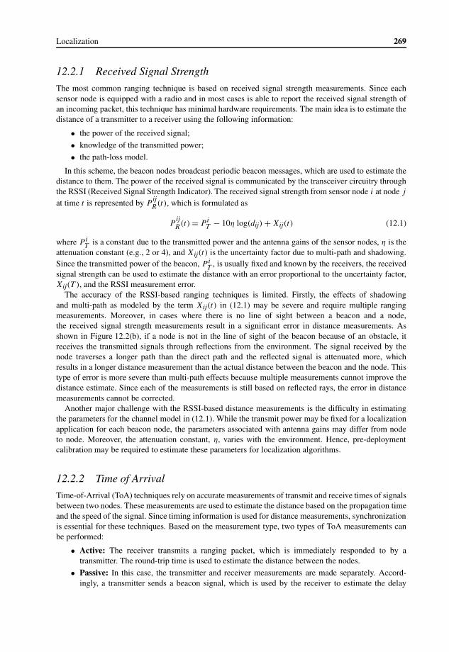
Localization 269
12.2.1 Received Signal Strength
The most common ranging technique is based on received signal strength measurements. Since eachsensor node is equipped with a radio and in most cases is able to report the received signal strength ofan incoming packet, this technique has minimal hardware requirements. The main idea is to estimate thedistance of a transmitter to a receiver using the following information:
• the power of the received signal;
• knowledge of the transmitted power;
• the path-loss model.
In this scheme, the beacon nodes broadcast periodic beacon messages, which are used to estimate thedistance to them. The power of the received signal is communicated by the transceiver circuitry throughthe RSSI (Received Signal Strength Indicator). The received signal strength from sensor node i at node jat time t is represented by P ij
R(t), which is formulated as
PijR(t)= P iT − 10η log(dij)+Xij(t) (12.1)
where P iT
is a constant due to the transmitted power and the antenna gains of the sensor nodes, η is theattenuation constant (e.g., 2 or 4), and Xij(t) is the uncertainty factor due to multi-path and shadowing.Since the transmitted power of the beacon, P i
T, is usually fixed and known by the receivers, the received
signal strength can be used to estimate the distance with an error proportional to the uncertainty factor,Xij(T ), and the RSSI measurement error.
The accuracy of the RSSI-based ranging techniques is limited. Firstly, the effects of shadowingand multi-path as modeled by the term Xij(t) in (12.1) may be severe and require multiple rangingmeasurements. Moreover, in cases where there is no line of sight between a beacon and a node,the received signal strength measurements result in a significant error in distance measurements. Asshown in Figure 12.2(b), if a node is not in the line of sight of the beacon because of an obstacle, itreceives the transmitted signals through reflections from the environment. The signal received by thenode traverses a longer path than the direct path and the reflected signal is attenuated more, whichresults in a longer distance measurement than the actual distance between the beacon and the node. Thistype of error is more severe than multi-path effects because multiple measurements cannot improve thedistance estimate. Since each of the measurements is still based on reflected rays, the error in distancemeasurements cannot be corrected.
Another major challenge with the RSSI-based distance measurements is the difficulty in estimatingthe parameters for the channel model in (12.1). While the transmit power may be fixed for a localizationapplication for each beacon node, the parameters associated with antenna gains may differ from nodeto node. Moreover, the attenuation constant, η, varies with the environment. Hence, pre-deploymentcalibration may be required to estimate these parameters for localization algorithms.
12.2.2 Time of Arrival
Time-of-Arrival (ToA) techniques rely on accurate measurements of transmit and receive times of signalsbetween two nodes. These measurements are used to estimate the distance based on the propagation timeand the speed of the signal. Since timing information is used for distance measurements, synchronizationis essential for these techniques. Based on the measurement type, two types of ToA measurements canbe performed:
• Active: The receiver transmits a ranging packet, which is immediately responded to by atransmitter. The round-trip time is used to estimate the distance between the nodes.
• Passive: In this case, the transmitter and receiver measurements are made separately. Accord-ingly, a transmitter sends a beacon signal, which is used by the receiver to estimate the delay

270 Wireless Sensor Networks
S
B–A
TDoAC–A
AB
C
TDoA
(a) Multi-node time difference of arrival method
B
rf
tdelay
tus
time
A
t
(b) Multi-signal time difference of arrival method
Figure 12.4 Two TDoA methods.
between the two nodes. However, for this technique, the time of signal transmission needs to beknown.
ToA techniques can be used to measure the propagation time between two nodes. The nodes thenestimate the relative distance to a beacon by applying the measured propagation time to a complexdistance formula.
ToA techniques require very accurate hardware to measure the actual received time of the beaconsignals. Any small error in time measurement can result in large distance estimate errors because of thehigh propagation speed of RF signals in air. Therefore, ToA techniques are not practical for traditionalWSNs. On the other hand, as we will see in Chapter 17 and Chapter 16, challenging environmentssuch as under water and underground exhibit low propagation speeds because of the properties of thecommunication media. Therefore, ToA techniques may be more suitable for these environments.
12.2.3 Time Difference of Arrival
While actual propagation time measurements of a signal require sophisticated measurement hardware,the difference between the receive times of two separate signals can be used to estimate the distancebetween nodes. Since less accurate measurements are tolerated, time difference of arrival (TDoA)techniques can be used for WSNs in practice. TDoA techniques can be classified into two:
• Multi-node TDoA: These techniques use ToA measurements of signals transmitted frommultiple beacon nodes for distance measurement. As shown in Figure 12.4(a), three beacons canbe used to accurately locate a node using TDoA measurements. Firstly, the node to be localized,i.e., node S, measures the arrival time of beacons sent from three beacon nodes A, B, and C. Ifthe three nodes are synchronized and transmit the beacon signals at the same time, the differencebetween a pair of beacon nodes defines a hyperbola on which node S should lie. These lines areshown as TDoAB−A and TDoAC−A in Figure 12.4(a). The intersection of the two hyperbolas isthen used to locate the node.
• Multi-signal TDoA: These techniques require multiple beacon nodes to perform localization ofa node. Moreover, precise synchronization between beacon nodes is essential for accurate timedifference measurements. Instead, two different kinds of signals can be used by a node to estimateits distance to another node. By using two signals that have different propagation speeds, the timedifference of arrival of these signals can be used to estimate the distance. Multi-signal TDoA isshown in Figure 12.4(b) for a node A, which transmits two signals, and node B, which estimatesthe distance to node A based on the difference in ToA of the two signals. A common approachfor the multi-signal TDoA is to use an RF signal in conjunction with an ultrasound microphoneand speaker such as the Crossbow Cricket motes [1]. As shown in Figure 12.4(b), node A first

Localization 271
S
BαC
αA A(x ,y )A A
B(x ,y )B B
C(x ,y )C C
α
Figure 12.5 AoA measurements for three beacon nodes A, B, and C, and a node S with unknown location.
transmits an RF signal which is received by node B at time trf . Node A then waits for a timetdelay, which is also known by node B, and transmits an ultrasound signal. This signal is receivedby node B at time tus. Then, the distance between two nodes is calculated as
dAB = (srf − sus)(tus − tdelay − trf ) (12.2)
where srf is the speed of RF waves and sus is the speed of ultrasound. Since RF waves travelsignificantly faster than ultrasound waves, the difference between the receive times of these twosignals can be used to accurately measure the distance [1]. Using Cricket nodes, localizationaccuracy up to centimeters is possible [10].
The multi-signal TDoA technique provides high accuracy under line-of-sight conditions. However,similar to the RSSI-based techniques, NLoS communication may lead to high localization errors.Because of the different paths either type of signal may follow, NLoS communication leads tosignificantly different propagation delays. Consequently, localization protocols based on multi-signalTDoA techniques need to consider the NLoS communication case to improve the accuracy. Moreover,compared to RSSI-based localization, TDoA techniques require additional transmitter–receiver pairsin each node for the second type of signal. Hence, these techniques may not be suitable for someWSN applications.
12.2.4 Angle of Arrival
In addition to signal strength and time, the direction of the received signal can also be exploited forlocalization. Angle-of-arrival (AoA) techniques rely on directional antennas or special multiple antennaconfigurations to estimate the AoA of the received signal from beacon nodes. As shown in Figure 12.5,a node S with an unknown location, (xS , yS ), receives beacon signals from nodes A, B, and C with well-known locations, (xA, yA), (xB , yB ), and (xC , yC ), respectively. Then, node S estimates the AoA of eachbeacon, i.e., αA, αB , and αC . AoA measurements are then combined with their locations to estimate thelocation of node S.
AoA techniques provide high localization accuracy depending on the measurement accuracy.However, higher complexity antenna arrays are required for direction measurement, which increasesthe cost. Furthermore, antenna arrays require a certain spacing to provide spatial diversity and toaccurately measure the AoA. Considering the size of typical sensor nodes, such a separation may notbe feasible, which makes AoA techniques impractical for certain WSNs. Finally, AoA techniques alsosuffer from multi-path and scattering as well as NLoS conditions. Since the direction of arrival is usedfor localization, the error due to NLoS components of the received signal may be even more severecompared to that of RSSI- or TDoA-based techniques.

272 Wireless Sensor Networks
Several other localization protocols exist that provide location information in a network of sensornodes. The localization protocols can be classified into two categories. Range-based techniques exploitthe ranging techniques we explored in Section 12.2 as a building block. Then, distributed techniques areused to improve the accuracy of these protocols. Range-free techniques, on the other hand, do not relyon ranging measurements and provide localization services through interactions between sensor nodesas well as local computations.
12.3 Range-Based Localization ProtocolsRange-based localization protocols exploit multiple pairwise range measurements to estimate thelocations of nodes. Multiple range measurements between a node and its different neighbors can beused to improve the accuracy of the location estimate. Localization techniques vary, depending on theranging technique. We first overview the basic localization techniques and then describe the localizationprotocols based on them. There exist three main localization techniques [11]:
• Trilateration: If a node has distance measurements between its neighbors, then trilaterationtechniques can be used to estimate its location. As shown in Figure 12.6(a), in a 2-D spacethree neighbor nodes with known locations are sufficient to localize a node through distancemeasurements. Each distance measurement defines a circle around the neighbor with radius equalto the measurement, on which the node should lie. The intersection of three such circles from threenonlinear neighbors defines the exact location for the node. However, this technique assumesperfect distance measurements, which is not feasible in WSNs because of ranging errors. Hence,more than three nodes are required for localization.
• Triangulation: If the AoA technique is used for ranging, then the angle information from twobeacon nodes is used to localize the node. As shown in Figure 12.6(b), two beacon nodes and theunknown node define a triangle. Using basic trigonometric relations, the location of the unknownnode can be found using the locations of the two beacon nodes and the AoA measurements at theunknown node.
• Maximum likelihood multilateration: The trilateration technique fails to provide an accurateestimate of position if the distance measurements are noisy. Instead, maximum likelihood (ML)estimation methods are necessary to incorporate distance measurements from multiple neighbornodes. In this case, the difference between the distance measurements and the estimated distanceis minimized to find the location of the node.
12.3.1 Ad Hoc Localization System
The ad hoc localization system (AHLoS) provides localization service using either RSS or ToAmeasurements [11]. AHLoS consists of two procedures: firstly, ranging measurements are performedby each node and then location estimation is performed according to the ranging measurements to nodeswith known locations. The ML (multilateration) technique is used to estimate the location of unknownnodes in the network.
The basic building block for localization in AHLoS is atomic multilateration, which is the simplestform of multilateration as explained next.
EXAMPLE 12.2
Atomic multilateration is shown in Figure 12.6(c), where an unknown node S receives beaconsignals from multiple beacon nodes, A, B, C, and D, with known locations. Let us assume that ToAmeasurement is performed with ultrasound signals and the time it takes for a signal to reach node Sfrom a beacon i is given by ti,S . The location of the node (xS , yS ) is estimated by calculating the

Localization 273
S
A A
B(x ,y )B B
C(x ,y )C C
A(x ,y )
(a) Trilateration
S
A A
B(x ,y )B BαA
d AB
αB
A(x ,y )
(b) Triangulation
C
BA
D
S
(c) Multilateration
Figure 12.6 Range-based localization techniques.
difference between the measured distance and the estimated distance between a beacon node asfollows:
fi(x, y, v)= vti,x −√(xi − x)2 + (yi − y)2 (12.3)
where v is the speed of the ultrasound signal, and (xi , yi ) is the location of beacon i. Using atleast three beacon nodes, the location of the unknown node, S, can then be estimated by takingthe MMSE of the system of fi equations [11].
The atomic multilateration explained in Example 12.2 provides localization of a single node whichhas at least three neighboring beacon nodes. However, WSNs are usually deployed with a limited numberof beacon nodes. Furthermore, because of ranging errors, more than three beacon nodes are required foraccurate location estimation. Hence, AHLoS utilizes the location estimates of neighbor nodes to improvethe estimation of unknown node locations. Based on atomic multilateration, a multi-hop network ofsensors can be localized with the help of a subset of beacon nodes. This procedure is called iterativemultilateration.

274 Wireless Sensor Networks
2nd Iteration
A A
B(x ,y )B B
C(x ,y )C CD(x ,y )D D
T
S
1st Iteration
A(x ,y )
(a) Iterative multilateration
TB B
C(x ,y )C CD(x ,y )D D
A(x ,y )A ASB(x ,y )
(b) Collaborative multilateration
Figure 12.7 Multilateration techniques of AHLoS.
EXAMPLE 12.3
Iterative multilateration is illustrated in Figure 12.7(a), where two unknown nodes S and T aresurrounded by four beacon nodes, A, B, C, and D. Note that node S is surrounded by three beaconnodes, whereas node T has only two beacon nodes as neighbors. Since node S can communicatewith at least three beacon nodes, atomic multilateration can be used to estimate its location.However, atomic multilateration cannot be applied to node T, which requires additional distanceinformation to a node with known location. In this case, iterative multilateration is used, wherenode S first estimates its location and becomes a beacon node. Using the additional informationfrom node S, node T can then perform atomic multilateration and calculate its position. Thisinformation can in turn be used by node S to further improve the accuracy of its estimate. As aresult, the uncertainty in location estimation as shown by the circles around nodes S and T can bedecreased at each iteration.
There may be cases in the network where a node does not have any neighbors with enough beaconnodes as neighbors. This case is illustrated in Figure 12.7(b), where nodes S and T cannot performatomic multilateration or iterative multilateration since neither of them has at least three neighbor beaconnodes. In this case, collaborative multilateration is used where one of the nodes solves a joint set oflocation estimate functions using multi-hop information from an unknown neighbor node to find thelocations of both nodes simultaneously.
Collaborative multilateration leads to unique location solutions only when a participating node hasat least three participating neighbors. A participating neighbor is defined as a node which is either abeacon node or a node that has at least three participating neighbors.

Localization 275
A'B
C D
A
B'
(a) Ambiguity in localization
b
CD
B A
θ
(b) Robust quadrilateral
Figure 12.8 Ambiguity and robustness in localization.
EXAMPLE 12.4
Consider the example in Figure 12.7(b). If node S wants to perform collaborative multilateration,it has two beacon neighbors as participating neighbors and node T as an unknown node. Sincenode T also has two beacon nodes and node S as a participating neighbor, node T is also aparticipating node. Consequently, node S solves a set of location estimate equations in the formof
f (xu, yu)= di,u −√(xi − xu)2 + (yi − yu)2 (12.4)
where xu and yu are the locations of the unknown nodes S and T, xi and yi are the locations ofthe beacon nodes A, B, C, and D, and di,u is the estimated distance between a known and anunknown node. As a result, f (xu, yu) is the difference between the estimated distance, di,u, andthe Euclidean distance found from the location estimate (xu, yu).
Qualitative Evaluation
As a result of collaborative multilateration, the number of nodes with location estimates can beincreased and these nodes can be used for iterative multilateration. Consequently, using three differentmultilateration techniques, AHLoS aims to provide distributed localization in WSNs. An importantadvantage of AHLoS is that it does not rely on a single type of ranging technique. The localizationresults using both RSS and ToA techniques yield acceptable localization accuracy in the range of tensof centimeters in small-scale networks. This is because of the improvement of localization estimationthrough iterative multilateration. On the other hand, for large-scale networks, iterative multilaterationleads to inaccurate results since the initial estimation errors are propagated through the network.
12.3.2 Localization with Noisy Range Measurements
The location estimation primitive shown in (12.3) aims to minimize the error between measureddistances and the distance according to location estimates. However, this distance error minimizationmetric cannot guarantee the actual locations of the nodes to be found. Such an example topology isshown in Figure 12.8(a), where node A can be localized in two different locations, without violating theinternode distance constraints. Consequently, minimizing the distance error as in (12.3) will still lead toambiguity in localization.
To prevent ambiguity, the localization protocol with noisy range measurements relies on robustquadrilaterals as building blocks of localization [8]. A robust quad is a collection of four nodes, which

276 Wireless Sensor Networks
can be localized unambiguously even in the presence of noisy distance measurements. An example ofa robust quadrilateral is shown in Figure 12.8(b) with four nodes, A, B, C, and D. The six distancemeasurements among these four nodes provide constraints such that the relative locations of these nodesare unique up to a rotation, translation, or reflection. Consequently, the quadrilateral is called globallyrigid. However, rigidity does not guarantee unique position estimates if the distance measurements arenoisy. Hence, the quadrilateral should also be robust to provide such a guarantee. This is accomplishedby dividing the quad into four triangles (ABC, ABD, ACD, and BCD). A triangle is defined as a robusttriangle if it meets the following constraint:
b sin2 θ > dmin (12.5)
where b is the length of the shortest side of the triangle and θ is the smallest angle as shown for triangleABC in Figure 12.8(b), and dmin is the robustness threshold. If all the four triangles of a quad are robust,the quad is defined as a robust quad and is used as a building block of the localization protocol.
Two or more robust quads can also be connected to form a larger rigid graph if they share threevertices. All the positions of the nodes in this graph can be localized with a high confidence leveleven under errors in distance measurements. These subgraphs are defined as clusters and the protocoloperation is based on these clusters of multiple robust quads. The protocol operation is conducted inthree main phases: cluster localization, cluster optimization, and cluster transformation. We describeeach phase next, in detail:
• Cluster localization: The first phase is initiated by each node to find the largest connectedrobust subgraph according to the robust quad definition above. Assume a node i initiates thelocalization process. Firstly, a robust quad is found through neighbor message exchanges. This isaccomplished by each neighbor, which broadcasts its distance measurements to the node i. Nodei then computes the robust quads and the cluster. Once these clusters are found, localization isperformed among the nodes in the cluster [8].
• Cluster optimization: The location estimates can also be refined by local computations after allthe location information in the cluster has been exchanged by the members of the cluster. Thisoptional phase improves the localization accuracy at the cost of increased processing at each node.
• Cluster transformation: Since localization is performed independently, each cluster has a uniquecoordinate system. In a multi-hop network, these coordinate systems need to be transformed toprovide consistent localization. The transformation among clusters is performed if there are atleast three non-collinear nodes that are members of both clusters. Using these common nodes,the location at each cluster can be transformed to the coordinate system of other clusters.Consequently, location transformation is performed instead of maintaining a common coordinatesystem within the network. The location of any given node can then be found through thesetransformations.
Using robust quads as a building block for localization provides probabilistic bounds on thelocalization error. If the individual distance measurements include an error that is normally distributedwith standard deviation σ , then the localization protocol bounds the worst case probability of error,which is found to be
P(x > d + derr)=�(derr
σ
)(12.6)
where derr is the worst case error. Consequently, if the threshold dmin in (12.5) is chosen as a multipleof the standard deviation σ of the distance measurement, then the worst case probability of error isbounded.
12.3.3 Time-Based Positioning Scheme
The time-based positioning scheme (TPS) exploits the TDoA ranging technique described in Section12.2.3 [4]. The localization scheme is based on a network structure as shown in Figure 12.9(a), where

Localization 277
S
B B
C(x ,y )C C
A(x ,y )A A
dAB
dAC
dBC
dSB
dSA
dSC
B(x ,y )
(a) Network architecture
(b) Localization scheme
Figure 12.9 Time-based positioning scheme (TPS) [4].
three beacon nodes are deployed around the sensor network. The beacon nodes are equipped withpowerful transceivers and can reach all the nodes in the network.
Localization of the network is performed by each node independently using the beacons broadcast bythe beacon nodes. Each beacon node periodically broadcasts a beacon with a period of T seconds. TPSdoes not require the beacon nodes to be synchronized and the beacons can be transmitted at differenttimes. As shown in Figure 12.9(b), a node S can receive beacons from three beacon nodes A, B, and Cwith known locations (xA, yA), (xB , yB ), and (xC , yC ), respectively. Node S tries to estimate its location(xS , yS ) through TDoA measurements from these beacon nodes.
TPS consists of two steps: range detection and location computation. In the first step, one of the basestations is used as a master base station and the signal round-trip time between the master base stationand the other base stations is used by node S to estimate its location.

278 Wireless Sensor Networks
EXAMPLE 12.5
The range detection phase for node S is illustrated in Figure 12.9(b). Firstly, node A broadcastsa beacon, which is received at tA,S , tA,B , and tA,C at nodes S, B, and C, respectively. Uponreceiving the beacon, node B replies back after a delay, �tb, to node A. Nodes C and S receivethis signal at tB,C and tB,S , respectively. Finally, node C replies to nodes A and B after �tc,which is received by node S at time tC,S .
After node S receives the three beacon messages it calculates the following equations:
dSB = dSA + k1 (12.7)
dSC = dSA + k2 (12.8)
where dSA, dSB, and dSC are the distances from node S to beacon nodes A, B, and C, respectively,and
k1 = v · (�t1 −�tb)− dAB, k2 = v · (�t2 −�tc)− dAC, (12.9)
with v the speed of the RF signal, �t1 = tBS − tAS and �t2 = tCS − tAS.The second phase of TPS is location computation, where the distance from node S to node A,
i.e., dSA, and the location of node S, (xS , yS ), are calculated. To this end, based on the rangingprocedure explained above, each node solves a set of equations as follows:
(xS − xA)2 + (yS − yA)2 = d2SA (12.10)
(xS − xB)2 + (yS − yB)2 = (dSA + k1)2 (12.11)
(xS − xC)2 + (yS − yC)2 = (dSA + k2)2. (12.12)
As discussed in Section 12.2.3, various factors such as multi-path and shadowing affect the TDoAmeasurements. The measurement errors can be minimized by using techniques such as ML multilater-ation, which is used by AHLoS as explained in Section 12.3.1. However, ML multilateration results inexcessive computations because of the nonlinearity of the operations and becomes a significant sourceof energy consumption. TPS, on the other hand, improves the localization accuracy by using multiplemeasurements in the first phase of the protocol. More specifically, the parameters k1 and k2 are definedin (12.9) for a single beacon interval. Instead of using these values at each interval and estimating thelocation, multiple consecutive intervals are considered to find an average of these values as follows [4]:
k1 = vI
[ I∑i=1
(�ti1 −�tib)]− dAB (12.13)
k2 = vI
[ I∑i=1
(�ti2 −�tic)]− dAC (12.14)
where I is the number of intervals used for averaging and subscript i denotes the measurement ininterval i. Accordingly, the location of the node is estimated at each l interval. Since only simpleoperations are performed by each node, the computational overhead of the localization protocoldecreases while improving the accuracy as we explain next.
Similar to the previous localization protocols, the accuracy of localization in TPS depends on theaccuracy of the TDoA measurements. More specifically, for TPS, if the distances between the beaconnodes are large compared to the distances between sensor nodes, the variance of xS is a function of thevariance of k1, while the variance of yS is a function of the variance of k2. Consequently, decreasing theuncertainty in the measurements of k1 and k2 by averaging over multiple intervals directly improves thelocalization accuracy.

Localization 279
Sensor nodes
p (t)i Sensor node i
Figure 12.10 Use of mobile robots in sensor networks.
Qualitative Evaluation
TPS is a distributed localization technique which relies on independent TDoA measurements at eachsensor node. Compared to AHLoS explained in Section 12.3.1 and the localization protocol with noisyrange measurements explained in Section 12.3.2, TPS does not require internode communication forlocalization. This significantly decreases energy consumption since internode communication increasesas the density in the network increases. On the other hand, TPS requires powerful beacon nodes whichare capable of broadcasting their messages to the whole network. This requirement may not be valid forsome WSN architectures, where such nodes do not exist.
12.3.4 Mobile-Assisted Localization
The range-based localization protocols discussed so far utilize ranging measurements from nodes withfixed locations. Consequently, the localization accuracy is inherently limited depending on the networktopology and the deployment strategy. Since a uniform network deployment is not feasible in practice,some portions of the network may have a lower density and the neighbors of a node may not be sufficient.Moreover, the locations of the beacon nodes may not be optimal for each node in the network. Sincethe topology of the sensor network rarely changes because of the limited (or lack of) mobility, thelocalization accuracy of particular nodes cannot be improved through these techniques.
Mobile-assisted localization (MAL) employs mobile agents to improve the localization accuracy inWSNs [9]. As described in Section 12.3.2, the uniqueness of the multilateration technique depends onforming globally rigid subgraphs. The global rigidity of a subgraph is satisfied if (1) the removal ofany vertices leaves the graph connected and (2) the removal of any edge leaves the graph locally rigid.The localization with noisy measurements scheme described in Section 12.3.2 performs localizationby finding already existing rigid subgraphs in the network through pairwise distance measurements.However, this may not be the case for some portions of the network because of low density. MAL usesa mobile agent to gather additional distance measurements to form globally rigid subgraphs.
Compared to the range-based localization protocols described in earlier sections, in MAL, sensornodes do not perform distance measurements. Instead, a mobile agent, which travels throughout thenetwork, is used to find the distance between multiple sensor nodes and itself to estimate the distancebetween these sensor nodes as shown in Figure 12.10. As an example, the mobile agent can findthe pairwise distance between four nodes with an additional seven measurements provided that thesemeasurements are not collinear.

280 Wireless Sensor Networks
Accordingly, MAL is initialized by the mobile agent, which finds four nodes to create a globally rigidsubgraph. The mobile agent then selects seven locations and measures its distance to the from nodesfrom these locations. The pairwise distances between the four nodes are then found by solving a set ofequations involving the distance measurements. After the pairwise distance values are estimated, MALlocalizes the nodes using multilateration techniques.
The second phase following initialization is to increase the rigid subgraph by adding additionalneighbor nodes. From the rigid graph, the mobile agent selects a node and moves around this node.In this way, the mobile agent searches for additional non-localized nodes. If a non-localized node isfound, the mobile agent uses the selected localized nodes along with some of its localized neighbors toperform similar localization for the non-localized node. The technique is repeated until all the nodes inthe network are localized or the mobile agent cannot improve localization any further.
Qualitative Evaluation
The advantage of MAL is that sensor nodes do not need to perform additional distance measurementsor solve complex localization equations. Instead, a mobile agent is used to perform the localizationtasks. In this way, for each sensor node, sufficient distance measurements can be made. On the otherhand, MAL requires a mobile agent, which can be a robot or a human, to perform the localizationtasks. Since a mobile agent may not be available for most applications, MAL has limited applicability.Furthermore, the localization performance depends on the measurements and calculations performed at asingle node in the network. Hence, any errors in the measuring algorithm or the localization calculationscan affect the whole network. Similarly, such a dependency creates single point-of-failure problems inWSNs. Finally, MAL has been developed for a single mobile agent. Therefore, for large networks, thelocalization latency may be significantly large because of the time it takes for the mobile node to traversethe whole network.
12.4 Range-Free Localization Protocols
Range-based localization protocols described in Section 12.3 rely on ranging measurements for dis-tributed location estimates. Depending on the protocol, these ranging measurements may need to beperformed among each neighbor of a node or with only a smaller number of beacon nodes. While theaccuracy of the range-based localization protocols is high, the cost associated with them is also highbecause of the additional energy consumption for ranging measurements. On the other hand, severalapplications of WSNs do not require very accurate location information and only coarse localization maybe sufficient. The range-free localization protocols provide an efficient way to localize the sensor nodeswithout specific ranging measurements. Instead, connectivity information between nodes is exploited todetermine constrains on the location of the nodes. Similar to the range-based protocols, beacon nodesare also used to provide a reference for localization. Next, we describe two range-free protocols in detail:convex position estimation [5] and the approximate point-in-triangle (APIT) [6] protocol.
12.4.1 Convex Position Estimation
The lack of ranging information poses additional challenges for localization since a limited amountof information is available. However, even without accurate distance measurements, the connectivityinformation between a node and its neighbors can still be exploited to constrain the location of the nodeas described in the following example.

Localization 281
C
BA
D
S
(a) Connectivity constraints
C
B
D
A
S
(b) Angular constraints
Figure 12.11 Connectivity and angular constraints can be exploited for convex position estimation.
EXAMPLE 12.6
Consider the case shown in Figure 12.11(a), where node S is within the communication rangeof nodes A, B, C, and D. If the location of node B and its transmission range R are known,then node S can deduce that it is located in a circle centered around node B with radius R. Anyadditional neighbor with location information such as nodes A, C, and D further constrains thepossible location of node S. As a result, the connectivity of a node provides a proximity constraintparameter, which can be utilized to solve an optimization problem and estimate the location ofthe node.
The convex position estimation (CPE) algorithm provides an optimization framework, where thelocations of the nodes in a WSN are found as a result of a joint optimization problem [5]. The goalof the algorithm is to estimate the locations of unknown nodes in a WSN, where a subset of the beaconnodes have accurate location information as shown in Figure 12.11(a). Using the location information ofthe beacon nodes and the connectivity information of all the nodes in the network, the locations of theremaining nodes can be estimated.
The protocol operation is as follows. Each node exchanges messages with its neighbors to populatea connectivity table representing its immediate neighbors. Connectivity information consists of nodesfrom which a node receives messages. Considering the limited transmission range of wireless sensornodes, the connectivity information provides natural bounds on the distance between two connectednodes. This information is sent to a central location such as the sink, where a centralized optimizationproblem, which exploits these constraints, is formulated.
On collecting the connectivity information from the nodes in the network, the central controllerformulates a linear program (LP) to find the positions of the nodes in the network, where the connectivityinformation is used as a constraint. The LP is a feasibility problem, which is to find the unknownlocations satisfying the connectivity constraints between unknown and known nodes. The solution tothe optimization problem is the vector x= [x1, y1, . . . , xm, ym, xm+1, ym+1, . . . , xn, yn], where thefirstm elements are the locations of the beacon nodes (known) and the remaining n−m are the estimatedlocations of the unknown nodes.

282 Wireless Sensor Networks
B
S
A
C
ED
(a) Network architecture
S
A
C
ED
B
(b) Reference triangles formed by the APIT protocol
S
A
C
ED
B
(c) The PIT test
V
S
A
C
ED
BT
U
(d) The approximate PIT (APIT) test
Figure 12.12 The APIT protocol [6].
As shown in Figure 12.11(a), the maximum communication ranges of the nodes can be used asconstraints for the optimization framework. If AoA information is available, angular constraints canalso be used for estimation as shown in Figure 12.11(b). By combining the connectivity constraints frommultiple neighbors of a node, the central controller creates a bounding box in which the node shouldreside. As shown in Figure 12.11(a) and Figure 12.11(b), the bounding box is a rectangle which includesthe possible locations of the node subject to the connectivity or angular constraints, i.e., feasible positionsets. Then, the center of the bounding box is selected as the location of the node.
The bounding box is generally generated from the connectivity information from beacon nodes.However, in case of a lack of sufficient beacon nodes, the unknown nodes are also included in theconnectivity information to further constrain the location of the node. This is similar to the iterativemultilateration technique used in AHLoS. However, the location estimates of the unknown nodes containuncertainty in the location estimation. Therefore more of these nodes are required for accurate locationestimation. More specifically, using the CPE algorithm, close to eight connections to unknown nodesare required to achieve the same level of certainty achieved through a connection to a single beaconnode [5]. Exploiting the additional constraints imposed by the neighboring unknown nodes improves theaccuracy of the localization algorithm, especially in high-density WSNs.
Although the CPE algorithm provides high accuracy for localization in WSNs, it can be viewed as aguideline for the development of localization solutions for WSNs due to its centralized nature. The CPEalgorithm necessitates the connectivity information being collected at a centralized location. Moreover,after the joint optimization problem is solved, the location information needs to be disseminated toeach node in the network. This requirement can significantly increase the overhead and the energyconsumption of the protocol. Moreover, the localization protocol relies on a single node and it is

Localization 283
vulnerable to single points of failure. Furthermore, the connectivity information of a node can changefrequently because of the changes in the wireless channel. This necessitates frequent informationexchange throughout the network, which makes the solution impractical for large-scale WSNs.
12.4.2 Approximate Point-in-Triangulation (APIT) Protocol
The APIT protocol relies on a network that consists of wireless sensor nodes as well as beacon nodes withknown locations [6]. However, localization of the sensor nodes is performed without ranging techniques.Instead, the RSS information from multiple nodes is used to estimate the relative locations of thesenodes. Consequently, the APIT protocol does not require any additional hardware such as sounders andmicrophones, which are required for timing measurements.
The network architecture of the APIT protocol is shown in Figure 12.12(a), where multiple beaconnodes are distributed in the network field. These nodes have known locations and periodically broadcastbeacons to the rest of the nodes in the field. Each sensor node can receive beacons from a subset ofthese beacon nodes and localize itself. The locations of the beacon nodes are used to form triangles byeach node.
EXAMPLE 12.7
Referring to Figure 12.12(a), let us assume that node S receives beacon signals from beaconnodes A, B, C, D, and E. Since node S is aware of the positions of the beacon nodes, it can formtriangles using any three of these nodes as shown in Figure 12.12(b). If the node can determinewhether it is inside or outside of these triangles, the intersections of these triangles can be used todefine a small area in which the node should reside. Consequently, using multiple beacon signals,a node can localize itself up to a certain accuracy.
Based on the architecture in Example 12.7, the APIT protocol consists of four phases: (1) beaconexchange, (2) PIT testing, (3) APIT aggregation, and (4) center of gravity (COG) calculation. Next, wedescribe each phase of the protocol:
• Beacon exchange: Upon receiving beacons from the beacon nodes, a node populates a tablewith the locations of each beacon node and the value of the received signal strength fromthat node. This information is then broadcast to the neighbors of the node. Consequently, eachnode is informed about the connectivity of each of its neighbors to the beacon nodes and thecorresponding RSS values. This information is used to estimate whether a node is inside a triangleformed by three beacon nodes in the PIT testing phase.
• PIT testing: The PIT test is performed to determine whether a node is inside a triangle formed bythree beacon nodes. Ideally, this can be performed by moving the node along any axis as shownin Figure 12.12(c). The node is outside the triangle if there exists a direction such that whenevera node is moved in this direction, its distances to the three vertexes of the triangle increase ordecrease simultaneously. Otherwise, the node is inside the triangle. PIT testing is illustrated inthe following example based on the topology in Example 12.7.
EXAMPLE 12.8
As shown in Figure 12.12(c), when node S is moved in the direction shown by the arrow, itsdistance to nodes C, D, and E increases. Hence, it can be concluded that node S is outside thetriangle CDE. However, since its distance to node A decreases, but increases for nodes C and D,it is inside the triangle ACD. This is referred to as the point-in-triangulation (PIT) test. However,in WSNs, since a node cannot be moved, an approximate PIT (APIT) test is performed instead.

284 Wireless Sensor Networks
The APIT test is illustrated in Figure 12.12(d), which exploits the high density of WSNs.Instead of moving a node, each node checks the connectivity information of its neighbors. Fora given triangle ACD, a node S first determines the neighbor nodes (T, U, V in Figure 12.12(d))that also receive beacons from these beacon nodes. Then, node S checks whether it has a neighborthat is farther from the three beacon nodes simultaneously. To this end, the RSS values are used.Although the RSS values are not used to calculate the exact distance, the difference between theRSS values of two nodes is used to determine whether a node is farther or closer to the beaconnode. If a node finds such a neighbor, then it determines that it is outside the particular triangle.
The APIT test is performed for each triangle and then APIT aggregation is performed to constrain thelocation of the node.
• APIT aggregation: The APIT test determines the triangles in which node S resides. As shownin Figure 12.12(b), the intersection of these triangles defines the region where the node shouldreside. Following the APIT test, node S calculates the maximum overlapping area to estimate itslocation through APIT aggregation.
• COG calculation: The last phase of the APIT protocol is the COG calculation. In this phase, thenode determines its location as the COG of the overlap area found in the previous phase. Thislocation is shown as a dot in Figure 12.12(b).
Qualitative Evaluation
The APIT protocol provides a range-free localization technique through simple geometric calculationsusing beacon signals from specific nodes. Consequently, the complexity of the protocol is significantlylow compared to range-based algorithms. On the other hand, the localization accuracy of the algorithmis also low and is proportional to the number of nonlinear beacon nodes that a node is connected to.However, based on the impact of localization errors on other protocols such as routing and tracking,a localization error less than 0.4R is acceptable, where R is the transmission range of the beaconnodes. Consequently, the APIT protocol is applicable to scenarios where high localization accuracyis not required; however, minimizing protocol overhead is of major concern.
References[1] Cricket indoor location system. http://nms.lcs.mit.edu/projects/cricket.
[2] MTS420 environment sensor board. Available at http://xbow.com.
[3] J. Aspnes, W. Whiteley, and Y. R. Yang. A theory of network localization. IEEE Transactions on MobileComputing, 5(12):1663–1678, December 2006.
[4] X. Cheng, A. Thaeler, G. Xue, and D. Chen. TPS: A time-based positioning scheme for outdoor wireless sensornetworks. In Proceedings of IEEE INFOCOM’04, volume 4, pp. 2685–2696, Hong Kong, China, March 2004.
[5] L. Doherty, K. Pister, and L. Ghaoui. Convex position estimation in wireless sensor networks. In Proceedingsof IEEE INFOCOM’01, volume 3, pp. 1655–1663, Anchorage, AL, USA, April 2001.
[6] T. He, C. Huang, B. Blum, J. Stankovic, and T. Abdelzaher. Range-free localization schemes for large scalesensor networks. In Proceedings of ACM MobiCom 2003, pp. 81–95, San Diego, CA, USA, September 2003.
[7] K. Langendoen and N. Reijers. Distributed localization in wireless sensor networks: a quantitative comparison.Computer Networks, 43(4):499–518, 2003.
[8] D. Moore, J. Leonard, D. Rus, and S. Teller. Robust distributed network localization with noisy range measure-ments. In Proceedings of ACM SenSys, Baltimore, MD, USA, November 2004.
[9] N. B. Priyantha, H. Balakrishnan, E. D. Demaine, and S. Teller. Mobile-assisted localization in wireless sensornetworks. In Proceedings of IEEE INFOCOM’05, volume 1, pp. 172–183, Miami, FL, USA, March 2005.

Localization 285
[10] N. B. Priyantha, A. K. Miu, H. Balakrishnan, and S. Teller. The Cricket compass for context-aware mobileapplications. In Proceedings of ACM MobiCom’01, Rome, Italy, July 2001.
[11] A. Savvides, C. Han, and M. Strivastava. Dynamic fine-grained localization in ad-hoc networks of sensors. InProceedings of ACM MobiCom 2001, pp. 166–179, Rome, Italy, July 2001.


13Topology Management
The topology of a network can be defined according to graph theory as the locations of the nodes thatare available for communication, i.e., the vertex, and the wireless links between these nodes used forcommunication, i.e., the edges. Topology management solutions generate network topologies that aretailored to guarantee a certain requirement such as connectivity, coverage, or lifetime [1, 9, 12, 13, 15,17]. The resulting topology directly affects the performance of each individual protocol as well as theoverall performance of the network. Therefore, topology management is a crucial part of the WSNcommunication protocols.
In WSNs, topology refers to not only the locations of the nodes but also their activity states, i.e., whichnodes are active for communication, as well as the links between them. Hence, several techniques existfor topology management. The four main topology management techniques are shown in Figure 13.1.These techniques can be used individually as well as in conjunction with each other since differentproperties of the topology are controlled by each one.
• Deployment: The first phase of topology management is network deployment as shown inFigure 13.1(a). Deployment techniques determine the locations of the nodes in the network,which plays an important role in the coverage as well as the connectivity of the network.Accordingly, the maximum area that can be covered by the on-board sensors can be maintained.Similarly, deployment affects the links that can potentially be formed given the limitations of thewireless channel.
• Power control: The topology is partly defined by the links between the nodes. In a wirelessnetwork, these links depend on the capabilities of the transceiver. Power control solutions controlthe transmit power of the transceivers to maintain the communication range of a node as shown inFigure 13.1(b). Accordingly, the number of neighbors of a node or the hop length in a multi-hoppath can be determined for energy efficiency, reliability, or latency goals.
• Activity control: In a WSN, the transceiver of the sensor node can be turned off during certainperiods to increase energy efficiency. As a result, certain nodes become disconnected fromthe network during their sleep states. Hence, the network topology can also be maintained bymanaging the activity of the sensor nodes as shown in Figure 13.1(c). Accordingly, redundantnodes can be turned off while still maintaining the connectivity and capacity of the network.
• Clustering: In addition to flat topology-based techniques, the network can also be partitionedinto clusters as shown in Figure 13.1(d) to improve scalability and energy efficiency. In this case,a group of nodes are placed into clusters, which are controlled through cluster heads (CHs).
Topology management approaches for WSNs are described in the following sections. Theseapproaches are classified into four as shown in Figure 13.2. We provide general rules for deploymentin WSNs in Section 13.1. The power control problem and its solutions are described in Section 13.2.In Section 13.3, activity scheduling protocols are discussed. Finally, we explain clustering solutions inSection 13.4.
Wireless Sensor Networks Ian F. Akyildiz and Mehmet Can Vuranc© 2010 John Wiley & Sons, Ltd

288 Wireless Sensor Networks
Sink
(a) Deployment
Sink
(b) Transmit Power Control
Sink
(c) Activity Control
���
���
���
���
Sink
(d) Clustering
Figure 13.1 Topology management techniques.
Topology Control Solutions
Deployment Power Control Activity SchedulingHierarchical [3,4]HEED [24]CPCP [21]
LMA [11]
CONREAP [16]
LMN [11]
ClusteringLMST [14]
ASCENT [6]
PEAS [23]SPAN [7]
GAF [22]
STEM [18]LLISE [5]
VFA [26]
Figure 13.2 Overview of topology control solutions.
13.1 Deployment
The physical location of the nodes in a WSN is crucial in terms of both communication and sensing.Since sensor nodes are equipped with radios of limited range, the communication is performed in a multi-hop fashion [2]. Hence, connectivity is an important factor considered for sensor deployment. Moreover,

Topology Management 289
since a physical phenomenon with spatio-temporal characteristics is observed via the WSN, thedeployment of the nodes also affects the accuracy of the samples collected regarding the phenomenon.Hence, coverage is also important for sensor deployment.
A WSN should be deployed according to the coverage and connectivity of the network. Severalmethods exist for determining network connectivity and coverage given a node reliability model [19, 20].The node reliability refers to the probability that a node is active in the network. Moreover, given apower budget, an estimate of the minimum required node reliability for meeting a system reliabilityobjective can be found. Using a grid-based topology for WSNs, theoretical bounds and an insight intothe deployment of WSNs can be obtained. As an example, as the node reliability decreases, the sufficientcondition for connectivity becomes weaker than the necessary condition for coverage. This implies thatconnectivity in a WSN does not necessarily imply coverage. Furthermore, the power required per activenode for connectivity and coverage decreases at a rate faster than the rate at which the number of nodesincreases. Thus, as the number of nodes increases, the total power required to maintain connectivity andcoverage decreases.
The relationship between reduction in sensor duty cycle and redundancy in sensor deployment isalso important [8]. Two main approaches, namely random and coordinated sleep algorithms, can becompared in terms of two performance metrics, i.e., extensity and intensity. Extensity refers to theprobability that any given point is not covered, while intensity gives the tail distribution of a givenpoint not covered for longer than a given period of time. As the density of the network is increased, theduty cycle of the network can be decreased for a fixed coverage. However, beyond a certain threshold,increased redundancy in the sensor deployment does not provide the same amount of reduction in theduty cycle. Moreover, coordinated sleep schedules can achieve higher duty cycle reduction at the cost ofextra control overhead. Using the intensity analysis of the network, random sleeping schedules can bedeveloped for a satisfactory coverage [8].
The virtual force algorithm (VFA) enhances sensor coverage by moving sensor nodes after an initialrandom deployment [26]. The algorithm assumes a cluster-based architecture and is executed at theCHs. The VFA uses virtual positive or negative forces between nodes based on their relative locations.Moreover, using this cluster-based architecture, target localization can be performed in a distributedmanner. The simulation results reveal that the VFA improves coverage of the sensor network andincreases accuracy in the target localization. However, the algorithm requires either mobile sensor nodesor redeployment of nodes accordingly, which is not applicable for all WSNs.
13.2 Power ControlAs described in Chapter 4, the wireless channel quality can be improved by increasing the transmit powerof a node. As a result of increased transmit power, a node can communicate with more nodes. Similarly,in high-density networks, the transmit power can be decreased to limit the number of neighbors of a node,i.e., the node degree. This can reduce interference and increase network lifetime. Consequently, powercontrol algorithms encounter a tradeoff in terms of reducing interference and increasing network lifetimevs. reducing network connectivity. By controlling the transmit power of each node, certain networkproperties such as connectivity, interference, latency, and lifetime can be maintained. Accordingly, powercontrol mechanisms are developed to achieve the following goals:
• Connectivity: The main goal of power control algorithms is to preserve connectivity by choosingminimum transmit power for nodes.
• Minimum spanning: Reducing transmit power results in a decrease in the average hop length formulti-hop transmission since longer links that require high transmit power are eliminated fromthe network. This increases the path length between any node and the sink. The transmit powercontrol algorithm should ensure that the resulting path between any node and the sink in thenetwork should be longer at most by a constant factor than the shortest path achievable throughmaximum transmit power level [5].

290 Wireless Sensor Networks
• Distributed operation: Since it is infeasible to control the transmit power levels of each nodeby a single entity in WSNs, the power control algorithms should be distributed. Furthermore, thedeveloped protocols should be scalable so that networks of large numbers of nodes can still besupported.
• Discrete power levels: Typical sensor node architectures provide a limited number of transmitpower levels. Hence, solutions that choose any power level are not feasible and discrete powerlevels should be supported.
We discuss the following power control mechanisms next: LMST [14], LMA and LMN [11],interference-aware power control [5], and CONREAP [16].
13.2.1 LMST
The local minimum spanning tree (LMST) algorithm aims to construct a minimum spanning tree (MST)through local decisions for power control [14]. The protocol depends on the locational knowledge of thenodes to make localized decisions. The protocol operation can be divided into three phases: informationcollection, topology construction, and transmission power determination. Moreover, an additional phase,topology construction with bidirectional links, can also be performed.
Similar to most distributed topology control protocols, LMST is initiated with an informationcollection phase. Each node broadcasts HELLO messages at the maximum transmit power to exchangenode-specific information. These messages are periodically broadcast throughout the protocol operationand contain the node ID and the position of the node. As a result, each node is informed about thepositions of its neighbors in its visible neighborhood. A visible neighborhood of a node i is the setof nodes from which node i can receive information during the information collection phase and isdenoted as NVi (G). Accordingly, the network topology with maximum transmit power is denoted as anundirected graph G= (V , E), where V is the set of nodes and E = {(i, j) : d(i, j) ≤ dmax, i, j ∈ V },and where dmax is the maximum distance that a node can reach using its maximum transmit power.
The visible neighborhood information is used by each node to construct the local MST, Ti =(V (Ti ), E(Ti)) of Gi , which is the graph that contains the visible neighborhood of node i. For theconstruction of the topology, the transmission power required for successful communication for eachedge is used as the weight of that edge. Neglecting the effects of multi-path fading and shadowing,1
the required transmission power and, hence, the weight can be directly mapped to the distance betweentwo nodes. In the case of equal distances, node IDs are used to assign unique weights to each edge.Accordingly, a unique MST can be formed by each node.
Based on the MST, the relation between each node and its neighbors is defined by the neighborrelation. More specifically, node j is referred to as a neighbor of node i if and only if it is in the MSTof node i, i.e., (i, j) ∈ E(Ti). This relation is denoted as i→ j . Accordingly, the neighbor set of i isdenoted as N(i)= {j ∈ V (Gi) : i→ j}. Using the neighbor relation between each node, the resultingnetwork topology with the LMST protocol is defined as G0 = (V0, E0), where V0 = V is the set of allnodes in the network and E0 = {(i, j) : i→ j, i, j ∈ V (G)} is the set of all edges in the MST of eachnode in the network.
Following the topology construction phase, each node determines the transmit power to all of itsneighbors in its local MST. This is performed using the HELLO messages received from each neighbor.As explained above, HELLO messages are sent using the maximum transmit power level, Pmax. Thus,the received power level, Pr , of each HELLO message represents the path loss, PL, between the nodesthat sent and received the HELLO message. More specifically,
PL= Pr
Pmax. (13.1)
1For details see Chapter 4.

Topology Management 291
Assuming symmetric channels, this path loss can be used to adjust the transmit power level, Pt , so thatthe neighbor can receive the packets with a receive power level of Pth. Accordingly,
Pt = Pth · PL (13.2)
= PthPr
Pmax(13.3)
The value of Pth is determined such that the packet can be received without any errors.Additionally, the LMST algorithm can be used to ensure that all the links in the constructed topology
are bidirectional, i.e., if i→ j then j → i. This is performed in two ways. If a unidirectional linki→ j exists, an additional link j → i is added to the constructed graph or is removed from the graphcompletely. Accordingly, the resulting LMST has bidirectional links, which is important for supportingtwo-way communication between nodes in the network.
The LMST algorithm provides a connected network by constructing local MSTs and controlling thetransmit power at each link. As a result, the overall energy consumption can be decreased compared tothe case where maximum transmit power is used. Moreover, the resulting LMST consists of fewer linksbetween the nodes in the network. This reduces the interference in the network, which improves theenergy efficiency.
On the other hand, LMST requires accurate location information for path-loss determination.Moreover, a simpler channel model is considered, which neglects the random effects of multi-path fadingand shadowing. In case of location errors and practical channel effects, the transmit power determinationscheme can result in either higher energy consumption or communication errors. Furthermore, the time-varying nature of the wireless channel has not been considered in LMST, which may lead to fluctuationsin communication success and connectivity.
13.2.2 LMA and LMN
The LMST algorithm determines the transmit power level for each link for a node. As a result, foreach communication link, a node should change its transmit power level according to the determinedvalue. This results in considerable amounts of delay and energy consumption during transmit poweradjustments. The local mean algorithm (LMA) and local mean of neighbors (LMN) algorithm addressthis overhead by finding the best transmit power for a node to be used throughout the network operationwithout hampering the connectivity of the network [11]. The objective of these algorithms is to maximizethe network lifetime.
The LMA aims to adjust the transmit power such that the number of neighbors of a node is limited.Accordingly, each node periodically broadcasts a life message (LifeMSg) with an initial transmit powerlevel. The neighbors of this node that receive this message reply with a LifeAckMsg. The senderkeeps track of the number of LifeAckMsgs and adjusts its transmit power accordingly. The numberof LifeAckMsgs is indicated by nr and LMA aims to maintain this value between two predeterminedlimits: nmin and nmax.
If a node receives responses from a number of neighbors that are less than nmin, then it increases itstransmit power level to reach more nodes. The new transmit power P new
t is updated as follows:
P newt =min{BmaxPt , Ainc(nmin − nr)Pt }. (13.4)
Accordingly, the transmit power is compensated for each required neighbor to reach the lower bound,nmin. Moreover, the update rule ensures that the transmit power is not increased by more than a factorof Bmax.
If, on the other hand, the number of received responses is more than nmax, then the transmit powerlevel is decreased. Similarly, the update rule is as follows:
P newt =max{BminPt , Adec(1− (nr − nmax))Pt }. (13.5)

292 Wireless Sensor Networks
D
AB
C
Figure 13.3 Neighborhood information exchange in LMN [11].
Moreover, the transmit power is kept constant if nmin ≤ nr ≤ nmax.While LMA maintains the number of neighbors a node has, the second algorithm, i.e., the LMN
algorithm, maintains the number of neighbors of the neighbors of a node.
EXAMPLE 13.1
In the LMN algorithm, in addition to the LifeAckMsgs, the responding nodes also include thenumber of their neighbors. This is shown in Figure 13.3, where node A broadcasts a LifeMsg.Nodes B, C, and D receive this message and reply with LifeAckMsgs indicating the number ofneighbors they have, i.e., {6, 4, 3}. Accordingly, node A finds the mean of these values and usesthis mean for power control. In our example, nr = 4. The update policy of LMA is used similarly.
In the protocol operation, the limits of nmin = 4 and nmax = 7 are used. Both protocols generallyconverge within a limited number of message exchanges. On average, the LMN algorithm results in0.003% of the nodes not connected, while this number is 0.37% for LMA. This shows that bothprotocols provide high connectivity whereas the LMN algorithm results in a stronger connectivity.Furthermore, both algorithms perform very close to the global optimum, which can only be achievedthrough centralized solutions.
13.2.3 Interference-Aware Power Control
The transmit power control schemes presented above (LMST, LMA, and the LMN algorithm) reducetransmit power to improve the network lifetime while maintaining network connectivity. However, theamount of interference caused as a result of the distributed transmit power operation is not consideredas a design metric in these solutions. It is generally accepted that reducing the node degree byreduced transmit power results in a reduction in interference. However, this does not result in minimuminterference in the network. In this section, we describe the effect of interference on topology controland, more specifically, on transmit power control algorithms.
EXAMPLE 13.2
In a wireless network, the interference is modeled based on the area that is covered by thecommunication between two nodes. Consider the case in Figure 13.4, where two nodes i and j arecommunicating. Based on the distance between these nodes, di,j , the transmit power levels can beadjusted to maintain successful communication with minimum energy expenditure. Consideringa circular communication range, the communication coverage of an edge e = (i, j) between two

Topology Management 293
ji
Figure 13.4 Communication coverage of an edge e= (i, j) [5].
nodes i and j is defined as follows [5]:
Cov(e)= {k ∈ V |k ∈D(i, di,j )} ∪ {k ∈ V |k ∈D(j, di,j )} (13.6)
whereD(i, r) is the disc centered at node i with radius r . Accordingly, the interference of a graph,G, is defined as follows:
I (G)=maxe∈E Cov(e). (13.7)
According to the definition of connectivity in (13.7), an interference-aware topology control algorithmcan be developed. This is performed by finding a set of edges that minimize the interference constrainedby the fact that the resulting topology is connected.
The interference can be minimized to find the interference-optimal spanning forest, which includesthe set of trees that maintains connectivity with minimum interference. This is performed by the low-interference forest establisher (LIFE) algorithm [5]. The LIFE algorithm assigns the coverage, Cov(e),of an edge as the weight of each edge and finds the minimum spanning forest (MSF) of the resultinggraph.
The interference-optimal topology control algorithm LIFE can be performed only with globalknowledge of the network. However, distributed optimization of the interference minimization problemwith connectivity is not feasible. The optimization problem can be modified such that, instead of theconnectivity requirement, the resulting graph is required to be a t-spanner. A t-spanner of a graphincludes edges such that the path length between any nodes of the graph is within a constant factor ofthe shortest path in the original graph. This is distributively solved by the local low-interference spannerestablisher (LLISE) algorithm.
EXAMPLE 13.3
The operation of the LLISE algorithm is illustrated in Figure 13.5. For a given factor t for thet-spanner requirement, each node collects information regarding its (t/2) neighborhood for eachof its edges. Let us consider the edge e = (i, j) as shown in Figure 13.4. The (t/2) neighborhoodof the edge, e, is defined as the set of edges that can be reached through a path p, where |p| ≤t/2|e|, and |p| and |e| are the lengths of the path, p, and the edge, e, respectively. Using the (t/2)neighborhood of the edge, e, node i finds the minimum interference path for e.

294 Wireless Sensor Networks
ji
Figure 13.5 Interference-optimal t-spanner of the link e = (i, j) as a result of the LLISE algorithm.
Firstly, node i orders the edges in the (t/2) neighborhood according to their coverage. Then, asubgraph is formed by using these edges in ascending order until a shortest path p(i, j) is foundso that |p| ≤ t |e|. This is performed for each edge of the node. The resulting graph is shown inFigure 13.5, which is interference optimal with the t-spanner property.
The distributed LLISE algorithm performs very close to the centralized LIFE algorithm, especiallywhen t is increased. In other words, interference in the network can be reduced closer to the globaloptimum by using longer paths compared to the shortest path. Moreover, compared to topologycontrol protocols that consider reducing energy consumption with connectivity constraints, the LLISEalgorithm results in lower interference. This may improve the lifetime of the network in the long term.Transmit power control mechanisms generally determine the optimum transmit power between twonodes without considering the interference. Hence, in a typical network operation, competing flowscan cause interference, which increases the required power level for successful communication. In thiscase, the chosen transmit power can lead to retransmissions and an increase in energy consumption asa result. While interference-aware topology control mechanisms do not necessarily find the minimumpower, the overall energy consumption can be decreased by avoiding interference between links.
13.2.4 CONREAP
The transmit power control mechanisms explained so far are based on a rather simplistic channel model.Based on a specific transmit power level, the nodes are considered connected if they are within a certaindistance, and disconnected otherwise. This is based on the unit disc graph model. The wireless channel,however, exhibits a higher uncertainty than the unit disc graph as discussed in Chapter 4 in detail.More specifically, a transitional region exists for wireless connectivity, where the nodes in this regionare neither fully connected nor fully disconnected. Instead, a percentage of the packets sent can besuccessfully received. In practical settings, the transitional region can include the same number of nodes(or even more) than the connected region, where almost 100% reliability is possible. Hence, consideringonly the connected region for topology control can significantly limit the energy efficiency of the WSN.
Compared to the previously explained topology control protocols, which consider connectivity as adesign parameter, the CONREAP algorithm performs distributed opportunity-based topology control,where unreliable links in the transitional region are also considered [16].

Topology Management 295
The operation of the CONREAP algorithm is based on the concept of link reachability. Similar to othertopology control mechanisms, the network is modeled as a directed graph, G(V, E), with set of nodes,V , and set of edges, E. Instead of defining edges only if two nodes are connected, a link reachability,λe, is assigned to each edge, e = (i, j), where λe ∈ (0.1]. Moreover, the set of nodes that can receive apacket from the sink is denoted as Vr . Accordingly, the network reachability, λ(G), can be defined as afunction of the expected number of nodes that can receive a packet from the sink:
λ(G)= E(|Vr |)|V | (13.8)
which can be found by defining node reachability as λG(i) for a node i. Accordingly, the networkreachability is
λ(G)=∑i∈V λG(i)|V | (13.9)
which is a function of the average node reachability over all the nodes in the network.In addition to the network reachability, the cost associated with the communication is also important.
Accordingly, the network energy cost is defined as
ε(G)= εTx(G)+ εRx(G) (13.10)
where εTx(G) and εRx(G) are the transmitting and receiving cost, respectively. To determine theefficiency of the algorithm, the reachability-to-energy ratio can be defined as
η(G)= λ(G)ε(G)
. (13.11)
EXAMPLE 13.4
The notion of opportunistic topology control can be illustrated using the definitions above andthe sample topology in Figure 13.6(a), where a network of four nodes is shown. The reachabilityof each link is also shown. The connectivity-based topology control algorithms construct thesubgraph G1 as shown in Figure 13.6(b). Since nodes S and A, and A and B, are connected, onlythese edges are selected. Since node C does not have 100% connectivity with any of the nodes,it is not included in the subgraph. Considering the node reachability of A, B, and C as 1, 1,and 0, respectively, the network reachability is λ(G1)= 0.67. Moreover, considering a singleunit for both transmitting and receiving energy, the network energy cost is ε(G)= 4. Finally, thereachability-to-energy ratio is η(G1)= 0.167.
Instead of considering only connected nodes, the lossy links can also be considered in topologymanagement to construct the topology, G2, in Figure 13.6(c). In this case, the network reachabil-ity, network energy cost, and the reachability-to-energy ratio are λ(G2)= 0.93, ε(G2)= 4, andη(G2)= 0.233, respectively. Compared to the connectivity-based graph, G1, the opportunisticgraph, G2, results in the same network energy cost but significantly improves the networkconnectivity and energy efficiency. This simple example illustrates the advantages of consideringlossy links in topology management.
Most WSN applications do not require 100% reliability. As a result, a certain loss rate can be toleratedas long as the network lifetime is high. Accordingly, the network reachability can be lower than 1. TheCONREAP algorithm aims to establish a topology, GR , such that the network energy cost is minimizedwith the constraint that network reachability is above some threshold, i.e., λ(GR)≥ λTh.
The calculation of λ(GR) requires reachability information from all the nodes in the networkaccording to (13.8). However, this is not feasible in a distributed protocol. Moreover, node reachability

296 Wireless Sensor Networks
S
0.9
1.0
1.0
0.9
B
C
A
(a) Sample topology
S
1.0
A
C
1.0B
(b) Connectivity-based topologygraph
0.91.0
A
0.9S
B
C
(c) Opportunistic topology graph
Figure 13.6 Opportunistic topology control.
is also not easy to obtain locally. As a result the CONREAP algorithm aims to approximate both nodereachability and network reachability through local decisions.
The protocol is initiated through a HELLO message broadcast by each node to its neighbors.Accordingly, the node receives the link reachability information from its neighbors. This informationis used as a weight to calculate the shortest path to each neighbor. The information is used iteratively toconstruct multiple trees until the average reachability is above the threshold, λTh.
The CONREAP algorithm significantly reduces the energy cost for establishing a topology with arequired reachability compared to connectivity-based approaches. Accordingly, the network lifetimecan be extended by as much as a factor of 6. The gains are significant when the reachability requirementis not high. However, the CONREAP energy cost approaches connectivity-based approaches as thereachability requirement is close to 1. Since distributed decisions are made to reach the target λTh,the protocol results in a higher network reachability than required. This suggests that more efficientdistributed solutions can still be employed to further improve the energy efficiency of opportunity-basedtopology control schemes.
13.3 Activity Scheduling
In WSNs, it is clear that, during operation, it would be difficult or even impossible to access the individualsensor nodes [10]. Moreover, sensor topology changes due to node failures and energy depletion. Hence,even when an efficient deployment is in place, the WSN topology should be controlled for longernetwork lifetime and efficient communication.
Activity scheduling mechanisms control the active and sleep states of the nodes to maintain certainnetwork properties. Among these, connectivity and coverage are the two main metrics considered inthe design of activity scheduling protocols. For connectivity maintenance, distributed construction of aconnected dominating set (CDS) or the corresponding unit disc graph is important. As a result, a certainnumber of nodes are selected to be active in the network so that connectivity is still maintained.
These selected nodes form a backbone in the network as shown in Figure 13.1(c). Accordingly, thesenodes are referred to as backbone nodes, coordinators, or simply active nodes. The backbone nodesare responsible for relaying traffic throughout the network and maintaining connectivity. The remainingnodes can be completely turned off or activated only to transmit their sensor readings to the closestbackbone node. In activity scheduling protocols, the terms turn off or sleep are generally used to refer tothe transceiver component only. Therefore, the sensing and processing activities can still be performedeven if a node is not selected as a backbone node. As a result of activity scheduling protocols, theredundancy in the network is exploited to use a limited number of nodes for relaying while extendingthe network lifetime.

Topology Management 297
r
321
r
A
E
CB
D
Figure 13.7 Virtual grid structure in the GAF algorithm [22].
The activity scheduling protocols generally reside between the MAC and network layers in theprotocol stack. The local interactions between nodes are informed by the MAC layer. Moreover, sincethe activity scheduling protocols control the active nodes and affect the resulting topology, they shouldbe closely integrated with routing protocols.
In the following, we describe five main activity scheduling protocols: GAF [22], ASCENT [6],SPAN [7], PEAS [23], and STEM [18].
13.3.1 GAF
The geographical adaptive fidelity (GAF) algorithm aims to reduce energy consumption in the networkby selecting backbone nodes according to their location in the network [22]. The main goal is to decreasethe energy waste because of idle listening by selecting a small number of backbone nodes to maintainconnectivity in the network.
The backbone selection mechanism of the GAF algorithm relies on the geographical locations ofthe nodes. Thus, each node is expected to be aware of its location, which can be provided through anintegrated GPS module or with the help of a localization algorithm as discussed in Chapter 12. The GAFalgorithm divides the deployment area into virtual grids of size r as shown in Figure 13.7. The grid sizeis selected so that each node in one grid can communicate with any node in the adjacent grids. Thisrequirement results in the following relation
r ≤ R√5
(13.12)
between the grid size r and the communication range of a node R.
EXAMPLE 13.5
The notion of virtual grid is shown in Figure 13.7, where node A in grid 1 can communicate withany of the nodes B, C, and D in grid 2. Similarly, these nodes are connected to node E in grid 3.Thus, nodes B, C, and D are equivalent in terms of routing if node A has a packet to send tonode E. Accordingly, only one of the nodes in grid 2 can be activated while the other two nodesswitch to sleep state to save energy.
The GAF algorithm aims to create virtual grids and maintain only a single node in each grid in adistributed way. This preserves the network connectivity while decreasing overall energy consumptionand improving the lifetime of the network. The distributed operation is performed through the followingthree states:

298 Wireless Sensor Networks
T expiresa
T expiress
T expiresd
Sleep
Active
Discovery
Receive discover msgfrom higher rank node
Figure 13.8 Operation states of the GAF algorithm [22].
• Discovery state: When a node is initialized, it is in the discovery state. In this state, the nodeexchanges discovery messages with its neighbors. The discovery message consists of the nodeID, grid ID, estimated node active time (enat), and node state.
• Active state: In this state, the node participates in routing and handles all communication in itsgrid. The goal of the GAF algorithm is to activate a single node in each grid.
• Sleep state: Nodes that are determined as redundant for each grid switch to sleep state, where thetransceiver is turned off to save energy.
The state transitions of the GAF algorithm are shown in Figure 13.8. Whenever a node enters thediscovery state, it sets a timer Td . In this state, it receives discovery messages from other nodes andswitches to sleep state if a node with a higher ranking sends a discovery message. The rank of a nodeis determined from its state and the expected lifetime, enat. A node in the active state has a higher rankthan that in the discovery state. Moreover, a node with a higher enat has a higher rank and, hence, isused as a backbone node. If the node does not receive any discovery message from a higher ranked node,then it switches to the active state on expiration of timer Td .
In the active state, each node sets a timer Ta and periodically broadcasts discovery messages withinterval Td . When the timer Ta expires, the node switches back to the discovery state. This lets othernodes in the grid assume the backbone duty. Finally, the nodes that are not selected as backbone nodesswitch to sleep state for a duration of Ts . After this timer expires, the node switches back to thediscovery state.
The GAF algorithm provides a lifetime extension of 2–4 times compared to the case without activityscheduling. The protocol operation relies on virtual grids, which depend on the locations of the nodes.The main assumption with the virtual grids is that each node in a grid can communicate with the nodesin adjacent grids. Assuming a unit disc graph model, where the communication range is defined as theradius of a circle, the grid size can be determined according to the communication range. However, multi-path fading and shadowing effects impact the communication. As a result, the connectivity between anychosen backbone node in adjacent grids cannot be guaranteed. This reduces the packet delivery ratio by10% over the lifetime of the network compared to the unit disc graph model.
The performance of the GAF algorithm also relies on accurate location information at each node.Since GPS may not be available in all scenarios, localization protocols are required to provide thisinformation. The inherent error resulting from these protocols may impact the performance of backbonenodes. In cases where the location error is correlated, the GAF algorithm still maintains high accuracysince decisions are made relative to neighbor node positions. Moreover, if the location error is smallerthan the virtual grid size, data delivery can still be guaranteed. On the other hand, the GAF algorithm

Topology Management 299
T expiress
T expiresp
T expirest
Passive
Active
Test
SleepNeighbors NT
DL LT
Neighbors NT
DL LT
Figure 13.9 Operation states of the ASCENT scheme [6].
is not applicable for cases where location error is higher than the virtual grid size or localizationinformation is not available.
13.3.2 ASCENT
The adaptive self-configuring sensor network topologies (ASCENT) scheme relies on local measure-ments of nodes for activity scheduling [6]. The communication performance of each node is used tomaintain connectivity in the network while decreasing the number of active nodes. The ASCENTscheme has been developed for highly dense networks, where a large number of nodes are deployed. Theredundancy provided by the high density is exploited to extend the overall system lifetime by controllingthe activities of the nodes. Accordingly, only a small number of active nodes participate in forming abackbone for the whole network while the remaining passive nodes periodically check the medium toadapt to the network changes.
The ASCENT scheme employs a distributed scheduling mechanism so that each node reacts to theconnectivity in its surroundings. Each node is in one of the four states shown in Figure 13.9 and explainedbelow:
• Test: Each node is initialized in the test state. In this state, the node exchanges control messageswith its neighbors to determine the number of active neighbors in its surroundings.
• Active: In this state, the transceiver of the node is on and it acts as a relay for the packetstransmitted in the network.
• Passive: In this state, the transceiver of the node is also on but it does not participate incommunication. Instead, nodes overhear ongoing traffic and gather information about the networkcondition and data loss rate.
• Sleep: If a node is not required for connectivity in the network, it switches to sleep state and turnsoff its transceiver.
Each node monitors the number of neighbors and the data loss rate in its environment. According tothis information, the operation state is determined. The goal of the ASCENT scheme is to maintain thenumber of active neighbors above a neighbor threshold (NT) and data loss rate above a loss threshold(LT) in any part of the network. The NT controls the connectivity in the network and affects thecontention rate. The LT indicates the communication performance around a particular node and mayresult in an increase of active node if it is low.
As shown in Figure 13.9, the state transitions are performed according to the local measured values.When the node is initialized, it is in the test state and exchanges neighbor announcement messages withits neighbors. Moreover, it sets up a timer Tt and switches to the active state when the timer expires.

300 Wireless Sensor Networks
During the message exchange, if the node determines its number of neighbors to be larger than NT, itswitches to the passive state instead of active state.
In the passive state, a node continues to collect information about its neighborhood but does nottransmit any messages. Upon entering this state, the node sets a timer Tp and transmits a new passivenode announcement message. This message is used by the active nodes in its surroundings to estimatethe node density and send it back to the node. Moreover, the data loss rate (DL) is also updated. Duringthis state, if the number of active neighbors is less than NT or DL is higher than LT, the node switchesto the test state. Otherwise, with the expiration of timer Tp , the node switches to sleep state.
In sleep state, the node turns off its transceiver and sets a timer Ts . In this state, the node isdisconnected from the network and cannot participate in communication or gather information regardingthe network state. When Ts expires, the node switches back to the passive state. Finally, in the activestate, the node continues to communicate until its energy is depleted.
The operation of the ASCENT scheme depends on local measurements of the DL and the number ofneighbors. The DL is determined during the passive state. Each node assigns a sequence number to thepackets it transmits. The neighbors of this node can assess the DL by monitoring the sequence numbers.Moreover, the DL is monitored according to an exponentially weighted moving average as follows:
DL= ρDLmeasured + (1− ρ)DLprevious (13.13)
where ρ controls the weight of the recently measured DL on the overall DL value.The number of neighbors is determined according to the communication success between the node and
its potential neighbors. This success is based on a neighbor loss threshold (NLS). A node is determinedas a neighbor if the loss rate from this node does not exceed NLS. The value of NLS is determined fromthe number of neighbors N already available as follows:
NLS= 1− 1
N. (13.14)
As a result, NLS increases as the number of neighbors increases. Since a large N implies a largercontention in an area, increasing NLS prevents inaccurate loss rate measurements because of collisions.
In addition to local monitoring, nodes can also request additional neighbors to be active if their lossrate is high. This is explained by the following example shown in Figure 13.10.
EXAMPLE 13.6
In Figure 13.10(a), two active nodes A and B communicate with each other. The passive neighborsare also shown. If B experiences high DL for packets sent by A, it can request some of thepassive nodes to switch to the active state. This is accomplished by broadcasting a help messageas shown in Figure 13.10(b). The passive nodes that receive this message switch to the test stateand broadcast neighbor announcement messages as shown in Figure 13.10(c). When the numberof active nodes reaches a certain value, network operation continues as shown in Figure 13.10(d).In this case, nodes A and B can communicate through additional relays C, D, and E, which providelower DL.
The performance evaluations and testbed experiments show that the ASCENT scheme achieves energyefficiency and high throughput even when the network density is increased. On the other hand, latencyis increased since a fixed number of nodes are used for data forwarding in the ASCENT scheme.
13.3.3 SPAN
SPAN addresses activity scheduling through distributed selection of backbone nodes [7]. Activityscheduling schemes such as GAF and ASCENT consider connectivity as the main goal for selecting

Topology Management 301
BA
(a)
BA
Help
(b)
BA
C
D E
(c)
BA
C
D E
(d)
Figure 13.10 ASCENT scheme self-configuration [6].
backbone nodes. However, a connected backbone may not preserve the capacity of the network sincethe number of potential paths from a sensor node to the sink is decreased. This may lead to congestionat the backbone nodes and decrease the network capacity. Thus, in addition to connectivity, SPAN alsoconsiders the capacity of the network for the selection of backbone nodes.
EXAMPLE 13.7
The effect of backbone nodes on capacity is shown in Figure 13.11, where white nodes are thebackbone nodes, through which the other nodes (A, B, C, D, and E) can communicate with eachother. With this selection, the packets between nodes C and D share a portion of the path betweennodes A and B. As a result of interference between two paths, the network capacity decreases.However, if node E is selected as a backbone node, the traffic between C and D can be decoupled.
Similar to previous activity scheduling mechanisms, SPAN employs a distributed backbone nodeselection, where each node determines to become a backbone node according to its local neighborhoodinformation. This information is gathered through periodic exchanges between nodes. Each node broad-casts HELLO messages to its neighbors. The HELLO message consists of the following information:(1) node status (backbone node or not), (2) the list of backbone nodes it is connected to, and (3) itsneighbors. As the HELLO messages are exchanged, each node is aware of the backbone nodes in itssurroundings and can determine to become a backbone node if required. This information is also usedby the routing protocol so that relay nodes are selected only among the backbone nodes.
The exchange of HELLO messages provides a broad view of the neighborhood of a node. Accordingly,the number of backbone nodes in the neighborhood, the number of neighbor nodes, as well as thebackbone nodes that these neighbors are connected to, can be communicated to the node. A nodedetermines that it should become a backbone node according to the coordinator eligibility rule in SPAN.
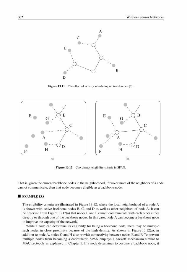
302 Wireless Sensor Networks
E
B
D
A
C
Figure 13.11 The effect of activity scheduling on interference [7].
H
G
A
B
D
C
F
E
(a)
H
G
A
B
D
C
F
E
(b)
Figure 13.12 Coordinator eligibility criteria in SPAN.
That is, given the current backbone nodes in the neighborhood, if two or more of the neighbors of a nodecannot communicate, then that node becomes eligible as a backbone node.
EXAMPLE 13.8
The eligibility criteria are illustrated in Figure 13.12, where the local neighborhood of a node Ais shown with active backbone nodes B, C, and D as well as other neighbors of node A. It canbe observed from Figure 13.12(a) that nodes E and F cannot communicate with each other eitherdirectly or through one of the backbone nodes. In this case, node A can become a backbone nodeto improve the capacity of the network.
While a node can determine its eligibility for being a backbone node, there may be multiplesuch nodes in close proximity because of the high density. As shown in Figure 13.12(a), inaddition to node A, nodes G and H also provide connectivity between nodes E and F. To preventmultiple nodes from becoming a coordinator, SPAN employs a backoff mechanism similar toMAC protocols as explained in Chapter 5. If a node determines to become a backbone node, it

Topology Management 303
broadcasts a HELLO message with its updated status. However, this message is delayed accordingto a random amount of time.
The backoff delay depends on two parameters: the utility and residual energy of the node. Theutility of the node is measured according to the number of pairs to which the node provides additionalconnectivity. If a node i has Ni neighbors,
(N2)
potential links exist. Among these links, if the node i
provides additional connectivity to Ci links, then the utility of the node is defined as Ci/(N
2). The second
parameter is the residual energy of the node. If a node has Er units of remaining energy and Em is themaximum amount of energy, then Er/Em is used as a metric in delay calculation. Accordingly, thebackoff delay of SPAN is
Di =((
1− Er
Em
)+(
1− Ci(Ni2
))+ R)NiT (13.15)
where R is a random number selected within [0, 1] and T is the round-trip delay between two nodes.Through the backoff delay, nodes with higher utility and residual energy have a smaller backoff delayand can broadcast the HELLO message earlier than other candidates.
If a node determines to become a backbone node, it sets a backoff timer to Di and continues to listento the channel. If during the backoff duration, it receives a HELLO message from a new backbone node,it reevaluates its coordinator eligibility. This is shown next.
EXAMPLE 13.9
As shown in Figure 13.12(b), node A becomes a backbone node if it broadcasts a HELLOmessage earlier than nodes G and H. Then, the other two nodes determine that all of theirneighbors are connected and do not try to become backbone nodes. With the help of the backoffdelay, SPAN prevents redundant nodes from becoming backbone nodes while preserving thecapacity of the network.
Contrary to some of the other schemes, SPAN does not preserve the backbone duty of a node for along time. Instead, each backbone node periodically checks its neighborhood and withdraws from thisduty if every other neighbor can communicate with the help of other backbone nodes. Moreover, whena node becomes a backbone node, it sets a timer to limit its backbone duty. On expiration of the timer,the backbone node checks whether its neighbors can be connected with the help of other nodes even ifthese nodes are not backbone nodes. Accordingly, the node withdraws from backbone duty.
Withdrawal from backbone duty gives other nodes the opportunity to become backbone nodesand distributes the additional energy consumption for backbone duties evenly. The withdrawal of abackbone node starts with an announcement through the HELLO message. Other nodes that hear thisannouncement contend to become backbone nodes and broadcast their HELLO message if they win thecontention. The departing backbone node waits for this HELLO message before switching its radio off.Accordingly, disconnection in the network is prevented.
Simulations with SPAN show that the capacity of the network is preserved compared to an always-onnetwork and a slight decrease in latency is observed because of the longer number of hops in each path.On the other hand, SPAN saves energy by a factor of 3.5 or more compared to a network without SPAN.Moreover, network lifetime can be doubled using SPAN.
13.3.4 PEAS
Activity scheduling is generally performed by maintaining neighborhood state information such asnumber of neighbors, number of backbone nodes, or DL between neighbors as in SPAN and ASCENT.While this information leads to informed decisions regarding backbone node selection, it may lead to
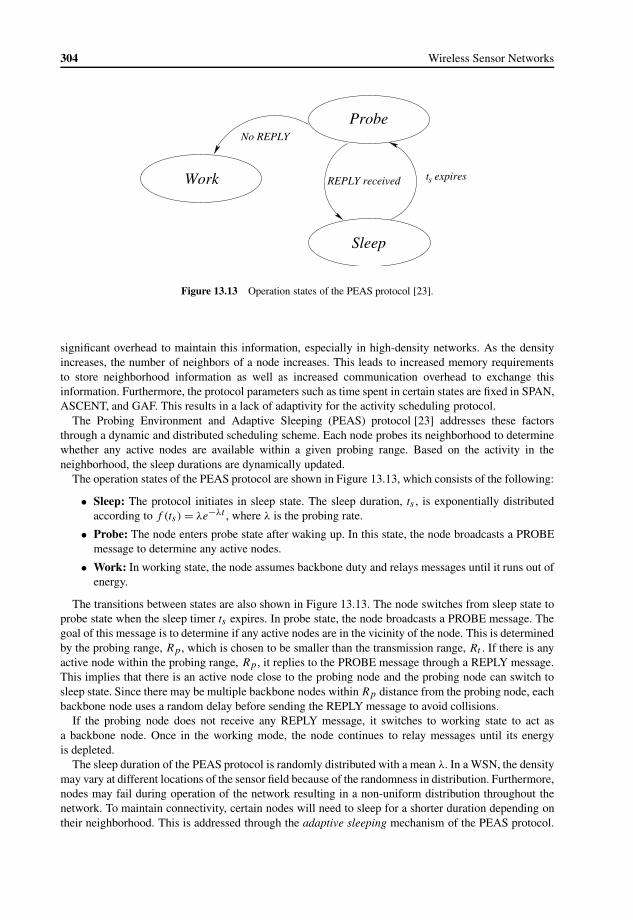
304 Wireless Sensor Networks
t expiress
Probe
Sleep
Work REPLY received
No REPLY
Figure 13.13 Operation states of the PEAS protocol [23].
significant overhead to maintain this information, especially in high-density networks. As the densityincreases, the number of neighbors of a node increases. This leads to increased memory requirementsto store neighborhood information as well as increased communication overhead to exchange thisinformation. Furthermore, the protocol parameters such as time spent in certain states are fixed in SPAN,ASCENT, and GAF. This results in a lack of adaptivity for the activity scheduling protocol.
The Probing Environment and Adaptive Sleeping (PEAS) protocol [23] addresses these factorsthrough a dynamic and distributed scheduling scheme. Each node probes its neighborhood to determinewhether any active nodes are available within a given probing range. Based on the activity in theneighborhood, the sleep durations are dynamically updated.
The operation states of the PEAS protocol are shown in Figure 13.13, which consists of the following:
• Sleep: The protocol initiates in sleep state. The sleep duration, ts , is exponentially distributedaccording to f (ts)= λe−λt , where λ is the probing rate.
• Probe: The node enters probe state after waking up. In this state, the node broadcasts a PROBEmessage to determine any active nodes.
• Work: In working state, the node assumes backbone duty and relays messages until it runs out ofenergy.
The transitions between states are also shown in Figure 13.13. The node switches from sleep state toprobe state when the sleep timer ts expires. In probe state, the node broadcasts a PROBE message. Thegoal of this message is to determine if any active nodes are in the vicinity of the node. This is determinedby the probing range, Rp , which is chosen to be smaller than the transmission range, Rt . If there is anyactive node within the probing range, Rp , it replies to the PROBE message through a REPLY message.This implies that there is an active node close to the probing node and the probing node can switch tosleep state. Since there may be multiple backbone nodes withinRp distance from the probing node, eachbackbone node uses a random delay before sending the REPLY message to avoid collisions.
If the probing node does not receive any REPLY message, it switches to working state to act asa backbone node. Once in the working mode, the node continues to relay messages until its energyis depleted.
The sleep duration of the PEAS protocol is randomly distributed with a mean λ. In a WSN, the densitymay vary at different locations of the sensor field because of the randomness in distribution. Furthermore,nodes may fail during operation of the network resulting in a non-uniform distribution throughout thenetwork. To maintain connectivity, certain nodes will need to sleep for a shorter duration depending ontheir neighborhood. This is addressed through the adaptive sleeping mechanism of the PEAS protocol.

Topology Management 305
The mean sleep duration, λ, is updated by each node based on activity in its neighborhood to reach adesired mean interval, λd .
The mean sleep interval of each node is controlled by the working node associated with that nodebased on the average probing rate in the neighborhood. Each working node keeps a record of the timeit takes to receive a specific number, k, of PROBE messages from any of its probing neighbors. If theworking node starts counting the PROBE messages at time t = t0 and receives k PROBE messages attime t = tk , the average probing rate is
λ= k
tk − t0 . (13.16)
The average probing rate, λ, is communicated to each probing node that sends a PROBE message throughthe REPLY message. Accordingly, each probing node updates its average sleep duration as follows:
λnew = λλdλ
(13.17)
which is used to select a new sleeping period.The PEAS protocol aims to address the unreliable nature of sensors through a probabilistic approach.
Each node probes its neighborhood to make local decisions and adapts its protocol parameters based onthe activity of its neighbors. Accordingly, dynamic changes of the network such as node failures andnon-homogeneous network deployment can be captured through the adaptive protocol operation.
13.3.5 STEM
Topology control schemes such as GAF [22] and ASCENT [6] coordinate the activities of each node topreserve network connectivity. These solutions improve network lifetime by switching redundant nodesin the network to sleep mode. The redundancy is determined from the connectivity of the network.However, these approaches consider only the reporting state and aim to preserve the connectivity ofthe network at all times. The resulting network operation is applicable to monitoring applications,where nodes continuously send their readings to the sink. However, with event-based applications,network traffic is sporadic and connectivity is not required at all times. In other words, the nodesare generally in monitoring state until an event of interest occurs. Hence, considering the event-basedapplication requirements, providing connectivity at all times through activity scheduling may decreasethe network lifetime.
The Sparse Topology and Energy Management (STEM) protocol addresses this issue by employinga more aggressive activity scheduling mechanism [18]. Instead of providing continuous connectivity,nodes are switched to sleep state most of the time. This decreases the energy consumption but results ina disconnected network. In case an event occurs, the nodes need to be activated to efficiently relay thepackets to the sink. For efficient node activation, STEM relies on a dual-radio architecture.
The sensors are assumed to be equipped with two radios: one for scheduling and listening to thechannel and another one for actual data communication. Each radio uses a different channel (f1 andf2) so that both radios can be used simultaneously. The first channel, f1, is used for activity schedulingpurposes and is referred to as the wakeup plane. Whenever the sender and the receiver are activated, datacommunication is performed by the second radio through the second channel, f2, which is referred toas the data plane. Hence, in the STEM protocol, nodes turn their radio off and periodically listen to thechannel to check if any node is trying to communicate. In the case of a communication attempt, the dataradio is turned on and the communication takes place.
If there is no traffic in the network, the second radio is turned off. To maintain connectivity with theneighbors of a node, the first radio is periodically turned on for a short listen duration. This is similarto the duty cycle-based MAC protocols explained in Chapter 5. Accordingly, if a node i has a packetdestined for a particular neighbor j , node i can wake up its neighbor by transmitting a wakeup signal

306 Wireless Sensor Networks
t1 t2
t3
t4
t5
Tw TRx
Tx Rx Rx Rx
Tx to j Rx from k
wakeup plane
data plane
Figure 13.14 Operation timeline for the STEM protocol [18].
during the listen duration of node j . If the intended receiver wakes up, the data plane is used for actualdata transfer.
The operation of the STEM protocol for a particular node i is shown in Figure 13.14. The timelineon the top depicts operation on the wakeup plane, whereas the timeline at the bottom shows datacommunication on the data plane. Each node listens to the wakeup plane for a duration of TRX witha period of Tw . Let us assume node i has a packet to send to one of its neighbors j . At time t1, node iinitiates communication by broadcasting a series of beacons on the wakeup plane until it receives aresponse from node j at time t2. Upon receiving a response, node i starts transmitting its data packet(s)on the data plane, which lasts until time t3. At this time, both nodes (i and j ) switch off their secondradios and continue the scheduling process on the wakeup plane. Let us also assume that, between t3 andt4, a third node k aims to reach node i and starts transmitting beacons. At time t4, node i listens to thewakeup plane, hears the beacon from node k, sends a reply, and activates its second radio. Accordingly,node k can send its data packet(s), which lasts until time t5.
Activity scheduling protocols such as SPAN, ASCENT, and GAF maintain active nodes at all timesfor connectivity. Instead, the STEM protocol activates links on a demand basis. The success of this linkactivation approach depends on the fact that when a node listens to the wakeup plane, it can detect anyother neighbor that is trying to make contact. In other words, the listen duration, TRX , should be longenough to detect incoming beacons. This is illustrated in Figure 13.15. Assuming that a beacon transmitduration is BTX and the interval between each beacons is Bi , the minimum listen interval should be
TRX ≥ 2BTX + Bi (13.18)
to ensure correct detection. Similarly, to reach a particular node, the maximum number of beacons to betransmitted, nmax
B, is
nmaxB ≥ T − TRX + 2BTX + Bi
BTX + Bi . (13.19)
According to (13.18),
nmaxB ≥ T
BTX + Bi . (13.20)
The STEM protocol decreases energy consumption by minimizing it in the monitoring state, whichimproves the lifetime of a node. However, this improvement comes at the cost of increased latency inswitching from the monitoring state to the reporting state. Since the radio is turned off for the majority of

Topology Management 307
TRX
Bi
BTX
Figure 13.15 The relation between beacon interval, Bi , beacon duration, BTX , and wakeup duration, TRX [18].
the time, route setup latency increases as a penalty for energy conservation. Since node synchronizationis not required for the STEM protocol, a node may start to broadcast beacons at any time during thescheduling period T of a node. Accordingly, the average latency in waking up a node is given by
Tw = T + BTX + Bi2
. (13.21)
To find the relative energy gain of the STEM protocol, we need to calculate the energy consumed atboth the wakeup plane, Ew, and the data plane, Ed . Accordingly, the energy consumption of the STEMprotocol in an interval of t seconds is given by
ESTEM = Ew + Ed (13.22)
where the energy consumption for the wakeup plane is
Ew = Pw · tw + Pnode(t − tw). (13.23)
Here Pw and tw are, respectively, the power and time spent for switching from sleep state to active state,whereas Pnode is given by
Pnode =Psleep(T − TRX)+ PRXTRX
T(13.24)
where Psleep and PRX are the sleep and receive power, respectively.2 The second term in (13.22) is theenergy consumption at the data plane, which is given by
Ed = Psleep(t − tdata)+ Pdata · tdata. (13.25)
Compared to STEM, a protocol without topology management requires a single radio and the energyconsumption is given by
Eorig = Pidle(t − tdata)+ Pdata · tdata. (13.26)
Accordingly, the energy consumption gain of the STEM protocol can be found by
�E =Eorig − ESTEM (13.27)
from (13.22) and (13.26). In a long enough interval t , assuming the traffic rate is low, we can disregardthe time taken for data communication, tdata. Moreover, for typical transceivers, wakeup time, twakeup,and sleep power, Psleep, can also be disregarded. Finally, by letting Pidle = PRX , the energy consumption
2More accurately, PRX is a combination of idle, receive, and transmit power but can be approximated by receive power.

308 Wireless Sensor Networks
gain is approximated as
�E � PRX · t ·(
1− TRX
T
). (13.28)
Accordingly, using (13.21), the tradeoff between the relative gain in energy consumption and the wakeuplatency can be shown to be
∂E = �E
Eorig= 1− TRX
2Tw − BTX − Bi. (13.29)
As a result, as the cost for link activation, Tw , increases, the gain in energy consumption increases forthe STEM protocol. Accordingly, by increasing the listen interval, T , significant energy savings arepossible. This, however, increases the end-to-end delay of a packet, since the protocol spends Tw on theaverage at each hop. Accordingly, the advantages of the STEM protocol in terms of energy efficiency aremore pronounced in applications where the monitoring state greatly dominates the reporting state. Morespecifically, energy savings are possible compared to the case without topology management if the timespent in the monitoring state is 50% or more of the total network lifetime.
The STEM protocol can be combined with a topology management protocol such as GAF or SPANto improve energy efficiency in the reporting state as well. As explained in Section 13.3.1, the GAFalgorithm follows a virtual grid structure, where each grid is represented by one node inside thisgrid. This node is denoted as the virtual node. By limiting the size of the grid, each virtual nodecan successfully communicate with the other virtual nodes in the neighboring grids. Accordingly,connectivity is maintained while decreasing the energy consumption by letting redundant nodes sleep.
STEM and GAF can be combined to exploit the advantages of each protocol. Firstly, the GAFalgorithm is run to determine the virtual nodes in the network. Then, each virtual node follows the STEMprotocol to further decrease the energy consumption during idle times. By modifying the routing protocolsuch that virtual nodes are used to create routes, STEM and GAF can successfully be operated on thesame nodes. Accordingly, STEM combined with GAF can reduce the network energy consumption byup to 66% compared to the GAF algorithm alone. Similarly, energy savings of up to 7% are possiblecompared to the STEM protocol alone.
The STEM protocol provides significant savings in energy consumption for the monitoring state.However, its applicability is limited to low-rate event-based applications, where the network is mostlydormant, i.e., in the monitoring state. Furthermore, end-to-end delivery latency is traded off for increasedlifetime since nodes need to spend considerable amounts of time at each hop to establish links with theirnext hop neighbor toward the sink. This increased latency also impacts certain event-based applications,where event information delivery should be performed with minimum delay. As an example, in a forestfire monitoring network, the WSN is in sleep state for a very long time (months or even years) if a firedoes not occur. However, in case of a fire, this information should be delivered to the sink immediatelyto take the required precautions. Furthermore, the energy savings of the STEM protocol are limitedin monitoring applications, where the nodes in the network continuously send sampled information tothe sink.
13.4 ClusteringIn WSNs, high-density deployment is one of the major differences between traditional networks. Inthe wireless domain, a high density has advantages in terms of connectivity and coverage as well asdisadvantages in terms of increased collision and overhead for protocols that require neighborhoodinformation. As a result, scalability is an important problem in WSN protocols as the node numbersincrease. The topology control mechanisms discussed so far focus on a flat topology, where each nodein the network sends its information to the sink through a multi-hop route. Although these protocols aimto decrease the contention through either power control or node scheduling, scalability is still an issue.
The disadvantages of the flat-architecture protocols can be addressed by forming a hierarchicalarchitecture, where the nodes are grouped in clusters. In this section, we discuss a fourth class

Topology Management 309
Sink
Cluster member
Cluster head
Figure 13.16 Cluster-based topology in WSNs.
of topology control mechanisms: cluster-based topology control. Clustering algorithms limit thecommunication in a local domain and transmit only necessary information to the rest of the network. Thisstructure is depicted in Figure 13.16. A group of nodes form a cluster and the local interactions betweencluster members are controlled through a cluster head (CH). Cluster members generally communicatewith the cluster head and the collected data are aggregated and fused by the cluster head to conserveenergy. The cluster heads can also form another layer of clusters among themselves before reachingthe sink.
Overall, clustering protocols have the following advantages in WSNs:
• Scalability: Cluster-based protocols limit the number of transmissions between nodes, therebyenabling a higher number of nodes to be deployed in the network.
• Collision reduction: Since most of the functionalities of nodes are carried out by the CHs, fewernodes contend for channel access, improving the efficiency of channel access protocols.
• Energy efficiency: In a cluster, the CH is active most of the time, while other nodes wake up onlyin a specified interval to perform data transmission to the CH. Further, by dynamically changingthe CH functionalities among nodes, the energy consumption of the network can be significantlyreduced.
• Local information: Intracluster information exchange between the CH and the nodes helpssummarize the local network state and sensed information of the phenomenon state at theCH [24, 25].
• Routing backbone: Cluster-based approaches also enable efficient building of the routingbackbone in the network, providing reliable paths from sensor nodes to the sink. Since theinformation to the sink is initiated only from CHs, route-thru traffic in the network is decreased.
Clustering is an integral part of hierarchical routing protocols as explained in Chapter 7. Hence,several clustering mechanisms have been developed as part of these routing protocols such as LEACH,PEGASIS, TEEN, and APTEEN. In addition to these mechanisms, in the following we explain clusteringschemes that can be used with any communication mechanism.
13.4.1 Hierarchical Clustering
The energy-efficient hierarchical clustering algorithm is developed to minimize the overall energyconsumption of the network by constructing clusters in a distributed manner [3, 4]. The notion of the

310 Wireless Sensor Networks
Figure 13.17 Hierarchical clustering.
clustering mechanism is illustrated in Figure 13.17. Each sensor in the network can be selected as a CHaccording to a probability, p. According to this probability, a node transmits a message indicating its CHduty. In this case, the CH is denoted as the voluntary cluster head (black nodes in Figure 13.17). Thetransmitted message is propagated up to k hops in the network. Each node that receives this messagebecomes a part of the cluster if it is not a CH. This mechanism is shown in Figure 13.17 for k = 2.
As shown in Figure 13.17, there may be several nodes that do not receive a CH message within agiven amount of time (gray nodes). These nodes then designate themselves as a CH and advertise theirduty. In this case, the CH is called the forced cluster head. The resulting topology groups each node inthe network into one of the clusters.
The performance of the energy-efficient hierarchical clustering algorithm depends on the selection ofthe two parameters p and k. The overall energy consumption can be minimized through an appropriateselection of these parameters.
The optimum value of p that minimizes the overall energy consumption can be found by assumingthat the network is distributed on a Poisson basis, where the number of nodes N in an area A has meanλA. Given the number of nodes as n, the average number of CHs is np. Firstly, the energy consumptionbetween these CHs and the sink is found.
Since the CHs are evenly distributed in the network, the average distance between a CH and the sinkis found as
E[Dch|N = n] =∫A
√x2i + y2
i
(1
4a2
)dA (13.30)
= 0.765a (13.31)
where the sensors are dispersed in a square of size 2a. Accordingly, the total distance between each CHand the sink is 0.765npa and the energy consumption for communication between CHs and the sink is
E[Ech|N = n] = 0.765npa
r(13.32)
where energy consumption for a single hop is assumed in Joules. To find the energy consumptionbetween the cluster members and the CH, we first consider two Poisson processes PP1 and PP0 withintensity λ1 = pλ and λ0 = (1− p)λ, respectively. PP1 and PP0 are the distributions of the locations ofCHs and cluster members, respectively. Accordingly, the average energy consumption in each cluster is
E[Ecluster|N = n] = λ0
2λ3/21 r
. (13.33)

Topology Management 311
Since there are np clusters on average, the overall energy consumption in the network is given as
E[E|N = n] = np(1− p)r2p3/2
√λ+ 0.765npa
r. (13.34)
Finally, removing the condition on N , the average energy consumption is
E[E] = λA(
np(1− p)r2p3/2
√λ+ 0.765npa
r
). (13.35)
Minimizing this function leads to the optimum p value. Similarly, the optimum value of k is found asfollows:
k = 1r
√−0.917 ln(α/7)
p1λ. (13.36)
Moreover, the clustering algorithm is also extended to form multiple layers of hierarchical clusters.However, the protocol parameters are calculated from only the density of the network. Since ahomogeneous distribution is assumed, the energy efficiency of the clustering protocol may not be optimalin the case of a non-uniform distribution of nodes.
13.4.2 HEED
The hybrid energy-efficient distributed (HEED) clustering algorithm combines transmit power controlwith clustering to form single-hop clusters [24]. The main goal is to minimize the energy consumptionfor communication by constructing clusters in a distributed fashion. This is performed according to theresidual energy of the nodes, where nodes with high residual energy are selected as CHs. Furthermore,the overall communication cost inside a cluster, i.e., intracluster communication cost, is also consideredin cluster formation.
The HEED clustering mechanism is performed with a period of TCP + TNO seconds, where TCP is thetime it takes for the clustering protocol to converge and TNO is the time for normal network activities,i.e., network operation interval. In each period, certain nodes are selected as CHs and the remainingnodes join to each cluster.
The clustering mechanism is initiated by CH selection. This phase is performed by each nodeaccording to a probability based on the remaining energy. More specifically, an initial probability, Cprob,is determined. Based on this probability, each node determines the probability that it will become a CH:
CHprob =max(CProb
Eresidual
Emax, pmin
)(13.37)
where Eresidual and Emax are the residual and the maximum energy of a node, respectively. The CHprobability, CHprob, depends on the relative lifetime of a node and is lower bounded by a threshold,pmin, to ensure convergence within a limited number of iterations.
EXAMPLE 13.10
The CH selection is performed over several iterations in each phase as shown in Figure 13.18. Ineach iteration, a node determines to be a CH with probability CHprob. In the first iteration, theCH probability is determined according to (13.37) for each node. Accordingly, nodes determineto be CHs and are denoted as tentative CHs. Since CHprob is a function of the remaining energy,the nodes with higher residual energy have a greater chance of becoming tentative CHs. Thetentative CHs advertise their duties through a CH message, which includes the node ID, selectionstatus (tentative CH or final CH), and cost. According to the advertised costs, the remaining nodesselect the tentative CH with the lowest cost as their CH. As shown in Figure 13.18(a), in the first

312 Wireless Sensor Networks
A
B
C
D
(a)
F
E
A
B
C
D
(b)
G
F
E
HA
B
C
D
(c)
Figure 13.18 CH selection in HEED.
iteration nodes A, B, C, and D are selected as tentative CHs and the nodes in their cluster areshown as connected to these nodes.
In the following iterations, CHprob is doubled for each node and the same procedure is repeated.This allows the remaining nodes to be tentative CHs. Similarly, if a tentative CH receives anadvertisement from another tentative CH with a lower cost, it can select that node as its CH andleave CH duty. This is shown in Figure 13.18(b), where nodes E and F are also tentative CHs.While node C is selected as a tentative CH in the first iteration, it is connected to node F in thesecond iteration since node F has a lower cost. After an iteration, if a node has a CHprob of 1or larger, it becomes a final CH and assumes CH duty for the rest of the clustering period. Aftera limited number of iterations, HEED results in a topology where each node is either a CH orconnected to a CH as shown in Figure 13.18(c).
Cluster membership is established according to the cost of each CH as discussed above. HEED utilizesthree different cost functions for clustering based on different application requirements. In an applicationwhere load distribution is important, the cost function is selected as the node degree. Accordingly, a nodeselects the CH with the fewest neighbors. On the other hand, if dense clusters are required, 1/node degreeis used as the cost function. Finally, a third cost function, average minimum reachability power (AMRP),of a node i is defined as follows:
AMRPi =∑Mj=1 min(Pwr)j
M(13.38)
where M is the number of nodes within the cluster range of node i and min(Pwr)j is the minimumpower required by a node j to reach node i. The AMRP is used as a measure of the expected intracluster

Topology Management 313
G
F
E
HA
B
C
D
Sink
Figure 13.19 Multi-hop routing from CHs to the sink in HEED.
communication energy consumption. As a result, minimizing this cost function to form clusters resultsin lower energy consumption throughout the network.
If a node receives advertisement messages from multiple CHs, then the cost function is used to selectthe best CH. Accordingly, the clusters are formed. The iteration procedure ensures that within a limitednumber of iterations, the clustering algorithm converges.
After the clusters are formed, intracluster communication is maintained by the CHs and each membercan forward its data to its CH. Intercluster communication, on the other hand, is performed between CHsusing a higher transmit power level. Since clusters are formed with nodes within one hop away from theCH, with an appropriate transmit power level the set of CHs forms a connected network. Consequently,CHs can forward their data to the sink using a multi-hop route through other CHs. As an example, asshown in Figure 13.19, the CH labeled D can reach the sink through a path G–A–B using other CHs.
The HEED algorithm is shown to terminate in a limited number of steps and outperforms genericweight-based clustering protocols.
13.4.3 Coverage-Preserving Clustering
The majority of the clustering protocols for WSNs are designed based on energy efficiency. Clusterformation and CH selection are performed using certain energy cost functions. Accordingly, the goalis to improve network lifetime by distributing the CH duties to nodes with higher residual energy.From network operation considerations, this approach leads to very efficient solutions. However, thesesolutions generally do not consider the application scenarios for clustering.
In addition to communication, sensor nodes are also responsible for gathering data from theenvironment through on-board sensors. Similar to communication, each sensor has a limited range inwhich it can sense events. As a result, each sensor covers a certain area that it can sense as shownin Fig 13.20. Since sensor nodes are generally not homogeneously distributed, all sensor nodes do notequally contribute to network coverage. As an example, node A in Figure 13.20 is more significant fornetwork coverage compared to its neighbors B, C, and D since its sensing area includes certain areasnot covered by any of the other nodes. On the other hand, node B provides redundant coverage sinceits sensing area is covered by nodes A, C, and D. In this setting, selecting node A as a CH would bedetrimental to network coverage since its energy drains much faster because of both CH and sensingduties. Instead, by selecting node B as the CH, topology management duties can be better distributed.This can be performed by coverage-aware clustering mechanisms.

314 Wireless Sensor Networks
A B
C
D
Figure 13.20 Coverage and CH selection in CPCP.
The Coverage-Preserving Clustering protocol (CPCP) uses several coverage-aware clustering metricsto construct a topology that will extend network lifetime without hampering network coverage [21].The clustering is performed using three different metrics that can be selected according to applicationrequirements. These metrics are: minimum weight coverage cost, weighted sum coverage cost, andcoverage redundancy cost.
These clustering metrics are constructed from the following definitions. The sensing area of a node i isdenoted as C(si ). Since a node usually has overlapping sensing areas with other nodes, certain portionsof the sensing area of a node can also be sensed by other nodes. Then, the total coverage of a point canbe defined as
Ototal(x, y)=∑
sj :(x,y)∈C(sj)1 (13.39)
which considers the number of nodes that cover the point (x, y). Similarly, using the remaining energyof each node j , E(j), the total energy Etotal(x, y) that is available for sensing a specific location (x, y)is given by
Etotal(x, y)=∑
sj :(x,y)∈C(sj)E(sj ). (13.40)
Etotal(x, y) depends on two factors: the number of nodes that cover the specific location (x, y) and theremaining energy of these nodes. According to this definition, the minimum weight coverage cost is
Cmw(si )=max1
Etotal(x, y)(x, y) ∈ C(si). (13.41)
As a result, the cost of each node is defined as a function of the available energy to sense the mostcritically covered point in the sensing area of this node. Similarly, the weighted sum coverage cost is
Cws(si)=∫C(Si)
dx dy
Etotal(x, y)(13.42)
which considers the weighted average of the available energy to cover all points in the sensing area of anode. Moreover, the coverage redundancy cost considers only the number of nodes covering a particularpoint and is defined as
Ccc(si )=∫C(si)
dx dy
Ototal(x, y). (13.43)

Topology Management 315
AAC
AB
AA,B AB,C
AA,CAA,B,C
A
A
C
B
Figure 13.21 Sensing areas of nodes A, B, and C.
EXAMPLE 13.11
The coverage-aware costs can be found according to the sensing areas and the remaining energylevels of each node in a local neighborhood. As an example, in Figure 13.21, three nodes A, B,and C are shown with respective sensing areas. Assuming the remaining energy of these nodesas {E(A), E(B), E(C)} = {2, 4, 1} and using the above definitions, the coverage-aware costs fornode A are as follows:
Cmw(A)= 1
2(13.44)
Cws(A)= |AA|2+ |AA,B |
6+ |AA,C |
3+ |AA,B,C |
7(13.45)
Ccc(A)= |AA| + |AA,B | + |AA,C |2+ |AA,B,C |
3(13.46)
where |A| is the size of area A.
CH selection is performed based on the coverage-aware costs of each node. Each node that is amember of a cluster sends its information only to its CH. However, CH to sink communication isperformed on a multi-hop path from the CH to the sink that involves other sensor nodes. Similar tothe coverage-aware cost of a node, the coverage-aware cost of a path from node i to the sink can also bedefined as follows:
Cfinal(si )=∑
sj ,sk∈p(si,ssink)
Clink(sj , sk) (13.47)
where Clink(si , sk) is the cost for each link and is given by
Clink(si , sk)= C(si)Etx(si, sk)+ C(sk)Erx(si , sk) (13.48)
where C(si) is the cost of a node based on one of the cost functions, and Etx(si, sk) and Erx(si, sk) arethe energy consumption for transmitting and receiving a packet, respectively. Using (13.47) and (13.48),the minimum cost path from a CH to the sink can be found.
Based on the cost functions, CPCP operation is performed in six phases as shown in Figure 13.22. InFigure 13.22(a), an example network topology shows the coverage areas of each node. In the first phase,nodes exchange residual energy information with their neighbors. At the end of this phase, each nodecalculates its coverage-aware cost. The second phase is the CH election phase. Each node determines an

316 Wireless Sensor Networks
Sink
(a)
Sink
(b)
Sink
(c)
Sink
(d)
Sink
(e)
Figure 13.22 CPCP operation.
activation time based on its cost to become a CH. During this time, if a node receives a CH announcementmessage from any of its neighbors within Rcluster distance, it resets its timer and continues listening toany further announcements. If no message is heard during the activation time, the node becomes a CHand broadcasts an announcement informing its neighbors about its CH status. At the end of this phase,nodes with minimum cost in their neighborhood are elected as CHs as shown in Figure 13.22(b). Notethat, in most cases, the coverage area of the CH is mostly covered by the neighboring nodes.
In the third phase, end-to-end paths between the CHs and the sink are established as shown inFigure 13.22(c). This is initiated by the sink node through route discovery messages, which areforwarded by each node based on its coverage-aware cost. The coverage-aware cost is used to delay the

Topology Management 317
broadcast of each relay node. As a result, any node in the network receives the route discovery messagefrom the sink by the minimum cost path first. Cluster formation is performed in the fourth phase basedon the elected CH. Each non-CH node selects the closest CH and joins the cluster using a join message.Accordingly, each node joins the cluster with the CH closest to its location as shown in Figure 13.22(d).
Once the clusters are formed, the sensor activation phase is initiated. In this phase, nodes are activatedto collect physical information according to their costs. An activation timer is associated with each nodeproportional to its coverage-aware cost. If the timer expires, each node broadcasts an ACTIVATIONmessage to indicate its neighbors. If a node receives ACTIVATION messages from some of its neighborsso that its sensing area is covered, the activation timer is reset and the node switches to sleep state.This phase results in a minimum number of active sensors while preserving the coverage as shown inFigure 13.22(e). Finally, in the sixth phase, each active node collects information from its sensor andforwards this to the CH, which can aggregate the data from multiple sensors and send that data tothe sink.
The three cost functions provide different advantages for coverage-aware clustering. The minimumweight cost, Cmw, and the weighted sum cost, Cws, improve the energy efficiency by providing longercoverage time compared to clustering metrics that consider only energy consumption. Compared to thesetwo metrics, the coverage redundancy cost, Ccc, results in a shorter coverage time if 100% is required.However, the advantage of this metric is observed for long-term deployments. If 100% coverage is notessential, Ccc maintains coverage at high levels, e.g., > 80% for a longer amount of time comparedto the other two metrics. Since redundant nodes are not selected for either clustering or multi-hopcommunication, over the long term these nodes can be used as the previously selected nodes die.
CPCP maintains high coverage through coverage-aware CH selection and route establishment.Compared to clustering schemes such as HEED, which are based on energy consumption, the balancebetween coverage and lifetime can be better maintained through coverage-aware schemes. However,CPCP requires precise knowledge of the coverage areas of sensors, which may, in practice, changeaccording to sensor type, node hardware, and even time. Moreover, each node should collect informationfrom its neighbors for CH election. This increases the overhead of the protocol compared to schemeswhere only local knowledge of the node is used for CH selection.
References[1] A. A. Abbasi and M. Younis. A survey on clustering algorithms for wireless sensor networks. Computer
Communications, 30(14–15):2826–2841, October 2007.
[2] I. F. Akyildiz, W. Su, Y. Sankarasubramaniam, and E. Cayirci. Wireless sensor networks: a survey. ComputerNetworks, 38(4):393–422, March 2002.
[3] S. Bandyopadhyay and E. Coyle. An energy-efficient hierarchical clustering algorithm for wireless sensornetworks. In Proceedings of IEEE INFOCOM’03, volume 3, pp. 1713–1723, San Francisco, CA, USA, April2003.
[4] S. Bandyopadhyay and E. J. Coyle. Minimizing communication costs in hierarchically clustered networks ofwireless sensors. Computer Networks, 44(1):1–16, January 2004.
[5] M. Burkhart, P. von Rickenbach, R. Wattenhofer, and A. Zollinger. Does topology control reduce interference?In Proceedings of ACM MobiHoc’04, pp. 9–19, Tokyo, Japan, May 2004.
[6] A. Cerpa and D. Estrin. ASCENT: adaptive self-configuring sensor networks topologies. IEEE Transactions onMobile Computing, 3(3):272–285, July 2004.
[7] B. Chen, K. Jamieson, H. Balakrishnan, and R. Morris. SPAN: an energy-efficient coordination algorithm fortopology maintenance in ad hoc wireless networks. In Proceedings of ACM MobiCom’01, pp. 85–96, Rome,Italy, July 2001.
[8] C. Hsin and M. Liu. Network coverage using low duty-cycled sensors: random and coordinated sleep algorithms.In Proceedings of ACM IPSN’04, volume 1, pp. 433–442, Berkeley, CA, USA, April 2004.
[9] S. Jardosh and P. Ranjan. A survey: topology control for wireless sensor networks. In Proceedings of ICSCN’08,pp. 422–427, Chennai, India, January 2008.

318 Wireless Sensor Networks
[10] A. Karnik and A. Kumar. Distributed optimal self-organisation in a class of wireless sensor networks. InProceedings of IEEE INFOCOM 2004, volume 1, pp. 536–547, Hong Kong, China, March 2004.
[11] M. Kubisch, H. Karl, A. Wolisz, L. C. Zhong, and J. Rabaey. Distributed algorithms for transmission powercontrol in wireless sensor networks. In Proceedings of IEEE WCNC’03, volume 1, pp. 558–563, New Orleans,USA, March 2003.
[12] P. Kumarawadu, D. J. Dechene, M. Luccini, and A. Sauer. Algorithms for node clustering in wireless sensornetworks: a survey. In Proceedings of ICIAFS 2008, pp. 295–300, Colombo, Sri Lanka, December 2008.
[13] Mo Li and Baijian Yang. A survey on topology issues in wireless sensor network. In Proceedings of ICWN’06,pp. 503–509, Las Vegas, NV, USA, June 2006.
[14] N. Li, J. C. Hou, and L. Sha. Design and analysis of an MST-based topology control algorithm. IEEETransactions on Wireless Communications, 4(3):1195–1206, May 2005.
[15] X. Li, Y. Mao, and Y. Liang. A survey on topology control in wireless sensor networks. In Proceedings ofICARCV’08, pp. 251–255, Hanoi, Vietnam, December 2008.
[16] Y. Liu, Q. Zhang, and L. Ni. Opportunity-based topology control in wireless sensor networks. In Proceedings ofthe International Conference on Distributed Computing Systems, pp. 421–428, Santa Fe, NM, USA, June 2008.
[17] P. Santi. Topology control in wireless ad hoc and sensor networks. ACM Computing Surveys, 37(2):164–194,June 2005.
[18] C. Schurgers, V. Tsiatsis, and M. B. Srivastava. STEM: topology management for energy efficient sensornetworks. In Proceedings of the IEEE Aerospace Conference, volume 3, pp. 1099–1108, Big Sky, MT, USA,2002.
[19] S. Shakkottai, R. Srikant, and N. Shroff. Unreliable sensor grids: coverage, connectivity, and diameter. InProceedings of IEEE INFOCOM 2003, volume 2, pp. 1073–1083, San Francisco, USA, April 2003.
[20] S. Shakkottai, R. Srikant, and N. Shroff. Unreliable sensor grids: coverage, connectivity and diameter. Ad HocNetworks, 3(6):702–716, November 2005.
[21] S. Soro and W. Heinzelman. Cluster head election techniques for coverage preservation in wireless sensornetworks. Ad Hoc Networks, 7:955–972, 2009.
[22] Y. Xu, J. Heidemann, and D. Estrin. Geography-informed energy conservation for ad hoc routing. In Pro-ceedings of the 7th Annual ACM/IEEE International Conference on Mobile Computing and Networking(MobiCom’01), Rome, Italy, July 2001.
[23] F. Ye, G. Zhong, J. Cheng, S. Lu, and L. Zhang. PEAS: a robust energy conserving protocol for long-lived sensornetworks. In Proceedings of IEEE ICDCS’03, Los Alamitos, CA, USA, 2003.
[24] O. Younis and S. Fahmy. Distributed clustering in ad-hoc sensor networks: a hybrid, energy-efficient approach.In Proceedings of IEEE INFOCOM 2004, Hong Kong, China, March 2004.
[25] O. Younis and S. Fahmy. Distributed clustering in ad-hoc sensor networks: a hybrid, energy-efficient approach.IEEE Transactions on Mobile Computing, 3(4):366–379, 2004.
[26] Y. Zou and K. Chakrabarty. Sensor deployment and target localization based on virtual forces. In Proceedingsof IEEE INFOCOM 2003, pp. 1293–1303, San Francisco, USA, March 2003.

14Wireless Sensor and ActorNetworks
WSNs provide extensive information from the physical world through distributed sensing solutions.Generally, this information is processed at the sink node(s) for the detection of events that occur inthe physical world. In this respect, WSNs result in one-way information delivery, where informationfrom the physical world is provided to the “cyber world.” With the emergence of low-cost actuatorsand robots that can affect the environment, a two-way information exchange is possible. As a result,information that is sensed from the environment can be utilized to act on the environment. This led tothe emergence of distributed wireless sensor and actor networks (WSANs) that are capable of observingthe physical world, processing the data, making decisions based on the observations, and performingappropriate actions. A WSAN can be an integral part of systems such as battlefield surveillance andmicroclimate control in buildings, nuclear, biological, and chemical attack detection, home automationand environmental monitoring [5, 16].
An important example of the application areas of WSANs is fire detection. Distributed sensors candetect the origin and intensity of fire and relay this information to water sprinklers, i.e., actors, to controlthe fire. Accordingly, the fire can easily be extinguished before it becomes uncontrollable. Throughan autonomous architecture of wirelessly connected sensors and actors, this control mechanism can berealized without any human intervention to avoid delays and errors. Similarly, motion and light sensorsin a room can detect the presence of people in smart space applications. According to the identity andlocation of the user, the sensors can command the appropriate actors to execute actions based on thepre-specified user preferences such as controlling the electric power in a room or switching lights onor off.
WSANs consists of two classes of components: sensors and actors. The phenomena of sensing andacting are performed by sensor and actor nodes, respectively. These two classes of components have thefollowing distinct characteristics:
• Sensors: Sensors are low-cost, low-power devices with limited sensing, computation, andwireless communication capabilities. A sensor node may consist of multiple sensors and observedifferent physical phenomena through these sensors. Using on-board MCUs, local processing ofthe data is possible. The processed data are further sent to neighboring sensors, appropriate actors,or the sink through wireless transceivers.
• Actors: Actors are resource-rich nodes equipped with higher processing capabilities, highertransmission power, and potentially longer battery life. In addition, actors may be mobile, whichimproves the effective areas in which they can act. Similar to sensor nodes, an actor node maybe embedded with different actuators to perform different tasks. Using their communication andcomputation capabilities, multiple actors can coordinate to decide on appropriate actions basedon information received from multiple sensors.
Wireless Sensor Networks Ian F. Akyildiz and Mehmet Can Vuranc© 2010 John Wiley & Sons, Ltd

320 Wireless Sensor Networks
: actor
: sensor
Sink
NodeTask Manager
Sensor/actor field
Figure 14.1 The architecture of WSANs including sensors, actors, and a sink.
The typical architecture of WSANs is shown in Figure 14.1, where multiple sensor nodes are deployedin an area to observe a physical phenomenon. The gathered information is relayed to actor nodes thatare also deployed in the sensing area. In addition, a sink node can be involved in monitoring, decisionmaking, and task assignment. Based on the different capabilities of sensors and actors, the number ofsensor nodes deployed in a target area may be very high. On the other hand, it is usually not necessaryfor actor nodes to be deployed in large numbers. Since actors generally have higher capabilities, theircoverage may be significantly larger than a sensor. Moreover, actors can be mobile robots, whichcan move around the sensor–actor field based on the information gathered by the sensors. Such aheterogeneous architecture introduces several challenges for the operation of WSANs. Accordingly,WSANs have the following unique characteristics:
• Heterogeneity: WSANs consist of heterogeneous components including low-end sensor nodesand more powerful actor nodes. As a result, the communication, computation, and memorycapabilities of each component in the network vary significantly. Hence, efficient task allocationschemes that exploit this heterogeneity are required. Moreover, various types of traffic coexist inWSANs, such as sensing information from a large number of sensors to actors, coordinationof information between actors, and network maintenance messages from actors to sensors.Accordingly, heterogeneous sets of network protocols are required.
• Real-time requirement: WSANs are essentially closed-loop systems, where decisions are madeaccording to the input from the sensors. In many applications where a timely response by actorsto the input from sensors is important, real-time guarantees should be provided by the networkprotocols. As an example, in the fire monitoring application, if a fire is detected, the sensors shouldrelay this information to the appropriate sprinklers to immediately put out the fire. Moreover, thecollected and delivered sensor data must still be valid at the time of acting. In the case of the smartspace application, if sensors detect a person inside a room, the appropriate actions such as turningon the lights should be performed while the person is still in the room. Therefore, the issue ofreal-time communication is essential in WSANs.
• Coordination: Unlike WSNs where a central entity, i.e., the sink, performs the functions ofdata collection and coordination, in WSANs, new networking phenomena called sensor–actor

Wireless Sensor and Actor Networks 321
and actor–actor coordination may be required. Since multiple actors that may act on thesame phenomenon exist, sensor–actor coordination enables the transmission of event featuresfrom sensors to the most appropriate actors. After receiving event information, actors needto coordinate with each other, i.e., actor–actor coordination, to make decisions on the mostappropriate way to perform the action.
As we have seen so far, several protocols and algorithms have been proposed for WSNs. However,since the above requirements impose stricter constraints, they may not be well suited for the uniquefeatures and application requirements of WSANs. To this end, several solutions that consider theheterogeneity of WSANs have been developed. In this chapter, we provide an overview of the WSANarchitecture and the coordination problems. Moreover, key issues in the development of a protocol stackfor WSANs are discussed. More specifically, in Section 14.1, we present the architecture of WSANs.We explain the challenges and the solutions to the sensor–actor and actor–actor coordination problemsin Section 14.2 and Section 14.3, respectively. In Section 14.4, we investigate the protocol stack of nodesand corresponding challenges for both sensor–actor and actor–actor communications.
14.1 Characteristics of WSANsWSANs consist of sensor and actor nodes which collect data from the environment and performappropriate actions based on these collected data, respectively. The architecture of a WSAN is shown inFigure 14.1, where the sensor and actor nodes are distributed in the sensor/actor field and the network ismonitored through the sink. A user can interface with the sink and hence the network through the taskmanager, which can communicate with the sink.
14.1.1 Network Architecture
WSANs can be organized into two main architectures. When a sensor detects a phenomenon, either itcan send this information to the actor nodes in its surroundings, or the data from all the sensors can becollected at the sink. These two types of architectures are shown in Figure 14.2:
• Automated architecture: This type of architecture is shown in Figure 14.2(a), where sensorssend their observations to appropriate actors. The actors may coordinate among each other todecide on the appropriate action and perform task assignment. Due to the non-existence of acentral controller, e.g., sink or human interaction, this architecture is called automated. In thiscase, the observations are distributed among actors and they need to coordinate to make decisions.
• Semi-automated architecture: In this case, the sink, i.e., central controller, collects data andcoordinates the acting process. Sensors detecting a phenomenon route data back to the sink,which may issue action commands to actors.
Depending on the type of application, one of these architectures may be used. The advantage of thesemi-automated architecture is that it is similar to the architecture already used in WSN applications.Thus, most of the existing communication solutions can be adopted. However, this architecture resultsin an increased delay in actions because of the two-way communication between sensors to the sink andthe sink to the actors. Moreover, the semi-automated architecture is prone to single points of failure,where the failure of the sink affects all the tasks in the network.
On the other hand, the automated architecture has the following advantages:
1. Lower latency: Actors are generally located in the sensor/actor field or nearby. As a result,communication of the observed information from sensors to actors has a much smaller latencycompared to sending this information to the sink.
2. Longer network lifetime: Information delivery in the semi-automated architecture results inhigher load for the sensors located close to the sink. This increases the load on those sensors
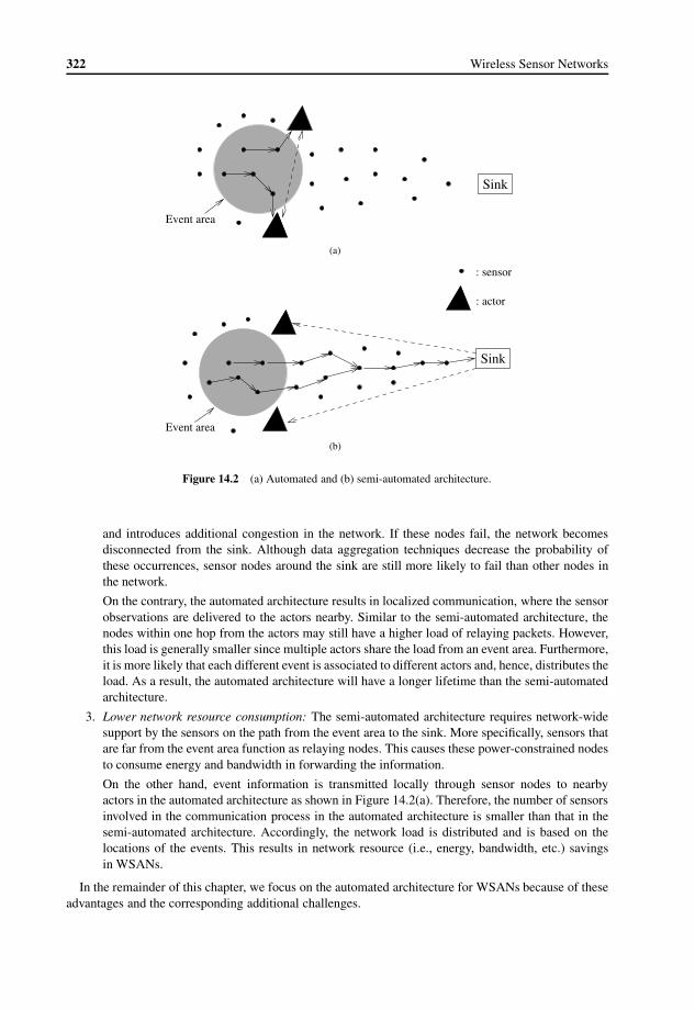
322 Wireless Sensor Networks
Sink
Event area
(a)
: actor
: sensor
Event area
Sink
(b)
Figure 14.2 (a) Automated and (b) semi-automated architecture.
and introduces additional congestion in the network. If these nodes fail, the network becomesdisconnected from the sink. Although data aggregation techniques decrease the probability ofthese occurrences, sensor nodes around the sink are still more likely to fail than other nodes inthe network.
On the contrary, the automated architecture results in localized communication, where the sensorobservations are delivered to the actors nearby. Similar to the semi-automated architecture, thenodes within one hop from the actors may still have a higher load of relaying packets. However,this load is generally smaller since multiple actors share the load from an event area. Furthermore,it is more likely that each different event is associated to different actors and, hence, distributes theload. As a result, the automated architecture will have a longer lifetime than the semi-automatedarchitecture.
3. Lower network resource consumption: The semi-automated architecture requires network-widesupport by the sensors on the path from the event area to the sink. More specifically, sensors thatare far from the event area function as relaying nodes. This causes these power-constrained nodesto consume energy and bandwidth in forwarding the information.
On the other hand, event information is transmitted locally through sensor nodes to nearbyactors in the automated architecture as shown in Figure 14.2(a). Therefore, the number of sensorsinvolved in the communication process in the automated architecture is smaller than that in thesemi-automated architecture. Accordingly, the network load is distributed and is based on thelocations of the events. This results in network resource (i.e., energy, bandwidth, etc.) savingsin WSANs.
In the remainder of this chapter, we focus on the automated architecture for WSANs because of theseadvantages and the corresponding additional challenges.

Wireless Sensor and Actor Networks 323
&
Power Unit
StorageADC
Unit
Sensing
Transmitter
ReceiverProcessor
(a)
Power Unit
Transmitter
Receiver
Unit Storage
Actuation&
ProcessorController(Decision Unit)
DAC
(b)
Figure 14.3 (a) The components of (a) sensors and (b) actors.
14.1.2 Physical Architecture
Similar to the physical architecture of the sensor node presented in Chapter 3, sensor and actor nodesalso consist of similar components. The main components of sensor and actor nodes are shown inFigure 14.3(a) and Figure 14.3(b), respectively.
As discussed in Chapter 3, sensor nodes are equipped with a power unit, communication subsystems(receiver and transmitter), storage and processing resources, an analog-to-digital converter (ADC) anda sensing unit, as shown in Figure 14.3(a). The sensing unit consists of one or more sensors, throughwhich information regarding a physical phenomenon is collected. The collected analog information isconverted to digital data by the ADC, processed by the MCU, and transmitted to nearby sensors or actors.
As shown in Figure 14.3(b), actor nodes are generally composed of similar components as the sensornodes. However, each component has usually a higher capacity. More specifically, a more powerfulMCU, a higher capacity memory, or larger battery power can be integrated. In addition, more powerfultransceivers such as WLAN cards can also be included to provide longer communication range betweenactors and the sink.
In addition to a transceiver and an MCU, an actor node also consists of a decision unit (controller) andan actuation unit. The decision unit (controller) functions as an entity that takes sensor readings collectedfrom nearby sensors as input and generates action commands as output. These action commands are thenconverted to analog signals by the digital-to-analog converter (DAC) and are transformed into actionsvia the actuation unit as shown in Figure 14.3(b). The actuation unit may include several actuators basedon the application requirements.
Since a distributed operation is employed, a single actor may not have complete information about anevent. Instead, sensor readings are generally distributed among multiple actors that reside in the eventarea. In this case, actor nodes communicate instead of initiating an action alone. The messages thatwill be exchanged between the actor nodes are constructed by the controller unit and sent through thetransceiver. The type of message depends on coordination of the actor nodes.
Sensing and actuation capabilities may not be distributed among different nodes in a WSAN. Instead,integrated sensor/actor nodes that are embedded with both sensors and actuators may replace actornodes. In this case, the integrated sensor/actor node has a sensing unit and ADC in addition to all thecomponents of an actor node shown in Figure 14.3(b).

324 Wireless Sensor Networks
(a) (b)
(c) (d)
Figure 14.4 Examples of robots: (a) aerial mapping helicopter, (b) robotic mule, (c) sub-kilogram intelligent tele-robots (SKITs), and (d) mini-robot.
A typical example of an integrated sensor/actor node is a robot which consists of an MCU, atransceiver, and on-board sensors and actuators including a mobility unit. Through a network of multiplerobots and stationary sensors in the field, the sensing and action capabilities of a single robot can besignificantly improved. More specifically, stationary sensors transmit their readings to nearby robots,which process all sensor readings including their own sensor data. In addition, multiple robots cancollaborate to improve the reliability of their knowledge of the overall event. Accordingly, the decisionunit takes appropriate decisions and the actuation unit performs actions as in an actor node.
Depending on the application, many different actors can be used in a WSAN. Several examples ofrobots designed by several robotics research laboratories and used in distributed WSANs are shown inFigure 14.4. The low-flying helicopter platform shown in Figure 14.4(a) provides ground mapping andair-to-ground cooperation of autonomous robotic vehicles [17]. This platform can be complemented withseveral additional actuation functionalities such as water sprinkling or disposal of a gas. An exampleof a robotic mule, called an autonomous battlefield robot and designed for the US Army, is shownin Figure 14.4(b). In the USA, there are several autonomous battlefield robot projects sponsored bythe Space and Naval Warfare Systems Command [9] and Defense Advanced Research Projects Agency(DARPA) [1]. These developed battlefield robots can detect and mark mines, carry weapons, function astanks, or perhaps in the future totally replace soldiers on the battlefield. Moreover, the SKITs shown inFigure 14.4(c) are networked tele-robots that have a radio turret which enables communication overUHF frequencies at 4800 kbps[3]. Coordination of these robots is performed through their wirelesscommunication capabilities and a group of SKITs can perform the tasks determined by the application.Finally, possibly the world’s smallest autonomous untethered robot (1/4 cubic inch and weighing lessthan an ounce) has been developed in Sandia National Laboratories [2] as shown in Figure 14.4(d).

Wireless Sensor and Actor Networks 325
14.2 Sensor–Actor Coordination
Due to the distributed nature of WSAN communication, effective coordination between the sensorsand actors is required. The most important requirement of sensor–actor coordination is to provide lowcommunication delay due to the proximity of sensors and actors. Accordingly, the following three mainchallenges arise for this coordination:
1. Requirements of sensor–actor communication: One of the main requirements of sensor–actorcommunication is energy efficiency as in WSNs. Moreover, in most WSAN applications, thecommunication traffic is typically delay sensitive. Therefore, efficient solutions that supportreal-time traffic for sensor–actor communication are required. An additional requirement forcommunication in WSANs is the need to ensure the ordering of event data reported to the actors.Consider a multi-hop WSAN, where multiple sensors report different events to a group of actorsin overlapping regions. To preserve action integrity, the information related to each event mustbe delivered to the actors in the order in which it was detected. This is essential to ensure thecorrectness of the actions. It is referred to as the ordered delivery of information collected by thesensors [5].
2. Actor selection: As shown in Figure 14.1, in WSANs multiple actors can be in the vicinity ofthe event area and sensors can use any of these actors to send their information. Therefore,actor selection as a destination for sensor–actor communication is an important challenge. Thiscan be addressed by letting every sensor node decide independently to which actor it will sendits readings. However, as a result of these decisions, too many and unnecessary actors can beactivated, which hampers the energy efficiency of the network. Instead, sensors detecting an eventshould coordinate to associate each sensor with the best actor.
3. Communication technique: Given the communication requirements and the selected actors, thebest communication technique in terms of reliability, delay, and energy should be chosen for theheterogeneous WSAN architecture.
In this section, we focus on the first two challenges of sensor–actor communication in WSANs anddefer the last challenge to Section 14.4.
14.2.1 Requirements of Sensor–Actor Communication
Sensor–actor communication provides the necessary tools for the sensors and actors to coordinate toact on a specific event. Hence, energy efficiency, real-time communication, and ordered delivery areimportant for communication between sensors and actors. Moreover, in a WSAN, if there are multiplesensors reporting an event, the information from different sensors should arrive at the concerned actorsapproximately at the same time.
Synchronization of event execution can be performed through actor–actor coordination as we describein Section 14.3. However, it is also conceivable that the sensors can enable this synchronization. In someapplications, where the event takes place at different locations, it might also be necessary that the eventsare passed on to the set of actors not necessarily close to or within the event area when the event wasdetected, but to the closest set of actors to the event when it is reported to them. In such cases, thesensors must be able to track the event and use this information to determine the set of actors to sendthe information.
Accordingly, the main requirements for sensor–actor communication for WSANs are as follows:
• Real-time bounds: Protocols should provide real-time services with given delay boundsaccording to the application constraints.
• Energy efficiency: WSAN protocols should ensure energy-efficient communication amongsensors and actors.

326 Wireless Sensor Networks
• Event ordering: The different events should be appropriately ordered as they are reported to theactors.
• Event synchronization: Communication protocols should also provide synchronization amongdifferent sensors reporting the same event to multiple actors or the same actor. This ensures acoherent response to events in the entire event area.
• Actor selection support: The communication protocols should provide the capabilities to trackand report the sensed phenomena to a different set of actors not necessarily based on proximityor energy limitations for the case when the events take place at different locations.
Based on these main requirements for sensor–actor communication, the second main challenge isthe distributed selection of actors for information delivery. We discuss such actor selection and thecorresponding challenges next.
14.2.2 Actor Selection
The actor selection problem is a major challenge in sensor–actor communication due to the dynamicand distributed nature of information delivery in WSANs. The actions and the actors that perform themdepend on the events that are sensed by the sensors. As a result, for each event, the appropriate actorgroup may be different. This requires event-based actor selection. Furthermore, an event may occur in alarge area such that no single sensor can be informed about all the features. Consequently, collaborativeactor selection is required to distributively find the appropriate set of actors.
In general, for the sources/destinations involved in sensor–actor communication, there are fouralternatives for actor selection:
• Minimum actor set: A minimal set of actors to cover the event region.
• Minimum sensor set: The minimum number of sensors to report the sensed event.
• Minimum actor and sensor set: Both cases above.
• Area-based set: The entire set of actors and sensors in the vicinity of the region.
The first three classifications are referred to as the redundancy elimination problem in WSANs [5].This can be tackled by minimizing the average power consumption of all the sensors and actors that arelocated in the vicinity of the event, as illustrated in the following example.
EXAMPLE 14.1
As shown in Figure 14.5, if the minimal set of actors to cover the event area is 9 and if thereare 20 actors in that region, then the remaining 11 actors need not act on the environment. In thesame example, it might also be desired that only the minimal set of sensors sense and report theenvironment. As a result, sensors and actors can be chosen such that a minimal set is selected tocover the event.
In addition to the minimum cover set selection, a stricter requirement in some applications might bethat the regions covered by different actors are not only a minimal set but also mutually exclusive. Forexample, if there is an application where the sensors report the amount of moisture in the ground and theactors have to irrigate the area uniformly, then the actors should not only cover the entire region but alsomake sure that the acting regions do not overlap.
The actors can also be selected according to transmission type. More specifically, single hop or multi-hop routes can be created between the sensors and the actor. In WSNs, single hop communicationis generally inefficient because of the long distance between the sensors and the sink. However, inWSANs, single hop communication may be preferred since actors are located close to the sensors asdiscussed in Section 14.1. In fact, the location of the actor determines the effectiveness of the singlehop communication.

Wireless Sensor and Actor Networks 327
Acting RangeEvent Area
Sensors
Inactive actors
Active set ofactors
Figure 14.5 Redundancy elimination: minimal set of actors.
Event area
(a)
: actor
: sensorEvent area
(b)
Figure 14.6 (a) Multi-actor (MA) and (b) single actor (SA) selection.
For example, if the event area is small and there is an actor in the middle of it, the nodes located fartheraway from the actor may still reach the actor without large energy consumption. However, in cases wherethe event area is large or the actors are at the edge or outside of it, multi-hop communication may bemore efficient than single hop communication. Similar to traditional WSNs, the long distance betweenthe actor and the sensor nodes increases the energy consumption if single hop communication is used.Therefore, the type of transmission depends on the deployment and location of actor nodes as well aswhat sensors are associated with which actors.
Actor selection can be classified into two cases according to the number of actors selected as shownin Figure 14.6:
• Single actor (SA) selection: In this case, only one actor receives event features from all thesensors that sense the event, as shown in Figure 14.6(b). One of the main challenges for SAselection is to determine the best SA node to which sensors will send their readings. Selecting anactor node may be based on certain criteria such that (1) the distance between the event area andthe actor is minimized so that delays and energy consumption are minimized; (2) the minimumenergy path from sensors to the actor is selected; or (3) the actor with the most appropriate actionrange is selected so that appropriate actions are performed on the event area.

328 Wireless Sensor Networks
• Multi-actor (MA) selection: As shown in Figure 14.6(a), multiple actors can also be selectedto receive the information from sensors about the sensed phenomenon. For MA selection, everysensor node can independently decide to which actor it will send its readings. However, a lack ofcoordination between the sensors can result in too many and unnecessary actors being activatedand as a result the total energy consumption of sensor–actor communication can increase. Toavoid this situation, sensors should coordinate with each other to form clusters. For each cluster,a single actor should collect the data. These clusters may be formed in such a way that (1) theevent transmission time from sensors to actors is minimized; (2) the events from sensors to actorsare transmitted through the minimum energy paths; or (3) the action regions of the actors coverthe entire event area.
SA selection can be considered as a special case of MA selection. However, for the SA case, there isno guarantee that the action range of the selected actor covers the entire event area. Therefore, instead ofconsidering distance, energy, or timing issues, sensors should try to find the “best" actor for that event,i.e., the actor which has enough action coverage, energy, and capability to perform the required actionon the event area. In this situation, the actor which receives the event information will be able to performthe required action itself without coordinating with other actors.
As a result of SA selection, the actor can immediately perform the action if it has a wide actionrange and sufficient energy. Accordingly, the overall action response latency between sensing and actingcan be minimized with SA. However, in cases where one actor is not sufficient for the required action,coordination between additional actors is required. If an actor is not well suited to perform the requiredaction alone because of coverage or energy constraints, it coordinates with other actors through anannouncement message as will be explained in Section 14.3. Based on feedback from other actors, oneor more other actors can be selected to perform the appropriate actions.
Compared to SA selection, MA selection provides more capabilities to actors in terms of determiningthe event location. The intensity of events may not be uniform inside an event area. As a result, theinformation received from sensors by each actor may be different. Actors can compare their receivedsamples with each other and determine the areas where the event intensity is high. This can result inmore effective actions by moving mobile actors toward the center of the event or selecting a subset ofactors that are closer to the event area.
The disadvantage of MA is that actor–actor coordination is mostly based on the negotiation (seeSection 14.3) among multiple actors unlike the announcement message in SA stated above. Since eachactor has partial information regarding the event, actors need to coordinate with each other and exchangeevent information to take appropriate action decisions. Actor–actor coordination, as will be discussed inSection 14.3, may result in high communication overhead and high latency.
14.2.3 Optimal Solution
The optimal solution to the sensor–actor coordination problem can be analyzed through a centralizedview of the network [15]. In this section, a sensor–actor coordination algorithm, which is based on anevent-driven clustering paradigm, is described. The cluster formation is triggered by an event and theclusters are created on-the-fly to optimally react to the event. Accordingly, only the event area is clusteredand each cluster consists of those sensor nodes that send their data to the same actor. The resultingarchitecture is shown in Figure 14.7. Since cluster maintenance can be costly, the event-driven clusteringapproach eliminates the communication overhead of maintaining clusters when no events occur.
As discussed in Section 14.2.1, sensor–actor communication may have real-time requirements, whichshould be met through efficient coordination techniques. To characterize these requirements, thefollowing definitions will be used:

Wireless Sensor and Actor Networks 329
: sensor
: actor/collector
: actor
Event area
Figure 14.7 Event-driven clustering with multiple actors.
• Latency bound B: This is the maximum allowed time between the instant when the physicalfeatures of the event are sampled by the sensors and the instant when the actor receives a datapacket describing these event features.
• Expired and reliable packets: If a data packet is received within the latency bound B, it is saidto be unexpired and hence reliable. On the other hand, if the packet does not meet the latencybound B when it is received by an actor, it is said to be expired and hence unreliable.
• Event reliability, r: This is the ratio of reliable data packets over all the packets generated in adecision interval.
• Event reliability threshold, rth: This is the minimum event reliability required by the applica-tion.
• Lack of reliability: This is the difference (rth − r) between the required event reliabilitythreshold rth and the observed event reliability r at a given time. A negative lack of reliabilityindicates a reliability above the required threshold and is also referred to as an excess of reliability.
According to these definitions, the sensor–actor coordination problem can be stated as follows. Whatare the best data paths from each sensor residing in the event area to the actors so that (1) the observedreliability r is above the event reliability threshold rth (i.e., r ≥ rth) and (2) the energy consumptionassociated with data delivery paths is a minimum? The solution to the sensor–actor coordination problemis referred to as event-driven clustering with multiple actors, which can be modeled as an integer linearprogram (ILP).
Network Model
Let us represent the network of sensors and actors as a graph G(SV , SE ), where SV = {v1, v2, . . . , vN }is a finite set of nodes (vertexes) in a finite-dimension terrain, with N = |SV |, and SE is the set of links(edges) among nodes, i.e., eij ∈ SE iff nodes vi and vj (also i and j for simplicity in the following) are
within each other’s transmission range. Let SA represent the set of actors, with NA = |SA|. An actorthat collects traffic from one or more sources is referred to as a collector. Let SS be the set of trafficsources, with NS = |SS |. This set represents the sensor nodes that detect the event, i.e., the sensors thatreside in the event area. Since the set of sources is disjoint from the set of actors, SA ⊂ SV , SS ⊂ SV ,

330 Wireless Sensor Networks
and SA ∩ SS = ∅. Accordingly, the source–destination connections are represented as P = {(s, a) : s ∈S, a ∈A}. For the solution of the sensor–actor connectivity problem, the traffic matrix can be omittedfrom the model when all sources generate information at the same data rate. Accordingly, the energyconsumption can be modeled as follows based on the models represented in Chapter 3.
The energy consumption per bit at the physical layer is
E = Etranselec + βdα + Erec
elec (14.1)
where the first term, Etranselec , is the distance-independent term that takes into account the overheads of
transmitter electronics (PLLs, VCOs, bias currents, etc.) and digital processing. The second term in(14.1), βdα , is the distance-dependent term that accounts for the radiated power necessary to transmit 1bit over a distance d between source and destination. At the receiver, the third term, Erec
elec, models thedistance-independent term that takes into account the overhead of receiver electronics.
Integer Linear Program
The objective of the optimization problem is to find data aggregation trees (da-trees) from all the sensorsthat reside in the event area (referred to as sources) to the appropriate actors. A da-tree is compiled byaggregating individual flows, where a flow is defined as a connection between a sensor and an actor.
The solution to the sensor–actor coordination problem can be divided into two: (1) actor selection,i.e., selection of the optimal subset of actors to which sensor readings will be transmitted; and (2) da-tree construction, i.e., construction of the minimum energy da-trees toward those selected actors thatmeet the required event reliability constraint. As shown in Figure 14.7, each resulting da-tree defines acluster, which is constituted by all source nodes in the tree.
The optimal strategy for event-driven clustering can be found using an integer linear program (ILP)formalization [4]. For this formalization, the network topology is assumed to be 1-connected, i.e., atleast one path exists between each sensor and actor. Accordingly, the ILP aims to minimize the totalcost, CTOT , which is defined as
CTOT =∑k∈SA
∑(i,j)∈SE
xkij · cij + γ ·Q. (14.2)
The first term in (14.2) is the total energy consumption at each path from the sources to the actors,where xkij equals 1 if the link (i, j) is a part of the da-tree associated with actor k and cij is the energyconsumption for communication between nodes i and j . The second term in (14.2) is the penalty forusing source nodes that cannot transmit their information within the latency bound B, where Q isthe number of non-compliant nodes and gamma is the penalty coefficient. Accordingly, the optimumclusters and da-tree paths are found with minimum energy consumption and number of non-compliantnodes.
The ILP problem is solved according to several constraints [15], which ensure that a sensor node isconnected to only one actor node, aggregation is performed in the da-tree, and non-compliant sourcesare selected according to the latency bound, B. However, this problem is NP -complete and can only besolved for networks of moderate size (up to 100 nodes) and requires global knowledge of the network.While important for the analysis of WSANs, for operational purposes a distributed solution of thisproblem is required. Next, we describe a distributed suboptimal but scalable algorithm: namely, theDistributed Event-driven Clustering and Routing (DECR) protocol.
14.2.4 Distributed Event-Driven Clustering and Routing (DECR) Protocol
Similar to the centralized solution, the DECR protocol aims to construct da-trees between sourcesand actors to provide the required reliability, rth, with minimum energy expenditure. The routes

Wireless Sensor and Actor Networks 331
Figure 14.8 State transition diagram for a sensor node.
are constructed according to the geographical routing solutions that are explained in Chapter 7. Thereliability is maintained through periodic advertisements from each actor related to its observedreliability. Accordingly, each individual sensor updates da-tree formation to meet the reliabilityrequirements with minimum energy consumption. The reliability is controlled by modifying the end-to-end path length from a sensor to an actor through transmit power control.
The DECR protocol consists of four different states, namely idle, start-up, speed-up, and aggregationstate as shown in Figure 14.8. Based on these states, a sensor node adjusts the number of hops and theend-to-end delay to a particular actor according to the observed reliability advertised by that actor. Thisis achieved by probabilistically modifying the behavior of the sensor nodes at the routing layer, i.e.,inducing them to select their next hop so as to increase the delay and reduce the energy consumptionwhen the reliability is high, and, vice versa, reducing the delay at the expense of energy consumptionwhen the reliability is low.
The observed reliability is determined by each actor during a decision interval: each actor computesthe event reliability r as the ratio of unexpired packets over all generated packets and periodicallybroadcasts its value similar to the ESRT and RT2 protocols described in Chapter 8. The sensor nodeswhich are associated with a particular collector actor base their state transitions on the reliabilityobserved by the collector, which is broadcast at the end of each decision interval. When the advertisedvalue r is below the so-called low event reliability threshold r−th , where r−th = rth − ε−, i.e., the lackof reliability (rth − r) is above a certain positive margin ε−, then it is necessary to speed up the datadelivery process by reducing the end-to-end delay. Conversely, when the advertised value r is above theso-called high event reliability threshold r+th , where r+th = rth + ε+, i.e., the excess of reliability (r − rth)is above a certain margin ε+, then there is excess reliability that can be traded off against energy savings.The coefficients ε+ and ε− are used to define a tolerance zone around the required reliability thresholdfor practical purposes (i.e., reduce oscillations that might lead to instability).
Each sensor node starts in the idle state, where it samples the environment for occurring events andmonitors the channel for incoming data packets. A sensor enters the start-up state when it either sensesan event or receives the first data packet from a neighboring sensor. The collective operation of the sensor

332 Wireless Sensor Networks
nodes in the start-up state allows timely establishment of paths to an actor for each source that resides inthe event area.
The protocol operation depends on the feedback sent from the actors that indicates the observedreliability. If the reliability is below the low reliability threshold (r < r−th ), the sensor node in the start-upstate enters the speed-up state with probability Pst−sp, which is a monotonically increasing functionof the lack of reliability. If the event reliability r is above the high event reliability threshold r+th (i.e.,r > r+th ), it is possible to save energy. Hence, a node in the start-up state enters the aggregation state withprobability Pst−ag, which is a monotonically increasing function of the excess of reliability.
Based on the observed reliability, a sensor can alternate between the speed-up and the aggregationstate to respond to the collector. As shown in Figure 14.8, a sensor in the speed-up state enters theaggregation state with probability Psp−ag when r > r+th , while a sensor in the aggregation state entersthe speed-up state with probability Pag−sp when r < r−th . A sensor goes back to the idle state if it doesnot generate or receive packets for idleTimeout seconds.
Based on this overall protocol operation, each state is described next:
• Start-up state: The main notion of the start-up state is to construct efficient routes from thesource nodes to the actors. A sensor node i may be in the start-up state either as a source or as arelay. The next hop is selected based on the two-hop rule, where node i selects as the next hopamong its neighbors the node j that minimizes the sum of the energy consumption from i to jand the energy consumption from j to the actor cj closest to j . The cost of energy consumptionis computed according to the link energy model in (14.1). Note that the latter link may or maynot exist.
The two-hop rule selects as the next hop the node j associated with the minimum two-hop energyconsumption. This procedure is repeated iteratively by each sensor along the path from the sourceto the actor until the path is established. Once a collector actor receives a packet from one of thesource nodes, it transmits its identifier on the reverse da-tree in order to inform the source sensorsabout its own identity.
• Speed-up state: In case of low reliability, the initial paths which have been set up at theend of the start-up state should be improved. This is achieved by applying the greedy routingscheme (GRS) [10] forwarding rule, where each node sends the packet to the node closest to thedestination within transmission range. While this rule minimizes the number of hops in the path,energy consumption may increase.
• Aggregation state: When the reliability is high, the existing paths can be updated such that theoverall energy consumption is decreased. This is performed in the aggregation state by relying ondata fusion algorithms to aggregate data packets by any node in the network. Each node routesdata to the closest node in its neighborhood that is part of the da-tree.
As previously discussed, after da-trees are established, each sensor knows which collector actor itis associated with. By overhearing transmissions on the shared medium, each sensor learns whichof its neighbors are part of a da-tree (as some neighbor sensors may not even be in the event area)and which da-tree (if any) they are part of, i.e., which collector actor they are associated with.Hence, node vi in the aggregation state first evaluates the cost of transmitting data to those of itsneighbors that are part of a da-tree. This way, it can identify a minimum cost neighbor, i.e., theneighbor vmin that requires minimum energy consumption to be reached among those associatedwith one of the da-trees.
The transitions between different states are driven by feedback from actors. Feedback is sent by eachactor periodically, with a period equal to �f seconds. At each decision instant k, the actor feedbackis determined using three different reliability measures, namely the reliability r[k], the short-termreliability rsh[k], and the predicted reliability r[k + 1]. The actor calculates the reliability r[k] observedduring the last decision interval, �d . Similarly, it calculates the short-term reliability rsh[k] as thereliability observed during the last short decision interval, �dsh, with �d >�dsh. Based on the current

Wireless Sensor and Actor Networks 333
reliability r[k] and on the history of past measurements r[k − 1], r[k − 2], . . . , the actor also calculatesthe predicted reliability r[k + 1] = f (r[k], r[k − 1], r[k − 2], . . .). The feedback packet contains theadvertised value of reliability radv[k], calculated on the basis of these three measures, and is actuallysent only if the advertised value of reliability is above the high reliability threshold r+th or below the lowreliability threshold r−th . If the sensors receive no feedback, they assume that the reliability lies withinr+th and r−th .
14.2.5 Performance
The performance of the distributed protocol compared to the optimal solution is particularly important.To this end, we describe the results of simulations that have been performed for particular networkscenarios [15].
As discussed in Section 14.2.3, the optimal solution to the sensor–actor coordination can only befound for smaller networks. Hence, firstly, a network of 70 nodes with a circular deployment area of 20 mradius is considered. For each deployed sensor, the distance from the center of the area and the angleare uniformly distributed random variables. The comparison is performed for different configurations,where the DECR protocol operates in one of the states during the simulation. To this end, start-up andspeed-up configurations are designed as well as two aggregation configurations, where the aggregationstate is achieved following the start-up state or the speed-up state.
A comparison between the energy consumption profile of the optimal solution and that of the differentstates of the distributed solution is shown in Figure 14.9 as a function of the event range. As event rangeincreases, the number of sources that send information to the actor(s) increases. More specifically, theoverall network cost, i.e., the energy needed to transmit 1 bit from each source to the actors, is shownin Figure 14.9. As expected, the optimal solution results in the lowest energy consumption. Moreover,the energy consumption of the optimal solution is almost independent of the event range. This is relatedto the tradeoff between the number of sensors and the effect of aggregation. As the number of sourcesincreases with event range, overall energy consumption increases due to the activities of the sourcenodes. On the other hand, as more nodes are involved in communication, better accuracy can be achievedin aggregation, which improves the energy savings.
Compared to the optimal solution, the DECR protocol is dependent on the event range. An aggregationconfiguration reached from a start-up configuration leads to an almost-optimal energy consumption,while by reaching the aggregation configuration from a speed-up configuration, the energy consumptioncan still be decreased consistently, but not as much as in the previous case. Since the initial structureof the da-trees depends on the start-up/speed-up configuration, these states result in higher energyconsumption. However, the distributed aggregation operation modifies the structure of the da-trees toreach an energy configuration that is between the speed-up and the aggregation from start-up curves inFigure 14.9.
In a second scenario, a network of 1000 sensors and four actors is considered, where the nodesare randomly deployed in a square area of 100 m× 100 m. Figure 14.10 shows the overall energyconsumption for the start-up, speed-up, and aggregation configurations. The speed-up configurationoutperforms the start-up configuration in terms of number of hops, and this is achieved with a limitedadditional energy expenditure. This is also reflected in the distribution of packet delays. Figure 14.11shows a comparison of packet delays from sensor to actor with 400 nodes, between the speed-up andstart-up configurations when the event range is set to 12 m, which corresponds to 20 sources on average.In the start-up configuration, delays are shown to be high in the transient phase at the beginning ofthe simulation. The average delay (thick line in the figure) converges to a value around 0.3 s. In thespeed-up configuration, delays are much smaller and their average is below 0.1 s. Figure 14.12(a) andFigure 14.12(b) show the distribution of delays in the same scenario. In the speed-up configuration(Figure 14.12(b)), the delay is below 0.5 s for almost 100% of the packets, while in the start-up

334 Wireless Sensor Networks
0 2 4 6 8 10 12 140
0.5
1
1.5
2
2.5x 10
4 Cost vs Event Range for optimum, start–up, speed–up and aggregation
Event Range [m]
Cos
t[nJ]
@ N
um. o
f sen
sors
=70
optimumstart–upspeed–upaggregation from start–upaggregation from speed–up
Figure 14.9 Comparison of the optimal solution, speed-up, start-up, and aggregation configurations with 70 nodes.
0 2 4 6 8 10 12 140
1
2
3
4
5
6x 10
4 Cost vs Event Range for start–up, speed–up and aggregation
Event Range [m]
Cos
t[nJ]
@ N
um. o
f sen
sors
=10
00
start–upspeed–upaggregation from start–upaggregation from speed–up
Figure 14.10 Comparison of energy consumption for start-up, speed-up, and aggregation configurations with 1000sensors.
configuration (Figure 14.12(a)) the variability of delays is much higher and their value can be as highas 2.5 s.
In addition to the performance in various states, the convergence of the DECR protocol is alsoimportant. To investigate this, we describe next the simulation results with 100 sensors that are randomly

Wireless Sensor and Actor Networks 335
0 20 40 60 80 100 120 140 160 180 2000
0.5
1
1.5
2
2.5
Packet Delay for Start–up vs Time
Time [s]
Del
ay [s
]
DelayAverage Delay
(a)
0 20 40 60 80 100 120 140 160 180 2000
0.2
0.4
0.6
0.8
1
1.2
1.4
1.6
1.8
2
Packet Delay for Speed–up vs Time
Time [s]
Del
ay [s
]
DelayAverage Delay
(b)
Figure 14.11 Scenario 3: Delays (a–b) for start-up and speed-up configurations, 400 sensors, event range = 12 m,sources generating 2 packets/s.
deployed in a 100 m× 100 m terrain [15]. Moreover, the probabilities that govern the transitions amongdifferent states are set as follows. The probability Pst−sp of moving from the start-up state to the speed-up state is set to 0.5 when the advertised reliability r < r−th − (0.1 · r−th ) (very low reliability). Otherwise,if the reliability is low but close to the threshold, Pst−sp = 0.1. The probabilities Pst−ag and Psp−ag ofmoving to the aggregation state from the start-up and speed-up states, respectively, are equally set to 0.05

336 Wireless Sensor Networks
0 0.5 1 1.5 2 2.50
50
100
150Distribution of data delivery delays in Start–up configuration
Delay [s]
No.
of r
ecei
ved
pack
ets
(a)
0 0.5 1 1.5 2 2.50
20
40
60
80
100
120
140
160
180
200Distribution of data delivery delays in Speed–up configuration
Delay [s]
No.
of r
ecei
ved
pack
ets
(b)
Figure 14.12 Distribution of delays (a–b) for start-up and speed-up configurations, 400 sensors, event range =12 m, sources generating 2 packets/s.
if the advertised reliability is equal to 1, and 0.02, otherwise. In any case, the probability of switching tothe aggregation state needs to be low (less than 0.1), as higher values almost invariably cause instabilities,provoking sudden drops in the observed reliability of the transients. Finally, the transition probabilityPag−sp from the aggregation to the speed-up state is set to 0.2 if the current, predicted, and short-termreliabilities are all below the threshold r−th . Similarly, Pag−sp is set to 0.1 if only the short-term and

Wireless Sensor and Actor Networks 337
predicted reliabilities are below the threshold while the current reliability is still above it, while Pag−spis set to 0.05 if only the short-term reliability is below the threshold while the others are still above it.
The convergence of the DECR protocol is shown in Figure 14.13(a), where the event reliability asobserved by the actor is shown. Immediately after the initial phase, when nodes establish data paths tothe actor in the start-up state, the reliability drops below the threshold. Hence, the actor advertises lowreliability and a higher number of sensors start moving to the speed-up state. As a result, the reliabilityis increased above the threshold and a small portion of the sensor nodes move to the aggregation state.The network operation converges to a stable state after a few oscillations, where the reliability is withinthe high and low reliability thresholds. Accordingly, the number of sensors in each of the three activestates is shown in Figure 14.13(b), where the transitions between states can be clearly seen.
14.2.6 Challenges for Sensor–Actor Coordination
The following research issues related to actor selection exist for sensor–actor coordination in WSANs:
• In-sequence delivery of different events detected in a region is required for both SA andMA selection to ensure that there are no adverse effects on the target environment. Similarly,synchronization should be ensured in the reporting time of the sensed phenomena betweendifferent actors responsible for acting on the event.
• In certain applications where multiple events occur in different locations, it may be necessary forthe sensed information to be sent to an actor or to a set of actors determined according to thelocation of the event.
• In MA, it may sometimes be necessary to address the redundancy in the set of actors to which thesensed information is sent in order to save average energy consumed by the actors in the region.In these cases, it is necessary to send the information only to a subset of actors which cover theentire event region.
14.3 Actor–Actor CoordinationThe sensor–actor coordination explained in Section 14.2 results in information related to the events bedelivered to the actors. In addition to this communication, in most situations actor–actor communicationis also required to perform the most appropriate action in WSANs. Actors are resource-rich nodes withhigh transmission power. Hence, unlike sensor–actor communication, actor–actor communication canbe long range. Moreover, a smaller number of (mobile) resource-rich actor nodes are involved in actor–actor communication. Therefore, it is similar to the communication paradigm of ad hoc networks. In thissection, we investigate the characteristics and challenges of actor–actor coordination which deals withthe actions performed by actors after receiving event information.
Actor–actor communication occurs in the following situations:
• Task distribution: In certain cases, the actor that receives the sensor data may not act on theevent area due to a small action range or insufficient energy. In this case, the appropriate taskshould be distributed to nearby actors.
• Event information exchange: If multiple actors receive the same event information, only partialinformation is available at each actor. Hence, these actors should “talk” to each other to gather theoverall event information, decide on the appropriate action, and assign the tasks to appropriateactors.
• Task coordination: In certain applications, if multiple actors are required to cover the entireevent region, it may be necessary to ensure that these regions are non-overlapping or mutuallyexclusive in order to ensure uniform acting behavior over the entire region.
• Synchronization: If multiple actors receive information from multiple sensors for the same event,it may be necessary to ensure that these multiple actors act on the environment at the same

338 Wireless Sensor Networks
0 20 40 60 80 100 120 140 160 1800.4
0.5
0.6
0.7
0.8
0.9
1Reliability vs. Time
Time [s]
Rel
iabi
lity
ReliabilityReliability ThresholdHigh and Low Reliability Threshold
(a) Reliability of the event observed at the collector/actor
0 20 40 60 80 100 120 140 160 1800
5
10
15
20
25
30State Evolution vs. Time
Time [s]
No.
of S
enso
rs
Start–up StateSpeed–up StateAggregation State
(b) Number of sensors in each state with increasing simulation time
Figure 14.13 Convergence of DECR.
time. This synchronization requirement in the execution of the task is required in applicationswhere a partial execution of the task alters the state of the event in the region where it has notbeen executed.
• Task execution: In case multiple events occur simultaneously, task execution can be done viaactor–actor communication. Also, it may be desired that the tasks are executed sequentially. Thisconstraint is referred to as ordered execution of tasks.
Wireless Sensor and Actor Networks 339
• Event information relay: After an actor node receives event information, if the event is spreadingto other actors’ acting areas, the actor node can relay the sensor data or action command to thoseactors. In this way, there will be no need for sensors in those areas to send information to thenearby actors as it will be forwarded by the initial set of actors.
All of the above situations indicate the necessity of actor–actor coordination and condense to thefollowing question: “What actor(s) should execute which action(s)?”
The answer to this question can be given by exploiting the coordination between actor nodes. Actorsshould, whenever possible, coordinate strongly with each other in order to maximize their overall taskperformance [11]. Then, the above question can be restated as follows: “How should MA task assignmentbe done?”
The task assignment problems in WSANs can be classified using the following two axes:
• Single actor task (SAT) vs. multi-actor task (MAT): SAT refers to the cases where each taskrequires exactly one actor. On the other hand, MAT refers to the cases where a task requiresmultiple actors. Accordingly, MAT assignment problems involve tasks that require the combinedeffort of multiple actors.
• Centralized decision (CD) vs. distributed decision (DD): In WSANs there is a need to take adecision on the action to be performed according to the event. The decision can be performedin a centralized way (called CD) or in a distributed way (DD). DD allows neighboring actors tocoordinate locally, which provides timely actions and network size-independent coordination. Onthe other hand, CD provides action decisions to be taken in an organized way since the decisionis taken only at one actor node which may be equipped with more powerful communicationfacilities.
In the following, we describe the task assignment problem as well as its optimal and distributedsolutions. Further challenges related to actor–actor coordination are also discussed.
14.3.1 Task AssignmentEvent information delivery and task execution are two distinct operations in WSANs that involve sensorsand actors. While information delivery is performed by sensors to the actors, task execution is performedby the actors. However, the set of actors that receives event information and the set of actors needed toperform the task associated with the event may be different. This requires actor–actor communicationto find the best set of actors and the task assignments for each actor. Accordingly, task assignment canbe accomplished in different ways depending on (1) the set of actors that receives event information,i.e., SA vs. MA, (2) the set of actors that is required to perform the task, i.e., SAT or MAT, and (3) thedecision methodology, i.e., DD or CD.
MAT
For MATs, the coordination depends on the set of actors that receives the event information and thedecision mechanism. If multiple actors receive event information from sensors and DD is performed, theactors negotiate with each other and coordinate locally to select the “best” actors for the task. The “best”actor generally refers to the one which (1) is close to the event area, (2) has high capability and residualenergy, or (3) has small action completion time.
On the other hand, in the CD case, the actors directly transmit the specifications of the event suchas location, intensity, etc., to the predetermined actor node which functions as the decision center. Thisdecision center, which already has information about the actors in the network, selects the “best” actorsfor that task and triggers them to initiate the action.
The selected actors (through both DD and CD) may not be the same set of actors that receives sensordata via sensor–actor coordination. As discussed earlier, this is based on the fact that the actors thatreceive the event information may not be the “best” actors for that task. For example, they may not beclose enough to the event area, or they may not be capable of performing the required task.

340 Wireless Sensor Networks
In case only one actor receives event information at the end of the sensor–actor coordination phase,there is still a need for coordination among actors in order to determine the actors that will act on theevent area. However, in this case, since all sensor data are collected at one actor, this actor can functionas the central decision unit. It then broadcasts an announcement message to other actors, which containsdetails about the event and the task. Based on the feedback from other actors, it selects the “best” actorsand assigns the action task to them.
Following task assignment, each selected actor performs the associated actions within its action range.Note that, depending on the characteristics of actors or the task assignment rules, if an actor is chosen, iteither acts on its action range or may act selectively on part of its action area. However, in order to reactto a certain event, the union of the action ranges of the selected actors should cover the entire event area.
Another challenge for distributed task assignment is the relation between the area in which the actionshould be performed and the action range of the actors. Depending on the actuator capabilities, certainportions of the event area may require more than one actor to perform an action. This depends on theevent intensity and the capabilities of actors in that area. On the other hand, if the action range of theactors is much larger than the task specifications, the actions may be performed outside the event area.Depending on the application, this may lead to unfavorable results as well as unnecessary consumptionof actor resources. Similarly, if the action ranges of several actors overlap with each other and all actorsact at the same time, the resulting action may surpass the requirements of the task. Thus, while assigningtasks to actors, considerations of the action coverage must also be taken into account.
Overall, regardless of the number of actors receiving sensor data, the objective of MAT is to select the“best” actors while meeting the action coverage requirements of the corresponding application and theevent. The type of actor selection (i.e., MA or SA) in the sensor–actor coordination phase only affectsthe coordination mechanism selecting the “best” actors.
SAT
Similar to MAT, the main objective of the SAT assignment problem is to select the “best” actor. Thisactor is selected so that the resulting action range covers exactly or most of the entire event area for theaction task. In fact, if the type of actor selection is MA, the coordination for SAT can be considered as aspecial case of MAT, where actors that receive the sensor data coordinate either in DD or CD and selectthe “best” actor.
On the other hand, if a SA is informed about the event features, the major challenge is selection ofthe best actor. More specifically, the SA can make a decision in an isolated fashion and thus initiatesthe action by itself. Instead, the actor may also communicate with other actors or the decision center tofind the best actor. Intuitively, if sensor–actor communication takes a long time and the application isdelay intolerant (the delay bound of received sensor data is low), then as long as the actor can providethe minimum requirements of the task (e.g., it should be able to act on the whole event area and to haveenough energy), initiating an action immediately is reasonable in order to perform the action on time.This way, perhaps the action is not performed by the “best” actor; however, it is guaranteed that the actionis completed in a timely manner. On the other hand, if the delay bound of the data is not very low or theactor does not provide the minimum requirements of the task, it should not immediately start to performthe action by itself; instead, in CD it should communicate with the decision center and allow it to choosethe appropriate actor, or in DD it should broadcast an announcement message, as explained above, toinform the other actors about the task and then should select the “best” one according to their responses.
14.3.2 Optimal SolutionThe optimal solution to the actor–actor coordination problem is based on the objective of optimallyallocating tasks to the different actors to collaboratively achieve a global goal. More specifically, theactor–actor coordination problem can be defined as a task assignment problem and formulated as amixed integer nonlinear program (MINLP) [7]. The objective of the actor–actor coordination is to select

Wireless Sensor and Actor Networks 341
the best actor(s) to perform the appropriate action in an event area. To this end, the following definitionswill be used:
• Action area: An event area is identified according to the information sent by the sensor nodes.This information defines the action area, i.e., the area where the actors should act.
• Action range: The action range defines the circular area where an actor is able to act. In particular,each collector receives data from a subset of the sources. However, the collector may not be ableto act on the entire action area, i.e., this area may not be totally within the collector’s action range.
• Action completion time: This is the time it takes for an actor to complete an action. In addition tothe action range, action completion time is also important for satisfying real-time bounds relatedto a particular event–action pair.
• Action completion bound: This is the maximum allowed latency between the time when theevent is sensed and the time the action is completed.
In addition, the collector may not be the “best” actor for the task in terms of action completion timeand/or energy consumption. For these reasons, actor–actor coordination is required before initiating theaction. The particular challenges in this problem are illustrated in Example 14.2.
EXAMPLE 14.2
A topology with several actors and their action ranges are shown in Figure 14.14. It can beobserved that multiple actors can act on a certain area, which is referred to as an overlappingarea. The overlapping areas are numbered from 1 to 8 in Figure 14.14. In an overlapping area,the actor–actor coordination problem consists of selecting a subset of the actors and their actionpowers to optimally divide the action workload, so as to maximize the residual energy of theactors while respecting the action completion bound. Moreover, certain areas are covered by onlya single actor, which are referred to as non-overlapping areas. The non-overlapping areas areshown as unshaded regions in Figure 14.14. For such an area, the coordination problem simplifiesto selecting the power level for the actor that minimizes energy consumption while respecting theaction completion bound.
Based on these definitions, we describe the action area and the actor models next and represent theformulation of the actor–actor coordination problem as a mixed integer nonlinear program (MINLP) inSection 14.2.
Action Area and Actor Model
Let SA be the set of actors, with NA = |SA|, and let SC be the set of collectors (SC ⊆ SA). An actor isidentified by a ∈ SA with coordinates CAa = (xAa , yAa ) and action range Ra , which defines the circulararea AAa where it can act. Accordingly, ACc is the cluster area that is under the responsibility of collector
c ∈ SC , and the whole event area is thus⋃|SC |c=1 ACc . AC,hc,nov and AC,mc,ov are the hth non-overlapping and
the mth overlapping areas, respectively, inside the portion of area under the responsibility of collector c.Hc represents the number of non-overlapping areas, while Mc represents the number of overlappingareas. SA,mc,ov is the set of actors that can act on the mth overlapping area AC,mc,ov that is under theresponsibility of collector c.
Each actor a is characterized by the following parameters: Ra [m] is the action range of a andPMaxa [W] is the maximum power that actor a can use to perform the action. Actors can select their
power from L different levels
Pa,p = PMaxa
L· p, p = 1, 2, . . . , L (14.3)

342 Wireless Sensor Networks
1
2
34 5
6
7 8
32 ,
,
,1
45 ,
6 ,
78 ,
a
b
c
d
ea ba ea ,b eb,ed eb db,,
dc
c
Cluster area
Action range actor/collector:: actor
Figure 14.14 Cluster area for collector c.
where Pa,p is the pth power level for actor a. Moreover, a higher power corresponds to a lower actioncompletion time. Moreover, the efficiency of actor a is denoted as ηa and EAv
a [J] is the available energyof actor a, discounted with the energy needed to act on non-overlapping areas where only actor a can act.
Mixed Integer Nonlinear Program (MINLP)
The actor–actor coordination problem can be formulated as a MINLP. The objective is to find, for eachportion of the event area, the subset of actors that maximizes the average residual energy of all actorsinvolved in the action, under the constraint of the action completion bound. For this formalization, theenergy required to perform the action is assumed to be orders of magnitude higher than the energyrequired for communication. Moreover, it is assumed that actors are able to selectively act on part oftheir action area. Accordingly, the MINLP aims to maximize the average residual energy per actor,ERes
Avg, which is defined as
EResAvg =
∑NAa=1 haE
Resa∑NA
a=1 ha. (14.4)
The MINLP is solved according to several constraints [15], which define the energy required for actora to complete the action on the overlapping areas where it is involved and ensure that each actor usesonly one power level from its power levels. Moreover, each overlapping area is ensured to be acted onby at least one actor. If multiple actors act on the same area, the time to complete the action is reduced.Accordingly, the overall action completion time for multiple actors acting on the area is limited to besmaller than the action completion bound, for each overlapping area. Solution of the MINLP providesimportant insight into the actor–actor coordination problem. However, a distributed solution is requiredfor efficient operation in a WSAN. Next, the Localized Auction Protocol (LAP) is described.

Wireless Sensor and Actor Networks 343
14.3.3 Localized Auction Protocol
The distributed solution to the actor–actor coordination problem is based on the behavior of agents in amarket economy, where the allocation of resources occurs as a result of interactions between buyers andsellers [14, 11]. The Localized Auction Protocol (LAP) is based on a real-time auction protocol, wherethe objective of the auction is to select the best set of actors to perform the action on each overlappingarea. Following the analogy with the market economy, overlapping areas are items that are traded by theactors. Accordingly, an actor assumes one of the following roles:
• Seller: A seller is the actor that is responsible for a portion of event area, i.e., the actor thatreceives event features for that area. It corresponds to a collector.
• Auctioneer: An auctioneer is the actor that is in charge of conducting the auction on a particularoverlapping area. It is selected for each overlapping area by the collector/seller responsible forthat area.
• Buyer: A buyer is one of the actors that can act on a particular overlapping area.
A localized auction takes place in each overlapping area. The bid of each actor participating in theauction consists of a power level and the corresponding action completion time, i.e., the time neededby that actor to complete the action on the whole area as well as the available energy of the actor. Theobjective is to maximize the total revenue of the team, where the team consists of the actors participatingin the auction and the revenue depends on the residual energy, i.e., ERes
Avg.Multiple localized auctions take place in parallel under the responsibility of different auctioneers.
When seller c (the collector) receives the event features from the sensors, it decides whether an actionneeds to be performed on the area it is responsible for and computes all the non-overlapping andoverlapping areas. The coordination problem arises for the overlapping areas where more than oneactor can act, while for the non-overlapping areas the seller directly assigns the action task to thecorresponding actor.
Seller c selects Mc auctioneers, one for each overlapping area, from the actors that can act on eachof these areas. Let s(m) ∈ SA be the auctioneer selected by seller c to conduct the auction for the mthoverlapping area. This auctioneer is selected to be the closest actor to the center of the overlappingarea. This way, since the auctioneer is close to each actor in the overlapping area, the energy spenton communication and the auction time are reduced. After selecting the auctioneer s(m), the seller cprovides it with the area AC,mc,ov where the auction should take place, the action completion bound δ,and the auction time bound τc, which is the maximum allowed time for the auction. The auctioneerdetermines the winners of the auction based on the bids it receives from the buyers.
At the beginning of the auction, the auctioneer sends a JOIN_AUCTION message to all the buyerscompeting for the area. After a buyer a hears this announcement, it submits its available energy, EAv
a ,
and L two-dimensional bids ba = {b1a, b
2a, . . . , b
La }, where b(p)a = [P (m)a,p ; T (m)a,p ], p = 1, 2, . . . , L.
If the bids are sorted such that T (m)a,1 ≤ T (m)a,2 ≤ · · · ≤ T (m)a,L
, the auctioneer determines the winners
by calculating the optimal solution for the residual energy maximization problem PResMax defined in
Section 14.2. However, in this case the problem is limited to the overlapping area that the auctioneeris responsible for. This way, since the bids are submitted to the auctioneer only once, signaling overheadis reduced [13].
14.3.4 Performance Evaluation
In this section, the performance of the optimal and distributed solutions to the actor–actor coordinationproblem is described.
The average residual energy for three different solution approaches are shown in Figure 14.15(b).More specifically, the optimal, 1-actor, and localized auction solutions are compared. In the optimal

344 Wireless Sensor Networks
4 6 8 10 12 14600
650
700
750
800
850
900
950
1000Average Residual Energy of Involved Actors vs. No. of Homogeneous Actors
No. of Homogeneous Actors
Ave
rage
Res
idua
l Ene
rgy
of In
volv
ed A
ctor
s [J
]
OptimalSub–Optimal (1 Actor)Localized Auction
(a)
4 6 8 10 12 14600
650
700
750
800
850
900
950
1000Average Residual Energy of Involved Actors vs. No. of Heterogeneous Actors
No. of Heterogeneous Actors
Ave
rage
Res
idua
l Ene
rgy
of In
volv
ed A
ctor
s [J
]
OptimalSub–Optimal (1 Actor)Localized Auction
(b)
Figure 14.15 Average residual energy of the involved actors in the homogeneous (a) and heterogeneous (b) case.
solution, the best set of actors is chosen so that the average residual energy of the involved actors ismaximized, while guaranteeing that the action is completed before the action completion time. In the1-actor heuristic, the action is performed by one actor only for each overlapping area. In the localizedauction, each overlapping area is taken care of by an auctioneer that divides it among the actors basedon their bids.

Wireless Sensor and Actor Networks 345
For the experiments, a heterogeneous network structure is considered such that half of the actorsare low-efficiency actors (γa = 0.6) and half are high-efficiency actors (γa = 0.9). As shown inFigure 14.15(b), LAP leads to near-optimal residual energy, as each auctioneer calculates the optimalsolution separately for its overlapping area. However, this greatly simplifies the problem and canbe achieved with local communications among actors. Moreover, in the heterogeneous scenario, theproposed localized solution effectively exploits the high-efficiency actors, thus reducing the dissipatedenergy to complete the action.
14.3.5 Challenges for Actor–Actor Coordination
Actors may coordinate either in a centralized or a distributed way to solve the task assignment problemin WSANs. Accordingly, actor–actor coordination encounters the following challenges:
• A communication model is needed between actors, which is valid for both SAT and MAT cases.Although, as mentioned in Section 14.1, actors can perform long-range communication and thusgenerally can communicate directly with their neighbor actors, if the distance between neighboractors is larger than the transmission range of actors, they cannot directly communicate with eachother. In those situations, actors use sensor nodes as intermediaries, which means that actor–actorcoordination is performed via sensor nodes.
• In DD, for both SAT and MAT cases, in-sequence execution of different events detected in aregion may be required to ensure that there are no adverse effects on the target environment. Werefer to this requirement as the ordered execution of tasks for a series of events.
• In both DD and CD, for MAT, some applications may require synchronization of actors to act onthe event at the same time. In this case, the actors have to coordinate either in a distributed orcentralized fashion to determine the time of execution of the task.
• For both CD and DD, and both SAT and MAT cases, when the events are in different locations itmay be necessary for the task to be executed by a set of actors that are not necessarily close to thelocation of an event when it was first sensed. In these cases, based on the location of the event,the actors receiving the event information forward it to a different set of actors corresponding tothe estimated new position of the event.
• In both CD and DD, for MAT, it may be necessary to address the redundancy in the set of actorsthat performs a task in order to save on the average energy consumed by the actors in the region.In these cases, it is necessary for only a subset of actors covering the entire event region to beselected to carry out the task.
• In CD, the challenge is to select the actor which will function as a decision unit. Moreover, there isa need for an effective mechanism to provide the decision unit actor with knowledge of the currentcharacteristics (location, capability, etc.) of other actors in the network so that it can trigger themost appropriate actors for the task.
• One of the most important requirements of actor–actor coordination is to minimize the taskcompletion time. Thus, coordination and communication protocols should support real-timeproperties of WSANs.
14.4 WSAN Protocol StackThe protocol stack for sensor and actor nodes consists of three planes: the communication plane,coordination plane, and management plane, as shown in Figure 14.16.
• Communication plane: This plane consists of five layers, namely the application, transport,routing, MAC, and physical layers. The information exchange among the nodes of the network isenabled through this plane.

346 Wireless Sensor Networks
Pow
er Managem
ent Plane
Mobility M
anagement P
lane
Fault M
anagement P
lane
Application Layer
Transport Layer
MAC Layer
Physical Layer
Routing Layer
Coordination Plane
Figure 14.16 WSAN protocol stack.
• Coordination plane: The data received by a node at the communication plane are submittedto the coordination plane which decides how the node acts on the received data. Moreover,the coordination plane provides nodes to be modeled as a social entity, i.e., in terms of thecoordination and negotiation techniques it possesses.
• Management plane: This plane is responsible for monitoring and controlling a sensor/actor nodeso that it operates properly. It also provides information needed by the coordination layer to makedecisions.
In the following, we discuss the requirements and characteristics of each plane for both sensor–actorand actor–actor coordination problems.
14.4.1 Management Plane
The functions performed by the management layer can be categorized into the following three areas:
• Power management plane: This plane manages how a node uses its power. For example, whenthe power level of a node is low, this plane informs the coordination plane so that the node willnot participate in sensing, relaying, or acting activities.
• Mobility management plane: This plane detects and registers the movements of nodes so thatnetwork connectivity is always maintained.
• Fault management plane: This plane refers to the detection and resolution of node problems.For example, when the sensitivity of a sensing unit or the accuracy of the actuation unit degrades,the fault management plane informs the coordination plane about this situation.
14.4.2 Coordination Plane
The coordination plane determines how a node behaves according to the data received from thecommunication plane and management plane. After sensing an event, sensors communicate theirreadings with each other. At each sensor node, the exchanged data are submitted to the coordinationplane for decisions. Accordingly, sensors are able to coordinate among themselves on a higher levelsensing task. Moreover, sensor–sensor coordination may also be required to determine nodes which willnot transmit data (due to low power or applied MAC protocol), to perform multi-hop routing and dataaggregation, and, most importantly, to select actor(s) to which sensor data will be transmitted.
The existence of the coordination plane is much more critical for actors than for sensors, sinceactors may need to collaborate with each other in order to perform appropriate actions. When an event

Wireless Sensor and Actor Networks 347
occurs, the common goal of all actors is to provide the required action on that event. Thus, socialabilities, i.e., sophisticated coordination and negotiation abilities, are necessary in WSANs to ensurecoherent behavior in the community of actors. These required social abilities of an actor are defined inthe coordination plane. Specifically, which layer in actor–actor coordination is responsible for makingdecisions about which actors act on what part of the event area and whether to have these actors actconcurrently or, if sequentially, then in what order [12].
14.4.3 Communication Plane
The communication plane receives commands from the coordination plane regarding the decisionon how the node will behave. Accordingly, the link relation between nodes is established by usingcommunication protocols. Specifically, the communication plane deals with the construction of physicalchannels, access of the node into the medium (MAC), the selection of routing paths through which thenode transmits its data, and the transport of packets from one node to another.
In addition to the conventional reliability, the new transport protocols must also support real-timerequirements in WSANs. For instance, when the transport protocol for sensor–actor communicationdetects low reliability, the transport protocol for actor–actor communication regulates the traffic betweenactors so that the actor receiving low reliable event information can inform the other nearby actorsabout this situation as soon as possible. Since sensor–actor and actor–actor communications occurconsecutively in WSANs, a unified transport protocol is needed which works well for both cases.
In WSANs, when sensors detect an event, there is no specific actor to which a message will besent. This uncertainty occurs due to the existence of multiple actors and causes problems in terms ofrouting solutions. Selecting the appropriate actor node is one of the challenges for a source sensor node.The source data should then be routed toward the selected actor in an energy-efficient way. While thesource data are transmitted through relaying sensors toward an actor node, the data may be aggregated orforwarded in order to achieve high efficiency. In addition to determining path selection and data delivery,the routing protocol should support real-time communication by considering different deadlines due todifferent validity intervals. Moreover, the routing protocol should also consider the issue of prioritizationand should provide data with low delay bounds to reach the actor on time.
For actor–actor communication, routing protocols developed for ad hoc networks such as DSR,AODV, OLSR [6] can be used as long as they are improved so that real-time requirements are metand the communication overhead occurring at sensor nodes due to actor-actor communication is low.
In order to effectively transmit the event information from a large number of sensors to actors thereis a need for the MAC protocol. Moreover, in some applications (i.e., distributed robotics) actors maybe mobile. As they move, they may leave the transmission regions of some sensors and enter othersensors’ regions or they may become disconnected from the network. Therefore, another functionof the MAC protocol in WSANs is to maintain network connectivity between sensors and mobileactors. Furthermore, as discussed earlier, timely detection, processing, and delivery of information areindispensable requirements in a sensor/actor network application.
Classical contention-based protocols are not appropriate for real-time sensor–actor communicationsince contention-based channel access requires handshaking, which increases the latency of the data.Instead, reservation-based protocols are mostly used for WSAN traffic. Such protocols are suitable forWSANs because they can potentially reduce the delay and provide real-time guarantees as well as savepower by eliminating collisions.
For actor–actor communication, the existing MAC protocols developed for ad hoc networks cannot bedirectly used. They should be improved so that they support real-time traffic, since in WSANs, dependingon the application, interaction with the world may impose a real-time constraint on computationand communication.
In addition to the layered protocol stack, cross-layer solutions are also adopted for WSANs. One of themain factors which causes low event reliability is network congestion. In the case of high congestion,

348 Wireless Sensor Networks
the MAC layer reacts locally by exponential backoff, while the transport layer reacts by lowering thetransmission rates of sensors. However, normally these two layers act independently of each other,which causes inefficiencies due to the duplication of functions. By using a cross-layering approach,each protocol shares its data with other protocols, which avoids those inefficiencies. In addition to theinteractions among the transport, MAC, routing, and physical layers, in WSANs, there should also beinterdependency between the application layer and those lower layers. The application layer must adaptto time-varying QoS parameters offered by the lower layers. While the network provides the best possibleQoS to the application, this QoS will vary with time as channel conditions and network topology change.Thus, applications must also adapt to the QoS offered. The basic ideas of cross-layer communication arealso valid for actor–actor communication.
The effectiveness of the sensor networking can experience a profound leap if the actors are also anintegral part of the deployed network. When the sensor field is complemented with actors, there will beone more option called acting as well as sensing and deciding on a human controller. On the other hand,the realization of WSANs needs to satisfy the requirements introduced by the coexistence of sensorsand actors.
Based on the characteristics and challenges of WSANs described in this chapter, several communica-tion protocols have been developed for WSANs. We refer interested readers to [5, 8].
References[1] DARPA tactical mobile robotics. Available at http://www.darpa.mil/sto/smallunitops/tmr.html.
[2] Sandia National Laboratories. Available at http://www.sandia.gov/media/NewsRel/NR2001/minirobot.htm.
[3] Sub-kilogram intelligent tele-robots (SKITs). Available athttp://robotics.usc.edu/?l=Projects:FormerProjects:SKIT:index.
[4] R. K. Ahuja, T. L. Magnanti, and J. B. Orlin. Network Flows: Theory, Algorithms, and Applications. PrenticeHall, 1993.
[5] I. F. Akyildiz and I. H. Kasimoglu. Wireless sensor and actor networks: research challenges. Ad Hoc Networks,2(4):351–367, October 2004.
[6] M. Conti, S. Giordano, G. Maselli, and G. Turi. Cross-layering in mobile ad hoc network design. IEEEComputer, 37(2):48–51, February 2004.
[7] J. Czyzyk, M. P. Mesnier, and J. Moré. The NEOS server. IEEE Journal on Computational Science andEngineering, 5(3):68–75, July–September 1998.
[8] F. Dressler. Self-Organization in Sensor and Actor Networks. John Wiley & Sons, Ltd, 2007.
[9] H. R. Everett and D. W. Gage. A third generation security robot. In SPIE Mobile Robot and Automated VehicleControl Systems, volume 2903, pp. 118–126, Boston, MA, USA, November 1996.
[10] G. G. Finn. Routing and addressing problems in large metropolitan-scale internetworks. Technical reportISU/RR-87-180, ISI, March 1987.
[11] B. P. Gerkey and M. J. Mataric. Sold! Auction methods for multirobot coordination. IEEE Transactions onRobotics and Automation, 18(5):758–768, October 2002.
[12] V. Lesser. Reflections on the nature of multi-agent coordination and its implications for an agent architecture.Autonomous Agents and Multi-Agent Systems, 1:89–111, January 1998.
[13] P. Maille and B. Tuffin. Multibid auctions for bandwidth allocation in communication networks. In Proceedingsof IEEE INFOCOM’04, volume 1, p. 65, Hong Kong, China, March 2004.
[14] R. P. McAfee and J. McMillan. Auctions and bidding. Journal of Economic Literature, 25(2):699–738, June1987.
[15] T. Melodia, D. Pompili, V. C. Gungor, and I. F. Akyildiz. A distributed coordination framework for wirelesssensor and actor networks. In Proceedings of ACM MobiHoc’05, p. 110, Urbana–Champaign, IL, USA, May2005.
[16] E. M. Petriu, N. D. Georganas, D. C. Petriu, D. Makrakis, and V. Z. Groza. Sensor-based information appli-ances. Instrumentation & Measurement Magazine, IEEE, 3(4):31–35, December 2000.
[17] S. Thrun, M. Diel, and D. Hähnel. Scan alignment and 3-D surface modeling with a helicopter platform.In Proceedings of the International Conference on Field and Service Robotic (FSR’03), pp. 287–297, LakeYamanaka, Japan, 2003.

15Wireless Multimedia SensorNetworks
Recent progress in CMOS technology has enabled the development of single chip camera modules thatcould easily be embedded into inexpensive transceivers. Moreover, microphones have for long been usedas an integral part of wireless sensor nodes. The interconnection of multimedia sources with inexpensivecommunication devices has fostered research in the networking of multimedia sensors. Consequently,wireless multimedia sensor networks (WMSNs) became the focus of research in a wide variety ofareas including digital signal processing, communication, networking, control, and statistics in recentyears [13, 29, 44]. The union of the experience gained from each of these areas independently helps todevelop WMSNs that allow the retrieval of video and audio streams and still images, as well as deliveringthis information in real time. In addition to the ability to retrieve multimedia data, WMSNs are also beable to store, process in real time, correlate, and fuse multimedia data originating from heterogeneoustraffic sources.
This chapter focuses on these important aspects and provides a broad overview of the protocols,algorithms, applications, and research challenges for WMSNs. The realization of these networks willenable a wide variety of application areas that were not possible before with scalar sensor networks. Themost important application areas can be summarized as follows:
• Multimedia surveillance: Video, image, and audio collection capabilities of sensors in WMSNsenable broader and enhanced surveillance applications. Using feeds from multiple heterogeneoussensors, extensive coverage of a particular area can be provided. Moreover, it is possible to conveymuch more detailed information to the user compared to traditional WSNs.
• Traffic avoidance, enforcement, and control: Traffic is a major problem in metropolitan areas.Easily deployable wireless multimedia devices can help to solve many problems related to trafficjams by rerouting individuals according to information from a network of camera sensors orindicating empty lots in parking areas in real time. Moreover, multimedia sensors may monitorthe flow of vehicular traffic on highways and retrieve aggregate information such as averagespeeds and the number of cars. This helps for remote detection of violations and identification ofviolators through video feeds.
• Automated assistance for the elderly and family monitors: WMSNs provide novel techniquesfor monitoring and studying the behavior of elderly people without disturbing their daily routines.As a result, the causes of illnesses that affect them, such as dementia [49], can be identified.Furthermore, remote assistance to elderly people through video or audio sensors is also possible.
• Environmental monitoring: Visual information content provided through either still images orvideo streams improves the capabilities of environmental monitoring applications. In addition toscalar data such as temperature or humidity, visual information helps also for closer monitoringof the habitat without significant interactions or interference.
Wireless Sensor Networks Ian F. Akyildiz and Mehmet Can Vuranc© 2010 John Wiley & Sons, Ltd

350 Wireless Sensor Networks
• Industrial process control: Control and monitoring of the industrial environment are crucial forthe efficiency of an industrial plant. Multimedia content may be used for time-critical industrialprocess control. A manufacturing process for products such as semiconductor chips, automobiles,food, or pharmaceuticals can be monitored and analyzed through WMSNs. Integration of machinevision systems with WMSNs can simplify and add flexibility to these systems while decreasingthe costs for maintenance and operation.
Distributed vision systems that will emerge from the research in WMSNs have potential advantagesin addition to the applications described above. In particular, traditional monitoring and surveillancesystems can be improved through three main advancements: namely, enlarging the view, enhancingthe view, and providing multiple viewpoints of the same phenomenon [21]. When a single camera isconsidered for a surveillance application, the coverage of the application is only limited by the fieldof view (FoV) of a fixed camera or the field of regard (FoR) of a pan–tilt–zoom camera. On theother hand, deploying multiple, low-cost visual sensors both improves the coverage of the applicationand provides a more robust operation. Similarly, multiple cameras provide necessary redundancy toenhance the observations that would not be possible through a single camera. This also prevents singlepoints of failure or problems related to obstruction of a camera’s line of sight. Furthermore, multiplevisual sources provide the flexibility to adaptively extract data depending on the requirements of theapplication. Accordingly, a multi-resolution description of the scene and multiple levels of abstractioncan be provided.
While developments and solutions in WSNs provide a great deal of information for designingthe multimedia counterparts of these networks, many aspects of the sensor network paradigm needto be rethought. Especially, the need for various quality of service (QoS) demands of multimediaapplications is the major challenge. Furthermore, experience from several research areas is needed toconverge to efficient and flexible solutions for WMSNs. More specifically, energy-constrained wirelesscommunication theory and image and video processing techniques need to be combined for advancedmultimedia communication.
In this chapter, the state of the art in algorithms, protocols, and hardware for the development ofWMSNs is discussed. Furthermore, several open research issues are highlighted. Section 15.1 pointsout the characteristics of WMSNs as well as their differences from traditional WSNs. In Section 15.2,various architectures that could be adopted for WMSNs are described. The existing platforms as well asthe deployed research testbeds are introduced in Section 15.3. Sections 15.4, 15.5, 15.7, 15.8, and 15.9focus on existing solutions at the physical, link, network, transport, and application layers of theprotocol stack, respectively. Section 15.10 provides cross-layer design aspects in WMSNs. Finally, inSection 15.11 additional complementary research areas are discussed.
15.1 Design Challenges
The design of WMSNs needs expertise from a wide variety of research areas including communication,signal processing, control theory, and embedded systems. The convergence of these areas will enablemore powerful networks that are able to interact with the environment and provide even more meaningfuldata than the traditional data-only WSNs. There are several design challenges to realizing WMSNs aswe explain below.
15.1.1 Multimedia Source Coding
The generation, processing, and transmission of multimedia traffic such as audio, video, and still imagesresult in major challenges. Transmission of multimedia content has for long been associated withmultimedia source coding techniques because of the large amounts of traffic generated by multimediasources such as cameras. For example, a single monochrome frame in the NTSC-based Quarter Common

Wireless Multimedia Sensor Networks 351
Intermediate Format (QCIF, 176 × 120), requires around 21 kB, and at 30 frames per second (fps) avideo stream requires over 5 Mbps bandwidth. As a result, the raw data have to be compressed throughsophisticated coding techniques that exploit the redundancy in the video or still images.
Multimedia source coding aims to reduce the information to be sent through the wired or wirelessmedia by exploiting the redundancy in the video or still image. In a still image, this could be doneby extracting the interrelations between each pixel in the picture. In video, two types of source codingtechniques are used. Firstly, at each frame, the correlation between pixels is extracted much like the stillimages. This is called intraframe compression. Furthermore, each consecutive frame in a video streamis inherently correlated because of the large portion of background image that stays consistent as wellas the movement of certain objects between frames. These correlation aspects are exploited throughinterframe compression to further reduce the amount of data to be transmitted. Interframe compressionis also known as predictive encoding or motion estimation.
The compression techniques certainly decrease the information to be transmitted to convey a videostream. This compression, however, comes at the cost of degradation of the video quality that is usuallyreferred to as distortion. Effective compression techniques developed so far result in good rate-distortionlevels to efficient multimedia transmission.
Despite their significant compression capabilities and good rate-distortion performance, traditionalsource coding techniques are not directly applicable to resource-constrained WMSNs. This is mainlyrelated to the fact that predictive encoding requires complex encoders and powerful processingalgorithms, which significantly increase the energy consumption. Hence, these techniques are notdirectly suitable for low-cost multimedia sensors. To this end, the traditional balance of complexencoders and simple decoders can be reversed through distributed versions of the traditional encodingtechniques or within the framework of so-called distributed source coding [28], which exploits the sourcestatistics at the decoder, and by shifting the complexity at this end allows the use of simple encoders.Clearly, such algorithms are very promising for WMSNs and especially for networks of video sensors,where it may not be feasible to use existing video encoders at the source node due to processing andenergy constraints. These techniques will be covered in more detail in Section 15.9.
15.1.2 High Bandwidth Demand
Although multimedia coding techniques significantly decrease the transmitted information, the com-pressed information still surpasses the current capabilities of wireless sensor nodes. More specifically,video streams require transmission bandwidth that is orders of magnitude higher than what is supportedby currently available sensors. This high bandwidth demand requires new transmission techniquesthat provide larger bandwidth at acceptable energy consumption levels. Furthermore, novel hardwarearchitectures for multimedia-capable transceivers need to be developed. To this end, the ultra-wide-bandtechnique can be exploited as discussed in Section 15.4.
15.1.3 Application-Specific QoS Requirements
The networking and communication techniques proposed so far for WSNs generally follow a best effortservice approach. In other words, no tight guarantees in terms of energy consumption, delay, jitter, orthroughput are provided. On the other hand, multimedia applications specifically require these typesof guarantees for efficient delivery of the sensed phenomenon. Moreover, the type of application (stillimage transmission or video streaming) affects the QoS requirements in the network. Furthermore, aswill be discussed in Section 15.9, each multimedia stream contains information that requires differentlevels of QoS guarantees. Consequently, the design of WMSNs requires the development of algorithmsthat support application-specific QoS requirements. These requirements may be in terms of bounds onenergy consumption, delay, reliability, distortion, or network lifetime.

352 Wireless Sensor Networks
15.1.4 Multimedia In-network Processing
In-network processing has been exploited for energy-efficient data delivery in WSNs. The same isalso true for WMSNs but the characteristics of the multimedia content require novel approaches forthis area. An important difference is that, in WSNs, in-network processing has usually been used foraggregation operations. Considering the correlated information sensed by nearby sensors, aggregatingthis information is an easy solution for data traffic. Moreover, with scalar data, it is straightforward toperform linear operations such as additions or taking averages. This is mainly because a single packetcontains meaningful data to process in scalar data-based WSNs. Aggregation is not straightforward inWMSNs since the multimedia information is carried through multiple packets in a stream. As a result,to infer meaningful information from a stream of traffic, the whole stream needs to be collected andthe image or video needs to be decoded. This requires significant storage and processing capabilities atintermediate nodes. Only after decoding can an intermediate node perform aggregation tasks on multipletraffic streams. This branch of in-network processing is therefore not practical for WMSNs. On theother hand, resource-hungry encoding operations can be distributed among a group of nodes to leveragethe energy consumption for a multimedia flow. This idea has been used in distributed JEPG encodersdeveloped for WMSNs as will be discussed in Section 15.9.
15.1.5 Energy Consumption
Energy consumption is of major concern in traditional WSNs. This fact is even more pronounced inWMSNs due to two fundamental differences. Multimedia applications generate high volumes of traffic,which require longer transmission times for the battery-constrained sensor devices. While transmission isusually mitigated through in-network processing solutions in traditional WSNs, the extensive processingrequirements of multimedia data may make these techniques unsuitable for WMSNs. Solutionsfor WMSNs need to guarantee the QoS requirements of applications while minimizing the energyconsumption.
15.1.6 Coverage
Scalar sensors are usually indifferent to the direction of data acquisitions. This results in relativelycircular sensing ranges as discussed in Chapter 13. Multimedia sensors, however, are characterizedby their directivity. Especially, video and image sensors have a limited field of view that results inconic coverage areas substantially different from those of scalar sensors. Moreover, the sensing range inthis field of view is significantly longer than scalar sensors. These fundamental differences in coveragemotivate novel approaches in topology control and design in WMSNs.
15.1.7 Resource Constraints
Similar to traditional WSNs, each component in WMSNs is constrained in terms of battery, memory,processing capability, and data rate [14]. The increased traffic volume as well as the significantly higherprocessing requirements of encoders signify the importance of energy-efficient operation in WMSNs.Consequently, the existing resources need to be efficiently consumed for multimedia delivery.
15.1.8 Variable Channel Capacity
Multimedia communication has been investigated for wired and wireless networks during the last fewyears. Providing QoS guarantees in terms of delay, jitter, and throughput has been the main focus of

Wireless Multimedia Sensor Networks 353
research in this area. While many lessons can be learned from previous research, the characteristics ofWMSNs create novel challenges.
15.1.9 Cross-layer Coupling of Functionalities
Cross-layer design has been driving the research in WSNs as discussed in Chapter 10. It is important toexploit and consider the cross-layer effects of each layer functionality on every other layer and developcommunication protocols accordingly. While the cross-layer design principles also apply to WMSNs,an additional dimension exists because of the direct influence of the application layer on the multimediatraffic. Joint source and channel coding algorithms have been developed for wireless multimediacommunication in cellular and ad hoc networks. Coupled with the close interaction of other protocollayers in WMSNs, a complete cross-layer design is necessary for energy-efficient communication.
15.2 Network Architecture
WMSNs are envisioned to be composed of heterogeneous sensor devices that have various capabilities interms of sensing, processing, and communication. Consequently, various types of traffic can be generatedby these heterogeneous sensor devices, such as still images, audio, video, or scalar data. To handle thisvariety, a heterogeneous architecture must be designed.
Architecture design issues in traditional WSNs have been focused on scalable network architectures.The scalability is usually achieved through flat, homogeneous architectures in which every sensor hasthe same physical capabilities and can only interact with neighboring sensors.
Contrary to the homogeneous nature of traditional WSNs, the inherent heterogeneity due to varioustechnologies that support different sensor types as well as the traffic generated by these sensors requirea different approach. As an example, the large amount of traffic generated by multimedia sensors maynot be handled by flat topologies consisting of low-end transceivers. Likewise, the requirements forprocessing power for data processing and the power for communication may be different for everydifferent sensor. A sensor node embedded with only a microphone may generate relatively low datathat can be handled by existing low-end sensor nodes. On the other hand, the excessive power requiredfor video processing and the bandwidth required for even encoded video frames may require differentprocessor and transceiver technologies. Consequently, to process and transfer data simultaneously maynot be possible at each device in the network.
These intrinsic differences of WMSNs led to the realization of heterogeneous network architectures.These architectures are mainly classified into: single tier and multi-tier. Single tier architectures arebased on a flat topology, where the network can be composed of either homogeneous or heterogeneouscomponents. Multi-tier architectures, on the other hand, exploit the higher processing and communica-tion capabilities of high-end nodes and yield a hierarchical network operation. An overview of thesepossible architectures for WMSNs is shown in Figure 15.1, where three sensor networks with differentcharacteristics are shown. We describe each of these architecture types next. Furthermore, we explain indetail coverage issues that are fundamentally different in WMSNs.
15.2.1 Single Tier Architectures
The first cloud on the left of Figure 15.1(a) shows a single tier network of video sensors. In thisarchitecture, a subset of the deployed sensors may have higher processing capabilities. These nodes arereferred to as processing hubs, which can be used for local processing of the sensed media information.Moreover, multiple processing hubs can be used to perform a single processing job distributively, whichconstitutes a distributed processing architecture.

354 Wireless Sensor Networks
InternetInternet
Gateway
Multimedia
processing hub
Video sensor
Audio sensor
High end
video sensor
Wireless
gateway
LEGEND
Storage hub
(a)
Single-tier flat,
homogeneous sensors,
distributed processing,
centralized storage
(b)
Single-tier clustered,
heterogeneous sensors,
centralized processing,
centralized storage
Sink
(c)
Multi-tier,
heterogeneous sensors,
distributed processing,
distributed storage
Scalar sensor
Figure 15.1 Reference architecture of a WMSN.
In the single tier architecture, the multimedia content recorded and/or processed by the sensor nodesis relayed to a wireless gateway through a multi-hop path. The wireless gateway is interconnected toa storage hub, which is in charge of storing multimedia content locally for subsequent retrieval. As aresult, recorded and processed data can be stored at a central location to relieve the storage restrictionson the sensor nodes and to perform more sophisticated processing jobs offline.
Instead of a centralized storage architecture, a distributed storage scheme, where all the nodes insidethe network store a part of the collected information, can also be implemented. Such a scheme mayresult in energy savings since, by storing it locally, the multimedia content does not need to be wirelesslyrelayed to remote locations. The wireless gateway is also connected to a central sink, which implementsthe software front-end for network querying and tasking.
The single tier architecture can also be deployed for networks consisting of heterogeneous compo-nents. Such a reference architecture is shown in Figure 15.1(b). In this case, nodes can be organizedinto clusters, where a central cluster head controls other video, audio, and scalar sensors in the cluster.Moreover, the cluster head can be used to perform more resource-hungry procedures such as intensivemultimedia processing, or aggregation. Consequently, in this architecture, the cluster heads can also beused as processing hubs. The information gathered by the cluster head is then relayed to a wirelessgateway or a storage hub for further processing and storage.
15.2.2 Multi-tier Architecture
The last cloud shown in Figure 15.1(c) represents a multi-tiered network, with heterogeneous sensors.This hierarchical structure provides the flexibility to use network resources adaptively. The multi-tier architecture employs low-end scalar sensors at the lower hierarchical levels to perform simpler

Wireless Multimedia Sensor Networks 355
Sink
(a)
Sink
(b)
Figure 15.2 Illustration of the coverage of (a) scalar sensors and (b) video sensors.
tasks. The information gathered by these sensors can, then, be used to initiate more complex sensingtasks such as real-time video monitoring to adapt to and communicate any events that occur in thesurroundings. These tasks are accomplished by high-end sensor nodes equipped with video camerasat higher hierarchical levels. Furthermore, image and video processing and storage can be initiatedonly when there is sufficient interest in the sensed phenomenon reported by the low-end devices.Such a hierarchical architecture extends the lifetime of the network while improving the adaptivity andefficiency of the deployed heterogeneous sensors. As shown in Figure 15.1(c), the multi-tier architecturemay include clusters in each tier. As a result, autonomous operation for each cluster can be performed,which decreases the energy consumption due to communication between these sensors. Moreover,necessary information to be communicated to the higher tiers may be aggregated at the cluster headsminimizing the traffic in the network.
15.2.3 Coverage
Defining an architecture for WMSNs also depends on the coverage of the network. In order to providesufficient coverage for a specific application, the architecture should be defined by considering thecoverage issues for each of the components in the network. An important challenge in this areastems from the different coverage properties of multimedia sensors such as cameras and microphonescompared to the scalar sensor types such as temperature or humidity sensors.
When traditional WSNs are considered, the sensing capability and hence the sensing range of a sensorare characterized as omnidirectional in nature. In other words, the sensor is generally indifferent to thedirection of sensing. As a result, the coverage area of a scalar sensor can generally be modeled as acircle centered around the sensor as shown in Figure 15.2(a). Then, the coverage of a sensor can easilybe modeled using its sensing range. As explained in Chapter 13, the recent work on coverage in WSNsmainly investigates the tradeoff between sensing range and communication range, which defines therange that a node can reach through wireless communication. Consequently, the coverage problem inWSNs is generally tied to connectivity in the network [17].
Coverage for multimedia sensors, on the other hand, exhibits fundamentally different characteristicsin terms of directivity, range, line of sight, and dynamic view as explained next.

356 Wireless Sensor Networks
Directivity
Contrary to the omnidirectional nature of the scalar sensors, audio and especially video sensors collectinformation based on its direction. For example, in video sensors, the coverage area concept is exchangedwith the field of view (FoV), which defines the area that a video sensor can “see.”
EXAMPLE 15.1
The difference in coverage for scalar sensors and that for visual sensors is illustrated inFigure 15.2. As shown in Figure 15.2(a), the coverage of a scalar sensor is generally circular.On the other hand, in Figure 15.2(b), the FoVs of the video sensors in a WMSN are shown. Itcan therefore be seen that the coverage of a WMSN depends on the direction of the sensors in thenetwork as well as the characteristics of the sensors that define the shape of the FoV. As shown inFigure 15.2(b), different types of cameras result in different FoV shapes and sizes.
This fundamental difference in coverage incurs additional information requirements for the coverageoptimization problem in this area. While, in WSNs, the location and the sensing range of a sensorare sufficient to characterize its coverage, in WMSNs, many parameters such as FoV shape and sizeand direction of the sensor should also be considered. Furthermore, each multimedia sensor/cameraperceives the environment or the observed object from a different and unique viewpoint, given thedifferent orientations and positions of the cameras relative to the observed event or region.
Range
Sensing range in WSNs is usually fixed due to the omnidirectional nature of the scalar sensors. Moreover,the coverage area of scalar sensors is closely related to the location of the sensor. However, due to thedirectional changes, the sensing range changes based on the direction of a sensor. Moreover, multimediasensors such as cameras generally have larger sensing ranges compared to scalar sensors. Therefore, thelocation of a sensor can be unrelated to its FoV. As an example, in a distributed surveillance application,where multiple video sensors are deployed in a room, multiple sensors that are located farther away canbe monitoring the same area. Due to the long range of the multimedia sensors, conventional topologycontrol protocols as well as coverage optimization solutions are not applicable to WMSNs. Anotherimportant factor in the coverage range of multimedia sensors is that the range of a multimedia sensordepends on the application type. An object that is very close to a camera can be viewed with highresolution, while a farther object cannot be clearly monitored due to the limited resolution of the cameralens. For an application where the monitored object is required to be visualized with high precision, therange of this sensor is limited. On the other hand, if only the presence of an object is important for adifferent application, the coverage area and, hence, the range of a sensor would be much larger.
Line of Sight
The coverage of WMSNs also depends on the obstacles in the surroundings. A camera sensor can onlycapture an image of an object only if there is no obstacle in between. Therefore, the coverage of a sensorand, hence, of the network is closely related to its line of sight. This fact results in different challengesfor coverage problems in WMSNs.
Dynamic Coverage
The pan and tilt capabilities of today’s cameras, as well as their zoom capabilities, make the coverage ofWMSNs dynamic. This adds flexibility to the operation of WMSNs but also a challenge for their design.The ability to change the FoV of sensors in the network results in a more adaptive operation depending

Wireless Multimedia Sensor Networks 357
on the conditions in the surroundings. During the lifetime of the network, a group of video sensorscan be directed to a location of interest to gather more information using the pan and tilt propertiesof video sensors. Similarly, the FoV of a video sensor can be focused onto a smaller area using itszoom capability. These local changes in the orientation and the focus of the video sensors dynamicallychange the coverage of the network. While controlling the coverage of the network provides severaladvantages, this dynamic change should be communicated efficiently in the network to provide completecoverage of the interested area. However, in WMSNs, the FoVs of video sensors are usually unrelatedto their location. As a result, two sensors with overlapping FoVs can be located at distant positions.Consequently, the change in view of one of these sensor should be effectively communicated to theother sensor through a multi-hop path.
15.3 Multimedia Sensor HardwareThe fundamental difference in the design of WMSNs is the capabilities of the multimedia sensor devices.Embedding audio or video capture devices in resource-constrained wireless sensor devices provides asignificantly diverse set of functionalities for WMSNs. However, the hardware architecture as well as thecomponents of the wireless devices need to accommodate the higher bandwidth and processing powerrequirements of multimedia sensing. In this section, we overview the existing platforms in this field. Inparticular, audio sensors and low- and medium-resolution video sensors are described.
The existing hardware for WMSNs can be classified into three categories. The first category isthe audio sensors. These sensors include microphones that have already been included in the earlierversions of wireless sensor boards. The second and third categories are low-resolution sensors andmedium-resolution video sensors, respectively. The low-resolution video sensors are built specificallyfor WMSNs and are part of an embedded system which may consist of low-end transceivers as wellas specialized processor and memory units that are required for low-power image processing andstorage. The high-resolution video sensors usually include a webcam connected to a high-end wirelessdevice for communication. In the following, we will describe the existing hardware in these categories.Furthermore, currently existing research testbeds composed of these components are described.
15.3.1 Audio Sensors
Audio sensors already exist in conventional sensing boards for WSNs. Although audio sensors arecommon components in these cases, not many applications have so far been developed for audio signaldetection and transmission in WSNs. Microphones used in these boards are usually low-end devices witha low sensitivity and can detect audio signals with frequencies usually lower than 5 kHz. Two examplesof audio sensors are the Panasonic WM-62A used in Crossbow sensor boards (MTS300/310, MTS510)and the wireless, battery-less wearable microphones.
Mic-on-board
The audio sensor used in one of the most common sensor boards, Crossbow’s MTS300/310 andMTS510, is the Panasonic WM-62A microphone (Figure 15.3). It draws a small current of 500µA.The microphone circuitry is composed of a preamplifier and a second-stage amplifier with a digital-potcontrol [1]. The output of the preamplifier can be used for recording audio or measurements. The outputof the second-stage amplifier is used for tone detection and to perform more complex audio processingtasks. The microphone works in an omnidirectional manner such that sounds coming from any directioncan be recorded. Sound waves with a frequency smaller than 5 kHz can be successfully received by theseaudio sensors.
The most common usage of the on-board microphones is acoustic ranging. The main idea is to usethe difference between the propagation speed of a radio wave and an acoustic signal to estimate the

358 Wireless Sensor Networks
Figure 15.3 MTS310 sensor board with on-board microphone seen at the top left corner of the board.
distance between two nodes. In these applications, a node transmits a packet and activates its soundersimultaneously. Another node that receives the packet initiates a timer and records the time differencebetween reception of the packet and the tone sent by the other node. This time difference can be used toroughly estimate the distance between these nodes.
Another promising application for audio sensors is speech recognition and audio signal transmission.However, the limitation that signals only up to 5 kHz range can be detected is a major problem for theseapplications. This limitation is basically due to the processing speed of the Mica2 or MicaZ nodes thatthese boards are connected to. Considering that the human voice has frequency components higher than5 kHz, providing high-quality voice recording may not be feasible with mic-on-boards. However, manypotential applications such as sound detection are still possible with the low-end microphones.
Wireless, Battery-less Wearable Microphones
A wireless and battery-less microphone for health monitoring has been implemented at MIT [18]. Themicrophone is in the shape of a mole and can be attached to any part of the human body to capturerespiratory, lung, or surrounding sounds. Multiple sensors can be attached to different parts of the bodyto collect internal and external sounds. Communication is performed between a wearable reader and thesensors through magnetic induction. The transceiver in the reader generates an electromagnetic fieldand the sensor modulates this field by changing its capacitance according to the observed acousticwave. Consequently, only the reader is battery powered and the sensors operate battery-less. Thisprovides flexibility for operation on the human body since no wires or heavy batteries are necessaryfor the sensors.
15.3.2 Low-Resolution Video Sensors
Traditionally, charge-coupled device (CCD) technology has been used for the development of videocameras. CCD chips consist of millions of photosensitive diodes called photosites that, when exposed tolight, can record the intensity of light for a short period of time. This information is then processed byan image processor to construct an image. The intrinsic properties and the processing requirements ofthe CCD technology, however, prevent the construction of single chip cameras. Instead, CCD cameras

Wireless Multimedia Sensor Networks 359
Table 15.1 Specifications of video sensors.
Frame Processor Datarate speed Embedded rate
Name Resolution (fps) (MHz) transceiver (kbps)
Cyclops 352 × 288 N/A 7.3 No N/ACMUcam 80× 143 16.7 75 No N/ACMUcam2 176 × 255 26 75 No N/ACMUcam3 352 × 288 50 60 No N/AMeshEye (low-res.) 30× 30 N/A 50 Yes 250MeshEye (high-res.) 352× 288 15Panoptes 320 × 240 20 206 Yes 1024Acroname Garcia 640 × 480 30 400 Yes 250, 1024
have usually been implemented in three- to eight-chip packages. This requirement increases the size ofthe camera as well as the processing and energy consumption requirements.
Recently, a new technology called CMOS (Complementary Metal Oxide Semiconductor), which isgenerally used for the manufacture of computer processors, has been used for video cameras. UsingCMOS technology, image sensors can be implemented with a lens, an image sensor, and an imageprocessing circuit on the same chip. This significantly reduces the scale and cost of image sensors.Consequently, CMOS image sensors have been used in many recent electrical devices such as cellphones, PDAs, and digital cameras. Also, low-resolution, small-size video sensors have been embeddedinto systems with wireless transceivers to manufacture stand-alone multimedia sensors. Since CMOSimage quality closely follows CCD quality for low- and medium-resolution sensors, the reduction insize does not affect the quality. Finally, CMOS sensors consume much less energy than their CCDcounterparts, which makes them suitable candidates for WMSNs (see Table 15.1). Next, we describe therecent embedded multimedia sensor nodes built specifically for WMSNs.
Cyclops
Cyclops is a sister-board developed for Mica2 and MicaZ nodes [48]. Much like the sensor boards,Cyclops is connected to a Mica2 or MicaZ node for communication purposes. It includes an imagesensor, a microcontroller unit (MCU), a complex programmable logic device (CPLD), an externalSRAM, and an external flash memory. This board separates the complexity of the vision algorithmsfrom the network node. The separate MCU has two advantages for Cyclops. Firstly, image processingtasks can be performed separately on the sister-board without loading the main MCU on the main boardthat is also responsible for communication tasks. Secondly, tasks such as capturing and interpreting animage to produce an inference as well as simple image processing tasks such as background subtractionare usually time consuming. Due to the serial task scheduling principle of TinyOS, which is generallyused in Mica-family nodes, performing such tasks on the main board leads to a high delay for other tasksand then to starvation problems. Cyclops prevents this problem by parallel processing using the MCUand the CPLD on the sister-board (Figure 15.4).
The microcontroller on the Cyclops board is used to control the imager and run local computationon the captured images to produce an inference. The CLDP has a higher processing speed, which isnecessary to perform more complex image processing tasks as well as provide synchronization andmemory control for image capture. The external SRAM and the flash memory provide the necessarymemory for storage and further processing of captured images. The Cyclops firmware includes TinyOSlibraries that are also compatible with the Mica-family motes. The libraries provide simple manipulation

360 Wireless Sensor Networks
Figure 15.4 Cyclops video sensor mote.
(a) (b) (c)
Figure 15.5 CMUcam family of embedded camera systems: (a) CMUcam, (b) CMUcam2, and (c) CMUcam3.
capabilities as matrix operations as well as more advanced processes such as background subtractionand coordinate conversion for image compression and analysis.
CMUcam
Another platform for image sensors is the CMUcam family of embedded camera systems. So farCMUcam, CMUcam2, and CMUcam3 have been developed as shown in Figure 15.5(a), 15.5(b),and 15.5(c), respectively. CMUcam consists of a CMOS camera, a microcontroller, and a level shifterfor the RS232 interface [50]. An important feature of CMUcam is that a second microcontroller can beconnected to perform image processing tasks in parallel. CMUcam is a camera module that needs to beconnected to a transceiver unit for communication.
CMUcam2 is an improved version of the first generation that has a more powerful processor in termsof memory (RAM, 252 vs. 136 bytes; ROM, 4096 vs. 2048 words) and a camera chip with a higherresolution. Moreover, a frame buffer is added to the sensor to enable more complex image processingtasks on-board.
The latest version, CMUcam3, is an embedded camera endowed with a CIF resolution (352× 288)RGB color sensor that can load images into memory at 26 fps. CMUcam3 has software for JPEG

Wireless Multimedia Sensor Networks 361
Figure 15.6 MeshEye video sensor mote.
compression and a basic image manipulation library, and can be interfaced with an IEEE 802.15.4-compliant TelosB mote [4].
MeshEye
MeshEye sensor motes (Figure 15.6) have been developed for applications that may require multiplecameras on a single sensor mote [22]. The mote can accommodate a maximum of two CIF (352× 288)image sensors and four low-resolution (30× 30) optical sensors. A transceiver is also embedded intothe board that is compatible with the IEEE 802.15.4 standard with a data rate of 250 kbps similar toMica-family and Telos motes. The expansion interface on the sensor board allows up to six camerasto be used concurrently. A external FRAM and flash memory can also be interfaced with the mote forstorage and computation.
15.3.3 Medium-Resolution Video Sensors
In addition to the embedded platforms that include low-power, low-resolution cameras that arespecifically designed for WMSNs, high-power solutions that usually include webcams also exist. Thesesolutions are usually based on platforms such as the ones used in PDAs or the Crossbow Stargate boardsthat possess higher processing, storage, and communication capabilities than typical sensor motes. Theenhanced processing capabilities of these devices enable an off-the-shelf webcam to be integrated toform a stand-alone visual sensor. These devices can be used in applications where higher resolution andimage processing are necessary. Here, we explain two sample architectures that use sophisticated systemboards and webcams for the implementation of a medium-resolution video sensor.
Panoptes
Panoptes is one of the first stand-alone visual sensor platforms (Figure 15.7) to be implemented usingmostly off-the-shelf components [26]. The Panoptes video sensor uses the Intel StrongARM embeddedplatform that is used in Compaq IPAQ PDAs. StrongARM has an embedded processor that runs at206 MHz with 64 MB of memory, which significantly surpasses the capabilities of the low-resolution

362 Wireless Sensor Networks
Figure 15.7 Panoptes video sensor platform.
platform explained above. The Linux operating system is used in these embedded platforms. Thesecapabilities make the Panoptes video sensors suitable for use as high-end devices in a heterogeneoussensor network. Panoptes can communicate with other nodes through IEEE 802.11 wireless cards,which have significantly higher communication bandwidth compared to the traditional sensor motes.Consequently, these platforms can also be used as gateways to collect and transfer high volumes ofinformation gathered from several low-end sensors. The Panoptes video sensor is interfaced with aUSB-based video camera that can capture video of 320× 240 resolution at 18–20 fps. The Panoptesvideo sensor is also equipped with a software architecture that includes many image processing toolsincluding video capture, JPEG and differential JPEG compression, filtering for compression, buffering,and streaming.
GARCIA Mobile Video Sensor
The GARCIA mobile video sensor incorporates mobility into the high-resolution video sensors. Thishigh-end video sensor consists of a pan–tilt camera installed on an GARCIA robotic platform [2, 5]as shown in Figure 15.8. The GARCIA robot is equipped with two separate 40 MHz processorsto handle motion control, sensor inputs, serial interface, and infrared (IR) communication. Therobot is equipped with eight IR sensors that are located on its front, sides, and bottom. Thisprovides environmental awareness of the robot for automated motion control, obstacle detection, andmaneuvering. A microprocessor can be connected to the main board to provide sensing tasks as well ascommunication. The GARCIA robot can also be interfaced with a pan–tilt camera bloom to connect awebcam on top of it, which constitutes a mobile video sensor as shown in Figure 15.8. This platform canbe used for adaptive sampling in a heterogeneous sensor network.
15.3.4 Examples of Deployed Multimedia Sensor Networks
There have been several recent experimental studies, as follows, mostly limited to video sensor networks.
SensEye
The SensEye testbed is an example of how heterogeneous components can be used in a WMSN toprovide a surveillance application [32]. This application aims to accomplish three tasks: object detection,recognition, and tracking. The SensEye network architecture follows a multi-tier architecture asdiscussed in Section 15.2. Heterogeneous components with various sensing and processing capabilitiesare organized into a hierarchical structure. This structure provides continuous and adaptive surveillance

Wireless Multimedia Sensor Networks 363
Figure 15.8 Acroname GARCIA, a mobile robot with a mounted pan–tilt camera and endowed with IEEE 802.11as well as ZigBee interfaces.
Tier 1
Tier 2
Tier 3
Scalar Sensors + Mote
Low-res cam + Mote
Webcam + Stargate
Video stream
handoff
wakeup
wakeup
Tier 1
Tier 2
Tier 3
Scalar Sensors + Mote
Low-res cam + Mote
Webcam + Stargate
Video stream
handoff
wakeup
wakeup
Figure 15.9 The multi-tier architecture of SensEye [32].
operation while minimizing energy consumption. The multi-tier architecture of SensEye is shown inFigure 15.9, which is composed of three tiers.
The lowest tier of the SensEye testbed consists of low-end motes that provide continuous sensingof the surveillance area through vibration sensors. Any activity recorded by the lowest tier sensors is

364 Wireless Sensor Networks
communicated to the second tier for object recognition through low-resolution video sensors. In this tier,the low-resolution video sensors are used for object detection and recognition. The objects which aredetected through the vibration sensors on the lowest tier can then be visualized by adaptively wakingup the video sensors on this tier. The third tier consists of medium-resolution webcams interfacedwith Crossbow Stargate boards. These boards are capable of communicating with both the lower tiercomponents through the low-data-rate communication interface and also a control center through theIEEE 802.11 interface. The higher storage and processing capabilities of these nodes on the third tier arealso exploited to perform gateway functionalities as well as handling resource-hungry image processingtasks. Furthermore, higher resolution images of an interested area can be recorded on this tier, whenrequested by the low-resolution video sensors on the second tier. In addition to this architecture, a fourthtier consisting of high-resolution, pan–tilt–zoom cameras and PCs can be used for more complex objecttracking tasks. The hierarchical tasks improve energy efficiency by reducing the energy consumptionby an order of magnitude when compared to a flat architecture. This is achieved by using the higherend devices and their resources only when necessary while still providing complete coverage for thesurveillance application.
Meerkats Testbed
The Meerkats testbed has been constructed to investigate the energy consumption profile of WMSNs ofmedium-resolution video sensor nodes [39]. Similar to the SensEye testbed, Stargate boards interfacedwith Logitech webcams are used in the testbed. Communication between nodes in the network isperformed through IEEE 802.11 wireless network cards connected to each Stargate board.
The Meerkats testbed is used to measure the energy consumption for different types of operations thatare typical of a WMSN. More specifically, five main categories are investigated: idle, processing, storage,communication, and visual sensing. These categories build up a benchmark for energy consumptionin WMSNs. Both steady state and transient energy consumption behavior are obtained by directmeasurements of current with a digital multimeter. Shown in Figure 15.10 is the energy consumptionfor the five major operations as well as sleep mode, where all the circuits on the sensor are switched tosleep. Furthermore, the breakdown of the energy consumption in the processor, sensor, and radio canalso be observed. An important observation is that image processing applications as well as readingfrom or writing to flash memory are more energy consuming than communication. This contradicts theconventional balance of energy consumption for processing and communication in WSNs, which favorsprocessing. Moreover, visual sensing consumes almost as much energy as communication, which is alsoan important characteristic of WMSNs. In WMSNs, delays and additional amounts of energy consumeddue to transitions (e.g., to go to sleep mode) are not negligible and must be accounted for in the networkand protocol design.
IrisNet
IrisNet (Internet-scale Resource-Intensive Sensor Network Services) [45] is an example softwareplatform for deploying heterogeneous services on WMSNs. IrisNet allows a global, wide area sensornetwork to be harnessed by performing Internet-like queries on this infrastructure. Video sensors andscalar sensors are spread throughout the environment, and collect potentially useful data. IrisNet allowsusers to perform Internet-like queries to video sensors. The user views the sensor network as a singleunit that can be queried through a high-level language. Each query operates on data collected from theglobal sensor network, and allows simple Google-like queries as well as more complex queries involvingarithmetic and database operators.
The architecture of IrisNet is two tiered: heterogeneous sensors implement a common shared interfaceand are called sensing agents (SAs), while the data produced by sensors is stored in a distributeddatabase that is implemented on organizing agents (OAs). Different sensing services run simultaneously

Wireless Multimedia Sensor Networks 365
Idle FFT Read Write Image TX RX Sleep0
100
200
300
400
500
600
700
800
Avg
. Cur
rent
(m
A)
Processor OnlyProcessor + SensorProcessor + RadioProcessor + Sensor + Radio
Figure 15.10 The average current consumed for various tasks in a multimedia testbed and the distribution amongnode components [39].
on the architecture. Hence, the same hardware infrastructure can provide different sensing services. Forexample, a set of video sensors can provide a parking space finder service, as well as a surveillanceservice. Sensor data are represented in the Extensible Markup Language (XML), which allows easyorganization of hierarchical data. A group of OAs are responsible for a sensing service, collect dataproduced by that service, and organize the information in a distributed database to answer the class ofrelevant queries. IrisNet also allows sensors to be programmed with filtering code that processes sensorreadings in a service-specific way. A single SA can execute several such software filters (called senselets)that process the raw sensor data based on the requirements of the service that needs to access the data.After senselet processing, the distilled information is sent to a nearby OA.
15.4 Physical Layer
The physical layer for currently existing multimedia sensors consists of IEEE 802.11 WLAN cards,Bluetooth, or IEEE 802.15.4 ZigBee-compatible transceivers. Due to the high volume of trafficgenerated by multimedia applications, some of these physical layer technologies may not be the preferredtechnique for WMSNs. Especially, providing multimedia communication through low-data-rate ZigBee-compatible transceivers is a major challenge. On the other hand, while WLAN cards provide excessivebandwidth that is sufficient for the transmission of still images and video, the energy consumed bythis technology is significantly high. As a result, high-density deployments with a high number ofvideo sensors would not be feasible for the realization of WMSNs. Hence, it is imperative that newphysical layer technologies are adapted to the low-power, high-data-rate, multimedia communicationneeds of WMSNs.
In this section, we discuss the ultra-wide-band technology that has the potential to support higher datarates at low power. Ultra wide band (UWB) is a wireless radio technology designed to transmit dataat very high bandwidths (∼ 480 Mbps) within short ranges (∼ 10 m) using little power [43]. UWB hasbeen used in radars for decades and recently utilized for wireless personal area networks (WPANs) toexchange data between consumer electronics, home theater systems, PCs, PC peripherals, and mobile

366 Wireless Sensor Networks
10.6
IEEE 802.11a (BW: 100 MHz)
UWB (BW: 7.5 GHz)
5.725 5.825
41.3
Frequency (GHz)3.1
Signal Strength (dBm)
Figure 15.11 Illustration of the spectrum of UWB and the coexistence with IEEE 802.11a at 5 GHz [37].
devices. The low-power operation and the high bandwidth provided by this technology also make it apotential candidate for multimedia sensor communication.
The realization of UWB technology was made possible through the recent FCC Report and Orderissued in February 2002 that allowed a spectrum of 7.5 GHz for unlicensed use of UWB devices [11].This spectrum was chosen as the 3.1–10.6 GHz band and is the largest allocation for unlicensed usageso far. The UWB signal is defined by the FCC to have a bandwidth of at least 500 MHz with effectiveisotropic radiated power (EIRP) below −41.3 dBm. The large bandwidth lends its name to the UWBsignal. Moreover, the limited EIRP of the UWB signal minimizes interference with other devices in thishuge spectrum.
The interference limitation governed by the FCC regulations enables UWB devices to operate ina large spectrum band that is occupied by existing radio services without causing interference. Mostexisting techniques depend on dividing the spectrum into bands and avoid transmitting at the samebands simultaneously. Instead, the UWB technology relies on transmitting signals at low power overa large spectrum such that the effect of transmission is regarded as noise by other devices. This isillustrated in Figure 15.11, where the coexistence of UWB communication and IEEE 802.11a thatoperates in the 5 GHz band is shown. Because of the very low power at a given spectrum band, UWBcommunication minimizes interference to other users. This ensures that existing wireless networks andservices are protected.
In addition to preventing interference with other networks, the realization of UWB communicationalso requires multi-access techniques that govern multiple UWB transceivers transmitting in closeproximity. There exist two main variants of UWB that are classified according to the multi-access schemedeployed: time-hopping impulse radio UWB (TH-IR-UWB) and multicarrier UWB (MC-UWB). Wewill describe these two schemes next.
15.4.1 Time-Hopping Impulse Radio UWB (TH-IR-UWB)
In this scheme, the transmission scheme is based on a time-slotted structure much like a TDMA scheme.The time is divided into frames, each of which consists several chips. The information is transmitted

Wireless Multimedia Sensor Networks 367
during these very short-duration chips. In order to prevent collisions with multiple transmitters, eachtransmitter selects a different chip at each frame in a pseudo-random manner.
An important requirement of TH-IR-UWB is the extremely precise synchronization for transmittingvery short pulses. This requires transceivers capable of very fast switching. A major advantage of TH-IR-UWB systems is that simple transceivers can be very inexpensive to construct.
15.4.2 Multicarrier UWB (MC-UWB)
MC-UWB is based on orthogonal frequency division multiplexing (OFDM) such that information istransmitted through multiple carriers simultaneously [23]. Consequently, the vulnerability to interfer-ence can be reduced by choosing carriers such that narrow-band interference is avoided. Moreover,MC-UWB provides more flexibility and scalability, but requires an extra layer of control at thephysical layer. Implementing a MC-UWB front-end can be challenging, compared to TH-IR-UWB,due to the continuous variations in power over a wide bandwidth. This is particularly the case for thepower amplifier.
15.4.3 Distance Measurements through UWB
The high bandwidth produced through UWB communication provides many capabilities to transceivers.One such feature is very precise distance measurements through UWB signals. Positioning capabilitiesare needed to associate physical meaning to the information gathered by sensors. Moreover, knowledgeof the position of each network device allows for scalable routing solutions. As we discussed inChapter 12, angle-of-arrival localization techniques and signal strength-based techniques usually sufferfrom non-line-of-sight and multi-path effects. In this respect, UWB techniques allow ranging accuracyon the order of centimeters [27], which is crucial in WMSNs.
15.5 MAC LayerThe main challenges in the MAC layer and solutions for WSNs were discussed in Chapter 5.The peculiarities of multimedia traffic, however, impose additional challenges for MAC protocoldevelopment. Specifically, the MAC protocols need to enable reliable data transfer with minimumenergy expenditure while supporting application-specific QoS requirements. While protocols in WSNsare usually tailored for a single type of traffic, multimedia traffic, namely audio, video, and still images,requires service differentiation. Even a flow associated to a single image transfer contains a separate classof information due to the different types of information generated by the state-of-the-art compressiontechniques. As an example, the JPEG 2000 standard, which was developed for image compression [6],provides the flexibility to encode different parts of an image at different resolutions, i.e., region of interest(ROI). Consequently, even from a single image, different types of traffic can be generated that requirevarious prioritization support throughout the network. Consequently, the MAC layer should supportprioritization mechanisms and QoS.
In the following, we investigate the channel access policies for WMSNs. As explained in Chapter 5,the main causes of energy loss in sensor networks are related to packet collisions and subsequentretransmissions, overhearing packets destined for other nodes, and idle listening, a state in which thetransceiver circuits remain active even in the absence of data transfer. Thus, regulating access to thechannel assumes primary importance and several solutions have been proposed in the literature. Next,we overview three major channel access policies and how they can be applied to WMSNs. Furthermore,we will describe two major solutions that have been developed for WMSNs:
• Contention-based protocols: Contention-based protocols developed for WSNs usually assume asingle radio architecture. To improve energy efficiency, the devices are put to sleep whenever they

368 Wireless Sensor Networks
are not needed. However, the applicability of existing contention-based protocols to multimediatraffic is limited, primarily because of the strict QoS requirements of this type of traffic.
Many contention-based protocols developed for WSNs aim to reduce energy consumption at thecost of latency and throughput degradation. While energy consumption is still a major constraintin WMSNs, protocols need to provide strict bounds on latency and throughput for efficientdelivery of multimedia traffic. This requires new duty cycle calculations based on permissibleend-to-end delay needs. Furthermore, current compression algorithms for still image and videoprovide variable output rates, which mainly depend on the contents of the image or video.Consequently, fixed duty cycle-based operations are not applicable for this type of dynamic traffic.
• Contention-free protocols: Contention-free protocols usually exploit reservation schemes suchas a slotted time frame to coordinate the traffic in a localized region through clusters. Thebursty nature of the multimedia traffic and the high-bandwidth requirements impose additionalchallenges for protocol design for contention-free protocols.
The strict latency requirements of real-time streaming video require scheduling policies suchthat packets with shorter delay tolerance are given priority in the network. Consequently, theMAC protocol should also provide prioritization to nodes according to their packets. Based onthe allowed packet loss of the multimedia stream, the dependencies between packet droppingrate, arrival rate, and delay tolerance [51] can be used to decide the TDMA frame structure andschedules of individual nodes. Especially, variable TDMA (V-TDMA) schemes are preferablewhen heterogeneous traffic is present in the network. Since real-time streaming media are delaybounded, the link layer latency introduced in a given flow in order to satisfy data-rate requirementsof another flow needs to be analyzed well when V-TDMA schemes are used.
• Multi-channel protocols: Existing hardware platforms developed for WSNs usually providedata rates on the order of hundreds of kbps. The fact that this bandwidth is also shared bymultiple competing devices in the wireless channel also degrades the available bandwidth for aspecific flow. Furthermore, multi-hop communication has adverse affects on the bandwidth that atraffic experiences. Considering these effects, the available bandwidth provided by conventionalWSNs is not sufficient for multimedia traffic. While developing new low-cost communicationtechnologies is a clear-cut solution, an imminent solution can also be found through multi-channelprotocols. Current wireless sensor devices such as the Crossbow Mica-family [3] and Rockwell’sWINS [10] provide the capability to operate in multiple frequency bands and change these bandsin real time. By using multiple channels in a spatially overlapped manner, existing bandwidthcan be efficiently utilized for supporting multimedia applications. An important challenge in thisaspect is to develop distributed channel assignment protocols to adapt to both the dynamic natureof the multimedia traffic and topology considerations. Furthermore, the increased latency due toswitching to a different channel [33] needs to be carefully accounted for, as its cumulative natureat each hop affects real-time media.
Another common technique is to use a low-cost transceiver in addition to the communication radioas we saw in Chapter 5 to develop wakeup schemes. These schemes can be used to develop wakeupmechanisms that will adapt to the dynamic and bursty nature of the multimedia traffic. For example,enforcing wakeups based on the packet backlog is a better design approach compared to those withstatic timer-based schemes [40].
The MAC layer solutions developed for WMSNs mainly exploit contention-free multi-channel accessprinciples to provide the QoS guarantees required by WMSNs. In the following, we explain twovariations of this idea, i.e., the FRASH [16] and RICH [35] protocols. Furthermore, exploitation ofmultiple input, multiple output (MIMO) technology at the MAC layer is also discussed.

Wireless Multimedia Sensor Networks 369
D
E
F A
B
C
Figure 15.12 Architecture assumed for the FRASH MAC protocol.
15.5.1 Frame Sharing (FRASH) MAC Protocol
One of the major challenges in contention-free protocols is the design of the frame structure and theschedules of each node in the time frames. Moreover, since MAC protocols for WMSNs should alsoprovide QoS requirements for different flows, scheduling becomes a major challenge in this area. TheFRASH MAC protocol [16] aims to address this challenge by adapting the earliest deadline first (EDF)scheduling scheme distributively.
EDF scheduling has been used in real-time multimedia protocols in the Internet [34]. The main ideabehind the EDF approach is to label each packet in the network with a deadline to reach a destination.This deadline can be specified according to the requirements of the application. As the packets areinserted into the network, each node schedules the received packets according to their deadlines. As aresult, as the name implies, the packets with earlier deadlines have higher priority over nodes with laterdeadlines even if they have been received later by the node.
The FRASH MAC protocol exploits the EDF scheduling algorithm in a TDMA-based medium accessmechanism. The network structure is designed such that each node in the network is organized intocells motivated by the architecture of cellular networks as shown in Figure 15.12. Accordingly, eachnode in a cell can communicate with any node inside the cell. Moreover, the traffic generated in thecell for network-wide usage is transmitted to other cells through specialized nodes called router nodes.Inter-cell interference in this architecture is prevented by assigning different operating frequencies toeach cell in the network following the spatial reuse property generally used in cellular networks. As anexample, seven different channels are used in the entire network such that no neighbor cell uses the samefrequency. The nodes inside the cell communicate through multicast messages at the same frequency.Inter-cell communication is performed through router nodes that are able to communicate in variousfrequency channels to the neighbor router nodes.
Based on the cellular architecture, the FRASH MAC protocol is designed for periodic multimediatraffic. Each node in the network schedules its transmission according to the EDF scheme. An importantassumption in the FRASH protocol is that each node generates sensory information in a periodic manner.Consequently, each node in a cell can determine the transmission schedule of other nodes. Based on thisinformation, each node replicates a global EDF schedule for packet transmission. The periodic natureof the traffic assumed in this algorithm removes the need for explicit contention control mechanisms.

370 Wireless Sensor Networks
Intra-cellFrame
Intra-cellFrame
Intra-cellFrame
Intra-cellFrame
Intra-cellFrame
B directionA direction C direction D direction E direction F direction
Figure 15.13 The frame structure of the FRASH protocol.
The frame structure of the FRASH protocol is shown in Figure 15.13. The time is divided into framessuch that inter-cell and intra-cell communication are divided. Moreover, the inter-cell communicationframes are allocated according to the communication direction in the hexagonal cell structure. In eachintra-cell frame, the time is further divided into slots. In this frame, nodes are scheduled according to theEDF scheme. In case a node does not use its allocated slot, other nodes can use this slot for aperiodicmessages. Furthermore, the information generated in the cell is then transferred to other cells by therouter nodes during the intra-cell frame.
The FRASH protocol provides explicit delay bounds for the generated traffic in the network. TheEDF mechanism is exploited for QoS provision. The drawback of the protocol is that the periodictraffic is assumed to distributively implement the EDF mechanism. Therefore, event-based applications,where the network generates significant amounts of data only in the case of object detection, cannot besupported. Another drawback of the FRASH protocol is that strict synchronization between nodes isrequired to implement the TDMA structure.
15.5.2 Real-Time Independent Channels (RICH) MAC Protocol
The RICH MAC protocol [35] aims to provide QoS support to WMSNs by exploiting CDMAcommunication. The drawback of the FRASH protocol, i.e., that synchronized operation is required forthe TDMA-based scheme, is overcome by exploiting the CDMA principles. Consequently, each node inthe network is assigned a specific pseudo-random CDMA code such that interference between neighbornodes is minimized.
The RICH protocol is also based on the cellular architecture assumed by the FRASH protocol. Eachnode is assumed to be equipped with seven different radios such that a node can receive from six nodesand transmit at a different channel simultaneously. Consequently, simultaneous transmissions betweennodes are possible. Accordingly, each node follows a distributed EDF scheduling algorithm. In thisalgorithm, the sampling rates and the transmission frequency of each node are optimized according tothe available bandwidth of its neighbors.
The RICH protocol exploits the information between each neighbor to perform a localized optimiza-tion at each node for EDF scheduling. Accordingly, fast convergence to the centralized optimal result canbe achieved. Based on these principles, the RICH protocol provides strict deadlines for different trafficclasses in a WMSN. However, the main drawback of this protocol is that very complex transceiverarchitectures are required to support simultaneous CDMA communication at each node. While thisprovides great flexibility to the MAC protocol, many WMSN applications that require simple and low-cost components may not be amenable to this approach.
15.5.3 MIMO Technology
The high data rate required by multimedia applications can be addressed by spatial multiplexing inMIMO systems that use a single channel but employ interference cancellation techniques. Recently,virtual MIMO schemes have been proposed for sensor networks [30], where nodes in close proximityform a cluster. Each sensor functions as a single antenna element, sharing information and thussimulating the operation of a multiple antenna array. A distributed compression scheme for correlatedsensor data that specially addresses multimedia requirements is integrated with the MIMO framework

Wireless Multimedia Sensor Networks 371
in [31]. However, a key consideration in MIMO-based systems is the number of sensor transmissionsand the required signal energy per transmission. As the complexity is shifted from hardware to sensorcoordination, further research is needed at the MAC layer to ensure that the required MIMO parameters,like channel state and desired diversity/processing gain, are known to both the sender and receiver at anacceptable energy cost.
15.5.4 Open Research Issues
The MAC layer provides many capabilities that are crucial for efficient communication in WMSNs. Inaddition to the already existing solutions, there are still open research issues to be addressed in this area.
• In TDMA-based schemes, bounds on unequal slot/frame lengths for differentiated services shouldbe decided by the allowed per-hop delay (and consequently end-to-end delay). Schedules, oncecreated, should also be able to account for a dynamically changing topology due to nodes dyingoff or new ones being added.
• Multi-channel protocols utilize bandwidth better, and thus may perform favorably in those caseswhen applications demand a high data rate [33]. An open question is whether switching delaycan be successfully hidden with only one interface per node. If this is possible, it may greatlysimplify the design of communication protocols while also performing as a multi-channel, multi-interface solution. Also, the sleep–awake schedule of the radios should be made dynamic in orderto accommodate the varying frame rate for video sensors.
• Multi-channel protocols are not completely collision free because of their susceptibility to controlpacket collisions [19, 42, 52]. All available channels cannot be assumed to be perfectly non-overlapping. This may require dynamic channel assignment, taking into account the effect ofadjacent channel interference, in order to maintain the network QoS.
• Coordinating link and transport layer error recovery schemes is a challenge that remains to beaddressed. In order to ensure that buffer overflow conditions do not occur, mechanisms that detectincreased MAC level contention and regulate data generation rate could be implemented.
• In-network storage schemes [15], in which data are stored within the sensor node itself andaccessed on demand, may further reduce available buffer capacity of the sensor nodes. Thusallocation of optimum buffer sizes truly merits a cross-layer approach, spanning application layerarchitecture to existing channel conditions seen at the physical layer.
15.6 Error Control
The low-power wireless channel results in high error rates that need to be minimized for efficientmultimedia transfer. This increased effect of the wireless channel has been considered in manynetworking protocols developed for WSNs by incorporating error control schemes such as forward errorcorrection (FEC) to multi-hop communication. While these effects should still be considered, streamingof real-time multimedia data over a sensor network brings new challenges. Since the QoS requirementsof audio or video streams as well as still images need to be guaranteed, highly unreliable communicationlinks need to be prevented. As we saw in Chapter 6, the selection of a suitable error control schememainly depends on the requirements of the application as well as the characteristics of the network.
Error control for WMSNs exhibits fundamentally different characteristics due to the content of thedata to be transmitted. Contrary to WSNs, where each packet of a flow is equally important for theapplication, the multimedia traffic includes unequal importance between packets. More specifically, notall packets have the same importance for correct reconstruction of the multimedia content. Moreover,a packet that contains some errors can still be used in reconstructing the multimedia content and theoriginal content can be reconstructed with tolerable distortion. The effects of unequal importance can be

372 Wireless Sensor Networks
overcome through unequal protection, where variable strength FEC code is applied to different parts ofthe video stream depending on their relative importance.
Delivering error-resilient multimedia content and minimizing energy consumption are contradictingobjectives. Additionally, the multimedia traffic type also influences the error control scheme to beemployed. Although multimedia transfer over wireless channels has been investigated comprehensively,the energy constraints of the sensor nodes make most of these solutions impractical. Therefore, energy-efficient error control schemes are yet to be developed in this area. As we will see next, energyconsumption can be jointly reduced by optimizing source coding, channel coding, and transmissionpower control parameters. The image coding and transmission strategies are adaptively adjustedto match current channel conditions by exploiting the characteristics of multimedia data, such asunequal importance.
15.6.1 Joint Source Channel Coding and Power Control
The Joint Source Channel Coding and Power Control (JSCCPC) protocol, which considers a singlehop WMSN, is an initial step in providing error control in multi-hop networks [56]. More specifically,energy-efficient image transfer is considered through an adaptive error control scheme, where theQoS requirements are also met. This is accomplished through determining source and channel codingparameters as well as transmit power for the transmission.
In WMSNs, image data need to be transmitted in a compressed form due to the significantly lowbandwidth. One of the efficient compressing schemes is JPEG 2000, which uses wavelet-based imagecompression such that the image is compressed into several resolution levels each of which consists ofsubbands. This layering provides dynamic packetization such that packets are generated according tothe bit-rate constraint and the image distortion requirement. In other words, by using a combination ofdifferent layers, higher compression can be performed at the cost of increased distortion. The packetsassociated to each layer are then further encoded using FEC codes for channel error protection.
JSCCPC leverages channel information for the design of an optimal number of layers used fortransmission as well as the FEC code power, and the transmission power. The design is realized such thatthe energy consumption is minimized and the distortion constraints are met. More specifically, JSCCPCdetermines a class of configurations called layers such that, at each layer, a combination of encodingquality for the image compression, the FEC code power for protection, and transmission power level aredetermined. The packets are protected through rate-compatible punctured convolutional (RCPC) codesthat enable multiple levels of protection through the same coding structure.
A transmission strategy for a layer in JSCCPC is denoted by sl = 〈ssl , scl , srl , spl〉, where
• ssl ∈ Ssl is the level of source error resilient coding,
• scl∈ Sc
lis the RCPC code rate,
• srl∈ Sr
lis the header protection strength,
• spl∈ Sp
lis the transmit power level,
and s = 〈s1, s2, . . . sL〉 is the transmission strategy of the whole image. The goal of JSCCPC is to findthe best strategy s such that
arg minsE(s) s.t.D(s)≤Dmax (15.1)
where E(s) is the overall energy consumption with the strategy s, and D(s) is the resulting distortion.Next, we describe how these are determined.
Considering an image that contains L layers, the overall expected gain in applying L levels ofencoding to the image is given as
G(s)=L∑l=1
Gl(sl). (15.2)

Wireless Multimedia Sensor Networks 373
Therefore, the overall distortion is the difference between the expected gain, G(s), and the distortion,Dtotal, when no layers are received:
D(s)=Dtotal −G(s). (15.3)
Similarly, the energy consumption is the sum of the amount of energy consumed for each layer l
E(s)=L∑l=1
El(sl). (15.4)
The operation of JSCCPC depends on the estimation of the energy consumption and the distortionfor each layer l. Consequently, the most efficient energy consumption is selected by an iterativeapproach. The feasible transmission strategies are first ordered according to their energy consumption.Consequently, for layer l, switching from strategy sl to s′
lresults in an increase in energy consumption
and a decrease in distortion given by
�El(sl , s′l )= El(s′l )− El(sl), (15.5)
�Gl(sl , s′l )=Gl(s′l )−Gl(sl), (15.6)
respectively.Defining the normalized gain as
gl(sl , s′l )=
�Gl(sl , s′l )
�El(sl , s′l), (15.7)
then the feasible strategies are selected according to the following conditions:
mink<i
gl(sk , si ) > 0, (15.8)
mink<i
gl(sk , si ) >max
j>igl(s
i , sj ), (15.9)
which ensure that the selected strategy is within the acceptable energy and gain values for a particularlayer. As a result, a strategy for each layer is determined by selecting the strategy that results in minimumenergy consumption while meeting both the feasibility and distortion constraints.
The dynamic nature of JSCCP provides energy-efficient and reliable image transmission over singlehop WMSNs. Many degrees of freedom are provided in terms of source and channel coding as well astransmission power control. The lessons learned through this algorithm can help design error controlmechanisms that are also efficient in multi-hop scenarios.
15.6.2 Open Research Issues
There exist several open research issues for the development of MAC protocols for WMSNs, as outlinedbelow:
• Error control schemes developed for WSNs usually disregard the content of data while focusingon the peculiarities of the low-power communication. In WMSNs, there is a need to developmodels and algorithms to integrate source and channel coding schemes in existing error controlschemes.
• Since multimedia data are usually error tolerant, new packet dropping schemes for multimediadelivery have to be delivered for buffer management. New schemes should be capable ofselectively dropping packets that will not impact the perceived quality at the end-user.

374 Wireless Sensor Networks
• Energy-constrained sensor networks naturally call for selective repeat ARQ techniques. However,this can introduce excessive latency. There is a need to study tradeoffs between the degree ofreliability required (i.e., acceptable packet error rate) and the sustainable delay at the applicationlayer.
• Packet length clearly has a bearing on reliable link level communication and may be adjustedaccording to application delay sensitivity requirements. More specifically, the problems asso-ciated with burst-error channel and the adaptation of video quality have to be considering indetermining an optimal packet length. Depending on the information content of the data and thechannel conditions, variable length FEC codes can be used to reduce the effects of transmissionerrors at the decoder.
15.7 Network Layer
Research on the network layer, especially on routing protocols, has always been the driving forcebehind the development of WSNs. The same is true for WMSNs, considering many of the challengesof delivering multimedia traffic over a multi-hop network. Especially, delivering QoS guarantees fordifferent types of traffic is a challenging task considering the energy and processing constraints of sensornodes and the unreliability of communication through the wireless channel. In this section, we discussthe existing research directions for the network layer functionalities, while stressing their applicabilityto delay-sensitive and high-bandwidth needs.
The concerns of routing in WSNs differ significantly from the specialized service requirements ofmultimedia streaming applications. The desired data rate of an application may not be provided by anypath in the network, which requires the routing algorithm to revert to multi-hop routing techniques.Similarly, the latency requirements of a streaming application require accurate resource estimation andreservation schemes at the routing layer with support to provide this estimated bound on latency. Inthis section, we discuss various routing protocols for WMSNs. Before going into the details of eachprotocol, it is important to list the features which must be possessed by a routing protocol for WMSNs.More specifically, the network layer for WMSNs should consider the following three major points inroute establishment:
• Network conditions: A common issue for any routing protocol is that the network layer shouldconsider the network state in many respects. Network conditions may include interference seenat intermediate hops, the number of backlogged flows along a path, the residual energy of thenodes, as well as channel conditions. A routing decision based on these metrics can avoid pathsthat may not support high-bandwidth applications or introduce retransmission because of badchannel conditions.
• Traffic classes: As we saw in Section 15.3, a WMSN may consist of heterogeneous types ofnodes that are able to collect audio, video, and still images. The nature and requirements ofthe types of data are different for efficient “reconstruction” at the sink. Furthermore, the sametypes of sensors can generate various types of data depending on the queries associated to theuser. Consequently, the content and nature of the sensed data also vary. This requires differentpriorities assigned to video data, audio traffic, and images. In parallel, different types of routeestablishment techniques may be applied to these types of traffic to guarantee heterogeneous QoSrequirements.
• Support for streaming: The real-time nature of some applications such as audio and videotransfer imposes additional challenges on the network layer that have not been considered before.Although solutions from multimedia delivery in wireless cellular or ad hoc networks can beapplied, the unique properties of wireless sensor nodes prohibit many of these applications.Consequently, strict QoS guarantees need to be provided instead of the best effort approachesused so far in WSNs.
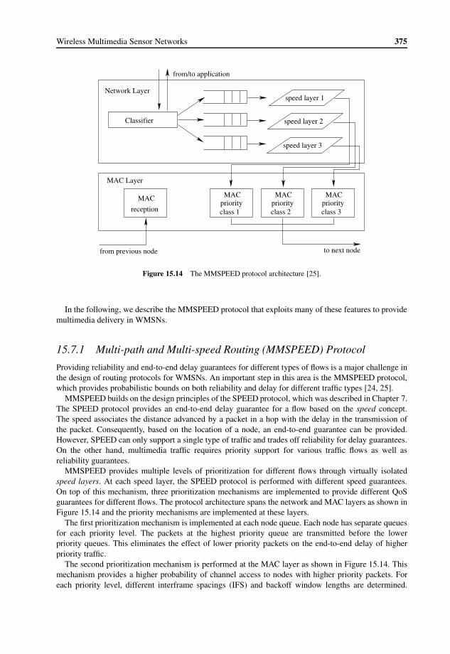
Wireless Multimedia Sensor Networks 375
MACpriorityclass 1
MACpriorityclass 2
MACpriorityclass 3
Classifier
speed layer 1
speed layer 2
speed layer 3
Network Layer
MAC
reception
MAC Layer
to next nodefrom previous node
from/to application
Figure 15.14 The MMSPEED protocol architecture [25].
In the following, we describe the MMSPEED protocol that exploits many of these features to providemultimedia delivery in WMSNs.
15.7.1 Multi-path and Multi-speed Routing (MMSPEED) Protocol
Providing reliability and end-to-end delay guarantees for different types of flows is a major challenge inthe design of routing protocols for WMSNs. An important step in this area is the MMSPEED protocol,which provides probabilistic bounds on both reliability and delay for different traffic types [24, 25].
MMSPEED builds on the design principles of the SPEED protocol, which was described in Chapter 7.The SPEED protocol provides an end-to-end delay guarantee for a flow based on the speed concept.The speed associates the distance advanced by a packet in a hop with the delay in the transmission ofthe packet. Consequently, based on the location of a node, an end-to-end guarantee can be provided.However, SPEED can only support a single type of traffic and trades off reliability for delay guarantees.On the other hand, multimedia traffic requires priority support for various traffic flows as well asreliability guarantees.
MMSPEED provides multiple levels of prioritization for different flows through virtually isolatedspeed layers. At each speed layer, the SPEED protocol is performed with different speed guarantees.On top of this mechanism, three prioritization mechanisms are implemented to provide different QoSguarantees for different flows. The protocol architecture spans the network and MAC layers as shown inFigure 15.14 and the priority mechanisms are implemented at these layers.
The first prioritization mechanism is implemented at each node queue. Each node has separate queuesfor each priority level. The packets at the highest priority queue are transmitted before the lowerpriority queues. This eliminates the effect of lower priority packets on the end-to-end delay of higherpriority traffic.
The second prioritization mechanism is performed at the MAC layer as shown in Figure 15.14. Thismechanism provides a higher probability of channel access to nodes with higher priority packets. Foreach priority level, different interframe spacings (IFS) and backoff window lengths are determined.

376 Wireless Sensor Networks
e i,je i,j
e i,je i,j
e i,j
j
i sink
Figure 15.15 At each hop, the local error rate and the hop distance are assumed to be the same for the followinghops to estimate the reachability probability [25].
Consequently, a node with a higher priority packet performs backoff for a shorter duration, whichincreases its chance to access the channel compared to nodes with lower priority packets. In addition, themedium access delay for higher priority packets is also decreased through this prioritization mechanism.
The first two prioritization mechanisms of MMSPEED improve the delay performance for differenttypes of traffic. However, since the SPEED mechanism explained in Chapter 7 is used for each speedlayer, reliability is not provided. This problem is addressed by assigning multiple routes for high-prioritytraffic. This is accomplished first by determining a target reliability level for the traffic type. This levelcan be determined based on the QoS requirements of each traffic type. For example, a real-time videostreaming application may compensate for loss frames and hence a lower target reliability level canbe chosen, e.g., 0.2. In this case, single path routing would be sufficient to achieve the low targetreliability level without high energy consumption. On the other hand, for compressed image transfer,a higher reliability level, e.g., 0.8, is necessary since the redundancy of the image to be transferred isalready filtered by the compression. In this case, MMSPEED exploits multi-path routing to improve thereliability of the packet. More specifically, a node forwards the packet to more than one node accordingto the loss rates of its neighbors.
Once a target level is set, the originator of the traffic, e.g., node i, can determine the number of multiplepaths according to the reliability levels of each of its neighbors, e.g., node j . To this end, each node jmaintains the recent average of packet loss ratios and informs its neighbors. As a result, node i hasthe average packet loss ratio between itself and node j , ei,j . Accordingly, an end-to-end reachabilityprobability from node i to the sink s via node j can be calculated as follows:
RPsi,j = (1− ei,j )(1− ei,j ) dj,s /di,j � (15.10)
where ei,j is the average packet loss percentage between nodes i and j , dj,s and di,j are the distancesbetween node j and the sink, and between nodes i and j , respectively. This estimate for the end-to-endreachability probability has the following assumptions as illustrated in Figure 15.15: (1) the error rate ateach hop from node i to the sink s is the same as the error rate at the first hop, i.e., between nodes i andj , ei,j ; (2) the hop distance at each hop is the same as the first hop distance, di,j , hence the number ofhops between node j and the sink is dj,s/di,j .
Using the reachability probability estimate in (15.10), the number of multiple paths that will ensure thetarget reliability level can be found iteratively by adding additional paths. To this end, the total reachingprobability (TRP) of a packet is given by
TRP= 1− (1− TRP′)(1− RPsi,j ) (15.11)
where TRP′ is the total reaching probability before adding the path with node j . By calculating the TRP,the target reliability level can be found by iteratively adding a path through one of the neighbors in thevicinity.

Wireless Multimedia Sensor Networks 377
i
j
k
l
RP=0.3
RP=0.25
RP=0.45
(a)
Packet RP=0.2Packet RP=0.2
i
j
k
l
(b)
Packet RP=0.5
Packet RP=0.4
Packet RP=0.2
i
j
k
l
(c)
Figure 15.16 MMSPEED protocol operation: (a) an example topology with three potential neighbors, (b) singlepath route selection for low-reliability traffic, (c) multi-path route selection for high-reliability traffic.
EXAMPLE 15.2
An example of MMSPEED protocol operation is shown in Figure 15.16(a), where node i has threeneighbors j , k, and l with estimated reachability probabilities of 0.3, 0.25, and .0.45, respectively.If node i has a packet with a target reliability level of 0.2, one of the neighbor nodes can beused to forward the packet as shown in Figure 15.16(b), where node k is selected with a requiredreliability level of 0.2. However, if a packet with a target reliability level of 0.5 needs to beforwarded, none of the immediate neighbors provide such a reliability alone and multiple pathsshould be selected. Accordingly, node i selects nodes j and l since the total reaching probabilityis 1− (1− 0.3)(1− 0.45) > 0.5 as shown in Figure 15.16(c).
The reachability probability RP given in (15.10) assumes a fixed packet loss percentage and hop lengthfor each hop in the end-to-end path. However, dynamic changes in both hop length and packet losspercentage can occur. MMSPEED reacts to these changes by assigning new target reliability levels foreach chosen branch so that the original target reliability level can still be met. According to the schemein Example 15.2, the new target probabilities are calculated as 0.2 for node j and 0.4 for node l. Thechanges in reachability probability and the hop distance for the following hops for these two nodes arethen compensated dynamically. With this dynamic compensation, the end-to-end reaching probability islikely met, although the packet forwarding decision is made locally.
EXAMPLE 15.3
The dynamic compensation property of MMSPEED is illustrated in Figure 15.17. In this case, thesource node i1 generates a packet that needs to be transmitted with a reachability target of P req =0.8. Now, suppose that this node has two neighbors i2 and i3 with reachability probabilities ofRPsi1,i2 = 0.7 and RPsi1,i3 = 0.6, respectively. Accordingly, choosing these nodes satisfies the

378 Wireless Sensor Networks
i1
i2
i4
i3
i6
i5
P = 0.8req
P = 0.5req
P = 0.3req
P = 0.3req
P = 0.6req
P = 0.6req
RP = 0.7i1,i2s
RP = 0.6i1,i3s RP = 0.3i3,i5
s
RP = 0.3i3,i6s
RP = 0.9i2,i4s
sink
Figure 15.17 An example for the dynamic compensation in MMSPEED [25].
reachability target since 1− (1− 0.7)(1− 0.6)= 0.88> 0.8. When node i1 transmits the packetto nodes i2 and i3 the updated reachability targets are assigned as 0.6 and 0.5 respectively.
At the second hops, nodes i2 and i3 make routing decisions according to their local estimatesof reachability probability for their neighbors. Accordingly, node i2 finds node i4 with RPi2,i4 =0.9> 0.6, which satisfies the reachability target. However, node i3 cannot ensure the assignedreachability target 0.5 through any of its neighbors i5 and i6 since they both have a RP of0.3. Then, node i3 creates another branch and forwards the packet to both of its neighbors.Accordingly, each following node dynamically compensates the previous wrong decision as thepacket travels to the final destination, branching more paths throughout the progress of the packetas shown in Figure 15.17.
To decrease the delay and energy consumption associated with creating multiple paths from asingle node, MMSPEED uses multicast at the MAC layer to transmit the packet to several next hopssimultaneously.
Overall, MMSPEED provides delay and reliability support for different traffic types through thevirtual layering mechanism. A cross-layer approach including buffer management, routing, and MAC isdeveloped. Although strict delay and jitter bounds, which are crucial for multimedia streaming, cannotbe supported, MMSPEED is an important step in providing QoS in WMSNs.
15.7.2 Open Research Issues
There exist many open research issues for the development of efficient routing solutions for WMSNs, asoutlined below:
• The identification of the optimal routing metrics is an important subject for research. Most routingprotocols that consider more than one metric, such as energy, delay, etc., form a cost function thatis then minimized. The choice of the weights for these metrics needs to be undertaken, and is often

Wireless Multimedia Sensor Networks 379
subject to dynamic network conditions. Thus, further work is needed to shift this decision-makingprocess and network tuning from the user end into the network.
• As the connectivity between different domains improves, end-to-end QOS guarantees arecomplicated by the inherent differences in the nature of the wired and wireless media. Whensensed data from the field are sent via the Internet, a single routing metric is unsuitable for theentire path between source and end-user. Decoupling reliability and routing parameters at suchnetwork boundaries and a seamless integration of schemes better suited to wired or wirelessdomains, respectively, need to be explored.
15.8 Transport Layer
The high-data-rate traffic generated by multimedia applications makes the transport layer solutions animportant part of communication in WMSNs. More specifically, providing end-to-end reliability andcongestion control mechanisms in an energy-constrained network is a challenging task. Particularly inWMSNs, several additional considerations are in order to accommodate both the unique characteristicsof the WSN paradigm and multimedia transport requirements.
Conventional transport protocols that have been developed for WSNs as explained in Chapter 8 focuson event-based reliability. In other words, information regarding a geographical area is important ratherthan the individual items of data from each of the sensors in this area. Consequently, a collectivereliability notion is generally adopted in WSNs [12]. Although this notion may still be true for WMSNs,the contents of the transmitted packets are also important. Consequently, a transport protocol shouldconsider the interdependencies and the priority levels of transmitted packets to provide a high-qualityreconstruction of the images or videos at the sink.
In traditional WSNs, when congestion occurs, packets are randomly dropped. However, in WMSNs,transmitted packets usually depend on other packets for reliable reconstruction at the sink node. Aswe will explain in Section 15.9, image and video coding algorithms usually result in multiple prioritylevels. As an example, the MPEG-4 algorithm generates multiple P-frames that depend on an I-frame.Consequently, congestion in a WMSN should be avoided considering these interdependencies andpriority levels inherent in the multimedia traffic. Based on these unique properties of multimedia traffic,the transport layer should consider the following main topics in WMSNs:
• Congestion control: The high load due to multimedia transfer makes congestion control veryimportant in WMSNs. While typical transmission rates for sensor nodes are between 40 and250 kbps, indicative data rates of constant bit-rate voice traffic may be 64 kbps while video traffic,on the other hand, may be bursty and on the order of 500 kbps [57]. The effect of congestion iseven more pronounced considering also that multiple simultaneous traffic may be flowing throughthe network. Consequently, if congestion occurs in the network, it leads to both performancedegradation and energy depletion in each node. Traditional congestion control mechanisms reactto congestion after it occurs in the network. For WMSNs, where congestion has adverse effects,control mechanisms are necessary which prevent congestion before it occurs.
• Reliability: Reliability has always been the primary concern of transport protocols in bothtraditional wireless networks and WSNs. The content of multimedia streams, however, requiresthe notion of reliability to be rethought. This is because the reliability notion in a multimediastream directly depends on the type of encoding performed. As an example, MPEG-4 encodescertain frames based on previously sent frames called I-frames. This makes I-frames moreimportant than the intermediate frames. On the other hand, sometimes losing even a wholeframe may not degrade the quality of a video depending on the importance of the particularframe. Thus, it is important that reliability is enforced on a per-packet basis to best utilize theexisting networking resources. Clearly, this requires cross-layer interactions with the multimediaencoders.

380 Wireless Sensor Networks
• Use of multiple paths: In WMSNs, the channel conditions and contention in the channel may notpermit a high data rate for the entire duration of multimedia flows. By allowing multiple paths, theeffective data rate at each path is reduced and the application can be supported. The availabilityof multiple paths between source and sink can be exploited by opening multiple connections formultimedia traffic [46]. In this case, the order of packet delivery is strongly influenced by thecharacteristics of the route chosen. However, in real-time video/audio feeds or streaming media,information that cannot be used in the proper sequence becomes redundant. Hence, efficienttechniques for packet reordering are necessary for the transport layer.
Based on these considerations, novel transport protocols need to be developed for WMSNs. Wedescribe next representative solutions for video and image transfer.
15.8.1 Multi-hop Buffering and Adaptation
In multi-hop networks, one way to provide reliability is to use efficient buffer management schemes.The multi-hop buffering and adaptation scheme is an example that aims to provide reliability inWMSNs characterized by video traffic. More specifically, non-real-time video transfer is considered.Consequently, high-quality reconstruction of the frames generated by the sensor nodes is crucial insteadof the end-to-end delay requirements. Furthermore, 100% reliability is not required in these typesof traffic since scalable encoding can be performed, exploiting the redundancy in the transmittedinformation.
In the event of congestion, the multi-hop buffering and adaptation scheme acts in two steps. Firstly,the congestion is minimized by dropping the lower priority packets in the node’s buffer. As a result,high-priority packets are not affected by the congestion in the network and a certain level of qualitycan be achieved at the sink during reconstruction. Secondly, a backpressure message is sent toward thedata generator. Consequently, the nodes along the path are informed to stop transmitting lower prioritypackets. The rationale behind the backpressure message is explained through the following example.
EXAMPLE 15.4
In a distributed priority queuing mechanism, each node in the network responds to congestionby dropping the lowest priority packets in its queue. In a distributed network, each node mayhave packets of different priority level. Consider the case in Figure 15.18, where a multi-hoppath composed of several nodes is shown. The direction of flow and the packets with prioritylevels stored in each node’s buffer are also shown in Figure 15.18. In this case, a lower numberrepresents a higher priority level. In case congestion occurs at node D, this node drops the lowestpriority level packet in its queue, i.e., a packet with priority level 2. However, if the other nodeson this path are not informed of this action, they will continue to send their stored packets. Thisresults in priority level 2 packets at node B still being delivered to node D. To prevent this, themulti-hop buffering and adaptation scheme deploys a coordination mechanism such that when anode drops a packet of a particular priority level, e.g., 2, this is communicated to the upstreamnodes in the route. As a result, node B drops level 2 packets and node A drops the level 3 packet.This backpressure message also helps to inform the source node such that the encoding rate canbe decreased to send lower quality data. Using the specific characteristics of the transmitted datahelps to develop efficient transport layer protocols.
15.8.2 Error Robust Image Transport
While video data have important characteristics to be exploited in transport protocols, image transfer isvery different due to its intrinsic characteristics. An important difference is the relatively low amount of

Wireless Multimedia Sensor Networks 381
222
1
A
B
CD
31
1211
Figure 15.18 Priority mismatch in a multi-hop network.
Cluster head
Cluster nodes
S
D
Figure 15.19 Forwarding scheme in error robust image transport.
traffic of image transmission compared to video, which consists of multiple frames. On the other hand,the correlation between frames in a video transmission can be exploited to decrease the amount of traffictransmitted. In image transmission, however, only the pixel correlation in the image can be exploited toreduce the information content. This relatively smaller redundancy requires each image produced by thesensor nodes to be reliably transmitted to the sink.
The reliability of a multi-hop communication protocol can be improved through in-network processingand multi-path transmission. The error robust image transport scheme achieves this through a cross-layer solution in a cluster-based network architecture [55] as shown in Figure 15.19. The network ispartitioned into clusters, each of which is controlled by a cluster head. The coordination and routeselection inside a cluster is performed by cluster heads.
Traditional multi-path routing protocols generate uncorrelated routes such that the reliability of thetransmission is improved. Consequently, no common nodes usually exist in these multiple paths. Whileefficient, such a strategy for the transmission of images in WMSNs leads to inefficiency in terms of

382 Wireless Sensor Networks
end-to-end reliability. The reason behind this is that image data are usually in high volume and requireFEC codes to be used for energy-efficient transfer in a hop. As a result, any error in transmission maypropagate through the multi-hop network until the sink reconstructs the image from the multiple routes.
In the error robust image transport scheme, on the other hand, the multiple paths are constructedspecifically to intersect at cluster heads as shown in Figure 15.19, leading to a cross-layer reliabilitymechanism that involves the link, routing, and transport layers. Each image source encodes the capturedimage and creates multiple copies to be sent to different nodes in the cluster. These nodes are selectedby the cluster head randomly. At each link FEC is used to further improve the error resiliency. Therelay nodes then transport the copies to the next cluster head for in-network processing. At each clusterhead, multiple copies of the image are collected and processed to regenerate the original image. Anyerrors during the transmission are corrected through multiple copies. Once the image is regenerated, it isencoded again and multiple copies are sent. As a result, redundancy is created through both FEC codesand multiple paths for reliable communication. This redundancy also helps to eliminate the losses dueto node failures, which is also common in WSNs.
An important drawback of the error robust image transport scheme is that significant resourcesare consumed in reliably transporting an image. Firstly, multiple copies of the same image traversethe network, increasing the consumed energy for an image. Secondly, cluster heads need to performimage decoding and encoding for in-network processing. For this, cluster heads need to wait for eachcopy to arrive in order to perform encoding, which adds to the end-to-end delay. These costs aredefinitely important for the operation of the network. On the other hand, in networks with heterogeneouscomponents, where cluster heads are resource-rich devices and image delivery has no delay bounds, theerror robust image transport scheme provides high reliability.
15.8.3 Open Research Issues
In summary, the transport layer mechanisms that can simultaneously address the unique challenges posedby the WMSN paradigm and multimedia communication requirements must be incorporated. Whileseveral approaches were discussed, some open issues remain and are outlined below:
• In WMSN applications, the data gathered from the field may contain multimedia informationsuch as target images, acoustic signals, and even video captures of a moving target, all of whichenjoy a permissible level of loss tolerance. The presence or absence of an intruder, however, mayrequire a single data field but needs to be communicated without any loss of fidelity. Thus, whena single network contains multimedia as well as scalar data, the transport protocol must decidewhether to focus on one or more functionalities so that the application needs are met withoutunwarranted energy expense.
• Despite the existence of reliable transport solutions for WSNs as discussed in Chapter 8, noneof these protocols provide real-time communication support for applications with strict delaybounds. Therefore, new transport solutions which can also meet certain application deadlinesmust be developed.
• The success in energy-efficient and reliable delivery of multimedia information extracted fromthe phenomenon directly depends on selecting the appropriate coding rate, number of sensornodes, and data rate for a given event [53]. However, to this end, the event reliability should beaccurately measured in order to efficiently adapt the multimedia coding and transmission rates.For this purpose, new reliability metrics coupled with application layer coding techniques shouldbe investigated.

Wireless Multimedia Sensor Networks 383
15.9 Application Layer
The multimedia content of the traffic in WMSNs requires additional capabilities at the applicationlayer. Especially, the heterogeneity in traffic as well as the dynamic resource availability in a multi-hop network make efficient control a challenging task. Consequently, the application layer for WMSNsneeds to consider the following two services: (1) providing traffic management and admission controland (2) performing source coding according to the application requirements and hardware constraints,by leveraging advanced multimedia encoding techniques. In this section, we provide an overview ofthese challenges.
15.9.1 Traffic Management and Admission Control
Providing QoS guarantees in a network, in general, requires sophisticated traffic management andadmission control procedures. This requirement is even more important in networks of low-power,low-data-rate sensor nodes, where network resources are scarce and dynamic. Hence, differentiationof traffic classes and resource management are important in WMSNs. Because of the heterogeneity inmultimedia traffic, WMSNs will need to provide support and differentiated service for several differenttraffic classes. These traffic classes are characterized according to two major metrics, namely reliabilityand delay. Moreover, since multimedia information coexists with scalar data such as information fromother sensors or control information in WMSN, they should also be differentiated. Consequently, thefollowing traffic classes can be defined in WMSNs:
• Real-time, loss-tolerant, multimedia streams: Video and audio streams usually constitutethis class. In addition, more heterogeneous streams consisting of audio/video and other scalardata (e.g., temperature readings), as well as metadata associated with the stream, can also beconsidered. A major requirement is that the information needs to reach the sink within strict delaybounds. One reason is that in real-time monitoring applications, timely information retrieval iscrucial. Moreover, since data may be flowing through multiple paths, a general delay bound oneach path is required for efficient decoding of the multimedia stream. On the other hand, sincevideo streams generally allow a certain level of distortion, this traffic class is loss tolerant. Trafficin this class usually has a high-bandwidth demand.
• Delay-tolerant, loss-tolerant, multimedia streams: For applications such as video storagefor offline processing, real-time delivery is not important. Hence, strict delay bounds are notnecessary as long as the multimedia stream is delivered to the sink with acceptable loss. Animportant requirement of this class is to provide sufficient bandwidth throughout the network sothat the limited buffers of the sensors are not exceeded.
• Real-time, loss-tolerant data: Real-time applications also require scalar data to complementthe multimedia information generated by the sensors. In the case of densely deployed networks,where the collected data include a high degree of redundancy due to spatial correlation, theinformation gathered by the nodes needs to be timely delivered to the sink. In this case, packetlosses may be tolerated due to the correlation between nodes. Hence, sensor data have to bereceived timely but the application is moderately loss tolerant.
• Real-time, loss-intolerant data: Control data or scalar sensor monitoring data need to be reliablydelivered to the sensors in the network or the sink in a timely fashion. Therefore, the applicationlayer has to provide necessary resources for this type of traffic.
• Delay-tolerant, loss-intolerant data: This class includes data from critical monitoring processesthat require some form of offline postprocessing.
• Delay-tolerant, loss-tolerant data: This class includes environmental data from scalar sensornetworks, or non-time-critical snapshot multimedia content, with a low- or moderate-bandwidthdemand.

384 Wireless Sensor Networks
Admission control has been investigated in traditional WSNs as we discussed in Chapter 9. Whilethese approaches address application-level QoS considerations, they fail to consider multiple QoSrequirements (e.g., delay, reliability, and energy consumption) simultaneously. Especially, in WMSNs,packets that belong to even the same stream may require different QoS requirements. While real-timeand orderly delivery may be important for all packets, the reliability requirements may differ for differenttypes of packets. Therefore, cross-layer admission control techniques that consider both the informationcontent of the traffic and the peculiarities of communication in WMSNs need to be developed.
15.9.2 Multimedia Encoding Techniques
Multimedia encoding techniques focus on two main goals for efficient transmission of multimedia data.Firstly, the correlation between pixels of an image/frame or between frames of a video stream canbe exploited to significantly reduce the information content to be transmitted without major qualitydegradation. This is usually referred to as source coding. Secondly, the compressed data should beefficiently represented to allow reliable transmission over lossy channels. This is usually referred toas channel coding or error-resilient coding. Furthermore, multimedia encoding techniques for WMSNsshould also consider minimizing the processing and transmission power necessary to effectively deliverthe multimedia content. Consequently, the main design objectives of a multimedia encoder for WMSNsare as follows:
• High compression efficiency: It is necessary to achieve a high ratio of compression to effectivelylimit bandwidth and energy consumption.
• Low complexity: The resource constraints of multimedia sensors in terms of processing andenergy consumption require encoder techniques to be of low complexity to reduce cost and formfactors, and low power to prolong the lifetime of the sensor nodes.
• Error resiliency: Low-power wireless communication increases the errors in the channel. Asa result, the encoders should be designed to account for these effects and provide robust anderror-resilient coding.
Multimedia encoding techniques have been investigated extensively in the context of the Internet andwireless networks. The results of this research have led to powerful standards for both still image andvideo encoding. In the following two sections, applications of the state-of-the-art solutions to WMSNsare presented.
15.9.3 Still Image Encoding
Still image capture and transmission is one of the most promising applications for WMSNs. While videostreaming can demand high resources and complex QoS-aware protocols, still image transmission staysas a transition between scalar data transmission in WSNs and multimedia transmission in WMSNs. Themost important encoding schemes for still images are JPEG and the recent JPEG 2000 standard. Sinceit is both more recent and more superior to JPEG, we will explain the applicability of the JPEG 2000standard to WMSNs.
JPEG 2000 in WMSNs
The generation of a bit stream from an image requires many computations that increase the energyconsumption during compression of an image. Hence, it is important to assess the cost of using JPEG2000 while enjoying the features provided by it.
JPEG 2000 contains several features that are directly applicable to WMSNs. Some of these featuresthat make JPEG 2000 a strong candidate for WMSNs are as follows [20, 38]:

Wireless Multimedia Sensor Networks 385
• Low-bit-rate performance: JPEG 2000 is superior to other still image standards at low bit rates,which refers to the number of bits used to encode a pixel on the image, i.e., bits per pixel (bpp).JPEG 2000 provides high-quality images even at bit rates lower than 0.25 bpp, which is importantfor WMSNs equipped with low-data-rate transceivers.
• Progressive transmission: This refers to the fact that, using JPEG 2000, an image can stillbe constructed before all the encoded packets are received. Depending on how the packets areordered in the network, as more packets are received the decoder can increase the resolution ofthe image, the size of the image, or the focus of the image. This provides great flexibility forcommunication in WMSNs since the amount of multimedia traffic to be sent can be tailoredaccording to the application needs.
• Parsing: Packets in a JPEG 2000 stream are identical to each other in format. Hence, the changein the progression technique is possible only by changing the order of the packets. This providesexcessive in-networking capabilities while the image is being transmitted without decoding.
• Error resiliency: Compared to current standards, JPEG 2000 provides higher resiliency. Thismeans that even if some bits or packets of an image stream are lost, the image can still be decodedat a high enough quality.
JPEG 2000 provides many advantages for image compression in low-data-rate applications. However,processing cost is still high, primarily because of wavelet coding. Hence, image compression using theJPEG 2000 scheme may be infeasible for resource-constrained WMSNs. An alternative for performingcompression in the network is to divide the workload among multiple sensor nodes so that distributedcompression is performed [54]. The energy- efficient distributed JPEG 2000 image compression schemeprovides two methods for distributing the compression tasks among multiple sensors: parallel waveletdecomposition and tiling.
Parallel wavelet decomposition: The first method is based on the parallel wavelet transform, where animage is partitioned into blocks of multiple rows and a 1-D wavelet transformation is performed on eachof the blocks independently. In a distributed WMSN, this technique is adopted in a cluster through atwo-round compression architecture. The compression is controlled by the cluster head. As shown inFigure 15.20, the image source first distributes each block of the image to the nodes in the cluster. Afterthe first 1D discrete wavelet transform (DWT), the outputs are sent to the cluster head, which combinesthe results and divides them into columns for the second-round DWT. Then, each node sends its resultsto the next cluster head. This process is repeated at each cluster until the required number of layers isprocessed. While the processing burden on each node is significantly decreased, this scheme leads toa higher number of transmissions because of the dissemination and collection of the image data. Onthe other hand, since the parallel wavelet transform does not introduce any artifacts, the output of thedistributed compression is not affected.
Tiling: The second scheme divides the original image into tiles and multiple nodes compress a part ofthe image independently. Instead of distributing the wavelet decomposition process, the image can bepartitioned into tiles to make each node operate on a small image. In this method, the image is firstpartitioned into tiles and each tile is sent to several nodes in a cluster. Each tile is compressed separatelyand sent to the next cluster head. This process decreases the energy consumption at each node whileproviding an acceptable level of communication for the distributed operation. A major drawback is thatif the number of tiles is large, the quality loss and blocking artifacts increase.
Both schemes are based on a clustered network architecture, where each cluster is responsible forperforming a layer of the JPEG compression. Each cluster head manages the distributed compressionoperation and directs the nodes to forward their computations to the next cluster. As a result, the rawimage generated by a single source is distributively encoded while the image is transmitted to the sink.

386 Wireless Sensor Networks
Control data
Compressed data
S
D
Cluster head
Cluster nodes
Route data
Figure 15.20 The parallel wavelet decomposition architecture.
15.9.4 Distributed Source Coding
Video encoding requires higher processing capabilities to extract the redundancy in frames of a videofeed as well as between each consecutive frame. In this section, we present the applications of distributedsource coding in video encoding in WMSNs. The traditional high-complexity encoder/low-complexitydecoder architecture generally used for multimedia applications is not applicable for WMSNs. This isdue to two main reasons: firstly, each node in a WMSN that will be responsible for encoding has scarceenergy resources, frequently preventing high-complexity and energy-consuming operations. Secondly,the distributed nature of the WMSNs allows novel approaches that can also consider the relationshipbetween multiple multimedia sources. To accomplish this major goal, the encoder/decoder complexityhas to be swapped for more energy-efficient encoding without affecting the compression efficiency.
Distributed source coding (DSC) techniques have been explained in Chapter 9. Among these, Wyner–Ziv coding is a promising solution for distributed compression in WMSNs. There are two main aspects,where the results of DSC can be used to transmit still image or video in resource-constrained WMSNs:
• DSC with spatial correlation: The existence of multiple sources for multimedia results inspatially correlated information content residing in WMSNs. As we discussed in Chapter 5,spatial correlation in WSNs is a common concept, which is usually exploited in the design ofcommunication protocols. In WSNs, spatial correlation is directly related to the location of thenodes. In WMSNs, due to the directivity of the video cameras, spatial correlation is related to theFoV of cameras. As a result, nodes with overlapping FoVs observe correlated information thatcan be exploited to encode the multimedia content. This case is particularly applicable to stillimage encoding.
• DSC with temporal correlation: Video frames are inherently temporally correlated. Thiscorrelation at each encoder can be exploited to develop low-complexity encoders based on theresults of Wyner–Ziv coding. This results in the encoding of reference frames and intermediateframes very similar to the MPEG standards with a significantly lower complexity at the encoders.

Wireless Multimedia Sensor Networks 387
Despite the theoretical advantages, practical solutions for DSC have not been developed until recently.Clearly, such techniques are promising for WMSNs and especially for networks of video sensors. Theencoder can be simple and low power, while the decoder at the sink will be complex and loaded withmost of the processing and energy burden. The objective of a Wyner–Ziv video coder is to achievelossy compression of still images or video streams and a performance comparable to that of interframeencoding (e.g., MPEG), with a complexity at the encoder comparable to that of intraframe coders (e.g.,JPEG). Next, we introduce some of the applications of DSC in WMSNs.
Pixel Domain Wyner–Ziv Coding
As explained above, the temporal correlation between frames in a video can be exploited to apply theresults of Wyner–Ziv coding. One way to implement this idea is to use a combination of intraframecompression at the encoder side and exploit the temporal correlation through interframe decoding at thedecoder side [8, 9].
The encoder side of this scheme consists of two different encoding techniques. For regularly spacedframes, interframe compression is performed to reduce the information content using the spatialcorrelation between the pixels of the frame. These frames are called key frames and sent to the decoderas side information. Other frames between each key frame are called Wyner–Ziv frames and are codedusing Wyner–Ziv encoding.
At the decoder side, each key frame is extrapolated and used as side information for the decoding ofWyner–Ziv frames. The decoder also uses previously decoded Wyner–Ziv frames as side information. Toapply the Wyner–Ziv coding techniques, a correlation function is chosen between the side informationand the information to be decoded. If reliable decoding is impossible, the decoder requests additionalparity bits from the encoder buffer.
The pixel domain Wyner–Ziv encoder exploits the DSC techniques. The interframe coded key framesare used to generate side information for the Wyner–Ziv frames. A major difference between thepixel domain Wyner–Ziv encoding and DSC is the following. In DSC, encoding of the correlatedinformation X is performed without the knowledge of side information, Y . In video encoding, thisinformation is present at the encoder since all the frames are generated by the same encoder.However, since exploiting this correlation for encoding requires motion prediction techniques, whichare computationally expensive, it is left to the decoder to exploit it.
One of the main disadvantages of the pixel domain Wyner–Ziv coding is that the decoder relies onfeedback from the encoder for proper decoding. This incurs additional delay and energy consumptionthat result from the multi-hop communication requirement of each feedback. This prevents offlineprocessing of video since encoding cannot provide the necessary feedback in case of errors.
Transform Domain Wyner–Ziv Coding
Spectral information can be exploited instead of pixels to reduce the information content in imageor video encoding. This is successfully accomplished through the discrete cosine transform (DCT)or wavelet coding in conventional compression schemes. A similar approach is also possible in DSCthrough transform domain Wyner–Ziv coding [7, 47].
In the transform domain Wyner–Ziv coding scheme, the frames are decomposed into spectralcoefficients by the DCT. These coefficients are then independently quantized, grouped into coefficientbands, and compressed. As in the pixel domain encoder described in the previous section, the decodergenerates a side information frame based on the previously reconstructed frames. Based on the sideinformation, a bank of decoders reconstructs the quantized coefficient bands independently.
Compared to the pixel domain case, the transform domain Wyner–Ziv coding has a better performancein terms of video quality. Furthermore, rate-distortion performance is between conventional intraframetransform coding and conventional motion-compensated transform coding.

388 Wireless Sensor Networks
Power-Efficient Robust High-Compression Syndrome-Based Multimedia Coding (PRISM)
The solutions for DSC that we have described so far are based on the classical Wyner–Ziv codingtechniques. A major drawback of these schemes is the feedback mechanism required at the decoder.In order to correctly decode the received bits, the decoder may request additional parity bits from theencoder. In multi-hop networks, this leads to significant delays and energy consumption based on thelocation of the encoder in the network.
The need for feedback from the encoder for decoding is removed through the PRISM scheme [47].The main goal is to shift the motion compensation task from the encoder to the decoder. As a result, thecomplexity is shifted to the decoder instead of the encoder. Similar to the Wyner–Ziv coding schemes,side information is generated to be exploited at the decoder for motion compensation. At the encoder, theinput X, which is a spatial region in a frame, and the side information Y , which is the highest correlatedspatial region of the reference frame, are assumed to be correlated in the following form:
Y =X +N (15.12)
where N is the correlated noise. The decoder tries to estimate the correlated noise to correctly decodethe information, X, sent by the encoder. As a result, estimating the correlated noise, N , serves as motioncompensation at the decoder.
15.9.5 Open Research Issues
Application layer protocols tailored specifically for WMSNs are still missing for the efficient realizationof WMSNs. Hence, the following research topics need to be established:
• While theoretical results on Slepian–Wolf and Wyner–Ziv coding have existed for 30 years, thereis still a lack of practical solutions. The net benefits and the practicality of these techniques stillneed to be demonstrated.
• It is necessary to fully explore the tradeoffs between the achieved fidelity in the description of thephenomenon observed and the resulting energy consumption. As an example, the video distortionperceived by the final user depends on source coding (frame rate, quantization) and on channelcoding strength. For instance, in a surveillance application, the objective of maximizing the eventdetection probability is in contrast to the objective of minimizing the power consumption.
• There is a need for simple yet expressive high-level primitives for applications to leveragecollaborative, advanced, in-network multimedia processing techniques.
15.10 Cross-layer DesignAs described in Chapter 10, in WSNs, there is a strict interdependence among functions handledat different layers of the communication stack. This interdependence is even more pronounced inWMSNs because the performance of multimedia encoding that is performed at the application layerdirectly depends on the channel coding that is performed at the physical layer. Furthermore, in multi-hop networks, the encoding performance can be affected by the operation of the layers in between.Consequently, the application layer has to perform source coding based on information from the lowerlayers to maximize the multimedia performance. At one end, there have been many improvementsin cross-layer communication protocols as we discussed in Chapter 10. However, the influence ofmultimedia coding has not been considered as part of this work. At the other end, cross-layer approachesdeveloped for most of the multimedia compression or encoding schemes consider only a point-to-pointchannel, including only the effects of the wireless channel.
WMSNs require the sensor network paradigm to be rethought in view of the need for mechanismsto deliver multimedia content with a predefined level of QoS. We describe next a new cross-layer

Wireless Multimedia Sensor Networks 389
CROSS LAYER CONTROL UNIT
(XLCU)
QoS Scheduler
UWB Transceiver
LOCALIZATION SUBSYSTEM
NETWORKCOORDINATION
UNIT (NCU)
GeoRouting
Rate Control
Channel Coder Source Coder
SYNCHRONIZATION SUBSYSTEM
Admission Control
TO NETWORK PEERS
FLOW REQUIREMENTS
Capacity Assignment
Coding Rate
Next Hop Selection
Data Rate
QoS Contracts
CROSS LAYER CONTROL UNIT
(XLCU)
QoS SchedulerQoS Scheduler
UWB Transceiver
LOCALIZATION SUBSYSTEM
NETWORKCOORDINATION
UNIT (NCU)
GeoRouting
Rate Control
Channel Coder Source CoderSource Coder
SYNCHRONIZATION SUBSYSTEM
Admission Control
TO NETWORK PEERS
FLOW REQUIREMENTS
Capacity Assignment
Coding Rate
Next Hop Selection
Data Rate
QoS Contracts
Figure 15.21 Architecture of the cross-layer controller.
communication architecture based on the TH-IR-UWB technology, whose objective is to reliably andflexibly deliver QoS to heterogeneous applications in WMSNs, by leveraging and controlling interactionsamong different layers of the protocol stack according to the requirements of the application.
15.10.1 Cross-layer Control Unit
The cross-layer control unit (XLCU) [40, 41] is based on a cross-layer communication architecture,where the main goal is to reliably and flexibly deliver QoS to heterogeneous applications in WMSNs, bycontrolling the functionalities of different layers. The communication protocol is based on the TH-IR-UWB transmission technique. Accordingly, the following approaches have been unified in the XLCUarchitecture:
• Network layer QoS support: The XLCU resides at the network layer to provide packet-levelservice differentiation. The XLCU architecture is shown in Figure 15.21, where the networkingfunctionalities of the physical, MAC, and network layers are controlled. The operational decisionsare based on the application requirements as well as the information from each individualcomponent in the architecture.
• Geographical forwarding: The accurate positioning capabilities of the UWB technology areleveraged to provide geographical forwarding mechanisms according to the QoS requirements.
• Hop-by-hop QoS contracts: To provide end-to-end QoS support, the XLCU employs hop-by-hop QoS contracts such that the next hops are selected according to locally determined criteria.These criteria are determined according to a localized optimization framework.
• Receiver-centric scheduling: To mitigate interference from neighbor nodes, receiver-centricscheduling is performed such that each receiver acts according to local measurements andconsequently control loss recovery and rate adaptation.
• Dynamic channel coding: Since power control is not beneficial in TH-IR-UWB, adaptation tointerference at the receiver is achieved through dynamic channel coding. The encoder at node ireceives a block of L uncoded bits, and selects the encoding rate RE,i among the set RE =

390 Wireless Sensor Networks
[R1E, R2
E, . . . , RP
E]. Accordingly, when code Rp
Eis selected, the encoder produces a block of
coded bits of length L/RpE
.
To provide service differentiation between different flows in the network, the XLCU defines variousclasses of traffic according to the delay requirements (real time or delay tolerant), reliability requirements(loss intolerant or loss tolerant), and type of flow (multimedia stream or data flow). Each class isidentified through its requirements, which are described as a set of tuples �A = {ψa(δa, βa, ζ a), a ∈1, . . . , NA
ψ}, where ψa, a ∈ 1, . . . , NA
ψ, are NA
ψdifferent subflows of the flow generated by the
application A. For each subflow ψa , δa is the maximum allowed end-to-end delay for packets associatedwith the subflow, βa is the required bandwidth, and ζ a is the end-to-end packet error rate (PER) that canbe allowed by the application. The communication decisions are made according to these requirements.
The application’s requirements are used to determine hop-by-hop QoS contracts for packet transmis-sion. The global end-to-end requirements are then guaranteed by the individual guarantees of each devicealong the path to the destination. Considering a flow ψa(δa, βa, ζ a) generated at node i, a multi-hoppath from i to the destination N needs to be established, with maximum end-to-end delay δa , minimumguaranteed bandwidth βa , and maximum end-to-end packet error rate ζa .
The required bandwidth βa needs to be provided at each hop. Moreover, the delay and packet errorrate requirements are determined according to the geographical advance of the packet. More specifically,
δaij =( 〈dij〉iN
diN
)· δa (15.13)
and
ζ aij ≤ 1− (1− ζ a) NHopij �
−1
(15.14)
where 〈dij〉iN is the advance of the packet if it has been transmitted from node i to node j and diNrepresents the distance between i and the destination. According to the single hop distance, in (15.14), theend-to-end path is assumed to consist of NHop
ij hops and the packet error rate requirement is determinedaccordingly.
Based on the local requirements, the next hop is selected according to an admission control protocol.A node i with a packet to send first broadcasts a short CONTRACT_REQUEST packet, which describesthe requirements of the service at i, i.e., Fi . If a neighbor j of i (1) has positive advance toward the sinkN with respect to i and (2) is able to provide the requested service with the required QoS, it replies withan ADM_GRANTED packet. This initial handshake informs the sender node about the potential neighborsfor the service. Accordingly, the sender node performs a local optimization process to select the optimalrelay node. This is communicated to the selected node through a CONTRACT_REQUEST packet and thehandshake is concluded through a CONTRACT_ESTABLISHED message. The hop-by-hop admissioncontrol mechanism helps forward the packet until the destination.
The admission control protocol relies on a local optimization problem, which is solved at each hop.Accordingly, the problem can be cast as follows:
Pdist: Distributed Admission Control, Routing, and Channel Coding Problem
Given: i, N, Si, PNi , Epulse, FiFind: j∗ ∈ Si ∩PNi , RaE,i ∀a ∈ Fi
Minimize: Ebit(i,j) =
1
βtot
∑a∈F(i)
Epulse · NTX,aij
· NHopij · βa
RaE,j(15.15)
Subject to:

Wireless Multimedia Sensor Networks 391
packet error rate:
RaE,i ≤min
(E(r)i
γ aC,j (ζaij )[ηj + (σ 2/Tf,j )
∑k∈F (i),k =i E
(r)k ]
, 1
), ∀a ∈ Fi; (15.16)
rate admission control:∑a∈Fj
βa
RaE,Nj
(γ aC,Nj(ζ ajNj
))
+∑a∈Fj
βa
RaE,Uaj (γ
aC,j (ζ
aUaj j ))
+R
sched,upj
RschedE,j
+R
sched,downj
RschedE,j
≤ R0,j ; (15.17)
delay admission control:∑a∈Fi
LR0,j
RaE,Nj
+ T sched,up + T sched,down
+∑a∈Fi
L
(1+
baj
φaj
)· 1
R0,jRaE,j
+ L
R0,j RaE,j
≤ δaij , ∀a ∈ Fi (15.18)
where the following parameters are used:
• Epulse = 2 · Epulseelec + PTX · Tf,i [J/pulse] is the energy to transmit one pulse from node i to
node j , where Epulseelec is the energy per pulse needed by transmitter electronics and digital
processing; P TX [W] and Tf,i [s] are the average transmitted power and the frame length,respectively.
• NTX,aij is the average number of transmissions of a packet from flow a required for the packet to
be correctly decoded at receiver j .
• NHopij =max(diN/〈dij〉iN, 1) is the estimated number of hops from node i to the destination N
when j is selected as the next hop.
• Si is the neighbor set of node i, while PNi
is the positive advance set of i, i.e., j ∈ PNi
iffdjN < diN .
• Fi is the set of incoming or generated flows at node i.
• The bandwidth requirement βa of application a can be expressed as βa = Ra0,i · RaE,i , whereRa0,i [pulses/s] represents the raw pulse rate for application a required to achieve the rate βa ,when a coding rate RaE,i is used.
• βtot =∑a∈Fi βa represents the total bandwidth requirement, in bps, for flows incoming orgenerated at i.
Once the next hop is selected, rate assignment is performed such that the signal-to-interference plusnoise ratio (SINR) of the communication is bounded by
SINRai ≥ γ aC,i (ζ ai ), (15.19)
for an allowed PER ζ ai
at receiver i, where γ aC,i(ζai) is the SINR threshold that guarantees the PER ζ a
i.
The rate is selected such that Rai= Ra
E,iR0,i , and is bounded by
RaE,i ≤min
(E(r)i
γ aC,i(ζai )[ηi + (σ 2/Tf,i)
∑j∈F(i),j =i E
(r)j ]
, 1
). (15.20)

392 Wireless Sensor Networks
Hence, the optimal coding rate for flow a is selected as
RaE,i = max1≤p≤P R
pE
s.t. (15.20) holds. (15.21)
After the next hop is selected with the optimal rate, finally, receiver-centric scheduling is performedto determine the transmission times for the contracted flow. This is performed according to a schedule,which is a vector of appointments, i.e., tuples (a, u, tak , R
aE,u), where a is an application flow, u is a
node, u ∈ Fi , tak is the starting time for transmission of the kth packet from flow a at u, and RaE,u isthe required coding rate. The scheduling mechanism of the XLCU is based on a procedure inspiredby the wireless fair scheduling (WFS) paradigm, which is designed to guarantee delay-bounded andthroughput-guaranteed access in single hop, single rate wireless packet networks. More specifically, thewireless fair service approach [36] is extended for a UWB multi-rate, multi-hop environment.
The XLCU architecture is based on an innovative design that aims at providing differentiation inthe domains of throughput, delay, reliability, and energy consumption, based on a modular cross-layercontroller that performs admission control, routing, scheduling, bandwidth assignment, and coding tosatisfy application requirements. This solution provides delays that are very low and with low jitter,and the throughput is fairly constant in time, while energy consumption is structurally much lower thanCSMA/CA systems due to the lower transmitted power and no idle listening.
15.11 Further Research Issues
Most of the challenges in realizing a practical implementation of WMSNs can be classified into layer-specific considerations as we have discussed so far in this chapter. Nevertheless, there are still additionalareas that need to be addressed for a complete realization of WMSNs. In this section, we overview thestill open research issues in many contexts for the realization of WMSNs.
15.11.1 Collaborative In-network Processing
In-network processing has long been the main theme for networking in traditional WSNs. Consideringthe heavy processing requirements and increased bandwidth needs of multimedia applications, it isclear that WMSNs will also require efficient in-network processing algorithms. Consequently, it isnecessary to flexibly perform these functionalities in-network with minimum energy consumption andlimited execution time. Similar to image or video compression, the objective of in-network processingis to further reduce the amount of injected information into the network and communicate onlynecessary information.
The information communicated in the network is also not always of the same context in distributednetworks. The content requested from the same set of sensor nodes can vary significantly dependingon the application type as well as the query. Consequently, both networking protocols and compressiontechniques should be developed to be highly adaptive to efficiently respond to this dynamic nature of thequeries. Consequently, application-specific querying and processing is crucial in WMSNs. Moreover,it is necessary to develop efficient querying languages, and also to develop distributed compression,filtering, and in-network processing architectures, to allow real-time retrieval of useful information.
Aggregation and fusion of both inter-media and intra-media are necessary considering the funda-mental differences between WMSNs and WSNs. Especially, the computational burden exposed throughcomplex multimedia operations prevents well-established distributed processing schemes that havebeen developed for WSNs being used in this context. In WSNs, it is well known that processing isalways cheaper than communication. This is, however, not completely true in WMSNs. In particular,the tradeoffs between compression at end-nodes and communicating raw data have yet to be clearlyanalyzed. This leads to fundamental architecture decisions such as whether this processing can be done

Wireless Multimedia Sensor Networks 393
on sensor nodes (i.e., a flat architecture of multifunctional sensors that can perform any task), or if theneed for specialized devices, e.g. computation hubs, arises.
Next, we will introduce two main directions for in-network processing in WMSNs. It is clear thatthese directions will likely drive research on architectures and algorithms for the distributed processingof multimedia data.
Data Alignment and Image Registration
The distributed nature of WMSNs results in multiple observations of probably the same phenomenonfrom different sensor nodes, at different times. Similar to WSNs, the central location, however, isinterested in observing the phenomenon that is of interest to the network instead of the individualobservations of the sensor nodes. Consequently, information gathered from different sources shouldbe combined wisely to provide better information than what is possible from individual observations.
In image or video processing, the concept of merging information from multiple sources isinvestigated under the umbrella of data alignment approaches. More specifically, image registration,which is widely used in areas such as remote sensing, medical imaging, and computer vision, is apromising field for WMSNs. The basic idea of image registration is to align different images of thesame scene taken at different times, from different viewpoints, and/or by different sensors.
Image registration consist of four steps as we will describe next:
• Feature detection: Image registration depends solely on determining common objects indifferent images to determine the viewpoints or locations that are associated with each image.To extract this information, distinctive objects are detected. This is accomplished by definingclosed-boundary regions, edges, contours, line intersections, corners, etc.
• Feature matching: Features detected in each image should be compared among different imagesto determine the relationship between images. Feature matching techniques try to match the sameobjects on different images to provide this relationship.
• Transform model estimation: Once correlated images are determined, accurate models totransform each image into a common reference need to be used. This is accomplished by definingmapping functions and estimating their parameters. Using these functions, each image can betransformed to produce a common frame of information using multiple sources.
• Image resampling and transformation: In this last step, the sensed image is transformed bymeans of the mapping functions.
Data alignment and image registration operations generally consume large amounts of processingpower. Therefore, exploiting these techniques in-network is a major challenge for WMSNs. Moreover,efficient information transmission methods need to be devised such that these techniques are exploitedat resource-rich processing hubs or at the sink.
WMSNs as Distributed Computer Vision Systems
Efficient transmission of still image and video frames has been the primary focus of research in WMSNs.While many important insights have been learned so far from these approaches, the distributed natureof WMSNs is still open to different approaches in visual systems. Especially, transmitting imagesand video from a distributed network of nodes can still be seen as raw information transfer. The in-network processing approaches developed so far mainly focus on distributing the high processing loadof compression techniques through a parallel processing architecture composed of multiple sensors.However, raw data transfer is still of major concern. Then, it is left solely to the central location tocollect a high volume of information from multiple sensors and process it centrally.
As with WSNs, intelligent information rather than raw data is important in WMSNs. This correspondsto local processing of visual information and the transmission of information of interest. Spreading the

394 Wireless Sensor Networks
processing load on every sensor in the network provides the transition from a distributed camera networkto a distributed computer vision system. This research topic is very important in WMSNs.
Visual observations across the network can be performed in WMSNs through distributed computationson observations from multiple nodes. Consequently, simple but efficient tools are necessary to expressdata as an observation that is of interest to the user. To this end, it is necessary to coordinate computationsacross the nodes in the network efficiently and return only the results of interest to the end-user.
15.11.2 Synchronization
Synchronization is an important aspect of networking in WSNs and is required by many algorithmsfor efficient operation as we discussed in Chapter 11. It is clear that the need for synchronization alsoexists in WMSNs for the same reasons. Moreover, in the case of WMSNs, synchronization becomeseven more pronounced because of the information content of distributed nodes and the dependence ofthis multimedia information on time. This increases the need for accurate synchronization solutions inWMSNs as well.
In-network processing tools for WMSNs require the whole image/video be decoded at an aggregatepoint to further decrease the content of information. In addition, the whole information content frommultiple flows needs to be available at the same time. Since storing this huge amount of information isvery costly, multiple flows to be aggregated need to be generated at closely intervals and received withincertain delay bounds. This prevents buffer overflows and makes aggregation of multiple streams possible.
Multimedia data returned by sensors can be heterogeneous, and possibly correlated. As an example,video and audio samples could be collected over a common geographical region, or still pictures maycomplement scalar data containing field measurements. While the temporal correlation between thesemultiple streams can be estimated from the content of the data at a central location, this requires extensivecomputation. This might not be suitable for applications that require fast and accurate responses forevents occurring in a surveillance system. Therefore, inter-media synchronization schemes that canbe implemented inside the network would improve the efficiency of such applications. Providing acommon frame for markers that can be associated with each multimedia flow gives the end-user theflexibility to process these data. The problem of multimedia synchronization is cross-layer in natureand influences primarily the physical and application layers. At the physical layer, data from differentmedia are multiplexed over shared wireless connections, or are stored in common physical storage.The application layer is concerned with the inter-media synchronization necessary for presentation orplayout, i.e., with the interactions between the multimedia application and the various media.
References[1] MTS/MDA Sensor Board Users Manual.
[2] Acroname GARCIA robotic platform. http://www.acroname.com/garcia/garcia.html.
[3] Crossbow MICA2 mote specifications. http://www.xbow.com.
[4] Crossbow TelosB mote specifications. http://www.xbow.com.
[5] SENSONET sensor network testbed. Available at http://www.ece.gatech.edu/research/labs/bwn/.
[6] JPEG 2000 requirements and profiles. ISO/IEC JTC1/SC29/WG1 N1271, March 1999.
[7] A. Aaron, S. Rane, E. Setton, and B. Girod. Transform-domain Wyner–Ziv codec for video. In Proceedingsof the Society of Photo-Optical Instrumentation Engineers – Visual Communications and Image Processing,pp. 520–528, San Jose, CA, USA, January 2004.
[8] A. Aaron, S. Rane, R. Zhang, and B. Girod. Wyner–Ziv coding for video: applications to compression and errorresilience. In Proceedings of the IEEE Data Compression Conference (DCC’03), pp. 93–102, Snowbird, UT,USA, March 2003.

Wireless Multimedia Sensor Networks 395
[9] A. Aaron, E. Setton, and B. Girod. Towards practical Wyner–Ziv coding of video. In Proceedings of the IEEEInternational Conference on Image Processing (ICIP’03), volume 3, pp. 869–872, Barcelona, Spain, September2003.
[10] R. Agre, L. P. Clare, G. J. Pottie, and N. P. Romanov. Development platform for self-organizing wireless sensornetworks. In Proceedings of the Society of Photo-Optical Instrumentation Engineers, volume 3713, pp. 257–268, Orlando, FL, USA, April 1999.
[11] G. R. Aiello and G. D. Rogerson. Ultra-wideband wireless systems. IEEE Microwave Magazine, 4:36–47, June2003.
[12] Ö. B. Akan and I. F. Akyildiz. Event-to-sink reliable transport in wireless sensor networks. IEEE/ACMTransactions on Networking, 13(5):1003–1016, October 2005.
[13] I. F. Akyildiz, T. Melodia, and K. Chowdury. A survey on wireless multimedia sensor networks. ComputerNetworks, 51(4):921–960, March 2007.
[14] I. F. Akyildiz, W. Su, Y. Sankarasubramaniam, and E. Cayirci. Wireless sensor networks: a survey. ComputerNetworks, 38(4):393–422, March 2002.
[15] R. Biswas, K. R. Chowdhury, and D. P. Agrawal. Data-centric attribute allocation and retrieval (DCAAR)scheme for wireless sensor networks. In Proceedings of the IEEE International Conference on Mobile Ad-hocand Sensor Systems (MASS’05), pp. 422–429, Washington DC, USA, November 2005.
[16] M. Caccamo, L. Y. Zhang, L. Sha, and G. Buttazzo. An implicit prioritized access protocol for wireless sensornetworks. In Proceedings of the IEEE Real-Time Systems Symposium (RTSS’02), pp. 39–48, Austin, TX, USA,December 2002.
[17] Y. Charfi, N. Wakamiya, and M. Murata. Visual sensor networks: opportunities and challenges. In Informationand Communication Technologies International Symposium (ICTIS’07), Sydney, Australia, April 2007.
[18] K. J. Cho and H. H. Asada. Wireless, battery-less stethoscope for wearable health monitoring. In Proceedingsof the IEEE Northeast Bioengineering Conference, pp. 187–188, Philadelphia, PA, USA, April 2002.
[19] K. R. Chowdhury, N. Nandiraju, D. Cavalcanti, and D. P. Agrawal. CMAC – a multi-channel energy efficientMAC for wireless sensor networks. In Proceedings of the IEEE Wireless Communications and NetworkingConference (WCNC’06), volume 2, pp. 1172–1177, Las Vegas, NV, USA, April 2006.
[20] C. Christopoulos, A. Skodras, and T. Ebrahimi. The JPEG 2000 still image coding system: an overview. IEEETransactions on Consumer Electronics, 46(4):1103–1127, November 2000.
[21] R. Cucchiara. Multimedia surveillance systems. In Proceedings of the ACM International Workshop on VideoSurveillance and Sensor Networks, pp. 3–10, Singapore, November 2005.
[22] I. Downes, L. B. Rad, and H. Aghajan. Development of a mote for wireless image sensor networks. InProceedings of COGnitive systems with Interactive Sensors (COGIS’06), Paris, France, March 2006.
[23] Anuj Batra et al. Multi-band OFDM physical layer proposal for IEEE 802.15 task group 3a. IEEE P802.15Working Group for Wireless Personal Area Networks (WPANs), March 2004.
[24] E. Felemban, C.-G. Lee, E. Ekici, R. Boder, and S. Vural. Probabilistic QoS guarantee in reliability andtimeliness domains in wireless sensor networks. In Proceedings of IEEE INFOCOM 2005, volume 4, pp. 2646–2657, Miami, FL, USA, March 2005.
[25] E. Felemban, C.-G. Lee, and Eylem Ekici. MMSPEED: multipath multi-speed protocol for QoS guarantee ofreliability and timeliness in wireless sensor networks. IEEE Transactions on Mobile Computing, 5(6):738–754,June 2006.
[26] W.-C. Feng, B. Code, E. Kaiser, M. Shea, W.-C. Feng, and L. Bavoil. Panoptes: Scalable low-power videosensor networking technologies. In Proceedings of the 11th ACM International Conference on Multimedia,pp. 562–571, Berkeley, CA, USA, November 2003.
[27] S. Gezici, Z. Tian, G. B. Giannakis, H. Kobayashi, A. F. Molisch, H. V. Poor, and Z. Sahinoglu. Localizationvia ultra-wideband radios. IEEE Signal Processing Magazine, 22(4):70–84, July 2005.
[28] B. Girod, A. Aaron, S. Rane, and D. Rebollo-Monedero. Distributed video coding. Proceedings of the IEEE,93(1):71–83, January 2005.
[29] E. Gürses and Ö. B. Akan. Multimedia communication in wireless sensor networks. Annals of Telecommunica-tions, 60(7-8):872–900, July–August 2005.
[30] S. K. Jayaweera. An energy-efficient virtual MIMO communications architecture based on V-BLAST process-ing for distributed wireless sensor networks. In Proceedings of the IEEE International Conference on Sensorand Ad-hoc Communications and Networks (SECON’04), pp. 299–308, Santa Clara, CA, USA, October 2004.

396 Wireless Sensor Networks
[31] S. K. Jayaweera and M. L. Chebolu. Virtual MIMO and distributed signal processing for sensor networks –an integrated approach. In Proceedings of the IEEE International Conference on Communications (ICC’05),volume 2, pp. 1214–1218, Seoul, South Korea, May 2005.
[32] P. Kulkarni, D. Ganesan, P. Shenoy, and Q. Lu. SensEye: a multi-tier camera sensor network. In Proceedings ofACM Multimedia, Singapore, November 2005.
[33] P. Kyasanur and N. H. Vaidya. Capacity of multi-channel wireless networks: impact of number of channels andinterfaces. In Proceedings of ACM MobiCom’05, Cologne, Germany, August 2005.
[34] C. L. Liu and J. W. Layland. Scheduling algorithms for multiprogramming in hard real time environment.Journal of the ACM, 20(1):40–61, 1973.
[35] X. Liu, Q. Wang, W. He, M. Caccamo, and L. Sha. Optimal real-time sampling rate assignment for wirelesssensor networks. ACM Transactions on Sensor Networks, 2(2):263–295, 2006.
[36] S. Lu, T. Nandagopal, and V. Bharghavan. Design and analysis of an algorithm for fair service in error-pronewireless channels. ACM Wireless Networks, 6(4):323–343, January 2000.
[37] K. Mandke, H. Nam, L. Yerramneni, and C. Zuniga. The evolution of UWB and IEEE 802.15.3a for very highdata rate WPAN. High Frequency Electronics, Technology Report, 2(5):22–32, September 2003.
[38] M. W. Marcellin, A. Bilgin, M. J. Gormish, and M. P. Boliek. An overview of JPEG-2000. In Proceedings ofthe Conference on Data Compression, p. 523, Snowbird, UT, USA, 2000.
[39] C. B. Margi, V. Petkov, K. Obraczka, and R. Manduchi. Characterizing energy consumption in a visual sensornetwork testbed. In Proceedings of the IEEE/Create-Net International Conference on Testbeds and ResearchInfrastructures for the Development of Networks and Communities (TridentCom’06), Barcelona, Spain, March2006.
[40] T. Melodia and I. F. Akyildiz. Cross-layer quality of service support for UWB wireless multimedia sensornetworks. In Proceedings of the IEEE INFOCOM Mini-Conference’08, Phoenix, AZ, USA, April 2008.
[41] T. Melodia and I. F. Akyildiz. Cross-layer QoS-aware communication for ultra wide band wireless multimediasensor networks. IEEE Journal on Selected Areas in Communications, 2010.
[42] M. J Miller and N. H. Vaidya. A MAC protocol to reduce sensor network energy consumption using a wakeupradio. IEEE Transactions on Mobile Computing, 4(3):228–242, May/June 2005.
[43] F. R. Mireles and R. A. Scholtz. Performance of equicorrelated ultra-wideband pulse-position-modulated signalsin the indoor wireless impulse radio channel. Proceedings of IEEE Communications, Computers and SignalProcessing, 2:640–644, August 1997.
[44] S. Misra, M. Reisslein, and G. Xue. A survey of multimedia streaming in wireless sensor networks. IEEECommunications Surveys & Tutorials, 10(4):18–39, 2008.
[45] S. Nath, Y. Ke, P. B. Gibbons, B. Karp, and S. Seshan. A distributed filtering architecture for multimediasensors. In Proceedings of BaseNets’04, San Jose, CA, USA, October 2004.
[46] T. Nguyen and S. Cheung. Multimedia streaming with multiple TCP connections. In Proceedings of the IEEEInternational Performance Computing and Communications Conference (IPCCC’05), Phoenix, AZ, USA, April2005.
[47] R. Puri and K. Ramchandran. Prism: a new robust video coding architecture based on distributed compressionprinciples. In Proceedings of the Allerton Conference on Communication, Control, and Computing, Allerton,IL, USA, October 2002.
[48] M. Rahimi, R. Baer, O. Iroezi, J. Garcia, J. Warrior, D. Estrin, and M. Srivastava. Cyclops: in situ image sensingand interpretation in wireless sensor networks. In Proceedings of the ACM Conference on Embedded NetworkedSensor Systems (SenSys), San Diego, CA, USA, November 2005.
[49] A. A. Reeves. Remote monitoring of patients suffering from early symptoms of dementia. In InternationalWorkshop on Wearable and Implantable Body Sensor Networks, London, UK, April 2005.
[50] A. Rowe, C. Rosenberg, and I. Nourbakhsh. A low cost embedded color vision system. In Proceedings of theIEEE/RSJ International Conference on Intelligent Robots and Systems (IROS), Lausanne, Switzerland, October2002.
[51] C. Santivanez and I. Stavrakakis. Study of various TDMA schemes for wireless networks in the presence ofdeadlines and overhead. IEEE Journal on Selected Areas in Communications, 17(7):1284–1304, July 1999.
[52] C. Schurgers, V. Tsiatsis, and M. B. Srivastava. STEM: topology management for energy efficient sensornetworks. In Proceedings of the IEEE Aerospace Conference, volume 3, pp. 1099–1108, Big Sky, MT, USA,2002.

Wireless Multimedia Sensor Networks 397
[53] M. C. Vuran, Ö. B. Akan, and I. F. Akyildiz. Spatio-temporal correlation: theory and applications for wirelesssensor networks. Computer Networks, 45(3):245–261, June 2004.
[54] H. Wu and A. Abouzeid. Energy efficient distributed image compression in resource constrained multihopwireless networks. Computer Communications, 28(14):1658–1668, September 2005.
[55] H. Wu and A. A. Abouzeid. Error resilient image transport in wireless sensor networks. Computer Networks,50(15):2873–2887, October 2006.
[56] W. Yu, Z. Sahinoglu, and A. Vetro. Energy-efficient JPEG 2000 image transmission over wireless sensornetworks. In Proceedings of the IEEE Global Communications Conference (GLOBECOM), pp. 2738–2743,Dallas, TX, USA, January 2004.
[57] X. Zhu and B. Girod. Distributed rate allocation for multi-stream video transmission over ad hoc networks.In Proceedings of the IEEE International Conference on Image Processing (ICIP), pp. 157–160, Genoa, Italy,September 2005.


16Wireless Underwater SensorNetworks
Wireless underwater sensor networks (UWSNs) are envisioned to enable applications for a widevariety of purposes such as oceanographic data collection, pollution monitoring, offshore exploration,disaster prevention, assisted navigation, and tactical surveillance [7]. Multiple unmanned or autonomousunderwater vehicles (UUVs, AUVs), equipped with underwater sensors, will also find application inexploration of natural undersea resources and scientific data gathering in collaborative monitoringmissions. To make these applications viable, there is a need to enable communications among underwaterdevices. Similar to the requirements of WSNs, underwater sensor nodes and vehicles must possessself-configuration capabilities, i.e., they must be able to coordinate their operations by exchangingconfiguration, location, and movement information, and to relay monitored data to an onshore station.
The traditional approach for ocean-bottom or ocean-column monitoring is to deploy underwatersensors that record data during the monitoring mission, and then recover the instruments [29]. Thisapproach has the following disadvantages:
• No real-time monitoring: The recorded data cannot be accessed until the instruments arerecovered, which may be several days, weeks, or months after beginning the monitoring mission.In surveillance or environmental monitoring applications such as seismic monitoring, however,real-time data retrieval is crucial.
• No online system reconfiguration: Interaction between onshore control systems and themonitoring instruments is not possible. This impedes any adaptive tuning of the instruments;nor is it possible to reconfigure the system after particular events occur.
• No failure detection: If failures or misconfigurations occur, it may not be possible to detect thembefore the instruments are recovered. This can easily lead to the complete failure of a monitoringmission.
• Limited storage capacity: The amount of data that can be recorded during the monitoringmission by every sensor is limited by the capacity of the onboard storage devices (memories,hard disks).
These disadvantages of traditional underwater monitoring techniques limit the possible applicationsfor this environment. On the other hand, the distributed sensor network paradigm may providecapabilities that significantly surpass the existing underwater applications. Therefore, there is a needto deploy underwater networks that will enable real-time monitoring of selected ocean areas, remoteconfiguration, and interaction with onshore human operators. All this can be obtained by connectingunderwater instruments by means of wireless links and forming underwater sensor networks as we willexplain in this chapter. The above features enable a broad range of underwater applications:
Wireless Sensor Networks Ian F. Akyildiz and Mehmet Can Vuranc© 2010 John Wiley & Sons, Ltd

400 Wireless Sensor Networks
• Ocean sampling networks: Networks of sensors and autonomous underwater vehicles (AUVs),such as the Odyssey-class AUVs [1], can perform synoptic, cooperative adaptive sampling of the3-D coastal ocean environment [3]. Recent underwater experiments demonstrate the advantagesof bringing together sophisticated new robotic vehicles with advanced ocean models to improvethe ability to observe and predict the characteristics of the oceanic environment [5].
• Environmental monitoring: Underwater sensor networks can perform pollution monitoring(chemical, biological, and nuclear). For example, it may be possible to detail the chemical slurryof antibiotics, estrogen-type hormones, and insecticides to monitor streams, rivers, lakes, andocean bays (water quality in-situ analysis) [43]. Monitoring ocean currents and winds, improvedweather forecast, detecting climate change, understanding and predicting the effect of humanactivities on marine ecosystems, biological monitoring such as tracking fishes or microorganisms,are other possible applications. More specifically, underwater sensor networks can be used todetect extreme temperature gradients (thermoclines), which are considered to be a breedingground for certain marine microorganisms [44].
• Undersea explorations: Underwater sensor networks can help detect underwater oilfields orreservoirs, determine routes for laying undersea cables, and assist in the exploration for valuableminerals.
• Disaster prevention: Sensor networks that measure seismic activity from remote locations canprovide tsunami warnings to coastal areas [34], or study the effects of submarine earthquakes(seaquakes).
• Assisted navigation: Sensors can be used to identify hazards on the seabed, to locate dangerousrocks or shoals in shallow waters, mooring positions, and submerged wrecks, and to performbathymetry profiling.
• Distributed tactical surveillance: AUVs and fixed underwater sensors can collaborativelymonitor areas for surveillance, reconnaissance, targeting, and intrusion detection systems. Asan example, a 3-D underwater sensor network can realize a tactical surveillance system that isable to detect and classify submarines, small delivery vehicles (SDVs), and divers based on thesensed data from mechanical, radiation, magnetic, and acoustic microsensors. With respect totraditional radar/sonar systems, underwater sensor networks can reach a higher accuracy, highercoverage, and robustness as well as enable detection and classification of low-signature targets byalso combining measures from different types of sensors.
• Mine reconnaissance: The simultaneous operation of multiple AUVs with acoustic and opticalsensors can be used to perform rapid environmental assessment and detect mine-like objects.
The potential capabilities of underwater sensor networks and the wide variety of new applicationsthat will be enabled by them motivate the development of communication techniques for the underwaterenvironment. While the vast amount of solutions for terrestrial WSNs that we have discussed in theprevious chapters provides a valuable insight into networking in this environment, there exist manychallenges unique to underwater communication. Especially, the significantly different characteristics ofcommunication in water require many networking paradigms to be revisited. Consequently, the majorchallenges in the design of underwater sensor networks are as follows:
• The available bandwidth is severely limited.• Propagation delay under water is five orders of magnitude higher than that in RF terrestrial
channels and extremely variable.• The underwater channel is severely impaired, especially because of multi-path and fading
problems.• High bit error rates and temporary losses of connectivity (shadow zones) can be experienced due
to the extreme characteristics of the underwater channel.• Battery power is limited and usually batteries cannot be recharged; also, solar energy cannot be
exploited.

Wireless Underwater Sensor Networks 401
• Underwater sensors are prone to failure because of fouling and corrosion.
In this chapter, we discuss several fundamental aspects of underwater communications and sensornetworks. The remainder of this chapter is organized as follows. In Sections 16.1 and 16.3 we introducethe communication architecture and design challenges, respectively, of underwater sensor networks.In Section 16.4, we investigate the underwater acoustic communication channel and summarize theassociated physical layer challenges for underwater networking. In Sections 16.5, 16.6, 16.7, 16.8,and 16.9, we discuss physical, data link, network, transport, and application layer issues in underwatersensor networks, respectively. In Section 16.10 we highlight cross-layer approaches for communicationin UWSNs.
16.1 Design ChallengesFirstly, we present the main differences between terrestrial and underwater sensor networks and detailthe key design issues and deployment challenges for underwater sensors.
16.1.1 Terrestrial Sensor Networks vs. Underwater Sensor Networks
While many aspects of networking under water have similarities with the terrestrial sensor networks,there exist many differences that require communication protocols to be tailored for underwater sensornetworks.
The fundamental difference between terrestrial and underwater sensor networks is the communicationmedium. As explained in more detail in Section 16.4, the underwater environment results in differentpropagation, attenuation, and fading characteristics than in air. In fact, despite the fact that underwaternetworking is a rather unexplored area, underwater communications have been experimented on sinceWorld War II, when, in 1945, an underwater telephone was developed in the USA to communicate withsubmarines [30]. The results of research in this area reveal that acoustic communication is the typicalphysical layer technology for underwater networks.
The propagation characteristics of water dictate that electromagnetic waves propagate at longdistances through conductive sea water only at extra low frequencies (30–300 Hz). This requirementrequires large antennae and high transmission power, which are not suitable for the deploymentof sensor networks. For example, the Berkeley Mica2 mote, which is one of the most popularexperimental platforms in the terrestrial sensor networking community, has a transmission range of120 cm under water at 433 MHz, according to the experiments performed at the Robotic EmbeddedSystems Laboratory (RESL) at the University of Southern California. Therefore, electromagnetic wavecommunication is not the best candidate for underwater communication.
In contrast to electromagnetic waves, optical waves do not suffer from such high attenuation. However,optical wave communication under water suffers from significant scattering. Moreover, the transmissionof optical signals requires high precision in pointing the narrow laser beams. Therefore, optical wavesare only used for short-range communication in the underwater environment. Thus, links in underwaternetworks are based on acoustic wireless communications [37].
In addition to the communication techniques, the following differences between terrestrial andunderwater sensor networks are also important:
• Size and cost: While terrestrial sensor nodes are expected to become smaller in size andincreasingly inexpensive, underwater sensors are expensive devices. This is especially due tothe more complex underwater transceivers and to the hardware protection needed in the extremeunderwater environment.
• Deployment: While terrestrial sensor networks are densely deployed, the deployment is deemedto be more sparse under water, due to the cost involved and to the challenges associated with thedeployment itself.

402 Wireless Sensor Networks
• Power: The power needed for acoustic underwater communications is higher than that interrestrial radio communications due to the greater distances and to more complex signalprocessing at the receivers to compensate for the impairments of the channel. Therefore, moreenergy is consumed and, hence, higher battery capacity is required.
• Memory: While terrestrial sensor nodes have very limited storage capacity, underwater sensorsmay need to be able to do some data caching as the underwater channel may be intermittent.
16.1.2 Real-Time Networking vs. Delay-Tolerant Networking
As in terrestrial sensor networks, depending on the application there may be very different requirementsfor data delivery. For example, surveillance applications may need very fast reactions to events and thusnetworking protocols that provide guaranteed delay-bounded delivery are required. Hence, it is necessaryto develop protocols that deal with the characteristics of the underwater environment in order to quicklyrestore connectivity when lost and that react to unpaired or congested links by taking appropriate action(e.g., dynamical rerouting) in order to meet the given delay bound. Conversely, other applications mayproduce large bundles of data to be delivered to the onshore sink without particular delay constraints. Inthis respect, the Delay-Tolerant Networking Research Group (DTNRG) [2, 14] developed mechanismsto resolve the intermittent connectivity, long or variable delays, asymmetric data rates, and high errorrates by using a store and forward mechanism based on middleware between the application layer andthe lower layers. Similar methodologies may be particularly useful for applications, such as those thatrecord seismic activity, that have very low duty cycle and produce, when activated, large bundles of datathat need to be relayed to a monitoring station where they can be analyzed to predict future activity. Onthe other hand, sensor networks intended for disaster prevention such as those that provide earthquake ortsunami warnings require immediate delivery of information and hence real-time protocols. Therefore,the design of networking solutions for underwater acoustic sensor networks should always be aware ofthe difference between real-time and delay-tolerant applications and jointly tune existing solutions to theapplication needs and to the characteristics of the underwater environment.
16.2 Underwater Sensor Network ComponentsThe design challenges and the unique characteristics of underwater sensor networks require differentcomponents for the realization of these networks. In this section, we describe these components in twoparts, i.e., the underwater sensors that are used to collect information about the underwater environment,and the autonomous underwater vehicles that are used to provide many capabilities to underwater sensornetworks such as mass data retrieval, connectivity establishment, and network management.
16.2.1 Underwater Sensors
Based on the various unique challenges posed by the underwater environment, several underwatersensors have been developed. The typical internal architecture of an underwater sensor is shown inFigure 16.1. It consists of a main controller/CPU which is interfaced with an oceanographic instrumentor sensor through sensor interface circuitry. The controller receives data from the sensor and can store thedata in the on-board memory, process them, and send them to other network devices by controlling theacoustic modem. The electronics are usually mounted on a frame which is protected by a PVC housing.Sometimes all sensor components are protected by bottom-mounted instrument frames that are designedto permit azimuthally omnidirectional acoustic communications, and protect sensors and modems fromthe potential impact of trawling gear, especially in areas subject to fishing activities. The protectingframe may be designed so as to deflect trawling gear on impact, by housing all components beneath alow-profile pyramidal frame [12].

Wireless Underwater Sensor Networks 403
Figure 16.1 Internal organization of an underwater sensor node.
In addition to the main controller and the transceiver circuitry, underwater sensor devices are equippedwith a vast variety of sensors. These devices include sensors to measure the quality of water andto study its characteristics such as temperature, density, salinity (interferometric and refractometricsensors), acidity, chemicals, conductivity, pH (magnetoelastic sensors), oxygen (Clark-type electrode),hydrogen, dissolved methane gas (METS), and turbidity. Disposable sensors, which detect ricin –the highly poisonous protein found in castor beans and thought to be a potential terrorism agent– also exist. DNA microarrays can be used to monitor both abundance and activity-level variationsamong natural microbial populations. Other existing underwater sensors include hydrothermal sulfide,silicate, voltammetric sensors for spectrophotometry, gold-amalgam electrode sensors for sedimentmeasurements of metal ions (ion-selective analysis), amperometric microsensors for H2S measurementsfor studies of anoxygenic photosynthesis, sulfide oxidation, and sulfate reduction of sediments. Inaddition, force/torque sensors for underwater applications requiring simultaneous measurements ofseveral forces and moments have also been developed, as well as quantum sensors to measure lightradiation and sensors for the measurement of harmful algal blooms.
Examples of currently available underwater sensors and modems are shown in Figure 16.2. TheAquacomm underwater modem, shown in Figure 16.2(a), provides reliable communication on the orderof 10−6 bit error rate at 100–480 bps data rates. The modem can be operated down to a depth of120 m with a communication range of 3 km. The LinkQuest underwater acoustic modems, shown inFigure 16.2(b), are short-range sensor nodes with a range of 300 m and can work at a depth of 200 m.The modems can support a communication rate of 7 kbps.
16.2.2 AUVs
In addition to static sensor nodes, several types of AUVs exist as experimental platforms for underwaterexperiments. Examples of existing AUVs are shown in Figure 16.3. Some of the AUVs resemble small-scale submarines (such as the Odyssey-class AUVs [1] developed at MIT shown in Figure 16.3(a)).Other type of AUVs are simpler devices that do not encompass such sophisticated capabilities. Forexample, drifters and gliders are oceanographic instruments often used in underwater exploration.Drifter underwater vehicles, an example of which is shown in Figure 16.3(b), drift with local currentand have the ability to move vertically through the water column, and are used for taking measurementsat preset depths [18]. Underwater gliders [13] are battery-powered AUVs that use hydraulic pumps

404 Wireless Sensor Networks
(a) (b)
Figure 16.2 Examples of underwater sensor nodes: (a) Aquacomm underwater modem and (b) LinkQuestunderwater sensor nodes.
(a) (b)
(c)
Figure 16.3 Examples of AUVs: (a) Odyssey AUV, (b) view of a drifter from above (left) and from below (right),and (c) Spray glider.
to vary their volume by a few hundred cubic centimeters in order to generate the buoyancy changesthat power their forward gliding. When they emerge on the surface, GPS is used to locate the vehicle.This information can be relayed to the onshore station while operators can interact by sending controlinformation to the gliders. Depth capabilities range from 200 to 1500 m while operating lifetimesrange from a few weeks to several months. These long durations are possible because gliders movevery slowly, typically 25 cm/s (0.5 knots). Spray glider, shown in Figure 16.3(c), is an example of anunderwater glider.

Wireless Underwater Sensor Networks 405
While these existing products provide extensive communication capabilities, the still existingchallenges related to the deployment of low-cost, low-scale underwater sensors can be listed as follows:
• Size: It is necessary to develop less expensive, robust “nano-sensors”, e.g., sensors basedon nanotechnology, which involves the development of materials and systems at the atomic,molecular, or macromolecular levels in the dimension range of approximately 1–500 nm.
• Maintenance: It is necessary to devise periodic cleaning mechanisms against corrosion andfouling, which may affect the lifetime of underwater devices. For example, some sensors forpCO2, pH, and nitrate measurement, and fluorometers and spectral radiometers, may be limitedby bio-fouling, especially on a long time scale.
• Self-configuration: There is a need for robust, stable sensors at a high range of temperatures sincesensor drift of underwater devices may be a concern. To this end, protocols for in-situ calibrationsof sensors to improve the accuracy and precision of sampled data must be developed.
• New sensor types: There is a need for new integrated sensors for synoptic sampling of physical,chemical, and biological parameters to improve the understanding of processes in marine systems.
16.3 Communication Architecture
We now introduce the reference architectures for 2-D and 3-D underwater networks, as well as 3-Dnetworks of AUVs, which can enhance the capabilities of underwater sensor networks [7].
The network topology is in general a crucial factor in determining the energy consumption, thecapacity, and the reliability of a network. Hence, the network topology should be carefully engineeredand post-deployment topology optimization should be performed, when possible.
Underwater monitoring missions can be extremely expensive due to the high cost of underwaterdevices. Hence, it is important that the deployed network be highly reliable, so as to avoid unsuccessfulmissions due to the failure of single or multiple devices. For example, it is crucial to avoid designingthe network topology with single points of failure that could compromise the overall functioning ofthe network.
The network capacity is also influenced by the network topology. Since the capacity of the underwaterchannel is severely limited, as will be discussed in Section 16.4, it is very important to organize thenetwork topology in such a way that no communication bottleneck is introduced.
The communication architectures introduced here are used as a basis for discussing the challengesassociated with underwater sensor networks (UWSNs). In the remainder of this section, we discuss thefollowing architectures:
• Static 2-D UWSNs for ocean bottom monitoring: These are constituted by sensor nodes that areanchored to the bottom of the ocean, as will be discussed in Section 16.3.1. Typical applicationsmay be environmental monitoring, or monitoring underwater plates in tectonics [16].
• Static 3-D UWSNs for ocean-column monitoring: These include networks of sensors whosedepth can be controlled by means of various techniques and will be discussed in Section 16.3.2,and may be used for surveillance applications or monitoring of ocean phenomena (oceanbio/geo/chemical processes, water streams, pollution).
• The 3-D networks of AUVs: These networks include fixed portions composed of anchored sen-sors and mobile portions constituted by autonomous vehicles, as will be detailed in Section 16.3.3.
Next, we present these three different architectures for UWSNs in detail. However, these are not theonly ways to deploy these networks. Depending on the application, users may have different deploymentoptions for these networks under water. Also none of these architectures have yet been standardized.

406 Wireless Sensor Networks
Figure 16.4 Architecture for 2-D UWSNs.
16.3.1 The 2-D UWSNs
A reference architecture for 2-D underwater networks is shown in Figure 16.4. A group of sensornodes are anchored to the bottom of the ocean with deep-ocean anchors. Underwater sensor nodes areinterconnected to one or more underwater sinks (uw-sinks) by means of wireless links. The uw-sinks, asshown in Figure 16.4, are network devices in charge of relaying data from the ocean-bottom network to asurface station. To achieve this objective, uw-sinks are equipped with two acoustic transceivers, namelya vertical and a horizontal transceiver. The horizontal transceiver is used by the uw-sink to communicatewith the sensor nodes in order: (1) to send commands and configuration data to the sensors (uw-sink tosensors) and (2) to collect monitored data (sensors to uw-sink). The vertical link is used by the uw-sinksto relay data to a surface station. In deep-water applications, vertical transceivers must be long-rangetransceivers as the ocean can be as deep as 10 km. The surface station is equipped with an acoustictransceiver that is able to handle multiple parallel communications with the deployed uw-sinks. It isalso endowed with a long-range RF and/or satellite transmitter to communicate with the onshore sink(os-sink) and/or to a surface sink (s-sink).
Sensors can be connected to uw-sinks via direct links or through multi-hop paths. In the former case,each sensor directly sends the gathered data to the selected uw-sink. However, in UWSNs, the powernecessary to transmit may decay with powers greater than 2 of the distance [36], and the uw-sink may befar from the sensor node. Consequently, although direct link connection is the simplest way to networksensors, it may not be the most energy-efficient solution. Furthermore, direct links are very likely toreduce the network throughput because of increased acoustic interference due to high transmissionpower. In the case of multi-hop paths, as in terrestrial sensor networks [8], the data produced by a sourcesensor are relayed by intermediate sensors until the data reach the uw-sink. This results in energy savingsand increased network capacity, but increases the complexity of the routing functionality as well. In fact,every network device usually takes part in a collaborative process whose objective is to diffuse topologyinformation such that efficient and loop-free routing decisions can be made at each intermediate node.This process involves signaling and computation. Since energy and capacity are precious resources inunderwater environments, as discussed above, in UWSNs the objective is to deliver event features by

Wireless Underwater Sensor Networks 407
Figure 16.5 Architecture for 3-D UWSNs.
exploiting multi-hop paths and minimizing the signaling overhead necessary for constructing underwaterpaths at the same time.
16.3.2 The 3-D UWSNs
The 3-D underwater networks are used to detect and observe phenomena that cannot be adequatelyobserved by means of ocean-bottom sensor nodes, i.e., to perform cooperative sampling of the 3-Docean environment. In 3-D underwater networks, sensor nodes float at different depths in order toobserve a given phenomenon. One possible solution would be to attach each uw-sensor node to asurface buoy, by means of wires whose length can be regulated so as to adjust the depth of each sensornode [11]. However, although this solution allows easy and quick deployment of the sensor network,multiple floating buoys may obstruct ships navigating on the surface, or they can be easily detectedand deactivated by potential enemies in military settings. Furthermore, floating buoys are vulnerable toweather and tampering or pilfering.
For these reasons, a different approach may be to anchor sensor devices to the bottom of the ocean. Inthis architecture, depicted in Figure 16.5, each sensor is anchored to the ocean bottom and equipped witha floating buoy that can be inflated by a pump. The buoy pushes the sensor toward the ocean surface. Thedepth of the sensor can then be regulated by adjusting the length of the wire that connects the sensor tothe anchor, by means of an electronically controlled engine that resides on the sensor. A challenge to beaddressed in such an architecture is the effect of ocean currents on the described mechanism to regulatethe depth of the sensor.
Many challenges arise with such an architecture, which need to be solved in order to enable 3-Dmonitoring, including:
• Sensing coverage: Sensors should collaboratively regulate their depth in order to achieve 3-Dcoverage of the ocean column, according to their sensing ranges. Hence, it must be possible toobtain sampling of the desired phenomenon at all depths.

408 Wireless Sensor Networks
• Communication coverage: Since in 3-D underwater networks there may be no notion of uw-sink, sensors should be able to relay information to the surface station via multi-hop paths. Thus,network devices should coordinate their depths in such a way that the network topology is alwaysconnected, i.e., at least one path from every sensor to the surface station always exists.
Sensing and communication coverage in a 3-D environment are rigorously investigated in [31]. Thediameter and the minimum and maximum degree of the reachability graph that describes the networkare derived as a function of the communication range, while different degrees of coverage for the 3-Denvironment are characterized as a function of the sensing range. These techniques could be exploitedto investigate coverage issues in UWSNs.
16.3.3 Sensor Networks with AUVs
AUVs can function without tethers, cables, or remote control, and therefore have a multitude ofapplications in oceanography, environmental monitoring, and underwater resource study. Previousexperimental work has shown the feasibility of relatively inexpensive AUV submarines equipped withmultiple underwater sensors that can reach any depth in the ocean [1]. Hence, they can be used toenhance the capabilities of UWSNs in many ways. The integration and enhancement of fixed sensornetworks with AUVs is an almost unexplored research area which requires new network coordinationalgorithms such as:
• Adaptive sampling: This includes control strategies to command the mobile vehicles to move toplaces where their data will be most useful. This approach is also known as adaptive samplingand has been used in monitoring missions such as in [5]. For example, the density of sensornodes can be adaptively increased in a given area when a higher sampling rate is needed for agiven monitored phenomenon.
• Self-configuration: This includes control procedures to automatically detect connectivity holesdue to node failures or channel impairment and request the intervention of an AUV. Furthermore,AUVs can be used either for installation and maintenance of the sensor network infrastructure orto deploy new sensors. They can also be used as temporary relay nodes to restore connectivity.
One of the design objectives of AUVs is to make them rely on local intelligence and less dependenton communications from onshore [19]. In general, control strategies are needed for autonomouscoordination, obstacle avoidance, and steering strategies. Solar energy systems allow the lifetime ofAUVs to be increased, i.e., it is not necessary to recover and recharge the vehicle on a daily basis.Hence, solar-powered AUVs can acquire continuous information for periods of time on the order ofmonths [20].
The distributed coordination of AUVs can be controlled through the virtual bodies and artificialpotentials (VBAP) methodology [24]. VBAP controls the movement of multiple objects in a virtualbody shape through control commands referred to as artificial potentials. The virtual body is created bylinked, moving reference points called virtual leaders. Hence, an AUV is selected as a virtual leader andthe movement of each AUV in the group is controlled according to the virtual leader.
VBAP defines three artificial potentials. The potential between each vehicle i and j is denoted asVI (xij), which is a function of locations of the nodes with respect to the center of mass of the virtualbody. Moreover, the potential between a particular vehicle i and a virtual leader k is denoted as Vh(hik),which depends on the relative distance of the vehicle to the virtual leader. Finally, Vr(θik) controls theangle between the vehicle and the virtual leader. The movement of a vehicle is defined as minus thegradient of the sum of these potentials. As a result, each vehicle is located not too close to anotherbut close enough to the virtual leader. Moreover, the speed of each vehicle is controlled based on theformation error. Therefore, a group of AUVs slow down if the formation error grows. The group isconstrained to maintain a uniform distribution as needed, but is free to spin and possibly wiggle with the
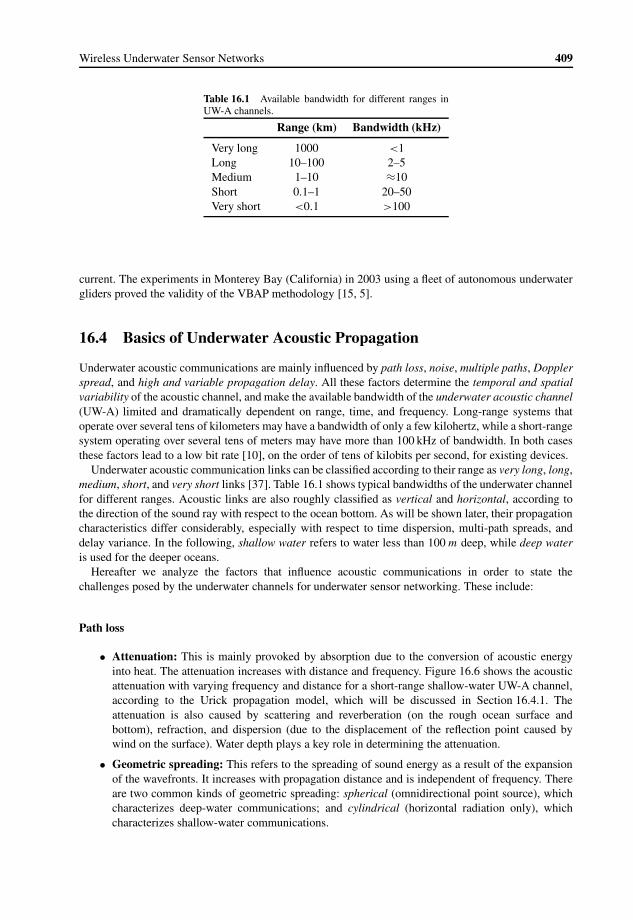
Wireless Underwater Sensor Networks 409
Table 16.1 Available bandwidth for different ranges inUW-A channels.
Range (km) Bandwidth (kHz)
Very long 1000 <1Long 10–100 2–5Medium 1–10 ≈10Short 0.1–1 20–50Very short <0.1 >100
current. The experiments in Monterey Bay (California) in 2003 using a fleet of autonomous underwatergliders proved the validity of the VBAP methodology [15, 5].
16.4 Basics of Underwater Acoustic Propagation
Underwater acoustic communications are mainly influenced by path loss, noise, multiple paths, Dopplerspread, and high and variable propagation delay. All these factors determine the temporal and spatialvariability of the acoustic channel, and make the available bandwidth of the underwater acoustic channel(UW-A) limited and dramatically dependent on range, time, and frequency. Long-range systems thatoperate over several tens of kilometers may have a bandwidth of only a few kilohertz, while a short-rangesystem operating over several tens of meters may have more than 100 kHz of bandwidth. In both casesthese factors lead to a low bit rate [10], on the order of tens of kilobits per second, for existing devices.
Underwater acoustic communication links can be classified according to their range as very long, long,medium, short, and very short links [37]. Table 16.1 shows typical bandwidths of the underwater channelfor different ranges. Acoustic links are also roughly classified as vertical and horizontal, according tothe direction of the sound ray with respect to the ocean bottom. As will be shown later, their propagationcharacteristics differ considerably, especially with respect to time dispersion, multi-path spreads, anddelay variance. In the following, shallow water refers to water less than 100m deep, while deep wateris used for the deeper oceans.
Hereafter we analyze the factors that influence acoustic communications in order to state thechallenges posed by the underwater channels for underwater sensor networking. These include:
Path loss
• Attenuation: This is mainly provoked by absorption due to the conversion of acoustic energyinto heat. The attenuation increases with distance and frequency. Figure 16.6 shows the acousticattenuation with varying frequency and distance for a short-range shallow-water UW-A channel,according to the Urick propagation model, which will be discussed in Section 16.4.1. Theattenuation is also caused by scattering and reverberation (on the rough ocean surface andbottom), refraction, and dispersion (due to the displacement of the reflection point caused bywind on the surface). Water depth plays a key role in determining the attenuation.
• Geometric spreading: This refers to the spreading of sound energy as a result of the expansionof the wavefronts. It increases with propagation distance and is independent of frequency. Thereare two common kinds of geometric spreading: spherical (omnidirectional point source), whichcharacterizes deep-water communications; and cylindrical (horizontal radiation only), whichcharacterizes shallow-water communications.

410 Wireless Sensor Networks
0200
400600
8001000
0
10
20
30
40
5020
30
40
50
60
70
80
90
Distance [m]Frequency [kHz]
Aco
ustic
Pow
er A
ttenu
atio
n [d
B]
Path Loss vs Distance and Frequency in Band 1--50 kHz
Figure 16.6 Path loss of short-range shallow UW-A channel vs. distance and frequency in the band 1–50 kHz.
Noise
• Human-made noise: This is mainly due to machinery (pumps, reduction gears, power plants)and shipping activity (hull fouling, animal life on hull, cavitation), especially in areas of heavyvessel traffic.
• Ambient noise: This is related to hydrodynamics (movement of water including tides, currents,storms, wind, and rain) and to seismic and biological phenomena. In [17], boat noise and snappingshrimps have been found to be the primary sources of noise in shallow water by means ofmeasurement experiments on the ocean bottom.
Multiple Paths
• Multi-path propagation may be responsible for severe degradation of the acoustic communicationsignal, since it generates intersymbol interference (ISI).
• The multi-path geometry depends on the link configuration. Vertical channels are characterized bylittle time dispersion, whereas horizontal channels may have extremely long multi-path spreads.
• The extent of the spreading is a strong function of depth and the distance between the transmitterand receiver.
High Delay and Delay Variance
• The propagation speed in the UW-A channel is five orders of magnitude lower than in theradio channel. This large propagation delay (0.67 s/km) can reduce the throughput of the systemconsiderably.
• The very high delay variance is even more harmful for efficient protocol design, as it preventsaccurate estimation of the round-trip time (RTT), which is the key parameter for many commoncommunication protocols.

Wireless Underwater Sensor Networks 411
Doppler Spread
• The Doppler frequency spread can be significant in UW-A channels [37], causing a degradation inthe performance of digital communications: transmissions at a high data rate cause many adjacentsymbols to interfere at the receiver, requiring sophisticated signal processing to deal with thegenerated ISI.
• The Doppler spread generates a simple frequency translation, which is relatively easy for areceiver to compensate for, and a continuous spreading of frequencies, which constitutes a non-shifted signal, which is more difficult to compensate for.
• If a channel has a Doppler spread with bandwidth B and a signal has symbol duration T , thenthere are approximately BT uncorrelated samples of its complex envelope. When BT is much lessthan unity, the channel is said to be underspread and the effects of the Doppler fading can beignored, while, if BT is greater than unity, the channel is said to be overspread [22].
Most of the above factors are caused by the chemical–physical properties of the water medium suchas temperature, salinity, and density, and by their spatio-temporal variations. These variations, togetherwith the waveguide nature of the channel, cause the acoustic channel to be highly temporally andspatially variable. In particular, the horizontal channel is by far more rapidly varying than the verticalchannel, in both deep and shallow water. The main factor is the propagation loss for underwater acousticcommunications, which is generally described by the Urick propagation model. We will describe thismodel next, then the characteristics of shallow- and deep-water channels will be described in detail.
16.4.1 Urick Propagation Model
The acoustic channel is characterized by the Urick path-loss formula which is as follows:
TL(d, f )= χ · log(d)+ α(f ) · d + A (16.1)
where the path loss, TL(d, f ), is shown in dB as a function of internode distance d and operatingfrequency f . The term χ is the geometric spreading, which can be spherical for deep water andcylindrical for shallow water. The last term A is the transmission anomaly.
The underwater propagation has three components as shown in (16.1). The first component is thedistance-dependent attenuation, which is common in many transmission media. The term χ accountsfor the geometric spreading under water and varies depending on the depth of the water. For shallow-water environments, cylindrical spreading is observed, where the signal spreads horizontally due to lowdepth. As a result, a higher percentage of the signal is preserved as the distance increases. Therefore,usually χ = 10 is used. On the other hand, in deep water, the signal spreads spherically leading to higherattenuation as the distance increases. For deep water, χ = 20 is used.
The second component in (16.1) is the frequency-dependent attenuation, where α(f ) [dB/m] is themedium absorption, which is a function of the operating frequency f . The determination of α(f ) isusually done in three ways: theoretical calculation, Fisher&Simmon’s model, and Thorp’s model, whichare based on experiments. The medium absorption is shown in Figure 16.7 as a function of f .
Finally, the last component, A [dB], accounts for the transmission anomaly, which results fromdegradation of the acoustic intensity caused by multiple path propagation, refraction, diffraction, andscattering of sound. This value is usually between 5 and 10 dB and is higher for shallow-water horizontallinks, where multi-path effects are higher.
Moreover, the propagation speed of acoustic signals under water is given as follows:
q(z, S, t)= 1449.05 + 45.7 · t − 5.21 · t2 + 0.23 · t3
+ (1.333− 0.126 · t + 0.009 · t2) · (S − 35)+ 16.3 · z+ 0.18 · z2 (16.2)

412 Wireless Sensor Networks
10–1
100
101
102
10–7
10–6
10–5
10–4
10–3
10–2
10–1
Absorption vs. Frequency
Frequency [kHz]
Abs
orpt
ion
[dB
/m]
Theoretical AbsorptionFisher&Simmons AbsorptionThorp Absorption
Figure 16.7 The medium absorption coefficient, α, as a function of operating frequency, f .
where t = T/10 (T is the temperature in ◦C), S is the salinity in ppt, and z is the depth in km. The aboveexpression provides a useful tool to determine the propagation speed, and thus the propagation delay, indifferent operating conditions, and yields values in [1460, 1520]m/s, centered around 1500 m/s.
16.4.2 Deep-Water Channel Model
The deep-water acoustic channel is not severely affected by multiple paths. Instead, a higher attenuationis present due to the spherical spreading of the acoustic signal. The path of the acoustic signals underwater is also unique. The signals bend toward the region of slower sound speed, i.e., sound is lazy. Asshown in (16.2), the propagation speed of acoustic signals depends on the depth and temperature. As aresult, the propagation path depends mainly on the location of the transmitter and also on the thermalstructure of the particular medium. Figure 16.8 shows the four main types of thermal structures and theresulting signal paths. These four types of thermal structures are isothermal gradient, negative gradient,positive gradient, and negative gradient over positive.
In isothermal environments, water temperature is uniform at the surface and decreases below acertain depth. This causes the signal split as shown in Figure 16.8(b). For negative gradient thermalstructure, the water temperature decreases with increasing depth. This causes the acoustic signalsto bend down as shown in Figure 16.8(c). The opposite is true for positive gradient as shownin Figure 16.8(d), where acoustic signals bend toward surface. For the last thermal structure, thetemperature gradient also changes with depth. In this case, a channel forms close to the surface with longranges and the signal travels through this channel as shown in Figure 16.8(e). The unique propagationcharacteristics of acoustic signals under water cause communication regions as well as shadow zoneswhere acoustic signals cannot reach. The deployment and operation of UWSNs significantly depend onthese propagation properties.

Wireless Underwater Sensor Networks 413
Sound Velocity
Dep
th
Isothermal
Negative Gradient
Positive Gradient
Negative Gradient over Positive
(a)
Dep
th
(b)
Dep
th
(c)
Dep
th
(d)
Dep
th
(e)
Figure 16.8 Sound propagation paths underwater: (a) depth vs. sound speed profiles; and propagation paths for(b) isothermal gradient, (c) negative gradient, (d) positive gradient, and (e) negative gradient over positive.
In addition to ray bending, the deep-water wireless channel also exhibits randomness in the receivedsignal. This randomness in the channel is usually modeled using the Rayleigh fading channel model,where the envelope of the signal is modeled as a Rayleigh distributed random variable, α. Consequently,the received energy per bit per noise power spectral density is given by γ = α2Eb/N0, which has adistribution as follows:
f�(γ )= 1
γ0exp
(γ
γ0
)(16.3)
where γ0 = E[α2]Eb/N0 and Eb/N0 is the received energy per bit per noise power spectral density,which can be directly found from the signal-to-noise ratio (SNR) of the channel. The SNR is given in

414 Wireless Sensor Networks
(1)
(2)
(3)
Figure 16.9 Possible paths for communication in shallow-water channels.
dB in underwater acoustic channels as
ψdB(d, f )= SLdB re uPa − TLdB(d, f )− NLdB re uPa (16.4)
where SLdB re uPa and NLdB re uPa are the signal level at the transmitter and the noise level given in dBwith reference to µPa and TLdB(d, f ) is the path loss given in (16.1). Then, Eb/N0 = ψ BN/R, whereψ = 10ψdB(d,f )/10, BN is the noise bandwidth, and R is the data rate. The signal level, SL, in (16.4) canbe related to the intensity, It , and hence the transmit power, Pt , of the transceiver as follows:
It = Pt
2π 1mH(16.5)
SL= 10 log
(It
0.67× 10⁻¹⁸
)(16.6)
where Pt is the transmit power in W, and H is the depth in m.
16.4.3 Shallow-Water Channel Model
The shallow-water channel is greatly affected by multiple paths due to, firstly, multiple reflected raysfrom either the sea bottom or surface, and, secondly, ray bending as a result of sound speed variationswith respect to depth. Depending on the depth of the environment, communication in shallow wateris performed through three paths as shown in Figure 16.9: (1) direct path, (2) reflection from surface,and (3) reflection from bottom. For configurations where the sensor network is deployed close to thesurface in a location of high depth, the reflection from the sea bottom is usually neglected due tothe high attenuation in this path. Moreover, reflections from other objects under water also affect thecommunication performance.
The reflections from the surface or sea bottom constitute the so-called macro-multipath, which candeterministically be modeled. However, the surface and sea bottom are not perfectly level. The waves onthe surface and the uneven texture of the sea bottom introduce imperfections into the received signals ona particular path. These time-dependent variations are usually called the micro-multipath and modeledstatistically. In shallow-water communication, the wireless channel is modeled as a multi-ray Rayleighfading channel, where each one of the three main paths is modeled as a Rayleigh fading channel. Thecomposition of these rays at the receiver then governs the success of the communication.
16.5 Physical LayerUntil the beginning of the last decade, due to the challenging characteristics of the underwater channel,underwater modem development was based on non-coherent frequency shift keying (FSK) modulation.

Wireless Underwater Sensor Networks 415
Table 16.2 Evolution of underwater modulation techniques.
Type Year Rate (kbps) Band (kHz) Range (km)a
FSK 1984 1.2 5 3sPSK 1989 500 125 0.06dFSK 1991 1.25 10 2dPSK 1993 0.3–0.5 0.3–1 200d–90sPSK 1994 0.02 20 0.9sFSK 1997 0.6–2.4 5 10d–5s
DPSK 1997 20 10 1dPSK 1998 1.67–6.7 2–10 4d–2s
16-QAM 2001 40 10 0.3saThe subscripts d and s stand for deep and shallow water, respectively.
Non-coherent FSK relies on energy detection and, hence, does not require phase tracking, which is a verydifficult task mainly because of the Doppler spread in the UW-A channel, described in Section 16.4. FSKmodulation schemes developed for under water try to suppress the multi-path effects by inserting timeguards between successive pulses to ensure that the reverberation, caused by the rough ocean surfaceand bottom, vanishes before each subsequent pulse is received. Dynamic frequency guards can alsobe used between frequency tones to adapt the communication to the Doppler spread of the channel.Although non-coherent modulation schemes are characterized by a high power efficiency, their lowbandwidth efficiency makes them unsuitable for high-data-rate multi-user networks. Hence, coherentmodulation techniques have been developed for long-range, high-throughput systems. In the last fewyears, fully coherent modulation techniques, such as phase shift keying (PSK) and quadrature amplitudemodulation (QAM), have become practical due to the availability of powerful digital processors. Channelequalization techniques are exploited to leverage the effect of ISI, instead of trying to avoid or suppressit. Decision-feedback equalizers (DFEs) track the complex, relatively slowly varying channel responseand thus provide high throughput when the channel is slowly varying. Conversely, when the channelvaries faster, it is necessary to combine the DFEs with a phase-locked loop (PLL) [38], which estimatesand compensates for the phase offset in a rapid, stable manner. The use of DFEs and PLLs is driven bythe complexity and time variability of ocean channel impulse responses. Table 16.2 shows the evolutionfrom non-coherent modems to recent coherent modems.
Differential phase shift keying (DPSK) serves as an intermediate solution between non-coherent andfully coherent systems in terms of bandwidth efficiency. DPSK encodes information relative to theprevious symbol rather than to an arbitrary fixed reference in the signal phase and may be referredto as partially coherent modulation. While this strategy substantially alleviates carrier phase-trackingrequirements, the penalty is an increased error probability over PSK at an equivalent data rate.
With respect to Table 16.2, it is worth noticing that early phase-coherent systems achieved higherbandwidth efficiencies (bit rate/occupied bandwidth) than their non-coherent counterparts, but theyhave not yet outperformed non-coherent modulation schemes. In fact, coherent systems had lowerperformance than incoherent systems for long-haul transmissions on horizontal channels until ISIcompensation via DFEs for optimal channel estimation was implemented [39]. However, these filteringalgorithms are complex and not suitable for real-time communications, as they do not meet real-time constraints. Hence, suboptimal filters have to be considered, but the imperfect knowledge ofthe channel impulse response that they provide leads to channel estimation errors, and ultimately todecreased performance.
Another promising solution for underwater communications is the orthogonal frequency division mul-tiplexing (OFDM) spread-spectrum technique, which is particularly efficient when noise is spread overa large portion of the available bandwidth. OFDM is frequently referred to as multicarrier modulation

416 Wireless Sensor Networks
because it transmits signals over multiple subcarriers simultaneously. In particular, subcarriers thatexperience higher SNR are allotted a higher number of bits, whereas fewer bits are allotted to subcarriersexperiencing attenuation. This concept is referred to as bit loading and requires channel estimation.Since the symbol duration for each individual carrier increases, OFDM systems perform robustly insevere multi-path environments, and achieve a high spectral efficiency.
Many of the techniques discussed above require underwater channel estimation, which can beachieved by means of probe packets [21]. An accurate estimate of the channel can be obtained witha high probing rate and/or with a large probe packet size, which, however, results in a high overhead andin the consequent drain of channel capacity and energy. Moreover, the latency in channel estimation dueto high propagation delay introduces inconsistencies in the adaptive modulation schemes.
16.6 MAC Layer
In this section, we discuss techniques for multiple access control in UWSNs. As explained in Chapter 5,MAC constitutes one of the major challenges in sensor networks. However, in addition to the manychallenges discussed in Chapter 5, MAC in UWSNs poses additional challenges due to the peculiaritiesof the underwater channel as explained in Section 16.4. In particular, MAC protocols for UWSNs aretailored to consider the very limited available bandwidth and high and variable propagation delay of theacoustic channel. Furthermore, the existence of communication regions and shadow zones as explainedin Section 16.4 requires sophisticated methods for MAC to alleviate these effects.
Among many MAC techniques available in terrestrial wireless networks, only two major techniques,i.e., CSMA and CDMA, are applicable to communication under water. Especially, frequency divisionmultiple access (FDMA) is not suitable for UWSNs due to the narrow bandwidth in UW-A channels.Since FDMA systems further divide the channel into smaller bands, the FDMA communication greatlysuffers from fading and multi-path effects.
Similarly, time division multiple access (TDMA), alone, results in a limited bandwidth efficiency.This is related to the high RTT due to very long propagation delay and the delay variance due to multiplepaths under water as discussed in Section 16.4. As a result, long time guards must be designed betweeneach time slot in order to minimize packet collisions from adjacent time slots. Moreover, the variabledelay makes it very challenging to realize precise synchronization with a common timing reference,which is required for TDMA. On the other hand, in hybrid MAC schemes, TDMA is mainly used inconjunction with CDMA, where multiple clusters are designed. In these schemes, TDMA is used forintercluster communication, where the propagation delay and delay variance are at manageable levels.These schemes will be described in Section 16.6.3.
In the following, we will describe the existing MAC schemes used in UWSNs. These schemes areclassified into three main groups: CSMA-based (Section 16.6.1), CDMA-based (Section 16.6.2), andhybrid (Section 16.6.3) MAC protocols.
16.6.1 CSMA-Based MAC Protocols
The CSMA scheme is the most used technique in terrestrial sensor networks as we discussed inChapter 5. CSMA techniques aim to prevent collisions with the ongoing transmissions by introducinga carrier sense mechanism and a backoff procedure at the transmitter side. These procedures, however,should be adjusted according to the propagation delay in the network. In the case of UWSNs, wherevery long and variable propagation delays exist, these procedures are dramatically affected, leading toinefficient operation.
The use of contention-based techniques that rely on handshaking mechanisms may be impracticalunder water for the following reasons:

Wireless Underwater Sensor Networks 417
C
A
B
D
(a)
t
CTS DATA
RTS
A
C
RTS
RTS
CTS DATA
CTS
RTSB
(b)
Figure 16.10 A potential problem for CSMA-based MAC schemes in the underwater environment: (a) topologyand (b) transmission scenario.
• Due to the high propagation delay of UW-A channels, when carrier sense is used, it is more likelythat the channel will be sensed idle while a transmission is ongoing, since the signal may not havereached the receiver.
• The high variability of delay in handshaking packets makes it impractical to predict the start andfinish times of the transmissions of other stations. Thus, collisions are highly likely.
• Large delays in the propagation of RTS/CTS control packets lead to low throughput.
As we discussed in Chapter 5, CSMA techniques result in fairly efficient operation in terms ofcollision avoidance. However, this efficiency is achieved only in networks where the propagation delaycan be very small compared to the transmission time of a control packet, and, hence, can be neglected.Therefore, the main reason for the inefficiency of CSMA-based MAC schemes in environments withlong propagation delays is the high dependency between the transmission time and the distance betweentwo nodes. Consider four underwater sensor nodes, A, B, C, and D, as shown in Figure 16.10(a), whereA, B, and D are very close to each other, while C is farther apart and can only hear the transmissionsof node B. As shown in Figure 16.10(b), when node A wants to transmit a packet to node B, it firstsends an RTS packet. This RTS packet reaches node B quickly since node A and node B are closelylocated and node B sends back a CTS packet indicating that it can receive the packet. The only waynode C is informed about this transmission is if it receives the CTS packet from node B. As shown inFigure 16.10(b), however, the CTS packet reaches node C very late and during the DATA transmissionfrom node A to node B. If node C has a packet to send, it may sense the channel as idle before receiptof the CTS packet and send an RTS to node B, which would collide with the DATA transmission fromnode A.
A solution for this problem has been provided in terrestrial networks through the Floor AcquisitionMultiple Access (FAMA) protocol, which requires certain conditions for RTS and CTS packet sizes.

418 Wireless Sensor Networks
Accordingly, the RTS packet length should be larger than the maximum propagation delay, while theCTS packet length should be larger than the RTS length plus the maximum round-trip propagationdelay plus the transition time of the transceiver from transmit to receive mode. In underwater networks,however, these conditions require very long RTS and CTS packet sizes since the propagation delay is onthe order of seconds. Therefore, the bandwidth efficiency can be significantly decreased.
Another potential problem with the CSMA schemes is the virtual sensing operation, which coordinatesthe backoff times according to the duration of the ongoing transmission through RTS or CTS packetsas explained in Chapter 5. Since the propagation delay is variable based on the distance between twonodes, the start and end times of a DATA packet transmission are hard to predict from the receipt of aRTS or CTS packet. In order to alleviate this variability, long guard times are necessary, which, on theother hand, significantly decrease the efficiency of the MAC protocols.
Finally, the high propagation delay in underwater acoustic communication decreases the efficiencyas the number of control packets needed for handshaking increases. As an example, sending RTS andCTS packets before the transmission requires nodes that are in the vicinity of the transmission to waitfor a longer time. This additional time is on the order of a round-trip propagation time in addition tothe transmission of DATA packet. As a result, both the time and the energy consumed for transmissionof a packet almost double considering that the transmission time of a data packet is shorter than thepropagation delay. Furthermore, since a longer time is spent for a single packet, the collision rate in aregion increases, leading to inefficient operation and increased medium access delays.
Many novel access schemes have been designed for terrestrial sensor networks, whose objective,similar to UWSNs, is to prevent collisions in the access channel, thus maximizing the network efficiency.These similarities would suggest tailoring those efficient schemes for the underwater environment.However, the impact of the propagation delay on the CSMA mechanism, as described above, requiresother novel functionalities to be included in the MAC protocol design. Furthermore, the main focusin MAC in terrestrial WSNs is on energy–latency tradeoffs. Most proposed schemes developed forterrestrial sensor networks aim at decreasing the energy consumption by using sleep schedules withvirtual clustering as explained in Chapter 5. However, these techniques may not be suitable for anenvironment where dense sensor deployment cannot be assumed, as discussed in Section 16.3. Next,we describe three main solutions for CSMA-based MAC protocols in UWSNs.
Slotted Floor Acquisition Medium Access (FAMA)
Slotted FAMA [23] is based on the channel access discipline of FAMA as described above and combinesboth carrier sensing (CS) and RTS/CTS exchange between the source and receiver prior to datatransmission. As noted above, the main drawback of FAMA is that it requires very long RTS and CTSpackets to guarantee collision avoidance in the wireless channel with long propagation delays. SlottedFAMA, which has been developed specifically for UWSNs, overcomes this problem by slotting the timeand preventing asynchronous transmission of control and data packets. As a result, each node is awareof the time when a node can start sending a RTS, CTS, or DATA packet and controls its carrier sensingduration according to the slot time.
The operation of Slotted FAMA is shown in Figure 16.11, where the time is divided into slots. Eachnode can only transmit packets at the beginning of each slot. The slot duration is determined to accountfor the maximum propagation delay in the network. Consequently, the slot length is τ + γ , where τ isthe maximum propagation delay and γ is the transmission time of a RTS or CTS packet. Accordingly,when a RTS or CTS packet is transmitted at the beginning of a slot, it is received by all the nodes thatcan hear this transmission by the end of the slot. This slotting mechanism addresses the hidden terminalproblem that occurs due to variable delays explained at the beginning of this section. In this scheme, theduration of the DATA packet is announced in terms of number of slots so that each neighbor can deferits transmission accordingly.

Wireless Underwater Sensor Networks 419
ACK
DATA ACKCTS
t
CTS
CTS
τ + γ
RTS
B
C
A
DATA
D DATA
RTS ACK
RTS
Figure 16.11 The operation of Slotted FAMA.
The communication between two nodes is carried out through a four-way handshake similar to theIEEE 802.11 protocol explained in Chapter 5. The only difference is that each packet is sent at thebeginning of a slot as shown in Figure 16.11. The successful receipt of a DATA packet is indicated bytransmitting an ACK packet, while a NACK packet is sent in case the DATA packet is not receivedcorrectly. In this case, DATA is retransmitted.
The operation of Slotted FAMA can be explained by referring to Figure 16.10(a). When a node sendsa RTS packet, the nodes that receive this packet and are not the intended receiver (node D) defer theirtransmissions for two slots to wait for the DATA packet. If a node hears a CTS packet that is not destinedfor itself (node C), it waits for the duration of the DATA packet and an additional slot to receive theACK packet. If a NACK packet is received, then the nodes further defer their transmissions to allowthe retransmission of a DATA packet. In Slotted FAMA, the case where a node may receive a corruptedpacket or senses interference in the channel is also considered. Consequently, the node assumes the worstcase so that a CTS packet, which is not destined for itself, is received and defers transmission to allow aDATA and ACK transmission.
The requirement that very long RTS and CTS packets are sent is overcome by the slotting techniquein Slotted FAMA. The slotting technique prevents collisions due to variable propagation delays underwater. However, the protocol still suffers from inefficiency since the nodes have to wait for the durationof the slot for each packet transmission, which introduces significant energy consumption due to idlelistening. Slotted FAMA aims to improve the efficiency by introducing trains of packets during thecommunication. More specifically, during a transmission, if a node has more than one packet to sendto a receiver, it sends multiple packets during a single handshake. In this case, the sender sets a flag inthe DATA packet that is being sent to indicate the existence of another packet to be sent. The receiveracknowledges this packet through the ACK packet it sends for each DATA packet. Consequently, theneighbor nodes that receive either of these packets defer their transmission further to allow for aconsecutive packet. With the trains of packets, the inefficiency caused by sending RTS/CTS packetsfor each DATA packet is improved since, now, a single RTS/CTS exchange accounts for multipleDATA packets.
Although time slotting eliminates the asynchronous nature of the protocol and the need for excessivelylong control packets, thus providing savings in energy, guard times should be inserted in the slot durationto account for any system clock drift. In addition, due to the high propagation delay of underwateracoustic channels, the handshaking mechanism may lead to low system throughput, which is particularlyimportant in UWSNs, where the available bandwidth is severely limited.

420 Wireless Sensor Networks
A
B
C A B
D
Node join
t
A
B
C
C L
A
A
L
L
B
C
C
TB
TA
TC
D
D∆
D∆
B
Figure 16.12 The operation of the UWAN-MAC mechanism.
Data TxMissing Listen
τ
SYNC
Figure 16.13 The transmission packet structure and the listen duration for the UWAN-MAC mechanism.
Energy-Efficient MAC for Underwater Acoustic Wireless Networks (UWAN-MAC)
UWAN-MAC [32] also deploys CSMA-based MAC and has been primarily developed for high-density UWSNs. Rather than bandwidth optimization, UWAN-MAC is focused on energy efficiencyby introducing sleep schedules similar to its terrestrial counterparts.
Each node has a sleep schedule such that each node wakes up periodically in the network to transmit itsdata. At the beginning of each cycle, a node broadcasts a SYNC packet indicating its period of the sleepschedule. As a result, the neighbor nodes that receive this packet wake up at the next scheduled time tolisten to the node. Consequently, every node wakes up for each of its neighbors to receive data in additionto its scheduled wakeup time to transmit data. Note that since relative time information is exchanged bythe SYNC packets, UWAN-MAC does not require the propagation delay to be known by each node.As long as the propagation time stays constant, the information about the sleep duration of a nodehelps keep each node synchronized. The operation of the UWAN-MAC synchronization mechanism isshown in Figure 16.12. When node A broadcasts a SYNC packet, it indicates its sleep period as TA.Accordingly, when node A’s neighbors receive this SYNC packet, they schedule to wake up TA secondsafter receipt of the SYNC packet. Similarly, node A also receives SYNC packets from its neighbors andschedules wakeup times for them.
The data transmission packet structure of each node is shown in Figure 16.13, which consists ofMissing, SYNC, Data Tx, and Listen periods. The SYNC period is used to broadcast SYNC packets asexplained before, while Data Tx is used to transmit the DATA packets. Since each of the neighborsof node A is listening to the transmission period of the node, it can transmit its DATA without anycollisions. The Missing and Listen periods are used to handle node failures/removals and node joins.
Wireless Underwater Sensor Networks 421
At each sleep period, a node collects the list of its neighbors that it has received SYNC messagesfrom. In case there is a change in this list (a SYNC message from a particular node is not received),the node creates a missing node list and broadcasts this information during the Missing period shown inFigure 16.13. This list serves as notification to the nodes in the missing list that a communication errormay have occurred earlier. If a node does not hear from its neighbors in the missing list for a couple ofconsecutive cycles, it deletes this node from its neighbor list. On the other hand, the node that is in themissing list replies back to the sender of the SYNC message as if it is a newcomer node. The procedurefor newcomer nodes is explained next.
The Listen period in the transmission period shown in Figure 16.13 is used to include newcomers tothe network. This situation is illustrated in Figure 16.12, where node D joins the network while node Cis transmitting a SYNC packet. When node D joins the network, it listens to the channel for the SYNCpackets from its neighbors. When it receives a SYNC packet from node C, it replies to this packet witha HELLO packet to indicate its existence. The Listen period at the end of each transmission periodensures that node C receives this HELLO packet. Then, node C includes the newcomer node D in its listof neighbors. In the HELLO packet, node F also indicates the time left for its next wakeup time, i.e.,�D . Node C can then wake up for the scheduled wakeup time of node D and receive its SYNC packetas shown in Figure 16.12. Node D indicates its schedule to other nodes similarly.
The operation of UWAN-MAC so far assumes that the propagation delay between two nodes doesnot change. This enables the relative wakeup announcements by the SYNC packets to synchronizenodes. However, as explained in Section 16.4, the underwater acoustic channel suffers from high variablepropagation delays and channel fluctuations due to many reasons such as drifts of nodes, scatteringobjects in the water, and multi-path effects. As a result, the propagation delay fluctuates randomly. Inorder to account for this fluctuation, UWAN-MAC introduces guard times before and after each listenduration for each of its neighbors. This ensures that a packet is correctly and fully received even if itarrives earlier or later than expected. A potential problem with this extension is that a node’s transmissionschedule and its listen period may overlap because of the guard times. In this case, the node changes itstransmission schedule and broadcasts this via a SYNC packet.
UWAN-MAC achieves significant energy consumption through the sleep schedules. Since it isdeveloped for delay-tolerant applications, the sleep schedules may induce very high medium accessdelays for communication. Moreover, the throughput of the protocol is decreased due to the overhead inmaintaining schedules and the sleep schedule operation.
16.6.2 CDMA-Based MAC Protocols
CDMA is the most promising physical layer and multiple access technique for UWSNs. It is quite robustto frequency-selective fading caused by underwater multiple paths. This advantage depends on the factthat CDMA distinguishes simultaneous signals transmitted by multiple devices by means of pseudo-noise codes that are used for spreading the user signal over the entire available band. This allows thetime diversity in the UW-A channel to be exploited by leveraging Rake filters [35] at the receiver. Thesefilters are designed to match the pulse spreading, the pulse shape, and the channel impulse response, so asto compensate for the multi-path effects. As a result, CDMA allows a reduction in the number of packetretransmissions, which results in decreased battery consumption and increased network throughput.
There are two main approaches for the CDMA techniques, i.e., direct sequence spread spectrum(DSSS) and frequency hopping spread spectrum (FHSS). In this section, we describe the CDMA-basedMAC protocols based on these techniques.
Underwater Medium Access Control (UW-MAC)
UW-MAC [28] is a transmitter-based CDMA scheme that incorporates a novel closed-loop dis-tributed algorithm to set the optimal transmit power and code length to minimize the near–far effect.

422 Wireless Sensor Networks
Figure 16.14 Data and broadcast message transmissions.
It compensates for the multi-path effect by exploiting the time diversity in the underwater channel, thusachieving high channel reuse and a low number of packet retransmissions, which result in decreasedbattery consumption and increased network throughput. UW-MAC leverages a multi-user detector onresource-rich devices such as surface stations, uw-gateways and AUVs, and a single user detector onlow-end sensors. UW-MAC aims at achieving a threefold objective, i.e., to guarantee (1) high networkthroughput, (2) low access delay, and (3) low energy consumption. UW-MAC relies on the distributedpower and code self-assignment optimization, where the transmitter nodes select the transmission powerand the spreading codes according to the neighbor information broadcast by other nodes periodically.Consequently, in order to allow node i to set its transmit power, Pij, and spreading factor, wij, associatedwith the data transmission toward node j , it needs to leverage information on the multiple accessinterference (MAI) and normalized receiving spread signal of neighboring nodes. This information isbroadcast periodically by active nodes, as depicted in Figure 16.14. In particular, to limit such broadcasts,a generic node n transmits only significant values ofNIn and Sn, i.e., out of predefined tolerance ranges.Consequently, each node performs power and code self-assignment optimization. This optimizationproblem is investigated for deep-water and shallow-water channels as follows.
Deep Water
For the deep-water acoustic channel, the transmission loss T Lij between nodes i and j is modeledaccording to (16.1), where multi-path affects are not considered.
The power constraints that node i needs to respect to limit the near–far effect when it transmits to j ,and avoid impairing ongoing communications, are
N0 + IjPij/TLij
≤ wij ·�( ˆBERj )
N0 + Ik + Pij/TLik
Sk≤ wtkk ·�( ˆBERk), ∀k ∈Ki ,
(16.7)
where, N0 [W] is the average noise power, Ij and Ik [W] are the MAI at nodes j and k ∈Ki , Kibeing the set of nodes whose ongoing communications may be affected by node i’s transmit power, and

Wireless Underwater Sensor Networks 423
wij and wtkk are the bandwidth spreading factors characterizing the ongoing transmissions from i toj and from tk to k, respectively, tk being the node which k is receiving from. In addition, Pij [W] isthe power transmitted by i in the communication toward j when an ideal channel (without multi-path,i.e., A= 0 dB) is assumed, i.e., when no power margin is considered to face the fading dips, TLij andTLik are the transmission losses from i to j and from i to k ∈Ki , respectively, Sk [W] is the user signalpower that receiver k is decoding, and �() is the MAI threshold which depends on the target bit errorrate ( ˆBER) at the receiver node.
The first constraint in (16.7) states that the power Pij transmitted by node i needs to be sufficientlyhigh to allow receiver j to successfully decode it, given its current noise and MAI power level (NIj =N0 + Ij ); the second constraint in (16.7) states that the power Pij transmitted by node i should not beso high as to impair the ongoing communications toward nodes k ∈Ki , given their normalized receiveduser spread signals (Sk), and noise and MAI level (NIk). Denoting the noise and MAI power of ageneric node n as NIn =N0 + In, and the normalized received spread signal, i.e., the signal power afterdespreading, as Sn = Sn ·wtnn ·�( ˆBERn), the constraints in (16.7) can be represented as
NIj · TLij
wij ·�( ˆBERj )≤ Pij ≤ min
k∈Ki
[(Sk − NIk) · TLik]. (16.8)
In order to save energy, node i will select a transmit power Pij and a code length cij in such a way thatconstraints (16.8) are met, and the energy per bit Ebij(Pij, cij)= (Ptx + Pij) · cij/r [J/bit] be minimized,where Ptx [W] is a distance-independent component accounting for the power needed by the transmittingcircuitry, and r [cps] the constant underwater chip rate, which depends on the available acoustic spectrumB [Hz] and on the modulation spectrum efficiency ηB , i.e., r = ηB · B. Since Ebij decreases as thetransmit power and code length decrease, and the relation between the spreading factor wij and thecode length cij depends on the family of codes, i.e., wij =WC (cij), the optimal solution is c∗ij = cmin
and P ∗ij = NIj · TLij/[α · cmin ·�( ˆBERi )], where the spreading factor is assumed to be proportional tothe code length, i.e., wij = α · cij. Note that this solution achieves the threefold objective of minimizingthe energy per bit Ebij that i needs in order to successfully communicate with j in the minimum possibletime, i.e., minimize the energy consumption while transmitting at the highest possible data rate r/cmin.
Shallow Water
For shallow-water communication, the multi-path effects should also be considered. In UW-MAC,the channel fading is modeled by a Rayleigh random variable, and the transmission loss between iand j is TLij · ρ, where TLij = dij + 10[α(f )·dij+A]/10, with A ∈ [5, 15] dB, and ρ has a unit meanRayleigh cumulative distribution Dρ(ρ)= 1− exp(−πρ2/4). A transmission margin for link (i, j) isalso defined asmij, where P ∗ij ·mij [W] is the actual transmit power, while P ∗ij [W] represents the optimaltransmission power in an ideal channel, as computed previously. The packet error rate PERij experiencedon link (i, j) when sender i transmits power P ∗ij ·mij can be defined as the probability that the receivedpower at node j be smaller than that required in an ideal channel where no multi-path is experienced,i.e.,
PERij = Pr
{P ∗ij ·mij
TLij · ρ <Pij∗
TLij
}= Pr {ρ ≥mij}
= 1−Dρ(mij)= exp
(−πm2
ij
4
). (16.9)
Hence, the average number of transmissions of a packet such that receiver j correctly decodes itwhen sender i chooses transmission marginmij isNTij (mij)= [1− PERij]−1 =Dρ(mij)
−1. For shallowwater, the power and code optimization self-assignment problem in a Rayleigh channel is cast as follows:

424 Wireless Sensor Networks
P: Power and Code Self-assignment Problem
Given: Pmax, r, TLij, NIj , ˆBERj , Sk, NIk, ∀k ∈KiFind: c∗ij ∈ [cmin, cmax], m∗ij, P ∗ij ·m∗ij ∈ (0, Pmax]
Minimize: Ebij(cij, Pij, mij)=(Ptx + Pij ·mij) · cij
r· NTij (mij)
Subject to:
NTij (mij)=Dρ(mij)−1 =
[1− exp
(−πm2
ij
4
)]−1; (16.10)
Pminij (cij)=
NIj · TLij
α · cij ·�( ˆBERj )= �ij
cij; (16.11)
Pmaxij = min
k∈Ki
[(Sk − NIk) · TLik]; (16.12)
Pminij (cij) ≤ Pij ≤min [Pmax
ij , Pmax]; (16.13)
Pminij (cij) ≤ Pij ·mij ≤min [Pmax
ij , Pmax]. (16.14)
In constraints (16.13) and (16.14), the transmit power lower bound, Pminij , is a function that depends on
the chosen code length cij, which is a solution variable of P, whereas the transmit power upper bound,min [Pmax
ij , Pmax], is a constant only depending on the node maximum transmit power (Pmax) and on
the broadcast MAI (NIk) and normalized received spread signal (Sk).A low-complexity solution for P can be found by noting that the minimum energy per bit Ebij
monotonically decreases as Pij and the code length cij decreases. P may admit a feasible solution ifin (16.13) Pmin
ij (cij) ≤min [Pmaxij , Pmax] holds, i.e., if cij ≥ �ij/min [Pmax
ij , Pmax]. Consequently, tominimize the objective function, the optimal code length c∗ij is
c∗ij =max
[min
[γ · �ij
min [Pmaxij , Pmax] , cmax
], cmin
](16.15)
where γ is a margin on the code length aimed at absorbing information inaccuracy. By substituting(16.15) into (16.11), given (16.13), the optimal transmit power before applying the margin on thechannel, P ∗ij , can be found as
P ∗ij =min
[�ij
c∗ij, Pmax
]. (16.16)
Finally, by substituting (16.15) and (16.16) into the objective function, the energy per bit can be obtainedas function of the margin only,
Ebij(mij)=Ptx · c∗ij + �ij ·mij
r · [1− exp(−πm2ij/4)]
, (16.17)
which can then be easily minimized to obtain the optimal margin m∗ij as a numeric solution of thefollowing equation:
dEbij
dmij= 0⇒−π
2m∗ij
2 +πPtxc
∗ij
2�ijm∗ij + 1= exp
(−πm∗ij
2
4
). (16.18)

Wireless Underwater Sensor Networks 425
Note that P is feasible iff the optimal solution (c∗ij, P ∗ij , m∗ij) meets constraint (16.14), i.e., iff P ∗ij ·m∗ij ≤min [Pmax
ij , Pmax]. Otherwise, an energy-efficient suboptimal solution is c+i= cmax and P+ij ·m+ij =
min [Pmaxij , Pmax].
Differently from the deep-water case, the energy per bit in a Rayleigh channel “skyrockets” whenan adequate power margin is not used, due to the high number of packet retransmissions, as can beseen in (16.10). Moreover, a tradeoff between the optimal transmit power and code length occurs, whichsuggests that it is not always possible to jointly achieve the highest data rate and the lowest energyconsumption, as it is possible in a channel that is not affected by multi-path effects. As previouslyanticipated, when the MAI at the receiver side is higher than a certain threshold (NIj ≥ 1.24 mW) it isno longer possible to select the highest data rate, i.e., the shortest code, to achieve the minimum energyper bit. Conversely, with low MAI at the receiver, this twofold objective can still be achieved.
It is shown that UW-MAC manages to simultaneously meet the three objectives in deep-water commu-nications, which are not severely affected by multi-path effects, while in shallow-water communications,which are heavily affected by multi-path effects, UW-MAC dynamically finds the optimal tradeoffamong high throughput, and low access delay and energy consumption, according to the applicationrequirements. The main features of UW-MAC are: (1) it provides a unique and flexible solution fordifferent architectures such as static 2-D deep water and 3-D shallow water, and architectures withmobile AUVs; (2) it is fully distributed, since code and transmit power are distributively selected byeach sender without relying on a centralized entity; (3) it is intrinsically secure, since it uses chaoticcodes; (4) it efficiently supports multicast transmissions, since spreading codes are decided at thetransmitter side; and (5) it is robust against inaccurate node position and interference information causedby mobility, traffic unpredictability, and packet loss due to channel impairment.
16.6.3 Hybrid MAC Protocols
Centralized and distributed solutions for MAC provide different advantages in terms of deployment andnetwork operation. Considering the advantages of each technique, a hybrid solution is the multi-clusterMAC protocol, which we will explain next.
Multi-cluster MAC
The multi-cluster MAC protocol [33] has been developed for networks of mobile AUVs such thatthe network is organized in multiple clusters, each composed of adjacent vehicles. Instead of a flattopology, where each AUV is connected to each of its neighbors, clusters are formed to decrease thepacket transmission delay as well as scalability of the MAC protocol. These clusters are formed byclosely located AUVs. This formation decreases the effects of high propagation delays in the acousticwireless channel. Consequently, inside each cluster, TDMA is used. Each time slot in the TDMA frameis followed by long guard bands to overcome the effect of propagation delay. Since vehicles in the samecluster are close to one another, the negative effect of very high underwater propagation delay is limited.Moreover, the relatively short propagation delay between closely located nodes requires shorter timeguards, which minimize the effects of using TDMA techniques in long propagation delay networks.
The nodes in the network have three types of duties in this protocol. Very similar to other cluster-basedprotocols such as S-MAC or LEACH, which were discussed in Chapter 5, a node can be a cluster head,cluster connector (border node), or ordinary node. Because of the mobility in the network, each nodecan assume one of these duties at any time.
Cluster heads in the multi-cluster MAC protocol can communicate directly with any node in thecluster. Hence, in each cluster, nodes are at most two hops away from each other. This property decreasesthe propagation delay in the cluster. Cluster management is performed by the cluster heads in each

426 Wireless Sensor Networks
cluster. The cluster connectors are part of more than one cluster and perform intercluster communication.Finally, the ordinary nodes are connected to only one cluster head in the network.
In each cluster, TDMA slots are used to coordinate the traffic. The TDMA frames are composed ofmultiple time slots. The first and last slot is used by the cluster head, while the other slots are assignedto the members of the cluster. The cluster head uses the first slot for its communication and the lastslot is used for cluster management information. Since the network is composed of mobile AUVs, thecluster head uses the last slot in each frame to inform the members of the cluster about cluster formation.During each frame, each node in the cluster estimates its location and informs the cluster head, whichthen determines the nodes that should be in the cluster based on their locations. This information isbroadcast at the end of the TDMA frame. Consequently, the dynamic topology changes are captured incluster maintenance.
Since there may be multiple clusters in close proximity, interference among different clustersneeds to be minimized. This is achieved by assigning different spreading codes to different clusters.Consequently, a hybrid TDMA–CDMA communication scheme is applied. The code selection is againperformed by the cluster head from the information from the cluster connectors. Nodes that haveinformation about the neighbor clusters inform the cluster head about their code selection. Accordingly,the cluster head selects the spreading code among the unused codes and informs the cluster members.
Although it is designed for mobile AUVs, the multi-cluster MAC protocol exploits the advantages ofmany medium access techniques in a hybrid fashion. While centralized control is used for the clusters,this control is limited inside the cluster, improving the scalability of the protocol. Similarly, the clusterformation enables the use of TDMA techniques, which are otherwise inefficient for UWSNs. Similarly,potential interference between clusters is avoided through CDMA techniques.
16.7 Network Layer
The network layer is in charge of determining the path between a source (the sensor that samples aphysical phenomenon) and a destination node (usually the surface station). In general, while manyimpairments of the underwater acoustic channel are adequately addressed at the physical and data linklayers, some other characteristics, such as the extremely long propagation delays, are better addressed atthe network layer.
As we saw in Chapter 7, many routing protocols have been developed for terrestrial wirelesssensor networks. However, the intrinsic properties of the underwater applications and the uniquecharacteristics of the acoustic channel as explained in Section 16.4 prevent these solutions from beingdirectly applicable to UWSNs. Especially, proactive protocols, which require paths from one node toanother node to be established, require high control overhead. Consequently, the effective throughputof the communication, which is already affected by the limited bandwidth of the acoustic channel, isdiminished. Similarly, reactive protocols, which initiate a route discovery process only when required,also incur high latency in path establishment since end-to-end paths need to be constructed. Reactiveprotocols are deemed to be unsuitable for UWSNs because they also cause a high latency in theestablishment of paths, which may even be amplified under water by the slow propagation of acousticsignals. Furthermore, links are likely to be asymmetrical, due to the characteristics of the bottom andvariability in the sound speed channel. Hence, protocols that rely on symmetrical links, such as most ofthe reactive protocols, are unsuited for the underwater environment. Another class of routing protocolsis the geographical routing protocols, where the location information of sensor nodes is exploited toforward packets through the networks. These protocols are favored in terrestrial sensor networks dueto their scalability and low control overhead. However, the localization required by these protocols isan important problem in UWSNs, where precise location management may not be possible. Firstly,GPS receivers do not work properly under water. Moreover, the precise synchronization requirements oflocalization protocols may not be guaranteed in high and variable latency acoustic channels.

Wireless Underwater Sensor Networks 427
RTS
CTS
Data
RTS
CTS
Data
BA C
DataData
Half-duplex Protocol
Full-duplex Protocol
BA C
Figure 16.15 Delay in half-duplex and full-duplex communication under water.
Various routing solutions exist for these challenges in UWSNs. Mainly, the solutions can be classified,according to the locations where routing decisions are made, as centralized, distributed, and hybrid.More specifically, centralized solutions exploit the fact that in many deployments for UWSNs, acentralized manager exists as a gateway at the surface to collect information from underwater nodes. Thehigh processing power and large storage capacity of this entity are exploited in many routing protocols,where the routing decisions are made centrally at this manager and disseminated to the network foroperation. These solutions also rely on the fact that the network topology is fairly static except for theeffects of drift under water. Distributed solutions, on the other hand, aim to decrease the latency andhigh energy consumption in making centralized decisions for routing by enabling each node to constructroutes. Finally, hybrid solutions combine the advantages of these two types of approaches to constructroutes under water. Next, we examine each of these solutions in the context of this classification.
16.7.1 Centralized Solutions
Full-Duplex Communication-Based Routing
Wireless communication in WSNs is usually characterized by a half-duplex channel, where a transceivercan only transmit or receive at a given time. This restriction is usually due to the single channel operationin terrestrial WSNs and the low-cost requirements of sensor nodes. In UWSNs, however, propagationlatency is significantly higher and half-duplex communication introduces additional delay since nodesneed to wait for the packets to be received before responding. Channel utilization is severely affectedif a three- or four-way handshaking mechanism is used. On the other hand, full-duplex communication,where a node can both transmit and receive at the same time, improves channel utilization.
A multi-hop situation is shown in Figure 16.15, where node A needs to transmit a packet to node C.In the case of half-duplex communication, the communication delay is more than three times thetotal propagation delay between nodes A and C, i.e., d ≥ 3(d1 + d2). On the other hand, if full-duplexcommunication is deployed, the communication delay is almost equal to the total propagation delaybetween nodes A and C, i.e., d ≈ (d1 + d2).
Using the full-duplex communication principles, a centralized routing protocol is feasible evenin the underwater environment that is characterized by high propagation delay. The full-duplexcommunication-based routing scheme [41] relies on a master node that dynamically manages thetopology of the network and constructs routes between any pair of nodes. This communicationarchitecture is motivated by the fact that in underwater applications, generally there exists a gateway

428 Wireless Sensor Networks
C
AB
D
E
F
G H
Master Node
TCNTDM
Figure 16.16 Topology discovery message (TDM) and topology completion notice (TCN) propagation for full-duplex communication-based routing.
on the water surface that has higher processing power than the sensor nodes under water. The routesare established through the topology discovery message (TDM) that is generated by the master nodeand broadcast to the network. TDMs propagate through the network from top to bottom as shown inFigure 16.16. When a node receives a TDM, it first checks the allocated channels indicated in the TDM.Then, it selects a free channel. This channel is also entered into the TDM and broadcast further downthe network. As a result, each node selects a channel to transmit during the topology discovery. If morethan one node randomly selects the same channel, the parent resolves the conflict by sending a conflictresolution message to all but one of the nodes.
The TDM terminates at the leaf nodes of the network as shown in Figure 16.16. A node determinesthat it is a leaf node if it does not receive a response to the TDM in a specific time. When this occurs,the leaf node generates a topology completion notice (TCN) and transmits this notice up the network.The nodes that receive this message insert the information about their neighbors into this message andbroadcast it toward the central manager. The TCNs received by the central manager from the leaf nodesare then used to manage traffic sessions across the network. This information is exploited by the managerto establish efficient data delivery paths in a centralized fashion, which allows congestion to be avoidedand provides some form of QoS guarantee.
UWA Routing
A similar approach for centralized routing is based on the observation that, similar to the terrestrial case,multi-hop routing under water saves energy compared to single hop communication, especially whenthe communication distance are on the orders of kilometers. Underwater acoustic (UWA) routing [36]exploits this fact by constructing routes through a central manager. The protocol works in two phases:initialization and route establishment. The difference to full-duplex communication-based routing is thattopology discovery is initiated by each node in the network instead of the central manager.
During initialization, each node in the network transmits random polling messages to its neighbors.The replies to these messages are used to create neighbor tables at each node such that a list of allthe neighbors and the channel quality between them are stored. The neighbors’ tables are then sent tothe central manager, where the routes are established. The manager determines primary and secondaryroutes from itself to each node in the network. The secondary routes are used as an alternative routein case the primary routes are not reachable due to dynamic changes in the network and the channel

Wireless Underwater Sensor Networks 429
conditions. In this respect, the robustness of the network is improved. The central manager informs eachnode in the network about the established routes, which ends the initialization phase.
During network operation, if a node determines that its connection with a neighbor is lost, it informsthe central manager. Accordingly, the routes are recalculated and communicated to the nodes that areaffected by this change.
16.7.2 Distributed Solutions
AUV Assisted Routing
AUV assisted routing [40] relies on mobile AUVs to collect information from underwater sensors. Thisway of routing is similar to data muling, which has been used for terrestrial WSNs. AUV assistedrouting also exploits two communication techniques available for UWSN, i.e., optical and acousticcommunication. As we discussed in Section 16.1.1, optical communication provides higher bandwidththan acoustic communication. However, optical communication suffers from a limited range and theline-of-sight requirement. Hence, the mobility of AUVs can be exploited to provide a short-range line-of-sight communication between sensor nodes, and thus to improve the throughput of the network.
The AUV assisted routing protocol is based on a hybrid architecture such that optical communicationis used for communication between an AUV and a sensor node, while acoustic communication is usedfor signaling and communication of small amounts of data. The AUVs move around the network tocollect data from nodes. The nodes inform the AUVs through their acoustic interface and when theAUVs come close enough, optical communication is used to upload large amounts of sensor data. Thesedata can then be communicated to a central location by the AUV.
The AUV assisted routing protocol is composed of five stages: (1) locating the first node, (2) locatingthe next nodes in the sequence, (3) controlling hover mode, (4) data transfer, and (5) clock synchro-nization. The first node is located through GPS-aided surface navigation and once the AUV is closeenough, optical communication is used, where the AUV performs a spiral search to locate the transceiverof the node. The next nodes are located in two different ways. One solution is to provide a map ofthe network to the AUV. As the second solution, acoustic communication can be exploited to provideaccurate localization between nodes in the network.
Once an AUV is close to a node, it uses two ways to locate the transceiver and station such that a lineof sight is established with the node. In case ambient light exists, the AUV can locate the nodes by visualservoing to a calibrated color model. On the other hand, localization can be performed through activebeaconing using optical communication without the need for ambient light. Once the AUV is locatedin sight of the node’s transceiver, data transfer is performed using optical communication. Furthermore,during this transfer, the clocks of the nodes are synchronized to the AUV to provide consistent dataretrieval.
AUV assisted routing minimizes the communication requirement at the nodes by implementingthe routing intelligence of the AUVs. However, the drawback of this scheme is the requirement fora complex transceiver which is capable of both acoustic and optical communication. Furthermore,complex maneuvering algorithms and hardware capabilities are necessary at the AUVs to provideaccurate localization and prevent perturbations created by currents.
Vector-Based Forwarding (VBF)
Vector-based forwarding (VBF) [42] focuses on mobile 3-D underwater network topologies and limitsthe nodes in a route through a location-based approach. Packets are forwarded along multiple paths froma source to a destination to increase the robustness in dynamic underwater channel conditions. VBF relieson state information in the packets and, hence, does not require each node in the network to store stateinformation about its neighbors. VBF constructs multiple paths from a sender to the receiver such that the

430 Wireless Sensor Networks
W
Figure 16.17 The routing pipe and the routes generated by vector-based forwarding (VBF).
packets are forwarded inside a routing pipe as shown in Figure 16.17. The principal axis of the routingpipe is the vector from the sender to the destination, hence the name vector-based forwarding. The radiusof the pipe (W in Figure 16.17) is indicated by the packet sent by the sender. Moreover, each packetcarries the positions of the sender, the destination, and the forwarder. Upon receiving a packet, a nodecomputes its position relative to the forwarder by measuring its distance to the forwarder and the angle ofarrival of the signal. If a node is positioned inside the routing pipe and closer to the destination, it assumesthe forwarding duty, includes its own position in the packet, and forwards it. Otherwise, it discards thepacket. Note that multiple nodes that are inside the pipe can assume the forwarding duty, resulting inVBF constructing multiple redundant paths, which makes the protocol robust against packet losses andnode failures. Therefore, VBF can be regarded as a form of geographically controlled flooding.
Routing is initiated in VBF through query packets similar to the directed diffusion explained inChapter 7. The query packets are initiated either by the sink or the source nodes themselves. The sink-initiated queries can be location dependent such that a group of nodes are targeted in a specific area.In this case, the same principles of VBF are used to forward these query packets to the target area. Forlocation-independent queries, the query packets are flooded through the network. For source-initiatedqueries, the location of the sink needs to be determined. Hence, when a source has data to send, it firstfloods a DATA_READY packet with its location as the center of the coordinate system. This packethelps other nodes determine their positions according to the source-based coordinate system. Once thesink receives this packet, the position of the source is transformed into the sink-based coordinate systemand the sink sends a location-dependent query packet to the source.
In VBF, each node in the routing pipe can forward a packet, which increases energy consumption.To minimize this effect, a localized and distributed self-adaptation algorithm is used to enhance theperformance of VBF. The self-adaptation algorithm allows each node to calculate a desirableness factoraccording to its location as shown in Figure 16.18. The desirableness factor, α, of a node A is defined as
α = p
W+ R − d × cos θ
R(16.19)
where p is the projection of A to the routing vector, d is the distance between node A and the forwardernode F, and θ is the angle between the forwarder source vector and the forwarder node A vector asshown in Figure 16.18. R is the transmission range and W is the radius of the routing pipe. The lowerthe value of α, the more desirable it is for the node to become the forwarder. Accordingly, when a node

Wireless Underwater Sensor Networks 431
θ
d
W
A
p
F
Figure 16.18 Sample topology for the calculation of desirableness factor for VBF.
inside the routing pipe receives a packet it waits for a time Tadaptation to forward the packet. If a nodereceives multiple forwarded packets during this time, it recalculates the desirableness factor and discardsthe packet if this value is above a threshold value. The waiting time Tadaptation is given as follows:
Tadaptation=√αTdelay + R − d
v0(16.20)
where Tdelay is the predefined maximum delay and v0 is the propagation speed. Accordingly, a node witha smaller desirableness factor waits less and the number of nodes that forward the packet is decreasedwhile still providing efficient forwarding.
Routing Algorithms for Delay-Insensitive and Delay-Sensitive Applications
In this section, we explain two routing algorithms developed for delay-insensitive and delay-sensitiveapplications [27]. These algorithms rely on geographical routing techniques in the 3-D underwatertopology to meet the requirements of delay-insensitive and delay-sensitive underwater applications.Both algorithms are characterized by efficient optimization algorithms running on various sensor nodesthrough a distributed routing solution.
In particular, the proposed routing solutions allow two apparently conflicting objectives to beachieved, i.e., increasing the efficiency of the channel by transmitting a train of short packets backto back, and limiting the PER by keeping the transmitted packets short. The packet-train concept allowseach node to jointly select its best next hop, the transmitted power, and the FEC rate for each packet, withthe objective of minimizing the energy consumption, taking into account the condition of the underwaterchannel and the application requirements. As a result, instead of sending headers for each packet, theheader information is inserted at the beginning of the packet tree to minimize the overhead. We explainthese two algorithms in detail next.
Delay-Insensitive ApplicationsThe first algorithm deals with delay-insensitive applications, and tries to exploit links that guaranteea low PER, to maximize the probability that a packet is correctly decoded at the receiver, and thusminimize the number of required packet retransmissions. The objective of the algorithm is to efficientlyexploit the channel and to minimize the energy consumption. The proposed algorithm relies on the

432 Wireless Sensor Networks
packet-train transmission scheme. In a distributed fashion, it allows each node to jointly select its bestnext hop, the transmitted power, and the FEC code rate for each packet, with the objective of minimizingthe energy consumption. Furthermore, it tries to exploit those links that guarantee a low PER, in orderto maximize the probability that the packet is correctly decoded at the receiver. For these reasons, theenergy efficiency of the link is weighted with the number of retransmissions required to achieve linkreliability, with the objective of saving energy.
Accordingly, each node i selects as the next hop that node j∗ among its neighbors by solving anoptimization problem that satisfies the following requirements: (1) it is closer to the surface station than
i; and (2) it minimizes the link metric E(j)i∗, which is explained next. The optimization problem can be
cast as follows:
Pdistinsen: Delay-insensitive Distributed Routing Problem
Given: i, Si , PNi , L∗P , LHP , Ebelec, r, N0j , PTXi,max
Find: j∗ ∈ Si ∩PNi , P TXij∗∗ ≤ P TX
i,max
Minimize: E(j)i= Ebij ·
L∗P
L∗P − LHP − LFP ij
· NTXij · NHop
ij (16.21)
Subject to:
Ebij = 2 · Ebelec +PTX
ij
r; (16.22)
LFP ij =�F−1(L∗P , PERij, �
M(
P TXij
N0j · r · TLij
)); (16.23)
NTXij =
1
1− PERij; NHop
ij =max
(diN
〈dij〉iN , 1
); (16.24)
where:
• L∗P = LHP + LFP ij + LNP ij [bit] is the fixed optimal packet size, where LHP is the fixed header size
of a packet, whileLFP ij is the variable FEC redundancy that is included in each packet transmitted
from node i to j . Thus, LNP ij = L∗P − LHP − LFP ij is the variable payload size of each packet
transmitted in a train on link (i, j).
• Ebelec = Etranselec =Erec
elec [J/bit] is the distance-independent energy to transit 1 bit, where Etranselec is
the energy per bit needed by transmitter electronics (PLLs, VCOs, bias currents, etc.) and digitalprocessing, and Erec
elec represents the energy per bit utilized by receiver electronics.
• Ebij = 2 · Ebelec + PTXij /r [J/bit] accounts for the energy to transmit 1 bit from node i to node j ,
when the transmitted power and the bit rate are PTXij [W] and r [bps], respectively. The second
term represents the distance-dependent portion of the energy necessary to transmit a bit.
• TLij [dB] is the transmission loss from i to j .
• NTXij is the average number of transmissions of a packet sent by node i such that the packet is
correctly decoded at receiver j .
• NHopij =max(diN/〈dij〉iN , 1) is the estimated number of hops from node i to the surface station
(sink) N when j is selected as next hop, where dij is the distance between i and j , and 〈dij〉iN(which we refer to as advance) is the projection of dij onto the line connecting node i withthe sink.

Wireless Underwater Sensor Networks 433
• BERij = φM(Ebrec/N0j ) represents the bit error rate on link (i, j); it is a function of the ratiobetween the energy of the received bit, Ebrec = P TX
ij /(r · T Lij), and the expected noise at node j ,
N0j , and it depends on the adopted modulation scheme M.
• LFP ij = ψF−1
(L∗P, PERij, BERij) returns the needed FEC redundancy, given the optimal packet
sizeL∗P , the PER and bit error rate on link (i, j), and it depends on the adopted FEC technique F .
• Si is the neighbor set of node i, while PNi is the positive advance set, composed of nodes closerto sink N than node i, i.e., j ∈PN
iiff djN < diN .
In summary, node i will select node j∗ as its best next hop iff
j∗ = arg minj∈Si∩PN
iE(j)i
∗(16.25)
where E(j)i
∗represents the minimum energy required to successfully transmit a payload bit from node i
to the sink, taking the condition of the underwater channel into account, when i selects j as the nexthop. This link metric, objective function (16.21) in Pdist
insen, takes into account the number of packet
transmissions (NTXij ) associated with link (i, j), given the optimal packet size (L∗
P) and the optimal
combination of FEC (LFP ij∗) and transmitted power (P TX
ij∗). Moreover, it accounts for the average hop
path length (NHopij ) from node i to the sink when j is selected as the next hop, by assuming that the
following hops will guarantee the same advance toward the surface station (sink).
The link metric E(j)i
∗in (16.25) stands for the optimal energy per payload bit when i transmits a
packet train to j using the optimal combination of power PTXij∗
and FEC redundancy LFP ij∗
to achieve
link reliability, jointly found by solving problem Pdistinsen. This interpretation allows node i to optimally
decouple Pdistinsen into two subproblems: firstly, minimize the link metric E(j)
ifor each of its feasible
next-hop neighbors; secondly, pick as the best next hop that node j∗ associated with the minimal linkmetric. This means that the generic node i does not have to solve a complicated optimization problemto find its best route toward a sink. Moreover, this operation does not need to be performed each time asensor has to route a packet, but only when the channel conditions have consistently changed.
Delay-Sensitive ApplicationsThe second algorithm is designed for delay-sensitive applications. The objective is to minimize theenergy consumption while statistically limiting the end-to-end packet delay and PER by estimatingat each hop the time to reach the sink and by leveraging the statistical properties of underwaterlinks. Differently from the previous delay-insensitive routing solution, next hops are selected by alsoconsidering maximum per-packet allowed delay, while unacknowledged packets are not retransmitted tolimit the delay.
Contrary to the previous algorithm, this algorithm includes two new constraints to statistically meetthe delay-sensitive application requirements:
1. The end-to-end PER should be lower than an application-dependent threshold PERe2emax.
2. The probability that the end-to-end packet delay is over a delay bound Bmax should be lower thanan application-dependent parameter γ .
Accordingly, the optimization problem that each node will solve periodically can be cast as follows:

434 Wireless Sensor Networks
Pdistsen : Delay-sensitive Distributed Routing Problem
Given: i, Si , PNi , Ebelec, r, N0j , PTXi,max, �B
(m)i
, Qij
Find: j∗ ∈ Si ∩PNi , P TXij∗∗ ≤ P TX
i,max
Minimize: E(j)i = Ebij ·
L∗PL∗P− LH
P− LF
P ij
· NHopij (16.26)
Subject to:
Ebij = 2 · Ebelec +PTX
ij
r; (16.27)
LFP ij =�F−1(L∗P , PERij, �
M(
P TXij
N0j · r · TLij
)); (16.28)
NHopij =max
(diN
〈dij〉iN , 1
); (16.29)
1− (1− PERij) NHop
ij � ≤ PERe2emax; (16.30)
dij
qij+ δ · σqij ≤ min
m=1,...,M
(�B
(m)i
NHopij
)− Qij −
L∗P
r; (16.31)
where:
• M = �(L∗T − LHT )/L∗P � is the fixed number of packets transmitted in a train on each link, whereL∗T
and L∗P
are the train length and packet size, respectively.
• PERe2emax and Bmax [s] are the application-dependent end-to-end PER threshold and delay bound,respectively.
• �B(m)i = Bmax − [t (m)i,now − t (m)0 ] [s] is the time to live of packet m arriving at node i, where
t(m)i,now is the arrival time of m at i, and t (m)0 is the time m was generated, which is timestamped in
the packet header by its source.
• Tij = L∗P /r + Tqij [s] accounts for the packet transmission delay and the propagation delay
associated with link (i, j), where Tij �N (L∗P/r + T qij , σ qij
2).
• Qi [s] and Qj [s] are the average queuing delays of node i (at the time the node computes itstrain next hop) and node j .
• Qij [s] is the network queuing delay estimated by node i when j is selected as the next hop.
The formulation of Pdistsen is similar to Pdist
insen, except for two important differences:
1. The objective function (16.26) does not include NTXij as in (16.21), since no selective packet
retransmission is performed.
2. Two new constraints are included, (16.30) and (16.31), which address the two considered delay-sensitive application requirements, i.e., the end-to-end PER should be lower than an application-dependent threshold PERe2emax, and the probability that the end-to-end packet delay is over a delaybound Bmax should be lower than an application-dependent parameter γ , respectively.
Note that (16.30) adjusts the PER PERij that will be experienced by packet m on link (i, j) to respectthe application end-to-end PER requirement (PERe2emax), given the estimated number of hops to reach the

Wireless Underwater Sensor Networks 435
sink if j is selected as the next hop (NHopij ). Interestingly, since the packet is assumed to be correctly
forwarded up to node i, there is no need to consider the hop count number in (16.30), i.e., the numberof hops of packet m from the source to the current node i. In fact, since node i is assumed to receive thepacket, the conditional probability of its being correct is 1.
16.7.3 Hybrid Solutions
Resilient Routing Algorithm
In general, most routing protocols for terrestrial ad hoc networks are based on packet switching such thatthe routing function is performed separately for each single packet and paths are dynamically established.The resilient routing algorithm, on the other hand, employs virtual circuit routing techniques [26]. Inthese techniques, paths are established a priori between each source and sink and each packet froma source follows the same path. This requires centralized coordination and implies a less flexiblearchitecture, but allows the exploitation of powerful optimization tools on a centralized manager.
The resilient routing algorithm is focused on the problem of data gathering for 3-D UWSNs byconsidering the interactions between the routing functions and the characteristics of the underwateracoustic channel. The algorithm consist of two phases with the objective of guaranteeing survivabilityof the network to node and link failures. In the first phase, energy-efficient node-disjoint primary andbackup paths are optimally configured, by relying on topology information gathered by a surface station,while in the second phase paths are locally repaired in case of node failures.
In the first phase of the resilient routing algorithm, the network manager determines optimal node-disjoint primary and backup multi-hop data paths such that the energy consumption of the nodes isminimized. This is performed through powerful optimization tools at the centralized manager. This isneeded because, unlike in terrestrial sensor networks where sensors can be redundantly deployed, theunderwater environment requires minimization of the number of sensors. Hence, protection is necessaryto avoid network connectivity being disrupted by node or link failures.
Once the routes are computed and communicated to the network, in the second phase an onlinedistributed solution guarantees survivability of the network, by locally repairing paths in case ofdisconnections or failures. Moreover, in case of severe failures, the data traffic is switched to the backuppaths. The emphasis on survivability is motivated by the fact that underwater long-term monitoringmissions can be extremely expensive. Hence, it is crucial that the deployed network be highly reliable, soas to avoid failure of missions due to failure of single or multiple devices. The resilient routing algorithmcan be classified as a hybrid solution since it consists of both centralized and distributed mechanisms toperform routing in UWSNs.
16.8 Transport LayerThe transport layer of UWSNs is a rather unexplored area. In this section, we discuss the fundamentalchallenges for the development of an efficient reliable transport layer protocol, which addresses therequirements of UWSNs.
Noticeably, in sensor networks, reliable event detection at the sink should be based on collectiveinformation provided by source nodes and not on any individual report from each single source [6].Hence, conventional end-to-end reliability definitions and solutions can be inapplicable in the underwatersensor field, and could lead to wasting scarce sensor resources. On the other hand, the absence ofa reliable transport mechanism altogether can seriously impair event detection due to the underwaterchallenges. Thus, the UWSN paradigm requires a new event transport reliability notion rather than thetraditional end-to-end approaches.
A transport layer protocol is needed in UWSNs not only to achieve reliable collective transportof event features, but also to perform flow control and congestion control. The primary objective is

436 Wireless Sensor Networks
to save scarce sensor resources and increase network efficiency. A reliable transport protocol shouldguarantee that the applications are able to correctly identify event features estimated by the sensornetwork. Congestion control is needed to prevent the network from being congested by excessive datawith respect to the network capacity, while flow control is needed to avoid network devices with limitedmemory being overwhelmed by data transmissions.
Most existing TCP implementations are unsuited for the underwater environment since the flowcontrol functionality is based on a window-based mechanism that relies on an accurate estimate ofthe RTT, which is twice the end-to-end delay from source to destination. The underwater RTT can bemodeled as a stochastic variable with a high mean value, which reflects the sum of the high delays of thelinks composing the end-to-end path, and a high delay variance, which reflects the sum of the high delayvariances of the composing link. This high mean, high variance RTT would affect the throughput of mostTCP implementations. Furthermore, the high variability of the RTT would make it hard to effectively setthe timeout of the window-based mechanism which most current TCP implementations adopt.
Rate-based transport protocols also seem unsuited for this challenging environment. In fact, althoughthey do not adopt a window-based mechanism, they still rely on feedback control messages sent back bythe destination to dynamically adapt the transmission rate, i.e., to decrease the transmission rate whenpacket loss is experienced or to increase it otherwise. The high delay and delay variance can thus causeinstability in the feedback control.
Furthermore, due to the unreliability of the acoustic channel, it is necessary to distinguish betweenpacket losses due to the high bit error rate of the acoustic channel and those caused by packets beingdropped from the queues of sensor nodes due to network congestion. Most TCP implementationsthat are designed for wired networks assume that congestion is the only cause of packet loss. Dueto this assumption, when a packet loss occurs, these protocols reduce the transmission rate to avoidinjecting more packets into the network. Conversely, in underwater, as in terrestrial, wireless networks,it is important to discriminate between losses due to impairments of the channel and those caused bycongestion. When congestion is the cause of the packet loss, the transmission rate should be decreasedto avoid overwhelming the network, while in case of losses due to bad channel quality, the transmissionrate should not be decreased to preserve throughput efficiency.
For these reasons, it may be necessary to devise completely new strategies to achieve underwater flowcontrol and reliability. The transport layer in UWSNs is still a relatively unexplored field with severalresearch challenges.
16.8.1 Open Research Issues
In order to develop a new, efficient, cross-layer reliable protocol specifically tailored to underwateracoustic sensor networks, the following issues must be studied:
• New flow control strategies need to be devised in order to tackle the high delay and delay varianceof the control messages sent back by the receivers.
• New effective mechanisms tailored to the underwater acoustic channel need to be developed inorder to efficiently infer the cause of packet losses.
• New event transport reliability metrics need to be devised, based on the event model and on theunderwater acoustic channel model.
• Optimal update policies for the sensor reporting rate are needed, to prevent congestion andmaximize the network throughput efficiency as well as the transport reliability in bandwidth-limited underwater networks.
• The effects of multiple event occurrences on the reliability and network performance require-ments must be studied, as well as efficient mechanisms to deal with it.
• It is necessary to statistically model the loss of connectivity events in order to devise mechanismsenabling delay-tolerant applications tailored to the specific underwater requirements.

Wireless Underwater Sensor Networks 437
• Different functionalities at the data link and transport layers such as channel access, reliability,and flow control should be jointly designed and studied. A cross-layer approach is highlyrecommended to optimize these mechanisms accordingly and make them adaptable to thevariability of the characteristics of the underwater channel.
16.9 Application LayerAlthough many application areas for UWSNs can be outlined, the definition of an application layerprotocol for UWSNs remains largely unexplored.
The purpose of an application layer is multifold: (1) to provide a network management protocol thatmakes the hardware and software details of the lower layers transparent to management applications;(2) to provide a language for querying the sensor network as a whole; (3) to assign tasks and to advertiseevents and data.
No efforts in these areas have been made to date that address the specific needs of the underwateracoustic environment. A deeper understanding of the application areas and the communication problemsin UWSNs is crucial for outlining some design principles on how to extend or reshape existingapplication layer protocols [8] for terrestrial sensor networks.
Some of the latest developments in middleware may be studied and adapted to realize a versatileapplication layer for UWSNs. For example, the San Diego Supercomputing Center’s Storage ResourceBroker (SRB) [4, 9] is client–server middleware that provides a uniform interface for connecting toheterogeneous data resources over a network and accessing replicated data sets. SRB provides a way toaccess data sets and resources based on their attributes and/or logical names rather than their names orphysical locations.
16.10 Cross-layer DesignWhile the research on underwater networking so far has followed the traditional layered approachfor network design, it is an increasingly accepted opinion in the wireless networking community thatimproved network efficiency, especially in critical environments, can be obtained with a cross-layerdesign approach. These techniques will entail a joint design of different network functionalities, frommodem design to MAC and routing, from channel coding and modulation to source compression andthe transport layer, with the objective of overcoming the shortcomings of a layered approach thatlacks information sharing across protocol layers, forcing the network to operate in a suboptimal mode.Hence, the underwater environment particularly requires cross-layer design solutions that allow moreefficient use of the scarce available resources. However, it is important to consider the ease of designby following a modular design approach. This also allows the improvement and upgrading of particularfunctionalities without the need to redesign the entire communication system. Next, we describe thecross-layer communication solution to support multimedia applications in UWSNs.
The cross-layer communication solution [25] is built on the distributed underwater routing protocols[27], described in Section 16.7.2, and the UW-MAC protocol [28] described in Section 16.6.2. Morespecifically, it relies on a distributed optimization problem to jointly control the routing, MAC, and phys-ical functionalities. To this end, a 3-D geographical routing algorithm, a distributed CDMA/ALOHA-based scheme, and an optimized solution for the joint selection of modulation, FEC, and transmit powerare combined in a cross-layer fashion.
The cross-layer design is aimed at maximizing the link net rate by jointly deciding three communi-cation parameters. Firstly, the modulation scheme and its constellation, which affect the link raw rate,are selected. Secondly, the transmit power, which affects the bit error rate (BER), is selected. Thirdly,the FEC type and strength, which affect the PER given the BER, are determined. In addition to thephysical layer properties, the MAC functionality of the cross-layer design combines Direct SequenceCode Division Multiple Access (DS-CDMA) with a simple yet effective ALOHA access for control

438 Wireless Sensor Networks
traffic. For multi-user operation, the CDMA scheme uses locally generated chaotic codes to spreadtransmitted signals on the optimal band, which provides good auto- and cross-correlation properties. TheMAC functionality also incorporates a closed-loop distributed algorithm that interacts with the physicalfunctionality, to set the optimal transmit power and code length. The determination of the next hop isalso related to the interference levels at the neighboring nodes. This captures the interactions betweenthe routing and physical layer functionalities by trying to compose, in a distributed manner, paths usingshort links to exploit their higher bandwidth.
Accordingly, a node i will select j∗ as its best next hop iff
j∗ =
arg min
j∈Si∩PNiE(j)∗i
(Objective 1)
OR
arg maxj∈Si∩PN
iR(j)∗i
(Objective 2)
(16.32)
where E(j)∗i[J/bit] is the minimum energy required to successfully transmit a bit from node i to the
sink, R(j)∗i[bps] is the maximum bit rate that can be achieved from node i, Si is the set of neighbors of
node i, and PNi is the positive advance set, which is composed of nodes closer to sink N than node i,i.e., j ∈PN
iiff djN < diN .
The optimization problem considers different multimedia traffic classes that optimize the transmissionfrom node i by choosing the optimal power spectral density (p.s.d.) of the transmitted signal as wellas band (K∗, f ∗0 , B∗), modulation (M∗), FEC (F∗, LF
P
∗), and code length (c∗). The objective is set
depending on the high-level application requirements. Accordingly, the cross-layer link optimizationproblem can be cast as follows:
Pcrosslayer(i, j): Cross-layer Link Optimization Problem
Find: K∗ij, f ∗0ij , B∗ij, M∗ij, F∗ij , LFP∗ij, c∗ij
Objective 1: Minimize E(j)i = Ebij ·�e2e
ij (16.33)
OR Objective 2: Maximize R(j)i =Rbij ·�e2e
ij−1
(16.34)
Subject to:
Class-independent Constraints/Relationships
Rbij =η(Mij) · Bij
cij, Ebij = 2Ebelec +
Pij
Rbij
(16.35)
�e2eij =L∗P
L∗P − LHP − LFP ij
· NTij · NHopij (16.36)
SINRij =Kij
∫f0ij ,Bij
TLij(f )−1 df∫
f0ij ,BijNIj (f ) df
− 1 (16.37)
BERij =�Mij (SINRij) (16.38)
PERij =�Fij (L∗P , LFPij, BERij) (16.39)
NHopij =max
(diN
〈dij〉iN , 1
)(16.40)
Pminij (cij, BERij)≤ Pij ≤min[Pmax
ij , Pmaxi ] (16.41)

Wireless Underwater Sensor Networks 439
where
Pij =Kij · Bij −∫〈f0ij ,Bij〉
NIj (f ) · TLij(f ) df (16.42)
Pminij (cij, BERij)=
∫〈f0ij ,Bij〉 NIj (f ) · TLij(f ) df
α · cij ·�(BERij)(16.43)
Pmaxij = min
k∈Ki
[(Rk − NIk) · TLik]. (16.44)
Class-dependent Constraints/Relationships
Class I=N
Tij = 1
1− (1− PERij) NHop
ij +N(m)HC � ≤ PERe2e,(m)max
Class II={NTij = (1− PERij)
−1
Class III=
NTij = 1
1− (1− PERij) NHop
ij +N(m)HC � ≤ PERe2e,(m)max
dij
qij+ δ(γ ) · σqij ≤
(�D
(m)i
NHopij
)− Qij −
L∗P
Rbij
Class IV=
NTij = (1− PERij)
−1
dij
qij+ δ(γ ) · σqij ≤
(�D
(m)i
NHopij
)− Qij −
L∗P
Rbij
.
The optimization problem includes both class-dependent and class-independent constraints. Tosupport the requirements of various applications, four different traffic classes are defined and theoptimization problem is solved for each traffic class according to the corresponding constraints. Thetraffic classes are: (I) delay-tolerant, loss-tolerant, (II) delay-tolerant, loss-sensitive, (III) delay-sensitive,loss-tolerant, and (IV) delay-sensitive, loss-sensitive.
The parameters used in the optimization problem are as follows:
• L∗P= LH
P+ LF
P ij + LNP ij [bit] is the fixed packet size, where LHP
is the header size of a packet,
while LFP ij is the variable FEC redundancy of each packet from i to j .
• Ebelec = Etranselec = Erec
elec [J/bit] is the distance-independent energy to transit 1 bit, where Etranselec is
the energy per bit needed by transmitter electronics and digital processing, and Erecelec represents
the energy per bit utilized by receiver electronics.
• Ebij [J/bit] is the energy to transmit 1 bit from i to j , when the transmitted power and the bit rate
are Pij [W] and Rbij [bps], respectively. The second term Pij/Rbij is the distance-dependent portion
of the energy to transmit a bit.
• Pmaxi [W] is the maximum transmitting power for node i.
• BER=�M(SINR) is the BER, given the SINR and the modulation scheme M ∈M, while η(M)is the modulation spectrum efficiency.
• PER= ψF (LP , LFP , BER) represents the link PER, given the packet size LP , the FEC redun-dancy LF
P, and the BER (BER), and it depends on the adopted FEC technique F ∈F .
• NTij is the number of transmissions of the packet.

440 Wireless Sensor Networks
• NHopij =max(diN /〈dij〉iN, 1) is the estimated number of hops from node i to the surface station
(sink) N when j is selected as next hop and 〈dij〉iN is the advancement toward the sink.
The notations used in the class-dependent constraints/relationships are as follows:
• PERe2e,(m)max is the maximum allowed end-to-end PER to packet m, while NHopmax is the maximum
expected number of hops.
• N(m)HC is the hop count, which reports the number of hops of packet m from the source to thecurrent node.
• �D(m)i=Dmax − (t (m)i,now − t (m)0 ) [s] is the time to live of packet m arriving at node i, where
t(m)i,now is the arrival time of m at i, and t (m)0 is the time m was generated, which is timestamped in
the packet header by its source, and Dmax [s] is the maximum end-to-end delay.
• Tij = L∗P /Rbij + Tqij [s] accounts for the packet transmission delay and the propagation delay
associated with link (i, j); we consider a Gaussian distribution for Tij, i.e., Tij �N (L∗P/Rbij +
Tqij , σ
qij
2).
• Qij [s] is the network queuing delay estimated by node i when j is selected as the next hop,computed according to the information carried by incoming packets and broadcast by neighboringnodes.
The solution of the optimization problem can be achieved by decoupling the routing decision, so that,firstly, the link metric, E(j)
i , is minimized and, secondly, the best next hop node j∗ associated withthe best link metric is selected. This decreases the complexity of the optimization solution. Once thesolution is found, node i accesses the channel by transmitting an extended header (EH), which containsinformation about the final destination, the chosen next hop, i.e., j∗, and the parameters that node i willuse to generate the chaotic spreading code. Immediately after transmission of the EH, the data packetis transmitted.
The extra header EH serves as a control packet for channel access using a ALOHA-like MAC protocoland the data packet is sent using CDMA techniques. This approach aims to mitigate the effects of thehuge propagation delay affecting the underwater environment. With successful decoding of the EH,the receiver node adjusts its communication parameters using the locally generated chaotic code. Thereceiver node also sends an ACK message upon correctly receiving the packet from node i. In the caseof retransmissions, node i increases the code strength to improve the probability of communicationsuccess. The cross-layer solution for UWSNs provides differentiated access to the underwater channelaccording to the requirements of the applications and is the first cross-layer communication protocol forthe underwater medium.
References[1] AUV Laboratory at MIT Sea Grant. Available at http://auvlab.mit.edu/.
[2] The Delay Tolerant Networking Research Group. Available at http://www.dtnrg.org.
[3] Ocean engineering at Florida Atlantic University. Available at http://www.ome.fau.edu/lab_ams.htm.
[4] SDSC storage resource broker. Available at http://www.npaci.edu/DICE/SRB/.
[5] Second field test for the AOSN program, Monterey Bay. Available athttp://www.mbari.org/aosn/MontereyBay2003/MontereyBay2003Default.htm, August 2003.
[6] Ö. B. Akan and I. F. Akyildiz. Event-to-sink reliable transport in wireless sensor networks. IEEE/ACMTransactions on Networking, 13(5):1003–1016, October 2005.
[7] I. F. Akyildiz, D. Pompili, and T. Melodia. Underwater acoustic sensor networks: research challenges. Ad HocNetworks, 3(3):257–279, March 2005.

Wireless Underwater Sensor Networks 441
[8] I. F. Akyildiz, W. Su, Y. Sankarasubramaniam, and E. Cayirci. Wireless sensor networks: a survey. ComputerNetworks, 38(4):393–422, March 2002.
[9] C. Baru, R. Moore, A. Rajasekar, and M. Wan. The SDSC storage resource broker. In Proceedings of the 1998Conference of the Centre for Advanced Studies on Collaborative research, p. 5, Toronto, Ontario, Canada,November 1998.
[10] J. Catipovic. Performance limitations in underwater acoustic telemetry. IEEE Journal of Oceanic Engineering,15:205–216, July 1990.
[11] E. Cayirci, H. Tezcan, Y. Dogan, and V. Coskun. Wireless sensor networks for underwater surveillance systems.Ad Hoc Networks, 4(4):431–446, April 2006.
[12] D. L. Codiga, J. A. Rice, and P. A. Baxley. Networked acoustic modems for real-time data delivery fromdistributed subsurface instruments in the coastal ocean: initial system development and performance. Journal ofAtmospheric and Oceanic Technology, 21(2):331–346, February 2004.
[13] R. E. Davis, C. E. Eriksen, and C. P. Jones. Autonomous buoyancy-driven underwater gliders. In G. Griffiths,editor, The Technology and Applications of Autonomous Underwater Vehicles. Taylor & Francis, 2002.
[14] K. Fall. A delay-tolerant network architecture for challenged internets. In Proceedings of ACM SIGCOMM’03,pp. 27–34, Karlsruhe, Germany, August 2003.
[15] E. Fiorelli, N. E. Leonard, P. Bhatta, D. Paley, R. Bachmayer, and D. M. Fratantoni. Multi-AUV control andadaptive sampling in Monterey Bay. In Proceedings of IEEE/OES Autonomous Underwater Vehicles, pp. 134–147, Sebasco Estates, ME, USA, June 2004.
[16] L. Freitag and M. Stojanovic. Acoustic communications for regional undersea observatories. In Proceedings ofOceanology International, London, UK, March 2002.
[17] S. A. L. Glegg, R. Pirie, and A. LaVigne. A study of ambient noise in shallow water. In Florida AtlanticUniversity Technical Report, 2000.
[18] M. Hinchey. Development of a small autonomous underwater drifter. In Proceedings of IEEE NECEC’04,St. John’s, NF, Canada, October 2004.
[19] B. M. Howe, T. McGinnis, and H. Kirkham. Sensor networks for cabled ocean observatories. In The 3rdInternational Workshop on Scientific Use of Submarine Cables and Related Technologies, pp. 216–221, Tokyo,Japan, June 2003.
[20] J. C. Jalbert, D. R. Blidberg, and M. Ageev. Some design considerations for a solar powered AUV: energymanagement and its impact on operational characteristics. Unmanned Systems, 15(4):26–31, 1997.
[21] D. N. Kalofonos, M. Stojanovic, and J. G. Proakis. Performance of adaptive MC-CDMA detectors in rapidlyfading Rayleigh channels. IEEE Transactions on Wireless Communications, 2(2):229–239, March 2003.
[22] D. B. Kilfoyle and A. B. Baggeroer. The state of the art in underwater acoustic telemetry. IEEE Journal ofOceanic Engineering, 25:4–27, January 2000.
[23] M. Molins and M. Stojanovic. Slotted FAMA: a MAC protocol for underwater acoustic networks. In Proceed-ings of the MTS/IEEE Conference and Exhibition for Ocean Engineering, Science and Technology (OCEANS),Boston, MA, USA, September 2006.
[24] P. Ogren, E. Fiorelli, and N. E. Leonard. Cooperative control of mobile sensor networks: adaptive gradientclimbing in a distributed environment. IEEE Transactions on Automatic Control, 49:1292–1302, August 2004.
[25] D. Pompili and I. F. Akyildiz. A cross-layer communication solution for multimedia applications in underwateracoustic sensor networks. In Proceedings of IEEE MASS’08, Atlanta, GA, USA, September 2008.
[26] D. Pompili, T. Melodia, and I. F. Akyildiz. A resilient routing algorithm for long-term applications in underwatersensor networks. In Proceedings of MedHocNet’06, Lipari, Italy, June 2006.
[27] D. Pompili, T. Melodia, and I. F. Akyildiz. Routing algorithms for delay-insensitive and delay-sensitiveapplications in underwater sensor networks. In Proceedings of ACM MobiCom’06, Los Angeles, USA,September 2006.
[28] D. Pompili, T. Melodia, and I. F. Akyildiz. A CDMA-based medium access control for underwater acousticsensor networks. IEEE Transactions on Wireless Communications, 8(4):1899–1909, April 2009.
[29] J. G. Proakis, J. Rice, E. Sozer, and M. Stojanovic. Shallow water acoustic networks. In J. G. Proakis, editor,Encyclopedia of Telecommunications. John Wiley & Sons, Inc., 2003.
[30] A. Quazi and W. Konrad. Underwater acoustic communication. IEEE Communications Magazine, 20(2):24–29,March 1982.
442 Wireless Sensor Networks
[31] V. Ravelomanana. Extremal properties of three-dimensional sensor networks with applications. IEEE Transac-tions on Mobile Computing, 3(3):246–257, July/September 2004.
[32] V. Rodoplu and M. K. Park. An energy-efficient MAC protocol for underwater wireless acoustic networks.In Proceedings of the MTS/IEEE Conference and Exhibition for Ocean Engineering, Science and Technology(OCEANS), Washington, DC, USA, September 2005.
[33] F. Salva-Garau and M. Stojanovic. Multi-cluster protocol for ad hoc mobile underwater acoustic networks. InProceedings of IEEE OCEANS’03, San Francisco, USA, September 2003.
[34] N. N. Soreide, C. E. Woody, and S. M. Holt. Overview of ocean based buoys and drifters: present applicationsand future needs. In Proceedings of the MTS/IEEE Conference and Exhibition OCEANS, volume 4, pp. 2470–2472, Honolulu, HI, USA, November 2001.
[35] E. M. Sozer, J. G. Proakis, M. Stojanovic, J. A. Rice, A. Benson, and M. Hatch. Direct sequence spreadspectrum based modem for underwater acoustic communication and channel measurements. In Proceedingsof OCEANS’99, volume 1, pp. 228–233, Seattle, WA, USA, November 1999.
[36] E. M. Sozer, M. Stojanovic, and J. G. Proakis. Underwater acoustic networks. IEEE Journal of OceanicEngineering, 25(1):72–83, January 2000.
[37] M. Stojanovic. Acoustic (underwater) communications. In John G. Proakis, editor, Encyclopedia of Telecommu-nications. John Wiley & Sons, Inc., 2003.
[38] M. Stojanovic, J. Catipovic, and J. Proakis. Phase coherent digital communications for underwater acousticchannels. IEEE Journal of Oceanic Engineering, 19(1):100–111, January 1994.
[39] M. Stojanovic, J. Proakis, and J. Catipovic. Analysis of the impact of channel estimation errors on the perfor-mance of a decision feedback equalizer in multipath fading channels. IEEE Transactions on Communications,43(2/3/4):877–886, February/March/April 1995.
[40] I. Vasilescu, K. Kotay, D. Rus, M. Dunbabin, and P. Corke. Data collection, storage, and retrieval with anunderwater sensor network. In Proceedings of ACM SenSys, San Diego, CA, USA, November 2005.
[41] G. Xie and J. H. Gibson. A network layer protocol for UANs to address propagation delay induced performancelimitations. In Proceedings of IEEE OCEANS’01, volume 4, pp. 2087–2094, Honolulu, HI, USA, November2001.
[42] P. Xie, J. Cui, and L. Lao. VBF: vector-based forwarding protocol for underwater sensor networks. InProceedings of IFIP Networking’06, pp. 1216–1221, Coimbra, Portugal, 2006.
[43] X. Yang, K. G. Ong, W. R. Dreschel, K. Zeng, C. S. Mungle, and C. A. Grimes. Design of a wireless sensornetwork for long-term, in-situ monitoring of an aqueous environment. Sensors, 2:455–472, 2002.
[44] B. Zhang, G. S. Sukhatme, and A. A. Requicha. Adaptive sampling for marine microorganism monitoring. InIEEE/RSJ International Conference on Intelligent Robots and Systems, Sendai, Japan, 2004.

17Wireless Underground SensorNetworks
Wireless underground sensor networks (WUSNs) consist of wireless devices that operate below theground surface. These devices are either buried completely under dense soil, or placed within a boundedopen underground space, such as mines and road/subway tunnels. WUSNs promise to enable a widevariety of novel applications that were not possible with current underground monitoring techniques.Compared to the current underground sensor networks, which use wired communication methods fornetwork deployment, WUSNs have several remarkable merits, such as concealment, ease of deployment,timeliness of data, reliability, and coverage density [2].
Using sensors for underground purposes has attracted significant attention in a broad range of fieldsranging from commercial agriculture and geology to security and navigation. In particular, in agriculturalapplications, underground sensors are used to monitor soil conditions such as water and mineralcontent [1]. Sensors are also successfully used to monitor the integrity of below-ground infrastructuressuch as plumbing [39]. Furthermore, landslide and earthquake incidents are monitored using buriedseismometers [18]. The current technology for underground sensing, however, consists of deploying aburied sensor that is wired to a data-logger on the surface and writing the collected data to the data-logger.Data-loggers may be equipped with a device for wired or wireless communication with a centralizedsink, but often data are manually retrieved by physically visiting the data-logger [6]. All of these existingsolutions require sensor devices to be deployed at the surface and wired to a buried sensor [26]. Whilethe usefulness of these applications of sensor network technology is clear, there remain shortcomingsthat can impede new and more varied uses.
Compared to the current underground sensor networks, which use wired communication methods fornetwork deployment, WUSNs have merits such as concealment, ease of deployment, timeliness of data,reliability, and coverage density [2]. More specifically, the advantages of WUSNs are as follows:
• Concealment: Current underground sensing systems require data-loggers for data collection.Similarly, wireless sensor nodes can be used at the surface and wired to underground sensors [7,26] to avoid the challenge of wireless communication underground. Therefore, above-grounddevices are required at each location where an underground sensor is required. These above-ground components, however, are vulnerable to agricultural and landscaping equipment such aslawnmowers and tractors, which can damage the devices. Visible devices may also be unaccept-able for performance or aesthetic reasons when monitoring sports fields or gardens. WUSNs, onthe other hand, place all equipment required for sensing and transmitting underground, where itis out of sight, protected from damage by surface equipment and secure from theft or vandalism.
• Ease of deployment: WUSNs provide advantages also in the post-deployment phase. For tradi-tional underground monitoring systems, the expansion of the coverage area requires deploymentof additional data-loggers and underground wiring. Even if terrestrial WSN technology is used
Wireless Sensor Networks Ian F. Akyildiz and Mehmet Can Vuranc© 2010 John Wiley & Sons, Ltd
444 Wireless Sensor Networks
for underground monitoring [26], underground wiring must still be deployed to connect anunderground sensor to a surface transceiver device. As a result, both the cost and the effort ofmaintaining such systems are significantly high. WUSNs provide flexibility in re-deploymentsince additional sensors can be deployed simply by placing them in the desired location andensuring that they are within communication range of another device.
• Real-time data delivery: The existing underground sensing systems rely on data-loggers, whichlack the support for real-time monitoring. Readings collected by the sensors are uploadedmanually to a data-logger and then processed. Thus, real-time processing of the information isnot possible. On the other hand, WUSNs provide wireless delivery of sensor readings to a centralsink in real time.
• Robustness: Data-loggers introduce single points of failure for monitoring applications sinceall the information from tens of sensors is collected at the data-logger. Consequently, a possiblefailure of a data-logger could be catastrophic to a sensing application. WUSNs, however, providea distributed service and the ability to independently forward readings. Additionally, WUSNs areself-healing. As a result, device failures can be automatically routed around, and the networkoperator can be alerted to device failure in real time. Consequently, the reliability of undergroundmonitoring can be significantly improved with WUSNs compared to existing techniques.
• Coverage density: The coverage area and density of a traditional underground monitoring systemdepend on the locations of the data loggers. Since wired connections are generally requiredbetween sensors and the data logger, the sensors are usually deployed such that the distancesbetween the data logger and the nodes are minimized. This can result in an uneven deployment,where the density is high in the vicinity of the data-logger, but low elsewhere in the environment.Furthermore, since each sensor has to be visited for data collection, the density of the networkis usually limited. WUSNs allow sensors to be deployed independently of the location of adata-logger. Furthermore, since autonomous data collection is possible, the coverage area andthe number of sensors in a network can be easily increased without any additional cost indata retrieval.
WUSNs provide extensive capabilities for underground applications compared to the existingmethods. The realization of these networks, however, poses important and unique challenges interms of communication channel characterization, communication protocols, as well as environment-aware networking principles. The main challenge in the realization of WUSNs is the realization ofefficient and reliable underground links. The main difference between the well-established techniques interrestrial WSNs is the communication medium. For WUSNs that are deployed in soil, the propagationcharacteristics of electromagnetic (EM) or magnetic waves in soil are significantly different comparedto those in air. Hence, a straightforward characterization of the underground wireless channel is notpossible. Similarly, for WUSNs that are deployed in underground mines and tunnels, although the EMwaves propagate through air, the channel characteristics are drastically influenced by the propertiesof the underground space. To this end, advanced models and techniques are necessary to completelycharacterize the underground wireless channel and lay out the foundations for efficient communication inthis environment. In addition, the previous expertise on WSNs should be leveraged to develop new cross-layer communication protocols that will allow for an efficient utilization of the underground channel.
The remainder of the chapter is organized as follows. In Section 17.1, an overview of potentialapplications for WUSNs is provided. Section 17.2 describes several factors that are important in thedesign of WUSNs and proposes possible network topologies. In Section 17.4 and Section 17.5, theunderground channel model and the associated challenges are described for WUSNs in soil with EM andmagnetic induction (MI) techniques, respectively. The channel model for WUSNs deployed in mines andtunnels is presented in Section 17.6. Section 17.7 examines the communication architecture of WUSNsand explains the challenges existing at each layer of the protocol stack.

Wireless Underground Sensor Networks 445
Figure 17.1 A WUSN deployed for monitoring a golf course.
17.1 Applications
WUSNs enable a vast number of applications that are in current use and have potential in thefuture. Generally, these applications can be categorized into four areas: environmental monitoring,infrastructure monitoring, location determination, and border patrol and security monitoring. Wedescribe the possible applications in each area as follows:
17.1.1 Environmental Monitoring
As described above, underground sensors are being used in agriculture to monitor underground soilconditions, such as water and mineral content, and to provide data for appropriate irrigation andfertilization. A wireless underground system, however, can provide a significant refinement to the currentapproach for more targeted and efficient soil care. For example, since installation of WUSNs is easierthan existing wired solutions, sensors can be more densely deployed to provide local detailed data.Rather than irrigating an entire field in response to broad sensor data, individual sprinklers could beactivated based on local sensors. In a greenhouse setting, sensors could even be deployed within thepot of each individual plant. The concealment offered by a WUSN also makes it a more attractiveand broadly viable solution than the current terrestrial agricultural WSNs. Visible and physicallyprominent equipment such as surface WSN devices or data-loggers would most likely be unacceptablefor applications such as lawn and garden monitoring. An additional practical feature of undergroundsensors is that they are protected from equipment such as tractors and lawnmowers.
The concealment provided by the WUSNs makes them particularly applicable to sports fieldmonitoring, where they can be used to monitor soil conditions at golf courses (see Figure 17.1), soccerfields, baseball fields, and grass tennis courts. For all of these sports, poor turf conditions generallycreate an unfavorable playing experience. Hence, soil maintenance is especially important to ensurehealthy grass. On the other hand, the nature of these sports results in particular parts of the field beingmore damaged than others. Consequently, localized management of these sports fields, which can beprovided by WUSNs, is a more efficient solution.
Monitoring the presence and concentration of various toxic substances is another important appli-cation. This is especially important for soil near rivers and aquifers, where chemical runoff couldcontaminate drinking water supplies. In these cases, it may be desirable to utilize a hybrid networkof underground and underwater sensors.

446 Wireless Sensor Networks
In addition to monitoring soil properties, WUSNs can be used for landslide prediction by monitoringsoil movement [33]. Current methods of predicting landslides are costly and time consuming to deploy,preventing their use in poorer regions that stand to benefit the most from such technology. Similar toterrestrial WSN devices, WUSN devices should be inexpensive, and deployment is as simple as buryingeach device. WUSN technology will allow for a much denser deployment of sensors so that landslidescan be better predicted and residents of affected areas can be warned sufficiently early to evacuate.
Another possible application is monitoring air quality in underground coal mines. Buildup of methaneand carbon monoxide is a dangerous problem that can lead to explosions or signify a fire in the mine,and the presence of these gases must be continually monitored [11]. This application would necessitatea hybrid architecture of underground open-air sensors and underground embedded sensors deployedbetween the surface of the ground and the roof of the mine tunnel. This would allow data from sensorsin the mine to be quickly routed to surface stations vertically, rather than through the long distances ofthe mine tunnels.
Another mining application would include audio sensors (i.e., powerful, high-sensitivity, and low-power microphones suitable for underground environments) attached to the distributed undergroundsensor nodes to assist in the location and rescue of trapped miners. WUSN devices with microphoneswould also be useful for other applications, such as studying the noises of underground animals in theirnatural habitats.
Earthquake monitoring and prediction can also be facilitated by WUSN technology. Unlike landslideprediction, where soil movement near the surface is of interest, useful data for earthquakes come frommultiple depths below the surface. The multi-hop nature of WUSNs will allow data to be routed back toan above-ground sink through a multi-depth topology.
17.1.2 Infrastructure Monitoring
A large amount of underground infrastructure exists, such as pipes, electrical wiring, and liquid storagetanks, where WUSNs can be used for monitoring applications. For example, fuel stations store fuelin underground tanks, which must be carefully monitored to ensure that no leaks are present and tocontinually determine the amount of fuel in the tank.
Homes in locations without a sewer usually have an underground septic tank, which must be monitoredto prevent overflow. This is a typical application scenario for WUSNs, where monitoring can be done inreal time without human interaction. WUSNs will also be useful in monitoring underground plumbing,where sensors can be deployed along the path of pipes so that leaks can be quickly localized and repaired.
Sensors may also be useful in monitoring the structural health of any underground components of abuilding, bridge, or dam [29]. Wireless devices could be embedded within key structural components tomonitor stress, strain, and other parameters [8]. This could enable timely monitoring of wear and tear ina building and prevent catastrophic events.
17.1.3 Location Determination of Objects
Stationary underground sensor devices that are aware of their location can be used as a beaconfor location-based services. One can imagine devices deployed beneath the surface of a road thatcommunicate with a car as it drives over. A possible service would be to alert the driver to an upcomingstop sign or traffic signal. The car would receive the information about the upcoming signal and relaythis to the driver.
Location information could also serve as a navigational aid for autonomous systems, e.g., anautonomous fertilizer unit, which navigates around the area to be fertilized based on undergroundlocation beacons and soil condition data from underground sensors.
WUSN technology can also be used to locate people in the event of collapse of a building. Devicescould be deployed throughout a building and programmed with their physical location. The building’s

Wireless Underground Sensor Networks 447
occupants would then carry a device on their person. In the event of a collapse, the occupant’s devicecould be localized to a specific section of the building by communicating with the stationary devices.This could provide rescuers with a general area to search for survivors. Although this application is notstrictly underground, the dense nature of rubble from a collapsed building poses challenges to wirelesscommunication similar to soil.
17.1.4 Border Patrol and Security Monitoring
WUSNs can be used to monitor the above-ground presence and movement of people or objects. Similarto location determination, the deployed devices must be stationary and aware of their location. Unlikelocation determination, however, where objects announce their presence via direct communication withthe embedded device, monitoring presence requires the use of sensors, such as pressure, acoustic, ormagnetic sensors, to determine the presence of a person or object. This application is useful for home andcommercial security, where sensors could be deployed underground around the perimeter of a buildingin order to detect intruders. Since the sensors are hidden, intruders would be less likely to know aboutthem and thus take action to disable the security system.
On a larger scale, WUSNs can be very useful for border patrol. Wireless pressure sensors deployed ata shallow depth along the length of a border could be used to alert authorities to illegal crossings. Eachsensor would be programmed with location information as it is deployed, allowing the exact location ofan illegal crossing to be easily determined and giving a general area in which to deploy the authoritiesfor a search. Rural areas are those needing the most security, and WUSN technology would allow amonitoring system to be easily deployed in these areas without any necessary infrastructure since theyare self-powered.
17.2 Design Challenges
The realization of WUSNs requires several challenges unique to this domain to be addressed. Especially,the close interaction between the environment (soil properties, temperature, weather, location) andcommunication parameters results in several challenges including impaired underground channel,antenna design, and the effects of soil characteristics on communication. In this section, we describe fourmain topics: energy efficiency, topology design, antenna design, and environmental extremes, in detail.
17.2.1 Energy Efficiency
Depending on the intended application, WUSN devices should have a lifetime of at least several yearsin order to make their deployment cost efficient. This challenge is complicated by the lossy undergroundchannel, which requires that WUSN devices have radios with greater transmission power than terrestrialWSN devices. Longer network lifetime is also crucial considering that underground sensors cannot easilybe recharged or replaced. As a result, energy efficiency is a primary concern in the design of WUSNs.
As explained in the previous chapters, WSNs necessitate energy-efficient solutions to enhance thelifetime of the network that is constrained by the limited self-contained power source of each device.Like terrestrial WSNs, the lifetime of WUSNs is also limited by the energy constraints of each device.Furthermore, access to WUSN devices will be much more difficult than access to terrestrial WSN devicesin most deployments, making retrieval of a device to recharge or replace its power supply less feasible,if not impossible. Deployment of new devices to replace failed ones is similarly difficult. Additionally,terrestrial WSN devices can be equipped with a solar cell [17, 42] to supplement or even replace atraditional power source, which is obviously not an option for WUSN devices. Scavenging opportunitiesfor WUSN devices, such as converting seismic vibrations or thermal gradients to energy [28, 32, 35],

448 Wireless Sensor Networks
do exist, but it remains to be explored whether these methods can provide sufficient energy to operate adevice in the absence of a traditional power supply.
The additional peculiarities of WUSNs, compared to WSNs, make energy efficiency more pronouncedin the design of these networks. While it is possible to increase the lifetime of a device by providing itwith a larger stored power source, this is not necessarily desirable since it will increase the cost and sizeof sensor devices. Hence, energy efficiency should be achieved by utilizing power-efficient hardware andcommunication protocols, which is the main goal in WUSNs.
17.2.2 Topology Design
The design of an appropriate topology for WUSNs is of critical importance to network reliabilityand energy efficiency. WUSN topologies will likely be significantly different from their terrestrialcounterparts. For example, the location of a WUSN device will usually be carefully planned, giventhe effort involved in the excavation necessary for deployment. Also, 3-D topologies will be common inWUSNs, with devices deployed at varying depths dictated by the sensing application.
The application of WUSNs will play an important role in dictating their topology; however, powerusage minimization and deployment cost should also be considered in the design. A careful balancemust be reached among these considerations to produce an optimal topology. Consequently, the designof a WUSN topology faces the following considerations:
• Intended application: Sensor devices must be located close to the phenomenon they aredeployed to sense, which dictates the depth at which they are deployed. Some applicationsmay require very dense deployments of sensors over a small physical area, while others maybe interested in sensing phenomena over a larger physical area but with less density. Securityapplications, for example, will require a dense deployment of underground pressure sensors,while soil monitoring applications may need fewer devices since differences in soil propertiesover very small distances may not be of interest. Depending on the application type, the locationsrequired by the application may not constitute the whole topology. Since connectivity is a majorconcern in network deployment, applications that require high-depth sensor deployment wouldrequire intermediate sensors at relatively lower depths to provide communication paths betweenthe sensed phenomenon and the ground surface.
• Power usage minimization: Intelligent topology design can help to conserve power in WUSNs.Since attenuation is proportional to the distance between a transmitter and receiver, power usagecan be minimized by designing a topology with a large number of short-distance hops rather thana smaller number of long-distance hops. Furthermore, the underground wireless channels need tobe carefully studied since they exhibit significantly different characteristics than their counterpartsin air. A network topology that considers these characteristics would lead to an energy-efficientnetwork operation.
• Cost: Unlike terrestrial sensor devices, where deployment simply requires physically distributingdevices, significant labor, and thus cost, is involved in the excavation necessary to deploy WUSNs.The deeper a sensor device is, the more the excavation required to deploy it, and the greater thecost of deploying that device. Additional costs will be incurred when the power supply of eachdevice has been exhausted and the device must be unearthed to replace or recharge it. Thus, whencost is a factor, deeper deployment of devices should be avoided if possible, and the number ofdevices should be minimized. Minimizing the deployment conflicts with the dense deploymentstrategy suggested by power considerations, and an appropriate tradeoff must be established.
• Soil type and condition: An important characteristic of underground communication is its closeinteraction between the soil type and the condition in which the network is deployed. Dependingon the soil type, the attenuation characteristics may drastically change, which significantly affectstopology design. Furthermore, even for the same type of soil, the changing conditions due to

Wireless Underground Sensor Networks 449
humidity and weather introduce channel variability depending on the season. Therefore, WUSNtopology design needs to consider the close effects of the soil that the network is deployed in forefficient and reliable communication.
17.2.3 Antenna Design
Wireless underground communication constitutes one of the major challenges in the design of WUSNs.The significant differences between WUSNs and WSNs may lead to completely different hardware forunderground communication. In this respect, the design of an underground transceiver and, hence, theselection of a suitable antenna for WUSN devices are further challenging problems. The challengesfacing the design are as follows:
• Variable requirements: Different devices may serve different communication purposes, andtherefore may require antennas with differing characteristics. For example, devices deployedwithin several centimeters of the surface may need special consideration due to the reflection ofEM radiation that will be experienced at the soil–air interface. Additionally, near-surface deviceswill likely act as relays between deeper devices and surface devices. Deeper devices acting asvertical relays to route data toward the surface may require antennas focused in both the horizontaland vertical directions.
• Size: To achieve practical transmission ranges of several meters, it is necessary for theunderground transceivers to work at frequencies in the megahertz or lower ranges. However,decreasing the operating frequency necessitates larger antennas [24]. As an example, at afrequency of 100 MHz, a quarter-wavelength antenna would measure 0.75 m. While providingan acceptable transmission range, such an antenna would contradict with the goal to keepunderground sensor devices small.
• Directionality: As explained above, WUSNs can be deployed at multiple depths to provideboth coverage and connectivity in the network. This necessitates antennas that are capable ofcommunicating in three dimensions. However, using a single omnidirectional antenna may notbe feasible since the radiation patterns of these antennas contain nulls for vertical communica-tion [24]. Therefore, underground sensors may need to be equipped with either two antennas thatare oriented for both horizontal and vertical communication or a smart antenna that is capable ofdynamically changing the radiation pattern according to the communication needs.
The design considerations regarding antenna design have so far focused on EM wave communication.However, as will be discussed in Section 17.4, it remains to be determined whether other technologies arebetter suited to this environment. Consequently, newer antenna designs may be required for undergroundcommunication.
17.2.4 Environmental Extremes
The underground environment is far from an ideal location for electronic devices. Water, temperatureextremes, animals, insects, and excavation equipment all represent threats to a WUSN device, and itmust be provided with adequate protection. Processors, radios, power supplies, and other componentsmust be resilient to these factors. Additionally, the physical size of the WUSN device should be keptsmall, as the expense and time required for excavation increase for larger devices. Battery technologymust be chosen carefully to be appropriate for the temperatures of the deployment environment whilebalancing environmental considerations with physical size and capacity concerns. Devices will also besubjected to pressure from people or objects moving overhead or, for deeply deployed devices, theinherent pressure of the soil above.
In addition to the physical factors that affect the lifetime of an underground sensor, the sameenvironmental factors also affect the communication performance of WUSNs. Especially, the soil

450 Wireless Sensor Networks
Wireless Underground Sensor Networks
Deployed in Soil Deployed in Mines & Tunnels
Underground Hybrid Tunnel Room & Pillar
Figure 17.2 Overview of WUSN architectures.
composition and the water content of the soil affect the underground wireless channel conditions. Theseenvironmental effects on communication will be discussed in detail in Section 17.4.
17.3 Network ArchitectureThe peculiarities of underground communication and the close interaction between the soil content andthe communication performance increase the importance of network deployment and architecture forefficient operation. According to the applications, WUSNs can be deployed in soil or in undergroundcavities such as mines and road or subway tunnels. Accordingly, different types of topologies for WUSNscan be deployed to address these two major types of networks. An overview of the WUSN architecturesis shown in Figure 17.2. We describe next the network architecture types used for WUSNs in soil andWUSNs in mines and tunnels. The corresponding architectures also directly define the communicationcharacteristics of each network.
17.3.1 WUSNs in Soil
Based on the network requirements, WUSNs in soil are generally deployed in two types of topologies:underground topology and hybrid topology.
Underground Topology
In many applications where concealment is important, all the sensors in the network need to be deployedunderground. The only exception in this topology is the sink(s), which may be deployed undergroundor above ground as shown in Figure 17.3. The necessary information about the network is received bythe sink through the network of underground sensors. In this particular class, the topology can be eithersingle depth, i.e., all sensor devices are at the same depth, or multi-depth, i.e., the sensor devices are atvarying depths. Next, we describe each case in detail.
Single Depth Topology: As described above, in a single depth topology sensors are deployed in the soilat almost the same depth. This deployment strategy is usually used in low-depth scenarios, where thecommunication between each sensor in the network and an above-ground sink is possible. Consequently,even mobile sinks can be exploited, where information can be collected from any underground sensorby a mobile above-ground entity. In this topology, deployment can be done in two ways. The nodescan be placed according to a deployment plan, where the location of each node is pre-calculated. Thismethod can be used to monitor a particular area in the sensor field. Moreover, since deployment iscarefully engineered, an optimal number of nodes can be used to decrease redundancy in the network.On the other hand, such a strategy would increase the deployment cost because of the additional effort

Wireless Underground Sensor Networks 451
Figure 17.3 Underground topology.
in following the deployment plan for the sensor field. The other single depth deployment policy is torandomly place nodes under the surface of the soil. In this case, deployment can be relatively easiersince sensors can be placed randomly at a specific depth and then covered with soil.
Data collection in a single depth topology can be performed through either fixed or mobile above-ground sinks. Consequently, underground sensors also serve as aggregators to collect informationgenerated by the network and relay it to the sink. In this sense, network operation resembles traditionalWSNs. Additionally, mobile agents (MAs) can also be used to collect and aggregate data from each nodein the network. MAs can move in the field and receive data directly from sensors. When the MA movesto the communication range of a sensor, it will transfer its data to the MA.
Multi-depth Topology: In underground applications where information from a greater depth is required,multi-depth topology can be deployed as shown in Figure 17.3. Moreover, in cases where 3-D coverageof a volume of soil is necessary, multi-depth topology will be needed. Because of the limitations intransmission range for underground communication, multi-depth topology is usually necessary for high-depth applications to provide connectivity in the network. Since the sensors are located at differentdepths, the distances between each sensor and the ground is different. Consequently, in a multi-depthtopology, the sensors at high depths may not directly communicate with a sink above the ground. Thus,intermediate nodes need to be deployed at lower depths to provide multi-hop paths between nodeslocated deep underground and the above-ground sinks. Although these intermediate nodes may notcollect data, they serve as relays in the network. As a result, nodes at the lower depths transfer datato upper layer sensors first, and then the data are transferred in a multi-hop manner.
Similar to the single depth topology, the deployment of a multi-depth topology can also be done in twoways: through preplanning or randomly. However, considering the 3-D volume that should be coveredby the network and the connectivity that should be provided, preplanning may be necessary for most ofthe multi-depth topology applications to decrease deployment cost.
Both communication protocols and sensor device hardware for multi-depth networks require specialconsideration to ensure that data can be efficiently routed to a surface sink. The depth at which devicesare deployed will depend upon the application of the network, e.g., pressure sensors must be placedclose to the surface, while soil-water sensors should be located deeper near the roots of plants. Thistopology minimizes (or eliminates, in the case of an underground sink) the above-ground equipment,providing maximum concealment of the network. Devices deployed at a shallow depth may be able tomake use of a ground–air–ground path for the channel, which should produce lower path losses than aground–ground channel.

452 Wireless Sensor Networks
Figure 17.4 Hybrid topology.
Hybrid Topology
In addition to deploying the whole network underground, above-ground sensors can also be used forWUSNs in a hybrid topology. This is composed of a mixture of underground and above-ground sensordevices as shown in Figure 17.4. An important difference between the underground topology is that,in the former case, only sinks or MAs are above ground. Consequently, data “surface” only at thelast hop. With a hybrid topology, intermediate above-ground sensors can be used to route informationthrough the network. Since wireless signals are able to propagate through the air with lower lossthan through soil, such a deployment can improve the efficiency and lifetime of the network. Theabove-ground sensor devices require a lower transmit power to communicate over a given distancethan the underground sensor devices. A hybrid topology allows data to be routed from undergroundin fewer hops, thus trading power-intensive underground hops for less expensive hops in a terrestrialnetwork. Additionally, terrestrial devices are more accessible in the event that their power supply requiresreplacement or recharging. Thus, given a choice, power expenditures should be made by above-grounddevices rather than underground devices. The disadvantage of a hybrid topology is that the network isnot fully concealed as with a strictly underground topology.
A hybrid topology could also consist of underground and above-ground sensors as well as mobileterrestrial sinks which move around the surface of the underground network deployment area and collectdata from the underground sensors or terrestrial relays. Deeper devices can route their data to the nearestshallow device (which is able to communicate with both underground and above-ground devices) ora terrestrial relay, which will store the data until a mobile sink is within range. This topology shouldpromote energy savings in the network by reducing the number of hops to reach a sink, since effectivelyevery shallow device or terrestrial relay can act as a sink. The drawback of this topology is introduced bystoring data until a mobile collector is within range. Moreover, the limited storage capabilities of sensordevices may limit the capacity of the network.
17.3.2 WUSNs in Mines and Tunnels
In addition to deployments in soil, WUSNs can also be deployed underground in mines and road/subwaytunnels. Although EM waves propagate through the air in these cases, the propagation characteristics ofEM waves are significantly different from those of the terrestrial wireless channels because of the restric-tions caused by the structures of the mines and road/subway tunnels. In mines, multiple passageways aredeveloped to connect the above-ground entrance and different mining areas. The structure of the mining
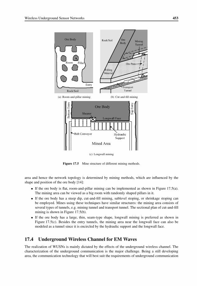
Wireless Underground Sensor Networks 453
Pillar
Ore Body
Entry
Room
Rock/Soil
(a) Room-and-pillar mining (b) Cut-and-fill mining
(c) Longwall mining
Figure 17.5 Mine structure of different mining methods.
area and hence the network topology is determined by mining methods, which are influenced by theshape and position of the ore body [14]:
• If the ore body is flat, room-and-pillar mining can be implemented as shown in Figure 17.5(a).The mining area can be viewed as a big room with randomly shaped pillars in it.
• If the ore body has a steep dip, cut-and-fill mining, sublevel stoping, or shrinkage stoping canbe employed. Mines using these techniques have similar structures: the mining area consists ofseveral types of tunnels, e.g. mining tunnel and transport tunnel. The sectional plan of cut-and-fillmining is shown in Figure 17.5(b).
• If the ore body has a large, thin, seam-type shape, longwall mining is preferred as shown inFigure 17.5(c). Besides the entry tunnels, the mining area near the longwall face can also bemodeled as a tunnel since it is encircled by the hydraulic support and the longwall face.
17.4 Underground Wireless Channel for EM WavesThe realization of WUSNs is mainly dictated by the effects of the underground wireless channel. Thecharacterization of the underground communication is the major challenge. Being a still developingarea, the communication technology that will best suit the requirements of underground communication

454 Wireless Sensor Networks
remains to be investigated. However, EM wave propagation through soil and rock has been studiedextensively with ground-penetrating radar in the past [9, 23, 43, 44]. Moreover, existing sensor motesutilize EM waves almost exclusively. Hence, the characteristics of EM waves in soil are of particularimportance for the realization of WUSNs. In this section, we describe the properties of the undergroundEM channel, the effect of various soil properties on this channel, and the underground wireless channelmodel in detail.
17.4.1 Underground Channel Properties
Underground communication is significantly different and challenging when compared to its terrestrialcounterpart. This is mainly because of the close interaction of the soil with communication performance.In the following, five main factors that impact communication with EM waves underground are identi-fied. These factors are extreme path loss, reflection/refraction, multi-path fading, reduced propagationvelocity, and noise:
• Extreme path loss: Path loss due to material absorption is a major concern when using EM wavesfor underground communication. Path loss for underground communication is determined by boththe frequency of the wave and the properties of the soil or rock through which it propagates. Animportant distinction to communication through air is that underground path losses are highlydependent on the soil type and water content. Soils are generally classified according to the sizeof their particles. In declining order of size they are sand, silt, and clay, or a mixture thereof [9].Sandy soils are generally more favorable to EM wave propagation than clay soils. In additionto the soil composition, the soil-water content also significantly affects the attenuation. Morespecifically, any increase in soil-water content will produce a significant increase in attenuation.
In addition to soil composition and condition, operating frequency is another factor that affectspath loss. In general, over a given distance and soil condition, lower frequencies propagateunderground with less attenuation than higher frequencies. Even frequencies in the megahertzrange may experience attenuation on the order of over 100 dB/m depending on the soil conditions.
• Reflection/refraction: The soil–air interface introduces reflection and refraction because of thedifferent attenuation characteristics of soil and air. WUSN devices deployed near the surfaceare able to communicate with both underground and surface devices, e.g., a surface sink, usinga single radio. This implies that a communication link partially underground and partially inthe air is necessary. When the propagating EM wave reaches the ground–air interface, it willbe partially reflected back into the ground and partially transmitted into the air. The reverse istrue for transmissions from surface devices to underground devices. Furthermore, devices thatare deployed close to the surface encounter changes in the received power even if they are bothdeployed underground. This is because of the reflected signal from the surface. Consequently,two main paths are formed for communication, referred to as the two-path channel model.The reflected signal may improve or impair the communication performance depending on thedistance between two entities and the deployment depth.
• Multi-path fading: The same mechanism described previously, whereby waves at mediumtransitions are partially transmitted and partially reflected, will also cause multi-path fading. Thiseffect will especially be pronounced for sensors deployed near the surface, where the wave isclose to the ground–air interface. Scattered rocks and plant roots underground, as well as varyingsoil properties, will act as scatterers and also produce fading.
• Reduced propagation velocity: EM waves propagating through a dielectric material such as soiland rock will experience a reduced propagation velocity compared to that of air. Since most soilshave dielectric constants in the range of 1–80, a minimum propagation velocity of about 10% ofthe speed of light is implied.

Wireless Underground Sensor Networks 455
• Noise: Even the underground channel is not immune to noise. On the contrary, undergroundnoise levels are close to the noise levels encountered in the air [3]. Sources of undergroundnoise include power lines, lightning, and electric motors [41]. Additionally, atmospheric noiseis present underground [27, 41]. However, underground noise is generally limited to relativelylow frequencies (below 1 kHz).
The above properties of the underground channel are also highly dependent on the soil propertiesbetween the transmitter and receiver. Therefore, a thorough understanding of how various soil parametersaffect the channel is necessary.
17.4.2 Effect of Soil Properties on the Underground Channel
The underground wireless channel is characterized by the direct influence of soil properties onunderground communication. This influence can be directly seen through the changes in attenuation ofan EM signal passing through the soil, which dictates the path loss between two communicating entities.The composition of a soil, and its volumetric water content, particle sizes, density, and temperature,combine to form its complex dielectric constant ε. This parameter directly affects the attenuation of anyEM wave passing through the soil, and it is thus useful to be able to predict its value. We now discuss indetail the effects of these and other parameters on signal attenuation:
• Volumetric water content: The moisture in the soil is by far the most significant factor thataffects signal loss through soil. The moisture in the soil is usually referred to as the volumetricwater content of the soil. Any increase in the volumetric water content will significantly increasethe attenuation. As an example, when the volumetric water content rises from dry to 13% fora particular type of soil, the path loss increases by about 137 dB/m [44]. The effect of a rise involumetric water content is also dependent on the type of soil. More specifically, sandy soils showless attenuation as water content increases than do clay soils [23]. As an example, at 900 MHzsandy and clay soils result in a propagation loss of 20 and 50 dB/m, respectively, with 40%volumetric water content [23].
• Particle size: In addition to the volumetric water content, soil composition is another factor thataffects the communication performance. Soils are classified by the diameter of their particles,and are generally described as some variation of sand, silt, or clay. Sandy soils produce the leastamount of loss and clay soils the most [23]. In addition, different soil particle types responddifferently to changes in water content. Furthermore, increasing soil density increases path loss:the denser the soil, the greater the signal attenuation.
• Temperature: Increasing the temperature of soil changes its dielectric properties and willincrease signal attenuation [9]. Additionally, changes in temperature will affect the dielectricproperties of any water present in the soil.
In addition to the properties of soil, attenuation through soil is also dependent on the frequencybeing used. Lower frequencies experience less attenuation at a given volumetric water content thanhigher frequencies. Consequently, depending on the soil type and the volumetric water content, differentoperating frequencies can be used in WUSNs. These properties are summarized in Table 17.1.
17.4.3 Soil Dielectric Constant
The soil dielectric constant, ε, is the key factor that binds the effects of soil characteristics with theattenuation of a wave. A major challenge for predicting attenuation in an underground link is to computethe dielectric constant of the soil in which the WUSN devices are deployed. Several models are availablefor accurately predicting the complex dielectric constant, ε, for a homogeneous soil sample. However,

456 Wireless Sensor Networks
Table 17.1 Soil properties and their effect on signalattenuation.
Effect on signalParameter Change attenuation
Water content
Temperature
Soil bulk density
% Sand
% Clay
predicting path losses for an underground channel is a challenge due to the inhomogeneous nature ofground. Soil makeup, density, and water content can all vary drastically over short distances [40].
In this section, we describe the Peplinski model [30], which associates key soil properties such asvolumetric water content, density, and particle size with the rate of signal attenuation by the soil. ThePeplinski model was constructed by taking measurements over a range of frequencies and for a variety ofdifferent soils and soil-water contents. Slightly different versions of the model are used for 0.3–1.3 GHzand 1.4–18 GHz. Both take as parameters the frequency, volumetric water content, bulk density, specificdensity of solid soil particles, mass fractions of sand and clay, and temperature.
Using the Peplinski model [30], the dielectric properties of soil in the 0.3–1.3 GHz band can becalculated as follows:
ε = ε′ − jε′′, (17.1)
ε′ = 1.15
[1+ ρb
ρs(εα
′s )+mβ
′v ε′α′fw−mv
]1/α′− 0.68, (17.2)
ε′′ = [mβ ′′v ε′′α′fw]1/α′, (17.3)
where εm is the relative complex dielectric constant of the soil–water mixture, mv is the water volumefraction (or volumetric water content) of the mixture, ρb is the bulk density in grams per cubic centimeter,ρs = 2.66 g/cm3 is the specific density of the solid soil particles, α′ = 0.65 is an empirically determinedconstant, and β ′ and β′′ are empirically determined constants dependent on soil type and given by
β′ = 1.2748 − 0.519S − 0.152C, β′′ = 1.33797 − 0.603S − 0.166C, (17.4)
where S and C represent the mass fractions of sand and clay, respectively. The quantities ε′fw
and ε′′fw
are the real and imaginary parts of the relative dielectric constant of free water. The Peplinski model [30]governs the value of the complex propagation constant of the EM wave in soil, which is given as γ =α + jβ, where
α = ω
√√√√µε′2
[√1+
(ε′′ε′)2− 1
], β = ω
√√√√µε′2
[√1+
(ε′′ε′)2+ 1
]; (17.5)
here ω = 2πf is the angular frequency, µ is the magnetic permeability, and ε′ and ε′′ are the real andimaginary parts of the dielectric constant as given in (17.2) and (17.3), respectively.

Wireless Underground Sensor Networks 457
From the above equations, it can be seen that the complex propagation constant, γ , of the EM wavein soil is dependent on the operating frequency, the composition of soil in terms of sand, silt, and clayfractions, the bulk density, and the volumetric water content. These factors also influence undergroundsignal propagation as we will describe next.
17.4.4 Underground Signal Propagation
The unique characteristics of signal propagation in soil necessitate the derivation of path loss consideringthe properties of soil. The Friis equation [36] characterizes the received signal strength in free space at adistance r from the transmitter as
Pr = Pt +Gr +Gt − L0 (17.6)
where Pt is the transmit power, Gr and Gt are the gains of the receiver and transmitter antennae, andL0 is the path loss in free space in dB. The path loss in free space, L0, is given by
L0 = 32.4 + 20 log(d)+ 20 log(f ) (17.7)
where d is the distance between the transmitter and the receiver i km, and f is the operating frequencyin MHz.
For the propagation in soil, a correction factor should be included in the Friis equation (17.6) toaccount for the effect of the soil medium. As a result, the received signal is
Pr = Pt +Gr +Gt − Lp (17.8)
where Lp = L0 + Ls , and Ls stands for the additional path loss caused by the propagation in soil. Ls iscalculated by considering the following differences of EM wave propagation in soil compared to that inair. The additional path loss, Ls , in soil is composed of two components:
Ls(dB)= Lβ + Lα (17.9)
where Lβ is the attenuation loss due to the difference between the wavelength of the signal in soil, λ, andthe wavelength in free space, λ0, and Lα is the transmission loss caused by attenuation. Consequently,
Lβ(dB)= 20 log
(λ0
λ
). (17.10)
Considering that, in soil, the wavelength is λ= 2π/β and in free space λ0 = c/f , where β is the phaseshifting constant, c = 3× 10⁸ m/s, and f is the operating frequency, Then Lβ becomes
Lβ = 154 − 20 log(f )+ 20 log(β). (17.11)
The second component in (17.9), Lα , can be represented by considering the transmission loss causedby the attenuation constant, α, as Lα = e2αd . In dB, Lα is given by
Lα = 8.69αd. (17.12)
Given that the path loss in free space is L0 = 20 log(4πd/λ0), the path loss of an EM wave in soil isfound by combining L0, (17.11), and (17.12) as follows:
Lp = 6.4+ 20 log(d)+ 20 log(β)+ 8.69αd (17.13)
where distance, d, is given in meters, the attenuation constant, α, is in 1/m, and the phase shiftingconstant, β, is in rad/m. The path loss, Lp in (17.13), depends on the attenuation constant, α, and thephase shifting constant, β. The values of these parameters depend on the dielectric properties of soil,which are derived in Section 17.4.3. The path loss, Lp , in soil can be found by using (17.1)–(17.5)in (17.13).

458 Wireless Sensor Networks
0.5 1 1.5 2 2.5 3 3.5 4 4.5 520
40
60
80
100
120
140
Pat
h Lo
ss (
dB)
Distance (m)
300MHz400MHz500MHz600MHz700MHz
(a)
0.2 0.3 0.4 0.5 0.6 0.7 0.8 0.9 120
40
60
80
100
120
140
160
Pat
h Lo
ss (
dB)
Frequency (GHz)
5%10%15%20%25%Free space
(b)
Figure 17.6 Path loss vs. (a) internode distance and operating frequency, and (b) operating frequency and soilmoisture.
EXAMPLE 17.1
Consider a site where the volumetric water content is 5%, the sand particle percentage is 50%,the clay percentage is 15%, the bulk density is 1.5 g/cm3, and the solid soil particle density is2.66 g/cm3. Accordingly, we evaluate the path loss in (17.13) to observe the relationship betweenpath loss and various parameters.
In Figure 17.6(a), path loss, Lp, in (17.13) is shown in dB versus distance, d, for differentvalues of operating frequency, f , varying from 300 to 900 MHz. It can be seen that the distancehas an important effect on path loss and the path loss increases with increasing distance d asexpected. Moreover, increasing operating frequency f also increases path loss, which motivatesthe need for lower frequencies for underground communication.
Next, the influence of soil moisture, i.e., volumetric water content, is shown in Figure 17.6(b),for values of 5%–25%. The difference between propagation in soil and that in free space is alsoevident in Figure 17.6(b). Since the attenuation significantly increases with higher water content,an increase of 30 dB is possible with a 20% increase in soil.
The significant effect of soil moisture on attenuation is particularly important since water contentnot only depends on the location of the network, but also varies during different seasons. Hence,network deployment, operation, and protocol design of WUSNs should consider this dynamic natureof the underground channel. The characteristics of path loss in soil constitute an important part ofcommunication in soil. However, besides the attenuation in soil, various channel effects influencethe performance of wireless communication. Multi-path spreading and fading are among the effectsthat should be considered. Moreover, the depth of the sensor nodes significantly affects the channelcharacteristics.
Next, the features of the underground channel are described in two main topics. Firstly, the effect ofreflection from the ground surface on path loss is analyzed in Section 17.4.5. Secondly, the multi-patheffects are described using a Rayleigh channel model and the bit error rate is derived for the undergroundwireless channel in Section 17.4.6.
17.4.5 Reflection from Ground Surface
The soil–air interface results in the waves being reflected from the ground surface. Hence, in general,underground communication results in two main paths for signal propagation as shown in Figure 17.7.

Wireless Underground Sensor Networks 459
H1 H2
d
r1
P L2
r2r
L1
Sensor 1 Sensor 2
L
Figure 17.7 Illustration of the two-path channel model.
The first path is the direct path between two sensors and the second path is the reflection path due to theground surface. While the direct path constitutes the main component of the received signal, the reflectedpath also affects communication, especially when the sensors are buried close to the surface. As a result,the signal propagation in the soil is also affected by these reflected rays in addition to the attenuation.Although this effect is mainly dependent on the depth of the sensors in soil, it should be considered inlow depths as we explain next.
If the sensors are buried near the surface of the ground, i.e., low depth, the influence of the wavereflected by the ground surface should be considered. For such a reflection, the total path loss of thetwo-path channel is given by
Lf (dB)= Lp(dB)− VdB, (17.14)
where Lp is the path loss due to the direct path as given in (17.13) and VdB is the attenuation factor dueto the second path in dB, i.e., VdB = 10 log V .
Consider the case where two sensors are buried at a depth of H1 and H2, respectively, at a horizontaldistance of L, and an end-to-end distance of d as illustrated in Figure 17.7. Then, the attenuation factor,V , can be found as follows:
V 2 = 1+ [� · exp(−α�(r))]2
− 2� exp(−α�(r)) cos
(π −
(φ − 2π
λ�(r)
))(17.15)
where � and φ are the amplitude and phase angle of the reflection coefficient at the reflection point P,�(r)= r − d is the difference of the two paths, and α is the attenuation constant mentioned before.
EXAMPLE 17.2
Consider a deployment where two sensors are buried at the same depth, i.e., H1 =H2 =H , andhence d = L. Using (17.15) in (17.14), the path loss can be found as a function of end-to-enddistance, d, operating frequency, f , buried depth, H , and volumetric water content.
In Figure 17.8(a), the path loss is shown as a function burial depth, H , for various values ofoperating frequency, f . It can be observed that, for the two-path model, the effect of operatingfrequency, f , is significant and mainly depends on the buried depth, H . For a particular operatingfrequency, an optimum buried depth exists such that the path loss is minimized. The effect offrequency and the volumetric water content is also shown in Figure 17.8(b), where the path lossfluctuates according to both parameters. This fluctuation is due to constructive or destructiveinterference from the second path based on the operating frequency and the volumetric watercontent.

460 Wireless Sensor Networks
0 0.2 0.4 0.6 0.8 1 1.2 1.4 1.6 1.8 280
90
100
110
120
130
140
Pat
h Lo
ss (
dB)
Depth (m)
300MHz
400MHz
500MHz
600MHz
700MHz
(a)
510
1520
25
0.2
0.4
0.6
0.8
180
90
100
110
120
130
140
150
Volumetric Water Content (%)Frequency (GHz)
Pat
h lo
ss (
dB)
(b)
Figure 17.8 Two-path channel model: path loss vs. (a) depth for different operating frequencies, (b) operatingfrequency, f , and volumetric water content.
The underground channel model can be classified into two according to the buried depth of thesensors. If this depth is larger than a certain value, i.e., high depth, the effect of reflection is negligibleand the channel is modeled through the single path model. In this case, the path loss is given in(17.13) as described in Section 17.4.4. More specifically, the underground channel exhibits a single pathcharacteristic when the buried depth is higher than a threshold value. The results shown for Example 17.2in Figure 17.8 reveal that if the buried depth is more than 2 m, the influence of reflection is negligibleand single path model should be used. On the other hand, for low-depth deployments (H ≤ 2 m),communication is modeled through the two-path channel model. In this case, the path loss is givenin (17.14).
17.4.6 Multi-path Fading and Bit Error Rate
The two-path channel model captures the main propagation characteristics of EM waves underground.However, in fact, the underground channel exhibits additional complications. Firstly, the surface of theground is not ideally smooth and, hence, causes not only reflection, but also refraction. Secondly, usuallythere are rocks or plant roots in soil and the clay of soil is generally not homogeneous. As a result ofthese impurities in the soil, multiple copies of the same signal can be reflected from these obstaclesand received at the receiver. Hence, multi-path fading should also be considered in addition to the basictwo-path channel model.
Multi-path fading has been explained in Chapter 4 for communication through air, where the randomrefraction due to air, the movement of objects, as well as other random effects result in the fluctuationand refraction of EM waves. Therefore, the amplitude and phase of the received signal exhibit randombehavior with time. Generally, this multi-path channel character obeys the Rayleigh or log-normalprobability distribution [45].
In underground communication, on the other hand, there is no random air refraction with time. Thisis because the channel between two transceivers is relatively stable when the composition of soil isconsidered. Hence, the channel is almost stable in each path with respect to time. On the other hand,considering a fixed internode distance, the received signal levels vary at different locations because thesignal travels through different multiple paths. As a result, randomness is due to the locations of the nodesrather than time, which still obeys the Rayleigh probability distribution. Accordingly, the envelope of thesignal from each path is modeled as an independent Rayleigh distributed random variable, χi, i ∈ {1, 2}.

Wireless Underground Sensor Networks 461
Consequently, for the one-path model, the received energy per bit per noise power spectral density isgiven by r = χ2Eb/N0, which has a distribution as follows:
f (r)= 1
r0exp(r
r0
)(17.16)
where r0 = E[χ2]Eb/N0 and Eb/N0 are directly related to the signal-to-noise ratio (SNR) of thechannel.
Similarly, for the two-path model, a two-path Rayleigh channel is used, where χ in this channel is
χ2 = χ21 + [χ2 · � · exp(−α�(r))]2 − 2χ1χ2� exp(−α�(r)) cos
(π −
(φ − 2π
λ�(r)
))(17.17)
where χ1 and χ2 are two independent Rayleigh distributed random variables of the two paths,respectively. � and φ are the amplitude and phase angle of the reflection coefficient at the reflectionpoint P, �(r)= r − d is the difference of the two paths, and α is the attenuation constant.
Based on the above model, the bit error rate (BER) characteristics of the underground channel aredescribed next. Assuming 2PSK as the modulation method, the BER can be shown to be
BER= 1
2erfc(√
SNR) (17.18)
where erfc(·) is the error function and SNR is given by
SNR= Pt − Lf − Pn (17.19)
where Pt is the transmit power, Lf is the total path loss given in (17.14), and Pn is the energy of thenoise. The transmit power, Pt , is usually between 10 and 30 dBm and the noise level, Pn, is found to be−103 dBm on average [3]. Although the noise, Pn, may change depending on the properties of the soil,this value is a representative value that can be used to show the properties of the BER underground.
EXAMPLE 17.3
Using (17.14) and (17.19) in (17.18), the BER is shown in Figure 17.9 for the single path modeland in Figure 17.10 for the two-path model. The effect of transmit power, Pt , on the BER isshown in Figure 17.9(a). As the transmit power increases, the BER decreases. Moreover, as shownin Figure 17.9(b), an increase from 5% to 10% in volumetric water content results in almost anorder of magnitude increase in the BER, which significantly affects the effective communicationrange of a sensor.
As explained earlier, for buried depths of less than 2 m, the two-path Rayleigh fading modelis suitable for WUSNs. In Figure 17.10, the effect on the BER of the reflected path from theground surface can be clearly seen. As shown in Figure 17.10(a), the communication distance canbe extended to 4.5–5 m with increased transmit power of 30 dBm and low operating frequency at400 MHz.
As discussed in Section 17.4.5 and shown in Figure 17.8(a), the path loss is significantlyaffected by the buried depth of sensors. This fluctuation also results in varying BER values asshown in Figure 17.10(b). As the buried depth increases, the fluctuations decrease and the BERbecomes more stable. These results reveal that for a particular operating frequency, there is anoptimal depth for communication where the BER is a minimum. Finally, the effect of volumetricwater content in the two-path model is shown in Figure 17.10(c). Compared to the single pathmodel results shown in Figure 17.9(b), higher volumetric water content is acceptable when theoperating frequency is low. Another observation is that for a particular volumetric water contentvalue, the BER fluctuates with changing frequency, contrary to the single path case. This isbasically because the reflection from the ground surface depends greatly on the frequency ofthe signal.

462 Wireless Sensor Networks
0 1 2 3 4 5 6 7 810
–6
10–5
10–4
10–3
10–2
10–1
100
Bit
Err
or R
ate
Distance (m)
10dBm15dBm20dBm25dBm30dBm
(a)
0.2 0.3 0.4 0.5 0.6 0.7 0.8 0.9 110
–4
10–3
10–2
10–1
100
Bit
Err
or R
ate
Frequency (GHz)
5%
10%
15%
20%
25%
(b)
Figure 17.9 One-path channel model: BER vs. (a) internode distance with different transmit power, (b) operatingfrequency, f , and volumetric water content.
0 1 2 3 4 5 6 7 810
–6
10–5
10–4
10–3
10–2
10–1
Bit
Err
or R
ate
Distance (m)
10dBm15dBm20dBm25dbm30dBm
(a)
0 0.5 1 1.5 210
–6
10–5
10–4
10–3
10–2
10–1
Bit
Err
or R
ate
Depth (m)
400MHz500MHz700MHz
(b)
0.2 0.3 0.4 0.5 0.6 0.7 0.8 0.9 110
–6
10–5
10–4
10–3
10–2
10–1
100
Bit
Err
or R
ate
Frequency (GHz)
5%10%15%20%25%
(c)
Figure 17.10 Two-path channel model: BER vs. (a) internode distance with different transmit power, (b) depth, h,and different operating frequencies, and (c) operating frequency and volumetric water content.

Wireless Underground Sensor Networks 463
17.5 Underground Wireless Channel for Magnetic InductionTraditional signal propagation techniques using EM waves encounter three major problems in the soilmedium: high path loss, dynamic channel condition, and large antenna size [3]. Firstly, EM wavesexperience high levels of attenuation due to absorption by soil, rock, and water. Secondly, the pathloss is highly dependent on numerous soil properties such as water content, soil makeup (sand, silt,or clay), and density. In addition, the path loss can change dramatically with time and space. As anexample, the soil-water content increases after rainfall and the soil properties may significantly changeover short distances. Therefore, the BER of the communication system also varies as a function of timeand location. Thirdly, operating frequencies in the megahertz or lower ranges are necessary to achievepractical transmission range [2]. To efficiently transmit and receive signals at that frequency, the antennasize would be too large to be deployed in the soil.
An alternative signal propagation technique for underground wireless communication is magneticinduction (MI). The MI techniques effectively address the dynamic channel condition and large antennasize challenges of the EM wave techniques. In particular, a dense medium such as soil and watercauses small variations in the attenuation rate of magnetic fields compared to that of air, since themagnetic permeabilities of the soil and air are similar [2, 16, 34]. Therefore the MI channel conditionsremain constant in the soil medium. Moreover, in the MI communication, transmission and reception areaccomplished with the use of a small coil of wire. Therefore, the antenna size is not a major limitation forMI techniques. However, the main challenge of MI-based communication is the attenuation: magneticfield strength falls off much faster than the EM waves [4, 5].
In this section, we first describe the path-loss expressions for the underground MI communicationchannel. Multiple factors are considered in the analysis, including the soil properties, coil size, thenumber of turns in the coil loop, coil resistance, and the operating frequency. In addition, we showhow the high path loss can be reduced to extend the transmission range through MI waveguidetechniques [37]. The MI waveguide has three advantages in underground wireless communication.Firstly, by carefully designing the waveguide parameters, the path loss can be greatly reduced. Secondly,the relay coils constituting the MI waveguide do not consume any energy and the cost is very small.Thirdly, the MI waveguide is not a continuous structure like a real waveguide, hence it is relativelyflexible and easy to deploy and maintain.
17.5.1 MI Channel Model
Transmission and reception in MI communication are accomplished with the use of a coil of wire,as shown in Figure 17.11(a), where at and ar are the radii of the transmission coil and receiving coil,respectively, r is the distance between the transmitter and the receiver, and (90◦−α) is the angle betweenthe axes of two coupled coils. Accordingly, the path loss for MI communication is [37]
Pr
Pt� ω
2µ2NtNra3t a
3r sin2 α
8r6· 1
4R0(2R0 + 12jωµNt )
(17.20)
where Nt and Nr are the number of turns of the transmitter coil and receiving coil, respectively, R0 isthe resistance of a unit length of the loop, µ is the permeability of the medium (i.e., soil), and ω is theangular frequency of the transmitted signal. If the low-resistance loop, the high signal frequency, and thelarge number of turns are employed (ωµNt � R0), then the ratio can be further simplified:
Pr
Pt� ωµNra
3t a
3r sin2 α
16R0r6
. (17.21)
According to (17.21), the received power loss is a sixth-order function of the transmission range r .A higher signal frequency ω, larger number of turns N , lower loop resistance R0, and larger coil size a

464 Wireless Sensor Networks
a αta
rr
Transmittercoil
Receivercoil
(a) MI system
a
r
Transmitter Receiver
...
RelayPoints
d
(b) MI waveguide system
Figure 17.11 The structure of the MI transceiver and the MI waveguide.
can increase the received power. The angle between the axes of two coupled coils also affects the receivedpower. Specifically, the smaller the angle, the higher the power received. An important characteristic ofMI communication is that the received power is not affected by the environmental conditions. The onlyparameter related to the environment for the received power is the permeability, µ, in (17.21). Moreover,the permeability, µ, of soil and water is similar to that of air.
The expression of the path loss in (17.21) can be further compared to the Friis transmission equationfor the EM wave communication, where
Pr
Pt�GtGr
(λ
4πr
)2=GtGr π
4µεω2r2. (17.22)
For EM waves, a higher operating frequency results in a greater path loss. On the other hand, for MI, anincreased frequency leads to a lower attenuation rate. However, the received power of MI communicationattenuates much faster than in the EM wave case (1/r6 vs. 1/r2). Moreover, the permittivity ε in (17.22)is much larger in soil than in air. Furthermore, ε varies greatly at different times and locations. Hence, thepath loss of EM waves is dramatically influenced by these environmental conditions. Accordingly, theMI technique has constant channel condition while the EM wave technique results in lower attenuation.
17.5.2 MI Waveguide
The MI techniques provide advantages over the EM wave techniques in terms of less dependency on theenvironment and antenna size. However, the received power loss is much higher than in the EM wavecase. For practical applications, this can be addressed by employing relay points between the transmitterand receiver.
Contrary to the relay points used for EM waves, the MI relay point is a simple coil without anyenergy source or processing device. This results in a passive operation for the relay points, where thecommunication is performed without any external power source. The sinusoidal current in the transmittercoil induces a sinusoidal current in the first relay point. This sinusoidal current in the relay coil theninduces another sinusoidal current in the second relay point. This continues until the destination isreached. The consecutive relay coils form an MI waveguide in underground environments, which acts asa waveguide to guide the so-called MI waves.
A typical MI waveguide structure is shown in Figure 17.11(b), where n relay coils are equally spacedalong one axis between the transmitter and receiver, r is the distance between the neighbor coils, d isthe distance between the transmitter and receiver, and d = (n+ 1)r where a is the radius of the coils.In fact, there exists mutual induction between any pair of the coils. The value of the mutual inductiondepends on how close the coils are to each other. For the MI waveguide model developed in this section,the distance between two relay coils is considered as 1 m and the coil radius is no more than 0.1 m.Therefore, the coils are sufficiently far from each other and only interact with their nearest neighbors.Hence, only the mutual induction between the adjacent coils needs to be taken into account.

Wireless Underground Sensor Networks 465
The path loss of the MI waveguide is given as [37]
Pr
Pt� ω
2µ2N2a6
8r61
4R0(2R0 + 12jωµN)
·[
j
4R0ωµN
( ra )3 + j ( ra )3 + ωµN
4R0+jωµN (ar )
3
]2n. (17.23)
Considering the high signal frequency and large number of turns employed (ωµN � R0), (17.23) canbe further simplified to
Pr
Pt� ωµN
16R0
(a
r
)6n= ωµN
16R0
[a
d(n+ 1)
]6n. (17.24)
It is shown in (17.24) that the transmission range d is divided into n+ 1 intervals with length r .However, the path loss becomes a 6nth-order function of the relay interval r . Hence, to reduce the pathloss of the MI waveguide, the relay interval r needs to be on a par with the coil size to make the term a/r
approximately 1. This means that if the coils with a radius of 0.1 m are utilized, these coils should bedeployed every 0.1 m, which is infeasible in underground communication considering the deploymentchallenges. Consequently, using simple relay coils does not effectively reduce the path loss.
From (17.23), if the last term with exponent 2n is made to converge to a value around 1, then the MIwaveguide path loss can be considerably reduced. This can be accomplished by adding a capacitor toeach coil and determining the capacitor value, the operating frequency, and the number of turns in thecoil to decrease the path loss. By assigning the capacitor C an appropriate value, the self-induction termcan be neutralized. Then, the term with exponent 2n can be significantly diminished. More specifically,if the value of the capacitor C is selected as
C = 2
ω2N2µπa(17.25)
then the MI waveguide path loss becomes
Pr
Pt= ω2µ2N2a6/4r6
2R0[4R0 + (ω2µ2N2a6)/(2R0 · 4r6)] ·[
j
4R0ωµN
( ra )3 + ωµN
4R0( ar )
3
]2n. (17.26)
Moreover, the operating frequency and the number of turns can be designed to further reduce the pathloss such that
ωµN
4R0
(a
r
)3= 1, (17.27)
and finally the path loss can be represented as
Pr
Pt= 1
3
(1
2
)2n. (17.28)
As shown in (17.28), the path loss for the MI waveguide path loss is considerably smaller than that forthe traditional MI and EM wave techniques. The path loss is a function of the number of relay points, n.Larger n results in higher path loss and is usually determined from the transmission distance d and therelay interval r . The value of r should be chosen as large as possible considering the constraints in (17.25)and (17.27). More specifically, in (17.27), the relay interval, r , and the coil size, a, both determine theoperating frequency, ω, and the number of turns, N . In (17.25), the capacitor value C is determined bya, N , and ω. Hence, when designing the relay interval, it should be ensured that the operating frequency,the number of turns, and the capacitor value can be assigned feasible and appropriate values. If theoperating frequency is considered to be several hundred megahertz and the coil radius is 0.1 m, the relayinterval of 1 m can be chosen to satisfy these requirements.

466 Wireless Sensor Networks
17.5.3 Characteristics of MI Waves and MI Waveguide in Soil
The comparison of the path loss for the traditional EM wave technique, the current MI technique, and theimproved MI waveguide technique for wireless underground communication is important in evaluatingthe characteristics of these techniques. In this section, we compare the techniques based on the followingconditions: the volumetric water content (VWC) is 5% and the operating frequency is 300 MHz. Thetransmitter, receiver, and relay coil all have the same radius of 0.1 m. The coil is made of copper wirewith a 0.5 mm diameter, hence the resistance of unit length R0 is 0.216�/m. The permeability of thesoil medium is the same as that in air, which is 4π × 10−7 H/m. The relay interval r of the MI waveguideis 1 m. The number of relay coils n is determined by the transmission distance d, where n= d/r�. Thecoil capacity is calculated by (17.25), which is around 20 pF.
Low Operating Frequency and Low VWC
In Figure 17.12(a), the path loss for the three techniques is shown in dB versus the transmission distanced using a 300 MHz signal in soil with 5% VWC. It can be seen that in the very near region (d < 1 m),the path loss of the MI technique is smaller than that of the EM wave technique. However, for longerdistances, the MI signal attenuates much faster than the EM wave signal. The difference is as high as20 dB compared to the EM wave signal. On the other hand, the MI waveguide technique reduces thesignal path loss compared to the other two techniques. Accordingly, the path loss of the MI waveguidesystem is less than 50% of the MI and EM wave cases at a certain range.
High Operating Frequency and Low VWC
In Figure 17.12(b), the VWC of the soil remains the same but the operating frequency is increased to900 MHz. The path loss of the EM wave system increases slightly. Since material absorption is themajor part of EM wave path loss in soil, the attenuation caused by the higher operating frequency isnot significant. On the other hand, the path loss of the MI system decreases as the operating frequencyincreases, which can be explained through (17.21), where the operating frequency ω is in the numerator.As a result, at high operating frequency, the path loss of the EM wave system becomes higher than thatof the MI system. The path loss of the MI waveguide system remains the lowest when a high operatingfrequency is used.
Low Operating Frequency and High VWC
In Figure 17.12(c), the influence of the VWC on the three propagation techniques is analyzed. Theperformance of the MI and MI waveguide systems is not affected by the environment since thepermeability µ remains the same between air, water, or the soil media. According to the channel modeldescribed in Section 17.4, the path loss of the three techniques in soil with a higher water content (25%VWC) is as shown in Figure 17.12(c). As expected, the path loss of the MI and MI waveguide systemsremains the same. However, the path loss of the EM wave system increases dramatically (up to 40 dB)in soil with a higher water content.
17.6 Wireless Communication in Mines and Road/Subway TunnelsIn addition to communication through soil with EM and MI techniques, WUSNs can also be deployedin underground cavities such as mines or tunnels. As explained in Section 17.3.2, different forms ofunderground structures exist. Accordingly, the wireless communication channels can be classified intotwo. The tunnel channel model is used to describe signal propagation in passageways and miningarea tunnels. The room-and-pillar channel model characterizes the wireless channel of room-and-pillar

Wireless Underground Sensor Networks 467
0 1 2 3 4 5 60
20
40
60
80
100
120
140
160
Path
Loss (
dB
)
Distance (m)
300 MHz; 5% VWC
EM Wave
MI
MI Waveguide
(a) 300 MHz signal in soil with 5% VWC
0 1 2 3 4 5 60
20
40
60
80
100
120
140
160
Path
Loss (
dB
)
Distance (m)
900 MHz; 5% VWC
EM Wave
MI
MI waveguide
(b) 900 MHz signal in soil with 5% VWC
0 1 2 3 4 5 60
20
40
60
80
100
120
140
160
180
Path
Loss (
dB
)
Distance (m)
300 MHz; 25% VWC
EM Waves
MI
MI Waveguide
(c) 300 MHz signal in soil with 25% VWC
Figure 17.12 Path loss of the three techniques using different operating frequency in soil with different VWC.
mining area [38]. The structure of the road/subway tunnels is similar to that of underground mine tunnelsand can be captured through the tunnel channel model.
In this section, we describe channel models for the tunnel and room-and-pillar environments throughthe multimode model, which lays out the foundations for reliable and efficient communication networksin mines and road tunnels [38]. For the tunnel environment, the multimode model can completelycharacterize the natural wave propagation in both near and far regions of the transmitter. For the room-and-pillar environment, the multimode model is combined with the shadow fading model to characterizethe random effects of the pillars in underground mines. The channel models for these two environmentsare explained in the following.
17.6.1 Tunnel Environment
The multimode model is a multimode operating waveguide model which exploits the GO channelmodel [22] to analyze the EM field distribution in a tunnel cross-section. This field distribution canbe considered as the weighted sum of the fields of all modes. Hence, the intensity of each mode isestimated by a mode-matching technique. Once the mode intensity is determined in the excitation plane,the propagation of each mode is mostly governed by the tunnel itself. Hence the EM field of the rest ofthe tunnel can be accurately predicted by summing the EM field of each mode.

468 Wireless Sensor Networks
4a
4b
I-2,3
I-2,2
I-2,1
I-2,0
I-2,-1
I-2,-2
I-1,3
I-1,2
I-1,1
I-1,0
I-1,-1
I-1,-2
I0,3
I0,2
I0,1
I0,0
I0,-1
I0,-2
I1,3
I1,2
I1,1
I1,0
I1,-1
I1,-2
I2,3
I2,2
I2,1
I2,0
I2,-1
I2,-2
Figure 17.13 The set of images in the excitation plane in a rectangular tunnel.
Multimode Model
The excitation plane of the EM field of each mode depends on the tunnel cross-section, which is generallyin the shape of a rectangle or a circle. Since the EM field distribution and attenuation of the modes inthe rectangular waveguide are almost the same as the circular waveguide [21], the tunnel cross-sectioncan be treated as an equivalent rectangle. A Cartesian coordinate system is set with its origin located atthe center of the rectangular tunnel. Denoting kv , kh, and ka as the complex electrical parameters of thetunnel’s vertical/horizontal walls and the air in the tunnel, respectively, they are defined as
kv = ε0εv + σv
jω, kh = ε0εh + σh
jω, ka = ε0εa + σa
jω(17.29)
where εv , εh, and εa are the relative permittivities for the vertical/horizontal walls and the air in thetunnel, ε0 is the permittivity in a vacuum, σv , σh, and σa are their conductivities, and ω is the angularfrequency of the signal. The three areas can be considered to have the same permeability µ0. The wavenumber in the tunnel space is given by k = ω√µ0ε0εa . Accordingly, the relative electrical parameterscan be defined as kv = kv/ka and kh = kh/ka for concise expression.
For the field analysis of the excitation plane by the GO model, the transmitter antenna is assumed tobe an X-polarized electric dipole. Moreover, the total field of a point in the excitation plane is equal tothe sum of ray contributions from all reflection images added to that of the source. The reflection imagesare located as shown in Fig 17.13 and have the following properties:
• The ray coming from image Ip,q experiences |p| times reflection from the vertical wall and |q|times reflection from the horizontal wall.
• Suppose that α is the incident angle on the horizontal wall, and β is the incident angle on thevertical wall. Then α and β are complementary. These angles remain the same for all reflectionsof a certain ray.
Considering that the transmitter antenna is located at (x0, y0), the major X-polarized field at thereceiver is then given by
ERxx = ETx
x ·∑p,q
[exp(−jkrp,q)
rp,q
]· S(kv)|p| · R(kh)|q| (17.30)

Wireless Underground Sensor Networks 469
where ETxx and ERx
x are the electric field at the transmitter and receiver, respectively, rp,q is thedistance between image Ip,q and the receiver, and R(kh) and S(kv) are the reflection coefficients onthe horizontal and vertical walls.
The modes in a rectangular tunnel are approximately orthogonal [31, 25], i.e.,
∫ a
−a
∫ b
−bExm,n · Ex
∗j,k dx dy �
{ξ2, if m= j and n= k0, otherwise
(17.31)
where ξ is the norm of the modes. The field of the modes can be viewed as a basis that spans the totalfield. Therefore, the mode intensity Cmn can be calculated by projecting the field of excitation planeobtained by the GO model (ERx
x in (17.30)) on the basis function Exm,n:
Cmn =∫ a
−a
∫ b
−bERxx · Exm,n dx dy (17.32)
which can be viewed as the sum of all the contributions of images: Cmn =∑p,q∈Z C(p,q)mn , where
C(p,q)mn =
∫ a
−a
∫ b
−b
{ETxx ·
exp(−jkrp,q )rp,q
· S(kv)|p| · R(kh)|q| · Exm,n}dx dy. (17.33)
By dividing the absolute mode intensity by the norm of the basis ξ with the field of reference positionEx(r0) (r0 apart from the antenna), then the normalized mode intensity is found as
C(p,q)mn = C
(p,q)mn
ξ · Ex(r0) =C(p,q)mn
ξ · ETxx · exp(−jkr0)/r0
(17.34)
� 1
ξ
∫ a
−a
∫ b
−br0 exp(−jkrp,q )
rp,q + r0 S(kv)|p|R(kh)
|q| · Exm,n dx dy.
The closed-form solution of (17.34) is derived by composite numerical integration, which is given by
C(p,q)mn � 4
3
√ab
mn
m−1∑u=0
n−1∑v=0
{r0 exp(−jkrp,q)
rp,q + r0 S(kv)|p|R(kh)
|q| · (−1)�m+n2 �+1+u+v}. (17.35)
The mode intensity is the summation of all contributions of the images; however, only the low-order images have significant effect. Specifically, for the X-polarized field, only images Ip,q withsubscript p = 0,±1 and q = 0,±1,±2 are considered. In addition, to reduce the computational cost, thereflection coefficients R and S are simplified to their approximate expressions by nonlinear regression.Therefore, the normalized intensity for the mnth-order mode is
Cmn � 4
3
√ab
mn
∑p=0,±1
q=0,±1,±2
{m−1∑u=0
n−1∑v=0
[r0 exp(−jkrp,q)
rp,q + r0 S|p|R|q| · (−1)�m+n2 �+1+u+v]}
(17.36)

470 Wireless Sensor Networks
where
R|q| = (−1)|q| exp
(−2|q| · yq
rp,q
√kh
)
S|p| =
1, if p = 0
1− 2 · 1
1+ (xp/rp,q )√kv
, if p =±1
xp =
∣∣∣∣2pa − x0 + a − 2a
m
(u+ 1
2
)∣∣∣∣, if p is odd∣∣∣∣2pa + x0 + a − 2a
m
(u+ 1
2
)∣∣∣∣, if p is even
yq =
∣∣∣∣2qb − y0 + b − 2b
n
(v + 1
2
)∣∣∣∣, if q is odd∣∣∣∣2qb + y0 + b − 2b
n
(v + 1
2
)∣∣∣∣, if q is even
rp,q =√x2p + y2
q .
Then, the predicted field at any position (x, y, z) inside the tunnel can be obtained by summing thefields of all significant modes at that position, which is given by
ERxx (x, y, z)= Ex(r0)
∑m,n
Cmn · Exm,n(x, y) · e−(αmn+jβmn)·z (17.37)
where αmn is the attenuation coefficient and βmn is the phase-shift coefficient [10, 13, 20]:
αmn = 1
a
(mπ
2ak
)2Re
kv√kv − 1
+ 1
b
(nπ
2bk
)2Re
1√kh − 1
βmn =√k2 −
(mπ
2a
)2−(nπ
2b
)2. (17.38)
Similarly, the predicted received signal power at the coordinate (x, y, z) is given by
Pr(x, y, z)= PtGtGr(
1
2kr0
∑m,n
Cmn · Exm,n(x, y) · exp [−(αmn + jβmn) · z])2
(17.39)
where Pt is the transmit power, and Gt and Gr are the antenna gains of the transmitter and receiver,respectively.
Channel Characteristics
According to the multimode model, the channel characteristics under various tunnel conditions aresummarized next based on the effects of operating frequency, tunnel size and antenna polarization,antenna position, and electrical parameters.

Wireless Underground Sensor Networks 471
0 400 800 1200 1600 2000
-60
-50
-40
-30
-20
-10
0
50%
100%
Axial distance (m)
Receiv
ed p
ow
er (d
B)
Received signal power and power distribution at 500 MHz
Rx Power 500MHz
The first 3 modes
4th to 15th mode
16th to 36th mode
Higher order modes
(a) 500 MHz
0 400 800 1200 1600 2000
-60
-50
-40
-30
-20
-10
0
50%
100%
Axial distance (m)
Receiv
ed p
ow
er (d
B)
Received signal power and power distribution at 1.5 GHz
Rx Power 1.5 GHz
The first 3 modes
4th to 15th mode
16th to 36th mode
Higher order modes
(b) 1.5 GHz
Figure 17.14 The received signal power and the power distribution among modes in tunnels at different operatingfrequencies.
Operating FrequencyThe effects of operating frequency on the channel characteristics are illustrated in Figure 17.14.In particular, in Figure 17.14(a) and Figure 17.14(b) the signal power and the corresponding powerdistribution among significant modes are shown as a function of axial distance at a frequency of 500 MHzand 1.5 GHz, respectively. In the near region, the received power attenuates quickly and fluctuates veryrapidly. This is attributed to the combined effect of multiple modes. On the other hand, in the far region,the decrease in the received power is gradual. This is due to the fact that the higher order modes attenuaterapidly as the distance increases. Hence, the field in the far region is governed by the few remaining low-order modes. Although the operating frequency does not significantly affect the power distribution ofmodes, it has an obvious influence on the propagation constants. Signals with higher frequency attenuateslower. Hence, as frequency increases, the signal attenuation decreases and the length of the rapidlyfluctuating region is increased.
Tunnel Size and Antenna PolarizationThe tunnel size has similar effects on the channel characteristics as the operating frequency. In tunnelswith larger dimensions, the attenuation constant, αmn, is smaller and more modes remain significantin the far region. Therefore, the rapidly fluctuating region is prolonged in larger tunnels, and viceversa. For horizontal polarized antennas, the tunnel width plays a more important role because thereflection coefficients on the horizontal walls are larger than those on the vertical walls. Hence, the signalattenuates slower and fluctuates longer in larger and wider tunnels for horizontally polarized antennas.Meanwhile, in larger and higher tunnels, the power of all the modes decreases slower for verticallypolarized antennas.
Antenna PositionIn Figure 17.15, the received power and the power distribution among modes are shown at differentantenna positions. When the transmitter antenna is placed near the center of the tunnel cross-section,as shown in Figure 17.15(a), the lowest modes are effectively excited (over 50% of the total power). Ifthe receiver is also at the center, both the signal attenuation and the fluctuation are small. If the receiveris placed near the tunnel walls, the attenuation and fluctuation are much more significant as shown inFigure 17.15(b). Near the excitation plane, higher order modes dominate (over 80% of the total power).In this case, the position of the receiver antenna does not affect the received signal.

472 Wireless Sensor Networks
0 400 800 1200 1600 2000
-100
-80
-60
-40
-20
0
50%
100%
Axial distance (m)
Receiv
ed p
ow
er (d
B)
Received power andpower distributionwithTXantennaplacednear tunnelcenter
Rx Power (Tx center; Rx center)
Rx Power (Tx center; Rx margin)
The first 3 modes
4th to 15th mode
16th to 36th mode
Higher order modes
(a) Tx antenna is placed near the tunnel center
0 400 800 1200 1600 2000
-100
-80
-60
-40
-20
0
50%
100%
Axial distance (m)
Receiv
ed p
ow
er (d
B)
Received power and power distributionwithTXantennaplacednear tunnelwall
Rx Power (Tx margin; Rx margin)
Rx Power (Tx margin; Rx center)
The first 3 modes
4th to 15th mode
16th to 36th mode
Higher order modes
(b) Tx antenna is placed near the tunnel wall
Figure 17.15 Channel characteristics with different antenna positions and polarization.
Electrical ParametersThe electrical parameters consist of permittivity, ε, and conductivity, σ . The temperature, humidity, andpressure in a tunnel have little influence on the permittivity of the air but may affect the conductivity.However, the effect of changes on the conductivity of tunnel air may be neglected, because it is verysmall compared to the permittivity. Therefore, the electrical parameters of tunnel air can be consideredthe same as those of normal air. For the electrical parameters of the tunnel walls [10], the permittivitiesof tunnel materials are in the range of 5ε0 to 10ε0 (ε0 is the permittivity in the vacuum space) and theconductivity is on the order of 10−2 S/m at the UHF band. In this value range, the electrical parameters ofeither the tunnel walls or tunnel air do not considerably influence the signal propagation inside the tunnel.
17.6.2 Room-and-Pillar Environment
The room-and-pillar environment can be regarded as a planar air waveguide superimposed withrandomly distributed and random shaped pillars. A simplified multimode model is able to describe theEM wave propagation in the planar air waveguide. The randomly distributed and random shaped pillarsform an environment very similar to a terrestrial metropolitan area with many buildings. Hence, theshadow fading model can be used to describe the slow fading of the signal.
Multimode Model
The GO model [22] can be utilized to analyze the excitation area. Since the planar air waveguide dependson only one coordinate, the excitation plane degenerates to a line that is perpendicular to the ceiling andfloor plane and contains the point of the transmission antenna. The geometry of the cross-section is justthe same as that of tunnels. The properties of the images and the reflection rays in the tunnel case arestill valid.
The main differences between the multimode model for the room-and-pillar environment and that forthe tunnel environment are: (1) only the y-coordinate is considered for the room-and-pillar environment;and (2) the incident angle on the ceiling and floor is a constant (0◦). Hence, the reflection coefficient is(1−√kh)/(1+
√kh) for the X-polarized field and (
√kh − 1)/(
√kh + 1) for the Y-polarized field.
The following derivation is given for a transmission antenna that is X-polarized. The result for aY-polarized antenna can be derived in a similar way. Firstly, assume that the transmitter is located at a

Wireless Underground Sensor Networks 473
height y0, and a reference point is set at the height y. The major field at the reference point is given by
ERxx = ETx
x ·∑q
[exp(−jkyq(y))
yq(y)
]·(
1−√kh1+√kh
)|q|(17.40)
where yq (y) is the distance between image Iq and the receiver, which is given by
yq(y)={|2qb − y0 − y|, if q is odd
|2qb + y0 − y|, if q is even.(17.41)
Secondly, the field of excitation lines obtained above is projected onto the orthogonal eigenfunctionsof the planar air waveguide modes. The eigenfunctions of X-polarized modes in a planar air waveguideare given by [31]
Exn(y)= Ex0 · cos
[(nπ
2b− j · nπ
2b2k
kh√kh − 1
)y + ϕy
](17.42)
where ϕy = π/2 if n is even and ϕy = 0 if n is odd.The mode intensity Cn is derived by projecting the field of excitation area (ERx
x in (17.40)) onto thebasis function Exn :
Cn =∫ b
−bERxx · Exn(y) dy
=∑q
[∫ b
−bETxx ·
[exp(−jkyq(y))
yq(y)
]·(
1−√kh1+√kh
)|q|· Exn(y) dy
]. (17.43)
Using the same numerical integration technique as in the tunnel case, the normalized mode intensityCn is
Cn � 1
n
√4a
3
∑q
{ n−1∑v=0
[r0 exp(−jkyq (y))
yq (y)+ r0
(1−√kh1+√kh
)|q|· (−1)�n/2�+1+v
]}. (17.44)
From the intensity and eigenfunction of each mode, the field at any position can be predicted for the casewithout pillars.
Shadow Fading Model
The shadow fading model is used to describe the slow fading caused by reflection and diffraction onthe pillars. The amplitude changes caused by shadow fading are often modeled using a log-normaldistribution [36]. Since one mode can be viewed as a cluster of rays with the same grasping angle, weassume that each mode experiences identically distributed and independent shadow fading when it goesthrough the pillars. Therefore, the predicted field at any position (b + y [m] above the floor, z [m] awayfrom the transmitter) can be obtained by summing the field of all modes, which is given by
ERxx (y, z)= Ex0
∑n
Cn · Exn(y) ·1
2πzexp (−(αn + jβn) · z) · χn (17.45)
where {χn} are identically distributed and independent log-normal random variables. The field is dividedby 2πz because the plane wave in the room-and-pillar environment spreads in all horizontal directions;αn is the attenuation coefficient and βn is the phase-shift coefficient, which are given by [10, 31]
αn = 1
b
(nπ
2bk
)2Re
1√kh − 1
; βn =√k2 −
(nπ
2b
)2. (17.46)

474 Wireless Sensor Networks
The resulting received signal power is given by
Pr(y, z)= PtGtGr(
1
2kr0
∑n
Cn · Exn(y) ·1
2πzexp (−(αn + jβn) · z) · χn
)2. (17.47)
Channel Characteristics
The operating frequency, room height, antenna position/polarization, and electrical parameters in theroom-and-pillar environment affect signal propagation in a similar way as in the tunnel case. However,their influence is much smaller. Compared to the tunnel case, signals in the room-and-pillar mining areaexperience extra multi-path fading caused by the pillars. Consequently, a higher path loss is experiencedby the wave spreading in the room.
17.6.3 Comparison with Experimental Measurements
In this section, we discuss the evaluation of the multimode model by comparing the theoretical resultsto experimental measurements in both the tunnel and room-and-pillar environments [12, 21, 38].
The experiments in [12] were conducted in a straight road tunnel. The tunnel is 3.5 km long andhas an equivalent rectangle (7.8 m wide and 5.3 m high, i.e. a = 3.9, b = 2.65) cross-section shape.In Figure 17.16(a), the calculated result at frequencies of 450 MHz and 900 MHz is compared to themeasurements shown in [12]. The theoretical curves are intentionally displaced vertically by 75 dB and40 dB, respectively, from the experimental curves for better comparison. The curves of the theoreticaland experimental results are close to each other. The multimode model accurately predicts the attenuationvelocity, fast fading in the near region, flat fading in the far region, and the effects of different operatingfrequency on the tunnel environment.
In [21], experiments were conducted in a room-and-pillar mining area with an average height of 6 m.In Figure 17.16(b), the calculated result at a frequency of 900 MHz is compared to the measurementsshown in [21]. The comparison indicates that the theoretical result also is in good agreement with theexperimental measurements in the room-and-pillar environment.
17.7 Communication ArchitectureThis section addresses the protocol stack of WUSNs. Figure 17.17 illustrates the classical layeredprotocol stack and its five layers, as well as the cross-layered power management and task managementplanes. The unique challenges of the underground environment cannot, however, be addressed byterrestrial WSN protocols. Therefore, it is necessary to reexamine and modify each of the layers to assurethat WUSNs operate as efficiently and reliably as possible. In addition, there are many opportunities inthis environment to enhance the efficiency of the protocol stack through cross-layered design. Althoughwe promote a cross-layered design approach for WUSNs, it is nonetheless important to first understandthe challenges at each layer of the traditional protocol stack. In this section, we examine each layer ofthe protocol stack and outline the research challenges that must be addressed to make WUSNs feasible.We then discuss cross-layered design opportunities for WUSNs.
17.7.1 Physical Layer
As explained throughout the chapter, WUSNs are characterized by the unique challenges in the physicallayer because of the effects of soil on communication. EM waves propagating through soil and rockexperience extreme losses. Furthermore, these losses change because of the dynamic nature of theunderground environment – loss rates are highly dependent on numerous soil properties, especially

Wireless Underground Sensor Networks 475
(a) 450 MHz and 900 MHz in a road tunnel (the theoreticalresult is shifted by 75 dB)
(b) 900 MHz in a room-and-pillar mining area (the theoreticalresult is shifted by 40 dB)
Figure 17.16 Experimental and theoretical received power.
Figure 17.17 WUSN protocol stack.
volumetric water content [23], which may vary over time. Wet soils cause extreme attenuation of EMwaves, even to the point of making communication impossible at any distance [44]. Losses produced byan increase in soil-water content, after rainfall for example, can last for a significant amount of time. Asa result, communication techniques that account for these peculiarities of underground communicationare required.
An integral part of the physical layer design for underground communication is designing an efficientantenna, given the challenging nature of EM wave propagation through soil. Embedding an antenna ina conductive medium such as soil can significantly affect its radiation and reception characteristics [19].

476 Wireless Sensor Networks
As discussed previously, when EM waves propagate through soil and rock, their lower frequenciesexperience less attenuation than higher frequencies [43], so communication at practical distances ofseveral meters will likely only be feasible when using these lower frequencies. However, traditional EMantennas at low frequencies are too large for a WUSN device.
In addition to the antenna design, the selection of a suitable modulation scheme is another challengeconsidering the power constraints and the need to use low frequencies. Earlier works that have addressedunderground wireless communication have focused solely on analog communication. Recently, thefeasibility of QPSK, QAM-16, and QAM-32 modulation schemes has been demonstrated [41]. With a4 kHz carrier and 10 W transmit power, a data rate of 2 kbps is possible. Apart from this work, however,modulation schemes for underground communication still remain an unexplored area.
The use of a lower carrier frequency means that less bandwidth is available for data transmission, soWUSNs will be constrained to a lower data rate than terrestrial WSNs. Extreme channel losses will alsoaffect the data rate in WUSNs. Consequently, channel-aware error control techniques that are adaptiveto intermediate communication in underground environments are necessary.
Open research issues at the physical layer are as follows:
• Although the bulk of the research in underground communication is focused on EM waves,additional analysis of EM, MI, and seismic communication underground needs to be carriedout to identify the most appropriate physical layer technology. In addition, the communicationcharacteristics for shallow nodes need to be investigated since they include both underground andsurface devices. Consequently, the technologies that are suitable for each communication scenarioneed to be determined.
• A power-efficient modulation scheme suitable for the dynamic high-loss underground channelmust be chosen. Research into varying the modulation scheme depending on underground channelconditions is needed. After rainfall, when the channel is severely impaired, for example, it may bebetter to trade higher data rates for a simpler modulation scheme. Modulation schemes requiringchannel estimation by means of probe packets should be avoided due to the energy overheadinvolved in probe transmission.
• The tradeoff between reliability and capacity must be examined. Lower frequencies propagateunderground with lower loss over a given distance, but also have less available bandwidth fordata transmission, reducing the channel capacity. Furthermore, an informative theoretical studyof the capacity of underground wireless communication channels is needed.
17.7.2 Data Link Layer
The existing MAC protocols intended for terrestrial WSNs as explained in Chapter 5 will likely performpoorly in WUSNs. These protocols for terrestrial WSNs are typically either contention based or TDMAbased, and focus on minimizing energy consumption by addressing four primary areas: idle listening,collisions, control packet overhead, and overhearing [15]. WUSNs require special consideration forMAC protocol development due to the characteristics of the underground wireless channel as explainedin detail in Section 17.4.
Although energy conservation is the main focus of existing MAC protocols for terrestrial WSNs,energy savings are captured by reducing idle listening time [15]. While this problem still exists inWUSNs, a major problem is that higher transmit powers may be required for communication toovercome the path loss incurred through soil. Consequently, underground MAC protocols need to bedesigned to minimize the transmission attempts of a node. An important difference is that the traditionalasymmetry between transmit and receive powers that exists in ad hoc networks may again be pronouncedfor WUSNs.
The type of the MAC protocol to be used is also an open research issue for WUSNs. Contention-basedprotocols that prevent collisions through RTS/CTS-type mechanisms may introduce additional energy

Wireless Underground Sensor Networks 477
consumption and overhead. On the other hand, reservation-based protocols require tight synchronizationbetween nodes, which is much more challenging in WUSNs compared to terrestrial WSNs.
Since WUSN devices will likely report sensor data infrequently, they can operate with a low dutycycle to save power. Unfortunately, a device’s clock may drift by a large amount during these periods ofsleep and the network may lose its synchronization.
The significantly higher path losses also introduce errors into any communication in WUSNs. Sincetransmission is a major concern, ARQ schemes that try to correct errors through retransmissions maynot be suitable. Instead FEC schemes or hybrid ARQ schemes may need to be developed that can adaptto the dynamic channel characteristics of underground communication.
Open research issues at the data link layer are as follows:
• Tradeoffs between the additional overhead of a TDMA-based protocol and the energy savingsrealized through collision elimination need to be explored to definitively determine whether aTDMA-based or contention-based MAC is most appropriate for WUSNs. A possible solutionmay be a hybrid MAC scheme, where, depending on network and underground wireless channelconditions, either a contention-based or a TDMA-based MAC may be optimal at a given time.
• Synchronization for very low duty cycles (on the order of minutes) needs to be explored.
• Adaptive FEC schemes need to be explored as a possible solution for the unique nature of theunderground channel. When the channel is impaired by wet soil, for example, more powerfulFEC schemes are necessary to overcome losses in the channel.
• Also, the optimal packet size for WUSNs needs to be determined, in particular by consideringthe underground channel effects in the calculations. Packet size will play an important role inboth power conservation and QoS. To maximize the power efficiency, it is desirable to minimizethe amount of overhead transmitted in the form of packet headers. This would suggest a largerpacket size, but then larger packet sizes encounter higher error rates, which significantly affectthe energy efficiency. An optimal tradeoff among these factors must be determined for WUSNs.
17.7.3 Network Layer
According to the classification in Chapter 7, three main routing categories exist: proactive, reactive, andgeographical. Among these solutions, proactive and reactive solutions may not be applicable to WUSNsdue to the excessive overhead incurred. Furthermore, these solutions usually use the same routes forlong periods of time to decrease the overhead in the network. However, the topology of the WUSN canchange drastically because of the very low duty cycles that can be used and the disconnections due tothe soil conditions. Therefore, a route that has been created may not be reused since the nodes that werepart of the route may be in sleep state or unreachable. Consequently, adaptive and low-power routingprotocols are required.
Geographical routing protocols exploit the location information of each node. Therefore, knowledgeof the location of sensor nodes is a major requirement. In WUSNs, geographical routing protocols canbe exploited because of the careful planning required to deploy these networks for some applications.As a result, each node can be programmed with its location information at the time of the deployment.
Alternatively, a WUSN may be deployed by randomly scattering sensor devices and then coveringthem with soil. This could be the case when constructing a road or laying the foundation of a buildingsince the site has already been excavated. In this scenario, location information for each device will notbe known, and geographical protocols will be less useful.
In most routing protocols developed so far for terrestrial WSNs, routes are constructed by treatingeach node equally. An alternative to this approach is to construct energy-efficient routes by respectingthe residual energy of each node. In WUSNs, however, the location of each node can affect itscommunication performance significantly. In large-area WUSNs, some parts of the deployment fieldmay be affected by rain and exhibit higher attenuation. Then, the routing protocol needs to construct

478 Wireless Sensor Networks
routes that will traverse the affected areas. Furthermore, in a hybrid topology, it would be much moreenergy efficient to route the data through above-ground relays. Consequently, network layer protocolsmust be aware of the unique challenges under ground in order to maximize the power efficiency and,thus, the network lifetime.
Open research issues at the network layer which must be addressed include the following:
• The effect of the low duty cycle of WUSNs on routing protocols must be examined. The networktopology can change drastically between sensing intervals and the network layer must handle thisefficiently.
• Research into routing protocols suitable for time-sensitive WUSN applications, such as presencemonitoring for security by underground pressure sensors, is necessary. Protocols for theseapplications must be able to establish a route between an event and a sink within a short intervalfollowing the event, while still coping with the challenges of the underground channel andremaining power efficient.
• The applicability of multi-path routing algorithms on WUSNs should also be examined. Thesealgorithms can avoid the need for complete path switching in the event of a link failure, andresearch is needed to make them as energy efficient as possible.
17.7.4 Transport Layer
Reliable transport, flow control, and congestion control are three main functionalities of the transportlayer protocols. Some of the techniques developed so far for terrestrial WSNs as explained in Chapter 8can be exploited in WUSNs. However, the high and variable loss rates of the underground channelrequire this layer to be reexamined.
The high error rates possible through underground communication make the provision of reliability amajor goal for transport protocols. Especially, consideration of the several sources of error in transportprotocols is crucial to correctly respond to these different cases. In addition to congestion and wirelesschannel errors, underground communication is also affected by the soil conditions. In the event ofrainfall, the communication link between any two nodes may be lost for long periods. As a result,transport protocols need to correctly differentiate these different sources of errors and respond. As anexample, treating packet drops due to disconnections as wireless channel errors may lead to crucialnetwork resources being wasted.
Due to the low data rates of WUSNs, congestion becomes an important problem, particularly nearthe sink. One method of avoiding this is to route data to terrestrial relays which are capable of ahigher data rate. This could be accomplished at the network layer, and points to an interesting cross-layered solution to the congestion problem. On the other hand, using above-ground relays in a hybridunderground topology may lead to new points of congestion around these relay nodes. As a result,intermediate congestion control may be required instead of end-to-end techniques.
Most existing TCP implementations are unsuited for WUSNs since the flow control functionality isbased on a window-based mechanism and retransmissions. As stated before, we try to avoid/reducethe number of retransmissions in WUSNs in order to save energy. Rate-based transport protocols alsoseem unsuited for this challenging environment. In fact, although they do not adopt a window-basedmechanism, they still rely on feedback control messages sent back by the destination to dynamicallyadapt the transmission rate, i.e., to decrease the transmission rate when packet loss is experiencedor to increase it otherwise. The high delay and delay variance can therefore cause instability in thefeedback control.
For these reasons, it may be necessary to devise completely new strategies to achieve undergroundflow control and reliability.
Open research issues at the transport layer which must be addressed include the following:

Wireless Underground Sensor Networks 479
• New effective mechanisms tailored to the underground channel need to be developed in order toefficiently infer the cause of packet losses.
• Definitions of a new event transport reliability metric need to be proposed, based on the eventmodel and on the underground channel model.
• Optimal update policies for the sensor reporting rate are needed, to prevent congestion andmaximize the network throughput efficiency as well as the transport reliability in bandwidth-limited underground networks.
• An acceptable loss rate in WUSNs needs to be determined. This can translate directly to powersavings for these severely power-constrained devices by reducing retransmissions. The acceptableloss rate is dependent on the application and the network topology, as well as on undergroundchannel conditions.
• How best to handle the variable reporting periods of a WUSN needs to be determined. A WUSNwill perform several tasks simultaneously, some of which may be more time sensitive than others.Soil-water content measurements may only be reported every hour, but the presence of any toxicsubstance in the soil should be reported immediately. Thus, research is needed on providingdifferentiated levels of service at the transport layer for different types of sensor data.
17.7.5 Cross-layer Design
Inherent in all the discussions about communication layers is that WUSNs require close couplingbetween the environment and protocol operation. Each individual problem discussed so far in this sectionhighlights the importance of cross-layer interactions in communication through soil. The major reasonbehind this is the close interaction between communication performance and soil properties. Based onthese observations, there are many challenges involving cross-layered protocol design in WUSNs. Here,we summarize some of them as follows:
• Utilizing sensor data for channel prediction: As described earlier, underground communicationis very dependent on the soil VWC. Moreover, monitoring the VWC will be a common use ofWUSNs and a large percentage of sensor devices will be equipped with moisture sensors. Thisargues for a cross-layer approach between the application layer, where water content readings aretaken, and the lower layers, which could utilize this information for adjusting radio output power,controlling congestion, appropriately choosing routes, and selecting an appropriate adaptive FECscheme.
• Utilizing channel data for soil property prediction: The opposite of the above, wherebychannel properties are predicted by sensor readings, can also be accomplished. Graduallyincreasing losses in the channel between two devices while other devices remain reachable maybe interpreted as increasing water content. This could be used to sense soil conditions in the areasbetween devices where no sensors are deployed, and points to an interesting interaction betweenthe application and network layers.
• Physical layer-based routing: Power savings can be achieved with the use of a cross-layerMAC and routing solution. Since soil conditions can vary widely over short distances, differentpower levels will be necessary to communicate with a given device’s neighbors. In the interestof prolonging network lifetime, routes should generally try to utilize links where lower transmitpowers are necessary. The information is gathered at the physical layer, but needs to be passedon to the network layer. Additionally, soil-water content readings from surrounding devices canbe processed to form a map of water content over the network’s deployment terrain, allowingpackets to be routed through dry areas where the soil produces less attenuation.
• Opportunistic MAC scheduling: Opportunistic scheduling at the MAC layer can be accom-plished with the help of application layer sensor data. For example, if a device detects continuallyincreasing soil-water content, it may try for a period to send packets at a higher power level to

480 Wireless Sensor Networks
overcome the additional losses incurred, followed by a period of silence where it caches outboundpackets, waiting for a decrease in soil-water content in order to conserve power. Waiting for watercontent to decrease means that a device will need fewer retransmissions and a lower transmitpower.
• Cross layer between link and transport layers: Transport layer functionalities can be tightlyintegrated with data link layer functionalities in a cross-layer integrated module. The purpose ofsuch an integrated module is to make information about the condition of the variable undergroundchannel available at the transport layer also. In fact, usually the state of the channel is knownonly at the physical and channel access sublayers, while the design principle of layer separationmakes this information transparent to the higher layers. This integration allows the efficiency ofthe transport functionalities to be maximized, and the behavior of data link and transport layerprotocols can be dynamically adapted to the variability of the underground environment.
In this chapter, the concept of WUSNs was introduced, where sensor devices are deployed completelybelow ground. There are existing applications of underground sensing, such as soil monitoring foragriculture. However, WUSNs provide benefits over current sensing solutions including: completenetwork concealment, ease of deployment, and increased timeliness of data. These benefits enable anew and wider range of underground sensing applications, from sports field and garden monitoring,where surface sensors could impede sports activity or are unsightly, to military applications such asborder monitoring, where sensors should be hidden to avoid detection and deactivation. The undergroundenvironment is a particularly difficult one for wireless communication and poses several researchchallenges for WUSNs. An important characteristic is that the underground channel depends on theproperties of the soil or rock in which devices are deployed, particularly the volumetric water content.Additionally, low frequencies are able to propagate with lower losses under ground and frequencies usedby traditional terrestrial WSNs are infeasible for this environment. The use of low frequencies, however,severely restricts the bandwidth available for data transmission in WUSNs. The close interactionsbetween communication performance and environmental effects necessitate cross-layer solutions forWUSNs, which is still an evolving field.
References[1] Advanced Aeration Systems, Inc. Rz-aer tech sheet.
[2] I. F. Akyildiz and E. P. Stuntebeck. Wireless underground sensor networks: Research challenges. Ad HocNetworks, 4:669–686, July 2006.
[3] I. F. Akyildiz, M. C. Vuran, and Z. Sun. Signal propagation techniques for wireless underground communicationnetworks. Physical Communication Journal, 2(3):167–183, September 2009.
[4] R. Bansal. Near-field magnetic communication. IEEE Antennas and Propagation Magazine, 46(2):114–115,April 2004.
[5] C. Bunszel. Magnetic induction: a low-power wireless alternative. RF Design, 24(11):78–80, November 2001.
[6] Campbell Scientific, Inc. Soil science brochure.
[7] R. Cardell-Oliver, K. Smettem, M. Kranz, and K. Mayer. A reactive soil moisture sensor network: design andfield evaluation. International Journal of Distributed Sensor Networks, 1(2):149–162, April–June 2005.
[8] S. Cheekiralla. Development of a wireless sensor unit for tunnel monitoring. Master’s thesis, MassachusettsInstitute of Technology, 2004.
[9] D. Daniels. Surface-Penetrating Radar. IEE, 1996.
[10] P. Delogne. Leaky Feeders and Subsurface Radio Communications. Peter Peregrinus, 1982.
[11] T. H. Dubaniewicz, J. E. Chilton, and H. Dobroski. Fiber optics for atmospheric mine monitoring. In Proceed-ings of the IEEE Industry Applications Society Annual Meeting, volume 2, pp. 1243–1249, Dearborn, MI, USA,September 1991.

Wireless Underground Sensor Networks 481
[12] D. G. Dudley, M. Lienard, S. F. Mahmoud, and P. Degauque. Wireless propagation in tunnels. IEEE Antennaand Propagation Magazine, 49(2):11–26, April 2007.
[13] A. G. Emslie, R. L. Lagace, and P. F. Strong. Theory of the propagation of UHF radio waves in coal minetunnels. IEEE Transactions on Antennas and Propagation, 23(2):192–205, March 1975.
[14] R. E. Gertsch and R. L. Bullock. Techniques in Underground Mining: Selections from Underground MiningMethods Handbook. Society for Mining, Metallurgy, and Exploration, 1998.
[15] K. Kredo II and P. Mohapatra. Medium access control in wireless sensor networks. Computer Networks,51(4):961–994, 2007.
[16] N. Jack and K. Shenai. Magnetic induction IC for wireless communication in RF-impenetrable media. InProceedings of the IEEE Workshop on Microelectronics and Electron Devices (WMED’07), pp. 47–48, Boise,ID, USA, April 2007.
[17] X. Jiang, J. Polastre, and D. Culler. Perpetual environmentally powered sensor networks. In Proceedings of theIEEE Workshop on Sensor Platform, Tools and Design Methods for Networked Embedded Systems (SPOTS’05),Los Angeles, USA, April 2005.
[18] S. G. Prejean K. Imanishi, and W. L. Ellsworth. Earthquake source parameters determined by the SAFOD pilothole seismic array. Geophysical Research Letters, 31(12):L12S09.1–L12S09.5, May 2004.
[19] R. W. P. King and G. S. Smith. Antennas in Matter: Fundamentals, Theory, and Applications. MIT Press, 1981.
[20] K. D. Laakmann and W. H. Steier. Waveguides: characteristic modes of hollow rectangular dielectric waveg-uides. Applied Optics, 15(5):1334–1340, May 1976.
[21] M. Lienard and P. Degauque. Natural wave propagation in mine environments. IEEE Transactions on Antennasand Propagation, 48(9):1326–1339, September 2000.
[22] S. F. Mahmoud and J. R. Wait. Geometrical optical approach for electromagnetic wave propagation inrectangular mine tunnels. Radio Science, 9(12):1147–1158, December 1974.
[23] T. W. Miller, B. Borchers, J. M. H. Hendrickx, S. Hong, L. W. Dekker, and C. J. Ritsema. Effects of soil physicalproperties on GPR for landmine detection. In Proceedings of the 5th International Symposium on Technologyand the Mine Problem, Monterey, CA, USA, 2002.
[24] T. A. Milligan. Modern Antenna Design, 2nd edition. IEEE Press, 2005.
[25] J. M. Molina-Garcia-Pardo, M. Lienard, P. Degauque, D. G. Dudley, and L. Juan-Llacer. Interpretation ofMIMO channel characteristics in rectangular tunnels from modal theory. IEEE Transactions on VehicularTechnology, 57(3):1974–1979, May 2008.
[26] R. Musaloiu, A. Terzis, K. Szlavecz, A. Szalay, J. Cogan, and J. Gray. Life under your feet: a wireless soilecology sensor network. In Proceedings of the 3rd IEEE Conference on Embedded Networked Sensors,Cambridge, MA, USA, 2006.
[27] E. F. Neuenschwander and D. F. Metcalf. A study of electrical earth noise. Geophysics, 7(1):69–77, January1942.
[28] J. Pan, B. Xue, and Y. Inoue. A self-powered sensor module using vibration-based energy generation forubiquitous systems. In 6th International Conference On ASIC, volume 1, pp. 443–446, Briançon, France, 2005.
[29] C. Park, Q. Xie, P. H. Chou, and M. Shinozuka. Duranode: wireless networked sensor for structural healthmonitoring. In Proceedings of IEEE Sensors’05, pp. 277–280, Irvine, CA, USA, 2005.
[30] N. R. Peplinski, F. T. Ulaby, and M. C. Dobson. Dielectric properties of soils in the 0.3–1.3-GHz range. IEEETransactions on Geoscience and Remote Sensing, 33(3):803–807, 1995.
[31] D. Porrat. Radio propagation in hallways and streets for UHF communications. PhD thesis, Stanford University,2002.
[32] S. Roundy, P. K. Wright, and J. Rabaey. A study of low level vibrations as a power source for wireless sensornodes. Computer Communications, 26(11):1131–1144, July 2003.
[33] A. Sheth, K. Tejaswi, P. Mehta, C. Parekh, R. Bansal, S. Merchant, T. Singh, U. B. Desai, C. A. Thekkath, andK. Toyama. Senslide: a sensor network based landslide prediction system. In SenSys’05: Proceedings of the 3rdInternational Conference on Embedded Networked Sensor Systems, pp. 280–281, San Diego, CA, USA, 2005.
[34] J. J. Sojdehei, P. N. Wrathall, and D. F. Dinn. Magneto-inductive (MI) communications. In Proceedings of theMTS/IEEE Conference and Exhibition (OCEANS 2001), volume 1, pp. 513–519, Honolulu, HI, USA, November2001.

482 Wireless Sensor Networks
[35] M. Stordeur and I. Stark. Low power thermoelectric generator-self-sufficient energy supply for micro systems.In International Conference on Thermoelectrics, pp. 575–577, Melbourne, Australia, 1997.
[36] G. L. Stuber. Principles of Mobile Communication, 2nd edition. Kluwer Academic, 2001.
[37] Z. Sun and I. F. Akyildiz. Underground wireless communication using magnetic induction. In Proceedings ofIEEE ICC 2009, Dresden, Germany, June 2009.
[38] Z. Sun and I. F. Akyildiz. Channel modeling of wireless networks in tunnels. In Proceedings of IEEEGLOBECOM’08, New Orleans, USA, November 2008.
[39] US Water News. Street spies detect water leakage, December 1998.
[40] R. L. Van Dam, B. Borchers, and J. M. H. Hendrickx. Methods for prediction of soil dielectric properties: areview. In Detection and Remediation Technologies for Mines and Minelike Targets X, volume 5794, pp. 188–197, 2005.
[41] J. Vasquez, V. Rodriguez, and D. Reagor. Underground wireless communications using high-temperaturesuperconducting receivers. IEEE Transactions on Applied Superconductivity, 14(1):46–53, 2004.
[42] T. Voigt, H. Ritter, and J. Schiller. Utilizing solar power in wireless sensor networks. In IEEE Local ComputerNetworks, 2003, pp. 416–422, 2003.
[43] J. Wait and J. Fuller. On radio propagation through earth. IEEE Transactions on Antennas and Propagation,19(6):796–798, 1971.
[44] T. P. Weldon and A. Y. Rathore. Wave propagation model and simulations for landmine detection. Technicalreport, University of North Carolina, Charlotte, NC, 1999.
[45] M. Zuniga and B. Krishnamachari. Analyzing the transitional region in low power wireless links. In Proceedingsof IEEE SECON’04, pp. 517–526, Santa Clara, CA, USA, October 2004.

18Grand Challenges
The vast number of solutions that have driven the research community over the years have made the WSNphenomenon a reality. The communication solutions and existing deployments explained throughoutthis book provide an extensive knowledge base of WSNs. However, their proliferation has so far beenlimited to the research community with just a limited number of commercial applications. To effectivelytransform these lessons into practical solutions, several grand challenges still exist.
As discussed extensively throughout the chapters of this book, the major challenge for the proliferationof WSNs is
ENERGYENERGYENERGYExtremely energy-efficient solutions are required for each aspect of WSN design to deliver the
potential advantages of the WSN phenomenon. Therefore, in both existing and future solutions forWSNs, energy efficiency is the grand challenge.
In addition to energy efficiency, there still exist several other grand challenges. In this chapter, wediscuss these challenges and highlight open research issues for addressing them.
18.1 Integration of Sensor Networks and the Internet
The evolution of wireless technology has enabled the realization of various network architectures fordifferent applications such as cognitive radio networks [11], mesh networks [9], and WSNs [6]. In orderto extend the applicability of these architectures and provide useful information anytime and anywhere,their integration with the Internet is very important. So far, research has progressed in each of theseareas separately, but realization of these networks will require tight integration and interoperability. Inthis respect, it is crucial to develop location- and spectrum-aware cross-layer communication protocols aswell as heterogeneous network management tools for the integration of WSNs, cognitive radio networks,mesh networks, and the Internet.
As we explained in Chapter 1, the 6LoWPAN [1] standard has been developed to integrate the IPv6standard with low-power sensor nodes. Accordingly, the IPv6 packet header is compressed to sizesthat are suitable for sensor motes. This provides efficient integration for communication between anIPv6-based device and a sensor mote. However, significant challenges in seamless integration betweenWSNs and the Internet still exist at the higher layers of the protocol stack. The coexistence of WLANsand WSNs is a major challenge at the MAC layer since they both operate in the same spectrumrange. End-to-end routing between a sensor node and an Internet device is not feasible using existingsolutions. Similarly, existing transport layer solutions for WSNs are not compatible with the TCP andUDP protocols, which are extensively used in the Internet. In most sensor deployment scenarios, thesink is usually assumed to reside within or very near to the sensor field, which makes it part of the
Wireless Sensor Networks Ian F. Akyildiz and Mehmet Can Vuranc© 2010 John Wiley & Sons, Ltd

484 Wireless Sensor Networks
multi-hop communication in receiving the sensor readings. However, it would be desirable to be ableto reach the sensor network from a distant monitoring or management node residing in the wirelessInternet. Therefore, new adaptive transport protocols must be developed to provide the seamless reliabletransport of event features throughout the WSN and next-generation wireless Internet. Moreover, Internetprotocols are generally prone to energy and memory inefficiency since these performance metrics arenot of interest. Instead, WSN protocols are tailored to provide high energy and memory efficiency. Thefundamental differences between the design principles for each domain may necessitate novel solutionsthat require significant modifications in each network to provide seamless operation.
18.2 Real-Time and Multimedia Communication
The majority of the developed solutions in WSNs focus on energy efficiency. These provide efficientmonitoring applications where strict delay guarantees are not employed. However, recent developmentsin robotics and the need to perform specialized tasks such as acting on environments based on sensedevents have led to the development of wireless sensor and actor networks (WSANs) [10] and, eventually,cyber-physical systems (CPS) [17], as explained in Chapter 14. In these networks, real-time operationguarantees need to be provided through the networking protocols. This requires integration of theexisting solutions from the real-time systems community [23] with the WSN phenomenon. Consideringthe non-deterministic nature of communication due to wireless channel errors and traffic characteristics,probabilistic analysis of network performance is crucial to provide quality of service (QoS) guarantees.
In WSANs, for sensor–actor coordination, algorithms that can provide ordering, synchronization, andelimination of the redundancy of actions need to developed. For actor–actor coordination, there is a needto provide a unified framework that can be exploited by different applications to always select the bestnetworking paradigm available, according to the events sensed and to the operation to be performed, soas to provide efficient actor–actor communication. In addition to specific coordination issues, there is aneed for an analytic framework to characterize the three planes, i.e., the management, coordination, andcommunication planes.
In WSANs, the application, transport, routing, MAC, and physical layers have common requirementsand are highly dependent on each other. Hence, leveraging a cross-layer approach can provide muchmore effective sensing, data transmission, and acting in WSANs. Several cross-layer integration issuesamong the communication layers should be investigated to improve the overall efficiency of WSANs.
In addition to energy efficiency, WSNs have so far been designed to carry scalar data, e.g.,temperature, humidity, acceleration, etc. Recent progress in CMOS technology has, however, enabledthe development of single chip camera modules that could easily be embedded into inexpensivetransceivers. Moreover, microphones have for long been used as an integral part of wireless sensor nodes.Consequently, wireless multimedia sensor networks (WMSNs) became the focus of research in a widevariety of areas including digital signal processing, communication, networking, control, and statisticsin recent years [3], as explained in Chapter 15. Aggregation and fusion of both inter-media and intra-media are necessary considering the fundamental differences between WMSNs and WSNs. Especially,the computational burden exposed through complex multimedia operations prevents well-establisheddistributed processing schemes that have been developed for WSNs being used in this context. Further,the tradeoffs between compression at end-nodes and communicating raw data have yet to be clearlyanalyzed. This leads to fundamental architecture decisions such as whether this processing can be doneon sensor nodes (i.e., a flat architecture of multifunctional sensors that can perform any task), or if theneed for specialized devices, e.g. computation hubs, arises.
At the physical layer, UWB communication for point-to-point links has been successfully accom-plished. However, multi-hop communication through the UWB technology is still an open researchissue. Although there exist recent efforts in this direction [14, 20], multi-user channel access and multi-hop communication techniques are yet to be defined for UWB networks. Moreover, comprehensiveanalytical models are needed to quantitatively compare different variants of UWB and determine the
Grand Challenges 485
tradeoffs in their applicability to high-data-rate and low-power-consumption devices such as multimediasensors. A promising research direction may also be to integrate UWB with advanced cognitive radio [7]techniques to increase utilization of the spectrum. For example, UWB pulses could be adaptively shapedto occupy portions of the spectrum that are subject to lower interference.
Although dedicated communication slots are possible in ZigBee, the low data rate limits its applica-bility for multimedia applications. The standard describes a self-organizing network but heterogeneousnodes necessitate some form of topology control in order to derive optimum ratios of FFD and RFDdevices. Such a ratio will depend on the region being monitored and the desired coverage accuracy,among others.
18.3 Protocol Stack
The MAC solutions explained in Chapter 5 are tailored to the unique challenges of the WSN paradigm.Although these solutions address many of the challenges in WSNs, there still exist many open researchissues for MAC protocols in WSNs.
Most MAC protocols are tailored to topologies where the nodes are static. However, developments inMEMS and robotics technology have enabled the production of mobile sensor nodes at low cost. Hence,mobility support at the MAC layer is also required for WSN applications. Neither the contention-basednor the reservation-based MAC protocols try to provide low-delay medium access. Moreover, the accesslatency is usually traded off against energy conservation. However, in order for WSNs to provide real-time support for delay-crucial applications, low-latency MAC protocols are required.
At the transport layer, some sensor applications and multimedia information such as target images,acoustic signals, and even video of a moving target need to be transported as we discussed in Chapter 15.However, the multimedia traffic has significantly different characteristics and, hence, different reliabilityand congestion notions are required to address these challenges. Therefore, new transport layer solutions,which address the requirements of multimedia delivery over WSNs, must be developed. Due to thesevere processing, memory, and energy limitations of sensor nodes, it is imperative that communicationis achieved with maximum efficiency. In this respect, cross-layer optimization of transport, routing, link,and physical layers must be investigated and the theoretical bounds should be identified to develop newcross-layer communication protocols for reliable transport in WSNs.
18.4 Synchronization and Localization
The synchronization protocols developed for WSNs provide a common reference frame for variousapplications while addressing the unique challenges of the WSN paradigm as discussed in Chapter 11.While several aspects of synchronization have been addressed by these protocols, there still exist manyopen research issues. As an example, the existing synchronization protocols result in an accuracythat is acceptable for most WSN applications with scalar data delivery. However, this accuracy is notacceptable for the evolving WMSN paradigm [3]. Real-time communication constraints and the stricttiming requirements of multimedia necessitate precise synchronization methods with a low overhead.As an example, in wireless video sensor networks, low-cost cameras distributed throughout the networkneed to be synchronized to perform distributed image processing algorithms and communicate with eachother. This requires multi-hop techniques where multiple distant nodes are synchronized.
The synchronization protocols developed for WSNs assume a mostly static topology, where messageexchanges can be used for time offset calculations. While this assumption is mostly true, recentdevelopments in embedded system design have enabled the realization of mobile WSNs. Consequently,the dynamic topology changes and the effect of mobility on timing measurements need to be addressed todevelop synchronization protocols for these networks. Furthermore, most synchronization protocols relyon simulations and experiments to determine the performance of multi-hop synchronization. In addition,

486 Wireless Sensor Networks
novel analytical tools are necessary to model the factors that affect synchronization in high-density,multi-hop WSNs.
Due to the multi-hop nature of WSNs, the synchronization protocols are closely coupled with routing.The path that a packet traverses also affects its timing information. Especially, the synchronizationprotocols that rely on time translation rather than network-wide synchronization require the routes toinclude translation nodes. Furthermore, MAC protocols significantly affect the non-deterministic delaybetween a pair of nodes. Based on these cross-layer interactions between several layers of the protocolstack, cross-layer synchronization protocols are necessary.
As explained in Chapter 12, the developed localization mechanisms provide several capabilities forlocation estimation through both range-based and range-free techniques. There is, however, still manyissues to be addressed for efficient localization protocols. Generally, localization protocols assume astatic topology for WSNs. By exploiting localized beacon nodes, several techniques have been developedto estimate the locations of the remaining nodes. In mobile WSNs, however, most of the assumptionsmade for the existing protocols do not hold true. Since the locations of the nodes change frequentlyin mobile WSNs, velocity estimation algorithms should be integrated to provide dynamic localization.Furthermore, the effects of mobility on ranging techniques should be investigated. While the theory forstatic localization through robust quadrilaterals is well established, necessary and sufficient conditionsfor localization in mobile WSNs require further investigation.
In addition to mobility support, novel ranging techniques are also required. Existing rangingtechniques such as received signal strength and time-of-arrival techniques suffer severely from non-line-of-sight factors. Moreover, the accuracy of these techniques is limited. While angle-of-arrivalmeasurements provide higher accuracy, higher cost and more severe vulnerability from non-line-of-sightconditions limit the applicability of these solutions. Hence, low-cost and robust ranging techniques arenecessary to improve the accuracy of localization algorithms without high computation demands.
The effects of non-line-of-sight operation make some of the ranging measurements erroneous forlocalization. Hence, efficient methods should be developed such that these situations are determinedand the information from unreliable nodes is disregarded. Moreover, similar to the synchronizationprotocols, the cross-layer interactions between the various layers of the communication stack and thelocalization algorithms need to be addressed for more efficient solutions. Since localization accuracyalso depends on communication success, MAC and routing solutions should be designed consideringthe requirements of the localization protocols. This leads to more deterministic ranging measurementsand efficient distributed localization algorithms.
18.5 WSNs in Challenging Environments
The promising advantages of the WSN phenomenon have opened up new application areas inchallenging environments such as under water and under ground, thus requiring communicationprotocols that are able to cope with the characteristics and impairments of the propagation mediumand the environmental characteristics of such environments. Underwater wireless sensor networks(UWSNs), explained in Chapter 16, are envisioned to enable applications for a wide variety of purposessuch as oceanographic data collection, pollution monitoring, offshore exploration, disaster prevention,assisted navigation, and tactical surveillance [4]. Similarly, the realization of wireless undergroundsensor networks (WUSNs), explained in Chapter 17, will lead to potential applications in the fields ofintelligent irrigation, border patrol, assisted navigation, sports field maintenance, intruder detection, andinfrastructure monitoring [5]. This is possible by exploiting real-time information of soil condition froma network of underground sensors and enabling localized interaction with the soil. In both these fields,however, RF signals have limited applicability. As explained in Chapter 16 and Chapter 17, acousticcommunication techniques have been utilized for UWSNs [4, 15, 18] and magnetic induction techniquescan be used in conjunction with RF radios for WUSNs [5, 8]. Therefore, novel communication protocolsare required that are designed considering the particular challenges in these environments.

Grand Challenges 487
For UWSNs, it is necessary to develop inexpensive transmitter/receiver modems for underwatercommunications. Accordingly, the design of low-complexity suboptimal filters characterized by rapidconvergence is necessary to enable real-time underwater communication with decreased energy expen-diture. In this respect, there is a need to overcome the stability problems in the coupling betweenthe phase-locked loop (PLL) and the decision feedback equalizer (DCE). To enable data link layersolutions specifically tailored to underwater acoustic sensor networks, extensive research is necessary.For CDMA-based solutions, access codes with high auto-correlation and low cross-correlation propertiesare necessary to achieve minimum interference among users. This needs to be achieved even when thetransmitting and receiving nodes are not synchronized.
UWSNs require efficient routing solutions to address the unique challenges of the underwaterenvironment. For delay-tolerant applications, there is a need to develop mechanisms to handle loss ofconnectivity without provoking immediate retransmissions. Strict integration with transport and datalink layer mechanisms may be advantageous to this end. Moreover, routing algorithms are required to berobust with respect to the intermittent connectivity of acoustic channels. Algorithms and protocols needto be developed that detect and deal with disconnections due to failures, unforeseen mobility of nodes, orbattery depletion. These solutions should be local so as to avoid communication with the surface stationand global reconfiguration of the network, and should minimize the signaling overhead. Furthermore,local route optimization algorithms are needed to react to consistent variations in the metrics describingthe energy efficiency of the underwater channel. These variations can be caused by increased bit errorrates due to acoustic noise and relative displacement of communicating nodes due to variable currents.In addition to sensor nodes, mechanisms are needed to integrate AUVs in underwater networks andto enable communication between sensors and AUVs. In particular, all the information available tosophisticated AUV devices (trajectory, localization) could be exploited to minimize the signaling neededfor reconfiguration.
Energy efficiency is one of the most important factors in the design of WSNs [6]. This is evenmore pronounced in WUSNs because of the environmental effects. Firstly, the higher attenuation inunderground communication requires higher transmit powers to establish reasonable communicationranges. Secondly, changing batteries is even harder, if not impossible, in WUSNs compared to theirterrestrial counterparts. Consequently, an energy-efficient design is crucial for the design of WUSNs.There are many possible methods to save energy in WUSNs. Although the underground channel exhibitsmulti-path effects with higher attenuation, it is stable for a particular pair of nodes in the short term.As a result, simple modulation schemes and error control techniques may be sufficient for efficientunderground communication. This in turn decreases the overhead incurred by these techniques andprovides a potential way of saving energy.
The results for maximum attainable communication range illustrate that the underground environmentis much more limited compared to the terrestrial one for WSNs. In particular, at the operating frequencyof 300–400 MHz, the communication range can be extended up to 5 m. This suggests that multi-hopcommunication is essential in WUSNs. Consequently, in the design of WUSN topology, multi-hopcommunication should be emphasized.
Another important factor is the direct influence of soil properties on the communication performance.It is clear that any increase in water content significantly hampers the communication quality. Thenetwork topology should be designed to be robust to such changes in channel conditions. Furthermore,soil composition at a particular location should be carefully investigated to tailor the topologydesign according to specific characteristics of the underground channel at that location. Undergroundcommunication is also affected by changes according to depth. As a result, different ranges ofcommunication distance can be attained at different depths. This requires a topology structure that isadaptive to the 3-D effects of the channel. Optimum strategies for providing connectivity and coverageshould be developed considering these peculiarities.
In WUSNs, communication quality is directly related to the environmental conditions. Besidesthe effect of soil type, seasonal changes result in the variation of volumetric water content, which

488 Wireless Sensor Networks
significantly affects the communication performance. Therefore, in the protocol design for WUSNs,the dynamics of the environment need to be considered. This implies an environment-aware protocoldesign paradigm that can adjust the operating parameters according to the surroundings. Furthermore,the dynamic nature of the physical layer and its direct influence on communication quality call for novelcross-layer design techniques that are adaptive to environmental changes for WUSNs.
18.6 Practical Considerations
WSNs are characterized by the cross-layer interactions at each level of the system. As an example,experimental evaluations reveal that the MAC layer collisions and wireless channel impurities havesignificant impacts on a simple flooding protocol, which is not evident through the unit disc graph modelused in several solutions [16]. Similarly, it has been found that the state-of-the-art protocols can onlyreach half of the theoretical throughput in both single channel and multi-channel communication and,more importantly, the reason was found to be the packet copying latency between the microcontroller andthe transceiver [21], which is almost never considered in the development of a communication protocol.Moreover, it has been found that intrinsic limitations of existing motes significantly affect the applicationlimits, e.g., the sampling rate is bounded by the memory access latency of MicaZ [22]. These empiricalfindings show that the state-of-the-art analytical models as well as simulation tools cannot capture thesecross-layer interactions. Moreover, performing real-life experiments at large scales are costly in termsof time and budget and may not be feasible at each step of the development cycle. This calls for acomprehensive set of tools in terms of both analytical models and simulation environments that caneffectively capture these intrinsic relations so that application- and platform-specific solutions can bedeveloped efficiently.
18.7 Wireless Nano-sensor Networks
The recent improvements in nanotechnology have enabled the realization of various componentsat the nano-scale. Nanotechnology mainly consists of the processing, separation, consolidation, anddeformation of materials by one atom or by one molecule [25]. With the help of this technology,nano-machines can be developed. Nano-machines are tiny components consisting of an arrangedset of molecules which are able to perform very simple sensing, actuation, computation, storage,and communication tasks [2]. The small sizes reduce the power requirements of the nano-machinessignificantly, which could be operated by small batteries or can be solar powered [19]. The nano-machines are envisioned to constitute the building blocks for wireless nano-sensor networks.
Nanotechnology can be instrumental in the development and implementation of several componentsof a sensor node at the nano-scale. Nanocrystalline materials and nanotubes have been successfully usedto develop nanobatteries, which have significantly larger energy density compared to state-of-the-artbatteries [24]. Accordingly, energy levels that are required for the operation of nano-machines can beeasily provided for long periods of time. In addition, carbon nanotube (CNT) technology can be utilizedto develop supercapacitors that can store as much as eight times more energy compared to state-of-the-art capacitors with a small form factor.
Nanotechnology is also used to develop nano-sensors that can convey biological, chemical, or physicalinformation at the nano-scale. Bio-sensors can be used to detect DNA and other biomaterials to anaccuracy that was not possible before. Similarly, chemical substances can be detected to enable thesensors to smell. CNTs are also used to develop processors that are 500 times smaller than their micro-counterparts and that can provide significantly higher processing speeds at a fraction of the powerwith negligible heat dissipation compared to state-of-the-art processors [24]. Nanotechnology memory(NRAM) units will also be available that can store a trillion bits per square inch for the development ofa stand-alone microprocessor unit (MCU).

Grand Challenges 489
These advances enable completely nano-scale sensor nodes, which can autonomously sense, process,and store data, to be developed. Communication between these autonomous entities to relay thisinformation and create networks similar to traditional WSNs is a grand challenge in this area. Nano-scale RF antennas are possible [13, 12]. However, the characteristics of these antennas are significantlydifferent to their micro-counterparts due to their smaller size and high inductance. Moreover, nano-scaleoperations allow molecular communication that opens up a wide array of possibilities for communicationin addition to RF waves [2].
Molecular communication is realized through nano-scale transmitters and receivers that are capable ofencoding/decoding information on various molecules. Accordingly, the transmitter encodes the messageonto molecules and inserts it into the medium. The medium can be wet or dry depending on theapplication, e.g., body implants or environmental monitoring. The message can also be attached tomolecular carriers, which are able to transport chemical signals or molecular structures containing theinformation. The message then propagates from the transmitter to the receiver. This propagation can taketimes that are orders of magnitude larger than those encountered in RF communication and is highlydependent on the medium. Once the molecules reach the receiver, they are detected and decoded.
While the communication structure is analogous to that in WSNs, the particular characteristicsof nano-communication are drastically different. Depending on the application scenario, variousencoding/decoding techniques, propagation medium, and carriers can be used. Hence, efficient com-munication models are required for each particular situation to better understand the features of nano-communication. This requires nano-scale measurement components, e.g., smaller counterparts of signalgenerators, oscilloscopes, etc. Moreover, development of communication components, testbeds, andsimulators is a major challenge for accurate evaluation. Furthermore, the theory of nano-communicationis still in its infancy and requires substantial amounts of research.
Once the basic nano-network components are built, the transmission is controlled, and the propagationis understood, advanced networking knowledge can be applied to design and realize more complexnano-networks [2]. The design, development, and implementation of networking protocols requireunique approaches that consider the peculiarities of nano-machines as well as nano-communication.For nano-scale RF communication, interference characteristics should be carefully studied for efficientMAC protocols. On the other hand, molecular communication provides additional tools that do notexist in traditional wireless networking. Since molecules are used for communication between parties,interference issues may not be severe and the delay in communication dominates medium accesschallenges. Besides point-to-point communication challenges, creating multi-hop routes between nano-machines is a major undertaking. This requires addressing schemes at the nano-scale using the molecularproperties of transmitters and receivers. Assuming multi-hop paths can be created in this domain, end-to-end reliability requirements of certain applications should be guaranteed. The significant per-hopdelay in molecular communication poses an important challenge for the development of end-to-endsolutions. Finally, cross-layer solutions are required that exploit the advantages of nano-machines andnano-communication for extremely energy-efficient wireless nano-sensor networks.
References[1] IPv6 over low power WPAN working group. http://tools.ietf.org/wg/6lowpan/.
[2] I. F. Akyildiz, F. Brunetti, and C. Blazquez. NanoNetworking: A new communication paradigm. ComputerNetworks, 52:2260–2279, June 2008.
[3] I. F. Akyildiz, T. Melodia, and K. Chowdury. A survey on wireless multimedia sensor networks. ComputerNetworks, 51(4):921–960, March 2007.
[4] I. F. Akyildiz, D. Pompili, and T. Melodia. Underwater acoustic sensor networks: research challenges. Ad HocNetworks, 3(3):257–279, March 2005.
[5] I. F. Akyildiz and E. P. Stuntebeck. Wireless underground sensor networks: research challenges. Ad HocNetworks, 4:669–686, July 2006.

490 Wireless Sensor Networks
[6] I. F. Akyildiz, W. Su, Y. Sankarasubramaniam, and E. Cayirci. Wireless sensor networks: a survey. ComputerNetworks, 38(4):393–422, March 2002.
[7] I. F. Akyildiz, M. C. Vuran, and Ö. B. Akan. A cross layer protocol for wireless sensor networks. In Proceedingsof the Conference on Information Sciences and Systems (CISS’06), pp. 1102–1107, Princeton, NJ, USA, March2006.
[8] I. F. Akyildiz, M. C. Vuran, and Z. Sun. Signal propagation techniques for wireless underground communicationnetworks. Physical Communication Journal, 2(3):167–183, September 2009.
[9] I. F. Akyildiz and X. Wang. A survey on wireless mesh networks. IEEE Communications Magazine, 43(9):S23–S30, September 2005.
[10] I. F. Akyildiz and I. H. Kasimoglu. Wireless sensor and actor networks: Research challenges. Ad Hoc Networks,2(4):351–367, October 2004.
[11] I. F. Akyildiz, W. -Y. Lee, M. C. Vuran, and S. Mohanty. NeXt generation/dynamic spectrum access/cognitiveradio wireless networks: a survey. Computer Networks, 50(13):2127–2159, September 2006.
[12] P. J. Burke, S. Li, and Z. Yu. Quantitative theory of nanowire and nanotube antenna performance. IEEETransactions on Nanotechnology, 5(4):314–334, 2006.
[13] P. J. Burke. An RF circuit model for carbon nanotubes. IEEE Transactions on Nanotechnology, 2(1):55–58,March 2003.
[14] F. Cuomo, C. Martello, A. Baiocchi, and F. Capriotti. Radio resource sharing for ad-hoc networking with UWB.IEEE Journal on Selected Areas in Communications, 20(9):1722–1732, December 2002.
[15] M. C. Domingo. Overview of channel models for underwater wireless communication networks. PhysicalCommunication, 1(3):163–182, March 2008.
[16] D. Ganesan, B. Krishnamachari, A. Woo, D. Culler, D. Estrin, and S. Wicker. An empirical study of epidemicalgorithms in large scale multihop wireless networks. Technical report IRB-TR-02-003, Intel Research, March2002.
[17] E. A. Lee. Cyber physical systems: design challenges. Technical report UCB/EECS-2008-8, EECS Department,University of California, Berkeley, January 2008.
[18] D. Lucani, M. Medard, and M. Stojanovic. Underwater acoustic networks: channel models and network codingbased lower bound to transmission power for multicast. IEEE Journal on Selected Areas in Communications,26(9):1708–1719, December 2008.
[19] M. U. Mahfuz and K. M. Ahmed. A review of micro-nano-scale wireless sensor networks for environmentalprotection: prospects and challenges. Science and Technology of Advanced Materials, 6(3–4):302–306, April–May 2005.
[20] R. Merz, J. Widmer, J.-Y. Le Boudec, and B. Radunovic. A joint PHY/MAC architecture for low-radiated powerTH-UWB wireless ad-hoc networks. Wireless Communications and Mobile Computing, 5(5):567–580, July2005.
[21] F. Österlind and A. Dunkels. Approaching the maximum 802.15.4 multi-hop throughput. In Proceedings of theACM Workshop on Embedded Networked Sensors (HotEmNets’08), Charlottesville, VA, USA, June 2008.
[22] J. Paek, K. Chintalapudi, J. Cafferey, R. Govindan, and S. Masri. A wireless sensor network for structural healthmonitoring: performance and experience. In Proceedings of the 2nd IEEE Workshop on Embedded NetworkedSensors (EmNetS-II), Sydney, Australia, May 2005.
[23] L. Sha, T. Abdelzaher, K.-E. Ârzén, A. Cervin, T. Baker, A. Burns, G. Buttazzo, M. Caccamo, J. Lehoczky, andA. K. Mok. Real time scheduling theory: a historical perspective. Real-Time Systems, 28(2–3):101–155, 2004.
[24] J. P. M. She and J. T. W. Yeow. Nanotechnology-enabled wireless sensor networks: from a device perspective.IEEE Sensors Journal, 6(5):1331–1339, October 2006.
[25] N. Taniguchi. On the basic concept of nano-technology. In Proceedings of the International Conference onProduction Engineering, Tokyo, Japan, 1974.

Index(RT)2, 1856LoWPAN, 8802.11 MAC protocol, 83
ACS, 253Actor node architecture, 323Actor selection, 325Actor–actor coordination, 337Actor-actor coordination, 345AHLoS, 272Amplitude shift keying (ASK), 63APIT, 283
APIT aggregation, 284beacon exchange, 283center of gravity calculation, 284PIT testing, 283
APTEEN, 151ASCENT, 299
neighbor loss threshold, 300Automatic repeat request (ARQ), 118Autonomous underwater vehicles (AUVs), 403AUV assisted routing, 429
B-MAC, 89clear channel assessment (CCA), 91
BCH codes, 60Bit error rate, 130Block error rate, 131BMA-MAC, 109Boomerang sniper detection system, 18Bounding box, 282Burrows–Wheeler transform, 192
Carrier sense multiple access (CSMA), 80CC-MAC, 92, 96
iterative node selection, 95Network MAC, 98
Challenging environments, 486CODA, 175
closed-loop multi-source regulation, 176open-loop hop-by-hop backpressure, 176receiver-based congestion detection, 175
CodeBlue, 28CONREAP, 294Contiki, 10Convex position estimation, 280COUGAR, 202Coverage preserving clustering, 313CRC codes, 60Critical path in synchronization, 248
Cross-layer control unit, 389CSMA-MPS, 102
Data aggregation, 200Data-centric routing, 141Deep water, 412Delay-insensitive routing, 431Delay-sensitive routing, 433Directed diffusion, 146
gradient setup, 146interest propagation, 146reinforcement, 147
Distance-based blacklisting, 156Distributed event-driven clustering and routing, 330Distributed source coding, 386DRAND, 111DSMAC, 98Dynamic voltage scaling, 45
Energy consumptioncommunication, 46data processing, 44sensing, 43
Environmental Applications, 21Error control coding (ECC), 59Error robust image transport, 380ESRT, 177
congestion detection, 179event-to-sink reliability, 178
Expected hop count, 125Expected hop distance, 125
FAMA, 418Fjords, 205Flooding, 143Forward error correction (FEC), 59, 119Frame sharing MAC, 369Frequency shift keying (FSK), 63
GAF, 297virtual grid, 297
GARUDA, 180core construction, 183first packet delivery, 181loss recovery, 183
Gossiping, 143Great Duck Island project, 21Greedy forwarding, 155
Wireless Sensor Networks Ian F. Akyildiz and Mehmet Can Vuranc© 2010 John Wiley & Sons, Ltd

492 Index
Health applications, 26HEED, 311
cluster-head selection, 311Hidden terminal problem, 81Home applications, 29Hop length extension, 122, 131Hybrid ARQ, 119
IEEE 802.15.4, 5, 72, 114Industrial applications, 31Interframe spacing (IFS), 80ISM bands, 42
Joint source channel coding and power control, 372jointly optimal congestion control and power control
(JOCP), 228JPEG 2000, 384
LEACH, 148advertisement, 149cluster setup, 149
Lightweight tree-based synchronization, 260LiteOS, 10Local mean algorithm, 291Local mean of neighbors, 291Local minimum spanning tree, 290Localization with noisy range measurements, 275Localized Auction Protocol, 343Low-power listening (LPL), 90
Magnetic induction waveguide, 464MANNA, 215
WSN maps, 215MECN, 153
relay region, 154subgraph formation, 153
Military applications, 17Mini sync, 258Minimum cost path forwarding, 160MMSPEED, 375
dynamic compensation, 377prioritization, 375
Mobile assisted localization, 279Multi-actor selection, 328Multi-actor task, 339Multi-cluster MAC, 425Multi-node TDoA, 270Multi-signal TDoA, 270Multilateration
Atomic multilateration, 272Collaborative multilateration, 274Iterative multilateration, 274Maximum likelihood multilateration, 272
Multimedia coverage, 355Multimedia encoding, 384Multimedia sensor node architecture, 357Multimedia source coding, 350Multimode model, 468
Network allocation vector (NAV), 83Network Time Protocol, 245
Onshore sink, 406
Packet error rate, 130Parallel wavelet decomposition, 385Partial topology knowledge forwarding (PTKF), 158Pattern MAC, 107PEAS, 303PEGASIS, 150
chain communication, 151Peplinski model, 456Phase shift keying (PSK), 63Platforms
CMUcam, 360Cricket, 2Cyclops, 359EYES, 4Garcia, 362Imote, 5Imote2, 2, 5Iris, 2MeshEye, 361Mica2, 2MicaZ, 2Panoptes, 361Stargate, 4SunSPOT, 2Telos, 2
Power control, 117PRADA, 157PRISM, 388Programming board, 2PSFQ, 171
fetch operation, 173pump operation, 173report operation, 174
Quadrature phase shift keying (QPSK), 64Query processing approaches, 199
RangingAngle of arrival, 271Received signal strength, 269Time difference of arrival, 270Time-of-arrival, 269
RBS, 251RDP, 257Real-time independent channels MAC, 370Receiver-based routing, 225Reception-based blacklisting, 157Resilient routing, 435RMST, 169
caching mode, 170non-caching mode, 170
robust quadrilateral, 275Room-and-pillar environment, 472RS codes, 60
S-MAC, 84adaptive listening, 87message passing, 88virtual clusters, 85

Index 493
SAR, 160Sensor board, 2Sensor LZW, 192Sensor network topology, 40Sensor node architecture, 37Sensor-actor coordination, 337Shallow water, 414Sift, 102Single actor selection, 327Single actor task, 339, 340Slepian–Wolf coding, 194Smart Dust, 17SMECN, 153SNMS, 216SPAN, 300
eligibility criteria, 302Spatial correlation model, 92SPEED, 162
Stateless non-deterministic geographicforwarding (SNGF), 162
SPIN, 144SQTL, 197
Sensor execution environment, 198STEM, 100, 305Surface sink, 406
T-MAC, 99TAG, 207
collection phase, 208distribution phase, 208
TDP, 254election/reelection procedure, 255false ticker isolation, 255load distribution, 255
TEEN, 151Tiny sync, 258TinyDB, 210
semantic routing tree, 211TinyOS, 9TOSSIM, 10TPS, 276
location computation, 278range detection, 278
TPSN, 248level discovery, 248synchronization, 249
TRAMA, 103
adaptive election algorithm, 105neighbor protocol, 104schedule exchange protocol (SEP), 104
Transmit power control, 134Triangulation, 272Trilateration, 272TSync, 261Tunnel environment, 467
Ultra wide band (UWB), 55, 365Underground electromagnetic wave propagation,
453Underground magnetic induction, 463Underwater acoustic propagation, 409Underwater sensors, 402Urick propagation model, 409UW-MAC, 421UWAN-MAC, 420UWB
Multicarrier, 367Time-hopping impulse radio, 366
Vector-based forwarding, 429routing pipe, 430
Video sensors, 358Virtual bodies and artificial potentials, 408Virtual force algorithm, 289Volumetric water content, 455
Wireless automatic meter reading, 33Wireless Industrial Networking Alliance, 9Wireless nano-sensor networks, 488WirelessHART, 7WiseMAC, 100WMSN architecture, 353WUSNs in mines and tunnels, 452WUSNs in soil, 450Wyner–Ziv coding, 195, 387
XLP, 229angle-based routing, 234initiative function, 230receiver contention, 232
Z-MAC, 111ZebraNet, 23ZigBee, 5