
Cranfield University at Silsoe
370
Devendra Singh Bundela Influence of Digital Elevation Models Derived from Remote Sensing on Spatio-Temporal Modelling of Hydrologic and Erosion Processes National Soil Resources Institute PhD Thesis
-
Upload
khangminh22 -
Category
Documents
-
view
1 -
download
0
Transcript of Cranfield University at Silsoe

Devendra Singh Bundela
Influence of Digital Elevation Models Derived from Remote Sensing on Spatio-Temporal Modelling of Hydrologic and Erosion Processes
National Soil Resources Institute
PhD Thesis
Cranfield University
National Soil Resources Institute
PhD Thesis
Academic Year 2004-2005
Devendra Singh Bundela
Influence of Digital Elevation Models Derived from Remote Sensing on
Spatio-Temporal Modelling of Hydrologic and Erosion Processes
Supervisor: Prof J. C. Taylor
4 November 2004
This thesis is submitted in fulfilment of the requirements for the Degree of Doctor of Philosophy
© Cranfield University, 2004. All rights reserved. No part of this publication may be reproduced without the written permission of the copyright holder.

i
Influence of Digital Elevation Models Derived from Remote Sensing on Spatio-Temporal Modelling of Hydrologic and Erosion Processes
Abstract
LISEM, a physically-based distributed and dynamic erosion model within the
PCRaster GIS, is used to investigate the influence of different spatial representations of
input parameters on surface hydrologic and erosion processes at three antecedent soil
moisture levels for a 6-hour heavy storm at catchment scale.
Two derived DEMs viz. Cartometric and PulSAR DEMs and three public
domain DEMs viz. Landmap, ASTER and SRTM were used in this study. These five
DEMs of various original resolutions along with a land use and land cover map and a
soil map of the Saltdean catchment were resampled into five spatial representations at
20, 40, 60, 80 and 100 m grid-cell sizes to create input parameters at each resolution.
Spaceborne radar interferometry was investigated for generating a suitable DEM for
modelling in the context of developing countries having poor availability of quality
DEMs. The land use and land cover map was derived from SPOT-1 data and the
infiltration parameters were estimated from the 1:250 000 soil map using pedotransfer
functions. Crop, soil and soil surface parameters were estimated for possible field
conditions in the catchment. Subsequently, twenty-five LISEM databases of 30 input
parameters each were created in PCRaster and tested in the model.
The results show that at increasing the grid-cell size of a DEM, the slope
gradient flattens and the drainage length shortens. Both of these have competing effects
on runoff and sediment flow routing. The catchment area also increases at larger grid-
cell sizes and influences these processes, which are then normalised for the comparison
of various resolution results.
In the absence of observed runoff and average soil loss data, a relative
evaluation across resolutions and DEMs was carried out in the context of developing
Devendra Singh Bundela PhD Thesis-2004
ii
countries. The results indicate that the PulSAR and Landmap DEMs have higher
variations in runoff and average soil loss than the ASTER DEM, Cartometric DEM, and
SRTM DEM at coarser resolutions at all three moisture levels with respect to their
result at 20 m. The SRTM DEM has lower variability than other DEMs at finer
resolutions. It is demonstrated that resampling a medium resolution SRTM DEM at
smaller grid-cell sizes does not improve the prediction of runoff and soil erosion. At 100
m resolution, the runoff is over predicted as compared to an 80 m resolution. Hence,
high resolution DEMs should be resampled to 80 m grid-cell size, but the resampling
reduces the spatial variability drastically.
The results also indicate that the prediction of runoff is improved for the
PulSAR DEM and Landmap DEM, and is slightly improved for the ASTER DEM as
compared to the Cartometric DEM, but it is not improved for the SRTM DEM. It is
related with their slope gradients.
The results support that the average soil loss is improved for the PulSAR DEM
and Landmap DEM and is slightly degraded for the SRTM DEM as compared to the
Cartometric DEM. It also suggests that both are suitable for erosion prediction due to
higher slope gradient mapped by remote sensing. The ASTER DEM did not produce
reliable soil losses at all the moisture levels. Therefore, it should not be used for the
prediction of soil erosion.
The results also indicate that small grid-cell size produces detailed soil erosion
and deposition outputs, which help in identifying the exact location of sediment source
and sink areas necessary for planning the effective conservation strategy in the
catchment.
Devendra Singh Bundela PhD Thesis-2004

iii
Acknowledgements
I wish to express my sincere gratitude to:
Prof J. C. Taylor, my supervisor for his guidance, and for his review and comments on
the thesis for the successful completion of the study,
Dr. G. Thomas, the Chairman of the thesis committee and the former supervisor for
keen interest, constant encouragement, guidance and useful suggestions,
Dr. C. S. Sannier, my second supervisor and the member of the thesis committee for his
valuable suggestions, discussions and support for radar interferometry on Linux
environment and GPS data processing, and
Mr T. Brewer for his support, useful discussions and valuable suggestions on digital
photogrammetry.
I wish to acknowledge and appreciate contribution from:
Dr. S. Hobbs, School of Aeronautics, Cranfield Campus, for useful discussions on radar
interferometry and sparing SAR SLC data for testing of InSAR processors,
Dr. R. P. C. Morgan for useful suggestions for modelling and providing useful
information on the Eastern South Downs study area,
Dr. J. H. Hollis and Dr. S. Hallett for providing pedotransfer functions for the UK soils,
Dr. T. Hess for providing the FEH parameters for the Saltdean catchment,
Dr. P. R. Chitty, University of Sussex, Falmer, Brighton for providing daily and hourly
rainfall data,
Mr. R. Burton, National Soil Resource Institute for providing NATMAP soil data of the
Eastern South Downs,
Devendra Singh Bundela PhD Thesis-2004

iv
My appreciation and thanks are also extended to:
The Commonwealth Award administrator at the Commonwealth Scholarship
Commission, London, for providing an excellent support during the study,
The staff of the British Council in Manchester, Cambridge and New Delhi,
The staff of the Department of Agricultural Research and Education (DARE) and Indian
Council of Agricultural Research (ICAR), New Delhi, and the Ministry of Human
Resources Development, Govt of India, New Delhi for granting the permission for
undertaking this study at Silsoe,
The Director, The Head (Division of Agricultural Engineering) and the Staff of ICAR
Research Complex for North Eastern Hills Region, Barapani (Umiam) for granting the
study leave for my studies at Silsoe,
the colleagues in Engineering Division especially, Dr. A K Mishra, Er. C. S. Sahay, Er.
K. N. Agrawal, Er. R. K Singh and others for kind help during the study,
Elizabeth Farmer, Mark Stephens, Simon Pettifer, Dr. Gavin Wood and Sandra Pires for
kind help and useful discussions, and
Dharminder Sharma and Grace Lhouvum for useful suggestions.
My appreciation is also extended to:
my wife for her support and encouragement and for bearing my absence while
completing this study,
my parents and parents-in law for kind support and for bearing my long absence, and
my two loving children for missing me a lot during my absence.
Devendra Singh Bundela PhD Thesis-2004

v
Table of Contents
Abstract i
Acknowledgements iii
Table of Contents v
List of Tables xiii
List of Figures xvi
List of Appendices xx
1. Introduction 1.1 Background of the Study…………………………………………………............. 1-1
1.2 Aim and Objectives……………………………………….….……….................... 1-3
1.2.1 Overall Aim……………………………………….….……….................. 1-3
1.2.2 Objectives…………………………………………….……….................. 1-3
1.3 Approaches to Hydrologic and Erosion Process Modelling……………................ 1-3
1.4 Role of Remote Sensing and GIS in Distributed Modelling………….………….. 1-5
1.5 Dynamic Erosion Modelling within a GIS……………………………………….. 1-6
1.6 Layout of the Thesis…………………………………………….………................ 1-8
1.7 Study Area…………………………………………………………………........... 1-9
1.7.1 The Eastern South Downs……………………………………….……….. 1-9
1.7.2 Present and Future Problems………………………………..…................. 1-10
1.7.3 Identification of a Catchment………………………………...…………... 1-11
1.7.4 The Saltdean Catchment………………………………………………….. 1-12
2. Selection of a Dynamic Erosion Model within a GIS
2.1 Introduction………………………………………………………………………. 2-1
2.2 Review of Hydrologic and Erosion Models……………………………………… 2-2
2.3 Selection of a Model……………………………………………………................ 2-3
2.4 Limburg Soil Erosion Model (LISEM)…………………………………………... 2-6
2.5 Hydrologic and Erosion Process Modelling……………………………………… 2-7
2.5.1 Rainfall…………………………………………………………................ 2-10
2.5.2 Interception……………………………………………………................. 2-10
2.5.3 Infiltration and Soil Water Transport in Soils……………………............. 2-11
Devendra Singh Bundela PhD Thesis-2004

vi
2.5.4 Surface Storage in Micro Depressions……………………….…............... 2-13
2.5.5 Overland and Channel Flow and Its Routing……………….……............. 2-15
2.5.6 Interflow………………………………………………………………….. 2-18
2.5.7 Soil Detachment by Raindrop Impact……………………….…………… 2-18
2.5.8 Soil Detachment by Flow…………………………………………............ 2-20
2.5.9 Transport Capacity of Overland Flow……………………………............. 2-21
2.5.10 Sediment Routing………………………………………………………… 2-21
2.5.11 Channel Detachment and Deposition…………………………………...... 2-22
2.5.12 Flow Networks……………………………………………………............ 2-23
2.5.13 Modelling Grass Strips……………………………………….................... 2-23
2.5.14 Quality Checks…………………………………………………………… 2-23
2.6 Selection of a GIS based Dynamic Modelling Language……………………….... 2-24
2.7 PCRaster………………………………………………………………………….. 2-25
2.7.11 The PCRaster Dynamic Modelling Language……………………............. 2-25
2.7.2 Software Platform and Characteristics……………………………............ 2-26
2.7.3 Structure and Components of the Database……………….………………2-27
2.7.4 Data and Cell Representations……………………………………............ 2-28
2.7.5 Map Projection…………………………………………….………………2-28
2.7.6 Data Exchange……………………………………………….…………… 2-29
2.7.7 Critical Assessment………………………………………….……............ 2-29
2.8 Requirement of Input Parameters……………………………………….………... 2-30
2.9 Model Outputs……………………………………………………………………. 2-31
2.10 Sensitivity Analysis and Calibration………………………………………........... 2-31
2.11 Concluding Remarks………………………………………………………........... 2-31
2.11.1 Discussion………………………………………………………………... 2-31
2.11.2 Conclusions………………………………………………………………. 2-32
3. Rainstorm Identification and Infiltration Modelling 3.1 Introduction…………………………………………………….…………………. 3-1
3.2 Identification of Rainstorms…………………………………………….………... 3-2
3.2.1 Rainfall Data Source………………………………………..….………… 3-2
3.2.2 Climate of the Eastern South Downs…………………………………….. 3-3
3.2.3 Spatio-Temporal Variability of Rainstorms…………………..………….. 3-3
3.2.4 Description of Raingauge Stations……………………………..………… 3-4
3.2.5 Identification of Rainstorms……………………………………………… 3-5
Devendra Singh Bundela PhD Thesis-2004

vii
3.2.6 Storm Characteristics of Autumn and Early Winter 2000……………….. 3-5
3.2.7 Analysis of Rainfall Pattern at Three Stations……………….…………... 3-10
3.2.8 Weather Radar………………………………………………..………….. 3-11
3.2.9 Rainfall Input to the LISEM Model……………………………………… 3-11
3.3 Infiltration Modelling…………………………………………………………….. 3-12
3.3.1 Soil Data Source………………………………………………………….. 3-12
3.3.2 Soil Variability…………………………………………………………… 3-13
3.3.3 Soils and Geology of the Eastern South Downs…………………………. 3-13
3.3.4 Soils of the Saltdean Catchment………………………………………….. 3-15
3.3.5 Limitations of Soil Data………………………………………………….. 3-17
3.3.6 Description of Soil Properties Data………………………………………. 3-17
3.3.7 Estimation of Soil Hydraulic Properties…………………………………. 3-18
3.3.8 Estimation of Infiltration Parameters………………………….................. 3-20
3.4 Concluding Remarks………………………………………………………………3-25
3.4.1 Discussion………………………………………………………………... 3-25
3.4.2 Conclusions………………………………………………………………. 3-26
4. Land Use and Land Cover Mapping 4.1 Introduction………………………………………………………………………. 4-1
4.2 Remote Sensing Approach……………………………………………………….. 4-2
4.3 Land Use and Land Cover Status………………………………………………… 4-3
4.4 Hierarchical Classification Scheme……………………………………………… 4-3
4.5 Image Preprocessing……………………………………………………………… 4-5
4.5.1 Availability and Description of Remotely Sensed Data…………………. 4-5
4.5.2 Selection of SPOT images……………………………………….............. 4-7
4.5.3 Geometric Correction…………………………………………….............. 4-8
4.5.4 Delineation of the Study Area…………………………………..………... 4-9
4.5.5 Evaluation of Multispectral Data…………………………………............ 4-9
4.5.6 Image Enhancement……………………………………………………… 4-10
4.6 Ground Data Survey Strategy…………………………………………………….. 4-11
4.6.1 Need for Ground Data……………………………………………………. 4-11
4.6.2 Integrated Survey Approach……………………………………………… 4-12
4.6.3 Sampling Framework………………………………………….…………. 4-12
4.6.4 Field Survey Essentials…………………………………………............... 4-14
4.6.5 Field Survey………………………………………………….................... 4-15
Devendra Singh Bundela PhD Thesis-2004

viii
4.6.6 Problems Experienced in the Field Survey……………………………… 4-16
4.7 Processing of Ground Data………………………………………….……………. 4-16
4.7.1 Digitisation of Ground Segments…………………………………………. 4-16
4.7.2 Creation of a Segment Database………………………………………….. 4-17
4.7.3 Direct Area Expansion and Results………………………………………. 4-18
4.8 Multispectral Image Classification………………………………………………. 4-21
4.8.1 Overview…………………………………………………………………. 4-21
4.8.2 Classification Methodology……………………………………………… 4-21
4.8.3 Unsupervised Classification……………………………………………… 4-21
4.8.4 Agglomerative Hierarchical Cluster Analysis…………………………… 4-23
4.8.5 Mosaicking of Segment Imagettes……………………………………….. 4-24
4.8.6 Spectral Signatures for Supervised Classification……………………….. 4-25
4.8.7 Spectral Homogeneity and Separability………………………………….. 4-26
4.8.8 Classification Decision Rule and Training………………………………. 4-27
4.8.9 Classification Results…………………………………………………….. 4-28
4.8.10 NDVI based Image Classification……………………………………….. 4-29
4.8.11 Band Ratio based Image Classification………………………………….. 4-35
4.9 Assessment of Classification Accuracy………………………………………….. 4-39
4.9.1 Confusion Matrix………………………………………………………… 4-39
4.9.2 Kappa Statistics………………………………………………………….. 4-39
4.10 Reclassification and Post Processing…………………………………………….. 4-42
4.11 Concluding Remarks………………………………………………………………4-46
4.11.1 Discussion………………………………………………………………... 4-46
4.11.2 Conclusions………………………………………………………………. 4-48
5. Generation and Quality Assessment of InSAR DEMs 5.1 Introduction………………………………………………………………………. 5-1
5.2 Elevation Data and Models………………………………………………………. 5-2
5.3 Characteristics of a DEM………………………………………………………… 5-4
5.4 Review of Elevation Mapping Technologies……………………………………... 5-5
5.4.1 Introduction………………………………………………………………. 5-5
5.4.2 Cartographic Data………………………………………………………… 5-5
5.4.3 Ground Surveys…………………………………………………………... 5-6
5.4.4 Digital Photogrammetry…………………………………………………. 5-7
5.4.5 Radargrammetry………………………………………………………….. 5-8
Devendra Singh Bundela PhD Thesis-2004

ix
5.4.6 Radar Altimetry…………………………………………………………... 5-9
5.4.7 Radar Interferometry……………………………………………………... 5-10
5.4.8 LiDAR Altimetry………………………………………………………… 5-11
5.5 Comparison of Mapping Technologies……………………………………………5-12
5.6 DEM Quality Assessment Procedure…………………………………………….. 5-13
5.7 Off the Shelf Public Domain DEM Data…………………………………………. 5-16
5.8 Generation of InSAR DEMs for Modelling……………………………………… 5-17
5.8.1 Introduction………………………………………………………………. 5-17
5.8.2 Review of SAR Interferometry…………………………………………... 5-19
5.8.3 Selection of SAR Data…………………………………………………… 5-21
5.8.4 Selection of SAR and InSAR Processors………………………………… 5-22
5.8.5 SAR Data Focussing……………………………………………………... 5-23
5.8.6 Creation of a Sub Scene Pair……………………………………………... 5-26
5.8.7 Estimation of Precise Baselines………………………………………….. 5-26
5.8.8 Precise Co-registration…………………………………………………… 5-28
5.8.9 Formation of Interferograms……………………………………………... 5-28
5.8.10 Multilook Processing…………………………………………………….. 5-30
5.8.11 Removal of Flat Earth Phase and Phase Filtering………………………... 5-31
5.8.12 Interferometric Coherence……………………………………………….. 5-32
5.8.13 Phase Unwrapping……………………………………………………….. 5-33
5.8.14 Orbit Geometry and Baseline Refinement……………………………….. 5-36
5.8.15 Phase to Height Conversion……………………………………………… 5-38
5.8.16 Geocoding………………………………………………………………... 5-38
5.8.17 Post Processing…………………………………………………………… 5-40
5.8.18 Error Sources in SAR Data and InSAR DEMs…………………………... 5-41
5.8.19 Strategies for Improving Accuracy with a Single Pair…………………… 5-41
5.9 Generation of a Validation DEM Data…………………………………………… 5-46
5.9.1 Introduction………………………………………………………………. 5-46
5.9.2 Scanning of Aerial Stereo Pairs………………………………………….. 5-47
5.9.3 Collection of GCPs for Exterior Orientation………………...................... 5-49
5.9.4 Computation of an Aerial Triangulation Model…………………………. 5-51
5.9.5 Image Matching and DEM Extraction…………………………………… 5-52
5.9.6 Post Processing and Error Sources…………………………..…………… 5-53
5.10 Quality Assessment of InSAR DEMs………………………………..…………… 5-55
5.10.1 Introduction……………………………………………….……………… 5-55
Devendra Singh Bundela PhD Thesis-2004

x
5.10.2 Statistical Properties of InSAR DEMs……………………….…………... 5-55
5.10.3 Quality Assessment against Reference Check Points……………………. 5-58
5.10.4 Quality Assessment against a Reference Drainage Network…………….. 5-60
5.11 Concluding Remarks………………………………………………………………5-62
5.11.1 Discussion…………………………………………………..……………. 5-62
5.11.2 Conclusions………………………………………………………………. 5-64
6. Analyses of Modelling Results 6.1 Introduction……………………………………………………………………….. 6-1
6.2 Selection of a Model Version……………………………………………….......... 6-2
6.3 Key Spatial Data of the Saltdean Catchment……………………………………... 6-3
6.3.1 Digital Elevation Models………………………………………………… 6-3
6.3.2 Land Use and Land Cover Data…………………………………...……... 6-5
6.3.3 Soil Data……………………………………………………..…………… 6-5
6.3.4 Distribution of Rainfall Intensity in the Catchment……………..……….. 6-6
6.4 Creation of LISEM Databases………………………………………….…............ 6-6
6.4.1 Topographic Parameters……………………….….................................... 6-7
6.4.2 Micro-topographic Parameter………………………………….…............ 6-7
6.4.3 Crop and Vegetation Parameters……………………………….………… 6-8
6.4.4 Soil Erosion Parameters……………………………………….…............. 6-8
6.4.5 Soil Surface Cover Parameters…………………………………………… 6-8
6.4.6 Channel Parameters………………………………………………………. 6-8
6.4.7 Hydraulic Parameter………………………………………….…………... 6-9
6.4.8 Infiltration Parameters…………………………………………................. 6-10
6.4.9 Creation of LISEM Databases……………………………….…………… 6-11
6.5 Effects of Resolution of DEM Derivatives……………………………………….. 6-12
6.5.1 Catchment Area…………………………………………………............... 6-12
6.5.2 Slope Gradient………………………………………………..…………... 6-19
6.5.3 Drainage Network……………………………………………................... 6-20
6.6 Effects of Resolution on Hydrologic and Erosion Processes…………………….. 6-21
6.6.1 Selection of a Time Step………………………………………................. 6-22
6.6.2 Interception…………………………………………………….................. 6-22
6.6.3 Infiltration…………………………………………………….………….. 6-23
6.6.4 Runoff Coefficient…………………………………………….................. 6-24
6.6.5 Peak Discharge…………………………………………………………… 6-28
Devendra Singh Bundela PhD Thesis-2004
xi
6.6.6 Peak Time………………………………………………………………… 6-28
6.6.7 Splash Detachment…………………………………………….................. 6-31
6.6.8 Flow Detachment…………………………………………..…………...... 6-31
6.6.9 Overland Deposition……………………………………………………… 6-34
6.6.10 Channel Erosion………………………………………………….............. 6-34
6.6.11 Channel Deposition………………………………………..……………... 6-37
6.6.12 Total Soil Loss…………………………………………………………… 6-37
6.6.13 Average Soil Loss……………………………………………..………..... 6-37
6.7 Effects on Resolution on Spatio-Temporal Outputs……………………………… 6-41
6.7.1 Erosion and Deposition…………………………………………………... 6-41
6.7.2 Hydrographs and Sedigraphs……………………………………………... 6-41
6.7.3 Spatio-Temporal Outputs……………………………………………….. 6-45
6.8 Sensitivity Analysis for DEM Parameters………………………………………... 6-45
6.9 Statistical Evaluation……………………………………………………………... 6-46
6.10 Propagation of Errors in Modelling………………………………………………. 6-46
6.10.1 Overview…………………………………………………………………. 6-46
6.10.2 Source of Errors in a GIS………………………………………………… 6-47
6.10.3 Error Propagation in Modelling……………………………….................. 6-47
6.11 Guidelines for Spatial Variability on Catchment Scale Modelling………………. 6-47
6.11 Concluding Remarks………………………………………………………………6-57
6.11.1 Discussion………………………………………………………………... 6-57
6.11.2 Conclusions………………………………………………………………. 6-61
7. General Discussion, Conclusions and Recommendation for Further Study 7.1 Introduction……………………………………………………………….………. 7-1
7.2 General Discussion………………………………………………………..……… 7-2
7.2.1 Selection of a Model Embedded within a GIS……………………............ 7-2
7.2.2 Rainstorm and Its Distribution………………………………….………... 7-3
7.2.3 Infiltration Parameters………………………….………………………… 7-3
7.2.4 Land Use and Land Cover ………………………….……………………. 7-4
7.2.5 Assessment of Public Domain DEMs……………………………………. 7-4
7.2.5 Generation and Quality Assessment of InSAR DEMs……….…………... 7-5
7.2.6 Creation of Different Spatial Representations……………….…………… 7-6
7.2.7 Dynamic Erosion Modelling …………………………………………….. 7-6
7.2.8 Effects of Resolution on Hydrologic and Erosion Processes…..……….... 7-7
Devendra Singh Bundela PhD Thesis-2004

xii
7.2.9 Guidelines for Spatial Variability on Catchment Scale Modelling………. 7-8
7.3 Conclusions………………………………………………………….……………. 7-10
7.4 Recommendations for Future Study……………………………….……………... 7-12
8. References…………………………………………………………..….............. 8-1
Appendices……………………………………………………………………… A-1
Devendra Singh Bundela PhD Thesis-2004

xiii
List of Tables
Chapter 1
Table 1.1: Definition of a model type on the basis of spatial structure……………………… 1-5
Chapter 2
Table 2.1: A list of hydrologic and erosion models…………………………………………. 2-3
Table 2.2: Comparison of hydrologic and erosion models………………………………….. 2-4
Table 2.3: Criteria for the selection of an event based erosion model……………………..... 2-5
Table 2.4: List of input parameters required for a simulation with different options.............. 2-7
Table 2.5: Process description in the LISEM model………………………………………... 2-8
Table 2.6: Data representations in the PCRaster and their applications…………………… 2-28
Chapter 3
Table 3.1: Periods of data collected along with the location of weather stations …………... 3-4
Table 3.2: The rainstorm events identified during autumn and early winter 2000…………...3-6
Table 3.3: Rainfall accumulations and their return period estimates………………………... 3-7
Table 3.4: Return periods of the storms based on their depth and duration…………………. 3-9
Table 3.5: Equations for area reduction factor coefficients…………………………………. 3-9
Table 3.6: Description of the soil associations in the Eastern South Downs………………... 3-14
Table 3.7: Distribution of the dominant soil associations in the Saltdean catchment………. 3-16
Table 3.8: Components of the soil associations in the Saltdean catchment…………………. 3-16
Table 3.9: Soil primary properties of first horizon of the Saltdean catchment……………… 3-23
Table 3.10: Comparison between available and predicted parameters for the first horizon… 3-24
Table 3.11: Infiltration parameters for four land uses of each soil series…………………… 3-24
Table 3.12: Green and Ampt parameters for the Andover and Marlow series……………… 3-25
Chapter 4
Table 4.1: Land use and land cover changes in the Eastern South Downs………………….. 4-4
Devendra Singh Bundela PhD Thesis-2004

xiv
Table 4.2: Hierarchical classification scheme for the Eastern South Downs……………….. 4-5
Table 4.3: Applications of the SPOT spectral bands………………………………………... 4-7
Table 4.4: General information of the selected scenes……………………………………… 4-7
Table 4.5: Statistics properties of the study area image (26 October 2000)………………… 4-10
Table 4.6: Estimates of class proportions from the ground survey in all the segments and the
study area………………………………………………………………………… 4-20
Table 4.7: Training dataset of 11 classes for supervised classification……………………... 4-26
Table 4.8: Statistical properties of signatures of 11 classes………………………………... 4-26
Table 4.9: Signature separability of 11 classes……………………………………………... 4-27
Table 4.10: Comparison of area of each class in both equal and area weight classified
mosaics…………………………………………………………………………. 4-29
Table 4.11: Statistical properties of NDVI image……………………………………………4-33
Table 4.12: Class statistics of unsupervised and density sliced clusters of NDVI image…... 4-33
Table 4.13: Statistical properties of apparent reflectance of 26 October image…………….. 4-34
Table 4.14: Statistical properties of apparent NDVI image…………………………………. 4-35
Table 4.15: Statistical properties of unsupervised classes of apparent NDVI image……….. 4-35
Table 4.16: Area of each class derived from unsupervised classification of DN based NDVI,
apparent NDVI and band ratio images………………………………………… 4-37
Table 4.17: Confusion matrix for supervised classification image with 11 classes ………... 4-41
Table 4.18: Confusion matrix for the reclassified image with 9 classes………………….… 4-44
Table 4.19: Comparison of area estimates by sampling and image classification………….. 4-45
Chapter 5
Table 5.1: Georeferencing parameters of spatial data used in the UK……………………… 5-5
Table 5.2: Vertical accuracies of stereo DEMs extracted from VNIR scanners……………. 5-8
Table 5.3: Vertical accuracies of radargrammetric DEMs derived from various sensors…... 5-9
Table 5.4: Vertical accuracies of InSAR DEMs from various sensors……………………… 5-11
Devendra Singh Bundela PhD Thesis-2004

xv
Table 5.5: Public domain digital elevation data of the Eastern South Downs …………… 5-17
Table 5.6: Temporal difference for the acquisition of a pair from satellite SAR sensors…… 5-22
Table 5.7: Scene parameters of a SAR raw data pair of the Eastern South Downs…………. 5-22
Table 5.8: SAR processors used at the ESA PAFs and in software…………………………. 5-24
Table 5.9: Effect of multilooking on pixel sizes of an interferogram………………………. 5-30
Table 5.10: Error sources in SAR data and derived InSAR DEMs………………………… 5-42
Table 5.11: Details of aerial photography for the Saltdean catchment and scanning……….. 5-49
Table 5.12: GCPs for aerial photogrammetry………………………………………………. 5-51
Table 5.13: Coordinate systems and projection of InSAR and other DEMs……................... 5-55
Table 5.14: Comparison of two InSAR processors…………………………………………. 5-57
Table 5.15: Statistical Properties of InSAR DEMs using different unwrappers and input
DEMs…………………………………………………………………………… 5-58
Table 5.16: Quality assessment of derived InSAR and public domain DEMs…………….. 5-59
Table 5.17: Quality assessment of DEM on the basis of stream-order lengths……………... 5-60
Chapter 6
Table 6.1: Key spatial data and their five spatial representations for modelling…………… 6-3
Table 6.2: Projection of five DEMs to the British National Grid…………………………… 6-4
Table 6.3: Area of land use and land cover class of the Saltdean catchment………………. 6-5
Table 6.4: Crop, soil and erosion parameter table for the Saltdean catchment……………… 6-9
Table 6.5: Calculated and calibrated parameters for a single layer Green and Ampt model... 6-11
Table 6.6: Limits of Green and Ampt parameters for the Saltdean catchment …………….. 6-11
Table 6.7: Effect of grid-cell size on infiltration at three soil moisture conditions for five DEM
datasets……………………………………………………………………………. 6-26
Devendra Singh Bundela PhD Thesis-2004

xvi
List of Figures
Chapter 1
Figure 1.1: Conceptual description of an erosion model……………………......................... 1-4
Figure 1.2: Approaches of integrating erosion models with a GIS………………………….. 1-7
Figure 1.3: Map of the Eastern South Downs and the Saltdean catchment………………… 1-13
Chapter 2
Figure 2.1: Conceptual diagram of the LISEM processes ………………………………….. 2-9
Figure 2.2: Structure of a dynamic model in PCRaster……………………………...………. 2-26
Chapter 3
Figure 3.1: A 6-hour segment from 29-30 October storm for modelling………………........ 3-6
Figure 3.2: Distribution of monthly rainfall in autumn and early winter 2000 at three
stations………………………………………………………………………….. 3-10
Figure 3.3: Distribution of annual rainfall at three stations…………………………………. 3-11
Figure 3.5: Geology of the Eastern South Downs…………………………………………… 3-15
Figure 3.6: Soil associations in the Saltdean Catchment……………………………………. 3-16
Chapter 4
Figure 4.1: Location map of the Eastern South Downs study area………………………...... 4-3
Figure 4.2: False colour composite of the Eastern South Down study area (26 Oct 2000)…. 4-11
Figure 4.3: Flow diagram of an integrated survey methodology……………………………. 4-12
Figure 4.4: Layout of ground sample segments in the study area…………………………… 4-13
Figure 4.5: Image segment (left) and map segment (right) produced for segment no. 11 at
1:10,000 scale………………………………………………………………….. 4-14
Figure 4.6: Digitised parcels of the segment no.11 at a 1:10 000 scale……………………... 4-17
Figure 4.7: A GIS database of field parcels from all the ground segments………………… 4-18
Devendra Singh Bundela PhD Thesis-2004

xvii
Figure 4.8: Flow diagram of a hybrid image classification…………………………………. 4-22
Figure 4.9: Unsupervised classification of the image with 11 classes………………………. 4-24
Figure 4.10: Image mosaic of 11 ground segments selected for field survey………………. 4-24
Figure 4.11: Equal weighted supervised classification of the image mosaic with 11 classes.. 4-30
Figure 4.12: Area weight supervised classification of the image mosaic with 11 classes….. 4-31
Figure 4.13: Area weighted supervised classification of the study area with 11 classes…… 4-32
Figure 4.14: Unsupervised classification of the NDVI image with six classes……………... 4-36
Figure 4.15: Unsupervised classified band ratio image of six classes……………………… 4-38
Figure 4.16: Area weighted supervised classified image with 9 classes……………………. 4-43
Chapter 5
Figure 5.1: Comparison of DEM unit price from various mapping technologies…………… 5-13
Figure 5.2: InSAR geometry of repeat pass observations…………………………………… 5-18
Figure 5.3: SAR raw data (left) and SAR single look complex image (right) of the Eastern South
Downs………………………………………………………………………....... 5-25
Figure 5.4: Multilooked SAR intensity image (left) and phase image (right) of the Eastern South
Downs………………………………………………………………………….. 5-25
Figure 5.5: Conceptual diagram of InSAR Processing……………………………………… 5-27
Figure 5.6: Phase interferogram before (left) and after removal of flat earth phase (right)…. 5-34
Figure 5.7: Filtered and flattened interferogram (left) and interferometric coherence image
(right)…………………………………………………………………………… 5-34
Figure 5.8: Unwrapped interferometric phase image………………………………………... 5-35
Figure 5.9: Geocoded InSAR DEMs derived from SARscape (left) and from PulSAR/InSAR
Toolkit (right)…………………………………………………………………... 5-39
Figure 5.10: Layover and shadow proportions in the ERS and SRTM images………………5-43
Figure 5.11: Digital photogrammetric processing chain…………………………………….. 5-48
Devendra Singh Bundela PhD Thesis-2004

xviii
Figure 5.12: 3D Coordinate transformation from WGS84 coordinates to British National Grid
coordinates……………………………………….……………………………... 5-50
Figure 5.13: Transformation of ellipsoid heights to orthometric heights above mean sea
level…………………………………………………………………………….. 5-50
Figure 5.14: Photogrammetric DEMs extracted for the Saltdean catchment a) a left photograph
pair, b) a right photograph pair and c) a mosaic showing clutters at edges
and holes in low tonal area with 100% level of detail……………………. 5-54
Figure 5.15: Comparison of SAR and InSAR processing chain in both SARscape and
PulSAR/InSAR Toolkit packages……………………………………………….5-56
Figure 5.16: Spatial distribution of check points for quality assessment……………………. 5-59
Figure 5.17: Drainage network derived from a) a SARscape DEM and b) a PulSAR DEM c) a
25 m Landmap DEM version 2, d) a 30 m ASTER DEM, (left), and e) 75 m
SRTM-3 DEM ……………………………………………………………...….. 5-61
Chapter 6
Figure 6.1: Location of the raingauge station with reference to the catchment…………....... 6-6
Figure 6.2: Catchment parameter maps………………………………………………............ 6-13
Figure 6.3: Land use and vegetation parameter maps……………………………………….. 6-14
Figure 6.4: Soil surface parameter maps…………………………………………………….. 6-15
Figure 6.5: Erosion and deposition parameter maps………………………………………... 6-16
Figure 6.6: Channel parameter maps………………………………………………………… 6-17
Figure 6.7: Infiltration parameter maps……………………………………………………… 6-18
Figure 6.8: Effect of grid-cell size on catchment area………………………………………. 6-19
Figure 6.9: Comparison of mean slope gradients among all five DEMs……………………. 6-20
Figure 6.10: Effect of grid-cell size on mean slope gradient (PulSAR DEM)…………........ 6-20
Figure 6.11: Effect of grid-cell size on drainage length and channel length………………... 6-21
Figure 6.12: Effect of simulation time-step on runoff coefficient at medium AMC………... 6-22
Devendra Singh Bundela PhD Thesis-2004

xix
Figure 6.13: Effect of grid-cell size on interception………………………………………… 6-23
Figure 6.14: Effect of grid-cell size on infiltration at three AMCs…………………………. 6-25
Figure 6.15: Effect of grid-cell size on runoff coefficient at three AMCs………………….. 6-27
Figure 6.16: Effect of grid-cell size on normalised peak discharge at three AMCs………… 6-29
Figure 6.17: Effect of grid-cell size on peak time to runoff at three AMCs………………… 6-30
Figure 6.18: Effect of grid-cell size on normalised splash detachment at three AMCs.......... 6-32
Figure 6.19: Effect of grid-cell size on normalised overland flow detachment at three
AMCs……………………………..…………………………………………… 6-33
Figure 6.20: Effect of grid-cell size on normalised overland deposition at three AMC……. 6-35
Figure 6.21: Effect of grid-cell size on channel erosion at three AMCs……………………. 6-36
Figure 6.22: Effect of grid-cell size on channel deposition at three AMCs………………… 6-38
Figure 6.23: Effect of grid-cell size on total soil loss at three AMCs………………………. 6-39
Figure 6.24: Effect of grid-cell size on average soil loss at three AMCs…………………… 6-40
Figure 6.25: Effect of resolution on the distribution of soil erosion with 8 classes…………. 6-42
Figure 6.26: Effect of resolution on the distribution of sediment deposition with 8 classes... 6-43
Figure 6.27: Effect of resolution on hydrographs at the catchment outlet…………………... 6-44
Figure 6.28: Effect of resolution on sediment discharge at the catchment outlet…………… 6-44
Figure 6.29: Model sensitivity to slope gradient at medium moisture level with 20 m PulSAR
DEM dataset…………………………………………………………………… 6-46
Figure 6.30: Runoff prediction as compared to the Cartometric DEM at three AMC……… 6-49
Figure 6.31: Prediction of average soil loss as compared to the Cartometric DEM at three
AMC………………………………………………………………………..… 6-51
Figure 6.32: Prediction of peak discharge as compared to the Cartometric DEM at three
AMC………………………………………………………………………..… 6-52
Figure 6.33: Change in runoff against 20 m grid-cell size at three AMC…………………… 6-54
Figure 6.34: Change in average soil loss against 20 m grid-cell size at three AMC……… 6-55
Figure 6.35: Change in peak discharge against 20 m grid-cell size at three AMC…………. 6-56
Devendra Singh Bundela PhD Thesis-2004

xx
List of Appendices
Appendix A
Appendix A-1: Input parameters for various categories and options in the model……..……A-1
Appendix A-2: Model outputs with their data formats for a storm event…………………… A-2
Appendix B
Appendix B-1: Weather stations active during 2000 from the BADC archive……………... B-1
Appendix B-2: Hourly weather data format of 30 October 2000 including rainfall depth and
intensity……………………………………………………………............. B-2
Appendix B-3: Tentative dates for identifying possible heavy storms from daily rainfall
data…………….…………………………………………………………… B-3
Appendix B-4: FEH parameters for the Saltdean catchment………………………………... B-4
Appendix B-5: Distribution and description of soil associations in the catchment………… B-5
Appendix B-6: Soil series associations in the Saltdean catchment…………………………. B-6
Appendix B-7a: Soil horizon data for the Andover soil series……………………………… B-7
Appendix B-7b: Soil horizon data for the Marlow soil series……………………………… B-8
Appendix B-8a: Pedotransfer functions for estimating bulk density……………………….. B-9
Appendix B-8b: Pedotransfer functions for deriving soil hydraulic properties…………….. B-13
Appendix C
Appendix C-1: Definitions of level-2 land use and land cover classes for the study area……C-1
Appendix C-2: Characteristics of the SPOT imaging sensors………………………………. C-2
Appendix C-3: Availability of SPOT data from the SIRIUS archive………………………. C-3
Appendix C-4: Preprocessing levels and location accuracy of SPOT data……………......... C-4
Appendix C-5: Scene acquisition parameters of the selected images……………………….. C-5
Appendix C-6: SPOT CEOS data distribution format………………………………………. C-6
Appendix C-7 (a): Co-ordinates of 31 GCPs for geometric correction of the 26 October sub
image…………………………………………………………………….… C-7
Devendra Singh Bundela PhD Thesis-2004

xxi
Appendix C-7 (b): Co-ordinates of 26 GCPs for geometric correction of the 18 June sub
image………….…………………………………………………………… C-8
Appendix C-8: Selected ground segments in the unaligned systematic random scheme with their
upper left corner co-ordinates………………..……………………………… C-9
Appendix C-9: Survey form of a ground segment with the description of land use and land
cover in the Eastern South Down…………………..……………………..... C-10
Appendix C-10: Accuracy of georeferencing of scanned segments……………………........ C-11
Appendix C-11: Aggregation of scheme classes during direct area estimation…………….. C-11
Appendix C-12: Accuracy analysis of class estimates by direct area estimation approach…. C-12
Appendix C-13: Statistical properties of 40 cluster groups of the 26 October image……..... C-13
Appendix C-14: Regrouping 40 clusters into 11 classes…………………………………….. C-14
Appendix C-15: Signature separability of 11 classes with the Transformed Divergence and
Jefferies-Matusita distance methods……………………..………………... C-15
Appendix C-16: Calibration method of the SPOT HRV-1 sensor………………………….. C-16
Appendix D
Appendix D-1: Off the shelf digital elevation data of the Eastern South Downs…………… D-1
Appendix D-2: List of spaceborne imaging radar sensors…………………………………... D-2
Appendix D-3: Evaluation of SAR/InSAR processors for DEM generation…………........... D-3
Appendix D-4: Description of SAR data CEOS distribution format for ERS satellites…….. D-4
Appendix D-5: Summary of SAR raw data processing…………………………………….. D-5
Appendix D-6: Setting parameters of Trimble Pathfinder PRO-XRS GPS…………………. D-6
Appendix D-7: Accuracy assessment of differential GPS survey……………………............ D-8
Appendix D-8: Aerial camera calibration information and project parameters……………... D-9
Appendix D-9: Photogrammetric processing control parameters…………………………… D-10
Appendix E Appendix E-1: Average slope of the Saltdean catchment from the 20 m PulSAR DEM…… E-1
Appendix E-2: Catchment area and cumulative rainfall calculations by two LISEM
versions……………………………………………………………………… E-1
Devendra Singh Bundela PhD Thesis-2004

xxii
Appendix E-3: Rainfall intensity breakpoint pair file of the storm with a standard structure. E-2
Appendix E-4: Import and export of key spatial data to and from PCRaster……………….. E-3
Appendix E-5: PCRaster script for creation of a LISEM database from key spatial data…... E-4
Appendix E-6: Batch file script for displaying the LISEM database………………………...E-7
Appendix E-7: Effect of resolution on catchment area……………………………………… E-9
Appendix E-8: Statistical properties of slope gradient map of the Saltdean catchment…….. E-9
Appendix E-9: Statistical properties of slope gradient of resampled PulSAR DEMs………. E-10
Appendix E-10: Drainage and channel lengths of resampled PulSAR DEM………………. E-10
Appendix E-11: Effect of resolution on interception at three AMCs……………………….. E-11
Appendix E-12: Effect of resolution on runoff coefficient at three AMCs…………………. E-12
Appendix E-13: Effect of resolution on normalised peak discharge at three AMCs………... E-13
Appendix E-14: Effect of resolution on time to peak runoff at three AMCs………………... E-14
Appendix E-15: Effect of resolution on normalised splash detachment at three AMCs E-15
Appendix E-16: Effect of resolution on normalised flow detachment at three AMCs……… E-16
Appendix E-17: Effect of resolution on normalised overland deposition at three AMCs....... E-17
Appendix E-18: Effect of resolution on normalised channel erosion at three AMCs………. E-18
Appendix E-19: Effect of resolution on normalised channel deposition at three AMCs……. E-19
Appendix E-20: Effect of resolution on normalised total soil loss at three AMCs…………. E-20
Appendix E-21: Effect of resolution on average soil loss at three AMCs…………………... E-21
Appendix E-22: Effect on resolution on distribution of soil erosion in the catchment……… E-22
Appendix E-23: Effects of resolution on peak time and peak discharge of hydrograph and
sedigraph…………………………………………………………………… E-23
Appendix E-24: Model sensitivity to slope gradient with 20 m PulSAR DEM dataset at medium
AMC………………………………………………………………………... E-24
Appendix F Appendix F-1: Content of the optical disk attached to the Thesis………………………… F-1
Devendra Singh Bundela PhD Thesis-2004

1-1
1 Introduction
This chapter introduces approaches to event-based distributed and
dynamic erosion modelling within a GIS. It also identifies the role of
remote sensing and GIS in the generation of key spatial data and model
input parameters and the need to test their sensitivity at different
resolutions to model predictive capacity.
1.1 Background of the Study
Soil erosion is one of the major threats to sustainable land management (Lal,
2001). It needs to be modelled spatio-temporally at catchment scale not only to quantify
surface runoff and erosion, but also to identify sediment source and sink areas in a
catchment. This will enable an effective conservation strategy for a catchment, for an
example, by encouraging stakeholders to adopt the best management practices.
Soil erosion models should capture the presence of physical control of
topography, vegetation and soils of a catchment on hydrologic and erosion processes
within a catchment. Therefore, physically-based models are preferred over empirical
and conceptual models due to their wider applicability to multiple situations. Integration
of physically-based models into a GIS provides a useful modelling environment for
predicting the surface runoff and sediment movement in space and time across a
catchment and helps in locating sediment source and sink areas. However, these models
require large amounts of spatial data and input parameters, which can be expensive and
Devendra Singh Bundela PhD Thesis-2004 Chapter 1
1-2
time consuming to collect through traditional methods. Therefore, optical and radar
remote sensing technology can be exploited as timely and cost effective tools for
generating high resolution and quality DEMs (digital elevation models) and land use
and land cover maps using radar interferometry and multispectral classification
respectively. These spatial data can further be used to derive input parameters with
minimal field surveys. In developing countries, requisite quality DEMs required for
distributed modelling are rarely available. Therefore, spaceborne radar interferometry is
explored for generating the quality DEMs required in this study. At the same time, the
usefulness of public domain DEMs also needs to be assessed for distributed modelling.
Spatial variability of catchment characteristics is integrated into a model either
by hydrological response unit (HRU) or by grid-cell representation (Engel, 1996).
HRU-based polygons use larger computational elements based on hydrologically
similar characteristics, which make the identification of source and sink areas in a
catchment difficult. Therefore, HRU representation is more applicable to larger
catchments and river basins to reduce the requirement of computation resource (Kite
and Pietroniro, 1996). Grid-cell representation uses smaller computational elements and
is better to locate the sediment source and sink areas in a catchment. Therefore, grid-cell
representation can be applied to smaller catchments. Although there has been a huge
improvement in computational power and storage, this approach still has a limitation for
larger catchments. The spatial variability of input parameters over the grid-cell is
assumed to be uniform. The grid-cell size is mainly determined by the inherent spatial
variability of catchment characteristics and affects the routing of hydrologic and erosion
processes in a distributed manner. Moreover, grid-cell based spatial data can be
obtained from remotely sensed data for model parameterisation. The original resolution
of spatial data and measurement scale on input parameters influence the model outputs.
Therefore, the influence of different resolutions, spatial variability representations and
data sources on the performance of a physically-based distributed and dynamic erosion
model needs to be investigated for a single event at catchment scale.
Devendra Singh Bundela PhD Thesis-2004 Chapter 1

1-3
1.2 Aim and Objectives
1.2.1 Overall Aim
The overall aim of the study was to investigate the influence of spatial
representations of terrain, vegetation and soil on the performance of GIS-based dynamic
modelling of surface runoff and erosion processes for a single storm event, at catchment
scale in order to identify guidelines for catchment scale modelling.
1.2.2 Objectives
The specific objectives of the study were to:
1) explore the application of radar interferometry for generating quality DEMs for
distributed modelling,
2) assess the usefulness of public domain DEMs for distributed modelling,
3) create different spatial representations of input parameters from key spatial data
using remote sensing and GIS,
4) generate model outputs for a single storm at three antecedent soil moisture levels
using different levels of spatial representations for sensitivity analysis, and
5) identify guidelines for the representation of spatial variability in catchment
modelling.
1.3 Approaches to Hydrologic and Erosion Process Modelling
A mathematical erosion model consists of a formulation of physical processes,
their spatial and temporal structure, and the scale of application (Figure 1.1).
Hydrological and erosion processes can be modelled by an empirically, a conceptually
or a physically-based formulation (Singh, 2002; Chow, 1964). Physically-based models
use equations of conservation of mass, momentum and energy to model both runoff and
sediment production and their routing in a linked manner. They simulate a more
realistic approximation of a catchment system. These models can be applied to multiple
situations, but they require extensive data collection for the estimation of large numbers
of input parameters. Their application was constrained in the past by inadequate
availability of input data and powerful computers. Instead empirically based models
were used, but their applications were limited to the data range from which they were
Devendra Singh Bundela PhD Thesis-2004 Chapter 1

1-4
originally developed. At the same time, conceptually based models were also applied
because they are based on a simplification of the underlying physical processes relying
either on water or sediment balance concept or both for model formulation. These
models did not require large computation power, but the runoff and sediment production
and their routing were not closely linked. Therefore, they produced some realistic and
skewed outputs in time. Of late, physically-based models are gaining popularity due to
advances in spatial data collection technology and computational power.
Catchment processes and characteristics Inputs Outputs
Governing equations
Initial and boundary conditions
Figure 1.1: Conceptual description of an erosion model (reproduced from Singh, 2002)
Spatial and temporal representations of a process are modelled by discretisation
of space and time in order to provide a more realistic approximation across a catchment.
Space can be discretised either as a series of contiguous grid-cells or as a series of
elements such as hydrological response units (HRUs). Grid-cell based representation
allows integration of remotely sensed data through a GIS for model parameterisation.
The spatial structure of a model can be determined from Table 1.1. Temporal
discretisation can be represented in the models either as a single event or a continuous
event. Single event models simulate processes for a single rainstorm event and run over
a short period that includes the rainstorm duration and time to drain the runoff from a
catchment while continuous models run for longer periods like a crop season, a year or
longer (Pullar and Springer, 2000). Single event based models provide a more realistic
prediction of processes, but they require precise initial conditions of the processes to be
modelled, which require a thorough understanding and knowledge of a physical system.
Devendra Singh Bundela PhD Thesis-2004 Chapter 1

1-5
Continuous models adjust the initial condition of each parameter over time during the
simulation. These models can either be static or dynamic on the basis of flow condition.
Static models such as WEPP or CREAMS simulate a steady state flow condition while
dynamic models simulate more or less a realistic unsteady state flow condition that
occurs in a catchment. It can be modelled by assigning a time step as an independent
variable in a model. According to the nature of outputs, these models can further be
classified as deterministic, stochastic or mixed. The scale of application of a model
often determines important physical processes to be included and formulated for a
catchment as the dominance of hydrologic and erosion processes varies with scales. For
this modelling study, a physically-based deterministic, dynamic and distributed model
was to be selected.
Table 1.1: Definition of a model type on the basis of spatial structure (reproduced from Singh, 2002)
Input Catchment characteristics
Component process
Governing equations Output Model type
Lumped Lumped Lumped Ordinary differential Lumped Lumped
Lumped Lumped Distributed Partial differential Distributed Distributed
Distributed Lumped Distributed Partial differential Distributed Distributed
Distributed Distributed Distributed Partial differential Distributed Distributed
1.4 Role of Remote Sensing and GIS in Distributed Modelling
With the advent of powerful desktop computers, more physically-based
distributed erosion models have been applied for a realistic simulation of catchment
processes. This has led to an increased demand for spatial data to derive input
parameters at catchment scale. However, collection of large amounts of spatial data
through traditional methods is expensive and time consuming and has been a deterrent
in the application of these models. Remote sensing technologies can be exploited as cost
effective and timely spatial data collection tools to improve the availability of spatial
information on physiographic characteristics of a catchment, which can further be used
for the model parameterisation. Land use and land cover and topography, and
Devendra Singh Bundela PhD Thesis-2004 Chapter 1

1-6
biophysical parameters have successfully been derived at catchment scale from
remotely sensed data (Müschen et al, 1999; Olivieri et al, 1995; Schultz, 1988).
The role of a GIS in modelling is to provide an environment for integration of
spatial data at multi scale collected from multi sources such as ground, air and space
borne sensors to create key spatial data of catchment characteristics. These data are
further used to derive spatial input parameters for distributed and dynamic modelling. A
GIS with spatial data management and analysis tools in addition to other standard
functionality provides an excellent environment to create the database of input
parameters at a particular scale or resolution. A GIS can be used for data creation and
management, visualisation, querying and analysing spatially referenced objects and
their non spatial attributes (Burrough and McDonnell, 1998). A GIS can also be
integrated with catchment scale distributed models or vice versa to simplify the process
of data exchange between a GIS and models.
1.5 Dynamic Erosion Modelling within a GIS
Hydrologic and erosion processes are spatially varied and dynamic in nature.
Erosion models have been integrated into a GIS to provide a powerful environment for
modelling these processes in a realistic spatio-temporal manner at catchment scale
(Pullar and Springer, 2000). Integration between models and a GIS can be achieved in
three ways: loose coupling, tight coupling and embedded coupling (Wesseling et al,
1996; De Roo, 1998) (Figure 1.2). In loose coupling (Figure 1.2a), a data conversion
program is involved to convert data between a model and a GIS for manipulation and
display of model inputs and outputs (De Roo et al, 1996; De Roo, 1998). Loose
coupling has few disadvantages such as time consuming data conversion and difficulty
in tracing errors in input parameter files. Development in GIS-based modelling
languages permits a move towards a tighter coupling (Figure 1.2b) where an interface
program written in a GIS macro language has been used to input data from a GIS to a
model and to display the model outputs (Brooks and MacDonald, 1999; De Roo, 1998).
Further development in tighter integration has resulted in a form of embedded
coupling either by adding simple GIS functionality to a model to provide an interactive
control to extract parameters and to display results (Figure 1.2c), for example,
Devendra Singh Bundela PhD Thesis-2004 Chapter 1

1-7
EROSION-3D (Schmidt, 2000; Werner, 2002) or by building up a model within a GIS-
based programming language (Wesseling et al, 1996) (Figure 1.2d), for example,
PCRaster. GIS-based models have advantages that models can be improved as and
when required and avoid the database programming. Dynamic modelling languages
have been introduced and incorporated into three GIS packages namely; PCRaster
(Wesseling et al, 1996), GRASS (Geographic resources analysis support system)
(GRASS, 2002) and IDRISI (Clark Lab, 2004). PCRaster and GRASS are gaining
popularity because of their capabilities for dynamic modelling. Functionality in IDRISI
is still limited. However, most commercial GIS packages provide the catchment
analysis tools for delineation of catchments and definition of drainage networks. A few
GIS packages have some more modelling capabilities, such as the grid-cell based AML
modelling language in ArcInfo. These are not sufficient for dynamic modelling.
However, the commercial GIS packages still lack dynamic functionality such as flow
routing required for spatio-temporal modelling (Wesseling et al, 1996).
Conversion program (Data processor)
Export Erosion Model
GIS Import ASCII/
Binary file
a. Loose coupling
Macro language
Erosion Model GIS DLLs
Parameter values
b. Tight coupling
GIS Erosion Model GIS based macro language or
advanced programming language
Erosion Model GIS
d. Embedding erosion models with GIS c. Embedding GIS with erosion models
Figure 1.2: Approaches of integrating erosion models with a GIS (adapted from Sui and Maggio, 1999)
Devendra Singh Bundela PhD Thesis-2004 Chapter 1

1-8
1.6 Layout of the Thesis
Chapter 1 introduced the approaches to event-based distributed and dynamic erosion
modelling within a GIS environment, role of remote sensing and GIS in generation of
digital elevation models, land use and land cover maps, and model input parameters,
and the need to test their sensitivity at different resolutions to model predictive capacity.
It included the background of the study with problem identification, overall aim and
objectives. It presents layout of the thesis, description of the study area with present and
future problems, identification and description of the Saltdean catchment. The selection
of a suitable erosion model within a GIS environment is described in next Chapter.
Chapter 2 presents the selection of an event based distributed and dynamic model,
description and theory of the LISEM model, input parameter requirement and model
outputs. It also includes the PCRaster capabilities for dynamic modelling with a
description of its functionality and limitations, and generic structure of its dynamic
database. Non-remotely sensed data such as rainfall and soil data for estimation of a few
model parameters are described in next Chapter.
Chapter 3 deals with non-remotely sensed data such as rainfall and soil data for
estimation of model input parameters. It firstly reports a procedure proposed for
identification of heavy rainstorms from daily and hourly rainfall, and secondly,
describes a methodology for extraction of infiltration parameters for a single layer
Green and Ampt model from the 1:250 000 scale National Soil Data using pedotransfer
functions. It also includes characteristics and analysis of October 2000 storms, and
description of soil and geology of the Eastern South Downs. The landuse and land cover
mapping is described in next Chapter.
Chapter 4 deals with remotely sensed data for landuse and land cover mapping. It treats
hybrid classification methodology of SPOT-1 multispectral data for mapping of land
use and land cover for a historical event. Generation of suitable interferometric
synthetic aperture radar (InSAR) DEMs for modelling is described in next chapter.
Chapter 5 reviews elevation mapping technologies in terms of their capabilities and
limitations and identifies spaceborne radar interferometry for generation of high
resolution and quality DEMs from an ERS-1 and ERS-2 tandem data pair, equally
Devendra Singh Bundela PhD Thesis-2004 Chapter 1

1-9
suitable for developing countries. It also includes generation of DEM validation data
using digital aerial photogrammetry and quality assessment of InSAR DEMs against
reference data. The model sensitivity analysis for different resolutions and DEMs is
described in next Chapter.
Chapter 6 deals with the creation of LISEM databases of input parameters at different
resolutions and DEMs obtained from various sources. It evaluates the model sensitivity
to different spatial representations of each DEM at three antecedent moisture conditions.
A general discussion and conclusions are described in next Chapter.
Chapter 7 summarises a general discussion and conclusions on model performance on
surface runoff and soil erosion at different resolutions of each DEM, and identifies the
guidelines for spatial variability for catchment modelling. It also includes the
recommendations for future work.
In addition to seven chapters, the thesis includes a comprehensive list of references and
appendices for supporting the study.
At the end of the thesis, an optical disk is attached, which contains the key spatial data,
25 LISEM databases, a PCRaster script file, two batch files, a rainfall intensity file,
spatio-temporal output files, AVI video files, a LISEM model and a PCRaster GIS. The
description of the optical disk is given in Appendix F.
1.7 Study Area
1.7.1 The Eastern South Downs
The Eastern South Downs were chosen as the study area for generating the
InSAR DEM, and land use and land cover map from remotely sensed data (Figure 1.3).
They are located between 520 000 to 542 000 m easting and 101 000 to 114 000 m
northing in the south east of England and encompass an area of 228.22 sq km. These are
a range of east-west, low lying, rolling chalk hills, composed of a soft cretaceous
limestone, draining towards the north and the south. These hills are bounded on
northern side by steep slopes with characteristics of rolling chalk downland and dry
valleys. The range of low rolling chalk hills is breached on the east by the river Ouse
Devendra Singh Bundela PhD Thesis-2004 Chapter 1
1-10
and on the west by the river Adur. Most of the south-facing slope is cultivated for arable
crops on slopes varying up to 50 per cent (Boardman, 2003). They rise up to 248 m
above the mean sea level. Mean annual rainfall varies from 750 to 1000 mm with peak
in autumn. The principal soils are thin, dark coloured and stony containing 60-80 per
cent of silt. The stones in soils are either chalk or flint (Jarvis et al, 1984). In valley
bottoms, superficial deposits of greater than 1 m depth can be found.
Rainfall is progressively less from west to east and from south to north because
the predominant south westerly winds bring weather fronts from the Atlantic. The
climate is favourable for a wide range of cropping, with a relatively long growing
season. The Eastern South Downs remain frost free in most of winter and experience a
few days of snowfalls in a normal year. January is usually the coldest month of year
while July is normally the warmest month. The mean annual temperature is 9.80 C with
a January mean of 3.90 C and a July mean of 16.30 C (Potts and Brownne, 1983).
1.7.2 Present and Future Problems
Before the Second World War, the Eastern South Downs were mainly grazed by
sheep and cattle. Later on, agricultural mechanisation and guaranteed price policy to
cereal growers brought more and more areas on steeper slopes under cereal cultivation.
In late 1970s, the higher yielding winter cereals replaced spring cereals and the first
serious flood occurred in winter 1976. In the 1980s, winter cereals were continued and
grown in about 55 per cent of cultivated area in the Eastern South Downs (Boardman,
1990) and two major floods occurred in 1982 and 1987. In the 1990s, two more floods
in 1991 and 1993 were experienced again even though cereals were on decline and
more oilseeds and set-aside was introduced. Cropland and winter cereals have been in
further decline in the Eastern South Downs due to implementation of set-aside and the
environmentally sensitive area (ESA) schemes, which encouraged a return to grassland.
A major autumn flood occurred in 2000 which caused serious damage to proximal
properties. Increased flooding could also be a result of climate change in which more
intense rainfalls are shifting towards autumn and early winter (Favis-Mortlock and
Boardman, 1995)
Devendra Singh Bundela PhD Thesis-2004 Chapter 1

1-11
Erosion causes depletion of soil on the site and flooding damage to proximal
properties in autumn and early winter. The local flooding problem still persists although
winter crop area has declined considerably. There is a need to understand the catchment
hydrology and erosion dynamics in order to assess soil erosion and local flooding in
future. This will help in mitigating local flooding problem through implementation of an
effective conservation strategy. Therefore, a physically-based dynamic erosion model
within a raster GIS is used for evaluating the effect of different spatial representations
of input parameters derived from key spatial data on simulation of erosion and runoff
for an extreme rainfall event.
1.7.3 Identification of a Catchment
For the purpose of this modelling study, an agricultural catchment of 10-50 sq
km was required to utilise remotely sensed derived key spatial data effectively. The
Eastern South Downs are composed of many small catchments less than 5 sq km.
Moreover, it was difficult to locate a catchment of required size. The Woodingdean
catchment was too small (approximately 1 sq km) to be used for the modelling purpose
(Favis-mortlock and Boardman, 1997; Boardman, 2000). However, there was another
catchment, which drains towards Brighton having a large area (more than 25 sq km)
with the majority of the land under urban land use but, its drainage was also modified
due to development of road and rail networks. Thus, this catchment too, was not
suitable as per the requirement of the model. After a thorough survey, a small catchment
of approximately 8 sq km area, located near Saltdean, was identified for this study. For
the purpose of this study, it is referred to as the ‘Saltdean catchment’. This catchment
experienced a number of floods in the past with the most recent one in October 2000. It
has drawn considerable attention from insurance companies and the local council from a
flood modelling point of view. Thus, it was chosen as the study catchment for the
modelling purpose. The drawback of this selection was that no previous study had been
carried out on this catchment. Therefore, no catchment characteristics and validation
dataset were available. The catchment characteristics were, therefore, derived from a
synergistic use of remote sensing and GIS with a minimal field survey.
Devendra Singh Bundela PhD Thesis-2004 Chapter 1

1-12
1.7.4 The Saltdean Catchment
The catchment is predominantly used for arable and grassland. It is located in
the north of Saltdean village and lies between 536 000 to 540 000 m easting and 102
000 to 108 000 m northing (Figure 1.3). This catchment is of low rolling chalk hills
with elevations ranging from 30 to 200 m above the mean sea level. The land uses of
the catchment consist of 35 per cent arable, 59 per cent grassland, 5 per cent woodland
and less than one percent built-up land. It has an average slope of 17 per cent. Mean
annual rainfall is similar to that of the Eastern South Downs, ranging from 750 to 1000
mm with peak in autumn. It contains two major soil associations namely, Andover and
Marlow. The Andover series soil has a single horizon layer with a depth of rarely more
than 250 mm thick in the catchment.
Devendra Singh Bundela PhD Thesis-2004 Chapter 1

1-13
Figure 1.3: Map of the Eastern South Downs and the Saltdean catchment
Devendra Singh Bundela PhD Thesis-2004 Chapter 1
2-1
2
Selection of a Dynamic Erosion Model within a GIS
The chapter presents criteria for the selection of an event-based erosion
model within a GIS for distributed and dynamic modelling, a description of
model theory, input parameter requirement and model outputs. The
dynamic modelling capabilities of a GIS and a description of dynamic
database structure are also included. After a review of models, LISEM in
the PCRaster GIS was identified to be suitable for modelling within storm
hydrology and erosion dynamics at catchment scale at a resolution. It
integrates remotely sensed derived data for model parameterisation.
2.1 Introduction
Single event-based erosion models range from an empirically-based lumped to a
physically-based distributed and dynamic one for the simulation of runoff and sediment
dynamics at catchment scale. Application of physically-based distributed and dynamic
models was constrained in the past by the requirement of a large number of spatial input
parameters and variables, and huge computational resources. In the recent past, there
has been an enormous increase in computational resources and availability of remote
sensed data that facilitate to create a database of spatial input parameters and variables
in a raster GIS environment for modelling (Müschen et al, 1999; Schultz, 1988). A GIS
with a dynamic modelling language provides an ideal modelling environment for
constructing dynamic models at catchment scale.
Devendra Singh Bundela PhD Thesis-2004 Chapter 2

2-2
After a review of models and their embedding into a GIS environment, the
LISEM model (Limburg Soil Erosion Model) (De Roo et al, 1996a & b) in PCRaster (a
PC-based raster GIS) (Wesseling et al, 1996) was selected for the study because of its
capability of integrating remotely sensed derived key spatial data for model
parameterisation. Therefore, this model was to be used in the UK for evaluating effects
of different spatial representations of a DEM and land use and land cover scenarios on
runoff and erosion dynamics for an extreme rainfall event. This chapter deals with a
review of hydrologic and erosion models, selection of a suitable model embedded into a
GIS environment with its advantages and disadvantages as compared to other models,
the theory of the LISEM Model, input parameter requirement and model outputs. It also
looks at the functionality, capabilities and limitations of the PCRaster GIS with its
dynamic database structure and integration approaches to models for dynamic and
distributed modelling.
2.2 Review of Hydrologic and Erosion Models
Soil erosion by water in Britain and Europe occurs with a few heavy rainstorms in
a year (Morgan et al, 1998), so an event-based model will be an appropriate for the
simulation of runoff and erosion at catchment scale. Single event-based erosion models
integrated into a GIS (Table 2.1 and Table 2.2) are grouped under two categories for the
review:
• Grid-cell based models such as LISEM, EROSION-3D (Schmidt, 2000; Schmidt
et al, 1999), EUROSEM in PCRaster (Van Dijck and Karssenberg, 2000),
ANSWERS (Beasley & Huggins, 1981; Beasley et al, 1980), AGNPS (Young et
al, 1989); and
• Elements or hydrologic response units (HRU)-based models such as EUROSEM
(Morgan et al, 1998), KINEROS2 (Smith et al, 1995), WEPP (Flaganan and
Nearing, 1995), GeoWEPP (Renschler, 2003)
The comparison of these models on the basis of formulation, spatial and temporal
structure, scale of application, advantages and limitations are presented in Table 2.3.
Devendra Singh Bundela PhD Thesis-2004 Chapter 2

2-3
Table 2.1: A list of hydrologic and erosion models
Model Expanded form References LISEM Limburg soil erosion model De Roo et al, 1996a & b EROSION-3D Erosion from small catchment/ hill profile Schmidt, 2000 EUROSEM European soil erosion model Morgan et al, 1998 ANSWERS Areal nonpoint source watershed environment
response simulation Beasley et al, 1981 & 1980
AGNPS Agricultural non point source Young et al, 1989 KINEROS 2 Kinematic runoff and erosion simulation Smith et al, 1999 & 1995 AVSWAT ArcView based soil and water assessment tool Di Luzio et al, 2004 CREAMS Chemical, runoff and erosion from agricultural
managed systems Knisel, 1982
WEPP Water erosion prediction program Flaganan & Nearing, 1995 GEOWEPP GIS interface of water erosion prediction
program Renschler, 2003
2.3 Selection of a Model
A single event-based erosion model needs to be selected on the basis of the
following criteria such as process component, process formulation, spatial and temporal
discretisation of a process, GIS integration and technical support. Every model contains
a mixture of these criteria:
• ANSWERS, AGNPS, and CREAMS are the USLE-based empirical models while
LISEM, EROSION-3D, EUROSEM, KINEROS2 and GEOWEPP are more
physically-based models.
• LISEM, EROSION-3D, WEPP grid version, AGNPS and ANSWERS are based
on grid-cell representation while GEOWEPP, KINEROS2, and EUROSEM are
based on series of element representation.
• GeoWEPP and AVSWAT are static simulation models while LISEM,
EUROSEM, AGNPS, and ANSWERS are dynamic models.
A grid-cell based model exploits remotely sensed derived spatial data whereas a
dynamic model simulates runoff and erosion precisely from a storm event. LISEM is
quite similar in the process description to EUROSEM, developed at Cranfield
University at Silsoe, and KINEROS2 (Morgan et al, 1998), but it is written in the
PCRaster GIS-based dynamic modelling language, which allows a greater flexibility for
model process improvement at user end.
Devendra Singh Bundela PhD Thesis-2004 Chapter 2

2-4
Table 2.2: Comparison of hydrologic and erosion models Name Formulation Structure Temporal Scale Application Advantage/limitation
Grid-based
LISEM
Physically-based
Distributed & dynamic
Single event
Small catchment (< 100 sq. km)
To predict runoff, erosion and deposition for single event.
The model has not been widely tested for forested and rural catchments
EROSION-3D Physically-based
Distributed & dynamic
Single event
Small catchment (< 30 sq km)
To calculate rainfall induced soil erosion and deposition.
Channel processes are not well represented.
It uses a time step of 1-15 min.
EUROSEM in PCRaster
Physically -based
Distributed & dynamic
Single event
Field/small catchment
To predict erosion, deposition, and sediment transport and yield
Applicable for agricultural and non-agricultural areas
Outputs are over predicted Hydrology component is
implemented only
ANSWERS Empirically-based
Distributed & dynamic
Single event
Agricultural catchment
To predict soil erosion and deposition for single event
Applicable for agricultural catchment
AGNPS Empirically-based
Distributed & dynamic
Single event
Watershed (up to 200 sq km)
To simulate surface runoff, sediment and agricultural pollutants
Total grid cells can be handled up to 1900 in the model.
Elements-based
EUROSEM
Physically-based
Distributed & dynamic
Single event Field/small catchment
To predict erosion, deposition, and sediment transport and yield
Applicable for agricultural and non-agricultural areas.
Outputs are over predicted Landscape consists of a series of
interlinked elements.
WEPP/ GeoWEPP
Physically- based
Distributed
Single event/ Continuous
Hill profile/ small watershed
Can be applied for a range of land uses.
Model can be applied to small catchment up to 2.5 sq. km.
Devendra Singh Bundela PhD Thesis-2004 Chapter 2

2-5
Table 2.3: Criteria for the selection of an event-based erosion model Major process LISEM EROSION-3D ANSWERS AGNPS CREAMS EUROSEM
(PCRaster) KINEROS2 GeoWEPP
(event)
Infiltration Holtan,
Green & Ampt,
SWATRE
Green & Ampt Holtan Holtan Empirical equation
Smith & Parlange
Smith & Parlange
Green & Ampt
Hydrology
Hortonian/saturation excess
Hortonian flow Hortonian Hortonian Hortonian Hortonian Hortonian Hortonian
Detachment Erosion-deposition theory
General theory USLE USLE USLE Erosion-deposition theory
Erosion-deposition theory
General theory
Transport ,, ,, USLE USLE USLE ,, ,, ,,
Deposition ,, ,, USLE USLE USLE ,, ,, ,,
Routing procedure Kinematic with Manning’s eq.
Lowest Neighbour
Manning’s with stage-discharge
Kinematic wave eq.
Lumped routing
Kinematic wave eq.
Kinematic wave eq.
Kinematic wave eq.
Spatial structure Grid-based Grid-based Grid-based Grid-based Lumped Grid-based Element-based
Element- based
GIS coupling Within a GIS Within a model Loose to tight Loose to tight
Loose to tight
Within a GIS No Tight
GIS package PCRaster ArcView -- -- -- PCRaster --- --
Input data Many (24) Moderate Moderate Moderate Moderate Many Many Many
Devendra Singh Bundela PhD Thesis-2004 Chapter 2

2-6
The technical support is available for the LISEM model refinement and application.
Therefore, LISEM model met the above stated requirements and was selected for the
study (Table 2.3). Another advantage of the LISEM model is that it is developed for a
European environment with a similar climate and site characteristics with respect to the
South Downs (Boardman et al, 1996).
2.4 Limburg Soil Erosion Model (LISEM)
The LISEM model (LISEM, 2004; De Roo et al, 1996a & b) is suitable for
catchments up to 100 sq. km. It is fully integrated to PCRaster, a PC-based raster GIS,
and is written with the PCRaster dynamic modelling language with a current
implementation of less than 200 lines of source code (De Roo et al, 1994). The model
simulates rainfall, interception, surface storage in micro depressions, infiltration,
vertical movement of water in the soil, overland flow, channel flow, detachment by
rainfall, throughfall and leaf drainage, detachment by overland flow, transport capacity
of the flow and deposition of soil particles within and from a catchment. It also models
different types of surfaces such as crusted, compacted due to tractor tramline, small
paved roads and grass strips within a grid cell.
LISEM is a powerful erosion model with a modular structure and consists of
five modules:
(1) LISEM Basic, for simulating runoff and erosion for different type of soil
surface inside a grid-cell,
(2) LISEM Wheeltracks, for simulating semi-permanent wheeltracks as a
network of channels,
(3) LISEM Multiclass, for simulating erosion and deposition in six texture
classes,
(4) LISEM Nutrients, for simulating nutrient losses (N and P) in solution and in
suspension and,
(5) LISEM Gullies (EUROWISE), for simulating gully incision and formation.
Its current version is 2.158 build 19 September 2003 (LISEM, 2004). It requires
a large number of spatial input parameters depending on the options chosen (Table 2.4).
Twenty four spatial input parameters are essentially required to run a basic simulation.
Devendra Singh Bundela PhD Thesis-2004 Chapter 2

2-7
Although it is a physically-based model, it still contains a few empirical equations, for
an example, the transport capacity equation. It was originally developed for small
agricultural catchments and it can be applied with care to small rural catchments
containing built up and forest land cover. It can no longer be applied to medium and
large catchments as catchment processes change with scale. A large amount of
parameter requirement has limited its application in data poor catchments.
Table 2.4: List of input parameters required for a simulation with different options
S. No. Categories No of parameters required 1. Catchment 5 2. Landuse and vegetation 5 3. Soil Surface 5 4. Erosion related 4 5. Green & Ampt - 1 layer 5 Minimum: 24
6. Channel 6 Infiltration options:
7. Green and Ampt- 2 layers 5 (additional) 8. Holtan empirical model 7 9. SWATRE (Richard’s equation) A large number
2.5 Hydrologic and Erosion Process Modelling
The theory of the LISEM model is described in the literature by LISEM (2004),
Jetten (2002), De Roo et al (1996 a & b), Morgan et al (1998a) and Smith et al (1995).
The complete model theory is covered in various articles, manuals and books. An
attempt was made to compile the complete theory from various sources in order to gain
deeper understanding and knowledge behind each and every process. As there was no
calibration dataset available for the study area, so it further helps to understand how a
grid-cell size of input parameters influences model outputs, which is the main theme of
this study.
The model simulates a number of surface hydrologic and erosion processes
important for a single storm event (Table 2.5). A conceptual diagram of process
descriptions and their interaction, and the parameter requirements of the LISEM model
are presented in Figure 2.1. A process modelled by a variety of approaches and relevant
Devendra Singh Bundela PhD Thesis-2004 Chapter 2

2-8
approaches is discussed in this Section with respect to the process description in the
model. This model belongs to the EUROSEM-KINEROS model family because many
processes in these models are common.
Table 2.5: Process description in the LISEM model
Process Process modelling Major parameters Hydrological processes
Rainfall Single or multi raingauge time series data Intensity-time pairs Interception Aston (1979) Cover, LAI Surface storage Kamphorst et al (2000), Onstad (1984) RR, Slope Evapotranspiration Not included Infiltration Richards, one or two layer Green-Ampt and
Holtan models K-θ-h
Runoff Hortonian & saturation excess overland flows LDD, n, slope Overland flow routing Kinematic wave with Manning’s equation LDD, n, slope Interflow Not included Ground water flow Not modelled
Erosion processes Splash detachment by rainfall
Generalised erosion-deposition theory Aggregate stability
Flow detachment Generalised erosion-deposition theory Soil cohesion Transport capacity Govers (1992 and 1990) D50 Deposition Govers (1992 and 1990) Tc Channel detachment and transport
Govers (1992 and 1990) Channel cohesion
Dynamic and distributed erosion modelling is fundamentally based on numerical
solutions of dynamic water and sediment mass balance equations over the surface of the
catchment and over the time of the runoff. The dynamic water volume balance equation
is expressed as:
qtA
xQ
=∂∂
+∂∂
… Eq. 2.1
The sediment discharge used in the mass balance equation is defined as a
product of the rate of runoff and sediment concentration in the flow at a given point in a
given time. The dynamic sediment mass balance equation is expressed as:
Devendra Singh Bundela PhD Thesis-2004 Chapter 2
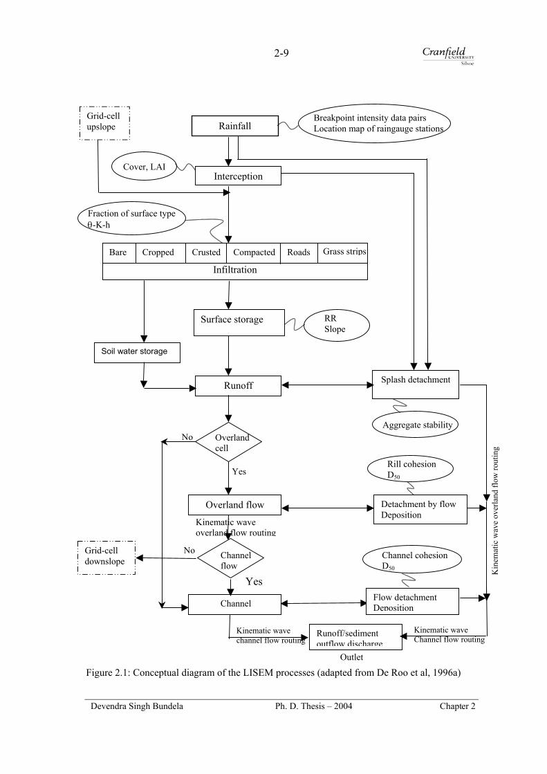
2-9
Cover, LAI
Cropped Bare Crus
Fraction of surface type θ-K-h
Su
O
No
Soil water storage
No Grid-cell downslope
Breakpoint intensity data pairs Location map of raingauge stations Rainfall
Grid-cell upslope
Figure 2.1: Conceptual diagram
Devendra Singh Bundela
Interception
Infiltration
ted Compacted Roads
rface storage RR Slope
Runoff
Splash detachment
ng
Aggregate stability
Overlandcell
verland flow Detachment by flow Deposition
Kin
emat
ic w
ave
over
land
flow
rout
i
Rill cohesion D50
Yes
g
Yes
Channel
Channelflow
Kinematic wave channel flow routing
of the LISEM processes
Ph. D. Th
Runoff/sediment outflow discharge
Outlet
(adapted from
esis – 2004
Channel cohesion D50
Kinematic wave overland flow routin
De Roo
Kinematic wave Channel flow routing
Grass strips
Flow detachment Deposition
et al, 1996a)
Chapter 2
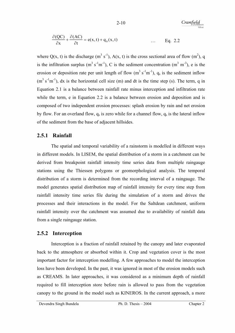
2-10
)t,x(q)t,x(et
)AC(x
)QC(s+=
∂∂
+∂
∂ … Eq. 2.2
where Q(x, t) is the discharge (m3 s-1), A(x, t) is the cross sectional area of flow (m2), q
is the infiltration surplus (m3 s-1m-1), C is the sediment concentration (m3 m-3), e is the
erosion or deposition rate per unit length of flow (m3 s-1m-1), qs is the sediment inflow
(m3 s-1m-1), dx is the horizontal cell size (m) and dt is the time step (s). The term, q in
Equation 2.1 is a balance between rainfall rate minus interception and infiltration rate
while the term, e in Equation 2.2 is a balance between erosion and deposition and is
composed of two independent erosion processes: splash erosion by rain and net erosion
by flow. For an overland flow, qs is zero while for a channel flow, qs is the lateral inflow
of the sediment from the base of adjacent hillsides.
2.5.1 Rainfall
The spatial and temporal variability of a rainstorm is modelled in different ways
in different models. In LISEM, the spatial distribution of a storm in a catchment can be
derived from breakpoint rainfall intensity time series data from multiple raingauge
stations using the Thiessen polygons or geomorphological analysis. The temporal
distribution of a storm is determined from the recording interval of a raingauge. The
model generates spatial distribution map of rainfall intensity for every time step from
rainfall intensity time series file during the simulation of a storm and drives the
processes and their interactions in the model. For the Saltdean catchment, uniform
rainfall intensity over the catchment was assumed due to availability of rainfall data
from a single raingauge station.
2.5.2 Interception
Interception is a fraction of rainfall retained by the canopy and later evaporated
back to the atmosphere or absorbed within it. Crop and vegetation cover is the most
important factor for interception modelling. A few approaches to model the interception
loss have been developed. In the past, it was ignored in most of the erosion models such
as CREAMS. In later approaches, it was considered as a minimum depth of rainfall
required to fill interception store before rain is allowed to pass from the vegetation
canopy to the ground in the model such as KINEROS. In the current approach, a more
Devendra Singh Bundela Ph. D. Thesis – 2004 Chapter 2

2-11
dynamic modelling is adopted in which the rainfall is allowed to pass from the canopy
to the ground at the same time as the interception store is being filled. This means that
some transfer of water from the canopy will take place right from the start of the storm.
This approach was adopted by Merriam (1973) and is used in the EUROSEM model.
The depth of the interception store for a time step is modelled as a function of the
cumulative rainfall from the start of a storm using an exponential relationship (Merriam,
1973).
In LISEM, a dynamic storage model is used to simulate the interception by
crops and vegetation in terms of cumulative interception during a storm event expressed
by an equation (Aston, 1979), which is a modified form of the Merriam’s equation
(Merriam, 1960):
−=
−max
cum
SP
k
maxp e1S*cS … Eq. 2.3
where S is the cumulative interception (mm), Pcum is the cumulative rainfall (mm), k is
the correction factor for crop and vegetation density which is equal to 0.046*LAI, LAI
is the leaf area index for crops and vegetation, Cp is the fraction of vegetation cover,
and Smax is the canopy storage capacity (mm) estimated from the LAI (Von Hoyningen-
Huene, 1981) as:
Smax = 0.935 + 0.498*LAI - 0.00575*LAI 2 … Eq. 2.4
2.5.3 Infiltration and Soil Water Transport in Soils
Infiltration and vertical transport of water in soils can be modelled on the basis
of an empirically, a semi-empirically, or a physically-based approach. In LISEM, two
physically-based models, SWATRE (Belmans et al, 1983) and the Green and Ampt (Li
et al, 1976) for one or two layers; and a semi empirically-based Holton model (Beasley
and Hoggins, 1981; Holtan, 1961) are incorporated. The SWATRE model, a finite
difference solution of the Richard’s equation, simulates both infiltration excess and
saturation excess overland flows for crusted, compacted and grass strip surfaces. Hence,
a priori knowledge of runoff production mechanism in a catchment is not needed. Both
Devendra Singh Bundela Ph. D. Thesis – 2004 Chapter 2

2-12
types of runoff production mechanisms can occur simultaneously in different areas of a
catchment. The theory of the SWATRE model is given in the literature (Belsman et al,
1983; Jetten, 2002). An infiltration excess flow occurs in arable and grassland-based
land uses while a saturation excess flow occurs in naturally vegetated and wild life
recreation areas. SWATRE is a very data intensive model and can be used for a
maximum of 20 soil horizons. It is applied when detailed soil properties data of a
catchment are available.
The Green and Ampt model (Li et al, 1976) for one or two layers is a simpler
approach to approximate the infiltration in homogeneous soils and simulates the
Hortonian overland flow for crusted, compacted and grass strip surfaces. Its
applicability is limited by the basic assumptions that the soil is homogeneous with
depth; the saturation behind the front is uniform; the infiltration wetting front is
perfectly sharp and the same everywhere in the horizons. When these assumptions are
no longer valid, the Green and Ampt model should not be applied. The theory of the
Green and Ampt model is described in the literature by Chow et al (1988). The Green
and Ampt equations for the cumulative infiltration and infiltration rate for a single layer
soil are expressed as:
Kth
tFhtF =
∆+∆−
θθ )(1ln)( … Eq. 2.5
+
∆= 1
)()(
tFhKtf θ … Eq. 2.6
Equation 2.5 can be solved for F (t) by either the method of successive substitution or
Newton’s iteration method for each time step. The value of F (t) is substituted in
Equation 2.6 to obtain the infiltration rate. When the wetting front is in upper layer, a
single layer Green and Ampt equations are used even for two layer soils.
When the wetting front enters the second layer, the two layer equations are applicable:
[ ] tHh
LHhKKHKKK
L =
+
++∆−∆+∆
12
21212212
212
2 1ln)(12 θθθ … Eq. 2.7
2211 LHF θ∆+θ∆= … Eq. 2.8
Devendra Singh Bundela Ph. D. Thesis – 2004 Chapter 2

2-13
)( 2121221
21 LHhKLKH
KKf +++
= … Eq. 2.9
where K1, h1, ∆θ1 are the hydraulic conductivity, wetting front suction head and soil
moisture storage capacity for the first layer, H1 is the thickness of the upper layer. K2,
h2, ∆θ2 are the hydraulic conductivity, wetting front suction head and soil moisture
storage capacity for lower layer, H2 is the thickness of the upper layer and L2 is the
distance of water front into the lower layer.
Equation 2.7 can be solved for L2 for each time step and then its value is
substituted in Equations 2.8 and 2.9 to obtain the cumulative infiltration and infiltration
rate respectively.
The Holton model is applicable when availability of soil properties data is
minimal and simulates the Hortonian overland flow only. The infiltration sub model is
selected according to the availability of soil data and intended purpose of the user. The
requirement of soil data increases with least for the Holtan model (1961)/Overton model
(1964) to intensive for the SWATRE model.
2.5.4 Surface Storage in Micro Depressions
Soil surface storage is a fraction of the net rainfall retained and detained on the
soil surface irregularities before initiating overland flow after meeting the infiltration
and or interception. The amount of surface storage is quantified by the surface
roughness, which is estimated from surface micro topographic elevation data. The
knowledge of surface storage modelling is extremely limited and hence it has been not
considered in erosion models in the past. However, it is empirically modelled in both
LISEM and EUROSEM to describe the different surfaces roughness produced by the
tillage.
The random roughness is used as a parameter to quantify the soil surface
roughness (Allmaras et al, 1966) and is determined from soil surface data measured by
the profile pin meter with a digital camera. Other methods have also been used to
measure it, such as the one metre long chain with 5 mm links, the laser profile meter
and close range stereo photogrammetry.
Devendra Singh Bundela Ph. D. Thesis – 2004 Chapter 2

2-14
Surface storage is estimated from the random roughness and slope in terms of
maximum depression storage (MDS) determined from a variety of surface conditions
and micro relief (Kamphorst et al, 2000). The surface depression storage was originally
modelled by Onstad (1984) and is estimated in LISEM using an equation (Kamphorst et
al, 2000):
MDS = 0.243RR + 0.010RR2 + 0.012RR* S … Eq. 2.10
where MDS is the maximum depression storage (mm), RR is the standard deviation of
surface heights (cm) and S is the terrain slope (per cent).
The width of the overland flow is assumed to be linearly related to the fraction
of ponded surface in the cell, which is related to the surface water depth and is
expressed (Jetten and De Roo, 2001) as:
)ah(
pa e1f −−= … Eq. 2.11
where fpa is the fraction of ponded area, h is the surface water depth (mm) and a is the
empirical factor ranging from 0.04 to 2.8 and can be estimated as:
942.0)RR*10(*406.1a −= … Eq. 2.12
The runoff before the water level reaches the maximum depression storage
height is calculated on the basis of the MDS and the fraction of ponded area under an
assumption of 10 per cent surface is ponded to start the runoff. Substituting this value
and taking logarithm of Equation 2.11 becomes as:
a)9.0ln(h
−= … Eq. 2.13
where h is called the start depression storage (SDS). The runoff gradually increases
nonlinearly when the water height is between the SDS and MDS. After the water height
has passed the MDS, the runoff height increases linearly with the water height. If h is
less than the SDS, no runoff (Q) is generated. If h is greater than the SDS, the runoff is
estimated as:
)e1(*)SDSh(Q )SDSMDS())SDSh(*h(
−−−
−−= … Eq. 2.14
Devendra Singh Bundela Ph. D. Thesis – 2004 Chapter 2
2-15
2.5.5 Overland and Channel Flow and Its Routing
Overland flow starts when the net rainfall intensity exceeds the infiltration rate
and surface depression storage of the soil. Two kinds of overland flows can occur in a
rural catchment: the Hortonian and (or) saturation excess overland flow. The Hortonian
overland flow occurs when rainfall intensity is higher than infiltration capacity of the
soil and is dominant in arable, pasture and barren lands while the saturation excess flow
occurs when the rainfall volume exceeds the moisture storage capacity of the soil and is
dominant in naturally vegetated and forest lands. The channel flow occurs when
overland flow concentrates in the defined rills and gullies. In the model, different types
of surfaces within a grid cell such as road, crusted, compacted, ponded or dry can be
simulated and the average water height is computed for each grid cell.
A four-point backward finite-difference solution of the kinematic wave together
with the Manning's equation using the Newton-Raphson technique is used for routing
of the distributed overland and channel flow over a drainage network in a catchment.
The local drainage network is derived from a digital elevation model using the
deterministic (D8) eight neighbour method. The kinematic wave method is based on
equations of conservation of mass and momentum (Chow et al, 1988). The kinematic
wave model assumes negligible inertial and pressure terms in the momentum equation
and the wave motion is described by an equation of continuity:
qtA
xQ
=∂∂
+∂∂
… Eq. 2.15
Term q is the infiltration surplus, which is the resulting flux of rainfall,
interception and infiltration. In order to deal with different types of surfaces, net
rainfall and infiltration are first added to the water level in the cell. When there is still
infiltration capacity left, this is added to the kinematic wave procedure. Thus, when
water is routed over a grid cell that still has the capacity to infiltrate, infiltration takes
place inside the kinematic wave routine. The equation of momentum for the
kinematic wave is expressed as:
S0 = Sf … Eq. 2.16
where S0 is the gravity force and Sf is the friction force.
Devendra Singh Bundela Ph. D. Thesis – 2004 Chapter 2

2-16
The equation of momentum can also be written in a curve rating form:
βα= Q*A … Eq. 2.17
where α and β are the empirical constants.
Discharge by the Manning’s equation per raster cell is expressed (Chow et al, 1988;
Moore and Foster (1990) :
2/1
03/2 S*R*
nAQ = … Eq. 2.18
The Manning’s equation can be rearranged in the curve rating form with S0 = Sf and R = A/P:
5/3
5/3
2/10
3/2Q
SnPA
= … Eq. 2.19
where A is wet cross section area (m2), n is the Manning’s roughness coefficient, P is
the wet perimeter (m), S is the sine of the slope (fraction), R is the hydraulic radius (m)
and Q is the discharge (m3 /s).
Comparing Equations 2.19 with Equation 2.17, expressions for α and β are deduced as:
5/3
3/23/10
3/2
P*Sn
=α and … Eq. 2.20
β = 3/5= 0.6
The alpha is constant for small rills and is the independent of slope and resistance
(Govers, 1992 and 1990).
For a finite difference numerical solution for flow routing, Equation 2.15 is
differentiated with respect to Q gives:
1Q
QA −βαβ=
∂∂
… Eq. 2.21
Devendra Singh Bundela Ph. D. Thesis – 2004 Chapter 2

2-17
Equation 2.21 is rearranged in terms of tA
∂∂ and is written as:
tQQ
tA 1
∂∂
αβ=∂∂ −β
… Eq. 2.22
Substituting tA
∂∂
from Equation 2.22 to Equation 2.15 results in:
qtQQ
xQ 1 =
∂∂
αβ+∂∂ −β
… Eq. 2.23
Equation 2.23 is written in a linear finite difference form as:
+=
∆−
+αβ+
∆− +
+++
++
−β+
++++
2qq
tQQ
2QQ
xQQ t
1x1t1x
t1x
1t1x
1t1x
1tx
1tx
1t1x
…Eq. 2.24
Equation 2.24 can be written in a simplified form of finite difference:
_t
1x1t1x
1_1tx
1t1x q
tQQ
Qx
QQ=
∆−
αβ+∆− +
++
−β+++
… Eq. 2.25
where t is the beginning of a time step, t+1 is the next time step, x is the upstream side
of grid cell, x+1 is the downstream side of grid cell, 1t+1xQ + is the new discharge, 1t+
xQ is
the new discharge at the upstream end of the grid cell (sum of all incoming water
generated by the kinematic wave), t1xQ + is the discharge present in the grid cell,
2/)QQ(Q t1x
1tx ++ +=
_ is the diagonal average (in a space-time domain),
−= ++
2qqq 1x1x
_ + t1t
is the average infiltration surplus over the length of the grid
cell.
The channel is located at the centre of the cell and a separate kinematic wave
routing procedure is applied for it. Channel cells receive a part of the overland flow,
depending on the velocity, thus the velocity in the channel is considered as an average
velocity in the cell. The distance of the channel from the grid cell edge is equal to cell
Devendra Singh Bundela Ph. D. Thesis – 2004 Chapter 2

2-18
width minus channel width, which is divided by two. A part of the water flows into the
channel (F) is expressed using an equation:
F = V*dt / ((grid-cell width - channel width) /2) … Eq. 2.26
2.5.6 Interflow
The infiltrated rainfall into the soil moves within the soil vertically and laterally.
Interflow is the lateral flow through the surface layers to open channels. Interflow can
occurs either in unsaturated or saturated flow conditions. Unsaturated interflow occurs
when the lateral hydraulic conductivity is greater than the vertical hydraulic
conductivity while saturated interflow occurs in situations where a thin soil overlies
bedrock; layers of low hydraulic conductivity exist within the soil profile; and piping or
artificial drainage occurs. Interflow has been proved to be of a minor importance for a
single event simulation (Ritsema et al, 1996). Hence, it is not modelled in LISEM.
2.5.7 Soil Detachment by Raindrop Impact
The soil erosion by water comprises of three main processes: detachment,
transport and deposition. Detachment modelling by rainfall and overland flow in
LISEM is based on a generalised erosion-deposition theory (Morgan et al, 1998a; Smith
et al, 1995) with an assumption that the transport capacity of the runoff reflects a
balance between detachment and deposition and is expressed as:
pfs DDDe −+= … Eq. 2.27
where e is the amount of sediment in transport process (kg s-1), Ds is the splash
detachment (kg s-1), Df is the flow detachment (kg s-1) and Dp is the deposition (kg s-1).
The LISEM model incorporates splash detachment by rainfall, throughfall and
leaf drainage as a function of their kinetic energy whilst most erosion models ignore the
effect of leaf drips. Leaf drainage modelling enables the effects of different heights of
crop and canopy covers on splash detachment. Splash detachment is modelled by an
equation developed from splash tests:
Devendra Singh Bundela Ph. D. Thesis – 2004 Chapter 2

2-19
A*P*96.2e*K*A
82.2D )h48.1(e
ss
+= −
… Eq. 2.28
where As is the soil aggregate stability in terms of the median number of drops to
decrease the aggregate size by 50 per cent (number), Ke is the kinetic energy of rainfall,
throughfall or leaf drainage (J m-2), h is the depth of surface water layer (mm), P is the
amount of rainfall in a time step (mm), A is the splash surface area over which the
splash takes place (m2).
The kinetic energy of the direct throughfall on reaching the ground surface is
assumed to be the same as that of the natural rainfall. The kinetic energy of the natural
rainfall (Ke r) or throughfall (Ket) through the plant canopy is estimated as:
Ke r = 8.95+8.44*log (I) … Eq. 2.29
The kinetic energy of the leaf drainage (Ked) is estimated from an equation:
Ked = (15.8*H0.5) −5.87 … Eq. 2.30
where I is the rainfall intensity (mm h-1) and H is the height of the plant or vegetation (m).
In the model, splash detachment area is estimated as the sum of all splash areas
under and besides plants (rainfall, throughfall and leaf drainage) and on ponded and dry
areas. The splash area for each condition is estimated separately and is summed up
according to the conditions. Areas for splash detachment by rainfall and leaf drainage in
ponded and dry areas in a cell are expressed as:
A(Ds_r ponded) = (ponded area fraction)*(1- crop cover)*A and Ke = Ke r … Eq. 2.31
A (Ds_t ponded) = (ponded area fraction)*(crop cover)*A and Ke = Ked … Eq. 2.32 A (Ds_rdry) = f*(1-ponded area fraction)*(1- crop cover)*A and Ke= Ker … Eq. 2.33
A (Ds_tdry) = f*(1-ponded area fraction)*(crop cover)*A and Ke= Ked … Eq. 2.34
Devendra Singh Bundela Ph. D. Thesis – 2004 Chapter 2
2-20
where f is the splash delivery fraction, which determines the amount of splashed soil
transported from the dry part of the grid cell to the wet part of the grid cell through the
air. Most splashes occur on the dry part of the grid cell and decrease exponentially with
the water height.
2.5.8 Soil Detachment by Flow
Soil detachment by flow is modelled in LISEM using a generalised erosion-
deposition theory (Morgan et al, 1998a; Smith et al, 1995) with an assumption that it is
independent of the transport capacity of flow and is only a function of the flow energy
exerted to detach. The detachment rate by flow is continually accompanied by the
deposition rate equal to a product of w, C and Vs in which w is the width of flow (m), C
is the sediment concentration in the flow (kg m-3) and Vs is the settling velocity of the
particles (m s-1). Transport capacity of the flow (Tc) represents the sediment
concentration at which the rate of erosion by the flow and accompanying rate of
deposition are in balance. In this condition, the net rate of erosion is zero and
detachment by flow (Df) is equal to the deposition rate (w*Tc*Vs). A general equation
for soil detachment by flow is expressed in terms of settling velocity and transport
capacity as:
dx*wV)CT(YD scf −= … Eq. 2.35
where Tc is the transport capacity of the flow (kg m-3), and Y is a flow detachment
efficiency coefficient. Y accounts for the detachment limited by the cohesion of wet
soil. Y is less than 1 for cohesive soils when C < Tc (detachment takes place). The
coefficient, Y for cohesive soils is calculated as (Rauws and Govers, 1988):
)Coh56.089.0(
1u
uY
c
min
+== … Eq. 2.36
where umin and uc are the minimum and critical shear velocities respectively (cm s-1),
and Coh is the cohesion of the saturated soil (kPa) and is the sum of bare soil cohesion
and cohesion by plant roots. The model accounts for cohesion by plant roots as well.
Deposition takes place only when C is larger than Tc and is modelled using an
exponential decay function (Equation 2.36) that simulates the effect of the settling of the
Devendra Singh Bundela Ph. D. Thesis – 2004 Chapter 2
2-21
particles slows down when they reach the bottom of the water layer on the surface.
Term, Y, then equals 1 as there is no effect of soil cohesion on deposition:
dx*w*h)e1)(CT(D )h/V*dt(cp
s−−= … Eq. 2.37
where h is the water depth (m), and h*w*dx is the volume of water in the grid cell.
2.5.9 Transport Capacity of Overland Flow
The transport capacity of overland flow is modelled in LISEM as a function of
the unit stream power (Govers, 1992 and 1990):
Tc = δs c (ω − ωc) d … Eq. 2.38
where Tc is the volumetric transport capacity (kg m-3), δs is the soil mass density (2650
kg m-3), ω is the unit stream power (a product of flow velocity* slope) and ωc is the
critical unit stream power (0.4 cm/s) defined by Govers (1992 and 1990) for a fairly
wide range of soils, c and d are the experimentally derived coefficients depending on
the soil median texture (D50). The transport capacity of the rill flow in the model can be
estimated as:
Tc = 2650 c (V* S*100 - 0.4) d … Eq. 2.39
where V is the rill velocity (m/s), S is the slope of the bed (fraction), c and d are the
experimentally derived coefficients depending on soil median particle size. The
coefficients are estimated using equations valid for soil median particle size larger than
30 µm, which is based on work of Govers (1992 & 1990),
c = [(D50 + 5)/0.32] – 0.6 and … Eq. 2.40
d = [(D50 + 5)/300] 0.25 … Eq. 2.41
The detachment by flow in the model is assumed to be the rill erosion. Currently,
interrill transport capacity is not included in the model.
2.5.10 Sediment Routing
A backward finite difference scheme with the Newton-Raphson iteration is used
to solve the dynamic sediment mass balance equation. For each time step, the grid cells
are re-arranged in an order of flow beginning from the top of the branches of the
Devendra Singh Bundela Ph. D. Thesis – 2004 Chapter 2

2-22
drainage network and progressing towards the outlet, using the sum of the discharges of
the upstream grid cells at the end of the time step, as input for the downstream grid cell.
Thus, the water is routed towards the outlet as a wave.
Suspended sediment is routed using the dynamic sediment mass balance
equation and it is assumed that an explicit solution can be used without iterations:
det
)AC(x
Qs −=∂
∂+
∂∂
… Eq. 2.42
Second part of left hand of Equation 2.42 is differentiated with respect to time, gives:
tAC
tCA
dt)AC(
∂∂
+∂∂
=∂
… Eq. 2.43
Substituting value of A and tA
∂∂ from Equations 2.17 and 2.22 to Equation 2.43 gives:
detQQC
tCQ
xQ 1s −=
∂∂
αβ+∂∂
α+∂
∂ −ββ … Eq. 2.44
Equation 2.44 is written in a form of linear finite difference approximation:
_t
1x1t1x
1__t1x
1t1x
_1tx
1t1x e
tQQ
QCtCC
QxQsQs
=∆−
αβ+∆−
α+∆− +
++
−β+
++
β+++
…Eq. 2.45
The average concentration can be calculated by the ratio of the average fluxes:
t1x
1tx
t1xs
1txs_
QQC
++
++
+
+= … Eq. 2.46
Substituting the value of C in Equation 2.45 is rewritten as:
( )
∆α+∆
−∆αβ−∆+
∆α+∆∆
=
++
β
+++
−β+
+
+β
++
1t1x
_
t1x
1t1x
1__1t
xst1x
t1x
__
1t1xs
QxQt
QQxQCtQQ
QsxQtxeQ …Eq. 2.47
All the variables on right hand side of Equation 2.47 are known and it can be solved
kinematically.
2.5.11 Channel Detachment and Deposition
Detachment, transport and deposition in channels are modelled in the same way
as detachment, transport and deposition in rills, although, the unit stream power concept
was originally developed for rill flow and it was later extended to the channel flow.
Devendra Singh Bundela Ph. D. Thesis – 2004 Chapter 2

2-23
Hence, the same equations are used except rill parameters are replaced by channel
parameters.
2.5.12 Flow Networks
Runoff and sediment routing in catchments with smaller slope is determined by
agricultural practices. The LISEM model simulates routing for three independent
drainage networks such as local drainage network, tillage network and wheel track
based network. For each network, a separate kinematic wave with the Manning's
equation is applied for routing the runoff and suspended sediment to the outlet.
2.5.13 Modelling Grass Strips
The model simulates grass strips as a type of surface. Different infiltration rates
for different surface types including grass strips are applied inside a gridcell to estimate
water height on each surface type. The average water height in a gridcell is calculated
using surface weighted average. The overland flow from an average water height is
routed to the outlet using a kinematic wave procedure. Generally, the water on the grass
strip surface is completely infiltered. Surplus infiltration is then applied to the water on
the other surfaces in the cell under an assumption that all the water within the grid-cell
flow perpendicular to the strip. It is intercepted by the grass strips. Then, an average
Manning’s roughness coefficient for the grid cell is estimated as the surface weighted
average of the Manning’s n for the grass strip and other surfaces in the grid cell.
2.5.14 Quality Checks
Two quality checks are in-built in the model to avoid an incorrect calculation of
soil detachment or deposition. The amount of detachment or deposition in a time step
depends on the settling velocity. For a too large time step, it happens that all the
sediments are already settled before the end of the time step. Therefore, the first quality
check ensures that deposition can never be more than the amount of transport capacity
surplus and is expressed as:
Dp = max (min (0, Tc - C), Dp) … Eq. 2.48
A second quality check for the flow detachment ensures that the amount of detached
soil cannot be more than the remaining carrying capacity of the flow and is expressed:
Devendra Singh Bundela Ph. D. Thesis – 2004 Chapter 2

2-24
Df = (Tc - C) Q dt … Eq. 2.49
2.6 Selection of a GIS-based Dynamic Modelling Language
It is known that the LISEM model is written in the PCRaster dynamic modelling
language. Therefore, PCRaster would be used to create the LISEM database of input
parameters for the simulation study. PCRaster has a few limitations in terms of data
exchange, data analysis, map composition and projection. Therefore, it would be better
to review the other dynamic modelling languages available to code dynamic models.
A GIS for dynamic modelling must have modelling functionalities to describe
the hydrologic and erosion processes in both space and time. It should also be capable
of handling huge amounts of spatial data of catchment characteristics collected from
various data sources including remotely sensed data. Therefore, there is a need for a
GIS-based modelling language environment that is capable of constructing the
physically-based dynamic erosion models.
After a review of modelling language in the GIS environment, it has been found
that a GIS-based dynamic modelling language is incorporated into three GIS packages
namely; PCRaster, GRASS (GRASS, 2004) and IDRISI (Clark Lab, 2004). The
PCRaster dynamic modelling language has been widely used to construct dynamic
erosion and environmental models such as LISEM (De Roo et al, 1996a), LISFLOOD
(De Roo, et al, 2000), RHINEFLOW (Van Deursen, 1995), EUROSEM in PCRaster
(Van Dijck, 2000; Van Dijck and Karssenberg, 2004). The GRASS GIS is gaining
popularity while the IDRISI dynamic language has not been popular for constructing
dynamic models. Therefore, the PCRaster GIS was chosen for dynamic erosion
modelling. Its dynamic modelling language (Van Deursen, 1995) has enough
functionality either to construct a new dynamic model or to improve the existing models
written with it.
The LISEM model written in the PCRaster language is already available in the
public domain, so there was no need to construct another new model, instead it was
decided to use an existing model. The major advantages of an embedded model into a
GIS are that the modeller can focus on the development and refinement of model
Devendra Singh Bundela Ph. D. Thesis – 2004 Chapter 2
2-25
processes rather than programming the GIS database. The structure of the GIS-based
modelling language is simple and straightforward so that the modellers no longer need
to programme the database structure, display tools or optimising algorithms of the
model.
2.7 PCRaster
PCRaster (Van Deursen, 1995; Wesseling et al, 1996) is a raster GIS-based
modelling toolkit to code a dynamic model using its dynamic modelling language. It
also includes cartographic, geostatistic and error propagation modelling functionalities.
The PCRaster GIS is a powerful modelling tool either to construct an iterative complex
dynamic model or to refine an existing model written in PCRaster. It includes
functionality for data storage, manipulation and visualisation of spatio-temporal data in
a raster format without data exchange between the model and GIS. It has a relatively
open database and the architecture of the system permits the integration of
environmental modelling functions with the GIS functions such as database
maintenance and visualisation.
2.7.1 The PCRaster Dynamic Modelling Language
The PCRaster dynamic modelling language uses an iterative procedure for
defining dynamic equations over a drainage network. It is an extension of the PCRaster
spatial modelling language (Van Deursen, 1995; Wesseling et al, 1996) based on the
map algebra (Tomlin, 1990) and the cartographic modelling language (Berry, 1993).
The PCRaster language is a high level GIS scripting language and has more than 150
spatio-temporal operators drawn from the map algebra, cellular automata, hydrological
routing and image filtering for the construction of both static and dynamic models
(PCRaster, 1996). The PCRaster dynamic modelling script is composed of structured
sequence of five sections to write a dynamic model (Figure 2.2) (PCRaster, 1996):
1. binding - it regulates the database management of the files in the program,
2. areamap – it defines the geographical attributes of the model area and the spatial
resolution,
3. initial - defines the initial conditions for the model,
Devendra Singh Bundela Ph. D. Thesis – 2004 Chapter 2
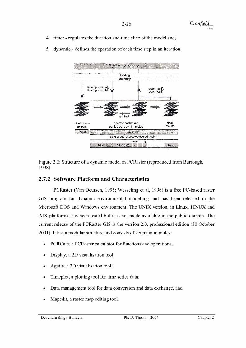
2-26
4. timer - regulates the duration and time slice of the model and,
5. dynamic - defines the operation of each time step in an iteration.
Figure 2.2: Structure of a dynamic model in PCRaster (reproduced from Burrough, 1998)
2.7.2 Software Platform and Characteristics
PCRaster (Van Deursen, 1995; Wesseling et al, 1996) is a free PC-based raster
GIS program for dynamic environmental modelling and has been released in the
Microsoft DOS and Windows environment. The UNIX version, in Linux, HP-UX and
AIX platforms, has been tested but it is not made available in the public domain. The
current release of the PCRaster GIS is the version 2.0, professional edition (30 October
2001). It has a modular structure and consists of six main modules:
• PCRCalc, a PCRaster calculator for functions and operations,
• Display, a 2D visualisation tool,
• Aguila, a 3D visualisation tool;
• Timeplot, a plotting tool for time series data;
• Data management tool for data conversion and data exchange, and
• Mapedit, a raster map editing tool.
Devendra Singh Bundela Ph. D. Thesis – 2004 Chapter 2
2-27
In addition to six standard modules, the PCRaster package also includes two extra
modules:
• GSTAT (Pebesma and Wesseling, 1998) for geostatistical modelling, kriging
interpolation, conditional simulation and random field generation, and
• ADAM (Heuvelink, 1998) for estimation of error propagation in the GIS.
The minimum requirement for the PCRaster installation is the Microsoft
Windows 98/NT or better with a minimum RAM memory of 64 MB and disk space of
50 MB. Recently, ‘Nutshell’, a shell-based window for PCRaster, has been introduced
to facilitate the running of PCRaster modules and commands from a single window
(LISEM, 2004). It is a user friendly window interface and can be used to create, edit and
display the raster maps and time series data and at the same time, it can also create, edit
and run the models.
2.7.3 Structure and Components of the Database
The PCRaster database holds four kinds of data:
• raster maps,
• point data,
• tables, for relationship between raster maps, and
• time-series, for representation of time varying attributes.
All these data contain six kinds of data type information, which describe the special
properties of the entities modelled in a database. The application of each data type is
described and is given in Table 2.6.
Raster maps are the most important data that enable the structured manipulation
of raster spatial data. A PCRaster map, a binary file in the cross system format, contains
three parts: a header, raster data and optional attributes (Wesseling, 1997). The header
contains information necessary for geographic and raster data. Raster information
contains both the location attributes and the data type of the map namely: number of
rows and columns, the cell size, the origin of the map projection, the type of data, and
the legend description. Optional attributes such as colour palettes and legends are
Devendra Singh Bundela Ph. D. Thesis – 2004 Chapter 2
2-28
located at the end of the file. Tables, time series and point data column files are in the
ASCII format with defined structures and can be analysed without a conversion. Two
formats of tables, column and matrix format, are used in this database with column table
by default while a matrix table is better to specify relations between two maps. The
format of a time series file must match with the timer section of a dynamic model. Two
types of format for time series data are used: time series with or without a header. The
point data column files consist of first two columns for x and y coordinates and one or
more columns for attribute data values. The column files should either be in a simplified
Geo-EAS format or a plain column file format.
Table 2.6: Data representations in the PCRaster database and their applications (adapted from the PCRaster, 1996)
Data type Description of attribute Domain Application
Boolean Boolean 0 (false), 1 (true) Catchment map
Nominal Classified, 0 - 255, whole values Land use and soil type maps
Ordinal Classified, order 0 - 255, whole values Classified elevation map
Scalar Continuous, linear - 1037-1037, real values DEM
Directional Continuous, directional 0-2 π (rad)/ 0-3600 (-1 for no direction), real
Slope map
LDD Local drain direction to neighbour cell
1-9 (5 for sink) Drainage network map
2.7.4 Data and Cell Representations
Data type and cell representations in PCRaster are not similar. Data type
representation describes the data type checking mechanism while the cell representation
determines the values of the cells stored and processed in the computer. The cell
representations in PCRaster are single real or double real for scalar and directional data,
and small integer or large integer for nominal and ordinal data. These are represented in
the computer by REAL4 (single real), REAL8 (double real), UINT1 (small integer) and
INT4 (large integer) (PCRaster, 1996).
2.7.5 Map Projection
Raster data are supported in a planar grid coordinate system in PCRaster. The
location attributes of a raster map is defined by the projection, upper left x and y
Devendra Singh Bundela Ph. D. Thesis – 2004 Chapter 2
2-29
coordinates, cell size, number of rows, number of columns and angle to position the
map with respect to a real world coordinate system and the shape and resolution of the
map. In projection, northing (Y-axis) decreasing and increasing from top to bottom are
only supported. PCRaster does not support data projection and coordinate
transformation.
2.7.6 Data Exchange PCRaster is a raster GIS and does not support the creation of vector spatial data,
so key vector spatial data are created outside PCRaster. The data management in terms
of data import and export is limited and is not user friendly. Widely used GIS raster
format data are not supported in PCRaster. Raster data from other GIS needs to be
either in ASCII or column file format including ArcInfo GRID ASCII format to import
to the PCRaster map format using an asc2map command. Similarly, the PCRaster maps
are in the binary format, which needs to be converted to the ASCII or Column file
format using a map2asc for import to other GIS package for map composition and
further analysis. Other kinds of data in the PCRaster database are the ASCII formatted
and can easily be created, analyzed and edited with other GIS packages.
2.7.7 Critical Assessment
The PCRaster dynamic modelling language is a powerful macro scripting
language, which uses more than 150 spatio-temporal operators (Burrough, 1998) for
constructing both static and dynamic models. A dynamic model written with the
PCRaster GIS contains about 200 lines of source code as compared to thousands of line
of code in an advanced computer programming language (Ungerer, 2000) but it takes
much longer to run than advanced computer programming language-based models. The
GIS-based language is easy to learn and implement for environmental modelling.
Moreover, it is a freeware and operates in the MS-DOS environment. Nutshell, a shell
window, has made PCRaster more user friendly by facilitating the running of PCRaster
modules and commands from a single window. Provision for developing a new model
in a short time and improving existing models makes it an even more attractive
modelling environment. It has limited import functionality and does not support widely
used raster GIS formats. It does not provide support for projection and coordinate
transformation. Moreover, it needs a supporting GIS for digitisation, rasterisation and
Devendra Singh Bundela Ph. D. Thesis – 2004 Chapter 2

2-30
coordinate transformation of key spatial data. Unfortunately, at the same time, most
commercial GIS packages are still deficient of providing built-in dynamic modelling
capabilities (Van Deursen, 1995; Peuquet, 1999).
2.8 Requirement of Input Parameters
All input parameters and variables of LISEM are required in the PCRaster GIS
format except rainfall intensity data. The model requires a large number of spatial input
parameters depending on the processes to be modelled. The spatial input parameters are
grouped into six categories:
1. catchment parameters, 2. land use and vegetation parameters, 3. soil surface parameters, 4. infiltration parameters, 5. erosion related parameters, and 6. channel parameters
A minimum of 24 parameters are required for a simple simulation. The
parameter requirements under various categories and options are described in Appendix
A-1. Catchment parameters are derived from a digital elevation model and a raingauge
location map. Land use and vegetation parameters are derived from a land use and land
cover map with field observations on their parameters. Soil surface and erosion related
parameters are generated from a soil map and a landuse and land cover map with field
observations on their parameters. Infiltration parameters are derived from a soil map
and its property database, and a landuse and land cover map with field observations.
Channel parameters are generated from a digital elevation model with field observations
on some parameters and a landuse and landcover map.
Generally, input parameters for the model either do not exist or are not available
in full for a catchment. For planned events, these parameters can be measured but for a
historic event simulation, synthetic techniques are resorted to estimate the representative
parameter value. There are problems encountered with available input data in regard to
their incompleteness, accuracy and inhomogeneity.
Devendra Singh Bundela Ph. D. Thesis – 2004 Chapter 2
2-31
2.9 Model Outputs
The model generates a wide variety of output information to evaluate an erosion
scenario in terms of total and time series outputs of the water and erosion balance
variables, hyetograph, hydrograph and sedigraph from a catchment (Appendix A-2).
The outputs are either in the PCRaster map format or CSV (comma separated value)
ASCII format. The map format outputs can be displayed in both static and dynamic 2D
and 3D environments. The CSV format hyetograph, hydrograph and sedigraph data can
be displayed in Timeplot.
2.10 Sensitivity Analysis and Calibration
Sensitivity analysis examines the model sensitivity to input parameters where
each individual input parameter is decreased and increased systematically to analyse its
effect on model outputs while keeping other parameters unchanged. There are several
approaches to perform the model sensitivity analysis. One at a time sensitivity analysis
approach is preferred in this study. Generally, most of the variation in the outputs is
caused by a small number of input parameters. The sensitivity analysis of the model is
carried out for topographic parameters and the results are discussed in Chapter 6.
Calibration is carried out to adjust some input parameters to match the model
behaviour to a set of measured data. In other words, it can be called as a restricted form
of parameterisation of a model. A calibration strategy of the model can be carried out
for different outputs. Total runoff from an event can be calibrated by changing the
initial moisture content and saturated hydraulic conductivity. The peak runoff or shape
of the hydrograph can be calibrated by changing the Manning’s roughness coefficient.
The correct erosion and soil loss from an event can be calibrated by changing the
aggregate stability and cohesion of the soil. Due to non availability of measured dataset
on runoff and erosion for the Saltdean catchment, no calibration was to be carried out.
2.11 Concluding Remarks
2.11.1 Discussion
A more physically-based distributed and dynamic model within a GIS
environment, LISEM, has been selected for surface hydrologic and erosion dynamics
Devendra Singh Bundela Ph. D. Thesis – 2004 Chapter 2
2-32
modelling for a storm at catchment scale on the basis of process formulation, process
component, spatial and temporal representation, GIS integration and technical support.
The model has an additional advantage of its development for a European climate and
the similar catchment characteristics with reference to the Saltdean catchment
(Boardman et al, 1996). The remotely sensed data derived products such as DEM and
land use and land cover, and the National Soil Data can be used to create databases of
input parameters of the catchment. The model is applied to simulate the runoff, erosion
and deposition within and from the catchment for an extreme rainstorm event of 30
October 2000.
PCRaster is a public domain GIS and is used to create the LISEM databases for
a simulation. Its dynamic modelling language has been widely used for constructing
dynamic erosion and environmental models such as LISEM, LISFLOOD,
RHINEFLOW and Celluna. It provides a powerful modelling environment, but it has
limitations in terms of data exchange, projections, hardcopy outputs and user
friendliness. It does not support widely used GIS formats and requires another GIS to
create and convert vector data to a raster format with a suitable resolution and
projection.
2.11.2 Conclusions
• The LISEM model written with the PCRaster dynamic modelling language is a
useful tool for predicting runoff and erosion dynamics at catchment scale from an
extreme real or a hypothetical rainstorm. It is also used to locate the sediment
source and sink areas to adopt an effective conservation strategy.
• It integrates remotely sensed data and other spatial database for model
parameterisation.
• It is used to evaluate the effect of different spatial representations of input
parameters and key spatial data on model predictive capacity.
Devendra Singh Bundela Ph. D. Thesis – 2004 Chapter 2

3-1
3
Rainstorm Identification and Infiltration Modelling
This chapter deals with non-remotely sensed data such as rainfall and
soil data for some input parameter definitions, which involve procedures
for identification of heavy rainstorms and extraction of infiltration
parameters for a single layer Green and Ampt model. Fifteen storms were
identified from daily rainfall data first and then locating the onset and
ending of the storms from hourly rainfall data. A single storm was used
for simulation study. Infiltration parameters were extracted from the
1:250000 scale National Soil Data using pedotransfer functions.
3.1 Introduction
A rainstorm event drives the hydrologic and erosion processes in a catchment.
Infiltration is one of the major hydrological processes and is controlled by the rainfall
rate before ponding and by the soil properties after the ponding occurs (Chow et al,
1988). An accurate estimation of infiltration is essential for physically-based erosion
modelling. At the same time, a better understanding of spatial and temporal variability
of a rainstorm at catchment scale is required to model these processes precisely. A few
heavy rainstorms with their spatial and temporal distribution are, therefore, required to
be identified to model the effect of DEM resolutions on hydrologic and erosion
processes in a catchment using LISEM.
Devendra Singh Bundela PhD Thesis-2004 Chapter 3
3-2
The LISEM model simulates infiltration and soil water transport in the soils.
Soil hydraulic properties and infiltration parameters can be derived from available soil
physical properties using pedotransfer functions (PTFs). These properties are known to
vary in space and their measurement can be expensive and time consuming at catchment
scale. Alternatively, available soil maps and a soil property database can be used to
derive infiltration parameters for a single layer Green and Ampt model.
This chapter deals with non-remotely sensed data such as rainfall and soil data to
describe methodologies for rainstorm identification and for estimating infiltration
parameters from the 1:250 000 scale National Soil Map data. It also describes the
rainstorm characteristics of autumn and early winter 2000 and advanced techniques of
rainfall measurement.
3.2 Identification of Rainstorms
3.2.1 Rainfall Data Source
Ideally, rainfall data of autumn and early winter 2000 recorded at shorter time
intervals is required to characterise the heavy rainstorms for modelling study. Rainfall
data could be obtained from many sources: British Atmospheric Data Centre (BADC),
Met Office, University of Sussex, Falmer and farmers’ personal weather stations.
Fourteen meteorological stations identified from the BADC archives (Appendix
B-1) were active during 2000 around the Saltdean catchment in the East and West
Sussex but they were far from the study catchment. Therefore, they were not considered
as a data source for storm identification. No weather station could be found in the
catchment from any source. The University of Sussex weather station at Falmer was the
nearest station from the study catchment and was selected as a source of the rainfall data
of hourly, daily and monthly rainfall interval. Monthly rainfall data from the Saltdean
and Newhaven weather stations were also obtained to assess the spatial variability of
rainfall around the catchment. The description of rainfall data collected from three
weather stations is described in Section 3.2.4.
Devendra Singh Bundela PhD Thesis-2004 Chapter 3
3-3
3.2.2 Climate of the Eastern South Downs
The Eastern South Downs is a part of south Eastern England climatic region
where a large percentage of rain falls in autumn and winter, arriving on south westerly
winds accompanied by the fronts or cyclones associated with depressions. There is an
orographic effect due to topography, resulting in heavy rains. Convective storms are
active during spring and summer and bring heavy rainfall. North of the South Downs
lies in a rain shadow area. Rainfall in the Eastern South Downs decreases progressively
from west to east and from south to north. The mean annual rainfall of the Eastern
South Downs varies from 750 to 1000 mm with the largest proportion being recorded in
winter. Rainfall is becoming more intense in winter and less intense in summer with
peak in autumn (Osborn et al, 2002; Mayes, 1997).
3.2.3 Spatio-Temporal Variability of Rainstorms
A distributed model requires a better spatio-temporal description of a rainstorm
to simulate hydrologic and erosion process in a catchment. A rainstorm is measured at a
finite number of points using rain gauges or pluviometers. Accuracy of spatial
variability of rainstorms is dependent on the density of a raingauge network. A better
spatial description of rainstorms can be achieved through a dense raingauge network,
but such a network is expensive to keep operational. Spatial distribution of a rainstorm
is generated from point rainfall data using spatial interpolators such as Thiessen
polygons, geomorphological analysis, inverse distance weighting, splines and kriging.
Applicability of these interpolation algorithms largely depend on the distribution of
raingauges in a catchment and should be used carefully as spatial interpolators violate
the physical aspect of a storm distribution in some cases. A few raingauges are required
to map the spatial distribution of frontal or cyclonic storms while a denser raingauge
network is required to map spatial distribution of convective and orographic storms.
Temporal distribution of a storm is recorded as the rainfall accumulations over
time intervals of 1, 5, 15 and 30 minutes and hourly in automatic weather stations. A
small catchment is more sensitive to a short temporal lumping of rainfall whereas a
large catchment is sensitive to an hourly time intervals. Single event-based hydrologic
and erosion models are more sensitive to small temporal resolution of rainfall depth and
Devendra Singh Bundela PhD Thesis-2004 Chapter 3

3-4
intensities. Hence, a short temporal resolution is required for a single event-based
modelling. The movement of a storm can possibly be tracked down by analysing several
raingauge data simultaneously and is seldom required in distributed erosion models.
When there is no raingauge station in a study catchment, a weather Doppler
radar can be used to provide a relatively accurate aerial estimates of spatial distribution
of a rainstorm and ground estimates when adjusted with raingauge data (Collier, 1996).
In an extreme case, when there is no raingauge and weather radar data available for a
remote catchment, environmental satellite data such as Geostationary operational
environmental satellite (GOES-1), METEOSAT (Meteorological satellites), NOAA
(North Oceanic and Atmospheric Administration) and TRMM (Tropical rainfall
measuring mission) can alternatively be used to provide rough estimates of rainfall
amounts for a larger area (New et al, 2001; Levizzani et al, 2000).
3.2.4 Description of Raingauge Stations
The University of Sussex weather station was installed on the roof of Pevensey-
1 building in the University Campus at Falmer, Brighton in May 1997. It continuously
records temperature, humidity, barometric pressure, solar energy, rainfall, and wind
speed and direction. The automatic weather station was configured to record all weather
variables at an hourly interval since May 1997 (Appendix B-2). Hence, the rainfall data
with less than an hour interval were not available (Chitty, 2002). Two other raingauges
at Saltdean and Newhaven were also selected to collect monthly and yearly rainfall data.
Table 3.1 presents the location coordinates of three weather stations and the kind of data
collected.
Table 3.1: Periods of data collected along with the location of weather stations
Data description/ location
University of Sussex, Falmer
Saltdean
Newhaven
Hourly data Sep-Dec 2000 (Select dates) --- --- Daily Jun 1997 – Feb 2002 --- --- Monthly data 1997-2003 1997-2003 1997-2003
Location: Latitude 500 51’ 52.8’’ N 500 47’ 45.6’’ N 500 47’ 39’’ N Longitude 00 05’ 11.3’’ W 00 02’ 2.4’’ W 00 02’ 39’’ E Altitude 77 m msl Not available Not Available
Devendra Singh Bundela PhD Thesis-2004 Chapter 3

3-5
3.2.5 Identification of Rainstorms
It was necessary to identify a few major wet days from the analysis of daily
rainfall data from 1998 to 2001 to locate the possible intense events as hourly data could
not be supplied. This was done using the following rules, which state that the daily
rainfall on a wet day must be more than 15 mm and should be preceded by one or two
days of rainfall with a minimum of 5 mm. Using these rules, the possible periods for
heavy rainstorm events were identified in autumn and early winter 2000 (Appendix B-
3). Hourly rainfall depth and intensity data were then obtained for that specific wet
period. Subsequently, the beginning and termination of rainstorm events were located
exactly by the analysis of hourly rainfall intensity data. A rainstorm event was defined
as the period of rain separated from preceding and succeeding rainfall periods by
approximately 2 hours. This definition was based on the time of concentration (~1 hour)
of the Saltdean catchment. Similar definitions of a storm based on catchment area have
been reported in the literature (Huff, 1967; Vogel, 1986). Fifteen storm events were
identified in autumn and early winter 2000 and their rainfall depth, duration, 1-hour
maximum rainfall and maximum intensity were given in Table 3.2. The storm on 29-30
October recorded the maximum intensity of 11.4 mm/hour. Therefore, a 6-hour segment
of this heavy storm (Figure 3.1) was used for simulation study due to the limitation of
large storage space required for simulation results from a complete single storm.
3.2.6 Storm Characteristics of Autumn and Early Winter 2000
In autumn and early winter months of September, October November and
December 2000, the storms were primarily the result of a continuous series of frontal
depressions coming from the North Atlantic and resulted in the high rainfall on the
Eastern South Downs. Autumn 2000 was the wettest autumn on record in the South
Downs with a rainfall of 737.7 mm (DEFRA, 2001). The rainfall of October and
November 2000 in the South Downs was 294 per cent higher than the regional average
while the rainfall of four months (September-December 2000) was 233 per cent higher
than the regional average. The regional average is used for calculating percentage of
average due to lack of the station average. The estimated return periods for a two month
and a four month rainfall were more than 200 years (DEFRA, 2001). Table 3.3 shows
the rainfall accumulations and the percentage of average.
Devendra Singh Bundela PhD Thesis-2004 Chapter 3
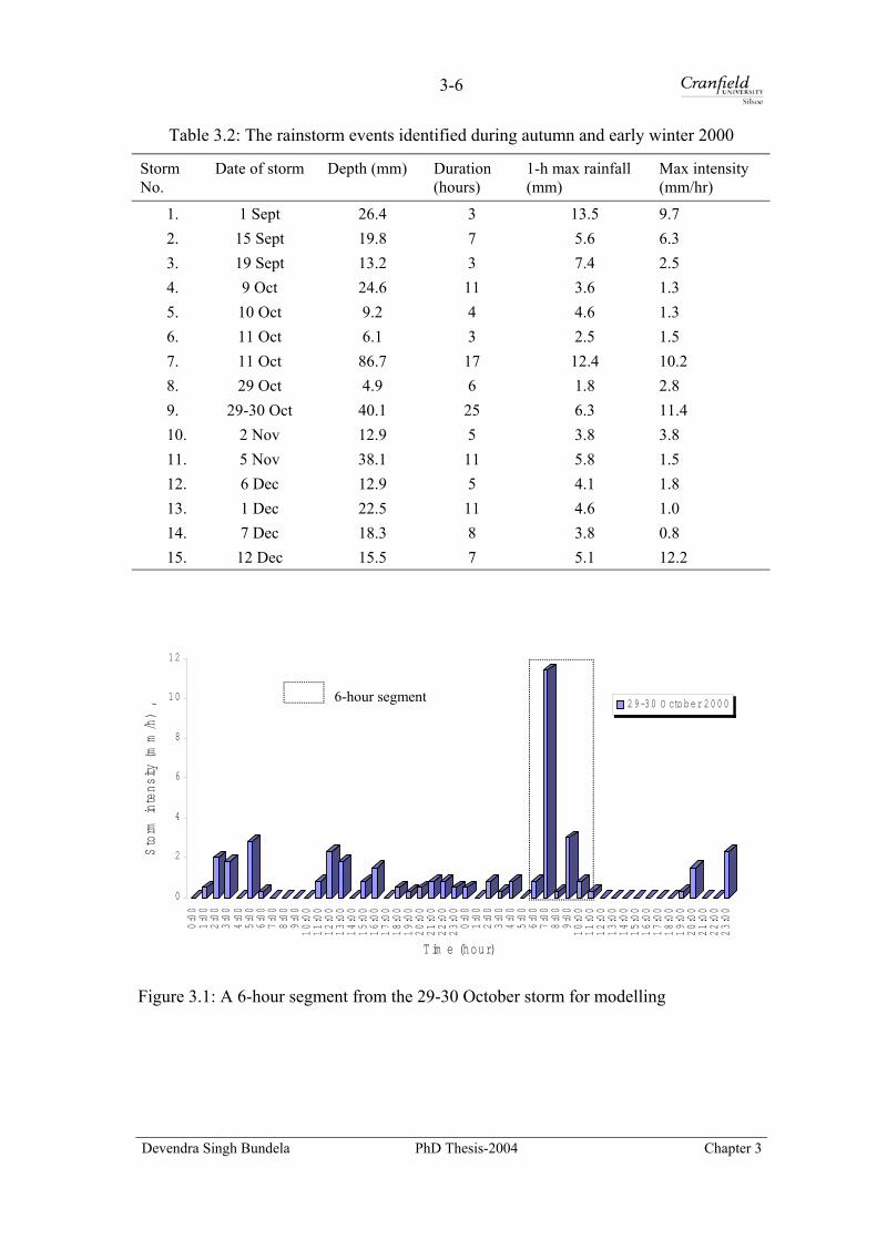
3-6
Table 3.2: The rainstorm events identified during autumn and early winter 2000
Storm No.
Date of storm Depth (mm) Duration (hours)
1-h max rainfall (mm)
Max intensity (mm/hr)
1. 1 Sept 26.4 3 13.5 9.7 2. 15 Sept 19.8 7 5.6 6.3 3. 19 Sept 13.2 3 7.4 2.5 4. 9 Oct 24.6 11 3.6 1.3 5. 10 Oct 9.2 4 4.6 1.3 6. 11 Oct 6.1 3 2.5 1.5 7. 11 Oct 86.7 17 12.4 10.2 8. 29 Oct 4.9 6 1.8 2.8 9. 29-30 Oct 40.1 25 6.3 11.4 10. 2 Nov 12.9 5 3.8 3.8 11. 5 Nov 38.1 11 5.8 1.5 12. 6 Dec 12.9 5 4.1 1.8 13. 1 Dec 22.5 11 4.6 1.0 14. 7 Dec 18.3 8 3.8 0.8 15. 12 Dec 15.5 7 5.1 12.2
0
2
4
6
8
1 0
1 2
Storm
intens
ity (mm/h) ,
0:00
1:00
2:00
3:00
4:00
5:00
6:00
7:00
8:00
9:00
10:00
11:00
12:00
13:00
14:00
15:00
16:00
17:00
18:00
19:00
20:00
21:00
22:00
23:00
0:00
1:00
2:00
3:00
4:00
5:00
6:00
7:00
8:00
9:00
10:00
11:00
12:00
13:00
14:00
15:00
16:00
17:00
18:00
19:00
20:00
21:00
22:00
23:00
T im e (hour)
29-3 0 O ctob e r 20 0 0
6-hour segment
Figure 3.1: A 6-hour segment from the 29-30 October storm for modelling
Devendra Singh Bundela PhD Thesis-2004 Chapter 3
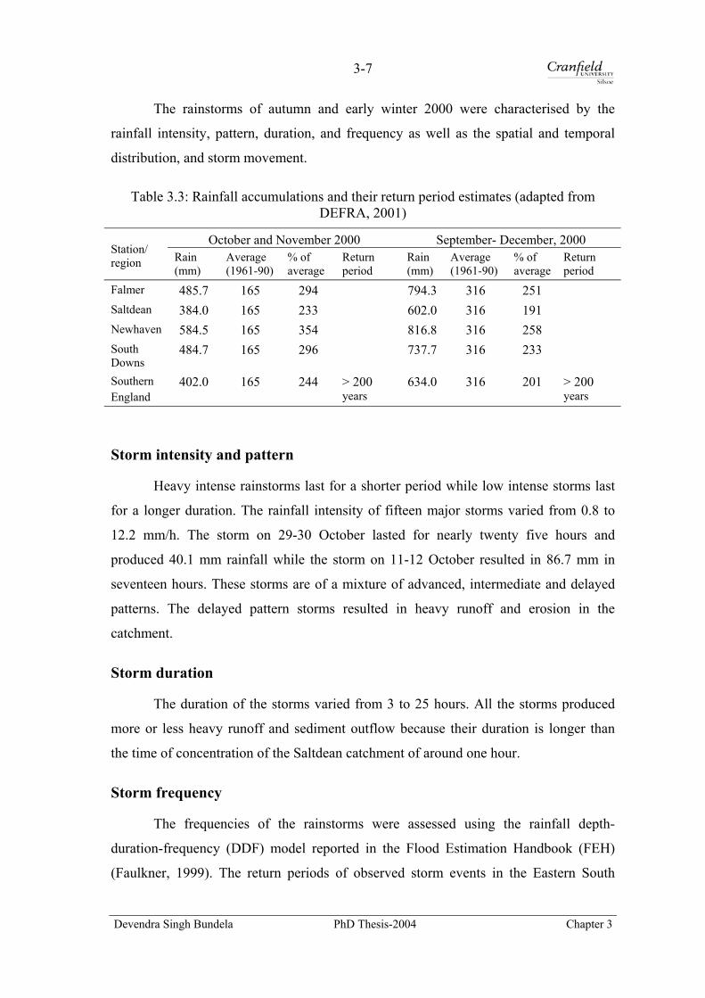
3-7
The rainstorms of autumn and early winter 2000 were characterised by the
rainfall intensity, pattern, duration, and frequency as well as the spatial and temporal
distribution, and storm movement.
Table 3.3: Rainfall accumulations and their return period estimates (adapted from DEFRA, 2001)
October and November 2000 September- December, 2000 Station/ region Rain
(mm) Average (1961-90)
% of average
Return period
Rain (mm)
Average (1961-90)
% of average
Return period
Falmer 485.7 165 294 794.3 316 251 Saltdean 384.0 165 233 602.0 316 191 Newhaven 584.5 165 354 816.8 316 258 South Downs
484.7 165 296 737.7 316 233
Southern England
402.0 165 244 > 200 years
634.0 316 201 > 200 years
Storm intensity and pattern
Heavy intense rainstorms last for a shorter period while low intense storms last
for a longer duration. The rainfall intensity of fifteen major storms varied from 0.8 to
12.2 mm/h. The storm on 29-30 October lasted for nearly twenty five hours and
produced 40.1 mm rainfall while the storm on 11-12 October resulted in 86.7 mm in
seventeen hours. These storms are of a mixture of advanced, intermediate and delayed
patterns. The delayed pattern storms resulted in heavy runoff and erosion in the
catchment.
Storm duration
The duration of the storms varied from 3 to 25 hours. All the storms produced
more or less heavy runoff and sediment outflow because their duration is longer than
the time of concentration of the Saltdean catchment of around one hour.
Storm frequency
The frequencies of the rainstorms were assessed using the rainfall depth-
duration-frequency (DDF) model reported in the Flood Estimation Handbook (FEH)
(Faulkner, 1999). The return periods of observed storm events in the Eastern South
Devendra Singh Bundela PhD Thesis-2004 Chapter 3

3-8
Downs were estimated from six parameters. These six parameters and the catchment
descriptors of the University of Sussex weather station and the Saltdean catchment were
extracted from the FEH CD-ROM (Bayliss,1999) (Appendix B-4). The return periods
of the observed storms were calculated using the rainfall depth and its duration and is
given in Table 3.4. It was found that there was no rainfall intensity-duration-frequency
(IDF) model available for the South Downs. Hence, the DDF model was used for the
return period analysis.
The return period of an observed storm event of any duration is estimated from
the six DDF parameters. The Gumbel variate (y) is computed using following equations
on the basis of storm duration:
For a storm duration less than 12 hours
eDln*cDln*dfRln
y 1
+−−
= … Eq. 3.1
For a storm duration between 12 and 48 hours
eDln*c
Dln12ln*d12ln*dfRlny 21
+−+−−
= … Eq. 3.2
where R is the rainfall depth (mm); D is the duration of a storm; and c, d1, d2, d3, e and f
are the DDF parameters.
The return period (T) of a storm is estimated from the Gumbel variate (y) using an equation:
−
=
− yee
11
1T … Eq. 3.3
Spatial distribution
Areal rainfall estimates are required for catchment scale distributed modelling.
The areal estimate of a rainstorm is generated either using a spatial interpolator from
multi point rainfall data in a catchment or using an areal reduction factor. A single
raingauge station data was available in the catchment, so a uniform spatial distribution
of rainfall was assumed. Alternatively, the point rainfall can be converted to the areal
rainfall multiplying by an appropriate rainfall areal reduction factor (ARF). This method
Devendra Singh Bundela PhD Thesis-2004 Chapter 3

3-9
is only applicable for rainfall depth, not for rainfall intensity. Hence, it was not used for
converting the point rainfall into the areal rainfall.
Table 3.4: Return periods of the storms based on their depth and duration
Storm No Date Duration (hrs) Rainfall (mm) Return period (years)
1 01 Sep 2000 3 26.4 4.5 2 15 Sep 7 19.8 1.11 3 19 Sep 3 13.2 1.06 4 9 Oct 11 24.6 1.15 5 10 Oct 4 9.2 <1 6 11 Oct 3 6.1 <1 7 11-12 Oct 17 86.7 53 8 29 Oct 6 4.9 <1 9 29-30 Oct 25 40.1 1.8
10 02 Nov 5 12.9 1 11 05 Nov 11 38.1 3.4 12 06 Dec 5 12.9 1 13 01 Dec 11 22.5 1.06 14 07 Dec 8 18.3 1.02 15 12 Dec 2000 7 15.5 1
The areal rainfall is calculated from a point rainfall from an equation:
ARF*RP Dareal = … Eq. 3.4
where Pareal is the areal rainfall in mm, ARF is the rainfall areal reduction factor and RD
is the point rainfall of duration, D and a return period, T.
The areal reduction factor (ARF) is expressed by an equation as quoted in the FEH
Handbook.
aD*b1ARF −−= … Eq. 3.5
where D is the duration in hours and a, and b are the ARF coefficients, which are the
function of the area, A, in sq km and are expressed by equations given in Table 3.5.
Table 3.5: Equations for area reduction factor coefficients
A (sq km) a b
A ≤ 20 0.40-0.0208 ln(4.6-lnA) 0.0394 A0.354
20 < A < 100 0.40-0.00382 ln(4.6-lnA)2 0.0394 A0.354
Devendra Singh Bundela PhD Thesis-2004 Chapter 3

3-10
Temporal distribution
The hourly rainfall intensity and depth data were used for the temporal analysis
of storms. It was found that an hourly temporal resolution rainfall data was not
sufficient for storm analysis. Some rainstorms of shorter duration might have gone
unrecorded. The data for a historical event was only available at an hourly interval.
Therefore, hourly data were used for modelling application.
Storm movement
The movement of a storm is possibly tracked down by analysing several
raingauge data simultaneously. The storm movement towards a catchment outlet
produces a heavy runoff and erosion. It was not possible to track down the storm due to
the availability of a single raingauge data in the catchment. Moreover, it was not
required in the LISEM model.
3.2.7 Analysis of Rainfall Pattern at Three Stations
The monthly rainfall distribution in autumn and early winter 2000 at Falmer,
Saltdean and Newhaven is given in Figure 3.2. It was found that October 2000 was the
wettest month at all three stations as the monthly rainfall occurred in October 2000 was
higher than that of the other months at all three stations. Year 2000 was also an
exceptionally wet year at all the stations as can be seen from Figure 3.3. There was no
specific trend in annual rainfall among station data.
0
100
200
300
400
S ep' 2000 O ct' 2000 N ov'2000 D ec'2000
M onth
Rainfall (m
m)
F alm er
S altdean
N ew haven
Figure 3.2: Distribution of monthly rainfall in autumn and early winter 2000 at
three stations
Devendra Singh Bundela PhD Thesis-2004 Chapter 3

3-11
1400
Rai
nfal
l (m
m)
1998 1000
1999600 2000
2001200
0Falmer Saltdean
Years (1998-2001) Newhaven
Figure 3.3: Distribution of annual rainfall at three stations
3.2.8 Weather Radar
The nearest weather Doppler radar from the study catchment is located at
Chenies, some 100 km distant. It is C-band (5.6 cm) radar with a range of 250 km and is
a part of the national weather radar network in the U. K. Radar completes a series of
scans about the vertical axis at each of four elevation angles every five minutes and the
precipitation products at resolutions of 1 km, 2 km and 5 km over the South Downs are
produced. The radar aerial estimates are compared with raingauge estimates to convert
the aerial estimates to the ground estimates. The radar data over a large river catchment
is more useful than a small catchment. Moreover, radar derived products for October
2000 historical events on the Saltdean catchment were not available. Hence, they were
not considered for the modelling.
3.2.9 Rainfall Input to the LISEM Model
The break point rainfall intensity data pairs of a storm are required to drive the
LISEM model (Jetten, 2002). These break points pairs are obtained by dividing a storm
into discrete time periods within which a nearly uniform intensity rainfall is recorded on
the basis of rainfall graph slope. The break points are defined by the time of the start of
each discrete period and nearly uniform rainfall intensity. It was not possible to extract
break point intensity pair data exactly from available hourly data. It was, therefore,
assumed that the same rainfall intensity continued a whole hour due to data limitation.
This assumption could be valid for some of frontal storms and might not be valid for the
storm considered for modelling study.
Devendra Singh Bundela PhD Thesis-2004 Chapter 3

3-12
3.3 Infiltration Modelling
3.3.1 Soil Data Source
The National Soil Resources Institute (NSRI) is the national repository of soil
information for England and Wales. Investigation of soil data at the NSRI revealed that
soil data for the Eastern South Downs was only available at 1:250 000 scale (NSRI,
2003). Therefore, it was chosen for parameter estimation of infiltration and soil water
transport sub model. The NATMAP vector data, a vector version of the 1:250 000 scale
National Soil Map, was obtained from the NSRI in the ESRI Shape file format along
with associated Profile and Horizon data. It was also revealed that even paper soil maps
at larger scales such as 1:25 000, 1:50 000, 1:63 360 and 1:100 000 were not available
for the study area (NSRI, 2003).
The NATMAP vector product is the most comprehensive national digital soil
map available at a scale of 1:250 000 and is the product of a ‘free soil survey’ with an
average of 2 to 3 soil observations per square kilometre (NSRI, 2004). It shows location
of the 297 mapped soil associations, each of which contains three to five soil series. The
map describes a wide range of soil conditions encountered across England and Wales.
The Profile and Horizon data provide the detailed information of key soil physical and
chemical properties of soil series identified in the soil map.
Soil property data supplied along with digital national soil map contained the
Profile and Horizon data of each series. The Profile data contained information on a soil
profile for each soil series while the Horizon data contained the properties of four
separate soil horizons (topsoil, upper and lower subsoil, and substrate) for the profiles
under four different land uses ranging from the arable to semi natural vegetation. These
data were linked to the soil association polygons of a digital soil map to derive the
thematic map and spatial parameters for infiltration and water transport sub models.
Devendra Singh Bundela PhD Thesis-2004 Chapter 3

3-13
3.3.2 Soil Variability
Soils are spatially heterogeneous at catchment scale and their variability affects
the measurements and predictions of soil properties. Soil variability is a result of many
of soil formation processes and is mapped using a hierarchical system of soil
classification. Soil series is the lowest category of the soil classification system and is
used to map soil variability at catchment scale during detailed soil surveys. Soil series is
characterised by the sequence of soil horizons present in a soil profile and the nature of
substrate material from which the soil is developed. It thus forms a unit of soil
characterisation for soil mapping purposes. Soil variability is mapped through a
statistically sound sampling procedure from which soil maps are generated at local scale.
The national scale soil map is generated by aggregating soil series to a soil association
level. Therefore, soil variability needs to be mapped to derive representative parameters
on infiltration and soil water transport at catchment scale for distributed modelling.
3.3.3 Soils and Geology of the Eastern South Downs
Soils of the Eastern South Downs comprise thirteen soil associations of which
the Andover-1, Coombe 2 and Upton 1 are the three dominant soil associations covering
about 80 per cent of the area (Table 3.6 and Figure 3.4). The soil association reflects the
dominant soil series in a mapping unit but there are a few other soil series in it as well.
Soils in the Eastern South Downs range from shallow to deep silty, deep silty to clay,
deep loam to clay and wet deep clay (Avery, 1990). The dominant soil texture is silty
loam, which is suitable for arable and grazing land uses due to the cool temperate
oceanic climate. Rolling chalk downland has a thin soil at top and side slopes, and a
deep soil in the stream terrace and valley.
Devendra Singh Bun
Figure 3.4: Soil associations in the Eastern South Downs
dela PhD Thesis-2004 Chapter 3

3-14
The low rolling hill range of the Eastern South Downs is composed of the
calcareous chalk, which is a sedimentary and weakly consolidated soft limestone. The
spatial distribution of chalk of the South Downs and South east England is presented in
Figure 3.5. Lithologically, chalks are divided into three divisions; lower, middle and
upper chalk. The lower chalk is least pure with 10-50 per cent clay and often grayish in
colour. The middle chalk contains 5-10 per cent clay while the upper chalk contains less
than 5 per cent clay and is the most pure. In the Sussex, middle and upper divisions are
not distinguishable.
Table 3.6 : Description of the soil associations in the Eastern South Downs
Map unit Name Area (%) Soil description Geology
342a Upton 1 7.64 Shallow silty over chalk Chalk
U342a Upton 1 0.26 Shallow silty over chalk Chalk
343h Andover 1 48.55 Shallow silty over chalk Chalk
U343h Andover 1 16.25 Shallow silty over chalk Chalk
U511f Coombe 1 1.81 Silty over chalk Chalky drift and chalk
511g Coombe 2 8.40 Silty over chalk Chalky drift and chalk
U511g Coombe 2 0.20 Silty over chalk Chalky drift and chalk
571j Frilsham 1.03 Loam over chalk Drift over chalk
U571j Frilsham 1.15 Loam over chalk Drift over chalk
U571m Charity 2 2.22 Deep silty to clay Flinty and chalky drift over chalk
571z Hamble 2 0.38 Deep silty Aeolian silty drift
U571z Hamble 2 2.76 Deep silty Aeolian silty drift
581d Carstens 2.00 Deep silty to clay Plateau drift and clay with flints
U581d Carstens 0.19 Deep silty to clay Plateau drift and clay with flints
581e Marlow 1.40 Deep loam to clay Plateau and river terrace drift
U581e Marlow 0.45 Deep loam to clay Plateau and river terrace drift
582c Hornbeam 2 0.40 Deep loam to clay Plateau drift
U582c Hornbeam 2 0.83 Deep loam to clay Plateau drift
711g Wickham 3 0.70 Seasonally wet loam to clayey over shale
Drift over Mesozoic and tertiary clay and loam
814b Newchurch 1 0.37 Seasonally wet deep clay Marine alluvium
814c Newchurch 2 3.01 Seasonally wet deep clay Marine alluvium
(Note: U in the map unit stands for soil in urban areas)
Devendra Singh Bundela PhD Thesis-2004 Chapter 3

3-15
3.3.4 Soils of the Saltdean Catchment
Three soil associations are dominant in the Saltdean catchment namely;
Andover-1, Marlow and Upton-1 (Figure 3.6). The urban Andover soil covered a small
area under farm buildings in the catchment (Appendix B-5), so it was merged with
Andover-1. Similarly, area under Upton-1 was also very small (0.05 percent) and it was,
therefore, merged with Andover-1 because of similar soil characteristics. Two main soil
associations namely, Andover-1 and Marlow (Table 3.7) and their description in
(Appendix B-6) were considered for deriving infiltration parameters for modelling
study. The Andover-1 soil association comprised five soil series with Andover as a
dominant soil series while the Marlow soil association comprised four soil series with
Marlow as a dominant soil series (Table 3.8). The Horizon data of the Andover and
Marlow series for four land uses are given in Appendices B-7 (a & b).
Figure 3.5: Geology of the Eastern South Downs (reproduced from Jarvis et al, 1984)
Devendra Singh Bundela PhD Thesis-2004 Chapter 3
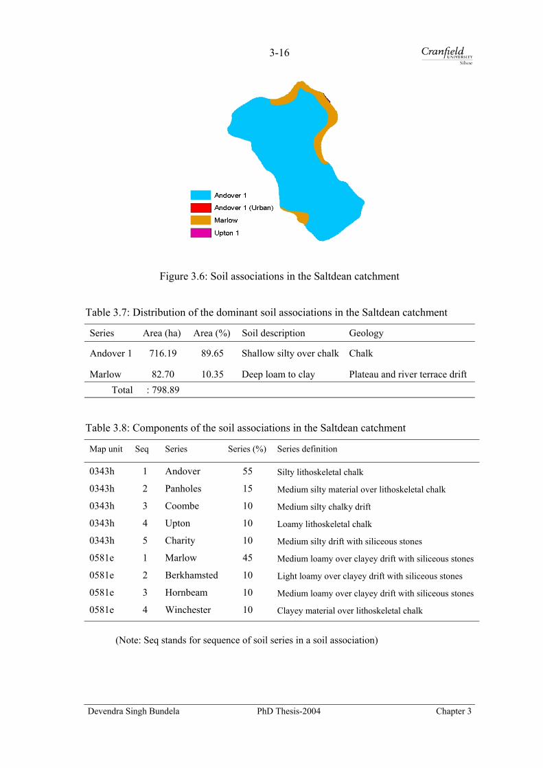
3-16
Figure 3.6: Soil associations in the Saltdean catchment
Table 3.7: Distribution of the dominant soil associations in the Saltdean catchment
Series Area (ha) Area (%) Soil description Geology
Andover 1 716.19 89.65 Shallow silty over chalk Chalk
Marlow 82.70 10.35 Deep loam to clay Plateau and river terrace drift Total : 798.89
Table 3.8: Components of the soil associations in the Saltdean catchment
Map unit Seq Series Series (%) Series definition
0343h 1 Andover 55 Silty lithoskeletal chalk
0343h 2 Panholes 15 Medium silty material over lithoskeletal chalk
0343h 3 Coombe 10 Medium silty chalky drift
0343h 4 Upton 10 Loamy lithoskeletal chalk
0343h 5 Charity 10 Medium silty drift with siliceous stones
0581e 1 Marlow 45 Medium loamy over clayey drift with siliceous stones
0581e 2 Berkhamsted 10 Light loamy over clayey drift with siliceous stones
0581e 3 Hornbeam 10 Medium loamy over clayey drift with siliceous stones
0581e 4 Winchester 10 Clayey material over lithoskeletal chalk
(Note: Seq stands for sequence of soil series in a soil association)
Devendra Singh Bundela PhD Thesis-2004 Chapter 3
3-17
3.3.5 Limitations of Soil Data
In the NATMAP soil map, each soil association polygon contains a dominant
and a few subsidiary soil series. It was not possible to locate constituent soil series
spatially in the polygons (Bradley, 2004), so it was assumed that each mapping polygon
contains a dominant soil series only. Accordingly, the hydraulic properties and
infiltration parameters were calculated for the dominant soil series of each polygon. In
this way, soil variability in each polygon is almost lost. Although the soil association is
not an appropriate mapping unit for catchment scale distributed modelling, detailed soil
map with mapping unit at soil series level is, in fact, required for an optimal
representation of soil variability at catchment scale. In the absence of a detailed soil
map and corresponding properties, infiltration parameters were estimated on the basis of
primary soil properties of the dominant soil series.
3.3.6 Description of Soil Properties Data
Soil mineral particle fractions, organic carbon and pH are calculated directly
from individual analyses of different soil horizon samples taken from soil profiles
during the field survey to characterise the soil series. The mineral particle size
distribution is independent of land use and, therefore, the same particle fractions are
used for all the four land uses. Both organic carbon and pH are dependent on land use
within a soil series, so they are stratified into four land uses of each series.
Bulk density of a soil series varies with landuse, soil horizon and parent material.
Bulk density data are estimated using pedotransfer functions and are stratified into 25
groupings on the basis of land use, soil horizon and parent material. The pedotransfer
functions are empirical equations relating the bulk density to mineral soil particle
fractions and organic carbon of the soil profile data. Each group is analysed statistically
to derive the best possible pedotransfer functions for bulk density. These functions
explain 77 per cent variations in bulk density with an overall standard deviation of
0.113 when compared with measured bulk densities data (Hollis et al, 1995).
Devendra Singh Bundela PhD Thesis-2004 Chapter 3
3-18
3.3.7 Estimation of Soil Hydraulic Properties
Soil hydraulic properties are characterised by two relationships: the soil water
retention (θ-h) curve and the hydraulic conductivity functions (K-θ/h). These are
predicted using pedotransfer functions derived from a combination of sand, silt, clay,
organic carbon and bulk density. Water retention and hydraulic conductivity values are
predicted from a theoretical basis using both closed form equations of Van Genuchten
and Hutson and Cass modification of Brooks-Corey. Initial estimation of soil water
potential and moisture content curve for each horizon is made from the profile data
using the Arya and Paris model (Arya and Paris, 1981). The Van Genuchten’s equation
is fitted to each curve to derive α and n parameters from sand, silt, clay, organic carbon
and bulk density. Saturated hydraulic conductivity values are predicted from empirical
curvilinear equations relating conductivity to air filled porosity at 5 kPa soil water
potential (drainable pore space). These relationships are derived from a limited dataset
of saturated hydraulic conductivity measurements. The hydraulic conductivity at 5 kPa
is then estimated from a relationship between saturated hydraulic conductivity,
unsaturated hydraulic conductivity and soil water content using closed form equations
of Van Genuchten (1980).
Pedotransfer functions (PTFs)
Soil hydraulic properties and infiltration parameters can be estimated from
available or cheaply measured soil data using pedotransfer functions (PTFs). PTFs are
empirical equations mostly developed from soil databases of the temperate region and
should be used with a great care for other climatic soils. PTFs rely on direct
measurement methods for validation and thus can not exist without them (Wösten et al,
2001; Wösten et al, 1995).
Pedotransfer functions are of three kinds: point PTFs, parametric PTFs, and
physico-empirical PTFs (McBratney et al, 2002). Parametric PTFs are preferred for
predicting the water-retention curve and hydraulic conductivity characteristics. These
can be predicted from soil properties either by the Van Genuchten and Mualem model
or by the Brooks-Corey model. Five parameters: θr, θs, α, n, and Ks are required for the
Van Genuchten and Mualem model to establish both soil water retention and soil
Devendra Singh Bundela PhD Thesis-2004 Chapter 3
3-19
hydraulic conductivity relationships. The relationship between soil water content and
water potential is expressed by an equation (Van Genuchten, 1980):
[ ] mne )h(1S
−α+= … Eq. 3.6
where Se is the degree of saturation or relative water content and is expressed as:
rs
reS
θ−θθ−θ
= … Eq. 3.7
Equation 3.7 can be rewritten after substituting Se from Equation 3.8:
mnrs
r))h(1(
)h(α+
θ−θ+θ=θ … Eq. 3.8
where θr and θs are the residual and saturated water content, α is the scaling parameter,
n and m are the curve shape parameters (m=1-1/n) and h is the soil water potential.
Relationships between hydraulic conductivity and soil water content or water
potential are expressed by equations (Mualem, 1976).
( ) 2mm/1eese S11S*K)S(K
−−= l
and … Eq. 3.9
( )( )
2
mn
mnmn
s)h(1
)h(1)h(1K)h(K
lα+
α+α−
=
−
… Eq. 3.10
where Ks is the saturated hydraulic conductivity and l is the empirical parameter
describing pore tortuosity (usually 0.5).
Water-retention and hydraulic conductivity characteristics can also be predicted
from soil physical properties using equations (Brooks-Corey, 1964):
θ−θ+θ
θ
=θ λ
hh
)()h( b
rsr
s
… Eq. 3.11
If h ≥ hb
If h < hb
If h ≥ hb
Devendra Singh Bundela PhD Thesis-2004 Chapter 3

3-20
= +λ 3/2es
se
S*K
K)S(K … Eq. 3.12 If h < hb
where hb is the bubbling pressure or air entry potential (cm), h is the wetting front
suction head, and λ is the pore size distribution index.
3.3.8 Estimation of Infiltration Parameters
Infiltration and vertical transport of water in the soils can be simulated by three
models in LISEM: Holton (Beasley and Hoggins, 1982), Green and Ampt (Li et al,
1976) for one or two layers, and SWATRE (Belmans et al, 1983; Feddes et al, 1978).
The Holtan and Green-Ampt models simulate the Hortonian overland flow only. The
SWATRE model simulates both the Hortonian and saturation excess overland flows.
Different surfaces such as crusted, compacted and grass strip can also be simulated in
both the SWATRE and Green and Ampt models. The selection of a model is done on
the basis of availability of soil data and the user understanding on catchment
characteristics and processes. Input data requirement increases from least for the Holtan
model to intensive for the SWATRE model.
The Holton model is a semi-empirical method and requires seven parameters to
simulate the infiltration process, which are described in the LISEM Manual (Jetten,
2002). These seven parameters can be derived from the 1:250 000 scale soil data. Being
an empirical model, it may not be an appropriate choice for simulating the infiltration
process for the Saltdean catchment.
The SWATRE model is a finite difference numerical solution of the Richards’s
equation and can be set up for a maximum of 20 soil horizons. It requires a series of
maps and tables of soil profiles and soil hydraulic properties that describe the profile of
each land use and land cover with K-θ-h values for each horizon (Jetten, 2002). In
other words, the SWATRE model requires a large number of parameters and some of
which can be measured from the laboratory experiments for each land use such as K-θ-h
relationships. It was not possible to derive the precise range of K-θ-h for each horizon
and land use from available soil data. Therefore, it was not used for modelling
infiltration of a historic storm event. It would be more appropriate to choose a
Devendra Singh Bundela PhD Thesis-2004 Chapter 3

3-21
physically-based model, which requires medium level of data requirement and simulates
infiltration more or less reasonably. The Green and Ampt model met this requirement
and was, therefore, selected for the Saltdean catchment with its parameters being
derived from the 1:250 000 scale soil map and its soil properties data.
Single layer Green and Ampt model
The Green and Ampt model is a physically-based approach, computationally
efficient and easy to derive its parameters from soil and land use information (Chow et
al, 1988). It assumes the homogeneous soil profile and soil moisture distribution.
Infiltration process can be modelled as a saturation wetting front crossing the soil
profile vertically. The soil moisture above the wetting front is at saturation and the soil
moisture below the wetting front is equal to the initial soil moisture. The model can also
simulate the infiltration for a soil depth limited by impermeable subsoil and different
types of surfaces such as, crusted, compacted and grass strips.
Application of a single layer Green and Ampt model requires the estimation of
its parameters: hydraulic conductivity, K; effective porosity, φe; and wetting front
suction head, h; initial volumetric soil moisture content, θi; and soil depth (d) (Jetten,
2002). First three parameters can be estimated from soil properties using pedotransfer
functions. Initial moisture content before a storm can either be measured or assumed.
Soil depth can be taken from the soil profile data. The Green and Ampt parameters can
be estimated either by the Brooks-Corey model or by the Van Genuchten model. The
Brooks-Corey model was used for computing the Green and Ampt parameters.
The effective porosity (φe) of a horizon in a soil series is calculated as:
rtotale θφφ −= … Eq. 3.13
where θr is the residual moisture content and φtotal is the total porosity which is
calculated using an equation:
PDBD1total −=φ … Eq. 3.14
where BD is the bulk density and PD is the particle density.
Devendra Singh Bundela PhD Thesis-2004 Chapter 3

3-22
The wetting front suction head is estimated using the Brooks and Corey soil water
retention parameters (Rawls et al, 1983):
+λ+λ
=2
h2232h b
… Eq. 3.15
where hb is the bubbling pressure (cm) and λ is the pore size distribution index and these
are computed using pedotransfer functions (Jarvis et al, 1997):
log hb = 0.4104 + 0.002684*sand +0.006354*silt + 0.17766*BD + 0.00013855*clay2
… Eq. 3.16
log λ= -0.475662 + 0.005165*sand + 0.002066*silt - 0.023327*clay -0.040628*BD +
0.6824*OC - 0.000136162*sand2 - 0.0000954716*silt2 + 0.000298891*clay2 -
0.0637*BD2- 3.1679*OC2 + 0.0000010388*sand3 + 0.0000010299*silt3 -
0.0000013251*clay3 … Eq. 3.17
where sand, silt and clay contents are in per cent; the bulk density is in g cm-1 and OC is
the organic carbon in g g-1.
Saturated hydraulic conductivity, Ks (cm/h) is estimated from the effective porosity,
bubbling or air entry pressure and pore size distribution index (Rawls et al, 1983) as:
3600*)2)(1(
)h/(*21K
22be
s +λ+λλθ
= … Eq. 3.18
Parameter estimation for the Saltdean catchment
The Saltdean catchment contains two dominant soil series such as Andover and
Marlow as described in Section 3.3.4. The Andover series consists of three horizons.
The soil properties are available for the first horizon only as other two horizons contain
the rubble and rock. The Marlow series contains four soil horizons. The soil properties
are available for all the horizons with four land uses each. Due to constraint of horizon
soil properties in the Andover series, a single layer Green-Ampt model was selected for
both series. Soil primary properties of the first horizon of the Andover and Marlow
series each (Table 3.9) were required for the estimation of hydraulic properties and
infiltration parameters. Ten hydraulic properties were predicted from the soil primary
Devendra Singh Bundela PhD Thesis-2004 Chapter 3

3-23
properties using pedotransfer functions (Hollis, 2004) (Appendices B-8a and b) and
were compared against the available hydraulic properties. As can be seen from Table
3.10, both available and predicted values have a very high correlation and reasonable
variability in most parameters.
Table 3.9: Soil primary properties of first horizon of the Saltdean catchment
S. No. Properties Unit Andover Marlow
1. Layer depth cm 25 25
2. Sand (60-2000 µm) per cent 22 41
3. Silt (2-60 µm) per cent 56 37
4. Clay (< 2µm) per cent 22 22
5. Organic carbon per cent 3.8 2.2
The bubbling pressure and pore size distribution index for four land uses of
each soil series were estimated using Equations 3.16 and 3.17. The effective porosity,
wetting front suction head and saturated hydraulic conductivity were then predicted for
four land uses of both soil series using Equations 3.13, 3.15 and 3.18. The wetting front
suction heads and saturated hydraulic conductivities for four land uses in each series
varied from 7.434 to 7.991 and from 4.833 to 6.979 respectively (Table 3.11). Moreover,
the predicted values need to be calibrated as they are at the higher end of parameter
range. Therefore, a single value for effective porosity, wetting front suction head and
saturated hydraulic conductivity for each series based on arable land use was used to
make calibration easier. Furthermore, validation of the model was not involved in the
study. Therefore, in this approach, it was considered acceptable to use a single set of
value for both series for infiltration modelling from a storm of high intensity, which
makes small variations in infiltration relatively unimportant.
Devendra Singh Bundela PhD Thesis-2004 Chapter 3
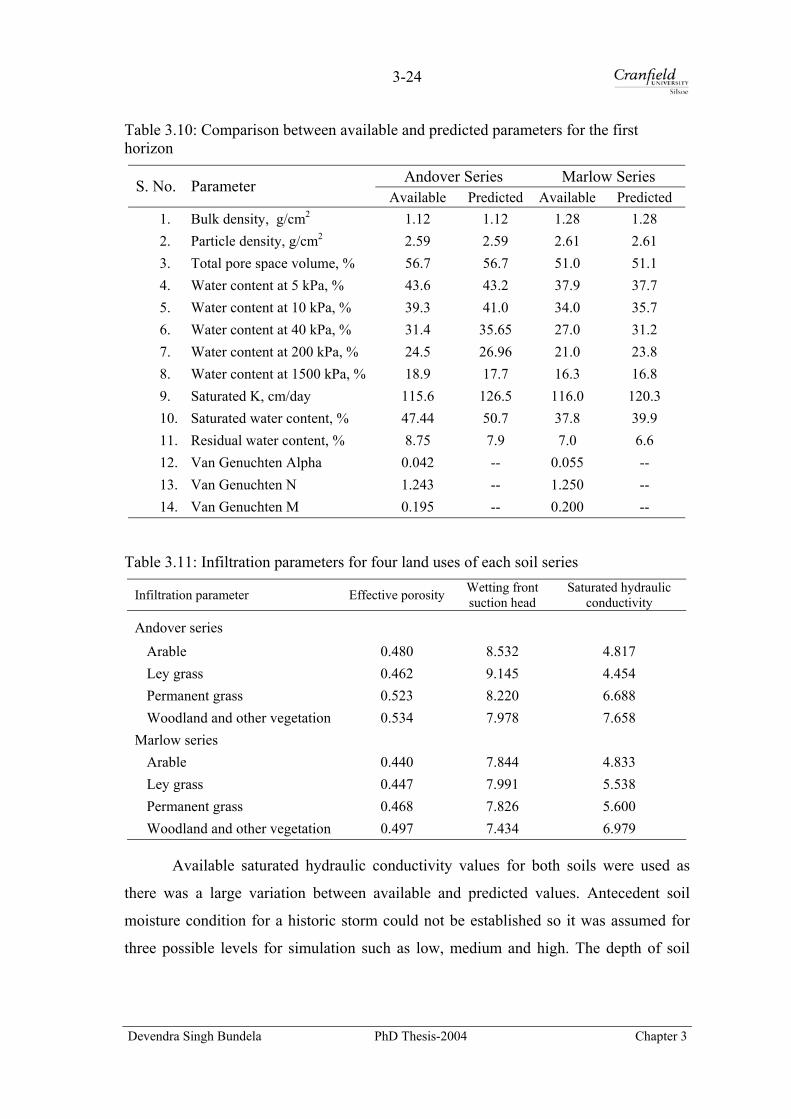
3-24
Table 3.10: Comparison between available and predicted parameters for the first horizon
Andover Series Marlow Series S. No. Parameter Available Predicted Available Predicted
1. Bulk density, g/cm2 1.12 1.12 1.28 1.28 2. Particle density, g/cm2 2.59 2.59 2.61 2.61 3. Total pore space volume, % 56.7 56.7 51.0 51.1 4. Water content at 5 kPa, % 43.6 43.2 37.9 37.7 5. Water content at 10 kPa, % 39.3 41.0 34.0 35.7 6. Water content at 40 kPa, % 31.4 35.65 27.0 31.2 7. Water content at 200 kPa, % 24.5 26.96 21.0 23.8 8. Water content at 1500 kPa, % 18.9 17.7 16.3 16.8 9. Saturated K, cm/day 115.6 126.5 116.0 120.3 10. Saturated water content, % 47.44 50.7 37.8 39.9 11. Residual water content, % 8.75 7.9 7.0 6.6 12. Van Genuchten Alpha 0.042 -- 0.055 -- 13. Van Genuchten N 1.243 -- 1.250 -- 14. Van Genuchten M 0.195 -- 0.200 --
Table 3.11: Infiltration parameters for four land uses of each soil series
Infiltration parameter Effective porosity Wetting front suction head
Saturated hydraulic conductivity
Andover series
Arable 0.480 8.532 4.817 Ley grass 0.462 9.145 4.454 Permanent grass 0.523 8.220 6.688 Woodland and other vegetation 0.534 7.978 7.658
Marlow series Arable 0.440 7.844 4.833 Ley grass 0.447 7.991 5.538 Permanent grass 0.468 7.826 5.600 Woodland and other vegetation 0.497 7.434 6.979
Available saturated hydraulic conductivity values for both soils were used as
there was a large variation between available and predicted values. Antecedent soil
moisture condition for a historic storm could not be established so it was assumed for
three possible levels for simulation such as low, medium and high. The depth of soil
Devendra Singh Bundela PhD Thesis-2004 Chapter 3

3-25
layer was taken from soil properties data. In this way, all the parameters for single layer
Green and Ampt model were derived for each series (Table 3.12).
Table 3.12: Green and Ampt parameters for the Andover and Marlow series
Parameter Andover series Marlow series Unit
Brooks-Corey parameters Bubbling pressure, hb 12.400 11.220 cm
Pore size distribution index, λ 0.124 0.113
Green and Ampt parameters
Effective porosity, e 0.48 0.44 cm3/cm3
Wetting front suction head, h 8.533 7.844 cm
Saturated hydraulic conductivity 4.817 4.833 cm/hr
Ksat (predicted from soil properties) 3.327 2.792 cm/hr
Depth of the first soil layer 25.00 25.00 cm
Antecedent soil moisture levels cm3/cm3
High (assumed) 0.46 0.44 Fraction
Medium (assumed) 0.24 0.22 ,,
Low (assumed) 0.08 0.07 ,,
Hydraulic conductivity for the Green and Ampt model is one half of the
saturated hydraulic conductivity predicted from the soil data (Bouwler, 1966). Therefore,
the saturated hydraulic conductivity and water front suction head were to be calibrated
to get reasonable outputs from a model.
3.4 Concluding Remarks
3.4.1 Discussion
A methodology is used to identify heavy wet periods from daily rainfall data to
obtain hourly data for the specific periods. Subsequently, fifteen storms were identified
from hourly rainfall in autumn and early winter 2000. The storm on 11-12 October 2000
has a return period of 53 years while all other storms have return periods less than 5
years. A 6-hour single storm from 30 October 2000 would be used for modelling study
to optimise the computer storage requirement. The spatial and temporal resolutions of
rainstorm data were coarse for the catchment. Storms were the result from frontal
depressions which last for at least a couple of hours. Therefore, a single raingauge data
Devendra Singh Bundela PhD Thesis-2004 Chapter 3
3-26
has provided a spatially representative rainfall data of the storms over the catchment. An
hour temporal resolution was too coarse for analysing the temporal variability of a
storm. Short duration storms might have gone unrecorded. Hourly data were more or
less representative for frontal storms and, therefore, were suitable for modelling study.
Infiltration and water transport in the soils is a major hydrologic process
controlling runoff and associated soil erosion. The soil map at a scale of 1:250 000 was
only available data for the Eastern South Downs and the Saltdean catchment. Although,
it was not the best soil data for catchment scale modelling, but it was used for
estimation of the Green and Ampt infiltration parameters and soil hydraulic properties
using pedotransfer functions. The soil was mapped at soil associations, which comprise
of a dominant and a few other soil series of similar origin. It was not possible by any
means to locate each constituent soil series spatially in a soil association polygon
(Bradley, 2004), therefore, it was assumed that each mapping polygon contained the
dominant soil series only. A single layer infiltration model was chosen because the
Andover series contains a single horizon soil properties data. These limitations result in
unrealistic parameter values, which ultimately affect the prediction capability.
3.4.2 Conclusions
• Fifteen rain storms were identified from daily rainfall data using rules to target
the specific heavy wet periods to obtain hourly rainfall data for a better
description of a storm. A 6-hour storm of 30 October 2000 would be used for the
simulation study. Hourly data was reasonably representative for describing
spatial and temporal distribution of the 30 October 2000 frontal storm.
• Infiltration parameters for a single layer Green and Ampt model were estimated
from the national soil map at a scale of 1:250 000 using pedotransfer functions.
Devendra Singh Bundela PhD Thesis-2004 Chapter 3

4-1
4 Land Use and Land Cover Mapping
This chapter treats a hybrid classification methodology for SPOT-1
multispectral data for mapping of land use and land cover for a historic
storm event. An overall classification accuracy of 90 per cent was
achieved which reflects reliable land use and land cover information
suitable for the modelling study.
4.1 Introduction
Land use and land cover are key spatial data derived from remotely sensing and
is necessary for distributed erosion modelling. They are used for deriving model spatial
input parameters by reclassifying the land use and land cover thematic map to produce
parameter maps. Performance of an event-based distributed model largely depends on
reliable information obtained on land use and land cover with its spatial and temporal
variations in a catchment because it is highly dynamic in nature and changes with
seasonal and climatic variations.
The Eastern South Downs have been transformed from a grazing landscape to an
arable landscape with more winter cereal crops in last fifty years of the 20th Century.
This led to severe soil erosion and degradation in fields and flooding in near by
residential areas during the winter season (Boardman, 2003). Landscape conservation
and enhancement schemes viz. Set-aside, Environmentally Sensitive Areas (ESA)
monitoring, Countryside Stewardship and Area of Outstanding Natural Beauty (AONB)
Devendra Singh Bundela PhD Thesis-2004 Chapter 4

4-2
are in operation to safeguard and conserve the chalk landscape from degradation and to
mitigate local flooding (Countryside Agency, 2001; DEFRA, 2003). Land use and land
cover of the Eastern South Downs was mapped three times using visual interpretation of
1:10 000 scale aerial photographs (ADAS, 1996a). Another source is the Land Cover
Map 2000 (Fuller et al, 2002), which provides broad land cover classes. The available
information does not meet the requirement for distributed modelling of the storm event
that occurred on 30 October 2000. The required information needs to be close to the
rainstorm event for obtaining reliable modelling results. Therefore, a remote sensing
approach needs to be employed to obtain this information close to the storm.
A quick and reliable method is required for mapping the spatial distribution of
land use and land cover close to the storm event from remotely sensed data. The format
of classification results and information required for the modelling needs to be
compatible for ingesting a thematic map directly to the model to derive model
parameters. This chapter is dedicated to exploring for a quick and reliable procedure for
mapping of land use and land cover of the Eastern South Downs.
4.2 Remote Sensing Approach
Reliable and timely land use and land cover information is necessary at
catchment scale for distributed modelling study. Conventional mapping approaches
alone are time consuming and expensive. Remote sensing can be exploited to provide
timely information, but it requires some form of ground data as a check to make it
reliable. Satellite remote sensing with a limited field work has been successfully used
for mapping a range of land use and land cover classes at a variety of spatial and
temporal scales (Schultz, 1988). It is a cost effective alternative and major source of
timely and reliable information for environmental distributed modelling, because of
repeated observations in relatively short period and synoptic multispectral coverage.
Multispectral classification techniques for land use and land cover mapping have been
proved to be promising as a key spatial input data to several erosion modelling studies.
Erosion models based on land use and land cover have been modified to directly
ingest thematic data derived from multispectral classification to identify land use and
Devendra Singh Bundela PhD Thesis-2004 Chapter 4

4-3
land cover classes in a catchment (Davis et al, 1991; Engman and Gurney, 1991).
4.3 Land Use and Land Cover Status
The Eastern South Downs was selected as the study site for land use and land
cover mapping (Figure 4.1). Land use and land cover of the Eastern South Downs was
first mapped extensively in 1987 and later revised in 1991 and 1995 using visual
interpretation of aerial photographs with some limited ground checking under the
Environmentally Sensitive Areas (ESAs) monitoring programme. These surveys
indicated that areas under arable, grassland and dense scrub and woodland were about
53, 22 and 18 percent respectively with 91 per cent classification accuracy for classes
(ADAS, 1996a). The change in land cover was remapped by comparison of aerial
photographs under revised ESAs and results of land cover of various surveys are given
in Table 4.1.
Figure 4.1: Location map of the Eastern South Downs study area
4.4 Hierarchical Classification Scheme
Land use and land cover mapping attempts should be accompanied by a suitable
classification scheme for use at a desired scale, for a designated area and within the
capability of information gathering techniques being used (Anderson et al, 1976). Land
use and land cover are conceptually different. The former is related to man’s activity on
Devendra Singh Bundela PhD Thesis-2004 Chapter 4

4-4
land while the latter describes the spatial distribution of actual land cover, mainly
variations in vegetation. A hierarchical classification scheme provides a better
framework for organising and categorising the information to be extracted at several
levels from an image (Jensen, 2000).
Table 4.1: Land use and land cover changes in the Eastern South Downs (adapted from ADAS, 1996a)
Area in per cent Land use and cover 1987 1991 1995
Arable 53.57 53.15 44.92 Grassland 22.22 21.61 29.69 Dense scrub and woodland 17.88 18.40 18.36 Non-agricultural land 6.03 6.54 6.72 Open water 0.30 0.30 0.31
A suitable hierarchical classification scheme for the Eastern South Downs was
worked out on the basis of a few classification schemes such as the South Downs
Environmentally Sensitive Areas Landscape Monitoring (ADAS, 1996a & b),
Monitoring Land cover Changes in National Parks of England and Wales (Taylor et al,
1991 a & b), USGS Land Use and Land Cover Classification System for Use with
Remote Sensor Data (Anderson et al, 1976) and Land cover Classification in
Countryside Survey 2000 under the UK Biodiversity Action Plan (Fuller et al, 2002). A
land use and land cover classification scheme (Table 4.2) was proposed and used for
mapping of land use and land cover of the study area. The definition of classes of the
scheme is given in Appendix C-1.
Devendra Singh Bundela PhD Thesis-2004 Chapter 4
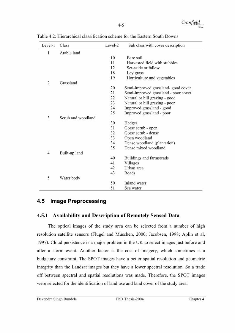
4-5
Table 4.2: Hierarchical classification scheme for the Eastern South Downs
Level-1 Class Level-2 Sub class with cover description
1 Arable land 10 Bare soil 11 Harvested field with stubbles 12 Set-aside or fallow 18 Ley grass 19 Horticulture and vegetables
2 Grassland 20 Semi-improved grassland- good cover 21 Semi-improved grassland - poor cover 22 Natural or hill grazing - good 23 Natural or hill grazing - poor 24 Improved grassland - good 25 Improved grassland - poor
3 Scrub and woodland 30 Hedges 31 Gorse scrub - open 32 Gorse scrub - dense 33 Open woodland 34 Dense woodland (plantation) 35 Dense mixed woodland
4 Built-up land 40 Buildings and farmsteads 41 Villages 42 Urban area 43 Roads
5 Water body 50 Inland water 51 Sea water
4.5 Image Preprocessing
4.5.1 Availability and Description of Remotely Sensed Data
The optical images of the study area can be selected from a number of high
resolution satellite sensors (Flügel and Müschen, 2000; Jacobsen, 1998; Aplin et al,
1997). Cloud persistence is a major problem in the UK to select images just before and
after a storm event. Another factor is the cost of imagery, which sometimes is a
budgetary constraint. The SPOT images have a better spatial resolution and geometric
integrity than the Landsat images but they have a lower spectral resolution. So a trade
off between spectral and spatial resolutions was made. Therefore, the SPOT images
were selected for the identification of land use and land cover of the study area.
Devendra Singh Bundela PhD Thesis-2004 Chapter 4
4-6
Description of the SPOT satellites The SPOT (Satellite Pour l’Observation de la Terre) satellite is the French earth
observing satellite system and consists of five satellites that operate from a sun-
synchronous, near polar orbit, 832 km above the earth. At present, three satellites are in
operation: SPOT-2 (since 1990), SPOT-4 (since 1998) and the recently launched SPOT-
5 (since 2002). SPOT-1 was active till 2002 while SPOT-3 was in orbit between 1993
and 1996. They are inclined 98.7 degrees, cross the equator at 10:30 AM local time and
have an orbital cycle of 26 days (SPOT Image, 2004; Brachet, 1986). The
characteristics of the SPOT satellite sensors are compared (Appendix C-2).
The SPOT-1 images are collected in visible and near-infrared bands from the
High Resolution Visible (HRV) sensors. The SPOT-1 satellite carries two HRVs with
the capability of scanning in either a multispectral mode or a panchromatic mode. The
multispectral mode captures images in three spectral bands: 0.50- 0.59, 0.61- 0.68 and
0.79- 0.89 µm. These bands are co-registered and have a ground resolution of 20 m. The
panchromatic mode collects images in the spectral range 0.51- 0.73 µm at a 10 m
ground resolution. Each nominal scene covers an area of 60 km by 60 km. The viewing
angle of each HRV sensor can be adjusted to collect images up to 27 degrees right or
left of satellite nadir. This cross-track pointing capability allows the same point on the
earth to be viewed from several different orbits and thus, enables the acquisition of
stereoscopic imagery.
Applications of SPOT data The SPOT multispectral imagery has widely been used for land use and land
cover mapping. The SPOT image applications with their respective discipline are
discussed in the literature (Brachet, 1986). The SPOT bands have also been applied to
many applications since the launch of the SPOT-1 HRV sensor. However, SPOT-1 had
only three band multispectral data. The principal applications of the SPOT bands are
described (Table 4.3).
Devendra Singh Bundela PhD Thesis-2004 Chapter 4
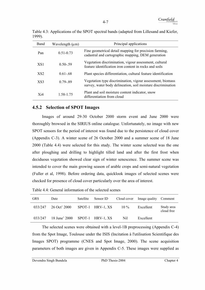
4-7
Table 4.3: Applications of the SPOT spectral bands (adapted from Lillesand and Kiefer, 1999).
Band Wavelength (µm) Principal applications
Pan 0.51-0.73 Fine geometrical detail mapping for precision farming, cadastral and cartographic mapping, DEM generation
XS1 0.50-.59 Vegetation discrimination, vigour assessment, cultural feature identification iron content in rocks and soils
XS2 0.61-.68 Plant species differentiation, cultural feature identification
XS3 0.79-.89 Vegetation type discrimination, vigour assessment, biomass survey, water body delineation, soil moisture discrimination
Xi4 1.58-1.75 Plant and soil moisture content indicator, snow differentiation from cloud
4.5.2 Selection of SPOT Images
Images of around 29-30 October 2000 storm event and June 2000 were
thoroughly browsed in the SIRIUS online catalogue. Unfortunately, no image with new
SPOT sensors for the period of interest was found due to the persistence of cloud cover
(Appendix C-3). A winter scene of 26 October 2000 and a summer scene of 18 June
2000 (Table 4.4) were selected for this study. The winter scene selected was the one
after ploughing and drilling to highlight tilled land and after the first frost when
deciduous vegetation showed clear sign of winter senescence. The summer scene was
intended to cover the main growing season of arable crops and semi-natural vegetation
(Fuller et al, 1998). Before ordering data, quicklook images of selected scenes were
checked for presence of cloud cover particularly over the area of interest.
Table 4.4: General information of the selected scenes
GRS Date Satellite Sensor ID Cloud cover Image quality Comment
033/247 26 Oct’ 2000 SPOT-1 HRV-1, XS 10 % Excellent Study area cloud free
033/247 18 June’ 2000 SPOT-1 HRV-1, XS Nil Excellent
The selected scenes were obtained with a level-1B preprocessing (Appendix C-4)
from the Spot Image, Toulouse under the ISIS (Incitation à l'utilisation Scientifique des
Images SPOT) programme (CNES and Spot Image, 2000). The scene acquisition
parameters of both images are given in Appendix C-5. These images were supplied as
Devendra Singh Bundela PhD Thesis-2004 Chapter 4
4-8
the standard scene in a CEOS structure with a CAP format (Appendix C-6) on an
optical disk. The scenes were imported to the ERDAS Imagine version 8.6 for further
processing.
4.5.3 Geometric Correction
The study area was small as compared to a full scene size and was identified in
the central part of the scene using distinct ground features. A subset larger than the
study area would be a better choice in order to utilise disk storage space efficiently and
to improve data processing. Therefore, the subset image of 1400 pixels by 700 pixels
was extracted from the 26 October scene. Similarly, the same area was also extracted
from the 16 June image and both images were then used for geometric correction.
Geometric correction is the process of transforming an image to conform to a
standard projection and coordinate system, to be integrated with other key spatial data
in a GIS (Williams, 1995). Satellite images usually contain significant geometric
distortions, which need to be corrected in two steps, systematic correction and local
correction. A systematic correction is usually applied at a ground station using a
parametric sensor model while image warping for local correction is applied to system
corrected images using a polynomial transform equation based on sufficient and well
distributed ground control points over a study area collected from various sources.
Local geometric correction involves locating the ground control points, computing the
transformation matrix and then creating an output file with a new projection by
resampling (ERDAS, 2002).
The images obtained with the Level-1B geometric format were already
geometrically corrected for systematic errors associated with sensor operation, and earth
motion and curvature (Richards and Xia, 1999). The study area image of 26 October
was geometrically corrected to the British National Grid coordinate system using a first
order polynomial transformation with 31 ground control points (GCPs) well distributed
all over the area (Appendix C-7(a)). The reference GCPs were collected from 1:25 000
scale Ordnance Survey Pathfinder series map, published in 1991. This map is based on
the Transverse Mercator projection, Airy spheroid, Ordnance Survey Great Britain 1936
datum and mean sea level vertical datum at Newlyn. The RMS error for the
Devendra Singh Bundela PhD Thesis-2004 Chapter 4

4-9
transformation was within an acceptable limit, less than a pixel (0.67 pixels). The input
image was resampled to a 20 m output image using the cubic convolution technique.
This rectified image was used for further processing.
An 18 June image subset was co-registered to a 26 October rectified image as
reference image using a first order polynomial transformation with 26 GCPs well
distributed over the image. The RMS error for the transformation was 0.40 pixel
(Appendix C-7 (b)) and output image was obtained with 20 m pixel size using the cubic
convolution resampling. An 18 June image was used for visual interpretation of major
land use and land cover classes, which were used to check the classes with a 26 October
image in case of confusion as there was a large time gap between the field survey and
the time of image acquisition. It was not used at all for digital classification.
4.5.4 Delineation of the Study Area
The geometrically corrected sub set image of 26 October 2000 was used in
conjunction with a 1:50 000 scale Ordnance Survey Landranger map of the South
Downs (sheet number 198, second series) with 10 m contour intervals, published in
April 2000, to delineate the Eastern South Downs study area. The study area was
delineated by an easting grid line of 542 000 m on the east, by the river Adur on the
west, by northing grid line of 114 000 m on the north and by sea on the south.
4.5.5 Evaluation of Multispectral Data
The univariate statistics, and variance-covariance and correlation matrices of the
study area image delineated from the 26 October 2000 image were computed to assess
the relationship between bands. Table 4.5 shows that the first band, XS1 and second
band, XS2 are highly correlated with each other while second and third bands, and third
and first bands are poorly correlated. Therefore, there is some redundancy of
information in the image. The false colour composite image of the study area delineated
from 26 October 2000 image is displayed in Figure 4.2.
Devendra Singh Bundela PhD Thesis-2004 Chapter 4

4-10
Table 4.5: Statistics properties of the study area image (26 October 2000)
Univariate statistics Parameter/band
XS1 XS2 XS3
Minimum 29 7 8 Maximum 235 112 150 Mean 47.83 25.18 56.62 Standard deviation 7.42 6.53 18.37 Median 47 24 54 Mode 46 22 44
Variance co-variance matrix
XS1 55.00 XS2 45.11 42.68 XS3 23.99 -0.98 337.35
Correlation matrix
XS1 1.000 XS2 0.931 1.000 XS3 0.176 -0.008 1.000
4.5.6 Image Enhancement
Image enhancement techniques are applied to increase the general sharpness and
separability of the data. These are in-built within most digital image processing software
and include contrast manipulation, grey level slicing, spatial filtering, band ratioing and
principal component analysis (Jensen, 1996). Linear, Gaussian, histogram equalisation,
standard deviations, gamma etc are a few of contrast enhancement functions. The
standard deviation enhancement was applied to both images to improve their
interpretability.
Devendra Singh Bundela PhD Thesis-2004 Chapter 4

4-11
Figure 4.2: False colour composite of the Eastern South Down study area (26 Oct 2000)
4.6 Ground Data Survey Strategy
4.6.1 Need for Ground Data
Ground data collection is an integral part of supervised classification and
involves field survey to record land use and land cover information and conditions of an
area of interest. The field survey is planned to collect the ground data information for:
• extracting training signatures for supervised classifier (Taylor et al, 1997;
Campbell, 1999),
• assessing the accuracy of supervised classification of remotely sensed data
(Congalton and Green, 1999; Congalton, 1991),
• verification of land use and cover classes generated by unsupervised classification
(Campbell, 1999), and
• identification of empirical relationships between biophysical parameters and
satellite observation (Colombo et al, 2003; Carlson, and Ripley, 1997).
Devendra Singh Bundela PhD Thesis-2004 Chapter 4
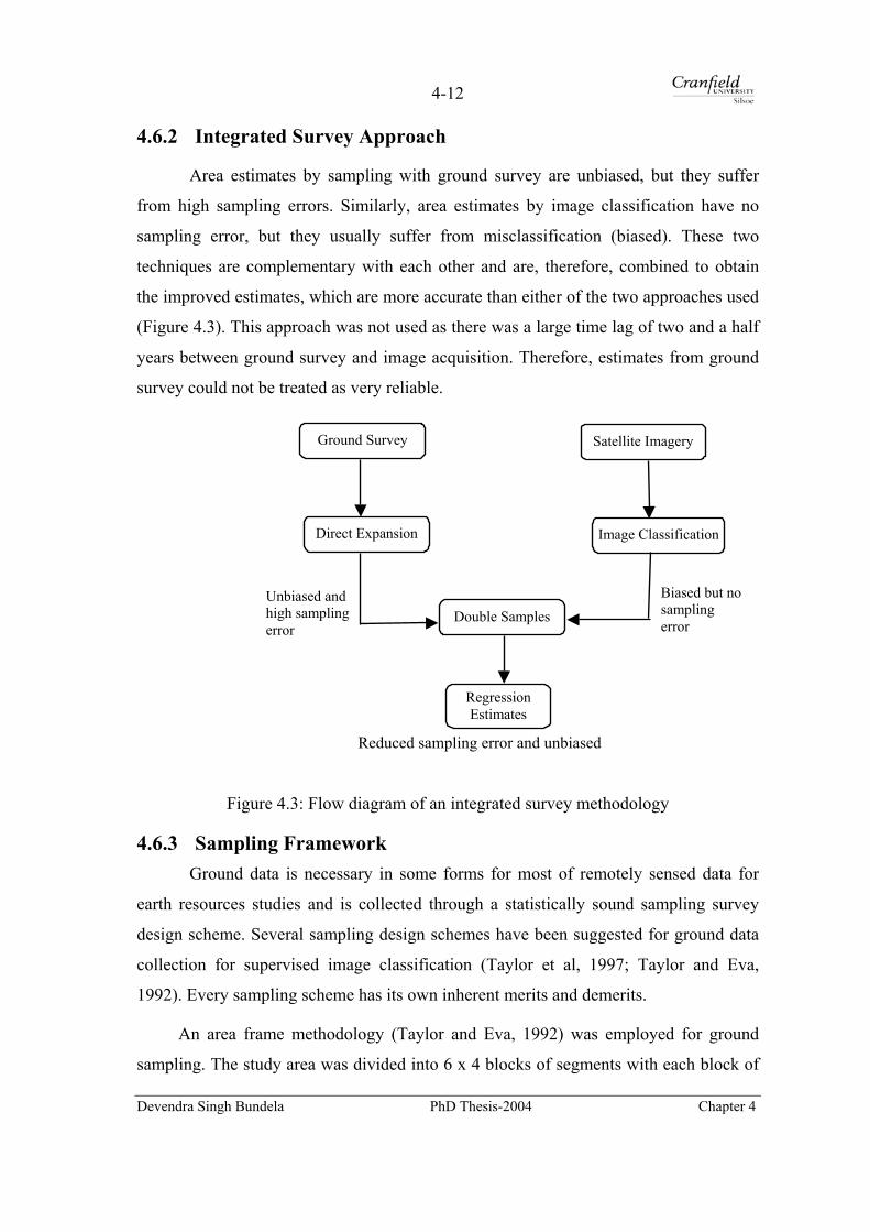
4-12
4.6.2 Integrated Survey Approach
Area estimates by sampling with ground survey are unbiased, but they suffer
from high sampling errors. Similarly, area estimates by image classification have no
sampling error, but they usually suffer from misclassification (biased). These two
techniques are complementary with each other and are, therefore, combined to obtain
the improved estimates, which are more accurate than either of the two approaches used
(Figure 4.3). This approach was not used as there was a large time lag of two and a half
years between ground survey and image acquisition. Therefore, estimates from ground
survey could not be treated as very reliable.
Ground Survey
Direct Expansion Image Classification
Double Samples
Regression Estimates
Satellite Imagery
Biased but no sampling error
Unbiased and high sampling error
Figure 4.3: Flow
4.6.3 Sampling FramewGround data is necess
earth resources studies and is
design scheme. Several sampl
collection for supervised ima
1992). Every sampling scheme
An area frame methodo
sampling. The study area was
Devendra Singh Bundela
Reduced sampling error and unbiased
diagram of an integrated survey methodology
ork ary in some forms for most of remotely sensed data for
collected through a statistically sound sampling survey
ing design schemes have been suggested for ground data
ge classification (Taylor et al, 1997; Taylor and Eva,
has its own inherent merits and demerits.
logy (Taylor and Eva, 1992) was employed for ground
divided into 6 x 4 blocks of segments with each block of
PhD Thesis-2004 Chapter 4

4-13
4 x 4 segments of 1 km x 1 km each. A segment sampling area frame of 1 km x 1 km
was selected because the same grid markings were available in the Ordnance Survey
maps. An unaligned systematic random sample design of segments was chosen from
blocks within the study area. No stratification was done in the sample design for the
Eastern South Downs because there was no basis for doing so. A random sampling
procedure was adopted which led to the selection of 14 segments highlighted in
Appendix C-8(a). Out of fourteen segments, three segments fell in urban areas. No
survey work was carried out as these samples were masked out separately by visual
interpretation. Eleven segments were finally selected for the field survey. The layout of
selected sample segments in the study area is given in Figure 4.4. The nominal sample
size was 4.82 per cent. The coordinates of top left corner of each segment selected for
field survey is given in Appendix C-8(b).
114 000 m
520
000 101 000 m
Urban segments
98 000 m
542
000
Figure 4.4: Layout of ground sample segments in the study area
Devendra Singh Bundela PhD Thesis-2004 Chapter 4

4-14
4.6.4 Field Survey Essentials
Image segments and map overlays
Eleven image segments of 1 km by 1 km each of the study area were extracted
from a false colour composite (FCC) image of 26 October using boundary coordinates
of sample segments. An image segment normally consisted of 50 pixels x 50 pixels of
20 m resolution. A buffer boundary of 200 m around an image segment was kept to
make recognition of large and continuous ground features easily and comparable with
adjoining image segments. All the image segments were produced at 1:10 000 scale for
ground data collection. An image segment with the buffer is shown in Figure 4.5, left.
In addition to the image segment of each survey site, a transparent map overlay
of each sample segment (Figure 4.5, right) was produced at 1:10 000 scale from the
Ordnance Survey maps available in the University Map Archive. The map overlay was
used as an aid to compare land use and land cover information in the field with an
image segment. Two map overlays were produced from 1:10 000 scale topographical
maps, published in 1991 and remaining nine were produced from 1:25 000 scale
Pathfinder second series maps, published in 1991, by the enlargement of the scale
because 1:10 000 scale maps were not available for all the segments in the Map
Archive.
Figure 4.5: Image segment (left) and map segme11 at 1:10 000
Devendra Singh Bundela PhD The
nt (right) produced for the segment no. scale
sis-2004 Chapter 4
4-15
Field documentation and maps
A field survey form was worked out and used to record field data corresponding
to field parcels on an image segment. A transparent sheet was overlaid on a map overlay
and an image segment to draw field parcel boundaries by a permanent marker pen and
record the land use and land cover of the parcels with all other details in a survey form.
An appropriate class definition of land use and land cover under a classification scheme
was also required during the field survey.
Maps and GPS instrument for navigation
The Ordnance Survey Pathfinder maps at 1:25 000 scale and a Landranger second
series map at 1:50 000 scale along with a Garmin GPS-12 handset were used for
navigating and locating ground sample segments in the study area. The handset was also
used for locating real time position within and outside a segment.
4.6.5 Field Survey
The field survey was carried out by visiting each sample segment to produce an
accurate spatial map of land use and land cover information of all the field parcels
existed within a segment. The field work was conducted during April - July 2003 to
make a full use of summer weather. In the field survey, individual parcels of each land
use and land cover in each sample segment were identified and drawn on a transparent
overlay sheet from a 1:10 000 scale image segment with the aid of a 1:10 000 scale map
overlay.
A Garmin GPS-12 Personal Navigator handset was used for navigation to locate
ground segments in the study area. The Pathfinder and Landranger series maps were
also used for route planning and for quick access to sample segments. The
topographical maps at 1:10 000 scale were used to locate field boundary in a segment.
A survey form of each segment was completed (Appendix C-9) corresponding to a
ground segment and a map overlay. All efforts were made to record the detailed
information of field parcels at the time of survey to enable to make an appropriate
judgment for possible land use and land cover at the time of a storm event.
Devendra Singh Bundela PhD Thesis-2004 Chapter 4

4-16
4.6.6 Problems Experienced in the Field Survey
A number of problems associated with the field survey were experienced in the
Eastern South Downs. Problems, which are important from survey accuracy point of
view, are as follows:
• Drawing of small and irregular shaped field parcels on a transparent overlay was
time consuming and less accurate in spatial extent.
• Many new features were found in the segments due to development taken place
and were not seen on the map overlays produced from the old topographical and
Pathfinder maps.
• Some new access paths to two segments were made, but they were not available
on the maps, which led to confusion and it took a long time to access the segments
through a long walk.
• Location coordinates of a point displayed in the Garmin GPS-12 Personal
Navigator handset were not accurate enough to locate field/parcel boundary
exactly and sometimes, the handset was not able to lock with the GPS satellite
network.
• A segment could not be accessed as there was no public footpath or bridleway.
Access through a private path was declined on request, so field survey was
completed from a distance which made some field work less accurate.
• A few fields in two segments were fenced with ‘live electric fences’ and were out
of bounds, so the field survey was completed from a distance.
• During a segment survey, I was surrounded by a cattle herd. Thank God, they
were friendly.
4.7 Processing of Ground Data
4.7.1 Digitisation of Ground Segments
Digitisation can be accomplished either in on-screen mode or table mode (Cohen,
1995) and the latter is more accurate than the former. With the development of an
optical intelligence mouse and improved GIS software, on-screen digitisation is now
Devendra Singh Bundela PhD Thesis-2004 Chapter 4

4-17
widely accepted within GIS community. A transparent overlay with drawn field parcels
of each surveyed segment was scanned at an appropriate resolution using a UMAX’s
Mirage II series flatbed desktop scanner. It was then georeferenced to the British
National Grid projection using a first order polynomial transformation with four corners
as control points in ArcGIS. The field parcels were subsequently digitised (Figure 4.6)
in on-screen mode in ArcGIS and their associated attributes were entered. The perimeter
and area of each parcel polygon in a segment were calculated. Similarly, ten other
overlays were scanned, georeferenced and digitised and their attributes were entered.
Care was taken to keep the error at the minimum level possible during scanning,
georeferencing and digitisation. The average error of digitisation of all the segments
was found to be 0.8 pixel. The RMS error of digitisation of each segment is given in
Appendix C-10.
Figure 4.6: Digitised parcels of the segment no.11 at a 1:10 000 scale
(The number in parcels refers to parcel serial number used in the survey form given in
Appendix C-9)
4.7.2 Creation of a Segment Database
All the digitised segments and their attribute database were merged to create a
single vector mosaic of all segments (Figure 4.7). The vector mosaic was linked to an
image mosaic for collection of training sites and accuracy assessment of supervised
classification.
Devendra Singh Bundela PhD Thesis-2004 Chapter 4
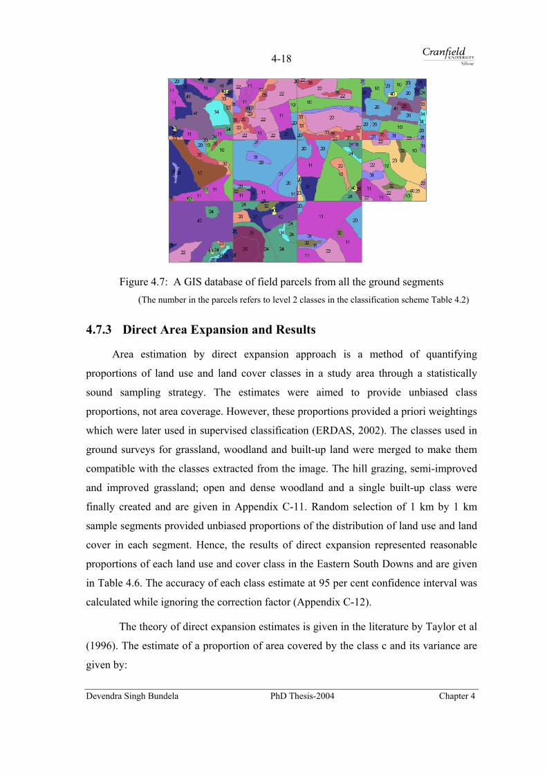
4-18
Figure 4.7: A GIS database of field parcels from all the ground segments (The number in the parcels refers to level 2 classes in the classification scheme Table 4.2)
4.7.3 Direct Area Expansion and Results
Area estimation by direct expansion approach is a method of quantifying
proportions of land use and land cover classes in a study area through a statistically
sound sampling strategy. The estimates were aimed to provide unbiased class
proportions, not area coverage. However, these proportions provided a priori weightings
which were later used in supervised classification (ERDAS, 2002). The classes used in
ground surveys for grassland, woodland and built-up land were merged to make them
compatible with the classes extracted from the image. The hill grazing, semi-improved
and improved grassland; open and dense woodland and a single built-up class were
finally created and are given in Appendix C-11. Random selection of 1 km by 1 km
sample segments provided unbiased proportions of the distribution of land use and land
cover in each segment. Hence, the results of direct expansion represented reasonable
proportions of each land use and cover class in the Eastern South Downs and are given
in Table 4.6. The accuracy of each class estimate at 95 per cent confidence interval was
calculated while ignoring the correction factor (Appendix C-12).
The theory of direct expansion estimates is given in the literature by Taylor et al
(1996). The estimate of a proportion of area covered by the class c and its variance are
given by:
Devendra Singh Bundela PhD Thesis-2004 Chapter 4

4-19
∑=
=n
1iic y
n1y and … Eq. 4.1
2n
1icic )yy(
)1n(n1
Nn1)y(Var ∑
=
−−
−= … Eq. 4.2
where yi is the proportion of segment i covered by the class c, N is the number of
segments in a study area and n is the number of segments selected for sampling.
When a sample fraction (n/N) is less than 5 per cent, the correction factor, (1-
(n/N)), for a finite population is omitted from Equation 4.3 (Cochran, 1977).
The estimate of class estimates and its variance are expressed as:
cc y*DZ = and … Eq. 4.3
)y(Var*D)Z(Var c2
c = … Eq. 4.4
where D is the area of study.
The accuracy of a class estimate (Accuracy) at 95 per cent confidence interval is
calculated by an equation:
)Z(Var*96.1ZAccuracy cc ±= … Eq. 4.5
Devendra Singh Bundela PhD Thesis-2004 Chapter 4

4-20
Table 4.6: Estimates of class proportions from the ground survey in all the segments and the study area
Segment No Arable 10 Arable 11 Arable 12 Rough grazing Improved grass Semi-improved grass
Open woodland Dense woodland Built-up land
1. 0.0000 0.2235 0.0000 0.0000 0.0571 0.2186 0.0581 0.1120 0.33072.
0.0261 0.2574 0.0000 0.4337 0.0000 0.0763 0.1083 0.0854 0.01273. 0.2568 0.0000 0.0000 0.4200 0.0000 0.0136 0.1574 0.1522 0.00004. 0.2600 0.0000 0.0000 0.0094 0.0399 0.3940 0.0608 0.0733 0.16265. 0.1923 0.1659 0.2301 0.0000 0.0000 0.2965 0.0360 0.0791 0.00006. 0.0000 0.1619 0.0000 0.0000 0.0000 0.7225 0.1043 0.0112 0.00007. 0.4345 0.1465 0.0000 0.0208 0.1209 0.1885 0.0622 0.0203 0.00638. 0.2512 0.0899 0.0000 0.5497 0.0000 0.0000 0.0585 0.0462 0.00459.
0.0000 0.0000 0.0000 0.0971 0.0902 0.0505 0.0095 0.0191 0.7337
10. 0.0000 0.0000 0.0000 0.0000 0.6420 0.1235 0.0458 0.0580 0.130711. 0.0000 0.6868 0.0000 0.1203 0.0000 0.0978 0.0535 0.0417 0.0000Mean 0.1292 0.1575 0.0209 0.1501 0.0864 0.1983 0.0686 0.0635 0.1256Sum Arable: 0.3075 Grassland : 0.4348 Woodland : 0.1321 Built-up land : 0.1256
Devendra Singh Bundela PhD Thesis-2004 Chapter 4

4-21
4.8 Multispectral Image Classification
4.8.1 Overview
Multispectral classification is the procedure of sorting all pixels in an image into
a finite number of land use and land cover classes or themes based on digital numbers
(DNs), which are measures of the surface reflectance. A classification technique uses
the spectral pattern present within data as a basis for an automated classification.
Proposed classes of a classification scheme rarely form distinct groups of clusters.
4.8.2 Classification Methodology
Two main procedures of digital image classification are widely used viz.,
unsupervised and supervised classification (Lillesand and Kiefer, 1999). There is no
single right approach to attain optimal results of a classification. Therefore, a hybrid
classification, a combination of both unsupervised and supervised classification (Figure
4.8) was used in this study.
4.8.3 Unsupervised Classification
Unsupervised classification is the clustering procedure of defining, identifying,
labelling and mapping of natural groupings or clusters within multispectral data without
a prior knowledge of existing classes (Campbell, 2002). Clustering procedures employ
K-means clustering viz. an ISODATA (Iterative self organising data analysis)
technique, (Lillesand et al, 2003) or RGB clustering (ERDAS, 2002) for unsupervised
classification. Advantages, disadvantages and limitations of unsupervised clustering are
discussed in detail in the literature (Campbell, 2002; ERDAS, 2002; Richards and Jia
1999; Mather, 1999).
Unsupervised classification methodology used for this study was based on a
hybrid and hierarchical classification approach (Figure 4.8). The number of classes in a
classification was based on a subjective judgement.
Devendra Singh Bundela PhD Thesis-2004 Chapter 4

4-22
SPOT image of the study area
Statistically sound samples
Mosaic of ground segments
Identification of segments
Divided into 40 spectral clusters
Ancillary data
Hierarchical cluster analysis
Collection of training sites
Image segment, map overlay
Field survey Agglomeration, SE & linkage
Evaluation of training sites
Regrouping into 11 major clusters
Digitisation of segments
Purification of class signatures
Evaluation of clusters Creation of GIS database Signature separability
Max likelihood classification Proportion of class in
segments Max likelihood classification
Direct expansion estimates
Unsupervised thematic image
Equi-probabilty supervised thematic image
Area weighted supervised thematic image
Figure 4.8: Flow diagram of a hybrid image classification
Devendra Singh Bundela PhD Thesis-2004 Chapter 4
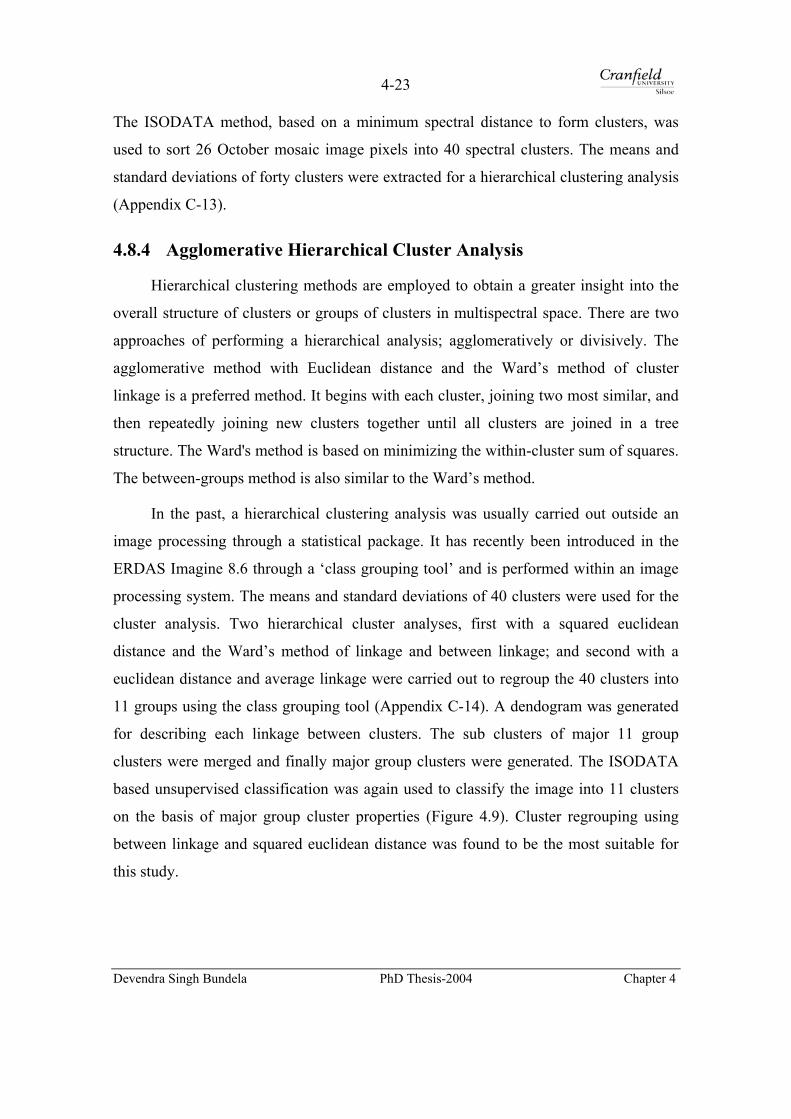
4-23
The ISODATA method, based on a minimum spectral distance to form clusters, was
used to sort 26 October mosaic image pixels into 40 spectral clusters. The means and
standard deviations of forty clusters were extracted for a hierarchical clustering analysis
(Appendix C-13).
4.8.4 Agglomerative Hierarchical Cluster Analysis
Hierarchical clustering methods are employed to obtain a greater insight into the
overall structure of clusters or groups of clusters in multispectral space. There are two
approaches of performing a hierarchical analysis; agglomeratively or divisively. The
agglomerative method with Euclidean distance and the Ward’s method of cluster
linkage is a preferred method. It begins with each cluster, joining two most similar, and
then repeatedly joining new clusters together until all clusters are joined in a tree
structure. The Ward's method is based on minimizing the within-cluster sum of squares.
The between-groups method is also similar to the Ward’s method.
In the past, a hierarchical clustering analysis was usually carried out outside an
image processing through a statistical package. It has recently been introduced in the
ERDAS Imagine 8.6 through a ‘class grouping tool’ and is performed within an image
processing system. The means and standard deviations of 40 clusters were used for the
cluster analysis. Two hierarchical cluster analyses, first with a squared euclidean
distance and the Ward’s method of linkage and between linkage; and second with a
euclidean distance and average linkage were carried out to regroup the 40 clusters into
11 groups using the class grouping tool (Appendix C-14). A dendogram was generated
for describing each linkage between clusters. The sub clusters of major 11 group
clusters were merged and finally major group clusters were generated. The ISODATA
based unsupervised classification was again used to classify the image into 11 clusters
on the basis of major group cluster properties (Figure 4.9). Cluster regrouping using
between linkage and squared euclidean distance was found to be the most suitable for
this study.
Devendra Singh Bundela PhD Thesis-2004 Chapter 4

4-24
Figure 4.9: Unsupervised classification of the image with 11 classes
4.8.5 Mosaicking of Segment Imagettes
A mosaic of eleven ground segments from 26 October image (Figure 4.10) was
created by extracting survey segments from the study area image using a FILQUILT
program written in Turbo C++ (Thomas, 1984). The mosaic was further used for
unsupervised classification, agglomerative hierarchical cluster analysis, training of a
classifier for supervised classification and also in assessing the accuracy of
classification (Taylor and Eva, 1992).
Figure 4.10: Image mosaic of 11 ground segments selected for field survey
Devendra Singh Bundela PhD Thesis-2004 Chapter 4

4-25
The FILQUILT, a DOS program, requires two inputs and an output information
viz., an input image file in the LAN format, an ASCII coordinate file of ground
segments with header information and an output ‘quilt’ file in the LAN format to create
a mosaic image of segments from an image file. The FILQUILT program creates a
mosaic image using map co-ordinates given in the coordinate file.
4.8.6 Spectral Signatures for Supervised Classification
Supervised classification is the process of using samples of known identity to
classify pixels of unknown identity in an image (Campbell, 2002). Advantages,
disadvantages and limitations of supervised classification are found in detail in the
literature (Campbell, 2002; ERDAS, 2002; Richards and Jia 1999; Mather, 1999).
Spectral signatures of classes can be obtained either from analyst chosen or from
geostatistically chosen training sets (Chen and Stow, 2002; Shine and Wakefield, 1999)
to collect representative training data from the ground segments. The former was used
for this study as the time of field survey and image acquisition was different. The
number of training sites chosen was proportional to the class proportion derived from
the ground sample survey. Training parcels were randomly selected from the image
mosaic of 26 October. It was carried out carefully to choose the spatially independent
training datasets from almost all of the ground sample segments for all eleven classes. A
total of 198 training sites for eleven classes was selected and used for the supervised
classification (Table 4.7). Out of eleven classes, five arable, three grassland and two
woodland classes and a single built-up class were finally used for collection of training
sites for classification. The mean and standard deviation values of pixels for each band
for all the classes are presented in Table 4.8.
Devendra Singh Bundela PhD Thesis-2004 Chapter 4
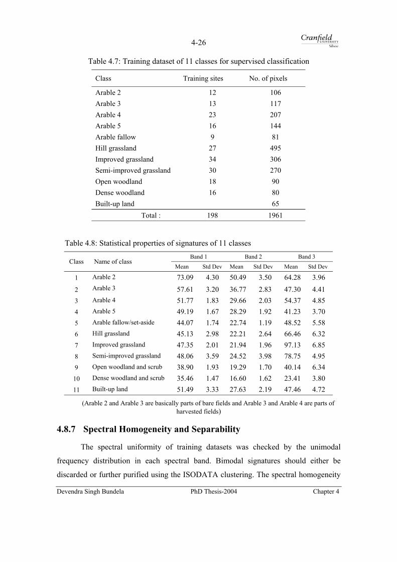
4-26
Table 4.7: Training dataset of 11 classes for supervised classification
Class Training sites No. of pixels
Arable 2 12 106 Arable 3 13 117 Arable 4 23 207 Arable 5 16 144 Arable fallow 9 81 Hill grassland 27 495 Improved grassland 34 306 Semi-improved grassland 30 270 Open woodland 18 90 Dense woodland 16 80 Built-up land 65 Total : 198 1961
Table 4.8: Statistical properties of signatures of 11 classes Band 1 Band 2 Band 3
Class Name of class Mean Std Dev Mean Std Dev Mean Std Dev
1 Arable 2 73.09 4.30 50.49 3.50 64.28 3.96
2 Arable 3 57.61 3.20 36.77 2.83 47.30 4.41 3 Arable 4 51.77 1.83 29.66 2.03 54.37 4.85 4 Arable 5 49.19 1.67 28.29 1.92 41.23 3.70 5 Arable fallow/set-aside 44.07 1.74 22.74 1.19 48.52 5.58 6 Hill grassland 45.13 2.98 22.21 2.64 66.46 6.32 7 Improved grassland 47.35 2.01 21.94 1.96 97.13 6.85 8 Semi-improved grassland 48.06 3.59 24.52 3.98 78.75 4.95 9 Open woodland and scrub 38.90 1.93 19.29 1.70 40.14 6.34
10 Dense woodland and scrub 35.46 1.47 16.60 1.62 23.41 3.80 11 Built-up land 51.49 3.33 27.63 2.19 47.46 4.72
(Arable 2 and Arable 3 are basically parts of bare fields and Arable 3 and Arable 4 are parts of harvested fields)
4.8.7 Spectral Homogeneity and Separability
The spectral uniformity of training datasets was checked by the unimodal
frequency distribution in each spectral band. Bimodal signatures should either be
discarded or further purified using the ISODATA clustering. The spectral homogeneity
Devendra Singh Bundela PhD Thesis-2004 Chapter 4

4-27
was also verified by overlaying signatures on unsupervised classified map. This helped
in minimising spectral confusion emanating from mixed pixels in a training dataset. All
pure signatures were merged together to produce a class signature for classification.
The class signatures were evaluated for spectral separability by two methods such
as scatterplot and divergence distance. Scatterplots of signatures were viewed in two
dimensional feature spaces by displaying two bands at a time using ellipses. The
overlapping of signature ellipses was checked to minimise the signature confusion.
Signature divergence, a statistical measure in multispectral space, was calculated to
analyse all the signatures for class separability. The transformed divergence (TD) and
the Jeffries Matusita (JM) distance methods were used (ERDAS, 2002; Swain and
Davis, 1978). The transformed divergence has a range from 0 to 2000 while the Jeffries
Matusita distance has a range from 0 to 1414. The upper limit reflects the total
separability and lower limit reflects total confusion in both methods. The TD and JM
distances were calculated for 11 class signatures. The average and minimum
separability of all the classes by both methods is given in Table 4.9. The each class
wise separability for both methods is given in Appendix C-15. Spectral confusion
between bare soil class and urban class was strongly evident. The polygons of spectrally
confused classes were separated and purified. Therefore, in this way, all the signature
files were purified and then used for classification.
Table 4.9: Signature separability of 11 classes
Parameter Transformed Divergence distance Jefferies-Matusita distance
Average separability 1893.03 1358.94
Minimum separability 1082.75 1082.75
4.8.8 Classification Decision Rule and Training
A variety of parametric decision rules are used in digital image processing
(Campbell, 2002; ERDAS, 2002). The decision boundary for each class was generated
during decision rule training. The Gaussian and Bayesian maximum likelihood decision
rules were used initially to classify the mosaic image and then the study area image. The
Gaussian decision rule is based on an assumption of equal probabilities of all classes
Devendra Singh Bundela PhD Thesis-2004 Chapter 4
4-28
while the Bayesian decision rule is based on priori probability weight factors of classes.
Both rules compare the variance and covariance of training class signatures with a
candidate pixel to assign a particular class according to a decision rule. The assumption
of normality in training class signatures is adhered in the maximum likelihood classifier
(Lillesand et al, 2003; ERDAS, 2002).
4.8.9 Classification Results
The Gaussian classifier with equal probabilities and the Bayesian classifier with
area weight probabilities, derived from direct area expansion, were used to produce
equal weighted and area weighted classified images. The mosaic image of 26 October
2000 was initially classified for 11 classes by the Gaussian classifier (Figure 4.11). In
case of the Bayesian classifier, direct area estimates were available for nine classes, not
for all the eleven classes. Arable 2 and Arable 3 classes were the parts of the bare soil
fields while Arable 4 and Arable 5 classes were parts of the harvested field. Hence,
direct area estimates of both bare soil and harvested field were split up equally and
shared by two clusters of each class. The image mosaic was classified for 11 classes
with area weight probabilities ( Figure 4.12) and both results are compared in Table
4.10. Both classified image were verified with the original image. Both classifications
were found to be equally acceptable and then, the study area image was classified with
area weighted training data set. Figure 4.13 shows the area weighted probability
classified image with 11 classes.
Devendra Singh Bundela PhD Thesis-2004 Chapter 4
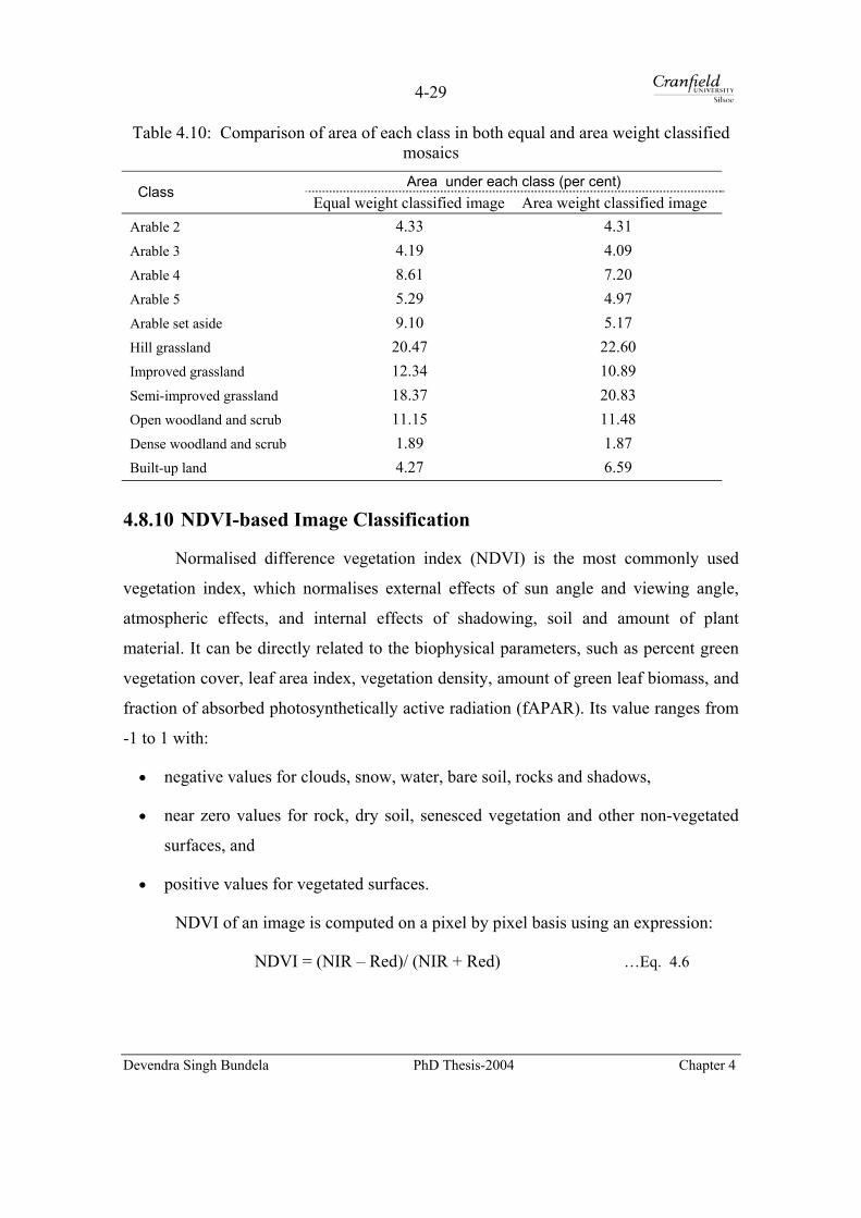
4-29
Table 4.10: Comparison of area of each class in both equal and area weight classified mosaics Area under each class (per cent)
Class Equal weight classified image Area weight classified image
Arable 2 4.33 4.31 Arable 3 4.19 4.09 Arable 4 8.61 7.20 Arable 5 5.29 4.97 Arable set aside 9.10 5.17 Hill grassland 20.47 22.60 Improved grassland 12.34 10.89 Semi-improved grassland 18.37 20.83 Open woodland and scrub 11.15 11.48 Dense woodland and scrub 1.89 1.87 Built-up land 4.27 6.59
4.8.10 NDVI-based Image Classification
Normalised difference vegetation index (NDVI) is the most commonly used
vegetation index, which normalises external effects of sun angle and viewing angle,
atmospheric effects, and internal effects of shadowing, soil and amount of plant
material. It can be directly related to the biophysical parameters, such as percent green
vegetation cover, leaf area index, vegetation density, amount of green leaf biomass, and
fraction of absorbed photosynthetically active radiation (fAPAR). Its value ranges from
-1 to 1 with:
• negative values for clouds, snow, water, bare soil, rocks and shadows,
• near zero values for rock, dry soil, senesced vegetation and other non-vegetated
surfaces, and
• positive values for vegetated surfaces.
NDVI of an image is computed on a pixel by pixel basis using an expression:
NDVI = (NIR – Red)/ (NIR + Red) …Eq. 4.6
Devendra Singh Bundela PhD Thesis-2004 Chapter 4

4-30
Figure 4.11: Equal weighted supervised classification of the image mosaic with 11
classes
Devendra Singh Bundela PhD Thesis-2004 Chapter 4
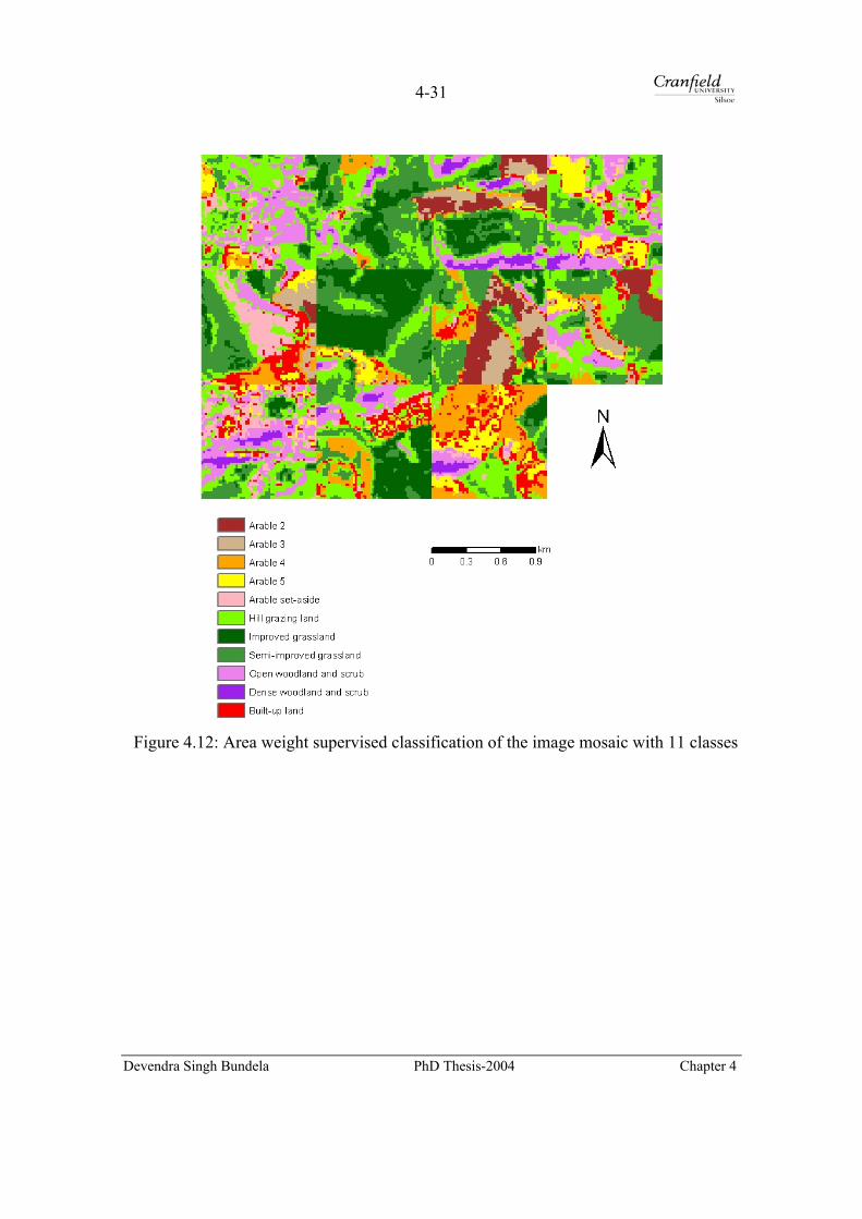
4-31
Figure 4.12: Area weight supervised classification of the image mosaic with 11 classes
Devendra Singh Bundela PhD Thesis-2004 Chapter 4

4-32
Figure 4.13: Area weighted supervised classification of the study area with 11 classes
The NDVI was used to infer information on major classes based green ground
cover to differentiate the major land use and land cover and to help to improve the
accuracy of supervised classification. Another aspect was to establish a direct
relationship with NDVI to extract the percent ground cover and leaf area index required
for modelling, which was also explored in this study. The NDVI derived land use and
land cover map could also be used as alternative to supervised classification based land
use and land cover map for quick assessment of the classes.
Raw DN-based NDVI classification NDVI not only varies with the spectral and spatial characteristics of a sensor but
also with the radiometric processing applied to an image data (Guyot and Gu, 1994).
NDVI can be computed from digital signal levels, top of atmospheric radiance, top of
atmospheric reflectance or atmospherically corrected surface reflectance. NDVI also
Devendra Singh Bundela PhD Thesis-2004 Chapter 4
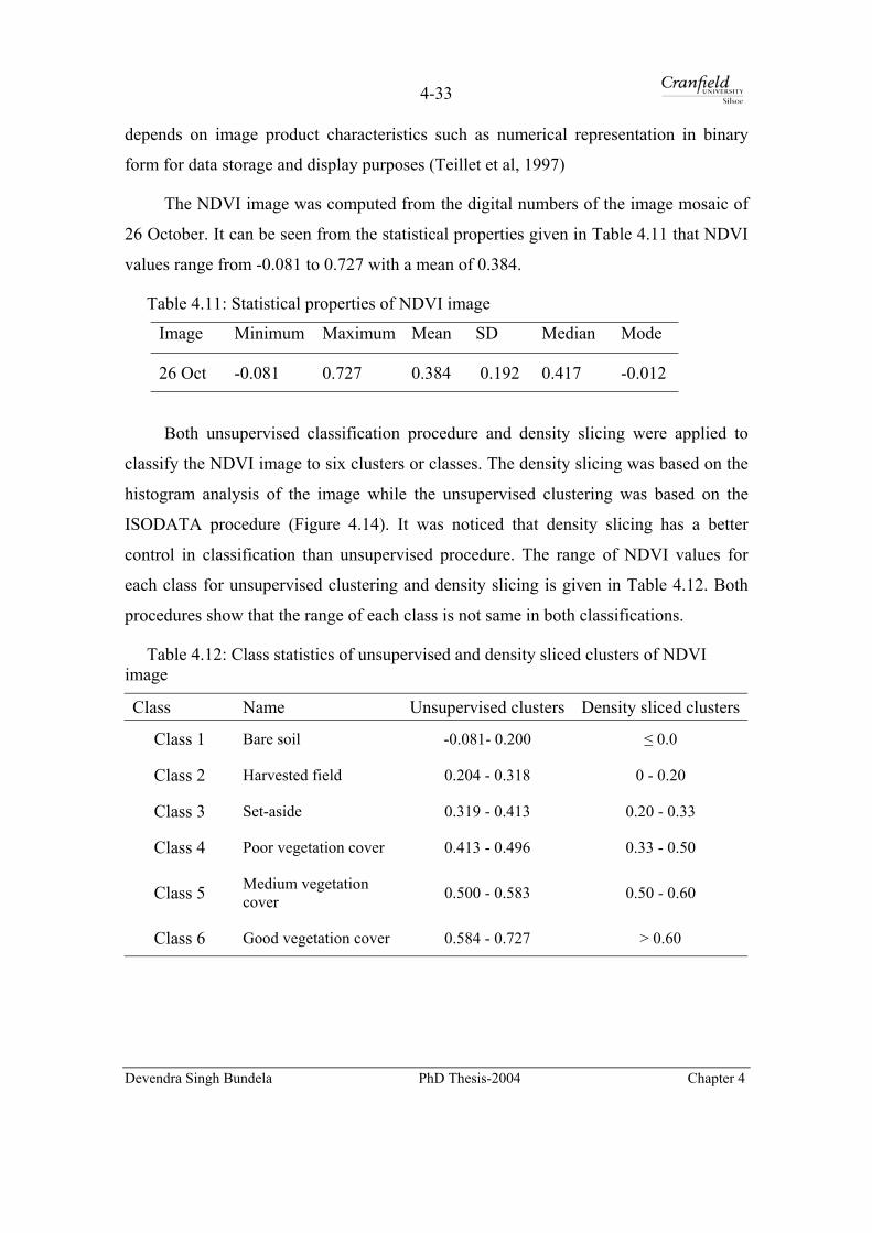
4-33
depends on image product characteristics such as numerical representation in binary
form for data storage and display purposes (Teillet et al, 1997)
The NDVI image was computed from the digital numbers of the image mosaic of
26 October. It can be seen from the statistical properties given in Table 4.11 that NDVI
values range from -0.081 to 0.727 with a mean of 0.384.
Table 4.11: Statistical properties of NDVI image
Image Minimum Maximum Mean SD Median Mode
26 Oct -0.081 0.727 0.384 0.192 0.417 -0.012
Both unsupervised classification procedure and density slicing were applied to
classify the NDVI image to six clusters or classes. The density slicing was based on the
histogram analysis of the image while the unsupervised clustering was based on the
ISODATA procedure (Figure 4.14). It was noticed that density slicing has a better
control in classification than unsupervised procedure. The range of NDVI values for
each class for unsupervised clustering and density slicing is given in Table 4.12. Both
procedures show that the range of each class is not same in both classifications.
Table 4.12: Class statistics of unsupervised and density sliced clusters of NDVI image
Class Name Unsupervised clusters Density sliced clusters
Class 1 Bare soil -0.081- 0.200 ≤ 0.0
Class 2 Harvested field 0.204 - 0.318 0 - 0.20
Class 3 Set-aside 0.319 - 0.413 0.20 - 0.33
Class 4 Poor vegetation cover 0.413 - 0.496 0.33 - 0.50
Class 5 Medium vegetation cover 0.500 - 0.583 0.50 - 0.60
Class 6 Good vegetation cover 0.584 - 0.727 > 0.60
Devendra Singh Bundela PhD Thesis-2004 Chapter 4

4-34
Calibration of the SPOT image NDVI values vary significantly and are functions of sensor calibration,
atmospheric conditions, directional surface reflectance effects and terrain relief. The
SPOT image of 26 October was calibrated to the reflectance at top of atmosphere (ρ0)
(Appendix C-16) using an equation (Guyot, and Gu, 1994; Henry, and Dinguirard,
1997). )(**
** 2
0 SZCosEAdDN
sunk
kπρ = ... Eq. 4.7
where ρ0
is the exoatmospheric reflectance at the satellite (0-1), Ak is the
absolute calibration gain in W-1m2 sr µm, DNk is the digital number for the band k, d2 is
the square of the Earth-Sun distance in astronomical units (~149.6 x 10⁶ km), Esun is the
mean solar exoatmospheric irradiance in W m-2 µm-1, and SZ is the sun zenith angle in
radians at time of scene acquisition.
Atmospherically corrected surface reflectance could not be computed due to non
availability of enough weather data at the time of image acquisition to model the
atmospheric condition. Moreover, it was beyond the scope of this study.
NDVI classification based on apparent reflectance 26 October image was calibrated to the apparent reflectance and the NDVI image
was then computed. The statistical properties of the apparent reflectance and NDVI are
given in Table 4.13 and Table 4.14. The mean of DN-based NDVI image is slightly
lower than the mean from apparent reflectance. This did not result in significance
difference in classification whether used DNs or apparent reflectance values.
Table 4.13: Statistical properties of apparent reflectance of 26 October image
Reflectance at top of atmosphere Band XS1 (G) XS2(R) XS3 (IR) Minimum 0.095 0.056 0.060 Maximum 0.262 0.270 0.561 Mean 0.141 0.107 0.294 Standard deviation 0.022 0.030 0.085 Median 0.139 0.098 0.283 Mode 0.136 0.094 0.234
Devendra Singh Bundela PhD Thesis-2004 Chapter 4
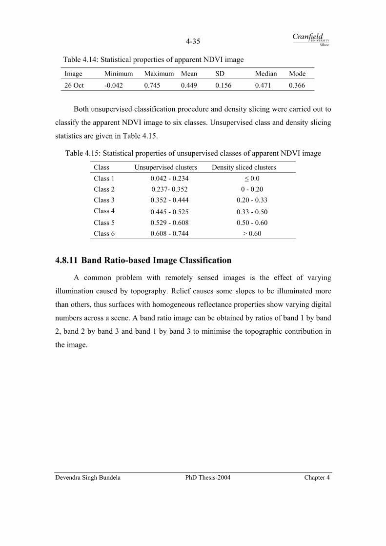
4-35
Table 4.14: Statistical properties of apparent NDVI image
Image Minimum Maximum Mean SD Median Mode
26 Oct -0.042 0.745 0.449 0.156 0.471 0.366
Both unsupervised classification procedure and density slicing were carried out to
classify the apparent NDVI image to six classes. Unsupervised class and density slicing
statistics are given in Table 4.15.
Table 4.15: Statistical properties of unsupervised classes of apparent NDVI image
Class Unsupervised clusters Density sliced clusters Class 1 0.042 - 0.234 ≤ 0.0 Class 2 0.237- 0.352 0 - 0.20 Class 3 0.352 - 0.444 0.20 - 0.33 Class 4 0.445 - 0.525 0.33 - 0.50 Class 5 0.529 - 0.608 0.50 - 0.60 Class 6 0.608 - 0.744 > 0.60
4.8.11 Band Ratio-based Image Classification
A common problem with remotely sensed images is the effect of varying
illumination caused by topography. Relief causes some slopes to be illuminated more
than others, thus surfaces with homogeneous reflectance properties show varying digital
numbers across a scene. A band ratio image can be obtained by ratios of band 1 by band
2, band 2 by band 3 and band 1 by band 3 to minimise the topographic contribution in
the image.
Devendra Singh Bundela PhD Thesis-2004 Chapter 4
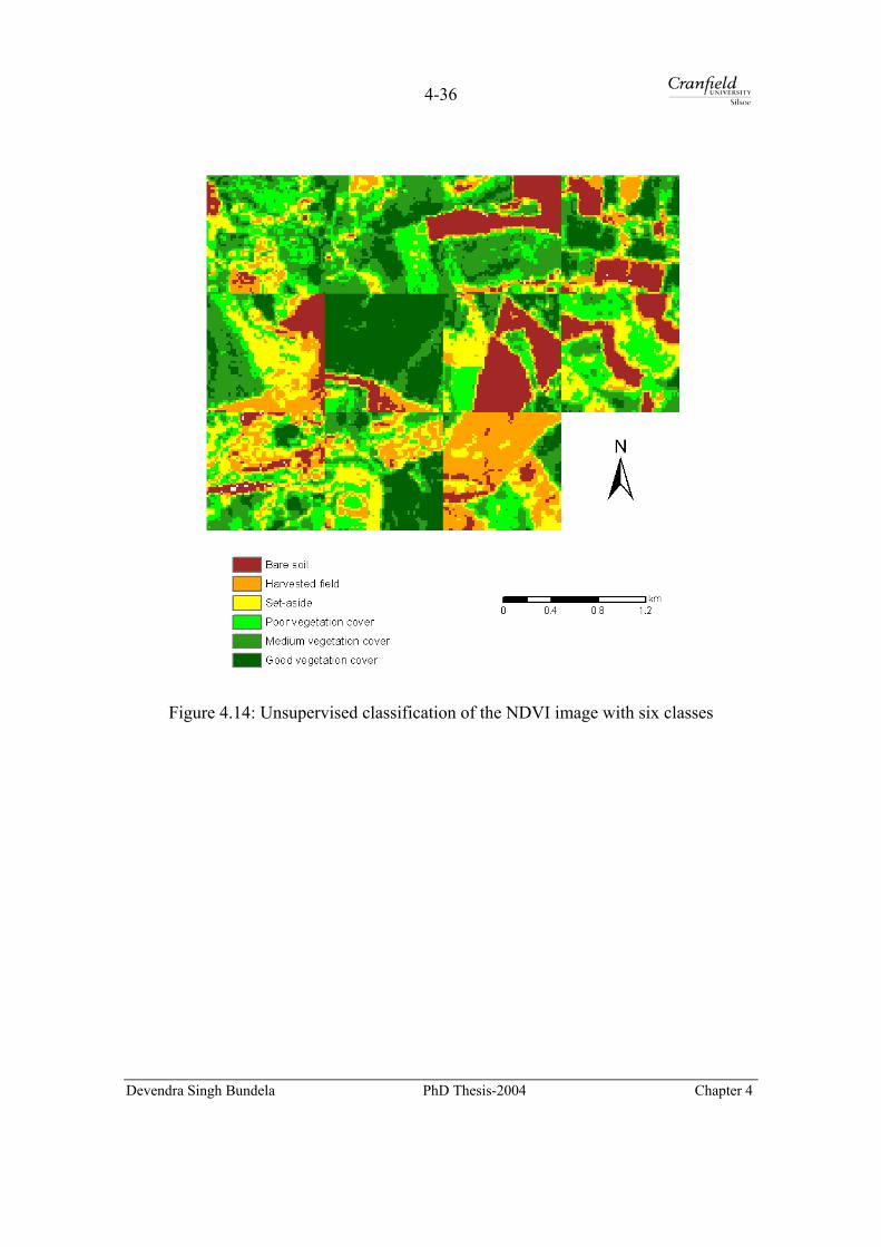
4-36
Figure 4.14: Unsupervised classification of the NDVI image with six classes
Devendra Singh Bundela PhD Thesis-2004 Chapter 4

4-37
A ratio image (B1/B2; B2/B3 and B1/B3) of the image mosaic was computed to
reduce the illumination effect by topography. The image was stretched to 8 bits and then
was classified to six classes based on an unsupervised clustering (Figure 4.15). The area
under each class derived from the band ratio image is compared with six classes derived
from unsupervised classification of DN-based NDVI and apparent NDVI images (Table
4.16). It was found that first four classes are over predicted in ratio images as compared
to both other images. There was not significance difference in area of each class derived
from DN-based and apparent NDVI images. In the DN-based image, 20 pixels were
turned into no data values during computing NDVI image.
Table 4.16: Area of each class derived from unsupervised classification of DN-based
NDVI, apparent NDVI and band ratio images
Area under each class (per cent) Class
DN-based NDVI Apparent NDVI Ratio image
Unclassified 0.07 0.00 0.00
Bare soil 13.13 12.71 15.99
Harvested field 13.80 14.14 20.07
Set-aside 16.70 16.82 19.99
Poor vegetation cover 19.36 19.39 15.89
Medium vegetation cover 20.21 20.05 9.90
Good vegetation cover 16.73 16.89 18.15
Devendra Singh Bundela PhD Thesis-2004 Chapter 4
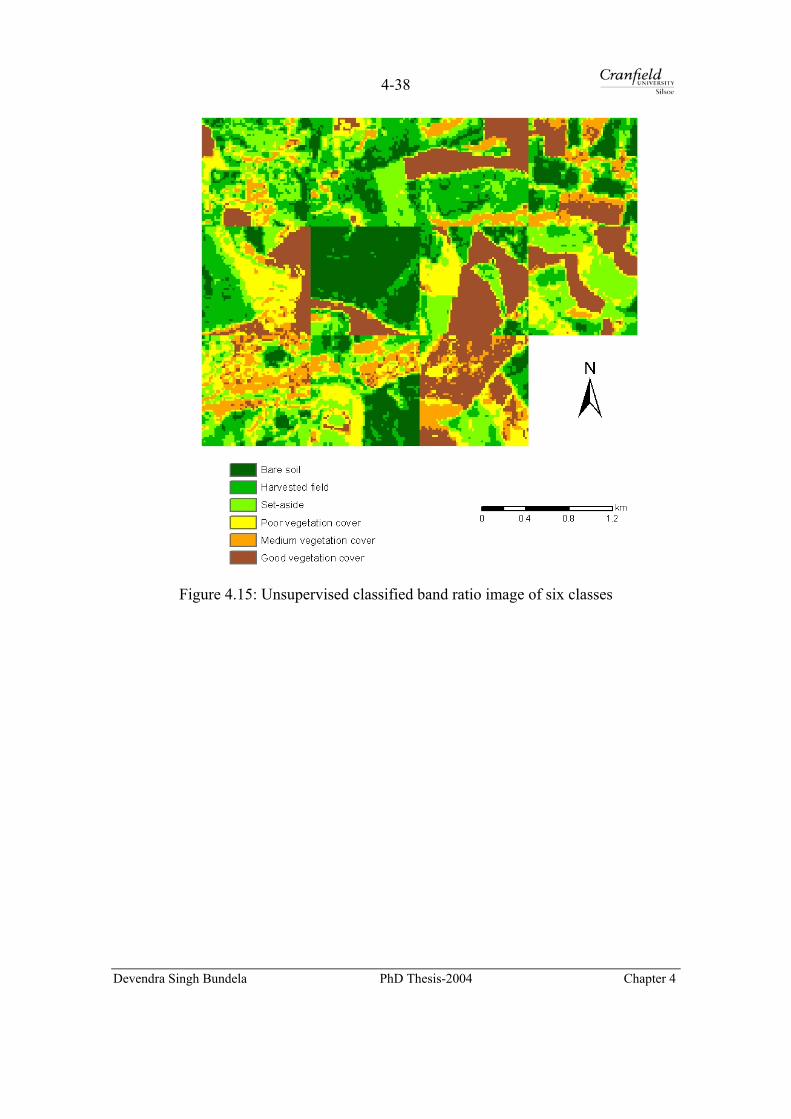
4-38
Figure 4.15: Unsupervised classified band ratio image of six classes
Devendra Singh Bundela PhD Thesis-2004 Chapter 4

4-39
4.9 Assessment of Classification Accuracy
In the context of thematic classifications of remotely sensed data, accuracy
refers to the degree of correctness of a classification in comparison to the ground data
(Foody, 2002; Campbell, 2002). Accuracy assessment measures are widely used to
quantify the error in classifications. Accuracy assessment in land use and vegetation
mapping studies is reviewed in the literature by Foody (2002) and Congalton (1991).
More than 250 reference pixels on a classified image are required to be randomly
selected to estimate the mean accuracy of a class within plus or minus five per cent
(Congalton, 1991).
4.9.1 Confusion Matrix
A confusion matrix (Congalton, 1991) is a basis to describe both classification
accuracy and errors and is used to derive accuracy assessment statistics. It also helps in
refining classification in case of an interclass confusion. Accuracy measures such as
errors of omission and commission, user and producer’s accuracies and the Kappa
coefficient (Congalton and Green, 1999) are derived from the confusion matrix to assess
the overall accuracy of classification. Confusion matrix and accuracy measures of 26
October image were calculated. The confusion matrix in Table 4.17 shows that the
overall classification accuracy, producer’s accuracy and user’s accuracy are 89.9, 60-
100 and 59-100 per cent respectively. The higher accuracy was achieved in the bare soil
class and least accuracy in the built-up area.
4.9.2 Kappa Statistics
Kappa statistics is a standard measure of classification accuracy. It compensates
for a chance agreement between the classified data and reference data (Congalton et al,
1983; Rosenfield and Fitzpatrick-Lins, 1986; Hudson and Ramm, 1987; Congalton,
1991) and is based on the maximum likelihood theory. Landis and Koch (1987) have
defined the agreement criteria for Kappa coefficient to assess a classification. The
agreement is poor when KHAT is less than 0.4, good when KHAT is in between 0.4 and
0.75 and excellent when KHAT is greater than 0.75. The kappa coefficient of agreement
Devendra Singh Bundela PhD Thesis-2004 Chapter 4

4-40
of 26 October scene is found to be 0.88. It can be concluded that there is good
agreement between mapped and observed classes. The thematic image represents
reliable information on land use and land cover. Therefore, it is suitable for modelling
study.
The variance of Kappa statistics and its application for testing of significance
difference between two confusion matrices are discussed in the literature (Congalton
and Green, 1999; Hudson and Ramm, 1987).
The formulation of Kappa statistics is expressed as:
∑
∑ ∑
=++
= =++
−
−= r
1iii
2
r
1i
r
1iiiii
xxN
xxxNk … Eq. 4.8
where + represents the summation of row index.
For a computation purpose, Equation 4.9 is used to calculate the Kappa coefficient, KHAT ( k );
2
21
1ˆ
θ−θ−θ
=k … Eq. 4.9
where θ1 is the proportion of units which agree, and θ2 is the proportion of units for
expected chance agreement. θ1 and θ2 are computed using Equations 4.10 and 4.11:
θ
1=
x iii =1
r
∑N and … Eq. 4.10
θ
2=
xi +x
+ ii= 1
r
∑
N2
… Eq. 4.11
where xij is the number of counts in the ijth cell of the confusion matrix, N is the total
number of counts in the confusion matrix, xi+ is the marginal total of row I and x+i is
the marginal total of column i.
Devendra Singh Bundela PhD Thesis-2004 Chapter 4

4-41
Table 4.17: Confusion matrix for 11 class based classification (26 October 2000)
Class 1 2 3 4 5 6 7 8 9 10 11 Total User's accuracy 1 106 106 100.0 2 114 1 1 116 98.28 3 180 2 4 13 199 90.45 4 2 3 132 9 146 90.41 5 2 1 72 8 5 2 90 80.00 6 1 210 15 3 1 230 91.30 7 292 14 306 95.42 8 2 30 14 241 287 83.97 9 6 78 3 87 89.66
10 4 77 81 95.06 11 1 14 9 3 39 66 59.09
Total 106 117 202 145 81 252 306 270 90 80 65 1714Producer's accuracy 100.0 97.44 89.11 91.03 88.89 83.33 95.42 89.26 86.67 96.25 60.00 Overall
accuracy = 89.9
KH = AT 0.88 Name of the classes: 1 Arable 2 2 Arable 3 3 Arable 4 4 Arable 5 5 Set aside/fallow 6 Hill grazing grassland 7 Improved grassland 8 Semi-improved grassland 9 Open woodland and scrub 10 Dense woodland and scrub 11 Built-up land
Devendra Singh Bundela PhD Thesis-2004 Chapter 4

4-42
4.10 Reclassification and Post Processing
Classification error is caused by the interaction of numerous factors including
landscape and its illumination characteristics, sensor resolution, spectral overlap,
preprocessing, image enhancement and classification procedures (Campbell, 2002). The
overall accuracy and Kappa coefficient of agreement of the classification with 11
classes was reasonably good. Therefore, the 11 class area weighted classified image was
reclassified into 9 major classes by combining the Arable 2 and Arable 4 into the bare
soil and Arable 4 and 5 into the harvested field on the basis of similar characteristics for
hydrologic and erosion modelling. The resultant reclassified image is presented in
Figure 4.16. The major urban area was not separated digitally. Therefore, it was
manually separated and added to the image after classification.
The overall accuracy of reclassified image was recalculated. It was found that
the user and producer accuracies range from 52.87 to 97.94 and 67.90 to 97.76 per cent
respectively. The overall accuracy and Kappa coefficient of agreement remained the
same (Table 4.18). The area estimates by sampling and image classification were
compared in Table 4.19. It was found that estimates from both methods were not
compared as such because of a large time lag between survey time and acquisition time.
There was strong evidence between bare soil and built-up land. Even after
reclassification, a few scattered pixel patches different from neighbouring pixels were
present in the reclassified image, so a majority filter of 3x3 window was, therefore,
applied to minimize noisiness in the thematic image. The disadvantage of filtering was
that it increased the minimum mapping unit substantially. The filtering and resampling
of 9 class based land use and land cover to five resolution datasets were discussed in
Section 6.3.2 to derive input parameters for modelling study.
Devendra Singh Bundela PhD Thesis-2004 Chapter 4

4-43
Figure 4.16: Area weighted supervised classified image with 9 classes
Devendra Singh Bundela PhD Thesis-2004 Chapter 4

4-44
Table 4.18: Confusion matrix for the reclassified image with 9 classes
Class 1 2 3 4 5 6 7 8 9 Total User's accuracy
1 218 3 3 1 225 96.89
2 4 309 16 329 93.92
3 55 1 4 1 61 90.16
4 1 5 217 9 3 1 236 91.95
5 2 34 255 21 312 81.73
6 6 285 291 97.94
7 9 79 3 91 86.81
8 4 77 81 95.06
9 1 31 9 46 87 52.87
Total 223 346 81 252 270 306 90 80 65 1713 Producer's accuracy 97.76 89.31 67.90 86.11 94.44 93.14 87.78 96.25 70.77 Overall
accuracy = 89.9
KHAT = 0.88 Name of Classes: 1 Bare soil 2 Harvested field with stubbles 3 Set aside/ fallow 4 Rough grazing land 5 Semi-improved grassland 6 Improved grassland 7 Open woodland and scrub 8 Dense woodland and scrub, and 9 Built-up land
Devendra Singh Bundela PhD Thesis-2004 Chapter 4

4-45
Table 4.19: Comparison of area estimates by sampling and image classification
Class Area by direct estimate (ha)
Area by image classification (ha)
For the study area Bare soil 2948.1 1736.5 Harvested field with stubbles 3593.4 2530.4 Set aside/ fallow 477.4 1684.2 Rough grazing land 3425.3 2560.4 Semi-improved grassland 4526.6 3819.6 Improved grassland 1971.2 1495.7 Open woodland and scrub 1565.2 2039.6 Dense woodland and scrub 1449.5 495.2 Built-up land 2865.7 6559.6
Sum : 22822.4 22921.1 For segment mosaic only
Bare soil 142.1 96.1 Harvested field with stubbles 173.2 137.6 Set aside/ fallow 23.0 100.7 Rough grazing land 165.1 231.2 Semi-improved grassland 218.2 201.3 Improved grassland 95.0 135.7 Open woodland and scrub 75.4 122.1 Dense woodland and scrub 69.9 20.8 Built-up land 138.1 54.5
Sum : 1100 1100
Devendra Singh Bundela PhD Thesis-2004 Chapter 4

4-46
4.11 Concluding Remarks
4.11.1 Discussion
Remote sensing approach
The usefulness of remote sensing for land use and land cover mapping using
multispectral classification is established and is evident in this study. The hierarchical
classification scheme was compatible with the land use map required by LISEM so that
it can be directly ingested to a LISEM database using PCRaster for deriving distributed
input parameters. Although the SPOT-1 HRV sensor was beyond its life expectancy but
it has captured the excellent quality of images, which were comparable with other earth
resource satellites. SPOT-1 has three bands only, which was a limitation as compared to
other sensors. The remote sensing approach for mapping should not be viewed in terms
of absolute quantified value of land use and land cover classes rather than a
representative value of classes in the study area.
Delineation of the study area
The study area was delineated from a 1:50 000 scale Landranger map. The water
body was intentionally not included in the study area to avoid spectral confusion
between sea water, urban area and bare soil during classification
Field documentations and navigation
Essential field survey documents with a well defined classification scheme help to
complete the segment survey quickly. With the preparation of a false colour composite
image, image segments and map overlays, the interpretation of segment parcels took
less time as compared to locating the boundaries of segments using the maps and a
GPS. Twelve year old maps led to confusion in a few segments due to either presence or
absence of some field features such as boundary hedges, new buildings and roads.
GPS was found to be a useful equipment for successful ground data collection
particularly with twelve year old maps. The Garmin GPS-12 Personal Navigator
handset without real time code correction was used and thus, resulted in less accurate
Devendra Singh Bundela PhD Thesis-2004 Chapter 4
4-47
coordinates. It was found that accuracy degradation was more than what was reported in
the equipment manual (15 m). In a few cases particularly in valleys, the accuracy was
further degraded. The real-time code corrected GPS equipment would be ideal for
locating ground segment parcels more accurately and quickly.
Ground segment sampling
Large discrepancy between the direct area and classification estimates resulted
due to some extent by possible spectral confusion between information classes, which
was further compounded by the large time lag between the field survey and the time of
image acquisition. This emphasises the importance of timely field survey. This
discrepancy could be reduced to some extent by choosing a larger sampling fraction.
Field problems
Significant problems were experienced in the field due to small scattered patches
of buildings, scrubs, trees and hedge lines. The smaller patches less than a pixel size
(400 sq m) were not considered. Access to a few segments was the problem due to
absence of public paths or bridleways and the field survey was completed from a
distance which made some segment survey less reliable. The larger time lag further
added the problems during the in field survey.
Image classification
A few significant problems were experienced during the classification due to
spectral confusion caused by bare fields, buildings, urban features and sea water; and
grasslands in valleys and slopes. The supervised classification assumes that images are
composed of spectrally homogeneous and separable classes. It was not really true in this
study. A smaller variability within each class was introduced to improve the supervised
classification. Therefore, a hybrid classification was found to be an appropriate solution
to identify the land use and land cover and achieved an overall accuracy of 90 per cent.
Devendra Singh Bundela PhD Thesis-2004 Chapter 4
4-48
Classes for modelling
The erosion model mostly relies on land use and land cover spatial data for
deriving its distributed parameters. Some input parameters could be derived by
reclassifying this key spatial data. Biophysical parameters such as per cent ground
cover, and LAI could not be related to NDVI because of absence of field observations in
this study. Land use and land cover map could be reclassified by establishing a direct
relationship between classes and parameters collected either through field observations
or estimation. There was a problem of different resolutions between key spatial data.
Therefore, they were resampled to the resolution of the thematic map.
4.11.2 Conclusions
• A statistically sound sampling scheme with a timely field survey is a
prerequisite for reliable image classification for modelling.
• The Garmin GPS-12 handset is not accurate enough for locating the boundaries
of ground segments. Therefore, a real-time code corrected differential GPS
should preferably be used for collecting location specific data. Some of the maps
used in the survey were approximately 12 years old and were not very useful, so
it emphasises the need and importance of updated maps in survey and
classification.
• The SPOT-1 HRV sensor, although working beyond of its expected life,
captured good quality images, which were found to be suitable for image
classification
• A large time lag between the image acquisition and field survey reduced
drastically the reliability of ground data for supervised classification. It suggests
the role of timely survey for modelling.
• Signature of each land use and land cover class was not very distinct as it was
assumed in the classification scheme. The problem was more aggravated due to
a large survey time lag, so a hybrid approach of image classification was found
to be an appropriate solution.
Devendra Singh Bundela PhD Thesis-2004 Chapter 4

4-49
• The overall accuracy and Kappa coefficient of classification was found to be
satisfactory and therefore, the image was reclassified for modelling study.
• Bare soils, urban areas and seashore water could not be separated digitally due to
strong spectral confusion. They were manually masked before classification and
added to the thematic map after classification.
• Spectral vegetation indices and band ratioing were also used in conjunction with
image classification procedures to verify possible land use and land cover at the
time of image acquisition to improve the classification accuracy
Devendra Singh Bundela PhD Thesis-2004 Chapter 4

5-1
5
Generation and Quality
Assessment of InSAR DEMs
This chapter reviews the elevation mapping technologies in terms of their
capabilities and limitations. Spaceborne radar interferometry was
identified and used for the generation of high resolution and quality DEMs
from an ERS-1 and ERS-2 SAR raw data pair. Their quality was
assessed against reference data. It was found that they are suitable for
distributed modelling.
5.1 Introduction
Topographic data is represented digitally by several forms of data models in a
computer. The digital elevation model (DEM) is one of the data models required for
distributed hydrologic and erosion modelling at catchment scale for extracting drainage
networks and topographic parameters (Moore et al, 1991). It is often not readily
available at an adequate resolution and quality at catchment scale. Topography can be
modelled digitally from elevation data collected from a variety of sources.
Elevation data collection by ground survey is expensive and time consuming at
catchment scale while topographic data is available worldwide at coarse resolutions
particularly in the developing countries. They can be applied at regional scale.
Moreover, they are not regularly updated. At the same time, remotely sensed mapping
technology has proved to be a timely and cost effective alternative for generation of
high resolution and quality DEMs at catchment scale. These technology have an
Devendra Singh Bundela PhD Thesis-2004 Chapter 5

5-2
advantage of potentially taking measurements from anywhere on the terrain, thus
avoiding the spatial interpolation problems of contours (Wise, 2000). Satellite images
can be obtained for an area of interest at a specific time unlike airborne data.
Availability of optical data is constrained by the persistence of cloud cover in the
developing countries, particularly in tropical regions. About 10 per cent of annually
acquired data in Europe are only useable for topographic mapping due to cloud cover
(Hanssen, 2001).
Synthetic aperture radar (SAR) has all weather and day-night capability to collect
data for elevation mapping. SAR interferometry has been applied worldwide and has
been successfully used in a few projects for generating high resolution and quality
DEMs such as Landmap (Landmap, 2003), Shuttle Radar Topography Mission (SRTM)
(USGS, 2003) and NEXTMap Britain (Mackay, 2002). These interferometric SAR
(InSAR) DEMs can further be used for the parameterisation of a distributed model.
Therefore, spaceborne radar interferometry was selected for this study to explore its
potential to generate quality DEMs for developing countries for distributed modelling.
For this study, an ERS-1 and ERS-2 tandem SAR raw pair was selected to derive
InSAR DEMs of the Eastern South Downs, which would be further used to investigate
the effect of different resolutions on model predictive capacity.
This chapter is dedicated to exploring the use of radar interferometry for
extracting high resolution and quality DEMs suitable for distributed modelling for
developing countries, in particular, and developed countries, in general. It also deals
with the generation of a validation DEM data using digital photogrammetry. Elevation
mapping technologies with respect to spaceborne radar interferometry is also reviewed
in terms of their capabilities and limitations.
5.2 Elevation Data and Models
The bare-earth terrain data is required for distributed hydrologic and erosion
modelling. Elevation data can either be from the first reflective surface or bare-earth
surface, which is largely a technology specific issue. In case of first reflective surface,
elevation data needs to be corrected to obtain bare earth terrain surface to meet one of
the requirements of modelling.
Devendra Singh Bundela PhD Thesis-2004 Chapter 5

5-3
There are three elevation data models used for the digital terrain representations
(Maune, 2001; Moore et al, 1991; Weibel and Heller, 1991): DEM, TIN (Triangular
irregular networks) and contour. The DEM data model is used in the LISEM erosion
model. DEMs are of two kinds: DSM and DTM. A digital surface model (DSM) refers
to the first reflective or highest elevation of the ground acquired from the space whereas
a digital terrain model (DTM) refers to the elevation information of the ground or water
surface. DEMs are simple two-dimensional regularly spaced raster grids and can be
produced by the interpolation of contours, profiles, breaklines and mass points collected
from various sources described below. DEMs can miss important ground features such
as stream, steep banks and other similar features due to the inherent limitation of having
uniform grid-cell spacing. However, DEMs are computationally efficient for handling
of large georeferenced spatial data due to simple topological data structure.
TIN and contour-based data models are not directly used in the LISEM model,
but they can be converted to the DEM data model for their application into the erosion
model. A TIN, the variable resolution data model, is based on irregularly spaced points,
lines and triangles interpreted as mass points and breaklines. It can be produced from
contours, profiles and mass points with a topology. It has major advantages over DEMs
in terms of efficient storage of elevation information in the high relief and low relief
terrains, thus avoiding a problem of data redundancy in the low relief terrain. It also
uses soft and hard breaklines to define smooth and interrupted surface. Soft breaklines
maintain constant z-values along a linear feature while hard breaklines define
interruptions in a smooth surface. Hard breaklines are used to represent stream
centrelines, top and bottom of stream banks, ridgelines, road crowns, seawall, road
embankments and other artificial features.
The contour-based data model is least preferred for distributed modelling due to
complex data structure. It is represented in the form of lines or polygons of equal
elevation and is produced from profiles and mass points. Profiles are the cross sections
produced from the ground survey, stereo photogrammetry and LiDAR. Mass points are
the irregularly spaced point cloud produced from photogrammetric auto image
correlation, radargrammetry, InSAR and LiDAR.
Devendra Singh Bundela PhD Thesis-2004 Chapter 5

5-4
5.3 Characteristics of a DEM
The main characteristics of a DEM are resolution, quality and usability (Maune,
2001), which are discussed below.
Resolution and quality
Resolution of a DEM refers to horizontal and vertical resolutions while quality
of a DEM refers to horizontal and vertical accuracies. The horizontal resolution is
defined by the horizontal grid spacing and the vertical resolution by the data type.
Integer data type can store the whole numbers while float data type can store smaller
quantity than integer data type. Float data type can represent smaller variation in
topography than integer data type, but it results in large file sizes. The horizontal and
vertical accuracies are assessed by standard procedures under National Standard for
Spatial Data Accuracy (NSSDA), (FGDC, 1998), which are discussed in Section 5.6.
Horizontal accuracy of a DEM is difficult to assess and can be performed by co-
registering it with an image or a DEM of higher resolution to make linear features
clearly visible. A poor horizontal accuracy may result in a poor vertical accuracy, so it
should be corrected to improve the vertical accuracy. Resolution and quality determine
the actual data requirements of distributed modelling
Usability
Usability addresses the issues of compatibility with other georeferenced spatial
data. The parameters for usability of a DEM with other georeferenced spatial data are
georeferencing information, file format, data type representation and metadata. The
georeferencing parameters such as ellipsoid, horizontal and vertical datums, and
coordinate system and projection are different for spatial data obtained from the various
sources such as Ordnance Survey topographic maps, ASTER DEM and GPS survey
(Table 5.1). The GPS positional coordinates are in geographic coordinates referenced to
WGS 84. The ASTER DEM coordinates are in UTM referenced to WGS 84 whereas
data supplied from the Ordnance Survey are in the British National Grid coordinates.
These data should either be converted to planar coordinates preferably or to geographic
coordinates with suitable datums to make them compatible with each other for
Devendra Singh Bundela PhD Thesis-2004 Chapter 5
5-5
overlaying and further analysis. Ellipsoid heights from GPS survey should be converted
to orthometric heights above the mean sea level using either local or global Geoid
models such as National Geoid Model, 2002 (OSGM02) or Global Equipotential
Gravitational Model 1996 (EGM96) as orthometric heights are required for distributed
modelling. File format should be compatible with image processing and GIS software
for quick import. A metadata file contains information about data and its processing
history. An FGDC-compliant metadata is usually better with a DEM (FGDC, 1998).
Table 5.1: Georeferencing parameters of spatial data used in the UK
Ellipsoid Horizontal datum
Vertical datum Coordinate system and projection
Airy OSGB1936 OS Datum Newlyn British National Grid, Transverse Mercator projection
WGS84 WGS84 WGS84 (EGM96) Geoid Planar coordinates, UTM projection (zone 29, 30 and 31)
WGS84 WGS84 WGS84 Ellipsoid Geographic WGS84 WGS84 WGS84 (EGM96) Geoid Geographic
5.4 Review of Elevation Mapping Technologies
5.4.1 Introduction
DEM data sources are grouped into three categories for the review namely,
cartographic, ground survey and remotely sensed data. There have been an enormous
change in cartographic data capture technology, ground survey and remotely sensed
mapping technologies. New digital elevation collection technologies include differential
GPS, laser total station, digital aerial stereo photography, image stereo grammetry, radar
stereogrammetry, radar interferometry, radar altimetry and laser altimetry. These
technologies have increased the acquisition speed and improved the horizontal and
vertical accuracies as well as coverage and reduced the cost. In the light of these
developments, DEM technologies are reviewed in terms of the type of technology,
accuracy, comparative performance, cost effectiveness and limitations.
5.4.2 Cartographic Data
Cartographic data at various scales are available worldwide. It is a standard
method of generating digital elevation data for large areas and remains as the main
Devendra Singh Bundela PhD Thesis-2004 Chapter 5

5-6
source of elevation data at coarser resolutions in the developing countries. On the
contrary, good quality cartographic data are available at 1:10 000 scale in the UK such
as Land-Form profile data at 10 m grid-cell spacing (Ordnance Survey, 2004). This
scale and resolution data are not at all available in the developing counties. The
hypsographic contours, spot heights and hydrographic features are digitised from
cartographic data to create cartometric DEMs using a suitable interpolation method.
Higher resolution of interpolation DEMs gives a better terrain representation and
vertical accuracy (Gao, 1997). The quality of cartometric DEMs also depends on the
map scale and contour interval as well as quality of original source data. Even during
the cartographic production, small scale features contained in the original measurements
are often filtered out and result in elevation data of a lower quality. The limitation of
this data source is that these data are not updated regularly and contains spatial
interpolation errors (Wise, 2000). Cartometric DEMs at coarser resolutions and lower
accuracy are still being applied at regional scale. Therefore, they can not be a preferred
data source for distributed modelling at catchment scale.
5.4.3 Ground Surveys
Elevation data collected from ground surveys are the most accurate because the
surveys are statistically designed to draw the most accurate information from an area of
interest. Surveying and subsequently interpolation result in high resolution and accurate
DEMs. Advanced methods of ground survey such as differential GPS and laser total
station can be used. A laser total station can capture roughly 1000 DEM points per day
while DGPS can collect approximately 2000 DEM points in an hour (Barret et al,
2000). Therefore DGPS survey is faster than total station based survey. Differential
GPS survey with survey grade equipment in a static mode results in a better accuracy
than in a kinematic mode. Both survey accuracies degrade further with a longer baseline
length. The horizontal accuracy is in the order of tens of centimetres and sub metre for
static and kinematic survey respectively with a shorter baseline of a few kilometres
(Barret et al, 2000). The vertical accuracy is one and half times of the horizontal
accuracy due to influence of tropospheric conditions. Surveys are time consuming and
not economically feasible at catchment scale. Therefore, they can not be used for this
study.
Devendra Singh Bundela PhD Thesis-2004 Chapter 5

5-7
5.4.4 Digital Photogrammetry
Remotely sensed mapping technology employs a variety of sensors and
methodologies to generate elevation data. Airborne elevation data result in a better
accuracy and resolution while spaceborne elevation data achieve larger ground coverage
in a relatively short span of time, though a lower resolution and accuracy. These
methods have the advantage of collecting measurements potentially from anywhere on
the terrain, thus avoiding the spatial interpolation problems. Mapping technologies
described here include digital stereo photogrammetry, radargrammetry, radar altimetry,
radar interferometry and LiDAR altimetry. Each technology is reviewed for both aerial
and space platforms in terms of DEM resolution, quality, and limitations.
Digital photogrammetry (also referred to as stereogrammetry for satellite images
is a standard approach for generating DEMs from stereo pairs of aerial photographs and
satellite imageries. Its theory is discussed in Section 5.8 and in the literature by Li et al
(2002), Wolf and Dewitt (2000), Mikhail et al (2001), ERDAS (2002), and PCI
Geomatics (2003). The performance of a stereogrammetry technique depends on several
factors including base to height ratio of a pair, the flying height of an aircraft, and image
texture. Image matching is a crucial step in an automated stereo processing, but it fails
in image area covered with the cloud, shadow, snow and glacier, and having poor
texture, geometric distortion and featureless area. Therefore, these factors influence the
accuracy of elevation measurements and limit the usability of both air and satellite
derived DEMs. A considerable post processing in terms of filling, filtering and
interpolation is required to make them usable for distributed modelling.
DEMs are derived from high resolution sensor data such as SPOT Pan, IRS Pan,
ASTER VNIR, Landsat 7 ETM+ Pan and MOMS; very high resolution sensor data such
as SPOT-5, IRS-P5, IKONOS-II, QuickBird and EROS-A; and mixed sensor data as
well. As can be seen from Table 5.2, accuracies of along-track stereo pairs are better
than that of adjacent-track stereo pairs. The adjacent-track stereo data are acquired from
two adjacent-track images with an overlapped area as Landsat did not have sensor
steering capability. Across-track and along-track stereo data are stereo images acquired
by steering the viewing angle of the sensor in the same track and from different tracks
respectively. Along-track stereo data are better for achieving high image correlation by
Devendra Singh Bundela PhD Thesis-2004 Chapter 5

5-8
avoiding the atmosphere disturbance. The mixed sensor stereo pairs resulted in lower
accuracies than both individual accuracies. The achieved accuracy varies considerably
with the image quality, base to height ratio and nature of terrain (Sasowsky et al, 1992).
Table 5.2: Vertical accuracies of stereo DEMs extracted from VNIR scanners
(adapted from Toutin, 2001 and 2002)
Spatial Vertical accuracy (m) Stereo-Pairs Resolution (m) Adjacent-track Across-track Along-track
IKONOS 1 1.5-2
SPOT Pan 10 5-15
MOMS-2P 18 10-30
IRS-1C/D 5.6 10-30
ASTER 30 15 12.5
MOMS-2 13.5 5-15
JERS OPS 20 20-40
Landsat TM 30 45-70
Landsat Pan 15 92
Mixed sensors
SPOT/ERS 10 /30 20-30
SPOT/Landsat 10 /30 35-50
5.4.5 Radargrammetry
The principles and methods of digital photogrammetry extended to satellite radar
stereo images to extract the elevation information are known as radargrammetry
(Leberl, 1990). Synthetic aperture radar (SAR) has been used for elevation mapping of
cloud-covered regions and of high altitude areas. The radargrammetric processing is
discussed in the literature by Leberl (1998 and 1990) and Mercer (1995). Airborne
stereo SAR technology such as STAR-1 was used for topographic mapping and the
vertical and horizontal accuracies achieved at 50 m grid-cell spacing were 15 - 25 m and
10 -15 m RMS respectively (Mercer, 1995). Satellite stereo SAR images from
RADARSAT-1, ERS-1, ERS-2, ENVISAT, JERS and mixed-sensor such as ERS-SAR
and SPOT-Pan (Toutin, 2000b) have been used for DEM generation (Toutin, 2000a).
The achievable DEM accuracy from RADARSAT-1 data is around 12 m for the fine
mode and 20 m for the standard mode independently of the method used (Toutin,
Devendra Singh Bundela PhD Thesis-2004 Chapter 5

5-9
2000a). The achieved vertical accuracy from RADARSAT stereo pairs is 10-15 m
(within 68 per cent) for moderate terrain (Mercer et al, 1998). The type of relief
influences the DEM accuracy and, therefore, it is assessed for different relief types. The
vertical accuracies achieved from different sensors with opposite side and same-side
stereo-pairs for various terrain types are presented in Table 5.3. The same-side and
opposite-side stereo pairs are acquired from same side and opposite side of the scene
centre respectively.
Table 5.3: Vertical accuracies of radargrammetric DEMs derived from various sensors
(adapted from Toutin and Gray, 2000).
Satellite Band- Resolution (m) Relief type Vertical accuracy (m)
polarisation Same-side Opposite-side Airborne STAR-1 X- band 10 Medium 2-4 Almaz S-HH Fine: 7-9 Low 8-10 20 15 High 30-50
Spaceborne RADARSAT C-HH Standard: 20-29 Medium 15-20 40 Wide: 20-40 High 25-30 ERS-1/2 C-VV 24 Medium 20 20 24 High 45 SIR - B L-HH 40 Medium 25 40 High 60 36 JERS L-VV 18 High 75 SIR-A L-HH 25 High 100
5.4.6 Radar Altimetry
Spaceborne radar altimeters deployed on ERS-1, ERS-2, SRTM and ENVISAT
have been designed to measure the ground surface, surface height over ocean, ice
surface, bathymetry and marine geoid characteristics. Altimeters provide accurate
elevation measurements regardless of weather conditions over ocean, and relatively flat
and lower slope ground surface, but they are prone to errors over steep sloped and
rugged terrain due to a relatively large footprint. Spaceborne altimeters have large
footprint up to 21 km and the resulting point measurement after correction represents
the average height within a first pulse limited footprint. New RA-2 altimeter on
Devendra Singh Bundela PhD Thesis-2004 Chapter 5
5-10
ENVISAT is used to generate terrain models. ENVISAT radar altimetry has been
proved to be a useful tool for tracking river and inland lake water levels (ESA, 2003).
5.4.7 Radar Interferometry
Radar interferometry from both air and space platforms is an operational
technology that has been used worldwide for topographic mapping. Interferometric
synthetic aperture radar is generally termed as InSAR or sometimes IfSAR or ISAR in
the literature. Interferometric data pairs can be collected from an aircraft in a single pass
and from space either in a single pass or repeat passes to generate the high resolution
DEMs. Airborne InSAR technologies such as STAR-3i, Aero Commander (AeS-1) and
TOPSAR have been successfully used for the regional and national topographic
mapping projects such as NEXTMap Britain (Mackay, 2002) while spaceborne InSAR
technologies have been used for national and global topographic mapping projects such
as Landmap (Muller et al, 2000) and SRTM global DEM (USGS, 2003; Balmer, 1999).
Airborne radar interferometry produces higher resolution and quality DEMs (1- 5
m grid-cell spacing with vertical accuracy of 10 cm - 3 m RMSE). The InSAR data
pairs and derived DEMs are not available worldwide. At the same time, spaceborne
radar interferometry produces high resolution DEMs with 15- 25 m grid-cell spacing
and accuracy of 10-20 m vertical RMSE and the datasets are available worldwide. This
is the most cost effective for large-area applications and produces the resolution and
accuracy of DEMs suitable for distributed erosion modelling at catchment scale.
Therefore, this technology was selected for this study to create high resolution and
quality DEMs and to investigate the influence of various resolutions of InSAR DEM on
predictive capacity of the LISEM model. The vertical accuracy from InSAR relies on a
baseline length and its orientation measurement error, phase measurement, unwrapping
errors, temporal decorrelation and geometric distortions. The vertical accuracies
achieved from both airborne and spaceborne derived InSAR DEMs are given in Table
5.4. The theory and processing of SAR interferometry is described in Section 5.8.
Devendra Singh Bundela PhD Thesis-2004 Chapter 5
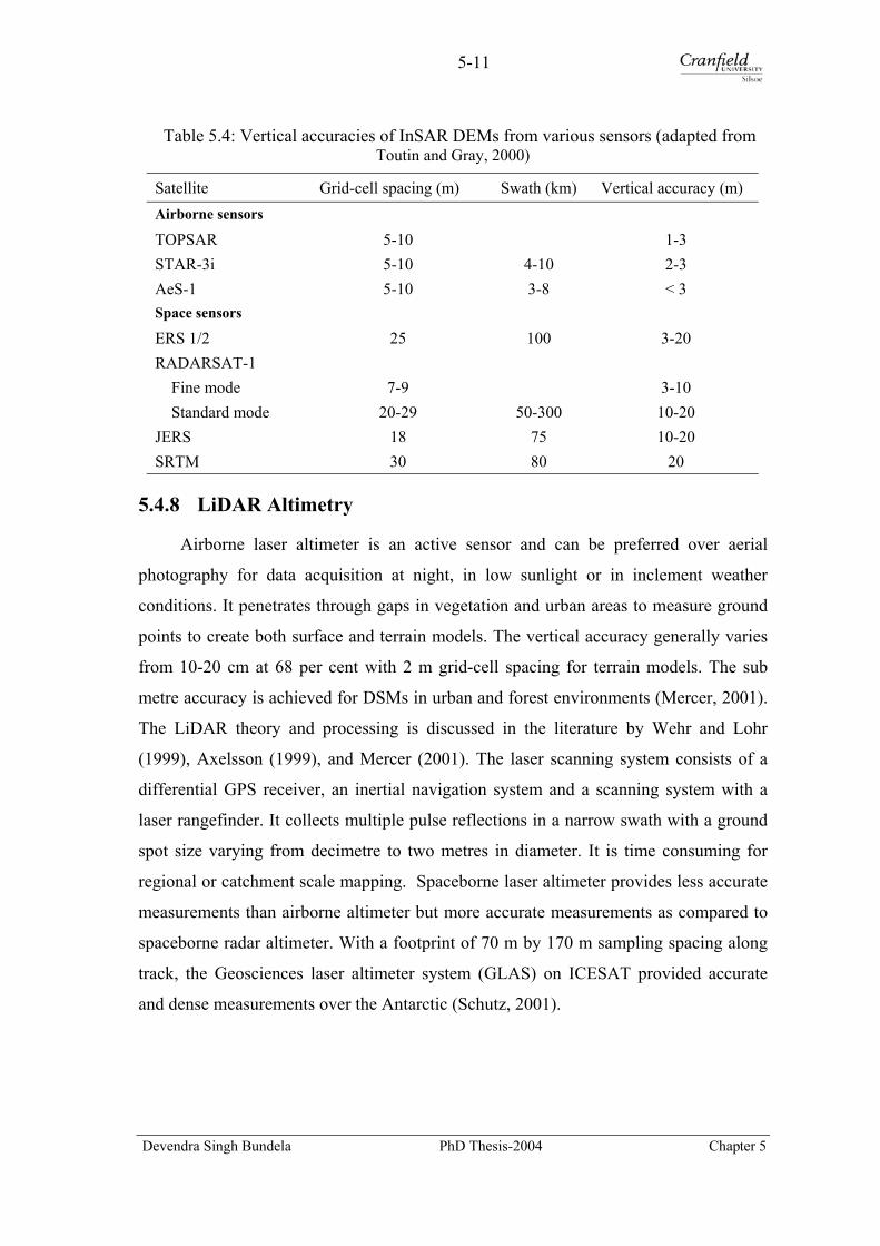
5-11
Table 5.4: Vertical accuracies of InSAR DEMs from various sensors (adapted from Toutin and Gray, 2000)
Satellite Grid-cell spacing (m) Swath (km) Vertical accuracy (m) Airborne sensors TOPSAR 5-10 1-3 STAR-3i 5-10 4-10 2-3 AeS-1 5-10 3-8 < 3 Space sensors ERS 1/2 25 100 3-20 RADARSAT-1 Fine mode 7-9 3-10 Standard mode 20-29 50-300 10-20 JERS 18 75 10-20 SRTM 30 80 20
5.4.8 LiDAR Altimetry
Airborne laser altimeter is an active sensor and can be preferred over aerial
photography for data acquisition at night, in low sunlight or in inclement weather
conditions. It penetrates through gaps in vegetation and urban areas to measure ground
points to create both surface and terrain models. The vertical accuracy generally varies
from 10-20 cm at 68 per cent with 2 m grid-cell spacing for terrain models. The sub
metre accuracy is achieved for DSMs in urban and forest environments (Mercer, 2001).
The LiDAR theory and processing is discussed in the literature by Wehr and Lohr
(1999), Axelsson (1999), and Mercer (2001). The laser scanning system consists of a
differential GPS receiver, an inertial navigation system and a scanning system with a
laser rangefinder. It collects multiple pulse reflections in a narrow swath with a ground
spot size varying from decimetre to two metres in diameter. It is time consuming for
regional or catchment scale mapping. Spaceborne laser altimeter provides less accurate
measurements than airborne altimeter but more accurate measurements as compared to
spaceborne radar altimeter. With a footprint of 70 m by 170 m sampling spacing along
track, the Geosciences laser altimeter system (GLAS) on ICESAT provided accurate
and dense measurements over the Antarctic (Schutz, 2001).
Devendra Singh Bundela PhD Thesis-2004 Chapter 5

5-12
5.5 Comparison of Mapping Technologies
Availability of DEMs with a requisite resolution and quality continues to be a
major area of concern for distributed modelling. Cartometric DEMs in the developing
countries are available at coarse resolutions and reasonable quality and can be applied
for regional scale modelling. A high resolution DEM with 20-30 m grid-cell spacing
with a reasonable vertical accuracy in the order of metres is required for modelling.
Therefore, cartometric DEMs can not be preferred for modelling study. Two emerging
remotely sensed mapping technologies such as radar interferometry and LiDAR have
potentials to improve the DEM quality and coverage (Maune, 2001). Radar
interferometry yields vertical accuracies and resolutions of DEMs comparable with
optical stereo DEMs. Airborne radar interferometry produces higher resolution and
accuracy DEMs than spaceborne InSAR technology, but the dataset is available only
from satellite platform for the developing countries. LIDAR is appropriate for more
detailed delineation of ground features in urban or forested environments. Airborne
stereo radar technology has been phased out due to lower resolution compared to
airborne InSAR. Spaceborne stereo radar is still in operation and produces much lower
resolution and vertical accuracy as compared to spaceborne InSAR. Interferometric
SAR DEM is the cost effective for large-area applications. Moreover, InSAR from both
air and spaceborne has been successfully used in a few research and commercial
applications such as Landmap, SRTM, and NEXTMap Britain. InSAR DEM generation
is also less cumbersome and expensive than the optical stereo and radargrammetric
DEM generation.
Advanced mapping technologies such as InSAR, LiDAR, optical stereo and radar
stereo produce superior quality DEMs, but they too contain errors which are technology
specific and vary from low to severe in some of the cases (Toutin and Gray, 2000;
Endreny et al, 2000; Kervyn, 2001; Leberl, 1990). Remotely sensed derived DEMs, in
fact, contain elevation data from first reflective surface, which requires a considerable
post processing to obtain a bare earth surface required for modelling study. Cost of a
DEM per square km increases with higher resolution and vertical accuracy, and varies
from technology to technology. As can be seen from Figure 5.1, InSAR DEM has better
vertical accuracy and lower cost than optical stereo and radar stereo DEMs.
Devendra Singh Bundela PhD Thesis-2004 Chapter 5

5-13
Unit price(US $/sq km)
Vertical accuracy (m) RMS Increasing details →
Figure 5.1: Comparison of DEM unit price from various mapping technologies
(adapted from Mercer et al, 1998)
5.6 DEM Quality Assessment Procedure
The quality of a DEM should be assessed before deriving the input parameters
of a distributed model. It can be assessed at two stages: firstly at engineering analysis
and quality control during acquisition and production processes, and secondly at an
independent DEM assessment against reference data. The former is used for quality
assessment of derived InSAR DEMs and the procedure is described below in terms of
most suitable quality measures, descriptors, criteria and reference data.
Quality assessment measures
The quality of a DEM is assessed mostly on the basis of its height values against
height values of the corresponding points from reference data. Ackermann (1996)
defined a more detailed quality measure using the first two derivatives of height: slope
(slope gradient and slope aspect) and convexity (profile and plan convexity). These
derivatives are more sensitive to change than the height accuracy.
Devendra Singh Bundela PhD Thesis-2004 Chapter 5

5-14
Quality descriptors
A few descriptors are used for DEM quality assessment namely, standard error,
root mean square error (RMSE), histogram analysis, vertical difference and fractal
dimension estimator. A quality descriptor is chosen on the basis of availability of
reference data. An RMS error is used for checkpoint reference data while the vertical
difference and histogram analysis descriptors are used for reference DEM data.
Quality criteria
The horizontal and vertical accuracies of a DEM are assessed using an
independent statistically sound testing methodology under the NSSDA (National
standard for spatial data accuracy) (FGDC, 1998) described below. The NSSDA
methodology is applied to estimate the horizontal and vertical accuracies of
georeferenced maps and digital spatial data derived from aerial photography, satellite
remotely sensed data and ground survey sources (FGDC, 1998). The horizontal and
vertical accuracies at 95 per cent confidence level is tested at ground scale against an
independent source of higher accuracy with a minimum of 20 check points well defined
and distributed over an area of interest (FGDC, 1998). The criteria for horizontal and
vertical accuracies are used on the basis of either normal or non-normal distribution of
random error.
For normally distributed case
The horizontal accuracy is assessed in terms of radial (also referred to as circular
accuracy) at 95 per cent confidence level (Accuracyr). Radial accuracy is the radius of a
circle of uncertainty within which 95 per cent of points are located. It is estimated using
Equations 5.1 and 5.2 for two cases, depending on x and y direction errors and
assuming that systematic errors are eliminated as best as possible and random errors are
normally distributed.
When RMSEx is equal to RMSEy, the circular accuracy is expressed:
rr RMSE*7308.1Accuracy = … (Eq. 5.1)
where RMSEr is the radial root mean square error and is calculated by:
22yxr RMSERMSERMSE +=
Devendra Singh Bundela PhD Thesis-2004 Chapter 5

5-15
When RMSEx is not equal to RMSEy and then the circular accuracy is given:
)(*5.0*4477.2 yxr RMSERMSEAccuracy +≈ … (Eq. 5.2)
The vertical accuracy (Accuracyz) is assessed in terms of vertical RMSE (RMSEz)
at 95 per cent confidence level and is defined as the linear uncertainty within which 95
per cent of points fall. It is given by Equation 5.3 assuming that systematic errors are
eliminated as best as possible and the vertical random error is normally distributed:
zz RMSE*9600.1Accuracy = … (Eq. 5.3)
For non normal distributed case
When errors are not normally distributed, the 95th percentile method is used
(Daniel and Tennant, 2001). An RMSE procedure is not applicable in such cases. The
95th percentile indicates that 95 per cent of errors are of equal or lesser value and 5 per
cent of errors are of larger value.
Reference data
Three kinds of reference data namely: check points, a DEM and a drainage
network can be used for quality assessment. First reference data source is the most
common and widely used for DEM quality assessment (FGDC, 1998; USGS, 1997). A
minimum of twenty independent check points is required and collected from the various
sources The descending order of preference for accepting check points is ground control
points (GCPs), aero-triangulated test points, spot heights, or contour points from maps
with appropriate contour intervals (USGS, 1997).
Another approach of quality assessment is based on an error free reference DEM
since it provides the possibility of comparing both DEMs on every grid-cell basis. The
reference DEM should be at least one order better than the DEM to be evaluated
statistically (USGS, 1997). DEM sources such as aerial photogrammetric DEM, stereo
optical DEM, InSAR DEM, LiDAR DEM, and even cartometric DEM can be used for
the purpose.
Devendra Singh Bundela PhD Thesis-2004 Chapter 5

5-16
The error free reference DEM assumption is rarely valid. The errors in both
DEMs are compared and they may not exhibit a true representation of error distribution.
A comparison of the drainage networks is another alternative to a reference DEM for
quality assessment. The reference drainage network can either be produced by
digitisation of an appropriate scale topographic map or extracted from a DEM using a
drainage extraction algorithm based on a single or multiple flows. Both networks are
compared on the basis of stream orders.
5.7 Off the Shelf Public Domain DEM Data
DEM data of the Eastern South Downs are available from both commercial and
public domain sources. The Landmap DEM was the only public domain source
available in the beginning of the study. Later on, the ASTER DEM and SRTM DEM
were made available in the public domain. Table 5.5 lists the ‘off the shelf DEMs’ of
the study area obtained from the public domain. In the developing world, researchers
either rely on public domain DEMs or cartometric DEMs, which can be generated at
their end. Therefore, it is a reason to look at the quality of public domain DEMs. The
commercial domain ‘off the self DEMs’ are also reviewed for the study area. It might be
available soon in the developing world. The commercial DEMs are created from various
sources such as contours, optical stereogrammetry, airborne radar interferometry,
LiDAR and mixed sources are given in Appendix D-1. Three public domain DEMs
(Table 5.5), namely Landmap, ASTER and SRTM-3, were used in this study to
investigate the influence of their resolutions on model predictive capacity. The selection
of a DEM should be based on its resolution and quality, which must be consistent with
the scale and physical processes in a model.
The Landmap DEM version 2.0 (Landmap, 2003), is a 25 m multipass InSAR
DEM derived from ERS tandem SAR data and is an improved version of original
version 1.0, which included some erroneous SAR strips. These strips are later detected
and reprocessed to remove the errors (Landmap 2003). The ASTER DEM (USGS,
2004) is a 30 m relative DEM generated from an along-track stereo pair of ASTER
Level 1A images acquired on 9 December 2002, which include bands 3N (nadir) and 3B
(aft-viewing) from the VNIR in the spectral range of 0.78 to 0.86 µm. This Relative
ASTER DEM is generated without ground control points (GCPs) and can be used to
Devendra Singh Bundela PhD Thesis-2004 Chapter 5

5-17
derive absolute slope gradient and slope aspect accurate up to 5 degrees over a
horizontal distance of over 100 metres and meets map accuracy standards for scales
from 1:50 000 to 1:250 000 (USGS, 2004). The SRTM-3 is a three arc second unedited
DEM generated from C-band single pass interferometry with data acquired during the
SRTM project (USGS, 2003). This DEM is produced by 3x3 averaging of one arc
second DEM data which contain ground clutter and water body artefacts. These errors
are reduced by this averaging by a factor of three approximately. This is also available
with 75 m postings in the British National grid coordinates from Landmap (Landmap,
2003).
Table 5.5: Public domain digital elevation data of the Eastern South Downs
DEM data Grid Spacing (m)
Extent of each tile (km x km)
Vertical accuracy (m) (RMSE)
Technique DEM Source
Landmap DEM 25 100 x 100 or user defined
Not available InSAR Landmap
SRTM DEM 3’’ 10 x 10 < 16 InSAR USGS/ Landmap
ASTER DEM 30 ~60 x 60 10-30 (relative height)
Optical stereo
USGS
5.8 Generation of InSAR DEMs for Modelling
5.8.1 Introduction
Radar (radio detection and ranging) operates in the microwave range from a
metre to a few millimetres in wavelength. There are two basic radar systems namely;
real-aperture radar and synthetic aperture radar and both differ principally by the
method used to achieve a better azimuth resolution (resolution in the direction of travel).
Real aperture radar produces a narrow angular beamwidth while synthetic aperture radar
(SAR) employs a small antenna and synthesises a relatively broad beam using the
Doppler principle and synthetic aperture data processing techniques to improve the
azimuth resolution (Sabins, 1997). The SAR processor is based on a two-dimensional
reference function and received signals. The SAR processing involves an accurate
modelling of the SAR response to a point target and a continuous field of targets
(Kramer, 2002). The SAR systems and SAR data processing is discussed in the
literature by Curlander and McDonough (1991).
Devendra Singh Bundela PhD Thesis-2004 Chapter 5
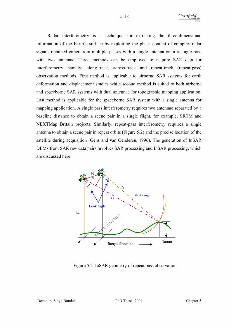
5-18
Radar interferometry is a technique for extracting the three-dimensional
information of the Earth’s surface by exploiting the phase content of complex radar
signals obtained either from multiple passes with a single antenna or in a single pass
with two antennae. Three methods can be employed to acquire SAR data for
interferometry namely; along-track, across-track and repeat-track (repeat-pass)
observation methods. First method is applicable to airborne SAR systems for earth
deformation and displacement studies while second method is suited to both airborne
and spaceborne SAR systems with dual antennae for topographic mapping application.
Last method is applicable for the spaceborne SAR system with a single antenna for
mapping application. A single pass interferometry requires two antennae separated by a
baseline distance to obtain a scene pair in a single flight, for example, SRTM and
NEXTMap Britain projects. Similarly, repeat-pass interferometry requires a single
antenna to obtain a scene pair in repeat orbits (Figure 5.2) and the precise location of the
satellite during acquisition (Gens and van Genderen, 1996). The generation of InSAR
DEMs from SAR raw data pairs involves SAR processing and InSAR processing, which
are discussed here.
Figure 5.2: InSAR geometry of repeat pass observations
Look angle
Slant range
α
θ
B
θ
r1
r2
h0
Range direction
P
h
Datum
Devendra Singh Bundela PhD Thesis-2004 Chapter 5
5-19
5.8.2 Review of SAR Interferometry
SAR interferometry has successfully been applied for topographic mapping
(Zebker and Goldstein, 1986; Goldstein et al, 1988; Gabriel and Goldstein, 1988),
thematic mapping (Ichoku et al, 1998; Askne and Hagberg, 1993) and atmospheric
delay mapping studies (Hanssen, 2001) while differential SAR interferometry has
successfully been demonstrated for earth deformation monitoring (Massonnet et al,
1993, Zebker, 2000) and recently for estimation of erosion and deposition by the water
(Smith, 2001; Smith et al, 2000).
Radar interferometry was begun with the observation of the surface of the Venus
and the Moon. Graham in 1974 theoretically introduced the synthetic aperture radar
(SAR) interferometric technique with a side looking airborne and spaceborne geometry
for topographic mapping of the Earth. First airborne SAR interferometer for
topographic mapping was successfully applied by Zebker and Goldstein (1986), but a
better vertical accuracy could not be achieved due to lack of aircraft roll data. The first
application of spaceborne repeat pass SAR interferometry for earth topography became
possible with data acquired during 100 day long SEASAT mission in 1978 and
subsequently its results were published (Gabriel et al, 1989). Gabriel and Goldstein
(1988) adapted the repeat pass interferometric technique to cross orbits data acquired in
October 1984 from SIR-B in a repeat orbit for an area in Canada. Li and Goldstein
(1990) studied the effects of multibaselines ranging from 60 to 1000 m on phase errors
and topographic heights and showed that the larger baseline length increases phase
errors and sensitivity of heights.
Since the launch of ERS-1 satellite with C-band SAR in July 1991 by the
European Space Agency (ESA), the research was mostly concentrated on potentials and
limitations of SAR interferometry. After the launch of ERS-2 in 1995 and
simultaneously operation in a tandem mission mode with a 24 hour time difference, the
applications of spaceborne SAR interferometry were greatly expanded worldwide with
availability of InSAR datasets. The assessment of DEMs from ERS tandem data
appeared most promising (Duchossois and Martin, 1995). Recent studies of Zebker et al
(1994) and Rufino et al (1998) showed that the achievable accuracy for DEM
generation is about 10 m and 5 m respectively in favourable situations. DEMs of
Devendra Singh Bundela PhD Thesis-2004 Chapter 5

5-20
Finland from ERS tandem mission using 35 image pairs of ascending and descending
pass showed an elevation accuracy of about 10 m (Herland, 1997). Zebker et al (1997)
also mentioned that the atmospheric effect might deteriorate DEM accuracy as much as
100 m at unfavourable baseline.
With the launch of JERS-1 in 1992, L-band repeat pass interferometry was
applied for topographic mapping due to its vegetation penetration capability and lower
sensitivity to temporal change. The vertical accuracies (RMSE) of 22 m (Werner et al,
2000), 6-16 m (Dammert and Wegmüller, 1999) and 27.7 m (Tokunaga, 1997) have
been reported for InSAR DEMs derived from JERS-1 SAR data. The orbital accuracy
of JERS-1 was not as precise as required for interferometry, so data were not
extensively exploited despite its potentials. SAR data of three bands (X, C and L) were
collected from SIR-C /X-SAR, flown on the space shuttle Endeavour on two missions in
1994. The InSAR DEMs were generated from L-band data (Sun and Ranson, 1997;
Lanari et al, 1996) with a vertical accuracy of 16.14 m (Chao et al, 1999). Since the
launch of RADARSAT in 1995, large amounts of InSAR data pairs were made
available with various look angles and swaths. Due to imprecise orbit parameters, its
full interferometric potential could not be exploited.
Two major problems of temporal decorrelation and atmospheric effect were
experienced in repeat pass interferometry for DEM generation. This experience
culminated in the Shuttle Radar Topographic Mission (SRTM) in early 2002 with a
single pass interferometry from space (Farr and Kobrick, 2000; Balmer, 1999). It
mapped the globe with C and X-bands and 30 m global DEMs have been generated
from the SRTM SAR data (Farr and Kobrick, 2000). Recently, SRTM-3 DEMs with
three arc second grid-cell spacing have been released to the scientific community
without accuracy assessment (USGS, 2003). In March 2002, the ESA launched the
ENVISAT with an advanced SAR system to continue ERS SAR data and to provide
improved capability on different spatial resolutions, incidence angles, swath and
polarisations for SAR interferometry (ESA, 2004).
Devendra Singh Bundela PhD Thesis-2004 Chapter 5

5-21
5.8.3 Selection of SAR Data
SAR raw or single look complex data pairs can be obtained from a number of
spaceborne imaging radar systems (Appendix D-2). A few parameters need to be
optimised for selecting a quality InSAR pair:
• terrain characteristics,
• radar band,
• baseline,
• temporal decorrelation, and
• orbital accuracy
The terrain is characterised by slopes and landcover types, which act as a guide
for selecting an optimal pair. There is an optimal baseline range for each radar band. For
steep slopes, shorter baseline data pairs are selected for best results while for lower
slopes, longer baseline data pairs are preferred for successful DEM generation. Larger
wavelength (L-band) radar can allow longer baseline, which has higher sensitivity to
height and also results in a higher DEM accuracy, but there is an upper limit of baseline
for a particular band. Increase of baseline decreases the phase coherence, a critical
parameter for interferometry. The optimal perpendicular baseline for ERS system is 50-
300 m for topographic mapping (ESA, 2004). The upper baseline limit has an
acceptable coherence loss but it is not preferred for high quality DEM generation.
Temporal decorrelation is related to the loss of phase coherence due to a time
difference between two acquisitions and depends on the nature of target and its
backscattering properties variation over time. Agricultural and grassland have stable
backscatters for a short time interval as compared to the forest cover. Large temporal
difference results in a significant coherence loss, which may not allow generation of
high quality DEMs. An optimal pair with least possible temporal difference for a given
situation should be selected from different spaceborne SAR sensors (Table 5.6). It
should be shorter time difference possible for agricultural and grassland catchments.
The best pairs can be obtained from ERS tandem data pairs, which were acquired with
24 hours time difference. Orbit errors directly affect the position and height accuracy of
a DEM and are translated into position and height shifts during phase to height
conversion and geocoding steps. Therefore, it is essential to select a sensor platform
Devendra Singh Bundela PhD Thesis-2004 Chapter 5
5-22
with precise orbit control and maintenance. Orbital accuracy of ERS and ENVISAT are
better than that of Radarsat-1 and JERS-1.
Table 5.6: Temporal difference for the acquisition of a pair from satellite SAR sensors
InSAR Pair Band Repeat pass temporal difference (days)
ERS-1 / ERS-1 C 3, 35 or multiple of 35 (3 days-during Ice phases)
ERS-1 / ERS-2 C 1 day (Tandem mission)
ERS-2 / ERS-2 C 35 or its multiple (Multidisciplinary phase)
ENVISAT / ENVISAT C 35 or its multiple (4 days with antenna steering)
JERS-1 / JERS-1 L 44 or its multiple
RADARSAT / RADARSAT for standard and fine mode
C 24 or its multiple
A suitable SAR raw data pair of the Eastern South Downs from the ERS tandem
mission archive (Table 5.7) was selected using both an online EOLI (Earthnet online
interactive) browser and an offline multi mission DESCW (Display earth remote
sensing swath coverage for windows) catalogue browser based on baseline and other
information of the pairs. The pair of quicklook images was also checked for data quality
and atmospheric perturbations. Selected dataset was obtained under the European
Research Club from the Eurimage, Italy via Infoterra.
Table 5.7: Scene parameters of a SAR raw data pair of the Eastern South Downs
Mission Date Orbit no _|_ Baseline ∆ Day Other information
ERS-1 13 March 1997 29598 -- -- Track: 051, Frame: 2583,
ERS-2 14 March 1997 9925 145 m 1 Descending path
5.8.4 Selection of SAR and InSAR Processors
Numerous commercial and research packages (also called processors) have been
developed to generate digital elevation models (DEMs) from SAR raw or SLC data. A
processor system with a precision phase preserving focussing and interferometric
processing was the preferred choice assuring the smooth import and analysis of input
data for interferometric analysis. Two processors viz. PulSAR/ InSAR Toolkit from the
Phoenix System on the Linux platform, and SARscape and SARscape DEM from the
Devendra Singh Bundela PhD Thesis-2004 Chapter 5
5-23
SARMAP on the Windows platform were used in this study. InSAR processing consists
of a standard processing chain of various steps with various options at each step to solve
a constraint. Most of the processors have inherent advantages and limitations, as they
are not available in all the operating platforms and do not support all the SAR sensors,
data formats, and processing and archive facilities (PAFs) (Gens, 1999). The processors
are compared from their capability point of view (Appendix D-3).
Both SAR and interferometric processing involve complicated tasks requiring a
lot of user interactions for obtaining the best results. The optimal processing procedures
for each task and of a complete chain were discussed on the basis of various processing
steps and available software functionalities in the following sections.
5.8.5 SAR Data Focussing
SAR data focusing or processing involves:
• range focusing,
• range migration compensation, and
• azimuth focusing
The range focusing is performed by matched filtering of a returned radar signal
with a replica of the transmitted signal. The range migration translates the radar return
from a target in successive pulses that it falls within one column of dataset. For ERS-1
and ERS-2 system, the maximum translation is less than one range bin (Curlander and
McDonough, 1991). The azimuth focusing is carried out by correlating the returns from
a target within successive pulses of the radar with a theoretical chirp function defined
according to the expected frequency shift and phase of the return from that target as it
passes through the radar antenna. All the above three steps are performed on patches of
data at least corresponding to the size of the radar footprint of 1200 pulses for ERS-1
and ERS-2 (Curlander and McDonough, 1991).
A SAR raw data pair was supplied in the CEOS SAR format on two optical
disks (Appendix D-4). A single scene SAR data contained four files namely, volume
directory, leader, data and null volume directory. Both leader and data files were mainly
used to extract the processing parameters and to ingest SAR data for each scene to the
SAR processing system. In the study, two precision phase preserving digital processors
such as range-Doppler (Zebker et al, 1994; Smith, 1991) and Omega-k in frequency
Devendra Singh Bundela PhD Thesis-2004 Chapter 5

5-24
domain (Cafforio et al, 1991; Balmer, 1992) were used to focus raw data to single look
complex (SLC) images (Figure 5.3). The image quality was checked for an optimal
focusing (Appendix D-5). The images were then multilooked with a single look in the
range and five looks in the azimuth direction to reduce the speckle noise and to view
pixels in a square shape (Figure 5.4, left). The phase of a single SLC image (Figure 5.4,
right) was found to be completely random in the most image areas and has not been
used for an application. The range-Doppler processor has been widely used in the most
commercial software and in the ESA PAFs’ SAR processors (Table 5.8). A few new
digital SAR processors have been developed (Hanssen, 2001), but they are not widely
used.
SAR SLC images obtained from the ESA PAFs are not optimally focussed for a
specific interferometric application such as topographic mapping but they are
reasonable processed images for the most applications. SAR processing at user end
could be optimally customised for the best resolution, focus, speckle reduction factors,
and many other image parameters which result in a better image quality for
interferometry (Lightstone, 1996). Many other interferometric applications can also be
benefited from such customised SAR processing at user end.
Table 5.8: SAR processors used at the ESA PAFs and in software
PAF/Software SAR Processor name Algorithm used
PulSAR/InSAR Toolkit PulSAR Range-Doppler
SARscape SARscape ω-k frequency domain
Gamma SAR Modular SAR Processor Range-Doppler
EarthView Advanced Precision Processor
Range-Doppler Chirp scaling (optional)
Vexcel’s InSAR FOCUS Range-Doppler
I-PAF VMP 6.8 Range-Doppler
UK-PAF VMP 6.8 Range-Doppler
D-PAF VMP 6.8 Range-Doppler
EECF, Italy VMP 6.8 Range-Doppler
Devendra Singh Bundela PhD Thesis-2004 Chapter 5
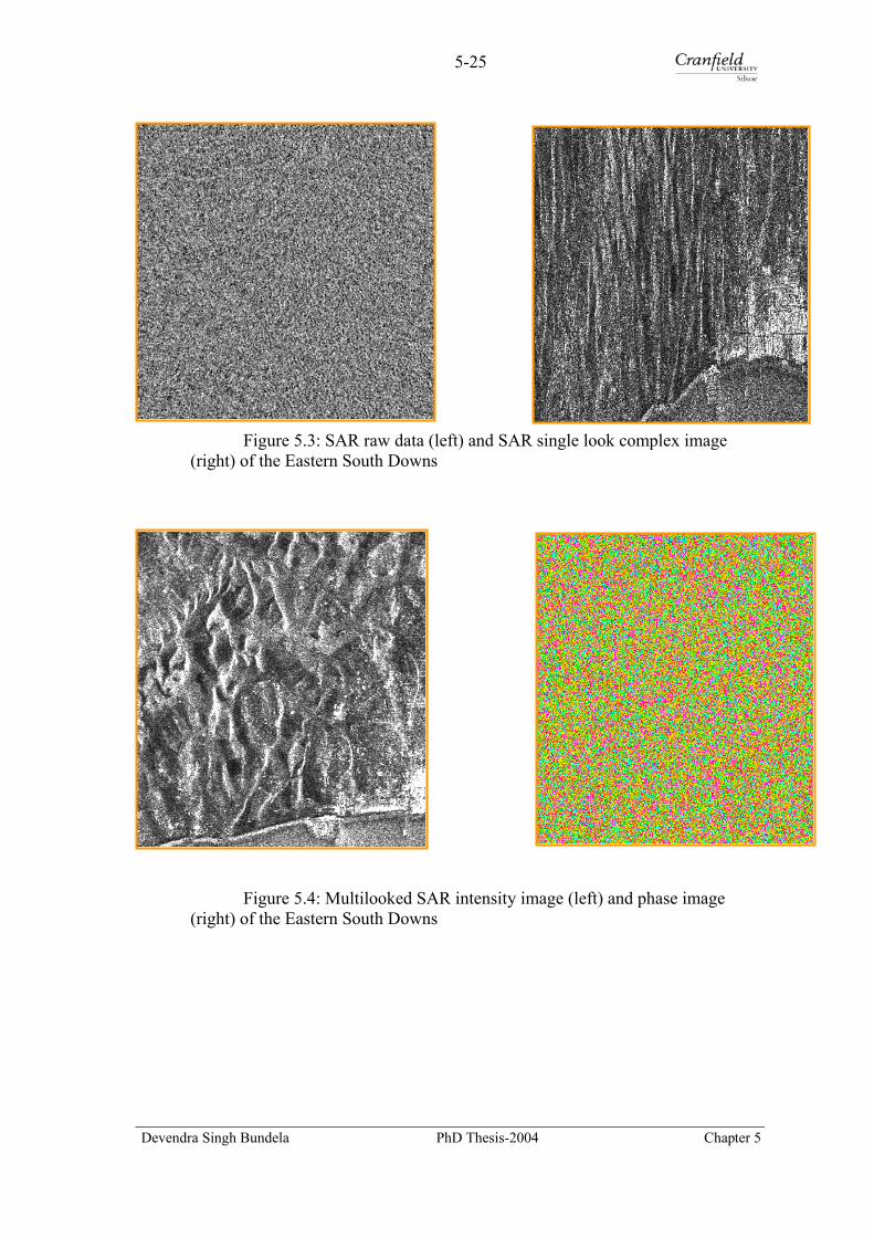
5-25
Figure 5.3: SAR raw data (left) and SAR
(right) of the Eastern South Downs
Figure 5.4: Multilooked SAR intensity i(right) of the Eastern South Downs
Devendra Singh Bundela PhD Thesis-20
single look complex image
m
0
age (left) and phase image
4 Chapter 5
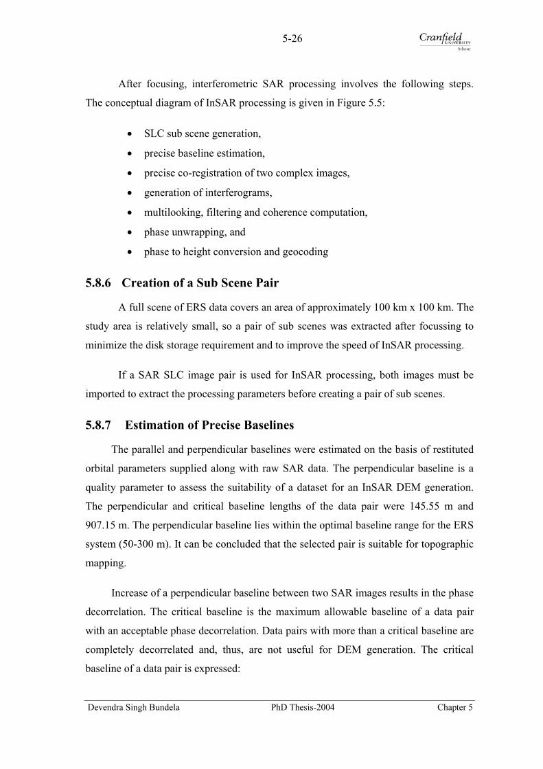
5-26
After focusing, interferometric SAR processing involves the following steps.
The conceptual diagram of InSAR processing is given in Figure 5.5:
• SLC sub scene generation,
• precise baseline estimation,
• precise co-registration of two complex images,
• generation of interferograms,
• multilooking, filtering and coherence computation,
• phase unwrapping, and
• phase to height conversion and geocoding
5.8.6 Creation of a Sub Scene Pair
A full scene of ERS data covers an area of approximately 100 km x 100 km. The
study area is relatively small, so a pair of sub scenes was extracted after focussing to
minimize the disk storage requirement and to improve the speed of InSAR processing.
If a SAR SLC image pair is used for InSAR processing, both images must be
imported to extract the processing parameters before creating a pair of sub scenes.
5.8.7 Estimation of Precise Baselines
The parallel and perpendicular baselines were estimated on the basis of restituted
orbital parameters supplied along with raw SAR data. The perpendicular baseline is a
quality parameter to assess the suitability of a dataset for an InSAR DEM generation.
The perpendicular and critical baseline lengths of the data pair were 145.55 m and
907.15 m. The perpendicular baseline lies within the optimal baseline range for the ERS
system (50-300 m). It can be concluded that the selected pair is suitable for topographic
mapping.
Increase of a perpendicular baseline between two SAR images results in the phase
decorrelation. The critical baseline is the maximum allowable baseline of a data pair
with an acceptable phase decorrelation. Data pairs with more than a critical baseline are
completely decorrelated and, thus, are not useful for DEM generation. The critical
baseline of a data pair is expressed:
Devendra Singh Bundela PhD Thesis-2004 Chapter 5
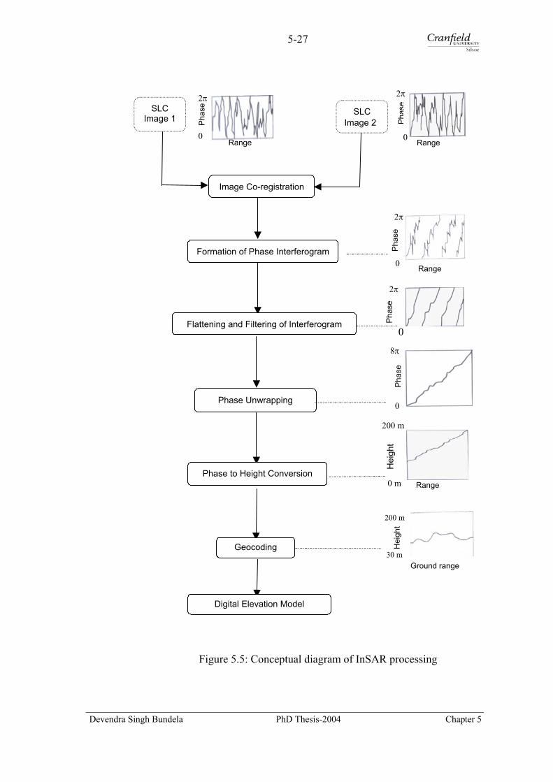
5-27
Range
Phas
e
2π
Range
Phas
e Ph
ase
Range
Hei
ght
Hei
ght
8π
Phase to Height Conversion
Phase Unwrapping
Flattening and Filtering of Interferogram
Formation of Phase Interferogram
Image Co-registration
SLC Image 2
2π
2π
200 m
Range
Phas
e
2π
0
0
0
0
200 m
0 m
Phas
e
SLC Image 1
0
Geocoding 30 m
Ground range
Digital Elevation Model
Figure 5.5: Conceptual diagram of InSAR processing
Devendra Singh Bundela PhD Thesis-2004 Chapter 5
5-28
… (Eq. 5.4)
c)tan(*r*W*B )critical(
α−θλ=⊥
where W is the bandwidth of a SAR system, r is the slant range from sensor to target, θ
is the angle of look, α is the local terrain slope in range direction and c is the velocity of
light.
5.8.8 Precise Co-registration
Co-registration is the crucial step of InSAR processing and involves alignment of
a slave image with a master image and resampling of amplitude and phase values of a
slave image. It was carried out in two steps namely; coarse and fine registration. Coarse
co-registration of the master and the slave images was performed from orbital state
vectors, the moments and the centre of the image. An accuracy of 2 pixels in range
direction and 10 pixels in azimuth direction was achieved. The fine registration based
on phase information in InSAR Toolkit and fringe detection in SARscape DEM was
performed. The range and azimuth offsets shifts between the SAR image pair were
found to be 8.046 pixels and -33.952 pixels respectively. The fine co-registration was
performed with an accuracy of 1/1000th of a pixel. Poor co-registration with a very
small offset results in a drastic loss of coherence. The precision of co-registration must
be better than half a pixel to minimise the loss of coherence.
5.8.9 Formation of Interferograms
Spectral range filtering was applied to minimise the decorrelation due to a non
overlapping range spectra. Similarly, common Doppler bandwidth filtering was applied
to the registered images to minimise the decorrelation due to a partial overlap of the
azimuth spectra. The interferogram (Figure 5.6, left) was then generated by multiplying
the complex value of the slave image to complex conjugate value of the master image
(Equation 5.9). The quality of fringes shows the high level of phase correlation in the
interferogram. The assumption of an identical object phase in both SAR images is only
valid for ERS tandem datasets.
Devendra Singh Bundela PhD Thesis-2004 Chapter 5

5-29
After focusing, the phase of a SAR image has two components namely: a
deterministic geometric phase due to the distance between sensor and object; and a
random phase component contributed by object phase and thermal noise (Equation 5.7).
Random phase component is the coherent sum of the signals from the randomly
arranged elemental scatters within the cell to the centre of the cell. This component,
although random from a resolution element to a resolution element, remains the same if
the viewing geometry is nearly identical and if the relative position of the elemental
scatterers within a cell remains the same. The thermal noise is the same for images
acquired in repeat pass observations due to the single antenna and depends on its
magnitude relative to the desired signal. It is different for transmitting and receiving
antennae used in single pass interferometry. The phase of a SAR image is the sum of a
deterministic phase, an object phase and a thermal phase and is expressed as (Balmer,
1997):
therobj φφφφ += det + … (Eq. 5.5)
The deterministic phase of an image pixel is directly proportional to the slant
range and is expressed:
rc
p*det
ω−=φ … (Eq. 5.6)
where p is acquisition mode factor and is equal to1 for a single pass interferometry and
2 for repeat pass interferometry, ω is the angular frequency, r is the slant range distance
and c is the speed of light. Hence, the phase of a pixel in a master image and a slave
image is given as:
therobjrc
φφω
φ += 112
+ and … (Eq. 5.7)
therobj22 rc
2φ+φ+
ω=φ … (Eq. 5.8)
The interferometric phase difference is computed as a hermitian product of
Equations 5.7 and 5.8 and is given as:
ess i )12(21
*12 ** φφρρ −= … (Eq. 5.9)
The phase difference of a pixel between two images is expressed assuming
random phase component between two acquisitions remains same:
Devendra Singh Bundela PhD Thesis-2004 Chapter 5
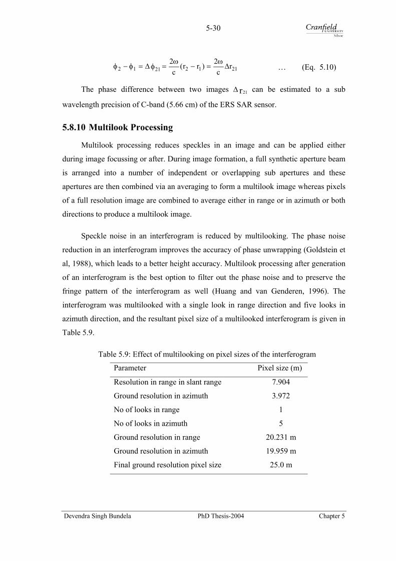
5-30
21122112 rc
2)rr(c
2∆
ω=−
ω=φ∆=φ−φ … (Eq. 5.10)
The phase difference between two images r21∆ can be estimated to a sub
wavelength precision of C-band (5.66 cm) of the ERS SAR sensor.
5.8.10 Multilook Processing
Multilook processing reduces speckles in an image and can be applied either
during image focussing or after. During image formation, a full synthetic aperture beam
is arranged into a number of independent or overlapping sub apertures and these
apertures are then combined via an averaging to form a multilook image whereas pixels
of a full resolution image are combined to average either in range or in azimuth or both
directions to produce a multilook image.
Speckle noise in an interferogram is reduced by multilooking. The phase noise
reduction in an interferogram improves the accuracy of phase unwrapping (Goldstein et
al, 1988), which leads to a better height accuracy. Multilook processing after generation
of an interferogram is the best option to filter out the phase noise and to preserve the
fringe pattern of the interferogram as well (Huang and van Genderen, 1996). The
interferogram was multilooked with a single look in range direction and five looks in
azimuth direction, and the resultant pixel size of a multilooked interferogram is given in
Table 5.9.
Table 5.9: Effect of multilooking on pixel sizes of the interferogram
Parameter Pixel size (m)
Resolution in range in slant range 7.904
Ground resolution in azimuth 3.972
No of looks in range 1
No of looks in azimuth 5
Ground resolution in range 20.231 m
Ground resolution in azimuth 19.959 m
Final ground resolution pixel size 25.0 m
Devendra Singh Bundela PhD Thesis-2004 Chapter 5

5-31
The multilook phase and intensity images are computed from a single look
complex image:
∑
∑=
=
−
=
ra m
1x )y,x(
)y,x(1m
1yraphase I
Qtan
m*m1g … (Eq. 5.11)
QIm*m
1g 2)y,x(
mr
1x
2)y,x(
ma
1yraensityint ∑ +∑=
== … (Eq. 5.12)
where mr and ma are the number of looks in range and azimuth, I is the real component
of a complex SAR image at location (x, y) and Q is the imaginary component of a
complex SAR image at location (x, y).
5.8.11 Removal of Flat Earth Phase and Phase Filtering
A derived interferogram comprises the phase components attributed by the flat
terrain, topography and a form of noise. The phase due to the flat terrain appears in the
form of periodic fringe pattern over range, which needs to be removed to obtain the
topography directly. Two methods are used for interferogram flattening: the ellipsoidal
flattening and the terrain flattening. The ellipsoidal flattening is achieved using either
orbital data or interferogram fringes. The terrain flattening is performed using a coarse
resolution DEM.
The flat earth phase component in SARscape DEM was removed from the
interferogram using Equation 5.13 based on the orbital parameters and an ellipsoidal
model of the earth’s surface. The resultant flattened interferogram is given in Figure 5.6
(right).
rtancr)(BCos2
dffe ∆θ
α−θω=φ … (Eq. 5.13)
where φfe is the phase contributed by the flat earth, B is the baseline distance, α is the
local slope angle and ∆rdf is the range difference between two acquisitions.
The fringes were not sharp and very clear in the interferogram and phase noise
was present in the flattened complex interferogram. The interferogram was filtered
Devendra Singh Bundela PhD Thesis-2004 Chapter 5
5-32
using an adaptive filter to improve the phase coherence for a trouble free unwrapping
and improving the height accuracy. The flattened and filtered interferogram is presented
in Figure 5.7 (left). In InSAR Toolkit, the terrain flattening was performed using a 1 km
coarse GTOPO30 DEM.
5.8.12 Interferometric Coherence
Interferometric coherence is a measure of phase correlation and its absolute value
varies between 0 and 1 with a lower limit reflecting complete phase decorrelation and
an upper limit, a full phase correlation. The interferometric coherence (Figure 5.7, right)
was calculated from a flattened and filtered interferogram before phase unwrapping to
assess the phase noise. The coherence value varied from 0.0003 to 0.9286 with a mean
of 0.617 and a standard deviation of 0.219. The coherence statistics reflected a low level
of noise in the interferogram, which is suitable for a smooth phase unwrapping. At the
same time, effort was made in processing to minimise the coherence loss during
interferogram generation.
The noise in an interferogram emanating from various sources may be a system
noise, a decorrelation noise and a processor noise. The system noise could not be
avoided, but it is quite small as compared to sensed signals. The decorrelation noise
resulted from the baseline and temporal decorrelation. The processor noise emanates
during focussing and co-registration and is brought under control using an optimisation
strategy. The temporal decorrelation decreases the coherence by changing of conditions
between two acquisitions such as the scattering geometry within the resolution cell, the
physical properties of the scattering mechanisms and the behaviour of the propagation
medium. Interferometric coherence depends on several factors before phase unwrapping
such as; system noise, terrain decorrelation, baseline decorrelation, temporal
decorrelation, low quality SAR focussing, and insufficient co-registration. Phase
coherence is the product of all the above factors and is given in Equation 5.14:
γγγγγγ regcogfocuthermalbaselinetemporal −= ****
sin … (Eq. 5.14)
Devendra Singh Bundela PhD Thesis-2004 Chapter 5
5-33
If the phase noise in an interferogram is high, some fringes are completely lost
and result in errors in the DEM. The sources of phase noise are described in the
literature by Zebker at al (1994) and Huang et al (1996).
Interferometric coherence is defined as the normalised complex cross section of
two interferometric SAR signals, s1 and s2 shown in Equation 5.15. The SNR (signal to
noise ratio) can also be expressed in terms of the interferometric coherence:
*2s2s*
1s1s
*2s1s
=γ … (Eq. 5.15)
γ−
γ=
1SNR … (Eq. 5.16)
where γ is the interferometric coherence, asterisk (*) is the complex conjugate operator
and angular brackets are the statistical expectation, realized by a spatial averaging
within a defined rectangular filter, a product of complex signal s1 and complex
conjugate of signal s2 for a SAR pair.
5.8.13 Phase Unwrapping
After removal of flat earth phase and phase filtering, the phase in an interferogram
is wrapped into intervals of 2л modulus and is directly related to the physical qualities
of the surface topography. In order to reconstruct a surface topography, the phase is
unwrapped by a phase unwrapping procedure for solving the integer ambiguities. A
number of phase unwrapping algorithms based on local and global approaches have
been developed (Gens, 2003). A thorough description on phase unwrapping is found in
the literature reviewed (Gens, 2003; Ghiglia and Pritt, 1998).
The interferogram (Figure 5.7, left) was unwrapped using a classical branch cut
unwrapper (Goldstein, 1988) and a minimum cost flow (MCF) network unwrapper
(Costantini, 1996) in InSAR Toolkit and using a region growing unwrapper (Xu and
Cumming, 1999) in SARscape DEM. The unwrapped phase interferogram is given in
Figure 5.8.
Devendra Singh Bundela PhD Thesis-2004 Chapter 5
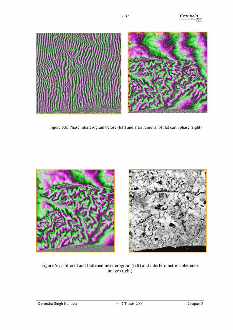
5-34
Figure 5.6: Phase interferogram before (left)
Figure 5.7: Filtered and flattened interferograimage (rig
Devendra Singh Bundela PhD T
and after removal of flat earth phase (right)
m (left) and interferometric coherence ht)
hesis-2004 Chapter 5

5-35
Figure 5.8: Unwrapped interferometric phase image
The phase in a flattened and filtered interferogram is unwrapped in an integer
multiple of 2 л and is given by Equation 5.17. Phase unwrapping algorithms attempt to
estimate the correct value of N for every pixel while considering unwrapping error
propagation in the image:
Nwrapunwrap
*2πφφ += … (Eq. 5.17)
The phase unwrapping is a two dimensional problem and is solved with local and
global approaches. The classical branch cut algorithm (Goldstein, 1988) is a local
approach based on the path following method. It relies on branch cuts between all
detected residues preventing any integration path from crossing these cuts. These
residues are either balanced by a residue of opposite polarity or by a branch cut
connected to the image border. The sum of the branch cut lengths are minimised in this
approach. It is computationally very efficient with a little memory requirement, but it
has a poor performance in areas of low coherence and with densely placed branch cuts.
The suggestions to improve the performance of this algorithm by different
preprocessing steps are discussed in the literature by Ghiglia and Pritt (1998) and
Goldstein and Werner (1998).
The minimum cost flow (MCF) unwrapping algorithm (Costantini, 1996) is based
on a classical branch cut method using a minimum cost flow networks for solving the
unwrapping problem. Phase difference of neighbouring pixels with an error of integer
Devendra Singh Bundela PhD Thesis-2004 Chapter 5

5-36
multiple of 2п leads to formulating the phase unwrapping problem as a global
minimization problem with integer variables: the weighted deviation between the
estimated and the unknown discrete derivatives of the unwrapped phase is minimized
subject to the constraint that the two functions must differ by integer multiples of 2. The
propagation of errors is prevented with this constraint and the resultant unwrapped
phase is identical to the original wrapped phase when rewrapped. The minimization
problem with integer variables is usually solved efficiently using the network structure
strategies.
The region-growing algorithm (Xu and Cumming, 1999) begins unwrapping
pixels of high coherence and proceeds along dynamic paths to pixels of high
unwrapping confidence. Difficult areas of low coherence are later approached from a
number of directions to unwrap. Thus, the algorithm is able to correct unwrapping
errors to a certain extent and minimise their error propagation into a whole image.
5.8.14 Orbit Geometry and Baseline Refinement
Precision orbital state vectors of the satellite position and velocity supplied along
with an ERS data pair have small errors of the order of tens of centimetres (ESA, 2004;
Massonnet et al, 1993), which are not accurate enough to allow a rigorous
transformation from the interferometric phase to the topographic height. The small orbit
errors are translated into horizontal and vertical shifts in a resultant DEM. In order to
minimise errors in orbit state vectors, a viewing geometry and baseline refinement
procedure is used to calibrate the phase to height transformation. Viewing geometry and
baseline are refined using a few GCPs well distributed in the image.
The ERS data pair was supplied with restituted orbital vector data due to
telemetry failure during the pair acquisition (Smith, 2003). It contained larger errors
than tens of centimetres error of precision orbital data. Therefore, viewing geometry
optimization was used using GCPs. In SARscape DEM, the baseline refinement was
achieved using 13 GCPs collected during a DGPS survey in the study area discussed
below. The horizontal and vertical shift adjustment was incorporated to correct orbit
error during geocoding in InSAR Toolkit.
Devendra Singh Bundela PhD Thesis-2004 Chapter 5
5-37
GPS data processing
13 GCPs for orbital geometry refinement were collected during a differential GPS
survey conducted with Trimble Pathfinder Pro-XRS GPS equipment with optimal
settings (Appendix D-6). The Trimble Pathfinder Pro-XRS GPS is a mapping grade
receiver and provides 10-30 cm accuracy with a carrier phase differential correction, but
its accuracy degrades with an increase of baseline distance between a base station and a
rover unit. The GPS data were logged for minimum 10 minute at a 15 second interval, a
compatible logging interval with the Ordnance Survey London Active Station, at each
point. The data were first real time code corrected with radio beacon of the UK Marine
differential GPS service (MDGPS) located at North Foreland. The code phase corrected
data were recorded during the survey. These code corrected positions are approximately
5 m accurate and the height accuracy is around two and half times lower than the
horizontal accuracy. The data were post processed against the London Active Station to
improve both horizontal and vertical accuracies. Trimble GPS Office Pathfinder version
3.00 software was used to determine the precise position and height coordinates of
control points in WGS 84 reference by applying differential correction evolved from
GPS code pseudo range and carrier phase measurements to minimise satellite ephemeris
and atmosphere refraction errors. The precise height determination was possible with a
single GPS receiver data when post processed for a differential correction against an OS
active station within a baseline distance of 100 km (Penna et al, 2002) because the OS
active station was 73 km from farther most point in the study area.
The RINEX data from the London Active Station for a longer duration than the
survey period was downloaded from the National GPS network website. Control point
data was post processed for code and carrier phase processing in which the code phase
data was first differentially corrected and then carrier phase data was corrected for a
high precision. The test points with shorter baselines were carrier phase corrected and
yielded a fixed ambiguity position solution accurate to 60 cm in position and 1.50 m in
height at 68 per cent of time while for longer baselines, lesser accuracy solution from
code phase post processing was possible to compute due to a greater noise in carrier
phase signal and yielded a float ambiguity position good to 1.2 m in position and 2.5 m
in height at 68 per cent of the time (Appendix D-7). For longer baselines, it was
Devendra Singh Bundela PhD Thesis-2004 Chapter 5

5-38
difficult to resolve the carrier phase ambiguities within GPS position computation due
to the ionospheric and tropospheric refraction effects. Main (2000) also reported that the
horizontal and vertical accuracies achieved with Trimble Pro XRS GPS are 0.2 m and
0.6 m for carrier phase post processing (with a base station set up within a few km) and
0.7 m and 1.5 m for real time code differential correction.
5.8.15 Phase to Height Conversion
The interferogram pattern is a function of both viewing geometry and surface
topography. The surface topography is inferred from an interferogram, if the viewing
geometry is accurately known. The topographic height is derived from an unwrapped
interferometric phase based on a viewing geometry determined by means of orbital
parameters using an equation:
z
crBCos
∆−
=∆∆θ
αθωφ sin)(2
… (Eq. 5.18)
The unwrapped phase was transformed to the height relative to the lowest point
on the basis of orbital parameters in InSAR toolkit while in SARscape DEM, the orbital
geometry and baseline were refined using 13 GCPs and then the phase was converted to
the height relative to the lowest point based on the refined orbit parameters.
5.8.16 Geocoding
Geocoding is the transformation of the height interferogram from radar
coordinates to a geographic coordinate system using range-Doppler approach in which
the slant range is converted to the ground range and the azimuth direction is rotated to
the north direction by resampling. Two methods are used to carry out geocoding
namely; forward geocoding and backward geocoding. Forward geocoding (also referred
to as ellipsoid geocoding) is applicable when no input DEM is used and is applied to
transform the radar image directly to map geometry based on current or refined orbit
parameters using a few well-distributed GCPs (Small et al, 1996). The backward
geocoding (also referred to as terrain geocoding) is applied when a coarse DEM is used.
The forward geocoding was used in SARscape DEM and the resultant DEM was
projected to geographic coordinates with the WGS84 ellipsoid at 1 arc second postings
Devendra Singh Bundela PhD Thesis-2004 Chapter 5

5-39
and with heights above the mean sea level (Figure 5.9. left). The backward geocoding
was performed in PulSAR/InSAR Toolkit using a 1 km coarse GTOPO30 DEM to
project the DEM to geographic coordinates with WGS 84 ellipsoid at 1 arc second grid-
cell spacing and with heights above the mean sea level (Figure 5.9, right).
Figure 5.9: Geocoded InSAR DEM
from PulSAR/InSAR
Backward geocoding
Backward geocoding is used to transforms
geometry and is a much faster than forward geoc
relate the position in the radar image to geodetic po
rpspsps 2s
2zz
2yy
2xx )()()( =−+−+−
f)vv(*pspsx2
refsp =−−−
λ
where sx, sy and sz are the spacecraft position ve
velocity vector, px, py, and pz are the positi
corresponding to spacecraft position S; vp is the ve
radar wavelength, rs is the slant range and fref is
image.
Devendra Singh Bundela PhD Thesi
s derived from SARscape (left) and
Toolkit (right)
from map geometry back to radar
oding. Range and Doppler equations
sitions on the earth’s surface as:
… (Eq. .5.19)
… (Eq. 5.20)
ctors at point S, vs is the spacecraft
on vectors at a DEM position P
locity vector of a DEM point, λ is the
the Doppler frequency of reference
s-2004 Chapter 5
5-40
The position P is iterated along a model of the spacecraft’s orbit until the Doppler
equation is satisfied. This provides the spacecraft position vector S and then the range
equation is used to solve for the local slant range rs.
Forward geocoding
Forward geocoding proceeds from radar geometry to map geometry. The extracted
output pixels are located irregularly in space and, hence, an interpolation is applied to
extract regularly spaced data. The interferometric height maps are geocoded to a map
projection through solutions of the Range, Doppler and Ellipsoid datum equations.
Range equation (Equation 5.19), Doppler equation (Equation 5.20) and Datum
equation based on three parameter datum shift transformation (Equation 5.21) are used
to locate the position in the radar image to geodetic position on the earth’s surface. The
datum equation is given as:
1)hb()zp(
)ha(
)yp(
)ha()xp(
2
20z
2
20y
2
20x =
+−
++
−+
+− … (Eq. 5.21)
where h is the height obtained from phase to height conversion, a and b are the semi
major and semi minor axes of local earth ellipsoid respectively. In the geocoding, a, b
and h are known, x, y and z coordinates of a point P (px, py and pz) are computed by
solving Equations 5.19, 5.20 and 5.21.
5.8.17 Post Processing
Visual inspection of a DEM in 3D display is used as a means of preliminary
quality check to identify the mistakes or systematic errors. Both of these can be
corrected by DEM editing. DEMs derived from remotely sensed data usually contain
either systematic or random or both. The random error can be reduced to some extent by
editing, but it can not be completely eliminated.
The InSAR DEMs are digital surface models, which contain first reflective
elevation of surface in woodlands, scrublands and built-up areas. These also contain
errors in forms of holes, spikes and failure values. Three methods of DEM editing are
used to improve InSAR DEM quality derived from a single pair dataset namely,
Devendra Singh Bundela PhD Thesis-2004 Chapter 5

5-41
filtering, filling and interpolation. Spikes are removed using mean filters. Small holes
are filled using interpolation and large holes are edited and then interpolated to fill it.
The derived DEMs of the Eastern South Downs from SARscape were edited to remove
a few spikes and to smooth the surface of water bodies. The DEM from PulSAR
/InSAR Toolkit were free from holes and failure values. It contains a few spikes and
top of canopies and buildings.
5.8.18 Error Sources in SAR Data and InSAR DEMs
Technically, SAR Interferometry is a sound mapping technology for extracting a
DEM in all weather conditions. It is influenced by the atmospheric perturbation between
pair acquisitions. The factors influencing the accuracy of SAR data and their derived
DEMs are listed in Table 5.10.
5.8.19 Strategies for Improving Accuracy with a Single Pair
The basic requirements for a repeat pass interferometry from ERS-1 and ERS-2
data pairs are stable terrain backscatter, similar atmospheric conditions, stable viewing
geometry between two acquisitions, and a phase preserving SAR focussing. The
accuracy of an InSAR DEM depends on the factors such as orbit accuracy, phase
accuracy, atmospheric disturbance, processing error propagation, temporal decorrelation
and phase height ambiguity discussed below.
Orbital accuracy
Current satellite navigation and tracking technology does not allow determining
the orbital vectors precisely. Orbital errors result in horizontal and vertical shift in an
entire DEM as well as height distortions. These are more evident and significant with
increasing swath width. The orbital errors of ERS satellites are in the order of tens of
centimetres and introduce systematic elevation errors ranging from metres to tens of
metres. The orbit errors are reduced by an optimisation approach to refine the baseline
and orbital geometry using the flat areas of known elevation, ground control points or
seashores. The orbit geometry and baseline were refined with 13 GCPs collected using a
differential GPS survey.
Devendra Singh Bundela PhD Thesis-2004 Chapter 5

5-42
Table 5.10: Error sources in SAR data and derived InSAR DEMs (adapted from Gens and van Genderen, 1996)
Major element Factors
Satellite System •
•
•
•
•
•
incidence angle spatial resolution internal clock drift approximate focusing image misregistration system noise
Orbit •
•
•
•
•
•
•
•
•
•
•
•
•
•
determination of accuracy (precise range and range rate equipment) baseline (coherence, geometric decorrelation) repeat phase (temporal decorrelation) non-parallel orbits (range mis-registrations)
Signal frequency polarization (backscattering behaviour) bandwidth (averaging) noise/speckle
Topography phase difference (volume scattering) direction of slope (angle of phase gradient) surface characteristics (e.g. frozen soil)
Weather conditions wind (backscattering behaviour) snow coverage (decorrelation)
Atmosphere Repeat pass SAR interferometry is not independent of clouds.
Phase accuracy
Phase noise originates at different stages of a DEM generation from acquisition,
telemetry link, SAR focussing to InSAR processing. Phase noise (Zebker et al, 1994;
Huang et al, 1996) is mainly caused by radar thermal noise, quantisation noise, speckle
noise, defocussing, baseline and temporal decorrelation, registration noise, unwrapping
error, processing artefacts, resampling and interpolation noise. The high phase noise can
lead to loss of some fringes completely in the interferogram.
Phase noise is added by a large perpendicular baseline and is expressed in terms
of height error using Equation 5.22, which was found to be 10.53 m for the selected data
pair:
… (Eq. 5.22) φ∆∆θ
πλ
=∆ 12*Sin*BR
4z
Devendra Singh Bundela PhD Thesis-2004 Chapter 5

5-43
Image co-registration is a crucial step in the entire InSAR processing chain. An
insufficient co-registration between two images causes a drastic loss of coherence. It
must be precise enough to achieve high phase coherence and must be more than half a
pixel. If phase noise has crept in co-registration stage due to insufficient registration, it
should be corrected before generating interferogram.
The geometric distortions in radar images depend on the characteristics of the
sensor looking geometry and terrain type. The distortions in radar images result in
forms of layover, shadow and foreshortening. Layover is caused by slopes steeper than
the sensor incidence angle while shadow is caused by slopes less than sensor incidence
angle. SAR images from ERS-1 and ERS-2 satellites contain almost no shadows due to
23 degree of incidence angle for earth observation (Eineder and Holzner, 2000), but
they contain large amount of layover and foreshortening for mountainous region (Figure
5.10). A catchment with a moderate topography (average slope of 17 per cent) was
selected to minimise these errors. The radiometric distortion was also lower for
moderate relief catchment.
Figure 5.10: Layover and shadow proportions in the ERS and SRTM images and
box showing range of that sensor (reproduced from Eineder and Holzner, 2000).
Atmospheric effects
Repeat pass interferometry relies on similar atmospheric conditions between two
acquisitions, which are rarely met. Hence, atmospheric perturbation has become a major
problem in images acquired in repeat pass observations particularly in the UK. It is
Devendra Singh Bundela PhD Thesis-2004 Chapter 5

5-44
mainly due to the spatio-temporal variations of atmospheric water vapour in the
ionosphere and troposphere. It generally affects the low frequency phase. Two methods
can be used to minimise this effect. The first method is based on use of a larger baseline
data pair to mitigate atmospheric perturbation, but the interferogram so derived is noisy
and difficult to unwrap. The second method is based on the use of a coarse DEM
available from public domains such as 1 km GTOPO30 DEM with an optimal baseline
single data pair. This was applied in this study. The phase due to topography of a coarse
DEM was subtracted from an interferogram and the residual interferogram was filtered
to remove the low frequency atmospheric phase and to preserve the high frequency
phase information. The filtered interferogram was unwrapped and the external
topographic phase was then added back to the unwrapped phase. It helped in
unwrapping phase in the low coherence areas. The influence of the ionosphere is still a
subject of research. Hence, it was assumed to be a constant in both images, which
cancelled out during interferogram formation.
Temporal decorrelation
Temporal decorrelation is a major problem in repeat pass acquisitions of InSAR
data pair using a single SAR antenna because of the few weeks time difference between
repeat pass acquisitions such as ERS-1, ERS-2, ENVISAT, Radarsat-1, JERS-1 etc
(Table 5.6). This decorrelation was minimised during the dedicated tandem mission
mode operation of ERS-1 and ERS-2 during 1995-96 to create valuable InSAR data
pairs worldwide with a 24-hour time difference between acquisitions. A data pair from
multidisciplinary mission with 24 hour was selected to minimise the temporal
decorrelation and hence, led to generation of a quality DEM.
Processing error propagation
The phase errors are introduced at various stages of InSAR DEM generation and
are identified using control parameters at that stage and needs to be minimised using an
effective alternative strategy before proceeding to the next stage.
Broadly, phase noise in the derived interferogram is the summation of topographic
phase, earth curvature error, orbital error, ionosphere and troposphere delay, and phase
noise due to processing. Any source of phase noise results in decorrelation and is
Devendra Singh Bundela PhD Thesis-2004 Chapter 5

5-45
characterised independently by the coherence. The level of noise in the interferogram is
assessed by the coherence value and is filtered out using adaptive complex filters.
Height sensitivity and ambiguity
The height ambiguity (Massonnet and Rabaute, 1993) is a function of radar
wavelength, satellite altitude, incidence angle and perpendicular baseline and represents
a specific elevation interval for each fringe cycle of 2 π for all fringes across the
interferogram. The height sensitivity is a function of phase ambiguity and is expressed
for a repeat pass InSAR data pair:
… (Eq. 5.23)
φ∆∆θπ
λ=φ∆∆
π=∆ π
12122
Z *Sin*BR
4*
2z
where is the corresponding height sensitivity, z is the height ambiguity, B is the
perpendicular baseline, θ is the look angle and ∆∆ is the phase error in the
interferogram.
Z∆ π2
12φ
The height ambiguity for each fringe is calculated:
θλ
=π Sin*BR
2Z2 … (Eq. 5.24)
where is the height ambiguity in metres for each fringe cycle of 2π. π2z
The height ambiguity per degree of each fringe is calculated by Equation 5.25
θπ
λ=π Sin*
BR
4Z2 … (Eq. 5.25)
For selected data set, the height ambiguity for fringe cycle of 2π and per degree
are 66.55 m and 0.185 m respectively.
Devendra Singh Bundela PhD Thesis-2004 Chapter 5

5-46
5.9 Generation of Validation DEM Data
5.9.1 Introduction
Digital photogrammetry was chosen to extract a reference DEM of a smaller area
in the Eastern South Downs from 1:25 000 colour aerial stereo photographs for rigorous
quality assessment of InSAR DEMs because it provides an independent DEM data set
of a higher order accuracy, which is required for quality assessment of 25 m InSAR
DEMs. Digital photogrammetry is the process based on digital stereo image analysis to
extract digital elevation models and digital orthophotos (ERDAS, 2002). It is applied to
stereo pairs collected by standard film and digital cameras and optical and SAR sensors
from aerial and satellite platforms.
Photogrammetry has passed through the phases of plane table photogrammetry,
analogue photogrammetry and analytical photogrammetry, and it is now in the phase of
digital photogrammetry (Konecny, 2002). Digital photogrammetry is also referred to as
softcopy photogrammetry. Its major application has been for the extraction of digital
elevation information and orthophotos for integrating with other geo referenced spatial
data in a GIS. Manual and automated digital photogrammetry both are used to extract
elevation information from stereo photographs and images. The processing of digital
photogrammetry and its quality assessment are discussed here.
Digital photogrammetry is performed by two broad ways for generating a DEM.
The first way is based on original images and triangulation results for a DEM extraction
and is used in the ERDAS Imagine OrthoBase Pro8.6 (ERDAS, 2002) while the second
way relies on an epipolar stereo pair for DEM extraction and is used in the Geomatica
OrthoEngine 9.1 (PCI Geomatics, 2003). The processing chain of DEM generation is
different in both packages. In OrthoBase Pro, mass points in an area of relief change
and good tonal contrast are generated to create a TIN model which is later converted to
a raster DEM. This gives poor results in the area of small relief and poor tonal variation.
On the other hand, Geomatica OrthoEngine generates regular mass points at specified
grid-cell spacing across the photo stereo overlap and, subsequently, a DEM is
generated. Geomatica OrthoEngine was preferred for this study and was chosen for
Devendra Singh Bundela PhD Thesis-2004 Chapter 5

5-47
extracting a DEM from 1:25 000 scale colour aerial stereo photographs of the Saltdean
catchment as compared to the Imagine OrthoBase Pro.
The photogrammetric processing chain (Figure 5.11) involves a number of
processing steps to generate a DEM using an aerial stereo-image pair:
• acquiring and scanning of a stereo photograph or diapositive film pair,
• collecting precise GCPs from DGPS ground survey,
• setting up stereo-model,
• image matching, and
• extracting elevation parallaxes and heights
The theory of digital photogrammetric processing is discussed in the literature by
Wolf and Dewitt (2000), Mikhail et al (2000), ERDAS (2002), and PCI Geomatics
(2003).
5.9.2 Scanning of Aerial Stereo Pairs
Two pairs of stereo colour diapositive films were obtained from Infoterra and
were scanned at an appropriate resolution of 20 µm (0.50 m ground equivalent pixel
size) through a UMAX desktop flatbed scanner (Table 5.11). Colour films are usually
scanned between 20 to 40 µm (Kasser, 2002; ERDAS, 2002). The digitised photographs
were stored in a TIFF format with a storage space of about 370 MB each and were used
to set up a photogrammetric project for elevation extraction. The scanning resolution
was kept high to identify small features in an image and to locate ground control points
precisely.
Although desktop scanners lack the image details and geometric accuracy but
they are appropriate for the validation of 25 m InSAR DEM. It is known that a
photogrammetric scanner produces high image quality and excellent position accuracy
of 4 µm or less and was not a requirement for this study. Therefore, it was considered
appropriate to use the desktop scanner for film scanning.
Devendra Singh Bundela PhD Thesis-2004 Chapter 5

5-48
Aerial Stereo Photographs
Scanning
Digital Photographs
Fiducial Collection Interior Orientation Camera Information
Exterior Orientation GCP & TP Collection
Aerial Triangulation
Epipolar Pair Generation
Stereo Autocorrelation
Mass Points/Raw
Editing
Geocoding
Photogrammetric DEM
Figure 5.11: Digital photogrammetric processing chain
Devendra Singh Bundela PhD Thesis-2004 Chapter 5

5-49
Table 5.11: Details of aerial photography for the Saltdean catchment and scanning
specifications
Description of photographic project
Name of photography project East/West Sussex
Type of photography: Colour
Date of photography 10 July 1991
Mission and flight line ID No: 43 and 91
Photo ID Number: 265, 264 and 263
Average photograph scale 1:25 000
Aircraft flying height 3805 m
Agency conducted survey NRSC (Now, Infoterra)
Camera make and series Leica, 15UAG 1072
Focal length 152.199 mm
Date of calibration 1 February 1991
Scanner UMAX Mirage II Series A3 colour flatbed
700 x 1400 dpi and 9800 dpi (interpolated)
Scanning resolution 20 µm (0.5 m ground equivalent)
5.9.3 Collection of GCPs for Exterior Orientation
Digital photogrammetry requires very precise measurements of interior and
exterior orientations of a photograph pair. Precise GCPs are required for estimating the
exterior orientation. Theoretically, three GCPs are required for estimating the exterior
orientation for a pair of images (ERDAS, 2002). Twelve GCPs well distributed in an
image area were used to increase the accuracy of an exterior orientation. These GCPs
(Table 5.12) were obtained through a DGPS survey. The GCP data were post processed
against the Ordnance Survey London Active Station discussed in Section 5.8.14. The
GCP coordinates were carrier phase corrected and yielded a fixed ambiguity solution
accurate to 60 cm RMSE in position and 1.50 m RMSE in vertical at 68 per cent. The
GCPs were in the geographic coordinates with WGS 84 reference and were transformed
to the British National Grid using the National Grid Transformation (OSTN02) (Figure
5.12), which provides better than 1 m transformation accuracy (Ordnance Survey,
2004). Similarly, the ellipsoid height were converted to the orthometric heights above
the mean sea level referenced to the ODN datum using the National Geoid Model
Devendra Singh Bundela PhD Thesis-2004 Chapter 5

5-50
(OSGM02) (Ordnance Survey, 2004) (Figure 5.13). The GCP coordinates in the British
National Grid were used for estimating the exterior orientations. However, achieved
horizontal and vertical accuracies of GCPs were adequate for exterior orientation. In
addition to control points, two 1:10 000 scale topographic maps were also used for
collection of validation data.
(Eastings, northings & ortho height)
Global Coordinate System Plane coordinates
Transverse Mercator projection
Geodetic coordinates (lat, long, h)
Airy ellipsoid
Transformation Models (OSTN02 &
OSGM02)
Cartesian coordinate (x, y, z)
Cartesian coordinate (x, y, z)
Geodetic coordinates (lat, long, h)
WGS84 (ETRS89) Ellipsoid
GPS Coordinates
British National Grid
Figure 5.12: 3D coordinate transformation from WGS 84 coordinates to the
British National Grid coordinates.
Figure 5.13: Transformation of ellipsoid heights to orthometric heights
above mean sea level (reproduced from Ordnance Survey, 2002)
Devendra Singh Bundela PhD Thesis-2004 Chapter 5
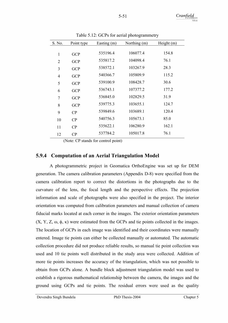
5-51
Table 5.12: GCPs for aerial photogrammetry
S. No. Point type Easting (m) Northing (m) Height (m)
1 GCP 535196.4 106077.4 154.8
2 GCP 535817.2 104098.4 76.1
3 GCP 538572.1 103267.9 28.3
4 GCP 540366.7 105809.9 115.2
5 GCP 539100.9 108428.7 30.6
6 GCP 536743.1 107377.2 177.2
7 GCP 536845.0 102829.5 31.9
8 GCP 539775.3 103655.1 124.7
9 CP 539849.6 103689.1 120.4
10 CP 540756.3 105673.1 85.0
11 CP 535622.1 106280.9 162.1
12 CP 537784.2 105017.8 76.1
(Note: CP stands for control point)
5.9.4 Computation of an Aerial Triangulation Model
A photogrammetric project in Geomatica OrthoEngine was set up for DEM
generation. The camera calibration parameters (Appendix D-8) were specified from the
camera calibration report to correct the distortions in the photographs due to the
curvature of the lens, the focal length and the perspective effects. The projection
information and scale of photographs were also specified in the project. The interior
orientation was computed from calibration parameters and manual collection of camera
fiducial marks located at each corner in the images. The exterior orientation parameters
(X, Y, Z, ω, φ, κ) were estimated from the GCPs and tie points collected in the images.
The location of GCPs in each image was identified and their coordinates were manually
entered. Image tie points can either be collected manually or automated. The automatic
collection procedure did not produce reliable results, so manual tie point collection was
used and 10 tie points well distributed in the study area were collected. Addition of
more tie points increases the accuracy of the triangulation, which was not possible to
obtain from GCPs alone. A bundle block adjustment triangulation model was used to
establish a rigorous mathematical relationship between the camera, the images and the
ground using GCPs and tie points. The residual errors were used as the quality
Devendra Singh Bundela PhD Thesis-2004 Chapter 5
5-52
parameters to determine the best possible solution for a triangulation model and
reflected the overall quality of the triangulation model. Four check points were also
introduced to provide an independent accuracy assessment of the triangulation model.
5.9.5 Image Matching and DEM Extraction
After an aerial triangulation model was established, the epipolar stereo pairs were
produced to eliminate the y-parallax as well as to increase the speed of an image
matching process. The epipolar images are a stereo pair reprojected such that both left
and right images have a common orientation and matching feature appears along a
common x-axis. An image matching process extracts matching pixels in an epipolar
stereo pair. The aerial geometry from computed triangulation model is then used to
calculate x, y, and z positions. There are three image matching approaches namely; area,
feature or hierarchical-based matching. The hierarchical matching was used in this study
as it is quick and reliable and minimises the number of mismatches.
Two epipolar DEMs were extracted using the hierarchical matching in the
overlap area between epipolar pairs at 15 m with defined options (Appendix D-9) as
there was more failure area at lower pixel spacing. Two DEMs derived from a left
epipolar and a right epipolar pairs are given in Figure 5.14. It can be seen that these
DEMs contained large areas at edges with clutter and holes. The mosaic of both DEMs
was also created (Figure 5.15). It is also clearly seen that clutters and holes are the main
feature at edges. The large clutter and holes at edges made this DEM not suitable as a
reference DEM. The derived DEMs contained poorly correlated areas and artefacts,
which need to be corrected either before or after the geocoding. The matching
correlation was used for quality assessment of image matching. The vector points were
generated from an epipolar DEM for 3D editing. The resultant DEMs could not be
edited at edges due to software glitch. Therefore, it was decided to use mass points as
reference data for quality assessment of the InSAR DEM because the derived
photogrammetric DEM contained clutters at its edges and holes and DEM editing was
very time consuming process so that it could be avoided by using mass points. After a
close inspection of mass points, it was found that they too contained spikes, so it was
further decided not to use the mass points for quality assessment of InSAR DEMs.
Devendra Singh Bundela PhD Thesis-2004 Chapter 5

5-53
5.9.6 Post Processing and Error Sources
The quality of the derived photogrammetric DEM was assessed qualitatively in
perspective view or 3D display. This has revealed many obvious serious anomalies in
the DEM surface such as spikes, holes, and clutter at edges shown in Figure 5.15. The
clutter in the DEM could not be edited in 3D editing environment as it was a time
consuming exercise. Therefore, it was considered to use the mass points as the reference
data to avoid 3D-DEM editing.
The quality of mass points was assessed in perspective view and it was found
that they too contained spikes and holes. In other words, the quality of the derived DEM
was so poor, so it was not appropriate to conduct its quality assessment. This DEM
could not be further used for quality assessment of InSAR DEMs because of poor
quality. The derived DEM accuracy depends on a number of factors (Smith and Smith,
1997) such as the scale and quality of the photographs, scanning resolution and quality,
image matching control parameters, the quality of the aerial triangulation solution,
DEM point spacing and terrain characteristics. The quality of ground control points also
contributes to the DEM accuracy.
Devendra Singh Bundela PhD Thesis-2004 Chapter 5

5-54
a)
c)
Figure 5.14: Photogrammetric DEMs of t
a) left photograph pair, b) right photograp
at edges and holes in low tonal area with 1
Devendra Singh Bundela PhD Th
b)
he Saltdean catchment extracted from
h pair and c) a mosaic showing clutter
00% level of details
esis-2004 Chapter 5
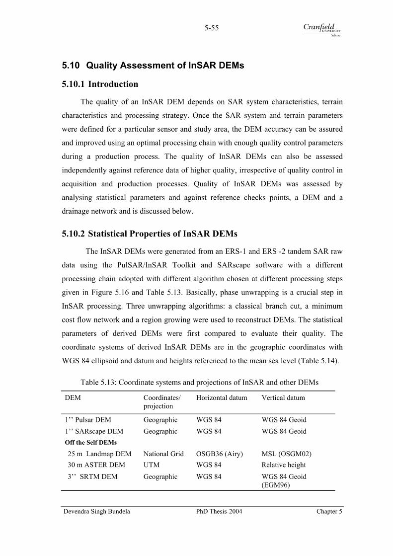
5-55
5.10 Quality Assessment of InSAR DEMs
5.10.1 Introduction
The quality of an InSAR DEM depends on SAR system characteristics, terrain
characteristics and processing strategy. Once the SAR system and terrain parameters
were defined for a particular sensor and study area, the DEM accuracy can be assured
and improved using an optimal processing chain with enough quality control parameters
during a production process. The quality of InSAR DEMs can also be assessed
independently against reference data of higher quality, irrespective of quality control in
acquisition and production processes. Quality of InSAR DEMs was assessed by
analysing statistical parameters and against reference checks points, a DEM and a
drainage network and is discussed below.
5.10.2 Statistical Properties of InSAR DEMs
The InSAR DEMs were generated from an ERS-1 and ERS -2 tandem SAR raw
data using the PulSAR/InSAR Toolkit and SARscape software with a different
processing chain adopted with different algorithm chosen at different processing steps
given in Figure 5.16 and Table 5.13. Basically, phase unwrapping is a crucial step in
InSAR processing. Three unwrapping algorithms: a classical branch cut, a minimum
cost flow network and a region growing were used to reconstruct DEMs. The statistical
parameters of derived DEMs were first compared to evaluate their quality. The
coordinate systems of derived InSAR DEMs are in the geographic coordinates with
WGS 84 ellipsoid and datum and heights referenced to the mean sea level (Table 5.14).
Table 5.13: Coordinate systems and projections of InSAR and other DEMs
DEM Coordinates/ projection
Horizontal datum Vertical datum
1’’ Pulsar DEM Geographic WGS 84 WGS 84 Geoid 1’’ SARscape DEM Geographic WGS 84 WGS 84 Geoid Off the Self DEMs 25 m Landmap DEM National Grid OSGB36 (Airy) MSL (OSGM02) 30 m ASTER DEM UTM WGS 84 Relative height 3’’ SRTM DEM Geographic WGS 84 WGS 84 Geoid
(EGM96)
Devendra Singh Bundela PhD Thesis-2004 Chapter 5
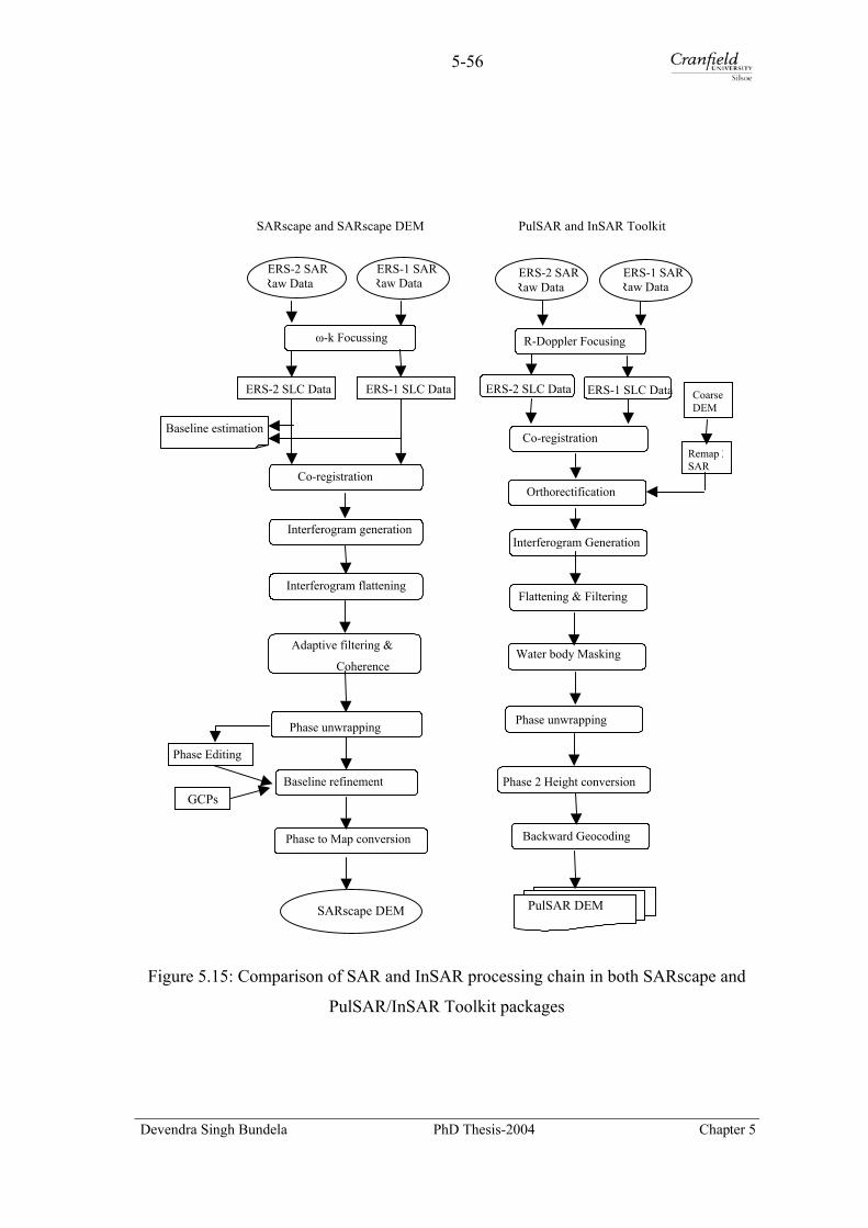
5-56
SARscape and SARscape DEM PulSAR and InSAR Toolkit
ERS-2 SAR Raw Data
ERS-1 SAR Raw Data
ERS-2 SAR Raw Data
ERS-1 SAR Raw Data
ω-k Focussing R-Doppler Focusing
ERS-2 SLC Data ERS-1 SLC Data ERS-2 SLC Data ERS-1 SLC Data Coarse DEM
Baseline estimation Co-registration
Remap 2SAR
Co-registration Orthorectification
Interferogram generation Interferogram Generation
Interferogram flattening Flattening & Filtering
Adaptive filtering &
Coherence Water body Masking
Phase unwrapping Phase unwrapping
Phase Editing
Baseline refinement Phase 2 Height conversion GCPs
Backward Geocoding Phase to Map conversion
PulSAR DEM SARscape DEM
Figure 5.15: Comparison of SAR and InSAR processing chain in both SARscape and
PulSAR/InSAR Toolkit packages
Devendra Singh Bundela PhD Thesis-2004 Chapter 5
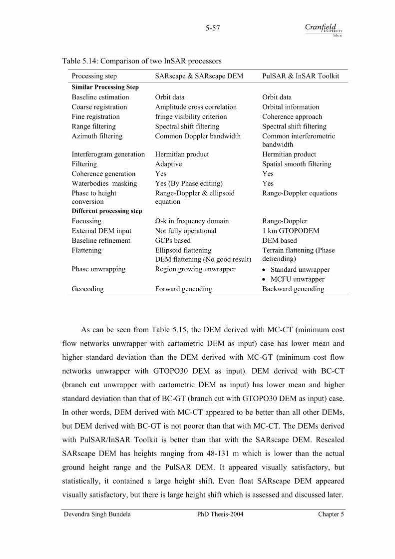
5-57
Table 5.14: Comparison of two InSAR processors
Processing step SARscape & SARscape DEM PulSAR & InSAR Toolkit Similar Processing Step Baseline estimation Orbit data Orbit data Coarse registration Amplitude cross correlation Orbital information Fine registration fringe visibility criterion Coherence approach Range filtering Spectral shift filtering Spectral shift filtering Azimuth filtering Common Doppler bandwidth Common interferometric
bandwidth Interferogram generation Hermitian product Hermitian product Filtering Adaptive Spatial smooth filtering Coherence generation Yes Yes Waterbodies masking Yes (By Phase editing) Yes Phase to height conversion
Range-Doppler & ellipsoid equation
Range-Doppler equations
Different processing step Focussing Ω-k in frequency domain Range-Doppler External DEM input Not fully operational 1 km GTOPODEM Baseline refinement GCPs based DEM based Flattening Ellipsoid flattening
DEM flattening (No good result) Terrain flattening (Phase detrending)
Phase unwrapping Region growing unwrapper • Standard unwrapper • MCFU unwrapper
Geocoding Forward geocoding Backward geocoding
As can be seen from Table 5.15, the DEM derived with MC-CT (minimum cost
flow networks unwrapper with cartometric DEM as input) case has lower mean and
higher standard deviation than the DEM derived with MC-GT (minimum cost flow
networks unwrapper with GTOPO30 DEM as input). DEM derived with BC-CT
(branch cut unwrapper with cartometric DEM as input) has lower mean and higher
standard deviation than that of BC-GT (branch cut with GTOPO30 DEM as input) case.
In other words, DEM derived with MC-CT appeared to be better than all other DEMs,
but DEM derived with BC-GT is not poorer than that with MC-CT. The DEMs derived
with PulSAR/InSAR Toolkit is better than that with the SARscape DEM. Rescaled
SARscape DEM has heights ranging from 48-131 m which is lower than the actual
ground height range and the PulSAR DEM. It appeared visually satisfactory, but
statistically, it contained a large height shift. Even float SARscape DEM appeared
visually satisfactory, but there is large height shift which is assessed and discussed later.
Devendra Singh Bundela PhD Thesis-2004 Chapter 5

5-58
Table 5.15: Statistical Properties of InSAR DEMs using different unwrappers and input DEMs
Unwrapper/DEM Parameter Data type Min Max Mean Std Dev
Median
Mode Case
GTOPO30 as input DEM Branch cut (BC) 2 byte -24 347 43.80 46.20 33 0 BC-GT
Minimum cost flow (MCF) networks
2 byte -12 326 43.65 45.41 35 0 MC-GT
250 m cartometric DEM as input DEM
Branch cut (BC) 2 byte -12 318 42.55 47.46 28 0 BC-CT
Minimum cost flow (MCF) networks
2 byte -19 319 42.38 47.58 28 0 MC-CT
SARscape DEM with GCPs
Region growing (Rescaled) 1 byte 48 131 85.54 12.29 84 84 RG-RS
Region growing (RG) Float 0 631 376.98
136.84 399.7 0 RG-FT
(GT stands for GTOPO30 DEM; CT for coarse Cartometric DEM; RS for rescaled to one
byte; FT for float data type)
5.10.3 Quality Assessment against Reference Check Points
Twenty two reference check points were collected during a differential GPS
survey to assess the accuracy of InSAR DEMs. The post processing of GPS data against
the OS London GPS Active Station is discussed in Section 5.9.14. The accuracy of 22
check points during differential GPS survey was assessed (Appendix D-7). The heights
in the InSAR DEMs were referenced to orthometric heights above the mean sea level
(WGS84 Geoid) while the heights in check points were referenced to WGS 84 ellipsoid
heights. Therefore, the GPS heights were transformed to orthometric heights above the
mean sea level using the Global Equipotential Gravity Model (EGM96) (Limoine et al,
1998). The distribution of reference points in the Eastern South Downs is presented in
Figure 5.17. The height values corresponding to the locations of 22 check points were
extracted from an InSAR DEM and are tabulated against height value of the
corresponding reference check points. First assessment was performed on the unfiltered
InSAR DEMs and resulted in large RMS errors of 20.3 m due to spikes and holes,
vegetation canopy and building tops. The accuracy assessment was also performed on
off the shelf DEM data and RMS errors are presented in Table 5.16.
Devendra Singh Bundela PhD Thesis-2004 Chapter 5

5-59
Figure 5.16: Spatial distribution of check points for quality assessment
Table 5.16: Quality assessment of derived InSAR and public domain DEMs
DEM Data type RMS Error (m)
Pulsar Raw DEM 2 byte integer 20.30
(12.8*) SARscape Raw DEM 1 byte integer 35.79
Public domain DEMs Landmap DEM 2 byte integer 6.17 ASTER DEM Float 5.94 SRTM DEM 2 byte integer 3.59
(* shows the recalculated RMSE after exclusion of four points close to obstructions)
When four check points were excluded from the accuracy assessment due to
closeness to the buildings, tree canopy and electric power line, the RMS error was
reduced to 12.8 m. Raw or unfiltered InSAR DEMs contained spikes and holes,
vegetation canopy and building tops can be filtered with a 3x3 low pass filters to
remove the spikes and holes. It was deliberately chosen to use raw DEM for the
modelling to compare results with the Landmap DEM.
Devendra Singh Bundela PhD Thesis-2004 Chapter 5

5-60
5.10.4 Quality Assessment against a Reference Drainage Network
The drainage network derived from the PulSAR DEM (Figure 5.18a) was
assessed against the reference drainage network drawn and digitised from the 1:10 000
scale Ordnance Survey topographic maps. The PulSAR DEM was first conditioned to
remove sinks using a standard flooding approach described by Jenson and Domingue
(1988). Later, a drainage network was extracted from the conditioned InSAR DEM
using a deterministic eight neighbours (D8) method on the basis of single flow
(O’Callaghan and Mark, 1984) using Arc Hydro Tools. The stream ordering (Strahler,
1964) was assigned to both networks and length of each order was computed for both
networks. The stream lengths of different stream orders were compared (Table 5.17).
The first order stream length derived from the PulSAR DEM is poorly related to the
reference drainage network while the second order stream length is better related
between PulSAR DEM and the reference drainage network. The drainage networks
from SARscape DEM (Figure 5.18b) and public domain DEMs (Figure 5.19, a, b, and
c) were also derived and were compared against PulSAR DEM visually. The drainage
network derived from SARscape is quite similar to that from PulSAR DEM. Other three
public domain DEMs produced the drainage network of lower quality.
Table 5.17: Quality assessment of DEM on the basis of stream order lengths
No of streams and total length (m) Stream order
1:10 000 map PulSAR DEM Change (%)
1 20 13898.07 4 2568.50 -81.52
2 9 3066.16 2 3263.48 6.44
3 9 5074.09 5 6728.43 32.60
Devendra Singh Bundela PhD Thesis-2004 Chapter 5
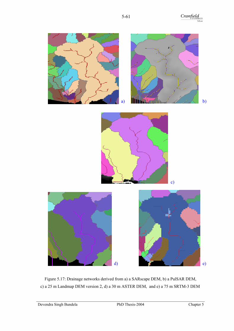
5-61
Figure 5.17: Drainage networks derived from a)
c) a 25 m Landmap DEM version 2, d) a 30 m AST
Devendra Singh Bundela PhD Th
a SA
ER
esis-
a)
Rscape DEM, b) a PulSAR DEM,
DEM, and e) a 75 m SRTM-3 DEM
2004 Chapter
b)
c)
d) e)5
5-62
5.11 Concluding Remarks
5.11.1 Discussion
In this chapter, elevation data collection technologies were reviewed with
reference to spaceborne SAR interferometry, which was explored to generate high
resolution and quality DEMs for distributed modelling at catchment scale in the context
of developing countries. The procedures and standards of quality assessment of a DEM
were also discussed. The InSAR DEM quality was assessed using reference check
points and a drainage network. Finally, strategies for deriving a high quality DEM from
a single SAR pair are also discussed here.
Topographic mapping technologies
Cartometric DEMs are available at coarse resolution in developing countries and
are the main source of elevation data because of non-availability of adequate quality
DEMs derived from advanced technology. They are not produced to provide heights of
the high density and accuracy required for distributed modelling (Shortridge, 2001).
GPS and laser total station ground survey have operational constraints at catchment
scale mapping. Remotely sensed topographic mapping technologies are cost effective
and timely for catchment scale mapping. This is evident from this study that InSAR
DEM was derived quickly from an ERS tandem data pair. Quality InSAR DEMs can be
generated for developing countries and are used for distributed modelling.
Selection of an optimal SAR data pair
One of major problems in radar interferometry is how to select an optimal
baseline data pair. The key parameters for selecting a quality InSAR pair: terrain type,
radar band, baseline distance, temporal decorrelation and orbital accuracy are discussed.
The optimal perpendicular baseline for ERS system is 50-300 m for topographic
mapping (ESA, 2004). Considering key parameters, a suitable raw SAR data pair with
145 m baseline for the Eastern South Downs study area was selected from the ERS
tandem mission archive.
Devendra Singh Bundela PhD Thesis-2004 Chapter 5

5-63
Selection of SAR and InSAR Processors
Five processors such as SARToolbox, Imagine IFSAR DEM, EarthView
InSAR, SARscape, PulSAR/InSAR Toolkit and ASF InSAR were tested in this study.
These processors were evaluated for their capabilities on sensor and data format
support, platform, processing facility and user friendliness. The SAR processor
combined with an interferometric SAR processing should be preferred for customised
raw data focussing, smooth import and analysis of input data for interferometric
analysis. PulSAR/InSAR Toolkit and SARscape include both SAR and InSAR
processing and were used for DEM generation.
InSAR DEM generation
Both SAR and InSAR processing involves a standard processing chain with a lot
of inputs for an optimal result. The optimal processing parameters at each step within
software functionalities were achieved to obtain the best results. InSAR DEMs were
derived from an ERS tandem raw data using two selected processors. Some
functionality in SARscape did not work satisfactorily as the software was not fully
operational while PulSAR/InSAR Toolkit was an operational processor. PulSAR/InSAR
Toolkit produced a better quality DEM than SARscape. This could be caused by
different SAR and InSAR processing algorithms available in software. The quality of an
InSAR DEM was optimised using the best processing strategy. InSAR DEM generation
is less cumbersome and expensive than the optical stereo and radargrammetric DEM
generation. A high accuracy could not be achieved for this pair discussed in following
section. The derived DEM appears suitable for catchment scale distributed modelling.
InSAR DEM Quality assessment
Firstly, the quality of InSAR DEMs was assessed independently against 22 check
points of higher quality collected from a DGPS survey. The accuracy of the raw DEM
was found to be 20.3 m RMSE. This large RMS error was a result of non availability of
precision orbital data because of satellite telemetry failure during the pair acquisition.
Secondly, a photogrammetric DEM was derived from 1:25 000 scale aerial
photographs. It was found that derived DEM was of poor quality because of spikes,
Devendra Singh Bundela PhD Thesis-2004 Chapter 5

5-64
holes and large clutter at edges. The quality of mass points was also poor. They too
contained similar problems, which made mass points unsuitable to be used as reference
data. Therefore, this validation DEM could not be used. The reason for this problem
was that the Sussex photography project was not intended for topographic mapping.
A third assessment was performed against a reference drainage network. First
order stream length has a poor correlation extracted from InSAR DEM and a reference
network. Second and third order stream lengths have a good correlation. It indicates that
a 25 m InSAR DEM is less suitable for the extraction of first order stream, but it is more
suitable for the extraction of second and third order stream. In other words, InSAR
DEMs are more appropriate for the extraction of a drainage network at 1:25 000 or
smaller scale.
Suitability of InSAR DEM for Modelling
The main characteristics of a DEM for distributed modelling are resolution and
quality. The horizontal and vertical resolutions of an InSAR DEM are 25 m and 1 m
respectively. The vertical resolution is consistent with resolvable power of the InSAR
technology. InSAR DEM generally provides the vertical accuracy on the order of
metres, which is appropriate for catchment modelling. In this study, achieved vertical
accuracy was on the order of tens of metres, which was caused by satellite telemetry
failure during pair acquisition. This error was a systematic error, which was minimised
during computation of slope gradient and aspect parameters for the model. Therefore,
this systematic error did not affect the modelling results. Therefore, the InSAR DEM
meets the modelling requirement despite a large vertical error.
5.11.2 Conclusions
• Elevation data collection technologies were reviewed with respect to radar
interferometry. It was found that DEMs derived from advanced technology are
not error free and contain some form of errors in some respect.
• SAR Interferometry has potential for catchment scale mapping in all weather
conditions and provides the vertical accuracy on the order of metres. The DEM
derived provided the vertical accuracy on the order of tens of metres despite
Devendra Singh Bundela PhD Thesis-2004 Chapter 5

5-65
imprecise orbital data of a selected data pair. It has also shown potential for
deriving quality DEMs for developing countries to meet the demand of the DEM
for distributed modelling.
• The strategies for selecting an optimal single SAR data pair and a suitable SAR
and InSAR processors are shown to be practicable. Five processors were tested
in this study and two of them were found to be useful for generation of InSAR
DEMs.
• InSAR DEM generation was found to be less cumbersome and expensive than
optical stereo and radargrammetric DEM generation.
• The error reduction strategies have shown to improve the DEM accuracy for a
single SAR data pair affected by orbital errors and atmospheric perturbations.
• The quality of InSAR DEMs was assessed against reference check points and the
accuracy was found to be 20 m (RMSE) for unfiltered DEMs. The accuracy
improved to 12.8 m after exclusion of four points, which were close to
obstructions.
• A photogrammetric DEM derived from 1:25 000 scale aerial photograph pairs
was found to be of poor quality due to clutter at edges and holes in low tonal
areas.
• The drainage network derived from an InSAR DEM was assessed independently
against a reference drainage network. It was found out that the InSAR DEM is
poor for delineating the first order stream and is better for second and third order
streams. The results indicate that InSAR DEMs are more appropriate for the
extraction of a drainage network at 1:25 000 or smaller scale.
Devendra Singh Bundela PhD Thesis-2004 Chapter 5

6-1
6
Analyses of Modelling Results
This chapter deals with the creation of twenty-five LISEM databases of
input parameters at five spatial representations from five DEMs and other
key spatial data. These databases were tested for model sensitivity to
five resolutions of each DEM at three antecedent soil moisture conditions
from a 6-hour storm. It was found that predicted runoff and soil loss
decreased at coarser resolutions for each DEM dataset.
6.1 Introduction
Distributed modelling incorporates the spatial variability of input parameters and
variables of catchment characteristics into the model response. Spatial variability of
parameters can be obtained by choosing an appropriate spatial scale in terms of grid-cell
resolution. A grid-cell resolution affects the routing of surface runoff and sediment
movement across the catchment. It also affects the model response in terms of spatial
distribution of runoff and sediment, and shapes of hydrograph and sedigraph observed
at an outlet. Antecedent soil moisture condition is another factor which influences the
model response is also considered in modelling. In this study, effects of different
resolutions on surface hydrologic and erosion processes at three antecedent moisture
conditions are, therefore, investigated from a 6-hour storm.
For this study, key spatial data of the Eastern South Downs: five DEMs from
various sources namely, three interferometric SAR DEMs, a cartometric DEM and an
optical stereo DEM; a land use and land cover map; and a soil map were resampled into
Devendra Singh Bundela PhD Thesis-2004 Chapter 6

6-2
five resolution datasets; 20, 40, 60, 80 and 100 m. Twenty-five datasets of the Saltdean
catchment were extracted at five resolutions each for five DEMs and were brought into
PCRaster to create twenty-five LISEM databases of catchment characteristics. These
databases were tested in the LISEM version 2.03 for model performance evaluation and
sensitivity analysis at three moisture conditions such as low, medium and high for a
storm on 30 October 2000. This chapter reports extraction of twenty-five datasets of the
catchment, creation of 25 LISEM databases of input parameters and testing performance
evaluation and their sensitivity to model outputs. It also includes the error propagation
in dynamic and distributed modelling.
6.2 Selection of a Model Version
A LISEM model version 2.03 was selected for this study because it was
developed for slope ranges of the Saltdean catchment. The slope in most of the
catchment (98.8 per cent) is below 50 per cent (Appendix E-1). This version resulted in
same catchment area and cumulative rainfalls from a single resolution dataset derived
from five DEM datasets unlike current versions discussed below. The disadvantage of
this model was that it did not include a surplus infiltration procedure to the kinematic
wave, which resulted in slightly less infiltration and, hence, a little more runoff. As this
study was mainly concerned with the effects of different spatial representations on
surface hydrologic and erosion processes, so it was considered appropriate to use the
model for this study.
Current LISEM versions namely, 2.158 and 2.154 have been modified for very
steep terrain catchments of China with slopes ranging from 50 to 250 per cent (Jetten,
2004; Hessel et al, 2003; LISEM, 2004). The slope has been added to modify new grid-
cell length in the direction of flow, which is equal to the grid-cell length divided by
cosine of its slope instead of actual grid-cell length. This affected many calculations in
the model and resulted in different cumulative rainfalls and catchment areas from a
single resolution dataset derived from five DEM datasets (Appendix E-2). Therefore,
the current version could not be used.
Devendra Singh Bundela PhD Thesis-2004 Chapter 6

6-3
6.3 Key Spatial Data of the Saltdean Catchment
A small agricultural catchment of approximately 800 hectares was selected from
the Eastern South Downs for modelling storm surface runoff and erosion dynamics. Key
spatial data of the Eastern South Downs derived from various sources were first
resampled into five resolutions namely, 20, 40, 60, 80 and 100 m using sampling
schemes discussed in the later part of this Section. Then, key spatial data of the Saltdean
catchment were extracted. A raingauge map is required to represent spatial variability of
a rainstorm in the catchment through multiple raingauge stations. Table 6.1 shows the
key spatial data source and their five resampled spatial representations. The extraction
of each key spatial data of the catchment is discussed in next sections.
Table 6.1: Key spatial data and their five spatial representations for modelling
Key spatial data Data source Spatial representations
DEMs 1’’ PulSAR DEM 20, 40, 60, 80, and 100 m
,, Cartometric DEM from 1:25 000 scale
20, 40, 60, 80, and 100 m
,, 25 m Landmap DEM 20, 40, 60, 80, and 100 m
,, 3 arc SRTM-3 DEM 20, 40, 60, 80, and 100 m
,, 30 m ASTER DEM 20, 40, 60, 80, and 100 m
Land use and land cover 20 m SPOT-1 XS data 20, 40, 60, 80, and 100 m
Soils NATMAP Vector 1:250 000 scale 20, 40, 60, 80, and 100 m
Raingauge location University of Sussex Single point raingauge data
6.3.1 Digital Elevation Models
Firstly, a few InSAR DEMs of the Eastern South Downs with 1” grid-cell
spacing were generated by radar interferometry from an ERS-1 and ERS-2 SAR raw
tandem pair. The best of them was used for modelling. The methodology of generating
InSAR DEMs and their quality assessment was discussed in Chapter 5.
Secondly, cartometric DEMs of the Saltdean area at five grid-cell sizes: 20, 40,
60, 80 and 100 m were generated using a nonlinear interpolation method from 849
points collected manually from a 1:25 000 scale Pathfinder map. Thirdly, three public
Devendra Singh Bundela PhD Thesis-2004 Chapter 6

6-4
domains DEMs namely, two interferometric SAR DEMs such as 25 m Landmap DEM
version 2.0 (Landmap, 2003) and 3” SRTM-3 DEM (USGS, 2003), and an optical
stereo DEM such as 30 m ASTER DEM with relative heights (USGS, 2004) were
obtained. The description of public domain DEMs was discussed in Section 5.7.
All five DEMs were in different coordinates, ellipsoids and datums (Table 6.2).
The PulSAR DEM was projected to the British National Grid coordinates at five grid-
cell sizes using a national coordinate transformation, OSTN02 and cubic convolution
resampling method. Similarly, SRTM and ASTER DEMs were suitably projected to the
British National Grid coordinates at five grid-cell sizes. The Cartometric and Landmap
DEMs were already in the British National Grid. Therefore, they were used as such.
DEMs of the Saltdean catchment at each resolution were extracted from five resampled
DEMs using a catchment area mask digitised from the 1:10 000 scale topographic maps.
These DEMs were imported to PCRaster for generation of LISEM databases discussed
in the next sections.
Table 6.2: Projection of five DEMs to the British National Grid
DEM Coordinates/ projection
Horizontal datum
Vertical datum Reprojected to
1’’ Pulsar DEM Geographic WGS 84 WGS 84 Geoid National Grid (OSTN02)
20 m Cartometric DEM National Grid
OSGB36 (Airy)
Mean sea level Not reprojected
25 m Landmap DEM National Grid
OSGB36 (Airy)
Mean sea level Not reprojected
3’’Raw SRTM DEM Geographic WGS 84 WGS 84 Geoid National Grid (OSTN02)
30 m ASTER DEM UTM WGS 84 Relative height National Grid
The choice of an appropriate DEM grid-cell resolution is one of the key
problems in distributed modelling in a GIS. Maidment (1996) suggested using one
thousand-million rule as a guide. The grid-cell resolution of a DEM for the Saltdean
catchment was worked out to be approximately 10 m as per rule, but there was a
constraint in data availability as the original resolutions of SPOT-1 multispectral data
Devendra Singh Bundela PhD Thesis-2004 Chapter 6
6-5
and InSAR DEM were 20 m and 25 m respectively, so a 20 m grid-cell resolution was
chosen as it matched with resolution of SPOT XS-1 data, thus avoiding resampling. The
minimum catchment area to be delineated using a DEM was worked out to be 40
hectares, which is lower than the area of the selected catchment. Therefore, it satisfies
the rule.
6.3.2 Land Use and Land Cover Data
The land use and land cover map of the Saltdean catchment was extracted from
the land use and land cover of the Eastern South Downs derived from digital
classification of SPOT multispectral data of 26 October 2000, described in Chapter 4.
Area weight classified image of nine classes was filtered four times using a 3x3
majority filter to remove the unrelated scattered pixel patches and to smooth the
thematic image. The smoothed classified image was used to extract the land use and
land cover map of the catchment at 20 m resolution. The smoothed thematic image was
further resampled using a nearest neighbour method to extract 40, 60, 80 and 100 m
resolution maps of the catchment to derive land use dependent model parameters. Table
6.3 shows the distribution of each land use and land cover class in the catchment at 20
m resolution.
Table 6.3: Area of land use and land cover class of the Saltdean catchment
S. No. Description of class Id Area (ha) Per cent
1. Bare soil - ploughed/sown field 1 114.04 14.06
2. Harvested field 2 150.24 18.52
3. Set-aside 3 21.64 2.67
4. Hill grassland 4 213.16 26.28
5. Semi-improved grassland 5 198.56 24.48
6. Improved grassland 6 64.6 7.96
7. Open wood and scrub land 7 40.08 4.94
8. Dense wood and scrub land 8 2.48 0.31
9. Built-up land 9 6.36 0.78
6.3.3 Soil Data
The soil map of the Eastern South Downs at a 1: 250 000 scale was rasterised to
five grid-cell resolutions (Table 6.1) on the basis of dominant soil series, discussed in
Devendra Singh Bundela PhD Thesis-2004 Chapter 6
6-6
Section 3.2. The soil map of the catchment at each resolution was then extracted. The
small fractions of Upton-1 and unsurveyed Andover associations were merged into the
Andover-1 association discussed in Section 3.4.3. Two dominant soil series were finally
used in the soil map of the catchment, which were used to assign the infiltration
parameter values to obtain infiltration parameter maps at five resolutions.
6.3.4 Distribution of Rainfall Intensity in the Catchment
Spatial distribution of the rainfall in a catchment can be computed from a
location map of multiple raingauge stations using either the Thiessen polygon or
geomorphological analysis technique. A single raingauge station data was available for
the catchment from the University of Sussex, Falmer, Brighton which is approximately
2.5 km from the northwest of catchment top boundary (Figure 6.1), described in
Chapter 3. Therefore, the distribution of rainfall intensity over the catchment was
assumed to be uniform, which is valid for a frontal storm considered for simulation. A
rain zone map was created from a raingauge station map using a ‘spreadzone’
command. A breakpoint rainfall intensity data file was created in the ASCII format with
a defined structure from hourly rainfall intensity data to drive the model (Appendix E-
3). The breakpoint rainfall intensity data are discussed in Section 3.2.9.
Figure 6.1: Location of the raingauge station with reference to the catchment
6.4 Creation of LISEM Databases
Three key spatial data such as a DEM, a land use and land cover map, and a soil
map at 20 m grid-cell resolution were first converted into the ArcInfo Grid ASCII
Devendra Singh Bundela PhD Thesis-2004 Chapter 6

6-7
format for importing to PCRaster as its import functionality is very limited. These key
spatial datasets were imported into PCRaster using an ‘asc2map’ command (Appendix
E-4). In addition to three key datasets in the PCRaster map format, crop, soil and
surface parameter values were required to create a LISEM database of input parameters.
Most of these parameters were estimated for possible field conditions observed and
assumed in the catchment for a storm on 30 October 2000 in combination with the
guidelines of parameters given in the LISEM and EUROSEM Manuals (Jetten, 2002;
De Roo et al, 1995; Morgan et al, 1998) and similar catchment datasets. The
characteristics of the Saltdean catchment are quite similar to that of the Catsop
catchment, South Limburg for which the model was originally developed, and Ganspoel
catchment where the model was applied (Boardman et al, 2000). It has also similarity
with flood prone region in France as well. These parameters are estimated and discussed
in the following sections. Similarly, four other resolution key spatial datasets were
imported into PCRaster to create LISEM databases at five resolutions each from five
DEMs.
6.4.1 Topographic Parameters
A DEM itself was not used in the model and its derived topographic parameters
such as slope gradient, local drainage direction (aspect), catchment area and outlet of
the catchment were used. These were derived from a DEM using the PCRaster
commands (Appendix E-5). The slope gradient used in the model was the sine of the
slope, not the tangent and its value lies between zero and one. The calculated slope
gradients of each resolution datasets were well in agreement with the defined limit.
6.4.2 Micro-topographic Parameter
Micro-topographic parameter such as random roughness for a storm of 30
October 2000 was not available. In that case, it was estimated for assumed field
conditions with the guidelines in the LISEM and EUROSEM Manuals (Jetten, 2002;
Morgan et al, 1998) and relevant random roughness data from similar catchments in the
Limburg, Waremme and Ganspoel. Random roughness value (Table 6.4) was taken for
same land use and nearly same time period from the Catsop, Waremme, and Ganspoel
Devendra Singh Bundela PhD Thesis-2004 Chapter 6

6-8
catchment datasets (LISEM, 2004). Similarly, other parameters for a historical event
were also estimated from relevant data of other catchments and standard tables.
6.4.3 Crop and Vegetation Parameters
Crop and vegetation parameters such as soil cover, crop height and leaf area
index (Table 6.4) were estimated for similar land use classes from the Manuals and
other catchment datasets. Leaf area index for each crop and vegetation at same time
period in the catchment were estimated from leaf area index data of crop and vegetation
for whole crop growth period given in the ANSWERS Manual (Dillaha, 2004; Beasley
and Huggins, 1981). Soil cover and crop height values were estimated for similar
conditions in the catchment from relevant catchment datasets.
6.4.4 Soil Erosion Parameters
Soil erosion parameters such as soil aggregate stability, soil cohesion, additional
cohesion by plant roots and soil median texture (Table 6.4) were estimated for possible
field conditions from a combination of parameter standard table and the Catsop and
Ganspoel catchment datasets (LISEM, 2004). Crop parameters for October month were
estimated from the Catsop catchment dataset for same month assuming that arable land
were either sown or fallow with nearly no soil cover. In the Manuals, erosion parameter
tables for winter-wheat, forest, orchards, grassland and bare soils were given indicating
input values for a particular land use.
6.4.5 Soil Surface Cover Parameters
Soil surface cover such as crust cover, wheel-track cover, grass strips, stone
cover and road cover were not possible to estimate from land use and land cover map
derived from remote sensing. Therefore, it was assumed that none of them existed in the
catchment. Hence, all cover parameters were set to zero (Table 6.4). The maps of zero
parameter values were created as they were required for running the model.
6.4.6 Channel Parameters
The local drainage direction (aspect) and slope gradient of the main channel
were derived from a DEM. Channel width and its cross section shape was measured
Devendra Singh Bundela PhD Thesis-2004 Chapter 6

6-9
during the field survey. The Manning’s roughness and cohesion of the channel were
estimated from a combination of parameter standard table and similar catchment
datasets (Table 6.4).
Table 6.4: Crop, soil and erosion parameter table for the Saltdean catchment
Units PER CH LAI RR N AGGRSTAB COH Landuse 0 1 2 3 4 5 6 7
Bare field 1 0.000 0.030 0.000 0.970 0.120 -1.000 3.000
Harvested field 2 0.150 0.150 0.390 0.970 0.140 10.000 3.000
Set-aside 3 0.500 0.050 0.450 0.970 0.140 10.000 3.000
Hill grassland 4 0.950 0.100 1.860 0.700 0.227 -1.000 3.000
Semi-improved grassland 5 0.950 0.100 1.860 0.700 0.227 -1.000 3.000
Improved grassland 6 0.950 0.100 1.860 0.700 0.227 -1.000 3.000
Open woodland and scrub 7 0.950 5.000 1.860 1.360 0.300 -1.000 3.000
Dense woodland and scrub 8 0.950 5.000 1.860 1.360 0.300 -1.000 3.000
Built-up land 9 0.000 0.000 0.000 0.500 0.010 200.00 9999
Units COHADD D50 ROADWIDT GRASSWID CRUSTFRC COMPFRC STONEFRC
0 8 9 10 11 12 13 14
1 0.100 30.00 0.00 0.00 0.00 0.00 0.00
2 0.600 30.00 0.00 0.00 0.00 0.00 0.00
3 0.600 30.00 0.00 0.00 0.00 0.00 0.00
4 3.320 30.00 0.00 0.00 0.00 0.00 0.00
5 3.320 30.00 0.00 0.00 0.00 0.00 0.00
6 3.320 30.00 0.00 0.00 0.00 0.00 0.00
7 2.800 30.00 0.00 0.00 0.00 0.00 0.00
8 2.800 30.00 0.00 0.00 0.00 0.00 0.00
9 9999 30.00 0.00 0.00 0.00 0.00 0.00
6.4.7 Hydraulic Parameter
The Manning's roughness (n) for overland and channel flow was estimated for
each land use and land cover from the standard table and similar catchment datasets.
Devendra Singh Bundela PhD Thesis-2004 Chapter 6

6-10
The Manning's n for channel flow was estimated for the channel condition and cross
section observed during the field survey (Table 6.4).
6.4.8 Infiltration Parameters
A single layer Green and Ampt model was chosen for simulating the infiltration
process in the catchment. Its parameters such as hydraulic conductivity, average suction
head at wetting front, effective porosity, antecedent moisture content and soil depth
were estimated from soil property dataset of the NATMAP data. Antecedent soil
moisture content (AMC) was assumed to be uniform for a soil series in the catchment
and was considered for three possible conditions. Low, medium and high AMCs were
assumed as 0.07 and 0.08; 0.22 and 0.24; and 0.44 and 0.46 for the Marlow and the
Andover series respectively for an extreme event on 30 October. The calculated values
of saturated hydraulic conductivity and corresponding suction head at the wetting front
(Table 6.5) were higher because the effective hydraulic conductivity used for an
unsaturated flow is not saturated hydraulic conductivity and is approximately half the
corresponding value for a saturated flow (Rawls, 1983). Moreover, a PTF used for
calculating saturated hydraulic conductivity was correlated with measured saturated
values which did not reflect hydraulic conductivity during a rain storm. Therefore, these
values were calibrated in the model on the basis of runoff coefficient and total amount
of erosion in the catchment and were finally set to 2.408 mm h-1 and 4.266 cm and
2.416 mm h-1 and 3.922 cm for the Andover series and Marlow series respectively for
the catchment (Table 6.5), except for built-up land where the parameter value was set to
zero. These assumptions simplified both the spatial and temporal variations to a large
extent. Nevertheless, this approach was considered to be acceptable given the very high
intensity of the storm event making small variations in infiltration being relatively
unimportant and the fact that surface conditions on arable fields were with nearly no soil
cover and fine seedbed during October 2000. The limit of each parameter value (Table
6.6) provides a cross check on calculated parameter value.
Devendra Singh Bundela PhD Thesis-2004 Chapter 6

6-11
Table 6.5: Calculated and calibrated parameters for a single layer Green and Ampt model
Soil series Unit Ksat1 Psi1 Thetas1 Thetai1 Soildep1
0 15 16 17 18 19
Calculated values
Andover 3 4.817 42.666 0.48 0.24 250.0
Marlow 8 4.833 39.218 0.44 0.22 250.0
Calibrated values
Andover 3 2.408 4.266 0.48 0.24 250.0
Marlow 8 2.416 3.922 0.44 0.22 250.0
Table 6.6: Limits of Green and Ampt parameters for the Saltdean catchment (adapted
from Chow et al, 1988) Soil Class Porosity Effective
porosity Wetting front suction head, cm
Ksat (cm/h)
Silt loam 0.501
(0.420-0.582)
0.486
(0.394-0.578)
16.68
(2.92-95.39)
0.65
(The number in parentheses below each parameter is one sigma of the parameter value given)
6.4.9 Creation of LISEM Databases
Crop and vegetation, soil and erosion parameters for each land use and land
cover class were estimated and tabulated with a defined structure to create each
parameter map by reclassifying the land use and land cover map (Table 6.4). Similarly,
infiltration parameters for dominant soil series were estimated and tabulated in a defined
structure table (Table 6.5). After having imported key spatial datasets of various grid-
cell resolutions into the PCRaster GIS, these data were used to derive individual input
parameter map using a PCRaster command. Or alternatively, a PCRaster script was
written for creating a LISEM database of input parameters from key spatial datasets and
two parameter tables (Appendix E-5). This script was run at the PCRaster prompt by a
single command and a LISEM database of 30 input parameters was created in a single
operation. Another PCRaster script batch file was written for quick displaying of
rainfall time series data, key spatial dataset and input parameters category wise from a
single batch command at the PCRaster prompt (Appendix E-6). A total of twenty-five
Devendra Singh Bundela PhD Thesis-2004 Chapter 6
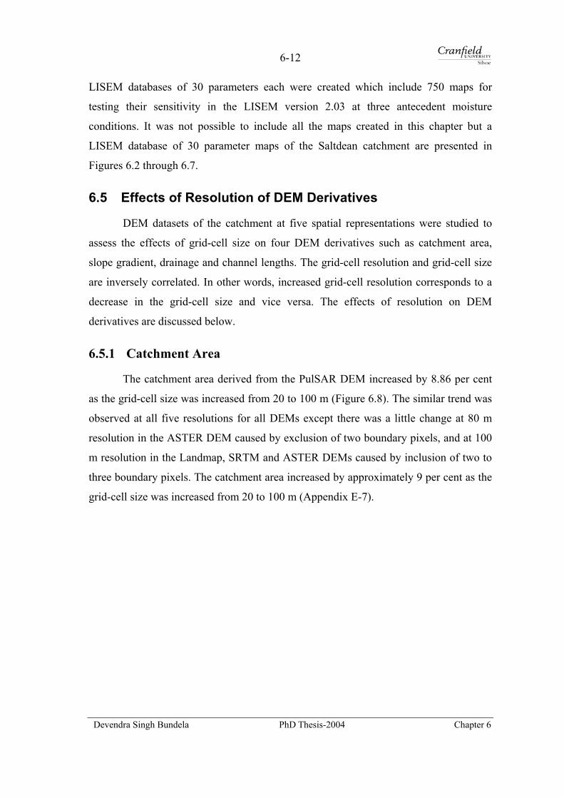
6-12
LISEM databases of 30 parameters each were created which include 750 maps for
testing their sensitivity in the LISEM version 2.03 at three antecedent moisture
conditions. It was not possible to include all the maps created in this chapter but a
LISEM database of 30 parameter maps of the Saltdean catchment are presented in
Figures 6.2 through 6.7.
6.5 Effects of Resolution of DEM Derivatives
DEM datasets of the catchment at five spatial representations were studied to
assess the effects of grid-cell size on four DEM derivatives such as catchment area,
slope gradient, drainage and channel lengths. The grid-cell resolution and grid-cell size
are inversely correlated. In other words, increased grid-cell resolution corresponds to a
decrease in the grid-cell size and vice versa. The effects of resolution on DEM
derivatives are discussed below.
6.5.1 Catchment Area
The catchment area derived from the PulSAR DEM increased by 8.86 per cent
as the grid-cell size was increased from 20 to 100 m (Figure 6.8). The similar trend was
observed at all five resolutions for all DEMs except there was a little change at 80 m
resolution in the ASTER DEM caused by exclusion of two boundary pixels, and at 100
m resolution in the Landmap, SRTM and ASTER DEMs caused by inclusion of two to
three boundary pixels. The catchment area increased by approximately 9 per cent as the
grid-cell size was increased from 20 to 100 m (Appendix E-7).
Devendra Singh Bundela PhD Thesis-2004 Chapter 6
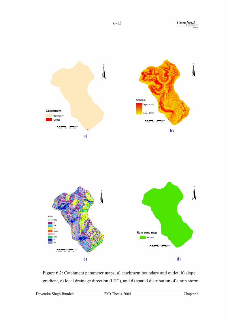
6-13
b) a)
c) d)
Figure 6.2: Catchment parameter maps; a) catchment boundary and outlet, b) slope
gradient, c) local drainage direction (LDD), and d) spatial distribution of a rain storm
Devendra Singh Bundela PhD Thesis-2004 Chapter 6
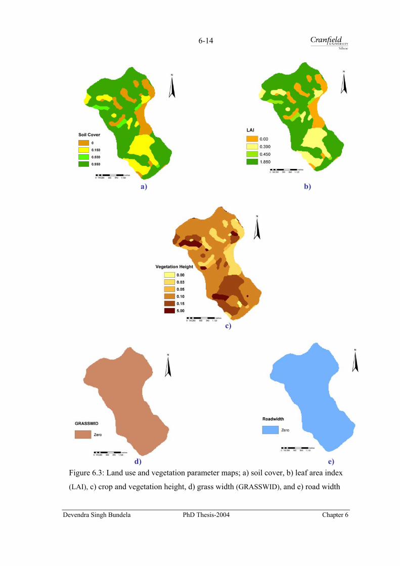
6-14
a) b)
c)
d) e)
Figure 6.3: Land use and vegetation parameter maps; a) soil cover, b) leaf area index
(LAI), c) crop and vegetation height, d) grass width (GRASSWID), and e) road width
Devendra Singh Bundela PhD Thesis-2004 Chapter 6
6-15
a) b)
c)
e) d)
Figure 6.4: Soil surface parameter maps; a) random roughness, b) Manning’s
roughness, c) crusted surface, d) stone covered surface, and e) compacted surface
Devendra Singh Bundela PhD Thesis-2004 Chapter 6
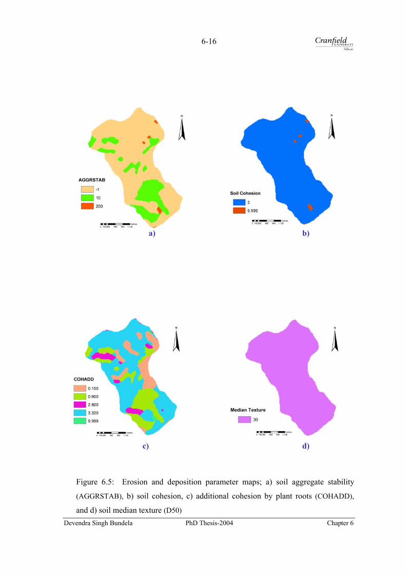
6-16
a) b)
c) d)
Figure 6.5: Erosion and deposition parameter maps; a) soil aggregate stability
(AGGRSTAB), b) soil cohesion, c) additional cohesion by plant roots (COHADD),
and d) soil median texture (D50) Devendra Singh Bundela PhD Thesis-2004 Chapter 6
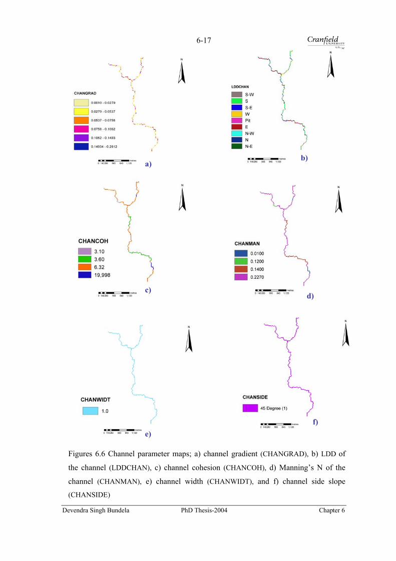
Devendra Singh Bundela PhD Thesis-2004 Chapter 6
6-17
b) a)
d) c)
f)
e)
Figures 6.6 Channel parameter maps; a) channel gradient (CHANGRAD), b) LDD of
the channel (LDDCHAN), c) channel cohesion (CHANCOH), d) Manning’s N of the
channel (CHANMAN), e) channel width (CHANWIDT), and f) channel side slope
(CHANSIDE)

6-18
a) b)
c) d)
e) Figures 6.7: Infiltration parameter maps; a) saturated hydraulic conductivity (KSAT1),
b) water front suction head (PSI1), c) moisture content at saturation (THETAS1), d)
antecedent moisture content (THETAI1), and e) soil depth (SOILDEP1)
Devendra Singh Bundela PhD Thesis-2004 Chapter 6

6-19
20 40 60 80 100
Grid-cell size, dx (m)
0
200
400
600
800
1000
Cat
chm
ent a
rea,
Ac
(ha)
Ac = 792.1856 + 0.9028*dx
( r = 0.9991)
PulSAR DEM Cartometric DEM Landmap DEM SRTM DEM ASTER DEM Fitted regression line
(All points are coincident)
Figure 6.8: Effect of grid-cell size on catchment area
6.5.2 Slope Gradient
The slope gradient used in the LISEM model is the sine of the slope in the
direction of local drainage direction. This was used to assess the effect of an
aggregation scheme on various sources of DEMs. The mean slope gradient was the
highest for the PulSAR DEM because of no smoothing applied and the lowest for the
SRTM DEM because of higher level of smoothing (Figure 6.9; Appendix E-8). The
mean slope gradient of the Landmap, Cartometric and ASTER DEMs lie between the
PulSAR DEM and SRTM DEM due to different level of smoothing applied during their
production. The mean slope gradient of the PulSAR DEM was flattened by 28 per cent
as the grid-cell size was increased (Figure 6.10; Appendix E-9). The same trend is
reported by Vieux (2000). It was caused by cutting of hills and filling of valleys at
lower resolutions by sampling. A similar trend was also observed with four other
DEMs.
Devendra Singh Bundela PhD Thesis-2004 Chapter 6
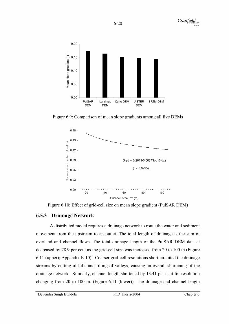
6-20
0.00
0.05
0.10
0.15
0.20
PulSARDEM
LandmapDEM
Carto DEM ASTERDEM
SRTM DEM
Mea
n sl
ope
grad
ient
(-)
,
Figure 6.9: Comparison of mean slope gradients among all five DEMs
20 40 60 80 100
Grid-cell size, dx (m)
0.00
0.03
0.06
0.09
0.12
0.15
0.18
Mea
n slop
e grad
ient, Grad (-)
Grad = 0.2611-0.0687*log10(dx)
(r = 0.9995)
Figure 6.10: Effect of grid-cell size on mean slope gradient (PulSAR DEM)
6.5.3 Drainage Network
A distributed model requires a drainage network to route the water and sediment
movement from the upstream to an outlet. The total length of drainage is the sum of
overland and channel flows. The total drainage length of the PulSAR DEM dataset
decreased by 78.9 per cent as the grid-cell size was increased from 20 to 100 m (Figure
6.11 (upper); Appendix E-10). Coarser grid-cell resolutions short circuited the drainage
streams by cutting of hills and filling of valleys, causing an overall shortening of the
drainage network. Similarly, channel length shortened by 13.41 per cent for resolution
changing from 20 to 100 m. (Figure 6.11 (lower)). The drainage and channel length
Devendra Singh Bundela PhD Thesis-2004 Chapter 6

6-21
shortening and slope flattening have profound effects on distributed simulation of runoff
and erosion processes.
0 20 40 60 80 10
Grid-cell size, dx (m)
0
100
200
300
400
500
Dra
inag
e le
ngth
, DL (k
m)
DL = 715.5458-14.2033*dx+0.0819*
(r=0.904)
0
0 20 40 60 80 100
Grid-cell size, dx (m)
0.0
1.5
3.0
4.5
6.0
7.5
9.0
Cha
nnel
leng
th, L
c (k
m)
Lc = 7.419 - 0.0123*dx (r=0.9753)
Figure 6.11: Effect of grid-cell size on drainage length (upper) and channel length
(lower) (PulSAR DEM)
6.6 Effects of Resolution on Hydrologic and Erosion Processes
Twenty-five LISEM databases were tested to investigate the effects of resolution
on hydrologic and erosion processes using LISEM version 2.03 at three antecedent soil
moisture levels for a 6-hour storm of 30 October 2000. The model was run seventy-five
times to process all datasets. The results of the effects of resolution on hydrologic and
erosion processes from a storm are discussed below.
Devendra Singh Bundela PhD Thesis-2004 Chapter 6

6-22
6.6.1 Selection of a Time Step
First and the most important thing in a dynamic simulation study was to choose an
appropriate time step. The time step in the model was studied by varying it from 10 to
60 seconds with every increase of 10 seconds for the 20 m resolution PulSAR dataset at
a medium antecedent moisture condition. It was found that the runoff coefficient
decreased by 0.1 per cent as the time step was increased from 10 to 60 s (Figure 6.12).
This was caused by the lower accuracy of the kinematic wave solution at larger time
steps. A smaller time step resulted in a greater accuracy of the kinematic wave solution.
Both either a smaller or a larger time step causes instability in numerical solution.
Therefore, a 30 second time step was chosen for the 20 m resolution datasets and it was
kept constant for testing all datasets. This time step also lies within a range of 0.2 - 2
times of the grid-cell size as recommended by the model developer to avoid instability
in the algorithm (Jetten, 2002).
4.0
4.2
4.4
4.6
4.8
5.0
5.2
0 10 20 30 40 50 60
T im e s te p (s )
Runoff co
efficient (%
) ,
Figure 6.12: Effect of simulation time-step on runoff coefficient at medium AMC
6.6.2 Interception
A dynamic storage model (Aston, 1979) was used to compute the interception
by crops and vegetation during the storm event. As can be seen from Figure 6.13, the
interception remained unchanged (0.03 per cent) for all DEM datasets as the grid-cell
size was increased. This trend was observed at all three antecedent moisture conditions.
The change in the interception was insignificant and it was caused by the rounding
Devendra Singh Bundela PhD Thesis-2004 Chapter 6

6-23
errors, which decreased at larger resolutions involving smaller number of grid-cells.
There was a slight decrease at 40 m resolution in all the DEM datasets (Appendix E-
11). This could be caused by the instability in the model algorithm.
0.00
0.80
1.60
2.40
3.20
4.00
0 20 40 60 80 100
Grid-cell size (m)
Inte
rcep
tion
(%) PulSAR DEM
Cartometric DEMLandmap DEMSRTM DEMASTER DEM
Figure 6.13: Effect of grid-cell size on interception
6.6.3 Infiltration
The infiltration was simulated using a single layer Green and Ampt model at
three moisture conditions. It is expressed in terms of percentage of rainfall for
comparison among DEMs. It was found that it increased for all DEM datasets as the
grid-cell size was increased from 20 to 100 m at three AMCs (Figure 6.14). Table 6.7
shows the effect of resolution on infiltration listed in a descending order at three
moisture conditions. Similarly, eleven result tables of effects of resolution on major
hydrologic and erosion processes are given in Appendices E-14 through E-23.
There was a large increase of 9.35 per cent at high AMC and a little increase of
0.06 per cent at low AMC. At high AMC, the infiltration was maximum for the SRTM
DEM dataset with an increase of 4.70 per cent and minimum for the PulSAR DEM
dataset with an increase of 9.35 per cent when the grid-cell size was increased.
Similarly, the infiltration was maximum for the SRTM DEM dataset at low and medium
AMCs, and minimum for the PulSAR DEM at medium AMC and for the Landmap at
low AMC. There was a slightly change in the infiltration at low AMC in all DEMs
when the grid-cell size was increased. It was found that there was a large variation in
Devendra Singh Bundela PhD Thesis-2004 Chapter 6

6-24
the infiltration at 20 m resolution among various DEMs at all AMCs (Table 6.7). It
narrowed down at coarser resolutions. High infiltration in the SRTM and Cartographic
DEMs was observed at all resolutions caused by the lower slope gradients which
resulted in slope flattening and, hence, more infiltration.
6.6.4 Runoff Coefficient
The effect of resolution on the Hortonian surface runoff was studied at three
antecedent moisture conditions. It was found that runoff coefficients decreased with an
increase in grid-cell size at all three AMCs (Figure 6.15). The runoff coefficient was
maximum for the PulSAR DEM dataset with a variability of 9.33, 2.97 and 0.24 per
cent at high, medium and low moistures when the grid-cell size was increased
(Appendix E - 12). Similarly, minimum runoff coefficient was observed for the SRTM
DEM dataset with a variability of 4.67, 2.49 and 0.11 per cent reduction at high,
medium and low moisture conditions when the grid-cell size was changed. There was a
large variation in runoff coefficients at higher resolutions at high AMC, which narrowed
down at larger grid-cell sizes. Similarly, the runoff coefficient has lower variations at
medium and low moistures which further narrowed in each case. The highest and the
lowest runoffs from the PulSAR DEM dataset and the SRTM DEM were caused by the
highest and the lowest mean slope gradient respectively.
Devendra Singh Bundela PhD Thesis-2004 Chapter 6

6-25
Infiltration at high AMC
0.0
20.0
40.0
60.0
80.0
0 20 40 60 80 100
Grid-cell size (m)
Infil
tratio
n (%
)
PulSAR DEMCartometric DEMLandmap DEMSRTM DEMASTER DEM
Infiltration at medium AMC
60.0
70.0
80.0
90.0
100.0
0 20 40 60 80 100
Grid-cell size (m)
Infil
tratio
n (%
) PulSAR DEMCartometric DEMLandmap DEMSRTM DEMASTER DEM
Infiltration at low AMC
80.0
85.0
90.0
95.0
100.0
0 20 40 60 80 100
Grid-cell size (m)
Infil
tratio
n (%
) PulSAR DEMCartometric DEMLandmap DEMSRTM DEMASTER DEM
Figure 6.14: Effect of grid-cell size on infiltration at three AMCs
Devendra Singh Bundela PhD Thesis-2004 Chapter 6

6-26
Table 6.7: Effect of grid-cell size on infiltration at three soil moisture conditions for five DEM datasets
Infiltration (per cent) DEM AMC Grid-cell size (m)
20 40 60 80 100 SRTM DEM High 67.57 67.42 69.53 70.89 72.27 (-0.15) (1.96) (3.32) (4.70) Cartometric DEM ,, 65.06 67.69 69.25 70.57 72.29 (2.63) (4.19) (5.51) (7.23) ASTER DEM ,, 64.20 66.95 69.16 70.36 72.60 (2.75) (4.96) (6.16) (8.41) Landmap DEM ,, 63.37 66.49 68.94 70.59 71.99 (3.12) (5.57) (7.22) (8.62) PulSAR DEM ,, 63.04 66.11 69.20 70.82 72.39 (3.07) (6.16) (7.78) (9.35) Difference among DEMs 4.53 1.31 0.59 0.53 0.61 SRTM DEM Medium 92.19 93.50 94.11 94.46 94.66 (1.32) (1.92) (2.27) (2.48) Cartometric DEM ,, 92.14 93.43 94.02 94.39 94.64 (1.29) (1.88) (2.24) (2.50) ASTER DEM ,, 91.92 93.31 93.85 94.29 94.59 (1.39) (1.94) (2.37) (2.67) Landmap DEM ,, 91.38 92.94 93.83 94.26 94.39 (1.56) (2.45) (2.88) (3.02) PulSAR DEM ,, 91.29 92.72 93.60 94.17 94.26 (1.43) (2.31) (2.88) (2.96) Difference among DEMs 0.90 0.78 0.51 0.29 0.40 SRTM DEM Low 95.96 96.05 96.03 96.05 96.05 (0.08) (0.06) (0.08) (0.09) Cartometric DEM ,, 95.91 96.01 96.00 96.01 96.03 (0.10) (0.09) (0.10) (0.11) ASTER DEM ,, 95.87 96.01 95.99 96.00 96.03 (0.14) (0.12) (0.14) (0.16) PulSAR DEM ,, 95.78 95.86 95.94 96.01 95.96 (0.09) (0.17) (0.23) (0.18) Landmap DEM ,, 95.77 95.94 95.96 96.00 95.99 (0.17) (0.20) (0.23) (0.22) Difference among DEMs 0.19 0.19 0.09 0.05 0.09
(Figures in parentheses show difference in per cent with respect to 20 m grid-cell size)
Devendra Singh Bundela PhD Thesis-2004 Chapter 6

6-27
Runoff at high AMC
0.0
7.0
14.0
21.0
28.0
35.0
0 20 40 60 80 100
Grid-cell size (m)
Run
off c
oeffi
cien
t (%
) PulSAR DEMCartometric DEMLandmap DEMSRTM DEMASTER DEM
Runoff at medium AMC
0.0
1.5
3.0
4.5
6.0
0 20 40 60 80 100
Grid-cell size (m)
Run
off c
oeffi
cien
t (%
)
PulSAR DEMCartometric DEMLandmap DEMSRTM DEMASTER DEM
Runoff at low AMC
0.00
0.15
0.30
0.45
0.60
0 20 40 60 80 100
Grid-cell size (m)
Run
off c
oeffi
cien
t (%
)
PulSAR DEMCartometric DEMLandmap DEMSRTM DEMASTER DEM
Figure 6.15: Effect of grid-cell size on runoff coefficient at three AMCs
Devendra Singh Bundela PhD Thesis-2004 Chapter 6
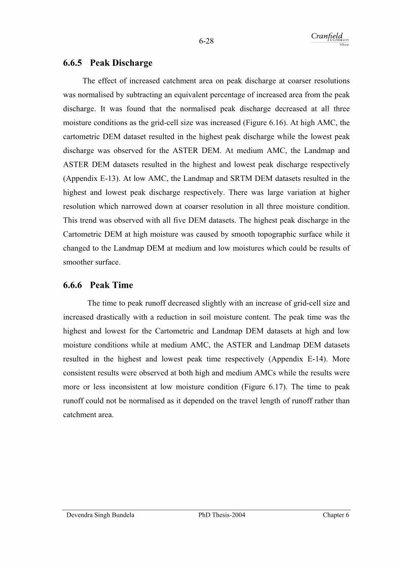
6-28
6.6.5 Peak Discharge
The effect of increased catchment area on peak discharge at coarser resolutions
was normalised by subtracting an equivalent percentage of increased area from the peak
discharge. It was found that the normalised peak discharge decreased at all three
moisture conditions as the grid-cell size was increased (Figure 6.16). At high AMC, the
cartometric DEM dataset resulted in the highest peak discharge while the lowest peak
discharge was observed for the ASTER DEM. At medium AMC, the Landmap and
ASTER DEM datasets resulted in the highest and lowest peak discharge respectively
(Appendix E-13). At low AMC, the Landmap and SRTM DEM datasets resulted in the
highest and lowest peak discharge respectively. There was large variation at higher
resolution which narrowed down at coarser resolution in all three moisture condition.
This trend was observed with all five DEM datasets. The highest peak discharge in the
Cartometric DEM at high moisture was caused by smooth topographic surface while it
changed to the Landmap DEM at medium and low moistures which could be results of
smoother surface.
6.6.6 Peak Time
The time to peak runoff decreased slightly with an increase of grid-cell size and
increased drastically with a reduction in soil moisture content. The peak time was the
highest and lowest for the Cartometric and Landmap DEM datasets at high and low
moisture conditions while at medium AMC, the ASTER and Landmap DEM datasets
resulted in the highest and lowest peak time respectively (Appendix E-14). More
consistent results were observed at both high and medium AMCs while the results were
more or less inconsistent at low moisture condition (Figure 6.17). The time to peak
runoff could not be normalised as it depended on the travel length of runoff rather than
catchment area.
Devendra Singh Bundela PhD Thesis-2004 Chapter 6
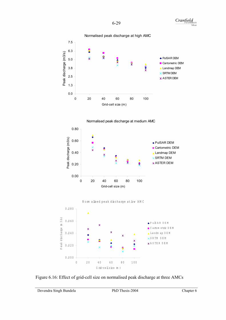
6-29
Normalised peak discharge at high AMC
0.0
1.3
2.5
3.8
5.0
6.3
7.5
0 20 40 60 80 100
Grid-cell size (m)
Pea
k di
scha
rge
(m3/
s)
PulSAR DEM
Cartometric DEM
Landmap DEM
SRTM DEM
ASTER DEM
Normalised peak discharge at medium AMC
0.00
0.20
0.40
0.60
0.80
0 20 40 60 80 100Grid-cell size (m)
Pea
k di
scha
rge
(m3/
s)
PulSAR DEMCartometric DEMLandmap DEMSRTM DEMASTER DEM
N orm alised peak discharge at low A M C
0 .0 0 0
0 .0 2 0
0 .0 4 0
0 .0 6 0
0 .0 8 0
0 2 0 4 0 6 0 8 0 1 0 0
G rid-cell size (m )
Peak discharge (m3/s)
P ulS A R D E M
C artom etric D E M
Landm ap D E M
S R TM D E M
A S TE R D E M
Figure 6.16: Effect of grid-cell size on normalised peak discharge at three AMCs
Devendra Singh Bundela PhD Thesis-2004 Chapter 6

6-30
Peak time at high AMC
0
50
100
150
200
250
0 20 40 60 80 100Grid-cell size (m)
Pea
k tim
e (m
in) PulSAR DEM
Cartometric DEMLandmap DEMSRTM DEMASTER DEM
Peak time at medium AMC
0
75
150
225
300
375
0 20 40 60 80 100
Grid-cell size (m)
Pea
k tim
e (m
in) PulSAR DEM
Cartometric DEMLandmap DEMSRTM DEMASTER DEM
Peak time at low AMC
0
100
200
300
400
500
0 20 40 60 80 100Grid-cell size (m)
Pea
k tim
e (m
in) PulSAR DEM
Cartometric DEMLandmap DEMSRTM DEMASTER DEM
Figure 6.17: Effect of grid-cell size on peak time to runoff at three AMCs
Devendra Singh Bundela PhD Thesis-2004 Chapter 6
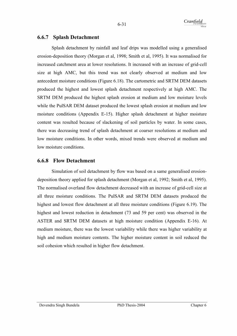
6-31
6.6.7 Splash Detachment
Splash detachment by rainfall and leaf drips was modelled using a generalised
erosion-deposition theory (Morgan et al, 1998; Smith et al, 1995). It was normalised for
increased catchment area at lower resolutions. It increased with an increase of grid-cell
size at high AMC, but this trend was not clearly observed at medium and low
antecedent moisture conditions (Figure 6.18). The cartometric and SRTM DEM datasets
produced the highest and lowest splash detachment respectively at high AMC. The
SRTM DEM produced the highest splash erosion at medium and low moisture levels
while the PulSAR DEM dataset produced the lowest splash erosion at medium and low
moisture conditions (Appendix E-15). Higher splash detachment at higher moisture
content was resulted because of slackening of soil particles by water. In some cases,
there was decreasing trend of splash detachment at coarser resolutions at medium and
low moisture conditions. In other words, mixed trends were observed at medium and
low moisture conditions.
6.6.8 Flow Detachment
Simulation of soil detachment by flow was based on a same generalised erosion-
deposition theory applied for splash detachment (Morgan et al, 1992; Smith et al, 1995).
The normalised overland flow detachment decreased with an increase of grid-cell size at
all three moisture conditions. The PulSAR and SRTM DEM datasets produced the
highest and lowest flow detachment at all three moisture conditions (Figure 6.19). The
highest and lowest reduction in detachment (73 and 59 per cent) was observed in the
ASTER and SRTM DEM datasets at high moisture condition (Appendix E-16). At
medium moisture, there was the lowest variability while there was higher variability at
high and medium moisture contents. The higher moisture content in soil reduced the
soil cohesion which resulted in higher flow detachment.
Devendra Singh Bundela PhD Thesis-2004 Chapter 6
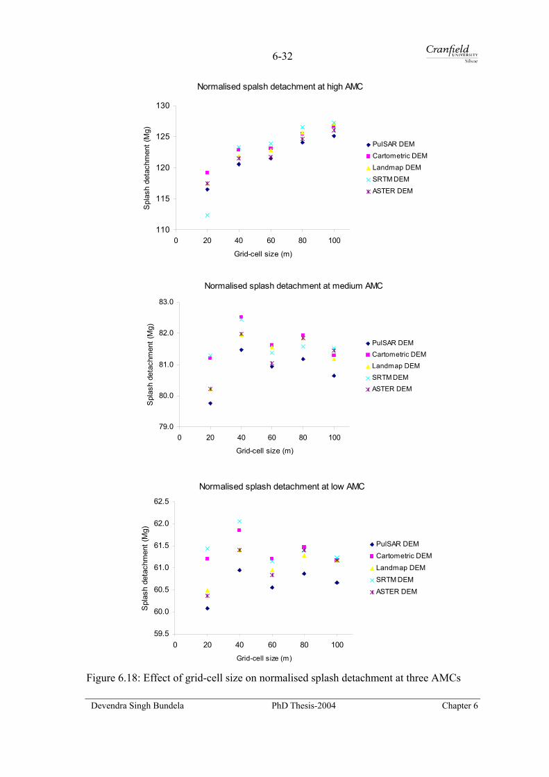
6-32
Normalised spalsh detachment at high AMC
110
115
120
125
130
0 20 40 60 80 100
Grid-cell size (m)
Spl
ash
deta
chm
ent (
Mg)
PulSAR DEMCartometric DEMLandmap DEMSRTM DEMASTER DEM
Normalised splash detachment at medium AMC
79.0
80.0
81.0
82.0
83.0
0 20 40 60 80 100
Grid-cell size (m)
Spl
ash
deta
chm
ent (
Mg)
PulSAR DEMCartometric DEMLandmap DEMSRTM DEMASTER DEM
Normalised splash detachment at low AMC
59.5
60.0
60.5
61.0
61.5
62.0
62.5
0 20 40 60 80 100
Grid-cell size (m)
Spl
ash
deta
chm
ent (
Mg)
PulSAR DEMCartometric DEMLandmap DEMSRTM DEMASTER DEM
Figure 6.18: Effect of grid-cell size on normalised splash detachment at three AMCs
Devendra Singh Bundela PhD Thesis-2004 Chapter 6

6-33
Normalised flow detachment at high AMC
0
7500
15000
22500
30000
37500
45000
0 20 40 60 80 100Grid-cell size (m)
Flow
det
ahcm
ent (
Mg)
PulSAR DEMCartometric DEMLandmap DEMSRTM DEMASTER DEM
Normalised flow detahcment at medium AMC
0
1500
3000
4500
6000
7500
9000
0 20 40 60 80 100
Grid-cell size (m)
Flow
det
achm
ent (
Mg)
PulSAR DEMCartometric DEMLandmap DEMSRTM DEMASTER DEM
Normalised flow detachment at low AMC
0
200
400
600
800
1000
1200
0 20 40 60 80 100Grid-cell size (m)
Flow
det
achm
ent (
Mg)
PulSAR DEMCartometric DEMLandmap DEMSRTM DEMASTER DEM
Figure 6.19: Effect of grid-cell size on normalised overland flow detachment at three AMCs
Devendra Singh Bundela PhD Thesis-2004 Chapter 6

6-34
6.6.9 Overland Deposition
Overland deposition was modelled using an exponential decay function
(Equation 2.36) discussed in Section 2.6, which simulates the effect of settling of
particles slows down when they reach the bottom of the water layer on the surface. The
deposition was based on runoff sediment concentration limiting. The sediment
deposition on overland increased with an increase of grid-cell size for all DEM datasets
at three moisture conditions (Figure 6.20). The PulSAR DEM dataset resulted in the
highest deposition at three moisture conditions while the SRTM dataset produced the
lowest sediment deposition at all moisture conditions (Appendix E-17). The results
were quite consistent at all three moisture levels. The higher deposition in the PulSAR
DEM dataset was caused by higher erosion which got deposited in the valley while
lower deposition in the SRTM DEM dataset was caused by lower soil erosion because
of lower slope gradient.
6.6.10 Channel Erosion
The effect of resolution on channel erosion at three moisture conditions was
studied and the results were normalised. The normalised channel erosion decreased as
the grid-cell size was increased at all moisture conditions. This trend was observed at
medium and low moisture conditions but this trend was not strongly seen at high
moisture level (Figure 6.21). The highest channel erosion was observed for the PulSAR
DEM dataset at high AMC, for the ASTER DEM dataset at medium AMC and for the
Landmap DEM dataset at low AMC respectively. The lowest channel erosion was
observed for the SRTM DEM dataset at all moisture conditions (Appendix E-18). The
higher soil moisture content resulted in higher runoff which led to higher channel
erosion. Channel erosion depends on soil cohesion of the channel material and amount
of flow to be handled in the model. Highest channel erosion in the PulSAR DEM,
ASTER DEM and Landmap DEM datasets at high, medium and low moisture
conditions respectively was caused by the higher slope gradient, which produced higher
runoff leading to higher channel erosion although the channel cohesion remained same
for these DEM datasets. The lowest erosion in the SRTM dataset at all moisture was
caused by lower slope gradient leading to lower runoff.
Devendra Singh Bundela PhD Thesis-2004 Chapter 6

6-35
Normalised overland deposition at high AMC
0
9000
18000
27000
36000
45000
0 20 40 60 80 100
Grid-cell size (m)
Dep
ositi
on (M
g) PulSAR DEM
Cartometric DEMLandmap DEMSRTM DEMASTER DEM
Normalised overland deposition at medium AMC
0
1500
3000
4500
6000
7500
9000
0 20 40 60 80 100
Grid-cell size (m)
Dep
ositi
on (M
g) PulSAR DEM
Cartometric DEMLandmap DEMSRTM DEMASTER DEM
Normalised overland deposition at low AMC
0
200
400
600
800
1000
1200
0 20 40 60 80 100
Grid-cell size (m)
Dep
ositi
on (M
g) PulSAR DEM
Cartometric DEMLandmap DEMSRTM DEMASTER DEM
Figure 6.20: Effect of grid-cell size on normalised overland deposition at three AMCs
Devendra Singh Bundela PhD Thesis-2004 Chapter 6

6-36
Normalised channel erosion at high AMC
0
2500
5000
7500
10000
12500
0 20 40 60 80 100Grid-cell size (m)
Cha
nnel
ero
sion
(Mg)
PulSAR DEM Cartometric DEMLandmap DEMSRTM DEMASTER DEM
Normalised channel erosion at medium AMC
0
1000
2000
3000
4000
5000
0 20 40 60 80 100Grid-cell size (m)
Cha
nnel
ero
sion
(Mg)
PulSAR DEM Cartometric DEMLandmap DEMSRTM DEMASTER DEM
Normalised channel erosion at low AMC
0
300
600
900
1200
1500
1800
0 20 40 60 80 100
Grid-cell size (m)
Cha
nnel
ero
sion
(Mg)
PulSAR DEM Cartometric DEMLandmap DEMSRTM DEMASTER DEM
Figure 6.21: Effect of grid-cell size on channel erosion at three AMCs
Devendra Singh Bundela PhD Thesis-2004 Chapter 6
6-37
6.6.11 Channel Deposition
Channel deposition was modelled on the basis of transport carrying capacity of
the runoff in the channel. It was normalised for increased catchment area effect. It
decreased at coarser grid-cell sizes for all five DEM datasets at all three moisture
conditions (Figure 6.22). The highest and lowest channel depositions were found for the
ASTER and SRTM DEM datasets respectively at high, medium and low moisture
conditions (Appendix E-19).
6.6.12 Total Soil Loss
The effect of resolution on normalised total soil loss from the catchment at three
moisture conditions was studied. It was found that it decreased at larger grid-cell sizes
(Figure 6.23). The PulSAR DEM dataset at high AMC and the Landmap DEM dataset
at medium and low AMCs produced the highest total soil erosion (Appendix E-20). The
ASTER DEM dataset produced the lowest at all three moisture conditions. The ASTER
DEM produced more inconsistent results at all moisture conditions while the SRTM
produced inconsistent results at low moisture condition.
6.6.13 Average Soil Loss
Figure 6.24 shows the effect of resolution on average soil loss at three moisture
conditions. It was found that it decreased as the grid-cell size was increased for all five
DEM datasets at all three moisture conditions. The PulSAR DEM dataset produced the
highest average soil loss at high moisture condition while the Landmap DEM resulted in
the highest at medium and low moisture conditions. The ASTER produced the lowest
average soil loss at all three moisture conditions, but its results were poor and
inconsistent (Appendix E-21).
Devendra Singh Bundela PhD Thesis-2004 Chapter 6

6-38
Normalised channel deposition at high AMC
0
2500
5000
7500
10000
12500
0 20 40 60 80 100Grid-cell size (m)
Cha
nnel
dep
ositi
on (M
g)
PulSAR DEM Cartometric DEMLandmap DEMSRTM DEMASTER DEM
Normalised channel deposition at medium AMC
0
1000
2000
3000
4000
5000
0 20 40 60 80 100Grid-cell size (m)
Cha
nnel
dep
ositio
n (M
g)
PulSAR DEM Cartometric DEMLandmap DEMSRTM DEMASTER DEM
Normalised channel deposition at low AMC
0
400
800
1200
1600
2000
0 20 40 60 80 100Grid-cell size (m)
Cha
nnel
ero
sion
(Mg)
PulSAR DEM Cartometric DEMLandmap DEMSRTM DEMASTER DEM
Figure 6.22: Effect of grid-cell size on channel deposition at three AMCs
Devendra Singh Bundela PhD Thesis-2004 Chapter 6

6-39
Normalised soil loss at high AMC
0
1500
3000
4500
6000
7500
9000
0 20 40 60 80 100Grid-cell size (m)
Tota
l soi
l los
s (M
g)
PulSAR DEM Cartometric DEMLandmap DEMSRTM DEMASTER DEM
Normalised soil loss at medium AMC
0
150
300
450
600
750
900
0 20 40 60 80 100
Grid-cell size (m)
Tota
l soi
l los
s (M
g)
PulSAR DEM Cartometric DEMLandmap DEMSRTM DEMASTER DEM
N orm alised soil loss at low A M C
0
10
20
30
40
50
60
0 20 40 60 80 100
G rid-cell size (m )
Total soil loss (Mg)
P ulS A R D E M
C artom etric D E M
Landm ap D E M
S R TM D E M
A S TE R D E M
Figure 6.23: Effect of grid-cell size on total soil loss at three AMCs
Devendra Singh Bundela PhD Thesis-2004 Chapter 6

6-40
Average soil loss at high AMC
0
2000
4000
6000
8000
10000
12000
0 20 40 60 80 100
Grid-cell size (m)
Ave
rage
soi
l los
s (k
g/ha
)
PulSAR DEMCartometric DEMLandmap DEMSRTM DEMASTER DEM
Average soil loss at medium AMC
0
200
400
600
800
1000
1200
0 20 40 60 80 100
Grid-cell size (m)
Ave
rage
soi
l los
s (k
g/ha
)
PulSAR DEMCartometric DEMLandmap DEMSRTM DEMASTER DEM
Average soil loss at low AMC
0
15
30
45
60
75
0 20 40 60 80 100
Grid-cell size (m)
Ave
rage
soi
l los
s (k
g/ha
) PulSAR DEMCartometric DEMLandmap DEMSRTM DEMASTER DEM
Figure 6.24: Effect of grid-cell size on average soil loss at three AMCs
Devendra Singh Bundela PhD Thesis-2004 Chapter 6
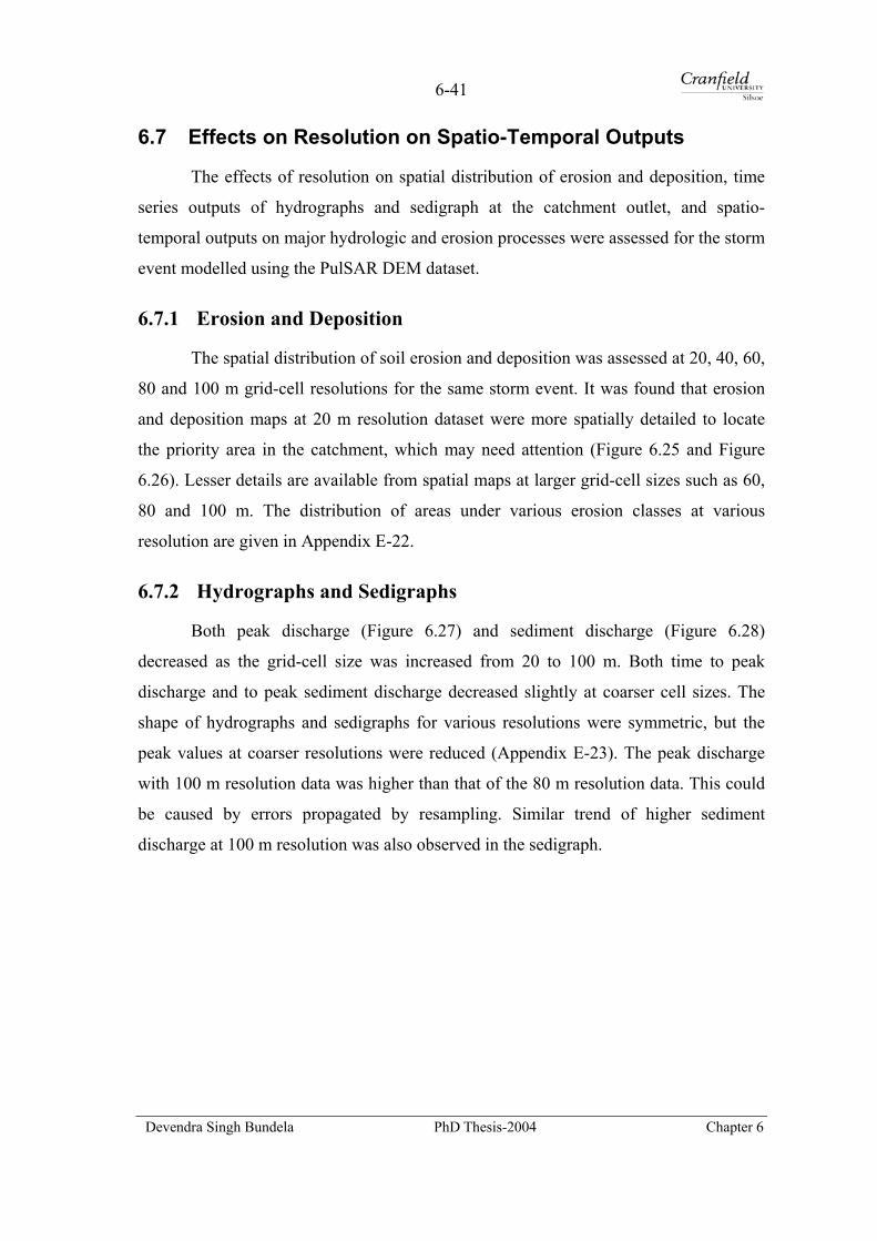
6-41
6.7 Effects on Resolution on Spatio-Temporal Outputs
The effects of resolution on spatial distribution of erosion and deposition, time
series outputs of hydrographs and sedigraph at the catchment outlet, and spatio-
temporal outputs on major hydrologic and erosion processes were assessed for the storm
event modelled using the PulSAR DEM dataset.
6.7.1 Erosion and Deposition
The spatial distribution of soil erosion and deposition was assessed at 20, 40, 60,
80 and 100 m grid-cell resolutions for the same storm event. It was found that erosion
and deposition maps at 20 m resolution dataset were more spatially detailed to locate
the priority area in the catchment, which may need attention (Figure 6.25 and Figure
6.26). Lesser details are available from spatial maps at larger grid-cell sizes such as 60,
80 and 100 m. The distribution of areas under various erosion classes at various
resolution are given in Appendix E-22.
6.7.2 Hydrographs and Sedigraphs
Both peak discharge (Figure 6.27) and sediment discharge (Figure 6.28)
decreased as the grid-cell size was increased from 20 to 100 m. Both time to peak
discharge and to peak sediment discharge decreased slightly at coarser cell sizes. The
shape of hydrographs and sedigraphs for various resolutions were symmetric, but the
peak values at coarser resolutions were reduced (Appendix E-23). The peak discharge
with 100 m resolution data was higher than that of the 80 m resolution data. This could
be caused by errors propagated by resampling. Similar trend of higher sediment
discharge at 100 m resolution was also observed in the sedigraph.
Devendra Singh Bundela PhD Thesis-2004 Chapter 6
6-42
Figure 6.25: Effect of resolution on the distribution of soil erosion with 8 classes
Devendra Singh Bundela PhD Thesis-2004 Chapter 6

6-43
Figure 6.26: Effect of resolution on the distribution of sediment deposition with 8 classes
Devendra Singh Bundela PhD Thesis-2004 Chapter 6

6-44
0
0.15
0.3
0.45
0.6
0.75
0 200 400 600 800 1000 1200Time (min)
Dis
char
ge (m
3/s)
20 m40 m60 m80 m100 m
Figure 6.27: Effect of resolution on hydrographs at the catchment outlet
0
20
40
60
80
100
120
0 200 400 600 800 1000 1200
Time (min)
Sedi
men
t dis
char
ge (k
g/s) 20 m
40 m 60 m 80 m 100 m
Figure 6.28: Effect of resolution on sediment discharge at the catchment outlet
Devendra Singh Bundela PhD Thesis-2004 Chapter 6

6-45
6.7.3 Spatio-Temporal Outputs
Two thousand six hundred spatio-temporal maps on each major hydrologic and
erosion processes such as infiltration, surface storage, runoff, runoff height, runoff
velocity, erosion, deposition, suspended sediment concentration, and overland transport
capacity were generated at every time-step for the storm event simulated. These
processes were viewed in the Aguila dynamic visualisation environment to see the each
process movement across the catchment. The efficiency of flow and sediment routing at
each grid-cell size was observed. These provide visuals to see what is happening across
the catchment at every time-step. These maps could not be attached to this chapter
either in static or dynamic mode, but they are provided separately on an optical disk
attached to the thesis for dynamic visualisation. A few AVI format video files are
created for quick dynamic visualisation of spatial-temporal outputs and are provided on
an optical disk under a ‘video’ folder.
6.8 Sensitivity Analysis for DEM Parameters
Three parameters derived from a DEM such as slope gradient, aspect (LDD)
channel gradient were used in the model for an event simulation. Sensitivity analysis to
decreasing trend of slope gradient was studied only with 20 m PulSAR DEM dataset
because the value of slope gradient must be within 0.001 and 1. It was found that the
infiltration, time to peak runoff and splash detachment were increased by 4.49, 38.38
and 6.11 per cent respectively when the slope gradient was reduced by 90 percent
(Appendix E-24). Similarly, the runoff coefficient, peak discharge, flow detachment,
overland deposition, channel erosion, channel deposition and total soil loss were
reduced by 81.85, 89.73, 100.0, 98.87, 43.10, 33.71 and 90.92 per cent respectively
when the gradient was reduced by 90 per cent. In other words, flattening of slope
gradient produces lower runoff and sediment yield from a catchment (Figure 6.29).
Sensitivity analysis of the LDD and channel gradient could not be studied because the
LDD holds a directional value and the variation in channel gradient was quite small.
Moreover, channel gradient did not have a significant effect on model outputs.
Devendra Singh Bundela PhD Thesis-2004 Chapter 6

6-46
0 25 50 75 100
Change in slope gradient (%)
-120
-100
-80
-60
-40
-20
0
20
40
60
Cha
nge
in o
utpu
ts (%
)
Infi ltration Runoff coefficient Peak discharge Peak time Total discharge Splash detachment Flow detachment Deposition Total soil loss Average soil loss
Figure 6.29: Model sensitivity to slope gradient at medium moisture level with 20 m
PulSAR DEM dataset
6.9 Statistical Evaluation
Statistical evaluation is necessary to assess the performance of a spatially
distributed and dynamic model for an event simulation. There are several statistical
criteria used for performance evaluation discussed in the literature by Quinton (1994).
For the Saltdean catchment, no statistical evaluation was carried out on model
performance because there was no validation dataset available.
6.10 Propagation of Errors in Modelling
6.10.1 Overview
Distributed modelling consists of three stages: firstly, data collection which
deals with collection of point or spatial data from various sources; secondly, creation of
a GIS database of model input parameters; and thirdly, testing input values in a model.
The errors can creep up at any of these stages. Errors in data is one aspect of error
propagation in modelling while the uncertainly in model parameters and the
mathematical expressions to represent processes in the model itself contribute to the
Devendra Singh Bundela PhD Thesis-2004 Chapter 6

6-47
error in modelling results. The estimation of error propagation in erosion modelling was
beyond the scope of the study. However, a brief overview of possible errors that might
be introduced in the distributed erosion modelling is discussed. This will act as
guidance for reliability of modelling results using LISEM.
6.10.2 Source of Errors in a GIS
The quality of key spatial data is fundamentally important to the reliability of
modelling results. A GIS is principally based on the spatial entities and non-spatial
attributes. The positional errors and attribute uncertainty are most important
characteristics of all spatial databases. These errors are propagated and amplified by
GIS operations, which adversely affect the potential application of GIS for extraction of
distributed model parameters. The sources of errors in the spatial data are discussed in
the literature by Burrough and McDonald (1998).
6.10.3 Error Propagation in Modelling
The quality of modelling results depends on the spatial data error and model
error (Burrough et al, 1996). A successful distributed modelling is more dependent on
data availability and its quality rather than by lack of process understanding and insight.
Model prediction can be affected by uncertainty and errors in the values of coefficients
and boundary conditions. The LISEM model assumes to have no residual error (Jetten,
2000), so most errors in prediction emanate from spatial data quality and model
parameter extraction.
6.11 Guidelines for Spatial Variability on Catchment Scale Modelling
Various grid-cell sizes of an original resolution of the DEM directly influence
runoff and erosion processes as the parameters are scale dependent. Increasing the grid-
cell size from 20 to 100 m flattens the slope gradient and shortens the drainage length.
Both have competing effect on the runoff and sediment flow routing. Over sampling of
a coarse DEM at fine resolution does not add any more information, but it may
introduce some kind of noise instead. Therefore, an appropriate resolution is necessary
Devendra Singh Bundela PhD Thesis-2004 Chapter 6

6-48
to identify to optimisation of data collection and computer resources for catchment scale
modelling.
Calibration is necessary to tune a physically based model with observed values
to develop the confidence in modelling results. The model should at least be calibrated
at a resolution to use for the prediction at other resolutions. In developing countires,
observed data on runoff and sediment yield for a catchment are rarely available. In the
absence of such observed dataset, a relative evaluation across various grid-cell sizes and
DEM sources was carried out.
For a given catchment scenario at a single soil moisture level, there is always a
single observed value of runoff, soil loss and peak discharge for a storm event. How
these outputs are predicted with a reasonable accuracy using whatever resolution and
whichever DEM needs to be examined. It was carried out for the runoff, average soil
loss and peak discharge individually. These outputs were predicted for five DEMs at
five resolutions each and are relatively compared against the Cartometric DEM as it is
widely used in developing countries for the modelling purpose. To what extent these
predictions could be improved using DEMs derived remote sensing against a
cartometric DEM.
Comparison among various DEMs
The runoff was improved by 6-7, 19-21 and 37-42 per cent for the PulSAR
DEM and Landmap DEM at high, medium and low moisture levels respectively as
compared to the Cartometric DEM at 20 m resolution. Similarly, it was improved by 2,
5 and 14 per cent for the ASTER DEM; and was under predicted by 8, 1 and 12 percent
for the SRTM DEM at high, medium and low moisture levels respectively (Figure
6.30). The PulSAR and Landmap DEMs improve the predictions because their slope
gradients are inherently better than the Cartometric DEM. It was found that resampling
of a coarse resolution SRTM DEM to smaller grid-cell sizes did not improve the
prediction of runoff at all three moisture levels. At 100 m, runoff was over predicted as
compared to an 80 m resolution. Therefore, a high resolution DEM should be resampled
to 80 m grid cell size, but the resampling reduces the spatial variability drastically.
Devendra Singh Bundela PhD Thesis-2004 Chapter 6

6-49
Runoff prediction at high AMC
-8.0
-4.0
0.0
4.0
8.0
20 40 60 80 100
Grid-cell size (m)
Cha
nge
(%)
PulSAR DEMLandmap DEMASTER DEMSRTM DEM
Runoff prediction at medium AMC
-5.0
0.0
5.0
10.0
15.0
20.0
25.0
20 40 60 80 100
Grid-cell size (m)
Cha
nge
(%)
PulSAR DEMLandmap DEMASTER DEMSRTM DEM
Runoff prediction at low AMC
-15.0
-5.0
5.0
15.0
25.0
35.0
45.0
20 40 60 80 100
Grid-cell size (m)
Cha
nge
(%)
PulSAR DEMLandmap DEMASTER DEMSRTM DEM
Figure 6.30: Runoff prediction as compared to the Cartometric DEM at three moisture
levels
Devendra Singh Bundela PhD Thesis-2004 Chapter 6
6-50
The average soil loss was improved by 71, 153-157 and 47-125 for the PulSAR
DEM and Landmap DEM at high, medium and low moisture levels respectively as
compared to the Cartometric DEM at 20 m resolution (Figure 6.31). Similarly, it was
absolutely under predicted by 100, 100 and 100 per cent for the ASTER DEM; and was
improved by 4, and 45, and under predicted by 98 for the SRTM DEM at high, medium
and low moisture levels respectively. The ASTER DEM could not be used for the
prediction of soil erosion because its results were poor at medium and low moisture
levels. Both the PulSAR DEM and Landmap DEM are suitable for erosion modelling
as they improve the prediction due to inherent better slope gradient mapped by remote
sensing. The average soil loss at 80 m for the SRTM DEM was under predicted by 100
percent at all three moisture levels. The SRTM DEM predicts better at other grid-cell
sizes than the original resolution. It emphasises that the released SRTM DEM contained
artefacts, so it should either be filtered or resampled to smaller or larger grid-cell size to
obtain a reasonable prediction. It should be used at original resolution for modelling in
any case.
The peak discharge was under predicted by 2-5 per cent at high moisture level
and was improved by 16-22 and 25-147 per cent at medium and low moisture levels for
the PulSAR DEM and Landmap DEM (Figure 6.32). Similarly, the peak discharge was
under predicted by 21 and 23 per cent and was improved by 58 per cent at high,
medium and low moisture levels for the ASTER DEM. The peak discharge is under
predicted by 18, 14 and 14 per cent for the SRTM DEM at high, medium and low
moisture levels. The PulSAR and Landmap DEMs improve the prediction of peak
discharge against the cartometric DEM. The SRTM DEM did not predict the peak
discharge very well. The ASTER DEM still predicts well. Therefore, the ASTER DEM
is reasonably good for the prediction of runoff only.
Devendra Singh Bundela PhD Thesis-2004 Chapter 6

6-51
Average soil loss at high AMC
-100-75
-50-25
025
5075
20 40 60 80 100Grid-cell size (m)
Cha
nge
(%) PulSAR DEM
Landmap DEMSRTM DEMASTER DEM
Average soil loss at Medium AMC
-125
-75
-25
25
75
125
175
20 40 60 80 100Grid-cell size (m)
Cha
nge
(%) PulSAR DEM
Landmap DEMSRTM DEMASTER DEM
Average soil loss at low AMC
-125-75-252575
125175
20 40 60 80 100
Grid-cell size (m)
Cha
nge
(%) PulSAR DEM
Landmap DEMSRTM DEMASTER DEM
Figure 6.31: Prediction of average soil loss as compared to the Cartometric DEM at
three moisture levels
Devendra Singh Bundela PhD Thesis-2004 Chapter 6
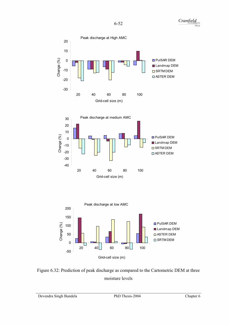
6-52
Peak discharge at High AMC
-30
-20
-10
0
10
20
20 40 60 80 100
Grid-cell size (m)
Cha
nge
(%)
PulSAR DEMLandmap DEMSRTM DEMASTER DEM
Peak discharge at medium AMC
-40
-30
-20
-10
0
10
20
30
20 40 60 80 100
Grid-cell size (m)
Cha
nge
(%)
PulSAR DEMLandmap DEMSRTM DEMASTER DEM
Peak discharge at low AMC
-50
0
50
100
150
200
20 40 60 80 100
Grid-cell size (m)
Cha
nge
(%)
PulSAR DEM Landmap DEMASTER DEMSRTM DEM
Figure 6.32: Prediction of peak discharge as compared to the Cartometric DEM at three
moisture levels
Devendra Singh Bundela PhD Thesis-2004 Chapter 6

6-53
Comparison among various resolutions
The runoff was reduced by 28, 40 and 60 per cent for the PulSAR DEM; by 26,
47 and 62 per cent for the Landmap DEM; by 26, 43 and 62 per cent for the ASTER
DEM; 16, 35 and 61 per cent for the SRTM DEM; and by 23, 38 and 61 per cent for the
Cartometric DEM at high, low and medium moisture levels respectively as compared to
20 m resolution (Figure 6.33). The PulSAR DEM, Landmap DEM and ASTER DEM
have little more variability than the Cartometric DEM. At medium moisture, all DEMs
show the same variability of around 60 per cent. The SRTM DEM has the lowest
variability at high and low moisture levels. Higher runoff variability for the PulSAR
dataset is caused by higher slope gradient. Lower variability for the SRTM is caused by
lowest slope gradient. The ASTER DEM dataset has a medium variability at all three
moisture levels.
The average soil loss at high moisture level was reduced by 24, 16, <1 and 18
per cent for the PulSAR DEM, Landmap DEM, SRTM DEM and Cartometric DEM
respectively at 100 m grid-cell size as compared to 20 m resolution (Figure 6.34).
Similarly, the average soil loss at medium moisture level was reduced by 62, 61, 59 and
19 per cent for the PulSAR DEM, Landmap DEM, SRTM DEM and Cartometric DEM.
At low moisture level, average soil loss was reduced by 88, 88, 155 and 68 per cent for
the PulSAR DEM, Landmap DEM, SRTM DEM and Cartometric DEM. The ASTER
DEM produces poor results at 20 m resolution at all three moisture levels. The SRTM
produces fairly well at medium moisture level.
The peak discharge was reduced by 38, 38, 31, 25, and 32 per cent at high
moisture level; by 66, 61, 63, 62 and 54 per cent at medium moisture level; and by 40,
48, 41, 52, and 24 per cent at low moisture level for the PulSAR, Cartometric DEM,
Landmap DEM, SRTM DEM and ASTER DEM respectively at 100 m grid-cell size as
compared to 20 m resolution (Figure 6.35). The lowest runoff variability was observed
at high moisture level among DEMs, highest at medium moisture level and medium at
low moisture level. Lower variability is observed at smaller grid-cell sizes.
Devendra Singh Bundela PhD Thesis-2004 Chapter 6

6-54
Runoff reduction at high AMC
-33-28-23-18-13-8-32
20 40 60 80 100Grid-cell size (m)
Red
uctio
n (%
) Cartometric DEMPulSAR DEMLandmap DEMASTER DEMSRTM DEM
Runoff reduction at medium AMC
-70-60-50-40-30-20-10
020 40 60 80 100
Grid-cell size (m)
Red
uctio
n (%
) Cartometric DEMPulSAR DEMLandmap DEMASTER DEMSRTM DEM
Runoff reduction at low AMC
-60
-50
-40
-30
-20
-10
020 40 60 80 100
Grid-cell size (m)
Red
uctio
n (%
) Cartometric DEMPulSAR DEMLandmap DEMASTER DEMSRTM DEM
Figure 6.33: Change in runoff against 20 m grid-cell size at three AMC
Devendra Singh Bundela PhD Thesis-2004 Chapter 6
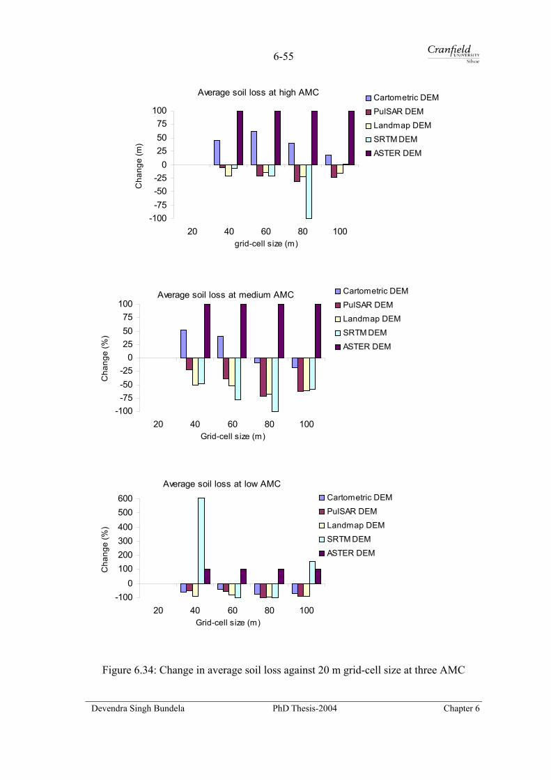
6-55
Average soil loss at high AMC
-100-75-50-25
0255075
100
20 40 60 80 100grid-cell size (m)
Cha
nge
(m)
Cartometric DEMPulSAR DEMLandmap DEMSRTM DEMASTER DEM
Average soil loss at medium AMC
-100-75-50-25
0255075
100
20 40 60 80 100Grid-cell size (m)
Cha
nge
(%)
Cartometric DEMPulSAR DEMLandmap DEMSRTM DEMASTER DEM
Average soil loss at low AMC
-1000
100200300400500600
20 40 60 80 100Grid-cell size (m)
Cha
nge
(%)
Cartometric DEMPulSAR DEMLandmap DEMSRTM DEMASTER DEM
Figure 6.34: Change in average soil loss against 20 m grid-cell size at three AMC
Devendra Singh Bundela PhD Thesis-2004 Chapter 6

6-56
Peak discharge reduction at high AMC
-50
-40
-30
-20
-10
0
1020 40 60 80 100
Grid-cell size (m)R
educ
tion
(%)
Cartometric DEMPulSAR DEMLandmap DEMASTER DEMSRTM DEM
Peak discharge reduction at medium AMC
-75
-60
-45
-30
-15
020 40 60 80 100
Grid-cell size (m)
Red
uctio
n (%
) Cartometric DEM
PulSAR DEMLandmap DEMASTER DEMSRTM DEM
Peak discharge reduction at low AMC
-100
-80
-60
-40
-20
0
2020 40 60 80 100
Grid-cell size (m)
Red
uctio
n (%
)
Cartometric DEMPulSAR DEMLandmap DEMASTER DEMSRTM DEM
Figure 6.35: Change in peak discharge against 20 m grid-cell size at three AMC
Devendra Singh Bundela PhD Thesis-2004 Chapter 6

6-57
6.12 Concluding Remarks
6.12.1 Discussion
The preceding sections of this chapter provide a comprehensive summary of
effects of various grid-cell resolutions on dynamic modelling results for a storm event
including sensitivity analysis and propagation of error in distributed modelling.
Key spatial data including three interferometric SAR DEMs, a
cartometric DEM and an optical stereo DEM, a land use and land cover map and a soil
map were resampled into five grid-cell resolutions. In additions to these datasets, crop,
soil and surface parameters were estimated for possible field conditions assumed in the
catchment in combination with the guidelines. Infiltration parameters for a single layer
Green and Ampt model were extracted for the dominant soil series from the soil map of
1: 250 000 scale. These datasets were brought into PCRaster to create 25 LISEM
databases of 30 parameters each for modelling the effects of various spatial
representations on surface hydrologic and erosion processes.
The effects of grid-cell size on the slope gradient, drainage network and
catchment area were studied. The mean slope gradient of the PulSAR DEM was the
highest in all five 20 m resolution DEM datasets because no smoothing and filtering
were performed deliberately while four other DEMs have undergone some level of
smoothing and filtering during their production. The mean slope gradient of the
PulSAR DEM reduced by 28 per cent as the grid-cell resolution was increased. This
trend is supported by Vieux (2000). It is a result of cutting of hills and filling of valleys
at larger resolutions by an aggregation scheme. The total drainage and channel lengths
shortened at larger grid-cell sizes. At larger grid-cell sizes, the drainage network and
channel length are short circuited because of cutting of hills and filling of valleys, thus,
causing an overall shortening of the drainage network and channel length. The results
indicate that the catchment area also increased by approximately 9 per cent as the grid-
cell size was increased from 20 to 100 m for all DEM datasets. The effect of increased
catchment area contribution on model outputs was normalised by subtracting an
equivalent percentage of increased area from outputs to make a sensible comparison
between different resolution outputs. An alternative way to address this issue is to
Devendra Singh Bundela PhD Thesis-2004 Chapter 6

6-58
constrain the catchment area to approximately same area by excluding boundary cells
manually (Molnár and Julien, 2000; Vieux, 2000). This approach could not be used
because of limited functionality in PCRaster.
The effects of resolution on surface hydrologic and erosion processes at three
moisture conditions were studied. The interception remained same for all DEM datasets
at all three antecedent moisture conditions as the grid-cell size was increased.
Interception is not influenced by the topography. Therefore, it is independent of grid-
cell sizes of the DEMs. The change in the interception at coarser resolutions was
insignificant (0.03 per cent) and it was purely caused by the rounding errors. The slight
decrease in the interception at 40 m resolution in all DEMs was observed which could
be caused by instability in the model algorithm.
The results indicate that the infiltration increases at coarser resolutions. Large
variation in the infiltration at 20 m grid-cell resolution was observed in all DEM
datasets. Its variability reduced from high to low soil moisture level as well as at coarser
resolutions. Higher infiltration with lower variability was observed for the SRTM and
cartometric DEM datasets at all moisture conditions. It was caused by slope flattening
because of smoothing applied and hence, more infiltration. Lower infiltration with
higher variability was observed for the PulSAR and Landmap DEM datasets because
the Landmap DEM is a multipass DEM, which has undergone some level of smoothing
during its production. The PulSAR DEM is an unfiltered DEM and has the highest slope
gradient. Hence, it resulted in the lowest infiltration. The ASTER DEM has medium
infiltration with medium variability at all three moisture conditions because it has
medium slope gradient.
The runoff coefficient decreases with an increase of grid-cell size. Large
variation in the runoff was observed at smaller grid-cell sizes and high moisture content
for all DEM datasets. Its variability reduced from high to low soil moisture as well as at
larger grid-cell size. Higher runoff with higher variability was observed for the PulSAR
and Landmap DEM datasets at all moisture conditions. It was results of higher slope
gradients and, hence, more runoff. Lower runoff with a lower variability was observed
for the SRTM and Cartometric DEM datasets because of their lower slope gradients.
Devendra Singh Bundela PhD Thesis-2004 Chapter 6
6-59
The ASTER DEM has medium runoff with medium variability at all three moisture
conditions.
The peak discharge decreases as the grid-cell size is increased. A large variation
in the peak discharge was observed at smaller grid-cell sizes and at high moisture
content in all DEM datasets. Its variability reduced from high to low soil moisture as
well as at coarser resolutions. Higher peak discharge with a higher variability was
observed for the Cartometric and Landmap DEM datasets at high moisture content.
Lower peak discharge with a lower variability was observed for the ASTER and SRTM
DEM datasets. The PulSAR DEM has a medium peak discharge. At medium moisture,
the Landmap DEM dataset produced the highest peak runoff while the ASTER DEM
produced the lowest peak discharge. At low moisture condition, the Landmap DEM
dataset produced the highest peak discharge while the ASTER DEM dataset produced
the lowest. An inconsistent result was observed in the ASTER DEM at 40 m at high
moisture condition.
The results suggest that the time to peak runoff decreases as the grid-cell size is
increased. At high moisture content, the Cartometric and Landmap DEM datasets
resulted in the highest and lowest peak time. The decreasing trend was observed for the
Cartometric, SRTM and ASTER DEM while no definite trend appeared for the PulSAR
and Landmap DEM datasets.
The results show that the splash detachment increases with an increase of
moisture content and grid-cell size while the overland flow detachment and sediment
deposition decreases at larger grid-cell sizes and at lower moisture conditions. The
variability of splash detachment reduced from high to low soil moisture as well as at
smaller grid-cell size. Higher splash detachment with a lower variability was observed
for the Cartometric and ASTER DEM datasets at high moisture condition while the
same was observed for the SRTM and Cartometric DEM datasets at medium and low
moisture conditions respectively. It was caused by lower mean slope gradients. Lower
splash detachment with a high variability was observed for the PulSAR and SRTM
DEM datasets at high moisture and for the PulSAR at medium and low moisture
conditions. Higher flow detachment and deposition with a higher variability was
Devendra Singh Bundela PhD Thesis-2004 Chapter 6

6-60
observed for the PulSAR and Landmap DEM datasets at all moisture conditions while
the lower splash detachment and deposition with a lower variability was observed for
the cartometric and SRTM DEM datasets at all three moisture conditions.
The channel erosion decreases at larger grid-cell sizes and lower moisture levels.
This trend was not observed at high moisture condition while it was strongly observed
at medium and low moisture conditions. The channel deposition decreased at coarser
grid resolutions and lower soil moisture levels for all the DEM datasets. The PulSAR,
ASTER and Landmap DEM datasets produced the highest channel erosion at high,
medium and low moisture conditions respectively. The SRTM has the lowest erosion
with the largest variability at high moisture and the lowest erosion with the lowest
variability at medium and low moisture conditions. The ASTER DEM has the highest
deposition with the largest variability at all moisture conditions while the SRTM DEM
has the lowest deposition with the lowest variability at all moisture conditions.
The results indicate that the total and average soil loss decreases at coarser grid-
cell sizes and lower soil moisture levels. The total and average soil loss was higher for
the PulSAR and Landmap DEMs and lower for the Cartometric and ASTER DEM
datasets at all moisture conditions. The results from the ASTER DEM were inconsistent
at 20 m resolution at all moistures and 40 m resolution at medium and low moisture
levels. The SRTM produced inconsistent results at all the resolutions except at 40 m at
low moisture conditions. The PulSAR, Landmap and Cartometric DEM datasets
produced fairly good results. The total and average soil loss at 100 m resolution was
always higher than that of the 80 m resolution. It could be caused by the error
propagated by resampling. Therefore, 100 m resolution dataset is inadequate for
representing spatial variability of the catchment characteristics for simulation of surface
hydrologic and erosion processes from a storm.
It is also observed that smaller grid-cell size datasets produce detailed outputs on
runoff and soil erosion, which are effective for identifying the exact location of
sediment source and sink areas required for planning soil conservation measures. Larger
grid-cell makes it difficult to identify the exact location of source and sink areas.
Devendra Singh Bundela PhD Thesis-2004 Chapter 6
6-61
Sensitivity analysis provides an insight on model sensitivity to DEM derived
parameters. The model sensitivity to the slope gradient was carried out. The results
indicate that the infiltration, time to peak runoff and splash detachment are increased at
lower slope gradients while the runoff coefficient, peak discharge, flow detachment,
deposition, channel erosion and deposition, and total soil loss are reduced when the
slope gradient is decreased. As the slope gradient is reduced, it produces lower runoff
and sediment yield from a catchment. The LDD and channel gradient sensitivity could
not be tested as it holds a directional data type. The variation in the channel gradient
was quite small, so no sensitivity analysis was carried out.
The PulSAR and Landmap DEM datasets predict both runoff and soil erosion
significantly better than the Cartometric DEM. Both show larger reductions in runoff
and soil loss variability when the grid-cell sizes are increased. The ASTER DEM under
predicts the average soil loss and is reasonably good for the prediction of runoff only.
The SRTM DEM predicts better at other grid-cell sizes than the original resolution,
which emphasises that the released SRTM DEM contained artefacts. Therefore, it
should either be filtered or resampled to smaller or larger grid-cell size to obtain a
reasonable prediction.
6.12.2 Conclusions
The influence of resolution on surface hydrologic and erosion processes at three
antecedent moisture levels were analysed and the following conclusions were drawn:
• The mean slope gradient flattened as the grid-cell size was increased.
• Both total drainage length and channel length shortened at larger grid-cell sizes.
• The interception remained same at all resolutions and soil moisture levels.
• The infiltration increased as the grid-cell size was increased. The variation in the
infiltration narrowed down at coarser grid-cell resolutions and at lower moisture
levels. It indicates that the SRTM DEM dataset produced higher infiltration at all
moisture levels because it has the lowest mean slope gradient by aggregation of 1
arc second to 3 arc second during production. The PulSAR and Landmap
produced the lowest at high and medium, and low moisture levels because these
Devendra Singh Bundela PhD Thesis-2004 Chapter 6
6-62
DEMs have higher mean slope gradient, which resulted in a quick drainage
response.
• The runoff coefficient and peak discharge decreased with an increase in grid-cell
size. Large variations at 20 m grid-cell resolution were observed in all the DEM
datasets. It narrowed down at coarser resolutions in both cases.
• The splash detachment increased with an increase of grid-cell size at all
antecedent moisture levels while the flow detachment and sediment deposition on
overland decreased with an increase of grid-cell resolution at all moisture levels.
• The channel erosion at high moisture level has no definite trend but it decreased
with an increase of grid-cell size at medium and low moisture levels while the
channel deposition increased at larger grid-cell sizes for all the DEMs at three
moisture levels.
• The total and average soil loss decreased at coarser grid-cell sizes. At high
moisture level, a definite decreasing trend was observed for the PulSAR DEM
dataset while no definite trend was observed for the other DEM datasets.
• Smaller grid-cell size datasets were found to be most suitable for identifying the
exact location of sediment source and sink areas required for planning effective
soil conservation measures.
• As the slope gradient was reduced in sensitivity analysis, the infiltration, time to
peak runoff and splash detachment were increased while the runoff coefficient,
peak discharge, flow detachment, deposition, channel erosion and deposition, and
total soil loss were reduced. In other words, it produced lower runoff and
sediment yield.
• The PulSAR and Landmap DEM datasets were found to be most suitable for
improving the prediction of both runoff and soil erosion as compared to the
Cartometric DEM. Guidelines presented highlight the role of remotely sensed
derived DEMs for improving model predictions. These guidelines demonstrate the
potential of this approach in developing countries.
Devendra Singh Bundela PhD Thesis-2004 Chapter 6

7-1
7
Discussion, Conclusions and
Recommendations for Future Study
In this chapter, a general discussion and conclusions on the influence of
different resolutions of five DEMs on surface hydrologic and soil erosion
processes at three antecedent soil moisture levels for a storm are
summarised. Suitable guidelines identified for spatial variability at
catchment scale modelling are also discussed. It also includes the
recommendations for future study.
7.1 Introduction
Distributed soil erosion models require input parameters at an appropriate spatial
scale (grid-cell size) for characterising the spatial variability of topography, vegetation
and soil in a catchment. However, these models require a large number of input
parameters, which can be derived from remotely sensed data and other spatial databases
through a GIS. An embedded integration of erosion models within a GIS provides a
powerful environment for modelling surface hydrologic and erosion processes at
catchment scale. This integration avoids the programming of a database and display. In
this context, the LISEM model was used with an aim to investigate the influence of
different spatial representations of terrain, vegetation and soil on the performance of
dynamic modelling on surface runoff and erosion processes in a GIS at catchment scale
for an event in order to identify guidelines on catchment scale modelling.
Devendra Singh Bundela PhD Thesis-2004 Chapter 7

7-2
The preceding chapters explain the procedures used to achieve the aim and
objectives of the study, namely selection of a dynamic erosion model within a GIS,
identification of rainstorm events, estimation of infiltration parameters, identification of
land use and land cover, assessment of the public domain DEMs, generation of an
InSAR DEM, creation of 25 LISEM databases at five resolutions and modelling the
effects of resolution on surface hydrologic and erosion processes at three antecedent soil
moisture levels for an event for the Saltdean catchment. All the previous chapters
contain a comprehensive discussion and a set of conclusions corresponding to the
findings of the each chapter. In this chapter, a general discussion and conclusions of the
study are summarised and the recommendations for the further study are outlined.
7.2 General Discussion
Several issues on generation of key spatial data and input parameters and effects
of resolution on modelling of surface hydrologic and erosion processes for a storm
event were addressed in this study. The factors which affect the selection of a suitable
model, the generation of key spatial data and input parameters, and modelling results
are discussed individually below.
7.2.1 Selection of a Model Embedded within a GIS
LISEM was selected to study the effects of resolution on hydrologic and erosion
processes for a storm because it allows spatial variability of input parameters at a
resolution and its parameters have physical meaning. Moreover, it is developed for a
European environment and catchment characteristics similar to the study catchment.
Hence, it is applied and some parameter values from these catchments would be used.
Since, it requires large amounts of input parameters and computational resources for a
simulation, remote sensing and other spatial data have proved a cost effective
alternative to parameterise the model.
The model simulates various options for infiltration, surface types, with or
without channel, runoff or both runoff and soil loss to suit a variety of catchments in
developing countries. It requires 24 parameters for a simple simulation. It could be
applied for data poor catchments in developing countries by parameterising using
remotely sensed and other spatial data. Being a physically-based model, it still contains
Devendra Singh Bundela PhD Thesis-2004 Chapter 7

7-3
some empirical equations for process description such as transport capacity equation.
PCRaster is a backbone of the LISEM model to create databases from various key
spatial data. It does not have vector functionality and does not support widely used GIS
data formats. It needs another supporting GIS for rasterisation of vector data and,
projection and conversion of data into a GRID ASCII format for import. Despite all
these limitations, PCRaster is a useful tool for dynamic and distributed erosion
modelling.
7.2.2 Rainstorm and Its Distribution
A 6-hour storm segment of 30 October 2000 is used for the modelling study
because of the limitation of computer disk space. The storm was a frontal storm, which
covers a wider area and lasts for a couple of hours. The assumption of a uniform rainfall
over the catchment due to single station rainfall data is largely valid for a frontal storm
for the small catchment (~800 ha). Therefore, a single point rainfall data has provided a
reasonable spatially representation of the storm over the catchment. A better spatial
distribution of a storm would improve the reliability of model results.
The model is driven by the rainfall intensity and is more sensitive to shorter
temporal resolution of the rainfall intensity. An hourly temporal resolution of the
rainfall data is too coarse for assessing the temporal variability of a storm. This
resolution of rainfall data is considered more or less representative for the frontal storm
under the situation, but they are not ideal for modelling. The break point intensity data
pairs of the storm could not be identified precisely from hourly data. This is one of the
limitations of hourly data. The assumption of a constant intensity rainfall for a whole
hour could rarely be valid for a frontal storm in reality. This assumption introduces a
higher response from erosion and deposition processes in the model. Shorter temporal
resolution storm data would be ideal for small catchments.
7.2.3 Infiltration Parameters
Infiltration parameters for a single layer Green and Ampt model were estimated
from an available 1:250 000 scale NATMAP soil map using pedotransfer functions,
described in Chapter 3. The soil associations in the map comprise a dominant and three
to four associated soil series, which could not be spatially located by any means in soil
Devendra Singh Bundela PhD Thesis-2004 Chapter 7
7-4
association polygons. Therefore, an assumption of the dominant soil series in each
mapping polygon has largely reduced the spatial variability of infiltration parameters in
the catchment. It affects the prediction of runoff and erosion in absolute quantity. For
this study, the variability of parameters is not absolutely required. Higher spatial
variability is better for model calibration and for comparison in absolute terms. Larger
scale soil data would be better for assessing the spatial variability of infiltration
parameters on hydrologic and erosion processes at catchment scale.
7.2.4 Land Use and Land Cover
Remote sensing is used for obtaining a reliable land use and land cover map
close to a historic storm event. A hybrid classification procedure, described in Chapter
4, was successfully used to identify a land use and land cover map with an overall
accuracy of 90 per cent from SPOT-1 data. There are a few significant problems with
classification because of the spectral confusion caused by bare fields, farm buildings,
urban areas and sea water; and grasslands in valleys and on slopes. These problems are
further compounded by the untimely ground survey. Reliability of ground data is
lessened during classification, which emphasises the importance of timely ground
survey. NDVI data could not be used to derive the percentage ground cover and leaf
area index for this study because of absence of field observations. Field observations are
necessary to establish the relationship between NDVI and biophysical parameters.
The model relies on land use and land cover map for deriving crop and
vegetation dependent parameters by reclassifying. Therefore, the classification accuracy
would affect the parameter accuracy and hence, the model outputs.
7.2.5 Assessment of Public Domain DEMs
Landmap, ASTER and SRTM-3 DEMs are used to investigate their usefulness on
model predictive capacity. These DEMs are described in Chapter 5. The Landmap DEM
is of good quality DEM with a vertical accuracy of 6 m, which is suitable for modelling,
but it still contains error in woodland and built-up areas in the catchment. The ASTER
DEM is a relative height DEM and its quality could not be assessed precisely. Its
vertical accuracy is assessed by a crude method. It has vertical accuracy similar to that
of the Landmap DEM. Relative height does not affect slope gradient used in the model.
Devendra Singh Bundela PhD Thesis-2004 Chapter 7
7-5
The SRTM-3 is a medium resolution unedited DEM and has a vertical accuracy of
about 4 m. These DEM are not error free and do contain ground clutter and water body
artefacts. How quality of these DEMs affects the modelling results are examined and
discussed later.
7.2.6 Generation and Quality Assessment of InSAR DEMs
Spaceborne SAR interferometry is explored for generating high resolution
DEMs from an ERS data pair in the context of developing countries, described in
Chapter 5. PulSAR/InSAR Toolkit is successfully used to generate reliable InSAR
DEMs. Processors used in this study had a major problem with data ingestion with data
supplied by the I-PAF. It was realised that there is no exhaustive guideline for the
selection of a quality data pair and a processor. Strategies for the selection of a quality
data pair and a processor are outlined. Despite exhaustive ERS data search for a good
data pair, a pair was selected for which no precision orbits data were available. This
information is still not available from many sources. It emphasises the importance of
guidelines for selection of a quality pair.
Quality assessment of the InSAR DEM reveals that it has a vertical accuracy
(RMSE) of 20 m at 25 m grid-cell spacing. This large error is attributed to the non-
availability of precision orbits data due to telemetry failure during the pair acquisition.
This issue is not well addressed on the European Space Agency’s website. It was known
lately when precision orbit data was ordered. These data are necessary for precise
geocoding. An attempt was made to rectify this systematic error using baseline
refinement procedure through the ground control points. However, it could not be fully
rectified and resulted in a vertical height error. Therefore, the necessity of precision
orbit data for SAR data is emphasised for obtaining high quality InSAR DEMs. The
model uses the slope gradient and aspect derived from a DEM, which are not influenced
by systematic height error present in the InSAR DEM. On the quality assessment of an
InSAR DEM against a reference drainage network, it found that InSAR DEMs are
suitable at 1:25 000 or smaller scale for distributed modelling.
A photogrammetric DEM reveals on its quality assessment that it contains
heavy clutter on the edges and holes in low tonal area because of the poor quality of
Devendra Singh Bundela PhD Thesis-2004 Chapter 7

7-6
aerial photographs. It was timey consuming to edit such a DEM for removing clutter. It
was learnt that the Sussex photography project was not intended for topographic
mapping. This DEM could not be used as a validation DEM. It emphasises the need to
select quality photograph pairs for an application. It was experienced in this study that
InSAR DEM generation is less cumbersome than the optical stereo and radargrammetric
DEM generation due to the presence of clouds and speckle respectively.
7.2.7 Creation of Different Spatial Representations
Five DEMs, a land use and land cover map and soil data each were resampled
into five resolution datasets to derive input parameters at each resolution. All input
parameters could not be extracted from these spatial data. Several crop, soil and surface
parameters are required for the creation of a LISEM database. These parameters are
generally not available in the developing world. They need to be estimated for possible
field conditions assumed for the catchment at the time of a storm using guidelines. This
requires some field observations to reclassify spatial data into parameter maps. These
can be measured from the field observations for a future storm event. This kind of
estimation may not yield an exact value, but it is representative for assumed conditions
in the catchment. This is one of the limitations of the model application for a historic
event. Moreover, an exact parameter value is not required for this study as it is
concerned with model sensitivity to different resolutions and DEM sources. There are
data import problem with PCRaster as it only supports data in GRID ASCII format. So
every data needs to be converted to this format for which another supporting GIS is
necessary.
7.2.8 Dynamic Erosion Modelling
Twenty-five LISEM databases with 30 parameters each were created and tested
in the model for sensitivity analysis for different resolutions and DEMs. The model
assumes no default parameter value. Everything should be defined for a simulation. It
requires a large storage space as a single simulation of 1300 min at a 30 seconds time
step produces spatio-temporal outputs of ~1.2 GB for a 20 m resolution dataset each for
8 sq km catchment. The model would have more limitations for catchments with larger
Devendra Singh Bundela PhD Thesis-2004 Chapter 7
7-7
areas in terms of storage space and computing power. The model also over predicts the
erosion and deposition.
7.2.9 Effects of Resolution on Hydrologic and Erosion Processes
As the grid-cell size increases, the slope gradient reduces and the drainage
length shortens. It also increases the catchment area, which affects the hydrologic and
erosion response for a storm caused by increased area contribution. It is normalised for
area dependent processes.
The runoff coefficient decreases as the grid-cell size increases. Large variation
in the runoff is observed at large grid-cell size at medium moisture level for all the
DEM datasets with respect to 20 m resolution. Its variability is highest, medium and
lowest at medium, low and high moisture levels. Higher runoff with higher variability is
observed for the PulSAR and Landmap DEM datasets at all moisture levels. The
PulSAR DEM dataset produces higher runoff than the Landmap DEM at high moisture
level because the PulSAR DEM has higher slope than the Landmap DEM dataset. The
Cartometric DEM has higher runoff variability than the SRTM DEM dataset but has
lower than the PulSAR and Landmap DEMs because the Cartometric DEM dataset has
a higher slope gradient than the SRTM DEM. The ASTER DEM dataset has medium
runoff with medium variability at all three moisture levels.
The average soil loss decreases at larger grid-cell sizes and at lower soil
moisture levels. The average soil loss is higher for the PulSAR and Landmap DEM
datasets and lower for the Cartometric and ASTER DEM datasets at all moisture levels.
The results from the ASTER DEM dataset are not consistent at 20 m resolution at all
moistures and 40 m resolution at medium and low moisture levels. The SRTM datasets
produces poor results at all the resolutions except at 40 m at low moisture level. The
PulSAR, Landmap and Cartometric DEM datasets produce fairly good results. The
average soil loss at 100 m resolution was always higher than that of the 80 m resolution.
It could be caused by the error propagated by resampling. Therefore, 100 m resolution
dataset is not fairly good for representing spatial variability of catchment characteristics
for the simulation on surface hydrologic and erosion processes from a storm.
Devendra Singh Bundela PhD Thesis-2004 Chapter 7

7-8
The normalised peak discharge decreases as the grid-cell size is increased. Large
variations in the peak discharge were observed at small grid-cell size and at high
moisture levels in all the DEM datasets. Its variability reduces from high to low at lower
soil moisture levels and at larger grid-cell sizes. Higher peak discharge with a higher
variability is observed for the Cartometric and Landmap DEM datasets at high moisture
content. Lower peak discharge with a lower variability is observed for the ASTER and
SRTM DEM datasets. The PulSAR DEM dataset has a medium peak discharge. At
medium moisture, the Landmap DEM dataset produced the highest peak runoff while
the ASTER DEM produced the lowest peak discharge. At low moisture level, the
Landmap DEM dataset produced the highest peak discharge while the ASTER DEM
dataset produced the lowest. A definite trend in peak discharge was observed in the
ASTER DEM dataset at 40 m at high moisture level.
7.2.10 Guidelines for Spatial Variability on Catchment Scale
Modelling
In developing countries, observed data on runoff and sediment yield for a
catchment are rarely available. In such case, a relative evaluation across resolutions and
DEMs can be carried out. In this study, a relative evaluation was carried out for the
runoff, average soil loss and peak discharge individually. These outputs were predicted
for five DEMs at five resolutions each and were relatively compared against the
Cartometric DEM. To what extent these predictions could be improved using DEMs
derived remote sensing against the Cartometric DEM.
Comparison against the Cartometric DEM
The prediction of runoff was considerably improved for the PulSAR DEM and
Landmap DEM and was marginally improved for the ASTER DEM at three moisture
levels against the Cartometric DEM at 20 m resolution. Conversely, it was under
predicted for the SRTM DEM by 1-12 per cent at three moisture levels. The runoff was
over predicted at 100 m as compared to an 80 m resolution. Hence, a high resolution
DEM should be resampled to 80 m grid cell size to obtain reasonable results, but the
resampling reduces the spatial variability drastically.
Devendra Singh Bundela PhD Thesis-2004 Chapter 7

7-9
The average soil loss was significantly for the PulSAR DEM and Landmap
DEM at all three moisture levels as compared to the Cartometric DEM at 20 m
resolution. Conversely, it was poorly predicted for the ASTER DEM and it was
reasonably predicted for the SRTM DEM at three moisture levels respectively. The
ASTER DEM should not be used for the prediction of soil erosion because its results
were poor at medium and low moisture levels. Both the PulSAR DEM and Landmap
DEM are suitable for erosion modelling as they improve prediction due to inherently
better slope gradient mapped by remote sensing. Average soil loss at 80 m for the
SRTM DEM was under predicted absolutely at all three moisture levels. The SRTM
DEM predicts better at other grid-cell sizes than the original resolution. It emphasises
the need for removing artefacts from the DEM. The SRTM DEM should either be
filtered or resampled to smaller or larger grid-cell size to obtain a reasonable prediction.
Comparison against various grid-cell sizes
The PulSAR DEM, Landmap DEM and ASTER DEM have shown little more
variability in runoff than the Cartometric DEM. At medium moisture, all DEMs show
the same variability of around 60 per cent. The SRTM DEM has the lowest variability
at high and low moisture levels. Higher runoff variability for the PulSAR dataset is
caused by higher slope gradient. Lower variability for the SRTM is caused by lowest
slope gradient. The ASTER DEM dataset has a medium variability at all three moisture
levels.
The PulSAR DEM has shown a higher variability in average soil loss than the
Cartometric DEM whereas the Landmap DEM has shown a lower variability than the
Cartometric DEM. At medium moisture, the PulSAR DEM, Landmap DEM and SRTM
DEM show the same variability of around 59-61 per cent. At low moisture level,
average soil loss was reduced by 88, 88, 155 and 68 per cent for the PulSAR DEM,
Landmap DEM, SRTM DEM and Cartometric DEM. The ASTER DEM produces poor
results at 20 m resolution at all three moisture levels. The SRTM produces fairly well at
medium moisture level. The ASTER should not be used for the prediction of soil
erosion.
Devendra Singh Bundela PhD Thesis-2004 Chapter 7

7-10
7.3 Conclusions
The general conclusions are listed according to the objectives set out for this
study in Chapter 1 as follows:
Objective 1
• SAR Interferometry has been tested for a study area in the UK and was found
suitable for catchment scale topographic mapping despite atmospheric
perturbations. A vertical accuracy of 20 m was achieved despite non-availability
of precision orbital data for a tandem pair of 1997. The orbit error was translated
into the systematic height error.
• InSAR DEM quality was also assessed independently against a reference drainage
network from the 1:10 000 scale topographic maps. It was found that the InSAR
DEM is suitable for the extraction of a drainage network at 1:25 000 or smaller
scale.
• The strategies for selection of optimal single SAR data pairs with suitable SAR
and InSAR processors are shown to be practicable and applicable for developing
countries. Furthermore, DEM accuracy is shown to be improved with optimal
strategies involving a single pair set.
Objective 2
• The quality assessment of the Landmap, ASTER DEM and SRTM DEMs were
found to be less 6 m RMS error and thereby suitable for modelling.
• The usefulness of the public domain DEMs for distributed modelling was tested
and it was found that the Landmap DEM results in reliable predictions of runoff
and soil loss. The ASTER DEM predicts runoff reasonably and soil loss poorly,
and the SRTM DEM was shown to under predict both runoff and soil loss as
compared to the Cartometric DEM.
Objective 3
• The LISEM model was shown as a useful tool for predicting effects of resolution
on surface runoff and erosion dynamics at the catchment scale for a heavy storm.
Devendra Singh Bundela PhD Thesis-2004 Chapter 7

7-11
• A 6-hour intense storm of 30 October 2000 was used for the simulation study due
to a limitation of computer disk storage. Although hourly rainfall data from a
single raingauge station was found too coarse for assessing the spatial and
temporal variability of the storm, it was considered representative for a frontal
storm. It was not possible to locate precise break point rainfall intensity pairs of a
storm from this hourly data.
• The spatial variability of infiltration parameters derived for a single layer Green
and Ampt model from the 1:250 000 scale soil map using pedotransfer functions
was shown to reduce considerably in the catchment.
• A large time lag between the image acquisition and field survey makes ground
data less reliable during supervised classification. A statistically sound sampling
scheme with a timely field survey is emphasised for reliable image classification.
• A hybrid classification approach was found to be the most effective solution for
this study. Overall accuracy and Kappa coefficient of classification were
satisfactory. Therefore, an eleven class thematic image was further reclassified to
nine classes and was post-processed for model parameterisation.
Objective 4
• As the grid-cell size increases from 20 to 100 m for all the DEMs, the catchment
area increases, the slope gradient flattens, and the drainage length shortens. Both
slope gradient and drainage length demonstrated a competing effect on runoff and
sediment routing.
• The runoff coefficient and peak discharge were seen to decrease with an increase
in grid-cell size. Large variations at 20 m resolutions were observed in all the
DEM datasets and reduced at larger grid-cell sizes in both cases.
• The average soil loss was shown to decrease at larger grid-cell sizes. At high
moisture levels, a definite decreasing trend was observed for the PulSAR DEM
dataset whilst no trend was observed for the other DEM datasets.
Devendra Singh Bundela PhD Thesis-2004 Chapter 7

7-12
Objective 5
• PulSAR and Landmap DEM datasets were shown to improve the prediction of
both runoff and soil erosion as compared to the Cartometric DEM. Guidelines are
presented highlighting the role remotely sensed derived DEMs offer in improving
model predictions. These guidelines demonstrate the potential of this approach in
developing countries.
• Smaller grid-cell size datasets are shown as the most suitable for identifying the
exact location of sediment source and sink areas, thereby facilitating the adoption
of, for example, effective soil conservation measures.
7.4 Recommendations for Future Study
A series of future recommendations are made, including:
• A further study needs to be conducted with a better spatial and temporal
distribution of the rainstorm particularly with a shorter temporal resolution rainfall
data to improve the reliability of modelling results;
• A detailed study needs to be undertaken with larger scale soil data with more or
less at a 1:50 000 scale with mapping unit as soil series to investigate the effect of
soil variability on estimation of infiltration parameters. It would yield more
realistic outputs and help in model calibration and validation;
• A further study with constrained similar catchment areas at various resolutions
needs to be undertaken to investigate the influence of resolutions on surface
hydrologic and erosion process and to compare with current results on
normalisation issue;
• A detailed study with timely field survey needs to be undertaken to map the land
use and land cover of the Eastern South Downs to improve classification accuracy.
Using current multispectral sensors would improve the classification accuracy,
providing improved spectral and spatial resolution;
Devendra Singh Bundela PhD Thesis-2004 Chapter 7

7-13
• A detailed study with an ERS SAR raw data pair with the precision orbit data
should be undertaken for deriving high resolution and quality InSAR DEMs with
vertical accuracy on the order of metres for distributed modelling; and
• Further studies transferring this approach to other parts of the world, for instance
developing countries, where land degradation has significant environmental and
societal implications.
Devendra Singh Bundela PhD Thesis-2004 Chapter 7

8-1
8
References
Ackermann, F. (1996) Techniques and strategies for DEM generation. In: C. Greve, ed. Digital
photogrammetry: An addendum to the manual of photogrammetry. Bethesda: American
Society of Photogrammetry and Remote Sensing, 135-141
ADAS (1996a) Landscape monitoring in the South Downs environmental sensitive areas (ESA),
1987–1995. Unpublished report to Ministry of Agriculture, Fisheries and Food. (Accessed:
10 December 2003)
http://www.defra.gov.uk/erdp/pdfs/esaspdfs/stage1/southlan.pdf
ADAS (1996b) Environmental monitoring in the South Downs ESA, 1987–1995. unpublished
report to Ministry of Agriculture, Fisheries and Food. (Accessed: 10 December 2003)
http://www.defra.gov.uk/erdp/pdfs/esaspdfs/stage1/southenv.pdf
Allmaras, R. R., Burwell, R. E., Larson, W. E. and Holt, R. F. (1966) Total porosity and random
roughness of interrow zone as influenced by tillage. USDA Conservation Research
Report, 7, as cited in Cremers, N. H. D. T., Van Dijck, P. M., De Roo, A. P. J. and
Verzandvoort, M. A. (1996) Spatial and temporal variability of soil surface roughness
and the application in hydrological and soil erosion modelling. Hydrological Processes,
10, 1035-1047
Anderson, J. R., Hardy, E. E., Roach, J. T. and Witmer, R. E. (1976) A land-use and land cover
classification system for use with remote-sensor data. U. S. Geological Survey
Professional paper 964, Washington: US Govt Printing Office. (Accessed: 17 February
2003) http://www.wsdot.wa.gov/environment/envinfo/docs/RSPrj_USGS_lulcclass.pdf
Devendra Singh Bundela PhD Thesis-2004 References
8-2
Aplin, P., Atkinson, P. M. and Curran, P. J. (1997) Fine spatial resolution satellite sensors for
the next decade. International Journal of Remote Sensing, 18 (18), 3873-3881
Arya, L. M. and Paris, J. F. (1981) A physico-empirical model to predict the soil moisture
characteristic from particle-size distribution and bulk density data. Soil Science Society of
America Journal, 45, 1023-1030
Askne, J. and Hagberg, J. O. (1993) Potential of interferometric SAR for classification of land
surfaces. In: Proceedings of the Geoscience and Remote Sensing Symposium, 1993
(IGARSS '93) on Better Understanding of Earth Environment held at Tokyo from 18-21
August, 1993, 3, 985-987
Aston, A. R. (1979) Rainfall interception by eight small trees. Journal of Hydrology, 42, 383-
396 as cited in Jetten, V. (2002) LISEM user manual, version 2.x. Draft version. Utrecht
Centre for Environment and Landscape Dynamics, Utrecht University, The Netherlands
Avery, B.W. (1990) Soils of the British Isles. Wallingford: CAB International
Axelsson, P. (1999) Processing of laser scanner data-algorithms and applications. ISPRS
Journal of Photogrammetry & Remote Sensing, 54(2-3), 138-147
Bamler, R. (1992) A comparison of range-Doppler and wavenumber domain SAR focusing
algorithms. IEEE Transactions on Geoscience and Remote Sensing, 30(4), 706-713,
Balmer, R. (1997) Digital terrain models from radar interferometry. In: D. Fritsch and D.
Hobbie, eds., Proccedings of Photogrammetric Week 97 , Heidelberg: Wichmann Verlag,
93-105. www.ifp.uni-stuttgart.de/publications/phowo97/bamler.pdf (16 August 2003)
Bamler, R. (1999) The Shuttle Radar Topographic mission (SRTM): A worldwide 30 m
resolution DEM from SAR interferometry in 11 days. In: D. Fritsch and R. Spiller, eds.
Proceedings of Photogrammetric week held at Wichmann Verlag, Heidelberg
http://www.ifp.uni-stuttgart.de/publications/phowo99/bamler.pdf (Accessed: 30 March
2004)
Barratt, G., Gaffney, V., Goodchild, H. and Wilkes, S. (2000) Survey at Wroxeter using carrier
phase, differential GPS surveying techniques. Archaeological Prospection, 7, 133-143
Bayliss, A. (1999) Catchment descriptors. Flood Estimation Handbook (FEH), 5, Wallingford:
Institute of Hydrology (Now CEH)
Devendra Singh Bundela PhD Thesis-2004 References
8-3
Beasley, D. B., Huggins, L. F., and Monke, E. J. (1980) ANSWERS: A model for watershed
planning. Transactions of the ASAE, 23(4), 938-944
Beasley, D. B. and Huggins, L. F. (1981) ANSWERS User’s Manual. Report No. EPA-905/9-
82-001, U.S. Environmental Protection Agency, Region V, Chicago, Illinois: Purdue
University, West Lafayette, Indiana
Belmans, C., Wesseling, J. G. and Feddes, R. A. (1983) Simulation model of the water balance
of a cropped soil: SWATRE. Journal of Hydrology, 63, 271-286
Berry, J. K. (1993) Cartographic modelling: the analytical capabilities of GIS. In: M. F.
Goodchild, B. Parks, and L. Steyaert, eds. Environmental modelling with GIS. New
York: Oxford University Press, 58-74
Boardman, J. (1990). Soil erosion on the South Downs: a review. In: J. Boardman, I. D. L.
Foster and J. A. Dearing, eds. Soil Erosion on Agricultural Land, Chichester: John Wiley
& Sons, 87-105
Boardman, J. (1996) Soil erosion by water: problems and prospects for research. In: M. G.
Anderson and S. M. Brooks, eds. Advances in Hillslope Processes, Chichester: John
Wiley & Sons, (1), 489-505
Boardman, J. (2003) Soil erosion and flooding on the eastern South Downs, southern England,
1976-2001.Transactions of the Institute of British Geographers, 28 (2), 176-196
Boorman, D. B., Hollis, J. M and Lilly, A (1995) Hydrology of soil types: a hydrologically-
based classification of the soils of the United Kingdom. Institute of Hydrology Report
No.126, Wallingford: Institute of Hydrology (Now, CEH)
Bouwer, H. (1966) Rapid field measurement of air entry value and hydraulic conductivity of
soil as significant parameters in flow system analysis. Water Resources Research, 2,
729-738 as cited in Rawls, W. J., Brakensiek, D. L. and Miller, N. (1983) Green-Ampt
infiltration parameters from soil data. ASCE Journal of Hydraulic Engineering, 109 (1),
62-69
Brachet, G. (1986) SPOT: The first operational remote sensing satellite In: K. Szekield, ed.
Satellite remote sensing for resources development. London: Graham & Trotman
Devendra Singh Bundela PhD Thesis-2004 References
8-4
Bradley, I. (2004) Personal communication, National Soil Resource Institute, Cranfield
University at Silsoe
Brazier, R. (2004) Quantifying soil erosion by water in the UK: a review of monitoring and
modelling approaches. Progress in Physical Geography, 28 (3), 340-365
Brooks, S. M. and McDonnell, R. A. (2000) Research advances in geocomputation for
hydrological and geomorphological modelling towards the twenty-first century.
Hydrological Processes, 14, 1899-1907
Brooks, R. H. and Corey, A. T. (1964) Hydraulic properties of porous media. Hydrology paper
no 3, Colorado Sate University, Ft. Collins, Co 27 as cited in Vieux, B. E. (2000)
Distributed hydrologic modelling using GIS. Dordrecht: Kluwer Academic Publishers
Burrough, P. A., van Rijn, R. and Rikken, M. (1996) Spatial data quality and error analysis
issues: GIS functions and environmental modelling. In: M. F. Goodchild, L. T. Steyaert,
B. O. Parks, C. Johnston, D, Maidment, M. Crane and S. Glendinning, eds. GIS and
environmental modelling: progress and research issue. Fort Collins: GIS World Books,
29-34
Burrough, P. A. (1998) Dynamic modelling and geocomputation. In: P. A. Longley, S. M.
Brooks, R. McDonnell, and B. Macmillan, eds. Geocomputation: a Primer. Chichester:
John Wiley & Sons, 165-191
Burrough, P. A. and McDonnell, R. A. (1998) Principles of geographical information systems.
2nd edition, Oxford: Oxford University Press
Cafforio, C., Prati, C. and Rocca, E. (1991) SAR data focusing using seismic migration
techniques, IEEE Transactions on Aerospace and Electronic Systems, 27 (2), 194-207
Campbell, J. B. (2002) Introduction to remote sensing. Third edition, London: Taylor and
Francis
Carlson, T. N. and Ripley, D. A. (1997) On the relation between NDVI, fractional vegetation
cover, and leaf area index. Remote Sensing of Environment, 62 (3), 241-252
Chao, W., Hong, Z., Guangdong, P. and Qingyou, Y. (1999) Retrieval of DEM from SIR-C data
in Kunlun Mountain, West China. In: Proceedings of the IGARSS '99 held at Hamburg,
Germany from 28 June - 2 July, 1999. IEEE 1999 International, 2, 1357 - 1359
Devendra Singh Bundela PhD Thesis-2004 References

8-5
Chen, D. and Stow, D. (2002) The effect of training strategies on supervised classification at
different spatial resolution. Photogrammetric Engineering & Remote Sensing, 68(11),
1155-1161
Chitty, P. R. (2002) Personal communication, University of Sussex, Falmer, Brighton
Chow, V. T. (1964) Handbook of applied hydrology: a compendium of water-resources
technology. New York: McGraw-Hill
Chow, V. T., Maidment, D. R. and Mays, L. W. (1988) Applied hydrology. New York:
McGraw-Hill
Clark Lab (2004) IDRISI: Image processing and GIS software.
http://www.idrisi.clarku.edu/IdrisiSoftware.asp?cat=2
CNES and Spot Image (1988) SPOT user’s handbook, volume I – reference manual. No.
SI/MR/88.0012a, Toulouse: CNES and Spot Image
CNES and MEDIAS (2004) Incentive for the scientific use of Images from SPOT system (ISIS).
(Accessed: 20Aug 2004)
http://medias.obs-mip.fr/isis/
Cochran, W. G. (1977) Sampling techniques. Third Edition, Wiley series in probability and
mathematical statistics, New York: John Wiley & Sons
Cohen, A. (1995) Digitizing options for hydrologic maps: scanning or hand digitizing? U. S.
Geological Survey, bulletin no. 2103 (4 January 2004)
http://pubs.usgs.gov/bul/b2103/b.html
Collier, C. G. (1996) Application of weather radar systems: a guide to uses of radar data in
meteorology and hydrology. 2nd edition, Chichester: Wiley-Praxis
Colombo, R., Bellingeri, D., Fasolini, D. and Marino, C. M. (2003) Retrieval of leaf area index
in different vegetation types using high resolution satellite data. Remote Sensing of
Environment, 86(1), 120-131
Congalton, R. G. and Green, K. (1999) Assessing the accuracy of remotely sensed data:
principles and practices. Mapping science series, Boca Raton: Lewis Publishers
Devendra Singh Bundela PhD Thesis-2004 References
8-6
Congalton, R. G. (1991) A review of assessing the accuracy of classification of remotely sensed
data, Remote sensing of environment, 37, 35-46
Congalton, R. G. and Mead, R. A. (1983) A quantitative method to test for consistency and
correctness of photointerpretation. Photogrammetric Engineering & Remote Sensing, 49
(1), 69-74
Costantini, M. (1998) A novel phase unwrapping method based on network programming.
IEEE Transactions on Geoscience and Remote Sensing, 36(3), 813-821
Curlander, J. C. and McDonough, R. N. (1991) Synthetic aperture radar: systems and signal
processing. Chichester: John Wiley & Sons
Dammert, P. B. G. and Wegmüller, U. (1999) JERS InSAR DEM quality assessment for a
boreal test site. In: Proceedings of the IGRASS’ 99 held at Honolulu from 28 June - 2 July
1999, IEEE International, 4, 1930-1932
Daniel, C. and Tennant, K. (2001) DEM quality assessment. In: D. F. Maune, ed., Digital
elevation model technologies and applications: The DEM users manual. Bethesda:
American Society of Photogrammetry and Remote Sensing Publication, 395-440
DEFRA, NERC and the Met Office (2001) To what degree can the October/November 2000
flood events be attributed to climate change? DEFRA Technical Report FD2304, revised
June 2001. CEH, Wallingford and the Met Office. (Accessed: 21 April 2004)
http://www.defra.gov.uk/environ/fcd/floodincidents/fd2304r4.pdf
De Roo, A. P. J., Wesseling, C. G., Cremers, N. H. D. T., Offermans, R. J. E., Ritsema, C. J.
and Oostindie, K. V. (1994) LISEM: a physically based hydrological and soil erosion
model incorporated in a GIS. In: Proceedings of the Fifth European Conference and
Exhibition on Geographic Information Systems, EGI 94, Utrecht: EGIS Foundation,
1994, 1,207-216 (Accessed: 14 May 2004)
http://libraries.maine.edu/Spatial/gisweb/spatdb/egis/eg94023.html
De Roo, A. P. J., Wesseling, C. G. and Ritsema, C. J. (1996a) LISEM: a single-event physically
based hydrological and soil erosion model for drainage basins. I: theory input and
output. Hydrological Processes, 10, 1107-1117
Devendra Singh Bundela PhD Thesis-2004 References
8-7
De Roo, A. P. J., Offermans, R. J. E. and Cremers, N. H. D. T. (1996b) LISEM: a single-event
physically based hydrological and soil erosion model for drainage basins. II:
sensitivity analysis, validation and application. Hydrological Processes, 10, 1119-
1126
De Roo, A. P. J. (1998) Modelling runoff and sediment transport using GIS. Hydrological
Processes, 12, 905-922
De Roo, A. P. J. and Jetten, V. G. (1999) Calibrating and validating the LISEM model for two
data sets from the Netherlands and South Africa. Catena, 37, 477-493
De Roo, A. P. J., Wesseling, C. G. and Van Deursen, W. P .A. (2000) Physically based river
basin modelling within a GIS: The LISFLOOD model. Hydrological Processes, 14,
1981-1992
Davis , F. W., Quattrochi, D. A., Ridd, I. K., Lam, N. S. N., Walsh, S. J., Michaelsen, J. C.,
Franklin, J., Stow, D. A., Johannen, C. J. and Johnston, C. A. (1991) Environmental
analysis using integrated GIS and remotely sensed data: Some research needs and
priorities. Photogrammetric Engineering & Remote Sensing, 57(6), 689-697
Dillaha, T. (2004) ANSWERS-2000. (Accessed: 16 August, 2004)
http://dillaha.bse.vt.edu/answers/
Di Luzio, M., Srinivasan R. and Arnold, J. G. (2004) A GIS-coupled hydrological model
system for the watershed assessment of agricultural nonpoint and point sources of
pollution. Transactions in GIS, 8(1), 113-136
Dowman, I. J., Chugani, K., Kitmitto, K., Muller, J. P. and Walker, A. H. (2000) Planimetric
quality assurance of the Landmap mosaic: methods and results. In: 26th Annual
Conference of the Remote Sensing Society (RSS), University of Leicester, 12-14
September 2000 (Accessed: 21 February 2004)
http://www.landmap.ac.uk/docs/RSS00_IJD_paperV2.pdf
Eineder, M and Holzner, J. (2000) Interferometric DEMs in Alpine Terrain – limits and options
for ERS and SRTM. In: Proceedings of the IGRASS’ 2000 held at Honolulu from 24-28
July 2000, IEEE, 7, 3210-3212
Devendra Singh Bundela PhD Thesis-2004 References

8-8
Endreny, T. A., Wood, E. F. and Lettenmaier, D. P. (2000) Satellite-derived digital elevation
model accuracy: hydrological modelling requirements, Hydrological Processes, 14 (2),
177-194
Engel, B. A. (1996) Methodologies for development of hydrologic response units based on
terrain, land cover and soils data. In: In: M. F. Goodchild, L. T. Steyaert, B. O. Parks, C.
Johnston, D, Maidment, M. Crane and S. Glendinning, eds. GIS and environmental
modelling: progress and research issues, Fort Collins: GIS World Books, 123-128
Engman, E. T. and Gurney, R. J. (1991) Remote sensing in hydrology. London: Chapman and
Hall
ERDAS (2002) ERDAS Imagine field guide. Six Edition, Atlanta: ERDAS LLC and Leica
Geosystems
ESA (2003) ENVISAT radar altimetry tracks river levels worldwide. Last update: 25 Sep 2003,
European Space Agency. (Accessed: 30 March 2004)
http://www.esa.int/export/esaSA/SEM7TF0P4HD_earth_0.html
ESA (2004) SAR interferometry. Document date 7 April 2004, Earthnet Online, European Space
Agency.(Accessed: 8 April 2004)
http://envisat.esa.int:80/rootcollection/eeo4.10075/002cb.html
Farr, T. G. and Kobrick, M. (2000) The Shuttle Radar Topography Mission: A Global DEM, In:
IGARSS Proceedings 2000, Honolulu, June 24-28, 2000
Faulkner, D. (1999) Rainfall frequency estimation. Flood Estimation Handbook (FEH), 2,
Wallingford: Institute of Hydrology (Now CEH)
Favis-Mortlock, D. and Boardman, J. (1995) Nonlinear responses of soil erosion to climate
change: a modelling study on the UK South Downs. Catena, 25(1-4), 365-387
Favis-Mortlock, D. and Boardman, J. (1998) Modelling soil erosion by water. Berlin : Springer
in cooperation with NATO Scientific Affairs Division,
Federal Geographic Data Committee, (1998a) Geospatial positioning accuracy standards; part
3: national standard for spatial data accuracy. FGDC-STD-007.3, Federal Geographic
Data Committee. Washington, D.C.
www.fgdc.gov/standards/status/sub1_3.html (Accessed: 18 February 2004)
Devendra Singh Bundela PhD Thesis-2004 References
8-9
Federal Geographic Data Committee (1998b) Content standards for digital geospatial metadata
(version 2.0). FGDC-STD-001, Federal Geographic Data Committee, Washington, D.C.
(Accessed: 18 February 2004)
www.fgdc.gov/standards/status/csdgmovr.html
Flanagan, D. C. and Nearing, M. A. (1995) USDA-Water erosion prediction project, hillslope
profile and watershed model documentation. NSERL Report -10, USDA-ARS
National Soil Erosion Research Laboratory, West Lafayette, Indiana (Accessed: 10
May 2004) http://topsoil.nserl.purdue.edu/nserlweb/weppmain/docs/readme.htm
Flügel, W.-A. and Müschen, B. (2000) Applied remote sensing and GIS integration for model
Parameterization (ARSGISIP). Final Report, Contract No. ENV4-CT97-0396, Jena:
Geographisches Institut, Annex D.2, V148-152 (Accessed: 16 August 2004)
www.geogr.unijena.de/~arsgisip/arsgisip_final_pdf/annexes/a_pp117to152_rspool.pdf
Foody, G. M. (2002) Status of land cover classification accuracy assessment. Remote Sensing of
Environment, 80, 185-201
Fuller, R. M., Smith, C. M., Sanderson, J. M., Hill, R. A. and Thomson, A. G. (2002) The UK
Land Cover Map 2000: Construction of a parcel-based vector map from satellite images.
The Cartographic Journal, 39 (1), 15-25
Gabriel, A. K. and Goldstein, R. M. (1988) Crossed orbit interferometry: theory and experiment
results from SIR-B. International Journal of Remote Sensing, 9 (5), 857-872
Gabriel, A. K., Goldstein, R. M. and Zebker, H. A. (1989) Mapping small elevation changes
over large areas: differential radar interferometry. Journal of Geophysical Research,
94(B7), 9183-9191 as cited in Rosen, P. A., Hensley, S., Joughin, I. R., Li, F. K.,
Madsen, S. N., Rodríguez, E. and Goldstein, R. M. (2000) Synthetic Aperture Radar
Interferometry. In: Proceedings of the IEEE, 88(3), 333-382
Gao, J. (1997) Resolution and accuracy of terrain representation by grid DEMs at a micro-scale.
International Journal of Geographical Information Science, 11 (2), 199-212
Gens, R. and van Genderen, J. L. (1996) SAR interferometry – issues, techniques and
applications. International Journal of Remote Sensing, 17(10), 1803-1835
Devendra Singh Bundela PhD Thesis-2004 References

8-10
Gens, R. (1999) SAR interferometry: software, data format and data quality. Photogrammetric
Engineering & Remote Sensing, 65(12), 1375-1378
Gens, R. (2003) Two-dimensional phase unwrapping for radar interferometry: developments
and new challenges. International Journal of Remote Sensing, 24(4), 703-710
Ghiglia, D. C. and Pritt, M. D. (1998) Two dimensional phase unwrapping: theory, algorithms
and software. Chichester: John Wiley & Sons
Goldstein, R. M., Zebker, H. A. and Werner, C. L. (1988) Satellite radar interferometry: two-
dimensional phase unwrapping. Radio Science, 23 (4), 713-720
Goldstein, R. M. and Werner, C. L. (1998) Radar interferogram filtering for geophysical
applications. Geophysical Research Letters, 25 (21), 4035-4038
Gooch, M. J. and Chandler, J. H. (1999) Failure prediction in automatically generated digital
elevation models. Computers and Geosciences, 27 (8), 913-920
Govers, G. (1990) Empirical relationships on the transporting capacity of overland flow.
International Association of Hydrological Sciences Publication, 189, 45-63
Govers, G. (1992) Evaluation of transporting capacity formulae for overland flow. In: A. J.
Parsons and A. D. Abrahams, eds., Overland flow: hydraulics and erosion mechanics.
London: University College London Press, 243-273
GRASS Team Development (2002) GRASS GIS-simulation models. (Accessed: 15 May 2004)
http://grass.baylor.edu/modelintegration.html
Guyot, G. and Gu, X. (1994) Effect of radiometric corrections on NDVI-determined from
SPOT-HRV and Landsat-TM data. Remote Sensing of Environment, 49(3), 169-180
Hanssen, R F. (2001) Radar interferometry: data interpretation and error analysis. Dordrecht:
Kluwer Academic Publication
Henry, P and Dinguirard, M (1997) SPOT data absolute calibration – a synthesis. Technical
report, Toulouse: Spot Image
Herland, E.-A. and Vuorela, A. (1997) Operational DEM generation by means of SAR
interferometry. In: Proceedings of the IGRASS’ 97 on Remote Sensing - A Scientific
Devendra Singh Bundela PhD Thesis-2004 References

8-11
Vision for Sustainable Development held at Singapore from 3-8 August 1997, IEEE, 3,
1344-1346
Hessel, R., Jetten, V., Baoyuanb, L., Yan, Z. and Stolte, J. (2003) Calibration of the LISEM
model for a small Loess Plateau catchment. Catena, 54, 235-254
Heuvelink, G. B. M. (1998) Error propagation in environmental modelling with GIS. London:
Taylor & Francis.
Hollis, J. M., Thanigasalam, P., Hallett, S. H., Mayr, T. R. and Jarvis, N. (1995) SEISMIC: User
manual. Soil Survey and Land Research Centre, Cranfield University, Silsoe, UK
Hollis, J. M (2004) Personal communication, National Soil Resources Institute, Cranfield
University at Silsoe
Holtan, H. N. (1961) A concept for infiltration estimates in watershed engineering. USDA-ARS
Bulletin, 41-51, Washington, D C, 25, as cited in Mishra, S. K., Tyagi, J. V. and Singh, V.
P. (2003) Comparison of infiltration models. Hydrological Processes, 17, 2629-2652
Hoyningen-Huene, J. V. (1981) Die Interzeption des Niederschlags in landwirtschaftlichen
Pflanzenbeständen. Arbeitsbericht Deutscher Verband für Wasserwirtschaft und
Kulturbau, DVWK, Braunschweig, 63 as cited in Jetten, V. (2002) LISEM user
manual, version 2.x. Draft version. Utrecht Centre for Environment and Landscape
Dynamics, Utrecht University, The Netherlands
Huang, Y. and Van Genderen, J. L. (1996) Comparison of several multilook processing
procedures in InSAR processing for ERS-1 & 2 tandem mode. In: Proceedings of Fringe
96: ESA workshop on applications of ERS SAR Interferometry from 30 Sept- 2
October,1996 held at Zurich (Accessed: 23 March 2004)
http://www.geo.unizh.ch/rsl/fringe96/papers/huang-genderen/
Hudson, W. D. and Ramm, C. W. (1987) Correct formulation of the Kappa coefficient of
agreement. Photogrammetric Engineering & Remote Sensing, 53(4), 421-422
Hutson, J. L. and Cass, A.. (1987) A retentivity function for use in soil water simulation models.
Journal of Soil Science, 38, 105-113
Devendra Singh Bundela PhD Thesis-2004 References

8-12
Ichoku, C., Karnieli, A., Arkin, Y., Chorowicz, J., Fleury, T. and Rudant, J-P. (1998)
Exploring the utility potential of SAR interferometric coherence images. International
Journal of Remote Sensing, 19 (6), 1147-1160
Jacobsen, K. (1998) Status and tendency of sensors for mapping. International Archives of
Photogrammetric Engineering & Remote Sensing, 32(1) 124-130
Jarvis M. G., Allen, S. J., Fordham, J., Hazelden, A. J., and Sturdy, R. G. (1984) Soils and their
use in South East England. Bulletin No.15, Herpenden: Soil Survey of England and
Wales
Jarvis, N. J., Hollis, J. M., Nicholls, P. H, Mayr, T. R. and Evans, S. P. (1997) MACRO-DB: a
decision support tool for assessing pesticide fate and mobility in soils. Environmental
Modelling & Software, 12(2-3), 251-265
Jensen, J. R. (2000) Remote sensing of the environment: an earth resource perspective. Prentice
Hall Series in GIS, New Jersey: Prentice Hall
Jetten, V. (2002) LISEM user manual, version 2.x. Draft version. Utrecht Centre for
Environment and Landscape Dynamics, Utrecht University, The Netherlands
Jetten, V., Govers, G. and Hessel, R. (2003) Erosion models: quality of spatial predictions.
Hydrological Processes, 17, 887-900
Jetten, V. (2004) Personal communication, University of Utrecht, The Netherlands
Jenson, S. K. and Domingue, J. O. (1988) Extracting topographic structure from digital
elevation data for Geographic Information System Analysis. Photogrammetric
Engineering & Remote Sensing, 54 (11), 1593-1600
Kamphorst, E., Jetten, V. G., Guerif, J., Pitkanen, J., Iversen, B., Douglas, J., and Paz Gonzales,
A., (2000) Predicting depressional storage from soil surface roughness. Soil Science
Society of America Journal, 64, 1749-1758
Kasser, M (2002) Use of scanners for the digitisation of aerial pictures. In: M. Kasser and V.
Egels, eds. Digital photogrammetry. London: Taylor & Francis
Kervyn, F. (2001) Modelling topography with SAR interferometry - illustrations of a favourable
and less favourable environment. Computers and Geosciences, 27(9), 1039-1050.
Devendra Singh Bundela PhD Thesis-2004 References

8-13
Kienzle, S. W. (2004) The effect of DEM raster resolution on first order, second order and
compound terrain derivatives. Transactions in GIS, 8(1), 83-111
Kite, G. W. and Pietroniro, A. (1996) Remote sensing applications in hydrological modelling.
Hydrological Sciences Journal—des Sciences Hydrologiques, 41(4) 563-592
Knisel, W. G. (1982) Systems for evaluating nonpoint source pollution: An
overview. Mathematics and Computers in Simulation, 24 (2-3), 173-184
Konecny, G. (2002) Geoinformation: remote sensing, photogrammetry and geographic
information systems. London: Taylor and Francis
Kramer, H. J. (2002) Observation of the earth and its environment: survey of missions and
sensors. Fourth edition, Berlin: Springer-Verlag
Lal, R (2001) Soil degradation by erosion. Land Degradation & Development, 12, 519-539
Lanari, R., Fornaro, G., Riccio, D., Migliaccio, M., Papathanassiou, K. P., Moreira, J. R.,
Schwabisch, M., Dutra, L., Puglisi, G., Franceschetti, G. and Coltelli, M.(1996)
Generation of digital elevation models by using SIR-C/X-SAR multifrequency two-pass
interferometry: the Etna case study. IEEE Transactions on Geoscience and Remote
Sensing, 34 (5), 1097-1114
Landmap (2003) Landmap: satellite image and elevation maps of the UK. (Accessed: 20 June
2004) http://www.landmap.ac.uk/download/100k_grids_selector_v2.htm
Landis, J. R., and Koch, G. G. (1977) The measurement of observer agreement for categorical
data. Biometrics, 33, 159-174 as cited in De Silva, R. P. (1997) Spatio-temporal
hydrological modelling with GIS for the Upper Mahaweli Catchment, Sri Lanka. PhD
Thesis, Cranfield University, Silsoe
Leberl, F. W (1990) Radargrammetric image processing. Norwood: Artech House
Leberl, F. W (1998) Radargrammetry. In: F. M. Henderson and A. J. Lewis, eds. Principles and
applications of imaging radar, Manual of remote sensing, third edition, volume 2, New
York: John Wiley & Sons, 183-269
Levizzani, V., Amorati, R. and Meneguzzo, F. (2000) A review of satellite-based rainfall
estimation methods. Deliverable 6.1, WP6, Multiple-Sensor Precipitation Measurements,
Devendra Singh Bundela PhD Thesis-2004 References

8-14
Integration, Calibration (MUSIC) and Flood Forecasting (Accessed: 20 April 2004)
http://www.geomin.unibo.it/orgv/hydro/music/reports/D6.1_SatPrecEst.pdf
Li, F. K. and Goldstein, R. M. (1990) Studies of multibaseline spaceborne interferometric SAR.
IEEE Transactions on Geoscience and Remote Sensing, 28(1), 88-97
Li, R., Stevens, M. A., and Simons, D. B. (1976) Solutions to the Green and Ampt infiltration
equation. Journal of Irrigation and Drainage Engineering, 2, 239-248
Li, R., Zhou, R. G., Schmidt, N. J., Fowler, C. and Tuell, G. (2002) Photogrammetric
processing of high-resolution airborne and satellite linear array stereo images for mapping
applications. International Journal of Remote Sensing, 23(10), 4451-4473
Lightstone, L. (1996) Desktop SAR processing: No longer the best kept secret. Earth
Observation Magazine (EOM), March Issue. (Accessed: 21 March 2004)
http://www.eomonline.com/Common/Archives/March96/lightstone.htm
Lillesand, T. M. and Kiefer, R. W. (1999) Remote sensing and image interpretation. Fourth
Edition, New York: John Wiley & Sons
Limoine, F. G., Kenyon, S. C., Factor, J. K., Trimmer, R. G., Pavlis, N. K., Chinn, D. S., Cox, C.
M., Klosko, S. M., . Luthcke, S. B, Torrence, M. H., Wang, Y. M., R. Williamson, G. E.,
Pavlis, C., Rapp, R. H. and Olson, T. R. (1998) The Development of the joint NASA
GSFC and NIMA geopotential model, EGM96. NASA/TP-1998-206861, NASA Goddard
Space Flight Center, Greenbelt, Maryland, 20771 USA, (Accessed: 3 November 2003)
http://cddisa.gsfc.nasa.gov/926/egm96/egm96.html
Lin, Q., Vesecky, J. F. and Zebker, H. A. (1992) New approaches in interferometric SAR data
processing. IEEE Transactions on Geoscience and Remote Sensing, 30 (3), 560-567
LISEM (2004) Limburg Soil Erosion Model. Faculty of Geosciences, Utrecht University, The
Netherlands. (Accessed: 20 June 2004)
http://www.frw.ruu.nl/lisem/
Mackay, H. (2002) Mapping Great Britain at one metre Z values. The Ranger, the journal of the
Defence Surveyors’ Association, Spring Issue, 21-24
Devendra Singh Bundela PhD Thesis-2004 References

8-15
Maidment, D. R. (1996) GIS and hydrologic modelling - an assessment of progress. In:
Proceedings of the Third International Conference on GIS and Environmental Modelling
held at Santa Fe, New Mexico from 22-26 January, 1996. (Accessed: 12 June 2004)
http://www.ce.utexas.edu/prof/maidment/gishydro/meetings/santafe/santafe.htm
Main, J. D. (2000) Precise ground control is essential for spatial accuracy, Imaging Notes, 15(4),
(Accessed: 12 March 2004)
http://www.imagingnotes.com/julaug00/default.htm
Massonnet, D. and Rabaute, T. (1993) Radar interferometry: limits and potentials. IEEE
Transactions on Geoscience and Remote Sensing, 31 (2), 455-464
Mather P. M. (1999) Computer processing of remotely sensed images: an introduction. Second
edition, Chichester: John Wiley & Sons
Maune, D. F. (2001) Digital elevation model technologies and applications: The DEM users
manual. Bethesda: American Society of Photogrammetry and Remote Sensing
Publication
Mayes, J. (1997) South-East England. In: D. Wheeler and J. Mayes, eds. Regional climates of
the British Isles. London: Routledge, 67-88
McBratney, A. B., Minasny, B., Cattle, S. R. and Vervoort, R. W. (2002) From pedotransfer
functions to soil inference systems. Geoderma, 109, 41-73
Mercer J. B. (1995) SAR technologies for topographic mapping. In: D. Fritsch and D. Hobbie,
eds., Proccedings of Photogrammetric Week 95 , Heidelberg: Wichmann Verlag, 117-
126. (16 August 2003) http://www.ifp.uni-stuttgart.de/publications/phowo95/Mercer.pdf
Mercer, J. B., Thornton, S. and Tennant, K. (1998) Operational DEM production from airborne
interferometry and from Radarsat stereo technologies. In: Proceedings of ASPRS - RTI
Annual Conference held at Tampa, Florida from 31 Mar-3April, 1998. (Accessed: 20
March 2004) http://www.intermap.ca/PDF_files/asprs98.pdf
Mercer, J. B. (2001) Comparing LiDAR and IFSAR: what can you expect? In: D. Fritsch and
Spiller, eds., Proceedings of Photogrammetric Week 2001, Stuttgart (Accessed: 15
August 2003) www.intermaptechnologies.com/PDF_files/paper_Stuttgart01_JBM3.pdf
Devendra Singh Bundela PhD Thesis-2004 References

8-16
Merriam, R. A. (1960) A note on the interception loss equation. Journal of Geophysical
Research, 65, 3850-3851 as cited in De Roo, A. P. J., Wesseling, C. G. and Ritsema,
C. J. (1996a) LISEM: a single-event physically based hydrological and soil erosion
model for drainage basins. I: theory input and output. Hydrological Processes, 10,
1107-1117
Merriam, R. A. (1973) Fog drip from artificial leaves in a fog wind tunnel. Water Resources
Research, 9, 1591-1598 as cited in Morgan, R. P.C., Quinton, J. N., Smith, R. E., Govers,
G., Poesen, W. A., Auerswald, K., Chisci, G, Torri, D. and Styczen, M. E. (1998a) The
European soil erosion model (EUROSEM): A dynamic approach for predicting sediment
transport from field and small catchments. Earth Surface Processes and Landform, 23,
527-544
Mikhail, E. M., Bethel, J. S. and McGlone, J. C. (2001) Introduction of modern
photogrammetry. New York: John Wiley & Sons
Molnár, K. and Julien, P. Y. (2000) Grid-size effects on surface runoff modelling. Journal of
Hydrologic Engineering, 5 (1), 8-16
Morgan, R. P.C., Quinton, J. N., Smith, R. E., Govers, G., Poesen, W. A., Auerswald, K., Chisci,
G, Torri, D. and Styczen, M. E. (1998a) The European soil erosion model (EUROSEM):
A dynamic approach for predicting sediment transport from field and small catchments.
Earth Surface Processes and Landform, 23, 527-544
Morgan R. P. C., Quinton, J. N., Smith, R. E., Govers, G., Poesen, J. W. A., Auerswald, K.,
Chisci, G., Torri, D., Styczen, M. E. and Folly, A. J. V. (1998b) The European soil
erosion model (EUROSEM): documentation and user guide, version 3.6. Cranfield
University, Silsoe
Moore, I. D. and Foster, G. R. (1990) Hydraulics and overland flow. In: M. G. Anderson and T.
P. Burt, eds. Process studies in hillslope hydrology. Chichester: John Wiley & Sons, 215-
254.
Moore, I. D., Grayson, R. B. and Ladson, A. R. (1991) Digital terrain modelling: a review of
hydrological, geomorphological and biological applications. Hydrological Processes, 5,
3-30
Devendra Singh Bundela PhD Thesis-2004 References

8-17
Mualem, Y. (1976) A new model for predicting the hydraulic conductivity of unsaturated media.
Water Resource Research, 12, 513-522, as cited in Jarvis, N. J., Hollis, J. M., Nicholls,
P. H, Mayr, T. R. and Evans, S. P. (1997) MACRO-DB: a decision support tool for
assessing pesticide fate and mobility in soils. Environmental Modelling & Software,
12(2-3), 251-265
Muller, J. P., Morley, J. G., Walker, A. H., Kitmitto, K., Mitchell, K. L., Chugani, K., Smith, A.,
Barnes, J., Keenan, R., Cross, P. A., Dowman, I. J. and Quarmby, N. (2000) The
Landmap project for the automated creation and validation of multi-resolution
orthorectified satellite image products and a 1" DEM of the British Isles from ERS
tandem SAR interferometry. In: 26th Annual Conference of the Remote Sensing Society,
RSS, University of Leicester, 12-14 September 2000 (Accessed: 12 March 2004)
http://www.landmap.ac.uk/docs/RSS00_JPM_paperV1.pdf
Müschen, B., Flugel, W.-A., Steinnocher, K., Fellah, K., Rodolfi, G., Colpaert, A., Krzywinski,
K. and Quiel, F. (1999) Parameterising hydrological, erosion and solute transport
models by application of remote sensing in the ARSGISIP project. In: Proceedings of
the IGARSS 99, June-2 July 1999. IEEE International, 5 (28), 2554 - 2556
New, M., Todd, M., Hulme, M. and Jones, P. (2001) Precipitation measurements and trends in
the twentieth century. International Journal of Climatology, 21 (15), 1899-1922
NSRI (2003) Publications: maps and books, technical and research reports, digital data and
software. National Soils Resource Institute, Cranfield University, Silsoe (Accessed: 15
May 2004)
http://www.silsoe.cranfield.ac.uk/nsri/services/publicationslist.pdf
NSRI (2004) Digital soil information, NSRI soil data gateway. National Soils Resource Institute,
Cranfield University, Silsoe (Accessed: 10 July 2004)
http://www.silsoe.cranfield.ac.uk/nsri/services/cf/nsriooi/information/intro.cfm
O’Callaghan, J. F. and Mark, D. M. (1984) The extraction of drainage networks from digital
elevation data. Computer Vision, Graphics and Image Processing, 28 (6), 323-344 as cited
in Tarboton, D. G. and Ames, D. P. (2001) Advances in the mapping of flow networks
from digital elevation data. In: Proceedings of the World Water and Environmental
Resources Congress, 20-24 May 2001, Orlando, Florida
Devendra Singh Bundela PhD Thesis-2004 References

8-18
Onstad, C. A. (1984) Depressional storage on tilled soil surfaces. Transactions of ASAE, 27,
729-732
Ordnance Survey (2004) Land-form PROFILE: technical information and specifications.
(Accessed: 19 March 2004)
http://www.ordnancesurvey.co.uk/oswebsite/products/landformprofile/techinfo.html
Ordnance Survey (2004) National GPS Network Information: surveying with National GPS
network. Last update: 14 April 2004, Ordnance Survey (Accessed: 12 May 2004)
http://www.gps.gov.uk/gpssurveying.asp#gpssurveying3
Osborn, T. J., Hulme, M., Jones, P. D. and Basnett, T. A. (2000) Observed trends in the daily
intensity of United Kingdom precipitation. International Journal of Climatology, 20 (4),
347-364
Overton, D. E. (1964) Mathematical refinement of an infiltration equation for watershed
engineering. ARS 41-99, U.S. Department of Agricultural Service, Washington, D. C. as
cited in Mishra, S. K., Tyagi, J. V. and Singh, V. P. (2003) Comparison of infiltration
models. Hydrological Processes, 17, 2629-2652
PCI Geomatics (2003) Geomatica OrthoEngine User Guide, Version 9.1. Richmond Hill: PCI
Geomatics
Pebesma, E. J. and Wesseling, C. G. (1998) Gstat: a program for geostatistical modelling,
prediction and simulation. Computers & Geosciences, 24 (1), 17-31.
PCRaster (1996) PCRaster version 2 manual. Department of Physical Geography, Utrecht
University and PCRaster Environmental Software (Accessed: 10 May 2004)
http://pcraster.geog.uu.nl/documentation/pcrman/book1.htm
Penna, N. T., Bingley, R. M. and Dodson, A. H. (2002) Single receiver heighting using the
active stations of the GPS network of Great Britain. Survey Review, 36(283), 340-350
Peuquet, D. J. (1999) Time in GIS and geographical databases. In: P. A. Longley, M. F.
Goodchild, D. J. Maguire and D. Rhind, eds., Geographic information systems:
principles and technical issues. 1, New York: John Wiley & Sons, 91-103
Devendra Singh Bundela PhD Thesis-2004 References

8-19
Potts, A. S. and Browne, T. E. (1983) The climate of Sussex In: Geographical Editorial
Committee eds, Sussex: environment, landscape and society. Gloucester: Alan Sutton,
88–106, as cited in Boardman, J. (2003) Soil erosion and flooding on the eastern South
Downs, southern England, 1976-2001.Transactions of the Institute of British
Geographers, 28(2), 176-196
Pullar, D. and Springer, D. (2000) Towards integrating GIS and catchment models.
Environmental Modelling and Software, 15 (5), 451-459
Quinton, J. N. (1994) Validation of physically based erosion models with particular reference to
EUROSEM. In: R. J. Rickson, ed. Conserving soil resources- European perspectives.
Wallingford: CAB International, 300-313
Rawls, W. J. (1983) Estimating bulk density from particle size analysis and organic matter
content. Soil Science, 135(2), 123-125
Rawls, W. J., Brakensiek, D. L. and Miller, N. (1983) Green-Ampt infiltration parameters from
soil data. ASCE Journal of Hydraulic Engineering, 109(1), 62-69
Rauws, G. and Govers, G. (1988) Hydraulic and soil mechanical aspects of rill generation on
agricultural soils. Journal of Soil Science, 39, 111-124 as cited in Jetten, V. (2002) LISEM
user manual, version 2.x. Draft version. Utrecht Centre for Environment and Landscape
Dynamics, Utrecht University, The Netherlands
Renschler, C. S. (2003) Designing geo-spatial interfaces to scale process models: the GeoWEPP
approach. Hydrological Processes, 17, 1005–1017
Richards, J. A. and Jia, X. (1999) Remote sensing digital image analysis: an introduction. Third
edition, Berlin: Springer-Verlag
Ritsema, C. J., Oostindie, K. V. and Stolte, J. (1996) Evaluation of vertical and later flow
through agricultural loessial hillslopes using a two dimensional computer simulation
model, Hydrological Processes, 10, 1091-1105
Rosen, P. A., Hensley, S., Joughin, I. R., Li, F. K., Madsen, S. N., Rodríguez, E. and Goldstein,
R. M. (2000) Synthetic Aperture Radar Interferometry. In: Proceedings of the IEEE,
88(3), 333-382
Devendra Singh Bundela PhD Thesis-2004 References
8-20
Rosenfield. G. H. and Fitzpatrick-Lins, K. (1986) A coefficient of agreement as a measure of
thematic classification. Photogrammetric Engineering & Remote Sensing, 52(2), 223-227
Rufino, G., Moccia, A. and Esposito, S. (1998) DEM generation by means of ERS tandem data.
IEEE Transactions on Geoscience and Remote Sensing, 36 (6), 1905-1912
Sabins, F. F. (1997) Remote sensing: principles and interpretation. Third edition, New York: W.
H. Freeman & Company
Sasowsky, K. C., Petersen, G. W. and Evans, B. M. (1992) Accuracy of SPOT digital elevation
model and derivatives: utility for Alaska's North Slope. Photogrammetric Engineering &
Remote Sensing, 58 (6), 815-824
Schmidt, J., Werner, M. V. and Michael, A. (1999) Application of the EROSION 3D model to
the CATSOP watershed, The Netherlands. Catena, 37, 449-456
Schmidt, J (2000) Soil erosion: Application of physically based models. Berlin: Springer-Verlag
Schultz, G. A. (1998) Remote sensing in hydrology. Journal of Hydrology, 100, 239-265
Schutz, B. E. (2001) Laser altimetry and lidar from ICESat/GLAS. In: Proceedings of IEEE
IGRASS 2001 held at Sydney from 9-13 July 2001, 3, 1016- 1019
Shine, J. A. and Wakefield, G. I. (1999) A comparison of supervised imagery classification
using analyst-chosen and geostatistically-chosen training sets. In: J. Diaz, R. Tynes, D.
Caldwell and J. Ehlen, eds. GeoComputation CD-ROM: Proceedings of the 4th
International Conference on GeoComputation, Fredericksburg, Virginia, 25-28 July 1999.
(Accessed: 27 November 2003) http://www.geocomputation.org/1999/044/gc_044.htm
Shortridge, A. M. (2001). Characterizing uncertainty in digital elevation models. In: C. T.
Hunsaker, M. F. Goodchild, M. A. Friedl and T. J. Case, eds., Spatial uncertainty in
ecology: implications for remote sensing and GIS applications. Springer: New York,
238-257
Singh, V. P. (2002) Computer models of watershed hydrology CD-ROM. Highlands Ranch:
Water resources publications
Devendra Singh Bundela PhD Thesis-2004 References

8-21
Small, D., Pasquali, P. and Fuglistaler, S. (1996) A comparison of phase to height conversion
methods for SAR interferometry. In: Proceedings of the IGARSS 96-Remote Sensing
for a Sustainable Future on 27-31 May 1996, IEEE International, 1, 342-344
Small, D. and Nüesch, D. (1996) Validation of Height Models from ERS Interferometry. In:
Proceedings of ESA-FRINGE' 96 Workshop held at Zürich, Switzerland from 30
September - 2 October 1996 (Accessed: 10 April 2004)
Smith, A. M. (1991) A new approach to range-Doppler SAR processing. International Journal
of Remote Sensing, 12(2), 235-251
Smith, A. M. (2003) Personal communication, Phoenix Systems and Associates Ltd.,
Kingston-upon-Thames, Surrey
Smith, M. J., Smith, D. G. and Tragheim, D. G. (1997) DEMs and ortho-images from aerial
photographs. The Photogrammetric Record, 15(90), 945-950
Smith, R. E., Goodrich, D. C. and Quinton, J. N. (1995) Dynamic, distributed simulation of
watershed erosion: The KINEROS2 and EUROSEM models. Journal of Soil and
Water Conservation, 50(5), 517-520
Smith, L. C., Alsdorf, D. E., Magilligan, F. J., Gomez, B., Mertes, L. A. K., Smith, N. D. and
Garvin, J. B. (2000) Estimation of erosion, deposition, and net volumetric change caused
by the 1996 Skeidararsandur Jokulhlaup, Iceland, from SAR interferometry. Water
Resources Research, 36(6), 1583-1594
Smith, L. C. (2002) Emerging applications of interferometric synthetic aperture radar (InSAR)
in geomorphology and hydrology. Annals of the Association of American Geographers,
92 (3), 385-398
Spot Image (1997) The SPOT scene standard digital product format.No. S4-ST-73-01-SI,
Edition 1 - Revision 2, 97/11/17, Toulouse: Spot Image Inc.
Spot Image (2004) Technical information. (Accessed: 12 July 2004)
http://www.spotimage.fr/html/_167_224_.php
Strahler, A. N. (1964) Quantitative geomorphology of drainage basins and channel networks. In:
V. T. Chow, ed. Handbook of Applied Hydrology: a compendium of water-resources
technology. New York: McGraw-Hill
Devendra Singh Bundela PhD Thesis-2004 References
8-22
Sui, D. Z. and Maggio, R. C. (1999) Integrating GIS with hydrological modelling: practices,
problems, and prospects. Computers, Environment and Urban Systems, 23, 33-51
Sun, G. and Ranson, K. J. (1997) Digital elevation models from SIR-C interferometric and
Shuttle Laser Altimeter (SLA) data. In: Proceedings of IGARSS 97, Remote Sensing -
A Scientific Vision for Sustainable Development, IEEE International, 1, 460-462
Swain, P. H. and Davis, S. M. (1978) Remote sensing: the quantitative approach. New York:
MacGraw-Hill
Takken, I., Beuselinck, L., Nachtergaele, J., Govers, G., Poesen, J, and Degraer, G. (1999)
Spatial evaluation of a physically-based distributed erosion model LISEM. Catena,
37, 431-447
Taylor, J. C., Bird, A. C., Brewer, T. R., Keech, M. A., and Stuttard, M. J. (1991a) Monitoring
landscape change in the national parks- methodology. Silsoe: Silsoe College
Taylor, J. C., Bird, A. C., Keech, M. A., and Stuttard, M. J. (1991b) Monitoring landscape
change in the national parks-main report. Silsoe: Silsoe College
Taylor, J. C., Bird, A. C., Keech, M. A., and Stuttard, M. J., (1991c) Monitoring landscape
change in the national parks-application of satellite remote sensing. Silsoe: Silsoe
College
Taylor, J. C. and Eva, H. D. (1992) Regional Inventories on Beds, Cambs and Northants (UK),
1992. Final Report to CEC - JRC, Silsoe: Silsoe College, 70
Taylor, J. C. and Eva, H. D. (1997) Comparison of crop area estimates using ground survey and
remote. Silsoe: Cranfield University, UK
Teillet, P. M., Staenz, K and Williams, D. J. (1997) Effects of spectral, spatial and radiometric
characteristics of remote sensing vegetation indices of forested regions. Remote Sensing
of Environment, 61, 139-149
Tomlin, C. D. (1990) Geographic information systems and cartographic modelling. Englewood
Cliffs, New Jersey: Prentice-Hall as cited in PCRaster (1996) PCRaster version 2
manual. Department of Physical Geography, Utrecht University and PCRaster
Environmental Software (Accessed: 10 May 2004)
http://pcraster.geog.uu.nl/documentation/pcrman/book1.htm
Devendra Singh Bundela PhD Thesis-2004 References
8-23
Thomas, G. (1984) Information manual for FILQUILT, REQUILT, and PIXCOUNT Turbo
C++ programs. Silsoe: Silsoe College, Cranfield University, UK
Tokunaga, M. (1997) DTM Accuracy derived from interferometry SAR. In: Proceedings of the
18th Asian Conference on Remote Sensing (ACRS) 97 held at Malaysia from 20-24
October, 1997 (Accessed: 13 April 2004)
http://www.gisdevelopment.net/aars/acrs/1997/ts6/ts6006.shtml
Tarboton, D. G. and Ames, D. P. (2001) Advances in the mapping of flow networks from digital
elevation data. In: Proceedings of the World Water and Environmental Resources
Congress, 20-24 May 2001, Orlando, Florida. (Accessed: 7 December 2003)
http://www.engineering.usu.edu/cee/faculty/dtarb/asce2001.pdf
Toutin, T. (2000a) Evaluation of radargrammetric DEM from RADARSAT images in high
relief areas. IEEE Transactions on Geoscience and Remote Sensing, 38(2), 782-789
Toutin, T. (2000b) Stereo-mapping with SPOT-P and ERS-1 SAR images. International
Journal of Remote Sensing, 21(8), 1657–1674
Toutin, T. (2001) Elevation modelling from satellite visible and infrared (VIR) data.
International Journal of Remote Sensing, 22(6), 1097-1125
Toutin, T (2002) DEM from stereo Landsat 7 ETM+ data over high relief areas. International
Journal of Remote Sensing, 23(20), 2133–2139
Toutin, T. and Gray, A. L. (2000) State of the art of elevation extraction from satellite SAR data.
ISPRS Journal of Photogrammetry and Remote Sensing, 55 (1), 13-33
Ungerer, M. J. (2000) Implementation of cellular automata models in a raster GIS dynamic
modelling environment: an example using the Clarke Urban Growth Model. In: 4th
International Conference on Integrating GIS and Environmental Modelling
(GIS/EM4): Problems, Prospects and Research Needs held at Banff, Alberta, from 2 -
8 September, 2000 (Accessed: 20 June 2004)
http://www.colorado.edu/research/cires/banff/pubpapers/147/
U. S. Geological Survey (1997) Standards for digital elevation models: part 3 – quality control.
National mapping programme, Technical instruction, National Mapping Division, U. S.
Geological Survey (Accessed: 2 March 2004)
http://rockyweb.cr.usgs.gov/nmpstds/acrodocs/dem/3DEM0897.PDF
Devendra Singh Bundela PhD Thesis-2004 References

8-24
U. S. Geological Survey (2003) SRTM documentation. Last update 11 May 2003 (Accessed: 2
March 2004) ftp://edcsgs9.cr.usgs.gov/pub/data/srtm/Documentation/SRTM_Topo.txt
U. S. Geological Survey (2004) GTOPO30 documentation. Last update: 5 January 2004, USGS-
NASA Distributed Active Archive Center (Accessed: 6 March 2004)
http://lpdaac.usgs.gov/gtopo30/README.asp
U. S. Geological Survey (2004) ASTER digital elevation model. (Accessed: 12 June 2004)
http://edcdaac.usgs.gov/aster/ast14dem.asp
Van Deursen, W. P. A. (1995) Geographical information systems and dynamic models:
development and application of a prototype spatial modelling language. Ph D Thesis,
Utrecht University, The Netherlands, NGS Publication, 190 (Accessed: 10 May 2004)
http://pcraster.geog.uu.nl/thesisWvanDeursen.pdf
Van Deursen, W. P. A. (1995) Implementation of the RHINEFLOW in PCRaster. (Accessed: 12
June 2004) http://rhine.geog.uu.nl/modelscript.html
Van Dijck, S. and Karssenberg, D. (2000) EUROSEM in PC Raster. (Accessed: 12 June 2004)
www.geog.uu.nl/pcraster/runoff/eurosem/
Van Deursen, W. P. A. and Wesseling, C. G. (2004) PCRaster Software. PCRaster
Environmental Software and Department of Physical Geography, University of
Utrecht. (Accessed: 15 May 2004) http://pcraster.geog.uu.nl/index.html
Van Genuchten, M. Th. (1980) A closed-form equation for predicting the hydraulic conductivity
of unsaturated soils. Soil Science Society of America Journal, 44, 892-898
Vieux, B. E. (2000) Distributed hydrologic modelling using GIS. Dordrecht: Kluwer Academic
Publishers
Walker, A. H., Muller, J.-P., and Naden, P. S. (1999) High resolution interferometric SAR
DEMs for hydrological network derivation. In: Proceedings of the IEEE IGARSS 99
held at Hamburg from 28 June -2 July 1999, IEEE International, 5, 2613-2615
Wehr, A. and Lohr, U. (1999) Airborne laser scanning - an introduction and overview. ISPRS
Journal of Photogrammetry and Remote Sensing, 54(2-3), 68-82
Devendra Singh Bundela PhD Thesis-2004 References

8-25
Weibel, R. and Heller, M. (1991) Digital terrain modelling. In: D. J. Maguire, M. F. Goodchild
and D. W. Rhind, eds. Geographical information systems: principles and applications.
Harlow: Longman & Wiley, 2, 269-297
Werner, C. L., Wiesmann, A., Siegert , F. and Kuntz, S. (2000) JERS InSAR DEM generation
for Borneo. In: Proceedings of the IGRASS’ 2000 held at Honolulu from 24-28 July 2000.
IEEE, 5, 2248-2250
Werner, M. v. (2002) EROSION-3D: a computer-based model for the simulation of soil erosion
by water, Vol. III, model basics: user manual. Department of Soil Science and Water
Protection, Fachgebiet Boden- und Gewässerschutz, Freiberg (Accessed: 12 June
2004) http://www.geog.fu-berlin.de/~erosion/manual_e/vol3/index.html
Wesseling, C. G., Van Deursen, W. P. A. and Burrough, P. A. (1996) A spatial modelling
language that unifies dynamic environmental models and GIS. In: Third International
Conference/Workshop on Integrating GIS and Environmental Modelling held at Santa
Fe, USA from 21-25 January’1996. (Accessed: 20 May 2004)
www.ncgia.ucsb.edu/conf/santa_fe_cdrom/sf_papers/wesseling_cees/santa_fe.html
Wesseling, C. G. (1997) Specification of cross system format (CSF) version 2 format and API.
Department of Physical Geography, University of Utrecht
Williams, J. (1995) Geographic information from space: Processing and application of
geocoded satellite images, Wiley Praxis series in remote sensing. Chichester: John Wiley
& Sons and Praxis Publishing
Wise, S.M. (2000) Assessing the quality for hydrological applications of digital elevation
models derived from contours. Hydrological Processes, 14, 1909-1929
Wolf, P. R. and Dewitt, B. A. (2000) Elements of photogrammetry with applications in GIS.
Third edition, Boston: McGraw Hill
Wösten, J. H. M., Finke, P. A. and Jansen, M. J. W. (1995) Comparison of class and continuous
pedotransfer functions to generate soil hydraulic characteristics. Geoderma, 66, 227-237
Wösten, J. H. M., Pachepsky, Y. A. and Rawls, W. J. (2001) Pedotransfer functions: bridging
gap between available basic soil data and missing soil hydraulic characteristics. Journal of
Hydrology, 251(3-4), 123-150
Devendra Singh Bundela PhD Thesis-2004 References
8-26
Xu, W. and Cumming, I. G. (1999) A region-growing algorithm for InSAR phase unwrapping.
IEEE Transactions on Geoscience and Remote Sensing, 37 (1), 124-134
Young, R. A., Onstad, C. A., Bosch, D. D. and Anderson, W. P. (1989) AGNPS: A nonpoint
source pollution model for evaluating agricultural watersheds. Journal of Soil Water
Conservation, 44, 168-173
Zebker, H. (2000) Studying the earth with interferometric radar. IEEE Computing in Science
and Engineering, 2 (3) 52-60
Zebker, H. A. and Goldstein, R. M. (1986) Topographic Mapping Derived from Synthetic
Aperture Radar Measurements. Journal of Geophysical Research, 91, 4993-4999 as
cited in Rosen, P. A., Hensley, S., Joughin, I. R., Li, F. K., Madsen, S. N., Rodríguez,
E. and Goldstein, R. M. (2000) Synthetic Aperture Radar Interferometry. In:
Proceedings of the IEEE, 88(3), 333-382
Zebker, H. A., Werner, C. L., Rosen, P. A. and Hensley, S. (1994) Accuracy of topographic
map derived from the ERS-1 interferometric radar. IEEE Transactions on Geoscience and
Remote Sensing, 32 (4), 823-836
Zebker, H. A., Rosen, P. A. and Hensley, S. (1997) Atmospheric effects in interferometric
synthetic aperture radar surface deformation and topographic maps. Journal of
Geophysical Research- Solid Earth, 102 (B4), 7547-7563
Devendra Singh Bundela PhD Thesis-2004 References

A-1
Appendix A
Appendix A-1: Input parameters for various categories and options in the model Categories Parameter Map name Unit Catchment Catchment area AREA Slope gradient in the direction of flow GRAD Local drain/overland flow direction LDD -- Main catchment outlet OUTLET -- Rain gauge influence zone ID --
Landuse & vegetation Surface cover by vegetation & residues PER Fraction Leaf area index of the plant cover LAI m2/m2 Plant height CH m Width of impermeable road ROADWIDTH m Width of grass strips GRASSWID m
Soil Surface Random roughness RR cm Manning’s roughness N -- Fraction of grid-cell covered with crust CRUSTFRC Fraction Fraction of grid-cell compacted soil COMPFRC Fraction Fraction of grid-cell covered by stones STONEFRC Fraction
Erosion & deposition Soil aggregate stability for splash erosion AGGRSTAB Number Cohesion of bare soil COH kPa Additional cohesion by plant roots COHADD kPa Median texture of the soil/suspended matter D50 µm
Channel LDD of main channel LDDCHAN -- Channel width CHANWIDT m Channel cross section shape CHANSIDE -- Slope gradient of channel bed CHANGRAD Manning’s roughness of channel bed CHANMAN -- Cohesion of channel bed CHANCOH kPa Infiltration: Green-Ampt: One layer Saturated hydraulic conductivity KSAT1 mm/h Average suction at the wetting front PSI1 cm Porosity THETAS1 Initial moisture content THETAI1 Depth SOILDEP1 cm Surface type Saturated hydraulic conductivity of crusts KSATCRST mm/hr Saturated K of compacted areas KSATCOMP mm/h Saturated K of grass strips KSATGRAS mm/hr
Green-Ampt: Two layer Saturated hydraulic conductivity KSAT2 mm/h Average suction at the wetting front PSI2 cm Porosity THETAS2 Initial moisture content THETAI2 Depth of a soil layer SOILDE2 cm
Holtan model Infiltration rate saturation FC mm/h Difference of initial and saturation rate A mm/h Soil moisture at field capacity FP Soil porosity TP cm3/cm3 Depth of infiltration control zone DF mm Initial soil moisture content ASM -- Coefficient of infiltration equation P -- SWATRE model A large number of parameters (20)
Devendra Singh Bundela PhD Thesis-2004 Appendix A

A-2
Appendix A-2: Model outputs with their data format for a storm event Categories Output Format Totals of an event Main screen output and totals JPEG
Total result CSV
Erosion map Map
Deposition map Map
Graphs for an event Hyetograph, hydrograph and sedigraph at outlet
CSV
Spatio-temporal outputs Surface storage Map/Timeplot
Infiltration Map/Timeplot
Runoff height (mm) Map/Timeplot
Water height (mm) Map/Timeplot
Runoff velocity Map/Timeplot
Runoff (l/s or l/s/m) Map/Timeplot
Erosion (ton/ha) Ma/Timeplot
Transport capacity Map/Timeplot
Deposition (ton/ha) Map/Timeplot
Sediment concentration (g/l) Map/Timeplot
Devendra Singh Bundela PhD Thesis-2004 Appendix A

B-1
Appendix B
Appendix B - 1: Weather stations active during 2000 from the BADC archive
S. No Station name Area Start date End date Latitude ( Degree)
Longitude (Degree)
1. Bexhill East Sussex 01-01-1908 Current 50.837 0.467 2. Brede East Sussex 01-01-1988 Current 50.938 0.594 3. Eastbourne East Sussex 01-01-1886 Current 50.758 0.284 4. Gatwick East Sussex 01-01-1958 Current 51.151 -0.191 5. Hastings East Sussex 01-01-1934 Current 50.855 0.570 6. Herstmonceux,
West End East Sussex 01-01-1992 Current 50.890 0.317
7. Newhaven East Sussex 01-01-1984 Current 50.781 0.058 8. Plumpton East Sussex 01-01-1954 Current 50.905 -0.069 9. Wych Cross East Sussex 01-06-1998 Current 51.064 0.033 10. Bognor Regis West Sussex 01-01-1898 Current 50.780 -0.676 11. Littlehampton West Sussex 01-10-1995 Current 50.826 -0.527 12. Shoreham
Airport West Sussex 01-07-1983 Current 50.835 -0.289
13. Thorney Island Saws West Sussex 01-01-1984 Current 50.813 -0.921
14. Wiggonholt West Sussex 01-01-1995 Current 50.936 -0.492
Devendra Singh Bundela PhD Thesis-2004 Appendix B
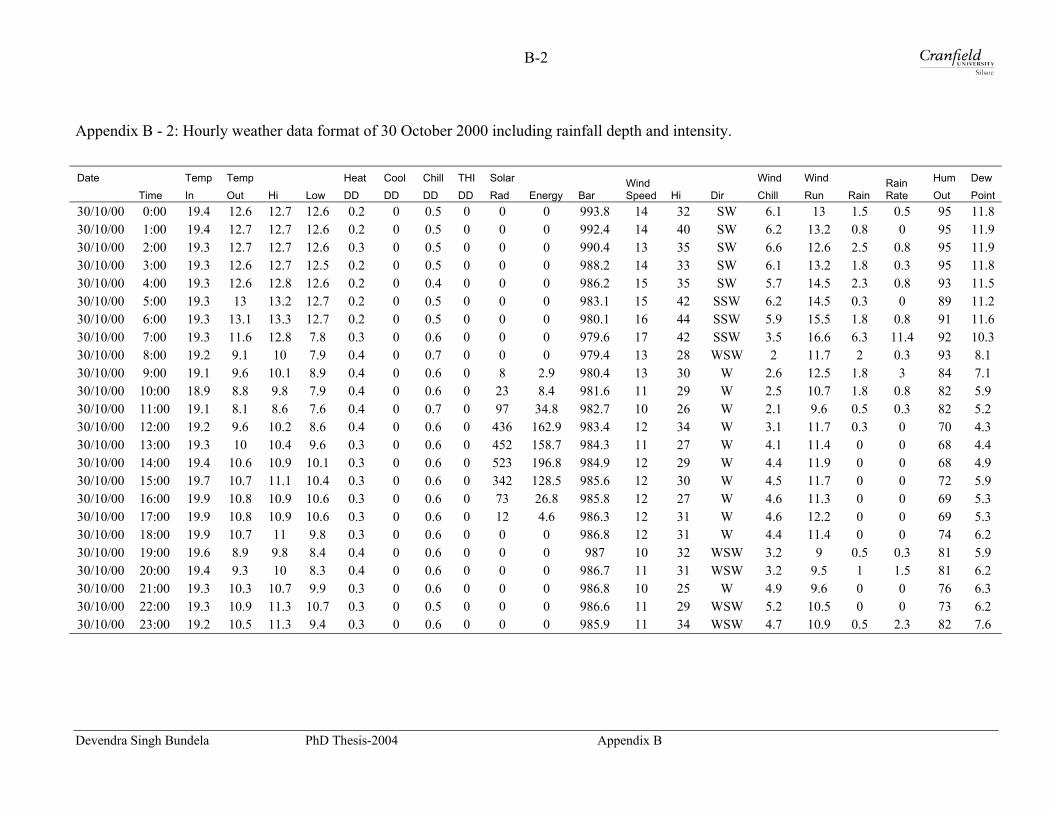
B-2
Appendix B - 2: Hourly weather data format of 30 October 2000 including rainfall depth and intensity.
Date Time In
Temp Temp Out Hi Low
Heat DD
Cool DD
Chill DD
THI DD
Solar Rad Energy Bar
Wind Speed Hi Dir
Wind Chill
Wind Run Rain
Rain Rate
Hum Out
Dew Point
30/10/00 0:00 19.4 12.6 12.7 12.6 0.2 0 0.5 0 0 0 993.8 14 32 SW 6.1 13 1.5 0.5 95 11.830/10/00
1:00 19.4 12.7 12.7 12.6 0.2 0 0.5 0 0 0 992.4 14 40 SW 6.2 13.2 0.8 0 95 11.930/10/00 2:00 19.3 12.7 12.7 12.6 0.3 0 0.5 0 0 0 990.4 13 35 SW 6.6 12.6 2.5 0.8 95 11.930/10/00 3:00 19.3 12.6 12.7 12.5 0.2 0 0.5 0 0 0 988.2 14 33 SW 6.1 13.2 1.8 0.3 95 11.830/10/00 4:00 19.3 12.6 12.8 12.6 0.2 0 0.4 0 0 0 986.2 15 35 SW 5.7 14.5 2.3 0.8 93 11.530/10/00 5:00 19.3 13 13.2 12.7 0.2 0 0.5 0 0 0 983.1 15 42 SSW 6.2 14.5 0.3 0 89 11.230/10/00 6:00 19.3 13.1 13.3 12.7
0.2 0 0.5 0 0 0 980.1 16 44 SSW 5.9 15.5 1.8 0.8 91 11.6
30/10/00 7:00 19.3 11.6 12.8 7.8 0.3 0 0.6 0 0 0 979.6 17 42 SSW 3.5 16.6 6.3 11.4 92 10.330/10/00 8:00 19.2 9.1 10 7.9 0.4 0 0.7 0 0 0 979.4 13 28 WSW 2 11.7 2 0.3 93 8.130/10/00 9:00 19.1 9.6 10.1 8.9 0.4 0 0.6 0 8 2.9 980.4 13 30 W 2.6 12.5 1.8 3 84 7.130/10/00 10:00 18.9 8.8 9.8 7.9 0.4 0 0.6 0 23 8.4 981.6 11 29 W 2.5 10.7 1.8 0.8 82 5.930/10/00 11:00 19.1 8.1 8.6 7.6 0.4 0 0.7 0 97 34.8 982.7 10 26 W 2.1 9.6 0.5 0.3
82 5.2
30/10/00 12:00 19.2 9.6 10.2 8.6 0.4 0 0.6 0 436 162.9 983.4 12 34 W 3.1 11.7 0.3
0 70 4.330/10/00 13:00 19.3 10 10.4 9.6 0.3 0 0.6 0 452 158.7 984.3 11 27 W 4.1 11.4 0 0 68 4.430/10/00 14:00 19.4 10.6 10.9 10.1 0.3 0 0.6 0 523 196.8 984.9 12 29 W 4.4 11.9 0 0 68 4.930/10/00 15:00 19.7 10.7 11.1 10.4 0.3 0 0.6 0 342 128.5 985.6 12 30 W 4.5 11.7 0 0 72 5.930/10/00 16:00 19.9 10.8 10.9 10.6 0.3 0 0.6 0 73 26.8
985.8 12 27 W 4.6 11.3 0 0 69 5.3
30/10/00 17:00 19.9 10.8 10.9 10.6 0.3 0 0.6 0 12 4.6 986.3 12 31 W 4.6 12.2 0 0 69 5.330/10/00 18:00 19.9 10.7 11 9.8 0.3 0 0.6 0 0 0 986.8 12 31 W 4.4 11.4 0 0 74 6.230/10/00 19:00 19.6 8.9 9.8 8.4 0.4 0 0.6 0 0 0 987 10 32 WSW 3.2 9 0.5 0.3 81 5.930/10/00 20:00 19.4 9.3 10 8.3 0.4 0 0.6 0 0 0 986.7 11 31 WSW 3.2 9.5 1 1.5 81 6.230/10/00 21:00 19.3 10.3 10.7 9.9 0.3 0 0.6 0 0 0 986.8 10 25 W 4.9 9.6 0 0 76 6.330/10/00 22:00 19.3 10.9 11.3 10.7
0.3 0 0.5 0 0 0 986.6 11 29 WSW 5.2 10.5 0 0 73 6.2
30/10/00 23:00 19.2 10.5 11.3 9.4 0.3 0 0.6 0 0 0 985.9 11 34 WSW 4.7 10.9 0.5 2.3 82 7.6
Devendra Singh Bundela PhD Thesis-2004 Appendix B

B-3
Appendix B - 3: Tentative dates for identifying possible heavy storms from daily rainfall data
Year Sep Rain (mm) Oct Rain (mm) Nov Rain (mm) Dec Rain (mm) Jan Rain (mm)
2001 0.3, 0.3, 5.6 1 0, 1.3, 0.3 0 0.8, 10.9, 9.1 27 18 2 24.9 29 16.3 5 26.2 3.3, 9.7 2, 0.8, 0.8 11.9, 0.5, 2 30 17.5 7 14 26 30 8 15 2000 0, 0, 2.3 0, 9.1, 5.8 9.7, 3.8 0.3, 4.1, 2.5 0 1 36.8 9 25.1 2 18.5 1 21.8 0, 0, 0.3 9.1 2.5, 0.3 7.9, 1, 0.8 15 25.4 11 29.5 5 34.5 7 18.3
0, 0, 12.7 12 69.1 6 18.5 7.9, 12.2, 12.4
19 19.8 0.3, 7.6, 13.5 12 25.4 29 23.1 30 26.2 1999 3.6, 0.3, 2.8 12.2, 5.3, 2.5 0 0.5, 5.1, 2.5 0 20 68.8 24 21.6 24 36.1 0.3, 2, 15 1.8 26 17.5 26 21.6 27 19.3 1998 0.3, 6.4 1 16.8 0 1.3, 2.8 0.8, 7.1, 7.6 3 13.7 23 17 1 15.5 4 17.8 8.1 2 16 0.3, 1.3, 0.8 25 12.4 3 13.2 30 31.8 26 10.9 1997 0 0, 0, 3.3 15.2, 6.9, 2 0, 0, 7.4 0 7 20.3 8 18 18 20.3 8 38.9 9 15.7 9 20.6 10 15.5 9.4 14, 2, 0.8 11 25.1 18 18.3 0, 0.3, 7.6 28 24.4
Storm identification rules: Rainfall on wet day should be more than 15mm and this should be preceded by one or
two day(s) of rain with minimum 5mm.
Devendra Singh Bundela PhD Thesis – 2004 Appendix B

B-4
Appendix B - 4: FEH parameters for the weather station and the Saltdean catchment
Parameter Weather Station, Falmer Saltdean National Grid Ref TQ 34600, 09000 TQ 38700, 04200 Grid Reference 534 600 m E; 109 000 m N 538 700 m E; 104 200 m N
Catchment descriptor AREA 8.71 6.92 FARL 1 1 PROPWET 0.34 0.34 ALTBAR 150 124 ASPBAR 170 171 ASPVAR 0.36 0.23 BFIHOST 0.967 0.957 DPLBAR 3.6 3.05 DPSBAR 117.9 164.2 LDP 5.99 5.27 RMED-1H 11.5 11.2 RMED-1D 37.9 36.5 RMED-2D 51.4 48.4 SAAR 928 862 SAAR4170 974 877 SPRHOST 5 5.9 URBCONC 0.639 -999999 URBEXT1990 0.014 0 URBLOC 0.114 -999999
Catchment average DDF parameter C -0.026 -0.026 D1 0.383 0.382 D2 0.314 0.285 D3 0.423 0.41 E 0.313 0.311 F 2.481 2.458
1 km grid point DDF parameter C -0.026 -0.026 D1 0.383 0.393 D2 0.315 0.282 D3 0.41 0.424 E 0.311 0.311 F 2.461 2.43
Devendra Singh Bundela PhD Thesis-2004 Appendix B

B-5
Appendix B - 5: Distribution and description of soil associations in the catchment Map unit Name Area (m2) Area (%) Soil description Geology 342a Upton 1 4046.5 0.05 Shallow silty over chalk Chalk 343h Andover 1 7157800 89.60 Shallow silty over chalk Chalk U343h Andover 1 45.7 ~ 0 Shallow silty over chalk Chalk 581e Marlow 827044 10.35 Deep loam to clay Plateau and river
terrace drift
Description of soil associations
Association Simple description Geology Dominant soil Andover 1 Shallow silty over chalk Chalk Shallow well drained calcareous silty soils
over chalk on slopes and crests Marlow Deep loam to clay Plateau and
river terrace drift
Well drained fine loamy over clayey and clayey soils.
Map unit Associated soil Site characteristics Land use Andover 1 Deep calcareous and non-
calcareous fine silty soils in valley bottoms
Striped soil patterns locally
Winter cereals and short term grassland with dairying and stock rearing; some woodland.
Marlow Some coarse and fine loamy over clayey soils with slowly permeable sub soils and slight seasonal waterlogging.
Cereals and short term grassland; coniferous woodland on slopes.
Devendra Singh Bundela PhD Thesis-2004 Appendix B

B-6
Appendix B - 6: Soil series associations in the Saltdean catchment
Andover soil association A) Shallow soils, chalk within 30 cm: silty
i) Brown topsoil : Andover ii) Grey topsoil : Upton iii) Dark, humose topsoil : Icknield B) Deeper soils a) Chalk within 80cm i) Subsoil calcareous above 40cm : Panholes ii) Subsoil non calcareous > 40cm : Garston b) Chalk below 80cm i) Subsoil calcareous above 80cm : Coombe or Millington ii) Subsoil non calcareous > 80cm : Charity Marlow soil association A) Soil with reddish or red mottled subsoil a) Loamy over clay 1) Unmottled i) Fine loamy over clay : Marlow ii) Fine silty over clayey : Carstens 2) Subsoil faintly mottled above 60 cm or distinctly mottled between 40 & 80 cm i) Coarse loamy over clay : Berkhamsted ii) Fine loamy over clayey : Hornbeam iii) Fine silty over clayey : Batcombe b) Clayey i) Chalk within 80 cm : Winchester ii) Chalk below 80 cm : Givendale B) Other soils; Unmottled i) Coarse loamy : Moulton ii) Fine loamy : Frilsham
Devendra Singh Bundela PhD Thesis-2004 Appendix B
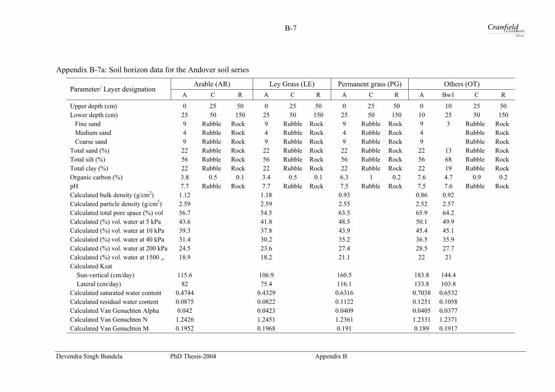
a Singh Bundela PhD Thesis-2004 Appendix B
B-7
Appendix B-7a: Soil horizon data for the Andover soil series
Arable (AR) Ley Grass (LE) Permanent grass (PG) Others (OT) Parameter/ Layer designation
A C R A C R A C R A Bw1 C R
Upper depth (cm) 0 25 50 0 25 50 0 25 50 0 10 25 50 Lower depth (cm) 25 50 150 25 50 150 25 50 150 10 25 50 150 Fine sand 9 Rubble Rock 9 Rubble Rock 9 Rubble Rock 9 3 Rubble Rock Medium sand 4 Rubble Rock 4 Rubble Rock 4 Rubble Rock 4 Rubble Rock Coarse sand 9 Rubble Rock 9 Rubble Rock 9 Rubble Rock 9 Rubble Rock Total sand (%)
22 Rubble Rock 22 Rubble Rock 22 Rubble Rock 22 13 Rubble RockTotal silt (%) 56 Rubble Rock 56 Rubble Rock 56 Rubble Rock 56 68 Rubble Rock Total clay (%) 22 Rubble Rock 22 Rubble Rock 22 Rubble
Rock 22 19 Rubble Rock
Organic carbon (%) 3.8 0.5 0.1 3.4 0.5 0.1 6.3 1 0.2 7.6 4.7 0.9 0.2pH 7.7 Rubble
Rock
7.7 Rubble
Rock
7.5 Rubble
Rock
7.5 7.6 Rubble
Rock Calculated bulk density (g/cm2) 1.12 1.18 0.93 0.86 0.92
Calculated particle density (g/cm2) 2.59 2.59 2.55 2.52 2.57Calculated total pore space (%) vol 56.7 54.5 63.5 65.9 64.2Calculated (%) vol. water at 5 kPa 43.6 41.8 48.5 50.1 49.9 Calculated (%) vol. water at 10 kPa 39.3 37.8 43.9 45.4 45.1 Calculated (%) vol. water at 40 kPa 31.4 30.2 35.2 36.5 35.9 Calculated (%) vol. water at 200 kPa 24.5 23.6 27.4 28.5 27.7 Calculated (%) vol. water at 1500 ,, 18.9 18.2 21.1 22 21 Calculated Ksat Sun-vertical (cm/day) 115.6 106.9 160.5 183.8 144.4 Lateral (cm/day) 82 75.4 116.1 133.8 103.8 Calculated saturated water content 0.4744 0.4329 0.6316 0.7038 0.6532 Calculated residual water content 0.0875 0.0822 0.1122 0.1251 0.1058 Calculated Van Genuchten Alpha 0.042 0.0423 0.0409 0.0405 0.0377 Calculated Van Genuchten N 1.2426 1.2451 1.2361 1.2331 1.2371 Calculated Van Genuchten M 0.1952 0.1968 0.191 0.189 0.1917
Devendr

B-8
Appendix B-7b: Soil horizon data for the Marlow soil series Arable (AR) Ley Grass (LE) Permanent grass (PG) Others (OT) Parameter/
Layer designation A E Bt C A E Bt C A E Bt C A E Bt CUpper depth (cm) 0 25 50 110 0 25 50 110 0 25 50 110 0 10 50 110 Lower depth (cm) 25 50 110 150 25 50 110 150 25 50 110 150 10 50 110 150 Fine sand 21 12 16 7 21 12 16 7 21 12 16 7 21 12 16 7 Medium sand 14 14 14 14 Coarse sand 6 6 6 6 Total sand (%)
41 29 29 15 41 29 29 15 41 29 29 15 41 29 29 15Total silt (%) 37 46 25 53 37 46 25 53 37 46 25 53 37 46 25 53Total clay (%) 22 25 46 32 22 25 46 32 22 25 46 32 22 25 46 32O C (%)
2.2 1 0.5 0.5 3.5 1 0.5 0.5 2.7 1 0.5 0.5 4.2 2 0.5 0.5
pH 6.7 5.4 5.7 5.7 5.9 5.4 5.7 5.7 6.3 5.4 5.7 5.7 5.6 5.4 5.7 5.7Calculated bulk density (g/cm2) 1.28 1.35 1.27 1.37 1.24 1.35 1.27 1.37 1.19 1.35 1.27 1.37 1.07 1.19 1.27 1.37Calculated particle density (g/cm2) 2.61 2.63 2.64 2.64 2.59 2.63 2.64 2.64 2.61 2.63 2.64 2.64 2.58 2.62 2.64 2.64Calculated total pore space (%) vol 51 48.7 51.9 48.1 52.2 48.7 51.9 48.1 54.3 48.7 51.9 48.1 58.5 54.5 51.9 48.1Calculated (%) vol. water at 5 kPa 37.9 38.3 44.3 41.7 38.3 38.3 44.3 41.7 40.4 38.3 44.3 41.7 43.3 40.6 44.3 41.7Calculated (%) vol. water at 10 kPa 34 34.8 41.2 38.5 34.3 34.8 41.2 38.5 36.2 34.8 41.2 38.5 38.8 36.9 41.2 38.5Calculated (%) vol. water at 40 kPa 27 28.4 35.3 32.3 27.2 28.4 35.3 32.3 28.7 28.4 35.3 32.3 30.7 30 35.3 32.3Calculated (%) vol. water at 200 kPa 21 22.8 29.8 26.6 21.2 22.8 29.8 26.6 22.3 22.8 29.8 26.6 23.8 23.8 29.8 26.6Calculated (%) vol. water at 1500 ,, 16.3 18.2 25.1 21.6 16.4 18.2 25.1 21.6 17.2 18.2 25.1 21.6 18.3 18.8 25.1 21.6Calculated Ksat Sub vertical (cm d-1 ) 116 63.9 25.7 14.6 132.9 63.9 25.7 14.6 134.4 63.9 25.7 14.6 167.5 134.4 25.7 14.6 Lateral (cm/day) 82.3 43.1 15 7.1 95.2 43.1 15 7.1 96.3 43.1 15 7.1 121.4 96.3 15 7.1Calculated saturated water content 0.3775 0.3444 0.4078 0.3538 0.3947 0.3444 0.4078 0.3538 0.4325 0.3444 0.4078 0.3538 0.5146 0.4158 0.4078 0.3538Calculated residual water content 0.0698 0.0755 0.1199 0.0888 0.0746 0.0755 0.1199 0.0888 0.0761 0.0755 0.1199 0.0888 0.0881 0.0856 0.1199 0.0888Calculated Van Genuchten Alpha 0.0546 0.0466 0.0485 0.0384 0.0544 0.0466 0.0485 0.0384 0.0541 0.0466 0.0485 0.0384 0.0534 0.0456 0.0485 0.0384Calculated Van Genuchten N 1.2501 1.2319 1.1993 1.212 1.2553 1.2319 1.1993 1.212 1.2475 1.2319 1.1993 1.212 1.2461 1.2328 1.1993 1.212Calculated Van Genuchten M 0.2001 0.1883 0.1662 0.1749 0.2034 0.1883 0.1662 0.1749 0.1984 0.1883 0.1662 0.1749 0.1975 0.1889 0.1662 0.1749
Devendra Singh Bundela PhD Thesis-2004 Appendix B
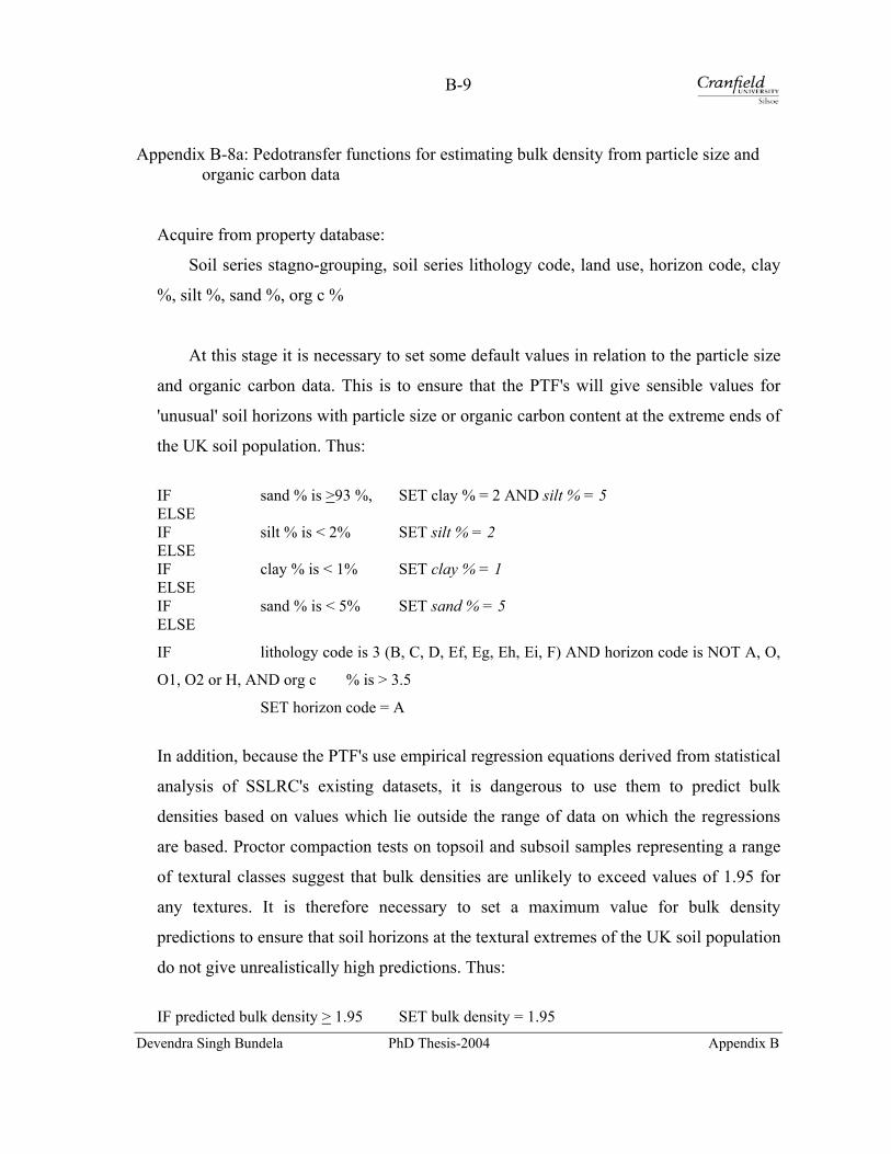
B-9
Appendix B-8a: Pedotransfer functions for estimating bulk density from particle size and
organic carbon data
Acquire from property database:
Soil series stagno-grouping, soil series lithology code, land use, horizon code, clay
%, silt %, sand %, org c %
At this stage it is necessary to set some default values in relation to the particle size
and organic carbon data. This is to ensure that the PTF's will give sensible values for
'unusual' soil horizons with particle size or organic carbon content at the extreme ends of
the UK soil population. Thus:
IF sand % is >93 %, SET clay % = 2 AND silt % = 5 ELSE IF silt % is < 2% SET silt % = 2 ELSE IF clay % is < 1% SET clay % = 1 ELSE IF sand % is < 5% SET sand % = 5 ELSE
IF lithology code is 3 (B, C, D, Ef, Eg, Eh, Ei, F) AND horizon code is NOT A, O,
O1, O2 or H, AND org c % is > 3.5
SET horizon code = A
In addition, because the PTF's use empirical regression equations derived from statistical
analysis of SSLRC's existing datasets, it is dangerous to use them to predict bulk
densities based on values which lie outside the range of data on which the regressions
are based. Proctor compaction tests on topsoil and subsoil samples representing a range
of textural classes suggest that bulk densities are unlikely to exceed values of 1.95 for
any textures. It is therefore necessary to set a maximum value for bulk density
predictions to ensure that soil horizons at the textural extremes of the UK soil population
do not give unrealistically high predictions. Thus:
IF predicted bulk density > 1.95 SET bulk density = 1.95
Devendra Singh Bundela PhD Thesis-2004 Appendix B

B-10
Then:
Compute: Bulk density (g/cm3) Db
Db
IF horizon code is H then:
= 0.575
ELSE IF horizon code is O then:
= 0.593 - (0.00745 x org c %)
ELSE IF horizon code is O1 then:
= 0.554 - (0.00589 x org c %)
ELSE IF horizon code is O2 then:
= 0.553 - (0.00797 x org c %)
ELSE IF horizon code is A AND land use is arable
= 1.46 - (0.0254 x Logeclay %) + (0.0279 x Logesand %) - (0.261 x Logeorg c %)
ELSE IF horizon code is A AND land use is ley
= 0.807 + (0.0989 x Logeclay %) + (0.106 x Logesand %) - (0.215 x Logeorg c %)
ELSE IF horizon code is A AND land use is permanent grass
= 0.999 + (0.0451 x Logeclay %) + (0.0784 x Logesand %) - (0.244 x Logeorg c
%)
ELSE IF horizon code is A AND land use is other
= 0.870 + (0.071 x Logeclay %) + (0.093 x Logesand %) - (0.254 x Logeorg c %)
ELSE IF horizon code is Bpodz
= 0.998 - (0.0702 x Logesilt %) + (0.0798 x Logesand %) - (0.131 x Logeorg c %)
ELSE IF stagno-grouping is non-stagno AND lithology code is 1 (Ec)
= 0.7132 - (0.0336 x org c %)
ELSE IF stagno-grouping is non-stagno AND lithology code is 2 (Ea, Eb, Ed, Ee)
= 1.56 - (0.00124 x silt %) - (0.00372 x clay %) - (0.0668 x org c %)
ELSE IF stagno-grouping is non-stagno AND lithology code is 3 (B, C, D, Ef, Eg, Eh, Ei, F)
AND horizon code is Eg
= 1.50 - (0.00067 x silt %) + (0.00262 x clay %) - (0.139 x org c %)
ELSE IF stagno-grouping is non-stagno AND lithology code is 3 (B, C, D, Ef, Eg, Eh, Ei, F)
AND horizon code is E
Devendra Singh Bundela PhD Thesis-2004 Appendix B

B-11
= 1.54 - (0.000583 x silt %) - (0.00008 x clay %) - (0.162 x org c %)
ELSE IF stagno-grouping is non-stagno AND lithology code is 3 (B, C, D, Ef, Eg, Eh, Ei, F)
AND horizon code is Bw1
= 1.55 - (0.00147 x silt %) - (0.00018 x clay %) - (0.209 x org c %)
ELSE IF stagno-grouping is non-stagno AND lithology code is 3 (B, C, D, Ef, Eg, Eh, Ei, F)
AND horizon code is Bg1
= 1.47 - (0.00727 x silt %) + (0.00716 x clay %) - (0.082 x org c %)
ELSE IF stagno-grouping is non-stagno AND lithology code is 3 (B, C, D, Ef, Eg, Eh, Ei, F)
AND horizon code is Bt
= 1.66 - (0.00069 x silt %) - (0.00827 x clay %) + (0.0123 x org c %)
ELSE IF stagno-grouping is non-stagno AND lithology code is 3 (B, C, D, Ef, Eg, Eh, Ei, F)
AND horizon code is Btg
= 1.67 + (0.000751 x silt %) - (0.0105 x clay %) + (0.0316 x org c %)
ELSE IF stagno-grouping is non-stagno AND lithology code is 3 (B, C, D, Ef, Eg, Eh, Ei, F)
AND horizon code is Bw2
= 1.54 - (0.00546 x silt %) + (0.00338 x clay %) - (0.160 x org c %)
ELSE IF stagno-grouping is non-stagno AND lithology code is 3 (B, C, D, Ef, Eg, Eh, Ei, F)
AND horizon code is Bg2
= 1.69 + (0.0021 x silt %) - (0.00231 x clay %) - (0.505 x org c %)
ELSE IF stagno-grouping is non-stagno AND lithology code is 3 (B, C, D, Ef, Eg, Eh, Ei, F)
AND horizon code is BC
= 1.49 - (0.00029 x silt %) + (0.00437 x clay %) - (0.314 x org c %)
ELSE IF stagno-grouping is non-stagno AND lithology code is 3 (B, C, D, Ef, Eg, Eh, Ei, F)
AND horizon code is C
= 1.50 - (0.00059 x silt %) + (0.00085 x clay %) - (0.254 x org c %)
ELSE IF stagno-grouping is stagno AND lithology code is 6 (Ef)
= 0.618 + (0.095 x Logesilt %) + (0.1 x Logeclay %) + (0.0195 x Logesand %)-
(0.178 x Logeorg c %)
ELSE IF stagno-grouping is stagno AND lithology code is 7 (Eg, Eh, Ei)
= -0.015 + (0.119 x Logesilt %) + (0.102 x Logeclay %) + (0.186 x Logesand %)-
(0.141 x Logeorg c %)
Devendra Singh Bundela PhD Thesis-2004 Appendix B

B-12
ELSE IF stagno-grouping is stagno AND lithology code is 10 (Fh, Fi, Fj, Fk, Fl)
= 1.96 - (0.0158 x Logesilt %) - (0.154 x Logeclay %) + (0.0102 x Logesand %)-
(0.113 x Logeorg c %)
ELSE IF stagno-grouping is stagno AND lithology code is LUMP1 OR LUMP2 (B, C, D, Fa,
Fb, Fc, Fd, Fe, Ff, Fg, Fm, Fn, Fo, Fp, Fq, Fr)
= 2.37 - (0.246 x Logesilt %) + (0.0266 x Logeclay %) - (0.0178 x Logesand %)-
(0.114 x Logeorg c %)
Devendra Singh Bundela PhD Thesis-2004 Appendix B

B-13
Appendix B-8b: Pedotransfer functions for deriving soil hydraulic properties from particle
size, organic carbon and bulk density data
Acquire from property database:
Soil series lithology code, horizon code, clay %, silt %, sand %, org c %, bulk den.
At this stage it is necessary to set some default values in relation to the particle size
and organic carbon data. This is to ensure that the PTF's will give sensible values for
'unusual' soil horizons with particle size or organic carbon content at the extreme ends of
the UK soil population. Thus:
IF sand % is >93 %, SET clay % = 2 AND silt % = 5 ELSE IF silt % is < 2% SET silt % = 2 ELSE IF clay % is < 1% SET clay % = 1 ELSE IF sand % is < 5% SET sand % = 5 ELSE IF pmlith is B, C, D, Ef, Eg, Eh, Ei, F AND horizon code is NOT A, O, O1, O2 or H, AND org c % is > 3.5 SET horizon code = A In addition, because the PTF's are based, at least in part, on theoretical relationships to
mineral particle size distribution, it is necessary to exclude all non-mineral horizons
comprising organic or carbonatic material, thin ironpans, or rock or rock rubble. Thus:
IF horizon code is O, O1, O2, H, or R, OR IF clay % is rock, rock rubble or thin
ironpan OR IF pmlith is Ec SET 'value' = -1
Then compute:
Particle density (g/cm3) PD
Total pore space (%vol) TP
Water content at saturation (% vol) θv0
Water content at 5 kPa tension (% vol) θv5
Water content at 10 kPa tension (% vol) θv10
Devendra Singh Bundela PhD Thesis-2004 Appendix B
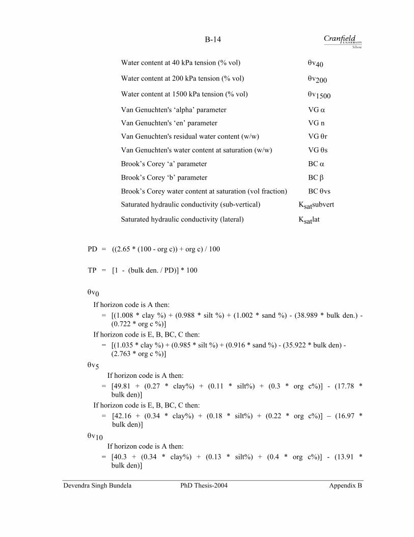
B-14
Water content at 40 kPa tension (% vol) θv40
Water content at 200 kPa tension (% vol) θv200
Water content at 1500 kPa tension (% vol) θv1500
Van Genuchten's ‘alpha’ parameter VG α
Van Genuchten's ‘en’ parameter VG n
Van Genuchten's residual water content (w/w) VG θr
Van Genuchten's water content at saturation (w/w) VG θs
Brook’s Corey ‘a’ parameter BC α
Brook’s Corey ‘b’ parameter BC β
Brook’s Corey water content at saturation (vol fraction) BC θvs
Saturated hydraulic conductivity (sub-vertical) Ksatsubvert
Saturated hydraulic conductivity (lateral) Ksatlat
PD = ((2.65 * (100 - org c)) + org c) / 100 TP = [1 - (bulk den. / PD)] * 100 θv0
If horizon code is A then: = [(1.008 * clay %) + (0.988 * silt %) + (1.002 * sand %) - (38.989 * bulk den.) -
(0.722 * org c %)] If horizon code is E, B, BC, C then: = [(1.035 * clay %) + (0.985 * silt %) + (0.916 * sand %) - (35.922 * bulk den) -
(2.763 * org c %)] θv5
If horizon code is A then: = [49.81 + (0.27 * clay%) + (0.11 * silt%) + (0.3 * org c%)] - (17.78 *
bulk den)] If horizon code is E, B, BC, C then: = [42.16 + (0.34 * clay%) + (0.18 * silt%) + (0.22 * org c%)] – (16.97 * bulk den)] θv10
If horizon code is A then: = [40.3 + (0.34 * clay%) + (0.13 * silt%) + (0.4 * org c%)] - (13.91 *
bulk den)]
Devendra Singh Bundela PhD Thesis-2004 Appendix B

B-15
If horizon code is E, B, BC, C then: = [30.86 + (0.4 * clay%) + (0.21 * silt%) + (1.26 * org c%)] – (12.46 * bulk den)] θv40
If horizon code is A then: = [26.68 + (0.39 * clay %) + (0.13 * silt %) + (0.46 * org c %)] - (7.72 *
bulk den)] If horizon code is E, B, BC, C then: = [22.05 + (0.47 * clay %) + (0.2 * silt %) + (0.93 * org c %)] – (9.56 * bulk den)] θv200
If horizon code is A then: = [9.38 + (0.47 * clay %) + (0.11 * silt %) + (0.69 * org c %)] If horizon code is E, B, BC, C then: = [4.31 + (1.08 * clay %) - (0.0079 * clay % 2)] θv1500
If horizon code is A then: = [6.11 + (0.4 * clay %) + (0.05 * silt %) + (0.5 * org c %)] If horizon code is E, B, BC, C then: = [1.25 + (0.92 * clay %) - (0.0062 * clay % 2)] VG θr = θv1500 / 2 / bulk den / 100
VG θs = θv0 / bulk den / 100
VG α = - 0.01926 + 0.438888 * [0.192526 * clay % -0.4 + 0.285901 * silt % -0.4 + 0.000157 * sand % 1.4 + 0.012966 * bulk den.]
VG n = 1.08235 + 0.426943 * [0.628785 * clay % -0.4 + 2.16201 * silt % -1.6 + 0.00000000372 * sand % 4 + 0.239019 * bulk den. *(org c % / clay %) 0.2]
(Check that VGα is greater than 0!) BC α = -4.9840297533 + 0.0509226283*sand +
0.1575152771*silt + 0.1240901644*bd - 0.1640033143*oc - 0.0021767278*silt**2 + 1.438224E-05*silt**3 + 8.040715E-04*clay**2 + 0.0044067117*oc**2
BC β = -0.8466880654 - 0.0046806123*sand +
0.0092463819*silt - 0.4542769707*bd - 0.0497915563*oc + 3.294687E-04*sand**2 -
Devendra Singh Bundela PhD Thesis-2004 Appendix B
1.689056E-06*sand**3 + 0.0011225373*oc**2

B-16
BC θvs = +0.2345971971 + 0.0046614221*sand +
0.0088163314*silt + 0.0064338641*clay - 0.3028160229*bd + 1.79762E-05*sand**2 - 3.134631E-05*silt**2
(Check that BC α and BC β are greater than 0!) Saturated hydraulic conductivity (sub-vertical) Ksatsubvert IF clay% <16, AND (silt% + (clay% * 2)) <31 AND (TP - θv0.05) < 7.5, then:
= 0.4535 *(TP - θv0.05)1.03423
ELSE, IF clay% <16, AND (silt% + (clay% * 2)) <31 Then:
= 8.03578 - (6.7707 * [TP - θv0.05]) + [0.833 * (TP - θv0.05)2]
ELSE, IF (TP - θv0.05) < 4.0,
then:
= 0.14143 * EXP0.46944 * (TP - θv0.05) ELSE:
= 5.8521 - (5.4125 * [TP - θv0.05]) + [1.05138 * (TP - θv0.05)2]
Saturated hydraulic conductivity (lateral) Ksatlat IF clay% <16, AND (silt% + (clay% * 2)) <31 AND (TP - θv0.05) < 7.5, then:
= 0.4535 *(TP - θv0.05)1.03423
ELSE, IF clay% <16, AND (silt% + (clay% * 2)) <31 then:
= 8.03578 - (6.7707 * [TP - θv0.05]) + [0.833 * (TP - θv0.05)2]
ELSE, IF (TP - θv0.05) < 5.5,
then:
= 0.14143 * EXP0.46944 * (TP - θv0.05) ELSE:
= 3.155 - (4.639 * [TP - θv0.05]) + [0.8143 * (TP - θv0.05)2]
Devendra Singh Bundela PhD Thesis-2004 Appendix B
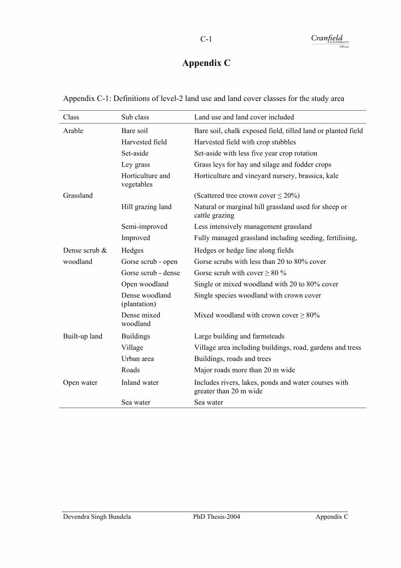
C-1
Appendix C
Appendix C-1: Definitions of level-2 land use and land cover classes for the study area
Class Sub class Land use and land cover included
Arable Bare soil Bare soil, chalk exposed field, tilled land or planted field Harvested field Harvested field with crop stubbles Set-aside Set-aside with less five year crop rotation Ley grass Grass leys for hay and silage and fodder crops Horticulture and
vegetables Horticulture and vineyard nursery, brassica, kale
Grassland (Scattered tree crown cover ≤ 20%) Hill grazing land Natural or marginal hill grassland used for sheep or
cattle grazing Semi-improved Less intensively management grassland Improved Fully managed grassland including seeding, fertilising,
Dense scrub & Hedges Hedges or hedge line along fields woodland Gorse scrub - open Gorse scrubs with less than 20 to 80% cover Gorse scrub - dense Gorse scrub with cover ≥ 80 % Open woodland Single or mixed woodland with 20 to 80% cover Dense woodland
(plantation) Single species woodland with crown cover
Dense mixed woodland
Mixed woodland with crown cover ≥ 80%
Built-up land Buildings Large building and farmsteads Village Village area including buildings, road, gardens and tress Urban area Buildings, roads and trees Roads Major roads more than 20 m wide
Open water Inland water Includes rivers, lakes, ponds and water courses with greater than 20 m wide
Sea water Sea water
Devendra Singh Bundela PhD Thesis-2004 Appendix C
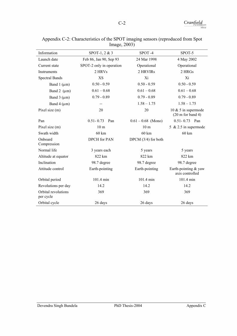
C-2
Appendix C-2: Characteristics of the SPOT imaging sensors (reproduced from Spot Image, 2003)
Information SPOT-1, 2 & 3 SPOT -4 SPOT-5 Launch date Feb 86, Jan 90, Sep 93 24 Mar 1998 4 May 2002 Current state SPOT-2 only in operation Operational Operational Instruments 2 HRVs 2 HRVIRs 2 HRGs Spectral Bands XS Xi Xi Band 1 (µm) 0.50 - 0.59 0.50 - 0.59 0.50 - 0.59
Band 2 (µm) 0.61 – 0.68 0.61 – 0.68 0.61 – 0.68
Band 3 (µm) 0.79 - 0.89 0.79 - 0.89 0.79 - 0.89
Band 4 (µm) -- 1.58 – 1.75 1.58 – 1.75 Pixel size (m) 20 20 10 & 5 in supermode
(20 m for band 4) Pan 0.51- 0.73 Pan 0.61 – 0.68 (Mono) 0.51- 0.73 Pan Pixel size (m) 10 m 10 m 5 & 2.5 in supermode Swath width 60 km 60 km 60 km Onboard Compression
DPCH for PAN DPCM (3/4) for both
Normal life 3 years each 5 years 5 years Altitude at equator 822 km 822 km 822 km Inclination 98.7 degree 98.7 degree 98.7 degree Attitude control Earth-pointing Earth-pointing Earth-pointing & yaw
axis controlled Orbital period 101.4 min 101.4 min 101.4 min Revolutions per day 14.2 14.2 14.2 Orbital revolutions per cycle
369 369 369
Orbital cycle 26 days 26 days 26 days
Devendra Singh Bundela PhD Thesis-2004 Appendix C

C-3
Appendix C-3: Availability of SPOT data from the SIRIUS archive
GRS Date SPOT
id Sensor ID Resolution
(m) Cloud cover
Quality Comment
033/247 5 May 2000 2 HRV-2 20 XS No OK ,, 18June 2000 1 HRV-1 20 XS No OK Selected ,, 18 June 2000 1 HRV-2 20 XS No OK
033/247 15 Oct 2000 1 HRV-1 20 XS Yes Not OK ,, 15 Oct 2000 1 HRV-2 20 XS Yes Not OK ,, 17 Oct 4 HRVIR 10 Pan Yes Not OK ,, 17 Oct 4 HRVIR 20 XS Yes Not OK 19 Oct 2 HRV-1 20 XS Little OK
,, 19 Oct 2 HRV-2 20 XS No OK ,, 26 Oct 1 HRV-1 20 XS No OK Selected ,, 29 Oct 2 HRV 20 XS Yes Not OK ,, 31 Oct 1 HRV 10 Pan Yes Not OK ,, 4 Nov 1 HRV 10 Pan No OK
032/247 30 May 2001 2 HRV 20 XS Yes Not OK 033/247 25 June 4 HRVIR 20 Xs No Incomplete
scene
,, 3 July 1 HRV 20 XS No Incomplete scene
032/247 30 July 4 HRVIR 10 Pan No Incomplete scene
,, 30 July 4 HRVIR 20 XS No Incomplete scene
Devendra Singh Bundela PhD Thesis-2004 Appendix C

C-4
Appendix C-4: Preprocessing levels and location accuracy of SPOT data
Standard preprocessing levels:
SPOT Scene products in the CAP format
Level 0 – Raw data collected at sensor (NOT distributed for SPOT sensors)
• Level 1A - radiometrically corrected image data
• Level 1B - radiometrically and geometrically corrected image data
• Level 2 A - radiometric and geometric corrections applied and projected to a standard
map projection (UTM, WGS 84) without ground control points (An entry level map
product)
SPOTView Products in the DIMAP Format
• Level 2B (Precision) - radiometric and geometric corrections applied and projected to a
standard map projection using ground control points for a better accuracy.
• Level 3 (Ortho) - radiometric and geometric corrections applied and projected to a
standard map projection using GCPs and a DTM
• Level S - radiometric processing and geometric resampling for two scene registration
o level S1 when one input scene is level 1B o level S2 when one input scene is level 2
Location accuracy of SPOT data
SPOT Scene SPOTView 3 (ortho) with DEM Satellite Band
1A 1B 2A 2B Reference3D Other sources
SPOT 1-3 20 m XS 10 m Pan
350 m 350 m
350 m
30 m
15 m
30 m
SPOT-4 10m XS 350 m 350 m 350 m 30 m 15 m 30 m SPOT-5 10 m XS
5 m XS 5 m Pan 2.5 m Pan
50 m 50 m 50 m 30 m 15 m 30 m
Devendra Singh Bundela PhD Thesis-2004 Appendix C
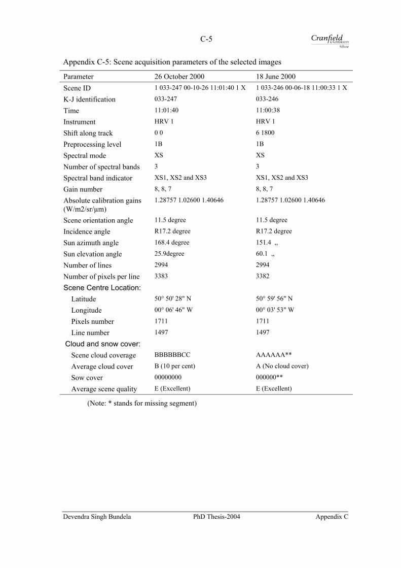
C-5
Appendix C-5: Scene acquisition parameters of the selected images
Parameter 26 October 2000 18 June 2000 Scene ID 1 033-247 00-10-26 11:01:40 1 X 1 033-246 00-06-18 11:00:33 1 X
K-J identification 033-247 033-246
Time 11:01:40 11:00:38
Instrument HRV 1 HRV 1
Shift along track 0 0 6 1800
Preprocessing level 1B 1B
Spectral mode XS XS
Number of spectral bands 3 3
Spectral band indicator XS1, XS2 and XS3 XS1, XS2 and XS3
Gain number 8, 8, 7 8, 8, 7
Absolute calibration gains (W/m2/sr/µm)
1.28757 1.02600 1.40646
1.28757 1.02600 1.40646
Scene orientation angle 11.5 degree 11.5 degree
Incidence angle R17.2 degree R17.2 degree
Sun azimuth angle 168.4 degree 151.4 ,,
Sun elevation angle 25.9degree 60.1 ,,
Number of lines 2994 2994
Number of pixels per line 3383 3382
Scene Centre Location:
Latitude 50° 50' 28" N 50° 59' 56" N
Longitude 00° 06' 46" W 00° 03' 53" W
Pixels number 1711 1711
Line number 1497 1497
Cloud and snow cover:
Scene cloud coverage BBBBBBCC AAAAAA**
Average cloud cover B (10 per cent) A (No cloud cover)
Sow cover 00000000 000000**
Average scene quality E (Excellent) E (Excellent)
(Note: * stands for missing segment)
Devendra Singh Bundela PhD Thesis-2004 Appendix C
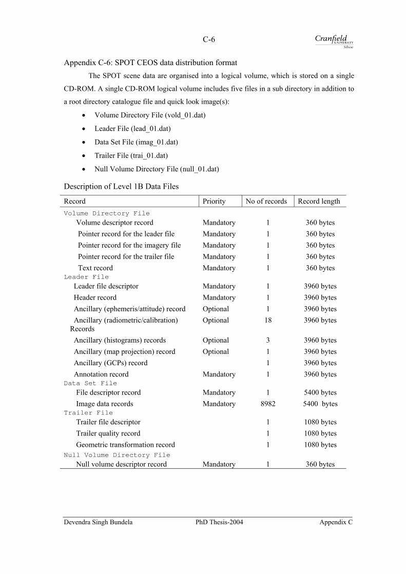
C-6
Appendix C-6: SPOT CEOS data distribution format The SPOT scene data are organised into a logical volume, which is stored on a single
CD-ROM. A single CD-ROM logical volume includes five files in a sub directory in addition to
a root directory catalogue file and quick look image(s):
• Volume Directory File (vold_01.dat)
• Leader File (lead_01.dat)
• Data Set File (imag_01.dat)
• Trailer File (trai_01.dat)
• Null Volume Directory File (null_01.dat)
Description of Level 1B Data Files
Record Priority No of records Record length Volume Directory File
Volume descriptor record Mandatory 1 360 bytes Pointer record for the leader file Mandatory 1 360 bytes Pointer record for the imagery file Mandatory 1 360 bytes Pointer record for the trailer file Mandatory 1 360 bytes Text record Mandatory 1 360 bytes
Leader File
Leader file descriptor Mandatory 1 3960 bytes Header record Mandatory 1 3960 bytes Ancillary (ephemeris/attitude) record Optional 1 3960 bytes Ancillary (radiometric/calibration) Records
Optional 18 3960 bytes
Ancillary (histograms) records Optional 3 3960 bytes Ancillary (map projection) record Optional 1 3960 bytes Ancillary (GCPs) record 1 3960 bytes Annotation record Mandatory 1 3960 bytes
Data Set File
File descriptor record Mandatory 1 5400 bytes Image data records Mandatory 8982 5400 bytes
Trailer File
Trailer file descriptor 1 1080 bytes Trailer quality record 1 1080 bytes Geometric transformation record 1 1080 bytes
Null Volume Directory File
Null volume descriptor record Mandatory 1 360 bytes
Devendra Singh Bundela PhD Thesis-2004 Appendix C

C-7
Appendix C-7 (a): Co-ordinates of 31 GCPs for geometric correction of 26 October sub image
GCP ID X Image Y Image X Map Y Map 1 2274.12 -1556.35 544323.0 102911.0 2 2202.18 -1344.18 543636.0 107355.0 3 2233.27 -1299.60 544433.0 108117.0 4 2293.55 -1254.53 545769.0 108787.0 5 2118.73 -1266.92 542263.0 109165.0 6 2047.75 -1105.44 541416.0 112568.0 7 1955.51 -1290.68 538984.0 109223.0 8 1814.01 -1462.02 535609.0 106359.0 9 1858.78 -1548.75 536167.0 104485.0
10 2002.19 -1632.06 538721.0 102345.0 11 1770.74 -1342.72 535175.0 108858.0 12 1632.40 -1337.98 532476.0 109437.0 13 1445.48 -1435.24 528465.0 108167.0 14 1451.11 -1231.06 529274.0 112163.0 15 1465.01 -1130.49 529915.0 114097.0 16 1239.07 -1492.25 524190.0 107740.0 17 1322.25 -1111.99 527153.0 114958.0 18 1076.67 -1591.27 520665.0 106340.0 19 980.76 -1238.03 520005.0 113657.0 20 1055.16 -1427.79 520812.0 109662.0 21 1054.84 -1340.87 521091.0 111367.0 22 1158.11 -1345.63 523126.0 110907.0 23 1596.33 -1564.08 530984.0 105097.0 24 1648.48 -1234.26 533160.0 111420.0 25 1936.64 -1531.92 537774.0 104563.0 26 1906.02 -1165.05 538442.0 111894.0 27 1925.59 -1452.82 537840.0 106158.0 28 2176.04 -1449.64 542768.0 105353.0 29 1311.05 -1224.59 526540.0 112788.0 30 2046.82 -1573.25 539788.0 103364.0 31 1294.61 -1029.59 526895.0 116669.0
Total RMSE : 0.669
Devendra Singh Bundela PhD Thesis-2004 Appendix C

C-8
Appendix C-7 (b): Coordinates of 26 GCPs for geometric correction of 18 June sub image
GCP ID X Image Y Image X Map Y Map
1 2313.13 -2431.13 544320 102914 2 2239.38 -2222.38 543595 107254 3 2157.63 -2140.63 542271 109172 4 2086.88 -1979.88 541434 112576 5 2332.63 -2128.38 545761 108803 6 1809.88 -2218.13 535163 108849 7 1334.63 -1904.13 526901 116690 8 1361.88 -1986.63 527155 114959 9 1541.375 -2244.13 529791 109270 10 1484.88 -2311.38 528453 108134 11 1268.13 -2390.38 523912 107326 12 1122.63 -2451.88 520837 106611 13 1023.38 -2296.63 519424 110014 14 1021.13 -2113.38 520012 113638 15 1179.52 -2239.00 522701 110615 16 1089.22 -2547.51 519845 104851 17 1615.40 -2417.22 530645 105595 18 1671.54 -2213.32 532463 109420 19 1853.74 -2340.96 535607 106259 20 1898.49 -2423.84 536187 104475 21 2041.49 -2507.26 538706 102343 22 1976.35 -2406.37 537781 104559 23 2215.21 -2323.21 542773 105355 24 1994.09 -2165.38 538964 109240 25 1904.61 -2033.25 537659 112161 26 1661.30 -2106.72 532621 111554
Total RMSE : 0.401
Devendra Singh Bundela PhD Thesis-2004 Appendix C

C-9
Appendix C-8: Selected ground segments in the unaligned systematic random scheme
with their upper left corner co-ordinates
1 (2)
521 000 114 000
2 (12)
270 000 112 000
3 (9)
528 000 112 000
4 (4)
535 000 114 000
5 (14)
537 000 111 000
(16)
x 6 (4) 523 000 110 000
7 (3) 526 000 110 000
(14)
529 000 107 000 Urban
(13)
532 000 107 000 Urban
8 (14)
537 000 107 000
9 (3)
540 000 110 000
(10)
Sea
(15)
Sea
(1) 528 000 106 000 Urban
10 (3)
534 000 106 000
11 (7)
538 000 105 000
(8)
X
Sea
Sea
Sea
Sea
(14)
Sea
(6)
Sea
Note:
First bold number on the left hand side in a block shows the segment ID of the selected
sample.
Number in parentheses on the right hand side in the block shows the segment number selected randomly from a 16-segment block.
Devendra Singh Bundela PhD Thesis-2004 Appendix C
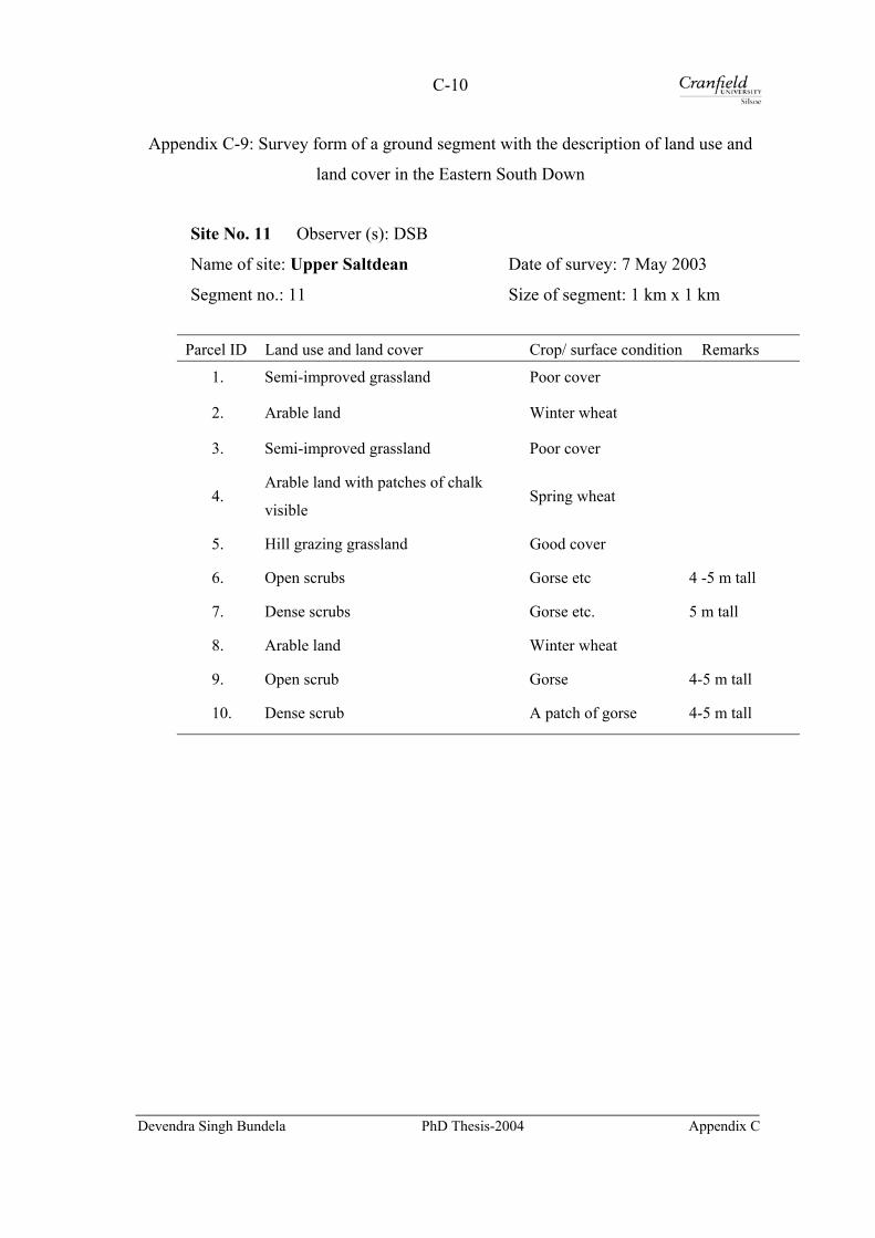
C-10
Appendix C-9: Survey form of a ground segment with the description of land use and
land cover in the Eastern South Down
Site No. 11 Observer (s): DSB
Name of site: Upper Saltdean Date of survey: 7 May 2003
Segment no.: 11 Size of segment: 1 km x 1 km
Parcel ID Land use and land cover Crop/ surface condition Remarks
1. Semi-improved grassland Poor cover
2. Arable land Winter wheat
3. Semi-improved grassland Poor cover
4. Arable land with patches of chalk
visible Spring wheat
5. Hill grazing grassland Good cover
6. Open scrubs Gorse etc 4 -5 m tall
7. Dense scrubs Gorse etc. 5 m tall
8. Arable land Winter wheat
9. Open scrub Gorse 4-5 m tall
10. Dense scrub A patch of gorse 4-5 m tall
Devendra Singh Bundela PhD Thesis-2004 Appendix C

C-11
Appendix C-10: Accuracy of georeferencing of scanned segments
Segment ID RMS error
1. 1.146
2. 0.563
3. 1.114
4. 0.960
5. 0.974
6. 0.979
7. 1.137
8. 0.739
9. 0.446
10. 0.686
11. 0.424
Average 0.833 (pixels)
(Details of a segment ID, please refer Appendix C.8.)
Appendix C-11: Aggregation of scheme classes during direct area estimation
Class Aggregation of classes
Bare soil 10
Harvested fields with stubbles
11
Set-aside /fallow 12
Semi-improved grassland 20+21
Hill grazing grassland 22+23
Improved grassland 24+25
Open woodland 31+33
Dense woodland 32+34+35
Built-up land 40+41+42
(Class number stands for the level-2 class in the classification scheme Table 4.2)
Devendra Singh Bundela PhD Thesis-2004 Appendix C
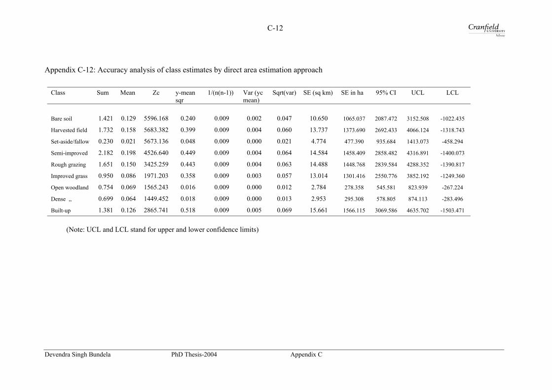
C-12
Appendix C-12: Accuracy analysis of class estimates by direct area estimation approach
Class Sum Mean Zc y-mean
sqr 1/(n(n-1)) Var (yc
mean) Sqrt(var) SE (sq km) SE in ha 95% CI UCL LCL
Bare soil 1.421
0.129 5596.168 0.240 0.009 0.002 0.047 10.650 1065.037 2087.472 3152.508 -1022.435
Harvested field 1.732 0.158 5683.382 0.399 0.009 0.004 0.060 13.737 1373.690 2692.433 4066.124 -1318.743
Set-aside/fallow 0.230 0.021 5673.136 0.048 0.009 0.000 0.021 4.774 477.390 935.684 1413.073 -458.294
Semi-improved 2.182 0.198 4526.640 0.449 0.009 0.004 0.064 14.584 1458.409 2858.482 4316.891 -1400.073
Rough grazing 1.651 0.150 3425.259 0.443 0.009 0.004 0.063 14.488 1448.768 2839.584 4288.352 -1390.817
Improved grass 0.950 0.086 1971.203 0.358 0.009 0.003 0.057 13.014 1301.416 2550.776 3852.192 -1249.360
Open woodland 0.754 0.069 1565.243 0.016 0.009 0.000 0.012 2.784 278.358 545.581 823.939 -267.224
Dense ,, 0.699 0.064 1449.452 0.018 0.009 0.000 0.013 2.953 295.308 578.805 874.113 -283.496
Built-up 1.381 0.126 2865.741 0.518 0.009 0.005 0.069 15.661 1566.115 3069.586 4635.702 -1503.471
(Note: UCL and LCL stand for upper and lower confidence limits)
Devendra Singh Bundela PhD Thesis-2004 Appendix C
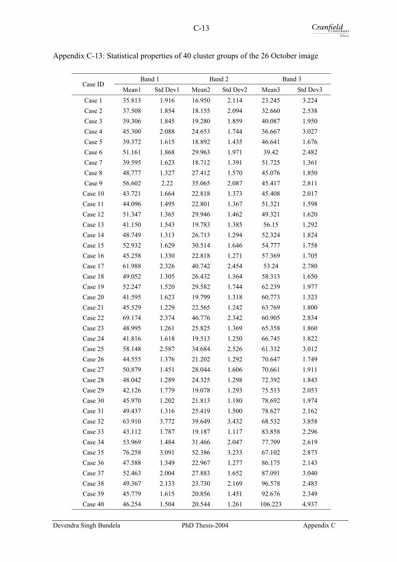
C-13
Appendix C-13: Statistical properties of 40 cluster groups of the 26 October image
Band 1 Band 2 Band 3 Case ID
Mean1 Std Dev1 Mean2 Std Dev2 Mean3 Std Dev3 Case 1 35.813 1.916 16.950 2.114 23.245 3.224 Case 2 37.508 1.854 18.155 2.094 32.660 2.538 Case 3 39.306 1.845 19.280 1.859 40.087 1.950 Case 4 45.300 2.088 24.653 1.744 36.667 3.027 Case 5 39.372 1.615 18.892 1.435 46.641 1.676 Case 6 51.161 1.868 29.963 1.971 39.42 2.482 Case 7 39.595 1.623 18.712 1.391 51.725 1.361 Case 8 48.777 1.327 27.412 1.570 45.076 1.850 Case 9 56.602 2.22 35.065 2.087 45.417 2.811
Case 10 43.721 1.664 22.818 1.373 45.408 2.017 Case 11 44.096 1.495 22.801 1.367 51.321 1.598 Case 12 51.347 1.365 29.946 1.462 49.321 1.620 Case 13 41.150 1.543 19.783 1.385 56.15 1.292 Case 14 48.749 1.313 26.713 1.294 52.324 1.824 Case 15 52.932 1.629 30.514 1.646 54.777 1.758 Case 16 45.258 1.330 22.818 1.271 57.369 1.705 Case 17 61.988 2.326 40.742 2.454 53.24 2.780 Case 18 49.052 1.305 26.432 1.364 58.313 1.650 Case 19 52.247 1.520 29.582 1.744 62.239 1.977 Case 20 41.595 1.623 19.799 1.318 60.773 1.323 Case 21 45.529 1.229 22.565 1.242 63.769 1.800 Case 22 69.174 2.374 46.776 2.342 60.905 2.834 Case 23 48.995 1.261 25.825 1.369 65.358 1.860 Case 24 41.816 1.618 19.513 1.250 66.745 1.822 Case 25 58.148 2.587 34.684 2.526 61.332 3.012 Case 26 44.555 1.376 21.202 1.292 70.647 1.749 Case 27 50.879 1.451 28.044 1.606 70.661 1.911 Case 28 48.042 1.289 24.325 1.298 72.392 1.843 Case 29 42.126 1.779 19.078 1.293 75.513 2.053 Case 30 45.970 1.202 21.813 1.180 78.692 1.974 Case 31 49.437 1.316 25.419 1.500 78.627 2.162 Case 32 63.910 3.772 39.649 3.432 68.532 3.858 Case 33 43.112 1.787 19.187 1.117 83.858 2.296 Case 34 53.969 1.484 31.466 2.047 77.709 2.619 Case 35 76.258 3.091 52.386 3.233 67.102 2.873 Case 36 47.588 1.349 22.967 1.277 86.175 2.143 Case 37 52.463 2.004 27.883 1.652 87.091 3.040 Case 38 49.367 2.133 23.730 2.169 96.578 2.483 Case 39 45.779 1.615 20.856 1.451 92.676 2.349 Case 40 46.254 1.504 20.544 1.261 106.223 4.937
Devendra Singh Bundela PhD Thesis-2004 Appendix C

C-14
Appendix C-14: Regrouping 40 clusters into 11 classes Class Case
Ward’s method and SED Between Linkage and SED Regrouping tool Case 1 1 7 1 Case 2 1 6 2 Case 3 1 6 3 Case 4 2 9 3 Case 5 3 8 3 Case 6 2 9 3 Case 7 3 8 3 Case 8 2 9 3 Case 9 4 4 3 Case 10 3 8 3 Case 11 3 8 3 Case 12 4 5 3 Case 13 5 1 3 Case 14 4 5 3 Case 15 4 5 6 Case 16 5 1 3 Case 17 4 4 5 Case 18 5 1 7 Case 19 6 5 3 Case 20 5 1 3 Case 21 7 1 3 Case 22 8 10 3 Case 23 7 1 3 Case 24 7 1 8 Case 25 6 5 3 Case 26 7 1 3 Case 27 9 2 3 Case 28 7 1 3 Case 29 7 1 3 Case 30 10 2 3 Case 31 10 2 11 Case 32 6 11 3 Case 33 10 2 3 Case 34 9 2 3 Case 35 8 10 3 Case 36 10 2 9 Case 37 11 2 4 Case 38 11 3 3 Case 39 11 3 3 Case 40 11 3 10
(SED stands for squared Euclidean distance)
Devendra Singh Bundela PhD Thesis-2004 Appendix C

C-15
Appendix C-15: Signature separability of 11 classes with the Transformed Divergence and Jefferies-Matusita distance methods
Transformed divergence distance Class 1 2 3 4 5 6 7 8 9 10 11
1 0 2 1903 0 3 2000 1952 0 4 2000 1882 1545 0 5 2000 2000 1939 1902 0 6 2000 2000 1760 1985 1594 0 7 2000 2000 2000 2000 2000 1895 0 8 2000 2000 1953 2000 1991 1233 1606 0 9 2000 2000 1998 1988 1429 1877 2000 2000 0
10 2000 2000 2000 2000 1997 2000 2000 2000 1724 0 11 2000 1926 1083 1245 1865 1871 2000 1998 1979 2000 0
Best average separability: 1893.03 and Best minimum separability: 1082.75
Jefferies-Matusita distance Class 1 2 3 4 5 6 7 8 9 10 11
1 0
2 1365 0
3 1414 1345 0
4 1414 1296 1222 0
5 1414 1414 1368 1358 0
6 1414 1413 1286 1396 1213 0
7 1414 1414 1414 1414 1414 1374 0
8 1414 1414 1389 1414 1408 1079 1227 0
9 1414 1414 1413 1409 1184 1367 1414 1414 0
10 1414 1414 1414 1414 1411 1414 1414 1414 1267 0
11 1414 1367 950 1059 1260 1331 1414 1412 1392 1414 0
Best average separability: 1358.94 and
Best minimum separability: 1082.75 Class Name of class 1 Arable2 2 Arable3 3 Arable4 4 Arable5 5 Arable fallow/set aside 6 Hill grazing grassland 7 Improved grassland 8 Semi-improved grassland 9 Open woodland and scrub 10 Dense woodland and scrub 11 Built-up land
Devendra Singh Bundela PhD Thesis-2004 Appendix C

C-16
Appendix C-16: Calibration method of the SPOT HRV-1 sensor
For SPOT-1 HRV sensor, the complex model to describe instrument behaviour is expressed as:
jkjkjmkkjmk CLgGAx +=
where xjmk is the raw digital output, k identifies the spectral band,
j is the pixel number along the spectral line,
m is the onboard gain number. Ak is the absolute
calibration coefficient,
Gmk is the viewing gain coefficient, gj is the pixel relative sensit
coefficient) and Cjk is the dark signal.
The equalisation process first determines the coefficients, Cjk an
normalisation is carried out to compute level 1A data:
jkmkkj
jkjmkjmk LGA
gCx
X =−
=
For calibration of level 1B data, Xjmk is the digital numbers (DNs)
simple equation:
DN = L0k * A0k* Gmk or L0k= DN/ (A0*Gmk) where, L0k is the radiance at sensor for a spectral band k, A0k is th
coefficient for a band k, and Gmk is the viewing gain coefficient for the ba
Gain coefficient is different for each sensor and is calculated with
from the following equations:
Gmk = 1.3 (m-3) for SPOT-1 Gmk = 1.5 (m-2) for SPOT-4
where m is the viewing gain number associated with the signal amplifiers
for SPOT system. The onboard gain number, m is given in the leader file (
740)
Gmk and Ak coefficients should be determined independently for arriving a
equivalent radiance. The absolute calibration coefficients are estimated on
account the change in detector sensitivity. This update coefficient table ca
the supplier and then coefficients for image acquisition date are interpolate
For 26 Oct 2000 image, gain coefficients were determined independently
coefficients could not be determined; as coefficient table was not up
imagery acquisition so alternative method was adopted. In this method, a
Devendra Singh Bundela PhD Thesis-2004
255
DN
ivity (equalisa
d gj, and then
and is express
e absolute cal
nd k
a very good a
and varies from
record 2, byte
t a more accur
a regular basi
n be requested
d from the tab
. Absolute ca
dated till the
multiplication
App
L
tion
dete
ed i
ibrat
ccur
1
s 72
ate
s to
from
le.
libra
dat
pro
end
Gain
ctor
n
ion
acy
to 8
5-
tion
e of
duct
ix C
C-17
(Ak*Gmk) called absolute calibration gain was used and is directly supplied in the leader file
(record 2, bytes 1765-2276). The accuracy of leader file supplied value is about 10%.
The final calibration equation can be expressed as:
kkk ADNL '/0 = Where L0k is the radiance measured at sensor for spectral band, k; A’k is the absolute calibration
gain for band k (W-1m2 sr µm) read directly from the leader file; and DNk is the digital number
for the band k.
Conversion of spectral radiance to exoatmospheric reflectance The apparent reflectance, ρ0, is related to the measured radiance, L0 to the solar irradiance
incident at the top of the atmosphere and is given as
)(*** 2
00 SZCosE
dL
sun
πρ =
where, ρ0 is the exoatmospheric reflectance at the satellite (0-1), L0 is the spectral radiance at
sensor aperture in W m-2 ster-1 µm-1.and d2 is the square of the Earth-Sun distance in
astronomical units (~149.6 x 10⁶ km) and is expressed as:
d = (1 - 0.01674 Cos (0.9856 (JD-4)))
where JD is the Julian Day of the image acquisition.
Note: The unit for the argument of the cosine function of 0.9856 x (JD-4) will be in
degrees.
Esun is the mean solar exoatmospheric irradiance in W m-2 µm-1 and SZ is the sun zenith
angle in radians at time of scene acquisition. Esun values can be obtained from the Spot Image
website.
Table: Solar equivalent irradiances for SPOT –1 (watt/sq m/micrometres) Band Bandwidth HRV-1 HRV-2 P/M 0.50-0.73 1680 1690 XS1 0.50-0.59 1855 1845 XS2 0.61-0.68 1615 1575 XS3 0.79-0.89 1090 1040
The zenith angle (SZ) is calculated by subtracting the sun elevation from 90° .
Devendra Singh Bundela PhD Thesis-2004 Appendix C

E-1
Appendix E
Appendix E-1: Average slope of the Saltdean catchment from a 20 m PulSAR DEM
Slope group (%) Area (%)
≤ 5 10.2
5-10 21.5
10-15 23.3
15-20 17.4
20-25 10.9
25-30 7.2
30-35 4.2
35-40 2.3
40-45 1.3
45-50 0.6
> 50 1.2
Average slope 17.23
Appendix E-2: Catchment area and cumulative rainfall calculations by two LISEM versions
Catchment area (ha) Cumulative rainfall (mm) 20 m resampled DEM
Original resolution
Ver 2.03 Ver 2.158 Ver 2.03 Ver 2.158
PulSAR DEM 25 m 811.160 832.050 16.601 16.184
Cartometric DEM 20 m 811.160 823.728 16.601 16.348
Landmap DEM 25 m 811.160 829.694 16.601 16.230
SRTM DEM 75 m 811.160 822.634 16.601 16.370
ASTER DEM 30 m 811.160 825.033 16.601 16.322
Devendra Singh Bundela PhD Thesis-2004 Appendix E

E-2
Appendix E-3: Rainfall intensity breakpoint pair file of the storm with a standard structure
RUU CSF TIMESERIE INTENSITY NORMAL 1 Raingauge_station_1 (time in min and rainfall intensity in mm/h)
0 0
60 0.8
120 11.4
180 0.3
240 3.0
300 0.8
360 0.3
420 0
750 0
Devendra Singh Bundela PhD Thesis-2004 Appendix E

E-3
Appendix E-4: Import and export of key spatial data to and from PCRaster
Creating a clone map of the Saltdean catchment using a ‘mapattr’ operator
mapattr <filename.map>
The following raster and geographic attributes of the Saltdean catchment are required to
create a clone map at a 20 m grid-cell size, for an example:
No. of rows : 229 No. of columns : 179 Data type : Scalar Cell representation : Small integer Projection : Y increases from bottom to top X_ULC : 536112.9 Y_ULC : 107974.0 Cell length : 20.0 Angle (degree) : 0.0 File_id : 0
Set the clone map as a global map using --clone function.
Import the ArcInfo GRID ASCII format data of DEM, landuse, soils, and raingauge base
maps using an asc2map operator
asc2map [options] <ArcInfo GRID ASCII file> <PCRaster output file> For an example, asc2map --clone <clonemap file> -<data type> -a <GRID ASCII filename>
<PCRaster output file>
Export of a PCRaster map to a GRID ASCII format, for an example:
Map2asc –m < null value> -a <input file> <output file>
Devendra Singh Bundela PhD Thesis-2004 Appendix E
E-4
Appendix E-5: PCRaster script for the creation of a LISEM database from key spatial data #! -f --matrixtable --lddin binding # binding section # Catchment key maps of various grid cell sizes dem = saltdemp20.map; # InSAR DEM derived from an ERS SAR pair landuse = saltlusep20.map; # Land use map from SPOT Data soil = saltsoilp20.map; # National Soil map (NATMAP) rgauge=rgauge.map # Raingauge location map mask = mask.map; # Mask for the catchment area # Catchment input tables utable1 = salt_utable.txt; # Crop and soil parameter table utable2 = infil_utable.txt; # Infiltration parameter table # CROP AND SOIL PARAMETER BASE TABLE # ---------------------------------- # 1 Surface cover (fraction) # 2 Crop and vegetation height (m) # 3 LAI (m2/m2) # 4 RR (cm) # 5 Manning's roughness coefficient, n (-) # 6 Aggregate stability (number) # 7 Soil cohesion (kPa) # 8 Additional cohesion by plant roots (kPa) # 9 Soil median texture, D50( µm) # 10 Road width (m) # 11 Grass width (m) # 12 Crust cover (m) # 13 Compacted soil (m) # 14 Stoniness (m) # INFILTRATION PARAMETER BASE TABLE # --------------------------------- # 15 Saturated hydraulic conductivity, ksat1 (mm/h) # 16 Average moisture section head, psi1 (cm) # 17 Saturated moisture content, (Porosity1) (cm3/cm3) # 18 Initial moisture content1 (cm3/cm3) # 19 Soil depth1 (cm) # Input constants Chanwidth = 1.5; # Channel width Chanside = 1; # 1 for 45 degree side slope channel # INPUT PARAMETER MAPS # Catchment parameters Ldd = ldd.map; # Local drain direction area = area.map; # Catchment area based on an outlet(boolean) Devendra Singh Bundela PhD Thesis-2004 Appendix E
E-5
area1 = area1.map; # Catchment area based on an outlet grad = grad.map; # Slope map outlet = outlet.map; # Location of outlets in the catchment id = id.map; # Rainfall intensity distribution map # Landuse and vegetation parameters per=per.map; ch=ch.map; lai=lai.map; roadwidt = roadwidt.map; grasswid=grasswid.map; # Soil surface parameters rr=rr.map; mann=n.map; crustfrc=crustfrc.map; compfrc=compfrc.map; stonefrc=stonefrc.map; # Soil erosion parameters aggrstab = aggrstab.map; coh = coh.map; cohadd = cohadd.map; D50 = d50.map; # Channel parameters chanmask= chanmask.map; lddchan = lddchan.map; chanwidt = chanwidt.map; chanside = chanside.map; changrad = changrad.map; chanman = chanman.map; chancoh = chancoh.map;
# Soil infiltration parameters: a single layer Green-Ampt model ksat1=ksat1.map; psi1=psi1.map; thetas1=thetas1.map; thetai1=thetai1.map; soildep1=soildep1.map; # Additional parameters for second layer G-A model (NOT USED) # ksat2=ksat2.map; # psi2=psi2.map; # thetas2=thetas2.map; # thetai2=thetai2.map; # soildep2=soildep2.map; areamap # Areamap section of the script mask; # Area map must exist along with base maps # or declare any base map as areamap initial # Initial section of the script Devendra Singh Bundela PhD Thesis-2004 Appendix E
E-6
# GENERATION OF THE LISEM DATABASE # Catchment parameters report Ldd = lddcreate(dem, 1e20,1e20,1e20,1e20); report outlet = pit(Ldd); report area1 = catchment(Ldd, outlet); # Area based on outlet report area = boolean(area1); report grad = max(0.001, sin(atan(slope(dem)))); # grad > 0.001 report id = spreadzone (rgauge, 0, 1); # Thiessen polygon #report id = spreadzone (rgauge,0,slope(dem))# by geomorphology
# Land use and vegetation parameters report per = lookupscalar(utable1, 1, landuse); report ch = lookupscalar(utable1, 2, landuse); report lai = lookupscalar(utable1, 3, landuse); report roadwidt = lookupscalar(utable1, 10, landuse); report grasswid = lookupscalar(utable1, 11, landuse); # Soil surface parameters report rr = lookupscalar(utable1, 4, landuse); report mann = lookupscalar(utable1, 5, landuse); report crustfrc= lookupscalar(utable1, 12, landuse); report compfrc = lookupscalar(utable1, 13, landuse); report stonefrc = lookupscalar(utable1, 14, landuse);
# Soil erosion parameters report aggrstab = lookupscalar(utable1, 6, landuse); report coh = lookupscalar(utable1, 7, landuse); report cohadd = lookupscalar(utable1, 8, landuse); report D50 = lookupscalar(utable1, 9, landuse); # Channel parameters report chanmask =scalar(if(accuflux(Ldd,cellarea())gt 680000,1)); report lddchan =lddcreate((dem*chanmask),1e20,1e20,1e20,1e20); report chanwidt = scalar( if (chanmask ne 0, Chanwidth)); report chanside = scalar( if (chanmask ne 0, Chanside)); report changrad =(grad*chanmask); report chancoh= ((coh + cohadd)*chanmask); report chanman= (mann*chanmask); # option chancoh=chanmask*scalar(Chancoh); # option chanman=chanmask*scalar(Chanman); # Parameters for a single layer GREEN and AMPT model report ksat1 = lookupscalar(utable2, 15, soil); report psi1 = lookupscalar(utable2, 16, soil); report thetas1 = lookupscalar(utable2, 17, soil); report thetai1 = lookupscalar(utable2, 18, soil); report soildep1 = lookupscalar(utable2, 19, soil);
# END
Devendra Singh Bundela PhD Thesis-2004 Appendix E

E-7
Appendix E-6: Batch file script for displaying a LISEM database
:: Batch file script for displaying a LISEM input parameter database :: saltinput.bat <File name> CLS @echo off echo 'LISEM DATABASE of the SALTDEAN CATCHMENT' echo. echo Displaying LISEM input parameter maps, category wise echo. echo RAINFALL Parameters: 2 echo. echo Rain intensity file, Raingage location and Rainzone map echo. echo Press any key to display: pause > nul echo "Please close all map display to go next category" echo. display id.map rgauge.map pause > nul echo. echo CATCHMENT Parameters : 4 echo. echo Catchment area, Gradient, LDD and Outlet echo. echo Press any key to display: pause > nul echo "Please close all map display to go next category" echo. display outlet.map ldd.map grad.map area.map pause > nul @echo off echo. echo LAND USE AND VEGETATION Parameters: 5 echo. echo Surface cover, Plant height, LAI, Roadwidth and Grassstrip width echo. echo Press any key to display: pause > nul echo "Please close all map display to display next category" echo. display grasswid.map roadwidt.map lai.map ch.map per.map pause > nul @echo off echo. echo SOIL SURFACE Parameters: 5 echo. echo Random roughness, Manning's roughness, crusted, compacted and stoniness echo. echo Press any key to display: echo. pause > nul
Devendra Singh Bundela PhD Thesis-2004 Appendix E

E-8
echo. echo "Please close all map display to go next category" echo. display stonefrc.map compfrc.map crustfrc.map n.map rr.map pause > nul @echo off echo. echo SOIL EROSION Parameters: 4 echo. echo Aggregate stability, Cohesion, Additional cohesion and Median texture echo. echo Press any key to display: pause > nul echo "Please close all map display to go next category" echo. display d50.map cohadd.map coh.map aggrstab.map Pause > nul @echo off echo. echo CHANNEL Parameters: 6 echo. echo LDD, width, Cross-section, Gradient, Manning's N and Cohesion of Main Channel echo. echo Press any key to display: pause > nul echo "Please close all map display to go next category" echo. display chancoh.map chanman.map changrad.map chanside.map chanwidt.map lddchan.map pause > nul @echo off echo. echo INFILTRATION Parameters – a single layer Green and Ampt Model: 5 echo. echo Saturated K, Front suction head, Initial and saturated moisture and soil depth echo. echo Press any key to display: echo. pause > nul echo. echo "Please close all map display to EXIT" echo. display soildep1.map thetas1.map thetai1.map psi1.map ksat1.map pause > nul echo. echo 'Ends' echo.
Devendra Singh Bundela PhD Thesis-2004 Appendix E

E-9
Appendix E-7: Effect of resolution on the catchment area
Catchment area (hectares) Grid-cell size (m) DEM Original
resolution 20 40 60 80 100
PulSAR DEM 25 m 811.16 828.00 845.28 863.36 883.00 (---) (2.08) (4.21) (6.44) (8.86) Cartometric DEM 20 m 811.16 828.16 845.28 863.36 882.00 (---) (2.10) (4.21) (6.44) (8.73) Landmap DEM 25 m 811.16 828.32 845.28 863.36 885.00 (---) (2.12) (4.21) (6.44) (9.10) SRTM DEM 75 m 811.16 828.32 845.28 863.36 885.00 (---) (2.12) (4.21) (6.44) (9.10) ASTER DEM 30 m 811.16 828.32 845.28 862.08 885.00 (---) (2.12) (4.21) (6.28) (9.10)
(Data in parenthesis show the change in catchment area in per cent)
Appendix E-8: Statistical properties of slope gradient maps of the Saltdean catchment
DEM Minimum Maximum Mean S. D. Median Mode
PulSAR DEM, 20 m 0.001 0.9203 0.1726 0.1170 0.1446 0.1051
Landmap DEM, 20 m 0.001 0.8992 0.1629 0.1109 0.1343 0.0782
Cartometric DEM 20 m 0.001 0.7663 0.1510 0.0811 0.1445 0.0010
SRTM DEM, 20 m 0.001 0.4797 0.1436 0.0803 0.1300 0.1057
ASTER DEM, 20 m 0.001 0.6772 0.1471 0.1007 0.1278 0.1093
Devendra Singh Bundela PhD Thesis-2004 Appendix E

E-10
Appendix E-9: Statistical properties of slope gradients of resampled PulSAR DEMs
DEM source Minimum Maximum Mean S. D. Median Mode
PulSAR DEM 20 m 0.0010 0.9203 0.1726 0.1170 0.1446 0.1051
40 m 0.0044 0.5275 0.1492 0.0824 0.1332 0.1168
60 m 0.0010 0.4282 0.1397 0.0744 0.1279 0.0761
80 m 0.0044 0.3559 0.1312 0.0707 0.1211 0.0923
100 m 0.0023 0.3241 0.1236 0.0645 0.1141 0.1217
Appendix E-10: Drainage and channel lengths of five resampled PulSAR DEMs
Grid-cell size (m) DEM Parameter
20 40 60 80 100
Drainage length (km) 479.790 244.773 165.919 126.796 101.226
Change (per cent) Ref -48.98 -65.42 -73.57 -78.90
Channel length (km) 7.125 6.913 6.835 6.368 6.170
Change (per cent) Ref -2.98 -4.08 -10.63 -13.41
Devendra Singh Bundela PhD Thesis-2004 Appendix E
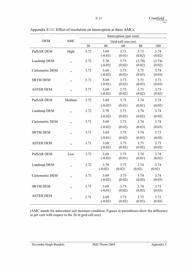
E-11
Appendix E-11: Effect of resolution on interception at three AMCs Interception (per cent)
DEM AMC Grid-cell size (m) 20 40 60 80 100 PulSAR DEM High 3.72 3.69 3.73 3.73 3.74 (-0.03) (0.01) (0.02) (0.02) Landmap DEM ,, 3.72 3.70 3.73 (3.74) (3.74) (-0.02) (0.02) (0.02) (0.02) Cartometric DEM ,, 3.71 3.69 3.73 3.73 3.74 (-0.02) (0.02) (0.03) (0.03) SRTM DEM ,, 3.71 3.69 3.73 3.73 3.73 (-0.01) (0.02) (0.03) (0.03) ASTER DEM ,, 3.71 3.69 3.73 3.73 3.73 (-0.02) (0.02) (0.02) (0.02)
PulSAR DEM Medium 3.72 3.69 3.73 3.74 3.74 (-0.03) (0.01) (0.01) (0.02) Landmap DEM ,, 3.72 3.70 3.73 3.74 3.74 (-0.02) (0.02) (0.02) (0.02) Cartometric DEM ,, 3.71 3.69 3.73 3.74 3.74 (-0.02) (0.02) (0.03) (0.03) SRTM DEM ,, 3.71 3.69 3.73 3.74 3.73 (-0.01) (0.02) (0.03) (0.03) ASTER DEM ,, 3.71 3.69 3.73 3.73 3.73 (-0.02) (0.02) (0.02) (0.02)
PulSAR DEM Low 3.72 3.69 3.73 3.74 3.74 (-0.03) (0.01) (0.01) (0.02)
Landmap DEM ,, 3.72 3.70 3.73 3.74 3.74 (-0.02) (0.02) (0.02) (0.02)
Cartometric DEM ,, 3.71 3.69 3.73 3.74 3.74 (-0.02) (0.02) (0.03) (0.03)
SRTM DEM ,, 3.71 3.69 3.73 3.74 3.73 (-0.01) (0.02) (0.03) (0.03) ASTER DEM ,, 3.71 3.69 3.73 3.73 3.73 (-0.02) (0.02) (0.02) (0.02)
(AMC stands for antecedent soil moisture condition; Figures in parentheses show the difference in per cent with respect to the 20 m grid-cell size)
Devendra Singh Bundela PhD Thesis-2004 Appendix E
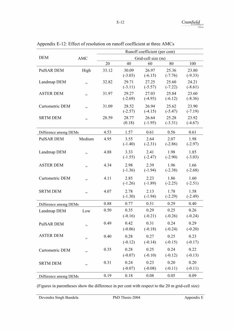
E-12
Appendix E-12: Effect of resolution on runoff coefficient at three AMCs Runoff coefficient (per cent) DEM AMC Grid-cell size (m) 20 40 60 80 100 PulSAR DEM High 33.12 30.09 26.97 25.36 23.80 (-3.03) (-6.15) (-7.76) (-9.33) Landmap DEM ,, 32.82 29.71 27.25 25.60 24.21 (-3.11) (-5.57) (-7.22) (-8.61) ASTER DEM ,, 31.97 29.27 27.03 25.84 23.60 (-2.69) (-4.93) (-6.12) (-8.36)
Cartometric DEM ,, 31.09 28.52 26.94 25.62 23.90 (-2.57) (-4.15) (-5.47) (-7.19) SRTM DEM ,, 28.59 28.77 26.64 25.28 23.92
(0.18) (-1.95) (-3.31) (-4.67)
Difference among DEMs 4.53 1.57 0.61 0.56 0.61 PulSAR DEM Medium 4.95 3.55 2.64 2.07 1.98 (-1.40) (-2.31) (-2.86) (-2.97)
Landmap DEM ,, 4.88 3.33 2.41 1.98 1.85 (-1.55) (-2.47) (-2.90) (-3.03)
ASTER DEM ,, 4.34 2.98 2.39 1.96 1.66 (-1.36) (-1.94) (-2.38) (-2.68)
Cartometric DEM ,, 4.11 2.85 2.23 1.86 1.60 (-1.26) (-1.89) (-2.25) (-2.51)
SRTM DEM ,, 4.07 2.78 2.13 1.78 1.58 (-1.30) (-1.94) (-2.29) (-2.49)
Difference among DEMs 0.88 0.77 0.51 0.29 0.40
Landmap DEM Low 0.50 0.35 0.29 0.25 0.26
(-0.16) (-0.21) (-0.26) (-0.24)
PulSAR DEM ,, 0.49 0.42 0.31 0.24 0.29
(-0.06) (-0.18) (-0.24) (-0.20) ASTER DEM ,, 0.40 0.28 0.27 0.25 0.23 (-0.12) (-0.14) (-0.15) (-0.17)
Cartometric DEM ,, 0.35 0.28 0.25 0.24 0.22
(-0.07) (-0.10) (-0.12) (-0.13)
SRTM DEM ,, 0.31 0.24 0.23 0.20 0.20
(-0.07) (-0.08) (-0.11) (-0.11)
Difference among DEMs 0.19 0.18 0.08 0.05 0.09 (Figures in parentheses show the difference in per cent with respect to the 20 m grid-cell size)
Devendra Singh Bundela PhD Thesis-2004 Appendix E

E-13
Appendix E-13: Effect of resolution on normalised peak discharge at three AMCs Normalised peak discharge (m3/s)
DEM AMC Grid-cell size (m) 20 40 60 80 100 Cartometric DEM High 6.449 5.968 5.237 4.566 3.967 (-7.45) (-18.80) (-29.20) (-38.48) Landmap DEM ,, 6.342 5.434 4.774 4.499 4.362 (-14.32) (-24.72) (-29.07) (-31.22) PulSAR DEM ,, 6.102 5.445 4.913 4.501 3.790 (-10.76) (-19.48) (-26.23) (-37.89) SRTM DEM ,, 5.291 5.208 4.185 4.367 3.989 (-1.56) (-20.91) (-17.47) (-24.61) ASTER DEM ,, 5.111 5.255 4.597 4.305 3.469 (2.81) (-10.05) (-15.78) (-32.13)
Difference among DEMs 1.338 0.76 1.052 0.261 0.893 Landmap DEM Medium 0.694 0.452 0.318 0.274 0.269 (-34.79) (-54.13) (-60.46) (-61.23) PulSAR DEM ,, 0.659 0.476 0.346 0.273 0.223 (-27.78) (-47.42) (-58.49) (-66.20) Cartometric DEM ,, 0.567 0.455 0.329 0.253 0.212 (-19.85) (-41.96) (-55.49) (-62.58) SRTM DEM ,, 0.489 0.342 0.221 0.222 0.186 (-30.08) (-54.67) (-54.53) (-61.92) ASTER DEM ,, 0.440 0.363 0.263 0.230 0.200 (-17.41) (-40.25) (-47.63) (-54.44)
Difference among DEMs 0.254 0.134 0.125 0.052 0.083 Landmap DEM Low 0.073 0.029 0.029 0.015 0.038 (-60.98) (-60.00) (-79.20) (-47.63) ASTER DEM ,, 0.047 0.053 0.041 0.036 0.028 (13.71) (-11.79) (-23.13) (-41.36) PulSAR DEM ,, 0.037 0.029 0.024 0.015 0.022 (-21.87) (-36.24) (-59.72) (-40.25) Cartometric DEM ,, 0.030 0.027 0.018 0.016 0.014 (-9.10) (-40.90) (-46.07) (-52.02) SRTM DEM ,, 0.026 0.017 0.019 0.010 0.019 (-33.67) (-24.42) (-59.46) (-24.30)
Difference among DEMs 0.047 0.036 0.023 0.026 0.024 (Figures in parentheses show the change in per cent with respect to the 20 m grid-cell size)
Devendra Singh Bundela PhD Thesis-2004 Appendix E
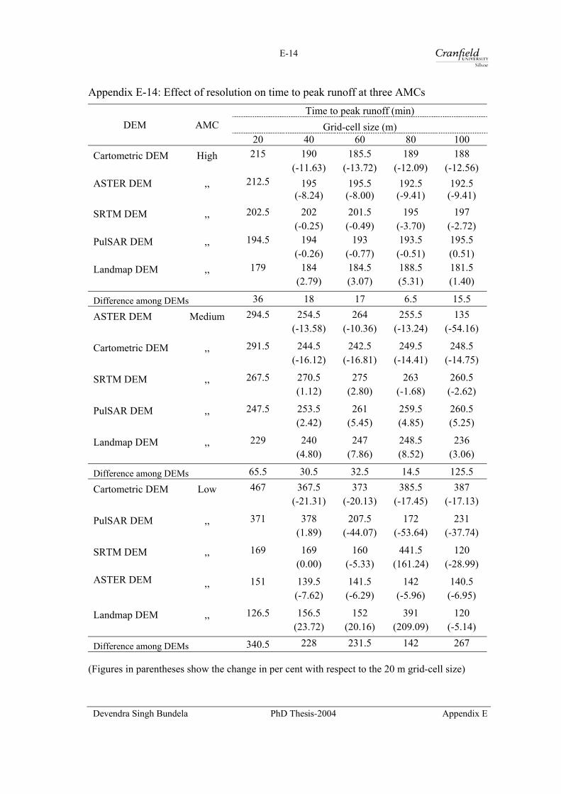
E-14
Appendix E-14: Effect of resolution on time to peak runoff at three AMCs Time to peak runoff (min)
DEM AMC Grid-cell size (m) 20 40 60 80 100 Cartometric DEM High 215 190 185.5 189 188 (-11.63) (-13.72) (-12.09) (-12.56) ASTER DEM ,, 212.5 195 195.5 192.5 192.5 (-8.24) (-8.00) (-9.41) (-9.41)
SRTM DEM ,, 202.5 202 201.5 195 197 (-0.25) (-0.49) (-3.70) (-2.72) PulSAR DEM ,, 194.5 194 193 193.5 195.5 (-0.26) (-0.77) (-0.51) (0.51) Landmap DEM ,, 179 184 184.5 188.5 181.5
(2.79) (3.07) (5.31) (1.40)
Difference among DEMs 36 18 17 6.5 15.5
ASTER DEM Medium 294.5 254.5 264 255.5 135
(-13.58) (-10.36) (-13.24) (-54.16)
Cartometric DEM ,, 291.5 244.5 242.5 249.5 248.5
(-16.12) (-16.81) (-14.41) (-14.75)
SRTM DEM ,, 267.5 270.5 275 263 260.5
(1.12) (2.80) (-1.68) (-2.62)
PulSAR DEM ,, 247.5 253.5 261 259.5 260.5
(2.42) (5.45) (4.85) (5.25)
Landmap DEM ,, 229 240 247 248.5 236
(4.80) (7.86) (8.52) (3.06)
Difference among DEMs 65.5 30.5 32.5 14.5 125.5
Cartometric DEM Low 467 367.5 373 385.5 387
(-21.31) (-20.13) (-17.45) (-17.13)
PulSAR DEM ,, 371 378 207.5 172 231
(1.89) (-44.07) (-53.64) (-37.74)
SRTM DEM ,, 169 169 160 441.5 120
(0.00) (-5.33) (161.24) (-28.99) ASTER DEM ,, 151 139.5 141.5 142 140.5 (-7.62) (-6.29) (-5.96) (-6.95)
Landmap DEM ,, 126.5 156.5 152 391 120
(23.72) (20.16) (209.09) (-5.14)
Difference among DEMs 340.5 228 231.5 142 267 (Figures in parentheses show the change in per cent with respect to the 20 m grid-cell size)
Devendra Singh Bundela PhD Thesis-2004 Appendix E
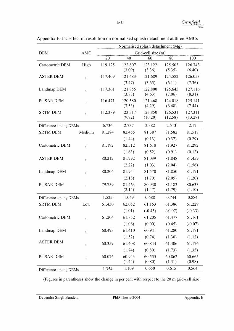
E-15
Appendix E-15: Effect of resolution on normalised splash detachment at three AMCs Normalised splash detachment (Mg) DEM AMC Grid-cell size (m) 20 40 60 80 100 Cartometric DEM High 119.125 122.807 123.122 125.503 126.743 (3.09) (3.36) (5.35) (6.40) ASTER DEM ,, 117.409 121.483 121.689 124.582 126.053 (3.47) (3.65) (6.11) (7.36) Landmap DEM ,, 117.361 121.855 122.800 125.645 127.116 (3.83) (4.63) (7.06) (8.31) PulSAR DEM ,, 116.471 120.580 121.468 124.018 125.141 (3.53) (4.29) (6.48) (7.44) SRTM DEM ,, 112.389 123.317 123.850 126.531 127.311 (9.72) (10.20) (12.58) (13.28)
Difference among DEMs 6.736 2.737 2.382 2.513 2.17 SRTM DEM Medium 81.284 82.455 81.387 81.582 81.517 (1.44) (0.13) (0.37) (0.29) Cartometric DEM ,, 81.192 82.512 81.618 81.927 81.292 (1.63) (0.52) (0.91) (0.12) ASTER DEM ,, 80.212 81.992 81.039 81.848 81.459 (2.22) (1.03) (2.04) (1.56) Landmap DEM ,, 80.206 81.954 81.570 81.850 81.171 (2.18) (1.70) (2.05) (1.20) PulSAR DEM ,, 79.759 81.463 80.930 81.183 80.633 (2.14) (1.47) (1.79) (1.10)
Difference among DEMs 1.525 1.049 0.688 0.744 0.884 SRTM DEM Low 61.430 62.052 61.153 61.386 61.229 (1.01) (-0.45) (-0.07) (-0.33) Cartometric DEM ,, 61.204 61.852 61.205 61.477 61.161 (1.06) (0.00) (0.45) (-0.07) Landmap DEM ,, 60.493 61.410 60.941 61.280 61.171 (1.52) (0.74) (1.30) (1.12) ASTER DEM ,, 60.359 61.408 60.844 61.406 61.176 (1.74) (0.80) (1.73) (1.35) PulSAR DEM ,, 60.076 60.943 60.555 60.862 60.665 (1.44) (0.80) (1.31) (0.98)
Difference among DEMs 1.354 1.109 0.650 0.615 0.564 (Figures in parentheses show the change in per cent with respect to the 20 m grid-cell size)
Devendra Singh Bundela PhD Thesis-2004 Appendix E
E-16
Appendix E-16: Effect of resolution on normalised flow detachment at three AMCs Normalised flow detachment (Mg)
DEM AMC Grid-cell size (m) 20 40 60 80 100 PulSAR DEM High 42001.264 30247.442 22150.606 15561.842 11528.069 (-27.98) (-47.26) (-62.95) (-72.55)
Landmap DEM ,, 39851.768 30231.437 21196.235 15906.520 11338.827 (-24.14) (-46.81) (-60.09) (-71.55)
ASTER DEM ,, 37363.024 27643.116 18222.833 13508.976 10081.267 (-26.01) (-51.23) (-63.84) (-73.02)
Cartometric DEM ,, 31404.470 26027.796 19265.641 14431.306 9936.003 (-17.12) (-38.65) (-54.05) (-68.36)
SRTM DEM ,, 25698.914 23624.346 18017.304 13852.430 10567.706
(-8.07) (-29.89) (-46.10) (-58.88)
Difference among DEMs 16302.35 6623.096 4133.302 2052.866 1592.066
PulSAR DEM Medium 7545.203 3267.885 1851.418 1195.320 823.266
(-56.69) (-75.46) (-84.16) (-89.09)
Landmap DEM ,, 7145.711 3373.476 1745.970 1129.827 736.001
(-52.79) (-75.57) (-84.19) (-89.70)
ASTER DEM ,, 5946.397 2807.571 1569.753 1030.673 655.077
(-52.79) (-73.60) (-82.67) (-88.98)
Cartometric DEM ,, 5581.460 2710.237 1451.088 931.674 635.513
(-51.44) (-74.00) (-83.31) (-88.61)
SRTM DEM ,, 4824.312 2275.671 1438.819 953.709 658.102
(-52.83) (-70.18) (-80.23) (-86.36)
Difference among DEMs 2720.892 1097.805 412.599 263.646 187.753
PulSAR DEM Low 959.916 519.898 296.176 195.284 134.575
(-45.84) (-69.15) (-79.66) (-85.98)
Landmap DEM ,, 931.430 412.917 214.958 136.064 90.578
(-55.67) (-76.92) (-85.39) (-90.28) ASTER DEM ,, 833.414 413.007 240.587 144.623 90.643 (-50.44) (-71.13) (-82.65) (-89.12)
Cartometric DEM ,, 654.937 318.164 167.548 112.130 83.113
(-51.42) (-74.42) (-82.88) (-87.31)
SRTM DEM ,, 597.433 293.123 198.121 127.876 85.654
(-50.94) (-66.84) (-78.60) (-85.66)
Difference among DEMs 362.483 226.775 128.628 83.154 51.462 (Figures in parentheses show the change in per cent with respect to the 20 m grid-cell size)
Devendra Singh Bundela PhD Thesis-2004 Appendix E
E-17
Appendix E-17: Effect of resolution on normalised overland deposition at three AMCs Normalised overland deposition (Mg)
DEM AMC Grid-cell size (m) 20 40 60 80 100 PulSAR DEM High -38327.648 -28593.434 -21397.294 -15238.761 -11866.728 (-25.40) (-44.17) (-60.24) (-69.04)
Landmap DEM ,, -35592.952 -28239.470 -20348.227 -15352.750 -11071.471 (-20.66) (-42.83) (-56.87) (-68.89)
ASTER DEM ,, -34871.256 -26339.577 -17733.672 -13142.296 -10028.699 (-24.47) (-49.15) (-62.31) (-71.24)
Cartometric DEM ,, -28282.208 -24768.797 -18528.501 -14122.568 -9918.505 (-12.42) (-34.49) (-50.07) (-64.93)
SRTM DEM ,, -24107.662 -22741.101 -17605.516 -13785.367 -10538.473
(-5.67) (-26.97) (-42.82) (-56.29)
Difference among DEMs 14219.986 5852.333 3791.778 2210.454 1948.223
PulSAR DEM Medium -7489.385 -3323.337 -1920.646 -1275.366 -911.717
(-55.63) (-74.36) (-82.97) (-87.83)
Landmap DEM ,, -7039.188 -3421.308 -1810.916 -1205.871 -810.363
(-51.40) (-74.27) (-82.87) (-88.49)
ASTER DEM ,, -5965.761 -2878.433 -1648.505 -1110.573 -734.833
(-51.75) (-72.37) (-81.38) (-87.68)
Cartometric DEM ,, -5569.643 -2786.028 -1530.040 -1012.099 -715.469
(-49.98) (-72.53) (-81.83) (-87.15)
SRTM DEM ,, -4857.588 -2355.373 -1518.534 -1034.438 -739.335
(-51.51) (-68.74) (-78.70) (-84.78)
Difference among DEMs 2631.797 1065.935 402.112 263.267 196.248
PulSAR DEM Low -1019.059 -580.699 -356.661 -256.107 -195.336
(-43.02) (-65.00) (-74.87) (-80.83)
Landmap DEM ,, -988.142 -472.243 -274.703 -197.137 -151.065
(-52.21) (-72.20) (-80.05) (-84.71)
ASTER DEM ,, -893.082 -474.115 -301.362 -205.914 -151.697 (-46.91) (-66.26) (-76.94) (-83.01)
Cartometric DEM ,, -715.815 -379.765 -228.685 -173.533 -144.218
(-46.95) (-68.05) (-75.76) (-79.85)
SRTM DEM ,, -658.823 -355.083 -259.228 -189.243 -146.866
(-46.10) (-60.65) (-71.28) (-77.71)
Difference among DEMs 360.236 225.616 127.976 82.574 51.118 (Figures in parentheses show the change in per cent with respect to the 20 m grid-cell size)
Devendra Singh Bundela PhD Thesis-2004 Appendix E
E-18
Appendix E-18: Effect of resolution on normalised channel erosion at three AMCs Normalised channel erosion (Mg)
DEM AMC Grid-cell size (m) 20 40 60 80 100 PulSAR DEM High 9638.816 9344.245 8316.964 7641.308 7828.750 (-3.06) (-13.71) (-20.72) (-18.78) Landmap DEM ,, 9059.666 8013.812 8532.064 8202.614 8432.342 (-11.54) (-5.82) (-9.46) (-6.92) ASTER DEM ,, 9030.044 10381.601 8411.287 9619.488 8615.111 (14.97) (-6.85) (6.53) (-4.60) Cartometric DEM ,, 8106.593 8132.194 9042.363 8549.292 6820.302 (0.32) (11.540 (5.46) (-15.87) SRTM DEM ,, 5361.450 5739.583 5986.773 5397.459 6675.768 (7.05) (11.66) (0.67) (24.51)
Difference among DEMs 4277.366 3604.662 3055.59 4222.029 1939.343 ASTER DEM Medium 4399.530 3383.696 2639.633 2046.999 1607.942 (-23.09) (-40.00) (-53.47) (-63.45)
Landmap DEM ,, 4162.578 2776.681 2086.501 1756.337 1542.895 (-33.29) (-49.870 (-57.81) (-62.93)
PulSAR DEM ,, 4149.039 3016.276 2189.494 1848.603 1624.295 (-27.30) (-47.23) (-55.45) (-60.85)
Cartometric DEM ,, 3245.540 2463.648 2265.683 1798.879 1153.458 (-24.09) (-30.19) (-44.57) (-64.46)
SRTM DEM ,, 1982.995 1719.928 1545.538 1231.326 1314.264 (-13.27) (-22.06) (-37.91) (-33.72)
Difference among DEMs 2416.535 1663.768 1094.095 815.673 470.837 Landmap DEM Low 1705.983 862.937 688.558 533.512 524.210 (-49.42) (-59.64) (-68.73) (-69.27) ASTER DEM ,, 1695.106 1024.196 738.944 524.848 383.045 (-39.58) (-56.41) (-69.04) (-77.40)
PulSAR DEM ,, 1639.451 1144.091 721.545 505.374 427.234 (-30.22) (-55.99) (-69.17) (-73.94)
Cartometric DEM ,, 1005.345 687.894 673.844 510.993 299.064 (-31.58) (-32.97) (-49.170 (-70.25)
SRTM DEM ,, 529.312 333.947 287.708 246.155 291.112 (-36.91) (-45.64) (-53.50) (-45.00)
Difference among DEMs 1176.671 810.144 451.236 287.357 233.098 (Figures in parentheses show the change in per cent with respect to the 20 m grid-cell size)
Devendra Singh Bundela PhD Thesis-2004 Appendix E

E-19
Appendix E-19: Effect of resolution on normalised channel deposition at three AMCs Normalised channel deposition (Mg) DEM AMC Grid-cell size (m) 20 40 60 80 100 ASTER DEM High -11637.144 -4719.526 -6961.645 -2693.871 -1835.919 (-59.44) (-40.18) (-76.85) (-84.22)
Cartometric DEM ,, -6828.500 -2951.779 -2579.134 -2719.245 -1684.690 (-56.77) (-62.23) (-60.18) (-75.33) Landmap DEM ,, -5727.808 -4022.667 -2967.062 -2959.543 -2385.503 (-29.77) (-48.20) (-48.33) (-58.35) PulSAR DEM ,, -5679.579 -3817.189 -3085.495 -2776.797 -2210.532 (-32.79) (-45.67) (-51.11) (-61.08) SRTM DEM ,, -2376.189 -2366.588 -2838.898 -5590.101 -2156.543 (-0.40) (19.47) (135.25) (-9.24) Difference among DEMs 9260.955 2352.938 4382.511 2896.230 700.813 ASTER DEM Medium -4460.159 -2974.409 -2641.825 -1595.928 -1159.487 (-33.31) (-40.77) (-64.22) (-74.00)
Landmap DEM ,, -3500.606 -2394.296 -1696.811 -1485.465 -1223.856 (-31.60) (-51.53) (-57.57) (-65.04)
PulSAR DEM ,, -3447.102 -2393.445 -1695.391 -1609.988 -1312.636 (-30.57) (-50.82) (-53.29) (-61.92)
Cartometric DEM ,, -3007.780 -1969.977 -1804.438 -1501.277 -888.364 (-34.50) (-40.01) (-50.09) (-70.46)
SRTM DEM ,, -1550.888 -1472.718 -1443.130 -1232.170 -1118.422 (-5.04) (-6.95) (-20.55) (-27.89)
Difference among DEMs 2909.271 1501.691 1198.695 377.818 424.272 ASTER DEM Low -1695.673 -1019.621 -738.994 -506.017 -364.398 (-39.87) (-56.42) (-70.16) (-78.51)
Landmap DEM ,, -1654.539 -858.583 -678.924 -529.828 -518.484 (-48.11) (-58.97) (-67.98) (-68.66)
PulSAR DEM ,, -1604.198 -1125.604 -706.112 -505.411 -423.114 (-29.83) (-55.98) (-68.49) (-73.62)
Cartometric DEM ,, -981.104 -678.426 -659.540 -504.758 -291.383 (-30.85) (-32.78) (-48.55) (-70.30)
SRTM DEM ,, -528.950 -331.267 -287.752 -246.174 -290.129 (-37.37) (-45.60) (-53.46) (-45.15)
Difference among DEMs 1166.723 794.337 451.242 283.654 228.355 (Figures in parentheses show the change in per cent with respect to the 20 m grid-cell size)
Devendra Singh Bundela PhD Thesis-2004 Appendix E

E-20
Appendix E-20: Effect of resolution on normalised total soil loss at three AMCs Normalised total soil loss (Mg)
DEM AMC Grid-cell size (m) 20 40 60 80 100 PulSAR DEM High 7749.263 7301.612 6106.285 5311.592 5880.795 (-5.78) (-21.20) (-31.46) (-24.11) Landmap DEM ,, 7707.784 6104.882 6535.760 5922.495 6441.269 (-20.80) (-15.21) (-23.16) (-16.43) SRTM DEM ,, 4688.708 4379.470 3683.526 0.946 4675.758 (-6.60) (-21.44) (-99.98) (-0.28) Cartometric DEM ,, 4519.401 6562.149 7323.413 6264.297 5279.830 (45.20) (62.04) (38.61) (16.83) ASTER DEM ,, 1.382 7086.981 2060.395 7416.837 6957.762 Too large Too large Too large Too large Difference among DEMs 3229.862 2922.142 4475.365 2105.245 2282.004 Landmap DEM Medium 848.622 416.481 406.302 276.680 325.847 (-50.92) (-52.12) (-67.40) (-61.60) PulSAR DEM ,, 837.400 648.832 505.793 239.749 314.811 (-22.52) (-39.60) (-71.37) (-62.41) SRTM DEM ,, 480.080 249.954 104.073 0.008 196.128 (-47.93) (-78.32) (-100.00) (-59.15) Cartometric DEM ,, 330.683 500.372 463.896 299.101 266.429
(51.31) (40.28) (-9.55) (-19.43)
ASTER DEM ,, 0.012 420.360 0.064 453.014 450.158 Too large 419.70 Too large Too large Difference among DEMs 517.939 398.878 401.720 213.265 254.030 Landmap DEM Low 55.211 6.436 10.825 3.891 6.409 (-88.34) (-80.39) (-92.95) (-88.39)
PulSAR DEM ,, 36.158 18.623 15.498 0.000 4.372 (-48.50) (-57.14) (-100.00) (-87.91)
Cartometric DEM ,, 24.529 9.714 14.366 6.308 7.739 (-60.40) (-41.43) (-74.28) (-68.45)
SRTM DEM ,, 0.395 2.771 0.000 0.000 1.000 (602.16) (-99.98) (-99.99) (153.29) ASTER DEM ,, 0.000 4.844 0.001 18.942 18.768 Too large 599.29 Too large Too large
Difference among DEMs 30.682 15.852 4.673 15.051 14.396 (Figures in parentheses show the change in per cent with respect to the 20 m grid-cell size)
Devendra Singh Bundela PhD Thesis-2004 Appendix E
E-21
Appendix E-21: Effect of resolution on average soil loss at three AMCs Average soil loss (kg/ha) DEM AMC Grid-cell size (m) 20 40 60 80 100 PulSAR DEM High 9553.31 9005.33 7541.19 6575.37 7307.17 (-5.74) (-21.06) (-31.17) (-23.51) Landmap DEM ,, 9502.17 7529.48 8071.58 7331.63 8007.16 (-20.76) (-15.06) (-22.84) (-15.73) SRTM DEM ,, 5780.25 5401.44 4549.11 1.17 5812.45 (-6.55) (-21.30) (-99.98) (0.56) Cartometric DEM ,, 5571.53 8093.39 9044.32 7754.75 6559.01 (45.26) (62.33) (39.19) (17.72) ASTER DEM ,, 1.70 8740.76 2544.56 9179.67 8649.22 Too large Too large Too large Too large Difference among DEMs 3981.78 3603.89 6499.76 2604.30 2836.70 Landmap DEM Medium 1032.35 800.23 624.65 296.79 391.17 (-22.48) (-39.49) (-71.25) (-62.11) PulSAR DEM ,, 1046.18 513.67 501.78 342.51 405.06 (-50.90) (-52.04) (-67.26) (-61.28) SRTM DEM ,, 591.84 308.28 128.53 0.01 243.81 (-47.91) (-78.28) (-100.00) (-58.81) Cartometric DEM ,, 407.67 617.13 572.91 370.27 330.98 (51.38) (40.53) (-9.17) (-18.81) ASTER DEM ,, 0.02 518.45 0.08 560.69 559.59 Too large 420.66 Too large Too large Difference among DEMs 624.68 491.95 496.12 263.90 315.78 Landmap DEM Low 68.06 7.94 13.37 4.82 7.97 (-88.34) (-80.36) (-92.92) (-88.29) PulSAR DEM ,, 44.58 22.97 19.14 0.00 5.43 (-48.47) (-57.06) (-100.00) (-87.81) Cartometric DEM ,, 30.24 11.98 17.74 7.81 9.61 (-60.38) (-41.33) (-74.18) (-68.21) SRTM DEM ,, 0.49 3.42 0.00 0.00 1.24 (602.49) (-99.98) (-99.99) (155.42) ASTER DEM ,, 0.00 5.97 0.00 23.44 23.33 Too large 616.67 Too large Too large Difference among DEMs 35.82 19.55 5.77 18.62 22.09
(Figures in parentheses show the change in per cent with respect to the 20 m grid-cell size)
Devendra Singh Bundela PhD Thesis-2004 Appendix E
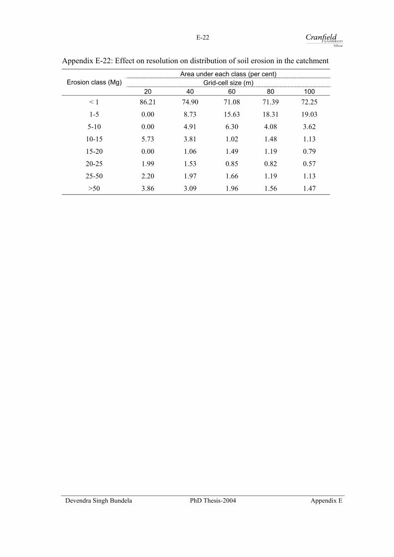
E-22
Appendix E-22: Effect on resolution on distribution of soil erosion in the catchment Area under each class (per cent)
Grid-cell size (m) Erosion class (Mg) 20 40 60 80 100
< 1 86.21 74.90 71.08 71.39 72.25
1-5 0.00 8.73 15.63 18.31 19.03
5-10 0.00 4.91 6.30 4.08 3.62
10-15 5.73 3.81 1.02 1.48 1.13
15-20 0.00 1.06 1.49 1.19 0.79
20-25 1.99 1.53 0.85 0.82 0.57
25-50 2.20 1.97 1.66 1.19 1.13
>50 3.86 3.09 1.96 1.56 1.47
Devendra Singh Bundela PhD Thesis-2004 Appendix E

E-23
Appendix E-23: Effects of resolution on peak time and peak discharge of hydrograph and sedigraph
Hydrograph First peak Second peak Resolution
Time (min) Discharge (m3/s) Time Discharge 20 162.5 0.4559 243.5 0.6745
40 171.5 0.4333 253.5 0.4858
60 168.0 0.2856 261.0 0.3615
80 166.5 0.2356 256.5 0.3283
100 172.0 0.1787 260.5 0.2417
Sedigraph
20 193.5 48.128 244 115.065
40 174.5 42.578 251.5 84.955
60 169.0 38.482 261.5 64.734
80 167.0 24.464 256.5 37.879
100 173.5 26.683 258.0 39.440
Devendra Singh Bundela PhD Thesis-2004 Appendix E
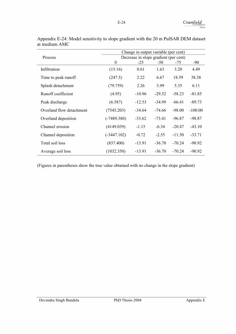
E-24
Appendix E-24: Model sensitivity to slope gradient with the 20 m PulSAR DEM dataset at medium AMC
Change in output variable (per cent) Process Decrease in slope gradient (per cent)
0 -25 -50 -75 -90 Infiltration (15.16) 0.61 1.63 3.20 4.49
Time to peak runoff (247.5) 2.22 6.67 18.59 38.38
Splash detachment (79.759) 2.26 3.99 5.35 6.11
Runoff coefficient (4.95) -10.96 -29.52 -58.23 -81.85
Peak discharge (6.587) -12.53 -34.99 -66.41 -89.73
Overland flow detachment (7545.203) -34.64 -74.66 -98.00 -100.00
Overland deposition (-7489.380) -33.62 -73.41 -96.87 -98.87
Channel erosion (4149.039) -1.15 -6.34 -20.47 -43.10
Channel deposition (-3447.102) -0.72 -2.55 -11.50 -33.71
Total soil loss (837.400) -13.91 -36.70 -70.24 -90.92
Average soil loss (1032.350) -13.91 -36.70 -70.24 -90.92
(Figures in parentheses show the true value obtained with no change in the slope gradient)
Devendra Singh Bundela PhD Thesis-2004 Appendix E

F-1
Appendix F
Appendix F-1: Content of the optical disk attached with the Thesis
Folder name Description of the content
Model LISEM model version 2.03
PCRaster PCRaster GIS Professional version 2.0
Basemaps Key spatial data of the Eastern South Downs,
25dbases 25 LISEM databases, a storm rainfall intensity file
PCRscript PCRaster script files to create LISEM databases
Batch Batch files to display the key spatial data and LISEM database
Outputs Spatio-temporal output files for dynamic visualisation in Aguila
Video AVI video files for viewing a single simulation
Devendra Singh Bundela PhD Thesis-2004 Appendix F