
AALBORG UNIVERSITY
150
AALBORG UNIVERSITY Department of Civil Engineering Evaluation of the power production performance of the WavePiston wave energy converter Supervisor: Jens Peter Kofoed Student reference: Elisa Angelelli 12023 9 th Semester 2009/2010
-
Upload
khangminh22 -
Category
Documents
-
view
0 -
download
0
Transcript of AALBORG UNIVERSITY

AALBORG UNIVERSITY Department of Civil Engineering
Evaluation of the power
production performance
of the WavePiston
wave energy converter
Supervisor:
Jens Peter Kofoed
Student reference:
Elisa Angelelli
12023
9th Semester
2009/2010

PREFACE
My name is Elisa Angelelli, I’m a student of the master degree and I come from Italy.
This document represents the conclusion of the last five years of university in Civil Engineering with the
Specialization in Hydraulic spent in Alma Mater Studiorum of Bologna.
The experimental studied included in this document were made possible thanks to the work in the
laboratory of Aalborg University, in Denmark.
During the ending of my university period I felt the need to spend a period abroad, the main reasons
belonged to two types: the first was that I regret the idea to finish the university study without carry out
any practical stuff, but only theoretical topics; and the second was about the disappointment that I felt to
go in the world of work with a limited knowledge of English and use of it even less.
Both the issues were approached and almost resolved during this period abroad as an Erasmus student.
And last but not least, the topic of my study: since in the last three years of university I chose a
specialization regarding the water, it was really likely that I found myself working in something related to
the water, but usually when you thought to the water you usually mean the fresh water: as aqueduct,
hydroelectric, etc...but the curiosity for new research and the willingness to find new prospects for green
energy led me to a new scenario: the energy of the sea!
Hence with the Erasmus period in Denmark, I could work in the laboratory on a new wave energy converter,
called the WavePiston, with the collaboration of two of its inventors (Kristian Glebøl and Martin von Bülow)
and Arthur Pecher, under the supervision of Jens Peter Kofoed.
To conclude, I would only add that I’ve never done before a kind of document as this, I mean for the English
language either for the scientific typology, thus I apologize for any inaccuracies of form or language.
May 2010, Aalborg

INDEX
Preface…………………………………………………………………………………………………………………………………………………………0
Abstract in English………………………………………………………………………………………………………………………………………..1
Abstract in English………………………………………………………………………………………………………………………………………..2
Figure Index…………………………………………………………………………………………………………………………………………………..I
Table Index…………………………………………………………………………………………………………………………………………………..V
1- Introduction…………………………………… ................. .......................................................................................... 3
1.1- Preface ......................................................... .......................................................................................... 3
1.2- Current energy situation. ............................ .......................................................................................... 6
1.3- Research of a green solution ....................... ........................................................................................ 11
1.3.1- United Kingdom ........................................ ........................................................................................ 13
1.3.1.1- The Orkney Islands ......................... ........................................................................................ 14
1.3.2- Portugal .................................................... ........................................................................................ 14
1.3.3- Denmark ................................................... ........................................................................................ 14
1.3.4- Italy ........................................................... ........................................................................................ 16
2- Marine Energy .................................................... ........................................................................................ 17
2.1- Main typology of ocean energy ................... ........................................................................................ 21
2.2- Wave Energy ................................................ ........................................................................................ 24
2.3- Wave Energy Converter .............................. ........................................................................................ 31
2.3.1- Classification of the Wave Energy Converters ............................................................................... 35
2.3.2- Examples of the Wave Energy Converters ..................................................................................... 41
2.3.2.1- LIMPET ......................................... ........................................................................................ 41
2.3.2.2- PENDULOR ................................... ........................................................................................ 43
2.3.2.3- WAVE DRAGON ........................... ........................................................................................ 43
2.3.2.4- PELAMIS ....................................... ........................................................................................ 44
2.3.2.5- SWEC ........................................... ........................................................................................ 44
3- WavePiston Device ............................................. ........................................................................................ 45
3.1- The real WavePiston.................................... ........................................................................................ 45
3.2 - WavePiston prototype ............................... ........................................................................................ 48
3.2.1 – Aalborg laboratory .............................. ........................................................................................ 48
3.2.2 – Model and experimental activity ........ ........................................................................................ 55
3.2.2.1- Test Program ................................... ........................................................................................ 59
3.2.2.1.1- Overview ............................... ........................................................................................ 59
3.2.2.1.2- Description of the wave state ........................................................................................ 60
3.2.2.1.3- Research of the reference configuration ....................................................................... 62
3.2.2.1.4- Wave Period and Wave Height variation ....................................................................... 63
3.2.2.1.5- Analysis of the influence of the incident wave angle .................................................... 64

3.2.2.1.6- Number and shape of the energy converter plates ...................................................... 65
3.2.2.2- Results ............................................. ........................................................................................ 65
3.2.2.2.1- Research of the reference configuration ....................................................................... 65
3.2.2.2.2- Wave Period and Wave Height variation ....................................................................... 68
3.2.2.2.3- Analysis of the influence of the incident wave angle .................................................... 71
3.2.2.2.4- Number and shape of the energy converter plates ...................................................... 72
3.2.2.2.5- Summary of the performance of the device ................................................................. 75
4- Future Installation ............................................. . ........................................................................................ 78
4.1- Italian Installation basing on laboratory results ................................................................................... 78
4.1.1- Italian Wave State. ................................ ........................................................................................ 79
4.1.2- Yearly average efficiency and yearly energy production............................................................... 82
4.2- Numerical Model ......................................... ........................................................................................ 86
4.2.1- Theoretical Equations ........................... ........................................................................................ 86
4.2.1.1- External forces’ investigation .......... ........................................................................................ 87
4.2.1.1.1- Fixed body in an oscillatory flow ........................................................................................ 87
4.2.1.1.2- Moving body in an oscillatory flow .................................................................................... 87
4.2.1.2- Simplifying assumptions ................. ........................................................................................ 89
5- Conclusions ......................................................... ........................................................................................ 95
5.1- Observations and suggestions ..................... ........................................................................................ 95
5.2- Summarizing ................................................ ........................................................................................ 96
5.3- Conclusions .................................................. ...................................................................................... 101
5.4- Possible inconveniences in real installation ...................................................................................... 105
List Appendix .......................................................... ...................................................................................... 106
Appendix A - File WaveLab ..................................... ...................................................................................... 107
Appendix B – File WavePiston.vi ........................... ...................................................................................... 113
Appendix C – List of experiments .......................... ...................................................................................... 114
Appendix D – Matlab Analysis file ......................... ...................................................................................... 119
Appendix E – Simulations with Matlab .................. ...................................................................................... 124

I
FIGURE INDEX
Figure 1.1: The regional GDP per capita of the human history before the Industrial Revolution. .................... 4
Figure 1.2: The voluntary gas stations decision to fix a limit. ........................................................................... 5
Figure 1.3: Total energy consumption in the 2006, source International Energy Agency (IEA). ....................... 7
Figure 1.4: Analogue energy consumption in the 2006, source Fuel Group. ..................................................... 7
Figure 1.5:The world’s proven oil reserves, source Statistical Review of World Energy .................................... 8
Figure 1.6: Major oil producer Nation in 2006, source Energy Information Administration ............................. 8
Figure 1.7: World map on the Carbon dioxide emission in 2009, source EDGAR .............................................. 9
Figure 1.8: Trend of the global atmospheric concentration of CO2, source UNEP ............................................ 9
Figure 1.9: The main greenhouse gases, source IPCC ...................................................................................... 10
Figure 1.10 : Wave and Tidal Resources in the UK……………………………………………………………………………………….13
Figure2.1: List of the Countries concerned in marine energy, source “Annual Report 2009” ......................... 17
Figure2.2: Ocean Energy Source ............................. ........................................................................................ 18
Figure2.3: Real example of wave energy converter: Wave Dragon, Nissum Brendning, Denmark ................ 18
Figure2.4: Real example of wave energy converter: Pelamis, Northern Portugal .......................................... 18
Figure2.5: Real example of wave energy converter: PowerBuoy free-floating point absorber, Hawaii ......... 19
Figure2.6: Real example of tidal current energy converter: The Blue Concept, Norway ................................. 19
Figure2.7: Real example of tidal current energy converter: Kinetic Hydro Power System, U.S.A. .................. 19
Figure2.8: Real example of tidal current energy converter: Seaflow, Devon, U.K. .......................................... 19
Figure2.9: Real example of tidal current energy converter: Enermar System, Messina, Italy ........................ 20
Figure2.10: Real example of tidal current energy converter: Open-Centre Turbine, Scotland ........................ 20
Figure2.11: Real example of osmotic energy converter, salinity gradient: Osmotic Power, Norway ............. 20
Figure2.12: Real example of thermal gradient OTEC Device Thermo-dynamic Rankine cycle, Japan ............ 20
Figure2.13: Tidal Energy Patterns .......................... ........................................................................................ 21
Figure2.14: Tidal Energy Patterns .......................... ........................................................................................ 21
Figure2.15: Map of Surface Ocean Currents. ......... ........................................................................................ 22
Figure2.16: Annual trend of energy wave in Scotland,source WERATLAS, European Wave Energy Atlas ...... 23
Figure2.17: Main parameters of a wave. ............... ........................................................................................ 25
Figure2.18: High-energy zone: Hot spots ............... ........................................................................................ 25
Figure2.19: The two component of the wave energy: the kinetic and the potential energy .......................... 26
Figure2.20: On the left: Decomposition of a 2D irregular wave state. ............................................................ 28
Figure2.21: 2D Spectrum, source Coastal Engineering Manual. ..................................................................... 30
Figure2.22: Pierson-Moskowitz and JONSWAP spectrums, source C.E.M. ...................................................... 30
Figure2.23: Average annual ocean wave power in kW/m,source ww.oceanpd.com ...................................... 31
Figure2.24: Europe: Average annual ocean wave power [kW/m]................................................................... 32
Figure2.25: Europe’s map: Wave Test Centres ....... ........................................................................................ 32
Figure2.26: Cataloguing of the WEC based on the location (Falnes, 2005) .................................................... 34
Figure2.27: Point Absorber, source EMEC .............. ........................................................................................ 35
Figure2.28: Attenuator, source EMEC .................... ........................................................................................ 35
Figure2.29: Second classification of the WEC based on the orientation (Falnes, 2005) .................................. 35
Figure2.30: Typical representation of a Overtopping Device .......................................................................... 36
Figure2.31: On the left: Section of the SSG, on the right: possible installation as a breakwater .................... 36
Figure2.32: Wave Dragon is an off-shore OTD ....... ........................................................................................ 36

II
Figure2.33: DEXA is an example of Wave Activated Body, source www.dexawave.com ............................... 37
Figure2.34: Submerged pressure differential, source www.emec.org.uk ....................................................... 37
Figure2.35: Oscillating Water Column, source renewable energy journal ...................................................... 38
Figure2.36: Oscillating Wave Surge Converter,source www.emec.org.uk ...................................................... 39
Figure2.37: Oscillating Wave Surge Converter ....... ........................................................................................ 39
Figure 2.38 : LIMPET’s section ................................ ........................................................................................ 40
Figure 2.39 : Cross sectional view of LIMPET .......... ........................................................................................ 41
Figure 2.40 : Real view of LIMPET ........................... ........................................................................................ 41
Figure 2.41 : Pendulor’s scheme ............................. ........................................................................................ 42
Figure 2.42 : Wave Dragon representation ............ ........................................................................................ 42
Figure 2.43 : PELAMIS – Schematic representation ........................................................................................ 43
Figure 2.44 : SWEC’s pressure system .................... ........................................................................................ 44
Figure 2.45 : Overview of the SWEC ....................... ........................................................................................ 44
Figure 3.1: motion of the water particles ............... ........................................................................................ 45
Figure 3.2: WavePiston envisaged design .............. ........................................................................................ 46
Figure 3.3: single module design ............................ ........................................................................................ 46
Figure 3.4: Overview of the laboratory in Aalborg University: ........................................................................ 48
Figure 3.5: Detail of the paddle system as a snake-front piston and of the gauges. ...................................... 49
Figure 3.5: Section and top view of the laboratory of Aalborg University ...................................................... 49
Figure 3.6: Screen of the AWASYS5 for the generation of a regular wave ...................................................... 50
Figure 3.7: Screen of the AWASYS5 for the generation of an irregular wave.................................................. 50
Figure 3.8: Screen of the WaveLab3.33 “Acquisition Data” ............................................................................ 51
Figure 3.9: Screen of the WaveLab3.33 “Reflection Analysis”......................................................................... 52
Figure 3.10: Screen of the WavePiston.vi “Sampling Graph” ......................................................................... 54
Figure 3.11: Box that connects the device and computer ............................................................................... 54
Figure 3.12: Support structure added ..................... ........................................................................................ 55
Figure 3.13: Single PTO, including the sliding rail with the load, the force transducer and the LVDT ............ 55
Figure 3.14: WavePiston Prototype and its configuration in the laboratory ................................................... 56
Figure 3.15: Plot of the different design conditions and the observed conditions. ......................................... 61
Figure 3.16: Reference configuration:2energy plates, shape 0,5mx0,1m,distance 2,40m, load 1,5kg .......... 62
Figure 3.17: In this picture the device has an angle of 20° respect the incoming waves. ............................... 64
Figure 3.18: In this picture the distance between two subsequent plates of the device is 0,45m. ................. 64
Figure 3.19: Trend of the overall efficiency of the device for the regular wave states in the scale 1:20. ....... 65
Figure 3.20: Trend of the overall efficiency for the three regular wave states in the scale 1:20. ................... 65
Figure 3.21: The increase of the ratio scale implies an increase in the efficiency. .......................................... 66
Figure 3.22: Efficiency for the different irregular wave states, for the load of 2,5kg and 1,5kg. .................... 66
Figure 3.23: Correlation between the wave state and the standard deviation of the force ........................... 67
Figure 3.24: Correlation between the wave state and the standard deviation of the force. .......................... 67
Figure 3.25: Relation between the efficiency of the device and the wave period. .......................................... 68
Figure 3.26: Relation between the efficiency of the device and the wave height. ........................................ 69
Figure 3.27: Relation between the efficiency of the device and the wave period. .......................................... 69
Figure 3.28: Ratio between the efficiency of the device and the incident wave angle ................................... 70
Figure 3.28: Ratio between the efficiency of the device and the incident wave angle. .................................. 70
Figure 3.29: Ratio between the efficiency of the device and the incident wave angle. .................................. 71
Figure 3.30: The performance referes to the configuration with two wings at a distance of 2,40m .............. 72

III
Figure 3.31: The performance referes to the configuration with two wings at a distance of 2,40m .............. 72
Figure 3.32: The efficiency increases with a decrease of the width of the plates ........................................... 73
Figure 3.33: The efficiency increases with an increase of the depth of the plates for all the wave states. .... 73
Figure 3.34: The efficiency decrease even if the shape of the plates doesn’t change ..................................... 74
Figure 3.35: The interpolation equation for the power generated.................................................................. 75
Figure 3.36: Representation of the average efficiency of a plate of 15m width of the WavePiston in the blue
line, the orange line is the product of the probability of occurrence and the available wave power. ........ 77
Figure 4.1: Position of the 15 Italian buoys ............ ........................................................................................ 78
Figure 4.2: Mazara del Vallo buoy .......................... ........................................................................................ 79
Figure 4.3: Mazara del Vallo position ..................... ........................................................................................ 79
Figure 4.4: Mazara del Vallo DATAWELL position .. ........................................................................................ 79
Figure 4.5: Mazara del Vallo DATAWELL ................ ........................................................................................ 80
Figure 4.6: Mazara del Vallo DATAWELL ................ ........................................................................................ 80
Figure 4.7: Trend of the irregular Danish Sea State ........................................................................................ 82
Figure 4.8: Trend of the irregular Italian Sea States ........................................................................................ 82
Figure 4.9: Comparison among the trend of the irregular Italian Sea States and the Danish one.................. 83
Figure 4.10: Danish efficiency trend for the WavePiston carries out by the laboratory result. ...................... 83
Figure 4.11: Italian efficiency trend for the WavePiston using the Danish efficiency trend. ........................... 84
Figure 4.12: Representation of the average efficiency of a plate of 15m width of the WavePiston ............... 85
Figure 4.13: A single unit of the WavePiston device is seen as a single degrees freedom body. .................... 86
Figure 4.14: Lab_fixed_body model: velocity plate-velocity flow .................................................................... 90
Figure 4.15: Lab_fixed_body model: Damping- displacement ........................................................................ 90
Figure 4.16: Lab_fixed_body model: Damping- velocity. ................................................................................ 91
Figure 4.17: Lab_fixed_body model: Damping- Std velocity ........................................................................... 91
Figure 4.18: Lab_fixed_body model: Damping- Std Force ............................................................................... 92
Figure 4.19: Lab_fixed_body model: Damping-Power .................................................................................... 92
Figure 4.20: Lab_fixed_body model: Std Lost Force-Power ............................................................................. 93
Figure 5.1: Typical efficiency trend of the WavePiston prototype ................................................................... 95
Figure 5.2: The non-linear trend of the overall efficiency ................................................................................ 96
Figure 5.3: The performance values are included in a range from 15,5% to 2,4%. ......................................... 97
Figure 5.4: The performance values are included in a range from 6% to 2,5% ............................................... 97
Figure 5.5: Ratio between the efficiency of the device and the incident wave angle ..................................... 98
Figure 5.6: The performance values are referenced to the reference configuration....................................... 98
Figure 5.7: The efficiency increases with a decrease of the width of the plates. ............................................ 98
Figure 5.8: The efficiency increases with an increase of the depth of the plates. ........................................... 99
Figure 5.9: Relation among the std of the force impressed, the wave incident power, the wave reflected
power and the power generated by the device itself. ............................................................................... 100
Figure 5.10: Relation among the std of the force impressed on the plate, the wave reflected power, the
power generated by the device itself and the power lost ......................................................................... 100
Figure 5.11: Representation of the average efficiency of a plate of 15m width of the WavePiston ............. 102
Figure 5.12: Representation of the average efficiency of a plate of 15m width of the WavePiston ............. 103
Figure 5.13: Rip current structure ........................... ...................................................................................... 104

IV
Figure 5.14: Beginning of corrosion effects in the mooring system of the WavePiston prototype ............... 104
Figure A.1: Screen of the “Show Sampled Signal” for the Irregular test ....................................................... 107
Figure A.2: Screen of the “Show Sampled Signal” for the Irregular test for the channel1 ............................ 108
Figure A.3: Zoom of the “Show Sampled Signal” for the Irregular test ........................................................ 108
Figure A.4: Zoom of the “Show Sampled Signal” for the Irregular test. ....................................................... 108
Figure A.5: Zoom of the “Show Sampled Signal” for the Regular test. ......................................................... 109
Figure A.6: Screen of the “Time Series Analysis” for the Irregular test......................................................... 109
Figure A.7: Screen of the “Time Series Analysis” for the Regular test. ......................................................... 110
Figure A.8: Screen of the “Reflection Analysis” for the Irregular test. .......................................................... 110
Figure A.9: Zoom of the “Reflection Analysis”, in the time domain analysis only for reflected waves ........ 111
Figure A.10: Zoom of the “Reflection Analysis” for the Irregular test, in the time domain analysis ............ 111
Figure A.11: Screen of the “Reflection Analysis” for the Regular test. ......................................................... 111
Figure D.1: Displacements of the front plate and the back plate during the sampling. ................................ 122
Figure D.2: Force impressed on the front plate and on the back plate during the sampling. ....................... 122
Figure D.3: Velocity on the front plate and on the back plate during the sampling…………………………………...123
Figure E.0: A single unit of the WavePiston device is seen as a single degrees freedom body……………………124
Figure E.1: Displacement for different damping values. ............................................................................... 129
Figure E.2: Velocity of the movement of the plate for different damping values. ........................................ 129
Figure E.3: Velocity comparison between the flow velocity and the velocity of the plate for the mean
damping values................................................... ...................................................................................... 130
Figure E.4: Trend of the velocity due to the variation of the damping values. ............................................. 130
Figure E.5: Trend of the force impressed due to the variation of the damping values................................. 130
Figure E.6: Trend of the average power generated due to the variation of the damping values. ............... 131
Figure E.7: Trend of the efficiency due to the variation of the damping values. .......................................... 131
Figure E.8: Trend of the power generated in relation with the standard deviation of the force impressed. 131
Figure E.9: Displacement for different damping values. ............................................................................... 136
Figure E.10: Velocity of the movement of the plate for different damping values. ...................................... 137
Figure E.11: Velocity comparison between the flow velocity and the velocity of the plate for the mean
damping values................................................... ...................................................................................... 137
Figure E.12: Trend of the velocity due to the variation of the damping values. ........................................... 137
Figure E.13: Trend of the force impressed due to the variation of the damping values............................... 138
Figure E.14: Trend of the average power generated due to the variation of the damping values. ............. 138
Figure E.15: Trend of the efficiency due to the variation of the damping values. ........................................ 138
Figure E.16: Trend of the standard deviation of the velocity in relation with the std of the force. ............... 139
Figure E.17: Trend of the power generated in relation with the std of the force impressed......................... 139
Figure E.18: Trend of the external force during the sampling for different damping values. ....................... 139

V
TABLE INDEX
Table 1.1: Quantities of energy resources available in 2006, source IEA .......................................................... 6
Table 2.1: Quick overview of the LIMPET performance ................................................................................... 41
Table 3.1: Summary of the laboratory experiments ........................................................................................ 59
Table 3.2: North Sea Wave state from Kofoed and Frigaard (2008) ............................................................... 60
Table 3.3: Scale Freud ............................................. ........................................................................................ 60
Table 3.4: Overview of the wave parameters for the regular and irregular waves in scale 1:20.................... 60
Table 3.5: Overview of the wave parameters for the regular and irregular waves in scale 1:30.................... 61
Table 3.6: The average of the efficiency among the values of the front and the back plate. ......................... 72
Table 3.7: Summary of the reference irregular wave states. .......................................................................... 74
Table 3.8: The table illustrates the values of the power generated used to the interpolation. ...................... 75
Table 3.9: Performance potentially converted into useful mechanical energy by the WavePiston model ..... 75
Table 3.10: Estimation of the energy converted into useful mechanical energy by the WavePiston. ............ 76
Table 3.11: Summary of the performance of the WavePiston wave energy converter ................................... 76
Table 3.12: Summary of the performance of the WavePiston wave energy converter. .................................. 77
Table 3.13: Performance of the WavePiston device subjected to irregular wave. .......................................... 77
Table 4.1: Probabilistic analysis for the wave parameters of Mazara del Vallo ............................................. 81
Table 4.2: Wave State for Mazara del Vallo. .......... ........................................................................................ 82
Table 4.3: Performance of the WavePiston wave energy converter in an Italian installation. ....................... 84
Table 4.4: Performance of the WavePiston wave energy converter in an Italian installation. ....................... 85
Table 4.5: Performance and the estimated energy converted into useful mechanical energy by the
WavePiston device subjected to irregular wave in the Italian Sea. ............................................................. 85
Table 5.1: Quick overview about the test program done ................................................................................ 97
Table 5.2: Average of the efficiency between the values of the front and the back plate .............................. 98
Table 5.3: Summary of the performance of the WavePiston model. .............................................................. 99
Table 5.4: Summary of the performance of the WavePiston wave energy converter ................................... 102
Table 5.5: Performance and the estimated energy converted into useful mechanical energy ..................... 102
Table 5.6: Performance of the WavePiston wave energy converter in an Italian installation. ..................... 103
Table 5.7: Performance and the estimated energy that can be converted from the waves into useful
mechanical energy by the WavePiston device subjected to irregular wave in the Italian Sea.................. 103

1
ABSTRACT
In the early 1970 the community has started to realize that have as a main principle the industry one, with
the oblivion of the people and health conditions and of the world in general, it could not be a guideline
principle.
Undoubtedly, the subsequent oil’s crisis, with a sudden price increase has accelerated the need for new
cleaner energy sources, more durable and more politically stable.
There are different typologies of renewable energy sources, from the solar energy, the wind energy, the
hydropower energy, to get the recent marine energy.
The sea, as an energy source, has the characteristic of offering different types of exploitation: from one
based on temperature difference between surface and depth, to one based on osmotic principles related to
different salinity, to the one likelier linked to tide drops, to finally the one a bit more discontinuous, but
perhaps best known: the wave energy.
Over the last 15 years the Countries interested in the renewable energies grew. Therefore many devices
have came out, first in the world of research, then in the commercial one; these converters are able to
achieve an energy transformation into electrical energy. There are different classifications of the wave
energy converters, for example, according to their placement, or by their operation.
The purpose of this work is to analyze the efficiency of a new wave energy converter, with the aim of
determine the feasibility of its actual application in different wave conditions: from the energy sea state of
the North Sea, to the more quiet of the Mediterranean Sea.
The following document is divided into several phases: in the first phase there is a description of the actual
energy situation and the past and present reasons for which is necessary to use different energy sources by
those currently mainly used, such as coal, oil and fuel oil. Conclusion of this phase is the rapid presentation
of the main renewable sources, with a particular attention to the marine energy and to those devices able
to exploit it.
The second phase of the project is the experimental investigation conducted at the University of Aalborg, in
Denmark, on a wave energy converter of recent invention called WavePiston. This study has the aim to
obtain a average annual value of the efficiency, an installed power generated value, and consequently a
relative value of annual energy extractable. To increase the reliability of this work, there are analyzed the
main characteristics that may affect the model efficiency, such as changes in wave height, wave period and
angle of wave incidence; friction problems (PTO loading), variations in efficiency due to the presence of
several energy absorption elements in the same device, or different shape of them.
Finally the last step proposes a numerical modelling of the device in question, to ascertain its efficiency
regardless the laboratory results. This phase is concluded with some comments and suggestions concerning
the system under consideration.
May 2010, Aalborg

2
ABSTRACT
È dai primi anni del 1970 che si è iniziato a capire che il solo principio dell’industria con l’incuranza delle
condizioni salutari delle persone e del mondo in generale non poteva essere un principio guida.
La successiva crisi del petrolio con un improvviso aumento del prezzo, ha sicuramente accelerato la
necessità di nuove fonti energetiche più pulite, più durature e più politicamente stabili.
Di fonti energetiche rinnovabili ne esistono di diverse tipologie dalla solare, all’eolica, all’idroelettrica per
arrivare alla più recente energia marina.
Il mare, come fonte energetica, ha la caratteristica di offrire diverse tipologie di sfruttamento: da quella
basata sulla differenza termica tra superficie e profondità, a quella basata sui principi osmotici legati a
differenti salinità, a quella più prevedibile legata ai dislivelli di marea, ad infine quella un po’ più discontinua
ma forse più conosciuta: l’energia da onda.
Negli ultimi 15 anni sono stati sempre più in aumento i Paesi interessati in questo ambito e di conseguenza,
si sono affacciati, prima nel mondo della ricerca, poi in quello commerciale, sempre più dispositivi atti a
realizzare questa trasformazione energetica. Di tali convertitori di energia ondosa ne esistono diverse
classificazioni, in base al loro collocamento, o in base al loro funzionamento.
Scopo di tale lavoro è quello di analizzare l’efficienza di un nuovo convertitore di energia ondosa al fine si
stabilire la fattibilità di una sua reale applicazione in diverse condizioni ondose: dalle più energetiche del
Mare del Nord, alle più quiete del Mar Mediterraneo.
Il seguente documento è articolato in più fasi: vi è una prima fase descrittiva della situazione energetica
odierna e dei motivi passati e presenti per i quali è necessario ricorrere a fonti energetiche differenti dalle
prevalenti attualmente in uso, quali carbone, petrolio e oli combustibili. Conclusione di tale fase è la veloce
presentazione delle principali fonti rinnovabili, mostrando particolare attenzione per quella marina e per i
dispositivi in grado di sfruttare quest’ultima.
La seconda fase del progetto rappresenta lo studio sperimentale condotto nell’Università di Aalborg, in
Danimarca, riguardo un convertitore di energia ondosa di recente invenzione chiamato WavePiston. Tale
studio ha l’intento di ottenere un valore di efficienza medio annuale, un valore di potenza nominale
generata e quindi un relativo valore di energia annua estraibile. Per rendere più attendibile tale lavoro si
sono analizzate le principali caratteristiche che possono influenzare l’efficienza del dispositivo come
variazioni delle caratteristiche ondose quali: altezza, periodo e angolo di incidenza dell’onda; problemi di
frizione (PTO loading), variazioni di efficienza legata alla presenza di più elementi di assorbimento
energetico nello stesso dispositivo, o ad elementi di diversa forma.
Infine l’ultima fase propone una modellazione numerica del dispositivo in esame, al fine di conoscere
l’efficienza dello stesso a prescindere dalla possibilità di avere risultati di laboratorio. Tale fase è conclusa
con alcune osservazioni e suggerimenti riguardanti il sistema in esame.
Maggio 2010, Aalborg

Introduction
3
1- Introduction
1.1- Preface
One of the most important principles of physics is called entropy, and it is related to the continuous and
perpetual transformation from one situation to another.
In physics, entropy is a quantity that is interpreted as a measure of the chaos of a physical system or the
universe in general. The concept of entropy was introduced in the early nineteenth century, as part of
thermodynamics, to describe the observation that all the transformations occurred invariably in one
direction only, namely towards greater disorder. Hence in classical thermodynamics the entropy is a state
function, which quantifies the unavailability of a system to generate work. The entropy of an isolated
system always increases; and the processes, which entropy increases, can occur spontaneously.
In particular, the term entropy was first introduced by Rudolf Clausius in his “Abhandlungen über die
mechanische Wärmetheorie” (Treaty on the mechanical theory of heat), published in 1864. In German, the
word entropy derives from the Greek εν, "inside", and τροπή, "change", "turning point", "revolution".
The concept of entropy gained great popularity between the ‘800 and the ‘900, and it was extended to
areas not strictly physical, such as social sciences, the signal theory, the information theory.
Not surprisingly, during the same period there is a huge transformation process that generally takes the
name of the Industrial Revolution.
The term “Industrial Revolution” means a process of economic evolution that leads from an agriculture and
craft-trade system to a modern industrial system characterized by the general use of machines fed by
power and by the use of new inanimate energy sources, such as fossil fuels. As with many historical
processes, even for the industrial revolution there is no certain start date, although the key invention is the
steam engine. It started in the United Kingdom, then subsequently it spread throughout Europe, North
America, and eventually the whole world.
The feature of the Industrial Revolution is the leap in the ability to produce goods; in human history the
greatest constraint on increasing the production of goods is the energy problem. For many centuries,
humanity had only mechanical energy provided by the work of men and animals, which did not give any
possibility to raise production. Industrial development required greater amounts of energy, much higher
than that provided by man, and the abundant coal deposits in England facilitated that kind of development,
and the steam engine gave a way to the production of a tremendous amount of energy, as never
experienced before.
The industrial revolution led to a profound and irreversible transformation of the productive, economic and
technological system as well as the whole social system. The consequences were an increased
consumption of goods, the share of income, different class relations, a change in culture, politics, general
living conditions, with expansionary effects on the level populations.

Introduction
4
In spite of several negative effects on the urban proletariat, due to initial conditions of economic
exploitation and uncontrolled urbanization, in the long run the Industrial Revolution raised the welfare
conditions of an increasingly larger percentage of the population, leading by the end of the nineteenth
century to a general improvement in the health conditions.
In the last two centuries, from the beginning of the industrial revolution, the European population grew
almost fourfold, life expectancy rose from values between 25 and 35 years to values exceeding 75 years.
The population raise became a factor in the development of the economy, pushing more and more people
towards various forms of consumerism, but also led to new social and political problems, such as the
related disorderly urbanization of large cities and the distribution of resources.
Figure 1.1: The regional GDP (Gross Domestic Production) per capita changed very little for the most of the human
history before the Industrial Revolution. The empty areas mean no data, and not very low levels.
The epoch of the development in the technology and comfort might be traced back to the beginning of the
industrial revolution. This era is characterized by an increasing world population and consequentially its
needs, such as different comfort: appliances and electricity, vehicles and petroleum.
The petroleum and the coal are called fossil fuels. Fossil fuels are non-renewable resources, because they
take millions of years to form, and the reserves are being depleted much faster than new ones are being
formed.
The use of these resources was not rational, and therefore as the demand increased as much as the huge
exploitation of the energy resources increased, mainly those called fossil fuels. The production and use of
fossil fuels raised environmental concerns, however a first downsizing came only after a the oil crisis in
1970.
The 1970s oil crisis really began in 1973. The major cause lay on the fact that oil prices were quadrupled by
OPEC, in fact the prices raised from only 25 cents to over a dollar in few months, and that was accompanied
with stock market crash. Along with the increased government spending which came with the Vietnam
War, the oil crisis led to severe inflations in the United States.
In October of 1973 Middles-eastern OPEC nations stopped exports to the U.S.A. and other western nations.
They meant to punish the western nations for supporting Israel, their foe, but they also realized their

Introduction
5
strong influence on the world through the oil control.
The embargo forced America to reconsider its policy about energy, its cost and supply, about which no one
had worried until 1973. There was an immediate drop in the building of houses with gas heating, because
other forms of energy were more affordable at this time. Tax credits were offered to those who developed
and used alternative sources for energy. These included solar and wind power. Nixon, who was president at
that time, ordered the department of defence to create a stockpile of oil in case the country needed the
military to carry it through a time of chaos. There was a large cutback in oil consumption. Nixon formed the
Department and it became a cabinet office. It developed the national energy policy. It made plans to make
the U.S.A. an energy independent company.
Figure 1.2: The voluntary gas stations decision to fix a limit.
Gas stations would voluntarily close on Sundays and also would not sell more than ten gallons of gasoline
to a customer at a time. They felt that these efforts would help the public to become more fuel-efficient.
The community helped to retain energy as well. Families turned their thermostats down and became more
fuel-efficient. Companies and industries switched their energy source to coal. People searched for
alternative energy sources. The embargo ended was in March 1975, when the Arabs began to ship oil to
Western nations again, but this time at inflated prices. Never had the price of an essential commodity risen
so quickly and dramatically. The vulnerability of the Western world had truly been revealed.

Introduction
6
1.2- Current energy situation
A global movement toward the generation of renewable energy is under way to help to solve the increased
energy needs. Awareness of the need of a more liveable world, combined with economical requirements
related to the exhaustibility of the major resources in use, is one of the main reasons for the current
research in the renewable energy.
As stated by the entropy principle, the natural climatic variations are always present, but in recent years
anthropological changes lead to a worse situation, with the consequent of a greater need to find efficient
and sustainable solutions.
The anthropological consequent are found in a variation of the mean of climate parameters, and moreover
in the change of the pattern of these values over the years. From this point of view, the main changes
caused by man are:
- woods deforestation in order to convert zone in arable grounds and grazes;
- great greenhouse effect: CO2 gasses emission from factories and vehicles;
- great greenhouse effect: methane from extensive breeding and rice fields.
Today the presence of many sources of energy enables a considerable development of infrastructure and
an acceleration of the industrialization process. Nevertheless, the main source remains the fossil fuel,
which cover, at present, about 80% of energy needs worldwide, in particular 34.3% oil, 20.9% gas, 25.1%
coal; and this implies three actual problems, which could affect irreparably natural resources availability for
future generations.
The first problem is intrinsic to the nature of the source itself, i.e. its exhaustibility. In the last 150 years,
around the half of the available resources was consumed, with a peak of the demand for energy in the last
30 years.
Reserves, i.e. quantities available Detected
[Gtoe] Estimated
[Gtoe]
Coal: 36% Europe, 30% Asia, 30% North America 700 3400
Oil: 60% Middle East, 11% Europe, 10% Central and South America, 6% North America, 10% Africa, 3% Asia
150 300
Natural gas: 40% Europe, 35% Middle East, 8% Asia, 5% North America 150 400
Uranio (235U): 25% Asia, 20% Ausralia, 20% North America (Canada), 18% Africa (Niger)
60 250
Uranio (238U) 3500 15000
Table 1.1: Quantities of energy resources available in 2006, source IEA. The values are expressed in Gtoe. A toe is a ton of oil equivalent and it is a unit of energy: it represents the amount of energy released by burning one ton of crude oil, approximately 42 GJ. Multiples of the toe are used, in particular the
megatoe (Mtoe, one million toe) and the gigatoe (Gtoe, one billion toe).

Introduction
7
Figure 1.3: Total energy consumption in the 2006, the 86% of human consumption is fossil fuel (natural gas, coal,
petroleum), source International Energy Agency (IEA).
Figure 1.4: Analogue energy consumption in the 2006, source Fuel Group.
The pictures above explain how the total consumption of 11Gtoe was allocated in 2006, in particular: 2.7
Gtoe for coal, 3.8 for oil, 2.3 for natural gas, 0.7 for nuclear, 0.2 for hydropower, and only 0.04 Gtoe for
geothermal, solar and wind.
Considering the reserves combined with the utilization, it is possible to estimate the duration for each not-
renewable energy resource. For example, the oil can be used for 150/3.8 = 39.4, about 40 years, while for
the coal, its duration is approximately 700/2.7 = 260 years.
Nevertheless, these estimates are optimistic because they do not consider the rate of consumption growth,
approximately 2% per year.

Introduction
8
The second problem is related to the particular distribution of fossil fuels on the planet. Although the
countries, defined as “developed”, have limited resources, they consume over 50% of the world energy.
Nearly 70% of oil reserves is located in the Middle East and more than 75% of natural gas reserves is
divided between the Middle East and the Countries of the former Soviet Union, which are far away from
areas of consumption, and certainly have a precarious political situation.
Figure 1.5:The world’s proven oil reserves, source Statistical Review of World Energy
Figure 1.6: Major oil producer Nation in 2006, source Energy Information Administration, U.S. Department of energy
http://tonto.eia.doe.gov/country/index.cfm

Introduction
9
A final aspect is related to environmental issues involved in the exploitation of fossil fuel. A huge amount of
carbon dioxide (CO2) emissions is caused by the combustion of these substances, which are responsible for
the greenhouse effect, and consequently the overheating of the lower atmosphere and earth crust.
According to several scientists, the climate change started many decades ago was due to the burning of
fossil resources.
Figure 1.7: World map on the Carbon dioxide emission in 2009, source Emission Database for Global Atmospheric
Research (EDGAR) http://egar.jrc.ec.europa.eu
Figure 1.8: Trend of the global atmospheric concentration of CO2, source Mauna Loa Observatory (UNEP)
The table below lists some of the main greenhouse gases and their concentrations in pre-industrial times and in 1994. GWP is an attempt to provide a simple measure of the relative effects of different greenhouse

Introduction
10
gases. The future global warming commitment of a greenhouse gas can be calculated over a chosen time horizon (such as 100 years) by multiplying the appropriate GWP by the amount of gas emitted, however
GWPs values have a typical uncertainty of 35%, and GWPs need to take into account any indirect effects of the emitted gases for a correct future warming.
Figure 1.9: The main greenhouse gases, source Intergovernmental Panel on Climate Change (IPCC)
In a short time, industrialized countries will need to reduce emissions of greenhouse gases against air
pollution, diversify the energy market and provide an adequate energy supply. On the other hand,
renewable energies are a real opportunity for developing countries, in order to start a sustainable progress.
The renewable (solar, wind, geothermal and ocean) energies might provide power at competitive prices
from inexhaustible sources and in a sustainable manner. In the wake of the 1970s energy crisis, a number
of wave energy Research & Development (R&D) programmes were established, but, in contrast with wind
energy, these efforts were not sustained, consequently there was very limited innovation in the ocean
energy sector from the mid-1980s to late 1990s.
Renewed policy interest (and public and private funding) over the last decade has motivated a resurgence
in innovation activity, and the emergence of multiple device designs.
An energy resource can only be successfully exploited if the resource itself is well understood and defined.
For this reason the next chapter deals with the study of a wave data analysis, such as wave theory and
wave power calculation procedure. The literature study is concluded with a discussion of the current wave
energy conversion technology. The environmental impact varies according to the type of device and
location, but usually tidal barrage has a most significant impact.

Introduction
11
1.3- Research of a green solution
This is a time of unprecedented attention on energy systems, certainly since the energy crisis of the 1970s.
The broad acceptance that carbon dioxide (CO2) and other greenhouse gas (GHG) emissions are responsible
for climate change has made of the decarbonisation an international policy priority (Intergovernmental
Panel on Climate Change, IPCC, 2007). Ambitious targets for economy-wide decarbonisation and low
carbon technology deployment are being established across international policy, industry and research
communities.
Although a replacement for the Kyoto Protocol was not successfully negotiated in Copenhagen, the issues
of greenhouse gas emissions reductions and energy efficiency are clearly introduced on the international
agenda.
The renewable energy, currently known and exploitable, are:
bio-energy geothermal hydropower
wind energy systems
hydrogen photovoltaic power
systems solar heating and cooling ocean energy systems
Introduction
12
As salt water covers about two-third of the world it seems to be a good candidate to study. Wave and tidal
energies are included in the ocean energy, and they are an emerging technology field with considerable
promise. Ocean energy innovation and industrial systems are at a relatively early stage of development as
compared, for example, to wind power. There is still a wide range of engineering concepts for capturing
wave energy, including oscillating water columns, overtopping devices, point absorbers, terminators,
attenuators and flexible structures. Tidal current energy exhibits less variety, with most prototype designs
based on horizontal axis turbines, but vertical-axis rotors, reciprocating hydrofoils and Venturi-effect
devices are also being developed. As related above, all this kind of devices are presented in the next
chapter.
Unfortunately, at the moment, none of the technologies associated with these renewable energy source
are developed sufficiently to provide a real and fast solution to the world’s energy needs, and this means
that the research and the funding in this area are recommended to go on.
1.3.1- United Kingdom
In 1956 coal supplied 85% of the UK’s energy needs. Then the growth in the use of petroleum for the
transport sector, gas and nuclear to generate electricity and gas for heating have seen coal share of energy
supplied fall below 50% in 1970 and below 20% in 1996. In 2007 gas supplied 41% of UK energy, petroleum
33% and coal 17% of UK Energy.
Renewable generation made up 5.9% of UK electricity supply in 2008. Provisional results show that UK
emissions of greenhouse gases stood at 624 million tonnes of carbon dioxide equivalent in 2008. This was
19% less than 1990, but the rate of decline has slowed in recent years. The British’s target is to collect 15%
of its energy requirements from renewable sources by 2020.
The UK has the largest wave and tidal resources in Europe, so marine renewable energy is a candidate for
contributing to this target. It is estimated that Britain has access to a third of Europe’s wave and half of
Europe’s tidal power resources. As the figure below shows, UK tidal resources are concentrated in 7 main
locations while wave resources are more extensive, both in the UK and worldwide.
The UK Government made a number of announcements about marine energy in the UK Renewable Energy
Strategy in July 2009, allocating up to an additional £60 million for a suite of measures which will accelerate
the development and deployment of wave and tidal energy in the UK, as investment in the New and
Renewable Energy Centre in Northumbria, expansion of the European Marine Energy Centre in Orkney,
alongside the planned fund in Wave Hub in Cornwall. This will provide the UK with an unparalleled marine
energy testing, development and demonstration infrastructure.

Introduction
13
Figure 1.10: On the left: Wave and Tidal Resources in the UK.
Red circles show some of the most significant tidal power sites.
Coloured bands show wave resource, with purple denoting the greatest resource.
Source Parliamentary Office of Science and Technology (postnote January 2009 Number 324 Marine Renewable)
On the right: Position of the Orkney Islands in the UK. Source http://maps.google.com
1.3.1.1- The Orkney Islands
The Orkney Islands cover an area of nearly 975 km2, comprising about 70 islands of which 17 are inhabited
by a population of approximately 20000. With 50 years experience in the renewable sector, Orkney is now
recognised internationally as having some of the best resources in Europe for the research, development
and testing of wind, wave and tidal technologies. It is estimated that the Orkney Islands could generate
18000 GWh of renewable energy annually and this is reflected in the location of the European Marine
Energy Centre (EMEC) wave and tidal test facilities: at a site, tidal steams run at up 4m/s and are among the
fastest in Europe; while the wave test site receives uninterrupted waves from across the Atlantic with a
maximum wave height of around 15m in the last 50 year.
The small island community of Westray has aims to supply its needs only with renewable energy, with a
combination of technologies including a run biogas facility. The number of local businesses and
organisations actively engaged in commercial scale on renewable energies continues to grow.
To support this project, it has been recently created a master's degree in Renewable Energy at the
International Centre for Island Technology. Due to the success of local renewable initiatives, plans are
now in place to increase the grid capacity such that Orkney can become a net energy producer to the UK in
the near future.

Introduction
14
1.3.2- Portugal
In Portugal, the main research and development activities focus on:
- oscillating water column (OWC) plants, in particular concerning the improvement of the operating
conditions about the Pico OWC plant that first entered into service in 1999, and also development
of equipment as turbines, for this technology;
- one and two bodies floating devices.
In the field of tidal energy, theoretical and numerical work has been carried out on the hydrodynamic
modelling of horizontal axis marine current turbines.
Wave Energy Centre (WavEC) is a private non-profit association created in 2003. WavEC’s objective is to
promote and support the cooperation among companies, research and financing institutions and other
entities, aiming at the development, promotion, support for commercialisation and transfer to the industry
of wave energy technologies. In the 2009 the main projects were connected to 3 European funded plans:
1. EquiMar – Equitable Testing and Evaluation of Marine Energy Extraction Devices in Terms of
Performance, Cost and Environmental Impact (FP7-RTD ); WavEC leads the environmental research
component;
2. Wavetrain2 – People Initial Training Network Programme of the European Union; project
coordinated by WavEC;
3. CORES – Components for Ocean Renewable Energy Systems (FP7-RTD ) – WavEC is responsible for
developing the numerical wave-to-wire model of a floating OWC system.
1.3.3- Denmark
Plans are being made to create a Danish Wave Energy Centre (DanWEC) for testing wave energy systems in
Hanstholm as a next step, following small-scale experiments in the sheltered sea in Nissum Bredning (NB).
During 2009, Wave Star Energy A/S installed a 50 kW section prototype in the North Sea in Hanstholm. At
the moment three different Danish concepts are installed in NB. Finally, the Lindø Offshore Renewables
Centre (LORC) has been founded with the vision to establish a world-class Research & Development centre
concernig future offshore renewable energy systems.
Funding for wave energy projects in Denmark can be applied in competition with other renewable energy
projects, through different national support programmes, to help companies involved in the project to
overcome the difficult phases leading to a full commercial exploitation.
Research & Development activities are carried on via the Public Service Obligation (PSO) on the basis of
tariffs charged for the transmission of electricity and natural gas in Denmark.
Energinet.dk administrates the funds and wave energy R&D can be supported within two support strings:
- ForskEL – Supports R&D within environmentally friendly technologies for electricity generation.
- ForskVE – Supports projects with the purpose of spreading small renewable-technologies as
photovoltage, wave-energy and biogas.
The programmes cover all renewable energies. Typically wave energy receives less than 5 % of these funds.
The Danish Council for Strategic Research and the Danish National Advanced Technology also cover non-
energy projects.

Introduction
15
The main Danish Universities and institutions active in ocean energy Research & Development projects are
Aalborg University and the Danish Hydraulic Institute (DH I) in Copenhagen.
The main wave energy technology projects being developed in Denmark are:
1. Wave Star Energy: A prototype section of the Wave Star converter was installed facing the North
Sea in 7 m deep water connected to shore in Hanstholm, in September 2009. The section consists
of two floats of diameter 5 m. The project has received funding from EUDP, PSO and private
investment. The local electricity company Thy-MorsEnergi is involved regarding the grid connection.
2. Floating Power Plant: Floating Power plant finished the first test at sea in 2009 at the sheltered sea
outside Vindeb. This will be followed by a second test starting in spring 2010. In parallel with open
sea testing, Research & Development work in wave flumes is being carried out.
3. Wave Dragon: Wave Dragon has been reinstalled in the scale test site Nissum Bredning (NB), the
structure has an installed power of 20 kW. The purpose of the extended test is to gain as much data
from the device as possible.
4. Dexa: Dexa wave energy converter has been built in scale 1:10 and being tested in Nissum Bredning
in 5 meter water depth. The device was installed in March 2009, the Power Take-Off (PTO) has
been improved and presently it has been operating successfully for the last two months.
5. Leacon: A 1:10 scale model of the Leacon device has been built and installed with one electrical
generator and one pneumatic damper for power dissipation. The device will be installed in the
spring of 2010 in Nissum Bredning and join the Wave Dragon and the 1:10 scale Wave Star.
6. Crestwing: this floating WEC has been tested at Aalborg University with positive results in 2009. In
2010 a design study will be carried out including survival and performance testing to evaluate the
costs of energy. Depending on the results the next phase could be the building of a prototype.
1.3.4- Italy
Some government initiatives, for example the high incentive concerning the renewable energy, imply an
increasing Italian interest in harnessing wave and tidal technologies to produce clean energy.
Many universities and companies specialized in research and innovative design are involved in Research
and Development in this field. Italy’s major policy to support the deployment of renewable energies is
based on a quota system combined with a green certificate trading scheme that became operational in
2001 (introduced by Legislative decree 79/99). During 2009, Law 244/07 has been enacted, which revises
the Green Certificates System (GC) and introduces a feed-in tariff mechanism, in particular an increase in
the incentive duration, that will be for 15 years, rather than 12 years. The total amount of GCs is
differentiated by energy source, according to their technology maturity, so wave and tidal energy receives
the higher support. The renewable obligation, set for 2009 at 5.3 %, increases annually by 0.75% up to 2012.
Universities are the key players involved in researches concerning the exploitation of marine tidal and river
current to produce energy. Among these, the Alma Mater Studiorum of Bologna, in particular the

Introduction
16
Department of Structural, Transport, Water and Survey Engineering (DISTART) is developing a project
called “Environmental Design of Low-Crested Structures”. This project is included in the “Theseus Project”
which is an European plan born after the consideration that most of the European coasts are highly
populated and economically essential, and they are already threatened by coastal erosion and flooding. The
aim is to develop an integration approach for the assessment and the management of erosion and flood
risk.
Furthermore, the University of Naples “Federico II”, in particular the ADAG research group of Department
of Aerospace Engineering (DIAS), in collaboration with Parco Scientifico e Tecnologico del Molise (Scientific
and Technological Park of Molise), has developed a very attractive project of the last period in the field of
renewable energy production using marine source, named GEM.
GEM project consists of a submerged floating body, linked to the seabed by a tether. In this hull there are
even electrical generators and auxiliary systems. Two turbines are installed outside the floating body. A
special diffuser has been designed to increase the output power for very low speed currents. Due to a
relatively safe and easy self-orienting behaviour, GEM is a good candidate to solve some problems involved
with oscillating and reversing streams, typical of tidal currents. An additional advantage is the possibility of
avoiding the use of expensive submarine foundations on the seabed. After several numerical investigations,
a series of experimental tests has been carried out in the towing tank of the Department of Naval
Engineering at the University of Naples. Now the full-scale prototype system (100 kW to operate in 2.5
knots water current) is ready to be built and it will be probably installed before the end of 2010 near Venice
in a very slow speed current.
At the moment there are other two different projects, which involve the ADAG Research Group of the
Department of Aerospace Engineering of the “Federico II” University. They are:
- The FRI-EL SEA POWER System: it consists of a vessel or pontoon, moored to seabed, to which
several lines of horizontal-axis hydro turbines are attached. After several numerical simulations,
first validation of the studies has been made by testing a prototype of the system in the water
towing tank of the Naval Engineering Department of the University of Naples “Federico II”.
- The KOBOLT Turbine is conducted in collaboration with “Ponte di Archimede international SPA”, a
company that works in the field of research and development into alternative and renewable
energy sources, specialising in the environmental aspects of this work. The Kobold Turbine is a
submerged vertical-axis turbine for exploitation of marine currents installed in the Strait of Messina,
150 m off the coast of Ganzirri, since 2002.
Wave Energy
17
2- Marine Energy
As mentioned above, the marine energy is one of the renewable energies, and in the recent years it is in
developing, and it could potentially represent a very practical solution. Indeed in accord to what is claimed
by the Marine Foresight Panel (UK) it is declarable that “if was possible to turn less than 0,1% of all
renewable available ocean energy into electric energy, it would be able to satisfy more than 5 times the
present global demand energy”. (UK Office of Science and Technology, 1999).
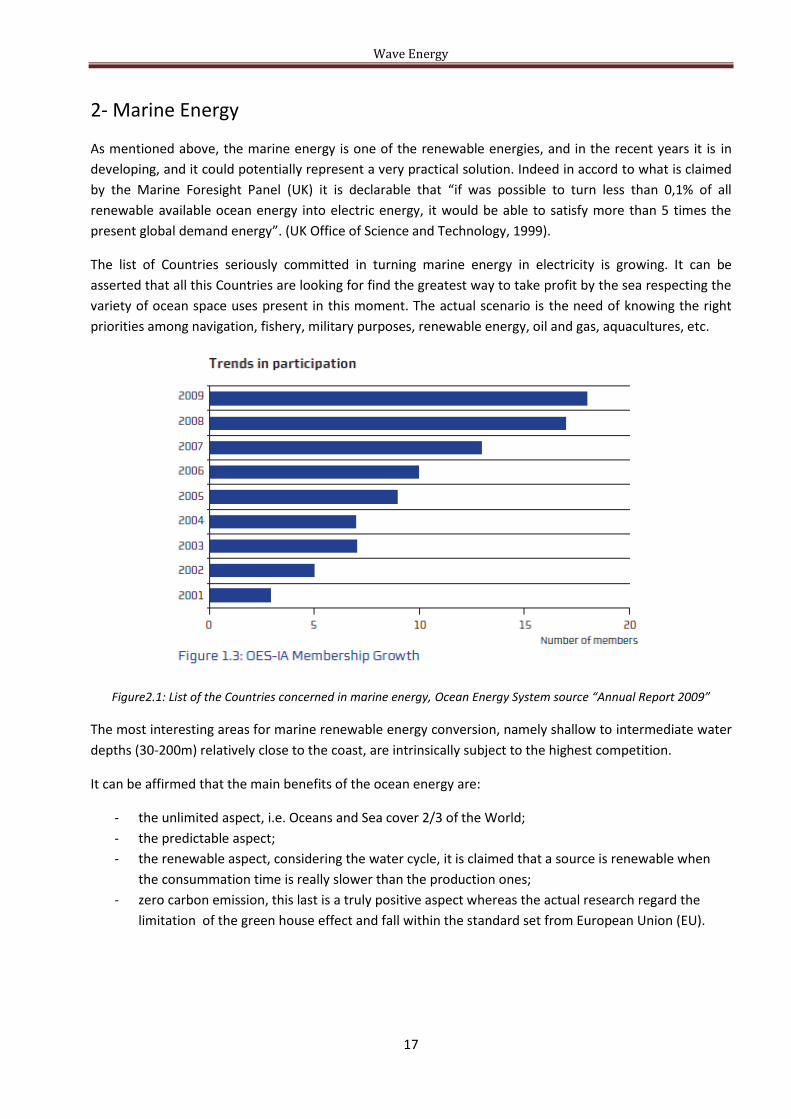
The list of Countries seriously committed in turning marine energy in electricity is growing. It can be
asserted that all this Countries are looking for find the greatest way to take profit by the sea respecting the
variety of ocean space uses present in this moment. The actual scenario is the need of knowing the right
priorities among navigation, fishery, military purposes, renewable energy, oil and gas, aquacultures, etc.
Figure2.1: List of the Countries concerned in marine energy, Ocean Energy System source “Annual Report 2009”
The most interesting areas for marine renewable energy conversion, namely shallow to intermediate water
depths (30-200m) relatively close to the coast, are intrinsically subject to the highest competition.
It can be affirmed that the main benefits of the ocean energy are:
- the unlimited aspect, i.e. Oceans and Sea cover 2/3 of the World;
- the predictable aspect;
- the renewable aspect, considering the water cycle, it is claimed that a source is renewable when
the consummation time is really slower than the production ones;
- zero carbon emission, this last is a truly positive aspect whereas the actual research regard the
limitation of the green house effect and fall within the standard set from European Union (EU).

Wave Energy
18
The renewable energy comes from the oceans appears in numerous forms, amongst salinity gradient by
osmotic energy, tidal energy, wave energy, different temperature by thermal energy (OTEC) , however the
most popular are the wave energy and the tidal energy.
Figure2.2: Ocean Energy Source “OCEAN ENERGY OPPORTUNITY, PRESENT STATUS AND CHALLENGES”
Figure2.3: Real example of wave energy converter: Wave Dragon, Nissum Brendning, Denmark
picture’s source Ocean Energy System “OCEAN ENERGY OPPORTUNITY, PRESENT STATUS AND CHALLENGES”
Figure2.4: Real example of wave energy converter: Pelamis, Northern Portugal
picture’s source Ocean Energy System “OCEAN ENERGY OPPORTUNITY, PRESENT STATUS AND CHALLENGES”

Wave Energy
19
Figure2.5: Real example of wave energy converter: PowerBuoy free-floating point absorber, Hawaii
picture’s source Ocean Energy System “OCEAN ENERGY OPPORTUNITY, PRESENT STATUS AND CHALLENGES”
Figure2.6: Real example of tidal current energy converter: The Blue Concept, Norway
picture’s source Ocean Energy System “OCEAN ENERGY OPPORTUNITY, PRESENT STATUS AND CHALLENGES”
Figure2.7: Real example of tidal current energy converter: Kinetic Hydro Power System, U.S.A.
picture’s source Ocean Energy System “OCEAN ENERGY OPPORTUNITY, PRESENT STATUS AND CHALLENGES”
Figure2.8: Real example of tidal current energy converter: Seaflow, Devon, U.K.
picture’s source Ocean Energy System “OCEAN ENERGY OPPORTUNITY, PRESENT STATUS AND CHALLENGES”

Wave Energy
20
Figure2.9: Real example of tidal current energy converter: Enermar System, Messina, Italy
picture’s source Ocean Energy System “OCEAN ENERGY OPPORTUNITY, PRESENT STATUS AND CHALLENGES”
Figure2.10: Real example of tidal current energy converter: Open-Centre Turbine, Scotland
picture’s source Ocean Energy System “OCEAN ENERGY OPPORTUNITY, PRESENT STATUS AND CHALLENGES”
Figure2.11: Real example of osmotic energy converter, salinity gradient: Osmotic Power, Norway
picture’s source Ocean Energy System “OCEAN ENERGY OPPORTUNITY, PRESENT STATUS AND CHALLENGES”
Figure2.12: Real example of thermal gradient OTEC Device Thermo-dynamic Rankine cycle, Japan
picture’s source Ocean Energy System “OCEAN ENERGY OPPORTUNITY, PRESENT STATUS AND CHALLENGES”

Wave Energy
21
2.1- Main typology of ocean energy
Even if there are different typology of ocean energy the most popular and widespread are the tidal and the
wave energy.
The tide is a natural motion of water masses caused essentially by Moon attraction on the water masses
combined with Earth rotation around the Sun. The dissipate energy by tidal movements causes on an
infinitesimal level a reduction of the distance between Earth and Moon and a slowing down of Earth. The
tidal energy consists in take advantage of the natural potential energy variations associated to the tidal ebb
and flow water elevation turns near to shore.
Figure2.13: Tidal Energy Patterns
The colours in the map indicate where tides are strongest, with blues being weaker areas and reds being
stronger. In almost a dozen places on this map the lines appear to converge. Notice how at each of these
places the surrounding colour is blue. These convergent areas are called amphidromes, places where there
is little or no apparent tide. This is not to say that the surface of the ocean in these places doesn't move, or
doesn't rise and fall with wind, momentum, inertia, and other forces acting on it. But for the purposes of
studying the tides from space in an effort to understand how energy is conserved and distributed, these
areas a mathematically still.
Figure2.14: Tidal Energy Patterns

Wave Energy
22
Even in the last map there is the tidal energy tidal; blue signifies places where the ocean level is lower than
the average reference height, and red shows areas where it's higher. Between the darkest blue and the
brightest red is a range of more than 15m, displaced by lunar tidal forces. White areas separating the blues
and reds approximate the "zero" point, a reference sea level against which other areas are compared. This
is called an amphidrome, a place with little or no tide at all.
Figure2.15: Map of Surface Ocean Currents.
On this illustration red arrows indicate warm currents, while cold currents are displayed in blue.
Instead, the wave energy is due to the water movement on the sea surface. The wind action on the water
surface causes the wave origination and development; since wind is due to the sun action on the
atmosphere, the wave are actually a solar energy stock. Under water surface, the individual water particles
carry out some circular movements, while the energy transmission is in the same direction of the wave
propagation. In the absence of streams no net water movement happens during energy transport; this one
is totally different from tidal energy, where water and energy move together. The wave power is expressed
in kW per meter of wave crest [kW/m], and its maximum value is around 70 kW/m, usually in the zone
between 30° and 60° of latitude, on both hemispheres cause of the wind blowing predominantly from
western direction.
Furthermore the wave energy has the vantage to be a concentrated source of energy with lower hourly and
daily variations than other renewable resources such as wind, sun or ocean currents.
In addiction the wave energy has the favorable seasonal variations that follows the trend of electricity
consumption in Western Europe. Finally, a further advantage of the energy produced by waves is the low
environmental impact and visual.

Wave Energy
23
Figure2.16: Annual trend of energy wave in Scotland, source WERATLAS, European Wave Energy Atlas,1996
Fugro OCEANOR is a global provider of integrated real-time environmental monitoring and information
systems for oceans, rivers and lakes, groundwater and soil. The systems are often used by institutes to
collect data for scientific studies, and are also often used in connection with offshore oil and gas production,
harbour monitoring, sea- and fresh-water quality monitoring and weather forecasting.
Based on their global wave data base, OCEANOR have carried out a number of wave energy pre-feasibility
and resource studies around the World over the last 15 years. For example a wave energy resource
assessment program was carried out during 1987 to 1995 for the South Pacific Applied Geoscience
Commission (SOPAC) based in Suva, Fiji with funding from the Norwegian Agency for International
Development (NORAD). The aim was to map the ocean wave climate off the shores of several South Pacific
island nations with the main objective to evaluate the wave energy resource of the islands needed to study
the feasibility of developing wave power as a future clean energy source. The data collection was primarily
carried out by moored data buoys off the shores of the following islands in the South Pacific: Rarotonga in
the Cook Islands, Kadavu in the Fiji group, Tongatapu in the Kingdom of Tonga, Funafuti in the Tuvalu group,
Efate in Vanuatu and Upolu in Western Samoa. Towards the end of the project this information was
supplemented by satellite data from OCEANOR’s World Wave Atlas data base.
0
20
40
60
80
100
120
140
160
180
KW/m
Annual trend of the energy wave in Barra, Scotland
(Based on WERATLAS, European Wave Energy Atlas, 1996)

Wave Energy
24
2.2- Wave Energy
Since the primary document’s purpose is to study successful the conversion of wave energy to electricity, it
is essential to have an adequate knowledge of energy wave.
In all the paper the linear wave theory was used to define the parameters relevant to wave power, due to
the reason that in deep sea and intermediate water depth the linear wave theory describes wave
parameters sufficiently accurate and in the easiest way.
The linear (or Airy) wave theory describes ocean waves as sum of simple sinusoidal waves. The part of the
wave profile with the maximum elevation above the still water level (SWL) is called the wave crest and the
part of the wave profile with the lowest depression is the wave trough.
The distance from the SWL to the crest or the trough is the amplitude (a) of the wave and the wave height
(H) is defined as the total distance from the trough to the crest, so it is the double of the amplitude. The
wavelength (L) of a regular wave at any depth is the horizontal distance between successive points of equal
amplitude and phase for example from crest to crest or trough to trough and is defined according to the
linear theory by:
Where:
- g = gravitation constant;
- T = wave period (the time required for one wavelength to pass a fixed point);
- h = water depth (distance from ocean floor to SWL);
In deep water where h is large (h/L> ½ ), the hyperbolic tanh function tends to unity and the equation
becomes:
The elevation of the water surface relative to the still water level is indicates with the symbol , and the
equation describing this free surface as a function of time t and horizontal distance x for a simple sinusoidal
wave is shown in the next equation:
The figure below illustrates all the relevant parameters for an oceanic wave, since now described.

Wave Energy
25
Figure2.17: Main parameters of a wave.
Off shore in a typical wave the molecules of water moving describe circular orbits. This behavior depends
on ratio between the wave height and the water depth through the waves move. When the waves
approach the coast the orbits change from circular to elliptical. For each wave the major lost of energy
happened when it start to warn the seabed and change the shape orbit. The dissipation gets relevant
when the water depth is lesser the half of length wave. Many natural factors as refraction and reflection,
generate points where the concentration of energy is high, called hot spot.
Figure2.18: High-energy zone: Hot spots

Wave Energy
26
The propagation speed or celerity of a regular wave is given by:
The rate at which wave energy propagates is directly dependant on the group velocity of the wave. The
group velocity (Cg) is given as a function of the velocity of a single wave as:
In deep water the constant n simplifies to n = 0.5, so the group velocity becomes the half of the velocity of
a single wave.
In reality the waves are mostly generated by wind, which exerts a shear stress on the surface of the sea.
This effect of friction, combined with air pressure differences between the upwind and the lee side of a
wave crest, contributes to transfer energy to the waves, causing their growth. The wave height is
determined by wind speed, the duration of time which the wind is blowing, the distance over wind blows
(the “fetch”), the depth and the shape of the seafloor. Larger waves are generally more powerful, but wave
power is also determined by wave speed, wave length and water density.
However in theory in agreement with the linear assumption there are precise hypothesis stating that the
wave power is dependent on energy density and equations to determine energy density is therefore
derived in the following section.
The total energy of a wave system is the sum of its kinetic energy and its potential energy. The kinetic
energy is that part of the total energy due to water particle velocities associated with wave motion.
Whereas the potential energy is that part of the energy resulting from part of the fluid mass being above
and below the medium water level.
Figure2.19: The two component of the wave energy: the kinetic and the potential energy

Wave Energy
27
The total energy of an oceanic wave is given by:
22 2 2
2 2 2
x L x L
K P
x h x
du w dE E E dz dx g dx
Where:
- EK = kinetic energy [J];
- EP = potential energy [J];
- ρ = density of sea water [kg/m3];
- u = fluid velocity in x-direction [m/s];
- w = fluid velocity in z-direction [m/s].
According to the linearity theory, if all waves are propagated in the same direction, potential and kinetic
energy components are equal, and the total wave energy in one wavelength per unit crest width (wc) is
given by:
2 2 2
16 16 8K P
gH L gH L gH LE E E
The total average wave energy per unit surface area is called Specific energy or energy density ( ) and it is
given by:
2
8
E gHE
L
Wave energy flux is the rate at which energy is transmitted in the direction of wave propagation across a
vertical plane perpendicular to the direction of the wave that advances and extends down the entire depth.
Assuming the linear theory, the average energy flux per unit wave crest width ( ) transmitted across a
vertical plane perpendicular to the direction of wave advance is:
1t r
t h
P p u dz dtT
Where:
- p = gauge pressure;
- t = start time;
- r = end time.
Integration of the equation that was shown above is simplified to: gP EnC EC

Wave Energy
28
The wave energy flux (P) is also called wave power. The wave theory indicates that wave power is
dependent on three basic wave parameters: wave height, wave period and water depth.
Nevertheless the real sea is composed by an irregular wave situations, in first approximation the following
formula can be used to estimate the energy flux of an irregular wave in deep water conditions:
2 2
eg T HP
Where:
- P= wave energy flux per unit wave crest length [kW/m];
- ρ = mass density of the sea water 1030 [kg/m3];
- g = acceleration by gravity 9.81 [m/s2];
- Te= energy period [s];
- β = is a coefficient may be 64 for irregular waves or 32 for regular waves.
The real sea is random and irregular as it is possible to note in the next two figures.
Figure2.20: On the left: Decomposition of a 2D irregular wave state.
On the right: Decomposition of a single irregular wave, it is analyzed as a sum of many single regular waves.
These figures show how random surface elevation records can be deconstructed into a series of sinusoidal
components using a Fourier series analysis. Each sinusoidal component has unique basic parameters. Its
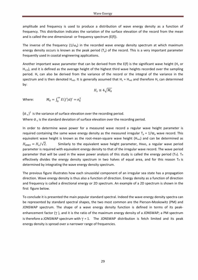
Wave Energy
29
amplitude and frequency is used to produce a distribution of wave energy density as a function of
frequency. This distribution indicates the variation of the surface elevation of the record from the mean
and is called the one dimensional- or frequency spectrum (E(f)).
The inverse of the frequency (1/ωp) in the recorded wave energy density spectrum at which maximum
energy density occurs is known as the peak period (Tp) of the record. This is a very important parameter
frequently used in coastal engineering applications.
Another important wave parameter that can be derived from the E(f) is the significant wave height (Hs or
H1/3), and it is defined as the average height of the highest third wave heights recorded over the sampling
period. Hs can also be derived from the variance of the record or the integral of the variance in the
spectrum and is then denoted Hm0. It is generally assumed that Hs ≈ Hm0 and therefore Hs can determined
by:
Where:
(σ η )2
is the variance of surface elevation over the recording period.
Where σ η is the standard deviation of surface elevation over the recording period.
In order to determine wave power for a measured wave record a regular wave height parameter is
required containing the same wave energy density as the measured irregular Tp = 1/ϖp wave record. This
equivalent wave height is known as the root-mean-square wave height (HRMS) and can be determined as
. Similarly to the equivalent wave height parameter, HRMS, a regular wave period
parameter is required with equivalent energy density to that of the irregular wave record. The wave period
parameter that will be used in the wave power analysis of this study is called the energy period (Te). Te
effectively divides the energy density spectrum in two halves of equal area, and for this reason Te is
determined by integrating the wave energy density spectrum.
The previous figure illustrates how each sinusoidal component of an irregular sea state has a propagation
direction. Wave energy density is thus also a function of direction. Energy density as a function of direction
and frequency is called a directional energy or 2D spectrum. An example of a 2D spectrum is shown in the
first figure below.
To conclude it is presented the main popular standard spectral. Indeed the wave energy density spectra can
be represented by standard spectral shapes, the two most common are the Pierson-Moskowitz (PM) and
JONSWAP spectrum. The shape of a wave energy density function is defined in terms of its peak-
enhancement factor (γ ), and it is the ratio of the maximum energy density of a JONSWAP; a PM spectrum
is therefore a JONSWAP spectrum with γ = 1. The JONSWAP distribution is fetch limited and its peak
energy density is spread over a narrower range of frequencies.

Wave Energy
30
Figure2.21: 2D Spectrum, source Coastal Engineering Manual.
Figure2.22: Pierson-Moskowitz and JONSWAP spectrums, source C.E.M.
In the real sea there is a last aspect to considerate, in particular as the waves approach shallower waters
begin to feel the bottom and the wavelength decreases while the wave height increases. This result in
increased wave steepness. When wave becomes so steep that it can no longer remain stable, it breaks.
Since wave breaking is related to water depth, the height of a breaking wave can be estimated from the
following equation:
Where:
- Hb= breaking wave height;
- hw= water depth.
The shallow water breaking wave height is dependent on seabed slope and bed characteristics, and can be
affected by strong winds or currents in the direction of the wave propagation. Breaking waves are classified
as spilling, plunging, or surging.
The kinematics of breaking waves are not as well understood as the kinematics of non-breaking waves.
Since kinematics are the prime factors that control wave induced loads, the loads due to breaking waves
are also not as well understood. Reasonable approximations of the forces from a breaking wave are on
order of two to four times that of a non-breaking wave.
For that reason the breaking cases won’t be study in this project.

Wave Energy
31
2.3- Wave Energy Converter
The potential global wave power has been estimated to be 86-87 kWh/year (which is equivalent to an
installed power generation capacity of 1 to 10 million MW), which is of the same order of magnitude as
world electrical energy consumption in the 70’s (Isaacs and Seymour, 1973; WEC, 1993).
Next image illustrates the highest wave power zones. In the zone from 30° to 60° north and south latitude
is found the highest annual average power level, that is between 20 to 70 kW/m or more. However,
significant wave climates are still found within ± 30º latitude where regular trade winds blow; the lower
power levels being compensated by the smaller wave power variability.
Figure2.23: Average annual ocean wave power in kW/m, source ww.oceanpd.com/Resource/Worldresourcemap.html
The map illustrates that the most energy rich coastlines in the world are Chile, South Australia, New
Zealand as well as parts of Western Europe, notably Ireland, Scotland and Iceland as well as western
Canada and South Africa.
This does not necessarily mean that these areas have the highest potential for wave energy exploitation.
Several of these areas are isolated with poor communications. The highest potential at the first stage for
wave energy is probably areas such as islands in the trade wind belt of the Pacific, where overall wave
energy is much lower but considerably more steady both in strength and direction.
North-east Atlantic area (including the North Sea) offers the availability of wave power of 290 GW, with
annual variations ranging between 25 kW/m in the area further south on the Atlantic coast, to 75 KW/m
corresponding to the Irish and Scottish coasts. In the North Sea, the energy source undergoes strong
fluctuations, ranging from 21 KW/m, in the most exposed (north) to a level of 10 kW/m.

Wave Energy
32
Figure2.24: Europe: Average annual ocean wave power [kW/m]
Wave energy conversion is not a new concept, in fact, the first patented Wave Energy Converter (WEC) is
dating back to the early 18th century. As presented in the previous chapter, the high oil prices in the 1970’s
forced governments of the world to consider alternative sources of energy. During this period ocean energy
was identified as one of alternative extractable sources. This lead to world-wide research to the field of
wave energy conversion.
However until post-2000 there existed few large-scale sites where wave energy machines could be tested,
and only two sites were available pre 2000: both of these were in Denmark and at that time they were not
registered externally as official test centres.
Figure2.25: Europe’s map: Wave Test Centres

Wave Energy
33
Even though wave energy is not a new search field, non formalised guidelines or recommended procedures
or best practice manuals appeared until 2003. Until that time the vanguard companies had to design their
own development schedules and test programmes on an ad hoc basis, and usually in isolation from each
other.
Most of the initial investigation took place in the UK, and in the early 1990s the European Union became
interested in the potential of ocean power supplying electricity into the member states energy portfolios.
One of the first proposals supported was the Offshore Wave Energy Converter Project (OWEC1). A test
programme was documented in 1995. However, nothing was advanced on this report and the schedule did
not become a standard approach to be applied throughout the member states researching the area.
The OWEC1 development schedule was used as the framework for the Irish Wave Energy Development &
Evaluation Protocol published and implemented in 2003 and the Danish wave energy programme, 1998-
2002.
Now in Denmark there is a particular and standardized assessment to determine the benefits and the
performance of new wave energy converters. This evaluation is constituted by four phases, and it is used in
the next chapters. These phases are:
1- Phase 1: Proof of concept. Rough estimates of energy production in five specified wave states
leading to an estimate of a yearly energy production. Suggestions for further development of the
device. Typical small indicative laboratory tests followed by a 10 page report. Cost 10.000 €.
2- Phase 2: Design and feasibility study. Typically through detailed laboratory tests in scale 1:50 to
1:20. Detailed Numerical calculations, estimates on cost, feasibility studies, Power take-off (PTO)
design, etc. Typical intensive laboratory tests (optimizations) or intensive numerical modelling. This
phase can consist of detailed investigations followed by 100 page reports. Cost 25.000-50.000 €.
3- Phase 3: Testing in real seas in scale 1:10 to 1:3. Normally Nissum Bredning where a “small” benign
piece of inner sea, a part of the Limfjord in the northern part of Denmark , has been used for this
purpose. Cost 0.5-5 million €.
4- Phase 4: Demonstration in half or full scale. Cost 5-20 million €.
The main instrument used under phase 1 and phase 2 to assess the wave energy devices is small scale
testing in a hydraulic laboratory. These tests are performed in order to gain knowledge on the devices
before they actually are built and deployed in the sea. The laboratory tests will give information on:
a. Loads on the device
b. Movements of the device
c. Run-up / overtopping of the device
d. Energy production
In phase 1 assessment, the test will give rough estimates (± 20%) on energy production. The main idea of
the Danish practice is that each of the phases should provide valuable information for the developers and
investors, before the project is taken to the next phase. Thus, the risk of using unnecessary resources on a
device before reliable estimates of the concepts potential is known and it is thereby minimized.
Furthermore, it eases the comparison of various projects at the same phases of development.
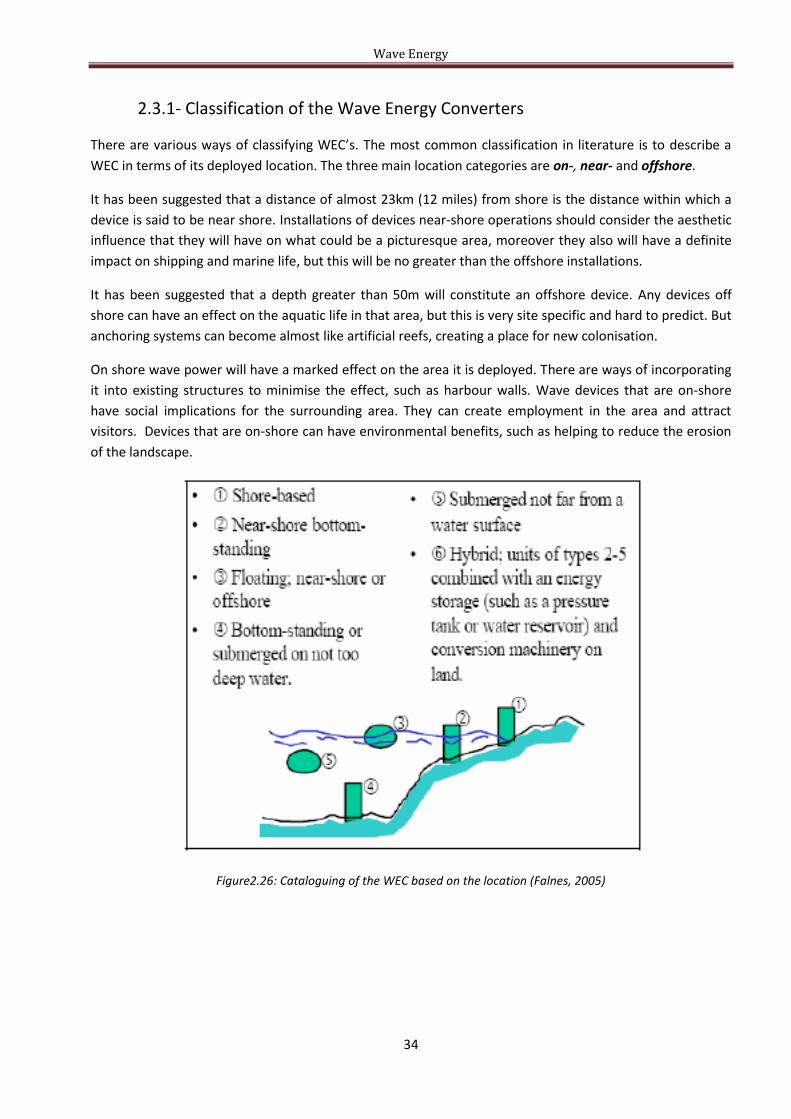
Wave Energy
34
2.3.1- Classification of the Wave Energy Converters
There are various ways of classifying WEC’s. The most common classification in literature is to describe a
WEC in terms of its deployed location. The three main location categories are on-, near- and offshore.
It has been suggested that a distance of almost 23km (12 miles) from shore is the distance within which a
device is said to be near shore. Installations of devices near-shore operations should consider the aesthetic
influence that they will have on what could be a picturesque area, moreover they also will have a definite
impact on shipping and marine life, but this will be no greater than the offshore installations.
It has been suggested that a depth greater than 50m will constitute an offshore device. Any devices off
shore can have an effect on the aquatic life in that area, but this is very site specific and hard to predict. But
anchoring systems can become almost like artificial reefs, creating a place for new colonisation.
On shore wave power will have a marked effect on the area it is deployed. There are ways of incorporating
it into existing structures to minimise the effect, such as harbour walls. Wave devices that are on-shore
have social implications for the surrounding area. They can create employment in the area and attract
visitors. Devices that are on-shore can have environmental benefits, such as helping to reduce the erosion
of the landscape.
Figure2.26: Cataloguing of the WEC based on the location (Falnes, 2005)

Wave Energy
35
Another classification method is to describe the WEC in terms of its size and orientation. In this
classification type there are three categories. A WEC can be classified as a point absorber, attenuator or
terminator.
A point absorber is a relatively small device compared to a typical wavelength. A point absorber is a floating
structure which absorbs energy in all directions through its movements at/near the water surface. The
power take-off system may take a number of forms, depending on the configuration of displacers/reactors.
Figure2.27: Point Absorber, source EMEC
An attenuator is a floating device with a length equal to/ or greater than one wavelength. This type of
device is aligned in the direction of wave propagation, so it works parallel to the wave direction. If this
same device is aligned perpendicular to the direction of wave propagation it is called a terminator device.
Figure2.28: Attenuator, source EMEC
Figure2.29: Second classification of the WEC based on the orientation (Falnes, 2005)

Wave Energy
36
A further classification of WEC units is based on technology with regards to its basic principle of energy
extraction. The classification categories include:
1. Overtopping Devices (OTD), they are device able to convert the potential energy of the water in
electricity, as a small hydro power scheme. The ocean waves are elevated through a ramp and
focus into a storage reservoir above the sea level. As more water enters into the reservoir, an equal
amount of water is forced through the turbines, that are usually low head Kaplan turbines. The
water entrance causes the rotation of the turbines and consequentially the electricity generation.
The difference water level between the reservoir and the sea is continuously annulled, because the
water passing through the turbines returns to the sea. The efficiency of the hydro power plant
component of the system is high (up to 80%) and this will minimise overall losses of the system.
Figure2.30: Typical representation of a Overtopping Device
The overtopping devices can be allocated on-shore or off-shore. One example of on-shore OTD is the SSG,
i.e. Seawave Slot-Cone generator.
Figure2.31: On the left: Section of the SSG, on the right: possible installation as a breakwater
Whereas one example off-shore is the Wave Dragon.
Figure2.32: Wave Dragon is an off-shore OTD

Wave Energy
37
2. Wave Activated Bodies (WAB) Device, they are also called two-bodies devices, because the
peculiarity of this kind of devices consists in the relative motion between the component parts of
the devices themselves. The oncoming waves activate the oscillatory motions between the parts, or
one part relative to another fixed part. By using an hydraulic system it is possible to convert the
relative motion into electricity by a turbine activated by the pressured fluid, who comes from the
hydraulic system. If this kind of devices is placed in a perpendicular direction with the wave
direction it becomes even a terminator, while if it is parallel it is even an attenuator. Common
examples of Wave Activated Body (WAB) are Pelamis, AquaBuoy, DEXA.
Figure2.33: DEXA is an example of Wave Activated Body, source www.dexawave.com
A subset of the Wave Activated Body is the Submerged pressure differential. These devices are typically
located near-shore and attached to the seabed. The motion of the waves causes the sea level to rise and
fall above the device, inducing a pressure differential in the device. The alternating pressure can then pump
fluid through a system to generate electricity.
Figure2.34: Submerged pressure differential, source www.emec.org.uk

Wave Energy
38
3. Oscillating water column (OWC) Devices, they are one of the most common devices for the energy
production, because since 1980’s some prototype of OWC are developed in several places in the
world, so the engineers have for this technology a great experience. The study of this category is
well delved because the device under consideration belongs to this category.
Usually an oscillating water column is a partially submerged and hollow structure. It is open to the
sea below the water line, enclosing a column of air on top of a column of water. Waves cause the
water column to rise and fall, which in turn compresses and decompresses the air column. This
trapped air is allowed to flow to and from the atmosphere via a turbine, which usually has the
ability to rotate regardless of the direction of the airflow. The rotation of the Wells turbine is used
to generate electricity. The main benefits of OWC technology include the following:
o shore based OWC devices provide easy access for operation and maintenance work;
o the near shore location reduces transmission costs;
o OWC devices can be incorporated into breakwaters and can be used to create calm sea
areas.
Some disadvantages associated with OWC devices are:
o the available wave power resource is less in the near-shore zone compared to off-shore
one due to energy dissipation processes;
o an OWC being a terminator device can disrupt sediment transport processes by reducing
the wave power reaching the shore;
o most OWC devices are non-tuneable and this reduces the system’s overall efficiency;
o shore based OWC structures can have a visual impact if they are not submerged.
Familiar Oscillating Water Column (OWC) Device is the Limpet.
Figure2.35: Oscillating Water Column, source renewable energy journal, mechanical ocean energy conversion, part II
A subset of the Oscillating Water Colum is the Oscillating Wave Surge Converter (OWSC). This is a new
shore-line or near-shore wave energy converter. The concept has developed from an analysis of the
performance of the LIMPET shoreline oscillating column.

Wave Energy
39
This analysis shows that the hydrodynamics of shoreline wave energy converter are highly non-linear, and
they have a qualitatively different response to similar device that are sited in deeper water. In particular,
the water particle motion in shallow water is predominantly horizontal. The OWSC are designed to use the
horizontal particle motion, so permitting large amplitude of motion.
The larger horizontal water particle motion in shallow water suggests that the working surface of the wave
energy converter should not move only in an approximately horizontal plane, and to minimise the required
volume of displacement, this suggest a relatively thin paddle. The horizontally aligned slides and straight-
line mechanisms are likely to be costly and difficult to maintain, hence the easiest choice can be between
hinging the paddle at the top or bottom. If the hinge point is above the water surface it is possible to
match better the average horizontal water particles motion, and in addition there are the benefits of
having a power take off more accessible and the no “end-stop” of the paddle.
Figure2.36: Oscillating Wave Surge Converter: scheme with the paddle hinged at the bottom, source www.emec.org.uk
Figure2.37: Oscillating Wave Surge Converter: scheme with the paddle working with a straight-line mechanisms
Units of the WavePiston Device, source www.wavepiston.dk
Furthermore the potential for the OWSC resides even in low construction and maintenance cost and in the
price for generate the electricity; in fact even if the OWC technology is inviting for its simplicity, it has the
problems in the low air turbine efficiency and in the not well-known hydrodynamic of the water column in
shallow water. Consequently the wave energy research at Queen’s University Belfast started to developed
a new kind of device called OWSC. A number of distinct embodiments of the OWSC can be envisaged.
These different embodiments all exploit the beneficial hydrodynamics of the paddle and the water column,
but differ in how this is achieved and consequently in their construction and performance.

Wave Energy
40
Even though there are many classes to which a device can belong, there are some device that due to their
unique different design or characteristics cannot be included in any class.
Regardless of the class, to design a device is necessary to take care in the material choice. The durability
aspect is crucial, the device have to withstand storm, high seas and corrosive salt water and their
maintenance cost are really high.
2.3.2- Examples of the Wave Energy Converters
2.3.2.1- LIMPET
LIMPET stands for “Land Installed Marine Powered Energy Transformer”. The LIMPET is a 500 kW OWC
developed by the Queen's University of Belfast and Wavegen Ltd in the United Kingdom. It was installed on
the Isle of Islay off the west coast of Scotland and was commissioned in November 2000.
The collector structure consists of reinforced concrete chamber and it has cross sectional dimensions of
21mx 7m. The structure is very robust in order to survive extreme loadings with 0.75 m thick walls. The
airflow caused by the oscillating water column drives two Wells turbines each with a 250 kW capacity and a
blade diameter of 2.6 m. The turbine has to be able to generated energy turning regardless of the direction
of flow of air.
Figure 2.38 : LIMPET’s section

Wave Energy
41
Figure 2.39 : Cross sectional view of LIMPET
Figure 2.40 : Real view of LIMPET
The available annual average wave
power resource in the deployment area
is 20 kW/m and the water depth is six
meters.
This device is currently generating 0.5MW of power that it supplies to the grid on the Island of Islay off the
west coast. This is an example of how this technology can be used to meet small-scale local needs.
Wavegen have said that at present the answer lies in not huge operating plants but small ones such as
these, which can concentrate on meeting local or regional needs.
It is possible to calculate how many homes it will supply, in following calculations were made with this aim.
max electricity generated [kWh/year] 500
max electricity generated [MWh] =500*8760 = 4380
Load factor or capacity factor 0,40
Electricity generated per year [MWh] =4380*40%= 1752
Average annual household consumption [kWh/day] 12
Average annual household consumption [kWh/year] 4377
Number of houses =1752*103/4377= 400
Table 2.1: Quick overview of the LIMPET performance

Wave Energy
42
2.3.2.2- PENDULOR
The “Pendulor” consists of a caisson with a top hinged paddle at the mouth of a water chamber. The length
of the chamber is ¼ of a wave length to produce harbour resonance. Unfortunately, typical wave periods
where wave energy converter are likely to be sited, would result in un-economically long water chambers.
Figure 2.41 : Pendulor’s scheme
2.3.2.3- WAVE DRAGON
The Wave Dragon is an off-shore reservoir storage WEC. This typology focus waves into a storage reservoir
and from here the stored water flows through low head turbines to generate power, similar to a small
hydro power scheme. The WAVEDRAGON is a floating and overtopping WEC device. It consists of two
parabolic reflecting arms, a double curved overtopping ramp, a storage basin and multiple low head
turbines. The reflecting arms focus waves onto the overtopping ramp and into the storage basin above sea
level. From the basin the water flows through modified Kaplan-turbines and generates electricity. This
device is slack moored and can orientate itself to face into the dominant wave direction. The structural
components of the WAVEDRAGON consist out of steel and reinforced concrete. The reservoir storage
ranges from 5000 to 14000 m3. It is designed to operate in water depths greater than 25 m.
Figure 2.42 : Wave Dragon representation

Wave Energy
43
2.3.2.4- PELAMIS
The PELAMIS is a WAB device. Usually the WAB device generate energy giving pumped fluid to a turbine.
The pumped fluid is obtain by the relative motion of a component relative to another device component.
The word “pelamis” is Latin for sea snake. The PELAMIS WEC is a floating device consisting of four tubular
sections connected at three hinges. These tubular sections move relative to each other as a wave crest
passes under it and power is generated through a digitally controlled hydraulic power conversion system.
The device is slack moored enabling it to orientate itself into the direction of the most dominant wave
conditions. The PELAMIS unit has a diameter of 4.6 m and a length of 150 m. It is designed to be deployed
in water depths deeper than 50 m.
Figure 2.43 : PELAMIS – Schematic representation
2.3.2.5- SWEC
The SWEC comprises of a pair of collectors (arms) coupled in a V-formation to a single air turbine and
power generator mounted above water level in a tower at the apex of the V. Each collector arm has OWC
chambers and the pressurised air is send along the arm to the power generator in the tower. This is a near
shore system founded on the seabed in water depth of between 15 to 20 m.
The design length of a collector arm is 300m with a 30° inclination angle to the shore. This gives the system
an effective width of 350m for power extraction.
The SWEC looks like the LEANCON, the main difference is that the LINCON is a floating device.

Wave Energy
44
Figure 2.44 : SWEC’s pressure system
Figure 2.45 : Overview of the SWEC
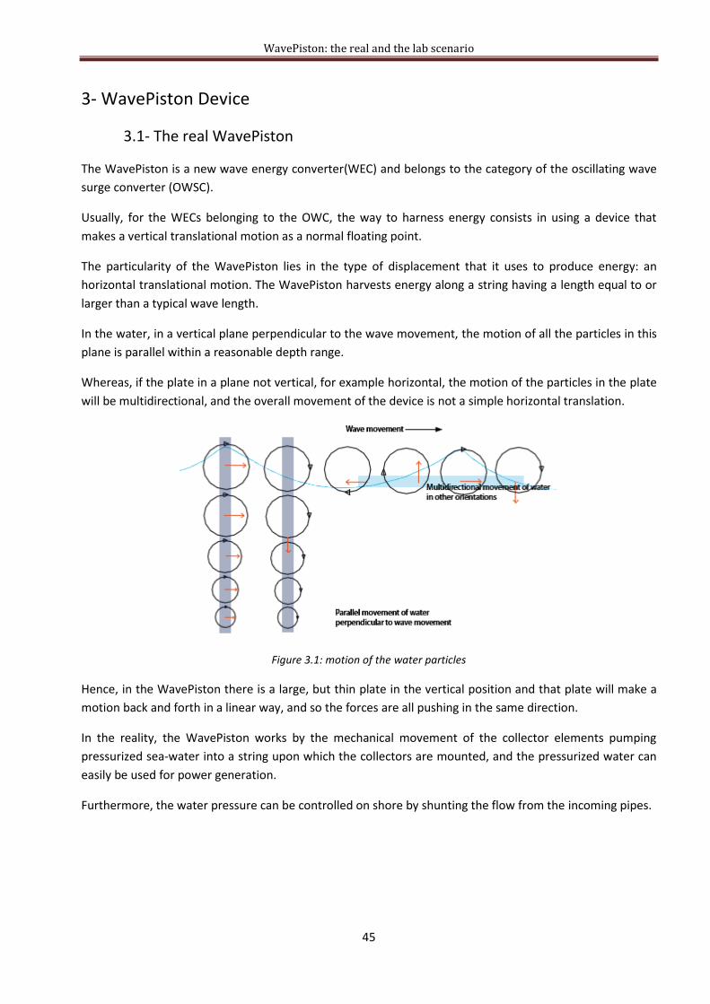
WavePiston: the real and the lab scenario
45
3- WavePiston Device
3.1- The real WavePiston
The WavePiston is a new wave energy converter(WEC) and belongs to the category of the oscillating wave
surge converter (OWSC).
Usually, for the WECs belonging to the OWC, the way to harness energy consists in using a device that
makes a vertical translational motion as a normal floating point.
The particularity of the WavePiston lies in the type of displacement that it uses to produce energy: an
horizontal translational motion. The WavePiston harvests energy along a string having a length equal to or
larger than a typical wave length.
In the water, in a vertical plane perpendicular to the wave movement, the motion of all the particles in this
plane is parallel within a reasonable depth range.
Whereas, if the plate in a plane not vertical, for example horizontal, the motion of the particles in the plate
will be multidirectional, and the overall movement of the device is not a simple horizontal translation.
Figure 3.1: motion of the water particles
Hence, in the WavePiston there is a large, but thin plate in the vertical position and that plate will make a
motion back and forth in a linear way, and so the forces are all pushing in the same direction.
In the reality, the WavePiston works by the mechanical movement of the collector elements pumping
pressurized sea-water into a string upon which the collectors are mounted, and the pressurized water can
easily be used for power generation.
Furthermore, the water pressure can be controlled on shore by shunting the flow from the incoming pipes.

WavePiston: the real and the lab scenario
46
If the WavePiston system is deployed in coastal waters, the necessary turbine and power conversion
systems (PTO) could be placed in the same structure onshore, so that the system can be controlled under
all conditions and even more, that will reduce the total cost.
The WavePiston system should be build from prefabricated modules that can be mass-produced at a low
cost. Each module consists of an energy collector and a piece of the static structure (pipe).
Figure 3.2: WavePiston envisaged design, it is possible to note the whole structure composed by a multitude of plates
united in a unique moored frame
The energy collector is a plate that can slide back and forth along a pipe in a static structure. The interface
between the plate and the pipe is a pump that pumps water into the pipe in both sliding directions. When
an energy collector gets near the limit movement, a spring will slowly close the pump valves to avoid
sudden bumps.
Figure 3.3: single module design: in the pictures you can see the single plate and the pipe that connects two sequent
plates, that is the mainly part of the device because it transports the seawater pressured to the turbine station.

WavePiston: the real and the lab scenario
47
Building the system from modules makes it easy to transport, deploy, and repair.
If a module fails, it will not compromise the entire system.
Faulty modules can be replaced or fixed on the spot, when weather allows it.
Due to the oscillatory nature of the water movement along the WavePiston, the forces on the individual
collectors will tend to cancel each other out, with the result that even very long WavePiston systems can be
moored using only moderate means.
The nature of the water movement also means that there is not a unique depth to put this device, but the
optimal depth range for a wave energy farm depends only on the nature of the sea condition.
The key for the efficiency is only the width and the depth of collector. As the amount of energy that can be
harvested is proportional to the available collector area, the collectors should be made as large as possible.
In view of the fact that the WavePiston concept is based on connecting multiple vertical energy collectors,
it is important to study the mutual distance between them; ideally, if two vertical plates are positioned
exactly at the distance of a half wave length from each other, they will move in opposite directions all the
time, hence they will work with the maximum efficiency.
Although most forces from the collector elements are cancelled out, the system still needs to be moored to
the seabed to compensate for residual forces, such as currents and winds. Moreover, at a certain energy
level, the waves will start breaking and the speed and force of water increases dramatically at surface level,
but anyway the mooring will be minimal, also because the Wave Piston system is almost fully submerged
and therefore less vulnerable to storms.

WavePiston: the real and the lab scenario
48
3.2 - WavePiston prototype
3.2.1 – Aalborg laboratory
The University of Aalborg is one of the most important universities in Denmark, and its particularity consists
in the way of teaching and developing the subjects. The idea is to give the students the possibility to solve
themselves different problems with group projects and that’s why this university has a lot of laboratories.
Specifically, the wave energy converters are studied in the wave laboratory that belongs to the Water and
Environment Department of Structure Engineering.
This laboratory is equipped with a reinforced concrete tank, with a rectangular shape of the dimensions of
15.7m x 8.5m and a maximum depth of 1,5m, where it is possible to reproduce 3D waves.
The tank is supplied with a paddle system as a snake-front piston type with a total of ten actuators to
simulate the sea wave, and an absorbent shore composed by gross gravel with a 1:4 slope. The motion of
each actuator is independent from one another, and this permits the generation of longitudinal waves as
well as oblique ones.
Figure 3.4: Overview of the laboratory in Aalborg University:
On the left you can see a part of the absorbent shore, and in the background the paddle system as a snake-front piston
type, whilst between the two piers there is the device in the configuration with four wings. Finally in the left
background, there are computers to make and analyze the waves.

WavePiston: the real and the lab scenario
49
Figure 3.5: Detail of the paddle system as a snake-front piston and of the gauges on the left part. Since the paddle
system is not provided with its own system of absorption of the reflection waves, on the sides of the tank and on the
blades of the paddle system, there are metallic breakwater.
Figure 3.5: Section and top view of the laboratory of Aalborg University

WavePiston: the real and the lab scenario
50
To control the paddle system, the university research group invented a software on purpose and it is called
AWASYS5. To create the different wave states, the program needs different parameters as:
- kind of the wave (regular or irregular wave)
- wave height
- wave period
- water depth
- duration of the test
- choice of the spectrum for irregular waves and peak factor
Figure 3.6: Screen of the AWASYS5 for the generation of a regular wave of 0,024m wave height and 1,02s of wave
period, corresponding to the first wave state, and for the duration of 5 minutes.
Figure 3.7: Screen of the AWASYS5 for the generation of an irregular wave of 0,033m wave height and 1,02s of wave
period, corresponding to the first wave state, and for the duration of 20 minutes. JONSWAP Spectrum has been used.

WavePiston: the real and the lab scenario
51
All the data were acquired and analyzed using a software called WaveLab3.33. The acquisition system
works at the sampling frequency of 20Hz.
Figure 3.8: Screen of the WaveLab3.33 “Acquisition Data”
The data acquired by WaveLab3.33 come from the connection with the gauges.
Indeed, for the measurement of the wave height, four wave gauges were collocated in the tank in front and
in line with the device and particularly between the device and the paddle system. Usually, to have the
most accurate representation of all the waves both incident and reflected, the wave gauges are collocated
in front and behind the device, but due to space, in the laboratory configuration it is permitted only the
positioning in the front part.
A wave gauge is an instrument that measures the fluctuations in the surface level; an ordinary instrument
in its type is the step-resistance wave gauge. This consists of a series of electrical contact points. The gauge
is attached in a vertical position to a supporting structure such as a pier, with the bottom below the lowest
expected wave trough. It’s essential to calibrate these probes every day, before starting with the sampling
and even more frequently during the same day, if the tests are stopped for more than two hours. The
calibration is necessary to prevent errors due to the different water temperature or conductivity.

WavePiston: the real and the lab scenario
52
For all the tests their configuration is at a distance of 1,5m from the paddle system, and the distance
between gauge1 and the subsequent is 0,15m; 0,40m; 1,0m, as it is shown in the configuration in the figure
n. 3.14 at page 56.
It is important that the relative distances between two probes are such that they are not among multiples
or dividers, to allow the separation of incident and reflected waves.
As you can see from figure 3.8, to save the data from the wave gauges, the software WaveLab3.33 needs
some parameters into account, such as: the sample frequency, the number of channels, the sample
duration, and the data file name. For each test, the data file name structure was AA_BB_CC_DD_EE_FF.dat
where:
AA indicates if the wave is regular (RW) or irregular (Ir);
BB indicates the wave height;
CC indicates the wave period;
DD indicates the distance between the wings in a particular configuration test;
EE indicates the load;
FF indicates the number of the test.
Under particular conditions, there is something else added at the end of the name, and this occurs when
the study is aimed to the importance of a particular parameter as the angle, or the wave period variation.
Figure 3.9: Screen of the WaveLab3.33 “Reflection Analysis”

WavePiston: the real and the lab scenario
53
As it is exposed in the figure 3.9, to obtain the main results for the incoming and reflected waves (for
example: the significant wave height, the wave period and the power per meter wave) the software
WaveLab3.33 needs some parameters into account such as: the data file, the three gauges channels, the
relative distance between the gauges under consideration and the water depth.
WaveLab3.33 analyzes the wave gauges data through the reflection analysis, using a numerical procedure
which implements the method of Mansard & Funke for the separation between incident and reflected
waves from the data of three level probes.
The method presented by Mansard & Funke assumes that the wave elevation is a sum of regular waves
travelling with different frequency and phase. Hence, using the Fourier analysis, the amplitude of the
incident and reflection waves for a given frequency can be estimated and moreover, it gives the variation of
the measured noise from wave gauge to wave gauge.
Further WaveLab3.33 has different main component as:
- the show and compare signal procedure: where it is possible to see the overview sampling signal
from only one sampling or from more than one samplings;
- the filtering component;
- generate and analysis of time series.
Moreover, at the time of the experiments, the laboratory was also equipped with an additional computer,
where runs the software “National Instruments LabView 8.5” that includes “WavePiston.vi”.
WavePiston.vi is a software appointed to harvest the data from the device, that transmits through four
cables the values of the linear displacement sensors, and of the force transducers.
That software saves the data with a sampling frequency 10Hz, hence this data are used for the calculation
of the power take off (PTO).
Before the sampling, a name is chosen to save the data, following the same criterion as for the one in
WaveLab3.33. The sampling gives a file.txt of the results that is composed of four columns, of which the
first two contain displacement information, while the last two contain force information.
The figure 3.10 shows what happens during the sampling, on the left part it is possible to see the trend of
the measurements, and on the right part their values, so that through the graph it is easy to understand,
even during the record, if there are some kind of problems.
The water depth during all the tests was 0.70m.

WavePiston: the real and the lab scenario
54
Figure 3.10: Screen of the WavePiston.vi “Sampling Graph”. On the left the picture shows the graph of the recording of
the four channels, and on the right the values of these sampling.
Figure 3.11: Box that connects the device and computer

WavePiston: the real and the lab scenario
55
3.2.2 – Model and experimental activity
The WavePiston prototype is invented by a Danish group including Martin von Bülow and Kristian Glejbøl,
both from Copenhagen.
That prototype was then studied in the laboratory of Aalborg University, Department of Civil Engineering, in
February and March 2010.
The peculiarity of the horizontal translational motion was difficult to reproduce in the laboratory, so the
prototype used was slightly different from a real world scenario.
Hence, the whole device, including the power take off unit(PTO), is modelled in a different way.
The main change made was to add a structure that supported the floating devices.
This structure was built very high compared to the size of the parties that constitute the core of the device,
in order to reduce the effect of an arm rotating around a fixed pivot.
As already reported in the presentation of the real device, every plate is connected to a unique power take
off system, while in the laboratory state, each plate has a singular power take off unit.
Figure 3.12: Support structure added
Figure 3.13: Single PTO for each energy collector plat, including the sliding rail with the load, the force transducer and
the LVDT

WavePiston: the real and the lab scenario
56
Figure 3.14: WavePiston Prototype and its configuration in the laboratory
Thanks to the support structure added it was also easily feasible the design configuration of the real
WavePiston, i.e. to have one moored reference frame supporting a multitude of working plates that are
placed in parallel and in line relative to the incoming wave. Further, this structured includes in itself the
mooring of the device, that is not a part to be designed.
The model was first designed in scale 1:20, but in the early tests, it was decided to change the scale in 1:30,
modifying neither the dimension of the device, nor the water depth. This means that, in the reality, the
device will become bigger than it was designed and it needs to be located more offshore.
In the examined prototype, only two of the plates can take measures, and in each of them there is the
measure of the displacement (LVDT), through a linear displacement sensor, and a transducer for the force;
the reason why only two water wings have measurements is due to the limited availability of measuring
instruments at the time, so they are located in the front and in the back position, with intent to put them
also in the middle positions. The load system consists of a rail on which weights were applied, from 0 kg to
5 kg, in order to change the friction.
As you can see in the figure 3.13, the PTO of the model consists of a friction wagon for the loading, a sensor
to measure the displacement and a force transducer to measure the force.
From these measurements the mechanical power (P) of a device can be defined by:
The velocity (v) of the device was calculated taking the difference of the displacement values of the plate in
two successive record instants and then multiplying this by the frequency of data acquisition.
For the force F(t) it is appropriate to consider not the values that the transducer gives moment by moment,
but this values subtracted by its offset, because the plates don’t come back at the original positions.

WavePiston: the real and the lab scenario
57
The device was tested with varying “PTO loads” on the plates. These loads apply a force that resists the
movement of the wings. This is done to find the ideal PTO loading, which corresponds to the highest
amount of energy that it is extractable from the device. The load itself was set by putting real weight on
the friction wagon, and the choice of the load range was from the situation without load (free movement)
to 5,0kg of maximum load, hence maximum resistance to the movement for the plate.
To have an idea of the overall behaviour of the device, it is necessary to fill in a table that includes the
efficiency, the average mechanical energy available to the PTO system of the device, the yearly mechanical
energy production of the device and the load factor.
These values are given for the average of the two instrumented plates, because the two energy collector
plates feel different wave incident force, decreasing from the front to the back.
The wave parameters of these wave states, such as the Hs, and Tp are based on the standardized Danish
North Sea, Kofoed & Frigaard (2009), at a scaling ratio of 1:30, and on 30m deep location.
The parameters of the table are defined as:
- the “efficiency” is the ratio between the power generated and the available power from the waves
relatively to the same width crest. The power generated is the converted energy from the waves
into useful mechanical energy. In the laboratory the efficiency was found for each wave state
dividing the average power generated, calculated as the equation showed before as multiplication
between the force and the velocity, by the wave power of the same wave state and relative the
same width.
- the “overall efficiency” is the efficiency corresponding to the device in the whole year, and it is
calculated as:
- the “Generating Power” corresponds to the efficiency of the device multiplied by the average
available power in the waves in a particular wave state. The maximum of these generating power
values is taken as the rated/installed capacity of the PTO system.
- the “power production” represents the average generated power of a wave state set on a year
base. This corresponds to multiplying the average product power in a wave state by the probability
of occurrence of that wave state.

WavePiston: the real and the lab scenario
58
- the sum of the power production of every wave state gives the yearly average available of
mechanical power to the PTO system. From this yearly average power production, the yearly total
energy production can be calculated.
- the “factor load” represents the average usage of the installed capacity, here set to the average
generated power in the highest of the tested wave states.
The summarizing table is showed at page 74 and following.

WavePiston: the real and the lab scenario
59
3.2.2.1- Test Program
The purpose of these tests is to find the efficiency of the device and a yearly average energy production.
3.2.2.1.1- Overview
The WavePiston prototype was subjected to different tests.
At the beginning the aim of the tests was to understand the mainly behaviour of the device and the optimal
configuration for the further tests, and for this plan some tests in regular wave were completed.
Subsequently to have a reasonable behaviour of the model several tests in irregular wave were done.
The regular wave tests were normally carried out over a period of 3 minutes, whereas the irregular test
were done for 30 or 15 minutes. All the irregular tests were performed following the JONSWAP Spectrum
with the coefficient factor peak of 3,3.
The table below shows an overview of all the assessments carried out.
TEST PROGRAM Configuration with 2 wings Configuration with 4 wings
Regular Wave
Choice of the best load X -
Different incident angle wave - X
Variation of wave period X X
Variation of wave height - X
Relative distance between plates X -
Irregular Wave
Choice of the best load X X
Different incident angle wave - X
Relative distance between plates - X
Different shape plates X -
Table 3.1: Summary of the laboratory experiments

WavePiston: the real and the lab scenario
60
3.2.2.1.2- Description of the wave state
In order to evaluate the performances of the device, regular and irregular wave states were made, as
described in “Assessment of Wave Energy Devices. Best Practice as used in Denmark”, Kofoed and Frigaard
et al.,2008.
The Danish part of the North Seas is characterized by five wave state, and for each one there is the
probability of occurrence.
Sea State Hs Tz Tp Energy flux Prob. Occurrence
[m] [sec] [sec] [kW/m] [%]
1 1.0 4.0 5.6 2.1 46.8
2 2.0 5.0 7.0 11.6 22.6
3 3.0 6.0 8.4 32.0 10.8
4 4.0 7.0 9.8 65.6 5.1
5 5.0 8.0 11.2 114.0 2.4
Table 3.2: North Sea Wave state from Kofoed and Frigaard (2008). In the table Hs means the significant wave height,
Tz is the average zero-crossing wave period, Tp is the peak period of the wave spectrum and the energy flux is the
average wave available power per crest meter.
To relate the real situation to the laboratory situation there is the need to apply a scale Freud:
Parameter Model Full Scale
Length 1 S
Area 1 S2
Volume 1 S3
Time 1 S0.5
Velocity 1 S0.5
Force 1 S3
Power 1 S3.5
Table 3.3: Scale Freud
For the Danish part of the North Seas it is possible to obtain the five wave state to reproduce in the
laboratory as the table below shows:
Scale 1:20 Regular Wave Scale 1:20 Irregular Wave
Sea State H [m] T [s] Hs [m] Tz [s] Tp [s]
1 0.035 1.25 0.050 0.89 1.25
2 0.070 1.57 0.100 1.12 1.57
3 0.105 1.88 0.150 1.34 1.88
4 0.140 2.20 0.200 1.57 2.20
5 0.175 2.50 0.250 1.79 2.50
Table 3.4: Overview of the wave parameters for the regular and irregular waves in scale 1:20
The first scale decision was the scale 1:20, because the device was built up for that scale, but soon it was
possible to see that it was better to change scale from 1:20 to 1:30, without changing the water depth and
the size of the device.

WavePiston: the real and the lab scenario
61
In scale 1:20 the real dimensions of the device becomes 10m for the width and 2 m for the depth, while in
scale 1:30 these dimensions would be 15m for the width and 3m for the depth.
Scale 1:30 Regular Wave Scale 1:30 Irregular Wave
Sea State H [m] T [s] Hs [m] Tz [s] Tp [s]
1 0.024 1.02 0.033 0.73 1.02
2 0.047 1.28 0.067 0.91 1.28
3 0.071 1.53 0.100 1.10 1.53
4 0.091 1.79 0.133 1.28 1.79
5 0.118 2.04 0.167 1.46 2.04
Table 3.5: Overview of the wave parameters for the regular and irregular waves in scale 1:30
The values in the table are the ones used to generate the waves. In reality, the realized waves might be
different due to all the influential parameters, such as the margin of uncertainties of the generating
equipment, the reflection in the tank and other details. This difference is showed in the figure below.
Figure 3.15: Plot of the different design conditions and the observed conditions. The observed conditions are calculated
by the reflection analysis of WaveLab3.33
All the results of the test have been analyzed on the same way, by the reflection analysis of WaveLab3.33
and by a Matlab Editor. Thanks to that analysis it is possible to note that the values of the reflected wave
are smaller than 5% of the values of the incident wave, hence they were neglected.
0
0,5
1
1,5
2
2,5
0 0,05 0,1 0,15 0,2
Wav
e p
erio
d [
s]
Wave height [m]
Design against Realized conditions
scale1:20
realized data scale 1:20
scale1:30
realized data scale1:30

WavePiston: the real and the lab scenario
62
3.2.2.1.3- Research of the reference configuration
The first configuration of the device is with only two wings, one on the front and one on the rear part of the
device, and these two plates were positioned at a distance of 2,40m. Each wings is constituted of a thin
plate, its shape is 0,5m of width and 0,1m of depth, that means in full scale 15m of width and 3m of depth.
The later lay out of the device is with four plates at the distance of 0,80m each other (with the same shape),
even if only the front and the back plate take measurements as before.
In both the configurations, different tests, both in regular and irregular wave, were done. The goal of that
part was choosing different load to simulate the friction effect. The load range was from 0kg, that means
free movement of the plate, to 5kg that represents the prevented or limited movement.
Some tests were made with another layout, such as with four plates, but even closer. To put more than two
plates gives the possibility to study a configuration nearer to the real installation, because it means that it is
possible to harvest energy from more than two plates, but at the same time it means that the plates that
are in the rear part of the device should be influenced by the damping made from the plates in the middle.
The middle added plates are simply flat wing with the same shape and the same load of the other two.
For the full-scale device the load setting is design to be able to change in function of the incoming waves,
however, in the laboratory configuration, a constant load was used for the different wave states.
The target of this step is the identification of the reference configuration and the possibility to do what was
done in previous tests with regular wave, and in order to fine-tune the load even in the tests with irregular
wave.
During all the tests, the configuration takes as reference was with only two wings at a distance of 2,40m,
each wings of the shape of 0,5m x 0,1m in width and depth, with 1,5kg, except when the effect of inter-
plate distance and/or the incident wave angle or other factors were investigated.
Figure 3.16: Reference configuration of the device: it is constituted by two energy collector plates, of the shape of
0,5mx0,1m in width and depth, at a distance of 2,40m and with the load of 1,5kg.

WavePiston: the real and the lab scenario
63
3.2.2.1.4- Wave Period and Wave Height variation
The aim of this investigation is to find out if there is a dependence of the device to either parameters.
To study the effects of changing the wave period with a fixed wave height of 0,06m, the testing set-up is
with a wave period in the range between 0,6s and 1,8s with a step of 0,2s from one experiment to the
subsequent.
Whereas, to study the effects of changing the wave height with a fixed wave period of 1,2s the testing set-
up is with a wave height in the range between 0,03m and 0,11m with a step of 0,02m from an experiment
to the subsequent.
To choose the range for the wave height and for the wave period it is necessary to considerate the limits of
the equipments.
The highest wave parameters were chosen to assure a good behaviour of the device and, at the same time,
prevent any kind of failure risk, while the lowest wave parameters are in relation with the limits of the
instrumentations and the basin.
The constant wave height was chosen because its value is between the one of the wave state 1 and the one
of the wave state 2, where the model performance is better and the instrumentation can provide
qualitative measurements. The constant wave period of 1.2s was chosen for the same reasons as the wave
height, but also because the results of the other test with the wave height constant seemed to have an
strange behaviour around this wave period.
These tests were only run with regular waves in order to analyse the dependence of the model to one
particular wave length and not to a whole wave spectrum.
3.2.2.1.5- Analysis of the influence of the incident wave angle
Several tests were performed for the second and third wave state to find out how the direction of the
incident waves would affect the energy production of the model. This investigation could help the real
mooring design, because the real device will be allowed to rotate to face the predominant direction of
incoming waves.
The device was tested for three different incident wave angles of 10° 20° and 30°. The results are
compared to a reference test performed at 0°.

WavePiston: the real and the lab scenario
64
Figure 3.17: In this picture the device has an angle
of 20° respect the incoming waves.
3.2.2.1.6- Number and shape of the energy converter plates
These tests were carried out with two targets: the first was to understand how the number and the
distance between the plates, each one with the same shape, influence the efficiency of the device; whereas
the second target was to note how the shape of each plate control the efficiency.
For the first aim the setup is with four plates mounted at a distance of 0,45m, then 0,55m and finally at
0,80m, and for the wave states number 2 and 3. Results are given for the first and rear plate, as only these
were equipped with a PTO system and relative to the reference case, which is the 2 plates setup with 2.4m
as inter-plate distance.
For the second aim the setup is with two plates mounted at a distance of 2,40m and for the irregular wave
states number 2 and 3. The shape of the different plates are: 0,38m width and 0,13m depth; then 0,38m
width and 0,10m depth; then 0,38m width and 0,07m depth; and finally 0,50m width and 0,10m depth with
hole section. Results are given relatively to the reference case, which is the 2 plates setup with the plate
shape as 0,50mx0,10m without hole.
Figure 3.18: In this picture the distance between two
subsequent plates of the device is 0,45m.
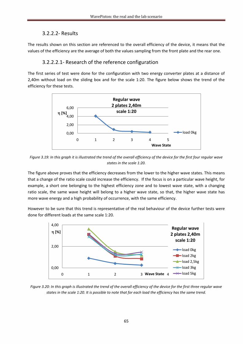
WavePiston: the real and the lab scenario
65
3.2.2.2- Results
The results shown on this section are referenced to the overall efficiency of the device, it means that the
values of the efficiency are the average of both the values sampling from the front plate and the rear one.
3.2.2.2.1- Research of the reference configuration
The first series of test were done for the configuration with two energy converter plates at a distance of
2,40m without load on the sliding box and for the scale 1:20. The figure below shows the trend of the
efficiency for these tests.
Figure 3.19: In this graph it is illustrated the trend of the overall efficiency of the device for the first four regular wave
states in the scale 1:20.
The figure above proves that the efficiency decreases from the lower to the higher wave states. This means
that a change of the ratio scale could increase the efficiency. If the focus is on a particular wave height, for
example, a short one belonging to the highest efficiency zone and to lowest wave state, with a changing
ratio scale, the same wave height will belong to a higher wave state, so that, the higher wave state has
more wave energy and a high probability of occurrence, with the same efficiency.
However to be sure that this trend is representative of the real behaviour of the device further tests were
done for different loads at the same scale 1:20.
Figure 3.20: In this graph is illustrated the trend of the overall efficiency of the device for the first three regular wave
states in the scale 1:20. It is possible to note that for each load the efficiency has the same trend.
0,00
2,00
4,00
6,00
0 1 2 3 4 5
[%]
Wave State
Regular wave2 plates 2,40m
scale 1:20
load 0kg
0,00
2,00
4,00
0 1 2 3 4
[%]
Wave State
Regular wave2 plates 2,40m
scale 1:20
load 0kg
load 2kg
load 2,5kg
load 3kg
load 5kg

WavePiston: the real and the lab scenario
66
Hence even if the device was built up for the scale 1:20, the great number of the tests were made
increasing the scale until the scale 1:30. The graph below confirms that this decision is the right one.
Figure 3.21: The diagram shows how the increase of the ratio scale implies an increase in the efficiency.
From the figure 3.20 it is possible to observe that the best load for the efficiency seems to be the 2,5kg. To
fine-tune the finest load some tests in irregular states were done.
Figure 3.22: Representation of the efficiency of the prototype for the different irregular wave states, for the load of
2,5kg and 1,5kg. From the diagram it is possible to understand that the best load is 1,5kg and not 2,5kg.
The analysis of the best load with the irregular waves tests articulates that the best load is 1,5kg instead of
2,5kg. This aspect is even better because for the high wave states with the load of 2,5kg the sliding box
went several time out of range, this was the reason because no more tests were done for the fifth wave
state. The load of 1,5kg is taken from design and reference load.
The next two graphs want to represent the relation between the standard deviation of the force impressed
on the plates, and the irregular wave states for the two best loads.
0,00
2,00
4,00
6,00
8,00
1 2 3 4
[%]
Wave State
ComparisonRegular wave
2 plates 2,40m
load 0kg-scale1:20
load 0kg-scale1:30
load 2kg-scale1:20
load 2kg-scale1:30
0
2
4
6
8
10
12
14
0 1 2 3 4 5
[%]
Wave State
Scale 1:30Irregular wave 2 plates 2,40m
load 1,5kg
load 2,5kg

WavePiston: the real and the lab scenario
67
Even the first graph asserts that is better the choice of the load 1,5kg rather than 2,5kg, hence its standard
deviation fluctuation is included in the range from 5,85N to 7,12N, while the standard deviation variation of
the load 2,5kg is included in a wide range from 6,79N to 10,70N.
Figure 3.23: Correlation between the wave state and the standard deviation of the force. Even from this graph it is
possible to declare that the load of 1,5kg is better than 2,5kg, indeed the standard deviation of the load 1,5kg is in a
range between 5,85N and 7,12N for all the wave state, whereas the standard deviation of the load 2,5kg is in a wide
range from 6,79N to 10 ,70N.
From the graph below it is again possible to observe that for the load 2,5kg, regardless of the wave states,
the standard deviation values of the force is greater than the one of the load 1,5kg.
Figure 3.24: Correlation between the wave state and the standard deviation of the force. In this representation the
standard deviation value is the average of the front and rear values.
5
6
7
8
9
10
11
0 1 2 3 4 5
Stan
dar
d D
evi
atio
n o
f th
e F
orc
e [
N]
Wave State
Scale 1:30Irregular wave 2 plates 2,40m
load 1,5kg-Front
load 1,5kg-Back
load 2,5kg-Front
load 2,5kg-Back
5,0
6,0
7,0
8,0
9,0
10,0
11,0
1 1,5 2 2,5 3
Stan
dar
d D
evi
atio
n o
f th
e F
orc
e [
N]
Load [kg]
Scale 1:30Irregular wave 2 plates 2,40m
wave state1
wave state2
wave state3
wave state4

WavePiston: the real and the lab scenario
68
Once decide that the design load is 1,5kg, the next step is to analyze the other parameters, such as the
number and the relative position of the energy collector plates, the influence in the efficiency of the wave
period, wave height and incident wave angle.
3.2.2.2.2- Wave Period and Wave Height variation
For these experiments the set-up is with the device with four energy converter plates at the distance of
0,80m each other and with the load of 1,5kg.
To study the effects of the variation of the wave period with a fixed wave height of 0,06m the range for the
wave period is between 0,6s and 1,8s with a step of 0,2s between two subsequent experiments.
Figure 3.25: Relation between the efficiency of the device and the wave period. In this representation the efficiency
value is the average of the front and rear values. The performance values are included in a range from 15,5% to 2,4%.
The image above shows that the efficiency of the device is between the range of 15,5% and 2,4%, and since
the trend seems similar to go on as before, hence the efficiency decrease from the lower to the higher
wave states.
This trend could be the sum of two aspect: the first is the intrinsic behaviour of the device having high
efficiency for waves characterized by a small wave height and a small wave period; and the second depends
on the load of 1,5kg.
Anyway, the trend suggests to focus more tests around the value of 1,2s. And for this reason, to study the
effects of the changing of the wave height together with a fixed wave period, the set-up was with 1,2s for
the wave period, and for the wave height in a range between 0,03m and 0,11m with a step of 0,02m from
one experiment to the subsequent.
The next graph illustrates that, having a variation of the wave height, the efficiency of the device is
between the range of 6% and 2,5%, and again the trend seems similar as before, hence the efficiency
decreases from a wave state with a small wave height, to a wave state with a higher wave height.
0
5
10
15
20
0,4 0,6 0,8 1 1,2 1,4 1,6 1,8 2
[%]
wave period [s]
Constant wave height of 0,06mVariation of the wave period from 0,6s to 1,8s
wave heigth 6cm

WavePiston: the real and the lab scenario
69
Figure 3.26: Relation between the efficiency of the device and the wave height. In this representation the efficiency
value is the average of the front and rear values. The performance values are included in a range from 6% to 2,5%.
Both the graphs demonstrate that the performance of the device increases for a wave state characterized
by a small wave height and a small wave period, rather than by a wave state with high values of wave
height and wave period, where the efficiency decreases.
In addition, the graphs prove that the device is more influenced by the wave period than by the wave
height, indeed changing the wave period, the efficiency changes from 15,5% to 2,4%, while changing the
wave height, the efficiency changes only from 6% to 2,5%.
To understand better the strange behaviour around the wave period of 1,2s several tests were carried out
to fine-tune the possible motivations. These tests were made with the reference configuration, i.e. the
device with two energy collector plates at a distance of 2,40m each other and differently to the reference
configuration, during these tests the load was of 2,0kg.
Figure 3.27: Relation between the efficiency of the device and the wave period. In this representation the efficiency
value is the average of the front and rear values. The performance values are included in a range from 17% to 2,4%.
Moreover this graph proves that this kind of curve is the sum of two contributions, in fact the peak moves to the left,
increasing the load.
Even if all these tests were only run with regular waves in order to analyse the dependency of the model to
a particular wave parameter and not to a whole wave spectrum, the results seem reliable.
1
3
5
7
3 5 7 9 11
[%]
wave height [cm]
Constant wave period of 1,2sVariation of the wave height from 0,03m to 0,11m
wave period 1,2s
0
5
10
15
20
0,4 0,6 0,8 1 1,2 1,4 1,6 1,8 2
[%]
wave period [s]
Constant wave height of 0,06mVariation of the wave period from 0,6s to 1,8s
load1,5kg
load 2kg

WavePiston: the real and the lab scenario
70
3.2.2.2.3- Analysis of the influence of the incident wave angle
For this analysis the device configuration is with four plates at the distance of 0,80m each other and with a
load of 1,5kg. The results are presented in reference to the configuration where the device is in line with
the incoming wave, hence for an angle of 0°.
Few tests were performed both for regular wave states that for irregular wave states, to find out how the
direction of the incident waves would affect the energy production of the model. The first set-up was with
regular waves, and in particular for 10° and 30° incident wave angle. In this case the results are not given by
reference.
Figure 3.28: Ratio between the efficiency of the device and the incident wave angle. In this representation the
efficiency value is the average of the front and rear values. The performance values are included in a range from 5,5%
to 3%. The wave incident angle seems not decrease so much the efficiency.
The second study concerns the irregular wave state and in this section the configurations with 10° 30° and
even 20° for the incident wave angle are analyzed.
Figure 3.28: Ratio between the efficiency of the device and the incident wave angle. The performance values are
referenced to the configuration where the device is in line with the wave propagation.
In the figure above, the results show that there is not a larger loss of efficiency, and furthermore that for
every incident direction the loss is less for the wave state number three than not for the number two.
0,00
3,00
6,00
1 2 3 4
[%]
Wave state
Scale 1:30Regular wave
incident wave angle10°
incident wave angle 30°
0,60
0,70
0,80
0,90
1,00
1 2 3 4
reference [%]
Wave state
Irregulare wavescale 1:30
angle 10°
angle 20°
angle 30°

WavePiston: the real and the lab scenario
71
The same results is verified in the figure below, where there is the ration between the average of the
efficiency of the device and the incident wave direction. The wave state number three presents a loss of
efficiency minor than the wave state number two.
Figure 3.29: Ratio between the efficiency of the device and the incident wave angle. The performance values are
referenced to the configuration where the device is in line with the wave propagation.
In conclusion, the angle of attack of the incoming waves doesn’t have a significant effect on the efficiency
of the device, indeed the greatest loss of efficiency is approximately the 30% and this was found for
incoming waves with an angle of attack of 30 °.
3.2.2.2.4- Number and shape of the energy converter plates
The last step of the laboratory analysis is constituted by two part.
The first section is the study of the number and the position of the energy collector plates. For this analysis
the usual shape of these plates is 0,5m in width and 0,1m in depth without hole. The results are
represented even in reference with the standard configuration of only two plates.
The second sector is the study of the shape of the energy collector plates, in this case the configuration of
the device is always with only two plates at a distance of 2,40m. The results are given in reference to the
standard configuration.
In both situations, experiments were made only about the irregular wave states and all the measurements
were taken from the front and the back plate, even in the configuration with four plates as before.
Hence for the first number and position aim the setup is with four plates mounted at a distance of 0,45m,
then 0,55m and finally at 0,80m.
As the figure 3.30 and 3.31 show, the multi-plates configuration has a loss in efficiency, but this loss is less
than the 20%, even in this case the wave state number three presents a loss of efficiency minor of the wave
state number two.
0,60
0,70
0,80
0,90
1,00
0 10 20 30 40
reference [%]
Incident wavedirection
Irregular wavescale 1:30
wave state2
wave state3

WavePiston: the real and the lab scenario
72
Figure 3.30: The performance values are referenced to the configuration where the device has two wings at a distance
of 2,40m, from the graph it is possible to note that the main loss in efficiency is less than 20%, that value is the average
of the values from the front and the back plate.
Figure 3.31: The performance values are referenced to the configuration where the device has two wings at a distance
of 2,40m, from the graph it is possible to observe that the main loss in efficiency is in the wave state number 2.
Wave State Hs [m] Tp [s] L [m] Distance
2,40m Distance
0,80m Distance
0,55m Distance
0,45m
2 0,067 1,28 2,42 6,41 5,55 5,21 5,63
3 0,100 1,53 3,21 3,41 3,37 3,15 3,42
Table 3.6: The values in the last four columns are the average of the efficiency among the values of the front and the
back plate. These values demonstrate that the efficiency doesn’t decrease so much with the increase of the number of
the plate, this aspect is fundamental because in the real scenario the device is constituted to a multitude of plates. It
can be noticed that the damping plates don’t reduce significantly the efficiency of the device.
The table reveals that the loss of efficiency is greatest for the configuration of four winds at a distance of
0,55m, hence a possible configuration of the real device should be with the plates as closer as possible.
0,800
0,900
1,000
1,100
1 2 3 4
reference [%]
Wave state
Irregular wavescale 1:30 distance 0,8m
distance 0,55m
distance 0,45m
0,800
0,850
0,900
0,950
1,000
1,050
0,35 0,45 0,55 0,65 0,75 0,85
reference [%]
Relative distance between the plates [m]
Irregular wavescale 1:30
wave state2
wave state3

WavePiston: the real and the lab scenario
73
Whereas for the shape aim the setup is the device with two energy collector plates at the distance of 2,40m,
the load is 1,5kg and different plates, and their shape are: 0,38m width and 0,13m depth; then 0,38m width
and 0,10m depth; then 0,38m width and 0,07m depth; and finally 0,50m width and 0,10m depth with hole
section. Results are given relatively to the reference case, which is the 2 plates setup with the plate shape
as 0,50mx0,10m without hole.
When these shape experiments were carried out in the tank there was one more device, so the only way to
have reliable results is to present them as reference between experiments of the same day. The reference
configuration is with the shape of 0,50m width and 0,10m depth without hole.
Figure 3.32: The graph shows how the efficiency increases with a decrease of the width of the plates, except for the
first irregular wave state. The greatest increase of the efficiency is about the 20%.
Figure 3.33: The graph shows how the efficiency increases with an increase of the depth of the plates for all the wave
states. The greatest increase of the efficiency is about the 300% reported to the shape of 0,38m x 0,10m that was just
more than the reference one of 0,50m x 0,10m.
0,3
0,8
1,3
1 2 3
reference [%]
Wave state
Scale 1:30--Irregulare waveDifferent shapes
same depth shape of 0,10m
width 0,5m
width 0,38m
0
1
2
3
4
1 2 3
reference [%]
Wave state
Scale 1:30--Irregulare waveDifferent shapes
same width shape of 0,38m
depth 0,1m
depth 0,07m
depth 0,13m

WavePiston: the real and the lab scenario
74
0
0,5
1
1,5
1 2 3
reference [%]
Wave state
Scale 1:30--Irregulare waveSame shape, different density
width 0,5m
width 0,5m hole
Figure 3.34: The graph shows how the
efficiency decrease even if the shape of the
plates doesn’t change. In this case the two
plates differ for the presence of the hole.
The most important cause of the efficiency
decrease is the different density of the two
plates: in fact the plate with the hole is
heavier respect the normal plate. However,
it is possible to consider unreliable the
values of the first wave state, while it
seems correct the value of the third wave
state and that means a loss of 70%.
3.2.2.2.5- Summary of the performance of the device
The main aim of this work is the determine the efficiency assignable to the device for all the yearlong and
of the yearly energy production, which is the quantity of energy that in a year the WavePiston can
transform from wave energy in mechanical energy.
Firstly it is presented a table to summarize the wave parameters, and particularly the wave height and the
wave power. The table 3.7 shows that there is different among the wave height corresponding to the real
wave state and the wave height observed, consequently a similar different is in the wave power. For the
following calculation the wave height corresponding to the real wave state and the wave power realized
are taken as a reference.
Wave state
Tp [s] Tz [s] Hs wanted
[m] Power wave
theoretical [W/m] Hs realized
[m] Power wave
calculated [W/m] Power wave
realized [W/m]
1 1,02 0,73 0,033 0,42 0,021 0,17 0,22
2 1,28 0,91 0,067 2,17 0,059 1,69 2,20
3 1,53 1,09 0,100 5,77 0,089 4,58 6,31
4 1,79 1,28 0,133 11,94 0,133 11,94 16,32
5 2,04 1,46 0,167 21,46 0,185 26,33 35,75
Table 3.7: Summary of the reference irregular wave states. The table shows the difference between the wave height
and the wave power wanted and realized. The wave height corresponding to the real wave state and the wave power
realized are taken as a reference.
A second problem is to determinate the power generated for all the wave state, because to preserve the
model the fifth wave state was not carried out. So to have the value of this wave state an interpolation was
done. To make this interpolation was possible to use the values regarding different test in irregular wave as

WavePiston: the real and the lab scenario
75
the ones with the same load of 1,5kg, but with the paddle at a diverse distance between them, finally the
values concerning the four plates at a distance of 0,80m were chosen.
Wave power generated [W/0,5m]
Wave state Front Back Average
1 0,0119 0,0153 0,0136
2 0,0731 0,0782 0,0756
3 0,1164 0,1133 0,1149
4 0,1640 0,1612 0,1626
Table 3.8: The table illustrates the values of the power generated used to the interpolation. These values are referred
to the reference condition of the model.
Figure 3.35: The figure illustrates the interpolation equation for the power generated.
Wave state
Tp [s]
Hs [m]
Power wave
[W/m]
Prob [%]
Prob*Power wave [W/m]
Power generated [W/0,5m]
Efficiency *Probability Prob*Power generated
[W/m]
1 1,02 0,033 0,22 47 0,101 0,014 0,13 0,0590 0,013
2 1,28 0,067 2,20 23 0,498 0,076 0,07 0,0155 0,034
3 1,53 0,100 6,31 11 0,682 0,115 0,04 0,0039 0,025
4 1,79 0,133 16,32 5,1 0,832 0,163 0,02 0,0010 0,017
5 2,04 0,167 35,75 2,4 0,858 0,214 0,01 0,0003 0,010
Table 3.9: Summary of the performance that can be converted from the waves into useful mechanical energy by the
WavePiston model. The reference configuration of the device is with two energy converter plates at the distance of
2,40m and with a load of 1,5kg. The device is subjected to irregular wave.
y = 1,4607x - 0,0299
0,000
0,020
0,040
0,060
0,080
0,100
0,120
0,140
0,160
0,180
0 0,02 0,04 0,06 0,08 0,1 0,12 0,14
ave
rage
eff
icie
ncy
wave height [m]
distance 240

WavePiston: the real and the lab scenario
76
To identify the yearly values is feasible do a sum of the values multiplied to the probability of occurrence.
yearly average wave power [W/m] 2,9708
overall efficiency 0,080
yearly average power production [W/m] 0,0986
max power generated [W/m] 0,4281
yearly energy production [kWh/year/m] 0,8636
Load factor 0,23 Table 3.10: Estimation of the energy that can be converted from the waves into useful mechanical energy by the
WavePiston device subjected to irregular wave.
The table above explains the output energy of the device for assumed 1:30 scaling lengths, the yearly
average wave power is of 2.97 W/m, and the yearly power generated is almost 0,10 W/m, corresponding to
a yearly energy production per meter of 0,86 kWh/y/m.
It is not possible to have a comparison between scale 1:20 and the 1:30, so it is not possible to know the
improve of the yearly energy production.
Although the study regarding a scale model is on purpose to realize a real installation, it is more fruitful
have the yearly power generated and consequently the yearly energy production of the real device.
The tables below show the output energy of the WavePiston wave energy converter, the yearly available
average wave power is relative to the Danish part of the North Sea and is of 12,0 kW/m, and the yearly
power generated is about 0,55 kW/m, corresponding to a yearly energy production per meter of 4,24
MWh/y/m.
Wave state
Hs [m]
Tp [s] Power wave
[kW/m]
Probability [%]
Prob*Power wave
[kW/m] Efficiency *Probability
Power generated
[kW/m]
Prob*Power generated
[kW/m]
1 1,00 5,60 2,11 46,8 0,988 0,13 0,061 0,275 0,128
2 2,00 7,00 10,56 22,6 2,387 0,07 0,016 0,739 0,167
3 3,00 8,40 28,51 10,8 3,079 0,04 0,004 1,140 0,123
4 4,00 9,80 59,14 5,1 3,016 0,02 0,001 1,183 0,060
5 5,00 11,20 105,60 2,4 2,534 0,01 0,000 1,056 0,025
Table 3.11: Summary of the performance of the WavePiston wave energy converter. The value of the power that can
be converted from the waves into useful mechanical power by the WavePiston model is referred to one plate of 15m of
width . The device is subjected to irregular wave.
In the next table, for a more immediate comprehension the same values are reported even referred to the
width of the plate, of 15m.

WavePiston: the real and the lab scenario
77
Wave state
Hs [m]
Tp [s] Power wave
[W/plate]
Probability [%]
Prob*Power wave
[W/plate] Efficiency *Probability
Power generated [W/plate]
Prob*Power generated [W/plate]
1 1,00 5,60 31,68 46,8 14,826 0,13 0,061 4,12 1,927
2 2,00 7,00 158,40 22,6 35,798 0,07 0,016 11,09 2,506
3 3,00 8,40 427,68 10,8 46,189 0,04 0,004 17,11 1,848
4 4,00 9,80 887,04 5,1 45,239 0,02 0,001 17,74 0,905
5 5,00 11,20 1584,00 2,4 38,016 0,01 0,000 15,84 0,380 Table 3.12: Summary of the performance of the WavePiston wave energy converter. The value of the power that can
be converted from the waves into useful mechanical power by the WavePiston model is referred to one plate of 15m of
width . The device is subjected to irregular wave.
yearly average wave power [kW/m] 12,00
yearly average wave power [kW/plate] 180,07
overall efficiency 0,080
yearly average power production [kW/m] 0,504
yearly average power production [kW/plate] 7,570
max power generated [kW/m] 1,183
max power generated [kW/plate] 17,74
yearly energy production [MWh/year/m] 4,42
yearly energy production [MWh/year/plate] 66,3
Load factor 0,39
Table 3.13: Summary of the performance and the estimated energy that can be converted from the waves into useful
mechanical energy by the WavePiston device subjected to irregular wave.
The tables are filled in following the explanation reported at page 57.
Figure 3.36: Representation of the average efficiency of a plate of 15m width of the WavePiston device in the blue line,
instead the orange line is the product of the probability of occurrence and the available wave power.
0,00
2,00
4,00
0
0,05
0,1
0,15
0 1 2 3 4 5 6
Effi
cie
ncy
[-]
Wave State
Wav
e P
ow
er
*Pro
bab
ility
[kW
/m]
Efficiency
WavePower*Probability
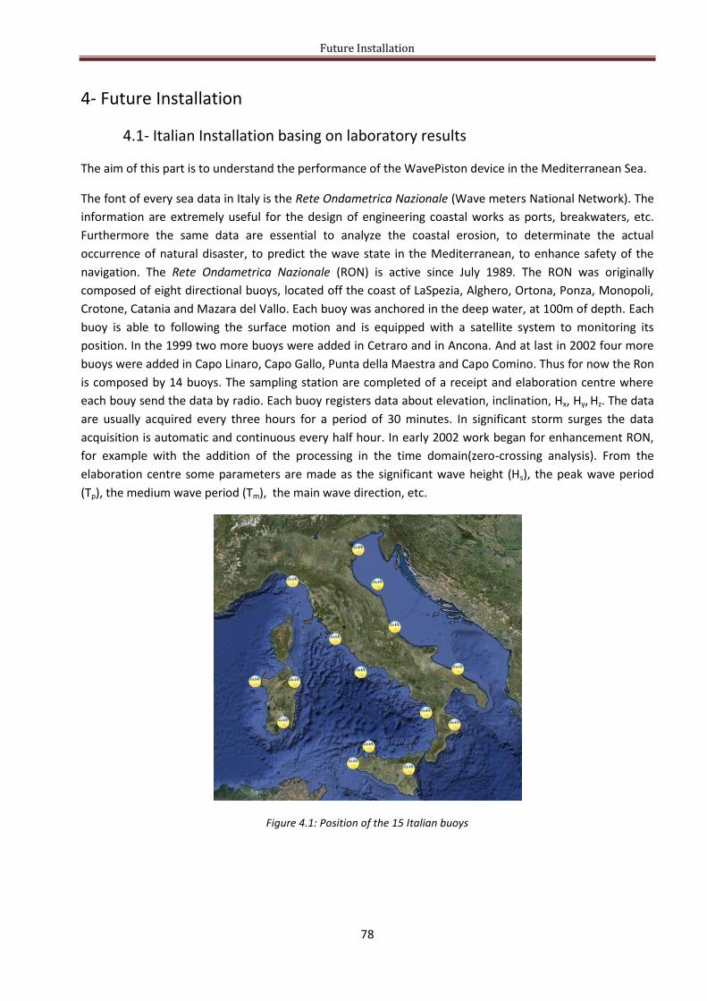
Future Installation
78
4- Future Installation
4.1- Italian Installation basing on laboratory results
The aim of this part is to understand the performance of the WavePiston device in the Mediterranean Sea.
The font of every sea data in Italy is the Rete Ondametrica Nazionale (Wave meters National Network). The
information are extremely useful for the design of engineering coastal works as ports, breakwaters, etc.
Furthermore the same data are essential to analyze the coastal erosion, to determinate the actual
occurrence of natural disaster, to predict the wave state in the Mediterranean, to enhance safety of the
navigation. The Rete Ondametrica Nazionale (RON) is active since July 1989. The RON was originally
composed of eight directional buoys, located off the coast of LaSpezia, Alghero, Ortona, Ponza, Monopoli,
Crotone, Catania and Mazara del Vallo. Each buoy was anchored in the deep water, at 100m of depth. Each
buoy is able to following the surface motion and is equipped with a satellite system to monitoring its
position. In the 1999 two more buoys were added in Cetraro and in Ancona. And at last in 2002 four more
buoys were added in Capo Linaro, Capo Gallo, Punta della Maestra and Capo Comino. Thus for now the Ron
is composed by 14 buoys. The sampling station are completed of a receipt and elaboration centre where
each bouy send the data by radio. Each buoy registers data about elevation, inclination, Hx, Hy, Hz. The data
are usually acquired every three hours for a period of 30 minutes. In significant storm surges the data
acquisition is automatic and continuous every half hour. In early 2002 work began for enhancement RON,
for example with the addition of the processing in the time domain(zero-crossing analysis). From the
elaboration centre some parameters are made as the significant wave height (Hs), the peak wave period
(Tp), the medium wave period (Tm), the main wave direction, etc.
Figure 4.1: Position of the 15 Italian buoys

Future Installation
79
4.1.1- Italian Wave State
It is been decided to study the performance of the WavePiston in Mazara del Vallo.
Figure 4.2: Mazara del Vallo buoy. Each buoy has a diameter of 1,7m and it is positionated at an height of 2,8m from
the waterline. The source of the picture is Idromare, web site www.idromare.it
Figure 4.3: Mazara del Vallo position. The source of the picture is Idromare, web site www.idromare.it
Figure 4.4: Mazara del Vallo DATAWELL position, source Idromare web site.
As told above, from the web site it is possible to find the data regarding the significant wave height, the
wave period and the direction of the waves propagation. These data are shown is the next figures.

Future Installation
80
Figure 4.5: Mazara del Vallo DATAWELL, Survey of the significant wave height in meter on the y-axis and the peak
wave period in second on the x-axis. The survey is referred to the period from 01/07/1989 to 04/04/2008. The expected
surveys are 61352 and the missed ones are 44457 (42%of the expected ones). 27% of the effectives are with a wave
height under 0,5m; source Idromare web site.
Figure 4.6: Mazara del Vallo DATAWELL, Survey of the significant wave height in meter on the y-axis and the medium
wave direction of the propagation in °N on the x-axis. The survey is referred to the period from 01/07/1989 to
04/04/2008. The expected surveys are 61352 and the missed ones are 44911 (42%of the expected ones). 8% of the
effectives are with a wave height under 0,5m; source Idromare web site.

Future Installation
81
In the tables above the numbers indicate the number of events happened. Since the analysis has the target
to focus the wave state of that location the data were utilized for operating limit state instead that ultimate
limit state. The difference is that in the ultimate limit analysis the aim is the investigation of the maxim
wave height to design the strength of different elements, whereas in the operating analysis the intent is to
examine the probability of occurrence for the final study of the power take off.
Therefore in this document there is not the comparison between the observed values and the values
predicted with a theoretical distribution as the Weibull or the Gumbel, instead there is an elaboration
based on the real possible performances.
For any event dividing the number of times of the event itself occurred by the total number of the
observations the probability of occurrence is given. At this point a table with for each division step of the
wave height corresponding vary wave periods with diverse probability is made. To be able to assign a single
wave period at a given wave height is to do an average weighted where the weight is the probability of
occurrence. The two tables below show this procedure.
sec 0,75 2,25 3,75 5,25 6,75 8,25 9,75 11,25 12,75 14,25 15,75 17,25 19
m TOT
0-0,5 0,02957 0,07843 0,08369 0,04521 0,01945 0,00159 0,00032 0,00007 0,00001 0,00963 0,26797
0,6-1,0 0,00405 0,07757 0,13220 0,07716 0,02755 0,00988 0,00149 0,00009 0,00003 0,00006 0,00387 0,33394
1,1-1,5 0,00992 0,05912 0,08163 0,02628 0,01145 0,00400 0,00030 0,00004 0,00007 0,19281
1,6-2,0 0,00009 0,01671 0,05168 0,02833 0,00834 0,00178 0,00038 0,00003 0,00003 0,10736
2,1-2,5 0,00172 0,01781 0,02200 0,00645 0,00105 0,00013 0,00001 0,00002 0,04918
2,6-3,0 0,00004 0,00421 0,01223 0,00681 0,00103 0,00008 0,00001 0,00003 0,02443
3,1-3,5 0,00089 0,00531 0,00554 0,00075 0,00004 0,01252
3,6-4,0 0,00003 0,00126 0,00330 0,00112 0,00007 0,00001 0,00577
4,1-4,5 0,00026 0,00166 0,00074 0,00009 0,00274
4,6-5,0 0,00011 0,00121 0,00064 0,00005 0,00201
5,1-5,5 0,00008 0,00032 0,00038 0,00008 0,00001 0,00086
5,6-6,0 0,00001 0,00008 0,00015 0,00007 0,00001 0,00031
6,1-6,5 0,00001 0,00003 0,00001 0,00005
6,6-7,0 0,00003 0,00003
7,1-7,5 0,00001 0,00001
Table 4.1: Probabilistic analysis for the significant wave height and the peak wave period of Mazara del Vallo. The
numbers in the table indicate the probability of occurrence of every event.

Future Installation
82
Wave State
H [m] Hs [m] Tp [sec] Tz [sec] Prob [%] P onda [kW/m]
1 0,175 0,250 5,48 3,92 26,80 0,13
2 0,525 0,750 5,78 4,13 33,39 1,23
3 0,875 1,250 6,63 4,73 19,28 3,91
4 1,225 1,750 7,24 5,17 10,74 8,37
5 1,575 2,250 7,88 5,63 4,92 15,05
6 1,925 2,750 8,56 6,11 2,44 24,41
Table 4.2: Wave State for Mazara del Vallo.
4.1.2- Yearly average efficiency and yearly energy production
Firstly a comparison among the Danish wave states and the Italian wave states was made.
Figure 4.7: Trend of the irregular Danish Sea State, from “Danish approach to development and evaluation of wave
energy devices” Kofoed & Frigaard (2009)
Figure 4.8: Trend of the irregular Italian Sea States
y = 1,4x + 4,2
5,00
7,00
9,00
11,00
13,00
0,00 1,00 2,00 3,00 4,00 5,00 6,00
Tp [s]
Hs [m]
Irregular Danish Sea state
Irregular Danish Sea state
y = 1,2735x + 5,0184
5,00
5,50
6,00
6,50
7,00
7,50
8,00
8,50
9,00
0,250 0,750 1,250 1,750 2,250 2,750
Tp [s]
Hs [m]
Irregular Italian Sea state
Irregular Italian Sea state

Future Installation
83
Figure 4.9: Comparison between the trend of the irregular Italian Sea States and the Danish one.
Due to the reason that in all the graphs above the trends are similar it was deemed appropriate to apply
the Danish results to the Italian case.
Furthermore to calculate the yearly average efficiency and the yearly energy production for the Italian
situation an hypothesis regarding the Danish efficiency trend was done. This hypothesis is concerning the
efficiency values for the wave state characterized by small wave height and small wave period, and in
particular it consists to declare that the trend efficiency is the same, there is no reason to presume a peak
or a different behaviour.
Figure 4.10: Danish efficiency trend for the WavePiston carries out by the laboratory result.
y = 1,2735x + 5,0184
y = 1,4x + 4,2
5,00
6,00
7,00
8,00
9,00
10,00
11,00
12,00
0,000 1,000 2,000 3,000 4,000 5,000 6,000
Tp [s]
Hs [m]
Irregular Italian Sea state
Irregular Danish Sea state
y = 0,2535e-0,638x
0
0,02
0,04
0,06
0,08
0,1
0,12
0,14
0,16
0,00 1,00 2,00 3,00 4,00 5,00 6,00
[%]
Hs [m]
Danish efficiency trend
Danish efficiency trend
Espo. (Danish efficiency trend)

Future Installation
84
Figure 4.11: Extrapolation of the Italian efficiency trend for the WavePiston using the Danish efficiency trend.
Note the efficiency and the wave power, it is feasible estimate the yearly efficiency and the yearly energy
production as just done in the previous chapter.
The tables below show the output energy of the WavePiston wave energy converter for an installation in
the South Italian Sea, the yearly available average wave power is 3,43 kW/m compared to the Danish of
12,0 kW/m, and the yearly power generated is about 0,30 kW/m compared to 0,55 kW/m of the Danish
Sea, corresponding to a yearly energy production per meter of 2,66 MWh/y/m compared to the Danish one
of 4,24 MWh/y/m.
Wave state
Hs [m]
Tp [s]
wave Power
[kW/m]
Probability [%]
Prob*Power wave [kW/m]
*
Probability
Power generated
[kW/m]
Pgenerated*Prob
[kW/m]
1 0,25 5,48 0,13 26,80 0,035 0,22 0,058 0,028 0,007
2 0,75 5,78 1,23 33,39 0,410 0,16 0,052 0,193 0,064
3 1,25 6,63 3,91 19,28 0,753 0,11 0,022 0,446 0,086
4 1,75 7,24 8,37 10,74 0,898 0,08 0,009 0,694 0,075
5 2,25 7,88 15,05 4,92 0,740 0,06 0,003 0,908 0,045
6 2,75 8,56 24,41 2,44 0,596 0,04 0,001 1,070 0,026
Table 4.3: Summary of the performance of the WavePiston wave energy converter in an Italian installation. The value
of the power that can be converted from the waves into useful mechanical power by the WavePiston model is referred
to one plate of 15m of width . The device is subjected to irregular wave.
In the next table, for a more immediate comprehension the same values are reported even referred to the
width of the plate.
y = 0,2535e-0,638x
0
0,05
0,1
0,15
0,2
0,25
0,00 1,00 2,00 3,00 4,00 5,00 6,00
[%]
Hs [m]
Danish efficiency trend
Italian efficiency trend
Espo. (Danish efficiency trend)

Future Installation
85
Wave state
Hs [m]
Tp [s]
wave Power
[kW/plate]
Probability [%]
Prob*Power wave
[kW/plate]
* Probability
Power generated [kW/plate]
Pgenerated*Prob [kW/plate]
1 0,25 5,48 1,94 26,80 0,519 0,22 0,058 0,419 0,112
2 0,75 5,78 18,40 33,39 6,146 0,16 0,052 2,891 0,965
3 1,25 6,63 58,58 19,28 11,294 0,11 0,022 6,689 1,290
4 1,75 7,24 125,49 10,74 13,474 0,08 0,009 10,416 1,118
5 2,25 7,88 225,68 4,92 11,100 0,06 0,003 13,616 0,670
6 2,75 8,56 366,09 2,44 8,944 0,04 0,001 16,054 0,392
Table 4.4: Summary of the performance of the WavePiston wave energy converter in an Italian installation. The value
of the power that can be converted from the waves into useful mechanical power by the WavePiston model is referred
to one plate of 15m of width . The device is subjected to irregular wave.
yearly average wave power [kW/m] 3,43
yearly average wave power [kW/plate] 51,48
overall efficiency 0,15
yearly average power production [kW/m] 0,30
yearly average power production [kW/plate] 4,55
max power generated [kW/m] 1,07
max power generated [kW/plate] 16,05
yearly energy production [MWh/year/m] 2,66
yearly energy production [MWh/year/plate] 39,84
Load factor 0,28 Table 4.5: Summary of the performance and the estimated energy that can be converted from the waves into useful
mechanical energy by the WavePiston device subjected to irregular wave in the Italian Sea.
Figure 4.12: Representation of the average efficiency of a plate of 15m width of the WavePiston device in the green
line, instead the red line is the product of the probability of occurrence and the available wave power.
0,00
0,50
1,00
0,00
0,10
0,20
0,30
0 1 2 3 4 5 6 7
Effi
cie
ncy
[-]
Wave State
Wav
e P
ow
er
*Pro
bab
ility
[k
W/m
]
Efficiency
WavePower*Probability

Future Installation
86
4.2- Numerical Model
4.2.1- Theoretical Equations
The intention of this part is to find out a numerical model able to predict the behaviour of the WavePiston
wave energy converter varying the wave parameters. This means that the purpose is to understand the
power take off of the device regardless the laboratory tests. In the next pages, the procedure is exposed,
starting with the theoretical equations. Each unit of the WavePiston, so each energy converter plate, is
equivalent to a single degrees freedom body, where the spring stiffness considers the real spring that will
stop the excessive movement of the plate and the damping is represented by the friction force and the
external force is explainable with the Morison equation.
Figure 4.13: A single unit of the WavePiston device is seen as a single degrees freedom body.
The equation for a single degrees freedom body is:
The external force is given by the Morison equation, as:
Where:
- FI is the inertial force;
- FD is the drag force;
- FFK is the Froude-Krylov force.
Their formulations are:
The problem to solve is represented by the following equation:

Future Installation
87
4.2.1.1- External forces’ investigation
In fluid dynamics the Morison equation is a semi-empirical equation for the inline force on a body in
oscillatory flow. This equation was introduced in the 1950 by Morison, O’Brien, Johnson and Schaaf. The
Morison equation is used to estimate the wave loads in the design of generic offshore structures.
Mainly the Morison equation is the sum of two forces: an inertia force, in phase with the local flow
acceleration, and a drag force proportional to the square of the instantaneous flow velocity. An empirical
hydrodynamic coefficient is contained in each force.
The Morison equation has two forms, one in the case of fixed body in an oscillatory flow and another
where the body is moving as well.
4.2.1.1.1- Fixed body in an oscillatory flow
In an oscillatory flow, with flow velocity u(t), the Morison equation gives the inline force parallel to the flow
direction as:
Where:
- F(t) is the total inline force on the object;
- FI(t) is the inertia force in this case the inertia force includes
the Froude-Krylov force, and cM is the added-mass coefficient, Volume is the volume of the body;
- FD(t) is the drag force
Area is the reference area, i.e.
the cross-sectional area of the body perpendicular to the flow direction.
For example, for a circular cylinder of diameter D in oscillatory flow, the reference area per unit cylinder
length is D and the cylinder volume per unit cylinder length is
. While for the device in
exam, the reference area is the product of the width and the depth of the plate.
Besides the inline force, there are also oscillatory lift forces perpendicular to the flow direction, due to
vortex shedding. These are not covered by the Morison equation, which is only for the inline forces.
4.2.1.1.2- Moving body in an oscillatory flow
In the case that, even the body is moving, with a velocity , the Morison equation becomes:
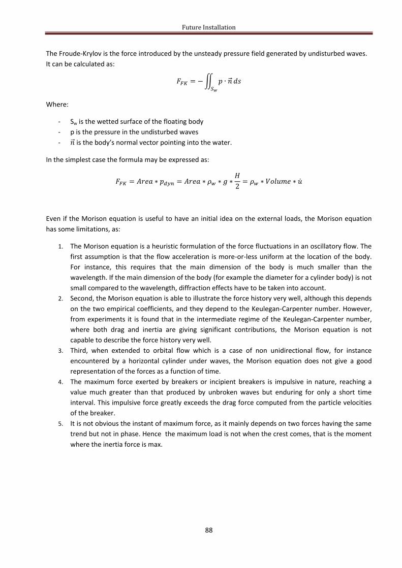
Future Installation
88
The Froude-Krylov is the force introduced by the unsteady pressure field generated by undisturbed waves.
It can be calculated as:
Where:
- Sw is the wetted surface of the floating body
- p is the pressure in the undisturbed waves
- is the body’s normal vector pointing into the water.
In the simplest case the formula may be expressed as:
Even if the Morison equation is useful to have an initial idea on the external loads, the Morison equation
has some limitations, as:
1. The Morison equation is a heuristic formulation of the force fluctuations in an oscillatory flow. The
first assumption is that the flow acceleration is more-or-less uniform at the location of the body.
For instance, this requires that the main dimension of the body is much smaller than the
wavelength. If the main dimension of the body (for example the diameter for a cylinder body) is not
small compared to the wavelength, diffraction effects have to be taken into account.
2. Second, the Morison equation is able to illustrate the force history very well, although this depends
on the two empirical coefficients, and they depend to the Keulegan-Carpenter number. However,
from experiments it is found that in the intermediate regime of the Keulegan-Carpenter number,
where both drag and inertia are giving significant contributions, the Morison equation is not
capable to describe the force history very well.
3. Third, when extended to orbital flow which is a case of non unidirectional flow, for instance
encountered by a horizontal cylinder under waves, the Morison equation does not give a good
representation of the forces as a function of time.
4. The maximum force exerted by breakers or incipient breakers is impulsive in nature, reaching a
value much greater than that produced by unbroken waves but enduring for only a short time
interval. This impulsive force greatly exceeds the drag force computed from the particle velocities
of the breaker.
5. It is not obvious the instant of maximum force, as it mainly depends on two forces having the same
trend but not in phase. Hence the maximum load is not when the crest comes, that is the moment
where the inertia force is max.

Future Installation
89
4.2.1.2- Simplifying assumptions
Even if the main target is the estimation of the WavePiston performance, regardless the laboratory results,
a first step of study is done to carry out a model that giving in input the laboratory condition gives in output
results comparable to the laboratory ones.
For that there were done some assumptions:
- the body is considered fixed in the Morison equation, this means that there is no Froude-Krylov
force and that there is no dependent by the velocity of the body movement;
- the solution is not in a closed analytical form, so it is not continue but it is studying with the finite
difference method, so the solution is known only in the particular time domain points.
With the finite difference method the equation becomes:
where u is the flow velocity, and it is expressed as:
The solution of the general equation was studied by the utilization of Matlab software.
In the Matlab editor further assumptions were made, as:
- the stiffness of the device should be carried out by particular laboratory test, where it is possible to obtain the corresponding force after the imposition of a known displacement. The stiffness should be the ratio between the difference of two displacements and the equivalent difference of the forces. To time question it was not possible to realize this experiment, hence it is assumed a stiffness of 100 [N/m], this value means that to move the energy converter plate of 1cm there is the necessity of a force of 1N;
- the damping coefficient assumes vary value, so it is possible to represent the variation of the
friction on the device, in order to find the best combination load-waves. Thus the damping
coefficient has not an unique value.
Through the Matlab script is achievable the trends of the displacements and the velocity of the energy
converters plates, and the power consequently to the variation of the damping value.
The results are reported below in a graph way.
In the figure below, with a red solid curve, there is the harmonic signal of the wave incident that represents
the external force. Whereas, velocity of the plate movement is symbolized with the magenta points.

Future Installation
90
Obviously, the plate velocity has a more limited range than the external force one, however it still has an
harmonious trend.
Figure 4.14: Lab_fixed_body model. Comparison between the flow velocity in the red solid line, and the velocity of the
body movement for a damping mean value.
The figure below is related to the same wave conditions, the three curves refer to different displacements
that the plate is subjected consequently to a variation of the damping value. The blue points represent the
situation without damping, while the black ones are for the maximum damping value in exam.
Clearly, the range of the displacement decreases from the situation without damping, that represents the
free movement, to the situation with the maximum damping, that correspond to the maximum movement
resistance.
Furthermore, as well as for the velocity, even for the displacement is predictable the same trend of the
external force, hence an harmonious one.
Figure 4.15: Lab_fixed_body model.
Different displacements due to the variation of the damping values from 0 to 100[Ns/m].

Future Installation
91
Figure 4.16: Lab_fixed_body model. Different curves, each represents the plate velocity during three different
simulations. A simulations differs from others due to the variation of the damping values from 0 to 100[Ns/m].
As before, the figure above is related to the same wave conditions, the three curves refer to different plate
velocity consequently to a variation of the damping value. The blue points represent the situation without
damping, while the black ones are for the maximum damping value in exam.
Clearly, the range of the velocity decreases from the situation without damping (that represents the free
movement where the plate should be integral with the water and its flow), to the situation with the
maximum damping (that correspond to the maximum movement resistance, and the plate should be
nearest to the fixed conditions).
The figures below summarize the effects of the variation of the damping value.
Figure 4.17: Lab_fixed_body model.
Different standard deviation of the plate velocities related to the variation of the damping values from 0 to 100[Ns/m].

Future Installation
92
As expected, the figure 4.17 summarizes a decrease in the standard deviation of the velocity from the
situation “free movement and damping zero” to the situation to maximum damping.
Whereas, the figure 4.18 qualifies that the standard deviation of the force increases with an increase of the
damping value, this is explainable because without damping, the plate is free to move as the water and so
the plate does not make any resistance, instead with a maximum damping it seems like the plate is fixed
and makes the maximum movement resistance.
Figure 4.18: Lab_fixed_body model. Different standard deviation of the force impressed on the plate related to the
variation of the damping values from 0 to 100[Ns/m].
In view of the fact that velocity and force have opposite trends, the best way to choose the best damping
value is to consider even the power generated trend. In fact, the power generated from the device is
obtained as a multiplication between the velocity and the force impressed.
Figure 4.19: Lab_fixed_body model. Different power generated related to the variation of the damping values from 0
to 100[Ns/m].The power generated is calculate as the multiplication between the plate velocity and its force impressed.

Future Installation
93
As expected, the best damping values is not little, otherwise the velocity might be high but not the force,
and at the same time it is not big, for the opposite reason. The results show that the best values is around a
damping value c, of 30Ns/m.
For an easier view, the same result is reported related to the standard deviation force. In this graph the
maximum power is for a standard deviation force of 0,65N, and from the figure 4.18 it is verifiable that
correspond to a damping value of 30Ns/m.
Figure 4.20: Lab_fixed_body model. Different power generated related to the variation of the damping values from 0
to 100[Ns/m].The power generated is calculate as the multiplication between the plate velocity and its force impressed.
To get closer to the main target of the numerical model, i.e. the estimation of the WavePiston performance,
regardless the laboratory results; the Matlab script is modified in order to consider the prototype body in
moving as well.
For this second model, some assumptions were done:
- as before, the solution is not in a closed analytical form, so it is not continue but it is studying with
the finite difference method, so the solution is known only in the particular time domain points;
- the movement of the body implies in the Morison equation that the external force is decreased
respect the fixed body case. The Froude-Krylov force is a third distinct contribution.
Other results related to this study are reported in the appendixes.

Future Installation
94
A last study might be the verification of the reflection analysis made by WaveLab3.33.
The reflection analysis consists in the comparison of the incident wave spectrum and the reflected wave
spectrum, with the aim to find the kR reflection coefficient. The reflection coefficient is defined as the ration
between HR, i.e. the reflected wave height and HI, i.e. the incident wave height.
Usually the reflection analysis starts with the evaluation of the elevation values measured by the wave
gauges, to separate the values of the incident waves to the ones referred to the reflected waves. Colleting
all the values of the wave height, a spectrum is made, and it is even possible to make a study in the
frequency domain. The frequency values could then been inserted in a Matlab script made on purpose, and
called reflexng.m, that is based on the linear wave theory. This script needs in input some parameters,
such as the wave height values measured through the wave gauges, the sampling frequency, the water
depth, etc. Through the same script, the main output is the trend of the wave height during the sampling
time, because thanks to it, the statistic distribution of the wave power can be built, and the system rapidity
response can be known as well.
This last part is not a part of the analyzing done.

Conclusions
95
5- Conclusions
5.1- Observations and suggestions
Even if during the laboratory period, all the obtained records from the measuring instruments are stored in
order to judge their overall performance and accuracy, unexpected and strange behaviours of the results
sometimes complicate the task of data analysis.
For example, several times, any kind of displacement measure is not recorded because the plate’s
movement is not fluent but it is a jerky movement. This sometimes limits the data’s validity of a part of the
sampling file or requires to repeat more times the same test.
For the same reason, in numerous tests, several velocity values are null values, due to the non
measurement of the displacement, hence the expected laboratory efficiency could plausibly be
underestimated.
It is reasonable that the real device doesn’t present some limitations that the laboratory prototype has,
such as the out range reached for the high wave state with the consequence of a possible rupture of the
model itself, obstacles represented by the fixed anchoring structure on the first front energy convertor
plate and, problems to estimate the real incident and reflected wave power due to the absence of the wave
gauges behind the device.
Most of the test were carried out with a scaling ratio of 1:30. The efficiency trend suggests that increasing
the scale from 1:30 to 1:40 or 1:50 could improve the performance and moreover the ratio scale increasing
could give more information about the hypothesis done on the continuous evolution of the efficiency
regarding the sea state characterized by a small wave height and a small wave period.
Figure 5.1: Typical efficiency trend of the WavePiston prototype
Therefore a higher scaling ratio would probably increase the average performance and power production of
the device. However, from the mechanical and structural point of view, the ratio scale increasing would
enhance stresses and loads.
The mechanical and structural limitations should be investigated thoroughly in order to identify the right
size.
1
2
3
4
0 1 2 3 4
[%]
Wave State
Regular wave2 plates 2,40m
load 2,5kg

Conclusions
96
Furthermore, due to the frequent movement of the prototype in and out of the wave tank during the
course of the testing, the exact setup was not perfectly constant. This is another source of likely small error
whose real affect is unknown.
5.2- Summarizing
To extrapolate the overall efficiency of the WavePiston device, a laboratory prototype was done and then
studied in the Aalborg University, in Denmark. The evaluation of the wave energy converter is achieved
following the “Assessment of Wave Energy Devices. Best Practice as used in Denmark”, Kofoed and Frigaard
et al.,2008.
The main key for the model performance is the shape of the energy collector plates. To obtain the
efficiency it is necessary to identify the mechanical power that the device can generated, this is the
multiplication between the velocity of the plate displacement and the force that is impressed on the plate
itself.
To model the friction effect, the device was tested with varying “PTO loads” on the plates, since to
represent different resistance conditions to the motion of the wings. The ideal PTO loading, which
corresponds to the highest amount of energy that it is extractable from the device, is equivalent at 1,5kg, or
analogously at 6,5N as average standard deviation of the impressed force, that it is reported to 1:30, while
for the full-scale this value is analogue to 27kN.
As numerous experiments on other OWCs and OWSCs asserted, the efficiency of the WavePiston decreases
in a non-linear way from the lower to the higher wave states. This means that a change of the ratio scale
could increase the efficiency. This trend represents the real behaviour of the device and it is not dependent
to the choice of the loads.
Figure 5.2: In this graph it is illustrated the non-linear trend of the overall efficiency of the device for the first three
regular wave states in the scale 1:20. It is possible to note that for each load the efficiency has the same trend.
The reference configuration, corresponding to the greatest power conversion from wave power to
mechanical power, is with only two wings at a distance of 2,40m, each wings of the shape of 0,5m x 0,1m in
width and depth. In scale 1:30 the real dimensions of the plate of the device becomes 15m for the width
and 3m for the depth.
0,00
2,00
4,00
0 1 2 3
[%]
Wave State
Regular wave2 plates 2,40m
scale 1:20load 0kg
load 2,5kg
load 3kg
load 5kg
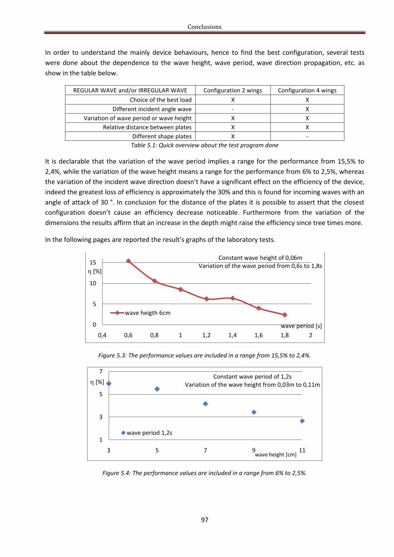
Conclusions
97
In order to understand the mainly device behaviours, hence to find the best configuration, several tests
were done about the dependence to the wave height, wave period, wave direction propagation, etc. as
show in the table below.
REGULAR WAVE and/or IRREGULAR WAVE Configuration 2 wings Configuration 4 wings
Choice of the best load X X
Different incident angle wave - X
Variation of wave period or wave height X X
Relative distance between plates X X
Different shape plates X -
Table 5.1: Quick overview about the test program done
It is declarable that the variation of the wave period implies a range for the performance from 15,5% to
2,4%, while the variation of the wave height means a range for the performance from 6% to 2,5%, whereas
the variation of the incident wave direction doesn’t have a significant effect on the efficiency of the device,
indeed the greatest loss of efficiency is approximately the 30% and this is found for incoming waves with an
angle of attack of 30 °. In conclusion for the distance of the plates it is possible to assert that the closest
configuration doesn’t cause an efficiency decrease noticeable. Furthermore from the variation of the
dimensions the results affirm that an increase in the depth might raise the efficiency since tree times more.
In the following pages are reported the result’s graphs of the laboratory tests.
Figure 5.3: The performance values are included in a range from 15,5% to 2,4%.
Figure 5.4: The performance values are included in a range from 6% to 2,5%.
0
5
10
15
0,4 0,6 0,8 1 1,2 1,4 1,6 1,8 2
[%]
wave period [s]
Constant wave height of 0,06mVariation of the wave period from 0,6s to 1,8s
wave heigth 6cm
1
3
5
7
3 5 7 9 11
[%]
wave height [cm]
Constant wave period of 1,2sVariation of the wave height from 0,03m to 0,11m
wave period 1,2s

Conclusions
98
Figure 5.5: Ratio between the efficiency of the device and the incident wave angle. The performance values are
referenced to the configuration where the device is in line with the wave propagation.
Figure 5.6: The performance values are referenced to the configuration where the device has two wings at a distance
of 2,40m, from the graph it is possible to observe that the main loss in efficiency is in the wave state number 2.
Wave State Distance
2,40m Distance
0,80m Distance
0,55m Distance
0,45m
2 6,41 5,55 5,21 5,63
3 3,41 3,37 3,15 3,42
Table 5.2: The values are the average of the efficiency between the values of the front and the back plate. It can be
noticed that the damping plates don’t reduce significantly the efficiency of the device.
Figure 5.7: The efficiency increases, with max value of 20%, with a decrease of the width of the plates.
0,60
0,70
0,80
0,90
1,00
0 10 20 30 40
reference [%]
Incident wavedirection
Irregulare wavescale 1:30
wave state2
wave state3
0,800
0,850
0,900
0,950
1,000
1,050
0,35 0,45 0,55 0,65 0,75 0,85
reference [%]
Relative distance between the plates [m]
Irregular wavescale 1:30
wave state2
wave state3
0,3
0,8
1,3
1 2 3
reference [%]
Wave state
Different shapes same depth shape of 0,10m
width 0,5m
width 0,38m

Conclusions
99
Figure 5.8: The efficiency increases with an increase of the depth of the plates for all the wave states. The greatest
increase of the efficiency is about the 300% reported to the shape of 0,38m x 0,10m that it is more than the reference
one of 0,50m x 0,10m. The depth of the plate can be considered a key parameter.
To fill the next summarizing table it is necessary to remember what the parameters represent.
The “efficiency” is the ratio between the power generated and the available power from the waves
relatively to the same width crest. The “overall efficiency” is the efficiency corresponding to the device
in the whole year.
The installed capacity of the PTO system is the maximum among the “generating power”, i.e. the efficiency
of the device multiplied by the average available power in the waves in a particular wave state.
The “power production” represents the average generated power of a wave state set on a year bases. This
corresponds to multiplying the average product power in a wave state by the probability of occurrence of
that wave state.
The sum of the power production of every wave state gives the yearly average available mechanical power
to the PTO system. From this yearly average power production, the yearly total energy production can be
calculated. The “factor load” represents the average usage of the installed capacity.
Wave state
Tp [s]
Hs [m]
Power wave
[W/m]
Prob [%]
Prob*Power wave [W/m]
Power generated [W/0,5m]
Efficiency *Probability
Prob*Power generated
[W/m]
1 1,02 0,033 0,22 47 0,101 0,014 0,13 0,0590 0,013
2 1,28 0,067 2,20 23 0,498 0,076 0,07 0,0155 0,034
3 1,53 0,100 6,31 11 0,682 0,115 0,04 0,0039 0,025
4 1,79 0,133 16,32 5,1 0,832 0,163 0,02 0,0010 0,017
5 2,04 0,167 35,75 2,4 0,858 0,214 0,01 0,0003 0,010
Table 5.3: Summary of the performance of the WavePiston model. The reference configuration of the device is with
two energy converter plates at the distance of 2,4m and with a load of 1,5kg. The device is subjected to irregular wave.
0
1
2
3
4
0 1 2 3
reference [%]
Wave state
Different shapes same width shape of 0,38mdepth 0,1m
depth 0,07m
depth 0,13m

Conclusions
100
The yearly energy production is 0,86 kWh/year/m.
This value is a paltry value, indeed a 100W light bulb on for one hour in a day for one year consumes
36,5kWh/year, this means that the WavePiston model with an energy plate converter of 1m of width is
capable to feed the same light bulb only for 2 minutes for day.
Figure 5.9: The graph shows the relation among the standard deviation of the force, impressed on the plate in the
reference cases with irregular wave, and the wave incident power, the wave reflected power and the power generated
by the device itself.
Figure 5.10: The graph shows the relation among the standard deviation of the force, impressed on the plate in the
reference cases with irregular wave, and the wave reflected power, the power generated by the device itself and the
power lost that it is calculated as the difference between the incident wave power and the power product by the device.
In the graphs above the x-axis is the average standard deviation of the force feels by the plates in the
reference configuration of two energy plates converter at the distance of 2,4m with a load of 1,5kg in the
cases of the first four irregular wave states.
Through both the graphs it is declarable that the power generated by the plates decreases from the first to
the last wave state, and consequently, at the same time, the power lost increases from the first to the last
wave state. Hence, one more time it means that the best performance is for the lower wave states.
75%
80%
85%
90%
95%
100%
6,01 6,81 6,55 7,00
Power
Standard Deviation [N]
power generated
power reflected
power incident
75%
80%
85%
90%
95%
100%
6,01 6,81 6,55 7,00
Power
Standard Deviation [N]
power generated
power reflected
power lost

Conclusions
101
5.3- Conclusions
As explained in the “Danish approach to development and evaluation of wave energy devices” the analysis
realized can be considered as a proof of concept.
In according to what that document declares, in the phase 1 all the main instruments used to assess the
wave energy devices are small scale testing in a hydraulic laboratory. These tests are performed in order to
gain knowledge on the devices before a company actually builds and deploys a wave energy device in the
sea. The laboratory tests will give information on:
1. Loads on the device
2. Movements of the device
3. Run-up / overtopping of the device
4. Energy production
The estimation of energy production in the first phase is rough. Typical small indicative laboratory tests cost
10000€ and they are followed by a 10 page report.
The examined prototype was design in reason to be fit to the laboratory conditions, though not exactly
corresponding to the future real realizations.
In the laboratory the closest situation was with the wings 0,45m distant, whilst in full scale additional
investigations should be made on the right inter-plate distance and on the amount of plates. In the full
scale should be less space limitations and this gives the possibility to do some investigations not possible in
the laboratory configurations.
Furthermore as the full-scale WavePiston wave energy converter design is intended to have a floating
structure with a flexible mooring instead of a fixed structure, several the tests should be repeated with a
flexible mooring instead of the fixed while measuring the mooring forces and the performance. The
observations might be different, as the flexible moored structure may move differently for different
wavelengths and/or wave states, and therefore perform as well. Moreover in case of floating structure it is
advisable to carry out some new tests about the distance between two device to know the best
configuration of them in the plan of a future farm.
Additionally the lab PTO system was a fixed load (weights), while the full-scale PTO system might consist of
an adaptable load depending on the wave state and some other components such as springs, in order to
keep the plates in place and/or reduce end-stop forces. This change in setup might give a different
performance curve.
Through the WavePiston investigation is reasonable to declare that the WavePiston WEC is able to convert
energy in the waves into useful mechanical energy, which then, through further mechanical and electrical
systems, can be converted into electricity. The average power production capabilities of the WavePiston
WEC have been estimated for a reference offshore location.

Conclusions
102
Wave state
Hs [m] Tp [s] Power wave
[W/plate] Probability [%] Efficiency
Power generated [W/plate]
1 1,00 5,60 31,68 46,8 0,13 4,12
2 2,00 7,00 158,40 22,6 0,07 11,09
3 3,00 8,40 427,68 10,8 0,04 17,11
4 4,00 9,80 887,04 5,1 0,02 17,74
5 5,00 11,20 1584,00 2,4 0,01 15,84 Table 5.4: Summary of the performance of the WavePiston wave energy converter. The value of the power that can be
converted from the waves into useful mechanical power by the WavePiston model is referred to one plate of 15m of
width . The device is subjected to irregular wave, in 30m water depth.
yearly average wave power [kW/m] 12,00
yearly average wave power [kW/plate] 180,07
overall efficiency 0,080
yearly average power production [kW/m] 0,504
yearly average power production [kW/plate] 7,570
max power generated [kW/m] 1,183
max power generated [kW/plate] 17,74
yearly energy production [MWh/year/m] 4,42
yearly energy production [MWh/year/plate] 66,3
Load factor 0,39
Table 5.5: Summary of the performance and the estimated energy that can be converted from the waves into useful
mechanical energy by the WavePiston device subjected to irregular wave.
Figure 5.11: Representation of the average efficiency of a plate of 15m width of the WavePiston device in the blue line,
instead the orange line is the product of the probability of occurrence and the available wave power.
In according to the Danish best practice, it is declarable that the risk of using unnecessary resources for the
WavePiston device is minimized.
For this reason, combined with the high performance for the ordinary wave states with a small wave height
and a small wave period it is rational an installation even in the moderate seas as the Italian sea.
0,00
2,00
4,00
0
0,1
0,2
0 1 2 3 4 5 6
Effi
cien
cy [
-]
Wave State
Wav
e P
ow
er
*Pro
bab
ility
[kW
/m]
Efficiency
WavePower*Probability

Conclusions
103
Wave state
Hs [m] Tp [s] wave Power [kW/plate]
Probability [%] Efficiency Power
generated [kW/plate]
1 0,25 5,48 1,94 26,80 0,22 0,419
2 0,75 5,78 18,40 33,39 0,16 2,891
3 1,25 6,63 58,58 19,28 0,11 6,689
4 1,75 7,24 125,49 10,74 0,08 10,416
5 2,25 7,88 225,68 4,92 0,06 13,616
6 2,75 8,56 366,09 2,44 0,04 16,054 Table 5.6: Summary of the performance of the WavePiston wave energy converter in an Italian installation. The value
of the power that can be converted from the waves into useful mechanical power by the WavePiston model is referred
to one plate of 15m of width . The device is subjected to irregular wave, in 30m water depth.
yearly average wave power [kW/m] 3,43
yearly average wave power [kW/plate] 51,48
overall efficiency 0,15
yearly average power production [kW/m] 0,30
yearly average power production [kW/plate] 4,55
max power generated [kW/m] 1,07
max power generated [kW/plate] 16,05
yearly energy production [MWh/year/m] 2,66
yearly energy production [MWh/year/plate] 39,84
Load factor 0,28
Table 5.7: Summary of the performance and the estimated energy that can be converted from the waves into useful
mechanical energy by the WavePiston device subjected to irregular wave in the Italian Sea.
Figure 5.12: Representation of the average efficiency of a plate of 15m width of the WavePiston device in the green line, instead the red line is the product of the probability of occurrence and the available wave power.
0,00
0,50
1,00
0,00
0,10
0,20
0,30
0 1 2 3 4 5 6 7
Effi
cien
cy [
-]
Wave State
Wav
e P
ow
er
*Pro
bab
ility
[k
W/m
]
Efficiency
WavePower*Probability

Conclusions
104
The WavePiston wave Energy converter is not affected by the background currents, but it could be
influenced by the surface currents as the return current called even rip current. This aspect is not
investigated in the analysis made.
Figure 5.13: Rip current structure.
In general, every wave energy converter is intended to be placed in an aggressive situation, hence the
corrosion resistance is one of the most important aspect to consider in the design and achievement of a
wave energy converter and of its material, because the maintenance cost could be higher than the
implementation cost.
Due to the movement of the prototype in and out the tank, it was possible to observe a beginning of the
corrosion effect, even if these observations concern more the mooring part, that it is absent in the real
future realization.
Figure 5.14: Beginning of corrosion effects in the mooring system of the WavePiston prototype.

Conclusions
105
There is good reason to be cautiously optimistic about the prospects of marine energy technologies
supplying significant amounts of clean electricity.
This optimism is supported by the number of devices that are progressing through a development
programme to begin sea trails at, or close to, full-size prototype scale.
5.4- Possible inconveniences in real installation
One of the most difficult aspect to considerate is not only the possibility of achieving a wave energy
converter, i.e. the performance and cost study; but it is the correct use of the sea space from all the
demands.
For example large-scale wave energy farms could be planned in areas that are in this moment intensely
used for navigation purposes. In busy navigation routes, any obstacle increases the potential hazard of ship
collisions and, ocean energy converters would be considered a danger within a rather large perimeter
around shipping routes, even outside the main routes and in the vicinity of more industrial major ports, this
may become the most important constraint for ocean energy converters development.
At the same time, advances in control and navigational warning systems can significantly improve the
safety ship situation, once the navigational sector gets accustomed to the additional infrastructures at sea.
From this point of view, even positive effects may arise regarding navigational safety and even maritime
control issues: the marker systems of wave farms could incorporate modern communication systems, and
assume the function of navigational guidance.
Further, farms distributed relatively widely over the open ocean could play an important role in a better
control of the common practice of illegal discharges of cargo ships, or even in ad-hoc actions in oil spills,
preventing major damages to the environment.
Another source of problem can be the fishing sector. Fishing is by far the most widespread and well-
established usage of ocean space and due to the strong traditions of the sector and the constantly
increasing need for seafood, it is considered a vital activity, hence it is logical that wave energy farms have
to struggle with the opposition of fishermen communities.
A possibility for the wave energy farms might be in the coexistence with floating wind farms. The floating
wind farms are typically moored in 50-200m deep water, and their distance would generally allow wave
farms to be installed in-between (in an advanced stage, once mooring systems of different floating devices
might be combined). This integration has more possibilities with the Oscillating Water Columns (OWCs) or
the Oscillating Wave Surge Converters (OWSCs).
At last there is the need to consider that a shoreline or near-shore device has the benefits to be accessible
directly from the shore, and so the operating and maintenance costs should be minimised, but at the same
time there are two significant problems. Firstly the research of a suitable site with a suitable wave climate.
Second problem is that a shore-side could be easily accessed by the public, with a consequentially high
safety risk.

106
APPENDIX
A- File .dat WaveLab
B- File .txt WavePiston.vi
C- List of experiments
D- Matlab Editor to analyze the data
E- Matlab Editor for
the numerical models

Appendix A
107
FILE .dat WAVELAB
The file .dat is the output file from the wave gauges sampling. Usually it is composed by a first short
description about which is the configuration used, and then by four columns, where there are the elevation
values recorded by the four wave gauges.
Through the software WaveLab3.33 the data come from the wave gauges can be analyzed, and among the
results, the most important are: the wave height and the wave period observed, the measured wave power
for meter of wave crest. All this results are given for the waves incident and even for the reflected waves.
All the figures below are related to the reference configuration of the prototype, i.e. two energy converter
plates at a distance of 2,40m of the shape of 0,5m of width and 0,1m of depth without hole. The device is
subject to an external load of 1,5kg, corresponding to 6,5N as average of the deviation standard of the
impressed force.
The exact data files are:
- RW_047_128_240_15_01 for the regular wave;
- IW_067_128_240_15_01 for the irregular wave.
Both files report the second Danish wave state.
Figure A.1: Screen of the “Show Sampled Signal” for the Irregular test, in the picture is represented all the data from all
the four channel, it is possible to show only one signal coming from a particular wave gauge choosing on the rigth the
corresponding channel. To obtain this signal WaveLab3.33 needs in input only the file name.

Appendix A
108
Figure A.2: Screen of the “Show Sampled Signal” for the Irregular test for the particular wave gauge of the channel1
that corresponds to the wave gauge nearest to the paddle system as a snake-front piston.
Figure A.3: Zoom of the “Show Sampled Signal” for the Irregular test.
The picture illustrates the signal with the data from all the four channel for a part of all the sampling time.
Figure A.4: Zoom of the “Show Sampled Signal” for the Irregular test.
The picture illustrates the signal with the data from all the four channel for a part of all the sampling time.

Appendix A
109
Figure A.5: Zoom of the “Show Sampled Signal” for the Regular test.
The picture illustrates the signal with the data from all the four channel for a part of all the sampling time.
It is possible to note that in this case the data from the different wave gauges are more similar, and their trend is
almost regular, and this is due to the aspect that all the waves have almost the same wave height.
Figure A.6: Screen of the “Time Series Analysis” for the Irregular test.
In the top, the picture illustrates the variance spectrumof the signal in the frequency domain analysis, while in the
bottom there is the time domain analysis that demonstrates the accuracy of the Rayleigh Distribution for the irregular
waves, in fact the measured values represent with a black point overlap to the blue Rayleigh Distribution.

Appendix A
110
Figure A.7: Screen of the “Time Series Analysis” for the Regular test. As before, in the top, the picture illustrates the
variance spectrumof the signal in the frequency domain analysis, and it is notable that the signal has an only main
frequence, because every wave is characterized by the same wave height and wave period. In the bottom there is the
time domain analysis that demonstrates that in this case the Rayleigh Distribution in not suittable for the regular
waves, the measured values represent with a black point don’t overlap to the blue Rayleigh Distribution, in fact the
mesured points present almost the same values and they are arranged on a nearly vertical line.
Figure A.8: Screen of the “Reflection Analysis” for the Irregular test.
In the top, the picture illustrates the variance spectrumof the signal in the frequency domain analysis, while in the
bottom there is the time domain analysis.

Appendix A
111
Figure A.9: Zoom of the “Reflection Analysis” for the Irregular test,in the time domain analysis only for reflected waves.
Figure A.10: Zoom of the “Reflection Analysis” for the Irregular test, in the time domain analysis for incident and
reflected waves.
Figure A.11: Screen of the “Reflection Analysis” for the Regular test.
In the top, the picture illustrates the variance spectrumof the signal in the frequency domain analysis, while in the
bottom there is the time domain analysis. In both cases there are the incident and the reflected waves.

Appendix A
112
WaveLab 3.34 The data is sampled on Tuesday the 2/23/2010 at 3:35:00 PM Measures includes calibration coefficient and offset Test description: Enter Description Here... Sample frequency: 20 Hz Sample duration: 1830 s
COLUMN 1:
Channel Description: Channel 01
Calibration Function: 0.05538*X
Offset: 1.828 V
Position (X-Coord.): 0 m
Position (Y-Coord.): 0 m
COLUMN 2:
Channel Description: Channel 02
Calibration Function: 0.04817*X
Offset: 2.094 V
Position (X-Coord.): 0 m
Position (Y-Coord.): 0 m
COLUMN 3:
Channel Description: Channel 03
Calibration Function: 0.05402*X
Offset: 1.861 V
Position (X-Coord.): 0 m
Position (Y-Coord.): 0 m
COLUMN 4:
Channel Description: Channel 04
Calibration Function: 0.04867*X
Offset: 2.072 V
Position (X-Coord.): 0 m
Position (Y-Coord.): 0 m
----------------------------------------------------------
-0.01318 -0.00911 0.01014 0.00719
-0.01433 -0.01220 0.00335 0.01178
-0.01398 -0.01416 -0.00348 0.01494
-0.01215 -0.01495 -0.00917 0.01773
There are four columns one for each wave gauges, the sampling is with 20 Hz, i.e. 20 records every second.

Appendix B
113
FILE .txt WavePiston.vi
The file .txt is the output file from the displacement sensors (LVDT) and the force transducers, those
present on the plate near the sliding rail with the weights, i.e. the plate representing the PTO system.
Usually it is composed by a first short description about which is the sampling time and the calibration
values, and then by five columns, where the first whose corresponds to the instant of the sampling, while
the second and the third are the displacement values related respectively to the front and back plate;
whereas the last two columns contain the impressed force filled by the plates related, again, respectively to
the front and the back plate. From the first column it is understandable that the sampling frequency is 10Hz.
Through a Matlab script made on purpose, the data come from the PTO system can be analyzed, and the
most important result is the average value of the power potentially generable from the device, because if
it is compared with the wave power available, it might give the efficiency of the model.
All the data below are related to the reference configuration of the prototype, i.e. two energy converter
plates at a distance of 2,40m of the shape of 0,5m of width and 0,1m of depth without hole. The device is
subject to an external load of 1,5kg, corresponding to 6,5N as average of the deviation standard of the
impressed force. The exact data file is IW_067_128_240_15_01, it is an irregular wave test, and it is
reported to the second Danish wave state.
Author,Administrator TimeStamp,23-02-2010 15:03 Sample Clock Rate,1000,00 Cal data 0,01 - 0,05 0,01 - 0,05 9,30 - 20,60 7,42 - 21,00
Sec after start LVDT 1 [m] LVDT 2 [m] Load 1 [N] Load 2 [N] 74,58 0,018 0,013 -0,909 6,759 74,68 0,018 0,012 7,467 6,587 74,78 0,017 0,011 8,351 6,322 74,88 0,016 0,010 7,936 5,073 74,98 0,015 0,010 7,970 1,521 75,08 0,015 0,010 8,473 -2,277 75,18 0,014 0,010 6,377 -1,819 75,28 0,014 0,010 -2,012 -1,389 75,38 0,016 0,010 -8,835 -5,150 75,48 0,019 0,011 -7,926 -8,958 75,58 0,022 0,012 -7,151 -8,588 75,68 0,023 0,013 -5,450 -8,023 75,78 0,023 0,014 3,079 -5,294

Appendix C
File name WS scale Hs [m] real Hs
[m] Tp [s]
Distance [m]
Load
Wave power
incident [W/m]
Wave power
reflected [W/m]
Power generated
front [W/0,5m]
back [W/0,5m]
average [W/m]
efficiency front
efficiency back
efficiency [%]
22/02/2010 RW_035_125_240_00_01 1 20 0,035 0,040 1,25 2,40 0 1,95 0,02 0,012 0,017 0,015 0,638 0,889 0,764
RW_070_157_240_00_01 2 20 0,070 0,068 1,57 2,40 0 7,95 0,02 0,026 0,029 0,055 0,323 0,361 0,342
RW_070_157_240_00_02 2 20 0,070 0,067 1,57 2,40 0 7,72 0,02 0,030 0,033 0,063 0,782 0,866 0,824
RW_110_188_240_00_01 3 20 0,110 0,113 1,88 2,40 0 24,83 0,65 0,091 0,086 0,177 0,735 0,690 0,713
RW_070_157_240_00_03 2 20 0,070 0,067 1,57 2,40 0 7,56 0,04 0,033 0,035 0,068 0,871 0,925 0,898
RW_110_188_240_00_02 3 20 0,110 0,108 1,88 2,40 0 21,89 0,65 0,044 0,045 0,089 0,404 0,415 0,410
RW_140_220_240_00_01 4 20 0,140 0,158 2,2 2,40 0 52,73 1,01 0,067 0,065 0,132 0,254 0,247 0,251
RW_070_157_240_20_01 2 20 0,070 0,065 1,57 2,40 2 7,01 0,02 0,091 0,127 0,218 2,596 3,618 3,107
RW_110_188_240_20_01 3 20 0,110 0,112 1,88 2,40 2 25 0,84 0,122 0,153 0,275 0,979 1,221 1,100
RW_140_220_240_20_01 4 20 0,140 0,161 2,2 2,40 2 54,31 1,55 0,206 0,250 0,456 0,757 0,919 0,838
RW_070_157_240_50_01 2 20 0,070 0,063 1,57 2,40 5 6,33 0,11 0,090 0,109 0,199 2,841 3,439 3,140
RW_110_188_240_50_01 3 20 0,110 0,119 1,88 2,40 5 28,59 1,15 0,202 0,186 0,388 1,411 1,302 1,357
RW_140_220_240_50_01 4 20 0,140 0,163 2,2 2,40 5 53,51 1,33 0,391 0,396 0,787 1,462 1,480 1,471
23/02/2010 RW_070_157_240_30_01 2 20 0,070 0,068 1,57 2,40 3 8,26 0,04 0,124 0,117 0,241 2,992 2,830 2,911
RW_110_188_240_30_01 3 20 0,110 0,116 1,88 2,40 3 28,23 0,73 0,175 0,171 0,346 1,241 1,214 1,228
RW_140_220_240_30_01 4 20 0,140 0,164 2,2 2,40 3 57,14 1,67 0,365 0,353 0,718 1,279 1,237 1,258
RW_070_157_240_25_01 2 20 0,070 0,069 1,57 2,40 2,5 8,17 0,04 0,153 0,144 0,297 3,745 3,513 3,629
RW_110_189_240_25_01 3 20 0,110 0,122 1,89 2,40 2,5 28,17 1,2 0,226 0,200 0,426 1,604 1,420 1,512
RW_140_291_240_25_01 4 20 0,140 0,165 2,91 2,40 2,5 57,32 1,67 0,333 0,347 0,680 1,162 1,211 1,187
RW_035_125_240_25_01 1 20 0,035 0,038 1,25 2,40 2,5 1,83 0,01 0,056 0,062 0,118 6,111 6,814 6,463
IR_067_128_240_25_01 2 30 0,067 0,064 1,28 2,40 2,5 2,59 0,05 0,073 0,075 0,148 5,631 5,761 5,696
IR_033_102_240_25_01 1 30 0,033 0,023 1,02 2,40 2,5 0,27 0,01 0,008 0,011 0,019 5,784 7,951 6,868
IR_100_153_240_25_01 3 30 0,100 0,096 1,53 2,40 2,5 7,26 0,19 0,134 0,134 0,268 3,691 3,681 3,686
IR_133_179_240_25_01 4 30 0,133 0,139 1,79 2,40 2,5 17,71 0,6 0,198 0,193 0,391 2,239 2,182 2,211
IR_167_204_240_25_01 5 30 0,167 0,185 2,04 2,40 2,5 35,75 1,76 0,270 0,215 0,485 1,512 1,202 1,357
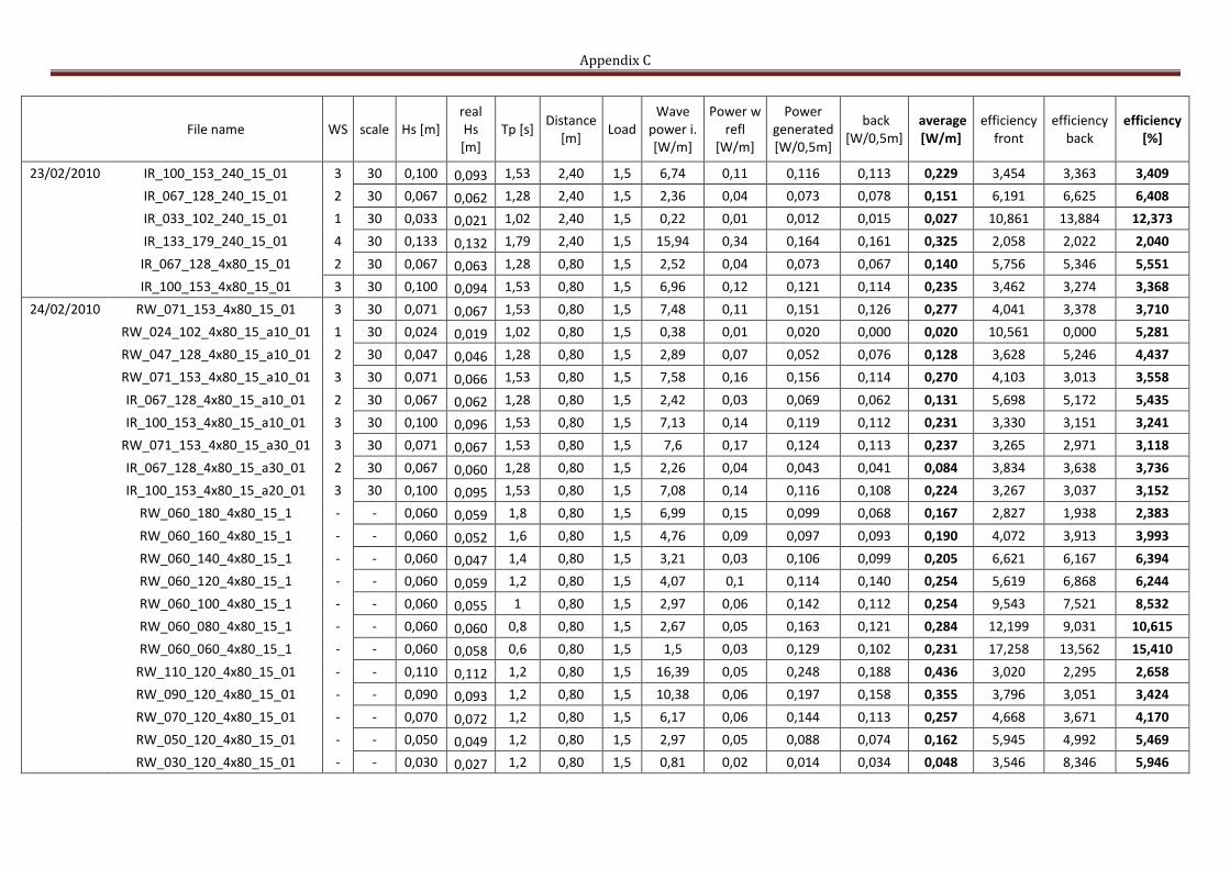
Appendix C
File name WS scale Hs [m] real Hs [m]
Tp [s] Distance
[m] Load
Wave power i. [W/m]
Power w refl
[W/m]
Power generated [W/0,5m]
back [W/0,5m]
average [W/m]
efficiency front
efficiency back
efficiency [%]
23/02/2010 IR_100_153_240_15_01 3 30 0,100 0,093 1,53 2,40 1,5 6,74 0,11 0,116 0,113 0,229 3,454 3,363 3,409
IR_067_128_240_15_01 2 30 0,067 0,062 1,28 2,40 1,5 2,36 0,04 0,073 0,078 0,151 6,191 6,625 6,408
IR_033_102_240_15_01 1 30 0,033 0,021 1,02 2,40 1,5 0,22 0,01 0,012 0,015 0,027 10,861 13,884 12,373
IR_133_179_240_15_01 4 30 0,133 0,132 1,79 2,40 1,5 15,94 0,34 0,164 0,161 0,325 2,058 2,022 2,040
IR_067_128_4x80_15_01 2 30 0,067 0,063 1,28 0,80 1,5 2,52 0,04 0,073 0,067 0,140 5,756 5,346 5,551
IR_100_153_4x80_15_01 3 30 0,100 0,094 1,53 0,80 1,5 6,96 0,12 0,121 0,114 0,235 3,462 3,274 3,368
24/02/2010 RW_071_153_4x80_15_01 3 30 0,071 0,067 1,53 0,80 1,5 7,48 0,11 0,151 0,126 0,277 4,041 3,378 3,710
RW_024_102_4x80_15_a10_01 1 30 0,024 0,019 1,02 0,80 1,5 0,38 0,01 0,020 0,000 0,020 10,561 0,000 5,281
RW_047_128_4x80_15_a10_01 2 30 0,047 0,046 1,28 0,80 1,5 2,89 0,07 0,052 0,076 0,128 3,628 5,246 4,437
RW_071_153_4x80_15_a10_01 3 30 0,071 0,066 1,53 0,80 1,5 7,58 0,16 0,156 0,114 0,270 4,103 3,013 3,558
IR_067_128_4x80_15_a10_01 2 30 0,067 0,062 1,28 0,80 1,5 2,42 0,03 0,069 0,062 0,131 5,698 5,172 5,435
IR_100_153_4x80_15_a10_01 3 30 0,100 0,096 1,53 0,80 1,5 7,13 0,14 0,119 0,112 0,231 3,330 3,151 3,241
RW_071_153_4x80_15_a30_01 3 30 0,071 0,067 1,53 0,80 1,5 7,6 0,17 0,124 0,113 0,237 3,265 2,971 3,118
IR_067_128_4x80_15_a30_01 2 30 0,067 0,060 1,28 0,80 1,5 2,26 0,04 0,043 0,041 0,084 3,834 3,638 3,736
IR_100_153_4x80_15_a20_01 3 30 0,100 0,095 1,53 0,80 1,5 7,08 0,14 0,116 0,108 0,224 3,267 3,037 3,152
RW_060_180_4x80_15_1 - - 0,060 0,059 1,8 0,80 1,5 6,99 0,15 0,099 0,068 0,167 2,827 1,938 2,383
RW_060_160_4x80_15_1 - - 0,060 0,052 1,6 0,80 1,5 4,76 0,09 0,097 0,093 0,190 4,072 3,913 3,993
RW_060_140_4x80_15_1 - - 0,060 0,047 1,4 0,80 1,5 3,21 0,03 0,106 0,099 0,205 6,621 6,167 6,394
RW_060_120_4x80_15_1 - - 0,060 0,059 1,2 0,80 1,5 4,07 0,1 0,114 0,140 0,254 5,619 6,868 6,244
RW_060_100_4x80_15_1 - - 0,060 0,055 1 0,80 1,5 2,97 0,06 0,142 0,112 0,254 9,543 7,521 8,532
RW_060_080_4x80_15_1 - - 0,060 0,060 0,8 0,80 1,5 2,67 0,05 0,163 0,121 0,284 12,199 9,031 10,615
RW_060_060_4x80_15_1 - - 0,060 0,058 0,6 0,80 1,5 1,5 0,03 0,129 0,102 0,231 17,258 13,562 15,410
RW_110_120_4x80_15_01 - - 0,110 0,112 1,2 0,80 1,5 16,39 0,05 0,248 0,188 0,436 3,020 2,295 2,658
RW_090_120_4x80_15_01 - - 0,090 0,093 1,2 0,80 1,5 10,38 0,06 0,197 0,158 0,355 3,796 3,051 3,424
RW_070_120_4x80_15_01 - - 0,070 0,072 1,2 0,80 1,5 6,17 0,06 0,144 0,113 0,257 4,668 3,671 4,170
RW_050_120_4x80_15_01 - - 0,050 0,049 1,2 0,80 1,5 2,97 0,05 0,088 0,074 0,162 5,945 4,992 5,469
RW_030_120_4x80_15_01 - - 0,030 0,027 1,2 0,80 1,5 0,81 0,02 0,014 0,034 0,048 3,546 8,346 5,946

Appendix C
File name WS scale Hs [m] real Hs [m]
Tp [s] Distance
[m] Load
Wave power i. [W/m]
Power w refl [W/m]
Power generated [W/0,5m]
back [W/0,5m]
average [W/m]
efficiency front
efficiency back
efficiency [%]
24/02/2010 IR_100_53_4x55_15_01 3 30 0,100 0,094 1,53 0,55 1,5 6,99 0,12 0,117 0,103 0,220 3,360 2,938 3,149
IR_100_53_4x45_15_01 3 30 0,100 0,061 1,53 0,45 1,5 6,78 0,12 0,121 0,111 0,232 3,562 3,268 3,415
IR_067_128_4x55_15_01 2 30 0,067 0,093 1,28 0,55 1,5 2,35 0,03 0,070 0,053 0,123 5,939 4,471 5,205
IR_067_128_4x45_15_01 2 30 0,067 0,061 1,28 0,45 1,5 2,3 0,04 0,070 0,060 0,130 6,084 5,173 5,629
11/03/2010 only 2Hz
results not reliable
12/03/2010 RW_060_180_4x80_15_05 - - 0,060 0,053 1,8 0,80 1,5 5,63 0,01 0,091 0,073 0,164 3,245 2,585 2,915
RW_060_160_4x80_15_05 - - 0,060 0,050 1,6 0,80 1,5 4,25 0,04 0,106 0,106 0,212 4,994 4,985 4,990
RW_060_140_4x80_15_05 - - 0,060 0,044 1,4 0,80 1,5 2,84 0,06 0,114 0,137 0,251 8,000 9,649 8,825
RW_060_120_4x80_15_05 - - 0,060 0,058 1,2 0,80 1,5 3,92 0,01 0,121 0,164 0,285 6,162 8,364 7,263
RW_060_100_4x80_15_05 - - 0,060 0,052 1 0,80 1,5 2,42 0,02 0,137 0,137 0,274 11,319 11,339 11,329
RW_060_080_4x80_15_05 - - 0,060 0,057 0,8 0,80 1,5 2,34 0,02 0,178 0,142 0,320 15,170 12,119 13,645
RW_060_060_4x80_15_05 - - 0,060 0,055 0,6 0,80 1,5 1,53 0,06 0,109 0,098 0,207 14,240 12,777 13,509
RW_024_102_4x80_15_01 1 30 0,024 0,015 1,02 0,80 1,5 0,2 0,01 0,001 0,000 0,001 0,633 0,000 0,317
RW_047_128_4x80_15_01 2 30 0,047 0,039 1,28 0,80 1,5 2,03 0,02 0,074 0,090 0,164 7,323 8,886 8,105
RW_071_153_4x80_15_02 3 30 0,071 0,060 1,53 0,80 1,5 5,94 0,02 0,138 0,150 0,288 4,631 5,053 4,842
IW_100_153_4x80_15_05 3 30 0,100 0,085 1,53 0,80 1,5 5,62 0,05 0,109 0,133 0,242 3,865 4,739 4,302
RW_024_102_4x80_17_01 1 30 0,024 0,015 1,02 0,80 1,7 0,19 0,01 0,000 0,000 0,000 0,000 0,000 0,000
RW_047_128_4x80_17_01 2 30 0,047 0,040 1,28 0,80 1,7 2,05 0,02 0,074 0,089 0,163 7,238 0,089 3,664
RW_071_153_4x80_17_01 3 30 0,071 0,060 1,53 0,80 1,7 5,96 0,02 0,159 0,149 0,308 5,338 5,002 5,170
IW_100_153_4x80_17_03 3 30 0,100 0,085 1,53 0,80 1,7 5,66 0,05 0,133 0,137 0,270 4,692 4,838 4,765
IW_033_102_4x80_17_S_01 1 30 0,033 0,020 1,02 0,80 1,7 0,2 0,01 0,013 0,006 0,025 16,806 8,229 12,518
IW_067_128_4x80_17_S_01 2 30 0,067 0,056 1,28 0,80 1,7 1,94 0,03 0,075 0,072 0,191 10,014 9,667 9,841
IW_100_153_4x80_17_S_01 3 30 0,100 0,085 1,53 0,80 1,7 5,69 0,05 0,134 0,136 0,351 6,099 6,184 6,142
10/04/2010 IW_033_102_240_15_S_50x10_01 1 30 0,033 0,022 1,02 2,40 1,5 0,24 0,01 0,018 0,014 0,032 14,650 11,611 13,131
IW_067_128_240_15_S_50x10_01 2 30 0,067 0,058 1,28 2,40 1,5 2,12 0,05 0,066 0,077 0,143 6,252 7,242 6,747
IW_100_153_240_15_S_50x10_01 3 30 0,100 0,084 1,53 2,40 1,5 5,45 0,08 0,120 0,132 0,252 4,412 4,848 4,630

Appendix C
File name WS scale Hs [m] real Hs
Tp [s] Distance
[m] Load
Wave power
Power w refl
Power generated
back [W/0,5m]
average [W/m]
efficiency front
efficiency back
efficiency [%]
10/04/2010 IW_033_102_240_15_S_38x13_01 1 30 0,033 0,019 1,02 2,40 1,5 0,18 0,01 0,013 0,012 0,032 19,088 16,873 17,981
IW_067_128_240_15_S_38x13_01 2 30 0,067 0,055 1,28 2,40 1,5 1,87 0,04 0,063 0,077 0,182 8,789 10,815 9,802
IW_100_153_240_15_S_38x13_01 3 30 0,100 0,083 1,53 2,40 1,5 5,46 0,09 0,117 0,141 0,335 5,633 6,798 6,216
IW_033_102_240_15_S_38x10_01 1 30 0,033 0,019 1,02 2,40 1,5 0,18 0,01 0,005 0,003 0,010 7,821 4,160 5,991
IW_067_128_240_15_S_38x10_01 2 30 0,067 0,054 1,28 2,40 1,5 1,85 0,04 0,049 0,056 0,136 7,016 7,906 7,461
IW_100_153_240_15_S_38x10_01 3 30 0,100 0,083 1,53 2,40 1,5 5,44 0,09 0,101 0,117 0,283 4,894 5,665 5,280
IW_033_102_240_15_S_38x07_01 1 30 0,033 0,018 1,02 2,40 1,5 0,16 0,01 0,000 0,000 0,000 0,123 0,000 0,062
IW_067_128_240_15_S_38x07_01 2 30 0,067 0,054 1,28 2,40 1,5 1,88 0,05 0,008 0,009 0,022 1,104 1,321 1,213
IW_100_153_240_15_S_38x07_01 3 30 0,100 0,084 1,53 2,40 1,5 5,53 0,09 0,026 0,025 0,066 1,237 1,190 1,214
11/04/2010 RW_060_060_240_20_01 - - 0,060 0,060 0,6 2,40 2 1,85 0,03 0,104 0,137 0,241 11,223 14,779 13,001
RW_060_080_240_20_01 - - 0,060 0,057 0,8 2,40 2 2,31 0,02 0,213 0,168 0,381 18,399 14,505 16,452
RW_060_100_240_20_01 - - 0,060 0,058 1 2,40 2 3,03 0,04 0,167 0,170 0,337 11,034 11,236 11,135
RW_060_120_240_20_01 - - 0,060 0,062 1,2 2,40 2 4,78 0,04 0,121 0,147 0,268 5,044 6,169 5,607
RW_060_140_240_20_01 - - 0,060 0,052 1,4 2,40 2 4,04 0,02 0,130 0,131 0,261 6,456 6,468 6,462
RW_060_160_240_20_01 - - 0,060 0,052 1,6 2,40 2 4,56 0,02 0,118 0,089 0,207 5,159 3,894 4,527
RW_060_180_240_20_01 - - 0,060 0,055 1,8 2,40 2 5,92 0,11 0,086 0,100 0,186 2,895 3,384 3,140
RW_024_102_240_20_02 1 30 0,024 0,012 1,02 2,40 2 0,13 0,005 0,000 0,000 0,000 0,000 0,000 0,000
RW_047_128_240_20_02 2 30 0,047 0,046 1,28 2,40 2 2,68 0,03 0,069 0,111 0,180 5,173 8,278 6,726
RW_071_153_240_20_02 3 30 0,071 0,065 1,53 2,40 2 6,35 0,1 0,134 0,185 0,319 4,207 5,825 5,016
RW_035_125_240_20_02 1 20 0,035 0,031 1,25 2,40 2 1,14 0,05 0,000 0,046 0,046 0,000 8,097 4,049
IW_033_102_240_20_02 1 30 0,033 0,021 1,02 2,40 2 0,21 0,01 0,008 0,001 0,009 7,508 0,805 4,157
RW_024_102_240_00_02 1 30 0,024 0,012 1,02 2,40 0 0,12 0,003 0,007 0,000 0,007 12,387 0,165 6,276
RW_047_128_240_00_02 2 30 0,047 0,043 1,28 2,40 0 2,43 0,03 0,036 0,037 0,073 2,925 3,014 2,970
RW_071_153_240_00_02 3 30 0,071 0,064 1,53 2,40 0 6,22 0,09 0,056 0,055 0,111 1,787 1,780 1,784
RW_035_125_240_00_02 1 20 0,035 0,030 1,25 2,40 0 1,13 0,04 0,024 0,022 0,046 4,198 3,914 4,056
IW_033_102_240_00_02 1 30 0,033 0,021 1,02 2,40 0 0,22 0,01 0,011 0,001 0,012 10,073 1,277 5,675
IW_033_102_240_15_S_50x10HOLE_01 1 30 0,033 0,021 1,02 2,40 1,5 0,21 0,01 0,000 0,000 0,000 0,006 0,024 0,015
IW_067_128_240_15_S_50x10HOLE_01 2 30 0,067 0,060 1,28 2,40 1,5 2,2 0,05 0,001 0,012 0,013 0,888 1,100 0,994
IW_100_153_240_15_S_50x10HOLE_01 3 30 0,100 0,090 1,53 2,40 1,5 6,44 0,09 0,047 0,052 0,099 1,472 1,608 1,540

Appendix C
118
In the previous pages, each table contains the main information concerning the laboratory results.
For example, the first test reported is RW_035_125_240_00_01. Hence, the data file name has a structure
as AA_BB_CC_DD_EE_FF, where:
AA indicates if the wave is regular (RW) or irregular (IR);
BB indicates the wave height;
CC indicates the wave period;
DD indicates the distance between the energy converter plates;
EE indicates the load;
FF indicates the number of the test.
The information contained in the file name are reported in the subsequent columns of the table, such as:
the wave state, the wave period, the wave height. Furthermore, in the table, the column subsequent to the
wave height corresponds to the measured wave height, whereas for the wave period this difference is
negligible.
The incident and the reflected wave power are referred to the values measured from the wave gauges, and
then analyzed through the software WaveLab3.33.
Regard the wave power, there are differences among the theoretical values and the measured ones, and
moreover among measured values in different tests, but referring to the same wave state. However, it is
declarable that these differences are insignificant for the work done.
The power generated values are calculated as the ratio between the total energy product by the device and
the total sampling duration, or analogously as the average among the power generated at each sampling
instant.
The value between the front plate and the back one, concerning the power generated, is determined refer
to a width of the plate of 1m, hence it is more understandable.
Whereas to obtain the efficiency values a comparison, between the power generated and the wave power
available, is done for each test.

Appendix D
119
MATLAB ANALISYS’ FILE
The wave is usually described through a harmonic signal, consequently the displacement and the force felt
by the energy converter plate should be represented through harmonic signals.
Through the sampling plot of one signal of the force, it is evident that the trend is harmonic how it should
be, but it has not a zero mean. This is a mistake, because it means that at t=0, when there should not be
any force, in reality there is an “inconvenience force” measured, which value coincides with the average
value of the signal. It is analogous to say that the graph is shifted, without modifying its trend.
Therefore it is necessary to subtract the offset value to each force measured value.
The offset problem is also present in the records of the displacements, and the meaning is obviously the
same, i.e. at the start instant, t=0, when there should not be any displacement, in reality the plate is not to
the original position. However, regard the displacements, the offset is not a problem, because the aim of
the study is to have the difference x between two subsequent record instants, and not the real
displacement x, for each record instant.
As it is predictable, immediately, the device doesn’t achieve the steady state. This aspect is illustrated in the
figure D.1, for this reason it is required to cut the first minute of the sampling for the regular tests, and the
first two or three minutes for the irregular tests. However, to consider the first few minutes does not
involve a serious mistake.
Moreover calculating the t, it is observable that several times the t is different to the one fixed with the
frequency sampling. It is declarable that:
- the time of recording could be wrong due to problem between usb/router, etc.
- the time, which the machine takes results, is correct and it corresponds to the frequency chosen.
In the next pages, the Matlab script and its results are reported.

Appendix D
120
% The target of this script is to analyze the results coming from % WavePiston.vi, to find: % - the average generated power % - the efficiency of the device for a particular wave state % - the standard deviation of the impressed force on the energy converter plate
clear all close all
addpath(genpath('LABORATOR'))
% specifies the path to search the file fid = fopen('RW_060_180_4x80_15_T_04.txt','rt');
% indicates which file take in examination
for i=1:15; line = fgetl(fid); end
deltat=0.1; % sampling frequency 10Hz
count = 1; while ~feof(fid), % while the file is not end line = strrep(line,',','.'); % string replace data(count,:) = sscanf(line,'%f %f %f %f %f')'; count = count+1; line = fgetl(fid); end line = strrep(line,',','.');
% when the while cycle is finished, there is one more line to read data(count,:) = sscanf(line,'%f %f %f %f %f')';
% the data matrix will contain all the numbers inside the input file fclose(fid);
% at the end of the while cycle, that the matrix data is finished, it is possible to create the displacement vector and force vector
% Creation of the displacement and force vector displacement = data(:,[2 3]); Force = data(:,[4 5]); offset = mean(data(:,[4 5])); % calculation of forces offset. offset1= offset(1,1); % It coincides with the mean, because the offset2= offset(1,2); % signal is harmonic
Force_ok(:,1) = Force(:,1)-offset1; Force_ok(:,2) = Force(:,2)-offset2;
% To create the velocity vector the easiest way is to use another counter velocity(1,:)=[0 0]; % initial condition for the velocity
for j= 1:(max(length(displacement))-1) velocity(j+1,:)=(displacement(j+1,:)-displacement(j,:))/deltat; end
power = velocity.*Force_ok; average_power = 2*mean(power);
% the multiplication for two is because the plate width is 0,5m,

Appendix D
121
% while the wave incident power is for 1m of width crest disp(['the front and the back average power,in W/m,are ',num2str(average_power)])
% Displacements figure(1) subplot(2,1,1), plot(data(:,2),'b') legend('displacement of the front plate') xlabel('time [s]'); ylabel('front plate'); subplot(2,1,2), plot(data(:,3),'r') legend('displacement of the back plate') xlabel('time [s]'); ylabel('back plate');
% Measured Forces figure(2) subplot(2,1,1), plot(data(:,4),'b') legend('measured forces in the front') ylabel('front plate'); xlabel('time [s]'); subplot(2,1,2), plot(data(:,5),'r') legend('measured forces in the back') ylabel('back plate'); xlabel('time [s]');
% Velocity calculated figure(3) subplot(2,1,1), plot(velocity(:,1),'b') legend('velocity of the front plate') xlabel('time [s]'); ylabel('front plate'); subplot(2,1,2), plot(velocity(:,2),'r') legend('velocity of the back plate') xlabel('time [s]'); ylabel('back plate');
the front and the back average power, in W/m, are -0.63609 -0.45974

Appendix D
122
Figure D.1: Displacements of the front plate and the back plate during the sampling.
It is obviously that the device requires several instants to get the steady state.
Figure D.2: Force impressed on the front plate and on the back plate during the sampling.
The regular trend of the displacement, it is due to the regular trend of the wave, and this is observable even in the
impressed forces’ trend.

Appendix D
123
Figure D.3: Velocity on the front plate and on the back plate during the sampling.
The velocity trend depends on the displacement one, so it has the same regular trend.

Appendix E
124
SIMULATIONS WITH MATLAB
1- Introduction
As presented before, the WavePiston device can be represented as a single degrees freedom body.
Figure E.0: A single unit of the WavePiston device is seen as a single degrees freedom body.
The main target of the numerical model is to predict the behaviour of the WavePiston device in different
location, changing the wave parameters of regular waves, and regardless the laboratory results.
Nevertheless, to achieve that aim, the first stage is to build a numerical model able to estimate the
efficiency in the laboratory case.
Furthermore, to begin the simulation analysis, some simplifying assumption are made; hence, below, it is
presented for first the numerical model able to guess the performance of a fixed body in the laboratory
condition, then there is the numerical model for the body in movement in the laboratory condition, and at
last there is the numerical model for the body in movement in real condition.
The wave is usually described through a harmonic signal, consequently the displacement and the force felt
by the energy converter plate should be represented through harmonic signals.
For all the numerical models concerning the laboratory conditions, a particular value for the stiffness is
hypothesized, i.e. kp= 100 N/m, it means that to move the plate of 1cm, it is necessary a force of 1N
(1N=100g). This value should be changed, depending on the result of particular test, where by imposing a
known displacement and reading the strength corresponding it is possible to find the stiffness as the ratio
F/x.
Whereas, for the damping coefficient, the two models have not an unique value for it, but there are many
values, and different results correspond to the variation of the damping values.
It is predictable that a small value of the damping implies a large range for the displacement, hence of the
velocity, but at the same time a low value of the force impressed, because the plate does not make
resistance to the flow motion.
Thus, to obtain the best performance, the damping value might have a mean value.
These comments are verified with the numerical models’ graphs.

Appendix E
125
2- First model: Simulation of a fixed body in the laboratory condition
% NUMERICAL MODEL_1 % Target: Reproduce laboratory conditions
% Basic equation is the dynamic equation for a normal oscillating body % m*acc+ c*vel+ k*x = External force % where External force is the force given by Morison Equation with a fixed body
is F(u, upunto, xpunto, x2punti)= F inertia + F drag % where u= is the flow velocity % x= is the plate displacement
clear all close all
row = 1030; % row= density salt water [kg/m3] ro= 7740; % ro= density of the steel plate [kg/m3] roprimo= ro-row; % roprimo=density of the steel plate inside the water [kg/m3]
w= 0.5; % w= width of the plate [m] d= 0.1; % d= depth of the plate [m] s= 0.001; % s= thickness [m]
kp=100; % kp= steel plate stiffness [N/m] % for the first attempt it is introduced a casual value.
% The hypothesis is 100N/m, it means that to move the plate of 1cm
it is necessary a force of 1N (1N=100g).
% This value should be changed,depending on the result of particular
test, where by imposing a known displacement and reading the
strength corresponding it is possible to find the stiffness as the
ratio F/x.
mass= roprimo*w*d*s; volume=w*d*s;
% Values of the First Danish Regular Wave State, in scale 1:30
Hs= 0.024; % Hs= significant wave height [m] Tp= 1.02; % T= Tp= wave period [s] L= 1.61; % L= wave length [m] h= 0.7; % h= water depth [m]
k= 2*pi/L; omega=2*pi/Tp;
% Wave Power per meter of wave crest [kW/m] Tz=Tp/1.4; Te=1.2*Tz; Wavepower=0.44*(Hs^2)*Te;
% External force CD=2; % CD= drag coefficient; CM=1; % CM= mass coefficient;

Appendix E
126
z=-(d/2); % presa di riferimento quota baricentro piatto rap=(cosh(k*(h+z))/sinh(k*h));
q=1; for vi=0:5:100 % C= damping [Ns/m]=[kg/s] % step of 5, from a cycle to the subsequent
j=1; vx(q,1)=0; % initial conditions vu(q,1)=0; % u= flow velocity vvel(q,1)=0;
for t=1:1:180 % computing time 3 minutes, with a step of 1 sec vt(1,j+1)=t; u=omega*(Hs/2)*rap*cos(omega*vt(1,j)); vu(q,j+1)=u;
upunto=-rap*(omega^2)*(Hs/2)*sin(omega*vt(1,j+1)); deltat=vt(1,j+1)-vt(1,j); % sampling frequency
Fi=ro*(1+CM)*volume*upunto; % Inertia force
modulo=cos(omega*vt(1,j+1));
% it is only depending on the trend of the velocity flow
if modulo>=0 C1= CD*ro*omega^2*(Hs^2)*rap^2*(cos(omega*vt(1,j+1)))^2/(8*roprimo*s);
%C1= Fd/mass Fexternal=Fi+C1*mass; % Fexternal=Fi+Fd; else C1= -CD*ro*omega^2*(Hs^2)*rap^2*(cos(omega*vt(1,j+1)))^2/(8*roprimo*s);
%C1= Fd/mass Fexternal=Fi+C1*mass; % Fexternal=Fi+Fd; end
B=(1/(deltat^2)+(vi/(mass*deltat))-(k/(2*mass))); C2=Fi/mass;
A=(1/(deltat^2)+(vi/(mass*deltat))+(k/(2*mass)));
x= (vx(q,j)*B+C1+C2)/A; % x= plate displacement vx(q,j+1)=x;
velocity=(vx(q,j+1)-vx(q,j))/deltat; vvel(q,j+1)=velocity;
Flost=vi*velocity; vFlost(q,j+1)=Flost; vStdFlost(1,q)=std(vFlost(q,:));
vFexternal(q,j+1)=Fexternal;
Fimpressed=Fexternal-Flost; vFimpressed(q,j+1)=Fimpressed;

Appendix E
127
stdFimpressed=std(vFimpressed(q,:));
Power=abs(velocity*Flost)/w;
% Calculation of the power generated per meter of plate’s width, in
a particular instant j vPower(q,j+1)=Power; averagePower=mean(vPower(q,:));
j=j+1; end
allvi(1,q)=vi;
stdvel=std(vvel(q,:)); vstdvel(1,q)=stdvel;
vStdFimpressed(1,q)=stdFimpressed; allAveragePower(1,q)=averagePower;
efficiency= allAveragePower(1,q)*100/(Wavepower*1000);
% To calculate the efficiency there is the need to compare the wave power
with the average power generated for each damping value veff(1,q)=efficiency;
q=q+1; end
% Flow velocity figure(1) plot(vt,vu,'r.-') xlabel('time [s]'); ylabel('flow velocity');
% Different displacement for different damping values figure(2); plot(vt,vx(1,:),'.b',vt,vx(10,:),'.m',vt,vx(21,:),'.k') legend('in blue damping=0','in magenta damping medium', 'in black damping
maximum') xlabel('time [s]'); ylabel('displacement');
% Different velocity for different damping values figure(3) plot(vt,vvel(1,:),'.b',vt,vvel(10,:),'.m',vt,vvel(21,:),'.k') legend('in blue damping=0','in magenta damping medium', 'in black damping
maximum') xlabel('time [s]'); ylabel('plate velocity');
% Velocity comparison between flow velocity and the one for the mean damping
values figure(4); plot(vt,vvel(10,:),'.m',vt,vu,'r.-') legend('in magenta damping medium', 'in red flow velocity') xlabel('time [s]');

Appendix E
128
ylabel('velocity comparison');
% Standard deviation of the velocity figure(5) plot(allvi,vstdvel,'.b') xlabel('Damping values'); ylabel('Standard Deviation of the plate velocity');
% Average power product for each damping value figure(6) plot(allvi,allAveragePower,'.k') xlabel('Damping values'); ylabel('Power generated');
% Standard deviation of the velocity figure(7) plot(allvi,vStdFlost,'.m') xlabel('Damping values'); ylabel('standard deviation of the Lost force');
% Efficiency for each damping value figure(8) plot(allvi,veff,'.b') xlabel('Damping values'); ylabel('efficiency');
figure(9) plot(allvi,vstdvel,'.b',allvi,vStdFlost,'.m',allvi,allAveragePower,'.g') legend('in blue standard deviation of the plate velocity','in magenta standard
deviation of the Lost force', 'in green power generated') xlabel('Damping values');
figure(10) plot(vStdFlost,vstdvel,'.r') xlabel('standard deviation of the Lost force'); ylabel('standard deviation of the plate velocity');
figure(11) plot(vStdFlost,allAveragePower,'.k') xlabel('standard deviation of the Lost force'); ylabel('power generated');
figure(12) subplot(2,2,1),plot(vt,vu,'r.-') ylabel('flow velocity'); subplot(2,2,2),plot(vt,vx(1,:),'.b',vt,vx(10,:),'.m',vt,vx(21,:),'.k') ylabel('displacement for different damping values'); subplot(2,2,3),plot(vt,vvel(1,:),'.b',vt,vvel(10,:),'.m',vt,vvel(21,:),'.k') ylabel('plate velocity for different damping values'); subplot(2,2,4),plot(vt,vvel(1,:),'.b',vt,vvel(10,:),'.m',vt,vvel(21,:),'.k',vt,v
u,'r.-') legend('plate velocity for different damping values compared to the flow
velocity');

Appendix E
129
Figure E.1: Displacement for different damping values.
In blue, it is the displacement for a zero value of damping.
In magenta, it is the displacement for a mean value of damping.
In black, it is the displacement for a maximum value of damping.
Figure E.2: Velocity of the movement of the plate for different damping values.
In blue, it is the velocity for a zero value of damping.
In magenta, it is the velocity for a mean value of damping.
In black, it is the velocity for a maximum value of damping.

Appendix E
130
Figure E.3: Velocity comparison between the flow velocity and the velocity of the plate for the mean damping values.
Figure E.4: Trend of the velocity due to the variation of the damping values.
Figure E.5: Trend of the force impressed due to the variation of the damping values.

Appendix E
131
Figure E.6: Trend of the average power generated due to the variation of the damping values.
Figure E.7: Trend of the efficiency due to the variation of the damping values.
Figure E.8: Trend of the power generated in relation with the standard deviation of the force impressed.

Appendix E
132
3- Second model: Simulation of a body in movement in the laboratory condition
% NUMERICAL MODEL_2 % Target: Reproduce laboratory conditions
% Basic equation is the dynamic equation for a normal oscillating body % m*acc+ c* vel+ k*x = External force % where External force is the force given by Morison Equation with a body % in movment F(u,upunto, xpunto, x2punti)= F inertia + F drag + F froude-Krylov % where u= is the flow velocity
x= is the plate displacement
clear all close all
row = 1030; % row= density salt water [kg/m3] ro= 7740; % ro= density of the steel plate = [kg/m3] roprimo= ro-row; % roprimo=density of the steel plate inside the water [kg/m3]
w= 0.5; % w= width of the plate [m] d= 0.1; % d= depth of the plate [m] s= 0.001; % s= thickness [m]
kp=100; % kp= steel plate stiffness [N/m] % for the first attempt it is introduced a casual value.
% The hypothesis is 100N/m, it means that to move the plate of 1cm
it is necessary a force of 1N (1N=100g).
% This value should be changed,depending on the result of particular
test, where by imposing a known displacement and reading the
strength corresponding it is possible to find the stiffness as the
ratio F/x.
mass= roprimo*w*d*s; volume=w*d*s; area=w*d;
% Values of the First Danish Regular Wave State, in scale 1:30
Hs= 0.024; % Hs= significant wave height [m] Tp= 1.02; % Tp= wave period [s] L= 1.61; % L= wave length [m] h= 0.7; % h= water depth [m]
k= 2*pi/L; omega=2*pi/Tp;
% Wave Power per meter of wave crest [kW/m]
Tz=Tp/1.4; Te=1.2*Tz; Wavepower=0.44*(Hs^2)*Te;
% external force CD=2; % CD= drag coefficient; CM=1; % CM= mass coefficient;

Appendix E
133
z=-(d/2); % presa di riferimento quota baricentro piatto rap=(cosh(k*(h+z))/sinh(k*h));
q=1; for vi=0:5:100 % C= damping [Ns/m]=[kg/s] % step of 5, from a cycle to the subsequent j=1; vx(q,1)=0; % initial conditions vu(q,1)=0; % u= flow velocity vvel(q,1)=0;
for t=0.1:1:180 % computing time 3 minutes, with a step of 1 sec
vt(1,j+1)=t; u=omega*(Hs/2)*rap*cos(omega*vt(1,j)); vu(q,j+1)=u;
upunto=-rap*(omega^2)*(Hs/2)*sin(omega*vt(1,j+1)); vupunto(q,j+1)=upunto; deltat=vt(1,j+1)-vt(1,j); % sampling frequency
partFi=ro*CM*volume*(vupunto(q,j+1));
% partFi= it is the part of the inertia force that is not depending
on the velocity of the plate
Ffk=ro*volume*upunto; % Ffk= body in movement
% Calculation of the displacement, assuming the abs positiv
Ba=-((1/(deltat^2))+(vi/(mass*deltat))+(k/(2*mass)));
% Ba= B part, not depending on abs sign Bmodulo=-(CD*ro*area/(2*mass))*((2*vu(q,j+1)/deltat)+(2*vx(q,j)/(deltat^2)); B=Ba+Bmodulo;
Ca=+vx(q,j)*((1/(deltat^2))+(vi/(mass*deltat))+
-(k/(2*mass))+((CM*ro*volume)/((deltat^2)*mass)));
% Ca= C1 part, not depending on abs sign Cmodulo=+vx(q,j)*((CD*ro*area)/(2*mass))*((vx(q,j)/(deltat^2))+
+(2*vu(q,j+1)/deltat))+((CD*ro*area)/(2*mass))*((vu(q,j+1))^2); C1=Ca+Cmodulo;
C2=partFi/mass; C3=Ffk/mass; C=C1+C2+C3;
A=((CD*ro*area)/(2*(deltat^2)*mass));
g= polyeig(C,B,A); % function to solve the equation: Ax^2+bx+C=0
% in input it needs the3 coefficients % in output it gives a vector g, including x1 e x2
x=mean(g); % x= plate displacment vx(q,j+1)=x;
Fexternal=0.5*CD*ro*area*((vu(q,j+1)-((vx(q,j+1)-vx(q,j))/deltat)))^2+
+ro*volume*CM*(vupunto(q,j+1)-(vx(q,j+1)-vx(q,j))/(deltat^2))+
+C3*mass;

Appendix E
134
vFexternal(q,j+1)=Fexternal;
modulo= vupunto(q,j+1)-((vx(q,j+1)-vx(q,j))/deltat);
if modulo>=0 vx(q,j+1)=x; else A=-A; % Re-calculation of the x value
Bmodulo= -Bmodulo; B=Ba+Bmodulo;
Cmodulo=-Cmodulo; C1=Ca+Cmodulo; C=C1+C2+C3;
g= polyeig(C,B,A); x=mean(g); % x= plate displacment vx(q,j+1)=x;
Fexternal=0.5*CD*ro*area*((vu(q,j+1)-((vx(q,j+1)-vx(q,j))/deltat)))^2+
+ro*volume*CM*(vupunto(q,j+1)-(vx(q,j+1)-vx(q,j))/(deltat^2))
+C3*mass; vFexternal(q,j+1)=Fexternal; end
velocity=(vx(q,j+1)-vx(q,j))/deltat; vvel(q,j+1)=velocity;
Flost=vi*velocity; vFlost(q,j+1)=Flost; vStdFlost(1,q)=std(vFlost(q,:));
Fimpressed=Fexternal-Flost; vFimpressed(q,j+1)=Fimpressed; stdFimpressed=std(vFimpressed(q,:));
Power=abs(velocity*Flost)/w;
% Calculation of the power generated per meter of length crest, in a instant j
vPower(q,j+1)=Power; averagePower=mean(vPower(q,:));
j=j+1;
end
allvi(1,q)=vi;
stdvel=std(vvel(q,:)); vstdvel(1,q)=stdvel;
vStdFimpressed(1,q)=stdFimpressed; allAveragePower(1,q)=averagePower;

Appendix E
135
% To calculate the efficiency there is the need to compare the wave power with
the average power generated for each damping value
efficiency= allAveragePower(1,q)*100/(Wavepower*1000); veff(1,q)=efficiency;
q=q+1; end
% Flow velocity figure(1) plot(vt,vu,'r.-') xlabel('time [s]'); ylabel('flow velocity');
% Different displacement for different damping values figure(2); plot(vt,vx(1,:),'.b',vt,vx(10,:),'.m',vt,vx(21,:),'.k') legend('in blue damping0','in magenta damping medium','in black damping maximum') xlabel('time [s]'); ylabel('displacement');
% Different velocity for different damping values figure(3) plot(vt,vvel(1,:),'.b',vt,vvel(10,:),'.m',vt,vvel(21,:),'.k') legend('in blue damping0','in magenta damping medium','in black damping maximum') xlabel('time [s]'); ylabel('plate velocity');
% Velocity comparison between flow velocity and the one for the mean damping
values figure(4); plot(vt,vvel(10,:),'.m',vt,vu,'r.-') legend('in magenta damping medium', 'in red flow velocity') xlabel('time [s]'); ylabel('velocity comparison');
% Standard deviation of the velocity figure(5) plot(allvi,vstdvel,'.k') xlabel('Damping values'); ylabel('Standard Deviation of the plate velocity');
% Average power product for each damping value figure(6) plot(allvi,allAveragePower,'.g') xlabel('Damping values'); ylabel('Power generated');
% Standard deviation of the force figure(7) plot(allvi,vStdFlost,'.m') xlabel('Damping values'); ylabel('standard deviation of the Lost force');
% Efficiency for each damping value

Appendix E
136
figure(8) plot(allvi,veff,'.b') xlabel('Damping values'); ylabel('efficiency');
figure(9) plot(allvi,vstdvel,'.b',allvi,vStdFlost,'.m',allvi,allAveragePower,'.g') legend('in blue standard deviation of the plate velocity', 'in magenta standard
deviation of the Lost force', 'in green power generated') xlabel('Damping values');
figure(10) plot(vStdFlost,vstdvel,'.r') xlabel('standard deviation of the Lost force'); ylabel('standard deviation of the plate velocity');
figure(11) plot(vt,vFexternal(1,:),'g.-',vt,vFexternal(10,:),'b.-',
vt,vFexternal(21,:),'r.-') legend('Variation External force due to damping');
figure(12) plot(vStdFlost,allAveragePower,'.k') xlabel('standard deviation of the Lost force'); ylabel('power generated');

Appendix E
137
4- Third model: Simulation of a body in movement in the real condition
% NUMERICAL MODEL_3 % Target: Use the model to find the power take off (PTO) changing the sea state
% Basic equation is the dynamic equation for a normal oscillating body % m*acc+ c* vel+ k*x = External force % where External force is the force given by Morison Equation with a body % in movement F(u,upunto, xpunto, x2punti)= F inertia + F drag + F froude-Krylov % where u= is the flow velocity % and x= is the plate displacement
clear all close all
row = 1030; % row= density salt water [kg/m3] ro= input('Insert the density of the steel plate, in kg/m3, ' ); roprimo= ro-row; % roprimo=density of the steel plate inside the water [kg/m3]
w= input('Insert the width of the plate, in m ' ); d= input('Insert the depth of the plate, in m ' ); s= input('Insert the thickness of the plate, in m ' ); kp= input('Insert the stiffness of the spring, in N/m ' ); vi= input('Insert the damping coefficient, in N*s/m ' ); mass= roprimo*w*d*s; volume=w*d*s; area=w*d;
Hs= input('Insert the significant wave height, in m ' ); Tp= input('Insert the peak wave period, in sec ' ); h= input('Insert water depth, in m ' );
g=9.81; % gravity acceleration [m/s2] Lhypothesis= 1.61; L=1.1; diff= L-Lhypothesis; while diff~=0 L=(g*(Tp^2)/(2*pi)*tanh(2*pi*h/Lhypothesis)); diff=L- Lhypothesis; end disp(['The wave length is ',L]); k= 2*pi/L; omega=2*pi/Tp;
% From off-shore to near-shore the wave period doesn't change if (h/L)>(1/2) % Potenza dell'onda per metro di cresta d'onda [kW/m] Tz=Tp/1.4; Te=1.2*Tz; Wavepower=0.44*(Hs^2)*Te; disp('water depth condition'); else disp('shallow water condition'); end

Appendix E
138
% external force CD=2; % CD= drag coefficient; CM=1; % CM= mass coefficient; z=-(d/2); rap=(cosh(k*(h+z))/sinh(k*h));
j=1; vx(1,1)=0; % initial condition vu(1,1)=0; % u= flow velocity vvel(1,1)=0;
for t=0.1:1:180 % computing time 3 minutes, with a step of 1 sec
vt(1,j+1)=t; u=omega*(Hs/2)*rap*cos(omega*vt(1,j)); vu(1,j+1)=u;
upunto=-rap*(omega^2)*(Hs/2)*sin(omega*vt(1,j+1)); vupunto(1,j+1)=upunto; deltat=t(j)-t(j-1); %sampling frequency
partFi=ro*CM*volume*(vupunto(q,j+1));
% partFi= inertia force part not depending on the movement of the plate Ffk=ro*volume*upunto; % Ffk= body in movement
% Calculation with abs positiv Ba=-((1/(deltat^2))+(vi/(mass*deltat))+(k/(2*mass)));
% B part not depending on abs sign Bmodulo=-(CD*ro*area)/(2*mass))*((2*vu(q,j+1)/deltat)+(2*vx(q,j)/(deltat^2)); B=Ba+Bmodulo;
Ca=+vx(q,j)*((1/(deltat^2))+(vi/(mass*deltat))-(k/(2*mass))+
+((CM*ro*volume)/((deltat^2)*mass)));
% C1 part not depending on abs sign Cmodulo=+vx(q,j)*((CD*ro*area)/(2*mass))*((vx(q,j)/(deltat^2))+
+(2*vu(q,j+1)/deltat))+((CD*ro*area)/(2*mass))*((vu(q,j+1))^2); C1=Ca+Cmodulo;
C2=partFi/mass; C3=Ffk/mass; C=C1+C2+C3;
A=((CD*ro*area)/(2*(deltat^2)*mass));
g= polyeig(C,B,A); % function to solve the equation: Ax^2+bx+C=0
% in input it needs the3 coefficients % in output it gives a vector g, including x1 e x2
x=mean(g); % x= plate displacement vx(q,j+1)=x;
Fexternal=0.5*CD*ro*area*((vu(q,j+1)-((vx(q,j+1)-vx(q,j))/deltat)))^2+
+ro*volume*CM*(vupunto(q,j+1)-(vx(q,j+1)-vx(q,j))/(deltat^2))+C3*mass;

Appendix E
139
vFexternal(q,j+1)=Fexternal; modulo= vupunto(q,j+1)-((vx(q,j+1)-vx(q,j))/deltat);
if modulo>=0 vx(q,j+1)=x; else A=-A; % Re-calculation of x value Bmodulo= -Bmodulo; B=Ba+Bmodulo;
Cmodulo=-Cmodulo; C1=Ca+Cmodulo; C=C1+C2+C3;
g= polyeig(C,B,A); x=mean(g); vx(q,j+1)=x;
Fexternal=0.5*CD*ro*area*((vu(q,j+1)-((vx(q,j+1)-vx(q,j))/deltat)))^2+
+ro*volume*CM*(vupunto(q,j+1)-(vx(q,j+1)-vx(q,j))/(deltat^2))+C3*mass; vFexternal(q,j+1)=Fexternal; end
velocity=(vx(1,j+1)-vx(1,j))/deltat; vvel(1,j+1)=velocity;
% Force Flost=vi*velocity; vFlost(1,j+1)=Flost; StdFlost=std(vFlost(1,:)); Fimpressed=Fexternal-Flost; vFimpressed(1,j+1)=Fimpressed; stdFimpressed=std(vFimpressed(1,:)); %Calculation of power generated per meter of width plate, at the instant j
Power=abs(velocity*Flost)/w;
vPower(1,j+1)=Power; averagePower=mean(vPower(1,:));
j=j+1; end % To calculate the efficiency there is the need to compare the wave power with
the average power generated efficiency= averagePower*100/(Wavepower*1000);
disp(['The efficiency is ',efficiency]);
%Displacement figure(1); plot(vt,vx,'.b') xlabel('time [s]'); ylabel('spostamento'); %Velocity figure(2) plot(vt,vu,'.r') xlabel('time [s]'); ylabel('velocità');

Reference
140
Chapter 1
- Williams, James. 2005. “Oil Price History and Analysis”
- Ocean Energy System, International Energy Agency (I.E.A.) (2009)“Annual Report”
- postnote January 2009 Number 324 Marine Renewable
- Gordon M. Barrow, “Physical Chemistry”, WCB, McGraw-Hill, 1979
- Berlanstein, Lenard R., (1992), “The Industrial Revolution and work in nineteenth-century Europe”
- Abbott Payson Usher (1920), “An Introduction to the Industrial History of England”,
http://books.google.com/books, retrieved 2009-07-26
Chapter 2
- Coastal Engineering Manual (CEM), US Army Corp of Engineers (2002)
- Wienke J., Sparboom U., Oumeraci H., “Breaking Wave Impact on a Slender Cylinder”
- Det Norske Veritas, 2005, “Guidelines on design and operation of wave energy converters”, Carbon
Trust.
- Ocean Energy System, International Energy Agency (I.E.A.) “Ocean Energy Opportunity, present
status and challenges”
- Ocean Energy System, International Energy Agency (I.E.A.) (2006) “Policy Report”
- Ocean Energy System, International Energy Agency (I.E.A.) (2009) “Annual Report”
- Folley, M, Whittaker, T, Osterried, M (2004). "The Oscillating Wave Surge Converter," ISOPE Paper
No. 2004-JSC-377
- J.R Joubert “An investigation of the wave energy resource on the South African Coast, focusing on the spatial distribution of the South West Coast”
Chapter 3
- Kofoed and Frigaard (2009) “The Dragon of Nissum Bredning--Danish approach to development and evaluation of wave energy devices” Journal of Ocean Technology 2009 Renewable Ocean Energy, Vol. 4, No. 4
- Arthur Pecher, J.P. Kofoed (2010) “Experimental Study on the WavePiston Wave Energy Converter”
Chapter 4
- Morison, J. R.; O'Brien, M. P.; Johnson, J. W.; Schaaf, S. A. (1950), "The force exerted by surface
waves on piles"
- “Basic Coastal Engineering”
Chapter 5
- Kofoed and Frigaard (2009) “The Dragon of Nissum Bredning--Danish approach to development and evaluation of wave energy devices” Journal of Ocean Technology 2009 Renewable Ocean Energy, Vol. 4, No. 4
- Ocean Energy System, International Energy Agency (I.E.A.) (2009) “Annual Report”

Web site
141
http:// www.aau.dk
http:// www.wavepiston.dk
http: recession.org/history/1970s_oil_crisis
http:// earthguide.ucsd.edu/fuels/1970.html
http:// www.iea-oceans.org
http:// www.idromare.it
http:// www.telemisura.it
http:// www.geni.org
http:// www.parliament.uk
http://www.esru.strath.ac.uk
http://www.emec.org.uk
http://www.oceanor.no
http://edgar.jrc.ec.europa.eu/index.php
http://www.carbontrust.co.uk