thesis.pdf - Utopia
262
-
Upload
khangminh22 -
Category
Documents
-
view
2 -
download
0
Transcript of thesis.pdf - Utopia


The Library of the
Department of Biochemistry
and Molecular Biology
ASTBURY BUILDING
The University Library
U
NIV
ER
SITY OF L
EE
DS

STRUCTURAL STUDIES OF
THE ARGININE REPRESSOR/ACTIVATOR
FROM Bacillus subtilis.
NICKOLAOS MENELAOU GLYKOS
Submitted in accordance with the requirements
for the degree of Doctor of Philosophy
The University of Leeds
The Department of Biochemistry and Molecular Biology
February 1995
The candidate confirms that the work submitted is his own
and that appropriate credit has been given where reference
has been made to the work of others.

Page i
Abstract
In the presence of L-Arginine, AhrC —the Arginine-dependent Repressor/Ac-
tivator from Bacillus subtilis— represses the transcription of the genes encod-
ing the anabolic and activates those encoding the catabolic enzymes of arginine
metabolism. AhrC is a homohexamer of total molecular mass 105 kDa. It shows
no homology to any of the characterised DNA-binding motifs or DNA-binding
proteins with the exception of ArgR, the Arginine Repressor from Escherichia
coli. ArgR does not act as a transcription activator but it has been shown
to be a necessary accessory protein for the resolution —through site-specific
recombination— of multimers of the ColE1 plasmid. Although the two proteins
share only 29% identity and are from such taxonomically distinct prokaryotes,
AhrC can complement E. coli ArgR− strains both in the regulation of Arginine
metabolism and the resolution of the ColE1 plasmid.
This thesis describes our attempts to determine the crystal structure of AhrC.
Three different crystal forms have been produced and characterised. Useful
derivatives have been prepared for two of these forms but the determination
of their heavy atom structures proved impossible. An attempt to determine the
low resolution structure of AhrC using Electron Microscopy has been unsuccess-
ful. Molecular Replacement using as a search model the crystal structure of the
hexameric core fragment of ArgR also failed to give a convincing solution.

Page ii
Acknowledgements
I should like to thank Professor Simon Phillips for his advice, encouragement
and support throughout the course of my studies.
Dr Amalia Aggeli for useful discussions and for recording and analysing a
FTIR spectrum of AhrC.
Don Akrigg for his help with computational aspects of this work.
Les Child for the photographic work.
Dr Maire Convery for useful discussions and for making valuable comments
on the first draft of this thesis.
Dr Greg van Duyne and Professor Paul Sigler for making the atomic coordi-
nates of their ArgR model available to me before publication.
Professor Stavros Hamodrakas for suggesting Leeds and for his continued
interest in my studies.
Carol Holtham, Coleen Miller, Isobel Parsons and Andrew Walsh for their
help with the purification of AhrC and of the AhrC-ArgR chimaera.

Page iii
Dr Andreas Holzenburg for useful discussions, especially about the Electron
Microscopical studies of AhrC, and for reading critically Chapter 6.
Paul McPhie for his help with the Electron Microscopes.
Dr Mark Parsons for useful discussions and for making valuable comments on
the manuscript.
Dr Jonathan Porter for useful discussions.
My family for their continued encouragement and support.

Page iv
Table of Contents
Abstract i
Acknowledgements ii
Table of Contents iv
List of Figures viii
List of Tables xix
List of Acronyms xx
List of Symbols xxi
1 Introduction 1
1.1 Biochemical and Genetical Data 7
1.2 Biophysical Data 13
2 Protein Preparation, Crystallisation,
and Preliminary Characterisation of AhrC Crystals 17
2.1 Protein Preparation 17
2.1.1 Protein Purification 17
2.1.2 Stability of AhrC During Storage 20
2.2 Crystallisation, and
Preliminary Characterisation of AhrC Crystals 21
2.2.1 Orthorhombic Form 24

Page v
2.2.2 Monoclinic Form 28
2.2.3 Trigonal Form 31
3 Preparation and
Preliminary Analysis of Heavy Atom Derivatives 36
3.1 Data Collection Strategy 36
3.2 Preparation of Heavy Atom Derivatives 39
3.3 Preliminary Analysis 52
3.3.1 The Niobium Cluster, Nb6Cl14 53
3.3.2 The H2IrCl6 Derivative 61
3.3.3 Other Derivatives 63
4 Self Rotation Function Studies
and a Model of the Crystal Packing 66
4.1 Introduction 66
4.2 Self Rotation Function Studies 70
4.2.1 Native Crystals 71
4.2.2 Heavy Atom Structures 74
4.3 A Model of the Crystal Packing 77
4.3.1 Pseudo-origin Peaks 77
4.3.2 Very Low Resolution Permutation Syntheses 81
4.3.3 A Packing Function 83
5 Attempts to Determine the
Heavy Atom Structures of AhrC Derivatives 86
5.1 Introduction 86
5.2 Direct Methods 87
5.2.1 SHELXS-86 90

Page vi
5.2.2 MULTAN77 92
5.2.3 The Cochran & Douglas Method 93
5.3 Patterson Methods 95
5.3.1 HASSP 102
5.3.2 GROPAT 103
5.3.3 A Method by Nixon, P.E., 105
5.3.4 Image-seeking Methods 107
5.3.5 A Patterson Interpretation Programme : MSS 114
5.3.6 The Argos & Rossmann Method 120
5.4 Other Methods 129
5.4.1 Permutation Syntheses Method 129
5.4.2 Molecular Replacement 133
5.4.3 Direct Maximisation of an Electron Density Function 134
5.4.4 Monte Carlo Methods 138
5.4.5 An Attempt to Obtain Phase Information ab initio 147
6 Electron Microscopy of AhrC Crystals 152
6.1 Introduction 152
6.2 Image Reconstruction 157
6.3 Specimen Preparation, Data Collection and Image Processing 162
6.4 Characterised Projections 165
6.4.1 The [001] Projection 165
6.4.2 The [010] Projection 170
6.4.3 The [101] Projection 174
6.4.4 The [130] Projection 176
6.5 Other Projections 176
6.6 The Calculation of a 30A Electron Density Map 179

Page vii
7 Molecular Replacement 186
7.1 The Model 186
7.2 Orthorhombic Form 189
7.2.1 The Programmes ALMN-TFFC and AMoRe 189
7.2.2 X-PLOR 190
7.3 Monoclinic Form 195
7.3.1 A Model of the Crystal Packing 195
7.3.2 Molecular Replacement 200
Discussion 203
Appendix A, Trigonal Form : A Redetermination 207
References 209

Page viii
List of Figures
Figure 1.1 Schematic diagrams of the crystal structures of some
transcription factor-DNA complexes.
3
Figure 1.2 Schematic diagrams of the crystal structures of some
transcription factor-DNA complexes.
4
Figure 1.3 Pathways of Arginine metabolism in Bacillus spp. 8
Figure 1.4 Sequence alignment of AhrC and ArgR. 10
Figure 1.5 Sequence alignment of the E. coli ARG box consensus
sequence and three putative AhrC operator sequences
located at the 5′ region of the argCJBD-cpa-argF clus-
ter.
11
Figure 1.6 Model of how AhrC may induce the formation of a
repression loop.
12
Figure 1.7 Secondary structure prediction for AhrC. 13
Figure 1.8 FTIR absorbance spectrum after solvent subtraction. 14
Figure 1.9 Band-fitted Amide I region. 16
Figure 2.1 Elution profile of the S-Sepharose column. 19

Page ix
Figure 2.2 High resolution SDS-PAGE of AhrC. 19
Figure 2.3 SDS-PAGE of AhrC three months after purification. 22
Figure 2.4 SDS-PAGE of AhrC crystals and precipitated AhrC
four months after purification.
22
Figure 2.5 A typical orthorhombic AhrC crystal. 26
Figure 2.6 Orthorhombic form, 8 precession photographs of (A)
the hk0 and (B) h0l zones.
26
Figure 2.7 A monoclinic AhrC crystal. 30
Figure 2.8 Monoclinic form. 7 precession photograph of the hk0
zone.
30
Figure 2.9 Typical trigonal AhrC crystals 32
Figure 2.10 (A) “Still” X-ray photograph and (B) 6.5 precession
photograph of a trigonal AhrC crystal (hk0 zone)
33
Figure 2.11 Trigonal form, hk1 level. 33
Figure 2.12 Trigonal form, 66-8A native Patterson projection along
[001]. Four unit cells are shown. Contours every 5% of
the origin peak; negative contours broken.
35
Figure 3.1 8 precession photographs of the hk0 zone from (A)
Native orthorhombic AhrC crystals and (B) A crystal
soaked for 20 hrs in 2 mM Nb6Cl14.
56
Figure 3.2 (A) Plot of the mean fractional isomorphous differ-
ence versus resolution for an orthorhombic AhrC crys-
tal soaked for 19 hrs in 0.7 mM Nb6Cl14. (B) Plot of
the Kemp versus resolution for the same crystal.
56

Page x
Figure 3.3 13–6A [E∆Fisom∆Fisom]2 synthesis for a type II crystal
soaked in 0.9 mM Nb6Cl14 for 24 hrs. Contours every
2% of the origin peak.
57
Figure 3.4 v=0.0 sections from (A) a ∆F 2isom and (B) a
[E∆Fisom∆Fisom]2 synthesis for a type I crystal soaked
in 1.5 mM Nb6Cl14 for 21 hrs. Contours every 2% of
the origin peak.
59
Figure 3.5 8precession photographs of the hk0 zone from (A) Na-
tive orthorhombic AhrC crystals and (B) Crystal
soaked for 12 hrs in 0.75 mM H2IrCl6.
62
Figure 3.6 (A) Plot of the mean fractional isomorphous differ-
ence versus resolution for an orthorhombic AhrC crys-
tal soaked for 18 hrs in 0.8 mM H2IrCl6. (B) Plot of
the Kemp versus resolution for the same crystal.
62
Figure 3.7 13–7A [E∆Fisom∆Fisom]2 Patterson synthesis for a type
II crystal soaked in 1.2 mM H2IrCl6 for 3 hrs. Contours
every 2% of the origin peak.
64
Figure 3.8 Mean fractional isomorphous difference versus resolu-
tion for type II crystals soaked in (A) 5% sat. PICMB
for 25 hrs, (B) 0.1 mM Uranyl acetate for 1.5 hrs and
(C) 4mM KAu(CN)4 for 16 hrs.
65
Figure 4.1 Self rotation functions for native AhrC crystals. 72
Figure 4.2 Self rotation functions for Nb6Cl14. 76
Figure 4.3 Self rotation function for H2IrCl6. 77

Page xi
Figure 4.4 A : Symmetry elements in the [010] projection of or-
thorhombic AhrC crystals, B : Closest non-overlapping
packing of 8 spherical molecules in the [010] projection.
79
Figure 4.5 A : A hypothetical structure consisting of four atoms
related by a non-crystallographic 2-fold axis parallel to
a crystallographic 2-fold, B : Schematic diagram of the
Patterson function of this structure.
79
Figure 4.6 Permutation syntheses for the [010] projection using
the four strongest, low resolution, h0l reflections.
82
Figure 4.7 Three sections from a packing function. 84
Figure F.1 Additional packing arrangements. The lines enclose
one unit cell.
84
Figure 4.8 The crystal packing of the orthorhombic form. Views
of the packing down the [100], [010] and [001] axes are
shown. The radius of the spheres (each representing
an AhrC hexamer) is 30A. In all views 3×3 unit cells
are shown.
85
Figure 5.1 Harker sections u=0.0, v=0.0 and w=0.5 from a 13–7A
[E∆Fisom∆Fisom]2 synthesis for the Nb6Cl14 derivative.
Contours every 2% of the origin peak.
96
Figure 5.2 Implication diagram of the Nb6Cl14 derivative. Con-
tours every 4% of the origin peak of the Patterson func-
tion.
97
Figure 5.3 (A) [010] Patterson projection for Nb6Cl14 : 17-5A ∆F 2
synthesis, (B) Sharpened synthesis, (C) Implication di-
agram using the sharpened function.
101

Page xii
Figure 5.4 Functions y(x) (top curve) and c tanh(y(x)/c) (bottom
curve). y(x) consists of three Gaussians centered at
x=0.0, 13.0 and -13.0 with σ=1.5, 3.0 and 5.0 corre-
spondingly. In this example c = 0.2.
106
Figure 5.5 (A) A hypothetical four-atom structure, (B) Its Patter-
son function, (C) The Patterson function seen as the
superposition of four images of the structure.
108
Figure 5.6 Vector superposition : The centrosymmetric case. 109
Figure 5.7 Vector superposition : The non-centrosymmetric case. 111
Figure 5.8 Atomic superposition : (A) A hypothetical two-atom
structure in p2, (B) Its Patterson function, (C) Super-
position of two copies of the Patterson function at the
two equivalent positions of one atom (black circles).
Double circles denote additional coincidences.
112
Figure 5.9 15-6A [001] Patterson projection for the Niobium
derivative.
115
Figure 5.10 hk0 weighted reciprocal lattice for Nb6Cl14. 115
Figure 5.11 [001] Vector superposition functions for the Niobium
derivative.
116
Figure 5.12 [010] Atomic superposition function for the Niobium
derivative.
116
Figure 5.13 MSS : pseudocode. 118
Figure 5.14 Argos & Rossmann, Type I search for Nb6Cl14, Molec-
ular centre unknown. Contours every 1.5σ with first
contour at 1.5σ above the mean.
123

Page xiii
Figure 5.15 Argos & Rossmann, Type I search for Nb6Cl14. Molec-
ular centre at x = 0.13, y = 0.09, z = 0.225.
124
Figure 5.16 Argos & Rossmann, Type II search for Nb6Cl14. Three
sections through the highest peak are shown.
125
Figure 5.17 Observed and calculated Patterson functions for the
Nb6Cl14 derivative.
127
Figure 5.18 10A [001] projection of native AhrC crystals. Phases
calculated from the Niobium derivative modelled as an
octahedral arrangement of six sites.
128
Figure 5.19 (A) A hypothetical 36 atom structure, (B) Its deriva-
tive, (C) The difference Patterson function, (D) A
Fourier synthesis based on modelling the derivative as
a single site at the molecular centre.
130
Figure 5.20 [010] & [001] projections of native AhrC crystals based
on modelling the Nb6Cl14 derivative as a single site at
the position of the molecular centre.
131
Figure 5.21 [001] permutation syntheses for the Niobium deriva-
tive.
133
Figure 5.22 u = 0.0 Harker section from the sharpened isomor-
phous difference Patterson function for the Niobium
derivative. Contours every 2% of the origin peak.
135
Figure 5.23 Three sections from the translation function using
BRUTE.
135
Figure 5.24 Comparison of two sections from the observed (top
row) and calculated Patterson function for a four-atom
structure.
136

Page xiv
Figure 5.25 Monte Carlo : Results from model calculations with
a hypothetical 12-atom structure. (A) R-factor, and,
(B) Free R value during minimisation, (C) The Patter-
son function, (D) The Fo exp(iφc) synthesis.
145
Figure 5.26 Monte Carlo : R-factor and Rfree during two minimisa-
tions using 15-7A h0l terms for the Niobium derivative,
(A) : T = 0.007, 12 atoms, (B) : T = 0.005, 16 atoms.
146
Figure 5.27 115–15A Fo exp(iφspheres) synthesis. Phases from a
sphere of constant density at the assumed position of
the molecular centre.
148
Figure 6.1 Linear aggregates of AhrC. 156
Figure 6.2 Variation of the transfer function versus resolution (in
nm−1) for different values of ∆f and Φ(α) : (A) 0 nm,
0 rad (B) 90,0 (C) 500,0 and (D) Superposition of 90,0
and 90,0.2
159
Figure 6.3 Focus series of a thin, negatively stained AhrC crystal
down the [001] axis. Approximate defocus values are
(A) in focus, (B) 640 nm, (C) 1200 nm, (D) 1900 nm,
(E) 3250 nm, (F) > 3500 nm.
161
Figure 6.4 Electron micrograph of crushed, negatively stained
AhrC crystals.
163
Figure 6.5 Modulus of the Fourier transform of a well preserved
image of the [001] projection. The positions of two
weak but observed reflections corresponding to spac-
ings of 21.5 (530) and 18.3A (040) are indicated.
166

Page xv
Figure 6.6 CCD image of the [001] projection recorded at ∆f ≈
640 nm.
166
Figure 6.7 (A) Modulus of the Fourier transform of an image of
the [001] projection, and, (B) The phases (in degrees)
and amplitudes (arbitrary units) of all observed reflec-
tions.
167
Figure 6.8 Results from the origin search using the 11 strongest
hk0 reflections. Contours every 0.5σ with first contour
at 0.5σ above the mean (45).
168
Figure 6.9 (A) and (B) : The [001] projection at 25A resolution us-
ing X-ray amplitudes and EM phases, (C) : Magnified
area from the filtered image.
169
Figure 6.10 Electron micrograph of an image of the [010] projec-
tion. Note the presence of one- and two-cell thick areas
near the bottom right-hand corner of the crystal.
171
Figure 6.11 (A) Modulus of the Fourier transform of the image
shown in Figure 6.10, and, (B) The phases and am-
plitudes of all observed reflections.
172
Figure 6.12 (A) and (B) : The [010] projection at 25A resolution us-
ing X-ray amplitudes and EM phases, (C) : Magnified
area from the filtered image.
173
Figure 6.13 Electron micrograph of the [101] projection. 174
Figure 6.14 [101] projection : (A) Modulus of the Fourier trans-
form, (B) Filtered image, (C) View of the model of the
crystal packing, (D) 4 precession photograph of the
hkh plane, and, (E) The intensity-weighted reciprocal
lattice.
175

Page xvi
Figure 6.15 [130] projection : (A) Modulus of the Fourier trans-
form, (B) Filtered image, (C) View of the model of the
crystal packing, (D) 50A synthesis using X-ray ampli-
tudes and EM phases.
177
Figure 6.16 Moduli of the Fourier transforms (first column) and fil-
tered images (second column) of two projections which
could not be characterised.
178
Figure 6.17 Electron micrograph showing different periodicities
within the same area.
179
Figure 6.18 Sections through (A) : the density of a hypothetical 32
hexamer at 30A resolution, (B) : a sphere of constant
density, (C) : the map calculated with the mixed phase
set, (D) : the difference map (C)-(A).
182
Figure 6.19 Sections through (A) : the density of a hypothetical
molecule at 30A resolution, (B) : a sphere of constant
density, (C) : the map calculated with the mixed phase
set, (D) : the difference map (C)-(A).
183
Figure 6.20 (A) : Surface representation of the 30A electron density
map, (B) : a stack of sections from the same map, and,
(C) the corresponding area from the [010] projection.
184
Figure 7.1 Schematic diagrams of the structure of the hexameric
core of ArgR.
187
Figure 7.2 Pairwise alignment of the C-terminal region of ArgR
and AhrC.
188
Figure 7.3 The value of the PC metric, (A) before, and, (B) after
PC refinement of the orientation of the hexamer for the
best 298 solutions from a rotation function calculated
with low resolution data.
192

Page xvii
Figure 7.4 The value of the PC metric, (A) before, and, (B) after
PC refinement of the orientation of the ArgR trimer for
the best 198 orientations from the rotation function.
193
Figure 7.5 The value of the PC metric after PC refinement of the
orientation of the ArgR hexamer for the best 216 ori-
entations from the “Direct Rotation Function”.
194
Figure 7.6 Results from a brute force search using X-PLOR. (A)
9-7A, (B) 7-5A.
195
Figure 7.7 Monoclinic form : (A) 202-12, and, (B) 202-15A [001]
native Patterson projection. Contours every 3% of the
origin peak.
196
Figure 7.8 Monoclinic form : [001] Permutation syntheses. 198
Figure 7.9 Results from a systematic search along x using discs
of constant density, (A) Correlation coefficient, (B) R-
factor.
199
Figure 7.10 [010] Projection : A 60A permutation synthesis (6 re-
flections : 101, 100, 101, 200, 201 and 300).
200
Figure 7.11 Values of the PC metric before (A and C) and after (B
and D) PC-refinement of the best solutions from two
rotation functions calculated using 12-7 and 8-5A data.
201
Figure 7.12 Monoclinic form : Results from two translation func-
tion calculations in X-PLOR (A) 12-7, (B) 8-5A. Con-
tours every 0.5σ above mean.
202

Page xviii
Figure D.1 Lane 1 : Intact AhrC, Lanes 2, 3, 4, ..., samples taken
after 2, 4, 8, ..., minutes of incubation in the presence
of 2% (w/w) V8 at 38C.
204
Figure A.1 8 precession photograph of a trigonal AhrC crystal in
a direction perpendicular to the crystallographic 3-fold
axis.
207
Figure A.2 Magnified area of the precession photograph shown in
Figure A.1.
208

Page xix
List of Tables
Table 1.1 Enzymes involved in Arginine metabolism. 9
Table 1.2 Summary of the FTIR assignments. 16
Table 2.1 Crystallisation conditions for the orthorhombic form. 25
Table 2.2 Crystallisation conditions for the monoclinic form. 29
Table 2.3 Crystallisation conditions for the trigonal form. 32
Table 3.1 Native data sets. 38
Table 3.2 Heavy atom soaking experiments : Orthorhombic form. 41
Table 3.3 Heavy atom soaking experiments : Monoclinic form. 48
Table 3.4 Data collections : Orthorhombic form. 49
Table 3.5 Data collections : Monoclinic form. 52

Page xx
List of Acronyms
DNA Deoxyribonucleic acid.
IPTG Isopropyl-1-thio-β-D-galactopyranoside.
MIR Multiple isomorphous replacement.
MIRAS Multiple isomorphous replacement with anomalous
scattering.
MPD 2-methyl-2,4-pentanediol.
MR Molecular replacement.
NMR Nuclear magnetic resonance.
PEG Polyethylene glycol.
RNA Ribonucleic acid.
SDS-PAGE Sodium dodecyl sulphate polyacrylamide gel elec-
trophoresis.
SIRAS Single isomorphous replacement with anomalous scat-
tering.

Page xxi
List of Symbols
x Vector in real space.
u Vector in Patterson space.
h Reciprocal lattice vector corresponding to a reciprocal lat-
tice point with coordinates hkl.
Fh Structure factor corresponding to the Bragg reflection h.
Fh or |Fh | Amplitude of the structure factor corresponding to the
Bragg reflection h.
∆Fh Isomorphous difference corresponding to the Bragg reflec-
tion h.
FH Structure factor of the heavy atom structure of a deriva-
tive.
FH or |FH | Amplitude of a structure factor of the heavy atom struc-
ture of a derivative.
FPH Structure factor of a derivative.
FPH or |FPH | Amplitude of a structure factor of a derivative.

I should not like to leave an impres-sion that all crystal structures are easyto solve.
I seem to have spent much more of mylife not solving structures than solvingthem.
Dorothy Crowfoot HodgkinNobel Lecture, .

Page 1
Chapter 1
Introduction
Life is evolution and evolution is heritable changes of information. There are two
sources of information in biological systems : information encoded in their ge-
netic material and information contained in pre-existing structures. It is the study
of this former source that has led to the explosive growth of Biology in recent
years. Nucleic acids —at least as we know them today— are chemically rather
inert molecules (catalytic RNA excluded). Each and every step in their life cy-
cle involves interactions with other macromolecules : replication, recombination,
transcription, translation, regulation, packaging, repair, all require recognition
by and interaction with proteins or other macromolecular assemblies (such as
ribosomes or snRNPs). Clearly, understanding protein-nucleic acid interactions
is understanding some of the most important events in the life of a cell.
Regulation of gene expression is of prime importance not only for its role in
determining the pattern of cellular processes, but also, for its role in cell growth
and differentiation. Gene activity in both prokaryotes and eukaryotes is regu-
lated primarily at the level of transcription. The most common mechanism for
this is through binding of proteins (transcription factors in eukaryotes, repressors
and activators in prokaryotes) to specific DNA sequences. These proteins exert
their regulatory effect either by causing (or stabilising) local changes in the struc-

Page 2
ture of DNA, or by interacting with proteins involved in transcription, or by a
combination of both.
The last five years have witnessed a significant increase in the amount of
structural detail available for these systems : well over 30 crystal or NMR struc-
tures are currently available for transcription factors and their complexes. The
majority of these proteins can be classified in six relatively well defined families
[ Helix-Turn-Helix, Homeodomain, Zinc-binding domains (3 classes), Basic Re-
gion Leucine Zipper, Basic Region / Helix-Loop-Helix / Leucine Zipper and the
β-Ribbon-Helix-Helix family ]. A number of transcription factors (such as the
TATA-box binding protein or the papillomavirus E2 protein) show no similarity
to any of these families. Figures 1.1 and 1.2 show schematic diagrams of the
crystal structures of some complexes for which coordinates were available from
the Protein Data Bank at the time of writing. Their beauty and diversity (two
unifying themes in protein-DNA complexes) are immediately obvious.
Although a detailed description of these DNA-binding motifs will not be given
here (excellent reviews can be found in Steitz, T.A., , Harrison, S.C. & Aggar-
wal, A.K., , Harrison, S.C., , Freemont, P.S., Lane, A.N. & Sanderson,
M.R., , Pabo, C.O. & Sauer, R.T., , Berg, J.M., , Burley, S.K.,
, Ellenberg, T., , Wright, P.E., , Phillips, S.E.V., ), some of the
most interesting results to emerge from these studies will be discussed in some
detail.
The most frequently observed mode of interaction between DNA and tran-
scription factors involves insertion of a secondary structure element (such as an
α-helix or a pair of β-strands) into the major groove of DNA and formation of
(i) DNA-sequence-specific hydrogen bonds between protein side or main chain
atoms and the exposed edges of the DNA base pairs, and, (ii) DNA-structure-
dependent hydrogen bonds or salt bridges between side or main chain atoms (not
necessarily from the recognition element) and the non-esterified phosphodiester

Page 3
MetJ-Ribbon-Helix-Helixβ
CAPHelix-Turn-Helix
Zif268Zn-binding domain, Class 1
Figure 1.1: Schematic diagrams of the crystal structures of some transcription
factor-DNA complexes.

Page 4
GAL4Zn-binding domain, Class 3
Papillomavirus-1 E2
Engrailed Homeodomain
Figure 1.2: Schematic diagrams of the crystal structures of some transcription
factor-DNA complexes.

Page 5
oxygens of DNA. This second set of contacts can help ‘align’ the protein on the
DNA and may also account for the ability of transcription factors to find their
targets by a one-dimensional random walk on the DNA. In addition, when the
structure of a given target sequence deviates from that of the canonical B-form
(by being bent or kinked or inherently flexible), the sequence-specificity of a
protein that can ‘sense’ these deviations will be enhanced. Other types of in-
teractions (such as hydrophobic interactions with the -CH3 group of thymine or
the deoxyribose rings in the DNA backbone, hydrogen bonds mediated by water
molecules, contacts in the minor groove, etc.) have also been observed, but are
less frequent.
The formation of hydrogen bonds between protein side chains and the edges of
the DNA base pairs is probably the most important source of sequence specificity.
One interesting result that emerged from the structural studies of transcription
factor-DNA complexes is the absence of a “recognition code” : the same side
chain can form hydrogen bonds with different DNA bases, and the same base can
be recognised by different side chains. This is not to say that all protein side
chains or DNA bases are used with similar frequencies. The side chains of argi-
nine, asparagine, glutamine and lysine account for the majority of the observed
contacts. Similarly, most of the hydrogen bonds are directed towards purines and
especially guanine. It is worth noting that the most frequently observed contacts
(arginine-guanine, asparagine-adenine and glutamine-adenine) all involve a pair
of hydrogen bonds between the side-chain and the base and their existence had
been predicted theoretically (Seeman, N.C., Rosenberg, J.M. & Rich, A., ).
In retrospect, the absence of a “universal recognition code” is not surprising : the
evolutionary pressure on these relatively small regulatory circuits is not as high
as in the case of, say, the translational apparatus or other systems with a more
general and immediate effect on the cell.
One last point concerns the conservation of symmetry in the known transcrip-

Page 6
tion factor-DNA complexes : if a regulatory protein has intramolecular symmetry,
then, in general, its DNA target will also have 2-fold or pseudo 2-fold symme-
try (depending on whether the DNA sequence is an exact palindrome or not),
and in their complex the intramolecular symmetry axes will coincide. Given the
number of transcription factors that are dimers or tetramers, symmetry conser-
vation appears to be an evolutionarily successful mechanism for increasing the
thermodynamic stability (and hence, specificity) of protein-DNA complexes.
This thesis describes our attempts to determine the crystal structure of AhrC,
the arginine repressor/activator from Bacillus subtilis. There are several reasons
which make AhrC a very interesting target for a structure determination. The
first, and probably the most important, is its functional multiplicity : in the
presence of L-Arginine, AhrC represses the genes encoding for the biosynthetic
and activates those encoding for the catabolic enzymes of arginine metabolism.
Furthermore, when AhrC is expressed in Escherichia coli cells it acts not only
as a regulator of the arginine metabolism but also as a necessary accessory pro-
tein for the resolution (through site-specific recombination) of multimers of the
ColE1 plasmid. Understanding the structural basis of the observed functional
multiplicity is clearly an exciting prospect.
Other unique features of AhrC include (i) its hexameric organisation [ AhrC
and its E. coli homologue (ArgR), are at the time of writing the only known
examples of hexameric regulatory proteins ], (ii) its unusual (inherently bent)
operator sequence, and, (iii) the absence of significant homology to any of the
characterised DNA-binding motifs or DNA-binding proteins.
What follows is a more detailed discussion of the biochemical, genetical and
biophysical data available for AhrC and closely related proteins.

Page 7
1.1 Biochemical and Genetical Data.
The pathways of arginine metabolism in Bacillus spp. and the enzymes involved
are shown in Figure 1.3 and Table 1.1 respectively. Starting from glutamate
(which is synthesised from NH+4 and α-ketoglutarate, a citric acid cycle inter-
mediate), arginine can be obtained in either seven (ArgBCDJFGH) or eight
(ArgABCDEFGH) steps depending on whether the product of the argJ gene
[which simultaneously removes the acetyl group from N-acetylornithine (to give
ornithine) and transfers it to glutamate (to form N-acetylglutamate)] is active.
It is not clear which of these two anabolic pathways is active in Bacillus subtilis,
although recent evidence suggests that it is the ArgJ pathway which is used for
ornithine synthesis (Baumberg, S. & Klingel, U., and references therein).
There are two major catabolic pathways for arginine : the first goes through
Arginase and Ornithine aminotransferase to glutamate γ-semialdehyde and gluta-
mate (1, 2, 3 in Figure 1.3). The second pathway is the reverse of the biosynthetic
reactions and goes via citrulline (through the action of Arginine deiminase) to or-
nithine and carbamoyl phosphate [catalyzed by Ornithine carbamoyltransferase,
(4, 5, 6 in Figure 1.3)].
The B. subtilis genes encoding for the enzymes involved in the anabolic path-
way of arginine metabolism have been mapped and cloned (Harwood, C.R. &
Baumberg, S., , Baumberg, S. & Harwood, C.R., , Mountain, A. &
Baumberg, S., , Baumberg, S. & Mountain, A., , Mountain, A., Mann,
N.H., Munton, R.N. & Baumberg, S., , Mountain, A., McChesney, J., Smith,
M.C.M. & Baumberg, S., , Smith, M.C.M., Mountain, A. & Baumberg, S.,
a). They are organised in two clusters : the first (argCJBD-cpa-argF) com-
prises the genes involved in the synthesis of up to and including citrulline, whereas
the second (argGH) encodes for the enzymes that catalyse the last two steps in the
pathway. Analysis of arginine hydroxamate-resistant (Ahr) mutants allowed the

Page 8
Glutamate
N-Acetylglutamate
N-Acetylglutamateγ-phosphate
N-Acetylglutamateγ-semialdehyde
N-Acetylornithine
Ornithine
Citrulline
Argininosuccinate
ARGININE
Carbamoylphosphate
NH+4 + HCO−
3
ATP
Glutamateγ-semialdehyde
∆1-Pyrroline5-carboxylate
argA
argB
argC
argD
argE
argJ
argF
argG
argH
1 4
5
6
2
3
spontaneous
Figure 1.3: Pathways of arginine metabolism in Bacillus spp. Dashed boxes
enclose intermediates of the catabolic pathways. Names or symbols for the genes
encoding the corresponding enzymes are shown in bold type.
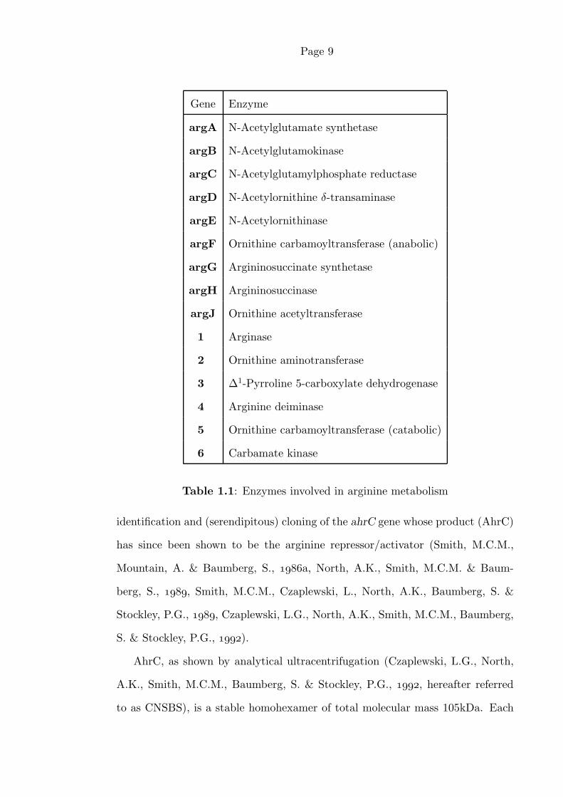
Page 9
Gene Enzyme
argA N-Acetylglutamate synthetase
argB N-Acetylglutamokinase
argC N-Acetylglutamylphosphate reductase
argD N-Acetylornithine δ-transaminase
argE N-Acetylornithinase
argF Ornithine carbamoyltransferase (anabolic)
argG Argininosuccinate synthetase
argH Argininosuccinase
argJ Ornithine acetyltransferase
1 Arginase
2 Ornithine aminotransferase
3 ∆1-Pyrroline 5-carboxylate dehydrogenase
4 Arginine deiminase
5 Ornithine carbamoyltransferase (catabolic)
6 Carbamate kinase
Table 1.1: Enzymes involved in arginine metabolism
identification and (serendipitous) cloning of the ahrC gene whose product (AhrC)
has since been shown to be the arginine repressor/activator (Smith, M.C.M.,
Mountain, A. & Baumberg, S., a, North, A.K., Smith, M.C.M. & Baum-
berg, S., , Smith, M.C.M., Czaplewski, L., North, A.K., Baumberg, S. &
Stockley, P.G., , Czaplewski, L.G., North, A.K., Smith, M.C.M., Baumberg,
S. & Stockley, P.G., ).
AhrC, as shown by analytical ultracentrifugation (Czaplewski, L.G., North,
A.K., Smith, M.C.M., Baumberg, S. & Stockley, P.G., , hereafter referred
to as CNSBS), is a stable homohexamer of total molecular mass 105kDa. Each

Page 10
subunit consists of 149 amino acids whose sequence shows significant homology
only to ArgR, the arginine repressor from E. coli (Figure 1.4). ArgR does not
act as a transcription activator but it has been shown to be a necessary accessory
protein for the resolution —through site-specific recombination— of multimers of
the ColE1 plasmid (Lim, D., Oppenheim, J.D., Eckhardt, T. & Maas, W.K., ,
Stirling, C.J., Szatmari, G., Stewart, G., Smith, M.C.M. & Sherratt, D.J., ).
ArgR is not a resolvase, but may be implicated in synapse formation. Although
the two proteins share only 29% identity and are from such taxonomically distinct
prokaryotes, AhrC can complement E. coli ArgR− strains both in the regulation
of arginine metabolism and the resolution of the ColE1 plasmid (it is worth noting
that the reverse is not true : ArgR can not complement B. subtilis AhrC− strains
in the regulation of arginine metabolism).
ArgR MRSSAKQEELVKAFKALLKEEKFSSQGEIVAALQEQGFDNINQSKVSRMLTKFGAVRTRN
AhrC MNKGQRHIKI----REIITSNEIETQDELVDMLKQDGY-KVTQATVSRDIKELHLVKVPT
* . .. . . .. . . .*.*.* *...*. .. *. *** . . *.
ArgR AKMEMVYCLPAEL---GVPTTSSPLKNLVLDIDYNDAVVVIHTSPGAAQLIARLLDSLGK
AhrC NNGSYKYSLPADQRFNPLSKLKRALMDAFVKIDSASHMIVLKTMPGNAQAIGALMDNLDW
. * ***. .. .* . . ** ..*. * ** ** *. *.*.*.
ArgR AEGILGTIAGDDTIFTTPANGFTVKDLYEAILELFDQEL -156
AhrC DE-MMGTICGDDTILIICRTPEDTEGVKNRLLELL -149
* ..*** *****. .. . .***.
Figure 1.4: Sequence alignment of AhrC and ArgR (CLUSTAL-V, Higgins,
D.G., Bleasby, A.J. & Fuchs, R., ). Identities (*) and similarities (.) are
indicated.

Page 11
Mutational analysis of ArgR (Tian, G. & Maas, W.K., , Burke, M.,
Merican, A.F. & Sherratt, D.J., ) suggested that the C-terminal region is
implicated in arginine binding and oligomerisation whereas the N-terminal region
is involved in DNA recognition and binding. The implied organisation of AhrC
and ArgR in two functionally and/or structurally distinct domains is consistent
with the the non-uniform distribution of homology between them (19% identity
for residues 1-80, 34% identity for residues 81-152) and the sensitivity of AhrC
to proteolytic cleavage.
Sequence analysis of the region 5′ to the argCJBD-cpa-argF cluster revealed
the presence of three putative operator sites similar to the E. coli arginine opera-
tor sequences (Figure 1.5, Smith, M.C.M., Mountain, A. & Baumberg, S., b).
ARG box consensus sequence : AATGAATAA TNATNCANT
AhrC operator sequence R1 : AATGTTAAA T AATTTCACA
R2 : ATTGAATTA ATTT TTATTCATG
R3 : AATGAATAA AA ATATTAAAT
Figure 1.5: Sequence alignment of the E. coli ARG box consensus sequence
and three putative AhrC operator sequences located at the 5′ region of the
argCJBD-cpa-argF cluster.
DNase I and hydroxyl radical footprinting experiments (CNSBS, ) showed
that AhrC protects (in an arginine-dependent manner) two of these regions (R1
and R2 in Figure 1.5) and a further site that lies within the coding sequence of
the argC gene (hereafter referred to as argCO2). The same experiments suggested
that (i) AhrC interacts with one face of the DNA over a length approximately
equal to five helical turns, and, (ii) three groups of nucleotides that are hyper-


Page 13
1.2 Biophysical Data.
Figure 1.7 is a graphical representation of the secondary structure prediction for
AhrC (based on eight different methods, programme PREDICT, Eliopoulos, E.,
Geddes, A.J., Brett, M., Pappin, D.J.C. & Findlay, J.B.C., , and references
therein).
Figure 1.7: Secondary structure prediction for AhrC.
This prediction suggests that AhrC is an α/β or an antiparallel β structure
with a high α-helical content. Although some very common secondary struc-
ture motifs are immediately obvious (such as the β-strand prediction centered at
residue 38 which is followed by a turn or coil prediction, an α-helix and another


Page 15
(blue line) Amide I region. The wavenumbers corresponding to the peaks of the
five bands are 1607 cm−1 (black line II), 1637 cm−1 (green), 1650 cm−1 (cyan),
1662.4 cm−1 (magenta) and 1679 cm−1 (red) (also shown in Table 1.2). The bands
at 1637 and 1679 cm−1 are indicative of the presence of antiparallel β-sheet struc-
ture, whereas the 1650 cm−1 band is characteristic of α-helical structure. The
1662.4 cm−1 band is characteristic of turns and the 1607 cm−1 band probably
arises from side-chain vibrations. A summary of these assignments is given in
Table 1.2.
These results, together with the indications from the secondary structure pre-
diction algorithms, suggest that AhrC has an antiparallel β structure. It is worth
noting that the intensities of the 1637–1679 and 1650 cm−1 bands suggest that
the dominant secondary structure elements are β-strands organised in antiparal-
lel β-sheets and not α-helices (as indicated by the secondary structure prediction
methods).


Page 17
Chapter 2
Protein Preparation,
Crystallisation,
and Preliminary Characterisation
of AhrC Crystals
2.1 Protein Preparation.
2.1.1 Protein Purification.
AhrC was purified as described by Czaplewski, L.G., et al, & Stockley, P.G.,
. Differential precipitation from low ionic strength solutions is used twice
during the purification, allowing an efficient initial separation before the final
chromatographic step.
Escherichia coli strain DS903(pUL2202) was grown at 37C in rich medium.
At an optical density at 600 nm of 1.5 the cells were induced by the addition of
IPTG and the incubation continued for 3 hrs. Cells were harvested by centrifu-
gation and were thawed and resuspended in Arg buffer (20 mM Tris-HCl, 10 mM
MgCl2, 10 mM 2-mercaptoethanol, 1 mM PMSF, 25 µM TPCK, pH 7.5).

Page 18
The cell suspension was sonicated on ice to prepare a cell extract and the
insoluble material (which included AhrC) was harvested by centrifugation. The
pellet was resuspended in Arg buffer and treated with DNase I. AhrC was solu-
bilised by the addition of solid NaCl to a final concentration of 0.5 M, and the
suspension incubated at 37C for 15 min.
The supernatant after DNase I and NaCl treatments was obtained by cen-
trifugation and extensively dialysed against Arg buffer containing 75 mM NaCl
at 4C. The precipitate which formed consisted mainly of AhrC. It was harvested
by centrifugation and resuspended in 250 mM NaCl Arg buffer. The protein
was loaded onto a S-Sepharose cation-exchange column with 250 mM NaCl Arg
buffer, and the column developed using a 250-600 mM NaCl linear gradient in
Arg buffer.
A typical elution profile of the S-Sepharose column is shown in Figure 2.1.
Peak I is the flow through of proteins that do not bind to the column and peak II
corresponds to proteolytically cleaved AhrC (Figure 2.2). The main peak (III),
is —as shown by high resolution SDS-PAGE (Schagger, H. & Jagow, G., ),
Figure 2.2— a mixture of intact AhrC and a faster migrating band which was
thought to represent AhrC with one or two amino acids missing (Stockley, P.G.,
personal communication). Attempts to separate those two bands using prepara-
tive isoelectric focusing have been unsuccessful (Walsh, A.P., personal communi-
cation). It is worth noting, that a SDS-PAGE of washed and subsequently dis-
solved AhrC crystals (orthorhombic form, Section 2.2) showed that these crystals
consist of only one protein species.
Later in this study, the plasmid carrying the ahrC gene was reconstructed.
This resulted in the apparent loss of the faster migrating band. Crystallisation
trials with this protein preparation showed that the conditions for optimum crys-
tal growth of the orthorhombic form had changed slightly. Furthermore, the
crystals produced from the new protein preparation were non-isomorphous with


Page 20
those grown in the past (the mean fractional isomorphous difference for all data
to 4A was 20%). It is worth noting that the unit cell dimensions of these two
types of the orthorhombic form are virtually identical.
The protein concentration was determined by measuring the absorbance at
280 nm, assuming that an OD280 of 1.0 corresponds to a protein concentration
of 1 mg ml−1 (Czaplewski, L.G., et al, & Stockley, P.G., ). Typically, 7 lt of
culture would give approximately 20 mg of protein. AhrC was precipitated with
23% (w/v) PEG 6000 and stored at 4C for further use.
2.1.2 Stability of AhrC During Storage.
Due to problems encountered with the reproducibility of the crystallisation exper-
iments (Section 2.2), it was decided to monitor the the behaviour of the purified
protein over the course of few months using SDS-PAGE. The main conclusions
from these experiments are presented below.
AhrC is very sensitive to proteolytic cleavage. Although protease inhibitors
such as PMSF or TPCK are present at all stages of protein purification and
also during storage, approximately 5 months after the protein preparation, low
molecular weight bands appear on SDS-PAGE (Figure 2.2, Lane 2). Futhermore,
after 2 months of storage higher molecular weight species start appearing on SDS-
PAGE of the purified protein (Figure 2.3). The molecular weights of these species
(as judged from their electrophoretic mobility, Figure 2.3) suggest that they may
correspond to covalently linked dimers and trimers of AhrC. The dominance of the
32 kDa band is consistent with chemical cross-linking experiments with bismido
esters (Czaplewski, L.G., et al, & Stockley, P.G., ). Although it is not clear
what the nature of the bonds that stabilise these multimers is, the formation of
disulphide bridges can probably be excluded since the protein is heated to 100C
in the presence of 2% (v/v) 2-mercaptoethanol during sample preparation.
It was not surprising to find that crystallised AhrC is more stable than the

Page 21
precipitated protein. Figure 2.4 shows that AhrC crystals which have been stored
for 4 months show little material outside the expected 16 kDa band, whereas a
sample from the same protein preparation which was stored as a precipitate
contains a significant amount of the covalently linked dimer.
An attempt to re-purify —using cation-exchange chromatography— the na-
tive AhrC hexamer from a protein preparation that had been stored for 4 months,
showed that all species present in the sample eluted as a single peak (data not
shown). This suggests that neither the molecular weight nor the charge of the
hexameric molecule changes during storage.
2.2 Crystallisation, and
Preliminary Characterisation
of AhrC Crystals.
The crystallisation of AhrC in a form suitable for a complete three-dimensional
X-ray structure determination has been reported (Boys, C.W.G., et al, & Stock-
ley, P.G., ). Unfortunately, crystallisation under the conditions described
therein was not reproducible (Boys, C.W.G., personal communication).
When this project started, it was decided that an attempt to crystallise AhrC
based on its very low solubility in low ionic strength solutions was a worthwhile
exercise. This approach proved very successful : all three crystal forms of AhrC
described in this thesis are grown from low ionic strength solutions.
Although conditions that produced crystalline material were found soon after
this project started, the production of crystals of a quality suitable for crystallo-
graphic studies was rather more difficult. In retrospect, the major problem was
the instability of AhrC upon storage (Section 2.1.2) : the quality of the crystals
and the reproducibility of the crystallisation experiments was inversely related to


Page 23
the length of time that the protein had been stored. Most of these problems dis-
appeared when it was realised that the protein should be used as soon as possible,
and in no case later than three weeks after its preparation.
All the crystallisation experiments were performed by hanging drop vapour
diffusion (McPherson, A., , Ducruix, A. & Giege, R., , Blundell, T.L. &
Johnson, L.N., ). The effects of some crystallisation parameters which were
found to be important for the three crystal forms grown from low ionic strength
are discussed below.
Temperature Crystallisation trials have been set up at 4C, 20C and 28C. The
solubility of AhrC increases with decreasing temperature but crystals of sim-
ilar quality can be grown at all these temperatures under slightly different
conditions. For technical reasons, most of the crystallisation experiments
were performed at 20C.
Ionic strength The ionic strength of the well solution was adjusted with ammo-
nium sulphate. Concentrations in the range 0 to 150 mM have given useful
results, with different crystal forms growing at different concentrations.
Buffer and pH range The pH of the protein solution was adjusted to 7.5 using
30 mM phosphate buffer. The pH of the well solution was varied in the range
4.5–8.5 in steps of 0.2 units using phosphate, citrate or cacodylate buffer.
Best results have been obtained from phosphate buffer at pH 4.9 (which is
very close to the isoelectric point of AhrC).
PEG concentration Although PEG is not required for crystallisation, it was
found that the addition of a small amount of a medium molecular weight
PEG improved the morphology and size of the crystals. Crystallisation tri-
als have been set up using 0.4, 1, 2, 4, 6, and 8 kDa PEG at concentrations
varying from 0 to 15% (w/v) for both the well and protein solution. Un-
fortunately, the variation in the composition of the commercially available

Page 24
PEGs led to a proportional variation of the optimum conditions for crystal
growth. Best results for the orthorhombic form have been obtained from
PEG 4000 at concentrations close to 5% (w/v).
Concentration of isopropanol Due to the sensitivity of AhrC to proteolytic
cleavage, small amounts of the protease inhibitors PMSF and TPCK were
included in all crystallisation trials. Because of their instability in aqueous
solutions, both inhibitors were prepared in isopropanol. It was later found
that isopropanol was affecting the crystal growth rate. Best results have
been obtained from 1% (v/v) isopropanol.
2.2.1 Orthorhombic Form.
Details of the crystallisation conditions are given in Table 2.1. It should be noted
that the conditions for optimal crystal growth may vary for different protein
batches and will almost certainly be different for different brands of PEG. It was
found necessary to optimise the concentration of ammonium sulphate and PEG
in the well solution for each protein batch individually.
These crystals grow as rectangular blocks elongated along [010] and bounded
on the (001) and (100) faces (Figure 2.5). Their typical size is 0.50×0.15×0.20
mm3 but crystals with dimensions up to 1.50×0.30×0.35 mm3 have been obtained.
The ratio of the dimensions of the crystals is inversely proportional to the ratio of
the unit cell dimensions with the longest crystal axis being parallel to the shortest
unit cell translation.
The space group was determined from precession photographs and found to
be C2221 with a=231.3A, b=74.4A and c=138.0A (Figure 2.61).
This crystal form is identical to the one reported by Boys, C.W.G., et al, &
Stockley, P.G., . Assuming that the equivalent of one hexamer is present in
1All zero level precession photographs were recorded with a crystal to film distance of 100 mmand are reproduced in this thesis on a scale of 1:1.

Page 25
Protein solution 50 µM TPCK
1.25 mM DTT
1.2 mM PMSF
30 mM Phosphate buffer, pH 7.5
150 mM Ammonium sulphate
1 % (v/v) isopropanol
10 mg ml−1 AhrC
Well solution 50 µM TPCK
1.25 mM DTT
1.2 mM PMSF
100 mM Phosphate buffer, pH 4.9
4% PEG 4000
60 mM Ammonium sulphate
1 % (v/v) isopropanol
Drops 4 µl protein plus 4 µl well solution
Table 2.1: Crystallisation conditions for the orthorhombic form.


Page 27
the asymmetric unit, the estimated solvent content is 55% (Matthews, ).
These crystals diffract X-rays to 3A resolution using laboratory sources and
to 2.7A using synchrotron radiation (Chapter 3). They are sensitive to radia-
tion damage : after 12 hours of exposure to 2.7 kW, monochromatised (CuKα)
X-rays at room temperature, only low (dmin ≥4.5A) resolution reflections could
be observed. An attempt was made to increase their useful life-time by soaking
them in solutions containing free-radical scavengers, such as styrene or methyl
methacrylate (Zaloga, G., & Sarma, R., ). Unfortunately, no improvement
was found. This was not the case when the crystals were cooled to 4C using
a device originally described by Marsh, D.J. & Petsko, G.A., . The useful
crystal life-time was almost doubled. Most of the data sets described in this thesis
were collected at this temperature. Alignment of the cold stream of air with the
axis of the X-ray capillary proved to be more difficult than expected resulting in
several crystals being lost due to water condensation. Most of these problems dis-
appeared when it was decided to mount the crystals in a solution containing low
gelling temperature agarose which set on cooling to maintain constant hydration
during data collection (Richmond, T.J., et al, & Klug, A., ).
An artificial mother liquor consisting of 10% MPD and 100 mM acetate buffer
at pH 4.9 has been developed. This was necessary for several reasons : Firstly,
under the crystallisation conditions described above the crystals are not stable.
Approximately 6 weeks after their appearance, they start dissolving, possibly due
to the presence of a higher concentration of PEG in the well solution which leads
to a gradual increase of the ionic strength in the hanging drops. Secondly, the
presence of ammonium sulphate and phosphate ions can cause serious problems
in heavy atom screening experiments (Blundell, T.L. & Johnson, L.N., ,
McPherson, A., ). A stabilising solution consisting of MPD and acetate
ions presents fewer problems. Finally, MPD at high concentrations can act as a
cryo-protective mother liquor (Petsko, G.A., ). It proved possible to transfer

Page 28
AhrC crystals to solutions containing up to 45% (v/v) MPD without any obvious
problems. Such high concentrations of MPD should allow cooling of these crystals
to at least −40C which can help to reduce their sensitivity to radiation damage
(Hope, H., , Singh, T.P., et al, & Huber, R., , Young, A.C.M. & Dewan,
J.C., ). All orthorhombic crystals used in this study were transferred to the
stabilising solution at least three days before experimentation.
2.2.2 Monoclinic Form.
The crystallisation conditions for this form are given in Table 2.2. These crystals
could be grown reproducibly from only one protein batch. It is not clear why
this is so, but, a possible explanation is that both bands seen on a SDS-PAGE
of protein purified at the beginning of this project are needed for crystallisation
(Section 2.1.1, Figure 2.2). The crystals grow as rhombic prisms elongated along
[010] with well developed (100) and (011) faces (Figure 2.7).
The space group, as determined from precession photographs, is P21 with unit
cell dimensions a=202.7A, b=72.6A, c=73.0A and β=97.8. They diffract X-rays
to better than 4A using laboratory sources and to 3.2A using synchrotron radia-
tion. Assuming that the crystallographic asymmetric unit contains two hexamers,
the estimated solvent content is 45%.
The pattern of strong, low resolution reflections in the hk0 zone (Figure 2.8)
is worth noting : strong reflections are present if 2h + k = 4n, which suggests
the presence (in the [001] projection) of a centered superlattice with a=202.7A
and b′=36.3A(=b/2).
Although the crystallisation conditions are very similar to those used for the
orthorhombic form, the monoclinic crystals are not stable in the artificial mother
liquor described in the previous section and most of these crystals are also un-
stable in their well solution. These problems made the heavy atom screening
experiments for this form rather adventurous (Chapter 3).

Page 29
Protein solution 50 µM TPCK
1.25 mM DTT
0.7 mM PMSF
30 mM Phosphate buffer, pH 7.5
150 mM Ammonium sulphate
1 % (v/v) isopropanol
10 mg ml−1 AhrC
Mixing solution 50 µM TPCK
1.25 mM DTT
0.7 mM PMSF
30 mM Phosphate buffer, pH 7.5
150 mM Ammonium sulphate
1 % (v/v) isopropanol
8 % PEG 6000
Well solution 50 µM TPCK
1.25 mM DTT
0.7 mM PMSF
100 mM Phosphate buffer, pH 5.2
4.4% PEG 6000
16 mM Ammonium sulphate
1 % (v/v) isopropanol
Drops 4 µl protein plus 4 µl mixing solution
Table 2.2: Crystallisation conditions for the monoclinic form.


Page 31
2.2.3 Trigonal Form.
Boys, C.W.G., et al, & Stockley, P.G., reported the growth of AhrC crystals
with a habit of “small, triangular rods” from 15% MPD, 100 mM phosphate
buffer, pH 7.5 and an 80-fold molar excess of L-arginine hydrochloride. These
crystals were too small for a space group determination (Boys, C.W.G., personal
communication).
In this study, crystals with a similar morphology have been obtained from low
ionic strength solutions (Figure 2.9). Refinement of the crystallisation conditions
(Table 2.3), allowed us to grow crystals of a size suitable for a preliminary char-
acterisation, but, due to the inherent disorder of this form, we have been unable
to collect a complete three-dimensional data set.
Figure 2.10(A) shows a “still” photograph taken with the long axis of the crys-
tal 8 away from the direct beam. The absence of well defined reflections and the
presence of almost continuous intensity in the various levels (most clearly seen in
the −1 level), suggests that these crystals are disordered. It was a surprise to find
that a zero level precession photograph from the same crystal (Figure 2.10(B))
showed well defined reflections out to 8A. The broadening of the higher resolution
reflections seen in this photograph indicates the presence of rotational disorder
about the morphological 3-fold.
An upper level (hk1) precession photograph (Figure 2.11) established that
the crystal system is trigonal. The order is preserved to a much lower resolution
with individual reflections merging to form arcs.
The space group determination was complicated by the crystal disorder and
will be discussed in detail. The hk0 zero level photograph has symmetry p6mm.
This means that the plane group of the projection of the electron density along
the [001] direction is either p3m1 or p31m. The only enantiomorphic, trigonal,
non-rhombohedral space groups consistent with either of these two plane groups
(for the projection along the 3-fold) are P312, P3112, P3212, P321, P3121 and


Page 34
P3221 (International Tables for X-ray Crystallography, Vol.I, ). The unit
cell dimensions as determined from the X-ray photographs are a=b=66.6A and
c=160A. This small unit cell suggests the presence of only two hexamers per unit
cell (with an estimated solvent content of 50%). The requirement for a space
group with a set of two equivalent positions further reduces the possible choices
to only two space groups : P312 (Wyckoff notation of possible sets : g, h, i) or
P321 (c, d). In the absence of any information in directions perpendicular to the
3-fold, these two space groups can not be differentiated. In both space groups the
point symmetry of the positions of these sets is 3 and the asymmetric unit contains
two protomers. The crystal packing is fixed by the space group symmetry : the
equivalent positions are 0, 0, z and 0, 0, z with the crystallographic and molecular
3-fold coinciding and the molecules forming columns parallel to the [001] direction.
A low resolution native Patterson projection along the [001] direction is shown
in Figure 2.12. The calculation of the Patterson projection involves no assump-
tions about the space group of the crystals and its consistency with the packing
arrangement derived from symmetry considerations is an independent confirma-
tion of the space group assignment2.
The crystal packing as described above suggests a model for the observed
disorder phenomena : the crystals suffer from translational disorder parallel to the
3-fold and to a lesser extent from rotational disorder about it. The translational
component arises from the different relative positions of the protein columns in
a direction parallel to the column axis (which coincides with the crystallographic
3-fold axis).
An important question is whether —based on the analysis above— the possi-
bility of the protein having a molecular 6-fold axis of symmetry can be excluded.
We believe that it can : due to the “special” position of the molecules, the order of
2The amplitudes of the hk0 reflections were estimated visually from the precession photographshown in Figure 2.10(B). The 18 observed reflections were classified as “very strong”, “strong” and“weak”, and amplitudes were assigned to these as follows : “very strong” → F=6 (1 reflection),“strong” → F=2 (7 reflections) and “weak” → F=0.5 (10 reflections).

Page 35
the crystallographic [001] axis depends (for the given crystal packing) on the or-
der of the molecular axis. If the molecular axis was a 6-fold then the space group
would be P622, but again, with two molecules per unit cell at 0, 0, z and 0, 0, z.
We can reach the same conclusion based on a purely geometrical argument : if the
order of the molecular axis was 6, then the individual protomers would have to
be ≈80A long and with a diameter less than ≈20A. Such dimensions are possible
but highly unlikely.
It is unfortunate that the crystal form most suitable for a crystal structure
determination is the most problematic of those described. Nevertheless, two
important conclusions can be drawn from this preliminary analysis : (i) AhrC
has maximal dimensions 66A by 66A by 80A and (ii) It possess an intramolecular
axis of symmetry of order 3.
0.0 u 2.0
v
2.0
Figure 2.12: Trigonal form, 66-8A native Patterson projection along [001]. Four
unit cells are shown. Contours every 5% of the origin peak; negative contours
broken.

Page 36
Chapter 3
Preparation and
Preliminary Analysis
of Heavy Atom Derivatives
3.1 Data Collection Strategy.
All data sets described in this thesis (with the exception of a medium (2.9A)
resolution data set collected using synchrotron radiation) have been collected us-
ing a X-100A Xentronics/Siemens multiwire, position sensitive, two-dimensional
area detector. The X-ray source was graphite-monochromatised CuKα radiation
from a Rigaku RU200 rotating anode operating at 2.7 kW with a 200 µm focus.
Each data set was collected from one crystal. The rotation method (Arndt, W. &
Wonacott, A.J., ) was used for all data collections with an oscillation angle
typically in the range 0.2 to 0.3.
Care was taken to keep the geometry of the data collections as much as pos-
sible the same for the native and derivative data sets : most data sets from
orthorhombic crystals have been collected with a crystal to detector distance of
17.5 cm and the detector set at an angle 2θ=6.5. With this setting all data

Page 37
between 138 and 5.0A (with some reflections to 3.9A) can be recorded. The
crystals were aligned (at ω=0) with their [001] direction parallel to the X-ray
beam and the [010] direction approximately 15 away from the rotation axis. The
15 tilt of the [010] axis has two consequences : (i) the Bijvoet pairs can not
be measured simultaneously and (ii) a ≈95% complete data set can be collected
through a single 90 rotation without the need for an additional data collection
with a different crystal orientation. The choice not to measure the hkl and hkl
terms under as similar conditions as possible is justified on the grounds that the
anomalous differences could not be measured accurately anyway : the crystals
are sensitive to radiation damage and the data sets had to be collected as fast as
possible, resulting in anomalous differences well below the noise level.
In the case of the monoclinic form, the crystal to detector distance was 25.5 cm
and the detector swing angle was 10. Due to the morphology of crystals, the [010]
axis was parallel to the rotation axis necessitating the collection of 180 of data.
The data frames were processed using the programme XDS (Kabsch, W.,
, ) and the intensities (corrected for Lorentz and polarisation factors)
were converted to a .LCF (and later to a .MTZ) file for further processing using
the CCP4 suite of programmes (Collaborative Computational Project, Number
4, ) : The programmes ROTAVATA and AGROVATA applied scales and
isotropic temperature factors to continuous batches of data each corresponding
to a 5 rotation. This step should compensate for (a) differences in the illuminated
crystal volume, (b) radiation damage and (c) absorption, although differences in
absorption are not expected to be significant since the crystals were embedded in
an agarose gel with a linear absorption coefficient very similar to that of the crys-
tals. Observations which differed by more that 3σ from the mean were rejected
(usually less than 0.06% of the total number of measurements for data sets with
an average multiplicity of 2). Data sets collected from crystals soaked in heavy
atom solutions were brought to the same relative scale as the native data through

Page 38
the application of an overall scale and temperature factor (programme ANSC).
Several data sets from native orthorhombic AhrC crystals have been collected
(Table 3.1). At least one native data set was collected after each protein prepara-
tion and was compared with those from previous preparations. Data sets collected
from different native AhrC crystals were not merged.
Two non-isomorphous types of the orthorhombic form have been used for data
collections (Section 2.1.1). The Type I crystals had been obtained from protein
preparations which showed two bands on a SDS-PAGE of the purified protein.
Type II crystals have been obtained from more recent protein preparations. Data
sets collected from native crystals of the same type are isomorphous (the average
mean fractional isomorphous difference between data sets collected from native
type II crystals is ≈5.0 % for all reflections between 30 and 4.0A).
Form and Type Resolution Rsymm Completeness Multiplicity
Orthorhombic, I 4.9 5.6 73 2.1
Orthorhombic, I 4.9 4.9 85 2.2
Orthorhombic, I 4.0 7.0 75 1.8
Orthorhombic, II 6.0 4.6 92 2.3
Orthorhombic, II 3.6 10.6 62 2.8
Orthorhombic, II 4.6 4.6 92 1.6
Orthorhombic, II 3.4 5.0 100 1.9 ‡
Orthorhombic, II 3.7 9.6 100 1.8 ‡
Orthorhombic, II 3.5 7.3 80 1.2
Orthorhombic, II 2.9 6.6 88 1.6 †
Monoclinic 4.5 4.9 78 1.7
Table 3.1: Native data sets.
‡ : Data collection of hk0 or h0l terms only.
† : Data set collected using synchrotron radiation.

Page 39
3.2 Preparation of Heavy Atom Derivatives.
The preparation of useful heavy atom derivatives of AhrC crystals proved to be
both time consuming and frustrating. Most of the compounds tried damaged the
crystals even at very low concentrations (Tables 3.2 and 3.3). This is especially
true for compounds containing heavy metals such as mercury or platinum which
can form covalent bonds with polarisable protein groups such as those found in
the side-chains of methionine, cysteine or histidine. This is rather unfortunate,
since the ability of those heavy atoms to form covalent complexes makes them
highly specific and, thus, more useful for the preparation of well substituted
and isomorphous heavy atom derivatives, with (hopefully) a small number of
substitution sites.
The great majority of the heavy atom soaking experiments have been per-
formed using orthorhombic AhrC crystals. This is due to (i) the presence of only
one hexamer in their asymmetric unit and (ii) the availability of only a limited
number of monoclinic AhrC crystals (Section 2.2.2).
The procedure followed for the heavy atom derivative search in the case of
the orthorhombic AhrC crystals is outlined below.
A concentrated heavy atom solution was prepared in 10% MPD, 100 mM
Acetate buffer, pH 4.9 (Section 2.2.1). A portion of this concentrated solution
was diluted with a volume of the same artificial mother liquor to give 500 µl of
a heavy atom solution at the required concentration. A small crystal was soaked
in this solution and its well being (or otherwise) was monitored every 2 to 4
hours. If the crystal survived the initial treatment without any obvious problems
(appearance of cracks, loss of birefringence, etc), an attempt was made to take a
precession photograph of the hk0 zone1. Depending on the presence or otherwise
1The h0l zone would have been a better choice, but, due to the morphology of crystals (Section2.2.1) mounting with the [010] direction parallel to the X-ray beam requires manual re-orientationof the crystal and was therefore avoided.

Page 40
of significant differences between this precession photograph and the native hk0
pattern, either a crystal was soaked using the same or higher concentration of the
heavy atom solution and a data set was collected from it, or the procedure was
repeated, but this time with a lower concentration of the heavy atom containing
compound.
In some experiments, concentrations as low as 0.2 µM have been used. In
others (marked as “m/p” in Table 3.2) stoichiometric amounts of the heavy atom
containing compounds were used to give a specific number of heavy atoms per
protein protomer2. At such low concentrations, the signal from specific heavy
atom binding can be very weak and might not be detected through comparison
of precession photographs. In these cases a data set was collected immediately.
The instability of the monoclinic crystals in both the previously described
artificial mother liquor and in their well solution, made the heavy atom soaking
experiments with this crystal form rather inaccurate : the coverslips with their
hanging drops were removed from the crystallisation plate, solid grains of the
heavy atom containing compounds were added directly to the drops and the
coverslips were replaced back on the crystallisation plate.
Attempts to crystallise AhrC in the presence of KHgI4, Ethylmercury phos-
phate or p-chloromercuribenzenesulphonic acid have also been unsuccessful. The
protein precipitated even in the presence of very low concentrations of these com-
pounds.
Tables 3.4 and 3.5 give details of the data sets collected from AhrC crystals
soaked in solutions containing heavy atoms. The methods used and the collection
strategy adopted have already been described. Data sets marked with (†) in
Table 3.4 have been collected from Type I crystals.
2Due to the relatively simple morphology of the orthorhombic crystals, fairly accurate mea-surements of their volumes are possible, allowing an equally good estimate of the number ofmolecules per crystal to be obtained.

Page 41
Compound Conditions Result
Baker’s dimercurial 1 mM 12 hrs Cracked
0.1 mM 5.5 hrs Cracked
30 µM 20 hrs Cracked
4 µM 20 hrs Cracked
2 µM 20 hrs Cracked
HgCl2 0.3 mM 5.5 hrs Cracked
60 µM 20 hrs Cracked
4 µM 21 hrs Disordered
2 µM 24 hrs Disordered
HgI2 0.4 % sat. 15 hrs Disordered
0.1 % sat. 23 hrs Data Collected
pCMB 1 % sat. 20 hrs Disordered
0.2 % sat. 69 hrs Disordered
Mersalyl acid 0.4 % sat. 15 hrs Cracked
0.1 % sat. 20 hrs Cracked
KAuCl4 1 mM 3 hrs Disordered
0.6 mM 1.5 hrs Disordered
0.5 mM 16 hrs Cracked
0.1 mM 18 hrs Disordered
2 µM 46 hrs Disordered
H2IrCl6 0.03 µM 78 hrs No Differences
0.75 mM 12 hrs Differences
0.6 mM 4 hrs Data Collected
1.2 mM 3 hrs Data Collected
(CH3COO)2Hg 5 mM 16 hrs Cracked
Table 3.2: Heavy atom soaking experiments : Orthorhombic form

Page 42
Mercurochrome 0.2 % sat. 20 hrs No Differences
5 % sat. 3 hrs No Differences
2.5 % sat. 16 hrs Disordered
3 % sat. 12 hrs Disordered
100 % sat. 3 hrs Data Collected
100 % sat. 5 hrs Data Collected
Sm(NO3)3 1 mM 160 hrs Differences
2 mM 18 hrs Disordered
0.4 mM 21 hrs Data Collected
K2PtCl6 2 mM 2 hrs Disordered
1 mM 2 hrs Disordered
0.2 mM 17 hrs Disordered
Pb(NO3)2 0.3 mM 19 hrs No Differences
3 mM 15 hrs Disordered
Pr(NO3)3 0.6 mM 17 hrs Differences
0.6 mM 17 hrs Data Collected
NdCl3 2 mM 16 hrs Differences
2 mM 18 hrs Data Collected
(NH4)2OsCl6 0.2 mM 6 hrs Cracked
0.04 mM 17 hrs Cracked
Ta2O5 10 % sat. 16 hrs No Differences
100 % sat. 16 hrs Data Collected
DCMNP 4 % sat. 15 hrs Disordered
4 % sat. 2 hrs Disordered
K3UO2F5 0.2 mM 25 hrs Differences
0.2 mM 20 hrs Data Collected
Table 3.2: Heavy atom soaking experiments : Orthorhombic form

Page 43
VOSO4 2 mM 16 hrs Cracked
CH3COOTl 0.8 mM 25 hrs No Differences
0.8 mM 17 hrs Data Collected
Ce(NO3)3 1 mM 16 hrs Cracked
1 mM 2 hrs Cracked
1 mM 60 min Disordered
TAMM 0.05 mM 15 hrs Disordered
0.01 mM 15 hrs Disordered
0.05 mM 30 min Data Collected
0.1 mM 25 min Data Collected
Thimerosal 0.2 mM 25 hrs Disordered
H3PO4·12WO3 0.2 mM 25 hrs Disordered
0.2 mM 6 hrs Data Collected
1 m/p 20 hrs Data Collected
Co[Hg(SCN)4] 100 % sat. 20 hrs Cracked
Erythrosin B 0.1 mM 40 hrs Disordered
0.05 mM 24 hrs Disordered
KReO4 0.4 mM 20 hrs No Differences
0.8 mM 40 hrs No Differences
0.8 mM 40 hrs Data Collected
AgNO3 2 µM 18 hrs Cracked
Gd2O3 0.5 mM 20 hrs Disordered
(CH3COO)2Pb 0.2 mM 6 hrs No Differences
0.2 mM 29 hrs Disordered
0.2 mM 18 hrs Data Collected
Hg(NO3)2 2 % sat. 6 hrs Cracked
Table 3.2: Heavy atom soaking experiments : Orthorhombic form

Page 44
KAu(CN)4 0.02 mM 20 hrs Data Collected
0.05 mM 14 hrs Data Collected
0.1 mM 16 hrs Data Collected
0.2 mM 14 hrs Data Collected
0.4 mM 16 hrs Data Collected
1 mM 16 hrs Data Collected
4 mM 2 hrs Data Collected
4 mM 16 hrs Data Collected
10 mM 1.5 hrs Data Collected
Ag2SO4 2 % sat. 6.5 hrs Cracked
K2HgI4 0.4 mM 6.5 hrs Cracked
pCMBS 0.2 mM 20 hrs Cracked
0.2 mM 6.5 hrs Cracked
0.2 mM 2 hrs Disordered
1 m/p 18 hrs Data Collected
3 m/p 18 hrs Data Collected
6 m/p 18 hrs Data Collected
12 m/p 3 hrs Data Collected
16 m/p 3 hrs Cracked
9 m/p 16 hrs Data Collected
EMP 0.1 mM 6.5 hrs Disordered
CMPN 100 % sat. 6.5 hrs No Differences
100 % sat. 29 hrs No Differences
100 % sat. 48 hrs No Differences
AgI 100 % sat. 48 hrs Disordered
2 % sat. 24 hrs Disordered
Table 3.2: Heavy atom soaking experiments : Orthorhombic form

Page 45
CH3COOAg 0.4 mM 6.5 hrs Disordered
Nb6Cl14 0.03 mM 24 hrs Differences
1.5 mM 21 hrs Data Collected
0.7 mM 48 hrs Data Collected
0.7 mM 20 min Data Collected
UO2(NO3)2 0.4 mM 24 hrs Differences
0.8 mM 11 hrs Data Collected
0.4 mM 3 hrs Data Collected
0.04 mM 16 hrs Data Collected
Eu2O3 0.6 mM 3 hrs Disordered
0.2 mM 20 hrs Disordered
(CH3)3PbCH2COOH 5 mM 6 hrs Differences
3 mM 2 hrs Data Collected
3 mM 16 hrs Data Collected
5 mM 16 hrs Data Collected
10 mM 2 hrs Data Collected
14 mM 16 hrs Data Collected
20 mM 18 hrs Data Collected
TaCl5 100 % sat. 6 hrs Cracked
pHMBA 100 % sat. 48 hrs Differences
100 % sat. 20 hrs Data Collected
PdCl2 100 % sat. 2 hrs Cracked
Tl2CO3 1 mM 20 hrs No Differences
AgCN 100 % sat. 2 hrs No Differences
100 % sat. 20 hrs Cracked
Hg(NO3)2 100 % sat. 2 hrs Cracked
Table 3.2: Heavy atom soaking experiments : Orthorhombic form

Page 46
HgBr2 100 % sat. 2 hrs Cracked
HgO 100 % sat. 2 hrs Cracked
Ce2(SO4)3 100 % sat. 20 hrs Cracked
Cl-Hg-(C6H4)-I 2 % sat. 25 hrs Data Collected
TlNO3 1 mM 20 hrs No Differences
2 mM 18 hrs No Differences
3.8 mM 20 hrs No Differences
2 mM 3 hrs Data Collected
Tl2SO4 1 mM 44 hrs No Differences
TlCl 100 % sat. 72 hrs No Differences
K2WO4 1 mM 20 hrs Cracked
K2PtBr6 0.2 mM 20 hrs Disordered
2 m/p 20 hrs Data Collected
3 m/p 20 hrs Data Collected
50 µM 35 min Disordered
Y(NO3)3 2 mM 20 hrs Cracked
La(NO3)3 1 mM 2 hrs Cracked
K2PdCl4 0.2 mM 2 hrs Cracked
Nd2(SO4)3 0.4 mM 20 hrs No differences
0.8 mM 20 hrs Disordered
[(CH3Hg)3O]OH 1 mM 2 hrs Disordered
CdSO4 0.4 mM 2 hrs No Differences
0.6 mM 48 hrs No Differences
SiO2·12WO3 1 mM 6 hrs Cracked
0.1 mM 6 hrs Cracked
0.5 m/p 20 hrs Data Collected
Table 3.2: Heavy atom soaking experiments : Orthorhombic form

Page 47
Er2O3 100 % sat. 42 hrs No Differences
Dy2O3 100 % sat. 70 hrs No Differences
UO2(CH3COO)2 0.2 mM 16 hrs Differences
0.1 mM 1.5 hrs Data Collected
0.2 mM 16 hrs Data Collected
Na2WO4 1 mM 4 hrs Cracked
(C6H5)Hg-Ac 100 % sat. 4 hrs Cracked
K2Pt(NO3)4 0.4 mM 4 hrs Disordered
K2Pt(CN)4 0.4 mM 15 hrs Differences
0.4 mM 20 hrs Data Collected
Pt(H2NCH2CH2NH2)Cl2 100 % sat. 2 hrs Cracked
Ag3C6H5O7 0.8 mM 2 hrs Cracked
PbCO3 100 % sat. 20 hrs No Differences
100 % sat. 72 hrs No Differences
W12H48N12O41 100 % sat. 20 hrs Disordered
Hg-dUTP 0.2 mM 14 hrs Cracked
0.2 mM 60 min No Differences
(NH4)6[Mo7O24] 0.6 mM 20 hrs Cracked
Mo12H3O40P 1 mM 2 hrs Cracked
Arg-Cys-Hg 4 mM 20 hrs No Differences
4 mM 76 hrs No Differences
Acetamide & 2 mM 2 hrs
(CH3COO)2Hg 0.4 mM 2 hrs Cracked
Acetamide & 4 mM 2 hrs
pCMBS 0.4 mM 20 hrs Disordered
Table 3.2: Heavy atom soaking experiments : Orthorhombic form

Page 48
HgSO4 100 % sat. 2 hrs Cracked
Nb6Cl14 & 2 mM 20 hrs
UO2(NO3)2 0.4 mM 4 hrs Data Collected
Nb6Cl14 & 2 mM 20 hrs
H2IrCl6 0.5 mM 20 hrs Data Collected
Table 3.2: Heavy atom soaking experiments : Orthorhombic form
Compound Conditions Result
Nb6Cl14 ≈1 mM 3 hrs Differences
≈1 mM 6 hrs Data Collected
TAMM 100 % sat. 3 hrs Cracked
H2IrCl6 ≈0.5 mM 5 hrs Cracked
pCMBS ≈0.5 mM 20 hrs Disordered
K2Pt(CN)4 ≈1 mM 20 hrs Disordered
Table 3.3: Heavy atom soaking experiments : Monoclinic form
m/p : Molecules of the heavy atom
containing compound per protein protomer.
Baker’s : 1,4-diacetoxymercuri-2,3-dimethoxybutane.
pCMB : p-chloromercuribenzoic acid.
pCMBS : p-chloromercuribenzenesulphonic acid.
pHMBA : p-hydroxymercuribenzoic acid.
EMP : Ethylmercury phosphate.
CMPN : 1-(4-Chloromercuriphenylato)-2-napthol.
TAMM : Tetrakis-(acetoxymercuri)methane.

Page 49
Compound Conditions Res Rsymm Comp Diff Kemp
(A) (%) (%) (%)
HgI2 0.1 % sat., 23 hrs 4.9 6.4 82 13.0 2.2 †
H2IrCl6 0.7 mM, 10 hrs 4.9 5.7 69 23.0 2.5 †
0.3 mM, 4 hrs 5.0 3.3 95 5.6 2.0
0.6 mM, 4 hrs 5.0 3.5 99 8.0 2.6
1.2 mM, 3 hrs 5.0 3.5 77 10.0 1.8
0.8 mM, 18 hrs 3.6 3.9 100 18.0 2.1 ‡
Mercurochrome 100 % sat., 3 hrs 5.0 4.2 55 7.0 1.7
100 % sat., 20 hrs 4.9 5.5 73 9.0 1.9 †
100 % sat., 5 hrs 5.0 4.4 94 12.0 1.8
Sm(NO3)3 0.4 mM, 21 hrs 6.0 4.0 99 6.0 1.2 †
Pr(NO3)3 0.6 mM, 17 hrs 4.9 3.5 89 12.0 1.7 †
NdCl3 2 mM, 18 hrs 4.9 5.6 37 15.0 2.0 †
Ta2O5 100 % sat., 16 hrs 4.9 6.4 80 16.0 1.4 †
K3UO2F5 0.2 mM, 20 hrs 6.0 5.5 90 10.0 2.4 †
0.4 mM, 20 hrs 6.5 5.5 76 19.0 3.7 †
CH3COOTl 0.8 mM, 17 hrs 4.9 5.5 87 15 1.4 †
TAMM 0.05 mM, 30 min 5.0 4.2 99 8.0 2.0
0.1 mM,25 min 5.0 2.9 98 4.5 1.5
H3PO4·12WO3 0.2 mM, 6 hrs 7.0 8.0 60 14.0 2.0 †
1 m/p, 20 hrs 4.4 3.7 97 4.5 1.2
KReO4 0.8 mM, 40 hrs 4.9 5.4 82 10.0 1.7 †
(CH3COO)2Pb 0.2 mM, 18 hrs 4.9 5.6 60 9.0 1.4 †
Cl-Hg-(C6H4)-I 5 % sat., 25 hrs 4.9 4.3 70 17.0 1.6 †
2 % sat., 18 hrs 4.5 4.0 91 14.0 3.6
Table 3.4: Data collections : Orthorhombic form.

Page 50
Compound Conditions Res Rsymm Comp Diff Kemp
(A) (%) (%) (%)
pCMBS 1 m/p, 18 hrs 4.5 3.8 98 4.0 1.5
3 m/p, 18 hrs 5.0 3.4 94 5.4 1.6
6 m/p, 18 hrs 5.0 3.9 80 7.3 1.9
12 m/p, 3 hrs 4.8 3.5 97 7.5 1.4
9 m/p, 30 µM, 16 hrs 5.0 4.0 90 7.9 1.7
9 m/p, 50 µM, 16 hrs 4.9 3.6 94 8.0 1.6
Nb6Cl14 1.5 mM, 21 hrs 4.2 5.4 70 16.0 3.2 †
1.0 mM, 48 hrs 6.0 4.0 96 24.9 7.0
0.7 mM, 20 min 6.5 4.4 90 8.9 2.9 †
0.6 mM, 24 hrs 5.0 3.9 5.4 15.0 2.3 †
0.9 mM, 24 hrs 5.0 3.6 96 20.0 6.0
1.2 mM, 20 hrs 4.0 6.4 100 23.0 3.3 ‡
0.8 mM, 18 hrs 6.0 6.5 100 13.0 2.1 ‡
1.2 mM, 26 hrs 4.5 7.6 100 20.0 3.3 ‡
0.7 mM, 19 hrs 3.5 4.0 100 18.0 2.7 ‡
0.7 mM, 23 hrs 5.0 4.1 95 21.0 4.5
TlNO3 1 mM, 18 hrs 5.5 4.9 87 14.8 1.2 †
2 mM, 3 hrs 5.0 3.0 46 4.5 1.5
TMLAc 3 mM, 2 hrs 5.0 3.8 99 11.0 1.2
3 mM, 16 hrs 5.0 4.2 44 12.0 1.5
5 mM, 16 hrs 5.5 5.0 87 15.1 1.4 †
10 mM, 2 hrs 5.0 4.1 38 9.0 1.6
14 mM, 16 hrs 5.0 4.4 98 10.2 1.6
20 mM, 18 hrs 5.0 3.5 97 8.8 1.5
Table 3.4: Data collections : Orthorhombic form.

Page 51
Compound Conditions Res Rsymm Comp Diff Kemp
(A) (%) (%) (%)
KAu(CN)4 0.02 mM, 20 hrs 4.5 3.9 84 6.4 1.6
0.05 mM, 14 hrs 4.5 4.4 97 7.5 1.4
0.1 mM, 16 hrs 5.0 3.9 77 6.5 1.9
0.2 mM, 14 hrs 4.5 3.6 95 8.3 1.6
0.4 mM, 16 hrs 4.5 4.8 95 8.5 2.0
1 mM, 16 hrs 5.0 5.2 99 11.0 1.5
4 mM, 2 hrs 5.0 4.8 93 15.0 1.7
4 mM, 16 hrs 5.0 4.5 90 19.0 2.8
10 mM, 1.5 hrs 5.0 5.0 96 12.3 1.8
4 mM, 18 hrs 7.0 8.6 70 15.0 1.4 †
UO2(NO3)2 0.8 mM, 11 hrs 6.0 5.4 85 32.0 6.2 †
0.4 mM, 3 hrs 5.0 3.5 90 15.0 1.4 †
0.04 mM, 16 hrs 5.0 4.0 95 6.0 1.9
K2PtBr6 1 m/p, 20 hrs 5.0 3.9 97 7.0 2.2
2 m/p, 20 hrs 5.0 3.7 90 9.5 2.7
3 m/p, 20 hrs 5.0 2.9 95 10.3 2.6
SiO2·12WO3 0.5 m/p, 20 hrs 5.0 3.5 45 7.0 1.5
UO2(CH3COO)2 0.1 mM, 1.5 hrs 5.0 5.0 81 15.0 2.0
K2Pt(CN)4 0.4 mM, 20 hrs 4.8 5.1 82 10.0 1.8 †
Nb6Cl14 & 2 mM, 20 hrs
UO2(NO3)2 0.4 mM, 4 hrs 5.0 3.7 92 26.5 5.0
Nb6Cl14 & 2 mM, 20 hrs
H2IrCl6 0.5 mM, 20 hrs 5.0 3.7 96 33.0 4.2
pHMBA 100 % sat., 20 hrs 5.0 3.7 85 13.0 1.4 †
Table 3.4: Data collections : Orthorhombic form.

Page 52
Compound Conditions Res Rsymm Comp Diff Kemp
(A) (%) (%) (%)
Nb6Cl14 1 mM, 6 hrs 7.0 5.0 99 23.0 10.0
Table 3.5: Data collection : Monoclinic form.
† : Type I orthorhombic crystals.
‡ : Data collection of hk0 or h0l terms only.
Res : Resolution cutoff for data set (A).
Rsymm : R-factor between symmetry related reflections (%).
Comp : Completeness of data set (%).
Diff : Mean fractional isomorphous difference (%).
Kemp : Overall Kemp(= 2∑
∆Fiso/∑
∆Fano).
TMLAc : (CH3)3PbCH2COOH.
pCMBS : p-chloromercuribenzenesulphonic acid.
pHMBA : p-hydroxymercuribenzoic acid.
TAMM : Tetrakis-(acetoxymercuri)methane.
3.3 Preliminary Analysis.
Good derivatives are those which give interpretable protein electron density maps,
but, when interpretation of the observed isomorphous differences in terms of the
correct heavy atom structure is complicated in itself, other criteria are needed if
time and effort is to be saved.
Several such criteria have been proposed (see for example Leslie, A.G.W.,
, Jones, Y. & Stuart, D., ). Most of these try to address the two most
important questions about the quality of a derivative : isomorphism and degree

Page 53
of substitution. For a good derivative the unit cell dimensions should remain
unchanged, the mean fractional isomorphous difference —assuming a random
distribution of the heavy atom sites— should decrease monotonically with reso-
lution and in a manner very similar to the form factor of the replacement groups,
the isomorphous difference Patterson maps calculated using data from different
resolution shells should be very similar, the isomorphous and anomalous differ-
ence Patterson map should be closely related, and finally, both the isomorphous
and the anomalous signal should be significantly above the noise level. When the
heavy atom structure is known other statistics such as the phasing power or the
figure of merit can give more reliable estimates of the “goodness” of a derivative
( Ito, N., ).
The list of possibly useful derivatives of AhrC crystals is disappointingly short.
Only five compounds gave any signs of specific binding and from those only
one (the Niobium cluster, Nb6Cl14) has the characteristics of a well substituted
and isomorphous (to at least 6A) derivative. A short analysis of the possibly
useful data sets collected from orthorhombic AhrC crystals soaked in solutions
containing heavy atoms is given below.
3.3.1 The Niobium Cluster, Nb6Cl14.
The lower halide complexes of Niobium and Tantalum (Nb6X14 and Ta6X14, X : Cl
or Br) have a long history. They were first synthesised at 1907 and their exact
chemical formulas caused considerable discussion in the early literature (espe-
cially about the oxidation number of the metals). Vaughan, P.A, Sturdivant,
J.H. and Pauling, L., , determined the structures of the Nb6Cl++12 , Ta6Cl++
12
and Ta6Br++12 groups through X-ray diffraction studies of their concentrated so-
lutions in ethanol (two of the fourteen chlorine atoms are easily removed as was
shown by Harned, H.S, ). The six Niobium atoms are at the corners of
a regular octahedron whose edges are 2.98A long. The twelve chlorine atoms

Page 54
are located on the radial perpendicular bisectors of the octahedron edges with a
shortest Nb-Cl distance of approximately 2.36A. The dimensions of the tantalum
complex are very similar. It was later proposed that the similarity both in charge
and dimensions of these two complexes could be used to form a pair of precisely
isomorphous protein crystals, the only difference being the presence of one or the
other of these clusters. Preliminary experiments with lysozyme crystals showed
the feasibility of the method, but, due to the non-isomorphism between the mod-
ified and the native crystals, no further progress was made (Corey, R.B., et al,
& Kay, L.M., , Stanford, R.H., et al, & Corey, R.B., ). More recently,
the Ta6Br14 cluster was used to prepare useful derivatives of two large proteins,
transketolase and ribulose-1,5-bisphosphate carboxylase/oxygenase (Schneider,
G. & Lindqvist, Y., ). The Nb6Cl14 cluster has been used in the structure
determination of glutamine synthetase (Almassy, R.J., et al, & Eisenberg, D.,
).
Comparison of a 8precession photograph of the hk0 zone from an orthorhom-
bic crystal soaked for 20 hours in 2 mM Nb6Cl14 with the native pattern (Fig-
ure 3.1) shows significant differences, especially at low angles (as would be ex-
pected from a cluster). The unit cell dimensions are similar to those of the native
crystals with an average fractional change of less than 0.3%. Although changes
of this magnitude make the derivative not very useful for spacings less than 4A
(Crick, F.H.C. & Magdoff, B.S., ), the difference for the resolution range
used in subsequent studies should be very small.
Several data sets have been collected from orthorhombic AhrC crystals soaked
in solutions containing Nb6Cl14 with concentrations ranging from 0.5 to 2 mM
(Table 3.4 and 3.5). In all cases the mean fractional isomorphous difference was
significantly above the noise level (5%, equal to the mean fractional isomorphous
difference between native crystals) and the same is true for the overall Kemp, al-
though for most of the data sets no attempt was made to measure the anomalous

Page 55
differences accurately (Section 3.1). A plot of the mean fractional isomorphous
difference versus resolution and of the Kemp versus resolution is shown in Fig-
ure 3.2 for an orthorhombic crystal soaked for 19 hrs in 0.7 mM Nb6Cl14.
The isomorphous difference Patterson maps are very similar for different data
collections. The linear (Pearson) correlation coefficients between isomorphous
difference Patterson functions calculated using different data sets or different res-
olution ranges from the same data set (usually 13-9A and 9-6A) were in the range
0.60 to 0.77. Also, when a data set collected from a crystal soaked for 24 hrs in
0.6 mM Nb6Cl14 was treated as native and was compared with a data set col-
lected from a crystal soaked for 21 hrs in 1.5 mM Nb6Cl14, the sets were found to
be significantly different and the isomorphous difference Patterson functions were
very similar to those obtained when the true native data set was used (suggesting
again that the observed differences arise not from some sort of non-isomorphism,
for example a rotation of the molecules, but from specific heavy atom binding).
The agreement between the isomorphous and anomalous difference Patterson
maps was poor for the majority of the data sets. This was expected since (i) the
anomalous signal was well below the noise level and (ii) no attempt was made to
measure the hkl and hkl terms under the same conditions (Section 3.1).
Figure 3.3 shows a sharpened difference Patterson function for Nb6Cl14 calcu-
lated using coefficients [E∆Fisom∆Fisom]2 where E∆Fisom
are the normalised struc-
ture factors corresponding to the observed isomorphous differences ∆Fisom =
|| FPH | − | FP ||. The normalised structure factors have not been calculated in
the usual way, E∆Fh= ∆Fh/(ε
N∑j=1
f 2j )1/2, because the number N of heavy atoms
with an atomic scattering factor f is not known in advance. Instead, their calcu-
lation (programme ECALC) is based on their second most important property,
namely that their distribution is independent of the complexity of the struc-
ture with < E2h >= 1 (Woolfson, M.M., ). The use of sharpened Patterson
functions was first suggested and their advantages demonstrated (using the [001]


Page 57
v=0/32 v=1/32 v=2/32
v=3/32 v=4/32 v=5/32
v=6/32 v=7/32 v=8/32
0.0 w 0.5
0.5
u
A
B
C
Figure 3.3: 13–6A [E∆Fisom∆Fisom]2 synthesis for a type II crystal soaked in
0.9 mM Nb6Cl14 for 24 hrs. Contours every 2% of the origin peak.

Page 58
Patterson projection of copper sulphate) by Patterson himself (Patterson, A.L.,
). Although the calculation of sharpened Patterson functions is a standard
procedure in small molecule crystallography (Hodgkin, D.C., , Robinson, W.
& Sheldrick, G.M., , Sheldrick, G., ), their use in macromolecular crys-
tallography is rather limited. With one or two hexamers per asymmetric unit
in the case of AhrC, the interpretation of the isomorphous difference Patterson
functions was expected to be difficult and the use of sharpened syntheses was
thought to offer considerable advantages mainly due to their effectively higher
resolution. This is more so for the Nb6Cl14 derivative since the scattering power
of the Niobium cluster falls rapidly with resolution and a ∆F 2isom synthesis would
be dominated by the large, low resolution terms, making the interpretation more
difficult and less accurate. Figure 3.4 shows the v=0.0 section from (A) a ∆F 2isom
and (B) a [E∆Fisom∆Fisom]2 synthesis for a type I orthorhombic crystal soaked in
1.5 mM Nb6Cl14 for 21 hrs. The approximate mirror plane at w=0.25 (arising
from the presence of non-crystallographic symmetry) is obvious in the sharpened
map but not in the ∆F 2isom synthesis. Other sharpened Patterson functions such
as [(E 3∆Fisom
∆F 2isom)1/2]2 have also been examined but it was found that in some
cases too much weight was given at relatively high resolution reflections with
rather inaccurate measurements.
The space group of the Patterson function is Cmmm with 16 equivalent posi-
tions and the conventional asymmetric unit is u : 0.0 to 0.50, v : 0.0 to 0.25 and
w : 0.0 to 0.50. The peaks marked as A, B, and C in Figure 3.3 are located on
the Harker sections u=0.0, v=0.0 and w=0.5 and they form a self consistent set
of Harker vectors corresponding to a site with coordinates x=0.13, y=0.09 and
z=0.225 or equivalent by Patterson symmetry. Their heights relative to the origin
peak are 27.5% 26% and 20% correspondingly. It was initially thought —mainly
due to the appearance of the unsharpened Patterson function, Figure 3.4— that
a derivative with one major substitution site had been obtained. Least squares

Page 59
0.0 w 0.5
u
0.5
(A) (B)
Figure 3.4: v=0.0 sections from (A) a ∆F 2isom and (B) a [E∆Fisom
∆Fisom]2 syn-
thesis for a type I crystal soaked in 1.5 mM Nb6Cl14 for 21 hrs. Contours every
2% of the origin peak.
refinement of this site against the observed isomorphous differences for all cen-
tric reflections between 35 and 5A resolution gave statistics of acceptable quality
(programme REFINE from the CCP4 suite) :
The Cullis R-factor (Cullis, A.F., et al, & North, A.C.T., ), defined as
Rc =∑ |FH(obs) − FH(calc) |∑
FH(obs)
where FH(obs) and FH(calc) are the observed and calculated amplitudes of the heavy
atom structure factors and the sums are taken over centric terms only , was
0.59. The weighted Cullis R-factor (wRc) was 0.57 (the weights used were 1/σ2,
where σ is the standard deviation of the observation based on counting statistics).
The linear (Pearson) correlation coefficient between the observed and calculated

Page 60
amplitudes of the heavy atom structure factors, defined as
C =∑
(FH(obs)− <FH(obs) >)(FH(calc)− <FH(calc) >)√∑(FH(obs)− <FH(obs) >)2
∑(FH(calc)− <FH(calc) >)2
was 0.48. Finally, the gradient (slope) of the least squares line for a FH(obs) versus
FH(calc) scatter plot was 0.43 (ideally it should be 1.0 corresponding to angle of
45).
It should be noted that the heavy atom site was modelled using a single Nb3+
ion, with a form factor as given in International Tables for X-ray Crystallography,
Vol. IV, . Due to the high correlation between occupancy and temperature
factor, they were refined independently in alternating cycles of least squares re-
finement. The temperature factor converged to a value B=157A2 for a site with
occupancy 14.5 (arbitrary units). This large temperature factor accounts for the
increase of the scattered intensity at low angles due to the “in phase” scattering
from the individual atoms of the cluster (the value B=157A2 is in very good
agreement with the temperature factor of 150A2 for a Nb6Cl14 derivative used
in the structure determination of Glutamine Synthetase (Almassy, R.J., et al, &
Eisenberg, D., )).
Single isomorphous replacement with anomalous scattering (SIRAS) phases
were calculated from the refined atomic parameters using the programme PHASE
from the CCP4 suite of programmes. The overall phasing power√
<(FH(obs)/ε)2 >,
where ε is the residual lack of closure, ε = FPH(obs)−FPH(calc), was 2.1 for all data
between 35 and 6A. The mean figure of merit was <m>=0.42 with
m =∫ 2πα=0 P (α) exp(iα)dα∫ 2π
α=0 P (α)dαand P (α) = exp(−
∑ε(α)2/2E2)
where P (α) is the normalised probability of the phase α being correct and E is
the total error which was estimated from centrosymmetric projections : <E2 > =
<(| FPH −FP | − FH(calc))2 > (Blow, D.M. & Crick, F.H.C, , Ramachandran,
G.N. & Srinivasan, R., , Blundell, T.L. & Johnson, L.N., ).

Page 61
Several attempts have been made to determine the heavy atom structure of
other possibly useful derivatives using cross difference Fourier syntheses, m(FPH−
FP )eiαP , followed by comparison of the observed isomorphous difference Patterson
functions with those calculated from the heavy atom structures suggested by the
difference Fourier syntheses. In all cases the agreement between the observed and
the calculated Patterson functions was poor. Double difference Fourier syntheses,
m(| FPH(obs) − FPH(calc) |)eiαP , allowed the identification of five possible minor
sites for the Nb6Cl14 derivative. Inclusion of these sites improved the quality of
the statistics both in least squares refinement and phase calculation but not the
quality of the phases themselves.
These problems suggested that the heavy atom structure of the Nb6Cl14
derivative was more complex than initially thought. Further attempts to de-
termine the heavy atom structure of this derivative are described in Chapter 5.
3.3.2 The H2IrCl6 Derivative.
Orthorhombic AhrC crystals soaked in solutions containing H2IrCl6 with concen-
trations ranging from 0.6 to 1.2 mM were found to be significantly different from
the native crystals. A 8 precession photograph of the hk0 zone from a crystal
soaked for 12 hours in 0.75 mM H2IrCl6 is shown in Figure 3.5. A plot of the
mean fractional isomorphous difference versus resolution and of the Kemp versus
resolution for an orthorhombic crystal soaked for 18 hrs in 0.8 mM H2IrCl6 is
shown in Figure 3.6. It is obvious that Iridium is also behaving like a cluster
with very large isomorphous differences at low angles and a rapid fall off with
increasing resolution. Although H2IrCl6 is not expected to be a cluster, Ito, N.,
, has also found that this compound binds as a cluster with three Iridium
atoms in the major substitution site of Galactose Oxidase. It is worth noting
that H2IrCl6 has a rather complicated photochemistry and that no precautions
had been taken to keep the compound in the dark.


Page 63
The [E∆Fisom∆Fisom]2 Patterson map (Section 3.3.1) for H2IrCl6 is shown in
Figure 3.7. It is obvious that this Patterson function can not be immediately
interpreted in terms of the heavy atom structure. Attempts to determine the
heavy atom structure of this derivative are described in Chapter 5.
3.3.3 Other Derivatives.
As well as the Niobium and Iridium clusters, Uranyl nitrate, Uranyl acetate,
KAu(CN)4 and p-iodochloromercuribenzoic acid (pICMB) showed signs of spe-
cific heavy atom binding. The isomorphism for all these derivatives is not well
preserved (Figure 3.8). The isomorphous difference Patterson maps for most of
these data sets and especially for the uranyl derivatives were featureless. This was
not surpising as the low specificity of Uranyl is well documented (Blundell, T.L.
& Johnson, L.N., ). The KAu(CN)4 and pICMB derivatives were expected
to be more useful but, again, the isomorphous difference Patterson functions
consisted of a more or less uniform distribution of peaks. Some of the methods
described in Chapter 5 have also been applied to these two derivatives.

Page 64
v=0/32 v=1/32 v=2/32
v=3/32 v=4/32 v=5/32
v=6/32 v=7/32 v=8/32
0.0 w 0.5
0.5
u
Figure 3.7: 13–7A [E∆Fisom∆Fisom]2 Patterson synthesis for a type II crystal
soaked in 1.2 mM H2IrCl6 for 3 hrs. Contours every 2% of the origin peak.


Page 66
Chapter 4
Self Rotation Function Studies
and a Model of the Crystal
Packing
4.1 Introduction.
Our attempts to prepare derivatives of the orthorhombic AhrC crystals useful
for a medium to high resolution three-dimensional structure determination using
multiple isomorphous replacement have been rather unsuccessful (Chapter 3).
The most useful derivative is the Niobium cluster Nb6Cl14 whose phasing power
at resolution higher than about 5A is very low. If high non-crystallographic
symmetry were not present, a low resolution study of AhrC would probably be the
only option available. But the presence of a six-fold redundancy in the observed
data together with the relatively high solvent content of the orthorhombic form,
makes possible the refinement and subsequent extension of a low resolution phase
set to the limit of the observed diffraction of the native crystals (2.9A). The theory
and practice of phase refinement and extension using real space averaging and
solvent flattening (or its reciprocal space equivalent in the form of the Molecular

Page 67
Replacement equations) is very well documented and will not be discussed in
detail (Theory and Reviews : Rossmann, M.G. & Blow, D.M., , Rossmann,
M.G. & Blow, D.M., , Main, P. & Rossmann, G.M., , Crowther, R.A.,
, Main, P., , Crowther, R.A., , Bricogne, G., , Bricogne, G.,
, Rossmann, M.G., , Lawrence, M.C., , Rossmann, M.G. et al, &
Choi, H.-K. & Lynch, R.E., , Brunger, A.T. & Nilges, M., ,
Applications : Jack, A., , Argos, P., Ford, G.C. & Rossmann, M.G., ,
Champness, J.N., Bloomer, A.C., Bricogne, G., Butler, P.J.G. & Klug, A., ,
Winkler, F.K., Schutt, C.E. & Harrison, S.C., , Bloomer, A.C., Champness,
J.N., Bricogne, G., Staden, R. & Klug, A., , Harrison, S.C., Olson, A.J.,
Schutt, C.E. & Winkler, F.K., , Rayment, I., et al, & Johnson, J.E., ,
Nordman, C.E., , Rayment, I., Baker, T.S., Caspar, D.L.D. & Murakami,
W.T., , Rayment, I., , Rayment, I., Baker, T.S. & Caspar, D.L.D.,
, Gaykema, W.P.J. et al, & Beintema, J.J., , Rossmann, M.G., et al, &
Vriend, G., , Almassy, R.J., et al, & Eisenberg, D., , Arnold, E., at al,
& Rossmann, M.G., , Luo, M., et al, & Palmenberg, A.C., , Luo, M.,
Vriend, G., Kamer, G. & Rossmann, M.G., , Acharya, R., et al, & Brown,
F., , Jones, E.Y., Walker, N.P.C. & Stuart, D.I., , Wu, H., Keller, W.,
Rossmann, M.G., , Fry, E., Acharya, R. & Stuart, D.I., , Tete-Favier,
F., Rondeau, J.-M., Podjarny, A. & Moras, D., ).
For the method to be applicable it is required that, (i) both the position
and the orientation of the non-crystallographic symmetry axes (with respect to
the crystallographic frame) are known, (ii) a sufficiently detailed envelope of the
repeating unit (or the whole assembly if the local axes form a point group) is
available and (iii) a starting phase set has been determined by other methods.
The orientation of the local symmetry axes is usually determined through a
study of the self rotation function of the native crystals or from the heavy atom
positions of a derivative (if these can be determined independently). The posi-

Page 68
tions of the local axes in the crystallographic frame can be determined from the
heavy atom positions or ‘packing considerations’ or from the special positions of
the molecules. An initial envelope is obtained from the starting phase set or from
a low resolution model determined for example from three-dimensional recon-
struction using electron microscopy. The starting phase set is usually determined
from multiple isomorphous replacement or from a model, although in cases of
very high non-crystallographic symmetry convergence can be achieved even from
random initial phase sets (Jack, A., ).
The strategy for the structure determination of AhrC can now be formulated
as follows : (A) Identification of the non-crystallographic symmetry axes and
determination of their orientation, (B) Determination of the heavy atom posi-
tions either independently or based on the knowledge of the orientation of the
local symmetry axes (and assuming that the heavy atom structure exhibits the
point group symmetry of the macromolecular assembly), (C) Determination of
the position of the molecular centre from the heavy atom positions (assuming
that the local symmetry axes form a point group), (D) Calculation of the initial
isomorphous replacement protein map to as high resolution as possible (depend-
ing on the quality of the phases available), (E) Determination of an approximate
envelope from the averaged isomorphous replacement map, (F) Refinement of
phases at constant resolution through real space averaging and solvent flattening
with optional redetermination of the envelope and refinement of the position of
the molecular centre and of the orientation of the local axes, (G) Gradual phase
extension and refinement to as high resolution as possible.
The power of the above procedure can be further increased, if needed, through
simultaneous averaging using both the orthorhombic and monoclinic forms giving
a total of an eighteen-fold redundancy in the observed data1.
1A major limitation here is the availability of only low, 4A resolution data for the monoclinicform. This is due to the non-reproducibility of the crystallisation trials which resulted in only asmall number of crystals being available for further analysis, Section 2.2.2.

Page 69
In the presence of high non-crystallographic symmetry, the interpretation of
isomorphous difference Patterson functions in the traditional way (identification
of possible heavy atom sites from the Harker sections, elimination of spurious
sites and reference of the correct sites to a common origin through examination
of cross vectors) can become very complicated or impossible. In the case of
the orthorhombic form of AhrC, a derivative with two sites per protomer would
give 9120 non-origin vectors. Accidental (or systematic) overlap of those vectors
can only make things worse. The standard method for the interpretation of the
Patterson function in such cases has been described by Argos & Rossmann in two
papers (Argos, P. & Rossmann, M.G., , Argos, P. & Rossmann, M.G., ,
but see also Tong, L. & Rossmann, M.G., ). A full description of the method
is given in Section 5.3.6. In short, the procedure is based on using the known
orientation of the local axes (possibly from a study of the self rotation function),
to reduce the size of the problem to that of determining the position of the heavy
atom sites in the non-crystallographic asymmetric unit. In the example given
above with two sites per protomer of AhrC, the problem would be reduced to
that of determining the positions of only two instead of twelve sites.
The preceding discussion makes clear that the determination of the non-
crystallographic symmetry is of utmost importance not only for the process of
phase refinement and phase extension but also for obtaining a phase set in the
first place. Unfortunately, the identification and determination of the orientation
of the local axes in the case of the orthorhombic form of AhrC proved difficult.
For most of this study, and mainly due to the problems encountered with the
interpretation of the self rotation functions, the non-crystallographic symmetry
present in these crystals was considered to be unknown. Section 4.2 describes our
attempts to determine the orientation of the local symmetry axes. Section 4.3
describes a model of the crystal packing of the orthorhombic form. Chapter 5 is
an account of our attempts to determine the heavy atom structures of some of

Page 70
the most promising heavy atom derivatives of orthorhombic AhrC crystals.
4.2 Self Rotation Function Studies.
A homohexamer like AhrC is expected to self-assemble in a regular (symmetrical)
manner. The most common point group for homohexamers is 32 although the
possibility of a point group 6 can not be excluded2. The analysis of the trigonal
form (Section 2.2.3) suggested that an intramolecular 3-fold is present, but these
crystals are disordered and it is not improbable that the molecular symmetry
and the disorder phenomena have a cause-effect relationship, in which case, no
conclusions can (safely) be drawn about the symmetry of the molecule.
The self-rotation function (Rossmann, M.G. & Blow, D.M., , Rossmann,
M.G., ),
R(C) =+∞∫
−∞P (u)P (Cu)U(u)dV
where P (u) is the value of the Patterson function at the end of the vector u, C is a
3×3 rotation matrix and U(u) is a ‘shape’ function defining the volume of the in-
tegration around the origin of the Patterson function, will have a large value when
C corresponds to a symmetry operator (crystallographic or non-crystallographic)
of the Patterson function. A systematic search of the asymmetric unit of the ro-
tation function (that is, the calculation of R(C) for all unique (for a given Laue
group) rotation matrices C) should give a map of the orientation of all symmetry
axes present in the Patterson function (within the chosen integration volume).
In practice, interpretation of the self rotation function can be anything from
straightforward, to very difficult (eg. Jones, E.Y., Walker, N.P.C & Stuart, D.I.,
) or even misleadingly straightforward (eg. Akervall, K., et al, & Moring,
2Strictly speaking, it is incorrect to use the crystallographic point group symbols to refer tomolecular point group symmetry. On the understanding that the meaning of the symbol “32” ismore obvious —both for the writer and the prospective readers— than that of the correspondingSchoenflies symbol, “D3”, we will continue using this incorrect symbolism throughout this thesis.The Schoenflies symbols corresponding to the 32 crystallographic point groups can be found inTable 3.9.1 (page 44) in the International Tables for X-ray Crystallography, Vol. I, .

Page 71
but see also Klug, A., in the same volume). “Special” orientations
of the non-crystallographic axes with respect to the crystallographic, “special”
packing of the molecules in the cell, etc., can result in an uninterpretable, or
(worse), a misleading self-rotation function. It is worth noting in this respect,
that a recent survey of 129 protein crystal structures with more than one molecule
per asymmetric unit, showed that in 83% of the structures examined, the orien-
tation of the non-crystallographic symmetry axes was “special”, that is, parallel
or orthogonal to face diagonals, body diagonals or unit cell edges (Wang, X. &
Janin, J., ).
All self-rotation functions have been calculated using the ‘fast’ rotation func-
tion (Crowther, R.A., ) as implemented in the programme POLARRFN
(written by Kabsch, W., and distributed with the CCP4 suite). The results will
be presented in the form of a polar stereographic projection with ω defining the
latitude and φ the longitude of a rotation axis of order (360/κ) where κ is the
angle of rotation (in degrees) about this axis. The orientation of the crystallo-
graphic frame is such that the x axis is horizontal (ω=90, φ=0), the y axis is
vertical (ω=90, φ=90) and the z axis is normal to the plane of the paper (ω=0,
φ=0). In all diagrams, contours are plotted every 5% of the origin peak with first
contour at 5% (the origin peak corresponds to no rotation or a rotation which is
equivalent to a crystallographic symmetry operator). The self rotation function
has symmetry mmm, but four asymmetric units will always be shown.
4.2.1 Native Crystals.
Figure 4.1 is a collection of sections κ=120 (search for 3-folds) and κ=180 (search
for 2-folds) from self rotation functions calculated using different resolution ranges
or integration radii. All functions shown have been calculated using a native data
set collected from one orthorhombic, type II, AhrC crystal. Very similar results
have been obtained from all native data sets examined.

Page 72
(A)
(B)
(C)
Figure 4.1: Self Rotation Functions for native AhrC crystals.

Page 73
(D)
(E)
(F)
Figure 4.1: Self Rotation Functions for native AhrC crystals.

Page 74
It is obvious that the appearance of the self-rotation function changes con-
siderably when different resolution ranges or integration radii are used : in the
various κ=120 sections shown there are indications of a non-crystallographic 3-
fold along x or y or z or at ω=60, φ=90 or at ω=15, φ=0 etc. Although
such a variability precludes a confident assignment of the orientation of the
non-crystallographic symmetry axes, the consistency of the function when only
medium to high resolution data are used is worth discussing :
All self rotation functions calculated using medium to high resolution data
(Figure 4.1, A & F) indicate the presence of a non-crystallographic 3-fold axis
parallel to x. The κ=180 sections from the same functions show strong peaks on
the yz plane as would be expected from a 32 hexamer. The peak at ω=30, φ=90,
κ=180 suggests that the orientation of the non-crystallographic 2-folds is such
that one of them is parallel to y. This would require the presence of a strong
(pseudo-origin) peak on the v=0 Harker section of the Patterson function for
the native crystals (see Section 4.3 and Figure 4.5). A native Patterson function
which was calculated using all data between 30 and 12A showed no major features
(the highest peak was 4% of the origin peak and it was located on the w=0.5
Harker section). The absence of strong features in the 12A native Patterson
function suggests that (i) there are no even-fold non-crystallographic symmetry
axes parallel to the crystallographic, and (ii) there are no simple translations
relating parts of the structure. It should be noted, however, that the above
considerations can not exclude the possibility that the non-crystallographic 3-
fold is parallel to x with one of the non-crystallographic 2-folds nearly, but not
exactly, parallel to y.
4.2.2 Heavy Atom Structures.
An analysis of the non-crystallographic symmetry present in the heavy atom
structure of a derivative is based on the same concepts as for the native crystals,

Page 75
the only difference being the use of the isomorphous difference Patterson function
instead of the native Patterson. For reasons that have already been discussed
(Section 3.1.1), most of the calculations have been performed using a sharpened
Patterson function.
Figure 4.2 shows the sections κ=120 and κ=180 from self rotation functions
for the Niobium derivative which have been calculated using different resolution
ranges. The strongest peaks on the κ=120 section are at ω=90, φ=60 and
ω=60, φ=90. Although the exact positions and relative strengths of the various
peaks are different when different resolution ranges are used for the calculation,
the overall appearance of the functions is preserved. The same sections from the
self rotation function for the Iridium derivative are shown in Figure 4.3. The
major peak on the κ=120 section is again at ω=90, φ=60. Taken together,
the self rotation functions for the Niobium and Iridium derivatives suggest the
presence of a non-crystallographic 3-fold at ω=90, φ=60. Although this result
is not consistent with any of the self rotation functions for the native crystals
(Figure 1.4), several attempts were made to determine the heavy atom structure
using the Argos & Rossmann method and assuming that the indications from
the self rotation functions for the heavy atom structures are correct. These are
discussed in Section 5.3.6.
In summary, a confident determination of the non-crystallographic symmetry
of the orthorhombic AhrC crystals is not possible. The strongest indication from
the native self rotation functions (a non-crystallographic 3-fold parallel to x) is
not consistent with the self rotation functions calculated using the isomorphous
difference Patterson function for two of the most promising derivatives.

Page 76
(A)
(B)
(C)
Figure 4.2: Self Rotation Functions for Nb6Cl14.

Page 77
Figure 4.3: Self Rotation Function for H2IrCl6.
4.3 A Model of the Crystal Packing.
4.3.1 Pseudo-origin Peaks.
The unit cell dimensions of the orthorhombic form AhrC crystals are a=231.3A,
b=74.4A and c=138.0A. If it is assumed that the AhrC hexamer (at very low
resolution) is approximately spherical, then its estimated radius is ≈32A. The
very short b translation would suggest that in this direction the molecules do
not overlap. An attempt was made to determine the approximate location of the
molecules in this projection. The plane group of the projection of the electron
density along [010] is pmg. Although the origin for this plane group is conven-
tionally taken at the 2-fold axis, we preferred to keep the origin at the same
position as for the space group, that is, at the intersection of a mirror and glide
line as shown in Figure 4.4A. Figure 4.4B shows the packing arrangement that
minimises the overlap between crystallographically related molecules (each circle
in this diagram represents the projection of an AhrC hexamer). The radius of

Page 78
the circles is 29.2A and the fractional coordinates of the centre of the circle which
is closest to the origin are x=0.126 and z=0.212. We saw in Chapter 3 that the
fractional coordinates of an atom at the position indicated by the very strong
peaks in the isomorphous difference Patterson function for the Niobium deriva-
tive are x=0.13, y=0.09 and z=0.225. The difference in the x and z coordinates
is only 0.8 and 1.8A respectively.
The agreement between the position of a “heavy atom” as determined from
the isomorphous difference Patterson for the Niobium cluster, and the posi-
tion of the molecular centre deduced from packing considerations, suggests that
the large peaks in the difference Patterson function are not due to the pres-
ence of a single major site, but arise from the “special” orientation of the non-
crystallographic symmetry axes of the heavy atom structure : when even-fold
non-crystallographic symmetry axes are parallel to crystallographic even-fold
axes, large pseudo-origin peaks will be observed on the corresponding Harker
sections (if the crystallographic axis is a 3-fold, then the heavy atom structure
must have a non-crystallographic 3- or 6-fold parallel to the crystallographic for
pseudo-origin peaks to be present). Figure 4.5A is a two-dimensional example
showing a four-atom heavy atom structure with a non-crystallographic 2-fold
axis parallel to a crystallographic one. Figure 4.5B is a schematic diagram of the
Patterson function of this structure. The large non-origin Patterson peaks arise
from the presence of a simple translation relating the two copies of the heavy
atom structure. The position of these peaks depends only on the position of
the non-crystallographic axes in the crystallographic frame and not on the heavy
atom structure itself. The title ‘pseudo-origin’ peaks can now be justified : the
pattern of vectors around the true origin peak and the large non-origin peaks is
identical. To put this in a different way, the observed Patterson function is the
convolution of the Patterson function of the isolated heavy atom structure with
a periodic function consisting of only the origin and pseudo-origin peaks (which


Page 80
are ‘structure-independent’). This provides a means for obtaining the Patterson
function of the heavy atom structure alone (as if there was no crystallographic
symmetry present). A more complete discussion of the peculiarities arising from
the presence of non-crystallographic symmetry axes which are parallel to crystal-
lographic is given in Chapter 5.
This interpretation of the isomorphous difference Patterson function for the
Niobium derivative suggests that the heavy atom structure has three intersecting
and mutually perpendicular even-fold non-crystallographic axes. There are sev-
eral point groups that satisfy this requirement (222, mmm, 422, 42m, 4/mmm,
622, 6/mmm, 432, m3m) but none of them belongs to the trigonal system. If it is
assumed that the heavy atom structure has the 32 point group as a subgroup, then
the unavoidable conclusion is that the point group of the heavy atom structure
must be 622, 6/mmm, 432 or m3m. The first two (hexagonal) point groups would
require the presence of a non-crystallographic 6-fold parallel to one of the major
axes, but this conclusion is not supported by the self rotation function of the
heavy atom structure (Figure 4.2). The two cubic point groups are not entirely
inconsistent with the observed self rotation function. Attempts to determine the
heavy atom structure using the Argos & Rossmann method and assuming a cubic
point group symmetry for the heavy atom structure, are described in Chapter 5.
The preceding analysis suggests that the molecular centre of an AhrC hexamer
in the orthorhombic form is at x=0.13, y=0.09 and z=0.225 or equivalent by Pat-
terson symmetry (the choice of enantiomorph is arbitrary at this stage). Further
evidence supporting this model of the crystal packing came from (i) Examination
of very low resolution permutation maps in the [010] projection (Section 4.3.2),
(ii) A systematic search of the asymmetric unit using a packing function as a
criterion (Section 4.3.3), and (iii) Electron microscopical studies of AhrC crystals
(Chapter 6).

Page 81
4.3.2 Very Low Resolution Permutation Syntheses.
The basis of the permutation syntheses method is very simple : given a set of
observed amplitudes for a number of structure factors, Fourier syntheses are cal-
culated for all unique phase combinations, and these are then examined for the
presence of correct —or, as is usually the case, for the absence of unreasonable—
features. The method is practical when (i) only a small number of centrosym-
metric terms is to be examined, and (ii) a suitable selection criterion is available.
Woolfson, M.M., , showed that examination of only 16 selected sign com-
binations of 7 terms will ensure that at least one of the syntheses will be calculated
with 6 signs out of 7 correct (the total number of sign combinations for 7 terms is
128). Woolfson’s method has been of some use in small molecule crystallography
(see for example Wright, W.B., a and b).
In protein crystallography, Boyes-Watson, J. and Perutz, M.F., , used
the permutation syntheses method to obtain “the first direct picture of a small
protein molecule” by determining the signs of the four observed h0l reflections
from air-dried haemoglobin crystals.
We applied the method to the [010] projection of the orthorhombic form. The
total number of unique phase combinations for the four strongest low resolution
reflections (201, 202, 002 and 402) is only 4 : the 002 and 402 terms are structure
semi-invariants (that is, their signs are independent of the choice of origin) and
all their sign combinations must be examined, but the 201 and 202 reflections
belong to the two parity groups needed to fix the origin and signs can thus
be allotted to them at will3. The four unique permutation maps are shown in
Figure 4.6. The syntheses B, C and D are unreasonable since, (i) there are peaks
with very high protein density either on the 2-folds or the mirror lines (B, C and
D), (ii) the solvent areas are unreasonably large (B and D), and (iii) the density is
3It should be noted that because the origin is not at a 2-fold, not all reflections have phases0 or π : the origin has been shifted by 0.25 along z, and so all reflections with l = 2n + 1 havephases ±π/2

Page 82
-0.25 z 1.25
x
1.25 (A) (B)
(C) (D)Figure 4.6: Permutation syntheses for the [010] projection using the four
strongest, low resolution, h0l reflections. The lines enclose one unit cell.

Page 83
not connected (B and D). Synthesis A shows a more or less uniform distribution
of connected density with a reasonably small solvent area.
The position of the highest peak in this map is consistent with the packing
model of the orthorhombic AhrC form and, as was found later in the course of
the investigation, map A is as a whole in very good agreement with low resolu-
tion images of the [010] projection as seen in electron micrographs of negatively
stained, crushed AhrC crystals (Chapter 6).
4.3.3 A Packing Function.
A programme was written which, for every unique packing arrangement of spheres
of a given radius in the known orthorhombic unit cell, calculated the amount of
overlap (expressed as fraction of the volume of the asymmetric unit) between
crystallographically related molecules.
If the radius of the spheres is sufficiently large, the result from this search will
be the closest, non-overlapping packing of spheres in the given cell. The search
was conducted on a grid covering the asymmetric unit of the search function,
which, since the origin and the enantiomorph are not fixed, is only 1/8th of the
asymmetric unit of the space group. Three sections from the search with a sphere
of radius 32A are shown in Figure 4.7. The peak seen on these sections corre-
spond to an overlap between symmetry related spheres of less than 0.001% of the
volume of the asymmetric unit. The position of the peak on the y=7/36 section
is at x=0.133, z=0.220, in very good agreement with the packing model. The
position along y is not well defined : all sections from y=0.0 to y=0.25 show the
same peak with more or less the same amount of overlap between crystallograph-
ically related spheres. This is not surprising, since the unit cell along the [010]
direction is only one molecule thick. The conclusion, therefore, is that although
the x and z coordinates of the molecular centre can be determined from packing
considerations alone, the y coordinate can only be determined accurately from the

Page 84
pseudo-origin peaks on the u=0.0 and w=0.5 Harker sections of the isomorphous
difference Patterson function for the Niobium derivative4.
0.0 z 0.25
x
0.25
y=7/36 y=8/36 y=9/36
Figure 4.7: Three sections from the packing function. The radius of the spheres
used for this search was 32A.
4 The validity of the results obtained from both the packing function (Section 4.3.3) and thepacking considerations (discussed in Section 4.3.1), depends on whether the implicit assump-tion that the crystallographic asymmetric unit contains one hexamer (and not two independenttrimers) is correct. There is no a priori reason why this should be so, and indeed, it is possibleto arrive at sensible packing arrangements by assuming that crystallographic 2-fold axes coincidewith non-crystallographic 2-fold axes of a 32 hexamer. The space group C2221 has two sets ofequivalent positions with point symmetry 2 : one set is at x,0,0 (and positions equivalent bycrystallographic symmetry) and the second is at 0,y,0.25 (and equivalent). If it is assumed thatthe molecules are approximately spherical and that they do not overlap in the [010] projection,then there are only two additional packing arrangements that must be examined.In the first (marked as A in Figure F.1) the two hexamers are atx1, 0, 0 and x2, 0, 0, and the molecules form columns parallel to x. Inthe second (F.1(B)) the two hexamers are at x1, 0, 0 and 0, y2, 0.25,and the projection down the [010] axis has an approximately hexago-nal appearance. The calculation of the permutation syntheses shownin Figure 4.6 involves no assumptions about the packing arrange-ment and their inconsistency with both F.1(A) and F.1(B) suggeststhat the crystallographic asymmetric unit contains a single hexamerand not two independent trimers. This conclusion is consistent withthe presence (and position) of the pseudo-origin peaks in the iso-morphous difference Patterson function for the Nb6Cl14 derivativeand the Electron Microscopical studies of AhrC crystals.

Page 85
Figure 4.8 shows views of the crystal packing down the [100], [010] and [001]
axes. The molecules form layers parallel to the xy planes, with alternating layers
being displaced by ≈13A in a direction parallel to y (most clearly seen by the zig-
zag arrangement of molecules in the [100] view). Large solvent channels (≈40A
in diameter) run parallel to z.
y
z
z
x
y
x
[100] [010] [001]
Figure 4.8: The crystal packing of the orthorhombic form. Views of the packing
down the [100], [010] and [001] axes are shown. The radius of the spheres (each
representing an AhrC hexamer) is 30A. In all views 3×3 unit cells are shown.

Page 86
Chapter 5
Attempts to Determine the
Heavy Atom Structures of AhrC
Derivatives
5.1 Introduction.
Chapter 4 made clear that the determination of the crystal structure of AhrC
had to continue in the absence of a firm knowledge of the orientation of the non-
crystallographic symmetry axes. This meant that the difference Patterson maps
had to be interpreted in all their complexity. This Chapter describes the methods
used in the attempt to determine the heavy atom structures of AhrC derivatives.
For clarity, we divided the methods we used into three major categories. In
the direct methods category are included all methods based on an algebraic for-
malism describing probabilistic phase relationships between structure factors of
known amplitudes. The second category includes those methods in which a direct
interpretation of the Patterson function is being attempted. A third category in-
cludes methods that are not directly related to either direct or Patterson based
methods. It should be noted that although direct and Patterson methods have

Page 87
been kept as separate categories, these methods are related and in some cases
they are formally equivalent (for example the Σ1 formula of Hauptman & Karle,
is directly related to the presence of Harker peaks in the Patterson function
(Cochran, W. & Woolfson, M.M., , Vand, V. & Pepinsky, R., , Cochran,
W., )).
Several of the methods described in this Chapter attempt to determine the
heavy atom structure from the centrosymmetric projections only. Although over-
lap is a serious problem when working with projections, the fact that the phases
—for the conventional choice of origin— are either 0 or π, makes all analyses far
more accurate1. The amplitudes of the heavy atom structure (assuming that care
has been taken to exclude the terms for which a “crossover”, FH = FPH + FP , is
possible) can be determined with an accuracy that is limited only by the standard
deviations of the individual measurements. This makes possible (i) the calculation
of reliable Patterson projection maps and (ii) the refinement of trial structures
without the problems associated with estimating FH for non-centrosymmetric
terms. Finally, phases can be calculated for the centrosymmetric terms of the
native crystals from only one derivative. Although a projection of the native
crystals is not very useful in the context of a three-dimensional structure deter-
mination, in our case, where the low resolution projection maps along [010] and
[001] were known in advance (Chapters 4 and 6), such a calculation can be seen
as an independent test of the correctness of a proposed heavy atom structure.
5.2 Direct Methods.
The use of direct methods for the determination of the heavy atom positions
in derivatives of protein crystals is well documented (Steitz, T.A., , Neidle,
1In the presence of anomalous scattering, the phase of FPH will, in general, be different from0 or π for the conventional choice of origin. For the rest of this thesis, the assumption will bemade that the imaginary dispersion correction term (∆f ′′) is so small that the errors introducedby treating FP and FPH as colinear are negligible compared with the errors of measurement.

Page 88
S., , Navia, M.A. & Sigler, P.B., , Wilson, K.S., , Sheldrick, G.M.,
). These studies showed that (i) it is feasible to use direct methods to
determine the heavy atom structure of derivatives from isomorphous difference
data, even at resolutions as low as 8A, (ii) whereas some relationships appear to
work well with ∆F data (such as the triple-product sign relationship), others (eg.
negative quartets) are less effective. It is clear that relationships in which active
use is made of very weak terms can not work properly with ∆F data, since a
small ∆F can still correspond to a large FH if FH ⊥ FP . This means that most of
the recent developments in the field of direct methods (see Woolfson, M.M.,
and references therein) are not expected to be very useful for the interpretation
of isomorphous difference data. What follows is a short description of only those
formulae that are needed for a discussion of our attempts to determine the heavy
atom structures.
Three papers, published in the same issue of Acta Crystallographica, showed
how the constraints of both positivity (which alone leads to the determinantal
inequalities of Karle & Hauptman, ) and atomicity of the electron density
give rise to relationships between structure factors : Sayre, D., used the
convolution theorem to show that for a structure consisting of equal resolved
atoms :
Fh =1
V Sh
∑k
FkFh−k (5.1)
where Sh is a function which accounts for the change of the atomic scattering
factor of the atoms in the “squared” (ρ2) structure and the summation is taken
over all terms to infinity. (It should be noted that Sayre’s equation is an exact
equality relationship valid for both centrosymmetric and non-centrosymmetric
structures). Cochran, W., suggested that for such a structure, a Fourier
synthesis calculated using only a subset of structure factors will be characterised
by a large value of the integral∫V
ρ3dV . He then showed that the requirement

Page 89
‘∫V
ρ3dV is maximum positive’ is equivalent to
Q =∑h
∑k
FhFkFh+k , is maximum positive (5.2)
For a centrosymmetric structure, the value of Q will be maximum positive when
most of the products FhFkFh+k are positive. This led him to the triple-product
sign relationship
s(h)s(k)s(h + k) ≈ +1 (5.3)
where s(h) means ‘sign of Fh’ and ≈ means ‘probably equals’. Zachariasen,
W.H., extended equation 5.3 to the general case when several pairs of k and
h + k terms give sign indications for the h term :
s(h) ≈ s
∑
k
s(k)s(h + k)
(5.4)
and used this equation to solve the structure of metaboric acid (this was the first
application of what later became known as “The Symbolic Addition Procedure”
(Karle, I.L. & Karle, J., , Karle, I.L. & Karle, J., , Karle, J. & Karle,
I.L., )). Equation 5.4 is equivalent to the∑
2 formula of Hauptman & Karle,
. The derivation of the probability formulas for relationships 5.3 and 5.4
was not straightforward (see Klug, A., and references therein). Cochran &
Woolfson, gave the first practically correct derivation, although it was Klug,
A., who gave the complete (and complex) treatment. Cochran & Woolfson’s
probability formula for the most useful equation 5.4 is :
P+(h) ≈ 12
+12
tanh
(σ3σ
−3/22 ) | Eh |
∑k
EkEh+k
(5.5)
where
σn =N∑
j=1
Znj
In the above equations Zj is the atomic number of the jth atom, and Eh is the
normalised structure factor.
For the case of a non-centrosymmetric crystal, Cochran, showed that
φ(h) ≈ φ(k) + φ(h − k) (5.6)

Page 90
where φ(h) is the phase angle of Fh. This is the triple-phase relationship. Al-
though the exact formula for the probability distribution of the above equation
will not be given here, it can be said that its general form is very similar to a
Gaussian centered on the expected value of φ(h) (Cochran, ). Finally, Karle
& Hauptman, produced the so called ‘tangent formula’ which can be used
to estimate φ(h) when several pairs of known phases are available :
tan(φ(h)) ≈
∑k| EkEh−k | sin[φ(k) + φ(h − k)]
∑k| EkEh−k | cos[φ(k) + φ(h − k)]
(5.7)
The last formula needed for the discussion of the programmes and methods
used in the study of AhrC, comes from the theory of ‘nested neighborhoods’.
Hauptman, H., showed that the expected value of the quartet :
Φ = φ(h) + φ(k) + φ(l) + φ(m) (5.8)
where
h + k + l + m = 0
is Φ = 0 if all | Eh |, | Ek |, | El |, | Em |, | Eh+k |, | Ek+l |, | El+h | are large,
but it is Φ = π if the ‘cross’ terms | Eh+k |, | Ek+l |, | El+h | are all small.
When some of the cross terms are small and other are large the probability
distribution is bimodal. The indications Φ = π (known as negative quartets)
are very useful for plane or space groups that lack translational symmetry (also
known as symmorphic groups), since they drive the development of phases away
from the trivial solution φ(h) = 0 for all h.
5.2.1 SHELXS-86.
An analysis of all data sets collected from possibly useful heavy atom derivatives
of AhrC crystals was attempted using the programme SHELXS-86 (Sheldrick,
G.M., , Sheldrick, G.M., , Robinson, W. & Sheldrick, G.M., ). The
programme is based on three relationships : the triple-phase relationship (which

Page 91
reduces to the triple-product sign relationship for centrosymmetric terms), the
negative quartets and a weighted tangent formula. SHELXS starts by forming
phase permutations of a subset of reflections chosen by the user and then refines
each permutation using the tangent formula. The best 10% of those permutations
(as judged by two figures of merit, see below) is then refined with all data above
a user defined threshold |Emin |. The two figures of merit used in SHELXS are
related to (i) how well the refined phases agree with their estimated values from
the known probability distributions, and (ii) how well the phase sets agree with
the indications from the negative quartets. The phase set with the best combined
figure of merit is then improved by a partial structure expansion procedure.
During our attempts to obtain a solution (mainly for the Niobium and Iridium
derivatives), the following parameters have been varied : the |Emin | threshold, the
expected number of atoms (a large number reduces the probabilities of the phase
relationships, Equation 5.5), the atom types, the inclusion or not of negative
quartets, the number of phase permutations to be examined, the composition
of the subset, the low and high resolution cutoff, the omission of the largest
E-values, and, finally, the use of FHLE instead of ∆F data.
The results from SHELXS-86 were evaluated as follows. If the best solution
was a ‘uranium atom solution’ (that is, the best E-map contained only one or two
very large peaks, usually at special positions or at the assumed molecular centre,
see Chapter 4), no further consideration was given to it. Most of the solutions
examined belonged to this category. If the best E-map contained several ap-
proximately equal peaks, the Patterson function corresponding to these sites was
calculated and compared with the observed Patterson. In the few cases where the
agreement was acceptable, the trial heavy atom structure was refined and SIRAS
phases were calculated for the native crystals as discussed in Section 3.3.1. These
phases were used to calculate a cross difference Fourier, m(∆FIr)eiφSIRAS, for a
different derivative. The atomic sites corresponding to the top six peaks in this

Page 92
map were then used to calculate a Patterson function and the agreement between
the observed and calculated Patterson functions was assessed. None of the so-
lutions examined required any further calculations to confirm their incorrectness
(or otherwise).
As already discussed, the centrosymmetric ∆F terms are probably the most
accurate isomorphous difference data available when the heavy atom structure
is unknown. We have collected the hk0 and h0l terms both from native crystals
and crystals soaked in Nb6Cl14 and H2IrCl6 to as high resolution as possible and
as accurately as practically feasible (Tables 3.1 & 3.4). Attempts to phase these
reflections using SHELXS have also been unsuccessful.
5.2.2 MULTAN77.
The approach used in MULTAN77 (Main, P., , Woolfson, M.M., ) is
outlined below : A list of all triple-phase relationships involving large E-values
is prepared. The CONVERGENCE procedure (Germain, G. & Woolfson, M.M.,
, Germain, G., Main, P. & Woolfson, M.M., ) is then used to exclude
reflections that are not well linked (through phase relationships) to many other
reflections. The result from this procedure is a small number of strong reflections
which, when assigned phases, will reliably propagate the phase information to a
large number of other terms. A starting phase set is obtained by defining the ori-
gin and the enantiomorph and by permuting the phase values for a small number
of reflections chosen from the CONVERGENCE procedure. The refinement and
extension of the starting phase set is based on a weighted tangent formula.
The results from MULTAN were evaluated as described in the previous sec-
tion. Again, the great majority of the E-maps examined contained essentially
one peak either at the molecular centre or at a special position. It must be noted,
however, that the various parameters have not been tested as extensively as for
SHELXS-86.

Page 93
5.2.3 The Cochran & Douglas Method.
The Cochran & Douglas method is one of the oldest computer-based direct
method algorithms (Cochran & Douglas, , Cochran & Douglas, ). It is
essentially a direct maximisation of Q in Equation 5.2 : if there are n centrosym-
metric structure factors related by m triple-product sign relationships (Equa-
tion 5.3), then for each unique combination of signs (2n in total) the value of
χ =∑h
∑k
UhUkUh+k (5.9)
where U is the unitary structure factor, is evaluated and its largest values stored
(the summations are over all m triple-product sign relationships). The sign com-
bination with the largest χ-value will be the one for which most of the strongest
phase indications are satisfied. If the assumptions behind the probability distri-
bution formulae are valid for the structure under examination, this will be the
most probable phase set.
Given that programmes as powerful as SHELXS or MULTAN have not found
a convincing solution for either of the two most promising derivatives, it would
appear that this algorithm is bound to fail. Nevertheless, Wright, W.B., a
and b, showed that the Cochran & Douglas method succeeded where several
other methods (including symbolic addition) failed (it is fair to note, however,
that the compound she examined (Glutathione) contained a ‘heavy’ atom, the
presence of which increased substantially the probability that the phase relation-
ships hold).
A programme was written which for a given number (≤ 32) of centrosymmetric
terms (i) prepared a list of all unique triple-product sign relationships, and (ii) for
every unique sign combination the sum in Equation 5.9 was evaluated (using
normalised instead of unitary structure factors) and if its value was greater than
a preset limit, the combination was stored. At the end of the procedure, all stored
sign combinations were listed in order of decreasing χ-values.
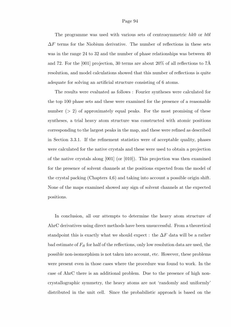
Page 94
The programme was used with various sets of centrosymmetric hk0 or h0l
∆F terms for the Niobium derivative. The number of reflections in these sets
was in the range 24 to 32 and the number of phase relationships was between 40
and 72. For the [001] projection, 30 terms are about 20% of all reflections to 7A
resolution, and model calculations showed that this number of reflections is quite
adequate for solving an artificial structure consisting of 6 atoms.
The results were evaluated as follows : Fourier syntheses were calculated for
the top 100 phase sets and these were examined for the presence of a reasonable
number (> 2) of approximately equal peaks. For the most promising of these
syntheses, a trial heavy atom structure was constructed with atomic positions
corresponding to the largest peaks in the map, and these were refined as described
in Section 3.3.1. If the refinement statistics were of acceptable quality, phases
were calculated for the native crystals and these were used to obtain a projection
of the native crystals along [001] (or [010]). This projection was then examined
for the presence of solvent channels at the positions expected from the model of
the crystal packing (Chapters 4,6) and taking into account a possible origin shift.
None of the maps examined showed any sign of solvent channels at the expected
positions.
In conclusion, all our attempts to determine the heavy atom structure of
AhrC derivatives using direct methods have been unsuccessful. From a theoretical
standpoint this is exactly what we should expect : the ∆F data will be a rather
bad estimate of FH for half of the reflections, only low resolution data are used, the
possible non-isomorphism is not taken into account, etc. However, these problems
were present even in those cases where the procedure was found to work. In the
case of AhrC there is an additional problem. Due to the presence of high non-
crystallographic symmetry, the heavy atoms are not ‘randomly and uniformly’
distributed in the unit cell. Since the probabilistic approach is based on the

Page 95
assumption that the atomic positions are random variables, this ‘non-randomness’
makes the validity of the probability distribution formulae questionable. Schenk,
H., , Krieger, W. & Schenk, H., showed —using model calculations—
how systematic overlap in the Patterson function leads to considerable deviations
from the theoretical models. Systematic overlap in the Patterson function is
exactly what we observe in the case of our best derivative (Section 4.3.1).
5.3 Patterson Methods.
Several Patterson function based methods have been used in the attempt to de-
termine the heavy atom structure of AhrC derivatives. Before discussing the
individual methods, it is useful to illustrate the size and peculiarities of the prob-
lem that these methods had to tackle.
Figure 5.1 shows the three Harker sections from the sharpened isomorphous
difference Patterson function for the Niobium derivative. The meaning of the
three large peaks (marked A,B & C) has already been discussed (Section 3.3.1 and
Section 4.3.1). It is obvious that the Harker sections contain several significant
peaks apart from the pseudo-origin peaks. It was thought that it would be
useful to know how many possible heavy atom sites are consistent with those
Harker sections and what their distribution would be. A programme was written
which for every position in the crystallographic asymmetric unit, calculated the
Harker vectors that would be observed if an atom was present at that position.
If the value of the Patterson function was greater than zero for all three Harker
vectors, then the sum of those values was stored at the corresponding position
of a map which was a copy of the asymmetric unit. Figure 5.2 is the result of
such a search using the sharpened Patterson function for the Niobium derivative
(Section y=2/32 contains no significant peaks and has been omitted). This map
is very similar to what Buerger, M.J., called an ‘implication diagram’. This

Page 96
0.0 w 0.5 0.0 v 0.5
u
0.5
v
0.5
A
B
C
Figure 5.1: Harker sections u=0.0, v=0.0 and w=0.5 from a 13–7A
[E∆Fisom∆Fisom]2 synthesis for the Nb6Cl14 derivative. Contours every 2% of the
origin peak.

Page 97
0.0 z 0.5
x
0.5y=0/32 y=1/32
y=3/32 y=4/32
Figure 5.2: Implication diagram of the Nb6Cl14 derivative. Contours every 4%
of the origin peak of the Patterson function.

Page 98
0.0 z 0.5
x
0.5y=5/32 y=6/32
y=7/32 y=8/32
Figure 5.2: Implication diagram of the Nb6Cl14 derivative. Contours every 4%
of the origin peak of the Patterson function.

Page 99
search is also similar to the ‘single atom search’ as used in several Patterson
solution programmes (such as HASSP or GROPAT), although in this case it is
not required that significantly large Harker peaks are present on all three Harker
sections.
Several features of this map are worth discussing. The first is that the im-
plication diagram has extra symmetry : its asymmetric unit is 1/8th of the
crystallographic asymmetric unit. This is because neither the enantiomorph nor
the origin are fixed in this type of search. The second point is the large num-
ber of possible heavy atom positions : well over 80 peaks can be found in the
asymmetric unit of the diagram. Most of these peaks arise from the presence
of cross vectors on the Harker sections of the Patterson function. In the case of
the Niobium derivative, the presence of cross vectors on the Harker sections is
not accidental. Because non-crystallographic symmetry axes are parallel to all
three crystallographic 2-folds, the non-crystallographic Harker sections coincide
with the crystallographic. In other words, the Harker sections contain vectors
between atoms related by both crystallographic and non-crystallographic sym-
metry. A third point is the presence of very large peaks on section y=0.0. These
arise because no correction has been made for the different multiplicities of the
various Patterson peaks. The last point is the very regular distribution of peaks
in the implication diagram : the majority of significant peaks are arranged on
lines parallel to z. These lines are again arranged in a regular manner : they form
layers perpendicular to the y axis. It is well known since the early days of protein
crystallography (see for example Dickerson, R.E, et al, & Weinzierl, J.E., )
that a small number of bad measurements of relatively low resolution reflections
can lead to isomorphous difference Patterson functions with a very regular ar-
rangement of peaks which are nothing more than ripples arising from those bad
measurements. There is evidence which suggests that the regular arrangement
of peaks in the difference Patterson map for Niobium arise from the heavy atom

Page 100
structure and not from errors of measurement : (i) the Patterson function re-
mains virtually unchanged when different native or derivative data sets are used
for the calculation, (ii) the presence of some of the largest ∆F terms has been
confirmed from comparison of precession photographs, (iii) the correlation coeffi-
cient between Patterson functions calculated using different resolution ranges is
acceptably high (Section 3.3.1), and finally, (iv) the implication diagram corre-
sponding to the [010] Patterson projection (Figure 5.3) shows the same pattern
of peaks although only the h0l terms have been used for this calculation and
the presence of the largest ∆F terms has been confirmed from examination of
precession photographs of that zone.
It is interesting to note that several authors have suggested that all ∆F terms
greater than four (or even three) times the mean value of the observed isomor-
phous differences should be excluded from all subsequent calculations. Their
argument is of a statistical nature and is based on calculating the probability of
∆F > n∆F . In the absence of any information about the heavy atom structure,
the best that can be done is to assume that the heavy atoms are distributed
randomly and uniformly in the unit cell. In the presence of non-crystallographic
symmetry, the distribution of heavy atoms will be non-random and since most of
these reagents are ionic (and, thus, bind on the surface of the macromolecule),
their distribution will also be non-uniform. This is not to imply that bad mea-
surements which result in very large differences should not be monitored and
excluded. The solution adopted in the case of AhrC, was to collect and compare
at least two data sets from each possibly useful derivative.
One final point that has to be made, concerns the evaluation of the results.
All methods described in this section are bound to produce trial heavy atom
structures whose Patterson function will be related to the observed Patterson.
This is more so for the Niobium derivative because the presence of regularities in
the heavy atom structure makes it very easy to obtain solutions which, although

Page 101
0.0 w 0.5
u
0.5
0.0 w 0.5
u
0.5
0.0 x 0.5
0.5
z
(A) (B)
(C)
Figure 5.3: (A) [010] Patterson projection for Nb6Cl14 : 17-5A ∆F 2, (B) Sharp-
ened synthesis, (C) Implication diagram using the sharpened function.

Page 102
wrong, can reproduce several of the strong peaks in the observed difference Pat-
terson. In these cases where the agreement with the observed Patterson function
was not sufficiently bad for the solution to be discarded immediately, refinement
of the trial structure followed by calculation of cross difference Fourier synthe-
ses for other derivatives proved to be a very powerful test of the correctness of
the proposed heavy atom structure (the paper from Dickerson, R.E, et al, &
Weinzierl, J.E., is again illuminating).
5.3.1 HASSP.
Terwilliger, T.C., Kim, S.-H. & Eisenberg, D., proposed a method of deter-
mining heavy atom positions which is based on using isolated Patterson peaks as
an aid to identify possible two-site solutions which are then extended through a
systematic search of the asymmetric unit for additional sites consistent with the
starting pair. They have implemented their ideas in the programme HASSP, a
short description of which is given below.
The programme starts with a systematic search for single-site solutions using
only the Harker sections. Probability measures are applied in order to identify
potentially significant solutions, but these possible single-site solutions are not
used in the subsequent calculations. The next step is to identify isolated peaks in
the Patterson function and to use each one of these in turn as a possible ‘single-
weight’ cross vector in a systematic search of the crystallographic asymmetric
unit : if u is the vector from the origin of the Patterson function to the isolated
cross peak, then for every crystallographically unique atomic position x, the
Harker vectors corresponding to a pair of atoms at x and x + u are calculated.
If the density of the Patterson function at these Harker vectors satisfies certain
probability criteria, then these atoms form a possible two-site solution. From all
possible two-site solutions for any given cross peak, the one which gives the most
significant Harker vectors is extended by searching the asymmetric unit for an

Page 103
additional atom whose Harker vectors and cross vectors with the starting pair are
significantly above the noise level. The procedure is repeated until no significant
additional sites can be found, or the limit of 6 possible atomic sites per solution
is reached.
Most of the data sets which showed signs of specific heavy atom binding
have been examined using HASSP. Attempts were made with both unsharpened
∆F 2 and sharpened [E∆Fisom∆Fisom]2 syntheses using various resolution ranges,
typically 13-6A and 10-5A. The single-site search was not very useful : In the
case of the Niobium derivative, only four significant single-site solutions could
be identified, two of which were on special positions while a third was at the
molecular centre. The reason for the very small number of possible single-atom
solutions is the requirement that all Harker peaks should be significantly above
the noise level. In the two-site search, all isolated peaks that the programme
could identify (usually about 40 peaks) were used. The solutions produced from
this search, were examined as described in the previous Section. Although several
of the most promising solutions for the Niobium derivative gave good statistics
during centric refinement (typical values were wRc = 0.55, C = 0.48, Gradient
0.45, see Section 3.3.1 for definitions), no further progress could be made with
any of them.
A possible explanation for these problems can be traced to the selection of the
“best” pair of atoms for any given cross vector. As the number of sites increases,
the probability that an incorrect solution can give a better fit to the Harker
sections increases. Furthermore, the Harker sections, especially for Niobium, are
dominated by cross vectors and can not be trusted in the early stages of the
development of a solution. A more cautious approach would be to compile a list
of all pairs which give positive Harker vectors and then to expand each one of
these in turn. The expansion step would also have to keep track of more than
just the “best” solution. It is obvious that this is a hierarchical tree structure

Page 104
in which the number of possibilities grows too fast for the calculation to be
practical (If at every step the best n solutions are kept and the decision as to
which combination is best is postponed until each combination consists of m
atoms, the total number of combinations for only one cross vector is nm. For 40
cross vectors and n = m = 8, it would be necessary to search the crystallographic
asymmetric unit 83,886,080 times and at the end of the procedure 671,088,640
combinations of 8 sites would have to be compared).
5.3.2 GROPAT.
Jones, Y. & Stuart, D., proposed a ‘brute force’ approach to the solution of
complex difference Patterson maps. Their algorithm is summarised below.
For every position in the crystallographic asymmetric unit, the values of the
Patterson function at the end of the predicted Harker vectors are used to cal-
culate an overall ‘probability’ that the position under examination corresponds
to a heavy atom site. Six criteria are used in calculating this probability :
the sum, product and minimum of the Patterson densities, their root mean
square, the mean probability for observing those values and, finally, the prod-
uct of these probabilities. The probabilities are calculated from the expression
exp[−(Pideal −Pobs)2/σ2], where, Pobs is the observed Patterson density at a given
grid point, Pideal is a user input parameter which should be equal to the Patterson
density expected from a single Harker vector, and σ is the expected error level in
the Patterson map (this is again a user-defined parameter but the authors suggest
that the root mean square deviation of the Patterson map can be used as an esti-
mate of the expected error). All pairwise combinations of the best 200 positions
from this search are then examined and the best 200 pairs (as judged from the
criteria outlined above but now considering cross vectors) are written out. This
list of best pairwise combinations forms the basis of the subsequent analysis : if
all heavy atom sites are present in the initial list of putative single-site solutions,

Page 105
then, the list of pairwise combinations should contain all possible pairs of those
sites. The problem is reduced to that of finding all possible sets of atomic sites
whose pairwise combinations are present in the list. These are possible heavy
atom structures.
Searching through a list of 200 pairs of atomic codes for the presence of all
pairwise combinations of an initially unknown number of sites invites mistakes.
A programme was written therefore, which searched this list for all possible 3-,
4-, 5- and 6-atom solutions. Even if some pairs of, say, a 6-atom solution are
missing from the initial list, the solution will not be missed since most of the
5-atom combinations will be present.
GROPAT has been tested with both ∆F 2 and [E∆F∆F ]2 syntheses for the
Niobium and Iridium derivatives. Again, as with HASSP, no convincing solution
could be identified. Considerations similar to those described in the previous
section apply here also : As the complexity of the problem increases, the prob-
ability that incorrect pairs of atoms (from the single-site search) will give cross
vectors on regions of the Patterson function with high density, is also increasing.
Furthermore, the presence of cross vectors on the Harker sections for Niobium,
makes the probability-based single-site search less reliable.
5.3.3 A Method by Nixon, P.E., 1978
The effect of non-randomness of the atomic positions on the probability distri-
bution of the basic phase-determining formulae has already been discussed (Sec-
tion 5.2.3). We have also seen that this non-randomness is best expressed in
terms of overlap of Patterson peaks. Nixon, P.E., suggested a method for
lessening the problems associated with overlapping Patterson peaks. Although
his method is based on using direct methods to solve the phase problem, it will
be discussed in this section since it involves a modification of the Patterson func-
tion. In this approach, the observed Patterson function P (u) is modified to give


Page 107
of reflections. In some cases, the classes of reflections that are systematically
weak or strong can be identified and the E-values (within each class) can be
re-normalised (although more complex algorithms do exist (Hai-Fu, F., Jia-Xing,
Y., Main, P. & Woolfson, M.M., )). Nixon’s method is an indirect way of
re-normalising the E-values for those classes of reflections that are systematically
strong without having to identify them explicitly.
A programme was written to modify a given Patterson function according
to Equation 5.10. The modified function was back-transformed using the pro-
gramme SFC from the CCP4 suite. The resulting intensities were input to the
direct methods programme SHELXS86 (Section 5.2.1). Most of the solutions ex-
amined belonged to the ‘uranium atom’ category. No convincing solutions could
be identified.
5.3.4 Image-seeking Methods.
The Patterson function of a structure consisting of N atoms can be viewed as the
superposition of N images of the structure, where the ith image (i = 1, . . . , N), is
obtained by placing the ith atom at the origin of the function, as shown in Fig-
ure 5.5. Image-seeking methods attempt to retrieve any one of these images. Sev-
eral different names (Atomic superposition, Vector superposition, Image-seeking)
have been proposed for methods that are in principle equivalent. Although these
procedures represent the most logical way to proceed in the analysis of a Patterson
function, the power and automation of direct methods, made them largely redun-
dant. The theory and practice of image-seeking methods is very well documented
and will not be discussed in great detail (Buerger, M.J., , Buerger, M.J.,
, Buerger, M.J., , Ramanchandran, G.N. & Srinivasan, , Fridrich-
sons, J. & Mathieson, A.McL., , Shoemaker, D.P., Barieau, R.E., Donohue,
J. & Lu, C.-S., , Donohue, J. & Bryden, J.H., , Simpson, P.G., Dobrott,
R.D. & Lipscomb, W.N., , Germain, G. & Woolfson, M.M., , and more

Page 108
(A) (B) (C)
Figure 5.5: (A) A hypothetical four-atom structure, (B) Its Patterson func-
tion, (C) The Patterson function seen as the superposition of four images of the
structure (Note the presence of four enantiomorphic images).
recently, Richardson, J.W. & Jacobson, R.A., , Sheldrick, G.M., ).
The principle of the vector-superposition method is illustrated in Figures 5.6
and 5.7 for the centrosymmetric and non-centrosymmetric cases respectively. Fig-
ure 5.6(A) shows a hypothetical two-dimensional centrosymmetric structure con-
sisting of 5 atoms, and Figure 5.6(B) is a schematic diagram of its Patterson
function. In Figure 5.6(C) two copies of the Patterson function (one represented
with open circles, the second with filled) have been superimposed so that the
origin of the second function coincides with the peak marked “I” in (B). It can be
seen that there are only five places where peaks from the two functions coincide,
and these are shown in Figure 5.6(E). This is the original structure. Peak “I” is
a single-weight Patterson peak which corresponds to the vector between the two
atoms that are furthest apart in the structure. If the multiple peak marked as
“II” in (B) is used for the superposition (shown in Figure 5.6(D)) then Patterson
peaks coincide at 8 places. Diagram (F) shows that these can be interpreted
as two images of the structure related by a simple translation. It is an inter-

Page 109
(A) (B)
(C) (D)
(E) (F)
I
II
Figure 5.6: Vector superposition : The centrosymmetric case.

Page 110
esting result that in the case of a centrosymmetric structure (or projection) a
superposition on a single-weight Patterson peak can reveal the structure.
Figure 5.7(A) shows a hypothetical non-centrosymmetric 4-atom structure
and 5.7(B) is its Patterson function. The superposition on a multiple peak
(marked as “II” in (B)) is shown in Figure 5.7(C). In (E) these coincidences
are interpreted as arising from two images of the structure (related by a simple
translation) plus their enantiomorphs. In (D), a single-weight vector was used
for the superposition. The result (shown in (F)) is the superposition of an image
of the structure and its enantiomorph. The ambiguity arising from the presence
of both enantiomorphs can be resolved either by a second superposition on a
different peak or by “hand exorcism” of one of the enantiomorphic images.
It is worth noting that, in general, the space (plane) group of the superposition
function is P1 (p1). Identification of a permissible origin (for the given space or
plane group) can be achieved either by visual examination of the superposition
map or by a systematic search for the position (in the superposition map) which
if chosen as a crystallographic origin will maximise the agreement between the
observed peaks.
If one or more atomic positions are known (from examination of Harker sec-
tions or lines, for example), then these can be used in a variation of the superpo-
sition method known as ‘Atomic Superposition’. If for a structure that belongs to
a plane or space group with m equivalent positions, the coordinates (with respect
to a permissible origin) of n atoms are known, then mn copies of the Patterson
function are superimposed with their origin peaks at all equivalent positions of
the n atoms, and the resulting superposition function is examined for the presence
of additional (and initially unknown) atomic sites (Figure 5.8). Since the space
or plane group symmetry is used explicitly, the atomic superposition function has
the space (plane) group of the structure.
Our first attempts with the vector superposition method were based on su-

Page 111
(A) (B)
(C) (D)
(E) (F)
I
II
Figure 5.7: Vector superposition : The non-centrosymmetric case.

Page 112
(A)
(B)
(C)
Figure 5.8: Atomic superposition : (A) A hypothetical two-atom structure in
p2, (B) Its Patterson function, (C) Superposition of two copies of the Patterson
function at the two equivalent positions of one atom (black circles). Double circles
denote additional coincidences.

Page 113
perimposing manually contoured Patterson projection functions. It was soon
realised that an automatic procedure was needed if the superpositions were to be
carried out accurately a large number of times : Two programmes have been de-
veloped. The first deals with the two-dimensional (centrosymmetric) case. Given
a Patterson projection P and a number n of grid points, the programme will su-
perimpose (using the sum, product or minimum function) n copies of P with their
origin peaks at the specified grid points. The superposition function is written
as a CCP4 map file which can be plotted using the programme PLUTO (from
the CCP4 suite of programmes). This superposition programme can be used for
both vector and atomic superposition.
The second programme deals with the general case of a three-dimensional Pat-
terson function and implements some of the ideas presented by Richardson, J.W.
& Jacobson, R.A., and Sheldrick, G.M., . Two copies of the Patterson
function are superimposed on a given Patterson peak using the minimum func-
tion. The position (in the superposition function) which if chosen as an origin of
the known space group will maximise the agreement between grid points related
by crystallographic symmetry is then identified through a systematic search :
the criterion used is the sum of the minimum density of all crystallographically
related grid points, for every given choice of origin. Once the “best” origin has
been identified, the superposition function is averaged using the crystallographic
symmetry and the final (averaged) map is written out in the CCP4 map format.
Most of our attempts with the superposition method concentrated on the
[001] and [010] Patterson projections of the Niobium and Iridium derivatives.
Although the [001] projection is down a 138A long axis, it was hoped that useful
results could still be obtained : the implication diagram (Figure 5.2) suggests
that the heavy atom sites of the Niobium derivative are arranged on lines parallel
to z and would, thus, overlap in the [001] projection. The [001] Patterson projec-
tion (Figure 5.9) clearly indicates the presence of a regular arrangement of heavy

Page 114
atom sites. The ∆F -weighted reciprocal lattice representation of the hk0 level
(Figure 5.10) shows a hexagonal arrangement of clusters of large ∆F terms with
two outstandingly large differences for the reflections 11,5,0 and 12,6,0. After
removal of these two terms, the projection remained virtually unchanged, sug-
gesting that the large differences are due to the underlying heavy atom structure
and not due to errors of measurement. The presence of regularities in the heavy
atom structure made the identification of single-weight Patterson peaks very dif-
ficult : Superpositions have been carried out on all relatively weak Patterson
peaks with density greater than zero. Some of the most promising superposition
functions showed an arrangement of peaks which was in very good agreement
with the model of the crystal packing (Figure 5.11). Unfortunately, none of these
solutions led to a projection of the native crystals with the expected arrangement
of solvent channels.
Several attempts using the [010] projection have also been unsuccessful. One
of the most promising atomic superposition functions is shown in Figure 5.12.
The presence of a non-crystallographic 2-fold axis at the position of the assumed
molecular centre is indicated. No progress could be made with this or any other
solutions examined.
Finally, a number of attempts using the second of the programmes described
above with the three-dimensional isomorphous difference Patterson function for
the Niobium derivative have been unsuccessful. This was mainly due to the
difficulty in identifying single-weight Patterson peaks and the presence of both
enantiomorphs in the superposition function.
5.3.5 A Patterson Interpretation Programme : MSS.
The discussion in sections 5.3.1 and 5.3.2 suggested that accepting (or rejecting)
partial two-site solutions very early during the development of a possible heavy
atom structure is not necessarily the best way forward. The most systematic

Page 115
-0.25 u 0.75
v
0.75
Figure 5.9: 15-6A [001] Patterson projection for the Niobium derivative.
h00
0k0
Figure 5.10: hk0 weighted reciprocal lattice for Nb6Cl14.

Page 116
-0.25 x 1.25
1.25
z
Figure 5.11: [001] Vector superposition functions for the Niobium derivative.
0.0 x 1.0
1.0
z
Figure 5.12: [010] Atomic superposition function for the Niobium derivative.

Page 117
(but least elegant) approach for the interpretation of a Patterson function would
be to evaluate the agreement between the observed Patterson function and the
Patterson function calculated from every crystallographically unique arrangement
of atoms. Such a procedure would be equivalent to a direct R-factor search, that
is, calculation of the R-factor for all unique atomic arrangements. This approach
is practical only for relatively small unit cells : in the case of the orthorhombic
form of AhrC, a systematic search of the “best” six-atom structure (as judged by
the R-factor or the correlation coefficient between the observed and calculated
structure factor amplitudes), would require the calculation of structure factors
3.4·1024 times (assuming that a 2A grid is used).
A Patterson function interpretation programme has been developed in which
the number of possible heavy atom structures that have to be examined is reduced
to a manageable size through the application of the following a priori assumptions
about the Patterson function :
1. For every heavy atom position x, the value of the implication diagram I(x)
is greater than zero, that is, the Patterson function has positive values for
all Harker vectors corresponding to x.
2. If x is a heavy atom position, then a pair of numbers n, m exists such that
(i) n out of the m atomic positions which give the largest sum of both
Harker and cross vectors with x, are also heavy atom positions, and, (ii)
the sum of the values of the Patterson function for all vectors between the
n heavy atom sites is the largest of all other combinations of n out of these
m sites.
The pseudocode for this programme is shown in Figure 5.13.
Although the requirement of the positivity of the Patterson function for all
Harker vectors of all heavy atom sites reduces significantly the volume of the
crystallographic asymmetric unit that has to be searched for possible heavy atom

Page 118
1. Calculation of the implication diagram I :
for (every grid point x of I)
if (the density of the Patterson function (P) for all Harker vectors
corresponding to a heavy atom site at x is greater than zero)
then I(x) =∑P(Harker(x))
else I(x) = 0
2. Development of n-site partial heavy atom structures :
for (every x in I)
if (I(x) > 0)
then (find m other grid points which give the largest sum of both Harker
and cross vectors with x. Find the combination of n out of these m
sites which give the largest sum of all predicted vectors and save
this n-site partial structure)
else (next grid point)
3. Extension of all n-site partial structures :
for (every n-site partial solution)
(Find additional sites for which I(x) > 0 and all predicted vectors with
the already known sites lie in positive areas of the Patterson function.)
4. Refinement and calculation of useful metrics :
for (every heavy atom structure)
if (before refinement : Corr(Eo, Ec) > limit1)
then (Refine the positional parameters using Hart’s algorithm. Target
function is the correlation coefficient between Eo and Ec for
centric terms)
if (after refinement : Corr(Eo, Ec) > limit2)
then (calculate lengths of vectors between heavy atom sites
and between heavy atoms and the molecular centre).
Figure 5.13: MSS : pseudocode.

Page 119
sites (≈ 10% for the Niobium derivative), the algorithm is still practical only for
relatively small values of n and m (typically n ≤ 6, m ≤ 12).
As an aid to the identification of possible correct solutions, the programme
refines the positional parameters of the heavy atoms using Hart’s algorithm (Hart,
R.G., ) and calculates the lengths of the vectors between heavy atoms and
between the molecular centre and the heavy atom sites (due to the presence of
non-crystallographic symmetry, the correct solution was expected to show clusters
of vectors of similar lengths).
The programme has been tested with hypothetical heavy atom structures con-
sisting of up to 20 atoms in the crystallographic asymmetric unit (space group
C2221), some of which had non-crystallographic symmetry axes parallel to crys-
tallographic. The correct solution could be identified for all structures consisting
of less than approximately 14 atoms. For the more complex structures, only
partially correct solutions were usually identified. The main reason for these
problems was a violation of the assumption of the positivity of all Harker vec-
tors : since the F000 term is not included in the calculation of the Patterson
function, it was not unexpected to find that for some vectors the value of the
Patterson function was negative. An attempt was made to lower the threshold
for the acceptance of a possible vector; the result was a very large number of pos-
sible heavy atom structures which made the identification of the correct solution
rather difficult.
Several attempts with both conventional and sharpened isomorphous differ-
ence Patterson functions for the most promising derivatives have been unsuc-
cessful. As before, some solutions gave very good statistics during least squares
refinement, but no further progress could be made with any of them.

Page 120
5.3.6 The Argos & Rossmann Method.
Argos, P. & Rossmann, M.G., ,, were the first to realise that in the
presence of known non-crystallographic symmetry, the problem of determining
the positions of the heavy atoms in the crystallographic asymmetric unit of
a derivative can be reduced to that of determining their positions in the non-
crystallographic asymmetric unit (assuming that the heavy atom structure obeys
the non-crystallographic symmetry of the macromolecular assembly).
When the position of the molecular centre in the crystallographic frame is not
known, their method is divided in two steps.
In the first step (Type I search), an attempt is made to determine the po-
sitions of the heavy atoms with respect to the molecular centre : for every po-
sition x in the non-crystallographic asymmetric unit, the positions of all non-
crystallographically equivalent positions of x are generated and the vectors be-
tween those sites are calculated. The sum of the density of the isomorphous
difference Patterson function at the end of the predicted vectors is a measure of
how well a heavy atom site at x agrees with the observed Patterson function.
It is obvious that at this stage, vectors between heavy atoms that are bound to
crystallographically related molecules, as well as vectors between multiple heavy
atom sites on the same protein subunit, are not been taken into account.
Once the positions of the substitution sites with respect to the molecular
centre are known, the position of the molecular centre with respect to a permis-
sible —for the given space group— origin, can be determined (Type II search) :
For every position of the molecular centre in the unit cell of the corresponding
Cheshire group (Hirshfeld, F.L., ), the sum of the values of the isomorphous
difference Patterson function at the end of all predicted vectors (now taking into
account the crystallographic symmetry) is evaluated. Clearly, this second step is
a translation function very similar to those discussed in Sections 5.4.2 and 7.2.1.
If the position of the molecular centre in the crystallographic frame is known,

Page 121
then it is possible to include this information in the Type I search : for every
equivalent (by non-crystallographic symmetry) position of x, the vector corre-
sponding to one of the equivalent positions of the molecular centre is added and
all crystallographically related sites are generated. The summation now is over
all unique vectors between heavy atoms related by both non-crystallographic and
crystallographic symmetry. The inclusion of vectors between heavy atoms that
are bound to crystallographically related molecules offers a significant improve-
ment of the signal to noise ratio.
If there is more than one heavy atom site per non-crystallographic asymmetric
unit and the positions (with respect to the molecular centre) of one or more of
these atoms have been determined, then, it is possible to repeat the Type I
search with these heavy atoms ‘fixed’ at their known positions. This search can
be performed with or without knowledge of the position of the molecular centre.
A set of programmes has been developed to carry out the calculations required
for these two types of searches. Since in our case the amount of calculation
involved is not as large as in the case of icosahedral viruses (discussed in detail
by Argos, P. & Rossmann, M.G., ), no attempt was made to reduce the
number of vectors that are used in the various steps of the procedure. The
programmes allow the Type I search to be conducted with or without knowledge
of the position of the molecular centre or of any ‘fixed’ heavy atom sites. In
the translation function step (Type II search), all known heavy atom sites in the
non-crystallographic asymmetric unit can be used.
Although the Type I search need only be done within the non-crystallographic
asymmetric unit (that is, in the molecular as opposed to the crystallographic
frame), in the case of AhrC where the non-crystallographic symmetry was not
known with certainty, a more general scheme was used : the search was carried
out in the (orthogonal) crystallographic frame and a volume equal to a hemi-
sphere around the molecular centre was examined (the radius of the sphere is a

Page 122
user-defined parameter). This means that in those of our attempts where 32 sym-
metry was assumed, the amount of calculation involved was as much as 3 times
that needed. The advantages of this approach are (i) any point group symmetry
can be used without any need for modifying the programmes, and, (ii) the anal-
ysis of the results is simplified since no conversion to the crystallographic frame
is necessary. The programmes have been tested with hypothetical heavy atom
structures obeying various non-crystallographic point group symmetries (32, 622,
432, etc.). These calculations showed that when the number of heavy atoms in
the non-crystallographic asymmetric unit was greater than about three, spurious
peaks appeared in the Type I search conducted without knowledge of the molec-
ular centre. When the position of the molecular centre was treated as known, the
heavy atom positions could be easily identified in all cases examined.
All indications from the self rotation functions for both the native crystals
and the heavy atom structures (Chapter 4), have been examined using the Argos
& Rossmann method with the isomorphous difference Patterson functions for the
most promising AhrC derivatives.
From these attempts, we will discuss in detail the results from the calcu-
lations for the Niobium derivative which were based on the assumption that
the point group symmetry of the heavy atom structure is 32 with the 3-fold
at ω = 90, φ = 60 and one of the 2-folds parallel to z (discussed in Section
4.2.2). Figure 5.14 shows the results from the Type I search conducted without
knowledge of the position of the molecular centre. Figure 5.15 is the same search
but this time assuming that the molecular centre is at x = 0.13, y = 0.09 and
z = 0.225 (Because the programme calculates a volume equal to a hemisphere
around the molecular centre, some of the peaks in these maps are related by
non-crystallographic symmetry. Such peaks are marked by the same numeral).
The similarity of these two functions suggests that the assumed non-crystallo-
graphic symmetry is consistent with the previously determined position of the

Page 123
-40.0 x 40.040.0
z
-40.0y=0A y=2A y=4A
y=6A y=8A y=10A
y=12A y=14A y=16A
y=18A y=20A y=22A
o o o
o o o
o o o
o o o
I I
I
I
II
II
II
III
III
III
Figure 5.14: Argos & Rossmann, Type I search for Nb6Cl14, Molecular centre
unknown. Contours every 1.5σ with first contour at 1.5σ above the mean.

Page 124
-40.0 x 40.040.0
z
-40.0y=0A y=2A y=4A
y=6A y=8A y=10A
y=12A y=14A y=16A
y=18A y=20A y=22A
o o o
o o o
o o o
o o o
I I
I
I
II
II
II
III
III
III
Figure 5.15: Argos & Rossmann, Type I search for Nb6Cl14. Molecular centre
at x = 0.13, y = 0.09, z = 0.225.

Page 125
molecular centre. Figure 5.16 shows the results from the Type II search using only
the six atoms corresponding to the peak marked as (I) in Figures 5.14 and 5.15.
The highest translation function peak is at x = 0.13, y = 0.09 and z = 0.22
as expected. Peak (I) in Figures 5.14 and 5.15 is clearly the most significant
feature of these maps. The six heavy atom sites corresponding to it (through
application of the non-crystallographic symmetry operators) are at the corners of
an approximately regular octahedron whose edges are ≈14A long. The orientation
of the octahedron is such that three orthogonal, intersecting, non-crystallographic
2-folds are parallel to the three crystallographic 2-fold axes, thus generating large
pseudo-origin peaks on all three Harker sections of the ∆F 2calc Patterson function2.
0.0 z 0.5
x
0.5 y=2/32 y=3/32 y=4/32
Figure 5.16: Argos & Rossmann, Type II search for Nb6Cl14. Three sections
through the highest peak are shown.
A comparison of the observed 13-7A sharpened isomorphous difference Pat-
terson function for the Nb6Cl14 derivative with the Patterson function calculated
2The three orthogonal non-crystallographic 2-folds are generated by the extra symmetry thatan octahedral arrangement of heavy atoms possesses : the point group symmetry of a regularoctahedron is m3m, which has the 32 point group as a subgroup.

Page 126
from these six heavy atom sites alone, is shown in Figure 5.17 (for clarity, the
contouring level for the observed Patterson has been increased to 3% of the ori-
gin peak). Although several of the most prominent peaks can be accounted for,
some of the predicted peaks are not present or are misplaced by 0.025 along w.
Least squares refinement of these six sites against all centric terms between 15
and 6A resolution converged to rather high R-factors and a very low correlation
coefficient between the observed and calculated amplitudes for the heavy atom
structure.
An attempt to determine the heavy atom structure of the Iridium derivative
using SIRAS phases calculated from the unrefined six atom structure for the Nio-
bium derivative was unsuccessful. These problems suggested that the indications
from the self rotation function for the Niobium derivative could not lead to a
successful structure determination.
It was a surprise to find that a Fourier synthesis for the native crystals which
was calculated using SIRAS phases from the unrefined six atom structure for
the Nb6Cl14 derivative (Figure 5.18) showed well defined solvent channels with
a distribution of density which was in very good agreement with the model of
the crystal packing and the electron microscopical studies of AhrC crystals. The
calculation of reasonable low resolution protein density maps from incorrect heavy
atom structures was unexpected. Further investigation of this problem led to the
conclusion that when the non-crystallographic point group symmetry of the heavy
atom structure is the same as (or is a supergroup of) the crystallographic point
group symmetry and the non-crystallographic and crystallographic symmetry
axes are parallel, then, protein phases calculated from any heavy atom structure
that obeys the non-crystallographic symmetry are not random, but will lead
to a protein density map consisting of images of the origin-removed Patterson
function of an isolated protein molecule. To put this in a more practical way,
protein phases calculated from any heavy atom structure that can generate the

Page 127
v=0/32
v=1/32
v=2/32
v=3/32
v=4/32
v=5/32
v=6/32
v=7/32
v=8/32
0.0 0.5
0.5
w
u
Observed Calculated Observed Calculated
Figure 5.17: Observed and calculated Patterson functions for the Nb6Cl14
derivative.

Page 128
-0.5 x 1.5
y
1.5
Figure 5.18: 10A [001] projection of native AhrC crystals, Top : (+), Bot-
tom : (−) hand. Phases calculated from the Niobium derivative modelled as an
octahedral arrangement of six sites.
large pseudo-origin peaks seen in the ∆F 2 Patterson function for the Niobium
derivative, are not random and are bound to generate reasonable, but incorrect
low resolution protein density maps.
Figure 5.19 shows the results of model calculations which were undertaken
in order to confirm the argument presented above. Figure 5.19(A) is the [010]
projection of the electron density of a hypothetical “native” crystal structure con-
sisting of 36 atoms obeying 32 symmetry with all non-crystallographic symmetry
axes at general orientations. Figure 5.19(B) is the projection of a “derivative”
of the structure shown in (A) : four “heavy” atoms have been added in such a
way that the heavy atom structure has point group symmetry 222 with the non-
crystallographic 2-fold axes parallel to all three crystallographic 2-folds (the space

Page 129
group of these hypothetical structures is C2221). Figure 5.19(C) shows the v = 0
section from the isomorphous difference Patterson function for this hypothetical
derivative. The large pseudo-origin peak at u = 0.25, w = 0.05 arises from the
parallelism between the non-crystallographic and crystallographic 2-folds. Least
squares refinement of a “heavy atom” site at the position of the molecular centre
against all centric terms between 13 and 6A resolution gave statistics of accept-
able quality (Rc = 0.55, C = 0.59). SIRAS phases were calculated from this
refined atomic position and a Fourier synthesis for the “native” crystals was cal-
culated using coefficients m(Fp)eiαSIRAS . This is shown in Figure 5.19(D). It is
obvious that this map has high density at the correct position but the density
itself is incorrect (it is an image of the origin removed Patterson function of an
isolated hypothetical molecule).
It was not a surprise to find that a Fourier synthesis for the native AhrC
crystals which was calculated using SIRAS phases from the Niobium derivative
modelled with one site at the molecular centre (Section 3.1.1), showed the now
familiar distribution of density down the [010] and [001] directions (Figure 5.20).
The agreement between the permutation map (A) in Figure 4.6 with the [010]
projection in Figure 5.20 is worth noting.
In conclusion, the presence of non-crystallographic symmetry axes which have
a “special” orientation with respect to the crystallographic, makes a reasonable
low resolution protein map a necessary but not sufficient condition for the cor-
rectness of a proposed heavy atom structure.
5.4 Other Methods.
5.4.1 Permutation Syntheses Method.
The application of the permutation syntheses method to centrosymmetric, low
resolution terms, has been described (Section 4.3.2). The extension of the method

Page 130
0.0 z 1.0
x
1.0 (A)
0.0 z 1.0
x
1.0 (B)
0.0 w 0.5
u
0.5 (C)
0.0 z 1.0
x
1.0 (D)
2
34
1
Figure 5.19: (A) A hypothetical 36 atom structure, (B) Its derivative, (C) The
difference Patterson function, (D) A Fourier synthesis based on modelling the
derivative as a single site at the molecular centre.

Page 131-0.5 z 1.5
x
1.5
-0.5 x 1.5
y
1.5
Figure 5.20: [010] & [001] projections of native AhrC crystals based on mod-
elling the Nb6Cl14 derivative as a single site at the position of the molecular
centre.

Page 132
in the special case of ∆F data is straightforward : Fourier syntheses are calculated
for all unique phase combinations of a small number of large ∆F terms, and the
most promising of these are further analysed by other methods (least squares
refinement, cross difference Fourier syntheses for other derivatives, etc.). The
resolution range over which these terms are chosen is important. Low resolution
∆F data are greatly affected by differences in the electron density of the solvent
of crystallisation and are not very useful for the determination of the heavy atom
positions. High resolution ∆F terms are sensitive to lack of isomorphism and
tend to give permutation maps with a grid pattern of fringes (this is due to the
small number of terms included in the syntheses). For most of our attempts, data
between 13 and 7A resolution were used.
The application of the method to ∆F data is complicated by the fact that the
only criteria for selecting those phase combinations which are likely to be correct
are (i) the absence of heavy atom sites from what was known to be solvent areas,
and, (ii) the concentration of electron density at few atomic sites. Since in the
[010] projection the solvent channels are less well defined, our efforts focused on
the [001] projection. Figure 5.21 shows two of the most promising permutation
syntheses for the [001] projection of the Niobium derivative using the seven largest
hk0 terms between 13 and 8A resolution. The agreement with the model of the
crystal packing and the concentration of the electron density at few atomic sites
is obvious, but, as further examination of these solutions suggested, it can only
be taken to mean that the data are not inconsistent with our presumptions.
Several sets of hk0 and h0l ∆F terms for the Niobium and Iridium derivative
have been examined. Although some of the heavy atom structures suggested by
the permutation maps could be refined with very good statistics, none of these
solutions led to protein projection maps with the expected distribution of density.

Page 133-0.5 x 1.5
y
1.5
Figure 5.21: [001] permutation syntheses for the Niobium derivative.
5.4.2 Molecular Replacement.
Examination of the sharpened isomorphous difference Patterson for the Niobium
and Iridium derivatives at the region around the origin of the function, led to the
development of several possible (partial) heavy atom structures. For example,
the u = 0.0 Harker section from the sharpened isomorphous difference Patterson
function for the Niobium derivative (Figure 5.22) shows strong peaks at the cor-
ners of an approximately regular hexagon centered at the origin of the function.
The average length of the vectors corresponding to those peaks is 14A. A partial
heavy atom structure consisting of three sites at the corners of an equilateral
triangle with the 3-fold parallel to x and one of the edges parallel to z can ac-
count for these features. Similarly, the u = 0.0, v = 0.0, w line shows a regular
arrangement of equidistant Patterson peaks which can be accounted for by four
heavy atom sites arranged on a line parallel to z with interatomic distances equal

Page 134
to 13.8, 41.1 and 13.8A.
The determination of the position of such models in the crystallographic frame
was attempted using the translation function programme BRUTE (Fujinaga, M.
& Read, R.J., ). For every crystallographically unique position of the search
model in the known cell, BRUTE calculates the correlation coefficient and the
R-factor between the observed and calculated intensities of the structure factors3.
Figure 5.23 shows three sections through the highest peak of the translation func-
tion for the second of the models described above. The major peak is at x = 0.13,
y = 0.09, z = 0.22 with a corresponding value of the linear correlation coefficient
of 0.42. The four heavy atom sites are symmetrically arranged about the as-
sumed position of the molecular centre. A comparison of the observed Patterson
function for the Niobium derivative with the Patterson function calculated from
these four heavy atom sites is shown in Figure 5.24. Because all four sites are
on a line parallel to z, the Patterson function calculated from this structure has
peaks only on sections v = 0.0 and v = 0.18. Although the agreement with the
observed Patterson function is acceptable (for a partial heavy atom structure),
these four sites could not be refined. Furthermore, a difference Fourier synthesis
for the Iridium derivative which was calculated using SIRAS phases from the
unrefined heavy atom positions, showed a more or less uniform distribution of
peaks that could not be interpreted in terms of a heavy atom structure. Very
similar results have been obtained from all models examined.
5.4.3 Direct Maximisation
of an Electron Density Function.
The [001] permutation syntheses in Figure 5.21 showed the level of clarity to be
expected even from few correctly phased hk0 terms. Our attempts to determine
3The procedure is made practical through the use of partial structure factors for each crys-tallographically related copy of the search model. In this way, the computationally expensiveFourier transforms can be avoided (Nixon, P.E. & North, A.C.T, )

Page 135
-0.25 w 0.5
v
0.5
Figure 5.22: u = 0.0 Harker section from the sharpened isomorphous difference
Patterson function for the Niobium derivative. Contours every 2% of the origin
peak.
0.0 z 0.5
x
0.5 y=2/32 y=3/32 y=4/32
Figure 5.23: Three sections from the translation function using BRUTE.

Page 136
0.0 w 0.5
u
0.5
Figure 5.24: Comparison of two sections from the observed (top row) and cal-
culated Patterson function for a four-atom structure.

Page 137
the phases of the hk0 terms using either the direct methods programme SHELXS-
86 (Section 5.2.1) or the Cochran & Douglas method (Section 5.2.3) have been
unsuccessful. The main problem with the application of the Cochran & Douglas
method to the hk0 terms, appears to be the absence of translational symmetry in
this projection. The plane group of the [001] projection is cmm for which F (hk) =
F (hk) = F (hk) = F (hk), that is, all crystallographically related structure factors
have the same phase and, thus, all triple sign products are satisfied with the trivial
solution s(Fh) = +1 for every h (This is not the case, for example, with the [010]
projection (plane group pmg) for which F (hk) = F (hk) = −F (hk) = −F (hk)
when l = 2n + 1). In other words, the “best” phase set from the Cochran
& Douglas method will be the one with all signs positive, and the phase sets
that follow will be linear combinations of the indices of the reflections that enter
the triple sign products. The solution with all signs positive will give a map
with a very large peak at the origin and will, thus, maximise the value of the
integral∫V
ρ3dV (Equation 5.2).
In the case of AhrC derivatives, where a large number of substitution sites
are present, the function∫V
ρ3dV —which reaches a maximum for the map with
the smallest number of peaks consistent with the data— is not very useful. An
attempt was made to identify an electron density function that would be more ap-
propriate for the given problem. The most promising results have been obtained
from the function∫V
ρ3dV/ max(ρ) is maximum positive. (5.11)
Model calculations showed that this function will take its maximum value for the
phase set which gives the largest number of peaks consistent with the data. The
same calculations showed that when a large number of sites is present, Equa-
tion 5.11 can give better results than Equation 5.2, that is, the correct phase
set can be closer to the top of the list of best solutions for Equation 5.11 than
for Equation 5.2 (Stanley, E.. , also discussed various electron den-

Page 138
sity functions, but his conclusion was that the most useful integral is∫V
ρ3dV .
Function 5.11 was not considered in his papers).
A programme was written, which for every unique phase combination of a
given number of terms, calculated the value of the function 5.11. At the end of
the procedure, the “best” phase sets were saved for further examination. Since
there is no analytical approximation to the value of max(ρ), it is necessary to
calculate a Fourier synthesis for each phase combination. This means that the
number of terms that can be examined is not as large as is the case for the
Cochran & Douglas method.
The programme has been tested with both hk0 and h0l ∆F data (the 21
largest differences between 13 and 7A resolution were used for both calculations).
The top 100 phase sets from each run were evaluated as discussed in Section 5.2.3.
No convincing solutions could be identified.
5.4.4 Monte Carlo Methods.
We have seen how all analytical approaches to the problem of determining the
heavy atom structures of the most promising AhrC derivatives were unsuccessful.
It was hoped that a method based on a modified direct minimisation of a suitable
statistical metric (such as the R-factor or (1-C), where C is the linear correlation
coefficient), although less elegant, would avoid the need for any assumptions
other than the basic crystallographic requirement that the global minimum of the
chosen statistic corresponds to the true crystal structure or one of its homometric
pairs4.
Our first attempt with such a method was based on refinement of randomly
chosen atomic configurations : The random number generator was used to prepare
a list of fractional coordinates for a given number of atoms in the crystallographic
4Strictly speaking, this requirement can only be true in the case of very accurate (smallmolecule) data. When the errors of measurement are significant, the correct treatment is givenby the Maximum Entropy methods.

Page 139
asymmetric unit. The positional parameters of those atoms were refined using
an implementation of Hart’s algorithm with target function the linear correlation
coefficient between the observed and calculated structure factor amplitudes. If the
value of the correlation coefficient after refinement was greater than a preset limit,
the refined positional parameters were stored for further use. The procedure was
repeated for a new random structure until a user-defined number of iterations had
been completed. In the final step, all atomic sites saved during the main part of
the the calculation were plotted on a map that was a copy of the crystallographic
asymmetric unit. If the procedure had been successful, these should cluster at
few, hopefully correct, atomic positions5.
Several tests with data calculated from hypothetical heavy atom structures
showed that the method could converge to the correct structure only when the
number of heavy atom sites was less that about six per asymmetric unit. This is
due to (i) the relatively small number of random structures that can be examined
(in the order of few thousands), and, (ii) the rather inefficient sampling of the
parameter space as will be discussed below. Several attempts with ∆F data for
the Niobium derivative showed no sign of convergence.
Khachaturyan, A., Semenovskaya, S. & Vainshtein, B., and Semen-
ovskaya, S.V., Khachaturyan, K.A. & Khachaturyan, A.G., (hereafter re-
ferred to as SKK) proposed a much more elegant and thoughtful Monte Carlo
approach to the determination of a crystal structure. They started by noting the
analogy between the determination of the thermodynamic equilibrium in statisti-
cal mechanics and the optimisation problem for a function of many variables, and
they argued that the problem of determining a crystal structure can be viewed
as that of determining the low-temperature state of a model gas composed of a
known number of atoms in a known unit cell, with the unit cell and the R-factor
5It is worth noting that following the development of this algorithm, an abstract of a paperby Vand, V., Niggli, A. & Pepinsky, was discovered in which a closely related method wasdescribed.

Page 140
being regarded as a vessel and a potential energy term respectively. They sug-
gested that the low-temperature state can be determined with the variation of the
Monte Carlo method proposed by Metropolis, N., Rosenbluth, A.W., Rosenbluth,
M.N., Teller, A.H. & Teller, E., (but see also Rosenbluth, M.N. & Rosen-
bluth, A.W., , Wood, W.W. & Parker, F.R., , Alder, B.J. & Wainwright,
T.E., , Hammersley, J.M. & Handscomb, D.C., ) :
When a classical system is in thermodynamic equilibrium with its surround-
ings, the expectation F of any state-function F (n) is given by
F =∫
F (n) exp(−En/kT )dn∫exp(−En/kT )dn
(5.12)
where En is the energy of the state n, k is Boltzmann’s constant, T is the absolute
temperature of the surroundings and dn is a volume element in the multidimen-
sional phase space (the dimension of the integral in Equation 5.12 equals the
number of degrees of freedom of the system. For a two-dimensional structure
consisting of N particles, the integral is 2N -dimensional). The simplest Monte
Carlo method for calculating F would be to choose a configuration n randomly,
calculate its energy En, give Fn a weight exp(−En/kT ) and iterate. When the
number of configurations tends to infinity, the weighted average of Fns will tend
to F . This procedure is inefficient because with high probability we choose low-
weight states (that is, configurations for which exp(−En/kT ) is very small). The
adaptation of this rather primitive Monte Carlo method to the crystallographic
problem is obvious : an atomic configuration n is chosen randomly, the structure
factors Fh,n are calculated, the agreement between the observed and calculated
amplitudes —in the form of the R-factor— is evaluated, the Fh,n are given a
weight exp(−Rn/kT ) and the procedure is iterated. When the number of struc-
tures examined tends to infinity, the weighted average of the structure factors will
tend to its thermodynamic average both in amplitude and phase. As the temper-
ature of the system tends to zero, the thermodynamic average of the structure
factors will tend to the true (crystal structure) value. Clearly, this approach is

Page 141
very similar to our first attempt with a Monte Carlo method as described above.
The objective of the Monte Carlo method proposed by Metropolis, N., Rosen-
bluth, A.W., Rosenbluth, M.N., Teller, A.H. & Teller, E., is to generate a
series (formally : a Markov chain) of configurations in which each state n recurs
with frequency exp(−En/kT ). When such a chain of configurations has been
attained, the expectation F of any state-function F (n) can be found by taking
the average of F over an infinitely long segment of the chain with all configura-
tions being given the same weight, or as the authors put it, “instead of choosing
configurations randomly and weighting them with exp(−E/kT ), we choose con-
figurations with a probability exp(−E/kT ) and weight them evenly”.
Their algorithm for choosing states with probability exp(−E/kT ), as modi-
fied by SKK for the crystallographic problem, is as follows. Initial coordinates
for all (N) atoms in the crystallographic asymmetric unit are chosen randomly
and uniformly. The random number generator selects one of these N atoms, and
one of the six nearest grid points to which that atom may migrate (the atoms are
constrained to move on a fine rectangular grid inscribed in the asymmetric unit).
Whether the atom will move to this new position or not is decided as follows : If
the new position is occupied by a different atom no migration occurs and the same
atomic configuration is used as a starting point for the next iteration. If the new
position is vacant, the change in the R-factor (∆R) resulting from the migration
to the new site is calculated. If ∆R ≤ 0, that is, the R-factor for the new config-
uration is lower, the move is accepted. If on the other hand, ∆R > 0 the move
may be realised with probability exp(−∆R/T ) : the random number generator
chooses a number ξ such that 0 < ξ < 1. If ξ < exp(−∆R/T ) the move is ac-
cepted, otherwise no migration will occur and the previous configuration is taken
to be the new configuration. Finally, a new atom is chosen and the procedure is
iterated. The proof that this algorithm chooses configurations with probability
exp(−R/T ) will not be given here (see Wood, W.W. & Parker, F.R., and

Page 142
Hammersley, J.M. & Handscomb, D.C., ). It is worth noting that since the
paper by SKK, this method of minimising the difference between the observed
and calculated amplitudes of the structure factors has been termed “the reverse
Monte Carlo method” and found uses in such diverse areas of science, as struc-
tural modelling of glasses (Keen, D.A. & McGreevy, and references therein)
and ab initio phasing of low resolution data from protein crystals (Subbiah, S.,
, , David, P.R. & Subbiah, S., ).
What we are interested in, is the average value of the structure factors over a
segment of this chain of configurations that is sufficiently remote from its starting
point. If we start taking our averages at a ‘time’ t0 from the starting point of
the chain and the averages are calculated for the time interval (t0, t0 + t), then at
t → ∞ the average value of any structure factor will tend to its thermodynamic
average. If the temperature T is low, the system will spend most of its time close
to the ground state (that is, close to the global minimum of the R-factor) and
the average value of the structure factors (both amplitudes and phases) will tend
to their true values. SKK noted that the value of
η(h, t) =|<Fh,t >||Fh | obs
(5.13)
where |<Fh,t >| is the amplitude of the average value of the structure factor
Fh at a time t and |Fh|obs is its observed value, will tend to 1 when the system
approaches the global minimum and to 0 when the system is in a disordered state
(it should be noted that there is no physical ‘time’ or ‘temperature’ involved in
these calculations. ‘Time’ is a variable counting successive atomic configurations,
whereas ‘temperature’ is a control parameter defining the average mobility of the
atoms). SKK used L-proline (which consists of 8 atoms excluding hydrogens)
as a model structure for testing their algorithm. For their calculations they
used a 15×15×15 grid (the average distance between grid points was 0.3A), the
averaging procedure was started at t = 2.24 · 106 and lasted 7.04 · 105 time units.
The maximum deviation of the final phases from their true values was only 23

Page 143
and the phases of all reflections for which η(h, t) > 0.4 were correct.
A programme was developed to implement the ideas presented above. Al-
though the basic algorithmic steps are identical with those given in SKK, some
minor alterations were found to be necessary. The first modification is the cal-
culation of the free R value (Rfree) for a randomly chosen subset of reflections
(usually 10% of the total) that were not allowed to enter the expression for the
R-factor during minimisation (Brunger, A.T., a). Because Rfree is an unbi-
ased indicator of the information content of the atomic model, it can be used to
differentiate between a minimum of the R-factor that corresponds to the correct
solution and a local minimum with no structural significance. Rfree can also be
helpful in deciding the approximate number of heavy atom sites which are likely
to be present in the derivative. The second modification concerns the compu-
tational efficiency of the algorithm : the limiting step of the whole procedure is
the structure factor calculation. In their paper, SKK used a space-group specific
geometrical structure factor calculation algorithm (International Tables for X-
ray Crystallography, Vol. I, ). When the number of atoms and reflections is
small, this approach can be faster than FFT. What escaped their notice, however,
is that because at each step only one atom is being moved, the calculation can
be made independent of the number of atoms : If at t = 0 the contribution of
each atom to each reflection is calculated, then for the rest of the minimisation
it is only necessary to calculate the contribution to the structure factors of only
the atom that is being tested. The method is fairly efficient : for 170 reflections,
a DEC 4000 can go through 2314 configurations in one second of CPU time inde-
pendently of the number of atoms involved (the same algorithmic improvement is
also applicable to the method described by Subbiah, S., , , David, P.R.
& Subbiah, S., ).
Figure 5.25 shows the results from model calculations using a hypothetical
12-atom structure in plane group pmg : (A) and (B) show the variation of the

Page 144
R-factor and the free R value during the first 4,200,000 time units of the min-
imisation (the programme calculates and saves the average value of these two
metrics over successive segments of the chain. In this example, the averages were
calculated every 20,000 time units). It can be seen, that at t = 4, 000, 000 the
system reached a deep minimum with R=18% and Rfree=24% (the R-factor is not
0 due to the finite size of the grid used. For this calculation we used 7A data with
a grid spacing of about 1.6A). This minimum corresponds to the true structure,
shown in Figure 5.25(D) (the noise in this map is due to the omission of 56 weak
reflections from the minimisation). Figure 5.25(C) shows the Patterson function
for this hypothetical 12-atom structure. It is interesting to note that several
attempts to determine the same structure using the direct methods programme
SHELXS-86 have been unsuccessful : the violation of the assumptions behind
direct methods is so serious that even error-free data can not help.
Figure 5.26 shows typical examples of the results obtained from minimisations
using ∆F data from the most promising AhrC derivatives : both R-factor and
Rfree show a more a less uniform distribution with relatively high average values.
For most of the reflections, the η(h, t) values (Equation 5.13) at the end of the
minimisation were very close to zero and the ∆Fo exp(iφaveraged) maps could not
be interpreted in terms of a heavy atom structure. Numerous attempts with
different temperatures, number of atoms (6 to 16), chain lengths (4,000,000 to
50,000,000), averaging intervals (2,000,000 to 5,000,000), number of reflections,
cooling protocols, etc., have all given very similar (negative) results.
There are several different possible explanations for these problems : the num-
ber of heavy atom sites could be larger than 16, the chain length or the averaging
interval may be too short for the given problem, the errors of measurement may
be too large for the method to work, etc. Model calculations with hypothetical
structures consisting of up to 18 atoms showed that as the number of degrees of
freedom of the system increases, the distribution of the R-factor (for the same

Page 145
(A)
(B)
(C) (D)
0.0 w 0.5
u
0.5
0.0 z 1.0
x
1.0
Figure 5.25: Monte Carlo : Results from model calculations with a hypothetical
12-atom structure. (A) R-factor, and, (B) Free R value during minimisation,
(C) The Patterson function, (D) The Fo exp(iφc) synthesis.

Page 146
(B)
(B)
(A)
(A)
Figure 5.26: Monte Carlo : R-factor and Rfree during two minimisations using
15-7A h0l terms for the Niobium derivative, (A) : T = 0.007, 12 atoms, (B) :
T = 0.005, 16 atoms.

Page 147
number of observations) becomes more uniform with local minima as deep as the
global minimum. The same behaviour was observed when random errors were
introduced to error-free data in order to simulate the situation with ∆F data.
Although the free R value can help discriminating between a local minimum and
the correct solution, it can not be used to find the global minimum. Further-
more, if local minima are as deep as the minimum corresponding to the correct
structure, extending the length of the chain or lowering the temperature of the
system, will not help. Clearly, the best solution in such cases is to increase the
number of observations by using higher resolution data, but this would give no
improvement in the case of ∆F data from a heavy atom cluster.
5.4.5 An Attempt to Obtain Phase Information ab initio.
The knowledge of the position of the molecular centre together with a very low
resolution approximation to an AhrC hexamer (a sphere of constant density),
made possible the construction of a rudimentary model of the electron density
for the orthorhombic form. A programme was written which given the radius
and position (in the crystallographic asymmetric unit) of a number of spheres,
prepared a electron density map (using the CCP4 map format) of the whole
unit cell with the required number of spheres of constant density. This map
was back-transformed using the programme SFC from the CCP4 suite of pro-
grammes and the resulting phases were combined with the observed amplitudes
in a Fo exp(iφspheres) synthesis. Figure 5.27 shows a 7.7A thick stack of four sec-
tions from a 115–15A synthesis using phases calculated from a sphere of radius
32A placed at the assumed position of the molecular centre.
Two features of this map are worth discussing : the first is the somewhat
peculiar distribution of the electron density in the form of concentric shells of
high density with regions of very low density between them. It is unlikely that
this is due to ripples arising from series termination errors, since the majority

Page 148
0.0 z 1.0
x
1.0
Figure 5.27: 115–15A Fo exp(iφspheres) synthesis. Phases from a sphere of con-
stant density at the assumed position of the molecular centre.

Page 149
of the very low resolution reflections had been included in the calculation (it
should be noted, however, that because these terms were estimated visually from
precession photographs, their errors could be very large).
The second feature is the presence of an approximate non-crystallographic
3-fold axis parallel to y (indicated in Figure 5.27). This is consistent with the
results obtained from self rotation functions calculated using low resolution data
from native AhrC crystals (Figure 4.1). The appearance of a non-crystallographic
3-fold axis, which was not part of the starting model, raised hopes that phase re-
finement and extension through iterative real space averaging and solvent flatten-
ing, could allow us to obtain reliable phase information to a resolution sufficient
for determining the heavy atom positions (≈8A for the Niobium cluster) : Ger-
ard Bricogne’s suite of programmes “Joy of skewing” was used to extract a box
containing a single hexamer from the Fo exp(iφspheres) map. This was averaged
about the assumed non-crystallographic 3-fold axis and the density of the result-
ing (averaged) map was interpolated back to the crystallographic frame with a
grid size identical to that of the original Fo exp(iφspheres) synthesis (Bricogne, G,
, ). A programme was written which reconstructed the whole C2221
cell from the averaged density of a single hexamer. It was at this stage that
regions outside a sphere of a given radius placed at the molecular centre (and its
crystallographically equivalent positions) were set to zero. An option to truncate
regions of very high negative or positive density was also available. The resulting
(averaged and solvent flattened) map was back-transformed using the programme
SFC, the observed and calculated amplitudes were brought to the same relative
scale using the programme RSTATS (from the CCP4 suite of programmes), and
the R-factor between them was calculated. The new phases could now be used to
calculate a Fo exp(iφc) synthesis and the procedure was iterated until convergence
(as judged from the R-factor between the observed and calculated amplitudes)
was achieved.

Page 150
Several attempts with Fo exp(iφspheres) syntheses calculated using data from
different resolution ranges failed to converge to convincingly low R-factors. Fur-
thermore, the electron density of the Fo exp(iφfinal) syntheses, where φfinal are the
phases from the last cycle of averaging, did not show the expected connectiv-
ity and were inconsistent with the low resolution images of the [001] and [010]
projections obtained from electron microscopy.
These problems suggested that the 3-fold appearance of the map shown in
Figure 5.27 is either accidental or an artifact of the procedure by which the phases
were obtained : The assumption that the molecule is a sphere of constant density
introduces extra (and probably unjustified) symmetry by imposing a centre of
symmetry on the phases calculated from it. Furthermore, the position of the
molecular centre is very close to 1/8th, 1/10th and 1/4th of the corresponding
unit cell translations (if the molecular centre is at 0.13, 0.09, 0.225 the differences
are ∆x = 1.15A, ∆y = 0.74A and ∆z = 3.45A). The proximity of the x and z
coordinates to these “special” values, causes certain classes of acentric terms to
behave as if centric (this is because the structure factors calculated from a sphere
of constant density are identical to those calculated from a point atom with an
unusual form factor at the centre of the sphere). For example, when h + k = 2n
and l = 2n the real and imaginary parts of the corresponding structure factors
are proportional to :
A = cos(2πhx)cos(2πky)cos(2πlz) ≈ cos(πh/4)cos(πk/5)cos(πl/2)
B = −sin(2πhx)sin(2πky)sin(2πlz) ≈ sin(πh/4)sin(πk/5)sin(πl/2)
Clearly, if l = 2n then sin(πl/2) = 0 and B = 0. Also, for h = 2n+2, cos(πh/4) =
0 and A = 0. In other words, these reflections have phases 0 or π except when
h = 2n + 2, in which case F = 0. Because the z coordinate deviates significantly
from the value 0.25, some of the reflections for which A = 0 will have B = 0 and
their phases will be ±π/2.

Page 151
It was not a surprise to find that a 20-12A difference Fourier synthesis for the
Niobium derivative which was calculated using phases from spheres of constant
density at the assumed molecular centre, could not be interpreted in terms of a
convincing heavy atom structure.

Page 152
Chapter 6
Electron Microscopy
of AhrC Crystals
6.1 Introduction.
Despite our best efforts, the determination of the heavy atom structures of the
most promising AhrC derivatives proved impossible. Nonetheless, it was still
hoped that the presence of a six-fold redundancy in the observed data would be
powerful enough to allow the refinement and extension of an initial, low reso-
lution phase set to a point where difference Fourier methods could be used to
determine the positions of the heavy atoms (≈8A for the Nb6Cl14 derivative). As
already discussed (Chapter 4), the major problems in this approach are the de-
termination of (i) the position of the molecular centre, (ii) the orientation of the
non-crystallographic symmetry axes, and, (iii) an initial, low resolution, phase
set. The main evidence supporting the model of the crystal packing presented
in Section 4.3, comes from the pseudo-origin peaks seen in the isomorphous dif-
ference Patterson map for the Niobium derivative. Although the agreement with
other, independent, methods suggested that this model was probably correct, the
possibility that the pseudo-origin peaks arise from non-crystallographic symmetry

Page 153
axes relating heavy atom sites bound on different (crystallographically related)
molecules could not be excluded with certainty, in which case all conclusions
drawn from this model would be incorrect. Clearly, an experimental demonstra-
tion of its correctness (or otherwise) would be very welcome. The determination
of the orientation of the non-crystallographic symmetry axes and of a low reso-
lution phase set can be combined. If a low resolution structure is available, the
orientation of the intramolecular symmetry axes (with respect to the density of
an isolated molecule) can be determined. The problem is then reduced to that of
correctly orienting the low resolution model in the given crystallographic frame
(assuming that the position of the molecular centre is known).
Electron microscopic image reconstruction methods are suitable both for con-
firming the model of crystal packing and for obtaining a low resolution image of
the structure of AhrC. The theory and practice of image reconstruction is very
well documented and will not be discussed in detail (Theory and Reviews : Klug,
A. & Berger, J.E., , Klug, A. & De Rosier, D.J. , De Rosier, D.J. &
Klug, A., , Crowther, R.A., De Rosier, D.J. & Klug, A., , Crowther,
R.A., Amos, L.A., Finch, J.T., De Rosier, D.J. & Klug, A., , De Rosier,
D.J. & Moore, P.B., , Crowther, R.A. & Amos, L.A., , De Rosier, D.J.,
, Erickson, H.P. & Klug, A., , Klug, A. & Crowther, R.A., , Unwin,
P.N.T., , Crowther, R.A. & Klug, A., , Misell, D.L., , Klug, A.,
, Stewart, M., a, b, Morgan, D.G. & De Rosier, D., ,
Applications : Finch, J.T., Klug, A., Stretton, A.O.W., , Williams, R.C. &
Fisher, H.W., , Finch, J.T. & Klug, A., , Mellema, J.E. & Klug, A.,
, De Rosier, D.J. & Klug, A., , Amos, L.A. & Klug, A., , Unwin,
P.N.T., , Unwin, P.N.T. & Henderson, R., , Henderson, R. & Unwin,
P.N.T., , Smith, P.R., Aebi, U., Josephs, R. & Kessel, M., , Finch, J.T.,
et al, & Klug, A., , Klug, A., Rhodes, D., Smith, J., Finch, J.T. & Thomas,
J.O., , Hamodrakas, S.J., Margaritis, L.H. & Nixon, P.E., , Jeng, T.-W.

Page 154
& Chiu, W., , Brisson, A. & Unwin, P.N.T., , Holzenburg, A. et al, &
Saenger, W., , Toyoshima, C. & Unwin, N., , Jeng, T.-W., Crowther,
R.A., Stubbs, G. & Chiu, W., , Toyoshima, C. & Unwin, N., , Stokes,
D.L. & Green, N.M., , Ceska, T.A. & Henderson, R., , Valpuesta, J.M.,
Henderson, R. & Frey, T.G., , Henderson, R., Baldwin, J.M., Ceska, T.A.,
Zemlin, F., Beckmann, E. & Downing, K.H., , Grant, R.A., Schmid, M.F.
& Chiu, W., , Schultz, P. et al, & Oudet, P., , Holzenburg, A., et al, &
Ford, R.C., , Unwin, N., , Kuhlbrandt, W., Wang, Da-N. & Fujiyoshi,
Y., , , Applications involving thin 3D crystals or a comparison with results
obtained from X-ray crystallography : De Rosier, D.J. & Oliver, R.M., ,
Cohen, C., Caspar, D.L.D., Parry, D.A.D. & Lucas, R.M., , Labaw, L.W.
& Davies, D.R., , Finch, J.T., Gilbert, P.F.C., Klug, A. & Leberman, R.,
, Langer, R., Poppe, C., Schramm, H.J. & Hoppe, W., , McPherson, A.
& Rich, A., , Shelley, K. & McPherson, A., , Akey, C.W. & Edelstein,
S.J., , Furcinitti, P.S., Oostrum, J. & Burnett, R.M., , Stoops, J.K., et
al, & Hackert, M.L., , Stewart, P.L., Fuller, S.D. & Burnett, R.M., ,
Voges, D., et al, & Huber, R., , Cheng, R.H., et al & Johnson, J.E., ).
The two problems that we wish to tackle have different requirements and dif-
ferent techniques are most suitable for solving them. To determine the crystal
packing we only need to identify and analyse two, preferably orthogonal, projec-
tions of thin three-dimensional AhrC crystals. Since the specimen preparation
procedure will involve crushing large crystals, only very small areas will be thin
enough to allow further analysis. This excludes the possibility of undertaking
electron diffraction experiments for this problem. In addition, the resolution re-
quirements are modest : even 30A data should be adequate for confirming (or
otherwise) the model present in Section 4.3. Negative staining is clearly the
method of choice for this problem.
To determine the structure of AhrC to as high resolution as possible, other

Page 155
methods are needed : examination using cryo-electron microscopic techniques of
sufficiently large (>1 µm2) two-dimensional crystals or of specimens exhibiting
helical symmetry, can give phase information to a resolution not very much lower
than X-ray crystallography (Jeng, T.-W., Crowther, R.A., Stubbs, G. & Chiu,
W., , Unwin, N., . Kuhlbrandt, W., Wang, Da-N. & Fujiyoshi, Y.,
), although negative staining of smaller two-dimensional crystals can also
prove adequate for our purposes.
Attempts at growing two-dimensional AhrC crystals suitable for electron mi-
croscopical studies have been unsuccessful. The majority of the conditions re-
sulted in amorphous precipitation of AhrC, although in some cases, linear aggre-
gates such as those shown in Figure 6.1 have been obtained (these may be related
to the trigonal form of AhrC).
The unavailability of two-dimensional AhrC crystals does not imply that a
low resolution structure can not be obtained from negatively stained thin three-
dimensional crystals : In the case of the orthorhombic form, there are 34 unique
reflections within the 30A sphere. 91% of these can be measured from only 5
projections ([010] (14 reflections), [001] (5), [100] (3), [110] (6) and [130] (3)). If
the phases of these reflections can be determined experimentally, the calculation
of a three-dimensional (electron density) map is feasible.
The objective of this piece of work was to identify and analyse projections
of thin, negatively stained fragments of orthorhombic AhrC crystals. The phase
information obtained from these projections could then be combined with the X-
ray amplitudes and the resulting electron density maps could be used to determine
the crystal packing and a low resolution structure of the molecule.


Page 157
6.2 Image Reconstruction.
The discussion in this section will focus only on those aspects of image recon-
struction that are relevant to the problem under examination. The fundamental
principle of the method is the projection theorem : The Fourier transform of a
projection of a three-dimensional object is identical to a section from the Fourier
transform of the object which passes through the origin of the transform and is
perpendicular to the projection axis.
If the electron microscopic images of the projections of a thin crystal were
identical to those projections (that is, if the microscope was a perfect imag-
ing instrument), the experimental procedure would be straightforward : Fourier
transformation of the various projections would give both the amplitudes and
phases of the corresponding central sections of the three-dimensional transform
of the crystal, the complete transform could be built up section by section and
the three-dimensional potential density distribution of the crystal could be re-
constructed by back-transforming the complete three-dimensional transform.
Erickson, H.P. & Klug, A., showed that the effect of the various parame-
ters that modify the image of an object (such as spherical aberration, astigmatism
and defocus) are best understood in terms of their effect on the Fourier transform
of the object rather than the object itself : The Fourier transform (in circular
coordinates) of a two-dimensional object with a potential density distribution
function σ(x, y), is given by
T o(α/λ, φ) =∫∫
σ(x, y)e−(2πi/λ)(xα cos(φ)+yα sin(φ))dxdy (6.1)
where α is the angle of scattering, λ is the electron wavelength and φ is the
azimuthal coordinate (in reciprocal space). The authors showed that if T i(α, φ)
is the Fourier transform of an image of the object, then,
T i(α, φ) = −T o(α, φ)f(α)A(α) sin [χ(α) + Φ(α)] (6.2)

Page 158
where f(α) is the atomic scattering factor for electrons, A(α) is a function defin-
ing the shape and dimensions of the objective aperture of the microscope and
sin [χ(α) + Φ(α)] is the so called contrast transfer function, with
χ(α) =2π
λ
[−Csα
4
4+
∆fα2
2
](6.3)
In the last equation, Cs is the spherical aberration coefficient and ∆f is the
amount of defocusing. (This formulation of χ(α) is valid only when the axial
astigmatism has been corrected for). Φ(α) in Equation 6.2 is related (i) to the
ratio of the number of electrons scattered outside the objective aperture to those
that pass through it, and, (ii) to the fraction of electrons that are inelastically
scattered. It is zero if there is no objective aperture and no inelastic scattering
and its value increases with decreasing radius of the aperture or increasing atomic
number of the atoms that constitute the specimen.
Equation 6.2 shows that the Fourier transform of the image is proportional to
the Fourier transform of the object modulated by three factors all of which are real
numbers, and thus, affect only the amplitude of the transform. Of these factors,
the effects of the transfer function sin [χ(α) + Φ(α)] on the transform of the object
will be discussed in some detail. Figure 6.2 shows the variation of the values of the
transfer function versus reciprocal resolution (in nm−1) for different values of ∆f
and Φ(α), and assuming that λ = 0.042A and Cs = 1.3mm. For ∆f = 0 nm and
Φ(α) = 0 rad (plot (A)), the transfer function has very small values for the region
from 0 to 0.5 nm−1, which means that all low resolution terms with dmin > 20A
do not contribute significantly to the image. The function reaches a maximum at
about 1.8 nm−1 (dmin = 5.5A) and these terms will contribute to the image with
maximum positive contrast. At about 4.6A resolution (2.15 nm−1) the function
goes to zero (and corresponding parts of the transform do no contribute to the
image) and then changes sign. The sign reversal means that the phases of all
terms between 4.6 and 3.9A resolution (when it reaches again zero) are shifted by
180 degrees. The physical interpretation of this phase shift is that corresponding

Page 159
(A)
(B)
(C)
(D)
Figure 6.2: Variation of the transfer function versus resolution (in nm−1) for
different values of ∆f and Φ(α) : (A) 0 nm, 0 rad (B) 90,0 (C) 500,0 and (D)
Superposition of 90,0 and 90,0.2

Page 160
parts of the transform of the object contribute with reversed contrast to the image
(areas that should be white will appear black). For ∆f = 90 nm, Φ(α) = 0 (plot
(B)), low resolution terms again do not contribute significantly to the image, but
the function remains close to its optimum value for a wide resolution range (from
about 12 to 4.5A resolution). When ∆f = 500 nm and Φ(α) = 0 (plot (C))
low resolution terms contribute to the image, but at higher angles the function
oscillates rapidly between positive and negative contrast. Finally, plot (D) shows
the effect which Φ(α) has on the transfer function. The two superimposed graphs
correspond to ∆f = 90 nm, Φ(α) = 0.2 rad and ∆f = 90 nm and Φ(α) =
0.0 rad (identical to (B)). It can be seen that the most important difference is
the enhanced contribution of the low resolution terms to the final image1.
In Figure 6.3, the effects of the transfer function on the images and their
transforms are illustrated through a series of images of the [001] projection of a
thin, negatively stained AhrC crystal, obtained at different values of ∆f . For
each image, the modulus of its Fourier transform is also shown. For the in focus
image (A) both the transform and the image have a smooth appearance, with
most of the reflections very weak or missing. At ∆f ≈ 640 nm (Image (B)),
all reflections out to 20A are strong and internal detail is clearly visible in the
image. As the value of ∆f increases from ≈1200 nm (C) to 1900 nm (D) and
3250 nm (E), the phases of some of the higher resolution reflections are reversed
and corresponding image details appear white instead of black, which together
with the enhanced contribution from low resolution terms, reduces the amount of
detail in the corresponding images. The effects of the contrast transfer function
on the transform are obvious. For example, the reflection 5,1 is relatively strong
in (C), it is missing in (D), and reappears in (E) but with its phase reversed.
Similarly, the reflection 0,2 in images (D) and (E) has its phase reversed.
The preceding analysis shows the importance of choosing the amount of un-
1A constant value for the function Φ(α) is unrealistic, but it illustrates its effect in the reso-lution range of interest for this study in a simple and direct manner.

Page 161
Imag
esFo
urie
r tr
ansf
orm
sIm
ages
Four
ier
tran
sfor
ms
(A) (B) (C)
(D) (E) (F)
[010]
[100]
0k0h00 (5,1)
(5,1)(0,2)
35.4 nm
Figure 6.3: Focus series of a thin, negatively stained AhrC crystal down the
[001] axis. Approximate defocus values are (A) in focus, (B) 640 nm, (C) 1200
nm, (D) 1900 nm, (E) 3250 nm, (F) > 3500 nm.

Page 162
derfocus that will optimise the value of the transfer function in the resolution
range of interest, but without introducing sign reversals. We will now discuss
what the resolution range of interest is in the case of AhrC. Negative staining
techniques set an upper resolution limit of about 18A. Since our intention is to
combine the phases determined from image reconstruction with the amplitudes
determined from X-ray crystallography, it is important to choose a resolution
range for which the phases of all terms are determined by the contrast between
protein and solvent of crystallisation and not by the internal structure of the
protein (Bragg, W.L. & Perutz, M.F., ). A safe estimate would be a high
resolution cutoff equal to the longest dimension of the largest domain of AhrC.
A value of 25A is probably an overcautious estimate, giving an optimum ∆f at
about 650 nm2.
The availability of amplitudes determined from X-ray crystallography makes
the whole procedure of image analysis much simpler. As long as the first zero
of the transfer function is outside the resolution range of interest, image recon-
struction can proceed as if the microscope was a perfect imaging instrument : no
corrections for the effects of the transfer function are necessary.
6.3 Specimen Preparation, Data Collection and
Image Processing.
AhrC crystals were crushed in a stabilising solution consisting of 10% MPD and
100 mM acetate buffer at pH=4.9. A droplet of the solution containing the
crystal fragments was transferred to a carbon-coated grid and allowed to stand
2It is worth noting that the difference in the contrast between protein and solvent in the crystalsand between stain and stain-excluding regions in the micrographs, affects only the amplitudes ofthe reflections and not their phases, and so, does not invalidate the process of combining X-rayamplitudes with electron microscopy phases. On the other hand, positive staining is a potentiallyserious problem. The assumption will be made that the amount of positive staining is so smallthat it can not reverse the sign of the strong reflections.


Page 164
by optical diffraction using a He/Ne LASER-powered optical diffractometer and
digitised using a Joyce-Lobel microdensitometer with a scan step of 25 µm. Fur-
ther processing of CCD images or digitised micrographs was performed using the
MRC/CCP4 suite of programmes, as follows.
The image was displayed using the programme DSLOAD, and a well pre-
served area was extracted using the programme BOXIM. This was transformed
using FFT and the transform was displayed and masked using DSLOAD. The
masked transform was back-transformed and the filtered image examined with
DSLOAD. If the projection could be identified (from the transform, the filtered
image or through an automatic procedure described below), the reciprocal lat-
tice parameters were refined (programme MMLATREF) and the amplitudes and
phases of the observed reflections were extracted (MMBOX). A programme was
written which determined the phase shifts that must be applied in order to move
the origin of the image to a permissible for the given plane group position. The
value of two useful phase residuals could now be calculated : The first residual is
applicable to centrosymmetric terms only, and equals the mean phase difference
between the observed phase angles and the values expected from symmetry con-
siderations. The second residual is the mean phase difference between symmetry
related reflections. In the final step, the phase angles were set to their expected
values, they were combined with the corresponding X-ray amplitudes and the
electron density map was calculated.
A programme was written to help with the identification of projections that
could not be recognised by inspection. The programme generated the coordinates
(in reciprocal space) of all reflections of the orthorhombic form within the 30A
sphere and calculated the agreement between the observed reciprocal lattice and
each of the unique reciprocal lattice planes (within the 30A sphere). At the end
of the procedure, a user-defined number of “best” solutions was written out for
further examination.

Page 165
6.4 Characterised Projections.
6.4.1 The [001] Projection.
The great majority of well preserved areas examined, belonged to this projec-
tion. This is consistent with the presence of protein layers parallel to the xy
plane (Section 4.3). Most of the [001] images analysed showed reflections out to
about 25A, although in one case, periodicities of the order of 18A could be de-
tected (Figure 6.5). A typical CCD image of this projection, recorded at ≈640 nm
underfocus, is shown in Figure 6.6. Figure 6.7(A) is the modulus of its Fourier
transform and Figure 6.7(B) shows the phases and amplitudes of individual reflec-
tions. It can be seen that most of the strongest reflections have phases very close
to the expected values (0 or π), and the phases of symmetry related reflections
are similar. Within the 25A sphere, the value of Rsymm for six pairs of sym-
metry related reflections is 20.2%, the mean phase difference from the expected
phase angles (0 or π) for 18 observed reflections is 23.0 and the mean phase
difference between symmetry related reflections (six pairs) is 26.5 (the expected
values of these two phase residuals for a random distribution of phase angles are
45 and 90 respectively). Figure 6.8 shows the variation of the mean phase dif-
ference between the observed phase angles and those expected from symmetry
considerations as the origin is moved systematically over the entire unit cell. The
four peaks are equivalent by crystallographic symmetry and they correspond to a
mean phase difference between observed and expected phase angles of 14.6 (only
the 11 strongest reflections have been used for this calculation).
Figure 6.9(A) shows the 25A FX−rays exp(iφEM) synthesis for this projection
and Figure 6.9(B) is the same map but with its contrast reversed. This should be
compared with Figure 6.9(C) which is a magnified area from the filtered image.
Given that map (C) is based on EM amplitudes which have not been corrected
for the effect of the transfer function and EM phases that have not been set to

Page 166
h00 0k0
530
_ 040
Figure 6.5: Modulus of the Fourier transform of a well preserved image of the
[001] projection. The positions of two weak but observed reflections corresponding
to spacings of 21.5 (530) and 18.3A (040) are indicated.
34.5 nm
Figure 6.6: CCD image of the [001] projection recorded at ∆f ≈ 640 nm.

Page 167
-94 (110)
-177 (1168)
25 (2298)
-164 (5722)
9 (291)
88 (211)
4 (2494)
168 (2936)
-11 (14768)
8 (17012)
-177 (3290)
-24 (3313)
129 (656)
163 (306)
29 (263)
163 (2199)
179 (2142)
-139 (3737)
-46 (259)
57 (340)
105 (194)
-16 (74)
-174 (284)
-70 (84)
-111 (162)
-153 (582)
-140 (809)
-123 (175)
56 (239)
73 (162)
38 (42)
-128 (54)
-66 (145)
-26 (54)
h00
0k0
0k0h00
(A)
(B)
Figure 6.7: (A) Modulus of the Fourier transform of an image of the [001]
projection, and, (B) The phases (in degrees) and amplitudes (arbitrary units)
of all observed reflections.

Page 168
0.0 y 1.0
x
1.0
Figure 6.8: Results from the origin search using the 11 strongest hk0 reflections.
Contours every 0.5σ with first contour at 0.5σ above the mean (45).
their expected values, the agreement between these two maps is unexpectedly
good.
Two points about this projection are worth discussing. The first is its con-
sistency with the model of the crystal packing : The density corresponding to
two overlapping AhrC hexamers is organised in three interconnected high-density
areas (marked as I, II and III in Figure 6.9(B)), which surround a central, low
density region. The x coordinate of the centre of gravity of these three domains
is 0.13, in very good agreement with the previously obtained value. Due to the
overlap, the y coordinate can not be determined accurately, but, the diameter of
the solvent channels suggests that its value must be close to zero, as expected.
The second point to note is that the distribution of density gives no hints about
the orientation of the non-crystallographic symmetry axes. This is not surprising,
given that this is a projection down a 138A long axis.

Page 169
1.25
y
-0.25 x 1.25
(A)
III
III
(B)
(C)
Figure 6.9: (A) and (B) : The [001] projection at 25A resolution using X-ray
amplitudes and EM phases, (C) : Magnified area from the filtered image.

Page 170
6.4.2 The [010] Projection.
This projection is not as common as the [001] and only a handful of images have
been obtained. Of these, only one image gave a Fourier transform which showed
reflections extending beyond the first or second order. The image is shown in
Figure 6.10. Figure 6.11(A) is the modulus of its Fourier transform, and in
(B), the phases and amplitudes of individual reflections are shown. The phase
relationships for this projection are more complex : For l = 2n + 1 the phases
should be ±π/2 with Fh0l = −Fh0l. When l = 2n the phases are expected to be 0
or π with Fh0l = Fh0l. Within the 25A sphere, the Rsymm for 13 pairs of reflections
is 14.0%, the mean phase difference between the observed phase angles and the
values expected from symmetry considerations is 21.5(31 reflections) and, finally,
the mean phase difference for 13 pairs of symmetry related reflections is 35.7.
Figure 6.12(A) is the 25A FX−rays exp(iφEM) synthesis for the [010] projection
and Figure 6.12(B) is the same map but with its contrast reversed. Figure 6.12(C)
is a magnified area from the filtered image. Maps (B) and (C) are again very
similar. The agreement between map (B) and the distribution of density in the
two-cell thick area of the original image (Figure 6.10), is worth noting.
The experimentally determined electron density of the [010] projection is again
consistent with the model of the crystal packing : The density corresponding to
a single AhrC hexamer is organised in three high-density areas, marked as I, II
and III in Figure 6.12(B) and a low density extension, marked as IV. Domains
I, II and IV are well connected, but the connectivity of area III is not obvious.
The z coordinate of the centre of gravity of domains I, II and III is very close
to the expected value of 0.22. It should be noted, however, that the position
of the geometrical centre is significantly different with z ≈ 0.17. Although this
projection is only one molecule thick, it is again difficult to interpret this electron
density map in terms of a projection of a hexamer with 32 point group symmetry.


Page 172
4
-127
95
-174
135
130
-28
-27
-48
-98
92
92
92
4
-41
63
158
19
19
2
-178
1
-5
33
-133
-48
124
-26
119
-66
82
69
177
-168
6
-160
176
7
-87
110
-90
100
-102
-154
-55
164
43
178
h00
00l
,(8)
,(22)
,(69)
,(387)
,(31)
,(8)
,(28)
,(54)
,(23)
,(277)
,(243)
,(39)
,(35)
,(17)
,(12)
,(15)
,(15)
,(36)
,(77)
,(141)
,(665)
,(201)
,(155)
,(22)
,(18)
,(13)
,(109)
,(78)
,(82)
,(135)
,(9)
,(19)
,(11)
,(100)
,(115)
,(101)
,(25)
,(15)
,(13)
,(13)
,(30)
,(23)
,(10)
,(17)
,(13)
,(22)
,(12)
,(9)
(B)
(A)
00l
h00
Figure 6.11: (A) Modulus of the Fourier transform of the image shown in
Figure 6.10, and, (B) The phases and amplitudes of all observed reflections.

Page 173
-0.25 x 1.25
1.25
z
(A)
(B)
(C)
I
IIIIIIV
Figure 6.12: (A) and (B) : The [010] projection at 25A resolution using X-ray
amplitudes and EM phases, (C) : Magnified area from the filtered image.


Page 175
(A) (B)
(C)
(E)(D)
h0h
0k0
14.8 nm
Figure 6.14: [101] projection : (A) Modulus of the Fourier transform, (B) Fil-
tered image, (C) View of the model of the crystal packing, (D) 4 precession
photograph of the hkh plane, and, (E) The intensity-weighted reciprocal lattice.

Page 176
6.4.4 The [130] Projection.
This projection was again identified through the automatic procedure described
in Section 6.3. Figure 6.15(A) shows the modulus of the Fourier transform of a
selected area and (B) is the corresponding filtered image. The order is not well
preserved : the highest resolution reflection is 311, corresponding to dmin = 49A.
Figure 6.15(C) is a view of the model of the crystal packing down the [130] axis
and, (D) is a tone representation of the 50A FX−rays exp(iφEM) synthesis for this
projection.
6.5 Other Projections.
It has not been possible to index the Fourier transforms of all relatively well
preserved images. Figure 6.16 shows two examples of transforms that resisted
all our attempts to index them, together with the corresponding filtered images.
One characteristic common to all these projections is that each has been observed
only once, which suggests that they may correspond to “rare events” of the spec-
imen preparation procedure. The electron micrograph in Figure 6.17 provides an
example of such an event : different areas of a seemingly uniform crystal have
striking differences both in their appearance and in the observed periodicities.
The simplest explanation is that the thickness of the corresponding areas is not
the same and that their difference is less than one unit cell along the projection
axis (adding one unit cell-thick layers should leave the projection unchanged).
Other possible problems arising from the preparation procedure are : (i) speci-
mens that are less than one unit cell thick along the projection axis, (ii) uniformly
distorted crystalline areas (usually through bending), (iii) one unit cell-thick crys-
tals that are tilted with respect to the electron beam, etc. All images whose
transform could not be indexed in terms of a projection of the three-dimensional
crystals, have been discarded.

Page 177
27.6 nm
3h,h,0
00l
z
z0.0 2.0
(A) (B)
(C)
(D)
Figure 6.15: [130] projection : (A) Modulus of the Fourier transform, (B)
Filtered image, (C) View of the model of the crystal packing, (D) 50A synthesis
using X-ray amplitudes and EM phases.

Page 178
Figure 6.16: Moduli of the Fourier transforms (first column) and filtered images
(second column) of two projections which could not be characterised.


Page 180
the crystal about the [101] axis in such a way that the [010] axis is parallel to the
tilt axis of the microscope, and, (ii) Tilt the crystal by 30.8or -30.8depending on
the orientation of the axes. This will be the [100] projection. The [110] projection
can now be reached by aligning the [001] direction with the tilt axis and then
rotating about it by 17.8. The two most serious problem with this procedure
are : (i) the great majority of well preserved areas belong to the [001] and [010]
projections, both of which are at right angles to the missing projections, and,
(ii) Because tilting increases the apparent thickness of the specimen, very thin
and relatively large crystals are needed. Attempts at finding crystals suitable for
this type of experiment have been unsuccessful.
The second solution would be to fix the crystals with, say, glutaraldehyde,
embed them in a polymer and cut sections perpendicular to the required axes
in an ultramicrotome. (as described, for example, in Labaw, L.W. & Davies,
D.R., or Langer, R., Poppe, C., Schramm, H.J. & Hoppe, W., ). AhrC
crystals proved very sensitive to this treatment : fixing them for 2 hrs in 0.5%
(v/v) glutaraldehyde resulted in a complete loss of the diffraction pattern. No
further consideration was given to this method.
Within the 30A sphere, there are 12 non-centrosymmetric terms whose phases
are unknown and 22 centrosymmetric terms whose signs are all known with the
exception of three 0kl terms. It was decided to calculate phases for all non-
centrosymmetric terms from a model of the electron density of the crystal con-
sisting of spheres of constant density at all crystallographically equivalent posi-
tions of the molecular centre. These would be combined with the experimentally
determined phases and a 30A three-dimensional electron density map could be
calculated.
The amount of error introduced into the final three-dimensional map from
this procedure depends on how good a model a sphere of constant density is
for the given structure. Figures 6.18 and 6.19 illustrate this : Column (A) in

Page 181
Figure 6.18 shows six sections through the density corresponding to a hypo-
thetical 32 hexamer at 30A resolution. Column (B) shows equivalent sections
through the density of a sphere of constant density from which phases for all
non-centrosymmetric terms were calculated. Column (C) is the map obtained
from the mixed phase set and (D) is the difference between (C) and (A). Clearly,
map (C) is a good approximation to the true density. Figure 6.19 shows the same
calculations but for a hypothetical molecule (Column (A)) for which a sphere of
constant density (Column (B)) is not a good model. The map calculated from the
mixed phase set (Column (C)) is now a bad approximation to the true density,
although, some correct features (such as the lack of density on section y = 10/16)
are still present.
These model calculations suggest that (i) the final three-dimensional map can
be a good approximation to the true structure only in favorable cases, (ii) the
errors introduced in the final model can not be predicted, and, (iii) if a sphere
of constant density is a bad approximation to the density of one molecule in the
final map, then, serious errors are almost certainly present.
Figure 6.20(A) is a surface representation (drawn at ≈1.5σ above mean) of
the 30A electron density map corresponding to one hexamer. The most striking
feature of this map is its lack of symmetry. The density is organised in six domains
(marked I to VI in Figure 6.20) : Domains I, II and III are well connected and the
same is true for domains IV, V and VI. Both trimers are irregular in shape and
their relative orientation deviates significantly from that expected from a regular
(32 or 6) hexamer. Figure 6.20(B) is a one molecule thick stack of sections
from the same map, but this time the view is down the [010] axis. This should be
compared with (C) which is the equivalent part of the experimentally determined
[010] projection. The three high-density areas in the [010] projection can be
identified with projections of the domains I, II and V; III and VI; and IV.
Although several features of this map might prove to be correct, the fact that

Page 182
(A) (B) (C) (D)
y=4/16
y=6/16
y=8/16
y=10/16
y=12/16
y=14/16
Figure 6.18: Sections through (A) : the density of a hypothetical 32 hexamer
at 30A resolution, (B) : a sphere of constant density, (C) : the map calculated
with the mixed phase set, (D) : the difference map (C)-(A).

Page 183
(A) (B) (C) (D)
y=4/16
y=6/16
y=8/16
y=10/16
y=12/16
y=14/16
Figure 6.19: Sections through (A) : the density of a hypothetical molecule at
30A resolution, (B) : a sphere of constant density, (C) : the map calculated with
the mixed phase set, (D) : the difference map (C)-(A).

Page 184
I II
III
IV
V
VI
10 Ao
x
z
y
I
II
III
IV
V
VI
z
x
(A)
(B) (C)
Figure 6.20: (A) : Surface representation of the 30A electron density map, (B) :
a stack of sections from the same map, and, (C) the corresponding area from the
[010] projection.

Page 185
a sphere of constant density is a bad approximation to its density and the absence
of the expected symmetry elements, suggested that this model contains serious
errors. Attempts to refine the phases (at constant resolution) though real space
averaging have been unsuccessful.

Page 186
Chapter 7
Molecular Replacement
7.1 The Model.
Greg van Duyne and Paul Sigler (Yale University) determined the crystal struc-
ture of the hexameric core (residues 80–152) of the Arginine Repressor from
Escherichia coli (ArgR) at 2.5A resolution. They generously made the atomic
coordinates of their model available to us before publication. Their help is grate-
fully acknowledged.
Richardson type diagrams (Richardson, J.S., , drawn using MOLSCRIPT,
Kraulis, P.J., ) of the structure of the protomer, trimer and hexamer are
shown in Figure 7.1 : (A) and (B) are orthogonal views of the structure of the
protomer (the rotation axis is parallel to the longest dimension of the page). It
consists of two adjacent β-hairpins and two α-helices which run approximately
parallel to each of the hairpins, with an inter-helix angle of ≈90. In (C) the
orientation of the protomer is identical to the one seen in the trimer when viewed
along the 3-fold axis (shown in (D)). Views (B) and (C) are approximately re-
lated by a 70 rotation about an axis parallel to the shortest dimension of the
page. (E) and (F) are views of the hexameric core along the 3-fold and one of
the 2-fold axes respectively. The hexamer is organised as a dimer of trimers in an
appoximately eclipsed conformation. Small deviations from exact 32 symmetry

Page 187
N N
C
N
C
N
C
(A) (B) (C)
(D)
(E) (F)
10 A o
Figure 7.1: Schematic diagrams of the structure of the hexameric core of ArgR
(Greg van Duyne and Paul Sigler, personal communication).

Page 188
are present.
A sequence alignment of AhrC and ArgR in the region of interest is shown in
Figure 7.2. From a total of 73 amino acids, 34% are identical and another 23%
are similar. Following Chothia, C. & Lesk, A.M., , the root mean square
deviation in the positions of main chain atoms is expected to be ≈1.37A.
ArgR 80- SPLKNLVLDIDYNDAVVVIHTSPGAAQLIARLLDSLGKAE
AhrC 78- RALMDAFVKIDSASHMIVLKTMPGNAQAIGALMDNLDWDE
.* . . ** ..*. * ** ** *. *.*.*. *
ArgR GILGTIAGDDTIFTTPANGFTVKDLYEAILELFDQEL -156
AhrC -MMGTICGDDTILIICRTPEDTEGVKNRLLELL -149
..*** *****. .. . .***.
Figure 7.2: Pairwise alignment of the C-terminal region of ArgR and AhrC.
The structure of the hexameric core of ArgR accounts for less than half of
the scattering material present in the asymmetric unit of the orthorhombic form
of AhrC. Determination of the structure of AhrC from the ArgR model alone,
although possible, would not be trivial. It was hoped that the phase information
obtained from even half of the structure would allow the determination of the po-
sitions of the heavy atoms. The MIRAS phases could, then, be combined with the
phases from the correctly oriented and positioned model, the non-crystallographic
symmetry operators and the molecular envelope(s) determined from the (hope-
fully) improved MIRAS-MR map and the procedure of phase refinement and
extension could be initiated.
The following sections describe the results from our attempts to solve the
molecular replacement problem for both the orthorhombic and monoclinic forms
of AhrC.

Page 189
7.2 Orthorhombic Form.
7.2.1 The Programmes ALMN-TFFC and AMoRe.
Our first attempts at determing the correct orientation of the hexameric core of
ArgR were based on the fast rotation function (Section 4.2) as implemented in the
programmes POLARRFN and ALMN from the CCP4 suite of programmes. The
result from numerous attempts with different resolution ranges and integration
radii was an inconsistent collection of uniform distributions of peaks. Some of
the orientations obtained were further tested using the Crowther & Blow, ,
T2 translation function as formulated by Harada, Y., Lifchitz, A., Berthou, J. &
Jolles, , and modified by Tickle, I.J., , to allow for subtraction of
all intramolecular vectors (programme TFFC from the CCP4 suite) :
T2(t) =∫V
(Po(u) − P11(u))(Pc(u, t)− P11(u))du (7.1)
where, u is a vector in Patterson space, Po is the Patterson function of the un-
known crystal, Pc(t) is the Patterson function calculated from a model structure
(in the space group of the unknown crystal) which is obtained by translating the
model by t before applying the crystallographic symmetry and P11 is the Pat-
terson function corresponding to the set of intramolecular vectors of the model
in the space group of the unknown crystal1. All translation functions examined
showed, as before, a more or less uniform distribution of peaks, none of which
was consistent with the assumed position of the molecular centre. Model calcu-
lations with data calculated from hypothetical structures in space group C2221
showed that these problems were not due to a space group specific bug in the
programmes.
Our next attempt at solving the molecular replacement problem was based
1Equation 7.1 represents the convolution of two Patterson functions, and by the convolutiontheorem, the Fourier transform of T 2 is the product of the Fourier transforms of these functions.T 2 can, thus, be obtained by Fast Fourier Transformation of a set of coefficients correspondingto the product of the Fourier coefficients of the Patterson functions.

Page 190
on AMoRe, a package of programmes developed by Navaza, J., (and refer-
ences therein), and modified by Dodson, E., for the CCP4 suite of programmes.
AMoRe uses a modified fast rotation function (Crowther, R.A., ) which is
made more accurate by (i) omitting low (angular) resolution spherical harmonic
coefficients, and, (ii) by using numerical integration instead of Fourier-Bessel ex-
pansions (Navaza, J, ). Because AMoRe calculates and stores the whole
molecular transform, both the fast rotation function and the Crowther & Blow
translation function are made even faster, thus allowing an automatic exploration
of a large number of rotation function solutions (typically the best 100 solutions).
Again, the great majority of cross rotation functions examined showed a more
or less uniform distribution of peaks, with no identifiable consistency between re-
sults obtained from different calculations. It should be noted, however, that when
low resolution data were used (12-6A), the translation functions corresponding to
some of the best orientations, gave top peaks at the assumed position of the molec-
ular centre. Difference Fourier syntheses for the Niobium derivative which were
calculated using phases from these solutions were uninterpretable. No progress
could be made with any of these solutions.
7.2.2 X-PLOR.
Brunger, A.T., , b, proposed a new strategy for solving the molecu-
lar replacement problem and incorporated his ideas in the programme X-PLOR
(Brunger, A.T., c). The first step in this approach, is the calculation of a
rotation function based on Huber’s real-space Patterson search algorithm (Hu-
ber, R., ) : the Patterson function of the search model placed in a P1 cell
is calculated, the vectors corresponding to a user-defined number of the highest
peaks are saved and, then, for every unique rotation matrix Ω, the value of
RF (Ω) =< PobsPmodel(Ω) > (7.2)

Page 191
is calculated. In this equation, Pobs is the Patterson function of the unknown crys-
tal and Pmodel(Ω) is the rotated Patterson function of the search model consisting
of only the selected peaks.
In the second step, a large number of the best solutions from the rotation
function are examined using the “Patterson Correlation refinement” procedure
(PC-refinement). This is a conjugate gradient minimisation of the target function
(1−PC(Ω, Ωi, ti)), where Ω is the rotation matrix defining the orientation of the
molecule, Ωi are rotation matrices of individual domains or other collections of
atoms that are treated as rigid bodies, ti are the corresponding translations, and
PC(Ω, Ωi, ti) =< E2
oE2c (Ω, Ωi, ti)− < E2
o >< E2c (Ω, Ωi, ti) >>√
< E4o− < E2
o >2> − < E4c (Ω, Ωi, ti)− < E2
c (Ω, Ωi, ti) >2>
(7.3)
The right-hand side of Equation 7.3 is the linear correlation coefficient between
the squared normalised amplitudes of the structure factors of the unknown crystal
(E2o) and of the model structure placed in a P1 cell identical in geometry with
the unknown crystal (E2c (Ω, Ωi, ti)). This is equivalent to calculating the linear
correlation coefficient between the (sharpened) observed Patterson function and
the Patterson function of the model structure in a P1 cell. Clearly, the aim of
PC-refinement is to maximise the agreement between the predicted and observed
intramolecular vectors, by making the tacit assumption that cross vectors between
crystallographically related molecules (in the unknown crystal) can be treated as
noise. If the procedure is successful, PC-refinement of the correct orientation will
converge to a much higher value of the correlation coefficient than any of the false
solutions. An additional advantage of this approach, is that the availability of a
refined model can offer a significant improvement of the signal to noise ratio in a
subsequent calculation of a translation function.
The translation function in X-PLOR is identical to the one used in BRUTE
(discussed in Section 5.4.2), the only difference being that X-PLOR uses E-values
instead of F s (although it is possible to do the calculation on F s).

Page 192
Several attempts with different resolution ranges, integration radii, number
of vectors and PC-refinement protocols, have all resulted in a more or less uni-
form distribution of the PC metric. When low resolution data were used, some
promising solutions appeared. Figure 7.3 shows the results from PC-refinement
of the best 298 orientations from a rotation function calculated with 13-5A data,
integration radius 25A and 1000 vectors : (A) is the value of the Patterson Cor-
relation coefficient before refinement of the orientation of the hexamer and (B)
is after 15 cycles of conjugate gradient minimisation of the target function.
(A)
(B)
Figure 7.3: The value of the PC metric, (A) before, and, (B) after PC refinement
of the orientation of the hexamer for the best 298 solutions from a rotation
function calculated with low resolution data.
A translation function which was calculated using the orientation correspond-
ing to the highest peak from this search (indicated by an arrow in (B)), gave a
uniform distribution of peaks none of which was close to the expected position
of the molecular centre. Similar results have been obtained from all orientations

Page 193
examined.
The organisation of the hexamer as a dimer of trimers and the not very
extensive interface between the two trimers suggested that the relative orientation
of the trimers about the 3-fold might not be the same for AhrC and ArgR.
Figure 7.4 shows the results from PC-refinement using as a search model only
the ArgR trimer. The lack of signal is again evident.
(A)
(B)
Figure 7.4: The value of the PC metric, (A) before, and, (B) after PC refinement
of the orientation of the ArgR trimer for the best 198 orientations from the
rotation function.
Similar calculations (using X-PLOR and AMoRe) have been carried out with
models of the hexameric core in which the two trimers have been rotated with
respect to each other by -15, -10, -5, 5, 10 and 15 (the rotation is about the
common 3-fold axis). Again, no convincing solutions could be identified.
Brunger, A.T., c, suggested a new “Direct Rotation Function” algorithm.
This is a calculation of the PC metric (without refinement) for all unique orien-

Page 194
tations of the molecule. The best solutions from this search are then subjected
to the usual PC-refinement. Figure 7.5 shows the results from this search.
Figure 7.5: The value of the PC metric after PC refinement of the orientation
of the ArgR hexamer for the best 216 orientations from the “Direct Rotation
Function”.
Our final attempt at solving the molecular replacement problem was a brute
force approach based on the knowledge of the position of the molecular centre :
for every unique orientation of the search model, the translation corresponding
to one of the equivalent positions of the molecular centre was applied, the crys-
tallographically related molecules (in the space group of the unknown crystals,
C2221) were generated, and 12 cycles of rigid-body refinement of the orientation
of the hexamer were carried out (target function was the correlation coefficient
between the observed and calculated amplitudes of the structure factors). Since
both intra- and inter-molecular vectors are used, this search is expected to be
more powerful than PC-refinement (assuming that the position of the molecular
centre is known with sufficient accuracy). Figure 7.6 shows the values of the
correlation coefficient (after rigid-body refinement) for 7030 unique orientations

Page 195
and for two searches conducted using data from different resolution ranges (a 10
step size of the three Eulerian angles (α, β, γ) was used for both calculations).
The search using 7-5A data has also been performed with the molecular centre
at x = −0.13, y = −0.09 and z = −0.225 but with similar (negative) results.
(A)
(B)
Figure 7.6: Results from a brute force search using X-PLOR. (A) 9-7A,
(B) 7-5A.
7.3 Monoclinic Form.
7.3.1 A Model of the Crystal Packing.
Analysis of the [001] and [010] projections of monoclinic AhrC crystals allowed
us to obtain a model of the crystal packing for this form. Because this model
was subsequently used to judge the results obtained from the translation function
calculations, the procedure by which it was determined will be discussed in this
Section.

Page 196
The presence of a centered superlattice in the [001] projection was inferred
from a precession photograph of the hk0 level (Figure 2.8 in Chapter 2). This
pattern of systematically weak and strong reflections generates a large peak at
u = 0.5, v = 0.25 in the low resolution [001] native Patterson projection (shown
in Figure 7.7).
1.25
-0.25 1.25u
v
(A)
(B)
Figure 7.7: Monoclinic form : (A) 202-12, and, (B) 202-15A [001] native Pat-
terson projection. Contours every 3% of the origin peak.
The height of this peak is ≈37% of the origin peak, fairly close to the value
expected for a Patterson peak arising from the presence in the unit cell of two
crystallographically independent molecules which are related by a simple transla-
tion. Given that both the b (=72.6A) and c (=73.0A) translations are too short
to allow significant overlap of two hexamers, we conclude that the four molecules
in the unit cell are resolved in this projection. Since the large peak is at u = 0.5,

Page 197
the two molecules whose projections are related by a simple translation must
belong to different asymmetric units, that is, the translation u = 0.5, v = 0.25
must relate the projection of one of the molecules in the asymmetric unit with
a crystallographically equivalent copy of the second. This immediately suggests
that the sum of the x coordinates of the two molecules in the asymmetric unit
is ≈0.5. Furthermore, since we require that after application of the crystallo-
graphic symmetry to the second molecule, its projection will be identical to that
of the first, we can conclude that the two molecules in the asymmetric unit are
related by a non-crystallographic “glide” line parallel to y with a translational
component of ≈0.25. Because the plane group of this projection (pg) is polar,
the y coordinate of one molecule can be set to 0.0 to fix the origin, in which
case the second molecule is at y ≈ 0.25. This leaves only one parameter to be
determined : the x coordinate of only one of the molecules in the asymmetric
unit, or equivalently, the separation between them.
We have determined this coordinate by three different methods : (i) examina-
tion of very low resolution permutation syntheses, (ii) analysis of the native Pat-
terson projection, and, (iii) through a systematic correlation search. Figure 7.8
shows the two unique permutation maps for the two strongest low resolution
[001] reflections (110 and 210)2. Clearly, the first synthesis is the only reasonable
solution. The two molecules in the asymmetric unit are seperated by 0.25 along
y as expected. Their x coordinates are x1 = 0.149 and x2 = 0.351 (=0.5-0.149).
The x coordinates of the projection of the two molecules in the asymmetric
unit can be determined more accurately from the [001] native Patterson projec-
tion : because the non-crystallographic symmetry (a “glide” line with a trans-
lational component of 0.25 parallel to y) is parallel to the crystallographic glide
2Because this projection is non-centrosymmetric, four possible phase angles were examined foreach reflection (±π/4, ±3π/4). Although the total number of phase combinations is 16, fixingthe origin and the enantiomorph leaves only 4 unique phase sets. The electron density mapscorresponding to these four sets are two syntheses plus their Babinet opposites. Because only tworeflections are used, the electron density maps of each pair of Babinet opposites are equivalent(related by a simple translation), leaving only two unique syntheses.

Page 198
1.25
-0.25 1.25x
y
Figure 7.8: Monoclinic form : [001] Permutation syntheses.
line, cross vectors between molecules related by both crystallographic and non-
crystallographic symmetry will coincide at u = 2x1, v = 0.5 and at u = 2x2,
v = 0.5, thus generating significant Patterson peaks at those positions. The
expected peaks are obvious in the 202-15A Patterson projection (marked by an
arrow in Figure 7.7(B)) but not in the 202-12A map, suggesting again that the
non-crystallographic symmetry is not exact. Their positions are u = 0.33 and
u = 0.67, giving x1 = 0.165 and x2 = 0.335. The difference from the values
determined from the permutation synthesis is 3.2A.
Finally, an attempt was made to determine the x coordinates through a sys-
tematic search : A programme was written which for every position (along x) of
a disc of constant density calculated the correlation coefficient and R-factor be-
tween the observed and calculated amplitudes of the structure factors. Figure 7.9
shows the results obtained from a search conducted with a disc of radius 28A and

Page 199
all data between 202 and 22A resolution (18 reflections). The highest peak is at
x ≈ 0.10 but the function has high values for the whole range from x=0.09 to
x=0.20.
(A)
(B)
Figure 7.9: Results from a systematic search along x using discs of constant
density, (A) Correlation coefficient, (B) R-factor.
The analysis of the [010] projection was again based on examination of low
resolution permutation syntheses and on a systematic search using discs of con-
stant density. Figure 7.10 shows the 60A permutation map that gave the best
agreement with the previously established x coordinates of the two molecules.
Their z coordinates (as determined from this map) are 0.138 and 0.550.
A programme was written which for every crystallographically unique combi-
nation of the coordinates of two discs of constant density, calculated the R-factor
and linear correlation coefficient between the observed and calculated amplitudes
of the structure factors. The best solution from this search (with C = 0.79 and
R = 0.38) placed the centre of the two discs at x1 = 0.10, z1 = 0.15 and x2 = 0.42,
z2 = 0.55.

Page 200
1.25
-0.25
1.25
z
x
Figure 7.10: [010] Projection : A 60A permutation synthesis (6 reflections :
101, 100, 101, 200, 201 and 300).
In conclusion, the positions of the molecular centres of the two hexamers in
the asymmetric unit of the monoclinic form have been determined as x1 ≈ 0.16,
y1 = 0.0, z1 ≈ 0.15 and x2 ≈ 0.34, y2 ≈ 0.25, z2 ≈ 0.55.
7.3.2 Molecular Replacement.
Several attempts (using AMoRe and X-PLOR) to solve the molecular replacement
problem for this crystal form have again been unsuccessful. When low resolution
data were used, some promising solutions appeared, but no progress could be
made with any of them.
Figure 7.11(C) and (D) shows results obtained from PC-refinement of the best
121 orientations from a rotation function calculated using 8-5A data. The uniform
distribution of peaks in these graphs is typical of the calculations performed.
Figure 7.11(A) and (B) shows results obtained from PC-refinement of the best
302 orientations from a rotation function calculated using very low resolution
data (12-7A). Comparison of Figures 7.11(A) and (B), shows that the two peaks

Page 201
(A)
(B)
(C)
(D)
Figure 7.11: Values of the PC metric before (A and C) and after (B and D)
PC-refinement of the best solutions from two rotation functions calculated using
12-7 and 8-5A data.

Page 202
0.5
0.0
0.5
x
z
(A)
(B)
Figure 7.12: Monoclinic form : Results from two translation function calcula-
tions in X-PLOR (A) 12-7, (B) 8-5A. Contours every 0.5σ above mean.
that are clearly above the noise level in (A), are still the highest peaks in (B),
but the distribution of the Patterson correlation coefficient after PC-refinement
is more uniform.
Figure 7.12 shows two translation functions which were calculated in X-PLOR
using the same orientation (the one corresponding to the highest peak from PC-
refinement) but different resolution ranges (12-7A for (A) and 8-5A for (B)).
The more or less uniform distribution of peaks and the inconsistency of the two
functions is obvious. Similar results have been obtained from all translation
functions examined.

Page 203
Discussion
Before discussing the future prospects of this project, the results from some
experiments which have not been mentioned in the preceding Chapters will be
presented.
We saw in Chapter 3 that most of the heavy atom containing compounds
damage the crystals even at very low concentrations. It was thought that these
problems were due to the presence of two cysteine residues in AhrC. Coleen
Miller (Department of Genetics, University of Leeds) prepared (using PCR-based
site-directed mutagenesis) three mutant forms of the ahrC gene encoding for
proteins in which either or both of the cysteine residues were substituted for
serine. Attempts to purify the products of these genes showed that their solubility
properties were totally different from that of the native AhrC; all three mutants
are insoluble in Arg buffer (Section 2.1.1) containing NaCl with concentrations
ranging from 100 mM to 3 M. A possible explanation of this result is that the
mutants can not fold properly and have, thus, formed inclusion bodies.
Carol Holtham (Department of Genetics, University of Leeds) prepared a gene
construct encoding for a chimaeric molecule consisting of the N-terminal (DNA-
binding) domain of AhrC (residues 1-87) and the C-terminal domain of ArgR

Page 204
(residues 91-156). The product of this gene has solubility properties very similar
to that of the native AhrC and it was purified as described in Chapter 2. At-
tempts to crystallise this AhrC-ArgR chimaera under conditions similar to those
used for AhrC have been unsuccessful. Further attempts using other, unrelated
crystallisation conditions (including a commercially available wide screen) have
also been unsuccessful.
The availability of a model for the hexameric core fragment of ArgR and the
problems encountered with obtaining a Molecular Replacement solution for the
AhrC crystals (Chapter 7) suggested that an attempt to prepare and crystallise
the core fragment of AhrC would be a worthwhile exercise : Its structure could
be determined by Molecular Replacement using the hexameric core fragment of
ArgR as a search model and the thus determined structure could, in turn, be used
as a search model for the native AhrC crystals. Due to the unavailability of a gene
construct encoding for the C-terminal domain of AhrC, it was decided to prepare
the core fragment through proteolytic cleavage of intact AhrC. Figure D.1 shows
the results from the attempt to cleave AhrC using the V8 endopeptidase.
1
Figure D.1: Lane 1 : Intact AhrC, Lanes 2, 3, 4, ..., samples taken after 2, 4,
8, ..., minutes of incubation in the presence of 2% (w/w) V8 at 38C.


Page 206
process of phase refinement and extension. Although our attempts at growing
two-dimensional crystals have not been successful, the range of conditions tried
is by no means exhaustive and further attempts may be in order.
One other promising way for determining the structure of AhrC is to pursue
the crystallographic studies of the AhrC-ArgR chimaera or of individual domains
of AhrC, especially the hexameric core fragment. Although proteolytic cleavage
of intact AhrC gave a relatively pure preparation of this fragment, a serious
crystallographic study would probably require the production of a gene construct
encoding for the C-terminal domain of AhrC.
Finally, crystallisation of an AhrC-DNA complex would not only be exciting
in itself, but it might also make the preparation of useful heavy atom derivatives
with few sites easier (through chemical modification of the DNA).


Page 208
tograph corresponds to a superposition of more than one reciprocal lattice plane
can not be excluded with certainty. For this reason a detailed interpretation will
not be attempted. One conclusion that can safely be drawn, however, is that
the lattice is rhombohedral and not primitive as was incorrectly deduced from
examination of the hk0 and hk1 precession photographs (Figures 2.10 and 2.11
in Chapter 2). The only possible enantiomorphic space groups are R3 and R32
and since the hk0 level has symmetry 6mm (Figure 2.10), the space group is R32
and not P312 or P321 as discussed in Section 2.2.3.
Figure A.2: Magnified area of the precession photograph shown in Figure A.1.

Page 209
References
Acharya, R., Fry, E., Stuart, D., Fox, G., Rowlands, D. & Brown, F. (),
“The Three-Dimensional Structure of Foot-and-Mouth Disease Virus at 2.9A
Resolution”, Nature, 337, 709–716.
Akervall, K., et al, & Moring, I. (), “X-ray Diffraction Studies of the
Structure of Satellite Tobacco Necrosis Virus”, Cold Spring Harbor Symp. Quant.
Biol., 36, 469–483.
Akey, C.W. & Edelstein, S.J. (), “Equivalence of the Projected Structure
of Thin Catalase Crystals Preserved for Electron Microscopy by Negative Stain,
Glucose or Embedding in the Presence of Tannic Acid”, J. Mol. Biol., 163,
575–612.
Alder, B.J. & Wainwright, T.E. (), “Studies in Molecular Dynamics. I.
General Method.”, J. Chem. Phys., 31, 459–466.
Almassy, R.J., Janson, C.A., Hamlin, R., Xuong, N-H. & Eisenberg, D.
(), “Novel subunit-subunit interactions in the structure of glutamine syn-
thetase.”, Nature, 323, 304–309.

Page 210
Amos, L.A. & Klug, A. (), “Arrangement of subunits in flagellar micro-
tubules”, J. Cell Sci., 14, 523–549.
Argos, P., Ford, G.C. & Rossmann, M.G. (), “An Application of the
Molecular Replacement Technique in Direct Space to a Known Protein Struc-
ture”, Acta Cryst., A31, 499–506.
Argos, P. & Rossmann, M.G. (), “Determining Heavy-Atom Positions
using Non-Crystallographic Symmetry”, Acta Cryst., A30, 672–677.
Argos, P. & Rossmann, M.G. (), “A Method to Determine Heavy-Atom
Positions for Virus Structures”, Acta Cryst., B32, 2975–2979.
Arndt, W. & Wonacott, A.J. (), “The Rotation Method in Crystallogra-
phy”, North Holland, Amsterdam.
Arnold, E., et al, & Rossmann, M.G. (), “The Structure Determination
of a Common Cold Virus, Human Rhinovirus 14”, Acta Cryst., A43, 346–361.
Baumberg, S. & Harwood, C.R. (), “Carbon and Nitrogen Repression of
Arginine Catabolic Enzymes in Bacillus subtilis”, J. Bacteriol., 137, 189–196.
Baumberg, S. & Klingel, U. (), “Biosynthesis of Arginine, Proline, and
Related Compounds” in “Bacillus subtilis and Other Gram-Positive Bacteria.
Biochemistry, Physiology, and Molecular Genetics” edited by Sonenshein, A.L.,
Hoch, J.A. & Losick, R., Washington D.C. : American Society for Microbiology,
299–306.
Baumberg, S. & Mountain, A. (), “Bacillus subtilis 168 Mutants Resistant
to Arginine Hydroxamate in the Presence of Ornithine or Citrulline”, J. Gen.
Microbiol., 130, 1247–1252.

Page 211
Berg, J.M. (), “Zinc-finger proteins”, Curr. Opin. Struct. Biol., 3,
11–16.
Bloomer, A.C., Champness, J.N., Bricogne, G., Staden, R. & Klug, A. (),
“Protein Disk of Tobacco Mosaic Virus at 2.8A Resolution Showing the Interac-
tions Within and Between Subunits”, Nature, 276, 362–368.
Blow, D.M. & Crick, F.H.C. (), “The Treatment of Errors in the Isomor-
phous Replacement Method”, Acta Cryst., 12, 794–802.
Blundell, T.L. & Johnson, L.N. (), “Protein Crystallography”, Academic
Press, London.
Boyes-Watson, J. & Perutz, M.F. (), “X-ray Analysis of Haemoglobin”,
Nature, 151, 714–716.
Boys, C.W.G, Czaplewski, L.G., Phillips, S.E.V., Baumberg, S. & Stock-
ley, P.G. (), “Crystallization of the Arginine-dependent Repressor/Activator
AhrC from Bacillus subtilis”, J. Mol. Biol., 213, 227–228.
Bragg, W.L. & Perutz, M.F. (), “The External Form of the Haemoglobin
Molecule. I”, Acta Cryst., 5, 277–283.
Bricogne, G. (), “Geometric Sources of Redundancy in Intensity Data
and Their Use for Phase Determination”, Acta Cryst., A30, 395–405.
Bricogne, G. (), “Methods and Programs for Direct-Space Exploitation
of Geometric Redundancies”, Acta Cryst., A32, 832–847.
Brisson, A. & Unwin, P.N.T. (), “Quaternary structure of the acetyl-
choline receptor”, Nature, 315, 474–477.

Page 212
Brunger, A.T. (), “Extension of Molecular Replacement : A New Search
Strategy based on Patterson Correlation Refinement”, Acta Cryst., A46, 46–57.
Brunger, A.T. (a), “Free R value : a novel statistical quantity for assess-
ing the accuracy of crystal structures”, Nature, 355, 472–475.
Brunger, A.T. (b), “Molecular Replacement with X-PLOR : PC-refinement
and free R value”, in the Proceedings of the CCP4 Study Weekend, January 31st,
February 1st, 1992, pp 49–61.
Brunger, A.T. (c), “X-PLOR Version 3.1. A System for X-ray Crystal-
lography and NMR”, Yale University Press, New Haven and London.
Brunger, A.T. & Nilges, M. (), “Computational Challenges for Macro-
molecular Structure Determination by X-ray Crystallography and Solution NMR-
Spectroscopy”, Quart. Rev. Biophys., 26, 49–125.
Buerger, M.J. (), “A New Approach to Crystal-Structure Analysis”, Acta
Cryst., 4, 531–544.
Buerger, M.J. (), “Vector Space and its Application in Crystal-Structure
Investigation”, John Wiley & Sons, New York.
Buerger, M.J. (), “Image Methods in Crystal-Structure Analysis” in “Ad-
vanced Methods of Crystallography” edited by Ramachandran, G.N., Academic
Press, London and New York.
Burke, M., Merican, A.F. & Sherratt, D.J. (), “Mutant Escherichia coli
arginine repressor proteins that fail to bind L-Arginine, yet retain the ability to
bind their normal DNA-binding sites”, Mol. Microbiol., 13, 609–618.

Page 213
Burley, S.K. (), “DNA-binding motifs from eukaryotic transcription fac-
tors”, Curr. Opin. Struct. Biol., 4, 3–11.
Ceska, T.A. & Henderson, R. (), “Analysis of High-resolution Electron
Diffraction Patterns from Purple Membrane Labelled with Heavy-atoms”, J. Mol.
Biol., 213, 539–560.
Champness, J.N., Bloomer, A.C., Bricogne, G., Butler, P.J.G. & Klug, A.
(), “The Structure of the Protein Disk of Tobacco Mosaic Virus to 5A Res-
olution”, Nature, 259, 20–24.
Cheng, R.H., et al, & Johnson, J.E. (), “Functional implications of quasi-
equivalence in a T=3 icosahedral animal virus established by cryo-electron mi-
croscopy and X-ray crystallography”, Structure, 2, 271–282.
Chothia, C. & Lesk, A.M. (), “The relation between the divergence of
sequence and structure in proteins”, EMBO J., 5, 823–826.
Cochran, W. (), “A Relation between the Signs of Structure Factors”,
Acta Cryst., 5, 65–67.
Cochran, W. (), “The Determination of Signs of Structure Factors from
the Intensities”, Acta Cryst., 7, 581–583.
Cochran, W. (), “Relations between the Phases of Structure Factors”,
Acta Cryst., 8, 473–478.
Cochran, W. & Douglas, A.S. (), “A New Application of EDSAC to
Crystal Structure Analysis”, Nature, 171, 1112–1113.
Cochran, W. & Douglas, A.S. (), “The Use of a High-Speed Digital Com-

Page 214
puter for the Direct Determination of Crystal Structures. I”, Proc. Roy. Soc.
Lond., A227, 486–500.
Cochran, W. & Woolfson, M.M. (), “Have Hauptman & Karle solved the
phase problem ?”, Acta Cryst., 7, 450–451.
Cochran, W. & Woolfson, M.M. (), “The Theory of Sign Relations Be-
tween Structure Factors”, Acta Cryst., 8, 1–12.
Cohen, C., Caspar, D.L.D., Parry, D.A.D. & Lucas, R.M. (), “Tropomyosin
Crystal Dynamics”, Cold Spring Harbor Symp. Quant. Biol., 36, 205–216.
Collaborative Computational Project, Number 4 (), “The CCP4 Suite :
Programs for Protein Crystallography”, Acta Cryst., D50, 760–763.
Corey, R.B., Stanford, R.H., Marsh, R.E. ,Leung, Y.C. & Kay, L.M. (),
“An X-ray Investigation of Wet Lysozyme Chloride Crystals. Preliminary Report
on Crystals Containing Complex Ions of Niobium and Tantalum.”, Acta Cryst,
15, 1157–1163.
Crick, F.H.C. & Magdoff, B.S. (), “The Theory of the Method of Isomor-
phous Replacement for Protein Crystals. I”, Acta Cryst., 9, 901–908.
Crowther, R.A. (), “A Linear Analysis of the Non-Crystallographic Sym-
metry Problem”, Acta Cryst., 22, 758–764.
Crowther, R.A. (), “The Use of Non-Crystallographic Symmetry for Phase
Determination”, Acta Cryst., B25, 2571–2580.
Crowther, R.A. (), “The Fast Rotation Function” in “The Molecular
Replacement Method” Edited by Rossmann, M.G., Gordon & Breach, New York.

Page 215
Crowther, R.A. & Amos, L.A. (), “Harmonic Analysis of Electron Micro-
scope Images with Rotational Symmetry”, J. Mol. Biol., 60, 123–130.
Crowther, R.A., Amos, L.A., Finch, J.T., De Rosier, D.J. & Klug, A. (),
“Three Dimensional Reconstructions of Spherical Viruses by Fourier Synthesis
from Electron Micrographs”, Nature, 226, 421–425.
Crowther, R.A. & Blow, D.M. (), “A Method for Positioning a Known
Molecule in an Unknown Crystal Structure”, Acta Cryst., 23, 544–548.
Crowther, R.A., De Rosier, D.J. & Klug, A. (), “The reconstruction of
a three-dimensional structure from projections and its application to electron
microscopy”, Proc. Roy. Soc. Lond., A317, 319–340.
Crowther, R.A. & Klug, A. (), “Structural Analysis of Macromolecular
Assemblies by Image Reconstruction from Electron Micrographs”, Ann. Rev.
Biochem., 44, 161–182.
Cullis, A.F., Muirhead, H., Perutz, M.F., Rossmann, M.G. & North, A.C.T.
(), “The Structure of Haemoglobin : VIII. A Three-Dimensional Fourier
Synthesis at 5.5A Resolution : Determination of the Phase Angles”, Proc. Roy.
Soc. Lond., A265, 15–38.
Czaplewski, L.G., North, A.K., Smith, M.C.M., Baumberg, S. & Stockley,
P.G. (), “Purification and initial characterization of AhrC : the regulator of
arginine metabolism genes in Bacillus subtilis”, Mol. Microbiol., 6, 267–275.
David, P.R. & Subbiah, S. (), “Low-resolution Real-Space Envelopes :
the Application of the Condensing-Protocol Approach to the ab initio Macro-
molecular Phase Problem of a Variety of Examples”, Acta Cryst., D50, 132–138.

Page 216
De Rosier, D.J. (), “Three-dimensional image reconstruction of helical
structures”, Phil. Trans. Roy. Soc. Lond., B261, 209–210.
De Rosier, D.J. & Klug, A. (), “Reconstruction of Three Dimensional
Structures from Electron Micrographs”, Nature, 217, 130–134.
De Rosier, D.J. & Klug, A. (), “Structure of the Tubular Variants of the
Head of Bacteriophage T4 (Polyheads)”, J. Mol. Biol., 65, 469–488.
De Rosier, D.J. & Moore, P.B. (), “Reconstruction of Three-dimensional
Images from Electron Micrographs of Structures with Helical Symmetry”, J. Mol.
Biol., 52, 355–369.
De Rosier, D.J. & Oliver, R.M. (), “A Low Resolution Electron-Density
Map of Lipoyl Transsuccinylase, the Core of the α-Ketoglutarate Dehydrogenase
Complex”, Cold Spring Harbor Symp. Quant. Biol., 36, 199–203.
Dickerson, R.E., Kopka, M.L., Varnum, J.C. & Weinzierl, J.E. (), “Bias,
Feedback and Reliability in Isomorphous Phase Analysis”, Acta Cryst., 23, 511–522.
Donohue, J. & Bryden, J.H. (), “The Interpretation of Patterson Func-
tions : An Application of the Superposition Method”, Acta Cryst., 8, 314–316.
Ducruix, A. & Giege, R. (), “Crystallization of Nucleic Acids & Proteins.
A Practical Approach.”, Oxford University Press, Oxford.
Eliopoulos, E., Geddes, A.J., Brett, M., Pappin, D.J.C., Findlay, J.B.C.
(), “A structural model for the chromophore-binding domain of ovine rho-
dopsin”, Int. J. Biol. Macromol., 4, 263–268.
Ellenberger, T. (), “Getting a grip on DNA recognition : structures of

Page 217
the basic region leucine zipper, and the basic region helix-loop-helix DNA-binding
domains”, Curr. Opin. Struct. Biol., 4, 12-21.
Erickson, H.P. & Klug, A. (), “Measurement and compensation of de-
focusing and aberrations by Fourier processing of electron micrographs”, Phil.
Trans. Roy. Soc. Lond., B261, 105–118.
Finch, J.T., Gilbert, P.F.C, Klug, A. & Leberman, R. (), “X-ray Analysis
of the Disk of Tobacco Mosaic Virus Protein”, J. Mol. Biol., 86, 183–192.
Finch, J.T. & Klug, A. (), “Three-dimensional reconstruction of the
stacked-disk aggregate of tobacco mosaic virus protein from electron micrographs”,
Phil. Trans. Roy. Soc. Lond., B261, 211–219.
Finch, J.T., Klug, A. & Stretton, A.O.W. (), “The structure of the “Poly-
heads” of T4 Bacteriophage”, J. Mol. Biol., 10, 570–575.
Finch, J.T., Lutter, L.C., Rhodes, D., Brown, R.S., Rushton, B., Levitt, M. &
Klug, A. (), “Structure of nucleosome core particles of chromatin”, Nature,
269, 29–36.
Freemont, P.S., Lane, A.N. & Sanderson, M.R. (), “Structural aspects of
protein-DNA recognition”, Biochem. J., 278, 1–23.
Fridrichsons, J. & Mathieson, A.McL. (), “Image-seeking. A Brief Study
of Its Scope and Comments on Certain Limitations”, Acta Cryst., 15, 1065–1074.
Fry, E., Acharya, R. & Stuart, D. (), “Methods Used in the Structure
Determination of Foot-and-Mouth Disease Virus”, Acta Cryst., A49, 45–55.
Fujinaga, M. & Read, R.J. (), “Experiences with a New Translation-

Page 218
Function Program”, J. Appl. Cryst., 20, 517–521.
Furcinitti, P.S., Oostrum, J. & Burnett, R.M. (), “Adenovirus polypep-
tide IX revealed as capsid cement by difference images from electron microscopy
and crystallography”, EMBO J., 8, 3563–3570.
Gaykema, W.P.J., et al, & Beintema, J.J. (), “3.2A Structure of the
Copper-containing Oxygen-carrying Protein Panulirus interruptus haemocyanin”,
Nature, 309, 23–29.
Germain, G., Main, P. & Woolfson, M.M. (), “On the Application of
Phase Relationships to Complex Structures II. Getting a Good Start”, Acta
Cryst., B26, 274–285.
Germain, G. & Woolfson, M.M. (), “Some Ideas on the Deconvolution of
the Patterson Function”, Acta Cryst., 21, 845–848.
Germain, G. & Woolfson, M.M. (), “On the Application of Phase Rela-
tionships to Complex Structures”, Acta Cryst., B24, 91–96.
Goodsell, D.S., Kaczor-Grzeskowiak, M. & Dickerson, R.E. (), “The Crys-
tal Structure of C-C-A-T-T-A-A-T-G-G. Implications for Bending of B-DNA at
T-A Steps”, J. Mol. Biol., 239, 79–96.
Grant, R.A., Schmid, M.F. & Chiu, W. (), “Analysis of Symmetry and
Three-dimensional Reconstruction of Thin gp32*I Crystals”, J. Mol. Biol., 217,
551–562.
Hai-Fu, F., Jia-Xing, Main, P. & Woolfson, M.M. (), “On the Application
of Phase Relationships to Complex Structures. XXIII. Automatic Determina-
tion of Crystal Structures having Pseudo-Translational Symmetry by a Modified

Page 219
MULTAN Procedure”, Acta Cryst., A39, 566–569.
Hammersley, J.M. & Handscomb, D.C. (), “Monte Carlo Methods”, Lon-
don : Methuen & Co Ltd, New York : John Wiley & Sons, Inc.
Hamodrakas, S.J., Margaritis, L.H. & Nixon, P.E. (), “Crystalline layer
in Drosophila melanogaster eggshell : arrangement of components as revealed by
negative staining and reconstruction”, Int. J. Biol. Macromol., 4, 25–31.
Harada, Y., Lifchitz, A., Berthou, J. & Jolles, P. (), “A Translation
Function Combining Packing and Diffraction Information : An Application to
Lysozyme (High-Temperature Form)”, Acta Cryst., A37, 398–406.
Harrison, S.C. (), “A structural taxonomy of DNA-binding domains”,
Nature, 353, 715–719.
Harrison, S.C. & Aggarwal, A.K. (), “DNA Recognition by Proteins with
the Helix-Turn-Helix Motif”, Annu. Rev. Biochem., 59, 933–969.
Harrison, S.C., Olson, A.J., Schutt, C.E. & Winkler, F.K. & Bricogne, G.
(), “Tomato Bushy Stunt Virus at 2.9A Resolution”, Nature, 276, 368–373.
Hart, R.G. (), “Refinement of heavy atom parameters other than relative
y’s”, Acta Cryst., 14, 1194–1195.
Harwood, C.R. & Baumberg, S. (), “Arginine Hydroxamate-resistant Mu-
tants of Bacillus subtilis with Altered Control of Arginine Metabolism”, J. Gen.
Microbiol., 100, 177–188.
Hauptman, H. (), “A New Method in the Probabilistic Theory of the
Structure Invariants”, Acta Cryst., A31, 680–687.

Page 220
Hauptman, H. & Karle, J. (), “The Solution of the Phase Problem :
I. The Centrosymmetric Crystal”, Am. Crystallogr. Assoc. Monogr., No.3,
Wilmington : The Letter Shop.
Henderson, R., Baldwin, J.M., Ceska, T.A., Zemlin, F., Beckmann, E. &
Downing, K.H. (), “Model for the Structure of Bacteriorhodopsin Based on
High-resolution Electron Cryo-microscopy”, J. Mol. Biol., 213, 899–929.
Henderson, R. & Unwin, P.N.T (), “Three-dimensional model of purple
membrane obtained by electron microscopy”, Nature, 257, 28–32.
Higgins, D.G., Bleasby, A.J. & Fuchs, R. (), “CLUSTAL-V : Improved
Software for Multiple Sequence Alignment”, CABIOS, 8, 189–191.
Hodgkin, D.C. (), “Patterson and Pattersons” in “Patterson and Patter-
sons. Fifty years of the Patterson Function”, Edited by Glusker, J.P., Patterson,
B.K., & Rossi, M., Oxford University Press, Oxford.
Holzenburg, A., et al, & Ford, R.C. (), “Three-dimensional structure of
photosystem II”, Nature, 363, 470–472.
Holzenburg, A., et al, & Saenger, W. (), “Structure of D-ribulose-1,5-
bisphosphate carboxylase/oxygenase from Alcaligenes eutrophus H16”, Nature,
325, 730–732.
Hope, H. (), “Cryocrystallography of Biological Macromolecules : a Gen-
erally Applicable Method”, Acta Cryst., B44, 22–26.
Huber, R. (), “Experience with the Application of Patterson Search Tech-
niques”, in the Proceedings of the CCP4 Study Weekend 15–16 February, 1985,
pp 58–61.

Page 221
International Tables for X-ray Crystallography, Vol. I, (), Edited by
Henry, N.F.M. & Lonsdale, K., Kynoch Press, Birmingham, England.
International Tables for X-ray Crystallography, Vol. IV, (), Edited by
Ibers, J.A. & Hamilton, W.C., Kynoch Press, Birmingham, England.
Ito, N. (), “X-ray Crystallographic Studies on Galactose Oxidase”, Ph. D.
thesis, University of Leeds.
Jack, A. (), “Direct Determination of X-ray Phases for Tobacco Mo-
saic Virus Protein using Non-crystallographic Symmetry”, Acta Cryst., A29,
545–554.
Jeng, T.-W. & Chiu, W. (), “Low Dose Electron Microscopy of the Cro-
toxin Complex Thin Crystals”, J. Mol. Biol., 164, 329–346.
Jeng, T.-W., Crowther, R.A., Stubbs, G. & Chiu, W. (), “Visualization of
α-helices in Tobacco Mosaic Virus by Cryo-electron Microscopy”, J. Mol. Biol.,
205, 251–257.
Jones, Y. & Stuart, D. (), “Locating Heavy Atom Sites by Automatic
Patterson Search — GROPAT” in the Proceedings of the CCP4 Study Weekend
25–26 January, 1991, pp 39–48.
Jones, Y.E., Walker, N.P.C. & Stuart, D.I. (), “Methodology Employed
for the Structure Determination of Tumour Necrosis Factor, a Case of High Non-
Crystallographic Symmetry”, Acta Cryst., A47, 753–770.
Kabsch, W. (), “Automatic Indexing of Rotation Diffraction Patterns”,
J. Appl. Cryst., 21, 67–71.

Page 222
Kabsch, W. (), “Automatic Processing of Rotation Diffraction Data from
Crystals of Initially Unknown Symmetry and Cell Constants”, J. Appl. Cryst.,
26, 795–800.
Karle, J. & Hauptman, H. (), “The Phases and Magnitudes of the Struc-
ture Factors”, Acta Cryst., 3, 181–187.
Karle, J. & Hauptman, H. (), “A Theory of Phase Determination for the
Four Types on Non-Centrosymmetric Space Groups 1P222, 2P22, 3P12, 3P22”,
Acta Cryst., 9, 635–651.
Karle, I.L. & Karle, J. (), “An Application of a New Phase Determination
Procedure to the Structure of Cyclo(hexaglycyl) Hemihydrate”, Acta Cryst., 16,
969–975.
Karle, I.L. & Karle, J. (), “An Application of the Symbolic Addition
Method to the Structure of L-Arginine Dihydrate”, Acta Cryst., 17, 835–841.
Karle, J. & Karle, I.L. (), “The Symbolic Addition Procedure for Phase
Determination for Centrosymmetric and Noncentrosymmetric Crystals”, Acta
Cryst., 21, 849–859.
Keen, D.A. & McGreevy, R.L. (), “Structural modelling of glasses using
reverse Monte Carlo simulation”, Nature, 344, 423–425.
Khachaturyan, A., Semenovskaya, S. & Vainshtein, B. (), “The Ther-
modynamic Approach to the Structure Analysis of Crystals”, Acta Cryst., A37,
742–754.
Klug, A. (), “Joint Probability Distributions of Structure Factors and the
Phase Problem”, Acta Cryst., 11, 515–543.

Page 223
Klug, A. (), “Interpretation of the Rotation Function Map of Satellite
Tobacco Necrosis Virus : Octahedral Packing of Icosahedral Particles”, Cold
Spring Harbor Symp. Quant. Biol., 36, 483–486.
Klug, A. (), “From Macromolecules to Biological Assemblies (Nobel Lec-
ture)”, Angew. Chem. Int. Ed. Engl., 22, 565–582.
Klug, A. & Berger, J.E. (), “An Optical Method for the Analysis of
Periodicities in Electron Micrographs, and some Observations on the Mechanism
of Negative Staining”, J. Mol. Biol., 10, 565–569.
Klug, A. & Crowther, R.A. (), “Three-dimensional Image Reconstruction
from the Viewpoint of Information Theory”, Nature, 238, 435–440.
Klug, A. & De Rosier, D.J. (), “Optical Filtering of Electron Micro-
graphs : Reconstruction of One-Sided Images”, Nature, 212, 29–32.
Klug, A., Rhodes, D., Smith, J., Finch, J.T. & Thomas, J.O. (), “A
low resolution structure for the histone core of the nucleosome”, Nature, 287,
509–516.
Kraulis, P.J. (), “MOLSCRIPT : A Program to Produce Both Detailed
and Schematic Plots of Protein Structures”, J. Appl. Cryst., 24, 946–950.
Krieger, W. & Schenk, H. (), “On the Reliability of the∑
2 Relation. II.
Artificial Structures in P21/c”, Acta Cryst., A29, 720–723.
Kuhlbrandt, W., Wang, Da-N. & Fujiyoshi, Y. (), “Atomic model of plant
light-harvesting complex by electron crystallography”, Nature, 367, 614–621.
Labaw, L.W. & Davies, D.R. (), “The Molecular Outline of Human

Page 224
γGI Immunoglobulin from an EM Study of Crystals”, J. Ultrastruct. Res., 40,
349–365.
Langer, R., Poppe, C., Schramm, H.J. & Hoppe, W. (), “Electron Mi-
croscopy of Thin Protein Crystal Sections”, J. Mol. Biol., 93, 159–165.
Lawrence, M.C. (), “The Application of the Molecular Replacement
Method to the de novo Determination of Protein Structure”, Quart. Rev. Bio-
phys., 24, 399-424.
Leslie, A.G.W. (), “Heavy Atom Derivative Screening” in the Proceedings
of the CCP4 Study Weekend, 25–26 January, 1991, pp 9–22.
Lim, D., Oppenheim, J.D., Eckhardt, T. & Maas, W.K. (), “Nucleotide
sequence of the argR gene of Escherichia coli K-12 and isolation of its product,
the arginine repressor”, Proc. Natl. Acad. Sci. USA, 84, 6697–6701.
Luo, M., et al, & Palmenberg, A.C. (), “The Atomic Structure of Mengo
Virus at 3.0A Resolution”, Science, 235, 182–191.
Luo, M., Vriend, G., Kamer, G. & Rossmann, M.G. (), “Structure De-
termination of Mengo Virus”, Acta Cryst., B45, 85–92.
Main, P. (), “Phase Determination Using Non-Crystallographic Symme-
try”, Acta Cryst., 23, 50–54.
Main, P. (), “MULTAN — A Program for the Determination of Crystal
Structures” in “Crystallographic Computing 3 : Data Collection, Structure De-
termination, Proteins, and Databases”, Edited by Sheldrick, G.M., Kruger, C. &
Goddard, R., Oxford University Press, Oxford.

Page 225
Main, P. & Rossmann, M.G. (), “Relationships among Structure Factors
due to Identical Molecules in Different Crystallographic Environments”, Acta
Cryst., 21, 67–72.
Marsh, D.J. & Petsko, G.A. (), “A Low-Temperature Device for Protein
Crystallography”, J. Appl. Cryst., 6, 76–80.
McPherson, A. (), “Preparation and analysis of protein crystals”, John
Wiley & Sons, New York.
McPherson, A. & Rich, A. (), “Preliminary Study of B. subtilis α-Amylase
Crystals by Electron Microscopy and Optical Diffraction”, J. Ultrastruct. Res.,
44, 75–84.
Mellema, J.E. & Klug, A. (), “Quartenary Structure of Gastropod Haemo-
cyanin”, Nature, 239, 146–150.
Metropolis, N., Rosenbluth, A.W., Rosenbluth, M.N., Teller, A.H. & Teller,
E. (), “Equation of State Calculations by Fast Computing Machines”, J.
Chem. Phys., 21, 1087–1092.
Misell, D.L. (), “Image Analysis, Enhancement and Interpretation”, Vol.
7 in “Practical Methods in Electron Microscopy” edited by Glauert, A.M., North-
Holland Publishing Company, Oxford.
Morgan, D.G. & De Rosier, D. (), “Processing images of helical struc-
tures : a new twist”, Ultramicroscopy, 46, 263–285.
Mountain, A. & Baumberg, S. (), “Map Locations of Some Mutations
Conferring Resistance to Arginine Hydroxamate in Bacillus subtilis 168”, Mol.
Gen. Genet., 178, 691–701.

Page 226
Mountain, A., Mann, N.H., Munton, R.N. & Baumberg, S. (), “Cloning
of a Bacillus subtilis restriction fragment complementing auxotrophic mutants of
eight Escherichia coli genes of arginine biosynthesis”, Mol. Gen. Genet., 197,
82–89.
Mountain, A., McChesney, J., Smith, M.C.M. & Baumberg, S. (), “Gene
Sequence Encoding Early Enzymes of Arginine Synthesis within a Cluster in
Bacillus subtilis, as Revealed by Cloning in Escherichia coli”, J. Bacteriol., 165,
1026–1028.
Navaza, J. (), “On the Fast Rotation Function”, Acta Cryst., A43,
645–653.
Navaza, J. (), “AMoRe : A New Package for Molecular Replacement”, in
the Proceedings of the CCP4 Study Weekend, January 31st, February 1st, 1992,
pp 20–32.
Navia, M.A. & Sigler, P.B. (), “The Application of Direct Methods to
the Analysis of Heavy-Atom Derivatives”, Acta Cryst., A30, 706–712.
Neidle, S. (), “On the Determination of Heavy-Atom Positions in various
Elastase Derivatives”, Acta Cryst., B29, 2645–2647.
Nixon, P.E. (), “Overlapping Patterson peaks and Direct Methods : The
Structure of Prostratin”, Acta Cryst., A34, 450–453.
Nixon, P.E. & North, A.C.T. (), “Crystallographic Relationship between
Human and Hen-Egg Lysozyme. I. Methods for the Establishment of Molecular
Orientational and Positional Parameters”, Acta Cryst., A32, 320–325.
Nordman, C.E. (), “Procedures for Detection and Idealization of Non-

Page 227
crystallographic Symmetry with Application to Phase Refinement of the Satellite
Tobacco Necrosis Virus Structure”, Acta Cryst., A36, 747–754.
North, A.K., Smith, M.C.M. & Baumberg, S. (), “Nucleotide sequence
of a Bacillus subtilis arginine regulatory gene and homology of its product to the
Escherichia coli arginine repressor”, Gene, 80, 29–38.
Pabo, C.O. & Sauer, R.T. (), “Transcription Factors : Structural Families
and Principles of DNA recognition”, Annu. Rev. Biochem., 61, 1053–1095.
Parsons, M.R. (), “Crystallographic Studies of L-Asparaginase and the
Structure of Turkey Egg Lysozyme”, Ph. D. thesis, University of Leeds.
Patterson, A.L. (), “A Direct Method for the Determination of the Com-
ponents of Interatomic Distances in Crystals”, Z. Krist., A90, 517–542.
Petsko, G.A. (), “Protein Crystallography at Sub-zero Temperatures :
Cryo-protective Mother Liquors for Protein Crystals”, J. Mol. Biol., 96, 381–392.
Phillips, S.E.V. (), “The β-Ribbon DNA Recognition Motif”, Annu. Rev.
Biophys. Biomol. Struct., 23, 671–701.
Ramachandran, G.N. & Srinivasan, R. (), “Fourier Methods in Crystal-
lography”, John Wiley & Sons, New York.
Rayment, I. (), “Molecular Replacement Method at Low Resolution :
Optimum Strategy and Intrinsic Limitations as Determined by Calculations on
Icosahedral Virus Models”, Acta Cryst., A39, 102–116.
Rayment, I., Baker, T.S. & Caspar, D.L.D. (), “A Description of the
Techniques and Application of Molecular Replacement Used to Determine the

Page 228
Structure of Polyoma Virus Capsid at 22.5A Resolution”, Acta Cryst., B39,
505–516.
Rayment, I., Baker, T.S. & Caspar, D.L.D. & Murakami, W.T. (), “Poly-
oma Virus Capsid Structure at 22.5A Resolution”, Nature, 295, 110–115.
Rayment, I., et al, & Johnson, J.E. (), “An 11A Resolution Electron
Density Map of Southern Bean Mosaic Virus”, Acta Cryst., B34, 567–578.
Richardson, J.S. (), “Schematic Drawings of Protein Structures”, in “Meth-
ods in Enzymology”, Vol. 115, edited by Wyckoff, H.W., Hirs, C.H.W. & Timash-
eff, S.N., Academic Press, London.
Richardson, J.W., Jr. & Jacobson, R.A. (), “Computer-aided Analysis
of Multi-solution Patterson Superpositions” in “Patterson and Pattersons. Fifty
years of the Patterson Function”, Edited by Glusker, J.P., Patterson, B.K., &
Rossi, M., Oxford University Press, Oxford.
Richmond, T.J., Finch, J.T., Rushton, B., Rhodes, D. & Klug, A. (),
“Structure of the nucleosome core particle at 7A resolution”, Nature, 311,
532–537.
Robinson, W. & Sheldrick, G.M. (), “SHELX” in “Crystallographic Com-
puting 4 : Techniques and New Technologies”, Edited by Isaacs, N.W. & Taylor,
M.R., Oxford University Press, Oxford.
Rosenbluth, M.N. & Rosenbluth, A.W. (), “Further results on Monte
Carlo Equations of State”, J. Chem. Phys., 22, 881–884.
Rossmann, M.G. (), “The Molecular Replacement Method”, Gordon &
Breach, New York.

Page 229
Rossmann, M.G. (), “The Molecular Replacement Method”, Acta Cryst.,
A46, 73–82.
Rossmann, M.G. & Blow, D.M. (), “The Detection of Sub-Units Within
the Crystallographic Asymmetric Unit”, Acta Cryst., 15, 24–31.
Rossmann, M.G. & Blow, D.M. (), “Determination of Phases by the
Conditions of Non-Crystallographic Symmetry”, Acta Cryst., 16, 39–45.
Rossmann, M.G. & Blow, D.M. (), “Solution of the Phase Equations
Representing Non-Crystallographic Symmetry”, Acta Cryst., 17, 1474–1475.
Rossmann, M.G., et al, & Choi, H.-K. & Lynch, R.E. (), “Molecular
Replacement Real-Space Averaging”, J. Appl. Cryst., 25, 166–180.
Rossmann, M.G., et al, & Vriend, G. (), “Structure of a Human Common
Cold Virus and Functional Relationship to other Picornaviruses”, Nature, 317,
145–153.
Sayre, D. (), “The Squaring Method : A New Method for Phase Deter-
mination”, Acta Cryst., 5, 60–65.
Schagger, H. & Jagow, G. (), “Tricine-Sodium Dodecyl Sulfate-Poly-
acrylamide Gel Electrophoresis for the Separation of Proteins in the Range from
1 to 100 kDa”, Anal. Biochem., 166, 368–379.
Schenk, H. (), “On the Reliability of the∑
2 Relation. I. Real Structures
in P21/c”, Acta Cryst., A29, 503–507.

Page 230
Schneider, G. & Lindqvist, Y. (), “Ta6Br14 is a Useful Cluster Compound
for Isomorphous Replacement in Protein Crystallography”, Acta Cryst., D50,
186–191.
Schultz, P., Celia, H., Riva, M., Sentenac, A. & Oudet, P. (), “Three-
dimensional model of yeast RNA polymerase I determined by electron microscopy
of two-dimensional crystals”, EMBO J., 12, 2601–2607.
Seeman, N.C., Rosenberg, J.M. & Rich, A. (), “Sequence-specific recog-
nition of double helical nucleic acids by proteins”, Proc. Natl. Acad. Sci. USA,
73, 804–808.
Semenovskaya, S.V., Khachaturyan, K.A. & Khachaturyan, A.G. (), “Sta-
tistical Mechanics Approach to the Structure Determination of a Crystal”, Acta
Cryst., A41, 268–273.
Sheldrick, G.M. (), Manual for SHELX–86.
Sheldrick, G.M. (), “SHELX-84” in “Crystallographic Computing 3”,
Edited by Sheldrick, G.M., Kruger, C. & Goddard, R., Oxford University Press,
Oxford.
Sheldrick, G.M. (), “Heavy Atom Location using SHELXS-90” in the
Proceedings of the CCP4 Study Weekend 25–26 January, 1991, pp 23–38.
Shelley, K. & McPherson, A. (), “Spatially filtered images of B. subtilis
α-amylase crystals”, J. Microscopy, 121, 201–210.
Shoemaker, D.P., Barieau, R.E., Donohue, J. & Lu, C.-S. (), “The Crystal
Structure of DL-Serine”, Acta Cryst., 6, 241–256.

Page 231
Simpson, P.G., Dobrott, R.D. & Lipscomb, W.N. (), “The Symmetry
Minimum Function : High Order Image Seeking Functions in X-ray Crystallog-
raphy”, Acta Cryst., 18, 169–179.
Singh, T.P., Bode, W. & Huber, R. (), “Low-Temperature Protein Crys-
tallography. Effect on Flexibility, Temperature Factor, Mosaic Spread, Extinction
and Diffuse Scattering in Two Examples : Bovine Trypsinogen and Fc Fragment”,
Acta Cryst., B36, 621–627.
Smith, M.C.M., Czaplewski, L., North, A.K., Baumberg, S. & Stockley, P.G.
(), “Sequences required for regulation of arginine biosynthesis promoters are
conserved between Bacillus subtilis and Escherichia coli”, Mol. Microbiol., 3,
23–28.
Smith, M.C.M., Mountain, A. & Baumberg, S. (a), “Cloning in Es-
cherichia coli of a Bacillus subtilis arginine repressor gene through its ability to
confer structural stability on a fragment carrying genes of arginine biosynthesis”,
Mol. Gen. Genet., 205, 176–182.
Smith, M.C.M., Mountain, A. & Baumberg, S. (b), “Sequence analysis
of the Bacillus subtilis argC promoter region”, Gene, 49, 53–60.
Smith, P.R., Aebi, U., Josephs, R. & Kessel, M. (), “Studies of the Struc-
ture of the T4 Bacteriophage Tail Sheath”, J. Mol. Biol., 106, 243–275.
Stanford, R.H., Marsh, R.E. & Corey, R.B. (), “An X-Ray Investigation of
Lysozyme Chloride Crystals Containing Complex Ions of Niobium and Tantalum :
Three-dimensional Fourier Plot Obtained from Data Extending to a Minimum
Spacing of 5A.”, Nature, 196, 1176–1178.
Stanley, E. (), “The Direct Determination of Centrosymmetric Electron

Page 232
Density Distributions by Maximizing the Integrated Cube of the Electron Den-
sity”, Acta Cryst., A35, 966–970.
Stanley, E. (), “ ‘Peakiness’ Test Functions”, Acta Cryst., A42, 297–299.
Steitz, T.A. (), “A New Method of Locating Heavy Atoms Bound to
Protein Crystals”, Acta Cryst., B24, 504–507.
Steitz, T.A. (), “Structural studies of protein-nucleic acid interaction :
the sources of sequence-specific binding”, Q. Rev. Biophys., 23, 205–280.
Stewart, M. (a), “Introduction to the Computer Image Processing of
Electron Micrographs of Two-Dimensionally Ordered Biological Structures”, J.
Electron Microsc. Tech., 9, 301–324.
Stewart, M. (b), “Computer Image Processing of Electron Micrographs
of Biological Structures with Helical Symmetry”, J. Electron Microsc. Tech., 9,
325–358.
Stewart, P.L., Fuller, S.D. & Burnett, R.M. (), “Difference imaging of
adenovirus : bridging the resolution gap between X-ray crystallography and elec-
tron microscopy”, EMBO J., 12, 2589–2599.
Stirling, C.J., Szatmari, G., Stewart, G., Smith, M.C.M. & Sherratt, D.J.
(), “The arginine repressor is essential for plasmid-stabilizing site-specific
recombination at the ColE1 cer locus”, EMBO J., 7, 4389–4395.
Stokes, D.L. & Green, N.M. (), “Structure of CaATPase : Electron Mi-
croscopy of Frozen-hydrated Crystals at 6A Resolution in Projection”, J. Mol.
Biol., 213, 529–538.

Page 233
Stoops, J.K. et al, & Hackert, M.L. (), “Comparisons of the Low-Reso-
lution Structures of Ornithine Decarboxylase by Electron Microscopy and X-ray
Crystallography : The Utility of Methylamine Tungstate Stain and Butvar Sup-
port Film in the Study of Macromolecules by Transmission Electron Microscopy”,
J. Electron Microsc. Tech., 18, 157–166.
Subbiah, S. (), “Low-Resolution Real-Space Envelopes : An Approach to
the Ab Initio Macromolecular Phase Problem”, Science, 252, 128–133.
Subbiah, S. (), “Low-resolution Real-Space Envelopes : Improvements to
the Condensing Protocol Approach and a New Method to Fix the Sign of Such
Envelopes”, Acta Cryst., D49, 108–119.
Terwilliger, T.C., Kim, S.-H. & Eisenberg, D. (), “Generalized Method
of Determining Heavy-Atom Positions Using the Difference Patterson Function”,
Acta Cryst., A43, 1–5.
Tete-Favier, F., Rondeau, J.-M., Podjarny, A. & Moras, D. (), “Struc-
ture Determination of Aldose Reductase : Joys and Traps of Local Symmetry
Averaging”, Acta Cryst., D49, 246–256.
Tian, G.L. & Maas, W.K. (), “Mutational Analysis of the Arginine Re-
pressor of Escherichia coli”, Mol. Microbiol., 13, 599–608.
Tickle, I.J. (), “Review of Space Group General Translation Functions
that Make Use of Known Structure Information and Can Be Expanded as Fourier
Series”, in the Proceedings of the CCP4 Study Weekend 15–16 February, 1985,
pp 22–26.
Tickle, I.J. (), “Fast Fourier Translation Functions”, in the Proceedings
of the CCP4 Study Weekend, January 31st, February 1st, 1992, pp 20–32.

Page 234
Tong, L. & Rossmann, M.G. (), “Patterson-Map Interpretation with Non-
crystallographic Symmetry”, J. Appl. Cryst., 26, 15–21.
Toyoshima, C. & Unwin, N. (), “Ion channel of acetylcholine receptor
reconstructed from images of postsynaptic membranes”, Nature, 336, 247–250.
Toyoshima, C. & Unwin, N. (), “Three-dimensional Structure of the
Acetylcholine Receptor by Cryoelectron Microscopy and Helical Image Recon-
struction”, J. Cell Biol., 111, 2623–2635.
Unwin, N. (), “Nicotinic Acetylcholine Receptor at 9A Resolution”, J.
Mol. Biol., 229, 1101–1124.
Unwin, P.N.T. (), “Electron Microscopy of the Stacked Disk Aggregate
of Tobacco Mosaic Virus Protein”, J. Mol. Biol., 87, 657–670.
Unwin, P.N.T. (), “Beef Liver Catalase Structure : Interpretation of
Electron Micrographs”, J. Mol. Biol., 98, 235–242.
Unwin, P.N.T. & Henderson, R. (), “Molecular Structure Determination
by Electron Microscopy of Unstained Crystalline Specimens”, J. Mol. Biol., 94,
425–440.
Valpuesta, J.M., Henderson, R. & Frey, T.G. (), “Electron Cryo-micro-
scopic Analysis of Crystalline Cytochrome Oxidase”, J. Mol. Biol., 214, 237–251.
Vand, V., Niggli, A. & Pepinsky, R. (), “The use of a Monte Carlo method
for obtaining trial and error structures.”, Acta Cryst., 13, 965–1164.
Vand, V. & Pepinsky, R. (), “The statistical approach of Hauptman &
Karle to the phase problem”, Acta Cryst., 7, 451–452.

Page 235
Vaughan, P.A., Sturdivant, J.H. & Pauling, L. (), “The Determination of
the Structures of Complex Molecules and Ions from X-ray Diffraction by Their
Solutions : The Structures of the Groups PtBr−−6 , PtCl−−
6 , Nb6Cl++12 , Ta6Br++
12 ,
and Ta6Cl++12 .”, J. Am. Chem. Soc., 72, 5477–5486.
Voges, D., et al, & Huber, R. (), “Three-dimensional Structure of Mem-
brane-bound Annexin V : A Correlative Electron Microscopy-X-ray Crystallog-
raphy Study”, J. Mol. Biol., 238, 199–213.
Wand, X. & Janin, J. (), “Orientation of Non-Crystallographic Symmetry
Axes in Protein Crystals”, Acta Cryst., D49, 505–512.
Weinstein, S., Jahn, W., Hansen, H., Wittmann, H.G. & Yonath, A. (),
“Novel Procedures for Derivatization of Ribosomes for Crystallographic Studies”,
J. Biol. Chem., 264, 19138–19142.
Williams, R.C. & Fisher, H.W. (), “Electron Microscopy of Tobacco Mo-
saic Virus under Conditions of Minimal Beam Exposure”, J. Mol. Biol., 52,
121–123.
Wilson, K.S. (), “The Application of MULTAN to the Analysis of Iso-
morphous Derivatives in Protein Crystallography”, Acta Cryst., B34, 1599–1608.
Winkler, F.K., Schutt, C.E. & Harrison, S.C. & Bricogne, G. (), “Tomato
Bushy Stunt Virus at 5.5A Resolution”, Nature, 265, 509–513.
Wood, W.W. & Parker, F.R. (), “Monte Carlo Equation of State of
Molecules Interacting with the Lennard-Jones Potential. I. A Supercritical Iso-
therm at about Twice the Critical Temperature”, J. Chem. Phys., 27, 720–733.

Page 236
Woolfson, M.M. (), “Structure Determination by the Method of Permu-
tation Syntheses”, Acta Cryst., 7, 65–67.
Woolfson, M.M. (), “Direct Methods in Crystallography”, Oxford Uni-
versity Press, Oxford.
Woolfson, M.M. (), “Direct Methods — from Birth to Maturity”, Acta
Cryst., A43, 593–612.
Wright, P.E. (), “POU domains and homeodomains”, Curr. Opin. Struct.
Biol., 4, 22–27.
Wright, W.B. (a), “The Crystal Structure of Glutathione”, Acta Cryst.,
11, 632–642.
Wright, W.B. (b), “A Comparison of the Methods Used in the Attempt
to Determine the Crystal Structure of Glutathione”, Acta Cryst., 11, 642–653.
Wu, H., Keller, W. & Rossmann, M.G. (), “Determination and Refine-
ment of the Canine Parvovirus Empty-Capsid Structure”, Acta Cryst., D49,
572–579.
Young, A.C.M. & Dewan, J.C. (), “Enhancement in resolution and lack of
radiation damage in a rapidly frozen lysozyme crystal subjected to high-intensity
synchrotron radiation”, J. Appl. Cryst., 23, 215–218.
Yvonne, J. & Stuart, D. (), “Locating heavy atom sites by automatic
Patterson search - GROPAT” in the Proceedings of the CCP4 Study Weekend,
25–26 January, 1991, pp 39–48.