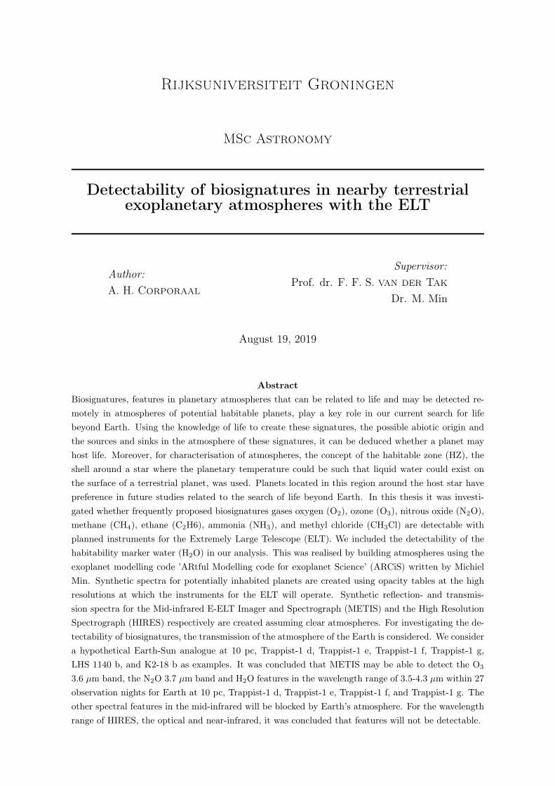
Rijksuniversiteit Groningen

MSc Astronomy

Detectability of biosignatures in nearby terrestrialexoplanetary atmospheres with the ELT

Author:A. H. Corporaal

Supervisor:Prof. dr. F. F. S. van der Tak

Dr. M. Min

August 19, 2019

AbstractBiosignatures, features in planetary atmospheres that can be related to life and may be detected re-motely in atmospheres of potential habitable planets, play a key role in our current search for lifebeyond Earth. Using the knowledge of life to create these signatures, the possible abiotic origin andthe sources and sinks in the atmosphere of these signatures, it can be deduced whether a planet mayhost life. Moreover, for characterisation of atmospheres, the concept of the habitable zone (HZ), theshell around a star where the planetary temperature could be such that liquid water could exist onthe surface of a terrestrial planet, was used. Planets located in this region around the host star havepreference in future studies related to the search of life beyond Earth. In this thesis it was investi-gated whether frequently proposed biosignatures gases oxygen (O2), ozone (O3), nitrous oxide (N2O),methane (CH4), ethane (C2H6), ammonia (NH3), and methyl chloride (CH3Cl) are detectable withplanned instruments for the Extremely Large Telescope (ELT). We included the detectability of thehabitability marker water (H2O) in our analysis. This was realised by building atmospheres using theexoplanet modelling code ’ARtful Modelling code for exoplanet Science’ (ARCiS) written by MichielMin. Synthetic spectra for potentially inhabited planets are created using opacity tables at the highresolutions at which the instruments for the ELT will operate. Synthetic reflection- and transmis-sion spectra for the Mid-infrared E-ELT Imager and Spectrograph (METIS) and the High ResolutionSpectrograph (HIRES) respectively are created assuming clear atmospheres. For investigating the de-tectability of biosignatures, the transmission of the atmosphere of the Earth is considered. We considera hypothetical Earth-Sun analogue at 10 pc, Trappist-1 d, Trappist-1 e, Trappist-1 f, Trappist-1 g,LHS 1140 b, and K2-18 b as examples. It was concluded that METIS may be able to detect the O3

3.6 µm band, the N2O 3.7 µm band and H2O features in the wavelength range of 3.5-4.3 µm within 27observation nights for Earth at 10 pc, Trappist-1 d, Trappist-1 e, Trappist-1 f, and Trappist-1 g. Theother spectral features in the mid-infrared will be blocked by Earth’s atmosphere. For the wavelengthrange of HIRES, the optical and near-infrared, it was concluded that features will not be detectable.

Acknowledgements

Foist of all, I would like to thank my thesis supervisors, Floris van der Tak and Michiel Min, fortheir assistance during this thesis. You were available for questions when I needed help with concepts,analysis or understanding codes. Thank you for giving opportunities to develop myself with oralpresentations and with research skills. I would like to acknowledge Migo Müller as the second reader ofthis thesis. Thanks for willing to read this thesis. I would like to thank the master students from room0134 for the fruitful (related and unrelated) discussions, the motivation and the scientific support ingood times and in tougher times.

I would like to thank the Kapteyn Astronomical Institute in general for educating me, for a greatambiance and for being a place were I could develop myself scientifically.

Last but not least, I want to thank my mom, my brother and my neighbours from number 64for providing continuous encouragement and emotional support. Not only throughout this thesis butduring my years of study, during my whole life, you have always been there for me. This thesis wouldnot have been possible without you.

1

Contents

1 Introduction 41.1 Exoplanets . . . . . . . . . . . . . . . . . . . . . . . . . . . . . . . . . . . . . . . . . . . 41.2 Life . . . . . . . . . . . . . . . . . . . . . . . . . . . . . . . . . . . . . . . . . . . . . . . 6

1.2.1 Definitions of life . . . . . . . . . . . . . . . . . . . . . . . . . . . . . . . . . . . . 61.2.2 Habitability and the habitable zone . . . . . . . . . . . . . . . . . . . . . . . . . 6

1.3 Biosignatures . . . . . . . . . . . . . . . . . . . . . . . . . . . . . . . . . . . . . . . . . . 91.3.1 Gaseous biosignatures . . . . . . . . . . . . . . . . . . . . . . . . . . . . . . . . . 101.3.2 Surface biosignatures . . . . . . . . . . . . . . . . . . . . . . . . . . . . . . . . . . 171.3.3 Temporal biosignatures . . . . . . . . . . . . . . . . . . . . . . . . . . . . . . . . 191.3.4 Antibiosignatures . . . . . . . . . . . . . . . . . . . . . . . . . . . . . . . . . . . . 21

1.4 Temperatures of planets . . . . . . . . . . . . . . . . . . . . . . . . . . . . . . . . . . . . 211.5 Goals and outline of this thesis . . . . . . . . . . . . . . . . . . . . . . . . . . . . . . . . 22

2 Characterisation of planetary atmospheres 232.1 Detection techniques for exoplanetary atmospheres . . . . . . . . . . . . . . . . . . . . . 23

2.1.1 Transit method, secondary eclipses and phase curves . . . . . . . . . . . . . . . . 232.1.2 Direct imaging . . . . . . . . . . . . . . . . . . . . . . . . . . . . . . . . . . . . . 25

2.2 The Extremely Large Telescope (ELT) . . . . . . . . . . . . . . . . . . . . . . . . . . . . 272.2.1 Exoplanet Imaging Camera and Spectrograph (EPICS) . . . . . . . . . . . . . . 282.2.2 Mid-infreared E-ELT Imager and Spectrograph (METIS) . . . . . . . . . . . . . 282.2.3 High Resolution Spectrograph (HIRES) . . . . . . . . . . . . . . . . . . . . . . . 29

2.3 The HITRAN molecular spectroscopic database . . . . . . . . . . . . . . . . . . . . . . . 30

3 Method 323.1 ARtful Modelling Code for exoplanetary Science (ARCiS) . . . . . . . . . . . . . . . . . 323.2 The Habitable Exoplanets Catalog . . . . . . . . . . . . . . . . . . . . . . . . . . . . . . 36

3.2.1 The Earth Similarity Index (ESI) . . . . . . . . . . . . . . . . . . . . . . . . . . . 373.2.2 The Habitable Zone Distance (HZD) . . . . . . . . . . . . . . . . . . . . . . . . . 373.2.3 The Habitability Zone Composition (HZC) . . . . . . . . . . . . . . . . . . . . . 373.2.4 The Habitable Zone Atmosphere (HZA) . . . . . . . . . . . . . . . . . . . . . . . 383.2.5 The Standard Primary Habitability (SPH) . . . . . . . . . . . . . . . . . . . . . 383.2.6 Planetary Mass Classification (PMC) . . . . . . . . . . . . . . . . . . . . . . . . 393.2.7 Planetary Thermal Classification (PTC) . . . . . . . . . . . . . . . . . . . . . . . 39

3.3 Simulated noise . . . . . . . . . . . . . . . . . . . . . . . . . . . . . . . . . . . . . . . . . 403.4 Detectability . . . . . . . . . . . . . . . . . . . . . . . . . . . . . . . . . . . . . . . . . . 41

2

4 Results 434.1 Simple isothermal atmosphere consisting of one gas . . . . . . . . . . . . . . . . . . . . . 43

4.1.1 Effect of the surface pressure . . . . . . . . . . . . . . . . . . . . . . . . . . . . . 444.1.2 Effect of the surface temperature . . . . . . . . . . . . . . . . . . . . . . . . . . . 46

4.2 Atmosphere with realistic P-T profile for one gas . . . . . . . . . . . . . . . . . . . . . . 474.2.1 Effect of surface pressure . . . . . . . . . . . . . . . . . . . . . . . . . . . . . . . 494.2.2 Effect of surface temperature . . . . . . . . . . . . . . . . . . . . . . . . . . . . . 52

4.3 Atmosphere consisting of a mixture of gases . . . . . . . . . . . . . . . . . . . . . . . . . 524.3.1 Molecules with a constant mixing ratio throughout the atmosphere . . . . . . . . 524.3.2 Molecules distributed vertically throughout the atmosphere like Earth . . . . . . 75

4.4 Atmospheres and detectability for some known planets . . . . . . . . . . . . . . . . . . . 804.4.1 HIRES . . . . . . . . . . . . . . . . . . . . . . . . . . . . . . . . . . . . . . . . . . 824.4.2 METIS . . . . . . . . . . . . . . . . . . . . . . . . . . . . . . . . . . . . . . . . . 85

4.5 Photon noise and Optimal resolution for characterising atmospheres with the ELT . . . 87

5 Discussion 89

6 Conclusion 926.1 Plans for the near future . . . . . . . . . . . . . . . . . . . . . . . . . . . . . . . . . . . . 92

3

Chapter 1

Introduction

The concept of life beyond Earth has been around for centuries. This has led to the hope of findinginhabited extrasolar planets and identifying whether we are alone. This interest has brought us tofind and characterise exoplanets around nearby stars. The first scientific paper related to the searchof alien life was published halfway the twentieth century. In their paper Cocconi and Morrison (1959)suggested to look for radio signals around the 21 cm line of neutral hydrogen to hunt for intelligent lifeforms on planets orbiting nearby stars (within 15 light years). In that way, they suggested, we wouldbe able communicate with those civilisations.

Remotely detecting life was first proposed in the 1960s for Solar System planets (Lederberg, 1965).It was realised that the environment, including the atmosphere, on Earth is altered by the presence oflife. This could therefore also have happened on other planets. A mature biosphere may change bothatmospheric and surface properties of a planet and these may be remotely detectable because of theinfluence life may have on the atmospheric composition (Lovelock, 1965, 1975). To date, telescopes areplanned and designed such that a biosphere may be remotely detectable. Before these telescopes areused to observe planetary systems outside the Solar System, a theoretical framework for interpretingthe data is needed (Lovelock, 1975).

One of the interesting questions that is tried to be answered in the exoplanet community is whetherexoplanets host life. Not necessarily intelligent life is considered to hunt for but signs of all life formsare subject of modern studies. The first proof of planets around other stars than the Sun came in1995 when 51 Pegasi b, a hot-Jupiter orbiting around the main-sequence star 51 Pegasi, was discoveredby Mayor and Queloz (1995). The first discovery of an exoplanet, however, came three years earlierwhen Wolszczan and Frail discovered exoplanets orbiting the pulsar PSR 1257+12 (Wolszczan & Frail,1992). The first Earth-sized planet located at such a distance from the star that it is located in theHabitable Zone (HZ) of that star was discovered in 2014 (Quitana et al., 2014). They reported thediscovery of Kepler-186f transiting an M-dwarf.

1.1 Exoplanets

The search for and characterisation of extrasolar planets, or exoplanets, planets orbiting other starsthan our Sun, are of importance for the goal and interest of finding life elsewhere. Finding life goesbeyond the detection of exoplanets. With 4106 confirmed exoplanets identified in August 20191, thefield is moving from the detection of exoplanets to the characterisation of exoplanets. Fig. (1.1) showsthe year of the planetary detection versus the planetary mass in units of Jupiter masses. The blackhorizontal line indicates the mass of Earth (1 M⊕). It can be seen that roughly 1% of the planets has

1exoplanet.eu

4

a mass of 1 M⊕ or less. This subset of all planets are discovered in the last decade. The distribution ofmasses also shows that there are planets more massive than Jupiter (i.e. >1 Mjup, roughly 300 M⊕).Most of these gaseous planets are orbiting close (within 0.01 AU) to their host star (hot Jupiters).Moreover, some of the newly discovered worlds have masses between the masses of Neptune and Earth(Super-Earths). These planets are only categorised by their mass. Super-Earths masses between 1 M⊕

and 10 M⊕ where the upper limit is somewhat arbitrary. At 10 M⊕ a planet can either be rocky orgaseous. To infer a first estimate of the composition of the planet, both the planetary mass and theradius need to be known (Kaltenegger, 2017). The discovery of these hot Jupiters and Super-Earthsreveal that there are populations of planets without a Solar System counterpart. The diversity ofexoplanets exceeds the planetary environments known from our own Solar System.

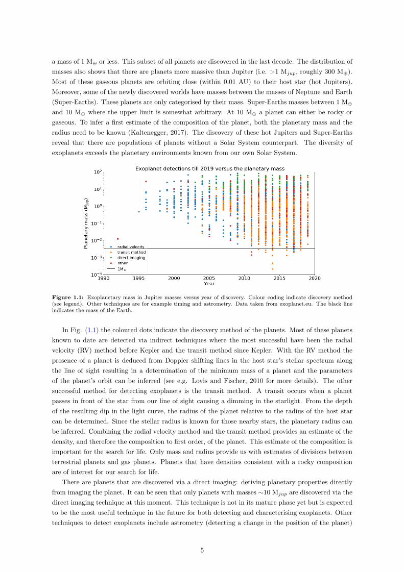
Figure 1.1: Exoplanetary mass in Jupiter masses versus year of discovery. Colour coding indicate discovery method(see legend). Other techniques are for example timing and astrometry. Data taken from exoplanet.eu. The black lineindicates the mass of the Earth.

In Fig. (1.1) the coloured dots indicate the discovery method of the planets. Most of these planetsknown to date are detected via indirect techniques where the most successful have been the radialvelocity (RV) method before Kepler and the transit method since Kepler. With the RV method thepresence of a planet is deduced from Doppler shifting lines in the host star’s stellar spectrum alongthe line of sight resulting in a determination of the minimum mass of a planet and the parametersof the planet’s orbit can be inferred (see e.g. Lovis and Fischer, 2010 for more details). The othersuccessful method for detecting exoplanets is the transit method. A transit occurs when a planetpasses in front of the star from our line of sight causing a dimming in the starlight. From the depthof the resulting dip in the light curve, the radius of the planet relative to the radius of the host starcan be determined. Since the stellar radius is known for those nearby stars, the planetary radius canbe inferred. Combining the radial velocity method and the transit method provides an estimate of thedensity, and therefore the composition to first order, of the planet. This estimate of the composition isimportant for the search for life. Only mass and radius provide us with estimates of divisions betweenterrestrial planets and gas planets. Planets that have densities consistent with a rocky compositionare of interest for our search for life.

There are planets that are discovered via a direct imaging: deriving planetary properties directlyfrom imaging the planet. It can be seen that only planets with masses ∼10 Mjup are discovered via thedirect imaging technique at this moment. This technique is not in its mature phase yet but is expectedto be the most useful technique in the future for both detecting and characterising exoplanets. Othertechniques to detect exoplanets include astrometry (detecting a change in the position of the planet)

5

and timing (e.g. pulsar timing by Wolszczan & Frail (1992)).The field of searching for planets continues with the Transiting Exoplanet Survey Satellite (TESS2,

Ricker et al., 2015), Gaia3, the Automated Planet Finder (APF4, Vogt et al., 2014), the Anglo-Australian Planet Search (AAPS5), High Accuracy Radial Velocity Planet Searcher (HARPS6), andmany more. In the meantime, the field of characterising exoplanets matures. In this thesis the focusis on the characterisation of exoplanetary atmospheres rather than on the detection of exoplanets.In particular, the study of exoplanet atmospheres is a way within technological reach to address afundamental question: is there life on other planets? However, there are a lot of hurdles in the searchfor signs of life that can be remotely detectable. Technology for detecting signals is planned but not yetoperating. Besides the observational part, we also do not understand what life really is (e.g. Walker& Davies, 2013) since we only have one example: life on planet Earth.

1.2 Life

1.2.1 Definitions of life

With our small subset of a range of possibilities for life to exist, there is not one particular definition oflife. However, a definition of life is necessary to be able to recognise it if we find it on other planets. Lifeas we know it is carbon based and needs water (H2O) as a solvent. On Earth biochemical reactionsneed liquid H2O as a solvent. H2O is the only solvent we know at the moment that can mediatebiochemical reactions (Cockell et al., 2016). Moreover, both the hydrogen atom and the oxygen atomare in the top three of most abundant species in the universe. Alternative solvents have been discussedwhere the use of liquid ammonia (NH3), methane (CH4), ethane (C2H6) and other organic solvents,formanide and sulfuric acid are speculated (Benner et al., 2004; Schlulze-Makuch and Irwin, 2006).Since we do not know life forms that can use alternative solvents, we do not consider these solvents inthis thesis.

Carbon based life seems to be favoured since the element carbon (C) is an abundant element in theuniverse, and it can form highly complex molecules. On Earth, C is embedded into life forms. However,alternative biochemical life may exist, and it is only based on life as we know it. Of course, we shouldnot limit ourselves to life as we know it but it is a good first step in the search for extraterrestrial life.Referring to the universality of the laws of chemistry and physics three requirements for life can benoted (e.g. Cockell et al., 2016; Schwieterman et al., 2018): (1) a liquid solvent to mediate metabolicreactions, (2) an energy source that can drive metabolic reactions, and (3) a suite of nutrients in orderto build enzymes that can function as a catalyst and to build biomass.

1.2.2 Habitability and the habitable zone

In this thesis, habitability is defined as a measure of the ability of the environment to support andmaintain the activity of one or more organisms (e.g. Cockell et al., 2016). An habitable environmentis therefore an environment which is suitable for the activity of at least one form of life. Note thatit is possible to have on uninhabitable environment on part of the planet. For example, on Earth,such an environment is found in fresh lava flows (Cockell, 2014). A world or environment can eitherbe instantaneously habitable or continuously habitable. Instantaneous habitability refers to the set ofconditions on a planet or environment that can support life on the planet for a part of the geological

2tess.mit.edu3sci.esa.int/gaia4apf.ucolick.org5newt.phys.unsw.edu.au/ cgt/planet/AAPS_Home.html6eso.org/sci/facilities/lasilla/instruments/harps.html

6

time period (i.e. Archean, Proterozic and Phanerozoic, therefore millions of years, see Fig. (1.2) for anoverview of these eons) (Cockell et al., 2016). Continuous habitability refers, however, to the abilityof the planet in general to support life, or at least habitable conditions, somewhere on or in the planetover geological time scales (see Cockell et al., 2016 for a detailed description).

One of the first steps in the remote detection of extraterrestrial life is to find planets located atdistances from the host star such that the planet has a temperature that liquid H2O could exist onthe surface. This forms the basis of the concept of the Habitable Zone (HZ). The concept of the HZwas first proposed by Huang (1959). The HZ, or more conveniently the circumstellar habitable zone,is a circular shell around a star where the planetary temperature could be such that the planet couldsupport liquid H2O on the surface of a terrestrial planet (e.g. Kasting et al., 1993; Kopparapu et al.,2013). Rocky planets in the HZ have priority in follow-up observations for projects concerning thesearch for life on exoplanets since they are considered most likely to host life.

In recent work there are several limits used to constrain the HZ. These limits are set by climaticconstrains. Limits that are generally used for the concept of habitability are the Conservative HabitableZone (CHZ) and the Optimistic Habitable Zone (OHZ). For the CHZ, the outer edge is given by themaximum greenhouse limit: the limit beyond which atmospheric carbon dioxide (CO2) addition cannotprevent oceans to freeze completely. The inner edge is given by the runaway greenhouse limit: thelimit where surface H2O of a planet can completely evaporate because the planet is unable to coolsufficiently to prevent the surface H2O from evaporating. The critical temperature is 647 K for pureH2O (Kasting et al., 2013). This may happen because greenhouse gases present in the atmosphereblock thermal radiation from the planet to the surroundings. This restricts the cooling of the planetwhich leads to evaporating of surface H2O.

The Optimistic Habitable Zone (OHZ) uses as boundaries the Recent Venus (RV) as an inner edgeand Early Mars (EM) as an outer edge. This empirical HZ is based on evidence that both Mars andVenus had liquid H2O on their surface in the past (e.g. Kasting et al., 1993). From observations of theD/H ratio (Donahue et al., 1982) it is estimated that Venus must have had liquid H2O on its surfaceat the moment the Sun was less bright by ∼ 8% of the total luminosity it has today (e.g. Kasting etal., 1993). The RV limit indicates that the inner edge of the HZ is at least 4% farther out than Venusorbital distance (Kasting et al., 2013). Based on the observation that Mars did not have surface H2Oafter about 3.8 Ga ago, the EM limit was set. The limits are such that the HZ of the Sun excludespresent day Venus at a distance of 0.723 AU from the Sun and it includes present day Mars. A planetlocated in the HZ does not imply that life is possible or exists on that planet but it is the region whereliquid water is possible on the surface of a geologically active rocky planet.

For different stellar spectral types and different stellar ages, the spectral energy distribution (SED)changes: for cooler stars the peak of the radiation shifts toward longer wavelengths while for hotterstars this peak shifts to smaller wavelengths. The shift in the peak makes that a cooler star is moreefficient in heating an Earth-like planet, partly because of Rayleigh scattering and partly becauseof near infrared (near-IR) H2O and CO2 absorption (Kaltenegger, 2017). The effect of Rayleighscattering (i.e. elastic scattering of radiation by particles smaller than ∼ 1/10 times the wavelengthof this radiation) decreases at longer wavelengths. The other effect that occurs for a cooler star isthat there is an increase in near-IR absorption by H2O and CO2. This leads to the finding that forthe same incident stellar flux at a planet surrounding a cool star and a planet orbiting a hot star, theplanet around the cool star will be heated more efficiently. The age of the main sequence star mattersbecause as the stellar age increases, the luminosity of the star increases. Therefore, the limits of theHZ change with stellar age. Moreover, stellar activity such as stellar magnetic field evolution has effectof the stellar emission at ultraviolet (UV) and X-ray wavelengths (Catling et al., 2018). Since the HZof M dwarfs are close to the host star, the planets in this region have to deal with intense radiation,

7

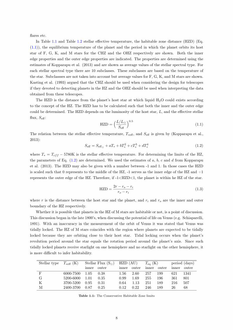
flares etc.In Table 1.1 and Table 1.2 stellar effective temperature, the habitable zone distance (HZD) (Eq.

(1.1)), the equilibrium temperature of the planet and the period in which the planet orbits its hoststar of F, G, K, and M stars for the CHZ and the OHZ respectively are shown. Both the inneredge properties and the outer edge properties are indicated. The properties are determined using theestimates of Kopparapu et al. (2013) and are shown as average values of the stellar spectral type. Foreach stellar spectral type there are 10 subclasses. These subclasses are based on the temperature ofthe star. Subclassses are not taken into account but average values for F, G, K, and M stars are shown.Kasting et al. (1993) argued that the CHZ should be used when considering the design for telescopesif they devoted to detecting planets in the HZ and the OHZ should be used when interpreting the dataobtained from these telescopes.

The HZD is the distance from the planet’s host star at which liquid H2O could exists accordingto the concept of the HZ. The HZD has to be calculated such that both the inner and the outer edgecould be determined. The HZD depends on the luminosity of the host star, L, and the effective stellarflux, Seff :

HZD =(L/L�

Seff

)0.5

(1.1)

The relation between the stellar effective temperature, T∗eff , and Seff is given by (Kopparapu et al.,2013):

Seff = Seff� + aT∗ + bT 2∗ + cT 3

∗ + dT 4∗ (1.2)

where T∗ = Teff − 5780K is the stellar effective temperature. For determining the limits of the HZ,the parameters of Eq. (1.2) are determined. We used the estimates of a, b, c and d from Kopparapuet al. (2013). The HZD may also be given with a number between -1 and 1. In those cases the HZDis scaled such that 0 represents to the middle of the HZ, -1 serves as the inner edge of the HZ and +1represents the outer edge of the HZ. Therefore, if -1<HZD<1, the planet is within he HZ of the star.

HZD =2r − ro − riro − ri

(1.3)

where r is the distance between the host star and the planet, and ri and ro are the inner and outerboundary of the HZ respectively.

Whether it is possible that planets in the HZ of M stars are habitable or not, is a point of discussion.This discussion began in the late 1800’s, when discussing the potential of life on Venus (e.g. Schiaparelli,1891). With an inaccuracy in the measurement of the orbit of Venus it was stated that Venus wastidally locked. The HZ of M stars coincides with the region where planets are expected to be tidallylocked because they are orbiting close to their host star. Tidal locking occurs when the planet’srevolution period around the star equals the rotation period around the planet’s axis. Since suchtidally locked planets receive starlight on one hemisphere and no starlight on the other hemisphere, itis more difficult to infer habitability.

Stellar type T∗eff (K) Stellar Flux (S�) HZD (AU) Teq (K) period (days)inner outer inner outer inner outer inner outer

F 6000-7500 1.05 0.38 1.56 2.60 257 199 621 1341G 5200-6000 1.01 0.35 0.99 1.69 255 196 361 801K 3700-5200 0.95 0.31 0.64 1.13 251 189 216 507M 2400-3700 0.87 0.25 0.12 0.22 246 189 26 68

Table 1.1: The Conservative Habitable Zone limits

8

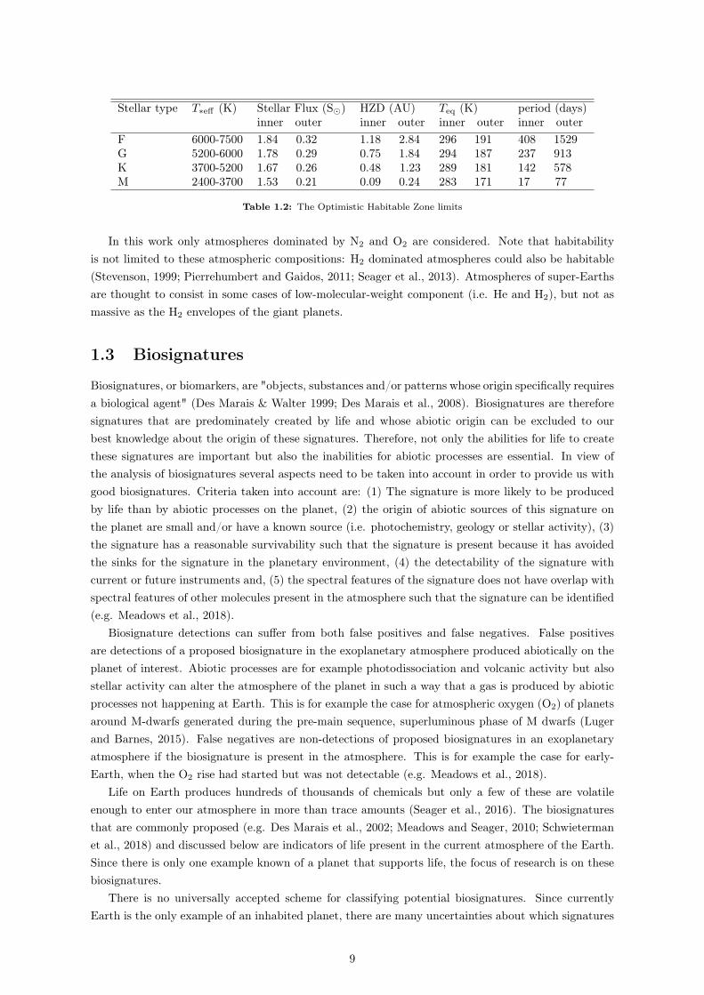
Stellar type T∗eff (K) Stellar Flux (S�) HZD (AU) Teq (K) period (days)inner outer inner outer inner outer inner outer

F 6000-7500 1.84 0.32 1.18 2.84 296 191 408 1529G 5200-6000 1.78 0.29 0.75 1.84 294 187 237 913K 3700-5200 1.67 0.26 0.48 1.23 289 181 142 578M 2400-3700 1.53 0.21 0.09 0.24 283 171 17 77

Table 1.2: The Optimistic Habitable Zone limits

In this work only atmospheres dominated by N2 and O2 are considered. Note that habitabilityis not limited to these atmospheric compositions: H2 dominated atmospheres could also be habitable(Stevenson, 1999; Pierrehumbert and Gaidos, 2011; Seager et al., 2013). Atmospheres of super-Earthsare thought to consist in some cases of low-molecular-weight component (i.e. He and H2), but not asmassive as the H2 envelopes of the giant planets.

1.3 Biosignatures

Biosignatures, or biomarkers, are "objects, substances and/or patterns whose origin specifically requiresa biological agent" (Des Marais & Walter 1999; Des Marais et al., 2008). Biosignatures are thereforesignatures that are predominately created by life and whose abiotic origin can be excluded to ourbest knowledge about the origin of these signatures. Therefore, not only the abilities for life to createthese signatures are important but also the inabilities for abiotic processes are essential. In view ofthe analysis of biosignatures several aspects need to be taken into account in order to provide us withgood biosignatures. Criteria taken into account are: (1) The signature is more likely to be producedby life than by abiotic processes on the planet, (2) the origin of abiotic sources of this signature onthe planet are small and/or have a known source (i.e. photochemistry, geology or stellar activity), (3)the signature has a reasonable survivability such that the signature is present because it has avoidedthe sinks for the signature in the planetary environment, (4) the detectability of the signature withcurrent or future instruments and, (5) the spectral features of the signature does not have overlap withspectral features of other molecules present in the atmosphere such that the signature can be identified(e.g. Meadows et al., 2018).

Biosignature detections can suffer from both false positives and false negatives. False positivesare detections of a proposed biosignature in the exoplanetary atmosphere produced abiotically on theplanet of interest. Abiotic processes are for example photodissociation and volcanic activity but alsostellar activity can alter the atmosphere of the planet in such a way that a gas is produced by abioticprocesses not happening at Earth. This is for example the case for atmospheric oxygen (O2) of planetsaround M-dwarfs generated during the pre-main sequence, superluminous phase of M dwarfs (Lugerand Barnes, 2015). False negatives are non-detections of proposed biosignatures in an exoplanetaryatmosphere if the biosignature is present in the atmosphere. This is for example the case for early-Earth, when the O2 rise had started but was not detectable (e.g. Meadows et al., 2018).

Life on Earth produces hundreds of thousands of chemicals but only a few of these are volatileenough to enter our atmosphere in more than trace amounts (Seager et al., 2016). The biosignaturesthat are commonly proposed (e.g. Des Marais et al., 2002; Meadows and Seager, 2010; Schwietermanet al., 2018) and discussed below are indicators of life present in the current atmosphere of the Earth.Since there is only one example known of a planet that supports life, the focus of research is on thesebiosignatures.

There is no universally accepted scheme for classifying potential biosignatures. Since currentlyEarth is the only example of an inhabited planet, there are many uncertainties about which signatures

9

can be signs of life on planets other than the Earth. One scheme is suggested by Meadows (2006, 2008)who proposed to group proposed biosignatures in how they will likely be revealed to the observer.This resulted in three kinds of biosignatures: gaseous-, surface-, and temporal biosignatures. Gaseousbiosignatures are direct or indirect products of chemical processes that take place in bodies of livingorganisms that help to maintain life (Meadows, 2006; 2008). Gaseous biosignatures are based on gasesbeing present in the atmosphere in thermodynamic disequilibrium (e.g., Lovelock, 1965; Lippincott etal., 1967; Meadows et al., 2018). Finding gaseous biosignatures in abundances inconsistent with ther-modynamic equilibrium will be suggestive of life altering the planetary atmosphere. For an overview ofhow thermodynamic disequilibrium works and is maintained in Earth’s atmosphere see Kleidon (2012).

Surface biosignatures are spectral features that can be related to radiation reflected or scatteredby life forms. Temporal biosignature are time-dependent modulations of gases or other signatures thatare present in measurable quantities that can be linked to biological activity and may be remotelyobservable (Meadows, 2006; 2008). These three kinds of biosignatures are discussed below. Indicatedare the signatures that are related to the classes.

1.3.1 Gaseous biosignatures

1.3.1.1 Oxygen (O2)

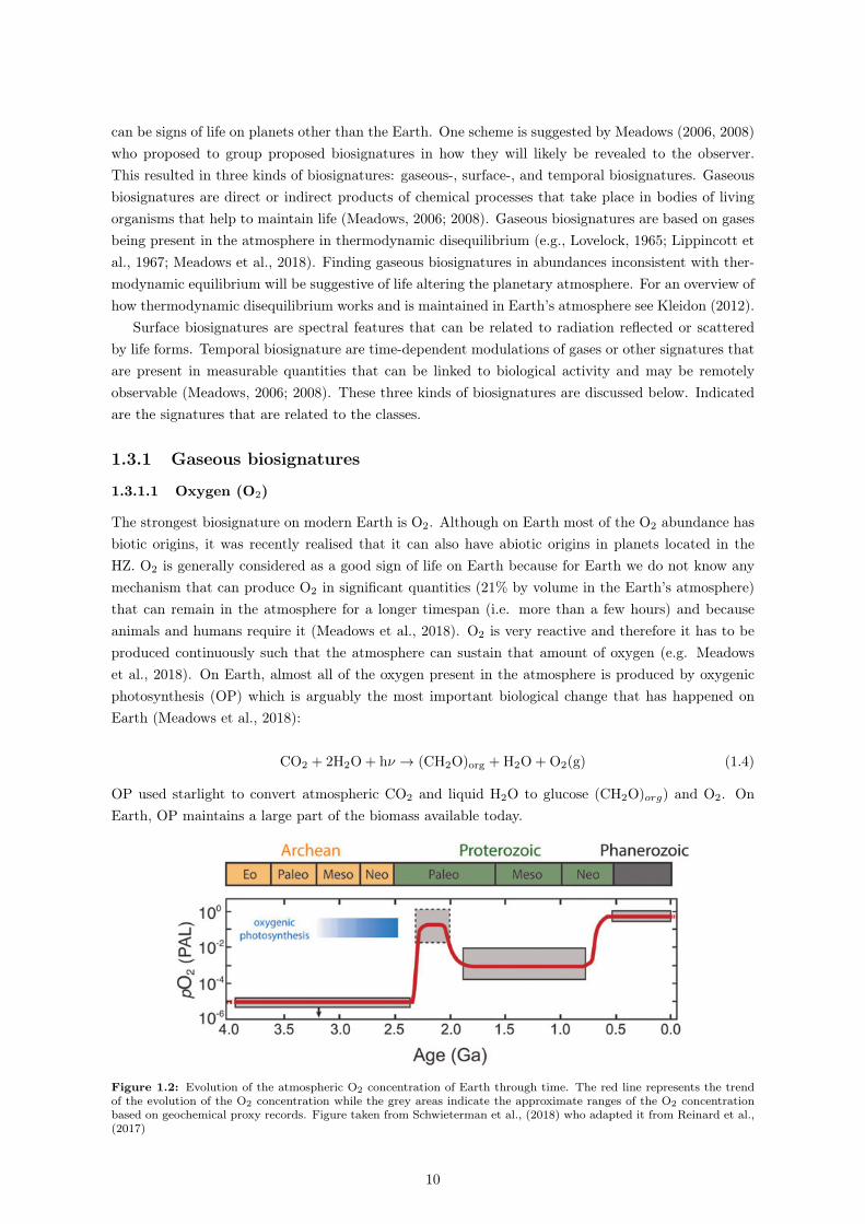
The strongest biosignature on modern Earth is O2. Although on Earth most of the O2 abundance hasbiotic origins, it was recently realised that it can also have abiotic origins in planets located in theHZ. O2 is generally considered as a good sign of life on Earth because for Earth we do not know anymechanism that can produce O2 in significant quantities (21% by volume in the Earth’s atmosphere)that can remain in the atmosphere for a longer timespan (i.e. more than a few hours) and becauseanimals and humans require it (Meadows et al., 2018). O2 is very reactive and therefore it has to beproduced continuously such that the atmosphere can sustain that amount of oxygen (e.g. Meadowset al., 2018). On Earth, almost all of the oxygen present in the atmosphere is produced by oxygenicphotosynthesis (OP) which is arguably the most important biological change that has happened onEarth (Meadows et al., 2018):

CO2 + 2H2O + hν → (CH2O)org + H2O + O2(g) (1.4)

OP used starlight to convert atmospheric CO2 and liquid H2O to glucose (CH2O)org) and O2. OnEarth, OP maintains a large part of the biomass available today.

Figure 1.2: Evolution of the atmospheric O2 concentration of Earth through time. The red line represents the trendof the evolution of the O2 concentration while the grey areas indicate the approximate ranges of the O2 concentrationbased on geochemical proxy records. Figure taken from Schwieterman et al., (2018) who adapted it from Reinard et al.,(2017)

10

Thus, O2 is present in detectable quantities in the atmosphere of Earth. O2 and is considered as aremotely detectable sign of life for Earth. However, if O2 is detected on a planet, it does not necessarilymean that O2 has biotic origins. O2 detections may suffer from false positives and false negatives. Newinsights in the production of O2 both on other planets and on our own younger planet showed thatthe idea behind O2 as a biosignature is quite complex. Advances in theoretical work in planet-starinteractions for planets around other stars gave new insight in the atmospheric O2 on early Earthand the potential false negatives related to these and relation between false positive O2 detection andplanets orbiting M-dwarfs. In the 4.6 billion years that the Earth exists, the planet has gone throughdifferent types of atmospheres. The evolution of the abundance of O2 in the atmosphere of the Earthis illustrated in Fig. (1.2). It is suggested that life started very early on in the history of the Earth butthe development of photosynthesis took place much later (Meadows et al., 2018). It seems likely fromisotope measurements that OP had been developed on early Earth before the atmospheric abundanceof O2 was as significant as nowadays (e.g. Czaja et al. 2012; Riding et al., 2014). It was shown thatbetween 3.0 and 2.65 Ga transient low levels of O2 were present in the Earth’s atmosphere which waslikely produced by OP. However, the global accumulation of atmospheric O2 occurred between 2.45and 2.2 Ga (e.g. Farquahar, 2000; Canfield, 2005).

Proposed mechanics for the irreversible O2 rise are the burial and removal of organic carbon from thesurface of the Earth (Kasting, 2001; Lyons et al., 2014), hydrogen escape from the upper atmosphere(Catling et al., 2001), and the evolution of volcanic and tectonic processes at the surface of the planetover a longer time span (i.e. centuries). Abiotic production of O2 is favoured for F and M stars throughphotochemical mechanisms (Domagal-Goldman et al., 2014).

Figure 1.3: Absorption features of oxygen at optical and infrared wavelengths for a temperature of 296 K and a pressureof 1 bar. The line intensities are taken from the HITRAN 2016 database.

Spectroscopically, O2 is one of the few biotic gases on Earth that has strong bands in the optical.Fig. (1.3) shows the optical, near-IR and mid-IR absorption as a function of wavelength. Since theExtremely Large Telescope (ELT) does not have instruments planned that can either go to lower orhigher wavelengths, those wavelengths longer or shorter than the optical or mid-IR are not of interestfor this thesis. In this wavelength range of interest, O2 has the γ band at 0.628 µm, a band at 0.688µm dubbed the B-band, the strong A-band at 0.762 µm, and the band at 1.269 µm called the a 1δg

(Gordon et al., 2017). Besides this region of interest, O2 has strong bands at wavelengths < 0.2µm,i.e. in the far-ultraviolet (far-UV).

The detectability of the O2 A-band has been explored several times. Snellen et al. (2013) andRodler & López-Morales (2014) investigated this for nearby transiting planets orbiting around M

11

stars. These measurements can be of great importance for transiting rocky planets in the habitablezone of M dwarfs but it is only limited to transiting planets.

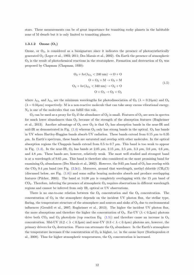
1.3.1.2 Ozone (O3)

Ozone, or O3, is considered as a biosignature since it indicates the presence of photosyntheticallygenerated O2 (Leger et al., 1993; 2011; Des Marais et al., 2002). On Earth the presence of atmosphericO3 is the result of photochemical reactions in the stratosphere. Formation and destruction of O3 wasproposed by Chapman (Chapman, 1930):

O2 + hν(λO2< 240 nm)→ O + O

O + O2 + M→ O3 + M

O3 + hν(λO3 < 340 nm)→ O2 + O

O + O3 → O2 + O2

(1.5)

where λO2 and λO3 are the minimum wavelengths for photodissociation of O2 (λ = 0.24µm) and O3

(λ = 0.34µm) respectively. M is a non-reactive molecule that can take away excess vibrational energy.N2 is one of the molecules that can fulfill this role.

O3 can be used as a proxy for O2 if the abundance of O2 is small. Features of O3 are seen in spectrafor much lower abundances than O2 because of the strength of the absorption features (Rugheimeret al., 2013). Another advantage of O3 over O2 is that O3 has absorption bands in the near-IR andmid-IR as demonstrated in Fig. (1.4) whereas O2 only has strong bands in the optical. O3 has bandsin UV where Hartley-Huggins bands absorb UV radiation. These bands extend from 0.15 µm to 0.35µm. In Earth’s spectrum, these bands are saturated and overlap with other molecules. In the opticalabsorption regions the Chappuis bands extend from 0.5 to 0.7 µm. This band is too weak to appearin Fig. (1.4). In the near-IR, O3 has bands at 2.05 µm, 2.15 µm, 2.5 µm, 3.3 µm, 3.6 µm, 4.6 µm,and 4.8 µm. These bands are, however, relatively weak. The most well studied and strongest bandis at a wavelength of 9.65 µm. This band is therefore also considered as the most promising band forexamining O3 abundances (Des Marais et al., 2002). However, the 9.65 µm band of O3 has overlap withthe CO2 9.4 µm band (see Fig. (2.3c)). Moreover, around that wavelength, methyl chloride (CH3Cl)(discussed below, see Fig. (1.8)) and some sulfur bearing molecules absorb and produce overlappingfeatures (Pilcher, 2003). The band at 14.08 µm is completely overlapping with the 15 µm band ofCO2. Therefore, inferring the presence of atmospheric O3 requires observations in different wavelengthregions and cannot be inferred from only IR, optical or UV observations.

There is no one-to-one relation between the O2 concentration and the O3 concentration. Theconcentration of O3 in the atmosphere depends on the incident UV photon flux, the stellar type,flaring, the temperature structure of the atmosphere and sources and sinks of O3 due to environmentalinfluences (Grenfell et al., 2007; Rugheimer et al., 2013). The higher the incident UV photon flux,the more absorptions and therefore the higher the concentration of O3. Far-UV (λ < 0.2µm) photonsdrive both CO2 and O2 photolysis (top reaction Eq. (1.5)) and therefore cause an increase in O3

concentration. Mid-UV (0.2 < λ < 0.3µm) and near-UV (0.3 < λ < 0.4µm) photons are, however, theprimary drivers for O3 destruction. Flares can attenuate the O3 abundance. In the Earth’s atmospherethe temperature increases if the concentration of O3 is higher, i.e. in the ozone layer (Stathopoulou etal., 2008). Thus for higher atmospheric temperatures, the O3 concentration is increased.

12

Figure 1.4: Absorption features of O3 at optical and infrared wavelengths for a temperature of 296 K and a pressureof 1 bar. The line intensities are taken from the HITRAN 2016 database.

Abiotic production of O3 results, like for O2, from photochemical mechanisms. The study byDomagal-Goldman et al. (2014) demonstrated that this abiotic production is favoured around M- andF-dwarfs.

1.3.1.3 Nitrous oxide (N2O)

Nitrous oxide, or N2O, is considered as a strong biosignature if it is present in terrestrial planetatmospheres in combination with O2. It is considered as a biosignature because it is present in Earth’satmosphere at high disequilibrium abundances, it has only small abiotic sources on modern Earth,and it has potentially detectable spectral features (e.g. Sagan et al., 1993; Segura et al., 2005). Bioticsources of N2O include algae and bacteria producing N2O via an incomplete conversion of soil andoceanic NO−

3 to N2 gas (Sagan et al., 1993, Schwieterman et al., 2018). A simplified reaction can bedescribed by:

NO−3 → NO−

2 → NO + N2O→ N2 (1.6)

Figure 1.5: Absorption features of N2O at optical and infrared wavelengths for a temperature of 296 K and a pressureof 1 bar. The line intensities are from the HITRAN 2016 database.

The preindustrial abundance of N2O was about 270 ppb (Myhre et al., 2013). During portionsof the Proterozoic epoch (i.e. between 2.5 and 0.5 Ga) H2O that was both anoxic and sulphuric

13

(i.e. euxinic, deplete with hydrogen sulfide) ensured that the last step in denitration was facilitated(i.e. reduction of N2O→ N2) (Schwieterman et al., 2018). This in turn allowed N2O to build up inEarth’s atmosphere in concentrations that could impact the climate (Roberson et al., 2011). Fromphotochemical modelling of rocky planets orbiting around M stars it was shown that N2O would beable to build up to higher concentrations than an Earth-Sun analogue due to lack of UV photons ofthose cool stars (e.g. Segura et al., 2005).

Sinks for N2O include photodissociation with an atmospheric lifetime of about half a century.Abiotic sources on Earth include lightning (Levine et al., 1979) and chemodenitrification happeningin Antarctica. For the latter the available NO−

3 needed for this requires O2 from OP (Samarkin et al.,2010). After all, this abiotic source is coming from biological activity on Earth.

N2O has spectral features at wavelengths between 1.3 µm and 20 µm as shown in Fig. (1.5). Thestrongest bands are centered at 3.7 µm, 4.5 µm, 7.8 µm, 8.6 µm, and 17 µm while weaker bands arebetween 1.3-2.2 µm and 9.5-10.7 µm. At Earth-like abundances most bands are weak and overlap withH2O (see Fig. (2.3a)), carbon dioxide (see Fig. (2.3c)) and/or methane (see Fig. (1.6)).

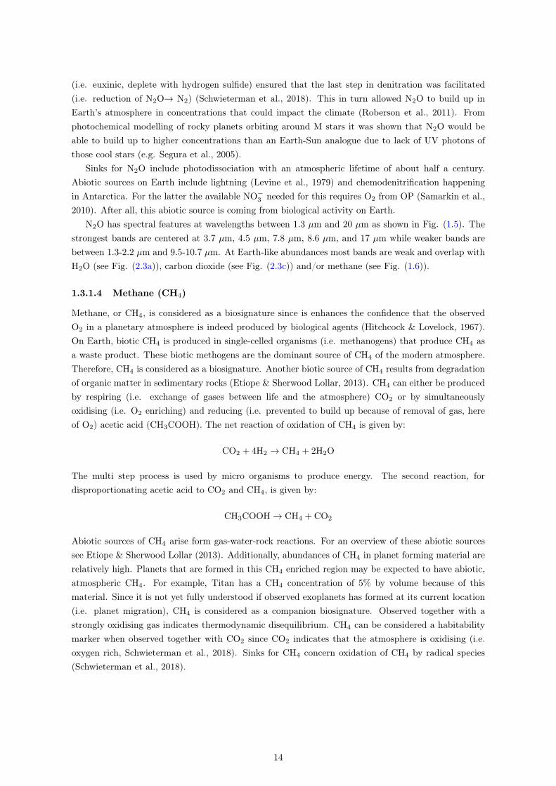
1.3.1.4 Methane (CH4)

Methane, or CH4, is considered as a biosignature since is enhances the confidence that the observedO2 in a planetary atmosphere is indeed produced by biological agents (Hitchcock & Lovelock, 1967).On Earth, biotic CH4 is produced in single-celled organisms (i.e. methanogens) that produce CH4 asa waste product. These biotic methogens are the dominant source of CH4 of the modern atmosphere.Therefore, CH4 is considered as a biosignature. Another biotic source of CH4 results from degradationof organic matter in sedimentary rocks (Etiope & Sherwood Lollar, 2013). CH4 can either be producedby respiring (i.e. exchange of gases between life and the atmosphere) CO2 or by simultaneouslyoxidising (i.e. O2 enriching) and reducing (i.e. prevented to build up because of removal of gas, hereof O2) acetic acid (CH3COOH). The net reaction of oxidation of CH4 is given by:

CO2 + 4H2 → CH4 + 2H2O

The multi step process is used by micro organisms to produce energy. The second reaction, fordisproportionating acetic acid to CO2 and CH4, is given by:

CH3COOH→ CH4 + CO2

Abiotic sources of CH4 arise form gas-water-rock reactions. For an overview of these abiotic sourcessee Etiope & Sherwood Lollar (2013). Additionally, abundances of CH4 in planet forming material arerelatively high. Planets that are formed in this CH4 enriched region may be expected to have abiotic,atmospheric CH4. For example, Titan has a CH4 concentration of 5% by volume because of thismaterial. Since it is not yet fully understood if observed exoplanets has formed at its current location(i.e. planet migration), CH4 is considered as a companion biosignature. Observed together with astrongly oxidising gas indicates thermodynamic disequilibrium. CH4 can be considered a habitabilitymarker when observed together with CO2 since CO2 indicates that the atmosphere is oxidising (i.e.oxygen rich, Schwieterman et al., 2018). Sinks for CH4 concern oxidation of CH4 by radical species(Schwieterman et al., 2018).

14

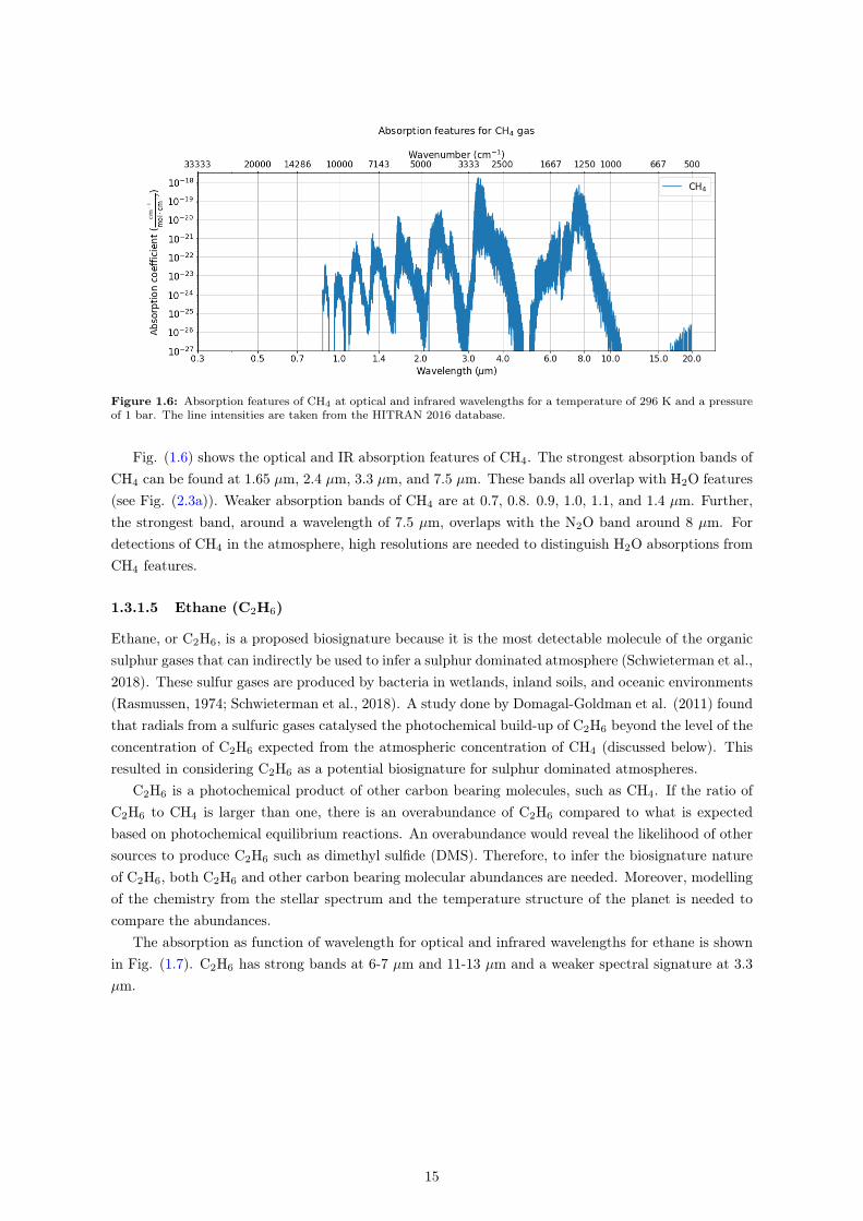
Figure 1.6: Absorption features of CH4 at optical and infrared wavelengths for a temperature of 296 K and a pressureof 1 bar. The line intensities are taken from the HITRAN 2016 database.

Fig. (1.6) shows the optical and IR absorption features of CH4. The strongest absorption bands ofCH4 can be found at 1.65 µm, 2.4 µm, 3.3 µm, and 7.5 µm. These bands all overlap with H2O features(see Fig. (2.3a)). Weaker absorption bands of CH4 are at 0.7, 0.8. 0.9, 1.0, 1.1, and 1.4 µm. Further,the strongest band, around a wavelength of 7.5 µm, overlaps with the N2O band around 8 µm. Fordetections of CH4 in the atmosphere, high resolutions are needed to distinguish H2O absorptions fromCH4 features.

1.3.1.5 Ethane (C2H6)

Ethane, or C2H6, is a proposed biosignature because it is the most detectable molecule of the organicsulphur gases that can indirectly be used to infer a sulphur dominated atmosphere (Schwieterman et al.,2018). These sulfur gases are produced by bacteria in wetlands, inland soils, and oceanic environments(Rasmussen, 1974; Schwieterman et al., 2018). A study done by Domagal-Goldman et al. (2011) foundthat radials from a sulfuric gases catalysed the photochemical build-up of C2H6 beyond the level of theconcentration of C2H6 expected from the atmospheric concentration of CH4 (discussed below). Thisresulted in considering C2H6 as a potential biosignature for sulphur dominated atmospheres.

C2H6 is a photochemical product of other carbon bearing molecules, such as CH4. If the ratio ofC2H6 to CH4 is larger than one, there is an overabundance of C2H6 compared to what is expectedbased on photochemical equilibrium reactions. An overabundance would reveal the likelihood of othersources to produce C2H6 such as dimethyl sulfide (DMS). Therefore, to infer the biosignature natureof C2H6, both C2H6 and other carbon bearing molecular abundances are needed. Moreover, modellingof the chemistry from the stellar spectrum and the temperature structure of the planet is needed tocompare the abundances.

The absorption as function of wavelength for optical and infrared wavelengths for ethane is shownin Fig. (1.7). C2H6 has strong bands at 6-7 µm and 11-13 µm and a weaker spectral signature at 3.3µm.

15

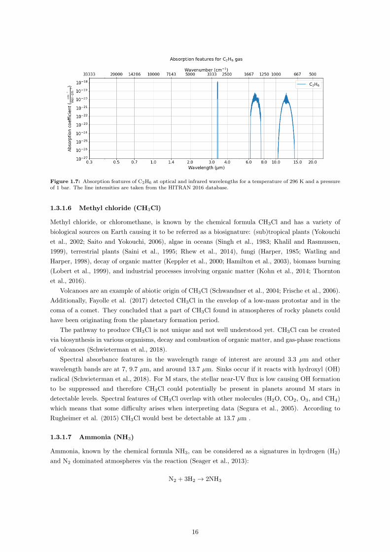
Figure 1.7: Absorption features of C2H6 at optical and infrared wavelengths for a temperature of 296 K and a pressureof 1 bar. The line intensities are taken from the HITRAN 2016 database.

1.3.1.6 Methyl chloride (CH3Cl)

Methyl chloride, or chloromethane, is known by the chemical formula CH3Cl and has a variety ofbiological sources on Earth causing it to be referred as a biosignature: (sub)tropical plants (Yokouchiet al., 2002; Saito and Yokouchi, 2006), algae in oceans (Singh et al., 1983; Khalil and Rasmussen,1999), terrestrial plants (Saini et al., 1995; Rhew et al., 2014), fungi (Harper, 1985; Watling andHarper, 1998), decay of organic matter (Keppler et al., 2000; Hamilton et al., 2003), biomass burning(Lobert et al., 1999), and industrial processes involving organic matter (Kohn et al., 2014; Thorntonet al., 2016).

Volcanoes are an example of abiotic origin of CH3Cl (Schwandner et al., 2004; Frische et al., 2006).Additionally, Fayolle et al. (2017) detected CH3Cl in the envelop of a low-mass protostar and in thecoma of a comet. They concluded that a part of CH3Cl found in atmospheres of rocky planets couldhave been originating from the planetary formation period.

The pathway to produce CH3Cl is not unique and not well understood yet. CH3Cl can be createdvia biosynthesis in various organisms, decay and combustion of organic matter, and gas-phase reactionsof volcanoes (Schwieterman et al., 2018).

Spectral absorbance features in the wavelength range of interest are around 3.3 µm and otherwavelength bands are at 7, 9.7 µm, and around 13.7 µm. Sinks occur if it reacts with hydroxyl (OH)radical (Schwieterman et al., 2018). For M stars, the stellar near-UV flux is low causing OH formationto be suppressed and therefore CH3Cl could potentially be present in planets around M stars indetectable levels. Spectral features of CH3Cl overlap with other molecules (H2O, CO2, O3, and CH4)which means that some difficulty arises when interpreting data (Segura et al., 2005). According toRugheimer et al. (2015) CH3Cl would best be detectable at 13.7 µm .

1.3.1.7 Ammonia (NH3)

Ammonia, known by the chemical formula NH3, can be considered as a signatures in hydrogen (H2)and N2 dominated atmospheres via the reaction (Seager et al., 2013):

N2 + 3H2 → 2NH3

16

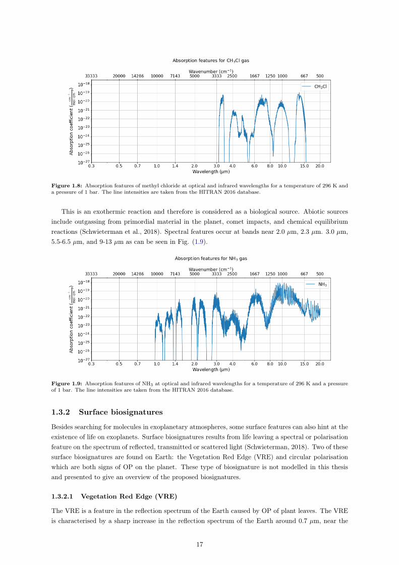
Figure 1.8: Absorption features of methyl chloride at optical and infrared wavelengths for a temperature of 296 K anda pressure of 1 bar. The line intensities are taken from the HITRAN 2016 database.

This is an exothermic reaction and therefore is considered as a biological source. Abiotic sourcesinclude outgassing from primordial material in the planet, comet impacts, and chemical equilibriumreactions (Schwieterman et al., 2018). Spectral features occur at bands near 2.0 µm, 2.3 µm. 3.0 µm,5.5-6.5 µm, and 9-13 µm as can be seen in Fig. (1.9).

Figure 1.9: Absorption features of NH3 at optical and infrared wavelengths for a temperature of 296 K and a pressureof 1 bar. The line intensities are taken from the HITRAN 2016 database.

1.3.2 Surface biosignatures

Besides searching for molecules in exoplanetary atmospheres, some surface features can also hint at theexistence of life on exoplanets. Surface biosignatures results from life leaving a spectral or polarisationfeature on the spectrum of reflected, transmitted or scattered light (Schwieterman, 2018). Two of thesesurface biosignatures are found on Earth: the Vegetation Red Edge (VRE) and circular polarisationwhich are both signs of OP on the planet. These type of biosignature is not modelled in this thesisand presented to give an overview of the proposed biosignatures.

1.3.2.1 Vegetation Red Edge (VRE)

The VRE is a feature in the reflection spectrum of the Earth caused by OP of plant leaves. The VREis characterised by a sharp increase in the reflection spectrum of the Earth around 0.7 µm, near the

17

boundary between optical and near-IR wavelengths. The VRE originates because there is a changein chlorophyll absorption at wavelengths between ∼ 0.65 − 0.70µm and between ∼ 0.75 − 1.10µmwavelengths. Photosynthetic plants are developed in such a way that they absorb effectively opticallight, but reflect IR light. A plant leave is reflective at the latter wavelength range because of thelayered structure of leaves (Seager et al., 2005). This results in an change in index of refractionbetween cells walls. Light can refracts through the cell walls and simultaneously reflect off of the cellwalls (Seager et al., 2005).

For Earth, the VRE was detected in observations of Earth from the Galileo spacecraft (Sagan et al.,1993), and in the Earth-shine spectrum obtained from observations of reflected light from the moon(Arnold et al., 2002; Woolf et al., 2002; Turnbull et al.,2006). From knowledge about the reflectivelyof deserts, oceans, ice, forests etc. it was possible to assign this rise in reflection observed to thevegetation.

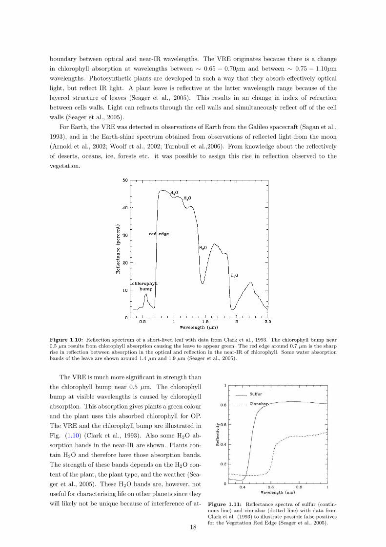
Figure 1.10: Reflection spectrum of a short-lived leaf with data from Clark et al., 1993. The chlorophyll bump near0.5 µm results from chlorophyll absorption causing the leave to appear green. The red edge around 0.7 µm is the sharprise in reflection between absorption in the optical and reflection in the near-IR of chlorophyll. Some water absorptionbands of the leave are shown around 1.4 µm and 1.9 µm (Seager et al., 2005).

Figure 1.11: Reflectance spectra of sulfur (contin-uous line) and cinnabar (dotted line) with data fromClark et al. (1993) to illustrate possible false positivesfor the Vegetation Red Edge (Seager et al., 2005).

The VRE is much more significant in strength thanthe chlorophyll bump near 0.5 µm. The chlorophyllbump at visible wavelengths is caused by chlorophyllabsorption. This absorption gives plants a green colourand the plant uses this absorbed chlorophyll for OP.The VRE and the chlorophyll bump are illustrated inFig. (1.10) (Clark et al., 1993). Also some H2O ab-sorption bands in the near-IR are shown. Plants con-tain H2O and therefore have those absorption bands.The strength of these bands depends on the H2O con-tent of the plant, the plant type, and the weather (Sea-ger et al., 2005). These H2O bands are, however, notuseful for characterising life on other planets since theywill likely not be unique because of interference of at-

18

mospheric H2O vapour.As for the gaseous biosignatures, the VRE may also

suffer from false positives. Seager et al. (2005) indi-cated that semiconductor crystals such as sulfur and cinnabar have similar reflectance edges at 0.45µm and 0.6 µm respectively (see Fig. (1.11)). Therefore, also surface biosignatures must be examinedwith care and other planetary observables need to be taken into context.

1.3.2.2 Circular polarisation

Measurements of both linear and circular polarisation can be used to characterise planetary atmo-spheres (Schwieterman, 2018). Polarisation is the propagation of light as a transverse wave. Thedirection of polarisation is defined by the direction of the electric field vector. Linearly polarisedlight has an electric field vector oscillating in one plane. Circular polarisations refer to the case whenthe magnitude of the factor is constant but the direction of the vector rotates as a function of time.Circular polarisation is a proposed surface biosignature that relies on remotely detecting chirality (orhandedness) of organic molecules (Sparks et al., 2009). Amino acids and sugars both are chiral com-pounds: asymmetric molecules that have a certain handedness. That means that a mirror image ofthese compounds cannot be superimposed on one another. Both amino acids and sugars are opticallyactive in the UV. Chiral compounds prefer to absorb either right handed or left handed circularlypolarised light. Circular polarisation of vegetation has a direct relation to the absorption spectra ofvegetation. However, surfaces without any biotic origin do not have such a relation (Spark et al.,2009). In this way, circular polarisation can be used to infer the presence of liquid H2O on the surface(Schwieterman et al., 2018).

1.3.3 Temporal biosignatures

Temporal signs of life are time-dependent modulations of e.g. the concentration of a certain gas or theplanetary albedo that can be linked to biological activity and may be remotely observable (Meadows,2006; 2008). These modulations can be seasonal, daily or stochastic in such a way that they can belinked to the presence of life on a planet. Temporal biosignatures are not modelled in most studies,including this thesis, since these signatures are more complex to understand than gaseous- and surfacebiosignatures. This is partially because additional planetary properties need to be taken into account.Examples of such properties include the axial tilt of the planet, its eccentricity, the distribution ofcontinents and oceans on the planetary surface, and the presumed response of life on these processes(Schwieterman, 2018). For now, with only one proven example of a planet hosting life available,modulations of atmospheric gases on Earth is taken as an example as a proof of concept.

1.3.3.1 Modulation of atmospheric gases

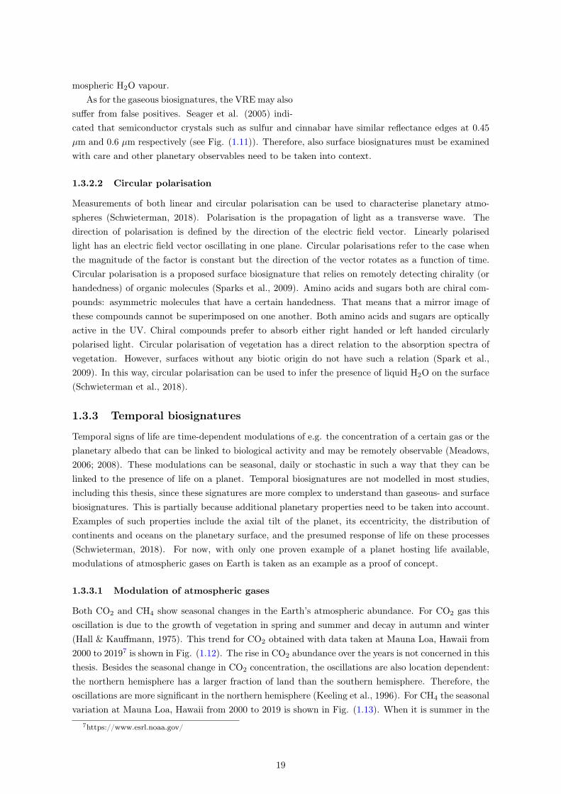
Both CO2 and CH4 show seasonal changes in the Earth’s atmospheric abundance. For CO2 gas thisoscillation is due to the growth of vegetation in spring and summer and decay in autumn and winter(Hall & Kauffmann, 1975). This trend for CO2 obtained with data taken at Mauna Loa, Hawaii from2000 to 20197 is shown in Fig. (1.12). The rise in CO2 abundance over the years is not concerned in thisthesis. Besides the seasonal change in CO2 concentration, the oscillations are also location dependent:the northern hemisphere has a larger fraction of land than the southern hemisphere. Therefore, theoscillations are more significant in the northern hemisphere (Keeling et al., 1996). For CH4 the seasonalvariation at Mauna Loa, Hawaii from 2000 to 2019 is shown in Fig. (1.13). When it is summer in the

7https://www.esrl.noaa.gov/

19

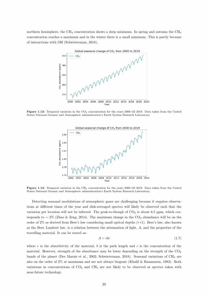
northern hemisphere, the CH4 concentration shows a deep minimum. In spring and autumn the CH4

concentration reaches a maximum and in the winter there is a small minimum. This is partly becauseof interactions with OH (Schwieterman, 2018).

Figure 1.12: Temporal variation in the CO2 concentration for the years 2000 till 2019. Data taken from the UnitedStates National Oceanic and Atmospheric administration’s Earth System Research Laboratory.

Figure 1.13: Temporal variation in the CH4 concentration for the years 2000 till 2019. Data taken from the UnitedStates National Oceanic and Atmospheric administration’s Earth System Research Laboratory.

Detecting seasonal modulations of atmospheric gases are challenging because it requires observa-tions at different times of the year and disk-averaged spectra will likely be observed such that thevariation per location will not be inferred. The peak-to-though of CO2 is about 6.5 ppm, which cor-responds to ∼ 2% (Zhao & Zeng, 2014). The maximum change in the CO2 abundance will be on theorder of 2% as derived from Beer’s law considering small optical depths (τ«1). Beer’s law, also knownas the Beer–Lambert law, is a relation between the attenuation of light, A, and the properties of thetravelling material. It can be stated as:

A = εbc (1.7)

where ε is the absorbtivity of the material, b is the path length and c is the concentration of thematerial. However, strength of the absorbance may be lower depending on the strength of the CO2

bands of the planet (Des Marais et al., 2002; Schwieterman, 2018). Seasonal variations of CH4 arealso on the order of 2% at maximum and are not always biogenic (Khalil & Rasmussen, 1983). Bothvariations in concentrations of CO2 and CH4 are not likely to be observed at spectra taken withnear-future technology.

20

1.3.4 Antibiosignatures

Besides searching for evidence of biological activity on a planet, evidence against the presence of life canalso be helpful in the search for life and the understanding of habitability. These remotely detectablesignatures are called antibiosignatures. Antibiosignatures can be useful to direct the search to morepromising targets and to avoid a false positive claim for the detection of life (Schwieterman et al., 2019).Also, finding uninhabited planets can inform us about the origin of life. An antibiosignature is evidencethat there is currently no life that uses the chemical free energy. Detection of an antibiosignature inan atmosphere does not imply that a planet is not inhabitable but rather that there is currently nolife on the surface of the planet.

One proposed antibiosignature is carbon monoxide (CO). The presence of CO suggests that thereis a source of unexploited chemical free energy present in the atmosphere and reduced carbon (e.g.Ragsdale 2004; Gao et al., 2015; Catling et al., 2018, Schwieterman et al., 2019). Moreover, CO is ableto build up in an atmosphere in the absence of water vapour. Identifying exoplanetary atmospheresincluding antibiosignatures are beyond the scope of this thesis.

1.4 Temperatures of planets

Besides the physical temperature of a planet, the equilibrium temperature is an important conceptrelated to the concept of planetary habitability. Temperature in general is a balance between all heatingand cooling mechanisms present in the system. Heating of a planet results from absorption of radiationfrom the host star and internal heating if available. The stellar radiation a planet receives depends onthe distance between the star and the planet and the luminosity of the host star. Cooling mechanismsare emission of thermal IR radiation which depends on the atmospheric composition and the abilityof the planet to effectively distribute the heat. The atmospheric composition in turn depends on thesources and sinks of the constituent gases and photochemical reactions happening in the planetaryatmosphere. The sources and sinks are linked to the crust material of the planet, whether or not ithas oceans, geological activity, and biological processes if present (Kaltenegger, 2017). The physicaltemperature of the planet is the surface temperature a planet has on average. This temperature ishard to determine for exoplanets with current technology because the physical temperature depends onmultiple quantities which cannot be determined with current instruments. Examples include internalheating, clouds (and therefore the albedo) and rotations.

The equilibrium temperature is the temperature that a planet would have if it is in thermal equi-librium assuming the planet behaves as a blackbody. The equilibrium temperature, Teq, can be de-termined from the balance between incoming stellar radiation from its host star and the amount ofradiation it re-radiates outwards and is given by:

Teq = Ts(1− a)1/4

√Rs2D

(1.8)

Where Ts is the host star’s effective temperature, a is the bond albedo of the planet, Rs is the stellarradius, and D is the semi-major axis. For Earth, Teq=255 K, compared to the surface temperature of288 K. This difference results from greenhouse gases which are present in Earth’s atmosphere. Thisresults in a higher surface temperature compared to the equilibrium temperature.

21

1.5 Goals and outline of this thesis

This thesis builds up a model for exoplanetary atmospheres with the intention to investigate whetherthe biosignature gases O2, O3, N2O, CH4, C2H6, NH3, and CH3Cl are detectable with the ELT.Included in the analysis is the detectabilility of H2O in planetary atmospheres. Moreover, a deter-mination of the optimal resolution for detecting biosignatures in exoplanetary atmospheres and anestimation of the photon noise will be made. Steps taken include investigating multiple atmospherictemperature and pressure structures and the effect of changing abundances of biosignatures. Thiswill be done considering a hypothetical Earth-Sun analogue located at a distance of 10 pc. Moreover,planets that are detected in previous observations that may be Earth-like and are lying in the HZ areconsidered. In Chapter 2 the details of the characterisation of planetary atmospheres will be outlined:the detection techniques used and planned for exoplanetary atmospheres and a description of whichinstruments on the ELT can be used for characterisation of exoplanetary atmospheres. In Chapter 3the method is outlined where after the results are described in Chapter 4. In Chapter 5 these resultsare interpreted with reference to previous studies and in Chapter 6 the conclusions are outlined.

22

Chapter 2

Characterisation of planetaryatmospheres

2.1 Detection techniques for exoplanetary atmospheres

To reach the goal of finding life beyond Earth, a step that needs to be taken is characterising(exo)planetary atmospheres. With current technology this is difficult, because of the extremely lowamplitude signals that an exoplanetary atmosphere provides and the current instrumental limitations.The detection of spectral lines from the atmosphere and knowledge about sources and sinks of moleculesare important for science of biosignatures. However, measurements of spectral lines from atmospheresare only possible with present day instrumentation for two kinds of planets. (1) For young planets stillglowing from their formation that are orbiting far from their host star using direct imaging techniquesand (2) for hot Jupiters orbiting closely their host star using the transit method. These methods arediscussed below.

2.1.1 Transit method, secondary eclipses and phase curves

The most successful technique for the characterisation of exoplanetary atmospheres and for detectingexoplanets to date has been the transit method. A planet can transit its host star from our point ofview such that light is transmitted at different wavelengths according to the wavelength dependentopacities of atmospheric chemical species. A transit obscures the light of the host star by an amountequal to the ratio of planet-to-star area. Using this area and the assumption that both the star andthe planet are spherical bodies, this can be translated to a ratio of planet-to-star radius (see Eq.(2.1)). From previous stellar observations the radius is already known for nearby stars and thereforethe planetary radius can be determined. One advantage of the transit method is that the techniquedoes not depend on the planet-star contrast, but it depends rather on the radii of both the planet andthe star:

∆F = FsR2p

R2s

(2.1)

where Rs and Rp are the stellar and planetary radii respectively, ∆F is the transit depth, and Fs isthe stellar flux. To use the transit method to detect a planet or characterise a planetary atmosphere,a planet has to transit the star from our line of sight in the first place. The probability, p, to transitto first order is given by:

p =Rs +Rp

a(2.2)

23

where a is the orbital semi-major axis of the planet (Borucki & Summers, 1984). From Eq. (2.1) it canbe estimated that the probability that an Earth-sized planet orbiting an G2 star at a distance of 1 AUwill be 0.47%. The probability for Trappist-1 e (R = 0.918 R⊕) transiting its host star Trappist-1(R = 0.117 R�) at a distance of a = 0.02812 AU is, however, about 2%. Therefore, Trappist-1 e ismuch more favourable for observing using transit photometry as compared to an Earth-Sun analogue.

Besides the transit depth the amplitude of the transit, δ,is an important characteristic of a transit.The amplitude of spectral features is given by:

δ =(Rp + nH)2

R2s

−R2p

R2s

≈ 2nRpH

R2s

(2.3)

where n is the number of scale heights crossed at wavelengths with higher opacity and H is theatmospheric scale height: the change in altitude at which the pressure decreases by a factor of e.Assuming an ideal gas law and hydrostatic equilibrium, the scale height can be expressed as:

H =kT

µmhg(2.4)

where k is the Boltzmann constant, T is the planetary surface temperature (or if not known theequilibrium temperature), µ is the mean molecular weight of the constituents of the atmosphere, mh

is the mass of the hydrogen atom, and g is the gravitational acceleration of the planet. Therefore,planets with a high temperature, relatively small host stars, a small gravitational acceleration, andsmall molecular weight of the atmosphere (i.e. gas giants) will have a higher amplitude and willtherefore be more favourable for characterising. Hot Jupiters are the ideal candidates but only haveδ ∼ 0.1% (Kreidberg, 2017). Earth-sized planets around Sun-like stars have an amplitude of about 3orders of magnitude smaller (Kreidberg, 2017). Therefore, studies to detect planets and characterisethe atmospheres favours planets that have orbits of a relatively short amount of time (a few days) inorder to be able to observe multiple transits and be able to extract the spectrum of the atmosphere.When such an event is captured by a telescope, a transmission spectrum can be obtained. Fig. (2.1)shows a transmission spectrum of the Earth as observed from lunar eclipse observations (Pallé et al.,2009). Studying the transmission spectrum of the Earth can be seen as a proxy for observations of atransit of Earth as seen from a planet outside our Solar System.

Figure 2.1: Transmission spectrum of Earth in the optical and near-infrared from observations of a lunar eclipse. Notethat the vertical axis is in units of the relative flux of the star and the planet and not in the planet to stellar radii.Figure adapted from Pallé et al. (2009).

The above description is both important for the detection of planets and the characterisation ofplanetary atmospheres. For a detection a few transits are needed to conclude whether a planet is

24

transiting while characterisation takes more effort. With the wavelength dependent opacities it ispossible to figure out which atoms and molecules are present in a planetary atmosphere. The planetblocks slightly more stellar flux at wavelengths where an atom or a molecule absorbs. The transitdepth is therefore a function of wavelength which results in the transmission spectrum. Variations inabsorption as a function of wavelength are measured by binning the light curve into spectrophotometricchannels.

The geometry of the transit method, the secondary eclipse and the phase curve is illustrated in Fig.(2.2). The transit, the case that a planet passes in front of the star from our point of view, is also calledthe primary eclipse. The secondary eclipse can be observed if a planet passes behind the star fromour point of view. During the secondary eclipse only the stellar spectrum is observed. By combiningobservations of the secondary eclipse and observations of the planet and star just after the secondaryeclipse, the spectrum of the planet alone can be deduced. When observing the complete orbit or phaseof the planet around its host star a phase curve can be inferred. A phase curve is therefore a spectrumwith data taken during the complete orbit. In a phase curve also the primary and secondary eclipsewill be prominent. By analysing a phase curve, not only the orbital parameters can be determined,but also the atmospheric composition can be inferred. Since all intermediate planetary temperaturescan be determined, a phase curve contains information about the heat circulation in the planetaryatmosphere. Since transits are more favourable for planets that orbit their host star close-in and theseplanets are mostly tidally locked (for both hot Jupiters and planets in the HZ of M-dwarfs (e.g. Barnes,2017)), this spectrum corresponds to the day-side of the planet. For tidally locked planets both theday-side and the night-side temperature can be estimated when a phase curve is taken.

Figure 2.2: Schematic of the geometry of a transiting planet. The primary eclipse is also referred to as the transit. Fromobservations following the complete orbit, represented here in black, a phase curve can be deduced. From observationsof the secondary eclipse, the spectrum of the star alone can be made and compared to spectra taken from the star andthe planet together to deduce the (day-side) spectrum of the planet. Figure taken from Seager & Deming, 2010.

2.1.2 Direct imaging

The method that will be most promising for future exoplanetary atmosphere characterisation is thedirect imaging technique. In high contrast imaging, or direct imaging, the point spread function ofa planet is attempted to be distinguished from the host star. The technique relies on the propertythat the planet reflects a portion of the light it receives from the host star. The reflected light from aplanet is observed, which contains information about the composition of the atmosphere. Atmosphericproperties that alter the amount of reflected light are the atmospheric constituents, the clouds, surfacetypes, and aerosols. The latter three atmospheric properties result in the planetary albedo (Tinetti

25

et al., 2009). Direct imaging requires telescopes with a high resolution and a high contrast. Highresolution can be obtained by a large telescope and extreme adaptive optics. High contrast is reachedby including a coronagraph to reduce photon noise. For the high-resolution, high-contrast technique tobe applicable, the star-planet system is spatially resolved and therefore the distance to the star plays acritical role. Exoplanets around stars which are located up to 10 pc away from us are best to considerusing this technique (Traub & Oppenheimer, 2010).

To date, the direct imaging technique is used for young, massive planets on wide orbits. Theseplanets are still glowing from their formation which gives them a high temperature and a large size.These properties result in planet-star flux ratios of about 10−7. Because of the wide orbits, stellarlight can be easier blocked allowing them to be detected. Mature planets have an effective temperaturecomparable to the equilibrium temperature derived from the stellar properties and the distance betweenthe star and the planet. These planets will be fainter in the IR compared to young, massive planets.Moreover, those terrestrial planets in the HZ will be relatively close to their host star (see Table1.1). Direct imaging is a promising technique for characterising exoplanetary atmospheres of terrestrialplanets inside the HZ in the near future. However, because of the small semi-major axis, sub-arcsecondangular resolution is needed to distinguish the stellar light from the scattered light by the planet (Traub& Oppenheimer, 2010).

For some near-future instruments on the ELT the focus will be on reflected light measurements.The measureable quantity is the planet-to-star flux ratio (Fp/Fs). For reflected light measurementsthe flux ratio is given by Eq. (2.5).

Fp(λ, α)

Fs(λ)= Ag(λ)g(α)

(Rpa

)2

(2.5)

where Fp(λ, α) is the reflected spectrum at phase angle α, Fs(λ) is the stellar spectrum as functionof the wavelength, Ag(λ) is the geometric albedo spectrum which is defined by Eq.(2.7), R is theradius of the planet, a is the orbital semi-major axis and g(α) is the phase function. A Lambertiansurface is defined as an absolute white, diffuse surface which reflects all radiation falling upon itisotropically. Therefore, for a Lambertian surface, the brightness is the same in all viewing directions.For a Lambertian surface, the phase function is given by:

g(α) =sinα+ (π − α) cosα

π(2.6)

The geometric albedo, Ag, is defined as the ratio of reflected flux of an object at full phase (α = 0◦),Fp(λ, α = 0), to the flux from a perfect Lambertian disk, F�,L(λ):

Ag =Fp(λ, α = 0◦)

F�,L(λ)(2.7)

The phase angle is defined as the angle between the incident light produced by the star and theradiation of the star that is received by the observer on Earth. In order to obtain reflection spectra,usually the radiance factor, I/F , is determined. I is the reflected intensity at a given wavelength andviewing angle, and πF is the incident stellar flux density upon the planet at a specific wavelength (dePater and Lissauer, 2013). I/F equals the geometric albedo if the planet is observed at α = 0◦. Aperfectly reflecting Lambertian surface would have I/F = 0 Reflection spectra can also be displayedwith flux units. In that case the flux of the planet is plotted versus the wavelength of observation.

Observations of reflected starlight only reveal the product of the albedo and the radius of the planetand therefore there is a degeneracy. This degeneracy can be broken by doing more observations (Quanzet al., 2015).

26

Direct imaging has several advantages over the transit method for planets in the HZ. First, ifthe planet is farther away from their host star, the probability that the planet is transiting from ourpoint of view is very small. Therefore, it can take years for characterising a planetary atmosphere.With direct imaging a planet can be observed not only during a transit, but over a great part oftheir orbit. Therefore, the direct imaging technique can characterise a planetary atmosphere in in lesstime. Moreover, the transit method is limited to a planet/star contrast of 10−5. This contrast, C iscalculated from:

C =Fp(λ)

Fs(λ)(2.8)

where Fp and Fs are the wavelength dependent planetary and stellar fluxes respectively. In the visible,Earth has a contrast of about C10−10 while Jupiter has a contrast of C ∼ 10−9 (Traub & Oppenheimer,2010). This means that the achievable contrast level with the transit method is to high. For directimaging, these contrast levels can be pushed down to 10−8 with current and planned technology andmay be pushed lower because techniques to suppress starlight mature.

For the characterisation of exoplanetary atmospheres to search for biosignatures, large telescopeslike the ELT are needed in order to collect enough photons while a high resolution (i.e. R >∼30, 000) is needed in order to disentangle the observed planets spectral features from the Earth’sspectrum. These telescopes therefore are ground-based because bringing a large telescope to spacewill be unfeasible. However, the Large UV Optical Infrared telescope (Luvoir1) and the HabitableExoplanet Observatory (HabEx2) have been proposed as future space based telescopes. Both Luvoirand Habex have been proposed to be launched in mid 2030s with the science goal of characterisingexoplanetary atmospheres using the direct imaging technique. While the 15-m and 8-m Luvoir hasbeen proposed as a multi-discipline mission, the mission of 4-m HabEx will mainly be to directlyimage Earth-like exoplanets. Those have a smaller collecting area compared to the ELT but do not havenoise from Earth’s atmosphere. Because ground-based telescopes necessarily look through atmosphericwater, observations of planets considered nowadays as potential habitable (i.e. with liquid H2O onthe surface and therefore likely also in the atmosphere), the Doppler shift needs to be large enough inorder to distinguish telluric water lines from exoplanetary water lines. Doppler effects can be takeninto account in Eq. (2.5) using the projected orbital velocity, vr. The fluxes of both the planet andthe star are Doppler-shifted by vr:

Fp(λ, vr, α)

Fs(λ, vr)= Ag(λ)g(α, vr)

(Rpa

)2

(2.9)

For Luvoir and HabEx, doppler shifts will play not a significant role.

2.2 The Extremely Large Telescope (ELT)

The 39-m ELT is scheduled for first light in 2025 and is currently under construction on the top ofCerro Armazones in the Atacama desert located in the north of Chile. The ELT will be importantfor exoplanetary science at optical and mid-infrared wavelengths. Not only the characterisation ofexoplanets is a major ELT science goal, also understanding the formation and evolution of planetarysystems and galaxies is important. The focus of this thesis is on the characterisation of exoplanetaryatmospheres. In particular, determining whether biosignatures can be detected and recognised inobservations conducted with the ELT are subject of this thesis. Therefore, only instruments plannedor proposed for the ELT that share this science case are discussed here.

1https://asd.gsfc.nasa.gov/luvoir/2https://www.jpl.nasa.gov/habex/

27

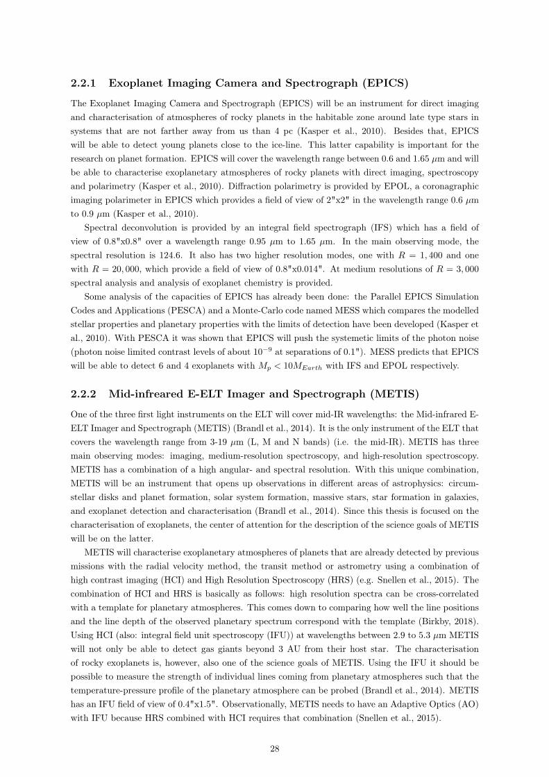
2.2.1 Exoplanet Imaging Camera and Spectrograph (EPICS)

The Exoplanet Imaging Camera and Spectrograph (EPICS) will be an instrument for direct imagingand characterisation of atmospheres of rocky planets in the habitable zone around late type stars insystems that are not farther away from us than 4 pc (Kasper et al., 2010). Besides that, EPICSwill be able to detect young planets close to the ice-line. This latter capability is important for theresearch on planet formation. EPICS will cover the wavelength range between 0.6 and 1.65 µm and willbe able to characterise exoplanetary atmospheres of rocky planets with direct imaging, spectroscopyand polarimetry (Kasper et al., 2010). Diffraction polarimetry is provided by EPOL, a coronagraphicimaging polarimeter in EPICS which provides a field of view of 2"x2" in the wavelength range 0.6 µmto 0.9 µm (Kasper et al., 2010).

Spectral deconvolution is provided by an integral field spectrograph (IFS) which has a field ofview of 0.8"x0.8" over a wavelength range 0.95 µm to 1.65 µm. In the main observing mode, thespectral resolution is 124.6. It also has two higher resolution modes, one with R = 1, 400 and onewith R = 20, 000, which provide a field of view of 0.8"x0.014". At medium resolutions of R = 3, 000

spectral analysis and analysis of exoplanet chemistry is provided.Some analysis of the capacities of EPICS has already been done: the Parallel EPICS Simulation

Codes and Applications (PESCA) and a Monte-Carlo code named MESS which compares the modelledstellar properties and planetary properties with the limits of detection have been developed (Kasper etal., 2010). With PESCA it was shown that EPICS will push the systemetic limits of the photon noise(photon noise limited contrast levels of about 10−9 at separations of 0.1"). MESS predicts that EPICSwill be able to detect 6 and 4 exoplanets with Mp < 10MEarth with IFS and EPOL respectively.

2.2.2 Mid-infreared E-ELT Imager and Spectrograph (METIS)

One of the three first light instruments on the ELT will cover mid-IR wavelengths: the Mid-infrared E-ELT Imager and Spectrograph (METIS) (Brandl et al., 2014). It is the only instrument of the ELT thatcovers the wavelength range from 3-19 µm (L, M and N bands) (i.e. the mid-IR). METIS has threemain observing modes: imaging, medium-resolution spectroscopy, and high-resolution spectroscopy.METIS has a combination of a high angular- and spectral resolution. With this unique combination,METIS will be an instrument that opens up observations in different areas of astrophysics: circum-stellar disks and planet formation, solar system formation, massive stars, star formation in galaxies,and exoplanet detection and characterisation (Brandl et al., 2014). Since this thesis is focused on thecharacterisation of exoplanets, the center of attention for the description of the science goals of METISwill be on the latter.

METIS will characterise exoplanetary atmospheres of planets that are already detected by previousmissions with the radial velocity method, the transit method or astrometry using a combination ofhigh contrast imaging (HCI) and High Resolution Spectroscopy (HRS) (e.g. Snellen et al., 2015). Thecombination of HCI and HRS is basically as follows: high resolution spectra can be cross-correlatedwith a template for planetary atmospheres. This comes down to comparing how well the line positionsand the line depth of the observed planetary spectrum correspond with the template (Birkby, 2018).Using HCI (also: integral field unit spectroscopy (IFU)) at wavelengths between 2.9 to 5.3 µm METISwill not only be able to detect gas giants beyond 3 AU from their host star. The characterisationof rocky exoplanets is, however, also one of the science goals of METIS. Using the IFU it should bepossible to measure the strength of individual lines coming from planetary atmospheres such that thetemperature-pressure profile of the planetary atmosphere can be probed (Brandl et al., 2014). METIShas an IFU field of view of 0.4"x1.5". Observationally, METIS needs to have an Adaptive Optics (AO)with IFU because HRS combined with HCI requires that combination (Snellen et al., 2015).

28

The HCI modes cover both imaging and spectrospopy. Choronographs are used for high spectralresolution in the L and M bands IFU and for imaging in the L, M and N bands. With HCI molecularbands can be resolved into individual lines. Moreover, strong Doppler effects due to the orbital motionof a planet can be distinguished from the telluric lines and the stellar lines from the host star fromthe planet in question. Hereby it is usually assumed that the telluric- and stellar lines are stationarywithin the time of the observation. With the combination of HCI and HRS it is possible to searchfor the O2 band in reflected light (Hawker et al., 2019). One advantage of this is that reflected lightmeasurements do not require planets to transit from our point of view.

Quanz et al. (2015) already provided some estimates of which planet sizes, temperatures andhost star properties will be possible to probe with METIS. Their analysis showed that cool planets(Teq = 255− 300 K) would be detectable in neither the L band nor the M band but will be detectablein the N band. It also shows that planets with Teq = 400− 600 K are best detectable in the L band.

2.2.3 High Resolution Spectrograph (HIRES)

The ELT High Resolution Spectrograph (E-ELT-HIRES, HIRES hereafter) is an instrument plannedfor the ELT that finished its phase A study at the end of 2018. HIRES is designed with the experienceand success of the Very Large Telescope (VLT). Two previous concept instruments were proposedbased on the VLT: CODEX (λ = 0.37− 0.61µm, R = 120, 00 and the Echelle SPectrograph for RockyExoplanets and Stable Spectroscopic Observations (ESPRESSO) (λ = 0.84 − 2.5µm, R = 130, 000,AO-assisted). These were to specific individually and therefore were combined to one instrument:HIRES (Maiolino et al., 2013). The proposed science cases for HIRES are related to a number ofastronomical research fields: the study of chemical composition of protoplanetary disks and accretiondisks, chemical enrichment study of the first stars related to the epoch of reionisation, studying theevolution of massive early type galaxies at z = 1−3, advances in the field of fundamental physics relatedto the fine structure constant measurements of the deuterium abundance, and, most importantly forthis thesis, the characterisation of exoplanetary atmospheres with the prospect of detecting signals oflife on rocky planets (Maiolino et al., 2013). This variety of science cases results in a set of requirementssuch that a progress in all these fields can be made when HIRES will be used to observe with the ELT.One requirement is that there is a primary high spectral resolution observing mode with R ∼ 100, 000.For the characteristation of exoplanetary atmosphere, this resolution is proposed to disentangle telluriclines from features of the planet of interest, to trace different atmospheric layers, and to detect narrowbands such as those from O2. Another requirements is the wavelength coverage: an instantaneouswavelength coverage of 0.37 µm to 2.5 µm with a wavelength accuracy of 10 cm s−1 for the exoplanetscience case. For some science cases, including the study of galaxy evolution and extragalactic starclusters, a moderate spectral resolution (R ∼ 10, 000 − 50, 000) mode is proposed such that the skybackground can be more accurately subtracted.

For the characteristion of exoplanetary atmospheres, the focus of HIRES will be on planets withmasses of Neptune and if possible to Earth-like masses (Maiolino et al., 2013). HIRES will providecharacterisation of atmospheres in terms of chemical composition, stratification and weather with theultimate goal to detect biosignatures. Moreover, a polarimetric mode is proposed to increase the chanceto detect biosignatures.

29

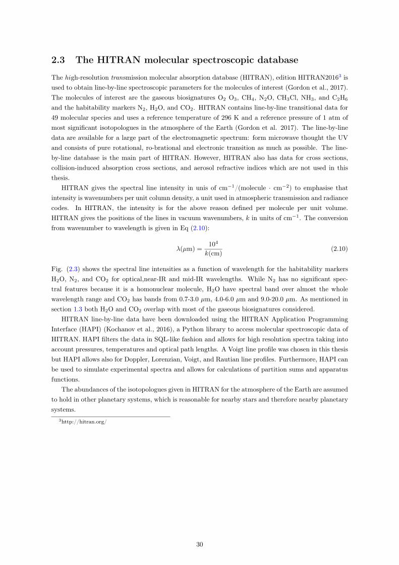
2.3 The HITRAN molecular spectroscopic database

The high-resolution transmission molecular absorption database (HITRAN), edition HITRAN20163 isused to obtain line-by-line spectroscopic parameters for the molecules of interest (Gordon et al., 2017).The molecules of interest are the gaseous biosignatures O2 O3, CH4, N2O, CH3Cl, NH3, and C2H6

and the habitability markers N2, H2O, and CO2. HITRAN contains line-by-line transitional data for49 molecular species and uses a reference temperature of 296 K and a reference pressure of 1 atm ofmost significant isotopologues in the atmosphere of the Earth (Gordon et al. 2017). The line-by-linedata are available for a large part of the electromagnetic spectrum: form microwave thought the UVand consists of pure rotational, ro-brational and electronic transition as much as possible. The line-by-line database is the main part of HITRAN. However, HITRAN also has data for cross sections,collision-induced absorption cross sections, and aerosol refractive indices which are not used in thisthesis.

HITRAN gives the spectral line intensity in unis of cm−1/(molecule · cm−2) to emphasise thatintensity is wavenumbers per unit column density, a unit used in atmospheric transmission and radiancecodes. In HITRAN, the intensity is for the above reason defined per molecule per unit volume.HITRAN gives the positions of the lines in vacuum wavenumbers, k in units of cm−1. The conversionfrom wavenumber to wavelength is given in Eq (2.10):

λ(µm) =104

k(cm)(2.10)

Fig. (2.3) shows the spectral line intensities as a function of wavelength for the habitability markersH2O, N2, and CO2 for optical,near-IR and mid-IR wavelengths. While N2 has no significant spec-tral features because it is a homonuclear molecule, H2O have spectral band over almost the wholewavelength range and CO2 has bands from 0.7-3.0 µm, 4.0-6.0 µm and 9.0-20.0 µm. As mentioned insection 1.3 both H2O and CO2 overlap with most of the gaseous biosignatures considered.

HITRAN line-by-line data have been downloaded using the HITRAN Application ProgrammingInterface (HAPI) (Kochanov et al., 2016), a Python library to access molecular spectroscopic data ofHITRAN. HAPI filters the data in SQL-like fashion and allows for high resolution spectra taking intoaccount pressures, temperatures and optical path lengths. A Voigt line profile was chosen in this thesisbut HAPI allows also for Doppler, Lorenzian, Voigt, and Rautian line profiles. Furthermore, HAPI canbe used to simulate experimental spectra and allows for calculations of partition sums and apparatusfunctions.

The abundances of the isotopologues given in HITRAN for the atmosphere of the Earth are assumedto hold in other planetary systems, which is reasonable for nearby stars and therefore nearby planetarysystems.

3http://hitran.org/

30

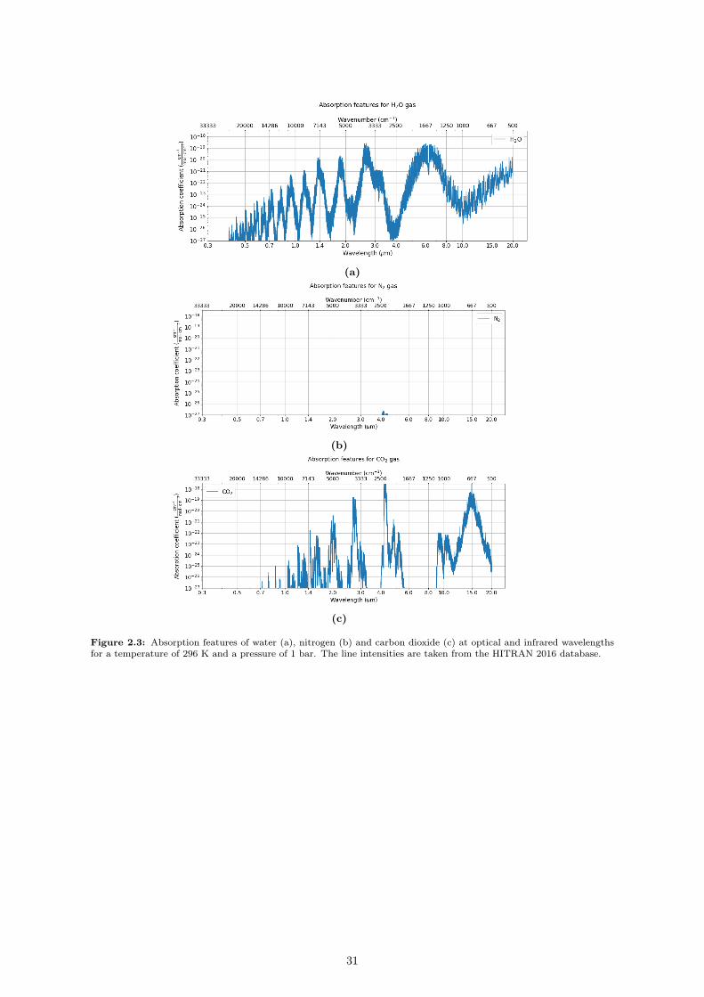
(a)

(b)

(c)

Figure 2.3: Absorption features of water (a), nitrogen (b) and carbon dioxide (c) at optical and infrared wavelengthsfor a temperature of 296 K and a pressure of 1 bar. The line intensities are taken from the HITRAN 2016 database.

31

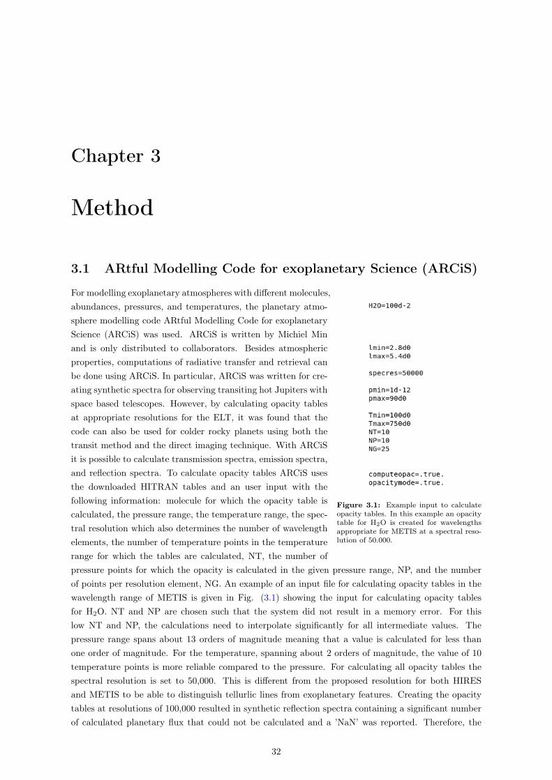
Chapter 3

Method

3.1 ARtful Modelling Code for exoplanetary Science (ARCiS)

Figure 3.1: Example input to calculateopacity tables. In this example an opacitytable for H2O is created for wavelengthsappropriate for METIS at a spectral reso-lution of 50.000.

For modelling exoplanetary atmospheres with different molecules,abundances, pressures, and temperatures, the planetary atmo-sphere modelling code ARtful Modelling Code for exoplanetaryScience (ARCiS) was used. ARCiS is written by Michiel Minand is only distributed to collaborators. Besides atmosphericproperties, computations of radiative transfer and retrieval canbe done using ARCiS. In particular, ARCiS was written for cre-ating synthetic spectra for observing transiting hot Jupiters withspace based telescopes. However, by calculating opacity tablesat appropriate resolutions for the ELT, it was found that thecode can also be used for colder rocky planets using both thetransit method and the direct imaging technique. With ARCiSit is possible to calculate transmission spectra, emission spectra,and reflection spectra. To calculate opacity tables ARCiS usesthe downloaded HITRAN tables and an user input with thefollowing information: molecule for which the opacity table iscalculated, the pressure range, the temperature range, the spec-tral resolution which also determines the number of wavelengthelements, the number of temperature points in the temperaturerange for which the tables are calculated, NT, the number ofpressure points for which the opacity is calculated in the given pressure range, NP, and the numberof points per resolution element, NG. An example of an input file for calculating opacity tables in thewavelength range of METIS is given in Fig. (3.1) showing the input for calculating opacity tablesfor H2O. NT and NP are chosen such that the system did not result in a memory error. For thislow NT and NP, the calculations need to interpolate significantly for all intermediate values. Thepressure range spans about 13 orders of magnitude meaning that a value is calculated for less thanone order of magnitude. For the temperature, spanning about 2 orders of magnitude, the value of 10temperature points is more reliable compared to the pressure. For calculating all opacity tables thespectral resolution is set to 50,000. This is different from the proposed resolution for both HIRESand METIS to be able to distinguish tellurlic lines from exoplanetary features. Creating the opacitytables at resolutions of 100,000 resulted in synthetic reflection spectra containing a significant numberof calculated planetary flux that could not be calculated and a ’NaN’ was reported. Therefore, the

32

resolution of the opacity tables was set as high as possible to avoid this: R=50,000.All opacity tables are created using a pressure range of 10−12 to 90 atm. The upper boundary of

Pmax = 90 atm was chosen such that it would be able to model Venus like atmosphere since Venushas a surface pressure of 90 atm. Keeping in mind the concept of the HZ, properties of Venus, Earthand Mars can be seen as limits for habitability. The temperature range was chosen such that thetemperature range of the atmosphere of Earth with and without temperature inversions is includedand accounted for planets having a higher and lower surface temperature. Habitable planets probablydo not have surface temperatures above 750 K because water would evaporate on those planetarysurfaces. The limit of 750 K was chosen because Venus has a surface temperature of about 750 K.

To illustrate the minimum pressure and the minimum temperature choices, an Earth-like planetaround a Sun-like star with an equilibrium temperature of 200 K is chosen. With Teq = 200 K a planetcan still be habitable since the equilibrium temperature is usually lower than the surface temperature,depending on the atmospheric content (e.g. Earth has Teq = 255 K and Ts = 288 K on average). Fig.(3.2) shows the pressure temperature profile (P-T profile) for an Earth-like atmosphere with both theaverage surface temperature of the Earth and the example temperature of T = 200 K taking for bothcases an atmospheric profile with the International Standard Atmosphere (ISA) as a reference (ISO,1975). It can be seen that the minimum pressure for a planetary equilibrium temperature of 200 Kgoes down to about 10−10 bar while the temperature decreases to about 100 K in the mesosphere.To include this minimum pressure and temperature of a planet with T = 200 K and to go a little bitlower in surface temperature, the minimum pressure and temperature were set to 1012 bar and 100 Krespectively.

The ISA is a static model of the Earth’s atmosphere published by the International Organizationfor Standardization (ISO) to provide a consistent way to model the pressure, the temperature, thedensity, and the viscosity as a function of altitude in their document ISO 2533:1975 (ISO, 1975). Inthe ISA, the lapse rate for the troposphere is 6.5 K/km up to the tropopause at 11 km above thesurface. In the pause the temperature remains constant. At a height of 20 km above the Earth’ssurface, the stratosphere begins. The lapse rate for the stratosphere is -1.0 K/km up to 32 km abovethe surface which means that there is a temperature inversion in this atmospheric layer. A temperatureinversion in the atmosphere is a reversal of the normal behaviour of the atmosphere to decrease withtemperature as a function of altitude. Then the temperature goes up more rapid as a function oftemperature with a lapse rate of -2.8 K/km up to an altitude of 47 km, where the stratopause begins.In the stratopause the temperature of 270 K remains constant. At an altitude of 51 km the mesospherebeings. In the mesosphere the temperature goes down as a function of altitude with a lapse rate of 2.8K/km up to 71 km and a lapse rate of 2.0 K/km up to a height of 80 km. At that height an isothermalpoint is reached which corresponds to a minimum temperature at the boundary of the mesosphere andthe thermosphere: the mesopause. Above the thermosphere the atmospheric pressure and temperatureprofiles are not modelled in the ISA. In this thesis the boundary was chosen because for the search forbiosignatures it is convenient to probe the lower atmosphere since life is more likely to alter the loweratmosphere compared to the upper atmosphere. In the ISA it is assumed that the air behaves as aperfect gas. The pressure profile in the ISA is exponentially dropping with altitude:

P = P0 exp (−z/H) (3.1)

where P0 is the surface pressure, z is the altitude and H is the atmospheric scale height given by Eq.(2.4).

33

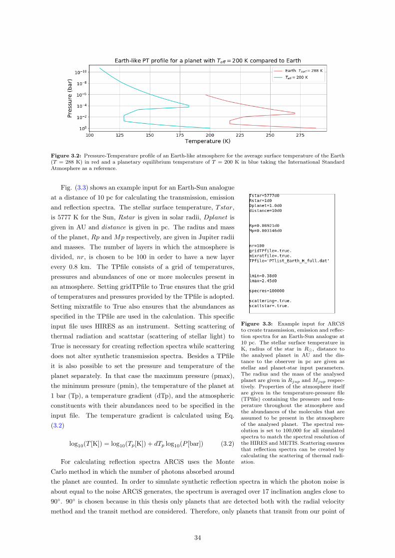
Figure 3.2: Pressure-Temperature profile of an Earth-like atmosphere for the average surface temperature of the Earth(T = 288 K) in red and a planetary equilibrium temperature of T = 200 K in blue taking the International StandardAtmosphere as a reference.

Figure 3.3: Example input for ARCiSto create transmission, emission and reflec-tion spectra for an Earth-Sun analogue at10 pc. The stellar surface temperature inK, radius of the star in R�, distance tothe analysed planet in AU and the dis-tance to the observer in pc are given asstellar and planet-star input parameters.The radius and the mass of the analysedplanet are given in Rjup and Mjup respec-tively. Properties of the atmosphere itselfare given in the temperature-pressure file(TPfile) containing the pressure and tem-perature throughout the atmosphere andthe abundances of the molecules that areassumed to be present in the atmosphereof the analysed planet. The spectral res-olution is set to 100,000 for all simulatedspectra to match the spectral resolution ofthe HIRES and METIS. Scattering ensuresthat reflection spectra can be created bycalculating the scattering of thermal radi-ation.

Fig. (3.3) shows an example input for an Earth-Sun analogueat a distance of 10 pc for calculating the transmission, emissionand reflection spectra. The stellar surface temperature, Tstar,is 5777 K for the Sun, Rstar is given in solar radii, Dplanet isgiven in AU and distance is given in pc. The radius and massof the planet, Rp and Mp respectively, are given in Jupiter radiiand masses. The number of layers in which the atmosphere isdivided, nr, is chosen to be 100 in order to have a new layerevery 0.8 km. The TPfile consists of a grid of temperatures,pressures and abundances of one or more molecules present inan atmosphere. Setting gridTPfile to True ensures that the gridof temperatures and pressures provided by the TPfile is adopted.Setting mixratfile to True also ensures that the abundances asspecified in the TPfile are used in the calculation. This specificinput file uses HIRES as an instrument. Setting scattering ofthermal radiation and scattstar (scattering of stellar light) toTrue is necessary for creating reflection spectra while scatteringdoes not alter synthetic transmission spectra. Besides a TPfileit is also possible to set the pressure and temperature of theplanet separately. In that case the maximum pressure (pmax),the minimum pressure (pmin), the temperature of the planet at1 bar (Tp), a temperature gradient (dTp), and the atmosphericconstituents with their abundances need to be specified in theinput file. The temperature gradient is calculated using Eq.(3.2)

log10(T [K]) = log10(Tp[K]) + dTp log10(P [bar]) (3.2)

For calculating reflection spectra ARCiS uses the MonteCarlo method in which the number of photons absorbed aroundthe planet are counted. In order to simulate synthetic reflection spectra in which the photon noise isabout equal to the noise ARCiS generates, the spectrum is averaged over 17 inclination angles close to90◦. 90◦ is chosen because in this thesis only planets that are detected both with the radial velocitymethod and the transit method are considered. Therefore, only planets that transit from our point of

34

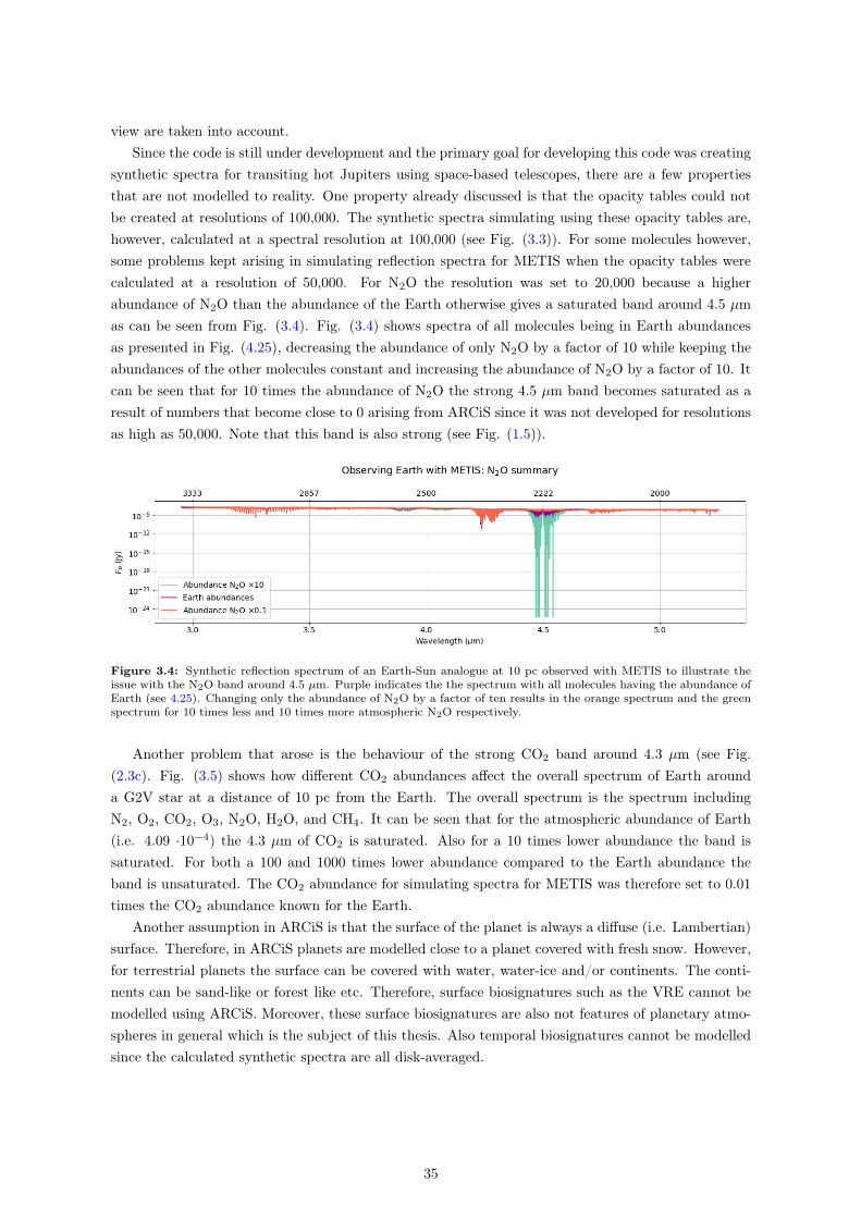
view are taken into account.Since the code is still under development and the primary goal for developing this code was creating

synthetic spectra for transiting hot Jupiters using space-based telescopes, there are a few propertiesthat are not modelled to reality. One property already discussed is that the opacity tables could notbe created at resolutions of 100,000. The synthetic spectra simulating using these opacity tables are,however, calculated at a spectral resolution at 100,000 (see Fig. (3.3)). For some molecules however,some problems kept arising in simulating reflection spectra for METIS when the opacity tables werecalculated at a resolution of 50,000. For N2O the resolution was set to 20,000 because a higherabundance of N2O than the abundance of the Earth otherwise gives a saturated band around 4.5 µmas can be seen from Fig. (3.4). Fig. (3.4) shows spectra of all molecules being in Earth abundancesas presented in Fig. (4.25), decreasing the abundance of only N2O by a factor of 10 while keeping theabundances of the other molecules constant and increasing the abundance of N2O by a factor of 10. Itcan be seen that for 10 times the abundance of N2O the strong 4.5 µm band becomes saturated as aresult of numbers that become close to 0 arising from ARCiS since it was not developed for resolutionsas high as 50,000. Note that this band is also strong (see Fig. (1.5)).

Figure 3.4: Synthetic reflection spectrum of an Earth-Sun analogue at 10 pc observed with METIS to illustrate theissue with the N2O band around 4.5 µm. Purple indicates the the spectrum with all molecules having the abundance ofEarth (see 4.25). Changing only the abundance of N2O by a factor of ten results in the orange spectrum and the greenspectrum for 10 times less and 10 times more atmospheric N2O respectively.

Another problem that arose is the behaviour of the strong CO2 band around 4.3 µm (see Fig.(2.3c). Fig. (3.5) shows how different CO2 abundances affect the overall spectrum of Earth arounda G2V star at a distance of 10 pc from the Earth. The overall spectrum is the spectrum includingN2, O2, CO2, O3, N2O, H2O, and CH4. It can be seen that for the atmospheric abundance of Earth(i.e. 4.09 ·10−4) the 4.3 µm of CO2 is saturated. Also for a 10 times lower abundance the band issaturated. For both a 100 and 1000 times lower abundance compared to the Earth abundance theband is unsaturated. The CO2 abundance for simulating spectra for METIS was therefore set to 0.01times the CO2 abundance known for the Earth.

Another assumption in ARCiS is that the surface of the planet is always a diffuse (i.e. Lambertian)surface. Therefore, in ARCiS planets are modelled close to a planet covered with fresh snow. However,for terrestrial planets the surface can be covered with water, water-ice and/or continents. The conti-nents can be sand-like or forest like etc. Therefore, surface biosignatures such as the VRE cannot bemodelled using ARCiS. Moreover, these surface biosignatures are also not features of planetary atmo-spheres in general which is the subject of this thesis. Also temporal biosignatures cannot be modelledsince the calculated synthetic spectra are all disk-averaged.

35

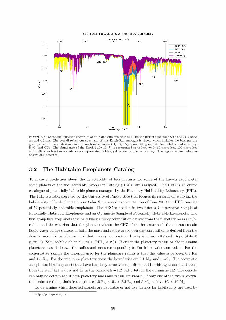
Figure 3.5: Synthetic reflection spectrum of an Earth-Sun analogue at 10 pc to illustrate the issue with the CO2 bandaround 4.3 µm. The overall reflections spectrum of this Earth-Sun analogue is shown which includes the biosignaturegases present in concentrations more than trace amounts (O2, O3, N2O, and CH4, and the habitability molecules N2,H2O, and CO2, The abundance of the Earth (4.09 1̇0−4) is represented in yellow, while 10 times less, 100 times lessand 1000 times less this abundance are represented in blue, yellow and purple respectively. The regions where moleculesabsorb are indicated.

3.2 The Habitable Exoplanets Catalog

To make a prediction about the detectability of biosignatures for some of the known exoplanets,some planets of the the Habitable Exoplanet Catalog (HEC)1 are analysed. The HEC is an onlinecatalogue of potentially habitable planets managed by the Planetary Habitability Laboratory (PHL).The PHL is a laboratory led by the University of Puerto Rico that focuses its research on studying thehabitability of both planets in our Solar System and exoplanets. As of June 2019 the HEC consistsof 52 potentially habitable exoplanets. The HEC is divided in two lists: a Conservative Sample ofPotentially Habitable Exoplanets and an Optimistic Sample of Potentially Habitable Exoplanets. Thefirst group lists exoplanets that have likely a rocky composition derived from the planetary mass and/orradius and the criterion that the planet is within the CHZ of the host star such that it can sustainliquid water on the surface. If both the mass and radius are known the composition is derived from thedensity, were it is usually assumed that a rocky composition density is between 0.7 and 1.5 ρ⊕ (4.4-8.3g cm−3) (Schulze-Makuch et al.; 2011, PHL, 2019)). If either the planetary radius or the minimumplanetary mass is known the radius and mass corresponding to Earth-like values are taken. For theconservative sample the criterion used for the planetary radius is that the value is between 0.5 R⊕

and 1.5 R⊕. For the minimum planetary mass the boundaries are 0.1 M⊕ and 5 M⊕. The optimisticsample classifies exoplanets that have less likely a rocky composition and is orbiting at such a distancefrom the star that is does not lie in the conservative HZ but orbits in the optimistic HZ. The densitycan only be determined if both planetary mass and radius are known. If only one of the two is known,the limits for the optimistic sample are 1.5 R⊕ < Rp < 2.5 R⊕ and 5 M⊕ <sin i ·Mp < 10 M⊕.

To determine which detected planets are habitable or not five metrics for habitability are used by1http://phl.upr.edu/hec

36

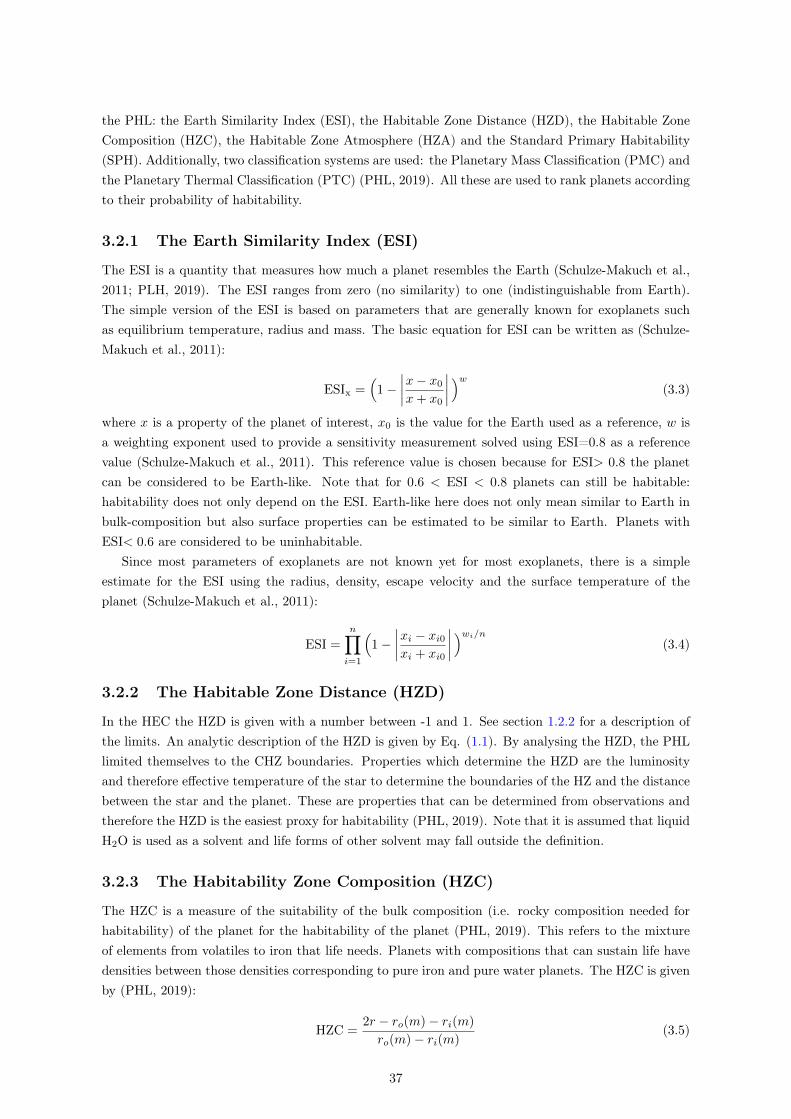
the PHL: the Earth Similarity Index (ESI), the Habitable Zone Distance (HZD), the Habitable ZoneComposition (HZC), the Habitable Zone Atmosphere (HZA) and the Standard Primary Habitability(SPH). Additionally, two classification systems are used: the Planetary Mass Classification (PMC) andthe Planetary Thermal Classification (PTC) (PHL, 2019). All these are used to rank planets accordingto their probability of habitability.

3.2.1 The Earth Similarity Index (ESI)

The ESI is a quantity that measures how much a planet resembles the Earth (Schulze-Makuch et al.,2011; PLH, 2019). The ESI ranges from zero (no similarity) to one (indistinguishable from Earth).The simple version of the ESI is based on parameters that are generally known for exoplanets suchas equilibrium temperature, radius and mass. The basic equation for ESI can be written as (Schulze-Makuch et al., 2011):

ESIx =(

1−∣∣∣∣x− x0

x+ x0

∣∣∣∣ )w (3.3)

where x is a property of the planet of interest, x0 is the value for the Earth used as a reference, w isa weighting exponent used to provide a sensitivity measurement solved using ESI=0.8 as a referencevalue (Schulze-Makuch et al., 2011). This reference value is chosen because for ESI> 0.8 the planetcan be considered to be Earth-like. Note that for 0.6 < ESI < 0.8 planets can still be habitable:habitability does not only depend on the ESI. Earth-like here does not only mean similar to Earth inbulk-composition but also surface properties can be estimated to be similar to Earth. Planets withESI< 0.6 are considered to be uninhabitable.

Since most parameters of exoplanets are not known yet for most exoplanets, there is a simpleestimate for the ESI using the radius, density, escape velocity and the surface temperature of theplanet (Schulze-Makuch et al., 2011):

ESI =

n∏i=1

(1−

∣∣∣∣xi − xi0xi + xi0

∣∣∣∣ )wi/n (3.4)

3.2.2 The Habitable Zone Distance (HZD)

In the HEC the HZD is given with a number between -1 and 1. See section 1.2.2 for a description ofthe limits. An analytic description of the HZD is given by Eq. (1.1). By analysing the HZD, the PHLlimited themselves to the CHZ boundaries. Properties which determine the HZD are the luminosityand therefore effective temperature of the star to determine the boundaries of the HZ and the distancebetween the star and the planet. These are properties that can be determined from observations andtherefore the HZD is the easiest proxy for habitability (PHL, 2019). Note that it is assumed that liquidH2O is used as a solvent and life forms of other solvent may fall outside the definition.

3.2.3 The Habitability Zone Composition (HZC)

The HZC is a measure of the suitability of the bulk composition (i.e. rocky composition needed forhabitability) of the planet for the habitability of the planet (PHL, 2019). This refers to the mixtureof elements from volatiles to iron that life needs. Planets with compositions that can sustain life havedensities between those densities corresponding to pure iron and pure water planets. The HZC is givenby (PHL, 2019):

HZC =2r − ro(m)− ri(m)

ro(m)− ri(m)(3.5)

37

where m is the mass of the exoplanet with a specific composition, ro is the outer limit for a pure waterplanet and ri is the inner limit representing a planet composed of pure iron. As for the HZD, theHZC is normalised such that exoplanets with values -1<HZC<1 likely have a habitable composition.Planets that have HZC<-1 have very dense iron bodies while planets with HZC>1 are considered gasplanets.

3.2.4 The Habitable Zone Atmosphere (HZA)

Besides the composition and the distance to the host star, the ability for the planet to have anatmosphere that can sustain life is also important. This is quantified with the HZA and is based onthermal escape. The HZA is given by (PHL, 2019):

HZA =2√m/r − veH − veNveH − veN

(3.6)

where r is the radius of the planet and veN and veH are the escape velocities of nitrogen and hydrogenrespectively given by:

vex =

√zTeq

Mwx

(3.7)

where the subscript x can be N or H for nitrogen and hydrogen respectively and MWN = 14 g/moland MWH = 1 g/mol are the molecular weights of nitrogen and hydrogen atoms. There are manymore processes regulating planetary atmospheres besides thermal escape and these are not taken intoaccount in the calculation of the HZA. Examples include stellar wind erosion, the impact of weathering(i.e. the process in which rocks and minerals are dissolved naturally when coming in contact with theatmosphere or biomass) and sequestration (long term build up of e.g. C in biomass and oceans havingpotential to be found in the atmosphere in the long term as CO2), and the presence of planetarymagnetic fields.

3.2.5 The Standard Primary Habitability (SPH)

The Standard Primary Habitability (SPH) is a measure of the ability of the planet to support primaryproduces (e.g. vegetation) (PHL, 2019). The SPH ranges from 0 (nominal environment) to 1 (bestenvironment for vegetation). The SPH is used by the PHL to evaluate the global climatic habitability ofplanets. For an estimate of the SPH two environmental variables are needed: the surface temperature,T , and the relative humidity, RH. The SPH is estimated by (PHL, 2019):

SPH = HT (T ) ·HRH(RH) (3.8)

where HT and HRH are habitability functions for temperature and relative humidity respectively. Thehabitability functions, Hx are given by:Hx =

[(x−xmin)(x−xmax)

(x−xmin)(x−xmax)−(x−xopt)2

]wxmin < x < xmaxandxmin < xopt < xmax

0, otherwise(3.9)

where the x can be replaced by either T or RH. The weighting exponent, w, is based on the globaltemperature and relative humidity measurements. xopt is the optimum value of the parameter whichis determined from SPH=1.

Planets with SPH=0 may not be able to sustain complex (i.e. multicelluar) life but such a planetmay be able to support microbial life. Earth has SPH=0.33 meaning that planet Earth is not fully

38

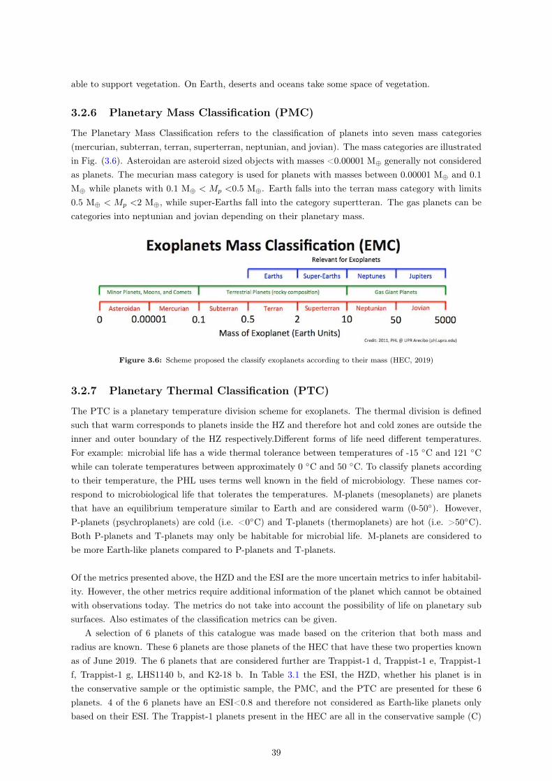
able to support vegetation. On Earth, deserts and oceans take some space of vegetation.

3.2.6 Planetary Mass Classification (PMC)

The Planetary Mass Classification refers to the classification of planets into seven mass categories(mercurian, subterran, terran, superterran, neptunian, and jovian). The mass categories are illustratedin Fig. (3.6). Asteroidan are asteroid sized objects with masses <0.00001 M⊕ generally not consideredas planets. The mecurian mass category is used for planets with masses between 0.00001 M⊕ and 0.1M⊕ while planets with 0.1 M⊕ < Mp <0.5 M⊕. Earth falls into the terran mass category with limits0.5 M⊕ < Mp <2 M⊕, while super-Earths fall into the category supertteran. The gas planets can becategories into neptunian and jovian depending on their planetary mass.

Figure 3.6: Scheme proposed the classify exoplanets according to their mass (HEC, 2019)

3.2.7 Planetary Thermal Classification (PTC)

The PTC is a planetary temperature division scheme for exoplanets. The thermal division is definedsuch that warm corresponds to planets inside the HZ and therefore hot and cold zones are outside theinner and outer boundary of the HZ respectively.Different forms of life need different temperatures.For example: microbial life has a wide thermal tolerance between temperatures of -15 ◦C and 121 ◦Cwhile can tolerate temperatures between approximately 0 ◦C and 50 ◦C. To classify planets accordingto their temperature, the PHL uses terms well known in the field of microbiology. These names cor-respond to microbiological life that tolerates the temperatures. M-planets (mesoplanets) are planetsthat have an equilibrium temperature similar to Earth and are considered warm (0-50◦). However,P-planets (psychroplanets) are cold (i.e. <0◦C) and T-planets (thermoplanets) are hot (i.e. >50◦C).Both P-planets and T-planets may only be habitable for microbial life. M-planets are considered tobe more Earth-like planets compared to P-planets and T-planets.

Of the metrics presented above, the HZD and the ESI are the more uncertain metrics to infer habitabil-ity. However, the other metrics require additional information of the planet which cannot be obtainedwith observations today. The metrics do not take into account the possibility of life on planetary subsurfaces. Also estimates of the classification metrics can be given.

A selection of 6 planets of this catalogue was made based on the criterion that both mass andradius are known. These 6 planets are those planets of the HEC that have these two properties knownas of June 2019. The 6 planets that are considered further are Trappist-1 d, Trappist-1 e, Trappist-1f, Trappist-1 g, LHS1140 b, and K2-18 b. In Table 3.1 the ESI, the HZD, whether his planet is inthe conservative sample or the optimistic sample, the PMC, and the PTC are presented for these 6planets. 4 of the 6 planets have an ESI<0.8 and therefore not considered as Earth-like planets onlybased on their ESI. The Trappist-1 planets present in the HEC are all in the conservative sample (C)

39

while LHS 1140 b and K2-18 b are both in the optimistic sample (O).

Planet ESI(1) HZD C/O(1) PMC(1) PTC(1)

Trappist-1 d 0.89 -0.80 C subterran warmTrappist-1 e 0.87 -0.38 C terran warmTrappist-1 f 0.70 0.19 C terran warmTrappist-1 g 0.59 0.70 C terran warmLHS 1140 b 0.69 0.41 O superterran warmK2-18 b 0.71 -0.88 O superterran warm

Table 3.1: Selected planets based on the criteria that both planetary mass and planetary radius are determined fromprevious observations. The ESI, the PMC, and the PTC are taken from the HEC. Column 4 represents whether theplanet is in the conservative sample (C) or the optimistic sample (O) in the HEC. The HZD (column 3) was calculatedfrom Eq. (1.3).(1) Parameters taken from PHL (2019)

3.3 Simulated noise

Since there is always instrumental noise the spectra obtained with ARCiS needs to be altered, orat least checked, for these noise sources such that the noise ARCiS generates is equal to the noiselevel of instruments of interest. Besides contributions from our own atmosphere when observing withground based telescopes, there is also systematic noise, instrumental noise, photon noise etc. To takeinto account atmospheric contributions, it was checked at which wavelengths the Earth’s atmospheretransmits light from other planets. The high resolution that is feasible for the considered instrumentsensures that the planetary lines can be separated from telluric lines. This is especially important forwater lines since water has absorption features that are strong in the optical, near-IR, and mid-IR.

The photon noise depends on the blackbody emission from the host star (Bλ), the telescope aperturesize, the integration time, the distance to the target, and the radius of the star. The main parameteris the number of photons received at the telescope at each wavelength of interest.

The stellar blackbody, Bλ(T ), can be can be determined from:

Bλ(T ) =2hc2

λ5

1

ehcλkT − 1

(3.10)

where T is the stellar temperature, h is Planck’s constant, c is the speed of light, k is Boltzmann’sconstant, λ is the wavelength of interest. Using cgs units, the blackbody function has units oferg/s/cm2/cm/steradian. Here ’cm’ refers to the units of the wavelength of interest while the ’cm2’refers to the units of the area of the emitting body. The units of time refer to the observation time and’steradian’ is the unit for the solid angle. For determining the photon noise the number of photons,it is necessary to multiply with units of ’cm’, ’cm2, ’s’, and ’steradian’ to arrive be left with unitsof energy. The unit of wavelength can be eliminated by multiplying with the wavelength bin of theinstrument. The telescope retrieves a flux value for a range of wavelengths defined by each wavelengthbin. Since R = λ/∆λ, ∆λ can be determined from the known spectral resolution and the wavelengthrange of the considered instrument. Note that ∆λ is a function of wavelength. The disk area, A∗, ofthe emitting body is given by:

A∗ = πR2∗ (3.11)

where R∗ is the stellar radius. Since the planet only notices the radiation of one hemisphere of thehost star, only that area is used. The integration time, tint, was set to 10 hours, approximately theequivalent of 1 night of observations depending on the season. The solid angle, φ, can be calculated

40

by:

φ =π(D/2)2

d2(3.12)

where D is the telescope size and d is the distance between the observer and the target. The energyof the target received by the instrument can be calculated by:

E = Bλ(T ) ·∆λ ·A∗ · tint · φ (3.13)

To convert this to a number of photons, the energy of a photon needs to be considered. Dividing thistotal energy by the energy per photon results in the number of photons, n:

n =Eλ

hc(3.14)

Notice that n ∝ λ2. The photon noise falls off as 1/√n (i.e. Poisson noise). Therefore, the larger

the number of photons on the detector, the smaller the photon noise. The noise budget is estimatedassuming that the total noise budget (i.e. including the systematic noises, the instrumental noises,and photon noises) are about 120% of the photon noise.

3.4 Detectability

The detectability of a gas in any exoplanetary atmosphere is a function of the abundance of that gas inthe atmosphere of the planet, the distance between Earth and the planet of interest, the star-to-planetcontrast, background noises, and instrumental noises. The signal to noise ratio (SNR), the ratio ofthe signal of interest and the background noises, is an important quantity for the detectability. TheELT receives a high level of radiation from the telescope, the instrument and the atmosphere of theEarth as it is a ground-based telescope. It is necessary to account for these effects when evaluatingthe detectability.

EPICS will not be sensitive enough to characterise the planets in either characterising the atmo-sphere of an Earth-Sun analogue at a distance of 10 pc or the planets listed in Table 3.1, since they allhave a distance beyond 4 pc (Kasper et al., 2010). Therefore, EPICS data is not considered for thesereal planets The instruments that are considered here are METIS and HIRES.

Concerning the detectability of biosignatures with METIS, the performance calculation of Kendrewet al. (2010) were used. They calculated the sensitivity of the three main observing modes (i.e. imagingmedium-resolution and the high-resolution IFU spectroscopy) of METIS for unresolved point sourcesat a SNR=10 for an exposure time of 1 hour. Only those for the IFU spectroscopy are used whereproperties of the atmosphere, the telescope and the instrument are taken into account. The analysiswas done at the time the ELT was intended to be 42 m in diameter and when the location of the ELTwas not decided yet. They did their analysis for three sites: Paranal at an altitude of 2.6 km, Highand dry at an altitude of 5.0 km and the Armazones at an altitude of 3.064 km. The ELT will be buildat the Armazones but sensitivity calculations to the IFS spectroscopy for this site are not performed.The sensitivities given for the low site and the high and dry sites are therefore the weighted averagesof the sensitivities per altitude were taken. This resulted in sensitivity estimates of 4.3 · 10−10 Jy at2.9 µm, 5.7 ·10−10 Jy at wavelengths of 3.8 µm, and 1.4 ·10−8 Jy at 5.3 µm. The increase in sensitivityis because of the step between the M and L band. These are the sensitivities for a SNR of 10 for anexposure time of 1 hour. Considered planets are all considered transiting planets and therefore are notvisible during the secondary eclipse. This duration is, however, short compared to the duration of anorbit of the planet around the host star and is not taken into account. Since the sensitivity increases

41

with√t, longer observing times will be able to probe atmospheres more effectively.

Since HIRES has just finish its phase A study, sensitivity calculations are not provided. Sensitivitycalculations were done using the method in Rauer et al. (2013). The signal to noise ratio (SNR) for aspectral band or line in transmission is calculated by:

SNRT = SNRsfA√

2=Fs · tint · fA

σtot(3.15)

where σtot is the assumed noise, here 1.2 times the photon noise. SNRs is the stellar signal to noiseratio. The stellar signal is given by:

Fs =1

N

R2s

d2Is ·A · q ·∆λ =

λ

hc

R2s

d2Is · πR2

tel · q · λ/R (3.16)

where N = hc/λ is a conversion to the number of photons, A and Rtel are the collecting area and theradius of the telescope respectively, d is the distance between the Earth and the star, Is is the spectralenergy flux of the star, q is an efficiency factor (0.5 for the ELT), λ is the wavelength of interest andR is the spectral resolution. fA is the additional transit depth:

fA =(Rp + he(λ))2

R2s

−R2p

R2s

(3.17)

where he is the effective height of the atmosphere as function of wavelength. SNRT is the transmissionsignal to noise ratio:

SNRT =Rp2

R2s

(3.18)

The factor of 1√

2 in Eq. (3.15) results from the consideration that the measurements of the differencein stellar flux transmitted to the planetary atmosphere if it is in and out of transit.

The integration time, tint, is set equal to the transit duration, Td, the time the planet of interest isin front of the star. Assuming the inclination is 90◦, Td can be derived from:

Td =P

πarcsin

(Rsa

)(3.19)

where P is the orbital period of the planet and a is the semi-major axis. Using Td the planetary SNRcan be calculated and the integration time can subsequently be calculated from:

ti = TD

(SNRtiSNRp

)2

(3.20)

42

Chapter 4

Results

The results for examining the detectability of biosignatures with the ELT are divided into severalsections. The idea behind the structure is building a more and more realistic atmosphere in subsequentsections and subsections starting from very simple atmospheres. As a first example, an Earth-Sunanalogue is simulated at a distance of 10 pc. It is assumed that the Earth-twin transits the Sun-twinfrom our point of view. Section 4.1 describes a simple atmosphere in which only one gas is present.The atmosphere is assumed to have a small pressure range and a single temperature throughout theatmosphere. In section 4.2 more realistic pressure-temperature structures are used for simulatingsimple atmospheres consisting of one gas. In section 4.3 the effect of a mixture of gases is discussed.This includes changing the abundances of the atmospheric gases by a factor of 10. In section 4.4spectra are shown for the 6 planets taken from the HEC. This section also includes an analysis ofmolecular abundances. In section 4.5 the optimal resolution for the characterisation of exoplanetaryatmospheres will be discussed using the design of the ELT.

4.1 Simple isothermal atmosphere consisting of one gas

In this section we assume simple atmospheres which have a small pressure range and are isothermal(i.e. have only one temperature throughout the atmosphere). This atmosphere is assumed to consist ofone gas. The pressures and temperatures are varied to investigate the effect of different pressures andtemperatures on the spectra. The pressures and temperatures are chosen such that a planet can behabitable. That is, because of our definition of life, a planet that can sustain liquid H2O. See section(3.1) for a detailed explanation of the adopted limits. In short, for determining ranges for pressures andtemperatures, the pressures and temperatures should be within the surface- pressure and temperaturerange of Mars-Earth-Venus. The effect of varying the temperature in an isothermal atmosphere isthat the temperature in the whole atmosphere is changed. For investigating the effect of the surfacepressure, however, the minimum pressure is set constant to P = 10−2 bar and to study the effect ofthe surface pressure on both the transmission and the reflection spectrum, the maximum pressure isvaried. The pressure varies linearly from the surface pressure to the pressure of 10−2 bar. For thedifferent wavelength regions were HIRES and METIS are sensitive to, different gases are assumed tobe present in the atmosphere for both instruments. For the wavelength range of HIRES, the opticaland the near-IR, O2 is used as an example. METIS is, however, sensitive to wavelengths in the mid-IRand O3 is used as an example. These molecules are chosen taking into account the spectral lines of themolecules and the importance for habitability of these molecules on Earth. The spectra in this sectionare simulated by considering 100% O2 and 100% O3 atmospheres for HIRES and METIS respectively.

43

4.1.1 Effect of the surface pressure

Except for the terrestrial planets in our solar system, the surface pressure of other discovered terrestrialplanets is not well determined. Therefore, investigating the effect of surface pressure is useful to inves-tigate whether it might be possible to determine the surface pressure from near-future observations.Since this is dependent on the pressure profile of the atmosphere, investigating whether determiningthe surface pressure is possible with near-future technology is beyond the scope of this thesis. In thisthesis, the effect of the surface pressure is shown to indicate why the spectrum changes with surfacepressure. Fixing the surface temperature to 300 K, about the average surface temperature of the Earthand a surface temperature within the CHZ limits, the surface pressure is varied between 0.5 and 50bar.

The effect of the surface pressure for an atmosphere consisting of 100% O2 observed with HIRES isshown in Fig. (4.1). The differences between the various surface pressures and 1 bar are shown in theresidual plot. The differences are represented in the same colours as the surface pressures other than 1bar. Changing the pressure results in a difference in the ratio of the planetary radius versus the stellarradius from about a wavelength of 0.5 µm. Because of the assumption that the ideal gas law holds forgases in the atmosphere, it should be noted that changing only the pressure in the atmosphere andkeeping the other parts constant causes the ideal gas law to be disobeyed.

Figure 4.1: Synthetic transmission spectrum of an 100% O2 atmosphere showing the effect of the the variation of thesurface pressure for an Earth-Sun analogue located at a distance of 10 pc as simulated for HIRES assuming isothermalatmospheres (T = 300 K) with a minimum pressure of 10−2 bar. The variation in transmission of O2 for surface pressuresof 0.5 bar (blue), 1 bar (green), 2 bar (purple), 5 bar (orange), 10 bar (cyan), 20 bar (yellow), and 50 bar (red) areshown. The residual plot below shows the difference between the different pressures and the reference pressure of 1 baras function of wavelength.

One result is that the width of the band at 1.3 µm increases slightly with increasing pressure ascan be seen from the residual plot consistent with the concept of pressure broadening. This is also thecase for the other spectral features but this broadening is less prominent for those lines. The effect ofpressure broadening is not very notable for pressure range spanning two orders of magnitude.

Assuming an atmosphere consisting of only O3 gas using METIS as an instrument and varyingthe surface pressures has a similar result. The reflection spectrum of such an atmosphere is shown inFig. (4.2). It can be seen that there is a difference of at most ∼ 10−8.5 bar. This can be considered

44

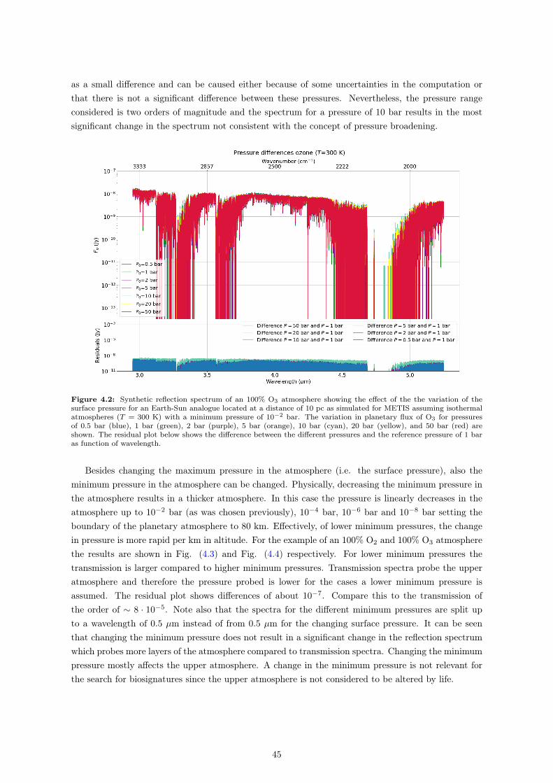
as a small difference and can be caused either because of some uncertainties in the computation orthat there is not a significant difference between these pressures. Nevertheless, the pressure rangeconsidered is two orders of magnitude and the spectrum for a pressure of 10 bar results in the mostsignificant change in the spectrum not consistent with the concept of pressure broadening.

Figure 4.2: Synthetic reflection spectrum of an 100% O3 atmosphere showing the effect of the the variation of thesurface pressure for an Earth-Sun analogue located at a distance of 10 pc as simulated for METIS assuming isothermalatmospheres (T = 300 K) with a minimum pressure of 10−2 bar. The variation in planetary flux of O3 for pressuresof 0.5 bar (blue), 1 bar (green), 2 bar (purple), 5 bar (orange), 10 bar (cyan), 20 bar (yellow), and 50 bar (red) areshown. The residual plot below shows the difference between the different pressures and the reference pressure of 1 baras function of wavelength.

Besides changing the maximum pressure in the atmosphere (i.e. the surface pressure), also theminimum pressure in the atmosphere can be changed. Physically, decreasing the minimum pressure inthe atmosphere results in a thicker atmosphere. In this case the pressure is linearly decreases in theatmosphere up to 10−2 bar (as was chosen previously), 10−4 bar, 10−6 bar and 10−8 bar setting theboundary of the planetary atmosphere to 80 km. Effectively, of lower minimum pressures, the changein pressure is more rapid per km in altitude. For the example of an 100% O2 and 100% O3 atmospherethe results are shown in Fig. (4.3) and Fig. (4.4) respectively. For lower minimum pressures thetransmission is larger compared to higher minimum pressures. Transmission spectra probe the upperatmosphere and therefore the pressure probed is lower for the cases a lower minimum pressure isassumed. The residual plot shows differences of about 10−7. Compare this to the transmission ofthe order of ∼ 8 · 10−5. Note also that the spectra for the different minimum pressures are split upto a wavelength of 0.5 µm instead of from 0.5 µm for the changing surface pressure. It can be seenthat changing the minimum pressure does not result in a significant change in the reflection spectrumwhich probes more layers of the atmosphere compared to transmission spectra. Changing the minimumpressure mostly affects the upper atmosphere. A change in the minimum pressure is not relevant forthe search for biosignatures since the upper atmosphere is not considered to be altered by life.

45

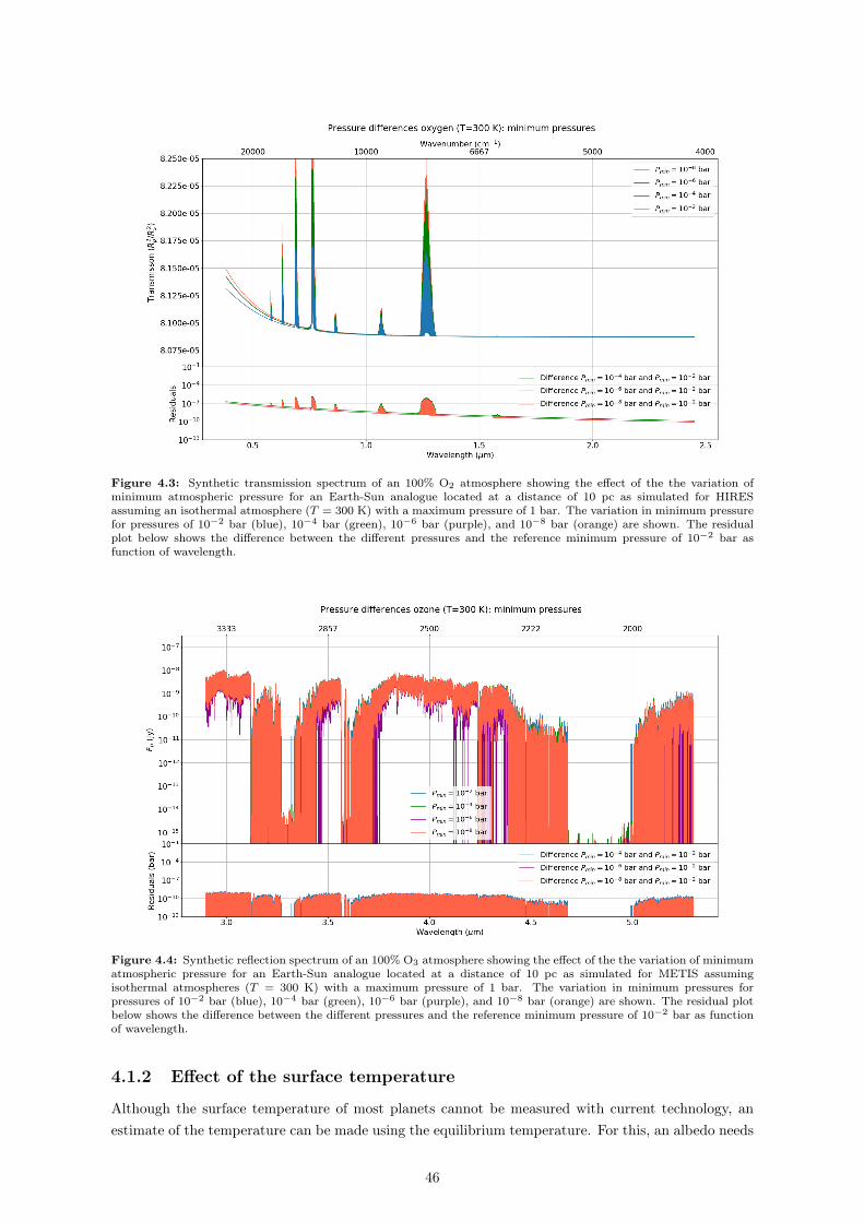
Figure 4.3: Synthetic transmission spectrum of an 100% O2 atmosphere showing the effect of the the variation ofminimum atmospheric pressure for an Earth-Sun analogue located at a distance of 10 pc as simulated for HIRESassuming an isothermal atmosphere (T = 300 K) with a maximum pressure of 1 bar. The variation in minimum pressurefor pressures of 10−2 bar (blue), 10−4 bar (green), 10−6 bar (purple), and 10−8 bar (orange) are shown. The residualplot below shows the difference between the different pressures and the reference minimum pressure of 10−2 bar asfunction of wavelength.

Figure 4.4: Synthetic reflection spectrum of an 100% O3 atmosphere showing the effect of the the variation of minimumatmospheric pressure for an Earth-Sun analogue located at a distance of 10 pc as simulated for METIS assumingisothermal atmospheres (T = 300 K) with a maximum pressure of 1 bar. The variation in minimum pressures forpressures of 10−2 bar (blue), 10−4 bar (green), 10−6 bar (purple), and 10−8 bar (orange) are shown. The residual plotbelow shows the difference between the different pressures and the reference minimum pressure of 10−2 bar as functionof wavelength.

4.1.2 Effect of the surface temperature

Although the surface temperature of most planets cannot be measured with current technology, anestimate of the temperature can be made using the equilibrium temperature. For this, an albedo needs

46

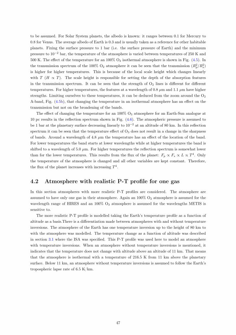
to be assumed. For Solar System planets, the albedo is known: it ranges between 0.1 for Mercury to0.8 for Venus. The average albedo of Earth is 0.3 and is usually taken as a reference for other habitableplanets. Fixing the surface pressure to 1 bar (i.e. the surface pressure of Earth) and the minimumpressure to 10−2 bar, the temperature of the atmosphere is varied between temperatures of 250 K and500 K. The effect of the temperature for an 100% O2 isothermal atmosphere is shown in Fig. (4.5). Inthe transmission spectrum of the 100% O2 atmosphere it can be seen that the transmission (R2

p/R2s)

is higher for higher temperatures. This is because of the local scale height which changes linearlywith T (H ∝ T ). The scale height is responsible for setting the depth of the absorption featuresin the transmission spectrum. It can be seen that the strength of O2 lines is different for differenttemperatures. For higher temperatures, the features at a wavelength of 0.8 µm and 1.1 µm have higherstrengths. Limiting ourselves to these temperatures, it can be deduced from the zoom around the O2

A-band, Fig. (4.5b), that changing the temperature in an isothermal atmosphere has an effect on thetransmission but not on the broadening of the bands.

The effect of changing the temperature for an 100% O3 atmosphere for an Earth-Sun analogue at10 pc results in the reflection spectrum shown in Fig. (4.6). The atmospheric pressure is assumed tobe 1 bar at the planetary surface decreasing linearly to 10−2 at an altitude of 80 km. In this reflectionspectrum it can be seen that the temperature effect of O3 does not result in a change in the sharpnessof bands. Around a wavelength of 4.8 µm the temperature has an effect of the location of the band.For lower temperatures the band starts at lower wavelengths while at higher temperatures the band isshifted to a wavelength of 5.0 µm. For higher temperatures the reflection spectrum is somewhat lowerthan for the lower temperatures. This results from the flux of the planet: Fp ∝ Fs ∝ L ∝ T 4. Onlythe temperature of the atmosphere is changed and all other variables are kept constant. Therefore,the flux of the planet increases with increasing T 4.

4.2 Atmosphere with realistic P-T profile for one gas

In this section atmospheres with more realistic P-T profiles are considered. The atmosphere areassumed to have only one gas in their atmosphere. Again an 100% O2 atmosphere is assumed for thewavelength range of HIRES and an 100% O3 atmosphere is assumed for the wavelengths METIS issensitive to.

The more realistic P-T profile is modelled taking the Earth’s temperature profile as a function ofaltitude as a basis.There is a differentiation made between atmospheres with and without temperatureinversions. The atmosphere of the Earth has one temperature inversion up to the height of 80 km towith the atmosphere was modelled. The temperature change as a function of altitude was describedin section 3.1 where the ISA was specified. This P-T profile was used here to model an atmospherewith temperature inversions. When an atmosphere without temperature inversions is mentioned, itindicates that the temperature does not change with altitude above an altitude of 11 km. That meansthat the atmosphere is isothermal with a temperature of 216.5 K from 11 km above the planetarysurface. Below 11 km, an atmosphere without temperature inversions is assumed to follow the Earth’stropospheric lapse rate of 6.5 K/km.

47

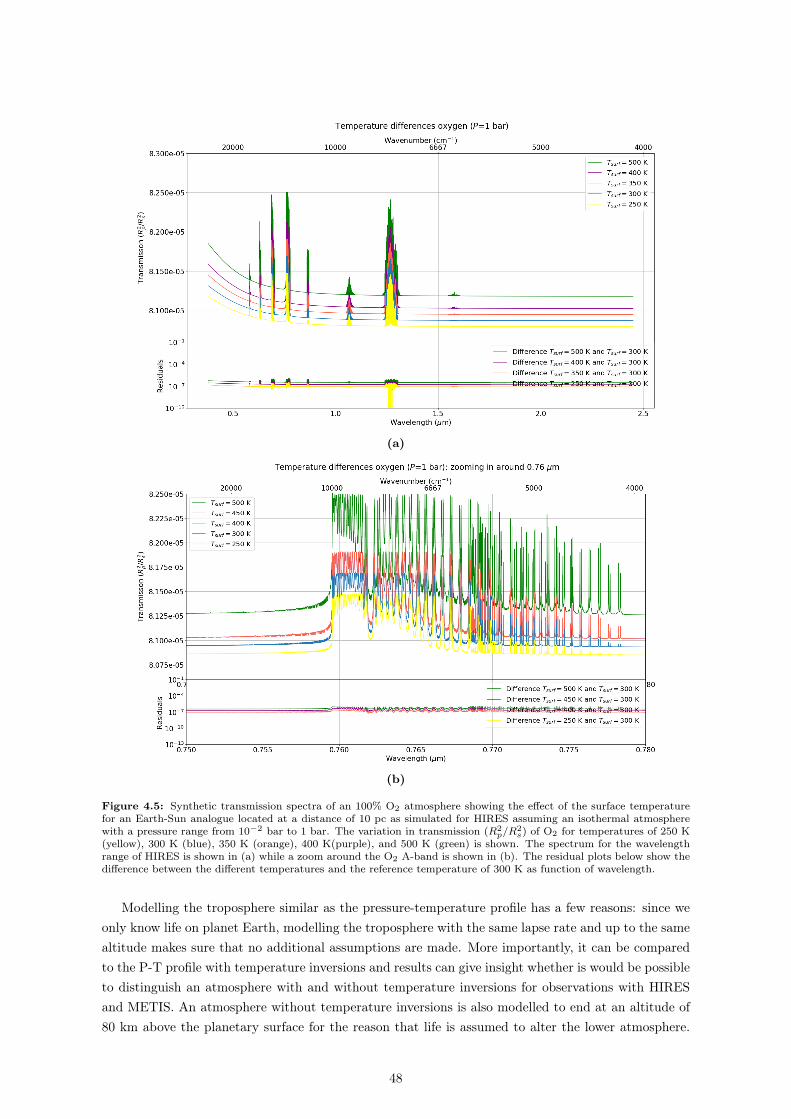
(a)

(b)

Figure 4.5: Synthetic transmission spectra of an 100% O2 atmosphere showing the effect of the surface temperaturefor an Earth-Sun analogue located at a distance of 10 pc as simulated for HIRES assuming an isothermal atmospherewith a pressure range from 10−2 bar to 1 bar. The variation in transmission (R2

p/R2s) of O2 for temperatures of 250 K

(yellow), 300 K (blue), 350 K (orange), 400 K(purple), and 500 K (green) is shown. The spectrum for the wavelengthrange of HIRES is shown in (a) while a zoom around the O2 A-band is shown in (b). The residual plots below show thedifference between the different temperatures and the reference temperature of 300 K as function of wavelength.

Modelling the troposphere similar as the pressure-temperature profile has a few reasons: since weonly know life on planet Earth, modelling the troposphere with the same lapse rate and up to the samealtitude makes sure that no additional assumptions are made. More importantly, it can be comparedto the P-T profile with temperature inversions and results can give insight whether is would be possibleto distinguish an atmosphere with and without temperature inversions for observations with HIRESand METIS. An atmosphere without temperature inversions is also modelled to end at an altitude of80 km above the planetary surface for the reason that life is assumed to alter the lower atmosphere.

48

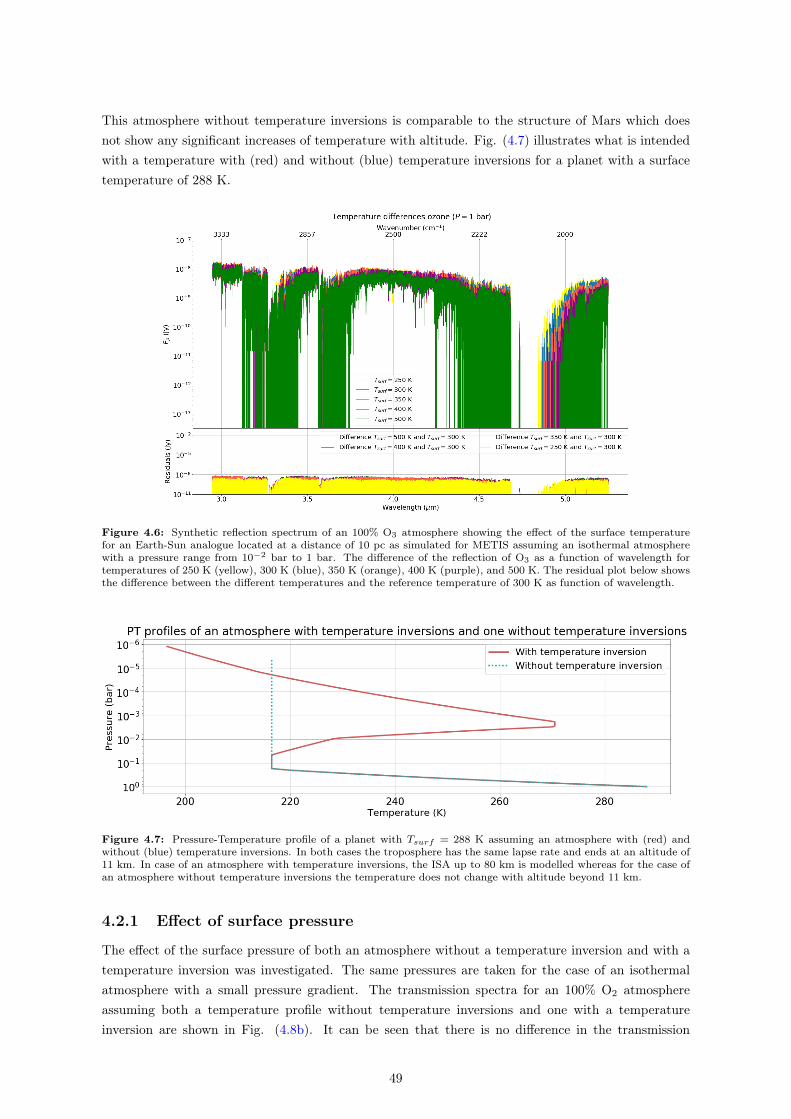
This atmosphere without temperature inversions is comparable to the structure of Mars which doesnot show any significant increases of temperature with altitude. Fig. (4.7) illustrates what is intendedwith a temperature with (red) and without (blue) temperature inversions for a planet with a surfacetemperature of 288 K.

Figure 4.6: Synthetic reflection spectrum of an 100% O3 atmosphere showing the effect of the surface temperaturefor an Earth-Sun analogue located at a distance of 10 pc as simulated for METIS assuming an isothermal atmospherewith a pressure range from 10−2 bar to 1 bar. The difference of the reflection of O3 as a function of wavelength fortemperatures of 250 K (yellow), 300 K (blue), 350 K (orange), 400 K (purple), and 500 K. The residual plot below showsthe difference between the different temperatures and the reference temperature of 300 K as function of wavelength.

Figure 4.7: Pressure-Temperature profile of a planet with Tsurf = 288 K assuming an atmosphere with (red) andwithout (blue) temperature inversions. In both cases the troposphere has the same lapse rate and ends at an altitude of11 km. In case of an atmosphere with temperature inversions, the ISA up to 80 km is modelled whereas for the case ofan atmosphere without temperature inversions the temperature does not change with altitude beyond 11 km.

4.2.1 Effect of surface pressure

The effect of the surface pressure of both an atmosphere without a temperature inversion and with atemperature inversion was investigated. The same pressures are taken for the case of an isothermalatmosphere with a small pressure gradient. The transmission spectra for an 100% O2 atmosphereassuming both a temperature profile without temperature inversions and one with a temperatureinversion are shown in Fig. (4.8b). It can be seen that there is no difference in the transmission

49

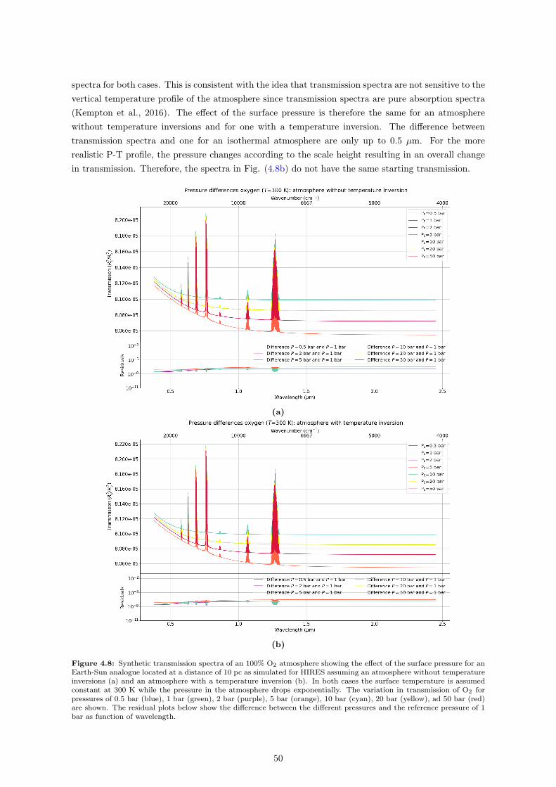
spectra for both cases. This is consistent with the idea that transmission spectra are not sensitive to thevertical temperature profile of the atmosphere since transmission spectra are pure absorption spectra(Kempton et al., 2016). The effect of the surface pressure is therefore the same for an atmospherewithout temperature inversions and for one with a temperature inversion. The difference betweentransmission spectra and one for an isothermal atmosphere are only up to 0.5 µm. For the morerealistic P-T profile, the pressure changes according to the scale height resulting in an overall changein transmission. Therefore, the spectra in Fig. (4.8b) do not have the same starting transmission.

(a)

(b)

Figure 4.8: Synthetic transmission spectra of an 100% O2 atmosphere showing the effect of the surface pressure for anEarth-Sun analogue located at a distance of 10 pc as simulated for HIRES assuming an atmosphere without temperatureinversions (a) and an atmosphere with a temperature inversion (b). In both cases the surface temperature is assumedconstant at 300 K while the pressure in the atmosphere drops exponentially. The variation in transmission of O2 forpressures of 0.5 bar (blue), 1 bar (green), 2 bar (purple), 5 bar (orange), 10 bar (cyan), 20 bar (yellow), ad 50 bar (red)are shown. The residual plots below show the difference between the different pressures and the reference pressure of 1bar as function of wavelength.

50

For the reflection spectra of atmospheres consisting of 100% O3 there is, however, a significantdifference between an atmosphere without any temperature inversion and one with a temperatureinversion as shown in Fig. (4.9). For an atmosphere without temperature inversion it seems that forhigher pressures the spectrum becomes saturated and the planetary flux drops to values ∼ 10−10 Jywhile for lower pressures the reflection is between 10−8 and 10−9 as is the case for an atmosphere witha temperature inversion and an isothermal atmosphere. The reflection spectrum of the atmospherewith temperature inversions seems to be closest to the isothermal case except for the 10 bar spectrum.Differences seem to be because of computational errors of ARCiS.

(a)

(b)

Figure 4.9: Synthetic reflection spectra of an 100% O3 atmosphere showing the effect of the surface pressure for anEarth-Sun analogue located at a distance of 10 pc as simulated for METIS assuming an atmosphere without temperatureinversions (a) and an atmosphere with a temperature inversion (b). In both cases the surface temperature is assumedconstant at 300 K while the pressure in the atmosphere drops exponentially. The variation in planetary flux of O3 forpressures of 0.5 bar (blue), 1 bar (green), 2 bar (purple), 5 bar (orange), 10 bar (cyan), 20 bar (yellow), ad 50 bar (red)are shown. The residual plots below show the difference between the different pressures and the reference pressure of 1bar as function of wavelength.

51

4.2.2 Effect of surface temperature

The effect of the surface temperature for an Earth-Sun analogue at 10 pc on the transmission spec-tra for both an atmosphere without any temperature inversion and one with a temperature inversionwith the instrumental characteristics of HIRES are shown in Fig. (4.10). Similar to the effect of thesurface pressure, transmission spectra are not sensitive to the temperature profile and therefore thetransmission spectra for an atmosphere without temperature inversion is indistinguishable from thetransmission spectra for an atmosphere with a temperature inversion. However, there is a discrimi-nation between the isothermal case and the ones with the more realistic P-T profile in terms of thestrengths of the O2 lines. The O2-A band has a transmission of almost 8.3 · 10−5 for T = 500 K for anatmosphere with more realistic P-T profile while the same band has a transmission of 8.25 · 10−5 forT = 500 K in the case of an isothermal temperature profile with a linear pressure decrease.

Synthetic reflection spectra for varying the surface temperature that can be seen with METIStaking again an Earth-Sun analogue at 10 pc as an example for both an atmosphere without anytemperature inversion and one with a temperature increase in the stratosphere is shown in Fig. (4.11).The reflection spectra assuming no temperature inversion is very dense: for T = 500 K the bandscentered at 3.6 and 4.6 µm are hardly distinguishable. The reason for this may lie in the fact thatthe temperature remains constant for about 85% of the atmospheric extent. However, the effect of theisothermal case and the case where the atmosphere has an Earth-like tropospheric lapse rate followedby an isothermal profile are expected to be more similar than seen in this study. The spectra for anatmosphere with a temperature inversion and for an isothermal atmosphere are, however, more similar.

4.3 Atmosphere consisting of a mixture of gases

This section is divided in two parts: one in which the abundances of the molecules assumed to bepresent in the atmosphere do not change higher in the atmosphere and one in which these abundancesdo change with height above the planetary surface. Again an Earth-Sun analogue at a distance of 10pc is chosen as an example. The detectability of the features themselves is discussed in section 4.4where the integration times are compared to Trappist-1 d, Trappist-1 e, Trappist-1 f, Trappist-1 g,LHS 1140 b and K2-18 b.

4.3.1 Molecules with a constant mixing ratio throughout the atmosphere

In order to take a next step toward building a more and more realistic atmosphere, molecules areassumed to be present in the atmosphere in quantities that do not change with altitude, i.e. thevertical distribution of molecules is constant. The values for the atmospheric abundances used hereare the mixing ratios of the Earth’s troposphere. Also, some of the proposed biosignatures which arenot present in the Earth’s atmosphere in significant quantities (e.g. the mixing ratio of CH3Cl is onthe order of parts per trillion in the Earth’s atmosphere) are added individually to the spectrum. ForC2H6, CH3Cl and NH3 the mixing ratios are assumed to be between 10−5 and 10−7. These valuesare chosen to cover the range of the mixing ratios for the molecules that are present in the Earth’satmosphere in more than trace amounts. The mixing ratios used for the assumed atmosphere withouta vertical distribution of molecules throughout the atmosphere for N2, O2, CO2, H2O, CH4, N2O, O3,C2H6, CH3Cl, and NH3 are displayed in Table 4.1.

52

(a)

(b)

Figure 4.10: Synthetic transmission spectra of an 100% O2 atmosphere showing the effect of the surface temperaturefor an Earth-Sun analogue located at a distance of 10 pc as simulated for HIRES assuming an atmosphere withouttemperature inversions (a) and an atmosphere with a temperature inversions (b). In both cases the surface pressure isassumed constant at 1 bar while the pressure in the atmosphere changes exponentially. The variation in transmission(R2

p/R2s) of O2 for temperatures of 250 K (yellow), 300 K (blue), 350 K (orange), 400 (purple), and 500 K (green) is

shown. The residual plots below show the difference between the different temperatures and the reference temperatureof 300 K as function of wavelength.

53

(a)

(b)

Figure 4.11: Synthetic transmission spectra of an 100% O3 atmosphere showing the effect of the surface temperaturefor an Earth-Sun analogue located at a distance of 10 pc as simulated for METIS assuming an atmosphere withouttemperature inversions (a) and an atmosphere with a temperature inversions (b). In both cases the surface pressure isassumed constant at 1 bar while the pressure in the atmosphere drops exponentially. The variation in planetary flux ofO3 for temperatures of 250 K (yellow), 300 K (blue), 350 K (orange), 400 (purple), and 500 K (green) is shown. Theresidual plots below show the difference between the different temperatures and the reference temperature of 300 K asfunction of wavelength.

54

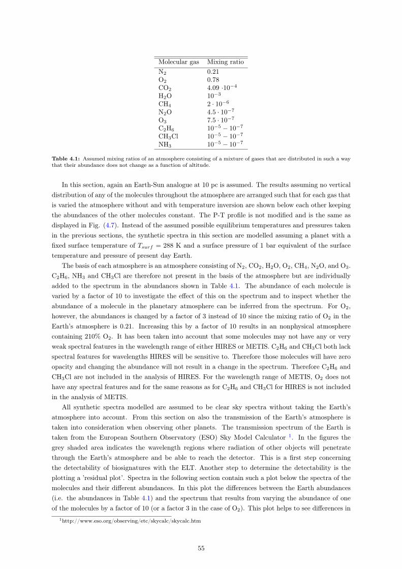
Molecular gas Mixing ratioN2 0.21O2 0.78CO2 4.09 ·10−4

H2O 10−3

CH4 2 · 10−6

N2O 4.5 · 10−7

O3 7.5 · 10−7

C2H6 10−5 − 10−7

CH3Cl 10−5 − 10−7

NH3 10−5 − 10−7

Table 4.1: Assumed mixing ratios of an atmosphere consisting of a mixture of gases that are distributed in such a waythat their abundance does not change as a function of altitude.

In this section, again an Earth-Sun analogue at 10 pc is assumed. The results assuming no verticaldistribution of any of the molecules throughout the atmosphere are arranged such that for each gas thatis varied the atmosphere without and with temperature inversion are shown below each other keepingthe abundances of the other molecules constant. The P-T profile is not modified and is the same asdisplayed in Fig. (4.7). Instead of the assumed possible equilibrium temperatures and pressures takenin the previous sections, the synthetic spectra in this section are modelled assuming a planet with afixed surface temperature of Tsurf = 288 K and a surface pressure of 1 bar equivalent of the surfacetemperature and pressure of present day Earth.

The basis of each atmosphere is an atmosphere consisting of N2, CO2, H2O, O2, CH4, N2O, and O3.C2H6, NH3 and CH3Cl are therefore not present in the basis of the atmosphere but are individuallyadded to the spectrum in the abundances shown in Table 4.1. The abundance of each molecule isvaried by a factor of 10 to investigate the effect of this on the spectrum and to inspect whether theabundance of a molecule in the planetary atmosphere can be inferred from the spectrum. For O2,however, the abundances is changed by a factor of 3 instead of 10 since the mixing ratio of O2 in theEarth’s atmosphere is 0.21. Increasing this by a factor of 10 results in an nonphysical atmospherecontaining 210% O2. It has been taken into account that some molecules may not have any or veryweak spectral features in the wavelength range of either HIRES or METIS. C2H6 and CH3Cl both lackspectral features for wavelengths HIRES will be sensitive to. Therefore those molecules will have zeroopacity and changing the abundance will not result in a change in the spectrum. Therefore C2H6 andCH3Cl are not included in the analysis of HIRES. For the wavelength range of METIS, O2 does nothave any spectral features and for the same reasons as for C2H6 and CH3Cl for HIRES is not includedin the analysis of METIS.

All synthetic spectra modelled are assumed to be clear sky spectra without taking the Earth’satmosphere into account. From this section on also the transmission of the Earth’s atmosphere istaken into consideration when observing other planets. The transmission spectrum of the Earth istaken from the European Southern Observatory (ESO) Sky Model Calculator 1. In the figures thegrey shaded area indicates the wavelength regions where radiation of other objects will penetratethrough the Earth’s atmosphere and be able to reach the detector. This is a first step concerningthe detectability of biosignatures with the ELT. Another step to determine the detectability is theplotting a ’residual plot’. Spectra in the following section contain such a plot below the spectra of themolecules and their different abundances. In this plot the differences between the Earth abundances(i.e. the abundances in Table 4.1) and the spectrum that results from varying the abundance of oneof the molecules by a factor of 10 (or a factor 3 in the case of O2). This plot helps to see differences in

1http://www.eso.org/observing/etc/skycalc/skycalc.htm

55

the spectra that are not seen by inspection by eye and show the level of the difference which is usefulwhen talking about detectability of the biosignature.

Fig. (4.12) shows synthetic transmission spectra of an Earth-Sun analogue at a distance of 10 pcof both an atmosphere without temperature inversions (Fig. (4.12a)) and one with a temperatureincrease in the stratosphere (Fig. (4.12b)) with the concept of HIRES. The main molecules that causeabsorption features are indicated in the plots. H2O, however, has spectral features over the wholewavelength region and is therefore not indicated in the plot but is causing the features not indicatedin the plot. Both of these spectra have an decrease in the transmission with a higher abundance ofO2 due to the increase of the mean molecular weight in the atmosphere with a higher abundance ofO2. The O2 molecule is relatively heavy. Since the scale height is inversely proportional to the meanmolecular weight of the constituents of the atmosphere and the scale height is mainly responsible forsetting the depth of the absorption features in the transmission spectrum, the overall spectrum showsa decrease in R2

p/R2s. This results in an overall difference of about 10−7 of the transmission (see the

residual plot). The differences in the strengths of the lines are also of the same order of magnitude, thestrongest features being the O2 1.3µm band and the O2 A-band. Comparing the transmission spectrafor an atmosphere without temperature inversions and the one with a temperature inversion, there isno change of the spectrum. This is again a result of the nature of a transmission spectrum: it is a pureabsorption spectra and therefore insensitive to the vertical temperature profile of the atmosphere. Thelast point also holds for all other molecules considered in the analysis of transmission spectra.

The synthetic transmission spectra as observed with HIRES considering an Earth-Sun analogue ata distance of 10 pc for both an atmosphere with and an atmosphere without temperature inversionsand changing the abundance of O3 by a factor of 10 are shown in Fig. (4.13). The transmission spectrashown that changing the abundance of O3 only has an effect of the spectrum between 2 µm and 2.5µm. The difference between an abundance of [O3]=7.5 · 10−7 (i.e. Earth abundance) by volume andan abundance of 7.5 ·10−6 (i.e. 0.1 · [O3]Earth) does not show a significant change. The only differenceseen is the feature at ∼ 2.2µm but is about 10−8 of the transmission. For ten times [O3]Earth, however,there are a change up to 10−7 transmission, the most strongest being the feature at ∼ 2.2µm. The O3

2.05 band will not be detectable because of the Earth’s atmospheric blocking.

56

(a)

(b)

Figure 4.12: Synthetic transmission spectra of an atmosphere of a mixture of gases without varying the verticalabundance of any gas (i.e. as function of altitude) showing the effect of changing the overall abundance of O2 by a factorof 10 for an Earth-Sun analogue located at a distance of 10 pc as simulated for HIRES assuming an atmosphere withouttemperature inversions (a) and an atmosphere with a temperature inversion (b). In both cases the surface temperatureis assumed to be similar to Earth (i.e. 288 K) while the pressure in the atmosphere drops exponentially. The variationin transmission (R2

p/R2s) is shown assuming Earth atmospheric abundances for all molecules (purple), 10 times more O2

(green) and 10 times less O2 (orange) keeping the other atmospheric abundances constant (i.e. the Earth abundances).The residual plots below show the difference between an atmosphere with ten times less O2 (orange) and ten timesmore O2 (green) compared to Earth’s atmosphere. The grey shaded areas indicate wavelength regions where the Earth’satmosphere blocks light coming from other sources.

57

(a)

(b)

Figure 4.13: Synthetic transmission spectra of an atmosphere of a mixture of gases without varying the verticalabundance of any gas (i.e. as function of altitude) showing the effect of changing the overall abundance of O3 by a factorof 10 for an Earth-Sun analogue located at a distance of 10 pc as simulated for HIRES assuming an atmosphere withouttemperature inversions (a) and an atmosphere with a temperature inversion (b). In both cases the surface temperatureis assumed to be similar to Earth (i.e. 288 K) while the pressure in the atmosphere drops exponentially. The variationin transmission (R2

p/R2s) is shown assuming Earth atmospheric abundances for all molecules (purple), 10 times more O3

(green) and 10 times less O3 (orange) keeping the other atmospheric abundances constant (i.e. the Earth abundances).The residual plots below show the difference between an atmosphere with ten times less O3 (orange) and ten timesmore O3 (green) compared to Earth’s atmosphere. The grey shaded areas indicate wavelength regions where the Earth’satmosphere blocks light coming from other sources.

Fig. (4.14b) shows the synthetic transmission spectrum of an Earth-Sun analogue at 10 pc whilevarying the abundance of N2O by a factor of 10 without varying the abundance as a function of altitude.Again, both an atmosphere with an and atmosphere without temperature inversions are consideredand the wavelength regions the Earth’s atmosphere blocks are indicated by the shaded grey regions.

58

The effect of changing the abundance such that [N2O]=4.5 · 10−6 is visible by eye around 2.3 µm,where the difference between the Earth abundance of N2O and 10 times this abundance is ∼ 10−7.In the residual plot it is shown that there are differences for 10 [N2O]Earth at wavelengths ∼ 1.3 µm,1.5-1.8 µm and 1.9-2.3 µm. The difference between [N2O]Earth and 0.1 · [N2O]Earth is, however, notsignificant in comparison with the former difference. The 1.3 µm band is not detectable because itis blocked by the Earth’s atmosphere. To overcome this, convolution between lines of Earth and theobserved planet need to be very good. Assuming this is not possible in the near-future, we do notconsider this line in depth.

For H2O, the results of synthetic transmission spectra of an Earth-Sun analogue at 10 pc are shownin Fig. (4.15). An atmosphere without any temperature inversion is shown in Fig. (4.15a) while anatmosphere including a temperature increase as function of altitude in the stratosphere is shown in Fig(4.15b). It can be seen that increasing the abundance of H2O does not increase the overall spectrumas was the case for O2 but the strength of the H2O lines increases. This increase is over the wavelengthregion of 0.7 to 2.4 µm. Note that the strength of the O2 features does not change when changingthe abundance of H2O by a factor of 10. Although O2 bands are rather narrow, the abundance of O2

and H2O can be determined separately. Whether there is an increase in the abundance of N2O or O3

compared to an increase in the abundance of H2O is hard to distinguish.

59

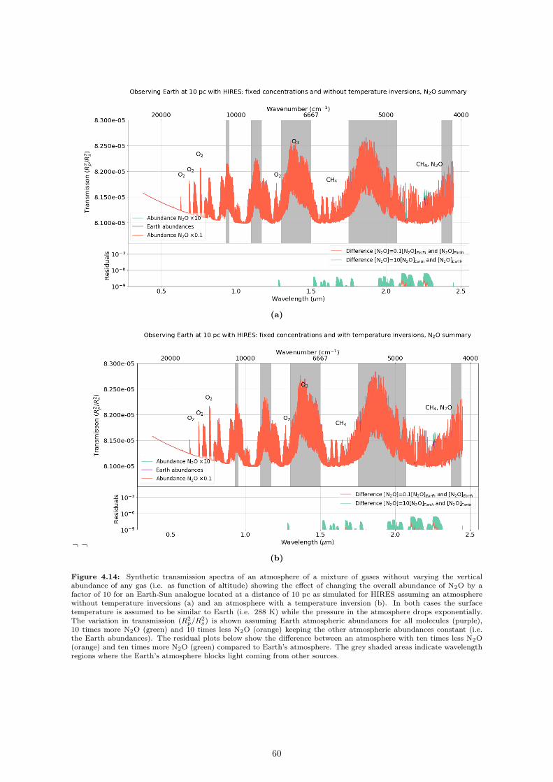
(a)

¬ ¬(b)

Figure 4.14: Synthetic transmission spectra of an atmosphere of a mixture of gases without varying the verticalabundance of any gas (i.e. as function of altitude) showing the effect of changing the overall abundance of N2O by afactor of 10 for an Earth-Sun analogue located at a distance of 10 pc as simulated for HIRES assuming an atmospherewithout temperature inversions (a) and an atmosphere with a temperature inversion (b). In both cases the surfacetemperature is assumed to be similar to Earth (i.e. 288 K) while the pressure in the atmosphere drops exponentially.The variation in transmission (R2

p/R2s) is shown assuming Earth atmospheric abundances for all molecules (purple),

10 times more N2O (green) and 10 times less N2O (orange) keeping the other atmospheric abundances constant (i.e.the Earth abundances). The residual plots below show the difference between an atmosphere with ten times less N2O(orange) and ten times more N2O (green) compared to Earth’s atmosphere. The grey shaded areas indicate wavelengthregions where the Earth’s atmosphere blocks light coming from other sources.

60

(a)

(b)

Figure 4.15: Synthetic transmission spectra of an atmosphere of a mixture of gases without varying the verticalabundance of any gas (i.e. as function of altitude) showing the effect of changing the overall abundance of H2O by afactor of 10 for an Earth-Sun analogue located at a distance of 10 pc as simulated for HIRES assuming an atmospherewithout temperature inversions (a) and an atmosphere with a temperature inversion (b). In both cases the surfacetemperature is assumed to be similar to Earth (i.e. 288 K) while the pressure in the atmosphere drops exponentially.The variation in transmission (R2

p/R2s) is shown assuming Earth atmospheric abundances for all molecules (purple),

10 times more H2O (green) and 10 times less H2O (orange) keeping the other atmospheric abundances constant (i.e.the Earth abundances). The residual plots below show the difference between an atmosphere with ten times less H2O(orange) and ten times more H2O (green) compared to Earth’s atmosphere. The grey shaded areas indicate wavelengthregions where the Earth’s atmosphere blocks light coming from other sources.

Fig. (4.16) shows the effect of changing the abundance of CH4 by a factor of 10 in an atmospherewithout changing the vertical distribution of any molecule for an Earth-Sun analogue at 10 pc takingHIRES as the instrument on the ELT. Again an atmosphere with and without a temperature inversionare considered. It can be seen that CH4 has an effect on the spectrum at wavelengths between ∼ 0.9

61

µ to 2.5 µm. The two band that cause the most significant change are the band around 1.6 µm andthe one around 2.3 µm. In these two bands, the difference between 10 · [CH4]Earth and [CH4]Earth(∼ 10−6) and 0.1 · [CH4]Earth and [CH4]Earth (∼ 10−7) are about one order of magnitude or less apart.The presence of CH4 for an atmosphere containing 10 times the Earth abundance will therefore morelikely to be detection compared to 10 times less the Earth abundance. Note that besides the spectralregions of H2O, the spectral regions of N2O overlap with CH4.

62

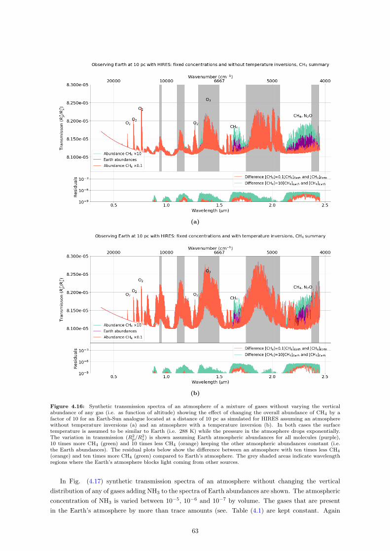
(a)

(b)

Figure 4.16: Synthetic transmission spectra of an atmosphere of a mixture of gases without varying the verticalabundance of any gas (i.e. as function of altitude) showing the effect of changing the overall abundance of CH4 by afactor of 10 for an Earth-Sun analogue located at a distance of 10 pc as simulated for HIRES assuming an atmospherewithout temperature inversions (a) and an atmosphere with a temperature inversion (b). In both cases the surfacetemperature is assumed to be similar to Earth (i.e. 288 K) while the pressure in the atmosphere drops exponentially.The variation in transmission (R2

p/R2s) is shown assuming Earth atmospheric abundances for all molecules (purple),

10 times more CH4 (green) and 10 times less CH4 (orange) keeping the other atmospheric abundances constant (i.e.the Earth abundances). The residual plots below show the difference between an atmosphere with ten times less CH4

(orange) and ten times more CH4 (green) compared to Earth’s atmosphere. The grey shaded areas indicate wavelengthregions where the Earth’s atmosphere blocks light coming from other sources.

In Fig. (4.17) synthetic transmission spectra of an atmosphere without changing the verticaldistribution of any of gases adding NH3 to the spectra of Earth abundances are shown. The atmosphericconcentration of NH3 is varied between 10−5, 10−6 and 10−7 by volume. The gases that are presentin the Earth’s atmosphere by more than trace amounts (see. Table (4.1) are kept constant. Again

63

both an atmosphere with an Earth-like temperature decrease in the troposphere and an isothermalatmosphere thereafter is assumed (Fig. (4.17a) and an atmosphere where the temperature increaseswith altitude in the stratosphere (Fig. (4.17b)) are modelled. It can be seen that NH3 has effect on thesynthetic transmission spectrum at wavelengths of ∼ 1.1 µm, 1.3 µm, 1.5 µm, 2.0 µ and 2.3 µm. Theband around 2.3 µm coincides with the bands of CH4 and N2O for bands of those molecules around2.3 µm. The abundance of CH4 should in that case be inferred from the 1.7 µm band while changingthe abundance of N2O does not show strong features in other wavelength regions. .

64

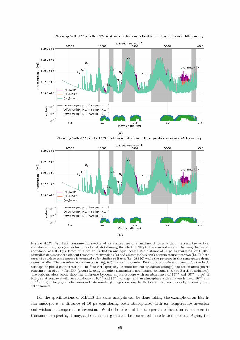
(a)

(b)

Figure 4.17: Synthetic transmission spectra of an atmosphere of a mixture of gases without varying the verticalabundance of any gas (i.e. as function of altitude) showing the effect of NH3 to the atmosphere and changing the overallabundance of NH3 by a factor of 10 for an Earth-Sun analogue located at a distance of 10 pc as simulated for HIRESassuming an atmosphere without temperature inversions (a) and an atmosphere with a temperature inversion (b). In bothcases the surface temperature is assumed to be similar to Earth (i.e. 288 K) while the pressure in the atmosphere dropsexponentially. The variation in transmission (R2

p/R2s) is shown assuming Earth atmospheric abundances for the basis

atmosphere plus a concentration of 10−5 of NH3 (purple), 10 times this concentration (orange) and for an atmosphericconcentration of 10−7 for NH3 (green) keeping the other atmospheric abundances constant (i.e. the Earth abundances).The residual plots below show the difference between an atmosphere with an abundance of 10−5 and 10−6 (blue) ofNH3, an atmosphere with an abundance of 10−5 and 10−7 (orange) and an atmosphere with an abundance of 10−6 and10−7 (blue). The grey shaded areas indicate wavelength regions where the Earth’s atmosphere blocks light coming fromother sources.

For the specifications of METIS the same analysis can be done taking the example of an Earth-sun analogue at a distance of 10 pc considering both atmospheres with an temperature inversionand without a temperature inversion. While the effect of the temperature inversion is not seen intransmission spectra, it may, although not significant, be uncovered in reflection spectra. Again, the

65

abundances of the molecules does not change as a function of altitude. Changing the abundanceof O3 by a factor of 10 while keeping all other abundances of the present gases constant results insynthetic reflection spectra with an almost constant change of about a factor of ∼ 10−8 Jy as is shownin Fig. (4.18). In the spectra the effect of changing the abundance of O3 is greatest around 4.7 µmwhere the differences between [O3]=7.5 · 10−6, 7.5 · 10−7, and 7.5 · 10−8 can be seen most clearly byinspection by eye. In this wavelength region the Earth’s atmosphere, however, blocks light from othersources as indicated by the grey shaded region. For the detectability this means that a variation in theconcentration of O3 is not observable with METIS. Moreover, the distinction of an atmosphere withand without temperature inversions cannot be made when changing the abundances of O3.

Fig. (4.19) shows synthetic reflection spectra of an Earth-Sun analogue at 10 pc demonstrationthe effect of changing the concentration of N2O by a factor of 10 without changing the abundances ofany molecule as a function of altitude. Again, the effect of temperature inversions is not noteworthy.Changing the abundances of N2O by a factor of 10 results in a considerable change in the reflectionspectra around wavelengths of 3.9 µm, 4.1 µm and 4.5 µm. The band around 4.5 µ is fully blocked byour own atmosphere while the other two bands are in the region where the atmosphere does not blocklight from other sources. These bands have a difference of ∼ 10−8 Jy between [N2O]= 4.5 · 10−7 andeither [N2O]= 4.5 · 10−6 or [N2O]= 4.5 · 10−8 by volume.

66

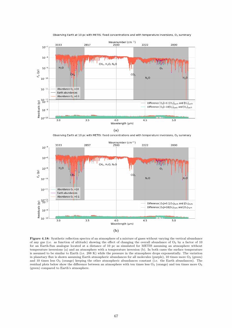
(a)

(b)

Figure 4.18: Synthetic reflection spectra of an atmosphere of a mixture of gases without varying the vertical abundanceof any gas (i.e. as function of altitude) showing the effect of changing the overall abundance of O3 by a factor of 10for an Earth-Sun analogue located at a distance of 10 pc as simulated for METIS assuming an atmosphere withouttemperature inversions (a) and an atmosphere with a temperature inversion (b). In both cases the surface temperatureis assumed to be similar to Earth (i.e. 288 K) while the pressure in the atmosphere drops exponentially. The variationin planetary flux is shown assuming Earth atmospheric abundances for all molecules (purple), 10 times more O3 (green)and 10 times less O3 (orange) keeping the other atmospheric abundances constant (i.e. the Earth abundances). Theresidual plots below show the difference between an atmosphere with ten times less O3 (orange) and ten times more O3

(green) compared to Earth’s atmosphere.

67

(a)

(b)

Figure 4.19: Synthetic reflection spectra of an atmosphere of a mixture of gases without varying the vertical abundanceof any gas (i.e. as function of altitude) showing the effect of changing the overall abundance of N2O by a factor of 10for an Earth-Sun analogue located at a distance of 10 pc as simulated for METIS assuming an atmosphere withouttemperature inversions (a) and an atmosphere with a temperature inversion (b). In both cases the surface temperatureis assumed to be similar to Earth (i.e. 288 K) while the pressure in the atmosphere drops exponentially. The variation inplanetary flux is shown assuming Earth atmospheric abundances for all molecules (purple), 10 times more N2O (green)and 10 times less N2O (orange) keeping the other atmospheric abundances constant (i.e. the Earth abundances). Theresidual plots below show the difference between an atmosphere with ten times less N2O (orange) and ten times moreN2O (green) compared to Earth’s atmosphere.

By changing the concentration of atmospheric H2O, the effect of one of the habitability markersis considered. Although H2O is not a biosignature, it is the habitability marker used to define theHZ. Changing the abundances by a factor of 10 compared to the Earth atmospheric abundance of[H20]=10−3 per unit volume in the troposphere and assuming this concentration remains constant

68

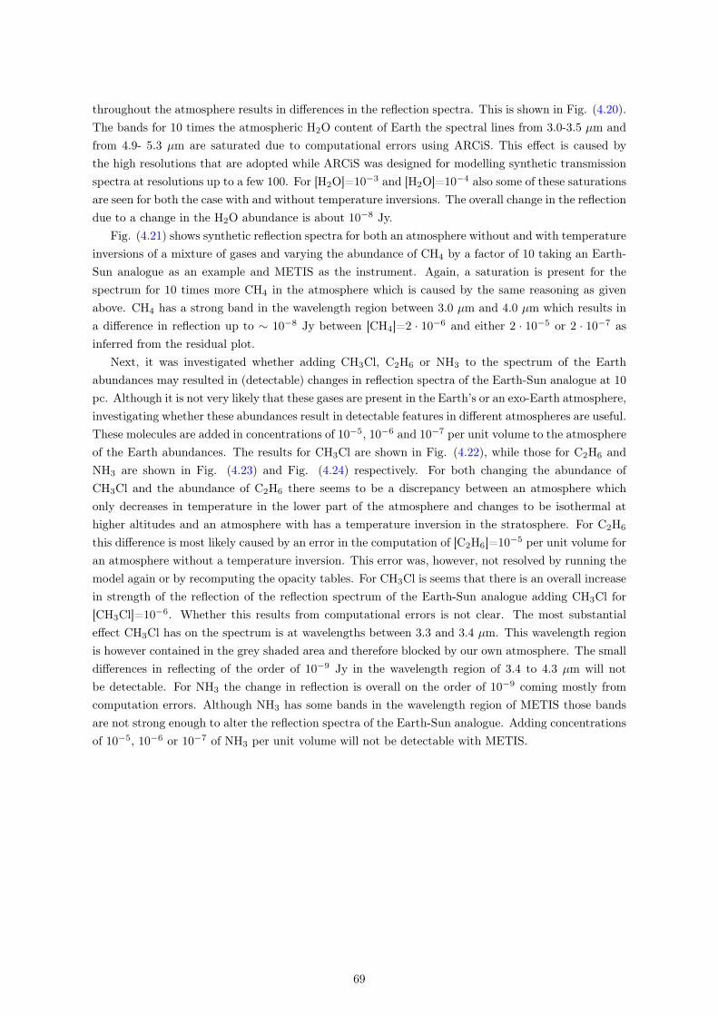
throughout the atmosphere results in differences in the reflection spectra. This is shown in Fig. (4.20).The bands for 10 times the atmospheric H2O content of Earth the spectral lines from 3.0-3.5 µm andfrom 4.9- 5.3 µm are saturated due to computational errors using ARCiS. This effect is caused bythe high resolutions that are adopted while ARCiS was designed for modelling synthetic transmissionspectra at resolutions up to a few 100. For [H2O]=10−3 and [H2O]=10−4 also some of these saturationsare seen for both the case with and without temperature inversions. The overall change in the reflectiondue to a change in the H2O abundance is about 10−8 Jy.

Fig. (4.21) shows synthetic reflection spectra for both an atmosphere without and with temperatureinversions of a mixture of gases and varying the abundance of CH4 by a factor of 10 taking an Earth-Sun analogue as an example and METIS as the instrument. Again, a saturation is present for thespectrum for 10 times more CH4 in the atmosphere which is caused by the same reasoning as givenabove. CH4 has a strong band in the wavelength region between 3.0 µm and 4.0 µm which results ina difference in reflection up to ∼ 10−8 Jy between [CH4]=2 · 10−6 and either 2 · 10−5 or 2 · 10−7 asinferred from the residual plot.

Next, it was investigated whether adding CH3Cl, C2H6 or NH3 to the spectrum of the Earthabundances may resulted in (detectable) changes in reflection spectra of the Earth-Sun analogue at 10pc. Although it is not very likely that these gases are present in the Earth’s or an exo-Earth atmosphere,investigating whether these abundances result in detectable features in different atmospheres are useful.These molecules are added in concentrations of 10−5, 10−6 and 10−7 per unit volume to the atmosphereof the Earth abundances. The results for CH3Cl are shown in Fig. (4.22), while those for C2H6 andNH3 are shown in Fig. (4.23) and Fig. (4.24) respectively. For both changing the abundance ofCH3Cl and the abundance of C2H6 there seems to be a discrepancy between an atmosphere whichonly decreases in temperature in the lower part of the atmosphere and changes to be isothermal athigher altitudes and an atmosphere with has a temperature inversion in the stratosphere. For C2H6

this difference is most likely caused by an error in the computation of [C2H6]=10−5 per unit volume foran atmosphere without a temperature inversion. This error was, however, not resolved by running themodel again or by recomputing the opacity tables. For CH3Cl is seems that there is an overall increasein strength of the reflection of the reflection spectrum of the Earth-Sun analogue adding CH3Cl for[CH3Cl]=10−6. Whether this results from computational errors is not clear. The most substantialeffect CH3Cl has on the spectrum is at wavelengths between 3.3 and 3.4 µm. This wavelength regionis however contained in the grey shaded area and therefore blocked by our own atmosphere. The smalldifferences in reflecting of the order of 10−9 Jy in the wavelength region of 3.4 to 4.3 µm will notbe detectable. For NH3 the change in reflection is overall on the order of 10−9 coming mostly fromcomputation errors. Although NH3 has some bands in the wavelength region of METIS those bandsare not strong enough to alter the reflection spectra of the Earth-Sun analogue. Adding concentrationsof 10−5, 10−6 or 10−7 of NH3 per unit volume will not be detectable with METIS.

69

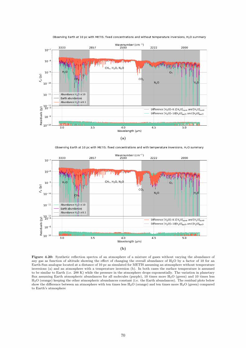
(a)

(b)

Figure 4.20: Synthetic reflection spectra of an atmosphere of a mixture of gases without varying the abundance ofany gas as function of altitude showing the effect of changing the overall abundance of H2O by a factor of 10 for anEarth-Sun analogue located at a distance of 10 pc as simulated for METIS assuming an atmosphere without temperatureinversions (a) and an atmosphere with a temperature inversion (b). In both cases the surface temperature is assumedto be similar to Earth (i.e. 288 K) while the pressure in the atmosphere drops exponentially. The variation in planetaryflux assuming Earth atmospheric abundances for all molecules (purple), 10 times more H2O (green) and 10 times lessH2O (orange) keeping the other atmospheric abundances constant (i.e. the Earth abundances). The residual plots belowshow the difference between an atmosphere with ten times less H2O (orange) and ten times more H2O (green) comparedto Earth’s atmosphere

70

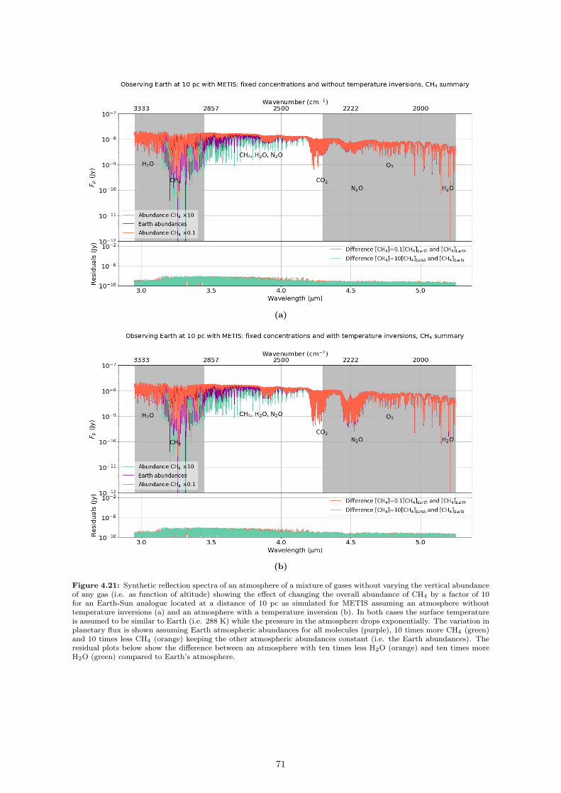
(a)

(b)

Figure 4.21: Synthetic reflection spectra of an atmosphere of a mixture of gases without varying the vertical abundanceof any gas (i.e. as function of altitude) showing the effect of changing the overall abundance of CH4 by a factor of 10for an Earth-Sun analogue located at a distance of 10 pc as simulated for METIS assuming an atmosphere withouttemperature inversions (a) and an atmosphere with a temperature inversion (b). In both cases the surface temperatureis assumed to be similar to Earth (i.e. 288 K) while the pressure in the atmosphere drops exponentially. The variation inplanetary flux is shown assuming Earth atmospheric abundances for all molecules (purple), 10 times more CH4 (green)and 10 times less CH4 (orange) keeping the other atmospheric abundances constant (i.e. the Earth abundances). Theresidual plots below show the difference between an atmosphere with ten times less H2O (orange) and ten times moreH2O (green) compared to Earth’s atmosphere.

71

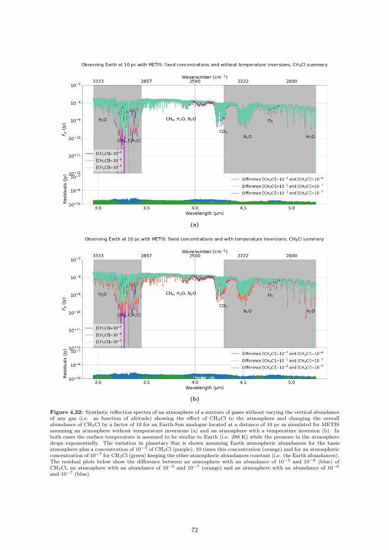
(a)

(b)

Figure 4.22: Synthetic reflection spectra of an atmosphere of a mixture of gases without varying the vertical abundanceof any gas (i.e. as function of altitude) showing the effect of CH3Cl to the atmosphere and changing the overallabundance of CH3Cl by a factor of 10 for an Earth-Sun analogue located at a distance of 10 pc as simulated for METISassuming an atmosphere without temperature inversions (a) and an atmosphere with a temperature inversion (b). Inboth cases the surface temperature is assumed to be similar to Earth (i.e. 288 K) while the pressure in the atmospheredrops exponentially. The variation in planetary flux is shown assuming Earth atmospheric abundances for the basisatmosphere plus a concentration of 10−5 of CH3Cl (purple), 10 times this concentration (orange) and for an atmosphericconcentration of 10−7 for CH3Cl (green) keeping the other atmospheric abundances constant (i.e. the Earth abundances).The residual plots below show the difference between an atmosphere with an abundance of 10−5 and 10−6 (blue) ofCH3Cl, an atmosphere with an abundance of 10−5 and 10−7 (orange) and an atmosphere with an abundance of 10−6

and 10−7 (blue).

72

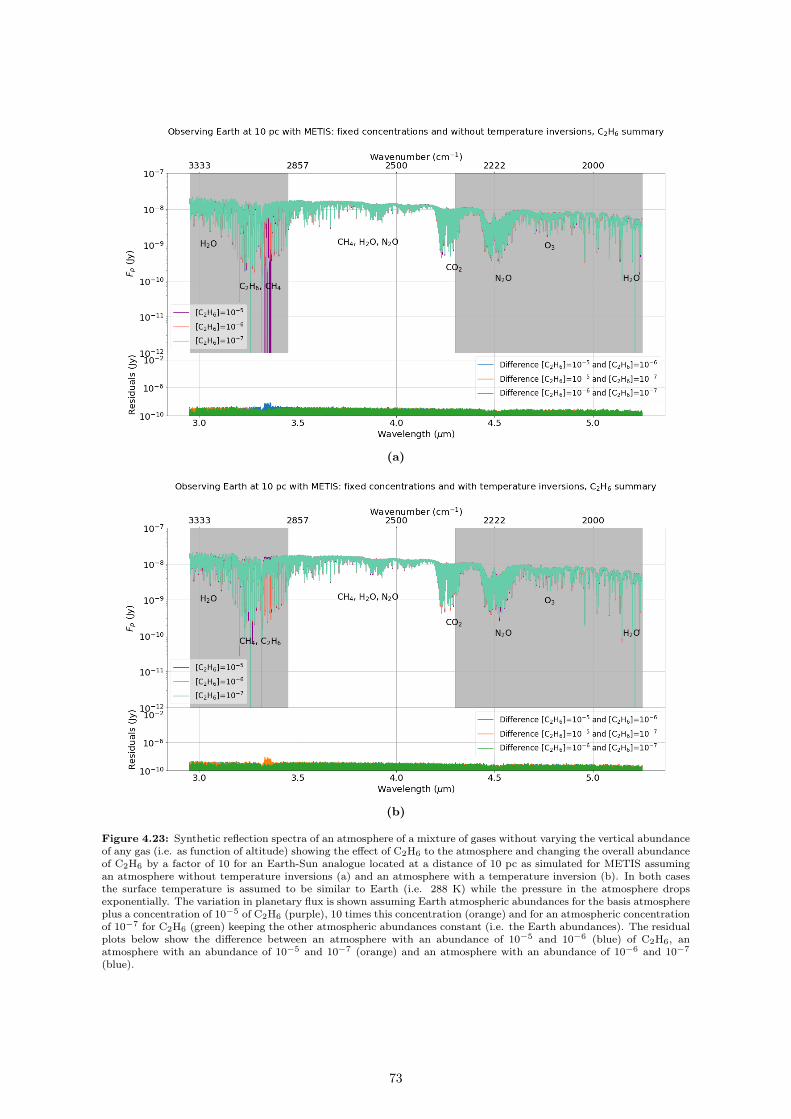
(a)

(b)

Figure 4.23: Synthetic reflection spectra of an atmosphere of a mixture of gases without varying the vertical abundanceof any gas (i.e. as function of altitude) showing the effect of C2H6 to the atmosphere and changing the overall abundanceof C2H6 by a factor of 10 for an Earth-Sun analogue located at a distance of 10 pc as simulated for METIS assumingan atmosphere without temperature inversions (a) and an atmosphere with a temperature inversion (b). In both casesthe surface temperature is assumed to be similar to Earth (i.e. 288 K) while the pressure in the atmosphere dropsexponentially. The variation in planetary flux is shown assuming Earth atmospheric abundances for the basis atmosphereplus a concentration of 10−5 of C2H6 (purple), 10 times this concentration (orange) and for an atmospheric concentrationof 10−7 for C2H6 (green) keeping the other atmospheric abundances constant (i.e. the Earth abundances). The residualplots below show the difference between an atmosphere with an abundance of 10−5 and 10−6 (blue) of C2H6, anatmosphere with an abundance of 10−5 and 10−7 (orange) and an atmosphere with an abundance of 10−6 and 10−7

(blue).

73

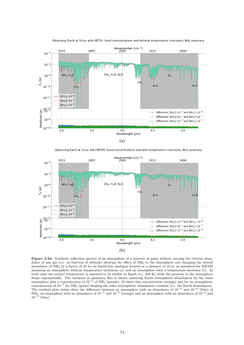
(a)

(b)

Figure 4.24: Synthetic reflection spectra of an atmosphere of a mixture of gases without varying the vertical abun-dance of any gas (i.e. as function of altitude) showing the effect of NH3 to the atmosphere and changing the overallabundance of NH3 by a factor of 10 for an Earth-Sun analogue located at a distance of 10 pc as simulated for METISassuming an atmosphere without temperature inversions (a) and an atmosphere with a temperature inversion (b). Inboth cases the surface temperature is assumed to be similar to Earth (i.e. 288 K) while the pressure in the atmospheredrops exponentially. The variation in planetary flux is shown assuming Earth atmospheric abundances for the basisatmosphere plus a concentration of 10−5 of NH3 (purple), 10 times this concentration (orange) and for an atmosphericconcentration of 10−7 for NH3 (green) keeping the other atmospheric abundances constant (i.e. the Earth abundances).The residual plots below show the difference between an atmosphere with an abundance of 10−5 and 10−6 (blue) ofNH3, an atmosphere with an abundance of 10−5 and 10−7 (orange) and an atmosphere with an abundance of 10−6 and10−7 (blue).

74

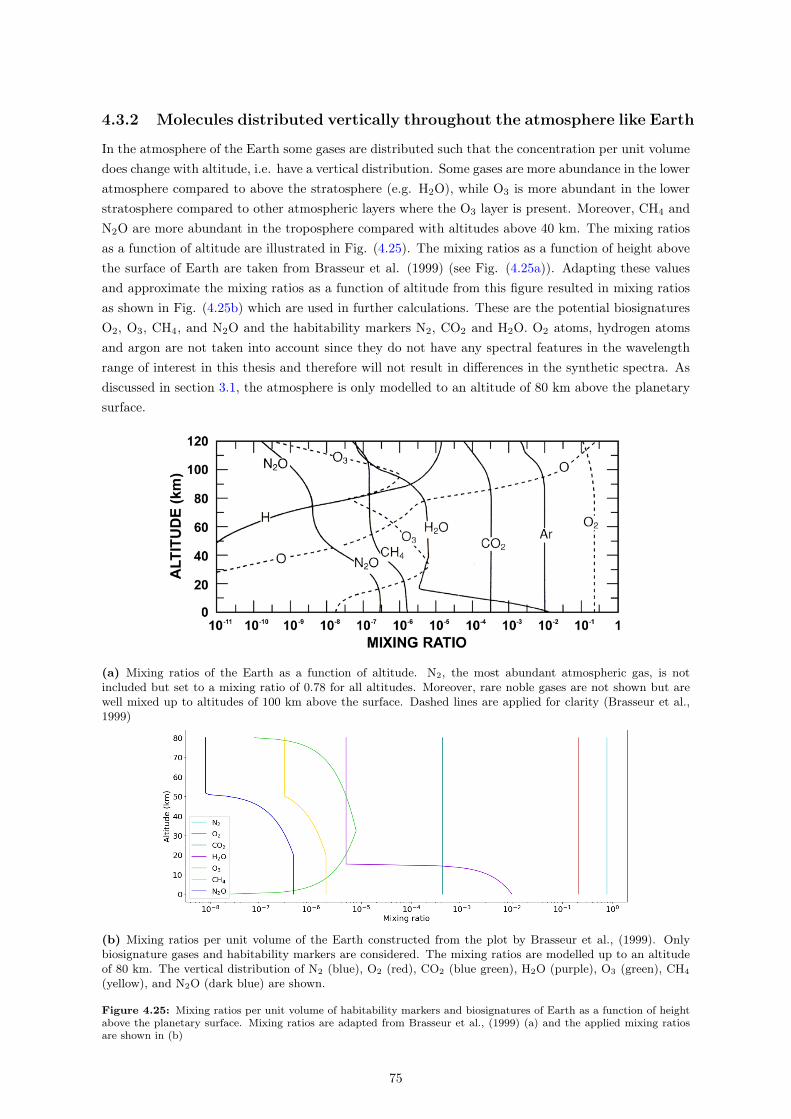
4.3.2 Molecules distributed vertically throughout the atmosphere like Earth

In the atmosphere of the Earth some gases are distributed such that the concentration per unit volumedoes change with altitude, i.e. have a vertical distribution. Some gases are more abundance in the loweratmosphere compared to above the stratosphere (e.g. H2O), while O3 is more abundant in the lowerstratosphere compared to other atmospheric layers where the O3 layer is present. Moreover, CH4 andN2O are more abundant in the troposphere compared with altitudes above 40 km. The mixing ratiosas a function of altitude are illustrated in Fig. (4.25). The mixing ratios as a function of height abovethe surface of Earth are taken from Brasseur et al. (1999) (see Fig. (4.25a)). Adapting these valuesand approximate the mixing ratios as a function of altitude from this figure resulted in mixing ratiosas shown in Fig. (4.25b) which are used in further calculations. These are the potential biosignaturesO2, O3, CH4, and N2O and the habitability markers N2, CO2 and H2O. O2 atoms, hydrogen atomsand argon are not taken into account since they do not have any spectral features in the wavelengthrange of interest in this thesis and therefore will not result in differences in the synthetic spectra. Asdiscussed in section 3.1, the atmosphere is only modelled to an altitude of 80 km above the planetarysurface.

(a) Mixing ratios of the Earth as a function of altitude. N2, the most abundant atmospheric gas, is notincluded but set to a mixing ratio of 0.78 for all altitudes. Moreover, rare noble gases are not shown but arewell mixed up to altitudes of 100 km above the surface. Dashed lines are applied for clarity (Brasseur et al.,1999)

(b) Mixing ratios per unit volume of the Earth constructed from the plot by Brasseur et al., (1999). Onlybiosignature gases and habitability markers are considered. The mixing ratios are modelled up to an altitudeof 80 km. The vertical distribution of N2 (blue), O2 (red), CO2 (blue green), H2O (purple), O3 (green), CH4

(yellow), and N2O (dark blue) are shown.

Figure 4.25: Mixing ratios per unit volume of habitability markers and biosignatures of Earth as a function of heightabove the planetary surface. Mixing ratios are adapted from Brasseur et al., (1999) (a) and the applied mixing ratiosare shown in (b)

75

In this section the vertical distribution of NH3, CH3Cl and C2H6 are kept constant and the abun-dances of these molecules are again assumed to vary between concentrations of 10−7 and 10−5 per unitvolume. Again an Earth-Sun analogue at a distance of 10 pc with a surface temperature of 288 K ischosen as an example. The assumed temperature profile is such that it has one temperature inversion(i.e. the red profile in Fig. (4.7)). As previously, the pressure profile is assumed such that it dropsexponentially with altitude. The synthetic transmission spectra for observing an atmosphere takingan Earth-Sun analogue at a distance of 10 pc as an example observed with HIRES are shown in Fig.(4.26). The abundance of O2 is changed by a factor of 3 and the abundances of O3, N2O, H2O, CH4

and NH3 are changed by a factor of 10. Comparing the plots in section 4.3.1 with Fig. (4.26) smaller’bumps’ appear in general in Fig. (4.26) compared to the figures in section 4.3.1 were it was assumedthat molecules present in the atmosphere do not change their abundance with altitude. This differenceis predominantly caused by the H2O features. Transmission spectra probe primarily the upper partsof the atmosphere. Since H2O is less abundant in the upper atmosphere compared to the tropospherethe abundance of atmospheric H2O is lower overall causing the decrease of transmission. This doesnot affect the strength of the O2 lines (see Fig. (4.26a)). The residual plot now gives the differencein just the O2 instead of also some overall difference between the spectra of the different abundances.The difference of strengths of the O2 bands are ∼ 10−7 and is strongest for the B-band, the A-band,and the a 1δg band.

For O3 the discrepancy between an atmosphere without a change abundance of any gas withaltitude (Fig. (4.13)) and an atmosphere where a change in abundance is assumed of some molecules(Fig. (4.26b)) is bigger. For the latter case, the residual plot shows differences between 10 times moreO3 and Earth abundances of O3 continuously over wavelengths between 0.7 and 2.5 µm while for the1 concentration case this difference was limited to the region between 2.0 and 2.5 µm. This resultedfrom the difference in mixing ratio: O3 is more abundant in the middle and upper atmosphere than inthe troposphere.

N2O is less abundant in the upper atmosphere compared to the troposphere. Therefore, the con-centration of N2O probed with transmission spectroscopy assuming an atmosphere with a verticaldistribution of molecules will result in probing the lower abundance compared to the case assumingthe abundances are equal to the Earth concentration in the troposphere. For N2O the differencesbetween Fig. (4.26c) and Fig. 4.14b) are primarily in the difference between the Earth abundancesand 10% of this abundance. For the latter case, there is no notable change between these whereasfor the former case, there is a difference of about 10−7 in transmission for almost the full wavelengthrange. Moreover, the concentration N2O has an effect on the strength of the O2 bands.

The concentration of H2O changes by more than 3 orders of magnitude in the first 20 km measuredfrom the surface. After that, the concentration stays approximately constant. Besides the overallchange in the transmission spectrum, there is a change in the residuals for the case where there is 10times more H2O present in the atmosphere. The residuals show a more saturated behaviour if thereis a vertical distribution of molecules (compare Fig. (4.26d) and Fig. (4.15b)) whereas for the casethere is no vertical distribution of molecules in the atmosphere, the residual for 10 times more and 10times less H2O vapour have similar shapes. Similarly for CH4, which is also less abundant at higheraltitudes compared to tropospheric concentrations, the residuals are saturated.

As expected, besides the overall change of transmission spectra due to H2O absorption features,there is no change in the transmission spectra for NH3 adjusting the vertical distribution of othermolecules since no assumed difference in vertical distribution was assumed in this section.

76

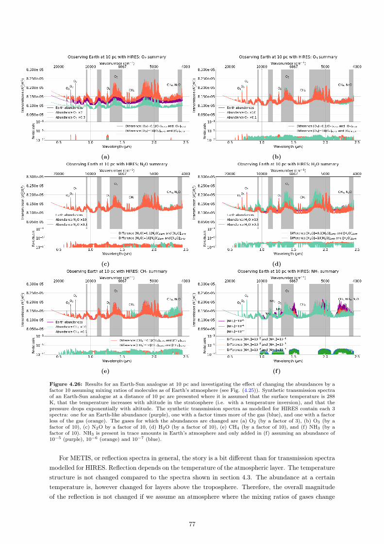
(a) (b)

(c) (d)

(e) (f)

Figure 4.26: Results for an Earth-Sun analogue at 10 pc and investigating the effect of changing the abundances by afactor 10 assuming mixing ratios of molecules as of Earth’s atmosphere (see Fig. (4.25)). Synthetic transmission spectraof an Earth-Sun analogue at a distance of 10 pc are presented where it is assumed that the surface temperature is 288K, that the temperature increases with altitude in the stratosphere (i.e. with a temperature inversion), and that thepressure drops exponentially with altitude. The synthetic transmission spectra as modelled for HIRES contain each 3spectra: one for an Earth-like abundance (purple), one with a factor times more of the gas (blue), and one with a factorless of the gas (orange). The gases for which the abundances are changed are (a) O2 (by a factor of 3), (b) O3 (by afactor of 10), (c) N2O by a factor of 10, (d) H2O (by a factor of 10), (e) CH4 (by a factor of 10), and (f) NH3 (by afactor of 10). NH3 is present in trace amounts in Earth’s atmosphere and only added in (f) assuming an abundance of10−5 (purple), 10−6 (orange) and 10−7 (blue).

For METIS, or reflection spectra in general, the story is a bit different than for transmission spectramodelled for HIRES. Reflection depends on the temperature of the atmospheric layer. The temperaturestructure is not changed compared to the spectra shown in section 4.3. The abundance at a certaintemperature is, however changed for layers above the troposphere. Therefore, the overall magnitudeof the reflection is not changed if we assume an atmosphere where the mixing ratios of gases change

77

with altitude compared to an atmosphere where all constituent gases doe not change concentrationas a function of altitude. Fig. (4.27) shows reflection spectra of O3, N2O, H2O, CH4, CH3Cl, NH3

and C2H6 when changing the atmospheric abundance by a factor of 10 assuming the Earth abundancereflection (purple) has abundances from Fig. (4.25).

Comparing the synthetic reflection spectra of O3 in Fig. (4.18b) and Fig. (4.27a) no difference isseen although the abundance of O3 has several abundances as a function altitude in the latter case.Comparing the spectra for N2O, there is, however, a difference between an atmosphere for the case themixing ratios were kept constant and for the case where those mixing ratios were subject to change.Comparing Fig. (4.19b) and Fig. (4.27b), the band a 4.6 µm shows a weakening in this N2O band inthe case there is a change in mixing ratio. The concentration of N2O decreases with altitude. Althoughimaging planets can probe more of the atmosphere, they still encounter the upper atmosphere first.Therefore, the concentration of N2O is lower. Note also that the H2O bands do not show any linesgoing to zero because the H2O abundance drops as a function of altitude. The same reasoning appliesfor the H2O bands In Fig. (4.27c). The shaded regions in Fig. 4.20b are saturated, but not in thecase that H2O is present mostly in the lower atmosphere. The concentration of CH4 is only slightlylower (i.e. less than one order of magnitude) in the case where the mixing ratio is assumed to varywith altitude compared to the case where the mixing ratio is assumed to be equal to the troposphericmixing ratios. Comparing Fig. (4.21b) and Fig. (4.27d shows that increasing the abundance of CH4

by a factor 10 results in weaker bands for the latter figure.For the molecules that are added to the spectrum, CH3Cl, C2H6 and NH3, there is probably an

inconsistency in the opacity tables used for calculating these synthetic spectra.

78

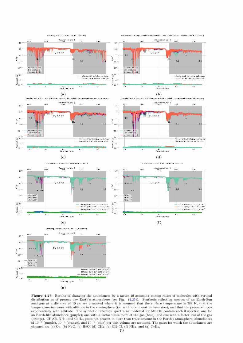
(a) (b)

(c) (d)

(e) (f)

(g)

Figure 4.27: Results of changing the abundances by a factor 10 assuming mixing ratios of molecules with verticaldistribution as of present day Earth’s atmosphere (see Fig. (4.25)). Synthetic reflection spectra of an Earth-Sunanalogue at a distance of 10 pc are presented where it is assumed that the surface temperature is 288 K, that thetemperature increases with altitude in the stratosphere (i.e. with a temperature inversion), and that the pressure dropsexponentially with altitude. The synthetic reflection spectra as modelled for METIS contain each 3 spectra: one foran Earth-like abundance (purple), one with a factor times more of the gas (blue), and one with a factor less of the gas(orange). CH3Cl, NH3, and C2H6, gases not present in more than trace amount in the Earth’s atmosphere, abundancesof 10−5 (purple), 10−6 (orange), and 10−7 (blue) per unit volume are assumed. The gases for which the abundances arechanged are (a) O3, (b) N2O, (c) H2O, (d) CH4, (e) CH3Cl, (f) NH3, and (g) C2H6.

79

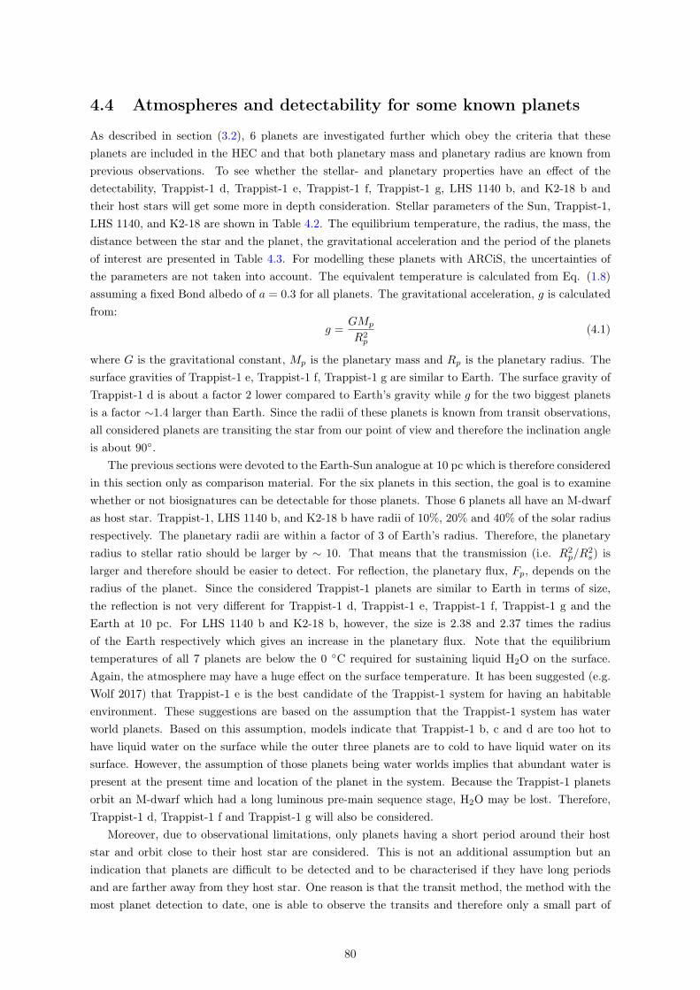
4.4 Atmospheres and detectability for some known planets

As described in section (3.2), 6 planets are investigated further which obey the criteria that theseplanets are included in the HEC and that both planetary mass and planetary radius are known fromprevious observations. To see whether the stellar- and planetary properties have an effect of thedetectability, Trappist-1 d, Trappist-1 e, Trappist-1 f, Trappist-1 g, LHS 1140 b, and K2-18 b andtheir host stars will get some more in depth consideration. Stellar parameters of the Sun, Trappist-1,LHS 1140, and K2-18 are shown in Table 4.2. The equilibrium temperature, the radius, the mass, thedistance between the star and the planet, the gravitational acceleration and the period of the planetsof interest are presented in Table 4.3. For modelling these planets with ARCiS, the uncertainties ofthe parameters are not taken into account. The equivalent temperature is calculated from Eq. (1.8)assuming a fixed Bond albedo of a = 0.3 for all planets. The gravitational acceleration, g is calculatedfrom:

g =GMp

R2p

(4.1)

where G is the gravitational constant, Mp is the planetary mass and Rp is the planetary radius. Thesurface gravities of Trappist-1 e, Trappist-1 f, Trappist-1 g are similar to Earth. The surface gravity ofTrappist-1 d is about a factor 2 lower compared to Earth’s gravity while g for the two biggest planetsis a factor ∼1.4 larger than Earth. Since the radii of these planets is known from transit observations,all considered planets are transiting the star from our point of view and therefore the inclination angleis about 90◦.

The previous sections were devoted to the Earth-Sun analogue at 10 pc which is therefore consideredin this section only as comparison material. For the six planets in this section, the goal is to examinewhether or not biosignatures can be detectable for those planets. Those 6 planets all have an M-dwarfas host star. Trappist-1, LHS 1140 b, and K2-18 b have radii of 10%, 20% and 40% of the solar radiusrespectively. The planetary radii are within a factor of 3 of Earth’s radius. Therefore, the planetaryradius to stellar ratio should be larger by ∼ 10. That means that the transmission (i.e. R2

p/R2s) is

larger and therefore should be easier to detect. For reflection, the planetary flux, Fp, depends on theradius of the planet. Since the considered Trappist-1 planets are similar to Earth in terms of size,the reflection is not very different for Trappist-1 d, Trappist-1 e, Trappist-1 f, Trappist-1 g and theEarth at 10 pc. For LHS 1140 b and K2-18 b, however, the size is 2.38 and 2.37 times the radiusof the Earth respectively which gives an increase in the planetary flux. Note that the equilibriumtemperatures of all 7 planets are below the 0 ◦C required for sustaining liquid H2O on the surface.Again, the atmosphere may have a huge effect on the surface temperature. It has been suggested (e.g.Wolf 2017) that Trappist-1 e is the best candidate of the Trappist-1 system for having an habitableenvironment. These suggestions are based on the assumption that the Trappist-1 system has waterworld planets. Based on this assumption, models indicate that Trappist-1 b, c and d are too hot tohave liquid water on the surface while the outer three planets are to cold to have liquid water on itssurface. However, the assumption of those planets being water worlds implies that abundant water ispresent at the present time and location of the planet in the system. Because the Trappist-1 planetsorbit an M-dwarf which had a long luminous pre-main sequence stage, H2O may be lost. Therefore,Trappist-1 d, Trappist-1 f and Trappist-1 g will also be considered.

Moreover, due to observational limitations, only planets having a short period around their hoststar and orbit close to their host star are considered. This is not an additional assumption but anindication that planets are difficult to be detected and to be characterised if they have long periodsand are farther away from they host star. One reason is that the transit method, the method with themost planet detection to date, one is able to observe the transits and therefore only a small part of

80

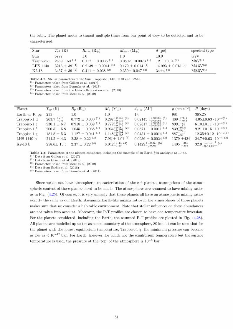
the orbit. The planet needs to transit multiple times from our point of view to be detected and to becharacterised.

Star Teff (K) Rstar (R�) Mstar (M�) d (pc) spectral typeSun 5777 1.0 1.0 10.0 G2VTrappist-1 2559± 50 (1) 0.117 ± 0.0036 (1) 0.0802± 0.0073 (1) 12.1 ± 0.4 (1) M8V(1)

LHS 1140 3216 ± 39 (4) 0.2139 ± 0.0041 (4) 0.179 ± 0.014 (4) 14.993 ± 0.015 (3) M4.5V(3)

K2-18 3457 ± 39 (2) 0.411 ± 0.038 (2) 0.359± 0.047 (2) 34±4 (4) M2.5V(4)

Table 4.2: Stellar parameters of the Sun, Trappist-1, LHS 1140 and K2-18.(1) Parameters taken from Gillion et al. (2017)(2) Parameters taken from Benneke et al. (2017)(3) Parameters taken from the Gaia collaboration et al. (2018)(4) Parameters taken from Ment et al. (2019)

Planet Teq (K) Rp (R⊕) Mp (M⊕) ds−p (AU) g (cm s−2) P (days)Earth at 10 pc 255 1.0 1.0 1.0 981 365.25Trappist-1 d 263.7 +7.7

−7.6 0.772 ± 0.030 (1) 0.297+0.039−0.035

(2) 0.02145 +0.00066−0.00063

(1) 489 +76.1−70.3 4.05±0.63 · 10−4(1)

Trappist-1 e 230.1 ± 6.7 0.918 ± 0.039 (1) 0.772+0.079−0.075

(2) 0.02817 +0.00083−0.00087

(1) 899+121−117 6.10±0.11 · 10−4(1)

Trappist-1 f 200.5 ± 5.8 1.045 ± 0.038 (1) 0.934+0.080−0.078

(2) 0.0371 ± 0.0011 (1) 839+95.5−94.1 9.21±0.15 · 10−4(1)

Trappist-1 g 181.8 ± 5.3 1.127 ± 0.041 (1) 1.148+0.098−0.095

(2) 0.0451 ± 0.0014 (1) 887+101−99 12.35±0.12 · 10−3(1)

LHS 1140 b 214.5 ± 4.3 2.38 ± 0.22 (3) 7.96 ± 1.91 (3) 0.0936 ± 0.0024 (3) 1379 ±424 24.7±0.63 · 10−4 (3)

K2-18 b 258.6± 13.5 2.37 ± 0.22 (4) 8.042+1.44−1.35

(4) 0.1429+0.0060−0.0065

(5) 1405 +365−354 32.9+1.0·10−4

−0.84·10−5(4)

Table 4.3: Parameters of the planets considered including the example of an Earth-Sun analogue at 10 pc.(1) Data from Gillion et al. (2017)(2) Data from Grimm et al. (2018)(3) Parameters taken from Ment et al. (2019)(4) Data from Sarkis et al. (2018)(5) Parameters taken from Benneke et al. (2017)

Since we do not have atmospheric characterisation of these 6 planets, assumptions of the atmo-spheric content of these planets need to be made. The atmospheres are assumed to have mixing ratiosas in Fig. (4.25). Of course, it is very unlikely that these planets all have an atmospheric mixing ratiosexactly the same as our Earth. Assuming Earth-like mixing ratios in the atmospheres of those planetsmakes sure that we consider a habitable environment. Note that stellar influences on these abundancesare not taken into account. Moreover, the P-T profiles are chosen to have one temperature inversion.For the planets considered, including the Earth, the assumed P-T profiles are plotted in Fig. (4.28).All planets are modelled up to the assumed boundary of the atmosphere, 80 km. It can be seen that forthe planet with the lowest equilibrium temperature, Trappist-1 g, the minimum pressure can becomeas low as < 10−12 bar. For Earth, however, for which not the equilibrium temperature but the surfacetemperature is used, the pressure at the ’top’ of the atmosphere is 10−6 bar.

81

Figure 4.28: Pressure-Temperature profile for Earth (red), Trappist-1 d (light-blue), Trappist-1 e (cyan), Trappist-1 f(green), Trappist-1 g (blue), LHS 1140 b (purple), and K2-18 b (yellow) assuming an atmosphere with a temperatureinversion. An atmosphere with temperature inversions has the same linear decrease in temperature in the troposphere, isisothermal in the tropopause, has a temperature increase in the stratosphere, an isothermal stratopause and a temperaturedecrease in the mesosphere.

This section is further divided in HIRES and METIS. The detectability of spectral features will bediscussed.

4.4.1 HIRES

Transmission spectra for HIRES for the six planets are simulated assuming an atmosphere that has avertical distribution of molecules as of Earth (Earth abundances) and changing again the mixing ratiosby a factor of 3 for O2 and 10 for O3, N2O, H2O, CH4 and NH3. These effects are shown in Appendix1 where the plots are shown per planet. For characterising planetary atmospheres of planets around Mstars there is an advantage over characterizing those planets located in the habitable zone of G starssince their periods are smaller. Synthetic transmission spectra of Trappist-1 d, Trappist-1 e, Trappist-1 f, Trappist-1 g, LHS 1140 b and K2-18 b assuming Earth-like abundances are shown in Fig(4.29).Trappist-1 d is both the least massive and the smallest planet considered in the sample resulting ina transmission of the order of 3.33e−3 (see Fig. (4.29a)), a factor of 41 times the transmission ofthe Earth. Trappist-1 e, considered as the planet with the largest change to be habitable at at leastportions of the planet, has a transmission of ∼ 5.0 · 10−3, a factor ∼60 larger compared to the Earth-Sun analogue at 10 pc. Trappist-1 f is only slightly larger than the Earth and has a transmission ofthe order of ∼ 6.12 · 10−3 (a factor ∼ 75. Trappist-1 g has a slightly larger transmission as Trappist-1f: on the order of 7.06 · 10−3. LHS 1140 b, being more than twice the size of the Earth and orbitingthe star LHS 1140, an earlier type M star than Trappist-1, has a transmission of ∼ 9.98 ·10−3 (a factorof ∼ 102 compared to Earth). Out of the 7 planets (6 planets in the HEC and the Earth-Sun analogueat 10 pc), LHS 1140 b has the largest transmission of close to 0.01. K2-18 b, located at a distance of34 pc, orbits the early type M dwarf K2-18 at a distance of 0.1429 AU has a transmission of about anorder of magnitude less compared to LHS 1140 b: R2

p/R2s ∼ 1.425 · 10−3.

Since the six planets all orbit around M stars, the stellar radiation emitted by their host star isshifted to the near-IR compared to the radiation emitted by the Sun. Since near-IR radiation is moreeasily absorbed by H2O vapour and H2O ice, radiative interactions are affected in the atmosphere andwith the surface (Shield et al., 2013).

Are spectral features for these planets expected to be detectable with the planned HIRES instru-ment? The total integration times in seconds for Earth at 10 pc, Trappist-1 d, Trappist-1 e, Trappist-1f, Trappist-1 g, LHS 1140 b, and K2-18 b to detect a signal for a SNR of 10 are shown in Table4.4. For molecules whose absorption features are in the grey shaded areas, the regions blocked by our

82

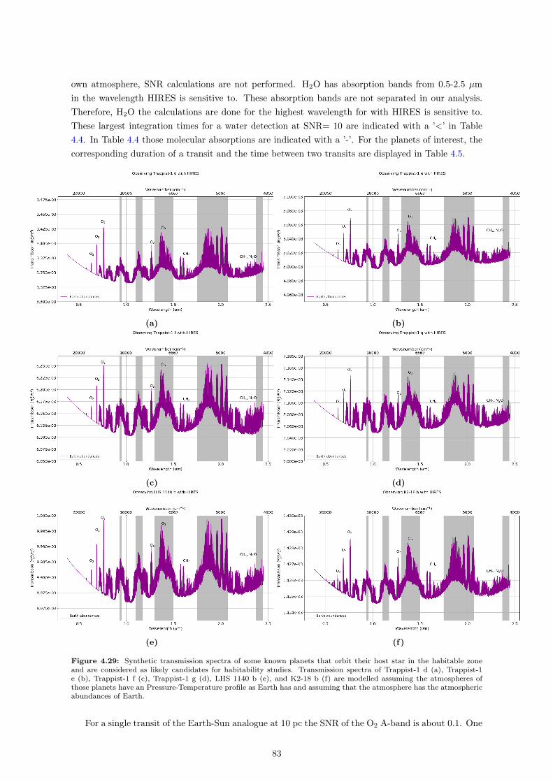
own atmosphere, SNR calculations are not performed. H2O has absorption bands from 0.5-2.5 µmin the wavelength HIRES is sensitive to. These absorption bands are not separated in our analysis.Therefore, H2O the calculations are done for the highest wavelength for with HIRES is sensitive to.These largest integration times for a water detection at SNR= 10 are indicated with a ’<’ in Table4.4. In Table 4.4 those molecular absorptions are indicated with a ’-’. For the planets of interest, thecorresponding duration of a transit and the time between two transits are displayed in Table 4.5.

(a) (b)

(c) (d)

(e) (f)

Figure 4.29: Synthetic transmission spectra of some known planets that orbit their host star in the habitable zoneand are considered as likely candidates for habitability studies. Transmission spectra of Trappist-1 d (a), Trappist-1e (b), Trappist-1 f (c), Trappist-1 g (d), LHS 1140 b (e), and K2-18 b (f) are modelled assuming the atmospheres ofthose planets have an Pressure-Temperature profile as Earth has and assuming that the atmosphere has the atmosphericabundances of Earth.

For a single transit of the Earth-Sun analogue at 10 pc the SNR of the O2 A-band is about 0.1. One

83

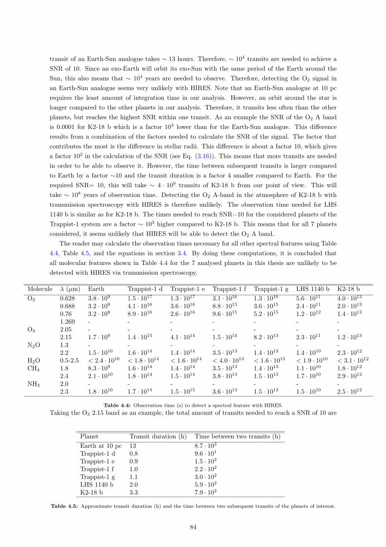
transit of an Earth-Sun analogue takes ∼ 13 hours. Therefore, ∼ 104 transits are needed to achieve aSNR of 10. Since an exo-Earth will orbit its exo-Sun with the same period of the Earth around theSun, this also means that ∼ 104 years are needed to observe. Therefore, detecting the O2 signal inan Earth-Sun analogue seems very unlikely with HIRES. Note that an Earth-Sun analogue at 10 pcrequires the least amount of integration time in our analysis. However, an orbit around the star islonger compared to the other planets in our analysis. Therefore, it transits less often than the otherplanets, but reaches the highest SNR within one transit. As an example the SNR of the O2 A bandis 0.0001 for K2-18 b which is a factor 103 lower than for the Earth-Sun analogue. This differenceresults from a combination of the factors needed to calculate the SNR of the signal. The factor thatcontributes the most is the difference in stellar radii. This difference is about a factor 10, which givesa factor 102 in the calculation of the SNR (see Eq. (3.16)). This means that more transits are neededin order to be able to observe it. However, the time between subsequent transits is larger comparedto Earth by a factor ∼10 and the transit duration is a factor 4 smaller compared to Earth. For therequired SNR= 10, this will take ∼ 4 · 109 transits of K2-18 b from our point of view. This willtake ∼ 108 years of observation time. Detecting the O2 A-band in the atmosphere of K2-18 b withtransmission spectroscopy with HIRES is therefore unlikely. The observation time needed for LHS1140 b is similar as for K2-18 b. The times needed to reach SNR=10 for the considered planets of theTrappist-1 system are a factor ∼ 103 higher compared to K2-18 b. This means that for all 7 planetsconsidered, it seems unlikely that HIRES will be able to detect the O2 A band.

The reader may calculate the observation times necessary for all other spectral features using Table4.4, Table 4.5, and the equations in section 3.4. By doing these computations, it is concluded thatall molecular features shown in Table 4.4 for the 7 analysed planets in this thesis are unlikely to bedetected with HIRES via transmission spectroscopy.

Molecule λ (µm) Earth Trappist-1 d Trappist-1 e Trappist-1 f Trappist-1 g LHS 1140 b K2-18 bO2 0.628 3.8 · 109 1.5 · 1017 1.3 · 1017 3.1 · 1016 1.3 · 1016 5.6 · 1011 4.0 · 1013

0.688 3.2 · 109 4.1 · 1016 3.6 · 1016 8.8 · 1015 3.6 · 1015 2.4 · 1011 2.0 · 1013

0.76 3.2 · 108 8.9 · 1016 2.6 · 1016 9.6 · 1015 5.2 · 1015 1.2 · 1012 1.4 · 1013

1.269 - - - - - - -O3 2.05 - - - - - - -

2.15 1.7 · 109 1.4 · 1015 4.1 · 1014 1.5 · 1014 8.2 · 1013 2.3 · 1011 1.2 · 1013

N2O 1.3 - - - - - - -2.2 1.5 · 1010 1.6 · 1014 1.4 · 1014 3.5 · 1013 1.4 · 1013 1.4 · 1010 2.3 · 1012

H2O 0.5-2.5 < 2.4 · 1010 < 1.8 · 1014 < 1.6 · 1014 < 4.0 · 1013 < 1.6 · 1013 < 1.9 · 1010 < 3.1 · 1012

CH4 1.8 8.3 · 109 1.6 · 1014 1.4 · 1014 3.5 · 1013 1.4 · 1013 1.1 · 1010 1.8 · 1012

2.4 2.1 · 1010 1.8 · 1014 1.5 · 1014 3.8 · 1013 1.5 · 1013 1.7 · 1010 2.9 · 1012

NH3 2.0 - - - - - - -2.3 1.8 · 1010 1.7 · 1014 1.5 · 1015 3.6 · 1013 1.5 · 1013 1.5 · 1010 2.5 · 1012

Table 4.4: Observation time (s) to detect a spectral feature with HIRES.Taking the O3 2.15 band as an example, the total amount of transits needed to reach a SNR of 10 are

Planet Transit duration (h) Time between two transits (h)Earth at 10 pc 13 8.7 · 103

Trappist-1 d 0.8 9.6 · 101

Trappist-1 e 0.9 1.5 · 102

Trappist-1 f 1.0 2.2 · 102

Trappist-1 g 1.1 3.0 · 102

LHS 1140 b 2.0 5.9 · 102

K2-18 b 3.3 7.9 · 102

Table 4.5: Approximate transit duration (h) and the time between two subsequent transits of the planets of interest.

84

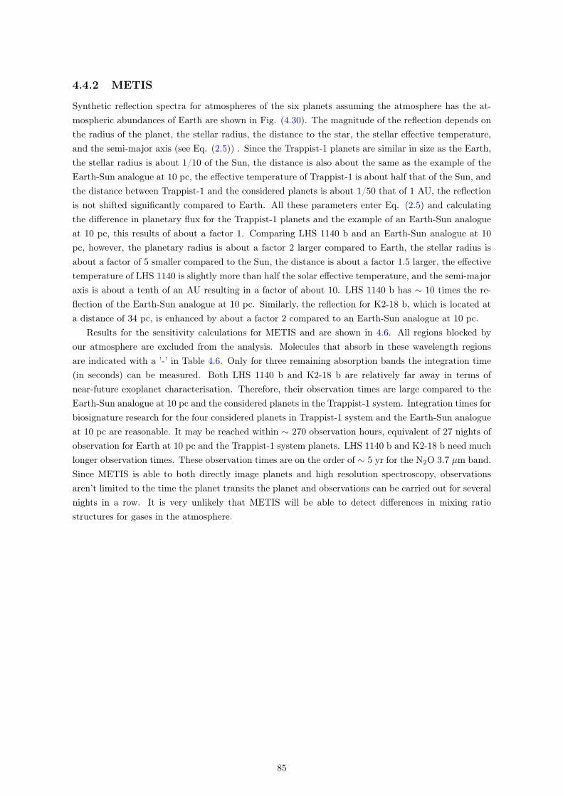
4.4.2 METIS

Synthetic reflection spectra for atmospheres of the six planets assuming the atmosphere has the at-mospheric abundances of Earth are shown in Fig. (4.30). The magnitude of the reflection depends onthe radius of the planet, the stellar radius, the distance to the star, the stellar effective temperature,and the semi-major axis (see Eq. (2.5)) . Since the Trappist-1 planets are similar in size as the Earth,the stellar radius is about 1/10 of the Sun, the distance is also about the same as the example of theEarth-Sun analogue at 10 pc, the effective temperature of Trappist-1 is about half that of the Sun, andthe distance between Trappist-1 and the considered planets is about 1/50 that of 1 AU, the reflectionis not shifted significantly compared to Earth. All these parameters enter Eq. (2.5) and calculatingthe difference in planetary flux for the Trappist-1 planets and the example of an Earth-Sun analogueat 10 pc, this results of about a factor 1. Comparing LHS 1140 b and an Earth-Sun analogue at 10pc, however, the planetary radius is about a factor 2 larger compared to Earth, the stellar radius isabout a factor of 5 smaller compared to the Sun, the distance is about a factor 1.5 larger, the effectivetemperature of LHS 1140 is slightly more than half the solar effective temperature, and the semi-majoraxis is about a tenth of an AU resulting in a factor of about 10. LHS 1140 b has ∼ 10 times the re-flection of the Earth-Sun analogue at 10 pc. Similarly, the reflection for K2-18 b, which is located ata distance of 34 pc, is enhanced by about a factor 2 compared to an Earth-Sun analogue at 10 pc.

Results for the sensitivity calculations for METIS and are shown in 4.6. All regions blocked byour atmosphere are excluded from the analysis. Molecules that absorb in these wavelength regionsare indicated with a ’-’ in Table 4.6. Only for three remaining absorption bands the integration time(in seconds) can be measured. Both LHS 1140 b and K2-18 b are relatively far away in terms ofnear-future exoplanet characterisation. Therefore, their observation times are large compared to theEarth-Sun analogue at 10 pc and the considered planets in the Trappist-1 system. Integration times forbiosignature research for the four considered planets in Trappist-1 system and the Earth-Sun analogueat 10 pc are reasonable. It may be reached within ∼ 270 observation hours, equivalent of 27 nights ofobservation for Earth at 10 pc and the Trappist-1 system planets. LHS 1140 b and K2-18 b need muchlonger observation times. These observation times are on the order of ∼ 5 yr for the N2O 3.7 µm band.Since METIS is able to both directly image planets and high resolution spectroscopy, observationsaren’t limited to the time the planet transits the planet and observations can be carried out for severalnights in a row. It is very unlikely that METIS will be able to detect differences in mixing ratiostructures for gases in the atmosphere.

85

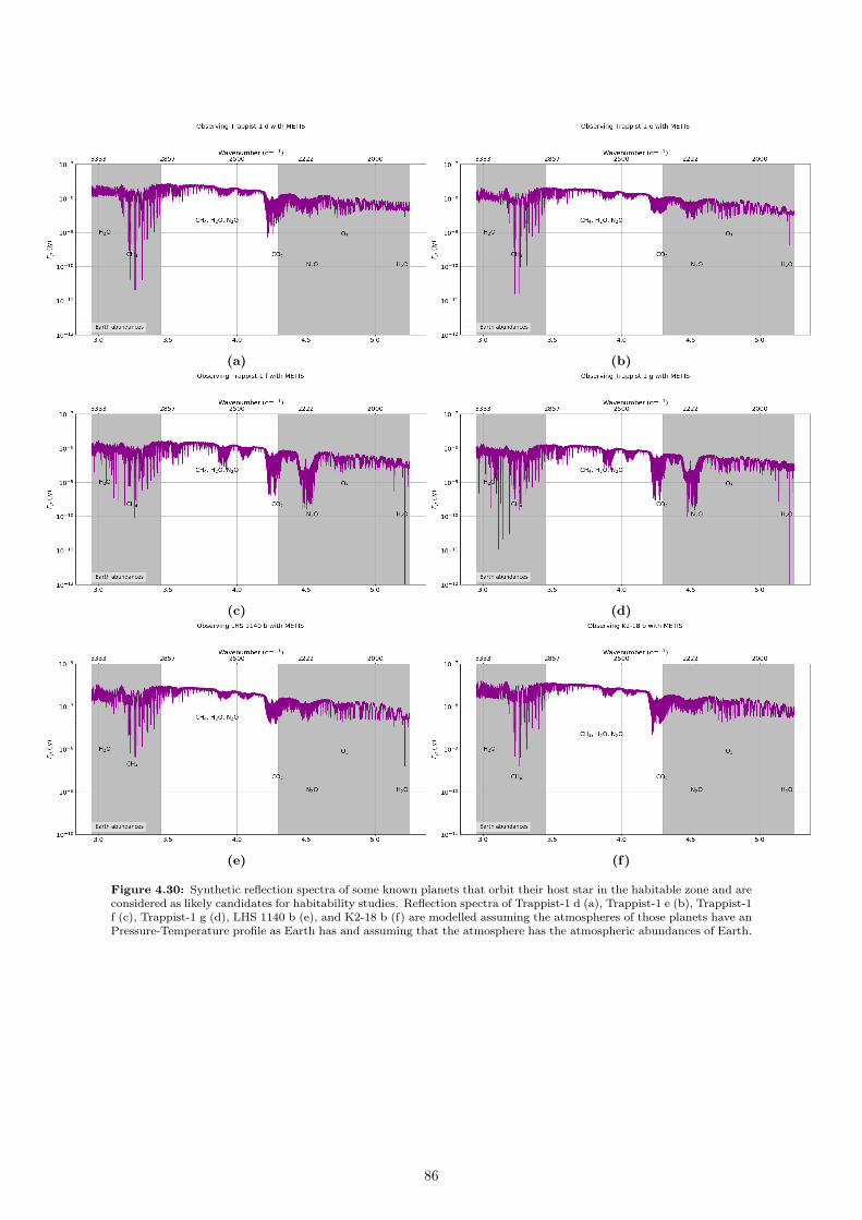
(a) (b)

(c) (d)

(e) (f)

Figure 4.30: Synthetic reflection spectra of some known planets that orbit their host star in the habitable zone and areconsidered as likely candidates for habitability studies. Reflection spectra of Trappist-1 d (a), Trappist-1 e (b), Trappist-1f (c), Trappist-1 g (d), LHS 1140 b (e), and K2-18 b (f) are modelled assuming the atmospheres of those planets have anPressure-Temperature profile as Earth has and assuming that the atmosphere has the atmospheric abundances of Earth.

86

Molecule λ (µm) Earth Trappist-1 d Trappist-1 e Trappist-1 f Trappist-1 g LHS 1140 b K2-18 b

O3 3.6 9.2 · 104 5.8 · 105 5.8 · 105 5.8 · 105 5.8 · 105 3.7 · 108 9.2 · 106

4.6 - - - - - - -4.8 - - - - - - -

N2O 3.7 9.7 · 105 9.7 · 105 9.7 · 105 9.7 · 105 9.7 · 105 1.5 · 106 1.5 · 106

4.5 - - - - - - -H2O 3.5-4.3 2.1 · 106- 2.1 · 106- 2.1 · 106- 2.1 · 106- 3.4 · 108- 3.4 · 109- 1.1 · 109-

3.9 · 103 3.9 · 103 3.9 · 103 6.1 · 102 1.5 · 106 9.7 · 104 5.2 · 104

CH4 3.3 - - - - - - -NH3 3.0 - - - - - - -C2H6 3.3 - - - - - - -CH3Cl 3.3 - - - - - - -

Table 4.6: Observation time (s) to detect a spectral feature with METIS.

4.5 Photon noise and Optimal resolution for characterising at-

mospheres with the ELT

The photon noise for an Earth-Sun analogue at 5 pc as observed in the optical with a 10m telescopewith a spectral resolution of R = 100 is about 1 photon/s/resolution element (M. Min, private com-munication). Based on this estimate, results from the analysis technique described in section 3.3 werechecked. In photon noise calculations the efficiency of the ELT (q = 0.5) was taken into account. Thefactor 1.2 for the total assumed noise budget is not taken into account for the photon noise calculationsin this section. Table 4.7 shows the estimates of the photon noises for the wavelength boundaries forHIRES (i.e. 0.37 µm and 2.5 µm) and METIS (i.e. 2.9 µm and 5.3 µm for the 7 considered planets.Photon noises, 1/

√n, are shown where n is given in photons per second. Therefore, in the calculations,

the observation time was set to 1 s. It can be seen that the optical has the lowest photon noise forall planets compared with the wavelengths in the IR. Moreover, the Trappist-1 planets have an overallhigher photon noise compared with an Earth-Sun analogue at 10 pc (∼1% of photon noise of Trappist-1planets), LHS 1140 b (∼ 15%) and K2-18 b (∼ 10%). The lower the photon noise, or at least the totalnoise budget, the easier would it be to observe the features. Therefore, at wavelengths in the near-IR,it would be easier to observe features because it can be considered as the photon noise limited regime.

Planet Wavelengths0.37 µm 2.5 µm 2.9 µm 5.3 µm

Earth at 10 pc 0.00086 0.00068 0.00076 0.0012Trappist-1 d 0.61 0.016 0.016 0.023Trappist-1 e 0.61 0.016 0.016 0.023Trappist-1 f 0.61 0.016 0.016 0.023Trappist-1 g 0.61 0.016 0.016 0.023LHS 1140 b 0.088 0.0082 0.0088 0.013K2-18 b 0.068 0.0089 0.0097 0.014

Table 4.7: Photon noise (i.e. 1√n, where n has units of photons per second) estimates for an Earth-Sun analogue at 10

pc, Trappist-1 d, Trappist-1 e, Trappist-1 f, Trappist-1 g, LHS 1140 b and K2-18 b for the boundaries of the wavelengthranges for which HIRES and METIS are sensitive to.

For determining the optimal resolution for both HIRES and METIS, some parameters need to beconsidered. The optical resolution depends on the intrinsic width of the stellar lines (Snellen et al.,2015). A high resolution is proposed because telluric lines need to be distinguished from planetaryabsorption lines in order to do characterisation of the atmosphere. However, because of the high

87

spectral resolution, fewer photons will be collected by the telescope. Moreover, the SNR for a singletransit is smaller for higher resolutions because it depends on the resolution (see e.g. Rauer et al.,2011). Is a lower R maybe better for HIRES when considering atmospheric characterisation? Snellenet al. (2015) come to a spectral resolution of 75.000 for the optical for HDS and HCL (i.e. a METISlike instrument in the optical). This can be deduced from the turbulent velocity, ∆v of the star andthe speed of light, c in:

R =c

∆v(4.2)

Depending on the star, the optimal resolution will be between 75.000 and 100.000. For HIRES, theproposed R = 120.000 − 130.000 and is not needed for characterisation of planetary atmospheres.This resolution was proposed to be able to cover all science cases proposed for HIRES. Similarly, forsensitivity calculations of METIS, the sensitivity also depends on 1/R. For higher R the sensitivitywill be higher. The optimal resolution depends on the velocity in the Mid-IR.

88

Chapter 5

Discussion

In this thesis the detectability of the frequently proposed biosignature gases O2, O3, N2O, CH4,NH3, C2H6, and CH3Cl and the habitability marker H2O was examined. This was done by buildingatmospheres with the exoplanet modelling code ARCiS. First, simple isothermal atmospheres withonly one gas (O2 for HIRES, O3 for METIS) were modelled and the effect of different temperaturesand pressures was examined. It was seen that pressure differences only have a small contribution toboth transmission and reflection spectra. The effect of pressure broadening is, however, present inboth transmission and reflection spectra. Increasing the temperature of the atmosphere resulted inincreasing the transmission. This is consistent with the concept of the atmospheric scale height. Forthe reflection spectra modelled with the characteristics of METIS, the O3 band at 4.8 µm changeslocation with different atmospheric temperatures.

Next, the effects of those temperatures and pressures on Earth-like atmospheres were examined.P-T profiles considered were (1) a temperature profile with one temperature inversion in the strato-sphere and (2) a temperature profile in which the temperature dropped in the troposphere and wasisothermal at higher altitudes. The pressure profile for both these atmospheres was assumed to followan exponential profile. It was concluded that for transmission spectra for the optical and near-IR thepressure profile had a small influence on the transmission because of the atmospheric scale height. Thetemperature profile, however, had no effect on the transmission. This was expected since transmissionspectra are not sensitive to the temperature profile of an atmosphere. For reflection spectra, boththe pressure profile and the temperature profile had an effect on the the flux of the planet and there-fore on the reflection spectra. Reflection spectra can probe deeper into atmospheres while the upperatmosphere is probed with transmission spectra.

In the next steps the atmospheres were modelled with O2, O3, N2O, CH4, CO2, H2O, and N2.Also NH3, CH3Cl and C2H6 were added to the spectrum. The effect of changing the abundances bya factor 3 for O2 and 10 for all other molecules was discussed. The goal here was to understand whatcaused the changes in both the transmission and reflection spectra and to infer whether these wouldbe detectable. For HIRES, changes in the absorbance of CH4, H2O and NH3 may be observed throughour own atmosphere, while for METIS those are for NH3, H2O and, although weak, O3. For HIRES,it will be extremely difficult to detect the atmospheric gases since transmission spectroscopy can onlybe done in the time the planet transits the star. In the wavelength range of METIS, most molecularspectral features are blocked by our own atmosphere and only the O3 3.6 µm band, the H2O bands,and the N2O 3.7 µm band will be detectable. For Earth, Trappist-1 d, e, f and g these features canbe seen in a reasonable observation time of about 27 observation nights. For LHS 1140 b and K2-18b, however, the observation times will be about a factor 104 times larger for the 3.6 µm O3 band andthe 3.7 µm N2O band. Therefore, it will be unfeasible to detect those signatures in the atmospheres

89

of LHS 1140 b and K2-18 b. LHS 1140 b and K2-18 b are also those planets that are in the optimisticsample of the HEC while the four Trappist-1 planets considered in this thesis are in the conservativesample.

The detectability of biosignatures in planetary atmospheres has been modelled by numerous authors(e.g. Rauer et al., 2011; Snellen et al., 2015; Krissansen-Totton et al., 2018; Serindag & Snellen, 2019)considering different telescopes. Research in the characterisation of exoplanetary atmospheres relynecessarily on assumptions since no other planet than Earth is found to host life. In this sectionthe assumptions made are discussed and the results are compared to previous work related to thedetectability of biosignatures with the ELT.

One assumption in each work considering biosignatures in exoplanetary atmosphere is the temper-ature and pressure structure in the atmosphere. In this work temperature structures were assumedto be completely isothermal, having a linear decrease in the troposphere followed by isothermal layersat higher altitudes or a profile with a linear decrease in the temperature in the troposphere and atemperature inversion in the stratosphere (which is caused by ozone heating on Earth). The effect ofsurface gravity on the temperature structure was neglected and the planetary equilibrium temperaturewas the only factor that changed the temperature structure. Rauer et al. (2011), however, did includethe effect of the surface gravity. They considered two planets with the same incident radiation. For ahigher surface gravity, the surface temperature decreases because of the lower vertical column mass.If there is less mass, there is less absorption and therefore less greenhouse effect and therefore a lowersurface gravity (Rauer et al., 2011). Moreover, they considered a temperature structure where themaximum temperature in the stratosphere decreases at higher pressures for higher surface gravitiesbecause O3 heating occurs at higher pressures. Also the effect of the surface gravity was shown in thevertical chemical profiles. For the same surface pressure, the tropospheric H2O number density wasdecreased for the higher surface gravity case compared to the lower surface gravity case. Because H2Ohas a relatively high mean molecular weight, this leads to a decrease in overall column mass.

Ohter properties not taken into account are the effect of the host star on the abundance of anyatmospheric gas and the effect of clouds on the synthetic transmission and reflection spectra. This wasbeyond the scope of this thesis because of the lack in knowledge regarding the effects of the host star.Rauer et al. (2011) took into account the increase in N2O abundance for increasing M-star class, thedecrease in O3 abundance for M-dwarfs (Segura et al., 2005; Rauer et al., 2011) and an increase inCH3Cl for cooler M-stars.

Snellen et al. (2015) simulated results of combining the techniques of high-resolution spectroscopyand high-contrast imaging for O2. They assumed an 1-1.5 R⊕ planet orbiting around α Cen (d = 1.3

pc) and concluded that a planet with Teq = 300 K around this star could be detected at a wavelengthof 4.8 µm at a S/N=5 within one observation night (i.e. 10 h). In this observation night, also reflectedlight in the optical of planet of the same size in the HZ of Proxima Centauri (d = 1.3 pc) may bedetected with S/N=10. These stars are located at a distance of a factor 7 to 26 times closer than thehost stars considered in this thesis. Since the detectability depends on the distance of the star squared,our values are expected to be a factor 50-700 higher than those of Snellen et al. (2015). However,since also properties of the stars and the size of the planets assumed in both works are different, thisestimation of the factor is not reliable.

Serindag and Snellen (2019) investigated the detectability of O2 in exoplanetary atmospheres usingHRS with the Extremely Large Telescopes (ELTs). They have found that O2 would be detectabile foran Earth-twin transiting an M5V star at a distance of 7 pc in 70-175 hours observation time. This timeis similar to 4-10 years when the transit time and the planetary period is taken into account. They useddata from the VLT and the characteristics of the VLT and the ELT to simulate real noise. Our resultwas that the strongest O2 band can be detected in 3.8 · 109 s, equivalent to 106 h. This discrepancy is

90

due to the fact that they considered a METIS-like instrument (i.e. an instrument combining HRS andHCI) assumed to be sensitive to optical wavelengths while we assumed HIRES (i.e. only HRS) as aninstrument for optical wavelengths. For METIS, most features in the IR can be distinguished within∼ 30 h, more consistent with the results of Snellen et al. (2015).

Krissansen-Totton et al. (2018) investigated the detectability of biosignatures with the JamesWebb Space Telescope (JWST) considering anoxic atmospheres. In particular, they examined whetheran atmosphere with both CH4 and CO2 in disequilibrium would be detectable with transmissionspectroscopy. This CH4/CO2 combination is proposed as a biosignature for anoxic atmospheres(Krissansen-Totton et al., 2018). Instead of assuming a modern Earth atmosphere, they assumedan atmosphere atmosphere more like early Earth. In particular, during the Archean eon the Earth’satmosphere likely had an disequilibrium between those two gases. They simulated synthetic trans-mission spectra and concluded that the CH4-CO2 disequilibrium biosignature would be detectable inabout 10 transits for Trappist-1 e assuming an Archean-like atmosphere. Based on the low numberof transits needed, the CH4-CO2 disequilibrium biosignature should be easier detectable than O2 orO3 with JWST. However, there is a probability of ∼ 9% that the observed CH4 abundance is abioticin origin. This probability decreases with the number of transits. They assumed similar temperaturestructures as this work. Moreover, their assumed abundances, although different, are similarly assumedto not vary with height.

91

Chapter 6

Conclusion

We analysed whether the commonly proposed gaseous biosignature O2, O3, N2O, CH4, CH3Cl, C2H6,and NH3 and the habitability marker H2O will be detectable with planned instruments on the ELT.Synthetic transmission and reflection spectra were modelled for HIRES and METIS respectively us-ing the exoplanetary modelling code ARCiS. We considered a hypothetical Earth-Sun analogue at adistance of 10 pc and built a realistic atmosphere. First, the effect of the pressure and temperaturewere examined considering a simple isothermal atmosphere in which only one gas is present. Thiswas followed by investigating the effect of temperature profiles and subsequently the distributions ofmolecules. Additionally, properties of six planets that were discovered in previous years using the tran-sit method and the radial velocity method were taken from the HEC. These planets were examined todetermine the detectability for these planets orbiting cool stars. For an Earth-Sun analogue at 10 pc itwould not be possible to detect biosignatures with transmission spectroscopy in the wavelength rangeof HIRES for a SNR of 10 within the lifetime of a human. Therefore, it was concluded that detectingbiosignatures present in the atmosphere of an Earth-Sun analogue at 10 pc will not be detectable withHIRES.

Considering METIS as an instrument, it can be concluded that most molecules absorbing in thisregion are not detectable because of blocking by our own atmosphere. For the case of Earth at 10pc and Trappist-1 d, Trappist-1 e, Trappist-1 f, and Trappist-1 g the observation times for detectingthe O3 3.6 µm band, the N2O 3.7 µm band and water features in the wavelength range of 3.5-4.3 µmare detectable within 27 observation nights. Biosignatures of habitability markers for LHS 1140 b andK2-18 b require much higher observation times that are considered as unreasonable and are thereforenot able to be detected.

The optimal resolution concerning the characterisation of exoplanetary atmospheres, the proposedresolutions are higher than needed. Optimal resolutions for this science case will be R = 75, 000 −100, 000 in both the optical and the IR. The value depends on the intrinsic width of the stellar lineswhich is also wavelength dependent. Photon noises are smallest in the near-IR and are on the order of10−2 for planets in the Trappist-1 system. This photon noise was calculated using number of photonsper second as units for n.

6.1 Plans for the near future

The search of biosignatures in exoplanetary atmospheres goes far beyond the investigation of the effectof surface pressures and temperatures, the effect of temperature inversions and the effect of changingthe abundance of a biosignature or a habitability marker. One important suggestion to examine inthe near future is the effect of clouds. Cloud chemistry is included in ARCiS but was not taken into

92

account in this thesis. Understanding clouds would help to interpret spectra obtained with near-futuretelescopes. One frequently cited example is GJ 1214 b which has a flat transmission spectrum (e.g.Berta et al., 2012). The flat spectrum is suggested to be caused by clouds high in the atmosphere.Most of the solar system planets have clouds. Earth has water clouds but Venus has sulphuric acidclouds. With a better understanding of clouds it would be possible to constrain the planetary albedowhich in turn ensures that the surface temperature can be better estimated. This in turn will giveus insight into whether we could expect liquid water on the surface. For future work in atmosphericcharacterisations it would be better to include or understand both the theoretical side of clouds andthe effect of clouds on the spectrum.

Besides the gaseous biosignatures investigated in this thesis, there are two other categories ofbiosignatures mentioned in section 1.3. Temporal biosignatures need more theoretical work in order tobe able to be modelled with significance. Surface biosignatures, in particular the VRE, can be modelledin exoplanetary spectra. ARCiS is not the appropriate code for this because the surface is modelledin such a way that it is fully reflective. If the VRE is considered, care should be taken with respectto where the reflection will be present in the reflection spectrum since the VRE could be shifted withrespect to ’our’ VRE due to differences in stellar flux and stellar activity.

ARCiS gave some limitations to our work. Besides the planetary surface is assumed to be a fullyreflective surface, the resolution for calculating opacity tables could not be set to higher resolutionsnecessary to model synthetic reflection and transmission spectra for HIRES and METIS in the searchfor biosignatures. In future work, a modelling code that is able to sustain such resolutions would work.One example in Exo-Transmit for modelling synthetic transmission spectra.

Besides planned telescopes having as a science goal the characteristion of exoplanetary atmospheressuch as the ELT and James Webb Space Telescope (JWST), the Atmospheric Remote-sensing InfraredExoplanet Large-survey (Ariel1) is proposed as the first space-based telescope fully dedicated to mea-suring the chemical composition and thermal structures of exoplanets. Ariel is scheduled for launchin 2028. During its mission, Ariel will study 1,000 exoplanets in both the optical and IR. Not onlyplanets in the HZ, but planets of all sizes and at all distances from the host star are subject of Ariel.Moreover, Luvoir and HabEx are proposed as large space based facilities to be launched in the 2030’s.These space-based instruments are interesting for exoplanetary science because data obtained is notcontaminated by our own atmosphere. That means that the resolution needed is also lower. Sincethese telescopes will be about 2.5 times smaller than the ELT, but probably have a lower R, about thesame order of photons will be detected.

1https://arielmission.space/

93

BibliographyArnold L., Gillet S., Lardière O., Riaud P. and Schneider J. (2002). Airborne spectral measurements of surface–atmosphere

anisotropy for arctic sea ice and tundra, int. j. remote sensing, 23, 18, 3763–3781.Barnes, R. (2017). Tidal locking of habitable exoplanets. Celestial Mechanics and Dynamical Astronomy, 129(4),

pp.509-536.Benneke, B., Werner, M., Petigura, E. et al. (2017). Spitzer Observations Confirm And Rescue the Habitable zone

super-Earth K2-18 b For Future Characterization. The Astrophysical Journal, 834(2), p.187.Benner S,. A., Ricardo, A., Carrigan, M. A. (2004). Is there a common chemical model for life in the universe? Curr

Opin Chem Biol, 8:672–689.Berta, Z., Charbonneau, D., Désert, J., Miller-Ricci Kempton, E., McCullough, P., Burke, C., Fortney, J., Irwin,

J., Nutzman, P. and Homeier, D. (2012). THE FLAT TRANSMISSION SPECTRUM OF THE SUPER-EARTHGJ1214b FROM WIDE FIELD CAMERA 3 ON THEHUBBLE SPACE TELESCOPE. The Astrophysical Journal,747(1), p.35.

Borucki, W. and Summers, A. (1984). The photometric method of detecting other planetary systems. Icarus, 58(1),pp.121-134.

Brandl, B. R., Markus, F., Alistair, G. et al., (2014). METIS: the mid-infrared E-ELT imager and spectrograph.Proceedings of the SPIE. 9147, 914821

Brasseur, G. P., Orlando, J. J. and Tyndall, G.S. (1999). Atmospheric Chemistry and Global Change. Oxford UniversityPress, Oxford. 654.

Canfield, D. E. (2005). The early history of atmospheric oxygen: homage to Robert M. Garrels. Ann Rev Earth PlanetSci 33: 1–36.

Catling, D. C., Zahnle, K. J., and McKay, C. P. (2001). Biogenic methane, hydrogen escape, and the irreversibleoxidation of early Earth. Science 293:839–843.

Catling, D. C., Krissansen-Totton, J., Kiang, N. Y., et al. (2018). Exoplanet Biosignatures: A Framework for TheirAssessment. Astrobiology, 18, 709

Chapman, S. (1930). A theory of atmospheric ozone. R Meteorol Soc Memoir 3:103–125.Clark, R. N., Swayze, G. A., Gallagher, A. J., King, T. V. V., and Calvin, W. M. (1993). The U.S. Geological Survey,

Digital Spectral Library: Version 1: 0.2 to 3 Microns. U.S. Geological Survey Open File Report 93–592, U.S.Geological Survey, Reston, VA

Cockell, C. (2014). Habitable worlds with no signs of life. Philosophical Transactions of the Royal Society A: Mathe-matical, Physical and Engineering Sciences, 372(2014), pp.20130082-20130082.

Cockell, C. S., Bush, T., Bryce, C. et al. (2016). Habitability: A Review. Astrobiology 16, 89–117Cocconi, G. and Morrison, P. (1959). Searching for Interstellar Communications. Nature, 184(4690), pp.844-846.Czaja, A. D., Johnson, C. M., Roden, E. E., et al. (2012). Evidence for free oxygen in the Neoarchean ocean based on

coupled iron-molybdenum isotope fractionation. GeochimCosmochim Acta 86:118–137.De Pater, I. and Lissauer, J. (2010). Planetary sciences. Cambridge: Cambridge University Press.Des Marais, D. J. and Walter, M. R. (1999). Astrobiology: Exploring the Origins, Evolution, and Distribution of Life

in the Universe. Ann. Rev. Ecol. syst. 30:397-420Des Marais, D., Harwit, M., Jucks, K., et al. (2002). Remote Sensing of Planetary Properties and Biosignatures on

Extrasolar Terrestrial Planets. Astrobiology, 2(2), pp.153-181.Des Marais, D. J., Nuth, J. A., Allamandola, L. J. et al. (2008). The NASA Astrobiology Roadmap. Astrobiology

8:715-730.Domagal-Goldman, S., Meadows, V., Claire, M. and Kasting, J. (2011). Using Biogenic Sulfur Gases as Remotely

Detectable Biosignatures on Anoxic Planets. Astrobiology, 11(5), pp.419-441.Domagal-Goldman, S. D., Segura, A., Claire, M. W., Robinson, T. D., and Meadows, V. S. (2014). Abiotic ozone and

oxygen in atmospheres similar to prebiotic earth. ApJ 792:43.Donahue, T., Hoffman, J., Hodges, R. and Watson, A. (1982). Venus Was Wet: A Measurement of the Ratio of Deuterium

to Hydrogen. Science, 216(4546), pp.630-633.Etiope, G. and Sherwood-Lollar, B. S. (2013). Abiotic methane on earth. Rev Geophys, 51:276–299.Farquhar, J. (2000). Atmospheric influence of earth’s earliest sulfur cycle. Science 289:756–758

94

Fayolle, E., Oberg, K., Jorgensen, J., et al. (2017). Protostellar and cometary detections of organohalogens. NatureAstronomy, 1(10), pp.703-708.

Frische, M., Garofalo, K., Hansteen, T. and Borchers, R. (2006). Fluxes and origin of halogenated organic trace gasesfrom Momotombo volcano (Nicaragua). Geochemistry, Geophysics, Geosystems, 7(5)

Gaia Collaboration, Brown, A. G. A., Vallenari, A., Prusti, T. et al. (2018). Gaia Data Release 2. Summary of thecontents and survey properties, Astronomy & Astrophysics, 616, A1

Gao, P., Hu, R., Robinson, T. D., et al. 2015, ApJ, 806, 249Gillon, M., Jehin, E., Lederer, S., Delrez, L., de Wit, J., Burdanov, A., Van Grootel, V., Burgasser, A., Triaud, A.,

Opitom, C., Demory, B., Sahu, D., Bardalez Gagliuffi, D., Magain, P. and Queloz, D. (2016). Temperate Earth-sizedplanets transiting a nearby ultracool dwarf star. Nature, 533(7602), pp.221-224.

Gordon, I. E., Rothman, L. S., Hill, C. (2017). The HITRAN2016 Molecular Spectroscopic Database. Journal ofQuantitative Spectroscopy and Radiative Transfer, 203, pp: 3-69.

Grenfell, J.L., Stracke, B., von Paris, P., et al. (2007). The response of atmospheric chemistry on earthlike planetsaround F, G and K Stars to small variations in orbital distance. Planet Space Sci, 55:661–671.

Grimm, S, Demory, B.-O., Gillon, M., Dorn, C., Agol, E., Burdanov, A., Delrez, L., et al. (2018). The nature of theTRAPPIST-1 exoplanets. Astronomy & Astrophysics, 613, A68

Hall, A. and Kaufmann, M. (1975). Stomatal Response to Environment with Sesamum indicum. L. Plant Physiology,55(3), pp.455-459.

Hamilton, J. T. G., McRoberts, W. C., Keppler, F., Kalin, R. M., and Harper, D. B. (2003). Chloride methylation byplant pectin: an efficient environmentally significant process. Science, 301:206–209.

Harper, D. B. (1985). Halomethane from halide ion—a highly efficient fungal conversion of environmental significance.Nature, 315:55–57.

Hitchcock, D. R. and Lovelock, J. E. (1967). Life detection by atmospheric analysis. Icarus, 7:149–159.Huang, S. -S. (1959) The problem of life in the universe and the mode of star formation. PASP 71: 421-424ISO. (1975). Standard Atmosphere. Ref. No. ISO 2533-1975Khalil, M. and Rasmussen, R. (1983). Sources, sinks, and seasonal cycles of atmospheric methane. Journal of Geophysical

Research: Oceans, 88(C9), pp.5131-5144.Kaltenegger, L. (2017). How to Characterize Habitable Worlds and Signs of Life. Annual Review of Astronomy and

Astrophysics, 55(1), pp.433-485.Kasper, M., Beuzit, J-L., Verinaud, C. et al. (2010). EPICS: direct imaging of exoplanets with the E-ELT. SPIE 7735,

84Kasting, J. F., Whitmire, D. P., and Reynolds, R. T. (1993). Habitable zones around main sequence stars. Icarus, 101,

pp.108-128Kasting, J.F. (2001). Earth history: the rise of atmospheric oxygen. Science 293:819–820.Kasting, J., Kopparapu, R., Ramirez, R. and Harman, C. (2013). Remote life-detection criteria, habitable zone bound-

aries, and the frequency of Earth-like planets around M and late K stars. Proceedings of the National Academy ofSciences, 111(35), pp.12641-12646.

Keeling, C., Chin, J. and Whorf, T. (1996). Increased activity of northern vegetation inferred from atmospheric CO2measurements. Nature, 382(6587), pp.146-149.

Keppler, F., Eiden, R., Niedan, V., Pracht, J., and Scholer, H. F. (2000). Halocarbons produced by natural oxidationprocesses during degradation of organic matter. Nature, 403:298–301.

Khalil, M. A. K. and Rasmussen, R. A. (1999). Atmospheric methyl chloride. Atmos Environ, 33:1305–1321.Kleidon, A. (2012). How does the Earth system generate and maintain thermodynamic disequilibrium and what does it

imply for the future of the planet?. Philosophical Transactions of the Royal Society A: Mathematical, Physical andEngineering Sciences, 370(1962), pp.1012-1040.

Kochanov, R., Gordon, I., Rothman, L., Wcisło, P., Hill, C. and Wilzewski, J. (2016). HITRAN Application Program-ming Interface (HAPI): A comprehensive approach to working with spectroscopic data. Journal of QuantitativeSpectroscopy and Radiative Transfer, 177, pp.15-30.

Kohn, M. P., Castaldi, M. J., and Farrauto, R. J. (2014), Biogas reforming for syngas production: the effect of methylchloride. Applied Catalysis B: Environmental, 144:353–361

Kopparapu, R., Ramirez, R., Kasting, J., Eymet, V., Robinson, T., Mahadevan, S., Terrien, R., Domagal-Goldman,S., Meadows, V. and Deshpande, R. (2013). HABITABLE ZONES AROUND MAIN-SEQUENCE STARS: NEWESTIMATES. The Astrophysical Journal, 765(2), p.131.

Krissansen-Totton, J., Garland, R., Irwin, P. and Catling, D. (2018). Detectability of Biosignatures in Anoxic Atmo-spheres with the James Webb Space Telescope: A TRAPPIST-1e Case Study. The Astronomical Journal, 156(3),p.114.

Kreidberg, L. (2017). Exoplanet Atmosphere Measurements from Transmission Spectroscopy and other Planet-StarCombined Light Observations. Handbook of Exoplanets, eds. Hans J. Deeg and Juan Antonio Belmonte (Springer-Verlag).

95

Lederberg, J. (1965). Signs of Life: Criterion-System of Exobiology. Nature, 207(4992), pp.9-13.Léger, A., Pirre, M., and Marceau, F. J. (1993). Search for primitive life on a distant planet: relevance of O2 and O3

detections. Astron Astrophys 277:309.Léger, A., Fontecave, M., Labeyrie, A., Samuel, B., Demangeon, O., and Valencia, D. (2011). Is the presence of oxygen

on an exoplanet a reliable biosignature? Astrobiology 11:335–341.Levine, J. S., Hughes, R. E., Chameides, W. L., and Howell, W. E. (1979). N2O and CO production by electric discharge:

atmospheric implications. Geophys Res Lett, 6:557–559.Lippincott, E., Eck, R., Dayhoff, M. and Sagan, C. (1967). Thermodynamic Equilibria in Planetary Atmospheres. The

Astrophysical Journal, 147, p.753.Lobert, J. M., Keene, W. C., Logan, J. A., and Yevich, R. (1999). Global chlorine emissions from biomass burning:

reactive Chlorine Emissions Inventory. J Geophys Res Atmos, 104:8373–8389.Lovelock, J. (1965). A Physical Basis for Life Detection Experiments. Nature, 207(4997), pp.568-570.Lovelock, J. (1975). Thermodynamics and the recognition of alien biospheres. Proceedings of the Royal Society of

London. Series B. Biological Sciences, 189(1095), pp.167-181.Lovis, C. and Fischer, D., Radial Velocity, Yale University Press, 2010.Luger, R. and Barnes, R. (2015). Extreme Water Loss and Abiotic O2 Buildup on Planets Throughout the Habitable

Zones of M Dwarfs. Astrobiology, 15(2), pp.119-143.Lyons, T., Reinhard, C. and Planavsky, N. (2014). The rise of oxygen in Earth’s early ocean and atmosphere. Nature,

506(7488), pp.307-315.Maiolino, R., Haehnelt, M., Murphy, M. T. et al. (2013). A Community Science Case for E-ELT HIRES. arXiv:1310.3163Mayor, M. and Queloz, D. (1995). A Jupiter-mass companion to a solar-type star. Nature, 378(6555), pp.355-359.Meadows, V.S. (2006). Modelling the diversity of extrasolar terrestrial planets. Proc Int Astron Union 1:25.Meadows, V.S. (2008). Planetary environmental signatures for habitability and life. In: Exoplanets, edited by J.W.

Mason, Springer Berlin Heidelberg, Berlin, Heidelberg, pp 259–284.Meadows, V. and Seager, S. (2010). Terrestrial Planet Atmospheres and Biosignatures. Exoplanets, edited by S. Seager.

Tucson, AZ: University of Arizona Press, 526 pp. ISBN 978-0-8165-2945-2., p.441-470., v. S., Reinhard, C. T., Arney, G. N. et al. (2018). Exoplanet Biosignatures: Understanding Oxygen as a Biosignature

in the Context of Its Environment. Astrobiology, 18(6).Ment, K., Dittmann, J., Astudillo-Defru, N., et al. (2019). A Second Terrestrial Planet Orbiting the Nearby M Dwarf

LHS 1140. The Astronomical Journal, 157(1), p.32.Myhre, G., Shindell, D., Breon, F.-M., et al. (2013). Anthropogenic and natural radiative forcing. In Climate Change

2013—The Physical Science Basis, edited by Intergovernmental Panel on Climate Change (Ed.), Cambridge Univer-sity Press, Cambridge, pp 659–740.

Pallé, E., Osorio, M., Barrena, R., Montañés-Rodríguez, P. and Martín, E. (2009). Earth’s transmission spectrum fromlunar eclipse observations. Nature, 459(7248), pp.814-816.

PHL. (2019). The Habitable Exoplanets Catalog - Planetary Habitability Laboratory @ UPR Arecibo. [online] Availableat: http://phl.upr.edu/projects/habitable-exoplanets-catalog [Accessed 24 Jun. 2019].

Pierrehumbert, R. and Gaidos, E. (2011). Hydrogen Greenhouse Planets Beyond The Habitable Zone. The AstrophysicalJournal, 734(1), p.L13.

Pilcher, C. B. (2003). Biosignatures of early earths. Astrobiology, 3:471–486.Quanz, S., Amara, A., Meyer, M., Girard, J., Kenworthy, M. and Kasper, M. (2015). CONFIRMATION AND CHAR-

ACTERIZATION OF THE PROTOPLANET HD 100546 b—DIRECT EVIDENCE FOR GAS GIANT PLANETFORMATION AT 50 AU. The Astrophysical Journal, 807(1), p.64.

Quintana, E. V., Barclay, T., Raymond, S. N. et al. (2014). An Earth-sized planet in the habitable zone of a cool star.Science 344(6181):277–280 .

Ragsdale, S. W. (2004). Life with carbon monoxide. Crit. Rev. Biochem. Mol. Biol., 39, 165.Rasmussen, R. A. (1974). Emission of biogenic hydrogen sulfide. Tellus, 26:254–260.Rauer, H., Gebauer, S., Paris, P., Cabrera, J., Godolt, M., Grenfell, J., Belu, A., Selsis, F., Hedelt, P. and Schreier, F.

(2011). Potential biosignatures in super-Earth atmospheres. Astronomy & Astrophysics, 529, p.A8.Reinhard, C., Olson, S., Schwieterman, E. and Lyons, T. (2017). False Negatives for Remote Life Detection on Ocean-

Bearing Planets: Lessons from the Early Earth. Astrobiology, 17(4), pp.287-297.Rhew, R. C., Whelan, M. E., and Min, D. H. (2014). Large methyl halide emissions from south Texas salt marshes.

Biogeosciences, 11:6427–6434.Ricker G. R., Winn J. N., Vanderspek R. et al. (2015) Transiting Exoplanet Survey Satellite, J. Astron. Telesc. Instrum.

Syst., 1(1), 014003.Riding, R., Fralick, P., and Liang, L. (2014). Identification of an Archean marine oxygen oasis. Precambrian Res

251:232–237Roberson, A .L., Roadt, J., Halevy, I., and Kasting, J. F. (2011). Greenhouse warming by nitrous oxide and methane in

the Proterozoic Eon. Geobiology, 9:313–320.

96

Rodler, F. and López-Morales, M. (2014). Feasibility studies for the detection of O2 in an Earth-like exoplanet. TheAstrophysical Journal, 781(1), p.54.

Rugheimer, S., Kaltenegger, L., Zsom, A., Segura, A. and Sasselov, D. (2013). Spectral Fingerprints of Earth-like PlanetsAround FGK Stars. Astrobiology, 13(3), pp.251-269.

Rugheimer, S., Segura, A., Kaltenegger, L., and Sasselov, D. (2015). UV surface environment of Earth-like planetsorbiting FGKM stars through geological evolution. Astrophysical Journal, 806:137.

Sagan, C., Thompson, W., Carlson, R., Gurnett, D. and Hord, C. (1993). A search for life on Earth from the Galileospacecraft. Nature, 365(6448), pp.715-721.

Saini, H. S., Attieh, J. M., and Hanson, A. D. (1995). Biosynthesis of halomethanes and methanethiol by higher-plantsvia a novel methyltransferase reaction. Plant Cell Environ, 18: 1027–1033.

Saito, T. and Yokouchi, Y. (2006). Diurnal variation in methyl halide emission rates from tropical ferns. Atmos Environ,40:2806–2811.

Samarkin, V. A., Madigan, M. T., Bowles, M. W. et al. (2010). Abiotic nitrous oxide emission from the hypersalineDon Juan Pond in Antarctica. Nat Geosci, 3:341–344.

Sarkis, P., Henning, T., Kürster, M. et al. (2018). The CARMENES Search for Exoplanets around M Dwarfs: ALow-mass Planet in the Temperate Zone of the Nearby K2-18. The Astronomical Journal, 155(6), p.257.

Schiaparelli, G. V. Considerazioni sul Moto Rotatorio del Pianeta Venere. Memorie della Societa Degli SpettroscopistiItaliani, 19:220–221, 1891.

Schulze-Makuch, D. and Irwin, L. (2006). The prospect of alien life in exotic forms on other worlds. Naturwissenschaften,93(4), pp.155-172.

Schulze-Makuch, D., Méndez, A., Fairén, A., von Paris, P., Turse, C., Boyer, G., Davila, A., António, M., Catling, D.and Irwin, L. (2011). A Two-Tiered Approach to Assessing the Habitability of Exoplanets. Astrobiology, 11(10),pp.1041-1052.

Schwandner, F., Seward, T., Gize, A., Hall, P. and Dietrich, V. (2004). Diffuse emission of organic trace gases from theflank and crater of a quiescent active volcano (Vulcano, Aeolian Islands, Italy). Journal of Geophysical Research:Atmospheres, 109(D4).

Schwieterman, E. W. (2018). Surface and temporal biosignatures. Handbook of Exoplanets, ISBN 978-3-319-55332-0.Springer International Publishing AG, part of Springer Nature, id.69

Schwieterman, E., Kiang, N., Parenteau, M., Harman, C., DasSarma, S., Fisher, T., Arney, G., Hartnett, H., Reinhard,C., Olson, S., Meadows, V., Cockell, C., Walker, S., Grenfell, J., Hegde, S., Rugheimer, S., Hu, R. and Lyons, T.(2018). Exoplanet Biosignatures: A Review of Remotely Detectable Signs of Life. Astrobiology, 18(6), pp.663-708.

Schwieterman, E., Reinhard, C., Olson, S., Ozaki, K., Harman, C., Hong, P. and Lyons, T. (2019). Rethinking COAntibiosignatures in the Search for Life Beyond the Solar System. The Astrophysical Journal, 874(1), p.9.

Seager, S., Turner, E., Schafer, J. and Ford, E. (2005). Vegetation’s Red Edge: A Possible Spectroscopic Biosignatureof Extraterrestrial Plants. Astrobiology, 5(3), pp.372-390.

Seager, S. and Deming, D. (2010). Exoplanet Atmospheres. Annual Review of Astronomy and Astrophysics, 48(1),pp.631-672.

Seager, S., Bains, W. and Hu, R. (2013). Biosignature Gases in H2-dominated Atmospheres On Rocky Exoplanets. TheAstrophysical Journal, 777(2), p.95.

Seager, S., Bains, W. and Petkowski, J. (2016). Toward a List of Molecules as Potential Biosignature Gases for theSearch for Life on Exoplanets and Applications to Terrestrial Biochemistry. Astrobiology, 16(6), pp.465-485.

Segura, A., Kasting, J., Meadows, V., Cohen, M., Scalo, J., Crisp, D., Butler, R. and Tinetti, G. (2005). Biosignaturesfrom Earth-Like Planets Around M Dwarfs. Astrobiology, 5(6), pp.706-725.

Singh, H. B., Salas, L. J., and Stiles, R. E. (1983). Methyl halides in and over the eastern Pacific (40-degrees-N-32-degrees-S). J Geophys Res Oceans Atmos, 88:3684–3690.

Serindag, D. and Snellen, I. (2019). Testing the Detectability of Extraterrestrial O2 with the Extremely Large TelescopesUsing Real Data with Real Noise. The Astrophysical Journal, 871(1), p.L7.

Snellen, I., de Kok, R., le Poole, R., Brogi, M. and Birkby, J. (2013). FINDING EXTRATERRESTRIAL LIFE USINGGROUND-BASED HIGH-DISPERSION SPECTROSCOPY. The Astrophysical Journal, 764(2), p.182.

Snellen, I., de Kok, R., Birkby, J., Brandl, B., Brogi, M., Keller, C., Kenworthy, M., Schwarz, H. and Stuik, R. (2015).Combining high-dispersion spectroscopy with high contrast imaging: Probing rocky planets around our nearestneighbors. Astronomy & Astrophysics, 576, p.A59.

Sparks, W., Hough, J., Germer, T. A., et al. (2009). Detection of circular polarization in light scattered from photosyn-thetic microbes. Proceedings of the National Academy of Sciences, 106 (19), 7816-7821

Stathopoulou, E., Mihalakakou, G., Santamouris, M. and Bagiorgas, H. (2008). On the impact of temperature ontropospheric ozone concentration levels in urban environments. Journal of Earth System Science, 117(3), pp.227-236.

Stevenson, D. J. (1999). Life-sustaining planets in interstellar space?. Nature, 400, 32.

97

Thornton, B. F., Horst, A., Carrizo, D., and Holmstrand, H. (2016). Methyl chloride and methyl bromide emissionsfrom baking: an unrecognized anthropogenic source. Sci Total Environ, 551-552:327–333.

Tinetti, G., Cash, W. C., Glassman, T. M. et al. (2009). Characterization of Extra-Solar Planets with Direct-ImagingTechniques. Science White Paper Submitted to Astro2010.

Traub, W. A. and Oppenheimer, B. R. (2010). Direct Imaging of Exoplanets. Exoplanets, edited by S. Seager. Tucson,AZ: University of Arizona Press, 2010, 526 pp. ISBN 978-0-8165-2945-2., p.111-156

Turnbull, M., Traub, W., Jucks, K., et al. (2006). Spectrum of a Habitable World: Earthshine in the Near-Infrared.The Astrophysical Journal, 644(1), pp.551-559.

Vogt, S. S., Radovan, M., Kibrick, R. et al. (2014). APF - The Lick Observatory Automated Planet Finder. Publicationsof the Astronomical Society of the Pacific, 126, 938, pp. 359-379

Walker, S.I. and Davies, P.C.W. (2013). The algorithmic origins of life. J R Soc Interface 10:20120869Watling, R. and Harper, D. B. (1998). Chloromethane production by wood-rotting fungi and an estimate of the global

flux to the atmosphere. Mycol Res, 102:769–787.Wolf, E. (2017). Assessing the Habitability of the TRAPPIST-1 System Using a 3D Climate Model. The Astrophysical

Journal, 839(1), p.L1.Wolszczan, A. and Frail, D. (1992). A planetary system around the millisecond pulsar PSR1257 + 12. Nature, 355(6356),

pp.145-147.Woolf, N., Smith, P., Traub, W. and Jucks, K. (2002). The Spectrum of Earthshine: A Pale Blue Dot Observed from

the Ground. The Astrophysical Journal, 574(1), pp.430-433.Yokouchi, Y., Ikeda, M., Inuzuka, Y., and Yukawa, T. (2002). Strong emission of methyl chloride from tropical plants.

Nature, 416:163–165.Zhao, F. and Zeng, N. (2014). Continued increase in atmospheric CO2; seasonal amplitude in the 21st century projected

by the CMIP5 Earth system models. Earth System Dynamics, 5(2), pp.423-439.

98

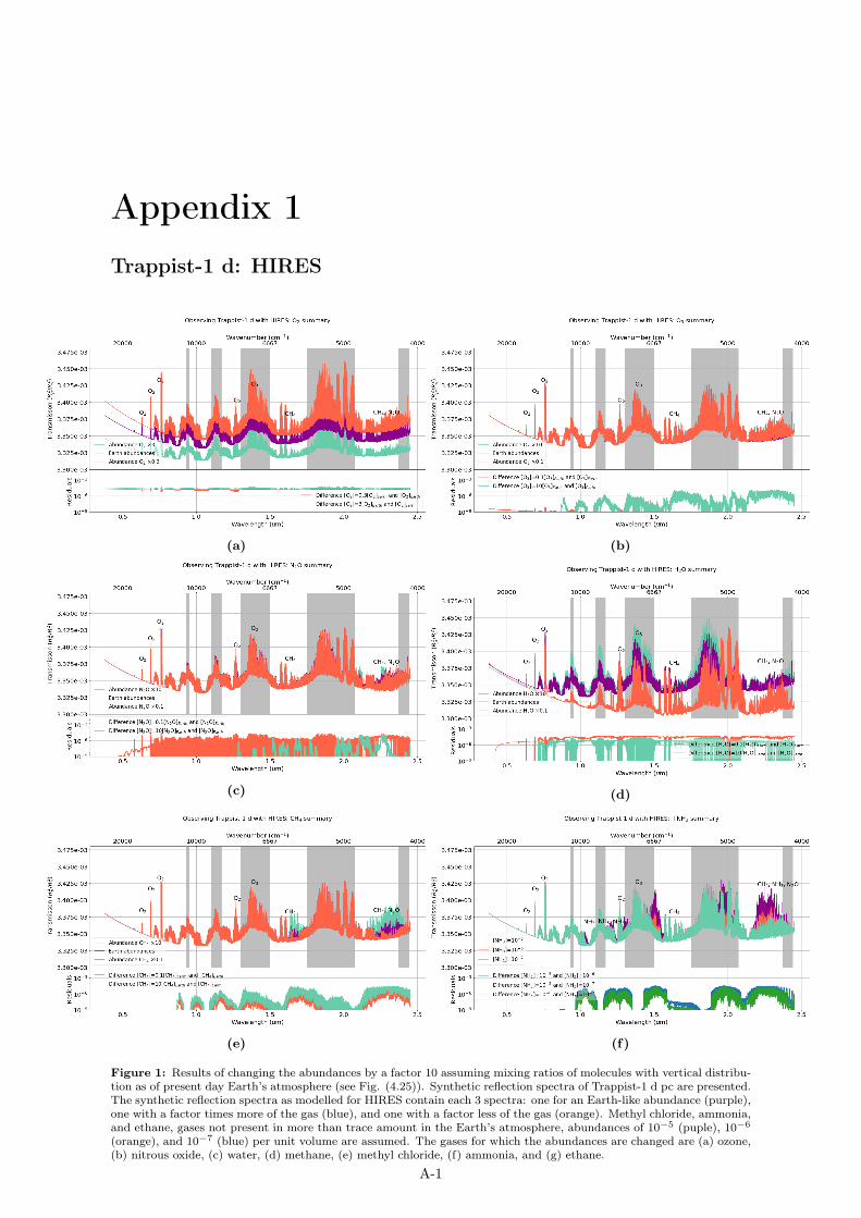
Appendix 1Trappist-1 d: HIRES

(a) (b)

(c) (d)

(e) (f)

Figure 1: Results of changing the abundances by a factor 10 assuming mixing ratios of molecules with vertical distribu-tion as of present day Earth’s atmosphere (see Fig. (4.25)). Synthetic reflection spectra of Trappist-1 d pc are presented.The synthetic reflection spectra as modelled for HIRES contain each 3 spectra: one for an Earth-like abundance (purple),one with a factor times more of the gas (blue), and one with a factor less of the gas (orange). Methyl chloride, ammonia,and ethane, gases not present in more than trace amount in the Earth’s atmosphere, abundances of 10−5 (puple), 10−6

(orange), and 10−7 (blue) per unit volume are assumed. The gases for which the abundances are changed are (a) ozone,(b) nitrous oxide, (c) water, (d) methane, (e) methyl chloride, (f) ammonia, and (g) ethane.

A-1

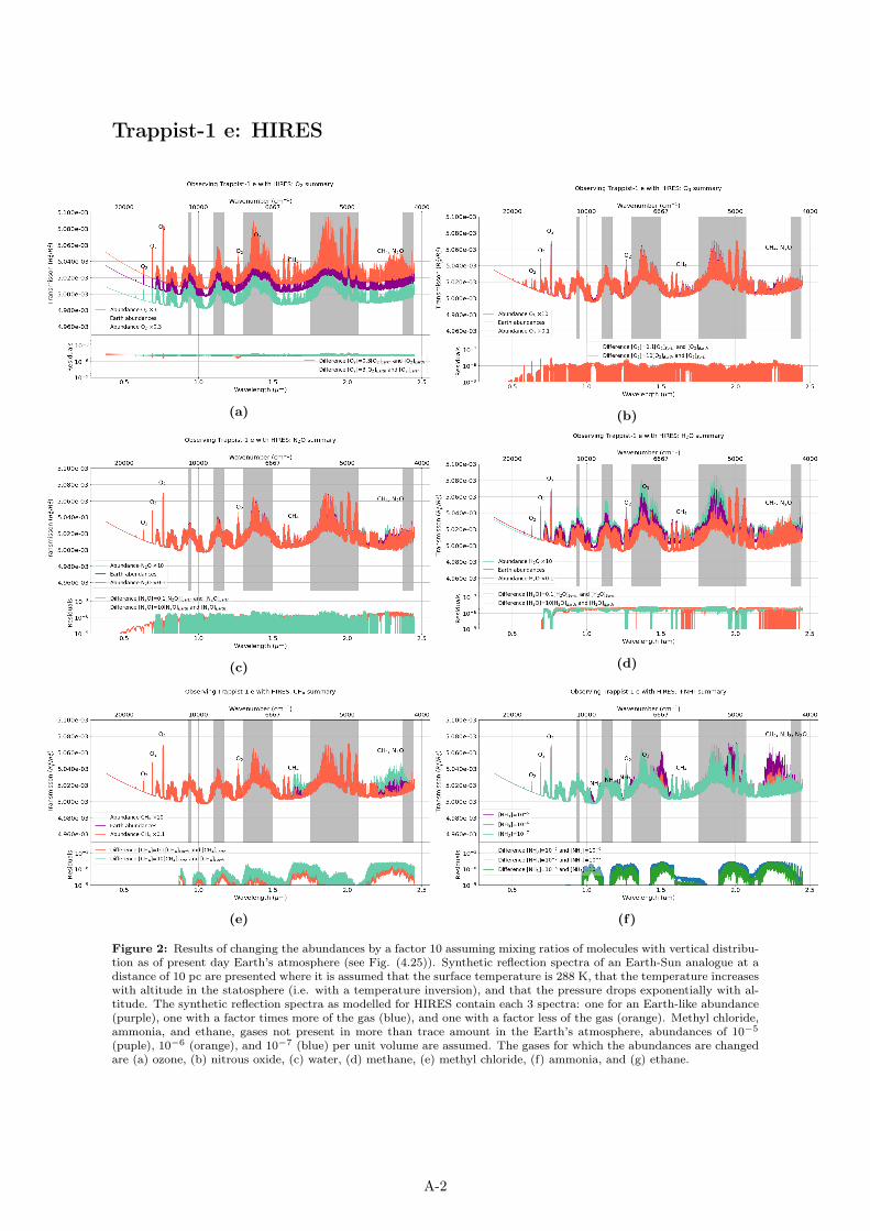
Trappist-1 e: HIRES

(a) (b)

(c) (d)

(e) (f)

Figure 2: Results of changing the abundances by a factor 10 assuming mixing ratios of molecules with vertical distribu-tion as of present day Earth’s atmosphere (see Fig. (4.25)). Synthetic reflection spectra of an Earth-Sun analogue at adistance of 10 pc are presented where it is assumed that the surface temperature is 288 K, that the temperature increaseswith altitude in the statosphere (i.e. with a temperature inversion), and that the pressure drops exponentially with al-titude. The synthetic reflection spectra as modelled for HIRES contain each 3 spectra: one for an Earth-like abundance(purple), one with a factor times more of the gas (blue), and one with a factor less of the gas (orange). Methyl chloride,ammonia, and ethane, gases not present in more than trace amount in the Earth’s atmosphere, abundances of 10−5

(puple), 10−6 (orange), and 10−7 (blue) per unit volume are assumed. The gases for which the abundances are changedare (a) ozone, (b) nitrous oxide, (c) water, (d) methane, (e) methyl chloride, (f) ammonia, and (g) ethane.

A-2

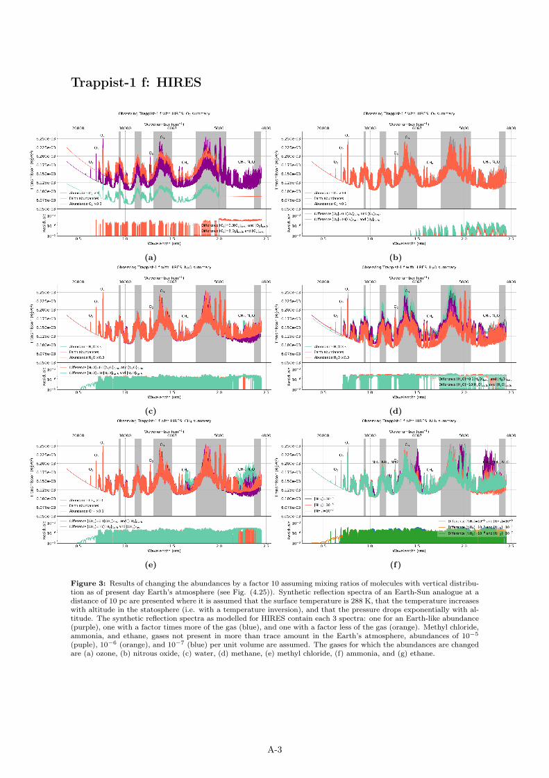
Trappist-1 f: HIRES

(a) (b)

(c) (d)

(e) (f)

Figure 3: Results of changing the abundances by a factor 10 assuming mixing ratios of molecules with vertical distribu-tion as of present day Earth’s atmosphere (see Fig. (4.25)). Synthetic reflection spectra of an Earth-Sun analogue at adistance of 10 pc are presented where it is assumed that the surface temperature is 288 K, that the temperature increaseswith altitude in the statosphere (i.e. with a temperature inversion), and that the pressure drops exponentially with al-titude. The synthetic reflection spectra as modelled for HIRES contain each 3 spectra: one for an Earth-like abundance(purple), one with a factor times more of the gas (blue), and one with a factor less of the gas (orange). Methyl chloride,ammonia, and ethane, gases not present in more than trace amount in the Earth’s atmosphere, abundances of 10−5

(puple), 10−6 (orange), and 10−7 (blue) per unit volume are assumed. The gases for which the abundances are changedare (a) ozone, (b) nitrous oxide, (c) water, (d) methane, (e) methyl chloride, (f) ammonia, and (g) ethane.

A-3

Trappist-1 g: HIRES

(a) (b)

(c) (d)

(e) (f)

Figure 4: Results of changing the abundances by a factor 10 assuming mixing ratios of molecules with vertical distribu-tion as of present day Earth’s atmosphere (see Fig. (4.25)). Synthetic reflection spectra of an Earth-Sun analogue at adistance of 10 pc are presented where it is assumed that the surface temperature is 288 K, that the temperature increaseswith altitude in the statosphere (i.e. with a temperature inversion), and that the pressure drops exponentially with al-titude. The synthetic reflection spectra as modelled for HIRES contain each 3 spectra: one for an Earth-like abundance(purple), one with a factor times more of the gas (blue), and one with a factor less of the gas (orange). Methyl chloride,ammonia, and ethane, gases not present in more than trace amount in the Earth’s atmosphere, abundances of 10−5

(puple), 10−6 (orange), and 10−7 (blue) per unit volume are assumed. The gases for which the abundances are changedare (a) ozone, (b) nitrous oxide, (c) water, (d) methane, (e) methyl chloride, (f) ammonia, and (g) ethane.

A-4

LHS 1140 b: HIRES

(a) (b)

(c) (d)

(e) (f)

Figure 5: Results of changing the abundances by a factor 10 assuming mixing ratios of molecules with vertical distribu-tion as of present day Earth’s atmosphere (see Fig. (4.25)). Synthetic reflection spectra of an Earth-Sun analogue at adistance of 10 pc are presented where it is assumed that the surface temperature is 288 K, that the temperature increaseswith altitude in the statosphere (i.e. with a temperature inversion), and that the pressure drops exponentially with al-titude. The synthetic reflection spectra as modelled for HIRES contain each 3 spectra: one for an Earth-like abundance(purple), one with a factor times more of the gas (blue), and one with a factor less of the gas (orange). Methyl chloride,ammonia, and ethane, gases not present in more than trace amount in the Earth’s atmosphere, abundances of 10−5

(puple), 10−6 (orange), and 10−7 (blue) per unit volume are assumed. The gases for which the abundances are changedare (a) ozone, (b) nitrous oxide, (c) water, (d) methane, (e) methyl chloride, (f) ammonia, and (g) ethane.

A-5

K2-18 b: HIRES

(a) (b)

(c) (d)

(e) (f)

Figure 6: Results of changing the abundances by a factor 10 assuming mixing ratios of molecules with vertical distribu-tion as of present day Earth’s atmosphere (see Fig. (4.25)). Synthetic reflection spectra of an Earth-Sun analogue at adistance of 10 pc are presented where it is assumed that the surface temperature is 288 K, that the temperature increaseswith altitude in the statosphere (i.e. with a temperature inversion), and that the pressure drops exponentially with al-titude. The synthetic reflection spectra as modelled for HIRES contain each 3 spectra: one for an Earth-like abundance(purple), one with a factor times more of the gas (blue), and one with a factor less of the gas (orange). Methyl chloride,ammonia, and ethane, gases not present in more than trace amount in the Earth’s atmosphere, abundances of 10−5

(puple), 10−6 (orange), and 10−7 (blue) per unit volume are assumed. The gases for which the abundances are changedare (a) ozone, (b) nitrous oxide, (c) water, (d) methane, (e) methyl chloride, (f) ammonia, and (g) ethane.

A-6

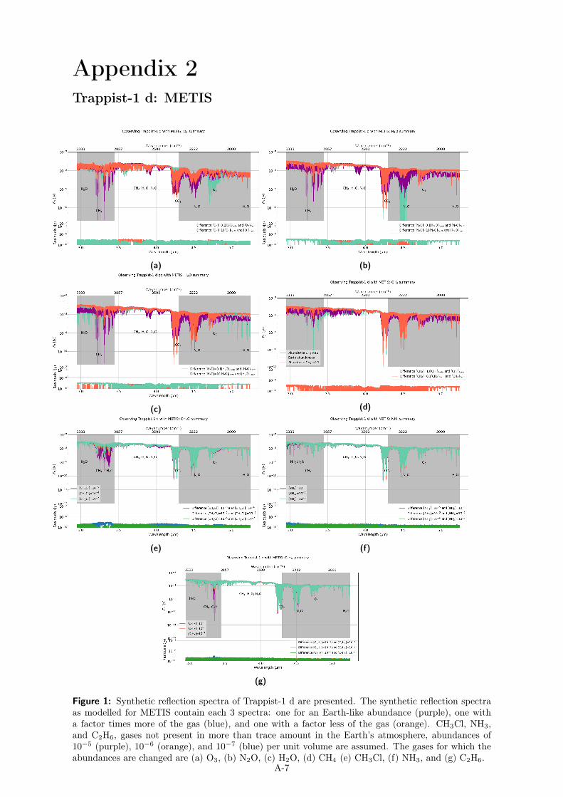
Appendix 2Trappist-1 d: METIS

(a) (b)

(c) (d)

(e) (f)

(g)

Figure 1: Synthetic reflection spectra of Trappist-1 d are presented. The synthetic reflection spectraas modelled for METIS contain each 3 spectra: one for an Earth-like abundance (purple), one witha factor times more of the gas (blue), and one with a factor less of the gas (orange). CH3Cl, NH3,and C2H6, gases not present in more than trace amount in the Earth’s atmosphere, abundances of10−5 (purple), 10−6 (orange), and 10−7 (blue) per unit volume are assumed. The gases for which theabundances are changed are (a) O3, (b) N2O, (c) H2O, (d) CH4 (e) CH3Cl, (f) NH3, and (g) C2H6.

A-7

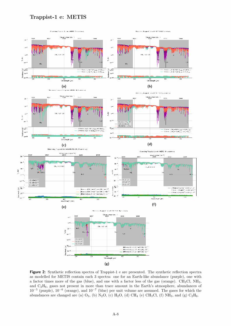
Trappist-1 e: METIS

(a) (b)

(c) (d)

(e)(f)

(g)

Figure 2: Synthetic reflection spectra of Trappist-1 e are presented. The synthetic reflection spectraas modelled for METIS contain each 3 spectra: one for an Earth-like abundance (purple), one witha factor times more of the gas (blue), and one with a factor less of the gas (orange). CH3Cl, NH3,and C2H6, gases not present in more than trace amount in the Earth’s atmosphere, abundances of10−5 (purple), 10−6 (orange), and 10−7 (blue) per unit volume are assumed. The gases for which theabundances are changed are (a) O3, (b) N2O, (c) H2O, (d) CH4 (e) CH3Cl, (f) NH3, and (g) C2H6.

A-8

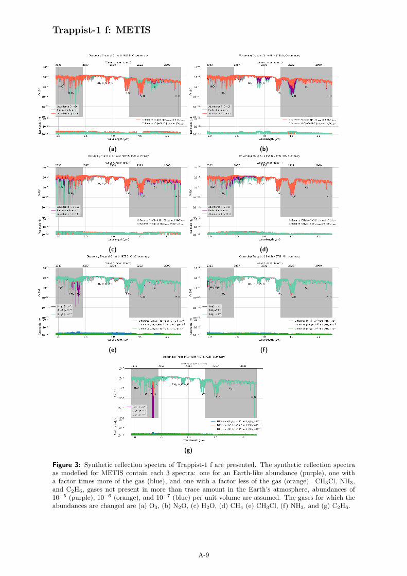
Trappist-1 f: METIS

(a) (b)

(c) (d)

(e) (f)

(g)

Figure 3: Synthetic reflection spectra of Trappist-1 f are presented. The synthetic reflection spectraas modelled for METIS contain each 3 spectra: one for an Earth-like abundance (purple), one witha factor times more of the gas (blue), and one with a factor less of the gas (orange). CH3Cl, NH3,and C2H6, gases not present in more than trace amount in the Earth’s atmosphere, abundances of10−5 (purple), 10−6 (orange), and 10−7 (blue) per unit volume are assumed. The gases for which theabundances are changed are (a) O3, (b) N2O, (c) H2O, (d) CH4 (e) CH3Cl, (f) NH3, and (g) C2H6.

A-9

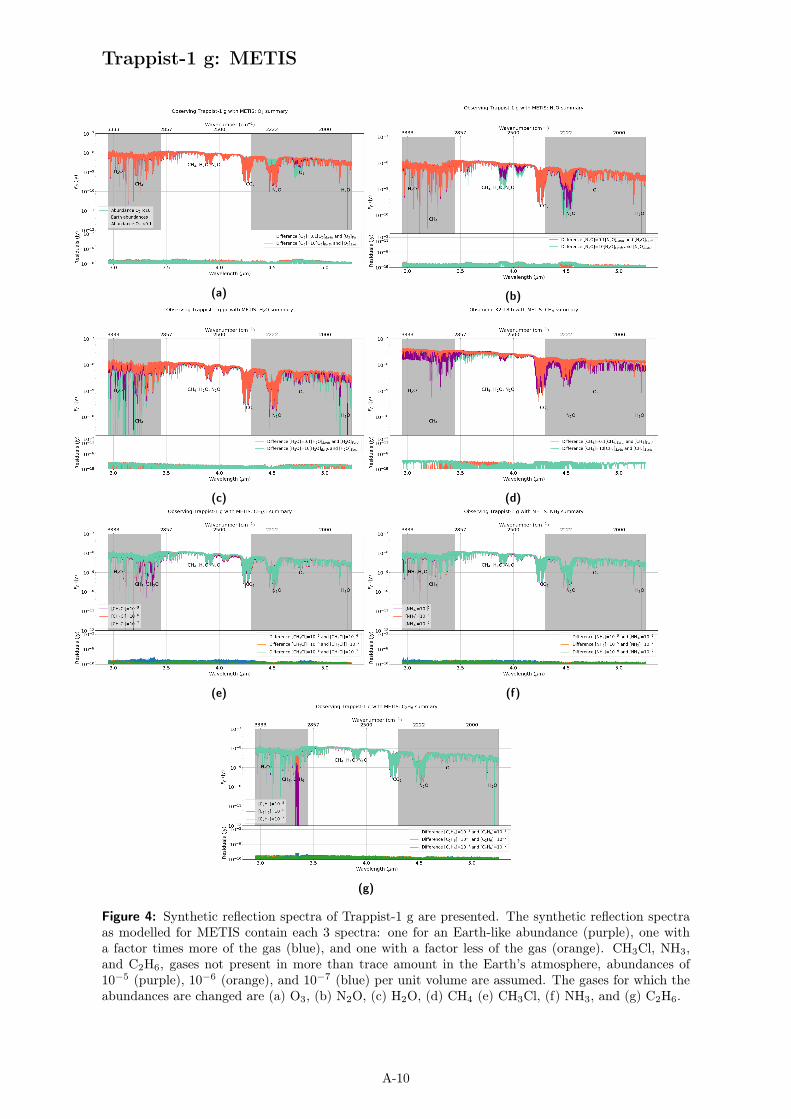
Trappist-1 g: METIS

(a) (b)

(c) (d)

(e) (f)

(g)

Figure 4: Synthetic reflection spectra of Trappist-1 g are presented. The synthetic reflection spectraas modelled for METIS contain each 3 spectra: one for an Earth-like abundance (purple), one witha factor times more of the gas (blue), and one with a factor less of the gas (orange). CH3Cl, NH3,and C2H6, gases not present in more than trace amount in the Earth’s atmosphere, abundances of10−5 (purple), 10−6 (orange), and 10−7 (blue) per unit volume are assumed. The gases for which theabundances are changed are (a) O3, (b) N2O, (c) H2O, (d) CH4 (e) CH3Cl, (f) NH3, and (g) C2H6.

A-10

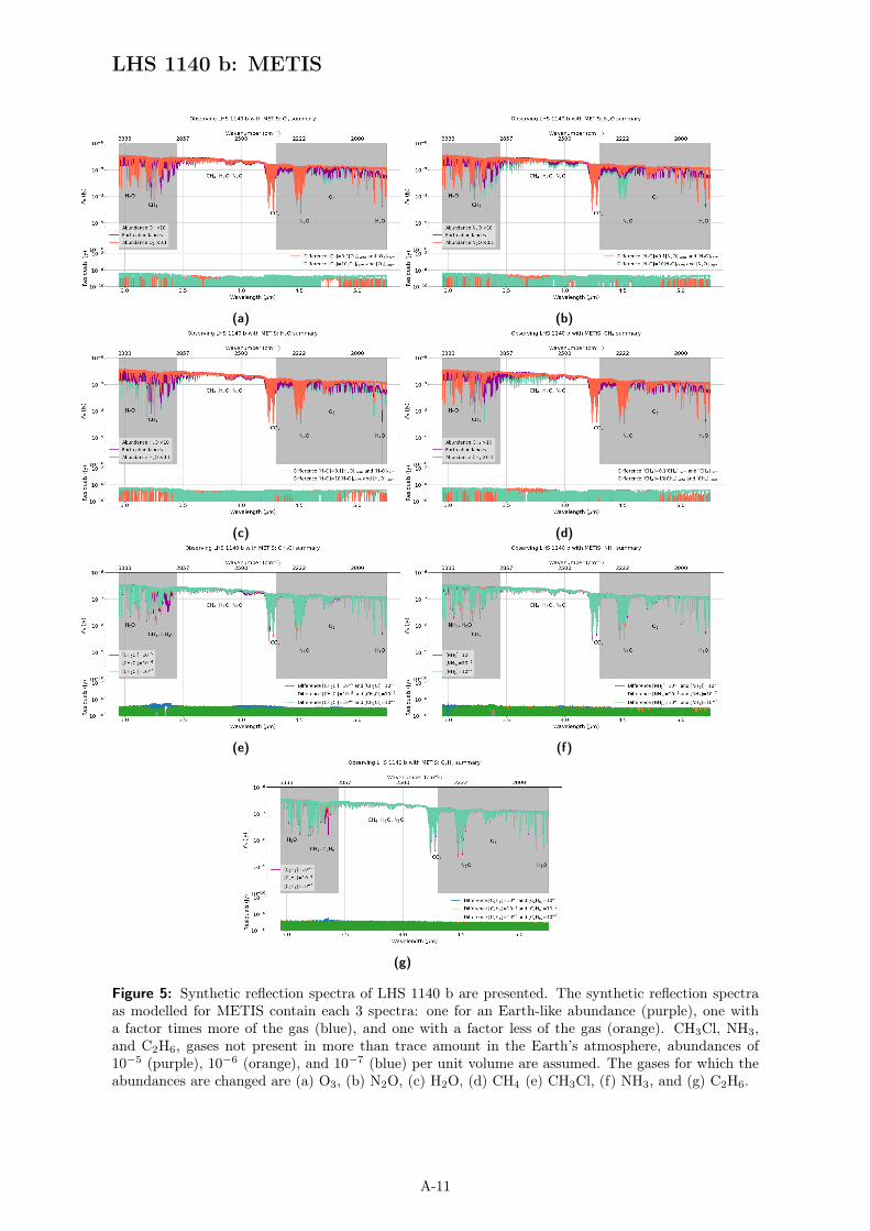
LHS 1140 b: METIS

(a) (b)

(c) (d)

(e) (f)

(g)

Figure 5: Synthetic reflection spectra of LHS 1140 b are presented. The synthetic reflection spectraas modelled for METIS contain each 3 spectra: one for an Earth-like abundance (purple), one witha factor times more of the gas (blue), and one with a factor less of the gas (orange). CH3Cl, NH3,and C2H6, gases not present in more than trace amount in the Earth’s atmosphere, abundances of10−5 (purple), 10−6 (orange), and 10−7 (blue) per unit volume are assumed. The gases for which theabundances are changed are (a) O3, (b) N2O, (c) H2O, (d) CH4 (e) CH3Cl, (f) NH3, and (g) C2H6.

A-11

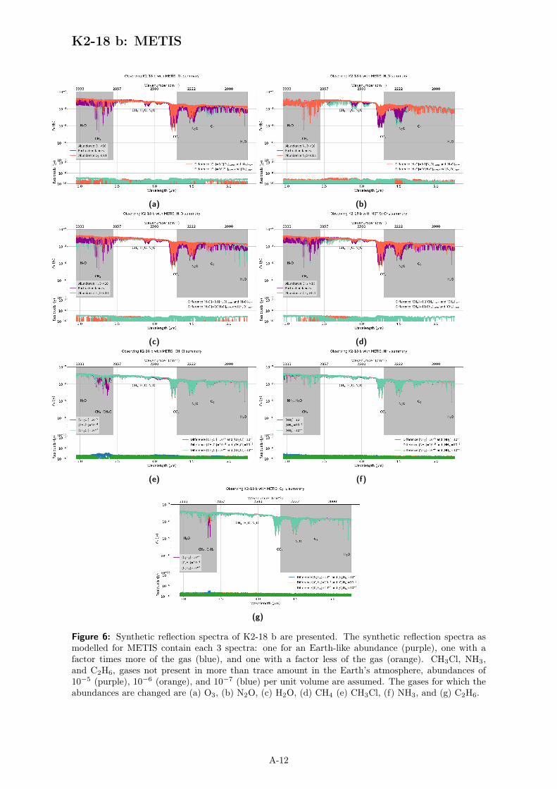
K2-18 b: METIS

(a) (b)

(c) (d)

(e) (f)

(g)

Figure 6: Synthetic reflection spectra of K2-18 b are presented. The synthetic reflection spectra asmodelled for METIS contain each 3 spectra: one for an Earth-like abundance (purple), one with afactor times more of the gas (blue), and one with a factor less of the gas (orange). CH3Cl, NH3,and C2H6, gases not present in more than trace amount in the Earth’s atmosphere, abundances of10−5 (purple), 10−6 (orange), and 10−7 (blue) per unit volume are assumed. The gases for which theabundances are changed are (a) O3, (b) N2O, (c) H2O, (d) CH4 (e) CH3Cl, (f) NH3, and (g) C2H6.

A-12