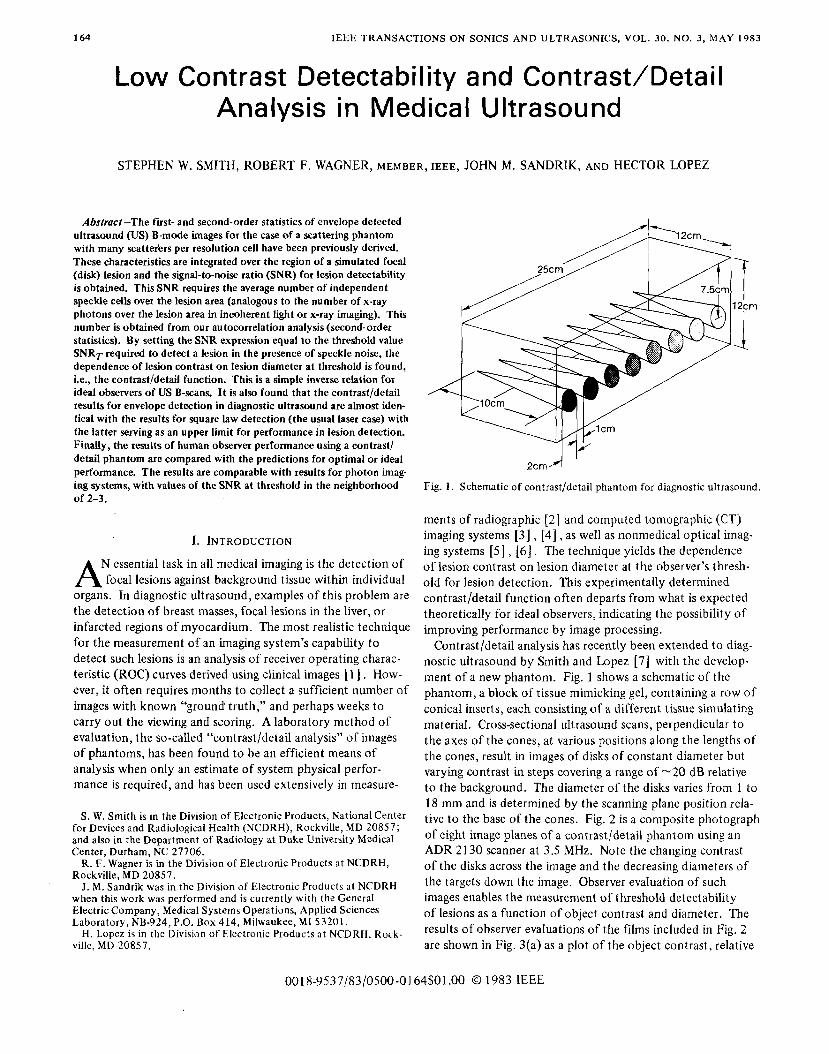
1 64 IEEE TRANSACTIONS ON SONICS AND ULTRASONICS, VOL. 30 , NO. 3, MAY 1983

Low Contrast Detectability and Contrast/DetaiI Analysis in Medical Ultrasound

STEPHEN W. SMITH, ROBERT F. WAGNER, MEMBER, IEEE, JOHN M. SANDRIK, AND HECTOR LOPEZ

Abstruct-The first- and second-order statistics of envelope detected ultrasound (US) B-mode images for the case of a scattering phantom with many scatteiers per resolution cell have been previously derived. These characteristics are integrated over the region of a simulated focal (disk) lesion and the signal-to-noise ratio (SNR) for lesion detectability is obtained. This SNR requires the average number of independent speckle cells over the lesion area (analogous to the number of x-ray photons over the lesion area in incoherent light or x-ray imaging). This number is obtained from our autocorrelation analysis (second-order statistics). By setting the SNR expression equal to the threshold value SNRT required to detect a lesion in the presence of speckle noise, the dependence of lesion contrast on lesion diameter at threshold is found, i.e., the contrast/detail function. This is a simple inverse relation for ideal observers of US B-scans. I t is also found that the contrast/detail results for envelope detection in diagnostic ultrasound are almost iden- tical with the results for square law detection (the usual laser case) with the latter serving as an upper limit for performance in lesion detection. Finally, the results of human observer performance using a contrast/ detail phantom are compared with the predictions for optimal or ideal performance. The results are comparable with results for photon imag- ing systems, with values of the SNR at threshold in the neighborhood of 2-3.

A I. INTRODUCTION

N essential task in all medical imaging is the detection of focal lesions against background tissue within individual

organs. In diagnostic ultrasound, examples of this problem are the detection of breast masses, focal lesions in the liver, or infarcted regions of myocardium. The most realistic technique for the measurement of an imaging system’s capability to detect such lesions is an analysis of receiver operating charac- teristic (ROC) curves derived using clinical images [ 1 ] , How- ever, it often requires months to collect a sufficient number of images with known “ground truth,” and perhaps weeks to carry out the viewing and scoring. A laboratory method of evaluation, the so-called “contrast/detail analysis” of images of phantoms, has been found to be an efficient means of analysis when only an estimate of system physical perfor- mance is required, and has been used extensively in measure-

S. W. Smith is in the Division of Electronic Products, National Center for Devices and Radiological Health (NCDRH), Rockville, MD 20857; and also in the Department of Radiology at Duke University Medical Center, Durham, NC 27706.

R. F. Wagner is in the Division of Electronic Products at NCDRH, Rockville, MD 20857.

J . M. Sandrik was in the Division of Electronic Products at NCDRH when this work was performed and is currently with the General Electric Company, Medical Systems Operations, Applied Sciences Laboratory, NB-924, P.O. Box 414, Milwaukee, MI 53201.

ville, MD 20857. H. Lopez is in the Division of Electronic Products a t NCDRH, Rock-

2cm

Fig. 1. Schematic of contrast/detail phantom for diagnostic ultrasound.

ments of radiographic [ 2 ] and computed tomographic (CT) imaging systems [ 3 ] , [4], as well as nonmedical optical imag- ing systems [5], [ 6 ] . The technique yields the dependence of lesion contrast on lesion diameter at the observer’s thresh- old for lesion detection. This experimentally determined contrastldetail function often departs from what is expected theoretically for ideal observers, indicating the possibility of improving performance by image processing.

Contrast/detail analysis has recently been extended to diag- nostic ultrasound by Smith and Lopez [7] with the develop- ment of a new phantom. Fig. 1 shows a schematic of the phantom, a block of tissue mimicking gel, containing a row of conical inserts, each consisting of a different tissue simulating material. Cross-sectional ultrasound scans, perpendicular to the axes of the cones, at various positions along the lengths of the cones, result in images of disks of constant diameter but varying contrast in steps covering a range of -20 dB relative to the background. The diameter of the disks varies from 1 to 18 mm and is determined by the scanning plane position rela- tive to the base of the cones. Fig. 2 is a composite photograph of eight image planes of a contrast/detail phantom using an ADR 21 30 scanner at 3.5 MHz. Note the changing contrast of the disks across the image and the decreasing diameters of the targets down the image. Observer evaluation of such images enables the measurement of threshold detectability of lesions as a function of object contrast and diameter. The results of observer evaluations of the films included in Fig. 2 are shown in Fig. 3(a) as a plot of the object contrast, relative

0018-9537/83/0.500-0164$01.00 0 1983 IEEE

SMITH er al.: DETECTABILITY AND ANALYSIS IN MEDICAL ULTRASOUND 165

Echo Amplitude Fig. 2. Composite photograph of eight image planes of contrastldetail

phantom imaged with ADR Model 2130 scanner at 3.5 MHz.

to the background, versus the diameter of the disks at the threshold of detection by the observers. Analogous results for a Unirad GZD scanner at 3.5 MHz are shown in Fig. 3(b). The figures show that at high contrasts (>4 dB), the detection capability of the scanner is only weakly dependent on object contrast and approaches the two point spatial resolution of the imaging system in the simulated tissue, included in the plots at a contrast of 20 dB (more in Section IV). For low contrast objects (echo amplitude <4 dB relative to background) the diameter for threshold detection is strongly dependent on object contrast.

for radiographic systems and CT by Cohen er al. [2] -[4] . Several investigations have been made to predict theoretically the ideal contrast/detail relationships for these imaging modal- ities [8] -[lo] based on an understanding of the spatial resolu- tion and the statistics of the noise for a given imaging tech- nique. This paper describes the extension of these ideas to ultrasound B-scans.

In diagnostic ultrasound (US) the spatial resolution or point response is well-understood and depends on diffraction and the frequency characteristics of the transducerlscanner. How- ever, an understanding of the image noise of US B-scans is still incomplete. The texture in the image of parenchymal tissue may be viewed as image signal or as undesirable noise, a speckle interference pattern. In this paper the texture will be treated as coherent speckle, and an analysis of diagnostic ultrasound contrast/detail detection in the presence of speckle will be developed based on stochastic signal and noise analysis. The discussion will be limited to lesion detection about andbeyond

These results are similar to analogous data previously reported

2o r \ ' 3.5 MHz

t

0' I 1 2 A L

20 - L

18 - .

Diameter (mm) (a)

I, 6 - 0

L u

- P 8 10 20

I 2

\*

3.5 MHz

4

Diometer(mm) (b)

Fig. 3 . (a) Results of threshold detection of simulated lesions in images of contrast/detail phantom for ADR Model 2130 scanner with a 3.5 MHz AA transducer: Object contrast relative to the background ver- sus diameter. (b) Same as (a), but for Unirad GZD scanner at 3.5 MHz.

166 IEEE TRANSACTIONS ON SONICS AND ULTRASONICS, VOL. 30, NO. 3 , MAY 1983

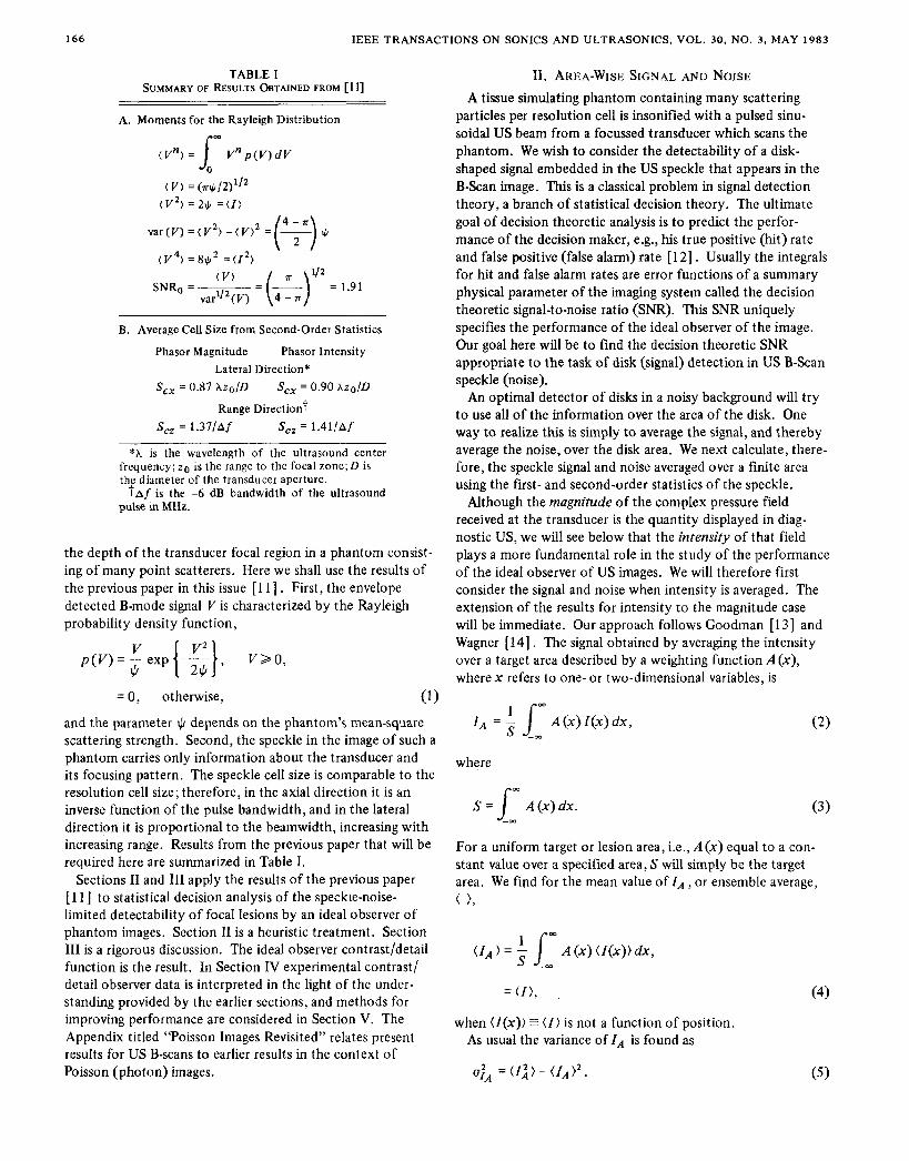
TABLE I SUMMARY OF RESULTS OBTAINED FROM [ I l]

A. Moments for the Rayleigh Distribution

( V ) = (n$/2)'/' ( V') = 211, = ( I )

B. Average Cell Size from Second-Order Statistics ~~ ~

Phasor Magnitude Phasor Intensity Lateral Direction*

S,, = 0.87 Azo/D S,, = 0.90 hz0/D

Range Direction7 S, = 1.37/A f S,, = 1.4l/Af

*h is the wavelength of the ultrasound center frequency; zo is the range to the focal zone;D is the diameter of the transducer aperture.

pulse in MHz. taf is the -6 dB bandwidth of the ultrasound

the depth of the transducer focal region in a phantom consist- ing of many point scatterers. Here we shall use the results of the previous paper in this issue [l l ] . First, the envelope detected B-mode signal V is characterized by the Rayleigh probability density function,

= 0, otherwise, (1 1 and the parameter II/ depends on the phantom's mean-square scattering strength. Second, the speckle in the image of such a phantom carries only information about the transducer and its focusing pattern. The speckle cell size is comparable to the resolution cell size; therefore, in the axial direction it is an inverse function of the pulse bandwidth, and in the lateral direction it is proportional to the beamwidth, increasing with increasing range. Results from the previous paper that will be required here are summarized in Table I.

Sections I1 and I11 apply the results of the previous paper [ l l ] to statistical decision analysis of the speckie-noise- limited detectability of focal lesions by an ideal observer of phantom images. Section I1 is a heuristic treatment. Section 111 is a rigorous discussion. The ideal observer contrast/detail function is the result. In Section IV experimental contrast/ detail observer data is interpreted in the light of the under- standing provided by the earlier sections, and methods for improving performance are considered in Section V. The Appendix titled "Poisson Images Revisited" relates present results for US B-scans to earlier results in the context of Poisson (photon) images.

11. AREA-WISE SIGNAL AND NOISE A tissue simulating phantom containing many scattering

particles per resolution cell is insonified with a pulsed sinu- soidal US beam from a focussed transducer which scans the phantom. We wish to consider the detectability of a disk- shaped signal embedded in the US speckle that appears in the B-Scan image. This is a classical problem in signal detection theory, a branch of statistical decision theory. The ultimate goal of decision theoretic analysis is to predict the perfor- mance of the decision maker, e.g., his true positive (hit) rate and false positive (false alarm) rate [ 121 . Usually the integrals for hit and false alarm rates are error functions of a summary physical parameter of the imaging system called the decision theoretic signal-to-noise ratio (SNR). This SNR uniquely specifies the performance of the ideal observer of the image. Our goal here will be to find the decision theoretic SNR appropriate to the task of disk (signal) detection in US B-Scan speckle (noise).

An optimal detector of disks in a noisy background will try to use all of the information over the area of the disk. One way to realize this is simply to average the signal, and thereby average the noise, over the disk area. We next calculate, there- fore, the speckle signal and noise averaged over a finite area using the first- and second-order statistics of the speckle.

Although the magnitude of the complex pressure field received at the transducer is the quantity displayed in diag- nostic US, we will see below that the intensity of that field plays a more fundamental role in the study of the performance of the ideal observer of US images. We will therefore first consider the signal and noise when intensity is averaged. The extension of the results for intensity to the magnitude case will be immediate. Our approach follows Goodman [l31 and Wagner [14]. The signal obtained by averaging the intensity over a target area described by a weighting function A (x), wherex refers to one- or two-dimensional variables, is

= 2 j-; A(x)Z(x)dx, ( 2 )

where

S = L A(x)dx. m

(3)

For a uniform target or lesion area, i.e., A(x) equal to a con- stant value over a specified area, S will simply be the target area. We find for the mean value of IA, or ensemble average, ( ),

(fA ) = l: A (x) ( I ( x ) ) dx,

= ( I ) , , (4)

when ( l ( x ) ) E ( 1 ) is not a function of position. As usual the variance of I A is found as

=(f;)- ( I A ) ' . ( 5 )

SMITH et al.: DETECTABILITY AND ANALYSIS IN MEDICAL ULTRASOUND 167

We require therefore

( I 2 ) = 4 /- d X l / I d w 2 A ( x , ) A ( x 2 ) < / ( X I ) I ( x 2 ) ) , S -m

(6) where the ensemble average in the integrand is recognized as the autocorrelation function of intensity, R z ( x l , x 2 ) (see [l 1 , eqs. (5)-(8)J). When the latter depends only on the co- ordinate difference, A x = x 2 - x l , we may write

( z j ) = + J- dX1 d x 2 A ( x , ) A ( x , ) R z ( x 2 - X I ) S -m

1 =- [ A ( - A ~ ) ~ R ~ ( A ~ ) O A ( A X ) ] ~ , = ~ S 2 (7)

a double convolution with the resulting variable Ax = 0. That is, we have simply the linear systems result [l51 , analogous to [l 1 , eq. (lo)] evaluated at the origin.

The autocorrelation function RI can be expressed in terms of the autocovariance function Cz (see [ l 1 , eq. (7)]),

R z ( A x ) = Cz(Ax) + ( I Y . (8)

Therefore, we obtain

1 = 3 [A ( A X ) 0 Cz(Ax) 0 A ( A X ) ] h = o , (9)

since

1 S 2

( I ) ’ =- [ A ( A x ) @ ( I ) ~ @ A ( A X ) ] ~ = ~ = ( I A ) ’ , (10)

and we have assumed a symmetric area function A . In the frequency domain this is simply [ 151

cm

where the Wiener spectrum W, is the Fourier transform of C,, and TA is the transform of A (x) /S .

In general, it is necessary to carry out the specified integrals to obtain u:~. However, a useful approximation follows immediately from (9). If the area of the disk is much greater than the region where the autocovariance Cz is appreciable, then

A ( A x ) 0 CZ(Ax) X A ( A x ) [ d(Ax) Cz (Ax) ] m

That is, the convolution does not alter the shapeofA,it merely rescales it. The integral in brackets is a length (area) in one- (two-) dimensions and is called the correlation cell S, of the

speckle pattern [l31 :

The correlation cell was evaluated in the previous article [ 1 1 ] from the ultrasound speckle autocovariance function. In the lateral direction the size of the correlation cell S,, -o.9hzo/D for both intensity and magnitude (see Table I-B). In the range direction the size of the cell was found to be S,, = 1.4/Af in millimeters where Afis the full-width half-maximum trans- ducer bandwidth in MHz. We may then write

= - {;z / [ A ( A x ) @ A ( A x ) ] a , = o . S ; C z ( O ) . (14)

The reciprocal of the factors within the curly brackets repre- sents an effective measurement area S,, which for a uniform area S is simply S. We write finally

.lA = z- . c S

z(0) = CZ(O)/M, (1 5)

where M is then the number of speckle correlation cells within the sample (measurement) area; in this case the sample area is a disk. Note that the concept of the cell size is equivalent to making the speckle correlation equal to unity over the cell and zero otherwise. Similarly, we would find the variance of the measurement of the averaged magnitude V ,

ugA = CV (O)/M. (1 6 )

We may now use (4), (15), and (16) to write the following estimates for the SNR when averaging over a disk target area S, that is large with respect to the speckle cell S,:

for averaged intensities, since C;/2 (0) = ( I ) from [ 1 1, eq. (30)] and

for averaged magnitudes, since <V)/C$*(O) = 1.91, the signal- to-noise at a point in an ultrasound speckle image [ 1 1 ] .

These SNRs refer to the estimate of a signal averaged over an area. Suppose the task is to distinguish a signal in a given area from the average background over a similar area. This is related to the statistical problem of estimating the difference between two noisy levels: the new signal of interest is level 1 (in signal area) minus level 2 (in background area); the new error or variance is the sum of the variances at level 1 and at level 2 . That is, for intensity say,

< A I ) E ZI - f 2 (1 9 )

u i z = (I: + I$)/Mz (20)

yielding the SNR for the difference signal

168 IEEE TRANSACTIONS ON SONICS AND ULTRASONICS, VOL. 3 0 , NO. 3, MAY 1983

Similarly, for magnitudes we have

For the low contrast limit, where I I = I 2 = I , V, ‘5 V2 = V, we find

and

where we have used

I = v2 and

A I = 2V(AV).

It is tempting at this detail function from

(25)

point to deduce the sought after contrast/ the SNRs of (21) and (22). We will show

in the next section that only one of these is fundamentally related to the performance of a lesion detection task. We will therefore postpone discussion of the SNRs of this section until that point.

111. STATISTICAL DECISION THEORY FOR US B-SCANS We next calculate from first principles the performance of

the optimal observerldecision maker that uses the peak or envelope detected signal to perform a given signal detection task. The result will yield the optimal, or best performance, contrast/detail function. This will be accomplished by con- structing a decision function to be used by an ideal observer of a B-mode image who must decide on the presence or ab- sence of a given signal. It is shown in texts on signal detection theory [ 121 that using as a decision function the odds em- bodied in the likelihood ratio (defined below), or a quantity monotonic with the likelihood ratio, is equivalent to a number of “best performance” criteria. That is, we are able to calcu- late the best performance possible for detecting a signal of specified characteristics; this level of performance then be- comes a goal or standard for the development of actual hard- ware, detectors, and displays for human observer applications. We limit our discussion of “performance” here to a calculation of the decision theoretic SNR that serves as the argument of the error functions that determine performance [16]. For actual contrast/detail analysis it is a fixed level of performance, that is, a fixed decision theoretic SNR that is of interest.

We consider the following task. An observer looks at the peak-detected image signal in the area where a target (here a disk) will be, if it is present. His task is to determine whether the disk is present or only background is present. We will calculate his performance when he uses the optimal decision rule.

The maximum number of independent samples available to the decision maker over the specified target area is given by the number of cells M determined in the previous section. It

is interesting that in photon imaging (see Appendix) there is a quantity analogous to M , namely, the expected number of photons over the signal area. In the statistics of coherent imaging the speckle correlation cell plays the role of a count or quantum; in the sampling sense, the number of speckle spots is the number of degrees of freedom.

Which M should be used, MV or MI? Numerically it makes little difference, but conceptually which is correct? At this point it seems natural to use M v . We will use simply M until the argument advances further.

are the random variables available to the decision maker. He calculates the likelihood ratio or odds for the set of cell read- ing { Vi) from the following probabilities. First, using the Rayleigh pdf characteristic of the B-mode image, the likeli- hood or probability of the readings {Vi} given the presence of the signal level G1 is

The values of the peak detected echo strengths 5 , l i < M

M ~({vi>IJ/,>=n (vi/ i l l)exP(-v;/2!w. (26) i=l

The likelihood or probability of the readings given the presence of only the background level $2 is

i =l

The likelihood ratio for the readings is then

7;z =~({511$1)/L({vi}I4b)

=E exp [$ (i - i)]. 1 = 1

We now define a quantity monotonic with the log likelihood ratio and therefore monotonic with the likelihood ratio

The factors involving the $ are constants related to the mean- square scattering strengths of regions 1 and 2, and are there- fore independent of the measured values of the random vari- ables Vi, so it is sufficient to study

i = l

as our decision function. The decision maker will respond that the disc is either present or absent depending on whether the value of yl2 is greater or smaller than some criterion or cut-off value. This is called a decision rule.

We now gain some insight concerning the value of M. The ideal decision function for magnitude images involves squaring and summing the readings over the cells. That is, it is a pre- scription for using the intensity values. There are MI such independent values. Therefore, as we study the statistics of the decision function it is MI, not M V , which is more funda-

SMITH er a l . : DETECTABILITY AND ANALYSIS IN MEDICAL ULTRASOUND 169

mental. Henceforth M will refer to M I , since we will be deal- ing with squared magnitude, i.e., intensity values. The slight ambiguity about the number of cells arises from the fact that we are actually making an approximation to an exact solu- tion of the problem. The exact solution requires finding a representation in which the noise is uncorrelated (i.e., an eigenvalue problem). Goodman [ 131 has shown that working with the correlation cell concept for intensity yields a very good approximation to the exact solution.

We now require the distribution for yI2 to determine the performance of the decision maker. Since each Vi comes from a Rayleigh distribution, V; will come from an exponen- tial distribution, p (V’) = 1 /(2 $) { exp (- V 2 / 2 $)}, V 2 > 0 (corresponding to the intensity in the laser case, as shown in [ 1 1, eqs. (2)-(4)]); the sum over i will tend to a Gaussian distribution, as i goes to infinity, according to the central limit theorem. From [13, fig. 2.131 we see that for a value of M of about 10 the Gaussian approximation becomes reason- able in practice. We require then only the mean of yI2 given that the target is present, E [y12 1 3 , the mean of y12 given that the target is not present, E [y12 1 $’ ] , and the correspond- ing variances. Using the results in Table I for each term in (29) these are found to be

E[y12I$11 =2M$1; E [ y 1 2 I $ 2 1 =2M$2

var [ylz I $ 1 I = 4M$: ; var [y12 I$2 I = 4 ~ $ ; . (3 1)

The summary measure of the performance of this decision maker that determines hit and error rates is the ideal decision maker, i.e., optimal signal-to-noise ratio SNh, , = Ap/o, where

AP=E[yl’ l$I l -E[y12I$21

= 2M[$1 - $2 1 a = (var [TI’ I $ 1 1 + var [Y12 l$2 I P’

= 2M112[$: t $$] ‘ l2 (3 2)

or

(3 3)

The quantity C$ defined by this equation will be found to function as a contrast for small signal differences, but we should remember that it is fundamentally a signal-to-noise ratio. We may now find the ideal contrast/detail function for the detec- tion of a disk lesion of diameter d , and “contrast” C$ by setting S N h , , equal to some designated threshold value SNRT:

(34)

where we have assumed that the speckle cell shape is elliptical. This translates into an ideal contrast/detailor contrast-diameter curve with a slope - 1 in log-log coordinates. That is, for a fixed level of ideal observer performance characterized by the

value S N k P t = SNRT, a plot of log threshold “contrast” versus log threshold diameter has slope - 1. The precise “hit” and “error” rates depend on the cut-off or criterion level chosen for the decision rule. These details are neglected in the present analysis.

If we repeat the above exercise for a detector that senses in- tensity, Z = V ’ , as in the laser case, the exponential distribu- tion for Ii is required,

1 2 a

p ( I ) = 7 exp (-1/2a2), I > 0,

= 0, otherwise.

We find in this case

(3 5)

which is formally identical to (33), since $ a I . This could have been anticipated from a general result of signal detection theory: a transformation from a decision variable X to a deci- sion variable Y by a one-to-one relation e.g., I = V 2 , does not change detection performance [ 171 .

The results in (33) and (36) are identical to the result of (21). The process of working through the statistical decision theory for the optimal performance using a peak-detected or magnitude image has brought us back to the fundamental SNR for intensities. It is a description of the best possible performance using a magnitude (or intensity) image: the best possible performance is achieved by integrating V’ or I over the lesion and comparing this to the integrated value over a background of the same size. No statement is made here with regard to human performance.

The SNR of (22) for magnitudes was seen to have the same low contrast behavior as (21), i.e., the SNR of this section. That is, the heuristic approach of the previous section and the decision theoretic approach here agree for low contrasts. However, in the limit of high contrasts (l2 + 0) the magnitude SNR of (22) exceeds the intensity SNR by the ratio 1.91/1.00, as was the case for the point SNRs. The magnitude SNR cannot, therefore, be a true decision theoretic or best perfor- mance SNR, since (33) or (36) describes best performance. Otherwise it would suggest that improvements without limit would result from successive square roots of the B-scan image. The magnitude SNR’s bearing the factor 1.91 cannot be used alone to calculate a fundamental measure of signal detect- ability, but would be useful if the true probability distribution function for the integrated magnitude were known. (For further discussion of this fundamental point, see [ 161 .) Once the phase information is lost from a signal there is no funda- mental advantage to using magnitudes instead of intensities, since they are easily retrievable from each other by an ideal detector.

The result of George et al. [6] is only an approximation to the rigorous result given here. The former result ignores the dependence of the speckle noise on the signal level $, and is therefore only exact in the limit of small contrasts. That is, the earlier result ignores the multiplicative nature of the noise [181.

IEEE TRANSACTIONS ON SONICS AND ULTRASONICS, VOL. 30, NO. 3, MAY 1983

1.0 -

0.6 - - -

0.3 - c,

0.2 -

0.1 -

3.4 mm l

J 1 2 3 6 10 20

Diameter (mm) (a)

1.0 -

0.6 -

0.3 - c,

0.2 -

0.1 L

Slope = r =

-0.86 t 0.14 -0.98 -0.86 t 0.14 -0.98

3.7 mm

I I l t , I I I , , I 1 2 3 6 10 20

Diameter (mm) cb)

Fig. 4. (a) Contrastjdetail data from Fig. 3(a) replotted in terms of C (33) versus diameter. Error bars are *l standard derivation. (by Contrast/detail data from Fig. 3(b) replotted in terms of C$ versus diameter.

N. SOME HUMAN OBSERVER RESULTS

Having derived a framework in which to analyze contrast/ detail performance, we now return to the measurements by Smith and Lopez [7] of the threshold detectability of simu- lated lesions in a tissue simulating phantom and the resulting dependence of threshold contrast (defined as V, /Vl in deci- bels) on lesion diameter for human observers. In Fig. 4(a) we have replotted the contrastldetail data from Fig. 3(a) in terms of C, versus diameter. Similarly in Fig. 4(b) the experimental contrastldetail data from Fig. 3(b) are plotted in terms of C$ versus diameter. The results are seen to be reasonably well fit in log-log coordinates with a single straight line from a weighted regression analysis. The regression slopes and correlation coef- ficients for Figs. 4(a) and 4(b) are shown in the figure inserts.

We may compare the results for the slopes with the pre- dicted slope of - 1 for an ideal observer. For a given high con- trast performance, the more negative the slope, the greater the low contrast sensitivity. The slopes of the experimental curves, -0.86 and -0.75, thus indicate that the performance of the human observer is less than ideal. Analogous data have been measured for x-ray noise (see Appendix), i.e., the slopes for the performance of human observers are equal to or less nega- tive than the slope for the performance of the ideal observer.

y-intercepts of the regression lines are nonphysical points. However, one can estimate the decision theoretic SNR, for the high contrast value C, = 1. From (34) one notes that at

Because the contrast CJ, is limited to the range of 0 to 1, the

c, = 1.

SMITH et al . : DETECTABILITY AND ANALYSIS IN MEDICAL ULTRASOUND 171

TABLE I1 DETECTABILITY PARAMETERS FOR Two SCANNERS

d (mm) @C+ = 1.0 S,, (mm) S,, (mm)

ADR Model 21 30 3.5 MHz AA Transducer 3.39 5 1.07 2.87 0.91

Unirad GZD 13 mm, 3.5 MHzTransducer 3.72 i 1.78 2.65 1.32

d = SNRT(S,, . S,,)”z. (3 7)

In Table I1 we list the values of d , lesion diameter, for C, = 1 from the regression data as well as values of S,, and S, cal- culated from [l l , eqs. (32) and (34)] for the two imaging systems. Using these parameters, one arrives at the value SNRT = 2.10 _+ 0.66 and 1.99 2 0.95 for the ADRlhuman and the Unirad/human observer systems, respectively.

Much of the data of Cohen and collaborators in radiology [2] and CT [3] , [4] yield a value of SNRT = 5 . The work of Burgess et al. [l91 with x-ray noise and the method of adjust- ment gave a value of SNRT = 2.5. (The values cited in this and the preceding paragraph should be multiplied by fi for com- parison with the Rose scale. See [5] and Appendix.) At this time we speculate that the range of values is due more to the criteria used by the observers than to the imaging modalities. There is a need now to develop: consensus among investigators using contrast/detail phantoms to establish comparable and therefore portable threshold criteria; statistical tests for the difference of two contrast/detail curves; and observer effi- ciency measurements to determine the actual level of human performance on the absolute scale determined by the ideal limit [20]. We currently have programs underway in these areas.

Finally, we note that the number of speckle cells per disk lesion, or M, takes on values less than 10 for C , greater than 0.7. As observed just preceding (31), the Gaussian assumption in our derivation of the ideal observer contrast/detail function begins to break down under those conditions. A more com- plete treatment is required to bridge the low contrast analysis of this paper with the high contrast regime where the limita- tions are due more to resolution loss in the conventional sense, i.e., point and edge blurring.

V. SUMMARY DISCUSSION In this paper we have presented a first principles analysis of

the problem of the detection by an ideal observer of a focal lesion in an US B-scan of a scattering phantom with many fine particles per resolution cell, where the speckle cell size is com- parable to the resolution cell size. We provided both a heuristic and a decision theoretic derivation of the SNR for detection as a function of the lesion size and contrast. The results of the two derivations agree in the low contrast regime and predict an inverse relation between threshold contrast and threshold diameter for the ideal observer of disk-shaped lesions. Experi- mental results for human observers indicate performance that is not quite ideal, but is nevertheless quite similar to the per- formance of the human observer with other classes of noise- limited images.

Having arrived at an understanding of the detectability of focal lesions in ultrasound images, we should examine what technological developments might improve the performance of ultrasound scanning systems. The slopes of the experimen- tal data, -0.75 and -0.86, indicate that some image processing techniques might be helpful in achieving the slightly more negative slope of - 1, characteristic of the ideal observer. Smoothing techniques might be examined in tlvs regard. Since t h s would degrade resolution limited detail, separate display for high and low contrast information might be necessary.

Detection is also enhanced by reducing the parameter (Scx . SCz) of (34), i.e., reducing the correlation cell size to lower they-intercept of Figs. 4(a) and 4(b). S, is essentially a measure of system resolution in the lateral direction. There- fore, use of higher frequency transducers to improve the two- point lateral resolution of the scanner should also improve detection of large low contrast lesions, as long as bandwidth and system sensitivity are maintained, and relative object contrast does not change. This shrinking of the speckle cell permits more independent samples of the target lesion to be taken. It must be accomplished at the transducer during the complex summation. Any nonlinear postprocessing, such as an nth root detector that reduces the speckle contrast, would be merely cosmetic. We saw earlier that working with the magnitude, or the square root of intensity, instead of intensity yields a lower speckle contrast but does not affect the intrinsic detectability of low contrast lesions, at least for the ideal observer. Cosmetic approaches may offer slight gains for real observers.

In choosing a higher ultrasound frequency to increase sam- pling of a lesion, one must recall that backscatter, a major source of lesion contrast, is a function of the scatterer size compared to the ultrasound wavelength [21]. This function ranges through anf4 dependence to frequency independence (specular targets). Thus the object contrast of a low contrast target against a given background may also be frequency dependent.

lesions by superimposing uncorrelated ultrasound images of the same target [22]. This technique can be treated im- mediately within the context of our analysis. The number of independent samples of a lesion,M in (33), increases linearly with the number of independent superimposed com- pound images. Therefore, (33) for signal-to-noise ratio, and (34) for the contrast/detail relation can be modified to become

Spatial compounding improves the detection of low contrast

and

(3 9)

where N is the number of independent images compounded. Burckhardt [22] has shown that when spatial compounding by interrogating the target at different angles, the transducer must be moved a distance comparable to the aperture size to achieve uncorrelated data from the same target volume. In practice, then, spatial compounding will also increase image acquisition time.

172 IEEE TRANSACTIONS ON SONICS A N D ULTRASONICS, VOL. 30, NO. 3, MAY 1983

Axial resolution and detectability are simultaneously im- proved through reducing the parameter S,, by expanding the transducer bandwidth. Broad-band transducers can also be used for frequency compounding [ 2 3 ] . In this case a given transducer bandwidth is broken down into several narrower band components to obtain separate uncorrelated images which are superimposed, thus increasing the independent sampling of the target. Magnin [24] has discussed measure- ments of the requirements for uncorrelated images when frequency compounding.

ing the detectability of low contrast lesions: There are, thus, at least four possible techniques for improv-

1) higher transducer frequencies; 2 ) spatial compounding; 3) broader bandwidth transducers; 4) frequency compounding; and perhaps 5) image smoothing.

In comparing the relative effectiveness of these methods, one must consider the possible changes in object contrast, and the trade-offs with patient exposure and image acquisition time. These will serve as additional dimensions, beyond those of the present paper, on which one may carry out a complete optimi- zation of ultrasonic imaging systems for the detection of focal lesions in parenchymal tissue.

APPENDIX: POISSON IMAGES REVISITED In photon imaging, such as photography or radiography, the

image statistics are characterized by the Poisson distribution-a one parameter distribution for which the variance U’ in the number of photons counted is equal to the expected number p . Suppose we have to detect a difference between the area density N 1 of detected particles over a disk of area A , and the density NZ in similar areas in a uniform background. The total available signal will be the difference in the expected number of photons in each area, which is (NI - N z ) A . The noise will be the square root of the variance of this quantity which will be (Nl t Nz)1/’A1/2. Then the signal-to-noise ratio SNRp is

As in all SNR analysis, the signals of interest subtract and the noise variances add. Note the symmetry with the US results of (33) and (36). In the limit of a small signal difference N I = N 2 = N , we have

= C ( N A ) 1 1 2 / 2 1 / z , ( A 4

where we have defined the contrast C = AN/N. It can be shown that the results in ( A l ) and (A2) are rigorous for ideal observers (See [25] for general expression and references). Also, the low contrast result is a rather well-known form that is variously referred to as the Rose model, Rose-&hade model, or matched filter [ 5 ] , [ 141. The popular Rose version of this expression neglects the 2lI2 in the denominator. Rose and

- A 1 L

1.0 E 0.6

0.3 - 0.4

-

- 0.2

-

0.1

- .04

- .06

:

.03 - .02

-

.01 I ’ I ’ ‘ I “ I I I 1 I I 1 I l l

0.5 1 2 3 5 10 20 30 50 Diameter (mrad)

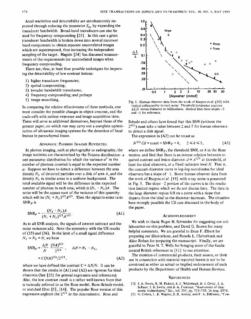
Fig. 5 . Human observer data from the work of Burgess et al. [20] with typical radiographic (x-ray) noise: Threshold luminance contrast h L / L versus diameter in milliradians. Dashed lines have slopes -2 and -1 for reference.

Schade and others have found that this SNR (without the 21/2) must take a value between 2 and 5 for human observers to detect a disk signal.

The expression in (A2) can be recast as

NI/’ Cd = const = SNRT = k , 2 Q k 5 , (A31

where we define SNRT, the threshold SNR, or k in the Rose version, and find that there is an inverse relation between re- quired contrast and lesion diameter d a A l l 2 at threshold, at least for ideal observers, at a fixed radiation level N . That is, the contrast-diameter curve in log-log coordinates for ideal observers has a slope of - 1. Some human observer data from the work of Burgess et al. [ 191 with x-ray noise is presented in Fig, 5 . The slope -2 portion of the curves is in the resolu- tion limited regime which we do not discuss here. The data in the large diameter region fall on a curve with a slope that departs from the ideal as the diameter increases. The situation here strongly parallels the US case discussed in the body of the paper.

ACKNOWLEDGMENT We wish to thank Roger H. Schneider for suggesting our col-

laboration on this problem, and David G. Brown for many helpful comments. We are grateful to Dean F. Elbert for preparing our illustrations, and Pamela L. Clatterbuck and Alice Rohan for preparing the manuscript. Finally, we are grateful to Peter N. T. Wells for bringing some of the funda- mental British references in [ l l ] to our attention.

The mention of commercial products, their source, or their use in connection with material reported herein is not to be construed as either an actual or implied endorsement of such products by the Department of Health and Human Services.

REFERENCES

[ l] J. A. Swets, R. M. Pickett, S. F. Whitehead, D. 1. Getty, J. A. Schnur, J. B. Swets, and B. A. Freeman, “Assessment of diag- nostic technologies,” Sci., vol. 205, pp. 753-759,24 Aug. 1979.

[2 ] G . Cohen, L. K. Wagner, S. R. Amtey, and F. A. DiBianca, “Con-

SMITH e? al.: DETECTABILITY AND ANALYSIS IN MEDICAL ULTRASOUND 173

trast-detail-dose and dose efficiency analysis of a scanning digital and a screen-film-grid radiographic system,” Med. Phys., vol. 8, no. 3, pp. 358-367,1981. G . Cohen and F. A. DiBianca, “The use of contrast-detail-dose evaluation of image quality in a computed tomographic scanner,” J. Comput. Assist. Tomogr., vol. 3, pp. 189-195,1979. G. Cohen, “Contrast-detail-dose analysis of six different com- puted tomographic scanners,” J. Comput. Assist. Tomogr., vol. 3,

A. Rose, Vision: Human and Electronic. New York: Plenum Press, 1973. N. George, C. R. Christensen, I. S. Bennett, and B. D. Guenther, “Speckle noise in displays,” J. Opt. Soc. Amer., vol. 66, no. 11,

S. W. Smith and H. Lopez, “A contrast-detail analysis of diag- nostic ultrasound imaging,”Med. Phys., vol. 9, no. 1, pp. 4-12, 1982. R. F. Wagner, D. G . Brown, and M. S. Pastel, “Application of information theory to the assessment of computed tomography,” Med. Phys., vol. 6 , no. 2, pp. 83-94, 1979. K. M. Hanson, “Detectability in computed tomographic images,” Med. Phys., vol. 6, no. 5, pp. 441-451, 1979. R. F. Wagner, “Imaging with photons; A unified picture evolves,” IEEE Trans. Nucl. Sci., vol. NS-27, no. 3, pp. 1028-1033, June 1980. R . F. Wagner, S. W. Smith, J. M. Sandrik, and H. Lopez, “Statis- tics of speckle in ultrasound B-scans,”lEEE TransSonics Ultra- son., vol. SU-30, no. 3, pp. 156-163, May 1983. D. M. Green and J. A. Swets, Signal Detection Theory and Psychophysics, revised ed. Huntington, NY: Krieger, 1974, ch. 1. J. W. Goodman, “Statistical properties of laser speckle patterns,” in Laser Speckle and RelatedPhenomena, J. C. Dainty, Ed. Berlin: Springer-Verlag, 1975, pp. 9-75. R. F. Wagner, “Decision theory and the detail signal-to-noise ratio

pp. 197-203,1979.

pp. 1282-1290, NOV. 1976.

of Otto Schade,” Photog. Sci. Engr., vol. 22, pp. 41-46, 1978. [ 15 1 A. Papoulis, Probability, Random Variables, and Stochastic

Processes. New York: McGraw-Hill, 1965, ch. 10. [ l 61 C. W. Helstrom, ‘The detection and resolution of optical sig-

nals,” IEEE Trans. Inform. Theory, vol. IT-10, pp. 215-281, 1964.

[ 171 J. P. Egan,Signal Detection Theory and ROC Analysis. New York: Academic, 1975, append. B. (This point was brought to our attention through a derivation by David G . Brown ofNCDRH of the invariance of the likelihood function under a change of variable that is one-to-one.)

[ l 81 H. H. Arsenault and G . April, “Properties of speckle integrated with a finite aperture and logarithmically transformed,” J. Opt. Soc. Amer., vol. 66, pp. 1130-1163, Nov. 1976.

[ l 91 A. E. Burgess, K. Humphrey, and R. F. Wagner, “Detection of bars and discs in quantum noise,” in Proc. of the Soc. ofPhoto- OpticalInstr. Engrs., vol. 173, pp. 34-40, 1979.

“Efficiency of human visual signal discrimination,” Sci., vol. 214, [20] A. E. Burgess, R. F. Wagner, R. J. Jennings, and H. B. Barlow,

pp. 93-94, 2 Oct. 1981. [ 21 1 M. O’Donnell and J. G . Miller, “Quantitative broadband ultra-

sonic backscatter: An approach to nondestructive evaluation in acoustically inhomogeneous materials,” J. Appl. Phys., vol. 52, no. 2, pp. 1056-1065, Feb. 1981.

[22] C. B. Burckhardt, “Speckle in ultrasound B-mode scans,”IEEE Trans. Sonics Ultrason., vol. SU-25, no. 1, pp. 1-6, Jan. 1978.

[23] N. George and A. Jain, “Space and wavelength dependence of speckle intensity,” Appl. Phys., vol. 4, pp. 201-212,1974.

[24] P. A. Magnin, 0. T. von Ramm, and F. L. Thurstone, “Frequency compounding for speckle contrast reduction in phased array images,” Ultrason. Imag., vol. 4, no. 3, pp. 267-281, 1982.

[25] R. F. Wagner, D. G . Brown, and C. E. Metz, “On the multiplex advantage of coded source/aperture photon imaging,” in Proc. of the Soc. o f Photo-Optical Instr. Engrs., vol. 314, pp. 72-76, Bellingham, WA, 1981.