Phase Unwrapping for SAR Interferometry—A Data Fusion Approach by Kalman Filtering

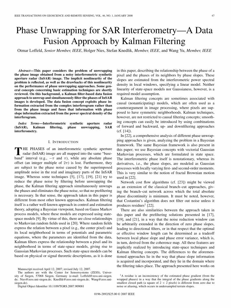
IEEE TRANSACTIONS ON GEOSCIENCE AND REMOTE SENSING, VOL. 46, NO. 1, JANUARY 2008 47

Phase Unwrapping for SAR Interferometry—A DataFusion Approach by Kalman Filtering

Otmar Loffeld, Senior Member, IEEE, Holger Nies, Stefan Knedlik, Member, IEEE, and Wang Yu, Member, IEEE

Abstract—This paper considers the problem of unwrappingthe phase image obtained from a noisy interferometric syntheticaperture radar (InSAR) image. The implicit nonlinearity of theproblem is reflected, as well as the drawbacks of this nonlinearityon the performance of phase unwrapping approaches. Some gen-eral concepts concerning basic estimation techniques are shortlyreviewed. On this background, a Kalman filter-based data fusionapproach to unwrap and simultaneously filter the phases of InSARimages is developed. The data fusion concept exploits phase in-formation extracted from the complex interferogram rather thanfrom the phase image and fuses that information with phaseslope information extracted from the power spectral density of theinterferogram.

Index Terms—Interferometric synthetic aperture radar(InSAR), Kalman filtering, phase unwrapping, SARinterferometry.

I. INTRODUCTION

THE PHASES of an interferometric synthetic apertureradar (InSAR) image are all mapped into the same “base-

band” interval (e.g., −π and π), while any absolute phaseoffset (an integer multiple of 2π) is lost. Furthermore, theyare subject to the phase noise caused by the superimposedamplitude noise in the real and imaginary parts of the InSARimage. Whereas some techniques [5], [17], [19], [21] try toreduce the phase noise by filtering before unwrapping thephase, the Kalman filtering approach simultaneously unwrapsthe phases and eliminates the phase noise, so that no prefilteringis necessary. In that sense, the approach taken in this paper isdifferent from most other known approaches. Kalman filteringitself is a rather well-known approach in control and estimationtheory, adopting a Bayesian viewpoint, based on Gauss Markovprocess models, where these models are expressed using state-space models [9]. By virtue of this, there are close relationshipsto Markovian random fields used in [20]. Where random fieldsexpress the relation between a pixel (e.g., the center pixel) andits local neighborhood in terms of potentials and parametricequations, where the parameters are identified from the data,Kalman filters express the relationship between a pixel and itsneighborhood in terms of state-space models, giving rise toGaussian Markovian processes. Such state-space models can bebased on physical or signal theoretic descriptions, as it is done

Manuscript received April 12, 2007; revised July 12, 2007.The authors are with the Center for Sensorsystems (ZESS), Univer-

sity of Siegen, 57068 Siegen, Germany (e-mail: [email protected]; [email protected]; [email protected]; [email protected]).

Digital Object Identifier 10.1109/TGRS.2007.909081

in this paper, describing the relationship between the phase of apixel and the phases of its neighbors by phase slopes. Theseslopes are estimated from the interferometric power spectraldensity in local windows, specifying a linear model. Neitherlinearity of state-space models nor Gaussianess, however, is arequired model assumption.

Kalman filtering concepts are sometimes associated withcausal (nonanticipating) models, which are often used as acounterargument in image processing, where pixels are sup-posed to have symmetric neighborhoods. Kalman techniques,however, are not restricted to causal filtering concepts; smooth-ing concepts can easily be introduced by using combinationsof forward and backward, up- and downfiltering approaches(cf. [14]).

In [22], a comprehensive analysis of different phase unwrap-ping approaches is given, analyzing the problem in a Bayesianframework. The same Bayesian framework is also present inthis paper; we use Bayesian concepts with vectorial GaussianMarkovian processes, which are formulated in state space.The interferometric phase itself is nonstationary, whereas itsderivatives, i.e., the phase slopes, are modeled as Gaussianprocesses with locally varying first- and second-order moments.This is very similar to the notion of fractal Brownian motionused in [22].

Network cost flow algorithms (cf. [23]) might be viewedas an extension of the classical branch–cut approaches, giv-ing the branch–cut network across which the total absolutephase discontinuity is minimum. It must be noted, however,that Costantini’s algorithm does not filter out noise unless itproduces residues1 [22].

There are also similarities between the approach taken inthis paper and the prefiltering solutions presented in [17],[19], and [21], in a way that the noise reduction window canbe arbitrarily extended in the direction of zero phase slopes,leading to directional filters, or in that respect that the optimalor effective window length can be determined as a tradeoffbetween local phase slope and phase error variance, which is,in turn, derived from the coherence map. All these features areimplicitly realized by introducing state-space techniques andKalman filtering concepts. The differences to the aforemen-tioned approaches lie in the way that phase slope informationis acquired and incorporated, and they lie in the domain wherethe filtering takes place. The approach presented here works on

1A residue is an inconsistency of the estimated phase gradient (from thewrapped phases) in a way that the integral of the phase gradients along thesmallest closed path (a square of 2 × 2 pixels) is different from zero due tonoise or aliasing, which occurs in undersampled terrain slopes.

0196-2892/$25.00 © 2007 IEEE

48 IEEE TRANSACTIONS ON GEOSCIENCE AND REMOTE SENSING, VOL. 46, NO. 1, JANUARY 2008

the complex interferogram values, whereas most of the otherapproaches work on the interferometric phases. The approachpresented here acquires the phase slope information from theinterferogram’s power spectral density, giving the directionalphase slope information, whereas, for example, the directionalfiltering approach in [21] acquires that information from thefringe image, while [19] follows the same approach as thispaper, additionally giving a tradeoff between signal-to-noiseratio and optimal window length for the locally adaptive powerspectral density estimation. In [18], a complex domain filtercascade of pivoting median and Vondrak filter, as applied ina two-stage filtering process, is presented as a prefilter, whichis shown to achieve remarkable noise cancellation and goodpreservation of details. The window size for the median filterand the smoothing parameters of the Vondrak filter are empir-ically determined from the coherence. Kalman filters basicallyperform exponentially weighted averaging. The eigenvalues ofthe filter’s time-varying state transition matrix in our approachare implicitly determined from the coherence, the phase slopes,and the slope estimates’ variances, also realizing a good trade-off between noise reduction and preservation of details.

It is, however, not the goal of this paper to show that Kalmanfilter-based phase unwrapping yields superior solutions to anyother known phase unwrapping algorithm; rather, the authorswant to point out that and how Kalman filtering or smoothingconcepts can provide an alternative description and a viablesolution to the phase unwrapping problem, yielding remark-able results, even for low coherence regions. The approach inthis paper does not work on wrapped phases and furthermorederives the phase slope information from the complex inter-ferogram rather than from the wrapped phase image. Hence,noise-induced “residues” do not explicitly enter the concept: byremoving the phase noise, the Kalman filter implicitly removesthe noise-induced residues.

This paper is organized in the following way. First, the prob-lem of obtaining phase information from complex noisy data(giving rise to the wraparound effect), particularly the problemof obtaining phase slope information from the wrapped (andnoisy) phases, is shortly reconsidered. Then, the foundationof estimation approaches and their implicit interrelations tothe underlying observation models are elaborated. Based onthe specific model of the interferometric phase, an extendedKalman filter is derived, which additionally fuses phase slopeestimation that is calculated from the interferogram’s powerspectral density. The approach is first tested with simulateddata, then compared with a branch-cut algorithm and finallyapplied to real data from the European Remote Sensing satellite(ERS)-1/ERS-2 tandem mission.

II. INTERFEROGRAM, PHASE NOISE,AND WRAP-AROUND EFFECT

For the complex SAR interferogram, we have in polar nota-tion at point (n,m)

z(n,m) = a(n,m) · exp [jϕ(n,m)] (1)

with a(n,m) being the observed interferometric amplitude, andϕ(n,m) being the interferometric phase modulo 2π mapped,

where the modulo 2π mapping is generally expressed by

α = [α]|2π = α± n · 2π ∈ (−π, π] and |α| ≤ π. (2)

Simplifying the notation to a 1-D position dependence, wefollow the reasoning in [12] and write

ϕ(k) = [ϕ(k) + eϕ(k)]|2π

=[ϕ(k) + [eϕ(k)]|2π

]|2π

= [ϕ(k) + eϕ(k)]|2π (3)

where ϕ(k) is the true unambiguous phase at time or point k,eϕ(k) is the true phase error, eϕ(k) is the mapped phase errorat point k, and the stochastic parameters, such as probabilitydensity and moments of which, are investigated and publishedin [1]–[4] and [12]. These parameters primarily depend on thedegree of coherence and, secondarily, on the type of preprocess-ing applied to the data. We note that (3), despite of appearinglinear at first sight, is implicitly nonlinear—this is the basicproblem of all linear phase unwrapping algorithms directlyapplied to the phases. As a drawback, no linear algorithm ap-plied to interferometric phase data will operate optimally—thepenalty for disregarding the nonlinearity is at least twofold:biased unwrapped phases and artifacts.

A lot of algorithms start with phase gradients: they at firstform the “discrete derivative” of the phase by computing thephase difference from one pixel to the next, i.e.,

∆ϕ(k) = [ϕ(k + 1)− ϕ(k)]|2π (4)

which can be shown [12] to yield

∆ϕ(k) =[δϕ(k) + [eϕ(k + 1)− eϕ(k)]|2π

]|2π

. (5)

δϕ(k) is the true discrete phase derivative, the modulus ofwhich must be always smaller than π to avoid undersamplingof sloped regions. Equation (5) shows the error (from [12]) thatwe commit when forming the discrete derivative from modulo2π mapped noisy data. If there were no phase errors present, theresult would be entirely correct, but since phase errors alwaysoccur in normal interferograms, we introduce a systematic errorwhen “differentiating” modulo 2π mapped data, yielding a biastoward smaller absolute values of the phase slope. This bias hasbeen calculated in [12] for one-look interferometric data andhas been plotted in Fig. 1.

This bias error in the phase slope leads to biased phase esti-mates after integrating the phase slopes and is the explanationfor the mystery of lost fringes.2

2The term mystery of lost fringes describes the “mysterious” effect that anicely unwrapped phase image after rewrapping contains less fringes than theoriginal phase image—some fringes get lost during the unwrapping.

LOFFELD et al.: PHASE UNWRAPPING FOR SAR INTERFEROMETRY 49

Fig. 1. Bias error over phase slope.

III. ESTIMATION APPROACHES

The problems described in Section II are commonly known,but sometimes rather generally attributed to least squares es-timation approaches, which are too general and, hence, notcorrect. Least squares estimation techniques can be weightedor unweighted, they can be linear or nonlinear, and in thisspecific case, the nonlinear nature of the problem cannot beaddressed with linear least squares approaches. There are strongrelations between weighted least squares (WLS) techniquesand other more stochastically motivated estimation approaches,e.g., maximum likelihood (ML), maximum a posteriori (MAP),and conditional mean estimation. Least squares approaches arethe specific and widely known representatives of the class ofestimation approaches, minimizing a quadratic error criterion.In some cases, such as linear models in conjunction withGaussian statistics, the optimal estimate can be shown to bea linear function of the measurements and to be identical withthe linear minimum variance estimate, representing a specialleast squares estimate. The reasons for the wide applicationof least squares arguments are their intuitive appeal from anengineering point of view and that they can be easily appliedwith very little knowledge about stochastics. What seems to bean advantage on first sight, in fact, turns out to be a serious lackon the second: implicit assumptions concerning the underlyingobservation model and the stochastics being involved are nottaken into account. A linear least squares estimator withoutany weighting is optimal, if and only if the observation modelis linear, if no a priori knowledge is available, and if theobservation errors are identically distributed and zero mean. Atleast two of these assumptions are not met in phase unwrapping,so the linear unweighted least squares estimator will not proveoptimal. On the other hand, it will be shown in the followingthat nonlinear WLS approaches will, in fact, provide a muchbetter solution.

Any estimation approach assumes that a measurement (e.g.,the wrapped phase or directly the complex values of theinterferogram) is only (more or less direct) observations ofthe variable of interest (e.g., the unwrapped phase), which iscorrupted by some observation error. If the observation erroris of stochastic nature, and a number of different realizationsof the same measurement are available, then estimation tech-niques can be used to diminish the individual observationerror.

A. Linear Estimation Approaches

In the linear case, we assume that

y = C · x + v (6)

where C is the observation3 matrix, relating the measurementvector y (containing the collection of all available measure-ments) to the variable x, which has to be determined from thedata and which is assumed to be the same for all measurements.If the variable x varies from one observation to the next, thenstate-space arguments must be applied, giving rise to Kalmanfilter techniques. v is the vector of observation errors, which areassumed to be zero mean. If there is any bias, a new unbiasedobservation vector can be introduced by

y = y −E{v} = C · x + v. (7)

In the simplest case of a static stochastic model, these errorsare assumed to consist of zero-mean white Gaussian noise withcovariance matrix

R = E{

[v − E{v}] · [v − E{v}]T}. (8)

The state variable x is supposed to be a Gaussian randomvariable with mean and covariance, i.e.,

E{x} = x− and E{

[x− E{x}] · [x− E{x}]T}

= P− (9)

where the superscript − expresses a priori availableinformation.1) Conditional Mean Estimate and MAP Estimate: For any

Gaussian conditional density of x conditioned on y, the MAPestimate and the conditional mean estimate are identical andgiven (cf. [7] and [9]) by

xMAP = P+ · (P−)−1 · x− + P+ · CT ·R−1 · y

where

P+MAP =

[(P−)−1 + CT ·R−1 · C

]−1. (10)

P+ is the error covariance of the estimate x after optimallycombining the a priori information x− with the measurementinformation contained in y. The term

F = CT ·R−1 · C (11)

is called Fisher’s information, which is a measure of the amountof information contained in the measurements. It is well knownthat the conditional mean estimator is unconditionally unbiased,

3In (6), y is the observation of the variable x, and C is the mapping fromthe vector space of x into the observation space containing y. In this case, themapping is linear, as opposed to (16), where the observation mapping is notlinear.


yielding unbiased estimates that exhibit the smallest error vari-ance. Thus, it is also a linear minimum variance estimator. Asa by-product, it also minimizes any symmetric error criterion,particularly any quadratic error criterion. We see that linearobservation models in conjunction with Gaussian statisticsyield estimators of linear structure without explicitly claiminglinearity. This changes, however, if either the observation modelgets nonlinear or the Gaussianess is lost.2) ML and WLS Estimation: If no a priori knowledge about

x is available, this can be conceptually handled in (10) by letting(P−)−1 → 0. Then, the MAP estimate converges to the MLestimate, i.e.,

xML =P+ · CT ·R−1 · y

= [CT ·R−1 · C]−1 · CT ·R−1 · y

where

P+ML = [CT ·R−1 · C]−1 = F−1 (12)

is the Cramer–Rao lower bound.Since (P−)−1 is obviously nonnegative definite, we conclude

from (10) that the ML estimator (MLE) will always showa larger error covariance than the conditional mean or MAPestimator. The first part of (12) can be regarded as a specialcase of a WLS estimator, i.e.,

xWLS = [CT ·W · C]−1 · CT ·W · y (13)

where W is some quadratic positive definite weighting matrixin the cost functional

J =12[y − C · xWLS]

T ·W · [y − C · xWLS] (14)

which is minimized by the WLS estimate. We note that if W =R−1, then the WLS estimate is identical with the ML estimateand identical with the MAP estimate, if no further a prioriinformation is available. Letting W = R−1, the observationswill be weighted inversely proportionally to the correspondingerror covariance [in the same way as the deviations in (14)].Letting W = I (identity matrix), all measurements, as well asthe deviations, will be identically treated, which is optimal if themeasurement errors are all of the same strength. Letting W = Iyields the (unweighted) linear least squares estimate

xLS = [CT · C]−1 · CT · y (15)

where the expression C# = [CT · C]−1 · CT is the pseudoin-verse of the matrix C, which is also known from solving overdetermined systems of equations.3) Summary of Linear Estimation Approaches: The com-

mon property of all estimation approaches that are consideredso far is that they all are approximations of the optimal con-ditional mean estimator, which for linear observation modelsand Gaussian statistics turns out to be a linear algorithm. It isworth noting that even the simple least squares algorithm in(15) can be optimal in that specific case, where we have a linearobservation model and Gaussian error statistics, which are thesame for each measurement, and no a priori information about

the state. These assumptions, however, do not hold in the caseof phase unwrapping: neither the observation model is linear,nor are the observation errors Gaussian, nor is the a prioriinformation completely unknown.4) Recursive Estimation Techniques: So far, all algorithms

have been formulated in batch processing structure. Any setof measurements, independently from whether having beensequentially acquired or not, is arranged in one observationvector y and then processed in one step. Recursive operation,however, can process individual components of the observationor partitions one after the other, thus also allowing the statevariable x to change from one measurement to the other, intro-ducing dynamical concepts. In fact, all the algorithms presentedso far can be implemented in a recursive way by applying thematrix inversion lemma [7]–[9]. In [7]–[10], it is also shownthat the recursive formulation does not degrade the estimationperformance if the measurement noise covariance matrix is ofdiagonal or block-diagonal form. The recursive formulation ofthe conditional mode and MAP estimator for linear models withGaussian noises is the well-known Kalman filter [15], which,in fact, fulfills any criterion of optimality4 for this class ofproblems (cf. [7], [9], and [15]). In the same way in which wederived the ML, the WLS, and the least squares algorithm fromthe MAP estimator, we can derive the corresponding recursiveformulations of any of these algorithms from the Kalman filteralgorithm, simply by introducing additional assumptions. Adetailed treatment of all these relationships can be found in [7]or [9].

If any of the conditions, either the linearity of the underlyingmodels or the Gaussianess, is not met, then the conditionalmode estimate and the conditional mean, as well as the MLE,will no longer be obtained by a linear estimator structure fromthe data, and neither the linear Kalman filter nor any of thelinear least squares algorithms will be anymore optimal. Itcan be shown, however, that the Kalman filter, under rathergeneral conditions, remains the best linear approximation ofthe optimal (nonlinear) estimator [9]. If the performance of thelinear suboptimal approximation is not sufficient, there are first-or second-order extensions of the linear formulations, actuallyyielding much better performance. In this case, however, therecursive formulation is absolutely preferable, and the Kalmanfilter in the extended linearized form (to be considered later)is one formulation, which allows a systematic treatment ofthe problem. Due to the involved stochastic concepts, Kalmanfiltering theory, in spite of being implicitly linear, provides athorough understanding of the problem, its solution, and thelimitations of the solution. Most of these insights are preservedwhen we formally extend a linear Kalman filter to the nonlinearformulation of an extended linearized filter. Naturally, this filterwill also be suboptimal, but, as we will see, with nearly optimalperformance.5) Phase Unwrapping—Nonlinear Problem: In fact, the

mapping of the true and unambiguous phase to the wrappedphase or to the complex interferogram pixel is a nonlinearone. Converting the interferogram’s complex pixel value to a

4The optimality is shown in [7], [9], and [15].


phase does not remove that nonlinearity; rather, the wrappedphase is still a nonlinear observation of the true phase, andfurthermore, the wrapped phase error statistics get more in-volved. We conclude that the wraparound effect is a drawbackof working on the interferometric phases rather than workingon the complex interferogram values, where no wraparoundeffect is present. The procedure of first creating wrappedphases with more complex error statistics, which need to beunwrapped in a second step, may be the best ad hoc solution.Optimal estimation theory, however, states [10] that we shouldmaintain the nonlinear observation model, work on the com-plex interferogram values, and find an estimator to optimallyinvert the observation model and yield unambiguous phaseestimates.

B. Nonlinear Estimation Approaches

We start with a dynamical formulation of the problem. Letthe (vectorial) observations y(k) of some varying (vector)quantity x(k) be given by

y(k) = h (x(k)) + v(k) (16)

where y(k) in the case of phase unwrapping contains real andimaginary parts of the complex interferogram pixel k, and x(k)contains the state that describes the true unambiguous phase ofthat pixel. Thus, phase unwrapping is a nonlinear estimationproblem; it is nonlinear because of the nonlinear mappingh(x(k)).1) Nonlinear MAP Estimate in Batch Form: In the nonlinear

static case, (16) becomes

y = h(x) + v. (17)

We can introduce a linearized observation matrix (the Hessian)by differentiating the observation with respect to the compo-nents of the state vector

CF =d

dxy|x0

=

d

dx1y1

ddx2

y1d

dx3y1 . . . d

dxny1

ddx1

y2d

dx2y2

ddx3

y2 . . . ddxn

y2· · · · ·· · · · ·

ddx1

ymd

dx2ym

ddx3

ym . . . ddxn

ym

|x0

(18)

which is an [m× n] matrix of the first derivative of h(x) inthe point x0. With that matrix, we can maintain the linearMAP estimation equation by substituting the linear observationmatrix C by its linearized equivalent, i.e.,

xMAP∼= P+ · (P−)−1 · x− + P+ · CT

F ·R−1 · y

where

P+MAP

∼=[(P−)−1 + CT

F ·R−1 · CF

]−1. (19)

Obviously, (19) only calculates a linearly approximated MAPestimate and an approximated error covariance. This estimate

need not be poor, if the point of linearization x0 is properlychosen and the true value of x is the same for all measurements.This already implies that this first-order approximation is onlyvalid in the static case and will fail for time- or space-varyingstate variables, as described in (16).2) Nonlinear MAP Estimate in Recursive Form—EKF: The

recursive formulation of the first-order linearized MAP esti-mate, allowing time- or space-varying state variables, is theextended linearized Kalman filter (EKF) [10], which is actuallya nonlinear filter. The algorithm extensively makes use of a first-order linearization of the nonlinear mapping in (16). However,in contrast to (18), the linearization is performed around adynamically varying point of operation, which is the predictionestimate that is calculated by the Kalman filter. The algorithmis given by

x−k+1 =A·x+k +uk

P−(k+1) =A·P+(k)·AT +Q(k)

K(k+1) =P−(k+1)·CTF (k+1)

·[CF (k+1)·P−(k+1) ·CT

F (k+1)+R(k+1)]−1

rk+1 = yk+1− h(x−k+1

)x+k+1 = x−k+1 + K(k + 1) · rk+1

P+(k+1) =P−(k+1)−K(k + 1) · CF (k + 1) · P−(k + 1)

(20)

where the linearized observation matrix is given by

CF (k + 1) =d

dxh[x]|x−

k+1. (21)

A is the state transition matrix describing the dynamicalchanges of the variable, which is to be estimated with respectto time or space, and u is any deterministic or known influencechanging the state x(k) from one pixel to the next x(k + 1).R(k + 1) is the measurement noise covariance, and Q(k) is thedriving noise covariance describing the uncertainty of the statetransition. A detailed treatment of the meaning of the filteringparameters and the filter operation can be found in [8] and [9]or in any other textbook about Kalman filtering techniques.

Tuning a Kalman filter to a specific application, first andforemost, means finding the correct state space and observationmodel, describing the problem in the proper way. It partic-ularly means describing the measures of uncertainty of themeasurements on one side and the uncertainty of the state-space model on the other. Having found such a model, theKalman filter is readily designed. As a “rule of thumb,” a viablestate-space model should be “parsimonious”—it should be assimple as possible and only describe the dominant dynamicalterms (the dominant poles or eigenvalues of the dynamical sys-tem), thus yielding a Kalman filter, which does not overinterpretthe measurements.


IV. NONLINEAR PHASE UNWRAPPING

A. Vectorial Nonlinear Observation Model

Normalizing the interferometric amplitude in (1) does notchange the phase statistics and gives an observation vector, con-sisting of in-phase and quadrature components of the complexinterferogram as two noisy observations of the true interfero-metric phase. Substituting again the n,m dependence by a 1-Dk dependence, we let

y(k) =

Re{

z(k)a(k)

}Im{

z(k)a(k)

} ∆=

[cos (ϕ(k))sin (ϕ(k))

]+[v1(k)v2(k)

]=h (x(k)) + v(k). (22)

ϕ(k) is the true unambiguous phase since, in the complexdomain, there is no difference between true and wrapped phase.Thus, any filter directly operating on the complex data, ratherthan on the phases calculated from the complex values, willimplicitly not suffer from the wraparound effect. The phasenoise in (3) is now replaced by two independent linearlysuperimposed additive noise processes. The noise processesv1(k) and v2(k) are assumed to be zero-mean white Gaussian(the Gaussianess assumption is not correct in the strict sense,but practically not very crucial) noise with known covariancedepending on the coherence γ, i.e.,

E {v(k)} =0

E{v(k) · v(j)T

}= I ·

[1

2|γ|2 −12

]· δ(k, j)

=R(k) · δ(k, j) (23)

where I denotes the identity matrix and

δ(k, j) ={

1, if k = j0, else

is the discrete Dirac impulse.It must be noted, however, that the right side of (22) is

actually more of a definition or a model than, in a strict sense,an equality, since the absolute value of the left-hand side is1, whereas the absolute value of the right-hand side of thedefinition is not equal to 1. If we require the absolute valueof the right-hand side to be equal to 1, this would create cor-related and, hence, not independent noise contributions v1(k)and v2(k), which would, furthermore, not be independent ofh(x(k)). In particular, this last drawback would make theobservation model intractable for a Kalman filter, whereas thecorrelation between the noise contributions could be easilyhandled in the measurement noise covariance matrix (23).Hence, the right-hand side of (22) is, in fact, a model of the“reality” expressed on the left-hand side. Without normalization[cf. (1)], it is clear that the phase error is basically generated bythe two independent measurement noise processes v1(k) andv2(k). Normalizing the interferometric amplitude to 1 removesthe need to simultaneously and additionally estimate the inter-ferometric amplitude in the Kalman filter, but does not changethe phase statistics and their basic relationship to the two

independent (complex) noise processes. This fact is maintainedon the right-hand side model. Hence, it must be regarded asthe better model, yielding better estimates, which could alsobe verified by earlier simulations. It must be furthermore notedthat the measurement noise processes do not directly affect thenumerical realizations in the Kalman filter; only their second-order moments in form of the covariance matrix affect theKalman gain matrix [cf. (34)], which weights the measurementinformation.

B. State-Space Model

A simple but very effective state-space model for the wantedunambiguous phase is given in [11]. Starting with the interfer-ometric phase in a discrete-time representation, we assume that

x1(k + 1)=ϕ(k + 1) = x1(k) + u(k)

u(k) = u(k) + w(k) (24)

E {w(k)} =0

E {w(k) · w(j)} = q(k) · δ(k, j). (25)

Formally, u(k) is the phase slope, which is conceptually relatedto the instantaneous frequency. w(k) is the (unknown) estima-tion error if we substitute the true phase slope u(k) by a phaseslope estimate that is determined from the complex interfero-gram. q(k) is the scalar driving noise variance. It is the centralsecond moment of white Gaussian noise that is used to describethe uncertainty in the estimate u(k). The variance can be spacevarying, which is indicated by the dependence on k. Summariz-ing, we have a scalar and simple state-space model of the form

x(k + 1) =A · x(k) + w(k) + u(k)

y(k) =h (x(k)) + v(k). (26)

Now, the idea is to additionally estimate the phase slopeu(k) and its variance from the interferogram and then use theextended Kalman filter algorithm to optimally fuse this infor-mation. If we were additionally interested in obtaining optimalphase slope estimates, it would be reasonable to introduce thephase slope as a second state-space variable, model it by afirst-order Markovian process, and then treat the phase slopeestimates as linear but noisy observations of that state variable.In this case, the error variance of the phase slope estimate wouldform the measurement noise covariance.1) Estimating Phase Slopes: The interferometric phase at

time t is decomposed into the sum of three terms, i.e.,

ϕ(t) =ϕ(t0)+

t∫t0

ϕ(τ)dτ =ϕ(t0)+ 2π ·t∫

t0

(f0+f(τ))dτ

=ϕ(t0)+ 2π · f0 · (t−t0)︸︷︷︸mean phase variation

+ 2π ·t∫

t0

f(τ)dτ

︸︷︷︸dynamic phase variation

.

(27)


Substituting this decomposition into (1) with normalized am-plitude and using complex notation, we have

z(t) = exp

{j

[ϕ(t0)+2πf0 (t−t0)+2π

t∫t0

f(τ)dτ

]}+ n(t)

= c · exp

j2π ·t∫

t0

f(τ)dτ

︸︷︷︸frequency modulation︸︷︷︸

complex frequency-modulated signal s (t)

· exp {j2πf0t}︸︷︷︸spectral shift

+ n(t)︸︷︷︸complex noise

= s(t) · exp {j2πf0t}+ n(t). (28)

The mean fringe frequency f0, corresponding to the meanphase slope with respect to a given observation window, can beobserved as a spectral shift in the interferogram’s power spec-tral density. Hence, we might use any local frequency estimator,such as Madsen’s correlation Doppler estimator [16], and applyit to the complex interferogram to estimate the spectral shiftfrom the complex correlation kernel of the interferogram. Like-wise, we could also apply any other local frequency estimationbecause the instantaneous frequency can be directly calculatedfrom the complex data by

fi(t) =12π

d

dtϕ(t) =

12π

z(t)z(t)

, where z(t) =dz(t)dt

.

(29)

Rather, we will estimate the spectral shift in the frequencydomain from the interferogram’s power spectral density that isobtained in a locally shifted window. The technique is ratherconventional, i.e., calculating the power spectral density in alocal window (5 × 5) and applying some subpixel resolutiontechnique to identify the maximum with subpixel resolution.

To complete the state-space model, we must determine theerror variance of the estimate of the mean phase slope.2) Power Spectral Density and Fisher’s Information:

Fisher’s information, i.e., the information about a variable thatcan be gained from a set of measurements, can be calculatedfrom the conditional density of the measurements conditionedon the searched variable [13] by

IFisher = −+∞∫

ξ1=−∞

· · ·+∞∫

ξn=−∞

fy|x(ξ|x)

× ∂2

∂ξ · ∂ξTln(fy|x(ξ|x)

) ∣∣∣∣x=xMLE

dξ

or

=

+∞∫ξ1=−∞

· · ·+∞∫

ξn=−∞

1fy|x(ξ|x)

·[∂

∂ξfy|x(ξ|x)

]2 ∣∣∣∣x=xMLE

dξ (30)

where

y = [ y1 y2 · · · yn ]T

ξ = [ ξ1 ξ2 · · · ξn]T .

Obviously, Fisher’s information, which is the inverse of theCramer–Rao lower bound, measures the width of the distrib-ution density or the steepness of the maximum. The broaderthe density, the larger the Cramer–Rao bound. In fact, weconsider the second-order derivative, which is evaluated in theML estimate. The first-order derivative is zero, whereas thesecond-order derivative (which is negative due to the maxi-mum) measures the slope of the zero crossing and, thus, thewidth of the maximum.

In estimating the phase slope from the maximum of thepower spectral density, we have an analog problem. The slopeestimation accuracy will be proportional to the width of thespectral density’s maximum. Since the power spectral density isnonnegative (as a probability density), we can easily introducea normalized power spectral density Φzz(f) = Φzz(fr, fa),which is normalized to unit power by letting

Φzz(f) =Φzz(f)

∞∫fr=−∞

∞∫fa=−∞

Φzz(f)df. (31)

The driving noise covariance measures the squared error ofthe phase slope estimate that is obtained from the powerspectral density; thus, the (optimistic) lower bound can beobtained as the Cramer–Rao bound from the normalized powerspectral density (31) by inverting the Fisher’s informationin (30), i.e.,

I−1F =

+∞∫fr=−∞

+∞∫fa=−∞

1

Φzz(f)·[∂

∂fΦzz(f)

]T

·

∂

∂fΦzz(f)

df−1

. (32)

Finally, we obtain the driving noise covariance matrix in the2-D case by

Q∆ϕ = (2π)2 ·[

∆Tr 00 ∆Ta

]· I−1F ·

[∆Tr 0

0 ∆Ta

](33)

where the matrix elements are the pixel distances in the rangeand azimuth directions. Further details of the derivation and thediscrete implementation are given in [11].


C. Phase Unwrapping With the EKF

In the case of phase unwrapping, we have, due to (22) and(24), a scalar state and a vectorial observation, containing thecomplex interferogram pixel

x−k+1 = x+k + uk ← estimate of phase slope

P−(k + 1) =P+(k) + q(k)← error variance of

phase slope estimate

K(k + 1) =P−(k + 1) · CTF (k + 1)

·[CF (k+1)·P−(k+1)·CT

F (k+1)+R(k+1)]−1

rk+1 = yk+1− h(x−k+1

)x+k+1 = x−k+1 + K(k + 1) · rk+1

P+(k+1) =P−(k+1)−K(k+1)·CF (k+1)·P−(k+1)

(34)

where the linearized observation matrix is given by

CF (k + 1) =d

dxh[x]|x−

k+1=[− sin

(x−k+1

), cos

(x−k+1

)]T.

(35)

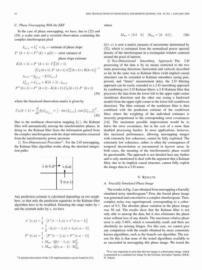
Due to the nonlinear observation mapping h(·), the Kalmanfilter will automatically unwrap the interferometric phases. Indoing so, the Kalman filter fuses the information gained fromthe complex interferogram with the slope information extractedfrom the interferometric power spectrum.1) Two-Dimensional Procedure5: For the 2-D unwrapping,

the Kalman filter algorithm works along the sketched integra-tion paths:

Any prediction estimate is calculated depending on two neigh-bors, so that only the prediction equations in the Kalman filteralgorithm have to be modified. Denoting the range index by rand the azimuth index by a, we have

x−(r, a) =12·[x+(r − 1, a) + x+(r, a− 1)

]+

12· [ur(r − 1, a) + ua(r, a− 1)]

P−(r, a) =14·[P+(r − 1, a) + P+(r, a− 1)

]+ Mwr ·Q(r − 1, a) ·MT

wr

+ Mwa ·Q(r, a− 1) ·MTwa

5A detailed derivation of the 2-D implementation can be found in [11].

where

Mwr = [ 0.5 0 ] Mwa = [ 0 0.5 ] . (36)

Q(r, a) is now a matrix measure of uncertainty determined by(32), which is estimated from the normalized power spectraldensity of the interferogram in a rectangular window centeredaround the pixel of interest.2) Two-Dimensional Smoothing Approach: The 2-D

processing of the data is by no means restricted to the twomain processing directions (horizontal and vertical) describedso far. In the same way as Kalman filters (with implicit causalstructure) can be extended to Kalman smoothers (using past,present, and “future” measurement data), the 2-D filteringapproach can be easily extended to a 2-D smoothing approachby combining two 2-D Kalman filters: a 2-D Kalman filter thatprocesses the data from the lower left to the upper right corner(north/east direction) and the other one (using a backwardmodel) from the upper right corner to the lower left (south/westdirection). The filter estimate of the north/east filter is thencombined with the prediction estimate of the south/westfilter, where the weighting of the individual estimates isinversely proportional to the corresponding error covariances[14]. The maximum possible improvement would be tohalve the error covariance, but at the cost of a more thandoubled processing burden. In most applications, however,this increased performance, allowing unwrapping imageswith extremely low coherence, cannot be fully exploited. Theextremely low coherence, rather, is often the consequence oftemporal decorrelation or encountered in layover areas. Inboth cases, the meaning of the interferometric phase wouldbe questionable. The approach is not detailed here any furtherand is only mentioned to deal with the argument that a Kalmanfilter, due to its implicit causal structure, cannot fully exploitthe image data in a 2-D sense.

V. RESULTS

A. Fractally Simulated Phase Image

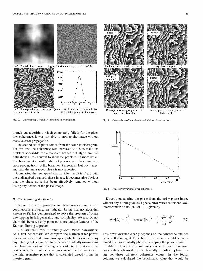
The results in Fig. 2 are obtained from unwrapping a fractallysimulated noisy interferogram.6 First, the fractal phase imagewas generated and converted to a complex interferogram. Then,complex noise was superimposed, corresponding to a coher-ence of 0.3. The absolute phase variation in the phase imagewas 50 rad. The results show that the Kalman filter is notonly able to unwrap the data, but it also eliminates the phasenoise without loss of any details. The maximum relative phaseerror is only 5.46%, which is remarkably small, and there areabsolutely no missing fringes. For this case, we cannot giveany comparison with the results obtained by more commonlyknown algorithms, such as the branch–cut algorithm. The rea-son for this is that none of the tested algorithms available tous succeeded in unwrapping this phase image. We tested the

6It is very important to note that this test image is a third-party image, whichis generated as a standard test image by the German Aerospace Agency (DLR;N. Adam).


Fig. 2. Unwrapping a fractally simulated interferogram.

branch–cut algorithm, which completely failed: for the givenlow coherence, it was not able to unwrap the image withoutmassive error propagation.

The second set of plots comes from the same interferogram.For this test, the coherence was increased to 0.8 to make theproblem accessible for a standard branch–cut algorithm. Weonly show a small cutout to show the problems in more detail.The branch–cut algorithm did not produce any phase jumps orerror propagation, yet the branch–cut algorithm lost one fringe,and still, the unwrapped phase is much noisier.

Comparing the rewrapped Kalman filter result in Fig. 3 withthe undisturbed wrapped phase image, it becomes also obviousthat the phase noise has been effectively removed withoutlosing any details of the phase image.

B. Benchmarking the Results

The number of approaches to phase unwrapping is stillcontinuously growing, an indicator being that no algorithmknown so far has demonstrated to solve the problem of phaseunwrapping in full generality and complexity. We also do notclaim this here; we only point out some unique features of theKalman filtering approach.1) Comparison With a Virtually Ideal Phase Unwrapper:

As a first benchmark, we compare the Kalman filter perfor-mance with a virtual phase unwrapper, which does not employany filtering but is assumed to be capable of ideally unwrappingthe phase without introducing any artifacts. In that case, thebest achievable phase error variance would be the variance ofthe interferometric phase that is calculated directly from theinterferogram.

Fig. 3. Comparison of branch–cut and Kalman filter results.

Fig. 4. Phase error variance over coherence.

Directly calculating the phase from the noisy phase imagewithout any filtering yields a phase error variance for one-lookinterferometric data (cf. [2]–[4]), given by

var{∆} =π2

12+ arccos

(|γ|)2 − 1

2·∞∑

p=1

|γ|2p

p2. (37)

This error variance clearly depends on the coherence and hasbeen plotted in Fig. 4. This phase error variance would be main-tained after successfully phase unwrapping the phase image.

Table I shows the phase error variances and maximumerror values obtained for the fractally simulated phase im-age for three different coherence values. In the fourthcolumn, we calculated the benchmark value that would be


TABLE IPHASE ERROR MEASURES OBTAINED BY KALMAN FILTER AND

BENCHMARK VALUE OF VIRTUAL PHASE UNWRAPPER

achieved by a nonfiltering phase unwrapper without anyprefiltering. The shading in rows 2 and 3 indicates thatthe branch–cut algorithm failed and produced phase jumpswith error propagation (and, hence, did not even reach thebenchmark).

The improvement factor in using the Kalman filter is at leastten if the coherence is 0.7 and below. This clearly demonstratesthe potential of the approach.

A further point needs to be stressed. The phase error varianceis only meaningful if and only if the phase error is, in fact,zero mean, which implies that the phase unwrapping must bephase slope preserving. This is not the case for a lot of standardalgorithms, such as the branch–cut algorithm or the classicallinear least squares algorithm (cf. Sections II and III).2) Comparison With Prefiltering Unwrapping Approaches:

One might argue then that the phase noise might be removedor reduced by preprocessing the complex data or by post-processing the phase values. This is a conventional technique,sacrificing spatial resolution for noise reduction. The strongerthe blurring effects, the larger the phase slopes, and the largerthe multilook averaging window.

One might further argue that spatially averaging the com-plex interferogram data is an ML approach and, hence,cannot be outperformed. This is only half the truth: anyMLE can be beaten by a Bayesian estimator, which em-ploys the correct model, and the Kalman filter is a Bayesianestimator.

Recent publications [17], [18], [21] point out that the optimalcombination of the ML multilooking technique and dynamicmodel is a phase-slope-adaptive directional weighted averager,dynamically extending its window in the direction of thesmallest phase slope. The Kalman filter approach exactly re-alizes this in an implicit way: by incorporating the phaseslope estimates into the prediction estimates [first equationin (34)], the filter “recenters” the value before combiningwith the new observation. The weighting between new ob-servation and “recentered” a priori value is determined bythe ratio of the observation error covariance and phase slopeestimation error covariance, thus realizing a tradeoff be-tween the individual accuracies. If the coherence is high, themeasurement noise covariance R will be small, giving highweight to the in-phase and quadrature observations of thephase, the exact value depending on the driving noise co-variance q. If, furthermore, the error covariance of the phaseslope estimate is high, this driving noise covariance q will behigh, and as a result, the phase slope will be almost com-pletely ignored. If the phase slope error covariance is small,

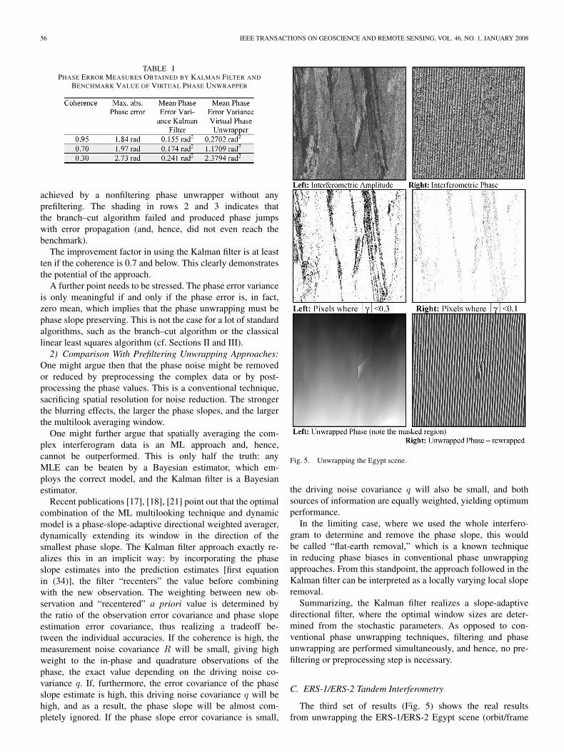
Fig. 5. Unwrapping the Egypt scene.

the driving noise covariance q will also be small, and bothsources of information are equally weighted, yielding optimumperformance.

In the limiting case, where we used the whole interfero-gram to determine and remove the phase slope, this wouldbe called “flat-earth removal,” which is a known techniquein reducing phase biases in conventional phase unwrappingapproaches. From this standpoint, the approach followed in theKalman filter can be interpreted as a locally varying local sloperemoval.

Summarizing, the Kalman filter realizes a slope-adaptivedirectional filter, where the optimal window sizes are deter-mined from the stochastic parameters. As opposed to con-ventional phase unwrapping techniques, filtering and phaseunwrapping are performed simultaneously, and hence, no pre-filtering or preprocessing step is necessary.

C. ERS-1/ERS-2 Tandem Interferometry

The third set of results (Fig. 5) shows the real resultsfrom unwrapping the ERS-1/ERS-2 Egypt scene (orbit/frame


no. 11374/3015A, 18.09.93). The mean coherence was 0.59,which is not bad for a two-pass interferogram, on the one hand;on the other hand, this coherence is already too low to unwrapthe scene with a classical branch–cut algorithm without anymultilook prefiltering. Furthermore, a small region, where thecoherence was below 0.1, had to be masked out. The plots inthe middle row of Fig. 5 show those image pixels where thecoherence was below 0.3 and 0.1, respectively. We see thatthese regions are quite large, and inspecting Fig. 5 (upper rightimage), it is clear that the phase in these regions is almostpure noise. Again, the classical approach would be to takethe average in these regions; again, this implies a significantloss of details, which can be avoided by the Kalman filtertechnique.

Inspecting the unwrapping results in the lower row of Fig. 5,it becomes obvious that, again, the phase noise has beenalmost completely removed, and there are again no missingfringes, no error propagation, and no other artifacts (and theflat-earth phase does not have to be removed). Introducinga further global flat-earth phase removal step before phaseunwrapping did not give significantly different results in theexperiments.

VI. CONCLUSION AND OUTLOOK

It has been shown that Kalman filtering concepts can be ad-vantageously applied to phase unwrapping problems, achievinggood phase noise cancellation and phase unwrapping in oneprocessing step. The Kalman filter directly incorporates com-plex interferogram values rather than phases and additionallyuses phase slope (directional) information that is obtained fromthe power spectral density.

As a result, the proposed approach implicitly realizes direc-tional phase filtering ideas, phase flattening concepts, as well asphase information weighting that achieves a tradeoff betweensteepness of phase slope and “noisiness” of the phase informa-tion itself. This noisiness, however, is not determined from theinterferometric phase data, but rather from the complex inter-ferogram itself, using the coherence map of the interferogram.As opposed to the empirically found solutions, the Kalmanfilter approach maintains physical modeling insights into theproblem and combines them with a clear stochastic framework[9], [10], [15]. It does not remove, however, the geometri-cally induced residues in undersampled sloped regions. Theconsistency of sampled and continuous phase image, however,is a basic assumption (cf. Section II) in the derivation ofnearly all phase unwrapping algorithms. In [22], a second-orderregularization scheme based on residue analysis is described,which seems to be able to deal with aliased interferograms.It will be investigated in a future work how the approachcited in [22] or the minimum cost flow approaches can beapplied to the phase slope estimates that are derived from theinterferogram’s power spectral density and to what extent thiswill enable the approach to also deal with undersampled slopedregions.

The technique will be used in a Principal Investigatorproject to unwrap repeat-pass TerraSAR-X interfereometricdata, where, based on the availability of the algorithms, exten-

sive comparisons with the cited phase unwrapping procedureswill be performed.

ACKNOWLEDGMENT

The authors would like to thank the anonymous reviewers fortheir constructive criticism and helpful comments.

REFERENCES

[1] H. A. Zebker and J. Villasenor, “Decorrelation in interferometric radarechoes,” IEEE Trans. Geosci. Remote Sens., vol. 30, no. 5, pp. 950–959,Sep. 1992.

[2] D. Just and R. Bamler, “Phase statistics and decorrelation inSAR interferograms,” in Proc. IGARSS, Tokyo, Japan, 1993, pp. 980–984.

[3] J. W. Goodman, “Statistical properties of laser speckle patterns,” inLaser Speckle and Related Phenomena, J. C. Dainty, Ed. New York:Springer-Verlag, 1975.

[4] D. B. Middleton, Introduction to Statistical Communication Theory.New York: McGraw-Hill, 1960.

[5] R. M. Goldstein, H. A. Zebker, and C. L. Werner, “Satellite radar interfer-ometry: Two-dimensional phase unwrapping,” Radio Sci., vol. 23, no. 4,pp. 713–720, Aug. 1988.

[6] O. Loffeld, “Demodulation of noisy phase or frequency modulated sig-nals with Kalman filters,” in Proc. ICASSP, Adelaide, Australia, 1994,pp. IV/177–IV/180.

[7] O. Loffeld, Estimationstheorie I, Grundlagen und stochastische Konzepte.München, Germany: Oldenburg, 1990.

[8] O. Loffeld, Estimationstheorie II, Anwendungen—Kalman Filter.München, Germany: Oldenburg, 1990.

[9] P. S. Maybeck, Stochastic Models, Estimation and Control, vol. 1. NewYork: Academic, 1980.

[10] P. S. Maybeck, Stochastic Models, Estimation and Control, vol. 2. NewYork: Academic, 1980.

[11] R. Krämer, “Auf Kalman-Filtern basierende Phasen- und Parame-terestimation zur Lösung der Phasenvieldeutigkeitsproblematik beider Höhenmodellerstellung aus SAR-Interferogrammen,” DissertationFB 12, Universität-GH Siegen, Siegen, Germany, 1989.

[12] O. Loffeld and C. Arndt, “Estimating the derivative of modulo mappedphases,” in Proc. IEEE Int. Conf. Acoust., Speech, Signal Process.,Munich, Germany, 1997, vol. IV, pp. 2841–2844.

[13] C. Arndt, Informationsgewinnung und -verarbeitung in nichtlinearen dy-namischen Systemen. Aachen, Germany: Shaker-Verlag, 1997. ZESS-Forschungsbericht No.2.

[14] D. C. Fraser and J. E. Potter, “The optimum linear smoother as a combina-tion of two linear filters,” IEEE Trans. Autom. Control, vol. AC-14, no. 4,pp. 387–390, Aug. 1969.

[15] R. E. Kalman, “A new approach to linear filtering and prediction prob-lems,” Trans. ASME Series D, J. Basics Eng., vol. 82, no. 1, pp. 35–45,Mar. 1960.

[16] S. N. Madsen, “Estimating the Doppler centroid of SAR data,” IEEETrans. Aerosp. Electron. Syst., vol. AES-25, no. 2, pp. 134–140,Mar. 1989.

[17] J.-S. Lee, K. P. Papathanassiou, T. L. Ainsworth, M. R. Grunes, andA. Reigber, “A new technique for noise filtering of SAR interferomet-ric phase images,” IEEE Trans. Geosci. Remote Sens., vol. 36, no. 5,pp. 1456–1465, Sep. 1998.

[18] D. Meng, V. Sethu, E. Ambikairajah, and L. Ge, “A novel techniquefor noise reduction in InSAR images,” IEEE Geosci. Remote Sens. Lett.,vol. 4, no. 2, pp. 226–230, Apr. 2007.

[19] N. Wu, D.-Z. Feng, and J. Li, “A locally adaptive filter of interferometricphase images,” IEEE Geosci. Remote Sens. Lett., vol. 3, no. 1, pp. 73–77,Jan. 2006.

[20] A. B. Suksmono and A. Hirose, “Adaptive noise reduction of InSARimages based on a complex-valued MRF model and its application tophase unwrapping problem,” IEEE Trans. Geosci. Remote Sens., vol. 40,no. 3, pp. 699–709, Mar. 2002.

[21] Q. Yu, X. Yang, S. Fu, X. Liu, and X. Sun, “An adaptive contouredwindow filter for interferometric synthetic aperture radar,” IEEE Geosci.Remote Sens. Lett., vol. 4, no. 1, pp. 23–26, Jan. 2007.

[22] G. Nico, G. Palubinskas, and M. Datcu, “Bayesian approaches to phaseunwrapping: Theoretical study,” IEEE Trans. Signal Process., vol. 48,no. 9, pp. 2545–2552, Sep. 2000.

[23] M. Costantini, A. Farina, and F. Zirilli, “A fast phase unwrapping al-gorithm for SAR interferometry,” IEEE Trans. Geosci. Remote Sens.,vol. 37, no. 1, pp. 452–460, Jan. 1999.


Otmar Loffeld (M’05–SM’06) received theDiploma degree in electrical engineering from theTechnical University of Aachen, Aachen, Germany,in 1982 and the Dr.Eng. degree and the Habilitationdegree in the field of digital signal processing andestimation theory from the University of Siegen,Siegen, Germany, in 1986 and 1989, respectively.

He then joined the University of Siegen, wherehe worked on various problems of optimal filtering,estimation, and control for linear and nonlinear prob-lems. In 1991, he was appointed as a Professor for

digital signal processing and estimation theory with the same university. In1995, he became a member of the Center for Sensorsystems (ZESS), which is acentral scientific research establishment at the University of Siegen. Since 2000,he has been a Vice Chairman of ZESS. Since 2002, he has been the Speaker ofthe International Postgraduate Programme Multisensorics, ZESS, University ofSiegen. He is the author of two textbooks on estimation theory. His currentresearch interests include multisensor data fusion, Kalman filtering techniquesfor data fusion, optimal filtering and process identification, SAR processing andsimulation, SAR interferometry, phase unwrapping, and baseline estimation.His recent field of interest is bistatic SAR processing.

Prof. Loffeld is a member of the German InformationstechnischeGesellschaft (ITG/VDE) and a Senior Member of the IEEE Geoscience and Re-mote Sensing Society. He was the recipient of the scientific award of Nordrhein-Westfalen (Bennigsen-Foerder Preis) in 1990 for his work on applying Kalmanfilters to phase estimation problems, such as Doppler centroid estimation inSAR and phase and frequency demodulation.

Holger Nies received the Diploma degree in elec-trical engineering from the University of Siegen,Siegen, Germany, in 1999.

Since 1999, he has been a member of the Centerfor Sensorsystems (ZESS), University of Siegen, anda Lecturer with the Department of Signal Processingand Communication Theory. His current researchinterests are in the areas of SAR processing, phaseunwrapping, and orbit modeling.

Stefan Knedlik (M’04) received the Diploma degreein electrical engineering and the Dr.Eng. degree fromthe University of Siegen, Siegen, Germany, in 1998and 2003, respectively.

Since 1998, he has been a member of the Centerfor Sensorsystems (ZESS), University of Siegen, anda Researcher and Lecturer with the Department ofSignal Processing and Communication Theory. Inseveral projects, e.g., in cooperation with the GermanAerospace Agency (DLR) and Dornier, he developedstate and parameter estimation strategies within SAR

interferometry. Together with Prof. Loffeld, he was a Principal Investigator forthe calibration of the interferometrical baseline for the SRTM/X-SAR system.Since 2002, he has also been the Executive Director of the International Post-graduate Programme Multisensorics, ZESS, University of Siegen. His currentresearch interests include signal processing and applied estimation theory, aswell as data fusion in SAR interferometry and navigation.

Wang Yu (M’07) received the Diploma degree inautocontrol from the University of Henan, Henan,China, in 2002 and the Dr.Eng. degree from theGraduate University of the Chinese Academy ofSciences, Beijing, China, in 2007.

Since March 2007, he has been a Guest Sci-entist with the Center for Sensorsystems (ZESS),University of Siegen, Siegen, Germany. His currentareas of interest include monostatic and bistatic SARsignal processing, signal processing for advancedSAR modes, airborne SAR motion compensation,and real-time SAR signal processing.

Phase Unwrapping for SAR Interferometry—A Data Fusion Approach by Kalman Filtering

Documents

Transcript of Phase Unwrapping for SAR Interferometry—A Data Fusion Approach by Kalman Filtering