Improving Adaptive KalmanEstimation in GPS/INS Integration

Weidong Ding, Jinling Wang and Chris Rizos

(The University of New South Wales)

(Email : weidong.ding@unsw.edu.au)

Doug Kinlyside

(Department of Lands, NSW )

The central task of GPS/INS integration is to effectively blend GPS and INS data togetherto generate an optimal solution. The present data fusion algorithms, which are mostly based

on Kalman filtering (KF), have several limitations. One of those limitations is the stringentrequirement on precise a priori knowledge of the system models and noise properties.Uncertainty in the covariance parameters of the process noise (Q) and the observation

errors (R) may significantly degrade the filtering performance. The conventional way ofdetermining Q and R relies on intensive analysis of empirical data. However, the noise levelsmay change in different applications. Over the past few decades adaptive KF algorithms

have been intensively investigated with a view to reducing the influence of the Q and Rdefinition errors. The covariance matching method has been shown to be one of the mostpromising techniques. This paper first investigates the utilization of an online stochasticmodelling algorithm with regards to its parameter estimation stability, convergence, optimal

window size, and the interaction between Q and R estimations. Then a new adaptive processnoise scaling algorithm is proposed. Without artificial or empirical parameters being used,the proposed adaptive mechanism has demonstrated the capability of autonomously tuning

the process noise covariance to the optimal magnitude, and hence improving the overallfiltering performance.

KEY WORDS

1. GPS. 2. INS. 3. Adaptive Kalman filter.

1. INTRODUCTION. Integrated positioning and navigation systems usingGlobal Positioning System (GPS) receivers and Inertial Navigation System (INS)sensors have demonstrated great utility for real-time navigation, mobile mapping,location based services, and many other applications. Besides providing a fullsolution for position and attitude, the other benefits of integrating GPS and INSinclude the long term stable positioning accuracy, the high data updating rate,the robustness to GPS signal jitter and interference, and the continuous calibrationof INS errors. Despite various integration architectures, the central challenge of

THE JOURNAL OF NAVIGATION (2007), 60, 517–529. f The Royal Institute of Navigationdoi:10.1017/S0373463307004316 Printed in the United Kingdom

implementing such integrated systems is how well the GPS and INS measurementdata can be fused together to generate the optimal solution.

The Kalman filter (KF) is the most common technique for carrying out thistask. The operation of the KF relies on the proper definition of the dynamic and thestochastic models (Brown and Hwang, 1997). The dynamic model describes thepropagation of system states over time. The stochastic model describes the stochasticproperties of the system process noise and observation errors.

The uncertainty in the covariance parameters of the process noise (Q) and theobservation errors (R) has a significant impact on Kalman filtering performance(Grewal and Andrews, 1993; Grewal and Weil, 2001; Salychev, 2004). Q and Rinfluence the weight that the filter applies between the existing process informationand the latest measurements. Errors in any of them may result in the filter beingsuboptimal or even cause it to diverge.

The conventional way of determining Q and R requires good a priori knowledgeof the process noise and measurement errors, which typically comes from intensiveempirical analysis. In practice, the values are generally fixed and applied duringthe whole application segment. The performance of the integrated systems suffers intwo respects due to this inflexibility. First, process noise and measurement errorsare dependent on the application environment and process dynamics. For genericapplications, the settings of the stochastic parameters have to be conservative inorder to stabilise the filter for the worst case scenario, which leads to performancedegradation. Second, the so-called KF ‘‘tuning’’ process is complicated, often left toa few ‘‘experts ’’, and thus hampers its successful application across a wider range offields.

Over the past few decades, adaptive KF algorithms have been intensivelyinvestigated to reduce the influence of the Q and R definition errors. Popularadaptive methods used in GPS/INS integration can be classified into severalgroups, such as covariance scaling, multi-model adaptive estimation, and adaptivestochastic modelling (Hide et al., 2004a). The covariance scaling method improvesthe filter stability and convergent performance by introducing a multiplicationfactor to the state covariance matrix. The calculation of the scaling factorcan either be fully empirical or based on certain criteria derived from filterinnovations (Hu et al., 2003; Yang, 2005; Yang and Gao, 2006; Yang and Xu,2003). The multi-model adaptive estimation method requires a bank of simul-taneously operating Kalman filters in which slightly different models and/or para-meters are employed. The output of multi-model adaptive estimation is theweighted sum of each individual filter’s output. The weighting factors can be cal-culated using the residual probability function (Brown and Hwang, 1997; Hideet al., 2004b). Adaptive stochastic modelling includes innovation-based adaptivemodelling (Mohamed and Schwarz, 1999) and residual-based adaptive modelling(Wang, 2000; Wang et al., 1999). By online monitoring of the innovation andresidual covariances, the adaptive stochastic modelling algorithm estimates directlythe covariance matrices of process noise and measurement errors, and ‘‘ tunes ’’them in real-time.

In this paper the online stochastic modelling method is investigated for GPS/INS integration. Besides its successful implementation, one observed limitation isthat the estimation algorithm is very sensitive to coloured noises and changes in theobserved satellites. Theoretically, this sensitivity is mainly due to two reasons. First,

518 WEIDONG DING AND OTHERS VOL. 60

the covariance estimation of the innovation and residual sequences is very noisydue to the short data sets, the coloured noises, and the non-stationary noise propertyduring a short time span. On the other hand, smoothing covariance estimation byincreasing the estimation window size would degrade the dynamic response of theadaptive mechanism, and may cause violation of the stationarity assumption.Second, with a limited number of ‘‘rough’’ covariance observations it is difficult toderive precise process noise and observation error estimates. Considering the largematrix dimension of process noise when the INS Psi model is used, a full estimationof the Q and R matrices is very challenging.

Hence, an adaptive algorithm with fewer estimable parameters is desirable. Itis well known that the innovation and residual sequences of the KF are a reliableindicator of KF filtering performance. For an optimal filter, the innovation andresidual sequences should be white Gaussian noise sequences with zero mean (Brownand Hwang, 1997; Mehra, 1970). By comparing the covariance estimates ofinnovation and residual series with their theoretical values computed by the filter,the status of the filter operation can be monitored. In this paper a new covariancematching based process noise scaling algorithm is proposed. Without using artificialor empirical parameters, the proposed adaptive mechanism has the capability ofautonomously tuning the Q matrix to the optimal magnitude. This proposed algor-ithm has been analysed using road test data. Significant improvements on the filteringperformance have been achieved.

In Section 2, the Kalman filter and the online stochastic modelling algorithm areintroduced. Then a new covariance based process noise scaling method is derived.The test results and analyses are presented in Section 3.

2. ADAPTIVE KALMAN FILTERING.2.1. Conventional Kalman filter. Considering a multivariable linear discrete

system for the integrated GPS/INS system:

xk=Wkx1xkx1+wkx1 (1)

zk=Hkxk+vk (2)

where xk is (nr1) state vector,Wk is (nrn) transition matrix, zk is (rr1) observationvector, Hk is (rrn) observation matrix. Variable wk and vk are uncorrelated whiteGaussian noise sequences with means and covariances :

E wkf g=E vkð Þ=0

E wkvTi

� �=0

E wkwTi

� �=

Qk

0

(i=k

ilk

E wkvTi

� �=

Rk

0

(i=k

ilk

(3)

NO. 3 IMPROVING ADAPTIVE KALMAN ESTIMATION 519

where E{.} denotes the expectation function. The Qk and Rk are the covariancematrix of process noise and observation errors, respectively. The KF state predictionand state covariance prediction are:

x̂xxk =Wkx1x̂xkx1

P̂Pxk =Wkx1P̂Pkx1W

Tkx1+Qkx1

(4)

where x̂k denotes the KF estimated state vector ; x̂k the predicted state vector for thenext epoch; P̂k the estimated state covariance matrix; and P̂k

x the predicted statecovariance matrix. The Kalman measurement update algorithms are:

Kk=P̂Pxk HT

k HkP̂Pxk HT

k+Rk

� �x1

x̂xk=x̂xxk +Kk zkxHkx̂x

xk

� �P̂Pk= IxKkHkð ÞP̂P

xk

(5)

where Kk is the Kalman gain, which defines the updating weight between newmeasurements and predictions from the system dynamic model.

The innovation sequence is defined as:

dk=zkxHkx̂xxk (6)

and the residual sequence as:

ek=zkxHkx̂xk (7)

2.2. Online stochastic modelling. The adaptive stochastic modelling algorithmcan be derived with the covariance matching principles. Substituting the measure-ment model (2) into (6) gives :

dk= Hkxk+vkð ÞxHkx̂xxk

=Hk xkxx̂xxk

� �+vk

(8)

As pointed out earlier, the innovation sequences dk are white Gaussian noisesequences with zero mean when the filter is in optimal mode. Taking variances (sameas autocorrelation here) on both sides of (8), and considering (3) and the orthogon-ality between observation error and state estimation error:

E dkdTk

� �=HkP̂P

xk HT

k+E vkvTk

� �=HkP̂P

xk HT

k+Rk

(9)

When the innovation covariance E{dkdkT} is available, the covariance of the obser-

vation error Rk can be estimated directly from equation (9). Calculation of theinnovation covariance E{dkdk

T} is normally carried out using a limited number ofinnovation samples:

E dkdTk

� �=

1

m

Xmx1

i=0

dkxidTkxi (10)

520 WEIDONG DING AND OTHERS VOL. 60

wherem is the ‘estimation window size’. For (10) to be valid, the innovation sequencehas to be ergodic and stationary over the m steps.

Details of the derivation of Q can be found in Mohamed and Schwarz (1999) ;Wang et al. (1999). Adaptive estimation of R is linked with the Q due to the factthat the derivation is based on the Kalman filtering process. This can be seen from (9),that in order to estimate R, the calculation of the predicted state covariance P̂k

x

has used the Q. The normal practice is to fix one, say Q as defined by the INS errorcharacteristics given by the manufacturers, and estimate the other one.

2.3. Scaling of process noise. To improve the robustness of the adaptive filteringalgorithm, a new process noise scaling method is proposed here.

For an optimal filter, the predicted innovation covariance should be equal to theone directly calculated from the innovation sequence, as illustrated by (10). Anydeviation between them can be ascribed to the wrong definition of P̂k

x and/or Rk in(9). Considering that the Kalman gain Kk is dependent on the relative magnitudes ofP̂kx and Rk, and Rk has several other ways to be assessed for GPS/INS integration

performance, Rk is assumed to be perfectly known for adaptation purposes. So,

1

m

Xm=1

i=0

dkxidTkxi=Hk

~PPxk HT

k+Rk (11)

where P̃kx denotes the estimation of the process noise prediction. Since attempting

to directly resolve the P̃kx from (11) is not practical (although a partial adaptation

might be possible), to simplify, a scaling factor is defined as:

a=trace Hk

~PPxk HT

k

� �trace HkP̂P

xk HT

k

n o=trace 1

m

Pmx1

i=0dkxid

TkxixRk

� �

trace HkP̂Pxk HT

k

n o (12)

where the scaling factor a implies a rough ratio between the calculated innovationcovariance and the predicted one, since

P̂Pxk =Wkx1P̂Pkx1W

Tkx1+Qkx1 (13)

By substituting (13) into (12), a can be expressed as:

a=trace Hk Wkx1P̂Pkx1W

Tkx1+ ~QQkx1

� �HT

k

n otrace Hk Wkx1P̂Pkx1W

Tkx1+Qkx1

� �HT

k

n o (14)

From (12) and (14), an intuitive adaptation rule is defined as:

Q̂Qk=Qkx1

ffiffiffia

p(15)

The square root in equation (15) is used to contribute a smoothing effect, which is notessential. Directly tuning P̂k

x based on equation (12) is not considered viable due tothe concerns of filtering smoothness and parameter consistency.

Compared with the existing covariance scaling methods, the distinct features ofthis proposed algorithm are:

’ the adaptive algorithm is not applied to tuning the state covariancematrix P̂k

x ;

NO. 3 IMPROVING ADAPTIVE KALMAN ESTIMATION 521

’ the factor a can be a scaling factor either larger than one or smaller than one,which provides a full range of options to tune Q̂k. Only when the predictedinnovation covariance and the calculated innovation covariance are consistentlyequal, a is then stabilised at the value of one.

The innovation covariance still needs to be estimated using equation (10). Whencompared with the adaptive stochastic modelling method, the process noise scalingmethod is more robust to covariance estimation bias due to fewer parameters beinginvolved in the tuning, and the tuning process is a smooth feedback. However, sinceonly the overall magnitude of Q̂k is tuned rather than individual elements, optimalallocation of noise to each individual source cannot be achieved. This is one funda-mental difference between the adaptive stochastic modelling methods and thecovariance scaling methods.

3. TESTING.3.1. Test Configuration. The tests employed two sets of Leica System 530 GPS

receivers and one BEI C-MIGITS II (DQI-NP) INS unit. One of the GPS receiverswas set up as static reference, and the other one placed on top of the test vehicletogether with the INS unit. The data were recorded for post processing. The BEI’sC-MIGITS II has its own GPS receiver (the MicroTracker) to synchronize the INSdata to GPS time. Table 1 shows the DQI-NP’s technical data for reference. Thespecified parameters were used in setting up the Q estimation in the standard Kalmanfiltering process. Figure 1 shows the ground track of the test vehicle.

Table 1. DQI-NP’s technical specifications.

Gyro Accelerometer

Bias 5 deg/hr 500 mg

Scale factor 500 ppm 800 ppm

Random walk/ white noise 0.035 deg/sqrt(hr) 180 mg/sqrt(hr)

151.2308 151.231 151.2312151.2314

-33.9198

-33.9196

-33.9194

-33.9192

Longitude

Lat

itud

e

Figure 1. Ground track of the test vehicle.

522 WEIDONG DING AND OTHERS VOL. 60

3.2. Evaluation of adaptive stochastic modelling algorithm. The covariance ofobservation error R is estimated using different window sizes, as illustrated inFigure 2. All estimates converged to a value of about 0.05 m. The estimation oscil-lation becomes obvious when shorter window sizes are used, such as 128. This

0 200 400 600 800 10000

0.05

0.1

0.15

0.2

0.25

0.3

0.35

epoch

=128=256=384=512=640

met

res

Figure 2. Influence of different window sizes on R estimation.

0 200 400 600 800 10000

0.05

0.1

0.15

0.2

0.25

0.3

epoch

=0.01=0.03=0.1

0 200 400 600 800 10000

0.05

0.1

0.15

0.2

0.25

0.3

epoch

=0.01=0.03=0.1

0 200 400 600 800 10000

0.05

0.1

0.15

0.2

0.25

0.3

epoch

=0.01=0.03=0.1

met

res

met

res

met

res

Figure 3. Influence of biased initial values on R estimation (Top left) SQRT of R(1,1) (Top right)

SQRT of R(2,2) (Bottom) SQRT of R(3,3).

NO. 3 IMPROVING ADAPTIVE KALMAN ESTIMATION 523

confirms the earlier analysis that a short window size may lead to unstable estimation.The step jumps of the estimation are due to the switch over from the initial settingsto the online estimation.

Assuming precise a priori knowledge is not available, the initial values of R canbe defined approximately. Figure 3 shows that different initial values of Q and R haveonly impacts on the transition period of the estimations. The initial deviationsare damped out quickly and the estimation converges with time. The stringent re-quirements on precise a priori knowledge of the stochastic model have thus beenalleviated.

Since the errors are estimated by the Kalman filter in a GPS/INS integrated system,if the whole system was perfectly modelled and the estimation was optimal andstable, the series of state estimations should be zero-mean white noise series with theminimum covariance. The state estimation STDs have been plotted in Figure 4against the window sizes used for estimation. Window size zero indicates the con-ventional KF solution. The STDs are generally smaller when the adaptive estimationmethod has been used.

128 256 384 512 6400.01

0.015

0.02

0.025

0.03

0.035

0.04

0.045

0.05

STD

Window size for R estimation

NorthEastDown

128 256 384 512 6400

1

2

3

4

5

6

7

8x 10-3

STD

Window size for R estimation

NorthEastDown

128 256 384 512 6402

4

6

8

10

12

14x 10-5

STD

Window size for R estimation

NorthEastDown

Figure 4. Comparison of filtering performance with different window sizes (Top left) position

(Top right) velocity (Bottom) attitude.

524 WEIDONG DING AND OTHERS VOL. 60

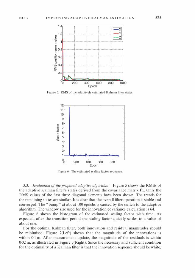
3.3. Evaluation of the proposed adaptive algorithm. Figure 5 shows the RMSs ofthe adaptive Kalman filter’s states derived from the covariance matrix P̂k. Only theRMS values of the first three diagonal elements have been shown. The trends forthe remaining states are similar. It is clear that the overall filter operation is stable andconverged. The ‘‘bump’’ at about 100 epochs is caused by the switch to the adaptivealgorithm. The window size used for the innovation covariance calculation is 64.

Figure 6 shows the histogram of the estimated scaling factor with time. Asexpected, after the transition period the scaling factor quickly settles to a value ofabout one.

For the optimal Kalman filter, both innovation and residual magnitudes shouldbe minimised. Figure 7(Left) shows that the magnitude of the innovations iswithin 0.1 m. After measurement update, the magnitude of the residuals is within0.02 m, as illustrated in Figure 7(Right). Since the necessary and sufficient conditionfor the optimality of a Kalman filter is that the innovation sequence should be white,

RM

S p

osi

tion

erro

r m

etre

s

Epoch0 200 400 600 800 1000

0

0.2

0.4

0.6

0.8

1

1.2

1.4XYZ

Figure 5. RMS of the adaptively estimated Kalman filter states.

Epoch

Sca

le f

act

or

0 200 400 600 8000

123456

789

101112

Figure 6. The estimated scaling factor sequence.

NO. 3 IMPROVING ADAPTIVE KALMAN ESTIMATION 525

the autocorrelation of the innovation sequence is plotted in Figure 8, which clearlyshows white noise features. A further check of the whiteness can be carried out usingthe method introduced by Mehra (1970).

Figures 9 and 10 show two groups of accelerometer bias and gyro bias estimatesfor comparison purposes. The process noise parameters used by the conventionalextended Kalman filter are calculated according to the manufacturer’s technicalspecification. It can be seen that all three configurations have generated similar esti-mates. The conventional extended Kalman filter provides the smoothest estimation.The estimates using the process scaling method are much noisier, which may be dueto its quick response to signal changes. The estimates on the Z axis have the worstconsistency. This may be due to its weak observability, since during the groundvehicle tests the Z axis has the least dynamics. Another reason could be that gravity

0 200 400 600 800 1000-0.5

-0.4

-0.3

-0.2

-0.1

0

0.1

0.2

0.3

Epoch

XYZ

0 200 400 600 800 1000-0.2

-0.15

-0.1

-0.05

0

0.05

0.1

0.15

Epoch

XYZ

KF

Inno

vatio

ns in

m

KF

Res

idua

ls m

etre

s

Figure 7. (Left) Innovation sequence (Right) Residual sequence.

Lags

Au

toco

rrel

atio

n fu

nctio

n

-1000 -500 0 500 1000-1

-0.5

0

0.5

1

1.5

2

2.5

3x 10-3

Figure 8. Autocorrelation of innovation sequence (unbiased).

526 WEIDONG DING AND OTHERS VOL. 60

uncertainties were not properly scaled. They may behave differently from the INSnoises.

4. CONCLUSION. Over the past few decades adaptive KF algorithms havebeen intensively investigated with a view to reducing the influence of the uncer-tainty of the covariance matrices of the process noise (Q) and the observation errors(R). The covariance matching method is one of the most promising techniques.

The online adaptive stochastic modelling method provides estimates of individualQ and R elements. However, practical implementation of an online stochastic mod-elling algorithm faces many challenges. One critical factor influencing the stochasticmodelling accuracy is ensuring precise and smooth estimation of the innovation andresidual covariances from data sets with limited length. Furthermore, the stochasticparameters are closely correlated with each other when using current estimation

0 200 400 600 800 1000-0.1

-0.05

0

0.05

0.1

0.15

Epoch

XYZ

0 200 400 600 800 1000-0.1

-0.05

0

0.05

0.1

Epoch

XYZ

0 200 400 600 800 1000-0.05

0

0.05

0.1

0.15

Epoch

XYZ

Acc

el b

ias

m/s

Acc

el b

ias

m/s

Acc

el b

ias

m/s

Figure 9. Estimates of accelerometer bias using different methods: (Top left) Standard Extended

KF (Top right) Extended KF with online stochastic modelling (bottom) Extended KF with the

proposed process scaling algorithm.

NO. 3 IMPROVING ADAPTIVE KALMAN ESTIMATION 527

algorithms, which make correct estimation more difficult. The online adaptivestochastic modelling method is not scalable for the estimation of a large number ofparameters.

In this paper, a new covariance-based adaptive process noise scaling method hasbeen proposed and tested. This method is reliable, robust, and suitable for practicalimplementations. Initial tests have demonstrated significant improvements of thefiltering performance. However, the optimal allocation of noise to each individualsource is not possible using scaling factor methods. This is a topic for furtherinvestigation.

ACKNOWLEDGEMENT

This research is supported by the Australian Cooperative Research Centre for SpatialInformation (CRC-SI) under project 1.3 ‘Integrated positioning and geo-referencing plat-

form’.

0 200 400 600 800 1000-0.02

-0.015

-0.01

-0.005

0

0.005

0.01

0.015

Epoch

XYZ

0 200 400 600 800 1000-0.03

-0.02

-0.01

0

0.01

0.02

0.03

Epoch

XYZ

0 200 400 600 800 1000-0.04

-0.03

-0.02

-0.01

0

0.01

0.02

Epoch

XYZ

Gyr

o bi

as °/

s

Gyr

o bi

as °/

s

Gyr

o bi

as °/

s

Figure 10. Estimates of gyro bias using different methods: (Top left) Standard Extended KF

(Top right) Extended KF with online stochastic modelling (Bottom) Extended KF with the pro-

posed process scaling algorithm.

528 WEIDONG DING AND OTHERS VOL. 60

REFERENCES

Brown, R. G. and Hwang, P. Y. C. (1997). Introduction to Random Signals and Applied Kalman Filtering.

John Willey & Sons, New York.

Grewal, M. S. and Andrews, A. P. (1993). Kalman Filtering Theory and Practice. Prentice Hall, USA.

Grewal, M. S. andWeil, L. R. (2001).Global Positioning Systems, Inertial Navigation, and Integration. John

Wiley & Sons, USA.

Hide, C., Michaud, F. and Smith, M. (2004a). Adaptive Kalman filtering algorithms for integrating GPS

and low cost INS, IEEE Position Location and Navigation Symposium, Monterey California, 227–233.

Hide, C., Moore, T. and Smith, M. (2004b). Multiple model Kalman filtering for GPS and low-cost INS

integration, ION GNSS 17th international technical meeting of the satellite division, Long Beach

California, 1096–1103.

Hu, C., Chen, W., Chen, Y. and Liu, D. (2003). Adaptive Kalman filtering for vehicle navigation, Journal

of Global Positioning Systems, 2(1), 42–47.

Mehra, R. K. (1970). On the identification of variances and adaptive Kalman filtering. IEEE Transactions

on automatic control, AC-15(2): 175–184.

Mohamed, A. H. and Schwarz, K. P. (1999). Adaptive Kalman filtering for INS/GPS, Journal of Geodesy,

73, 193–203.

Salychev, O. S. (2004). Applied Inertial Navigation Problems and Solutions. BMSTU press, Moscow.

Wang, J. (2000). Stochastic modelling for RTK GPS/GLONASS positioning and navigation, Journal of

the US Institute of Navigation, 46(4), 297–305.

Wang, J., Stewart, M. and Tsakiri, M. (1999). Online stochastic modelling for INS/GPS integration,

ION GPS-99 proceedings, Nashville, Tennessee, 1887–1895.

Yang, Y. (2005). Comparison of adaptive factors in Kalman filters on navigation results. The Journal of

Navigation, 58, 471–478.

Yang, Y. and Gao, W. (2006). An optimal adaptive Kalman filter. Journal of Geodesy, 80(4), 177–183.

Yang, Y. and Xu, T. (2003). An adaptive Kalman filter based on sage windowing weights and variance

components. The Journal of Navigation, 56, 231–240.

NO. 3 IMPROVING ADAPTIVE KALMAN ESTIMATION 529