GPS/INS system Integraion Based on Neuro-Wavelet Techniques

The 2006 International Arab Conference on Information Technology (ACIT'2006)

1

GPS/INS SYSTEM INTEGRATION BASED ON NEURO-WAVELET TECHNIQUES

* Salam Ismaeel **Ahmed Hassan and

*Informatics Institute for Postgraduate Studies, Iraqi Commission for Computers and Informatics, [email protected]

**Control and System Eng. Dept., University of Technology, [email protected] ABSTRACT

Global Positioning System (GPS) and Strapdown Inertial Navigation System (SDINS) can be integrated together to provide a reliable navigation system. This paper offers a new method for error estimation in a GPS/INS augmented system based on Artificial Neural Network (ANN) and Wavelet Transform (WT).

An ANN was adopted in this paper to model the GPS/INS position and velocity errors in real time to predict the error in the integrated system and provide accurate navigation information for a moving vehicle.

It was found that the proposed technique reduces the standard deviation error in the position by about 91% for X, Y, and Z axes, while in velocity it was reduced by about 94% for North, East, and Down directions. KKEEYYWWOORRDD:: vehicular navigation, inertial navigation, GPS, wavelet multi-resolution analysis, neural networks. 1. INTRODUCTION

Since the 1940s, navigation systems, in particular inertial navigation systems (INSs), have become important components in military and scientific applications. In fact, INSs are now standard equipment on most planes, ships, and submarines [1].

SDINS technologies are based on the principle of integrating specific forces and rates measured by accelerometers and rate gyros of an Inertial Measurement Unit (IMU) fixed on the moving body [4].

On the other hand, the GPS relies on the technique of comparing signals from orbiting satellites to calculate position (and possibly attitude) at regular time intervals. But being dependent on the satellites signals makes GPS less reliable than self contained INS due to the possibility of drop-outs or jamming [2, and 3].

The combination of GPS and INS has become increasingly common in the past few years, because the characteristics of GPS and INS are complementary. This paper looks at ways in high quality integration where low cost inertial sensors are used to obtain improved performance.

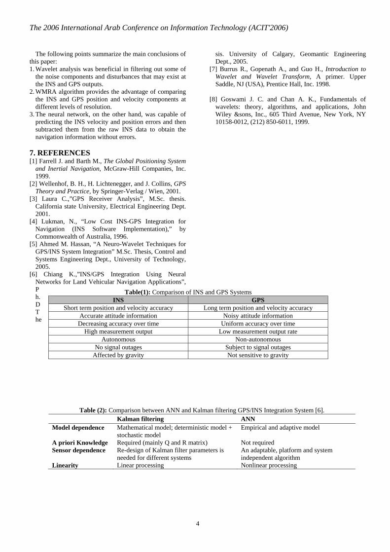
GPS and INS both can be used for wide range of navigation functions. Each has its strengths and weaknesses as illustrated in table (1).

2. PROBLEM STATEMENT

Many researches investigated and developed the INS/GPS integration systems using different approaches such as Kalman filtering, accelerometer and gyro calibration and compensation, also other methods which are described in [5]. While this paper is different in handling the deficiency in navigation systems utilizing the wavelet and neural techniques.

In general, GPS/INS integration employing ANN provides several advantages if compared to Kalman

filtering. A comparison between both techniques is given in table (2).

A new method will introduce in this paper based on ANN to fuse the outputs of INS and GPS and provide accurate positioning information and velocity for the vehicle. In addition, this paper suggests a wavelet multiresolution analysis (WMRA) algorithm to analyze and compare the INS and GPS outputs at different resolution levels before processing them by the ANN module during either the training or testing stages.

3. DISCRETE WAVELET TRANSFORM (DWT)

Since dealing with discrete-time inertial sensor signals, the (DWT) is implemented instead of the Continuous Wavelet Transform (CWT). The DWT of a discrete time sequence x(n) is given as[7]:

∑ −Φ=Φ=n

sks,

s/2ks,ks, knnxnnxC )2()(2)(),( )( … (1)

∑ −Ψ=Ψ=n

sks,

s/2ks,ks, knnxnnxd )2()(2)(),( )( … (2)

Where Φs,k is the scale function and ψs,k is the wavelet function and )2(2 )( kns

ks,s,2 −Φ , )2(2 )( kns

ks,s,2 −Ψ are the

scaled and shifted versions of Φs,k and ψs,k, respectively, based on the values of s (scaling coefficient) and k (shifting coefficient). The s and k coefficients take integer values for different scaling and shifted versions ofΦs,k (n),ψs,k (n) and Cs,k, ds,k, respectively.

The original signal x(n) can be generated from the corresponding wavelet function using the following equation:

∑ ∑∑ Ψ+Φ=k s k

ks,ks,ks,ks, ndnCnx )()()( … (3)


2

The wavelet function )(nks,Ψ is not limited to exponential functions as in the case of Fourier Transform (FT) or short-time Fourier transform (STFT). The only restriction on )(nks,Ψ is that it must be short and oscillatory (it must have zero average and decay quickly at both ends). This restriction ensures that the summation in the DWT transform equation is finite.

4. MULTI-RESOLUTION ANALYSIS ALGORITHM

In order to determine the INS/GPS error that can be used to model the INS position and velocity error a wavelet multi-level decomposition must be performed for each component of the INS and GPS output signals. The following steps describe the mathematical wavelet decomposition procedure: Step1: For each one of INS and GPS outputs signals, calculate the approximation coefficient at sth resolution level using [7]: ∑ −Φ=

n

ss/2ks, knnxC )2()(2 )( … (4)

Step2: Obtain the approximation from the approximation coefficient obtained from step1 above using [7]:

∑∞

−∞=

Φ=k

ks,ks,s nCnx )()( … (5)

Step3: Calculate the details coefficient at sth resolution level using: ∑ Ψ=

nksks nnxd )()( ,, … (6)

Step4: Obtain the detail from the details coefficient obtained from step3 above using:

∑∞

−∞=

Ψ=k

kskss ndng )()( ,, … (7)

Step5: Return to step one and continue the wavelet decomposition process until appropriate level of decomposition (LOD) is reached. Step6: Denoising the details of the INS and GPS signals by applying the thresholding technique. Step7: Compare the INS and GPS position and velocity components at several resolution levels (by subtracting the wavelet coefficients of each of the GPS outputs from the corresponding wavelet coefficients of each of the INS outputs). Step8: Reconstruct the INS/GPS error signal from the wavelet coefficients differences obtained in step7. 5. GPS/INS SYSTEM INTEGRATION USING NEURO-WAVELET TECHNIQUES

It seems that ANN is a promising candidate to handle the problem of error correction of the INS data for various trajectories and to predict the error for different types of IMU's used for any trajectory. It is well known that ANN's are a powerful for handling fast data processing, but their implementations suffers from lack of efficient constructive methods, such as determining the parameters of neurons, determining the network structure and falling into local

minimum. Inspired by both Feed Forward ANN's and wavelet decomposition, wavelet neural networks have been established as general and powerful techniques for GPS/INS system integration. 5.1 Artificial Neural Network

The history of Artificial Neural Networks (ANN) comes from attempts of modeling a system by simulating the most basic functions of human brains. In fact, the motivation of studies in ANNs comes from the flexibility and power of information processing that conventional computing machines do not have. The successes of ANNs in many application areas due to some features, such as the ability to learn, understand and adapt. The ANN system can “learn by examples and experience” and perform a variety of nonlinear functions that are difficult to describe mathematically [5].

The proposed neuro-wavelet techniques to be applied here consists of three stages:

5.2 Construct INS/GPS Error Signal Stage

In this stage, an INS/GPS error signal is constructed and the following three topics are very important in constructing the INS/GPS error signal using the WMRA algorithm described previously.

Selection of the Appropriate Wavelet Level of Decomposition (LOD):

In theory, the decomposition process can be continued indefinitely, but in reality it can be performed only until the individual details consist of a single sample. Practically, an appropriate LOD is chosen based on the nature of the signal or on a specific criterion [8].

In case of SDINS sensor data and GPS data, there are two modes of operation: static and kinematics. For both operation modes, the selection of an appropriate LOD is based on removing the high-frequency noise but keeping all the useful information contained in the signal [6].

For static inertial data, the sensors outputs contain the following signals: the Earth gravity components, the Earth rotation rate components, and the sensors long-term errors (such as biases). These signals have very low frequency, and hence, they can be separated easily from the high frequency noise components by the wavelet multi-resolution analysis.

To select an appropriate LOD in this case, several decomposition levels are applied and the Standard Deviation (STD) is computed for each approximation difference components (INS/GPS error) compared with the real INS error. The proper LOD will be the one with the difference between these two errors is a minimum.

After applying many levels of decomposition it was found that the appropriate LOD varies for each component of position and velocity. This depends on the INS/GPS error, which is nearly equal to the real INS-error, as shown in figures (1, and 2) with and without thresholding, respectively for worst INS and GPS data. Table (3) shows also, two cases of INS data (best and worst case) selected at the end of the vehicle's journey.


3

Also, it is unnecessary to increase the order of LOD because the features of the INS/GPS-error will disappear. In other words, it can't be used to model the INS error because the resulting error (INS/GPS error) will not equal the desired INS-error. On the other hand it must be mentioned that the main GPS errors can be denoised by wavelet denoising unlike the INS error where some of the error can be eliminated by wavelet denoising (optimal low pass filtering). Such error is called short-term error and the other part of the INS error is called long-term error. The latter is reduced by GPS/INS integration, which is accomplished by the multi-resolution algorithm described previously. The output of the multi-resolution for the GPS and INS is subtracted to obtain the INS/GPS error that can not be eliminated by the wavelet denoising technique. This INS/GPS error can be used for ANN modeling in order to cancel its effect as will be described latter.

Selection of the Appropriate Filter

The wavelet transform has a flexible feature of using a variety of filters that differ by their coefficients. The corresponding type of filter to the lowest standard deviation of INS/GPS error value is the perfect filter to be used. It should be mentioned that all calculations to chose the best filter to be used for each component of position and velocity is performed for first LOD.

Table (4) shows the best filters to the position and velocity components after use all types of wavelet filters for best and worst INS data.

Thresholding Algorithm in Wavelet Coefficients

Thresholding is a nonlinear operation that is performed on all wavelet coefficients, to avoid the shortcomings of the linear filtering. Often a nonlinear procedure is used to suppress the noise in the empirical wavelet coefficients. There are several research reports on finding thresholds; however, the main ideas of thresholding here are based on the fundamental properties of the wavelet transform [8]. Therefore, one can estimate the empirical wavelet coefficients independently, by comparing the absolute value of the empirical wavelet coefficient with a value called Threshold Value. The thresholding procedure allows for cuting off some of the noise in the error signal and improving its signal-to-noise ratio so that it can be efficiently modelled using ANN. In this paper, soft thresholding is applied only to the details coefficients. The thresholding technique is standard and can be reviewed in [7, and 8]. 5.3 Neural Network Training Stage

The proposed neural network is a feed forward back propagation neural network. The number of layers in the network was determined after applying many learning algorithms to reduce the computational complexity and avoid local minima. Each algorithm has its strength and weakness. Amongst these algorithms is the Levenberg-Marqudrt (L.M) learning algorithm which was chosen because it can converge faster than other learning algorithms. The L.M algorithm is that it suffers from a lack

of memory, since it stores all the intermediate results in the memory and this problem is not a critical one since most modern computer systems have large memory.

The next step was the determination of the number of neurons in hidden layer since the input and output layers are fixed to two input neurons (one for INS velocity or position components and the second for the instantaneous time) and one neuron in the output layer (INS-error). After several attempts, it was found that 10 neurons were adequate for this work. During the training procedure of the network (which is done while satellite signal is available), the INS data is fed to the network and the output is provided based on the INS velocity or position and the present time instant (the time is counted once the system is turned on), as shown in figure (3). The network output is compared to the INS/GPS error signal computed using WMRA algorithm. The error is fed to the ANN, which adjust the network parameters in a way to minimize the mean square value of the error.

A hyperbolic tangent function (tansigmoid) is employed inside the hidden neurons to model the non-linearity in the input/output relationship. A linear activation function is considered at the neuron of the output layer to perform as a linear superposition of the outputs of the hidden neurons. The output is obtained and compared to the target (desired performance) to determine the estimation error. This error is propagated through the network in the backward direction starting from the output layer and is utilized to update the computation of the network parameters.

The resulting neural network has the structure depicted in figure (4) it must be mentioned that each component of velocity and position has its own network, so, six networks have been adopted in this work.

5.4 Testing Stage

As demonstrate in previous sections, ANN used to model the INS/GPS error and provide a prediction for this error in real time. After the training is completed, the network is ready to work in the testing mode. However, the parameters of the networks are modified during the availability of the satellite signal (i.e. the training procedure continues) and the network is considered working in the update mode. In the case of satellite signal blocked, the network will use the latest estimated parameters saved in the reference set to perform the prediction mode.

Figure (5) shows the operation of the ANN in the testing mode during satellite blockage signal. It provides a prediction of the INS error based on the INS data and the particular time instant provided at the input. The predicted INS error is removed from the corresponding INS data to give precise and reliable velocity and position of the moving vehicle. This training procedure is usually known as online training. Table (5) shows the performance of the training and testing the ANN to predict INS error. Figure (6) shows the error in the position and velocity along all components after using the neuro-wavelet techniques. 6. CONCLUSION


4

The following points summarize the main conclusions of this paper: 1. Wavelet analysis was beneficial in filtering out some of

the noise components and disturbances that may exist at the INS and GPS outputs.

2. WMRA algorithm provides the advantage of comparing the INS and GPS position and velocity components at different levels of resolution.

3. The neural network, on the other hand, was capable of predicting the INS velocity and position errors and then subtracted them from the raw INS data to obtain the navigation information without errors.

7. REFERENCES [1] Farrell J. and Barth M., The Global Positioning System

and Inertial Navigation, McGraw-Hill Companies, Inc. 1999.

[2] Wellenhof, B. H., H. Lichtenegger, and J. Collins, GPS Theory and Practice, by Springer-Verlag / Wien, 2001.

[3] Laura C.,”GPS Receiver Analysis”, M.Sc. thesis. California state University, Electrical Engineering Dept. 2001.

[4] Lukman, N., “Low Cost INS-GPS Integration for Navigation (INS Software Implementation),” by Commonwealth of Australia, 1996.

[5] Ahmed M. Hassan, “A Neuro-Wavelet Techniques for GPS/INS System Integration” M.Sc. Thesis, Control and Systems Engineering Dept., University of Technology, 2005.

[6] Chiang K.,”INS/GPS Integration Using Neural Networks for Land Vehicular Navigation Applications”, Ph.D The

sis. University of Calgary, Geomantic Engineering Dept., 2005.

[7] Burrus R., Gopenath A., and Guo H., Introduction to Wavelet and Wavelet Transform, A primer. Upper Saddle, NJ (USA), Prentice Hall, Inc. 1998.

[8] Goswami J. C. and Chan A. K., Fundamentals of

wavelets: theory, algorithms, and applications, John Wiley &sons, Inc., 605 Third Avenue, New York, NY 10158-0012, (212) 850-6011, 1999.

Table(1): Comparison of INS and GPS Systems INS GPS

Short term position and velocity accuracy Long term position and velocity accuracy Accurate attitude information Noisy attitude information

Decreasing accuracy over time Uniform accuracy over time High measurement output Low measurement output rate

Autonomous Non-autonomous No signal outages Subject to signal outages

Affected by gravity Not sensitive to gravity

Table (2): Comparison between ANN and Kalman filtering GPS/INS Integration System [6]. Kalman filtering ANN

Model dependence Mathematical model; deterministic model + stochastic model

Empirical and adaptive model

A priori Knowledge Required (mainly Q and R matrix) Not required Sensor dependence Re-design of Kalman filter parameters is

needed for different systems An adaptable, platform and system independent algorithm

Linearity Linear processing Nonlinear processing


5

0 100 200 300 400 500 600-100

-80

-60

-40

-20

0

20

40

Time (1/10 s)

Erro

r in

X-a

xis

(m)

INS ErrorINS/GPS Error

0 100 200 300 400 500 600-50

0

50

100

150

200

250

300

Time (1/10 s)

Erro

r in

Y-a

xis

(m)


(a) (b)

0 100 200 300 400 500 600-20

0

20

40

60

80

100

120

Time (1/10 s)

Erro

r in

Z-ax

is (m

)


(c)

Figure (1): Comparison between INS and INS/GPS Error position in (a) X-axis, (b) Y-axis, and (c) Z-axis (before using thresholding).

0 100 200 300 400 500 600-100

-80

-60

-40

-20

0

20

Time (1/10 s)

Erro

r in

X-a

xis

(m)


0 100 200 300 400 500 600-50

0

50

100

150

200

250

Time(1/10 s)

Erro

r in

Y-a

xis

(m)


(a) (b)

0 100 200 300 400 500 600-20

0

20

40

60

80

100

120

Time (1/10 s)

Erro

r in

Z-ax

is (m

)


(c)

Figure (2): Comparison between INS and INS/GPS Error position in (a) X-axis, (b) Y-axis, and (c) Z-axis (after using thresholding).


6

Table (3): Multi-resolution algorithm application to obtain INS/GPS standard deviation error.

Types of data Components Direction INS-Error

Estimated INS /GPS

error

Level of Decomposition

(LOD)

Bes

t IN

S da

ta

Position (m) X-axis 1.3394 1.3960 10 Y-axis 1.2884 1.3561 11 Z-axis 0.0418 0.0659 15

Velocity (m/s) North 0.0023 0.0032 19 East 0.0618 0.0863 17

Down 0.0016 0.0020 22

Wor

st IN

S da

ta Position (m)

X-axis 92.2495 91.5469 2 Y-axis 238.8248 229.4452 1 Z-axis 113.4915 115.2453 1

Velocity (m/s) North 2.8079 4.0708 10 East 7.8505 10.7992 11

Down 4.1089 5.8583 11

Table (4): Results of using different types of wavelet filters for best and worst INS data.

Filter Standard Deviation for 1st LOD of INS/GPS Error Position (m) Velocity (m/s)

X-axis Y-axis Z-axis North East Down Best Db4 Db9 Db6 Bior5.5 Bior2.2 Coif2

Worst Db10 Bior2.2 Db4 Bior5.5 Bior2.2 Coif2

INS GPS

WMRA

-

INS/GPS Error signal

GPS data

INS data

Adjust training

parameters

Output of ANN (error of INS)

Time

Real INS data (True)

Save training

parameterANN

-

+Difference between desired

and actual o/p Position or Velocity component

+


7

Figure (3): Block diagram of neuro-wavelet during training stage (INS with GPS signals).

Figure (4): The Architecture of An Artificial Neural Network for each component of position (X, Y, and Z)

and velocity (North, East, and Down).

Figure (5): Block diagram of neuro-wavelet during testing stage when No GPS signals (INS signals only).

Input Layer (2 node)

Hidden Layer (10 node)

Output Layer (1 node)

.

.

.

.

INS Velocity or Position component

Time

INS

ANN Time

Real INS data (True)

Output of ANN (error of INS) -

+

latest training

parameter

Position or Velocity component

INS data


8

Table (5): Performance of training and testing the neural network to predict the INS error.

0 100 200 300 400 500 600-10

0

10

Time (1/10 s)

Pos

ition

Erro

r (m

) X-Axis

0 100 200 300 400 500 600-10

0

10

Time (1/10 s)

Pos

ition

Erro

r (m

) Y-Axis

0 100 200 300 400 500 600-20

0

20

Time (1/10 s)

Pos

ition

Erro

r (m

) Z-Axis

Types of data Position Velocity X-axis (m) Y-axis (m) Z-axis (m) North (m/s) East (m/s) Down (m/s)

Bes

t IN

S da

ta MSE 9.7095e-7 9.6308e-7 9.8054e-10 9.91182e-13 9.9528e-11 2.8108e-14

No. of iteration 298 201 42 139 457 14

STD

Err

or of each

component 0.5088 0.6172 0.0153 2.4443e-4 0.0147 1.9421e-4

between desired and actual o/p 9.8300e-4 9.7204e-4 3.1330e-5 9.7095e-7 9.9848e-6 1.1876e-6

wor

st IN

S da

ta

MSE 9.8864e-6 0.0009974 9.90172e-9 2.3792e-7 8.7392e-7 9.9989e-6 No. of iteration 342 193 414 9 62 415

STD

Err

or of each

component 25.0270 76.6196 29.5849 0.3791 2.4819 0.7727

between desired and actual o/p 0.0031 0.0316 0.0052 3.8934e-4 9.2995e-4 0.0032


9

0 100 200 300 400 500 600-15

-10

-5

Time (1/10 s)

Vel

ocity

Erro

r (m

/s) North Direction

0 100 200 300 400 500 600-15

-10

-5

Time (1/10 s)

Vel

ocity

Erro

r (m

/s) East Direction

0 100 200 300 400 500 600-15

-10

-5

Time (1/10 s)

Vel

ocity

Erro

r (m

/s) Down Direction

Figure (6): Position and Velocity errors along all components.

http://www.world-academy-of-science.org/worldcomp06/ws/publications/icai06/index_html/contents

GPS/INS system Integraion Based on Neuro-Wavelet Techniques

Documents

Transcript of GPS/INS system Integraion Based on Neuro-Wavelet Techniques