Numerical simulation of shaking table tests on 3D reinforced concrete structures

Structural Engineering and Mechanics, Vol. 48, No. 2 (2013) 151-171

DOI: http://dx.doi.org/10.12989/sem.2013.48.2.151 151

Copyright © 2013 Techno-Press, Ltd.

http://www.techno-press.org/?journal=sem&subpage=8 ISSN: 1225-4568 (Print), 1598-6217 (Online)

Numerical simulation of shaking table tests on 3D reinforced concrete structures

Beyhan Bayhan

Department of Civil Engineering, Bursa Technical University, 16330, Bursa, Turkey

(Received March 8, 2013, Revised September 16, 2013, Accepted October 2, 2013)

Abstract. The current paper presents the numerical blind prediction of nonlinear seismic response of two full-scale, three dimensional, one-story reinforced concrete structures subjected to bidirectional earthquake simulations on shaking table. Simulations were carried out at the laboratories of LNEC (Laboratorio Nacional de Engenharia Civil) in Lisbon, Portugal. The study was motivated by participation in the blind prediction contest of shaking table tests, organized by the challenge committee of the 15th World Conference on Earthquake Engineering. The test specimens, geometrically identical, designed for low and high ductility levels, were subjected to subsequent earthquake motions of increasing intensity. Three dimensional nonlinear analytical models were implemented and subjected to the input base motions. Reasonably accurate reproduction of the measured displacement response was obtained through appropriate modeling. The goodness of fit between analytical and measured results depended on the details of the analytical models.

Keywords: reinforced concrete structures; shaking table test; blind prediction; nonlinear modeling;

numerical simulation; Opensees

1. Introduction

Empirical evidence provides a basis for judging the accuracy of modeling assumptions that are

used in simulation of the actual response of reinforced concrete (RC) structures. The most realistic

method for verifying these assumptions is the dynamic testing of full-scale structures. In this

context, shaking table is a good tool for experimental testing and understanding the seismic

behavior of RC structures. Several benchmark shaking table tests (e.g., Kabeyasawa et al. 2012,

Panagiotou et al. 2012, Bayhan et al. 2013, Peloso et al. 2012, Gallo et al. 2012) for seismic

assessment and rehabilitation of RC structures have been carried out in many facilities worldwide

(e.g., NIED E-Defense Laboratory in Miki City, Japan; LHPO Shake Table, UC San Diego in

USA; NCREE in Taiwan; EUCENTRE Trees Lab in Italy; Structural Laboratory of the University

of Canterbury in New Zealand). However, shaking table tests including bidirectional dynamic

loading of full-scale, three dimensional RC structures are scarce.

This study was motivated by participation in a blind prediction contest that was organized by

the challenge committee of the 15th World Conference on Earthquake Engineering (15WCEE).

Corresponding author, Associate Professor, E-mail: [email protected]

mailto:[email protected]

Beyhan Bayhan

(a) (b)

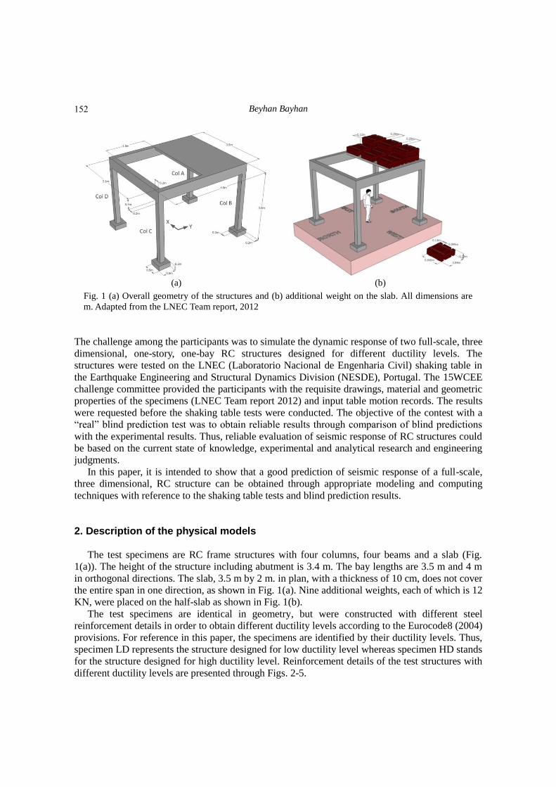
Fig. 1 (a) Overall geometry of the structures and (b) additional weight on the slab. All dimensions are

m. Adapted from the LNEC Team report, 2012

The challenge among the participants was to simulate the dynamic response of two full-scale, three

dimensional, one-story, one-bay RC structures designed for different ductility levels. The

structures were tested on the LNEC (Laboratorio Nacional de Engenharia Civil) shaking table in

the Earthquake Engineering and Structural Dynamics Division (NESDE), Portugal. The 15WCEE

challenge committee provided the participants with the requisite drawings, material and geometric

properties of the specimens (LNEC Team report 2012) and input table motion records. The results

were requested before the shaking table tests were conducted. The objective of the contest with a

“real” blind prediction test was to obtain reliable results through comparison of blind predictions

with the experimental results. Thus, reliable evaluation of seismic response of RC structures could

be based on the current state of knowledge, experimental and analytical research and engineering

judgments.

In this paper, it is intended to show that a good prediction of seismic response of a full-scale,

three dimensional, RC structure can be obtained through appropriate modeling and computing

techniques with reference to the shaking table tests and blind prediction results.

2. Description of the physical models

The test specimens are RC frame structures with four columns, four beams and a slab (Fig.

1(a)). The height of the structure including abutment is 3.4 m. The bay lengths are 3.5 m and 4 m

in orthogonal directions. The slab, 3.5 m by 2 m. in plan, with a thickness of 10 cm, does not cover

the entire span in one direction, as shown in Fig. 1(a). Nine additional weights, each of which is 12

KN, were placed on the half-slab as shown in Fig. 1(b).

The test specimens are identical in geometry, but were constructed with different steel

reinforcement details in order to obtain different ductility levels according to the Eurocode8 (2004)

provisions. For reference in this paper, the specimens are identified by their ductility levels. Thus,

specimen LD represents the structure designed for low ductility level whereas specimen HD stands

for the structure designed for high ductility level. Reinforcement details of the test structures with

different ductility levels are presented through Figs. 2-5.

152


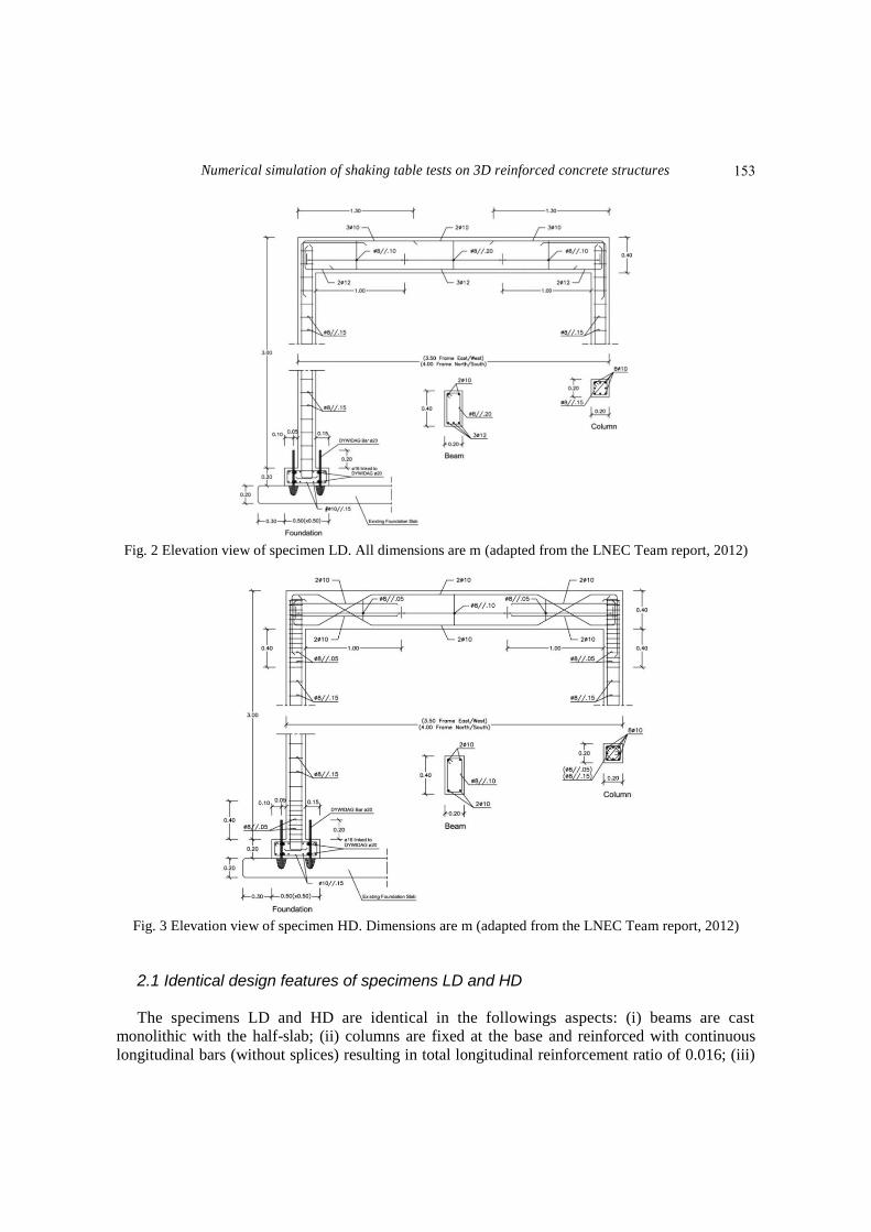
Fig. 2 Elevation view of specimen LD. All dimensions are m (adapted from the LNEC Team report, 2012)

Fig. 3 Elevation view of specimen HD. Dimensions are m (adapted from the LNEC Team report, 2012)

2.1 Identical design features of specimens LD and HD The specimens LD and HD are identical in the followings aspects: (i) beams are cast

monolithic with the half-slab; (ii) columns are fixed at the base and reinforced with continuous

longitudinal bars (without splices) resulting in total longitudinal reinforcement ratio of 0.016; (iii)

153

Beyhan Bayhan

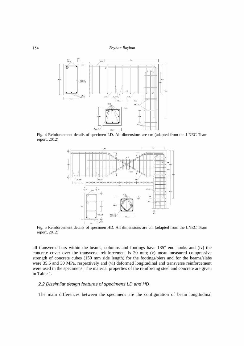
Fig. 4 Reinforcement details of specimen LD. All dimensions are cm (adapted from the LNEC Team

report, 2012)

Fig. 5 Reinforcement details of specimen HD. All dimensions are cm (adapted from the LNEC Team

report, 2012)

all transverse bars within the beams, columns and footings have 135° end hooks and (iv) the

concrete cover over the transverse reinforcement is 20 mm; (v) mean measured compressive

strength of concrete cubes (150 mm side length) for the footings/piers and for the beams/slabs

were 35.6 and 30 MPa, respectively and (vi) deformed longitudinal and transverse reinforcement

were used in the specimens. The material properties of the reinforcing steel and concrete are given

in Table 1.

2.2 Dissimilar design features of specimens LD and HD The main differences between the specimens are the configuration of beam longitudinal

154


Table 1 Mean measured compressive strength of concrete samples and reinforcing steel properties

Concrete

Mean compressive

strength of cubical

concrete samples, MPa

Equivalent

cylinder

strength, MPa Steel

Mean yield tensile

strength, MPa

Ultimate

strength, MPa

fcm

fcm fym fum

Footings

& Piers 35.6 1.4 29.7 1.1

8mm 561 4.0 654 1.2

10mm 559 3.6 632 2.1

Beams

& Slabs 30 0.1 25 0.0

12mm 566 5.3 630 3.1

*σ: Standard deviation (measured values were obtained from the LNEC Team report, 2012)

reinforcement, anchorage of beam bottom reinforcement in the beam-column joints and transverse

reinforcement ratios of the beams and columns. These dissimilarities are detailed in the following

sections.

2.2.1 Specimen LD Beam bottom reinforcement of specimen LD was anchored in the corner joints by hooks having

tails extending 27 cm up in the joint while top reinforcement was anchored in the joint extending

30 cm in the column (Fig. 4). The provided transverse reinforcement ratio, ρ”, for all beams was

0.0025 (ρ” = Ast/bs where Ast is the area of transverse reinforcement parallel to the plane of the

frame with spacing s, and b is the beam width) in the mid-span with a spacing of b and 0.0050 in

the confined regions with a spacing of 0.50b. The provided transverse reinforcement ratio for all

columns was 0.0033 in both mid-span and confined regions with a spacing of 0.75b, thus showing

that no confined regions at column ends were considered in the design of specimen LD.

2.2.2 Specimen HD Beam bottom reinforcement of specimen HD was anchored in the corner joints by hooks

having tails extending toward the joint mid-height while top reinforcement was anchored in the

joint extending 30 cm in the column (Fig. 5). Top and bottom reinforcements are inclined with 30

degrees starting 10 cm distance from the column surface. Four additional longitudinal

reinforcement bars extend from the joint to the beam along a distance of 100 cm. The provided

transverse reinforcement ratio for all beams was 0.005 in the mid-span with a spacing of 0.5b and

0.02 in the confined regions with a spacing of 0.25b. The transverse reinforcement ratio for all

columns was 0.0057 in the mid-span with a spacing of 0.75b and 0.0172 in the confined regions

with a spacing of 0.25b.

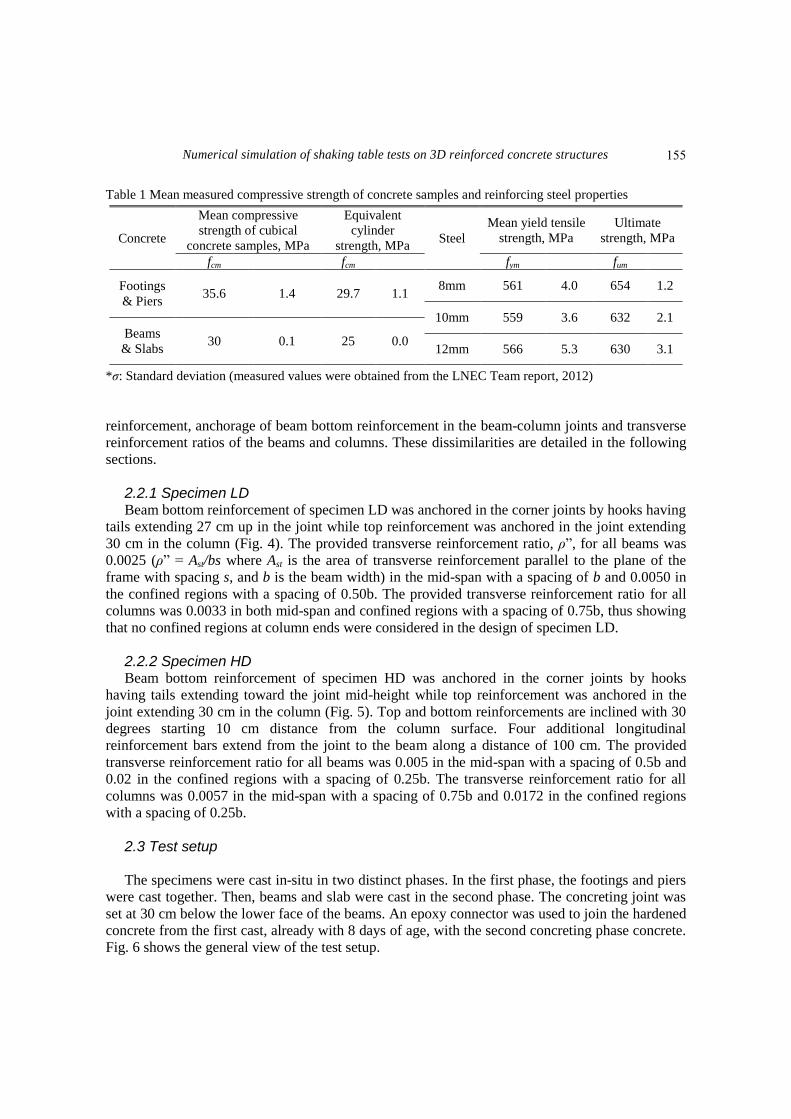
2.3 Test setup The specimens were cast in-situ in two distinct phases. In the first phase, the footings and piers

were cast together. Then, beams and slab were cast in the second phase. The concreting joint was

set at 30 cm below the lower face of the beams. An epoxy connector was used to join the hardened

concrete from the first cast, already with 8 days of age, with the second concreting phase concrete.

Fig. 6 shows the general view of the test setup.

155

Beyhan Bayhan

Fig. 6 General view of the test setup (adapted from the LNEC Team report, 2012)

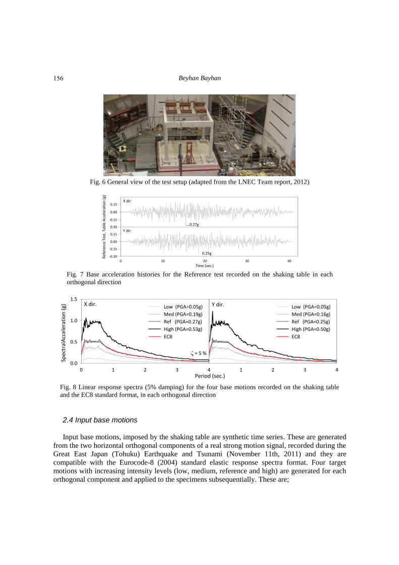
Fig. 7 Base acceleration histories for the Reference test recorded on the shaking table in each

orthogonal direction

Fig. 8 Linear response spectra (5% damping) for the four base motions recorded on the shaking table

and the EC8 standard format, in each orthogonal direction

2.4 Input base motions Input base motions, imposed by the shaking table are synthetic time series. These are generated

from the two horizontal orthogonal components of a real strong motion signal, recorded during the

Great East Japan (Tohuku) Earthquake and Tsunami (November 11th, 2011) and they are

compatible with the Eurocode-8 (2004) standard elastic response spectra format. Four target

motions with increasing intensity levels (low, medium, reference and high) are generated for each

orthogonal component and applied to the specimens subsequentially. These are;

-0.15

0.00

0.15

Ref

eren

ce T

est,

Tab

le A

ccel

erat

ion

(g)

X dir

Time (sec.)

X Data

0 10 20 30 40-0.30

-0.15

0.00

0.15

0.30Y dir.

0.27g

0.25g

Period (sec.)1 2 3 4

Spec

tral

Acc

eler

atio

n (

g) Low (PGA=0.05g)

Med (PGA=0.16g)

Ref (PGA=0.25g)

High (PGA=0.50g)

EC8

0 1 2 3 40.0

0.5

1.0

1.5

Low (PGA=0.05g)

Med (PGA=0.19g)

Ref (PGA=0.27g)

High (PGA=0.53g)

EC8

Y dir.X dir.

= 5 %

156


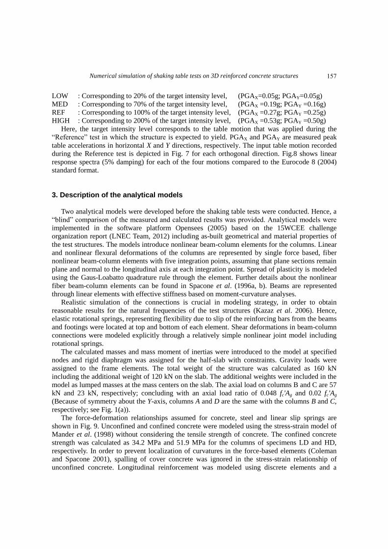
LOW : Corresponding to 20% of the target intensity level, (PGAX=0.05g; PGAY=0.05g)

MED : Corresponding to 70% of the target intensity level, (PGAX =0.19g; PGAY =0.16g)

REF : Corresponding to 100% of the target intensity level, (PGAX =0.27g; PGAY =0.25g)

HIGH : Corresponding to 200% of the target intensity level, (PGAX =0.53g; PGAY =0.50g)

Here, the target intensity level corresponds to the table motion that was applied during the

“Reference” test in which the structure is expected to yield. PGAX and PGAY are measured peak

table accelerations in horizontal X and Y directions, respectively. The input table motion recorded

during the Reference test is depicted in Fig. 7 for each orthogonal direction. Fig.8 shows linear

response spectra (5% damping) for each of the four motions compared to the Eurocode 8 (2004)

standard format.

3. Description of the analytical models

Two analytical models were developed before the shaking table tests were conducted. Hence, a

“blind” comparison of the measured and calculated results was provided. Analytical models were

implemented in the software platform Opensees (2005) based on the 15WCEE challenge

organization report (LNEC Team, 2012) including as-built geometrical and material properties of

the test structures. The models introduce nonlinear beam-column elements for the columns. Linear

and nonlinear flexural deformations of the columns are represented by single force based, fiber

nonlinear beam-column elements with five integration points, assuming that plane sections remain

plane and normal to the longitudinal axis at each integration point. Spread of plasticity is modeled

using the Gaus-Loabatto quadrature rule through the element. Further details about the nonlinear

fiber beam-column elements can be found in Spacone et al. (1996a, b). Beams are represented

through linear elements with effective stiffness based on moment-curvature analyses.

Realistic simulation of the connections is crucial in modeling strategy, in order to obtain

reasonable results for the natural frequencies of the test structures (Kazaz et al. 2006). Hence,

elastic rotational springs, representing flexibility due to slip of the reinforcing bars from the beams

and footings were located at top and bottom of each element. Shear deformations in beam-column

connections were modeled explicitly through a relatively simple nonlinear joint model including

rotational springs.

The calculated masses and mass moment of inertias were introduced to the model at specified

nodes and rigid diaphragm was assigned for the half-slab with constraints. Gravity loads were

assigned to the frame elements. The total weight of the structure was calculated as 160 kN

including the additional weight of 120 kN on the slab. The additional weights were included in the

model as lumped masses at the mass centers on the slab. The axial load on columns B and C are 57

kN and 23 kN, respectively; concluding with an axial load ratio of 0.048 fc'Ag and 0.02 fc'Ag

(Because of symmetry about the Y-axis, columns A and D are the same with the columns B and C,

respectively; see Fig. 1(a)).

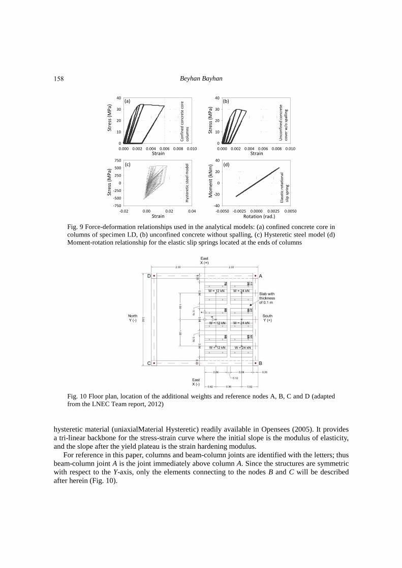
The force-deformation relationships assumed for concrete, steel and linear slip springs are

shown in Fig. 9. Unconfined and confined concrete were modeled using the stress-strain model of

Mander et al. (1998) without considering the tensile strength of concrete. The confined concrete

strength was calculated as 34.2 MPa and 51.9 MPa for the columns of specimens LD and HD,

respectively. In order to prevent localization of curvatures in the force-based elements (Coleman

and Spacone 2001), spalling of cover concrete was ignored in the stress-strain relationship of

unconfined concrete. Longitudinal reinforcement was modeled using discrete elements and a

157

Beyhan Bayhan

Fig. 9 Force-deformation relationships used in the analytical models: (a) confined concrete core in

columns of specimen LD, (b) unconfined concrete without spalling, (c) Hysteretic steel model (d)

Moment-rotation relationship for the elastic slip springs located at the ends of columns

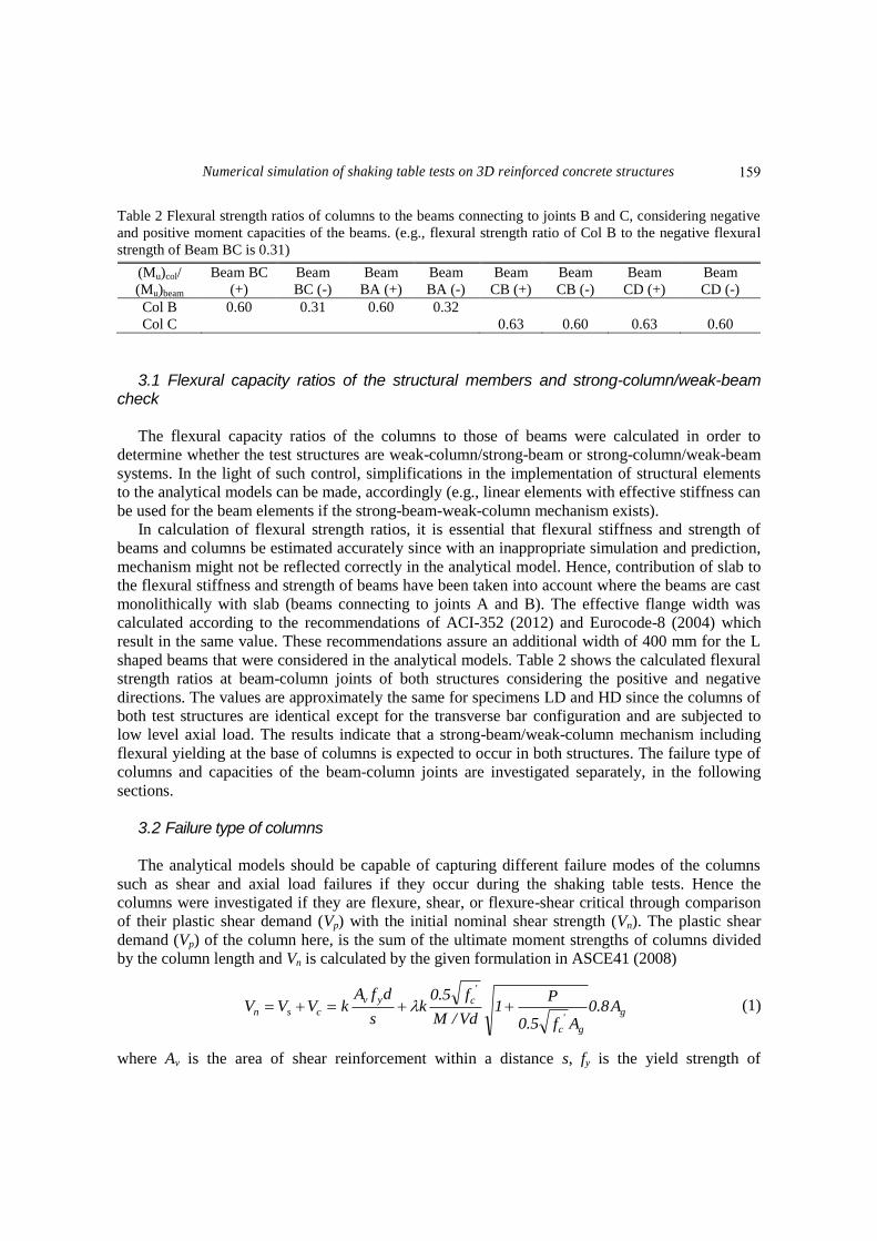
Fig. 10 Floor plan, location of the additional weights and reference nodes A, B, C and D (adapted

from the LNEC Team report, 2012)

hysteretic material (uniaxialMaterial Hysteretic) readily available in Opensees (2005). It provides

a tri-linear backbone for the stress-strain curve where the initial slope is the modulus of elasticity,

and the slope after the yield plateau is the strain hardening modulus.

For reference in this paper, columns and beam-column joints are identified with the letters; thus

beam-column joint A is the joint immediately above column A. Since the structures are symmetric

with respect to the Y-axis, only the elements connecting to the nodes B and C will be described

after herein (Fig. 10).

0.000 0.002 0.004 0.006 0.008 0.010

0

10

20

30

40

0.000 0.002 0.004 0.006 0.008 0.010

0

10

20

30

40

Stre

ss (

MP

a)

-0.02 0.00 0.02 0.04

-750

-500

-250

0

250

500

750

-0.0050 -0.0025 0.0000 0.0025 0.0050

-40

-20

0

20

40

StrainStrain

Stre

ss (

MP

a)

Stre

ss (

MP

a)

Strain Rotation (rad.)

Mo

men

t (k

Nm

)

Co

nfi

ned

co

ncr

ete

core

colu

mn

s

Un

con

fin

ed c

on

cret

e co

ver

w/o

sp

allin

g

Hys

tere

tic

stee

l mo

del

Elas

stic

ro

tati

on

al s

lip s

pri

ng

(a) (b)

(c) (d)

158


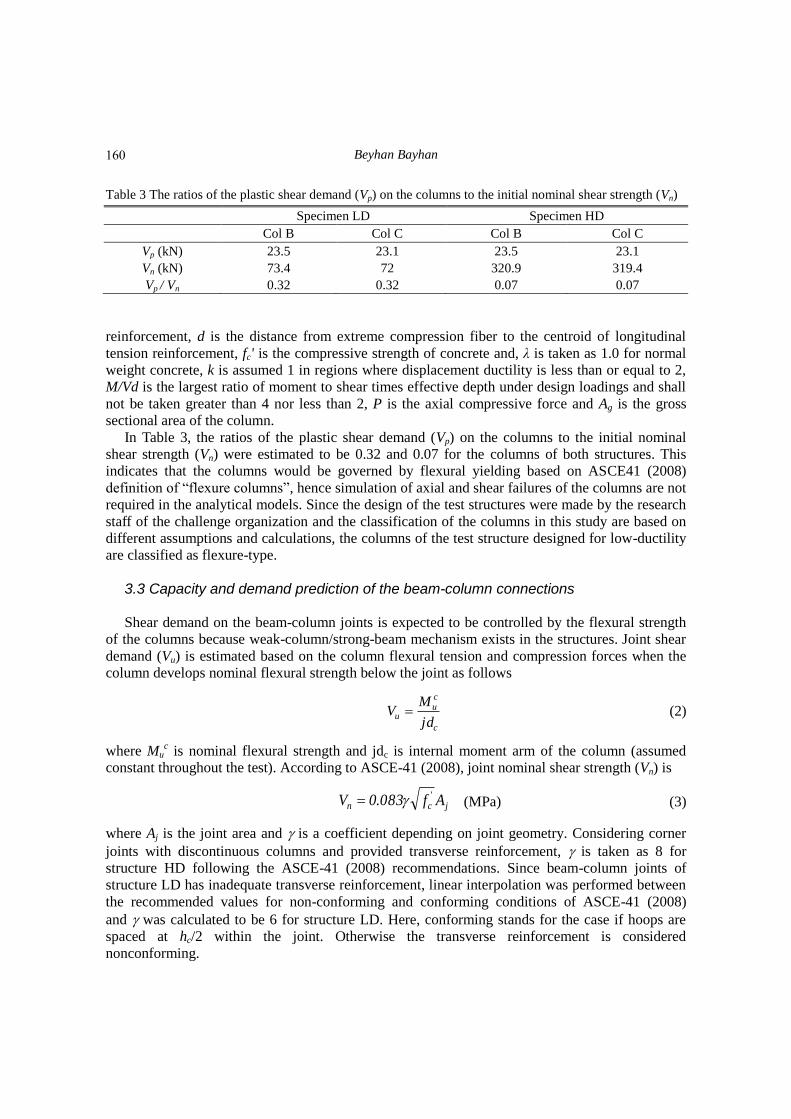
Table 2 Flexural strength ratios of columns to the beams connecting to joints B and C, considering negative

and positive moment capacities of the beams. (e.g., flexural strength ratio of Col B to the negative flexural

strength of Beam BC is 0.31)

(Mu)col/

(Mu)beam

Beam BC

(+)

Beam

BC (-)

Beam

BA (+)

Beam

BA (-)

Beam

CB (+)

Beam

CB (-)

Beam

CD (+)

Beam

CD (-)

Col B 0.60 0.31 0.60 0.32

Col C 0.63 0.60 0.63 0.60

3.1 Flexural capacity ratios of the structural members and strong-column/weak-beam

check The flexural capacity ratios of the columns to those of beams were calculated in order to

determine whether the test structures are weak-column/strong-beam or strong-column/weak-beam

systems. In the light of such control, simplifications in the implementation of structural elements

to the analytical models can be made, accordingly (e.g., linear elements with effective stiffness can

be used for the beam elements if the strong-beam-weak-column mechanism exists).

In calculation of flexural strength ratios, it is essential that flexural stiffness and strength of

beams and columns be estimated accurately since with an inappropriate simulation and prediction,

mechanism might not be reflected correctly in the analytical model. Hence, contribution of slab to

the flexural stiffness and strength of beams have been taken into account where the beams are cast

monolithically with slab (beams connecting to joints A and B). The effective flange width was

calculated according to the recommendations of ACI-352 (2012) and Eurocode-8 (2004) which

result in the same value. These recommendations assure an additional width of 400 mm for the L

shaped beams that were considered in the analytical models. Table 2 shows the calculated flexural

strength ratios at beam-column joints of both structures considering the positive and negative

directions. The values are approximately the same for specimens LD and HD since the columns of

both test structures are identical except for the transverse bar configuration and are subjected to

low level axial load. The results indicate that a strong-beam/weak-column mechanism including

flexural yielding at the base of columns is expected to occur in both structures. The failure type of

columns and capacities of the beam-column joints are investigated separately, in the following

sections.

3.2 Failure type of columns

The analytical models should be capable of capturing different failure modes of the columns

such as shear and axial load failures if they occur during the shaking table tests. Hence the

columns were investigated if they are flexure, shear, or flexure-shear critical through comparison

of their plastic shear demand (Vp) with the initial nominal shear strength (Vn). The plastic shear

demand (Vp) of the column here, is the sum of the ultimate moment strengths of columns divided

by the column length and Vn is calculated by the given formulation in ASCE41 (2008)

g

g

'

c

'

cyv

csn A8.0Af5.0

P1

Vd/M

f5.0k

s

dfAkVVV

(1)

where Av is the area of shear reinforcement within a distance s, fy is the yield strength of

159

Beyhan Bayhan

Table 3 The ratios of the plastic shear demand (Vp) on the columns to the initial nominal shear strength (Vn)

Specimen LD Specimen HD

Col B Col C Col B Col C

Vp (kN) 23.5 23.1 23.5 23.1

Vn (kN) 73.4 72 320.9 319.4

Vp / Vn 0.32 0.32 0.07 0.07

reinforcement, d is the distance from extreme compression fiber to the centroid of longitudinal

tension reinforcement, fc' is the compressive strength of concrete and, λ is taken as 1.0 for normal

weight concrete, k is assumed 1 in regions where displacement ductility is less than or equal to 2,

M/Vd is the largest ratio of moment to shear times effective depth under design loadings and shall

not be taken greater than 4 nor less than 2, P is the axial compressive force and Ag is the gross

sectional area of the column.

In Table 3, the ratios of the plastic shear demand (Vp) on the columns to the initial nominal

shear strength (Vn) were estimated to be 0.32 and 0.07 for the columns of both structures. This

indicates that the columns would be governed by flexural yielding based on ASCE41 (2008)

definition of “flexure columns”, hence simulation of axial and shear failures of the columns are not

required in the analytical models. Since the design of the test structures were made by the research

staff of the challenge organization and the classification of the columns in this study are based on

different assumptions and calculations, the columns of the test structure designed for low-ductility

are classified as flexure-type.

3.3 Capacity and demand prediction of the beam-column connections

Shear demand on the beam-column joints is expected to be controlled by the flexural strength

of the columns because weak-column/strong-beam mechanism exists in the structures. Joint shear

demand (Vu) is estimated based on the column flexural tension and compression forces when the

column develops nominal flexural strength below the joint as follows

c

cu

ujd

MV (2)

where Muc is nominal flexural strength and jdc is internal moment arm of the column (assumed

constant throughout the test). According to ASCE-41 (2008), joint nominal shear strength (Vn) is

j'cn Af083.0V (MPa) (3)

where Aj is the joint area and is a coefficient depending on joint geometry. Considering corner

joints with discontinuous columns and provided transverse reinforcement, is taken as 8 for

structure HD following the ASCE-41 (2008) recommendations. Since beam-column joints of

structure LD has inadequate transverse reinforcement, linear interpolation was performed between

the recommended values for non-conforming and conforming conditions of ASCE-41 (2008)

and was calculated to be 6 for structure LD. Here, conforming stands for the case if hoops are

spaced at hc/2 within the joint. Otherwise the transverse reinforcement is considered

nonconforming.

160


Table 4 Calculated joint shear strengths (Vn) and probable demand (Vu) values


Col B Col C Col B Col C

Vn (kN) 99.6 99.6 132.8 132.8

Vu (kN) 95.4 93.7 95.4 93.7

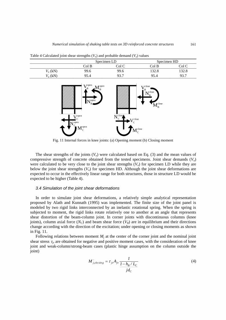
Fig. 11 Internal forces in knee joints: (a) Opening moment (b) Closing moment

The shear strengths of the joints (Vn) were calculated based on Eq. (3) and the mean values of

compressive strength of concrete obtained from the tested specimens. Joint shear demands (Vu)

were calculated to be very close to the joint shear strengths (Vn) for specimen LD while they are

below the joint shear strengths (Vn) for specimen HD. Although the joint shear deformations are

expected to occur in the effectively linear range for both structures, those in structure LD would be

expected to be higher (Table 4).

3.4 Simulation of the joint shear deformations In order to simulate joint shear deformations, a relatively simple analytical representation

proposed by Alath and Kunnath (1995) was implemented. The finite size of the joint panel is

modeled by two rigid links interconnected by an inelastic rotational spring. When the spring is

subjected to moment, the rigid links rotate relatively one to another at an angle that represents

shear distortion of the beam-column joint. In corner joints with discontinuous columns (knee

joints), column axial force (NC) and beam shear force (VB) are in equilibrium and their directions

change according with the direction of the excitation; under opening or closing moments as shown

in Fig. 11.

Following relations between moment Mj at the center of the corner joint and the nominal joint

shear stress jv are obtained for negative and positive moment cases, with the consideration of knee

joint and weak-column/strong-beam cases (plastic hinge assumption on the column outside the

joint)

C

CBjvjvgsinclo,j

jd

L/h1

1AM

(4)

open

BV open

BM

open

BN

open

CM

open

CN

open

CV

close

BV

close

CM

close

CN

close

CV

close

BM

close

BN

161

Beyhan Bayhan

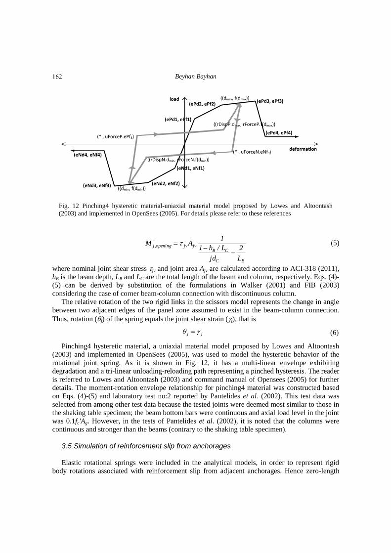
Fig. 12 Pinching4 hysteretic material-uniaxial material model proposed by Lowes and Altoontash

(2003) and implemented in OpenSees (2005). For details please refer to these references

BC

CBjvjvopening,j

L

2

jd

L/h1

1AM

(5)

where nominal joint shear stress jv and joint area Ajv are calculated according to ACI-318 (2011),

hB is the beam depth, LB and LC are the total length of the beam and column, respectively. Eqs. (4)-

(5) can be derived by substitution of the formulations in Walker (2001) and FIB (2003)

considering the case of corner beam-column connection with discontinuous column.

The relative rotation of the two rigid links in the scissors model represents the change in angle

between two adjacent edges of the panel zone assumed to exist in the beam-column connection.

Thus, rotation (j) of the spring equals the joint shear strain (j), that is

jj (6)

Pinching4 hysteretic material, a uniaxial material model proposed by Lowes and Altoontash

(2003) and implemented in OpenSees (2005), was used to model the hysteretic behavior of the

rotational joint spring. As it is shown in Fig. 12, it has a multi-linear envelope exhibiting

degradation and a tri-linear unloading-reloading path representing a pinched hysteresis. The reader

is referred to Lowes and Altoontash (2003) and command manual of Opensees (2005) for further

details. The moment-rotation envelope relationship for pinching4 material was constructed based

on Eqs. (4)-(5) and laboratory test no:2 reported by Pantelides et al. (2002). This test data was

selected from among other test data because the tested joints were deemed most similar to those in

the shaking table specimen; the beam bottom bars were continuous and axial load level in the joint

was 0.1fc'Ag. However, in the tests of Pantelides et al. (2002), it is noted that the columns were

continuous and stronger than the beams (contrary to the shaking table specimen).

3.5 Simulation of reinforcement slip from anchorages Elastic rotational springs were included in the analytical models, in order to represent rigid

body rotations associated with reinforcement slip from adjacent anchorages. Hence zero-length

load ((dmax, f(dmax)) (ePd3, ePf3) (ePd2, ePf2)

(ePd1, ePf1) ((rDispP.dmax, rForceP.f(dmax))

(ePd4, ePf4)

deformation (* , uForceN.eNf3)

((rDispN.dmin, rForceN.f(dmin))

(eNd1, eNf1)

(eNd2, eNf2) ((dmin, f(dmin))

(eNd3, eNf3)

(eNd4, eNf4)

(* , uForceP.ePf3)

162


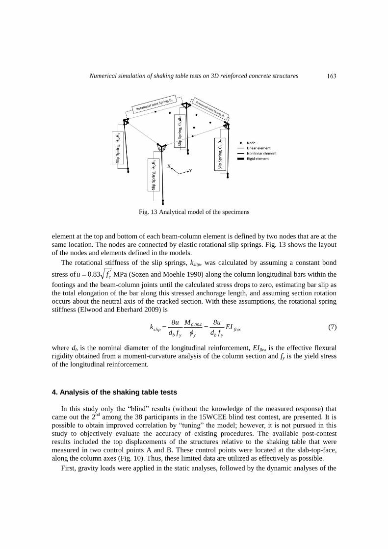
Fig. 13 Analytical model of the specimens

element at the top and bottom of each beam-column element is defined by two nodes that are at the

same location. The nodes are connected by elastic rotational slip springs. Fig. 13 shows the layout

of the nodes and elements defined in the models.

The rotational stiffness of the slip springs, kslip, was calculated by assuming a constant bond

stress of'83.0 cfu MPa (Sozen and Moehle 1990) along the column longitudinal bars within the

footings and the beam-column joints until the calculated stress drops to zero, estimating bar slip as

the total elongation of the bar along this stressed anchorage length, and assuming section rotation

occurs about the neutral axis of the cracked section. With these assumptions, the rotational spring

stiffness (Elwood and Eberhard 2009) is

flex

yby

004.0

yb

slip EIfd

u8M

fd

u8k

(7)

where db is the nominal diameter of the longitudinal reinforcement, EIflex is the effective flexural

rigidity obtained from a moment-curvature analysis of the column section and fy is the yield stress

of the longitudinal reinforcement.

4. Analysis of the shaking table tests

In this study only the “blind” results (without the knowledge of the measured response) that

came out the 2nd

among the 38 participants in the 15WCEE blind test contest, are presented. It is

possible to obtain improved correlation by “tuning” the model; however, it is not pursued in this

study to objectively evaluate the accuracy of existing procedures. The available post-contest

results included the top displacements of the structures relative to the shaking table that were

measured in two control points A and B. These control points were located at the slab-top-face,

along the column axes (Fig. 10). Thus, these limited data are utilized as effectively as possible.

First, gravity loads were applied in the static analyses, followed by the dynamic analyses of the

163

Beyhan Bayhan

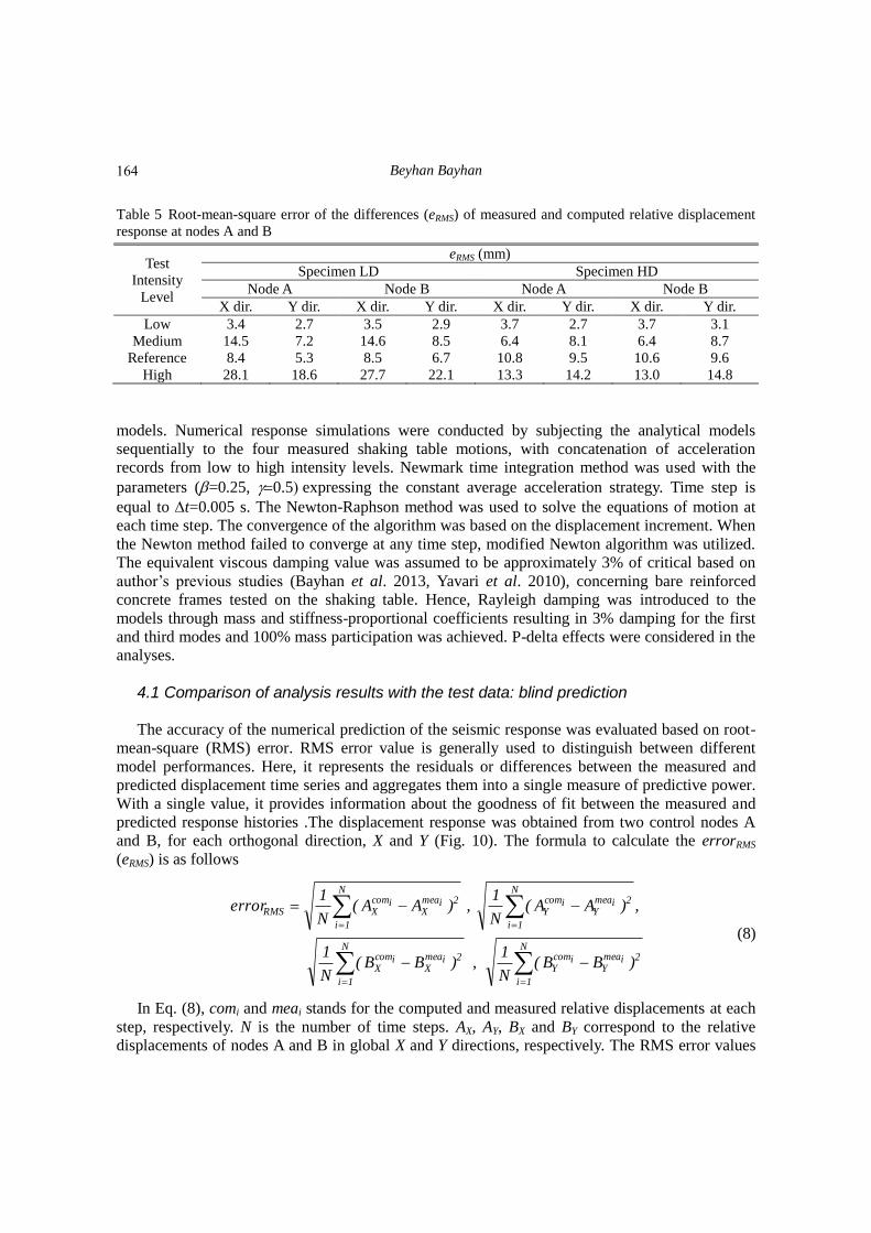
Table 5 Root-mean-square error of the differences (eRMS) of measured and computed relative displacement

response at nodes A and B

Test

Intensity

Level

eRMS (mm)


Node A Node B Node A Node B

X dir. Y dir. X dir. Y dir. X dir. Y dir. X dir. Y dir.

Low 3.4 2.7 3.5 2.9 3.7 2.7 3.7 3.1

Medium 14.5 7.2 14.6 8.5 6.4 8.1 6.4 8.7

Reference 8.4 5.3 8.5 6.7 10.8 9.5 10.6 9.6

High 28.1 18.6 27.7 22.1 13.3 14.2 13.0 14.8

models. Numerical response simulations were conducted by subjecting the analytical models

sequentially to the four measured shaking table motions, with concatenation of acceleration

records from low to high intensity levels. Newmark time integration method was used with the

parameters (=0.25, 0.5expressing the constant average acceleration strategy. Time step is

equal to t=0.005 s. The Newton-Raphson method was used to solve the equations of motion at

each time step. The convergence of the algorithm was based on the displacement increment. When

the Newton method failed to converge at any time step, modified Newton algorithm was utilized.

The equivalent viscous damping value was assumed to be approximately 3% of critical based on

author’s previous studies (Bayhan et al. 2013, Yavari et al. 2010), concerning bare reinforced

concrete frames tested on the shaking table. Hence, Rayleigh damping was introduced to the

models through mass and stiffness-proportional coefficients resulting in 3% damping for the first

and third modes and 100% mass participation was achieved. P-delta effects were considered in the

analyses.

4.1 Comparison of analysis results with the test data: blind prediction The accuracy of the numerical prediction of the seismic response was evaluated based on root-

mean-square (RMS) error. RMS error value is generally used to distinguish between different

model performances. Here, it represents the residuals or differences between the measured and

predicted displacement time series and aggregates them into a single measure of predictive power.

With a single value, it provides information about the goodness of fit between the measured and

predicted response histories .The displacement response was obtained from two control nodes A

and B, for each orthogonal direction, X and Y (Fig. 10). The formula to calculate the errorRMS

(eRMS) is as follows

N

1i

2imeaY

icomY

N

1i

2imeaX

icomX

N

1i

2imeaY

icomY

N

1i

2imeaX

icomXRMS

)BB(N

1,)BB(

N

1

,)AA(N

1,)AA(

N

1error

(8)

In Eq. (8), comi and meai stands for the computed and measured relative displacements at each

step, respectively. N is the number of time steps. AX, AY, BX and BY correspond to the relative

displacements of nodes A and B in global X and Y directions, respectively. The RMS error values

164


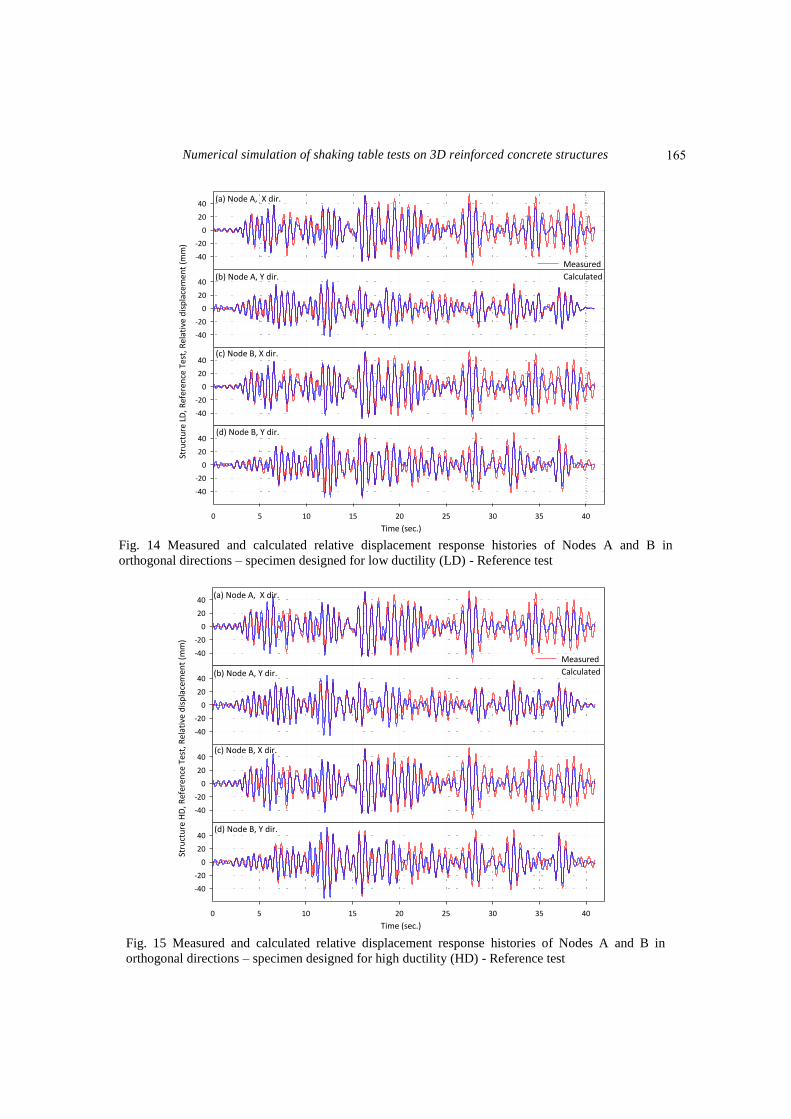
Fig. 14 Measured and calculated relative displacement response histories of Nodes A and B in

orthogonal directions – specimen designed for low ductility (LD) - Reference test

Fig. 15 Measured and calculated relative displacement response histories of Nodes A and B in

orthogonal directions – specimen designed for high ductility (HD) - Reference test

-40

-20

0

20

40 (a) Node A, X dir.

-40

-20

0

20

40 (b) Node A, Y dir.

-40

-20

0

20

40

0 5 10 15 20 25 30 35 40

-40

-20

0

20

40

(c) Node B, X dir.

(d) Node B, Y dir.

Stru

ctu

re L

D, R

efer

ence

Tes

t, R

elat

ive

dis

pla

cem

ent

(mm

)

Time (sec.)

Measured

Calculated

-40

-20

0

20

40 (a) Node A, X dir.

-40

-20

0

20

40 (b) Node A, Y dir.

-40

-20

0

20

40

0 5 10 15 20 25 30 35 40

-40

-20

0

20

40

(c) Node B, X dir.

(d) Node B, Y dir.

Stru

ctu

re H

D, R

efer

ence

Tes

t, R

elat

ive

dis

pla

cem

ent

(mm

)

Time (sec.)

Measured

Calculated

165

Beyhan Bayhan

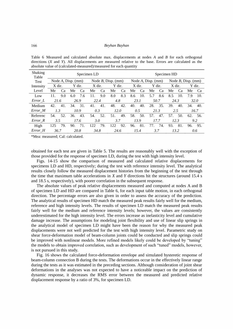
Table 6 Measured and calculated absolute max. displacements at nodes A and B for each orthogonal

directions (X and Y). All displacements are measured relative to the base. Errors are calculated as the

absolute value of (calculated-measured)/measured for each quantity

Shaking

Table

Test

Intensity

Level


Node A, Disp. (mm) Node B, Disp. (mm) Node A, Disp. (mm) Node B, Disp. (mm)

X dir. Y dir. X dir. Y dir. X dir. Y dir. X dir. Y dir.

Me

a*

Ca

l*

Me

a

Ca

l

Me

a

Ca

l

Me

a

Ca

l

Me

a

Ca

l

Me

a

Ca

l

Me

a

Ca

l

Me

a

Ca

l Low 11.

4 9.0 6.0 7.6 11.

6 9.0 8.0 8.3 8.6 10.

5 5.7 8.6 8.5 10.

5 7.9 10.

4 Error_L

ow (%) 21.6 26.9 22.4 4.8 23.1 50.7 24.3 32.0

Medium 42.

1

41.

5

34.

8

31.

0

41.

4

41.

5

48.

2

42.

4

40.

4

40.

6

28.

8

35.

0

39.

6

40.

6

34.

4

40.

2 Error_M

ed (%) 1.3 10.9 0.3 12.0 0.5 21.3 2.5 16.7

Referenc

e

54.

4

52.

5

36.

9

43.

4

54.

1

52.

5

51.

2

49.

3

58.

5

50.

3

57.

5

47.

3

57.

4

50.

3

62.

0

56.

3 Error_R

ef (%) 3.5 17.6 3.0 3.7 13.9 17.7 12.3 9.2

High 125

.5

79.

5

90.

5

71.

7

122

.0

79.

5

122

.0

92.

0

96.

0

81.

2

77.

1

74.

2

93.

5

81.

2

96.

5

95.

9 Error_H

igh (%) 36.7 20.8 34.8 24.6 15.4 3.7 13.2 0.6

*Mea: measured; Cal: calculated.

obtained for each test are given in Table 5. The results are reasonably well with the exception of

those provided for the response of specimen LD, during the test with high intensity level.

Figs. 14-15 show the comparison of measured and calculated relative displacements for

specimens LD and HD, respectively; during the test with reference intensity level. The analytical

results closely follow the measured displacement histories from the beginning of the test through

the time that maximum table accelerations in X and Y directions hit the structures (around 15.4 s

and 18.5 s, respectively), with poorer correlation in the subsequent response.

The absolute values of peak relative displacements measured and computed at nodes A and B

of specimen LD and HD are compared in Table 6, for each input table motion, in each orthogonal

direction. The percentage errors are also given in order to assess the accuracy of the prediction.

The analytical results of specimen HD match the measured peak results fairly well for the medium,

reference and high intensity levels. The results of specimen LD match the measured peak results

fairly well for the medium and reference intensity levels; however, the values are consistently

underestimated for the high intensity level. The errors increase as inelasticity level and cumulative

damage increase. The assumptions for modeling joint flexibility and use of linear slip springs in

the analytical model of specimen LD might have been the reason for why the measured peak

displacements were not well predicted for the test with high intensity level. Parametric study on

shear force-deformation model of beam-column joints could be conducted and slip springs could

be improved with nonlinear models. More refined models likely could be developed by “tuning”

the models to obtain improved correlation, such as development of such “tuned” models, however,

is not pursued in this study.

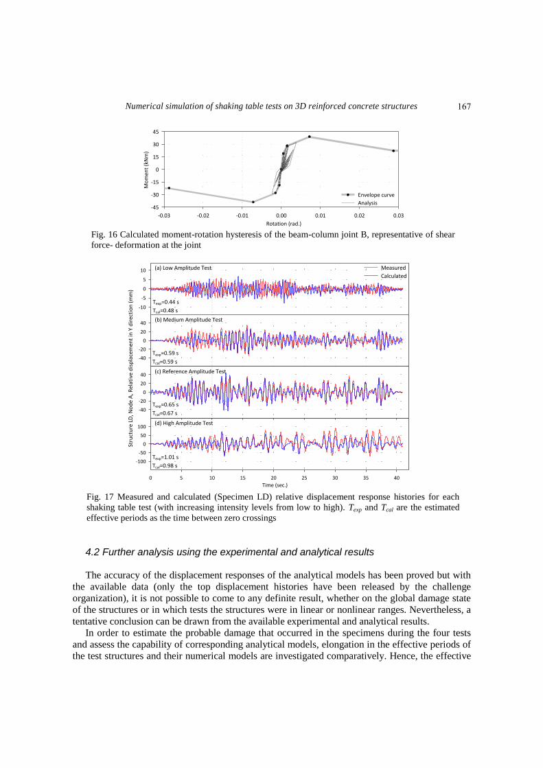
Fig. 16 shows the calculated force-deformation envelope and simulated hysteretic response of

beam-column connection B during the tests. The deformations occur in the effectively linear range

during the tests as it was estimated in the preceding sections. Although consideration of joint shear

deformations in the analyses was not expected to have a noticeable impact on the prediction of

dynamic response, it decreases the RMS error between the measured and predicted relative

displacement response by a ratio of 3%, for specimen LD.

166


Fig. 16 Calculated moment-rotation hysteresis of the beam-column joint B, representative of shear

force- deformation at the joint

Fig. 17 Measured and calculated (Specimen LD) relative displacement response histories for each

shaking table test (with increasing intensity levels from low to high). Texp and Tcal are the estimated

effective periods as the time between zero crossings

4.2 Further analysis using the experimental and analytical results The accuracy of the displacement responses of the analytical models has been proved but with

the available data (only the top displacement histories have been released by the challenge

organization), it is not possible to come to any definite result, whether on the global damage state

of the structures or in which tests the structures were in linear or nonlinear ranges. Nevertheless, a

tentative conclusion can be drawn from the available experimental and analytical results.

In order to estimate the probable damage that occurred in the specimens during the four tests

and assess the capability of corresponding analytical models, elongation in the effective periods of

the test structures and their numerical models are investigated comparatively. Hence, the effective

-0.03 -0.02 -0.01 0.00 0.01 0.02 0.03

-45

-30

-15

0

15

30

45

Envelope curve

Analysis

Mo

men

t (k

Nm

)

Rotation (rad.)

Time (sec.)

0 5 10 15 20 25 30 35 40

-100

-50

0

50

100

Stru

ctu

re L

D, N

od

e A

, Rel

ativ

e d

isp

lace

men

t in

Y d

irec

tio

n (

mm

)

-10

-5

0

5

10 Measured

Calculated

(a) Low Amplitude Test

-40

-20

0

20

40

-40

-20

0

20

40

(b) Medium Amplitude Test

(c) Reference Amplitude Test

(d) High Amplitude Test

Texp=0.44 s

Tcal=0.48 s

Texp=0.59 s

Tcal=0.59 s

Texp=0.65 s

Tcal=0.67 s

Texp=1.01 s

Tcal=0.98 s

167

Beyhan Bayhan

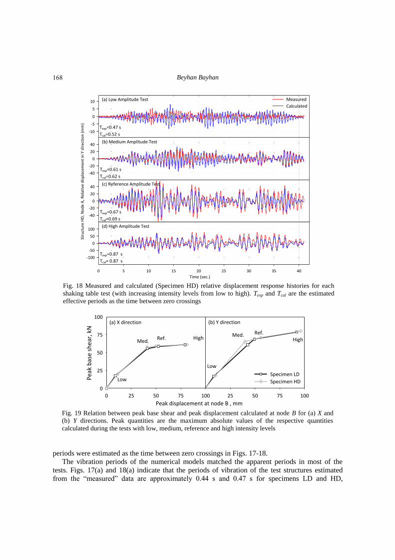
Fig. 18 Measured and calculated (Specimen HD) relative displacement response histories for each

shaking table test (with increasing intensity levels from low to high). Texp and Tcal are the estimated

effective periods as the time between zero crossings

Fig. 19 Relation between peak base shear and peak displacement calculated at node B for (a) X and

(b) Y directions. Peak quantities are the maximum absolute values of the respective quantities

calculated during the tests with low, medium, reference and high intensity levels

periods were estimated as the time between zero crossings in Figs. 17-18.

The vibration periods of the numerical models matched the apparent periods in most of the

tests. Figs. 17(a) and 18(a) indicate that the periods of vibration of the test structures estimated

from the “measured” data are approximately 0.44 s and 0.47 s for specimens LD and HD,

Stru

ctu

re H

D, N

od

e A

, Rel

ativ

e d

isp

lace

men

t in

Y d

irec

tio

n (

mm

)

-10

-5

0

5

10 Measured

Calculated

(a) Low Amplitude Test

-40

-20

0

20

40

-40

-20

0

20

40

Time (sec.)

0 5 10 15 20 25 30 35 40

-100

-50

0

50

100

(b) Medium Amplitude Test

(c) Reference Amplitude Test

(d) High Amplitude Test

Texp=0.61 s

Tcal=0.62 s

Texp=0.67 s

Tcal=0.69 s

Texp=0.87 s

Tcal= 0.87 s

Texp=0.47 s

Tcal=0.52 s

25 50 75 100

Specimen LD

Specimen HD

Peak displacement at node B , mm

0 25 50 75 100

Pea

k b

ase

she

ar, k

N

0

25

50

75

100

Low

Ref.High

Med.HighRef.

Low

Med.

(a) X direction (b) Y direction

168


respectively. They elongated to 1.03 and 0.98 s at the end of the tests (Figs. 17(d) and 18(d)),

suggesting that the effective flexibility of the structures had increased by factors of

(1.01/0.44)2=5.3 and (0.87/0.47)

2=3.4, respectively. The periods of vibration of the specimens

estimated from the “calculated” data are approximately 0.48 s and 0.52 s (Figs. 17(a) and 18(a))

for specimens LD and HD, respectively. They elongated to 0.98 s and 0.87 s at the end of the tests

with high intensity level (Figs. 17(d) and 18(d)), suggesting that the effective flexibility of the

structures had increased by factors of (0.98/0.48)2=4.2 and (0.87/0.52)

2=2.8, respectively. This

shows that the numerical models capture the significant elongation in periods of the specimens

fairly well. The difference between the factors estimated from the measured and calculated data is

mainly due to the error in estimation of the measured initial periods of the structures (Figs. 17(a)

and 18(a)).

Relation between the peak base-shear and the peak displacement demand was investigated in

order to predict the stages in which the test specimens were in linear or nonlinear range, using the

calculated data. Fig. 19 plots relation between peak base shears and peak displacements calculated

for each of the four earthquake simulations. Both structures are in nonlinear range during the tests

with reference and high intensity levels.

5. Conclusions

This paper presents the numerical models of two full-scale, 3d, one-story RC structures and

simulation of their seismic response to the shaking table excitations. The structures, designed for

low and high ductility levels, are geometrically identical. They were subjected to four consecutive

shaking table motions with increasing intensity from PGA=0.05g to PGA=0.53g. The excitations

were applied bidirectionally in horizontal orthogonal axes.

3d analytical models of the test structures were developed. The numerical models predicted the

earthquake responses of the specimens fairly well and this was provided by the comparison of

blind prediction results with the experimental data, including response histories of relative

displacements recorded at the predetermined control points. Reasonably accurate results were

provided in general, except for the high level intensity simulation of the specimen with low

ductility level. The success of numerical models simulating the nonlinear dynamic response of the

three dimensional structures subjected to bidirectional loading particularly depends on the

following statements:

• Material nonlinearity, dynamic and stiffness properties of the test structures, boundary

conditions and application of load are reasonably well defined.

• The calculated masses and mass moment of inertias were introduced to the model at specified

nodes and rigid diaphragm was assigned for the half-slab with constraints.

• Elastic rotational slip springs, considering flexibility due to slip of the reinforcing bars from

the beams and footings, are located at top and bottom of nonlinear beam-column elements.

• The beam-column joint shear deformation is taken into account with a nonlinear joint model.

The discrepancy between the predicted and experimental results might be related to either input

modelling parameters, coupling effects, strain rate effects in dynamic testing, capabilities of the

analysis program or combination of these factors. It is not possible to isolate the source with the

available data; however, in the future, this study can be improved by (i) tunning the beam-column

joint shear force-deformation model particularly for the structure with low ductility level; (ii)

introducing nonlinear slip-springs to the models and (iii) considering coupling effects that would

169

Beyhan Bayhan

affect shear and slip deformation in beam-column and column-footing connections, respectively.

This study has shown that successful simulation of a 3d reinforced concrete structure subjected

to bidirectional dynamic loading can be achieved through a relatively simple numerical model if

essential features of nonlinear behaviour are properly introduced to the model. Thus, nonlinear

dynamic analysis of larger structural systems would not require huge amount of computational

effort.

The reasonably accurate correlation with the measured data of the model for the blind

prediction contest is motivating, but combined effort for experimental-analytical studies on the

seismic response of 3d, reinforced concrete buildings is needed to isolate each component

contributing to the system.

This study, for the limited conditions in which it was applied, also contributes to the current

research by helping us to see explicitly how successful we are in predicting seismic response of

reinforced concrete structures tested in the laboratory, where less uncertainty exists compared to

the field conditions.

Acknowledgments

The author is grateful to Dr. Gökhan Ö zdemir for providing constructive comments during the

course of this study. The assistance of the 15WCEE challenge organization and LNEC team is

greatly appreciated.

References ACI 318 (2011), Building Code Requirements for Structural Concrete and Commentary, ACI Committee

318, American Concrete Institute, Farmington Hills, Michigan.

ACI 352 (2012), Guide for Design of Slab-Column Connections in Monolithic Concrete Structures, ACI

Committee 352, American Concrete Institute, Farmington Hills, Michigan.

Alath, S. and Kunnath, S.K. (1995), “Modeling inelastic shear deformations in RC beam-column joints”,

Proceedings of 10th Engineering Mechanics Conference, University of Colorado at Boulder, New York,

May.

ASCE/SEI 41 Supplement 1 (2008), Seismic Rehabilitation of Existing Buildings, American Society of Civil

Engineers, Reston, VA.

Bayhan, B., Moehle, J.P., Yavari, S., Elwood, K.J., Lin, S.H., Wu, C.L. and Hwang, S.J. (2013), “Seismic

Response of a Concrete Frame with Weak Beam-Column Joints”, Earthq Spectra, doi:

10.1193/071811EQS179M.

Coleman, J. and Spacone, E. (2001), Localization issues in nonlinear frame elements, Modeling of Inelastic

Behavior of RC Structures Under Seismic Loads, Eds. Shing, P.B. and Tanabe, T.A., ASCE/SEI

Publication, Reston, VA.

Elwood, K.J. and Eberhard, M.O. (2009), “Effective stiffness of reinforced concrete columns”, ACI Struct.

J., 106(4), 476-484.

Eurocode 8 (2004), Design of structures for earthquake resistance, Part 1: General rules, seismic actions

and rules for buildings, European Standard EN 1998-1, Comité Européen de Normalisation, Bruxelles.

FIB (2003), Seismic Assessment and Retrofit of Reinforced Concrete Buildings, state of the art report,

bulletin no: 24, International Federation for Structural Concrete, Lausanne, Switzerland.

Gallo, P.Q., Akgüzel, U., Pampanin, S. and Carr, A.J. (2011), “Shake table tests of non-ductile as-built and

repaired RC frames”, Proceedings of the Ninth Pacific Conference on Earthquake Engineering Building

170


an Earthquake-Resilient Society, Auckland, New Zealand, April.

Kazaz, İ., Yakut, A. and Gülkan, P. (2006), “Numerical simulation of dynamic shear wall tests: a

benchmarkstudy”, Computers and Structures, 84(8-9), 549-562.

Kabeyasawa, T., Kabayasewa, T., Matsumori, T., Kabayasewa, T. and Kim, Y. (2007), “3-D collapse tests

and analyses of the three-story reinforced concrete buildings with flexible foundation”, Structures

Congress 2007 Structural Engineering Research Frontiers-ASCE, Long Beach, CA, May.

LNEC Team (2012), Preliminary test, blind test design, material and construction report, 15WCEE Blind

Test Challenge, Lisbon, Portugal.

Lowes, L.N. and Altoontash, A. (2003), “Modeling reinforced-concrete beam-column joints subjected to

cyclic loading”, J Struct Eng-ASCE, 129(12), 1686-1697.

Mander, J.B., Priestley, M.J.N. and Park, R. (1988), “Theoretical stress–strain model for confined concrete”,

J. Struct. Eng., ASCE, 114(8), 1804-1826.

OpenSees (2005), Open system for earthquake engineering simulation, Pacific Earthquake Engineering

Research Center, UC Berkeley, Available from: http://www.opensees.berkeley.edu.

Panagiotou, M., Restrepo, J. and Conte, J. (2011), “Shake-table test of a full-scale 7-story building slice.

Phase I: rectangular wall”, J. Struct. Eng., 137(6), 691-704.

Pantelides, C.P., Clyde, C. and Reaveley, L.D. (2002), “Performance-based evaluation of reinforced

concrete building exterior joints for seismic excitation”, Earthq. Spectra, 18(3), 449-480.

Peloso, S., Zanardi, A. and Pavese, A. (2012), “Improvement of a simplified method for the assessment of

3D R.C. frames”, 15th World Conference on Earthquake Engineering, Lisbon, Portugal.

Sozen, M.A. and Moehle, J.P. (1990), “Development and lap-splice lengths for deformed reinforcing bars in

concrete”, A Report to the Portland Cement Association, Skokie, IL, and the Concrete Reinforcing Steel

Institute, Schaumburg, IL.

Spacone, E., Filippou, F.C. and Taucer, F.F. (1996a), “Fiber beam–column model for non-linear analysis of

R/C frames. Part I: formulation”, Earthq. Eng. Struct. D., 25(7), 711-725.

Spacone, E., Filippou. F.C. and Taucer, F.F. (1996b), “Fiber beam–column model for non-linear analysis of

R/C frames. Part II: application”, Earthq. Eng. Struct. D., 25(7), 727-742.

Walker, S. (2001), “Seismic performance of existing reinforced concrete beam-column joints”, Master of

Science thesis, Department of Civil Engineering, University of Washington, Seattle, WA.

Yavari, S., Lin, S.H., Elwood, K.J., Wu, C.L., Hwang, S.J., Bayhan, B. and Moehle, J.P. (2010), “Shake

table tests on the collapse of reinforced concrete frames subjected to moderate and high axial loads”,

Proceedings of the 9th U.S. National and 10th Canadian Conference on Earthquake Engineering,

Toronto, Ontario, Canada.

171

http://www.opensees.berkeley.edu/

Numerical simulation of shaking table tests on 3D reinforced concrete structures

Documents

Transcript of Numerical simulation of shaking table tests on 3D reinforced concrete structures