arX

iv:n

ucl-

th/0

1030

13v3

2 O

ct 2

001

Nuclear fission: The ”onset of dissipation”

from a microscopic point of view

H. Hofmann 1, F.A. Ivanyuk1,2, C. Rummel 1 and S. Yamaji3

1) Physik-Department der TU Munchen, D-85747 Garching, Germany

2) Institute for Nuclear Research, 03028 Kiev-28, Ukraine

3) Cyclotron Lab., Riken, Wako-Shi, Saitama, 351-01 Japan

Revised Version

August 01, 2001

Abstract

Semi-analytical expressions are suggested for the temperature dependence of thosecombinations of transport coefficients which govern the fission process. This is basedon experience with numerical calculations within the linear response approach and thelocally harmonic approximation. A reduced version of the latter is seen to comply withKramers’ simplified picture of fission. It is argued that for variable inertia his formulahas to be generalized, as already required by the need that for overdamped motion theinertia must not appear at all. This situation may already occur above T ≈ 2 MeV,where the rate is determined by the Smoluchowski equation. Consequently, comparisonwith experimental results do not give information on the effective damping rate, as oftenclaimed, but on a special combination of local stiffnesses and the friction coefficientcalculated at the barrier.

PACS number(s): 24.10.Pa, 24.75.+i,25.70.Jj,25.70.Gh

1

Contents

1 Introduction 3

2 Rate formulas 4

3 Microscopic transport coefficients 6

3.1 Shell effects on potential landscape . . . . . . . . . . . . . . . . . . . . . . . 83.2 Temperature dependence of transport coefficients . . . . . . . . . . . . . . . 8

3.2.1 Local stiffness . . . . . . . . . . . . . . . . . . . . . . . . . . . . . . . 93.2.2 Local inertia . . . . . . . . . . . . . . . . . . . . . . . . . . . . . . . . 103.2.3 Vibrational frequency . . . . . . . . . . . . . . . . . . . . . . . . . . . 103.2.4 Ratio of friction to inertia . . . . . . . . . . . . . . . . . . . . . . . . 113.2.5 Ratio of friction to stiffness . . . . . . . . . . . . . . . . . . . . . . . 113.2.6 The influence of pairing . . . . . . . . . . . . . . . . . . . . . . . . . 13

4 Temperature dependent decay rates 14

4.1 Rate from microscopic transport coefficients . . . . . . . . . . . . . . . . . . 144.2 Comparison with phenomenological models . . . . . . . . . . . . . . . . . . . 154.3 Relation to the statistical model . . . . . . . . . . . . . . . . . . . . . . . . . 154.4 Isotopic effects . . . . . . . . . . . . . . . . . . . . . . . . . . . . . . . . . . 17

5 Summary and discussion 18

A Implications from a variable inertia 20

A.1 Kramers’ decay rate formula extended to variable inertia . . . . . . . . . . . 22A.2 The relation to the transition state result . . . . . . . . . . . . . . . . . . . . 25A.3 The Smoluchowski limit . . . . . . . . . . . . . . . . . . . . . . . . . . . . . 25A.4 Strutinsky’s derivation of the rate formula . . . . . . . . . . . . . . . . . . . 26

B A schematic microscopic model 26

B.1 The Lorentz-model for intrinsic motion . . . . . . . . . . . . . . . . . . . . . 26B.2 Benefits and shortcomings of this model . . . . . . . . . . . . . . . . . . . . 28

B.2.1 Weak damping . . . . . . . . . . . . . . . . . . . . . . . . . . . . . . 28B.2.2 Strong damping . . . . . . . . . . . . . . . . . . . . . . . . . . . . . . 28B.2.3 Temperature dependence through collisional damping . . . . . . . . . 29

2

1 Introduction

It is of considerable interest to understand the temperature dependence of transport prop-erties associated with slow collective motion of large scale. Fission is a prime example, andindeed, for this case there is growing experimental evidence [1] - [5] that damping effectivelyincreases with T . One often tries to characterize this feature by one parameter, the effec-tive damping rate η which is related to the equation of average motion for a locally defineddamped oscillator

Md2q

dt2+ γ

dq

dt+ Cq(t) = 0 , (1)

through

η =γ

2√

M | C |. (2)

The q = Q−Q0 measures the deviation of the collective variable Q from some fixed value Q0.In the following we will also need other combinations of inertia M , stiffness C and frictionγ, namely

τcoll =γ

|C| =~

Γcoll

, τkin =M

γ=

~

Γkin

and 2 =| C |M

. (3)

The τcoll sets the scale for (local) relaxation of collective motion in a given potential of (local)stiffness C. The τkin, on the other hand, measures the relaxation of the kinetic energy tothe equilibrium value of the Maxwell distribution. Typically, for slow collective motion weexpect this time to be smaller than the former. The limit of overdamped motion applies forτkin ≪ τcoll. Using the η introduced in (2) the following useful relation for their ratio is easilyverified

2η =Γkin

~= τcoll =

√

τcoll

τkin. (4)

For a positive stiffness (C > 0) and underdamped motion, the would be the frequencyof the vibration and the Γkin its width. It should be noted that in the literature a differentnotation is sometimes used where γ stands for η, and often the Γkin/~ is referred to as β.

To understand the dynamics in phase space one also needs the diffusion coefficients. Atsmall temperatures they may deviate from the classic Einstein relation (see [6]), but thesefiner details will be neglected here. For such a situation the fission decay rate is commonlycalculated within Kramers’ ”high viscosity” limit [7], for which the dependence on frictionis given by

Rh.v.K (ηb)

Rh.v.K (ηb = 0)

=√

1 + η2b − ηb ≡

(

√

1 + η2b + ηb

)−1

. (5)

Here, the index ”b” refers to the fact that the transport coefficients are to be calculated atthe barrier. It has been reported, see e.g. Fig.5 of [2], experimental data to suggest, whenanalyzed on the basis of (5), the η to be negligibly small at very low temperatures but to

3

rise more or less sharply around T ≃ 1 MeV. This result is in qualitative agreement withmicroscopic calculations of the transport coefficients within linear response theory [6, 8, 9],although caution is still warranted here. Let us leave aside the fact that at lower temperaturesthe one dimensional potential may attain more structure than that found in one minimumand one barrier, which is the picture underlying formula (5) and which for the sake ofsimplicity shall be applied in the sequel. As will be demonstrated below, even then itis not permissible to entirely parameterize the truly complicated transport process by thesingle quantity η. Rather, other combinations of M, γ and C are needed for more realisticdescriptions. Moreover, one should be guided by the theoretical fact, that not all transportcoefficients are equally well accessible both theoretically as well as numerically, as is so forthe inertia, for instance.

Unfortunately, when physicists address transport problems, all too often one disregardsthe importance of the inertia, and in particular its variation with the collective coordinate.Indeed, in studies based on the Caldeira-Leggett Hamiltonian (see e.g. [10]) or in applicationsof the Random Matrix Theory (see [11]) the inertia is the one of the unperturbed collectivepart of the total Hamiltonian, treated as an (unknown) parameter. In the case of nuclearphysics the situation is more complicated. Firstly, there, no unperturbed inertia exists atall; it may only show up in the final effective equation of motion as one manifestation ofthe existence of collective dynamics. Secondly, the inertia M may depend sensitively onthe collective degree of freedom. This feature is already well known from the traditionalcase of undamped motion at zero thermal excitation [12]. There is no a priori reason whythis should be different at finite temperature, with perhaps two exceptions or modifications.With increasing T the M gets close to the liquid drop value [13], which only varies smoothlywith Q and which is quite small. Simultaneously the friction strength increases, so that onemay quickly reach the situation of overdamped motion, for which no trace of the inertia canbe seen anymore. Such features have been seen within the linear response approach (see[6]), but to the best of our knowledge no other transport model has so far addressed thisquestion.

2 Rate formulas

Like in the analysis underlying [3, 4] we want to make use of a simple formula for the decayrate. In slight modification of Kramers’ [7] classic one we write1:

Rh.v.K (ηb) =

a

2π

√

Ma

Mbexp(−Eb/T )

(

√

1 + η2b − ηb

)

. (6)

The indices ”a” and ”b” refer to the minimum and maximum of the potential V (Q), locatedat Qa and Qb, respectively. The Eb stands for the height of the barrier Eb = V (Qb)−V (Qa).The factor

√

Ma/Mb, not contained in Kramers’ original work, is meant to account for themodification one gets for variable inertia. Notice, that this inertia both influences the currentover the barrier as well as the number of ”particles” (phase space points) sitting in the well.Commonly both quantities are calculated with the same M which then drops out; see e.g.

1Since we are only looking at stationary situations we leave out the time dependent factor which sometimesis taken into account to simulate the ”transient time” it takes before the stationary current has built up.

4

0.0 1.0 2.0 3.0 4.0 η

0.0

0.5

1.0

RK(η

) / R

K(η

=0)

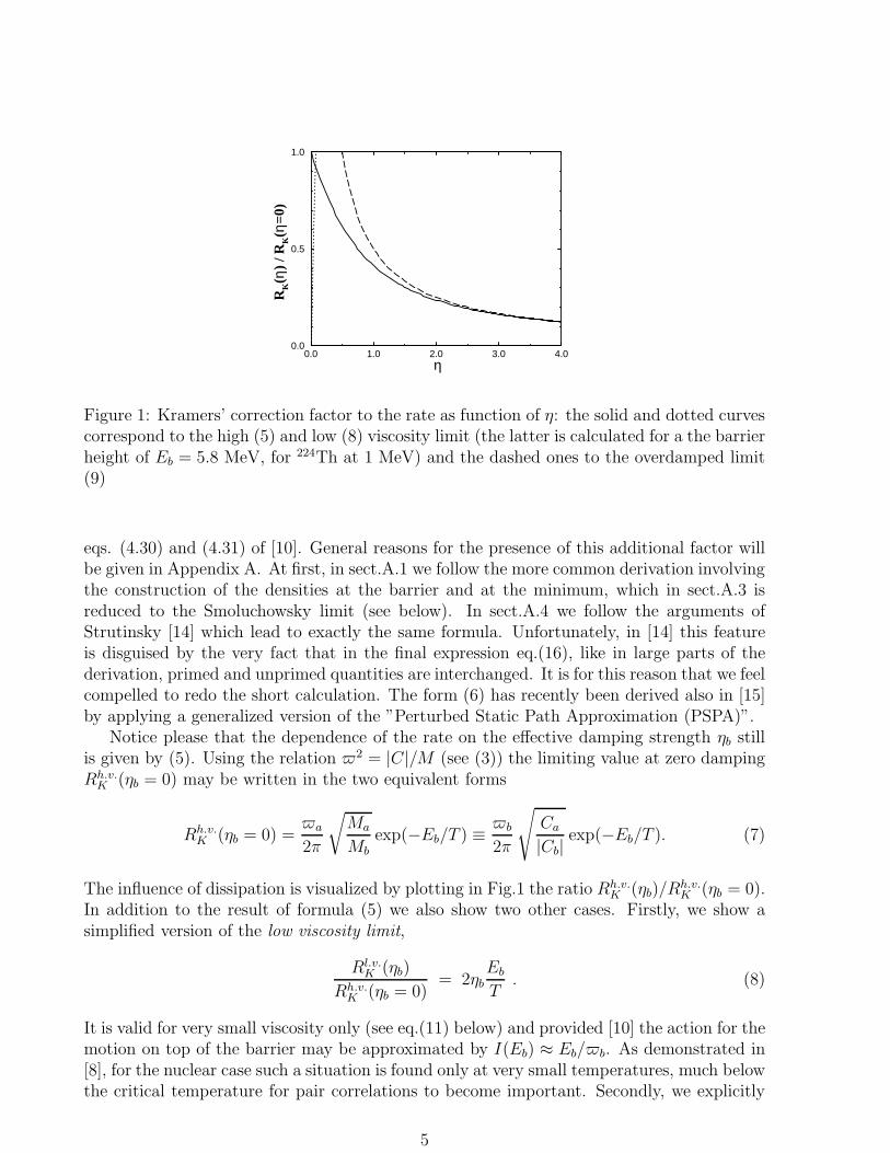
Figure 1: Kramers’ correction factor to the rate as function of η: the solid and dotted curvescorrespond to the high (5) and low (8) viscosity limit (the latter is calculated for a the barrierheight of Eb = 5.8 MeV, for 224Th at 1 MeV) and the dashed ones to the overdamped limit(9)

eqs. (4.30) and (4.31) of [10]. General reasons for the presence of this additional factor willbe given in Appendix A. At first, in sect.A.1 we follow the more common derivation involvingthe construction of the densities at the barrier and at the minimum, which in sect.A.3 isreduced to the Smoluchowsky limit (see below). In sect.A.4 we follow the arguments ofStrutinsky [14] which lead to exactly the same formula. Unfortunately, in [14] this featureis disguised by the very fact that in the final expression eq.(16), like in large parts of thederivation, primed and unprimed quantities are interchanged. It is for this reason that we feelcompelled to redo the short calculation. The form (6) has recently been derived also in [15]by applying a generalized version of the ”Perturbed Static Path Approximation (PSPA)”.

Notice please that the dependence of the rate on the effective damping strength ηb stillis given by (5). Using the relation 2 = |C|/M (see (3)) the limiting value at zero dampingRh.v.

K (ηb = 0) may be written in the two equivalent forms

Rh.v.K (ηb = 0) =

a

2π

√

Ma

Mbexp(−Eb/T ) ≡ b

2π

√

Ca

|Cb|exp(−Eb/T ). (7)

The influence of dissipation is visualized by plotting in Fig.1 the ratio Rh.v.K (ηb)/R

h.v.K (ηb = 0).

In addition to the result of formula (5) we also show two other cases. Firstly, we show asimplified version of the low viscosity limit,

Rl.v.K (ηb)

Rh.v.K (ηb = 0)

= 2ηbEb

T. (8)

It is valid for very small viscosity only (see eq.(11) below) and provided [10] the action for themotion on top of the barrier may be approximated by I(Eb) ≈ Eb/b. As demonstrated in[8], for the nuclear case such a situation is found only at very small temperatures, much belowthe critical temperature for pair correlations to become important. Secondly, we explicitly

5

indicate the limit the ratio (5) takes on for overdamped motion

Rh.v.K (ηb)

Rh.v.K (ηb = 0)

=1

2ηbfor ηb ≫ 1 . (9)

Whenever the ”high viscosity limit” applies the influence of dissipation manifests itself ina reduction of the decay rate over the value given by (7). This deviation is claimed to allowfor deducing a possible temperature dependence of dissipation through the ”measurable”rate. It must be noted, however, that for overdamped motion it is not the effective damping

factor ηb which one deduces. Indeed, overdamped motion is governed by the Smoluchowski

equation in which no inertia appears (see Appendix A). But the latter not only is present inηb but in Rh.v.

K (ηb = 0) as well. A better way of writing the rate formula in this case is

Rovd = Rh.v.K (ηb & 1) =

1

2π

√

Ca

|Cb||Cb|γb

exp(−Eb/T ) ≡ 1

2π

√

Ca

|Cb|1

τ bcoll

exp(−Eb/T ) . (10)

Here, the time scale τ bcoll appears which is relevant for overdamped motion across the barrier,

see below. As can be inferred from Fig.1 this limit is actually given for values of ηb justabove unity. Notice, please, that it is only with the additional factor

√

Ma/Mb included in(6), on top of Kramers’ classic version, that the inertia drops out in the overdamped limit.

A few comments are in order on the validity of the rate formulas of the high viscositylimit, for which the following assumptions must hold true:

• On the way from the minimum to the barrier the temperature must not change.

• The barrier must be sufficiently pronounced, first of all in the sense that its height belarge as compared to the temperature, viz Eb ≫ T , for further details see sect.A.1.

• The effective damping rate must not be too small

ηb ≥T

2Eb, (11)

otherwise formula (8) would have to be applied.

It may be quite a delicate matter to fix or calculate the temperature which is at stake here.For instance, a temperature TCN associated to the total available energy for the compound

nucleus might be much larger, as for high initial thermal excitations the system may cooldown by emissions of neutrons or γ’s before it fissions. Finally, we should like to remarkonce more that presently any possible quantum features are discarded, which might show upat low temperatures [8].

3 Microscopic transport coefficients

Evidently, the temperature dependence of the rate will greatly be influenced by that of thetransport coefficients — on top of the influence through the Arrhenius factor exp(−Eb(T )/T ).Let us first look into results obtained applying linear response theory within the locallyharmonic approximation [6], before we turn to discuss other forms used in the literature,

6

like in [4]. In this theoretical approach the transport coefficients of average motion areobtained by relating in the low frequency regime the strength distribution of a microscopicallycalculated response function χqq(ω) to the one of the damped oscillator. The latter is definedas

(χosc(ω))−1 q(ω) ≡ −(

Mω2 + iγω − C)

q(ω) = −qext(ω) . (12)

and thus may be obtained by adding to (1) the term −qext(t) on the right and performing aFourier transformation. For overdamped motion the response function turns into

χovd(ω) =i

γ

1

ω + iC/γ. (13)

In accord with the remarks from above on the Smoluchowski limit no inertia appears any-more.

This approach permits one to calculate the transport coefficients as functions of shapeand temperature for any given nucleus. The formulation is done in such a way that on topof shell effects and pairing (see [9] with references to previous works) collisional dampingis accounted for as well (for a review see [6]). As one may imagine, such computations arequite involved, last not least because much knowledge is required about various aspects ofthe dynamics of complex nuclear systems. This is one of the reasons why as yet numericalcomputations have been done only for particular nuclei or for more schematic cases [16] -[20], [9]. Nevertheless, this experience may allow us to deduce some gross features whichmay be considered generic to a wider class of nuclear systems. This is what we are goingto do below. It seems appropriate, however, to first add some general remarks concerningcalculations based on the deformed shell model as an approximation to the general meanfield.

The output of calculations of the type just mentioned contains much more detailed in-formation than at present one may possibly relate to observable quantities. The coordinatedependence of the transport coefficients, for instance, is one prime example. Often in nucleartransport theories one simply has aimed at constant coefficients for inertia and friction. Ifcalculated within the linear response approach, on the other hand, sizable variations withshape are seen. One may recall that a similar feature is already seen in the potential land-scape, when calculated with the Strutinsky procedure, for instance. Besides the maxima andminima which are typical for gross shell effects one sees detailed fine structure. Such featuresmay depend on peculiarities of the underlying shell model, and may thus be unphysical innature already by that reason. For the dynamic transport coefficients themselves furtherimplications arise from quasi-crossings of levels. To large extent such effects can be expectedto become much weaker in a multidimensional treatment, which at present still is infeasible.

One should not forget that problems of this type are intimately related to the fact thattransport coefficients of inertia, stiffness and friction are those of average motion, calculated

on the level of the mean field. Finally, however, they are needed for an equation of motion ofFokker-Planck type which accounts for dynamical fluctuations. The latter will help to smoothout the variations of the transport coefficients in most natural way. Evidently, the problemat stake here reflects the general deficiency of mean field theory. In a more appropriatetreatment one would be able to treat self-consistently both the mean field as well as itsfluctuations. Since such a theory is not available we suggest some other, more pragmatic

7

procedure. As described previously already, see e.g. [9], one may smooth static energiesas well as the other transport coefficients with respect to their dependence on deformation.The averaging interval in Q is to be chosen large enough to wash out the rapid fluctuationsbut small enough to preserve gross shell structures.

3.1 Shell effects on potential landscape

The static energy is calculated in the usual way as sum of a liquid drop part and theshell correction, both of which depend on temperature, for details see [19]. An example ofthe deformation dependence of this potential energy is shown in Fig.2. The dotted curverepresents the case of zero thermal excitation. On top of the typical gross shell structurefluctuations of smaller scale are recognized as well. Features of this type lead to the rapidvariations of the transport coefficients we talked about above; for the local stiffness as thesecond derivative of the static energy this is immediately evident. As mentioned, we considersuch fluctuations as unphysical, for which reason we like to remove them by averaging overan appropriate interval ∆Q but to keep the gross shell structure. For the free energy, forinstance, the smoothing can be done in the following way:

⟨

F(Q, T )⟩

av=

∑

i F(Qi, T )fav(Q−Qi

∆Q)

∑

i fav(Q−Qi

∆Q)

(14)

The smoothing function fav(x) in (14) is taken to be that of the Strutinsky shell correctionmethod and the Qi are some points in deformation space. The use of the Strutinsky smooth-ing function guarantees stability of the averaging procedure: the smooth component of thedeformation energy is restored after smoothing again. This implies that the liquid drop partof the energy is unchanged by this averaging.

In the figure we also show the averaged potential corresponding to temperatures T =0, 1, 2 and 3 MeV. As to be expected, with increasing temperature the deformation energybecomes much smoother and the height of the fission barrier gets reduced. This is due tothe reduction of shell effects, as well as to the temperature dependence of the liquid droppart. At temperatures above T ≈ 3 MeV the shell effects have disappeared completely andthe averaged deformation energy coincides with its liquid drop component. As seen from thefigure, at smaller temperatures the shell correction, albeit averaged, does contribute to thedeformation energy and, hence, to the stiffness. For example, at T = 1 MeV the stiffnessat the barrier (maximum of the deformation energy) is still several times larger than that ofthe liquid drop part.

It should be mentioned that in [18] a somewhat different (averaging) procedure was used.There the deformation energy was approximated by two parabolas and the stiffness (at theminimum and the barrier) was defined by the curvature of these parabola. In this way shelleffects are washed out to larger extent, not only with respect to the fine structure but evenwith respect to gross shell features. Consequently, the stiffness defined in this way is ratherclose to the liquid drop stiffness.

3.2 Temperature dependence of transport coefficients

8

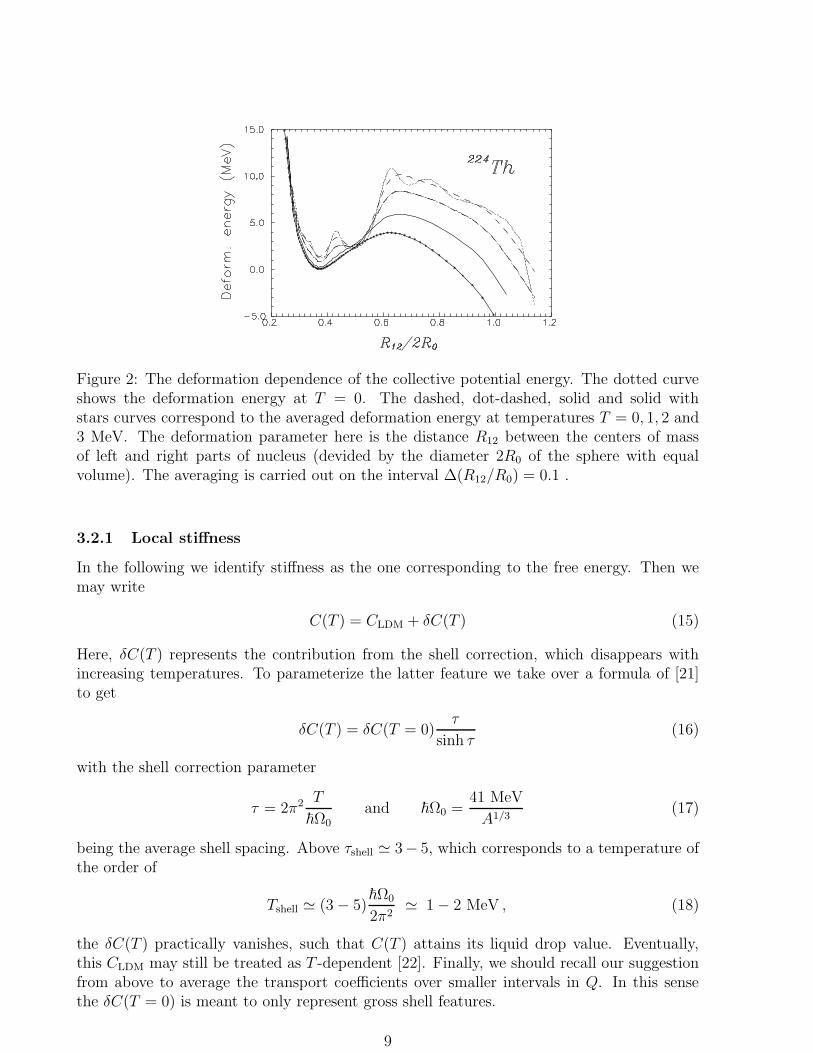
Figure 2: The deformation dependence of the collective potential energy. The dotted curveshows the deformation energy at T = 0. The dashed, dot-dashed, solid and solid withstars curves correspond to the averaged deformation energy at temperatures T = 0, 1, 2 and3 MeV. The deformation parameter here is the distance R12 between the centers of massof left and right parts of nucleus (devided by the diameter 2R0 of the sphere with equalvolume). The averaging is carried out on the interval ∆(R12/R0) = 0.1 .

3.2.1 Local stiffness

In the following we identify stiffness as the one corresponding to the free energy. Then wemay write

C(T ) = CLDM + δC(T ) (15)

Here, δC(T ) represents the contribution from the shell correction, which disappears withincreasing temperatures. To parameterize the latter feature we take over a formula of [21]to get

δC(T ) = δC(T = 0)τ

sinh τ(16)

with the shell correction parameter

τ = 2π2 T

~Ω0and ~Ω0 =

41 MeV

A1/3(17)

being the average shell spacing. Above τshell ≃ 3− 5, which corresponds to a temperature ofthe order of

Tshell ≃ (3 − 5)~Ω0

2π2≃ 1 − 2 MeV , (18)

the δC(T ) practically vanishes, such that C(T ) attains its liquid drop value. Eventually,this CLDM may still be treated as T -dependent [22]. Finally, we should recall our suggestionfrom above to average the transport coefficients over smaller intervals in Q. In this sensethe δC(T = 0) is meant to only represent gross shell features.

9

3.2.2 Local inertia

As mentioned already in the Introduction, one should expect the inertia to vary with tem-perature. It is more than tempting to assume a form similar to the one for the stiffness,namely

M(T ) = MLDM + δM(T ) (19)

in which the last term drops to zero like given in (16). Indeed, within the linear responseapproach a behavior of that type has been observed in a numerical study [13]. There, thevalue reached at larger temperatures was given by that of irrotational flow, which for thepresent notation means to identify MLDM = Mirrot. To the best of our knowledge, there is noother theoretical model where such a transition is seen explicitly — although one must saythat in phenomenological applications of transport models commonly the Mirrot is taken torepresent the macroscopic value of inertia. At present the conjecture behind (19) still lacks adirect and general proof. However, in [23] the nucleonic response function has been studiedapplying Periodic Orbit Theory (POT). There it was seen that its ”fluctuating part” δχ(ω)decreases with T like the shell correction to the static energy. For slow collective motionthe inertia is determined by the second derivative of this response function with respect tofrequency calculated at ω = 0 (see App.B and eq.(B.8) in particular). Therefore, within sucha model the ”shell correction” to the inertia was indeed proven to behave as claimed above,although several questions remain open. Amongst others, it is unclear to which extentthis proof would get modified after considering ”collisional damping”. The latter cannotbe treated within POT but should play a major role for the transition to hydrodynamicbehavior. Possible reasons for rendering a microscopic approach quite difficult have beenreported in [18, 19, 6]. On the microscopic level they are related to the strength distributionfor the local collective motion. The liquid drop model, on the other hand, represents motionof a system having a sharp surface, in contrast to microscopic calculations involving thediffuse surface of the mean field and, hence, of the density, for details see [19]. Fortunately,however, at larger T when the collisions become more and more important the motion getsstrongly damped such that the inertia drops out anyway, see (13).

Because of these difficulties in microscopic computations we propose to fix the M(T )through the vibrational frequency and the local stiffness by the relation given in (3),namely M = |C|/2. For our version of Kramers’ rate formula this was easily achieved inusing the second variant shown in (7).

3.2.3 Vibrational frequency

At the extremal points of the potential landscape this frequency is a well defined quantity.To some extent it is even accessible to experimental verification, at least for zero thermalexcitation. At the minimum it may be associated with the energy of a collective mode (forvery recent work on this subject see [24]) and for the barrier it influences the penetrability,as encountered for instance in neutron induced fission [25]. Generally, the ~ is believed tobe of the order of 1 MeV. Indeed, numerical calculations for 224Th [18, 19] show this to bequite insensitive to temperature; to lesser extent this is true also for the variation with shapeand mass number. Altogether, for a first orientation the following choice seems appropriate

~a ≃ ~b ≃ 1 MeV (20)

10

0 1 2 3 4T (MeV)

0

2

4

6

8

10

γ/M

(M

eV/h

)

0 1 2 3 40

2

4

6

8

10

γ/M

(M

eV/h

)

0 1 2 3 4T (MeV)

0

1

2

3

4

hϖ (

MeV

)

0 1 2 3 40

1

2

3

4

hϖ (M

eV)224

Th, min.

224Th, barr.

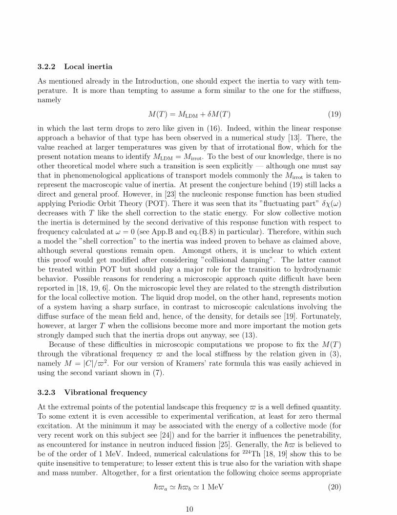
Figure 3: The inverse relaxation time 1/τkin = Γkin/~ (left panel) and ~ (right panel) asfunction of temperature: the microscopic results (solid curves) compared to the approxima-tions (20) and (21) (dotted curves).

with deviations being within a factor of 2 or less. This appears to be the case even whenpairing is included at smaller T . In Fig.3 we take up the case of 224Th, again. The calculationis the same as reported in [9]; more details will be given below in sect.3.2.6. From the rightpanel it is seen that this conjecture is pretty much fulfilled.

3.2.4 Ratio of friction to inertia

As said above, see eq.(3), the ratio γ/M determines the inverse relaxation time to theMaxwell distribution. For underdamped motion this quantity also defines the width Γkin

of the strength distribution. In Fig.3 we show it on the left hand panel as function of T .The dashed curve represents the following approximation, details of which are discussed inApp.B, namely

γ

M~ = Γkin ≈ 2Γsp(µ, T ) =

2

Γ0

π2T 2

1 + π2T 2/c2≈ 0.6T 2

1 + T 2/40MeV (T in MeV) . (21)

As expected it represents the microscopic result quite well at smaller values of T whichcorrespond to smaller values of damping. Recall, please, that the overdamped limit is givenalready for values of the damping factor ηb slightly above 1, see Fig.1.. As can be inferredfrom Fig.3 and the estimate (20), this happens at temperatures above 2 MeV; mind thatη = (γ/M)(2ω)−1.

3.2.5 Ratio of friction to stiffness

In Fig.4 we plot, as function of T , the time τcoll = γ/|C|, which measures the local relaxationin the coordinate. We may recall from (3) that for the overdamped case this is the only

11

0 1 2 3 4T (MeV)

0

1

2

3

4

5

0 1 2 3 4T (MeV)

0

1

2

3

4

5

γ /

C (

h/M

eV)

224Th, min. 224

Th, barr.

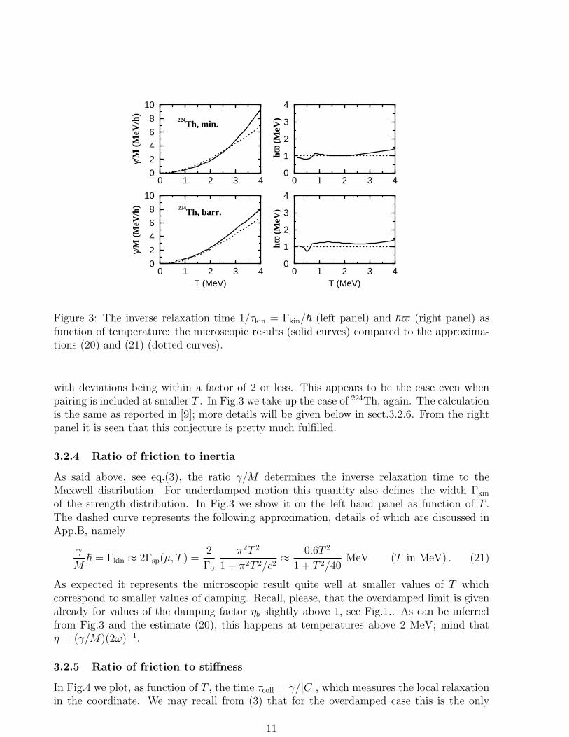
Figure 4: The relaxation time τcoll for collective motion at the potential minimum and at thebarrier: the microscopic result (solid curve) compared to the approximation (22-24) (dottedcurve).

relevant time scale left. Its inverse determines the width of the strength distribution alongthe imaginary axis (see (13)). Likewise the decay rate (10) associated to the Smoluchowskiequation is proportional to τ−1

coll. In Fig.4, again, the fully drawn line shows the microscopicresult. The dashed curves represent an approximation, into which the following two featuresare incorporated, the decrease of the stiffness (as given in (15) and (16)) and the fact thatwith increasing T the friction coefficient reaches a plateau [17, 18]. To combine both effectswe chose a functional form similar to the one for the Γkin of (21) (see App.B) but with adifferent cut-off parameter cmacro:

τcoll =γ

|C| ≈2

~2Γ0

π2T 2

1 + π2T 2/c2macro

≈ 0.6T 2

1 + π2T 2/c2macro

~

MeV(T, cmacro in MeV) ,

(22)

with ~ ≈ 1 MeV. One should expect the τcoll to reach a macroscopic limit like

τcoll|Th.T=

γ(T )

|C(T )|

∣

∣

∣

∣

Th.T

≈ γwall/2

|CLDM(T )| , (23)

at larger temperatures. With a parameterization as in (22) the limit is obtained aboveTh.T ≃ cmacro/π, for which reason the cmacro would be given by

c2macro =

~2Γ0

2

γwall/2

|CLDM(T )| ≈ 8.2γwall

|CLDM(T )|MeV3

~. (24)

Here, we accounted for results obtained by several previous numerical calculations, see e.g.[18,19, 6]. They showed that the value of friction at large T is somewhat below the wall formula.The factor 1/2 is only to be considered a rough rule of thumb. For the stiffness, on the otherhand, the macroscopic limit evidently is given by the liquid drop model. As the microscopiccalculation was done with a T -dependent |CLDM(T )| we chose the same one in this fit. Inboth curves the effects of pairing were included, which we are going to address now.

12

0.0 0.5 1.0T (MeV)

0.0

0.5

1.0

0.0 0.5 1.0T (MeV)

0.00

0.25

0.50

γ/M

(M

eV/h

)

224Th, min. 224

Th, barr.

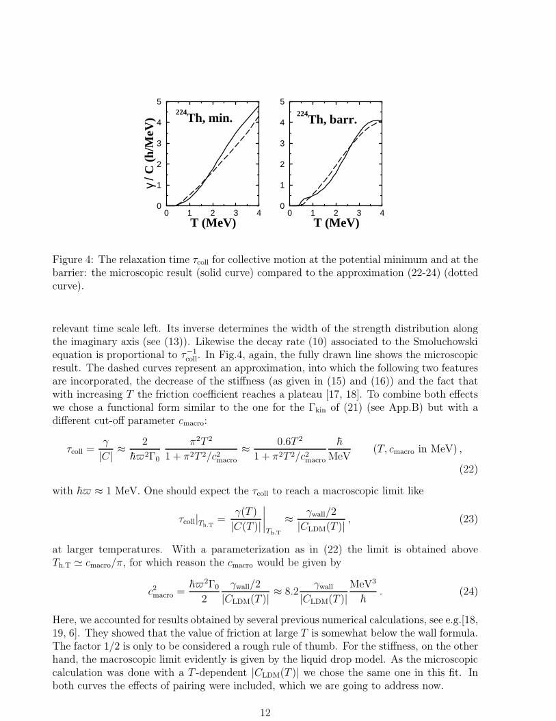
Figure 5: The influence of pairing on the inverse relaxation time τ−1kin = Γkin/~. The micro-

scopic results of [9] are compared with approximation (25).

3.2.6 The influence of pairing

This problem has recently been studied in [9]. The fully drawn lines shown in the previousfigures refer to such a calculation. Whereas in [9] one concentrated on the regime in whichpairing is expected to be effective, the present results extend up to T = 4 MeV. Calculationsin that regime had been reported before in [19]. The underlying shell model is the same inboth cases, but a different procedure is applied for the single particle width Γsp. For theunpaired case the form (B.11) was used, for which the frequency dependence of Γsp(ω, T )leads to convolution integrals in the response functions. They are known to reduce thecollective widths [6]. In the paired case such a calculation is no longer feasible, for whichreason there a constant Γsp(µ, ∆, T ) had been assumed, with ∆ being the pairing gap. Tohave a more or less smooth transition to the unpaired case, we now approximate the Γsp(ω, T )by the Γsp(µ, ∆, T ) which above the critical temperature for pairing reduces to the Γsp(µ, T )given in (B.13). For this reason our present friction coefficient may be overestimated slightly.For Γkin/~ = γ/M the new results are shown in Fig.5, where we concentrate on temperaturesup to 1 MeV. To simulate the apparent effect of pairing to reduce friction we suggest themodified formulas

γ

M= fpair

γ(∆ = 0)

M(∆ = 0)≡ fpair

Γkin(∆ = 0)

~(25)

and

γ

|C| = τkin = fpair τkin(∆ = 0) . (26)

Here, fpair parameterizes the decrease of friction due to pair correlations: An ansatz like

fpair =1

1 + exp(−a(T − T0)), (27)

may do with the following parameters: a = 10 MeV−1 and T0 = 0.55 MeV at the barrier,and a = 12 MeV−1, T0 = 0.48 MeV at the minimum. It was found that this choice fits best

13

the microscopic results (with the functional form (25)). It is seen that these values vary withshape, which may be an indication that they are perhaps different for different nuclei. Fora first orientation such details might be discarded. Then an average of the two values couldbe used both for a and T0. Finally, we should like to remark that this influence of pairing ismost dramatic for friction, and much less so for M and C. Therefore, we suggest to neglectthe influence on the latter.

4 Temperature dependent decay rates

If one wants to gain information on the transport coefficients and their T -dependence, inparticular, one needs to separate the influence of the pre-factors from the more or less trivialexponential part (the ”Arrhenius factor”). Commonly, this feature is then simply identifiedby Kramers’ conventional factor which only depends on ηb. A systematic study performedin [26] has revealed the appearance of a threshold temperature Tthresh above which deviationsfrom the statistical model are seen over a wide range of fissioning systems. Moreover, itsratio over the temperature dependent barrier heights EBar(T ) ≡ Eb(T ) showed a remarkableinsensitivity on mass number A. For later purpose it is more convenient to divide that ratioby two to get

T

2Eb(T )

∣

∣

∣

∣

thresh

≃ 0.13 from Fig. 4 of [26]. (28)

We are now going to view this result in the light of our microscopic transport coefficients.At first we shall concentrate on the ratio Rh.v.

K (ηb)/Rh.v.K (ηb = 0), to comment later on the

T -dependence of the additional factors seen in (7), and which involve ratios of the inertiasor stiffnesses.

4.1 Rate from microscopic transport coefficients

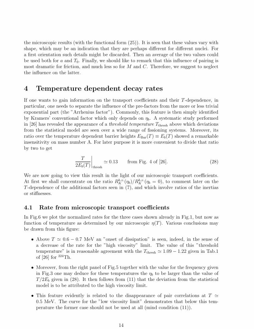
In Fig.6 we plot the normalized rates for the three cases shown already in Fig.1, but now asfunction of temperature as determined by our microscopic η(T ). Various conclusions maybe drawn from this figure:

• Above T ≃ 0.6 − 0.7 MeV an ”onset of dissipation” is seen, indeed, in the sense ofa decrease of the rate for the ”high viscosity” limit. The value of this ”thresholdtemperature” is in reasonable agreement with the Tthresh ≃ 1.09 − 1.22 given in Tab.1of [26] for 224Th.

• Moreover, from the right panel of Fig.5 together with the value for the frequency givenin Fig.3 one may deduce for these temperatures the ηb to be larger than the value ofT/2Eb given in (28). It then follows from (11) that the deviation from the statisticalmodel is to be attributed to the high viscosity limit.

• This feature evidently is related to the disappearance of pair correlations at T ≃0.5 MeV. The curve for the ”low viscosity limit” demonstrates that below this tem-perature the former case should not be used at all (mind condition (11)).

14

0.0 1.0 2.0 3.0 4.0T (MeV)

0.0

0.5

1.0

RK(η

) / R

K(η

=0)

224Th

Figure 6: Temperature dependence through a microscopic η = η(T ) (fully drawn line); thedashed curve represents the overdamped case as given by (9), the dotted one corresponds tothe low viscosity limit as given by (8) for the same barrier height as in Fig.(1).

• As indicated earlier, above T ≃ 2 MeV the overdamped limit applies, for which wesuggested to use formula (10).

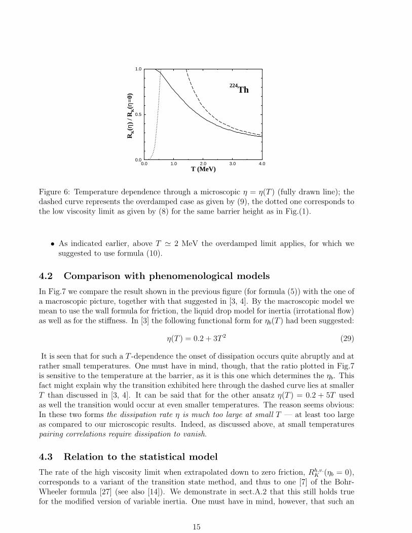
4.2 Comparison with phenomenological models

In Fig.7 we compare the result shown in the previous figure (for formula (5)) with the one ofa macroscopic picture, together with that suggested in [3, 4]. By the macroscopic model wemean to use the wall formula for friction, the liquid drop model for inertia (irrotational flow)as well as for the stiffness. In [3] the following functional form for ηb(T ) had been suggested:

η(T ) = 0.2 + 3T 2 (29)

It is seen that for such a T -dependence the onset of dissipation occurs quite abruptly and atrather small temperatures. One must have in mind, though, that the ratio plotted in Fig.7is sensitive to the temperature at the barrier, as it is this one which determines the ηb. Thisfact might explain why the transition exhibited here through the dashed curve lies at smallerT than discussed in [3, 4]. It can be said that for the other ansatz η(T ) = 0.2 + 5T usedas well the transition would occur at even smaller temperatures. The reason seems obvious:In these two forms the dissipation rate η is much too large at small T — at least too largeas compared to our microscopic results. Indeed, as discussed above, at small temperaturespairing correlations require dissipation to vanish.

4.3 Relation to the statistical model

The rate of the high viscosity limit when extrapolated down to zero friction, Rh.v.K (ηb = 0),

corresponds to a variant of the transition state method, and thus to one [7] of the Bohr-Wheeler formula [27] (see also [14]). We demonstrate in sect.A.2 that this still holds truefor the modified version of variable inertia. One must have in mind, however, that such an

15

0.0 1.0 2.0 3.0 4.0T (MeV)

0.0

0.5

1.0

RK(η

) / R

K(η

=0)

224Th

Figure 7: Temperature dependence of the decay rate in high viscosity limit: Fully drawncurve: same as in Fig.6; dashed curve: ηb given by (29); dashed-dotted curve: wall frictionand liquid drop values for stiffness and inertia.

extrapolation may be meaningless as, by its very construction, the transition state methodbases on the assumption of a complete equilibrium. The latter is given only if sizablefriction forces provide sufficiently fast relaxation to this global equilibrium. Our result forthe temperature dependence of friction then imply that any version of the transition stateresult must be taken with reservation when applied at small thermal excitations. At thispoint it would be too much to compare complicated evaluations of the Bohr-Wheeler formulawith estimates of Kramers’ rate which have our microscopic transport coefficients as input.This must be subject of further studies.

What is feasible, however, is to compare our results with those of a statistical model, inwhich the Bohr-Wheeler formula [27] is approximated by

Rstat =T

2π~exp(−Eb/T ) , (30)

see e.g.[28, 29]. This approximate form comes up when in the Bohr-Wheeler formula [27] thelevel density at the barrier is identified as that of the total system, whereas in the correctexpression the collective degree of freedom has to be excluded (see e.g.[14]). That such anapproximation may lead to erroneous results when interpreting data has been pointed outalso in [30]. We may briefly follow up this discussion by using our microscopic input.

The ratio RK/Rstat may be calculated for the three cases we looked at before, low andhigh viscosity limit as well as the overdamped limit. For ”high viscosity” one gets from (6)(mind (7)):

Rh.v.K

Rstat=

~b

T

√

Ca

|Cb|

(

√

1 + η2b − ηb

)

. (31)

For overdamped motion, expression (10) leads to

RK

Rstat

=

√

Ca

|Cb||Cb|γb

~

T. (32)

16

1.0 2.0 3.0 4.0T (MeV)

0.0

0.5

1.0

RK /

Rst

at

224Th

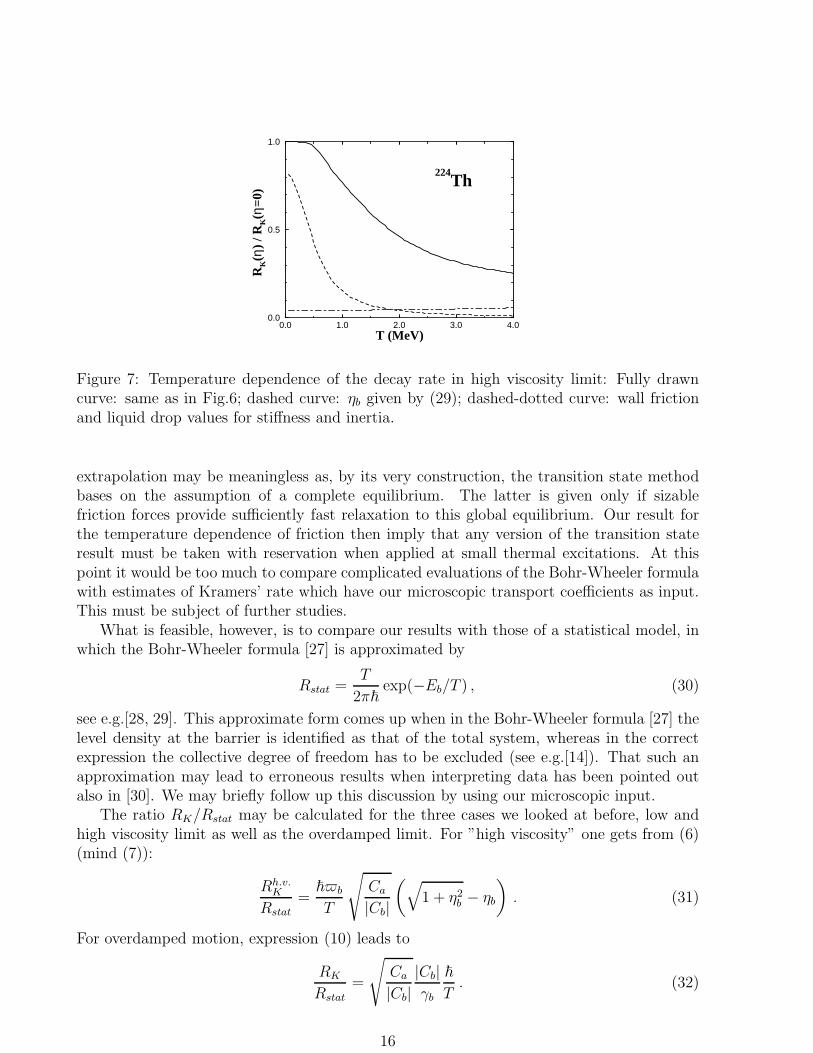
Figure 8: The ratio (32) of Kramers’ rate to that of the statistical model (fully drawn line).The dotted curve demonstrates the influence of the stiffnesses, which now are calculatedfrom the liquid drop model, but with friction unchanged.

The result (30) can be expected to deviate sizably from Kramers’ one. This is demonstratedin Fig.8 by the fully drawn line which represents the ratio given in (31). Here, the ”onset ofdissipation” seemingly is even more pronounced, and the deviation starts at a much highertemperature. However, these effects are not only related to dissipation. Besides the more orless obvious fact of the prefactor in (30) being not identical to the frequency ~a ≃ ~b, thereappears the square root of the ratios of the two stiffnesses. The latter is largely influenced byshell effects, which are known to be sensitive to variations of temperature. The implicationof this feature on the ratio RK/Rstat is exhibited in Fig.8 by the dotted curve. Its deviationfrom the solid one is solely due to the stiffnesses being evaluated from the (T -independent)liquid drop model CLDM(T = 0).

Obviously, the Rstat becomes small at small temperatures, say below about 0.5 MeV. Inthis range nuclear friction is small, too, not only at the barrier but also inside the well (seeFigs.3 and 4). Discarding any quantum effects, which in this regime may become important[8], one might then use Kramers’ low viscosity limit. As mentioned previously, any transitionstate result, however, does not apply, for which reason a comparison of both is meaningless.For the Bohr-Wheeler formula to be valid the system inside the well has to be in complete

equilibrium [10]. Such a situation is given only for sufficiently large damping.

4.4 Isotopic effects

In [3] different nuclei have been studied experimentally and analyzed with respect to atemperature dependence of the dissipation strength ηb (called γ there). In particular twoisotopes of Thorium have been examined, namely 224Th and 216Th corresponding to neutronnumbers of N = 134 and 126, respectively. The different behavior seen in experiment hasbeen fully attributed to this ηb and in this way very different values of ηb have been found,together with a different increase with T . Evidently such features cannot be explained withina macroscopic picture. One needs to account properly for shell effects. From our experiencewith microscopic computations it seems unlikely that they would have such a big influence

17

1 2 3 4T (MeV)

0

1

2

3

4

5

(Ca/C

b)1/

2

1 2 3 4T (MeV)

0.0

0.5

1.0

RK /

Rst

at

134 126134

126

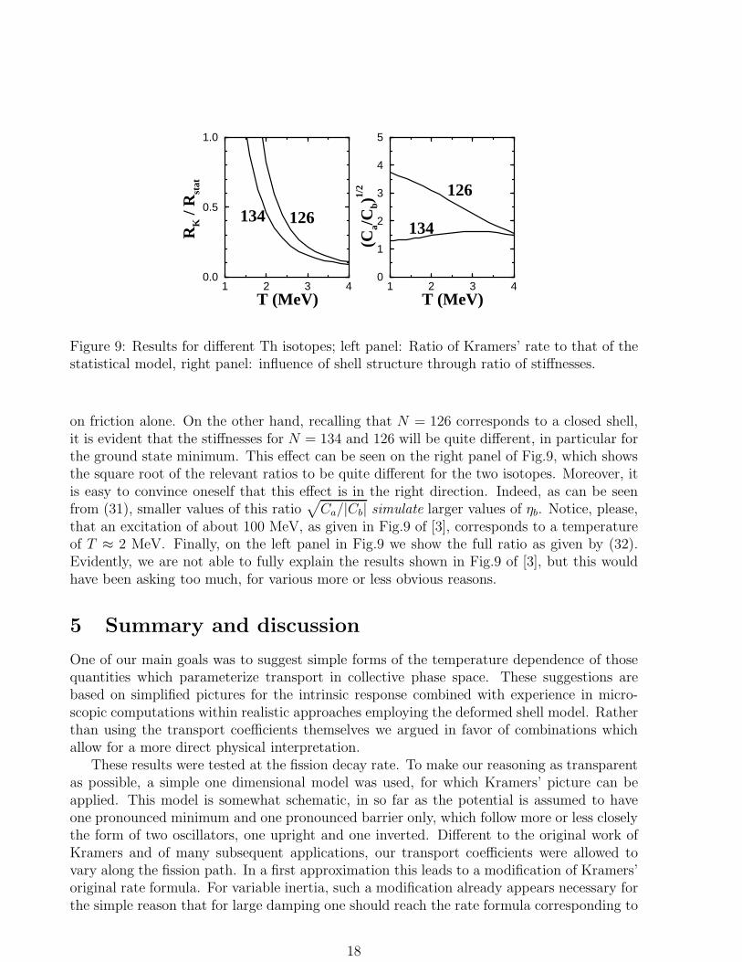
Figure 9: Results for different Th isotopes; left panel: Ratio of Kramers’ rate to that of thestatistical model, right panel: influence of shell structure through ratio of stiffnesses.

on friction alone. On the other hand, recalling that N = 126 corresponds to a closed shell,it is evident that the stiffnesses for N = 134 and 126 will be quite different, in particular forthe ground state minimum. This effect can be seen on the right panel of Fig.9, which showsthe square root of the relevant ratios to be quite different for the two isotopes. Moreover, itis easy to convince oneself that this effect is in the right direction. Indeed, as can be seenfrom (31), smaller values of this ratio

√

Ca/|Cb| simulate larger values of ηb. Notice, please,that an excitation of about 100 MeV, as given in Fig.9 of [3], corresponds to a temperatureof T ≈ 2 MeV. Finally, on the left panel in Fig.9 we show the full ratio as given by (32).Evidently, we are not able to fully explain the results shown in Fig.9 of [3], but this wouldhave been asking too much, for various more or less obvious reasons.

5 Summary and discussion

One of our main goals was to suggest simple forms of the temperature dependence of thosequantities which parameterize transport in collective phase space. These suggestions arebased on simplified pictures for the intrinsic response combined with experience in micro-scopic computations within realistic approaches employing the deformed shell model. Ratherthan using the transport coefficients themselves we argued in favor of combinations whichallow for a more direct physical interpretation.

These results were tested at the fission decay rate. To make our reasoning as transparentas possible, a simple one dimensional model was used, for which Kramers’ picture can beapplied. This model is somewhat schematic, in so far as the potential is assumed to haveone pronounced minimum and one pronounced barrier only, which follow more or less closelythe form of two oscillators, one upright and one inverted. Different to the original work ofKramers and of many subsequent applications, our transport coefficients were allowed tovary along the fission path. In a first approximation this leads to a modification of Kramers’original rate formula. For variable inertia, such a modification already appears necessary forthe simple reason that for large damping one should reach the rate formula corresponding to

18

the Smoluchowski equation. Still, the deviation from the undamped case is solely determinedby the damping strength ηb calculated at the barrier. However, for a complete understandingof temperature effects of the decay rate it does not suffice to concentrate only on this dampingstrength.

Of course, such a simple model for the static energy may not apply at all at (smaller)temperatures when shell effects lead to important deviations. It is unclear how one couldgeneralize the formulas of Kramers and Bohr-Wheeler to realistic cases with two or perhapsthree barriers having minima in between. To calculate the decay rate for such potentials it isperhaps simpler to use the more general description in terms of Fokker-Planck or Langevinequations. It may then also be possible to account better for the variations of the othertransport coefficients with coordinate and temperature, namely inertia and friction. To thebest of our knowledge so far in such calculations only the transport coefficients of macroscopicmodels have been used. However, the content of Fig.7 indicates that greater deviations canbe expected for microscopic inputs.

Nevertheless, within our model we are able to clarify a few important points which mustnot be discarded even at temperatures at which shell effects do not really dominate theprocess.

• The transition to overdamped motion already occurs at temperatures around T ≃2 MeV. Then the decay rate should be calculated from the Smoluchowski equation.

• In this case no inertia appears any more. Thus neither the frequency nor the effectivewidth Γkin = ~γ/M (sometimes referred to as ~β) play any role.

• The solely important quantities are the ratio of friction to stiffness, γ/C, and (for thedecay rate) the ratio Ca/Cb of the stiffnesses. Physically, the former determines therelaxation time for sliding motion in the potential, see (22). In passing we may notethat it is essentially this time which determines the saddle to scission time, an effectnot considered here. Notice that these stiffnesses are subject to large shell effects whichmay easily be accounted for by the shell correction method. As a first demonstrationof this effect we have calculated the impact of these stiffnesses on the decay rate of theThorium isotopes N = 134 and N = 126.

• In principle, the vibrational frequency should be obtained from microscopic com-putations (for T < 2 MeV). But a simple and quite fair estimate may be given by~a ≃ ~b ≃ 1 MeV (20), which is almost exact for the case of 224Th. Evidently, the may be greatly influenced by shell effects, but from our experience we claim thatthe deviations are within a factor of about two.

• Finally, we should like to briefly comment on the paper [31]. There scaling rules havebeen derived for the case of the Smoluchowski equation, and based on phenomenologicalinput. In the schematic model underlying the discussion a few assumptions had beenmade which are not in accord with microscopic results. First of all, the ratio of barrierheight to temperature definitely decreases with T . Secondly, as the authors monitorthemselves, a frequency at the barrier of the order of 20 MeV is much too high. Togetherwith the value used for β, namely β ≡ Γkin/~ ≃ 1022 sec−1 one gets an ηb of ≃ 0.2. Thisimplies the motion around the barrier to be under damped rather than overdamped.

19

Moreover, for several cases studied in this paper, the ηb is seen to be of the order ofor even smaller than T/2Eb. Thus, according to (11) not even Kramers’ high viscositylimit seems appropriate.

Let us turn now to very low temperatures, say to the regime where pairing correlationsbecome important. They imply an additional reduction of dissipation, such that one maytruly speak of the onset of dissipation when pair correlations disappear. It must be saidthough that this transition occurs at temperatures definitely smaller than those suggested in[1] - [5]. As mentioned earlier, one has to make sure, however, that one speaks of the sametemperature. The one of the compound nucleus might be larger than the one the systemstill has when it passes the barrier.

It ought to be stressed that a small damping strength at small temperatures may havequite drastic implications. In case the ”high viscosity limit” still applies quantum correctionsto the decay rate would lead to an increase of the latter [8]. If, however, the dissipationstrength falls below the limit given by (11) the nature of the diffusion process would changecompletely. Then dissipation is too weak to warrant relaxation to a quasi-equilibrium. Thisnot only violates Kramers’ rate formula (for the high viscosity limit), or our extension of it,but also the Bohr-Wheeler formula becomes inapplicable. Moreover, so far no method existsof how one might incorporate collective quantum effects.

Finally we should like to indicate that our transport coefficients are not free of uncer-tainties in some of the parameters specifying our microscopic input. The most difficult oneis found in the single particle width. It has been parameterized in [32] by referring to theoptical model for nucleons in finite nuclei through a kind of local density approximation.There the Γ0 and its dependence on the nuclear density had been traced back to microscopiccomputations of the self energies in a generalized Brueckner type description. This impliesan uncertainty of perhaps a factor of two in all formulas where the friction coefficient ap-pears, as in (21) or (22) as well as in the η of (4). Since any microscopic answer on suchquestions is extremely difficult, there is hope of narrowing down this uncertainty by moreelaborate comparisons with experimental results.

A Implications from a variable inertia

In Kramers’ seminal paper [7] the equation for the density in phase space was written andapplied to the decay of a metastable system for the case of constant transport coefficients.In nuclear physics both the inertia as well as the friction coefficient vary with the collectivecoordinate. This has been accounted for already in early applications to heavy ion collisions,where globally Gaussian solutions (centered at the classical trajectories) were used to cal-culate reaction cross sections see e.g. [33]. Written in compact form for one variable thetransport equation should read:

∂

∂tf(Q, P, t) =

[

− P

M(Q)

∂

∂Q+

∂

∂Q

(

P 2

2M(Q)+ V (Q)

)

∂

∂P

+∂

∂P

(

P

M(Q)γ(Q) + D(Q)

∂

∂P

)]

f(Q, P, t) .

(A.1)

20

Neglecting any quantum effects, which might show up at small temperatures only [6, 8], thediffusion coefficient is given by the classic Einstein relation D(Q) = γ(Q)T . A possible T -dependence of the transport coefficients has not been indicated explicitly. This is immaterialas long as we treat temperature as a fixed parameter, which is assumed to hold true in theentire paper. As is easily verified, one stationary solution of (A.1) is the distribution ofglobal equilibrium,

feq(Q, P ) =1

Zexp(−βH(Q, P )) (A.2)

with the energy given by the classical Hamilton function

H(Q, P ) =P 2

2M(Q)+ V (Q) . (A.3)

The reason is due to the following features: (i) The conservative part of the equation hasthe form of Liouville’s equation, namely

∂

∂tf(Q, P, t) =

H(Q, P ) , f(Q, P, t)

. (A.4)

(ii) The terms which represent dissipative and fluctuating forces are assumed independentof the momentum P , such that P only appears quadratically in the kinetic energy. (iii) Thechoice of the diffusion coefficient by D(Q) = γ(Q)T makes the second line of (A.1) vanishonce applied to (A.2).

The structure of these equations not only allow for the proper equilibrium, it also warrantsthe continuity equation to be valid in the form

∂

∂tn(Q, t) +

∂

∂Qj(Q, t) = 0, (A.5)

with the current and spatial densities being defined as

j(Q, t) =

∫

dPP

M(Q)f(Q, P, t) (A.6)

and

n(Q, t) =

∫

dP f(Q, P, t) , (A.7)

respectively. This is easily verified with the help of (A.1) exploiting partial integrations withrespect to momentum P (for which no ”surface terms” survive).

Both in Liouville’s equation as well as in the transport equation (A.1) a term appearswhich needs to be treated with special care. It is the one which results from the spatialderivative of the kinetic energy, and reads

(

∂

∂Q

P 2

2M(Q)

)

∂

∂Pf(Q, P, t) . (A.8)

Indeed, this term is absent in the common derivation of the rate formula (see e.g. [10]),where always a constant inertia is assumed to be given. It may be noted that this term

21

may imply difficulties with ”saddle point approximation”, as needed in Kramers’ stationarysolution. Moreover, and more important for the present purpose, this term is also neglectedin extracting the transport coefficients within the linear response approach. There, a locallyharmonic approximation is exploited, which for the sake of simplicity is formulated only withrespect to the coordinate. What that means may be visualized in the following way. Lookat the Liouville part of the transport equation, in particular at the term which involves thederivative of the Hamilton function with respect to Q. First of all there is the ordinary forcefrom the potential, which in the expansion around a Q0 to harmonic order may be writtenas

− ∂

∂QV (Q) ≡ K(Q) ≈ K(Q0) − C(Q0)(Q − Q0) , (A.9)

with the second derivative of the potential defining the local stiffness C(Q0). In additionthere is the term

(

∂

∂Q

P 2

2M(Q)

)

= P 2 ∂

∂Q

(

1

2M(Q)

)

(A.10)

which is of second order (namely in P ). In a consistent treatment one would have to introducea P0 and expand all terms locally in collective phase space around the (Q0, P0) to secondorder both in Q−Q0 and P −P0 (see [33]). So far this has not been done when extrapolatingtransport coefficients from the microscopic linear response approach. This does not implythat our inertia may not change with the coordinate at all. It only means that the termsincluding its derivative have been discarded. With respect to the basic transport equation(A.1) this approximation may be phrased as

∣

∣

∣

∣

(

∂

∂Q

P 2

2M(Q)

)

∂

∂Pf(Q, P, t)

∣

∣

∣

∣

≪∣

∣

∣

∣

∂

∂P

(

−K(Q) +P

M(Q)γ(Q)

)

f(Q, P, t)

∣

∣

∣

∣

. (A.11)

A.1 Kramers’ decay rate formula extended to variable inertia

For reasons given above, we still want to make use of the condition (A.11). Nevertheless, itis necessary to re-derive an expression for the rate, which still is defined as

R =jb

Na

. (A.12)

To calculate the quantities involved we need a global solution fglob(Q, P ) of equation (A.1)which corresponds to a small but finite, (quasi-)stationary current across the barrier. Thiscurrent may be calculated from (A.6), with f(Q, P, t) replaced by fglob(Qb, P ). The proba-bility Na of finding the system inside the well at Qa may be calculated as follows

Na =

Qa+∆∫

Qa−∆

dQ

∫

dP fglob(Q, P ) =

Qa+∆∫

Qa−∆

dQ nglob(Q) . (A.13)

The integration range 2∆ has to be smaller than Qb − Qa but large enough such that itcontains the vast majority of the ensemble points sitting in the well. An approximation for

22

fglob(Q, P ) may be constructed by matching together at some intermediate point Q localsolutions valid at the minimum Qa and at the barrier Qb. The global solution fglob(Q, P )will have an overall normalization factor which drops out when calculating the rate from(A.12). The normalization of the local solutions f(Q ≈ Qa, P ) and f(Q ≈ Qb, P ), on theother hand, might be different. It has to be chosen in appropriate fashion such that bothsolutions match properly at Q.

For a sufficiently high barrier the particles inside the potential well may be assumed tostay close to a local equilibrium associated to the temperature T . In case that the corre-sponding fluctuations 〈∆Q2〉eqa concentrate on a region around the minimum, the potentialmay be replaced by a harmonic oscillator and the associated local phase-space density maybe approximated by:

fa(Q, P ) ≡ f(Q ≈ Qa, P ) = Na exp

(

−β

(

P 2

2Ma+ V (Qa) +

Ca

2(Q − Qa)

2

))

. (A.14)

This is a reasonable estimate up to a Q with

(

Q − Qa

)2& 〈∆Q2〉eqa ≡ T

Ca. (A.15)

Likewise, approximating the barrier by an inverted oscillator, the phase-space density maybe represented by Kramers’ stationary solution [7, 10] (neglecting any quantum effects, seee.g. [6])

fb(Q, P ) ≡ f(Q ≈ Qb, P ) =Nb exp

(

−β

(

P 2

2Mb+ V (Qb) −

|Cb|2

(Q − Qb)2

))

×∫ P−A(Q−Qb)

−∞

du1√2πσ

exp

(

−u2

2σ

)

,

(A.16)

where

A =|Cb|

b

(

√

1 + η2b − ηb

) and σ = TMb

(

1(

√

1 + η2b − ηb

)2 − 1

)

(A.17)

This latter solution must be joined to the one given by (A.14) in some intermediate region,say at Q. It would be too much to require this to be possible for any P , in particular as weare not able to treat the inertia in continuous fashion, for reasons given above. However, asthe rate is determined by the ratio of two quantities which are averaged over momentum itturns out sufficient to match only the reduced Q-space densities. Like suggested by (A.7),the latter are obtained by integrating out the momentum P in (A.14) and (A.16) to get

na(Q) = Na

√

2πMaT exp

(

−β

(

V (Qa) +Ca

2(Q − Qa)

2

))

(A.18)

and

nb(Q) = Nb

√

πMbT

2exp

(

−β

(

V (Qb) −|Cb|2

(Q − Qb)2

))

(

1 + erf

(√

|Cb|2T

(Q − Qb)

))

(A.19)

23

To obtain the last expression identities for error functions have been applied. Still it is notof a form for which a condition like na(Q) = nb(Q) would make much sense. For this weneed the additional assumption

|Cb| (Q− Qb)2 ≫ T , (A.20)

which renders the error-function in (A.19) close to unity. Then the two densities matchsmoothly at a Q satisfying

V (Qa) +Ca

2(Q − Qa)

2 = V (Qb) −|Cb|2

(Q − Qb)2 , (A.21)

if only the normalization constants are chosen according to

Na = Nb

√

Mb

Ma. (A.22)

Now we are in the position to calculate the rate from (A.12). Plugging (A.22) into (A.14)the number of ”particles” at the minimum (A.13) becomes:

Na ≈ Nb

√

2πMbT

√

2πT

Ca

exp(−βV (Qa)) = Nb 2πT

√

Mb

Ca

exp(−βV (Qa)) (A.23)

To get this simple expression it was assumed that the ∆, which in (A.13) defines the rangeof integration, is of the order of or larger than the fluctuation 〈∆Q2〉eqa given in (A.15), suchthat the Gaussian integral can be calculated for ∆ → ∞. The current at the barrier maybe evaluated from (A.16) and (A.6) with Q = Qb. After a lengthy but straight forwardcalculation involving identities for error-integrals, once more, one arrives at

jb = Nb T

√

Mb

|Cb|b

(

√

1 + η2b − ηb

)

exp(−βV (Qb)) (A.24)

From (A.24) and (A.23) the decay rate (A.12) turns into

Rh.v.K =

b

2π

√

Ca

|Cb|

(

√

1 + η2b − ηb

)

exp(−βEb)

=a

2π

√

Ma

Mb

(

√

1 + η2b − ηb

)

exp(−βEb) ,

(A.25)

confirming the expression (6) used in the text. We may note again that the result (A.25)was derived before in [15] within an extension of the Perturbed Static Path Approximation(PSPA).

Finally, we like to come back once more to the conditions (A.15) and (A.20) imposedbefore. They go along with the relation (A.21) for Q and the barrier height Eb = V (Qb) −V (Qa). The latter must then satisfy Eb = Ca

2(Q − Qa)

2 + |Cb|2

(Q − Qb)2 ≫ T . It may be

useful to visualize these relations with the help of the following schematic potential:

V (Q) =

V (Qa) + Ca

2(Q − Qa)

2 for Q < Q,

Eb + V (Qa) − |Cb|2

(Q − Qb)2 for Q > Q .

(A.26)

Choosing the Q according to Q = (CaQa + |Cb|Qb)/(Ca + |Cb|) the two parabolas matchsmoothly with a continuous first derivative. Possible errors related to (A.15) and (A.20)may easily be estimated from elementary properties of the error function.

24

A.2 The relation to the transition state result

In transition state theory one assumes to be given a system that is totally equilibrizedinside the barrier and for which at the barrier current only flows outward discarding anybackflow. Within its most general version, the fission rate has been estimated by N. Bohrand J.A. Wheeler through their famous formula [27]. There the equilibrium is the one of amicro canonical ensemble as represented by the density of states (of the total system at theminimum and of the intrinsic system at the barrier). To the extent that the micro canonicalensemble may be represented by a canonical one, with one and the same temperature at theminimum and at the barrier, the calculation of the rate can be done as follows, looking onlyat the collective degree of freedom. The outward current (at the barrier) is given by

jtransb =

∫ ∞

0

dPP

Mbfeq(Qb, P ) ∝

∫ ∞

−∞

dPP

Mbexp

(

−βP 2

2Mb

)

Θ(P ) . (A.27)

Comparing with Kramers’s stationary solution shown in (A.16) one realizes [34] the onlydifference being the replacement of the Theta function Θ(P ) of (A.27) by the integral (forQ = Qb) which appears in the second line of (A.16). Because of the following representationof the Theta function

Θ(P ) = limσ→0

∫ P

−∞

du1√2πσ

exp

(

−u2

2σ

)

, (A.28)

it is seen that (for finite temperature)

Rtrans = Rh.v.K (η = 0) . (A.29)

This follows immediately with the help of the expression given for σ in (A.17).

A.3 The Smoluchowski limit

Performing in (A.25) the limit ηb ≫ 1, with the effective damping rate defined by (2), onegets:

Rh.v.K −→ b

2π

√

Ca

|Cb|1

2ηbexp(−βEb) =

1

2π

1

γb

√

Ca|Cb| exp(−βEb)

= Rovd .

(A.30)

This expression coincides with the formula (10) associated above with the Smoluchowskilimit. As a matter of fact, this result can be obtained directly from the Smoluchowskiequation

∂

∂tn(Q, t) =

∂

∂Q

(

1

γ(Q)

∂V (Q)

∂Q+

T

γ(Q)

∂

∂Q

)

n(Q, t) =∂

∂Qj(Q, t) . (A.31)

The calculation of the decay rate is quite easy in this case. Indeed, eq.(A.31) gives an explicitform of the j(Q, t) as a function of the density n(Q, t). Although in our case the frictioncoefficient varies with Q the common derivation of the rate formula (see e.g. [35]) may betaken over without much difficulties.

25

Notice, please, that the transition from an equation like (A.1) to (A.31) only requires theη(Q) to be large enough at any Q. Such a transition may be performed also in the case of avariable inertia, at least if condition (A.11) is fulfilled. In any case, in the overdamped limitthe inertia has to drop out. We may note in passing that this transition is in accord withthe locally harmonic approximation in the form discussed in sect.2.2.5 of [6]. Following thearguments of sect.10.1 and 10.4 of [35] eq.(A.31) can strictly be derived from (A.1) neglectingthe term (A.8).

A.4 Strutinsky’s derivation of the rate formula

The essential idea exploited in [14] is written there below eq.(6). Different to the approachdescribed in sect.A.1, the number of particles Na at the minimum is estimated by multiplyingthe density nb(Q) of Kramers’ stationary solution calculated at Qa by an ”effective length”,which in turn is determined by the mean fluctuation of the oscillator at this Qa times

√2π,

viz by

√2π (∆Q)eq =

√

2πT

Ca

. (A.32)

(The additional factor√

2π is required to ensure the appropriate measure needed for thenormalization of a Gaussian). In this way one gets from (A.24) and (A.19)

Rh.v.K =

b

2π

√

Ca

|Cb|

(

√

1 + η2b − ηb

)

exp(−βEb) . (A.33)

Here, it was assumed (i) that the Qb − Qa is sufficiently large such that in (A.19) theerror function could be replaced by unity, and (ii) that the barrier height can be estimatedas Eb ≈ (|Cb|/2)(Qa − Qb)

2. The result (A.33) has the same form as given in (A.25). Asexplained earlier, it is equivalent to (6) or the second line of (A.25) which involve the inertias.This latter expression is identical to the one given in eq.(16) of [14] if one only interchanges

there primed and unprimed quantities.

B A schematic microscopic model

B.1 The Lorentz-model for intrinsic motion

Let us assume that the nucleonic excitations can be parameterized by the response function(in this section we set ~ = 1)

χ(ω) = −F 2

[

1

ω − Ω + iΓ/2− 1

ω + Ω + iΓ/2

]

(B.1)

Here, the average matrix element F 2 of the one body operator F , which acts as the generatorof collective motion, measures the overall strength of the distribution. The states reachedby that coupling are centered at Ω with an effective bandwidth Γ (measured here in unitsof MeV/~). For real frequencies the reactive and dissipative response functions, χ′ and

26

χ′′, are readily calculated noticing that they represent real and imaginary parts of χ(ω) =χ′(ω) + iχ′′(ω). The static response is given by

χ(0) =2ΩF 2

Ω2 + (Γ/2)2= χ′(ω = 0) . (B.2)

It is useful to rewrite this (intrinsic) response function χ(ω) in terms of the form of theoscillator response given in (12).

χ(ω) =−2ΩF 2

ω2 + iΓω − (Ω2 + (Γ/2)2)=

−1/Mint

ω2 + iΓintω − 2int

. (B.3)

In this way transport coefficients for intrinsic motion appear

Mint =1

2ΩF 2, Γint = Γ, 2

int = Ω2 + (Γ/2)2 . (B.4)

Next we turn to the collective response. For the F -mode it is given by [6]

χcoll(ω) =χ(ω)

1 + kχ(ω)=

11

χ(ω)+ k

=−1/MF

ω2 + iΓF ω − 2F

, (B.5)

with the inverse coupling constant

−1

k= C(0) + χ(ω = 0); (B.6)

and C(0) being the stiffness of the free energy. The transport coefficients for the collectiveF -mode are:

MF = Mint, ΓF = Γint, CF ≡ MF 2F = Mint

2int + k (B.7)

To get those for the Q-mode one needs to multiply these quantities by 1/k2. For slow modesit so turns out that to a good approximation the C(0) in (B.6) may be neglected as comparedto the χ(0). This leads to

M =1

k2MF ≈

(

χ(0))2

2ΩF 2=

2ΩF 2

(

Ω2 + (Γ/2)2)2 =

χ(0)

Ω2 + (Γ/2)2=

1

2

∂2χ′

∂ω2

∣

∣

∣

∣

ω=0

. (B.8)

In the last expression we have made use of (B.2). Last not least this has been done becausethe static response seems to be quite insensitive to the increase of temperature [36], at leastfor not too large T . The transformation from the F - to the Q- mode leaves ratios betweentransport coefficients unchanged. The collective width, the ratio between friction and inertia,thus becomes Γkin = Γ. For friction this implies

γ = ΓkinM =Γ

Ω2 + (Γ/2)2χ(0) =

∂χ′′

∂ω

∣

∣

∣

∣

ω=0

, (B.9)

27

and for the stiffness one gets the expected result C ≈ C(0), which follows because the CF of(B.7) can be written as

CF = MF 2F =

1

χ(0)+ k =

C(0)

χ(0)(

C(0) + χ(0)) ≈ C(0)

(

χ(0))2 . (B.10)

The second equation follows from (B.4) and (B.2).Finally, we should like to note that for the schematic model with only one mode the

inertia always is the one which defines the value of the energy weighted sum. Likewise, asone may see from (B.9) for friction and (to lesser extent) from (B.8) for the inertia, thesetransport coefficients are well represented by their ”zero frequency limits”.

B.2 Benefits and shortcomings of this model

B.2.1 Weak damping

For this model weak damping is defined as Ω ≫ Γ/2. In this case static response and inertiaturn into the expressions known from the so called ”degenerate model” [21] χ(0) = 2F 2/Ωand M = 2F 2/Ω3. Notice that the inertia has the typical structure of the cranking inertia.For friction one gets γ = 2ΓF 2/Ω3.

The degenerate model becomes most transparent if it is applied to the case that nucleonsmove in oscillator potentials, in particular if any spin dependent forces are neglected. Thenthe intrinsic excitation is given by ~Ω = ∆N~Ω0 ≡ ∆N (41 MeV/A1/3), where ∆N is thedifference in the major quantum numbers of those states which are coupled through themultipole operator F . Whereas for the quadrupole there is only one possibility, namely∆N = 2, this is no longer true for other multipoles, for which more than just one mode arepossible. The same holds true as soon as a spin orbit force is introduced. Then even for thequadrupole transitions with ∆N = 0 are possible. It is them which lead to the low frequencymodes we are typically interested in, as they resemble closest the fission mode. If one stilllikes to stick to the (degenerate or) Lorentz model — which only allows for one mode — theeffective frequency Ω will only be a fraction of the shell spacing parameter Ω0.

B.2.2 Strong damping

It is tempting to apply this schematic model also to the extreme case of very strong damp-ing when Γ becomes comparable to or larger than the frequency Ω of the typical intrinsicexcitation. Plain confidence into the formula (B.9) would lead to γ ≃ (4/Γ)χ(0). Thisseems particularly intriguing if on the one hand the static response does indeed not changemuch with T , and if, on the other hand, the Γ is associated to the widths the single particlestates, as will be discussed below. According to (B.13) there might then be some range inwhich the friction force would show the typical 1/T 2 dependence one expects for liquids inthe ”collision dominated regime”, see also sect.5.3 of [17]. However, we claim that for finitenuclei the situation is more complicated. Evidently, the effects of strong collisions are due tothe increasing importance of residual interactions. But the latter imply other consequencesas well, last and not least a mixing with more complicated states such that with increasingthermal excitations many particle - many hole states become more and more important. As

28

has been demonstrated in previous papers, see e.g. [13, 6] amongst others, this effect impliesthat high frequency modes shift to lower frequencies such that the typical mode at stake inthe transport model gets more and more strength — implying that finally its inertia is givenby the sum rule limit. Moreover, it has been demonstrated that this feature goes along withthe disappearance of shell effects at T = Tshell. This problem is addressed in the text.

B.2.3 Temperature dependence through collisional damping

Looking back at the intrinsic response function introduced in (B.1), one realizes that theonly quantity which can be expected to change sensitively with excitation is the width Γ. Toget some first orientation we may relate it to the single particle width. For a Fermi systemthe latter can be expected to be of the form [6] 2

Γsp(ω, T ) =1

Γ0

(ω − µ)2 + π2T 2

1 +(

(ω − µ)2 + π2T 2)

/c2, (B.11)

with the parameters

1

Γ0= 0.03 MeV−1 and c = 20 MeV . (B.12)

For slow collective motion we may omit the frequency dependence and evaluate this widthat the Fermi surface and put ω − µ = 0 in (B.11) . Along this approximation we may put

Γkin ≈ 2Γsp(µ, T ) ≈ 0.6T 2

1 + T 2/40MeV (T in MeV) . (B.13)

Evidently the correction term in the denominator only becomes important at temperaturesof the order of T ≃ 6 MeV. This is already beyond that value were the other effects comeinto play we discussed in sect.B.2.2. For this reason the actual Γ(T ) is changed in the maintext.

Finally we may note that our schematic model is not capable of accounting for pairing.The latter will modify the transport properties at temperatures below T ≃ Tpair. This isdiscussed in the text.

Acknowledgements

The authors gratefully acknowledge financial support by the Deutsche Forschungsge-meinschaft, and they are grateful to J. Ankerhold, B. Back, A. Kelic and M. Thoennessenfor enlightening discussions. Two of us (F.A.I. and S.Y) would like to thank the PhysikDepartment of the TUM for the hospitality extended to them during their stay.

References

[1] D.J. Hofman, B.B. Back, I. Dioszegi, C.P. Montoya, S. Schadmand, R.Varma, andP. Paul, Phys. Rev.Let. 72, (1994) 470; see also: P. Paul and M. Thoennessen,Ann.Rev.Part.Nucl.Sci. 44, (1994) 65.

2Different to the notation used in [6] here energies are measured with respect to the Fermi surface µ

29

[2] D.J. Hofman, B.B. Back and P. Paul, Phys. Rev. C 51, 2597 (1995).

[3] B.B. Back, D.J. Blumenthal, C.N. Davids et al. Phys.Rev. C60, (1999) 044602.

[4] I. Dioszegi, N.P. Shaw, I. Mazumdar, A. Hatzikoutelis and P. Paul, Phys.Rev. C 61,(2000) 024613.

[5] G. Rudolf and A. Kelic, Nucl. Phys. A679, 2516 (2001).

[6] H. Hofmann, Phys. Rep. 284, 137 (1997).

[7] H.A. Kramers, Physica (Amsterdam) 7, 284 (1940).

[8] H. Hofmann and F.A. Ivanyuk, Phys.Rev.Lett. 82, 4603 (1999).

[9] F.A. Ivanyuk and H. Hofmann, Nucl.Phys. A657, 19 (1999).

[10] P. Hanggi, P. Talkner and M. Borkovec, Rev. Mod. Phys. 62, 251 (1990).

[11] A. Bulgac, G. Do Dang and D. Kusnezov, Physica E 9, 429 (2001); E. Lutz and H.A.Weidenmuller, Physica A 267, 354 (1999).

[12] M. Brack, J. Damgaard, A. S. Jensen, H. C. Pauli, V. M. Strutinsky and C. Y. Wong,Rev. Mod. Phys. 44, 320 (1972); see also T. Ledergerber and H.C. Pauli, Nucl. Phys.A207, 1 (1973).

[13] H. Hofmann, S. Yamaji and A.S. Jensen, Phys.Lett. B 286, 1 (1992).

[14] V.M. Strutinsky, Phys. Lett. B 47, 121 (1973).

[15] C. Rummel, Diploma TUM 2000; C. Rummel and H. Hofmann, to appear in Phys. Rev.E

[16] S. Yamaji, H. Hofmann and R. Samhammer, Nucl. Phys. A475, 487 (1988).

[17] H. Hofmann, F.A. Ivanyuk and S. Yamaji, Nucl. Phys. A598, 187 (1996).

[18] S. Yamaji, F.A. Ivanyuk and H. Hofmann, Nucl. Phys. A612, 1 (1997).

[19] F.A. Ivanyuk, H. Hofmann, V.V. Pashkevich and S. Yamaji, Phys. Rev. C 55, 1730(1997); nucl-th/9701032

[20] F.A. Ivanyuk, Acta Physica Slovaca, 49, 53 (1999).

[21] A. Bohr and B.R. Mottelson, ”Nuclear Structure”, Vol. II (Benjamin, London, 1975)

[22] C. Guet, E. Strumberger and M. Brack, Phys. Lett. B 205, 427 (1988).

[23] A.G. Magner, S. Vydrug-Vlasenko and H. Hofmann, Nucl. Phys. A524, 31 (1991)

[24] M Hunyadi et al., ”Excited superdeformed Kπ = 0+ rotational bands in β-vibrationalfission resonances of 240Pu”, submitted to Phys.Lett.B.

30

[25] S.Bjornholm and L.E.Lynn, Rev. Mod. Phys. 52, 725 (1980).

[26] M. Thoennessen and G.F. Bertsch, Phys. Rev. 26, 4303 (1993).

[27] N. Bohr and J.A. Wheeler, Phys. Rev. 56, 426 (1939).

[28] P.J. Siemens and A.S. Jensen, ”Elements of Nuclei: Many-Body Physics with the StrongInteraction”, Addison and Wesley, 1987, New York

[29] R. Vandenbosch and J.R. Huizenga, ”Nuclear Fission”, Academy Press, 1973, London

[30] M. Thoennessen, Nucl. Phys. A599, 1 (1996)

[31] H.A. Weidenmuller and J.-S. Zhang, Phys.Rev. C 29, 879 (1984).

[32] A.S.Jensen, H.Hofmann, P.Siemens, in: S.S.Wu, T.T.S.KUO (Eds.), Nucleon-NucleonInteraction and the Nuclear Many-Body Problems (World Scientific, Singapore, 1984)

[33] H. Hofmann and C. Ngo, Phys. Lett B 65, 97 (1976); C. Ngo and H. Hofmann, Z. f.Physik A282, 83 (1977).

[34] One of us (H.H.) gratefully acknowledges an enlightening discussion with W.J. Swiateckion this subject.

[35] H. Risken, The Fokker-Planck–Equation, Springer-Verlag, Berlin Heidelberg, 1989

[36] D. Kiderlen, H. Hofmann and F.A. Ivanyuk, Nucl.Phys. A550, 473 (1992).

31